.

UNIVERSIDAD COMPLUTENSE DE MADRID

FACULTAD DE CIENCIAS FÍSICAS Departamento de Óptica

ROUGH DIFFRACTION GRATINGS: APPLICATIONS TO LINEAR OPTICAL

ENCODERS.

MEMORIA PARA OPTAR AL GRADO DE DOCTOR

PRESENTADA POR

Francisco José Torcal Milla

Bajo la dirección del doctor

Eusebio Bernabeu Martínez Luis Miguel Sánchez Brea

Madrid, 2009

• ISBN: 978-84-692-8452-0 ©Francisco José Torcal Milla, 2009

- 1 -

UNIVERSIDAD COMPLUTENSE DE MADRID

DEPARTAMENTO DE ÓPTICA-OPTICS DEPARTMENT

APPLIED OPTICS COMPLUTENSE GROUP

ROUGH DIFFRACTION GRATINGS:

APPLICATIONS TO LINEAR OPTICAL ENCODERS

Thesis dissertation presented by

Francisco José TORCAL MILLA

in order to obtain the Doctor Degree in Physics.

Madrid, 20 de Abril de 2009

Thesis advisors: Eusebio BERNABEU MARTINEZ and Luis Miguel SANCHEZ BREA.

- 2 -

- 1 -

A mis padres, Feli y Paco, y a mi hermano, Juan

- 2 -

- 3 -

“Pero daré a conocer lo poco que he aprendido para que alguien mejor que yo pueda atisbar la verdad, y en su obra, pueda probar y criticar mi error. Así, me regocijare a pesar de todo de haber sido un medio a través del cual salga a la luz la verdad.”

Alberto Durero

- 4 -

- 5 -

AGRADECIMIENTOS

Me gustaría empezar mostrando mi gratitud a mis directores de tesis. Debo agradecer al profesor Eusebio Bernabeu la confianza que ha depositado en mí desde el principio, el haberme dado la oportunidad de trabajar en su grupo y la total financiación de cursos, seminarios, etc, que han contribuido a mejorar e incrementar mi experiencia y conocimientos. Debo agradecer también a mi otro director de tesis, Luís Miguel Sánchez Brea, que ha llegado a ser mucho más que un director de tesis, un gran amigo, su trabajo constante, su modo de trabajar, sus buenas ideas, sus bromas, de lo cual he aprendido tanto. Yo firmo esta tesis, pero sabes que al menos la mitad es tuya, gracias Luismi.

Agradezco también a Fagor Automation, y en particular a Tomás Morlanes por haberme proporcionado ideas, discutido mi trabajo y enviado muestras de redes para analizar, toda su ayuda, en general.

También me siento afortunado por haber podido realizar esta tesis en un insuperable ambiente de trabajo. Se lo agradezco a toda la gente de “la Cueva”, las risas interminables y las conversaciones con Paco, la no siempre buena música de Infor (estoy bromeando hombre!), la tradición de los jueves de Isidoro, las conversaciones acerca de cualquier cosa con cada uno de ellos, Quiroga, Alfredo, Natalia, Cuqui, Chema, Paloma, Agustín y en general todo el Grupo Complutense de Óptica Aplicada.

Por otro lado, no puedo olvidar mis comienzos en la Universidad de Zaragoza. No habría empezado esta etapa de mi vida sin ellos. Tengo que dar las gracias a todas “mis chicas” del laboratorio. Agradezco mucho a Eva sus conversaciones, su verdadera amistad, su alegría y su sonrisa, incluso en momentos duros, a Ayalid su amistad, su confianza y sus consejos, y a Viqui su valiosa ayuda y su sonrisa constante. Debo agradecer también a Jesús Atencia que me contratase hace ya unos años y al profesor Manuel Quintanilla su curiosidad y sus preguntas constantes acerca de mi trabajo. No puedo olvidar tampoco al resto de la gente, así que, gracias a todos.

Muchas gracias también a mis compañeros de carrera. Pablo, Luis, recordáis aquel día, antes de un examen? Futbol, algo de cerveza, y aprobamos el examen!!, esos guiñotes por la tarde y esas pochas. Alfonso, cuanto sudor nos costó acabar la carrera, pero ¡lo hicimos!. Gracias por aquellos momentos

- 6 -

juntos, estudiando, fumando o hablando. Gracias a Lorenzo y todos los demás. Gracias por vuestra amistad.

Quiero agradecer también a Fernando Perez Quintián y Ariel Lutenberg su más que calurosa recepción y trato durante mi estancia en su laboratorio en Buenos Aires. Aprendí muchas cosas de vosotros, una nueva forma de trabajar, de vivir, etc. Gracias por ese inolvidable periodo!.

Gracias a todos mis amigos, Javi, Cristian, Fer, David, Melus, Nacho, Antonio, etc. Gracias por interesaos en lo que estaba haciendo y por aquellos ratos en los que me hicisteis olvidar mis preocupaciones por un momento. Espero que entendáis que necesitaría muchas páginas para escribir todos vuestros nombres, pero estáis todos aquí, en este párrafo.

Para concluir, y a pesar de que estáis al principio en mis pensamientos, quiero agradecer a mis padres, Feli y Paco, todo. A mi hermano, Juan Luis, el mejor hermano, al menos para mí. A mi abuela Felisa; estoy seguro de que estás en un lugar mejor ahora mismo. Tú siempre me preguntabas que tal me iba aunque no entendieras nada, te hecho de menos. También a mis abuelos, Julián y Maria Luisa, de los que he aprendido tantas cosas. Y al resto de mi familia por su puesto.

Este trabajo de Tesis ha sido financiado por el proyecto DPI2005-02860 del Ministerio de Educación y Ciencia de España.

Por último, muchas gracias a todos los que alguna vez os habéis interesado por mí y a ti, por estar leyendo esto.

- 7 -

RESUMENRESUMENRESUMENRESUMEN

En este trabajo de Tesis Doctoral presentamos un análisis teórico, numérico y experimental del comportamiento de redes de difracción con características no perfectas. En un primer lugar hemos realizado un estudio de las redes de difracción grabadas sobre fleje de acero. Este tipo de redes se pueden encontrar en dispositivos de trascendencia industrial como son los codificadores ópticos para medida de largar distancias (>3 m). Los objetivos principales de este trabajo son encontrar un formalismo analítico que describa el comportamiento de redes de difracción sobre fleje de acero tanto en campo cercano como en campo lejano. También proponemos un nuevo tipo de red de difracción basada en variaciones periódicas en las propiedades micro-topográficas de la superficie. Además, analizamos otros tipos de imperfecciones tales como la aparición de bordes rugosos en las franjas de la propia red de difracción, que pueden ser debidos al proceso de fabricación. Otro resultado relevante de este trabajo es la cancelación del efecto Talbot usando mascaras compuestas por dos redes de difracción. Este trabajo ha sido motivado por una larga colaboración con la industria relacionada con la fabricación de sistemas de metrología de precisión.

- 8 -

- 9 -

CAPITULO 1: IntroducciónCAPITULO 1: IntroducciónCAPITULO 1: IntroducciónCAPITULO 1: Introducción

Las redes de difracción son elementos que producen cambios periódicos en una o más propiedades del haz que incide sobre ellas. Este tipo de elementos han sido analizados y estudiados desde finales del siglo XVIII. Los tipos más comunes de redes de difracción son aquellos que modulan la amplitud o la fase del haz incidente. Las redes de amplitud están compuestas por franjas que permiten o no permiten pasar la luz, colocadas alternadamente. Como puede deducirse, la intensidad incidente queda reducida a la mitad tras atravesar la red. Por otro lado, las redes de fase producen una modulación en la fase del haz incidente. El grado de modulación depende del escalón de fase que contenga la red, que puede ir de cero a 2π . En los últimos años, se han desarrollado otro tipo de redes basadas en polarización. Esta familia de redes cambia periódicamente el estado de polarización del haz incidente. Un ejemplo podría ser una red compuestas por polarizadores lineales cruzados colocados alternadamente.

Teniendo en cuenta el comportamiento de la luz tras atravesar la red de difracción, en campo cercano se produce una réplica de la red a ciertas distancias de esta. Este fenómeno es conocido como Efecto Talbot. Se han realizado numerosos trabajos analizando el Efecto Talbot, para incidencia oblicua, para luz policromática, para luz parcialmente coherente, cuando la red presenta defectos e incluso cuando se utiliza luz polarizada. Por otro lado, en campo lejano aparecen órdenes de difracción, cuyas direcciones dependen del periodo de la red y del número de orden.

Las redes de difracción son uno de los elementos ópticos más trascendentales. Se pueden encontrar en campos de la ciencia tan diversos como fotónica, química, biología, astrofísica, ingeniería mecánica, en multitud de aplicaciones específicas como espectroscopia, metrología óptica, interferometría Moire, sistemas de iluminación, etc y en muy diverso instrumental, tal como codificadores ópticos de la posición, nanoposicionadores, colorímetros, telescopios, espectrómetros, máquina-herramienta, etc.

En nuestro caso, y debido a una larga colaboración con la empresa privada, una de nuestras líneas de investigación más importantes es el análisis y mejora de sistemas de codificación óptica de la posición. Los codificadores ópticos son instrumentos que sirven para medir desplazamientos entre dos partes diferentes de otro instrumento o incluso para dar la posición absoluta. En la mayoría de

- 10 -

los casos se usan redes de difracción de cromo sobre vidrio, pero cuando es necesario medir largas distancias este tipo de redes no son útiles, ya que son difíciles de fabricar y de manejar en estas longitudes. En estos casos se usan redes grabadas sobre fleje de acero. Estas redes son fabricadas grabando la red sobre el sustrato metálico. El uso de estas redes permite medir largas distancias, pero por el contrario introduce otro tipo de problemas, ya que su comportamiento no es ideal, debido a su topografía. Hasta hace algunos años, el periodo mínimo con el que se fabricaban estas redes era de 100 micras y los efectos debidos a difracción eran despreciables. En la actualidad se están consiguiendo periodos más bajos y los efectos difractivos empiezan a cobrar relevancia. En este trabajo analizamos el comportamiento de este tipo de redes en campo lejano y campo cercano, mostrando que en campo cercano producen Efecto Talbot. Para el análisis, hemos considerado la rugosidad de la red y la hemos modelado haciendo uso de los parámetros estadísticos que describen la topografía aleatoria, la desviación estándar y la longitud de correlación. Hemos observado que el contraste de las autoimágenes decae en términos de las variables que describen la topografía, siendo esta caída gaussiana o exponencial, dependiendo de la función de distribución que describe la topografía. Además, hemos encontrado que en campo lejano, la anchura de los órdenes difractados crece en términos de estos mismos parámetros estadísticos.

Ya que estas redes se usan en sistemas de codificación óptica de la posición con configuraciones de doble red, hemos analizado los casos más comúnmente utilizados. Estas son las configuraciones de Moire, Lau y Autoimagen Generalizada. En el caso de Moire, el contraste de las señales desaparece cuando separamos las redes más allá de una cierta distancia, que viene establecida por la longitud de correlación de la rugosidad del fleje. Por el contrario, en las configuraciones Lau y Autoimagen Generalizada, el contraste de las señales o de las autoimágenes permanece sin alteración.

Hemos desarrollado y analizado un nuevo tipo de red de difracción basada en micro-topografía. Esta red está compuesta por franjas lisas y rugosas colocadas alternadamente. Hemos realizado un estudio estadístico de la difracción por estas redes rugosas tanto en campo cercano como en campo lejano. Hemos simulado las franjas rugosas como rugosidad aleatoria con altura media igual a cero. Para describir la red son necesarias la desviación estándar y la longitud de correlación, al igual que en el caso de la red sobre fleje de acero. Hemos

- 11 -

demostrado que este elemento actúa como una red de difracción únicamente debido a la rugosidad.

En campo cercano aparecen autoimágenes, aproximadamente como si se tratase de una red de amplitud corriente. La diferencia es que en este caso aparecen gradualmente. Por otro lado, en campo lejano, se producen órdenes de difracción, pero al mismo tiempo aparece un halo de luz rodeando a los mismos.

También hemos analizado otro tipo de imperfecciones en redes de difracción, como por ejemplo, el hecho de que los bordes de las franjas no sean perfectamente rectos. Hemos obtenido expresiones analíticas para los casos en los que ha sido posible y simulaciones numéricas para los que no ha sido posible. Se han realizado los experimentos convenientes que han validado los resultados obtenidos.

Como hemos mencionado antes, una red de difracción en campo cercano produce Efecto Talbot. Este es un efecto a tener en cuenta cuando se va a llevar a cabo el diseño de un codificador óptico de la posición. Hemos realizado varios análisis sobre la posible cancelación del efecto Talbot usando una única red o dos redes en tándem. Para el caso de una única red, hemos encontrado que utilizando una red de fase bajo ciertas condiciones se consigue eliminar el efecto Talbot. A su vez se dobla el periodo de las franjas. Por otro lado, utilizando dos redes de difracción hemos encontrado que también es posible cancelar el Efecto Talbot, cuadruplicando el periodo de las franjas. Este hecho es de gran relevancia en sistemas de codificación óptica de la posición ya que mejora tanto las tolerancias mecánicas del instrumento como su precisión.

Para terminar, también hemos desarrollado un nuevo método para el cálculo del contraste basado en la función variograma, que permite mejorar en gran medida el cálculo de contraste en comparación con la definición estándar.

CAPITULO 2: PCAPITULO 2: PCAPITULO 2: PCAPITULO 2: Principios de funcionamiento de un codificadorrincipios de funcionamiento de un codificadorrincipios de funcionamiento de un codificadorrincipios de funcionamiento de un codificador

En este capítulo, se muestra una breve introducción sobre los principios de funcionamiento de un codificador de la posición. Se describen los tipos de codificadores existentes, magnéticos, ópticos, basados en efectos difractivos, interferométricos, etc. Se explican todas las posibles configuraciones y se muestran las diferentes partes que conforman un codificador, como son la

- 12 -

escala y la cabeza lectora. Por otro lado, también se explica cómo las señales magnéticas u ópticas son transformadas en señales eléctricas que más tarde nos darán la lectura del movimiento relativo o de la posición absoluta. Para terminar se detallan algunos errores típicos sobre la medida producidos por estos sistemas.

CAPITULO 3: HerramiCAPITULO 3: HerramiCAPITULO 3: HerramiCAPITULO 3: Herramientas matemáticas para el análisis de entas matemáticas para el análisis de entas matemáticas para el análisis de entas matemáticas para el análisis de redes de difracciónredes de difracciónredes de difracciónredes de difracción

A lo largo de este trabajo se han aplicado varias herramientas matemáticas a los cálculos y análisis de las redes de difracción. En este capítulo realizamos una breve introducción de las herramientas utilizadas. En primer lugar se presenta una breve introducción a la teoría de la difracción, incluyendo las ecuaciones de Maxwell, la descomposición en ondas planas, las aproximaciones de Fresnel, Fraunhofer y Rayleigh-Sommerfeld y sus aplicaciones a redes de difracción. En el tratamiento escalar hemos supuesto la Aproximación de Elemento Delgado (TEA), la cual consiste en asumir que el elemento difractivo puede simularse como una transmitancia. Esta aproximación da un resultado correcto y permite obtener soluciones analíticas a los problemas cuando se cumple que el periodo de la red es mucho mayor que la longitud de onda y la altura del elemento óptico es mucho menor que la longitud de onda. Por otro lado, el los casos en los que la aproximación de elemento delgado no es posible, se ha utilizado el análisis riguroso por ondas acopladas (RCWA) que da un resultado exacto a las ecuaciones de Maxwell siempre que el objeto a estudiar sea periódico. Estos formalismos son explicados a lo largo del capítulo.

CAPITCAPITCAPITCAPITULO 4: Principios ópticos de los codificadoresULO 4: Principios ópticos de los codificadoresULO 4: Principios ópticos de los codificadoresULO 4: Principios ópticos de los codificadores con redes con redes con redes con redes de difracción idealesde difracción idealesde difracción idealesde difracción ideales

Se muestra una descripción general de los principios ópticos en los que se basa un codificador óptico de la posición y sus posibles configuraciones. En primer lugar aplicamos las aproximaciones de Fresnel y Fraunhofer a una red de difracción obteniendo el bien conocido Efecto Talbot en campo cercano y los órdenes de difracción en campo lejano. En segundo lugar, también se analizan las configuraciones de doble red utilizadas en sistemas de codificación, como son Moire, Lau y Autoimagen Generalizada. Por último analizamos como estas configuraciones son utilizadas para la medida de desplazamientos.

- 13 -

CAPITULO 5: Difracción de Fresnel por redes sobre fleje de CAPITULO 5: Difracción de Fresnel por redes sobre fleje de CAPITULO 5: Difracción de Fresnel por redes sobre fleje de CAPITULO 5: Difracción de Fresnel por redes sobre fleje de aceroaceroaceroacero

Realizamos un análisis del comportamiento en campo cercano de una red de difracción sobre fleje de acero. Existen algunas diferencias con respecto al caso ideal explicado en el capítulo 4. La topografía de la red en este caso no es perfectamente lisa sino que presenta rugosidad. Esto hace que sea necesario el uso de parámetros estadísticos para describirla. En primer lugar hemos asumido que la iluminación es monocromática y colimada. La transmitancia de la red ha sido simulada como la multiplicación de la transmitancia de una red de amplitud y la transmitancia de una red con rugosidad aleatoria. Hemos encontrado que en campo cercano se produce Efecto Talbot, pero que su contraste decae con la distancia, en términos de los parámetros estadísticos que definen la rugosidad. En segundo lugar hemos realizado el mismo análisis pero utilizando como iluminación un haz de perfil gaussiano. Hemos encontrado que el contraste de las autoimágenes también decae y que además, en campo lejano, la anchura de los órdenes de difracción crece con la rugosidad. Todos los cálculos han sido realizados para aproximación de alta y baja rugosidad.

CAPITULO 6: Sistemas de doble red con una rede sobre fleje CAPITULO 6: Sistemas de doble red con una rede sobre fleje CAPITULO 6: Sistemas de doble red con una rede sobre fleje CAPITULO 6: Sistemas de doble red con una rede sobre fleje de acerode acerode acerode acero

En este capítulo se muestra la determinación de las señales ópticas producidas por un sistema de doble red en el cual una de las redes es de fleje de acero y la otra es de cromo sobre vidrio, que consideramos ideal. Del resultado general hemos obtenido las configuraciones más habituales en sistemas de codificación óptica de la posición, Moire, Lau y Autoimagen generalizada. Hemos encontrado que para el caso de Moire, la rugosidad provoca un decrecimiento o incluso pérdida del contraste de las franjas Moire. Por el contrario, la rugosidad no afecta en gran medida a las otras dos configuraciones, siendo lo más relevante el efecto sobre la anchura de las autoimágenes en la configuración de Autoimagen Generalizada.

- 14 -

CAPITULO 7: Difracción por redes rugosasCAPITULO 7: Difracción por redes rugosasCAPITULO 7: Difracción por redes rugosasCAPITULO 7: Difracción por redes rugosas

En este capítulo introducimos un nuevo tipo de red de difracción. Las redes que normalmente se usan en aplicaciones son aquellas que modulan la amplitud o la fase del haz incidente. La red que introducimos en este capítulo está basada en la variación de la micro-topografía y está formada por franjas lisas y rugosas colocadas alternadamente. Ya que consideramos que la topografía de las franjas rugosas es aleatoria, se hace necesario el uso de herramientas estadísticas para su definición y análisis. Obtenemos el comportamiento en difracción tanto en campo lejano como en campo cercano demostrando que este tipo de elemento periódico se comporta como una red de difracción. En campo cercano se produce efecto Talbot y en campo lejano ordenes de difracción, pero con algunas diferencias en comparación con otros tipos de redes. El efecto Talbot no aparece justo después de la red si no gradualmente. La distancia a la cual aparece el efecto Talbot depende de los parámetros estadísticos de la rugosidad. Por otro lado, rodeando a los órdenes de difracción aparecen halos de luz, que también dependen de los parámetros estadísticos de la rugosidad. Además, se han realizado tanto simulaciones numéricas como desarrollos experimentales para confirmar la validez del formalismo obtenido.

CAPITULO 8: Redes de difracción con bordes rugososCAPITULO 8: Redes de difracción con bordes rugososCAPITULO 8: Redes de difracción con bordes rugososCAPITULO 8: Redes de difracción con bordes rugosos

En este capítulo analizamos el efecto sobre el campo difractado por una red cuyas franjas tienen los bordes rugosos. Realizamos el análisis tanto en campo cercano como en campo lejano, obteniendo soluciones analíticas en los casos en que es posible. En los demás casos, realizamos el análisis mediante simulaciones numéricas. Para poder realizar una comprobación experimental de los resultados obtenidos, fabricamos una red con bordes rugosos de características estadísticas conocidas a priori mediante litografía. Hemos encontrado que las autoimágenes van siendo más sinusoidales al aumentar el orden de autoimagen y que es posible eliminar los órdenes de difracción superiores, quedándonos solo con los órdenes 0, 1± , para algunos valores de rugosidad en los bordes.

- 15 -

CAPITULO 9:CAPITULO 9:CAPITULO 9:CAPITULO 9: Apéndice 1. Eliminación de Efecto TalbotApéndice 1. Eliminación de Efecto TalbotApéndice 1. Eliminación de Efecto TalbotApéndice 1. Eliminación de Efecto Talbot

El efecto Talbot es uno de los problemas más importantes en sistemas de codificación óptica de la posición. Este efecto provoca que las tolerancias mecánicas de los codificadores sean menores que las deseadas, siendo muy estricta la distancia a la que debe mantenerse la cabeza lectora de la escala para dar una lectura correcta del movimiento o la posición. En este apéndice realizamos un análisis de la posible cancelación del Efecto Talbot usando una única red de difracción o dos redes de difracción en tándem, encontrando a su vez soluciones al problema para los dos casos. También verificamos experimentalmente los resultados obtenidos.

CAPITULO 10: Apéndice 2. Técnicas para el cálculo del CAPITULO 10: Apéndice 2. Técnicas para el cálculo del CAPITULO 10: Apéndice 2. Técnicas para el cálculo del CAPITULO 10: Apéndice 2. Técnicas para el cálculo del contrastecontrastecontrastecontraste

En este capítulo se describen las diferentes técnicas utilizadas para el cálculo del contraste durante el transcurso de este trabajo. Se describe la definición clásica de contraste, usada habitualmente para cálculos teóricos, otra basada en la simulación de detectores, usada principalmente cuando el contraste a medir es de señales y por último se desarrolla una nueva técnica basada en la función variograma que mejora en gran medida los resultados obtenidos con la definición estándar de contraste, haciéndolos más fidedignos. Esta última técnica se ha usado para el cálculo de contraste en medidas experimentales.

- 16 -

CONCLUSIONESCONCLUSIONESCONCLUSIONESCONCLUSIONES

Las principales contribuciones originales de esta Tesis Doctoral son las siguientes

• Hemos obtenido soluciones analíticas para el patrón de difracción producido por redes de difracción sobre fleje de acero bajo iluminación colimada y de perfil gaussiano. El contraste de las autoimágenes de Talbot decae con la distancia de la red al plano de observación. Este decaimiento depende de los parámetros estocásticos que describen la topografía. Se han obtenido a su vez verificaciones experimentales. Las autoimágenes son más sinusoidales que para el caso de redes sin rugosidad. Cuando la iluminación es gaussiana, los órdenes de difracción siguen siendo de perfil gaussiano, pero sus anchuras aumentan debido a la rugosidad. Por otro lado no existe redistribución de energía entre órdenes.

• También han sido analizadas las configuraciones más típicas de doble red, incluyendo una red sobre fleje de acero en el sistema. Se ha mostrado que la rugosidad puede producir pérdida de señal en la configuración Moiré cuando la separación entre las dos redes supera cierta distancia. Por el contrario, el contraste de las autoimágenes en la configuración de Autoimagen Generalizada no es afectado por la rugosidad, pero si la anchura de las autoimágenes. La configuración Lau no presenta dependencia con la rugosidad. Se han obtenido soluciones analíticas para los tres casos.

• Hemos desarrollado y analizado un nuevo tipo de red de difracción basado en rugosidad. En campo lejano, aparecen los órdenes de difracción, pero su anchura y eficiencia dependen de la rugosidad. Para el límite de alta rugosidad, los órdenes de difracción aparecen rodeados de un “halo” de luz. Para el límite de baja rugosidad, el perfil de los órdenes es Lorentziano. En campo cercano, aparece efecto Talbot. El contraste de las autoimágenes es nulo junto a la red pero crece gradualmente hasta estabilizar su valor máximo a cierta distancia, la cual depende de la rugosidad. Se han obtenido soluciones analíticas y se han validado usando el formalismo de Rayleigh-Sommerfeld.

- 17 -

• A su vez se han analizado defectos en los bordes de las franjas que conforman la red de difracción. En campo lejano, la potencia de los órdenes decrece fuertemente dependiendo este decrecimiento tanto de la rugosidad como del orden de difracción al que nos refiramos. En campo cercano las autoimágenes de Talbot son más suaves que la propia imagen de la red.

• Usando una máscara con dos redes de difracción es posible cancelar el efecto Talbot. Bajo ciertas condiciones la frecuencia de las franjas se cuadruplica con respecto a la de las redes. Estos dos hechos tienen gran relevancia en el diseño de codificadores ópticos de la posición, ya que sería posible aumentar tanto sus tolerancias mecánicas con su precisión. Se han realizado comprobaciones experimentales para validar los resultados teóricos.

• Se ha desarrollado un nuevo método para el cálculo del contraste basado en la función variograma, mejorando los resultados obtenidos con la definición estándar de contraste. Esta técnica es particularmente interesante cuando las señales a medir presentan ruido o grandes fluctuaciones y ha sido aplicada con éxito en la determinación experimental del contraste de las franjas a lo largo de este trabajo.

- 18 -

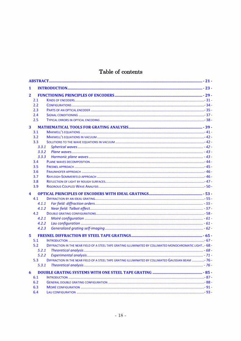
Table of contentsTable of contentsTable of contentsTable of contents

ABSTRACT ...................................................................................................................................................................... - 21 -

1 INTRODUCTION.................................................................................................................................................. - 23 -

2 FUNCTIONING PRINCIPLES OF ENCODERS ............................................................................................... - 29 - 2.1 KINDS OF ENCODERS...............................................................................................................................- 31 - 2.2 CONFIGURATIONS ..................................................................................................................................- 34 - 2.3 PARTS OF AN OPTICAL ENCODER ...............................................................................................................- 35 - 2.4 SIGNAL CONDITIONING ...........................................................................................................................- 37 - 2.5 TYPICAL ERRORS IN OPTICAL ENCODING ......................................................................................................- 38 -

3 MATHEMATICAL TOOLS FOR GRATING ANALYSIS ................................................................................ - 39 - 3.1 MAXWELL’S EQUATIONS .........................................................................................................................- 41 - 3.2 MAXWELL’S EQUATIONS IN VACUUM .........................................................................................................- 42 - 3.3 SOLUTIONS TO THE WAVE EQUATIONS IN VACUUM .......................................................................................- 42 -

3.3.1 Spherical waves ........................................................................................................................... - 42 - 3.3.2 Plane waves ................................................................................................................................. - 43 - 3.3.3 Harmonic plane waves ................................................................................................................ - 43 -

3.4 PLANE WAVES DECOMPOSITION ................................................................................................................- 44 - 3.5 FRESNEL APPROACH ...............................................................................................................................- 45 - 3.6 FRAUNHOFER APPROACH ........................................................................................................................- 46 - 3.7 RAYLEIGH-SOMMERFELD APPROACH .........................................................................................................- 46 - 3.8 REFLECTION OF LIGHT BY ROUGH SURFACES.................................................................................................- 47 - 3.9 RIGOROUS COUPLED WAVE ANALYSIS .......................................................................................................- 50 -

4 OPTICAL PRINCIPLES OF ENCODERS WITH IDEAL GRATINGS .......................................................... - 53 - 4.1 DIFFRACTION BY AN IDEAL GRATING...........................................................................................................- 55 -

4.1.1 Far field: diffraction orders .......................................................................................................... - 55 - 4.1.2 Near field: Talbot effect............................................................................................................... - 57 -

4.2 DOUBLE GRATING CONFIGURATIONS ..........................................................................................................- 58 - 4.2.1 Moiré configuration .................................................................................................................... - 61 - 4.2.2 Lau configuration ........................................................................................................................ - 61 - 4.2.3 Generalized grating self-imaging ................................................................................................ - 62 -

5 FRESNEL DIFFRACTION BY STEEL TAPE GRATINGS ............................................................................. - 65 - 5.1 INTRODUCTION .....................................................................................................................................- 67 - 5.2 DIFFRACTION IN THE NEAR FIELD OF A STEEL TAPE GRATING ILLUMINATED BY COLLIMATED MONOCHROMATIC LIGHT ..- 68 -

5.2.1 Theoretical analysis ..................................................................................................................... - 68 - 5.2.2 Experimental analysis .................................................................................................................. - 71 -

5.3 DIFFRACTION IN THE NEAR FIELD OF A STEEL TAPE GRATING ILLUMINATED BY COLLIMATED GAUSSIAN BEAM ............- 76 - 5.3.1 Theoretical analysis ..................................................................................................................... - 76 -

6 DOUBLE GRATING SYSTEMS WITH ONE STEEL TAPE GRATING ...................................................... - 85 - 6.1 INTRODUCTION .....................................................................................................................................- 87 - 6.2 GENERAL DOUBLE GRATING CONFIGURATION ..............................................................................................- 88 - 6.3 MOIRÉ CONFIGURATION .........................................................................................................................- 91 - 6.4 LAU CONFIGURATION .............................................................................................................................- 93 -

- 19 -

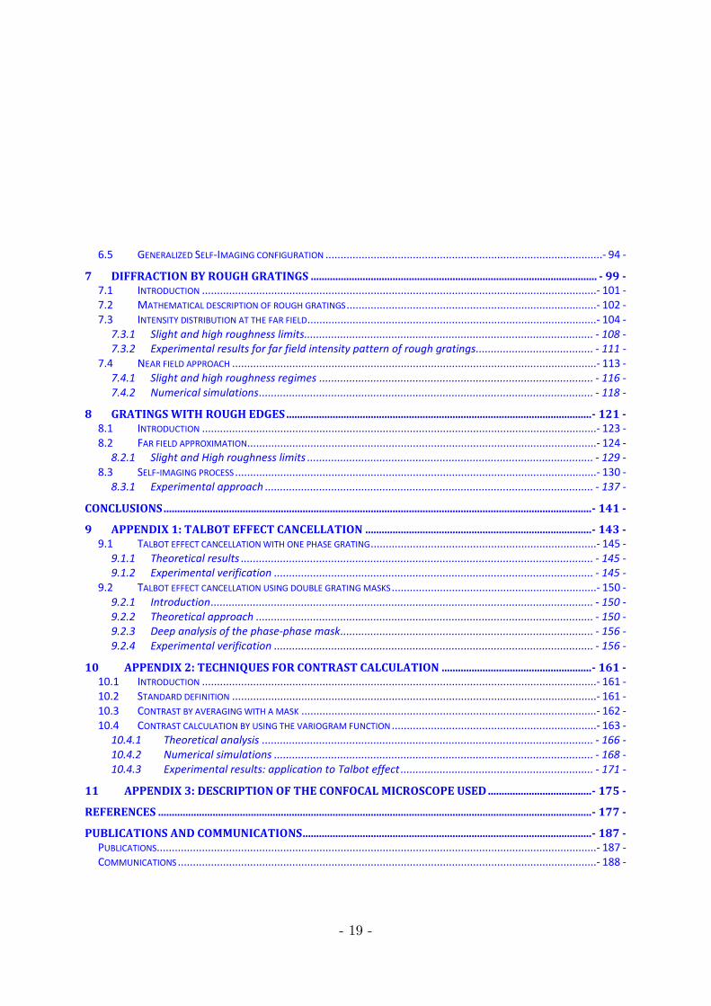
6.5 GENERALIZED SELF-IMAGING CONFIGURATION ............................................................................................- 94 -

7 DIFFRACTION BY ROUGH GRATINGS ......................................................................................................... - 99 - 7.1 INTRODUCTION ...................................................................................................................................- 101 - 7.2 MATHEMATICAL DESCRIPTION OF ROUGH GRATINGS ...................................................................................- 102 - 7.3 INTENSITY DISTRIBUTION AT THE FAR FIELD ................................................................................................- 104 -

7.3.1 Slight and high roughness limits................................................................................................ - 108 - 7.3.2 Experimental results for far field intensity pattern of rough gratings ....................................... - 111 -

7.4 NEAR FIELD APPROACH .........................................................................................................................- 113 - 7.4.1 Slight and high roughness regimes ........................................................................................... - 116 - 7.4.2 Numerical simulations ............................................................................................................... - 118 -

8 GRATINGS WITH ROUGH EDGES ................................................................................................................ - 121 - 8.1 INTRODUCTION ...................................................................................................................................- 123 - 8.2 FAR FIELD APPROXIMATION....................................................................................................................- 124 -

8.2.1 Slight and High roughness limits ............................................................................................... - 129 - 8.3 SELF-IMAGING PROCESS ........................................................................................................................- 130 -

8.3.1 Experimental approach ............................................................................................................. - 137 -

CONCLUSIONS ............................................................................................................................................................. - 141 -

9 APPENDIX 1: TALBOT EFFECT CANCELLATION ................................................................................... - 143 - 9.1 TALBOT EFFECT CANCELLATION WITH ONE PHASE GRATING ...........................................................................- 145 -

9.1.1 Theoretical results ..................................................................................................................... - 145 - 9.1.2 Experimental verification .......................................................................................................... - 145 -

9.2 TALBOT EFFECT CANCELLATION USING DOUBLE GRATING MASKS ....................................................................- 150 - 9.2.1 Introduction ............................................................................................................................... - 150 - 9.2.2 Theoretical approach ................................................................................................................ - 150 - 9.2.3 Deep analysis of the phase-phase mask .................................................................................... - 156 - 9.2.4 Experimental verification .......................................................................................................... - 156 -

10 APPENDIX 2: TECHNIQUES FOR CONTRAST CALCULATION ....................................................... - 161 - 10.1 INTRODUCTION ...................................................................................................................................- 161 - 10.2 STANDARD DEFINITION .........................................................................................................................- 161 - 10.3 CONTRAST BY AVERAGING WITH A MASK ..................................................................................................- 162 - 10.4 CONTRAST CALCULATION BY USING THE VARIOGRAM FUNCTION ....................................................................- 163 -

10.4.1 Theoretical analysis .............................................................................................................. - 166 - 10.4.2 Numerical simulations .......................................................................................................... - 168 - 10.4.3 Experimental results: application to Talbot effect ................................................................ - 171 -

11 APPENDIX 3: DESCRIPTION OF THE CONFOCAL MICROSCOPE USED ...................................... - 175 -

REFERENCES ............................................................................................................................................................... - 177 -

PUBLICATIONS AND COMMUNICATIONS .......................................................................................................... - 187 - PUBLICATIONS ..................................................................................................................................................- 187 - COMMUNICATIONS ...........................................................................................................................................- 188 -

- 20 -

- 21 -

AbstractAbstractAbstractAbstract

In this Thesis work we present theoretical, numerical and experimental analyses of the behavior of non-perfect diffraction gratings. We have performed an analysis of diffraction gratings engraved on a steel tape. This kind of gratings can be found in industrial devices such as optical encoders for long range measurements (> 3 m). The main objectives of this Thesis work are to find a theoretical formalism which describes the behavior of this kind of gratings in near and far field approaches. We also propose a new kind of diffraction grating based on periodical variations in the micro-topographic properties of the surface. Besides, we analyze other kind of imperfections in gratings like rough edges, which can be produced during the fabrication process. Another important result is the cancellation of Talbot effect using masks formed by two gratings. This Thesis work has been motivated by a long collaboration with private industry related with fabrication of high accuracy metrology systems.

- 22 -

- 23 -

1111 IntroductionIntroductionIntroductionIntroduction

Diffraction gratings are elements which produce periodical changes in one or more properties of the incident light beam, [1]-[4]. These elements have been analyzed and used since late XVIII century. The most common kinds of diffraction gratings are amplitude and phase gratings. Amplitude gratings are composed by strips which alternatively allow and no-allow crossing the light. Thus, just after the grating the field is composed by bright and dark fringes. On the other hand, phase gratings produce a modulation in the phase of the incident beam. They are preferred in many applications since all the light passes the diffraction grating. This degree of modulation depends on the phase retardation between both levels of the grating, which can vary from zero to 2π . In recent years, other kinds of gratings have been proposed, such as polarization grating [5]-[8]. This family of gratings changes periodically the state of polarization of the incident beam. For example, even strips can be horizontal linear polarizers and odd strips can be linear vertical polarizers.

Taking into account the optical behavior of diffraction gratings, in the near field, a replication of the grating at some distances is produced when it is illuminated by monochromatic collimated light. This effect is known as Talbot effect [9]. Several works on the subject have been performed recently analyzing Talbot effect for oblique angle of light propagation [10], polychromatic light [11], partial coherent light illumination [12], when the grating presents different kinds of flaws [13], and when polarized light is used [14].

- 24 -

On the other hand, considering the applications of diffraction gratings, they can be found in a lot of different research fields as photonics, chemistry, biology, astrophysics, mechanical engineering, etc, and different devices, such as linear optical encoders, nanopositioners, colorimeters, telescopes, spectrometers, machine tools, etc. It can also be found in multitude of specific applications such as spectroscopy, optical metrology, moiré interferometry, laser array illumination, phase locking of a laser array, etc. [15]-[18].

In our case, and due to a long collaboration with industry, the analysis and improvement of linear optical encoders is a very important research line in our group. Optical encoders are used to control and measure the relative or absolute displacement between two different parts of other device, [19].

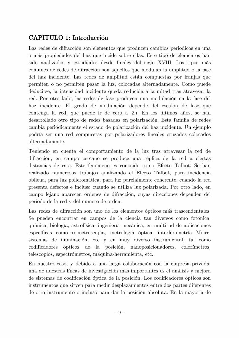
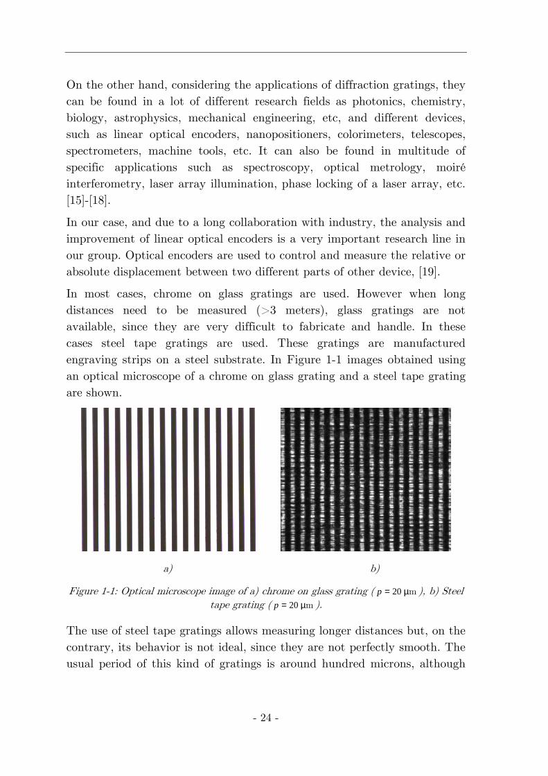
In most cases, chrome on glass gratings are used. However when long distances need to be measured (>3 meters), glass gratings are not available, since they are very difficult to fabricate and handle. In these cases steel tape gratings are used. These gratings are manufactured engraving strips on a steel substrate. In Figure 1-1 images obtained using an optical microscope of a chrome on glass grating and a steel tape grating are shown.

a) b)

Figure 1-1: Optical microscope image of a) chrome on glass grating ( 20p = µm ), b) Steel tape grating ( 20p = µm ).

The use of steel tape gratings allows measuring longer distances but, on the contrary, its behavior is not ideal, since they are not perfectly smooth. The usual period of this kind of gratings is around hundred microns, although

1. Introduction

- 25 -

in recent years lower period steel tape gratings have been manufactured. When the period of the grating is high, its behavior can be analyzed from a geometrical point of view, but for lower periods, diffractive effects appear and Talbot effect becomes important. In this thesis work we have analyzed the behavior or these gratings in the Fresnel and Fraunhofer regimes, showing the Talbot effect is produced for near distances, [20]. For this, we have considered the roughness of the grating and we have modeled it by means of a random distribution of the topography, [21]. This random distribution can be modeled giving its second order statistical properties, its correlation length and standard deviation. We have observed that the contrast of the self-images decays in terms of the correlation length, being this decay gaussian or exponential depending on the statistical distribution that describes the random topography. In addition, for far distances (Fraunhofer regime), we have found that the width of the diffraction orders increases in terms of the correlation length of the roughness, [22].

Since these gratings are used in optical encoders with double grating configurations, we have analyzed the three most common configurations used in optical codification, but introducing a steel tape grating into the system. These configurations are Moiré, Lau and Generalized Self-imaging. In Moiré case, contrast of the signals disappears when we separate both gratings farer from a certain distance. This distance depends on the correlation length of the roughness. On the other hand, contrast of the self-images remains for Lau and Generalized Self-imaging configurations, [23]. Although, the depth of focus of the self-images decreases in terms of the roughness parameters in Generalized Self-Imaging configuration.

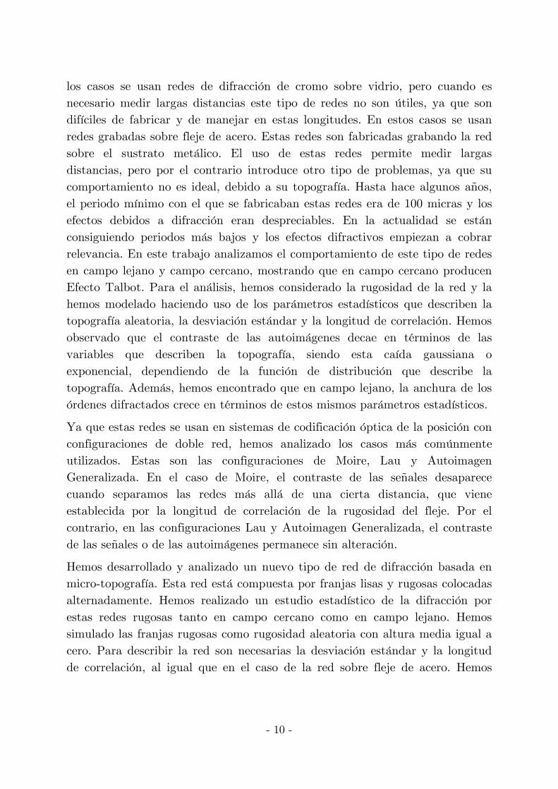
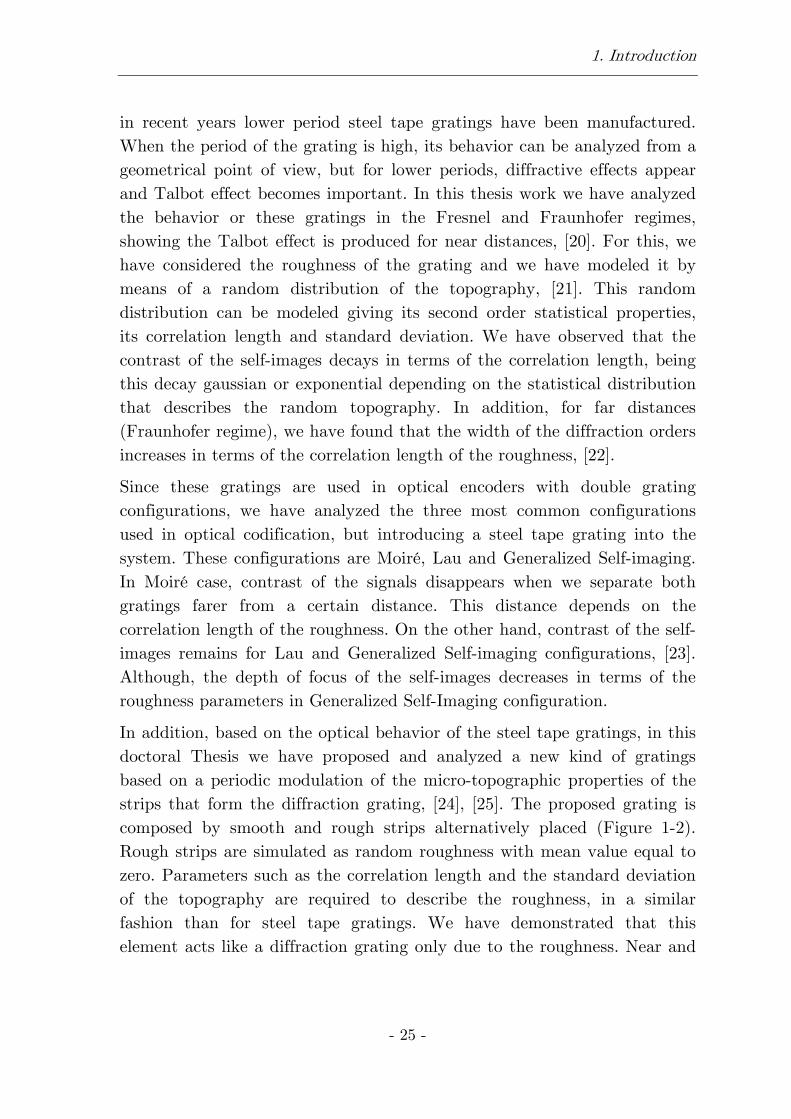
In addition, based on the optical behavior of the steel tape gratings, in this doctoral Thesis we have proposed and analyzed a new kind of gratings based on a periodic modulation of the micro-topographic properties of the strips that form the diffraction grating, [24], [25]. The proposed grating is composed by smooth and rough strips alternatively placed (Figure 1-2). Rough strips are simulated as random roughness with mean value equal to zero. Parameters such as the correlation length and the standard deviation of the topography are required to describe the roughness, in a similar fashion than for steel tape gratings. We have demonstrated that this element acts like a diffraction grating only due to the roughness. Near and

- 26 -

far field analysis have been performed showing a different behavior compared to the standard amplitude and phase gratings behavior.

Figure 1-2: Grating with microscopic roughness ( p is the period and α is the fill factor).

In Fresnel regime, self-images of the grating appear, more or less like those that are produced by an amplitude grating, [25], but gradually. On the other hand, in Fraunhofer regime, diffraction orders are produced, although at the same time, a halo of light around each order appears, [24].

Other kinds of imperfections in diffraction gratings have been analyzed, such as that the edges of the strips are not perfectly smooth but rough. Near field approach has been applied to analyze these gratings, [26]. Analytical expressions for the intensity distribution in the near field have been obtained in the cases where it is possible. In other cases, numerical simulations using the Rayleigh-Sommerfeld approach, [27], or the Rigorous Coupled Wave Analysis method, [28]-[30], have been obtained. Besides, experimental verifications of the obtained results have been performed in most cases.

A very important handicap in optical encoders design is that, in general, diffraction gratings produce Talbot effect in the near field. Due to this, we have focused on the cancellation of Talbot effect by using one or two diffraction gratings. For the case of one diffraction grating we have found that Talbot effect cancellation occurs for a phase grating under certain restricted conditions. On the other hand, we have found that it is possible to cancel Talbot effect using two gratings, even quadrupling the frequency of the fringes. This fact may improve the accuracy of optical encoders without needing gratings with low period. Besides, it also can improve the mechanical tolerances of the devices.

1. Introduction

- 27 -

To conclude, along this thesis work, contrast calculation has been performed many times. The signals are not perfect and we have had to developed a method based on the variogram function, which improve the results obtained using the standard definition of contrast in experimental measurements.

- 29 -

2222 Functioning principles of encodersFunctioning principles of encodersFunctioning principles of encodersFunctioning principles of encoders

In this chapter, a brief introduction of the functioning principles of an encoder for measuring linear or angular displacements is shown. All types of encoders, such as magnetic and optical, or based on diffractive or interferometric effects are explained. Besides, configurations for single and double grating encoders are explained. The different parts which compound an encoder, such as the scale and the reading head, are shown. After, it is also shown how the optical or magnetic signals are transformed to electrical signals that allow measuring the movement or absolute position of the reading head with respect to the scale. In addition, the typical measurement errors are described.

- 30 -

2. Functioning principles of encoders

- 31 -

2.12.12.12.1 Kinds of encodersKinds of encodersKinds of encodersKinds of encoders

From a general point of view, an encoder is a device which provides the relative displacement between a fixed scale and a moveable reading head [31]-[37]. There are also encoders which give the absolute position using reference signals or pseudorandom codes, [38]-[41].

Attending to the physical background which allows the functioning of the encoder, we can separate them in optical and magnetic encoders, [42]-[45]. The scale in magnetic encoders is composed by north and south poles placed alternatively. The reading head moves on the scale and detects the variations of the magnetic field. There are magnetic encoders based on Hall effect, [45], and in magnetoresitive effects, [44]. Those based on Hall effect detect the variation in the magnetic field produced on a voltage. On the contrary, those based on magnetoresistive effects detect the variation in a resistance due to the magnetic field. The scale in optical encoders, except in interferometric, is a diffraction grating (Figure 2-1).

Figure 2-1: Chrome on glass diffraction grating showing the scale.

As optical encoders, we can find based on interferometry, others based on diffraction and others based on interfero-diffraction.

Interferometric encoders are in fact interferometers, as Michelson or Mach-Zender interferometers, [46], [47]. The phase retardation between both arms of the interferometer produces interferences when both beams are collected on the same place. Every oscillation in the intensity pattern corresponds to

- 32 -

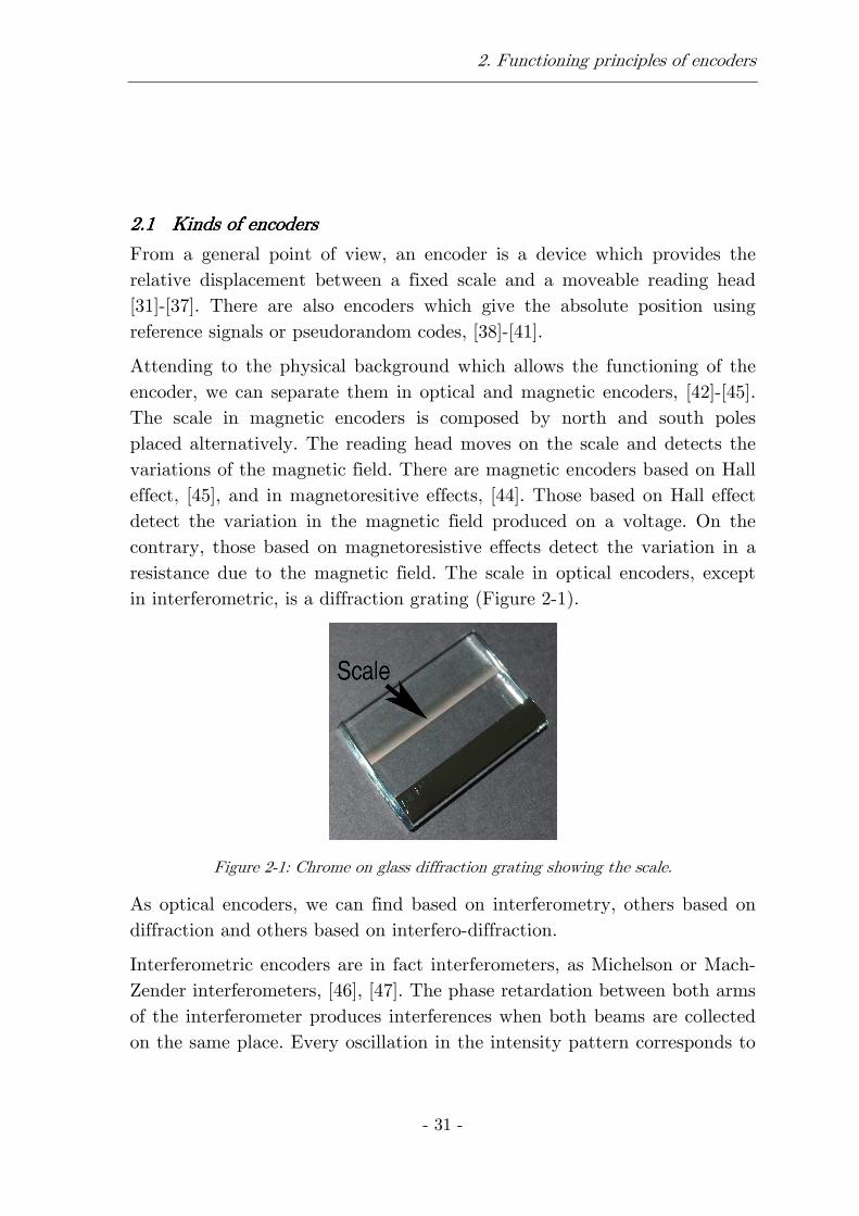
a half wavelength displacement. This kind of encoders is the most accurate but it needs very stable wavelength and very clean environment. They are normally used for lab applications and for calibrating other kinds of encoders, [46]. As an example, in Figure 2-2 it is shown an example of encoder based on interferometry.

Figure 2-2: Twynman-Green interferometer.

In this case, it is a Twynman-Green interferometer but other kinds of interferometers, as Michelson or Mach-Zender are possible. The beam splitter divides the light into two different beams, which after impinge to the cube corners, are recovered and mixed to generate the fluctuations in the output beam, which gives the displacement of one of the arms of the interferometer with respect to the other one. In some cases, polarizing elements are included to detect the sense of the movement.

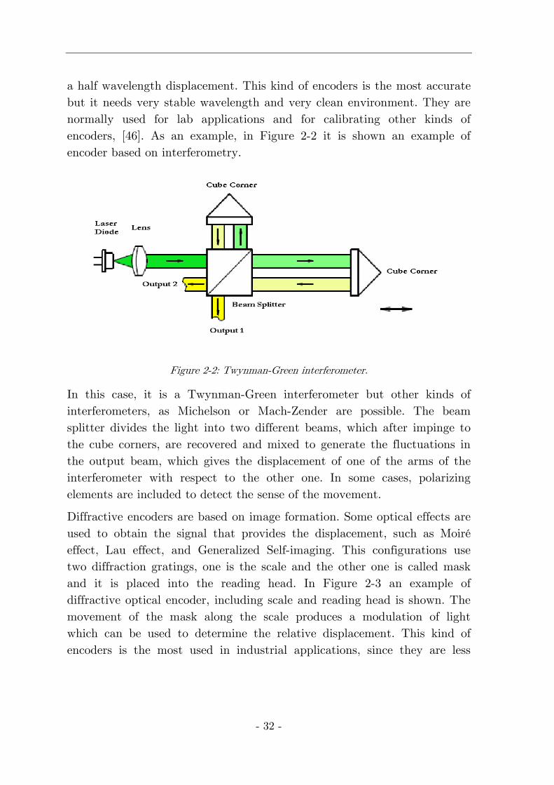
Diffractive encoders are based on image formation. Some optical effects are used to obtain the signal that provides the displacement, such as Moiré effect, Lau effect, and Generalized Self-imaging. This configurations use two diffraction gratings, one is the scale and the other one is called mask and it is placed into the reading head. In Figure 2-3 an example of diffractive optical encoder, including scale and reading head is shown. The movement of the mask along the scale produces a modulation of light which can be used to determine the relative displacement. This kind of encoders is the most used in industrial applications, since they are less

2. Functioning principles of encoders

- 33 -

restrictive than interferometric encoders with respect environmental conditions and wavelength stability.

Figure 2-3: Scheme of diffractive transmission optical encoder.

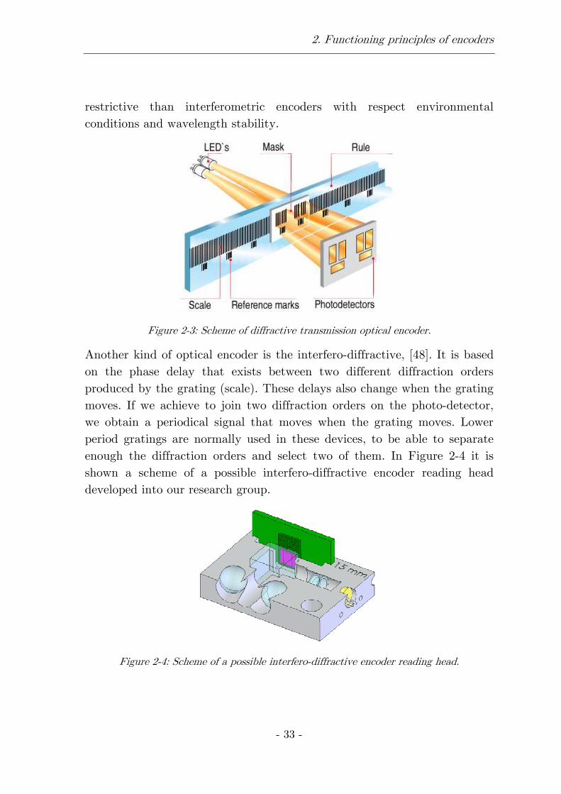
Another kind of optical encoder is the interfero-diffractive, [48]. It is based on the phase delay that exists between two different diffraction orders produced by the grating (scale). These delays also change when the grating moves. If we achieve to join two diffraction orders on the photo-detector, we obtain a periodical signal that moves when the grating moves. Lower period gratings are normally used in these devices, to be able to separate enough the diffraction orders and select two of them. In Figure 2-4 it is shown a scheme of a possible interfero-diffractive encoder reading head developed into our research group.

Figure 2-4: Scheme of a possible interfero-diffractive encoder reading head.

- 34 -

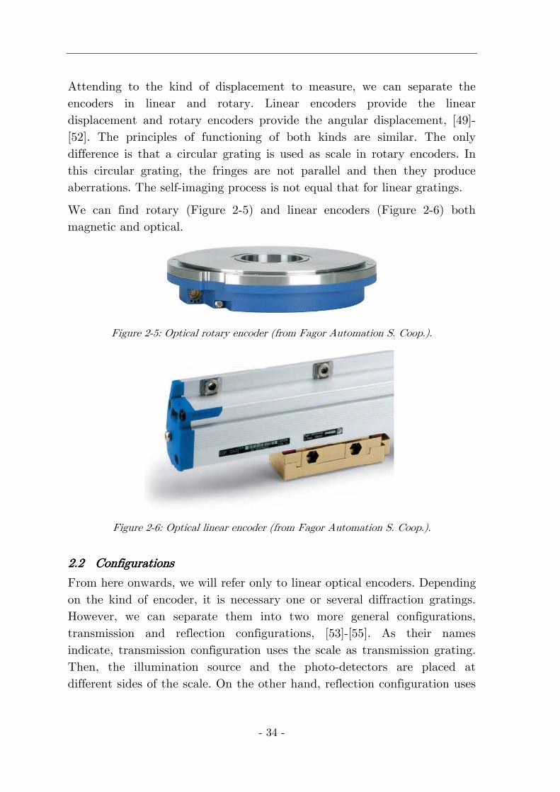
Attending to the kind of displacement to measure, we can separate the encoders in linear and rotary. Linear encoders provide the linear displacement and rotary encoders provide the angular displacement, [49]-[52]. The principles of functioning of both kinds are similar. The only difference is that a circular grating is used as scale in rotary encoders. In this circular grating, the fringes are not parallel and then they produce aberrations. The self-imaging process is not equal that for linear gratings.

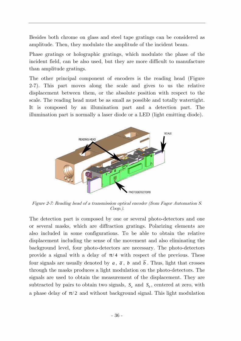
We can find rotary (Figure 2-5) and linear encoders (Figure 2-6) both magnetic and optical.

Figure 2-5: Optical rotary encoder (from Fagor Automation S. Coop.).

Figure 2-6: Optical linear encoder (from Fagor Automation S. Coop.).

2.22.22.22.2 ConfigurationsConfigurationsConfigurationsConfigurations

From here onwards, we will refer only to linear optical encoders. Depending on the kind of encoder, it is necessary one or several diffraction gratings. However, we can separate them into two more general configurations, transmission and reflection configurations, [53]-[55]. As their names indicate, transmission configuration uses the scale as transmission grating. Then, the illumination source and the photo-detectors are placed at different sides of the scale. On the other hand, reflection configuration uses

2. Functioning principles of encoders

- 35 -

the scale as reflection grating and places the illumination source and the photo-detectors at the same side of the scale. For transmission configuration, gratings engraved in glass must be used, since they allow crossing light. On the contrary, for reflection configuration both glass and steel tape gratings can be used.

If we attend now on double grating configurations, we can separate into optical encoders based on Moiré effect, [54], Lau effect, [56], [57] and Generalized Self-imaging, [58]-[60]. With double gratings configurations, we mean that the optical encoder has a mask, which acts as second grating. The particularities of double grating configurations under an optical point of view will be explained more in depth in Section 4.2.

2.32.32.32.3 Parts of an optical encoderParts of an optical encoderParts of an optical encoderParts of an optical encoder

As we have introduced in section 2.1, an encoder can be divided into two different parts, the scale and the reading head. The scale is a diffraction grating. In most cases chrome on glass gratings are used. These gratings are easy to manufactured, even for low periods. We can find chrome on glass gratings from tens of microns to units of microns. These gratings can act as both transmission and reflection gratings. In transmission configuration, the chrome strips act as dark zones but in reflection configuration act as mirrors. Simple theoretical models explain very accurately the experimental behavior of these gratings. When it is necessary to measure long distances (> 3 m), the use of chrome on glass gratings becomes very difficult, since glass is very fragile. In these cases, steel tape gratings are used. Steel tape gratings are diffraction gratings engraved on a steel substrate. In this case, long gratings are easy to manufacture and handle but other problems appear, [20], [22]. Steel tape gratings only can be used in reflection configurations and their optical behavior moves away from ideal. The manufacture method and also the self nature of the substrate produce roughness on its surface. Roughness produces a decreasing of the contrast of the Talbot self-images (see Section 4.1.2) in terms of the distance from the grating. This fact is detrimental and must be taken into account for optical encoders designing.

- 36 -

Besides both chrome on glass and steel tape gratings can be considered as amplitude. Then, they modulate the amplitude of the incident beam.

Phase gratings or holographic gratings, which modulate the phase of the incident field, can be also used, but they are more difficult to manufacture than amplitude gratings.

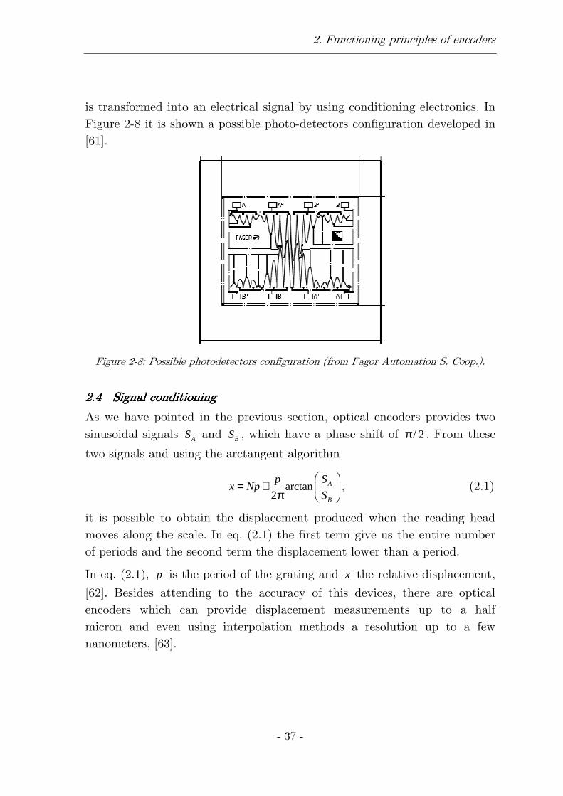
The other principal component of encoders is the reading head (Figure 2-7). This part moves along the scale and gives to us the relative displacement between them, or the absolute position with respect to the scale. The reading head must be as small as possible and totally watertight. It is composed by an illumination part and a detection part. The illumination part is normally a laser diode or a LED (light emitting diode).

Figure 2-7: Reading head of a transmission optical encoder (from Fagor Automation S. Coop.).

The detection part is composed by one or several photo-detectors and one or several masks, which are diffraction gratings. Polarizing elements are also included in some configurations. To be able to obtain the relative displacement including the sense of the movement and also eliminating the background level, four photo-detectors are necessary. The photo-detectors provide a signal with a delay of / 4π with respect of the previous. These

four signals are usually denoted by a , a , b and b . Thus, light that crosses through the masks produces a light modulation on the photo-detectors. The signals are used to obtain the measurement of the displacement. They are subtracted by pairs to obtain two signals, aS and bS , centered at zero, with

a phase delay of / 2π and without background signal. This light modulation

2. Functioning principles of encoders

- 37 -

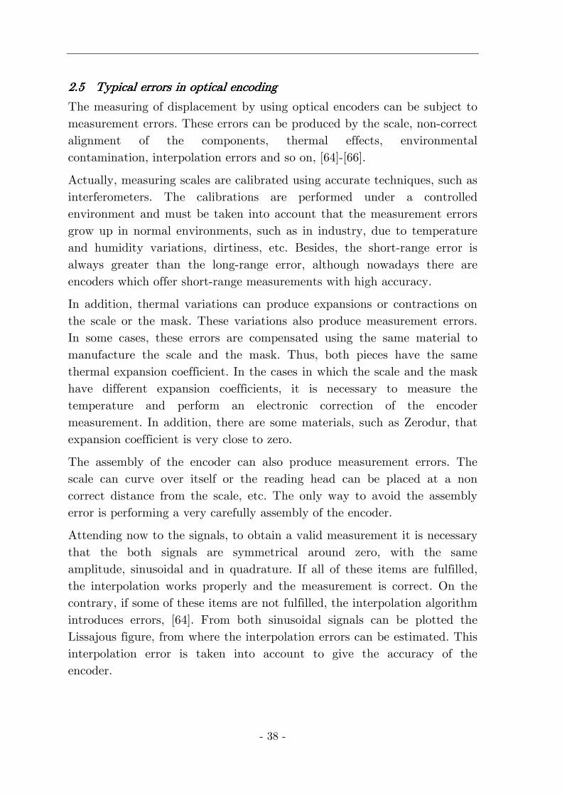
is transformed into an electrical signal by using conditioning electronics. In Figure 2-8 it is shown a possible photo-detectors configuration developed in [61].

Figure 2-8: Possible photodetectors configuration (from Fagor Automation S. Coop.).

2.42.42.42.4 Signal conditioningSignal conditioningSignal conditioningSignal conditioning

As we have pointed in the previous section, optical encoders provides two sinusoidal signals AS and BS , which have a phase shift of / 2π . From these

two signals and using the arctangent algorithm

arctan2

A

B

Spx Np

S

= + π

, (2.1)

it is possible to obtain the displacement produced when the reading head moves along the scale. In eq. (2.1) the first term give us the entire number of periods and the second term the displacement lower than a period.

In eq. (2.1), p is the period of the grating and x the relative displacement,

[62]. Besides attending to the accuracy of this devices, there are optical encoders which can provide displacement measurements up to a half micron and even using interpolation methods a resolution up to a few nanometers, [63].

- 38 -

2.52.52.52.5 Typical errors in optical encodingTypical errors in optical encodingTypical errors in optical encodingTypical errors in optical encoding

The measuring of displacement by using optical encoders can be subject to measurement errors. These errors can be produced by the scale, non-correct alignment of the components, thermal effects, environmental contamination, interpolation errors and so on, [64]-[66].

Actually, measuring scales are calibrated using accurate techniques, such as interferometers. The calibrations are performed under a controlled environment and must be taken into account that the measurement errors grow up in normal environments, such as in industry, due to temperature and humidity variations, dirtiness, etc. Besides, the short-range error is always greater than the long-range error, although nowadays there are encoders which offer short-range measurements with high accuracy.

In addition, thermal variations can produce expansions or contractions on the scale or the mask. These variations also produce measurement errors. In some cases, these errors are compensated using the same material to manufacture the scale and the mask. Thus, both pieces have the same thermal expansion coefficient. In the cases in which the scale and the mask have different expansion coefficients, it is necessary to measure the temperature and perform an electronic correction of the encoder measurement. In addition, there are some materials, such as Zerodur, that expansion coefficient is very close to zero.

The assembly of the encoder can also produce measurement errors. The scale can curve over itself or the reading head can be placed at a non correct distance from the scale, etc. The only way to avoid the assembly error is performing a very carefully assembly of the encoder.

Attending now to the signals, to obtain a valid measurement it is necessary that the both signals are symmetrical around zero, with the same amplitude, sinusoidal and in quadrature. If all of these items are fulfilled, the interpolation works properly and the measurement is correct. On the contrary, if some of these items are not fulfilled, the interpolation algorithm introduces errors, [64]. From both sinusoidal signals can be plotted the Lissajous figure, from where the interpolation errors can be estimated. This interpolation error is taken into account to give the accuracy of the encoder.

- 39 -

3333 Mathematical tools for grating Mathematical tools for grating Mathematical tools for grating Mathematical tools for grating analysisanalysisanalysisanalysis

Along this work, several mathematical tools are applied for analyses and calculations. In this chapter these tools are briefly explained. In the first place, an introduction to the diffraction theory is presented, including Maxwell equations, plane waves decomposition of general waves, Fresnel and Fraunhofer approximations for diffraction, their application to a diffraction grating, and Rayleigh-Sommerfeld approach. In a scalar treatment of the problem of diffraction, the thin element approximation (TEA) is used. It consists of the assumption that the diffractive element can be modeled using a transmittance function. This approximation is useful to simplify the calculations but it is not always valid. Nevertheless, this approximation gives a correct result in most cases. When these simple scalar techniques are no valid, Rigorous Coupled Wave Analysis (RCWA) is used since it provides an exact solution of the Maxwell equations for periodical objects.

- 40 -

3. Mathematical tools for grating analysis

- 41 -

3.13.13.13.1 MaxwellMaxwellMaxwellMaxwell’s’s’s’s equationsequationsequationsequations

Maxwell equations provides a theoretical formalism to solve all problems that include electromagnetic fields, [67],[68].

An electromagnetic field is defined using two vectorial quantities, the

electric field ( , )E r t� �

and the magnetic field ( , )H r t� �

. These two quantities are

complex quantities and can be separated into their temporal and spatial dependences. The Maxwell’s equations can be expressed as

0

0 0 0

,

0,

,

,

E

B

BE

t

EB J

t

ρ∇ =ε

∇ =

∂∇ ∧ = −∂

∂∇ ∧ = µ + ε µ∂

�

�

��

�� �

(3.1)

where B� is the magnetic induction, J

� is the electric current, ρ is the

charge density, 0ε is the electric permittivity in vacuum, and 0µ is the

magnetic permeability in vacuum

12 3 1 4 2

0

6 2 20

8,854210 ,

1,256610 .

m kg s A

m kg s A

− −

− − −

ε =

µ = (3.2)

Besides, it is necessary to include the called constitutive relationships, whose linear equations are

,

,

,

B H

D E

J E

= µ

= ε

= σ

� �

� �

� � (3.3)

being µ the magnetic permeability in the medium , ε the electric

permittivity in the medium, D� the displacement vector and σ the

conductivity. An important property of the Maxwell’s equations is that

they are linear. Thus, if 1E� and 2E

� are solutions, also 1 2E E+

� � is solution.

- 42 -

3.23.23.23.2 Maxwell’s equations in vacuumMaxwell’s equations in vacuumMaxwell’s equations in vacuumMaxwell’s equations in vacuum

In this case we consider that there are neither charges nor currents. Then, Maxwell’s equations simplify to

0 0

,

,

0,

0.

BE

t

EB

t

E

B

∂∇ ∧ = −∂

∂∇ ∧ = µ ε∂

∇ =

∇ =

��

��

�

�

(3.4)

From eq. (3.4), it is possible to obtain two wave equations for both components of the electromagnetic field

22

0 0 2

22

0 0 2

,

.

EE

t

BB

t

∂∇ = µ ε∂∂∇ = µ ε∂

��

��

(3.5)

From this, we extract that the electric and magnetic fields must follow a

wave equation with velocity 0 01c = µ ε , which is the velocity of light in

vacuum.

3.33.33.33.3 SolutionSolutionSolutionSolutionssss to the wave equations in vacuumto the wave equations in vacuumto the wave equations in vacuumto the wave equations in vacuum

As we have seen in the previous section, the electromagnetic fields follow a wave equation in their propagation. In addition, its solution depends on the generation of the fields, the characteristics of the medium, source distance, etc. Now some easier solutions to the wave equations in vacuum are shown.

3.3.13.3.13.3.13.3.1 Spherical wavesSpherical wavesSpherical wavesSpherical waves

We take as solution a general expression given by ( , )f r tζ = , which is a

function dependent on the spatial coordinates and time.

The wave equation can be expressed as

( ) ( )2 2

2 2 2

1r r

r v t

∂ ξ ∂ ξ=

∂ ∂, (3.6)

where v is the velocity of light.

3. Mathematical tools for grating analysis

- 43 -

This equation has as solutions, waves on the form

( )

( )

1

2

1,

1.

f vt rr

g vt rr

ξ = −

ξ = + (3.7)

These waves are spherical waves, since they depend on the distance r from the source. One of them goes away from the source and the other one goes to the source.

3.3.23.3.23.3.23.3.2 Plane wavesPlane wavesPlane wavesPlane waves

Plane waves are also solutions of the wave equation. This waves are on the

form ( , ) ( , )V h k r t h t= ⋅ = ζ� �

, with x y zk r k x k y k z⋅ = + + = ζ� �

and ˆkk k u=�

. k is the

wave number. Checking this solution into the wave equation and performing the following variable changes, vt pζ − = , vt qζ + = , we can

express it as

2

0V

p q

∂ =∂ ∂

. (3.8)

Thus, the general solution is

( )( )

1

2

,

.

k

k

V f u r vt

V g u r vt

= ⋅ −

= ⋅ +

� �

� � (3.9)

These functions are dependent on the spatial component parallel to the direction of propagation of the wave.

3.3.33.3.33.3.33.3.3 Harmonic plane wavesHarmonic plane wavesHarmonic plane wavesHarmonic plane waves

This case is very important, since, as it will be shown, every harmonic wave can be break down into a sum of harmonic plane waves. Besides, this solution allows solving the Maxwell equations in an exact way. If the solutions for magnetic and electric field are plane waves

( )( )

0 0

0 0

exp( ),

exp( ).

E r E i k r

B r B i k r

= ⋅

= ⋅

�� �� �

�� �� � (3.10)

- 44 -

Maxwell equations solve easily obtaining for the electric field

2 2

2

cE k E= −

ω

�� �, (3.11)

with ω the frequency, λ the wavelength and / 2 /k c= ω = π λ . From here the exact solutions for magnetic and electric fields result

( )( )

0

0

, exp ( ) ,

, exp ( ) .

E r t E i k r t

B r t B i k r t

= ⋅ − ω

= ⋅ − ω

�� �� �

�� �� � (3.12)

3.43.43.43.4 Plane wavesPlane wavesPlane wavesPlane waves decompositiondecompositiondecompositiondecomposition

A useful procedure to solve the propagation of a general harmonic wave is decomposing it as a sum of harmonic plane waves. As we have shown before, Maxwell equations are linear and then a sum of solutions is also solution. This decomposition is possible since plane waves are an orthogonal base of functions. From this, we can propagate every plane wave separately and obtain the total result as a sum of the propagated waves. Supposing that the initial field in two-dimensions is

0( 0, 0) ( , )E z t E= = = ξ η� �

, and using the Fourier transform, it can be

decomposed in planes waves resulting

( )2

0 0

1 ˆ( , ) ( , )e2

x yi k k

x y x yE E k k dk dkξ+ η ξ η = π

∫ ∫�

. (3.13)

The spatial frequency spectrum is obtained as

( )0 0

ˆ ( , ) ( , )e x yi k k

x yE k k E d d− ξ+ η= ξ η ξ η∫ ∫

�. (3.14)

A plane wave propagates in vacuum, according to Maxwell equations, as

( )2

( , ) 0

1 ˆ( , , ) ( , )e e2

x y z

x y

i k x k y k z i tk k x yE x y z E k k

+ + − ω = π

�, (3.15)

where the components of k� must follow the relationship

( )22 2 2 2 2 /x y zk k k k+ + = = π λ . So it also must be fulfilled that 2 2 2z x yk k k k= − + .

After propagating every plane wave, the field is calculated as the summation of them, resulting

3. Mathematical tools for grating analysis

- 45 -

( )2

0

1 ˆ( , , ) e ( , )e2

x y zi k x k y k zi tx y x yE x y z E k k dk dk

+ +− ω = π ∫ ∫

�. (3.16)

Using eq. (3.13), eq. (3.14) and reorganizing, the field can be expressed as

0( , , ) ( , ) ( , )E x y z E h x y d d= ξ η − ξ − η ξ η∫ ∫� �

, (3.17)

where 2 2 22

1( , ) e

2

x y x yi k k k k k z

x yh dk dk ξ+ η+ − − ξ η = π

∫ ∫ is the two-dimensional Green

function.

3.53.53.53.5 Fresnel approach Fresnel approach Fresnel approach Fresnel approach

Eq. (3.17) cannot be solved analytically in most cases. However, we can perform some approximations in the Green function ( , )h ξ η . Assuming that

( )2 2 2 2 2 / 2x y x yk k k k k k k− − ≈ − + , the Green function can be calculated as

2

2 21 1 1( , ) e exp exp

2 2 2ikz

x x x y y y

z zh i k k dk i k k dk

k k

ξ η = − + ξ − + η π ∫ ∫ ,

(3.18)

resulting

( )2 21 1( , ) exp

2h ik z

i z z

ξ η = + ξ + η λ . (3.19)

Introducing eq. (3.19) into eq. (3.17) it is obtained the Fresnel Approximation for diffraction

( ) ( ) ( )2 2

0

1( , , ) e ( , ) , exp

2ikz k

E x y z E t i x y d di z z

= ξ η ξ η − ξ + − η ξ η λ ∫ ∫

� �, (3.20)

where we have introduced the factor ( ),t ξ η which represents the

transmittance of a diffractive element under TEA approximation.

According to the Thin Element Approximation, TEA, the field just after the diffraction grating can be computed as the multiplication of the

incident field ( ),iE ξ η and the Complex Amplitude Transmittance of the

diffraction grating ( ),t ξ η

( ) ( ) ( )0 , , ,iE E tξ η = ξ η ξ η , (3.21)

- 46 -

where ( ),t ξ η is

( ) ( )0, ( , )exp ( , )t A ik n n hξ η = ξ η − ξ η , (3.22)

being n the refraction index of the diffraction grating, 0n the refraction

index of the surrounding medium, ( , )h ξ η the profile of the grating and

( , )A ξ η the amplitude of the grating.

3.63.63.63.6 Fraunhofer approach Fraunhofer approach Fraunhofer approach Fraunhofer approach

There are a lot of applications in which the observation plane is situated far from the source. In this case, the Green function can be approximated by its linear term and the field can be calculated as

( )2 2

( )2 ( )

0( , , ) ( , ) ,

x yik z kz i x y

ze

E x y z E t e d di z

++− ξ+ η

= ξ η ξ η ξ ηλ ∫

�, (3.23)

where we have introduced also the factor ( ),t ξ η which is the transmittance

of a diffractive element.

3.73.73.73.7 RayleighRayleighRayleighRayleigh----Sommerfeld approachSommerfeld approachSommerfeld approachSommerfeld approach

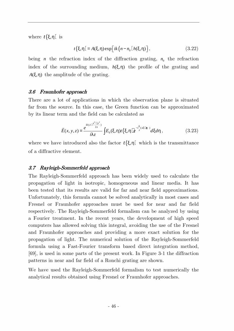
The Rayleigh-Sommerfeld approach has been widely used to calculate the propagation of light in isotropic, homogeneous and linear media. It has been tested that its results are valid for far and near field approximations. Unfortunately, this formula cannot be solved analytically in most cases and Fresnel or Fraunhofer approaches must be used for near and far field respectively. The Rayleigh-Sommerfeld formalism can be analyzed by using a Fourier treatment. In the recent years, the development of high speed computers has allowed solving this integral, avoiding the use of the Fresnel and Fraunhofer approaches and providing a more exact solution for the propagation of light. The numerical solution of the Rayleigh-Sommerfeld formula using a Fast-Fourier transform based direct integration method, [69], is used in some parts of the present work. In Figure 3-1 the diffraction patterns in near and far field of a Ronchi grating are shown.

We have used the Rayleigh-Sommerfeld formalism to test numerically the analytical results obtained using Fresnel or Fraunhofer approaches.

3. Mathematical tools for grating analysis

- 47 -

x (µm)

y (µ

m)

−200 −100 0 100 200

−200

−100

0

100

200

x (µm)

y (µ

m)

−10 0 10−15

−10

−5

0

5

10

15

a) b)

Figure 3-1: Examples of diffraction by a Ronchi grating performed using the Rayleigh-Sommerfeld approach, a) Fresnel regime, b) Fraunhofer regime.

To obtain the diffraction orders image it is necessary to include a lens and take the intensity at its focal plane. The main problems of this method are the edge effects and the accuracy. This approach takes a finite window to calculate the propagation of light. Edge effects appear and then, only the central region of the pattern is exact when the element that is simulated is infinite. The number of points in which is divided the field is critical and the method can give a wrong result. These two effects must be taken into account when this formalism is used.

3.83.83.83.8 Reflection of light by Reflection of light by Reflection of light by Reflection of light by rough rough rough rough surfacessurfacessurfacessurfaces

When a wave impinges into a smooth plane which separates two different media its behavior is longer known, [68]. If both media are transparent, the light which crosses the plane behaves following the well known Snell law. This law tells to us the direction which takes the refracted light if we know previously the index of diffraction and the angle of incidence. Light which is reflected, takes the specular direction. By using the Fresnel coefficients for reflection and transmission, the reflected and transmitted light is obtained.

- 48 -

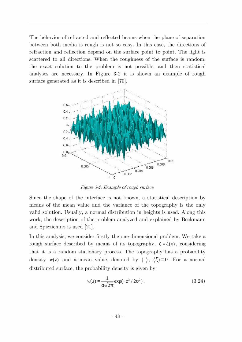
The behavior of refracted and reflected beams when the plane of separation between both media is rough is not so easy. In this case, the directions of refraction and reflection depend on the surface point to point. The light is scattered to all directions. When the roughness of the surface is random, the exact solution to the problem is not possible, and then statistical analyses are necessary. In Figure 3-2 it is shown an example of rough surface generated as it is described in [70].

Figure 3-2: Example of rough surface.

Since the shape of the interface is not known, a statistical description by means of the mean value and the variance of the topography is the only valid solution. Usually, a normal distribution in heights is used. Along this work, the description of the problem analyzed and explained by Beckmann and Spizzichino is used [21].

In this analysis, we consider firstly the one-dimensional problem. We take a rough surface described by means of its topography, ( )xζ = ζ , considering

that it is a random stationary process. The topography has a probability

density ( )w z and a mean value, denoted by , 0ζ = . For a normal

distributed surface, the probability density is given by

2 21( ) exp( / 2 )

2w z z= − σ

σ π, (3.24)

3. Mathematical tools for grating analysis

- 49 -

where σ is the standard deviation. On the other hand, the characteristic function associated with a normal distribution is given by

2 2( ) exp( / 2)zv vχ = −σ , (3.25)

being zv the z-component of a vector in the scattering direction. Besides,

we define the correlation coefficient between two different points separated a distance τ as

( ) 2 2exp( / )C Tτ = −τ , (3.26)

where T is the correlation length. Then, the surface is described by means of its standard deviation, σ , and its correlation length, T .

The two-dimensional normal distribution of two variables with standard deviations σ and correlated by a correlation coefficient C is given by

2 21 1 2 2

1 2 2 22 2

21( , ) exp

2 (1 )2 (1 )

z Cz z zw z z

CC

− += − σ −πσ − . (3.27)

From eq. (3.27), the characteristic function is given by

2 22( , ) exp (1 )z z zv v v C χ − = − σ − . (3.28)

Introducing (3.26) into (3.28) and performing a series expansion, the characteristic function results

( ) 2 22

0

( , ) exp exp /!

m

z zm

gv v g m T

m

∞

=

χ − = − − τ ∑ , (3.29)

with [ ]2 21 2cos( ) cos( ) 2 /zg v= σ = θ + θ π λ , 1θ the incidence angle and 2θ the

scattering angle, with respect of the normal vector to the surface.

From these results, we can assume the characteristic function of a surface

as 2 ( ) *( ')t x t xχ = , being ( )t x its transmittance or reflectance.

The solution of the problem shown in [21] is for a general rough surface but the description and its use involving diffraction gratings will be explained more in depth into the next chapters.

- 50 -

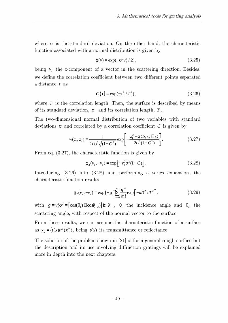
3.93.93.93.9 Rigorous Coupled Wave AnalysisRigorous Coupled Wave AnalysisRigorous Coupled Wave AnalysisRigorous Coupled Wave Analysis

Rigorous Coupled Wave Analysis (RCWA) is a rigorous electromagnetic technique to obtain the diffracted fields and intensity by an optical element in the near field, [28]-[30], solving numerically the Maxwell´s equations. This is a vectorial treatment of the problem and it is restricted to periodical elements. RCWA method is used when it is not possible to apply the Thin Element Approximation (TEA) to the optical element under analysis. Due to this vectorial character, it is very useful for analyzing diffraction gratings with period on the order of the wavelength, where a classical analysis is not valid, and also for obtaining the behavior of the element under different beam polarization states. This method is based on a decomposition of the diffractive element in several regions and layers. We obtain better results in terms of the number of layers in which we decompose the grating. The propagation trough the grating is decomposed using a Fourier analysis. It generates second order differential equations, which can be solved using matrix techniques. The obtained results are exact since this method solves exactly the Maxwell´s equations except for numerical errors (discretization, truncations, etc). Besides, it allows calculating the field for transversal magnetic (TM) and transversal electric (TE) polarizations. Unfortunately, for longer periods the calculations are too slow.

From the Fourier analysis and taking into account that the element is periodical, we can extract the field in the first region, Figure 3-3. The field in the first region is the sum of the incident wave, which we suppose plane wave, and a discrete number of reflected plane waves, whose coefficients are unknown.

Figure 3-3: Scheme of the problem of diffraction by periodical structures.

3. Mathematical tools for grating analysis

- 51 -

Thus, the electric field in the first region results

( ) ( )1 exp expll

E i R i∞

=−∞= + ⋅ + − ⋅∑1 1lk r k r , (3.30)

where 1i = − , ⋅1k r the incident beam direction, lR are the reflectance

coefficients and ⋅1lk r are the directions of the reflected waves. In the third

region, the field can be also represented by a sum of transmitted plane waves

( )3 ˆexpll

E T i∞

=−∞= − ⋅ ∑ 3lk r-dz , (3.31)

where lT are the transmittance coefficients, ( )ˆ⋅3lk r-dz the directions of the

transmitted beams and ˆdz the thickness of the diffractive element. The most complicated region is the second region. To solve the field into this region we cut it into N layers. Every layer is described by a particular distribution of the dielectric constant, ( )xε .

Into the second region, the dielectric constant for every layer can be represented by a series expansion as

( ) ( ) ( ),, expn n I III I h nh

x z ihqx∞

=−∞ε = ε + ε − ε ε∑ ɶ , (3.32)

with coefficients ( ) ( ) ( ), 01/ , exp

p

h n np f x z ihqx dxε = −∫ɶ .

The field into the second region is assumed as diffracted waves which propagate along the layer and coupled the energy between the previous and the next layer.

The main objective is to solve the wave equation into every layer. Like outline conditions we have the field which impinges into every layer and the field which goes out from every layer. The wave equations to solve are

( )2 22, 2,, 0n n n nE k x z E∇ + ε = . (3.33)

- 52 -

x (µm)

z (µ

m)

TE

0 5 10 15

0

10

20

30

40

50

1

2

3

4

5

6

7

x (µm)

z (µ

m)

TM

0 5 10 15

0

10

20

30

40

50

1

2

3

4

5

6

7

a) b)

x (µm)

z (µ

m)

TE

0 5 10 15

0

10

20

30

40

50

0.5

1

1.5

2

2.5

3

3.5

4

x (µm)

z (µ

m)

TM

0 5 10 15

0

10

20

30

40

50

0.5

1

1.5

2

2.5

3

3.5

c) d)

Figure 3-4: a) TE intensity pattern (phase Ronchi grating), b) TM intensity pattern (phase Ronchi grating), c) TE intensity pattern (amplitude Ronchi grating), d) TM intensity pattern (amplitude Ronchi grating).

This problem can be represented in a matrix way, where the unknown factors are the reflection and transmission coefficients in the first and third regions and the Fourier coefficients of the dielectric constant series expansion for each layer in the second region. This problem is computable and its result is the field all over the space, into the three regions and also in the frontiers. As an example, it is shown the diffracted intensity pattern of amplitude and phase Ronchi gratings for TE and TM, Figure 3-4.

- 53 -

4444 OpticaOpticaOpticaOpticallll principles of principles of principles of principles of encoderencoderencoderencoderssss with with with with ideal gratingsideal gratingsideal gratingsideal gratings

In this chapter a general description of the optical principles of an ideal optical encoder and its possible configurations are described. In first place, we apply the Fresnel and Fraunhofer approaches to a general diffraction grating to obtain the well known Talbot effect and the diffraction orders in near and far field respectively. Secondly, double gratings configurations are analyzed. The most common configurations in optical encoders, such as Moiré, Lau and Generalized Self-imaging, are described in detail. Finally, we show how these configurations are used to measure the displacement.

- 54 -

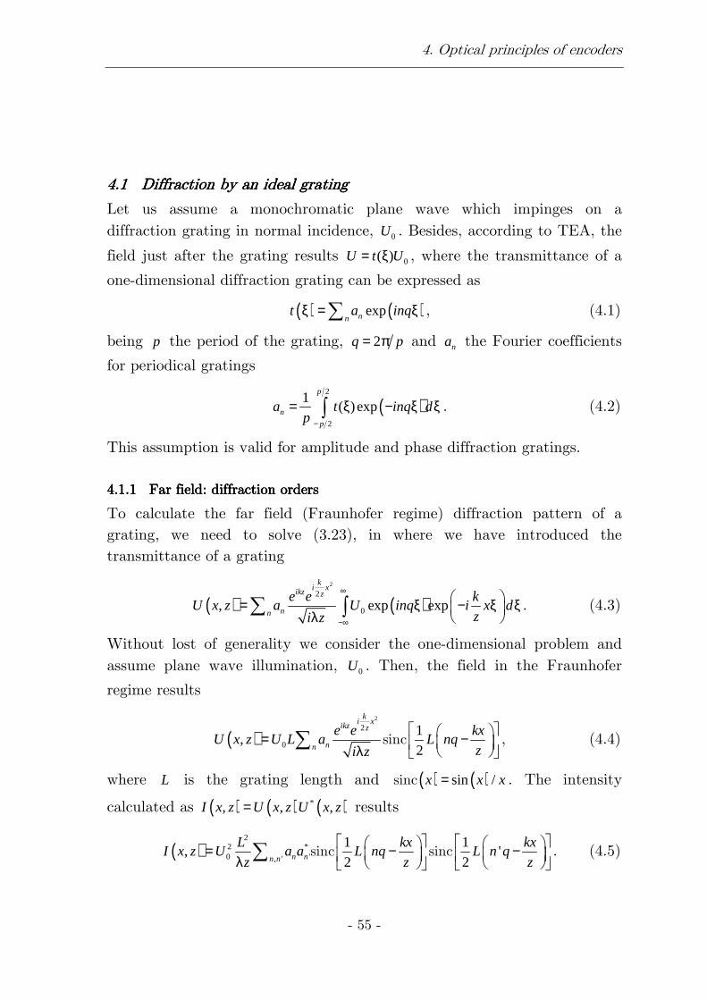
4. Optical principles of encoders

- 55 -

4.14.14.14.1 DiffDiffDiffDiffraction by an ideal gratingraction by an ideal gratingraction by an ideal gratingraction by an ideal grating

Let us assume a monochromatic plane wave which impinges on a diffraction grating in normal incidence, 0U . Besides, according to TEA, the

field just after the grating results 0( )U t U= ξ , where the transmittance of a

one-dimensional diffraction grating can be expressed as

( ) ( )expnnt a inqξ = ξ∑ , (4.1)

being p the period of the grating, 2q p= π and na the Fourier coefficients

for periodical gratings

( )2

2

1( )exp

p

n

p

a t inq dp −

= ξ − ξ ξ∫ . (4.2)

This assumption is valid for amplitude and phase diffraction gratings.

4.1.14.1.14.1.14.1.1 Far field: diffraction ordersFar field: diffraction ordersFar field: diffraction ordersFar field: diffraction orders

To calculate the far field (Fraunhofer regime) diffraction pattern of a grating, we need to solve (3.23), in where we have introduced the transmittance of a grating

( ) ( )2

2

0, exp exp

ki xikz z

nn

e e kU x z a U inq i x d

zi z

∞

−∞

= ξ − ξ ξ λ ∑ ∫ . (4.3)

Without lost of generality we consider the one-dimensional problem and assume plane wave illumination, 0U . Then, the field in the Fraunhofer

regime results

( )2

2

0

1,

2

ki xikz z

nn

e e kxU x z U L a L nq

zi z

= − λ ∑ sinc , (4.4)

where L is the grating length and ( ) ( )sin /x x x=sinc . The intensity

calculated as ( ) ( ) ( )*, , ,I x z U x z U x z= results

( )2

2 *0 ', '

1 1, '

2 2n nn n

L kx kxI x z U a a L nq L n q

z z z

= − − λ ∑ sinc sinc . (4.5)

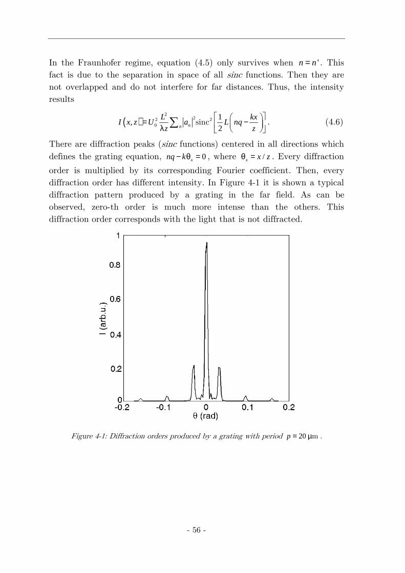
- 56 -

In the Fraunhofer regime, equation (4.5) only survives when 'n n= . This fact is due to the separation in space of all sinc functions. Then they are not overlapped and do not interfere for far distances. Thus, the intensity results

( )2

22 20

1,

2nn

L kxI x z U a L nq

z z

= − λ ∑ sinc . (4.6)

There are diffraction peaks (sinc functions) centered in all directions which defines the grating equation, 0xnq k− θ = , where /x x zθ = . Every diffraction

order is multiplied by its corresponding Fourier coefficient. Then, every diffraction order has different intensity. In Figure 4-1 it is shown a typical diffraction pattern produced by a grating in the far field. As can be observed, zero-th order is much more intense than the others. This diffraction order corresponds with the light that is not diffracted.

Figure 4-1: Diffraction orders produced by a grating with period 20p = µm .

4. Optical principles of encoders

- 57 -

4.1.24.1.24.1.24.1.2 Near field: Talbot effectNear field: Talbot effectNear field: Talbot effectNear field: Talbot effect

To calculate the diffraction pattern of a diffraction grating in the Fresnel regime, it is only necessary to introduce its transmittance into eq. (3.20) and perform the integral. Without lost of generality, we perform the one-

dimensional integral, also considering plane wave illumination, ( ) 0,U Uξ η = .

Then the integral which must be solved is

( ) ( ) ( )

( )

2

0

220

, exp exp2

exp exp2

ikz

nn

nn

e kU x z U a inq i x d

zi z

U qa inqx i n z

kz

∞

−∞

= ξ − ξ ξ λ

= − λ

∑ ∫

∑. (4.7)

After obtaining the field, the intensity in the Fresnel regime can be

calculated easily as ( ) ( ) ( )*, , ,I x z U x z U x z= , resulting

( ) ( ) ( )2 2

* 2 20', '

, exp ' exp '2n nn n

U qI x z a a iqx n n i n n z

z k

= − − λ

∑ . (4.8)

Eq. (4.8) shows that a light modulation is produced in the near field. Modulation is produced along both, the x-axis (first exponential factor) and the z-axis (second exponential factor). The modulation period along the x-axis is equal to the period of the grating. On the contrary, the second exponential factor produces the self-imaging phenomenon. This effect consists of replications of the real grating, that appear periodically after it, every Tz given by

2

T

pz =

λ. (4.9)

This effect is known as Talbot effect and was discovered by H. F. Talbot in 1836 [9]. This effect is very important in designs which include diffraction gratings. In Figure 4-2 the diffraction pattern produced by an amplitude grating in the near field (Fresnel regime) is shown.

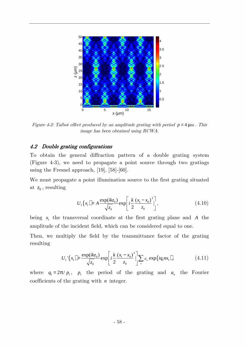
- 58 -

x (µm)

z (µ

m)

0 5 10 15

0

5

10

15

20

25

30

35

40

45

50

0.5

1

1.5

2

2.5

3

3.5

4

Figure 4-2: Talbot effect produced by an amplitude grating with period 4p = µm . This image has been obtained using RCWA.

4.24.24.24.2 Double grating configuratioDouble grating configuratioDouble grating configuratioDouble grating configurationsnsnsns

To obtain the general diffraction pattern of a double grating system (Figure 4-3), we need to propagate a point source through two gratings using the Fresnel approach, [19], [58]-[60].

We must propagate a point illumination source to the first grating situated at 0z , resulting

( )2

0 1 01 1

00

exp( ) ( )exp

2

ikz x xkU x A i

zz

−=

, (4.10)

being 1x the transversal coordinate at the first grating plane and A the

amplitude of the incident field, which can be considered equal to one.

Then, we multiply the field by the transmittance factor of the grating resulting

( ) ( )2

0 1 01 1 1 1

00

exp( ) ( )' exp exp

2

ikz x xkU x i iq nx

zz

−=

∑ n

n

a , (4.11)

where 1 12 /q p= π , 1p the period of the grating and na the Fourier

coefficients of the grating with n integer.

4. Optical principles of encoders

- 59 -

Figure 4-3: General scheme of a double grating system for optical encoding.

Now, we must propagate the field to the second grating plane, situated at

1z z= , resulting

( ) ( )2

0 1 02 2 1 1

00

22 1

11

exp( ) ( )exp exp

2

( )exp ,

2

ikz x xkU x i iq nx

zz

x xki dx

z

∞

−∞

−=

−×

∑ ∫n

n

a

(4.12)

where 2x is the transversal coordinate at the second grating plane.

Now, we multiply by the transmittance of the second grating,

( )2 2 2( ) expmm

t x b iq mx=∑ , resulting

( ) ( )

( )

20 1 0

2 2 1 100

22 1

2 2 11

exp( ) ( )' exp exp

2

( )exp exp ,

2 mm

ikz x xkU x i iq nx

zz

x xki b iq mx dx

z

∞

−∞

−=

−×

∑ ∫

∑

n

n

a

(4.13)

where 2 22 /q p= π , 2p the period of the grating and mb the Fourier

coefficients of the grating with m integer.

Then, propagating the field to the final observation plane situated at 2z ,

the field results

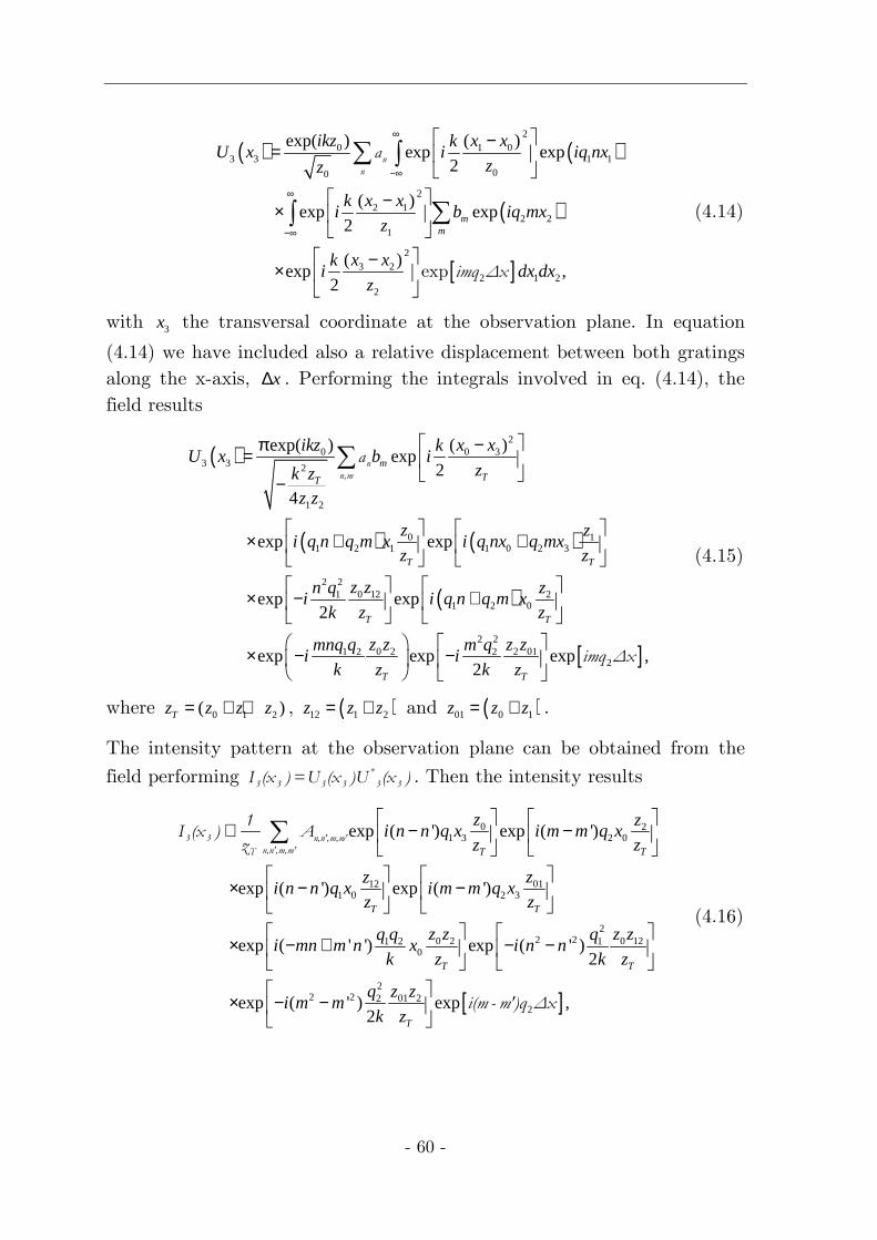
- 60 -

( ) ( )

( )

[ ]

20 1 0

3 3 1 100

22 1

2 21

23 2

2 1 22

exp( ) ( )exp exp

2

( )exp exp

2

( )exp ,

2

mm

ikz x xkU x i iq nx

zz

x xki b iq mx

z

x xki dx dx

z

∞

−∞

∞

−∞

−=

−×

−×

∑ ∫

∑∫

exp

n

n

a

imq ∆x

(4.14)

with 3x the transversal coordinate at the observation plane. In equation

(4.14) we have included also a relative displacement between both gratings along the x-axis, x∆ . Performing the integrals involved in eq. (4.14), the field results

( )

( ) ( )

( )

20 0 3

3 3 2

1 2

0 11 2 1 1 0 2 3

2 20 121 2

1 2 0

2 20 2 2 011 2 2

exp( ) ( )exp

2

4

exp exp

exp exp2

exp exp2

mTT

T T

T T

T T

ikz x xkU x b i

zk z

z z

z zi q n q m x i q nx q mx

z z

z zn q zi i q n q m x

k z z

z z z zmnq q m qi i

k z k z

π −= −

× + +

× − +

× − −

∑ n

n,m

a

[ ]2exp ,

imq ∆x

(4.15)

where 0 1 2( )Tz z z z= + + , ( )12 1 2z z z= + and ( )01 0 1z z z= + .

The intensity pattern at the observation plane can be obtained from the

field performing *

3 3 3 3 3 3I (x ) =U (x )U (x ) . Then the intensity results

0 21 3 2 0

01121 0 2 3

22 20 2 0 121 2 1

0

exp ( ') exp ( ')

exp ( ') exp ( ')

exp ( ' ') exp ( ' )2

exp

T T

T T

T T

z zi n n q x i m m q x

z z

zzi n n q x i m m q x

z z

z z z zq q qi mn m n x i n n

k z k z

i

∝ − −

× − −

× − + − −

× −

∑3 3 n,n',m,m'

n,n',m,m'T

1I (x ) A

z

[ ]2

2 2 01 222( ' ) exp ,

2 T

z zqm m

k z

−

i(m - m')q ∆x

(4.16)

4. Optical principles of encoders

- 61 -

where * *' ' ' 'nn mm n n m mA a a b b= . Following, we obtain from equation (4.16) the main

three configurations used in double grating displacement optical encoders. In Figure 4-3 it is shown a general scheme of a double grating system, without including illumination and detection.

4.2.14.2.14.2.14.2.1 MoirMoirMoirMoiréééé configuraconfiguraconfiguraconfigurationtiontiontion

Moiré configuration consists of two Ronchi gratings with the same period illuminated by a collimated beam, [31], [71], [72]. The observation plane is normally placed just after the second grating. Then, to obtain this configuration from eq. (4.16) it is necessary to realize the following considerations, 1 2p p= , 0z → ∞ and 2 0z → . Thus, after simplifying equation

(4.16), intensity for Moiré configuration results

[ ]

[ ]

1 3

22 2 1

1 1

exp ( ' ')

exp ( ' ) exp .2

i n n m m q x

qi n n z

k

∝ − + −

× − −

∑3M 3 n,n',m,m'

n,n',m,m'

I (x ) A

i(m - m')q ∆x

(4.17)

As it can be observed, a modulation along the x axis appears but also appears Talbot effect (modulation along the z-axis) between both gratings.

The periods of the modulations are 1p and 21 /p λ respectively. Then, to

obtain a useful signal moving one of the gratings along the x-axis, the distance between both must be very constant and equal to an integer number of Talbot distances, since in this way, the contrast of fringes at the second grating plane remains constant. Besides it is necessary to include a lens to collimate the illumination source. These two items are important handicaps for designing an optical encoder based on Moiré effect.

4.2.24.2.24.2.24.2.2 Lau configurationLau configurationLau configurationLau configuration

Another common configuration used in optical encoders is the Lau configuration, [19], [73], [74]. It consists of two Ronchi gratings with the same period and an infinite illumination source (incoherent source). The observation plane is placed at the focal plane of a lens or at infinity (Figure 4-4).

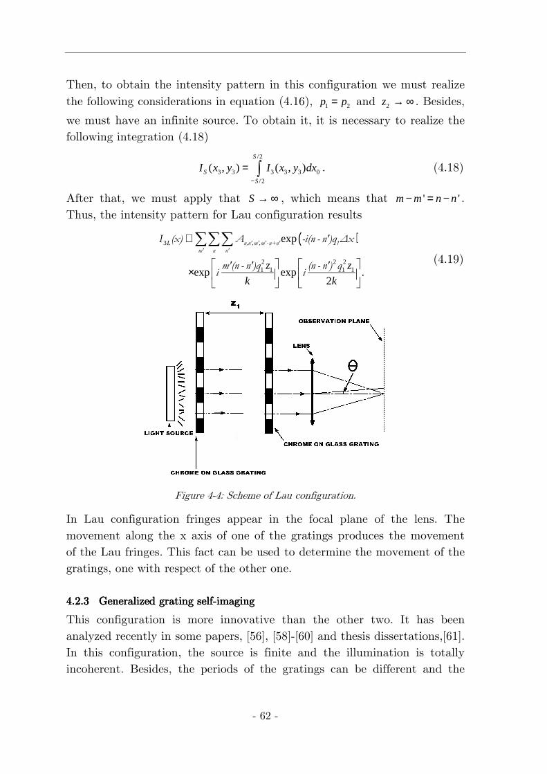
- 62 -

Then, to obtain the intensity pattern in this configuration we must realize the following considerations in equation (4.16), 1 2p p= and 2z → ∞ . Besides,

we must have an infinite source. To obtain it, it is necessary to realize the following integration (4.18)

/2

3 3 3 3 3 0

/2

( , ) ( , )S

S

S

I x y I x y dx−

= ∫ . (4.18)

After that, we must apply that S → ∞ , which means that ' 'm m n n− = − . Thus, the intensity pattern for Lau configuration results

( )3

2 2 21 1 1 1

exp

exp exp .2

L

z z

k k

∝

×

∑∑∑ n,n',m',m'-n+n' 1

m' n n'

I (x) A -i(n - n')q ∆x

m'(n - n')q (n - n') qi i

(4.19)

Figure 4-4: Scheme of Lau configuration.

In Lau configuration fringes appear in the focal plane of the lens. The movement along the x axis of one of the gratings produces the movement of the Lau fringes. This fact can be used to determine the movement of the gratings, one with respect of the other one.

4.2.34.2.34.2.34.2.3 Generalized grating selfGeneralized grating selfGeneralized grating selfGeneralized grating self----imagingimagingimagingimaging

This configuration is more innovative than the other two. It has been analyzed recently in some papers, [56], [58]-[60] and thesis dissertations,[61]. In this configuration, the source is finite and the illumination is totally incoherent. Besides, the periods of the gratings can be different and the

4. Optical principles of encoders

- 63 -

observation plane is placed at a finite distance from the second grating. Applying this considerations, the intensity pattern for generalized self-imaging configuration results

[ ] ( )

( )

1 3 0 2 3 0 1'

0 1 2 0 1 2

1 2 0 22

0 1 2

2 2 2 2 21 0 1 2

0 1 2

( ') ( ') ( )exp exp

( ' ')exp ) exp

( ' ) ( ) ( ' )exp exp

2

i n n q x z i m m q x z z

z z z z z z

i mn m n q q z z

k z z z

i n n q z z z i m m

k z z z

− − +∝ + + + +

−× + +

− + −× + +

∑3GSI 3 n,n',m,m

n,n',m,m'

I (x ) A

-iq ∆x(m - m'

( )

( )

22 2 0 1

0 1 2

2 2 1 1 2

0 1 2

( )

2

( ') ( ') ( )sinc .

2

q z z z

k z z z

m m z n n z zS

z z z

+ + +

− + − +× + +

q q

(4.20)

Firstly, this configuration provides advantages with respect to the other two, since lenses are not necessary, the source has not to be collimated and besides it is spatially incoherent (LED can be used). This configuration produces self-images at some distances from the second grating. The position of the self images, 2z , depends on the periods of the gratings and

the separation between them following the next relationship

1 2

2

z zQ

Rz

+ = , (4.21)

where 1 2/R p p= and /Q n m= a rational number.

- 65 -

5555 Fresnel dFresnel dFresnel dFresnel diffraction by steel tape iffraction by steel tape iffraction by steel tape iffraction by steel tape gratingsgratingsgratingsgratings

In this chapter, an analysis of the diffraction pattern produced by a steel tape grating in the near field (Fresnel regime) is performed. There are some differences with respect to the ideal case depicted in chapter 4. The topography is not perfect, but presents roughness. It produces that the topography is not purely periodical and a statistical approach should be considered. We have assumed that the illumination source is a collimated monochromatic beam. The transmittance of the grating is simulated as an amplitude grating but including a random transmittance due to the surface roughness. In the general case, Talbot effect appears in near distances. For chrome on glass gratings contrast of Talbot self-images remains constant but we have analytically found and experimentally demonstrated that for steel tape gratings the contrast decreases in terms of the distance. This decreasing follows the same function as that describes the random distribution in heights of the surface roughness. The same analysis using a gaussian beam as illumination source is performed. We have found that also the contrast of the self-images decreases. Besides, the width of all diffraction orders grows in terms of the roughness. Analytical solutions for both situations have been obtained for high and slight roughness approximations.

- 66 -

5. Fresnel diffraction by steel tape gratings

- 67 -

5.15.15.15.1 IntroductionIntroductionIntroductionIntroduction

In most applications, glass gratings are used because of its good optical behavior, with periods ranging from fifty microns to lower than one micron. However, there are applications in which very long displacements need to be measured (> 3 meters). In these cases, glass gratings are not available since they are difficult to manufacture and handle. As a consequence, steel substrates are used. Gratings on a steel substrate experimentally present a worse behavior due to their fabrication process. The steel tape where the grating is engraved is not perfectly smooth but it presents a certain roughness. Also, the technique to engrave the slits produces much more rough surfaces. This roughness produces adverse effects in the self-imaging process, [20], [22]. The period of gratings on a steel substrate is larger than in chrome on glass gratings (around 100 microns). Due to this long period, Talbot effect is not observed (Figure 5-1a) and steel reflection gratings are normally studied under a geometrical optics approach. However, nowadays we can find steel tape gratings with periods below 40 microns, [75], and as a consequence, diffractive effects become more important since Talbot distances present a quadratic dependence with the period of the grating. As a result, Talbot effect becomes a matter for the mechanical tolerances of the devices. In this chapter, we analyze the effect of roughness in the self-imaging process of steel tape reflection gratings which are illuminated by collimated beam (section 5.2) and Gaussian beam (section 5.3). We have modeled the grating as an amplitude binary grating with roughness in only one of the two levels of the grating. This assumption is motivated by the experimental evidence that when the grating is imaged using a CMOS camera with an objective microscope (to can observe all self-images in the experimental set-up), only one the levels of the grating present a significant light intensity (Figure 5-1b). The reason of this effect is that one of the levels of the grating is very rough and scatters light into all directions. As it is expected, Talbot effect appears. Due to the random topography of the surfaces, statistical optics techniques are required in order to determine the intensity of the self-images. We have theoretically found that contrast of the self-images decreases as we separate from the grating. Experimental results are obtained which corroborates the dependence of the contrast of

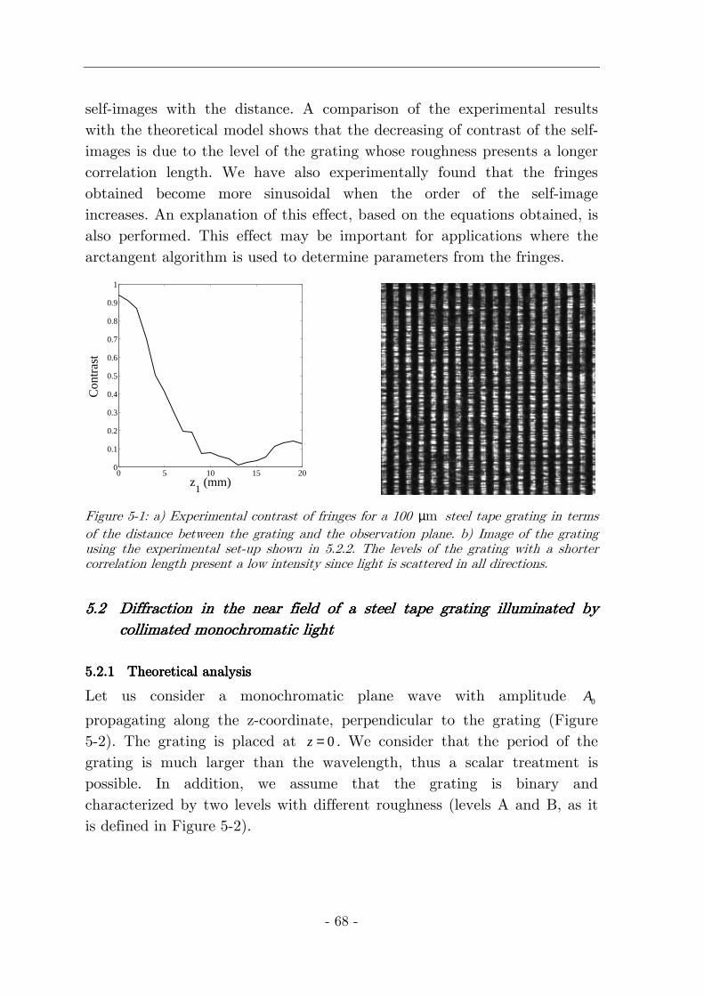
- 68 -

self-images with the distance. A comparison of the experimental results with the theoretical model shows that the decreasing of contrast of the self-images is due to the level of the grating whose roughness presents a longer correlation length. We have also experimentally found that the fringes obtained become more sinusoidal when the order of the self-image increases. An explanation of this effect, based on the equations obtained, is also performed. This effect may be important for applications where the arctangent algorithm is used to determine parameters from the fringes.

0 5 10 15 200

0.1

0.2

0.3

0.4

0.5

0.6

0.7

0.8

0.9

1

z1 (mm)

Con

tras

t

Figure 5-1: a) Experimental contrast of fringes for a 100 µm steel tape grating in terms of the distance between the grating and the observation plane. b) Image of the grating using the experimental set-up shown in 5.2.2. The levels of the grating with a shorter correlation length present a low intensity since light is scattered in all directions.

5.25.25.25.2 DDDDiffraction in the near field of a steel tape gratingiffraction in the near field of a steel tape gratingiffraction in the near field of a steel tape gratingiffraction in the near field of a steel tape grating illuminated by illuminated by illuminated by illuminated by collimated monochromatic lightcollimated monochromatic lightcollimated monochromatic lightcollimated monochromatic light

5.2.15.2.15.2.15.2.1 Theoretical analysisTheoretical analysisTheoretical analysisTheoretical analysis

Let us consider a monochromatic plane wave with amplitude 0A

propagating along the z-coordinate, perpendicular to the grating (Figure 5-2). The grating is placed at 0z = . We consider that the period of the grating is much larger than the wavelength, thus a scalar treatment is possible. In addition, we assume that the grating is binary and characterized by two levels with different roughness (levels A and B, as it is defined in Figure 5-2).

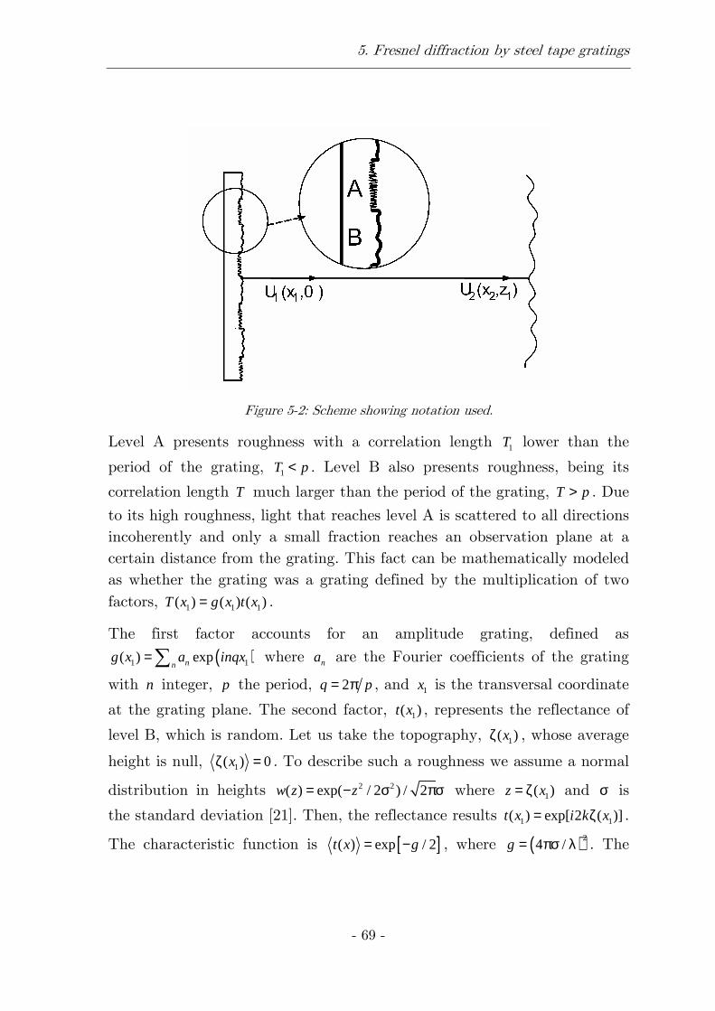
5. Fresnel diffraction by steel tape gratings

- 69 -

Figure 5-2: Scheme showing notation used.

Level A presents roughness with a correlation length 1T lower than the

period of the grating, 1T p< . Level B also presents roughness, being its

correlation length T much larger than the period of the grating, T p> . Due

to its high roughness, light that reaches level A is scattered to all directions incoherently and only a small fraction reaches an observation plane at a certain distance from the grating. This fact can be mathematically modeled as whether the grating was a grating defined by the multiplication of two factors, 1 1 1( ) ( ) ( )T x g x t x= .

The first factor accounts for an amplitude grating, defined as

( )1 1( ) expnng x a inqx=∑ where na are the Fourier coefficients of the grating

with n integer, p the period, 2q p= π , and 1x is the transversal coordinate

at the grating plane. The second factor, 1( )t x , represents the reflectance of

level B, which is random. Let us take the topography, 1( )xζ , whose average

height is null, 1( ) 0xζ = . To describe such a roughness we assume a normal

distribution in heights 2 2( ) exp( / 2 ) / 2w z z= − σ πσ where 1( )z x= ζ and σ is

the standard deviation [21]. Then, the reflectance results 1 1( ) exp[ 2 ( )]t x i k x= ζ .

The characteristic function is [ ]( ) exp / 2t x g= − , where ( )24 /g = πσ λ . The

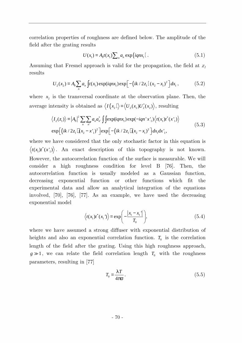
- 70 -

correlation properties of roughness are defined below. The amplitude of the field after the grating results

( )1 0 1 1( ) ( ) expnnU x A t x a iqnx= ∑ . (5.1)

Assuming that Fresnel approach is valid for the propagation, the field at z1 results

( ) 22 2 0 1 1 1 2 1 1( ) ( )exp( )exp / 2 ( )n

n

U x A a t x iqnx ik z x x dx = − − ∑ ∫ , (5.2)

where 2x is the transversal coordinate at the observation plane. Then, the

average intensity is obtained as ( ) *2 2 2 2 2( ) ( )I x U x U x= , resulting

( ) ( )

2 * *2 1 0 ' 1 1 1 1

'

2 21 2 1 1 2 1 1 1

( ) exp( )exp( ' ' ) ( ) ( ' )

exp / 2 ( ' ) exp / 2 ( ) ' ,

n nn n

I z A a a iqnx iqn x t x t x

ik z x x ik z x x dx dx

= −

− − −

∑∑ ∫ ∫ (5.3)

where we have considered that the only stochastic factor in this equation is *

1 1( ) ( ' )t x t x . An exact description of this topography is not known.

However, the autocorrelation function of the surface is measurable. We will consider a high roughness condition for level B [76]. Then, the autocorrelation function is usually modeled as a Gaussian function, decreasing exponential function or other functions which fit the experimental data and allow an analytical integration of the equations involved, [70], [76], [77]. As an example, we have used the decreasing exponential model

1 1*1 1

0

'( ) ( ') exp

x xt x t x

T

− = −

, (5.4)

where we have assumed a strong diffuser with exponential distribution of heights and also an exponential correlation function. 0T is the correlation

length of the field after the grating. Using this high roughness approach, 1g ≫ , we can relate the field correlation length 0T with the roughness

parameters, resulting in [77]

0 4

TT

λ=πσ. (5.5)

5. Fresnel diffraction by steel tape gratings

- 71 -

Substituting eq. (5.4) into eq. (5.3), it results that average intensity at the observation plane is

[ ]

22 * 2 2

2 1 0 ' 2 1'

1

0

( ) exp ( ' ) exp ( ' )2

exp ' .

n nn n

qI z A a a iqx n n i n n z

k

zn n

pT

= − −

λ× − −

∑∑ (5.6)

The first exponential factor is related to the transversal profile of the fringes, the second factor accounts for Talbot effect and the third exponential factor accounts for the effect of roughness on the self-images intensity. Roughness makes the intensity exponentially decrease as the distance 1z increases. The distance at which the intensity decays 1/ e for

the first harmonic results 0 /W pT= λ .

There exist experimental cases where the autocorrelation function of the surface cannot be fitted to an exponential, but to a Gaussian function

( )2* 21 1 1 1 0( ) ( ') exp ' /t x t x x x T = − −

. Then, eq. (5.3) can also be analytically

solved, resulting

[ ]2

2 * 2 22 1 0 ' 2 1

'

2

1

0

( ) exp ( ' ) exp ( ' )2

exp ( ')

n nn n

qI z A a a iqx n n i n n z

k

zn n

pT

= − −

λ × − −

∑∑. (5.7)

The structure of this equation is equivalent to eq. (5.6), substituting the exponential function by a Gaussian function.

5.2.25.2.25.2.25.2.2 Experimental Experimental Experimental Experimental analysisanalysisanalysisanalysis

The experimental set-up is shown in Figure 5-3. A monochromatic collimated laser beam of wavelength 650 nm (MC6707O model by Monocrom) impinges on a steel tape grating (period 40 microns) with normal incidence with respect to its surface. The steel tape grating is placed on a motorized linear stage along the z direction. The diffracted light is reflected by the beam splitter and it is collected by a CMOS

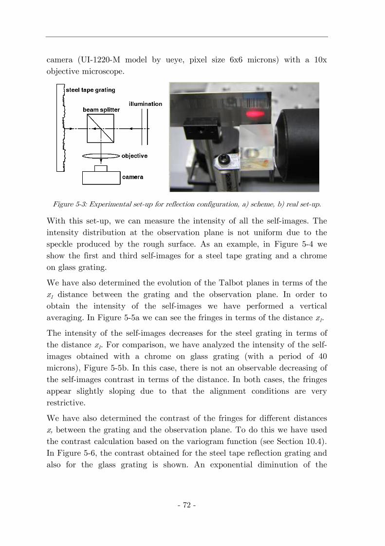
- 72 -

camera (UI-1220-M model by ueye, pixel size 6x6 microns) with a 10x objective microscope.

Figure 5-3: Experimental set-up for reflection configuration, a) scheme, b) real set-up.

With this set-up, we can measure the intensity of all the self-images. The intensity distribution at the observation plane is not uniform due to the speckle produced by the rough surface. As an example, in Figure 5-4 we show the first and third self-images for a steel tape grating and a chrome on glass grating.

We have also determined the evolution of the Talbot planes in terms of the z1 distance between the grating and the observation plane. In order to obtain the intensity of the self-images we have performed a vertical averaging. In Figure 5-5a we can see the fringes in terms of the distance z1.

The intensity of the self-images decreases for the steel grating in terms of the distance z1. For comparison, we have analyzed the intensity of the self-images obtained with a chrome on glass grating (with a period of 40 microns), Figure 5-5b. In this case, there is not an observable decreasing of the self-images contrast in terms of the distance. In both cases, the fringes appear slightly sloping due to that the alignment conditions are very restrictive.

We have also determined the contrast of the fringes for different distances z, between the grating and the observation plane. To do this we have used the contrast calculation based on the variogram function (see Section 10.4). In Figure 5-6, the contrast obtained for the steel tape reflection grating and also for the glass grating is shown. An exponential diminution of the

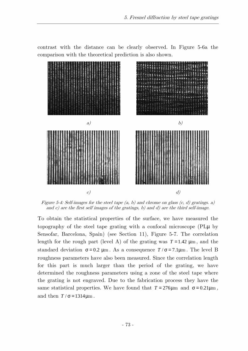
5. Fresnel diffraction by steel tape gratings

- 73 -

contrast with the distance can be clearly observed. In Figure 5-6a the comparison with the theoretical prediction is also shown.

a) b)

c) d)

Figure 5-4: Self-images for the steel tape (a, b) and chrome on glass (c, d) gratings. a) and c) are the first self images of the gratings, b) and d) are the third self-image.

To obtain the statistical properties of the surface, we have measured the

topography of the steel tape grating with a confocal microscope (PLµ by Sensofar, Barcelona, Spain) (see Section 11), Figure 5-7. The correlation length for the rough part (level A) of the grating was 1.42T = µm , and the

standard deviation 0.2σ = µm . As a consequence / 7.1T σ = µm . The level B

roughness parameters have also been measured. Since the correlation length for this part is much larger than the period of the grating, we have determined the roughness parameters using a zone of the steel tape where the grating is not engraved. Due to the fabrication process they have the same statistical properties. We have found that 276T = µm and 0.21σ = µm , and then / 1314T σ = µm .

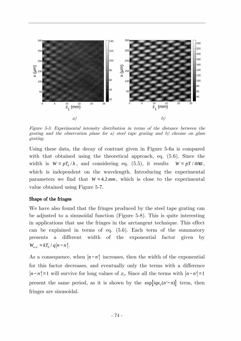
- 74 -

z1 (mm)

x (µ

m)

0 5 10 15 20 25

50

100

150

200

250

300

20

40

60

80

100

120

140

z

1 (mm)

x (µ

m)

0 5 10 15 20 25

50

100

150

200

250

300

40

60

80

100

120

140

160

180

200

220

240

a) b)

Figure 5-5: Experimental intensity distribution in terms of the distance between the grating and the observation plane for a) steel tape grating and b) chrome on glass grating.

Using these data, the decay of contrast given in Figure 5-6a is compared with that obtained using the theoretical approach, eq. (5.6). Since the width is 0 /W pT= λ , and considering eq. (5.5), it results / 4W pT= πσ ,

which is independent on the wavelength. Introducing the experimental parameters we find that 4.2W mm= , which is close to the experimental

value obtained using Figure 5-7.

ShaShaShaShappppe of e of e of e of the the the the fringesfringesfringesfringes

We have also found that the fringes produced by the steel tape grating can be adjusted to a sinusoidal function (Figure 5-8). This is quite interesting in applications that use the fringes in the arctangent technique. This effect can be explained in terms of eq. (5.6). Each term of the summatory presents a different width of the exponential factor given by

, ' 0 / 'n nW kT q n n= − .

As a consequence, when 'n n− increases, then the width of the exponential

for this factor decreases, and eventually only the terms with a difference

' 1n n− = will survive for long values of z1. Since all the terms with ' 1n n− =

present the same period, as it is shown by the [ ]2exp ( ' )iqx n n− term, then

fringes are sinusoidal.

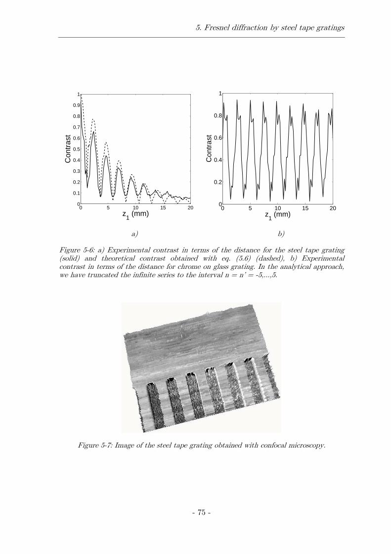
5. Fresnel diffraction by steel tape gratings

- 75 -

0 5 10 15 200

0.1

0.2

0.3

0.4

0.5

0.6

0.7

0.8

0.9

1

z1 (mm)

Con

tras

t

0 5 10 15 200

0.2

0.4

0.6

0.8

1

z1 (mm)

Con

tras

t

a) b)

Figure 5-6: a) Experimental contrast in terms of the distance for the steel tape grating (solid) and theoretical contrast obtained with eq. (5.6) (dashed), b) Experimental contrast in terms of the distance for chrome on glass grating. In the analytical approach, we have truncated the infinite series to the interval n = n’ = -5,...,5.

Figure 5-7: Image of the steel tape grating obtained with confocal microscopy.

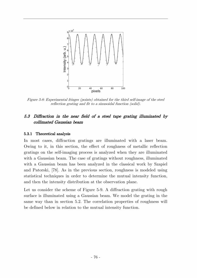
- 76 -

0 20 40 60 80 1000

1

2

3

4

5

6

7

8

9x 10

4

pixels

Inte

nsity

(ar

b. u

.)

Figure 5-8: Experimental fringes (points) obtained for the third self-image of the steel reflection grating and fit to a sinusoidal function (solid).

5.35.35.35.3 DDDDiffraction in the near field of a steel tape gratingiffraction in the near field of a steel tape gratingiffraction in the near field of a steel tape gratingiffraction in the near field of a steel tape grating illuminated by illuminated by illuminated by illuminated by collimated collimated collimated collimated Gaussian Gaussian Gaussian Gaussian beambeambeambeam

5.3.15.3.15.3.15.3.1 Theoretical analysisTheoretical analysisTheoretical analysisTheoretical analysis

In most cases, diffraction gratings are illuminated with a laser beam. Owing to it, in this section, the effect of roughness of metallic reflection gratings on the self-imaging process is analyzed when they are illuminated with a Gaussian beam. The case of gratings without roughness, illuminated with a Gaussian beam has been analyzed in the classical work by Szapiel and Patorski, [78]. As in the previous section, roughness is modeled using statistical techniques in order to determine the mutual intensity function, and then the intensity distribution at the observation plane.

Let us consider the scheme of Figure 5-9. A diffraction grating with rough surface is illuminated using a Gaussian beam. We model the grating in the same way than in section 5.2. The correlation properties of roughness will be defined below in relation to the mutual intensity function.

5. Fresnel diffraction by steel tape gratings

- 77 -

Figure 5-9: Scheme that shows the propagation of the diffraction orders in the near field produced by a grating with roughness.

Let us consider that the diffraction grating is illuminated with a monochromatic Gaussian beam. The period of the grating, p , is assumed

much larger than the wavelength, λ , of the incident field, thus a scalar treatment is possible. For simplicity, the waist of the Gaussian beam is placed at the grating plane

2

00 0 0

0

( ) expx

U x A = − ω

, (5.8)

where 0A is the maximum amplitude and 0ω is the beam width. Then, the

amplitude of the field just after the grating is

( ) ( )2

11 1 0 1 1

0

( ) exp expnn

xU x A t x a iqnx

= − ω

∑ . (5.9)

Due to roughness, statistical properties of the field need to be considered. In particular, the mutual intensity of the beam just after the grating is, [79],

( )1 1 1 1 1 1, ' ( ) *( ' )J x x U x U x= , (5.10)

where • means averaging. Usually, the topography, ( )1xζ , is unknown.

However, the statistical properties of the surface are included in the

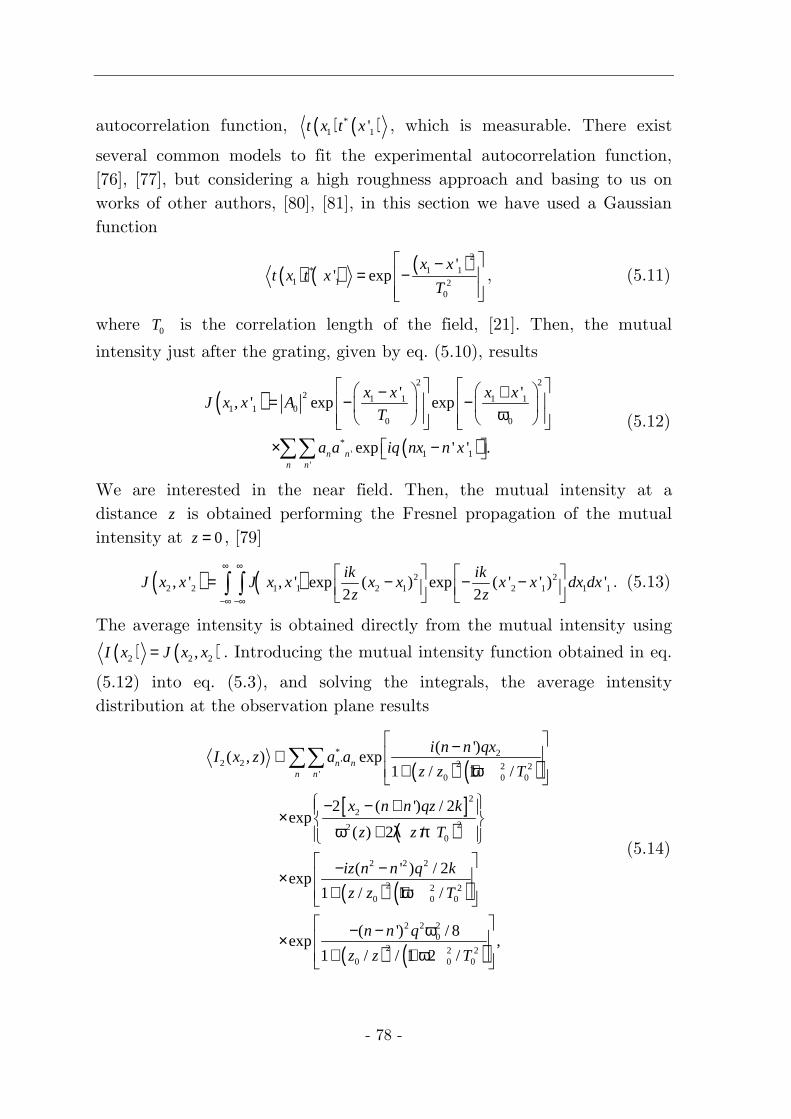
- 78 -

autocorrelation function, ( ) ( )*1 1't x t x , which is measurable. There exist

several common models to fit the experimental autocorrelation function, [76], [77], but considering a high roughness approach and basing to us on works of other authors, [80], [81], in this section we have used a Gaussian function

( ) ( ) ( )2

1 1*1 1 2

0

'' exp

x xt x t x

T

−= −

, (5.11)

where 0T is the correlation length of the field, [21]. Then, the mutual

intensity just after the grating, given by eq. (5.10), results

( )

( )

2 22 1 1 1 1

1 1 00 0

*' 1 1

'

' ', ' exp exp

exp ' ' .n nn n

x x x xJ x x A

T

a a iq nx n x

− + = − − ω

× − ∑∑ (5.12)

We are interested in the near field. Then, the mutual intensity at a distance z is obtained performing the Fresnel propagation of the mutual intensity at 0z = , [79]

( ) ( ) 2 22 2 1 1 2 1 2 1 1 1, ' , ' exp ( ) exp ( ' ' ) '

2 2

ik ikJ x x J x x x x x x dx dx

z z

∞ ∞

−∞ −∞

= − − − ∫ ∫ . (5.13)

The average intensity is obtained directly from the mutual intensity using

( ) ( )2 2 2,I x J x x= . Introducing the mutual intensity function obtained in eq.

(5.12) into eq. (5.3), and solving the integrals, the average intensity distribution at the observation plane results

( ) ( )[ ]

( )

( ) ( )

( ) ( )

* 22 2 ' 2 2 2

' 0 0 0

2

222

0

2 2 2

2 2 20 0 0

2 2 20

2 2 20 0 0

( ')( , ) exp

1 / 1 /

2 ( ') / 2exp

( ) 2 /

( ' ) / 2exp

1 / 1 /

( ') / 8exp ,

1 / / 1 2 /

n nn n

i n n qxI x z a a

z z T

x n n qz k

z z T

iz n n q k

z z T

n n q

z z T

− ∝ + + ω

− − + × ω + λ π

− − × + + ω

− − ω × + + ω

∑∑

(5.14)

5. Fresnel diffraction by steel tape gratings

- 79 -

where ( )22 20 0( ) 1 /z z z ω = ω +

and 20 0 /z = πω λ is the Rayleigh distance, [82].

The first exponential factor of eq. (5.14) accounts of the period of the

fringes which results ( ) ( )2 2 20 0 0ˆ 1 / 1 /p p z z T = + + ω

. In principle, p depends

on roughness. However, this dependence is not usually significant since it is notorious when 0z z>> , and in this regime the intensity goes to zero due to

the exponential diminishing factors of eq. (5.14). The second exponential factor of eq. (5.14) accounts of the direction of propagation of the different diffraction orders and their profiles. It can be observed that the profile of the diffraction orders is also Gaussian. However, the width of the diffracted

beams, ( )22 20( ) 2 /Rough z z Tω = ω + λ π , increases when the correlation length 0T

decreases. The third exponential factor accounts of the Talbot effect and shows the positions where Talbot self-images are formed. Finally, the fourth exponential factor gives account of an interaction between different orders of diffraction.

In order to understand the self-imaging process under Gaussian illumination in presence of roughness, several computations have been performed. For this, we have assumed that a metallic grating can be modeled as a binary phase grating. Then, the Fourier coefficients of the grating are

( ) ( )

( )1 sinc 0

1 1 0

i

n i

e n na

e n

− δ

− δ

α − πα ≠= α − + =

, (5.15)

where α is the ratio between the upper and the lower part of the grating and δ is the phase retardation produced by the grating.

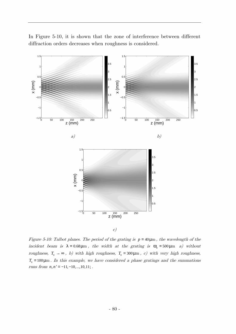
- 80 -

In Figure 5-10, it is shown that the zone of interference between different diffraction orders decreases when roughness is considered.

z (mm)

x (m

m)

0 50 100 150 200 250−1.5

−1

−0.5

0

0.5

1

1.5

0.5

1

1.5

2

2.5

3

3.5

z (mm)

x (m

m)

0 50 100 150 200 250−1.5

−1

−0.5

0

0.5

1

1.5

0.5

1

1.5

2

2.5

3

3.5

a) b)

z (mm)

x (m

m)

0 50 100 150 200 250−1.5

−1

−0.5

0

0.5

1

1.5

0.5

1

1.5

2

2.5

3

3.5

c)

Figure 5-10: Talbot planes. The period of the grating is 40p = µm , the wavelength of the incident beam is 0.68λ = µm , the width at the grating is 0 500ω = µm a) without

roughness, 0T → ∞ , b) with high roughness, 0 300T = µm , c) with very high roughness,

0 100T = µm . In this example, we have considered a phase gratings and the summations runs from 11, 10,...,10,11, ' ;n n − −= .

5. Fresnel diffraction by steel tape gratings

- 81 -

For the limit case of null roughness ( 0T → ∞ ) the intensity results

( )

[ ]

( ) ( )

2

2* 22 2 ' 2 2

' 0

2 2 22 2 20

2 2

0 0

2 ( ') / 2( ')( , ) exp exp

( )1 /

( ') / 8( ' ) / 2exp exp .

1 / 1 /

n nn n

x n n qz ki n n qxI x z a a

zz z

n n qiz n n q k

z z z z

− − +− ∝ ω+

− − ω− −× + +

∑∑ (5.16)

Finally, when we take plane wave illumination, 0ω → ∞ , the classical result

for Talbot effect is recovered, [9],

[ ]2

* 2 22 2 ' 2

'

( , ) exp ( ') exp ( ' )2n n

n n

qI x z a a i n n qx i n n z

k

∝ − −

∑∑ . (5.17)

To characterize the quality of the self-images produced by the steel tape grating, an important parameter is the contrast, which is defined as the

classical definition ( ) ( )/MAX MIN MAX MINC I I I I= − + (according to Section 10.2),

where MAXI and MINI are the maximum and minimum intensity of the

fringes, respectively. Since the incident beam is Gaussian, the intensity depends on the location 2x of the beam with respect of the origin of

coordinates. A solution is to determine the contrast at 2 0x = , where the

intensity of the incident beam presents a maximum. Then, we define the maximum and minimum intensity as those obtained at 0x∆ = and

/ 2x p∆ = , where x∆ is a relative displacement of the grating is a

displacement in the direction parallel to the grating.

Then, contrast results

( ){ }( ){ }

*, ' '

'

*, ' '

'

( ) 1 exp '

( ) 1 exp '

n n n nn n

n n n nn n

z a a i n nC

z a a i n n

∞ ∞

=∞ =∞∞ ∞

=∞ =∞

Γ − π − =

Γ + π −

∑ ∑

∑ ∑, (5.18)

where

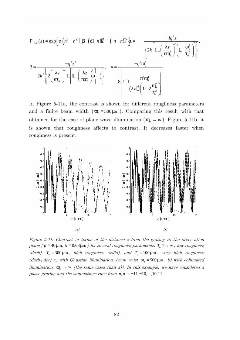
- 82 -

( ) ( ) ( )

( )

22 22 2

, ' 2 20

2 20 0

2 22 20

2 2

2 22 402

00 02

2 02

0

( ) exp ' ' ' , ,

2 1 1

,

2 2 18 1

1 2

n n

iq zz n n n n n n

zk

T

qq z

z zk

T

zT

− Γ = α − + β + + γ − α = ωλ

+ + πω

− ω−β = γ = λ λ + + ω π ωπ πω + ωλ +

.

In Figure 5-11a, the contrast is shown for different roughness parameters and a finite beam width ( 0 500ω = µm ). Comparing this result with that

obtained for the case of plane wave illumination ( 0ω → ∞ ), Figure 5-11b, it

is shown that roughness affects to contrast. It decreases faster when roughness is present.

a) b)

Figure 5-11: Contrast in terms of the distance z from the grating to the observation plane ( 40 , 0.68p = µ λ = µm m ) for several roughness parameters: 0T =→ ∞ , low roughness

(dash), 0 300T = µm , high roughness (solid), and 0 100T = µm , very high roughness

(dash+dot) a) with Gaussian illumination, beam waist 0 500ω = µm , b) with collimated

illumination, 0ω → ∞ (the same cases than a)). In this example, we have considered a phase grating and the summations runs from , ' 11, 10,...,10,11n n = − − .

5. Fresnel diffraction by steel tape gratings

- 83 -

We can also observe that when high roughness is present only the first Talbot self-images appear and eventually disappear for very high roughness.

NonNonNonNon----interference zoneinterference zoneinterference zoneinterference zone

As it is shown in Figure 5-10, there is a distance from which the diffraction orders do not interfere. This distance corresponds to 0 / 2Nz p= ω λ , which

can be easily obtained from a geometrical analysis. For distances longer than Nz , Talbot planes disappear since the different diffraction orders do

not overlap. In this regime, Nz z> the intensity results

( )

( )

222

2 2 220

2 /( , ) exp

( ) 2 /n

n

z n pI x z a

z z T

− θ − λ∝

ω + λ π ∑ , (5.19)

where 2 /x zθ = .

As it is well known, several diffraction beams appear. The maxima of the diffracted Gaussian beams are placed at p nθ = λ , which is the linear version

of the well-known grating equation. It is observed that, when the autocorrelation function of roughness is Gaussian, eq. (5.11), the diffracted beams are also Gaussian. The width of the Gaussian beams is affected by

roughness, increasing from 2( )zω to ( )220( ) 2 /z z Tω + λ π , that is, for shorter

correlation length of roughness, wider diffracted beams. This increasing can be observed in Figure 5-10.

It is also important to analyze whether roughness produces a redistribution of the power amongst diffraction orders. Power is defined as the total intensity for each order n, which results, [82],

( )( )

22 2

2222 20

0

0 0

2

0

2 /1exp

( ) 2 /1 1

.2

n n

n

x n z pP a dx

z z Tz

z T

a

∞

−∞

− − λ=

ω + λ π ω + +

π= ω

∫

(5.20)

- 84 -

The power of every diffraction order is independent on the correlation length of the field. As a consequence, there is not a redistribution of power amongst the diffraction orders due to roughness.

.

- 85 -

6666 Double grating systems with one steel Double grating systems with one steel Double grating systems with one steel Double grating systems with one steel tape gratingtape gratingtape gratingtape grating

In this chapter, the general solution of diffraction in the near field trough two gratings, being one of them a steel tape grating and the other one a chrome on glass grating, is performed. As illumination source, we have considered initially a monochromatic point source. We have obtained a general analytical solution for the intensity in the Fresnel regime. From it we have obtained the analytical expressions for the more common double grating configurations, which are Moiré configuration, Lau configuration and Generalized Self-imaging configuration. We have found that for Moiré configuration, roughness of the steel tape grating produces a decreasing and even losing of the contrast of the Moiré fringes. On the contrary, roughness almost does not affect to the fringes formation in Lau and Generalized Grating Imaging configurations. It only affects to the depth of focus of the self-images in Generalized Self-imaging configuration.

- 86 -

6. Double grating systems with one steel tape grating

- 87 -

6.16.16.16.1 IntroductionIntroductionIntroductionIntroduction

Double grating systems are used in numerous applications such as metrology, interferometry [83]-[85], spectrometry [86], [87], etc, existing several common configurations [15], [88]. In Moiré configuration, a plane wave illuminates a system formed by two gratings of the same period, [89]. Then fringes are observed just after the second grating. This configuration presents drawbacks, such as the necessity of a point source, which does not exist physically and the necessity of a big lens to properly collimate the beam. In so-called Lau configuration, a point source is not required.[90], [91]. The observation plane is located at infinite and, in practice, a lens is used to detect fringes at its focal plane, [73]. In Generalized Grating Self-Imaging configuration both gratings may have equal or different periods and fringes are obtained at finite distances from the second grating [19], [58], [59], [74]. As a consequence, the devices which use this configuration are more compact and robust, since no lenses are required and the illumination source may have a finite extension.

As it is explained in Chapter 5, steel tape gratings must be used in some applications, for example, when it is necessary to measure distances longer than 3 meters, using an optical encoder. In this chapter we analyze double grating systems in which one of the gratings is a steel tape grating. In particular we have analyzed the fringe formation when the first grating is a steel tape grating and the second grating is an amplitude grating (for example, a chrome on glass grating). A scalar Fresnel approach is used for the propagation calculations since the period of the gratings is much larger than the wavelength of the light used. Also, owing to the rough surface, statistical techniques need to be used to determine the average intensity distribution at the observation plane. The case where the first grating is an amplitude grating and the second grating is a steel tape grating can be easily derived from this analysis.

- 88 -

6.26.26.26.2 General double grating configurationGeneral double grating configurationGeneral double grating configurationGeneral double grating configuration

The general configuration for a double grating system is shown in Figure 6-1. Let us consider a monochromatic light source with a wavelength λ . The periods of the gratings 1p and 2p , respectively, are assumed much

larger than the wavelength and then a scalar approach is possible. The distance between the source and the first grating is 0z , from the first to the

second grating is 1z , and from the second grating to the observation plane

is 2z ..

Figure 6-1: Standard set-up for a double grating system showing the parameters involved.

Due to the symmetry of the configuration, a 2-D analysis can be performed. Since the steel tape grating is opaque the configuration depicted in Figure 6-1 is only valid for theoretical purposes and a practical set-up is that it is shown in Figure 6-2, where a beam splitter is used to illuminate the grating.

This configuration can be used to analyze all double grating configurations. The light source is made up of punctual emitters which incoherently generate divergent spherical waves. By the moment, let us consider one of these punctual emitters placed at a distance 0x from the axis.

The amplitude just before the first grating is given by the Fresnel propagation of a single point source

6. Double grating systems with one steel tape grating

- 89 -

201 1 0 1 0

00

( , ) exp ( )2

A ikU x z x x

zi z

= − λ

, (6.1)

being 0A the amplitude, 2 /k = π λ and 1x the transversal coordinate at the

first grating plane.

Figure 6-2: Set up when a steel tape grating is used. Since the first grating is opaque, a beam splitter is required for illuminating the system.

The light is reflected by the first grating (steel tape grating). As it is shown in [20], the steel tape grating presents two roughness levels. The high roughness level scatters light to all directions and the contribution to the diffraction pattern is a constant background intensity. Then, the reflectance of diffraction grating can be mathematically described as the product of two terms, 1 1 1 1( ) ( ) ( )T x g x t x= . The first term is a binary

amplitude grating whose infinite Fourier series is ( )1 1 1 1( ) expnng x a inq x=∑ ,

where 1 12q p= π . The second term includes the topography of the rough

surface. It is defined using a stochastic function, 1( )xζ , whose average

height is null 1( ) 0xζ = . Considering the thin element approach, the

reflectance due to roughness is given by 1 1( ) exp[ 2 ( )]t x ik x= − ζ , [21], [70].

Then, the amplitude of the field after the grating results

( )201 0 1 0 1 1 1

00

ˆ ( , ) exp ( ) ( ) exp2 nn

A ikU x z x x t x a inq x

zi z

= − λ

∑ . (6.2)

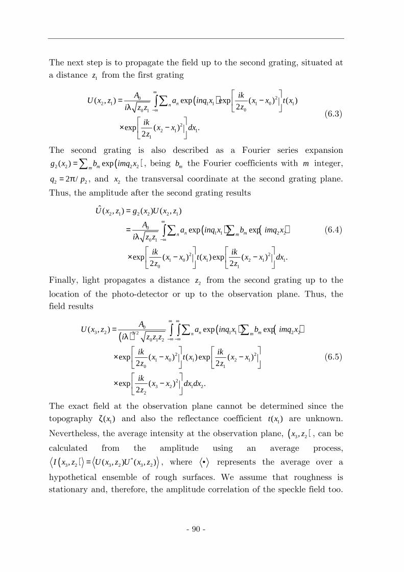
- 90 -

The next step is to propagate the field up to the second grating, situated at a distance 1z from the first grating

( ) 202 1 1 1 1 0 1

00 1

22 1 1

1

( , ) exp exp ( ) ( )2

exp ( ) .2

nn

A ikU x z a inq x x x t x

zi z z

ikx x dx

z

∞

−∞

= − λ

× −

∑∫ (6.3)

The second grating is also described as a Fourier series expansion

( )2 2 2 2( ) expmmg x b imq x=∑ , being mb the Fourier coefficients with m integer,

2 22 /q p= π , and 2x the transversal coordinate at the second grating plane.

Thus, the amplitude after the second grating results

( ) ( )

2 1 2 2 2 1

01 1 2 2

0 1

2 21 0 1 2 1 1

0 1

ˆ ( , ) ( ) ( , )

exp exp

exp ( ) ( )exp ( ) .2 2

n mn m

U x z g x U x z

Aa inq x b imq x

i z z

ik ikx x t x x x dx

z z

∞

−∞

=

=λ

× − −

∑ ∑∫ (6.4)

Finally, light propagates a distance 2z from the second grating up to the

location of the photo-detector or up to the observation plane. Thus, the field results

( )( ) ( )0

3 2 1 1 2 23/2

0 1 2

2 21 0 1 2 1

0 1

23 2 1 2

2

( , ) exp exp

exp ( ) ( )exp ( )2 2

exp ( ) .2

n mn m

AU x z a inq x b imq x

i z z z

ik ikx x t x x x

z z

ikx x dx dx

z

∞ ∞

−∞ −∞

=λ

× − −

× −

∑ ∑∫ ∫

(6.5)

The exact field at the observation plane cannot be determined since the topography 1( )xζ and also the reflectance coefficient 1( )t x are unknown.

Nevertheless, the average intensity at the observation plane, ( )3 2,x z , can be

calculated from the amplitude using an average process,

( ) *3 2 3 2 3 2, ( , ) ( , )I x z U x z U x z= , where • represents the average over a

hypothetical ensemble of rough surfaces. We assume that roughness is stationary and, therefore, the amplitude correlation of the speckle field too.

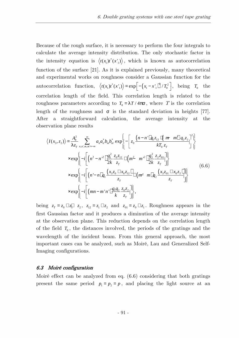
6. Double grating systems with one steel tape grating

- 91 -

Because of the rough surface, it is necessary to perform the four integrals to calculate the average intensity distribution. The only stochastic factor in

the intensity equation is *1 1( ) ( ' )t x t x , which is known as autocorrelation

function of the surface [21]. As it is explained previously, many theoretical and experimental works on roughness consider a Gaussian function for the

autocorrelation function, ( )2* 21 1 1 1 0( ) ( ' ) exp ' /t x t x x x T = − −

, being 0T the

correlation length of the field. This correlation length is related to the roughness parameters according to 0 / 4T T= λ πσ , where T is the correlation

length of the roughness and σ is the standard deviation in heights [77]. After a straightforward calculation, the average intensity at the observation plane results

( ) ( )

( ) ( )

( ) ( ) ( ) ( )

221 12 2 2* *0

3 2 ' ' 0, ', , ' 0

2 22 2 2 20 12 2 011 2

3 0 0 12 3 01 0 21 2

' '( , ) exp

exp ' '2 2

exp ' '

n n m mn n m mT T

T T

T T

n n q z m m q zAI x z a a b b z

z kT z

z z z zq qi n n m m

k z k z

x z x z x z x zi n n q m m q

z z

∞

=−∞

− + − = − λ

× − − + −

+ + × − − + −

∑

( ) 0 21 2exp ' ' ,T

z zq qi mn m n

k z

× − −

(6.6)

being 0 1 2Tz z z z= + + , 12 1 2z z z= + and 01 0 1z z z= + . Roughness appears in the

first Gaussian factor and it produces a diminution of the average intensity at the observation plane. This reduction depends on the correlation length of the field 0T , the distances involved, the periods of the gratings and the

wavelength of the incident beam. From this general approach, the most important cases can be analyzed, such as Moiré, Lau and Generalized Self-Imaging configurations.

6.36.36.36.3 Moiré configurationMoiré configurationMoiré configurationMoiré configuration

Moiré effect can be analyzed from eq. (6.6) considering that both gratings present the same period 1 2p p p= = , and placing the light source at an

- 92 -

infinite distance 0z → ∞ . Then, the mean intensity for Moiré configuration

results

( ) ( )

( ) ( )

( ) ( ){ } ( )

2

12 2* *3 ' '

, ', , ' 0

22 2 2 2

12 2

2

3 2

' '( ) exp

exp ' '2

exp ' ' exp ' ' .

n n m mn n m m

n n z m m zI x a a b b q

kT

qi n n z m m z

k

qiqx n n m m i mn m n z

k

∞

=−∞

− + − ∝ −

× − − + −

× − + − − −

∑

(6.7)

Classically, Moiré effect is analyzed when the observation plane coincides with the second grating plane, 2 0z → , thus the equation simplifies to

( )

( ) ( ) ( ){ }

2

1* *3 ' '

, ', , ' 0

22 2

1 3

'( ) exp

exp ' exp ' ' .2

n n m mn n m m

n n zI x a a b b q

kT

qi n n z iqx n n m m

k

∞

=−∞

− ∝ −

× − − − + −

∑ (6.8)

z1 (mm)

x 3 (µm

)

0 1 2 3 4−40

−30

−20

−10

0

10

20

30

40

z

1 (mm)

x 3 (µm

)

0 1 2 3 4−40

−30

−20

−10

0

10

20

30

40

a) b)

Figure 6-3: Fringes obtained with a Moiré configuration when the wavelength is .68λ = µm and the period of both gratings is 20p = µm a) The first grating is a chrome

on glass grating, b) The first grating is a steel tape grating whose roughness parameters are .1σ = µm , 50T = µm .

In Moiré configuration, the apparition of roughness produces a Gaussian diminution of the intensity in terms of 1z , how it is shown in Figure 6-3.

6. Double grating systems with one steel tape grating

- 93 -

The relative displacement x∆ between gratings can be included in the

equations using the following change, ( )expn na a iqn x→ ∆ . Then the mean

intensity distribution results

( ) ( )

( ) ( ) ( ){ }

2

1* *3 ' '

, ', , ' 0

22 2

1 3

'( ) exp ' exp

exp ' exp ' ' .2

n n m mMn n m m

n n zI x a a b b iq n n x q

kT

qi n n z iqx n n m m

k

∞

=−∞

− ∝ − ∆ −

× − − − + −

∑ (6.9)

When 1 0 /z kT q>> the only terms that survive are those that fulfill 'n n= .

Then the information about the relative displacement between gratings disappears and the second grating observes a constant field. On the other hand, when roughness is null, 0T → ∞ , the classical expression of Moiré

effect is recovered.

6.46.46.46.4 Lau configurationLau configurationLau configurationLau configuration

Lau effect can also be obtained from eq. (6.6) considering that the source presents an infinite size, assuming 1 2p p p= = and placing the observation

plane at infinite, 2z → ∞ . In the first place, we will consider a finite source

with size S . For this reason we perform an integration in 0x with the

following limits, 0/ 2 / 2S x S− < < .

Thus, it results that the average intensity is

( )

( ) ( )

( ) ( ){ }( ) ( )

2

* * 0' '

, ', , ' 0

2 22 2 2 2

0 01

0 01

2

0

( ) exp ' '

exp ' exp '2 2

exp ' '

exp ' ' ' ' ,2

n n m mn n m m

z qI a a b b n n m m

kT

q qi n n z i m m z

k k

iq n n z m m z

q qSi mn m n z n n m m

k

∞

=−∞

θ ∝ − − + −

× − − − −

× θ − + −

× − + − + −

∑

sinc

(6.10)

where we have performed the following changes of variable 3 2/x zθ = and

( ) ( )sinc sin /x x x= . For an infinite source we need to consider the limit

- 94 -

S → ∞ , and then the sinc function is converted to a Kronecker delta function ( )' 'n n m mδ − + − . The average intensity simplifies to

( ) ( )

( ) ( )

22* *

' ' 1' ', ', '

2

1 1

( ) exp '2

exp ' ' exp ' .

n n mn n mn n m

qI a a b b i n n z

k

qi n n m z iq n n z

k

∞

− + +=−∞

θ ∝ − −

× − − − θ −

∑ (6.11)

Roughness dependence disappears from the equation and the expression corresponds with the classical expression for Lau effect, [19].

6.56.56.56.5 Generalized SelfGeneralized SelfGeneralized SelfGeneralized Self----Imaging Imaging Imaging Imaging configurationconfigurationconfigurationconfiguration

Generalized Self-Imaging configuration is nowadays very used since no lenses are required to obtain fringes. Then the devices are more compact and robust. The period of the gratings can be equal or different and the light source has a finite size, S. Fringes are formed at finite distances from the second grating. The expression for generalized grating imaging when a finite source is considered can be determined from eq. (6.6). The light source can be considered as a sum of incoherent point sources.

Then the average intensity can be obtained as an integration of eq. (6.6)

between 0/ 2 / 2S x S− < < , /2

3 2 0/2( ,

S

GGI SI I x z dx

−= ∫ resulting in

( ) ( )[ ]

( ) ( )

( ) ( )[ ]

( )

* *

3 2 ' ', ', , '

2

01 12 2 2

0

2 2 2 2 2 2

1 0 12 2 2 01

31 0 2 01

0 21 2

( , )

exp ' '

1exp ' '

2

exp ' '

exp ' '

n n m mn n m m

T

T

T

T

I x z a a b b

zn n q z m m q z

kT z

i n n q z z m m q z zkz

ixn n q z m m q z

z

z zq qi mn m n

k z

∞

=−∞

∝

× − − + −

× − − + −

× − − + −

× − −

∑

( ) ( )[ ]1 12 2 2sinc ' ' .2 T

Sn n q z m m q z

z× − + −

(6.12)

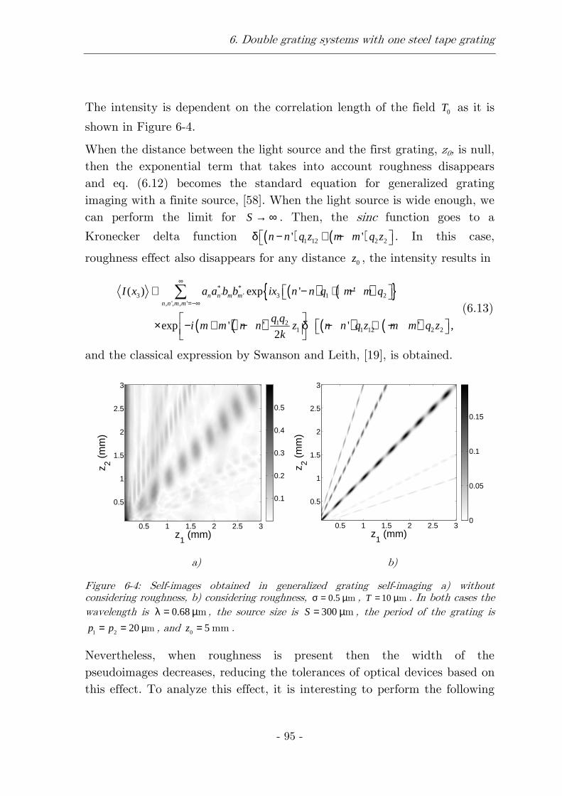
6. Double grating systems with one steel tape grating

- 95 -

The intensity is dependent on the correlation length of the field 0T as it is

shown in Figure 6-4.

When the distance between the light source and the first grating, z0, is null, then the exponential term that takes into account roughness disappears and eq. (6.12) becomes the standard equation for generalized grating imaging with a finite source, [58]. When the light source is wide enough, we can perform the limit for S → ∞ . Then, the sinc function goes to a

Kronecker delta function ( ) ( )1 12 2 2' 'n n q z m m q zδ − + − . In this case,

roughness effect also disappears for any distance 0z , the intensity results in

( ) ( ){ }

( )( ) ( ) ( )

* *3 ' ' 3 1 2

, ', , '

1 21 1 12 2 2

( ) exp ' '

exp ' ' ' ' ,2

n n m mn n m m

I x a a b b ix n n q m m q

q qi m m n n z n n q z m m q z

k

∞

=−∞∝ − + −

× − + − δ − + −

∑ (6.13)

and the classical expression by Swanson and Leith, [19], is obtained.

z1 (mm)

z 2 (m

m)

0.5 1 1.5 2 2.5 3

0.5

1

1.5

2

2.5

3

0.1

0.2

0.3

0.4

0.5

z1 (mm)

z 2 (m

m)

0.5 1 1.5 2 2.5 3

0.5

1

1.5

2

2.5

3

0

0.05

0.1

0.15

a) b)

Figure 6-4: Self-images obtained in generalized grating self-imaging a) without considering roughness, b) considering roughness, 0.5σ = µm , 10T = µm . In both cases the wavelength is 0.68λ = µm , the source size is 300S = µm , the period of the grating is

1 2 20p p µ= = m , and 0 5z = mm .

Nevertheless, when roughness is present then the width of the pseudoimages decreases, reducing the tolerances of optical devices based on this effect. To analyze this effect, it is interesting to perform the following

- 96 -

changes of variables, ( ', 'N n n M m m= − = − , / 2, / 2u n N v m M= − = − ), in eq.

(6.12). As a result, the mean intensity is

( )

( ) ( )

( ) ( ){ }

33 2 1 0 2 01

,

2

01 12 2 2 1 12 2 2

0

* *' ' 11 12 22 12

,

( , ) exp

exp2

exp 2 ,

N M T

T T

n n m mu v

ixI x z Nq z Mq z

z

zSNq z Mq z Nq z Mq z

z kT z

a a b b i u N M v M N

∞

=−∞

∞

=−∞

∝ − +

× + − +

× π γ + γ + γ + γ

∑

∑

sinc (6.14)

where 11 0 12 / Tz z z zλγ = , 222 2 01 / Tz z R z zλγ = , 12 0 2 / Tz z R z zλγ = , 1 2/R p p= , and

21 /Tz p= λ . A given pseudoimage (N, M) presents a maximum value when

the argument of the sinc function in eq. (6.14) is null, that is

2 1

1

1z z

RQ=

−. (6.15)

where Q = -M/N. At the exact locations of the pseudoimages, the sinc factor and the Gaussian factor are equal to one and the intensity does not depend on the roughness parameters. For usual distances (millimeters-centimeters), pseudoimages are quite narrow and they do not overlap (pseudoimage isolation, regime 3 of ref. [60]). The sinc and the Gaussian factors control the width of the pseudoimage being both competitive. We will define the width of a given pseudoimage as

( )2

1 2 12( , )

2 1

( )

( )N M

z z Amp z dz

Amp z dz

−ω = ∫

∫, (6.16)

where 1 2 1 2 1( ) / ( )z z Amp z dz Amp z z= ∫ ∫ and 2 , 3 2( ) max ( , )N MAmp z I x z=

, 3 2min ( , )N MI x z− . The width of a given pseudoimage (N, M) is dependent

on the correlation length of roughness 0T , as it is shown in Figure 6-5.

For low values of 0T , the Gaussian factor controls the width of the

pseudoimage which increases linearly as

0( , )

0 12T

N M

kT z

z Nqω ≈ . (6.17)

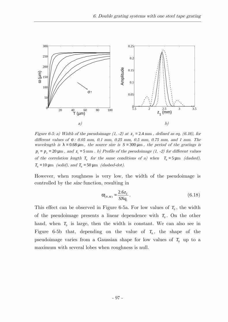
6. Double grating systems with one steel tape grating

- 97 -

20 40 60 80 1000

50

100

150

200

250

300

T (µm)

ω (

µm)

σ

1.5 2 2.5 3 3.50

0.05

0.1

0.15

0.2

0.25

z1 (mm)

Am

plitu

de

a) b)

Figure 6-5: a) Width of the pseudoimage (1, -2) at 2 2.4z = mm , defined as eq. (6.16), for different values of σ : 0.05 mm, 0.1 mm, 0.25 mm, 0.5 mm, 0.75 mm, and 1 mm. The wavelength is 0.68λ = µm , the source size is 300S = µm , the period of the gratings is

1 2 20p p= = µm , and 1 5z = mm . b) Profile of the pseudoimage (1, -2) for different values

of the correlation length 0T for the same conditions of a) when 0 5T = µm (dashed),

0 10T = µm (solid), and 0 50T = µm (dashed-dot).

However, when roughness is very low, the width of the pseudoimage is controlled by the sinc function, resulting in

( , )1

2.6 TN M

z

SNqω ≈ . (6.18)

This effect can be observed in Figure 6-5a. For low values of 0T , the width

of the pseudoimage presents a linear dependence with 0T . On the other

hand, when 0T is large, then the width is constant. We can also see in

Figure 6-5b that, depending on the value of 0T , the shape of the

pseudoimage varies from a Gaussian shape for low values of 0T up to a

maximum with several lobes when roughness is null.

- 99 -

7777 Diffraction by rDiffraction by rDiffraction by rDiffraction by rough gratingsough gratingsough gratingsough gratings

In this chapter we introduce a new kind of grating based on random micro-topography. This grating is formed by smooth and rough strips placed alternatively. Since the topography of the rough strips is considered random, stochastic tools are necessary to analyze its behavior. Near and far field diffraction patterns are obtained. Analytical solutions for far and near field diffraction are obtained. We demonstrate that this kind of periodic element acts as a diffraction grating. Talbot effect occurs in near field and diffraction orders appear at far field but with some differences with respect to amplitude and phase gratings. Talbot effect does not appear just after the grating but gradually, depending on the roughness level. In addition, the efficiency of the diffraction orders depends also on the roughness parameters. Finally, we demonstrate the validity of the formalism performing experimental and numerical verifications based on the Rayleigh-Sommerfeld formula.

- 100 -

7. Diffraction by rough gratings

- 101 -

7.17.17.17.1 IntroductionIntroductionIntroductionIntroduction

Diffraction gratings are elements that change periodically one or more than one properties of a light beam. In most cases, amplitude or phase gratings are used, which modulate the amplitude or phase of the incident light respectively [68], [92]-[94]. There are also other possibilities to modulate the incident light such as polarization gratings which modulate the state of polarization [95]-[97]. In the present chapter we develop and analyze a new type of diffraction grating, which we have called “Rough grating”. This element acts like a diffraction grating only due to its micro-topography. Here, we assume a grating with different roughness. In fact, surfaces always present a certain roughness. The characteristics of the near and far field diffraction patterns are determined in terms of the statistical properties of roughness. In section 7.3 the far field behavior of this kind of gratings is analyzed. The mutual intensity and the efficiency of the diffraction orders are obtained, which are shown to depend on the roughness parameters. The intensity of the far field diffraction pattern is also obtained for high and low roughness limits. Experimental results for the case of a transmission grating where one of the levels is rough are also obtained, corroborating the validity of the proposed framework. In section 7.4, the near field approach for this kind of gratings is analyzed. Analytical expressions for the intensity are obtained in general, slight and high roughness level approximations. Talbot effect appears over an ensemble of gratings, but not considering an only grating. Besides, the self-images do not appears just after the gratings, but gradually. From a certain distance that depends on the roughness parameters, the contrast of the self-images remains constant. Experimental and numerical verifications of the behavior proposed are performed, showing the validity of the analytical expressions.

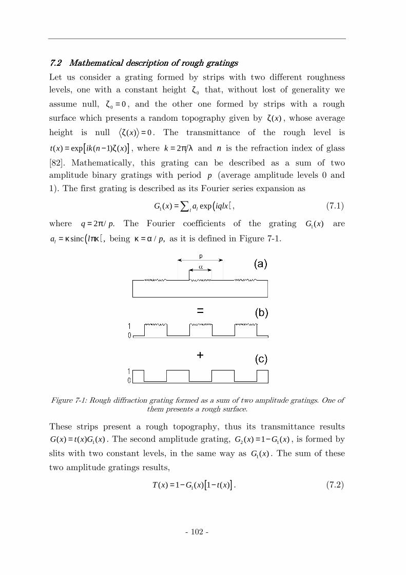
- 102 -

7.27.27.27.2 Mathematical Mathematical Mathematical Mathematical description of rough gratingsdescription of rough gratingsdescription of rough gratingsdescription of rough gratings

Let us consider a grating formed by strips with two different roughness levels, one with a constant height 0ζ that, without lost of generality we

assume null, 0 0ζ = , and the other one formed by strips with a rough

surface which presents a random topography given by ( )xζ , whose average

height is null ( ) 0xζ = . The transmittance of the rough level is

[ ]( ) exp ( 1) ( )t x ik n x= − ζ , where 2k = π λ and n is the refraction index of glass

[82]. Mathematically, this grating can be described as a sum of two amplitude binary gratings with period p (average amplitude levels 0 and

1). The first grating is described as its Fourier series expansion as

( )1( ) expllG x a iqlx=∑ , (7.1)

where 2 / .q p= π The Fourier coefficients of the grating 1( )G x are

( )sinc ,la l= κ πκ being / ,pκ = α as it is defined in Figure 7-1.

Figure 7-1: Rough diffraction grating formed as a sum of two amplitude gratings. One of them presents a rough surface.

These strips present a rough topography, thus its transmittance results

1( ) ( ) ( )G x t x G x= . The second amplitude grating, 2 1( ) 1 ( )G x G x= − , is formed by

slits with two constant levels, in the same way as 1( )G x . The sum of these

two amplitude gratings results,

[ ]1( ) 1 ( ) 1 ( )T x G x t x= − − . (7.2)

7. Diffraction by rough gratings

- 103 -

( )T x describes the whole structure, which acts stochastically on the phase

of the incident wave. When roughness is null, then ( ) 1t x = and the grating

disappears, since the transmittance is ( ) 1T x = .

For the general case, the transmission coefficient ( )T x produces a random

change in the phase of the incident beam when it passes through the rough strips. For simplicity and without lost of generality, we consider the one-dimensional problem. Besides, the transmission variation owed to Fresnel coefficients is not included.

Considering the formalism proposed in section 3.8, to describe the random topography of the rough strips a normal distribution in heights is assumed,

( )2 2( ) exp / 2 / 2w z z= − σ πσ , where ( )z x= ζ , and σ is the standard deviation,

[21]. The characteristic function which describes the average transmittance of this distribution results in

( ) ( ) [ ] ( )exp ( 1) exp / 2t x w z ik n z dz g= − = −∫ , (7.3)

where [ ]2( 1)kg n= σ − .

Now, let us consider that a plane wave in normal incidence whose amplitude is 0A illuminates the grating. The amplitude just after the

grating is 1 0( ) ( )U x A T x= . From here, we will assume that the random

process that represent the fields produced by a hypothetical ensemble of diffusers is stationary and, therefore, the mutual intensity function

2

1 1 0( , ) ( ) ( ) ( ) ( )J x y U x U x A T x T x∗ ∗′ ′= = , results

( )1 12

0

1 1

( , )1 ( ) ( ') ( ) 1

( ) ( ') ( ) ( ) 2 ( ) 1 ,

J x yG x G x t x

A

G x G x t x t x t x

∗

∗ ∗

= + + −

′+ − +

(7.4)

where we have considered that ( )* ( ') ( ) exp / 2t x t x g= = − and the angle

brackets represent the average over the ideal ensemble of transmittance coefficients. Some more assumptions about the statistical properties of the topography, ( )xζ , are required. We consider that the two-dimensional

- 104 -

distribution of heights 1 1( )z x= ζ and 2 2( )z x′= ζ , at two different points x

and x′ , with mean values zero and variances 2σ , is

( )2 21 1 2 2

1 2 2 22

21( , ) exp

2 12 1

z Cz z zw z z

CC

− + = −

σ − πσ −

, (7.5)

where the autocorrelation coefficient is Gaussian 2 2 2

1 2 1 0( ) / exp /C T τ = ζ ζ ζ = −τ , x x′τ = − and 0T is the correlation length.

As a result, the characteristic function of this two-dimensional distribution results, [21],

[ ]{ }2

*1 1 20

0

( ) ( ' ) exp 1- ( ) exp( ) exp!

m

m

gt x t x g C g m

m T

∞

=

τ= − τ = − −

∑ . (7.6)

Inserting eq. (7.6) into eq. (7.4), we obtain the mutual intensity function, [79],

( )

( )2

20

*1 12

0

-2* -1 1 1

( , )1 ( ) ( ') 1 exp / 2

( ) ( ') 1 exp / 2 .!

Tm m

g

m

J x xG x G x g

A

gG x G x g e e

m

τ∞

=

′ = − + − −

+ − − +

∑

(7.7)

In Figure 7-2, the mutual intensity function, ( , )J x x′ , just after the

diffraction grating is represented for several cases with different roughness

parameters. The average intensity distribution, ( )I x , just after the

grating is obtained from the mutual intensity, [79], ( ) ( , )I x J x x= . This

value corresponds to the diagonal of the mutual intensity function and in

all cases, it is constant, 2

0( , )I x x A′ = .

7.37.37.37.3 Intensity distribution at the far fieldIntensity distribution at the far fieldIntensity distribution at the far fieldIntensity distribution at the far field

The amplitude, 2 2 2( , )U x y , at the far field can be determined using the

Fraunhofer approach (section 3.6). Let us consider now that the grating presents finite length and width. Then the amplitude of the field just after the grating results

1 0( , ) ( , ) ( / ) ( / )x yU x y A T x y x R y R= ∏ ∏ , (7.8)

where ( )x∏ is the rectangle function

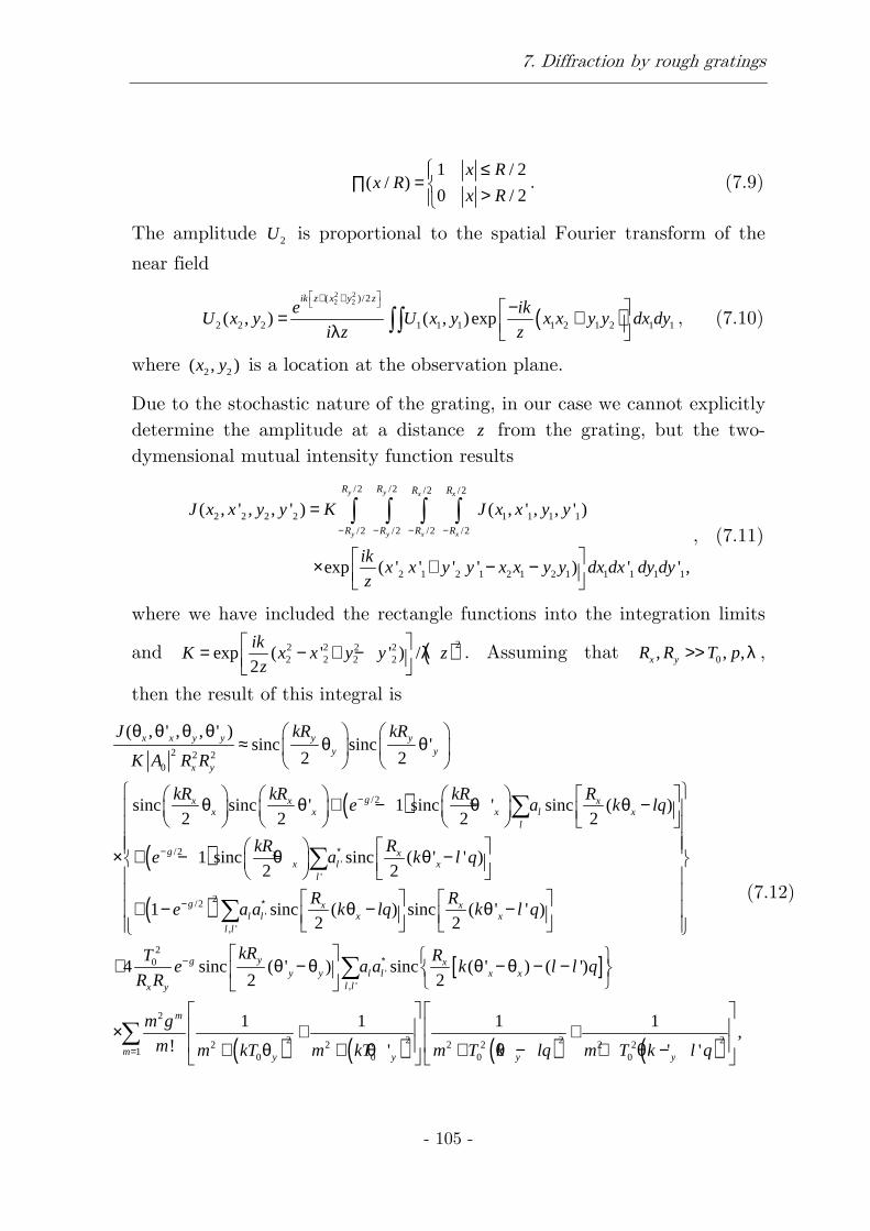
7. Diffraction by rough gratings

- 105 -

1 / 2

( / )0 / 2

x Rx R

x R

≤∏ = >. (7.9)

The amplitude 2U is proportional to the spatial Fourier transform of the

near field

( )2 22 2( )/2

2 2 2 1 1 1 1 2 1 2 1 1( , ) ( , )expik z x y z

e ikU x y U x y x x y y dx dy

i z z

+ + − = + λ ∫∫ , (7.10)

where 2 2( , )x y is a location at the observation plane.

Due to the stochastic nature of the grating, in our case we cannot explicitly determine the amplitude at a distance z from the grating, but the two-dymensional mutual intensity function results

/2 /2 /2 /2

2 2 2 2 1 1 1 1

/2 /2 /2 /2

2 1 2 1 2 1 2 1 1 1 1 1

( , ' , , ' ) ( , ' , , ' )

exp ( ' ' ' ' ) ' ' ,

y y x x

y y x x

R R R R

R R R R

J x x y y K J x x y y

ikx x y y x x y y dx dx dy dy

z

− − − −

=

× + − −

∫ ∫ ∫ ∫, (7.11)

where we have included the rectangle functions into the integration limits

and ( )22 2 2 22 2 2 2exp ( ' ' ) /

2

ikK x x y y z

z = − + − λ

. Assuming that 0, , ,x yR R T p>> λ ,

then the result of this integral is

( )

( )

2 2 20

/2

/2'

'

( , ' , , ' )sinc sinc '

2 2

sinc sinc ' 1 sinc ' sinc ( )2 2 2 2

1 sinc sinc ( ' ' )2 2

1

x x y y y yy y

x y

gx x x xx x x l x

l

g x xx l x

l

J kR kR

K A R R

kR kR kR Re a k lq

kR Re a k l q

−

− ∗

θ θ θ θ ≈ θ θ

θ θ + − θ θ −

× + − θ θ −

+

∑

∑

( )

[ ]

( ) ( )

2/2'

, '

20

', '

2

2 22 21 0 0

sinc ( ) sinc ( ' ' )2 2

4 sinc ( ' ) sinc ( ' ) ( ')2 2

1 1

! '

g x xl l x x

l l

yg xy y l l x x

l lx y

m

my y

R Re a a k lq k l q

kRT Re a a k l l q

R R

m g

m m kT m kT

− ∗

− ∗

=

− θ − θ −

+ θ − θ θ − θ − −

× + + θ + θ

∑

∑

∑ ( ) ( )2 22 2 2 20 0

1 1,

' 'y ym T k lq m T k l q

+ + θ − + θ −

(7.12)

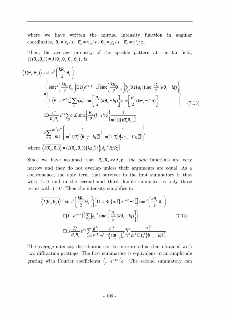
- 106 -

where we have written the mutual intensity function in angular coordinates, 2 /x x zθ = , 2' /x x z′θ = , 2 /y y zθ = , 2' /y y z′θ = .

Then, the average intensity of the speckle pattern at the far field, ( , ) ( , , , )x y x x y yI Jθ θ = θ θ θ θ , is

( ) ( )

( )

2

2 /2

2/2'

, '

20

', '

( , ) sinc2

sinc 2 1 sinc Re sinc ( )2 2 2

1 sinc ( ) sinc ( ' )2 2

8 sinc

yx y y

gx x xx x l x

l

g x xl l x x

l l

gl l

l lx y

kRI

kR kR Re a k lq

R Re a a k lq k l q

Te a a

R R

−

− ∗

− ∗

θ θ = θ

θ + − θ θ − × + − θ − θ −

+

∑

∑

∑ ( )

( ) ( )

220

2

2 22 2 2 21 0 0

1( ')

2

1 1,

! '

x

y

m

m x x

Rl l q

m kT

m g

m m T k lq m T k l q=

− + θ

× +

+ θ − + θ − ∑

(7.13)

where ( ) ( )22 2 20( , ) ( , ) /x y x y x yI I z A R Rθ θ = θ θ λ .

Since we have assumed that , ,x yR R p>> λ , the sinc functions are very

narrow and they do not overlap unless their arguments are equal. As a consequence, the only term that survives in the first summatory is that with 0l = and in the second and third double summatories only those terms with 'l l= . Then the intensity simplifies to

( ) ( )

( )

( ) ( )

2 /2 20

2 2/2 2

22 20

2 22 221 00

( , ) sinc 1 2Re 1 sinc2 2

1 sinc ( )2

16 .!

y g xx y y x

g xl x

l

mlg

m lx y xy

kR kRI a e

Re a k lq

aT g me

R R m m T k lqm kT

−

−

−

=

θ θ = θ + − θ

+ − θ −

++ θ −+ θ

∑

∑ ∑

(7.14)

The average intensity distribution can be interpreted as that obtained with two diffraction gratings. The first summatory is equivalent to an amplitude

grating with Fourier coefficients ( )/21 gle a−− . The second summatory can

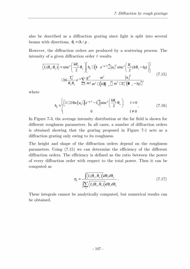
7. Diffraction by rough gratings

- 107 -

also be described as a diffraction grating since light is split into several beams with directions, /l l pθ = λ .

However, the diffraction orders are produced by a scattering process. The intensity of a given diffraction order l results

( )

( ) ( )

2 22 /2 20

22 20

2 22 221 00

( , ) sinc 1 sinc ( )2 2

16 ,!

y g xl x y y l x

mlg

mx y xy

kR RI h e a k lq

aT g me

R R m m T k lqm kT

−

−

=

θ θ = θ + − θ −

++ θ −+ θ

∑ (7.15)

where

( ) ( )/2 2

00

1 2Re 1 sinc 02

0 0

g xx

kRa e l

h

l

− + − θ = = ≠

. (7.16)

In Figure 7-3, the average intensity distribution at the far field is shown for different roughness parameters. In all cases, a number of diffraction orders is obtained showing that the grating proposed in Figure 7-1 acts as a diffraction grating only owing to its roughness.

The height and shape of the diffraction orders depend on the roughness parameters. Using (7.15) we can determine the efficiency of the different diffraction orders. The efficiency is defined as the ratio between the power of every diffraction order with respect to the total power. Then it can be computed as

( , )

( , )

l x y x y

l

l x y x yl

I d d

I d d

θ θ θ θη =

θ θ θ θ

∫

∑∫. (7.17)

These integrals cannot be analytically computed, but numerical results can be obtained.

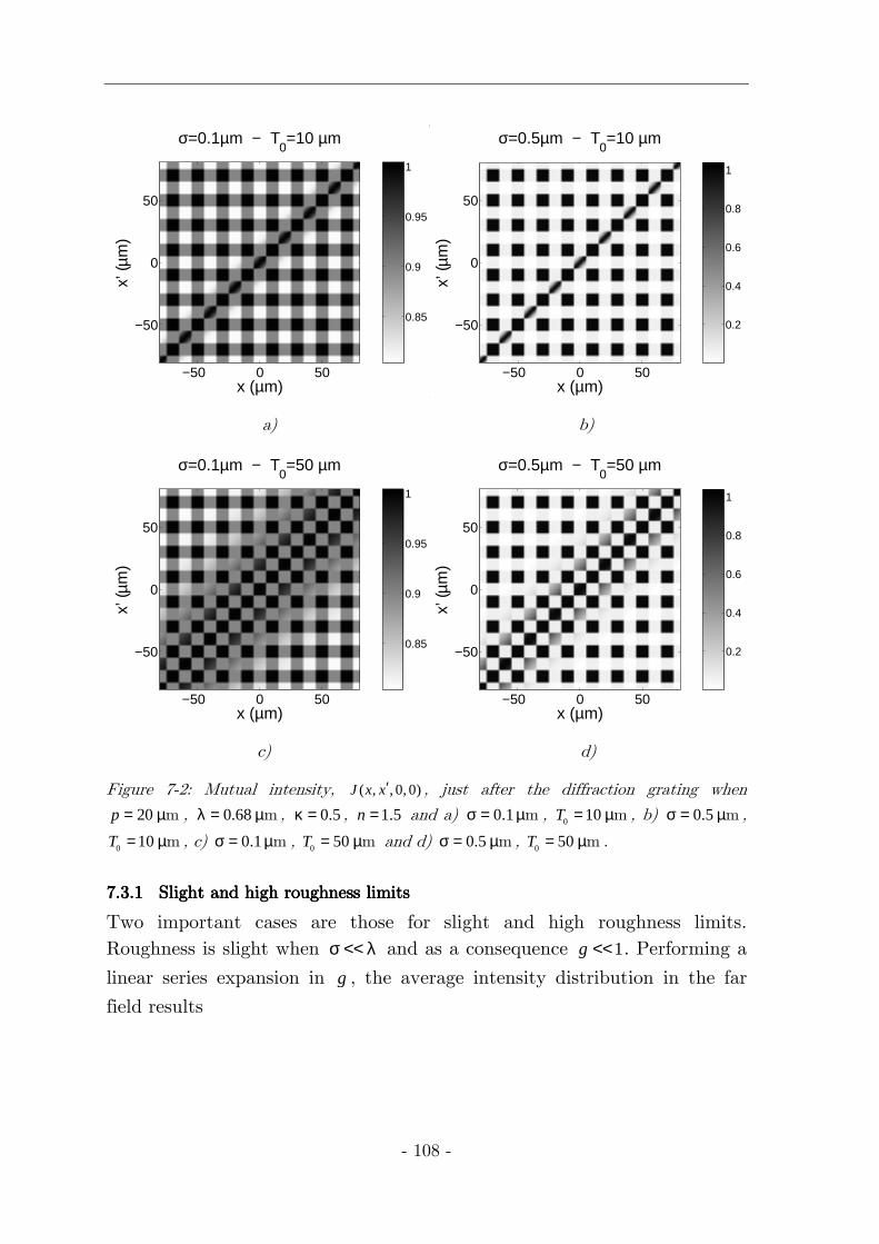
- 108 -

x (µm)

x’ (µ

m)

σ=0.1µm − T0=10 µm

−50 0 50

−50

0

50

0.85

0.9

0.95

1

x (µm)

x’ (µ

m)

σ=0.5µm − T0=10 µm

−50 0 50

−50

0

50

0.2

0.4

0.6

0.8

1

a) b)

x (µm)

x’ (µ

m)

σ=0.1µm − T0=50 µm

−50 0 50

−50

0

50

0.85

0.9

0.95

1

x (µm)

x’ (µ

m)

σ=0.5µm − T0=50 µm

−50 0 50

−50

0

50

0.2

0.4

0.6

0.8

1

c) d)

Figure 7-2: Mutual intensity, ( , , 0, 0)J x x′ , just after the diffraction grating when

20p = µm , 0.68λ = µm , 0.5κ = , 1.5n = and a) 0.1σ = µm , 0 10T = µm , b) 0.5σ = µm ,

0 10T = µm , c) 0.1σ = µm , 0 50T = µm and d) 0.5σ = µm , 0 50T = µm .

7.3.17.3.17.3.17.3.1 Slight and high roughness limitsSlight and high roughness limitsSlight and high roughness limitsSlight and high roughness limits

Two important cases are those for slight and high roughness limits. Roughness is slight when σ << λ and as a consequence 1g << . Performing a

linear series expansion in g , the average intensity distribution in the far

field results

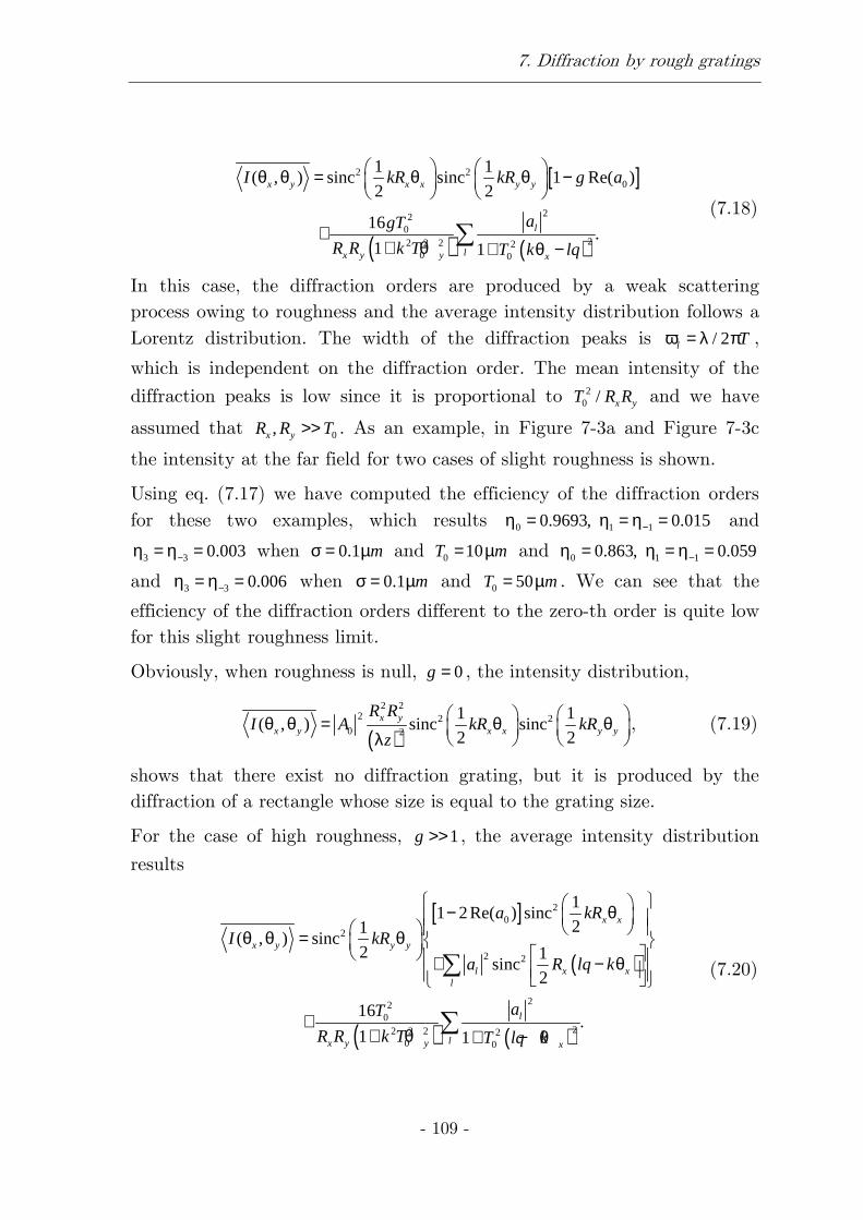
7. Diffraction by rough gratings

- 109 -

[ ]

( ) ( )

2 20

220

22 2 2 20 0

1 1( , ) sinc sinc 1 Re( )

2 2

16.

1 1

x y x x y y

l

lx y y x

I kR kR g a

agT

R R k T T k lq

θ θ = θ θ −

++ θ + θ −

∑ (7.18)

In this case, the diffraction orders are produced by a weak scattering process owing to roughness and the average intensity distribution follows a Lorentz distribution. The width of the diffraction peaks is / 2l Tω = λ π ,

which is independent on the diffraction order. The mean intensity of the

diffraction peaks is low since it is proportional to 20 / x yT R R and we have

assumed that 0,x yR R T>> . As an example, in Figure 7-3a and Figure 7-3c

the intensity at the far field for two cases of slight roughness is shown.

Using eq. (7.17) we have computed the efficiency of the diffraction orders for these two examples, which results 0 1 10.9693, 0.015−η = η = η = and

3 3 0.003−η = η = when 0.1 mσ = µ and 0 10T m= µ and 0 1 10.863, 0.059−η = η = η =

and 3 3 0.006−η = η = when 0.1 mσ = µ and 0 50T m= µ . We can see that the

efficiency of the diffraction orders different to the zero-th order is quite low for this slight roughness limit.

Obviously, when roughness is null, 0g = , the intensity distribution,

( )

2 22 2 2

0 2

1 1( , ) sinc sinc

2 2x y

x y x x y y

R RI A kR kR

z

θ θ = θ θ λ

, (7.19)

shows that there exist no diffraction grating, but it is produced by the diffraction of a rectangle whose size is equal to the grating size.

For the case of high roughness, 1g >> , the average intensity distribution

results

[ ]

( )

( ) ( )

20

2

2 2

220

22 2 2 20 0

11 2Re( ) sinc

21( , ) sinc

2 1sinc

2

16.

1 1

x x

x y y y

l x xl

l

lx y y x

a kR

I kR

a R lq k

aT

R R k T T lq k

− θ θ θ = θ

+ − θ

++ θ + − θ

∑

∑

(7.20)

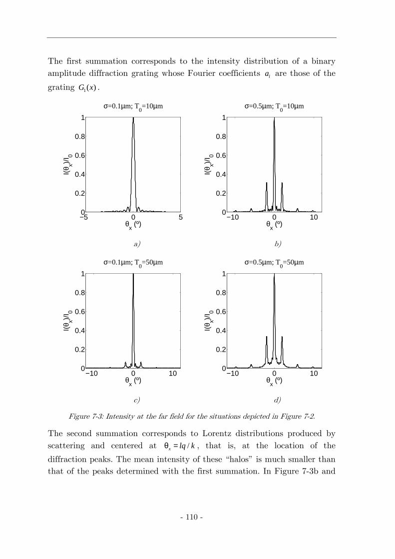
- 110 -

The first summation corresponds to the intensity distribution of a binary amplitude diffraction grating whose Fourier coefficients la are those of the

grating 1( )G x .

−5 0 50

0.2

0.4

0.6

0.8

1

θx (º)

I(θ x)/

I 0

σ=0.1µm; T0=10µm

−10 0 100

0.2

0.4

0.6

0.8

1

θx (º)

I(θ x)/

I 0

σ=0.5µm; T0=10µm

a) b)

−10 0 100

0.2

0.4

0.6

0.8

1

θx (º)

I(θ x)/

I 0

σ=0.1µm; T0=50µm

−10 0 100

0.2

0.4

0.6

0.8

1

θx (º)

I(θ x)/

I 0

σ=0.5µm; T0=50µm

c) d)

Figure 7-3: Intensity at the far field for the situations depicted in Figure 7-2.

The second summation corresponds to Lorentz distributions produced by scattering and centered at /x lq kθ = , that is, at the location of the

diffraction peaks. The mean intensity of these “halos” is much smaller than that of the peaks determined with the first summation. In Figure 7-3b and

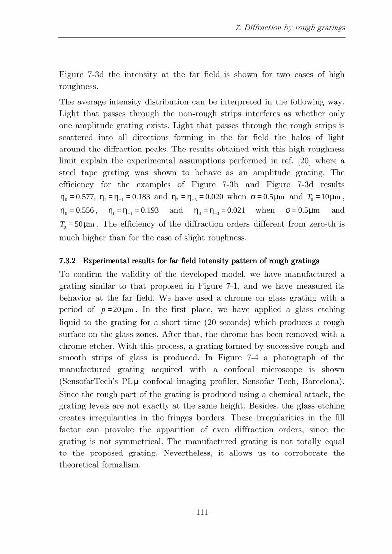
7. Diffraction by rough gratings

- 111 -

Figure 7-3d the intensity at the far field is shown for two cases of high roughness.

The average intensity distribution can be interpreted in the following way. Light that passes through the non-rough strips interferes as whether only one amplitude grating exists. Light that passes through the rough strips is scattered into all directions forming in the far field the halos of light around the diffraction peaks. The results obtained with this high roughness limit explain the experimental assumptions performed in ref. [20] where a steel tape grating was shown to behave as an amplitude grating. The efficiency for the examples of Figure 7-3b and Figure 7-3d results

0 1 10.577, 0.183−η = η = η = and 3 3 0.020−η = η = when 0.5σ = µm and 0 10T = µm ,

0 0.556η = , 1 1 0.193−η = η = and 3 3 0.021−η = η = when 0.5σ = µm and

0 50T = µm . The efficiency of the diffraction orders different from zero-th is

much higher than for the case of slight roughness.

7.3.27.3.27.3.27.3.2 Experimental Experimental Experimental Experimental results for far field intensity pattern of rough gratingsresults for far field intensity pattern of rough gratingsresults for far field intensity pattern of rough gratingsresults for far field intensity pattern of rough gratings

To confirm the validity of the developed model, we have manufactured a grating similar to that proposed in Figure 7-1, and we have measured its behavior at the far field. We have used a chrome on glass grating with a period of 20p = µm . In the first place, we have applied a glass etching

liquid to the grating for a short time (20 seconds) which produces a rough surface on the glass zones. After that, the chrome has been removed with a chrome etcher. With this process, a grating formed by successive rough and smooth strips of glass is produced. In Figure 7-4 a photograph of the manufactured grating acquired with a confocal microscope is shown (SensofarTech’s PLµ confocal imaging profiler, Sensofar Tech, Barcelona).

Since the rough part of the grating is produced using a chemical attack, the grating levels are not exactly at the same height. Besides, the glass etching creates irregularities in the fringes borders. These irregularities in the fill factor can provoke the apparition of even diffraction orders, since the grating is not symmetrical. The manufactured grating is not totally equal to the proposed grating. Nevertheless, it allows us to corroborate the theoretical formalism.

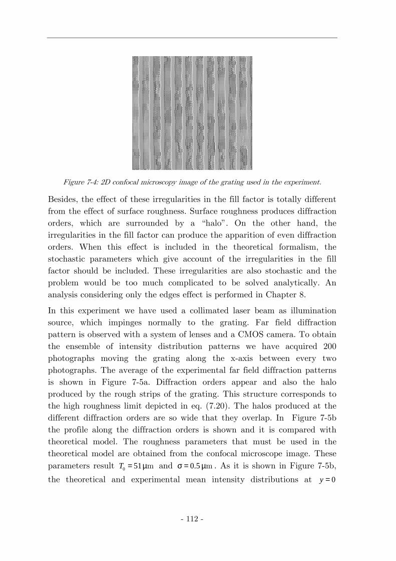
- 112 -

Figure 7-4: 2D confocal microscopy image of the grating used in the experiment.

Besides, the effect of these irregularities in the fill factor is totally different from the effect of surface roughness. Surface roughness produces diffraction orders, which are surrounded by a “halo”. On the other hand, the irregularities in the fill factor can produce the apparition of even diffraction orders. When this effect is included in the theoretical formalism, the stochastic parameters which give account of the irregularities in the fill factor should be included. These irregularities are also stochastic and the problem would be too much complicated to be solved analytically. An analysis considering only the edges effect is performed in Chapter 8.

In this experiment we have used a collimated laser beam as illumination source, which impinges normally to the grating. Far field diffraction pattern is observed with a system of lenses and a CMOS camera. To obtain the ensemble of intensity distribution patterns we have acquired 200 photographs moving the grating along the x-axis between every two photographs. The average of the experimental far field diffraction patterns is shown in Figure 7-5a. Diffraction orders appear and also the halo produced by the rough strips of the grating. This structure corresponds to the high roughness limit depicted in eq. (7.20). The halos produced at the different diffraction orders are so wide that they overlap. In Figure 7-5b the profile along the diffraction orders is shown and it is compared with theoretical model. The roughness parameters that must be used in the theoretical model are obtained from the confocal microscope image. These parameters result 0 51T = µm and 0.5σ = µm . As it is shown in Figure 7-5b,

the theoretical and experimental mean intensity distributions at 0y =

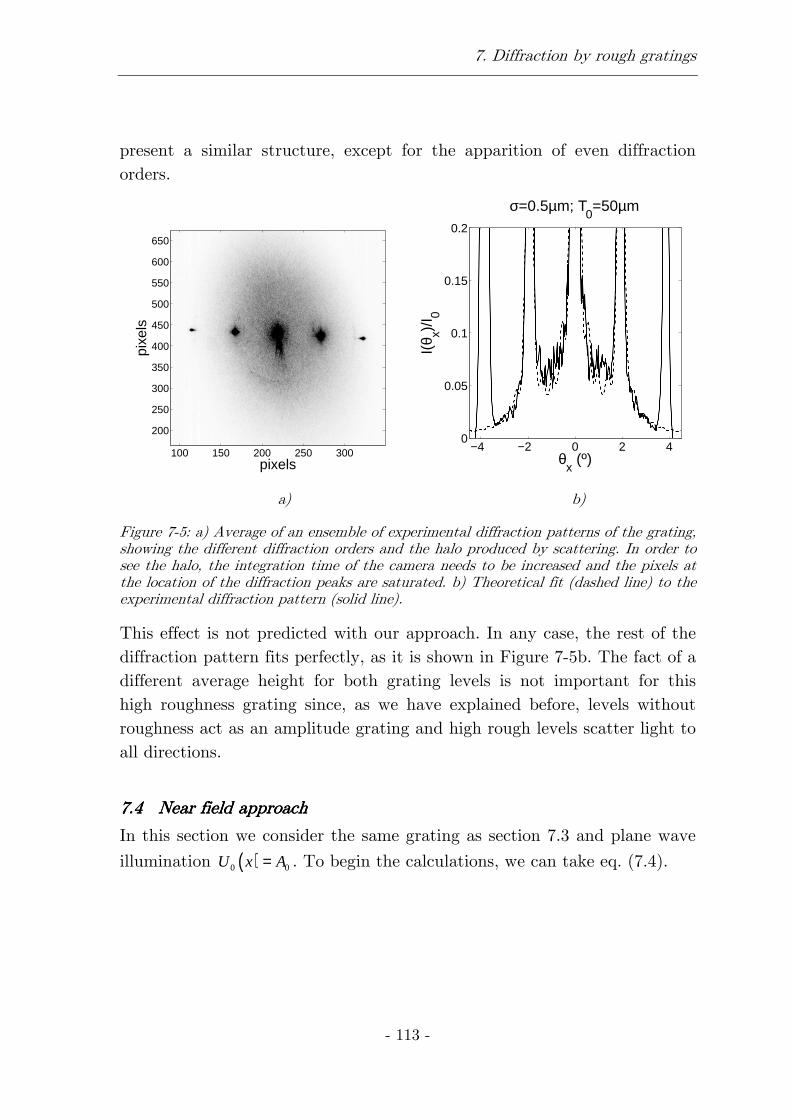
7. Diffraction by rough gratings

- 113 -

present a similar structure, except for the apparition of even diffraction orders.

pixels

pixe

ls

100 150 200 250 300

200

250

300

350

400

450

500

550

600

650

−4 −2 0 2 40

0.05

0.1

0.15

0.2

θx (º)

I(θ x)/

I 0

σ=0.5µm; T0=50µm

a) b)

Figure 7-5: a) Average of an ensemble of experimental diffraction patterns of the grating, showing the different diffraction orders and the halo produced by scattering. In order to see the halo, the integration time of the camera needs to be increased and the pixels at the location of the diffraction peaks are saturated. b) Theoretical fit (dashed line) to the experimental diffraction pattern (solid line).

This effect is not predicted with our approach. In any case, the rest of the diffraction pattern fits perfectly, as it is shown in Figure 7-5b. The fact of a different average height for both grating levels is not important for this high roughness grating since, as we have explained before, levels without roughness act as an amplitude grating and high rough levels scatter light to all directions.

7.47.47.47.4 Near field approachNear field approachNear field approachNear field approach

In this section we consider the same grating as section 7.3 and plane wave

illumination ( )0 0U x A= . To begin the calculations, we can take eq. (7.4).

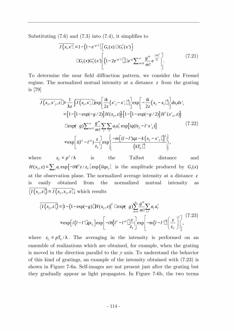
- 114 -

Substituting (7.6) and (7.3) into (7.4), it simplifies to

( ) ( )

( )2

20

- /2 *1 1

* - /2 -1 1 0

, ' 1 1 ( ) ( ')

( ) ( ') 1 2 .!

g

mmTg g

m

J x x e G x G x

gG x G x e e e

m

− τ∞

=

= − − +

+ − +

∑ (7.21)

To determine the near field diffraction pattern, we consider the Fresnel regime. The normalized mutual intensity at a distance z from the grating is [79]

( ) ( ) ( ) ( )

[ ]{ } [ ]{ }[ ]

( )

2 2

2 2 1 1 2 1 2 1 1 1

*2 2

*' 2 21

'

2 22 2

1, ' , , ' exp ' ' exp '

2 2

1 1 exp( / 2) ( , ) 1 1 exp( / 2) ( ' , )

exp( ) exp ( ' ' )!

( ') 'exp ( ' ) exp

m

l lml l

T

ik ikJ x x z J x x x x x x dx dx

z z z

g H x z g H x z

gg a a iq lx l x

m

m l l qz k x xzi l l

z

∞

=

= − − − λ

= − − − − − −

+ − −

− − − − × −

∫

∑ ∑∑

( )

2

2

0

,kT

(7.22)

where 2 /Tz p= λ is the Talbot distance and

( ) ( )22 2( , ) exp / expl Tl

H x z a i l z z ilqx= − π∑ is the amplitude produced by 1( )G x

at the observation plane. The normalized average intensity at a distance z is easily obtained from the normalized mutual intensity as

( ) ( )2 2 2, , ,I x z J x x z= , which results

( ) ( )

( ) ( ) ( )

2 *2 2 '

1 , '

222 2

2

, 1 1 exp( ) ( , ) exp( )!

exp ' exp ' exp ' ,

m

l lm l l

T C

gI x z g H x z g a a

m

z zi l l qx i l l m l l

z z

∞

=

= − − − + −

× − − π − − −

∑ ∑ (7.23)

where 0 /Cz pT= λ . The averaging in the intensity is performed on an

ensemble of realizations which are obtained, for example, when the grating is moved in the direction parallel to the y axis. To understand the behavior of this kind of gratings, an example of the intensity obtained with (7.23) is shown in Figure 7-6a. Self-images are not present just after the grating but they gradually appear as light propagates. In Figure 7-6b, the two terms

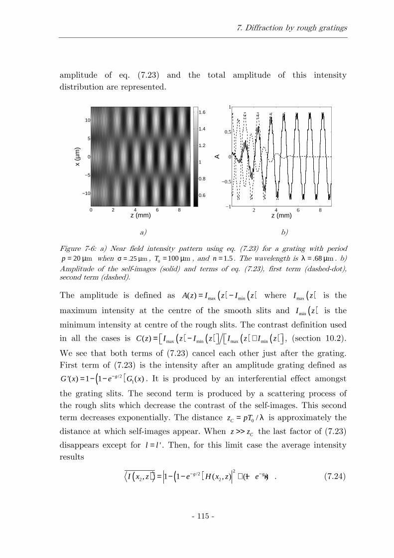
7. Diffraction by rough gratings

- 115 -

amplitude of eq. (7.23) and the total amplitude of this intensity distribution are represented.

z (mm)

x (µ

m)

0 2 4 6 8

−10

−5

0

5

10

0.6

0.8

1

1.2

1.4

1.6

2 4 6 8

−1

−0.5

0

0.5

1

z (mm)A

a) b)

Figure 7-6: a) Near field intensity pattern using eq. (7.23) for a grating with period 20p = µm when .25σ = µm , 0 100T = µm , and 1.5n = . The wavelength is .68λ = µm . b)

Amplitude of the self-images (solid) and terms of eq. (7.23), first term (dashed-dot), second term (dashed).

The amplitude is defined as ( ) ( )max min( )A z I z I z= − where ( )maxI z is the

maximum intensity at the centre of the smooth slits and ( )minI z is the

minimum intensity at centre of the rough slits. The contrast definition used

in all the cases is ( ) ( ) ( ) ( )max min max min( )C z I z I z I z I z= − + , (section 10.2).

We see that both terms of (7.23) cancel each other just after the grating. First term of (7.23) is the intensity after an amplitude grating defined as

( )/21'( ) 1 1 ( )gG x e G x−= − − . It is produced by an interferential effect amongst

the grating slits. The second term is produced by a scattering process of the rough slits which decrease the contrast of the self-images. This second term decreases exponentially. The distance 0 /Cz pT= λ is approximately the

distance at which self-images appear. When Cz z>> the last factor of (7.23)

disappears except for 'l l= . Then, for this limit case the average intensity results

( ) ( ) 2/2

2 2, 1 1 ( , ) (1 )g gI x z e H x z e− −= − − + − κ . (7.24)

- 116 -

The effect of roughness in this case is just to produce the self-imaging process as it was an amplitude grating with modified Fourier coefficients.

7.4.17.4.17.4.17.4.1 Slight and high roughness regimesSlight and high roughness regimesSlight and high roughness regimesSlight and high roughness regimes

In Figure 7-7 the self-imaging process for several values of σ is represented, which cover the most important situations that we can find. The general case has been explained in the previous section. Two important cases are those for slight and high roughness which will be analyzed here in detail. Roughness is considered slight when σ << λ and as a consequence 1g << .

Performing a linear series expansion in g , the mean intensity distribution

in the near field results

( ) ( )

( ) ( )

2 *2 2 ' 2

, '

22 2 2

, 1 cos exp '

exp ' exp ' .

l l ll l lT

C T

zI x z g a lqx l g a a i l l qx

z

z zl l i l l

z z

= − + + −

× − − − −

∑ ∑ (7.25)

As it can be observed, the cosinusoidal term remains along the z axis. Talbot effect is produced, but the intensity is changed by a multiplicative factor, g . On the other hand, the third term decays with z. The contrast of

the self-images decreases with g . An example of the contrast produced

considering slight roughness regime is shown in Figure 7-7a. Obviously,

when roughness is null, 0g = , the intensity distribution, ( ) 2

2 0,I x z A= ,

shows that there exist no diffraction grating.

When roughness is high, 1g >> , then the autocorrelation function given in

(7.6) is approximately ( )2* 2( ) ( ') exp ' / Ft x t x x x T = − −

, where

[ ]0 0/ / ( 1)FT T g T k n= = σ − . Then, the average intensity distribution in the

near field results

( ) 2

2 2, 1 ( , )I x z H x z= − + κ . (7.26)

An example of the contrast produced considering this regime is shown in Figure 7-7c. The first term is the near field intensity distribution produced by a binary amplitude diffraction grating whose Fourier coefficients are

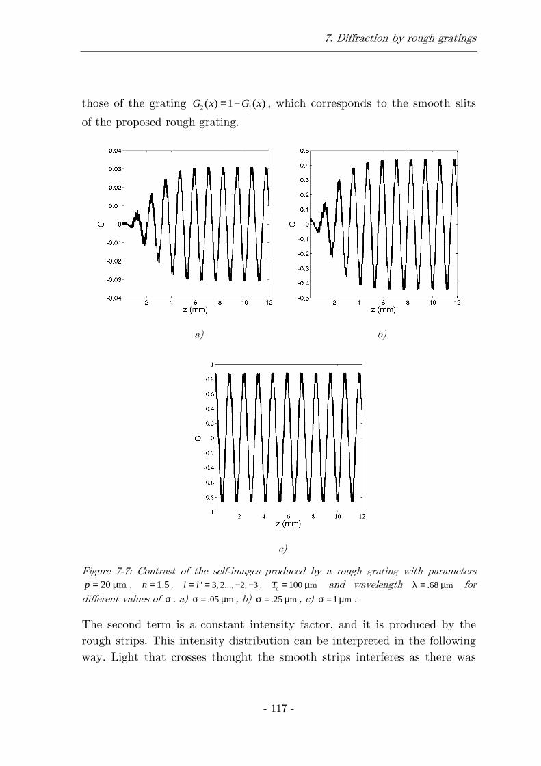
7. Diffraction by rough gratings

- 117 -

those of the grating 2 1( ) 1 ( )G x G x= − , which corresponds to the smooth slits

of the proposed rough grating.

a) b)

c)

Figure 7-7: Contrast of the self-images produced by a rough grating with parameters 20p = µm , 1.5n = , ' 3, 2..., 2, 3l l= = − − ,

0100T = µm and wavelength .68λ = µm for

different values of σ . a) .05σ = µm , b) .25σ = µm , c) 1σ = µm .

The second term is a constant intensity factor, and it is produced by the rough strips. This intensity distribution can be interpreted in the following way. Light that crosses thought the smooth strips interferes as there was

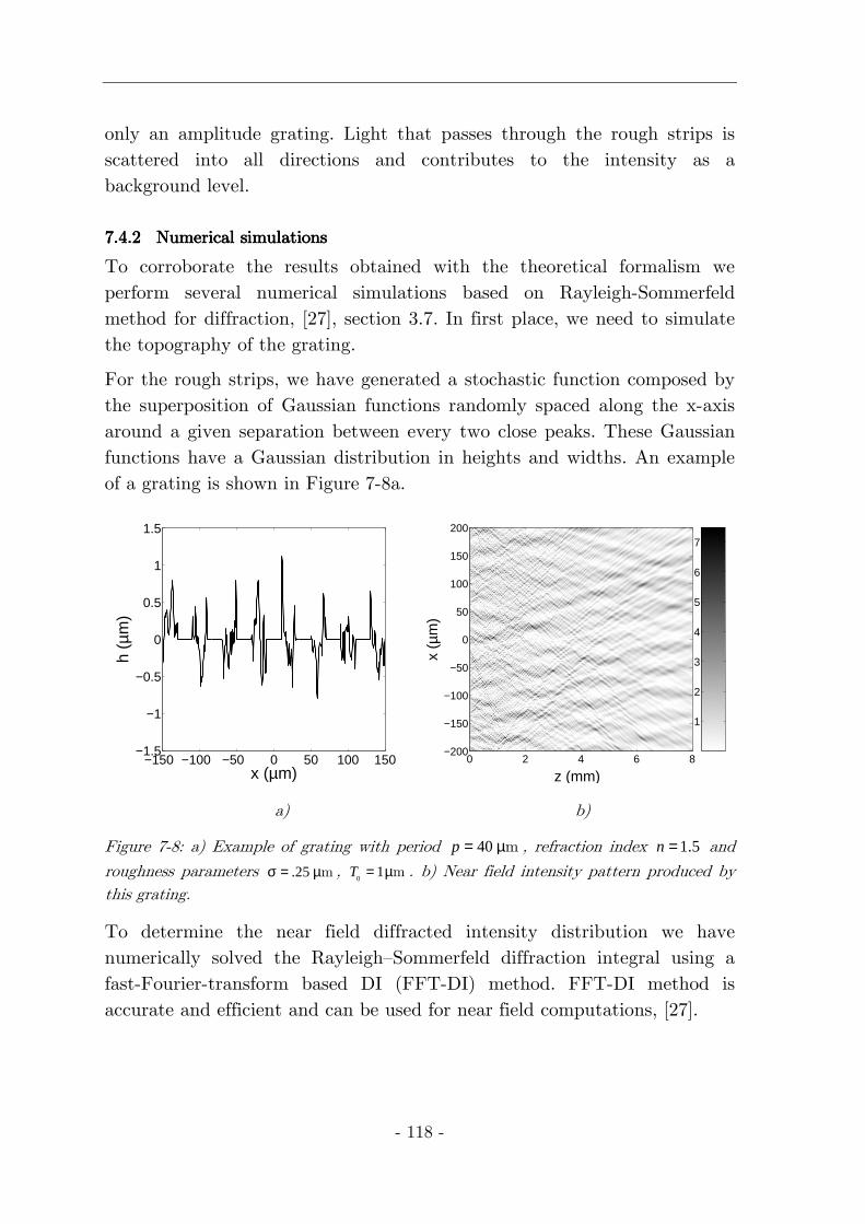
- 118 -

only an amplitude grating. Light that passes through the rough strips is scattered into all directions and contributes to the intensity as a background level.

7.4.27.4.27.4.27.4.2 Numerical simulationsNumerical simulationsNumerical simulationsNumerical simulations

To corroborate the results obtained with the theoretical formalism we perform several numerical simulations based on Rayleigh-Sommerfeld method for diffraction, [27], section 3.7. In first place, we need to simulate the topography of the grating.

For the rough strips, we have generated a stochastic function composed by the superposition of Gaussian functions randomly spaced along the x-axis around a given separation between every two close peaks. These Gaussian functions have a Gaussian distribution in heights and widths. An example of a grating is shown in Figure 7-8a.

−150 −100 −50 0 50 100 150−1.5

−1

−0.5

0

0.5

1

1.5

x (µm)

h (µ

m)

z (mm)

x (µ

m)

0 2 4 6 8−200

−150

−100

−50

0

50

100

150

200

1

2

3

4

5

6

7

a) b)

Figure 7-8: a) Example of grating with period 40p = µm , refraction index 1.5n = and

roughness parameters .25σ = µm , 0

1T = µm . b) Near field intensity pattern produced by this grating.

To determine the near field diffracted intensity distribution we have numerically solved the Rayleigh—Sommerfeld diffraction integral using a fast-Fourier-transform based DI (FFT-DI) method. FFT-DI method is accurate and efficient and can be used for near field computations, [27].

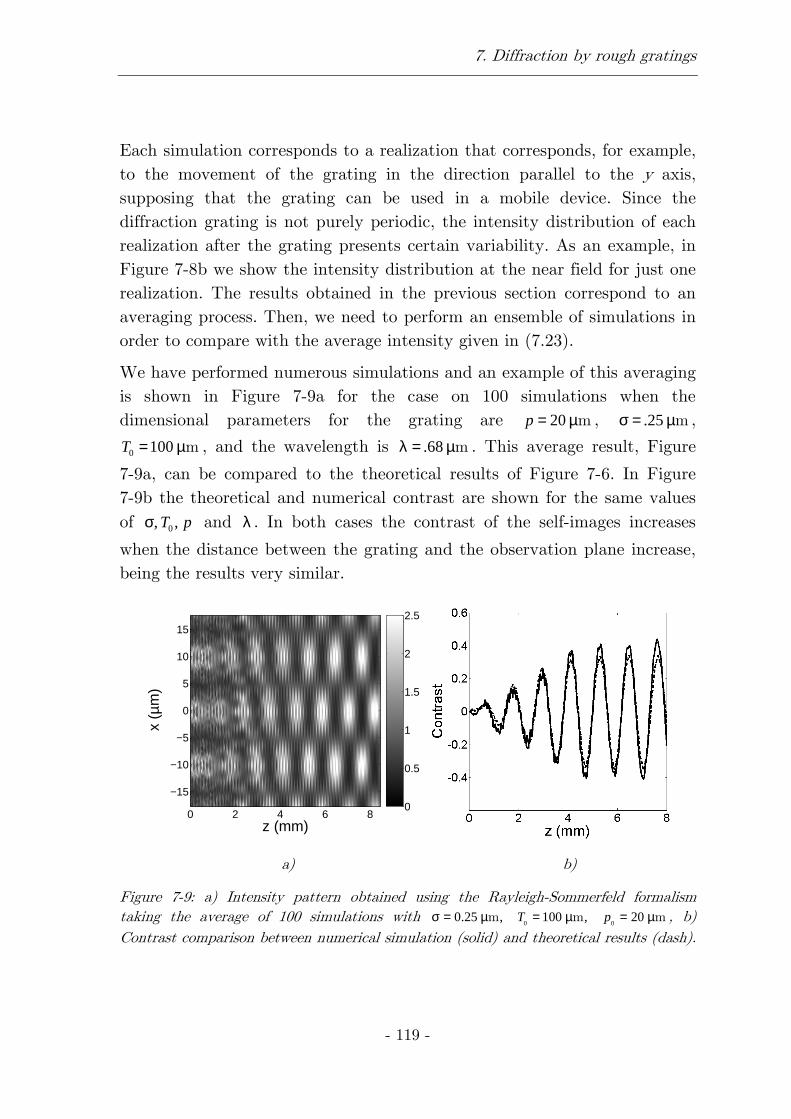
7. Diffraction by rough gratings

- 119 -

Each simulation corresponds to a realization that corresponds, for example, to the movement of the grating in the direction parallel to the y axis, supposing that the grating can be used in a mobile device. Since the diffraction grating is not purely periodic, the intensity distribution of each realization after the grating presents certain variability. As an example, in Figure 7-8b we show the intensity distribution at the near field for just one realization. The results obtained in the previous section correspond to an averaging process. Then, we need to perform an ensemble of simulations in order to compare with the average intensity given in (7.23).

We have performed numerous simulations and an example of this averaging is shown in Figure 7-9a for the case on 100 simulations when the dimensional parameters for the grating are 20p = µm , .25σ = µm ,

0 100T = µm , and the wavelength is .68λ = µm . This average result, Figure

7-9a, can be compared to the theoretical results of Figure 7-6. In Figure 7-9b the theoretical and numerical contrast are shown for the same values of 0, ,T pσ and λ . In both cases the contrast of the self-images increases

when the distance between the grating and the observation plane increase, being the results very similar.

z (mm)

x (µ

m)

0 2 4 6 8

−15

−10

−5

0

5

10

15

0

0.5

1

1.5

2

2.5

a) b)

Figure 7-9: a) Intensity pattern obtained using the Rayleigh-Sommerfeld formalism taking the average of 100 simulations with

0 00.25 , 100 , 20T pσ = µ = µ = µm m m , b)

Contrast comparison between numerical simulation (solid) and theoretical results (dash).

- 121 -

8888 Gratings with rough edgesGratings with rough edgesGratings with rough edgesGratings with rough edges

In this chapter, an analysis of a possible manufacturing error in diffraction gratings is analyzed. We study the behavior of a diffraction grating whose strips present rough edges. Near and far field approaches are analyzed, obtaining analytical solutions in the cases in which is possible. On the contrary, in cases in which analytical solutions are not possible, numerical simulations have been performed. In addition, experimental verifications of the analytical and numerical results have been obtained. A grating with rough edges has been manufactured in order to know a priori the stochastic characteristics of the edges. We have found that Talbot self-images become more sinusoidal for higher orders of self-image. In far field, it is possible to eliminate high diffraction orders, remaining only 0, 1± , for some values of the

edges roughness. This fact allows a sinusoidalization of the signal in the near field.

- 122 -

8. Gratings with rough edges

- 123 -

8.18.18.18.1 IntroductionIntroductionIntroductionIntroduction

Theoretical approaches normally assume that diffraction gratings present an ideal optical behavior. As it is shown in chapter 3, this assumption produces simple results to predict the intensity after the grating. In addition, chrome on glass gratings and phase gratings behave very accurately according to this model. However, manufactured diffraction gratings are not always ideal. Flaws or defects can be produced, such as lost strips, during the fabrication process [13], [98]-[101]. Other non-ideal behavior, which has been analyzed in Chapters 5 and 6, is owing to roughness on the surface of the gratings, as it happens for steel tape gratings. Also, stochastical irregularities in the shape of the edges can be produced. This effect is not normally present in chrome on glass gratings or phase glass gratings, but strips with rough edges can be detected in some other manufacturing processes, such as laser ablation or chemical attack [24], [98]. In this chapter we theoretically, numerically and experimentally analyze the behavior of amplitude gratings with rough edges. In particular, the far field intensity distribution and the Talbot effect are studied in detail. Due to the stochastic properties of the edges, a statistical approach needs to be used. We theoretically show that the intensity of the diffraction orders depends on roughness parameters of the edges. Selecting the roughness level for the edges, we can suppress ± 3 and higher orders, remaining orders 0 and reduce only slightly orders ± 1. On the other hand, for the near field, a theoretical analysis is not possible since the integrals cannot be solved analytically. Then, a numerical analysis based on Rayleigh-Sommerfeld formalism is performed for determining the properties of the self-images produced by the grating with rough edges, [27]. The properties of the self-images are obtained for single realizations and also for statistical averages. In both cases, the edges of the self-images are smoother than the edges of the grating. Finally, we fabricate a grating with rough edges and we analyze the near field behavior, which is in accordance to the theoretical results.

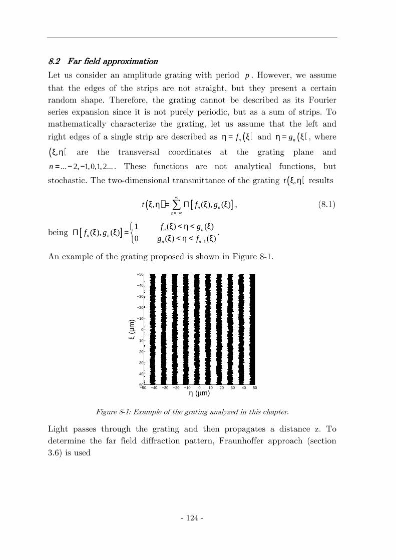
- 124 -

8.28.28.28.2 Far field approximationFar field approximationFar field approximationFar field approximation

Let us consider an amplitude grating with period p . However, we assume

that the edges of the strips are not straight, but they present a certain random shape. Therefore, the grating cannot be described as its Fourier series expansion since it is not purely periodic, but as a sum of strips. To mathematically characterize the grating, let us assume that the left and

right edges of a single strip are described as ( )nfη = ξ and ( )ngη = ξ , where

( ),ξ η are the transversal coordinates at the grating plane and

... 2, 1,0,1,2...n = − − . These functions are not analytical functions, but

stochastic. The two-dimensional transmittance of the grating ( ),t ξ η results

( ) [ ], ( ), ( )n nn

t f g∞

=−∞ξ η = Π ξ ξ∑ , (8.1)

being [ ]1

1 ( ) ( )( ), ( )

0 ( ) ( )n n

n nn n

f gf g

g f +

ξ < η < ξΠ ξ ξ = ξ < η < ξ

.

An example of the grating proposed is shown in Figure 8-1.

η (µm)

ξ (µ

m)

−50 −40 −30 −20 −10 0 10 20 30 40 50

−50

−40

−30

−20

−10

0

10

20

30

40

50

Figure 8-1: Example of the grating analyzed in this chapter.

Light passes through the grating and then propagates a distance z. To determine the far field diffraction pattern, Fraunhoffer approach (section 3.6) is used

8. Gratings with rough edges

- 125 -

( ) ( ) ( ) ( )

2 2

exp2

, , , expi

x yik z

z kU x y t U i x y

i z z

++ = ξ η ξ η − ξ + η ξ η λ

∫ d d , (8.2)

being λ the wavelength of the incident light, 2k = π λ , x and y the

transversal coordinates at the observation plane, z the distance between

the grating and the observation plane, and ( ),iU ξ η the incident field that,

for simplicity, we will consider that is a monochromatic plane wave in

normal incidence, ( ) 0,iU Uξ η = .

Thus, the intensity results in

( ) ( )

( )

( ) ( )'

'

2 /2 /2/22 0

2, ' /2 /2 /2

( ) (4 1) /4 ( ') (4 ' 1) /4

( ) (4 1) /4 ( ') (4 ' 1) /4

, , '

exp ' ' ',n n

n n

L LN

n n N L L

f n p f n p

g n p g n p

UI x y U x y

z

ki x y

z

=− − −

ξ + − ξ + −

ξ + + ξ + +

= = ξ ξλ

× η − ξ − ξ + η − η η

∑ ∫ ∫

∫ ∫

d d

d d

(8.3)

where N is the number of strips and L is their length.

In eq. (8.3) we have transferred the square functions of eq. (8.1) to the limits of the involved integrals. Performing the integrals in η and 'η the

intensity results

( )( )

( )

( ) [ ]{ }( ) [ ]{ }

( ) [ ]{ }

( )

2 /2 /20

2, ' /2 /2

'

'

'

, 'exp '2

exp ' exp ( ) ( ')

exp ' exp ( ) ( ')

exp 2 ' 1 exp ( ) ( ')2

exp 2 ' 12

L L

xn n L Ly

y y n n

y y n n

y y n n

y

UI x y ik

z

ik p n n ik f f

ik p n n ik g g

pik n n ik f g

pik n n

− −

= ξ ξ θ ξ − ξ π θ

θ − θ ξ − ξ

+ θ − θ ξ − ξ

× − θ − + θ ξ − ξ

− θ − −

∑ ∫ ∫d d

[ ]{ }'

,

exp ( ) ( ')y n nik g f

θ ξ − ξ

, (8.4)

where x x zθ = and y y zθ = . The exact shape of the edges ( )nf ξ and ( )ng ξ

is not known but it is possible to describe these functions by means of some stochastic parameters, such as their correlation length T and their

standard deviation σ , [21]. Let us assume that ( )nf ξ and ( )ng ξ present the

same statistical distribution, that ( )nf ξ and ( )ng ξ are totally uncorrelated,

- 126 -

and ( )nf ξ and ( )' 'nf ξ are also totally uncorrelated except for 'n n= . To

describe the edges, a normal distribution with standard deviation σ is assumed. We will also assume a Gaussian autocorrelation coefficient with correlation length T . Then the characteristic functions for this distribution result in, [21],

( )

( )

( ) ( ) ( )

( ) ( )

2

2'

2

22

2' '

( ) ( ) 2

( ) ( ')

2 '( ) ( ') ( ) ( ')

0

( ) ( ') ( ) ( ')

,

,

,

,

!

'

n n

n n

n n n n

n nn n

i f i g

i f g

m mi f f i g g T

m

i f f i g gfor

e e e

e e

e e e em

e e e n n

ασ−α ξ α ξ

α ξ − ξ − ασ

ξ−ξ∞ −α ξ − ξ α ξ − ξ − ασ

=

α ξ − ξ α ξ − ξ − ασ

= =

=

ασ= =

= = ≠

∑

(8.5)

being in our case ykα = θ . Performing an averaging process in (8.4), using

the relationships given in (8.5), and reorganizing the terms, the average intensity is

( )( )

( )

( ) ( )

( ) ( )

( ) ( )

220

2

/2 /2

, ' /2 /2

/2 /22

/2 /2

2

2

2, 1 cos exp

22

exp ' exp ' '

exp exp ' '

exp exp!

y y

y

L L

y xn n L L

L L

y x

L L

y

y x

U pI x y k k

z

ik p n n ik

N k ik

kN k ik

m

− −

− −

= − θ − θ σ π θ

× θ − θ ξ − ξ ξ ξ

− − θ σ θ ξ − ξ ξ ξ

θ σ + − θ σ θ ξ − ξ

∑ ∫ ∫

∫ ∫

d d

d d

( )

( )

2 2

0 2 2

2

2

'

'' ,

L L

m L L

T

∞

= − −

ξ − ξ × − ξ ξ

∑ ∫ ∫

mexp d d

(8.6)

where the averaging in the intensity is performed on an ensemble of realizations which are obtained, for example, when the grating is moved in the direction parallel to the y axis. Let us assume that the length of the strips, L , is large, although not infinite. Then, the integrals have a simple analytical solution and the average intensity results

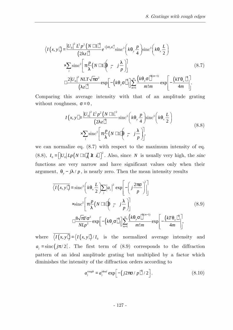
8. Gratings with rough edges

- 127 -

( ) ( )( )

( )

( )

( )( ) ( ) ( )

22 22 2

0 22

2( 1)2 2220

21

1,

4 22

1

2exp exp .

! 4

yk

y x

y

m

y xy

m

U L p N p LI x y e k k

z

pN j

p

kU NLT kTk

m m mz

− θ σ

−∞

=

+ = θ θ λ

λ× π + θ − λ

θ σπσ θ + − θ σ − λ

∑

∑

2

2

j

sinc sinc

sinc (8.7)

Comparing this average intensity with that of an amplitude grating without roughness, 0σ = ,

( ) ( )( )

( )

2 22 20 2

2

1,

4 22

1 ,

y x

y

U L p N p LI x y k k

z

pN j

p

+ = θ θ λ

λ× π + θ − λ ∑

2

2

j

sinc sinc

sinc

(8.8)

we can normalize eq. (8.7) with respect to the maximum intensity of eq.

(8.8), ( ) ( ) 2

0 0 1 2I U Lp N z= + λ . Also, since N is usually very high, the sinc

functions are very narrow and have significant values only when their argument, /y j pθ − λ , is nearly zero. Then the mean intensity results

( )

( )

( ) ( ) ( )

22

2( 1) 222

21

2, exp

2

1

8exp exp ,

! 4

x

y

m

y xy

m

LI x y k a j

p

pN j

p

k kTTk

NLp m m m

−∞

=

πσ = θ −

λ× π + θ − λ

θ σ θπ σ + − θ σ −

∑

∑

2j

j

2

sinc

sinc (8.9)

where ( ) ( ) 0, , /I x y I x y I= is the normalized average intensity and

( )/ 2a j= πj sinc . The first term of (8.9) corresponds to the diffraction

pattern of an ideal amplitude grating but multiplied by a factor which diminishes the intensity of the diffraction orders according to

( )2exp 2 / / 2rough ideala a j p = − πσ

j j . (8.10)

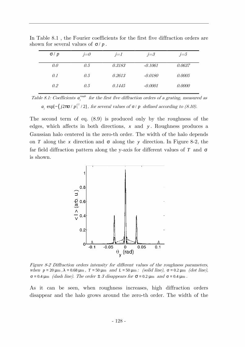
- 128 -

In Table 8.1 , the Fourier coefficients for the first five diffraction orders are shown for several values of / pσ .

/ pσ j=0 j=1 j=3 j=5

0.0 0.5 0.3183 -0.1061 0.0637

0.1 0.5 0.2613 -0.0180 0.0005

0.2 0.5 0.1445 -0.0001 0.0000

Table 8.1: Coefficients roughaj for the first five diffraction orders of a grating, measured as

( )2exp[ 2 / / 2]a j p− πσj , for several values of / pσ defined according to (8.10).

The second term of eq. (8.9) is produced only by the roughness of the edges, which affects in both directions, x and y . Roughness produces a

Gaussian halo centered in the zero-th order. The width of the halo depends on T along the x direction and σ along the y direction. In Figure 8-2, the

far field diffraction pattern along the y-axis for different values of T and σ is shown.

Figure 8-2 Diffraction orders intensity for different values of the roughness parameters, when 20p = µm , 0.68λ = µm , 50T = µm and 50L = µm : (solid line), 0.2σ = µm (dot line),

0.4σ = µm (dash line). The order ± 3 disappears for 0.2= µσ m and 0.4σ = µm .

As it can be seen, when roughness increases, high diffraction orders disappear and the halo grows around the zero-th order. The width of the

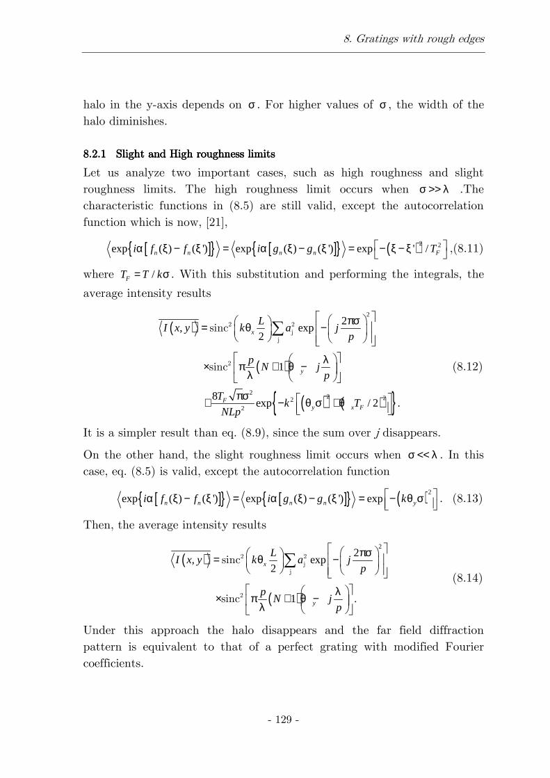
8. Gratings with rough edges

- 129 -

halo in the y-axis depends on σ . For higher values of σ , the width of the halo diminishes.

8.2.18.2.18.2.18.2.1 Slight and High roughness limitsSlight and High roughness limitsSlight and High roughness limitsSlight and High roughness limits

Let us analyze two important cases, such as high roughness and slight roughness limits. The high roughness limit occurs when σ >> λ .The characteristic functions in (8.5) are still valid, except the autocorrelation function which is now, [21],

[ ]{ } [ ]{ } ( )2 2exp ( ) ( ') exp ( ) ( ') exp ' /n n n n Fi f f i g g T α ξ − ξ = α ξ − ξ = − ξ − ξ

,(8.11)

where /FT T k= σ . With this substitution and performing the integrals, the

average intensity results

( )

( )

( ) ( ){ }

2

22 22

2

2, exp

2

1

8exp / 2 .

x

y

Fy x F

LI x y k a j

p

pN j

p

Tk T

NLp

πσ = θ −

λ× π + θ − λ

πσ + − θ σ + θ

∑2 2j

j

2

sinc

sinc (8.12)

It is a simpler result than eq. (8.9), since the sum over j disappears.

On the other hand, the slight roughness limit occurs when σ << λ . In this case, eq. (8.5) is valid, except the autocorrelation function

[ ]{ } [ ]{ } ( )2exp ( ) ( ') exp ( ) ( ') expn n n n yi f f i g g k α ξ − ξ = α ξ − ξ = − θ σ

. (8.13)

Then, the average intensity results

( )

( )

22

, exp2

1 .

x

y

LI x y k a j

p

pN j

p

πσ = θ −

λ× π + θ − λ

∑2 2j

j

2

sinc

sinc

(8.14)

Under this approach the halo disappears and the far field diffraction pattern is equivalent to that of a perfect grating with modified Fourier coefficients.

- 130 -

8.38.38.38.3 SelfSelfSelfSelf----imaging processimaging processimaging processimaging process

The intensity distribution in the near field can be obtained in a simple way replacing the Fraunhofer kernel with the Fresnel kernel in (8.3). Unfortunately it is not possible to obtain analytical solutions for these integrals. As a consequence, we have performed a numerical analysis to determine the characteristics of the intensity distribution in the near field. For the numerical implementation we have used a fast-Fourier-transform based direct integration method which uses the Rayleigh-Sommerfeld approach, [27], section 3.7.

In first place we are interested in how the self-images of this grating with rough edges are formed. In Figure 8-3 we show for comparison the self-images produced by a perfect grating, that is, without rough edges and in Figure 8-4 c) d)

Figure 8-4 and Figure 8-5, two examples of gratings with rough edges and the first three self-images for different values of / pσ . Although the edges

of the grating present a high roughness, the edges of the self-images are quite smooth. The reason is that Talbot effect is a cooperative effect since the intensity at a given point ( , )x y of the image is obtained as an

integration of the amplitude at the diffraction grating. It performs an averaging in the intensity distribution. In addition, an interferential process happens and produces a kind of speckle in the fringes. Since the algorithm does not consider that the grating is periodic, an edge effect is produced. We show the central region of the intensity pattern to avoid this edge effect.

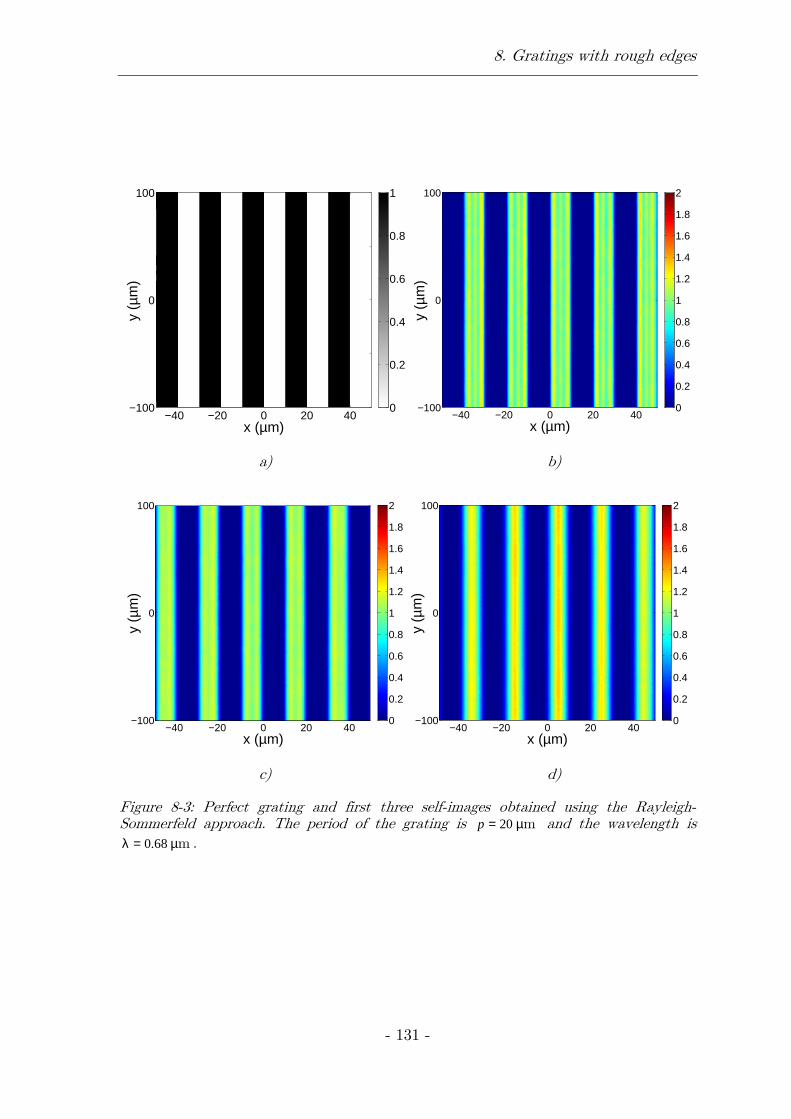
8. Gratings with rough edges

- 131 -

x (µm)

y (µ

m)

−40 −20 0 20 40−100

0

100

0

0.2

0.4

0.6

0.8

1

x (µm)y

(µm

)

−40 −20 0 20 40−100

0

100

0

0.2

0.4

0.6

0.8

1

1.2

1.4

1.6

1.8

2

a) b)

x (µm)

y (µ

m)

−40 −20 0 20 40−100

0

100

0

0.2

0.4

0.6

0.8

1

1.2

1.4

1.6

1.8

2

x (µm)

y (µ

m)

−40 −20 0 20 40−100

0

100

0

0.2

0.4

0.6

0.8

1

1.2

1.4

1.6

1.8

2

c) d)

Figure 8-3: Perfect grating and first three self-images obtained using the Rayleigh-Sommerfeld approach. The period of the grating is 20p = µm and the wavelength is

0.68λ = µm .

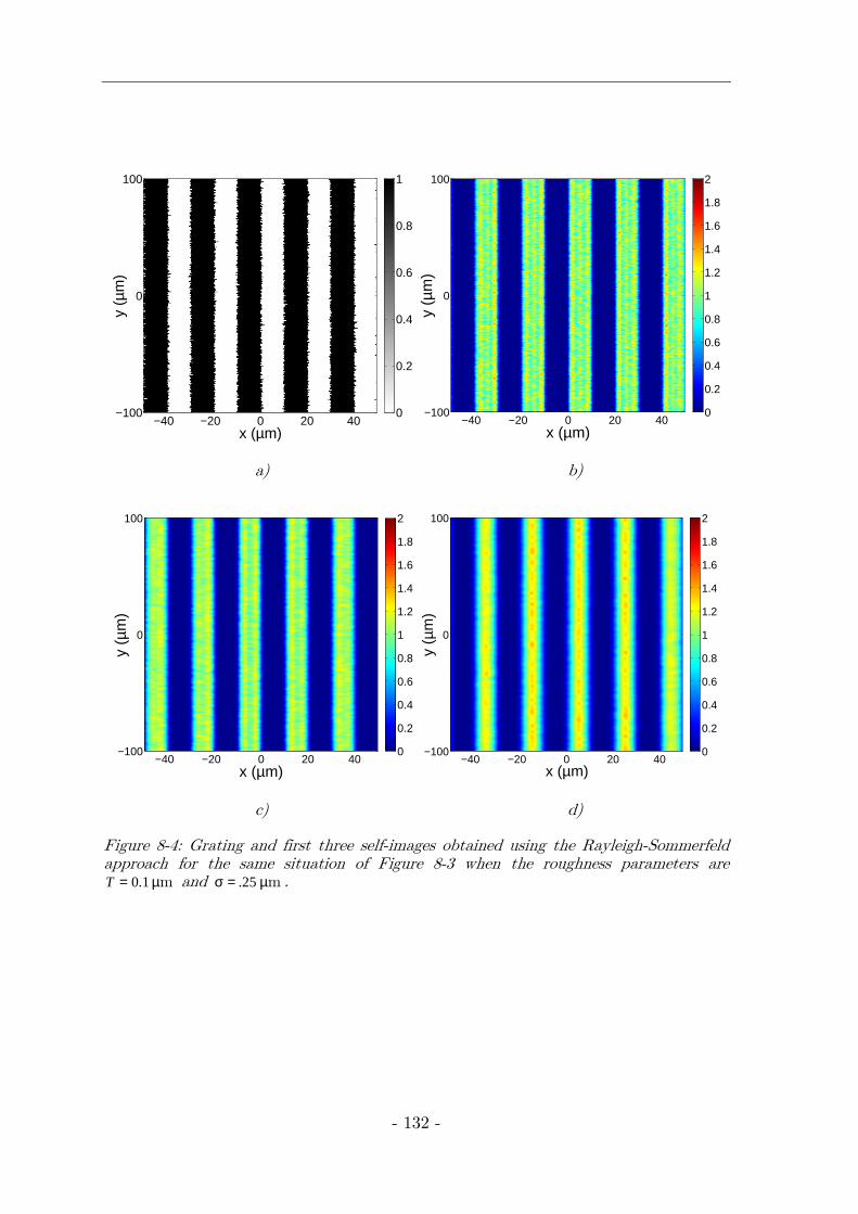
- 132 -

x (µm)

y (µ

m)

−40 −20 0 20 40−100

0

100

0

0.2

0.4

0.6

0.8

1

x (µm)y

(µm

)

−40 −20 0 20 40−100

0

100

0

0.2

0.4

0.6

0.8

1

1.2

1.4

1.6

1.8

2

a) b)

x (µm)

y (µ

m)

−40 −20 0 20 40−100

0

100

0

0.2

0.4

0.6

0.8

1

1.2

1.4

1.6

1.8

2

x (µm)

y (µ

m)

−40 −20 0 20 40−100

0

100

0

0.2

0.4

0.6

0.8

1

1.2

1.4

1.6

1.8

2

c) d)

Figure 8-4: Grating and first three self-images obtained using the Rayleigh-Sommerfeld approach for the same situation of Figure 8-3 when the roughness parameters are

0.1T = µm and .25σ = µm .

8. Gratings with rough edges

- 133 -

x (µm)

y (µ

m)

−40 −20 0 20 40−100

0

100

0

0.2

0.4

0.6

0.8

1

x (µm)

y (µ

m)

−40 −20 0 20 40−100

0

100

0

0.2

0.4

0.6

0.8

1

1.2

1.4

1.6

1.8

2

a) b)

x (µm)

y (µ

m)

−40 −20 0 20 40−100

0

100

0

0.2

0.4

0.6

0.8

1

1.2

1.4

1.6

1.8

2

x (µm)

y (µ

m)

−40 −20 0 20 40−100

0

100

0

0.2

0.4

0.6

0.8

1

1.2

1.4

1.6

1.8

2

c) d)

Figure 8-5: Grating and first three self-images obtained using the Rayleigh-Sommerfeld approach for the same situation of Figure 8-3 when the roughness parameters are

1T = µm , 1σ = µm .

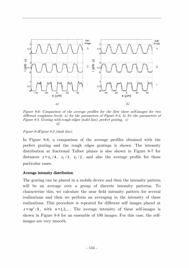
- 134 -

a) b)

Figure 8-6: Comparison of the average profiles for the first three self-images for two different roughness levels, a) for the parameters of Figure 8-4, b) for the parameters of Figure 8-5. Grating with rough edges (solid line), perfect grating, c) d)

Figure 8-3Figure 8-3 (dash line).

In Figure 8-6, a comparison of the average profiles obtained with the perfect grating and the rough edges gratings is shown. The intensity distribution at fractional Talbot planes is also shown in Figure 8-7 for distances / 4Tz z= , / 3Tz , / 2Tz , and also the average profile for these

particular cases.

Average intensity distributionAverage intensity distributionAverage intensity distributionAverage intensity distribution

The grating can be placed in a mobile device and then the intensity pattern will be an average over a group of discrete intensity patterns. To characterize this, we calculate the near field intensity pattern for several realizations and then we perform an averaging in the intensity of these realizations. This procedure is repeated for different self images placed at

2 /z np= λ , with 1,2,...n = . The average intensity of these self-images is

shown in Figure 8-8 for an ensemble of 100 images. For this case, the self-images are very smooth.

8. Gratings with rough edges

- 135 -

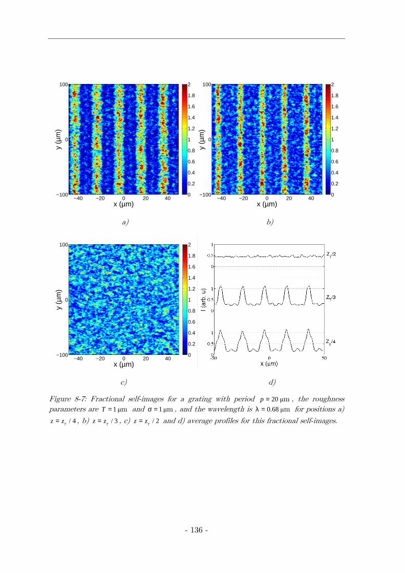
- 136 -

x (µm)

y (µ

m)

−40 −20 0 20 40−100

0

100

0

0.2

0.4

0.6

0.8

1

1.2

1.4

1.6

1.8

2

x (µm)y

(µm

)

−40 −20 0 20 40−100

0

100

0

0.2

0.4

0.6

0.8

1

1.2

1.4

1.6

1.8

2

a) b)

x (µm)

y (µ

m)

−40 −20 0 20 40−100

0

100

0

0.2

0.4

0.6

0.8

1

1.2

1.4

1.6

1.8

2

c) d)

Figure 8-7: Fractional self-images for a grating with period 20µp = m , the roughness parameters are 1µT = m and 1µσ = m , and the wavelength is 0.68µλ = m for positions a)

/ 4T

z z= , b) / 3T

z z= , c) / 2T

z z= and d) average profiles for this fractional self-images.

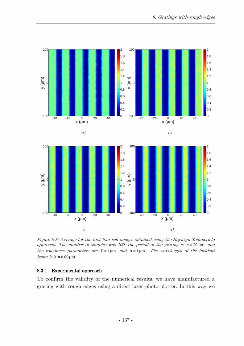
8. Gratings with rough edges

- 137 -

x (µm)

y (µ

m)

−40 −20 0 20 40−100

0

100

0

0.2

0.4

0.6

0.8

1

1.2

1.4

1.6

1.8

2

x (µm)

y (µ

m)

−40 −20 0 20 40−100

0

100

0

0.2

0.4

0.6

0.8

1

1.2

1.4

1.6

1.8

2

a) b)

x (µm)

y (µ

m)

−40 −20 0 20 40−100

0

100

0

0.2

0.4

0.6

0.8

1

1.2

1.4

1.6

1.8

2

x (µm)

y (µ

m)

−40 −20 0 20 40−100

0

100

0

0.2

0.4

0.6

0.8

1

1.2

1.4

1.6

1.8

2

c) d)

Figure 8-8: Average for the first four self-images obtained using the Rayleigh-Sommerfeld approach. The number of samples was 100, the period of the grating is 20p = µm and the roughness parameters are 1T = µm and 1σ = µm . The wavelength of the incident beam is 0.65λ = µm .

8.3.18.3.18.3.18.3.1 Experimental approachExperimental approachExperimental approachExperimental approach

To confirm the validity of the numerical results, we have manufactured a grating with rough edges using a direct laser photo-plotter. In this way we

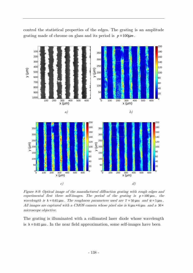
- 138 -

control the statistical properties of the edges. The grating is an amplitude grating made of chrome on glass and its period is 100p m= µ .

x (µm)

y (µ

m)

100 200 300 400 500 600

100

200

300

400

500

600

700

800

900

1000

x (µm)

y (µ

m)

0 100 200 300 400 500 6000

50

100

150

200

250

300

350

0

20

40

60

80

100

120

140

160

180

200

a) b)

x (µm)

y (µ

m)

0 100 200 300 400 500 6000

50

100

150

200

250

300

350

0

20

40

60

80

100

120

140

160

180

200

x (µm)

y (µ

m)

0 100 200 300 400 500 6000

50

100

150

200

250

300

350

0

20

40

60

80

100

120

140

160

180

200

c) d)

Figure 8-9: Optical image of the manufactured diffraction grating with rough edges and experimental first three self-images. The period of the grating is 100p = µm , the wavelength is 0.65λ = µm . The roughness parameters used are 50T = µm and 5σ = µm . All images are captured with a CMOS camera whose pixel size is 6 6µ × µm m and a 30× microscope objective.

The grating is illuminated with a collimated laser diode whose wavelength is 0.65λ = µm . In the near field approximation, some self-images have been

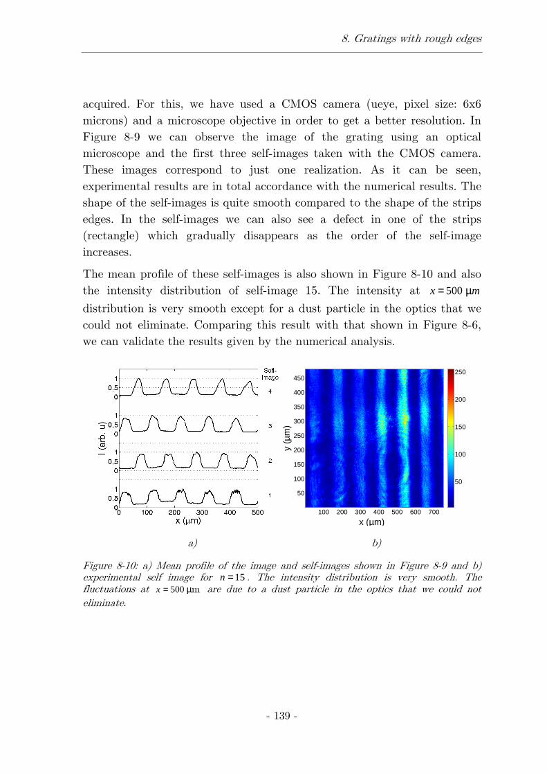
8. Gratings with rough edges

- 139 -

acquired. For this, we have used a CMOS camera (ueye, pixel size: 6x6 microns) and a microscope objective in order to get a better resolution. In Figure 8-9 we can observe the image of the grating using an optical microscope and the first three self-images taken with the CMOS camera. These images correspond to just one realization. As it can be seen, experimental results are in total accordance with the numerical results. The shape of the self-images is quite smooth compared to the shape of the strips edges. In the self-images we can also see a defect in one of the strips (rectangle) which gradually disappears as the order of the self-image increases.

The mean profile of these self-images is also shown in Figure 8-10 and also the intensity distribution of self-image 15. The intensity at 500x m= µ

distribution is very smooth except for a dust particle in the optics that we could not eliminate. Comparing this result with that shown in Figure 8-6, we can validate the results given by the numerical analysis.

x (µm)

y (µ

m)

100 200 300 400 500 600 700

50

100

150

200

250

300

350

400

450

50

100

150

200

250

a) b)

Figure 8-10: a) Mean profile of the image and self-images shown in Figure 8-9 and b) experimental self image for 15n = . The intensity distribution is very smooth. The fluctuations at 500x = µm are due to a dust particle in the optics that we could not eliminate.

- 141 -

ConclusionsConclusionsConclusionsConclusions

The main and original contributions of this Doctoral Thesis are presented below

• We have obtained analytical solutions for the diffraction pattern produced by steel tape gratings illuminated with collimated and Gaussian beams. Contrast of the Talbot self-images decreases in terms of the distance between the grating and the observation plane. This decay depends on the stochastic parameters of the topography. An experimental verification is also performed. The self-images are more sinusoidal than for gratings without roughness. For Gaussian illumination diffraction orders remain Gaussian but their widths increase in terms of roughness. On the other hand, power redistribution between different orders does not occur.

• Double grating configurations with one steel tape grating are also analyzed. We have shown that roughness can produce the lost of the signal in Moiré configuration when the separation between both gratings exceeds certain distance. On the other hand, the contrast of the self images in Generalized Grating Imaging configuration is not affected by roughness but their depth of focus decreases. Lau configuration does not present dependence on the roughness. Analytical solutions of these three configurations have been obtained.

• We have developed and analyzed a new kind of diffraction grating based on roughness. In the far field, diffraction orders appear but the efficiency and the shape of them depend on roughness. For high

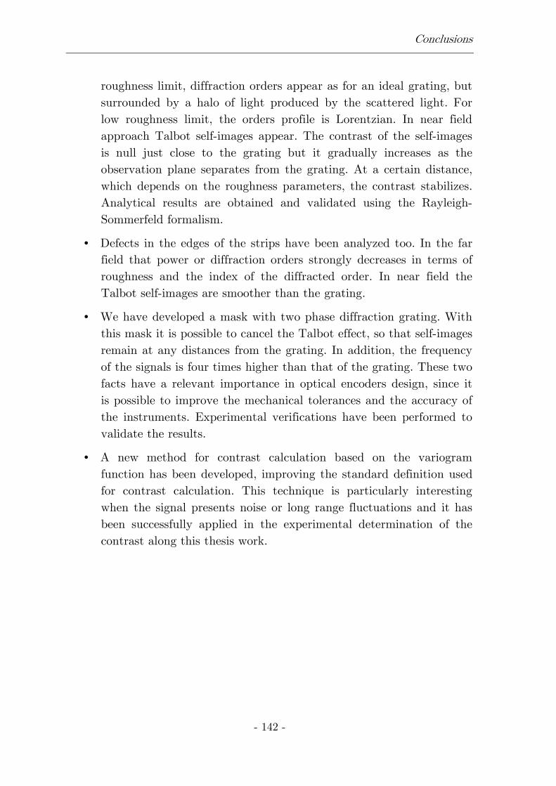
Conclusions

- 142 -

roughness limit, diffraction orders appear as for an ideal grating, but surrounded by a halo of light produced by the scattered light. For low roughness limit, the orders profile is Lorentzian. In near field approach Talbot self-images appear. The contrast of the self-images is null just close to the grating but it gradually increases as the observation plane separates from the grating. At a certain distance, which depends on the roughness parameters, the contrast stabilizes. Analytical results are obtained and validated using the Rayleigh-Sommerfeld formalism.

• Defects in the edges of the strips have been analyzed too. In the far field that power or diffraction orders strongly decreases in terms of roughness and the index of the diffracted order. In near field the Talbot self-images are smoother than the grating.

• We have developed a mask with two phase diffraction grating. With this mask it is possible to cancel the Talbot effect, so that self-images remain at any distances from the grating. In addition, the frequency of the signals is four times higher than that of the grating. These two facts have a relevant importance in optical encoders design, since it is possible to improve the mechanical tolerances and the accuracy of the instruments. Experimental verifications have been performed to validate the results.

• A new method for contrast calculation based on the variogram function has been developed, improving the standard definition used for contrast calculation. This technique is particularly interesting when the signal presents noise or long range fluctuations and it has been successfully applied in the experimental determination of the contrast along this thesis work.

- 143 -

9999 AppendixAppendixAppendixAppendix 1111:::: Talbot effect cancellationTalbot effect cancellationTalbot effect cancellationTalbot effect cancellation

Talbot effect is one of the most important problems in displacement optical encoders. This effect produces a decreasing of the mechanical tolerances. The relative position between both gratings must be very strict since Talbot self-images are formed at certain distances from the grating. The second grating must be placed at one of these Talbot distances in order to measure the transversal displacement between the gratings. In this appendix an analysis of Talbot effect cancellation by using a phase grating is performed and also by using masks formed by two gratings. We have numerically and experimentally verified the correct functioning of the gratings proposed.

- 144 -

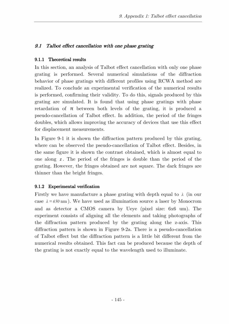
9. Appendix 1: Talbot effect cancellation

- 145 -

9.19.19.19.1 Talbot effect Talbot effect Talbot effect Talbot effect cancellation cancellation cancellation cancellation with one phase gratingwith one phase gratingwith one phase gratingwith one phase grating

9.1.19.1.19.1.19.1.1 Theoretical resultsTheoretical resultsTheoretical resultsTheoretical results

In this section, an analysis of Talbot effect cancellation with only one phase grating is performed. Several numerical simulations of the diffraction behavior of phase gratings with different profiles using RCWA method are realized. To conclude an experimental verification of the numerical results is performed, confirming their validity. To do this, signals produced by this grating are simulated. It is found that using phase gratings with phase retardation of π between both levels of the grating, it is produced a pseudo-cancellation of Talbot effect. In addition, the period of the fringes doubles, which allows improving the accuracy of devices that use this effect for displacement measurements.

In Figure 9-1 it is shown the diffraction pattern produced by this grating, where can be observed the pseudo-cancellation of Talbot effect. Besides, in the same figure it is shown the contrast obtained, which is almost equal to one along z . The period of the fringes is double than the period of the grating. However, the fringes obtained are not square. The dark fringes are thinner than the bright fringes.

9.1.29.1.29.1.29.1.2 Experimental verificationExperimental verificationExperimental verificationExperimental verification

Firstly we have manufacture a phase grating with depth equal to λ (in our case nmλ = 650 ). We have used as illumination source a laser by Monocrom

and as detector a CMOS camera by Ueye (pixel size: 6x6 um). The experiment consists of aligning all the elements and taking photographs of the diffraction pattern produced by the grating along the z-axis. This diffraction pattern is shown in Figure 9-2a. There is a pseudo-cancellation of Talbot effect but the diffraction pattern is a little bit different from the numerical results obtained. This fact can be produced because the depth of the grating is not exactly equal to the wavelength used to illuminate.

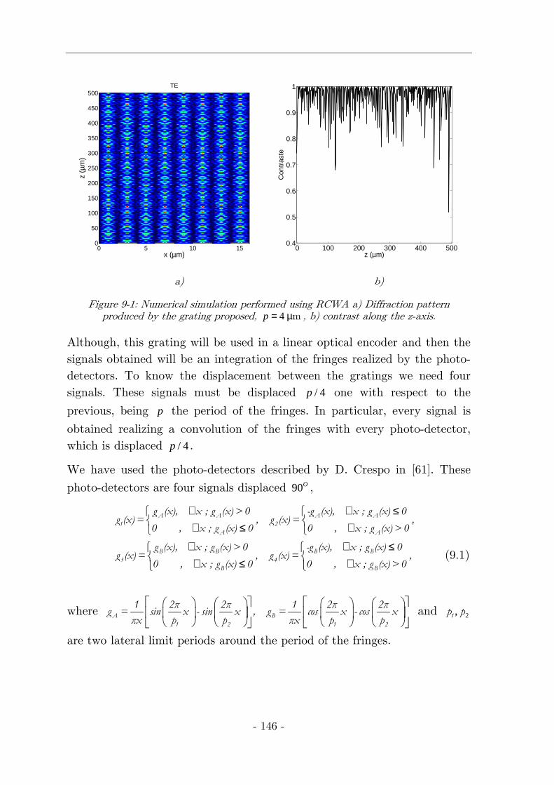
- 146 -

x (µm)

z (µ

m)

TE

0 5 10 150

50

100

150

200

250

300

350

400

450

500

0 100 200 300 400 500

0.4

0.5

0.6

0.7

0.8

0.9

1

z (µm)

Con

tras

te

a) b)

Figure 9-1: Numerical simulation performed using RCWA a) Diffraction pattern produced by the grating proposed, 4p = µm , b) contrast along the z-axis.

Although, this grating will be used in a linear optical encoder and then the signals obtained will be an integration of the fringes realized by the photo-detectors. To know the displacement between the gratings we need four signals. These signals must be displaced / 4p one with respect to the

previous, being p the period of the fringes. In particular, every signal is

obtained realizing a convolution of the fringes with every photo-detector, which is displaced / 4p .

We have used the photo-detectors described by D. Crespo in [61]. These

photo-detectors are four signals displaced 90O ,

∀ ∀ ≤ ∀ ≤ ∀

∀ ∀ ≤ ∀ ≤ ∀

A A A A

1 2

A A

B B B B

3 4

B B

g (x), x ; g (x)> 0 -g (x), x ; g (x) 0g (x) = , g (x) = ,

0 , x ; g (x) 0 0 , x ; g (x)> 0

g (x), x ; g (x)> 0 -g (x), x ; g (x) 0g (x) = , g (x) = ,

0 , x ; g (x) 0 0 , x ; g (x)> 0 (9.1)

where

A B

1 2 1 2

1 2 2 1 2 2g = sin x - sin x , g = cos x - cos x

x p p x p p and 2,1p p

are two lateral limit periods around the period of the fringes.

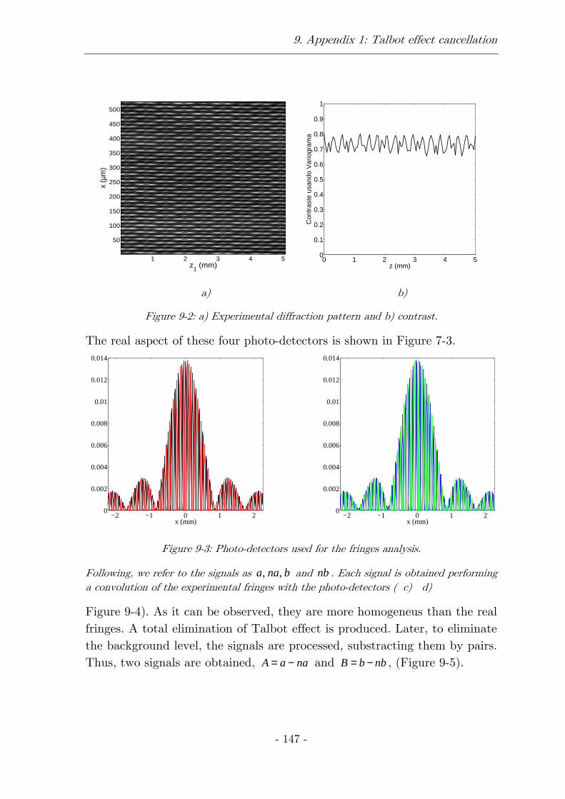
9. Appendix 1: Talbot effect cancellation

- 147 -

z1 (mm)

x (µ

m)

1 2 3 4 5

50

100

150

200

250

300

350

400

450

500

0 1 2 3 4 50

0.1

0.2

0.3

0.4

0.5

0.6

0.7

0.8

0.9

1

z (mm)

Con

tras

te u

sand

o V

ario

gram

a

a) b)

Figure 9-2: a) Experimental diffraction pattern and b) contrast.

The real aspect of these four photo-detectors is shown in Figure 7-3.

−2 −1 0 1 20

0.002

0.004

0.006

0.008

0.01

0.012

0.014

x (mm)

−2 −1 0 1 20

0.002

0.004

0.006

0.008

0.01

0.012

0.014

x (mm)

Figure 9-3: Photo-detectors used for the fringes analysis.

Following, we refer to the signals as , ,a na b and nb . Each signal is obtained performing a convolution of the experimental fringes with the photo-detectors ( c) d)

Figure 9-4). As it can be observed, they are more homogeneus than the real fringes. A total elimination of Talbot effect is produced. Later, to eliminate the background level, the signals are processed, substracting them by pairs. Thus, two signals are obtained, A a na= − and B b nb= − , (Figure 9-5).

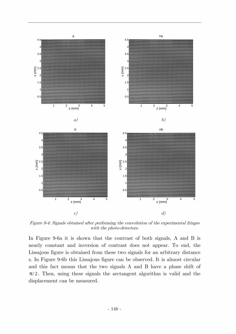
- 148 -

z (mm)

x (m

m)

a

1 2 3 4 5

0.5

1

1.5

2

2.5

3

3.5

4

4.5

z (mm)

x (m

m)

na

1 2 3 4 5

0.5

1

1.5

2

2.5

3

3.5

4

4.5

a) b)

z (mm)

x (m

m)

b

1 2 3 4 5

0.5

1

1.5

2

2.5

3

3.5

4

4.5

z (mm)

x (m

m)

nb

1 2 3 4 5

0.5

1

1.5

2

2.5

3

3.5

4

4.5

c) d)

Figure 9-4: Signals obtained after performing the convolution of the experimental fringes with the photo-detectors.

In Figure 9-6a it is shown that the contrast of both signals, A and B is nearly constant and inversion of contrast does not appear. To end, the Lissajous figure is obtained from these two signals for an arbitrary distance z. In Figure 9-6b this Lissajous figure can be observed. It is almost circular and this fact means that the two signals A and B have a phase shift of

/ 2π . Then, using these signals the arctangent algorithm is valid and the displacement can be measured.

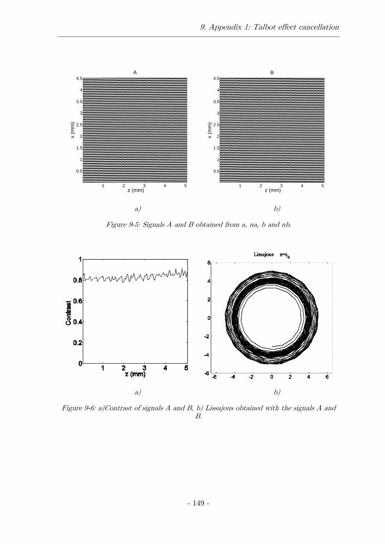
9. Appendix 1: Talbot effect cancellation

- 149 -

z (mm)

x (m

m)

A

1 2 3 4 5

0.5

1

1.5

2

2.5

3

3.5

4

4.5

z (mm)

x (m

m)

B

1 2 3 4 5

0.5

1

1.5

2

2.5

3

3.5

4

4.5

a) b)

Figure 9-5: Signals A and B obtained from a, na, b and nb.

a) b)

Figure 9-6: a)Contrast of signals A and B, b) Lissajous obtained with the signals A and B.

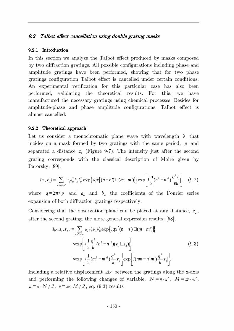
- 150 -

9.29.29.29.2 Talbot effect Talbot effect Talbot effect Talbot effect cancellation cancellation cancellation cancellation using double grating masksusing double grating masksusing double grating masksusing double grating masks

9.2.19.2.19.2.19.2.1 IntroductionIntroductionIntroductionIntroduction

In this section we analyze the Talbot effect produced by masks composed by two diffraction gratings. All possible configurations including phase and amplitude gratings have been performed, showing that for two phase gratings configuration Talbot effect is cancelled under certain conditions. An experimental verification for this particular case has also been performed, validating the theoretical results. For this, we have manufactured the necessary gratings using chemical processes. Besides for amplitude-phase and phase amplitude configurations, Talbot effect is almost cancelled.

9.2.29.2.29.2.29.2.2 Theoretical approachTheoretical approachTheoretical approachTheoretical approach

Let us consider a monochromatic plane wave with wavelength λ that incides on a mask formed by two gratings with the same period, p and

separated a distance 1z (Figure 9-7). The intensity just after the second

grating corresponds with the classical description of Moiré given by Patorsky, [89],

[ ]{ }2

* * 2 2 11 ' ' ( ') ( ') ( ' )

2n m

q zz qx n n m m i n n

k

π− + − − π ∑ exp expn m

n,n',m,m'

I(x, ) = a a b b i , (9.2)

where 2 /q p= π and na and mb the coefficients of the Fourier series

expansion of both diffraction gratings respectively.

Considering that the observation plane can be placed at any distance, 2z ,

after the second grating, the more general expression results, [58],

[ ]{ }* *1 2 ' '

22 2

1 2

2 22 2

2 2

, ( ') ( ')

1( ' )( )

2

1( ' ) ( ' ') .

2

n mz z qx n n m m

qn n z z

k

q qm m z nm n m z

k k

− + −

× − +

× − −

∑ exp

exp

exp exp

n m

n,n',m,m'

I(x, ) = a a b b i

i

i i

(9.3)

Including a relative displacement ∆x between the gratings along the x-axis and performing the following changes of variable, N =n - n' , M=m- m' , u =n - N /2 , v =m - M /2 , eq. (9.3) results

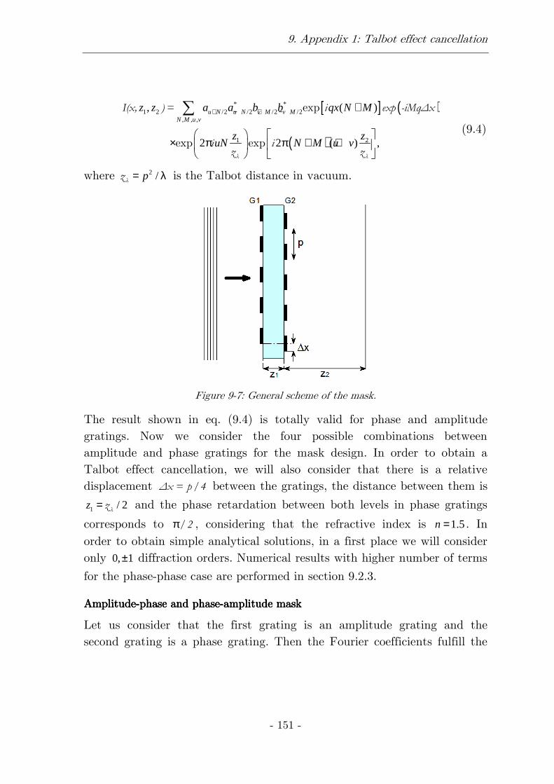
9. Appendix 1: Talbot effect cancellation

- 151 -

[ ] ( )

( )

* *1 2 /2 /2 /2 /2

, , ,

1 2

, ( )

2 2 ( ) ,

u N u N v M v MN M u v

z z a a b b qx N M

z zuN N M u v

+ − + − +

× π π + +

∑ exp

exp expλ λ

I(x, ) = i exp -iMq∆x

i iz z

(9.4)

where 2 /p= λλz is the Talbot distance in vacuum.

Figure 9-7: General scheme of the mask.

The result shown in eq. (9.4) is totally valid for phase and amplitude gratings. Now we consider the four possible combinations between amplitude and phase gratings for the mask design. In order to obtain a Talbot effect cancellation, we will also consider that there is a relative displacement ∆x = p /4 between the gratings, the distance between them is

1 / 2z = λz and the phase retardation between both levels in phase gratings

corresponds to π/ 2 , considering that the refractive index is 1.5n = . In order to obtain simple analytical solutions, in a first place we will consider only 0, 1± diffraction orders. Numerical results with higher number of terms

for the phase-phase case are performed in section 9.2.3.

AmplitudeAmplitudeAmplitudeAmplitude----phase and phasephase and phasephase and phasephase and phase----amplitude maskamplitude maskamplitude maskamplitude mask

Let us consider that the first grating is an amplitude grating and the second grating is a phase grating. Then the Fourier coefficients fulfill the

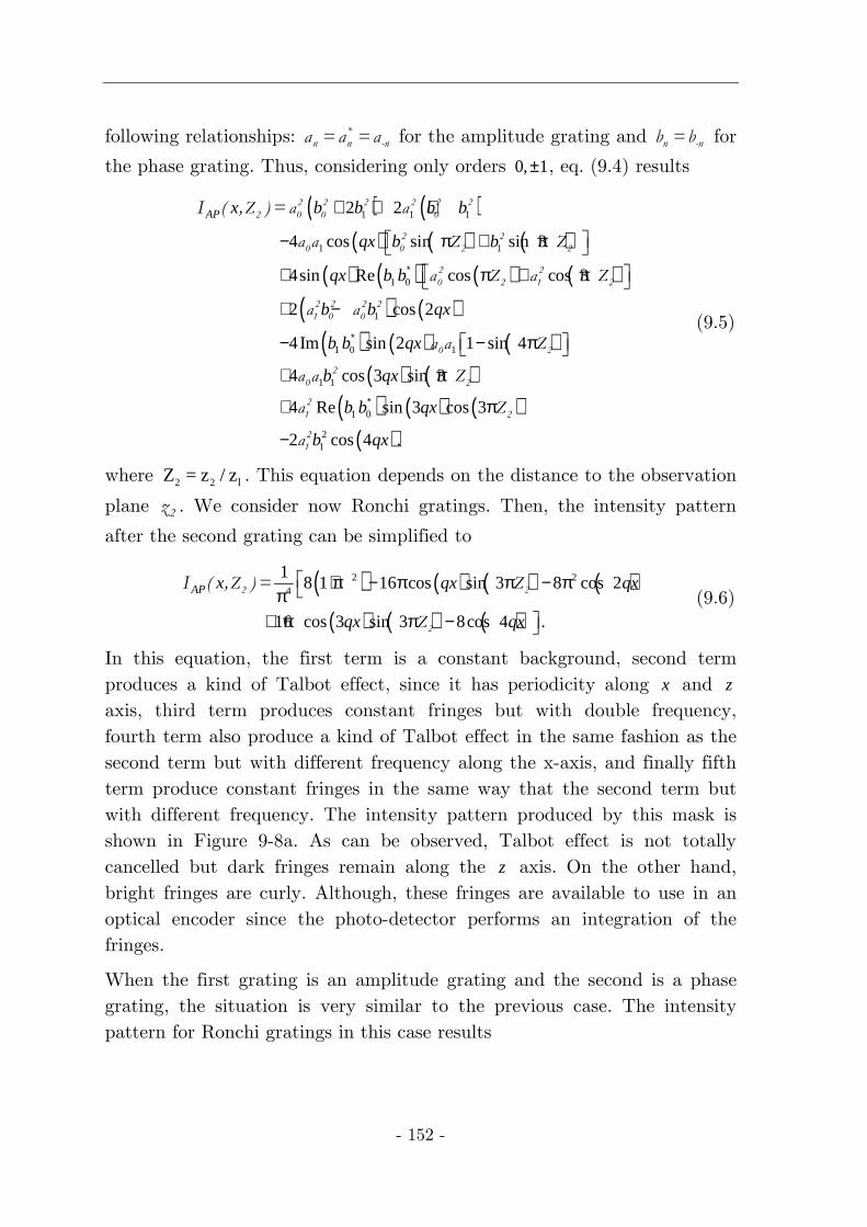
- 152 -

following relationships: *n n -na = a = a for the amplitude grating and n -nb =b for

the phase grating. Thus, considering only orders 0, 1± , eq. (9.4) results

( ) ( )( ) ( ) ( )

( ) ( ) ( ) ( )( ) ( )

( ) ( ) ( )( ) ( )

( ) ( )

1 1 1

1 1

1 0

1

1 0 1

1 1

1 0

2 2

4 cos sin sin 3

4sin Re cos cos 3

2 cos 2

4Im sin 2 1 sin 4

4 cos 3 sin 3

4 Re sin 3 c

AP x b b b b

qx b b

qx b b

b b qx

b b qx

b qx

b b qx

∗

∗

∗

+ + +

− π + π

+ π + π

+ −

− − π

+ π

+

2 2 2 2 2 2

2 0 0 0

2 2

0 0 2 2

2 2

0 2 1 2

2 2 2 2

1 0 0

0 2

2

0 2

2

1

Z a a

a a Z Z

a Z a Z

a a

a a Z

a a Z

a

I ( , ) =

( )( )2

1

os 3

2 cos 4 .b qx

π

−2

2

1

Z

a

(9.5)

where 2 2 lZ = z / z . This equation depends on the distance to the observation

plane 2z . We consider now Ronchi gratings. Then, the intensity pattern

after the second grating can be simplified to

( ) ( ) ( ) ( )

( ) ( ) ( )

2 24

18 1 16 cos sin 3 8 cos 2

16 cos 3 sin 3 8cos 4 .

AP x qx qx

qx qx

+ π − π π − ππ+ π π −

2 2

2

Z Z

Z

I ( , ) = (9.6)

In this equation, the first term is a constant background, second term produces a kind of Talbot effect, since it has periodicity along x and z axis, third term produces constant fringes but with double frequency, fourth term also produce a kind of Talbot effect in the same fashion as the second term but with different frequency along the x-axis, and finally fifth term produce constant fringes in the same way that the second term but with different frequency. The intensity pattern produced by this mask is shown in Figure 9-8a. As can be observed, Talbot effect is not totally cancelled but dark fringes remain along the z axis. On the other hand, bright fringes are curly. Although, these fringes are available to use in an optical encoder since the photo-detector performs an integration of the fringes.

When the first grating is an amplitude grating and the second is a phase grating, the situation is very similar to the previous case. The intensity pattern for Ronchi gratings in this case results

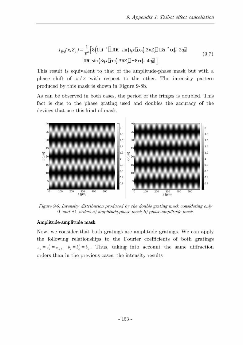
9. Appendix 1: Talbot effect cancellation

- 153 -

( ) ( ) ( ) ( )

( ) ( ) ( )

2 24

18 1 16 sin cos 3 8 cos 2

16 sin 3 cos 3 8cos 4 .

PA x qx qx

qx qx

+ π + π π + ππ+ π π −

2 2

2

Z Z

Z

I ( , ) = (9.7)

This result is equivalent to that of the amplitude-phase mask but with a phase shift of /2 with respect to the other. The intensity pattern produced by this mask is shown in Figure 9-8b.

As can be observed in both cases, the period of the fringes is doubled. This fact is due to the phase grating used and doubles the accuracy of the devices that use this kind of mask.

z (µm)

x (µ

m)

0 100 200 300 400 5000

5

10

15

20

25

30

35

40

0.2

0.4

0.6

0.8

1

1.2

1.4

1.6

1.8

2

z (µm)

x (µ

m)

0 100 200 300 400 5000

5

10

15

20

25

30

35

40

0.2

0.4

0.6

0.8

1

1.2

1.4

1.6

1.8

2

Figure 9-8: Intensity distribution produced by the double grating mask considering only 0 and 1± orders a) amplitude-phase mask b) phase-amplitude mask.

AmplitudeAmplitudeAmplitudeAmplitude----amplitude maskamplitude maskamplitude maskamplitude mask

Now, we consider that both gratings are amplitude gratings. We can apply the following relationships to the Fourier coefficients of both gratings

*

n n -na = a = a , *

n n -nb = b = b . Thus, taking into account the same diffraction

orders than in the previous cases, the intensity results

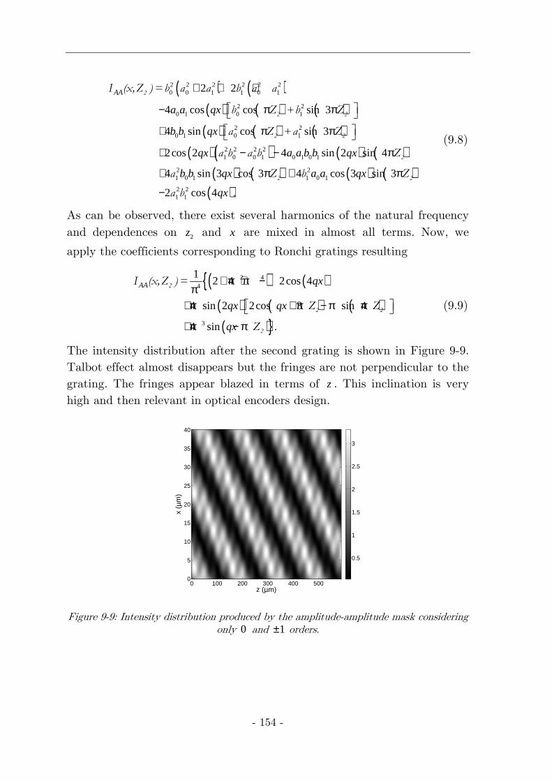
- 154 -

( ) ( )( ) ( ) ( )

( ) ( ) ( )( ) ( ) ( ) ( )

( ) ( ) ( ) ( )

2 2 2 2 2 20 0 1 1 0 1

2 20 1 0 1

2 20 1 0 1

2 2 2 21 0 0 1 0 1 0 1

2 21 0 1 1 0 1

2 21 1

2 2

4 cos cos sin 3

4 sin cos sin 3

2cos 2 4 sin 2 sin 4

4 sin 3 cos 3 4 cos 3 sin 3

2 c

AA

a a qx

b b qx

qx a a b b qx

b b qx a a qx

+ + +

− π π

+ π π

+ − − π

+ π + π

−

2

2 2

2 2

2

2 2

+

+

I (x,Z )=b a a b a a

b Z b Z

a Z a Z

a b a b Z

a Z b Z

a b ( )os 4 .qx

(9.8)

As can be observed, there exist several harmonics of the natural frequency and dependences on 2z and x are mixed in almost all terms. Now, we

apply the coefficients corresponding to Ronchi gratings resulting

( ) ( ){( ) ( ) ( )( )}

2 44

3

12 4 2cos 4

4 sin 2 2cos 3 sin 4

4 sin .

AA qx

qx qx

qx

+ π + π −π

+ π + π − π π

+ π − π

2

2 2

2

I (x,Z )=

Z Z

Z

(9.9)

The intensity distribution after the second grating is shown in Figure 9-9. Talbot effect almost disappears but the fringes are not perpendicular to the grating. The fringes appear blazed in terms of z . This inclination is very high and then relevant in optical encoders design.

z (µm)

x (µ

m)

0 100 200 300 400 5000

5

10

15

20

25

30

35

40

0.5

1

1.5

2

2.5

3

Figure 9-9: Intensity distribution produced by the amplitude-amplitude mask considering only 0 and 1± orders.

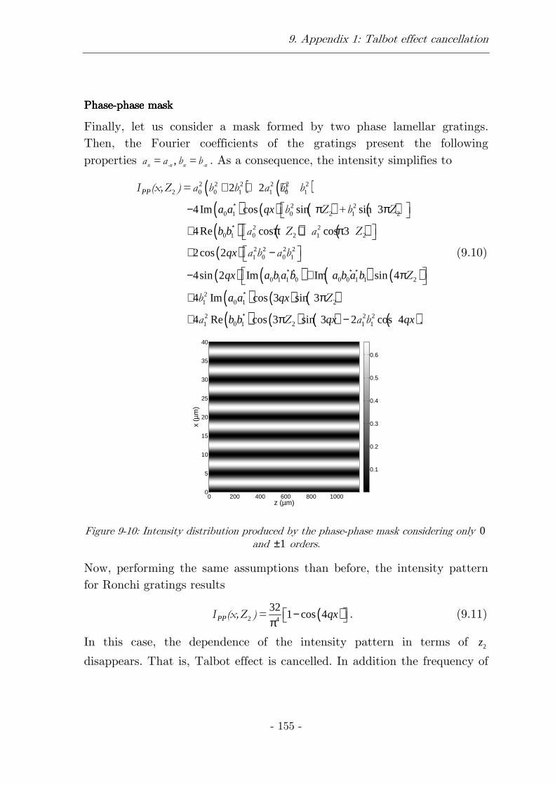
9. Appendix 1: Talbot effect cancellation

- 155 -

PhasePhasePhasePhase----phase maskphase maskphase maskphase mask

Finally, let us consider a mask formed by two phase lamellar gratings. Then, the Fourier coefficients of the gratings present the following properties ,n -n n -na = a b = b . As a consequence, the intensity simplifies to

( ) ( )( ) ( ) ( ) ( )( ) ( ) ( )( )( ) ( ) ( ) ( )

( ) ( ) ( )

2 2 2 2 2 22 0 0 1 1 0 1

2 20 1 0 2 1 2

2 20 1 0 2 1 2

2 2 2 21 0 0 1

0 1 1 0 0 0 1 1 2

21 0 1 2

2 2

4Im cos sin sin 3

4Re cos cos 3

2cos 2

4sin 2 Im Im sin 4

4 Im cos 3 sin 3

4

PP

a a qx

b b

qx

qx a b a b a b a b

a a qx

∗

∗

∗ ∗ ∗ ∗

∗

+ + +

− π π

+ π + π

+ −

− + π

+ π

+

+

I (x,Z )= a b b a b b

b Z b Z

a Z a Z

a b a b

Z

b Z

( ) ( ) ( ) ( )2 2 21 0 1 2 1 1Re cos 3 sin 3 2 cos 4 .b b qx qx∗ π −a Z a b

(9.10)

z (µm)

x (µ

m)

0 200 400 600 800 10000

5

10

15

20

25

30

35

40

0.1

0.2

0.3

0.4

0.5

0.6

Figure 9-10: Intensity distribution produced by the phase-phase mask considering only 0 and 1± orders.

Now, performing the same assumptions than before, the intensity pattern for Ronchi gratings results

( )2 4

321 cos 4PP qx− π

I (x,Z )= . (9.11)

In this case, the dependence of the intensity pattern in terms of 2z

disappears. That is, Talbot effect is cancelled. In addition the frequency of

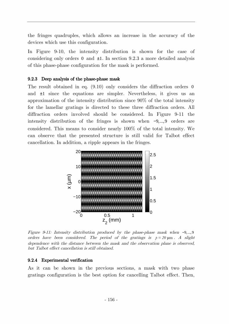
- 156 -

the fringes quadruples, which allows an increase in the accuracy of the devices which use this configuration.

In Figure 9-10, the intensity distribution is shown for the case of considering only orders 0 and 1± . In section 9.2.3 a more detailed analysis of this phase-phase configuration for the mask is performed.

9.2.39.2.39.2.39.2.3 DeepDeepDeepDeep analysis of analysis of analysis of analysis of the the the the phasephasephasephase----phase maskphase maskphase maskphase mask

The result obtained in eq. (9.10) only considers the diffraction orders 0 and 1± since the equations are simpler. Nevertheless, it gives us an approximation of the intensity distribution since 90% of the total intensity for the lamellar gratings is directed to these three diffraction orders. All diffraction orders involved should be considered. In Figure 9-11 the intensity distribution of the fringes is shown when 9,...,9− orders are

considered. This means to consider nearly 100% of the total intensity. We can observe that the presented structure is still valid for Talbot effect cancellation. In addition, a ripple appears in the fringes.

z2 (mm)

x (µ

m)

0 0.5 1−20

−10

0

10

20

0

0.5

1

1.5

2

2.5

Figure 9-11: Intensity distribution produced by the phase-phase mask when 9,..., 9− orders have been considered. The period of the gratings is µmp = 20 . A slight dependence with the distance between the mask and the observation plane is observed, but Talbot effect cancellation is still obtained.

9.2.49.2.49.2.49.2.4 Experimental verification Experimental verification Experimental verification Experimental verification

As it can be shown in the previous sections, a mask with two phase gratings configuration is the best option for cancelling Talbot effect. Then,

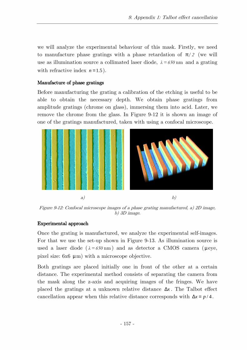
9. Appendix 1: Talbot effect cancellation

- 157 -

we will analyze the experimental behaviour of this mask. Firstly, we need to manufacture phase gratings with a phase retardation of π/ 2 (we will use as illumination source a collimated laser diode, nmλ = 650 and a grating

with refractive index 1.5n = ).

Manufacture of phase gratingsManufacture of phase gratingsManufacture of phase gratingsManufacture of phase gratings

Before manufacturing the grating a calibration of the etching is useful to be able to obtain the necessary depth. We obtain phase gratings from amplitude gratings (chrome on glass), immersing them into acid. Later, we remove the chrome from the glass. In Figure 9-12 it is shown an image of one of the gratings manufactured, taken with using a confocal microscope.

a) b)

Figure 9-12: Confocal microscope images of a phase grating manufactured, a) 2D image, b) 3D image.

Experimental approachExperimental approachExperimental approachExperimental approach

Once the grating is manufactured, we analyze the experimental self-images. For that we use the set-up shown in Figure 9-13. As illumination source is used a laser diode ( nmλ = 650 ) and as detector a CMOS camera (µeye,

pixel size: 6x6 µm) with a microscope objective.

Both gratings are placed initially one in front of the other at a certain distance. The experimental method consists of separating the camera from the mask along the z-axis and acquiring images of the fringes. We have placed the gratings at a unknown relative distance x∆ . The Talbot effect cancellation appear when this relative distance corresponds with / 4x p∆ = .

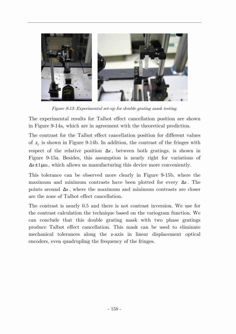
- 158 -

Figure 9-13: Experimental set-up for double grating mask testing.

The experimental results for Talbot effect cancellation position are shown in Figure 9-14a, which are in agreement with the theoretical prediction.

The contrast for the Talbot effect cancellation position for different values of 2z is shown in Figure 9-14b. In addition, the contrast of the fringes with

respect of the relative position x∆ , between both gratings, is shown in Figure 9-15a. Besides, this assumption is nearly right for variations of

1x∆ ± µm , which allows us manufacturing this device more conveniently.

This tolerance can be observed more clearly in Figure 9-15b, where the maximum and minimum contrasts have been plotted for every x∆ . The points around x∆ , where the maximum and minimum contrasts are closer are the zone of Talbot effect cancellation.

The contrast is nearly 0.5 and there is not contrast inversion. We use for the contrast calculation the technique based on the variogram function. We can conclude that this double grating mask with two phase gratings produce Talbot effect cancellation. This mask can be used to eliminate mechanical tolerances along the z-axis in linear displacement optical encoders, even quadrupling the frequency of the fringes.

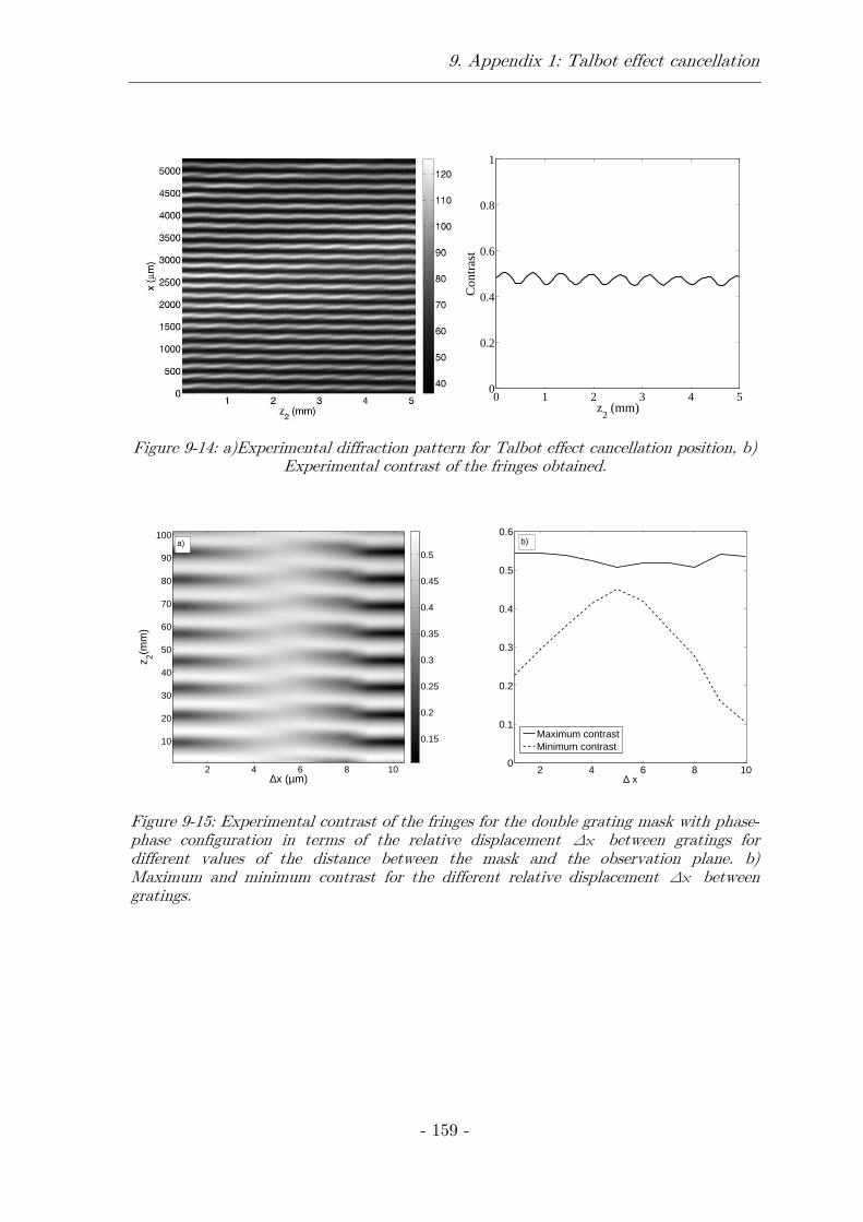
9. Appendix 1: Talbot effect cancellation

- 159 -

0 1 2 3 4 50

0.2

0.4

0.6

0.8

1

z2 (mm)

Co

ntr

ast

Figure 9-14: a)Experimental diffraction pattern for Talbot effect cancellation position, b) Experimental contrast of the fringes obtained.

∆x (µm)

z 2(mm

)

2 4 6 8 10

10

20

30

40

50

60

70

80

90

100

0.15

0.2

0.25

0.3

0.35

0.4

0.45

0.5a)

2 4 6 8 10

0

0.1

0.2

0.3

0.4

0.5

0.6

∆ x

Maximum contrastMinimum contrast

b)

Figure 9-15: Experimental contrast of the fringes for the double grating mask with phase-phase configuration in terms of the relative displacement ∆x between gratings for different values of the distance between the mask and the observation plane. b) Maximum and minimum contrast for the different relative displacement ∆x between gratings.

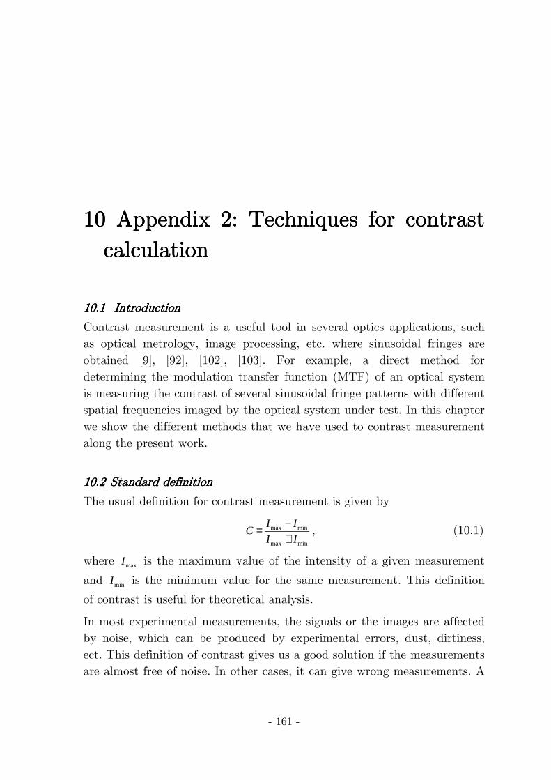
- 161 -

10101010 Appendix Appendix Appendix Appendix 2:2:2:2: Techniques for contrast Techniques for contrast Techniques for contrast Techniques for contrast calculationcalculationcalculationcalculation

10.110.110.110.1 IntroductionIntroductionIntroductionIntroduction

Contrast measurement is a useful tool in several optics applications, such as optical metrology, image processing, etc. where sinusoidal fringes are obtained [9], [92], [102], [103]. For example, a direct method for determining the modulation transfer function (MTF) of an optical system is measuring the contrast of several sinusoidal fringe patterns with different spatial frequencies imaged by the optical system under test. In this chapter we show the different methods that we have used to contrast measurement along the present work.

10.210.210.210.2 Standard definitionStandard definitionStandard definitionStandard definition

The usual definition for contrast measurement is given by

max min

max min

I IC

I I

−=+

, (10.1)

where maxI is the maximum value of the intensity of a given measurement

and minI is the minimum value for the same measurement. This definition

of contrast is useful for theoretical analysis.

In most experimental measurements, the signals or the images are affected by noise, which can be produced by experimental errors, dust, dirtiness, ect. This definition of contrast gives us a good solution if the measurements are almost free of noise. In other cases, it can give wrong measurements. A

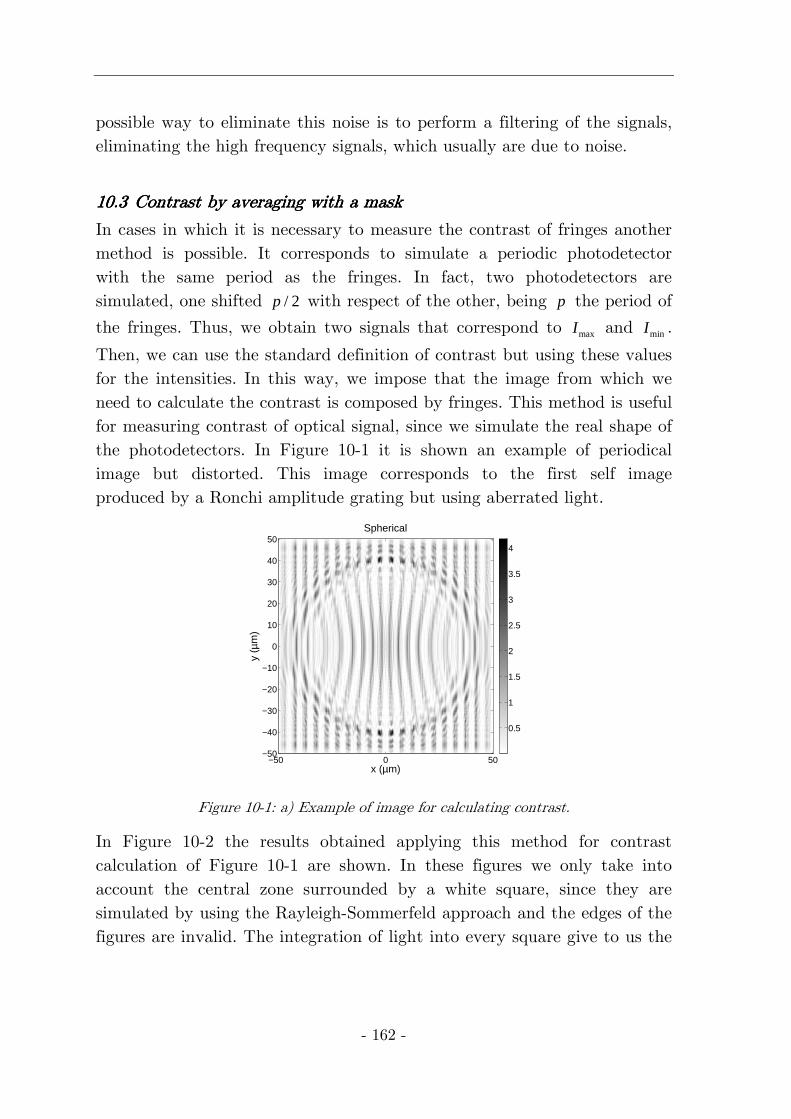
- 162 -

possible way to eliminate this noise is to perform a filtering of the signals, eliminating the high frequency signals, which usually are due to noise.

10.310.310.310.3 Contrast by averaging with a maskContrast by averaging with a maskContrast by averaging with a maskContrast by averaging with a mask

In cases in which it is necessary to measure the contrast of fringes another method is possible. It corresponds to simulate a periodic photodetector with the same period as the fringes. In fact, two photodetectors are simulated, one shifted / 2p with respect of the other, being p the period of

the fringes. Thus, we obtain two signals that correspond to maxI and minI .

Then, we can use the standard definition of contrast but using these values for the intensities. In this way, we impose that the image from which we need to calculate the contrast is composed by fringes. This method is useful for measuring contrast of optical signal, since we simulate the real shape of the photodetectors. In Figure 10-1 it is shown an example of periodical image but distorted. This image corresponds to the first self image produced by a Ronchi amplitude grating but using aberrated light.

x (µm)

y (µ

m)

Spherical

−50 0 50−50

−40

−30

−20

−10

0

10

20

30

40

50

0.5

1

1.5

2

2.5

3

3.5

4

Figure 10-1: a) Example of image for calculating contrast.

In Figure 10-2 the results obtained applying this method for contrast calculation of Figure 10-1 are shown. In these figures we only take into account the central zone surrounded by a white square, since they are simulated by using the Rayleigh-Sommerfeld approach and the edges of the figures are invalid. The integration of light into every square give to us the

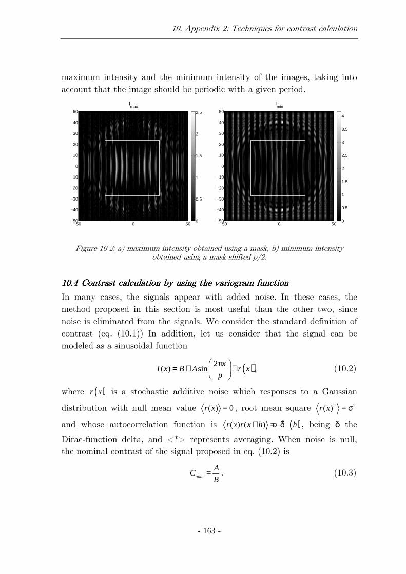
10. Appendix 2: Techniques for contrast calculation

- 163 -

maximum intensity and the minimum intensity of the images, taking into account that the image should be periodic with a given period.

Imax

−50 0 50−50

−40

−30

−20

−10

0

10

20

30

40

50

0

0.5

1

1.5

2

2.5

Imin

−50 0 50−50

−40

−30

−20

−10

0

10

20

30

40

50

0

0.5

1

1.5

2

2.5

3

3.5

4

Figure 10-2: a) maximum intensity obtained using a mask, b) minimum intensity obtained using a mask shifted p/2.

10.410.410.410.4 Contrast calculation by using the variogram functionContrast calculation by using the variogram functionContrast calculation by using the variogram functionContrast calculation by using the variogram function

In many cases, the signals appear with added noise. In these cases, the method proposed in this section is most useful than the other two, since noise is eliminated from the signals. We consider the standard definition of contrast (eq. (10.1)) In addition, let us consider that the signal can be modeled as a sinusoidal function

( )2( ) sin

xI x B A r x

p

π= + +

, (10.2)

where ( )r x is a stochastic additive noise which responses to a Gaussian

distribution with null mean value ( ) = 0r x , root mean square 2 2( ) =r x σ

and whose autocorrelation function is ( )2( ) ( ) =r x r x h h+ σ δ , being δ the

Dirac-function delta, and <*> represents averaging. When noise is null, the nominal contrast of the signal proposed in eq. (10.2) is

nom

AC

B= . (10.3)

- 164 -

On the other hand, when the signal presents noise or background variations, it is not convenient to apply eq. (10.1) directly for contrast measurement since the determination of Imax and Imin is very sensitive to noise. The contrast obtained using eq. (10.1) results

st

A KC

B

+ σ= , (10.4)

where K is a factor which depends on the number of data used which normally ranges between 2 and 3 [104]. The relative error in the contrast measurement is

st nomst

nom

C Ce K

C A

− σ= = , (10.5)

which is linear with / Aσ . A better approach to determine the amplitude of the signal is the root mean square (rms) function, defined as [105]

( )

1/22( )I x I dx

rmsdx

− =

∫∫

. (10.6)

With this definition, all the data are considered for determining the amplitude of a signal, instead of just two data. The contrast results

2rms

rmsC

I= . (10.7)

Using eq. (10.6), the amplitude for a sinusoidal function without noise is

then 2A rms= . However, when an additive noise which responses to a Gaussian distribution noise defined previously in eq. (10.2) is present, then

2 2 2/ 2rms A= + σ . The mean value of eq. (10.2) is I B= and, as a

consequence, the contrast results

2 22

rms

AC

B

+ σ= . (10.8)

This technique is also affected by the presence of an additive Gaussian noise. The relative error in the contrast estimation is

2

1 2 1rms nomrms

nom

C Ce

C A

− σ = = + −

. (10.9)

10. Appendix 2: Techniques for contrast calculation

- 165 -

When noise is small compared to the amplitude of the signal, then

( )2/rmse A≈ σ which is lower than with eq. (10.5). On the other hand, when

noise is much greater than the amplitude of the signal, the error in the

contrast estimation presents a linear dependence, 2 /rmse A≈ σ .

Another possibility to determine the contrast is to fit the experimental data to a sine function. However, experimentally a number of effects such as local variations of the period of the fringes, local variations of the amplitude or offset of the signal, normally appear which avoids a correct fitting. Other robust techniques to evaluate the contrast of a fringe pattern have been proposed, such as the histogram, suggested by Lai and von Bally [106]. Nevertheless, the algorithm proposed in that work does not match the definition of contrast given by eq. (10.1), even when no noise is present. A better technique for contrast measurement in presence of additive noise and with patterns composed of non-straight fringes has been developed [107]. It is based on fitting the histogram of the fringe pattern to the histogram of a model function that depends on several parameters. The technique has been proven to obtain good results for contrast estimation even with the presence of high levels of noise. However, the computation algorithm is quite slow as it requires the fitting of the histogram to a function with several parameters.

In this work, a completely different approach is applied for estimating the contrast. Using the variogram function ( )hγ , see below, we demonstrate

that the difference between the maximum and minimum values of the variogram is equal to the square of the amplitude of the signal, even when an additive noise is present. Since the variogram is obtained as an average process, noise affects very little to the contrast estimation. An expression for the relative error in the contrast determination is obtained showing that it only depends on the signal to noise ratio and on the number of data. Numerical simulations with different modifications on the signal are performed which corroborates the robustness and validity of the technique. Finally, as an example, the contrast of signals obtained at a certain distance from a diffraction grating when it is illuminated with a monochromatic collimated light beam is obtained. This corresponds to the well-known Talbot effect.

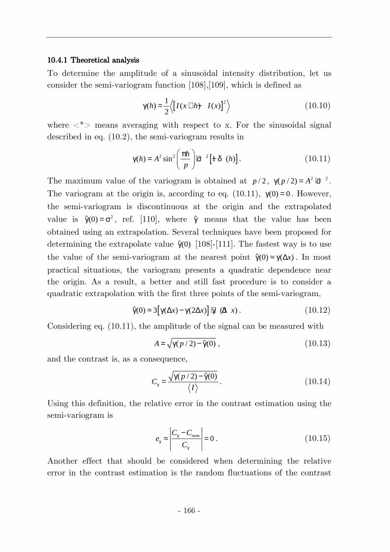
- 166 -

10.4.110.4.110.4.110.4.1 Theoretical analysisTheoretical analysisTheoretical analysisTheoretical analysis

To determine the amplitude of a sinusoidal intensity distribution, let us consider the semi-variogram function [108],[109], which is defined as

[ ]21( ) ( ) ( )

2h I x h I xγ = + − (10.10)

where <*> means averaging with respect to x. For the sinusoidal signal described in eq. (10.2), the semi-variogram results in

[ ]2 2 2( ) sin 1 ( )h

h A hp

πγ = + σ − δ

. (10.11)

The maximum value of the variogram is obtained at / 2p , 2 2( / 2)p Aγ = + σ .

The variogram at the origin is, according to eq. (10.11), (0) 0γ = . However,

the semi-variogram is discontinuous at the origin and the extrapolated

value is 2ˆ(0)γ = σ , ref. [110], where γ means that the value has been

obtained using an extrapolation. Several techniques have been proposed for determining the extrapolate value ˆ(0)γ [108]-[111]. The fastest way is to use

the value of the semi-variogram at the nearest point ˆ(0) ( )xγ ≈ γ ∆ . In most

practical situations, the variogram presents a quadratic dependence near the origin. As a result, a better and still fast procedure is to consider a quadratic extrapolation with the first three points of the semi-variogram,

[ ]ˆ(0) 3 ( ) (2 ) (3 )x x xγ ≈ γ ∆ − γ ∆ + γ ∆ . (10.12)

Considering eq. (10.11), the amplitude of the signal can be measured with

ˆ( / 2) (0)A p= γ − γ , (10.13)

and the contrast is, as a consequence,

ˆ( / 2) (0)p

CIγ

γ − γ= . (10.14)

Using this definition, the relative error in the contrast estimation using the semi-variogram is

0nomC Ce

Cγ

γγ

−≈ = . (10.15)

Another effect that should be considered when determining the relative error in the contrast estimation is the random fluctuations of the contrast

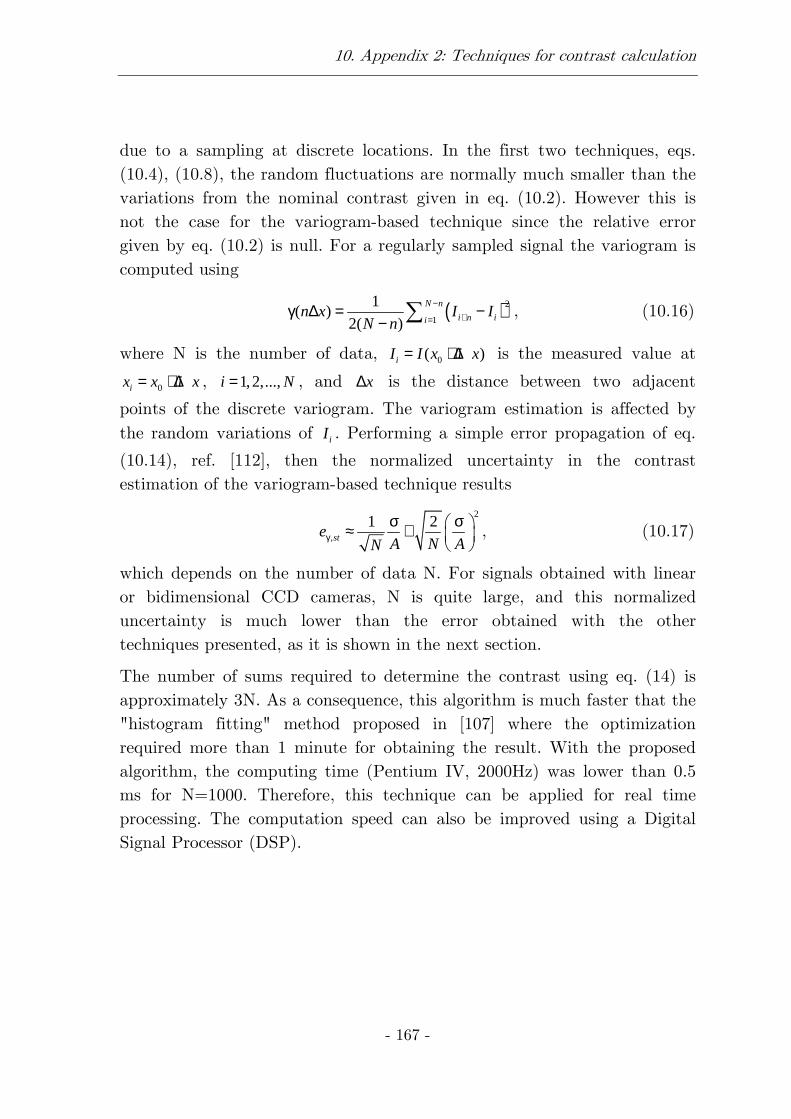
10. Appendix 2: Techniques for contrast calculation

- 167 -

due to a sampling at discrete locations. In the first two techniques, eqs. (10.4), (10.8), the random fluctuations are normally much smaller than the variations from the nominal contrast given in eq. (10.2). However this is not the case for the variogram-based technique since the relative error given by eq. (10.2) is null. For a regularly sampled signal the variogram is computed using

( )2

1

1( )

2( )

N n

i n iin x I I

N n

−+=

γ ∆ = −− ∑ , (10.16)

where N is the number of data, 0( )iI I x i x= + ∆ is the measured value at

0ix x i x= + ∆ , 1,2,...,i N= , and x∆ is the distance between two adjacent

points of the discrete variogram. The variogram estimation is affected by the random variations of iI . Performing a simple error propagation of eq.

(10.14), ref. [112], then the normalized uncertainty in the contrast estimation of the variogram-based technique results

2

,

1 2ste

A N ANγ

σ σ ≈ +

, (10.17)

which depends on the number of data N. For signals obtained with linear or bidimensional CCD cameras, N is quite large, and this normalized uncertainty is much lower than the error obtained with the other techniques presented, as it is shown in the next section.

The number of sums required to determine the contrast using eq. (14) is approximately 3N. As a consequence, this algorithm is much faster that the "histogram fitting" method proposed in [107] where the optimization required more than 1 minute for obtaining the result. With the proposed algorithm, the computing time (Pentium IV, 2000Hz) was lower than 0.5 ms for N=1000. Therefore, this technique can be applied for real time processing. The computation speed can also be improved using a Digital Signal Processor (DSP).

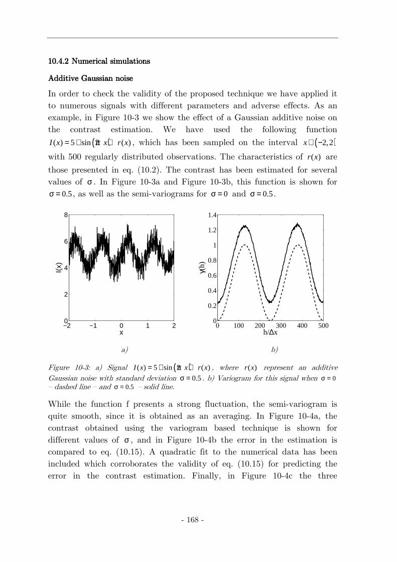
- 168 -

10.4.210.4.210.4.210.4.2 Numerical simulationsNumerical simulationsNumerical simulationsNumerical simulations

Additive Gaussian noiseAdditive Gaussian noiseAdditive Gaussian noiseAdditive Gaussian noise

In order to check the validity of the proposed technique we have applied it to numerous signals with different parameters and adverse effects. As an example, in Figure 10-3 we show the effect of a Gaussian additive noise on the contrast estimation. We have used the following function

( )( ) 5 sin 2 ( )I x x r x= + π + , which has been sampled on the interval ( )2,2x ∈ −

with 500 regularly distributed observations. The characteristics of ( )r x are

those presented in eq. (10.2). The contrast has been estimated for several values of σ . In Figure 10-3a and Figure 10-3b, this function is shown for

0.5σ = , as well as the semi-variograms for 0σ = and 0.5σ = .

−2 −1 0 1 20

2

4

6

8

x

I(x)

0 100 200 300 400 500

0

0.2

0.4

0.6

0.8

1

1.2

1.4

h/∆x

γ(h)

a) b)

Figure 10-3: a) Signal ( )( ) 5 sin 2 ( )I x x r x= + π + , where ( )r x represent an additive Gaussian noise with standard deviation 0.5σ = . b) Variogram for this signal when 0σ = — dashed line — and 0.5σ = — solid line.

While the function f presents a strong fluctuation, the semi-variogram is quite smooth, since it is obtained as an averaging. In Figure 10-4a, the contrast obtained using the variogram based technique is shown for different values of σ , and in Figure 10-4b the error in the estimation is compared to eq. (10.15). A quadratic fit to the numerical data has been included which corroborates the validity of eq. (10.15) for predicting the error in the contrast estimation. Finally, in Figure 10-4c the three

10. Appendix 2: Techniques for contrast calculation

- 169 -

techniques (direct definition, rms, and variogram) have been compared for different noise levels. For very low noise, the rms technique and the variogram based technique for contrast estimation present a similar behaviour. However, for high noise levels, the proposed variogram based technique is much better.

Offset fluctuationsOffset fluctuationsOffset fluctuationsOffset fluctuations

We have also analyzed the validity of the variogram based method when other effects on the signal appear as, for example, when the signal presents offset fluctuations. There are many cases where these local contrast variations provide us with information about fluctuations of the parameter to measure. However, there are also many situations where they are due undesired effects, such as dust or a non-uniform illumination. Then, an average of the contrast is required.

This is the case of the experimental example presented in section 10.4.3, where local inhomogeneities in the light source or the gratings produce undesired fluctuations in the offset or amplitude of the signals. As an example, we have simulated the following offset fluctuations:

( ) ( )( ) 5 sin sin 8I x k x x= + π + π in order to show that the variogram based

technique is valid to determine the average contrast value. This function

has been sampled 1000 points between ( )2,2x ∈ − .

The first sine function acts as a slowly variation function that avoids a correct average contrast estimation using standard techniques. In Figure 10-5a the function ( )I x for k = 0.5 is shown, and in Figure 10-5b the

relative error in the contrast estimation is shown for several values of k and for the three techniques. The variogram-based technique for contrast estimation is not very affected for this fluctuation, while the other techniques present a worse behaviour.

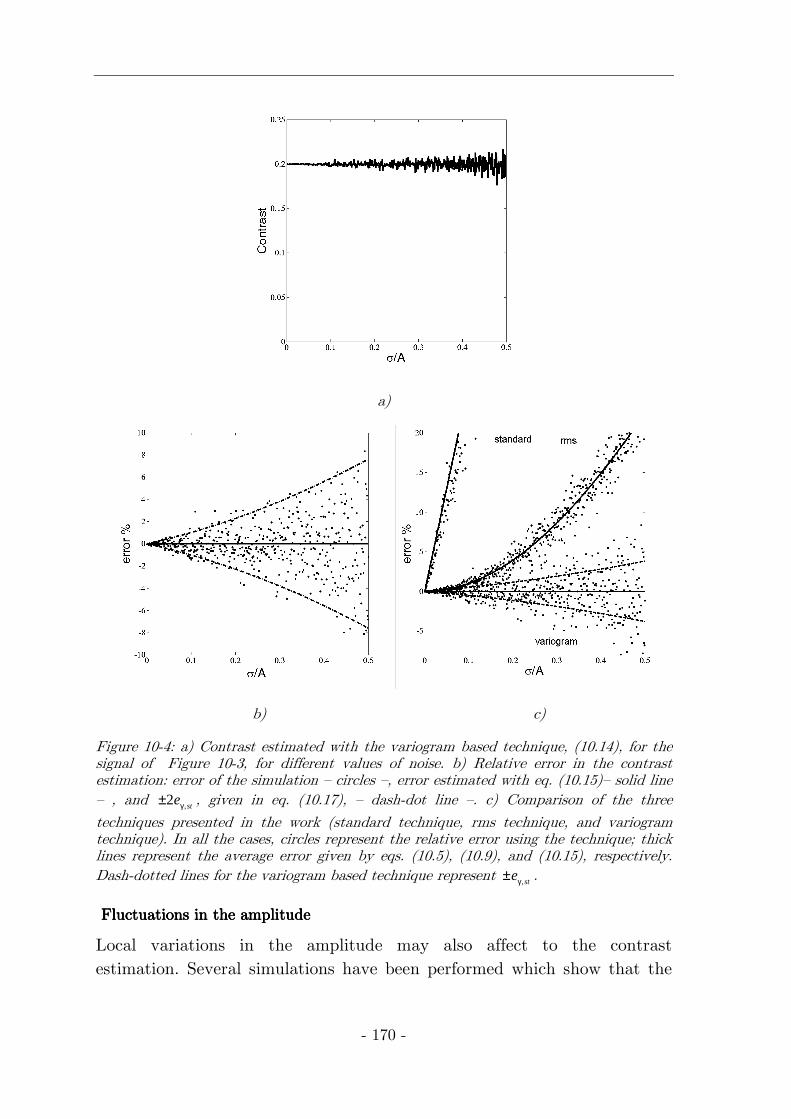
- 170 -

a)

b) c)

Figure 10-4: a) Contrast estimated with the variogram based technique, (10.14), for the signal of Figure 10-3, for different values of noise. b) Relative error in the contrast estimation: error of the simulation — circles —, error estimated with eq. (10.15)— solid line — , and ,2 steγ± , given in eq. (10.17), — dash-dot line —. c) Comparison of the three

techniques presented in the work (standard technique, rms technique, and variogram technique). In all the cases, circles represent the relative error using the technique; thick lines represent the average error given by eqs. (10.5), (10.9), and (10.15), respectively. Dash-dotted lines for the variogram based technique represent ,steγ± .

Fluctuations in the amplitudeFluctuations in the amplitudeFluctuations in the amplitudeFluctuations in the amplitude

Local variations in the amplitude may also affect to the contrast estimation. Several simulations have been performed which show that the

10. Appendix 2: Techniques for contrast calculation

- 171 -

variogram technique for contrast estimation is better than the other standard techniques.

−2 −1 0 1 20

1

2

3

4

5

6

7

x

I(x)

0 0.1 0.2 0.3 0.4 0.5

0

5

10

15

ker

ror

%

variogram

rms

standard

a) b)

Figure 10-5: a) Signal ( ) ( )( ) 5 sin 8 sinI x x k x= + π + π sampled 1000 points between

( )2, 2x ∈ − for k=0.5. b) Relative error in the contrast estimation in terms of k: Direct definition of contrast, eq. (10.1)—dashed-dot line—; Rms technique, eq. (10.7)—dashed line—; and Variogram technique, eq. (10.14). — solid line— .

As an example, in Figure 10-6a, the signal ( )[ ] ( )( ) 10 1 cos / 2 sin 4I x a x x= + + π π

is shown for a = 0.5, and in Figure 10-6b, the relative error in the contrast estimation is shown for different values of a. We can also see that the relative error is lower for the variogram technique than for the other standard techniques.

10.4.310.4.310.4.310.4.3 Experimental results: application to Talbot effectExperimental results: application to Talbot effectExperimental results: application to Talbot effectExperimental results: application to Talbot effect

In order to experimentally show the advantage of the variogram based technique with respect to other techniques for contrast estimation, we have measured the contrast for the case of Talbot effect [113]. For this, we have used a diffraction grating made of chrome on a glass substrate with a period of 100 mµ . In Figure 10-7a, the experimental intensity distribution

captured with a CMOS camera is shown in terms of the distance z between the diffraction grating and the observation plane. It appears a self-imaging process. The grating is reproduced at regular distances, known as Talbot

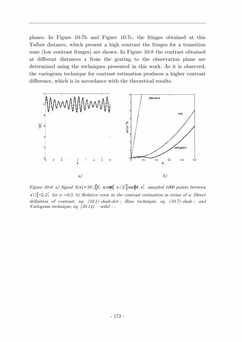
- 172 -

planes. In Figure 10-7b and Figure 10-7c, the fringes obtained at this Talbot distance, which present a high contrast the fringes for a transition zone (low contrast fringes) are shown. In Figure 10-8 the contrast obtained at different distances z from the grating to the observation plane are determined using the techniques presented in this work. As it is observed, the variogram technique for contrast estimation produces a higher contrast difference, which is in accordance with the theoretical results.

a) b)

Figure 10-6: a) Signal ( )[ ] ( )( ) 10 1 cos / 2 sin 4I x a x x= + + π π sampled 1000 points between

( )2, 2x ∈ − for a =0.5. b) Relative error in the contrast estimation in terms of a: Direct definition of contrast, eq. (10.1)—dash-dot—; Rms technique, eq. (10.7)—dash—; and Variogram technique, eq. (10.14). — solid — .

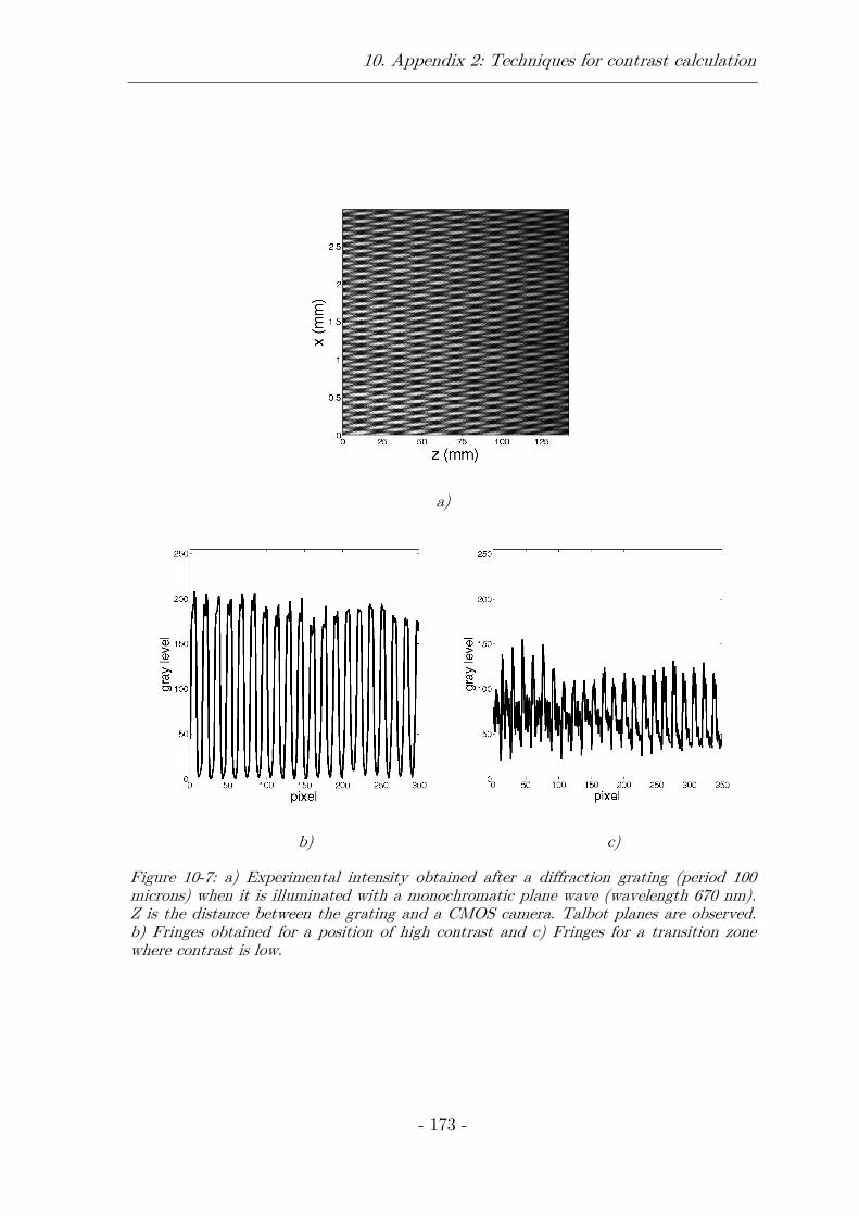
10. Appendix 2: Techniques for contrast calculation

- 173 -

a)

b) c)

Figure 10-7: a) Experimental intensity obtained after a diffraction grating (period 100 microns) when it is illuminated with a monochromatic plane wave (wavelength 670 nm). Z is the distance between the grating and a CMOS camera. Talbot planes are observed. b) Fringes obtained for a position of high contrast and c) Fringes for a transition zone where contrast is low.

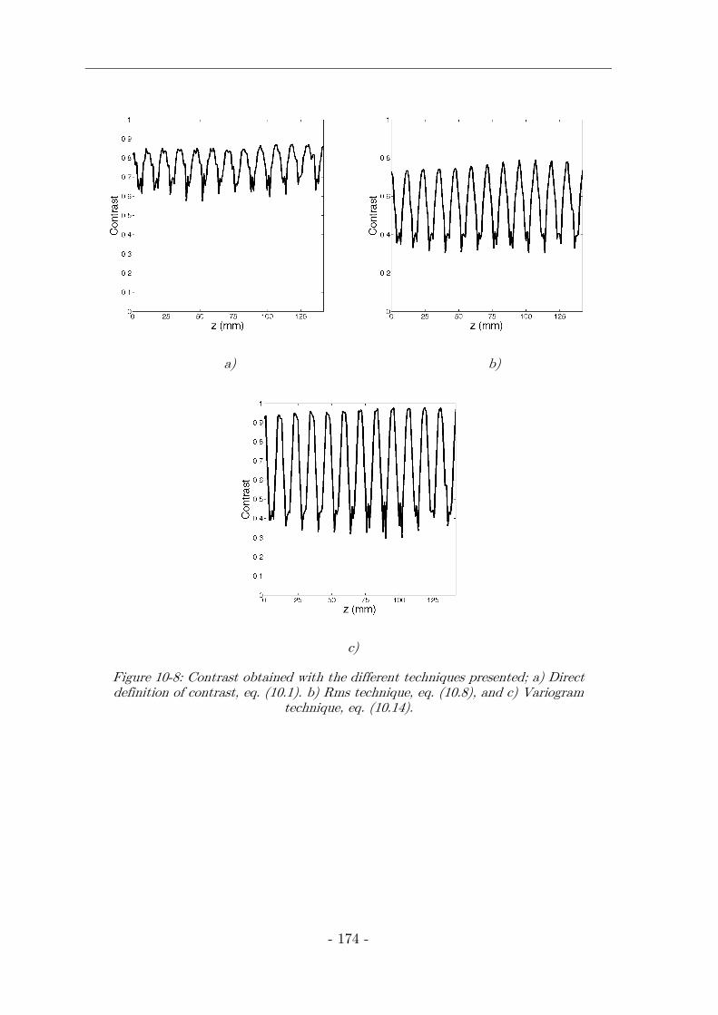
- 174 -

a) b)

c)

Figure 10-8: Contrast obtained with the different techniques presented; a) Direct definition of contrast, eq. (10.1). b) Rms technique, eq. (10.8), and c) Variogram

technique, eq. (10.14).

- 175 -

11111111 Appendix 3: DescAppendix 3: DescAppendix 3: DescAppendix 3: Description of ription of ription of ription of the the the the Confocal microscopeConfocal microscopeConfocal microscopeConfocal microscope usedusedusedused

Conventional microscopy techniques are based on collecting all the light that is reflected or transmitted by the object. Thus, some parts of the object appear diffused. The image is not clear if it is necessary a high resolution in depth. Confocal microscopy is based on collecting only the light reflected or transmitted by the focused parts of the object. A general scheme of a confocal microscope is shown in Figure 11-1. The light passes through a pin hole and is directed using a beam splitter to the target. Before comes to the target, the light is focused with an objective microscope. Then, the light reflected by the object is directed to the camera. Before the camera a pin hole is placed. This pin hole is situated just in the focal plane of the objective microscope used. Thus, only the focused parts of the object come to the camera. In our case, we use a confocal microscope by Sensofar (Plµ ). It works with white light. There are

other kinds of confocal microscopes which work with laser illumination, but they are use in photo-luminescence techniques. The operation way of the microscope consists in taking images of the focused parts of the object at different heights. Then, using these images, it builds a 3D image which shows us the topography of the object.

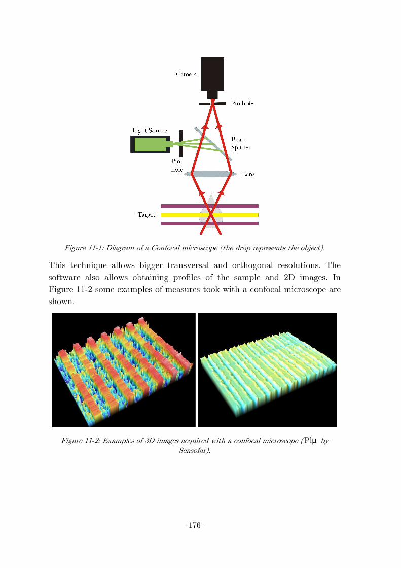
- 176 -

Figure 11-1: Diagram of a Confocal microscope (the drop represents the object).

This technique allows bigger transversal and orthogonal resolutions. The software also allows obtaining profiles of the sample and 2D images. In Figure 11-2 some examples of measures took with a confocal microscope are shown.

Figure 11-2: Examples of 3D images acquired with a confocal microscope ( µPl by Sensofar).

- 177 -

ReReReReferencesferencesferencesferences

[1] M. C. Hutley, “Diffraction gratings”, Techniques of Physics, London:

Academic Press (1982).

[2] C. Palmer, E. Loewen, “Diffraction gratings handbook”, Newport; 6th

edition (2005).

[3] E. Loewen, “Diffraction gratings and applications”, CRC; 1st edition

(1997).

[4] J. Guild, “Diffraction Gratings as Measuring Scales: Practical guide to

the metrological use of Moire Fringes”, Oxford (1960).

[5] G. Piquero, R. Borghi, M. Santarsiero, “Gaussian Schell-model beams

propagating through polarization gratings”, J. Opt. Soc. Am. A,,

18(6), 1399-1405, (2001).

[6] F. Gori, “Measuring Stokes parameters by means of a polarization

grating”, Opt. Letters, 24(9), 584-586, (1999).

[7] C. G. Someda, “Far field of polarization gratings”, Opt. Letters,

24(23), 1657-1659, (1999).

[8] G. Cincotti, “Polarization gratings: Design and applications”, IEEE

Proc. Of Quantum electronics, 39(12), 1645-1652, (2003).

[9] W. H. F. Talbot, ”Facts relating to optical science”, Philos. Mag., 9,

401—407, (1836).

- 178 -

[10] M. Testorf, J. Jahns, N.A. Khilo, A.M. Goncharenko, ”Talbot effect

for oblique angle of light propagation”, Opt. Comm., 129, 167-172,

(1996).

[11] N. Guérineau, B. Harchaoui, J. Primot, “Talbot experiment re-

examined: demonstration of an achromatic and continuous self-

imaging regime”, Opt. Comm., 180, 199-203, (2000).

[12] S. Teng, L. Liu, J. Zu, Z. Luan, De’an "Uniform theory of the Talbot

effect with partially coherent light illumination", J. Opt. Soc. Am. A,

20(9), 1747-1754, (2003).

[13] Y. Lu, Changhe Zhou, H. Luo, "Talbot effect of a grating with

different kinds of flaws", J. Opt. Soc. Am. A, 22(12),, 2662-2667,

(2005).

[14] Y. Lu, C. Zhou, S. Wang, B. Wang "Polarization-dependent Talbot

effect", J. Opt. Soc. Am. A, 23 (9), 2154- 2160, (2006).

[15] A. W. Lohmann, D. E. Silva, "An interferometer based on the Talbot

effect" Opt. Commun., 2, 413—415, (1971).

[16] G. Schirripa Spagnolo, D. Ambrosini, D. Paoletti "Displacement

measurement using the Talbot effect with a Ronchi grating", J. Opt.

A: Pure Appl. Opt., 4, S376—S380, (2002).

[17] B.F. Oreb, R.G. Dorsch, "Profilometry by phase-shifted Talbot

images", Appl. Opt., 33, 7955—62, (1994).

[18] S. Wei, S. Wu, I. Kao, F.P. Chiang, "Measurement of wafer surface

using shadow moire technique with Talbot effect", Trans. ASME J.

Electron. Packag. ,120, 166—70, (1998).

[19] G.J. Swanson, E.N. Leith, “Analysis of the Lau effect and generalized

grating imaging”, J. Opt. Soc. Am. A, 2, 789-793, (1985).

[20] F.J. Torcal-Milla, L.M. Sanchez-Brea, E. Bernabeu, "Talbot effect

with rough reflection gratings", Appl. Opt., 46, 3668- 3673, (2007).

[21] P. Beckmann, A. Spizzichino, “The Scattering of Electromagnetic

Wawes from Rough Surfaces”, Artech House INC (1987).

References

- 179 -

[22] L.M. Sanchez-Brea, F.J. Torcal-Milla, E. Bernabeu, " Talbot effect in

metallic gratings under Gaussian illumination", Opt. Comm., 278, 23-

27, (2007).

[23] F.J. Torcal-Milla, L.M. Sanchez-Brea, E. Bernabeu, "Double grating

systems with one steel tape grating", Opt. Commun., 281, 5647-5652,

(2008).

[24] L.M. Sanchez-Brea, F.J. Torcal-Milla, E. Bernabeu, "Far field of

gratings with rough strips", J. Opt. Soc. Am. A, 25, 828-833, (2008).

[25] F.J. Torcal-Milla, L.M. Sanchez-Brea, E. Bernabeu, "Self-imaging of

gratings with rough strips", J. Opt. Soc. Am. A,, 25(10), 2390-2394,

(2008).

[26] F.J. Torcal-Milla, L.M. Sanchez-Brea, E. Bernabeu, "Diffraction of

gratings with rough edges", Opt. Exp., 16(24), 19757-19769, (2008).

[27] F. Shen and A. Wang, “Fast-Fourier-transform based numerical

integration method for the Rayleigh—Sommerfeld diffraction formula”,

Appl. Opt., 45, 1102-1110, (2006).

[28] M. G. Moharam, T. K. Gaylord, “Diffraction analysis of dielectric

surface-relief gratings”, J. Opt. Soc. Am., 72(10), 1385-1392, (1982).

[29] N. Chateau, J. P. Hugonin, “Algorithm for the rigorous coupled wave

analysis of grating diffraction”, J. Opt. Soc. Am. A, 11(4), 1321-1331,

(1994).

[30] N. I. Chang, C. J. Kuo, “Algorithm based on rigorous coupled wav

analysis for diffractive optical elements design”, J. Opt. Soc. Am. A,

18(10), 2491-2501, (2001).

[31] K. Engelhardt, P. Seitz, “High-resolution optical encoder with large

mounting tolerances”, Appl. Opt., 36(13), 2912-2916, (1997).

[32] D. Crespo, J. Alonso, T. Morlanes, E. Bernabeu, “Optical encoder based on Lau effect”, Opt. Eng., 39(3), 817-824, (2000).

[33] C. F. Kao, M.H. Lu, “Optical encoder based on the fractional Talbot

effect”, Opt. Commun., 250, 16-23, (2005).

- 180 -

[34] M. Maghoo, J. Marcou, “A wavelength encoded rotary displacement

sensor”, Meas. Sci. Technol., 4, 860-864, (1993).

[35] A. Lutenberg, F. Perez-Quintian, M. A. Rebollo, “Optical encoder

based on a nondiffractive beam”, Appl. Opt., 47, 2201-2206, (2008).

[36] A. Lutenberg, F. Perez-Quintian, “Optical encoder based on a

nondiffractive beam II”, Appl. Opt., 48, 414-424, (2009).

[37] R. M. Pettigrew, “Analysis of grating imaging and its applications to

displacement metrology”, Proc. SPIE, 136, 325-332, (1997).

[38] J. Saez-Landete, J. Alonso, E. Bernabeu, “Design of zero reference

codes by means of a global optimization method”, Opt. Express,

13(1), 195-201, (2005).

[39] J. Saez-Landete, J. Alonso, E. Bernabeu, “Design of two-dimensional

zero reference codes by means of a global optimization method”, Opt.

Express, 13(11), 4230-4236, (2005).

[40] J. Saez-Landete, S. Salcedo-Sanz, M- Rosa-Zurera, J. Alonso, E.

Bernabeu, “Optimal design of optical reference signals by use of a

genetic algorithm”, Opt. Lett., 30(20), 2724-2726, (2005).

[41] J. Saez-Landete, J. Alonso, E. Bernabeu, “Design of two-dimensional

zero reference codes by means of a global optimization method”, Opt.

Lett., 31(11), 1648-1650, (2006).

[42] K. Miyashita, T. Takahashi, S. Kawamata, S- Morinaga, Y. Hoshi,

“Noncontact magnetic torque sensor”, IEEE (Transactions on

magnetics), 26(5), 1560-1562, (1990).

[43] K. Miyashita, T. Takahashi, M. Yamanaka, “Features of a magnetic

rotary encoder”, IEEE (Transactions on magnetics), 23(5), 2182-2184,

(1987).

[44] P. Campbell, “Magnetoresistive sensors for rotary encoders”, IEEE

(Transactions on magnetics), 26(5), 2029-2031, (1990).

[45] W. D. McCall, E. J. Rohan, “ A linear position transducer using a

magnet and hall effect devices”, IEEE (Transactions on

instrumentation and measurement), 26(2), 133-136, (1977).

References

- 181 -

[46] M. Sawabe, F. Maeda, Y. Yamaryo, T. Simomura, Y. Saruki, T.

Kubo, H. Sakai, S. Aoyagi, “ A new vacuum interferometric

comparator for calibrating the fine linear encoders and scales”,

Precission Eng., 28(3), 320-328, (2004).

[47] C. F. Lam, R. Vrijen, D. T. K. Tong, M. C. Wu, E. Yablonobitch,

“Experimental demonstration of spectrally encoded optical

CDMAsystem using Mach-Zender encoder chains”, Lasers and

Electro-Optics, 1998. CLEO 98. Technical Digest. Summaries of

papers presented at the Conference on, 455, (1998)

[48] Y. Jourlin, J. Jay, O. Parriaux, “Compact diffractive interferometric

displacement sensor in reflection”, Precission Engineering-Journal of

the international societies for precision engineering and

nanotechnology, 26(1), 1-6 (2006).

[49] J.H. Zhang, L. Cai, “Autofocus laser rotary encoder”, Appl. Opt.,

37(13), 2691-2695, (1998).

[50] H. Iwai, K. Mitsui, “ Development of a measuring method for motion

accuaracy of NC machine tools using links and rotary encoders”,

international Journal of machine tools & manufacture, 99-108, (2009).

[51] X. Wen-Zhuo, K. Zhi-Yong, Z. Wei, “ Phase correction of quartering

deviation of photoelectric rotary encoder”, Opt & Prec. Eng., 1745-

1748, (2007).

[52] T. Kabashina, T. Arinaga, K. Uemura, “A novel magnetic rotary

encoder for servo motors”, Transactions of the institute of electrical

engineers of japan, part D, 126D(9), 1202-1207, (2006).

[53] C. F. Kao, S. H. Lu, M. H. Lu, “High resolution planar encoder by

retro-reflection”, Review of scientific instruments, 76(8), (2005).

[54] D. Crespo, J. Alonso, E. Bernabeu, “Reflection optical encoders as

three-grating moiré systems”, Appl. Opt., 39(22), 3805-3813, (2000).

[55] J. H. Zhang, L. Cai, “Autofocus laser rotary encoder”, Appl. Opt.,

37(13), 2961-2965, (1998).

- 182 -

[56] G.J. Swanson, E.N. Leith, “Analysis of the Lau effect and generalized

grating imaging”, J. Opt. Soc. Am. A, 2, 789-793, (1985).

[57] S.C. Som, A. Satpathi, “The generalised Lau effect”, J. Mod. Opt., 37,

1215-1226, (1990).

[58] D. Crespo, J. Alonso, E. Bernabeu, “Generalized grating imaging

using an extended monochromatic light source”, J. Opt. Soc. Am. A,

17, 1231-1240, (2000).

[59] D. Crespo, J. Alonso, E. Bernabeu, “Experimental measurements of

generalized grating images”, Appl. Opt., 41(7), 1223-1228, (2002).

[60] L. Garcia-Rodriguez, J. Alonso, E. Bernabeu, “Grating pseudo-

imaging with polychromatic and finite extensión sources”, Opt.

Express, 12, 2529-2541, (2004).

[61] D. Crespo, “Nuevas herramientas aplicadas a la codificación óptica”,

Thesis dissertation, Optics department, Universidad Complutense de

Madrid, (2001).

[62] L. M. Sanchez-Brea, T. Morlanes, “Metrological errors in optical

encoders”, Meas. Sci. Technol., 19, (2008).

[63] K. P. Birch, “Optical fringe subdivision with nanometric accuracy”,

Prec. Eng., 12, 195-198, (1990).

[64] L. M. Sanchez-Brea, T. Morlanes, “Metrological errors in optical

encoders”, Meas. Sci. Technol., 19, 115104, (2008)

[65] H. Zongsheng, Q. Shiqiao, W. Xingshu, Z. Dejun, “Error analysis of

optical angular encoder and its calibration with ring laser gyro”,

Chinese Journal of Scientific Instrument, 28(10), 1866-1869, (2007).

[66] H. F. F. Castro, M. Burdekin, “Dynamic calibration of the positioning

accuracy of machine tools and coordinate measuring machines using a

laser interferometer”, Int. J. Mach. Tool. Manu., 43(9), 947-954,

(2003).

[67] J. D. Jackson, “Classical Electrodynamics”, 3rd edition ,John Wiley &

Sons, Inc. (1998).

References

- 183 -

[68] M. Born, E. Wolf, “Principles of Optics”, 6th edition, Pergamso Press

(1991).

[69] F. Shen and A. Wang, “Fast-Fourier-transform based numerical

integration method for the Rayleigh—Sommerfeld diffraction formula”,

Appl. Opt., 45, 1102-1110, (2006).

[70] J. A. Ogilvy, “Theory of Wave Scattering from Random Rough

Surfaces” IOP (1991).

[71] D. Crespo, J. Alonso, T. Morlanes, E. Bernabeu, “Reflection optical

encoders as three-grating Moiré systems”, Appl. Opt., 39(22), 3805-

3813, (2000).

[72] G. N. Rassudova, “Moire interference fringes in a system consisting of

a transmission and a reflection diffraction grating. Part I”, Opt.

Spectrosc., 22, 73—78, (1967).

[73] J. Jahns, W. Lohmann, “The Lau effect (a diffraction experiment with

incoherent illumination)”, Opt. Commun., 28, 263-267, (1979).

[74] S.C. Som, A. Satpathi, “The generalised Lau effect”, J. Mod. Opt., 37,

1215-1226, (1990).

[75] Fagor Automation S. Coop. (www.fagorautomation.com].

[76] J. C. Dainty, “Laser Speckle and Related Phenomena”, Springer-

Verlag (1984).

[77] F. Perez-Quintián, A. Lutenberg, M. A. Rebollo, "Linear displacement

measurement with a grating and speckle pattern illumination", Appl.

Opt., 45(20), 4821-4825, (2006).

[78] S. Szapiel and K. Patorski, “Fresnel diffraction images of periodic

objects under Gaussian beam illumination”, Optica Acta , 26(4), 439-

446, (1979).

[79] J. W. Goodman, “Statistical Optics”, John Wiley &Sons, New York

(1985).

[80] V. Ya. Mendeleev, S. N. Skovorod’ko, Optics and Spectroscopy.

“Relation for estimating the reflectance of a very rough surface with

- 184 -

an approximately one-dimensional distribution of roughness”, 94(3),

437-443, (2003).

[81] V. Celli, A. A. Maradudin, A. M. Marvin, A. R. McGurn, “Some

aspects of light scattering from a randomly rough metal surface”, J.

Opt. Soc. Am. A, 2(12), 2225-2239, (1985).

[82] B. E. A. Saleh and M. C. Teich, “Fundamentals of Photonics”, John

Wiley & Sons (1991).

[83] G.W.R. Leibbrandt, G. Harbers, P. J. Kunst, “Wave-front analysis

with high accuracy by use of a double-grating lateral shearing

interferometer”, App. Opt., 35, 6151-6161, (1996).

[84] Y. Xu, O. Sasaki, T. Suzuki, “Double-grating interferometer with a

one-to-one correspondence with a Michelson interferometer”, Opt.

Lett., 28, x1751-1753, (2003).

[85] Y. Xu, O. Sasaki, T. Suzuki, App. Opt., “Double-grating

interferometer for measurement of cylindrical diameters”, 43, 537-541,

(2004).

[86] I.B. Gornushkin, N. Omenetto, B. W. Smith, J. D. Winefordner, App.

Spectrosc., 58, 1341-1346, (2004).

[87] S. Grabarnik, R. Wolffenbuttel, A. Emadi, M. Loktev, E. Sokolova, G.

Vdovin, “Planar double-grating microspectrometer”,Opt. Express, 15,

3581-3588, (2007).

[88] K. Patorski, "The self-imaging phenomenon and its applications",

Progress in Optics, 27, 1—108, (1989).

[89] K. Patorski, “Moirè Metrology”, Pergamon, New York (1998).

[90] E. Lau. “Beugungserscheinungen an Doppelrastern”, Ann. Phys., 6,

417-423, (1985).

[91] D. Crespo, J. Alonso, T. Morlanes, E. Bernabéu, “Optical encoder

based on the Lau effect”, Opt. Eng., 39, 817-824, (2000).

[92] J.W. Goodman, “Introduction to Fourier Optics”, Mc Graw Hill, New

York (1996).

References

- 185 -

[93] E.G. Loewen, E. Popov, “Diffraction gratings and applications”,

Marcel Dekker, New York,(1997).

[94] C. Palmer, “Diffraction Grating Handbook”, Richardson Grating

Laboratory, New York (2000).

[95] F. Gori, "Measuring Stokes parameters by means of a polarization

grating", Opt. Lett., 24(9), 584-586, (1999).

[96] C.G. Someda, "Far field of polarization gratings", Opt. Lett., 24,

1657- 1659, (1999).

[97] G. Piquero, R. Borghi, A. Mondello, M. Santarsiero, ”Far field of

beams generated by quasi-homogeneous sources passing through

polarization gratings“, Opt. Comm., 195, 339-350, (2001).

[98] P. P. Naulleau, G. M. Gallatin, “Line-edge roughness transfer function

and its application to determining mask effects in EUV resist

characterization”, Appl. Opt., 42(17), 3390-3397, (2003).

[99] T. R. Michel, “Resonant light scattering from weakly rough random

surfaces and imperfect gratings”, J. Opt. Soc. Am. A, 11(6), 1874-

1885, (1994).

[100] V.A. Doroshenko, “Singular integral equations in the problem of wave

diffraction by a grating of imperfect flat irregular strips”,

Telecommunications and Radio Engineering, 57(6-7), 65-72, (2002).

[101] M.V. Glazov, S.N. Rashkeev, “Light scattering from rough surfaces

with superimposed periodic structures”, Appl. Phys. B, 66, 217—223,

(1998).

[102] G. C. Holst, “CCD Arrays, Cameras, and Displays, Society for Photo-

Optical Instrumentation Engineers”, Bellingham, Wash. (1996).

[103] P. Hariharan, “Optical Interferometry”, Academic Press (1989).

[104] International Standardization Organization, Guide to the Expression

of the Uncertainty in Measurement, Geneva, (1995)

[105] E.W. Weisstein "Root-Mean-Square." From MathWorld--A Wolfram

Web Resource. http://mathworld.wolfram.com/Root-Mean-

Square.html

- 186 -

[106] S. Lai, G. Von Bally, "Fringe contrast evaluation by means of

histograms", in OPTIKA '98: 5th Congress on Modern Optics, G.

Ákos, G. Lupkovics, P. András, editors, Proc. of SPIE, 3573, 384-387,

(1998)

[107] L.M. Sanchez-Brea, J.A. Quiroga, A. Garcia-Botella, E. Bernabeu,

"Histogram-based method for contrast measurement", Applied Optics,

39(23), 4098-4106, (2000).

[108] R. Christiensen, “Linear Models for Multivariate, Time Series, and

Spatial Data”, Springer-Verlag, Berlin (1985).

[109] N. A. Cressie, “Statistics for Spatial Data”, J. Wiley & sons, New

York (1991).

[110] L. M. Sanchez-Brea, E. Bernabeu, "On the standard deviation in CCD

cameras: a variogram-based technique for non-uniform images",

Journal of Electronic Imaging., 11(2), 121-126, (2002).

[111] L. M. Sanchez-Brea, E. Bernabeu, "Estimation of the standard

deviation in three-dimensional microscopy by spatial statistics",

Journal of Microscopy, 218(2), 193—197, (2005).

[112] P. Bevington, “Data Reduction and Error Analysis for the Physical

sciences”, McGraw-Hill, New York (1969).

[113] E. Keren, O. Kafri, "Diffraction effects in moire deflectometry", J.

Opt. Soc. Am. A, 2(2), 111-120, (1985).

- 187 -

PublicationsPublicationsPublicationsPublications and Communicationsand Communicationsand Communicationsand Communications

PublPublPublPublicationsicationsicationsications

F.J. Torcal-Milla, L.M. Sanchez-Brea, E. Bernabeu, "Talbot effect with

rough reflection gratings", Appl. Opt. 46(18), 3668- 3673 (2007).

L.M. Sanchez-Brea, F.J. Torcal-Milla, E. Bernabeu, Variogram-based

method for contrast measurement”, App. Opt. 46(22), 5027-5033

(2007).

L.M. Sanchez-Brea, F.J. Torcal-Milla, E. Bernabeu "Talbot effect in

metallic gratings under Gaussian illumination" Opt. Comm. 278, 23—

27 (2007).

L.M. Sanchez-Brea, F.J. Torcal-Milla, E. Bernabeu, “Far field of gratings

with rough strips” J. Opt. Soc. Am. A 25(4), 828-833 (2008).

F.J. Torcal-Milla, L.M. Sanchez-Brea, E. Bernabeu, “Self-imaging of

gratings with rough strips” J. Opt. Soc. Am. A 25(10), 2390-2394

(2008).

F.J. Torcal-Milla, L.M. Sanchez-Brea, E. Bernabeu, “Double grating

systems with one steel tape grating”, Opt. Commun. 281, 5647-5652

(2008).

F.J. Torcal-Milla, L.M. Sanchez-Brea, E. Bernabeu, “Diffraction of gratings

with rough edges”, Opt. Express. 16(24), 19757-19769 (2008).

- 188 -

CommunicationsCommunicationsCommunicationsCommunications

F.J. Torcal-Milla, L.M. Sanchez-Brea, E. Bernabeu, “Effect of roughness in

reflection gratings”, oral presentation, ODIMAP V, Mostoles (Madrid)

(2007).

L.M. Sanchez-Brea, F.J. Torcal-Milla, E. Bernabeu, T. Morlanes,

“Interfero-difractive linear optical encoder with nanometric

resolution”, poster presentation, NANOSPAIN 2008, Braga (Portugal)

(2008).

L.M. Sanchez-Brea, F.J. Salgado-Remacha, F.J. Torcal-Milla, “Effect of

surface defects on the self-images produced by diffraction gratings”,

poster presentation accepted, Optical Metrology (SPIE) Munich

(Germany) (2009).

F.J. Torcal-Milla, L.M. Sanchez-Brea, E. Bernabeu, “Talbot effect with

aberrated beams”, poster presentation accepted, Optical Metrology

(SPIE) Munich (Germany) (2009).

F.J. Torcal-Milla, L.M. Sanchez-Brea, F.J. Salgado-Remacha,

“Autoimagenes producidas por redes de difracción binarias de fase-

amplitud”, poster presentation accepted, Reunión nacional de Óptica,

Vigo (Spain) (2009).

F.J. Salgado-Remacha, I. Jimenez-Castillo, F.J. Torcal-Milla, T. Morlanes,

L.M. Sanchez-Brea, E. Bernabeu, “Autoimagenes producidas por redes

de difracción grabadas sobre fleje de acero mediante ablación laser”,

poster presentation accepted, Reunión nacional de Óptica, Vigo

(Spain) (2009).