rotational sliding contact dynamics in a non-linear cam-follower

Contents lists available at SciVerse ScienceDirect

Journal of Sound and Vibration

Journal of Sound and Vibration 332 (2013) 4280–4295

0022-46http://d

n CorrE-m

journal homepage: www.elsevier.com/locate/jsvi

Rotational sliding contact dynamics in a non-linearcam-follower system as excited by a periodic motion

Sriram Sundar, Jason T. Dreyer, Rajendra Singh n

Acoustics and Dynamics Laboratory, Department of Mechanical and Aerospace Engineering, The Ohio State University, Columbus,OH 43210, USA

a r t i c l e i n f o

Article history:Received 9 October 2012Received in revised form20 February 2013Accepted 27 February 2013
Handling Editor: L.N. Virgin
operates in both sliding contact and no-contact regimes. The Hertzian contact theory is

Available online 15 April 2013

0X/$ - see front matter & 2013 Elsevier Ltd.x.doi.org/10.1016/j.jsv.2013.02.035

esponding author. Tel.: þ1 614 292 9044.ail address: [email protected] (R. Singh).

a b s t r a c t

The rotational sliding contact dynamics of a cam-follower system is investigated using asingle degree-of-freedom system given a periodic motion by the cam rotating about afixed pivot. This mechanical system includes kinematic, dry friction, and contact non-linearities (loss of contact, non-linear contact stiffness, and non-linear damping) as it

used to calculate the contact stiffness under both line and point contacts. The non-linearformulation is numerically solved to calculate the dynamic motions and forces in time andfrequency domains. Alternate damping formulations, including combined viscous-impactdamping models, are assessed under impacting conditions, and the results are success-fully compared with experimental results as available in the literature. The applicability ofthe coefficient of restitution model is critically analyzed. The friction and contact non-linearities of the system are investigated in the sliding contact regime. Finally, thekinematic non-linearity is studied in comparison with a linearized model.

& 2013 Elsevier Ltd. All rights reserved.

1. Introduction

The dynamics of cam-follower systems have traditionally been described by lumped parameter, linear system theory forthe follower with motion input from the cam, as reported by Chen [1] in a literature survey (1977). More recent investigatorshave employed piecewise linear system models to study the loss of contact in a cam-follower system [2–4], and somestudies [5–7] have examined the stability issues. In particular, Alzate et al. [8,9] and Koster [10] studied bifurcations in anon-linear cam-follower system, though they did not focus on the kinematic non-linearity. Alzate et al. [8] used thecoefficient of restitution concept to model the contact between the cam and follower. Such coefficient of restitution typemodels usually have several deficiencies as stated by Gilardi and Sharf [11]. Overall, the contact stiffness and damping non-linearities of a cam-follower system are yet to be rigorously studied. Also the effect of dry friction non-linearities has beenneglected in the cam-follower models [1–10] since there is no motion along the direction of friction. The chief goal of thispaper is, therefore, to overcome the void in the literature and study the rotational sliding contact dynamics (only in thecontext of a single degree-of-freedom system) given a periodic motion by the cam rotating about a fixed pivot. The proposedformulation would include kinematic, friction and contact non-linearities.

Sliding and/or rolling contacts are of interest in many mechanical systems such as pin-disk models [12–15], gearedtransmission systems [16–18], and bearings [19]. However, the dynamics of the sliding contact are sometimes studied usingsimple translating systems [20–26]. Rolling contacts have been investigated by Remington using a lumped system model[27] and experiments [28]. Gray and Johnson [29] have analyzed the rolling contact problem using a simple vibration model

All rights reserved.

www.elsevier.com/locate/jsvi

www.elsevier.com/locate/jsvi

http://dx.doi.org/10.1016/j.jsv.2013.02.035



http://crossmark.dyndns.org/dialog/?doi=10.1016/j.jsv.2013.02.035&domain=pdf



mailto:[email protected]


Fig. 1. Cam-follower system in the general state where a non-linear contact stiffness model, kλ(ψi(t)), is employed.

S. Sundar et al. / Journal of Sound and Vibration 332 (2013) 4280–4295 4281

that included the contact mechanics concept. This paper will examine only the rotational sliding contact and utilize some ofthe contact mechanics principles employed in other mechanical system [30,31].

2. Problem formulation

Fig. 1 shows a single degree-of-freedom (SDOF) cam-follower system in the general position, when the cam and follower arenot in contact. The fixed orthogonal coordinate system ðex,eyÞ describes the horizontal and vertical directions, with its origin at E.The circular cam of radius, rc, is considered; it rotates about the fixed pivot E, which is at a distance, e, from the geometric centerof the cam (Gc). The angular movement of the cam is given by Θ(t), the angle made by GcE

��!with the horizontal line in the

counter-clockwise direction; it is also the motion input to the system. The follower is described by a rectangular bar(with width,wb), which is pivoted at its center of gravity to a fixed pivot Pwhich is at a distance, dy, above the ground. The angleα(t) made by the follower with the horizontal line in the clockwise direction is the only generalized coordinate. The follower issupported by a linear follower spring (ks) at a distance, dx, from P. The contact between the cam and follower is represented bymeans of non-linear contact stiffness (kλ(ψi(t))) and damping (cλ(ψi(t))) terms. Contact points in the follower and cam are Ob andOc, respectively. During the operation, the system can be in either the sliding contact regime or the non-contact regime at agiven instant, which is determined by the sign of ψi(t). The coefficient of friction between the cam and follower is given by time-varying μ(t). When the follower just touches the cam (QOc

��!¼ 0!

) for a given Θ0, the state of the system is denoted as the 0-state.This 0-state (where Q0, O0

b and O0c are coincident) is used to define the geometry of the cam-follower system and to derive the

relationship between the fixed coordinates and moving coordinates ði, jÞ as attached to the follower at Q. This system is similarto the cam-follower experiment that has been studied by Alzate et al. [8]; the results will be discussed later in Section 4.

The cam-follower system, as discussed in this article, includes kinematic (from the geometry of the system), dry friction,and contact non-linearities. The friction non-linearity arises due to the dependence of the friction force, Ff(t), on themagnitude as well as on the direction of the relative velocity of sliding, vr(t). The contact non-linearity is from the non-linearHertzian point contact model, the non-linear contact damping model (function of the displacement and velocity of contactpoints), and the discontinuity during the contact. The key assumptions in the proposed formulation include the following:(i) the bearings at the pivots of the cam and follower are frictionless and rigid, allowing only rotation without anytranslation; (ii) cam and follower are elastic bodies, and their surfaces are smooth; (iii) the contact force between the camand follower follows the Hertzian theory [32]; and (iv) the bending moment of the follower is negligible.

The objectives of this article are as follows: (a) Develop a contact mechanics model for the cam-follower system withrotational sliding contact; (b) Examine the applicability of different viscous and impact damping models and the coefficientof restitution concept by comparing the predictions with the experimental results reported by Alzate et al. [8]; (c) Study theeffects of contact and friction non-linearities in the sliding contact regime; and (d) Analyze the effect of kinematic non-linearity of the system by comparing it with a linearized model. Since all the non-linearities are inter-related with eachother, the dynamic system is very complex even with a single degree-of-freedom formulation.

3. Analytical model

3.1. Relationship between the coordinate systems

In Fig. 1, QOc��!

is represented by ψ iðtÞiþψ jðtÞj in the moving coordinate system, and ψi(t) and ψj(t) are used to calculate thecontact force and the moment imparted by the cam on the follower, respectively. A non-negative value of ψi(t) indicates that

S. Sundar et al. / Journal of Sound and Vibration 332 (2013) 4280–42954282

the cam and follower are not in contact. When ψi(t) is negative, the system is in the sliding contact regime with themagnitude of ψi(t) representing the deflection of the contact spring. At any instant, ψi(t) and ψj(t) can be calculated for agiven α(t) and Θ(t) from the system geometry as shown below. From Fig. 1 the vectors are calculated as follows:

POb��!¼ PE

�!þEGc��!þGcOb

��!, (1)

POb��!¼ χðtÞcosðαðtÞÞþ wb

2sinðαðtÞÞ

h iexþ −χðtÞsinðαðtÞÞþ wb

2cosðαðtÞÞ

h iey, (2)

EGc��!¼−ecosðΘðtÞÞex−esinðΘðtÞÞey, (3)

GcOb

��!¼ −ðrcþψ iðtÞÞsinðαðtÞÞex−ðrcþψ iðtÞÞcosðαðtÞÞey: (4)

Here, χ(t)¼χ0−ψj(t), where χ(t) and χ0 are the components of jPOb��!j and jPO0

b

��!j, respectively, alongbj. The constant vector PE

�!is

evaluated based on the 0-state as follows, where α0 is the angle of the follower at the 0-state:

PE�!¼ χ0cos α0

� �þ rcþwb

2

� �sin α0� �þecos Θ0� �h i

ex

þ −χ0sin α0� �þ rcþ wb

2

� �cos α0� �þesin Θ0� �h i

ey: (5)

Using Eqs. (2)–(5) in Eq. (1) and rearranging, ψi (t) and ψj(t) are evaluated as

ψ iðtÞ ¼ χ0sinðαðtÞ−α0Þþ rcþwb

2

� �ðcosðαðtÞ−α0Þ−1Þ

þe½sinðαðtÞþΘ0Þ−sinðαðtÞþΘðtÞÞ�, (6)

ψ jðtÞ ¼ χ0 1−cosðαðtÞ−α0Þ� �þ rcþ wb

2

� �sinðαðtÞ−α0Þ

−e½cosðαðtÞþΘ0Þ−cosðαðtÞþΘðtÞÞ�: (7)

Next, differentiate Eqs. (6) and (7) with respect to time to yield the following:

ψ_ iðtÞ ¼ χ0cosðαðtÞ−α0Þα_ðtÞ− rcþwb

2

� �sinðαðtÞ−α0Þα_ðtÞ

þe½cosðαðtÞþΘ0Þα_ðtÞ−cosðαðtÞþΘðtÞÞðα_ðtÞþ _Θ ðtÞÞ�; (8)

ψ_jðtÞ ¼ χ0sinðαðtÞ−α0Þα_ðtÞþ rcþwb

2

� �cosðαðtÞ−α0Þα_ðtÞ

þe½sinðαðtÞþΘ0Þα_−sinðαðtÞþΘðtÞÞðα_ðtÞþ _ΘðtÞÞ�: (9)

3.2. Equations of motion

Fig. 2 shows the free body diagram of the follower in the sliding contact regime. The moment balancing about P yieldsthe following equation of motion for the follower in the sliding contact regime, where IPb is the mass moment of inertia ofthe follower about P:

IPbα€ðtÞ ¼ −FsðtÞdxþFnðtÞχðtÞ−0:5Ff ðtÞwb: (10)

Fig. 2. Free body diagram of the follower in the sliding contact regime.


The elastic force (Fs(t)) from the follower spring is given by the following, where Lus is the un-deflected length of thefollower spring:

FsðtÞ ¼ ks½Lus−dyþdxtanðαðtÞÞ−0:5wbsecðαðtÞÞ�: (11)

The normal contact force (Fn(t)) is given by

FnðtÞ ¼−kλðψ iðtÞÞψ iðtÞ−cλðψ iðtÞÞ _ψ iðtÞ: (12)

The Hertzian theory [32] for line contact is used to define kλ(ψi(t)) as follows, where lλ is the length of line contact, and Yis the equivalent Young's modulus (with subscript e denoting equivalent)

kλðψ iðtÞÞ ¼π

4Yelλ: (13)

The equivalent Ye of the two materials in contact is calculated based on the Hertzian theory [32] as well

Ye ¼1−ν2cYc

þ 1−ν2bYb

" #−1: (14)

Here, ν is the Poisson's ratio of the material, and the subscripts b and c represent the follower and cam, respectively. Theforce Ff(t) due to sliding friction exerted on the follower by the cam is Ff ðtÞ ¼ μðtÞFnðtÞ where two models for time varying μ(t) are utilized (discussed later in this section). The equation of motion for the system in the non-contact regime is derivedbelow, similar to the sliding contact regime, but now with Fs(t)¼0 and Fn(t)¼0.

IPbα€ðtÞ ¼−FsðtÞdx: (15)

Eqs. (10) and (15) are numerically solved using MATLAB's [33] ODE solver for stiff problems (which uses simultaneousfirst and fifth order Runge–Kutta formulations) for a given initial value of α(t). These results were found not to differsignificantly from the results from the slower but accurate fourth and fifth order Runge–Kutta formulations for some testcases. One must, however, keep track of the condition for switching between the contact regimes (‘event detection’ featureof MATLAB [33] is used) based on the value of ψi(t) as discussed earlier.

3.3. Static equilibrium and linearized natural frequency

The force Fs(t) is assumed to be sufficiently large at the static equilibrium point to maintain the cam-follower contact.The equations for the static equilibrium point (given by superscript n) are derived for Θ(t)¼Θ0 by replacing α(t), ψi(t), andψj(t) with the corresponding values at the static equilibrium point (αn, ψi

n, and ψj

n, respectively), and forcing all time

derivative terms to zero in Eqs. (6), (7), and (10), as follows:

χ0sinðα*−α0Þþ rcþ wb

2

� �cosðα*−α0Þ− rcþ wb

2

� �−ψ i*¼ 0, (16)

χ0 1−cosðα*−α0Þ� �þ rcþwb

2

� �sinðα*−α0Þ−ψ j*¼ 0, (17)

−ksdx Lus−dyþdxtan α*ð Þ−0:5wbsec α*ð Þ� �þ π

4Yelλψ i*ðχ0−ψ j*Þ ¼ 0: (18)

Simultaneous Eqs. (16–18) are numerically solved to find αn, ψin, and ψj

n. The system is then linearized about the static

equilibrium point. Writing the linearized equation of motion of the system in the sliding contact regime in state space formas _Ξ ¼ hðΞÞ, where

Ξ ¼ ðαðtÞ,α_ðtÞÞT ¼ ðε1ðtÞ,ε2ðtÞÞT , (19a)

hðΞÞ ¼ ðh1ðΞÞ,h2ðΞÞÞT : (19b)

The state space equations are derived below from Eq. (10) as

_ε1ðtÞ ¼ ε2ðtÞ ¼ h1ðΞÞ, (20a)

_ε2ðtÞ ¼½−FsðtÞdxþFnðtÞχðtÞ−0:5wbFf ðtÞ�

IPb¼ h2ðΞÞ: (20b)

The Jacobian matrix (J) at the static equilibrium point is

J ¼ ½∂hi=∂εj�*; i,j¼ 1,2: (21)

The following partial derivatives are calculated to evaluate J at the static equilibrium point:

∂h1∂ε1

*¼ 0; (22a)


∂h1∂ε2

*¼ 1; (22b)

∂h2∂ε1

*¼ −ð∂Fs=∂αÞdxþð∂Fn=∂αÞχþFnð∂χ=∂αÞ−0:5wbð∂Ff =∂αÞ

IPb

" #*; (22c)

∂h2∂ε2

*¼ −ð∂Fs=∂α_Þdxþð∂Fn=∂α_ÞχþFnð∂χ=∂α_Þ−0:5wbð∂Ff =∂α_Þ

IPb

" #*: (22d)

The linearized natural frequency (ϑ) is calculated as follows where the operator, Im, yields the imaginary part of theoperand, and the operator, Eig, gives the eigenvalues of a square matrix

ϑ¼ jImðEig½J�Þj0:5 (23)

3.4. Contact damping and dry friction models

Five different damping models are utilized for cλ(ψi(t)), as described in Eq. (12), to examine the dissipation of energy byimpact and other mechanisms. First is the pure viscous damping formulation (denoted as damping model A) where thedamping coefficient cAλ ψ iðtÞ

� �is time-invariant and is calculated as follows from Eqs. (10) and (12) using the linearized modal

viscous damping ratio ζ (with a superscript representing the damping model) and χ*¼ χ0−ψ *j :

cAλ ðψ iðtÞÞ ¼2ζAϑIPbðχ*Þ2

: (24)

Two pure impact damping formulations (denoted as damping models B and C) are analyzed next; these models aresuggested by Padmanabhan et al. [34] and Zhang et al. [35], respectively; here β is the impact damping factor:

cBλ ðψ iðtÞÞ ¼ βBkλψ iðtÞ; (25)

cCλ ðψ iðtÞÞ ¼ βC jψ iðtÞj0:25: (26)

The dissipation of energy in the system might be through impact from the point of contact (at t¼ta) to the point ofmaximum deformation of the contact spring (at t¼tb and where _ψ i ¼ 0), and then through the material until the followergoes out of contact of the cam (at t¼tc). Therefore, combined viscous-impact damping formulations (as denoted dampingmodels D and E) are proposed as follows:

cDλ ðψ iðtÞÞ ¼βDkλψ iðtÞ; taototb

2ζDϑIPbðχ*Þ2 ; tbototc

;

8<: (27a,b)

cEλ ðψ iðtÞÞ ¼βEjψ iðtÞj0:25; taototb

2ζEϑIPbðχ*Þ2 ; tbototc

:

8<: (28a,b)

The time-varying coefficient of friction between the cam and follower is described using two well known dry frictionformulations: Coulomb friction (model I) and Smoothened Coulomb friction (model II). Fig. 3 shows these as a function ofthe vr(t) between the cam and follower; here, vr(t) is given by vrðtÞ ¼ _ψ jðtÞ−ðrcþesinðαðtÞþΘðtÞÞÞðα_ðtÞþ _ΘðtÞÞ. Model I (with amaximum value of μm) is given by μIðtÞ ¼ μmsgnðvrðtÞÞ and has a sharp discontinuity at vr(t)¼0, which is smoothened bymodel II using a regularizing factor (s) for the hyperbolic tangent function as: μIIðtÞ ¼ μmtanhðsvrðtÞÞ.

4. Examination of the contact non-linearity and alternate damping models

The proposed contact mechanics model is used to represent the physics of the cam-follower experimental system asreported by Alzate et al. [8]. In the prior experiment [8], the follower (along with its spring) is above the cam, unlike in Fig. 1where the follower (and its spring) is placed below the cam. The follower is pivoted at its center of gravity, and themagnitude of Fs(t) is assumed to be the same in tension or compression. Consequentially, the proposed contact mechanicsmodel is representative of the cam-follower experiment [8], and hence calculations can be compared with the reportedmeasurements.

The results are viewed in terms of the residual response (αr(t)) for a given constant rotational speed of the cam (Ωc),where the measurements are available at 110, 135, 143, 148, 150, 155, and 159 rev/min. Mathematically, αr(t) is given byαr(t)¼α(t)−αi(t), where αi(t) is the response assuming the follower to be in contact with the cam, and αi(t) is calculated from

Fig. 3. Normalized dry friction models (equations are given in Section 3.4). Key: , Coulomb friction (Model I); , Smoothened Coulombfriction (Model II).


the kinematics of Fig. 1 as follows:

αiðtÞ ¼ cos−1

0B@½ðjPGc��!j4x þjPGc

��!j2x jPGc��!j2y−jPGc

��!j2x ðrcþ0:5wbÞ2Þ�0:5þjPGc��!jyðrcþ0:5wbÞ

jPGc��!j2xþjPGc

��!j2y

1CA: (29)

Here, jPGc��!jx and jPGc

��!jy, the magnitudes jPGc��!j along x and y directions, respectively, are functions of Θ(t). At any Ωc, αr(t) is

predicted using the contact mechanics model with the parameter values given in [8], and the input is Θ(t)¼Θ0þΩctwith thestatic equilibrium point as the initial condition. The contact stiffness is evaluated using the Hertzian theory [32] for a steelcam and follower (with Yc¼200 GPa, Yb¼200 GPa, νc¼0.3, and νb¼0.3) and by assuming line contact of length lλ as 16 mm.For several measurement cases, the cam-follower system impacts and stays in the non-contact regime for most of the time.Consequentially, friction model I is used with μm¼0.3 since the dry friction does not play a major role in the response.Alternate damping models are first used to predict the root-mean-square of residual response (αrrms) using the contactmechanics model, and then appropriate damping parameter(s) are identified for each model based on the best correlationwith the measurements [8]. The following damping parameters are identified where superscripts denote the model type:ζA¼0.125, βB¼3.25 s/m, βC¼0.325 MNs/m1.25, ζD¼0.119, βD¼4.25 s/m, ζE¼0.096 and βE¼0.325 MNs/m1.25.

Fig. 4 shows the variation in αrrms and the peak-to-peak of the residual amplitude (αrp) for five damping models (using theseidentified parameters), along with the digitized experimental and analytical results of Alzate et al. [8]. Fig. 5 compares predictednormalized residual responses (αr ðtÞ) with different damping models along with experimental data [8] in the time domain.The cam-follower system in [8] is observed to go into a chaotic state beyond 155 rev/min, and it is accompanied by increasedamplitude. From Figs. 4 and 5 it is inferred that damping models A and C are still periodic (at Ωc¼155 rev/min), while dampingmodel E seems to yield chaotic motions even before 155 rev/min. Only two damping models (B and D) start to behave chaoticallyforΩc4155 rev/min; this is similar to the previous experiment [8]. Hence, these two dampingmodels are deemedmore applicableto the cam-follower system during impacts. The pure viscous damping model and the impact damping model suggested by Zhanget al. [35] do not seem to predict the physics for the current example. Even though the applicability of contact damping models arespecific to a given contact element or mechanical system, dampingmodels A, C or E should be suitable for other impacting systems.

The combined damping model D (with ζD¼0.119 and βD¼4.25 s/m) is utilized for further analyses. Fig. 6 shows sampletime domain and frequency domain comparisons of the normalized residual responses (αr ) at Ωc¼155 rev/min; thepredictions from the contact mechanics model is compared with the experimental result [8]. The normalized time scale (t) iscalculated based on the period required for one revolution of the cam; the normalized frequency scale (f ) is calculated basedon the speed of the cam, and αr ðtÞ is calculated based on the time average of αr(t) for one revolution of the cam. A goodcorrelation between the previous experiment [8] and the proposed formulation is observed in both the time and frequencydomains. Using the inverse kinematics [36], the Ωc needed for the follower to lose contact is predicted as 130 rev/min fromthe contact mechanics model, which closely matches the measured value of 125 rev/min as reported by Alzate et al. [8].These comparisons validate the contact mechanics model.

5. Assessment of the coefficient of restitution (ξ) concept

Alzate et al. [8] assumed the coefficient of restitution, ξ, to be a function of Ωc. They empirically determined ξ for variousΩc using a linear interpolation for which no reference was cited. Also, they employed a very small range of Ωc with very few

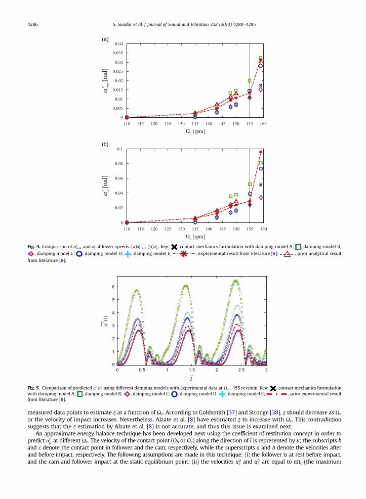
Fig. 4. Comparison of αrrms and αrpat lower speeds. (a)αrrms; (b)αrp . Key: , contact mechanics formulation with damping model A; , damping model B;

, damping model C; , damping model D; , damping model E; , experimental result from literature [8]; , prior analytical result

from literature [8].

Fig. 5. Comparison of predicted αr ðtÞ using different damping models with experimental data at Ωc¼155 rev/min. Key: , contact mechanics formulationwith damping model A; , damping model B; , damping model C; , damping model D; , damping model E; , prior experimental resultfrom literature [8].


measured data points to estimate ξ as a function of Ωc. According to Goldsmith [37] and Stronge [38], ξ should decrease as Ωc

or the velocity of impact increases. Nevertheless, Alzate et al. [8] have estimated ξ to increase with Ωc. This contradictionsuggests that the ξ estimation by Alzate et al. [8] is not accurate, and thus this issue is examined next.

An approximate energy balance technique has been developed next using the coefficient of restitution concept in order topredict αrp at different Ωc. The velocity of the contact point (Ob or Oc) along the direction of i is represented by u; the subscripts band c denote the contact point in follower and the cam, respectively, while the superscripts a and b denote the velocities afterand before impact, respectively. The following assumptions are made in this technique: (i) the follower is at rest before impact,and the cam and follower impact at the static equilibrium point; (ii) the velocities ua

c and ubc are equal to eΩc (the maximum

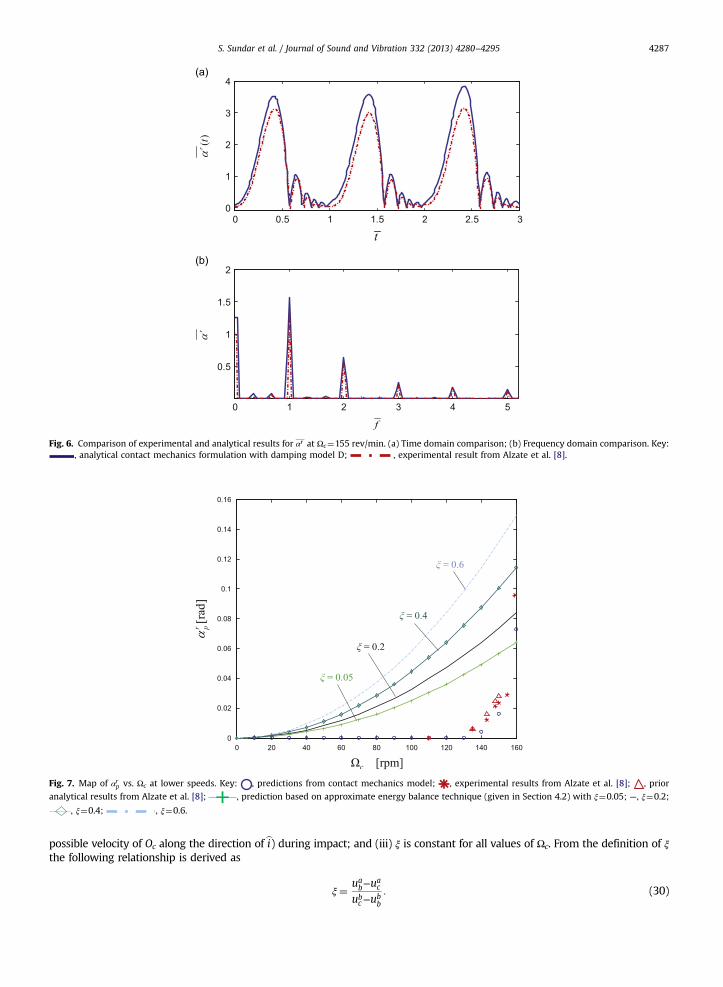
Fig. 6. Comparison of experimental and analytical results for αr at Ωc¼155 rev/min. (a) Time domain comparison; (b) Frequency domain comparison. Key:, analytical contact mechanics formulation with damping model D; , experimental result from Alzate et al. [8].

Fig. 7. Map of αrp vs. Ωc at lower speeds. Key: , predictions from contact mechanics model; , experimental results from Alzate et al. [8]; , prior

analytical results from Alzate et al. [8]; , prediction based on approximate energy balance technique (given in Section 4.2) with ξ¼0.05; —, ξ¼0.2;

, ξ¼0.4; , ξ¼0.6.


possible velocity of Oc along the direction of bi) during impact; and (iii) ξ is constant for all values of Ωc. From the definition of ξthe following relationship is derived as

ξ¼ uab−u

ac

ubc−ub

b

: (30)

Fig. 8. Map of αrp vs. Ωc over a broad range of speeds. Key: , predictions from contact mechanics formulation; , experimental results from Alzate et al.[8]; , prior analytical results from Alzate et al. [8]; —, prediction based on approximate energy balance technique (given in Section 4.2) with ξ¼0.2;

, ξ¼0.6; , ξ¼1.


Based on the assumption made, ubb¼0. Using this value of ub

b and the assumptions in Eq. (30), uabis calculated as

uab ¼ ð1þξÞe Ωc: (31)

The maximum angular velocity of the follower after impact is ð1þξÞe Ωc=χ*. Therefore, the kinetic energy (T) of thefollower after impact is

Tb ¼ 0:5IPbðð1þξÞe Ωc=χ*Þ2: (32)

This kinetic energy, Tb, is equal to an increase in the potential energy (ΔV) of the system essentially deflecting thefollower spring. The increase in the potential energy of the system is given by

ΔV ¼Z αp

α*ks½Lus−dyþdxtan ðαÞ−0:5wbsecðαÞ�½dxsec2ðαÞ−0:5wbsecðαÞ tan ðαÞ�dα: (33)

By equating Tb and ΔV (from the Eqs. (32) and (33), respectively), αp, and hence αrp, are calculated at each Ωc. Fig. 7 showsa map of αrp vs. Ωc for the approximate energy balance technique (with ξ¼0.05, 0.2, 0.4 and 0.6). Results from the contactmechanics model and the literature [8] are also given. It is inferred that below 160 rev/min, ξ should be less than 0.05 forsuccessfully predicting αrpwith the approximate energy balance technique. In contrast, Alzate et al. [8] have used muchhigher values of ξ, say from 0.37 (Ωc¼130 rev/min) to 0.6 (Ωc¼155 rev/min). This clearly suggests an ambiguity in using thecoefficient of restitution method for predicting the non-linear the response of the system.

The study using the contact mechanics model is extended to higher speeds in Fig. 8 where the proposed model, theprevious experiment [8], and the approximate energy balance technique (with ξ¼0.2, 0.6 and 1) are compared. Also fromFig. 8, it is inferred that Alzate et al. [8] have analyzed a very small range of Ωc in their study. As observed, αrp is very low forΩco160 rev/min. With an increase in speed, αrp increases and saturates at 1.36 rad, which corresponds to α¼901. Unlike thecontact mechanics model, the approximate energy balance technique using the coefficient of restitution concept yields onlya global (but a smooth) trend for different values of ξ. This supports the claim made by Gilardi and Sharf [11] that thecoefficient of restitution model has inherent problems.

6. Study of the line and point contact models in the sliding contact regime

The speed, Ωc, at which the follower would lose contact with the cam, is calculated for different values of ks using inversekinematics [36]. Fig. 9 shows the sliding contact and impacting regimes in terms of the ks–Ωc map given e¼0.1rc for aconstant speed of the cam. Higher Ωc is needed to lose contact with the increase in ks. For further analysis in the slidingcontact regime ks¼2000 N/m and Ωc¼300 rev/min are chosen. The non-linear analyses in the sliding contact regime, asreported in this study, cannot be obviously performed using the coefficient of restitution model developed in [8].

Fig. 9. Identification of contact domains based on ks–Ωc mapping at a constant cam speed with e¼0.1rc.


Recall that a line contact (with lλ¼16 mm) is assumed between the cam and follower in the previous section. However,this contact can be approximated as a non-linear Hertzian point contact [32] for small lλ as

kλðψ iðtÞÞ ¼43Yeðrcjψ iðtÞjÞ0:5: (34)

To have a meaningful comparison of the line and point contact stiffness models, lλ has been reduced to 1.6 mm. Only theCoulomb friction (with μm¼0.3) and combined damping model D (with ζD¼0.01 and βD¼4.25 s/m) are utilized in thecomparison of the α spectra of both line and point contact models as shown in Fig. 10 for e¼0.1rc. The α spectra with the twocontact models do not differ in the lower frequencies shown in Fig. 10(a) which are dominated by the harmonics of Ωc.However, the spectra differ at the resonant peaks shown in Fig. 10(b). For the line contact, the frequency is 2182 Hz but forthe point contact the frequency is 1331 Hz, mainly because the linearized contact stiffness at the static equilibrium point forline and point contacts are 138 MN/m and 34.2 MN/m respectively.

7. Analysis of the friction non-linearity

7.1. Effect of direction

The dynamic effects of friction non-linearity are studied for the cam-follower system next since such issues are ofimportance in mechanical systems [39–41]. The system is a self-energizing type when vr(t)40 (the cam rotates clockwise),as the friction force tends to increase the normal force; and the system is a de-energizing type when vr(t)o0 (the camrotates counter-clockwise). The comparison of the α spectra for the two different systems with the same cam speed(300 rev/min) with the Coulomb friction model is shown in Fig. 10. Due to different directions of Ff(t), ϑ is 2182 Hz for thede-energizing system and 2125 Hz for the self-energizing system, which can be identified by the peaks in the spectrum inFig. 10(b). The harmonics of Ωc (in the lower frequency range) of both systems match well, as seen in Fig. 10(a). The effect ofchange in the direction of rotation is more pronounced in the Fn(t) time history that is displayed in Fig. 11. The self-energizing system has a higher mean component of Fn(t) compared to the de-energizing system; this is because the Ff(t)increases the Fn(t) in the self-energizing system which in turn increases Ff(t).

7.2. Dynamic bearing and friction forces

The friction models are found to more significantly affect the dynamic forces than the displacement or the acceleration.As such, the response of the system with the alternate friction models is found not to vary significantly as long as vr(t) staysin the same direction. Consequentially, a change in direction in vr(t) is introduced (twice per revolution of the cam) byincreasing e to 0.7rc as observed from Fig. 12; the system is verified to be in the sliding contact regime at 50 rev/min, usingthe inverse kinematics [36]. The force time histories Ff(t) and Nx(t) (dynamic bearing force along horizontal direction) areshown in Fig. 13 (a) and (b), respectively, for the alternate dry friction models. Note that Nx(t) is calculated from Fig. 2 as,

NxðtÞ ¼ Ff ðtÞcosðαðtÞÞþFnðtÞsinðαðtÞÞ (35)

As seen from Fig. 13 the forces Ff(t) and Nx(t) with friction model I (with mm¼0.3) are discontinuous during the change indirection of vr(t) followed by some high frequency oscillations. This discontinuity is smoothened by using a small value of

Fig. 10. Comparison of α spectra (with mm¼0.3, ζD¼0.01 and βD¼4.25 s/m). (a) Spectra showing harmonics of Ωc; (b) Spectra showing natural frequency ofthe system. Key: , de-energizing system with line contact (lλ¼0.0016 m, Ωc¼300 rev/min); , self-energizing system with line contact(lλ¼0.0016 m, Ωc¼−300 rev/min); , de-energizing system with point contact (Ωc¼300 rev/min).


s¼10 for friction model II, but the result of the friction model II should be close to that of the friction model I for a highvalue of s.

Next, it is assumed that the cam oscillates with a particular frequency (ωc); the motion of the cam is described by Θ(t)¼Θ(0)þ0.5Θp sin(ωct), where Θp is the peak-to-peak value of Θ(t). Fig. 14 shows that vr(t)o0 for nearly half the period ofoscillation (π/ωc), and vr(t)40 for the other part of the period; here Θp¼π rad, ωc¼40 rev/min, and e¼0.7rc. Hence, thesystem acts as self-energizing and de-energizing types on a cyclic basis. Fig. 15 shows the periodic profiles of the forces Ff(t)and Nx(t) where a discontinuity is observed for friction model I when vr(t) changes its sign; this discontinuity is smoothenedusing the friction model II. When |vr(t)|⪢0, the forces Ff(t) and Nx(t) predicted by model I and II are very close.

8. Study of kinematic non-linearity

The system is linearized next by assuming small angles and by carrying out a perturbation analysis about the staticequilibrium point with the following limitations: (i) the system must always be in the sliding contact regime, and (ii) μ(t)must be time-invariant, hence the Coulomb friction model (where the magnitude of μ(t) is constant for all vr(t)) must beused, and the sign of vr(t) must be time-invariant. By implementing the above limitations, the friction non-linearity and thecontact non-linearity (in the equations for the sliding contact regime as discussed in Section 3.2) have been eliminatedresulting in only the kinematic non-linearity of the system. The linearized equation of motion for this particular systemwith

Fig. 11. Comparison of Fn(t) for different direction of cam rotation with line contact (lλ¼0.0016 m, μm¼0.3, ζD¼0.01 and βD¼4.25 s/m). Key: ,de-energizing (Ωc¼300 rev/min); , self-energizing (Ωc¼−300 rev/min).

Fig. 12. Comparison of relative sliding velocity vr(t) for two dry friction models of Fig. 3 (with Ωc¼50 rev/min, e¼0.7rc, ζD¼0.01 and βD¼4.25 s/m).Key: , Coulomb friction; , Smoothened Coulomb friction.


line contact is derived below by replacing α(t)¼αnþδα(t) in Eq. (10), where δα(t) is the perturbation of α(t) about αn

IPbδðα ðtÞÞþksdx

Lus−dyþ dx1þ cosð2α*Þ ðsinð2α*Þþ2δðαÞÞ

− 0:5wb1þcosð2α*Þ ð2cosðα*Þþ2sinðα*ÞδðαÞÞ

24 35

þkλðχ*−0:5μwbÞδðαÞ χ0cosðα*−α0Þþecosðα*þΘ0Þ

−ðrcþ0:5wbÞsinðα*−α0Þ

" #

þ χ0sinðα*−α0Þþðrcþ0:5wbÞðcosðα*−α0Þ−1Þþesinðα*þΘ0Þ−esinðα*þΘðtÞÞ

" #8>>>>><>>>>>:

9>>>>>=>>>>>;þcλðχ*−0:5μwbÞ δðα_Þ χ0cosðα*−α0Þ−ðrcþ0:5wbÞsinðα*−α0Þ

þecosðα*þΘ0Þ

" #( )¼ 0: (36)

Rearrange Eq. (36) and write it in the standard form as follows:

IPbδðα€ ðtÞÞþClδðα_ ÞþKlδðαÞ ¼ FlðtÞ: (37)

Fig. 13. Comparison of forces for two dry friction models of Fig. 3 (with Ωc¼50 rev/min, e¼0.7rc, ζD¼0.01 and βD¼4.25 s/m). (a) Nx(t); (b) Ff(t). Key: ,Coulomb friction; , Smoothened Coulomb friction.


Here, the effective damping coefficient (Cl), stiffness (Kl), and time-varying forcing function (Fl(t)) are given as follows:

Cl ¼ cλðχ*−0:5μwbÞχ0cosðα*−α0Þ−ðrcþ0:5wbÞsinðα*−α0Þ

þecosðα*þΘ0Þ

" #, (38a)

Kl ¼ksdx½2dx−wbsinðα*Þ�

1þcosð2α*Þ þkλðχ*−0:5μwbÞχ0cosðα*−α0Þþecosðα*þΘ0Þ

−ðrcþ0:5wbÞsinðα*−α0Þ

" #, (38b)

FlðtÞ ¼−ksdx Lus−dyþdxsinð2α*Þ−wbcosðα*Þ

1þcosð2α*Þ

−kλðχ0−0:5μwbÞðrcþ0:5wbÞðcosðα*−α0Þ−1Þþ

χ0sinðα*−α0Þþesinðα*þΘ0Þ

−sin α*þΘðtÞð Þ

!26643775: (38c)

The α spectra of the linearized and the non-linear systems are compared in Fig. 16. Observe that the linear system hasonly the fundamental harmonic of Ωc while the non-linear system exhibits the super-harmonics of Ωc as shown in Fig. 16(a).The linear system has a single peak at the natural frequency of the system, but the non-linear system displays side bandsassociated with this peak as seen in Fig. 16(b). Therefore, the linear system approximation does not accurately predict theresults of the system with only kinematic non-linearity.

Fig. 14. Comparison of relative sliding velocity vr(t) for two dry friction models of Fig. 3 (with ωc¼40 rev/min, e¼0.7rc, ζD¼0.01 and βD¼4.25 s/m).Key: , Coulomb friction; , Smoothened Coulomb friction.

Fig. 15. Comparison of forces for two dry friction models of Fig. 3 (with ωc¼40 rev/min, e¼0.7rc, ζD¼0.01 and βD¼4.25 s/m). (a) Ff(t); (b) Nx(t). Key: ,Coulomb friction; , Smoothened Coulomb friction.


9. Conclusion

The non-linear dynamics of the cam-follower system have been analyzed in this study. First, a contact mechanicsformulation for a cam-follower system with rotational sliding contact has been developed, and the predictions withcombined viscous-impact damping models are successfully compared with the experimental results reported by Alzate et al.

Fig. 16. Comparison of α spectra (with mm¼0.3, Ωc¼300 rev/min, ζD¼0.01 and βD¼4.25 s/m). (a) Spectra showing harmonics of Ωc; (b) Spectra showingnatural frequency of the system. Key: , Non-linear system; , Linear system.


[8]. Second, the accuracy of the coefficient of restitution concept is analyzed using the approximate energy balancetechnique, and the estimated value of the coefficient of restitution by Alzate et al. [8] is found to be much lower than theestimates of this study; this suggests that there is some ambiguity in employing this concept for the cam-follower system.Third, the effect of friction non-linearity on the dynamic forces is studied using discontinuous and smoothened dry frictionmodels. Finally, a linearized system is found to be inadequate in representing the system with only kinematic non-linearity.

Several contributions emerge from this study over the current literature on the cam-follower dynamics [1–10]. The newcontact mechanics formulation successfully predicts the dynamics of the cam-follower system with rotational slidingcontact in both impacting regime and sliding contact regimes. A better understanding of the applicability of differentdamping models and the inaccuracies of the coefficient of restitution model to the cam-follower system during impacts isobtained. Even though the applicability of contact damping models are specific to the cam-follower system, this articleprovides better insights into the damping mechanisms of a family of mechanical systems. This analysis also yields a betterunderstanding of the roles of the friction and kinematic non-linearities in the sliding contact regime. The chief limitation ofthe article is the utilization of a single degree-of-freedom model that assumes the cam is rigidly pivoted about its center ofrotation. This deficiency should be removed in future study with a higher degree-of-freedom system. Also, semi-analyticalsolutions can be sought.

Acknowledgment

The authors gratefully acknowledge the Vertical Lift Consortium, Inc. for partially supporting this research.


References

[1] F.Y. Chen, A survey of the state of the art of cam system dynamics, Mechanism and Machine Theory 12 (3) (1977) 201–224.[2] T.L. Dresner, P. Barkan, New methods for the dynamic analysis of flexible single-input and multi-input cam-follower systems, ASME Journal of

Mechanical Design 117 (1995) 150.[3] N.S. Eiss, Vibration of cams having two degrees of freedom, ASME Journal of Engineering for Industry 86 (1964) 343.[4] R.L. Norton, Cam design and manufacturing handbook, Industrial Press Inc (2009).[5] L. Cveticanin, Stability of motion of the cam–follower system, Mechanism and Machine Theory 42 (9) (2007) 1238–1250.[6] G. Osorio, M. di Bernardo, S. Santini, Corner-impact bifurcations: a novel class of discontinuity-induced bifurcations in cam-follower systems, Journal of

Applied Dynamical Systems 7 (2007) 18–38.[7] H.S. Yan, M.C. Tsai, M.H. Hsu, An experimental study of the effects of cam speeds on cam-follower systems, Mechanism and Machine Theory 31 (4)

(1996) 397–412.[8] R. Alzate, M. di Bernardo, U. Montanaro, S. Santini, Experimental and numerical verification of bifurcations and chaos in cam-follower impacting

systems, Nonlinear Dynamics 50 (3) (2007) 409–429.[9] R. Alzate, M. di Bernardo, G. Giordano, G. Rea, S. Santini, Experimental and numerical investigation of coexistence, novel bifurcations, and chaos in a

cam-follower system, SIAM Journal on Applied Dynamical Systems 8 (2009) 592–623.[10] M.P. Koster, Vibrations of Cam Mechanisms: Consequences of Their Design, Macmillan, 1974.[11] G. Gilardi, I. Sharf, Literature survey of contact dynamics modeling, Mechanism and Machine Theory 37 (2002) 1213–1239.[12] V. Aronov, A.F. D'Souza, S. Kalpakjian, I. Shareef, Interactions among friction, wear, and system stiffness. Part 2. Vibrations induced by dry friction,

ASME Journal of Lubrication Technology 106 (1984) 59–64.[13] Y. Masayuki, N. Mikio, A fundamental study on frictional noise (1st report, the generating mechanism of rubbing noise and squeal noise), Bulletin of

JSME 22 (1979) 1665–1671.[14] Y. Masayuki, N. Mikio, A fundamental study on frictional noise (3rd report, the influence of periodic surface roughness on frictional noise), Bulletin of

JSME 24 (1981) 1470–1476.[15] Y. Masayuki, N. Mikio, A fundamental study on frictional noise (5th report, the influence of random surface roughness on frictional noise), Bulletin of

JSME 25 (1982) 827–833.[16] S. He, R. Gunda, R. Singh, Effect of sliding friction on the dynamics of spur gear pair with realistic time-varying stiffness, Journal of Sound and Vibration

301 (2007) 927–949.[17] S. Kim, R. Singh, Gear surface roughness induced noise prediction based on a linear time-varying model with sliding friction, Journal of Vibration and

Control 13 (2007) 1045–1063.[18] Y. Michlin, V. Myunster, Determination of power losses in gear transmissions with rolling and sliding friction incorporated, Mechanism and Machine

Theory 37 (2002) 167–174.[19] M.N. Sahinkaya, A.-H.G. Abulrub, P.S. Keogh, C.R. Burrows, Multiple sliding and rolling contact dynamics for a flexible rotor/magnetic bearing system,

IEEE/ASME Transactions on Mechatronics 12 (2007) 179–189.[20] B.L. Stoimenov, S. Maruyama, K. Adachi, K. Kato, The roughness effect on the frequency of frictional sound, Tribology International 40 (4) (2007)

659–664.[21] M. Othman, A. Elkholy, Surface-roughness measurement using dry friction noise, Experimental Mechanics 30 (3) (1990) 309–312.[22] M. Othman, A. Elkholy, A. Seireg, Experimental investigation of frictional noise and surface-roughness characteristics, Experimental Mechanics 30 (4)

(1990) 328–331.[23] A. Le Bot, E. Bou Chakra, Measurement of friction noise versus contact area of rough surfaces weakly loaded, Tribology Letters 37 (2010) 273–281.[24] A. Le Bot, E. Bou-Chakra, G. Michon, Dissipation of vibration in rough contact, Tribology Letters 41 (2011) 47–53.[25] H. Ben Abdelounis, H. Zahouani, A. Le Bot, J. Perret-Liaudet, M.B. Tkaya, Numerical simulation of friction noise, Wear 271 (2011) 621–624.[26] A. Soom, J.-W. Chen, Simulation of random surface roughness-induced contact vibrations at Hertzian contacts during steady sliding, ASME Journal of

Tribology 108 (1986) 123–127.[27] P.J. Remington, Wheel/rail rolling noise, I: Theoretical analysis, Journal of the Acoustical Society of America 81 (1987) 1805–1823.[28] P.J. Remington, Wheel/rail rolling noise, II: Validation of the theory, Journal of the Acoustical Society of America 81 (1987) 1824–1832.[29] G.G. Gray, K.L. Johnson, The dynamic response of elastic bodies in rolling contact to random roughness of their surfaces, Journal of Sound and Vibration

22 (1972) 323–342.[30] P.R. Kraus, V. Kumar, Compliant contact models for rigid body collisions, IEEE International Conference on Robotics and Automation, vol.2, 1997,

pp. 1382–1387.[31] O. Ma, Contact dynamics modelling for the simulation of the space station manipulators handling payloads, IEEE International Conference on Robotics

and Automation, vol.21995, pp. 1252–1258.[32] K.L. Johnson, Contact Mechanics, Cambridge University Press, Cambridge, 1987.[33] MATLAB User's Guide, The Math Works Inc., Natick, MA, 1993.[34] C. Padmanabhan, R. Singh, Dynamics of a piecewise non-linear system subject to dual harmonic excitation using parametric continuation, Journal of

Sound and Vibration 184 (1995) 767–799.[35] D. Zhang, W.J. Whiten, The calculation of contact forces between particles using spring and damping models, Powder Technology 88 (1996) 59–64.[36] F.Y. Chen, Mechanics and Design of Cam Mechanisms, Pergamon Press, 1982.[37] W. Goldsmith, Impact: The Theory and Physical Behavior of Colliding Solids, Dover Publications, New York, 2001.[38] W.J. Stronge, Impact Mechanics, Cambridge University Press, New York, 2000.[39] F.-J. Elmer, Nonlinear dynamics of dry friction, Journal of Physics A: Mathematical and General 30 (1997) 6057–6063.[40] M. Vaishya, R. Singh, Sliding friction-induced non-linearity and parametric effects in gear dynamics, Journal of Sound and Vibration 248 (2001)

671–694.[41] R.I. Leine, D.H. van Campen, A. de Kraker, L. van den Steen, Stick-Slip vibrations induced by alternate friction models, Nonlinear Dynamics 16 (1998)

41–54.

rotational sliding contact dynamics in a non-linear cam-follower

Documents