ROTATING SCINTILLATIONCAMERA SPECT ACCEPTANCE

TESTING AND QUALITY CONTROL

REPORT OF AAPMSPECT TASK GROUP*

MEMBERS

Jeffry A. Siegel (Chairman)Anthony R. BenedettoRonald J. JaszczakJack L. LancasterMark T. MadsenWesley W. WootenRobert E. Zimmerman

*The Task Group is part of the AAPM Nuclear Medicine Committee,Mark T. Madsen, Chairman.

June 1987

Published for theAmerican Association of Physicists in Medicine

by the American Institute of Physics

Further copies of this report may be obtained from

Executive OfficerAmerican Association of Physicists in Medicine

335 E. 45 StreetNew York, NY 10017

Library of Congress Catalog Card Number: 87-72509International Standard Book Number: O-883 18-549-O

International Standard Serial Number: 0271-7344

Copyright © 1987 by the American Associationof Physicists in Medicine

All rights reserved. No part of this publication may bereproduced, stored in a retrieval system, or transmittedin any form or by any means (electronic, mechanical,photocopying, recording, or otherwise) without the

prior written permission of the publisher.

Published by the American Institute of Physics, Inc.,335 East 45 Street, New York, New York 10017

Printed in the United States of America

ROTATING SCINTILLATION CAMERA SPECT ACCEPTANCETESTING AND QUALITY CONTROL

TABLE OF CONTENTS

I. IntroductionII. Pre-Test Conditions

III. Log BookIV. Test Equipment RequiredV. Protocol

A. Single Head Systems1.0 Physical Inspection for Shipping Damages

and Production Flaws2.0 System Alignment

2.1 Determination of Center of Rotation(COR)

2.2 Determination of COR as Function ofAxial Position AlongAxis of Rotation

2.3 Collimator Hole Angulation3.0 Uniformity

3.1 Tomographic Slice Uniformity3.2 Rotational Uniformity or Electronic

Stability During Rotation4.0 Sensitivity

4.1 Planar Sensitivity4.2 Per Axial Centimeter Volume Sensitivity4.3 Total Volume Sensitivity4.4 Estimation of System Sensitivity to Scatter

5.0 Pixel Calibration6.0 Spatial Resolution

6.1 Transverse Plane ResolutionWithout Scatter (In Air)

6.2 Transverse Plane Resolution withScatter

6.3 Axial Slice Thickness7.0 Image Contrast8.0 Attenuation Correction and Patient

Contour Positioning9.0 Total System Performance Evaluation

10.0 Acceptance Testing and Quality ControlTime Schedule

B. Additional Considerations for Dual Head SystemsVI. References

Appendix AAppendix BAppendix C

I. IntroductionThe purpose of this document is to present a uniform

set of procedures that can be used for acceptance testing andquality control of a scintillation camera-based SPECT system.

Emission computed tomography has a number ofadvantages over conventional nuclear medicine imaging:

1. Contrast improvement2. Total volume imaging3. Quantitation

a. Detection of lesion and its locationb. Determination of length and volumec. Absolute regional radionuclide

concentrationsIn order to realize these advantages. strict quality

control procedures must be performed on a routine basis.Important considerations for tomography. unlike planar imaging.include levelness of gantry. collimator hole angulation, strictattention to field uniformity, attenuation correction,filtering. and camera response at different angular orientationsof the camera head. In addition, both linear and angularsampling are of concern: use of the finest matrix size andangular sampling are recommended. Using a 64 x 64 acquisitionmatrix will make certain measurements unrealiable. e.g..resolution and linearity. If the system is capable, a minimummatrix size of 128 x 128 (3 mm linear sampling, 400 mm FOV)should be employed. Angular sampling can be performed witheither a continuous rotation or "step-and shoot" acquisitionusing a circular or noncircular orbit.

Tomographic techniques are very sensitive to inadequatecalibration procedures. Additional time must be set aside forthe quality control of SPECT studies in order to ensureartifact-free images. As a caveat. if the measurement protocolsdescribed herein are to be used for acceptance testing, then theburden is upon the prospective buyer to negotiate theperformance specifications with the manufacturer prior to thesubmission of a purchase order.

II. Pre-Test Conditions

When performing the acceptance and quality controltests, sources of radioactivity should be handled in accordancewith proper techniques. All containers of unsealed sourcesshould be kept on absorbent pads and handled by gloved personnelwearing appropriate dosimeters. In all cases the measurementsshould be performed with the room background as low asachievable and other sources (such as patients who have receivedradiopharmaceuticals) excluded from the area. During the periodof time the crystal is not protected by the collimator, forexample, when performing intrinsic studies. extreme care must betaken not to damage the crystal by mechanical or thermal insult.

If transparency film is used, the processor should bechecked to assure that it is operating within specifications.The same type of film should be used for acceptance testing aswill be used for quality control and routine clinical studies.

III. Log BookAt the time of acceptance testing a new system, a

permanent record book should be initiated for that system. Theuser should obtain all available performance data from themanufacturer and include this in the log book. The results ofthe performance testing should be recorded, including thelabeled images and all information necessary to duplicate theresults at some later date. Parameters recorded should includethe date and time, radionuclide. source activity, configurationof source, console and system parameters. collimator, dataacquisition time, number of counts, matrix size. number ofprojection angles, continuous rotation or "step-and-shoot"acquisition, radius of rotation, reconstruction filter, slicethickness, and scatter material. If the system provides theactual total number of counts that contributed to a specificsectional image then that value should be recorded.Furthermore, any pre- and/or post-processing procedures (e.g..two dimensional prefiltering of projection data, threedimensional volume smoothing of reconstructed images) should berecorded. Some console parameters may change if adjustments aremade on the camera.

Subsequent quality control. component failure andmaintenance records should be recorded in the same book.

IV. Test Equipment Required

1. Tc-99m or Co-57 point sources.The point sources should contain sufficient activity

to produce count rates of 10,000 cps with the collimatoron the camera. A convenient method of preparing a Tc-99mpoint source is to draw 0.05 ml into a 1 ml syringe. Besure to remove the needle and cap the syringe to preventleakage.

2. Tc-99m line sourceThe line source should contain sufficient activity to

produce a count rate of 10,000 cps with the collimator onthe camera. It should have an internal diameter of lessthan 1.5 mm and be of sufficient length to cover theuseful axial field of view. Plastic or glass capillarytubes can be used as line sources, however, care must betaken to avoid spills. Refillable line sources arecommercially available (Appendix C).

3. Tc-99m flood or Co-57 sheet source with +/- 1% uniformity.The liquid-filled flood source should contain 5 - 7

mCi of Tc-99m. Caution should be taken to ensure uniformfilling. Refillable flood phantoms, especially those oflarger diameter designed for large field of view systems,may sag in the center during rotation and thus becomenonuniform (hot center). The count rate from either theTc-99m flood or Co-57 sheet source must be below 30 kcpswith the collimator on the camera.

4. Water-filled cylindrical phantom with various sized coldsphere inserts.

The phantom should have a diameter of 20 - 22 cm anda height of at least 15 cm. The sphere diameters shouldvary from approximately one FWHM to >3 x FWHM (e.g., ifsystem FWHM is 12 mm, then spheres should range indiameter from <12 mm to > 36 mm) and be centered at thesame level in the phantom. The phantom should contain10-15 mCi of Tc-99m. Appropriate vendors of commerciallyavailable phantoms are listed in Appendix C.

5. Jig or rigid holder for line source positioning

6. Rigid support for cylindrical phantom positioning

7. Small platform jack

8. Bubble level and level-protractor

9. Smith orthogonal phantom

V. Protocol

A. Single-Head Systems

1.0

1.1

1.2

1.3

1.4

1.5

2.0

Physical Inspection for Shipping Damages and ProductionFlaws.

Procedures described in AAPM Report No. 9, section 1.1-1.7and 1.9 should be followed.

GantryInspect the tomographic gantry alignment, vertically andhorizontally. and all cables, switches, or other controls.

Scan TableInspect the bed alignment, vertically and horizontally.and other controls.

Angle IndicationsCheck registration of angle indicators by rotating camera360 degrees, one indicator at a time, using alevel-protractor. Check accuracy of angular velocity forcontinuous gantry rotation.

Patient Safety DevicesInspect patient safety devices (e.g.. touch pads,emergency stop) to ensure proper operation.

System AlignmentTomographic sections are reconstructed from

projections acquired at multiple angles about the objectbeing imaged. The rotating detector has an axis ofrotation (Figure 1). This axis is a line fixed in spaceparallel to the scan table and perpendicular to the planeof the gantry. It should intersect the gantry plane veryclose to its center.

FIGURE L Schematic drawing of a SPECT system illustra-ting the center and axis of rotation.

In order to reconstruct the tomographic sections it isnecessary to know where the projection of the axis ofrotation (AOR) is located on the planar image pixelmatrix. This location is referred to as the center ofrotation (COR) as shown in Figure 1. The alignment ofthis mechanical axis of rotation of the detector withrespect to the image pixel matrix, i.e., the center ofthe collection matrix of the computer, and its stabilityduring rotation are important physical calibrations fortransverse-section tomography.

Since errors as small as +/- 1.5 mm (or 0.5 pixelsusing a 128 x 128 matrix, 400 mm field of view) willdegrade the quality of the reconstructed images, it isnecessary to determine the COR to within +/- 1 mm. Inaddition to accurately knowing where the COR is located,it is preferable that it coincide with the center of theimage matrix. This yields the best field of view andreduces the effect of changing gains and matrix size. It

is therefore recommended that the offset calibration ofthe COR used by the reconstruction program from thecenter of the image matrix be <6 mm (or <2 pixels for a128 x 128 matrix). Note: this does not imply that CORerrors as great as 6 mm can be tolerated.

The COR may vary due to mechanical problems withdetector rotation, changes in amplifier gain and offset,errors in the analog to digital converter, and lack ofparallelism between the collimator/detector plane and theaxis of rotation.

2.1 Determination of Center of Rotation (COR)

2.1.1

2.1.2

Prepare a point source of Tc-99m.

Center a 20% window symmetrically about theTc-99m photopeak and place a low-energy allpurpose collimator (or the one which will beroutinely used) on the camera.used) on the camera.

2.1.3 Position the point source 5 cm from the axis ofrotation and extend it over the edge of theimaging table. Use a bubble level to ensure thatthe collimator is level, i.e. parallel to theaxis of rotation.

2.1.4 Acquire a 360 degree tomographic study using a128 x 128 matrix and 32 projections (or with theangular and linear sampling as supplied by themanufacturer). 20,000 counts per projection,and a circular orbit with a radius of rotation of15 cm. Note: The largest available matrix sizeshould be used: more projections are notnecessary.

2.1.5 Create a sinogram image (using themanufacturer- supplied algorithm or the FORTRANalgorithm as given in Appendix A) using thecentral row (i.e.. row 64 for a 128 x 128 matrix)from each of the 32 projection images. Make surethat the activity is present on all views. Thesinogram should look like a sine wave (Figure 2).

2.1.6 Quantitative Analysis

2.1.6.1 Find the x centroid for each row in thesinogram image.

2.1.6.2 Fit these values to a sine function:A sin (q + Ø + B. where A is the amplitude,q is the angle of rotation,q is thephase angle of the fitted sine function,and B is the best fit center of rotation.A FORTRAN algorithm for the sine fit isgiven in Appendix B.

2.1.6.3 Compare B to the expected center of theimage matrix. i.e., 64.5 for a 128 x 128matrix This difference is the meanoffset, R. from the COR.R = (N+1)/2 - Bwhere N is the matrix size.

2.1.6.4 The fitted sine curve should besubtracted from the curve obtained fromstep 2.1.6.1 to step 2.1.6.1 obtain theoffset error as a function of angle.R (θ) .

2.1.6.5 Alternate Method: The offset error, Ρ(θ).as obtained from steps 2.1.6.1 - 2.1.6.4can also be calculated byΡ(θ) = [N+l - X (θ) - X θ + 180)]/2where N is the matrix dimension in the xdirection,X (θ) is the centroid for the projectionat degrees, andX (θ + 180) is the centroid for theprojection at θ plus 180 degrees.R(8) should be calculated for each pairof angles separated by 180 degrees togenerate offset values as a function ofangle for each slice.

2.1.6.6 Record the results as a maximum offset(Rmax), an average offset (Rav),

and offset as a function of angle, R (θ).The maximum offset from the center ofrotation, R (θ). should be less than 2pixels (6 mm). Note: The COR (obtainedfrom step 2.1.6.2) should be known towithin 1.5 mm.

2.1 .6.7 In addition to the COR. the yaxis must be parallel to the axis ofrotation. The constancy of the y-axisalignment during rotation should becalculated as described in section 2.1.6after a 90 degree rotation of the rawdata. The y-axis offset should beindependent of angle, i.e., a linear plotshould be obtained (Figure 2. 1.Deviations of greater than 0.5 pixels

from the average y axis offset indicate aproblem with head tilt. collimator holeangulation. or gantry alignment.

2.2 Determination of COR as Function of Axial Position AlongAxis of Rotation

2.2.1 Prepare a line source of Tc-99m.

2.2.2 Center a 20% window symmetrically about theTc-99m photopeak and place a low energy allpurpose collimator on the camera.

FIGURE 2. In the tranverse (x) direction, the sourcemoves sinusoidally across the field of view as thescintillation camera rotates. A plot of the source loca-tion as a function of gantry angle results in a sinu-soid.

In the axial (y) direction, the source locationshould remain fixed and a plot of the source location asa function of angle should be a straight line.

2.2.3 Position the line source 5 cm from the axis ofrotation and extend it over the edge of theimaging table. The line source should beparallel to the AOR. Use a bubble level toensure that the collimator is also parallelto the AOR.

Repeat tomographic acquisition in section 2.1.4.2.2.4

2.2.5

2.2.6

2.3 Collimator Hole Angulation

Repeat 2.1.5 - 2.1.6.6 for every sixteenthtransverse 1 pixel (3 mm) thick slice (5 cmincrements) in the useful axial field of view.Note: Gantry sag and angular registration problemsare global and will be identical in each sinogram.Nonlinearities which show up only in certain slicesare the result of intrinsic or collimator spatialnonlinearities.

Record the results as a maximum offset, an averageoffset. and offset as a function of angle for eachslice. Acceptable performance is less than a 0.5pixel (1.5 mm) deviation throughout.

For SPECT imaging, the angulation of the holes in aslant hole collimator must be known in order to ensure itsproper set up during a tomographic acquisition, i.e., itsholes must be perpendicular to the AOR. The displacementof the image of a point source is examined as the sourceis moved vertically i.e., away from the collimator face(Figure 3). In order to ensure the accurate alignment ofthe source, it will be necessary to have a jig which willsupport the source at two vertical distances from thecollimator face.

2.3.1

2.3.2

2.3.3

2.3.4

Prepare a Tc-99m or Co-57 point source.

Center a 20% window symmetrically about theTc-99m or Co-57 photopeak and place a slant holecollimator on the camera.

Contruct a holder which will allow theaccurate positioning of the point source at twovertical settings separated by 10 cm.Alternatively, a small platform jack can be usedfor this purpose.

Position the source holder containing thepoint source under the center of the collimator SO

that it is approximately 5 cm from the face of thecollimator. The levelness of both the sourceholder and the collimator face should be checkedwith a bubble level. It is very important that theholder is accurately aligned with the collimator.

2.3.5 Acquire a 50K count conventional planar imageusing the largest available matrix size.

2.3.6 Lower the holder exactly 10 cm (100 mm) andacquire a second planar image as in 2.3.5.

2.3.7 Determine the x and y centroids of the two pointimages:

lower position - (xl,yl)upper position - (xu,yu)

2.3.8 Calculate the distance (d) between the images

according to d = ((xl-xu)2 + (yl-yu)2)1/2

Use the pixel calibration factor from section 5.6to calculate d in mm.

2.3.9 Calculate the hole angulation (HA) according toHA = arctan (d/100). Record value of HA.

2.3.10 Repeat 2.3.5 - 2.3.9 at other locations onthe collimator.

FIGURE 3. Configuration for the collimator hole angula-tion test. A measurement is made at source location A.The source is then displaced vertically by 10 cm tolocation B where a second measurement is made.

3.0 Uniformity3.1 Tomographic Slice Uniformity

The uniformity of the camera should first be testedwithout regard to tomography or gantry rotation toestablish the static performance of the system. Theprocedures described in AAPM Report No. 9. section 3should be used to test integral and differentialuniformity for comparison to manufacturer'sspecifications. The effects of count rate and PHAmisadjustment on uniformity should also be tested.

The tomographic reconstruction process placesstringent demands on detector uniformity. Camerauniformity must be corrected to within 0.5 - 1.0% in orderto keep image distortion minimal. The correction isaccomplished with a matrix of multiplicative correctionfactors applied to the projected raw views. Virtually allmanufacturers provide software to do this. The correctionfactors are based on a high count reference flood.

3.1.1

3.1.2

3.1.3

3.1.4

Prepare a liquid-filled flood source withTc-99m or use a Co-57 sheet source with +/- 1%uniformity.

Center a 20% window symmetrically abouteither the Tc-99m or Co-57 photopeak and place alow energy all purpose collimator on the camera.

Acquire a flood field with a 1% precisionper pixel. This requires 30 million counts for a64 x 64 matrix. Thirty million counts are alsoadequate for a 128 x 128 matrix if the floodfield image is smoothed.

Check tomographic slice uniformity bytomographic imaging of a uniform cylindricalphantom containing a uniform distribution ofactivity.

3.1.4.1 Prepare a water-filledcylindrical phantom containing Tc-99m.The long axis of the phantom must beparallel to the axis of rotation.

3.1.4.2 Repeat step 3.1.2.

3.1.4.3 Acquire a 360 degreetomographic study using a 128 x 128matrix, the finest angular samplingpossible, and a circular orbit with aradius of rotation of 15 cm. Acquisitiontime should be sufficient to accumulateat least 500K counts per planar view.Note: It may be necessary to extend thephantom over the edge of the table in

3.1.4.4

3.1.4.5

3.1.4.6

3.1.4.7

order to achieve a 15 cm radius ofrotation. This can be accomplished byplacing the phantom on a rigid supportwhich is securely fastened to thetable.

After data acquisition, uniformitycorrect each projection image withthe field from 3.1.3.

Reconstruct images using 4pixel (12 mm) thick slices (eachcontaining at least 2 millioncounts). a ramp filter (or thefilter which will be routinelyused). and attenuation correction.Use the attenuation coefficientdetermined in section 8.8.

Review each transversesection image for concentric ringor "bulls-eye" artifacts, if theyoccur.

Quantitatively assess uniformity in eachtransverse section by obtaining integraland differential uniformity and thestatistical uniformity index together withhigh and low pixel images as described inAAPM Report No. 9, section 3.2. Recordthese values.

3.1.5 Repeat tests in section 3.1.4 for a tomographicacquisition using a noncircular orbit, if thisoption is available.

3.1.6 Repeat sections 3.1.2 - 3.1.4 for allcollimators to be routinely used.

Note: The zoom and energy windowsettings must be the same for thereference flood as for the clinicalacquisition. The reference flood mustalso be acquired with the samecollimator as the clinical acquisition.If the collimator is changed. a newreference flood is required.

3.2 Rotational Uniformity or Electronic Stability duringRotation

Global and local changes in camera sensitivityduring gantry rotation should be maintained below 1%.Nearly all recently manufactured ECT systems haveincorporated magnetic shielding to avoid interactionsbetween the PM tubes and weak magnetic fields, but

earlier systems were not adequately shielded againstmagnetic fields and variations on the order of 10% wereobserved. In addition to magnetic field effects, theremay also be gravitational-mechanical effects withpotential to change camera sensitivity during gantryrotation.

3.2.1 Global Measure of Constancy during Rotation

3.2.1.1

3.2.1.2

3.2.1.3

3.2.1.4

3.2.1.5

3.2.1.6

3.2.1.7

Rigidly mount a Co-57 sheet sourceon top of a low-energy all purposecollimator. It should be emphasized thatgreat care must be used in securing thesource to the gamma camera.

Center a 20% window symmetricallyabout the Co-57 photopeak.

Acquire a 360 degree tomographic studyusing the smallest angular samplingavailable with a 64 x 64 matrix.Acquisition time should be sufficient toaccumulate 300 counts per pixel perprojection image.

Identify a single pixel. Let xi.be the counts in that pixel in the i thprojection image.Assuming Poisson statistics.VAR(xi )= xi

The total variance of all the valuesfor xi is calculated by:

where N is the number of projectionimages, and x is the average of the Nvalues for x..

The within groups variance isthe variance due to the assumed Poissonstatistics of each pixel count and isgiven by

Subtract the within groupsvariance from the total variance. Theremainder is the variance for this pixeldue to changes in sensitivity with gantryangle (variance of the means):VARM = VART - VARW

3.2.1.8

3.2.1.9

The variance of the means isnormalized by the square of the averagepixel count for this pixel. Thisnormalized variance is rho squared:

3.2.2. Local Measure of Constancy during Rotation

3.2.2.1 If a local constancy problemmust be ruled out repeat steps in section3.2.1 but adjust acquisition time toachieve at least 600 counts per pixel perframe.

3.2.2.2 Flag pixel locations where rho is greaterthan 0.02 and save these locations.

3.2.2.3 Repeat acquisition and computation.

3.2.2.4 If same pixel or group of pixelsare flagged again for a high value forrho, there is likely to be a localconstancy problem.

4.0 SensitivityIncreased or decreased sensitivity at certain locations

within each projection can lead to reconstruction artifacts.These artifacts are independent of the character of theprojection data and become more noticeable towards the axis ofrotation Sensitivity measurements should include planarsensitivity, per axial centimeter volume sensitivity, and totalvolume sensitivity. The scatter fraction (scatter-to-nonscatterevent ratio) should also be estimated since it directly affectsvolume sensitivity, i.e., volume sensitivity will be larger forsystems with a large scatter contribution although imagecontrast will be degraded. Sensitivity measurements aredependent upon collimator type , window width, deadtime. gammaray energy. slice thickness. field of view, filter type,attenuation-correction method, and other factors.

4.1 Planar sensitivityThe planar sensitivity should be measured for allcollimators according to the procedure described in AAPMReport No. 9. section 3.4.

4.2 Per Axial Centimeter Volume Sensitivity

4.2.1 Prepare a water-filled cylindricalphantom containing Tc-99m. The actual diameterof the cylinder should be recorded. The activityconcentration must be accurately determined. Thelong axis of the phantom must be parallel to theaxis of rotation.

4.2.2 Center a 20% window symmetrically aboutthe Tc-99m photopeak and place a low-energy allpurpose collimator on the camera.

4.2.3 Acquire a 1 million count conventionalplanar image using a 128 x 128 matrix. Noteacquisition time, Tacq.

4.2.4 Draw a rectangular region of interest(ROI) 20 centered on the image. The length ofthe ROI should be large enough to cover thecylinder diameter and the width should be 20pixels in the axial direction. Record the numberof counts in the ROI,CROI.

4.2.5 Calculate the axial width of the ROI,AW ROI:

AWROI(cm) = 20 pix X PC(mm/pix) X cm/l0mm.

where PC = pixel calibration. The determinationof the pixel calibration is described in section5.

4.2.6 Calculate the per axial volume sensitivity, AVS,by dividing the ROI counts by the product ofthe activity concentration (AC).acquisition time (T acq) and axial ROI width(AWROI):

4.2.7 Record per axial centimeter volume sensitivity.

4.3 Total Volume SensitivityThe total volume sensitivity is the product of theper axial centimeter volume sensitivity and theaxial width of the gamma camera field of view.

4.3.1 Calculate the total volume sensitivity, TVS, bymultiplying the per axial volume sensitivity from4.2.6 by the width of the useful field of viewin the axial direction, AWUFOV:

TVS(cps/uCi/cm 3) = AVS(cps/uCi/cm2) X AWUFOV(cm)

4.3.2 Record total volume sensitivity.

4.4 Estimation of System Sensitivity to Scatter

4.4.1

4.4.2

4.4.3

4.4.4

4.4.5

4.4.6

4.4.7

4.4.8

Place a large diameter (6 cm) nonradioactive,water-filled sphere near the center of thecylindrical phantom prepared in step 4.2.1.Repeat step 4.2.2.

Acquire a 360 degree tomographic studyusing a 128 x 128 matrix, the finest angularsampling possible, and a circular orbit with aradius of rotation of 15 cm. Acquisition timeshould be sufficient to accumulate at least 250Kcounts per planar view.

Uniformity correct the planar images andreconstruct the projection data using 4 pixel (12mm) thick slices, a ramp reconstruction filter,and attenuation correction. Use the attenuationcoefficient determined in section 8.8.

Center a 5 x 5 pixel rectangular region ofinterest in the cold sphere in a central slice andrecord counts per pixel (cpp).

Place a rectangular region of interest of thesame dimensions in a background region (5 pixelsfrom the edge of the cold sphere) in the sameslice and record cpp.

Estimate system's sensitivity to scatter(SFest) according to:

SF est=cpp in sphere/(cpp in bkgd-cpp in sphere).

Record value of SFest. It should be noted

that what has been measured is not exactly equalto the true scatter fraction. The determinationof the true SF is extremely difficultexperimentally; however, the measurement proceduredescribed above is simple and will provide auseful and reproducible indication of the system'sability to reject scattered photons.

5.0 Pixel CalibrationPixel, actually voxel. dimensions are necessary for ray

length calculation in attenuation correction algorithms, foraccurate image scaling, for oblique axis transformation, andfor quantitative measurements. Voxel dimensions are subject todrift and variation due to changes in camera tuning, ADC gain,and offset.

5.1

5.2

Prepare two point sources of Tc-99m or Co-57.

Center a 20% window symmetrically about the Tc-99mphotopeak and place a low-energy all purpose collimator onthe camera.

5.3 Position the point sources along the x axis and exactly 20cm apart. The sources should be at least 5 cm from thecollimator face to eliminate collimator septa-induceddistortion.

5.4 Acquire a 100K count conventional planar image using thelargest available matrix size. Ensure that no zoom is used.

5.5 Generate a count profile that passes through the center ofboth point sources.

5.6 Determine the distance in pixels between the centroidsof the two sources. The mm/pixel calibration factor isgiven by: mm/pixel = 200 mm/(number of pixels)

5.7 Record calibration factor in x direction.

5.8 Repeat 5.2 - 5.6 with the point sources along the y axis.

5.9 Record calibration factor in y direction.

5.10 Note: Calibration factors in x and y directions should bewithin 5% of each other.

5.11 Repeat 5.2 - 5.9 for all zoom settings to be routinely usedfor tomographic acquisition (ensure that both point sourcesare within the field of view).

6.0 Spatial ResolutionThe intrinsic and extrinsic spatial resolution of the

gamma camera should be initially tested according to theprocedure described in AAPM Report No. 9, section 6. Inaddition to evaluating the extrinsic resolution at 10 cm,measurements should also be made at 15 cm and optionally at 20and 25 cm. The 15 cm determination is performed to allowcomparison between the planar and tomographic resolution at thesame distance. The finest linear sampling possible should beused. A 64 x 64 matrix (6 mm sampling) is not adequate andwill likely yield misleading results, particularly for closedistances and high resolution collimators.

The tomographic plane resolution is dependent upon thegammma ray energy, the presence or absence of scatteringmaterial, the radius of rotation, window width. collimation, aswell as the reconstruction filter. The type of orbit, i.e.,circular or noncircular will also affect tomographic planeresolution. The system resolution should be tested in all ofthe above configurations which will be routinely used.6.1 Transverse Plane Resolution Without Scatter (In Air)

6.1.16.1.2

6.1.3

6.1.4

6.1.5

6.1.6

6.1.7

6.1.8

Prepare a line source of Tc-99m.ICenter a 20% window symmetrically about the

Tc-99m photopeak and place a low-energy allpurpose collimator on the camera.Position the long axis of the line source onthe axis of rotation. A jig or rigid holder isrecommended for this purpose.Acquire a 360 degree tomographic study usingthe largest matrix size and finest angular samplingpossible and a circular orbit with a radius ofrotation of 15 cm. Acquisition time should besufficient to accumulate at least 250K counts perplanar view.Reconstruct the projection data using 1 pixel(3 mm) thick slices and a ramp reconstructionfilter.Find the transverse section in which the image ofthe line source first appears (it should appear asa point source). Generate two count profiles.The first is obtained from counts along ahorizontal profile (x direction) which passesthrough the maximum pixel count. The second isobtained from counts along a vertical profile (ydirection) that passes through the maximum pixelcount.Using the count profiles, calculate the full-widthat half-maximum (FWHM) and full-width attenth-maximum (FWTM) for the horizontal andvertical profiles. Use linear interpolation tocalculate each FWHM and FWTM to 0.1 pixel. A moreprecise approach would be to perform a leastsquares Gaussian fit of the spread function dataas described in AAPM Report No. 9. section 6.Use the pixel calibration factors obtained insection 5.7 and 5.9 to express the FWHM and FWTMin mm. Record both values for the horizontal andvertical profiles. The corresponding values ofFWHM and FWTM for the X and Y profiles should bewithin 1 mm of each other. In addition. the FWHMand FWTM should be within 1 mm of the measuredplanar resolution (measured at 15 cm). assumingadequate linear sampling was used.

6.1.9

6.1.10

6.1.11

6.1.12

6.1.13

Repeat 6.1.6 - 6.1.8 for every sixteenth transverseslice (5 cm increments for 128 x 128 matrix).

Repeat steps 6.1.5 - 6.1.9 for each of the commonlyused reconstruction filters. A description thatidentifies the filters should be included in thereport. Note: The reconstructed FWHM and FWTM maynow be larger than the planar values due to thefilter cutoff frequency.

Repeat 6.l.4 - 6.1.9 with the line sourcedisplaced 10 cm laterally from the axis of rotationThere should be little difference in the resultsobtained from the two separate line sourceplacements. Note: The off-axis source willlikely be asymmetric in shape, i.e., thetangential FWHM will be < the radial FWHM.

Repeat 6.1.5-6.1.11 for a tomographic acquisitionusing a noncircular orbit. if this option isavailable.

Repeat the above for all radionuclides andcollimators to be routinely used.

6.2 Transverse Plane Resolution With ScatterThis test is identical to that described in section7.1 except that the line source is positioned in awater-filled phantom.

6.2.1 Place the line source prepared in section 6.1.1 ina water-filled cylindrical phantom with a diameterof 20-22 cm and a height of at least 15 cm in thesame orientation as described in section 6.1.3.

6.2.2 Repeat 6.1.4 - 6.1.11.

6.2.3 Repeat the above for all radionuclides andcollimators to be routinely used.

6.3 Axial Slice ThicknessThe thickness of a tomographic slice (Z axis

dimension) can be determined by measuring the spreadfunction from a point source or a line source alignedparallel to the x-axis (perpendicular to AOR) through aset of tomographic sections.

Slice thickness will depend on the factors listedabove for the SPECT system resolution includingcollimation, photon energy, window width, radius ofrotation, and the presence or absence of scatter.However. changes in the slice thickness resolution can beestimated from the changes in spatial resolution under thedifferent configurations. Therefore, a measurement withTc-99m under scatter conditions with a radius of rotationof 15 cm should suffice to characterize the slicethickness.

6.3.1 Prepare a point source of Tc-99m or Co-57.The line source prepared in section 6.1.1 may alsobe used: it must be aligned parallel to the x-axisof the camera.

6.3.2

6.3.3

Place the point source on the axis of rotation.

Repeat steps 6.1.2 and 6.1.4.(20,000 counts perplanar view are sufficient).

6.3.4 Uniformity correct the planar images andreconstruct the transverse section images using aramp reconstruction filter.

6.3.5 Find the transverse section in which the point sourceis most clearly seen. Generate a one pixel regionof interest on the pixel with the maximum count.Using this ROI, obtain a curve of counts versustransverse section. Note: If the tomographicstudy is configured as a dynamic study, standardtime-activity curve software can be used togenerate this curve.

6.3.6 Determine FWHM and FWTM as in 6.1.7.

6.3.7 Use the pixel calibration factor obtained in section5.6 to express the FWHM and FWTM in mm. Recordboth values. The axial resolution should be within1 mm of the values found in section 6.1.8, providedthat at least a 128 x 128 matrix (3 mm linearsampling) was used.

7.0 Image ContrastResolution as measured by FWHM or FWTM is not sufficient

as a descriptor of performance for tomography since scatter,attenuation, and collimator penetration greatly affect themeasured contrast for cold spherical objects in a warm or hotbackground. In addition, reconstruction filters also affectcontrast. In this section, a number of cold spheres will beused to evaluate image contrast. It is difficult to obtainconsistent results for small sphere sizes. i.e., of diameter< 2 x FWHM due to finite spatial resolution, partial volumeeffects, and problems in defining ROIs. A large number ofcounts (at least one million counts per transaxial slice) willbe collected to reduce the effects of noise. This approachwill allow the machine-limited contrast to be determined.

7.1 Prepare a water-filled cylindrical phantom containing thevarious sized cold spheres (refer to section IV.4) withTc-99m. The long axis of the phantom must be parallel tothe axis of rotation.

7.2 Center a 20% window symmetrically about the Tc-99mphotopeak and place a low-energy all purpose collimator onthe camera.

7.3 Acquire a 360 degree tomographic study using a 128 x 128matrix, the finest angular sampling possible. and acircular orbit with a 15 cm radius of rotation.Acquisition time should be sufficient to accumulate atleast 500K counts per planar view.

7.4 Uniformity correct the planar images and reconstruct theprojection data using 4 pixel (12 mm) thick slices, a rampfilter with no window or rolloff, and attenuationcorrection using the attenuation coefficient determined insection 8.8. Attenuation correction is very importanthere.

7.5 Using 2 x 2 pixel rectangular regions of interestcentered in image of sphere and in background, calculateimage contrast ( Ci m a g e) or all sphere diameters accordingto:

C i m a g e= (cppbackground - cppsphere)/cpp background

where cppbackground are the background counts per pixel,

and cppsphere are the sphere counts per pixel.

7.6

7.7

Note: The contrast values obtained for the smallerspheres (diameter 2x FWHM) will have larger uncertaintiesassociated with them, mainly due to their low contrast anddifficulty in positioning the ROIs.Record results from section 7.5 along with the images.

Repeat 7.3 - 7.6 for all other collimators. radionuclides,and reconstruction filters which will be routinely used.

8.0 Attenuation Correction and Patient Contour PositioningAttenuation correction is required to compensate for

count loss due to absorption and scatter of gamma rays withinthe body. Reconstructed images of large homogeneousorgans such as the liver which are not corrected forattenuation will exhibit a "hot rim" artifact. Severalof the commercial systems perform an attenuationcorrection based on the assumption of an ellipticalshape for the body contour. Other systems use dualenergy windows to measure the patient contour from dataacquired in an energy window set on the Compton scatterportion of the energy spectrum. In this section. theellipse accuracy and attenuation correction will beevaluated.

The measurement of the effective attenuationcoefficient (µeff ) for Tc-99m is determined from a singleprojection image of the uniformity phantom. It requires thefollowing parameters which have been previously measured:

8.1

8.2

8.3

8.4

8.5

8.6

8.7

8.8

1. The activity concentration in the phantom. AC(µCi/cm3) -section 4.

2. The system sensitivity, SS (counts/min/µCi) -section 4.

3. The pixel calibration factor, PC (mm/pixel) -section 5, and

4. The phantom thickness. D (cm). Note: For acylindrical phantom, D is the internal diameterand for an elliptical phantom. D is theinternal width of the minor axis.

Prepare a water-filled cylindrical phantom containingTc-99m. Alternatively. a cylindrical phantom of ellipticalcross section with major and minor axes of approximately30.5 and 22 cm, respectively, and a height of at least 15cm can be used. The long axis of the phantom must beparallel to the axis of rotation.

Center a 20% window on the Tc-99m photopeak and placea low energy all purpose collimator on the camera.

Acquire a conventional planar image of the phantomusing a 128 x 128 matrix. The phantom should be alignedalong the AOR with a 15 cm radius of rotation. Theacquisition time, T a c q, should be long enough so that a

maximum pixel count of 500 is attained. Tacq (min)

must be accurately known.

Generate a count profile across the phantom image.The slice width (SW) should be approximately 6 cm wide (20pixels for 128 x 128 matrix).Find the maximum counts in the count profile, CM obs.

Calculate the expected count maximum, CM exp, assuming no

attenuation. First, find the volume (V) of activity in cm 3

corresponding to the maximum counts in the count profile:

V(cm3)=D(cm) x SW(pix)2 x PC2(mm/pix) 2x cm2/100 mm2

The expected count maximum from the activity in V is thendetermined from

CMexp=AC(µCi/cm3) x V(cm3) x SS(cpm/µCi) x T acq(min)

Calculate the ratio R = CMobs/CMexp

It can be shown thatR = (l-exp(-µeffD))/µ effD or

µeff = (l-exp(-µeffD))/RD.

8.9

8.10

8.11

8.12

8.13

8.14

8.15

Although this cannot be solved analytically, µeff can be

accurately estimated with an iterative calculation.In the first iteration, let

µl = (l-exp(-0.12 x D))/RD, which is approximately

equal to 0.9/RD for D = 20 cm.In the second iteration. calculateµeff = (1-exp(-µ1 x D))/RD.

Acquire a 360 degree tomographic study using thecylindrical phantom with a 128 x 128 matrix, the finestangular sampling available and a circular orbit of 15 cmradius of rotation. The acquisition time should besufficient to allow at least 250K counts per planar view.

Reconstruct projection data obtained from section 8.9using attenuation coefficient (µ eff) calculated in section

8.8. Save the elliptical contour generated for theattenuation correction if the software allows.

Superimpose the contour over the reconstructed transverseslice and check the correspondence.

Repeat 8.11 for each transverse section image in the study.

Generate a count profile through the center of the sourcedistribution. Verify that count uniformity is within +/-10% across the count profile.

Repeat 8.13 for each transverse section image in thestudy.

Repeat 8.1 - 8.8 for all other radionuclides which will beroutinely used.

9.0 Total System Performance EvaluationA water-filled cylindrical phantom containing a variety of

cold sphere inserts as described in section 8.1 can be used tomonitor any system degradation that occurs after the initialacceptance testing of the SPECT system.

9.1 Repeat steps 7.1 - 7.4.

9.2 Assess uniformity as described in sections 3.1.4.6 - 3.1.4.7for uniform regions of the phantom.

9.3 Note smallest-sized cold sphere detected and measure itsimage contrast as described in section 7.5.

9.4 Record the results from sections 9.2 and 9.3. Theroutine quality control results should agree with thoseobtained at acceptance. Any degradation of performanceshould be further evaluated with the more specific testsdescribed in this document.

9.5 Repeat 9.2-9.4 for a tomographic acquisition using anoncircular orbit, if this option is available.

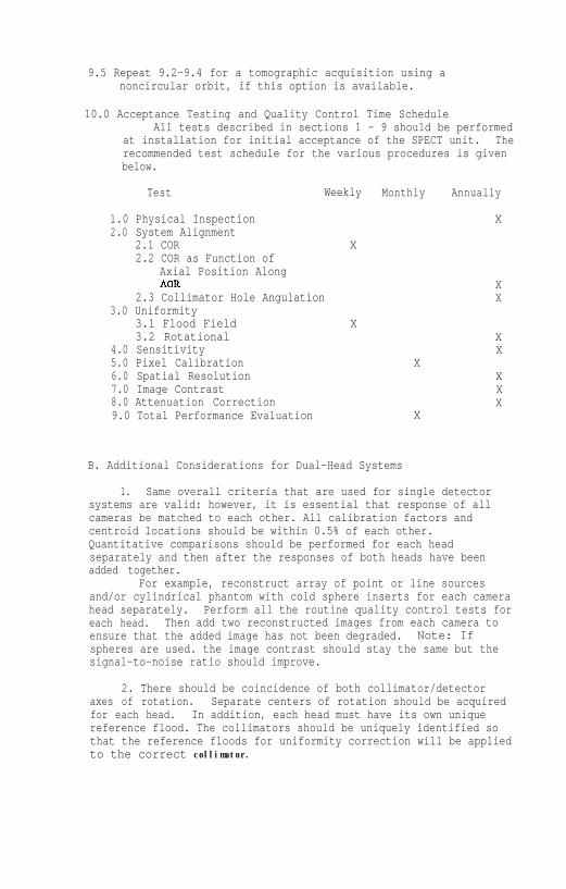
10.0 Acceptance Testing and Quality Control Time ScheduleAll tests described in sections 1 - 9 should be performed

at installation for initial acceptance of the SPECT unit. Therecommended test schedule for the various procedures is givenbelow.

Test Weekly Monthly Annually

1.0 Physical Inspection X2.0 System Alignment

2.1 COR X2.2 COR as Function of

Axial Position AlongAOR X

2.3 Collimator Hole Angulation X3.0 Uniformity

3.1 Flood Field X3.2 Rotational X

4.0 Sensitivity X5.0 Pixel Calibration X6.0 Spatial Resolution X7.0 Image Contrast X8.0 Attenuation Correction X9.0 Total Performance Evaluation X

B. Additional Considerations for Dual-Head Systems

1. Same overall criteria that are used for single detectorsystems are valid: however, it is essential that response of allcameras be matched to each other. All calibration factors andcentroid locations should be within 0.5% of each other.Quantitative comparisons should be performed for each headseparately and then after the responses of both heads have beenadded together.

For example, reconstruct array of point or line sourcesand/or cylindrical phantom with cold sphere inserts for each camerahead separately. Perform all the routine quality control tests foreach head. Then add two reconstructed images from each camera toensure that the added image has not been degraded. Note: Ifspheres are used. the image contrast should stay the same but thesignal-to-noise ratio should improve.

2. There should be coincidence of both collimator/detectoraxes of rotation. Separate centers of rotation should be acquiredfor each head. In addition, each head must have its own uniquereference flood. The collimators should be uniquely identified sothat the reference floods for uniformity correction will be appliedto the correct collimator.

3. Ideally. the centroid of the projection (image) of a pointsource located anywhere in the source distribution volume ofinterest should be within 1 mm of its true geometrically projectedvalue (based on the relative location of the point source in space,and the locations of the gamma cameras) for all angularorientations of the gamma cameras.

4. In general the +/-x and +/-y absolute integral linearityshould be within 1 mm, and matched, if possible. A similar commentis valid for absolute differential linearity.

5. Energy windows and collimators should also be matched.

VI.

1.

2.

3.

4.

5.

6.

7.

8.

9.

10.

References

Single Photon Emission Computed Tomography and Other SelectedComputer Topics, Proceedings of the 10th Annual Symposium,Society of Nuclear Medicine Computer Council. Society ofNuclear Medicine, NY, 1980Emission Computed Tomography: The Single Photon Approach.HHS Publication FDA 81-8177. US Dept of Health and HumanServices/PHS/FDA/BRH, 1981Ell PJ and Holman BL (eds): Computed Emission Tomography. TheUniversities Press Ltd., Belfast, 1982Computer-aided scintillation camera acceptance testing. AAPMReport No. 9, American Association of Physicists in Medicine.New York, 1982Greer KL, Coleman RE, Jaszczak RJ: SPECT: A practicalguide for users. J Nucl Med Tech 11:61, 1983Harkness BA, Rogers WL, Clinthome NH, Keyes JW: SPECT:Quality control procedures and artifact identification. JNucl Med Tech 11:55, 1983Esser PD (Editor): Emission Computed Tomography: CurrentTrends. Society of Nuclear Medicine. New York, 1983Greer K, Jaszczak R, Harris C, Coleman RE: Quality control inSPECT. J Nucl Med Tech 13:76, 1985Croft BY: Single-Photon Emission Computed Tomography.Year Book Medical Publishers, Chicago, 1986Performance Measurements of Scintillation Cameras. StandardsPublication, NU 1-1986. NEMA, Washington, D.C., 1986

APPENDIX AFORTRAN Algorithm for Sinogram Generation

Since different systems have different ways of handling fileoperations, only general statements are included for these commands.

IMAGE (128,128)ISINOG (128,128)JROWJTHCK

; Projection Image Data; Sinogram Image: Projection level of Sinogram; Thickness of cut

Open Projection Image FileDO 10 K = 1,128Read projection image L into the array IMAGEDO 20 I = 1,128ISINOG (I,K) = 0DO 20 J= JROW-JTHCK,JROW+JTHCKISINOG (1,K) = ISINOG(I,K)+IMAGE(I,J)

20 CONTINUE10 CONTINUE

APPENDIX B

FORTRAN algorithm for the fit to function A sin ( θ + φ ) + Bas given in section 2.1.6.2.

DIMENSION Y(128)C Y is the array with the centroid locations of the sinogram

M is a variable indicating the number of angular samplesPI = 4*ATAN (1.)DTHETA = (PI/M)*2.SUM= 0.S1 = 0.C1 = 0.DO 10 I = 1,MTHETA = FLOAT(I-1)*DTHETASUM = SUM+Y(I)S1 = S1 + Y(I)*SIN(THETA)C1 = C1 + Y(I)*COS(THETA)

10 CONTINUEA = SQRT(S1*S1 + C1*C1)PHI = ATAN(S1/C1)B = SUM/l28.

APPENDIX CVendors of Commercially Available SPECT Phantoms and Accessories

1. Data Spectrum Corporation2307 Honeysuckle RoadChapel Hill, NC 27514(919) 942-6192

2. Nuclear Associates100 Voice RoadCarle Place, NY 11514(516) 741-6360