room geometries with non-classical reverberation times · room geometries with non-classical...
TRANSCRIPT

Room Geometries with non-classical Reverberation Times
Asta Rønning Fjærli
Master of Science in Physics and Mathematics
Supervisor: Jon Andreas Støvneng, IFYCo-supervisor: Peter Svensson, Institutt for elektronikk og telekommunikasjon
Magne Skålevik, Brekke & Strand Akustikk AS
Department of Physics
Submission date: June 2015
Norwegian University of Science and Technology


Problem Description
Room Geometries with non-classical Reverberation Times
Classical diffuse field theory is a simplified theory in room acoustics, whichleads to Sabine’s and Eyring’s predictions of reverberation time. Fora room with highly scattering surfaces, Sabine’s and Eyring’s estimatesof reverberation time will be closely related to the real conditions. Inrooms with a low degree of scattering and an uneven distribution ofabsorption, however, Sabine’s and Eyring’s formulae often underestimatesthe reverberation time. In this case, an increase of the scattering willalways lead to a shorter reverberation time,
In this project, there will be examined which type of rooms that can give ashorter reverberation time than Sabine’s and Eyring’s predictions. Typesof rooms suggested by Stephenson, and rooms with the tendency of afocus effect, can be studied. Computer simulations based on geometricalacoustics can be used, together with other existing reverberation timeformulae than the classical formulae by Sabine and Eyring.
Romgeometrier med ikke-klassiske etterklangstider
Klassisk diffusfeltsteori er en forenklet teori innen romakustikk som ledertil Sabines og Eyrings prediksjoner av etterklangstid. Hvis et rom harhøy grad av spredning vil Sabines og Eyrings etterklangsestimat megetofte være nært de virkelige forholdene. I rom med lav grad av spredningog ujevn fordeling av absorpsjon er det derimot ofte slik at Sabines ogEyrings likninger underestimerer etterklangstiden. I slike fall vil en økningav spredningen i rommet alltid lede til kortere etterklangstid.
I dette prosjektet skal det undersøkes hvilke typer rom som kan gi kortereetterklangstid enn Sabines og Eyrings prediksjoner. Typer av rom somer foreslått av Stephenson, og rom med tendenser til fokuseffekter, kanstuderes. Datasimuleringer basert på geometrisk akustikk kan brukes,sammen med andre eksisterende etterklangsformler enn de klassiske avSabine og Eyring.
iii


Abstract
In this Master’s thesis, it has been examined whether it is possible to findrooms of such a geometry that the reverberation time becomes shorter thanthe predicted value of Sabine and Eyring. This was investigated usingthe computer program CATT-Acoustic, which is based on geometricalacoustics. The geometries of the rooms were polyhedral approximations ofa dome; respectively a decahedron, a nonahedron and a hexahedron, thelatter of which also representing a ”shoe-box shaped” room with inclinedwalls.
The results of the simulations show a clear tendency of a loweredreverberation time compared to the two classical formulae. For a largefloor absorber and a scattering coefficient of s > 10 − 20%, the threepolyhedral approximations all give a ratio of T30
TEyring< 1. However, it is
not possible to conclude that a focusing effect, like what one can find in adome, is the reason for this ratio. The lack of support for such a focusingeffect follows follows from the dependency on the number of surfaces in thepolyhedral approximation. The decahedron is a closer approximation to adome than the hexahedron, but the three polyhedra give approximately thesame ratio of simulated and predicted reverberation times. The simulatedvalues were also compared to what can be found using Millington-Sette’sreverberation formula and Kuttruff’s formula for the absorption coefficient.These formulae both gave significantly lower values of the reverberationtime than the simulations. Therefore, the alternative formulae do not seemto be any better alternatives than the classical Eyring’s formula. Detailedcalculation using ray tracing should anyway be used for cases like thosetested here, with uneven distributions of absorption.
v


Sammendrag
Det har i denne masteroppgaven blitt undersøkt om det finnes romav en slik geometri at etterklangstiden blir kortere enn de beregnedeverdiene fra Sabines og Eyrings likninger. Dette ble undersøkt ved ågjennomføre simuleringer i CATT-Acoustic, som er en programvare basertpå geometrisk akustikk. Geometriene implemetert i CATT-Acoustic varpolyhedratilnærminger av et kuppelrom; henholdsvis et dekahedron, etnonahedron og et hexahedron. Sistnevnte representerer et ”skoeskerom”med tiltede vegger.
Resultatene fra simuleringene viser en tendens til en redusert etterklangstidsammenliknet med de to klassiske formlene. For en stor gulvabsorbent ogen spredningskoeffisient på s > 10−20% gir de tre polyhedratilnærmingeneen ratio på T30
TEyring< 1. Det er imidlertid ikke mulig å konkludere med at en
fokuseffekt, som den man finner i en kuppel, er grunnen til dette forholdet.Årsaken til at man ikke kan påstå at en fokuseffekt er forklaringenfølger av sammenhengen med antall flater i polyhedratilnærmingen. Etdekahedron er en bedre tilnærming til en kuppel enn et heksahedron, mende tre polyhedraene gir likevel tilnærmet likt forhold mellom simulert ogberegnet etterklangstid. De simulerte verdiene ble også sammenlignet medetterklangstidene man får ved å bruke Millington-Settes etterklangsformelog Kuttruffs formel for absorpsjonskoeffisienten. Disse formlene ga beggebetraktelig lavere verdier for etterklangstiden enn simuleringene gjorde. Dealternative formlene for etterklangstid ser derfor ikke ut til å være bedrealternativer enn den klassiske Eyrings formel. Detaljerte beregninger medbruk av ray tracing må uansett benyttes for tilfeller som de som er studerti denne masteroppgaven, der absorpsjonen er ujevnt fordelt.
vii

Preface
This Master’s thesis is the response to the problem description Room ge-ometries with non-classical reverberation times suggested by Professor Pe-ter Svensson and Senior Acoustic Consultant Magne Skålevik. The sub-ject was given by the Department of Electronics and Telecommunicationsspring 2015, but the report is presented as the result of the course TFY4900- Physics, Master’s thesis. This course is mandatory in the 10th semesterof the master program of applied physics.
Peter Svensson and Magne Skålevik have been the supervisors on thisthesis, with Jon Andreas Støvneng as the contact at the department ofphysics. I would like to thank Peter and Magne for valuable guidance andinteresting discussions on my work with this report, and Jon Andreas forhelping with the practical issues by performing my Master’s thesis for theDepartment of Electronics and Telecommunications. Finally I would liketo thank Anne Birgitte Rønning and Erik Fjærli for correcting my typosand mistakes in the manuscript and give constructive advices in the writ-ing process.
Asta Rønning FjærliTrondheim, June 25, 2015
ix


CONTENTS
Contents
1 Introduction 11.1 Motivation . . . . . . . . . . . . . . . . . . . . . . . . . . . 11.2 Previous work . . . . . . . . . . . . . . . . . . . . . . . . . 31.3 Report structure . . . . . . . . . . . . . . . . . . . . . . . 4
2 Theory 52.1 Reverberation time . . . . . . . . . . . . . . . . . . . . . . 5
2.1.1 The absorption coefficient . . . . . . . . . . . . . . 72.1.2 Diffuse sound fields . . . . . . . . . . . . . . . . . . 82.1.3 The mean free path . . . . . . . . . . . . . . . . . . 92.1.4 Sabine’s formula . . . . . . . . . . . . . . . . . . . 102.1.5 Eyring’s formula . . . . . . . . . . . . . . . . . . . 112.1.6 Millington-Sette’s formula . . . . . . . . . . . . . . 132.1.7 The influence of air absorption . . . . . . . . . . . . 142.1.8 Fitzroy’s formula . . . . . . . . . . . . . . . . . . . 152.1.9 Kuttruff’s absorption formula . . . . . . . . . . . . 152.1.10 Early decay time . . . . . . . . . . . . . . . . . . . 16
2.2 Geometrical variations . . . . . . . . . . . . . . . . . . . . 172.2.1 Wall inclination . . . . . . . . . . . . . . . . . . . . 172.2.2 Ceiling profile . . . . . . . . . . . . . . . . . . . . . 182.2.3 Focusing effects . . . . . . . . . . . . . . . . . . . . 19
2.3 Predictions of the reverberation time . . . . . . . . . . . . 192.3.1 The Image Source Method . . . . . . . . . . . . . . 202.3.2 Ray Tracing and Cone Tracing . . . . . . . . . . . 21
2.4 CATT-Acoustic . . . . . . . . . . . . . . . . . . . . . . . . 222.4.1 The Universal Cone Tracer (TUCT) . . . . . . . . 23
xi

CONTENTS
3 Method 253.1 Investigation of the TUCT mode . . . . . . . . . . . . . . 253.2 Simulations . . . . . . . . . . . . . . . . . . . . . . . . . . 26
3.2.1 Room geometries . . . . . . . . . . . . . . . . . . . 263.2.2 Settings in the prediction mode . . . . . . . . . . . 293.2.3 Settings in the TUCT mode . . . . . . . . . . . . . 30
3.3 Statistical approach . . . . . . . . . . . . . . . . . . . . . . 30
4 Simulation results 314.1 Investigation of the TUCT mode . . . . . . . . . . . . . . 314.2 Simulations in the hexahedron room . . . . . . . . . . . . 35
4.2.1 Influence of the scattering coefficient . . . . . . . . 364.2.2 Influence of the size of the absorber . . . . . . . . . 404.2.3 Influence of the inclination angle . . . . . . . . . . 41
4.3 Simulations in the nonahedron room . . . . . . . . . . . . 424.3.1 Influence of the scattering coefficient . . . . . . . . 434.3.2 Influence of the size of the absorber . . . . . . . . . 44
4.4 Simulations in the decahedron room . . . . . . . . . . . . . 454.4.1 Influence of the scattering coefficient . . . . . . . . 464.4.2 Influence of the size of the absorber . . . . . . . . . 47
4.5 Influence of the room geometry . . . . . . . . . . . . . . . 484.6 Alternative reverberation time
formulae . . . . . . . . . . . . . . . . . . . . . . . . . . . . 494.7 Signs of a non-exponential decay . . . . . . . . . . . . . . 50
5 Discussion 535.1 Investigation of the TUCT mode . . . . . . . . . . . . . . 535.2 Simulations in the hexahedron room . . . . . . . . . . . . 54
5.2.1 Influence of the scattering coefficient . . . . . . . . 545.2.2 Influence of the size of the absorber . . . . . . . . . 555.2.3 Influence of the inclination angle . . . . . . . . . . 56
5.3 Simulations in the nonahedron and the decahedron rooms . 575.3.1 Influence of the scattering coefficient . . . . . . . . 575.3.2 Influence of the size of the absorber . . . . . . . . . 57
5.4 Influence of the room geometry . . . . . . . . . . . . . . . 58
xii

CONTENTS
5.5 Alternative reverberation timeformulae . . . . . . . . . . . . . . . . . . . . . . . . . . . . 58
5.6 Uncertainty and statistics . . . . . . . . . . . . . . . . . . 615.6.1 Placing of the source and receiver . . . . . . . . . . 615.6.2 Signs of a non-exponential decay . . . . . . . . . . 625.6.3 The mean free path and volume considerations in
CATT-Acoustic . . . . . . . . . . . . . . . . . . . . 625.7 General comments . . . . . . . . . . . . . . . . . . . . . . 635.8 Further work . . . . . . . . . . . . . . . . . . . . . . . . . 65
6 Conclusion 67
A Tables IA.1 Coordinates for the hexahedron . . . . . . . . . . . . . . . IA.2 Absorption coefficients . . . . . . . . . . . . . . . . . . . . II
B Mean values III
C Matlab code VC.1 Corners of a polygon . . . . . . . . . . . . . . . . . . . . . VC.2 Read out from .txt-file . . . . . . . . . . . . . . . . . . . . VII
xiii


LIST OF FIGURES
List of Figures
1.1 The scale model diffuser used in the specialization projectautumn 2014. . . . . . . . . . . . . . . . . . . . . . . . . . 3
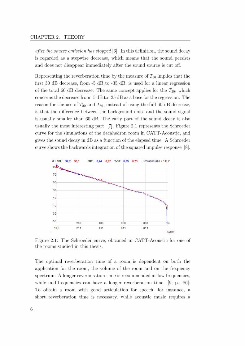
2.1 The Schroeder curve, obtained in CATT-Acoustic for one ofthe rooms studied in this thesis. . . . . . . . . . . . . . . . 6
2.2 The image source method, illustrating the image sources(the blue and green dots) and the specular echogram. . . . 20
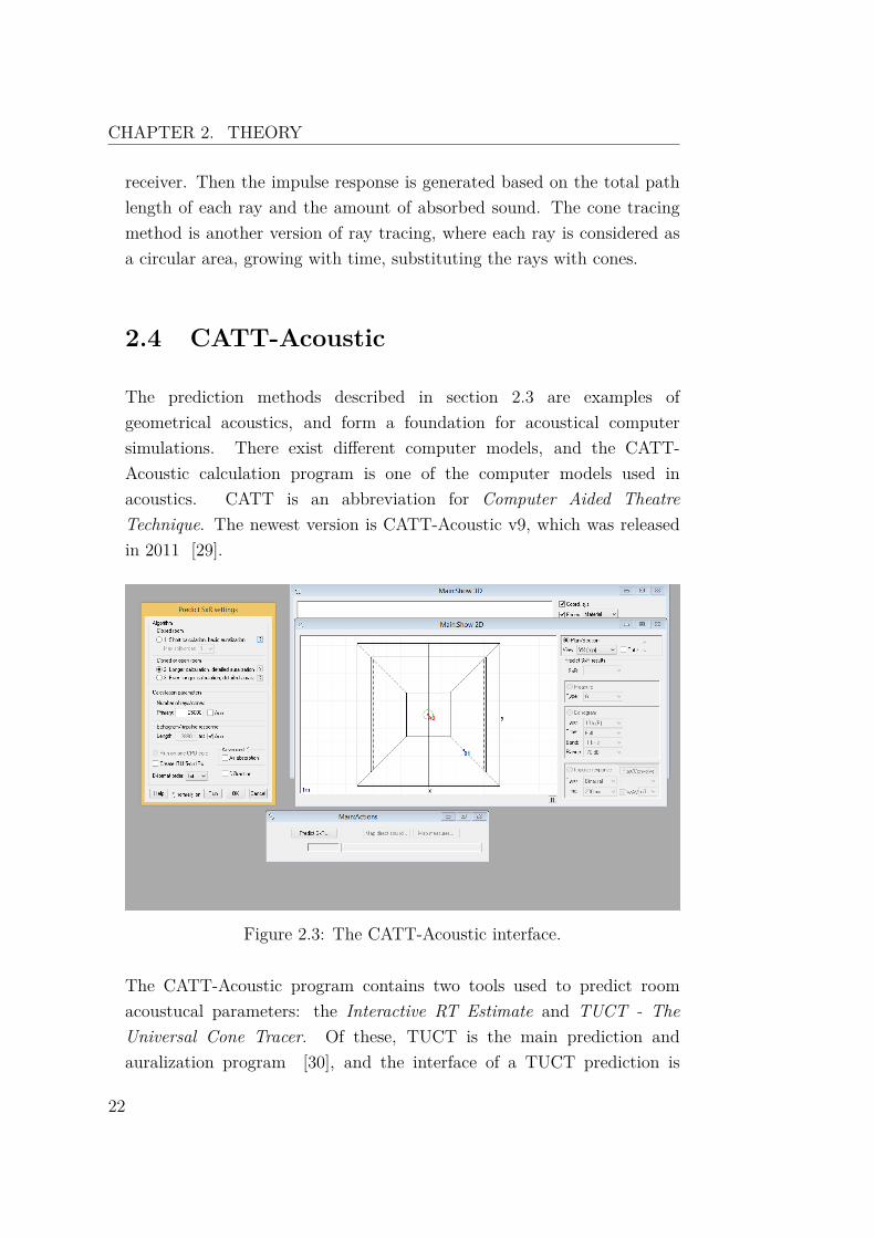
2.3 The CATT-Acoustic interface. . . . . . . . . . . . . . . . . 22
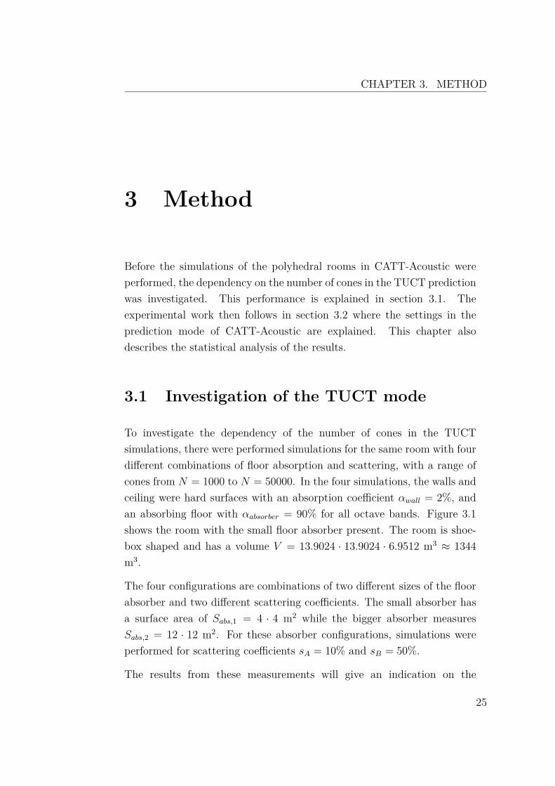
3.1 The room used to investigate the TUCT, here representedby the large absorber. . . . . . . . . . . . . . . . . . . . . . 26
3.2 Coordinates of the three polyhedra. . . . . . . . . . . . . . 273.3 The hexahedron approach of a dome. . . . . . . . . . . . . 273.4 The nonahedron approach of a dome. . . . . . . . . . . . . 283.5 The decahedron approach of a dome. . . . . . . . . . . . . 28
4.1 The room used for the simulations on the TUCT mode. . . 324.2 TUCT simulation in a shoe-box shaped room with 10%
scattering and a small absorber. . . . . . . . . . . . . . . . 334.3 TUCT simulation in a shoe-box shaped room with 10%
scattering and a large absorber. . . . . . . . . . . . . . . . 334.4 TUCT simulation in a shoe-box shaped room with 50%
scattering and a small absorber. . . . . . . . . . . . . . . . 344.5 TUCT simulation in a shoe-box shaped room with 50%
scattering and a large absorber. . . . . . . . . . . . . . . . 344.6 The room used for the simulations in the hexahedron
approximation. . . . . . . . . . . . . . . . . . . . . . . . . 35
xv

LIST OF FIGURES
4.7 Reverberation time as a function of the scattering coeffi-cient, hexahedron approximation and large absorber, angleθ = 35o. . . . . . . . . . . . . . . . . . . . . . . . . . . . . 36
4.8 Reverberation time as a function of the scattering coeffi-cient, hexahedron approximation and large absorber, angleθ = 45o. . . . . . . . . . . . . . . . . . . . . . . . . . . . . 37
4.9 Reverberation time as a function of the scattering coeffi-cient, hexahedron approximation and large absorber, angleθ = 60o. . . . . . . . . . . . . . . . . . . . . . . . . . . . . 37
4.10 Reverberation time as a function of the scattering coeffi-cient, hexahedron approximation and large absorber, angleθ = 75o. . . . . . . . . . . . . . . . . . . . . . . . . . . . . 38
4.11 Reverberation time as a function of the scattering coeffi-cient, hexahedron approximation and large absorber, angleθ = 82.5o. . . . . . . . . . . . . . . . . . . . . . . . . . . . 38
4.12 Reverberation time as a function of the scattering coeffi-cient, hexahedron approximation and large absorber, angleθ = 87.5o. . . . . . . . . . . . . . . . . . . . . . . . . . . . 39
4.13 Reverberation time as a function of the scattering coeffi-cient, hexahedron approximation and large absorber, angleθ = 90o. . . . . . . . . . . . . . . . . . . . . . . . . . . . . 39
4.14 Reverberation as a function of the size of the absorber,hexahedron approximation and θ = 60o. . . . . . . . . . . . 40
4.15 Reverberation as a function of the wall inclination angle θ,hexahedron approximation and large absorber. . . . . . . . 41
4.16 The room used for the simulations in the nonahedronapproximation. . . . . . . . . . . . . . . . . . . . . . . . . 42
4.17 Reverberation time as a function of the scattering coeffi-cient, nonahedron approximation and large absorber. . . . 43
4.18 Reverberation time as a function of the size of the absorber,nonahedron approximation. . . . . . . . . . . . . . . . . . 44
4.19 The room used for the simulations in the decahedronapproximation. . . . . . . . . . . . . . . . . . . . . . . . . 45
4.20 Reverberation time as a function of the scattering coeffi-cient, decahedron approximation and large absorber. . . . 46
xvi

LIST OF FIGURES
4.21 Reverberation time as a function of the size of the absorber,decahedron approximation. . . . . . . . . . . . . . . . . . . 47
4.22 Reverberation time for the three polyhedral approximations,large absorber. . . . . . . . . . . . . . . . . . . . . . . . . 48
4.23 Reverberation according to reverberation formulae, fordifferent polyhedra, together with the simulated values fromCATT. . . . . . . . . . . . . . . . . . . . . . . . . . . . . . 49
4.24 T20/T30 for hexahedron, angle θ = 60o, as a function of thesize of absorber. . . . . . . . . . . . . . . . . . . . . . . . . 50
4.25 T20/T30 for nonahedron as a function of the size of absorber. 514.26 T20/T30 for decahedron as a function of the size of absorber. 51
B.1 The mean values for the simulations of polyhedra with largefloor absorber. . . . . . . . . . . . . . . . . . . . . . . . . . III
xvii


LIST OF TABLES
List of Tables
2.1 Optimal reverberation times for different sound sources. . . 7
3.1 Corners of the polyhedra . . . . . . . . . . . . . . . . . . . 27
5.1 The deviation between simulated reverberation time andtheoretical formulae T30/TFormula. . . . . . . . . . . . . . . 60
5.2 Room volumes and mean free path calculated in CATT-Acoustics and in Matlab . . . . . . . . . . . . . . . . . . . 63
A.1 Corners of the polyhedra, given different inclination angles. IA.2 Absorption coefficients. . . . . . . . . . . . . . . . . . . . . II
xix


ABBREVIATIONS AND SYMBOLS
Abbreviations and symbols
• ISM - Image Source Method
• RT - Ray Tracing
• mfp - Mean free path
• CI - Confidence interval
• IR - Impulse response
• CATT - CATT-Acoustic
• TUCT - The Universal Cone Tracer
• T - Reverberation time
• V - Volume
• S - Surface area
• s - Scattering coefficient
• α - Absorption coefficient
• ρ - Reflection coefficient
• θ - Wall inclination angle
xxi


CHAPTER 1. INTRODUCTION
1 Introduction
1.1 Motivation
In the work of an acoustic consultant, it passes up to several years fromthe planning of a new project till it is finished and verifying measurementscan be performed. Basing following projects on the same idea maytherefore have unsure outcomes. Consequently, it is of vital interest forthe consultant sector to get more control on the prediction phase of aproject to prevent surprises on the finish line.
One solution to this problem is to perform scale model measurementsbefore starting the construction of a full scale room or building. However,this is often an expensive solution. In addition, there are limitations in theusage of scale model measurements as well, both in the choice of materialsthat correspond to the full scale materials and in the treatment of airabsorption. There exist several acoustic simulation programs based ongeometrical acoustic methods like ray tracing (RT) and the image sourcemethod (ISM), that can predict the outcome of a new idea. The use of suchprograms is less expensive and more time efficient alternatives comparedto scale model measurements. Examples of acoustic simulation programsare programs are ODEON and CATT-Acoustic, and CATT-Acoustic is thesoftware that will be used in this Master’s thesis.
As will be presented in section 1.2, the author has earlier investigatedthe effect of a new type of ceiling diffusers first used by Arau Acoustica[1], using a scale model. The measurements of Arau Acoustica showed aprolonged reverberation time with the ceiling diffuser present compared
1
CHAPTER 1. INTRODUCTION
to initial measurements, which is a surprising result considering existingreverberation formulae which only give a relationship between thereverberation time, the room volume and the average absorption in theroom.
The following situation may be regarded as the opposite of what was donein the Theatre of Liceu:
An existing room has a ceiling diffuser, and the interest of the acousticianis to increase the volume of the room, assuming a prolonged reverberationtime based on Sabine’s and Eyring’s equations. Therefore, the diffuser isremoved, and one expects to get a longer value for the reverberation time.However, in the case of the rehearsal room in Liceu, the reverberation timewithout the diffuser is shorter, even if the room volume is larger withoutthe diffuser.
The result of a shortened reverberation time with a larger room volume issurprising compared to the classical predictions. This is the motivation tostudy the problem further, and to try to find other room geometries thatgive shorter values than Sabine’s and Eyring’s formulae predict. It is alsointeresting to investigate whether there exist other reverberation formulaethat give better values for such room geometries than the classical formulaeof Sabine and Eyring.
A focusing room shape, like a dome with a reflecting ceiling and anabsorbing ground flate, could make a floor absorber more effective, andthus lead to a shorter reverberation time than TSabine [2]. An oppositeof this situation is the so-called Hard Case [3], [4]. The Hard Case isa cuboid room represented by hard walls and a hard floor, with a ceilingabsorber as the only absorbing element. In this case, the reverberationtime becomes longer than Sabine’s and Eyring’s predictions. In addition,due to an almost two-dimentional sound field at high frequecies, flutterecho may occur.
2

CHAPTER 1. INTRODUCTION
1.2 Previous work
In the specialization project carried out by the same author the autumnsemester 2014, the findings of Arau-Puchade’s work in the RehearsalRoom of the Great Theatre of Liceu [1] were examined in a scale modelwith a scale factor of 1 : 8. Arau-Puchades installed a ceiling diffuserin this rehersal room, consisting of a regular metal grid with verticalpolycarbonate plates forming a labyrinth structure. The scale modeldiffuser is shown in Figure 1.1 Arau-Puchades’ acoustic measurementsbefore and after the diffuser was installed show a significantly shorteningreverberation time, considering both the T30 and the EDT .
Figure 1.1: The scale model diffuser used in the specialization projectautumn 2014.
The reverberation time measurements in the scale model did not followthe same pattern as the full scale measurements of Arau, but studies ofthe curvature C showed that the ceiling diffuser made a significant impacton the diffusivity of the room. The results of this specialization projectlead to further questions about the validity of the classical reverberationtime formulae and the treatment of non-diffuse sound fields.
3

CHAPTER 1. INTRODUCTION
1.3 Report structure
A theoretical background for the simulations is first presented in chapter2, together with a study of the classical diffuse field theory. In chapter3, the experiments in CATT-Acoustic are explained. The result of thesesimulations is presented in chapter 4 and further discussed in chapter 5.The concluding remarks follow in chapter 6.
There are three appendices to this report. Appendix A contains two tables;a table of the corners in the hexahedron approximation given differentinclination angles and a table for the absorption coefficient given differentmaterials. The mean values of the simulations are plotted in appendix B.Finally, the Matlab code used to find the corners of a polygon follows inappendix C together with the Matlab code generated to read the TUCT-text files from CATT-Acoustic.
4

CHAPTER 2. THEORY
2 Theory
This chapter will introduce some of the parameters that will be analyzedin this thesis, primarily concerning reverberation time and characteristicsof a diffuse sound field. There are different approaches to a theoreticalvalue of the reverberation time, which will be presented together withtheir historical background. The importance of a diffuse sound field forthese formulae to be valid is also introduced. Geometrical variations inroom design and their influence of the reverberation time will then bepresented, and thereafter the theory underlying the simulation softwareCATT-Acoustic and other room acoustic computer models.
2.1 Reverberation time
When it comes to room acoustics the reverberation time is usually judgedto be the most important parameter. The reverberation time is oftenrepresented by T30 and can be measured in a room using the impulseresponse, it can be predicted by reverberation formulae or it can bepredicted using geometrical acoustic methods. The reverberation time isa global parameter, which means that the measure is independent of thepositions in a room [5]. By contrast, acoustical parameters such as soundstrength (G), early decay time (EDT ), clarity (C80), lateral energy fraction(LEF ) and the late sound level (Glate) are local acoustical parameters anddependent on the location of the listener.
ISO 3382-2 defines the reverberation time as the duration required for thespace-averaged sound energy density in an enclosure to decrease by 60 dB
5
CHAPTER 2. THEORY
after the source emission has stopped [6]. In this definition, the sound decayis regarded as a stepwise decrease, which means that the sound persistsand does not disappear immediately after the sound source is cut off.
Representing the reverberation time by the measure of T30 implies that thefirst 30 dB decrease, from -5 dB to -35 dB, is used for a linear regressionof the total 60 dB decrease. The same concept applies for the T20, whichconcerns the decrease from -5 dB to -25 dB as a base for the regression. Thereason for the use of T20 and T30, instead of using the full 60 dB decrease,is that the difference between the background noise and the sound signalis usually smaller than 60 dB. The early part of the sound decay is alsousually the most interesting part [7]. Figure 2.1 represents the Schroedercurve for the simulations of the decahedron room in CATT-Acoustic, andgives the sound decay in dB as a function of the elapsed time. A Schroedercurve shows the backwards integration of the squared impulse response [8].
Figure 2.1: The Schroeder curve, obtained in CATT-Acoustic for one ofthe rooms studied in this thesis.
The optimal reverberation time of a room is dependent on both theapplication for the room, the volume of the room and on the frequencyspectrum. A longer reverberation time is recommended at low frequencies,while mid-frequencies can have a longer reverberation time [9, p. 86].To obtain a room with good articulation for speech, for instance, ashort reverberation time is necessary, while acoustic music requires a
6

CHAPTER 2. THEORY
longer reverberation time. Church music is an extreme and requires areverberation time of several seconds. To obtain the optimal reverberationtime, it is also necessary to consider the size of the room. For a largerroom volume longer reverberation time would be preferable.
The optimal reverberation times for different sound sources are presentedin Table 2.1 [10, p. 504], [11, p. 313]. Beranek’s value for symphonyorchestras is based on best ratings of 40 concert halls presented in Concerthalls and opera houses and is valid for mid-frequencies. The lowest ratedhalls in Beranek’s study had in comparison a reverberation time in therange of T = 1.5− 1.8 s.
Table 2.1: Optimal reverberation times for different sound sources.
Sound source Optimal reverberation time [s]Symphonical music (Beranek) 1.8 - 2.0Symphony orchestra (Gade) 2.0 - 2.4
Chamber music (Gade) 1.5Opera (Gade) 1.4 - 1.8
Rythmic music (Gade) 0.8 - 1.5
2.1.1 The absorption coefficient
An important parameter that influences the reverberation time in a roomis the absorption coefficient and the average absorption. For a room withtotal surface area S and segmental absorption areas Si with correspondingabsorption coefficients αi, the average absorption is given by
α = 1S
∑i
(Siαi) (2.1)
This equation does not tell how the absorption is distributed in a room.The effect of uneven distribution of absorption will be introduced in section2.1.2 and discussed further in section 5.7.
7
CHAPTER 2. THEORY
2.1.2 Diffuse sound fields
The length of a sound decay is dependent on the structure of the soundfield in a room. The classical formulae, like the formulae of Sabine andEyring, assumes a diffuse sound field. In a diffuse sound field, all directionsof sound propagation are equally likely, and the sound pressure level isindependent of the location [12]. The measured reverberation time willtherefore be constant for all positions of the sound source and the receiversin a room. In real life, however, one will never achieve a perfect diffusesound field.
For a diffuse sound field, theory predicts a pure exponential sound decay[11, p. 307-308]. For such a decay the dB-curve is linear. In this situation,the reverberation time T is independent of the evaluated decay range,giving T30 = T20 = T60. The intensity of a sound field is given by I(φ, ν)where φ and ν give the directions of the distribution. The energy densityis then given by dw = I(φ,ν)
cdΩ [13, p. 129], where c is the speed of sound
and dΩ represents a very small solid angle in a collection of nearly parallellsound rays. For a 3-dimentional diffuse sound field, this intensity isconstant, which gives total sound energy density in all directions w = 4πI
c.
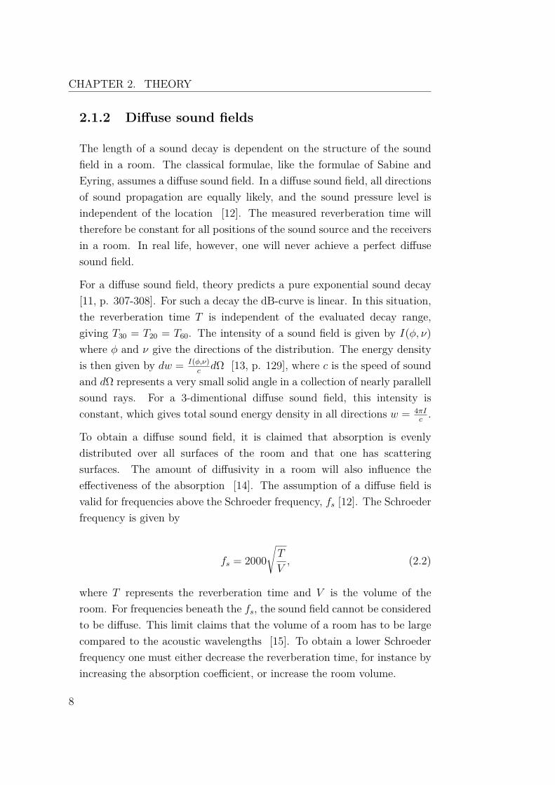
To obtain a diffuse sound field, it is claimed that absorption is evenlydistributed over all surfaces of the room and that one has scatteringsurfaces. The amount of diffusivity in a room will also influence theeffectiveness of the absorption [14]. The assumption of a diffuse field isvalid for frequencies above the Schroeder frequency, fs [12]. The Schroederfrequency is given by
fs = 2000√T
V, (2.2)
where T represents the reverberation time and V is the volume of theroom. For frequencies beneath the fs, the sound field cannot be consideredto be diffuse. This limit claims that the volume of a room has to be largecompared to the acoustic wavelengths [15]. To obtain a lower Schroederfrequency one must either decrease the reverberation time, for instance byincreasing the absorption coefficient, or increase the room volume.
8

CHAPTER 2. THEORY
Examples of rooms that cannot be classified as diffuse are rooms with amajority of the absorption concentrated on one side, for instance the so-called Hard Case, and coupled rooms. An example of the absorbing surfaceis acoustic ceiling tiles, or it can be the audience giving an absorbing floor.Odd-shaped rooms, for instance a long corridor measuring A · B · C withC A and C B, will also be classified as non-diffuse.
For a unit area of 1 m2 and a unit time of 1 s, the acoustic intensity in thediffuse sound field with energy density dw is given by [9, p. 66]:
I = c
4E. (2.3)
This can be compared to the acoustic intensity of a plane wave at normalincidence of the wall, I = cE, being four times the acoustic intensity in adiffuse sound field.
2.1.3 The mean free path
The mean free path (mfp), lm, is the mean distance between two soundreflections. The mfp represents the average distance travelled by the soundwaves of sound speed c after a time t from the first wave progagation,
lmn = ct, (2.4)
where n is the number of reflections [9, 68].
For a 3-dimentional room of volume V with a diffuse sound field and surfacearea S, the mean free path is given by [15]
lm = 4VS. (2.5)
Equation 2.5 for the mean free path is only valid for strongly diffuse soundfields. Such fields are an assumption for Sabine’s and Eyring’s formulae.
9

CHAPTER 2. THEORY
2.1.4 Sabine’s formula
The first scientist to introduce the reverberation time T [s] as a measure ofthe reverberation in a room was W. C. Sabine. In The American Arcitect[16, p. ix], 1900, Sabine presented a relationship between the room volumeV , the equivalent absorption area A and the reverberation time T as
T ∝ V
A. (2.6)
In other words, he found the reverberation time to be proportional tothe volume of the room and inverse proportional to the absorption, by aproportionality factor K.
Sabine’s formula is based on experimental work, but it can also be deducedtheoretically. From measurements in the lobby of the Fogg museum and theJefferson physical laboratory, he found an average proportionality factorof 0.164 [16, p. 50], using SI-units. This value is later found to be 0.161for sound speed c = 343 m/s, giving Sabine’s formula
T = 0.161VA
, (2.7)
where A gives the equivalent absorption area A = Sα = ∑i Siαi for i
surfaces. A is given in metric sabin. This formula is neglecting the influenceof air absorption. The air absorption is represented by a term presentedin section 2.1.7
Sabine’s formula follows from the relationship of the total energy in a roomwith surface area S and energy density E [9, p. 66],
VdE
dt= W − cESα
4 . (2.8)
Substituting S · α = A, and name the initial values E = 0 and t = 0, gives
E = 4WcA
[1− e−(cA/4V )/t]. (2.9)
10
CHAPTER 2. THEORY
When time passes, t→∞, the energy will approach the steady-state valueE0 = 4W
cA. This leads to the total energy reduction in the room,
E = E0e−(cA/4V )/t, (2.10)
which gives the decay rate D = 10log(ecA/4V ) with a unit dB per second.
The definition of the reverberation time was presented in section 2.1, andthe reverberation time T can be expressed mathematically as
T = 60D
= 6010 · log(ecA/4V ) = 6 · 4V
cA · log(e) = const · VA. (2.11)
The constant in equation 2.11 is given by
K = 24c · log(e) ≈ 55.3 · 1
c. (2.12)
For room temperature, T = 20 o, the speed of sound equals c = 343 m/s,and the constant, using SI-units, approximates K = 0.161. This givesSabine’s formula as presented in equation 2.7.
2.1.5 Eyring’s formula
The experimental rooms in which Sabine used to find the reverberationformula all had a reverberation time T ε [1.5 − 4] s [17]. Such roomscan be classified as "live" rooms. For "dead" rooms, when the averageabsorption approaches T = 1, a weakness of the Sabine’s formula appears.For α→ 1, A = Sα ≈ S and the reverberation time TSabine ≈ 0.161V
S. This
is the opposite of what one would assume for a highly absorbent roomwhere the sound is rapidly damped. This was the motivation of C. F.Eyring, who in 1929 released his alternative to a reverberation formula.
Eyring’s formula is based on the assumption that a sound field is composedof plane sound waves. Such waves will lose energy each time they hit anabsorbing surface. The fraction of energy lost due to absorption is equal
11

CHAPTER 2. THEORY
to (1− α) where α is the absorption coefficient of the surface. For a givennumber n of surface reflections, the energy loss is then given by [9, p. 68]
E = E0 · (1− α)n = E0 · en·ln(1−α), (2.13)
With the mean free path expressed as in section 2.1.2, the sound waves willtravel an average distance of lmn = ct where t is the time after the firstwave propagation. Substituting n = ct/lm in equation 2.13, the energydensity yields
E = E0 · ec
lm·ln(1−α)t (2.14)
after a time t.
A 60 dB decrease in sound level means that the energy has dropped toE = 10−6 · E0, giving
ec
lm·ln(1−α)T = 10−6, (2.15)
or
c
lm· ln(1− α)T = −6 · ln(10). (2.16)
The formula of Eyring then follows from the mean free path in a diffusesound field, given in equation 2.5, and the sound speed for a temperatureof 20o C, c = 343 m/s. The reverberation formula is presented as
T = 6ln(10) · 4V−cSln(1− α) = 0.161V
−Sln(1− α) . (2.17)
For rooms with a high average absorption, Eyring’s theory gives a bettervalue for the reverberation time than the theory of Sabine. With α → 1,which is the situation of the anechoic room, Sabine’s formula will givea value of T → 0.161V
S, while Eyring’s formula, as expected for this room,
gives T → 0. For a low average absorption, α < 0.3 [2], however, the energy
12

CHAPTER 2. THEORY
density as viewed from a surface element can be considered continous sincea majority of the incoming energy is reflected. As a result, −1
ln(1−α) ≈1αand
TEyring ≈ TSabine.
2.1.6 Millington-Sette’s formula
Millington (1932) [18] and Sette (1933) [19] investigated an alternativeto Eyring’s reverberation formula. The average absorption coefficientintroduced in section 2.1.1 and used in the formulae of Sabine and Eyringregards the number N of collisions by a sound particle as a statistical value,with expectation value Ni = NSi/S [13, p. 141].
By use of the exact value of N rather than the statistical value, the energydistribution will still follow the exponential equation given in 2.10, butwith an average absorption given by
α′ = − 1S
∑i
Siln(1− αi). (2.18)
With this absorption coefficient, Millington and Sette predict a shorterreverberation time than Eyring’s formula. This reverberation time is givenby
TMillington−Sette = 0.161 V
Sα′. (2.19)
The difference between the formula of Millington-Sette and the formulaeof Sabine and Eyring lies in the treatment of the absorption coefficient. Inequation 2.18, one considers the average of the terms −Siln(1 − αi) andsums over these values rather than taking the logarithm of the averageabsorption as Eyring did.
Millington-Sette’s formula is not meant as a general formula for thereverberation time, but as a supplement to Eyring’s formula for the specialcases of which Eyring’s prediction is not valid [19]. While Eyring’s formulagives the expected value of T → 0 for an average absorption of α = 1,the Millington-Sette’s absorption coefficient will develop as α′ → ∞ for
13

CHAPTER 2. THEORY
αi = 1, independent of the size of the corresponding Si. The resultingreverberation time will then be zero, which is a counterintuitive result.
2.1.7 The influence of air absorption
The three equations 2.7, 2.17 and 2.19, are all presented on the easiestform, neglecting the air absorption. This assumption is only valid for lowfrequencies. If one includes the air absorbtion, another absorption termA = 4mV is included in the reverberation formula. Here, m is a frequencydependent absorption coefficient for the air absorption [20, p. 338],
m = 5.5 · 10−4(50h
)(f
1000
)1.7
, (2.20)
giving
Aair = 4 · 0.275f 1.7
hV. (2.21)
In this equation, h is the percentage of humidity in the room and f is thefrequency.
Including the air absorption, Sabine’s, Eyring’s and Millington-Sette’sequations are modified and given in equations 2.22, 2.23 and 2.24:
T60,Sabine = 0.161 · VA+ 4mV , (2.22)
T60,Eyring = 0.161 · V−Sln(1− α) + 4mV , (2.23)
T60,Millington−Sette = 0.161 · VSα′ + 4mV . (2.24)
By concidering the air absorption term in the equations above, it is clearthat the air absorption will mostly influence the reverberation in rooms ofa large volume and for high frequencies. In scale model measurements, the
14

CHAPTER 2. THEORY
frequency f , the volume V and scale factor σ are related by fscale = freal ·σand Vscale = Vreal · σ3. The treatment of the air absorption is therefore animportant issue in scale model measurements.
2.1.8 Fitzroy’s formula
In the study of rooms with uneven absorption distribution, Fitzroy[21] found that Sabine’s and Eyring’s predictions are too low in manycases. Therefore, he came up with a different approach to a theoreticalreverberation formula, valid for shoe-box shaped rooms with hard wallsand floor and a highly absorbing ceiling. Fitzroy’s formula follows fromequation 2.25.
Ttot =(x
S
) [ 0.161V−Slog(1− αx)
]+(y
S
) [ 0.161V−Slog(1− αy)
]+(z
S
) [ 0.161V−Slog(1− αz)
].
(2.25)
In this formula, x represents the total area of the side walls, y is the totalarea of the ceiling and floor and z is the total area of the end wall. Forthe surfaces i = x, y, z, αi is the average absorption of the respective area.S is the total surface area and V is the volume of the room.
2.1.9 Kuttruff’s absorption formula
In the fourth edition of Room Acoustics [22, p. 141], H. Kuttruff introducesan alternative formula for the absorption distribution in a room, which canbe used together with Eyring’s equation to get a more accurate predictionof the reverberation time for rooms in which the sound field is not diffuse.Kuttruff claims that each boundary gives diffuse reflections, and takes theaverage number of reflections by a sound particle into account.
Using this absorption formula, one expects a more correct value ofabsorption for cases where the effective absorption is greater than theabsorption coefficient predicted in Eyring’s formula. These are cases where
15

CHAPTER 2. THEORY
the real reverberation time will be shorter than the one predicted byEyring.
Kuttruff’s absorption formula assume the irradiation strength [22, p. 139]to be constant, and yields
a∗ ≈ aEyring +∑ρn(ρn − ρ)S2
n
(ρS)2 . (2.26)
In this formula, ρ is the average reflection, ρ = 1− α. A totally absorbingsurface is then characterized by ρ = 0. Kuttruff claims that this correctionapplies well for situations where only one surface has absorption in whichdiffers from the n − 1 remaining surfaces, for instance the case of a roomwith hard walls and a floor occupied by an (absorbing) audience [15].
2.1.10 Early decay time
The early decay time, EDT , is another measure of the reverberation timein a room. Unlike T20 and T30 this quantity focuses on the early part of theimpulse response, and uses the first 10 dB decrease of the sound pressurelevel, from 0 dB to -10 dB. When this value is multiplied by 6, the total 60dB decrease is obtained. The reverberation time will often decrease morerapidly in this time window compared to the full impulse response, andthis is the reason why the EDT is usually shorter than T30 and T20.
The EDT is more important for subjective impressions and it is related tothe perceived reverberation [13, p. 237], while T30 is more related to thephysical reverberation [23]. The early decay time is more dependent onthe early reflections in the room, and will thus be more dependent on theroom geometry.
16
CHAPTER 2. THEORY
2.2 Geometrical variations
The reflected sound rays are important in concert halls and other roomswhere there is a considerable distance from the sound source to the listener.The listener will receive reflections from the surfaces of the room, primarilythe walls, the ceiling and a non-absorbing floor in addition to the directsound. An uneven distribution of sound reflections will contribute to aroom where acoustic quality differs between the listener positions.
Geometrical variations between rooms will influence on the distributionof sound reflections. The geometrical variations viewed in this thesis arebased on polyhedral approximations of a dome with respectively six, nineand ten surfaces.
2.2.1 Wall inclination
In a trapezoid room, a case of the hexahedron shape, the reverberationtime will be affected by the inclination angle θ of the walls. This effectis more significant for reflecting ceiling and walls. According to Norgesbyggforskningsinstitutt [12], the reverberation time can be doubled in themost extreme cases, and one will get maximal change in reverberationtime when the walls are tilted approximately 5 o compared to the cuboidroom. An angle θ > 90o represents an outwards tilt, prolonging thereverberation time. If the walls are tilted inwards, θ < 90o, a shorteningof the reverberation time can be expected.
The reason for the prolonged reverberation time with inclination angleθ > 90o can be explained by following the ray paths. In this case, the rayswill be reflected towards the reflecting ceiling to a higher degree, prolongingthe reverberation time. When the walls are tilted inwards, a larger part ofthe sound will be reflected towards the floor which is the absorbing surfacein the room for the situation of an absorbing audience. The reverberationtime will then be shortened compared to the reverberation time of a shoe-box shaped room, and it may also be shorter than the predicted values bySabine and Eyring.
17

CHAPTER 2. THEORY
2.2.2 Ceiling profile
U. Stephenson has been studying rooms of odd geometrical shape andthe influence of the shape on the reverberation time. He states that thereverberation time is highly dependent on the room shape, especially inrooms where the absorption is unevenly distributed [24]. In the case of aconcert hall, for instance, the total absorption is dependent on the size ofthe audience and will thus vary with the number of visitors.
In a paper from 2007 [25], Stephenson studied the dependency on thereverberation time by the longitudinal section of an auditorium andinvestigated whether it is possible to obtain reverberation times shorterthan Sabine’s prediction for certain ceiling profiles. It is known that theearly decay time (EDT ), together with the Deutlichkeit (D50) and thedecay of the sound pressure level are parameters that are dependent onthe longitudinal section in general, and the ceiling profile in particular.Examples of concert halls with a ’tent shaped’ ceiling profile are thePhilharmonie in Berlin and the Elbphilharmonie in Hamburg. The latteris still in the state of construction.
The optimal volume per seat of a room is given by V/N = 3 − 4 m3 forspeech, V/N = 6− 12 m3 for music and V/N = 5− 8 m3 in mulitipurposehalls [12]. Beranek [10, p. 541] operates with an optimalization ofV/N = 9 m3 based on a selection concert halls, and a given reverberationtime of T = 2.0 s.
The Elbphilharmonie is drafted for a number of 2150 in the audience, witha floor area of A = 40 · 60 m2 and a maxiumum height of h = 30 m.This height is the height in the middle of the room and the ceiling willhave a tent shape, like a traditional circus. This makes the total volumeV > 30000 m3 giving an estimate of the volume per seat of V/N ≈ 15m3 [25], which is above the recommended value of Beranek. Beranek’srecommendation is, however, obtained in for instance the Philharmonie inBerlin.
In his examination of tent shaped halls, Stephenson found that thereverberation time decreased with the room angle. With specularly
18

CHAPTER 2. THEORY
reflecting walls, the reverberation time decreased by a factor of 1.5. For ahigher diffusivity degree, the same effect could not be discovered.
2.2.3 Focusing effects
The shape of the ceiling surface is another factor that influences the sounddistribution in a room, and consequently affects the reverberation time.Concave surfaces may have a focusing effect on the sound. For a curvatureradius equal to the room height or twice the room height, these effects aremost severe [12]. While a plane surface reflects specularly, a convex surfacewill disperse the sound and a concave surface, like a dome, will assemblethe sound rays [26, p. 22]. If the concave surface has a focal point at thesound source or the sound receiver, the reflection may be heard as an echo.
By placing an acoustic absorber in the focal point of a concave surface,one may obtain a high efficiency of the absorber, making the effectiveabsorption larger than the absorption coefficient given for the absorptionmaterial.
2.3 Predictions of the reverberation time
In acoustic computer models, geometrical acoustics is a common base forthe simulations. Examples of geometrical acoustics are the two methodsimage source method (ISM) and ray tracing (RT). There are benefits anddisadvantages with both methods, and they are preferred for differentapplications. The two methods have in common that wavelength, orequivalent the frequency, is not a built-in characteristic [9, p. 235].Therefore, the ISM and the RT often create higher order of reflectionsthat one would obtain with wave theoretical acoustics.
A frequency dependent scattering coefficient of the surface is one way toimplement the wave nature of the sound in geometrical acoustics. Theimplementation of the scattering coefficient in the simulations will befurther described in section 3.2.2. The scattering coefficient will influence
19

CHAPTER 2. THEORY
the diffusivity of the sound field. A scattering coefficient of zero meansthat there are only specular reflections.
2.3.1 The Image Source Method
The image source method (ISM) is based on the boundary condition for ahard wall, where the particle velocity is zero, which makes it possible toreplace the wall by a mirror source. A mirror source is an identical soundsource as the main source, mirrored about the wall. The direct sound fromthe mirror source to the receiver will then be the exact specular reflectionfrom the wall. [13, p. 102-109] For this to be valid, the reflections haveto be purely specular, and it is not possible to implement a scatteringcoefficient in this method.
Figure 2.2: The image source method, illustrating the image sources (theblue and green dots) and the specular echogram.
20

CHAPTER 2. THEORY
The paragraph above explains how one concerns one specular reflection.To obtain a higher order of reflections, each mirror source is used as anew sound source and mirrored about the wall planes to obtain the totalimpulse response. This impulse response is then used to obtain parameterslike the reverberation time. Figure 2.2 shows the implementation of theimage source method, with the respective image sources, for 2nd order ofreflections.
For a large number of reflections, use of the ISM is complicated and aprediction can take long time. The number of potential image sourcesgrows exponentially with the number of reflections, but only a few areactually valid image sources. The ISM is therefore a good and accuratechoice for simple, rectangular rooms where a low reflection order issufficient. It is not preferred for complicated rooms where a high numberof sound reflections is necessary to obtain a reliable result.
2.3.2 Ray Tracing and Cone Tracing
The 3-dimentional ray tracing method was first introduced at NTNU,Trondheim. Asbjørn Krokstad, Svein Strøm and Svein Sørsdal presentedthis method in 1968 [27]. The ray tracing method is still in use, based onthe same principle as published in 1968.
In a ray tracing prediction one follows a large number of rays sent out fromthe sound source. Each time a ray hits a wall, it will be reflected eitherspecularly, after Snell’s law, nisin(θi) = nrsin(θr), or diffusely. A diffusereflection will follow Lambert’s law [28].
Whether the reflection is specular or diffuse is determined by the scatteringcoefficient s of the wall. The scattering coefficient is defined as theamount of energy which is not reflected specularly and has a value between0 and 1. s = 0 means a pure specular reflection, while s = 1 gives a purediffuse reflection. For a scattering coefficient between the two integers, thecoefficient gives the probability of a diffuse reflection. Moreover, it followsthat ray tracing is a stochastic method.
In a ray tracing the rays are followed for each reflection until they hit the
21
CHAPTER 2. THEORY
receiver. Then the impulse response is generated based on the total pathlength of each ray and the amount of absorbed sound. The cone tracingmethod is another version of ray tracing, where each ray is considered asa circular area, growing with time, substituting the rays with cones.
2.4 CATT-Acoustic
The prediction methods described in section 2.3 are examples ofgeometrical acoustics, and form a foundation for acoustical computersimulations. There exist different computer models, and the CATT-Acoustic calculation program is one of the computer models used inacoustics. CATT is an abbreviation for Computer Aided TheatreTechnique. The newest version is CATT-Acoustic v9, which was releasedin 2011 [29].
Figure 2.3: The CATT-Acoustic interface.
The CATT-Acoustic program contains two tools used to predict roomacoustucal parameters: the Interactive RT Estimate and TUCT - TheUniversal Cone Tracer. Of these, TUCT is the main prediction andauralization program [30], and the interface of a TUCT prediction is
22

CHAPTER 2. THEORY
showed in Figure 2.3. The benefit of the Interactive RT-Estimate is that itindicates in which octave bands the assumptions of geometrical acousticscan be supposed to hold. This is also a prediction method that takesshorter time than the TUCT, so that one can use it to investigate theeffect of diffuse reflections before performing a full TUCT.
2.4.1 The Universal Cone Tracer (TUCT)
TUCT modeling, which is a more detailed analysis than the Interactive RTEstimate, includes three different algorithms for cone tracing. These arebased on the geometry of the room and the placing of sources and receivers.TUCT gives an opportunity for auralization, audience area mapping andestimation of room acoustical parameters. In this thesis only the estimatedreverberation time from the echogram together with the formulae of Sabineand Eyring are investigated.
The TUCT is based on three algorithms of different complexity for asound-receiver echogram or impulse response prediction and auralization.Algorithm 1 is only used for short calculations while algorithm 2 and 3are used for the final calculations. All algorithms concern the frequencydependency of diffusivity and absorption. They use a combination of theimage source method and ray tracing. In the case of the ISM, maximumthird order reflections are concerned.
The first algorithm is a shorter calculation that uses a randomized diffusereflection. This algorithm can handle the case of scattering s = 0.The second and third algorithms are longer calculations, and the secondalgorithm will be used in this thesis. Catt defines this algorithm as a Moreadvanced prediction based on actual diffuse ray split up suitable for moredifficult cases, uneven absorption, open or very dry rooms. Also gives alow random run to run variation at the expense of a longer calculationtime [31].
23

CHAPTER 3. METHOD
3 Method
Before the simulations of the polyhedral rooms in CATT-Acoustic wereperformed, the dependency on the number of cones in the TUCT predictionwas investigated. This performance is explained in section 3.1. Theexperimental work then follows in section 3.2 where the settings in theprediction mode of CATT-Acoustic are explained. This chapter alsodescribes the statistical analysis of the results.
3.1 Investigation of the TUCT mode
To investigate the dependency of the number of cones in the TUCTsimulations, there were performed simulations for the same room with fourdifferent combinations of floor absorption and scattering, with a range ofcones from N = 1000 to N = 50000. In the four simulations, the walls andceiling were hard surfaces with an absorption coefficient αwall = 2%, andan absorbing floor with αabsorber = 90% for all octave bands. Figure 3.1shows the room with the small floor absorber present. The room is shoe-box shaped and has a volume V = 13.9024 · 13.9024 · 6.9512 m3 ≈ 1344m3.
The four configurations are combinations of two different sizes of the floorabsorber and two different scattering coefficients. The small absorber hasa surface area of Sabs,1 = 4 · 4 m2 while the bigger absorber measuresSabs,2 = 12 · 12 m2. For these absorber configurations, simulations wereperformed for scattering coefficients sA = 10% and sB = 50%.
The results from these measurements will give an indication on the
25

CHAPTER 3. METHOD
importance of the number of cones necessary for a truth worthy resultwith the TUCT estimation tool and whether a systematic variation withinthe same geometry was present.
Figure 3.1: The room used to investigate the TUCT, here represented bythe large absorber.
3.2 Simulations
3.2.1 Room geometries
In the search for rooms which give a shorter reverberation time thanSabine’s and Eyring’s formulae, polyhedral approximations of a dome weretested. To find the coordinates for the corners, the Matlab script addedin appendix C.1 was run. This script gives, in cartesian coordinates, anoutput for the corners in a polygon approximation of a full circle, and bysymmetry considerations the corner coordinates for the rooms implementedin CATT-Acoustic were found. The polygons correspond to a circle ofradius 5 m with respectively 6, 8 and 10 corners; a hexagon, an octagonand a decagon, and the polyhedra were therefore approximations of adome with this radius. To calculate the volumes and surface areas of the
26

CHAPTER 3. METHOD
polyhedra, the rooms were decomposed into simpler geometries and theformulae found in the Mathematical formulae-handbook [32, p. 32-37].The corner coordinates can be found in Table 3.1.
Table 3.1: Corners of the polyhedra
Polyhedron A (X, Y) B (X, Y) C (X, Y) D (Z) E (Z)Hexahedron 5.4982 2.7491 4.7616Nonahedron 5.2695 3.7621 0 3.7621 5.2695Decahedron 5.1695 4.1822 1.5975 3.0386 4.9165
The X, Y, Z-coordinates are presented in Figure 3.2. The X- and Y -coordinates are equal due to symmetry. Figures 3.3, 3.4 and 3.5 showsthe CATT files for these three geometries.
Figure 3.2: Coordinates of the three polyhedra.
Figure 3.3: The hexahedron approach of a dome.
27

CHAPTER 3. METHOD
Figure 3.4: The nonahedron approach of a dome.
Figure 3.5: The decahedron approach of a dome.
For the hexahedron approach, there were also performed simulations fordifferent wall inclination angles. The angles were varied for a roomwith constant volume and room height, given by the perfect domeapproximation of inclination angle θ = 60o. With a constant room height,the surface area and average absorption did not vary significantly.
28

CHAPTER 3. METHOD
3.2.2 Settings in the prediction mode
In the prediction settings, air absorbtion was neglected, and the sameaccounts for the theoretical values where the air absorbtion term was notincluded. The influence of the air absorption is presented in section 2.1.7,and a consequence of neglecting the air absorption is that the simulated andpredicted reverberation time will be higher than what one would measurein a real room.
Neglecting the air absorption, together with a choice of equal absorption-and scattering coefficients for all octave bands, give a selection ofeight values corresponding to the octave bands from f = 125 Hz tof = 16 kHz. The values were used as a base for the statistical analysis,since the reverberation time is supposed to be independent of the frequencywith the settings listed above.
The walls were chosen as hard walls, similar to those that were used in thescale model measurements carried out fall 2014. The absorption coefficientwas therefore chosen as αhardwall = 0.02. The floor absorber was given anabsorption coefficient of αabsorber = 0.90. These values can be comparedto linoleum floor on concrete, that varies from α = 0.02 to α = 0.04 forthe different octave bands, and perforated panel over isolation blanket, 10% open area, that varies from α = 0.85 to α = 0.90 for the octave bandsin the range [250 Hz - 4 kHz]. A table of the absorbtion coefficient for thetwo materials can be found in appendix A.1 [20, p 341]. The size of thisabsorber varied between S1 = 4 · 4 m2, S2 = 6 · 6 m2 and S3 = 8 · 8 m2.
In the CATT setup, there were used one omnidirectional sound source andone receiver. The source was placed in the center of the room, with aheight of hsource = 0.3 m. The receiver was placed in (X, Y ) = (A2 ,
A2 ) with
a height of hreceiver = 1.0 m.
29

CHAPTER 3. METHOD
3.2.3 Settings in the TUCT mode
Based on the investigation explained in section 3.1, a number of n = 25000cones were chosen. The length of the impulse response was set to auto.CATT-Acoustic will then base the length of the impulse response on theEyring value for the reverberation time. It is important to have a satisfyinglength of the impulse response to avoid a truncation effect where theresulting reverberation time becomes shorter than the true value.
The TUCT reverberation time estimations were done for scatteringcoefficients between s = 1% and s = 90% for the three polyhedra. Thesimulations then give a base for investigations of the relation betweenthe size of the absorber, the number of surfaces, the scattering coefficientand the inclination angles of the hexahedron room. The relation will bepresented in chapter 4.
3.3 Statistical approach
With settings kept independent of the frequency, the measured reverber-ation time will give a foundation of eight values for calculating the meanvalue and a 95%-confidence interval using the student-t-distribution [33,p. 261].
30

CHAPTER 4. SIMULATION RESULTS
4 Simulation results
This chapter contains the results of the simulations performed in CATT-Acoustics. The figures are plotted as reverberation time (T30, TSabineand TEyring) in seconds, as a function of the scattering coefficient. Thesimulated values from TUCT are represented by a 95%-confidence interval.The mean values can be found in appendix B. When the dependency onthe size of the floor absorber, the inclination angle θ in the hexahedronapproximation and the geometry are examined, the figures are plotted asr = T30,T UCT
TEyring. A ratio r < 1 implies that the simulated result is shorter than
Eyring’s prediction of the reverberation time. For the dependency of theabsorber, the ratio T20
T30is also investigated for each polyhedron. The results
of the investigation of the TUCT-mode in CATT-Acoustic are presentedfirst, and the last section in this chapter contains a plot of the theoreticalvalues for reverberation time.
4.1 Investigation of the TUCT mode
Figures 4.2, 4.3, 4.4 and 4.5 show the reverberation time T30 estimatedwith the CATT-Acoustic’s TUCT-tool in a shoe-box shaped room shownin Figure 4.1, as a function of the number of rays used in the simulation.
The error bars in the figures indicate that the results of the simulations withthe large absorber have a larger confidence interval than the simulationswith the small floor absorber. Both the size of the confidence interval andthe values of T30 appear to be independent of the number of rays. TheTUCT estimate does vary within the same room, but this variation does
31

CHAPTER 4. SIMULATION RESULTS
not follow the value of N . The random variation indicates an uncertaintyof the simulations.
A low scattering coefficient, as shown in Figure 4.2 and 4.3, seems togive a greater variation of the T30. The size of the absorber gives anindication of the relationship between the values of Sabine and Eyringand the estimated reverberation time, which follows the classical theorywhere one would assume the measured reverberation time to be longerthan Sabine’s and Eyring’s formulae for an uneven absorption distributionand a low scattering, like the cases illustrated in Figure 4.2 and 4.3. Forthe scattering s = 50%, the simulated and predicted reverberation timesare almost identical.
Figure 4.1: The room used for the simulations on the TUCT mode.
32

CHAPTER 4. SIMULATION RESULTS
N [103 rays]
1 5 10 15 20 25 30 35 40 45 50
Reverb
era
tion tim
e T
30 [s]
1
2
3
4
5
6
7
8
9
10
11
12
13
14
15
16
17
18SabineTUCT T
30
Eyring
Figure 4.2: TUCT simulation in a shoe-box shaped room with 10%scattering and a small absorber.
N [103 rays]
1 5 10 15 20 25 30 35 40 45 50
Reverb
era
tion tim
e T
30 [s]
1
2
3
4 SabineTUCT T
30
Eyring
Figure 4.3: TUCT simulation in a shoe-box shaped room with 10%scattering and a large absorber.
33

CHAPTER 4. SIMULATION RESULTS
N [103 rays]
1 5 10 15 20 25 30 35 40 45 50
Reverb
era
tion tim
e T
30 [s]
1
2
3
4
5
6
7
8
9 SabineTUCT T
30
Eyring
Figure 4.4: TUCT simulation in a shoe-box shaped room with 50%scattering and a small absorber.
N [103 rays]
1 5 10 15 20 25 30 35 40 45 50
Reverb
era
tion tim
e T
30 [s]
1
2
3 SabineTUCT T
30
Eyring
Figure 4.5: TUCT simulation in a shoe-box shaped room with 50%scattering and a large absorber.
34

CHAPTER 4. SIMULATION RESULTS
4.2 Simulations in the hexahedron room
This section presents the results of the simulations of the hexahedron ap-proximation to a sphere, the room showed in Figure 4.6. First, the vari-ation in reverberation time as a function of the scattering coefficient ispresented for a selection of inclination angles and the large floor absorberin the room. To show the dependency of the size of the absorber, a figurefor the inclination angle θ = 60o and scattering coefficients of s = 10%,s = 50% and s = 90% with respect to the floor is shown in section 4.2.2.The dependency on the inclination angle then follows for the same scat-tering coefficients and absorber size.
Figure 4.6: The room used for the simulations in the hexahedronapproximation.
35

CHAPTER 4. SIMULATION RESULTS
4.2.1 Influence of the scattering coefficient
The relation between the simulated reverberation time TUCT T30 and theestimations of Sabine and Eyring as a function of the scattering coefficientis plotted for seven inclination angles θ. There are some differences betweenthese results which can be pointed out. For an angle θ = 60o, the simulatedreverberation time is independent of the scattering coefficient. θ = 90o,the case of a cuboid room, gives a room with a pronounced dependency onthe scattrering coefficient. Figure 4.8 shows a notable high value for thesimulated reverberation time for s = 1%.
Scattering coefficient [%]1 10 20 30 40 50 60 70 80 90
Reverb
era
tion tim
e T
30 [s]
0.5
1
1.5
2
2.5 SabineEyringTUCT T
30,
CI
Figure 4.7: Reverberation time as a function of the scattering coefficient,hexahedron approximation and large absorber, angle θ = 35o.
36

CHAPTER 4. SIMULATION RESULTS
Scattering coefficient [%]1 10 20 30 40 50 60 70 80 90
Reverb
era
tion tim
e T
30 [s]
0.5
1
1.5
2
2.5 SabineEyringTUCT T
30,
CI
Figure 4.8: Reverberation time as a function of the scattering coefficient,hexahedron approximation and large absorber, angle θ = 45o.
Scattering coefficient [%]1 10 20 30 40 50 60 70 80 90
Reverb
era
tion tim
e T
30 [s]
0.5
1
1.5
2
2.5 SabineEyringTUCT T
30,
CI
Figure 4.9: Reverberation time as a function of the scattering coefficient,hexahedron approximation and large absorber, angle θ = 60o.
37

CHAPTER 4. SIMULATION RESULTS
Scattering coefficient [%]1 10 20 30 40 50 60 70 80 90
Reverb
era
tion tim
e T
30 [s]
0.5
1
1.5
2
2.5 SabineEyringTUCT T
30,
CI
Figure 4.10: Reverberation time as a function of the scattering coefficient,hexahedron approximation and large absorber, angle θ = 75o.
Scattering coefficient [%]1 10 20 30 40 50 60 70 80 90
Reverb
era
tion tim
e T
30 [s]
0.5
1
1.5
2
2.5 SabineEyringTUCT T
30,
CI
Figure 4.11: Reverberation time as a function of the scattering coefficient,hexahedron approximation and large absorber, angle θ = 82.5o.
38

CHAPTER 4. SIMULATION RESULTS
Scattering coefficient [%]1 10 20 30 40 50 60 70 80 90
Reverb
era
tion tim
e T
30 [s]
0.5
1
1.5
2
2.5 SabineEyringTUCT T
30,
CI
Figure 4.12: Reverberation time as a function of the scattering coefficient,hexahedron approximation and large absorber, angle θ = 87.5o.
Scattering coefficient [%]1 10 20 30 40 50 60 70 80 90
Reverb
era
tion tim
e T
30 [s]
0.5
1
1.5
2
2.5
3 SabineEyringTUCT T
30,
CI
Figure 4.13: Reverberation time as a function of the scattering coefficient,hexahedron approximation and large absorber, angle θ = 90o.
39

CHAPTER 4. SIMULATION RESULTS
4.2.2 Influence of the size of the absorber
Figure 4.14 gives the relation between the size of the absorber and thereverberation time r = T30
TEyring. A ratio r < 1 indicates that the mean
value from TUCT is lower than the estimated value using Eyring’s formula.Since Sabine’s value is higher than Eyring’s value for all situations, a ratior < 1 implies that also the ratio r = T30
TSabine< 1. Using the large absorber
gives the lowest ratio.
Size [m2]
4*4 6*6 8*8
T3
0/T
Eyri
ng
0.75
1
1.25
10 % scattering50 % scattering90 % scattering
Figure 4.14: Reverberation as a function of the size of the absorber,hexahedron approximation and θ = 60o.
40

CHAPTER 4. SIMULATION RESULTS
4.2.3 Influence of the inclination angle
The dependency on the inclination angle can be seen in Figure 4.15. Inthis figure, the room with the large absorber is considered. From thisfigure, one can see that the result of the shoe-box case (θ = 90o) is highlydependent on the scattering coefficient. For a higher scattering coefficient,it is not possible to discover the same extreme in the relationship of T30
TEyring
and the geometry of the room.
Angle θ [o]
35O
45O
60O
75O
82.5O
87.5O
90O
T3
0/T
Eyri
ng
0.75
1
1.25
1.5
1.75
2
2.2510 % scattering50 % scattering90 % scattering
Figure 4.15: Reverberation as a function of the wall inclination angle θ,hexahedron approximation and large absorber.
41

CHAPTER 4. SIMULATION RESULTS
4.3 Simulations in the nonahedron room
For the nonahedron approximation, illustrated in Figure 4.16, the wall in-clination angle and the roof angle were kept constant. There were thereforetwo variables examined for this room; the scattering coefficient and the sizeof the absorber.
Figure 4.16: The room used for the simulations in the nonahedronapproximation.
42

CHAPTER 4. SIMULATION RESULTS
4.3.1 Influence of the scattering coefficient
From Figure 4.17 one can see that the scattering dependency on thereverberation time is most dominate for a low scattering coefficient. Whenthe scattering increases (s > 20%), the relationship between Sabine’s andEyring’s values and the simulated reverberation time is nearly constant,with T30 < TEyring < TSabine.
Scattering coefficient [%]1 10 20 30 40 50 60 70 80 90
Reverb
era
tion tim
e T
30 [s]
0.5
1
1.5
2
2.5 SabineEyringTUCT T
30,
CI
Figure 4.17: Reverberation time as a function of the scattering coefficient,nonahedron approximation and large absorber.
43
CHAPTER 4. SIMULATION RESULTS
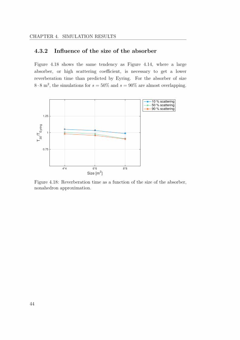
4.3.2 Influence of the size of the absorber
Figure 4.18 shows the same tendency as Figure 4.14, where a largeabsorber, or high scattering coefficient, is necessary to get a lowerreverberation time than predicted by Eyring. For the absorber of size8 · 8 m2, the simulations for s = 50% and s = 90% are almost overlapping.
Size [m2]
4*4 6*6 8*8
T3
0/T
Eyri
ng
0.75
1
1.25
10 % scattering50 % scattering90 % scattering
Figure 4.18: Reverberation time as a function of the size of the absorber,nonahedron approximation.
44

CHAPTER 4. SIMULATION RESULTS
4.4 Simulations in the decahedron room
As for the nonahedron approximation, the inclination angles were keptconstant for the decahedron room. This room is illustrated in Figure 4.19.The dependency on the scattering coefficient and the size of the absorberfollows in section 4.4.1 and 4.4.2. As for the hexahedron and the nona-hedron, the plot of the reverberation time as a function of the size of theabsorber is given by r = T30
TEyring.
Figure 4.19: The room used for the simulations in the decahedronapproximation.
45

CHAPTER 4. SIMULATION RESULTS
4.4.1 Influence of the scattering coefficient
In Figure 4.20, the large floor absorber was used and the dependencyon the scattering coefficent on the reverberation time is plotted. For alow scattering coefficient, s < 20%, the simulated value overlaps with theestimation of Eyring. For a higher scattering coefficient, however, thereis a significant decrease of the simulated reverberation time, compared toSabine’s and Eyring’s values.
Scattering coefficient [%]1 10 20 30 40 50 60 70 80 90
Reverb
era
tion tim
e T
30 [s]
0.5
1
1.5
2
2.5 SabineEyringTUCT T
30,
CI
Figure 4.20: Reverberation time as a function of the scattering coefficient,decahedron approximation and large absorber.
46

CHAPTER 4. SIMULATION RESULTS
4.4.2 Influence of the size of the absorber
As one can see in Figure 4.21, a large absorber and a sufficientscattering coefficient is needed to generate a situation where the simulatedreverberation time is shorter than Eyring’s prediction. For s = 10%, r > 1for the small and medium absorber, and it is only slightly lower than onefor the large absorber.
Size [m2]
4*4 6*6 8*8
T3
0/T
Eyri
ng
0.75
1
1.25
10 % scattering50 % scattering90 % scattering
Figure 4.21: Reverberation time as a function of the size of the absorber,decahedron approximation.
47

CHAPTER 4. SIMULATION RESULTS
4.5 Influence of the room geometry
To investigate the dependency on the number of surfaces in the polyhedra,Figure 4.22 illustrates the reverberation times in the three rooms forscattering coefficients of respectively s = 10%, s = 50% and s = 90 %.The results follow from the simulations with the large absorber of S = 8 ·8m. From the figure, one can see that the relationship is nearly independentof the number of surfaces for a high scattering coefficient. The variationwith geometry is more dominant for a low scattering coefficient.
Polyhedronhexahedron nonahedron decahedron
T3
0/T
Eyri
ng
0.75
1
1.25
10 % scattering50 % scattering90 % scattering
Figure 4.22: Reverberation time for the three polyhedral approximations,large absorber.
48

CHAPTER 4. SIMULATION RESULTS
4.6 Alternative reverberation timeformulae
In chapter 2, four different approaches to a theoretical value of thereverberation time were presented; Millington-Sette and Kuttruff inaddition to Sabine’s and Eyring’s reverberation formulae. Reverberationtimes according to these formulae are presented in Figure 4.23, for the sameroom volumes and surface areas as the polyhedra which were simulated inCATT. The formula of Fitzroy, given in equation 2.25, is not includedin this figure because it assumes a shoe-box shaped room, which is notthe case in the rooms explored in this thesis. The theoretical values arepresented together with the simulated values for a large absorber andrespectively 10%, 50% and 90% scattering.
Polyhedronhexahedron nonahedron decahedron
Reverb
era
tion tim
e T
30 [s]
0.25
0.5
0.75
1
SabineEyringMillington-SetteKuttruffCATT 10 % scatteringCATT 90 % scatteringCATT 90 % scattering
Figure 4.23: Reverberation according to reverberation formulae, fordifferent polyhedra, together with the simulated values from CATT.
49

CHAPTER 4. SIMULATION RESULTS
4.7 Signs of a non-exponential decay
The relationship between the reverberation time based on respectively thefirst 20 dB decrease and the first 30 dB decrease indicates the linearityof the sound decay and thus the diffusivity of the sound field. Thisrelationship r = T20
T30was investigated for the three polyhedra, as a function
of the size of the floor absorber, and is presented in Figures 4.24, 4.25 and4.26.
In the hexahedron, the ratio r ≈ 1, and the relationship appears to belinear for all sizes of the floor absorber and independent of the scatteringcoefficient. The results are more dependent on the scattering coefficientfor the nonahedron and the decahedron, where the large absorber pointsout with the lowest ratio.
Size [m2]
4*4 6*6 8*8
T2
0/T
30
0.8
0.9
1
1.1
1.2
10 % scattering50 % scattering90 % scattering
Figure 4.24: T20/T30 for hexahedron, angle θ = 60o, as a function of thesize of absorber.
50

CHAPTER 4. SIMULATION RESULTS
Size [m2]
4*4 6*6 8*8
T2
0/T
30
0.8
0.9
1
1.1
1.2
10 % scattering50 % scattering90 % scattering
Figure 4.25: T20/T30 for nonahedron as a function of the size of absorber.
Size [m2]
4*4 6*6 8*8
T2
0/T
30
0.8
0.9
1
1.1
1.2
10 % scattering50 % scattering90 % scattering
Figure 4.26: T20/T30 for decahedron as a function of the size of absorber.
51


CHAPTER 5. DISCUSSION
5 Discussion
Chapter 4 presented the results of the simulations in CATT-Acoustic,investigating the concequences of adjusting different parameters in therooms. These results were also compared to theoretical values for thereverberation time. This chapter will discuss the results further. Adiscussion of the validity of the results will then follow, before a suggestionfor further work is presented.
5.1 Investigation of the TUCT mode
The simulations in a shoe-box shaped room in TUCT described in section3.1 were performed to investigate the importance of the number of conesnecessary in a TUCT-estimate for different combinations of scattering andabsorption. The two combinations with a high scattering coefficient gaverooms where the resulting reverberation time is known by Sabine’s andEyring’s formulae.
The examination does not show a clear connection between the number ofrays (N) in a simulation and the resulting reverberation time (T30). TheTUCT estimate does vary, but it is not a clear correlation to the numberof cones. Figures 4.2 and 4.3 give an indication that a low scatteringcoefficient (s = 10%) gives a higher variation between the simulations andthus a higher systematic error, while Figure 4.4 and 4.5 give more stablevalues of the T30.
53
CHAPTER 5. DISCUSSION
The combinations of scattering and absorption in the investigation of theTUCT mode also follow the theory regarding an increase in the scatteringfor a room with non-uniform absorption distribution and the measuredreverberation time. While Sabine’s and Eyring’s values, based on themean free path, show a little variation for one size of the floor absorber,the simulated values are highly dependent on the scattering coefficient.
5.2 Simulations in the hexahedron room
The scattering coefficient, the absorber size and the inclination angle werethe three factors adjusted to investigate the resulting reverberation time inthe hexahedron approximation. The correlation between these factors andthe simulated reverberation time compared to the estimations of Sabineand Eyring will be discussed in this section. In the cases where thescattering coefficient and the inclination angle were adjusted, the largeabsorber was used. When the floor absorber and the inclination anglewere varied, the chosen scattering coefficients were s = 10%, s = 50% ands = 90%.
5.2.1 Influence of the scattering coefficient
Figures 4.7, 4.8, 4.9, 4.10, 4.11, 4.12 and 4.13 in section 4.2.1 showthe dependency on the scattering coefficient for inclination angles ofrespectively θ1 = 35o, θe = 45o, θ3 = 60o, θ4 = 75o, θ5 = 82.5o, θ6 = 87.5o
and θ7 = 90o. The result for θ4 = 60o shows an independency of thescattering coefficient that cannot be found from the other wall inclinationangles. A possible explanation for this independency can be that the floorabsorber has a higher efficiency when the angles of the polyhedron give aperfect approximation of a dome. This follows from the theory presentedin section 2.2.3. However, as will be discussed in section 5.4, the numberof surfaces in a polyhedra does not indicate that a focus effect can be theexplanation.
54

CHAPTER 5. DISCUSSION
For the smallest inclination angles. θ1 = 35o and θ2 = 45o, a low scatteringcoeffient gives a significant longer reverberation time than predicted bySabine and Eyring. This is a reasonable result, and one can see thesame tendency also for larger inclination angles and scattering coefficients = 1%.
For an increasing scattering coefficient, the reverberation time appears tobe less dependent on the inclination angle and the geometry. For θ1 andθ2, the simulated reverberation time approximates Eyring’s and Sabine’svalues also for a high scattering coefficient. In the other simulations,however, the simulated reverberation time appears to be lower than theestimated values, as stated in the problem description.
5.2.2 Influence of the size of the absorber
The figure presented in section 4.2.2 shows an interrelationship betweenthe size of the absorber and the ratio r = T30
TEyring, which becomes lower
relative to the size of the absorber. For the small absorber of Sabs = 4 · 4m2, the estimated and simulated reverberation times are almost identical,giving a ratio r ≈ 1 independent of the scattering. The same result appliesfor a low scattering coefficient and the medium-sized floor absorber. Tolower the ratio of T30
TEyring, one can see that it is necessary to apply a high
scattering coefficient to the room with the medium absorber or to use thelarge floor absorber. A larger absorber, covering most of the floor, gives aresult that is almost independent of the scattering coefficient.
In the latter case, a majority of the rays will hit the absorber, and thusshorten the sound decay in the room to a greater extent than the formulaeof Sabine and Eyring predict. The opposite happens for the small absorber,especially for smaller angles θ resulting in a large floor area compared tothe ceiling area, where a majority of the rays hit the floor outside of theabsorber. A consequence is that a larger part of the rays is reflected, eitherspecularly or diffusely, which prolongs the sound decay.
55

CHAPTER 5. DISCUSSION
5.2.3 Influence of the inclination angle
From Figure 4.15, one can see that the angle between floor and walls inthe hexagon approximation has an influence on the reverberation time.The reverberation time following the formulae of Sabine and Eyring, asgiven in equations 2.7 and 2.17, does not vary significantly. The reasonfor this is that the volume is kept constant for all angles, and that thetotal absorption area only has a minor deviation. However, one can seesome variations in the theoretical values as well. The reason for thesevariations is that CATT-Acoustic calculates the volume of a room basedon the resulting mean free path from a simulation, which may vary, as willbe discussed in section 5.6.3. Smaller angles give simulated values closerto the reverberation times predicted by Sabine and Eyring, with a ratior ≈ 1.
An interesting result is found for θ7 = 90o, the cuboid room, and s = 10%,where the simulated value exceeds the estimated value giving a ratio ofT30
TEyring 1. This is the same result as can be found in in the TUCT-
investigation, illustrated in section 4.1. For higher scattering coefficients,the simulated value lies cloes to Eyring’s prediction.
Figure 4.15 also supports what was stated in section 5.2.1, that thereverberation time is more dependent on the geometry for a low scatteringcoefficient. One can find a significant peak for θ2 = 45o and θ7 = 90o
(the shoe-box shape), where the results for the shoe-box identify as highlydependent on the scattering coefficient.
An inclination angle α3 = 60o gives the perfect approximation of a dome.From the results in section 4.2.3, one can see that the results also for thisgeometry are less dependent on the scattering coefficient and the size ofthe a bsorber, and give a ratio of r = T30
TEyring≈ 1. The connection between
this geometry and the other polyhedra will be discussed further in section5.4.
56

CHAPTER 5. DISCUSSION
5.3 Simulations in the nonahedron and thedecahedron rooms
The simulations in the nonahedron and the decahedron room were donefor a varying scattering coefficient and three different floor absorbers, witha scattering coefficient of the surfaces varying from s = 1.0% to s = 90%.The discussion for the two rooms is presented together in this sectionbecause the results show the same tendency for both polyhedra and thesame parameters were adjusted in the two rooms.
5.3.1 Influence of the scattering coefficient
With the exception of a scattering coefficient of s = 1%, the simulationsfrom the nonahedron room with an absorber of 8 · 8 m2 follows the samepattern as the hexahedron approximation with angle θ = 60o, which is asexpected for the dome approximation.
For a low scattering coefficient, the resulting reverberation time is higherthan what the formulae predict, due to a lower diffusivity in the room. Inthis case, the cone tracing will give a higher amount of specular reflections,and a smaller potential area of where a reflected cone may hit the nextsurface.
The simulations in the decahedron room do not show the same extremeas the nonahedron for a scattering of 1%, where the result givesa reverberation time of approximately the same value as Eyring’sreverberation formula. For higher scattering coefficients, the simulationsin the nonahedron and the decahedron rooms are almost identical.
5.3.2 Influence of the size of the absorber
A certain size of the floor absorber is necessary to finding the relationship inwhich the simulated reverberation time is shorter than Eyring’s estimate.For the small absorber, S = 4 · 4 m2, the results give T30
TEyring> 1, which
57

CHAPTER 5. DISCUSSION
implies a prolonged reverberation time, which is what have been statedfor rooms of other geometries (for instance a shoe-box shape with unevenabsorption distribution) earlier. One can see that a higher value of thescattering coefficient leads to a reverberation time that is less dependenton the size on the absorber. This follows from both Figure 4.18 and 4.21.
5.4 Influence of the room geometry
With a high scattering coefficient, the resulting ratio T30TEyring
is independentof the room geometry, and identical for the three polyhedra. Witha scattering of 10%, the hexahedron stands out with a ratio r < 1independent of the size of the floor absorber. Figures 4.14, 4.18 and4.21 shows the same tendency for the effect of the floor absorber, wherethis effect is largest for a high scattering coefficient. The results of thehexahedron simulations, which has the same ratio of r ≈ 0.88 with thelarge absorber for all scattering coefficients, differs from the nonahedronand the decahedron.
A decahedron is the polyhedral approximation which is closest to thedome shaped room. One could therefore assume a possible focus effectto be stronger in this room. However, this is not the case, and the threepolyhedra gives approximately the same ratio when the scattering is high.This is why a focus effect due to a dome shaped ceiling cannot be claimedto be the reason of why Sabine’s and Eyring’s formulae predicts a longerreverberation time than the simulations.
5.5 Alternative reverberation timeformulae
From Figure 4.23, one can see that the simulated results lie closer thethe Eyring value than the estimations of Millington-Sette and Kuttruff.Sabine’s and Eyring’s values are based on an assumption of a diffuse sound
58
CHAPTER 5. DISCUSSION
field, which is not the case for the polyhedral rooms with uneven absorptioninvestigated in chapter 4.
The Millington-Sette’s formula was introduced with the purpose to bevalid for rooms of uneven absorption distribution. One would thereforeassume this formula to give a better estimate for the rooms examinedin this thesis. However, as the figure shows, Millington-Sette predicts alower value than the simulations in CATT-Acoustic. Using the absorptionconsideration of Kuttruff, the estimate is closer to the one found usingTUCT, but also this value has a significant deviation from the simulationsin CATT-Acoustic. One would assume Kuttruff’s value lie closer to thesimulated values since the situations all have T30 < TEyring, which is therange for the reverberation time in which Kuttruff’s absorption formula isstated to be valid.
The fact that both Millington-Sette and Kuttruff predict a reverberationtime shorter than Eyring and Sabine is an indication that the roomgeometries that have been investigated have provoked the differencebetween the reverberation formulae.
By investigating the deviation in the relations between respectively Eyring,Kuttruff and Millington-Sette and the simulated T30 for different scatter-ing coefficients, the validity of the different formulae can be stated. Thisdeviation is presented in Table 5.1. From these numbers, one can read thatEyring’s formula stands out as the best approach to the result from thesimulations in CATT-Acoustic. The formula of Kuttruff and Millington-Sette both give larger deviations from the true value. They correct, asis the intention of the formulae, for the fact that the absorbtion is un-evenly distributed and the reverberation time therefore has to be lowerthan Eyring’s prediction. However, both formulae can be told to overcom-pensate for this effect.
59

CHAPTER 5. DISCUSSION
Table 5.1: The deviation between simulated reverberation time andtheoretical formulae T30/TFormula.
Polyhedron Sabine Eyring Millington-Sette KuttruffScattering s = 10%
Hexahedron 0.7930 0.8863 1.9329 1.5596Nonahedron 0.7988 0.8927 1.9470 1.5710Decahedron 0.8016 0.8958 1.9538 1.5765
Scattering s = 50%Hexahedron 0.8870 1.0072 2.1777 1.7585Nonahedron 0.8176 0.9284 2.0074 1.6209Decahedron 0.8019 0.9107 1.9690 1.5899
Scattering s = 90%Hexahedron 0.8658 0.9811 2.1239 1.7148Nonahedron 0.7924 0.8979 1.9438 1.5694Decahedron 0.7939 0.8996 1.9475 1.5724
From this table, one can see that there is a large positive deviation forMillington-Sette’s formula and also a noticeable deviation in Kuttruff’sformulae. This indicates that the simulated reverberation time is in somecases more than double the theoretical estimate.
These values could be compared to values presented by Neubauer andKang [34] for their cases of a shoe-box shaped room with an absorbingceiling (α = 0.8) and reflecting walls and floor (α = 0.05). Neubauer andKang use an average over the frequency bands of f = 500 Hz and f = 1kHz, and compare values by the formulae of Sabine, Eyring, Millington-Sette, and also Fitzroy, Arau and Fitzroy-Kuttruff, to simulations withCATT-Acoustic and the radiosity model. In their predictions, two soundsources and one receiver are used and the rooms have a constant diffusionof 10%. In both rooms, the simulated reverberation time is higher thanSabine’s and Eyring’s predictions, which is the classical example stated inthe problem description.
The interesting element is their study of theoretical reverberation. In thefirst room, measuring 10 · 10 · 8 m3, the ratio of rEyring = TEyring
TMillington−Sette
equals r = 1.140.69 = 1.65. The ratio of rSabine = TSabine
TMillington−Settein this room
has a value of rSabine = 1.270.69 = 1.84. For the room measuring 10 · 10 · 3
m3, the ratios equals rEyring = 0.450.28 = 1.61 and rSabine = 0.53
0.28 = 1.89.
60

CHAPTER 5. DISCUSSION
Even if these ratios are not as extreme as what one can find in Table5.1, they give the same tendency of TMillington−Sette TEyring when onlyone surface is absorbing. The value of Fitzroy-Kuttruff, using Kuttruff’sabsorbtion approach as presented in section 2.1.9 in combination withFitzroy’s reverberation formula, lies between Millington-Sette and Eyring,which is the same relation as Kuttruff’s aborption values in combinationwith Eyring’s formula in the study of this thesis.
5.6 Uncertainty and statistics
A source of error that have already been introduced is the length of theimpulse response in the TUCT-prediction. If the IR is too short, there isa risk of a truncation error [29, p. 110], which will lead to a simulatedreverberation time that is shorter than the true value. To avoid sucha situation, the length was set to auto. The length is then based onEyring’s value for the reverberation time. In this study, this length shouldbe acceptable since the rooms studied have the relationship T30 < TEyring.
Other sources of error to be discussed are the locations of the source andthe receiver, the degree of an exponential decay and the computation ofthe volume, which is based on the mean free path.
5.6.1 Placing of the source and receiver
In scale model measurements or full scale measurements of the reverbera-tion time in a room, the measurement setup of sound sources and receiverswould follow the ISO standard for measurements of reverberation timein ordinary rooms [6] and include multiple locations and heights of thesource and the receiver. In this project, however, only one position for thesound source and one position for the receiver were chosen. The reason forthis choice is that the reverberation time is considered a global parameter,and therefore independent of the location. This has been confirmed in aseparate study in CATT-Acoustic which will not be presented in this the-sis. The mean values and the statistical considerations were based on the
61

CHAPTER 5. DISCUSSION
values for the respective frequency bands, which are independent of thefrequency as a consequence of the settings presented in section 3.2.
5.6.2 Signs of a non-exponential decay
In the characteristics of a global paramenter, it follows that the sounddecay is a pure expontential decay, meaning that the reverberation curve,given in dB, follows a linear curve. This is valid in most rooms, butexceptions follow for instance in coupled rooms.
By studies of the relation between T20 and T30, as presented in Figures4.24, 4.25 and 4.26, it is claimed that the two values will be identical ifone has a pure exponential sound decay. T30 is based on the decay from -5dB to -35 dB, while T20 is based on the decay from -5 B to -25 dB. Thereason for excluding the first 5 dB decay is that the first part of the sounddecay is strongly related to the direct sound in a room rather than thereverberation.
From the figures in section 4.7, one can see that the ratio T20/T30 ≈ 1 inall polyhedra for the small and medium floor absorber. In the hexahedron,this relationship also applies for the large absorber, and indicates a pureexponential sound decay. The other polyhedra, and in particular thenonahedron, seems to have a weakness for the large absorber, giving aratio og T20/T30 < 1, which means that the sound decay is not perfectlylinear.
5.6.3 The mean free path and volume considerationsin CATT-Acoustic
In the calculations of the total volume in CATT-Acoustic, the mean freepath is used as a foundation, following from equation 2.5. The mfp is re-lated to the average number of reflections in a ray tracing procedure, whichis not a constant value. The reason that the Sabine and Eyring values havea variation within the same room is that these values are dependent on thevolume V, which is supposed to be constant. A study of the difference in
62
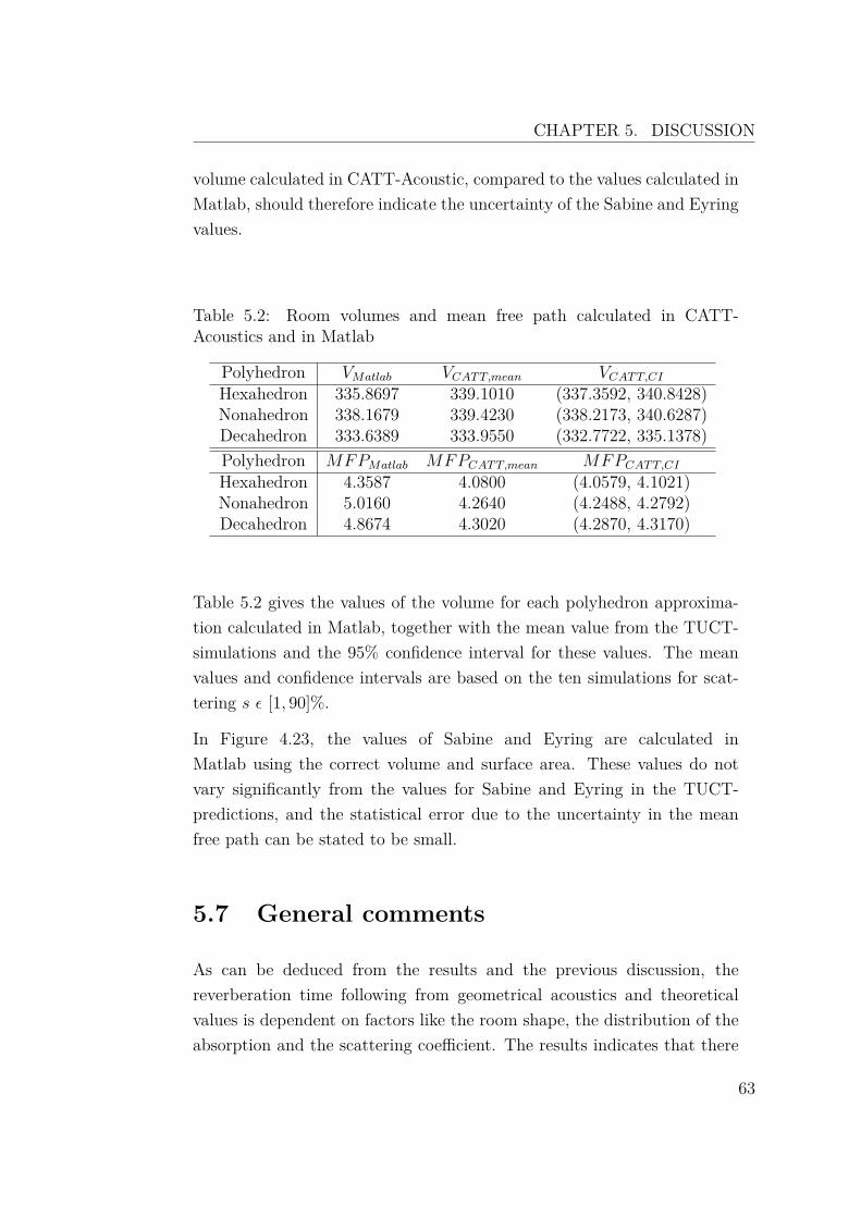
CHAPTER 5. DISCUSSION
volume calculated in CATT-Acoustic, compared to the values calculated inMatlab, should therefore indicate the uncertainty of the Sabine and Eyringvalues.
Table 5.2: Room volumes and mean free path calculated in CATT-Acoustics and in Matlab
Polyhedron VMatlab VCATT,mean VCATT,CIHexahedron 335.8697 339.1010 (337.3592, 340.8428)Nonahedron 338.1679 339.4230 (338.2173, 340.6287)Decahedron 333.6389 333.9550 (332.7722, 335.1378)Polyhedron MFPMatlab MFPCATT,mean MFPCATT,CIHexahedron 4.3587 4.0800 (4.0579, 4.1021)Nonahedron 5.0160 4.2640 (4.2488, 4.2792)Decahedron 4.8674 4.3020 (4.2870, 4.3170)
Table 5.2 gives the values of the volume for each polyhedron approxima-tion calculated in Matlab, together with the mean value from the TUCT-simulations and the 95% confidence interval for these values. The meanvalues and confidence intervals are based on the ten simulations for scat-tering s ε [1, 90]%.
In Figure 4.23, the values of Sabine and Eyring are calculated inMatlab using the correct volume and surface area. These values do notvary significantly from the values for Sabine and Eyring in the TUCT-predictions, and the statistical error due to the uncertainty in the meanfree path can be stated to be small.
5.7 General comments
As can be deduced from the results and the previous discussion, thereverberation time following from geometrical acoustics and theoreticalvalues is dependent on factors like the room shape, the distribution of theabsorption and the scattering coefficient. The results indicates that there
63
CHAPTER 5. DISCUSSION
is a limit for the scattering coefficient around slimit = 20%, where s < slimit
gives simulated reverberation times which are not significantly shorter thanTEyring, and in some cases higher than Eyring’s prediction. The case ofs > slimit does, however, give a ratio of T30
TEyring< 1. The hexahedron with
nclination angle θ = 60o is an exception, and shows an independency ofthe scattering coefficient. As stated earlier, the assumption is that a lowscattering coefficient gives a higher dependency on the room geometry, butthis does not seem to be the case for this study. A low scattering coefficientresults in most cases in a higher reverberation time, but the value for alow scattering coefficient does not seem to be dependent on the polyhedralapproximations.
The formulae of Sabine and Eyring both assume a diffuse sound field,and give the same value for a room of constant volume and averageabsorption, while simulations based on the image source method and raytracing give a variation with the respective factors. The study showsthat neither Sabine, Eyring, Millington-Sette or Kuttruff can predict thesame value for reverberation time as the TUCT-simulations in CATT-Acoustic. While Sabine and Eyring predict a value of the reverberationtime higher than what was obtained in the simulations performed withCATT-Acoustic, Millington-Sette and Kuttruff give lower values than thesimulated. The study shows that the value of Eyring lies closest to thesimulated reverberation time.
The findings of Millington-Sette and Kuttruff both predicting reverbera-tion times shorter than the values found by the TUCT-predictions indicatesthat the polyhedral room geometries in this study have resulted in the sit-uations where the difference between the classical formulae by Sabine andEyring and the correcting formulae by Millington-Sette’ and Kuttruff’sabsorption formulae arises. The reason for these differences lies in theapproach to the absorption coefficient and the absorption distribution.
64

CHAPTER 5. DISCUSSION
5.8 Further work
As a consequence of what have been obtained in this thesis, thereare several topics suggested for further work. It could be interestingto implement as scale model rooms, the rooms on which has beeninvestigated in CATT-Acoustic, to see if the same tendency with ameasured reverberation time lower than what Sabine and Eyring predictscan be found by performing measurements in a scale model. A correctionfor air absorption must then be included.
From the simulations in CATT-Acoustic, one could also study other roomacoustical parameters than the reverberation time and their behavior ina polyhedron room. When studying the local parameters, one has to useseveral positions for the source and receiver, because one cannot assumethese parameters to be the same in all positions.
Only a couple of theoretical approaches to a reverberation time have beeninvestigated in this study, and there exist other alternatives as well. Anexample of a formula to investigate is Arau’s reverberation formula [35].Stephenson and Drechsler also suggest an Anisotropic Reverberation Model(ARM) [2], [36] assuming an anisotropic sound field, which can beinvestigated for the polyhedral rooms. Finally, the approach of Tohyama[37], based on an almost 2-dimentional diffuse field theory, could as wellbe tested on the polyhedra.
65


CHAPTER 6. CONCLUSION
6 Conclusion
In this Master’s thesis, the relationship between estimated reverberationtimes using classical equations and simulated reverberation times usingthe computational program CATT-Acoustic has been studied. Thesesimulations are based on a combination of the image source method and acone tracing-procedure.
The rooms that have been investigated are polyhedral approximations ofa dome. As suggested by Stephenson, a tendency of a focus effect could bethe case for such rooms. This effect could not be found in this study. Therooms implemented in CATT-Acoustic all had hard surfaces of αwall = 2%and a floor absorber on parts of the floor of αfloor = 90%. The parametersvaried for each polyhedron were the size of the floor absorber and thescattering coefficient s. In the hexahedron approximation, also the wallinclination angle was adjusted, from θ = 35o to θ = 90o. For thesecombinations, studies of the reverberation time were performed.
The simulations gave reverberation times shorter than Sabine’s andEyring’s predictions for the polyhedra. It is, however, not possible to cometo a conclusion that the polyhedral dome-approximations give a focusingeffect; by increasing the number of surfaces in the polyhedron, the ratio ofT30
TEyringdid not vary significantly.
A reason for the difference between T30 and TEyring can be a highereffectiveness of the floor absorber when the side walls are tilted and theroom has a saddle roof. The sound rays in the polyhedral approximationsof a dome will then to a greater extent be reflected towards the absorbingfloor, compared to a shoe-box shaped room or a trapezoid room with aninclination angle θ > 90o.
67

CHAPTER 6. CONCLUSION
CATT-Acoustic has two approaches to finding the reverberation time.There is one simpler ray tracing tool, the interactive RT estimate andone more advanced, The Universal Cone Tracer. The latter one was usedin the work of this thesis. The investigations of the TUCT-mode show atendency to a variation in the simulated reverberation time for a varyingnumber of cones. These variations do not follow an increasing number ofcones, but seems to be a random variation.
For the polyhedral rooms, the ratio of T20T30
was calculated to investigatingthe degree of an exponential sound decay. If this ratio r ≈ 1, thereverberation time is independent of the dynamic range of the impulseresponse. r ≈ 1 in the hexahedron, for all three sizes of the floor absorberand for scattering coefficients of respectively s = 10%, s = 50% ands = 90%. In the study of the nonahedron and the decahedron, theratio r < 1 for the large floor absorber and a low scattering coefficient ofs = 10%, and indicates a tendency of a non-exponential decay. However,the ratio becomes r ≈ 1 for a higher scattering coefficient and by using thesmall and medium floor absorber.
The predicted values of Sabine’s and Eyring’s equations are based on thevolume which is related to the mean free path. This value varies within thesame room for consecutive simulations, and is a source of error. The exactvolume of the hexahedron and the nonahedron calculated with Matlab doesnot overlap with the 95%-confidence interval for the simulations in CATT-Acoustics. The confidence interval for the volume of the decahedron does,however, contain the exact value. For all three polyhedra, the mean freepath-calculations from Matlab give a higher value than the simulations.However, the formula implemented in Matlab assumes a diffuse soundfield which cannot be claimed for the polyhedral rooms with an unevendistribution of absorption.
Sabine’s reverberation formula takes into account the room volume andthe average absorption, in addition to a constant which is dependent onsound speed and thus temperature. The distribution of absorption isignored in this equation. As a consequence, Sabine’s formula predictsa reverberation time T → 0.161V
Sfor an absorption coefficient α = 1,
which is counterintuitive. Eyring wanted to correct for this weakness in the
68

CHAPTER 6. CONCLUSION
formula of Sabine, and the formula of Eyring is based on an logarithmicconsideration of the absorption coefficient, which gives the expected valueof T → 0 for α = 1. These two formulae give approximately the samevalues for a low average absorption.
Due to weaknesses also in Eyring’s formula, other approaches of areverberation time formula have been suggested. Two examples areMillington-Sette’s formula and Kuttruff’s formula, which have both beenapplied on the polyhedral rooms in this study. Millington-Sette andKuttruff predict a reverberation time significantly shorter than thesimulations in CATT-Acoustic. The relation of TSabine > TEyring >
T30,TUCT > TKuttruff > TMillington−Sette, indicates that the geometry of therooms considered in this Master’s thesis provoke the difference betweenhow the formulae treat the absorption distribution in a room.
The reverberation times predicted by Millington-Sette and Kuttruffare both significantly shorter than the classical Sabine’s and Eyring’svalues. Moreover, the computer simulations in CATT-Acoustic leads toa reverberation time which is closer to Eyring’s prediction than to thealternative formulae. This implies that Millington-Sette and Kuttruff donot seem to give a better alternative for the reverberation time in thisstudy. For cases like the polyhedral rooms with an uneven distribution ofabsorption, a prediction for the reverberation time should be based on adetailed ray tracing-procedure, like what have been performed in CATT-Acoustic.
69


BIBLIOGRAPHY
Bibliography
[1] H. Arau-Puchades, “The Refurbishment of the Orchestra RehearsalRoom of the Great Theater of Liceu,” Journal of Building Acoustics,vol. 19, no. 1, 2012.
[2] U. Stephensen, “Effects of scattering on the reverberation time - doesthe definition of an ’equivalent scattering area’ make sense?,” ForumAcusticum, 2014.
[3] J. Vennerød, “The Hard Case - Improving Room Acoustics in CuboidRooms by using Diffusors - A student project report on scale modelmeasurements, NTNU, Trondheim,” Published on akutek. info ,2013.
[4] M. Skålevik, “How much scattering is sufficient to soften the hardcase?,” Forum Acusticum, 2014.
[5] M. Skålevik, “Reverberation time - the mother of all room acousticalparameters,” BNAM, published on akutek. info , 2010.
[6] International Organization of Standardization, Acoustics – Measure-ment of room acoustic parameters – Part 2: Reverberation time inordinary rooms, 2008.
[7] Norsonic, “Reverberation time measurements.” Online; ac-cessed 15.05.2015, http://www.norsonic.com/?module=Articles&action=Article.publicOpen&id=503.
[8] M. R. Schroeder, “New method of measuring reverberation time,”Journal of the Acoustical Society of America, vol. 37, pp. 409–412,1965.
71
BIBLIOGRAPHY
[9] Z. Maekawa, J. H. Rindel, and P. Lord, Environmental andArchitectural Acoustics. Spon Press, Taylor and Francis Group,second ed., 2011.
[10] L. Beranek, Concert Halls and Opera Houses: Music, Acoustics, andArchitecture. Springer-Verlag, second ed., 2010.
[11] T. D. Rossing, ed., Springer Handbook of Acoustics. Springer,second ed., 2007.
[12] Byggforsk, “527.300 del 1, sending 2,” Byggforskserien - Byggdetaljer,1998.
[13] H. Kuttruff, Room Acoustics. Spon Press, Taylor and Francis Group,fifth ed., 2009.
[14] M. Skålevik, “Diffusivity and its significance to effective seatabsorption in concert halls,” Published on akutek. info .
[15] R. O. Neubauer, “Prediction of reverberation time in rectangularrooms with non uniformly distributed absorption using a newformula,” Acustica 2000, 2000.
[16] W. C. Sabine, Collected Papers on Acoustics. Harvard UniversityPress, 1922.
[17] C. F. Eyring, “Reverberation time in "dead" rooms,” The Journal ofthe Acoustic Society of America, vol. 1, pp. 217–241, 1929.
[18] G. Millington, “A modified formula for reverberation,” The Journalof the Acoustic Society of America, vol. 4, pp. 69–82, 1932.
[19] W. J. Sette, “A new reverberation time formula,” The Journal of theAcoustic Society of America, vol. 4, pp. 193–210, 1933.
[20] L. E. Kinsler, A. R. Frey, A. B. Coppens, and J. V. Sanders,Fundamentals of Acoustics. John Wiley & Sons Inc., fourth ed., 2000.
[21] D. Fitzroy, “Reverberation formula which seems to be more accuratewith nonuniform distribution of absorption,” The Journal of theAcoustic Society of America, vol. 31, no. 7, pp. 893–897, 1950.
72

BIBLIOGRAPHY
[22] H. Kuttruff, Room Acoustics. Spon Press, Taylor and Francis Group,fourth ed., 2000.
[23] International Organization of Standardization, Acoustics – Measure-ment of the reverberation time with reference to other acoustical pa-rameters, 1997.
[24] U. Stephensen and H. Winkler, “Nachhallzeit-regulierung von audi-torien durch neigung der seitenwände,” Fraunhofter-Institut für Bau-physic, 1991.
[25] U. Stephensen, “On the influence of the ceiling profile on thedistribution of the room acoustical parameters and the reverberationtime,” International Symposium on Room Acoustics, 2007.
[26] M. Barron, Auditorium Acoustics and Architectural Design. E & FNSpon, first ed., 1993.
[27] A. Krokstad, S. Strøm, and S. Sørsdal, “Calculating the acousticalroom response by the use of a ray tracing technique,” Journal of Soundand Vibration, vol. 8, pp. 118–125, 1968.
[28] B. I. Dalenbäck, “Engineering principles and techniques in roomacoustics prediction,” BNAM, 2010.
[29] CATT-Acoustic introduction manual.
[30] CATT-Acoustic TUCT manual.
[31] CATT-Acoustic v9: Computer simulation program. 2011, http://www.catt.se.
[32] K. Rottmann, Matematisk formelsamling, vol. 10. Spektrum forlag,2008.
[33] R. E. Walpole, R. H. Myers, S. L. Myers, and K. Ye, Probabilityand Statistics for Engineers and Scientists. Pearson EducationInternational, eight ed., 2007.
[34] J. Kang and R. O. Neubauer, “Predicting reverberation time:Comparison between analytic formulae and computer simulation,”International Congresses on Acoustics, 2001.
73
BIBLIOGRAPHY
[35] H. Arau-Puchades, “An improved reverberation formula,” Acoustica- International Journal of Acoustics, vol. 65, pp. 163–180, 1988.
[36] S. Drechsler and U. Stephenson, “A calculation model for anisotropicreverberation with specular and diffuse reflections,” DAGA - Darm-stadt, 2012.
[37] M. Tohyama and A. Suzuki, “Reverberation time in an almost-two-dimentional diffuse field,” Journal of Sound and Vibration, vol. 111,pp. 391–398, 1986.
74

APPENDIX A. TABLES
A Tables
A.1 Coordinates for the hexahedron
Table A.1 gives the coordinates for the hexahedron room given differentinclination angles, for a constant volume and room height.
Table A.1: Corners of the polyhedra, given different inclination angles.
Angle Θ A B C35 o 7.1121 0.3124 4.761645 o 6.3487 1.5871 4.761660 o 5.4982 2.7491 4.761675 o 4.8210 3.5452 4.761682.5 o 4.5058 3.8819 4.761687.5 o 4.3028 4.0949 4.761690 o 4.1993 4.1993 4.7616
I

APPENDIX A. TABLES
A.2 Absorption coefficients
Table A.2 [20, p. 341] gives the absorption coefficients for two materials,corresponding to the absorption coefficients used in the simulations inCATT-Acoustic.
Table A.2: Absorption coefficients.
Material 125 Hz 250 Hz 500 Hz 1 KHz 2 KHz 4 KHzLinoleum floor on concrete 0.02 0.03 0.03 0.03 0.03 0.02
Perforated panel over isolation
blanket, 10 % open area 0.20 0.90 0.90 0.90 0.85 0.85
II

APPENDIX B. MEAN VALUES
B Mean values
Scattering coefficient [%]1 10 20 30 40 50 60 70 80 90
Reverb
era
tion tim
e T
30 [s]
0.5
1
1.5
2
2.5
3 Hexahedron 35o
Hexahedron 45o
Hexahedron 60o
Hexahedron 75o
Hexahedron 82.5o
Hexahedron 87.5o
Hexahedron 90o
NonahedronDecahedron
Figure B.1: The mean values for the simulations of polyhedra with largefloor absorber.
III

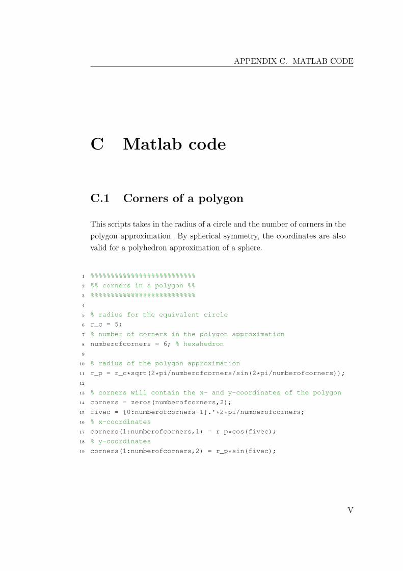
APPENDIX C. MATLAB CODE
C Matlab code
C.1 Corners of a polygon
This scripts takes in the radius of a circle and the number of corners in thepolygon approximation. By spherical symmetry, the coordinates are alsovalid for a polyhedron approximation of a sphere.
1 %%%%%%%%%%%%%%%%%%%%%%%%%%
2 %% corners in a polygon %%
3 %%%%%%%%%%%%%%%%%%%%%%%%%%
4
5 % radius for the equivalent circle
6 r_c = 5;
7 % number of corners in the polygon approximation
8 numberofcorners = 6; % hexahedron
9
10 % radius of the polygon approximation
11 r_p = r_c*sqrt(2*pi/numberofcorners/sin(2*pi/numberofcorners));
12
13 % corners will contain the x- and y-coordinates of the polygon
14 corners = zeros(numberofcorners,2);
15 fivec = [0:numberofcorners-1].'*2*pi/numberofcorners;
16 % x-coordinates
17 corners(1:numberofcorners,1) = r_p*cos(fivec);
18 % y-coordinates
19 corners(1:numberofcorners,2) = r_p*sin(fivec);
V


APPENDIX C. MATLAB CODE
C.2 Read out from .txt-file
In this script, a .txt-file from a TUCT-predition is read to find thereverberation times TSabine, TEyring, T30, T20 and T15.
1 %%%%%%%%%%%%%%%%%%%%
2 %% read TUCT-file %%
3 %%%%%%%%%%%%%%%%%%%%
4
5 inputfile = 'TUCT_C3_3_10.txt'; % name of TUCT-file
6
7 % open TUCT-file
8 fid = fopen(inputfile,'r');
9 if fid == 0
10 error(['ERROR: The file ',inputfile,' could not be opened.'])
11 end
12 B = fread(fid,inf,'char').';
13 fclose(fid);
14
15 % replace , by .
16 iv = find(B ==',');
17 B(iv) = '.';
18
19 stringtofind = '"s"';
20 iv_spaces = regexp(setstr(B),stringtofind);
21
22 stringtofind = '"RT''"';
23 iv_start = regexp(setstr(B),stringtofind);
24
25 % trim text from file
26 B = B(iv_start:iv_spaces(end));
27
28 % find lines that start with "(E)" and "s" in trimmed text file
29 stringtofind = '\(E\)';
30 iv_Epos = regexp(setstr(B),stringtofind);
31
32 stringtofind = '"s"';
33 iv_spos = regexp(setstr(B),stringtofind);
34
35 % find values for $T_30$, $T_20$ and $T_15$
VII

APPENDIX C. MATLAB CODE
36 T15string = setstr(B(iv_Epos(3)+4:iv_spos(8)));
37 T20string = setstr(B(iv_Epos(4)+4:iv_spos(11)));
38 T30string = setstr(B(iv_Epos(5)+4:iv_spos(14)));
39
40 % one vector contains values for all eight octave bands.
41 iv_15 = find(T15string =='.');
42 T15values = zeros(1,8);
43 for ii = 1:8
44 T15values(ii) = str2num(T15string(iv_15(ii)-2:iv_15(ii)+2));
45 end
46
47 % one vector contains values for all eight octave bands.
48 iv_20 = find(T20string =='.');
49 T20values = zeros(1,8);
50 for ii = 1:8
51 T20values(ii) = str2num(T20string(iv_20(ii)-2:iv_20(ii)+2));
52 end
53
54 % one vector contains values for all eight octave bands.
55 iv_30 = find(T30string =='.');
56 T30values = zeros(1,8);
57 for ii = 1:8
58 T30values(ii) = str2num(T30string(iv_30(ii)-2:iv_30(ii)+2));
59 end
60
61 % Find values for Eyring and Sabine
62 stringtofind = 'Sabine';
63 iv_Sabine = regexp(setstr(B),stringtofind);
64 TSabinestring = setstr(B_A_1(iv_Sabine+7:iv_spos(16)));
65
66 stringtofind = 'Eyring';
67 iv_Eyring = regexp(setstr(B),stringtofind);
68 TEyringstring = setstr(B(iv_Eyring+7:iv_spos(17)));
69
70 % one vector contains values for all eight octave bands.
71 iv_Sabine = find(TSabinestring_A_1=='.');
72 Sabinevalues = zeros(1,8);
73 for ii = 1:length(iv)
74 Sabinevalues(ii) = str2num(TSabinestring(iv(ii)-2:iv(ii)+2));
75 end
76
77 % one vector contains values for all eight octave bands.
VIII

APPENDIX C. MATLAB CODE
78 iv_Eyring = find(TEyringstring =='.');
79 Eyringvalues = zeros(1,8);
80 for ii = 1:length(iv)
81 Eyringvalues(ii) = str2num(TEyringstring(iv(ii)-2:iv(ii)+2));
82 end
IX