roofit - wordpress.com · roofit • introduction • basic functionality ... • visual...
TRANSCRIPT

Wouter Verkerke, NIKHEF
RooFit • Introduction
• Basic functionality
• Addition and convolution
• Building multidimensional models
• Managing data, discrete variables and simultaneous fits
• More on likelihood calculation and minimization
• Validation studies

Wouter Verkerke, NIKHEF
Introduction & Overview 1 • Introduction
• Some basics statistics
• RooFit design philosophy

Wouter Verkerke, NIKHEF
Introduction – Purpose
Model the distribution of observables x in terms of
• Physical parameters of interest p
• Other parameters q to describe detector effects
(resolution,efficiency,…)
Probability density function F(x;p,q)
• normalized over allowed range of the observables x w.r.t the parameters p and q
RooFit

Wouter Verkerke, NIKHEF
Introduction -- Focus: coding a probability density function
• Focus on one practical aspect of many data analysis in HEP: How do you formulate your p.d.f. in ROOT – For ‘simple’ problems (gauss, polynomial), ROOT built-in models
well sufficient
– But if you want to do unbinned ML fits, use non-trivial functions, or work with multidimensional functions you are quickly running into trouble
Wouter Verkerke, NIKHEF
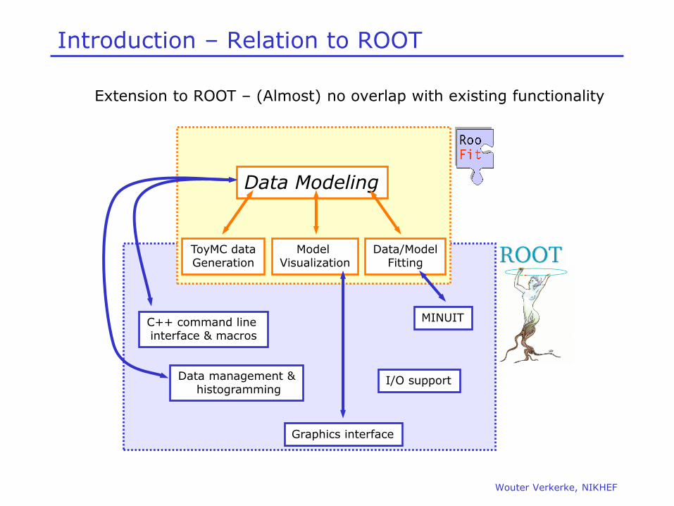
Introduction – Relation to ROOT
C++ command line interface & macros
Data management & histogramming
Graphics interface
I/O support
MINUIT
ToyMC data Generation
Data/Model Fitting
Data Modeling
Model Visualization
Extension to ROOT – (Almost) no overlap with existing functionality
Wouter Verkerke, NIKHEF
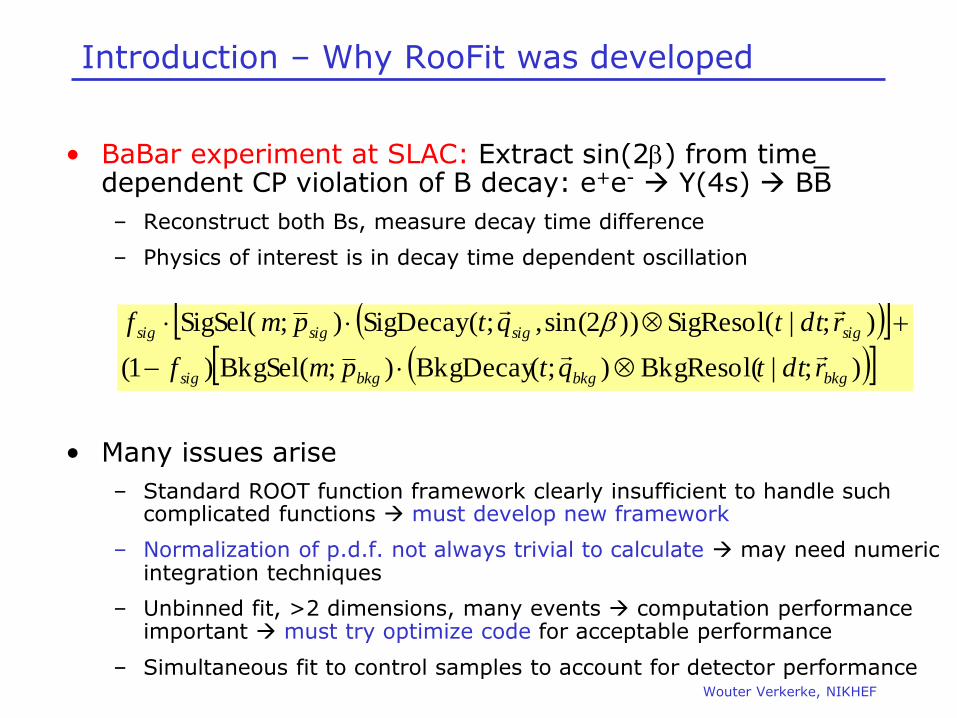
Introduction – Why RooFit was developed
• BaBar experiment at SLAC: Extract sin(2b) from time dependent CP violation of B decay: e+e- Y(4s) BB
– Reconstruct both Bs, measure decay time difference
– Physics of interest is in decay time dependent oscillation
• Many issues arise
– Standard ROOT function framework clearly insufficient to handle such complicated functions must develop new framework
– Normalization of p.d.f. not always trivial to calculate may need numeric integration techniques
– Unbinned fit, >2 dimensions, many events computation performance important must try optimize code for acceptable performance
– Simultaneous fit to control samples to account for detector performance
);|BkgResol();(BkgDecay);BkgSel()1(
);|SigResol())2sin(,;(SigDecay);SigSel(
bkgbkgbkgsig
sigsigsigsig
rdttqtpmf
rdttqtpmf
b

Wouter Verkerke, NIKHEF
Mathematic – Probability density functions
• Probability Density Functions describe probabilities, thus
– All values most be >0
– The total probability must be 1 for each p, i.e.
– Can have any number of dimensions
• Note distinction in role between parameters (p) and observables (x)
– Observables are measured quantities
– Parameters are degrees of freedom in your model
1),(max
min
x
x
xdpxg
1)( dxxF 1),( dxdyyxF
Wouter Verkerke, NIKHEF
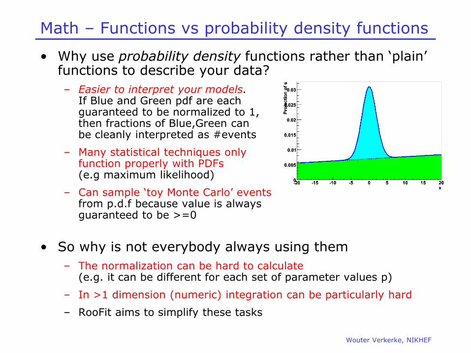
Math – Functions vs probability density functions
• Why use probability density functions rather than ‘plain’ functions to describe your data?
– Easier to interpret your models. If Blue and Green pdf are each guaranteed to be normalized to 1, then fractions of Blue,Green can be cleanly interpreted as #events
– Many statistical techniques only function properly with PDFs (e.g maximum likelihood)
– Can sample ‘toy Monte Carlo’ events from p.d.f because value is always guaranteed to be >=0
• So why is not everybody always using them
– The normalization can be hard to calculate (e.g. it can be different for each set of parameter values p)
– In >1 dimension (numeric) integration can be particularly hard
– RooFit aims to simplify these tasks

Wouter Verkerke, NIKHEF
Math – Event generation
• For every p.d.f, can generate ‘toy’ event sample as follows
– Determine maximum PDF value by repeated random sample
– Throw a uniform random value (x) for the observable to be generated
– Throw another uniform random number between 0 and fmax If ran*fmax < f(x) accept x as generated event
– More efficient techniques exist (discussed later)
f(x)
x
fmax

Wouter Verkerke, NIKHEF
Math – What is an estimator?
• An estimator is a procedure giving a value for a parameter or a property of a distribution as a function of the actual data values, i.e.
• A perfect estimator is
– Consistent:
– Unbiased – With finite statistics you get the right answer on average
– Efficient
– There are no perfect estimators for real-life problems
i
i
i
i
xN
xV
xN
x
2)(1
)(ˆ
1)(ˆ
Estimator of the mean
Estimator of the variance
aan )ˆ(lim
2)ˆˆ()ˆ( aaaV This is called the Minimum Variance Bound

Wouter Verkerke, NIKHEF
Math – The Likelihood estimator
• Definition of Likelihood
– given D(x) and F(x;p)
– For convenience the negative log of the Likelihood is often used
• Parameters are estimated by maximizing the Likelihood, or equivalently minimizing –log(L)
)...;();();()(i.e.,);()( 210 pxFpxFpxFpLpxFpLi
i
i
i pxFpL );(ln)(ln
0)(ln
ˆ
ii pp
pd
pLd
Functions used in likelihoods must be Probability Density Functions:
0);(,1);( pxFxdpxF
Wouter Verkerke, NIKHEF
p
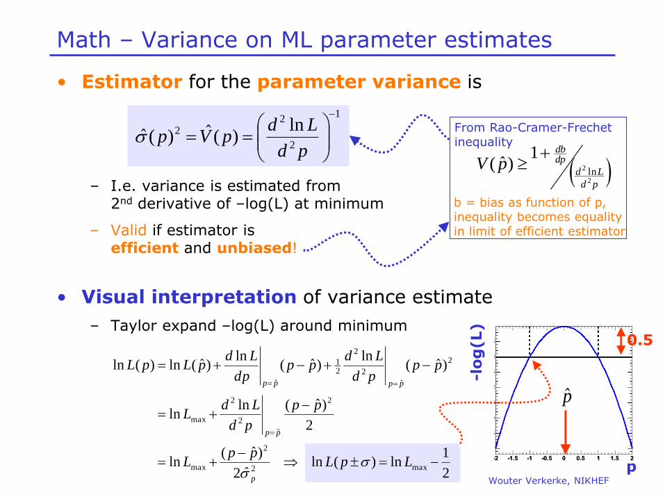
Math – Variance on ML parameter estimates
• Estimator for the parameter variance is
– I.e. variance is estimated from 2nd derivative of –log(L) at minimum
– Valid if estimator is efficient and unbiased!
• Visual interpretation of variance estimate
– Taylor expand –log(L) around minimum
1
2
22 ln
)(ˆ)(ˆ
pd
LdpVp
pd
Ld
dpdb
pV2
2 ln
1)ˆ(
From Rao-Cramer-Frechet inequality
b = bias as function of p, inequality becomes equality in limit of efficient estimator
2
1ln)(ln
ˆ2
)ˆ(ln
2
)ˆ(lnln
)ˆ(ln
)ˆ(ln
)ˆ(ln)(ln
max2
2
max
2
ˆ
2
2
max
2
ˆ
2
2
21
ˆ
LpLpp
L
pp
pd
LdL
pppd
Ldpp
dp
LdpLpL
p
pp
pppp
-lo
g(L)
p̂
0.5
Wouter Verkerke, NIKHEF
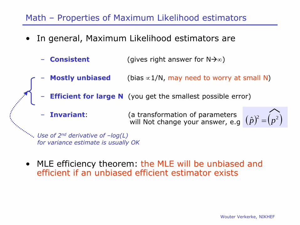
Math – Properties of Maximum Likelihood estimators
• In general, Maximum Likelihood estimators are
– Consistent (gives right answer for N)
– Mostly unbiased (bias 1/N, may need to worry at small N)
– Efficient for large N (you get the smallest possible error)
– Invariant: (a transformation of parameters will Not change your answer, e.g
• MLE efficiency theorem: the MLE will be unbiased and efficient if an unbiased efficient estimator exists
22ˆ pp
Use of 2nd derivative of –log(L) for variance estimate is usually OK
Wouter Verkerke, NIKHEF
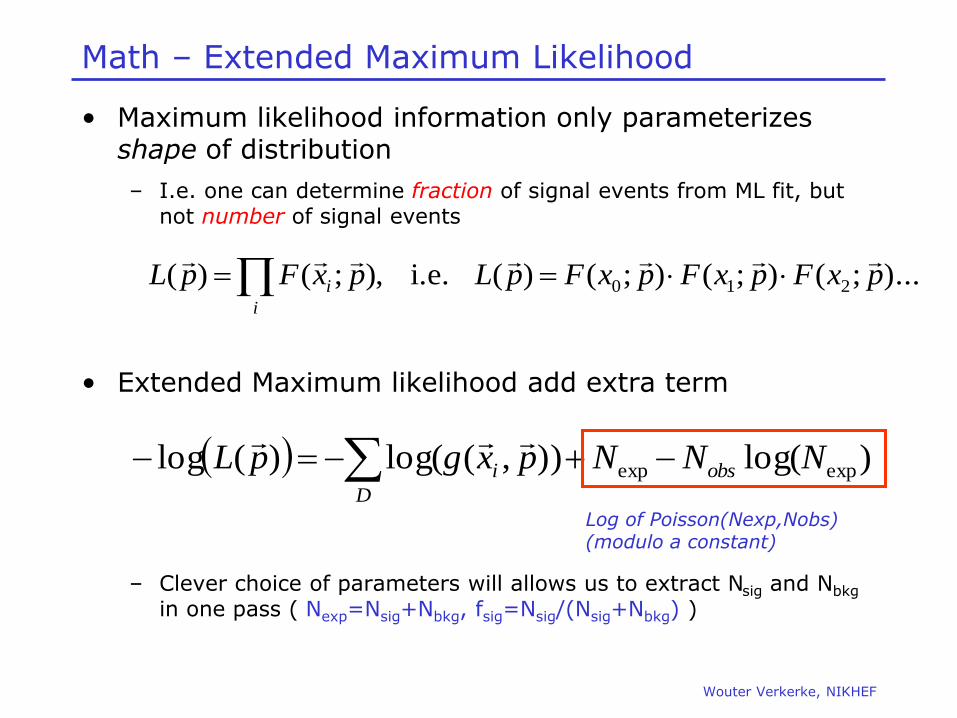
Math – Extended Maximum Likelihood
• Maximum likelihood information only parameterizes shape of distribution
– I.e. one can determine fraction of signal events from ML fit, but not number of signal events
• Extended Maximum likelihood add extra term
– Clever choice of parameters will allows us to extract Nsig and Nbkg in one pass ( Nexp=Nsig+Nbkg, fsig=Nsig/(Nsig+Nbkg) )
)...;();();()(i.e.,);()( 210 pxFpxFpxFpLpxFpLi
i
)log()),(log()(log expexp NNNpxgpL obs
D
i
Log of Poisson(Nexp,Nobs) (modulo a constant)
Wouter Verkerke, NIKHEF
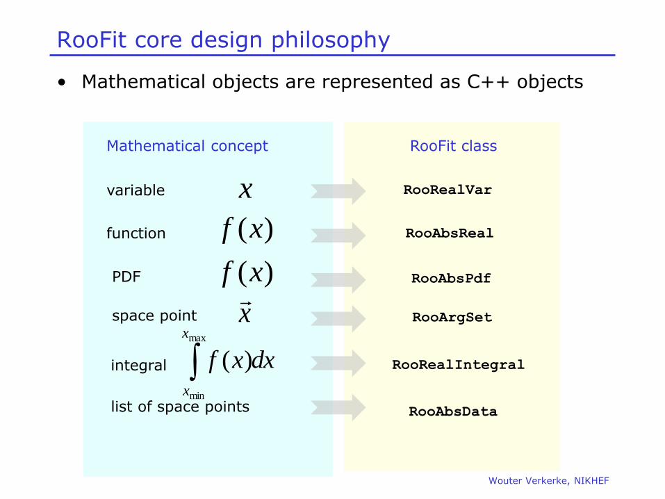
RooFit core design philosophy
• Mathematical objects are represented as C++ objects
variable RooRealVar
function RooAbsReal
PDF RooAbsPdf
space point RooArgSet
list of space points RooAbsData
integral RooRealIntegral
RooFit class Mathematical concept
)(xf
x
x
dxxf
x
x
max
min
)(
)(xf
Wouter Verkerke, NIKHEF
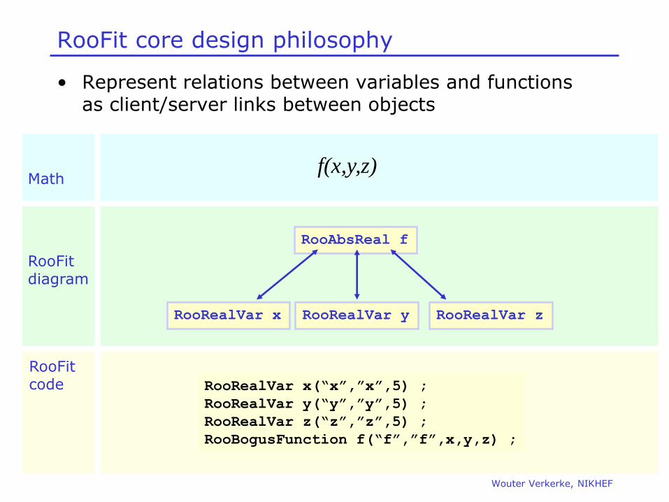
RooFit core design philosophy
• Represent relations between variables and functions as client/server links between objects
f(x,y,z)
RooRealVar x RooRealVar y RooRealVar z
RooAbsReal f
RooRealVar x(“x”,”x”,5) ;
RooRealVar y(“y”,”y”,5) ;
RooRealVar z(“z”,”z”,5) ;
RooBogusFunction f(“f”,”f”,x,y,z) ;
Math
RooFit diagram
RooFit code
Wouter Verkerke, NIKHEF
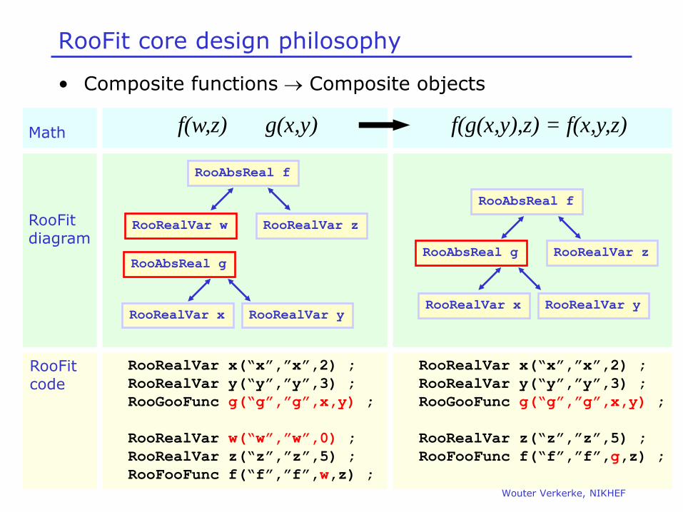
RooFit core design philosophy
• Composite functions Composite objects
g(x,y)
RooRealVar x RooRealVar y
f(w,z) f(g(x,y),z) = f(x,y,z)
RooRealVar x RooRealVar y
RooAbsReal g RooAbsReal g RooRealVar z
RooAbsReal f
RooRealVar w RooRealVar z
RooAbsReal f
RooRealVar x(“x”,”x”,2) ;
RooRealVar y(“y”,”y”,3) ;
RooGooFunc g(“g”,”g”,x,y) ;
RooRealVar z(“z”,”z”,5) ;
RooFooFunc f(“f”,”f”,g,z) ;
RooRealVar x(“x”,”x”,2) ;
RooRealVar y(“y”,”y”,3) ;
RooGooFunc g(“g”,”g”,x,y) ;
RooRealVar w(“w”,”w”,0) ;
RooRealVar z(“z”,”z”,5) ;
RooFooFunc f(“f”,”f”,w,z) ;
Math
RooFit diagram
RooFit code
Wouter Verkerke, NIKHEF
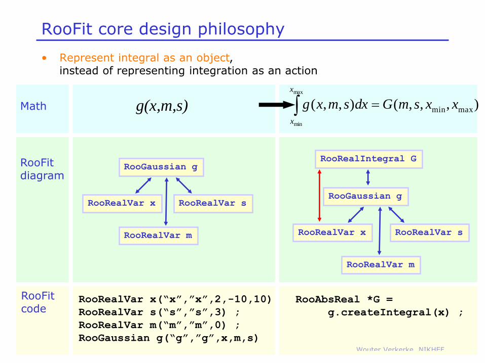
RooFit core design philosophy
• Represent integral as an object, instead of representing integration as an action
g(x,m,s) ),,,(),,( maxmin
max
min
xxsmGdxsmxg
x
x
RooRealIntegral G
RooRealVar x
RooRealVar m
RooRealVar s
RooGaussian g RooRealVar x
RooRealVar m
RooRealVar s
RooGaussian g
RooAbsReal *G =
g.createIntegral(x) ;
RooRealVar x(“x”,”x”,2,-10,10)
RooRealVar s(“s”,”s”,3) ;
RooRealVar m(“m”,”m”,0) ;
RooGaussian g(“g”,”g”,x,m,s)
Math
RooFit diagram
RooFit code
Wouter Verkerke, NIKHEF
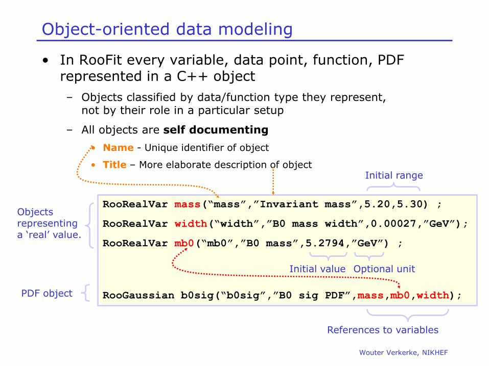
Object-oriented data modeling
• In RooFit every variable, data point, function, PDF represented in a C++ object
– Objects classified by data/function type they represent, not by their role in a particular setup
– All objects are self documenting
• Name - Unique identifier of object
• Title – More elaborate description of object
RooRealVar mass(“mass”,”Invariant mass”,5.20,5.30) ;
RooRealVar width(“width”,”B0 mass width”,0.00027,”GeV”);
RooRealVar mb0(“mb0”,”B0 mass”,5.2794,”GeV”) ;
RooGaussian b0sig(“b0sig”,”B0 sig PDF”,mass,mb0,width);
Objects representing a ‘real’ value.
PDF object
Initial range
Initial value Optional unit
References to variables
Wouter Verkerke, NIKHEF
RooFit designed goals for easy-of-use in macros
• Mathematical concepts mimicked as much as possible in class design
– Intuitive to use
• Every object that can be constructed through composition should be fully functional
– No implementation level restrictions
– No zombie objects
• All methods must work on all objects
– Integration, toyMC generation, etc
– No half-working classes

Wouter Verkerke, NIKHEF
Basic Functionality 2 • Creating a p.d.f
• Basic fitting, plotting, event generation
• Some details on normalization, event generation
• Library of basic shapes (including non-parametric shapes)
Wouter Verkerke, NIKHEF
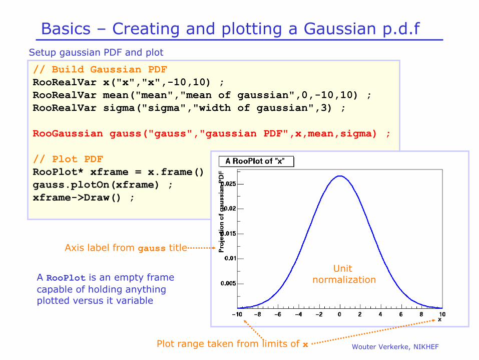
Basics – Creating and plotting a Gaussian p.d.f
// Build Gaussian PDF
RooRealVar x("x","x",-10,10) ;
RooRealVar mean("mean","mean of gaussian",0,-10,10) ;
RooRealVar sigma("sigma","width of gaussian",3) ;
RooGaussian gauss("gauss","gaussian PDF",x,mean,sigma) ;
// Plot PDF
RooPlot* xframe = x.frame() ;
gauss.plotOn(xframe) ;
xframe->Draw() ;
Plot range taken from limits of x
Axis label from gauss title
Unit normalization
Setup gaussian PDF and plot
A RooPlot is an empty frame
capable of holding anything plotted versus it variable
Wouter Verkerke, NIKHEF
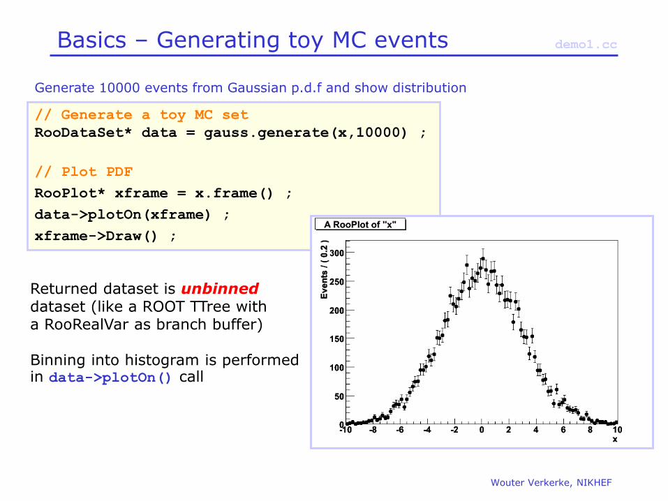
Basics – Generating toy MC events
// Generate a toy MC set
RooDataSet* data = gauss.generate(x,10000) ;
// Plot PDF
RooPlot* xframe = x.frame() ;
data->plotOn(xframe) ;
xframe->Draw() ;
demo1.cc
Generate 10000 events from Gaussian p.d.f and show distribution
Returned dataset is unbinned dataset (like a ROOT TTree with a RooRealVar as branch buffer) Binning into histogram is performed in data->plotOn() call
Wouter Verkerke, NIKHEF
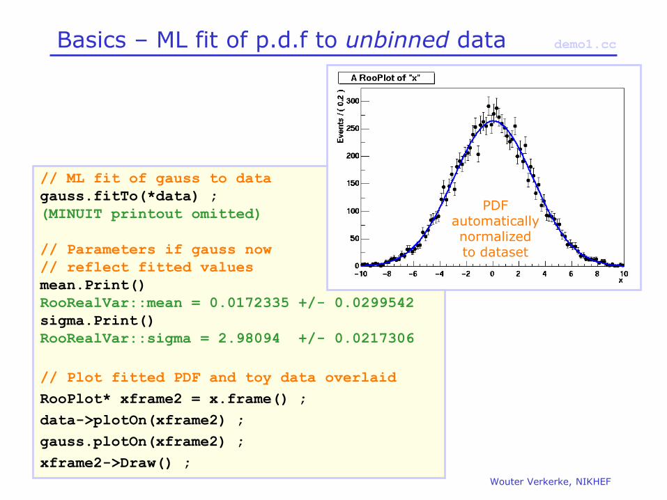
Basics – ML fit of p.d.f to unbinned data
// ML fit of gauss to data
gauss.fitTo(*data) ;
(MINUIT printout omitted)
// Parameters if gauss now
// reflect fitted values
mean.Print()
RooRealVar::mean = 0.0172335 +/- 0.0299542
sigma.Print()
RooRealVar::sigma = 2.98094 +/- 0.0217306
// Plot fitted PDF and toy data overlaid
RooPlot* xframe2 = x.frame() ;
data->plotOn(xframe2) ;
gauss.plotOn(xframe2) ;
xframe2->Draw() ;
demo1.cc
PDF automatically normalized to dataset
Wouter Verkerke, NIKHEF
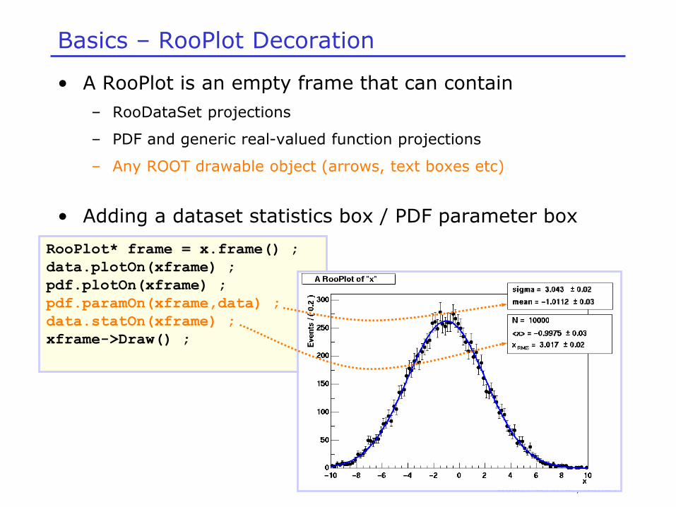
Basics – RooPlot Decoration
• A RooPlot is an empty frame that can contain
– RooDataSet projections
– PDF and generic real-valued function projections
– Any ROOT drawable object (arrows, text boxes etc)
• Adding a dataset statistics box / PDF parameter box
RooPlot* frame = x.frame() ;
data.plotOn(xframe) ;
pdf.plotOn(xframe) ;
pdf.paramOn(xframe,data) ;
data.statOn(xframe) ;
xframe->Draw() ;
Wouter Verkerke, NIKHEF
Basics – RooPlot decoration
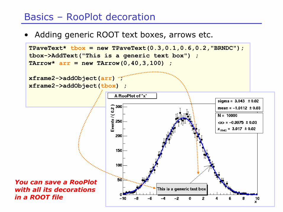
• Adding generic ROOT text boxes, arrows etc.
TPaveText* tbox = new TPaveText(0.3,0.1,0.6,0.2,"BRNDC");
tbox->AddText("This is a generic text box") ;
TArrow* arr = new TArrow(0,40,3,100) ;
xframe2->addObject(arr) ;
xframe2->addObject(tbox) ;
You can save a RooPlot with all its decorations in a ROOT file

Wouter Verkerke, NIKHEF
Basics – Observables and parameters of Gauss
• Class RooGaussian has no intrinsic notion of distinction
between observables and parameters
• Distinction always implicit in use context with dataset
– x = observable (as it is a variable in the dataset)
– mean,sigma = parameters
• Choice of observables (for unit normalization) always passed to gauss.getVal()
gauss.getVal() ; // Not normalized (i.e. this is _not_ a pdf)
gauss.getVal(x) ; // Guarantees Int[xmin,xmax] Gauss(x,m,s)dx==1
gauss.getVal(s) ; // Guarantees Int[smin,smax] Gauss(x,m,s)ds==1
Wouter Verkerke, NIKHEF
How does it work – Normalization
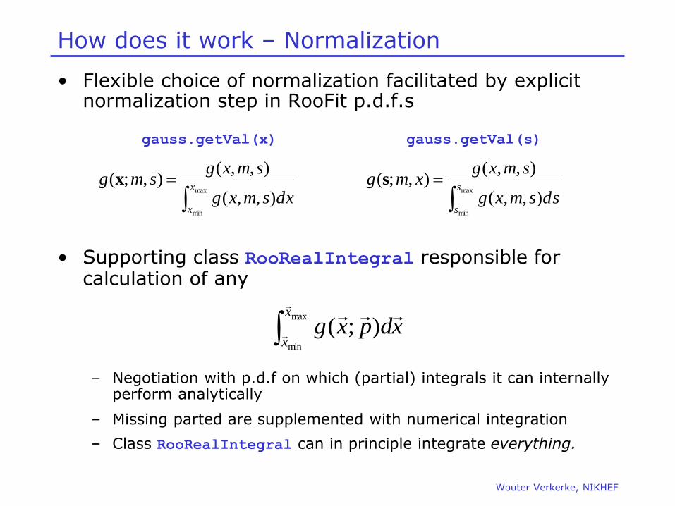
• Flexible choice of normalization facilitated by explicit normalization step in RooFit p.d.f.s
• Supporting class RooRealIntegral responsible for calculation of any
– Negotiation with p.d.f on which (partial) integrals it can internally perform analytically
– Missing parted are supplemented with numerical integration
– Class RooRealIntegral can in principle integrate everything.
max
min
),,(
),,(),;(
x
xdxsmxg
smxgsmg x
max
min
),,(
),,(),;(
s
sdssmxg
smxgxmg s
gauss.getVal(x) gauss.getVal(s)
max
min
);(x
xxdpxg

Wouter Verkerke, NIKHEF
How does it work – Normalization
• A peak in the code of class RooGaussian
// Raw (unnormalized value) of Gaussian
Double_t RooGaussian::evaluate() const {
Double_t arg= x - mean;
return exp(-0.5*arg*arg/(sigma*sigma)) ;
}
// Advertise that x can be integrated internally
Int_t RooGaussian::getAnalyticalIntegral(RooArgSet& allVars,
RooArgSet& analVars, const char* /*rangeName*/) const {
if (matchArgs(allVars,analVars,x)) return 1 ;
return 0 ;
}
// Implementation of analytical integral over x
Double_t RooGaussian::analyticalIntegral(Int_t code,
const char* rname) const {
static const Double_t root2 = sqrt(2.) ;
static const Double_t rootPiBy2 = sqrt(atan2(0.0,-1.0)/2.0);
Double_t xscale = root2*sigma;
return rootPiBy2*sigma*(RooMath::erf((x.max(rname)-mean)/xscale)
-RooMath::erf((x.min(rname)-mean)/xscale));
}
Wouter Verkerke, NIKHEF
Basics – Integrals over p.d.f.s
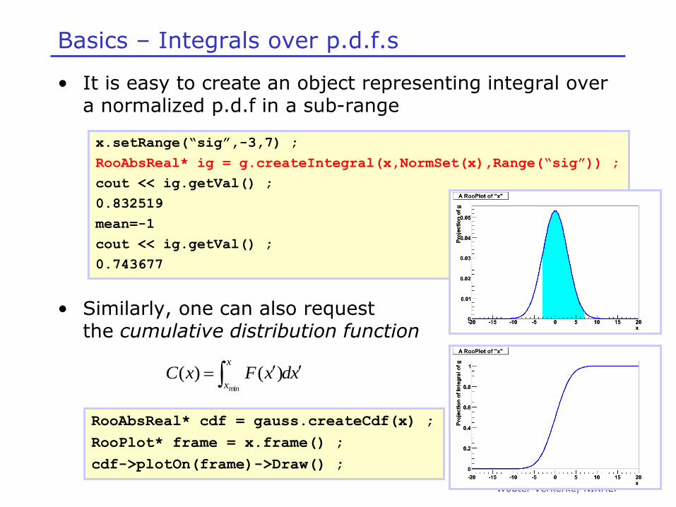
• It is easy to create an object representing integral over a normalized p.d.f in a sub-range
• Similarly, one can also request the cumulative distribution function
x.setRange(“sig”,-3,7) ;
RooAbsReal* ig = g.createIntegral(x,NormSet(x),Range(“sig”)) ;
cout << ig.getVal() ;
0.832519
mean=-1
cout << ig.getVal() ;
0.743677
xdxFxCx
x
min
)()(
RooAbsReal* cdf = gauss.createCdf(x) ;
RooPlot* frame = x.frame() ;
cdf->plotOn(frame)->Draw() ;

Wouter Verkerke, NIKHEF
How does it work – toy event generation
• By default RooFit implements an accept/reject sampling technique to generate toy events from a p.d.f.
1) Determine maximum of function fmax
2) Throw random number x
3) Throw another random number y
4) If y<f(x)/fmax keep x, otherwise return to step 2)
x
y
fmax

Wouter Verkerke, NIKHEF
How does it work – toy event generation
• Accept/reject method can be very inefficient
– Generating efficiency is
– Efficiency is very low for narrowly peaked functions
– Initial sampling for fmax requires very large trials sets in multiple dimension (~10000000 in 3D)
f(x)
x
fmax
maxminmax )(
)(min
max
fxx
dxxfx
x

Wouter Verkerke, NIKHEF
Toy MC generation – Inversion method
• Analoguous to integration, p.d.f can advertise internal generator in case it can be done with a more efficient technique
• E.g. function inversion
1) Given f(x) find inverted function F(x) so that f( F(x) ) = x
2) Throw uniform random number x
3) Return F(x)
• Maximally efficient, but only works for class of p.d.f.s that is invertible
Take –log(x)
x
-ln(x)
Exponential distribution

Wouter Verkerke, NIKHEF
Toy MC generation – hybrid method
• Hybrid technique of importance sampling applicable to larger class of p.d.f.s
1) Find ‘envelope function’ g(x) that is invertible into G(x) and that fulfills g(x)>=f(x) for all x
2) Generate random number x from G using inversion method
3) Throw random number ‘y’
4) If y<f(x)/g(x) keep x, otherwise return to step 2
– PRO: Faster than plain accept/reject sampling Function does not need to be invertible
– CON: Must be able to find invertible envelope function
G(x)
y
g(x)
f(x)
Wouter Verkerke, NIKHEF
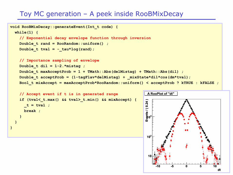
Toy MC generation – A peek inside RooBMixDecay
void RooBMixDecay::generateEvent(Int_t code) {
while(1) {
// Exponential decay envelope function through inversion
Double_t rand = RooRandom::uniform() ;
Double_t tval = -_tau*log(rand);
// Importance sampling of envelope
Double_t dil = 1-2.*mistag ;
Double_t maxAcceptProb = 1 + TMath::Abs(delMistag) + TMath::Abs(dil) ;
Double_t acceptProb = (1-tagFlav*delMistag) + _mixState*dil*cos(dm*tval);
Bool_t mixAccept = maxAcceptProb*RooRandom::uniform() < acceptProb ? kTRUE : kFALSE ;
// Accept event if t is in generated range
if (tval<_t.max() && tval>_t.min() && mixAccept) {
_t = tval ;
break ;
}
}
}
Wouter Verkerke, NIKHEF
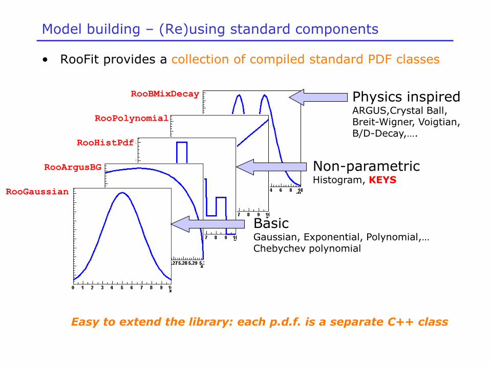
Model building – (Re)using standard components
• RooFit provides a collection of compiled standard PDF classes
RooArgusBG
RooPolynomial
RooBMixDecay
RooHistPdf
RooGaussian
Basic Gaussian, Exponential, Polynomial,… Chebychev polynomial
Physics inspired ARGUS,Crystal Ball, Breit-Wigner, Voigtian, B/D-Decay,….
Non-parametric Histogram, KEYS
Easy to extend the library: each p.d.f. is a separate C++ class

Wouter Verkerke, NIKHEF
Model building – Generic expression-based PDFs
• If your favorite PDF isn’t there and you don’t want to code a PDF class right away use RooGenericPdf
• Just write down the PDFs expression as a C++ formula
• Numeric normalization automatically provided
// PDF variables
RooRealVar x(“x”,”x”,-10,10) ;
RooRealVar y(“y”,”y”,0,5) ;
RooRealVar a(“a”,”a”,3.0) ;
RooRealVar b(“b”,”b”,-2.0) ;
// Generic PDF
RooGenericPdf gp(“gp”,”Generic PDF”,”exp(x*y+a)-b*x”,
RooArgSet(x,y,a,b)) ;
Wouter Verkerke, NIKHEF
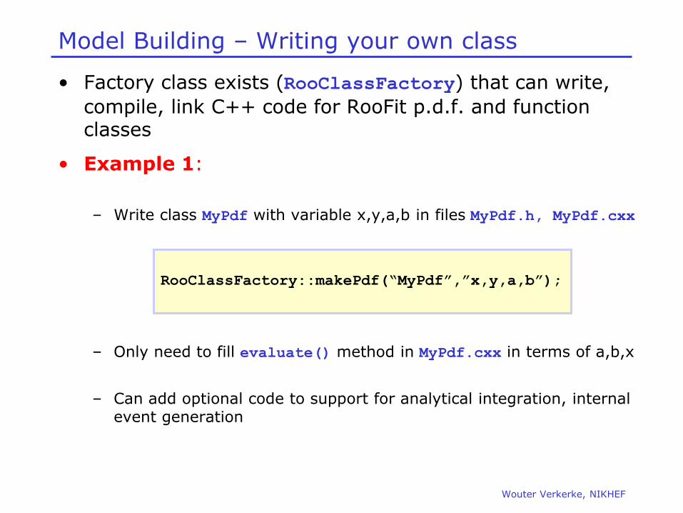
Model Building – Writing your own class
• Factory class exists (RooClassFactory) that can write,
compile, link C++ code for RooFit p.d.f. and function classes
• Example 1:
– Write class MyPdf with variable x,y,a,b in files MyPdf.h, MyPdf.cxx
– Only need to fill evaluate() method in MyPdf.cxx in terms of a,b,x
– Can add optional code to support for analytical integration, internal event generation
RooClassFactory::makePdf(“MyPdf”,”x,y,a,b”);
Wouter Verkerke, NIKHEF
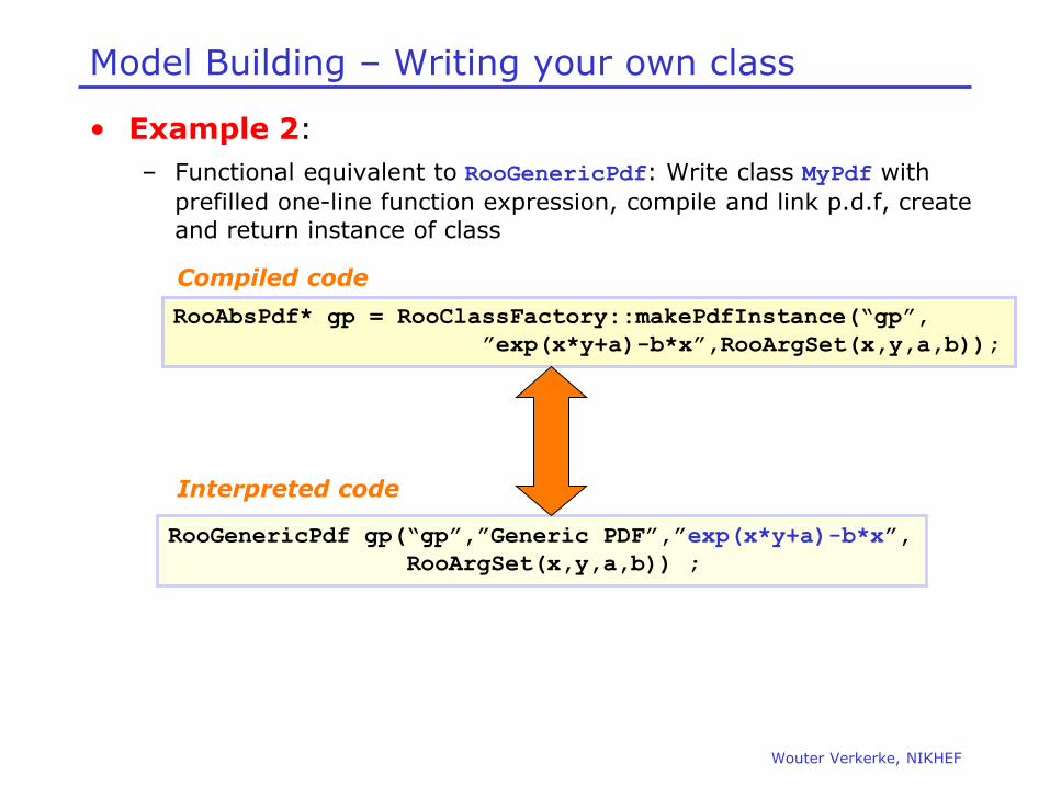
Model Building – Writing your own class
• Example 2:
– Functional equivalent to RooGenericPdf: Write class MyPdf with
prefilled one-line function expression, compile and link p.d.f, create and return instance of class
RooAbsPdf* gp = RooClassFactory::makePdfInstance(“gp”,
”exp(x*y+a)-b*x”,RooArgSet(x,y,a,b));
RooGenericPdf gp(“gp”,”Generic PDF”,”exp(x*y+a)-b*x”,
RooArgSet(x,y,a,b)) ;
Compiled code
Interpreted code
Wouter Verkerke, NIKHEF
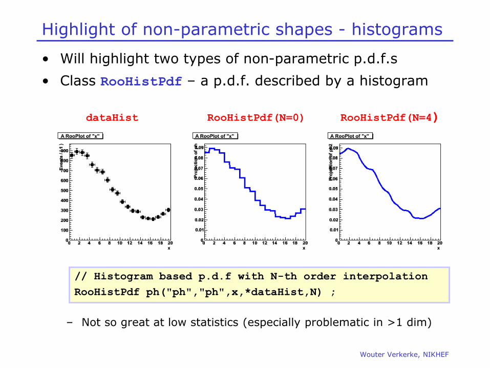
Highlight of non-parametric shapes - histograms
• Will highlight two types of non-parametric p.d.f.s
• Class RooHistPdf – a p.d.f. described by a histogram
– Not so great at low statistics (especially problematic in >1 dim)
// Histogram based p.d.f with N-th order interpolation
RooHistPdf ph("ph","ph",x,*dataHist,N) ;
dataHist RooHistPdf(N=0) RooHistPdf(N=4)
Wouter Verkerke, NIKHEF
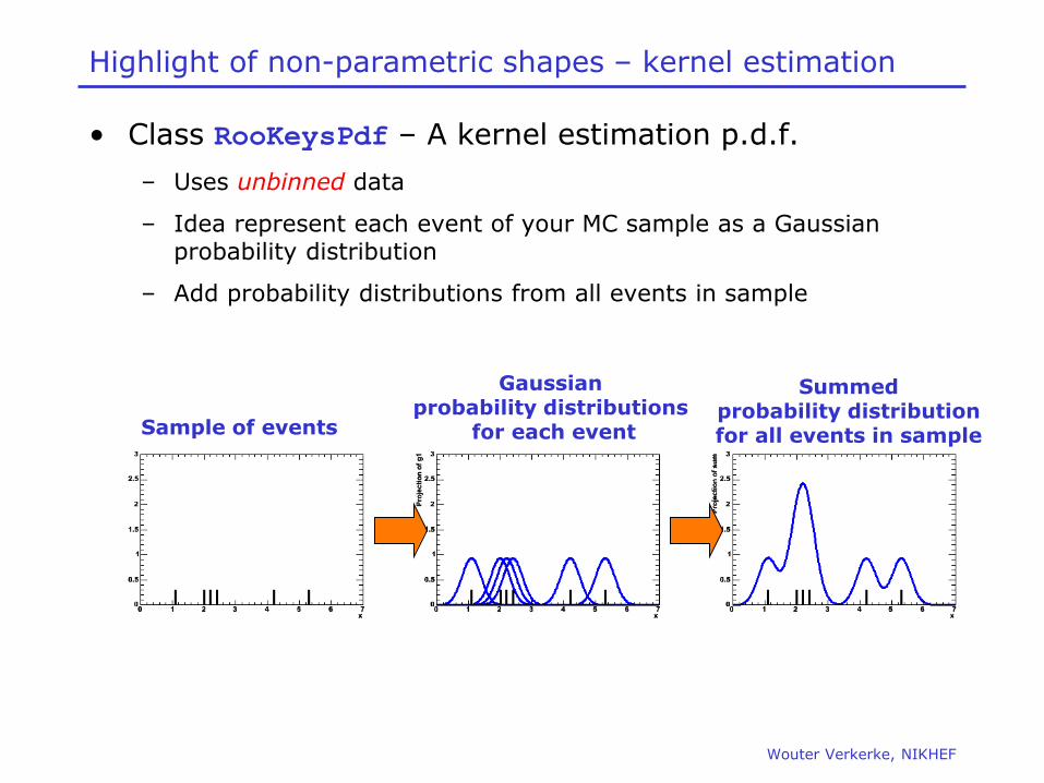
Highlight of non-parametric shapes – kernel estimation
• Class RooKeysPdf – A kernel estimation p.d.f.
– Uses unbinned data
– Idea represent each event of your MC sample as a Gaussian probability distribution
– Add probability distributions from all events in sample
Sample of events
Gaussian probability distributions
for each event
Summed probability distribution for all events in sample

Wouter Verkerke, NIKHEF
Highlight of non-parametric shapes – kernel estimation
• Width of Gaussian kernels need not be the same for all events
– As long as each event contributes 1/N to the integral
• Idea: ‘Adaptive kernel’ technique
– Choose wide Gaussian if local density of events is low
– Choose narrow Gaussian if local density of events is high
– Preserves small features in high statistics areas, minimize jitter in low statistics areas
– Automatically calculated
Static Kernel (with of all Gaussian identical)
Adaptive Kernel (width of all Gaussian depends
on local density of events)
Wouter Verkerke, NIKHEF
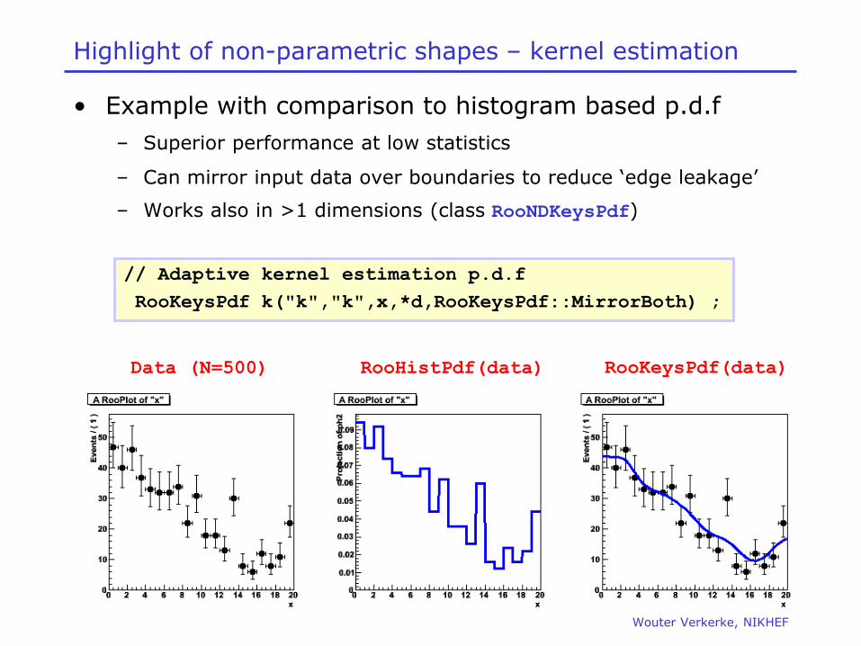
Highlight of non-parametric shapes – kernel estimation
• Example with comparison to histogram based p.d.f
– Superior performance at low statistics
– Can mirror input data over boundaries to reduce ‘edge leakage’
– Works also in >1 dimensions (class RooNDKeysPdf)
// Adaptive kernel estimation p.d.f
RooKeysPdf k("k","k",x,*d,RooKeysPdf::MirrorBoth) ;
Data (N=500) RooHistPdf(data) RooKeysPdf(data)

Wouter Verkerke, NIKHEF
P.d.f. addition & convolution 3 • Using the addition operator p.d.f
• Using the convolution operator p.d.f.
Wouter Verkerke, NIKHEF
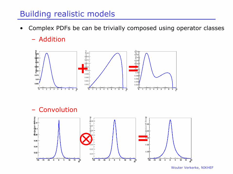
Building realistic models
• Complex PDFs be can be trivially composed using operator classes
– Addition
– Convolution
+ =
=

Wouter Verkerke, NIKHEF
RooBMixDecay
RooPolynomial
RooHistPdf
RooArgusBG
Model building – (Re)using standard components
• Most realistic models are constructed as the sum of one or more p.d.f.s (e.g. signal and background)
• Facilitated through operator p.d.f RooAddPdf
RooAddPdf +
RooGaussian

Wouter Verkerke, NIKHEF
Adding p.d.f.s – Mathematical side
• From math point of view adding p.d.f is simple
– Two components F, G
– Generically for N components P0-PN
• For N p.d.f.s, there are N-1 fraction coefficients that should sum to less 1
– The remainder is by construction 1 minus the sum of all other coefficients
)()1()()( xGfxfFxS
)(1)(...)()()(1,0
111100 xPcxPcxPcxPcxS n
ni
inn

Wouter Verkerke, NIKHEF
Constructing a sum of p.d.f.s
// Build two Gaussian PDFs
RooRealVar x("x","x",0,10) ;
RooRealVar mean1("mean1","mean of gaussian 1",2) ;
RooRealVar mean2("mean2","mean of gaussian 2",3) ;
RooRealVar sigma("sigma","width of gaussians",1) ;
RooGaussian gauss1("gauss1","gaussian PDF",x,mean1,sigma) ;
RooGaussian gauss2("gauss2","gaussian PDF",x,mean2,sigma) ;
// Build Argus background PDF
RooRealVar argpar("argpar","argus shape parameter",-1.0) ;
RooRealVar cutoff("cutoff","argus cutoff",9.0) ;
RooArgusBG argus("argus","Argus PDF",x,cutoff,argpar) ;
// Add the components
RooRealVar g1frac("g1frac","fraction of gauss1",0.5) ;
RooRealVar g2frac("g2frac","fraction of gauss2",0.1) ;
RooAddPdf sum("sum","g1+g2+a",RooArgList(gauss1,gauss2,argus),
RooArgList(g1frac,g2frac)) ;
Build 2 Gaussian
PDFs
Build ArgusBG
RooAddPdf constructs the sum of N PDFs with N-1 coefficients:
n
ni
inn PcPcPcPcPcS
1,0
11221100 1...
List of PDFs
List of coefficients
Wouter Verkerke, NIKHEF
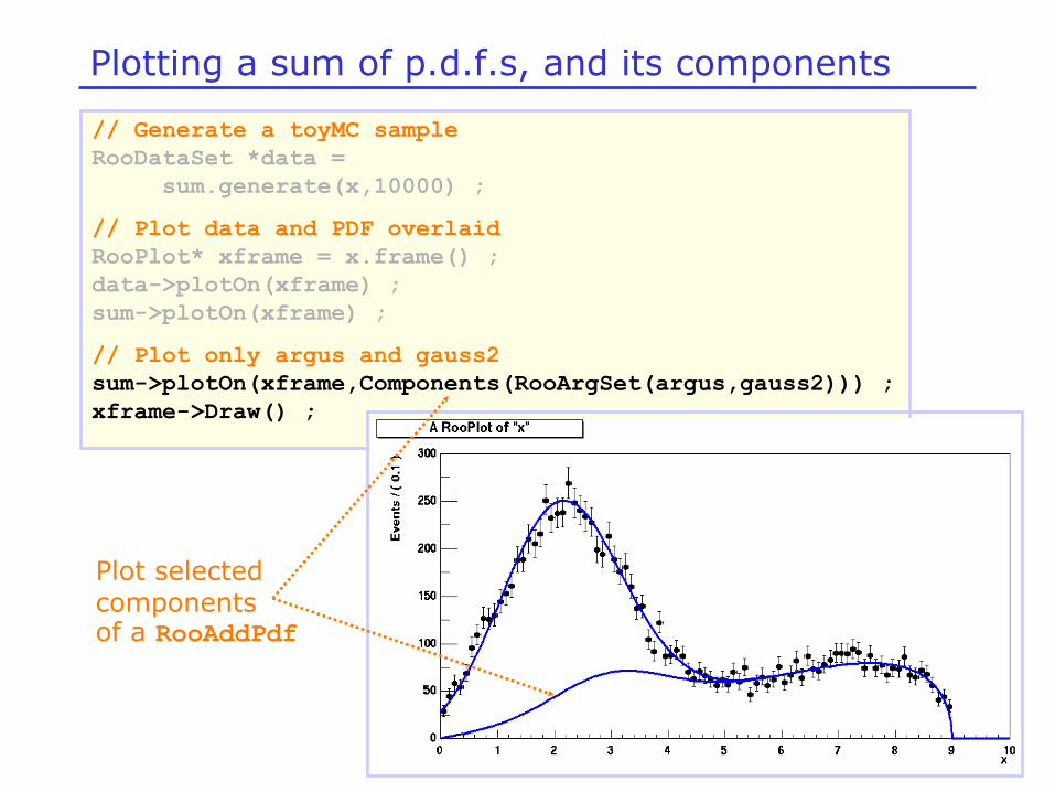
// Generate a toyMC sample
RooDataSet *data =
sum.generate(x,10000) ;
// Plot data and PDF overlaid
RooPlot* xframe = x.frame() ;
data->plotOn(xframe) ;
sum->plotOn(xframe) ;
// Plot only argus and gauss2
sum->plotOn(xframe,Components(RooArgSet(argus,gauss2))) ;
xframe->Draw() ;
Plotting a sum of p.d.f.s, and its components
Plot selected components of a RooAddPdf

Wouter Verkerke, NIKHEF
Component plotting - Introduction
• Also special tools for plotting of components in RooPlots
– Use Method Components()
• Example: Argus + Gaussian PDF
// Plot data and full PDF first
// Now plot only argus component
sum->plotOn(xframe,
Components(argus), LineStyle(kDashed)) ;

Wouter Verkerke, NIKHEF
Component plotting – Selecting components
There are various ways to select single or multiple components to plot Can refer to components either by name or reference
// Single component selection
pdf->plotOn(frame,Components(argus)) ;
pdf->plotOn(frame,Components(”gauss”)) ;
// Multiple component selection
pdf->plotOn(frame,Components(RooArgSet(pdfA,pdfB))) ;
pdf->plotOn(frame,Components(”pdfA,pdfB”)) ;
// Wild card expression allowed
pdf->plotOn(frame,Components(”bkgA*,bkgB*”)) ;
Wouter Verkerke, NIKHEF
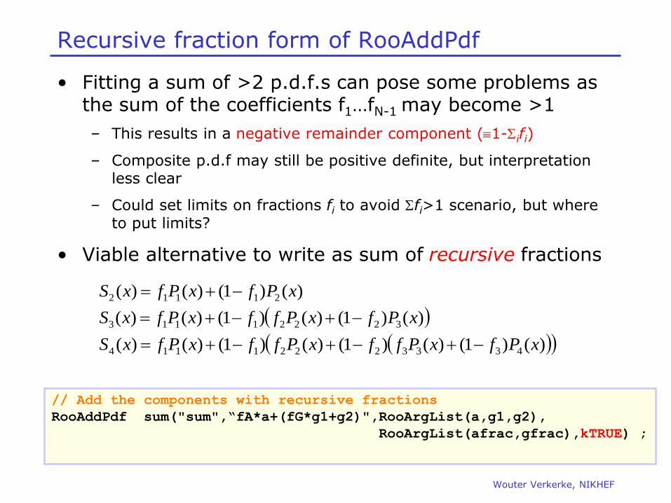
Recursive fraction form of RooAddPdf
• Fitting a sum of >2 p.d.f.s can pose some problems as the sum of the coefficients f1…fN-1 may become >1
– This results in a negative remainder component (1-ifi)
– Composite p.d.f may still be positive definite, but interpretation less clear
– Could set limits on fractions fi to avoid fi>1 scenario, but where to put limits?
• Viable alternative to write as sum of recursive fractions
)()1()()1()()1()()(
)()1()()1()()(
)()1()()(
43332221114
32221113
21112
xPfxPffxPffxPfxS
xPfxPffxPfxS
xPfxPfxS
// Add the components with recursive fractions
RooAddPdf sum("sum",“fA*a+(fG*g1+g2)",RooArgList(a,g1,g2),
RooArgList(afrac,gfrac),kTRUE) ;

Wouter Verkerke, NIKHEF
Extended p.d.f form of RooAddPdf
• If extended ML term is introduced, we can fit expected number of events (Nexp) in addition to shape parameters
• In case of sum of p.d.f.s it is convenient to re-parameterize sum of p.d.f.s.
• This transformation is applied automatically in RooAddPdf
if equal number of p.d.f.s and coefs are given
exp
exp
exp )1( NfN
NfN
N
f
sigbkg
sigsigsig
RooRealVar nsig(“nsig”,”number of signal events”,100,0,10000) ;
RooRealVar nbkg(“nbkg”,”number of backgnd events”,100,0,10000) ;
RooAddPdf sume(“sume”,”extended sum pdf”,RooArgList(gauss,argus),
RooArgList(nsig,nbkg)) ;
Wouter Verkerke, NIKHEF
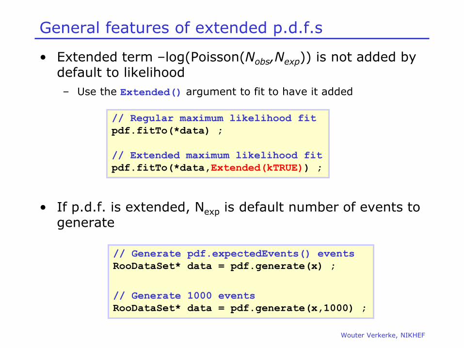
General features of extended p.d.f.s
• Extended term –log(Poisson(Nobs,Nexp)) is not added by default to likelihood
– Use the Extended() argument to fit to have it added
• If p.d.f. is extended, Nexp is default number of events to generate
// Regular maximum likelihood fit
pdf.fitTo(*data) ;
// Extended maximum likelihood fit
pdf.fitTo(*data,Extended(kTRUE)) ;
// Generate pdf.expectedEvents() events
RooDataSet* data = pdf.generate(x) ;
// Generate 1000 events
RooDataSet* data = pdf.generate(x,1000) ;
Wouter Verkerke, NIKHEF
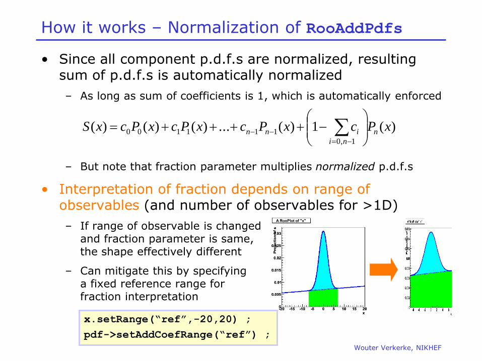
How it works – Normalization of RooAddPdfs
• Since all component p.d.f.s are normalized, resulting sum of p.d.f.s is automatically normalized
– As long as sum of coefficients is 1, which is automatically enforced
– But note that fraction parameter multiplies normalized p.d.f.s
• Interpretation of fraction depends on range of observables (and number of observables for >1D)
– If range of observable is changed and fraction parameter is same, the shape effectively different
– Can mitigate this by specifying a fixed reference range for fraction interpretation
)(1)(...)()()(1,0
111100 xPcxPcxPcxPcxS n
ni
inn
x.setRange(“ref”,-20,20) ;
pdf->setAddCoefRange(“ref”) ;
Wouter Verkerke, NIKHEF
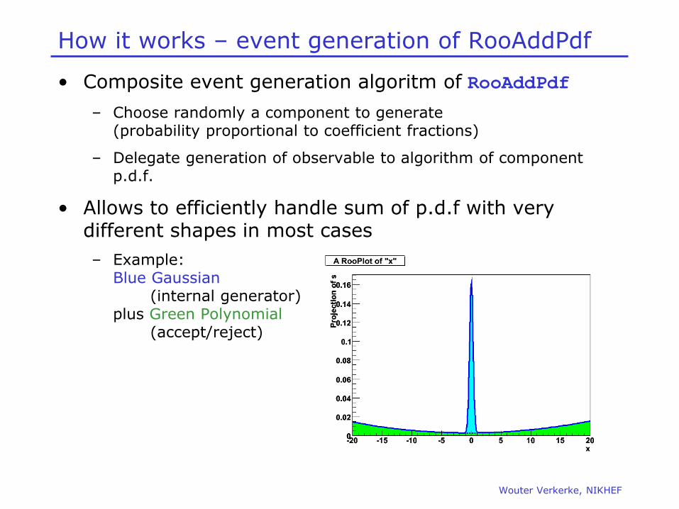
How it works – event generation of RooAddPdf
• Composite event generation algoritm of RooAddPdf
– Choose randomly a component to generate (probability proportional to coefficient fractions)
– Delegate generation of observable to algorithm of component p.d.f.
• Allows to efficiently handle sum of p.d.f with very different shapes in most cases
– Example: Blue Gaussian (internal generator) plus Green Polynomial (accept/reject)

Wouter Verkerke, NIKHEF
Dealing with composite p.d.f.s
• A RooAddPdf is an example of a composite p.d.f
– The value of the sum is represented by a tree of components
– The compositeness of a p.d.f. is completely transparent to most high-level operations
– Can e.g. do sum->fitTo(*data) or sum->generate(x,1000)
without being aware of composite nature of p.d.f.
RooAddPdf
sum
RooGaussian
gauss1
RooGaussian
gauss2
RooArgusBG
argus
RooRealVar
g1frac
RooRealVar
g2frac
RooRealVar
x
RooRealVar
sigma
RooRealVar
mean1
RooRealVar
mean2 RooRealVar
argpar
RooRealVar
cutoff

Wouter Verkerke, NIKHEF
Dealing with composite p.d.f.s
• The observables reported by a composite p.d.f and the ‘leaf’ of the expression tree
– For example, request for list of parameters of composite sum, will return parameters of components of sum
• In general, composite p.d.f.s work exactly the same as basic p.d.f.s.
RooArgSet *paramList = sum.getParameters(data) ;
paramList->Print("v") ;
RooArgSet::parameters:
1) RooRealVar::argpar : -1.00000 C
2) RooRealVar::cutoff : 9.0000 C
3) RooRealVar::g1frac : 0.50000 C
4) RooRealVar::g2frac : 0.10000 C
5) RooRealVar::mean1 : 2.0000 C
6) RooRealVar::mean2 : 3.0000 C
7) RooRealVar::sigma : 1.0000 C

Wouter Verkerke, NIKHEF
Visualization tools for composite objects
• Special tools exist to visualize the tree structure of composite objects
– On the command line
Root> sum.Print(“t”) ;
0x927b8d0 RooAddPdf::sum (g1+g2+a) [Auto]
0x9254008 RooGaussian::gauss1 (gaussian PDF) [Auto] V
0x9249360 RooRealVar::x (x) V
0x924a080 RooRealVar::mean1 (mean of gaussian 1) V
0x924d2d0 RooRealVar::sigma (width of gaussians) V
0x9267b70 RooRealVar::g1frac (fraction of gauss1) V
0x9259dc0 RooGaussian::gauss2 (gaussian PDF) [Auto] V
0x9249360 RooRealVar::x (x) V
0x924cde0 RooRealVar::mean2 (mean of gaussian 2) V
0x924d2d0 RooRealVar::sigma (width of gaussians) V
0x92680e8 RooRealVar::g2frac (fraction of gauss2) V
0x9261760 RooArgusBG::argus (Argus PDF) [Auto] V
0x9249360 RooRealVar::x (x) V
0x925fe80 RooRealVar::cutoff (argus cutoff) V
0x925f900 RooRealVar::argpar (argus shape parameter) V
0x9267288 RooConstVar::0.500000 (0.500000) V
Wouter Verkerke, NIKHEF
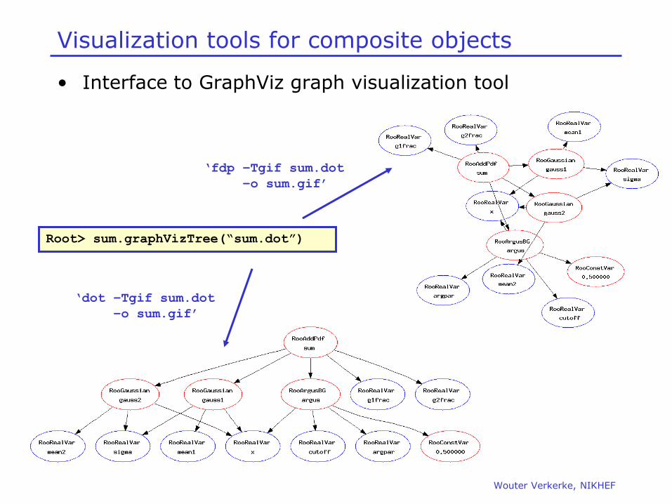
Visualization tools for composite objects
• Interface to GraphViz graph visualization tool
Root> sum.graphVizTree(“sum.dot”)
‘fdp –Tgif sum.dot
–o sum.gif’
‘dot –Tgif sum.dot
–o sum.gif’
Wouter Verkerke, NIKHEF
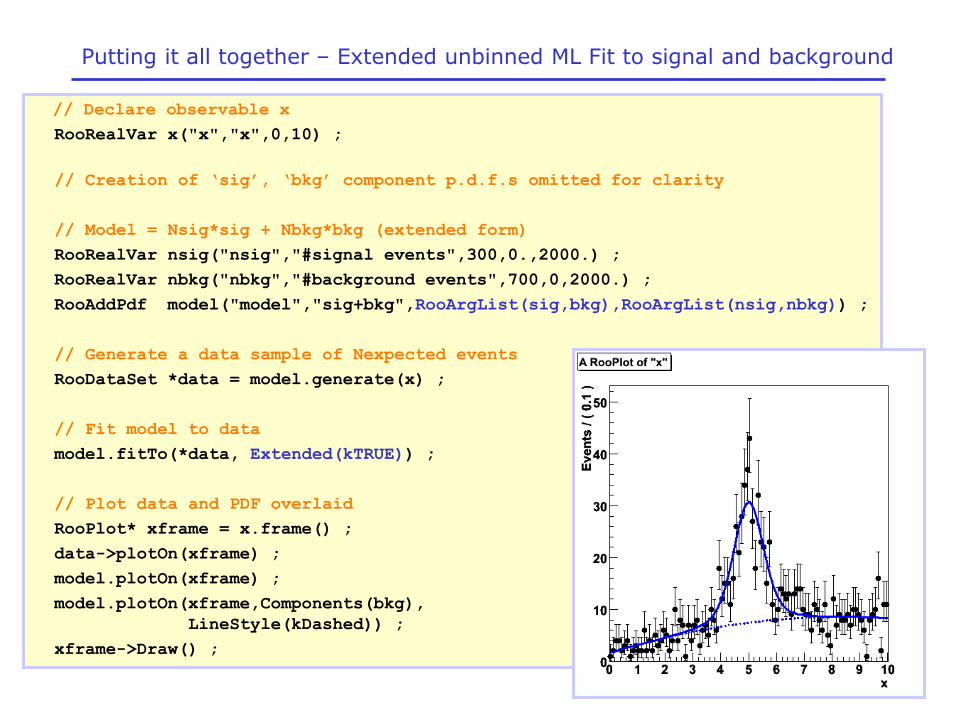
Putting it all together – Extended unbinned ML Fit to signal and background
// Declare observable x
RooRealVar x("x","x",0,10) ;
// Creation of ‘sig’, ‘bkg’ component p.d.f.s omitted for clarity
// Model = Nsig*sig + Nbkg*bkg (extended form)
RooRealVar nsig("nsig","#signal events",300,0.,2000.) ;
RooRealVar nbkg("nbkg","#background events",700,0,2000.) ;
RooAddPdf model("model","sig+bkg",RooArgList(sig,bkg),RooArgList(nsig,nbkg)) ;
// Generate a data sample of Nexpected events
RooDataSet *data = model.generate(x) ;
// Fit model to data
model.fitTo(*data, Extended(kTRUE)) ;
// Plot data and PDF overlaid
RooPlot* xframe = x.frame() ;
data->plotOn(xframe) ;
model.plotOn(xframe) ;
model.plotOn(xframe,Components(bkg),
LineStyle(kDashed)) ;
xframe->Draw() ;
Wouter Verkerke, NIKHEF
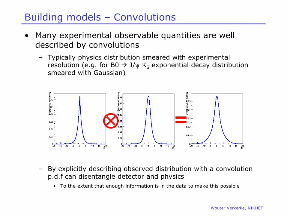
Building models – Convolutions
• Many experimental observable quantities are well described by convolutions
– Typically physics distribution smeared with experimental resolution (e.g. for B0 J/y KS exponential decay distribution
smeared with Gaussian)
– By explicitly describing observed distribution with a convolution p.d.f can disentangle detector and physics
• To the extent that enough information is in the data to make this possible
=
Wouter Verkerke, NIKHEF
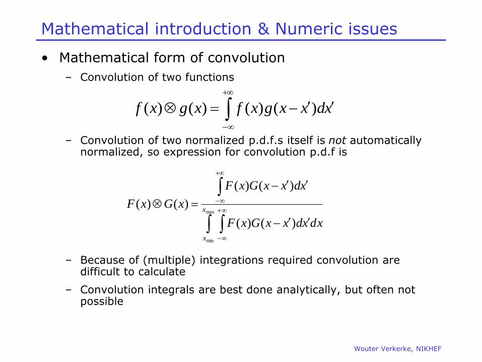
Mathematical introduction & Numeric issues
• Mathematical form of convolution
– Convolution of two functions
– Convolution of two normalized p.d.f.s itself is not automatically normalized, so expression for convolution p.d.f is
– Because of (multiple) integrations required convolution are difficult to calculate
– Convolution integrals are best done analytically, but often not possible
xdxxgxfxgxf )()()()(
max
min
)()(
)()(
)()(x
x
dxxdxxGxF
xdxxGxF
xGxF

Wouter Verkerke, NIKHEF
Convolution operation in RooFit
• RooFit has several options to construct convolution p.d.f.s
– Class RooNumConvPdf – ‘Brute force’ numeric calculation of
convolution (and normalization integrals)
– Class RooFFTConvPdf – Calculate convolution integral using discrete
FFT technology in fourier-transformed space.
– Bases classes RooAbsAnaConvPdf, RooResolutionModel. Framework
to construct analytical convolutions (with implementations mostly for B physics)
– Class RooVoigtian – Analytical convolution of
non-relativistic Breit-Wigner shape with a Gaussian
• All convolution in one dimension so far
– N-dim extension of RooFFTConvPdf foreseen in future

Wouter Verkerke, NIKHEF
Numeric convolutions – Class RooNumConvPdf
• Properties of RooNumConvPdf
– Can convolve any two input p.d.f.s
– Uses special numeric integrator that can compute integrals in [-,+] domain
– Slow (very!) especially if requiring sufficient numeric precision to allow use in MINUIT (requires ~10-7 estimated precision). Converge problems in MINUIT if precision is insufficient
// Construct landau (x) gauss
RooNumConvPdf lxg("lxg","landau (X) gauss",t,landau,gauss) ;
Landau Gauss Landau Gauss
Wouter Verkerke, NIKHEF
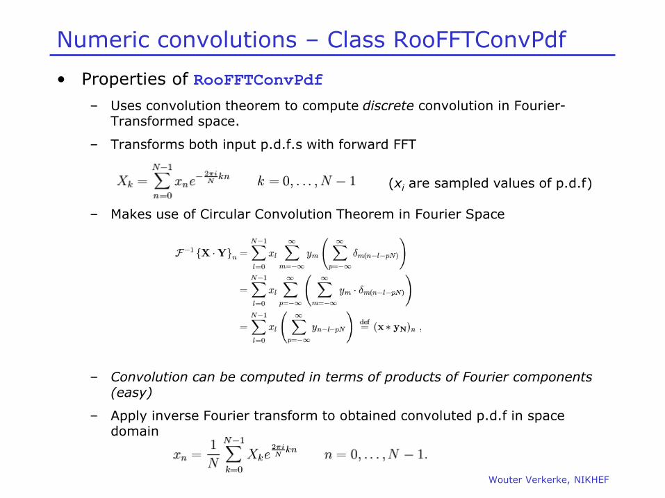
Numeric convolutions – Class RooFFTConvPdf
• Properties of RooFFTConvPdf
– Uses convolution theorem to compute discrete convolution in Fourier-Transformed space.
– Transforms both input p.d.f.s with forward FFT
– Makes use of Circular Convolution Theorem in Fourier Space
– Convolution can be computed in terms of products of Fourier components (easy)
– Apply inverse Fourier transform to obtained convoluted p.d.f in space domain
(xi are sampled values of p.d.f)
Wouter Verkerke, NIKHEF
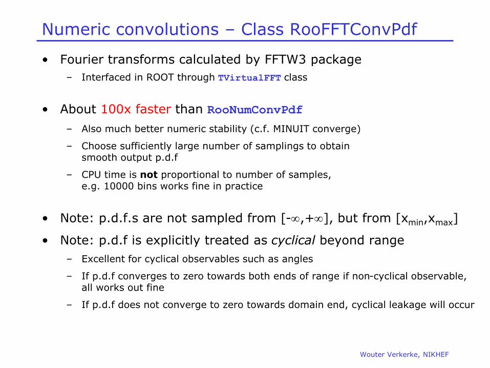
Numeric convolutions – Class RooFFTConvPdf
• Fourier transforms calculated by FFTW3 package
– Interfaced in ROOT through TVirtualFFT class
• About 100x faster than RooNumConvPdf
– Also much better numeric stability (c.f. MINUIT converge)
– Choose sufficiently large number of samplings to obtain smooth output p.d.f
– CPU time is not proportional to number of samples, e.g. 10000 bins works fine in practice
• Note: p.d.f.s are not sampled from [-,+], but from [xmin,xmax]
• Note: p.d.f is explicitly treated as cyclical beyond range
– Excellent for cyclical observables such as angles
– If p.d.f converges to zero towards both ends of range if non-cyclical observable, all works out fine
– If p.d.f does not converge to zero towards domain end, cyclical leakage will occur

Wouter Verkerke, NIKHEF
Numeric convolutions – Class RooFFTConvPdf
• Usage example
• Example with cyclical ‘leakage’
– Can reduce this by specifying a ‘buffer zone’ in FFT calculation beyond end of ranges conv.setBufferFraction(0.3)
// Construct landau (x) gauss (10000 samplings 2nd order interpolation)
t.setBins(10000,”cache”) ;
RooFFTConvPdf lxg("lxg","landau (X) gauss",t,landau,gauss,2) ;

Wouter Verkerke, NIKHEF
Framework for analytical calculations of convolutions
• Convoluted PDFs that can be written if the following form can be used in a very modular way in RooFit
k
kk dtRdtfcdtP ,...)(,...)((...),...)(
‘basis function’ coefficient
resolution function
)cos(),21(
,1
/||
11
/||
00
tmefwc
efwc
t
t
Example: B0 decay with mixing
demo6.cc

Wouter Verkerke, NIKHEF
Convoluted PDFs
• Physics model and resolution model are implemented separately in RooFit
k
kk dtRdtfcdtP ,...)(,...)((...),...)(
RooResolutionModel
RooConvolutedPdf (physics model)
User can choose combination of physics model and resolution model at run time (Provided resolution model implements all fk declared by physics model)
Implements Also a PDF by itself
,...)(,...)( dtRdtfi
Implements ck Declares list of fk needed
Wouter Verkerke, NIKHEF
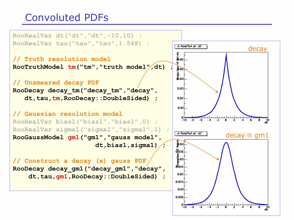
Convoluted PDFs
RooRealVar dt("dt","dt",-10,10) ;
RooRealVar tau("tau","tau",1.548) ;
// Truth resolution model
RooTruthModel tm("tm","truth model",dt) ;
// Unsmeared decay PDF
RooDecay decay_tm("decay_tm","decay",
dt,tau,tm,RooDecay::DoubleSided) ;
// Gaussian resolution model
RooRealVar bias1("bias1","bias1",0) ;
RooRealVar sigma1("sigma1","sigma1",1) ;
RooGaussModel gm1("gm1","gauss model",
dt,bias1,sigma1) ;
// Construct a decay (x) gauss PDF
RooDecay decay_gm1("decay_gm1","decay",
dt,tau,gm1,RooDecay::DoubleSided) ;
decay
decay gm1
Wouter Verkerke, NIKHEF
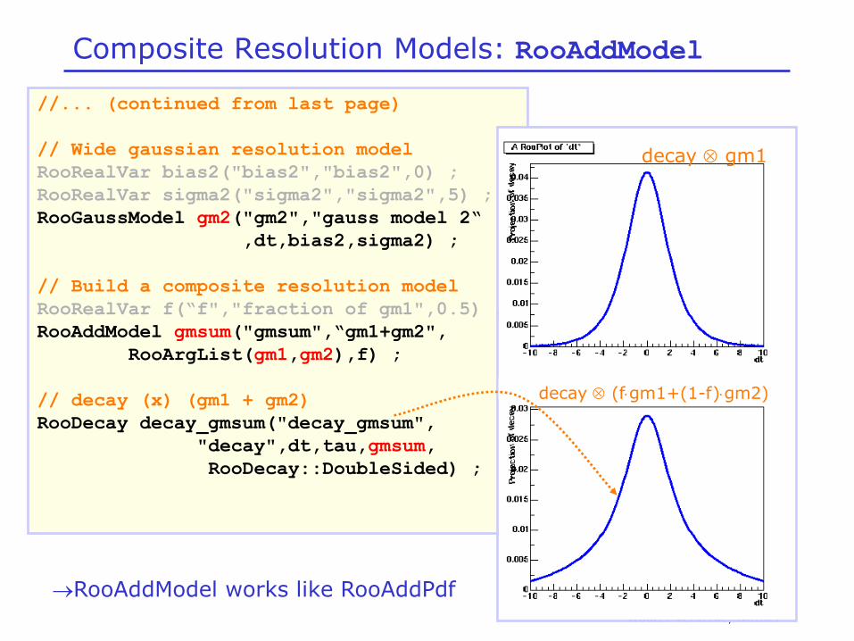
Composite Resolution Models: RooAddModel
//... (continued from last page)
// Wide gaussian resolution model
RooRealVar bias2("bias2","bias2",0) ;
RooRealVar sigma2("sigma2","sigma2",5) ;
RooGaussModel gm2("gm2","gauss model 2“
,dt,bias2,sigma2) ;
// Build a composite resolution model
RooRealVar f(“f","fraction of gm1",0.5) ;
RooAddModel gmsum("gmsum",“gm1+gm2",
RooArgList(gm1,gm2),f) ;
// decay (x) (gm1 + gm2)
RooDecay decay_gmsum("decay_gmsum",
"decay",dt,tau,gmsum,
RooDecay::DoubleSided) ;
RooAddModel works like RooAddPdf
decay gm1
decay (fgm1+(1-f)gm2)
Wouter Verkerke, NIKHEF
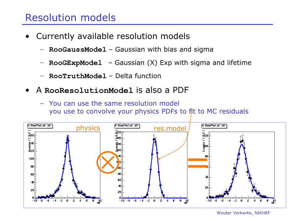
Resolution models
• Currently available resolution models
– RooGaussModel – Gaussian with bias and sigma
– RooGExpModel – Gaussian (X) Exp with sigma and lifetime
– RooTruthModel – Delta function
• A RooResolutionModel is also a PDF
– You can use the same resolution model you use to convolve your physics PDFs to fit to MC residuals
=
physics res.model

Wouter Verkerke, NIKHEF
How it works – generating events from convolution p.d.f.s
• A very efficient implementation of event generation is possible
– Reflect ‘smearing’ view of convolution
– Very fast as no computation of convolution integrals is required
– But only if both input p.d.f.s can generate observables in the range [-,+] which is not possible with accept/reject so this can only be done if both input p.d.f.s have an internal generator implementation
– If above conditions are not met, automatic fallback solution is to perform accept/reject sampling on convoluted p.d.f. shape
RPRP xxx
Wouter Verkerke, NIKHEF
Multidimensional models 4 • Uncorrelated products of p.d.f.s
• Using composition to p.d.f.s with correlation
• Products of conditional and plain p.d.f.s

Wouter Verkerke, NIKHEF
Building realistic models
– Multiplication
– Composition
* =
g(x;m,s) m(y;a0,a1)
=
g(x,y;a0,a1,s) Possible in any PDF No explicit support in PDF code needed

Wouter Verkerke, NIKHEF
RooBMixDecay
RooPolynomial
RooHistPdf
RooArgusBG
RooGaussian
Model building – Products of uncorrelated p.d.f.s
RooProdPdf *
)()(),( yGxFyxH

Wouter Verkerke, NIKHEF
Uncorrelated products – Mathematics and constructors
• Mathematical construction of products of uncorrelated p.d.f.s is straightforward
– No explicit normalization required If input p.d.f.s are unit
normalized, product is also unit normalized (this is true only because of the absence of correlations)
• Corresponding RooFit operator p.d.f. is RooProdPdf
– Returns product of normalized input p.d.f values
)()(),( yGxFyxH i
iii xFxH )()( }{}{}{
2D nD
RooGaussian gx("gx","gaussian PDF",x,meanx,sigmax) ;
RooGaussian gy("gy","gaussian PDF",y,meany,sigmay) ;
// Multiply gaussx and gaussy into a two-dimensional p.d.f. gaussxy
RooProdPdf gaussxy("gxy","gx*gy",RooArgList(gx,gy)) ;

Wouter Verkerke, NIKHEF
How it work – event generation on uncorrelated products
• If p.d.f.s are uncorrelated, each observable can be generated separately
– Reduced dimensionality of problem (important for e.g. accept/reject sampling)
– Actual event generation delegated to component p.d.f (can e.g. use internal generator if available)
– RooProdPdf just aggregates output in single dataset
Delegate Generate Merge
Wouter Verkerke, NIKHEF
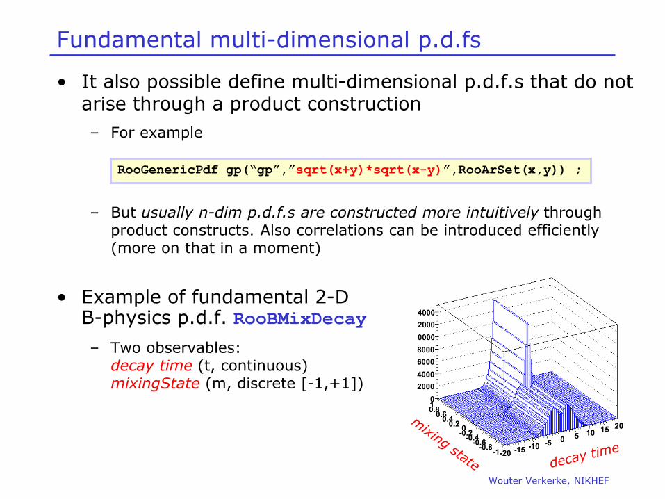
Fundamental multi-dimensional p.d.fs
• It also possible define multi-dimensional p.d.f.s that do not arise through a product construction
– For example
– But usually n-dim p.d.f.s are constructed more intuitively through product constructs. Also correlations can be introduced efficiently (more on that in a moment)
• Example of fundamental 2-D B-physics p.d.f. RooBMixDecay
– Two observables: decay time (t, continuous) mixingState (m, discrete [-1,+1])
RooGenericPdf gp(“gp”,”sqrt(x+y)*sqrt(x-y)”,RooArSet(x,y)) ;

Wouter Verkerke, NIKHEF
Plotting multi-dimensional PDFs
RooPlot* xframe = x.frame() ;
data->plotOn(xframe) ;
prod->plotOn(xframe) ;
xframe->Draw() ;
c->cd(2) ;
RooPlot* yframe = y.frame() ;
data->plotOn(yframe) ;
prod->plotOn(yframe) ;
yframe->Draw() ;
dyyxpdfxf ),()(
dxyxpdfyf ),()(
-Plotting a dataset D(x,y) versus x represents a projection over y
-To overlay PDF(x,y), you must plot Int(dy)PDF(x,y)
-RooFit automatically takes care of this!
•RooPlot remembers dimensions of plotted datasets

Wouter Verkerke, NIKHEF
Projecting out hidden dimensions
• Example in 2 dimensions
– 2-dim dataset D(x,y)
– 2-dim PDF P(x,y)=gauss(x)*gauss(y)
• 1-dim plot versus x
• 1-dim plot versus y
dxdyyxp
dxyxpyPp
),(
),()(
dxdyyxp
dyyxpxPp
),(
),()(
Wouter Verkerke, NIKHEF
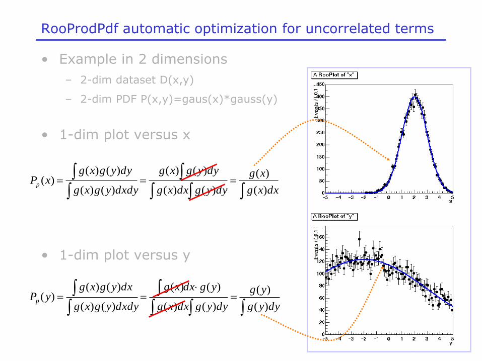
RooProdPdf automatic optimization for uncorrelated terms
• Example in 2 dimensions
– 2-dim dataset D(x,y)
– 2-dim PDF P(x,y)=gaus(x)*gauss(y)
• 1-dim plot versus x
• 1-dim plot versus y
dyyg
yg
dyygdxxg
ygdxxg
dxdyygxg
dxygxgyPp
)(
)(
)()(
)()(
)()(
)()()(
dxxg
xg
dyygdxxg
dyygxg
dxdyygxg
dyygxgxPp
)(
)(
)()(
)()(
)()(
)()()(
Wouter Verkerke, NIKHEF
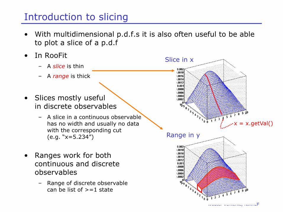
Introduction to slicing
• With multidimensional p.d.f.s it is also often useful to be able to plot a slice of a p.d.f
• In RooFit
– A slice is thin
– A range is thick
• Slices mostly useful in discrete observables
– A slice in a continuous observable has no width and usually no data with the corresponding cut (e.g. “x=5.234”)
• Ranges work for both continuous and discrete observables
– Range of discrete observable can be list of >=1 state
x = x.getVal()
Slice in x
Range in y

Wouter Verkerke, NIKHEF
Plotting a slice of a dataset
• Use the optional cut string expression
– Works the same for binned data sets
// Mixing dataset defines dt,mixState
RooDataSet* data ;
// Plot the entire dataset
RooPlot* frame = dt.frame() ;
data->plotOn(frame) ;
// Plot the mixed part of the data
RooPlot* frame_mix = dt.frame() ;
data->plotOn(frame,
Cut(”mixState==mixState::mixed”)) ;
Wouter Verkerke, NIKHEF
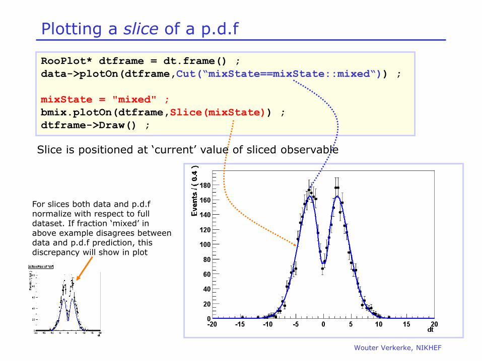
Plotting a slice of a p.d.f
RooPlot* dtframe = dt.frame() ;
data->plotOn(dtframe,Cut(“mixState==mixState::mixed“)) ;
mixState = "mixed" ;
bmix.plotOn(dtframe,Slice(mixState)) ;
dtframe->Draw() ;
Slice is positioned at ‘current’ value of sliced observable
For slices both data and p.d.f normalize with respect to full dataset. If fraction ‘mixed’ in above example disagrees between data and p.d.f prediction, this discrepancy will show in plot

Wouter Verkerke, NIKHEF
Plotting a range of a p.d.f and a dataset
RooPlot* xframe = x.frame() ;
data->plotOn(xframe) ;
model.plotOn(xframe) ;
y.setRange(“sig”,-1,1) ;
RooPlot* xframe2 = x.frame() ;
data->plotOn(xframe2,CutRange("sig")) ;
model.plotOn(xframe2,ProjectionRange("sig")) ;
model(x,y) = gauss(x)*gauss(y) + poly(x)*poly(y)
Works also with >2D projections (just specify projection range on all projected observables)
Works also with multidimensional p.d.fs that have correlations

Wouter Verkerke, NIKHEF
Physics example of combined range and slice plotting
// Plot projection on mB
RooPlot* mbframe = mb.frame(40) ;
data->plotOn(mbframe) ;
model.plotOn(mbframe) ;
// Plot mixed slice projection on deltat
RooPlot* dtframe = dt.frame(40) ;
data>plotOn(dtframe,
Cut(”mixState==mixState::mixed”)) ;
mixState=“mixed” ;
model.plotOn(dtframe,Slice(mixState)) ;
Example setup: Argus(mB)*Decay(dt) +
Gauss(mB)*BMixDecay(dt)
(background) (signal)
mB
dt (mixed slice)
Wouter Verkerke, NIKHEF
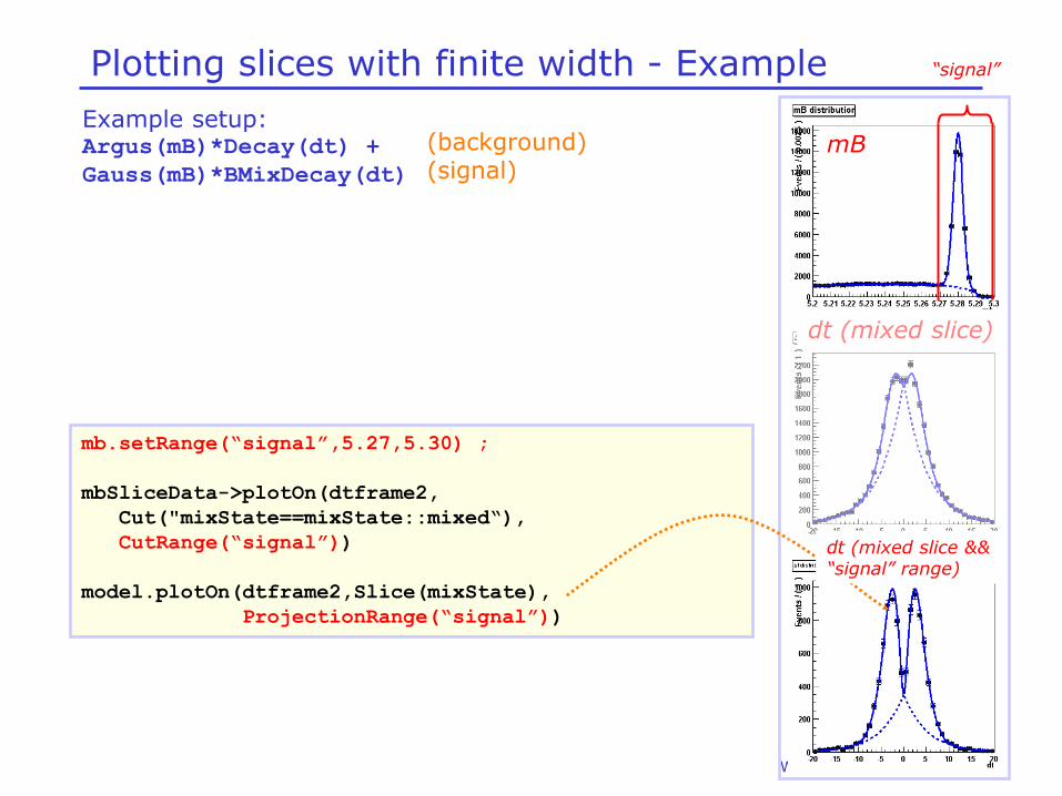
Plotting slices with finite width - Example
Example setup: Argus(mB)*Decay(dt) +
Gauss(mB)*BMixDecay(dt)
(background) (signal)
mb.setRange(“signal”,5.27,5.30) ;
mbSliceData->plotOn(dtframe2,
Cut("mixState==mixState::mixed“),
CutRange(“signal”))
model.plotOn(dtframe2,Slice(mixState),
ProjectionRange(“signal”))
mB
dt (mixed slice)
dt (mixed slice && “signal” range)
“signal”
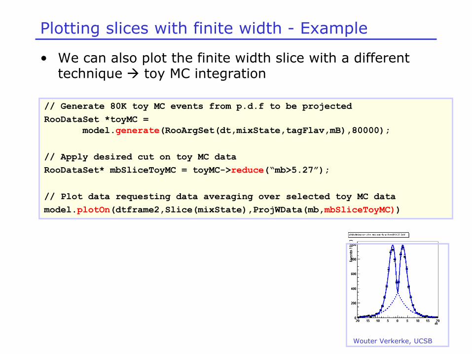
Plotting slices with finite width - Example
• We can also plot the finite width slice with a different technique toy MC integration
Wouter Verkerke, UCSB
// Generate 80K toy MC events from p.d.f to be projected
RooDataSet *toyMC =
model.generate(RooArgSet(dt,mixState,tagFlav,mB),80000);
// Apply desired cut on toy MC data
RooDataSet* mbSliceToyMC = toyMC->reduce(“mb>5.27”);
// Plot data requesting data averaging over selected toy MC data
model.plotOn(dtframe2,Slice(mixState),ProjWData(mb,mbSliceToyMC))

Wouter Verkerke, NIKHEF
Plotting non-rectangular PDF regions
• Why is this interesting? Because with this technique we can trivially implement projection over arbitrarily shaped regions.
– Any cut prescription that you can think of to apply to data works
• Example: Likelihood ratio projection plot
– Common technique in rare decay analyses
– PDF typically consist of N-dimensional event selection PDF, where N is large (e.g. 6.)
– Projection of data & PDF in any of the N dimensions doesn’t show a significant excess of signal events
– To demonstrate purity of selected signal, plot data distribution (with overlaid PDF) in one dimension, while selecting events with a cut on the likelihood ratio of signal and background in the remaining N-1 dimensions

Wouter Verkerke, NIKHEF
Plotting data & PDF with a likelihood ratio cut
• Simple example
– 3 observables (x,y,z)
– Signal shape: gauss(x)·gauss(y)·gauss(z)
– Background shape: (1+a·x)(1+b·y)(1+c·z)
– Plot distribution in x
// Plot x distribution of all events
RooPlot* xframe1 = x.frame(40) ;
data->plotOn(xframe1) ;
sum.plotOn(xframe1) ;
Integrated projection of data/PDF on X doesn’t reflect signal/background discrimination power of PDF in y,z Use LR ratio technique to only plot events with are signal-like according to p.d.f in projected observable (y,z)
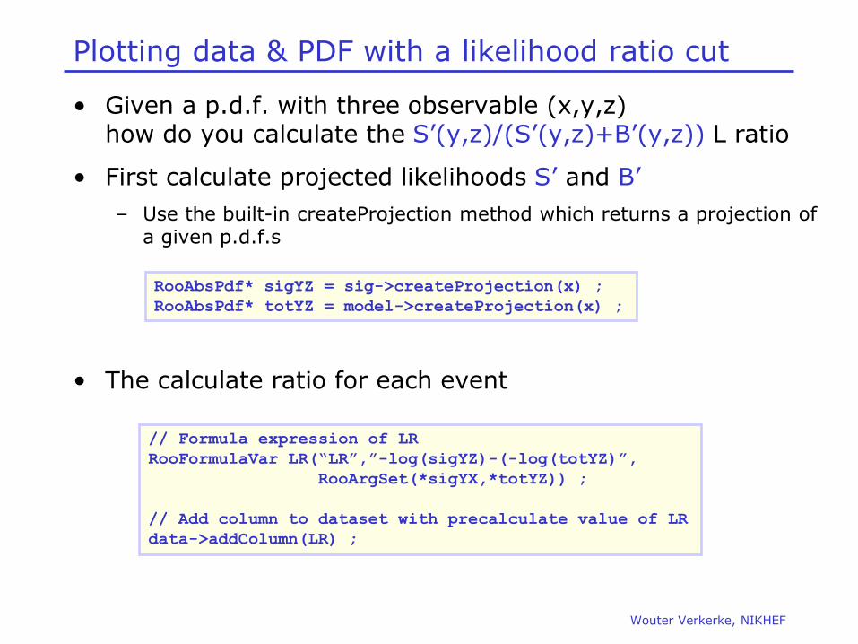
• Given a p.d.f. with three observable (x,y,z) how do you calculate the S’(y,z)/(S’(y,z)+B’(y,z)) L ratio
• First calculate projected likelihoods S’ and B’
– Use the built-in createProjection method which returns a projection of a given p.d.f.s
• The calculate ratio for each event
Wouter Verkerke, NIKHEF
Plotting data & PDF with a likelihood ratio cut
RooAbsPdf* sigYZ = sig->createProjection(x) ;
RooAbsPdf* totYZ = model->createProjection(x) ;
// Formula expression of LR
RooFormulaVar LR(“LR”,”-log(sigYZ)-(-log(totYZ)”,
RooArgSet(*sigYX,*totYZ)) ;
// Add column to dataset with precalculate value of LR
data->addColumn(LR) ;

Plotting data & PDF with a likelihood cut
• Look at distribution of per-event LR in toy MC sample and decide on suitable cut
• Apply cut to both data sample and toyMC sample for projection and make plot
Wouter Verkerke, NIKHEF
Wouter Verkerke, NIKHEF
Plotting in more than 2,3 dimensions
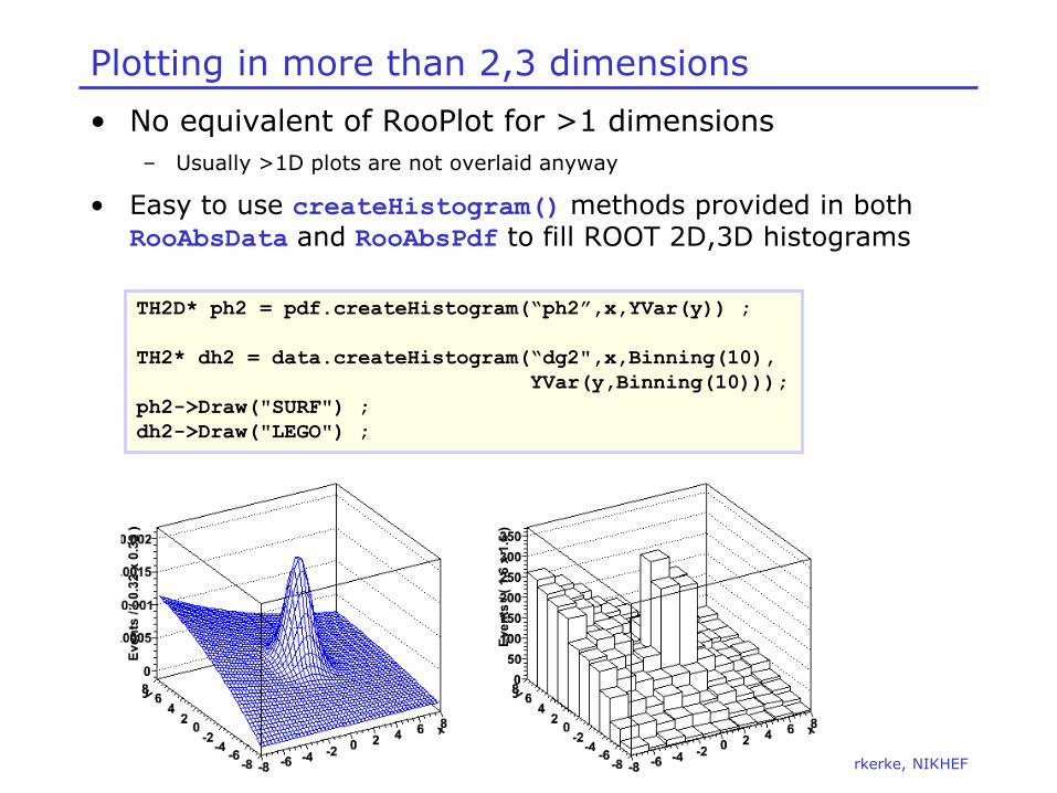
• No equivalent of RooPlot for >1 dimensions
– Usually >1D plots are not overlaid anyway
• Easy to use createHistogram() methods provided in both RooAbsData and RooAbsPdf to fill ROOT 2D,3D histograms
TH2D* ph2 = pdf.createHistogram(“ph2”,x,YVar(y)) ;
TH2* dh2 = data.createHistogram(“dg2",x,Binning(10),
YVar(y,Binning(10)));
ph2->Draw("SURF") ;
dh2->Draw("LEGO") ;
Wouter Verkerke, NIKHEF
Building models – Introducing correlations
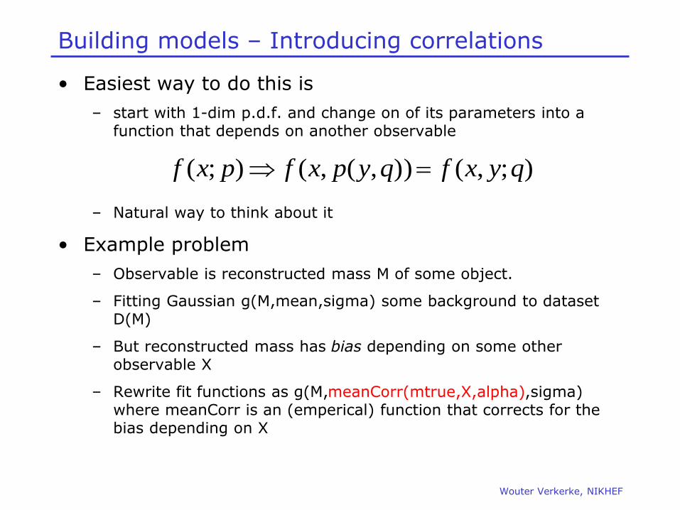
• Easiest way to do this is
– start with 1-dim p.d.f. and change on of its parameters into a function that depends on another observable
– Natural way to think about it
• Example problem
– Observable is reconstructed mass M of some object.
– Fitting Gaussian g(M,mean,sigma) some background to dataset D(M)
– But reconstructed mass has bias depending on some other observable X
– Rewrite fit functions as g(M,meanCorr(mtrue,X,alpha),sigma) where meanCorr is an (emperical) function that corrects for the bias depending on X
);,()),(,();( qyxfqypxfpxf

Wouter Verkerke, NIKHEF
Coding the example problem
RooRealVar x("x","x",-10,10) ;
RooRealVar y("y","y",0,3) ;
// Build a parameterized mean variable for gauss
RooRealVar mean0("mean0",“mean offset",0.5) ;
RooRealVar mean1("mean1",“mean slope",3.0) ;
RooFormulaVar mean("mean","mean0+mean1*y",
RooArgList(mean0,mean1,y)) ;
RooRealVar sigma("sigma","width of gaussian",3) ;
RooGaussian gauss("gauss","gaussian",x,mean,sigma);
How do you code the preceding example problem
PDF(x,y) = gauss(x,m(y),s)
m(y) = m0 + m1sqrt(y)
How do you do that? Just like that:
Build a function object m(y)=m0+m1*sqrt(y)
Simply plug in function mean(y)
where mean value is expected!
Plug-and-play parameters! PDF expects a real-valued object as input, not necessarily a variable

Wouter Verkerke, NIKHEF
Generic real-valued functions
• RooFormulaVar makes use of the ROOT TFormula
technology to build interpreted functions
– Understands generic C++ expressions, operators etc
– Two ways to reference RooFit objects By name: By position:
– You can use RooFormulaVar where ever a ‘real’ variable is requested
• RooPolyVar is a compiled polynomial function
RooFormulaVar f(“f”,”exp(foo)*sqrt(bar)”, RooArgList(foo,bar)) ;
RooFormulaVar f(“f”,”exp(@0)*sqrt(@1)”,RooArgList(foo,bar)) ;
RooRealVar x(“x”,”x”,0.,1.) ;
RooRealVar p0(“p0”,”p0”,5.0) ;
RooRealVar p1(“p1”,”p1”,-2.0) ;
RooRealVar p2(“p2”,”p2”,3.0) ;
RooFormulaVar f(“f”,”polynomial”,x,RooArgList(p0,p1,p2)) ;

Wouter Verkerke, NIKHEF
What does the example p.d.f look like?
• Make 2D plot of p.d.f in (x,y)
• Is the correct p.d.f for this problem?
– Constructed a p.d.f with correct shape in x, given a value of y OK
– But p.d.f predicts flat distribution in y Probably not OK
– What we want is a pdf for X given Y, but without prediction on Y Definition of a conditional p.d.f F(x|y)
Projection on Y
Projection on X
Wouter Verkerke, NIKHEF
Conditional p.d.f.s – Formulation and construction
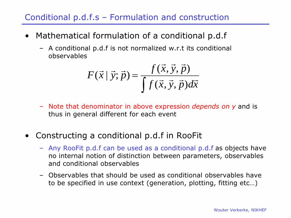
• Mathematical formulation of a conditional p.d.f
– A conditional p.d.f is not normalized w.r.t its conditional observables
– Note that denominator in above expression depends on y and is thus in general different for each event
• Constructing a conditional p.d.f in RooFit
– Any RooFit p.d.f can be used as a conditional p.d.f as objects have no internal notion of distinction between parameters, observables and conditional observables
– Observables that should be used as conditional observables have to be specified in use context (generation, plotting, fitting etc…)
xdpyxf
pyxfpyxF
),,(
),,();|(

Wouter Verkerke, NIKHEF
Using a conditional p.d.f – fitting and plotting
• For fitting, indicate in fitTo() call what the conditional observables are
– You may notice a performance penalty if the normalization integral of the p.d.f needs to be calculated numerically. For a conditional p.d.f it must evaluated again for each event
• Plotting: You cannot project a conditional F(x|y) on x without external information on the distribution of y
– Substitute integration with averaging over y values in data
pdf.fitTo(data,ConditionalObservables(y))
xdyxf
yxfyxF
),(
),()|(
Ni
D i
ip
dxyxp
yxp
NxP
,1
),(
),(1)(
dxdyyxp
dyyxpxPp
),(
),()(
Sum over all yi in dataset D Integrate over y
Wouter Verkerke, NIKHEF
Physics example with conditional p.d.f.s
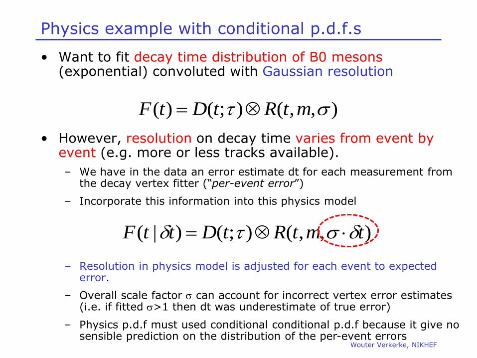
• Want to fit decay time distribution of B0 mesons (exponential) convoluted with Gaussian resolution
• However, resolution on decay time varies from event by event (e.g. more or less tracks available).
– We have in the data an error estimate dt for each measurement from the decay vertex fitter (“per-event error”)
– Incorporate this information into this physics model
– Resolution in physics model is adjusted for each event to expected error.
– Overall scale factor can account for incorrect vertex error estimates (i.e. if fitted >1 then dt was underestimate of true error)
– Physics p.d.f must used conditional conditional p.d.f because it give no sensible prediction on the distribution of the per-event errors
),,();()( mtRtDtF
),,();()|( tmtRtDttF
Wouter Verkerke, NIKHEF
Physics example with conditional p.d.f.s
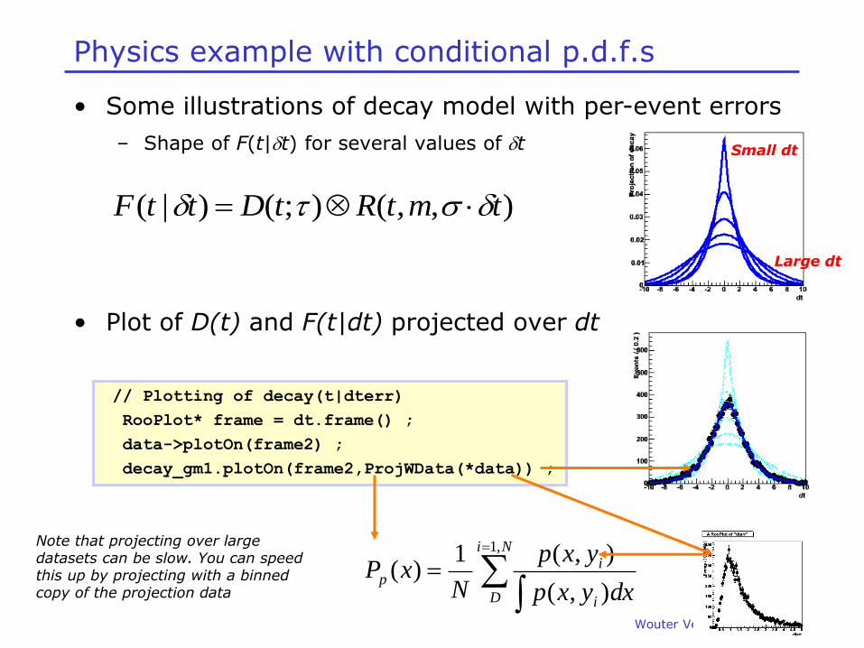
• Some illustrations of decay model with per-event errors
– Shape of F(t|t) for several values of t
• Plot of D(t) and F(t|dt) projected over dt
),,();()|( tmtRtDttF
Small dt
Large dt
// Plotting of decay(t|dterr)
RooPlot* frame = dt.frame() ;
data->plotOn(frame2) ;
decay_gm1.plotOn(frame2,ProjWData(*data)) ;
Ni
D i
ip
dxyxp
yxp
NxP
,1
),(
),(1)(
Note that projecting over large datasets can be slow. You can speed this up by projecting with a binned copy of the projection data
Wouter Verkerke, NIKHEF
How it works – event generation with conditional p.d.f.s
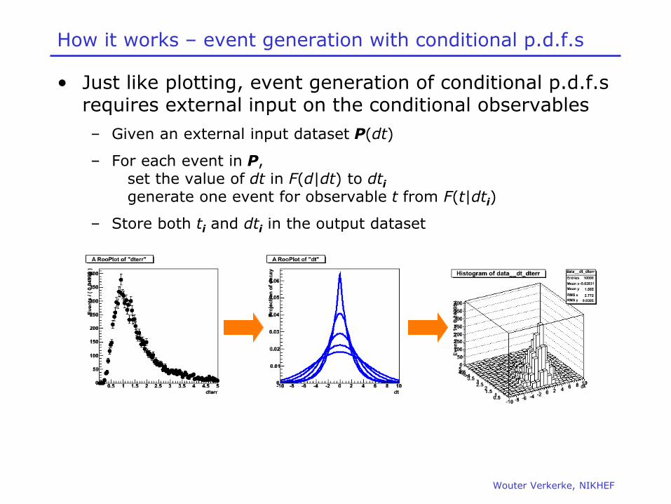
• Just like plotting, event generation of conditional p.d.f.s requires external input on the conditional observables
– Given an external input dataset P(dt)
– For each event in P, set the value of dt in F(d|dt) to dti generate one event for observable t from F(t|dti)
– Store both ti and dti in the output dataset

Wouter Verkerke, NIKHEF
Complete example of decay with per-event errors
RooRealVar dt("dt","dt",-10,10) ;
RooRealVar dterr("dterr","dterr",0.001,5) ;
RooRealVar tau("tau","tau",1.548) ;
// Build Gauss(dt,0,sigma*dterr)
RooRealVar sigma("sigma","sigma1",1) ;
RooGaussModel gm1("gm1","gauss model 1",dt,RooConst(0),sigma,dterr) ;
// Construct decay(t,tau) (x) gauss1(t,0,sigma*dterr)
RooDecay decay_gm1("decay_gm1","decay",dt,tau,gm1,RooDecay::DoubleSided) ;
// Toy MC generation of decay(t|dterr)
RooDataSet* toydata = decay_gm1.generate(dt,ProtoData(dterrData)) ;
// Fitting of decay(t|dterr)
decay_gm1.fitTo(*data,ConditionalObservables(dterr))
// Plotting of decay(t|dterr)
RooPlot* frame = dt.frame() ;
data->plotOn(frame2) ;
decay_gm1.plotOn(frame2,ProjWData(*data)) ;
Wouter Verkerke, NIKHEF
RooBMixDecay
RooPolynomial
RooHistPdf
RooArgusBG
RooGaussian
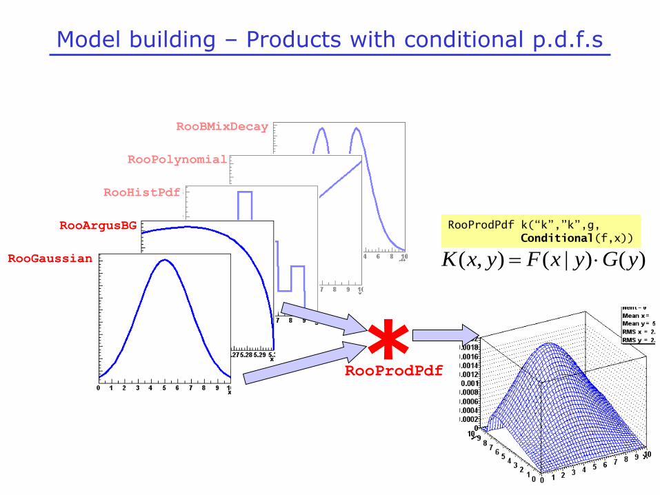
Model building – Products with conditional p.d.f.s
RooProdPdf *
)()|(),( yGyxFyxK
RooProdPdf k(“k”,”k”,g,
Conditional(f,x))
Wouter Verkerke, NIKHEF
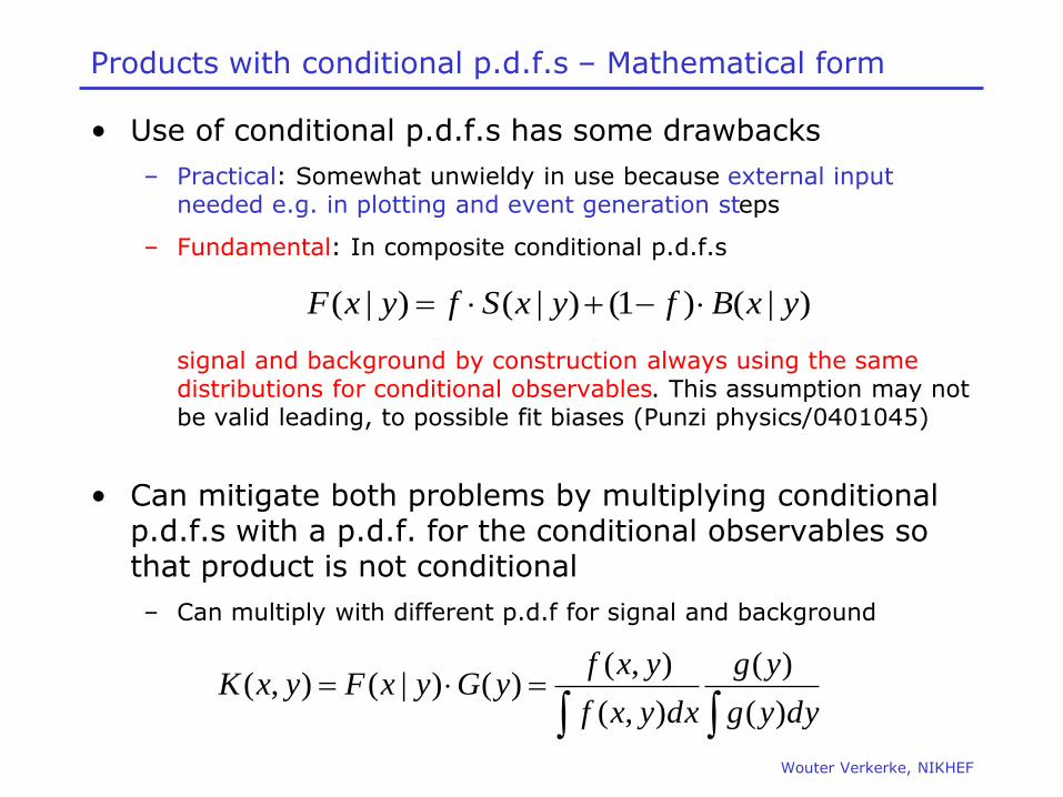
Products with conditional p.d.f.s – Mathematical form
• Use of conditional p.d.f.s has some drawbacks
– Practical: Somewhat unwieldy in use because external input needed e.g. in plotting and event generation steps
– Fundamental: In composite conditional p.d.f.s signal and background by construction always using the same distributions for conditional observables. This assumption may not be valid leading, to possible fit biases (Punzi physics/0401045)
• Can mitigate both problems by multiplying conditional p.d.f.s with a p.d.f. for the conditional observables so that product is not conditional
– Can multiply with different p.d.f for signal and background
)|()1()|()|( yxBfyxSfyxF
dyyg
yg
dxyxf
yxfyGyxFyxK
)(
)(
),(
),()()|(),(

Wouter Verkerke, NIKHEF
Normalization and event generation in conditional products
• Products of conditional and plain pdf’s are self normalized
– Proof is trivial
• Generation of events from products of conditional and plain p.d.fs can be handling by handling generation of observables in order
11)(
)(
),(
),(
)(
)(
),(
),(),(
dydyyg
ygdx
dxyxf
yxfdxdy
dyyg
yg
dxyxf
yxfyxK
)()|( yGyxF
)()|()|( zHzyGyxF
First generate y, then x
First generate z, then y, then x
Wouter Verkerke, NIKHEF
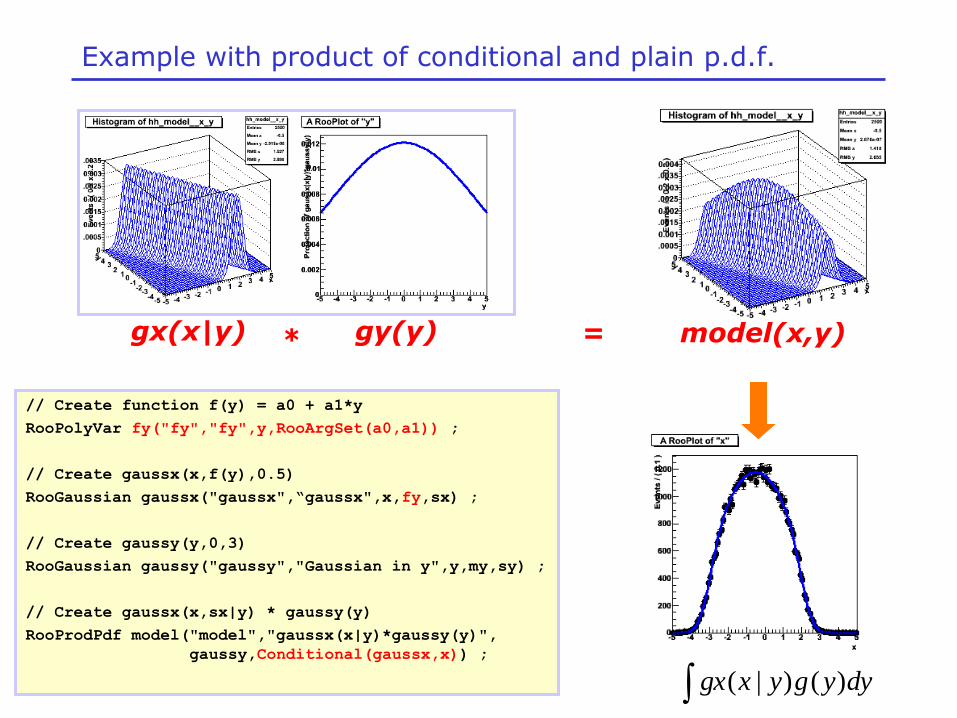
Example with product of conditional and plain p.d.f.
// Create function f(y) = a0 + a1*y
RooPolyVar fy("fy","fy",y,RooArgSet(a0,a1)) ;
// Create gaussx(x,f(y),0.5)
RooGaussian gaussx("gaussx",“gaussx",x,fy,sx) ;
// Create gaussy(y,0,3)
RooGaussian gaussy("gaussy","Gaussian in y",y,my,sy) ;
// Create gaussx(x,sx|y) * gaussy(y)
RooProdPdf model("model","gaussx(x|y)*gaussy(y)",
gaussy,Conditional(gaussx,x)) ;
gx(x|y) gy(y) * model(x,y) =
dyygyxgx )()|(

Wouter Verkerke, NIKHEF
Managing data, discrete variables simultaneous fits 5 • Binned, unbinned datasets
• Importing data
• Using discrete variable to classify data
• Simultaneous fits on multiple datasets
Wouter Verkerke, NIKHEF
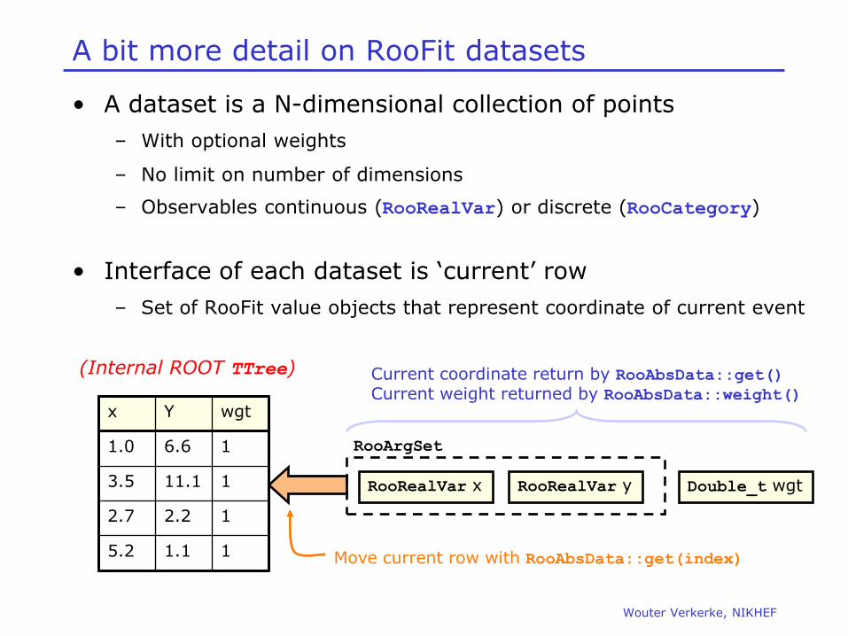
A bit more detail on RooFit datasets
• A dataset is a N-dimensional collection of points
– With optional weights
– No limit on number of dimensions
– Observables continuous (RooRealVar) or discrete (RooCategory)
• Interface of each dataset is ‘current’ row
– Set of RooFit value objects that represent coordinate of current event
x Y wgt
1.0 6.6 1
3.5 11.1 1
2.7 2.2 1
5.2 1.1 1
RooRealVar x RooRealVar y
RooArgSet
Double_t wgt
Current coordinate return by RooAbsData::get() Current weight returned by RooAbsData::weight()
Move current row with RooAbsData::get(index)
(Internal ROOT TTree)
Wouter Verkerke, NIKHEF
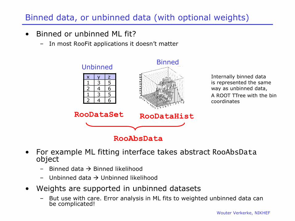
Binned data, or unbinned data (with optional weights)
• Binned or unbinned ML fit?
– In most RooFit applications it doesn’t matter
• For example ML fitting interface takes abstract RooAbsData object
– Binned data Binned likelihood
– Unbinned data Unbinned likelihood
• Weights are supported in unbinned datasets
– But use with care. Error analysis in ML fits to weighted unbinned data can be complicated!
x y z 1 3 5 2 4 6 1 3 5 2 4 6
Binned Unbinned
RooDataSet RooDataHist
RooAbsData
Internally binned data is represented the same way as unbinned data,
A ROOT TTree with the bin coordinates

Wouter Verkerke, NIKHEF
Importing unbinned data
• From ROOT trees
– RooRealVar variables are imported from /D /F /I tree branches
– RooCategory variables are imported from /I /b tree branches
– Mapping between TTree branches and dataset variables by name: e.g. RooRealVar x(“x”,”x”,-10,10) imports TTree branch “x”
– Only events with ‘valid’ entries are imported. In above example any events with |x|>10 or c<0 or c>30 are not imported
• From ASCII files
– One line per event, order of variables as given in RooArgList
RooRealVar x(“x”,”x”,-10,10) ;
RooRealVar c(“c”,”c”,0,30) ;
RooDataSet data(“data”,”data”,inputTree,RooArgSet(x,c));
RooDataSet* data =
RooDataSet::read(“ascii.file”,RooArgList(x,c)) ;

Wouter Verkerke, NIKHEF
Importing binned data
• From ROOT THx histogram objects
• From a RooDataSet
RooDataHist bdata1(“bdata”,”bdata”,RooArgList(x),histo1d);
RooDataHist bdata2(“bdata”,”bdata”,RooArgList(x,y),histo2d);
RooDataHist bdata3(“bdata”,”bdata”,RooArgList(x,y,z),histo3d);
RooDataHist* binnedData = data->binnedClone() ;
Wouter Verkerke, NIKHEF
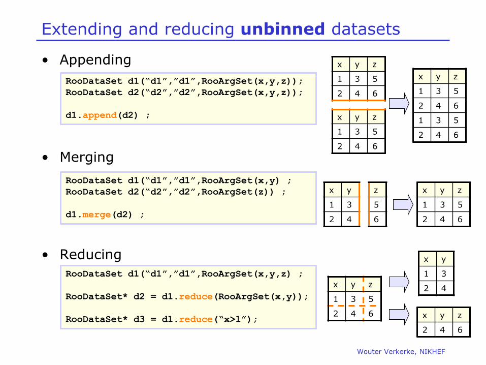
Extending and reducing unbinned datasets
RooDataSet d1(“d1”,”d1”,RooArgSet(x,y,z) ;
RooDataSet* d2 = d1.reduce(RooArgSet(x,y));
RooDataSet* d3 = d1.reduce(“x>1”);
• Appending
• Merging
• Reducing
RooDataSet d1(“d1”,”d1”,RooArgSet(x,y,z));
RooDataSet d2(“d2”,”d2”,RooArgSet(x,y,z));
d1.append(d2) ;
z
5
6
x y
1 3
2 4
x y z
1 3 5
2 4 6
x y z
1 3 5
2 4 6
x y z
2 4 6
x y z
1 3 5
2 4 6
1 3 5
2 4 6
RooDataSet d1(“d1”,”d1”,RooArgSet(x,y) ;
RooDataSet d2(“d2”,”d2”,RooArgSet(z)) ;
d1.merge(d2) ;
x y z
1 3 5
2 4 6
x y
1 3
2 4
x y z
1 3 5
2 4 6
Wouter Verkerke, NIKHEF
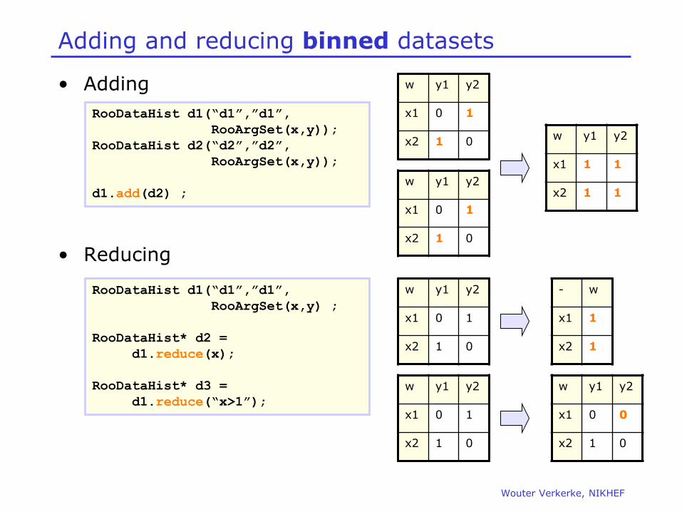
Adding and reducing binned datasets
RooDataHist d1(“d1”,”d1”,
RooArgSet(x,y) ;
RooDataHist* d2 =
d1.reduce(x);
RooDataHist* d3 =
d1.reduce(“x>1”);
• Adding
• Reducing
RooDataHist d1(“d1”,”d1”,
RooArgSet(x,y));
RooDataHist d2(“d2”,”d2”,
RooArgSet(x,y));
d1.add(d2) ;
w y1 y2
x1 1 1
x2 1 1 w y1 y2
x1 0 1
x2 1 0
- w
x1 1
x2 1
w y1 y2
x1 0 1
x2 1 0
w y1 y2
x1 0 0
x2 1 0
w y1 y2
x1 0 1
x2 1 0
w y1 y2
x1 0 1
x2 1 0
Wouter Verkerke, NIKHEF
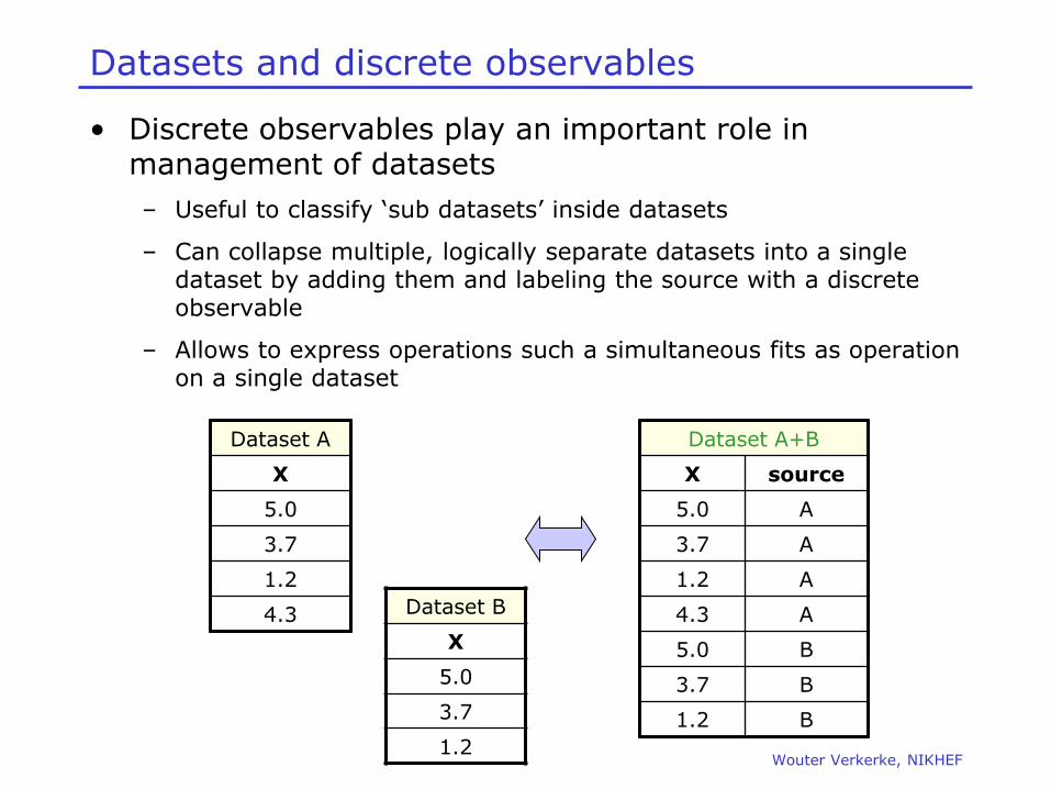
Datasets and discrete observables
• Discrete observables play an important role in management of datasets
– Useful to classify ‘sub datasets’ inside datasets
– Can collapse multiple, logically separate datasets into a single dataset by adding them and labeling the source with a discrete observable
– Allows to express operations such a simultaneous fits as operation on a single dataset
Dataset A
X
5.0
3.7
1.2
4.3 Dataset B
X
5.0
3.7
1.2
Dataset A+B
X source
5.0 A
3.7 A
1.2 A
4.3 A
5.0 B
3.7 B
1.2 B

Wouter Verkerke, NIKHEF
Discrete variables in RooFit – RooCategory
• Properties of RooCategory variables
– Finite set of named states self documenting
– Optional integer code associated with each state
• Used for classification of data, or to describe occasional discrete fundamental observable (e.g. B0 flavor)
// Define a cat. with explicitly numbered states
RooCategory b0flav("b0flav","B0 flavour") ;
b0flav.defineType("B0",-1) ;
b0flav.defineType("B0bar",1) ;
// Define a category with labels only
RooCategory tagCat("tagCat","Tagging technique") ;
tagCat.defineType("Lepton") ;
tagCat.defineType("Kaon") ;
tagCat.defineType("NetTagger-1") ;
tagCat.defineType("NetTagger-2") ;
At creation, a category
has no states
Add states with a label and index
Add states with a label only.
Indices will be automatically
assigned

Wouter Verkerke, NIKHEF
Datasets and discrete observables – part 2
• Example of appending datasets with label attachment
• But can also derive classification from info within dataset
– E.g. (10<x<20 = “signal”, 0<x<10 | 20<x<30 = “sideband”)
– Encode classification using realdiscrete mapping functions
RooCategory c(“c”,”source”)
c.defineType(“A”) ;
c.defineType(“B”) ;
// Add column with source label
c.setLabel(“A”) ; dA->addColumn(c) ;
c.setLabel(“B”) ; dB->addColumn(c) ;
// Make combined dataset
RooDataSet* dAB = dA->Clone(“dAB”) ;
dAB->append(*dB) ;

Wouter Verkerke, NIKHEF
// Mass variable
RooRealVar m(“m”,”mass,0,10.);
// Define threshold category
RooThresholdCategory region(“region”,”Region of M”,m,”Background”);
region.addThreshold(9.0, “SideBand”) ;
region.addThreshold(7.9, “Signal”) ;
region.addThreshold(6.1,”SideBand”) ;
region.addThreshold(5.0,”Background”) ;
A universal realdiscrete mapping function
• Class RooThresholdCategory maps ranges of input RooRealVar to states of a RooCategory
Sig Sideband background
Default state
Define region boundaries
Wouter Verkerke, NIKHEF
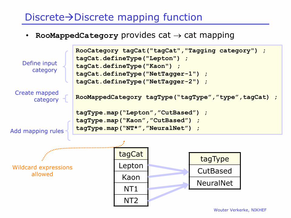
DiscreteDiscrete mapping function
• RooMappedCategory provides cat cat mapping
RooCategory tagCat("tagCat","Tagging category") ;
tagCat.defineType("Lepton") ;
tagCat.defineType("Kaon") ;
tagCat.defineType("NetTagger-1") ;
tagCat.defineType("NetTagger-2") ;
RooMappedCategory tagType(“tagType”,”type”,tagCat) ;
tagType.map(“Lepton”,”CutBased”) ;
tagType.map(“Kaon”,”CutBased”) ;
tagType.map(“NT*”,”NeuralNet”) ;
Define input category
Create mapped category
Add mapping rules
Wildcard expressions allowed
tagCat
Lepton
Kaon
NT1
NT2
tagType
CutBased
NeuralNet

Wouter Verkerke, NIKHEF
Discrete multiplication function
• RooSuperCategory/RooMultiCategory provides
category multiplication
// Define ‘product’ of tagCat and runBlock
RooSuperCategory prod(“prod”,”prod”,RooArgSet(tag,flav))
flav
B0
B0bar
tag
Lepton
Kaon
NT1
NT2
prod
{B0;Lepton} {B0bar;Lepton}
{B0;Kaon} {B0bar;Kaon}
{B0;NT1} {B0bar;NT1}
{B0;NT2} {B0bar;NT2}
X

Wouter Verkerke, NIKHEF
Exploring discrete data
• Like real variables of a dataset can be plotted, discrete variables can be tabulated
RooTable* table=data->table(b0flav) ;
table->Print() ;
Table b0flav : aData +-------+------+ | B0 | 4949 | | B0bar | 5051 | +-------+------+
Double_t nB0 = table->get(“B0”) ;
Double_t b0Frac = table->getFrac(“B0”);
data->table(tagCat,"x>8.23")->Print() ;
Table tagCat : aData(x>8.23) +-------------+-----+ | Lepton | 668 | | Kaon | 717 | | NetTagger-1 | 632 | | NetTagger-2 | 616 | +-------------+-----+
Tabulate contents of dataset by category state
Extract contents by label
Extract contents fraction by label
Tabulate contents of selected part of dataset

Wouter Verkerke, NIKHEF
Exploring discrete data
• Discrete functions, built from categories in a dataset can be tabulated likewise
data->table(b0Xtcat)->Print() ;
Table b0Xtcat : aData +---------------------+------+ | {B0;Lepton} | 1226 | | {B0bar;Lepton} | 1306 | | {B0;Kaon} | 1287 | | {B0bar;Kaon} | 1270 | | {B0;NetTagger-1} | 1213 | | {B0bar;NetTagger-1} | 1261 | | {B0;NetTagger-2} | 1223 | | {B0bar;NetTagger-2} | 1214 | +---------------------+------+
data->table(tcatType)->Print() ;
Table tcatType : aData +----------------+------+ | Unknown | 0 | | Cut based | 5089 | | Neural Network | 4911 | +----------------+------+
Tabulate RooSuperCategory states
Tabulate RooMappedCategory states

Wouter Verkerke, NIKHEF
Fitting multiple datasets simultaneously
• Simultaneous fitting efficient solution to incorporate information from control sample into signal sample
• Example problem: search rare decay
– Signal dataset has small number entries.
– Statistical uncertainty on shape in fit contributes significantly to uncertainty on fitted number of signal events
– However can constrain shape of signal from control sample (e.g. another decay with similar properties that is not rare), so no need to relay on simulations
Par FinalValue +/- Error
---- --------------------------
a0 -1.0544e-01 +/- 2.88e-02
a1 2.2698e-03 +/- 4.92e-03
nbkg 1.0933e+02 +/- 1.07e+01
nsig 1.0680e+01 +/- 3.92e+00
mean 2.9787e+00 +/- 6.25e-02
width 1.3764e-01 +/- 6.29e-02
Wouter Verkerke, NIKHEF
Fitting multiple datasets simultaneously
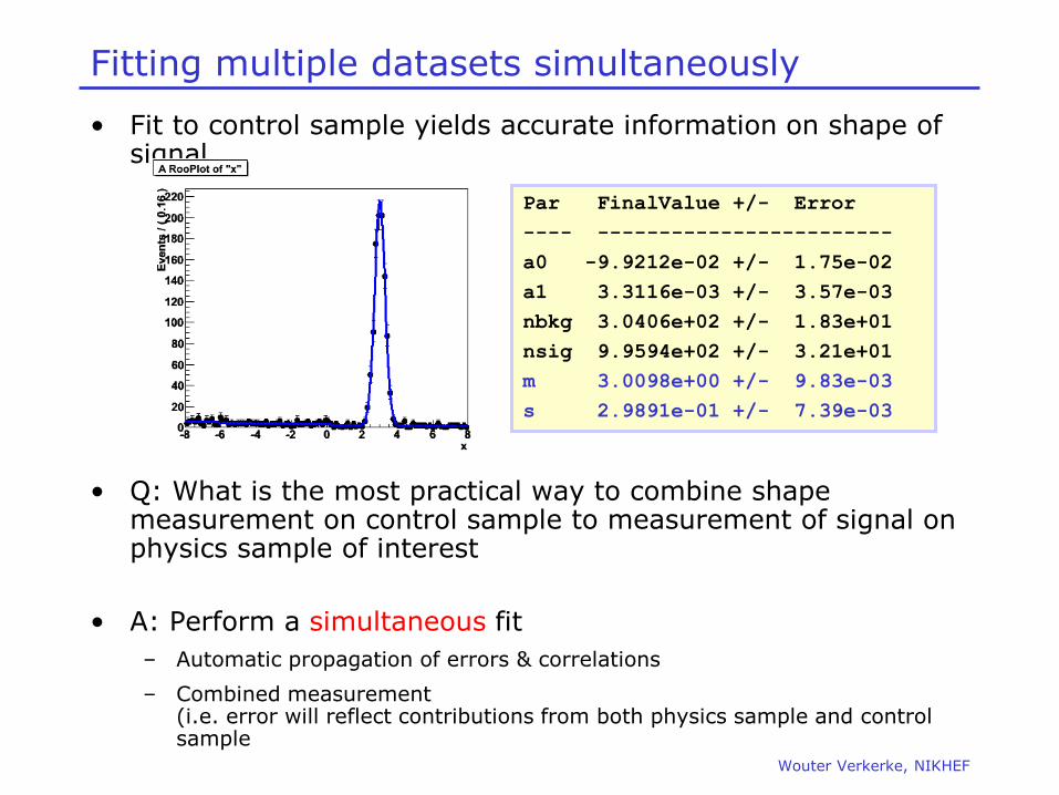
• Fit to control sample yields accurate information on shape of signal
• Q: What is the most practical way to combine shape measurement on control sample to measurement of signal on physics sample of interest
• A: Perform a simultaneous fit
– Automatic propagation of errors & correlations
– Combined measurement (i.e. error will reflect contributions from both physics sample and control sample
Par FinalValue +/- Error
---- ------------------------
a0 -9.9212e-02 +/- 1.75e-02
a1 3.3116e-03 +/- 3.57e-03
nbkg 3.0406e+02 +/- 1.83e+01
nsig 9.9594e+02 +/- 3.21e+01
m 3.0098e+00 +/- 9.83e-03
s 2.9891e-01 +/- 7.39e-03

Wouter Verkerke, NIKHEF
Discrete observable as data subset classifier
• Likelihood level definition of a simultaneous fit
• PDF level definition of a simultaneous fit
mi
i
BB
ni
i
AA DPDFDPDFL,1,1
))(log())(log()log(
RooSimultaneous implements ‘switch’ PDF: case (indexCat) {
A: return pdfA ;
B: return pdfB ;
}
Likelihood of switchPdf with composite dataset automatically constructs sum of likelihoods above
ni
i
BADsimPDFL,1
))(log()log(
Wouter Verkerke, NIKHEF
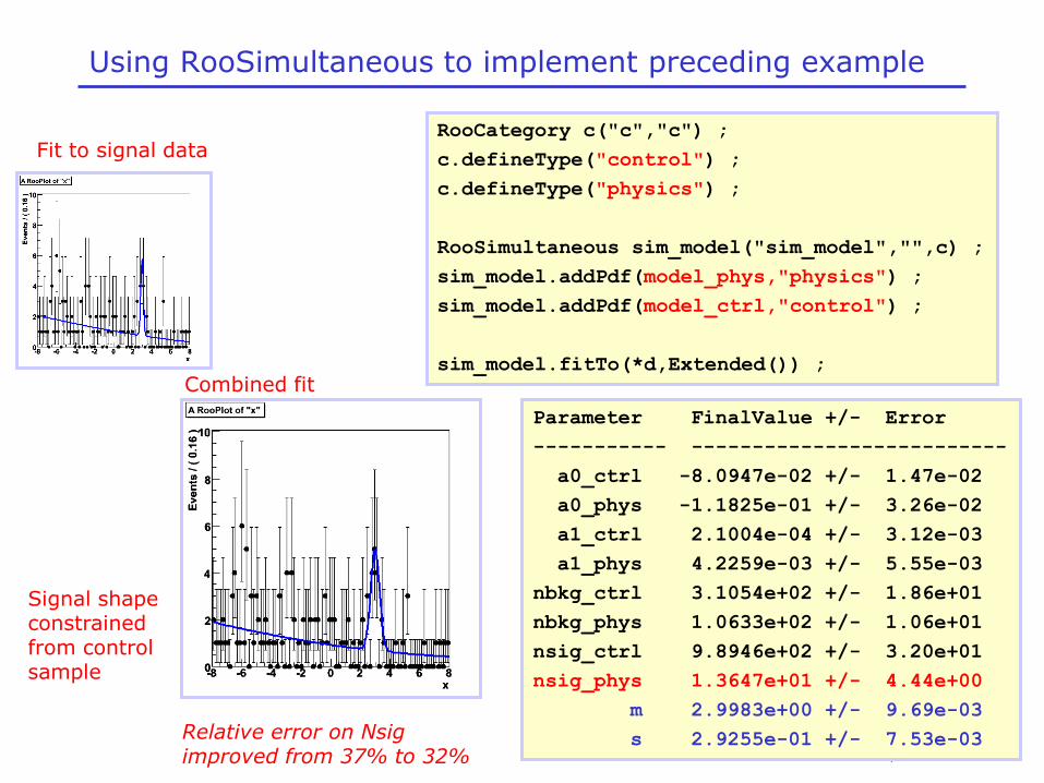
Using RooSimultaneous to implement preceding example
RooCategory c("c","c") ;
c.defineType("control") ;
c.defineType("physics") ;
RooSimultaneous sim_model("sim_model","",c) ;
sim_model.addPdf(model_phys,"physics") ;
sim_model.addPdf(model_ctrl,"control") ;
sim_model.fitTo(*d,Extended()) ;
Parameter FinalValue +/- Error
----------- --------------------------
a0_ctrl -8.0947e-02 +/- 1.47e-02
a0_phys -1.1825e-01 +/- 3.26e-02
a1_ctrl 2.1004e-04 +/- 3.12e-03
a1_phys 4.2259e-03 +/- 5.55e-03
nbkg_ctrl 3.1054e+02 +/- 1.86e+01
nbkg_phys 1.0633e+02 +/- 1.06e+01
nsig_ctrl 9.8946e+02 +/- 3.20e+01
nsig_phys 1.3647e+01 +/- 4.44e+00
m 2.9983e+00 +/- 9.69e-03
s 2.9255e-01 +/- 7.53e-03
Fit to signal data
Combined fit
Signal shape constrained from control sample
Relative error on Nsig improved from 37% to 32%
Other scenarios in which simultaneous fits are useful
• Preceding example was ‘asymmetric’
– Very large control sample, small signal sample
– Physics in each channel possibly different (but with some similar properties
• There are also ‘symmetric’ use cases
– Fit multiple data sets that are functionally equivalent, but have slightly different properties (e.g. purity)
– Example: Split B physics data in block separated by flavor tagging technique (each technique results in a different sensitivity to CP physics parameters of interest).
– Split data in block by data taking run, mass resolutions in each run may be slightly different
– For symmetric use cases pdf-level definition of simultaneous fit very convenient as you usually start with a single dataset with subclassing formation derived from its observables
• By splitting data into subsamples with p.d.f.s that can be tuned to describe the (slightly) varying properties you can increase the statistical sensitivity of your measurement
Wouter Verkerke, NIKHEF

Wouter Verkerke, NIKHEF
A more empirical approach to simultaneous fits
• Instead of investing a lot of time in developing multi-dimensional models Split data in many subsamples, fit all subsamples
simultaneously to slight variations of ‘master’ p.d.f
• Example: Given dataset D(x,y) where observable of interest is x.
– Distribution of x varies slightly with y
– Suppose we’re only interested in the width of the peak which is supposed to be invariant under y (unlike mean)
– Slice data in 10 bins of y and simultaneous fit each bin with p.d.f that only has different Gaussian mean parameter, but same width

Wouter Verkerke, NIKHEF
A more empirical approach to simultaneous fits
• Fit to sample of preceding page would look like this
– Each mean is fitted to expected value (-4.5 + ibin)
– But joint measurement of sigma
– NB: Correlation matrix is mostly diagonal as all mean_binXX parameters are completely uncorrelated!
Floating Parameter FinalValue +/- Error
-------------------- --------------------------
mean_bin1 -4.5302e+00 +/- 1.62e-02
mean_bin2 -3.4928e+00 +/- 1.38e-02
mean_bin3 -2.4790e+00 +/- 1.35e-02
mean_bin4 -1.4174e+00 +/- 9.64e-03
mean_bin5 -4.8945e-01 +/- 7.95e-03
mean_bin6 4.0716e-01 +/- 9.67e-03
mean_bin7 1.4733e+00 +/- 1.37e-02
mean_bin8 2.4912e+00 +/- 1.44e-02
mean_bin9 3.5028e+00 +/- 1.41e-02
mean_bin10 4.5474e+00 +/- 1.68e-02
sigma 2.7319e-01 +/- 2.46e-03
Wouter Verkerke, NIKHEF
A more empirical approach to simultaneous fits
• Preceding example was somewhat silly for illustrational clarity, but more sensible use cases exist
– Example: Measurement CP violation in B decay. Analyzing power of each event is diluted by factor (1-2w) where w is the mistake rate of the flavor tagging algorithm
– Neural net flavor tagging algorithm provides a tagging probability for each event in data. Could use prob(NN) as w, but then we rely on good calibration of NN, don’t want that
– Do simultaneous fit to CPV+Mixing samples, can measure w from the latter. Now not relying on NN calibration, but not exploiting event-by-event variation in analysis power.
– Now divide (CPV+mixing) data in 10 or 20 subsets corresponding to bins in prob(NN). Use identical p.d.f but only have separate parameter to express fitted mistag rate w_binXX.
– Simultaneous fit will now exploit difference in analyzing power of events and be insensitive to calibration of flavor tagging NN.
– If calibration of NN was OK fitting mistag rate in each bin of probNN will be average probNN value for that bin

Wouter Verkerke, NIKHEF
A more empirical approach to simultaneous fits
Event with little analyzing power
Event with great analyzing
power
NN predicted power
NN predicted power
NN predicted power
co
ntr
ol sam
ple
m
easu
red
po
wer
co
ntr
ol sam
ple
m
easu
red
po
wer
co
ntr
ol sam
ple
m
easu
red
po
wer
Perfect NN
OK NN
Lousy NN
In all 3 cases fit not biased by NN calibration
Better precision on CPV meas. because more sensitive events in sample
Worse precision on CPV meas. because less sensitive events in sample
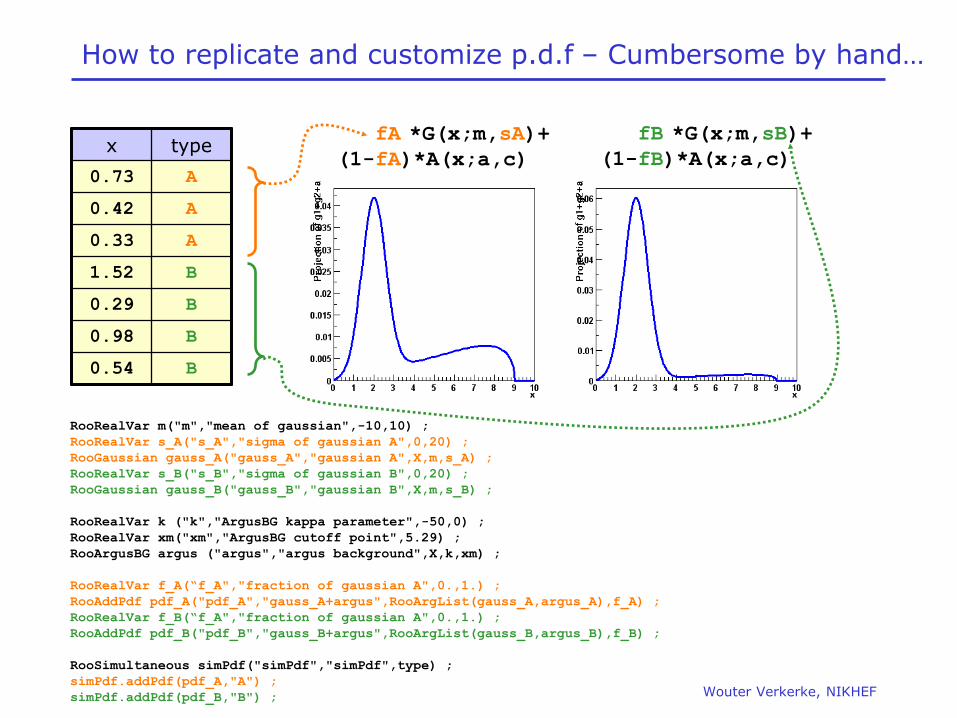
Wouter Verkerke, NIKHEF
How to replicate and customize p.d.f – Cumbersome by hand…
fA *G(x;m,sA)+
(1-fA)*A(x;a,c)
fB *G(x;m,sB)+
(1-fB)*A(x;a,c) x type
0.73 A
0.42 A
0.33 A
1.52 B
0.29 B
0.98 B
0.54 B
RooRealVar m("m","mean of gaussian",-10,10) ;
RooRealVar s_A("s_A","sigma of gaussian A",0,20) ;
RooGaussian gauss_A("gauss_A","gaussian A",X,m,s_A) ;
RooRealVar s_B("s_B","sigma of gaussian B",0,20) ;
RooGaussian gauss_B("gauss_B","gaussian B",X,m,s_B) ;
RooRealVar k ("k","ArgusBG kappa parameter",-50,0) ;
RooRealVar xm("xm","ArgusBG cutoff point",5.29) ;
RooArgusBG argus ("argus","argus background",X,k,xm) ;
RooRealVar f_A(“f_A","fraction of gaussian A",0.,1.) ;
RooAddPdf pdf_A("pdf_A","gauss_A+argus",RooArgList(gauss_A,argus_A),f_A) ;
RooRealVar f_B(“f_A","fraction of gaussian A",0.,1.) ;
RooAddPdf pdf_B("pdf_B","gauss_B+argus",RooArgList(gauss_B,argus_B),f_B) ;
RooSimultaneous simPdf("simPdf","simPdf",type) ;
simPdf.addPdf(pdf_A,"A") ;
simPdf.addPdf(pdf_B,"B") ;
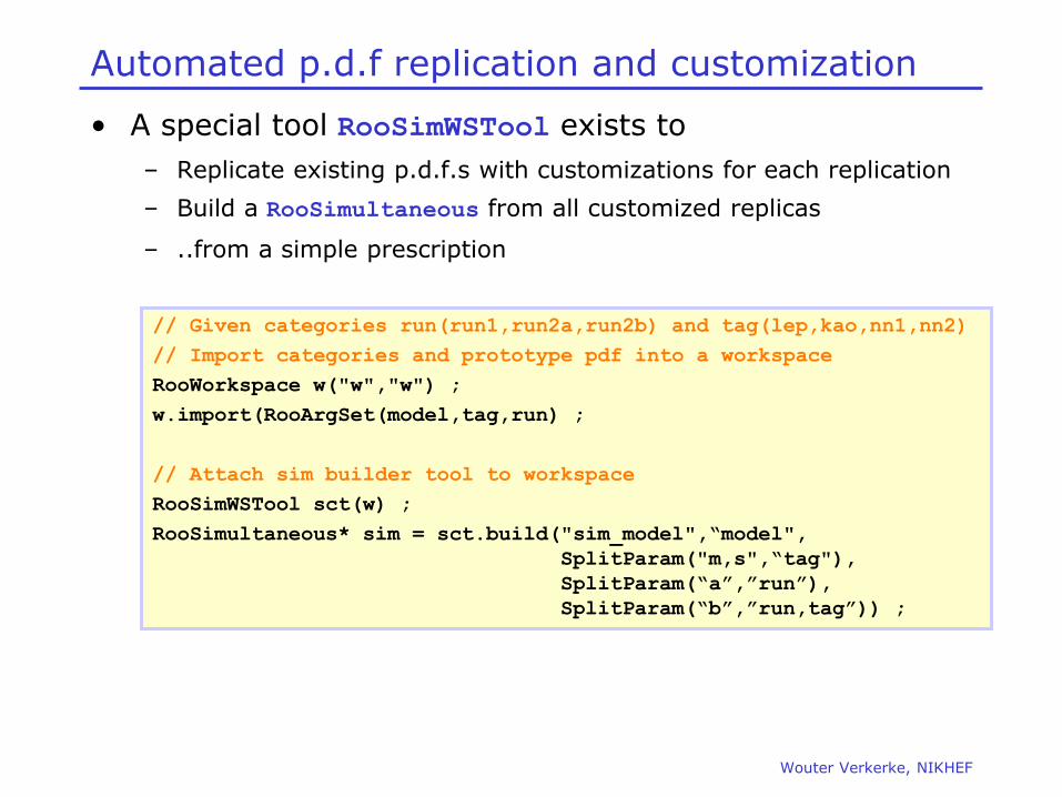
Wouter Verkerke, NIKHEF
Automated p.d.f replication and customization
• A special tool RooSimWSTool exists to
– Replicate existing p.d.f.s with customizations for each replication
– Build a RooSimultaneous from all customized replicas
– ..from a simple prescription
// Given categories run(run1,run2a,run2b) and tag(lep,kao,nn1,nn2)
// Import categories and prototype pdf into a workspace
RooWorkspace w("w","w") ;
w.import(RooArgSet(model,tag,run) ;
// Attach sim builder tool to workspace
RooSimWSTool sct(w) ;
RooSimultaneous* sim = sct.build("sim_model",“model",
SplitParam("m,s",“tag"),
SplitParam(“a”,”run”),
SplitParam(“b”,”run,tag”)) ;
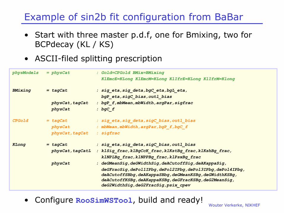
Example of sin2b fit configuration from BaBar
• Start with three master p.d.f, one for Bmixing, two for BCPdecay (KL / KS)
• ASCII-filed splitting prescription
• Configure RooSimWSTool, build and ready! Wouter Verkerke, NIKHEF
physModels = physCat : Gold=CPGold BMix=BMixing
KlEmcE=KLong KlEmcM=KLong KlIfrE=KLong KlIfrM=Klong
BMixing = tagCat : sig_eta,sig_deta,bgC_eta,bgL_eta,
bgP_eta,sigC_bias,outl_bias
physCat,tagCat : bgP_f,mbMean,mbWidth,argPar,sigfrac
physCat : bgC_f
CPGold = tagCat : sig_eta,sig_deta,sigC_bias,outl_bias
physCat : mbMean,mbWidth,argPar,bgP_f,bgC_f
physCat,tagCat : sigfrac
KLong = tagCat : sig_eta,sig_deta,sigC_bias,outl_bias
physCat,tagCatL : klSig_frac,klBgCcK_frac,klKstBg_frac,klKshBg_frac,
klNPLBg_frac,klNPPBg_frac,klPsxBg_frac
physCat : deGMeanSig,deGWidthSig,deACutoffSig,deAKappaSig,
deGFracSig,dePol1IPbg,dePol2IPbg,dePol3IPbg,dePol4IPbg,
deACutoffSBbg,deAKappaSBbg,deGMeanKSBg,deGWidthKSBg,
deACutoffKSBg,deAKappaKSBg,deGFracKSBg,deG2MeanSig,
deG2WidthSig,deG2FracSig,psix_cpev

Wouter Verkerke, NIKHEF
Likelihood calculation & minimization 6 • Details on the likelihood calculation
• Using MINUIT and RooMinuit
• Profile likelihoods

Wouter Verkerke, NIKHEF
Fitting and likelihood minimization
• What happens when you do pdf->fitTo(*data)
– 1) Construct object representing –log of (extended) likelihood
– 2) Minimize likelihood w.r.t floating parameters using MINUIT
• Can also do these two steps explicitly by hand
// Construct function object representing –log(L)
RooNLLVar nll(“nll”,”nll”,pdf,data) ;
// Minimize nll w.r.t its parameters
RooMinuit m(nll) ;
m.migrad() ;
m.hesse() ;

Constructing the likelihood function
• Class RooNLLVar works universally for all p.d.f.s and all
types of data
– Binned data Binned likelihood
– Unbinned data Unbinned likelihood
• Can add named arguments to constructor to control details of likelihood definition and mode of calculation
– Works like a regular RooFit function object, i.e. can retrieve value and make plots as usual
Wouter Verkerke, NIKHEF
RooNLLVar nll(“nll”,”nll”,pdf,data,Extended()) ;
Double_t val = nll.getVal() ;
RooArgSet* vars = nll.getVariables()
RooPlot* frame = p.frame() ;
nll.plotOn(frame) ;
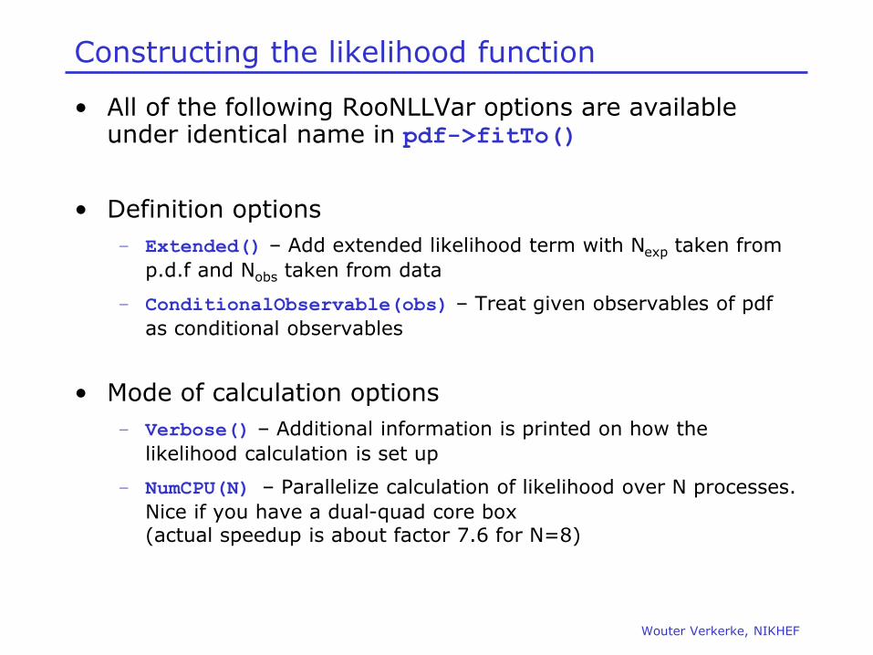
Constructing the likelihood function
• All of the following RooNLLVar options are available under identical name in pdf->fitTo()
• Definition options
– Extended() – Add extended likelihood term with Nexp taken from
p.d.f and Nobs taken from data
– ConditionalObservable(obs) – Treat given observables of pdf
as conditional observables
• Mode of calculation options
– Verbose() – Additional information is printed on how the
likelihood calculation is set up
– NumCPU(N) – Parallelize calculation of likelihood over N processes.
Nice if you have a dual-quad core box (actual speedup is about factor 7.6 for N=8)
Wouter Verkerke, NIKHEF
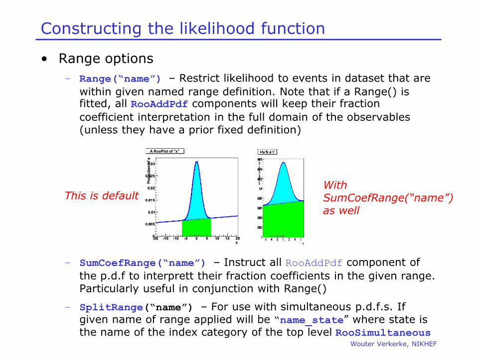
Constructing the likelihood function
• Range options
– Range(“name”) – Restrict likelihood to events in dataset that are
within given named range definition. Note that if a Range() is fitted, all RooAddPdf components will keep their fraction
coefficient interpretation in the full domain of the observables (unless they have a prior fixed definition)
– SumCoefRange(“name”) – Instruct all RooAddPdf component of
the p.d.f to interprett their fraction coefficients in the given range. Particularly useful in conjunction with Range()
– SplitRange(“name”) – For use with simultaneous p.d.f.s. If given name of range applied will be “name_state” where state is the name of the index category of the top level RooSimultaneous
Wouter Verkerke, NIKHEF
This is default With SumCoefRange(“name”) as well
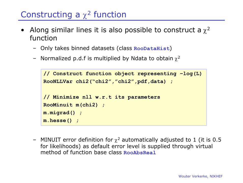
Constructing a c2 function
• Along similar lines it is also possible to construct a c2 function
– Only takes binned datasets (class RooDataHist)
– Normalized p.d.f is multiplied by Ndata to obtain c2
– MINUIT error definition for c2 automatically adjusted to 1 (it is 0.5 for likelihoods) as default error level is supplied through virtual method of function base class RooAbsReal
Wouter Verkerke, NIKHEF
// Construct function object representing –log(L)
RooNLLVar chi2(“chi2”,”chi2”,pdf,data) ;
// Minimize nll w.r.t its parameters
RooMinuit m(chi2) ;
m.migrad() ;
m.hesse() ;
Wouter Verkerke, NIKHEF
Automatic optimizations in the calculation of the likelihood
• Several automatic computational optimizations are applied the calculation of likelihoods inside RooNLLVar
– Components that have all constant parameters are pre-calculated
– Dataset variables not used by the PDF are dropped
– PDF normalization integrals are only recalculated when the ranges of their observables or the value of their parameters are changed
– Simultaneous fits: When a parameters changes only parts of the total likelihood that depend on that parameter are recalculated
• Lazy evaluation: calculation only done when intergal value is requested
• Applicability of optimization techniques is re-evaluated for each use
– Maximum benefit for each use case
• ‘Typical’ large-scale fits see significant speed increase
– Factor of 3x – 10x not uncommon.
Features of class RooMinuit
• Class RooMinuit is an interface to the ROOT implementation of the MINUIT minimization and error analysis package.
• RooMinuit takes care of
– Passing value of miminized RooFit function to MINUIT
– Propagated changes in parameters both from RooRealVar to MINUIT and back from MINUIT to RooRealVar, i.e. it keeps the
state of RooFit objects synchronous with the MINUIT internal state
– Propagate error analysis information back to RooRealVar
parameters objects
– Exposing high-level MINUIT operations to RooFit uses (MIGRAD,HESSE,MINOS) etc…
– Making optional snapshots of complete MINUIT information (e.g. convergence state, full error matrix etc)
Wouter Verkerke, NIKHEF
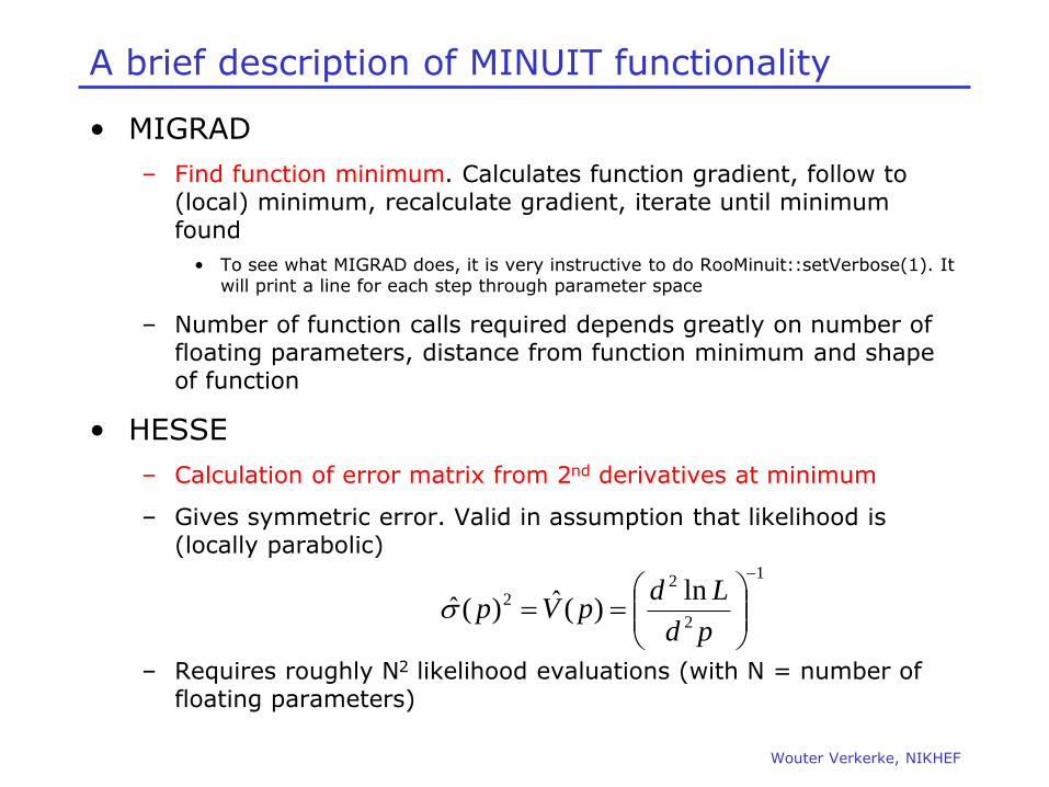
A brief description of MINUIT functionality
• MIGRAD
– Find function minimum. Calculates function gradient, follow to (local) minimum, recalculate gradient, iterate until minimum found
• To see what MIGRAD does, it is very instructive to do RooMinuit::setVerbose(1). It will print a line for each step through parameter space
– Number of function calls required depends greatly on number of floating parameters, distance from function minimum and shape of function
• HESSE
– Calculation of error matrix from 2nd derivatives at minimum
– Gives symmetric error. Valid in assumption that likelihood is (locally parabolic)
– Requires roughly N2 likelihood evaluations (with N = number of floating parameters)
Wouter Verkerke, NIKHEF
1
2
22 ln
)(ˆ)(ˆ
pd
LdpVp
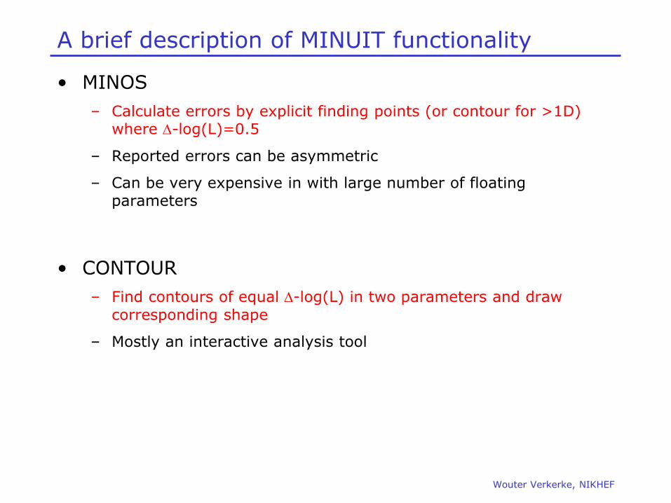
A brief description of MINUIT functionality
• MINOS
– Calculate errors by explicit finding points (or contour for >1D) where -log(L)=0.5
– Reported errors can be asymmetric
– Can be very expensive in with large number of floating parameters
• CONTOUR
– Find contours of equal -log(L) in two parameters and draw corresponding shape
– Mostly an interactive analysis tool
Wouter Verkerke, NIKHEF
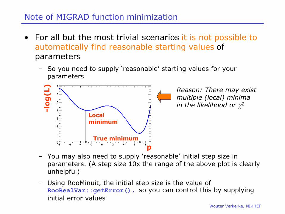
Wouter Verkerke, NIKHEF
Note of MIGRAD function minimization
• For all but the most trivial scenarios it is not possible to automatically find reasonable starting values of parameters
– So you need to supply ‘reasonable’ starting values for your parameters
– You may also need to supply ‘reasonable’ initial step size in parameters. (A step size 10x the range of the above plot is clearly unhelpful)
– Using RooMinuit, the initial step size is the value of RooRealVar::getError(), so you can control this by supplying
initial error values
Reason: There may exist multiple (local) minima in the likelihood or c2
p
-lo
g(L)
Local minimum
True minimum
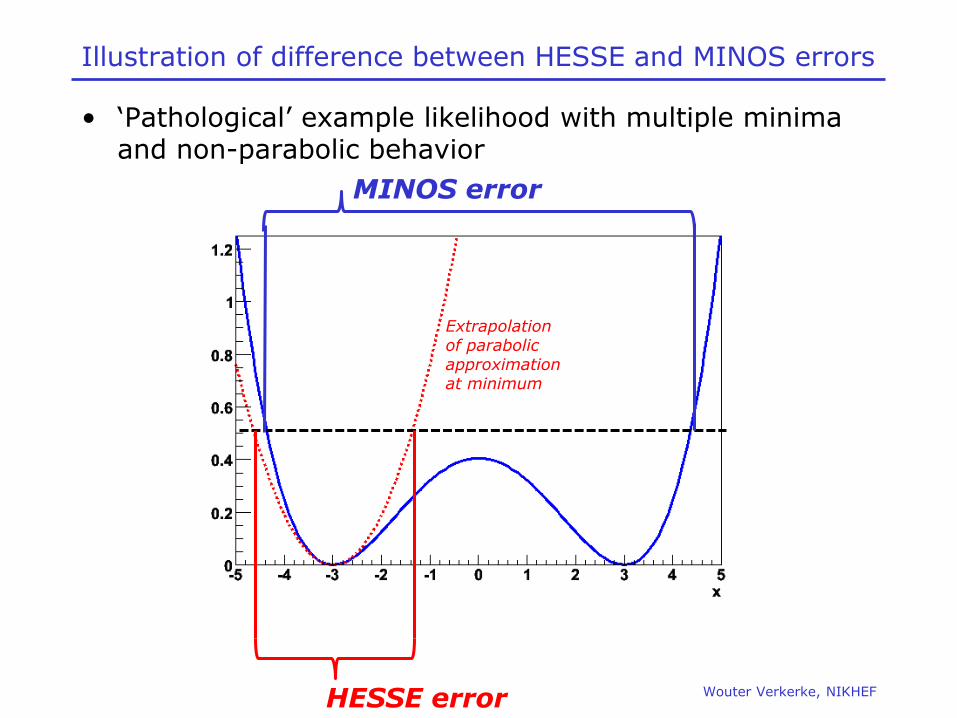
Wouter Verkerke, NIKHEF
Illustration of difference between HESSE and MINOS errors
• ‘Pathological’ example likelihood with multiple minima and non-parabolic behavior
MINOS error
HESSE error
Extrapolation of parabolic approximation at minimum
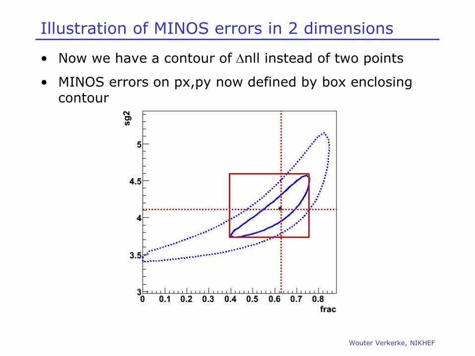
Illustration of MINOS errors in 2 dimensions
• Now we have a contour of nll instead of two points
• MINOS errors on px,py now defined by box enclosing contour
Wouter Verkerke, NIKHEF
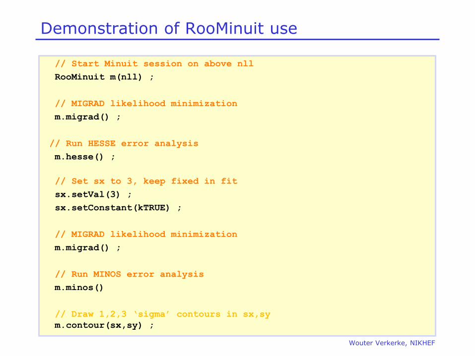
Demonstration of RooMinuit use
Wouter Verkerke, NIKHEF
// Start Minuit session on above nll
RooMinuit m(nll) ;
// MIGRAD likelihood minimization
m.migrad() ;
// Run HESSE error analysis
m.hesse() ;
// Set sx to 3, keep fixed in fit
sx.setVal(3) ;
sx.setConstant(kTRUE) ;
// MIGRAD likelihood minimization
m.migrad() ;
// Run MINOS error analysis
m.minos()
// Draw 1,2,3 ‘sigma’ contours in sx,sy
m.contour(sx,sy) ;
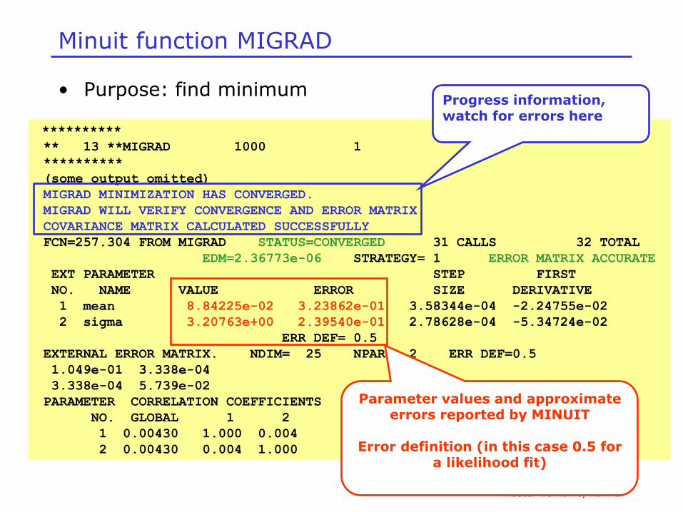
Wouter Verkerke, NIKHEF
Minuit function MIGRAD
• Purpose: find minimum
**********
** 13 **MIGRAD 1000 1
**********
(some output omitted)
MIGRAD MINIMIZATION HAS CONVERGED.
MIGRAD WILL VERIFY CONVERGENCE AND ERROR MATRIX.
COVARIANCE MATRIX CALCULATED SUCCESSFULLY
FCN=257.304 FROM MIGRAD STATUS=CONVERGED 31 CALLS 32 TOTAL
EDM=2.36773e-06 STRATEGY= 1 ERROR MATRIX ACCURATE
EXT PARAMETER STEP FIRST
NO. NAME VALUE ERROR SIZE DERIVATIVE
1 mean 8.84225e-02 3.23862e-01 3.58344e-04 -2.24755e-02
2 sigma 3.20763e+00 2.39540e-01 2.78628e-04 -5.34724e-02
ERR DEF= 0.5
EXTERNAL ERROR MATRIX. NDIM= 25 NPAR= 2 ERR DEF=0.5
1.049e-01 3.338e-04
3.338e-04 5.739e-02
PARAMETER CORRELATION COEFFICIENTS
NO. GLOBAL 1 2
1 0.00430 1.000 0.004
2 0.00430 0.004 1.000
Parameter values and approximate errors reported by MINUIT
Error definition (in this case 0.5 for
a likelihood fit)
Progress information, watch for errors here
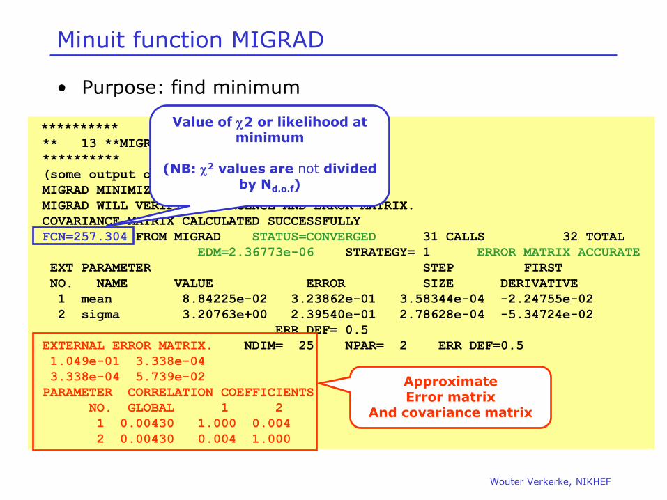
Wouter Verkerke, NIKHEF
Minuit function MIGRAD
• Purpose: find minimum
**********
** 13 **MIGRAD 1000 1
**********
(some output omitted)
MIGRAD MINIMIZATION HAS CONVERGED.
MIGRAD WILL VERIFY CONVERGENCE AND ERROR MATRIX.
COVARIANCE MATRIX CALCULATED SUCCESSFULLY
FCN=257.304 FROM MIGRAD STATUS=CONVERGED 31 CALLS 32 TOTAL
EDM=2.36773e-06 STRATEGY= 1 ERROR MATRIX ACCURATE
EXT PARAMETER STEP FIRST
NO. NAME VALUE ERROR SIZE DERIVATIVE
1 mean 8.84225e-02 3.23862e-01 3.58344e-04 -2.24755e-02
2 sigma 3.20763e+00 2.39540e-01 2.78628e-04 -5.34724e-02
ERR DEF= 0.5
EXTERNAL ERROR MATRIX. NDIM= 25 NPAR= 2 ERR DEF=0.5
1.049e-01 3.338e-04
3.338e-04 5.739e-02
PARAMETER CORRELATION COEFFICIENTS
NO. GLOBAL 1 2
1 0.00430 1.000 0.004
2 0.00430 0.004 1.000
Approximate Error matrix
And covariance matrix
Value of c2 or likelihood at minimum
(NB: c2 values are not divided
by Nd.o.f)
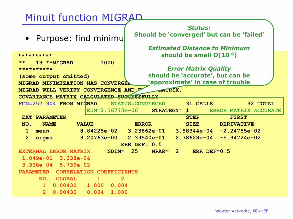
Wouter Verkerke, NIKHEF
Minuit function MIGRAD
• Purpose: find minimum
**********
** 13 **MIGRAD 1000 1
**********
(some output omitted)
MIGRAD MINIMIZATION HAS CONVERGED.
MIGRAD WILL VERIFY CONVERGENCE AND ERROR MATRIX.
COVARIANCE MATRIX CALCULATED SUCCESSFULLY
FCN=257.304 FROM MIGRAD STATUS=CONVERGED 31 CALLS 32 TOTAL
EDM=2.36773e-06 STRATEGY= 1 ERROR MATRIX ACCURATE
EXT PARAMETER STEP FIRST
NO. NAME VALUE ERROR SIZE DERIVATIVE
1 mean 8.84225e-02 3.23862e-01 3.58344e-04 -2.24755e-02
2 sigma 3.20763e+00 2.39540e-01 2.78628e-04 -5.34724e-02
ERR DEF= 0.5
EXTERNAL ERROR MATRIX. NDIM= 25 NPAR= 2 ERR DEF=0.5
1.049e-01 3.338e-04
3.338e-04 5.739e-02
PARAMETER CORRELATION COEFFICIENTS
NO. GLOBAL 1 2
1 0.00430 1.000 0.004
2 0.00430 0.004 1.000
Status: Should be ‘converged’ but can be ‘failed’
Estimated Distance to Minimum
should be small O(10-6)
Error Matrix Quality should be ‘accurate’, but can be ‘approximate’ in case of trouble
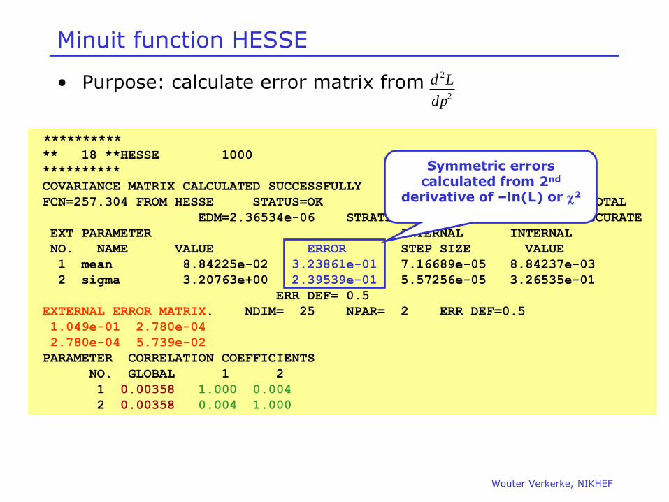
Wouter Verkerke, NIKHEF
Minuit function HESSE
• Purpose: calculate error matrix from
2
2
dp
Ld
********** ** 18 **HESSE 1000
**********
COVARIANCE MATRIX CALCULATED SUCCESSFULLY
FCN=257.304 FROM HESSE STATUS=OK 10 CALLS 42 TOTAL
EDM=2.36534e-06 STRATEGY= 1 ERROR MATRIX ACCURATE
EXT PARAMETER INTERNAL INTERNAL
NO. NAME VALUE ERROR STEP SIZE VALUE
1 mean 8.84225e-02 3.23861e-01 7.16689e-05 8.84237e-03
2 sigma 3.20763e+00 2.39539e-01 5.57256e-05 3.26535e-01
ERR DEF= 0.5
EXTERNAL ERROR MATRIX. NDIM= 25 NPAR= 2 ERR DEF=0.5
1.049e-01 2.780e-04
2.780e-04 5.739e-02
PARAMETER CORRELATION COEFFICIENTS
NO. GLOBAL 1 2
1 0.00358 1.000 0.004
2 0.00358 0.004 1.000
Symmetric errors calculated from 2nd
derivative of –ln(L) or c2
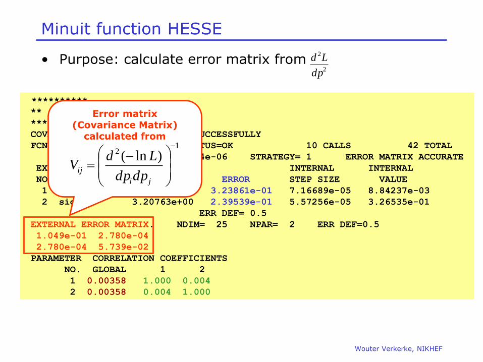
Wouter Verkerke, NIKHEF
Minuit function HESSE
• Purpose: calculate error matrix from
2
2
dp
Ld
********** ** 18 **HESSE 1000
**********
COVARIANCE MATRIX CALCULATED SUCCESSFULLY
FCN=257.304 FROM HESSE STATUS=OK 10 CALLS 42 TOTAL
EDM=2.36534e-06 STRATEGY= 1 ERROR MATRIX ACCURATE
EXT PARAMETER INTERNAL INTERNAL
NO. NAME VALUE ERROR STEP SIZE VALUE
1 mean 8.84225e-02 3.23861e-01 7.16689e-05 8.84237e-03
2 sigma 3.20763e+00 2.39539e-01 5.57256e-05 3.26535e-01
ERR DEF= 0.5
EXTERNAL ERROR MATRIX. NDIM= 25 NPAR= 2 ERR DEF=0.5
1.049e-01 2.780e-04
2.780e-04 5.739e-02
PARAMETER CORRELATION COEFFICIENTS
NO. GLOBAL 1 2
1 0.00358 1.000 0.004
2 0.00358 0.004 1.000
Error matrix (Covariance Matrix)
calculated from
12 )ln(
ji
ijdpdp
LdV
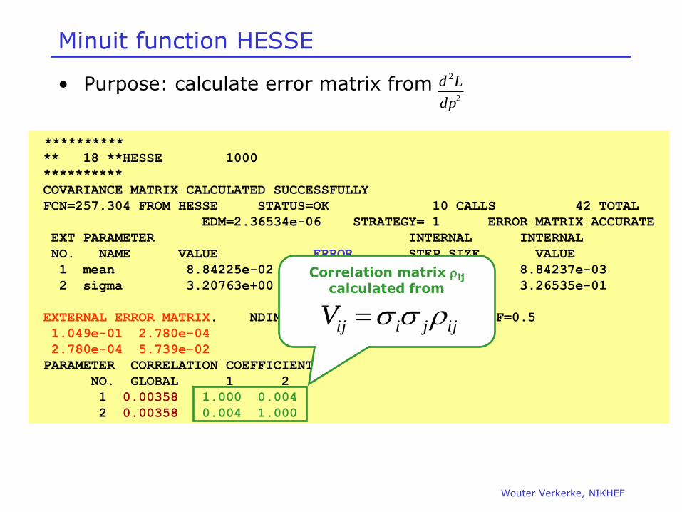
Wouter Verkerke, NIKHEF
Minuit function HESSE
• Purpose: calculate error matrix from
2
2
dp
Ld
********** ** 18 **HESSE 1000
**********
COVARIANCE MATRIX CALCULATED SUCCESSFULLY
FCN=257.304 FROM HESSE STATUS=OK 10 CALLS 42 TOTAL
EDM=2.36534e-06 STRATEGY= 1 ERROR MATRIX ACCURATE
EXT PARAMETER INTERNAL INTERNAL
NO. NAME VALUE ERROR STEP SIZE VALUE
1 mean 8.84225e-02 3.23861e-01 7.16689e-05 8.84237e-03
2 sigma 3.20763e+00 2.39539e-01 5.57256e-05 3.26535e-01
ERR DEF= 0.5
EXTERNAL ERROR MATRIX. NDIM= 25 NPAR= 2 ERR DEF=0.5
1.049e-01 2.780e-04
2.780e-04 5.739e-02
PARAMETER CORRELATION COEFFICIENTS
NO. GLOBAL 1 2
1 0.00358 1.000 0.004
2 0.00358 0.004 1.000
Correlation matrix rij calculated from
ijjiijV r

Wouter Verkerke, NIKHEF
Minuit function HESSE
• Purpose: calculate error matrix from
2
2
dp
Ld
********** ** 18 **HESSE 1000
**********
COVARIANCE MATRIX CALCULATED SUCCESSFULLY
FCN=257.304 FROM HESSE STATUS=OK 10 CALLS 42 TOTAL
EDM=2.36534e-06 STRATEGY= 1 ERROR MATRIX ACCURATE
EXT PARAMETER INTERNAL INTERNAL
NO. NAME VALUE ERROR STEP SIZE VALUE
1 mean 8.84225e-02 3.23861e-01 7.16689e-05 8.84237e-03
2 sigma 3.20763e+00 2.39539e-01 5.57256e-05 3.26535e-01
ERR DEF= 0.5
EXTERNAL ERROR MATRIX. NDIM= 25 NPAR= 2 ERR DEF=0.5
1.049e-01 2.780e-04
2.780e-04 5.739e-02
PARAMETER CORRELATION COEFFICIENTS
NO. GLOBAL 1 2
1 0.00358 1.000 0.004
2 0.00358 0.004 1.000
Global correlation vector: correlation of each parameter
with all other parameters
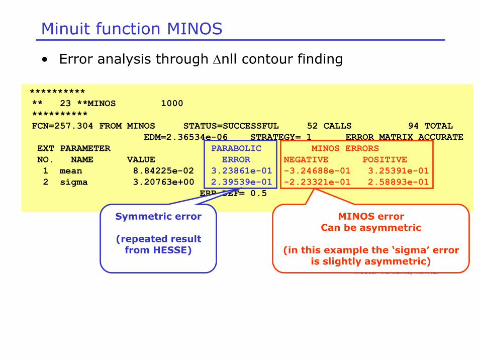
Wouter Verkerke, NIKHEF
Minuit function MINOS
• Error analysis through nll contour finding
**********
** 23 **MINOS 1000
**********
FCN=257.304 FROM MINOS STATUS=SUCCESSFUL 52 CALLS 94 TOTAL
EDM=2.36534e-06 STRATEGY= 1 ERROR MATRIX ACCURATE
EXT PARAMETER PARABOLIC MINOS ERRORS
NO. NAME VALUE ERROR NEGATIVE POSITIVE
1 mean 8.84225e-02 3.23861e-01 -3.24688e-01 3.25391e-01
2 sigma 3.20763e+00 2.39539e-01 -2.23321e-01 2.58893e-01
ERR DEF= 0.5
Symmetric error
(repeated result from HESSE)
MINOS error Can be asymmetric
(in this example the ‘sigma’ error
is slightly asymmetric)
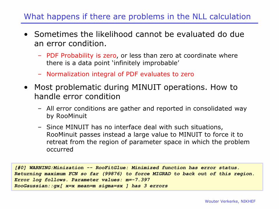
Wouter Verkerke, NIKHEF
What happens if there are problems in the NLL calculation
• Sometimes the likelihood cannot be evaluated do due an error condition.
– PDF Probability is zero, or less than zero at coordinate where there is a data point ‘infinitely improbable’
– Normalization integral of PDF evaluates to zero
• Most problematic during MINUIT operations. How to handle error condition
– All error conditions are gather and reported in consolidated way by RooMinuit
– Since MINUIT has no interface deal with such situations, RooMinuit passes instead a large value to MINUIT to force it to retreat from the region of parameter space in which the problem occurred
[#0] WARNING:Minization -- RooFitGlue: Minimized function has error status.
Returning maximum FCN so far (99876) to force MIGRAD to back out of this region.
Error log follows. Parameter values: m=-7.397
RooGaussian::gx[ x=x mean=m sigma=sx ] has 3 errors
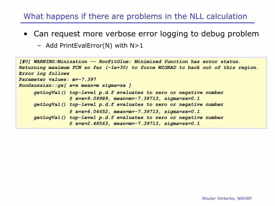
What happens if there are problems in the NLL calculation
• Can request more verbose error logging to debug problem
– Add PrintEvalError(N) with N>1
Wouter Verkerke, NIKHEF
[#0] WARNING:Minization -- RooFitGlue: Minimized function has error status.
Returning maximum FCN so far (-1e+30) to force MIGRAD to back out of this region.
Error log follows
Parameter values: m=-7.397
RooGaussian::gx[ x=x mean=m sigma=sx ]
getLogVal() top-level p.d.f evaluates to zero or negative number
@ x=x=9.09989, mean=m=-7.39713, sigma=sx=0.1
getLogVal() top-level p.d.f evaluates to zero or negative number
@ x=x=6.04652, mean=m=-7.39713, sigma=sx=0.1
getLogVal() top-level p.d.f evaluates to zero or negative number
@ x=x=2.48563, mean=m=-7.39713, sigma=sx=0.1
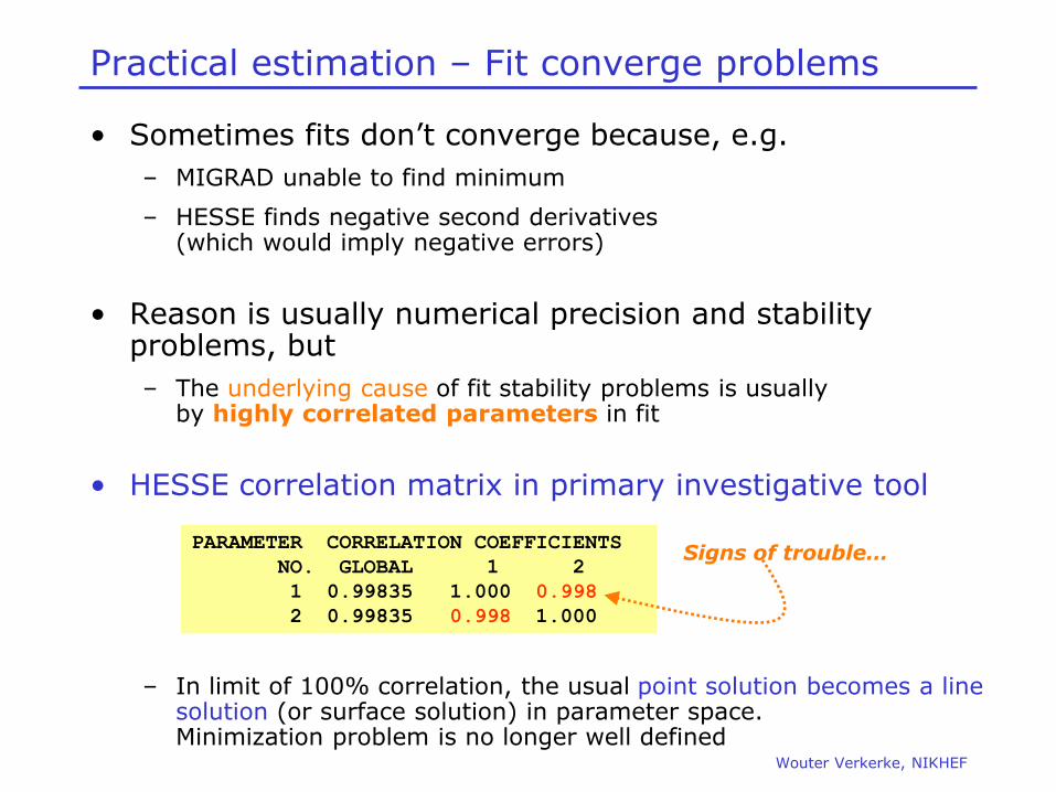
Wouter Verkerke, NIKHEF
Practical estimation – Fit converge problems
• Sometimes fits don’t converge because, e.g.
– MIGRAD unable to find minimum
– HESSE finds negative second derivatives (which would imply negative errors)
• Reason is usually numerical precision and stability problems, but
– The underlying cause of fit stability problems is usually by highly correlated parameters in fit
• HESSE correlation matrix in primary investigative tool
– In limit of 100% correlation, the usual point solution becomes a line solution (or surface solution) in parameter space. Minimization problem is no longer well defined
PARAMETER CORRELATION COEFFICIENTS
NO. GLOBAL 1 2
1 0.99835 1.000 0.998
2 0.99835 0.998 1.000
Signs of trouble…

Wouter Verkerke, NIKHEF
Mitigating fit stability problems
• Strategy I – More orthogonal choice of parameters
– Example: fitting sum of 2 Gaussians of similar width
),;()1(),;(),,,;( 221121 msxGfmsxfGssmfxF
PARAMETER CORRELATION COEFFICIENTS
NO. GLOBAL [ f] [ m] [s1] [s2]
[ f] 0.96973 1.000 -0.135 0.918 0.915
[ m] 0.14407 -0.135 1.000 -0.144 -0.114
[s1] 0.92762 0.918 -0.144 1.000 0.786
[s2] 0.92486 0.915 -0.114 0.786 1.000
HESSE correlation matrix
Widths s1,s2 strongly correlated fraction f
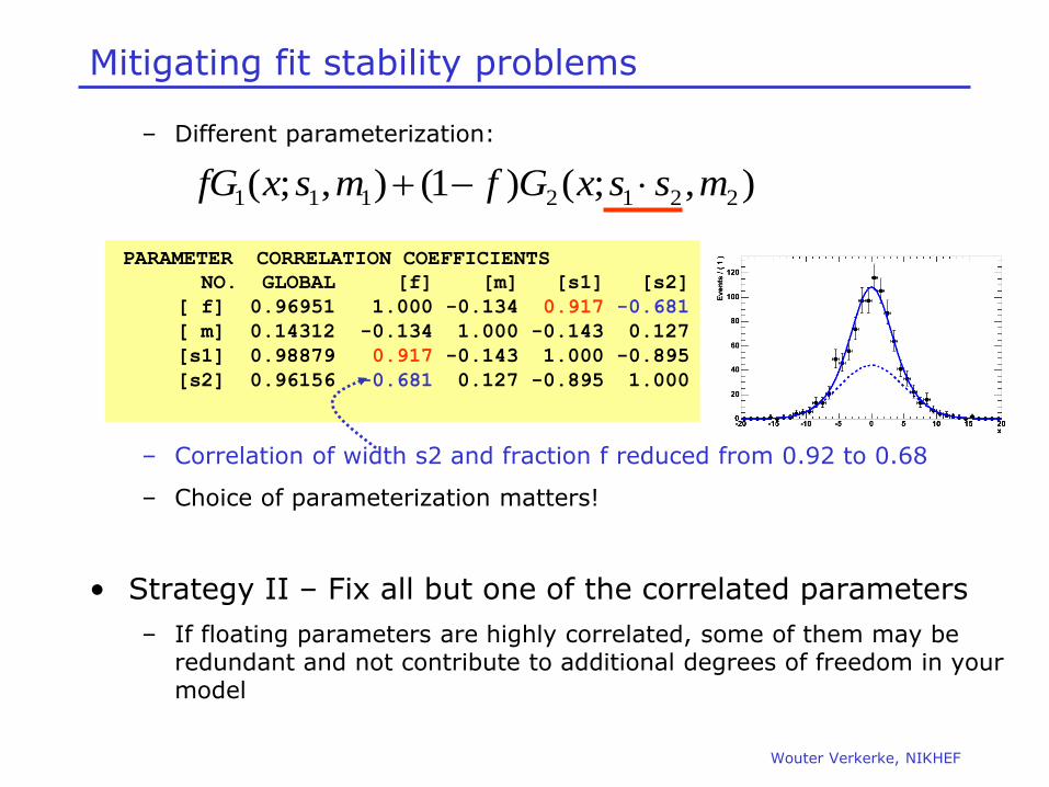
Wouter Verkerke, NIKHEF
Mitigating fit stability problems
– Different parameterization:
– Correlation of width s2 and fraction f reduced from 0.92 to 0.68
– Choice of parameterization matters!
• Strategy II – Fix all but one of the correlated parameters
– If floating parameters are highly correlated, some of them may be redundant and not contribute to additional degrees of freedom in your model
),;()1(),;( 2212111 mssxGfmsxfG
PARAMETER CORRELATION COEFFICIENTS NO. GLOBAL [f] [m] [s1] [s2]
[ f] 0.96951 1.000 -0.134 0.917 -0.681
[ m] 0.14312 -0.134 1.000 -0.143 0.127
[s1] 0.98879 0.917 -0.143 1.000 -0.895
[s2] 0.96156 -0.681 0.127 -0.895 1.000
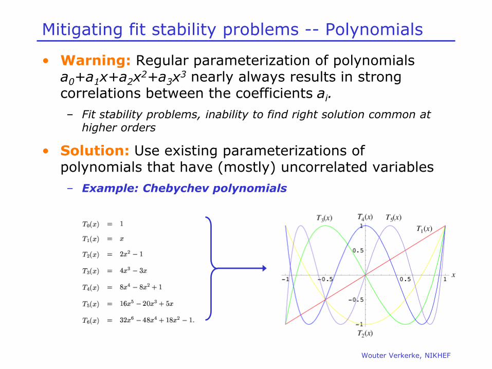
Wouter Verkerke, NIKHEF
Mitigating fit stability problems -- Polynomials
• Warning: Regular parameterization of polynomials a0+a1x+a2x
2+a3x3 nearly always results in strong
correlations between the coefficients ai.
– Fit stability problems, inability to find right solution common at higher orders
• Solution: Use existing parameterizations of polynomials that have (mostly) uncorrelated variables
– Example: Chebychev polynomials
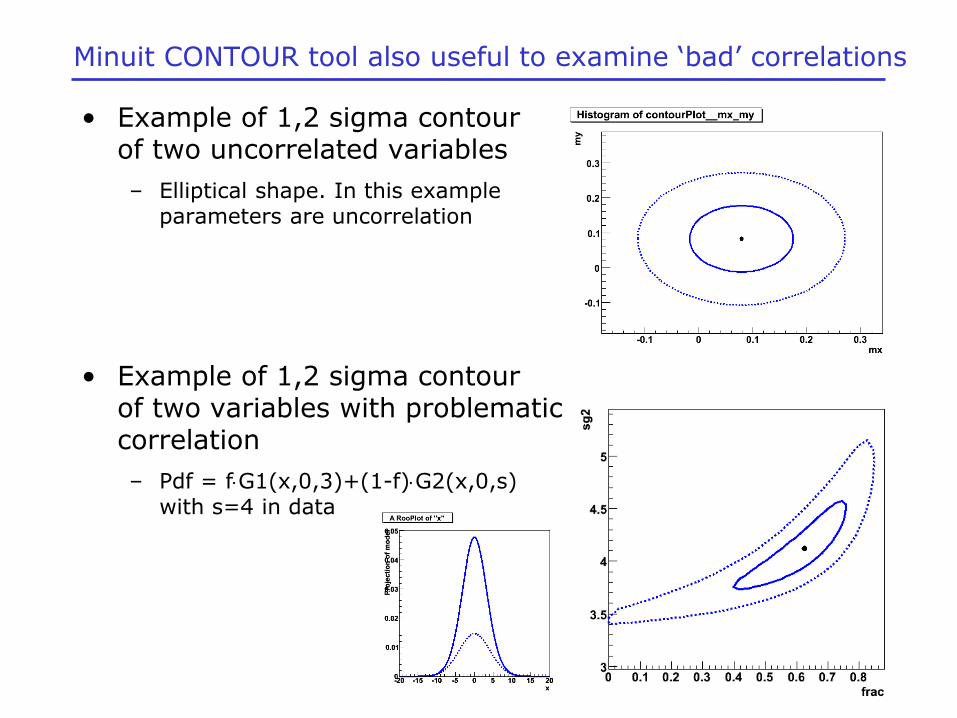
Wouter Verkerke, NIKHEF
Minuit CONTOUR tool also useful to examine ‘bad’ correlations
• Example of 1,2 sigma contour of two uncorrelated variables
– Elliptical shape. In this example parameters are uncorrelation
• Example of 1,2 sigma contour of two variables with problematic correlation
– Pdf = fG1(x,0,3)+(1-f)G2(x,0,s) with s=4 in data

Wouter Verkerke, NIKHEF
Practical estimation – Bounding fit parameters
• Sometimes is it desirable to bound the allowed range of parameters in a fit
– Example: a fraction parameter is only defined in the range [0,1]
– MINUIT option ‘B’ maps finite range parameter to an internal infinite range using an arcsin(x) transformation:
Bou
nd
ed
Param
ete
r s
pace
MINUIT internal parameter space (-∞,+∞)
Internal Error
Exte
rn
al Erro
r

Wouter Verkerke, NIKHEF
Practical estimation – Bounding fit parameters
• If fitted parameter values is close to boundary, errors will become asymmetric (and possible incorrect)
• So be careful with bounds!
– If boundaries are imposed to avoid region of instability, look into other parameterizations that naturally avoid that region
– If boundaries are imposed to avoid ‘unphysical’, but statistically valid results, consider not imposing the limit and dealing with the ‘unphysical’ interpretation in a later stage
Bo
un
ded
Param
ete
r s
pace
MINUIT internal parameter space (-∞,+∞)
Internal error
Exte
rn
al erro
r
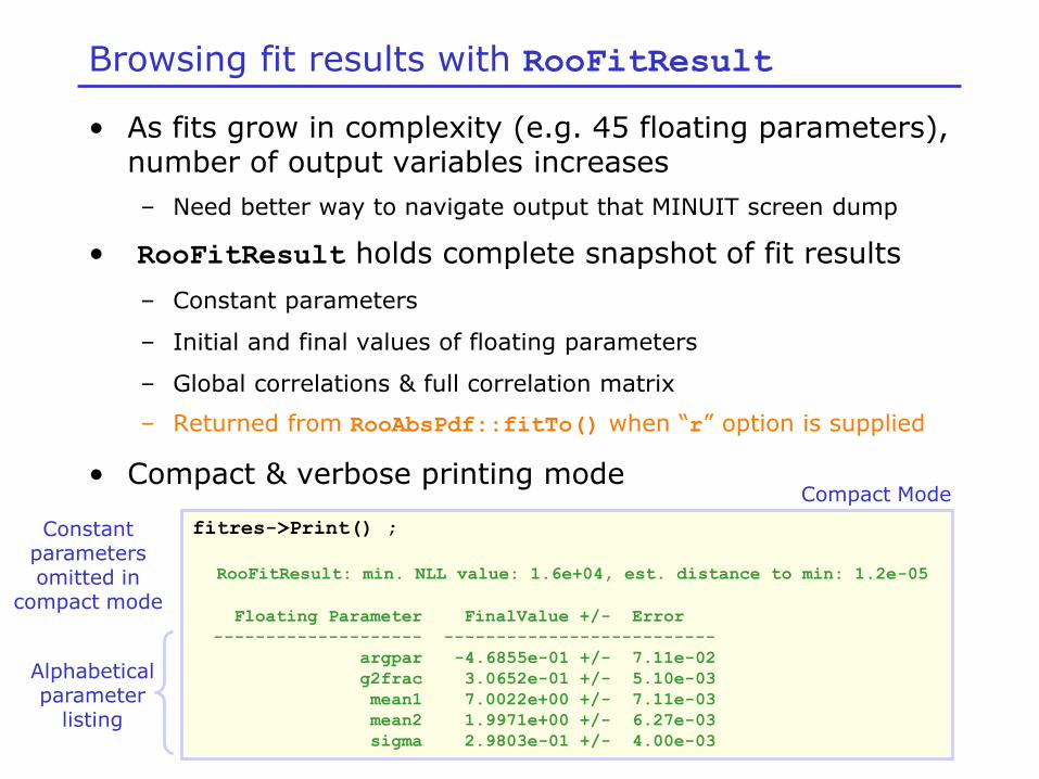
Wouter Verkerke, NIKHEF
Browsing fit results with RooFitResult
• As fits grow in complexity (e.g. 45 floating parameters), number of output variables increases
– Need better way to navigate output that MINUIT screen dump
• RooFitResult holds complete snapshot of fit results
– Constant parameters
– Initial and final values of floating parameters
– Global correlations & full correlation matrix
– Returned from RooAbsPdf::fitTo() when “r” option is supplied
• Compact & verbose printing mode
fitres->Print() ;
RooFitResult: min. NLL value: 1.6e+04, est. distance to min: 1.2e-05
Floating Parameter FinalValue +/- Error
-------------------- --------------------------
argpar -4.6855e-01 +/- 7.11e-02
g2frac 3.0652e-01 +/- 5.10e-03
mean1 7.0022e+00 +/- 7.11e-03
mean2 1.9971e+00 +/- 6.27e-03
sigma 2.9803e-01 +/- 4.00e-03
Alphabetical parameter
listing
Compact Mode
Constant parameters omitted in
compact mode

Wouter Verkerke, NIKHEF
Browsing fit results with RooFitResult
fitres->Print(“v”) ;
RooFitResult: min. NLL value: 1.6e+04, est. distance to min: 1.2e-05
Constant Parameter Value
-------------------- ------------
cutoff 9.0000e+00
g1frac 3.0000e-01
Floating Parameter InitialValue FinalValue +/- Error GblCorr.
-------------------- ------------ -------------------------- --------
argpar -5.0000e-01 -4.6855e-01 +/- 7.11e-02 0.191895
g2frac 3.0000e-01 3.0652e-01 +/- 5.10e-03 0.293455
mean1 7.0000e+00 7.0022e+00 +/- 7.11e-03 0.113253
mean2 2.0000e+00 1.9971e+00 +/- 6.27e-03 0.100026
sigma 3.0000e-01 2.9803e-01 +/- 4.00e-03 0.276640
Verbose printing mode
Constant parameters listed separately
Initial,final value and global corr. listed side-by-side
Correlation matrix accessed separately

Wouter Verkerke, NIKHEF
Browsing fit results with RooFitResult
• Easy navigation of correlation matrix
– Select single element or complete row by parameter name
–
• RooFitResult persistable with ROOT I/O
– Save your batch fit results in a ROOT file and navigate your results just as easy afterwards
r->correlation("argpar","sigma")
(const Double_t)(-9.25606412005910845e-02)
r->correlation("mean1")->Print("v")
RooArgList::C[mean1,*]: (Owning contents)
1) RooRealVar::C[mean1,argpar] : 0.11064 C
2) RooRealVar::C[mean1,g2frac] : -0.0262487 C
3) RooRealVar::C[mean1,mean1] : 1.0000 C
4) RooRealVar::C[mean1,mean2] : -0.00632847 C
5) RooRealVar::C[mean1,sigma] : -0.0339814 C
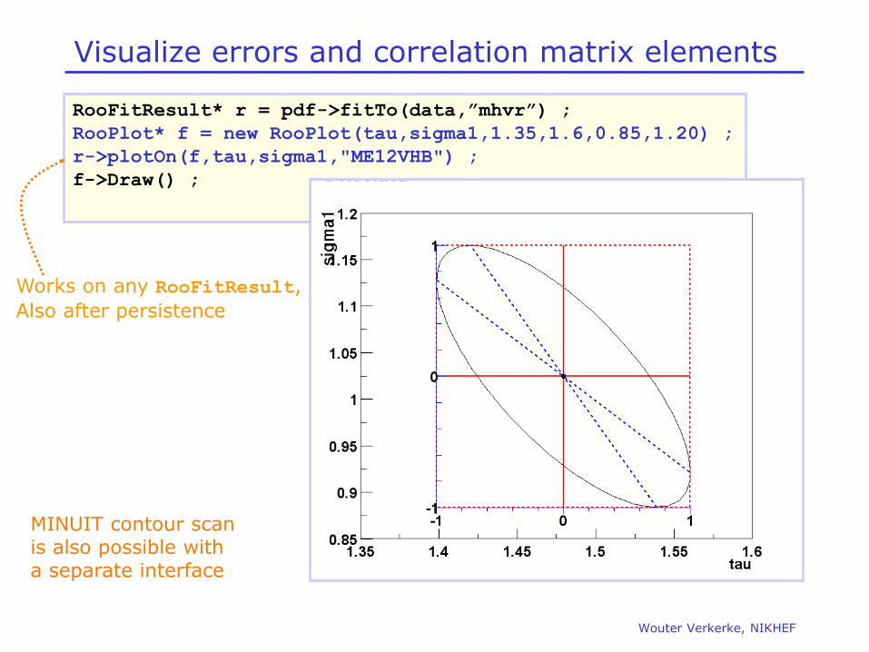
Wouter Verkerke, NIKHEF
RooFitResult* r = pdf->fitTo(data,”mhvr”) ;
RooPlot* f = new RooPlot(tau,sigma1,1.35,1.6,0.85,1.20) ;
r->plotOn(f,tau,sigma1,"ME12VHB") ;
f->Draw() ;
Visualize errors and correlation matrix elements
Works on any RooFitResult,
Also after persistence
MINUIT contour scan is also possible with a separate interface
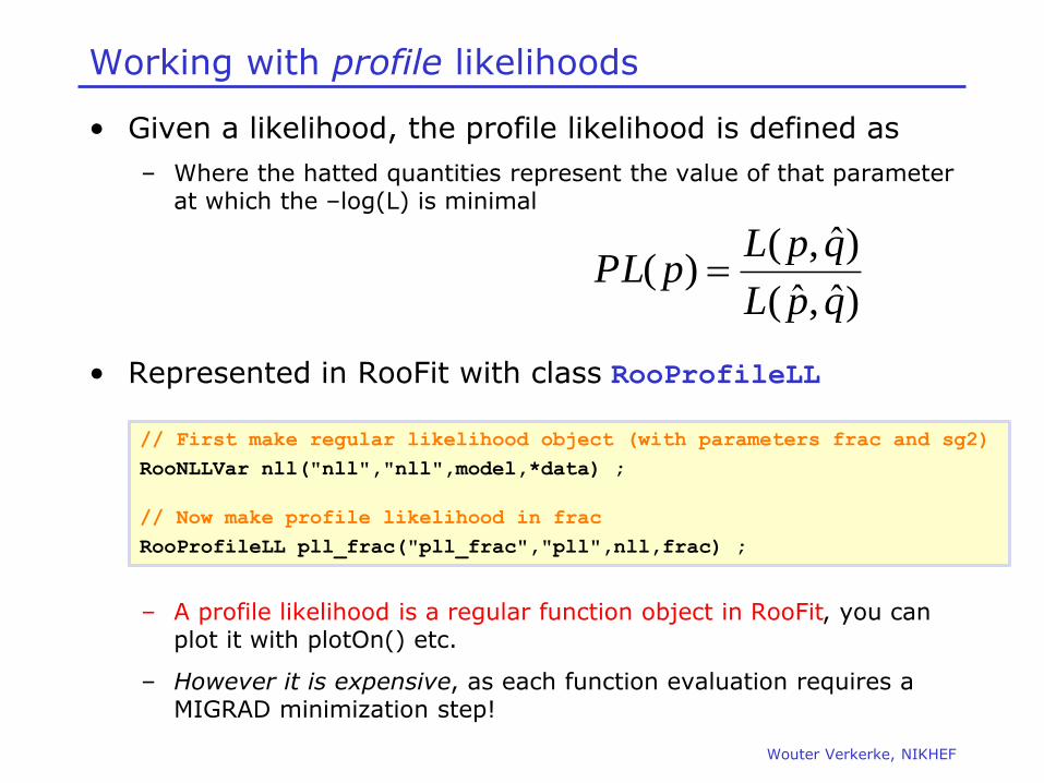
Working with profile likelihoods
• Given a likelihood, the profile likelihood is defined as
– Where the hatted quantities represent the value of that parameter at which the –log(L) is minimal
• Represented in RooFit with class RooProfileLL
– A profile likelihood is a regular function object in RooFit, you can plot it with plotOn() etc.
– However it is expensive, as each function evaluation requires a MIGRAD minimization step!
Wouter Verkerke, NIKHEF
)ˆ,ˆ(
)ˆ,()(
qpL
qpLpPL
// First make regular likelihood object (with parameters frac and sg2)
RooNLLVar nll("nll","nll",model,*data) ;
// Now make profile likelihood in frac
RooProfileLL pll_frac("pll_frac","pll",nll,frac) ;
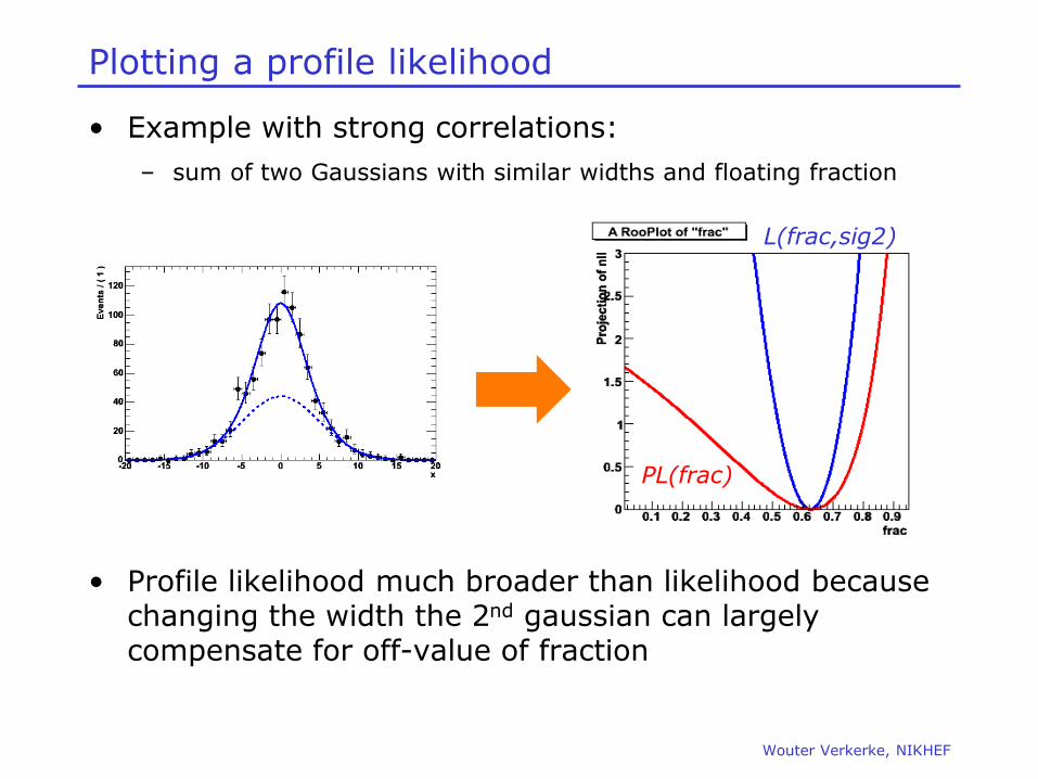
Plotting a profile likelihood
• Example with strong correlations:
– sum of two Gaussians with similar widths and floating fraction
• Profile likelihood much broader than likelihood because changing the width the 2nd gaussian can largely compensate for off-value of fraction
Wouter Verkerke, NIKHEF
L(frac,sig2)
PL(frac)

Wouter Verkerke, NIKHEF
Relation between MINOS errors and profile likelihood
• MINOS error box and profile likelihood give same error for multi-dimensional likelihood

Other uses of likelihood
• A likelihood may be considered the ultimate publication of a measurement
• Interesting to be able to digitally publish actual likelihood rather than
– Parabolic version (i.e. you publish your measurement and an error)
– Some parameterized form. Cumbersome in >1 dimension. No standard protocol for exchanging this time of information
• You can do this now in RooFit
– You can persist your data (previously possible) and your actual p.d.f or likelihood into a ROOT file that anyone can read and use
• Many potential applications
– Combining of Higgs channels, Heavy flavor averaging (CKMfitter) etc…
Wouter Verkerke, NIKHEF
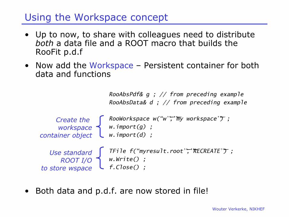
Wouter Verkerke, NIKHEF
Using the Workspace concept
• Up to now, to share with colleagues need to distribute both a data file and a ROOT macro that builds the RooFit p.d.f
• Now add the Workspace – Persistent container for both data and functions
• Both data and p.d.f. are now stored in file!
RooAbsPdf& g ; // from preceding example
RooAbsData& d ; // from preceding example
RooWorkspace w(“w”,”my workspace”) ;
w.import(g) ;
w.import(d) ;
TFile f(“myresult.root”,”RECREATE”) ;
w.Write() ;
f.Close() ;
Create the workspace
container object
Use standard ROOT I/O
to store wspace

Wouter Verkerke, NIKHEF
A look at the workspace
• What is in the workspace?
w.Print() ;
RooWorkspace(w) my workspace contents
variables
---------
(x,m,s)
p.d.f.s
-------
RooGaussian::g[ x=x mean=m sigma=s ] = 0
datasets
--------
RooDataSet::d(x)
RooRealVar* x = w.get(“x”) ;
RooAbsPdf* g = w.pdf(“g”) ;
RooAbsData* d = w.data(“d”) ;

Wouter Verkerke, NIKHEF
Using persisted p.d.f.s.
• Using both model & p.d.f from file
– Note that above code is independent of actual p.d.f in file
e.g. full Higgs combination would work with identical code
TFile f(“myresults.root”) ;
RooWorkspace* w = f.Get(“w”) ;
RooPlot* xframe = w->var(“x”)->frame() ;
w->data(“d”)->plotOn(xframe) ;
w->pdf(“g”)->plotOn(xframe) ;
RooNLLVar nll(“nll”,”nll”,*w->pdf(“g”),*w->data(“d”)) ;
RooProfileLL pll(“pll”,”pll”, nll,*w->var(“m”)) ;
RooPlot* mframe = w->var(“m”)->frame(-1,1) ;
pll.plotOn(mframe) ;
mframe->Draw()
Make plot of data
and p.d.f
Construct likelihood
& profile LH
Draw profile LH
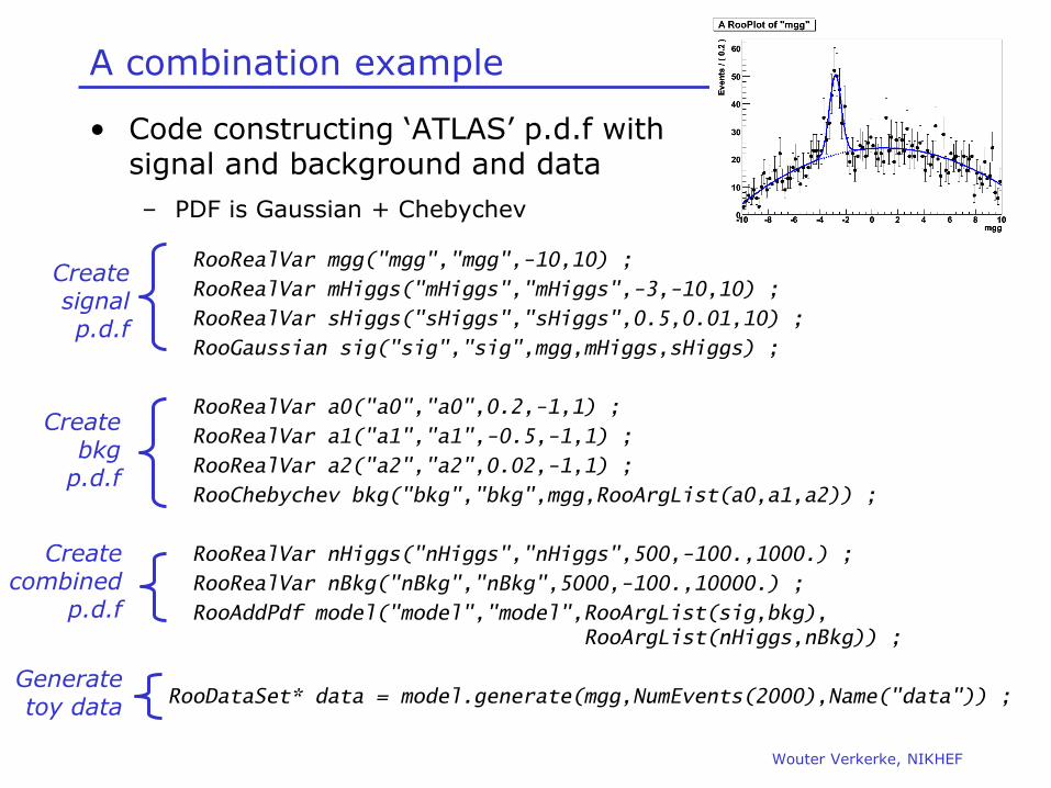
Wouter Verkerke, NIKHEF
A combination example
• Code constructing ‘ATLAS’ p.d.f with signal and background and data
– PDF is Gaussian + Chebychev
RooRealVar mgg("mgg","mgg",-10,10) ;
RooRealVar mHiggs("mHiggs","mHiggs",-3,-10,10) ;
RooRealVar sHiggs("sHiggs","sHiggs",0.5,0.01,10) ;
RooGaussian sig("sig","sig",mgg,mHiggs,sHiggs) ;
RooRealVar a0("a0","a0",0.2,-1,1) ;
RooRealVar a1("a1","a1",-0.5,-1,1) ;
RooRealVar a2("a2","a2",0.02,-1,1) ;
RooChebychev bkg("bkg","bkg",mgg,RooArgList(a0,a1,a2)) ;
RooRealVar nHiggs("nHiggs","nHiggs",500,-100.,1000.) ;
RooRealVar nBkg("nBkg","nBkg",5000,-100.,10000.) ;
RooAddPdf model("model","model",RooArgList(sig,bkg),
RooArgList(nHiggs,nBkg)) ;
RooDataSet* data = model.generate(mgg,NumEvents(2000),Name("data")) ;
Create signal p.d.f
Create bkg
p.d.f
Create combined
p.d.f
Generate toy data

Wouter Verkerke, NIKHEF
A combination example
• Code writing ‘ATLAS’ p.d.f and data into Workspace
– Variation of toy Gauss example: also create & persist likelihood function here
model.fitTo(*data,Extended(),Minos(kFALSE)) ;
RooNLLVar nll(“nll”,”nll”,model,*data,Extended()) ;
RooWorkspace atlas("atlas","atlas") ;
atlas.import(model) ;
atlas.import(*data) ;
atlas.import(nll) ;
TFile f("atlas.root","RECREATE") ;
atlas.Write() ;
f.Close() ;
Fit model to data (skip MINOS)
Create the workspace
container object
Use standard ROOT I/O
to store wspace
Create likelihood function

Wouter Verkerke, NIKHEF
A combination example
• Contents of the ATLAS workspace root [4] atlas->Print()
RooWorkspace(atlas) atlas contents
variables
---------
(mgg,mHiggs,sHiggs,nHiggs,a0,a1,a2,nBkg)
p.d.f.s
-------
RooAddPdf::model[ pdfs=(sig,bkg) coefficients=(nHiggs,nBkg) ] = 0
RooGaussian::sig[ x=mgg mean=mHiggs sigma=sHiggs ] = 0
RooChebychev::bkg[ x=mgg coefList=(a0,a1,a2) ] = 0
functions
---------
RooNLLVar::nll[ params=(mHiggs,sHiggs,a0,a1,a2,nHiggs,nBkg) ] = 0
datasets
--------
RooDataSet::data(mgg)
All component pdfs are visible as well
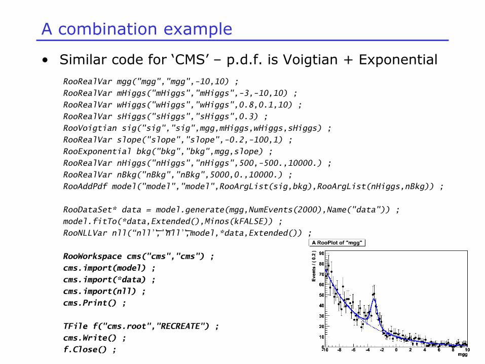
Wouter Verkerke, NIKHEF
A combination example
• Similar code for ‘CMS’ – p.d.f. is Voigtian + Exponential
RooRealVar mgg("mgg","mgg",-10,10) ;
RooRealVar mHiggs("mHiggs","mHiggs",-3,-10,10) ;
RooRealVar wHiggs("wHiggs","wHiggs",0.8,0.1,10) ;
RooRealVar sHiggs("sHiggs","sHiggs",0.3) ;
RooVoigtian sig("sig","sig",mgg,mHiggs,wHiggs,sHiggs) ;
RooRealVar slope("slope","slope",-0.2,-100,1) ;
RooExponential bkg("bkg","bkg",mgg,slope) ;
RooRealVar nHiggs("nHiggs","nHiggs",500,-500.,10000.) ;
RooRealVar nBkg("nBkg","nBkg",5000,0.,10000.) ;
RooAddPdf model("model","model",RooArgList(sig,bkg),RooArgList(nHiggs,nBkg)) ;
RooDataSet* data = model.generate(mgg,NumEvents(2000),Name("data")) ;
model.fitTo(*data,Extended(),Minos(kFALSE)) ;
RooNLLVar nll(“nll”,”nll”,model,*data,Extended()) ;
RooWorkspace cms("cms","cms") ;
cms.import(model) ;
cms.import(*data) ;
cms.import(nll) ;
cms.Print() ;
TFile f("cms.root","RECREATE") ;
cms.Write() ;
f.Close() ;
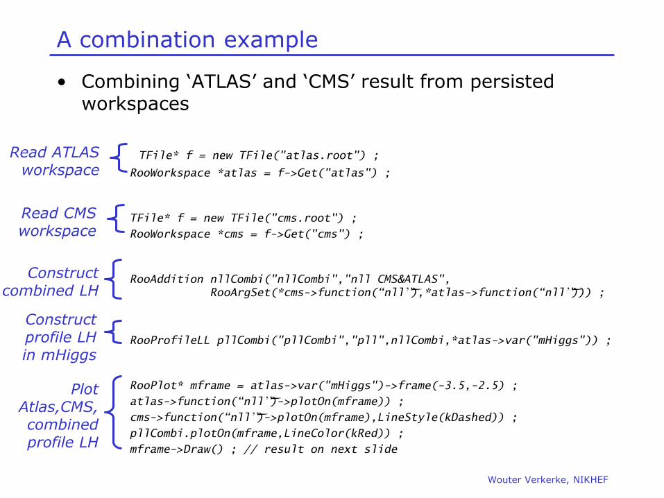
Wouter Verkerke, NIKHEF
A combination example
• Combining ‘ATLAS’ and ‘CMS’ result from persisted workspaces
TFile* f = new TFile("atlas.root") ;
RooWorkspace *atlas = f->Get("atlas") ;
TFile* f = new TFile("cms.root") ;
RooWorkspace *cms = f->Get("cms") ;
RooAddition nllCombi("nllCombi","nll CMS&ATLAS",
RooArgSet(*cms->function(“nll”),*atlas->function(“nll”))) ;
RooProfileLL pllCombi("pllCombi","pll",nllCombi,*atlas->var("mHiggs")) ;
RooPlot* mframe = atlas->var("mHiggs")->frame(-3.5,-2.5) ;
atlas->function(“nll”)->plotOn(mframe)) ;
cms->function(“nll”)->plotOn(mframe),LineStyle(kDashed)) ;
pllCombi.plotOn(mframe,LineColor(kRed)) ;
mframe->Draw() ; // result on next slide
Read ATLAS workspace
Read CMS workspace
Construct combined LH
Plot Atlas,CMS, combined profile LH
Construct profile LH in mHiggs

Wouter Verkerke, NIKHEF
A combination example
‘Atlas’ ‘CMS’
Combined
Pro
file
lik
elih
oo
d

Wouter Verkerke, NIKHEF
Fit validation,
Toy MC studies 7 • Goodness-of-fit, c2
• Toy Monte Carlo studies for fit validation

Wouter Verkerke, NIKHEF
How do you know if your fit was ‘good’
• Goodness-of-fit broad issue in statistics in general, will just focus on a few specific tools implemented in RooFit here
• For one-dimensional fits, a c2 is usually the right thing to do
– Some tools implemented in RooPlot to be able to calculate c2/ndf of curve w.r.t data double chi2 = frame->chisquare(nFloatParam) ;
– Also tools exists to plot residual and pull distributions from curve and histogram in a RooPlot frame->makePullHist() ;
frame->makeResidHist() ;
GOF in >1D, other aspects of fit validity
• No special tools for >1 dimensional goodness-of-fit
– A c2 usually doesn’t work because empty bins proliferate with dimensions
– But if you have ideas you’d like to try, there exists generic base classes for implementation that provide the same level of computational optimization and parallelization as is done for likelihoods (RooAbsOptTestStatistic)
• But you can study many other aspect of your fit validity
– Is your fit unbiased?
– Does it (often) have convergence problems?
• You can answer these with a toy Monte Carlo study
– I.e. generate 10000 samples from your p.d.f., fit them all and collect and analyze the statistics of these 10000 fits.
– The RooMCStudy class helps out with the logistics
Wouter Verkerke, NIKHEF
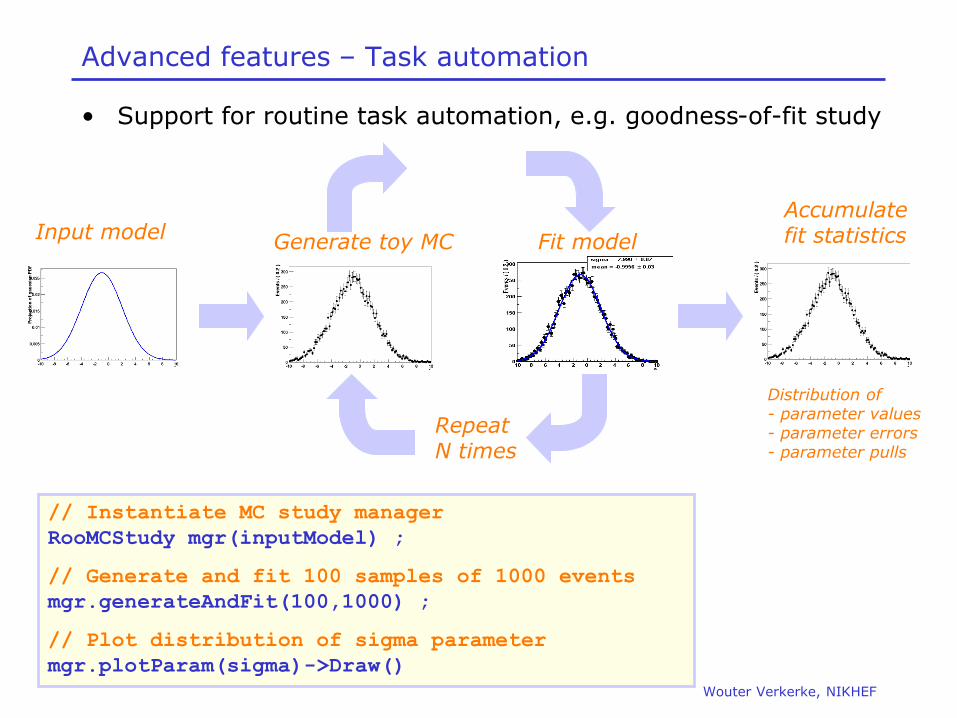
Wouter Verkerke, NIKHEF
Advanced features – Task automation
• Support for routine task automation, e.g. goodness-of-fit study
Input model Generate toy MC Fit model
Repeat N times
Accumulate fit statistics
Distribution of - parameter values - parameter errors - parameter pulls
// Instantiate MC study manager
RooMCStudy mgr(inputModel) ;
// Generate and fit 100 samples of 1000 events
mgr.generateAndFit(100,1000) ;
// Plot distribution of sigma parameter
mgr.plotParam(sigma)->Draw()

Wouter Verkerke, NIKHEF
How to efficiently generate multiple sets of ToyMC?
• Use RooMCStudy class to manage generation and fitting
• Generating features
– Generator overhead only incurred once Efficient for large number of small samples
– Optional Poisson distribution for #events of generated experiments
– Optional automatic creation of ASCII data files
• Fitting
– Fit with generator PDF or different PDF
– Fit results (floating parameters & NLL) automatically collected in summary dataset
• Plotting
– Automated plotting for distribution of parameters, parameter errors, pulls and NLL
• Add-in modules for optional modifications of procedure
– Concrete tools for variation of generation parameters, calculation of likelihood ratios for each experiment
– Easy to write your own. You can intervene at any stage and offer proprietary data to be aggregated with fit results
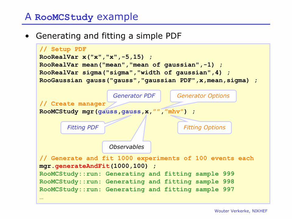
Wouter Verkerke, NIKHEF
A RooMCStudy example
• Generating and fitting a simple PDF
// Setup PDF
RooRealVar x("x","x",-5,15) ;
RooRealVar mean("mean","mean of gaussian",-1) ;
RooRealVar sigma("sigma","width of gaussian",4) ;
RooGaussian gauss("gauss","gaussian PDF",x,mean,sigma) ;
// Create manager
RooMCStudy mgr(gauss,gauss,x,””,”mhv”) ;
// Generate and fit 1000 experiments of 100 events each
mgr.generateAndFit(1000,100) ;
RooMCStudy::run: Generating and fitting sample 999
RooMCStudy::run: Generating and fitting sample 998
RooMCStudy::run: Generating and fitting sample 997
…
Fitting Options
Generator Options
Observables
Generator PDF
Fitting PDF
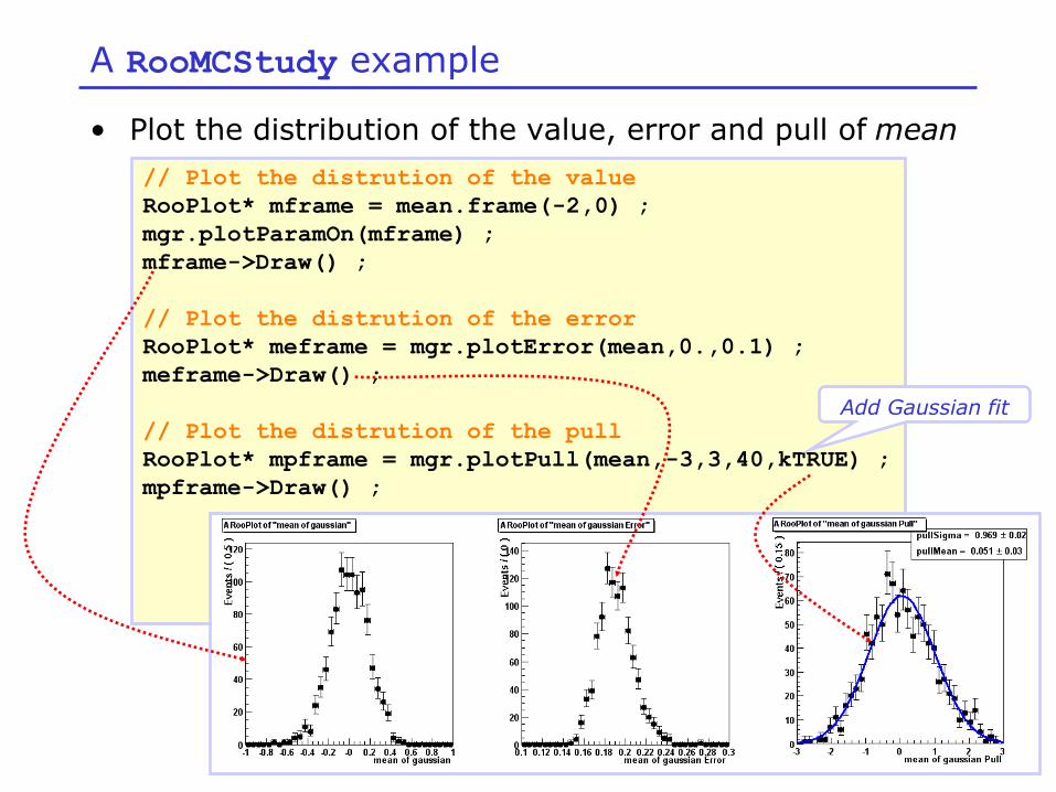
Wouter Verkerke, NIKHEF
A RooMCStudy example
• Plot the distribution of the value, error and pull of mean
// Plot the distrution of the value
RooPlot* mframe = mean.frame(-2,0) ;
mgr.plotParamOn(mframe) ;
mframe->Draw() ;
// Plot the distrution of the error
RooPlot* meframe = mgr.plotError(mean,0.,0.1) ;
meframe->Draw() ;
// Plot the distrution of the pull
RooPlot* mpframe = mgr.plotPull(mean,-3,3,40,kTRUE) ;
mpframe->Draw() ;
Add Gaussian fit
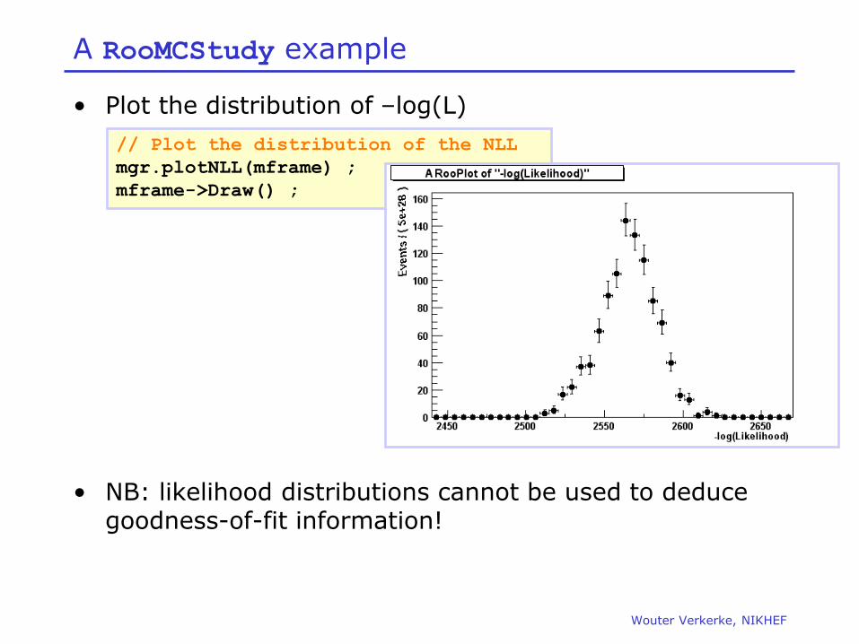
Wouter Verkerke, NIKHEF
A RooMCStudy example
• Plot the distribution of –log(L)
• NB: likelihood distributions cannot be used to deduce goodness-of-fit information!
// Plot the distribution of the NLL
mgr.plotNLL(mframe) ;
mframe->Draw() ;

Wouter Verkerke, NIKHEF
A RooMCStudy example
• For other uses, use summarized fit results in RooDataSet form
mgr.fitParDataSet().get(10)->Print(“v”) ;
RooArgSet:::
1) RooRealVar::mean : 0.14814 +/- 0.191 L(-10 - 10)
2) RooRealVar::sigma : 4.0619 +/- 0.143 L(0 - 20)
3) RooRealVar::NLL : 2585.1 C
4) RooRealVar::meanerr : 0.19064 C
5) RooRealVar::meanpull : 0.77704 C
6) RooRealVar::sigmaerr : 0.14338 C
7) RooRealVar::sigmapull : 0.43199 C
TH2* h = mean.createHistogram("mean vs sigma",sigma) ;
mgr.fitParDataSet().fillHistogram(h,RooArgList(mean,sigma)) ;
h->Draw("BOX") ;
Pulls and errors have separate entries for easy access and plotting

Wouter Verkerke, NIKHEF
A RooMCStudy example
• If the “r” fit option is supplied the RooFitResult output of each fit is be saved
mgr.fitResult(10)->Print(“v”) ;
RooFitResult: minimized NLL value: 2585.13, estimated distance to minimum: 3.18389e-06
Floating Parameter InitialValue FinalValue +/- Error GblCorr.
-------------------- ------------ -------------------------- --------
mean 0.0000e+00 1.4814e-01 +/- 1.91e-01 0.597596 <none>
sigma 4.0000e+00 4.0619e+00 +/- 1.43e-01 0.597596 <none>
mgr.fitResult(10)->correlation("sigma")->Print("v") ;
RooArgList::C[sigma,*]: (Owning contents)
1) RooRealVar::C[sigma,mean] : -0.597596 C
2) RooRealVar::C[sigma,sigma] : 1.0000 C
RooPlot* frame = new RooPlot(…)
mgr.fitResult(10)->plotOn(frame,meanx,
sigmax,"ME12VHB") ;

Wouter Verkerke, NIKHEF
Fit Validation Study – Practical example
• Example fit model in 1-D (B mass)
– Signal component is Gaussian centered at B mass
– Background component is Argus function (models phase space near kinematic limit)
• Fit parameter under study: Nsig
– Results of simulation study: 1000 experiments with NSIG(gen)=100, NBKG(gen)=200
– Distribution of Nsig(fit)
– This particular fit looks unbiased…
);();(),,,;( bkgsigbkgsig BSBS pmANpmGNppNNmF
Nsig(fit)
Nsig(generated)
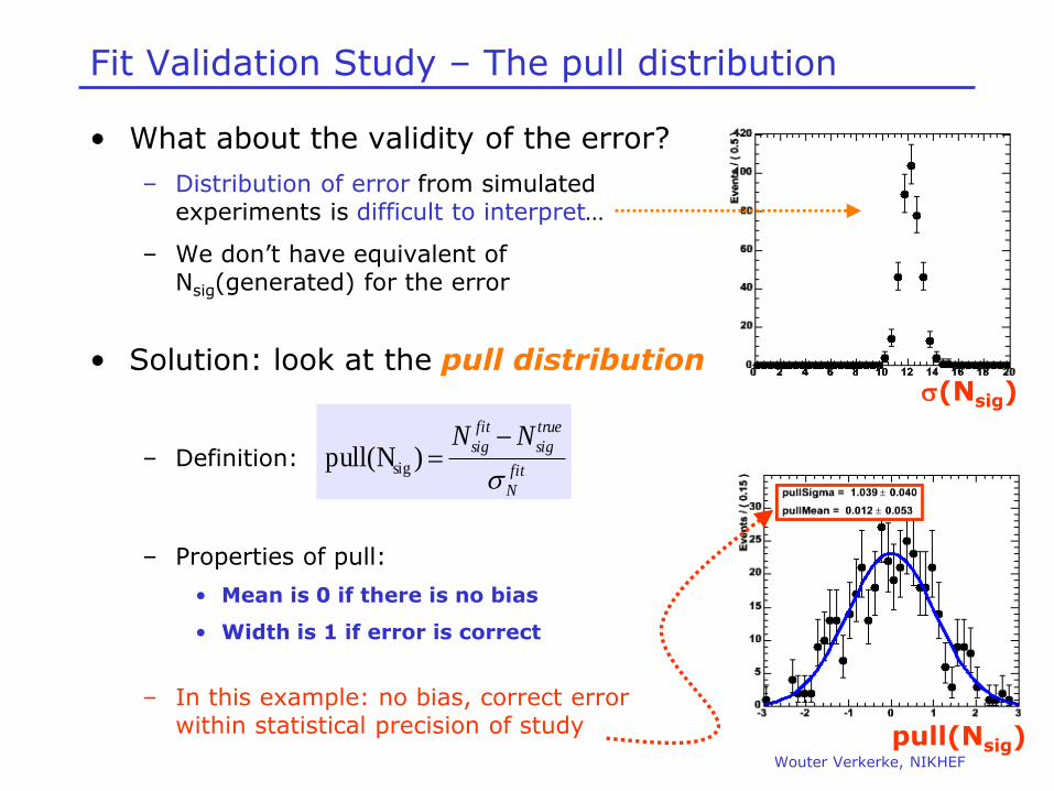
Wouter Verkerke, NIKHEF
Fit Validation Study – The pull distribution
• What about the validity of the error?
– Distribution of error from simulated experiments is difficult to interpret…
– We don’t have equivalent of Nsig(generated) for the error
• Solution: look at the pull distribution
– Definition:
– Properties of pull:
• Mean is 0 if there is no bias
• Width is 1 if error is correct
– In this example: no bias, correct error within statistical precision of study
(Nsig)
fit
N
true
sig
fit
sig NN
)pull(Nsig
pull(Nsig)

Wouter Verkerke, NIKHEF
Fit Validation Study – Low statistics example
• Special care should be taken when fitting small data samples
– Also if fitting for small signal component in large sample
• Possible causes of trouble
– c2 estimators may become approximate as Gaussian approximation of Poisson statistics becomes inaccurate
– ML estimators may no longer be efficient error estimate from 2nd derivative may become inaccurate
– Bias term proportional to 1/N of ML and c2 estimators may no longer be small compared to 1/sqrt(N)
• In general, absence of bias, correctness of error can not be assumed. How to proceed?
– Use unbinned ML fits only – most robust at low statistics
– Explicitly verify the validity of your fit

Wouter Verkerke, NIKHEF
Demonstration of fit bias at low N – pull distributions
• Low statistics example:
– Scenario as before but now with 200 bkg events and only 20 signal events (instead of 100)
• Results of simulation study
• Absence of bias, correct error at low statistics not obvious
NBKG(gen)=200
NSIG(gen)=20
Distributions become asymmetric at low statistics
NSIG(fit) (NSIG) pull(NSIG)
NSIG(gen)
Pull mean ~2 away from 0 Fit is positively biased!

Wouter Verkerke, NIKHEF
Documentation 10
Documentation, Forum and Release plans
• Some aspects were not covered for which tools exists
– E.g. constrained fits, fitting efficiencies, limit calculations
• Sources of documentation
– Class documentation (updated for ROOT 5.20)
– Users Manual (being updated, release this summer) 50 pages 100 pages
– Tutorial macros ($ROOTSYS/tutorial/roofit), 17 now, another 20 forthcoming
• Where to ask (technical) questions
– ROOT users Forum
• Release schedule
– ROOT development release 5.21/02 Aug 18, plus every month later up to
– ROOT production release 5.22, Dec 17
– Main new developments for 5.21 will be PROOF interfacing for distribution toy MC generation and multi-host fit parallelization
Wouter Verkerke, NIKHEF