rolling-element bearings · 14.1 cylindrical roller bearing problem ... the precision...

NASA Reference Publication 1105

June 1983

Rolling-Element Bearings

Bernard J. Hamrock and William J. Anderson

NASA RP 1105 c.1 /

1

LOAN COPY: RETURN -03 M'WLTECHNICAL LiBRMY KJPTLAND AFB, N.M.

.- -: ~ . . . . ._

%,,’ ‘. ‘, * ,

.,:

, -, : 1

”

https://ntrs.nasa.gov/search.jsp?R=19830018943 2018-06-11T05:13:23+00:00Z

TECH LIBRARY KAFB, NM

NASA Reference Publication 1105

1983

National Aeronautics and Space Administration

Scientific and Technical Information Branch

llllIIlnllllll~~lmIIInl lXlb3242


Bernard J. Hamrock Lewis Research Center Cleveland, Ohio

William J. Anderson Bearings and Lubrication North Olmsted, Ohio

ERRATA

NASA RP–1105


B.J. Hamrock and W.J. Anderson

Page 1, definition of F should read as follows:

F Load on element, N

Page 1, definition of R should read as follows:

R Effective radius of curvature, m

Page 2, definition of delta (δ) should read as follows:

δ Total race deflection including deformation and clearance takeup, m

Page 20, equation (44), based on ESDU 78035 (1978, as revised 1995) should read as follows:

(44)

Page 20, equation (47) should read as follows:

(47)

Issued February 2011

Contents

Page

Symbols .............................................................................................. 1

1. Introduction .................................................................................. 2 1.1 Historical Overview ...................................................................... 2 1.2 Conformal and Nonconformal Surfaces ............................................ 3 1.3 Bearing Selection ......................................................................... 3

2. Bearing Types ................................................................................ 4 2.1 Ball Bearings .............................................................................. 5 2.2 Roller Bearings ............................................................................ 7

3. Geometry.. .................................................................................... 8 3.1 Geometry of Ball Bearings ............................................................. 8 3.2 Geometry of Roller Bearings ......................................................... 12

4. Kinematics.. ................................................................................. 13

5. Materials and Manufacturing Processes .............................................. 15 5.1 Ferrous Alloys.. ......................................................................... 16 5.2 Ceramics .................................................................................. 16

6. Separators.. ................................................................................. 17

7. Contact Stresses and Deformations.. .................................................. 17 7.1 Elliptical Contacts ...................................................................... 17 7.2 Rectangular Contacts .................................................................. 20

8. Static Load Distribution.. ................................................................ 20 8.1 Load Deflection Relationships.. ..................................................... 20 8.2 Radially Loaded Ball and Roller Bearings ......................................... 20 8.3 Thrust-Loaded Ball Bearings ......................................................... 22 8.4 Preloading ................................................................................ 24

9. Rolling Friction and Friction in Bearings.. ........................................... 25 9.1 Rolling Friction ......................................................................... 25 9.2 Friction Losses in Rolling-Element Bearings ...................................... 27

10. Lubricants and Lubrication Systems .................................................. 27 10.1 Solid Lubrication ....................................................................... 27 10.2 Liquid Lubrication ..................................................................... 28

11. Elastohydrodynamic Lubrication ...................................................... 29 11.1 Relevant Equations ..................................................................... 29 11.2 Dimensionless Grouping .............................................................. 30

. . . III

11.3 Minimum-Film-Thickness Formula ................................................ 30 11.4 Pressure and Film Thickness Plots .................................................. 31

12. Rolling Bearing Fatigue Life ............................................................ 32 12.1 Contact Fatigue Theory ............................................................... 32 12.2 The Weibull Distribution.. ............................................................ 32 12.3 Lundberg-Palmgren Theory .......................................................... 33 12.4 The AFBMA Method .................................................................. 35 12.5 Life Adjustment Factors .............................................................. 35

13. Dynamic Analyses and Computer Codes.. ........................................... 36 13.1 Quasi-Static Analyses.. ................................................................ 36 13.2 Dynamic Analyses ...................................................................... 37

14. Applications ................................................................................ 37 14.1 Cylindrical Roller Bearing Problem ................................................ 37 14.2 Radial Ball Bearing Problem ......................................................... 39

References ......................................................................................... 42

iv

Rolling-element bearings are a precision, yet simple, machine element of great utility. In this report we draw together the current understanding of rolling-element bearings. A brief history of rolling-element bearings is reviewed in the Introduction, and subsequent sections are devoted to describing the types of rolling-element bearings, their geometry and kinematics, as well as the materials they are made from and the manufacturing processes they involve. The organization of this report is such that unloaded and unlubricated rolling-element bearings are considered in the first six sections, loaded but unlubricated rolling-element bearings are considered in sections 7 to 9, and loaded and lubricated rolling- element bearings are considered in sections 10 to 14. The recognition and understanding of elastohydrodynamic lubrication, covered briefly in sections 11, 12, and 14, represents one of the major developments in rolling- element bearings in the last 18 years.

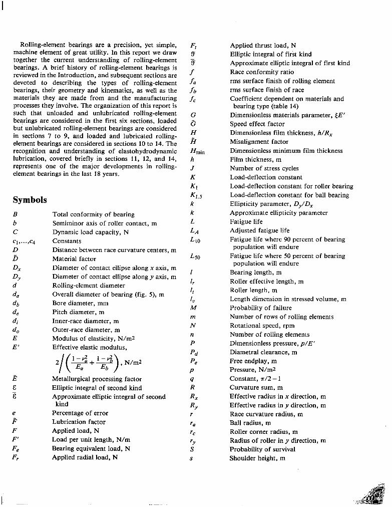
Symbols B b c Cl ,...,c4

D I3 4 DY d da db 4 di da E E’

B & z

e P F F’ Fe F,

Total conformity of bearing Semiminor axis of roller contact, m Dynamic load capacity, N Constants Distance between race curvature centers, m Material factor Diameter of contact ellipse along x axis, m Diameter of contact ellipse along y axis, m Rolling-element diameter Overall diameter of bearing (fig. 5), m Bore diameter, mm Pitch diameter, m Inner-race diameter, m Outer-race diameter, m Modulus of elasticity, N/m2 Effective elastic modulus,

, N/m2

Metallurgical processing factor Elliptic integral of second kind Approximate elliptic integral of second

kind Percentage of error Lubrication factor Applied load, N Load per unit length, N/m Bearing equivalent load, N Applied radial load, N

4 3 3 f

fa fb fc

G G H k H min

h J K K1 K1.5 k k L LA

LIO

ho

I

1,

1,

I” M m N n P pd

pe

P 9 R RX RY r ra rC

'Y S s

Applied thrust load, N Elliptic integral of first kind Approximate elliptic integral of first kind Race conformity ratio rms surface finish of rolling element rms surface finish of race Coefficient dependent on materials and bearing type (table 14)

Dimensionless materials parameter, [E’ Speed effect factor Dimensionless film thickness, h/R, Misalignment factor Dimensionless minimum film thickness Film thickness, m Number of stress cycles Load-deflection constant Load-deflection constant for roller bearing Load-deflection constant for ball bearing Ellipticity parameter, Dy/Dx Approximate ellipticity parameter Fatigue life Adjusted fatigue life Fatigue life where 90 percent of bearing population will endure

Fatigue life where 50 percent of bearing population will endure

Bearing length, m Roller effective length, m Roller length, m Length dimension in stressed volume, m Probability of failure Number of rows of rolling elements Rotational speed, rpm Number of rolling elements Dimensionless pressure, p/E’ Diametral clearance, m Free endplay, m Pressure, N/m2 Constant, n/2 - 1 Curvature sum, m Effective radius in x direction, m Effective radius in y direction, m Race curvature radius, m Ball radius, m Roller corner radius, m Radius of roller in y direction, m Probability of survival Shoulder height, m

T u u

V V

W x y X,Y,Z Z ZO

; P’ Of r 6 s 5

9 Absolute viscosity at gage pressure, N s/m2

90 Viscosity at atmospheric pressure, N s/m2 8 Angle used to define shoulder height A Film parameter (ratio of film thickness to

CL

V

P

PO

umax

YO

ti

$1

w

*B

Wb

Tangential force, N Dimensionless speed parameter, uqo/E’R, Mean surface velocity in direction of motion, (ua + ub) 12, m/s

Stressed volume, m3 Elementary volume, m3 Dimensionless load parameter, F/E’Rz Factors for calculation of equivalent load Coordinate system Constant defined by eq. (58) Depth of maximum shear stress, m Radius ratio, R/R, Contact angle, deg Iterated value of contact angle, deg Free or initial contact angle, deg Curvature difference Total elastic deformation, m Approximate total elastic deformation, m Pressure-viscosity coefficient of lubrication, m2/N

composite surface roughness) Coefficient of rolling friction Poisson’s ratio Lubricant density, N sWm4 Density at atmospheric pressure, N s2/m4 Maximum Hertzian stress, N/m2 Maximum shear stress, N/m2 Angular location Limiting value of $ Angular velocity, rad/s Angular velocity of rolling-element-race

contact, rad/s Angular velocity of rolling element about

its own center, rad/s Angular velocity of rolling element about shaft center, rad/s

Subscripts:

a

b i

0

XY,Z

Solid a

Solid b Inner race Outer race Coordinate system

Superscript:

0 Approximate

1. Introduction The purpose of a bearing is to provide relative

positioning and rotational freedom while transmitting a load between two structures, usually a shaft and a housing. The basic form and concept of the rolling- element bearing are simple. If loads are to be transmitted between surfaces in relative motion in a machine, the action can be facilitated in a most effective manner if rolling elements are interposed between the sliding members. The frictional resistance encountered in sliding is then largely replaced by the much smaller resistance associated with rolling, although the arrangement is inevitably afflicted with high stresses in the restricted regions of effective load transmission.

1.1 Historical Overview

The precision rolling-element bearing of the twentieth century is a product of exacting technology and sophisticated science. It is simple in form and concept and yet very effective in reducing friction and wear in a wide range of machinery. The spectacular development of numerous forms of rolling-element bearings in the twentieth century is well known and documented, but it is possible to trace the origins and development of these vital machine elements to periods long before there was a large industrial demand for such devices and certainly long before there were adequate machine tools for their effective manufacture in large quantities. A complete historical development of rolling-element bearings is given in Hamrock and Dowson (1981), and therefore only some of its conclusions are presented here.

The influence of general technological progress on the development of rolling-element bearings, particularly those concerned with the movement of heavy stone building blocks and carvings, road vehicles, precision instruments, water-raising equipment, and windmills is discussed in Hamrock and Dowson (1981). The concept of rolling-element bearings emerged in embryo form in Roman times, faded from the scene during the Middle Ages, was revived during the Renaissance, developed steadily in the seventeenth and eighteenth centuries for various applications, and was firmly established for individual road carriage bearings during the Industrial Revolution. Toward the end of the nineteenth century, the great merit of bal! bearings for bicycles promoted interest in the manufacture of accurate steel balls. Initially, the balls were turned from bar on special lathes, with individual general machine manufacturing companies making their own bearings. Growing demand

2

for both ball and roller bearings encouraged the formation of specialist bearing manufacturing companies at the turn of the century and thus laid the foundations of a great industry. The advent of precision grinding techniques and the availability of improved materials did much to confirm the future of the new industry.

The essential features of most forms of modern rolling- element bearings were therefore established by the second half of the nineteenth century, but it was the formation of specialist, precision-manufacturing companies in the early years of the twentieth century that finally established rolling-element bearings as a most valuable, high-quality, readily available machine component. The availability of ball and roller bearings in standard sizes has had a tremendous impact on machine design throughout the twentieth century. Such bearings still provide a challenging field for further research and development, and many engineers and scientists are currently engaged in exciting and demanding research projects in this area. In many cases, new and improved materials or enlightened design concepts have extended the life and range of application of rolling-element bearings, yet in other respects much remains to be done in explaining the extraordinary operating characteristics of bearings that have served our technology so very well for almost a century. Recent developments in the understanding and analysis of one important aspect of rolling- element performance -the lubrication mechanism in small, highly stressed conjunctions between the rolling element and the rings or races -is considered in the elastohydrodynamic lubrication section.

1.2 Conformal and Nonconformal Surfaces

Hydrodynamic lubrication is generally characterized by surfaces that are conformal. That is, the surfaces fit snugly into each other with a high degree of geometrical conformity, as shown in figure 1, so that the load is carried over a relatively large area. Furthermore, the

Figure 1. - Conformal surfaces as shown in sliding surface bearing.

load-carrying surface area remains essentially constant while the load is increased. Fluid-film journal and slider bearings exhibit conformal surfaces. In journal bearings, the radial clearance between the shaft and bearing is typically one-thousandth of the shaft diameter; in slider bearings, the inclination of the bearing surface to the runner is typically one part in a thousand.

Many machine elements have contacting surfaces that do not conform to each other very well, as shown in figure 2 for a rolling-element bearing. The full burden of the load must then be carried by a very small contact area. In general, the contact areas between nonconformal surfaces enlarge considerably with increasing load, but they are still small when compared with the contact areas between conformal surfaces. Some examples of these nonconformal surfaces are mating gear teeth, cams and followers, and rolling-element bearings, as shown in figure 2.

The load per unit area in conformal bearings is relatively low, typically only 1 MN/m2 and seldom over 7 MN/m2. By contrast, the load per unit area in nonconformal contacts, such as those that exist in ball bearings, will generally exceed 700 MN/m2 even at modest applied loads. These high pressures result in elastic deformation of the bearing materials such that elliptical contact areas are formed for oil film generation and load support. The significance of the high contact pressures is that they result in a considerable increase in fluid viscosity. Inasmuch as viscosity is a measure of a fluid’s resistance to flow, this increase greatly enhances the lubricant’s ability to support load without being squeezed out of the contact zone.

1.3 Bearing Selection

Ball bearings are used in many kinds of machines and devices with rotating parts. The designer is often confronted with decisions on whether a rolling-element or hydrodynamic bearing should be used in a particular

Rolling element

7

Figure 2. -Nonconformal surfaces as shown in a rolling-element bearing.

3

application. The following characteristics make ball bearings more desirable than hydrodynamic bearings in many situations:

(1) Low starting and good operating friction (2) The ability to support combined radial and thrust

loads (3) Less sensitivity to interruptions in lubrication (4) No self-excited instabilities (5) Good low-temperature starting

Within reasonable limits, changes in load, speed, and operating temperature have but little effect on the satisfactory performance of ball bearings.

The following characteristics make ball bearings less desirable than hydrodynamic bearings:

(1) Finite fatigue life subject to wide fluctuations (2) Larger space required in the radial direction (3) Low damping capacity (4) Higher noise level (5) More severe alignment requirements (6) Higher cost

Each type of bearing has its particular strong points, and care should be taken in choosing the most appropriate type of bearing for a given application.

Useful guidance on the important issue of bearing selection has been presented by the Engineering Science Data Unit (ESDU 1965, 1967). These Engineering Science Data Unit documents provide an excellent guide to the selection of the type of journal or thrust bearing most likely to give the required performance when considering the load, speed, and geometry of the bearing. The following types of bearings were considered:

(1) Rubbing bearings, where the two bearing surfaces rub together (e.g., unlubricated bushings made from materials based on nylon, polytetrafluoroethylene, also known as PTFE, and carbon)

(2) Oil-impregnated porous metal bearings, where a porous metal bushing is impregnated with lubricant and thus gives a self-lubricating effect (as in sintered-iron and sintered-bronze bearings)

(3) Rolling-element bearings, where relative motion is facilitated by interposing rolling elements between stationary and moving components (as in ball, roller, and needle bearings)

(4) Hydrodynamic film bearings, where the surfaces in relative motion are kept apart by pressures generated hydrodynamically in the lubricant film

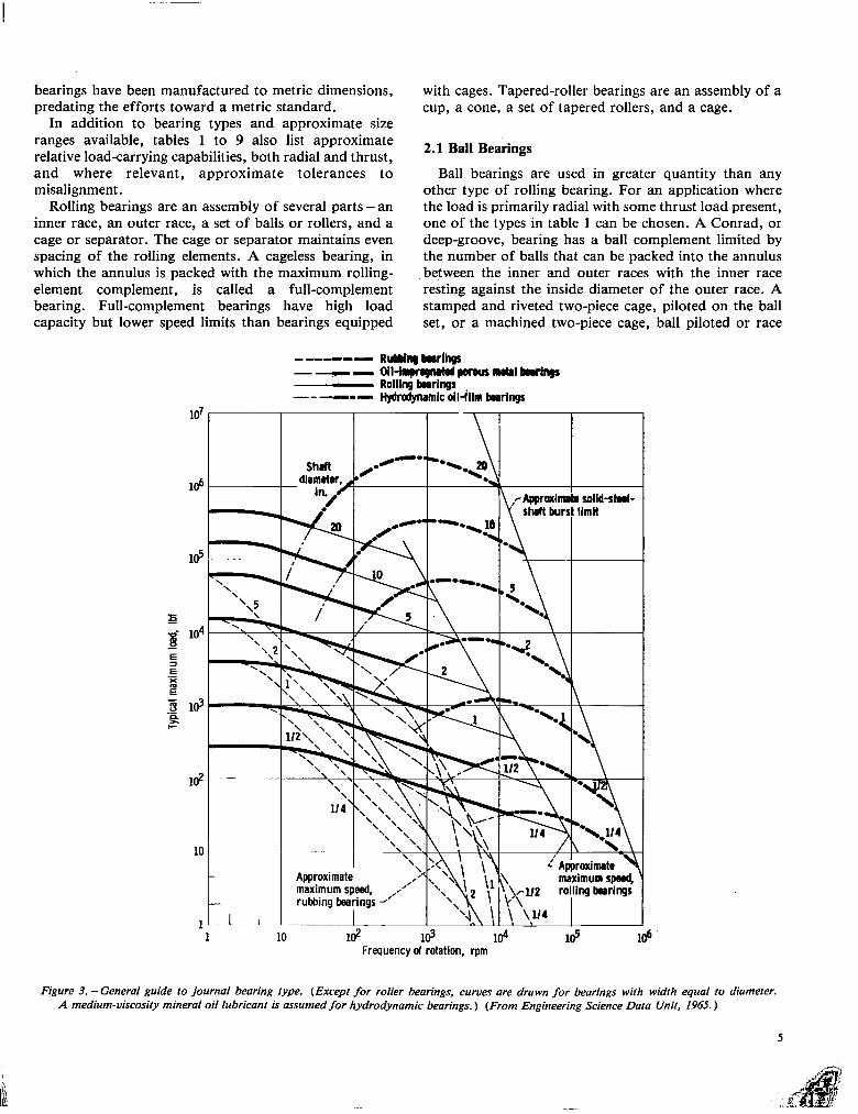
Figure 3, reproduced from the Engineering Science Data Unit publication (1965), gives a guide to the typical load that can be carried at various speeds, for a nominal life of 10 000 hr at room temperature, by journal bearings of various types on shafts of the diameters quoted. The heavy curves indicate the preferred type of journal bearing for a particular load, speed, and diameter and thus divide the graph into distinct regions. From figure 3 it is observed that rolling-element bearings are

preferred at lower speeds and hydrodynamic oil film bearings are preferred at higher speeds. Rubbing bearings and oil-impregnated porous metal bearings are not preferred for any of the speeds, loads, or shaft diameters considered. Also, as the shaft diameter is increased, the transitional point at which hydrodynamic bearings are preferred over rolling-element bearings moves to the left.

The applied load and speed are usually known, and this enables a preliminary assessment to be made of the type of journal bearing most likely to be suitable for a particular application. In many cases, the shaft diameter will already have been determined by other considerations, and figure 3 can be used to find the type of journal bearing that will give adequate load capacity at the required speed. These curves are based on good engineering practice and commercially available parts. Higher loads and speeds or smaller shaft diameters are possible-with exceptionally high engineering standards or specially produced materials. Except for rolling-element bearings, the curves are drawn for bearings with a width equal to the diameter. A medium-viscosity mineral oil lubricant is assumed for the hydrodynamic bearings.

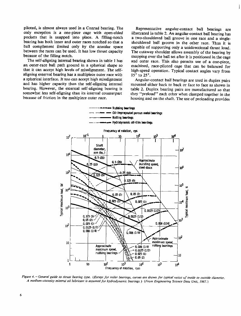
Similarly, figure 4, reproduced from the Engineering Science Data Unit publication (1967), gives a guide to the typical maximum load that can be carried at various speeds for a nominal life of 10 000 hr at room temperature by thrust bearings of various diameters quoted. The heavy curves again indicate the preferred type of bearing for a particular load, speed, and diameter and thus divide the graph into major regions. As with the journal bearing results (fig. 3) the hydrodynamic bearing is preferred at higher speeds and the rolling-element bearing is preferred at lower speeds. A difference between figures 3 and 4 is that at very low speeds there is a portion of the latter figure in which the rubbing bearing is preferred. Also, as the shaft diameter is increased, the transitional point at which hydrodynamic bearings are preferred over rolling-element bearings moves to the left. Note also from this figure that oil-impregnated porous metal bearings are not preferred for any of the speeds, loads, or shaft diameters considered.

2. Bearing Types A great variety of both designs and size ranges of ball

and roller bearings are available to the designer. The intent of this report is not to duplicate the complete descriptions given in manufacturers’ catalogs, but rather to present a guide to representative bearing types along with the approximate range of sizes available. Tables 1 to 9 illustrate some of the more widely used bearing types. In addition, there are numerous types of specialty bearings available; space does not permit a complete cataloging of all available bearings. Size ranges are given in metric units. Traditionally, most rolling-element

4

bearings have been manufactured to metric dimensions, predating the efforts toward a metric standard.

In addition to bearing types and approximate size ranges available, tables 1 to 9 also list approximate relative load-carrying capabilities, both radial and thrust, and where relevant, approximate tolerances to misalignment.

Rolling bearings are an assembly of several parts -an inner race, an outer race, a set of balls or rollers, and a cage or separator. The cage or separator maintains even spacing of the rolling elements. A cageless bearing, in which the annulus is packed with the maximum rolling- element complement, is called a full-complement bearing. Full-complement bearings have high load capacity but lower speed limits than bearings equipped

with cages. Tapered-roller bearings are an assembly of a cup, a cone, a set of tapered rollers, and a cage.

2.1 Ball Bearings

Ball bearings are used in greater quantity than any other type of rolling bearing. For an application where the load is primarily radial with some thrust load present, one of the types in table 1 can be chosen. A Conrad, or deep-groove, bearing has a ball complement limited by the number of balls that can be packed into the annulus between the inner and outer races with the inner race resting against the inside diameter of the outer race. A stamped and riveted two-piece cage, piloted on the ball set, or a machined two-piece cage, ball piloted or race

107

l&

ld

;- 104

5 .!i

ii

jj 103

s

ld

1c

1

-

-

-L I

----- RlWn# bhgs -ym 01I~prafsnublbarlqs

Rolling bariqs -- -0- Hydradynamic dliilm barlqs

n - ld ld 104 ld 16

Frequency of rotation, rpm 1

Figure 3. -General guide to journal bearing type. (Except for roller bearings, curves are drawn for bearings with width equal to diameter. A medium-viscosity mineral oil lubricant is assumed for hydrodynamic bearings. ) (From Engineering Science Data Unit. 1965. )

5

piloted, is almost always used in a Conrad bearing. The only exception is a one-piece cage with open-sided pockets that is snapped into place. A filling-notch bearing has both inner and outer races notched so that a ball complement limited only by the annular space between the races can be used. It has low thrust capacity because of the filling notch.

The self-aligning internal bearing shown in table 1 has an outer-race ball path ground in a spherical shape so that it can accept high levels of misalignment. The self- aligning external bearing has a multipiece outer race with a spherical interface. It too can accept high misalignment and has higher capacity than the self-aligning internal bearing. However, the external self-aligning bearing is somewhat less self-aligning than its internal counterpart because of friction in the multipiece outer race.

Representative angular-contact ball bearings are illustrated in table 2. An angular-contact ball bearing has a two-shouldered ball groove in one race and a single- shouldered ball groove in the other race. Thus it is capable of supporting only a unidirectional thrust load. The cutaway shoulder allows assembly of the bearing by snapping over the ball set after it is positioned in the cage and outer race. This also permits use of a one-piece, machined, race-piloted cage that can be balanced for high-speed operation. Typical contact angles vary from 15” to 25”.

Angular-contact ball bearings are used in duplex pairs mounted either back to back or face to face as shown in table 2. Duplex bearing pairs are manufactured so that they “preload” each other when clamped together in the housing and on the shaft. The use of preloading provides

--------- Rubbing harings - - - Oil-impregnated porous metal bearings

Rolling bearings - - -- Hydrodynamic oil-film bearings

Frequency d rotation, rps

10-l 1 10 1s 104 I

!d

I Shaft

I Awroxihate \ maximum speed, rubbing bearings J’

- 10

,l 11

1 10 ld ld 104 104 ld ld 16 16 Frequency of rotation, rpm

Figure 4. -General guide to thrust bearing type. (Except for roller bearihgs, curves are drawn for typical ratios of inside to outside diameter. A medium-viscosity mineral oil lubricant is assumed for hydrodynamic bearings, ) (From Engineering Science Data Unit, 1967. )

6

stiffer shaft support and helps prevent bearing skidding at light loads. Proper levels of preload can be obtained from the manufacturer. A duplex pair can support bidirectional thrust load. The back-to-back arrangement offers more resistance to moment or overturning loads than does the face-to-face arrangement.

Where thrust loads exceed the capability of a simple bearing, two bearings can be used in tandem, with both bearings supporting part of the thrust load. Three or more bearings are occasionally used in tandem, but this is discouraged because of the difficulty in achieving good load sharing. Even slight differences in operating temperature will cause a maldistribution of load sharing.

The split-ring bearing shown in table 2 offers several advantages. The split ring (usually the inner) has its ball groove ground as a circular arc with a shim between the ring halves. The shim is then removed when the bearing is assembled so that the split-ring ball groove has the shape of a gothic arch. This reduces the axial play for a given radial play and results in more accurate axial positioning of the shaft. The bearing can support bidirectional thrust loads but must not be operated for prolonged periods of time at predominantly radial loads. This results in three- point ball-race contact and relatively high frictional losses. As with the conventional angular-contact bearing, a one-piece precision-machined cage is used.

Ball thrust bearings (90” contact angle), table 3, are used almost exclusively for machinery with vertically oriented shafts. The flat-race bearing allows eccentricity of the fixed and rotating members. An additional bearing

’ , must be used for radial positioning. It has low load

capacity because of the very small ball-race contacts and consequent high Hertzian stress. Grooved-race bearings have higher load capacities and are capable of supporting low-magnitude radial loads. All of the pure thrust ball bearings have modest speed capability because of the 90” contact angle and the consequent high level of ball spinning and frictional losses.

2.2 Roller Bearings

Cylindrical roller bearings, table 4, provide purely radial load support in most applications. An Nor U type of bearing will allow free axial movement of the shaft relative to the housing to accommodate differences in thermal growth. An For J type of bearing will support a light thrust load in one direction; and a Ttype of bearing, a light bidirectional thrust load.

Cylindrical roller bearings have moderately high radial load capacity as well as high speed capability. Their speed capability exceeds that of either spherical or tapered- roller bearings. A commonly used bearing combination for support of a high-speed rotor is an angularcontact ball bearing or duplex pair and a cylindrical roller bearing.

As explained in the following section on bearing

geometry, the rollers in cylindrical roller bearings are seldom pure cylinders. They are crowned or made slightly barrel shaped, to relieve stress concentrations of the roller ends when any misalignment of the shaft and housing is present.

Cylindrical roller bearings may be equipped with one- or two-piece cages, usually race piloted. For greater load capacity, full-complement bearings can be used, but at a significant sacrifice in speed capability.

Spherical roller bearings, tables 5 to 7, are made as either single- or double-row bearings. The more popular bearing design uses barrel-shaped rollers. An alternative design employs hourglass-shaped rollers. Spherical roller bearings combine very high radial load capacity with modest thrust load capacity (with the exception of the thrust type) and excellent tolerance to misalignment. They find widespread use in heavy-duty rolling mill and industrial gear drives, where all of these bearing characteristics are requisite.

Tapered-roller bearings, table 8, are also made as single- or double-row bearings with combinations of one- or two-piece cups and cones. A four-row bearing assembly with two- or three-piece cups and cones is also available. Bearings are made with either a standard angle for applications in which moderate thrust loads are present or with a steep angle for high thrust capacity. Standard and special cages are available to suit the application requirements.

Single-row tapered-roller bearings must be used in pairs because a radially loaded bearing generates a thrust reaction that must be taken by a second bearing. Tapered-roller bearings are normally set up with spacers designed so that they operate with some internal play. Manufacturers’ engineering journals should be consulted for proper setup procedures.

Needle roller bearings, table 9, are characterized by compactness in the radial direction and are frequently used without an inner race. In the latter case the shaft is hardened and ground to serve as the inner race. Drawn cups, both open and closed end, are frequently used for grease retention. Drawn cups are thin walled and require substantial support from the housing. Heavy-duty roller bearings have relatively rigid races and are more akin to cylindrical roller bearings with long-length-to-diameter- ratio rollers.

Needle roller bearings are more speed limited than cylindrical roller bearings because of roller skewing at high speeds. A high percentage of needle roller bearings are full-complement bearings. Relative to a caged needle bearing, these have higher load capacity but lower speed capability.

There are many types of specialty bearings available other than those discussed here. Aircraft bearings for control systems, thin-section bearings, and fractured-ring bearings are some of the more widely used bearings

among the many types manufactured. A complete coverage of all bearing types is beyond the scope of this report.

Angular-contact ball bearings and cylindrical roller bearings are generally considered to have the highest speed capabilities. Speed limits of roller bearings are discussed in conjunction with lubrication methods. The lubrication system employed has as great an influence on bearing limiting speed as does the bearing design.

3. Geometry The operating characteristics of a rolling-element

bearing depend greatly on the diametral clearance of the bearing. This clearance varies for the different types of bearings discussed in the preceding section. In this section, the principal geometrical relationships governing the operation of unloaded rolling-element bearings are developed. This information will be of vital interest when such quantities as stress, deflection, load capacity, and life are considered in subsequent sections. Although bearings rarely operate in the unloaded state, an understanding of this section is vital to the appreciation of the remaining sections.

3.1 Geometry of Ball Bearings

Pitch diameter and clearance. -The cross section through a radial, single-row ball bearing shown in figure 5 depicts the radial clearance and various diameters. The pitch diameter de is the mean of the inner- and outer-race contact diameters and is given by

de=di+ i (do-di)

or

de=; (&+di) (1)

Also from figure 5, the diametral clearance denoted by Pd can be written as

Pd=do-di-2d (2)

Diametral clearance may therefore be thought of as the maximum distance that one race can move diametrally with respect to the other when no measurable force is applied and both races lie in the same plane. Although diametral clearance is generally used in connection with single-row radial bearings, equation (2) is also applicable to angular-contact bearings.

Race conformity. -Race conformity is a measure of the geometrical conformity of the race and the ball in a plane passing through the bearing axis, which is a line passing through the center of the bearing perpendicular to its plane and transverse to the race. Figure 6 is a cross section of a ball bearing showing race conformity, expressed as

f =r/d (3)

For perfect conformity, where the radius of the race is equal to the ball radius, f is equal to l/2. The closer the race conforms to the ball, the greater the frictional heat within the contact. On the other hand, open-race curvature and reduced geometrical conformity, which reduce friction, also increase the maximum contact stresses and consequently reduce the bearing fatigue life. For this reason, most ball bearings made today have race conformity ratios in the range 0.51 rf 50.54, with f =0.52 being the most common value. The race conformity ratio for the outer race is usually made slightly larger than that for the inner race to compensate for the closer conformity in the plane of the bearing between the outer race and ball than between the inner race and ball. This tends to equalize the contact stresses

Figure 5. -Cross sectron through radial, single-r0 w ball bearing. Figure 6. -Cross section of ball and outer race, showing race

conformity.

at the inner- and outer-race contacts. The difference in race conformities does not normally exceed 0.02.

Contact angle. - Radial bearings have some axial play since they are generally designed to have a diametral clearance, as shown in figure 7(a). This implies a free- contact angle different from zero. Angular-contact bearings are specifically designed to operate under thrust loads. The clearance built into the unloaded bearing, along with the race conformity ratio, determines the bearing free-contact angle. Figure 7(b) shows a radial bearing with contact due to the axial shift of the inner and outer rings when no measurable force is applied.

Before the free-contact angle is discussed, it is important to define the distance between the centers of curvature of the two races in line with the center of the ball in both figures 7(a) and (b). This distance -denoted by x in figure 7(a) and by D in figure 7(b) -depends on race radius and ball diameter. Denoting quantities referred to the inner and outer races by subscripts i and o, respectively, we see from figures 7(a) and (b) that

pd pd -T

+d+ 4 =ro-x+rj

or

X=r,-bri-d-P&

and

d=r,,-D+ri

or

D=r,+ri-d (4)

From these equations, we can write

X=D-Pd/2

This distance, shown in figure 7(b), will be useful in This is an alternative definition of the diametral clearance defining the contact angle. given in equation (2).

(a) Axis d rotation (blp - ~ Axis d rcMion ---

Figure 7. -Cross section of rodiol boll bearing. showing boll-rote contocf due to axial shift of inner ond outer rings. (II) Initioi position. (b) Shifed position.

By using equation (3), we can write equation (4) as

D=Bd (5)

where

B=fo+fi-1 (6)

The quantity B in equation (6) is known as the total conformity ratio and is a measure of the combined conformity of both the outer and inner races to the ball. Calculations of bearing deflection in later sections depend on the quantity B.

The free-contact angle /3f (fig. 7(b)) is defined as the angle made by a line through the points of contact of the ball and both races with a plane perpendicular to the bearing axis of rotation when no measurable force is applied. Note that the centers of curvature of both the outer and inner races lie on the line defining the free- contact angle. From figure 7(b), the expression for the free-contact angle can be written as

D - Pd/2 cos Of’ D

By using equations (2) and (4), we can write equation (7) as

,Bf = cos - ’ r,+ri-$(d,-di)

r,+ri-d 1 (8)

Equation (8) shows that if the size of the balls is increased and everything else remains constant, the free-contact angle is decreased. Similarly, if the ball size is decreased, the free-contact angle is increased.

From equation (7), the diametral clearance Pd can be written as

Pd = 20 (I- COS @I) (9

Endplay. -Free endplay P, is the maximum axial movement of the inner race with respect to the outer when both races are coaxially centered and no measurable force is applied. Free endplay depends on total curvature and contact angle, as shown in figure 7(b), and can be written as

P,=WsinPf (10)

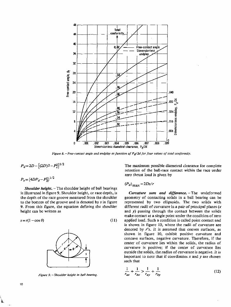
The variation of free-contact angle and endplay with the ratio P&d is shown in figure 8 for four values of total conformity normally found in single-row ball bearings. Eliminating Pf in equations (9) and (10) enables the establishment of the following relationships between free endplay and diametral clearance:

9

a

Dimensionless diametral ClearNICe, Pd/2d

Figure 8. -Free-contact angle and endploy OS function of Pd/2d for four values of totol conformity.

pd=w- [(w)2-p;t]1’2

Shoulder height. -The shoulder height of ball bearings is illustrated in figure 9. Shoulder height, or race depth, is the depth of the race groove measured from the shoulder to the bottom of the groove and is denoted by s in figure 9. From this figure, the equation defining the shoulder height can be written as

s=r(l -cos e) (11)

Figure 9. -Shoulder height in boll bearing.

The maximum possible diametral clearance for complete retention of the ball-race contact within the race under zero thrust load is given by

(pd) max = 2Ds/r

Curvature sum and difference. -The undeformed geometry of contacting solids in a ball bearing can be represented by two ellipsoids. The two solids with different radii of curvature in a pair of principal planes (x and JJ) passing through the contact between the solids make contact at a single point under the condition of zero applied load. Such a condition is called point contact and is shown in figure 10, where the radii of curvature are denoted by r’s. It is assumed that convex surfaces, as shown in figure 10, exhibit positive curvature and concave surfaces, negative curvature. Therefore, if the center of curvature lies within the solids, the radius of curvature is positive; if the center of curvature lies outside the solids, the radius of curvature is negative. It is important to note that if coordinates x and y are chosen such that

(12)

10

'by= -fd= -ri _ (15)

Figure 10. -Geometry of contacting elastic solids.

coordinate x then determines the direction of the semiminor axis of the contact area when a load is applied and y. the direction of the semimajor axis. The direction of motion is always considered to be along the x axis.

A cross section of a ball bearing operating at a contact angle /3 is shown in figure 11. Equivalent radii of curvature for both inner- and outer-race contacts in, and normal to, the direction of rolling can be calculated from this figure. The radii of curvature for the ball-inner-race contact are

r,=roy=d/2

rbx = de-dcos fl

2cosp

A

A

I

d,+d cos$ 2

dd2

IL 00 -

Figure I I. - Cross seciion of boll beoring.

(13)

(14)

The radii of curvature for the ball-outer-race contact are

r, = ray = d/2 (16)

d,+dcos 0 rbx= 2cosp (17)

rby = -fad = - r, (18)

In equations (14) and (17), 0 is used instead of flf since these equations are also valid when a load is applied to the contact. By setting 0 = 0”, equations (13) to (18) are equally valid for radial ball bearings. For thrust ball bearings, rbx= 00 and the other radii are defined as given in the preceding equations.

The curvature sum and difference, which are quantities of some importance in the analysis of contact stresses and deformations, are

where

1 1 1 -=- Rx r, + rbx

(20)

(21)

a = R,/R,

Equations (21) and (22) effectively redefine the problem of two ellipsoidal solids approaching one another in terms of an equivalent ellipsoidal solid of radii Rx and R, approaching a plane. From the radius-of-curvature expressions, the radii Rx and R, for the contact example discussed earlier can be written for the ball-inner-race contact as

R X

= d(de-dcos P)

2de (231

and for the ball-outer-race contact as

R X

= d(de+dcos PI 2de

(25)

11

fad Ry= 2fo-1

. (26)

3.2 Geometry of Roller Bearings

The equations developed for the pitch diameter de and diametral clearance Pd for ball bearings in equations (1) and (2), respectively, are directly applicable for roller bearings.

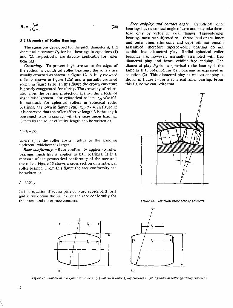
Crowning. -To prevent high stresses at the edges of the rollers in cylindrical roller bearings, the rollers are usually crowned as shown in figure 12. A fully crowned rol!er is shown in figure 12(a) and a partially crowned roller, in figure 12(b). In this figure the crown curvature is greatly exaggerated for clarity. The crowning of rollers also gives the bearing protection against the effects of slight misalignment. For cylindrical rollers, r,,/d= 102. In contrast, for spherical rollers in spherical roller bearings, as shown in figure 12(a), roy/d=4. In figure 12 it is observed that the roller effective length If is the length presumed to be in contact with the races under loading. Generally the roller effective length can be written as

&=I,-2r,

where r, is the roller corner radius or the grinding undercut, whichever is larger.

Race conformity. -Race conformity applies to roller bearings much like it applies to ball bearings. It is a measure of the geometrical conformity of the race and the roller. Figure 13 shows a cross section of a spherical roller bearing. From this figure the race conformity can be written as

f = r/2roy

In this equation if subscripts i or o are subscripted for f and r, we obtain the values for the race conformity for the inner- and outer-race contacts.

rr rr

Free endplay and contact angle. - Cylindrical roller bearings have a contact angle of zero and may take thrust load only by virtue of axial flanges. Tapered-roller bearings must be subjected to a thrust load or the inner and outer rings (the cone and cup) will not remain assembled; therefore tapered-roller bearings do not exhibit free diametral play. Radial spherical roller bearings are, however, normally assembled with free diametral play and hence exhibit free endplay. The diametral play Pd for a spherical roller bearing is the same as that obtained for ball bearings as expressed in equation (2). This diametral play as well as endplay is shown in figure 14 for a spherical roller bearing. From this figure we can write that

Figure 13. -Spherical roller bearing geometry.

/ - d

rr

Figure 12. -Spherical and cylindrical rollers. (a) Spheric01 roller (fully crowned). (b) Cylindrical roller (portiolly crowned).

12

cosy

or

Also from figure 14 the free endplay can be written as

Pe= 2ro(sin fi - sin 7) + Pd sin 7

Curvature sum and difference. -The same procedure will be used for defining the curvature sum and difference for roller bearings as was used for ball bearings. For spherical roller bearings, as shown in figure 13, the radii of curvature for the roller-inner-race contact can be written as

r ,=d/2

r0y=fi(ri/2)

rbx= (de-dcos P) 2 cos p

‘by = - 2f ir0y

Outer ring

Axis of rotation

Figure 14. - Schematic diogrom of spheric01 roller beoring, showing diometrol ploy ond endploy.

For the spherical roller bearing shown in figure 13 the radii of curvature for the roller-outer-race contact can be written as

r ,=d/2

Toy =fo (r,M

rbx= _ (de+dcos PI 2cosa

‘by = - 2foroy

Knowing the radii of curvature for the respective contact condition, we can write the curvature sum and difference directly from equations (19) and (20). Furthermore, the radius-of-curvature expressions Rx and R, for spherical roller bearings can be written for the roller-inner-race contact as

R X

= d(de-dcos PI 2de

and for the roller-outer-race contact as

R X

= d(de+dcos P)

2de

RY=$$ 0

4. Kinematics

(27)

(28)

(2%

(30)

The relative motions of the separator, the balls or rollers, and the races of rolling-element bearings are important to understanding their performance. The relative velocities in a ball bearing are somewhat more complex than those in roller bearings, the latter being analogous to the specialized case of a zero- or fixed- value-contact-angle ball bearing. For that reason the ball bearing is used as an example here to develop approximate expressions for relative velocities. These are useful for rapid but reasonably accurate calculation of elastohydrodynamic film thickness, which can be used with surface roughnesses to calculate the lubrication life factor.

The precise calculation of relative velocities in a ball bearing in which speed or centrifugal force effects, contact deformations, and elastohydrodynamic traction effects are considered requires a large computer to numerically solve the relevant equations. The reader is referred to the growing body of computer codes discussed in section 13 for precise calculations of bearing

13

performance. Such a treatment is beyond the scope of this section. However, approximate expressions that yield answers with accuracies satisfactory for many situations are available.

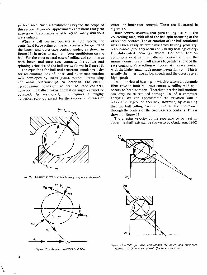
When a ball bearing operates at high speeds, the centrifugal force acting on the ball creates a divergency of the inner- and outer-race contact angles, as shown in figure 15, in order to maintain force equilibrium on the ball. For the most general case of rolling and spinning at both inner- and outer-race contacts, the rolling and spinning velocities of the ball are as shown in figure 16.

The equations for ball and separator angular velocity for all combinations of inner- and outer-race rotation were developed by Jones (1964). Without introducing additional relationships to describe the elastohydrodynamic conditions at both ball-race contacts, however, the ball-spin-axis orientation angle 0 cannot be obtained. As mentioned, this requires a lengthy numerical solution except for the two extreme cases of

we IS. - Conlacl angles m a ball bearing at appreciable speeds.

Figure 16. -Angular velocities of a ball.

outer- or inner-race control. These are illustrated in figure 17.

Race control assumes that pure rolling occurs at the controlling race, with all of the ball spin occurring at the other race contact. The orientation of the ball rotational axis is then easily determinable from bearing geometry. Race control probably occurs only in dry bearings or dry- film-lubricated bearings where Coulomb friction conditions exist in the ball-race contact ellipses, the moment-resisting spin will always be greater at one of the race contacts. Pure rolling will occur at the race contact with the higher magnitude moment-resisting spin. This is usually the inner race at low speeds and the outer race at high speeds.

In oil-lubricated bearings in which elastohydrodynamic films exist in both ball-race contacts, rolling with spin occurs at both contacts. Therefore precise ball motions can only be determined through use of a computer analysis. We can approximate the situation with a reasonable degree of accuracy, however, by assuming that the ball rolling axis is normal to the line drawn through the centers of the two ball-race contacts. This is shown in figure 11.

The angular velocity of the separator or ball set wc about the shaft axis can be shown to be (Anderson, 1970)

Figure 17. -Ball spin axci orrenrarrons Jor outer- and inner-race conrrol. (a) Ourer-race control. (b) Inner-race conrrol.

14

w = (oi+uo)/2 c de/2

=t [Wi(l-F)+Wo(l+F)] (31)

where Vi and u, are the linear velocities of the inner and outer contacts. The angular velocity of a ball about its Own axis Wb is

Vi-V0

Wb= de/2

=$[wi(I-F)-wo(l+F)] (32)

To calculate the velocities of the ball-race contacts, which are required for calculating elastohydrodynamic film thicknesses, it is convenient to use a coordinate system that rotates at wc. This fixes the ball-race contacts relative to the observer. In the rotating coordinate system the angular velocities of the inner and outer races become

Wir=Wi-Wc= (y%) (I+ q!)

w or=wo-wc= (!y) (I- cj.$)

The surface velocities entering the ball-inner-race contact for pure rolling are

uai = ubi = de-dcos 0 2 >

*ir

or

uai = ubi = de(wi-wo) 4 (1-y)

and those at the ball-outer-race contact are

u,, = ubo = d,+dcos P 2 >

war

or

uao = Ubo =

(34)

(35)

For a cylindrical roller bearing, /3=0” and equations (31), (32), (34), and (35) become, if d is roller diameter,

Wc=f [Wi(l-2) +Wo(lt;)]

? (36)

uao = ubo = de(wo-wi) 4

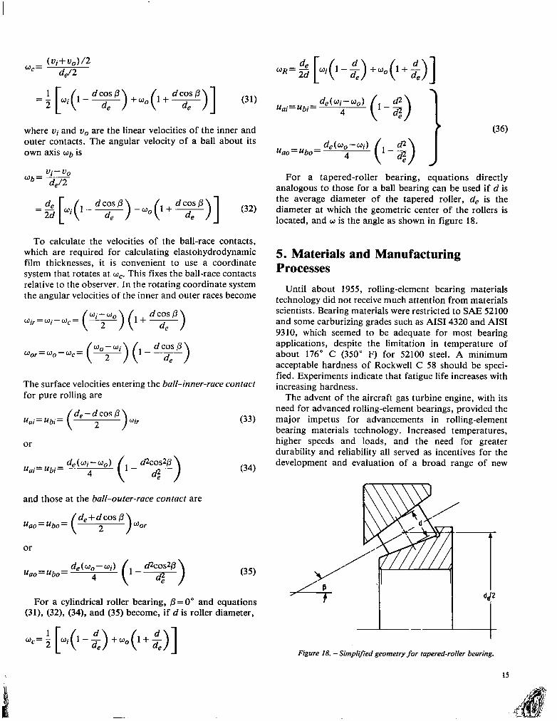
For a tapered-roller bearing, equations directly analogous to those for a ball bearing can be used if d is the average diameter of the tapered roller, d, is the diameter at which the geometric center of the rollers is located, and w is the angle as shown in figure 18.

5. Materials and Manufacturing Processes

Until about 1955, rolling-element bearing materials technology did not receive much attention from materials scientists. Bearing materials were restricted to SAE 52100 and some carburizing grades such as AISI 4320 and AM 9310, which seemed to be adequate for most bearing applications, despite the limitation in temperature of about 176” C (350” F) for 52100 steel. A minimum acceptable hardness of Rockwell C 58 should be speci- fied. Experiments indicate that fatigue life increases with increasing hardness.

The advent of the aircraft gas turbine engine, with its need for advanced rolling-element bearings, provided the major impetus for advancements in rolling-element bearing materials technology. Increased temperatures, higher speeds and loads, and the need for greater durability and reliability all served as incentives for the development and evaluation of a broad range of new

Figure 18. -Simplified geometry for tapered-roller bearing.

materials and processing methods. The combined research efforts of bearing manufacturers, engine manufacturers, and Government agencies over the past three decades have resulted in startling advances in rolling-element bearing life and reliability and in performance. The discussion here is brief in scope. For a comprehensive treatment of the research status of current bearing technology and current bearing designs, refer to Bamberger et al. (1980).

5.1 Ferrous Alloys

The need for higher temperature capability led to the evaluation of a number of available molybdenum and tungsten alloy tool steels as bearing materials (table 10). These alloys have excellent high-temperature hardness retention. Such alloys melted and cast in an air environment, however, were generally deficient in fatigue resistance because of the presence of nonmetallic inclusions. Vacuum processing techniques can reduce or eliminate these inclusions. Techniques used include vacuum induction melting (VIM) and vacuum arc remelting (VAR). These have been extensively explored, not only with the tool steels now used as bearing materials, but with SAE 52100 and some of the carburizing steels as well. Table 10 lists a fairly complete array of ferrous alloys, both fully developed and experimental, from which present-day bearings are fabricated. AISI M-50, usually VIM-VAR or consumable electrode vacuum melted (CEVM) processed, has become a very widely used quality bearing material. It is usable at temperatures to 315’ C (600” F), and it is usually assigned a materials life factor of 3 to 5 (section 12.5). T-l tool steel has also come into fairly wide use, mostly in Europe, in bearings. Its hot hardness retention is slightly superior to that of M-50 and approximately equal to that of M-l and M-2. These alloys retain adequate hardness to about 400” C (750" F).

Surface-hardened or carburized steels are used in many bearings where, because of shock loads or cyclic bending stresses, the fracture toughness of the through-hardened steels is inadequate. Some of the newer materials being developed, such as CBS 1000 and Vasco X-2 have hot hardness retention comparable to that of the tool steels (fig. 19). They too are available as ultraclean, vacuum- processed materials and should offer adequate resistance to fatigue. Carburized steels may become of increasing importance in ultra-high-speed applications. Bearings with through-hardened steel races are currently limited to approximately 2.5 million d@ (where db is bore diameter in millimeters and N is rotational speed in rpm) because, at higher d@ values, fatigue cracks propagate through the rotating race as a result of the excessive hoop stress present (Bamberger, et al., 1976).

In applications where the bearings are not lubricated with conventional oils and protected from corrosion at all

times, a corrosion-resistant alloy should be used. Dry- film-lubricated bearings, bearings cooled by liquefied cryogenic gases, and bearings exposed to corrosive environments such as very high humidity and salt water are applications where corrosion-resistant alloys should be considered. Of the alloys listed in table 10, both 44OC and AMS5749 are readily available in vacuum-melted heats.

In addition to improved melting practice, forging and forming methods that result in improved resistance to fatigue have been developed. Experiments indicate that fiber or grain flow parallel to the stressed surface is superior to fiber flow that intersects the stressed surface (Bamberger, 1970; Zaretsky and Anderson, 1966). Forming methods that result in more parallel grain flow are now being used in the manufacture of many bearings, especially those used in high-load applications.

5.2 Ceramics

Experimental bearings have been made from a variety of ceramics including alumina, silicon carbide, titanium carbide, and silicon nitride. The use of ceramics as bearing materials for specialized applications will probably continue to grow for several reasons. These include

(1) High-temperature capability - Because ceramics can exhibit elastic behavior to temperatures beyond 1000” C (1821” F), they are an obvious choice for extreme-temperature applications.

o-

2-

12 -

Material temperature, K

I 0 200 400 600 a00 iooo

Material temperature, OF

Figure 19. -Hot hardness of CBS 1000, CBS 1000M, Vasco X-2, and high-speed tool sreels. (From Anderson and Zarersky, 1975. )

16

(2) Corrosion resistance -Ceramics are essentially chemically inert and able to function in many environments hostile to ferrous alloys.

(3) Low density -This can be translated into improved bearing capacity at high speeds, where centrifugal effects predominate.

(4) Low coefficient of thermal expansion -Under conditions of severe thermal gradients, ceramic bearings exhibit less drastic changes in geometry and internal play than do ferrous alloy bearings.

At the present time, silicon nitride is being actively developed as a bearing material (Sibley, 1982; Cundill and Giordano, 1982). Silicon nitride bearings have exhibited fatigue lives comparable to and, in some instances, superior to that of high-quality vacuum-melted M-50 (Sibley, 1982). Two problems remain: (1) quality control and precise nondestructive inspection techniques to determine acceptability and (2) cost. Improved hot isostatic compaction, metrology, and finishing techniques are all being actively pursued. However, silicon nitride bearings must still be considered experimental.

6. Separators Ball and roller bearing separators, sometimes called

cages or retainers, are bearing components that, although never carrying load, are capable of exerting a vital influence on the efficiency of the bearing. In a bearing without a separator, the rolling elements contact each other during operation and in so doing experience severe sliding and friction. The primary function of a separator is to maintain the proper distance between the rolling elements and to ensure proper load distribution and balance within the bearing. Another function of the separator is to maintain control of the rolling elements in such a manner as to produce the least possible friction through sliding contact. Furthermore, a separator is necessary for several types of bearings to prevent the rolling elements from falling out of the bearing during handling. Most separator troubles occur from improper mounting, misaligned bearings, or improper (inadequate or excessive) clearance in the rolling-element pocket.

The materials used for separators vary according to the type of bearing and the application. In ball bearings and some sizes of roller bearings, the most common type of separator is made from two strips of carbon steel that are pressed and riveted together. Called ribbon separators, they are the least expensive to manufacture and are entirely suitable for many applications. They are also lightweight and usually require little space.

The design and construction of angular-contact ball bearings allow the use of a one-piece separator. The simplicity and inherent strength of one-piece separators

permit their fabrication from many desirable materials. Reinforced phenolic and bronze are the two most commonly used materials. Bronze separators offer strength and low-friction characteristics and can be operated at temperatures to 230” C (450” F). Machined, silver-plated ferrous alloy separators are used in many demanding applications. Because reinforced cotton-base phenolic separators combine the advantages of low weight, strength, and nongalling properties, they are used for such high-speed applications as gyro bearings. In high-speed bearings, lightness and strength are particularly desirable since the stresses increase with speed but may be greatly minimized by reduction of separator weight. A limitation of phenolic separators, however, is that they have a allowable maximum temperature of about 135” C (275” F).

7. Contact Stresses and Deformations The loads carried by rolling-element bearings are

transmitted through the rolling element from one race to the other. The magnitude of the load carried by an individual rolling element depends on the internal geometry of the bearing and the location of the rolling element at any instant. A load-deflection relationship for the rolling-element-race contact is developed in this section. The deformation within the contact is a function of, among other things, the ellipticity parameter and the elliptic integrals of the first and second kinds. Simplified expressions that allow quick calculations of the stresses and deformations to be made easily from a knowledge of the applied load, the material properties, and the geometry of the contacting elements are presented in this section.

7.1 Elliptical Contacts

When two elastic solids are brought together under a load, a contact area develops, the shape and size of which depend on the applied load, the elastic properties of the materials, and the curvatures of the surfaces. When the two solids shown in figure 10 have a normal load applied to them, the shape of the contact area is elliptical, with D, being the diameter in the y direction (transverse direction) and D, being the diameter in the x direction (direction of motion). For the special case where rpu=ray and rbX=rby, the resulting contact is a circle rather than an ellipse. Where ray and rby are both infinity, the initial line contact develops into a rectangle when load is applied.

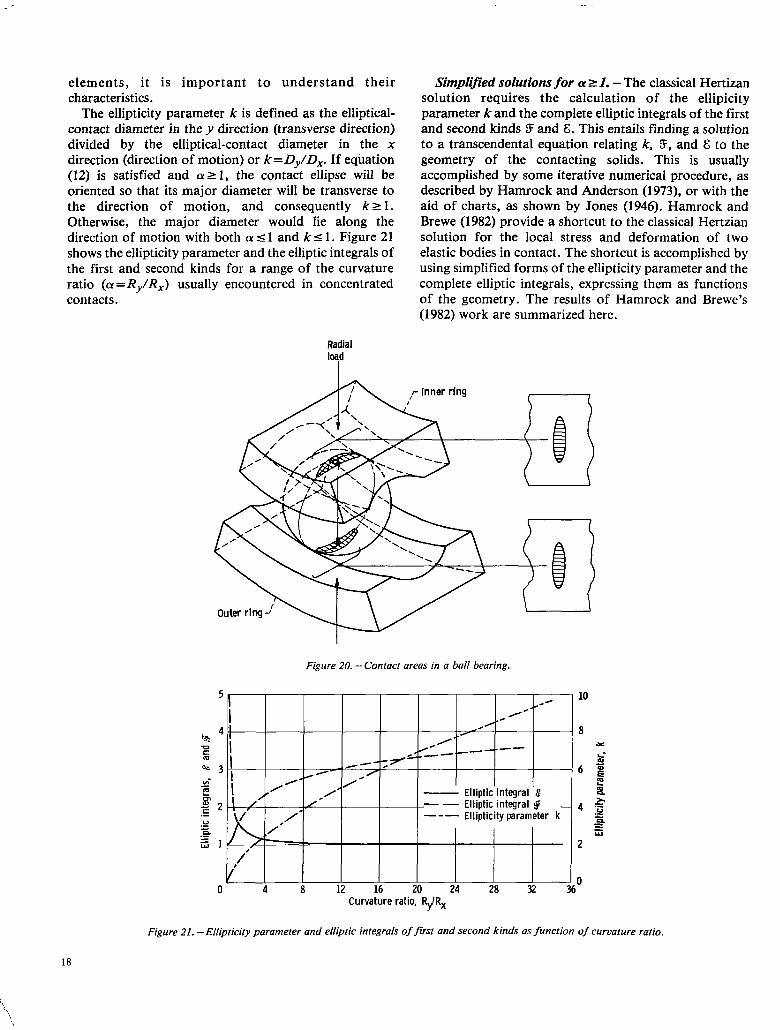
The contact ellipses obtained with either a radial or a thrust load for the ball-inner-race and ball-outer-race contacts in a ball bearing are shown in figure 20. Inasmuch as the size and shape of these contact areas are highly significant in the successful operation of rolling

17

elements, it is important to understand their characteristics.

The ellipticity parameter k is defined as the elliptical- contact diameter in the y direction (transverse direction) divided by the elliptical-contact diameter in the x direction (direction of motion) or k=Dy/D,. If equation (12) is satisfied and CY 2 1, the contact ellipse will be oriented so that its major diameter will be transverse to the direction of motion, and consequently k2 1. Otherwise, the major diameter would lie along the direction of motion with both (Y s 1 and k 5 1. Figure 21 shows the ellipticity parameter and the elliptic integrals of the first and second kinds for a range of the curvature ratio (a = Ry/R,.) usually encountered in concentrated contacts.

Simplified solutions for a 11. - The classical Hertizan solution requires the calculation of the ellipicity parameter k and the complete elliptic integrals of the first and second kinds 5 and E. This entails finding a solution to a transcendental equation relating k, 5, and & to the geometry of the contacting solids. This is usually accomplished by some iterative numerical procedure, as described by Hamrock and Anderson (1973), or with the aid of charts, as shown by Jones (1946). Hamrock and Brewe (1982) provide a shortcut to the classical Hertzian solution for the local stress and deformation of two elastic bodies in contact. The shortcut is accomplished by using simplified forms of the ellipticity parameter and the complete elliptic integrals, expressing them as functions of the geometry. The results of Hamrock and Brewe’s (1982) work are summarized here.

Radial load

I

,r Inner ring I

Figure 20. -Contact areas in a ball bearing.

5 10 e/

I ,’

*e ‘*

I a e’ x

_ ,--“=I s--- -- _.-- c $

/- / 6

/ /

t

- Elliptic integral I ii / - -

/* Elliptic integral $ - 4 0

--- Ellipticityparameter k Y ,/’

g iz

2

a/’

0 4 a 12 16 20 24 28 32 36O

Figure 21. -Elliptici(y parameter and elliptic integrals of first and second kinds as function of curvature

Curvature ratio, R,,IR,

ia

Table 11 shows various values of radius-of-curvature ratios and corresponding values of k, 5, and E obtained from the numerical procedure given in Hamrock and Anderson (1973). For the set of pairs of data [(ki, ai), i=l, 2 9 -a-, 261, a power fit using linear regression by the method of least squares resulted in the following equation:

for arl (37)

The asymptotic behavior of & and 5 ((y-1 implies E-5-7r/2, and (y-03 implies S-m and E-l) was suggestive of the type of functional dependence that E and 5 might follow. As a result, an inverse and a logarithmic curve fit were tried for & and 5, respectively. The following expressions provided excellent curve fits:

E=l+q/a forolrl (38)

S=a/2+qIn a forcyrl (3%

where q = a/2 - 1. Values of k, E, and 3 are presented in table 11 and compared with the numerically determined values of k, E, and 5. Table 11 also gives the percentage of error determined as

e= (i-z) 100

When the ellipticity parameter k (eq. (37)), the elliptic integrals of the first and second kinds (eqs. (39) and (38)), the normal applied load F, Poisson’s ratio u, and the modulus of elasticity E of the contacting solids are known, we can write the major and minor axes of the contact ellipse and the maximum deformation at the center of the contact, from the analysis of Hertz (1881), as

6=qz--)(-c-)2]“’ 2

E’ =

(41)

(42)

(43)

In these equations, D, and 0, are proportional to W3

and 6 is proportional t’o F2’3. -- - The maximum Hertzian stress at the center of the

contact can also be determined by using equations (40) and (41).

u ,,,= = 6F/irD,Dy

Simplified solutions for LY 11. -Table 12 gives the simplified equations for CY< 1 as well for (Y 2 1. Recall that (Y 2 1 implies k 2 1 and equation (12) is satisfied and CY C 1 implies k< 1 and equation (12) is not satisfied. It is important to make the proper evaluation of CY since it has a great significance in the outcome of the simplified equations. Figure 22 shows three diverse situations in which the simplified equations can be usefully applied. The locomotive wheel on a rail (fig. 22(a)) illustrates an example in which the ellipticity parameter k and the radius ratio cx are less than 1. The ball rolling against a flat plate (fig. 22(b)) provides pure circular contact (i.e., 01 = k = 1 .O). Figure 22(c) shows how the contact ellipse is formed in the ball-outer-ring contact of a ball bearing. Here the semimajor axis is normal to the direction of rolling and consequently CY and k are greater than 1. Table 13 uses this figure to show how the degree of conformity affects the contact parameters.

1-v; : l-z$ Ea Eb

Figure 22. - Three degrees of conformity. (a) Wheel on rail. (b ) Ball on plane. (c) Ball-outer-race contact.

19

7.2 Rectangular Contacts

For this situation the contact ellipse discussed in the

Similarly for a rectangular contact, equation (44) gives

preceding section is of infinite length in the transverse F=K16

direction (D, - 00 ). This type of contact is exemplified by a cylinder loaded against a plate, a groove, or another,

where

parallel, cylinder or by a roller loaded against an inner or outer ring. In these situations the contact semiwidth is K1= I

1

given by

b=R&ii% (“’ ) [~+ln(!.$Z)+ln(3)] (47)

where the dimensionless load

W=F’/E’R,

In general then,

and F’ is the load per unit length along the contact. The maximum deformation for a rectangular contact can be written as (ESDU, 1978)

in which j= 1.5 for ball bearings and 1.0 for roller bearings. The total normal approach between two races separated by a rolling element is the sum of the deformations under load between the rolling element and

(49) The maximum Hertzian stress in a rectangular contact can be written as

where

8. Static Load Distribution Having defined a simple analytical expression for the

deformation in terms of load in the previous section, it is possible to consider how the bearing load is distributed among the rolling elements. Most rolling-element bearing applications involve steady-state rotation of either the inner or outer race or both; however, the speeds of rotation are usually not so great as to cause ball or roller centrifugal forces or gyroscopic moments of significant magnitudes. In analyzing the loading distribution on the rolling elements, it is usually satisfactory to ignore these effects in most applications. In this section the load deflection relationships for ball and roller bearings are given, along with radial and thrust load distributions of statically loaded rolling elements.

di= [F/ (Kj) i] I” (51)

Substituting equations (49) to (51) into equation (48) gives

1 Kj=

[[&]‘“+ [&]“jj

Recall that (Kj), and (Kj)i are defined by equations (46) and (47) for elliptical and rectangular contacts, respectively. From these equations we observe that (Kj). and (Kj)i are functions of only the geometry of the contact and the material properties. The radial and thrust load analyses are presented in the following two sections and are directly applicable for radially loaded ball and roller bearings and thrust-loaded ball bearings.

8.1 Load Deflection Relationships

For an elliptical contact, the load deflection relationship given in equation (42) can be written as

8.2 Radially Loaded Ball and Roller Bearings

F= K+‘2

where

K,,5 = akE’-

(45)

(46)

A radially loaded rolling element with radial clearance Pd is shown in figure 23. In the concentric position shown in figure 23(a), a uniform radial clearance between the rolling element and the races of Pd/2 is evident. The application of a small radial load to the shaft causes the

20

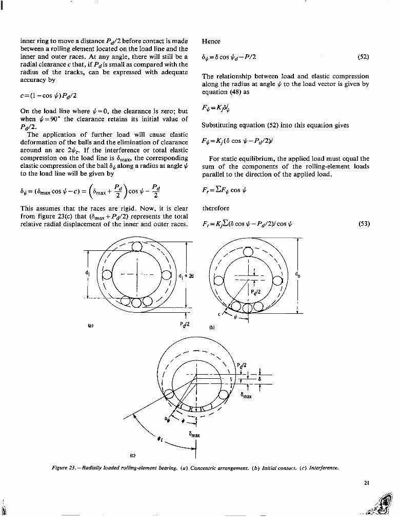
inner ring to move a distance Pd/2 before contact is made between a rolling element located on the load line and the inner and outer races. At any angle, there will still be a radial clearance c that, if Pd is small as compared with the radius of the tracks, can be expressed with adequate accuracy by

c=(l --cos ,‘)P&

On the load line where $=O, the clearance is zero; but when $=90” the clearance retains its initial value of P&

The application of further load will cause elastic deformation of the balls and the elimination of clearance around an arc 2$,. If the interference or total elastic compression on the load line is I&~, the corresponding elastic compression of the ball 64 along a radius at angle # to the load line will be given by

+= (&lax cos$-c)=(6,,+~)cos3-~

This assumes that the races are rigid. Now, it is clear from figure 23(c) that (6,,+Pd/2) represents the total relative radial displacement of the inner and outer races.

di + 2d

t P&2

Hence

6$ = 6 cos $d--P/2 (52)

The relationship between load and elastic compression along the radius at angle $ to the load vector is given by equation (48) as

FG = K,t%ii

Substituting equation (52) into this equation gives

F$=Kj(G COS $-Pd/2v

For static equilibrium, the applied load must equal the sum of the components of the rolling-element loads parallel to the direction of the applied load.

F,= cFG cos $

therefore

Fr= KjC(G COS $ -Pd/2p COS # (53)

(b)

Figure 23. -Radially loaded rolling-element bearing. (u) Concenfric arrangement. (6) Initial contact. (c) Interference.

The angular extent of the bearing arc 2$1 in which the rolling elements are loaded is obtained by setting the root expression in equation (53) equal to zero and solving for $.

$, = cos - ‘(P&6)

The summation in equation (53) applies only to the angular extent of the loaded region. This equation can be written for a roller bearing as

F,= $/- $sin $1 >

nKrU2~

and similarly in integral form for a ball bearing as

(54)

The integral in the equation can be reduced to a standard elliptic integral by the hypergeometric series and the beta function. If the integral is numerically evaluated directly, the following approximate expression is derived:

cos $ d$

=2.491 [[I+ (p~;y)‘]“‘lj

This approximate expression fits the exact numerical solution to within +2 percent for a complete range of P&6.

The load carried by the most heavily loaded ball is obtained by substituting $ =O” in equation (53) and dropping the summation sign

F max=Kj&i (55)

Dividing the maximum ball load (eq. (55)) by the total radial load for a roller bearing (eq. (54)) gives

F,= ’ I

(56) (1 -P&6)

and similarly for a ball bearing

F,= nF,,/Z (57)

Z= ?r( 1 - Pd/26)3/2

(58)

2.491 [F+ ( ,,,,)2]1%j

For roller bearings when the diametral clearance Pd is zero, equation (56) gives

F,= nF,,/4 (59)

For ball bearings when the diametral clearance Pd is zero, the value of Z in equation (57) becomes 4.37. This is the value derived by Stribeck (1901) for ball bearings of zero diametral clearance. The approach used by Stribeck was to evaluate the finite summation for various numbers of balls. He then derived the celebrated Stribeck equation for static load-carrying capacity by writing the more conservative value of 5 for the theoretical value of 4.37:

F,= nF,,,,/5 (60)

In using equation (60), it should be remembered that Z was considered to be a constant and that the effects of clearance and applied load on load distribution were not taken into account. However, these effects were considered in obtaining equation (57).

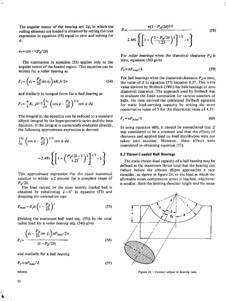
8.3 Thrust-Loaded Ball Bearings

The static-thrust-load capacity of a ball bearing may be defined as the maximum thrust load that the bearing can endure before the contact ellipse approaches a race shoulder, as shown in figure 24, or the load at which the allowable mean compressive stress is reached, whichever is smaller. Both the limiting shoulder height and the mean

where Figure 24, - Contact ellipse in bearing race.

22

compressive stress must be calculated to find the static- thrust-load capacity.

The contact ellipse in a bearing race under a load is shown in figure 24. Each ball is subjected to an identical thrust component F/n, where Ft is the total thrust load. The initial contact angle before the application of a thrust load is denoted by fif Under load the normal ball thrust load Facts at the contact angle /3 and is written as

F= F,/n sin p (61)

A cross section through an angular-contact bearing under a thrust load Ft is shown in figure 25. From this figure, the contact angle after the thrust load has been applied can be written as

p=cos-l (y-2) (62)

The initial contact angle was given in equation (7). Using that equation and rearranging terms in equation (62) give, solely from geometry (fig. 25),

h=D(s-1)

6= [&Jo+ [&Jo 1

Kj=

I Kj=

4.532 1 2/3 [-- 4.55; 1 2/3

ak&;(Ro~o) 1’2 + Tk$Ti( RiEi) 1”

where

l/2

Figure 25. -Angular-contact ball bearing under thrust load.

(63)

(64)

(65)

23

and k, r, and 3 are given (39), respectively.

From equations (61) and

Ft nsinp =F

by equations (37), (38), and

(64), we can write

7 (66)

L =sin/j(s-1)3’2 J nKp3/2

This equation can be solved numerically by the Newton- Raphson method. The iterative equation to be satisfied is

p’-p=

(67)

In this equation convergence is satisfied when /3’ -P becomes essentially zero.

When a thrust load is applied, the shoulder height is limited to the distance by which the pressure-contact ellipse can approach the shoulder. As long as the following inequality is satisfied, the pressure-contact ellipse will not exceed the shoulder height limit:

0 > /3 + sin - ~(D,/fi

From figure 9 and equation (1 l), the angle used to define the shoulder height 13 can be written as

e=cos-I(1 -s/f?

From figure 7, the axial deflection 6, corresponding to a thrust load can be written as

6,= (D+6) sin /3-Dsin Pf (68)

Substituting equation (63) into equation (68) gives

6 t = D sin@ - 0~) --

cos p

Having determined 0 from equation (67) and fir from equation (49), we can easily evaluate the relationship for 6,.

24

8.4 Preioading

The use of angular-contact bearings as duplex pairs preloaded against each other is discussed in section 2.1. As shown in table 2 duplex bearing pairs are used in either back-to-back or face-to-face arrangements. Such bearings are usually preloaded against each other by providing what is called “stickout” in the manufacture of the bearing. This is illustrated in figure 26 for a bearing pair used in a back-to-back arrangement. The magnitude of the stickout and the bearing design determine the level of preload on each bearing when the bearings are clamped together as in figure 26. The magnitude of preload and the load deflection characteristics for a given bearing pair can be calculated by using equations (7), (45), (61), (63), (64), (65), and (66).

The relationship of initial preload, system load, and final load for bearings a and b is shown in figure 27. The load deflection curve follows the relationship 6=KF2/3. When a system thrust load Ft is imposed on the bearing pairs, the magnitude of load on bearing b increases while that on bearing a decreases until the difference equals the system load. The physical situation demands that the change in each bearing deflection be the same (Aa = Ab in fig. 27). The increments in bearing load, however, are nof the same. This is important because it always requires a system thrust load far greater than twice the preload before one bearing becomes unloaded. Prevention of bearing unloading, which can result in skidding and early failure, is an objective of preloading.

Figure 26. -Angular-contact bearings in back-to-back arrangement, shown individually as manufactured and as mounted with preload. (a) Separated. (b) Mounted and preloaded.

9. Rolling Friction and Friction in Bearings

Bearing b load

----+----------

5; ,, Pnload

z Brring a load ----------

w A Axkl doflectlon, 4’

Figure 27. - Thrust load-axial deflection curve for a typical ball bearing.

9.1 Rolling Friction

The concepts of rolling friction are important generally in understanding the behavior of machine elements in rolling contact and particularly because rolling friction influences the overall behavior of rolling-element bearings. The theories of Reynolds (1875) and Heathcote (1921) attempted to explain rolling friction in terms of the energy required to overcome the interfacial slip that occurs because of the curved shape of the contact area. As shown in figure 28, the ball rolls about the y axis and makes contact with the groove from a to 6. If the groove

is fixed, then for zero slip over the contact area, no point within the area should have a velocity in the direction of rolling. The surface of the contact area is curved, however, so that points a and b are at different radii from they axis than are points c and d. For a rigid ball, points a and b must have different velocities with respect to they axis than do points c and d because the velocity of any point on the ball relative to the y axis equals the angular velocity times the radius from they axis. Slip must occur at various points over the contact area unless the body is so elastic that yielding can take place in the contact area to prevent this interfacial slip. The theory of Reynolds and later Heathcote assumed that this interfacial slip took place and that the forces required to make a ball roll were those required to overcome the friction due to this

F

Y ~- E - --- - - y’

0 ___--- ---- 0’

Figure 28. -Differential slip due IO curvature of contact ellipse.

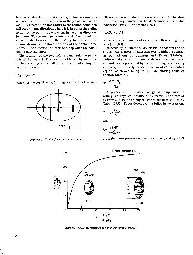
interfacial slip. In the contact area, rolling without slip will occur at a specific radius from the y axis. Where the radius is greater than this radius to the rolling point, slip will occur in one direction; where it is less than the radius to this rolling point, slip will occur in the other direction. In figure 28, the lines to points c and d represent the approximate location of the rolling bands, and the arrows shown in the three portions of the contact area represent the directions of interfacial slip when the ball is rolling into the paper.

The location of the two rolling bands relative to the axis of the contact ellipse can be obtained by summing the forces acting on the ball in the direction of rolling. In figure 29 these are

2Tb- T,=pF

where p is the coefficient_ofiolling friction. If a Hertzian

Figure 29. -Friction forces in contact ellipse.

ellipsoidal pressure distribution is assumed, the location of the rolling bands can be determined (Bisson and Anderson, 1964). For bearing steels

yo/Dy = 0.174

where D, is the diameter of the contact ellipse along they axis (eq. (40)).

In actuality, all materials are elastic so that areas of no slip as well as areas of microslip exist within the contact as pointed out by Johnson and Tabor (1967-68). Differential strains in the materials in contact will cause slip unless it is prevented by friction. In high-conformity contacts, slip is likely to occur over most of the contact region, as shown in figure 30. The limiting value of friction force T is

T- o*2r;D2$ ax

A portion of the elastic energy of compression in rolling is always lost because of hysteresis. The effect of hysteresis losses on rolling resistance has been studied by Tabor (1955). Tabor developed the following expression:

T=c4X Fz

where

x=4*

pm is the mean pressure within the contact, and c4 is l/3

Limit for comtdete slip _

r 0 20 43 60 80 100

2 I pnDyE

4Pr&Prn

Figure 30. -Frictional resistance of ball in conforming groove.

26

for rectangular contacts and 3/32 for elliptical contacts. Two hard-steel surfaces show a h of about 1 percent.

Of far greater importance in contributing to frictional losses in rolling-element bearings, especially at high speeds, is ball spinning. Spinning as well as rolling takes place in one or both of the ball-race contacts of a ball bearing. The situation is illustrated in figure 16.

High speeds cause a divergency of the contact angles pi and PO. In figure 17(b) the ball is rolling with inner-race control, so that approximately pure rolling takes place at the inner-race contact. The rolling and spinning vectors, wr and o,, at the outer-race contact are shown in figure 16. The higher the ratio us/+, the higher the friction losses.

9.2 Friction Losses in Rolling-Element Bearings

Some of the factors that affect the magnitude of friction losses in rolling bearings are

(1) Bearing size (2) Bearing type (3) Bearing design (4) Load (magnitude and type, either thrust or radial) (5) Speed (6) Oil viscosity (7) Oil flow

In a specific bearing, friction losses consist of (1) Sliding friction losses in the contacts between the

rolling elements and the races. These losses include differential slip and slip due to ball spinning. They are complicated by the presence of elastohydrodynamic lubrication films. The shearing of elastohydrodynamic lubrication films, which are extremely thin and contain oil whose viscosity is increased by orders of magnitude above its atmospheric pressure value, accounts for a significant fraction of the friction losses in rolling- element bearings.

(2) Hysteresis losses due to the damping capacity of the race and ball materials

(3) Sliding friction losses between the separator and its locating race surface and between the separator pockets and the rolling elements

(4) Shearing of oil films between the bearing parts and oil churning losses caused by excess lubricant within the bearing

(5) Flinging of oil off the rotating parts of the bearing Because of the dominant role played in bearing

frictional losses by the method of lubrication, there are no quick and easy formulas for computing rolling- element bearing power loss. Coefficients of friction for a particular bearing can vary by a factor of 5 depending on lubrication. A flood-lubricated bearing may consume five times the power of one that is merely wetted by oil- air mist lubrication.

AS a rough but useful guide, we can use the friction coefficients given by Palmgren (1959). These values were

computed at a bearing load that will give a life of 1 x 109 revolutions for the respective bearings. The friction coefficients for several different bearings are shown here:

Self-aligning ball.. ........................................ .O.OOlO Cylindrical roller, with flange-guided short

rollers ...................................................... .O.OOll Thrust ball.. ................................................ .0.0013 Single-row, deep-groove ball ........................... .O.OOlS Tapered and spherical roller, with flange-guided

rollers ...................................................... .0.0018 Needle roller ............................................... .0.0045

All of these friction coefficients are referenced to the bearing bore.

More accurate estimates of bearing power loss and temperature rise can be obtained by using one or more of the available computer codes that represent the basis for current design methodology for rolling-element bearings. These are discussed in Anderson (1979) and Pirvics (1980) and briefly reviewed later in this report.

10. Lubricants and Lubrication Systems A liquid lubricant has several functions in a rolling-

element bearing. It provides the medium for the establishment of separating films between the bearing parts (elastohydrodynamic between the races and rolling elements and hydrodynamic between the cage or separator and its locating surface). It serves as a coolant if circulated through the bearing either to an external heat exchanger or simply brought into contact with the bearing housing and machine casing. A circulating lubricant also serves to flush out wear debris and carry it to a filter where it can be removed from the system. Finally it provides corrosion protection. The different methods of providing liquid lubricant to a bearing are discussed here individually.

10.1 Solid Lubrication

An increasing number of rolling-element bearings are lubricated with solid-film lubricants, usually in applications such as extreme temperature or the vacuum of space where conventional liquid lubricants are not suitable.

Success in cryogenic applications where the bearing is cooled by the cryogenic fluid (liquid oxygen or hydrogen) has been achieved with transfer films of polytetrafluoroethylene (Scibbe, 1968). Bonded films of soft metals such as silver, gold and lead applied by ion plating as very thin films (0.2 to 0.3 pm) have also been used (Todd and Bentall, 1978). Silver, and lead in particular, have found use in bearings used to support the rotating anode in X-ray tubes. Very thin films are required in rolling-

27

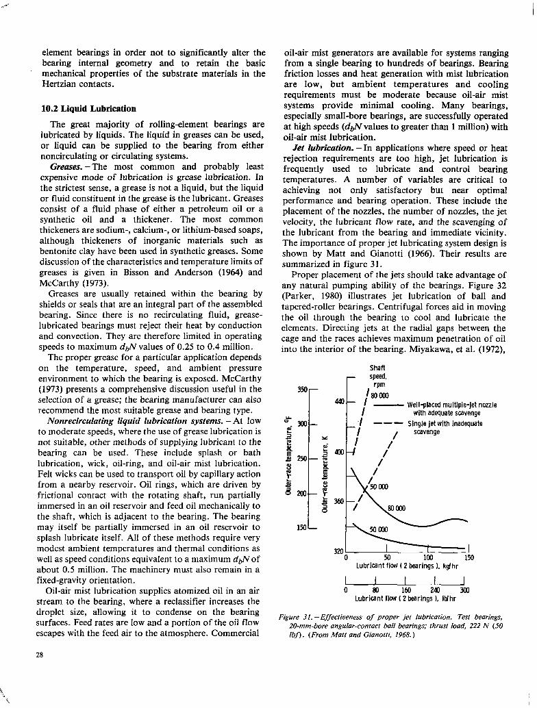
element bearings in order not to significantly alter the bearing internal geometry and to retain the basic mechanical properties of the substrate materials in the Hertzian contacts.

10.2 Liquid Lubrication

The great majority of rolling-element bearings are lubricated by liquids. The liquid in greases can be used, or liquid can be supplied to the bearing from either noncirculating or circulating systems.

Greases. -The most common and probably least expensive mode of lubrication is grease lubrication. In the strictest sense, a grease is not a liquid, but the liquid or fluid constituent in the grease is the lubricant. Greases consist of a fluid phase of either a petroleum oil or a synthetic oil and a thickener. The most common thickeners are sodium-, calcium-, or lithium-based soaps, although thickeners of inorganic materials such as bentonite clay have been used in synthetic greases. Some discussion of the characteristics and temperature limits of greases is given in Bisson and Anderson (1964) and McCarthy (1973).

Greases are usually retained within the bearing by shields or seals that are an integral part of the assembled bearing. Since there is no recirculating fluid, grease- lubricated bearings must reject their heat by conduction and convection. They are therefore limited in operating speeds to maximum d$\’ values of 0.25 to 0.4 million.

The proper grease for a particular application depends on the temperature, speed, and ambient pressure environment to which the bearing is exposed. McCarthy (1973) presents a comprehensive discussion useful in the selection of a grease; the bearing manufacturer can also recommend the most suitable grease and bearing type.

Nonrecirculating liquid lubrication systems. - At low to moderate speeds, where the use of grease lubrication is not suitable, other methods of supplying lubricant to the bearing can be used. These include splash or bath lubrication, wick, oil-ring, and oil-air mist lubrication. Felt wicks can be used to transport oil by capillary action from a nearby reservoir. Oil rings, which are driven by frictional contact with the rotating shaft, run partially immersed in an oil reservoir and feed oil mechanically to the shaft, which is adjacent to the bearing. The bearing may itself be partially immersed in an oil reservoir to splash lubricate itself. All of these methods require very modest ambient temperatures and thermal conditions as well as speed conditions equivalent to a maximum da of about 0.5 million. The machinery must also remain in a fixed-gravity orientation.

Oil-air mist lubrication supplies atomized oil in an air stream to the bearing, where a reclassifier increases the droplet size, allowing it to condense on the bearing surfaces. Feed rates are low and a portion of the oil flow escapes with the feed air to the atmosphere. Commercial

oil-air mist generators are available for systems ranging from a single bearing to hundreds of bearings. Bearing friction losses and heat generation with mist lubrication are low, but ambient temperatures and cooling requirements must be moderate because oil-air mist systems provide minimal cooling. Many bearings, especially small-bore bearings, are successfully operated at high speeds (dflvalues to greater than 1 million) with oil-air mist lubrication.

Jet lubrication. -In applications where speed or heat rejection requirements are too high, jet lubrication is frequently used to lubricate and control bearing temperatures. A number of variables are critical to achieving not only satisfactory but near optimal performance and bearing operation. These include the placement of the nozzles, the number of nozzles, the jet velocity, the lubricant flow rate, and the scavenging of the lubricant from the bearing and immediate vicinity. The importance of proper jet lubricating system design is shown by Matt and Gianotti (1966). Their results are summarized in figure 31.

Proper placement of the jets should take advantage of any natural pumping ability of the bearings. Figure 32 (Parker, 1980) illustrates jet lubrication of ball and tapered-roller bearings. Centrifugal forces aid in moving the oil through the bearing to cool and lubricate the elements. Directing jets at the radial gaps between the cage and the races achieves maximum penetration of oil into the interior of the bearing. Miyakawa, et al. (1972),

Shaft r speed, I rpm

- Well-placed multiple-jet nozzle with adequate scavenge

- - - Single jet with inadequate

/ scavenge

Lubricant flow ( 2 bearings 1, kglhr

hii+id+ 0 3al Lubricant flow (2 bearings ). Itihr

Figure 31. -Effectiveness of proper jet lubrication. Test bearings, 20-mm-bore angular-contact ball bearings; thrust load, 222 N (50 Ibf) . (From Matt and Gianotti, 1968. )

28

Anderson, et al. (1954), Zaretsky, et al. (1976), and Parker and Signer (1978) present useful data on the influence of jet placement and velocity on the lubrication of several types of bearings.

Under-race lubrication. -As bearing speeds increase, centrifugal effects become more predominant, making it increasingly difficult to effectively lubricate and cool a bearing. The jetted oil is thrown off the sides of the bearing rather than penetrating to the interior. At extremely high d@ values (2.4 million and higher), jet lubrication becomes ineffective. Increasing the flow rate only adds to heat generation through increased churning losses. Brown (1970) describes an under-race oiling system used in a turbofan engine for both ball and cylindrical roller bearings. Figure 33 illustrates the technique. The lubricant is directed radially under the bearings. Centrifugal effects assist in pumping oil out through the bearings through suitable slots and holes, which are made a part of both the shaft and mounting system and the bearings themselves. Holes and slots are provided within the bearing to feed oil directly to the ball- race and cage-race contacts.

This lubrication technique has been thoroughly tested for large-bore ball and roller bearings up to 3 million dfl. Pertinent data are reported by Signer, et al. (1974), Brown, et al. (1977), Schuller (1979), and Signer and Schuller (1982).

Inner raced’

Outer race -, =\ J-1

/’ ‘I Inner race1

ConeJ’

Figure 32. -Placement of jets for ball bearings with relieved rings and tapered-roller bearings.

11. Elastohydrodynamic Lubrication Elastohydrodynamic lubrication is a form of fluid-film

lubrication where elastic deformation of the bearing surfaces becomes significant. It is usually associated with highly stressed machine components such as rolling- element bearings. Historically, elastohydrodynamic lubrication may be viewed as one of the major developments in the field of lubrication in the twentieth century. It not only revealed the existence of a previously unsuspected regime of lubrication in highly stressed nonconforming machine elements, but it also brought order to the complete spectrum of lubrication regimes, ranging from boundary to hydrodynamic.

11.1 Relevant Equations

The relevant equations used in elastohydrodynamic lubrication are given here.

Lubrication equation (Reynolds equation )

where

u= (u,+ub)/2

Viscosity variation

\i, Under-race cooling grooves

,F- Oil discharge 7%

scoop

2e Oil jet

(b)

\ \I \ J Axial oil

cooling holes

Figure 33. -Under-race oiling system for main shaft bearings on turbofan engine. (a) Cylindrical roller bearing. (b) Ball thrust bearing. (From Brown, 1970.)

29

where ~0 is the coefficient of absolute or dynamic viscosity at atmospheric pressure and E is the pressure- viscosity coefficient of the fluid.

mean surface velocity in x direction, m/s pressure-viscosity coefficient of fluid, mz/N atmospheric viscosity, N s/m2

Density variation Cfor mineral oils) From these variables the following five dimensionless 0.6~

1+ 1.17p

where pu is the density at atmospheric conditions.

Elasticity equation

S=$ P(x,Y)~~Y A J (x-W+ 6J-YIP

where

2 E’ =

l-V;+ 1-Vg - - Ea Eb

Film thickness equation

h =ho +x2/2R,+y2/2Ry+6 (x,y)

where

1/R,= l/rau+ l/rb,

1 /R, = 1 /ray + 1 /‘by

(69)

(70)

The different radii expressed in equations (69) and (70) are depicted in figure 10.

The elastohydrodynamic lubrication solution therefore requires the calculation of the pressure distribution within the conjunction, at the same time allowing for the effects that this pressure will have on the properties of the fluid and on the geometry of the elastic solids. The solution will also provide the shape of the lubricant film, particularly the minimum clearance between the solids. A detailed description of the elasticity model one could use is given by Dowson and Hamrock (1976), and the complete elastohydrodynamic lubrication theory is given by Hamrock and Dowson (1976).

11.2 Dimensionless Grouping

The variables resulting from the elastohydrodynamic lubrication theory are

E’ effective elastic modulus, N/m2 F normal applied load, N h film thickness, m

RX effective radius in x (motion) direction, m

RY effective radius in y (transverse) direction, m

groupings can be established:

Dimensionless film thickness

H= h/R,

Ellipticity parameter

k = D,/D, = ( Ry/Rx) 2/~

Dimensionless load parameter

W= F/E’R;

Dimensionless speed parameter

(71)

U= qou/E’R,

Dimensionless materials parameter

(72)

G=EE’

The dimensionless minimum film thickness can thus be written as a function of the other four parameters

H=f(k, U, W, G)

The most important practical aspect of elastohydrodynamic lubrication theory is the determination of the minimum film thickness within a conjunction. That is, maintaining a fluid-film thickness of adequate magnitude is extremely important to the operation of machine elements like rolling-element bearings. Specifically, elastohydrodynamic film thickness influences fatigue life, as discussed in section 12.

11.3 Minimum-Film-Thickness Formula

By using the numerical procedures outlined in Hamrock and Dowson (19763, tha influence of the ellipticity parameter and the dimensionless speed, load, and materials parameters on minimum film thickness has been investigated by Hamrock and Dowson (1977). The ellipticity parameter k was varied from 1 (a ball-on-plate configuration) to 8 (a configuration approaching a rectangular contact). The dimensionless speed parameter U was varied over a range of nearly two orders of magnitude, and the dimensionless load parameter W over a range of one order of magnitude. Situations equivalent to using solid materials of bronze, steel, and silicon nitride and lubricants of paraffinic and naphthenic oils

30

were considered in the investigation of the role of the dimensionless materials parameter G. Thirty-four cases were used in generating the minimum-film-thickness formula given here.

I H min = 3.63 ,!JO.68G0.49W-0.073(1 - e-0.68k) (74)

In this equation the most dominant exponent occurs on the speed parameter, and the exponent on the load parameter is very small and negative. The materials parameter also carries a significant exponent, although the range of this variable in engineering situations is limited.

11.4 Pressure and Film Thickness Plots

A representative contour plot of dimensionless pressure is shown in figure 34 for k= 1.25, U=O.l68xlO-11, and G=4522. In this figure and in figure 35, the + symbol indicates the center of the Hertzian contact zone. The dimensionless representation of the X and Y coordinates causes the actual Hertzian contact ellipse to be a circle regardless of the value of the ellipticity parameter. The Hertzian contact circle is shown by asterisks. On this figure is a key showing the contour labels and each corresponding value of dimensionless pressure. The inlet region is to the left and

Figure 34. - Contour plot of dimensionless pressure. k= 1.25; U=O.l68x 10-11; W=O.llI x IO-% G = 4522.

D 1.4

Dimensiontess pressure, P - p/E’

1.7~10-~ 1.6 1.5

1.2 F 1.0

.7

.3

Dimensionless film thickness,

H = h/R,

A B

a FlD-6

C D 2: E a:o F 6.b G 7.4 H 8.2

Figure 35. -Contour plot of dimensionless film thickness. k=1.25; U=O.l68x 10-11; W=O.Ill x 10-6; G=4522.

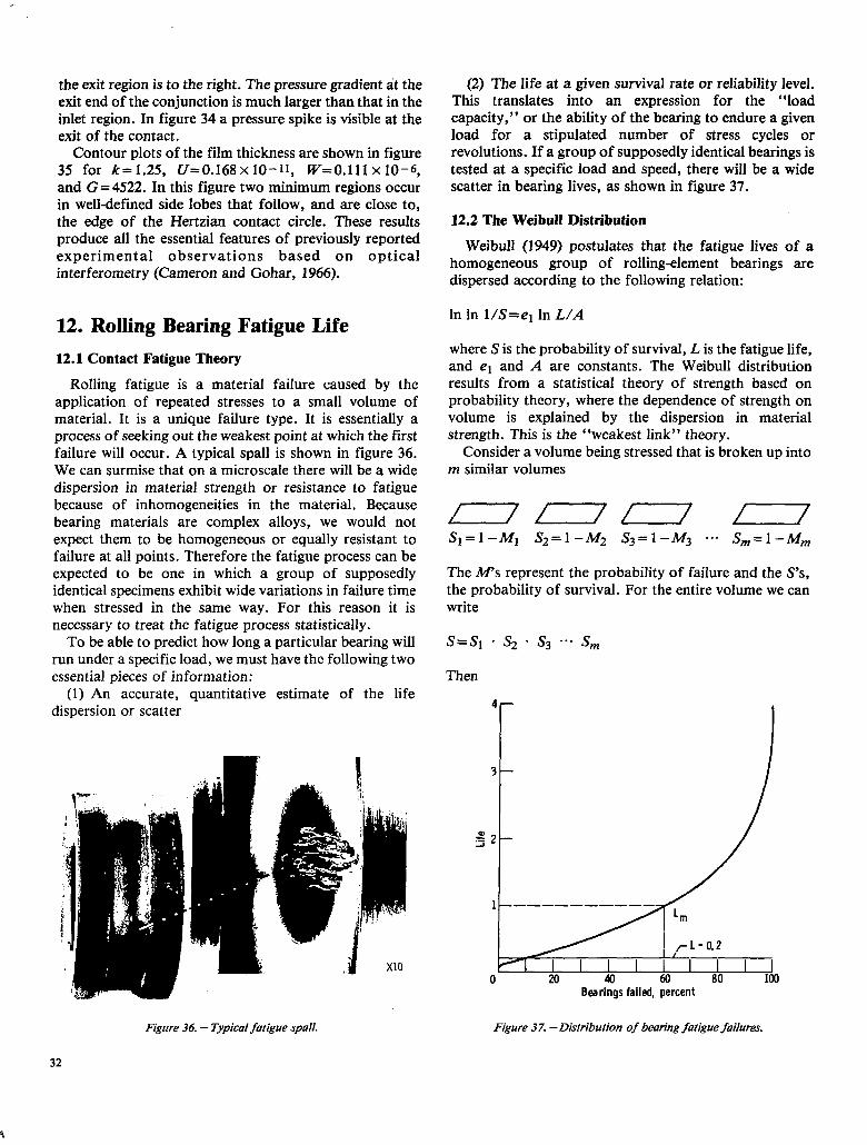
the exit region is to the right. The pressure gradient zit the exit end of the conjunction is much larger than that in the inlet region. In figure 34 a pressure spike is visible at the exit of the contact.

Contour plots of the film thickness are shown in figure 35 for k= 1.25, (/=0.168x 10-11, W=O.lll x 10-6, and G = 4522. In this figure two minimum regions occur in well-defined side lobes that follow, and are close to, the edge of the Hertzian contact circle. These results produce all the essential features of previously reported experimental observations based on optical interferometry (Cameron and Gohar, 1966).

12. Rolling Bearing Fatigue Life

12.1 Contact Fatigue Theory

Rolling fatigue is a material failure caused by the application of repeated stresses to a small volume of material. It is a unique failure type. It is essentially a process of seeking out the weakest point at which the first failure will occur. A typical spa11 is shown in figure 36. We can surmise that on a microscale there will be a wide dispersion in material strength or resistance to fatigue because of inhomogeneities in the material. Because bearing materials are complex alloys, we would not expect them to be homogeneous or equally resistant to failure at all points. Therefore the fatigue process can be expected to be one in which a group of supposedly identical specimens exhibit wide variations in failure time when stressed in the same way. For this reason it is necessary to treat the fatigue process statistically.

To be able to predict how long a particular bearing will run under a specific load, we must have the following two essential pieces of information:

(1) An accurate, quantitative estimate of the life dispersion or scatter

Figure 36. - Typical faiigue spa/l.

(2) The life at a given survival rate or reliability level. This translates into an expression for the “load capacity,” or the ability of the bearing to endure a given load for a stipulated number of stress cycles or revolutions. If a group of supposedly identical bearings is tested at a specific load and speed, there will be a wide scatter in bearing lives, as shown in figure 37.

12.2 The Weibull Distribution

Weibull (1949) postulates that the fatigue lives of a homogeneous group of rolling-element bearings are dispersed according to the following relation:

In In l/S=er In L/A

where S is the probability of survival, L is the fatigue life, and el and A are constants. The Weibull distribution results from a statistical theory of strength based on probability theory, where the dependence of strength on volume is explained by the dispersion in material strength. This is the “weakest link” theory.

Consider a volume being stressed that is broken up into m similar volumes

$=1--M, &=l-M2 S3=1-M3 ..* /3,=1-M,

The M’s represent the probability of failure and the S’s, the probability of survival. For the entire volume we can write

Then

4-

3-

Lz 22-

l-----------

I I I I I I I 0 20 40 60 80 100

Bearings failed, percent

Figure 37. - Dktribution of bearing fatigue failures.

32

1-M=(l-Md(l-M2)(1-M3) ase (l-M,,,)

1 -M=

s=

The probability of a crack starting in the ith volume is

Mi=f (X) Vi

where f (x) is a function of the stress level, the number of stress cycles, and the depth into the material where the maximum stress occurs and Vi is the elementary volume. Therefore

m s=

rT 11 -f (X)Vil

I=

In S= E In [l -f(X)Vi] i=l

N~wiff(x)Vi<<l, thenln [l-f(x)Vi]=-f(x)Viand

Ins=- Ef(X)Vi i=l

Let Vi-O; then

E f(X)Vi=f(X) dV=f(X) V i=l

Lundberg and Palmgren (1947) assume that f (x) could be expressed as a power function of shear stress 70, number of stress cycles J, and depth to the maximum shear stress ZO.

f(x) = 7c1J’*/z’ 0 O3

They also choose as the stressed volume

V= DyZ&

Then

(75)

For a specific bearing and load (e.g., stress) 70, Dp I,, and Z,J are all constant so that

In l/S=Jc2

Designating J as life L in stress cycles gives

In l/S= (L/A)‘2

or

lnln l/S=c2ln(L/A) (76)

This is the Weibull distribution, which relates probability of survival and life. it has two principal functions. First, bearing fatigue lives plot as a straight line on Weibull coordinates (log log vs. log), so that the life at any reliability level can be determined. Of most interest are the Llo life (S=O.9) and the LSO life (S=O.5). Bearing load ratings are based on the L,o life. Second, equation (76) can be used to determine what the Llo life must be to obtain a required life at any reliability level. The Llo life is calculated, from the load on the bearing and the bearing dynamic capacity or load rating given in manufacturers’ catalogs and engineering journals, by using the equation

L= (C/F,)rn

where

C basic dynamic capacity or load rating

Fe equivalent bearing load m 3 for elliptical contacts and 10/3 for rectangular

contacts

A typical Weibull plot is shown in figure 38.

12.3 Lundberg-Palmgren Theory

The Lundberg-Palmgren theory, on which bearing ratings are based, is expressed by equation (75). The exponents in this equation are determined experimentally from the dispersion of bearing lives and the dependence of life on load, geometry, and bearing size. As a standard of reference, all bearing load ratings are expressed in terms of the specific dynamic capacity C, which, by definition, is the load that a bearing can carry for 1 million inner-race revolutions with a 90 percent chance of survival.

Factors on which specific dynamic capacity and bearing life depend are

(1) Size of rolling element (2) Number of rolling elements per row (3) Number of rows of rolling elements (4) Conformity between rolling elements and races (5) Contact angle under load (6) Material properties (7) Lubricant properties

33

2 j ( I(

I 1 2 4 6 10

Specimen life, millions of stress cycles

Figure 38. - npical Weibull plot of bearing fatigue failures.

(8) Operating temperature (9) Operating speed

Only factors (1) to (5) are incorporated in bearing dynamic capacities developed from the Lundberg- Palmgren theory. The remaining factors must be taken into account in the life adjustment factors discussed in section 12.5.

The formulas for specific dynamic capacity as developed by Lundberg-Palmgren (1947, 1952) are as follows:

For radial ball bearings with ds25 mm,

C=f,(icos /3)0.%2/3 & “’ c >

where

d diameter of rolling element, m i number of rows of rolling elements

;f

number of rolling elements per row contact angle

fc coefficient dependent on material and bearing type

For radial ball bearings with dz2.5 mm,

C=f,(icos 8)0.7tW 1.4

For radial roller bearings,

where 1, is roller length in meters.

For thrust ball bearings with /I # 90”,

C=f,(icos @)u.T(tan P)n2/3 & “’ (. >

For thrust roller bearings,

C=f,( ices /3)0.7s(tan P)n3/4 & o’78 (. >

For thrust ball bearings with fl= 90”)

For thrust roller bearings with /3 = 90”,

For ordinary bearing steels such as SAE 52100 with mineral oil lubrication, f, can be evaluated by using tables 14 and 15, but a more convenient method is to use tabulated values from the most recent Antifriction Bearing Manufacturers Association (AFBMA) documents on dynamic load ratings and life (ISO, 1976). The value of C is calculated or determined from bearing manufacturers’ catalogs. The equivalent load Fe can be calculated from the equation

F,=XF,+ YFt

Factors X and Y are given in bearing manufacturers’ catalogs for specific bearings.

34

In addition to specific dynamic capacity C, every bearing has a specific static capacity, usually designated as Co. Specific static capacity is defined as the load that, under static conditions, will result in a permanent deformation of 0.0001 times the rolling-element diameter. For some bearings CO is less than C, so it is important to avoid exposing a bearing to a static load that exceeds CO. Values of CO are given in bearing manufacturers’ catalogs.

12.4 The AFBMA Method

Shortly after publication of the Lundberg-Palmgren theory, the AFBMA began efforts to standardize methods for establishing bearing load ratings and making life predictions. Standardized methods of establishing load ratings for ball bearings (AFBMA, 1960a) and roller bearings (AFBMA, 1960b) were devised, based essentially on the Lundberg-Palmgren theory. These early standards are published in their entirety in Jones (1964). In recent years, significant advances have been made in rolling-element bearing material quality and in our understanding of the role of lubrication in bearing life through the development of elastohydrodynamic theory. Therefore the original AFBMA standards in AFBMA (1960a and b) have been updated with life adjustment factors. These factors have been incorporated into IS0 (1976), which is discussed in the following section.

12.5 Life Adjustment Factors

A comprehensive study of the factors affecting the fatigue life of bearings, which were not taken account of in the Lundberg-Palmgren theory, is reported in Bamberger (1971). In that reference it was assumed that the various environmental or bearing design factors are multiplicative in their effect on bearing life. The following equation results:

- - - ^ - LA=(D) (E) (F) (G) (ff)Llo

or

LA=(b) (8) (P) (e) (k) (c/F,)m

where

B materials factor B metallurgical processing factor P lubrication factor 5; speed effect factor A misalignment factor FC? bearing equivalent load m load-life exponent; either 3 for ball bearings or

1013 for roller bearings

Factors B, ,!?, and P are briefly reviewed here. The reader is referred to Bamberger (1971) for a complete discussion of all five life adjustment factors.

Materials factors D and E. -For over a century, AISI 52100 steel has been the predominant material for rolling- element bearings. In fact, the basic dynamic capacity as defined by AFMBA in 1949 is based on an air-melted 52100 steel, hardened to at least Rockwell C 58. Since that time, as discussed in section 5.1, better control of air-melting processes and the introduction of vacuum remelting processes have resulted in more homogeneous steels with fewer impurities. Such steels have extended rolling-element bearing fatigue lives to several times the AFBMA or catalog life. Life improvements of 3 to 8 times are not uncommon. Other steel compositions, such as AISI M-I and AISI M-50, chosen for their higher temperature capabilities and resistance to corrosion, also have shown greater resistance to fatigue pitting when vacuum melting techniques are employed. Case-hardened materials, such as AISI 4620, AISI 4118, and AISI 8620, used primarily for roller bearings, have the advantage of a tough, ductile steel core with a hard, fatigue-resistant surface.

The recommended b factors for various alloys processed by air melting are shown in table 16. Insufficient definitive life data with case-hardened materials were found to recommend b factors for them. It is recommended that the user refer to the bearing manufacturer for the choice of a specific case-hardened material.

The metallurgical processing variables considered in the development of the ,? factor included melting practice (air and vacuum melting) and metal working (thermomechanical working). Thermomechanical working of M-50 has also been shown to result in improved life, but in a practical sense it is costly and still not fully developed as a processing technique. Bamberger (1971) recommend an ,!? factor of 3 for consumable-electrode-vacuum- melted materials.

The translation of these factors into a standard (ISO, 1976) is discussed later.

Lubrication factor i? -Until approximately 1960, the role of the lubricant between surfaces in rolling contact was not fully appreciated. Metal-to-metal contact was presumed to occur in all applications with attendant required boundary lubrication. The development of elastohydrodynamic lubrication theory showed that lubricant films of thicknesses of the order of microinches and tens of microinches occur in rolling contact. Since surface finishes are of the same order of magnitude as the lubricant film thicknesses, the significance of rolling- element bearing surface roughnesses to bearing performance became apparent. Tallian (1967) first reported on the importance to bearing life of the ratio of elastohydrodynamic lubrication film thickness to surface roughness. Figure 39 shows life as a percentage of

35

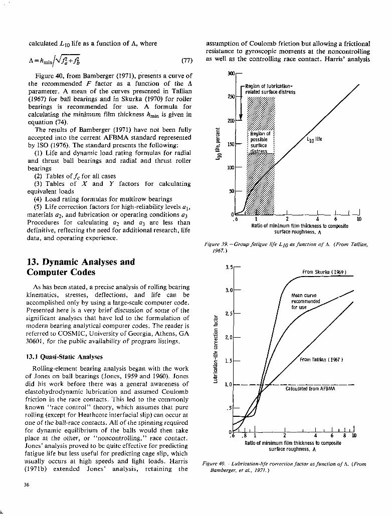
calculated Lto life as a function of A, where

^=hmin/a (77)

Figure 40, from Bamberger (1971), presents a curve of the recommended F factor as a function of the A parameter. A mean of the curves presented in Tallian (1967) for ball bearings and in Skurka (1970) for roller bearings is recommended for use. A formula for calculating the minimum film thickness hmin is given in equation (74).

The results of Bamberger (1971) have not been fully accepted into the current AFBMA standard represented by IS0 (1976). The standard presents the following:

(1) Life and dynamic load rating formulas for radial and thrust ball bearings and radial and thrust roller bearings

(2) Tables off, for all cases (3) Tables of X and Y factors for calculating

equivalent loads (4) Load rating formulas for multirow bearings (5) Life correction factors for high-reliability levels at,

materials ~2, and lubrication or operating conditions a3 Procedures for calculating a2 and a3 are less than definitive, reflecting the need for additional research, life data, and operating experience.

13. Dynamic Analyses and Computer Codes

As has been stated, a precise analysis of rolling bearing kinematics, stresses, deflections, and life can be accomplished only by using a large-scale computer code. Presented here is a very brief discussion of some of the significant analyses that have led to the formulation of modern bearing analytical computer codes. The reader is referred to COSMIC, University of Georgia, Athens, GA 30601, for the public availability of program listings.

13.1 Quasi-Static Analyses

Rolling-element bearing analysis began with the work of Jones on ball bearings (Jones, 1959 and 1960). Jones did his work before there was a general awareness of elastohydrodynamic lubrication and assumed Coulomb friction in the race contacts. This led to the commonly known “race control” theory, which assumes that pure rolling (except for Heathcote interfacial slip) can occur at one of the ball-race contacts. All of the spinning required for dynamic equilibrium of the balls would then take place at the other, or “noncontrolling,” race contact. Jones’ analysis proved to be quite effective for predicting fatigue life but less useful for predicting cage slip, which usually occurs at high speeds and light loads. Harris (1971b) extended Jones’ analysis, retaining the

36

assumption of Coulomb friction but allowing a frictional resistance to gyroscopic moments at the noncontrolling as well as the controlling race contact. Harris’ analysis

T r Resion of lubrication-

related surface distress

.6 1 2 4 6 10 Ratio of minimum film thickness to composite

surface roughness, A

Figure 39. - Group fatigue life LIO as function of A. (From Tdian. 1967. )

3.5 r from Skurka ( I%9 1

3.0 -

Calculated from AFBMA

Ratio of minimum film thickness to composite surface roughness, A

Figure 40. -Lubrication-Ii/e correciion facror as function of A. (From Bamberger, et al., 1971. )

-

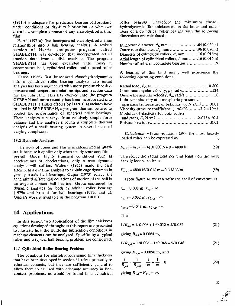
(1971 b) is adequate for predicting bearing under conditions of dry-film lubrication

performance or whenever

there is a complete absence of any elastohydrodynamic film.

Harris (197la) first incorporated elastohydrodynamic relationships into a ball bearing analysis. A revised version of Harris’ computer program, called SHABERTH, was developed that incorporated actual traction data from a disk machine. The program SHABERTH has been expanded until today it encompasses ball, cylindrical roller, and tapered-roller bearings.

Harris (1966) first introduced elastohydrodynamics into a cylindrical roller bearing analysis. His initial analysis has been augmented with more precise viscosity- pressure and temperature relationships and traction data for the lubricant. This has evolved into the program CYBEAN and more recently has been incorporated into SHABERTH. Parallel efforts by Harris’ associates have resulted in SPHERBEAN, a program that can be used to predict the performance of spherical roller bearings. These analyses can range from relatively simple force balance and life analyses through a complete thermal analysis of a shaft bearing system in several steps of varying complexity.

13.2 Dynamic Analyses

The work of Jones and Harris is categorized as quasi- static because it applies only when steady-state conditions prevail. Under highly transient conditions such as accelerations or decelerations, only a true dynamic analysis will suffice. Walters (1975) made the first attempt at a dynamic analysis to explain cage dynamics in gyro-spin-axis ball bearings. Gupta (1975) solved the generalized differential equations of motion of the ball in an angular-contact ball bearing. Gupta continued his dynamic analyses for both cylindrical roller bearings (1979a and b) and for ball bearings (1979c and d). Gupta’s work is available in the program DREB.

14. Applications In this section two applications of the film thickness

equations developed throughout this report are presented to illustrate how the fluid-film lubrication conditions in machine elements can be analyzed. Specifically a typical roller and a typical ball bearing problem are considered.

14.1 Cylindrical Roller Rearing Problem

The equations for elastohydrodynamic film thickness that have been developed in section 11 relate primarily to elliptical contacts, but they are sufficiently general to allow them to te used with adequate accuracy in line- contact problems, as would be found in a cylindrical

roller bearing. Therefore the minimum elastohydrodynamic film thicknesses on the inner and outer races of a cylindrical roller bearing with the following dimensions are calculated:

Inner-race diameter, di, mm . . . . . . . . . . . . . . . . . . . . . . 64 (0.064m) Outer-race diameter, do, mm . . . . . . . . . . . . . . . . . . . . .96 (0.096m) Diameter of cylindrical rollers, d, mm . . . . . . . . . . 16 (0.016m) Axial length of cylindrical rollers, I, mm . . . . . . . 16 (0.016m) Number of rollers in complete bearing, n . . . . . . . . . . . . . . . . . . ..9

A bearing of this kind might well experience the following operating conditions:

Radial load, F,, N . . . . . . . . . . . . . . . . . . . . . . . . . . . . . . . . . . . . . . . . . . 10 800 Inner-race angular velocity, pi, rad/s. . . . . . . . . . . . . . . . . . . . . .524 Outer-race angular velocity, PO, rad/s . . . . . . . . . . . . . . . . . . . . . . . 0 Lubricant viscosity at atmospheric pressure at

operating temperature of bearings, 70, N s/m2.. . . . . .O.Ol Viscosity-pressure coefficient, E, mz/N . . . . . . . . . . 2.2 x 10-s Modulus of elasticity for both rollers

and races, E, N/m2 . . . . . . . . . . . . . . . . . . . . . . . . . . . . . . . . 2.075 x 1011 Poisson’s ratio, v.. . . . . . . . . . . . . . . . . . . . . . . . . . . . . . . . . . . . . . . . . . . . .0.03

Culculufion. -From equation (59), the most heavi!y loaded roller can be expressed as ~\

F max = 4F,/n = 4( 10 800 N)/9 = 4800 N (59

Therefore, the radial load per unit length on the most heavily loaded roller is

F,!,,, = 4800 N/0.016 m = 0.3 MN/m (5%

From figure 41 we can write the radii of curvature as

r ,=0.008 m, I-,,,=m

~~,~=0.032 m, rby,i= 03

Q,~,~ = 0.048 m, Q,~,~= 03

Then

l/R,i= l/O.008 + l/0.032=5/0.032

giving R,i = 0.0064 m,

1 /Rx,, = l/O.008 - l/O.048 = 5/0.048

giving Rx,* = 0.0096 m, and

1 1 -= -2&+&o R,i Ry.*

giving Ry,i=Ry,o=m.

(21)

(21)

(22)

3-l

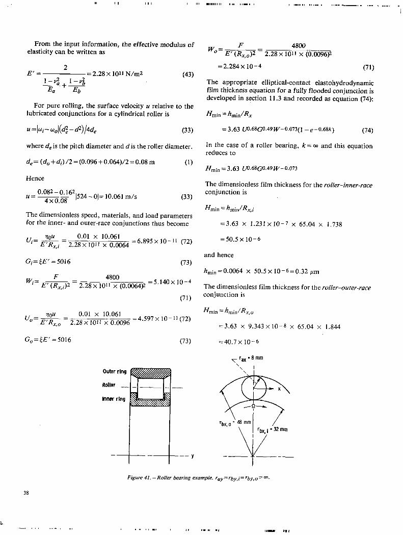
From the input information, the effective modulus of elasticity can be written as

2 E’ = = 2.28 x 1011 N/m2

1-v;+ I-V$ (43)

- - Ea Eb

For pure rolling, the surface velocity u relative to the lubricated conjunctions for a cylindrical roller is

u=Iwi-wol(d$-d2)/4de (33)

where de is the pitch diameter and d is the roller diameter.

de= (do + di) /2 = (0.096 + 0.064)/2 = 0.08 m (1)

Hence

u= 0.082-0.162 4x0.08

J524 -OJ= 10.061 m/s (33)

The dimensionless speed, materials, and load parameters for the inner- and outer-race conjunctions thus become

ui= E*, = 2 2~~:o~1 f*r$,64 z6.895 X lo-11 (72) x,, *

Gi=c$E’ ~5016 (73)

F 4800 Wi=E, (RSi)2 = 2j8Xf~~((o~jj =5.140x IO-4

(71)

77OU U”=-=

0.01 x 10.061 2.28 x 1011 x 0.0096

=4.597x lo-11 (72)

G,=.$E’ =5016 (73)

w,= F 4800 E’ (Rx,,)2 = 2.28 x 1011 x (0.0096)2

=2.284x IO-4 (71)

The appropriate elliptical-contact elastohydrodynamic film thickness equation for a fully flooded conjunction is developed in section 11.3 and recorded as equation (74):

N min =hrndRx

~3.63 U0.68G0.49W-0.073(1 -e-0.68k) (74)

In the case of a roller bearing, k= 00 and this equation reduces to

ffmin = 3.63 m.68G0.49W-0.073

The dimensionless film thickness for the roller-inner-race conjunction is

Hmin = hmin/Rx,i

=3.63 x 1.231 x10-7 x 65.04 x 1.738

=50.5x 10-b

and hence

hmin=0.0064 X 50.5 X 10~6~0.32 pm

The dimensionless film thickness for the roller-outer-race conjunction is

=3.63 x 9.343 x 10-s x 65.04 x 1.844

=40.7x 10-s

T ‘ax =8mm \

\ I \ I

\ rbx i = 32 mm

i

Figure 41. -Roller bearing example. ra,, = r&,i = ‘by.0 = 05.

38

and hence

hmin =0.0096 X 40.7 x IO-6cO.39 pm

It is clear from these calculations that the smaller minimum film thickness in the bearing occurs at the roller-inner-race conjunction, where the geometrical conformity is less favorable. It was found that, if the ratio of minimum film thickness to composite surface roughness is greater than 3, an adequate elastohydrodynamic film is maintained. This implies that a composite surface roughness of less than 0.1 pm is needed to assure that an elastohydrodynamic film is maintained.

14.2 Radial Ball Bearing Problem

Consider a single-row, radial, deep-groove ball bearing with the following dimensions:

Inner-race diameter, di, m ........................... .0.052291 Outer-race diameter, d,, m .......................... .0.077706 Ball diameter, d, m .................................... .0.012700 Number of balls in complete bearing, n.. ................... .9 Inner-groove radius, ri, m.. .......................... .0.006604 Outer-groove radius, ro, m .......................... .0.006604 Contact angle, P, deg ........................................... .O rms surface finish of balls,& pm ..................... .0.0625 rms surface finish of races,f,, pm .................... .0.0175

A bearing of this kind might well experience the following operating conditions:

Radial load, Fr, N ........................................... .8900 Inner-race angular velocity, pi, rad/s .................... ..4 00 Outer-race angular velocity, PO, rad/s ....................... . Lubricant viscosity at atmospheric pressure and effective operating temperature of bearing, 70, N s/m2 ....... .0.04

Viscosity-pressure coefficient, 5, mWN.. ....... .2.3 x 10-8 Modulus of elasticity for both balls

and races, E, N/ml.. .................................. .2x 1011 Poisson’s ratio for both balls and races, Y ............... .0.3

The essential features of the geometry of the inner and outer conjunctions (figs. 5 and 11) can be ascertained as follows:

Pitch diameter (eq. (1))

de=Om5(do+di) co.065 m

Diametral clearance (eq. (2))

Pd=do-di-2d=l.SX 10-s m

Race conformity (eq. (3))

fi=f,=r/d=0.52

Equivalent radius (eq. (23))

R,i=d(de-d)/2de=0.00511 m


R,,=d(de+d)/2de=0.00759 m


Ry,i=frd/(2fi- 1)=0.165 m


Ry,,=fod/(2fo- 1)=0.165 m

The curvature sum

l/Ri=l/R,i+ l/R,i=201.76 (1%

gives Ric4.956 x IO-3 m, and the curvature sum

l/R,= l/R,,+ l/R,,,= 137.81 (19)

gives R,=7.256X 10-J m. Also, ai=Ry,i/Rx,i=32.35 and c~,=R~,~/R,~=21.74.

The nature of the Hertzian contact conditions can now be assessed.

Ellipticity parameters

Ei=Cif’T=9.42 1

k,=ap=7.09 1

Elliptic integrals

q=?r/2- 1

Ei=l +q/Cri=l.O188 I

E, = 1 + q/a, = 1.0278 I’

(37)

(38)

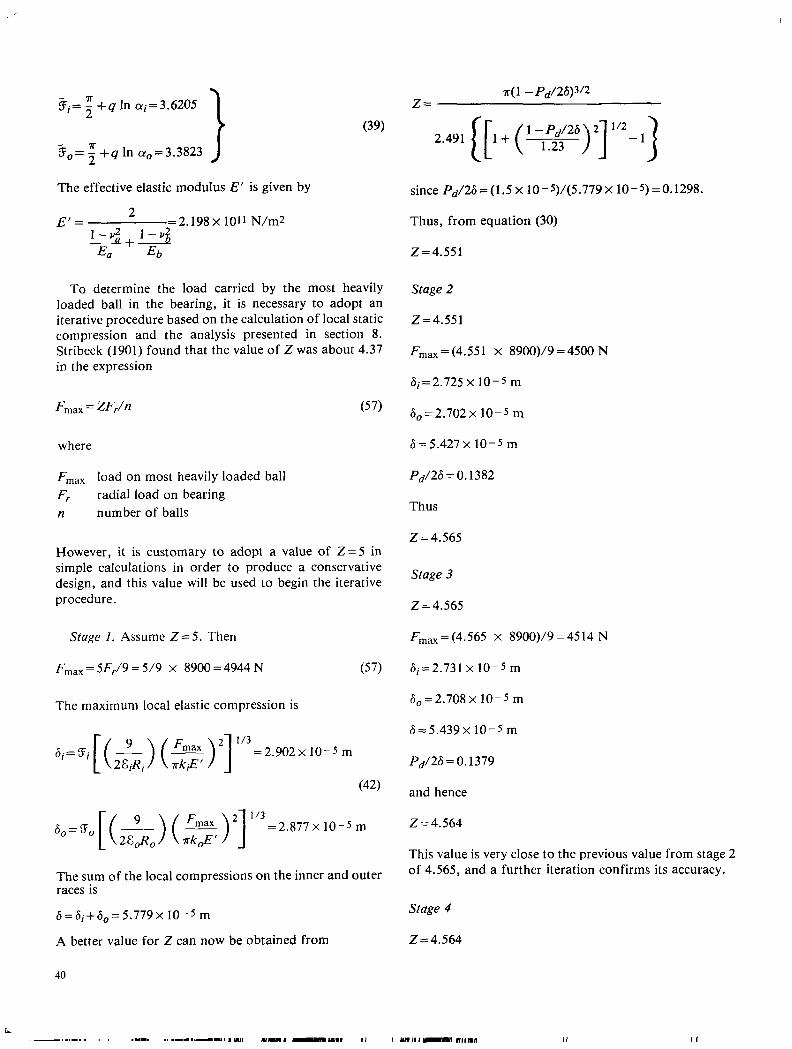
Si= 5 +q In oic3.6205

(39)

fk,,= z” +q In cr,=3.3823

The effective elastic modulus E’ is given by

2 E’ = =2.198x 1011 N/m2 1-v;+ I-Y2 - -

4, Eb

To determine the load carried by the most heavily loaded ball in the bearing, it is necessary to adopt an iterative procedure based on the calculation of local static compression and the analysis presented in section 8. Stribeck (1901) found that the value of Z was about 4.37 in the expression

F max = ZF,/n (57)

where

F max load on most heavily loaded ball

F, radial load on bearing n number of balls

However, it is customary to adopt a value of Z= 5 in simple calculations in order to produce a conservative design, and this value will be used to begin the iterative procedure.

Stage 1. Assume Z = 5. Then

F max = 5F,/9 = 519 x 8900 = 4944 N (57)

The maximum local elastic compression is

(42)

6,=5,[(&) (~)2]1’3=2.877x10-5m

The sum of the local compressions on the inner and outer races is

6=6j+6,=5.779x 10-5 m

A better value for Z can now be obtained from

40

z= ?r(i - pd/26)3/2

2.491 &+ (‘-lp$‘)2]1’2-lj

since PJ26=(1.5~ 10-5)/(5.779x lo-5)=0.1298.

Thus, from equation (30)

z=4.551

Stage 2

z=4.551

F ,,=(4.551 x 8900)/9=4500 N

6i=2.725 X 10m5 m

6,=2.702x 10-5 m

6=5.427x 10-5 m

P&i = 0.1382

Thus

Z=4.565

Stage 3

Z=4.565

F ,,=(4.565 x 8900)/9=4514 N

6i=2.731 X lop5 m

6,=2.708x IO-5 m

6=5.439x 10-5 m

P&6 = 0.1379

and hence

Z=4.564

This value is very close to the previous value from stage 2 of 4.565, and a further iteration confirms its accuracy.

Stage 4

Z=4.564

II , I

F max=(4.564 x 8900)/9=4513 N

6i=2.731 X lo-5 m

6,=2.707x 10-5 m

6=5.438x IO-5 m

P&6 = 0.1379

and hence

z=4.564

The load on the most heavily loaded ball is thus 4513 N. Elastohydrodynamic minimum film thickness. - For

pure rolling

u=Iwo-wil(~-d2)/4d,=6.252 m/s (33)

The dimensionless speed, materials, and load parameters for the inner- and outer-race conjunctions thus become

r]OU ui= E'R,~

0.04 x 6.252 = 2.198x 1011 x 5.11 x 10-3

=2.227x lo-to (72)

Gi=EE’ ~2.3 X 10-s X 2.198x1011 ~5055 (73)

F wi= E’ (Rx.i)’

4513 = 2.198x 1011 x (5.11)2x 10-h

= 7.863 x 10-4 (71)

7lou uo= E’R,,,

0.04 x 6.252 = 2.198x 1011 x 7.59x lo-3 =1.499x IO-10

Go=EE’=2.3x 10-s x 2.198xlOlt=5055

(72)

(73)

w,= F E’ (Rx,,)2

4513 = 2.198x 1011 x (7.59)2x IO-6

=3.564x IO-4 (71)

The dimensionless minimum elastohydrodynamic film thickness in a fully flooded elliptical contact is given by equation (74).

Hmin = hmin/Rx

~3.63 m.68G0.49W-0.073(] -e-0.68k) (74)

Ball-inner-race conjunction

(Hmi”)i=3.63 X 2.732~ 10-7 X 65.29

x 1.685 x 0.9983 (74)

=1.09x10-4

Thus

(h&i= 1.09X 10-4 R,i=0.557 pm

The lubrication factor A discussed in section 12.5 was found to play a significant role in determining the fatigue life of rolling-element bearings. In this case

*,= (h&i ’ *fi

0.557 x 10-b = [(O. 175)2 + (0.06225)2]1’2 x 10 - 6

= 3.00

Ball-outer-race conjunction

Thus

= 3.63 Go.68G0.49W-0.073(] -e-O.@ko)

=3.63 x 2.087x10-7 x 65.29

x 1.785 x 0.9919

=0.876x IO-4

(hmi,)o=0.876X 10-4 R5,=0.665 pm

In this case, the lubrication factor A is given by

A= 0.665 x IO-6 [(O. 175)2+ (0.0625)2]1’2 x 10-h

=3.58

(77)

(74)

(77)

Once again, it is evident that the smaller minimum film thickness occurs between the most heavily loaded ball and the inner race. However, in this case the minimum elastohydrodynamic film thickness is about three times the composite surface roughness, and the bearing lubrication can be deemed to be entirely satisfactory. Indeed it is clear from figure 40 that very little

41

improvement in the lubrication factor F and thus in the fatigue life of the bearing could be achieved by further improving the minimum film thickness and hence A.

References AFBMA (l%oa) “Method of Evaluating Load Ratings for Roller

Bearings,” AFBMA Standard System No. 11 (Anti-Friction Bearings Manufacturers Association, Inc., New York. N.Y.).

AFBMA (196Ob) “Method of Evaluating Load Ratings for Ball Bearings,” AFBMA Standard System No. 9, Revision No. 4 (Anti- Friction Bearing Manufacturers Association, Inc., New York, N.Y.).

Anderson, N. E. and Zaretsky, E. V. (1975) “Short-Term Hot Hardness Characteristics of Five Case-Hardened Steels,” NASA TN D-8031.

Anderson, W. J. (1970) “Elastohydrodynamic Lubrication Theory as a Design Parameter for Rolling Element Bearings,” ASME Paper 70-DE-19.

Anderson, W. J. (1979) “Practical Impact of Elastohydrodynamic Lubrication,” in Proceedings of Fyth Leeds-Lyon Symposium in Tribology on ‘EIPsrohydrodynamics and Related Topics, ” D. Dowson, C. M. Taylor, M. Godet, and D. Berthe, eds., Mechanical Engineering Publication, Bury St. Edmunds, Suffolk, England, pp. 217-226.

Anderson, W. J., Macks, E. J., and Nemeth, Z. N. (1954) “Comparison of Performance of Experimental and Conventional Cage Designs and Materials for 75-Millimeter-Bore Cylindrical Roller Bearings at High Speeds,” NACA TR-1177.

Bamberger, E. N. (1970) “Effect of Materials-Metallurgy Viewpoint,” in Interdisciplinary Approach to the Lubrication of Concentrated Contacts, P. M. Ku, ed., NASA SP-237, 1970.

Bamberger, E. N. (1971) Life Adjustment Factors for Bali and Roller Bearings -An Engineering Design Guide, American Society for Mechanical Engineers, New York, N.Y.

Bamberger, E. N., Zaretsky, E. V., and Signer, H. (1976) “Endurance and Failure Characteristics of Main-Shaft Jet Engine Bearings at 3 x 106 DN,” ASME Trans., Journal of Lubrication Technology, vol. 98, series F, no. 4, pp. 580-585.

Bamberger, E. N., et al. (1980) “Materials for Rolling Element Bearings,” in Bearing Design -Historical Aspects, Present Technology and Future Problems, W. J. Anderson, ed., American Society of Mechanical Engineers, New York, N.Y. pp. l-46.

Bisson, E. E. and Anderson, W. J. ‘(1964) Advanced Bearing Technology, NASA SP-38.

Brown, P. F. (1970) “Bearings and Dampers for Advanced Jet Engines,” SAE Paper 700318.

Brown, P. F., Dobek, L. C., Hsing, F. C., and Miner, J. R. (1977) “Mainshaft High Speed Cylindrical Roller Bearings for Gas Engines,” PWA-FR-8615, Pratt & Whitney Group, West Palm Beach, Fla.

Cameron, A. and Gohar, R. (1966) “Theoretical and Experimental Studies of the Oil Film in Lubricated Point Contact,” Proc. R. Sot. London, ser. A. vol. 291, pp. 520-536.

Cundill, R. T. and Giordano, F. (1982) “Lightweight Materials for Rolling Elements in Aircraft Bearings,” In Problems in Bearing and Lubrication, AGARD Conference Preprint No. 323, AGARD NATO, Paris, France, pp. 6-l to 6-10.

Dowson, D. and Hamrock, B. J. (1976) “Numerical Evaluation of the Surface Deformation of Elastic Solids Subjected to a Hertzian Contact Stress,” ASLE Transaction, vol. 19, no. 4, pp. 279-286.

ESDU (1%5) “General Guide to the Choice of Journal Bearing Type,” Engineering Science Data Unit, Item 65007, Institution of Mechanical Engineers, London, England.

ESDU (1%7) “General Guide to the Choice of Thrust Bearing Type,” Engineering Science Data Unit, Item 67033, Institution of Mechanical Engineers, London, England.

ESDU (1978) “Contact Stresses,‘ Engineering Science Data Unit, Item 78035, Institution of Mechanical Engineers, London, England.

Gupta, P. K. (1975) “Transient Ball Motion and Skid in Bali Bearings,” ASME Journal of Lubrication Technology, vol. 97, no. 2, pp. 261-269.

Gupta, P. K. (1979a) “Dynamics of Rolling Element Bearings-Part I, Cylindrical Roller Bearings Analysis,” ASME Journal of Lubrication Technology, vol. 101, no. 3, pp. 293-304.

Gupta. P. K. (1979b) “Dynamics of Rolling Element Bearings -Part II. Cylindrical Roller Bearing Results,” ASME Journal of Lubrication Technology, vol. 101, no. 3, pp. 305-311.

Gupta, P. K. (1979c) “Dynamics of Rolling Element Bearings-Part III, Ball Bearing Analysis,” ASME Journal of Lubrication Technology, vol. 101, no. 3, pp. 312-318.

Gupta, P. K. (1979d) “Dynamics of Rolling Element Bearings-Part IV, Ball Bearing Results,” ASME Journal of Lubrication Technology, vol. 101. no. 3, pp. 319-326.

Hamrock, B. J. and Anderson, W. J. (1973) “Analysis of an Arched Outer-Race Ball Bearing Considering Centrifugal Forces,” ASME Journal of Lubrication Technology, vol. 95, no. 3, pp. 265-276.

Hamrock, B. J. and Brewe, D. (1982) “Simptifred Solution for Stresses and Deformations,” ASME Journal of Lubrication Technology.

Hamrock, B. J. and Dowson, D. (1976) “Isothermal Elasto- hydrodynamic Lubrication of Point Contacts, Part I -Theoretical Formulation,” ASME Journal of Lubrication Technology, vol. 98, no. 22, pp. 223-229.

Hamrock, B. J. and Dowson, D. (1977) “Isothermal Elasto- hydrodynamic Lubrication of Point Contacts, Part III -Fully Flooded Results,” ASME Journal of Lubrication Technology, vol. 99, no. 2, pp. 264-276.

Hamrock, B. J. and Dowson, D. (1981) Ball Bearing Lubrication-The Efastohydrodynamics of Elliptica/ Contacts, Wiley, New York, N.Y.

Harris, T. A. (1966) “An Analytical Method to Predict Skidding in High Speed Roller Bearings,” ASLE Transactions, vol. 9, pp. 229-241.

Harris, T. A. (1971a) “An Analytical Method to Predict Skidding in Thrust-Loaded, Angular-Contact Ball Bearings,” ASME Journal of Lubrication Technology, vol. 93, no. 1, pp. 17-24.

Harris, T. A. (1971b) “Ball Motion in Thrust-Loaded, Angular Contact Bearings with Coulomb Friction,” ASME Journal of Lubrication Technology, vol. 93, no. 1, pp. 32-38.

Heathcote, H. L. (1921) “The Ball Bearing in the Making, Under Test and in Service,” Proceedings of the Institute of Automotive Engineers, London, England, vol. IS, pp. 569-702.

Hertz, H. (1881) “The Contact of Elastic Solids,” J. Reine Angew. Math., vol. 92, pp. 156-171.

IS0 (1976) “Rolling Bearings, Dynamic Load Ratings and Rating Life,” ISO/TC4/JC8, Revision of ISOR281. Issued by International Organization for Standardization, Technical Committee ISO/TC4.

Johnson, K. L. and Tabor, D. (1967-68) “Rolling Friction,” Proceedings of the Institution of Mechanical Engineers, vol. 182, part 3A, pp. 168-172.

Jones, A. B. (1946) “Analysis of Stresses and Deflections,” New Departure Engineering Data, General Motors Corp., Bristol, Conn.

42

-

Jones, A. B. (1959) “Ball Motion and Sliding Friction in Ball Bearings,” ASME Journal of Basic Engineering, vol. 81, no. 1, pp. I-12.

Jones, A. B. (1960) “A General Theory for Elastically Constrained Ball and Radial Roller Bearings Under Arbitrary Load and Speed Conditions,” ASME Journal of Basic Engineering, vol. 82, no. 2, pp. 309-320.

Jones, A. B. (1964) “The Mathematical Theory of Rolling Element Bearings,” in Mechanical Design and Systems Handbook, H. A. Rothbart, ed., McGraw-Hill, New York, N.Y. pp. 13-l to 13-76.

Lundberg, G. and Pabngren, A. (1947) “Dynamic Capacity of Rolling Bearings,” Acta Polytechnica, Mechanical Engineering Series, vol. I, no. 3.

Lundberg, G. and Palmgren, A. (1952) “Dynamic Capacity of Rolling Bearings,” Acta Polytechnica, Mechanical Engineering Series, vol. II, no. 4.

Matt, R. J. and Gianotti. R. J. (1966) “Performance of High Speed Ball Bearings with Jet Oil Lubrication,” Lubrication Engineering, vol. 22. no. 8, pp. 316-326.

McCarthy, P. R. (1973) “Greases,” . III Interdisciplinary Approach to Liquid Lubricant Technology,” P. M. Ku, ed., NASA SP-318, pp. 137-185.

Miyakawa, Y., Seki, K., and Yokoyama, M. (1972) “Study on the Performance of Ball Bearings at High DN Values,” NAL-TR-284, National Aerospace Lab., Tokyo, Japan. (NASA TTF-15017, 1973.)

Palmgren, A. (1959) Ball and Roller Bearing Engineering, third ed., SKF Industries, Inc. Philadelphia, Pa.

Parker, R. J. (1980) “Lubrication of Rolling Element Bearings,” in Bearing Design - HtFtorical Aspects, Present Technology and Future Problems, W. J. Anderson, ed., American Society of Mechanical Engineers, New York, N.Y., pp. 87-110.

Parker, R. J. and Signer, H. R. (1978) “Lubrication of High-Speed, Large Bore Tapered-Roller Bearings,” ASME Journal of Lubrication Technology, vol. 100, no. 1, pp. 31-38.

Pirvics, J. (1980) “Numerical Analysis Techniques and Design Methodology for Rolling Element Bearing Load Support Systems,” in Bearing Design - Htitorical Aspects, Present Technology and Future Problems, W. J. Anderson, ed.. American Society of Mechanical Engineers, New York, N.Y., pp. 47-86.

Reynolds, 0. (1875) “On Rolling Friction,” Philosophical Transactions of the Royal Society (London), part 1, vol. 166, pp. 155-174.

Schuller, F. T. (1979) “Operating Characteristics of a Large-Bore Roller Bearing to Speed of 3 x 106 DN, NASA TP-1413.

Scibbe. H. W. (1968) “Bearing and Seal for Cryogenic Fluids,” SAE Paper 680550.

Sibley, L. W. (1982) “Silicon Nitride Bearing Elements for High Speed High Temperature Applications,” AGARD Conference Pro- ceedings no. 323, AGARD. NATO, Paris, France.

Signer, H. R., Bamberger, E. N., and Zaretsky, E. V. (1974) “Parametric Study of the Lubrication of Thrust Loaded 120~mm Bore Ball Bearings to 3 Million DN,” ASME Journal of Lubrication Technology, vol. %, no. 3, pp. 515-524.

Signer, H. R. and Schuller. F. T. (1982) “Lubrication of 35Millimeter- Bore Ball Bearings of Several Designs at Speeds to 2.5 Million DN,” In Problems in Bearing and Lubrication, AGARD Conference Preprint no. 323, AGARD NATO, Paris, France, pp. 8-1 to 8-15.

Skurka, J. C. (1970) “Elastohydrodynamic Lubrication of Roller Bearings,” ASME Journal of Lubrication Technology, vol. 92, no. 2, pp. 281-291.

Stribeck, R. (1901) “Kugellager fur beliebige Belastungen,” Z. Ver, dt. Ing., vol. 45, no. 3, pp. 73-125.

Tabor, D. (1955) “The Mechanism of Rolling Friction. II. The Elastic Range,” Proceedings of the Royal Society (London), part A, vol. 229, pp. 198-220.

Tallian, T. E. (1967) “On Competing Failure Modes in Rolling Contact,” Transactions ASLE. vol. 10, pp. 418-439.

Todd, M. J. and Bentall, R. H. (1978) “Lead Film Lubrication in Vacuum,” Proceedings of 2nd ASLE International Conference on Solid Lubrication, pp. 148-157.

Walters, C. T. (1975) “The Dynamics of Ball Bearings,” ASME Journal of Lubrication Technology, vol. 93, no. 1, pp. l-10.

Weibull, W. (1949) “A Statistical Representation of Fatigue Failures in Solids,” Transactions Royal Institute of Technology, Stockholm, vol. 27.

Zaretsky, E. V. and Anderson, W. J. (1966) “Material Properties and Processing Variables and Their Effect on Rolling-Element Fatigue,” NASA TM X-52226.

Zaretsky, E. V., Signer, H., and Barnberger, E. N. (1976) “Operating Limitations of High-Speed Jet-Lubricated Ball Bearings,” ASME Journal of Lubrication Technology, vol. 98, no. 1, pp. 32-39.

.-.---. _

TABLE 1. - CHARACTERISTICS OF REPRESENTATIVE RADIAL BALL BEARINGS

Type

Conrad or deep groove

Approximate range Relative capacity Limiting Tolerance of bore sizes, mm speed to mis-

Radial Thrust factor alignmenl Minirmm Maximum

3 1060 1 .oo ao.7 1.0 xP15'

ity or filling 130 1.2-1.4 ao.2 1.0 W3'

counterbored 3 200 0.9-I .3 bo.5-o.9 1.0 W5'

Airframe or aircraft control

4.826 31.75 High static a0.5 0.2 O0 capacity

5 120 0.7 bo.2 1.0 d2°30'

--mm_- --me-- 1 .o ao.7 1.0 High

Double row, maximum

6 110 1.5 ao.2 1.0 W3'

Double row, deep groove

6 110 1.5 a1.4 1 .o O0

aTwo directions. bOne direction.

44

TABLE 2. - CHARACTERISTICS OF REPRESENTATIVE ANGULAR-CONTACT BALL BEARINGS

We

__~ Dne-directional thrust

kplex, tandem l!f@sl

Two-directional or split ring l@l

Double row pLnq -.

aOne direction. bDepends on contact angle. CTwo directions. din other direction.

Approximate range of bore sizes, mn

10 110

-==I 140

Ir 10 110

Relative capacity

Radial

'1.00-l.

1.85

1.85

1.85

1.15

1.5

1.65

15 z

Thrust

'lbl.5-2.3

4.5

Cl.5

a2.4

Cl.5

Cl.85

ao.5 dl.5

t

.imiting speed factor

'1.1-3.0

3.0

3.0

3.0

3.0

0.8

0.7

T

a

blerance to mis- lignment

902

O0

O0

O0

302

O0

O0

TABLE 3. - CHARACTERISTICS OF REPRESENTATIVE THRUST BALL BEARINGS

One directional,

aOne direction.

bAccepts eccentricity. CTwo directions.

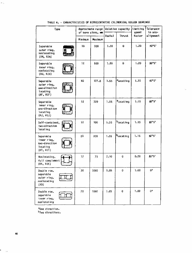
TABLE 4. - CHARACTERISTICS OF REPRESENTATIVE CYLINDRICAL ROLLER BEARINGS

Separable

one-direction

two-direction

Double row,

nonlocating

aDne direction. bTwo directions.

46

i -

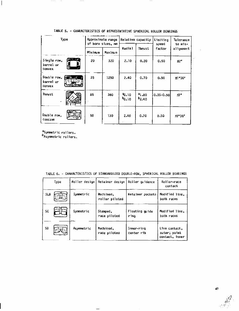
TABLE 5. - CHARACTERISTICS OF REPRESENTATIVE SPHERICAL ROLLER BEARINGS

Type Approximate range of bore sizes. amn

lelative capacity Limiting Tolerance speed to mis-

Radial Thrust 1 factor / alignment Maximum Yiniaum

20

25

-

! t C

I

I

t

C

1

I

L

0 C

320 2.10 jingle row, carrel or :onvex

2.40

ao.10 "1.80 0.35-0.50 53' bO.iO b2.40

2.40

1250

a5 360

50

aSymnetric rollers. bAsymnetric rollers.

TABLE 6. - CHARACTERISTICS OF STANDARDIZED DOUBLE-ROW, SPHERICAL ROLLER BEARINGS

loller design

Symnetric

Symmetric

Asynetric

Retainer design

Yachined, roller piloted

3tamped. race piloted

Machined, race piloted

Type loller guidance Roller-race contact

letainer pockets Modified line, both races

#:loating guide Modified line, ring both races

Inner-ring center rib

Line contact, outer; point contact, inner

SD

TABLE 7. - CHARACTERISTICS OF SPHERICAL ROLLER BEARINGS

Series Types Approximate range Approximate rela- Limiting of bore sizes, mm tive capacitya speed

factor Minimum Maxirmm Radial Thrust

202 Single-row barrel 20 320 1.0 0.11 0.5 203 Single-row barrel 20 240 1.7 .18 .5 204 Single-row barrel 25 110 2.1 .22 .4 212 SLB 35 75 1 .o .26 .6 213 SLB 30 70 1.7 .53

22. 22K SLB, SC, SD 30 320 1.7 .46 23, 23K SLB. SC, SD 40 280 2.7 1.0 1 30, 30K SLB. SC, SD 120 1250 1.2 .29 .7 31, 31K SLB, SC, SD 110 1250 1.7 .54 .6 32, 32K SLB, SC, SD 100 850 2.1 .78 .6 39, 39K SD 120

1 1250 .7 .18 .7

40. 40K SD 180 1 250 1.5 I ---- , .7

"Load capacities are comparative within the various series of spherical roller bearings only. For a given envelope size, a spherical roller bearing has a radial capacity approximately equal to that of a cylindrical roller bearing.

48

-

TABLE 8. - CHARACTERISTICS OF REPRESENTATIVE TAPERED ROLLER BEARINGS

Type Subtype Approximate range of bore sizes, mn

Single row.

(TS)

Two row, double cone, single cups (TDI)

Two row, double cup, single cones, adjustable iTDO)

Two row, double cup, single cones, nonadjustable (TNA)

TST - Tapered bore TSS - Steep angle TS - Pin cage TSE, TSK - keyway cones TSF, TSSF - flanged cup TSG - steering gear (without cone)

TDIK, TDIT, TDITP - tapered bore TDIE, TDIKE - slotted double cone TDIS - steep angle

TDO TDOS - steep angle

TNA 20 60 TNASW - slotted cones 30 260 TNASWE - extended cone rib 20 305 TNASWH - slotted cones, sealed 8 70 TNADA, TNHDADX - self-aligning cup AD -mm _-mm

TQO. TQOT - tapered bore

TQIT - tapered bore ----

Minimum Maxirmm

B 24 16

12 8

1690 430

1270 ----

380 1070 ----

30 1200 30 860 24 690 55 520

8 1830 20 1430

70 1500 250 1500

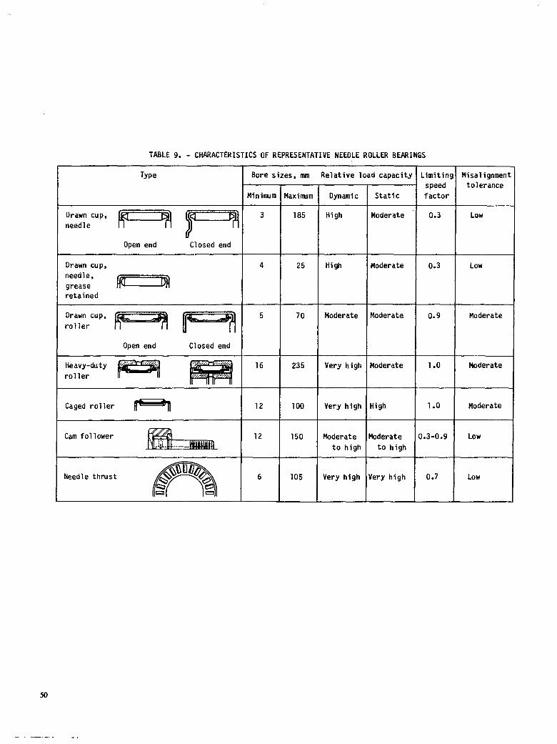
TABLE 9. - CHARACTERISTICS OF REPRESENTATIVE NEEDLE ROLLER BEARINGS

T I 1 Misalignment tolerance

Type Bore sizes, mm Relative load capacit.J Limitin: speed factor

0.3

L I

I

Mininum Maxinum Dynamic Static

Drawn cup, needle

Open end Closed end

3 185 High Moderate Low

Low Drawn cup, needle, grease retained

25 High

70 Moderate

235 Very high

4

5

16

Moderate

Moderate

Moderate

0.3

0.9 Drawn cup, roller

Moderate

Open end Closed end

1.0 Moderate

1.0 Very high High Moderate 12 100 Caged roller

Low Cam follower 12

6

3.3-0.9

0.7

150

105

Moderate to high

Very high

bderate to high

lery high Needle thrust Low

50

I -

TABLE 10. - TYPICAL CHEMICAL COMF'OSITIONS OF SELECTED BEARING STEELS (FROM BAMBERGER, 1980)

Designation

SAE 52100 1.00 MHTa 1.03 AISI M-l .80 AISI M-2 .83 AISI M-10 .85 AISS M-50 .BO T-l (18-4-l) .70 T15 1.52 44oc 1.03 AMS 5749 1.15 Vasco Matrix II .53 CRB-7 1.10 AISJ 931ob .lO CBS 60& .19 CBS lOcoMb .14 Vasco X-s .14

T C

aAlso contains 1.36% Al. bCarburizing grades.

P

max)

1.025 1.025 .025 .025 .030 .030

.OlO

.018

.012

.014

.016

.006

.007 .018 .Oll

.004

.014 ,004 .013 .003 .OOl .014

S max)

Mn

1.35 .35 .30 .30 .25 .30 .30 .26 .48 .50 .12 .43 .54 .61 .48 .24

1 (

1

Alloying element, wtX 1 Si Cr V W MO co Cb Ni

1.30 1.45 .35 1.50 .30 4.00 .30 3.85 .30 4.00 .25 4.00 .25 4.00 .25 4.70 .41 7.30 .30 4.50 .21 4.13 .31 4.00 .28 1.18

1.05 1.50 .43 1.12 .94 4.76

_---

----

1.00 1.90 2.00 1.00 1.00 4.90

.14 1.20 1.08 1.03 mm--

----- ----- 1.50 6.15

----- -----

18.0 12.5 m-e-- _----

1.40 ----- ----- ----- .----

1.40

-s--

8.00 5.00 8.00 4.25

_-m- ----

.45

_m-- .20 .50

4.00 4.80 2.02

.ll

.94 4.77 1.40

---- _--- --mm _-me _--- ---- -em- _--- ---- _--- _--- ---- ---- ---- ---- _-mm _-mm ---- ---- _--- mm--

5.10 _-mm _--- ---- -mm- -mm- _--- _--- _---

7.81 -me- 0.10 _--- 0.32 _-me ---- _--- 3.15 _--- _--- .18 _-me ---- 2.94

.03 _--- .lO

Radius-of- curvature

ratio, a

Ellipticity parameter,

k T Ellipticity T Complete elliptic inte-

gral of first kind

'ercent error,

e

s 'ercent error,

e

1.00 1.0000 l.OOOC 0 1.5708 1.57OL 0 1.25 1.1604 1.1526 .66 1.6897 1.6892 -.50 1.50 1.3101 1.2945 1.19 1.7898 1.802; -.70 1.75 1.4514 1.4280 1.61 1.8761 1.8902 -.75 2.00 1.5858 1.5547 1.96 1.9521 1.9664 -.73 3.00 2.0720 2.0125 2.87 2.1883 2.1979 -.44 4.00 2.5007 2.4170 3.35 2.3595 2.3621 -.ll 5.00 2.8902 2.7860 3.61 2.4937 2.4895 .17 6.00 3.2505 3.1289 3.74 2.6040 2.5935 .40 7.00 3.5878 3.4515 3.80 2.6975 2.6815 .59 8.00 3.9065 3.7577 3.81 2.7786 2.7577 -75 9.00 4.2096 4.0503 3.78 2.8502 2.8250 .88

10.00 4.4994 4.3313 3.74 2.9142 2.8851 1.00 15.00 5.7996 5.6069 3.32 3.1603 3.1165 1.38 20.00 6.9287 6.7338 2.81 3.3342 3.2807 1.60 25.00 7.9440 7.7617 2.29 3.4685 3.4081 1.74 30.00 8.8762 8.7170 1.79 3.5779 3.5122 1.84 35.00 9.7442 9.6158 1.32 3.6700 3.6002 1.90 40.00 10.5605 0.4689 .87 3.7496 3.6764 1.95 45.00 11.3340 I.2841 .44 I.8196 5.7436 1.99 50.00 12.0711 2.0670 .03 i.8821 3.8038 2.02 60.00 13.4557 3.5521 -.72 1.9898 I.9078 2.06 70.00 14.7430 4.9495 -1.40 1.0806 I.9958 2.08 80.00 15.9522 5.2759 -2.03 1.1590 1.0720 2.09 90.00 17.0969 7.5432 -2.61 1.2280 1.1393 2.10

100.00 18.1871 3.7603 -3.15 1.2895 1.1994 !.lO

TABLE 11. - COMPARISON OF NUMERICALLY DETERMINED VALUES WITH CURVE-FIT VALUES FOR GEOMETRICALLY DEPENDENT VARIABLES

[Rx = 1.0 cm.]

Complete elliptic integral of second kind

I r 'ercent error,

e

1.5708 1.5708 0

1.4643 1.4566 .52 1.3911 1.3805 .76 1.3378 1.3262 .87 1.2972 1.2854 .91 1.2002 1.1903 .83 1.1506 1.1427 .69 1.1205 1.1142 .57 1.1004 1.0951 .48 I .0859 1.0815 .40 1.0751 1.0713 .35 1.0666 1.0634 .30 1.0599 1.0571 .26 I .0397 1.0381 .15 1.0296 1.0285 .lD 1.0236 1.0228 .07 1.0196 1.0190 .05 1.0167 1.0163 .04 1.0146 1.0143 .03 I.0129 1.0127 .02 1.0116 1.0114 .02 .0096 / .0095 .Ol

1.0082 1.0082 .Ol .0072 8.0071 .Ol

1.0064 1.0063 0 .0057 .0057 0

52

TABLE 12. - SIMPLIFIED EQUATIONS

a>1

i; = p/i7

where q = f-l

- I =I+ 4

a

where R -1 D ",' + R-' Y

Dx = 2(F)l'3

a<1

i; = a2/n

>=" T+qlna

where q = 5 - 1

i= l+qa

where R -1 = ";' + R-' Y

TABLE 13. - PRACTICAL APPLICATIONS FOR DIFFERING CONFORMITIES

Contact parameter:

F

)"ax

ray

rbx

'by

a

k

iF

4

i-

s

s

DY

Dy

DX

D,

6

s

umax

amax

[E' = 2.197x107 N/cm2.]

Wheel on rail Ball on plane Ball - outer-race contact

l.00x105 N

50.1900 cm

2224111 N

0.6350 cm

222.4111 N

0.6350 cm

OD 0.6350 cm 0.6350 cm

OD 0

30.0000 cm 0

0.5977 1.0000

-3.8900 cm

-0.6600 cm

22.0905

0.7099 1.0000 7.3649

0.7206 1.0000 7.7738

1.3526 1.5708 1.0267

1.3412 7.5708 7.0258

1.8508 7.5708 3.3941

1.8645

1.0783 cm

1.5708

0.0426 cm

3.3375

0.1842 cm

1.0807 cm

1.5190 cm

0.0426 cm

0.0426 cm

0.7870 cm

0.0250 cm

1.4997 cm

0.0106 cm

0.0708 cm

1.166~10~ N/cm2

,17a4x105 N/cm2

0.0426 cm 0.0252 cm

7.13~10~~ cm 3.56~10~~ cm

7.13~10~~ cm 3.57x10m4 cm

!.34x105 N/cm2 1.22~10~ N/cm2

!.34x105 N/cm2 1.30~10~ N/cm2

54

TABLE 14. - CAPACITY FORMULAS FOR RECTANGULAR AND ELLIPTICAL CONTACTS

[Units in kg and mn.]

Function Elliptical contact of ball bearings Rectangular contact of roller bearings

C f f io.7N2/3dl.a ca ca

fC gcflf2

c 10/B -0.8

9, 10 1 ,+ i T- di(do - d) [ 1 Oa4'

Ci/Co f3 do(di - d)

Radial Thrust Radial Thrust

8 # go0 8 = 90" I3 f go0 6 = 9o"

Y d cos B d d cos & d

de T de <

fa (cos 6) 0.7

(cos B) 0.7

tan B 1 (cos 8) 719

(cos B) 719 tan B 1

fl 3.7-4.1 6-10 78-25 36-60

1.39 29/27 f

Z(l - y) 0.3 219 ,

2/9 2

(1 + y)"3 Y

(1 + y)1'3 Y

f3 104f4

f4 1 1.14 f4 f4

1

f4

55

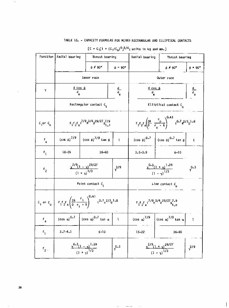
TABLE 15. - CAPACITY FORMULAS FOR MIXED RECTANGULAR AND ELLIPTICAL CONTACTS

[C = Ci[l + (Ci/Co)4]1'4; units in kg and am.1 - --

Function Radial bearing Thrust bearing Radial bearing Thrust bearing

f3 # 90" i3 = 9o" B # 9o" 6 = 90"

Inner race Outer race

d cos 6 d Y d

e B

d cos B d e

Cior Co

Rectangular contact Ci

flf2fa' .7/9N3'4D29'27Q;/q

,

-

Elliptical contact Co

~~ L-~__ ~--- ..~.. _

f a

(co6 6)7'9 (cos 6)7'9 tan 6 1

fl 78-25 36-60 3.5-3.9 6-10

1.39 f

2Di1 _ 29'27 3/9 y"*3( 1 + y) 0.3

2 (1 + y)1'3

Y (1 - y)"3

Y

Point contact Ci Line contact C 0

Ci or Co

fa

fl

f f f 12a

i7'9n3/4d29/27a7.9 ,

(cos o)"*7 (cos a)Oo7 tan a 1 (~20s a) 7'9 (coGaF

3.7-4.1 6-10 15-22 36-60

29'27

f2

0.3(, _ 1.39 0.3

Y y2'9( 1 + y) 2/9

(1 + y)1'3 (1 - y)"3 Y

56

TABLE 16. - MATERIAL FACTOR FOR THROUGH-HARDENED

BEARING MATERIALS

iFrom Bamberger, et al., 1971; air-melted materials assumed.]

T-Factor

2.0 .6 .6

2.0 2.0

.6 2.0

.2

.6 0.6-0.8

1. Report No. 2. Government Accession No. 3. Recipient’s Catalog No.

NASA RP-1105 4. Title and Subtitle 5. Report Date

ROLLING-ELEMENT BEARINGS June 1983 6. Performing Organization Code

505-32-42 7. Author(s) 8. Performing Organization Report No.

Bernard J. Hamrock and William J. Anderson E-1440 10. Work Unit No.

9. Performing Organization Name and Address

National Aeronautics and Space Administration Lewis Research Center

11. Contract or Grant No.

Cleveland, Ohio 44135 13. Type of Report and Period Covered

12. Sponsoring Agency Name and Address Reference Publication National Aeronautics and Space Administration Washington, D. C. 20546

14. Sponsoring Agency Code

15. Supplementarv Notes Bernard J. Hamrock, Lewis Research Center; William J. Anderson, Consulting Engineer - Bearings and Lubrication, North Olmsted, Ohio. Published as Chapter 33 in Mechanical Design and Systems Handbook, McGraw-Hill Book Co. , 1983.

6. Abstract

Rolling-element bearings are a precision, yet simple, machine element of great utility. This report draws together the current understanding of rolling-element bearings. A brief history of rolling-element bearings is reviewed in the introduction, and subsequent sections describe the types of rolling-element bearings, their geometry and kinematics, as well as the materials they are made from and the manufacturing processes they involve. Unloaded and unlubricated rolling-element bearings are considered in Sections 1 to 6, loaded but unlubricated rolling- element bearings are considered in Sections 7 to 9, and loaded and lubricated rolling-element bearings are considered in Sections 10 to 14. The recognition and understanding of elastohydrodynamic lubrication, covered briefly in Sections 11, 12, and 14, represents one of the major developments in rolling-element bearings since the last edition of the Mechanical Design and Systems Handbook was published in 1964.

7. Key Words (Suggested by Author(s) ) 18. Distribution Statement Fatigue life; Elastohydrodynamic lubrication; Ball Unclassified - unlimited and roller bearings; Materials and manufacturing STAR Category 37 processes; Contact stresses and deformations; Static load capacity; Rolling friction and friction in bearings; Lubricants and lubrication systems

3. Security Classif. (of this report) 20. Security Classif. (of this page) 21. No. of Pages 22. Price’

Unclassified Unclassified 59 A02

* For sale by the National Technical Information Service, Springfield, Virginia 22161 NASA-Langley, 1983

rolling-element bearings · 14.1 cylindrical roller bearing problem ... the precision...

Documents