role of interference and computational complexity in
TRANSCRIPT

Graduate Theses, Dissertations, and Problem Reports
2015
Role of Interference and Computational Complexity in Modern Role of Interference and Computational Complexity in Modern
Wireless Networks: Analysis, Optimization, and Design Wireless Networks: Analysis, Optimization, and Design
Salvatore Talarico
Follow this and additional works at: https://researchrepository.wvu.edu/etd
Recommended Citation Recommended Citation Talarico, Salvatore, "Role of Interference and Computational Complexity in Modern Wireless Networks: Analysis, Optimization, and Design" (2015). Graduate Theses, Dissertations, and Problem Reports. 6768. https://researchrepository.wvu.edu/etd/6768
This Dissertation is protected by copyright and/or related rights. It has been brought to you by the The Research Repository @ WVU with permission from the rights-holder(s). You are free to use this Dissertation in any way that is permitted by the copyright and related rights legislation that applies to your use. For other uses you must obtain permission from the rights-holder(s) directly, unless additional rights are indicated by a Creative Commons license in the record and/ or on the work itself. This Dissertation has been accepted for inclusion in WVU Graduate Theses, Dissertations, and Problem Reports collection by an authorized administrator of The Research Repository @ WVU. For more information, please contact [email protected].

Role of Interference and Computational
Complexity in Modern Wireless Networks:
Analysis, Optimization, and Design
Salvatore Talarico
Dissertation submitted to theStatler College of Engineering and Mineral Resources
at West Virginia Universityin partial fulfillment of the requirements
for the degree of
Doctor of Philosophyin
Electrical Engineering
Matthew C. Valenti, Ph.D., ChairBrian D. Woerner, Ph.D.Natalia A. Schmid, Ph.D.Daryl S. Reynolds, Ph.D.
Marcello R. Napolitano, Ph.D.
Lane Department of Computer Science and Electrical Engineering
Morgantown, West Virginia2015
Keywords: Information Theory, Interference, Spatial Modeling, Cellular Network,Optimization, Cooperative Communication, Cloud-RAN, Computational Complexity
Copyright 2015 Salvatore Talarico

Abstract
Role of Interference and Computational Complexity in Modern Wireless Networks:Analysis, Optimization, and Design
by
Salvatore TalaricoDoctor of Philosophy in Electrical Engineering
West Virginia University
Matthew C. Valenti, Ph.D., Chair
Owing to the popularity of smartphones, the recent widespread adoption of wirelessbroadband has resulted in a tremendous growth in the volume of mobile data traffic, andthis growth is projected to continue unabated. In order to meet the needs of future systems,several novel technologies have been proposed, including cooperative communications, cloudradio access networks (RANs) and very densely deployed small-cell networks. For thesenovel networks, both interference and the limited availability of computational resourcesplay a very important role. Therefore, the accurate modeling and analysis of interferenceand computation is essential to the understanding of these networks, and an enabler for moreefficient design.
This dissertation focuses on four aspects of modern wireless networks: (1) Modelingand analysis of interference in single-hop wireless networks, (2) Characterizing the tradeoffsbetween the communication performance of wireless transmission and the computationalload on the systems used to process such transmissions, (3) The optimization of wirelessmultiple-access networks when using cost functions that are based on the analytical findingsin this dissertation, and (4) The analysis and optimization of multi-hop networks, which mayoptionally employ forms of cooperative communication.
The study of interference in single-hop wireless networks proceeds by assuming that therandom locations of the interferers are drawn from a point process and possibly constrained toa finite area. Both the information-bearing and interfering signals propagate over channelsthat are subject to path loss, shadowing, and fading. A flexible model for fading, basedon the Nakagami distribution, is used, though specific examples are provided for Rayleighfading. The analysis is broken down into multiple steps, involving subsequent averaging ofthe performance metrics over the fading, the shadowing, and the location of the interfererswith the aim to distinguish the effect of these mechanisms that operate over different timescales. The analysis is extended to accommodate diversity reception, which is important forthe understanding of cooperative systems that combine transmissions that originate fromdifferent locations. Furthermore, the role of spatial correlation is considered, which providesinsight into how the performance in one location is related to the performance in anotherlocation.
While it is now generally understood how to communicate close to the fundamental lim-its implied by information theory, operating close to the fundamental performance bounds

iii
is costly in terms of the computational complexity required to receive the signal. Thisdissertation provides a framework for understanding the tradeoffs between communicationperformance and the imposed complexity based on how close a system operates to the perfor-mance bounds, and it allows to accurately estimate the required data processing resources ofa network under a given performance constraint. The framework is applied to Cloud-RAN,which is a new cellular architecture that moves the bulk of the signal processing away fromthe base stations (BSs) and towards a centralized computing cloud. The analysis developedin this part of the dissertation helps to illuminate the benefits of pooling computing assetswhen decoding multiple uplink signals in the cloud. Building upon these results, new ap-proaches for wireless resource allocation are proposed, which unlike previous approaches, areaware of the computing limitations of the network.
By leveraging the accurate expressions that characterize performance in the presence ofinterference and fading, a methodology is described for optimizing wireless multiple-accessnetworks. The focus is on frequency hopping (FH) systems, which are already widely used inmilitary systems, and are becoming more common in commercial systems. The optimizationdetermines the best combination of modulation parameters (such as the modulation indexfor continuous-phase frequency-shift keying), number of hopping channels, and code rate. Inaddition, it accounts for the adjacent-channel interference (ACI) and determines how muchof the signal spectrum should lie within the operating band of each channel, and how muchcan be allowed to splatter into adjacent channels.
The last part of this dissertation contemplates networks that involve multi-hop commu-nications. Building on the analytical framework developed in early parts of this dissertation,the performance of such networks is analyzed in the presence of interference and fading,and it is introduced a novel paradigm for a rapid performance assessment of routing proto-cols. Such networks may involve cooperative communications, and the particular cooperativeprotocol studied here allows the same packet to be transmitted simultaneously by multipletransmitters and diversity combined at the receiver. The dynamics of how the cooperativeprotocol evolves over time is described through an absorbing Markov chain, and the analysisis able to efficiently capture the interference that arises as packets are periodically injectedinto the network by a common source, the temporal correlation among these packets andtheir interdependence.

iv
Acknowledgements
I would like to thank all the people who contributed in some way to the work described
in this dissertation. First of all, I would like to gratefully and sincerely thank my advisor and
committee chair Dr. Matthew C. Valenti for welcoming me in his group, for his guidance,
understanding, and patience during my ”journey” at West Virginia University (WVU). His
attention to details, enthusiastic attitude, and his hard work have inspired me from the very
first moment I become one of his students, and I feel blessed I have had the opportunity to
work for him. He has been a terrific and supportive mentor, and has made available to me
many opportunities for both my professional and personal growth, for which I will always
be grateful.
I would like to thank Dr. Natalia A. Schmid, Dr. Daryl S. Reynolds, Dr. Brian D.
Woerner and Dr. Marcello R. Napolitano for being in my committee, and for all their
comments, questions, and feedback, that refined this work. I have been very blessed to take
classes and work for some of them, and I have tremendously benefit from their knowledge
and experience.
This work would have never been possible without the support of the external collab-
orators. I would like to thank in primis Dr. Don Torrieri, from the Army Research Lab
(ARL), for giving me the opportunity to work for him and for his invaluable help for the
research presented in Chaps. 2-4 and Chaps. 7-8. I would like to thank Dr. Peter Rost and
Dr. Andreas Maeder from Nokia Networks for their help in Chaps. 5-6 and Dr. Thomas R.
Halford from WPL Inc. for his support in Chap. 9.
I would like to thank all the students of the wireless communication research lab (WCRL)
for making this journey more pleasant. A special thank goes to Terry Ferrett for inducting
me to the usage of the cluster computing resources available for the WCRL’eers, which has
been very useful and has speeded up considerably the completion of this work. Another
thank goes to Marwan Alkhweldi, for his friendship, and his unconditioned support in all

ACKNOWLEDGEMENTS v
the difficult times.
I also wanted to thank WVU, for giving me the opportunity to meet a lot of good and
bright friends. Among all, I would like to thank Francesco Nicolo and Syvale Lee, for their
continuous help and support, since the very beginning I have moved to the USA. Another
special thank goes to Cesare Ciaccio, Zhengjun Wang, Peng Zheng, Tuhua Zhong, and all the
other friends from the WVU International soccer team, the WVU Evansdale Roundtable,
and the Keglers Wandererz’s team for the recreational and fun time, and the good discussions
I have had with them.
Lastly but certainly not less important, I would like to thank my parents Giovanni and
Teresa Bitonti as well as my sister Giovanna who have always believed in me, and supported
all my decisions. They have the capability to always cheer me up and to make each day a
little better. A very special thank goes to Betsy V. Neyra, who has been the most caring,
positive, supportive, patient, and the best girlfriend I could ever have. This dissertation
would have never been possible without her spiritual support, and this is why I dedicate it
to her.

vi
Contents
Acknowledgements iv
List of Figures x
List of Tables xiv
List of Abbreviations xv
Notation xx
1 Introduction 11.1 Modeling Interference in Wireless Networks . . . . . . . . . . . . . . . . . . 2
1.1.1 Statistical Interference Models . . . . . . . . . . . . . . . . . . . . . . 51.1.2 Models Describing the Effects of Interferences . . . . . . . . . . . . . 8
1.2 Techniques to Analyze the Network Performance . . . . . . . . . . . . . . . . 101.3 Computational Complexity in Wireless Networks . . . . . . . . . . . . . . . 121.4 Scope, Outline and Contributions . . . . . . . . . . . . . . . . . . . . . . . . 13
2 Channel Outage Analysis in Wireless Networks 162.1 Network Model . . . . . . . . . . . . . . . . . . . . . . . . . . . . . . . . . . 172.2 Conditional Outage Probability . . . . . . . . . . . . . . . . . . . . . . . . . 182.3 Spatially Averaged Outage Probability . . . . . . . . . . . . . . . . . . . . . 20
2.3.1 Binomial Point Processes . . . . . . . . . . . . . . . . . . . . . . . . . 202.3.2 Poisson Point Processes . . . . . . . . . . . . . . . . . . . . . . . . . 26
2.4 Spatial Interference Correlation . . . . . . . . . . . . . . . . . . . . . . . . . 282.4.1 Special Cases . . . . . . . . . . . . . . . . . . . . . . . . . . . . . . . 29
2.5 Numerical Results . . . . . . . . . . . . . . . . . . . . . . . . . . . . . . . . . 312.6 Chapter Summary . . . . . . . . . . . . . . . . . . . . . . . . . . . . . . . . 36
3 Cellular Networks: Modeling and Analysis 383.1 Modeling and Analysis for Cellular Networks . . . . . . . . . . . . . . . . . . 393.2 Network Model . . . . . . . . . . . . . . . . . . . . . . . . . . . . . . . . . . 403.3 Spatial Model . . . . . . . . . . . . . . . . . . . . . . . . . . . . . . . . . . . 423.4 Resource Allocation Policies . . . . . . . . . . . . . . . . . . . . . . . . . . . 43
3.4.1 Power Control . . . . . . . . . . . . . . . . . . . . . . . . . . . . . . . 43

CONTENTS vii
3.4.2 Rate Control . . . . . . . . . . . . . . . . . . . . . . . . . . . . . . . 453.4.3 Fixed-Rate Policies . . . . . . . . . . . . . . . . . . . . . . . . . . . . 473.4.4 Variable-Rate Policies . . . . . . . . . . . . . . . . . . . . . . . . . . 48
3.5 Cell Reselection . . . . . . . . . . . . . . . . . . . . . . . . . . . . . . . . . . 493.6 Performance Analysis . . . . . . . . . . . . . . . . . . . . . . . . . . . . . . . 49
3.6.1 Outage-Constrained Fixed-Rate Policy . . . . . . . . . . . . . . . . . 513.6.2 Outage-Constrained Variable-Rate Policy . . . . . . . . . . . . . . . . 513.6.3 Policy Comparison . . . . . . . . . . . . . . . . . . . . . . . . . . . . 533.6.4 Spreading factor . . . . . . . . . . . . . . . . . . . . . . . . . . . . . 543.6.5 Base-station Exclusion Zone . . . . . . . . . . . . . . . . . . . . . . . 543.6.6 Cell Association . . . . . . . . . . . . . . . . . . . . . . . . . . . . . . 54
3.7 Chapter Summary . . . . . . . . . . . . . . . . . . . . . . . . . . . . . . . . 56
4 Diversity Combining: Outage Analysis and Applications 574.1 Network Model . . . . . . . . . . . . . . . . . . . . . . . . . . . . . . . . . . 584.2 Conditional Outage Probability . . . . . . . . . . . . . . . . . . . . . . . . . 594.3 Applications . . . . . . . . . . . . . . . . . . . . . . . . . . . . . . . . . . . . 60
4.3.1 Multi-Cell Downlink Cooperation . . . . . . . . . . . . . . . . . . . . 604.3.2 MBSFN Networks . . . . . . . . . . . . . . . . . . . . . . . . . . . . . 66
4.4 Chapter Summary . . . . . . . . . . . . . . . . . . . . . . . . . . . . . . . . 71
5 The Role of Complexity in Cellular Networks 725.1 Cloud-RAN: A Brief Introduction . . . . . . . . . . . . . . . . . . . . . . . . 735.2 Complexity model . . . . . . . . . . . . . . . . . . . . . . . . . . . . . . . . . 76
5.2.1 Link Adaptation . . . . . . . . . . . . . . . . . . . . . . . . . . . . . 765.2.2 Complexity Model . . . . . . . . . . . . . . . . . . . . . . . . . . . . 77
5.3 Performance Metrics . . . . . . . . . . . . . . . . . . . . . . . . . . . . . . . 805.3.1 Computational outage probability . . . . . . . . . . . . . . . . . . . . 805.3.2 Outage complexity . . . . . . . . . . . . . . . . . . . . . . . . . . . . 805.3.3 Computational gain and diversity . . . . . . . . . . . . . . . . . . . . 815.3.4 Complexity-Rate Tradeoff . . . . . . . . . . . . . . . . . . . . . . . . 825.3.5 Average Achievable Rate . . . . . . . . . . . . . . . . . . . . . . . . . 82
5.4 A Framework for Complexity Analysis . . . . . . . . . . . . . . . . . . . . . 835.4.1 Full Power Control . . . . . . . . . . . . . . . . . . . . . . . . . . . . 835.4.2 Effect of Path Loss and Power Control . . . . . . . . . . . . . . . . . 855.4.3 Centralized Processing . . . . . . . . . . . . . . . . . . . . . . . . . . 86
5.5 Numerical Verification . . . . . . . . . . . . . . . . . . . . . . . . . . . . . . 875.6 Results . . . . . . . . . . . . . . . . . . . . . . . . . . . . . . . . . . . . . . . 90
5.6.1 Computational Gain . . . . . . . . . . . . . . . . . . . . . . . . . . . 905.6.2 Computational Diversity . . . . . . . . . . . . . . . . . . . . . . . . . 905.6.3 Complexity-Rate Tradeoff . . . . . . . . . . . . . . . . . . . . . . . . 92
5.7 Chapter Summary . . . . . . . . . . . . . . . . . . . . . . . . . . . . . . . . 94

CONTENTS viii
6 Resource Management in Cloud-RANs 956.1 Heuristic Approach to MCS Selection . . . . . . . . . . . . . . . . . . . . . . 96
6.1.1 Numerical Results . . . . . . . . . . . . . . . . . . . . . . . . . . . . 996.2 Optimal MCS Scheduling Policies . . . . . . . . . . . . . . . . . . . . . . . . 104
6.2.1 Max-Rate Optimization Problem . . . . . . . . . . . . . . . . . . . . 1056.2.2 Application to Limited Number of Rates and Multiple Users . . . . . 1076.2.3 Complexity Cut-Off . . . . . . . . . . . . . . . . . . . . . . . . . . . . 1086.2.4 Numerical Results . . . . . . . . . . . . . . . . . . . . . . . . . . . . 109
6.3 Chapter Summary . . . . . . . . . . . . . . . . . . . . . . . . . . . . . . . . 113
7 Frequency-Hopping: Optimization in Ad Hoc Networks 1157.1 Outage Analysis of Frequency-Hopping Networks . . . . . . . . . . . . . . . 116
7.1.1 Network Model . . . . . . . . . . . . . . . . . . . . . . . . . . . . . . 1177.1.2 Conditional Outage Probability . . . . . . . . . . . . . . . . . . . . . 1207.1.3 Spatially Averaged Outage Probability . . . . . . . . . . . . . . . . . 120
7.2 Modulation-Constrained Area Spectral Efficiency . . . . . . . . . . . . . . . 1227.3 Optimization and Rate Allocation Policies . . . . . . . . . . . . . . . . . . . 125
7.3.1 Fixed Rate Optimization . . . . . . . . . . . . . . . . . . . . . . . . . 1267.3.2 Rate Adaptation . . . . . . . . . . . . . . . . . . . . . . . . . . . . . 130
7.4 Chapter Summary . . . . . . . . . . . . . . . . . . . . . . . . . . . . . . . . 134
8 Geographic Routing Protocols in Ad Hoc Networks 1358.1 Network Model . . . . . . . . . . . . . . . . . . . . . . . . . . . . . . . . . . 1368.2 Network Simulation . . . . . . . . . . . . . . . . . . . . . . . . . . . . . . . . 1368.3 Interference Correlation . . . . . . . . . . . . . . . . . . . . . . . . . . . . . 1388.4 Routing Protocols . . . . . . . . . . . . . . . . . . . . . . . . . . . . . . . . . 1388.5 Implementation of Path Selection . . . . . . . . . . . . . . . . . . . . . . . . 1408.6 Performance Metrics . . . . . . . . . . . . . . . . . . . . . . . . . . . . . . . 1428.7 Performance Analysis . . . . . . . . . . . . . . . . . . . . . . . . . . . . . . . 1438.8 Chapter Summary . . . . . . . . . . . . . . . . . . . . . . . . . . . . . . . . 148
9 Stochastic Modeling of Cooperative Multi-hop Wireless Networks 1499.1 Markov Process and Multi-hop Wireless Networks . . . . . . . . . . . . . . . 1509.2 Application: Barrage Relay Networks . . . . . . . . . . . . . . . . . . . . . . 151
9.2.1 Barrage Relay Network . . . . . . . . . . . . . . . . . . . . . . . . . . 1529.2.2 Controlled Barrage Regions . . . . . . . . . . . . . . . . . . . . . . . 1539.2.3 Network Model . . . . . . . . . . . . . . . . . . . . . . . . . . . . . . 1559.2.4 Controlled Barrage Region as a Markov Process . . . . . . . . . . . . 1559.2.5 Inter-CBR Interference . . . . . . . . . . . . . . . . . . . . . . . . . . 1599.2.6 Intra-CBR Interference . . . . . . . . . . . . . . . . . . . . . . . . . . 164
9.3 Chapter Summary . . . . . . . . . . . . . . . . . . . . . . . . . . . . . . . . 169
10 Conclusion 17010.1 Summary and Publications . . . . . . . . . . . . . . . . . . . . . . . . . . . . 17110.2 Future Work . . . . . . . . . . . . . . . . . . . . . . . . . . . . . . . . . . . . 175

CONTENTS ix
A Conditional Outage Probability: Derivation 177
B Asymptotic Outage Analysis 1792.1 Direct Approach . . . . . . . . . . . . . . . . . . . . . . . . . . . . . . . . . 1792.2 Stochastic Geometry Approach . . . . . . . . . . . . . . . . . . . . . . . . . 182
C Correlation Coefficient in a BPP: Derivation 1833.1 Spatially Averaged First Moment . . . . . . . . . . . . . . . . . . . . . . . . 1833.2 Spatially Averaged Second Moment . . . . . . . . . . . . . . . . . . . . . . 1843.3 Spatially Averaged Joint First Moment . . . . . . . . . . . . . . . . . . . . 184
D Conditional Outage Probability for Diversity Combining: Derivation 186
E Expectation and Variance of the Decoding Complexity: Derivation 1885.1 Expectation of the Decoding Complexity . . . . . . . . . . . . . . . . . . . . 1885.2 Variance of the Decoding Complexity . . . . . . . . . . . . . . . . . . . . . . 190
F Max-Rate Optimization: Derivation 193
References 195
List of Publications 207

x
List of Figures
1.1 Vulnerability circle capture model. . . . . . . . . . . . . . . . . . . . . . . . 5
2.1 Typical network topology. The reference transmitter is located at the cen-ter. The two reference receivers are represented by the two red stars on thecircumference of radius r0. . . . . . . . . . . . . . . . . . . . . . . . . . . . 29
2.2 Conditional outage probability εj (Ω) as a function of SNR. Analytical curvesare solid while dots represent simulated values. Top curve: all channelsRayleigh. Middle curve: all channels mi,j = 4. Bottom curve: m0,j = 4for the source, and mi,j = 1 for the interferers. The network topology isshown in the inset. The receiver is represented by the star at the center ofthe radius-4 circle, the desired transmitter is the big red dot, while the 50interferers are shown as blue dots. . . . . . . . . . . . . . . . . . . . . . . . 32
2.3 Spatially averaged outage probability for a BPP as a function of the numberof interferers M for two values of p. For each p, curves are shown for the caseof no shadowing, and for shadowing with two values of σs. . . . . . . . . . . 33
2.4 Spatially averaged outage probability with interfering devices placed accordingto a PPP plotted as a function of the effective spatial density of interferingdevices λp. Curves are shown for three finite network radii (rout=[1,2,4]) andfor the asymptotic case (rout → ∞). The fading is Rayleigh, and there isno shadowing. Dots indicate the results of Monte Carlo simulation while thecurves are computed from the theoretical expressions. . . . . . . . . . . . . 34
2.5 Coverage probability εj = 1− εj as function of the network density λ. Resultsare shown for the case that the interferers are drawn from a BPP (solid lines)and from a PPP (dashed lines). From highest to lowest coverage probability,the curves correspond to the arbitrary shape (blue lines), the triangle (redlines), and the circle (green lines). . . . . . . . . . . . . . . . . . . . . . . . 34
2.6 Spatially averaged correlation coefficient as function of θ/π. Results are shownfor the case that the interferers are drawn from a BPP (solid lines) and froma PPP (dashed lines) and for three values of λp. . . . . . . . . . . . . . . . 35
3.1 Illustration of intracell (all the UEs within the light red area) and intercell (allUEs within the orange area) interference. BSs are represented by large circles,and UEs are represented by black dots with the exception of the reference UEwhich is a green star. Cell boundaries are represented by thick blue lines. . . 41
LIST OF FIGURES xi
3.2 Example network topologies. BSs are represented by large circles, and cellboundaries are represented by thick lines. Left subfigure: Actual BS locationsfrom a current cellular deployment. Right subfigure: Simulated BS locationsusing a BS exclusion zone rexbs
= 0.25. . . . . . . . . . . . . . . . . . . . . . 433.3 Outage probability of eight randomly selected uplinks (dashed lines) along
with the average outage probability for the entire network (solid line). Theresults are for a half-loaded network (M/K = G/2) with distance-dependentfading and shadowing (σs = 8 dB) and are shown as a function of the rate R. 46
3.4 Throughput of eight randomly selected uplinks (dashed lines) along with theaverage throughput for the entire network (solid line). System parameters arethe same used to generate Fig. 3.3. . . . . . . . . . . . . . . . . . . . . . . . 47
3.5 CCDF of the outage probability using an OCFR policy, R = 2, three networkloads, distance-dependent fading, and shadowing. . . . . . . . . . . . . . . . 51
3.6 Average rate of the OCVR policy as function of the load M/K for bothRayleigh and distance-dependent fading, and both shadowed (σs = 8 dB) andunshadowed cases. . . . . . . . . . . . . . . . . . . . . . . . . . . . . . . . . 52
3.7 CCDF of the rate for fully-loaded system (M/K = G) under the OCVR policyin Rayleigh and distance-dependent fading, and both shadowed (σs = 8 dB)and unshadowed cases. . . . . . . . . . . . . . . . . . . . . . . . . . . . . . . 52
3.8 ASE for the four network policies as function of the load M/K for distance-dependent fading and both shadowed (σs = 8 dB) and unshadowed cases.. . . . . . . . . . . . . . . . . . . . . . . . . . . . . . . . . . . . . . . . . . . 53
3.9 ASE as function of effective spreading factor Ge for two values of system load,distance-dependent fading, and shadowing with σs = 8 dB. . . . . . . . . . . 54
3.10 ASE as a function of the BS exclusion-zone radius rexbsfor four policies and
two values of path loss exponent α. . . . . . . . . . . . . . . . . . . . . . . . 553.11 ASE as a function of the maximum reselection distance rmax. . . . . . . . . 55
4.1 Illustration of the cell association: UE Y1 is only served by BS X1, since X1
is located at effective distance lower than rci; UE Y2 is instead served by aplurality of BSs within a maximum effective distance rmax, since there is noBSs at an effective distance lower than rci. . . . . . . . . . . . . . . . . . . . 61
4.2 ASE as a function of K/M with ERP and ETP policy, for both a shadowed(σs = 8 dB) and unshadowed environment. . . . . . . . . . . . . . . . . . . 64
4.3 CCDF of R for ERP and ETP policy for a half loaded system (K/M = 8) inShadowing (σs = 8 dB). . . . . . . . . . . . . . . . . . . . . . . . . . . . . . 65
4.4 Close-up of an example network topology. The BSs locations are given by thelarge filled circles, the Voronoi tessellation shows the radio cell boundaries,and MBSFN areas are illustrated with different colors. The white areas arethe portion of the network for which the outage probability is above a typicalvalue of εchannel = 0.1. . . . . . . . . . . . . . . . . . . . . . . . . . . . . . . 67
4.5 ABOT as a function of the threshold εchannel for both a shadowed (σs = 8 dB)and unshadowed environment with R = 0.5. . . . . . . . . . . . . . . . . . . 70
4.6 ABOT as a function of the minimum separation among BSs when R = 0.1,λ = 0.1 and dsfn = 6. . . . . . . . . . . . . . . . . . . . . . . . . . . . . . . . 70

LIST OF FIGURES xii
5.1 Illustration of the Cloud-RAN architecture. . . . . . . . . . . . . . . . . . . . 745.2 Complexity as a function of the SNR obtained both through simulations (blue)
and based on (5.3) (black curve), when the maximum number of iterationsused to decode a CB is limited to eight. . . . . . . . . . . . . . . . . . . . . . 79
5.3 Outage complexity to ensure per-cell outage constraint ε = 0.1 as functionof the number of BSs, whose signals are centrally processed. Solid lines areevaluated analytically, while dots are obtained through simulations using onemillion trials. The notches on the right side of each sub-figure show thebehavior as Ncloud →∞. . . . . . . . . . . . . . . . . . . . . . . . . . . . . . 89
5.4 Complexity gain for γud = 0 dB, α = 2, s = 0.1. The notches on the right sideof the first sub-figure show the behavior as Ncloud →∞. . . . . . . . . . . . . 91
5.5 Computational diversity as function of the target computational outage prob-ability. . . . . . . . . . . . . . . . . . . . . . . . . . . . . . . . . . . . . . . . 92
5.6 CRT as a function of Nc. The notches on the right side of the figure show thebehavior as Ncloud →∞. . . . . . . . . . . . . . . . . . . . . . . . . . . . . . 93
6.1 Code block error rate as a function of SNR for MCS 10 and MCS 11 after 2,3, and 8 decoder iterations. The arrow shows where the CBLER of MCS 10after 2 iterations is the same as that of MCS 11 after 8 iterations. . . . . . . 97
6.2 Raw throughput and computational effort as a function of the SNR for twoMCS selection schemes: computationally aware selection (CAS) and max-rateselection (MRS). . . . . . . . . . . . . . . . . . . . . . . . . . . . . . . . . . 98
6.3 Outage probability as a function of average SNR in the presence of Rayleighfading, both with and without a complexity constraint. . . . . . . . . . . . 100
6.4 Effective throughput as a function of average SNR in the presence of Rayleighfading, both with and without a complexity constraint. . . . . . . . . . . . 101
6.5 Base station locations. The cloud group consists of the highlighted cells inthe center of the diagram. . . . . . . . . . . . . . . . . . . . . . . . . . . . . 102
6.6 Sum throughput as function of the per-BS complexity constraint whenNcloud =8, with local processing (LP) and with cloud processing (CP). Two MCS-selection schemes are considered: computationally aware selection (CAS) andmax-rate selection (MRS). . . . . . . . . . . . . . . . . . . . . . . . . . . . . 103
6.7 Sum throughput with cloud processing as function of the density of UEs whenNcloud = 8. Two MCS-selection schemes are considered: computationallyaware selection (CAS) and max-rate selection (MRS). . . . . . . . . . . . . 104
6.8 The system is designed such that εcomp = 10 %, 1 %, 0.1 % and the curves areindicated by solid, dashed, and dash-dotted lines, respectively. The verticallines in the magnification of Fig. 6.8(a) show the corresponding value ofNcloudCmax used. . . . . . . . . . . . . . . . . . . . . . . . . . . . . . . . . . . 111
6.9 Sum-rate as a function of Ncloud. The system is designed such that it suffersfrom εcomp = 10 %, 0.1 % computational outage and the curves are indicatedby solid, and dash-dotted lines, respectively. . . . . . . . . . . . . . . . . . . 112

LIST OF FIGURES xiii
6.10 Sum-rate as a function of the user-density λ. The system is designed suchthat it suffers from εcomp = 10 %, 0.1 % computational outage in the case ofλ = 0.5 UEs/km2. The curves are indicated by solid, and dash-dotted lines,respectively. . . . . . . . . . . . . . . . . . . . . . . . . . . . . . . . . . . . 112
7.1 Illustration of the bandwidth usage in a FH spread spectrum system. . . . . 1177.2 Power spectral density of MSK as function of the normalized frequency. Dashed
lines delineate starting from the left the 95 and 99-percent power bandwidth. 1197.3 The symmetric-information rate C(h, γ) of noncoherent binary CPFSK with
modulation indices h = [0.2, 0.4, 0.6, 1]. The markers were found throughMonte Carlo integration while the curves are a polynomial fit. . . . . . . . . 123
7.4 Bandwidth efficiency Beff as function of the modulation index h for four valuesof the fractional in-band power ψ = [0.96, 0.97, 0.98, 0.99]. . . . . . . . . . . 124
7.5 CDF of the code rate when the network is optimized. Three curves are pro-vided: a) dense network (M = 50); b) moderate dense network (M = 25); c)sparse network (M = 5). . . . . . . . . . . . . . . . . . . . . . . . . . . . . 132
8.1 Average path reliability for both phases of each routing protocol as a functionof the distance between source and destination. . . . . . . . . . . . . . . . . 144
8.2 Normalized ASE of each routing protocol as a function of the distance betweensource and destination. . . . . . . . . . . . . . . . . . . . . . . . . . . . . . 145
8.3 Average conditional delay and normalized ASE of each routing protocol asa function of the maximum number of retransmissions during the message-delivery phase . . . . . . . . . . . . . . . . . . . . . . . . . . . . . . . . . . . 146
8.4 Normalized ASE of each routing protocol as a function of the effective spread-ing factor. . . . . . . . . . . . . . . . . . . . . . . . . . . . . . . . . . . . . . 147
8.5 Normalized ASE for each routing protocol as a function of the contentiondensity with the relay density as a parameter. . . . . . . . . . . . . . . . . . 148
9.1 Example of Barrage relay networs (BRNs), composed of multiple controlledbarrage regions (CBRs). Each CBR is composed a four-node network. . . . . 153
9.2 Markov chain for a CBR composed of four nodes (N = 2) and for the durationof three time slots. Transient states are in white, while the CBR successabsorbing state is in green and the CBR outage absorbing state is in red.Each of the two absorbing states is the union of several CBR states. . . . . . 156
9.3 CBR outage probability as a function of the SNR when CCI is neglected.The solid lines are obtained analytically while the markers are obtained fromMonte Carlo simulation. The network topology is a four node line networkshown in the inset, and α = 3.5. . . . . . . . . . . . . . . . . . . . . . . . . . 158
9.4 CBR outage probability for the kth CBR as function of the number of itera-tions used, when only the inter-CBR interference is considered. Set of curvesat the top: SNR = 0 dB. Set of curves at the bottom: SNR = 10 dB. Each setof curves is obtained using three values of α. . . . . . . . . . . . . . . . . . . 160
9.5 CBR outage probability for the kth CBR as function of the number of radioframes considered, when only the intra-CBR interference is taken into account.167

xiv
List of Tables
1.1 Common spatial point processes. . . . . . . . . . . . . . . . . . . . . . . . . 6
7.1 Optimal parameter values when ACI due to spectral splatter is ignored, andthe corresponding MASE in units of bps/kHz −m2. . . . . . . . . . . . . . 128
7.2 Optimal parameter values when ACI due to spectral splatter is considered,and the corresponding MASE in units of bps/kHz −m2. . . . . . . . . . . . 129
7.3 Optimal parameter values when ACI due to spectral splatter is considered,and the corresponding MASE in units of bps/kHz −m2 . . . . . . . . . . . 133
9.1 Optimization results when inter-CBR interference is considered. . . . . . . . 1639.2 Optimization results when intra-CBR interference is considered.. . . . . . . 168

xv
List of Abbreviations
ABOT area below an outage threshold
ACI adjacent-channel interference
AODV ad hoc on-demand distance-vector
ARQ automatic repeat request
ASE area spectral efficiency
AWGN additive white Gaussian noise
BBU baseband unit
BPP binomial point process
BRN Barrage relay network
BS base station
CAS computationally aware selection
CB code block
CBLER code block error rate
CBR controlled barrage region
CCDF complementary cumulative distribution function
CCI co-channel interference
CDF cumulative distribution function

LIST OF TABLES xvi
CDMA code division multiple access
CF characteristic function
CoMP coordinated multi-point
CP centralized processing
CPP cluster process process
CPFSK continuous-phase frequency-shift keying
C-RAN cloud/centralized radio access network
CRC cyclic redundancy check
CRT complexity-rate tradeoff
CSI channel state information
CSMA carrier sense multiple access
CSMA/CA carrier sense multiple access with collision avoidance
CTS clear-to-send
DDO denial due to overload
DS direct-sequence
DS-CDMA direct-sequence code division multiplex-access
DU data unit
ERP equal received power
ETP equal transmit power
FDMA frequency division multiple access
FEC forward error correction
FFT fast Fourier transform

LIST OF TABLES xvii
FH frequency-hopping
FHMA frequency-hopping multiple access
FLOPS floating-point operations per second
FT Fourier transform
GF greedy forwarding
HARQ hybrid automatic repeat request
HCPP hard core point process
ISI inter-symbol interference
IT information technology
LDPC low-density parity-check
LOS line-of-sight
LP local processing
LT Laplace transform
LTE Long Term Evolution
MAC medium access control
MANET mobile ad hoc network
MASE modulation-constrained area spectral efficiency
MBMS multimedia broadcast multicast service
MBSFN multicast-broadcast single-frequency network
MCC multi-cell cooperation
MCE multi-cell/multicast coordination entity
MCS modulation and coding scheme

LIST OF TABLES xviii
MIMO multiple-input and multiple-output
MLSE maximal-likelihood sequence estimation
MP maximum progress
MRC maximal-ratio combining
MRS max-rate selection
MSK minimum-shift keying
MTFR maximal-throughput fixed rate
MTVR maximal-throughput variable-rate
OCFR outage-constrained fixed rate
OCVR outage-constrained variable-rate
OFDMA orthogonal frequency-division multiple access
PCP Poisson cluster process
PDF probability density function
PDP power delay profile
PGFL probability generating functional
PPP Poisson point process
PMF probability mass function
RAN radio access network
RB resource block
RDO reselection due to overload
RE resource element
RRH remote radio head

LIST OF TABLES xix
RTS request-to-send
SCC scheduling with complexity cut-off
SC-FDMA single-carrier frequency division multiple access
SFN single-frequency network
SINR signal-to-interference-and-noise ratio
SNR signal-to-noise ratio
SWF scheduling with water-filling
TB transport block
TBLER transport block error rate
TC transmission capacity
TDMA time division multiple access
UCP uniform cluster process
UE user equipment
VM virtual machine
VTE vehicular test environment

xx
Notation
The following notation and symbols are used throughout this dissertation.
‖ · ‖ : Euclidian norm
| · | : Cardinality of a set
|A| : Network area
α : Path loss exponent
B : Spectral band in Hz
β : Signal-to-interference and noise ratio (SINR) threshold
c : Speed of light
C : Channel capacity
C : Decoding complexity
cf : Chip factor
Cmax : Maximum computational resources allocated to a base station
Ck : Number of code blocks for the kth MCS
D : Averaged conditional delay
D : Duty factor
diag (·) : Diagonal matrix
dcomp : Computational diversity
Dk : Number of information bits the kth MCS
dnet : Length of the side of a square area
d0 : Reference distance
δ(x) : Dirac delta function
∆γ : Signal-to-noise ratio margin
εall : Overall outage, which includes both channel and computational outage

xxi
εcomp : Computational outage
εj : Channel outage probability at the jth receiver
εchannel : Channel outage constraint
EX [·] : Expectation operator respect to the random variable x
η : Spectral efficiency
ffpc : Fractional power-control factor
fp : Fraction of the power dedicated to synchronization and channel estimation
fx(x) : Probability density function (PDF) of a random variable x
Fx(x) : Cumulative Distribution Function (CDF) of a random variable x
G : Processing gain
γ : Instantaneous signal-to-interference and noise ratio (SINR)
gcomp : Computational gain
gi,j : Power gain between for the link between the ith transmitter and the jth receiver
h : Modulation index for a CPFSK modulation
H : Averaged number of hops
K : Number of UE within the network
L : Number of sides in a regular polygon
Lmax : Maximum number of turbo iterations
L : Number of contiguous frequency channels
λ : Density of interferers
M : Number of interferers
mi,j : Nakagami-m factor for the link between the ith transmitter and the jth receiver
N : Noise power
µ : Service probability
Ncloud : Number of jointly processed base stations
Ntr : Maximum number of retransmissions allowed
Ωi,j : Normalized received power between the ith transmitter and the jth receiver
p : Probability of occurrence of a given event
Pi : Transmit power from the ith transmitter
px[x] : Probability mass function (PMF) of a random variable x
ψ : Fractional in-band power
R : Code rate

xxii
R : Averaged path reliability or probability of end-to-end success
ri,j : Distance between the ith transmitter and the jth receiver
ρ [x, y] : Correlation coefficient between random variable x and y
rex : Exclusion radius
rin : Radius of a circular exclusion zone
rmax : Maximum connection distance
rout : Radius of a circular network
rt : Transmission range
s : Compensation factor for fractional power control
Smbsfn : Number of MBSFN areas
Ssector : Number of sectors for a BS
Sase : Averaged area spectral efficiency
σs : Standard deviation for log-normal shadowing
T : Throughput
Tc : Chip period
TECP : Extended cyclic prefix
tcomp : Complexity-rate tradeoff
tr (·) : Trace operator
u(x) : Step function
ξi,j : Log-normal shadowing coefficient between the ith transmitter and the jth receiver
Bold case letters denote vectors.

1
Chapter 1
Introduction
As mobile data demand continues to increase exponentially, wireless networks need to
prepare for 1000X traffic growth over the next decade [1]. In order to meet the needs of
future systems, novel technologies have been proposed including very densely deployed small-
cell networks, Cloud-radio access networks (RANs), and cooperative communication protocols
and strategies. Future networks [2] are expected to be densely deployed, with a high degree of
cooperation among nodes, and empowered by the use of virtualization and cloud computing,
through the use of centralized cloud platforms, which will be used to coordinate cooperative
transmissions and be able to jointly process signals from multiple base stations (BSs). In
these novel networks, since both radio spectrum and computational resources allocated are
finite, both the effect of the interference and the computational resources available will play a
very important role. Therefore, analysis, modeling and estimation of them is very important
for a better understanding of these networks and for their better and more efficient design.
This dissertation focuses primarily on four aspects: 1) It models and analyzes the effect
of the interference, and introduces a novel analytical framework to compute the outage
probability for wireless networks with interferers located according with a point process
when the signal is subject to fading. This framework is applied to a variety of cases of
study in order to prove its wide applicability and its benefits in modeling both conventional
and cooperative networks; 2) It provides a better understanding of the interplay between
available computing resources and the required communications performance by building a
framework that estimates the required data processing resources under a given performance

Salvatore Talarico Chapter 1. Introduction 2
constraint for a Cloud-RAN. It also focuses on the resource management through the design
of computationally aware schedulers, which improve the overall performance by accounting
for the penalty in the quality of communications when the computational resources available
for processing the communication signals is limited; 3) It describes a novel methodology to
optimize multiple-access networks, including frequency-hopping (FH) systems, which will
be more widely employed in future networks with the aim to further mitigate the effect of
frequency-selective fading and prevent the near-far problem. The optimization procedure
accounts for the presence of fading and interference effects, including co-channel interference
(CCI) and adjacent-channel interference (ACI); 4) It provides a more efficient method to
stochastically model and study the performance of cooperative multi-hop wireless networks,
in presence of interference.
In order to provide to the reader some basic background and fundamentals, the remain-
der of this chapter gives a brief overview on modeling interference in wireless networks, a
summary of the existing methodologies used to analyze the effect of interference, and a
brief discussion on computational complexity in wireless networks. The chapter concludes
by providing an outline of this dissertation, together with a brief summary of the main
contributions.
1.1 Modeling Interference in Wireless Networks
A wireless communication network can be seen as a group of nodes, which can act as
transmitters or receivers, and they are located in a given arena. At a given time, some of the
nodes transmit simultaneously, in order to communicate with one or multiple receivers (in
cooperative systems each receiver can be served by a plurality of transmitters). The signal
propagates from each transmitter to all receivers through a given wireless link, which may
be jammed by the signals from the other transmitters.
The first step to model a wireless network is to create an interference model [3]. An
interference model can be viewed as the combination of the following components [4]:
1. Propagation model: This describes the effects of radio propagation on the signal as it
travels through the transmission media (e.g., over the air). The three main propagation

Salvatore Talarico Chapter 1. Introduction 3
effects considered when modeling wireless channels are [5]:
(a) Path loss: This models the attenuation suffered by signal while traveling from
the transmit antenna to the receiver antenna. A common model is Pr/Pt ∝ r−α,
where Pr and Pt are the average transmit and receive power levels, respectively,
r is the transmitter-receiver separation distance, and α is the path loss exponent.
(b) Large-scale fading: This characterizes the obstructions from large objects which
cause the average received power level to vary, for the same transmitter-receiver
separation distance. The large-scale fading is often called shadowing.
(c) Small-scale fading: In a typical wireless communication environment, propagation
occurs through multiple paths between transmitter and receiver, and several repli-
cas of the transmitted signal reach the receive antenna. These replicas combine
with each other in a constructive or destructive way, resulting in a received sig-
nal with rapid envelope fluctuation. The most common statistical distributions
used to model this phenomena include the Rayleigh, Nakagami-m and Ricean
distributions.
In a typical wireless environment, all three propagation effects described above are
present, such that the average power of the received signal decreases as the transmitter-
receiver separation distance increases, combined with fluctuations due to small scale
and large scale fading. However, depending on the propagation environment or the
scenario of application, some of these effects can be neglected.
2. Spatial model: This specifies how terminals, including the desired transmitters, refer-
ence receivers, and interfering transmitters, are distributed over the network area. The
model varies from a purely random distribution to an arbitrary terminal placement.
3. Traffic model: This describes the transmitter activity (when and which terminals access
the radio channel), and it is mainly dictated by the medium access control (MAC)
technique adopted in the network. The MAC techniques can be classified as random
access (e.g., CSMA and Aloha) or scheduled access (e.g., TDMA, CDMA and FDMA).

Salvatore Talarico Chapter 1. Introduction 4
In an interference model the components listed above can be either a deterministic or a
random process based on the scenario considered.
One of the key aspects that must be considered when modeling interference in wireless
communication is how interference effects the reception of a given desired signal. In this case
two models can be adopted:
1. Collision channel model [6]: This model assumes that if two or more messages are
transmitted at the same time, all messages are lost due to collision, regardless of their
transmit power levels.
2. Capture channel model [7]: This model, which is more realistic, assumes that successful
reception may occur if the received signal is sufficiently stronger than the interfering
signals. Two different versions of the capture channel model can be found in the
literature, which are:
(a) Vulnerability circle capture model [8]: According to this model, a message is cor-
rectly received if its received power is larger than the individual received power
of any other message by a factor βv. Under the assumption that the path loss
channel model is deterministic and all nodes transmit with the same power level,
the above condition is equivalent to state that only transmitters within a vulner-
ability circle of radius rv = β1nv r and centered at the receiver cause interference
to the signal from a link transmitter located at distance r from the receiver 1, as
illustrated in Fig. 1.1.
(b) Power capture model: This model states more realistically that a message is suc-
cessfully decoded if the received power from the ith transmitter Pi is at least
β times higher than the aggregated received power from all other transmitters
summed with the noise power N . In other words, the signal-to-interference-and-
noise ratio (SINR) of the desired message needs to satisfy a threshold β:
γ =Pi
N +∑j 6=i
Pj≥ β. (1.1)
1Note that the vulnerability circle capture model reduces to the collision channel model if βv →∞.

Salvatore Talarico Chapter 1. Introduction 5
These terminals do not
cause interference
Potential
interferers
r
RX TX
βv1/nr
Figure 1.1: Vulnerability circle capture model.
According to how the interference is described and used, the interference models used in the
literature for a wireless network can be classified into three large groups:
• statistical interference models;
• models that describe the effects of interference;
• graph-based interference models.
1.1.1 Statistical Interference Models
Statistical interference models are preferred when the randomness of the propagation
channel gains and the randomness of user activity are considered. These models assume that
the statistical characteristics of the interference depend on the statistics of the individual
interfering signals, such as the propagation effects, the interferer locations and the user
activity. In these models, the location of interferers relative to the receiver (or receivers)
plays an important role, since these distances determine the average power levels of the
interference signals. Two major classes of statistical interference models can be identified,
according to the nature (stochastic or arbitrary) of interferer location:

Salvatore Talarico Chapter 1. Introduction 6
Point Process Key Properties Practical Example
Poisson (PPP) Independency between node
locations
Ad hoc networks with random
channel access
Hard core (HCPP) Minimum distance between
nodes
Carrier sensing wireless net-
works with collision avoidance
Cluster (CPP) Clusters of nodes, with inde-
pendence between cluster lo-
cations
Sensor networks, and urban
networks with dense hotspots
Binomial (BPP) Independency between node
locations, which are fixed
number in a given area
A known number of relays or
mobile users deployed at ran-
dom in a cell of known size
Table 1.1: Common spatial point processes.
1. For the first kind of statistical interference model, the key source of randomness in the
interference is the random nature of interferer locations. For this type of statistical
interference model, the locations of the interferers are modeled according to a random
point process. In the following, the most common point processes are described below,
and their main characteristics are summarized in Table 1.1:
(a) The Poisson point process (PPP) has been by far the most popular spatial model
due to its analytical tractability. It can be used to model a practical situation
where transmitters and/or receivers are located or moved around randomly over
a large area. Indicate with λ the intensity of the process, which is the average
number of points per unit area. In a PPP, the number of points within a given
area A is Poisson distributed with density λ and the average number of points is
λ|A|. The probability that there are n points in A is equal to (λ|A|)n e−λ|A|n!
. Each
point is placed independently and uniformly in the area A.
(b) Even if a PPP can be used to model a wide range of scenarios, there are some
real-world situations that requires a different model. When the channel access
is not purely random (e.g., carrier sense multiple access with collision avoidance
(CSMA/CA)), a more regular structure for the interference locations is required
and in this case a Matern hard core point process (HCPP) is more appropriate

Salvatore Talarico Chapter 1. Introduction 7
[9–11]. A HCPP is a repulsive point process, where all its points are placed such
a way they are at least at distance rex from each other [12]. A Matern HCPP is a
type of HCPP, which is obtained transforming a PPP into a HCPP by applying a
thinning operation. Among the different types of Matern HCPPs, the most used
are:
• Matern HCPP type I: Starting from a PPP, type I is constructed by deleting
all the points from the PPP that co-exist within a distance less than the
hard core parameter rex. For this point process its spatial intensity λrex is a
function of the spatial intensity λ of the initial PPP [13]:
λrex = λe−πλr2ex . (1.2)
• Matern HCPP type II: In the type II Matern HCPP, each point of the PPP
has a random mark, which is an independent uniform random variable. A
point is deleted if only if there is another point of the PPP that lies within
distance rex with a smaller mark. The spatial intensity λrex of the Matern
HCPP can be obtained by the Slivnyak-Mecke’s theorem [14] as function of
the spatial intensity λ of the initial PPP:
λrex =1− e−πλr2
ex
πr2ex
. (1.3)
(c) In a binomial point process (BPP), similar to a PPP, the distribution of the given
number of points is independently and identically distributed, but unlike a PPP
the number of points is fixed. In the case the size of the network is fixed and the
number of relays or mobile users is known, a BPP is more realistic [15].
(d) Another common branch of point processes is the cluster process process (CPP),
which has been frequently used in the field of communication to model urban
networks with dense hotspots or in sensors networks [16].
One of the most used CPPs is a Poisson cluster process (PCP), which is obtained
by placing points using a PPP with intensity λ. Each of these points, called an
immigrant [17], generates a cluster, which is itself a finite point process. Given
the immigrants, the clusters are independent and identically distributed.

Salvatore Talarico Chapter 1. Introduction 8
Another commonly used CPP is the uniform cluster process (UCP), where the
number of relays or mobile users placed inside the network are fixed. In a UCP, as
a HCPP, the points are located in such a way that they are rex a part each other,
and for each point this region, where no other points can lie, is called exclusion
region. In particular a UCP can be obtained placing the points in the network
arena in sequence and the location of each new point is re-assigned as many times
as necessary until it does not fall within any exclusion regions of the existing
points.
When a statistical interference model is adopted in random networks, stochastic ge-
ometry [18–21], which is a rich branch of applied probability, is a valid and recently
widely used tool. Stochastic geometry was initially adopted for applications in biology,
astronomy and material science, but nowadays it is extensively used in the context of
communication networks. Stochastic geometry is particularly efficient and relevant to
large-scale networks, when the statistical interference model is ergodic. In this case,
stochastic geometry allows (by averaging over all possible topologies) to capture the
key dependencies of the network performance characteristics (connectivity, stability,
capacity, etc.) as functions of a relatively small number of parameters: typically they
are the densities of the point processes and the parameters of the protocols involved.
2. Another branch of statistical interference models is composed of the interference models
in arbitrary networks. In these models, the locations of the interferers is not random,
but rather are fixed, and typically the propagation effects are the key source of random-
ness of interference. The problem of statistically characterizing interference for these
models is based on deriving the statistics of the aggregate interference. In addition to
the assumption that interfering signals sum incoherently, often it is also assumed that
all interfering signals suffer from the same type of fading.
1.1.2 Models Describing the Effects of Interferences
An alternative approach in modeling wireless networks is to adopt models that describe
the effects of interference, rather than modeling interference itself. Basically, these models
Salvatore Talarico Chapter 1. Introduction 9
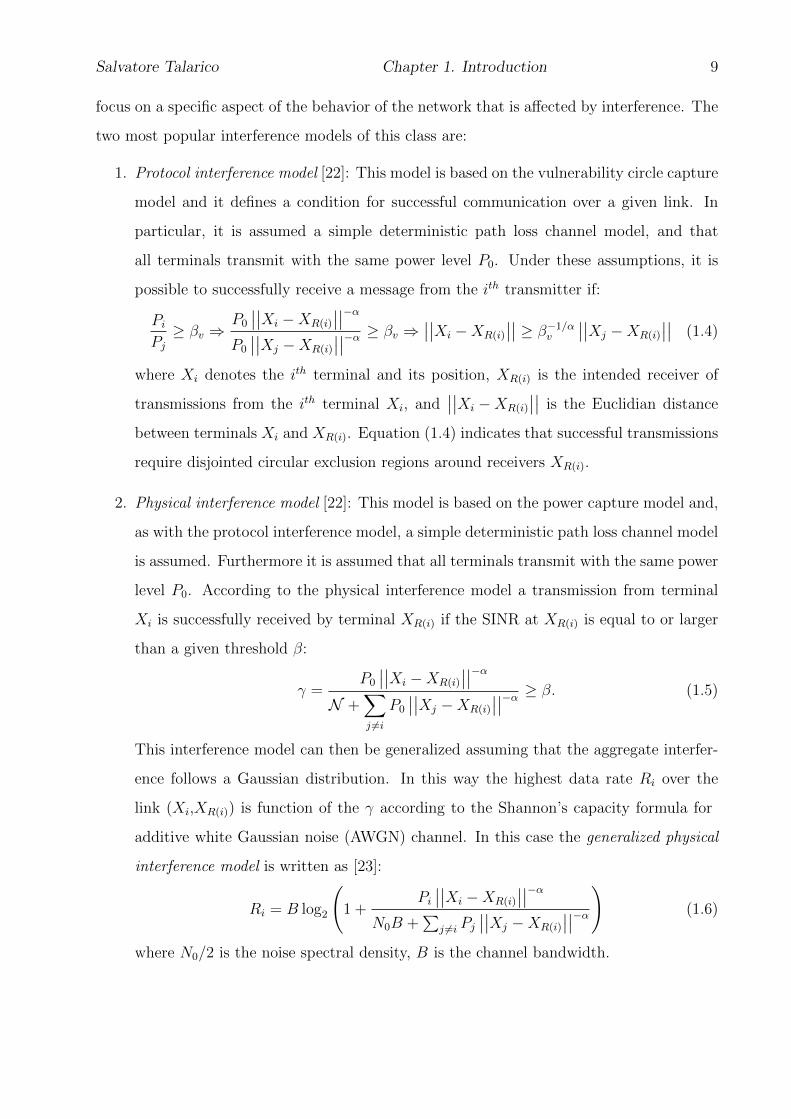
focus on a specific aspect of the behavior of the network that is affected by interference. The
two most popular interference models of this class are:
1. Protocol interference model [22]: This model is based on the vulnerability circle capture
model and it defines a condition for successful communication over a given link. In
particular, it is assumed a simple deterministic path loss channel model, and that
all terminals transmit with the same power level P0. Under these assumptions, it is
possible to successfully receive a message from the ith transmitter if:
PiPj≥ βv ⇒
P0
∣∣∣∣Xi −XR(i)
∣∣∣∣−αP0
∣∣∣∣Xj −XR(i)
∣∣∣∣−α ≥ βv ⇒∣∣∣∣Xi −XR(i)
∣∣∣∣ ≥ β−1/αv
∣∣∣∣Xj −XR(i)
∣∣∣∣ (1.4)
where Xi denotes the ith terminal and its position, XR(i) is the intended receiver of
transmissions from the ith terminal Xi, and∣∣∣∣Xi −XR(i)
∣∣∣∣ is the Euclidian distance
between terminals Xi and XR(i). Equation (1.4) indicates that successful transmissions
require disjointed circular exclusion regions around receivers XR(i).
2. Physical interference model [22]: This model is based on the power capture model and,
as with the protocol interference model, a simple deterministic path loss channel model
is assumed. Furthermore it is assumed that all terminals transmit with the same power
level P0. According to the physical interference model a transmission from terminal
Xi is successfully received by terminal XR(i) if the SINR at XR(i) is equal to or larger
than a given threshold β:
γ =P0
∣∣∣∣Xi −XR(i)
∣∣∣∣−αN +
∑j 6=i
P0
∣∣∣∣Xj −XR(i)
∣∣∣∣−α ≥ β. (1.5)
This interference model can then be generalized assuming that the aggregate interfer-
ence follows a Gaussian distribution. In this way the highest data rate Ri over the
link (Xi,XR(i)) is function of the γ according to the Shannon’s capacity formula for
additive white Gaussian noise (AWGN) channel. In this case the generalized physical
interference model is written as [23]:
Ri = B log2
(1 +
Pi∣∣∣∣Xi −XR(i)
∣∣∣∣−αN0B +
∑j 6=i Pj
∣∣∣∣Xj −XR(i)
∣∣∣∣−α)
(1.6)
where N0/2 is the noise spectral density, B is the channel bandwidth.

Salvatore Talarico Chapter 1. Introduction 10
3. Graph-based Interference Models [24]: Wireless multi-hop networks are often modeled
by employing graph theory, which allows to provide a representation of the network
and the interconnections among nodes. A graph is a representation of a set of objects,
where some pairs of objects can be connected each other by links. The interconnected
objects are represented by mathematical abstractions called vertices, and the links
that connect some pairs of vertices are called edges. Graphs have several features
that make them appropriate for modeling wireless networks, and in particular their
connectivity and interference. Graph-based interference models are particularly useful
in the context of resource allocation or topology control [25, 26]. The connectivity of
a wireless network can be modeled using a connectivity graph GC = (V,EC), where V
is the set of vertices that represent the terminals of the network, and E is the set of
edges connecting any two vertices, which represent the communication links between
the respective terminals. When the focus is on the interference, an interference graph
GI = (VI , EI) is used: if the intent is to model the interference between terminals,
VI is the set of terminals, while EI is the set of edges, which model the interference
between terminals; if the intent is to model the interference between links, VI is the set
of communication links, while EI is the set of edges, which represent the interference
between two links.
1.2 Techniques to Analyze the Network Performance
In the remainder of this dissertation a physical interference model is adopted, when
the dynamics of the channel (e.g., fading and shadowing) and the random locations of the
interferers are taken into account. In this case, γ becomes a random variable and the
cumulative distribution function (CDF) of the SINR is used as a metric for characterizing the
performance of wireless networks. In the literature, there are six different techniques [27,28],
which are used to evaluate the CDF of the SINR once an interference model with a distance
dependent power-law is adopted and interferers are drawn according to a specific point
process:

Salvatore Talarico Chapter 1. Introduction 11
1. Rayleigh fading assumption: since it is not always possible to find a closed-form expres-
sion for the probability density function (PDF) of the aggregate interference [20] and in
order to make the analysis tractable, it is common to assume Rayleigh fading. Under
this assumption, it is not still possible to determine the interference statistic (the CDF
of the aggregate interference), but the exact CDF of the SINR can be obtained, which
has the form:
Fγ (β) = P [γ ≤ β] = 1− exp −NaβLI(s)∣∣∣s=aβ
(1.7)
where LI(s) is the Laplace transform (LT) of the PDF of the aggregate interference I
and a is a constant. The key is to find the LT of the PDF of I, which thanks to the
probability generating functional (PGFL) is easy to compute for many cases involving
a PPP (e.g [14]) or other simple point processes such as a BPP (e.g [29]).
2. Dominant interferers assumption: when deterministic channel gains are assumed, this
technique is used. Under this approach only a subset of interferers is considered, and
in particular only the contribution from the interferers into a vulnerability region or
n nearest interferers are taken into account. Under a high path loss exponent (e.g.,
α = 4), the contribution from the further interferers is negligible and therefore this
approach leads to a tight lower bound for the CDF of the SINR.
3. Approximated PDF of the aggregate interference: in this approach, simulations are
used to empirically fit the PDF of I to a known distribution, such as a Gaussian or
shifted log-normal.
4. Usage of Plancherel-Parseval theorem: an alternative approach to the previously ones
is to use the Plancherel-Parseval theorem. This theorem states that if f1(t) and f2(t)
are square integrable complex functions, then∫Rf1(t)f ∗2 (t)dt =
∫RF1(ω)F∗2 (ω)dω (1.8)
where f ∗(t) is the conjugate of f(t), F1(ω) is the Fourier transform (FT) of f1(t), and
F2(ω) is the FT of f2(t). Since the FT of a PDF is equivalent to the characteristic

Salvatore Talarico Chapter 1. Introduction 12
function of that PDF, it is possible to state that F(ω) = L(s)∣∣∣s=iω
. This last property
allows the inverse LT to be replaced by an integral.
5. Laplace numerical inversion: this last technique makes use of numerical methods to
invert the LT of the PDF of the aggregate interference.
6. Usage of Gil-Pelaez inversion theorem: in [28], the authors obtained exact and approxi-
mated closed-form expressions for the CDF of the SINR by inverting the characteristic
function (CF) of the aggregate interference with the aid of the Gil-Pelaez inversion
formula. This theorem states that
FI (x) =1
2− 1
π
∫ ∞0
Im [exp (−itx) γI(t)]
tdt (1.9)
where γI(x) is the CF of the aggregated interference.
1.3 Computational Complexity in Wireless Networks
Wireless networks are designed to deliver information in real time, and therefore they
are subject to very tight hard real-time timing and protocol constraints, which need to be
regularly satisfied to guarantee their proper operation. One of the features that influences
the reliability and the performance of a network is the computational complexity required to
perform the processing of a signal. If, at a given time, a network requires more computational
resources than those available, or it requires more time to complete a given operation than the
one allowed, it is subject to an outage, and the information cannot be decoded. Therefore,
based on the likelihood of this event, the performance of the network can be greatly impacted.
In modern wireless networks, the computational resources required over time mainly de-
pends on the computational complexity of the channel decoder, which usually performs the
most computational intense operations that increase as the system works closer to channel
capacity. The computational resources are usually distributed in the network, and each
device has its own computational capacity to perform channel decoding. However, novel
architecture, such as Cloud-RAN [30] , use cloud-computing platform to perform central-
ized processing of multiple signals from a pool of BSs, which enables the flexible usage of

Salvatore Talarico Chapter 1. Introduction 13
processing resources through virtualization [31, 32]. Since these type of architectures are
designed with the aim to reduce deployment costs throughout a parsimonious provisioning
of the computational resources, they are particularly vulnerable to the detrimental effect of
computational complexity. For this reason in the past years, an increasing interest has grown
among researcher groups to better design these systems being aware of the computational
penalties that characterize them.
1.4 Scope, Outline and Contributions
The focus of this dissertation is on the effect of interference and computational complex-
ity in wireless communication systems. In particular, this work aims to build an alternative
approach to the one listed in Sec. 1.2, which is able to discard some of common assumptions
previously used and enables the more accurate modeling of both conventional and coopera-
tive wireless systems and provide insights on how to optimize them. Focus is also given on
estimating the data processing requirement for cellular networks that use centralized com-
puting platforms, such as a Cloud-RAN, to perform joint baseband processing on signals
from a group of BSs. The last part of this dissertation focuses then on FH systems and
cooperative protocols and how to model and optimize them when accounting for the effect
of interference.
The discussion starts in Chap. 2, which builds an alterative analytical framework to
evaluate the outage probability of a network subject to fading and with the location of the
interferers distributed according to a point process. In the literature [3, 14, 20, 21, 27, 33–35]
a common assumption is to assume an infinite network, both by having an infinite area, and
by having an infinite number of interferers. While this assumption simplifies the analysis,
it is important to bear in mind that no wireless network is actually infinite. Furthermore,
another drawback of the related literature is that the SINR variable combines the effects
of fading and interferer location, and outage probabilities are computed with respect to
both of these contributions. While certainly the long-term (c.f., ergodic) outage probability
depends on both fading and location, it is important to realize that these mechanisms operate
over time scales that are significantly different. Whereas the fading may change from one

Salvatore Talarico Chapter 1. Introduction 14
transmission to the next, the location of the active interferers will generally remain constant
over the course of many transmissions. In Chap. 2 both assumptions are relaxed by using
an approach which breaks the analysis into discrete steps that consider the fading and
the random topology separately for a finite network. Using the aforementioned analytical
framework, Chap. 2 continues by quantifying the effect of the spatial interference correlation
in finite networks. In order to prove the wide applicability of the framework introduced in
Chap. 2, Chap. 3 applies it to model and analyze the performance of direct-sequence code
division multiplex-access (DS-CDMA) cellular uplinks. The model and the analysis, as will
be more evident later, are very general and can handle a very large variety of MAC protocols
and resource allocation policies.
Chap. 4 extends the analysis introduced in Chap. 2 in order to account for the case when
the receiving device performs diversity combining. In this case, the analysis is applied to
two cases of study: DS-CDMA downlink multi-cell cooperation (MCC) and an Long Term
Evolution (LTE) transmission mode, called multicast-broadcast single-frequency network
(MBSFN), which will be introduced in detail in this chapter. In both cases, an accurate
model is build and a performance analysis is performed with the aim to emphasizing how
cooperative communications should be used in these networks to maximize their benefits.
Chap. 5 focuses on the Cloud-RAN architecture [30]. While most of the recent research
on Cloud-RAN has focused on the RAN functional split, the applicability of joint processing
(e.g. [32]), system performance and implementation options (e.g. [31,36]), and fronthaul re-
quirements (e.g. [37]), this chapter provides a better understanding of the interplay between
available computing resources and the required communications performance. In particular,
Chap. 5 builds an analytical framework to estimate the required data processing resources
under a given performance constraint, which allows to highlights the tradeoff between the
throughput and the computational complexity that characterizes these type of networks, that
is investigated in more details in Chap. 6. Chap. 6 provides insights on how the commu-
nications performance are effected by the computational resources available. Furthermore,
it provides how to optimally allocate the user rate under the assumption of limited compu-
tational resources in a centralized cloud platform and presents three computationally aware
schedulers.

Salvatore Talarico Chapter 1. Introduction 15
Chap. 7 focuses then on FH systems in general, and in particular, considers ad hoc
networks that use a non-coherent continuous-phase frequency-shift keying (CPFSK) modu-
lation. This modulation format depends on the modulation index, the number of frequency
channels in which the overall bandwidth is divided and the fractional in-band power, which
is the fraction of the signal power that lies within the band of each frequency channel. These
parameters are often chosen arbitrarily. However, in this chapter it is shown under two
different rate-allocation policies that optimally selecting them together with the rate, it is
possible to achieve a significant improvement in the performance of the system.
Chap. 8 introduces a new methodology to model and analyze the performance of multi-
hop routing protocols in ad hoc networks which builds on the analytical framework intro-
duced in Chap. 2. This chapter accounts for the effect of the interference and their spatial
correlation and evaluates the performance of two representative geographic routing protocols
in order to gain perspective about their advantages and disadvantages.
Chap. 9 introduces an efficient method to stochastically model and study the perfor-
mance of cooperative multi-hop networks when accounting for CCI originated by multiple
packets that simultaneously propagate along the network. The dynamics of how a coopera-
tive protocol evolves over time is described through an absorbing Markov chain, which uses
the analysis developed in Chap. 4 to evaluate the transmission probability of each relay.
This methodology differs from the ones existing in the literature, since the end-to-end prob-
ability of success of a cooperative network is not evaluated by starting from a single set of
channel realizations (as it is usually done) and then averaging over them, but through the
channel outage framework developed along this dissertation. As already stated, this frame-
work provides the channel outage probability already averaged over the fading and in this
context it drastically reduces the computational effort to model and analyze a cooperative
multi-hop network. As an example of its applicability, this framework is used in this chapter
to analyze the performance of a Barrage relay network (BRN) and perform an optimization
of such a system over a set of parameters, which includes the code rate, and the number of
relays used.
Finally, this dissertation concludes in Chap. 10, which provides some suggestions for
future work.
16
Chapter 2
Channel Outage Analysis in Wireless
Networks
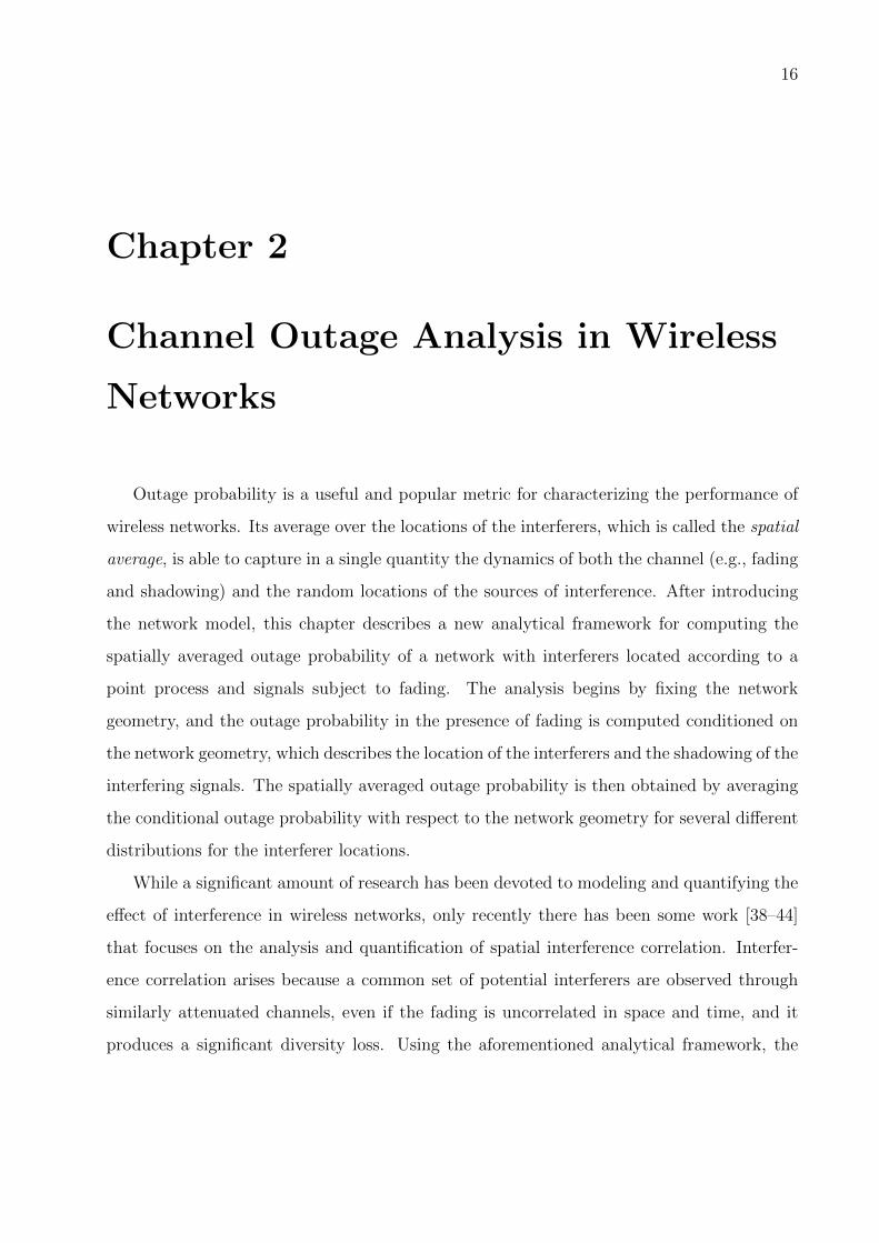
Outage probability is a useful and popular metric for characterizing the performance of
wireless networks. Its average over the locations of the interferers, which is called the spatial
average, is able to capture in a single quantity the dynamics of both the channel (e.g., fading
and shadowing) and the random locations of the sources of interference. After introducing
the network model, this chapter describes a new analytical framework for computing the
spatially averaged outage probability of a network with interferers located according to a
point process and signals subject to fading. The analysis begins by fixing the network
geometry, and the outage probability in the presence of fading is computed conditioned on
the network geometry, which describes the location of the interferers and the shadowing of the
interfering signals. The spatially averaged outage probability is then obtained by averaging
the conditional outage probability with respect to the network geometry for several different
distributions for the interferer locations.
While a significant amount of research has been devoted to modeling and quantifying the
effect of interference in wireless networks, only recently there has been some work [38–44]
that focuses on the analysis and quantification of spatial interference correlation. Interfer-
ence correlation arises because a common set of potential interferers are observed through
similarly attenuated channels, even if the fading is uncorrelated in space and time, and it
produces a significant diversity loss. Using the aforementioned analytical framework, the

S. Talarico Chapter 2. Channel Outage Analysis in Wireless Networks 17
chapter proceeds by analytically characterizing this effect, and semi-closed form expressions
are derived for some special cases. The last part of the chapter presents numerical results to
highlight the correctness of the analysis and draw some conclusions.
2.1 Network Model
Consider a network comprising M + 2 devices that include a reference receiver Yj, a
source or reference transmitter X0, and M interfering devices X1, ..., XM . The interferers
are located within an arbitrary region A, which has area |A|. The number of interferers
within A could be fixed (as in a BPP) or random (as in a PPP). Let ri,j denote the distance
from Xi and the receiver Yj, and let r = r1,j, ..., rM,j represent the set of distances to the
interferers, which corresponds to a specific network topology.
While the interfering devices can be located in any arbitrary region, it is assumed they
are located within the arbitrary region A, but outside a circular region with radius rin,
which is centered at the receiver. A nonzero rin may be used to model an exclusion or guard
zone [45, 46]. As mentioned in the previous chapter, an exclusion zone is a region where no
other transmitter is allowed to be located. On the other hand, another transmitter might be
within a guard zone, but this transmitter is suppressed by the MAC protocol. A guard zone
can be realized by having the receiver send a short clear-to-send (CTS) packet in response
to a request-to-send (RTS) packet sent by the transmitter. Under a carrier sense multiple
access (CSMA) protocol, devices within distance rin from the receiver that overhear the CTS
will suppress their transmissions.
Device Xi transmits a signal whose average received power in the absence of fading and
shadowing is Pi at a reference distance d0. At the reference receiver, Xi’s power is
ρi,j = Pigi,j10ξi,j/10f (r) (2.1)
where gi,j is the power gain due to fading, ξi,j is a shadowing coefficient, and f(r) is a
path loss function. Each gi,j = a2i,j, where ai,j has a Nakagami distribution with parameter
mi,j, and E[gi,j] = 1. In Rayleigh fading, mi,j = 1 and gi,j is exponential. In the presence
of log-normal shadowing, the ξi,j are independent and identically distributed zero-mean

S. Talarico Chapter 2. Channel Outage Analysis in Wireless Networks 18
Gaussian with standard deviation σs dB. In the absence of shadowing, ξi,j = 0. For r ≥ d0,
the path loss function is expressed as the attenuation power law
f (r) =
(r
d0
)−α(2.2)
where α > 2 is the attenuation power-law exponent, and d0 is sufficiently large that the
signals are in the far field.
The instantaneous SINR at the reference receiver Yj is
γj =ρ0,j
N +M∑i=1
Iiρi,j
(2.3)
where N is the noise power and Ii is a Bernoulli variable with P[Ii = 1] = pi, where the
activity probability pi can be used to model voice-activity factors or controlled silence.
Substituting (2.1) and (2.2) into (2.3), the SINR is
γj =g0,jΩ0,j
SNR−1 +M∑i=1
Iigi,jΩi,j
(2.4)
where SNR = dα0P0/N is the signal-to-noise ratio (SNR) when the transmitter is at unit
distance and fading and shadowing are absent, and
Ωi,j =
10ξ0,j/10r−α0,j i = 0
PiP0
10ξi,j/10r−αi,j i ≥ 1(2.5)
is the normalized received power due to Xi.
2.2 Conditional Outage Probability
Let β denote the minimum SINR required for reliable reception and Ω = Ω0,j, ...,ΩM,j
represent the set of normalized received powers. An outage occurs when the SINR falls below
β. When conditioned on Ω, the outage probability is
εj(Ω) = P[γj ≤ β
∣∣Ω]. (2.6)

S. Talarico Chapter 2. Channel Outage Analysis in Wireless Networks 19
Because it is conditioned on Ω, the outage probability depends on the locations of the devices
and the shadowing factors, which have dynamics over timescales that are much slower than
the fading.
Defining a variable
Zj = Sj −M∑i=1
Yi,j (2.7)
where Sj = β−1g0,jΩ0,j and Yi,j = Iigi,jΩi,j, the outage probability, conditioned on Ω, may
be expressed as
εj(Ω) = P[Zj ≤ SNR−1
∣∣Ω] = FZj
(SNR−1
∣∣Ω) (2.8)
which is the CDF of Zj conditioned on Ω and evaluated at SNR−1.
Theorem 2.2.1 The conditional outage probability is
εj(Ω) = 1− exp
(− βm0,j
Ω0,jSNR
)m0,j−1∑µ=0
(βm0,j
Ω0,jSNR
)µ µ∑t=0
SNRt
(µ− t)!∑`i≥0∑Mi=1 `i=t
M∏i=1
[(1− pi) δ`i +
piΓ(`i +mi,j)
`i!Γ(mi,j)
(Ωi,j
mi,j
)`i (βm0,jΩi,j
mi,jΩ0,j
+ 1
)−(mi,j+`i)]. (2.9)
Proof: The details of the derivation are given in Appendix A.
When all transmissions are subject to Rayleigh fading, the gi,j are i.i.d. unit-mean
exponential random variables, and by simply substituting m0,j = mi,j = 1 (2.9), the outage
probability conditioned on Ω is
εj(Ω) = 1− exp
(− β
Ω0,jSNR
) M∏i=1
(Ω0,j + β (1− pi) Ωi,j
Ω0,j + βΩi,j
). (2.10)
The above expression is obtained in [47] working iteratively. Alternatively, when the
distances are normalized such that the reference transmitter is at unit distance from the
receiver, shadowing is neglected and under the assumption that pi = p and Pi = P0 for all
i ∈ 1, ...,M, (2.10) can be found from [20] by substituting that reference’s (2.3) into its
(1.4).

S. Talarico Chapter 2. Channel Outage Analysis in Wireless Networks 20
2.3 Spatially Averaged Outage Probability
The spatially averaged outage probability is found by taking the expectation of ε(Ω)
with respect to the network geometry and shadowing factors. Let εj[M ] denote the spatially
averaged outage probability of a network with a fixed number of interferers, which is found
by taking the expectation of εj(Ω) with respect to Ω under the condition that there are M
interferers; i.e.,
εj[M ] = EΩ [εj(Ω)|M ] =
∫εj(Ω)fΩ (Ω|M) dΩ (2.11)
where fΩ (Ω|M) is the PDF of Ω when there are M interferers.
When the number of interferers is random, then the overall spatially averaged outage
probability, which we denote εj, can be found by taking the expectation of εj[M ] with
respect to the number of interferers in the region. In particular,
εj = EM [εj[M ]] =∞∑m=0
pM [m]εj[m] (2.12)
where pM [m] is the probability mass function (PMF) of M .
2.3.1 Binomial Point Processes
Assume that the M interferers are independently and uniformly distributed (i.u.d.) over
A. Thus, the interferers are drawn from a BPP of intensity λ = M/|A| [21]. Because the
Ωi,j are independent,
fΩ (Ω|M) =M∏i=1
fΩ(Ωi,j) (2.13)
where fΩ(Ωi,j) is the PDF of Ωi,j.
Substituting (2.9) and (2.13) into (2.11) and using the fact that the Ωi,j are identically
distributed, the spatially averaged outage probability can be found as follows
εj[M ] = 1− exp
(− βm0,j
Ω0,jSNR
)m0,j−1∑µ=0
(βm0,j
Ω0,jSNR
)µ µ∑t=0
SNRt
(µ− t)!
∑`i≥0∑Mi=1 `i=t
M∏i=1
[(1− pi) δ`i +
piΓ(`i +mi,j)
`i!Γ(mi,j)z (i, `i)
](2.14)

S. Talarico Chapter 2. Channel Outage Analysis in Wireless Networks 21
where
z (i, `i) =
∫ (Ωi,j
mi,j
)`i (βm0,jΩi,j
mi,jΩ0,j
+ 1
)−(mi,j+`i)
fΩ(Ωi, j) dΩi,j. (2.15)
If an unshadowed scenario is assumed, the normalized received power is equal to Ω0,j =
r−α0,j for the reference transmitter and Ωi,j = PiP0r−αi,j for each of the ith interferers. Since
the only source of randomness in Ωi,j is ri,j, which is the set of distances between the
reference receiver and the interferers, (2.15) can be simplified as follows:
z (i, `i) = P (i, `i)
∫rmi,jα [H (i, `i) r
α + 1]−(mi,j+`i) fr(r) dr (2.16)
where H (i, `i) =mi,jP0
βm0,jPi,jrα0,j, P (i, `i) = H (i, `i)
mi,j 1(rα0,jm0,jβ
)`i and fr(r) is the PDF of
the identically distributed ri,j.
L-sided Regular Polygon Network
Assume that the reference receiver is located at the origin and that A is an L-sided
regular polygon inscribed in a circle of radius rout. The polygon is centered at the origin,
and a circular exclusion zone of radius rin is removed from the center of the polygon to
ensure that all interferers are at least distance rin away. The area of this region is |A| =1
2Lr2
out sin
(2π
L
)− πr2
in. Let rc = rout sin(π(L− 2)/(2L)) be the distance from the origin to
any corner of the polygon. From [48], the identically distributed ri,j have the PDF
fr(r) =
2πr
|A|for rin ≤ r ≤ rc
2πr
|A|− 2Lr
|A|arccos
(rc
r
)for rc ≤ r ≤ rout
(2.17)
and zero elsewhere.
When (2.17) is substituted into (2.16), the integral is∫rmi,jα [H (i, `i) r
α + 1]−(mi,j+`i) fr(r) dr = T1 (i, `i)− T2 (i, `i) (2.18)
where
T1 (i, `i) =2π
|A|
∫ rout
rin
rmi,jα+1 [H (i, `i) rα + 1]−(mi,j+`i) dr (2.19)
T2 (i, `i) =2L
|A|
∫ rout
rc
rmi,jα+1 [H (i, `i) rα + 1]−(mi,j+`i) arccos
(rc
r
)dr. (2.20)

S. Talarico Chapter 2. Channel Outage Analysis in Wireless Networks 22
The first integral is
T1 (i, `i) =2π
|A|[Ψ1 (i, `i, rout)−Ψ1 (i, `i, rin)] (2.21)
where
Ψk(i, `i, y) =
∫ y
0
rmi,jα+k [H (i, `i) rα + 1]−(mi,j+`i) dr. (2.22)
By performing the change of variable r = yν1α ,
Ψk(i, `i, y) =ymi,jα+k+1
α
∫ 1
0
ν(mi,jα+k+1−α)/α [H (i, `i) yαν + 1]−(mi,j+`i) dν
=
(ymi,jα+k+1
mi,jα+k+1
)2F1
([mi,j +`i,
mi,jα+k+1
α
];mi,jα+k+1
α+1;−H (i,`i) y
α
)(2.23)
where 2F1 is the Gauss hypergeometric function,
2F1([a, b]; c;x) =Γ(c)
Γ(b)Γ(c− b)
∫ 1
0
νb−1(1− ν)c−b−1(1− xν)−a dν (2.24)
and since c = b+ 1, Γ(c)/(Γ(b)Γ(c− b)) = b. As the hypergeometric function only converges
for |x| < 1, it follows that convergence requires 1Hi > y, which is satisfied by the following
set of sufficient conditions: (1) β > 1 (or 0 dB), which is true for most modulation/coding
schemes of interest;(2) Pi ≤ P0, which is always true under all power control policies; (3)
y ≤ 1, which is true when the network is normalized to rout = 1; and (4) m0,j ≥ mi,j,
which is true when the reference transmitter is more line-of-sight (LOS) than the interferers.
Note also that (2.24) does not converge when c is a non-positive integer. Furthermore, it is
important to note that while the hypergeometric function is itself an integral, it is widely
known and is implemented as a single function call in most mathematical programming
languages, including Matlab.
The above analysis agrees with [49], which does not include an exclusion zone (rin = 0),
and uses numerical integration to evaluate (2.20). Alternatively, the second integral can be
found by substituting the Taylor series expansion of arccos given by [50]
arccos (x) =π
2−∞∑n=0
(2n)!x2n+1
4n (n!)2 (2n+ 1)(2.25)
into (2.20), resulting in
T2 (i, `i) =2L
|A|[K (i, `i, rout)−K (i, `i, rc)] (2.26)

S. Talarico Chapter 2. Channel Outage Analysis in Wireless Networks 23
where
K (i, `i, y) =π
2Ψ1 (i, `i, y)−
∞∑n=0
(2n)!r2n+1c
4n (n!)2 (2n+ 1)Ψ−2n (i, `i, y) . (2.27)
By substituting (2.18) into (2.16) with T1 (i, `i) given by (2.21) and T2 (i, `i) given by
(2.26), it yields
z (i, `i) =2P (i, `i)
|A|[πΨ1 (i, `i, rout) + LK (i, `i, rc)− πΨ1 (i, `i, rin)− LK (i, `i, rout)] .(2.28)
Finally by substituting (2.28) into (2.14) it is possible to obtain a closed form expression for
the spatially averaged outage probability.
If all transmissions are subject to Rayleigh fading (m0,j = mi,j = 1), and under the
assumption that pi = p and Pi = P0 for all i ∈ 1, ...,M, the spatially averaged outage
probability is [51]
ε[M ] = 1−exp
(−βrα0,jSNR
)[1 +
p
|A|Θ(rin, rc, rout)
]M(2.29)
where
Θ(x, y, z) = π [Φ(z)− Φ(x)]− 2L
βrα0j[K(z)−K(y)]− C(z) (2.30)
Φ(x) =2
βrα0jΨ1(x)− x2 (2.31)
C(x) = x2
[1
2L sin
(2π
L
)− π
](2.32)
Ψk(x) = Ψk (i, `i, x) (2.33)
K(x) = K (i, `i, x) . (2.34)
Annular Network
Assume that the reference receiver is located at the origin and that the interferers are
in an annular region with inner radius rin and outer radius rout. Clearly, this shape is the
limiting case of the polygon as L→∞. In this case, rc → rout, and substituting (2.28) into

S. Talarico Chapter 2. Channel Outage Analysis in Wireless Networks 24
(2.14),
εj[M ] = 1− exp
(− βm0,j
Ω0,jSNR
)m0,j−1∑µ=0
(βm0,j
Ω0,jSNR
)µ µ∑t=0
SNRt
(µ− t)!∑`i≥0∑Mi=1 `i=t
M∏i=1
(1− pi) δ`i +
2πpiΓ(`i +mi,j)P (i, `i)
`i!Γ(mi,j)|A|[Ψ1 (i, `i, rout)−Ψ1 (i, `i, rin)]
(2.35)
where |A| = π(r2out − r2
in).
If all transmissions are subject to Rayleigh fading and under the assumption that pi = p
and Pi = P0 for all i ∈ 1, ...,M, since rc → rout and C(rout)→ 0, (2.29) becomes [51]
εj[M ] = 1− e−βrα0j/SNR
(1 +
pπ
|A|[Φ (rout)− Φ (rin)]
)M. (2.36)
To compute the spatially averaged outage probability in the presence of shadowing, the
PDFs fΩ0,j(ω0,j), ...., fΩM,j(ωM,j) used in (2.14) need to be derived to account for the shadow-
ing distribution. First consider the normalized power of the desired signal from the reference
transmitter X0. Because the distance r0,j between the reference transmitter and receiver is
deterministic, Ω0,j = 10ξ0,j/10r−α0,j is a log-normal variable with PDF
fΩ0,j(ω) =
10 (2πσ2s )− 1
2
ln(10)ωexp
−102 log2
10 (rα0ω)
2σ2s
(2.37)
for 0 ≤ ω ≤ ∞, and zero elsewhere.
For i ≥ 1, corresponding to the devices drawn from the BPP, the PDF is
fΩi,j(ω) = ω−2+αα
[ζ (ciωrαout)− ζ (ciωr
αin)]
αc−2/αi (r2
out − r2in)
(2.38)
for 0 ≤ ω ≤ ∞, and zero elsewhere, where ci = (P0/Pi) and
ζ(z) = erf
(σ2
s ln2(10)− 50α ln (z)
5√
2ασs ln(10)
)eσ2
s ln2(10)
50α2 . (2.39)
By substituting (2.9) and (2.13) into (2.11), using (2.37) and (2.38) and after few algebraic
manipulations, the spatially averaged outage probability is found to be
εj[M ] = 1−m0,j−1∑s=0
s∑t=0
SNRt
(s− t)!∑`i≥0∑Mi=0 `i=t
∫ ∞0
exp
−βm0,j
ySNR
(βm0,j
ySNR
)s
×M∏i=1
[(1− pi)δ`i +
∫ ∞0
κ
(ω,βm0,j
y
)ϕ(ω)dω
]fΩ0,j
(y) dy
(2.40)

S. Talarico Chapter 2. Channel Outage Analysis in Wireless Networks 25
where
ϕ(ω) = ζ (ciωrαout)− ζ (ciωr
αin) (2.41)
κ(x, t) =piΓ(`i +mi,j)x
−( 2+αα )(
xmi,j
)`iαc
2/αi (r2
out − r2in)(`i!)Γ(mi,j)
(xtmi,j
+ 1)(mi,j+`i)
. (2.42)
In order to compute the outage probability, the integral inside the product in (2.40) can be
evaluated numerically by Simpson’s method, which provides a good tradeoff between accu-
racy and speed, while the second integral can be evaluated through Monte Carlo integration.
Arbitrary Area
Assume that the reference receiver is located at the origin and that the interferers are in
an arbitrarily shaped area. In this case, the integral in (2.16) cannot generally be evaluated
in closed form for an unshadowed scenario and the analysis doesn’t reduce to closed form
expression for a shadowed scenario as well. However, for the unshadowed scenario the integral
in (2.16) is just a one-dimensional integral and as such, it can easily be evaluated numerically
for each term of the multinomial summation in (2.14).
In Rayleigh fading, for an unshadowed scenario and under the assumption that pi = p
and Pi = P0 for all i ∈ 1, ...,M, the spatially averaged outage probability can be found by
substituting (2.10) and (2.13) into (2.11) and using the fact that the ri,j are identically
distributed:
εj[M ] = 1− exp
(−βrα0,jSNR
)[1− p+ p
∫fr(r)
rα
βrα0j + rαdr
]M. (2.43)
It follows that in this case computing the outage probability for a BPP boils down to eval-
uating a single one-dimensional integral.
In particular, the integral can be expressed as∫fr(r)
rα
βrα0j + rαdr = Er
[rα
βrα0j + rα
]. (2.44)
The right side of (2.44) suggests a simple numerical approach to solving the integral: Draw
a large number of points ri,j distributed according to fr(r), and for each one of the points

S. Talarico Chapter 2. Channel Outage Analysis in Wireless Networks 26
evaluate the function g(r) = (1 + βrα0jr−α)−1. The integral is then well approximated by the
average of the g(ri,j). This is an alternative to [49], which requires fr(r) to be determined
and substituted into the integral before it is numerically integrated. When the process is
homogeneous, the ri,j can be selected by placing the shape inside a box, randomly selecting
a point with uniform probability in the box and if the point falls within the shape, including it
in the set of ri,j, then repeating the process until ri,j is sufficiently large. This approach
is a Monte Carlo simulation, but it is a simple simulation of the location of a single interferer.
Importantly, it is not a simulation that requires the fading coefficients to be realized, and it
does not require all M interferers to be placed. Alternatively, the ri,j could be selected by
overlaying the shape with a fine grid of equally spaced points.
2.3.2 Poisson Point Processes
Suppose that the interferers are drawn from a PPP with intensity λ on the plane R2. Let
εj(A) denote the outage probability considering only those interferers located within region
A. The number of interferers M within region A is Poisson with mean E[M ] = λ|A|. It
follows that the PMF of the number of interferers within A is given by [21]
pM [m] =(λ|A|)m
m!exp (−λ|A|) , for m ≥ 0. (2.45)
The outage probability can then be found for any arbitrary A and for both a shadowed
and an unshadowed scenario by substituting (2.45) and the appropriate εj[m] into (2.12).
For the general case that m0,j may be any positive integer, the computation of (2.12) requires
the summation to be truncated. However, in the specific case of Rayleigh fading (mi,j = 1
for all i) and no shadowing, and under the assumption that the reference receiver is located
at the center of the network, the summation may be found in closed form.
L-sided Regular Polygon Network
Assuming Rayleigh fading and that both Pi = P0 and pi = p are common for all i,
substituting (2.45) and (2.29) into (2.12) gives
εj(A) = 1− exp
(−λ|A| −
βrα0,jSNR
) ∞∑m=0
1
m![λ|A|+ λpΘ(rin, rc, rout)]
m . (2.46)

S. Talarico Chapter 2. Channel Outage Analysis in Wireless Networks 27
By using the power-series representation of the exponential function given by [50]
∞∑m=0
am
m!(1− c · bm) = ea − c · ea·b (2.47)
into (2.46), the spatially averaged outage probability is found to be
εj(A) = 1− exp
− βr
α0
SNR+ λpΘ(rin, rc, rout)
. (2.48)
Annular Network
If A is a disk of radius rout, the outage probability can be found from (2.48) with rc = rout,
εj(A) = 1− exp
−βrα0,jSNR
+ πλp [Φ(rout)− Φ(rin)]
. (2.49)
Theorem 2.3.1 When A includes the interferers on the entire plane R2, the outage proba-
bility is
εj = 1− exp
−βr2
0,j
SNR− 2π2λp
αβ
2α r2
0,j csc
(2π
α
). (2.50)
Proof: The details of the derivation are given in Appendix B using both probability theory,
and tools from stochastic geometry [21].
In the absence of noise (SNR = ∞), (2.50) coincides with equation (3.4) of [14] and
equation (61) of [52]. The utility of (2.49) is that it generalizes those earlier two equations,
as it permits a non-zero exclusion zone, a finite network area, and a finite SNR.
Arbitrary Area
Assume that the interferers are in an arbitrarily shaped area. Similar to the case when
the interferers are distributed according to a BPP, generally the spatially averaged outage
probability cannot be evaluated in closed form, but it can be numerically evaluated.
In Rayleigh fading, when the distances are normalized such that the reference transmitter
is at unit distance from the receiver and under the assumption that pi = p and Pi = P0 for
all i ∈ 1, ...,M, the spatially averaged outage probability can be found by substituting

S. Talarico Chapter 2. Channel Outage Analysis in Wireless Networks 28
(2.44) and (2.45) into (2.12) and using the power-series representation of the exponential
function:
εj = 1− exp
−βrα0,jSNR
− pM + pM
∫fr(r)
rα
βrα0,j + rαdr
. (2.51)
It follows that in this case computing the outage probability for a PPP reduces to evaluating
a single one-dimensional integral, which can be solved either numerically or by a simple
Monte Carlo simulation as described in Sec. 2.3.1.
2.4 Spatial Interference Correlation
The spatial interference correlation describes how the outages at two different points in
space are correlated. Interference correlation arises because a common set of potential inter-
ferers are observed through similarly attenuated channels, even if the fading is decorrelated
in space and time. The spatial interference correlation can be used to analyze and design
multi-hop networks, and compression transmission strategies when cooperation is employed.
The spatial interference correlation is quantified by evaluating the correlation coefficient
of the outage probability at two different receivers (Y1 and Y2), which is
ρ [ε1 (Ω) , ε2 (Ω)] =EM,Ω [ε1 (Ω) ε2 (Ω)]− E2
M,Ω [εj (Ω)]
EM,Ω
[ε2j (Ω)
]− E2
M,Ω [εj (Ω)](2.52)
where EM,Ω [·] is the expectation operator, evaluated over the number of interferers and
their normalized powers, and either j = 1 or j = 2 could be used as the two receivers are
stochastically equivalent (they experience the same average outage probability).
Similar to the analytical framework described in Sec. 2.2 and Sec. 2.3, the expectations
in (2.52) can be first evaluated over the spatial distribution of the interferers, and then over
their number. Specifically, the spatially averaged first moment of the outage probability over
Ω conditioned over the number of interferers M can be evaluated by (2.11). The spatially
averaged second moment of the outage probability over Ω conditioned over the number of
interferers M is
EΩ
[ε2j (Ω) |M
]=
∫ε2j (Ω) fΩ (Ω|M) dΩ. (2.53)

S. Talarico Chapter 2. Channel Outage Analysis in Wireless Networks 29
r0
rout
θ
X0
Y2
Y1
Figure 2.1: Typical network topology. The reference transmitter is located at the center.The two reference receivers are represented by the two red stars on the circumference ofradius r0.
The spatially averaged first joint moment of the outage probability over Ω conditioned over
the number of interferers M is
EΩ [ε1 (Ω) ε2 (Ω) |M ] =
∫ε1 [Ω] ε2 [Ω] fΩ (Ω) dΩ. (2.54)
When the number of interferers is random, the overall spatially averaged first, second
and first joint moment of the outage probability can be obtained by averaging with respect
to M . In particular, it is possible to use the following equality
EM,Ω
[εxi (Ω) εyj (Ω)
]=
∞∑m=0
pM [m]EΩ
[εxi (Ω) εyj (Ω) |m
]. (2.55)
2.4.1 Special Cases
Assume the reference transmitter is located at the center of a circular network of radius
rout. Assume the receiver Y1 and Y2 are located on a circle of radius r0 within the network
(r0,1 = r0,2 = r0) and the vectors connecting their locations to the origin form an angle θ,
as depicted in Fig. 2.1. For simplicity of exposition, assume a Rayleigh-faded channel (for

S. Talarico Chapter 2. Channel Outage Analysis in Wireless Networks 30
Nakagami fading, a similar derivation can be performed), an unshadowed scenario. As in
the previous sections, assume Pi = P0 and pi = p0 for all i.
Binomial Point Process
Assume that the M interferers are independently and uniformly distributed (i.u.d.) over
A. Thus, the interferers are drawn from a BPP of intensity λ = M/|A|.
Theorem 2.4.1 The spatially averaged first moment of the outage probability is
EΩ [εj (Ω) |M ] = 1− exp
(βrα0SNR
)1− p+
2p
|A|
[π
βrα0Ψ1 (rout − r0) + Z1 (rout, r0)
]M(2.56)
where the function Zi (rout, r0) is given by (C.3).
Proof: The details of the derivation are given in Appendix C.
Theorem 2.4.2 The spatially averaged second moment of the outage probability is
EΩ
[ε2j (Ω) |M
]= 2EΩ [εj (Ω) |M ]− 1 + exp
(−2βrα0SNR
)SM (rout, r0) (2.57)
where the function S (rout, r0) is given by (C.6).
Proof: The details of the derivation are given in Appendix C.
Theorem 2.4.3 The spatially averaged joint first moment of the outage probability is
EΩ [ε1 (Ω) ε2 (Ω) |M ] = 2EΩ [εj (Ω) |M ]− 1 + exp
(−2βrα0SNR
)WM (rout, r0, θ) (2.58)
where the function W (rout, r0, θ) is given by (C.11).
Proof: The details of the derivation are given in Appendix C.
Finally, by substituting (2.56), (2.57) and (2.58) in (2.52), the correlation coefficient can
be evaluated.
Poisson Point Process
Suppose that the interferers are drawn from a PPP with intensity λ within an circular
region of radius rout. Set x = 0 and y = 1 in (2.55), and substitute (2.45), and (2.56) within

S. Talarico Chapter 2. Channel Outage Analysis in Wireless Networks 31
it. By applying the power-series representation of the exponential function, the spatially
averaged first moment of the outage probability is
EM,Ω [εi (Ω)] = 1− exp
− βr
α0
SNR− 2λp
[|A|2− π
βrα0Ψ1 (rout − r0) + Z1 (rout, r0)
]. (2.59)
Set x = 0 and y = 2 in (2.55), and substitute (2.45) and (2.57) within it. By applying
again the power-series representation of the exponential function, the spatially averaged
second moment of the outage probability is
EM,Ω
[ε2i (Ω)
]= 2EM,Ω [εi (Ω)]− 1 + exp
−2βrα0SNR
− λ|A| [1 + S (rout, r0)]
. (2.60)
Set x = 1 and y = 1 in (2.55), and substitute (2.45) and (2.58) within it. By using
the power-series representation of the exponential function, the spatially averaged first joint
moment of the outage probability is
EM,Ω [ε1 (Ω) ε2 (Ω)] = 2EM,Ω [εi (Ω)]− 1 + exp
−2βrα0SNR
− λ|A| [1 +W (rout, r0, θ)]
.(2.61)
Finally, by substituting (2.59), (2.60) and (2.61) in (2.52), the correlation coefficient can
be evaluated.
2.5 Numerical Results
In this section, numerical results are provided and, unless otherwise stated, it is assumed
that the network consists of a source transmitter placed at unit distance from the receiver
(i.e., r0,j = 1) and M interferers placed independently according to a given spatial distri-
bution in an annular region with inner dimension rin = 0.25 and outer dimension rout = 4.
Furthermore Ω is evaluated by assuming a path loss exponent α = 3, a common transmit
power Pi = P0, and the absence of shadowing. The activity probability is common for all
the transmitters pi = p, and the SINR threshold is set to β = 3.7 dB.
Fig. 2.2 shows the conditional outage probability ε (Ω) when the common activity prob-
ability is p = 1/200 and fifty interferers are independently placed according to a BPP in
an annular region as shown in the inset as function of SNR for three cases: 1) all channels
are Rayleigh faded; 2) Nakagami fading with all channels mi,j = 4, which represents the

S. Talarico Chapter 2. Channel Outage Analysis in Wireless Networks 32
−5 0 5 10 15 20 2510
−2
10−1
100
SNR (in dB)
Con
ditio
nal o
utag
e pr
obab
ility
, εj (
Ω)
Rayleigh
Nakagami
Mixed
Figure 2.2: Conditional outage probability εj (Ω) as a function of SNR. Analytical curvesare solid while dots represent simulated values. Top curve: all channels Rayleigh. Middlecurve: all channels mi,j = 4. Bottom curve: m0,j = 4 for the source, and mi,j = 1 for theinterferers. The network topology is shown in the inset. The receiver is represented by thestar at the center of the radius-4 circle, the desired transmitter is the big red dot, while the50 interferers are shown as blue dots.
situation where the source and interferer are equally visible to the receiver; 3) Mixed fading
with m0,j = 4 for the source and mi,j = 1 for the interferers, which represents a more typical
situation where the interferers are not in the LOS. The three curves are obtained by using
(2.9). Also shown are curves generated by simulation, which involve randomly generating the
Nakagami-distributed gi,j and selecting the interferers from a uniform distribution. The
analytical and simulation results coincide, which is to be expected because (2.9) is exact.
Any discrepancy between the curves can be attributed to the finite number of Monte Carlo
trials (one million trials were executed per SNR point).
The spatially averaged outage probability for a BPP is shown as a function of M for
two values of p in Fig. 2.3. A mixed-fading model is assumed, i.e. m0,j = 4 and mi,j = 1
for i ≥ 1, and SNR = 10 dB is fixed. For each value of p, three curves are shown, one
without shadowing and two with shadowing. To model log-normal shadowing, each ξi,j is
drawn from a zero-mean Gaussian distribution with standard deviation σs that varies among
the set σs = 4, 8 dB. From Fig. 2.3, it is observed that the outage probability degrades

S. Talarico Chapter 2. Channel Outage Analysis in Wireless Networks 33
0 10 20 30 40 50 6010
−2
10−1
100
p =0.1
p=0.01
M
Spa
tially
ave
rage
d ou
tage
pro
babi
lity,
ε j (M
)
σs = 8 dB
σs = 4 dB
No Shadowing
Figure 2.3: Spatially averaged outage probability for a BPP as a function of the number ofinterferers M for two values of p. For each p, curves are shown for the case of no shadowing,and for shadowing with two values of σs.
with increasing M and decreasing p, and that shadowing increases the average ε (M) with
increasing σs for the given parameters.
Fig. 2.4 shows the spatially averaged outage probabilities in unshadowed Rayleigh fading
as a function of λp, when the interfering devices are placed according to a PPP with intensity
λ in a circular region of radius rout (rin = 0) and SNR = 10 dB. Four network radii are
considered: rout = 1, 2, 4,∞. The outage probabilities of the three networks with finite
radius were computed using (2.49), while the outage probability of the infinite network
(shown by the dashed curve) was computed using (2.50). In addition, simulation results
(shown in this figure by dots) are shown for the three finite networks, which coincide with
the theoretical curves. For the simulations, one million trials were executed per λ point. Any
discrepancy between the theoretical result and the simulation is due to the finite number of
trials. Fig. 2.4 exhibits the effect of the finite spatial extent of a network and shows that
the outage probability increases with increasing λp and/or increasing rout.
The performances are compared when the reference receiver is at the center of the three
different shapes, which are shown in the inset of Fig. 2.5. The shapes are a disk of radius
rout = 2, a triangle (L = 3 polygon), and an arbitrary shape, which happens to look like a
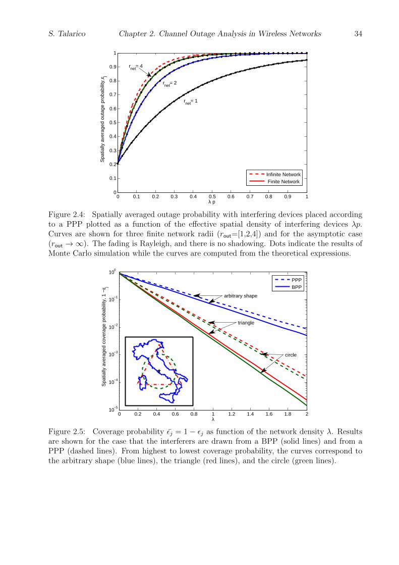
S. Talarico Chapter 2. Channel Outage Analysis in Wireless Networks 34
0 0.1 0.2 0.3 0.4 0.5 0.6 0.7 0.8 0.9 10
0.1
0.2
0.3
0.4
0.5
0.6
0.7
0.8
0.9
1
rnet= 4
rnet= 2
rnet= 1
λ p
Spa
tially
ave
rage
d ou
tage
pro
babi
lity,
ε j
Infinite Network Finite Network
Figure 2.4: Spatially averaged outage probability with interfering devices placed accordingto a PPP plotted as a function of the effective spatial density of interfering devices λp.Curves are shown for three finite network radii (rout=[1,2,4]) and for the asymptotic case(rout →∞). The fading is Rayleigh, and there is no shadowing. Dots indicate the results ofMonte Carlo simulation while the curves are computed from the theoretical expressions.
0 0.2 0.4 0.6 0.8 1 1.2 1.4 1.6 1.8 210
−5
10−4
10−3
10−2
10−1
100
λ
Spa
tially
ave
rage
d co
vera
ge p
roba
bilit
y, 1
− ε j
arbitrary shape
triangle
circle
PPPBPP
Figure 2.5: Coverage probability εj = 1− εj as function of the network density λ. Resultsare shown for the case that the interferers are drawn from a BPP (solid lines) and from aPPP (dashed lines). From highest to lowest coverage probability, the curves correspond tothe arbitrary shape (blue lines), the triangle (red lines), and the circle (green lines).

S. Talarico Chapter 2. Channel Outage Analysis in Wireless Networks 35
0 0.1 0.2 0.3 0.4 0.5 0.6 0.7 0.8 0.9 10
0.1
0.2
0.3
0.4
0.5
0.6
0.7
0.8
0.9
1
θ/π
Spa
tially
ave
rage
d co
rrel
atio
n co
effic
ient
, ρ[ε 1(Ω
),ε 2(Ω
)]
PPPBPPλp = 5/πλp = 25/πλp = 50/π
Figure 2.6: Spatially averaged correlation coefficient as function of θ/π. Results are shownfor the case that the interferers are drawn from a BPP (solid lines) and from a PPP (dashedlines) and for three values of λp.
map of Italy including the islands of Sicily and Sardinia (emphasizing that A need not be
contiguous). In all cases, the shapes are scaled so that they have the same area, |A| = 4π,
and there is no exclusion zone around the receiver; i.e., rin = 0. The spatially averaged
outage probability for each network was computed for interferer densities λ ≤ 2, path loss
exponent α = 3.2, threshold β = 0 dB, and average SNR = 10 dB. Results are shown for
both the BPP and the PPP cases. For the triangle, the series in (2.27) is truncated at the
25th term. For the arbitrary region, the integral in (2.43) and (2.51) is evaluated using a
fine grid of 125, 640 equally spaced points. The spatially averaged coverage probabilities,
defined as εj = 1 − εj are shown in Fig. 2.5. As can be seen, the disk-shaped network
has the worst spatially averaged coverage probability, while those that depart from a circle
have better performance. The spatially averaged coverage probability of the PPP is better
than that of the BPP. The irregularly shaped network has a very high spatially averaged
coverage probability, suggesting that the common assumption of a disk shaped network is
overly pessimistic for realistic networks with highly irregular shapes.
Finally, the spatially averaged correlation coefficient of the outage probability as a func-
tion of the angle θ formed between two receivers and the reference transmitter is shown in

S. Talarico Chapter 2. Channel Outage Analysis in Wireless Networks 36
Fig. 2.6. Results are shown in unshadowed Rayleigh fading for both the BPP and PPP
cases and for three values of λp. The network is circular with radius rout = 1, and both
receivers are at distance r0 = 0.25 from the reference transmitter located at the center. Fig.
2.6 shows that the outage probability is more correlated in a sparse network. This is because
in a sparse network, it is more likely that the same interferer will dominate at both receiver
locations. This is in contrast with a dense network, where the dominant interferer at the
first receiver location is usually different than the dominant interferer at the other location.
This is because in a sparse network, it is more likely that the same interferer will dominate
at both receiver locations. This is in contrast with a dense network, where the dominant
interferer at the first receiver location is usually different than the dominant interferer at
the other location. Furthermore, Fig. 2.6 shows that a PPP experiences a higher correlation
than a BPP, which might seam counterintuitive since a PPP adds an additional degree of
diversity due to the stochastic nature of the number of interference involved in the transmis-
sion. However, even if the values of the outage probability might vary more under a PPP
between one snapshot to another, this type of process can lead to snapshots of the network
in which the interferers are sparser than those obtained with a BPP, and this scenario as
explained above is characterized by a higher correlation.
2.6 Chapter Summary
While the standard way to find the spatially averaged outage probability is to use the LT
and PGFL, as outlined in [27], it is possible to obtain the same result in a more direct manner.
This chapter introduced a new analytical framework for computing the spatially averaged
outage probability of a network with interferers located according to a point process and
signals subject to fading. The starting point is to find the outage probability conditioned
on the network topology and shadowing factors. Next, the number of interferers is fixed
and the outage probability is averaged with respect their random positions and eventually
shadowing. The result is the outage probability for a BPP. Then, the outage probability for
a BPP is marginalized with respect to the number of interferers to get the outage probability
for a PPP, which generalizes the case when the network extends over the entire plane. In

S. Talarico Chapter 2. Channel Outage Analysis in Wireless Networks 37
fact, by allowing the network to be infinite, the classic result of Baccelli et al. [14, 52] is
obtained.
The main benefit of this approach is that it breaks the analysis into discrete steps that
consider the fading and the random topology separately, in contrast with lumping them
together as done by using tools from stochastic geometry [21]. This is useful, since the
two effects have a different timescales, and, in particular, fading changes more rapidly than
the locations of the interferers. Another benefit is that this approach provides a way to
deal with spatial distributions that are not mathematically tractable by using a Monte
Carlo simulation, without the need to average over the fading. Furthermore, the spatially
averaged outage probability in Rayleigh fading reduces to a single one-dimensional integral
for both a BPP and a PPP, which when closed form expression cannot be found, it can
be simply evaluated either numerically or by a Monte Carlo simulation of the location of a
single interferer.
Finally, this chapter concludes by applying the aforementioned analytical framework
in order to quantify the effect of the spatial interference correlation and semi-closed form
expressions are derived. Despite the fact that a direct approach is used, a key difference
with the previous work is that the interference correlation is quantified analytically for finite
networks, instead of relying on the common assumption of an infinite network.
38
Chapter 3
Cellular Networks: Modeling and
Analysis
This chapter applies the analytical framework developed in Chap. 2 to accurately model
and analyze cellular networks, by capturing the effect of the interference and the interdepen-
dence among some of the system parameters. This chapter provides a performance analysis
of the uplink of a DS-CDMA cellular network under different resource allocation policies.
While the focus of this chapter is on the uplink, a similar model and analysis can be also
applied to the downlink [53]. Furthermore, as will be more evident in this chapter, the
methodology described here is very general, and can be adapted to study the performance
of a large variety of MAC protocols and resource allocation policies.
The methodology introduced here [54, 55] is able to discharge some of the unrealistic
assumptions that are often made in literature, such as: 1) infinite network both in extent
and number of user equipments (UEs) and BSs; 2) regular or completely random deployment
of the network, which poorly mimics a real deployment; 3) circular or regular shaped radio
cells where the spatial distribution of both BSs and UEs are independent; 4) identical fading
conditions for each link; 5) path loss model characterized by a fixed path-loss exponent; 6)
absence of shadowing; 7) neglect of thermal noise.

S. Talarico Chapter 3. Cellular Networks: Modeling and Analysis 39
3.1 Modeling and Analysis for Cellular Networks
A cellular network is a wireless network that is distributed over land areas called cells,
each served by at least one fixed-location transceiver, known as a BS. A sector is defined
as the range of angles from which a directional sector antenna can receive signals. A UE
within the sector of a sector antenna is said to be covered by the sector antenna. Cells may
be divided into sectors by using several directional sector antennas or arrays, each covering
disjoint angles, at the BSs.
The classical analysis of the cellular downlinks (e.g., [56]) and uplinks (e.g., [57–59]) in
a cellular network entails a number of questionable assumptions, including the existence of
a lattice or regular grid of BSs and the modeling of intercell interference at a BS as a fixed
fraction of the total interference. Although conceptually simple and locally tractable, the grid
assumption is a poor model for actual BS deployments, which cannot assume a regular grid
structure due to a variety of regulatory and physical constraints. The intercell-interference
assumption is untenable because the fractional proportion of intercell interference varies
substantially with the UE and BS locations, the shadowing, and the fading.
More recent analyses of cellular networks (e.g., [60–66]) locate the UEs and/or the BSs
according to a two-dimensional PPP over a network that extends infinitely on the Euclidian
plane, thereby allowing the use of analytical tools from stochastic geometry. Although the
two principal limitations of the classical approach are eliminated, the PPP approach is
still unrealistic because it does not permit a minimum separation between BSs or between
UEs. However, both the minimum separations are characteristic of actual macro-cellular
deployments. Other problems with the PPP model are that no network has an infinite area
and that any realization of a PPP could have an implausibly large number of UEs or BSs
placed within a finite area.
When tools from stochastic geometry are used in order to considerably simplify the
tractability of the problem, the adoption of a simple point process to model the spatial
distribution of both BSs and UEs is not the only unrealistic assumption. In this case, in fact,
it is often assumed [65] that the radio cells are circular, and the spatial distribution of the UEs
and BSs are independent. This last assumption may lead to snapshots of the network where

S. Talarico Chapter 3. Cellular Networks: Modeling and Analysis 40
there are several overlapping cells, which is not realistic for macro-cellular deployments, while
however might well model an heterogeneous cellular network. For the aim of tractability,
often the effect of thermal noise and shadowing are also neglected. Furthermore, it is often
assumed identical fading conditions for each link and the analysis is constrained to the use of
a standard distance-dependent path loss model with a single slope or more recently with the
dual-slope [67]. While these two assumptions are widely used to design, model and analyze
cellular networks, they do not capture adequately the dependency of the fading and path loss
on the link distance, which is extremely important to properly model and analyze densely
deployed and millimeter wave cellular networks [68,69].
This chapter introduces a methodology based on the analysis built in Chap. 2, which
relaxes all the aforementioned assumptions to more realistically model cellular networks.
3.2 Network Model
Practical sector antennas have patterns with sidelobes that extend into adjacent sectors,
but the performance degradation due to overlapping sectors is significant only for a small
percentage of UE locations. Three ideal sector antennas and sectors per BS, each covering
2π/3 radians, are assumed in this section. The UE antennas are assumed to be omnidirec-
tional. The UEs in the directions covered by a sector antenna can cause intracell or intercell
multiple-access interference from a UE to its associated sector antenna, as illustrated in Fig.
3.1. Thus, the number of interfering signals on the uplink is reduced approximately by a
factor equal to the number of sectors.
In this section, assume the network comprises K BSs and cells, Ssector = 3K sectors
Y1, ..., YSsector, and M UEs X1, ..., XM. The BSs and UEs are confined to a finite arena
of area |A|. The sector boundary angles are the same for all BSs. Let Yj denote the set
of UEs covered by sector antenna Yj and Mj = |Yj| be the number of UEs served by Yj.
A UE Xi ∈ Yj will be associated with Yj if the UE’s signal is received at Yj with a higher
average power than at any other sector antenna in the network. Let Xj ⊂ Yj denote the set
of UEs associated with sector antenna Yj. Furthermore, let g(i) be a function that returns
the index of the sector serving Xi so that Xi ∈ Yj if g(i) = j. If Xi cannot connect to any

S. Talarico Chapter 3. Cellular Networks: Modeling and Analysis 41
Intercell interfererIntracell interferer
Figure 3.1: Illustration of intracell (all the UEs within the light red area) and intercell (allUEs within the orange area) interference. BSs are represented by large circles, and UEs arerepresented by black dots with the exception of the reference UE which is a green star. Cellboundaries are represented by thick blue lines.
BS, which is possible when a cell runs out of available channels, then g(i) = 0.
The power of Yj received at Xi depends on the fading and path loss models and as in the
previous chapter it is assumed that path loss has a power-law dependence on distance and
is perturbed by shadowing. The sector antenna Yg(i) that serves UE Xi is selected to be the
one with index
g(i) = argmaxj
10ξi,j/10r−αi,j
(3.1)
which is the sector antenna with minimum path loss to Xi. In the presence of shadowing, a
UE may actually be associated with a sector antenna that is more distant than the closest
one, if the shadowing conditions are sufficiently better.
Assume the use of orthogonal DS-CDMA, although the approach used here is general
enough to be able to model other types of access, such as orthogonal frequency-division
multiple access (OFDMA). Let Xo ∈ Xj denote a reference UE that transmits a desired
signal to Yj. Both intracell and intercell interference are received from other UEs within
the covered angle of the sector, but interference from UEs in extraneous sectors is negligible,
since duplexing is assumed to prevent it. The varying propagation delays from the interfering

S. Talarico Chapter 3. Cellular Networks: Modeling and Analysis 42
UEs cause their interference signals to be asynchronous with respect to the desired signal.
The power of Xi, i 6= o, received at Yj is nonzero only if Xi ∈ Yj and in this case it is effected
by the processing gain G. The power before despreading from multiple-access interferers is
in fact reduced after despreading by the effective processing gain Ge = G/cf (τo), where
cf (τo) is function of the chip waveform and the timing offset τo of the interference spreading
sequence relative to that of the desired or reference signal. If τo is assumed to have a uniform
distribution over [0, Tc] then the expected value of cf (τo) is the chip factor cf . Henceforth,
it is assumed that G/cf (τo) is a constant equal to G/cf at each receiver in the network, and
the normalized received power becomes
Ωi,j =
10ξi,j/10r−αi,j i = o
hPiGP0
10ξi,j/10r−αi,j i : Xi ∈ Yj\Xo
0 i : Xi /∈ Yj
(3.2)
Assuming the channel gains remain fixed for the duration of a time interval, but vary
independently from interval to interval (block fading), by substituting (3.2) in (2.9), it is pos-
sible to evaluate the conditional outage probability for each uplink, given a certain topology
of the network.
3.3 Spatial Model
In order to model more realistically the spatial distribution of both BSs and UEs in a
cellular network a uniform clustering model [46] is adopted. The uniform clustering model
is a constrained spatial model, that requires a minimum separation between interferers.
An exclusion zone of radius rexbssurrounds each BS, and no other BSs are allowed within
this zone. Similarly, an exclusion zone of radius rexmbsurrounds each UE where no other
UEs are allowed. The minimum separation between UEs is generally much smaller than
the minimum separation between the BSs. BS exclusion zones are primarily determined
by economic considerations and the terrain, whereas UE exclusion zones are determined by
the need to avoid physical collision. The value of rexbscould be empirically determined by
examining the locations of BSs in a real network. The value of rexbscould be selected to

S. Talarico Chapter 3. Cellular Networks: Modeling and Analysis 43
−6 −4 −2 0 2 4 6−6
−4
−2
0
2
4
6
distance in km
dist
ance
in k
m
−2 −1.5 −1 −0.5 0 0.5 1 1.5 2−2
−1.5
−1
−0.5
0
0.5
1
1.5
2
distance in km
dist
ance
in k
mFigure 3.2: Example network topologies. BSs are represented by large circles, and cellboundaries are represented by thick lines. Left subfigure: Actual BS locations from a currentcellular deployment. Right subfigure: Simulated BS locations using a BS exclusion zonerexbs
= 0.25.
provide the best statistical fit. This procedure is similar to determining values for fading
and shadowing parameters by statistically fitting actual data.
Example network topologies are shown in Fig. 3.2. The left subfigure shows the locations
of actual BSs in a small city with hilly terrain. The BS locations are given by the large filled
circles, and the Voronoi cells are indicated in the figure. The minimum BS separation is
observed to be about 0.43 Km. The right subfigure shows a portion of a randomly generated
network with a BS exclusion radius rexbs= 0.25 Km. The topological similarity of the two
subfigures supports the use of the uniform-clustering model.
3.4 Resource Allocation Policies
3.4.1 Power Control
A typical power-allocation policy for DS-CDMA networks is to select the transmit power
Pi for all UEs in Xj such that, after compensation for shadowing and power-law attenua-
tion, each UE’s transmission is received at sector antenna Yj with the same power P0, which

S. Talarico Chapter 3. Cellular Networks: Modeling and Analysis 44
is called full power control. In general, a UE in Xj can transmits with power Pi that satisfies
Pi10ξi,j/10r−αsi,j = P0, Xi ∈ Xj (3.3)
where s, 0 ≥ s ≤ 1, is the compensation factor for fractional power control, which is set to
s = 1 when full power control is adopted.
To accomplish the full power-control policy, sector-antenna receivers estimate the average
received powers of their associated UEs. Feedback of these estimates enables the associated
UEs to change their transmitted powers so that all received powers are approximately equal
[70].
For a reference UE Xo, the interference at sector antenna Yj is from the UEs in the set
Yj\Xo. This set can be partitioned into two subsets. The first subset Xj\Xo comprises the
intracell interferers, which are the other UEs in the same cell and sector as the reference
UE. The second subset Yj\Xj comprises the intercell interferers, which are the UEs covered
by sector antenna Sj but associated with a cell sector other than Xj.
Considering intracell interference, all of the UEs within the sector transmit with power
given by (3.3). Since P0 and Pi are obtained from (3.3), the middle line of (3.2) gives the
normalized mean received power of the intracell interferers:
Ωi,j =h
G10ξo,j/10r−αo,j , Xi ∈ Xj\Xo. (3.4)
Although the number of UEs Mj in the cell sector must be known to compute the outage
probability, the locations of these UEs in the cell are irrelevant to the computation of the
Ωi,j of the intracell interferers.
Considering intercell interference, the set Yj\Xj can be further partitioned into sets
Yj ∩ Xk, k 6= j, containing the UEs covered by sector antenna Yj but associated with some
other sector antenna Yk. For those UEs in Yj ∩ Xk, power control implies that
Pi10ξi,k/10r−αi,k = P0, Xi ∈ Xk ∩ Yj, k 6= j. (3.5)
Substituting (3.5), and (3.3) with i = o, into (3.2) yields
Ωi,j =h
G10ξ
′i,j/10
(ri,jro,jri,k
)−αξ′i,j = ξi,j + ξo,j − ξi,k, Xi ∈ Xk ∩ Yj, k 6= j (3.6)

S. Talarico Chapter 3. Cellular Networks: Modeling and Analysis 45
for Yj\Xj, which gives the normalized mean intercell interference power at the reference
sector antenna due to interference from UE i of sector k = g(i).
3.4.2 Rate Control
In addition to controlling the transmitted power, the rate Ri of each uplink needs to
be selected. Due to the irregular network geometry, which results in cell sectors of variable
areas and numbers of UEs, the amount of received interference can vary dramatically from
one sector antenna to another. With a fixed rate, or equivalently, a fixed SINR threshold
β for each sector, the result is a highly variable outage probability. An alternative to using
a fixed rate for the entire network is to adapt the rate of each uplink to satisfy an outage
constraint or maximize the throughput of each uplink [71,72].
To illustrate the influence of rate on performance, consider the following example, where
the following scenario is used also in the remaining of this section, if not otherwise stated.
The network has K = 50 BSs and M = 400 UEs placed in a circular network of radius
rout = 2. The BS exclusion zones have radius rexbs= 0.25, and the UE exclusion zones have
radius rexmb= 0.01. The spreading factor is G = 16, and under the assumption of rectangular
chip waveforms, h = 2/3 [73, 74]. Since M/K = G/2, the network is characterized as being
half loaded. The SNR is SNR = 10 dB, the activity factor is pi = 1, the path loss exponent
is α = 31, and lognormal shadowing is assumed with standard deviation σs = 8 dB. A
distance-dependent fading model is assumed, where a signal originating the UE Xi arrives
at the BS Yj with a Nakagami fading parameter mi,j that depends on the distance between
the UEs. In particular,
mi,j =
3 if ri,j ≤ rlos/2
2 if rlos/2 < ri,j ≤ rlos
1 if ri,j > rlos
(3.7)
where rlos is the LOS radius. The distance-dependent-fading model characterizes the situa-
tions where UEs close to the BS are in LOS, but UEs farther away are not.
Fig. 3.3 shows the outage probability as a function of rate. Assuming the use of a
1According to the analysis, note that the value of α doesn’t not need to be fixed for all the links and canbe provided based on a distance-dependent model.

S. Talarico Chapter 3. Cellular Networks: Modeling and Analysis 46
0 0.5 1 1.5 2 2.5 3 3.5 40
0.1
0.2
0.3
0.4
0.5
0.6
0.7
0.8
0.9
1
R
ε
AverageIndividual uplinks
Figure 3.3: Outage probability of eight randomly selected uplinks (dashed lines) along withthe average outage probability for the entire network (solid line). The results are for a half-loaded network (M/K = G/2) with distance-dependent fading and shadowing (σs = 8 dB)and are shown as a function of the rate R.
capacity-approaching code, two-dimensional signaling over an AWGN channel, and Gaussian
interference, the SINR threshold corresponding to rate R is β = 2R − 1. The dashed lines
in Fig. 3.3 were generated by selecting eight random uplinks and computing the outage
probability for each using this threshold. Despite the power control, there is considerable
variability in the outage probability. The outage probabilities εi were computed for all M
uplinks in the system, and the average outage probability,
E[ε] =1
M
M∑i=1
εi (3.8)
is displayed as a solid line in the figure.
Fig. 3.4 shows the throughput as a function of rate, where the throughput of the ith
uplink is found as
Ti = Ri(1− εi) (3.9)
and represents the rate of successful transmissions. The parameters are the same as those
used to produce Fig. 3.3, and again the SINR threshold corresponding to rate R is β = 2R−1.
The plot shows the throughput for the same eight uplinks whose outages were shown in Fig.

S. Talarico Chapter 3. Cellular Networks: Modeling and Analysis 47
0 0.5 1 1.5 2 2.5 3 3.5 40
0.5
1
1.5
2
2.5
R
T
AverageIndividual uplinks
Figure 3.4: Throughput of eight randomly selected uplinks (dashed lines) along with theaverage throughput for the entire network (solid line). System parameters are the same usedto generate Fig. 3.3.
3.3, as well as the average throughput
E[T] =1
M
M∑i=1
Ri(1− εi). (3.10)
3.4.3 Fixed-Rate Policies
A fixed-rate policy requires that all uplinks in the system must use the same rate; i.e.,
Ri = R for all uplinks. On the one hand, the rate could be selected to maximize the average
throughput. With respect to the example shown in Fig. 3.4, this corresponds to selecting
the R that maximizes the solid curve, which occurs at R = 1.81. However, at the rate that
maximizes throughput, the corresponding outage probability could be unacceptably high.
When R = 1.81 in the example, the corresponding average outage probability is E[ε] = 0.37,
which is too high for many applications. As an alternative to maximizing throughput, the
rate R could be selected to satisfy an outage constraint εchannel so that E[ε] ≤ εchannel. For
instance, setting R = 0.84 in the example satisfies an average outage constraint εchannel = 0.1
with equality. To distinguish between the two fixed-rate policies, the first policy is called
maximal-throughput fixed rate (MTFR) and the second policy is called outage-constrained

S. Talarico Chapter 3. Cellular Networks: Modeling and Analysis 48
fixed rate (OCFR).
3.4.4 Variable-Rate Policies
If R is selected to satisfy an average outage constraint, the outage probability of the
individual uplinks will vary around this average. Furthermore, selecting R to maximize the
average throughput does not generally maximize the throughput of the individual uplinks.
These issues can be alleviated by selecting the rates Ri independently for the different up-
links. The rates could be selected to require all uplinks to satisfy the outage constraint
εchannel; i.e., εi ≤ εchannel for all i. This is called the outage-constrained variable-rate (OCVR)
policy. Alternatively, the selection could be made to maximize the throughput of each up-
link; i.e., Ri = arg maxTi for each uplink, where the maximization is over all possible rates.
This is called the maximal-throughput variable-rate (MTVR) policy. Both policies can be
implemented by having the BS track the outage probabilities or throughputs of each uplink
and feeding back rate-control commands to ensure that the target performance is achieved.
The outage probability can be easily found by encoding the data with a cyclic redundancy
check (CRC) code and declaring an outage when a check fails.
It is much simpler to adapt the chip rate, code rate, or information rate than to implement
modulators and demodulators that can be adapted. Adapting the chip rate is generally
undesirable because that would require a change in bandwidth. Thus, for both variable-
rate policies, it is assumed that the code rate is adapted by maintaining the duration of
channel symbols while varying the number of information bits per symbol. The spreading
factor G and symbol rate are held constant, so there is no change in bandwidth. However,
a major drawback with rate control is that the rates required to maintain a specified outage
probability varies significantly among the UEs in the network. This variation results in low
throughput for some UEs, particularly those located at the edges of the cells, while other
UEs have a high throughput. Unequal throughputs may not be acceptable when a UE may
be stuck or parked near a cell edge for a long time, and an interior UE may have more
allocated throughput than it needs.
Due to the use of power control, the common intercell interference, and the lack of

S. Talarico Chapter 3. Cellular Networks: Modeling and Analysis 49
intracell interference, the average received SINR for all UEs in a sector will generally be
identical. When all uplinks have the same Nakagami-m factor, then the conditional outage
probabilities of all uplinks in the same sector will be identical. Thus, under rate control, all
links in the same sector are generally assigned the same rate. However, in the case that the
Nakagami-m factor is not the same for all links, such as in the distance-dependent fading
model, the outage probability will vary over the links, and different rates will be assigned to
the uplinks of the cell sector.
3.5 Cell Reselection
Because the number of orthogonal spreading sequences available to the cell is limited to
G, the number of served UEs is limited to Mj ≤ G. If there are Mj > G UEs for which
g(i) = j according to (3.1), then some of these UEs will either be refused service by Xi or
given service at a lower rate (through the use of an additional time multiplexing). In the
following, two policies are considered for handling this situation. With the first policy, which
is called denial due to overload (DDO), the Mj − G UEs whose path losses from the BS
are greatest are denied service, in which case they do not appear in the set Yj for any j,
and their rates are set to Ri = 0. With the second policy, which is called reselection due to
overload (RDO), each of these Mj − G UEs in an overloaded cell attempts to connect to
the BS with the next-highest path loss out to a maximum reassociation distance rmax. If no
available cell is found within distance rmax, the rate is set to Ri = 0, and the UE is denied
service. Note that the denial policy is the same as the reselection policy with rmax = 0.
3.6 Performance Analysis
Let EΩ[R] represent the mean value of the variable R, which can be found by numerically
averaging the values of R obtained using the procedure described above. While EΩ[R] is a
useful metric, it does not account for the loss in throughput due to the inability to successfully
decode during an outage, and it does not account for the spatial density of transmissions.
These considerations are taken into account by the area spectral efficiency (ASE), which can

S. Talarico Chapter 3. Cellular Networks: Modeling and Analysis 50
be expressed as [52,75]
Sase = λ (1− εchannel)EΩ[R] (3.11)
where λ = K/|A| is the density of transmissions in the network. ASE can be interpreted as
the spatial intensity of transmissions; i.e., the rate of successful data transmission per unit
area. The ASE is obtained by using a Monte Carlo approach as follows:
1. Draw a realization of the network is obtained by placing K BSs and M UEs within a
finite area A according to the uniform-clustering model with minimum BS separation
rexbsand minimum UE separation rexmb
.
2. Compute the path loss from each BS to each UE by applying randomly generated
shadowing factors, if shadowing is present.
3. Determine the set of UEs associated with each cell sector, applying the reselection
policy if one is used.
4. At each sector antenna, the power-control policy is applied to determine the power the
antenna receives from each UE that it serves.
5. In each cell sector, the rate-control policy is applied to determine the rate and SINR
threshold.
6. For each uplink, the outage probability is computed by applying the rate-control policy
and using (3.2) in (2.9), (3.4), and (3.6).
7. Equation (3.8) is applied to calculate the average outage probability for the network
realization. Equation (3.9) is applied to calculate the throughputs according to the
resource-allocation policy, and then (3.10) is applied to compute the average through-
put for the network realization.
8. Finally, multiplying by the density λ and averaging over all simulated network realiza-
tions, it is computed the average rate EΩ[R], the average outage probability EΩ[ε] and
the average ASE Sase.

S. Talarico Chapter 3. Cellular Networks: Modeling and Analysis 51
10−2
10−1
100
0
0.1
0.2
0.3
0.4
0.5
0.6
0.7
0.8
0.9
1
ε
1−F
ε(ε)
M/C=16M/C=8M/C=4
Figure 3.5: CCDF of the outage probability using an OCFR policy, R = 2, three networkloads, distance-dependent fading, and shadowing.
In the following, the Monte Carlo method is performed over Υ = 1, 000 network topolo-
gies. Two fading models are considered: Rayleigh fading, where mi,j = 1 for all i, and
distance-dependent fading given by (3.7), where rlos = rexbs. Both unshadowed and shadowed
(σs = 8 dB) environments are considered. For what concerns the cell reselection policy, DDO
is used (rmax = 0), if not otherwise stated.
3.6.1 Outage-Constrained Fixed-Rate Policy
As illustrated in Fig. 3.3, using an OCFR policy results in a high variability of outage
probabilities. Fig. 3.5 illustrates the variability of ε with respect to all uplinks and simulation
trials under a OCFR policy by plotting its complementary cumulative distribution function
(CCDF) with R = 2, three network loads, distance-dependent fading, and shadowing.
3.6.2 Outage-Constrained Variable-Rate Policy
With the OCVR policy, the rate Ri (equivalently, βi) of each uplink is selected such that
the outage probability does not exceed εchannel = 0.1. While the outage probability is fixed,
the rates of the uplinks will be variable. In Fig. 3.6, the average rate is shown as a function

S. Talarico Chapter 3. Cellular Networks: Modeling and Analysis 52
0 2 4 6 8 10 12 14 160
0.5
1
1.5
2
2.5
3
3.5
4
M/K
EΩ
[R]
Nakagami
Rayleigh
σs= 8 dB
No Shadowing
Figure 3.6: Average rate of the OCVR policy as function of the load M/K for both Rayleighand distance-dependent fading, and both shadowed (σs = 8 dB) and unshadowed cases.
10−1
100
0
0.1
0.2
0.3
0.4
0.5
0.6
0.7
0.8
0.9
1
ζR
P[R
>ζ R
]
Nakagami
Rayleigh
σs= 8 dB
No Shadowing
Figure 3.7: CCDF of the rate for fully-loaded system (M/K = G) under the OCVR policy inRayleigh and distance-dependent fading, and both shadowed (σs = 8 dB) and unshadowedcases.

S. Talarico Chapter 3. Cellular Networks: Modeling and Analysis 53
0 2 4 6 8 10 12 14 160.1
0.2
0.3
0.4
0.5
0.6
0.7
0.8
0.9
1
1.1
M/K
Sase
MTVR
MTFR
OCVR
OCFR
σs= 8 dB
No Shadowing
Figure 3.8: ASE for the four network policies as function of the load M/K for distance-dependent fading and both shadowed (σs = 8 dB) and unshadowed cases.
of the load M/K. In Fig. 3.7, the variability of Ri is illustrated by showing the CCDF of
the rate for a fully-loaded system (M/K = G = 16) in both Rayleigh fading and distance-
dependent fading, and both with and without shadowing. The fairness of the system can be
determined from this figure, which shows the percentage of uplinks that meet a particular
rate requirement.
3.6.3 Policy Comparison
Fig. 3.8 shows the average ASE Sase of the four network policies in distance-dependent
fading, both with and without shadowing, as a function of the load M/K. While the ASEs
of the MTFR and MTVR policies are potentially superior to those of the OCFR and OCVR
policies, this advantage comes at the cost of a variable and high value of ε, which is generally
too large for most applications. The OCVR policy has a higher average ASE than the OCFR
policy.

S. Talarico Chapter 3. Cellular Networks: Modeling and Analysis 54
0 10 20 30 40 50 600
0.5
1
1.5
2
2.5
3
3.5
4
4.5
Ge
Sase
MTVR, M/K=GMTVR, M/K=G/2MTFR, M/K=GMTFR, M/K=G/2OCVR, M/K=GOCVR, M/K=G/2OCFR, M/K=GOCFR, M/K=G/2
Figure 3.9: ASE as function of effective spreading factor Ge for two values of system load,distance-dependent fading, and shadowing with σs = 8 dB.
3.6.4 Spreading factor
Fig. 3.9 shows the ASE Sase as a function of the effective spreading factor Ge for the
shadowed distance-dependent-fading channel. Two loads are shown for each of the four
policies. An increase in Ge is beneficial for all policies, but the MTVR policy benefits the
most.
3.6.5 Base-station Exclusion Zone
Fig. 3.10 shows the ASE Sase for each of the four policies as a function of the BS
exclusion-zone radius rexbsfor M/K = G/2 and two values of path loss exponent α. The
distance-dependent fading model is used, and shadowing is applied with σs = 8 dB. The two
policies that constrain the outage probability are more sensitive to the value of rexbsthan the
two policies that maximize throughput. An increase in α increases Sase for all four policies.
3.6.6 Cell Association
In the previously shown results of this section, UEs were denied service if they were in an
overloaded sector. By allowing UEs to reselect BSs out to a distance of rmax, the probability

S. Talarico Chapter 3. Cellular Networks: Modeling and Analysis 55
0 0.05 0.1 0.15 0.2 0.25 0.3 0.35 0.40.2
0.4
0.6
0.8
1
1.2
rexbs
Sase
MTVR, α = 4
MTVR, α = 3
MTFR, α = 4
MTFR, α = 3OCVR, α = 4
OCVR, α = 3
OCFR, α = 4
OCFR, α = 3
Figure 3.10: ASE as a function of the BS exclusion-zone radius rexbsfor four policies and two
values of path loss exponent α.
0 0.2 0.4 0.6 0.8 1 1.2 1.4 1.6 1.8 20
0.2
0.4
0.6
0.8
1
1.2
1.4
1.6
rmax
Sase
MTVR, M/K = 13MTVR, M/K = 16MTFR, M/K = 13MTFR, M/K = 16OCVR, M/K = 13OCVR, M/K = 16OCFR, M/K = 13OCFR, M/K = 16
Figure 3.11: ASE as a function of the maximum reselection distance rmax.

S. Talarico Chapter 3. Cellular Networks: Modeling and Analysis 56
that they are denied service due to overload can be reduced. By setting rmax sufficiently
large, the probability that a UE is denied service due to overload can be made arbitrarily
small. The tradeoff for keeping these UEs connected is that Sase decreases because UEs must
transmit at a higher power, thereby causing more interference. This tradeoff is illustrated
in Fig. 3.11, which shows the ASE as a function of rmax for all four policies and two system
loads. In general, Sase decreases with increasing rmax, and the decrease is more pronounced
for the more heavily loaded system.
3.7 Chapter Summary
This chapter presented a new approach for modeling and characterizing the statistical
performance of a conventional cellular network based on the analytical framework provided
in Chap. 2. The proposed analytical approach provides a way to compare various resource
allocation and cell association techniques and study a cellular network in a more accurate
way, by discharging some of the unfeasible assumptions usually made. In this chapter, the
performance analysis for the uplink of a DS-CDMA system is provided in terms of ASE,
and several different resource allocations are considered. The performance analysis has
emphasized the key effect of the minimum separation among base stations and the spreading
factor.
57
Chapter 4
Diversity Combining: Outage
Analysis and Applications
Spatial diversity can be achieved through cooperative transmissions among UEs and
an appropriate combining of the signals at the destination. One technique, which is used in
many modern wireless communication systems, is diversity combining [76], where the receiver
combines multiple received signals in order to improve the quality of the decoding.
Nowadays, diversity combining is used in several wireless networks and transmission
modes, and while this diversity technique is widely known, the fundamental limits of the
networks that use it remain largely unknown due to the lack of an accurate and yet tractable
network model. This chapter develops an analytical framework to evaluate the channel
outage probability conditioned on the network geometry in a Nakagami faded channel when
signals arriving over different paths are diversity combined at the receiver in the presence
of noise and interference. The analysis is a generalization of the framework described in
Chap. 2, and is applied to study two different cooperative cellular networks, which are
both modeled using a constrained spatial model: DS-CDMA multi-cell cooperation (MCC)
downlink and an multicast-broadcast single-frequency network (MBSFN) network. For both
applications, an accurate model is built and a performance analysis is performed, emphasizing
how cooperative communications should be used to maximize their benefits. In particular,
insights are provided on how the cell edge should be defined and how inter-symbol interference
(ISI) effects performance.

S. Talarico Chapter 4. Diversity Combining: Outage Analysis and Applications 58
4.1 Network Model
Consider a network comprising M transmitters X1, ..., XM and a reference receiver Yj.
Let Xj be the set of transmitters, which in a tightly synchronized manner transmit a reference
signal to the receiver, and let Nj = |Xj| denote their number. It is assumed that the receiver
at UE Yj can combine all the resolvable multipath components from the set of Xj. This
is a valid assumption if at the receiver is used an appropriate equalizer (for instance, for a
DS-CDMA system, a rake receiver can be equipped at the UE). Furthermore, let Gj be the
set of the indexes of the transmitters serving Yj. In this case, the instantaneous SINR γj at
the receiving UE Xj is the sum of the SINR from each of the Nj serving transmitters [74,77]:
γj =∑k∈Gj
γk,j (4.1)
where γk,j is the SINR of the signal received from transmitter Xk (i.e., the SINR in the kth
branch) at the UE Yj, and by using the same notation as in Chap. 2 it can be written as
γk,j =ρk,j
N +∑i 6∈Gj
Iiρi,j. (4.2)
A commonly accepted approach to analyzing diversity combining is to assume that the
interference realizations in the different branches are the same; i.e., the interference is fully-
correlated among the branches (cf., [78–84]). While strictly speaking, this condition is not
always met, the assumption makes the analysis manageable. Furthermore, as a worst-case
scenario, the analysis makes it possible to obtain an upper bound on outage probability,
which happens to be tight [85, 86]. Under this assumption, the instantaneous SINR at UE
Yj is
γj =
Nj
∑i∈Gj
gi,jΩi,j
SNR−1 +∑i/∈Gj
Iigi,jΩi,j
(4.3)
where SNR = dα0P0/N and
Ωi,j =
10ξi,j/10r−αi,j i ∈ GjPi,jP0
10ξi,j/10r−αi,j i /∈ Gj(4.4)

S. Talarico Chapter 4. Diversity Combining: Outage Analysis and Applications 59
4.2 Conditional Outage Probability
Similar to Sec. 2.2, conditioning on Ω, the outage probability of UE Yj is
εj (Ω) = P[γj ≤ β
∣∣Ω] . (4.5)
By defining
Sj =∑i∈Gj
β−1gi,jΩi,j , Yi,j = Iigi,jΩi,j (4.6)
Zj = Sj −∑i/∈Gj
Yi,j (4.7)
the conditional outage probability may be expressed as
εj (Ω) = P[Zj ≤ SNR−1
∣∣Ω] = FZj
(SNR−1
∣∣Ω) (4.8)
which is the CDF of Zj conditioned on Ωj and evaluated at SNR−1.
Theorem 4.2.1 The conditional outage probability is [87]
εj (Ω)=∑k∈Gj
mk,j∑n=1
ΞNj
(k, n, mq,j∀q∈Gj ,
Ωq,j
βmq,j
∀q∈Gj
)1− exp
(− βmk,j
Ωk,jSNR
) n−1∑µ=0
(βmk,j
Ωk,jSNR
)µ µ∑t=0
SNRt
(µ− t)!∑`i≥0∑M−Nj
i=0 `i=t∏i/∈Gj
[(1− pi) δ`i +
piΓ(`i +mi,j)
`i!Γ(mi,j)
(Ωi,j
mi,j
)`i (βmk,j
Ωk,j
Ωi,j
mi,j
+ 1
)−(mi,j+`i)] (4.9)
where the function ΞL
(k, n, rqLq=1 , ηq
Lq=1
)is given by (D.2).
Proof: The details of the derivation are given in Appendix D.
Notice that (4.9) reduces to (2.9) when there is only one transmitter (Nj = 1). Further-
more, following the approach described in Chap. 2 and similar analytical steps, it is possible
to evaluate the spatially averaged outage probability for diversity combining receivers.

S. Talarico Chapter 4. Diversity Combining: Outage Analysis and Applications 60
4.3 Applications
In this section, the previously developed analytical framework is applied to two cases of
study. First, it is used to analyze the performance of an DS-CDMA MCC downlink (i.e., soft
handover) for different resource allocation policies, and to provide insight regarding how the
cell edge should be defined for this type of network in order to maximize the throughput.
Then, it is applied to study an LTE broadcasting transmission mode, called MBSFN, and
point out the tradeoff between the number of cooperative transmissions and ISI.
4.3.1 Multi-Cell Downlink Cooperation
One of the main factors limiting the throughput in cellular networks is intercell inter-
ference. A promising approach for mitigating such interference is MCC, which involves the
joint processing of signals transmitted to multiple BSs and/or received by them [77, 88, 89].
In practice, multi-cell cooperation is made possible by the presence of an infrastructure of
backhaul links connecting individual BSs to a central processor or to one another [90], which
allow BSs to exchange data and channel state information (CSI). For instance, the LTE-A
cellular standard can implement such backhaul links through the X2 interface [91]. Thereby,
cells can be grouped into finite clusters and BSs in a same cluster cooperate to decouple the
assigned UEs [92–94].
In this sub-section, the downlink signals use orthogonal DS-CDMA sequences with a com-
mon spreading factor G. A rake receiver is used at each UE, and the signals from the serving
BSs are assumed to be separated in time by at least a chip period, denoted by Tc. Because
the sequences transmitted by a particular BS are orthogonal, the only source of intracell
interference is due to the unresolvable multipath components and the corresponding loss of
orthogonality. However, if the ratio of the maximum-power and minimum-power unresolv-
able multipath components is sufficiently small, then the unresolvable multipath components
will have negligible effect. For this reason, the intracell interference is neglected and it is
assumed that the intercell interference is the only source of interference. An asynchronous
quadriphase direct-sequence systems is considered. Assume the networks is composed of M
BSs Xi, ..., XM and K UEs Yi, ..., YK placed in an area A. In this case the normalized

S. Talarico Chapter 4. Diversity Combining: Outage Analysis and Applications 61
rmaxmaxmaxmax
rcicicici
rcicicici
Y1
Y2X
1
X2
X3
Figure 4.1: Illustration of the cell association: UE Y1 is only served by BS X1, since X1 islocated at effective distance lower than rci; UE Y2 is instead served by a plurality of BSswithin a maximum effective distance rmax, since there is no BSs at an effective distance lowerthan rci.
received power at the UE Yj, when the BS Xi transmits, is
Ωi,j =
10ξi,j/10r−αi,j i ∈ GjhPi,jGP0
10ξi,j/10r−αi,j i /∈ Gj(4.10)
and the conditioned outage probability can be evaluated by substituting (4.10) in (4.9).
Cell Association
Let define the effective distance as
ri,j = 10−ξi,j/(10α)ri,j (4.11)
which is the distance perturbed by the shadowing. In the absence of shadowing, ri,j = ri,j.
Let rci represent the radius of the cell interior. Any UE that is within an effective distance
rci of a BS will be served by just that BS, and UEs beyond rci will attempt to connect to a
plurality of BSs out to some maximum distance rmax, where rci ≤ rmax, as illustrated by Fig.
4.1. It follows that UE Yj is served by those BSs Xi whose indices are in the set
Gj =
argmin
iri,j if min
i(ri,j) ≤ rci
i : ri,j < rmax if mini
(ri,j) > rci
(4.12)

S. Talarico Chapter 4. Diversity Combining: Outage Analysis and Applications 62
Let Yi be the set of UEs connected to BS Xi, and Ki = |Yi| be the number of UEs served
by Xi. Because there are only G orthogonal spreading sequences per cell, the number of UEs
connected to Xi is limited to Ki ≤ G. In the following, if there are Ki > G UEs a DDO
policy is adopted, which is described in Sec. (3.5). In particular, in this case it is assumed
that the first G UEs whose effective distances are closest to Xi are served, while the others
are refused service and marked as having zero rate.
Power allocation
It is assumed that the BSs transmit with a common power P0 such that
1
1− fp
∑j:Yj∈Yi
Pi,j = P0 (4.13)
for each BS, where fp is the fraction of the BS power reserved for pilot signals needed for
synchronization and channel estimation.
BS Xi allocates the power transmitted to UE Yj according to the fractional power-control
policy
Pi,j = P0 (1− fp)
1− ffpc
Ki
+ ffpcrαi,j
∑j:Yj∈Yi
rαi,j
−1 (4.14)
where 0 ≤ ffpc ≤ 1 is the fractional power-control factor. In this subsection, the two
extreme situations are considered: ffpc = 0, which corresponds to an equal transmit power
(ETP) policy, and ffpc = 1, which corresponds to an equal received power (ERP) policy.
In particular, when ffpc = 0, P0 is allocated with an equal-share policy, which involves BS
Xi, i ∈ Gj, transmitting to UE Yj with the same power, while when ffpc = 1 every UE
connected to a particular BS Xi has the same received power.
Rate allocation
Under the given power-allocation policy, the rate allocated to each user is selected to
satisfy an outage probability. In particular, the threshold βj of UE Yj is selected such
that the outage probability of UE Yj satisfies the constraint εj ≤ εchannel. Since the SINR
threshold βj is related to the code rate Rj, this corresponds to perform link adaptation.

S. Talarico Chapter 4. Diversity Combining: Outage Analysis and Applications 63
In the following, it is assumed a continuum of possible rates, and the Shannon capacity for
complex discrete-time AWGN channels is used to related this two entities: Rj = log2(1+βj).
This assumption is fairly accurate for systems that use capacity-approaching codes and a
large number of code rates and modulation schemes, such as modern cellular systems, which
use turbo codes with a large number of available modulation and coding schemes.
Performance Analysis
Under outage constraint εchannel, the performance of a given network realization is largely
determined by the set of achieved rates Rj of the users in the network. Similar to Chap.
3, a random spatial model is adopted, and in particular both BSs and UEs are distributed
according with a UCP with exclusion zone of radius rexbsfor the BSs, and exclusion zone
of radius rexmbfor the UEs, within a circular arena of radius rout. The distance-dependent
fading model given by (3.7) is used, and it is assumed that rlos = rexbs.
The statistics of R can be found as follows:
1. Draw a realization of the network by placing M BSs and K UEs within the disk of
radius rout according to a UCP.
2. Compute the path loss from each BS to UE, applying randomly generated shadowing
factors if shadowing is present.
3. Determine the set of UEs associated with each BS, applying the cell association policy.
4. At each BS, apply the power-allocation policy to determine the power it transmits to
each UE that it serves.
5. By setting the outage equal to the outage constraint, invert (4.9), once (4.10) is substi-
tuted within it, to determine the SINR threshold for each UE in the cell. By applying
the Shannon capacity for complex discrete-time AWGN channels, find the rate of the
UE.
6. Repeat this process for a large number of network realizations, all with the same values
of K,M, rout, rexbs, rexmb
, σs.

S. Talarico Chapter 4. Diversity Combining: Outage Analysis and Applications 64
0 2 4 6 8 10 12 14 160.2
0.4
0.6
0.8
1
1.2
1.4
1.6
1.8
2
K/M
Sase
ETP
ERP
σs = 8 dB, MCC w/ optimal rci,rmax
No shadowing, MCC w/ optimal rci,rmax
σs = 8 dB, One serving base station
No shadowing, One serving base station
Figure 4.2: ASE as a function of K/M with ERP and ETP policy, for both a shadowed(σs = 8 dB) and unshadowed environment.
The mean of the variable R is then found by numerically averaging the values of R
obtained using the procedure described in the previous paragraph. Since EΩ[R] does not
account for the loss in throughput due to the inability to successfully decode during an
outage, and it does not account for the spatial density of transmissions, the ASE Sase is used
as a performance metric, which is given by (3.11).
In this subsection, it is assumed a network with M = 50 BSs placed in a circular network
of radius rout = 2 with BS exclusion zones of radius rexbs= 0.25. A variable number K of
UEs are placed within the network using exclusion zones of radius rexmb= 0.01. The outage
constraint is set to εchannel = 0.1 and SNR = 10 dB.
Fig. 4.2 shows the ASE as a function of the ratio K/M , of both ERP and ETP policies in
an unshadowed environment as well as in the presence of shadowing. Results are shown for
an MCC system using the value of rci, rmax that maximizes ASE, as well as a conventional
system that limits each UE to being served by no more than one BS. The figure shows the
advantage of using MCC and the superior ASE of the ETP policy. The figure shows that
shadowing actually improves the performance, especially when MCC is used. This is because
shadowing can sometimes cause the effective distance between a UE and its serving BSs(s) to

S. Talarico Chapter 4. Diversity Combining: Outage Analysis and Applications 65
10−1
100
101
0
0.1
0.2
0.3
0.4
0.5
0.6
0.7
0.8
0.9
1
ζR
P[R
>ζ R
]
MCC w/ optimal rci,rmax, ERP
MCC w/ optimal rci,rmax, ETP
One serving base station, ERPOne serving base station, ETP
Figure 4.3: CCDF of R for ERP and ETP policy for a half loaded system (K/M = 8) inShadowing (σs = 8 dB).
decrease, while its effective distance to the interfering BSs is increased. When this situation
occurs, the rate can be significantly increased. While shadowing does not induce extremely
favorable conditions very often, when it does the improvement in rate is significant enough
to cause the average to increase.
The fairness of a particular power allocation policy can be further visualized by plotting
the CCDF of R, which is the probability that R exceeds a threshold ζR; i.e., P [R > ζR]. Fig.
4.3 shows the CCDF of R in presence of shadowing (σs = 8 dB), using the ETP and ERP
policies when the system is half loaded (K/M = 8). The CCDF curves for the ERP policy
are steeper than they are for the ETP policy, indicating less variability in the provided rates.
The lower variability in rate corresponds to improved fairness. For instance, all users are
provided rates of at least ζR = 0.1 under the ERP policy under MCC. However, when the
ETP policy is used, 95% of the users are provided rates of at least ζR = 0.1. This implies
that a significant fraction of the users are provided with lower rates when the ETP policy is
used.

S. Talarico Chapter 4. Diversity Combining: Outage Analysis and Applications 66
4.3.2 MBSFN Networks
MBSFN is a transmission mode defined in the LTE standard [91], and in particular
for the multimedia broadcast multicast service (MBMS) [95]. MBSFN is designed to send
multicast or broadcast data as a multicell transmission over a synchronized single-frequency
network (SFN). A group of those cells that are targeted to receive the same data is called
an MBSFN area. An MBSFN area can consist of multiple cells, and a single cell can also
be part of multiple, up to eight, MBSFN areas. MBSFN enables the efficient delivery of ap-
plications such as mobile TV, radio broadcasting, file delivery and emergency alerts without
the need of additional expensive licensed spectrum and without requiring new infrastruc-
ture and end-user devices. The transmissions from the different BSs in an MBSFN area are
tightly synchronized so as to avoid ISI and the MBSFN transmission appear to a UE as a
transmission from a single large cell over a time-dispersive channel (each BS transmission
appears as a separate multipath component). The usage of MBSFN transmission obviously
requires not only time synchronization among the cells participating in an MBSFN area,
but also usage of the same set of radio resources in each of the cells for a particular service.
This coordination is done by the multi-cell/multicast coordination entity (MCE), which is a
logical node in the radio-access network handling allocation of radio resources and transmis-
sion parameters across the cells in the MBSFN area. MBSFN transmission provides several
benefits:
1. Increased received signal strength, especially at the border between cells within the
same MBSFN area;
2. Reduced interference, since the signal received from neighboring cells within an MBSFN
area appears as a useful information, and not as interference;
3. Additional diversity against fading, since the transmission takes place on separated
geographically locations, making the overall channel appear as highly time-dispersive.
Despite the literature on MBSFN networks (i.e, [96–99]), which uses a classical approach
to model cellular networks, following from Chap. 3 a more accurate spatial model is used
here. In particular, an MBSFN network is synthesized by clustering macrocells formed by

S. Talarico Chapter 4. Diversity Combining: Outage Analysis and Applications 67
−5 0 5−5
−4
−3
−2
−1
0
1
2
3
4
5
distance in km
dist
ance
in k
m
Figure 4.4: Close-up of an example network topology. The BSs locations are given by thelarge filled circles, the Voronoi tessellation shows the radio cell boundaries, and MBSFNareas are illustrated with different colors. The white areas are the portion of the networkfor which the outage probability is above a typical value of εchannel = 0.1.
drawing BSs from a UCP in order to form the MBSFN areas [100], as shown in Fig. 4.4.
M BSs are deployed according with the constrained spatial model within a square area |A|
with sides of length dnet. The network comprises Smbsfn MBSFN areas, which are formed as
follows. Inside the network arena, Z1, ..., ZSmbsfn points are picked according to a regular
hexagonal grid and equally separated by dsfn. The zth MBSFN area is then formed by the
radio cells of all BSs that are closer to the location of Zz. To facilitate the analysis, the
coverage area of the network is discretized into a large number of points, and the variable Yj
is used here to indicate the location of the jth point within the network. Let Gj,z denote the
set of the indexes of the BSs that belong to the zth MBSFN area and serving location Yj.
Furthermore, let Zj denote the index of the MBSFN area that covers the location Yj and
Nj = |Gj,Zj | be the number of BSs that belongs to that area.
In a MBSFN OFDMA network, the transmissions are tightly synchronized and it is
possible to combine the signals that are sent by all BSs Xi, i ∈ Gj,Zj and received at the UE,
located at position Yj, if the signals arrive within the extended cyclic prefix, which is fixed
to be equal to TECP = 16.7µs [101]. The signal from BS Xi, i ∈ Gj,Zj to the UE at location

S. Talarico Chapter 4. Diversity Combining: Outage Analysis and Applications 68
Yj is then included in the maximal-ratio combining (MRC) combined signal passed to the
demodulator, if ||Xi − Yj|| < dmax, where dmax = c/TECP = 5 Km, where c = 3 · 108 m/s
and corresponds to the speed of light, otherwise it results in ISI. The set Gj,Zj contains the
indices of those BSs that are closer to ZZj and they are located such that their signals arrive
at Yj within the extended cyclic prefix. The set Gj,Zj is then selected such that i ∈ Gj,Zj if
||ZZj −Xi|| < ||Zs −Xi||, ∀s 6= Zj and also if ||Xi − Yj|| < dmax.
Assume block fading for the duration of a MBSFN subframe and log-normal shadowing,
which is characterized by the normalized autocorrelation function R (∆x), where ∆x is the
change in distance. The normalized autocorrelation function can be described with sufficient
accuracy by an exponential function as [102]
R (∆x) = exp
−||∆x||dcorr
ln 2
(4.15)
with the decorrelation length dcorr , which is dependent on the environment. For the vehicular
test environment (VTE), [103] proposes dcorr = 20 m. This correlation works satisfactorily
for distances up to approximately 500 m. Furthermore, the distance-dependent fading model
given by (3.7) is used, with rlos = rexbs.
In this case the normalized received power at the location Yj, when the BS Xi transmits,
is
Ωi,j =
10ξi,j/10r−αi,j i ∈ Gj,ZjPi,jP0
10ξi,j/10r−αi,j i /∈ Gj,Zj(4.16)
and the conditioned outage probability can be evaluated by substituting (4.16) in (4.9).
Performance Analysis
In order to analyze the network performance, the area below an outage threshold (ABOT)
is used, which is defined as the fraction of the network realization t that provides an outage
probability (averaged over the fading) that meets a threshold
A(t)bot = P [εj < εchannel] . (4.17)
The ABOT is an indicator of the percentage of the network that will successfully receive
the broadcast. In Fig. 4.4 it is shown a portion of an example network, where the area in

S. Talarico Chapter 4. Diversity Combining: Outage Analysis and Applications 69
white is the portion of the network for which the outage probability is above εchannel = 0.1
with β = 0 dB, SNR = 10 dB and α = 3.5, which as expected corresponds to the edge of the
MBSFN areas, that are here illustrated with different colors and obtained by fixing dsfn = 3.
The BS exclusion radius is fixed to rexbs= 0.5, M = 400 BSs are deployed into a square
network arena with side of length dnet = 20 Km. The BS locations are given by the large
filled circles and the Voronoi tessellation shows the radio cell boundaries that occur in the
absence of shadowing.
After computing A(t)bot for Υ network topologies, its spatial average can be computed as
following
Abot =1
Υ
Υ∑t=1
A(t)bot (4.18)
where in the following Υ = 1, 000.
In order to determine the performance of a typical network the following approach is used
here. Draw a realization of the network by placing BSs according to a uniform clustering
model with density λ = M/|A|. Group the BSs into MBSFN areas. Compute the path loss
from each BS to a very large number of locations, selected such that they form an extremely
dense grid that covers the entire network arena, applying randomly generated correlated
shadowing factors if shadowing is present. Determine the outage probabilities by using (4.9)
parameterized by the SINR threshold for all locations. For each of the previously selected
locations within the network, determine whether or not it satisfies the outage constraint.
Notice, that in order to exclude edge effects, the performance is evaluated only in the center
10 × 10 Km2 portion of the network. As in the previous subsection, the SINR threshold is
related to the code rate R through the Shannon capacity for complex discrete-time AWGN
channels.
Fig. 4.5 shows the ABOT as function of the outage threshold parameterized for three
values of dsfn when λ = 0.5 and R = 0.5. Fig. 4.5 shows that an increase in the size of
the MBSFN areas results in an improvement in performance, but only until a certain value.
After a certain value of dsfn, the ISI starts to increase and the regions at the edge of the
MBSFN areas don’t get any more benefit by increasing them furthermore. Fig. 4.6 shows
the area below an outage threshold as function of the minimum separation among BSs when
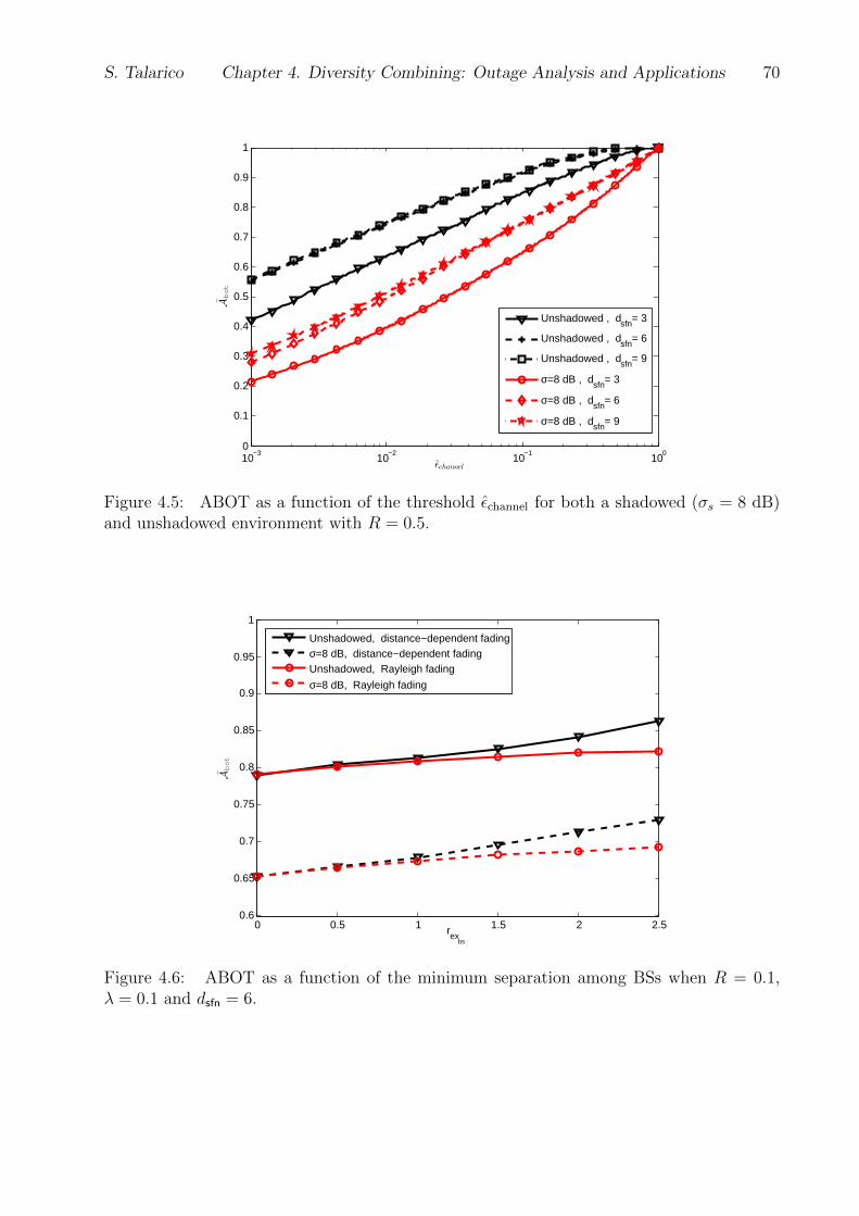
S. Talarico Chapter 4. Diversity Combining: Outage Analysis and Applications 70
10−3
10−2
10−1
100
0
0.1
0.2
0.3
0.4
0.5
0.6
0.7
0.8
0.9
1
εchannel
¯Abot
Unshadowed , dsfn= 3
Unshadowed , dsfn= 6
Unshadowed , dsfn= 9
σ=8 dB , dsfn= 3
σ=8 dB , dsfn= 6
σ=8 dB , dsfn= 9
Figure 4.5: ABOT as a function of the threshold εchannel for both a shadowed (σs = 8 dB)and unshadowed environment with R = 0.5.
0 0.5 1 1.5 2 2.50.6
0.65
0.7
0.75
0.8
0.85
0.9
0.95
1
rexbs
¯Abot
Unshadowed, distance−dependent fadingσ=8 dB, distance−dependent fadingUnshadowed, Rayleigh fading
σ=8 dB, Rayleigh fading
Figure 4.6: ABOT as a function of the minimum separation among BSs when R = 0.1,λ = 0.1 and dsfn = 6.

S. Talarico Chapter 4. Diversity Combining: Outage Analysis and Applications 71
R = 0.1, λ = 0.1 and dsfn = 6. The curves are shown for both a shadowed (σs = 8 dB) and
an unshadowed scenario and for both Rayleigh fading and a distance-depending fading. Fig.
4.6 shows that shadowing is always highly detrimental, the fraction of network that succeeds
to meet an outage constraint increases when BSs have a higher minimum separation, and
this effect is more prominent under a distance-depending fading.
4.4 Chapter Summary
This chapter presented a new approach for modeling and analyzing the performance of
cooperative networks that employ diversity combining. The chapter illustrates the perfor-
mance benefits that arise due to spatial diversity. The analysis is characterized by a new
closed-form expression for the conditional outage probability, when signals arriving over dif-
ferent paths are combined at the receiver in the presence of noise and interference, where the
conditioning is with respect to the network geometry. The channel model accounts for path
loss, shadowing, and Nakagami fading, and the Nakagami fading parameters do not need to
be identical for all links.
This chapter continues by applying this accurate analysis to two cases of study. First, it
models and analyzes the performance of a DS-CDMA MCC downlink and provides insight
regarding how the cell edge should be defined. The results show that, as expected, there is an
improvement in performance when MCC is used, rather than a conventional cellular network,
but the network needs a proper optimization. Finally, this chapter focuses on accurately and
efficiently modeling an MBSFN network, by combining the new closed form expression for
the outage probability, derived at the beginning of this chapter, and a constrained random
spatial model, which is used to synthesize more realistically such a network. The results show
that an increase in the size of an MBSFN areas leads to an improvement in performance only
until a certain dimension (and number of cooperative BSs) is reached, since the ISI starts to
become more prevalent and their effect more detrimental.

72
Chapter 5
The Role of Complexity in Cellular
Networks
Compared with today’s networks, future mobile networks will need to cope with a dra-
matic increase in the density and demand of users, and they will be characterized by tighter
hard real-time timing and protocol constraints. These constraints are described by mobile
communications standards such as 3GPP LTE [101] and must not be violated. In order to
fulfill these constraints, a pre-defined amount of computational resources must be provided
such that downlink and uplink processing can be performed within a given time interval,
and this must be done in an efficient and very cost effective way.
Recently the concept of Cloud-RAN has been introduced [30], which enables computa-
tional load balancing across multiple BSs to avoid peak-provisioning. For this novel architec-
ture, one of the goals is to dimension the computational assets of the network to exploit the
computational diversity present in a pool of resources, while still guaranteeing the commu-
nication service requirements of each individual cell. The utilization of processing resources
should be maximized for a given service guarantee. These goals require a framework that
enables the prediction of the required data processing resources under a given performance
constraint.
This chapter, after an introductory section on the Cloud-RAN architecture, considers its
computational requirements with the goal of illuminating the benefits of pooling computa-
tional resources. A new analytical framework is introduced to model, analyze the perfor-

S. Talarico Chapter 5. The Role of Complexity in Cellular Networks 73
mance, and determine the data processing requirements. The model is used to quantify the
computational load associated with the centralized processing of uplink signals in the pres-
ence of block Rayleigh fading, distance-dependent path loss, and fractional power control.
Several new performance metrics are defined, including computational outage probability,
outage complexity, computational gain, computational diversity, and the complexity-rate
tradeoff. The validity of the analytical framework is confirmed by comparing it numerically
with a simulator compliant with the 3GPP LTE standard. Using the developed metrics,
it is shown that centralizing the computing resources provides a higher net throughput per
computational resource as compared to local processing.
5.1 Cloud-RAN: A Brief Introduction
Traditional cellular network are composed of stand-alone BSs, which perform both radio
and baseband processing functionality locally at or near the cell site. In this architecture,
most of the hardware is placed in a base station cabinet located right below the antenna.
Starting from the third generation cellular networks (3G), the two groups of functionalities
have been physically separated. The radio functionalities are performed by a remote radio
head (RRH), which is installed on top of the tower, close to the antenna, in order to reduce
the cable loss. The baseband functionalities are performed at a baseband unit (BBU) or
data unit (DU), which can be placed further away from the RRH1, and it is connected to
it through optical fiber or microwave connection. This architecture has the advantage that
the BBU can be conveniently placed enabling a faster and less expensive maintenance and
upgrade of the system. However, due to the enormous increase in the number of users and
data shared, the current cellular architecture is reaching the limit of sustaining the amount of
data traffic on the network. Especially in densely populated areas, it is no longer acceptable
and sustainable to only increase the number of BSs in order to provide smooth network
accesses to users. The two main reasons are: i) economical since nowadays the deployment
1Note that the maximum distance at which the BBU can be placed depends on the latency of the mediumthrough which the signal is propagated. For instance for optical fiber, a reasonable maximum distance is≈ 40 Km when a repeater is not required. In this case, the medium produces a propagation delay of about0.1 ms.

S. Talarico Chapter 5. The Role of Complexity in Cellular Networks 74
Virtual BS Pool
Virtualized BS functions
Cloud RAN platform
Fronthaul/backhaul
BS 1
BS 2
BS 3
Figure 5.1: Illustration of the Cloud-RAN architecture.
of a new BS is very cost effective; and ii) due to the increment of the interference among
BSs, since the likelihood that the same radio resources are used increases.
In 2010 a new architecture has been proposed [30, 32, 104], which have been named C-
RAN, where the letter C can be interpreted as: Cloud, Centralized, Cooperative radio,
Collaborative or Clean 2. The Cloud-RAN is based on two tenets: centralization and vir-
tualization of BS baseband processing. In a Cloud-RAN network, the radio protocol stack
is executed by different physical entities. For a given group of cells, the lower parts of the
protocol stack are executed at the RRHs, while the upper parts are executed at a central
entity, called the Cloud-RAN platform. The RRHs use dedicated hardware, while the Cloud-
RAN is typically implemented with commodity general-purpose hardware. A Cloud-RAN
enables advanced interference coordination strategies while leveraging the elastic provision-
ing of resources provided by the cloud. It is particularly well suited for dense deployments,
such as within a large building where the RRHs are connected via fiber and many cells are
underutilized. The Cloud-RAN concept is illustrated Fig. 5.1. A Cloud-RAN system con-
sists of multiple RRHs, which perform only simple processing of the input signal, including
2The C is often interpreted as Centralized when the aim is to describe a system where the basebandprocessing for a group of cells is done at a central processing system. It is interpreted as Cloud when theprocessing is done on a pool of computing assets, made possible trough the use of virtualization. Note thatin the following the two terms are interchangeable.

S. Talarico Chapter 5. The Role of Complexity in Cellular Networks 75
sampling and optionally performing a fast Fourier transform (FFT) operation, a fronthaul
or backhaul connection, and a central data center. The data center manages a virtual BS
pool composed of a scalable number of virtual machines (VMs), each representing one or
more BSs and performing the majority of the baseband processing. Based on the actual
traffic and resulting computational demand, each VM is provisioned with resources that can
be elastically adjusted.
The major benefits of Cloud-RAN have been unveiled in [30]. Since a Cloud-RAN enables
computational load balancing across multiple BSs, it allows a more efficient use of BBUs
and reduces the cost of BSs deployment and operation. The required baseband processing
capacity of the pool is expected to be smaller than the sum of capacities of single BSs. In
particular, Bhaumik et al. have predicted in [105] that Cloud-RAN can save up to 22 % of
the data processing resources, by using the OpenAir [106] LTE implementation and real-
world measurements. Cloud-RAN is also expected to lead to save power consumption by
about 67 %-80 % compared to traditional RAN architecture. Due to the centralized nature
of this architecture, it provides increased flexibility in network upgrades and adaptability
to non-uniform traffic, which is particular useful in areas where the traffic demand changes
abruptly during the day. Furthermore, advanced features of LTE-A, such as coordinated
multi-point (CoMP) and interference mitigation, can be efficiently supported by the Cloud-
RAN, which is essential especially for small-cell deployments.
A Cloud-RAN architecture, which is characterized as mentioned above by several re-
markable benefits, has although several technical challenges that need to be addressed. One
of the main limitations of this architecture is the backhaul, which needs to be sufficiently fast
and with low latency, in order to meet very hard real-time timing. Furthermore, the compu-
tational load required to perform uplink or dowlink processing cannot exceed the available
resources, otherwise the signal cannot be properly decoded in time. This last limitation is
strictly dependent on the computational complexity of the decoder, and its role and effect
is subject of study of this chapter.

S. Talarico Chapter 5. The Role of Complexity in Cellular Networks 76
5.2 Complexity model
Consider a cloud group containing Ncloud BSs whose signals are jointly processed in a
virtual BS pool. Let γ = E[γ] indicate the average SINR. In the following, it is assumed
that the channel gain remains fixed for the duration of one transport block (TB), but varies
independently from TB to TB, which corresponds to a block-fading model. For each TB, the
channel is conditionally subject to AWGN. Under the assumption of infinite block-length,
the capacity for a given instantaneous SINR is given by log2(1+γ), which provides an upper
bound on rate. In practice, the rate is selected for a given γ from a set of modulation and
coding schemes (MCSs) in such a way that a constraint on outage probability is satisfied.
Because no finite-length code satisfies the capacity limit with equality, the rate is selected to
be below the corresponding capacity limit according to some margin trough link adaptation.
5.2.1 Link Adaptation
LTE features adaptive modulation and coding using turbo codes and hybrid automatic
repeat request (HARQ). The BS (called an eNodeB) commands the UE to transmit using
one of NR = 27 different MCSs, with Rk denoting the rate of kth MCS, k ∈ 1, ..., NR. Each
MCS is identified by an MCS index, Imcs = 0, ..., 26, and is characterized by a different
combination of code rate and modulation format [107, 108]. Three kinds of modulation are
used: QPSK (0 ≤ Imcs ≤ 10), 16-QAM (11 ≤ Imcs ≤ 20), and 64-QAM (21 ≤ Imcs ≤ 26).
When a TB is larger than 6144 bits, it is segmented into Ck code blocks (CBs), each of which
conveys Dk information bits. As advocated later, the selection of the MCS should take into
account the complexity of the turbo decoder, and in particular, the number of expected
iterations required to meet the outage constraint is the key factor in making the selection.
Suppose that the turbo decoder is run with a certain number of maximum iterations Lmax.
Let γRk indicate the minimum SINR for which the kth MCS satisfies the outage constraint
after the Lmax-th iteration, on average. The value of γRk for each MCS can be obtained
as follows. Simulations are used to obtain code block error rate (CBLER) curves for each
possible MCS and for an arbitrarily large number of maximum iterations. For the kth MCS,
γRk is selected to be the value of SNR for which the transport block error rate (TBLER)
S. Talarico Chapter 5. The Role of Complexity in Cellular Networks 77
satisfies a particular constraint for the channel outage εchannel (a transport block error occurs
when any of the code blocks in a transport block fails).
It is well known that the complexity of a turbo decoder depends on how much the channel
SINR exceeds the capacity limit. If a turbo code of rate Rk is transmitted over a channel
whose capacity is sufficiently higher than Rk, then typically only a few iterations are required.
Thus, to manage complexity, an SINR margin ∆γ may be used. With such a margin, the
SINR must be at least ∆γ above γRk in order to select the kth MCS. The rate selection for
channel SINR γ and SINR margin ∆γ can be represented by the function
R (γ,∆γ) =
R1 if γ
∆γ≤ γR1
Rk if γRk <γ
∆γ≤ γRk+1
RNR if γRNR <γ
∆γ.
(5.1)
5.2.2 Complexity Model
The computational effort required to decode a turbo code is linear in the number of iter-
ations and in the number of (information) bits. Thus a reasonable metric for computational
effort is the bit-iteration. For a given SINR γ, let the random variable Lr(γ,∆γ) be the
number of iterations required to decode a particular CB, and E [Lr(γ,∆γ)] be the average
number of iterations required to decode a CB. The expected decoding complexity (averaged
over the number of iterations required per CB) expressed in bit-iterations per channel use
(pcu) can be evaluated as
C(γ,∆γ) =DkCkE [Lr(γ,∆γ)]
Sre(5.2)
where Sre is the number of channel uses or resource elements (REs) required to convey
the TB. The expected number of decoding iterations can be found using the same set of
simulation curves used to determine the MCS thresholds γRk . For a given rate R (γ,∆γ),
the simulation results will show the CBLER for each iteration up to the Lmax-th iteration.
These CBLER curves can be interpreted as the PMF of the number of iterations at γ, and
from the PMF coefficients, the average number of iterations is easily computed.
To enable a deeper analysis of complexity issues, it is essential to build an accurate
yet wieldy complexity model. The groundwork for such a model is provided by [109], which

S. Talarico Chapter 5. The Role of Complexity in Cellular Networks 78
accurately predicts the power consumption of a decoder for a given code rate, coding scheme,
channel, and decoder type. According to [109, Eq. (4) and (9)], the expected decoding
complexity under a given instantaneous SINR γ and SINR margin ∆γ can be modeled as
C(γ,∆γ) =R (γ,∆γ)
log2 (ζ − 1)log2
[− log10(εchannel)
K ′ [log2(1 + γ)−R (γ,∆γ)]2ζ − 2
ζ+
2
ζ
]≈ R (γ,∆γ)
log2 (ζ − 1)log2
[− log10(εchannel)
K ′ [log2(1 + γ)−R (γ,∆γ)]2ζ − 2
ζ
]=
R (γ,∆γ)
log2 (ζ − 1)
[log2
(ζ − 2
K(εchannel)ζ
)− 2 log2 [log2(1 + γ)−R (γ,∆γ)]
](5.3)
where ζ is a parameter of the model related to the connectivity of the decoder when repre-
sented as a graph,
K(εchannel) = − K ′
log10(εchannel), (5.4)
K ′ is a parameter of the model, and εchannel is a constraint on the channel outage probability.
For the sake of simplicity K(εchannel) is denoted by K in the remainder of this dissertation.
When evaluating (5.3), the function R(γ,∆γ) is defined by (5.1). The relationship be-
tween each threshold γRk and the corresponding rate Rk in (5.1) can be modeled as
Rk = log2
(1 +
γRkν
)(5.5)
where ν is a parameter that models the gap between the capacity at γRk and the SINR for
the actual code to meet the performance objective at rate Rk. The values of (ζ,K ′, ν) could
be found for each MCS by statistically fitting the empirically observed complexity to the
complexity predicted by the model. However, it is more convenient to have values for these
parameters that are common to all the MCSs.
Example
As an example, let consider an LTE system that uses normal cyclic prefix and a 10 MHz
bandwidth corresponding to 50 resource blocks (RBs). However, since up to 5 RBs must be
reserved for the physical uplink control channel and the number of RBs must be a multiple of
2, 3, or 5 [107,108], the transmitted signal occupies 45 RBs. Since there are 12 information-
bearing single-carrier frequency division multiple access (SC-FDMA) symbols per sub-frame

S. Talarico Chapter 5. The Role of Complexity in Cellular Networks 79
−10 −5 0 5 10 15 200
5
10
15
20
25
SNR [dB]
C(γ,∆γ)[bit-iterpcu]
Empirical, max. 8 iter.Analytical
Figure 5.2: Complexity as a function of the SNR obtained both through simulations (blue)and based on (5.3) (black curve), when the maximum number of iterations used to decode aCB is limited to eight.
and 12 sub-carriers per RB, it follows that Sre = 45 × 12 × 12 = 6480. The MCS selection
is implemented according to (5.1) with threshold found for Lmax = 8 iterations, an outage
constraint εchannel = 0.1, and no excess margin (∆γ = 0 dB).
For this settings, the complexity computed empirically using (5.2) is shown in Fig. 5.2 by
the blue curve, while the black curve shows the complexity predicted by the complexity model
described above. For the complexity model, the values of (ζ,K ′, ν) have been found in order
to have the best fit with the empirical complexity, and they are found to be: ζ = 6, K ′ = 0.2,
and ν = 0.2 dB. As can be seen, these two curves are quite similar3, demonstrating the
effectiveness of the model. Fig. 5.2 further shows a highly volatile behavior, which results
from the link-adaptation process. When the system operates at the same MCS (rate), a
decoder requires fewer iterations as the SNR increases. However when link adaptation is
performed, the system requires more complexity each time it moves towards a higher MCS,
since it operates closer to capacity, which is the cause of the peaky behavior in Fig. 5.2.
3Note that a more accurate match could be achieved by determining a different set of (ζ,K ′, ν) for eachMCS, but this significantly complicates the notation.

S. Talarico Chapter 5. The Role of Complexity in Cellular Networks 80
5.3 Performance Metrics
This section provides the definition for several performance metrics, which are used
throughout this chapter to evaluate the performance of a Cloud-RAN system and highlight
its benefits over a distributed implementation.
5.3.1 Computational outage probability
Fig. 5.2 shows that the required computational complexity to decode a TB may differ sig-
nificantly depending on the SINR. Furthermore, when the system is distributed, each BS will
be provisioned with a limited amount of computational resources Cmax, while in a centralized
system the virtual BS pool will be equipped with a total limited amount of computational
resources, which scales linearly with the number of BSs. If the total required computational
effort exceeds the computational resources before a decoding deadline is reached, a compu-
tational outage will occur. From the operator’s perspective, a computational outage is no
different than a channel outage, because in both cases the information is not made available
to the end user.
More formally, the computational outage probability is defined by [110]
εcomp(Ncloud) = P
[Ncloud∑i=1
C(γi,∆γ) > NcloudCmax
]. (5.6)
When a computational outage occurs, the centralized processor is unable to finish the de-
coding of at least one uplink user. However, when this condition occurs it is still possible
that some of the uplink transport blocks can be decoded, even though at least one of the
blocks has failed.
5.3.2 Outage complexity
The outage complexity Coutage (εcomp, Ncloud) is the minimum amount of computational
resources required to satisfy an outage constraint on the per-cell computational outage prob-
ability εcomp (Ncloud). More formally, the outage complexity is defined as
Coutage(ε, Ncloud) = arg minCmax
P
[Ncloud∑i=1
C(γi,∆γ) > NcloudCmax
]≤ εcomp (Ncloud)
. (5.7)
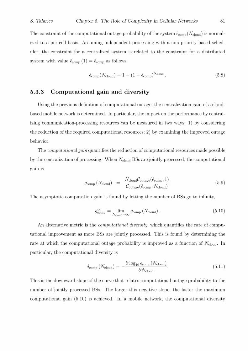
S. Talarico Chapter 5. The Role of Complexity in Cellular Networks 81
The constraint of the computational outage probability of the system εcomp(Ncloud) is normal-
ized to a per-cell basis. Assuming independent processing with a non-priority-based sched-
uler, the constraint for a centralized system is related to the constraint for a distributed
system with value εcomp (1) = εcomp as follows
εcomp(Ncloud) = 1− (1− εcomp)Ncloud . (5.8)
5.3.3 Computational gain and diversity
Using the previous definition of computational outage, the centralization gain of a cloud-
based mobile network is determined. In particular, the impact on the performance by central-
izing communication-processing resources can be measured in two ways: 1) by considering
the reduction of the required computational resources; 2) by examining the improved outage
behavior.
The computational gain quantifies the reduction of computational resources made possible
by the centralization of processing. When Ncloud BSs are jointly processed, the computational
gain is
gcomp (Ncloud) =NcloudCoutage(εcomp, 1)
Coutage(εcomp, Ncloud). (5.9)
The asymptotic computation gain is found by letting the number of BSs go to infinity,
g∞comp = limNcloud→∞
gcomp (Ncloud) . (5.10)
An alternative metric is the computational diversity, which quantifies the rate of compu-
tational improvement as more BSs are jointly processed. This is found by determining the
rate at which the computational outage probability is improved as a function of Ncloud. In
particular, the computational diversity is
dcomp (Ncloud) = −∂ log10 εcomp(Ncloud)
∂Ncloud
. (5.11)
This is the downward slope of the curve that relates computational outage probability to the
number of jointly processed BSs. The larger this negative slope, the faster the maximum
computational gain (5.10) is achieved. In a mobile network, the computational diversity
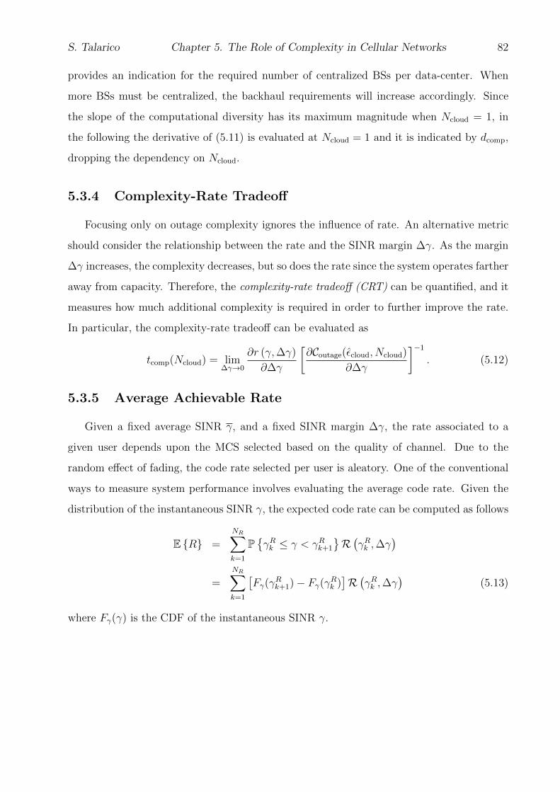
S. Talarico Chapter 5. The Role of Complexity in Cellular Networks 82
provides an indication for the required number of centralized BSs per data-center. When
more BSs must be centralized, the backhaul requirements will increase accordingly. Since
the slope of the computational diversity has its maximum magnitude when Ncloud = 1, in
the following the derivative of (5.11) is evaluated at Ncloud = 1 and it is indicated by dcomp,
dropping the dependency on Ncloud.
5.3.4 Complexity-Rate Tradeoff
Focusing only on outage complexity ignores the influence of rate. An alternative metric
should consider the relationship between the rate and the SINR margin ∆γ. As the margin
∆γ increases, the complexity decreases, but so does the rate since the system operates farther
away from capacity. Therefore, the complexity-rate tradeoff (CRT) can be quantified, and it
measures how much additional complexity is required in order to further improve the rate.
In particular, the complexity-rate tradeoff can be evaluated as
tcomp(Ncloud) = lim∆γ→0
∂r (γ,∆γ)
∂∆γ
[∂Coutage(εcloud, Ncloud)
∂∆γ
]−1
. (5.12)
5.3.5 Average Achievable Rate
Given a fixed average SINR γ, and a fixed SINR margin ∆γ, the rate associated to a
given user depends upon the MCS selected based on the quality of channel. Due to the
random effect of fading, the code rate selected per user is aleatory. One of the conventional
ways to measure system performance involves evaluating the average code rate. Given the
distribution of the instantaneous SINR γ, the expected code rate can be computed as follows
E R =
NR∑k=1
PγRk ≤ γ < γRk+1
R(γRk ,∆γ
)=
NR∑k=1
[Fγ(γ
Rk+1)− Fγ(γRk )
]R(γRk ,∆γ
)(5.13)
where Fγ(γ) is the CDF of the instantaneous SINR γ.

S. Talarico Chapter 5. The Role of Complexity in Cellular Networks 83
5.4 A Framework for Complexity Analysis
In order to evaluate the previously introduced performance metrics, an analytical frame-
work is developed [111] in this section to quantify the expected outage complexity in a
centralized network. In the following, the analysis is first built under the assumption of a
fixed average SINR γ, which is true when the uplink is fully power controlled. Subsequently,
the analysis is expanded to take into account the path loss and the fractional power control
policy when a user is distributed uniformly within a circle of unit radius centered at its
serving BS. Finally based on these derivations, the analytical framework is expanded fur-
thermore to be able to quantify the expected outage complexity for a Cloud-RAN composed
of Ncloud BSs.
5.4.1 Full Power Control
Consider a single-user with a fixed average SNR γ, and that this user is processed locally
(i.e., Nc = 1). The instantaneous value of γ is a random variable, which, for the sake
of tractability, we assume is an exponential random variable corresponding to the widely
accepted Rayleigh fading model4. The PDF of such a γ is given by:
fγ (γ) =1
γexp
(−γγ
), γ ≥ 0. (5.14)
Expected complexity
Theorem 5.4.1 The expected value of the decoding complexity conditioned on the average
SNR γ can be evaluated by
Eγ|γCi ≈NR∑k=1
R(γRk ,∆γ
)log2 (ζ − 1)
[I1
(γRk+1, γ
Rk
)+ I2
(γRk+1, γ
Rk
)](5.15)
where the functions I1 (·, ·) and I2 (·, ·) are given respectively by (E.3) and (E.13).
Proof: The details of the derivation are given in Appendix 5.1.
4Note that other distributions for γ may be used, in order to more accurately model the effects ofinterference, shadowing, and signal propagation, but this comes at the cost of reduced tractability. Forinstance the results from Cap. 2 could be used, but such distributions will require a simulation or numericalintegration to compute the performance metrics.

S. Talarico Chapter 5. The Role of Complexity in Cellular Networks 84
Variance of the complexity
Theorem 5.4.2 The variance of the computational complexity conditioned on the average
SNR γ can be evaluated by
Varγ|γ Ci ≈NR∑k=1
[2R(γRk ,∆γ
)log2 (ζ − 1)
]2
I4
(γRk+1, γ
Rk
)− Eγ|γCi2 (5.16)
where Eγ|γCi is evaluated using (5.15) and I4 (·, ·) is given by (E.31).
Proof: The details of the derivation are given in the Appendix 5.2.
Outage complexity
In the case of an isolated user processed locally, the outage complexity in a distributed
system is the value Coutage that satisfies the following expression
PCi ≥ Coutage(εcomp, 1) ≤ εcomp (5.17)
which can be evaluated once the CDF of the complexity is known.
The CDF of the complexity can be written as follows
FC(Cthr) = P Ci ≤ Cthr (5.18)
where Cthr is a complexity threshold chosen based on the quality of the channel and the
computational resources available. By using the notion that the complexity monotonically
decreases in γ in the interval [γRk ; γRk+1], (5.18) can be replaced by
FC(Cthr) =1
P γ > γR1
NR∑k=1
Pγk,min ≤ γ < γRk+1
(5.19)
where
γk,min = max[γRk ,min
(γRk+1, 2
∆R+r(γ,∆γ) − 1)]
(5.20)
∆R = 2−Cthrlog2(ζ−1)/[2r(γ,∆γ)]
√ζ − 2
Kζ. (5.21)
Finally, (5.19) can be written as follows
FC(Cthr) =1
1− Fγ (γR1 )
NR∑k=1
[Fγ(γRk+1
)− Fγ (γk,min)
](5.22)
where Fγ(·) is the CDF of γ with PDF given by (5.14).

S. Talarico Chapter 5. The Role of Complexity in Cellular Networks 85
5.4.2 Effect of Path Loss and Power Control
This subsection considers the case that the user is subject to a fractional power control
policy and is located randomly within the cell. For the sake of tractability5, assume a circular
cell of unit radius and that the user is placed according to a uniform distribution. Indicate
with Yi both the ith BS and its location. Each BS Yi serves only one user, which is located
at Xi and is ||Yi −Xi|| away from it.
Under a fractional power control policy and using a distance dependent attenuation power
law, as in Cap. 2, Xi will transmit using power
Pi = P0 ||Yi −Xi||αs . (5.23)
The average SNR received by Yi for the ith UE is given by
γi = γud ||Yi −Xi||−α(1−s) (5.24)
where γud is the average reference SNR, measured assuming unit-distance transmission.
In this case, it is not possible to determine a closed-form expression or a suitable approx-
imation for both the expected and the variance of the complexity. However, knowing that
the PDF of ri = ||Xi − Yi|| is
fri(ω) =
2ω , 0 ≤ ω ≤ 1
0 , otherwise(5.25)
the expected complexity ECi and variance VarCi can be obtained by performing a nu-
merical integration over r of (5.15) for the expected complexity and (5.16) for the complexity
variance.
However, under this scenario, the CDF of γ averaged over the spatial distribution can
be evaluated in closed form. By removing the conditioning over the spatial distribution, it
follows that
Fγ(γ) =
∫Fγ(γ∣∣ω) fri (ω) dω (5.26)
5A more complicated model for the placement of the user may be used, such as one that accounts forthe actual shape of the Voronoi region. While more accurate, this comes at the cost of tractability and willtypically require simulation or numerical integration.

S. Talarico Chapter 5. The Role of Complexity in Cellular Networks 86
where Fγ(γ∣∣ω) = 1 − exp
(−γγ
), γ ≥ 0 and γ is given by (5.24). Substituting (5.25) into
(5.26) yields
Fγ(γ) =
∫ 1
0
[1− exp
(− γ
γud
ωα(1−s))]
2ω dω
= 1− 2
∫ 1
0
exp
(− γ
γud
ωα(1−s))ω dω. (5.27)
After few algebraic manipulations and using the change of variable t =γ
γud
ωα(1−s), it yields
Fγ(γ) = 1−2(
γγud
)−2/[α(1−s)] [Γ(
2η(1−s) ,
γγud
)− Γ
(2
α(1−s) , 0)]
α(1− s)(5.28)
where the function Γ(z, x) is a gamma incomplete function, which is defined as [112]
Γ(z, x) =
∫ ∞x
tz−1 e−t dt. (5.29)
Since the CDF of γ is equal to (5.28), the outage complexity can be determined analytically.
In particular, even if (5.20) cannot be expressed in closed form, well-known algorithms such
as bisection, Newton, or gradient-search algorithm can be applied. Furthermore, the average
achievable rate can be determined by substituting (5.28) into (5.13).
5.4.3 Centralized Processing
Using the previously derived expressions for the expectation and the variance of the
complexity, in this section the analytical framework is expanded in order to be able to
compute through an approximation the maximum decoding complexity when Ncloud BSs are
centralized. More specifically, the central limit theorem (Lindeberg/Levy) is used, which
yields
Coutage(εcomp, Ncloud) =
√VarCiNcloud
√2Q−1
(2(1− εcomp)Ncloud − 1
)︸ ︷︷ ︸inv. norm. CDF
+ECi (5.30)
where Q−1(·) is the inverse error function, which has the following series representation [112]
Q−1(x) =∞∑k=0
vk2k + 1
(√π
2x
)2k+1
(5.31)
where v0=1 and
vk =k−1∑m=0
vmvk−1−m
(m+ 1)(2m+ 1). (5.32)

S. Talarico Chapter 5. The Role of Complexity in Cellular Networks 87
5.5 Numerical Verification
In order to evaluate the validity of the analytical framework derived in Sec. 5.4, in this
section numerical results are provided based on the 3GPP LTE standard and a 3GPP LTE
decoder. The numerical results are compared against those obtained through the previously
derived framework. A typical value for an LTE network of εchannel = 0.1 is chosen for the
channel outage constraint.
Assume all the available resources per cell are allocated to a single user. Furthermore, a
full-buffer scenario is assumed: each of the Ncloud BSs, whose signals are jointly processed at
a central cloud-processor, always serves a user over the complete bandwidth. However, 3GPP
LTE allows for multi-user opportunistic scheduling such that one TB may carry information
from more than one user. When resources are shared among multiple users more diversity
and therefore a lower outage complexity per cell can be achieved compared to the case when
all the resources are monopolized by a single user. Therefore, this assumption represents
a worst-case scenario regarding computational complexity, since it does not allow for any
computational diversity within a given cell.
A block Rayleigh fading channel is considered, although in practice a system experiences
more channel diversity due to multi-path propagation, and the computational complexity
varies from user to user and from CB to CB. This scenario, in an extreme case, leads the
users to experience a sufficient channel diversity for a close-to-AWGN channel, which results
in a lower computational gain and diversity.
The outage complexity Coutage(εcloud, Ncloud) is obtained through a simulation campaign.
During each trial, γi is drawn from an exponential distribution when we do not consider the
path loss, or from a distribution whose CDF is given by (5.28) when the path loss is taken
into consideration. The MCS scheme for a given γi is determined according to the value of
∆γ chosen. Each of the Ck CBs in the TB is marked as being in a channel outage with
probability εcb = 1 − (1− εchannel)1/Ck , which can be precomputed. If any of the CB are in
outage, then the entire TB is declared to be in an outage. If the rth CB is in an outage,
then Lr (γ,∆γ) = Lmax, which is the maximum number of attempted iterations. Otherwise,
Lr (γ,∆γ) is determined by drawing a random variable distributed according to the PDF of

S. Talarico Chapter 5. The Role of Complexity in Cellular Networks 88
Lr (γ,∆γ), which can be precomputed by tracking the error-rate as a function of the number
of iterations. Once the decoding complexity is computed, finally the outage complexity is
evaluated by (5.7). The outage complexity is obtained by using one million trials when
evaluated through simulations.
Fig. 5.3 shows the outage complexity to ensure per-cell outage constraint εcomp = 0.1 as
function of the number of BSs, whose signals are centrally processed. Results in Fig. 5.3(a)
consider a scenario characterized by a Rayleigh fading channel with γ = 10 dB, while in
Fig. 5.3(b) a distance dependent path loss model is taken into account, as described in Sec.
5.4.2. For both models, three values of ∆γ are considered. For Fig. 5.3(b), the path loss
exponent is fixed to α = 2, the average SNR at unit distance is set to γud = 0 dB, and the
compensation factor is s = 0.1, which is the value reported in [113] that maximizes the sum
throughput. Higher values of s would improve fairness at the cost of throughput. In Fig.
5.3, the solid lines are evaluated analytically as derived in Section 5.4.1 and 5.4.2, while the
dots are obtained through simulations using the methodology described above. The notches
on the right side of each sub-figure show the behavior as Ncloud →∞. Fig. 5.3 shows a good
agreement for both models between the simulated and the analytical results, emphasizing
the validity of the proposed analytical framework.
In Section 5.2.2, the complexity is assumed to be deterministic for a fixed SNR, while in
an actual implementation this would be a random variable with expectation C(γ,∆γ). This
additional source of randomness is not considered in the analytical framework, and it is one
of the reason for the slight mismatch between the empirical and analytical results. Another
reason for the slight mismatch is that a lower-bound on the complexity is not applied: an
actual decoder always performs at least one iteration which determines the minimum required
complexity. If C(γ,∆γ) is a random variable, the computational variance would increase.
This would consequently cause an increment of the computational gain for a Cloud-RAN.
Furthermore, if the lower bound is applied, it causes a slight increment of the expected
complexity, even if the variance might decrease, which lead also in this case to a higher
computational gain.

S. Talarico Chapter 5. The Role of Complexity in Cellular Networks 89
100
101
102
0
5
10
15
20
Ncloud
Coutage(ε,N
cloud)/N
cloud[bit-iterpcu]
∆γ = 0 dB
∆γ = 0.4 dB
∆γ = 0.9 dB
(a) Rayleigh fading
100
101
102
0
5
10
15
Ncloud
Coutage(ε,N
cloud)/N
cloud[bit-iterpcu]
∆γ = 0 dB
∆γ = 0.4 dB
∆γ = 0.9 dB
(b) Distance dependent path loss model
Figure 5.3: Outage complexity to ensure per-cell outage constraint ε = 0.1 as function of thenumber of BSs, whose signals are centrally processed. Solid lines are evaluated analytically,while dots are obtained through simulations using one million trials. The notches on theright side of each sub-figure show the behavior as Ncloud →∞.

S. Talarico Chapter 5. The Role of Complexity in Cellular Networks 90
5.6 Results
In this section, the analytical framework developed in Section 5.4 is applied to perform
an evaluation of a centralized system using some of the metrics introduced in Section 5.3.
In the following the path loss exponent is fixed to α = 2, the compensation factor is s = 0.1,
the per-cell constraint on the computational outage is set to εcomp = 0.1, and the average
SNR at unit distance is γud = 0 dB.
5.6.1 Computational Gain
At first, the computational gain gcomp and its dependence on the number of centralized
BSs and on the SNR margin ∆γ is considered. Fig. 5.4(a) shows the computational gain
as function of the number of centralized BSs. Fig. 5.4(b) shows the computational gain as
function of the target computational outage probability.
Fig. 5.4(a) shows that the computational gain increases sharply for small values of Ncloud,
before it becomes flat for larger values of Ncloud. Furthermore, it shows a high computational
gain compared to a distributed system, emphasizing the benefit of a centralized solution. The
notches on the right side of the sub-figure show the behavior as Ncloud →∞.
Fig. 5.4(b) shows that the computational gain increases as the target computational
outage probability decreases, since more computational resources are required to make sure
that also peak-requirements are satisfied. This is a consequence of the fact that the com-
plexity scales with − log10(εcomp) in (5.3). In this case, centralization provides more benefits
as diversity effects can be exploited to load balance between the individual BSs. Further-
more, the computational gain differs more significantly for different SNR offsets as the target
computational outage probability decreases. This effect is mainly due to the fact that at
lower target outage probability it is more challenging to operate close to capacity because
the decoder would be required to have a steeper error rate curve.
5.6.2 Computational Diversity
Fig. 5.5 shows the computational diversity as function of the target computational outage
probability. For each SNR margin ∆γ and target computational outage probability, the
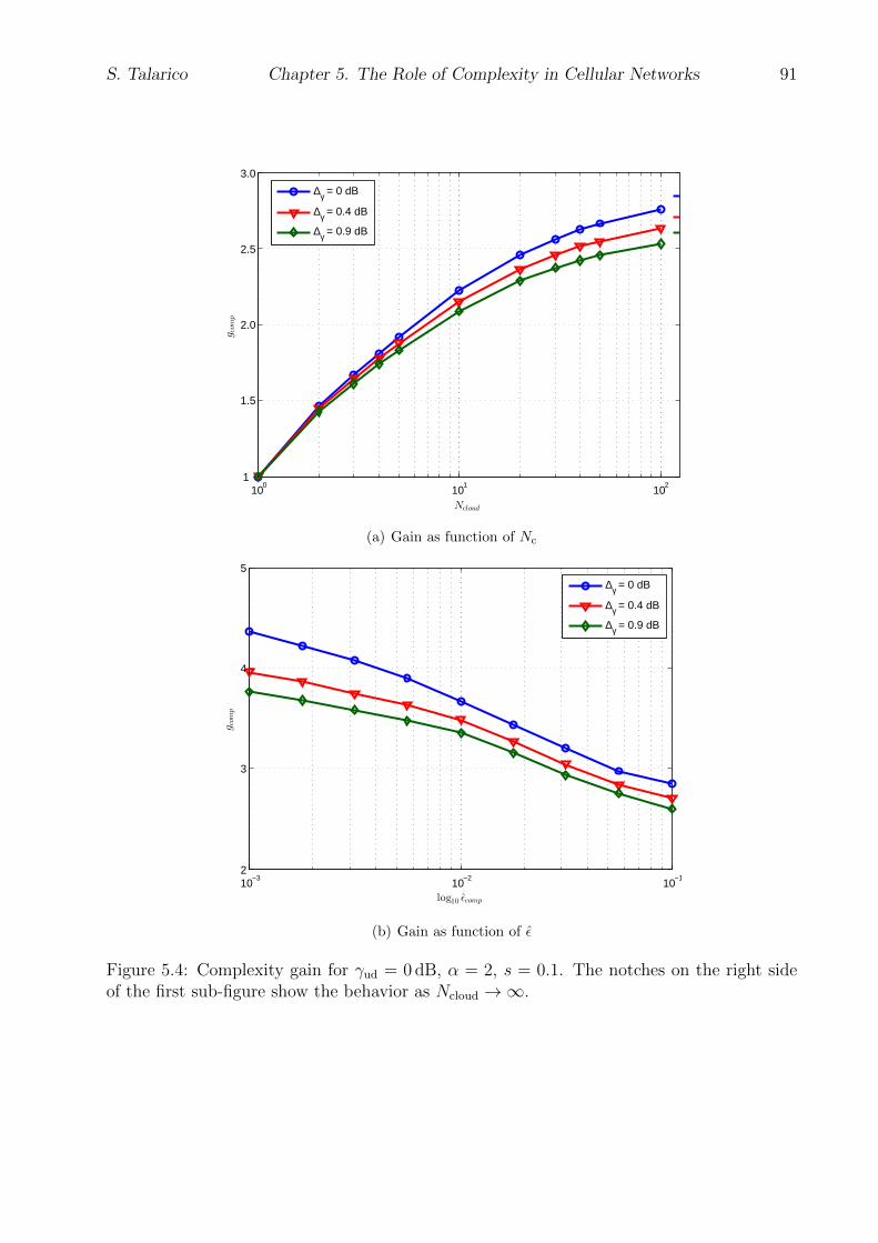
S. Talarico Chapter 5. The Role of Complexity in Cellular Networks 91
100
101
102
1
1.5
2.0
2.5
3.0
Ncloud
gcomp
∆γ = 0 dB
∆γ = 0.4 dB
∆γ = 0.9 dB
(a) Gain as function of Nc
10−3
10−2
10−1
2
3
4
5
log10 εcomp
gcomp
∆γ = 0 dB
∆γ = 0.4 dB
∆γ = 0.9 dB
(b) Gain as function of ε
Figure 5.4: Complexity gain for γud = 0 dB, α = 2, s = 0.1. The notches on the right sideof the first sub-figure show the behavior as Ncloud →∞.

S. Talarico Chapter 5. The Role of Complexity in Cellular Networks 92
10−3
10−2
10−1
0
2
4
6
8
log10 εcomp
dcomp
∆γ = 0 dB
∆γ = 0.4 dB
∆γ = 0.9 dB
Figure 5.5: Computational diversity as function of the target computational outageprobability.
computational diversity is computed by numerically evaluating the derivative in (5.11), once
the computational outage probability is obtained from (5.30). The computational diversity,
similar to the computational gain, decreases by increasing the target computational outage
probability. This is due to the over-provisioning of resources at lower target computational
outage probability. Furthermore, the computational diversity differs significantly for different
SNR offsets as the target computational outage probability decreases.
5.6.3 Complexity-Rate Tradeoff
Fig. 5.6 shows the CRT as function of the number of centralized BSs, which quantifies
the increase of the achievable rate as computational resources are added. Fig. 5.6 shows also
the dependency of the CRT on the SNR margin offset. The CRT defined in (5.12) is the ratio
between the slope of the average rate and the slope of the outage complexity both computed
at a given SNR margin. In Fig. 5.6, the two slopes are individually evaluated numerically
using (5.13) and (5.30) for each value of Ncloud and SNR margin ∆γ. The notches on the
right side of the figure show the behavior as Ncloud →∞.
Fig. 5.6 shows that the CRT increases as the margin offset is increased and this is due

S. Talarico Chapter 5. The Role of Complexity in Cellular Networks 93
100
101
102
0
0.02
0.04
0.06
0.08
0.1
0.12
Ncloud
tcomp
∆γ = 0 dB
∆γ = 0.4 dB
∆γ = 0.9 dB
Figure 5.6: CRT as a function of Nc. The notches on the right side of the figure show thebehavior as Ncloud →∞.
to the fact that the decoder operates farther away from capacity and therefore does not
cause high peak complexity. Hence, additional complexity is beneficial in order to gain ad-
ditional achievable rate. In other words, the closer the decoder operates to capacity, the
more resources must be invested to increase the achievable rate. Fig. 5.6 points out that an
optimum point to operate a system exists. Assume that a minimum average achievable rate
is required. In this case, the operator may use a less complex decoder, which reduces the re-
quired computational resources (and therefore reduces costs for information technology (IT)
infrastructures). However, a minimum computational complexity should be maintained since
the penalty in terms of achievable rate may otherwise be significant. In addition, due to the
lower per-cell achievable rate, more BSs must be deployed, which implies higher deployment
costs. Depending on the costs for IT infrastructure and mobile network infrastructure, an
optimal operating point can be determined where deployment costs are minimized.

S. Talarico Chapter 5. The Role of Complexity in Cellular Networks 94
5.7 Chapter Summary
Computational limitations in mobile wireless networks have a significant impact on the
network performance. Such computational limitations are of particular interest to small-
cell networks, where BSs are computationally limited due to economic constraints. The
computational constraints are also of fundamental importance to the design of Cloud-RAN
architectures. In this chapter a new analytical framework has been developed to evaluate
the data processing requirements of a cellular uplink, which is highly relevant to the analysis
and design of Cloud-RAN networks. Several performance metrics have been introduced to
quantify the benefit of such a network compared to a conventional RAN: computational
outage probability, computational gain, computational diversity and complexity-rate trade-
off. The novel concept of computational outage helps to quantify the complexity-throughput
tradeoff in Cloud-RAN platforms. Such a quantification allows for specifying computational
requirements for Cloud-RAN platforms in a meaningful way. Furthermore, insights into the
computational gain and computational diversity offered by centralized processing are pro-
vided. Finally, the complexity-rate tradeoff is used to measure the additional complexity
needed to further improve the achievable rate.
The analytical framework has been verified by comparing it numerically with a large-
scale system level simulator compliant with the 3GPP LTE standard. It has been shown
that the analytical framework provides a good match with simulations despite simplifying
assumptions, which are necessary for the tractability of the derivations.

95
Chapter 6
Resource Management in
Cloud-RANs
In cellular systems in general, and Cloud-RAN systems in particular, the amount of com-
putational resources available and the communications performance are strictly related. In
fact, a signal can be in outage not only if the channel is not adequate, but also if the com-
putational resources at the BBU are not enough to its baseband operations. In traditional
cellular systems, users must be allocated radio resources to satisfy the objectives of rate,
outage, and fairness. However, in a computationally limited environment, such as a Cloud-
RAN, resources should also be allocated with computational constraints in mind. Indeed,
the allocation of radio and computational resources are connected, as this will be shown in
this chapter. In particular, as the processing load imposed by each device depends on its
allocated transmission rate and channel quality, the rate-allocation aspect of the scheduling
should take into account the available computing resources.
This chapter provides insights into how the communications performance is effected by
the computational resources available, which in modern wireless systems that use capacity
approaching codes (i.e turbo or low-density parity-check (LDPC)) are mainly required to
perform iterative decoding. In this chapter, it is shown that the overall performance of
the network can be improved by adopting a computational aware scheduler, which selects a
MCS that requires a reduced number of expected iterations. While this produces a slight
loss in terms of instantaneous peak rate, this strategy has the potential to greatly reduce
S. Talarico Chapter 6. Resource Management in Cloud-RANs 96
the likelihood of computational outages and as a consequence improve the sum-throughput
of the system.
This chapter proposes other two computationally aware schedulers, which have the ob-
jective of maximizing the sum-rate of the system while satisfying a constraint on the offered
computational load. The first scheduler optimally allocates the rates among users and is
implemented according to a water-filling algorithm. The second scheduler is suboptimal,
but uses a simpler and intuitive complexity-cut-off approach. The performance of both
schedulers is evaluated and it is found that both schedulers are able to completely avoid
computational outages at the cost of a slight loss of sum-rate.
6.1 Heuristic Approach to MCS Selection
As already pointed out in Chap. 5, in a Cloud-RAN system there exists a tradeoff between
complexity and throughput. In particular, as a higher achievable rate is sought, a natural
choice is to select an MCS that allows the system to work closer to capacity. However, in
this case the iterative decoder requires more computational resources to successfully decode
the TB, and it is more likely to encounter computational outage. Thus, in modern wireless
systems, which uses iterative codes, the iterative nature of the decoding allows complexity to
be traded off for transmission rate. This concept is illustrated in Fig. 6.1, which shows the
CBLER εcb as a function of SNR (expressed as the ratio of the energy-per-symbol to noise
power) after 2, 3, and 8 iterations for two MCSs: Imcs = 10 and 11. The results in Fig. 6.1
and the remaining examples in this chapter are for an LTE system, with the same specifics
provided in Chap. 5. At εcb = 2.5 × 10⁻¹, the performance of MCS 10 with 2 iterations
is the same as the performance of MCS 11 with 8 iterations. Thus, by backing off from
MCS 11 to 10, the number of required iterations is cut by a factor of 4, on average. The
number of information bits in the TB that must be decoded is also reduced, in this case from
9216 to 8064, so the required number of bit-iterations is even further reduced. However, this
reduction in complexity comes at a cost, as the spectral efficiency of MCS 10 is lower than
that of MCS 11.
The MCS is selected to satisfy a channel outage constraint εchannel. When complexity is

S. Talarico Chapter 6. Resource Management in Cloud-RANs 97
1 2 3 4 5 6 710
−3
10−2
10−1
100
SNR [dB]
Cod
e B
LER
MCS 10 MCS 11
2 Iterations4 Iterations8 Iterations
Figure 6.1: Code block error rate as a function of SNR for MCS 10 and MCS 11 after 2, 3,and 8 decoder iterations. The arrow shows where the CBLER of MCS 10 after 2 iterationsis the same as that of MCS 11 after 8 iterations.
not a concern, the selected MCS is the highest one that satisfies an outage constraint εchannel
after a large number of decoder iterations. However, when complexity is a concern, the MCS
should be selected such that the outage constraint is met after a specific number of decoder
iterations. In order to show the benefits in terms of computational outage and through-
put when the total complexity requirements are reduced by upper bounding the maximum
number of turbo iterations to a lower value, two MCS-selection schemes are defined: i)
max-rate selection (MRS) [110], which is able to perform up to Lmax = 8 iterations (∆γ = 0
dB); computationally aware selection (CAS) [110], which performs up to Lmax = 2 iterations
(∆γ = 0.9 dB). The rate-complexity tradeoff for these two MCS-selection schemes is illus-
trated in Fig. 6.2. Fig. 6.2(a) shows the raw throughput of the MRS and CAS schemes as a
function of the SNR 1. For reference, the Shannon capacity limit is also shown. The reduc-
tion in rate when using CAS is evident from the figure. The average computational effort
required to decode a TB as a function of SNR for the two MCS selection policies is shown in
Fig. 6.2(b). As anticipated, using the complexity aware scheme reduces the average effort.
1The raw throughput Traw is simply the selected rate R (γ,∆γ) expressed in units of bits/second. Thisis in contrast with the effective throughput, which is the rate of correct transmission; i.e, Teff = (1− ε)Traw.

S. Talarico Chapter 6. Resource Management in Cloud-RANs 98
−5 0 5 10 15 200
5
10
15
20
25
30
35
40
45
SNR [dB]
Thr
ough
put [
Mbi
t/s]
CapacityMRSCAS
(a) Raw throughput
−5 0 5 10 15 200
50
100
150
200
250
300
SNR [dB]
Com
plex
ity [M
bit−
itera
tions
/s]
MRSCAS
(b) Computational effort
Figure 6.2: Raw throughput and computational effort as a function of the SNR for two MCSselection schemes: computationally aware selection (CAS) and max-rate selection (MRS).
Notice that the stairstep appearance of Fig. 6.2(a) and peaky behavior and Fig. 6.2(b) are
due to the use of a finite number of MCSs.

S. Talarico Chapter 6. Resource Management in Cloud-RANs 99
6.1.1 Numerical Results
In this section, the performance of the two aforementioned MCS-selection schemes are
analyzed using a system-level simulator that is compliant with the 3GPP LTE standard by
accounting for both the channel and the computational outage. In the following, the overall
outage probability εall, or simply outage probability, is in fact the probability that a TB is
lost due to either kind of outage. The performance are first provided in the case of a single
cell, followed by the case of a multicell environment where CCI has to be considered.
Outage in an Isolated Cell
Consider a network with just one cell containing a single active user served by a single
BS. There is no interference from other cells, and the signal received by the BS is processed
all by itself; hence, Ncloud = 1. Consider the complexity-throughput tradeoff in a Rayleigh
fading channel. The complexity-outage tradeoff is obtained through a simulation that works
as follows. During each trial, the SNR γ is drawn from an exponential distribution. The
MCS scheme for the given γ is determined according to the MCS selection policy. Each of
the C CBs in the TB is marked as being in a channel outage with probability εcb, which can
be precomputed. If any of the CB are in outage, then the entire TB is declared to be in an
outage. If the rth CB is in an outage, then Lr (γ,∆γ) = Lmax, which is the maximum number
of attempted iterations. Otherwise, Lr (γ,∆γ) is determined by drawing a random variable
distributed according to the pdf of Lr (γ,∆γ), which can be precomputed by tracking the
error-rate as a function of the number of iterations.
Fig. 6.3 shows the outage probability of both MCS-selection schemes in the presence
of Rayleigh fading when there is no complexity constraint (Cmax = ∞) and when there is a
complexity constraint of Cmax = 50 Mbit-iterations per second2. As can be seen, using the
more conservative CAS scheme greatly reduces the outage probability when complexity is
constrained. A non-monotonic behavior is observed in the complexity constrained outage
curves. At low SNR, channel outage dominates, as the conservative MCSs that must be
2The complexity of a typical software turbo decoder requires between 100 and 1, 000 floating-point op-erations per second (FLOPS) for each bit-iteration, depending on the actual implementation [114]. Forcomparison, modern general-purpose processors support up to 50-200 billion FLOPS.

S. Talarico Chapter 6. Resource Management in Cloud-RANs 100
−20 −10 0 10 20 30 400
0.1
0.2
0.3
0.4
0.5
0.6
0.7
0.8
0.9
1
SNR [dB]
ε all
C
max=∞, MRS
Cmax
=∞, CAS
Cmax
=50 Mbit−iter/s, MRS
Cmax
=50 Mbit−iter/s, CAS
Figure 6.3: Outage probability as a function of average SNR in the presence of Rayleighfading, both with and without a complexity constraint.
selected do not have particularly high computational requirements due to having few infor-
mation bits per TB. However, as the average SNR increases, higher MCSs are selected more
frequently and computational outage begins to dominate due to the additional computa-
tional burden associated with their larger payloads. However, at very high average SNR,
the instantaneous SNR is often much higher than the selection threshold for the highest
MCS, and the CBs for that MCS will usually be successfully decoded after just one or two
iterations, which is not enough load to trigger a computational outage.
In a complexity constrained system, the advantage of a complexity aware MCS selection
is a reduction in outage probability, but its disadvantage is a loss in the raw throughput.
However, if the outage probability is sufficiently lower, the effective throughput may be
higher despite the reduced raw throughput. This can be seen in Fig. 6.4, which shows the
effective throughput as a function of average SNR for the same cases that were shown in
Fig. 6.3. The loss in effective throughput due to the complexity constraint is evident in the
figure, but much of this loss can be recovered by using complexity aware MCS selection; i.e.,
the throughput curve for CAS is up to 9 dB higher than the curve for MRS.

S. Talarico Chapter 6. Resource Management in Cloud-RANs 101
−20 −10 0 10 20 30 400
5
10
15
20
25
30
35
SNR [dB]
Thr
ough
put [
MB
it/s]
Cmax=∞, MRS
Cmax=∞, CAS
Cmax=50 Mbit−iter/s, MRS
Cmax=50 Mbit−iter/s, CAS
Figure 6.4: Effective throughput as a function of average SNR in the presence of Rayleighfading, both with and without a complexity constraint.
Outage in a Network
Now consider a network with Ntotal BSs, where Ntotal could be arbitrarily large. Unlike
the single-cell scenario, there is co-channel interference on the uplink due to active UEs in
adjacent cells. For illustrative purposes, consider the network with Ntotal = 129 shown in
Fig. 6.5, which is a segment of an actual deployment by a major provider in the UK at 1800
MHz. Furthermore, the processing of the Ncloud = 8 cells highlighted in yellow is considered.
Two options are examined: i) centralized processing (CP), where the signals from all Ncloud
cells are processed in the cloud; ii) and local processing (LP), where the signals at each BS
are locally processed.
Assume that the UEs are distributed according a PPP with intensity λ users per km2.
BS Yi serves a cell with area |Ai|. The number of UEs in Yi’s cell is a Poisson variable with
mean λ |Ai|. While the SC-FDMA uplink channel is partitioned into a plurality of RBs that
could be allocated to different users, similar to Chap. 5, it is assumed that all of the available
resources of a particular subframe are allocated to a single UE. When there is more than
one user in Yi’s cell, then one of the users is selected at random to transmit on the uplink.
The likelihood of a transmitting user in Yi’s cell is the complement of the void probability.

S. Talarico Chapter 6. Resource Management in Cloud-RANs 102
0 5 10 15 20 25 300
5
10
15
20
25
30
Distance [Km]
Dis
tanc
e [K
m]
Figure 6.5: Base station locations. The cloud group consists of the highlighted cells in thecenter of the diagram.
Thus, there will be a UE transmitting to Yi with probability 1 − exp (−λ |Ai|), and when
there is a transmission, the location of the user is uniform within the cell. The location of
the UE transmitting to Yi is denoted by Xi. Fractional power control policy is adopted, and
it is assumed that s = 0.1. For this scenario,
γj =gj,j|Yj −Xj|α(s−1)
SNR−1 +∑i 6=j
gi,j|Yj −Xi|−α|Yi −Xi|sα. (6.1)
As in the single-cell case described in Section 6.1.1, the throughput is determined with the
assistance of a Monte Carlo simulation. During each trial, which corresponds to a subframe,
a UE is placed at random in the ith cell with probability 1 − exp (−λ |Ai|). Once the UEs
are placed, the fading coefficients gi,j are drawn from an exponential distribution and the
SINR at each BS in the cloud group is computed according to (6.1). The TBs that are
in a channel outage are identified and the computational effort C (γi,∆γ) for each TB is
determined as before.
Both LP and CP are considered. In the LP case, if C (γi,∆γ) > Cmax for a given TB,
then it is considered to be in an outage. For the CP case, if (5.6) is violated, then an outage
occurs in at least one of the uplink TBs. Scheduling in the virtual BS pool is assumed to

S. Talarico Chapter 6. Resource Management in Cloud-RANs 103
0 10 20 30 40 50 60 70 80 90 1000
10
20
30
40
50
60
70
80
Cmax [Mbit−iter/s]
Sum
Thr
ough
put [
Mbi
t/s]
CAS, CPMRS, CPCAS, LPMRS, LP
Figure 6.6: Sum throughput as function of the per-BS complexity constraint when Ncloud = 8,with local processing (LP) and with cloud processing (CP). Two MCS-selection schemes areconsidered: computationally aware selection (CAS) and max-rate selection (MRS).
process the signals with low SINR first. This allows those TBs that are sent at a low MCS,
and hence have a lower complexity requirement, to be first decoded, and the TBs that fail
are the ones that were sent at the highest MCSs.
Fig. 6.6 shows the sum throughput, which is the sum of the effective throughputs in
each cell of the cloud group, as a function of the per-BS complexity constraint Cmax with the
two MCS-selection policies. The plot was generated assuming a UE density of λ = 0.1, path
loss exponent α = 3.7, and average SNR SNR = 20 dB. As can be seen, CP is much more
computationally efficient than LP. For the same complexity constraint, the throughput of
CP is significantly higher than it is with LP. The computational diversity advantage of CP
is evident from its steeper curve. Alternatively, the complexity constraint required to achieve
a desired throughput is much lower for CP than it is for LP. These behaviors confirm the
computational diversity benefits of cloud processing. Furthermore, there is a benefit to using
the more conservative CAS policy for the LP system. For the CP system, CAS is beneficial
as long as Cmax ≤ 40 Mbit-iter/s; for systems with less of a complexity constraint MRS is
better.
Fig. 6.7 shows the effect of UE density λ on the sum throughput. Again, α = 3.7, and the

S. Talarico Chapter 6. Resource Management in Cloud-RANs 104
10−2
10−1
100
0
10
20
30
40
50
60
70
80
90
100
λ [UEs/Km2]
Sum
Thr
ough
put [
MB
it/s]
Cmax=∞, MRS
Cmax=∞, CAS
Cmax=30 Mbit−iter/s, MRS
Cmax=30 Mbit−iter/s, CAS
Figure 6.7: Sum throughput with cloud processing as function of the density of UEs whenNcloud = 8. Two MCS-selection schemes are considered: computationally aware selection(CAS) and max-rate selection (MRS).
average SNR Γ = 20 dB. The figure shows results for CP, both with no complexity constraint
(Cmax =∞) and with a constraint of Cmax = 30 Mbit-iter/s. The two MCS selection policies
are again considered. When there is no complexity constraint, the sum throughput rises
with λ. In this case, the throughput of MRS is higher than CAS. However, when there is
a complexity constraint, throughput falls with higher values λ when MRS is used. This is
due to a high prevalence of computational outages in heavily loaded systems. However, if
the more conservative CAS policy is used, performance is approximately the same as if there
were no complexity constraint. This confirms the effectiveness of using a more conservative
MCS-selection policy in dense networks.
6.2 Optimal MCS Scheduling Policies
The CAS scheduler presented in the previous section was heuristically designed with
no claims of optimality. This section takes a more formal approach to the derivation of a
scheduler with the objective of maximizing the sum-rate under complexity constraints. This
section derives in Sec. 6.2.1 an optimal water-filling scheduling policy when the rates are

S. Talarico Chapter 6. Resource Management in Cloud-RANs 105
drawn from a continuum of possible rates. Next, in Sec. 6.2.2 the optimization is modified
to account for the more practical case of having an MCS scheme with only finite number of
possible rates to pick from. In Sec. 6.2.3, an alternative low-complexity resource-allocation
strategy is proposed that is based on an intuitive complexity cut-off approach. Finally, this
section concludes by evaluating the performance of the proposed schedulers using a system-
level simulator, which is complaint with the 3GPP LTE standard.
6.2.1 Max-Rate Optimization Problem
Let Ri = R1, . . . RNc be the set of rates allocated to each uplink for the ith resource
allocation strategy. Then, the set R∗ = R1, . . .RNA with NA ≤ NNcR denotes the set of all
feasible rate allocations.
Suppose that the Cloud-RAN platform supports a maximum computational complexity
such that∑
k Ck ≤ NcloudCmax. Further, assume that the set of allocated rates may be drawn
from a continuum of possibilities. Our objective is to maximize the sum-rate of the system
while avoiding any computational outage, which can be formalized as follows:
Ropt = argmaxR⊂R′
∑Rk∈R
Rk, (6.2)
s.t.∑Rk∈R
Ck (γk,∆γ) ≤ NcloudCmax.
where Ck (γk,∆γ) is given by (5.3) and R′ is the set of all rate allocations satisfying 0 ≤
Rk ≤ log(1 + γk) for all k.
This scheduling problem implies a trade-off between the invested computational com-
plexity and the gained achievable rates. In order to solve (6.2), the partial derivative
∂Ck (γk,∆γ) /∂Rk is required, which determines how much the computational complexity
varies when the data rate is changed. However, the derivative of Ck (γk,∆γ) is rather com-
plex and difficult to apply in this optimization problem. Let recall the term lk(γk, Rk) defined
in Appendix 5.1, and let use that fact that from (5.1) R(γRk ,∆γ
)= Rk, then
lk(γk, Rk) = log2 (1 + γk)−Rk. (6.3)

S. Talarico Chapter 6. Resource Management in Cloud-RANs 106
Apply a piecewise linearization to (6.3), yields
l(γk, Rk) ≈ ekRk + gk (6.4)
where
ek =∂l(γk, Rk)
∂Rk
=−1
log(2) [log2 (1 + γk)−Rk]
gk = log2 [log2(1 + γk)−Rk]− ekRk.
Using (6.4), we can rewrite (5.3) as
Ck (γk,∆γ) = υkR2k + okRk (6.5)
where
υk = − 2eklog2 (ζ − 1)
ok =1
log2 (ζ − 1)
[log2
(ζ − 2
K(εchannel)ζ
)− 2gk
].
Theorem 6.2.1 The solution to the rate allocation problem in (6.2) can be well approxi-
mated by
Rk =1
2υk
(1
η− ok
)+
(6.6)
where 0 ≤ η ≤ 1/ok and∑
Rk∈RCk (γk,∆γ) ≤ NcloudCmax.
The proof follows similar arguments and methodology of the power allocation problem
[115], which leads to the well known water-filling method.
The details of the derivation are provided in Appendix F.
In (6.6) the parameter 1/η determines the water-level, which decides whether a UE is
served or not, while ok it is the cost (in terms of complexity) of transmitting. If the difference
between the selected rate Rk and the capacity log(1 +γk) is small, then the term ok becomes
very large (due to the large slope of ek). Hence, the UE is unlikely to be served. The
parameter υk scales the rate, i. e. if again the rate Rk operates close to capacity, υk will
be also very large and therefore scales down the assigned data rate in order to reduce the
necessary computational complexity.

S. Talarico Chapter 6. Resource Management in Cloud-RANs 107
6.2.2 Application to Limited Number of Rates and Multiple Users
The solution of (6.2) provided by Theorem 6.2.1 is not practical in the more realistic case
that the allocated rate must be drawn from among a finite set of discrete MCS levels. Assume
now that the allocation is over the set R∗ of feasible discrete allocations. The discretized
allocation may be stated as:
Rk(a)=
1
2υk
(1
η− ok
)(6.7)
(b)
≥
√Ck (γk,∆γ)
υk+
(ok
2υk
)2
− ok2υk
(6.8)
where (a) follows from Theorem 6.2.1 assuming that 0 ≤ η ≤ 1/ok and (b) results from (6.5),
assuming there is no constraint on the computational complexity.
Combining (6.7) and (6.8), it can be further stated that
1
η≥ 2υk
√Ck (γk,∆γ)
υk+
(ok
2υk
)2
(6.9)
=√
4υkCk (γk,∆γ) + o2k (6.10)
which gives the required water-level for each user.
Following from (6.10) and (F.8) (η > 1/ok =⇒ Rk = 0), yields√4υkCk (γk,∆γ) + o2
k ≥ ok =⇒ Rk = 0 (6.11)
which is a condition that makes sure that the computational resources released are invested
to those users, which can be served with higher assignable rates.
Another drawback of (6.2) is that it does not assign the computational resources in a
fair manner. In particular, the aforementioned solution always favors those users that have
a higher SINR and it allows them to transmit at the highest rates, as can be seen from
function lk(·, ·), while the other users might be dropped.
In order to schedule the rates more fairly from the set of allowed values, the following
iterative procedure can be used:
1. Initialization:

S. Talarico Chapter 6. Resource Management in Cloud-RANs 108
(a) Set R such that each user k receives the maximum possible rate Rk.
(b) Set Rk = 0 for all users for which (6.11) is satisfied.
2. Recursion: If∑
Rk∈RCk (γk,∆γ) > NcloudCmax then
(a) Compute (6.10) for each user and select k∗ user with the highest value: k∗ =
argmaxk√
4αCk (γk,∆γ) + o2k.
(b) Decrease the rate for user k to the next lower MCS and update R accordingly.
3. Decision:
(a) Halt the process if∑
Rk∈RCk (γk,∆γ) ≤ NcloudCmax. Otherwise, go back to step 2.
4. Attempt to serve dropped users:
(a) Find the users for which Rk = 0 and among them find k∗ such that k∗ =
argmaxk√
4αCk (γk,∆γ) + o2k.
(b) Assign to the user k∗ the rate provided in 1.a and update R accordingly.
(c) Halt the process if∑
Rk∈RCk (γk,∆γ) ≥ NcloudCmax, otherwise go back to 4a. If
∑Rk∈R
Ck (γk,∆γ) > NcloudCmax (6.12)
set Rk∗ = 0, and update R accordingly.
In the previously described method, step 1-3 iteratively reduce the MCS for the user with
the highest value of (6.10), until the complexity constraint is satisfied. Step 4 attempts to
assign eventual remaining computational resources to those users that were dropped even
though their MCS were sufficiently high. In the following, this process is called scheduling
with water-filling (SWF) [116].
6.2.3 Complexity Cut-Off
This sub-section introduces a slightly simpler and intuitive scheduling method. Instead
of applying (6.6), which requires the linearization described in (6.4) in order to determine

S. Talarico Chapter 6. Resource Management in Cloud-RANs 109
the parameters υk and ok, we select the users with the highest complexity and reduce their
MCS (and associated rate Rk) until the sum-complexity constraint NcloudCmax is fulfilled. In
this case an iterative method, similar to the one described in Sec. 6.2.2 can be used, which
works as follows:
1. Initialization: Set R such that each user k receives the maximum possible rate Rk,
2. Recursion: If∑
Rk∈RCk (γk,∆γ) > NcloudCmax then
(a) Select the user k∗ with the highest complexity: k∗ = argmaxk Ck (γk,∆γ).
(b) Decrease the rate for user k to the next lower MCS and update R accordingly.
3. Decision: Halt the process if∑
Rk∈RCk (γk,∆γ) ≤ NcloudCmax. Otherwise, go back to step
2.
As the result of this procedure, a rate allocation R ⊂ R∗ is obtained, which satisfies
the complexity constraint and always reduces the rate of those users that require the higher
complexity. The main difference to the previously discussed allocation algorithm is that this
is not necessarily sum-rate optimal. However, it is still very efficient as it is discussed in the
following of this section. In the following, this method is called scheduling with complexity
cut-off (SCC) [116].
6.2.4 Numerical Results
In this sub-section, the performance of the proposed rate allocation strategies are com-
pared in terms of complexity and sum-rate. Furthermore, the performance of SWF and SCC
are compared against MRS. The comparisons are made by using a system-level simulator
that is compliant with the 3GPP LTE standard. In the following, it is assumed Lmax = 8
and the complexity model parameters ζ,K ′, ν are chosen as in Chap. 5 for an objective
channel constraint εchannel = 0.1. For illustrative purposes, consider the same network used
in Sec. 6.1.1 and shown in Fig. 6.5. Again it is assumed block Rayleigh fading, the UEs are
distributed according to a PPP with intensity λ, a fractional power control policy is adopted

S. Talarico Chapter 6. Resource Management in Cloud-RANs 110
with s = 0.1, a distance-dependent path loss model is used with α = 3.7, and average SNR
SNR = 20 dB.
The sum-rate and the sum-complexity of the system are used in the following as perfor-
mance metrics to compare the proposed allocation strategies with MRS. Both performance
metrics are evaluated through simulations for each of the allocation strategies under exami-
nation as follows. During each trial, a UE is placed at random in the kth cell with probability
1 − exp (−λ |Ak|). Once the UEs are placed, the fading coefficients are drawn from an ex-
ponential distribution and the SINR at each of the Ncloud BSs is computed. By applying a
given allocation strategy, we find the selected MCS for each BS and the corresponding rate
based on the quality of the channel. Using (5.3), the complexity required to process the
uplink signal of each UE is evaluated. The sum-rate and sum-complexity are now computed
by summing up respectively the rates and complexity for all Ncloud BSs. Once the allocation
algorithm is applied, if∑
k Ck (γk,∆γ) > NcloudCmax, a computational outage occurs and the
sum-rate is set to zero.
Fig. 6.8 shows the CDFs of both the achieved sum-rate and the required computational
complexity over Ncloud = 8 BSs. The figure shows the curves for both SWF and SCC, when
the system is designed such that εcomp = 10 %, 1 %, 0.1 % computational outage holds (the
notches in the magnification of Fig. 6.8(a) show the corresponding value of NcloudCmax).
Fig. 6.8 shows as a benchmark the curve for the unconstrained case, which selects the
maximum possible rate that can be used since there is no computational constraint. Fig.
6.8(a) shows that a stronger constraint on the available computational resources implies
higher computational outage. More importantly, this figure highlights that while the required
computational complexity is significantly reduced by dimensioning the system to a higher
computational outage, the sum-rate only decreases slightly for both SWF and SCC, i. e. the
average sum-rate only decreases by ≈ 0.28 % for εcomp = 10 % and by ≈ 0.07 % for ε = 0.1 %.
This shows the efficiency of the proposed schedulers, which impact the achievable sum-
rate only marginally, while they reduce the required computational resources significantly.
Furthermore, Fig. 6.8 shows that the introduced schedulers are able to completely avoid any
computational outage, which would lead in the worst case to drop the connection to the UEs.
Even if one solution could be to dimension the system for a very low computational outage,

S. Talarico Chapter 6. Resource Management in Cloud-RANs 111
0 10 20 30 40 50 60 70 80 90 1000
0.1
0.2
0.3
0.4
0.5
0.6
0.7
0.8
0.9
1
Complexity [bit−iterations pcu]
CD
F
UnconstrainedSCCSWF
εcomp = 10%
εcomp = 1%
εcomp = 0.1%
50 60 70
0.985
0.99
0.995
1
(a) CDF of the computational complexity
0 5 10 15 20 25 30 35 400
0.1
0.2
0.3
0.4
0.5
0.6
0.7
0.8
0.9
1
Sum−Rate [bit pcu]
CD
F
UnconstrainedSCCSWF
εcomp = 10%
εcomp = 1%
εcomp = 0.1%
15.95 16 16.05
0.636
0.637
0.638
0.639
0.64
0.641
(b) CDF of the sum-rate
Figure 6.8: The system is designed such that εcomp = 10 %, 1 %, 0.1 % and the curves areindicated by solid, dashed, and dash-dotted lines, respectively. The vertical lines in themagnification of Fig. 6.8(a) show the corresponding value of NcloudCmax used.
i. e. εcomp = 10−6 %, the drawback is that the system will be significantly over-provisioned
and most of the time the allocated resources are under-utilized. By contrast, these proposed

S. Talarico Chapter 6. Resource Management in Cloud-RANs 112
1 2 3 4 5 6 7 8 9 100
2
4
6
8
10
12
14
16
18
20
Ncloud
Sum
−R
ate
[bit
pcu]
MRSSCCSWF
εcomp = 10%
εcomp = 0.1%
4.99 5 5.019.2
9.3
9.4
9.5
Figure 6.9: Sum-rate as a function of Ncloud. The system is designed such that it suffersfrom εcomp = 10 %, 0.1 % computational outage and the curves are indicated by solid, anddash-dotted lines, respectively.
10−2
10−1
100
4
6
8
10
12
14
16
λ [UEs/Km2]
Sum
−R
ate
[bit
pcu]
MRSSCCSWF
εcomp = 10%
εcomp = 0.1%
10−0.45
10−0.44
15.04
15.06
15.08
15.1
15.12
15.14
Figure 6.10: Sum-rate as a function of the user-density λ. The system is designed such thatit suffers from εcomp = 10 %, 0.1 % computational outage in the case of λ = 0.5 UEs/km2.The curves are indicated by solid, and dash-dotted lines, respectively.
schedulers allow to avoid computational outage, while maintaining a high server utilization.
Fig. 6.9 shows the sum-rate as a function of the number of BSs, which are centrally

S. Talarico Chapter 6. Resource Management in Cloud-RANs 113
processed at the Cloud-RAN platform. The performance figures are shown for SWF and
SCC as well as for MRS, which does not account for the computational constraint. Fig.
6.9 shows the impact of the computational outage targets on the different schedulers. As it
can be noticed, for all values of Ncloud, the impact of the constraint on the computational
resources is marginal for the computational aware schedulers. By contrast, as εcomp increases,
the impact on a system, which uses MRS, increases linearly with εcomp due to the increasing
computational outage. Furthermore, the magnification in Fig. 6.9 shows that there is only a
marginal difference between SWF and the SCC, emphasizing the fact that the less complex
SCC algorithm achieves almost the same performance as SWF.
In mobile networks, it may happen that the traffic demand differs significantly over
time. In this case the system experiences traffic peaks, e.g. when many people leave or
join the metro or an event. This may lead to cases where the system experiences a higher
computational outage than it was designed for. Fig. 6.10 shows the sum-rate of SWF, SCC
and MRS as function of the density of UEs per Km2 when the maximum computational
resources available lead to a computational outage of 10 % and 0.1 % in the case of λ =
0.5 UEs/Km2. Fig. 6.10 shows the ability of our proposed schedulers to provide services to
all the users while slightly reducing the system-throughput. Furthermore, it is shown that
the proposed scheduling algorithms are able to accommodate the increasing traffic demand,
while the MRS suffers gradually from the higher computational outage.
6.3 Chapter Summary
Computational limitations in mobile wireless networks have a significant impact on the
network performance. Such computational limitations are of particular interest to small-
cell networks, where BSs are computationally limited due to economic constraints. The
computational constraints are also of fundamental importance to the design of Cloud-RAN
architectures, and in the management of the resources available.
The first part of this chapter introduced an heuristic selecting policy for MCS selection.
By intentionally selecting a lower MCS value, the computational demand of the system is
reduced and the effective throughput increases due to a reduction in computational outage.

S. Talarico Chapter 6. Resource Management in Cloud-RANs 114
The second part of this chapter formulated a new analytical framework, which follows from
Chap. 5, and solves the user rate allocation problem under the assumption of limited com-
putational resources in a centralized cloud platform. The underlying optimization problem
can be solved with an adapted water-filling approach, making it feasible to fulfill the strict
timing requirements of the wireless access. This chapter further shows that an intuitive
complexity-cut-off approach delivers near-to-optimal results as well. Finally, the numerical
evaluation confirms that meeting computational complexity constraints does not lead to sig-
nificant penalties in terms of throughput, a fact which highlights the applicability of the
approach in practical systems.

115
Chapter 7
Frequency-Hopping: Optimization in
Ad Hoc Networks
The new generation of wireless networks are expected to use a large number of new
advanced technologies in order to reduce the deployment costs, decrease power consumption,
support the constant and exponential growth of the data traffic, and enhance the overall
throughput of the network. In this context, the well known technology of FH will also play
a very important rule, since it can improve the performance of the network by adding an
additional degree of diversity that will mitigate the effect of frequency-selective fading and
prevent a near-far problem. Furthermore, FH will provide an additional way to further
reduce the effect of interference.
This chapter, after providing a brief introduction about this technology and its benefits,
introduces the concept of modulation-constrained area spectral efficiency (MASE), which is a
form of ASE that accounts for the modulation format used. Two rate allocation policies are
considered, and for each one, a methodology is provided for analyzing and optimizing FH
ad hoc networks in the presence of Nakagami fading and shadowing with interfering devices
drawn from an arbitrary point process. In this chapter, it is assumed that the system
uses a capacity-approaching code (e.g., turbo or LDPC) and non-coherent binary CPFSK
modulation, which is the preferred modulation for FH systems. Although CPFSK has a
compact spectrum, some of the signal power inevitably splatters into adjacent frequency
channels, thereby causing ACI. The amount of ACI is controlled by setting the fractional in-

Salvatore Talarico Chapter 7. Frequency-Hopping: Optimization in an Ad Hoc Networks 116
band power; i.e., the fraction of the signal power that lies within the band of each frequency
channel, which is often selected arbitrarily.
The chapter first considers the case when a common rate is used among the network. In
this case, the optimization is performed with the aim of maximizing the MASE over the num-
ber of hopping channels, modulation index, code rate and fractional in-band power, which
are jointly optimized for a given channel model and spatial distribution of the interfering
devices.
Since in an ad hoc network interferers might move, join, or leave, under the aforemen-
tioned scenario there is a potential for wide swings in the outage probability. This results in
an unacceptably large delay jitter when a retransmission protocol is used and might lead to
outage probabilities that are not acceptable for some modern systems. In order to overcome
this issue, while it is not desirable to change the number of frequency-hopping channels, the
modulation index, or the fractional in-band power, link adaptation should be performed in
an effort to meet a constraint on outage probability. The last part of this chapter focuses
on adaptive FH systems, where the rate is adjusted in order to meet the performance objec-
tive, while the modulation format is optimized according with the channel model and spatial
distribution of the interfering devices in order to maximize the throughput of the network.
7.1 Outage Analysis of Frequency-Hopping Networks
An ad hoc network or peer-to-peer network comprises autonomous systems that commu-
nicate without a centralized control or assistance. Ad hoc networks include mobile commu-
nication networks that possess no supporting infrastructure, fixed or mobile; usually each
device has identical signal processing capability.
FH spread spectrum is a versatile channel access strategy for ad hoc networks [74].
With FH, a transmitter and its receiver periodically hop within a large set of frequency
channels over a given bandwidth according to a specific pseudo-random algorithm. When
the transmitter and the receiver remain tuned to the same center frequency, they are able to
communicate. FH can exploit a much wider bandwidth than is possible with a single carrier
frequency, and the band can be divided into noncontiguous segments. Fig. 7.1 illustrates the

Salvatore Talarico Chapter 7. Frequency-Hopping: Optimization in an Ad Hoc Networks 117
B
B/L
Selected channel
time t
time t+ ∆t
Figure 7.1: Illustration of the bandwidth usage in a FH spread spectrum system.
bandwidth usage for a transmitter in a FH spread spectrum system, when the bandwidth is
divided into L = 7 contiguous frequency channels, among which a transmitter switches from
time to time to perform a transmission.
Furthermore, FH provides inherent resistance to the near-far problem, without requiring
power control. These advantages [117,118] are decisive in many applications, and FH may be
added to almost any communication system to strengthen it against interference or fading.
Thus, FH may be applied to the set of carriers used in a multicarrier DS-CDMA system
or the subcarriers of an OFDMA system. For instance, in the LTE cellular communication
system, FH is used to randomize the channel assignment from one slot to the next [101].
7.1.1 Network Model
Consider an ad hoc network that use an ALOHA-type multiple-access protocol and
CPFSK modulation, which is commonly used for this type of system, since it has a very
compact spectrum and produces little spectral splatter. CPFSK modulation is characterized
by its modulation order, i.e., the number of possible tones, and by its modulation index h,

Salvatore Talarico Chapter 7. Frequency-Hopping: Optimization in an Ad Hoc Networks 118
which is the normalized tone spacing.
This chapter adopts a similar network model of Sec. 2.1. The network is composed of M+
2 devices, which are distributed within an annular region of outer radius rout and inner radius
rin: a reference receiver which is located at the center of the arena, a reference transmitter X0
and M potential interferers X1, ..., XM. The nonzero rin models an exclusion zone, which
represents the minimum distance to a potential interferer that is imposed by the multiple-
access protocol or constraints on the placement of the devices. The channel access is through
a slow frequency-hopping protocol. Assume a distance-dependant power law, and presence
of fading and shadowing. In particular, assume that the set of power gains due to fading
remains fixed for the duration of a hop, but vary independently from hop to hop. An overall
spectral band of B Hz is divided into L contiguous frequency channels, each of bandwidth
B/L Hz. The devices independently select their transmit frequencies with equal probability.
The source or reference transmitter X0 selects a frequency channel at the edge of the band
with probability 2/L and a frequency channel not at the edge with probability (L − 2)/L.
Let Di ≤ 1 be the duty factor of Xi, which is the probability that the device transmits any
signal.
Two types of collisions are possible: i) co-channel collisions, which involve the source and
interfering device selecting the same frequency channel, and ii) adjacent-channel collisions,
which involve the source and interfering device selecting adjacent channels. Let pc and pa
denote the probability of a co-channel collision and an adjacent-channel collision, respec-
tively. Assuming that Di = D is constant for every device, Le = L/D denotes the equivalent
number of frequency channels. If Xi, i ≥ 0, transmits a signal, then it will select the same
frequency as X0 with probability 1/L. Since Xi transmits with probability D, the proba-
bility that it induces a co-channel collision is pc = D/L. If Xi, i ≥ 0, transmits a signal,
it will select a frequency channel adjacent to the one selected by X0 with probability 1/L
if X0 selected a frequency channel at the edge of the band (in which case, there is only one
adjacent channel), otherwise it will select an adjacent channel with probability 2/L (since
there will be two adjacent channels). It follows that, for a randomly chosen channel, the

Salvatore Talarico Chapter 7. Frequency-Hopping: Optimization in an Ad Hoc Networks 119
0 0.2 0.4 0.6 0.8 1 1.2 1.4 1.6 1.8 210
−10
10−8
10−6
10−4
10−2
100
ψ = 0.95
ψ = 0.99
fT
Pow
er s
pect
ral d
ensi
ty (
in d
B)
Figure 7.2: Power spectral density of MSK as function of the normalized frequency. Dashedlines delineate starting from the left the 95 and 99-percent power bandwidth.
probability that Xi, i ≥ 0, induces an adjacent-channel collision is
pa = D
[(2
L
)(L − 2
L
)+
(1
L
)(2
L
)]=
2D(L − 1)
L2. (7.1)
Only a certain percentage of a device’s transmitted power lies within its selected fre-
quency channel. Let ψ represent the fractional in-band power, which is the fraction of power
in the occupied frequency channel. For illustrative purposes, Fig. 7.2 shows the power
spectral density of minimum-shift keying (MSK) (binary CPFSK with h = 0.5) as function
of the normalized frequency, and furthermore the 95 and 99-percent power bandwidth are
delineated. Assume that a fraction Ks = (1 − ψ)/2, called the adjacent-channel splatter
ratio, spills into each of the frequency channels that are adjacent to the one selected by a
device. For most practical systems, this is a reasonable assumption, as the fraction of power
that spills into frequency channels beyond the adjacent ones is negligible, since they are
sufficiently separated in frequency.
Under the model described above, the SINR is provided by (2.4), where the normalized
received power is
Ωi,j =
ψ10ξ0,j/10r−α0,j i = 0
PiP0
10ξi,j/10r−αi,j i ≥ 1(7.2)

Salvatore Talarico Chapter 7. Frequency-Hopping: Optimization in an Ad Hoc Networks 120
and Ii is a discrete random variable that may take on three values with the probabilities
Ii =
ψ with probability pc
Ks with probability pa
0 with probability pn
(7.3)
where pn = 1− pc − pa = 1−D(3L − 2)/L2 is the probability of no collision.
7.1.2 Conditional Outage Probability
Define the variable Yi,j = Iigi,jΩi,j, where Ii is given by (7.3). Taking into account the
Nakagami fading and the statistics of Ii, the PDF of Yi,j is [119]
fYi,j(y) = pnδ(y) +ymi−1
Γ(mi,j)
[pc
(mi,j
ψΩi,j
)mi,je−ymi,jψΩi,j + pa
(mi,j
KsΩi,j
)mi,je−
ymi,jKsΩi,j
]u(y) (7.4)
Theorem 7.1.1 The conditioned outage probability is
εj(Ω) = 1− exp
(− βm0,j
Ω0,jSNR
)m0,j−1∑µ=0
(βm0,j
Ω0,jSNR
)µ µ∑t=0
SNRt
(µ− t)!∑`i≥0∑Mi=1 `i=t
M∏i=1
G`i(Ωi,j) (7.5)
where
G`i(Ωi,j) = pnδ`i +Γ(`i +mi)
`i!Γ(mi,j)[pcφi,j(ψ) + paφi,j(Ks)] (7.6)
φi,j(x) =
(xΩi,j
mi,j
)`i (xβm0,jΩi,j
mi,jΩ0,j
+ 1
)−(mi,j+`i)
. (7.7)
Proof: The details of the derivation are the same given in Appendix A, with the only difference
that (7.4) is substitute in (A.9).
Notice that if ACI is neglected (ψ = 1), (7.5) reduces to (2.9).
7.1.3 Spatially Averaged Outage Probability
Assume that a fixed number M of interfering devices are independently and uniformly
distributed over the region of area |A|; i.e., that the interfering devices are drawn from a
BPP of intensity λ = M/|A|. Furthermore, consider an annular region with inner radius rin
and outer radius rout.

Salvatore Talarico Chapter 7. Frequency-Hopping: Optimization in an Ad Hoc Networks 121
Unshadowed Scenario
Following the same steps as in Sec. 2.3.1 and starting from (7.5), the spatially averaged
outage probability for a BPP can be expressed as
εj [λ] = 1− exp
(− βm0,j
Ω0,jSNR
)m0,j−1∑µ=0
(βm0,j
Ω0,jSNR
)µ µ∑t=0
SNRt
(µ− t)!∑`i≥0∑Mi=1 `i=t
M∏i=1
EΩ G`i(Ωi,j) (7.8)
where
EΩ G`i(Ωi,j) = pnδ`i +2m
mi,ji,j Γ(`i +mi,j)
α(`i!)c2αi (r2
out − r2in) Γ(mi,j) (βm0,j/Ω0,j)
(mi,j+`i)pc
[I(ψcirαout
)− I
(ψcirαin
)]+ pa
[I(Kscirαout
)− I
(Kscirαin
)](7.9)
I(x) =2F1
([mi,j + `i,mi,j + 2
α
];mi,j + 2
α+ 1;−mi,jΩ0,j
xβm0,j
)xmi,j+
2α
(mi,j + 2
α
) . (7.10)
Log-Normal Shadowing
In the presence of log-normal shadowing the coefficient ξi,j are independent and iden-
tically distributed zero-mean Gaussian with standard deviation σs dB. The spatially average
outage probability can be obtained from (7.8) by following the same steps as in Sec. 2.3.1. In
particular by bringing all the terms that are function of Ω inside the product, and averaging
over it, it follows that
εj [λ] = 1−m0,j−1∑µ=0
µ∑t=0
SNRt
(µ− t)!∑`i≥0∑Mi=1 `i=t
M∏i=1
EΩ
exp
(− βm0,j
Ω0,jSNR
)(βm0,j
Ω0,jSNR
)µG`i(Ωi,j)
(7.11)
When the distance between the reference receiver and the source transmitter r0,j is fixed,
but shadowing is present, Ω0,j becomes a log-normal random variable with PDF given by
(2.37), while Ωi,j, i = 1, ...,M , has PDF given by (2.38). Making these substitutions yields
εj [λ] =
m0,j−1∑s=0
s∑t=0
SNRt
(s− t)!∑`i≥0∑Mi=1 `i=t
∫ ∞0
exp
− βm0,j
ψySNR
(βm0,j
ψySNR
)s
×M∏i=1
[pnδ`i + pcφi,j(y, ψ) + paφi,j(y,Ks)] fΩ0,j(y)dy
(7.12)

Salvatore Talarico Chapter 7. Frequency-Hopping: Optimization in an Ad Hoc Networks 122
where
φi,j(y, χ) =Γ(`i +mi,j)
`i!Γ(mi,j)
∫ ∞0
fΩi,j(ω)
(χω
mi,j
)`i (χβm0,jω
ψmi,jy+ 1
)−(mi,j+`i)
dω. (7.13)
The integral in (7.13) can be evaluated numerically by Simpson’s method, which provides
a good tradeoff between accuracy and speed, while the integral in (7.12) can be evaluated
through Monte Carlo simulation.
7.2 Modulation-Constrained Area Spectral Efficiency
When written as a function of λ, the spatially averaged outage probability εj (λ) is often
constrained to not exceed a maximum value εchannel ∈ [0, 1]; i.e., ε (λ) ≤ εchannel. Under such
a constraint on the channel outage, the maximum density of transmissions is quantified by
the ASE, which is
Sase (ζ) = ε−1(εchannel)(1− εchannel)Traw (7.14)
where Traw is the raw per-link throughput in the absence of an outage, ε−1(εchannel) is the
density of the underlying process whose spatially averaged outage probability satisfies the
constraint ε(λ) ≤ εchannel, with equality1, and (1− εchannel) ensures that only successful trans-
missions are counted.
The ASE embodies the tradeoff between the outage probability and spatial density. In
(7.14), the tradeoff is quantified by fixing ε and varying λ. An alternative representation,
which is more applicable to the approach taken in this chapter, is to fix λ and allow ε to
vary. This allows the ASE to be expressed as a function of λ,
Sase (λ) = λ [1− ε [λ]] Traw. (7.15)
As originally defined in [75], the ASE is a function of the SINR threshold β and is
found without making any assumptions about the type of modulation or channel code. In
practice, β is a function of the modulation and coding that is used. Let C(γ) denote the
maximum achievable rate, in bps, that can be supported by the chosen modulation at an
1Since ε is a monotonically increasing function of λ, the ASE is maximized when the constraint ε ≤ εchannel
is met with equality.

Salvatore Talarico Chapter 7. Frequency-Hopping: Optimization in an Ad Hoc Networks 123
−10 −5 0 5 10 15 20 250
0.1
0.2
0.3
0.4
0.5
0.6
0.7
0.8
0.9
1
γ in dB
C(h
,γ)
h=1
h=0.6
h=0.4
h=0.2
Interpolating polynomialMonte Carlo Integration
Figure 7.3: The symmetric-information rate C(h, γ) of noncoherent binary CPFSK withmodulation indices h = [0.2, 0.4, 0.6, 1]. The markers were found through Monte Carlointegration while the curves are a polynomial fit.
instantaneous SINR of γ assuming equally likely input symbols; i.e., it is the modulation-
constrained capacity or symmetric-information rate. If a capacity-achieving rate-R code is
used, then an outage will occur when C(γ) ≤ R. Since C(γ) is monotonic, it follows that β
is the value for which C(β) = R, and therefore it can be written that β = C−1(R). If it is
assumed that each codeword is transmitted using one hop, then the outage probability with
SINR threshold β = C−1(R) provides an accurate prediction of the codeword error rate [74].
FH systems often use noncoherent CPFSK [74, 120]. As already mentioned, a key pa-
rameter in CPFSK systems is the modulation index h, which represents the relative spacing
between tones. To emphasize the dependence of the capacity on h, C(h, γ) denotes the
symmetric-information rate of CPFSK with modulation index h. The symmetric-information
rate of noncoherent CPFSK is given in [120] for various h, and is found by computing the
average mutual information between the channel input and the output of the noncoherent
AWGN channel. In a noncoherent system, the mutual integration integral cannot be solved
in closed form and is most effectively found using Monte Carlo integration. Fig. 7.3, which
is adapted from Fig. 1 of [120], shows the symmetric information rate of binary CPFSK as
a function of γ for various h. In the figure, Monte Carlo integration is used to obtain the

Salvatore Talarico Chapter 7. Frequency-Hopping: Optimization in an Ad Hoc Networks 124
0 0.1 0.2 0.3 0.4 0.5 0.6 0.7 0.8 0.9 10
0.5
1
1.5
2
2.5
h (modulation index)
Ban
dwid
th e
ffici
ency
Bef
f (H
z/bp
s)
Ψ=0.99
Ψ=0.98
Ψ=0.97
Ψ=0.96
Figure 7.4: Bandwidth efficiency Beff as function of the modulation index h for four valuesof the fractional in-band power ψ = [0.96, 0.97, 0.98, 0.99].
symmetric information rate at discrete values of γ, and a polynomial fit is used to determine
the other values. For any value of h, the value of the SINR threshold β can be found from
the corresponding curve by finding the value of γ for which C(h, γ) = R. For instance, when
R = 1/2 and h = 1, the required β = 3.7 dB. In [121], it was found that in practice, and
over a wide range of code rates, turbo-coded noncoherent CPFSK is consistently about 1 dB
away from the corresponding modulation-constrained capacity limit. Thus, the β required in
practice will generally be higher than the value obtained from the capacity limit by a small
margin. For instance, if the actual system requires a 1 dB margin over the capacity limit,
then the SINR threshold for noncoherent binary CPFSK with R = 1/2 and h = 1 should be
set to β = 4.7 dB.
When accounting for modulation and coding, the maximum data transmission rate is
determined by the bandwidth B/L of a frequency channel, the fractional in-band power ψ,
the spectral efficiency of the modulation, and the code rate. Let η be the spectral efficiency
of the modulation, given in symbols per second per Hz, and defined by the symbol rate
divided by the 100ψ%-power bandwidth of the modulation. Since many symbols per hop are
assumed, the spectral efficiency of CPFSK can be found by numerically integrating (3.4-61)

Salvatore Talarico Chapter 7. Frequency-Hopping: Optimization in an Ad Hoc Networks 125
of [122] and then inverting the result. Fig. 7.4 shows the bandwidth efficiency Beff (Hz/bps),
which is the inverse of the spectral efficiency, as function of the modulation index h for four
different values of the fractional in-band power ψ. To emphasize the dependence of η on
h and ψ, the spectral efficiency of CPFSK is denoted as η(h, ψ). When combined with a
rate-R code, the spectral efficiency becomes Rη(h, ψ) bps per Hertz (bps/Hz), where R is
the ratio of information bits to code symbols. Since the signal occupies a frequency channel
with 100ψ%-power bandwidth B/L Hz, the maximum data rate in bps supported by a single
link operating with a duty factor D is
Traw =RDη(h, ψ)B
L. (7.16)
Substituting (7.16) into (7.15) and dividing by the system bandwidth B gives the normalized
and spatially averaged MASE,
S ′ase(λ) =λRDη(h, ψ) [1− ε(λ)]
L(7.17)
which assumes units of bps/Hz per unit area. In contrast with (7.15), this form of ASE
explicitly takes into account the code rate R, the spectral efficiency of the modulation η(h, ψ),
and the number of frequency channels.
7.3 Optimization and Rate Allocation Policies
In this section two different rate allocation policies are considered. First, Sec. 7.3.1 as-
sumes that a common rate is chosen and an optimization methodology is described to jointly
and efficiently find the rate, modulation characteristics, and number of hopping frequencies
that maximize the throughput of the system. The description of the optimization method
is followed by several examples that highlights the effectiveness of the optimization. Sec.
7.3.2 assumes that the network is able to perform rate adaptation [123] based on the qual-
ity of the channel in order to meet a specific constraint on the channel outage. Similar to
the previous subsection, an optimization methodology is provided that finds the modulation
characteristics that maximize the MASE and this methodology is applied to several cases to
emphasize the benefit of the optimization.

Salvatore Talarico Chapter 7. Frequency-Hopping: Optimization in an Ad Hoc Networks 126
7.3.1 Fixed Rate Optimization
Let θ = L, R, h, ψ and Ccost(θ) represent a cost function. The goal of the network
optimization is to determine the θ that minimizes an appropriate cost function. Fix the
value of λ, and let S ′ase(θ) represent the normalized MASE at that λ as a function of θ. Fur-
thermore, Ccost(θ) = −S ′ase(θ) is chosen as cost function so that the optimization maximizes
the normalized MASE. For instance,
S ′opt = maxθS ′ase(θ). (7.18)
Downhill Simplex Optimization
After an initial study of the optimization surface [47, 124], which has been done by
performing an exhaustive evaluation of S ′ase(θ) over a large set of discretized θ, it is found
that it is convex. Because of this property of the optimization problem, a more efficient search
technique can be used. However, since S ′ase(θ) is a complicated nonlinear function of θ, it
is difficult to obtain analytical or numerical derivatives. For this reason, a direct search is
preferred over a gradient search. In particular, the Nelder-Mead method of downhill simplex
optimization [125] is an appropriate and efficient solution for this optimization problem.
In four dimensions, the Nelder-Mead method works by evaluating the cost function C(θ)
at the five corners of a pentachoron; i.e., a 4-dimensional convex regular polytope or hyper-
pyramid. After each iteration, one corner of the pentachoron is moved until it contains the
minimum, at which point the pentachoron is made smaller. In our implementation, the first
corner is initially at L, R, h, ψ = 20, 0.5, 0.5, 0.975 and the other corners are at distances
1, 0.025, 0.025, and 0.005 from the first corner along each of the four dimensions. Although
L needs to be an integer, during the optimization we allow it to be real valued to ensure a
continuous optimization surface.
Let θ1, ...,θ5 represent the corners of the pentachoron sorted in ascending cost; i.e.,
C(θ1) ≤ C(θ2) ≤ ... ≤ C(θ5). An iteration proceeds by first reflecting θ5 across the
opposing face of the pentachoron to produce a candidate corner θr whose cost is computed.
If C(θ1) ≤ C(θr) < C(θ4), then corner θ5 is replaced by θr. The points are re-sorted and the
algorithm moves on to the next iteration. If C(θr) < C(θ1), then an expanded pentachoron

Salvatore Talarico Chapter 7. Frequency-Hopping: Optimization in an Ad Hoc Networks 127
is considered by doubling the distance from θr to the face defined by the other four corners,
thereby producing another candidate corner θs whose cost is computed. If C(θs) < C(θr),
then the expanded pentachoron is accepted (by replacing θ5 with θs), otherwise the reflected
(but unexpanded) pentachoron is accepted by replacing θ5 with θr. If C(θr) ≥ C(θ4) then
a contraction is performed by halving the distance between the better of θ5 and θr and the
face defined by the other four corners. The contracted pentachoron is accepted if this new
corner has a lower cost than the one it displaced. Otherwise, if none of the above conditions
is satisfied then the minimum must lie inside the pentachoron, so it is shrunk by halving the
length of each edge while maintaining the same centroid.
Optimization Results
By using the Nelder-Mead method and the closed-form expressions provided in Sec. 7.1.3,
optimization results are obtained for a range of densities λ with interfering devices drawn
from a BPP. Unless otherwise stated, the remainder of this chapter considers a network
with M = 50 interfering devices. Assume the source is located at unit distance from the
reference receiver. Assume the transmitter uses binary CPFSK. The duty factor is fixed to
D = 1, the path loss exponent is α = 3, the SNR is SNR = 10 dB, and the exclusion zone
has radius rin = 0.25. Three fading models are considered: Rayleigh fading (mi,j = 1 for all
i), Nakagami fading (mi,j = 4 for all i), and mixed fading (m0,j = 4 and mi,j = 1 for i ≥ 1).
Both unshadowed (σs = 0 dB) and shadowed (σs = 8 dB) environments are considered. Two
values of rout are considered: rout = 2, and rout = 4, corresponding to a moderately dense
(λ ≈ 4) and sparse (λ ≈ 1) network, respectively.
The results of the optimization are summarized in Table 7.1 when ACI is neglected. For
each set of parameters, the L, R, h that maximize the MASE are listed, along with the
corresponding normalized MASE S ′opt.
When ACI is neglected, the optimal modulation index is h = 0.59 for all network con-
figurations, which coincides with the optimal value found in [120] for Rayleigh fading. The
optimal L is larger for denser networks and when the signals become more LOS (mi,j > 1).
The denser network requires a higher R than the sparser network. At first inspection, the
last result may seem counter-intuitive. One would ordinarily expect a denser network to

Salvatore Talarico Chapter 7. Frequency-Hopping: Optimization in an Ad Hoc Networks 128
Table 7.1: Optimal parameter values when ACI due to spectral splatter is ignored, and thecorresponding MASE in units of bps/kHz −m2.
rout σ2s m0,j mi,j L R h S ′opt S ′sub S ′1
2 0 1 1 31 0.61 0.59 15.92 3.31 13.37
4 4 42 0.66 0.59 17.09 4.05 14.43
4 1 36 0.65 0.59 19.82 4.13 16.69
8 1 1 30 0.63 0.59 16.65 3.30 14.07
4 4 38 0.65 0.59 17.63 4.00 14.61
4 1 33 0.64 0.59 20.29 4.08 17.10
4 0 1 1 12 0.54 0.59 9.73 0.89 7.86
4 4 15 0.50 0.59 10.65 1.12 8.46
4 1 14 0.51 0.59 11.85 1.12 9.49
8 1 1 11 0.54 0.59 10.08 0.89 8.22
4 4 14 0.52 0.59 10.77 1.10 8.64
4 1 13 0.53 0.59 12.01 1.10 9.68
require the error-protection of a lower-rate code. However, the sparser network uses a lower
value of L, and hence, has a higher probability of collision pi. The lower code rate used by
the sparse network helps to offset this higher collision probability.
From Table 7.1, the influence of the fading distribution can be observed. Performance
is worst under the assumption that all channels undergo Rayleigh fading, but this is a
pessimistic assumption. Performance improves when all channels have a common mi,j = 4,
but it is unrealistic to assume that all interferers are in the LOS. Performance is further
improved when the interferers undergo Rayleigh fading while the source undergoes better
than Rayleigh fading (m0,j = 4). Shadowing does not significantly influence performance,
and actually slightly improves the MASE while increasing the outage probability.
In addition to showing the performance when the optimal parameter values are used,
Table 7.1 shows the performance when a typical set L, R, h = 200, 0.5, 1 of suboptimal
parameters is used. For this R and h, the SINR threshold is β = 3.7 dB. The table lists
the normalized MASE S ′sub that results when this suboptimal set of parameters is used.
By comparing the values of S ′opt and S ′sub, it can be seen that using the optimized values

Salvatore Talarico Chapter 7. Frequency-Hopping: Optimization in an Ad Hoc Networks 129
Table 7.2: Optimal parameter values when ACI due to spectral splatter is considered, andthe corresponding MASE in units of bps/kHz −m2.
rout σ2s m0,j mi,j L R h ψ S ′opt S ′1
2 0 1 1 36 0.64 0.81 0.96 17.59 14.62
4 4 46 0.64 0.81 0.96 18.88 15.74
4 1 41 0.64 0.81 0.96 21.68 18.09
8 1 1 34 0.64 0.81 0.96 18.29 15.31
4 4 44 0.66 0.81 0.96 19.36 16.14
4 1 38 0.64 0.81 0.96 22.09 18.46
4 0 1 1 12 0.54 0.85 0.95 11.87 9.56
4 4 16 0.54 0.85 0.95 13.05 10.29
4 1 15 0.54 0.85 0.95 14.47 11.55
8 1 1 12 0.58 0.85 0.95 12.22 9.95
4 4 15 0.54 0.85 0.95 13.13 10.52
4 1 14 0.57 0.85 0.95 14.55 11.66
increases the MASE relative to the suboptimal system by a factor of approximately 5 and
10 in the dense and sparse networks, respectively.
The value of S ′opt given in Table 7.1 assumes that R, h, β are related by the modulation-
constrained AWGN capacity. This assumption requires that the interference be Gaussian
and that infinitely-long capacity-achieving codes be used. However, actual systems require a
threshold that is higher than this ideal value by some margin. The column labeled S ′1 gives
the normalized MASE when a 1-dB margin is used with the listed values of L, R, h. A
modest loss in MASE is observed when this margin is used.
In Table 7.2, the results of the optimization are summarized. The optimal fractional in-
band powers are ψ = 0.96 for the a dense network and ψ = 0.95 for a sparse network. The
optimal modulation indices h are larger than the ones found when ACI was not considered,
while the code rates are almost the same. The optimal numbers of channels L are the same
or slightly larger than the ones found when ACI was neglected. As before, the margin of 1
dB added to compensate the non-ideality of the channel degrades performance by a modest
amount.

Salvatore Talarico Chapter 7. Frequency-Hopping: Optimization in an Ad Hoc Networks 130
7.3.2 Rate Adaptation
Due to the fact that interferers move, join, or leave the network, the outage probability
can vary very substantially from time to time, and it might assume values that are not
supported in some of the modern applications. For this reason, the rate is often adapted (e.g.,
[126, 127]) by assigning a different code rate based on the quality of the channel to increase
the system capacity and/or to satisfy a specific outage constraint. While in the previous
subsection, an optimal common rate is found together with the modulation characteristics in
order to maximize the throughput of a FH system, here the effect of link adaptation is taken
into account by assuming that a mobile is able to estimate the channel and appropriately
adapt its rate in order to meet a given outage constraint. The adaptation assumes that
the distribution of the outage probability is known; i.e., that the transmitter has some way
to estimate (7.5) for its intended receiver. This function can be precisely estimated if the
transmitter locations, transmitter powers, shadowing coefficients, and the parameters in
(7.3), i.e. ψ, Ks, pc and pa, are known. Importantly, the instantaneous fading gains or the
particular channel selected by the transmitter need not be known. In the absence of these
parameters, a simple adaptive scheme could request a higher rate when the observed outage
probability (as determined by a CRC check) is below the target and requests a lower rate
when it is above. While the rate is adapted, the number of frequency-hopping channels, the
modulation index, and the fractional in-band power are jointly optimized.
Optimization Algorithm
Under an outage constraint, and averaging over the distribution of the rate when it is
adapted to meet a specific outage contraint, the MASE can be written as follows
S ′ase(λ) =λη (h, ψ)D(1− εchannel)EΩ [R]
L. (7.19)
which can be interpreted as the spatial density of transmission that achieves a target condi-
tional outage probability, where the conditioning is with respect to the network topology.
For a given modulation index h, a given number of frequency channels, and a given
fractional in-band power, the average code rate EΩ [R] can be found using a Monte Carlo
approach as follows. Draw a realization of the network by placing M devices within an area

Salvatore Talarico Chapter 7. Frequency-Hopping: Optimization in an Ad Hoc Networks 131
|A| according to a specific spatial distribution. Compute the path loss from each device
to each reference receiver, applying randomly generated shadowing factors. By setting the
outage equal to the outage constraint εchannel, invert the outage probability expression given
by (7.5) to determine the adequate SINR threshold β. Next, find the rate Ri = C(h, β)
that corresponds to the SINR threshold for the ith topology and store its value. Repeat this
process for a large number of networks Υ. Compute the average code rate as follows
EΩ [R] =1
Υ
Υ∑i=1
Ri. (7.20)
In this case, the optimization can be accomplished using an exhaustive search by per-
forming the following steps:
1. Pick a value of h.
2. Pick a value of Ψ.
3. Pick a value of L.
4. Compute the average code rate EΩ [R], as described above, and find the spectral effi-
ciency η(h,Ψ) corresponding to the current h and Ψ.
5. Use (7.19) to compute the normalized MASE.
6. Return to step 4 until all L are considered.
7. Return to step 3 until all Ψ are considered.
8. Return to step 2 until all h are considered.
The above procedure will find the S ′ase(λ) for each L, h,Ψ considered, and the optimal
value of these parameters are the ones that maximize S ′ase(λ). For instance,
S ′opt = maxL,h,Ψ
S ′ase(θ|EΩ [R]). (7.21)
By limiting L to be integer valued, the number of values is finite and an exhaustive search
up to some maximum value is feasible. For the exhaustive search results presented in this
subsection, h was quantized to a spacing of 0.01 over the range 0 ≤ h ≤ 1 and Ψ was
quantized to a spacing of 0.005 over the range 0.90 ≤ Ψ ≤ 0.99.

Salvatore Talarico Chapter 7. Frequency-Hopping: Optimization in an Ad Hoc Networks 132
10−1
100
0
0.1
0.2
0.3
0.4
0.5
0.6
0.7
0.8
0.9
1
ζR
P[R
<ζ R
]
M=50M=25M=5
Figure 7.5: CDF of the code rate when the network is optimized. Three curves are provided:a) dense network (M = 50); b) moderate dense network (M = 25); c) sparse network(M = 5).
Optimization Results
The optimization is done by considering Υ =10,000 different network topologies. Binary
CPFSK is used, and the rate is adapted in order to satisfy a typical outage constraint of
εchannel = 0.1.
Fig. 7.5 illustrates the variability of the code rate through its CDF in the presence of
mixed fading and shadowing. The figure shows three curves, corresponding to the case of
a dense network (M = 50), a moderately dense network (M = 25) and a sparse network
(M = 5). The outer radius of the annular network is fixed to rout = 2. The network
parameters are independently optimized for each network density. Fig. 7.5 shows that the
CDF of the code rate is quite steep for all three scenarios, which emphasizes the fairness
in the rate selection. However, the curves are steeper for dense networks than for sparse
networks, since in a sparse network there are fewer interferers and therefore more variability
in the SINR and code rate from one realization to the next.
The results of the optimization are shown in Table 7.3. For each set of parameters,
the L, h,Ψ that maximize the normalized MASE are listed, along with the corresponding

Salvatore Talarico Chapter 7. Frequency-Hopping: Optimization in an Ad Hoc Networks 133
Table 7.3: Optimal parameter values when ACI due to spectral splatter is considered, andthe corresponding MASE in units of bps/kHz −m2
rout σ2s m0,j mi,j L EΩ [R] h ψ S ′opt S ′sub
2 0 1 1 315 0.07 0.80 0.96 0.79 0.50
4 4 280 0.36 0.80 0.96 4.42 2.99
4 1 279 0.41 0.80 0.96 5.00 3.56
8 1 1 320 0.07 0.80 0.96 0.76 0.40
4 4 290 0.42 0.80 0.96 4.24 2.27
4 1 290 0.38 0.80 0.96 4.70 3.02
4 0 1 1 73 0.05 0.84 0.95 0.63 0.32
4 4 80 0.35 0.84 0.95 3.74 1.87
4 1 75 0.36 0.84 0.95 4.09 1.91
8 1 1 95 0.05 0.84 0.95 0.49 0.28
4 4 130 0.40 0.84 0.95 2.65 1.75
4 1 100 0.35 0.84 0.95 3.03 1.80
normalized MASE S ′opt. In addition to showing the normalized MASE when using the op-
timal parameters, the normalized MASE S ′sub is shown for a typical choice of parameters:
L, h,Ψ = 200, 0.5, 0.99.
The results shown in Table 7.3 highlight the importance of parameter optimization, and
point out that by selecting the optimal parameters it is possible to improve the normalized
MASE by a factor greater than two relative to arbitrary parameter selection. Optimization
results are given for different fading channel models and for both a shadowed and an unshad-
owed scenario. Performance is very poor for the pessimistic assumption of Rayleigh fading,
while it improves for a more realistic mixed fading, which implies that the source and desti-
nation are in the LOS, while the other links are not. Shadowing is always detrimental, and
even though it leads to a higher code rate, it requires a larger number of frequency channels.
While the optimal modulation index and fractional in-band power vary with the density of
interference per unit area and the distance of the transmitter from the receiver, similar to
Table 7.2 they remain constant under different channel models and shadowing conditions.
An increment in the density of interfering devices per unit area leads to an increment of

Salvatore Talarico Chapter 7. Frequency-Hopping: Optimization in an Ad Hoc Networks 134
the normalized MASE, as well as to a higher code rate, number of frequency channels, and
fractional in-band power and a lower modulation index.
7.4 Chapter Summary
When used with coded CPFSK, the performance of FH ad hoc networks depends on
the modulation index, the code rate, the number of frequency channels, and the fractional
in-band power ψ. These parameters are often chosen arbitrarily.
This chapter describes a new optimization method for analyzing and optimizing FH
ad hoc networks in the presence of Nakagami fading and shadowing with interfering devices
drawn from an arbitrary point process which can cause both co-channel and adjacent channel
interference. Under two different rate allocation policies, it has been shown here how to
properly optimize the modulation format (including modulation index, number of frequency
channels, and fractional-in-band power), and chose the appropriate code rate in order to
maximize the throughput of the network. In particular, it has been shown that the MASE
can be improved of a factor of 5-10 times when a common rate can be used, and of a factor
of 2 times when rate adaptation is performed, compared to a scenario where a typical set of
parameters is used under the same rate allocation policies.
In both cases, it has been highlighted the importance of adequately matching the band-
width of the frequency channels to a certain percent power bandwidth of the modulation,
which is typically and arbitrarily chosen to be 99-percent. In fact, it is possible to increase
the bit rate while fixing the channel bandwidth, thereby decreasing the fractional in-band
power and increasing the fraction of the signal power that splatters into adjacent channels.
While the resulting increased ACI will negatively affect performance, the increased bit rate
can be used to support a lower-rate error-correction code, thereby improving performance.

135
Chapter 8
Geographic Routing Protocols in Ad
Hoc Networks
In the past few years, there has been extensive research directed toward providing in-
sights into the tradeoffs among the reliabilities, delays, and throughput of such networks
with multi-hop routing (e.g., [128–134]). However, the mathematical models and necessary
assumptions have not been adequate for obtaining reliable results. This chapter introduces
a novel methodology [135–137] to evaluate the performance of multi-hop routing in ad hoc
networks, in which many unrealistic assumptions and restrictions of existing analyses are
discarded, such as: 1) absence of shadowing; 2) the neglect of thermal noise; 3) identical
fading conditions for each link; 4) the independence of the success probabilities of path from
the source to the destination even when paths share the same links; 5) the limiting of the
number of end-to-end retransmissions rather than link retransmissions.
The methodology is characterized by a dual method, composed of a closed-form analysis,
which follows from Chap. 2, and a lightweight simulation. While the methodology described
here can be used to evaluate the performance for a very wide range of routing protocols, this
chapter focuses on the performance of two representative geographic routing protocols [138].
Furthermore, a comparison is made with the popular ad hoc on-demand distance-vector
(AODV) routing protocol [139] to gain perspective about the advantages and disadvantages
of geographic routing. The effects of various system parameters are illustrated for finite ad
hoc networks with randomly placed devices.

S. Talarico Chapter 8. Geographic Routing Protocols in Ad Hoc Networks 136
8.1 Network Model
Consider a DS-CDMA network of asynchronous quadriphase direct-sequence systems,
composed of a source and a destination, which are indicated respectively by X0 and XM+1,
and M devices, which are potentially relays or sources of interference. Define µi to be
the service probability that device i can serve as a relay along a path from a source to a
destination. With probability pi, the ith device transmits in the same time interval as the
desired signal. The pi can be used to model voice-activity factors, controlled silence, or
failed link transmissions and the resulting retransmission attempts. When the ith device is in
service as a potential relay, pi = 0 is set. Denote by Xo a reference transmitter which which
attempts to communicate with device Xj, and denote by X the set of devices, which uses the
same radio resources than device Xo. By accounting for shadowing and a distance-dependent
path loss model, the normalized received power is
Ωi,j =
10ξo,j/10r−αo,j i = o
hPiGPk
10ξi,j/10r−αi,j i ∈ X
0 i 6∈ X , i 6= o
(8.1)
Under the assumption that the channel gains remain constant for the duration of a
transmission, but vary from transmission to transmission, by substituting (8.1) in (2.9), it
is possible to evaluate the conditional outage probability for a given transmission, when the
topology of the networks is known as well as the activity of the other devices.
In this section, the devices are assumed to be distributed within a circular arena according
with a uniform clustering model with exclusion zone rexmb , while the source and destination
devices are placed respectively at the center and at the distance ||XM+1−X0|| from it. The
distance-dependent-fading model given by (3.7) is adopted.
8.2 Network Simulation
The simulator is organized into four layers, each of which emulates a particular random
feature of the network. The layers are implemented as nested for loops. The top layer han-
dles the random network topology (i.e., the location of all devices in the network except for

S. Talarico Chapter 8. Geographic Routing Protocols in Ad Hoc Networks 137
the source and destination, which are fixed); the second layer is concerned with classifying
each device as either a potential source of interference or a potential relay; the third layer is
concerned with determining which of the potential interferers actually transmits (assuming
an Aloha protocol with random access probability pi is used), while the bottom layer de-
termines which links are actually in an outage. The routing is also handled at the bottom
layer.
During each iteration of the top layer, a network topology is generated by placing the
locations of the devices according to the uniform clustering model. First the source and
destination devices are placed in fixed positions, and then one by one, the location of each
of the M remaining Xi is drawn according to a UCP within the network region. This loop
is run Υ times, once per topology.
During each iteration of the second layer, which is run Kt1 times, each device is indepen-
dently marked as either being a potential relay (with probability µi) or a potential source of
interference. Those devices that are marked as potential relays cannot transmit interference,
and are forced to have transmission probability pi = 0.
During each iteration of the third loop, which is run Kt2 times, the set of transmitting
interferers X is found for each time slot t, up to some maximum time. Each X is found
by marking each potential interferer as transmitting by drawing a Bernoulli variable with
probability pi. Then, for each time slot t, a matrix is found containing the outage proba-
bilities between all devices that may participate in the route (i.e., all devices except for the
potential interferers).
During each iteration of the bottom layer, which is run Kt3 times, each link is marked
as either being in an outage or not for each time slot by drawing a Bernoulli variable with
probability equal to the corresponding entry in the channel outage matrices. Once the links
are marked as being in an outage or not, the set of links that may be used to support a
route is identified, and the corresponding routing protocols (described in the next subsection)
may be implemented. Counters are updated to keep track of the key network performance
metrics.

S. Talarico Chapter 8. Geographic Routing Protocols in Ad Hoc Networks 138
8.3 Interference Correlation
For a given network topology and service model, there is a common set of devices that
may produce interference. These devices are in locations that are relatively fixed when
compared to the timescales of communications. Because of the common randomness in
the locations of potentially interfering devices, there is correlation in the interference. The
correlation is both temporal, because subsequent interfering transmissions come from subsets
of the same common set of devices, and spatial, due to the common locations of interfering
transmissions within a given time slot. The spatio-temporal correlation exists even when
the devices use Aloha as the MAC protocol, which produces transmissions that are locally
uncorrelated. While interference correlation is usually neglected, it has become a subject of
recent interest [16].
The network model and simulator presented here naturally accounts for the interference
correlation. This is because during each iteration of the top layer of the simulation, the
topology is fixed. Hence, the interfering devices selected at the third layer of the simulation
is constrained to be drawn from this set. It follows that the calculation of outage probability
properly accounts for interference correlation1.
8.4 Routing Protocols
The three routing protocols that are considered are reactive or on-demand protocols that
only seek paths from the source to the destination when needed and do not require devices
to store details about large portions of the network.
The AODV protocol uses an on-demand approach for finding a route during its path-
discovery phase, which relies on flooding to seek the fewest-hops path, which is the path with
the smallest number of links or hops. The flooding diffuses request packets simultaneously
1Note that here the simulator assumes a simple Aloha protocol which is used by each potential interferer.However, other devices in the network are likely to be participating in some other, unknown, route. Theprotocol may be the same or different than the protocol used by the reference route. While it is possibleto extend the methology herein to simulate the separate routing action of neighboring nodes, allowing tocapture the temporal correlation more accurately, this would require assumptions to be made about thebehavior of the other nodes. In alternative, in order to capture the effect of temporal correlation, the valueof the transmission probability can be found by opportunely fitting it with measured data.

S. Talarico Chapter 8. Geographic Routing Protocols in Ad Hoc Networks 139
over multiple routes for the purpose of discovering a successful path to the destination
despite link failures along some potential paths. When the first request packet reaches the
destination, an acknowledgement is sent back to the source using the temporary fewest-hops
path discovered and each subsequent reception of request packets is ignored. By using this
route, the source sends subsequent message packets to the destination during a message-
delivery phase. This protocol has a very high overhead cost in establishing the fewest-hops
path during the path-discovery phase, and furthermore the fewest-hops path must be used
for message delivery before changes in the channel conditions cause an outage of one or more
of its links.
Geographic protocols limit information-sharing costs by minimizing the reliance of devices
on topology information [138, 140–142]. Since geographic routing protocols make routing
decisions on a hop-by-hop basis, they do not require a flooding process for path discovery.
Two geographic routing protocols are examined: the greedy forwarding (GF) protocol and
the maximum progress (MP) protocol. Both geographic routing protocols assume that each
device knows its physical location and the direction towards the destination.
The GF protocol relies on beacons, which are periodic brief messages exchanged among
devices that serve to identify neighboring active devices and their locations. Under the GF
protocol, a source forwards a packet to a relay that is selected from a set of neighboring
active devices that lie within a transmission range of radius rt. The next link in the path
from source X0 to destination XM+1 is the link to the relay within the transmission range
that shortens the remaining distance to XM+1 the most. There is no path-discovery phase
because the relays have the geographic information necessary to route the messages to the
destination.
The principal problems with beacons are that their overhead cost is high, they generate
additional interference that degrades data packets, and the location-information may be-
come outdated. With beaconless routing, these problems are substantially reduced. Mobiles
broadcast short request messages during a path-discovery phase only when they are ready to
transmit data packets. The responses to the request messages reveal the identity and location
of a neighboring active device that is suitable as the next relay during the message-delivery
phase.
S. Talarico Chapter 8. Geographic Routing Protocols in Ad Hoc Networks 140
The MP protocol is a contention-based beaconless protocol that comprises alternating
path-discovery phases and message-delivery phases. During a path-discovery phase, a single
link to a single relay is discovered. During the following message-delivery phase, a packet is
sent to that relay, and then the alternating phases resume until the destination is reached. In
a path-discovery phase, the next relay in a path to the destination is dynamically selected at
each hop of each packet and depends on the local configuration of available relays. A source
or relay broadcasts RTS messages to neighboring active devices that potentially might serve
as the next relay along the path to the destination. The RTS message includes the location of
the transmitter. Upon receiving the RTS, a neighboring device initiates a timer that has an
expiration time proportional to the remaining distance to the destination. When the timer
reaches its expiration time, the device sends a CTS message as an acknowledgement packet
to the transmitter. The earliest arriving CTS message causes the source or previous relay to
launch the message-delivery phase by sending message packets to the device that sent that
CTS message, and all other candidate devices receiving that CTS message cease operation
of their timers. The primary advantage of the RTS and CTS messages is that they can be
used to establish guard zones rg surrounding the transmitter and receiver [143]. Potentially
interfering devices that receive one of these messages within a guard zone are silenced during
the acknowledgement and message-delivery phases of the MP protocol. While it is possible to
transmit the data directly, without first going through the RTS/CTS phase, the unsilenced
interference is likely to cause an outage, therefore significantly degrading the throughput.
8.5 Implementation of Path Selection
Consider those protocols that have a path-discovery phase; i.e, AODV and MP routing.
A candidate link is a link that does not experience an outage during the path-discovery
phase. For AODV, the candidate paths from X0 to XM+1 are paths that can be formed by
using candidate links. The candidate path with the fewest hops from X0 to XM+1 is selected
as the fewest-hops path. This path is determined by using the Djikstra algorithm [144] with
the unit cost of each candidate link. If two or more candidate paths have the fewest hops,
the fewest-hops path is randomly selected from among them. If there is no set of candidate

S. Talarico Chapter 8. Geographic Routing Protocols in Ad Hoc Networks 141
links that allow a path from X0 to XM+1, then a routing failure occurs and is recorded. If
a fewest-hops path exists, then a Monte Carlo simulation is used to determine whether the
acknowledgement packet traversing the path in the reverse direction is successful. If it is not
or if the message delivery over the fewest-hops path fails, then a routing failure is recorded.
The geographic routing protocols have knowledge of the direction towards the destination,
and a distance criterion is used to exclude a link from device Xi to device Xj as a link in
one of the possible paths from X0 to XM+1 if ||Xj −XM+1|| > ||Xi −XM+1||. In fact, these
exclusions ensure that each possible path has links that always reduce the remaining distance
to the destination. All links connected to devices that cannot serve as relays are excluded
as links in possible paths from X0 to XM+1. Links that have not been excluded are called
eligible links.
For the GF protocol there is no path-discovery phase, and the eligible links are used to
determine the GF path from X0 to XM+1 during its message-delivery phase. If no path from
X0 to XM+1 can be found or if the message delivery fails, a routing failure is recorded.
A two-way candidate link is an eligible link that does not experience an outage in ei-
ther the forward or the reverse direction during the path-discovery phase. A Monte Carlo
simulation is used to determine the two-way candidate links. For the maximum progress
protocol, the two-way candidate link starting with source X0 with a terminating relay that
minimizes the remaining distance to destination XM+1 is selected as the first link in the MP
path. The link among the two-way candidate links that minimizes the remaining distance
and is connected to the relay at the end of the previously selected link is added successively
until the destination XM+1 is reached and hence the MP path has been determined. After
each relay is selected, a message packet is sent in the forward direction to the selected relay.
If no MP path from X0 to XM+1 can be found or if a message delivery fails, a routing failure
is recorded.
Each RTS or CTS message transmitted by the MP protocol during its path-discovery
phase establishes a guard zone. If a candidate link exists from the source of an RTS or CTS
message to a potentially interfering device within the source’s guard zone, then that device
is silenced during the acknowledgement and message-delivery phases. Silencing of a device
is modeled by removing it from the set X . Since the MP protocol is a geographic protocol,

S. Talarico Chapter 8. Geographic Routing Protocols in Ad Hoc Networks 142
potentially interfering devices know how far they are from the source of an RTS or CTS
message. If they are beyond the guard zone, then they can ignore the message and continue
their own transmissions.
In device ad hoc networks, the fading processes affecting different links of the same path
are not significantly correlated for two reasons. The exclusion zones surrounding the two
receivers ensure a significant physical separation. As a result, the two receivers have much
different multipath environments and hence experience largely uncorrelated fading. The
second reason is that the time between transmissions over successive links in a path usually
exceeds the channel coherence time. These two factors decorrelate the fading over different
links of the same path.
8.6 Performance Metrics
Let Ntr denote the maximum number of transmission attempts over a link of the path.
During the path-discovery phases, Ntr = 1. During the message-delivery phases, Ntr ≥ 1
because message retransmissions over an established link are feasible. For each eligible or
candidate link l = (i, j), a Bernoulli random variable with failure probability εl is repeatedly
drawn until there are either Ntr failures or success after Nl transmission attempts, where
Nl ≤ Ntr. The delay of link l of the selected path is NlDtol + (Nl − 1)De, where Dtol is the
delay of a transmission over a link, and De is the excess delay caused by a retransmission.
Each network topology t is used in Kt simulation trials. The path delay Ds,t of a path
from X0 to XM+1 for network topology t and simulation trial s is the sum of the link delays
in the path during the message-delivery phase:
Ds,t =∑l∈Ls,t
[NlDtol + (Nl − 1)De] (8.2)
where Ls,t is the set of links constituting the path. If there are Ntr transmission failures for
any link of the selected path, then a routing failure occurs.
If there are Ft routing failures for topology t and Kt simulation trials, then the probability
of end-to-end success or path reliability within topology t is
R(t) = 1− FtKt
. (8.3)

S. Talarico Chapter 8. Geographic Routing Protocols in Ad Hoc Networks 143
Let Tt denote the set of Kt − Ft trials with no routing failures. If the selected path for trial
s has hs,t links or hops, then among the set Tt, the average conditional number of hops from
X0 to XM+1 is
H(t) =1
Kt − Ft
∑s∈Tt
hs,t. (8.4)
Let Dpdp denote the link delay of packets during the path-discovery phase. The average
conditional delay fromX0 toXM+1 during the combined path-discovery and message-delivery
phases is
D(t) =1
Kt − Ft
∑s∈Tt
(Ds,t + 2dhs,tDpdp) (8.5)
where d = 0 for the GF protocol, and d = 1 for the MP and AODV protocols.
Given the density of the possible transmitters in the network λ = (M + 1)/ |A|, define
the normalized ASE for the Kt trials of topology t as
S(t)ase =
λ
Kt
∑s∈Tt
1
Ds,t + 2chs,tDpdp
(8.6)
where the normalization is with respect to the bit rate or bits per channel use. The nor-
malized ASE is a measure of the maximum end-to-end throughput in the network. After
computing R(t), H(t), D(t), and S(t)ase for Υ network topologies, the topological averages: R,
H, D, and Sase can be evaulated averaging over a large set of topologies.
The average values of the interference probability and the service probability are defined
as
p =1
M
M∑i=1
pi , µ =1
M
M∑i=1
µi (8.7)
respectively. The contention density λp is a measure of the average number of interfering
devices and the average number of simultaneous transmitted packets. The relay density λµ
is a measure of the average number of available relays.
8.7 Performance Analysis
Consider a network with M = 200 devices distributed within a circular arena with
normalized radius rout = 1. Delays are normalized by setting Dtol = 1, De = 1.2, and
Dpdp = 0.1. Assume the transmitted power Pi is equal for all the devices. The exclusion zone

S. Talarico Chapter 8. Geographic Routing Protocols in Ad Hoc Networks 144
0.1 0.2 0.3 0.4 0.5 0.6 0.7 0.8 0.9 10
0.1
0.2
0.3
0.4
0.5
0.6
0.7
0.8
0.9
1
|| XM+1 − X0 ||
¯ R
AODVMPGF, rt = 0.3
GF, rt = 0.4
Figure 8.1: Average path reliability for both phases of each routing protocol as a functionof the distance between source and destination.
for the devices is set to rexmb = 0.05 and the circular guard zones have radius rg = 0.15. The
SINR threshold is fixed to β = 0 dB, SNR = 0 dB, and α = 3.5. The Monte Carlo simulations
are run over Υ = 2, 000 topologies, where Kt = Kt1Kt2Kt3 = 106 (Kt1 = Kt2 = Kt3 = 100).
The service and interference probabilities are assumed to have the same values for all devices
so that µi = µ and pi = p. Therefore, λµ is the relay density, and λp = λp(1 − µ) is the
contention density. Unless otherwise stated, G/h = 96, Ntr = 4, rlos = 0.2, µ = 0.4, and
p = 0.3. When shadowing is present, it has a lognormal distribution with σs = 8 dB.
However, the transmitted packets encounter the same shadowing in both directions over the
same link during both routing phases.
Fig. 8.1 shows the overall average path reliabilities for the combined path-discovery
and message-delivery phases of all three routing protocols. The AODV protocol is the
least reliable. The MP protocol is much more reliable than the GF protocol if ||XM+1 −
X0|| is large, but it is not as reliable if ||XM+1 − X0|| ≤ 0.2 because of the relatively low
reliability of its request packets. The not monotonic behavior of the path reliability for
the MP protocol occurs because at short distances, there are very few relays that provide
forward progress, and often the only candidate or two-way candidate link is the direct link

S. Talarico Chapter 8. Geographic Routing Protocols in Ad Hoc Networks 145
0.1 0.2 0.3 0.4 0.5 0.6 0.7 0.8 0.9 10
10
20
30
40
50
60
70
|| XM+1 − X0 ||
¯ Sase
AODVMPGF, rt = 0.3
GF, rt = 0.4
Figure 8.2: Normalized ASE of each routing protocol as a function of the distance betweensource and destination.
from source to destination. As the distance increases, there are more candidate and two-way
candidate links, and hence the network benefits from the diversity. Furthermore, as the
destination approaches the edge of the network, the path discovery benefits from a decrease
in interference at the relays that are close to the destination.
The normalized ASE Sase for each routing protocol as a function of the distance between
the source and the destination is displayed in Fig. 8.2. The GF protocol has the highest
normalized ASE if ||XM+1 − X0|| is small, whereas the MP protocol has the highest if
||XM+1−X0|| is large. The reason is that the GF protocol needs only one hop for a message
to reach the destination when ||XM+1 − X0|| is small, whereas this protocol has reduced
reliability and significantly increased average conditional delay, as the distance between the
source and the destination is large.
The average conditional delay D and the normalized ASE Sase for each routing protocol
as a function of the maximum number of retransmissions during the message-delivery phase
when ||XM+1 −X0|| = 0.5 are displayed in Fig. 8.3. The GF protocol has a monotonically
increasing average conditional delay as the maximum number of retransmissions allowed
increases because new paths from the source to the destination with longer delays become

S. Talarico Chapter 8. Geographic Routing Protocols in Ad Hoc Networks 146
1 2 3 4 5 61
1.5
2
2.5
3
3.5
4
4.5
5
5.5
6
Ntr
¯ D
rlos = 0
rlos = 0.2
AODVMPGF, rt = 0.3
GF, rt = 0.4
(a) Average conditional delay
1 2 3 4 5 65
10
15
20
Ntr
¯ Sase
rlos = 0
rlos = 0.2
AODVMPGF, rt = 0.3
GF, rt = 0.4
(b) Normalized area spectral efficiency
Figure 8.3: Average conditional delay and normalized ASE of each routing protocol as afunction of the maximum number of retransmissions during the message-delivery phase
viable. However, an increase in the maximum number of retransmissions allowed has little
effect on the average conditional delay for the AODV and MP protocols. An increase from
Ntr = 1 to Ntr = 2 produces an increase in the normalized ASE for all three protocols,

S. Talarico Chapter 8. Geographic Routing Protocols in Ad Hoc Networks 147
0 1 2 3 4 5 6 7 810
−2
10−1
100
101
102
log2(Ge)
¯ Sase
AODVMPGF, rt = 0.3
GF, rt = 0.4
Figure 8.4: Normalized ASE of each routing protocol as a function of the effective spreadingfactor.
but further increases produce only a minor improvement. The reason is that the higher
path reliabilities are offset by the increased numbers of successful paths with longer delays.
Fig. 8.3 illustrates the losses incurred by the protocols when the fading is the more severe
Rayleigh fading (rlos = 0) instead of mixed fading.
The critical role of the spreading factor in suppressing interference is illustrated in Fig.
8.4 for ||XM+1 −X0|| = 0.5. The normalized ASE of each protocol increases monotonically
with the effective spreading gain Ge but the rate of increase is greatest for the MP protocol.
In the absence of spreading, the GF protocol provides the largest normalized ASE.
Fig. 8.5 shows the normalized ASE for each routing protocol when ||XM+1−X0|| = 0.5 as
a function of the contention density λp with the relay density λµ as a parameter. This figure
indicates the degree to which an increase in the contention density is mitigated by an increase
in the relay density. Fig. 8.5 was generated by varying p and µ while maintaining M = 200.
However, nearly the same plots are obtained by varying M or λ while maintaining p = 0.3
and µ = 0.4. Thus, the contention density and relay density are of primary importance, not
the individual factors p, µ, and λ.normalized ASE than the MP protocol. The GF protocol
with rt = 0.3 has a poor normalized ASE when the relay density is low because of the paucity

S. Talarico Chapter 8. Geographic Routing Protocols in Ad Hoc Networks 148
10−1
100
101
0
5
10
15
20
25
30
35
40
45
50
λp
¯ Sase
λµ = 50/π λµ = 100/πAODVMPGF, rt = 0.3
GF, rt = 0.4
Figure 8.5: Normalized ASE for each routing protocol as a function of the contention densitywith the relay density as a parameter.
of potential relays within its transmission range. When rt = 0.4 and both the relay density
and contention density are large, the GF protocol provides a normalized ASE superior to
that of the AODV protocol and approaching that of the MP protocol.
8.8 Chapter Summary
This chapter has presented a new approach for modeling and characterizing the statistical
performance of multi-hop routing ad hoc networks. This methodology can be used to provide
a significantly improved analysis of multi-hop routing protocols in ad hoc networks. Many
unrealistic and improbable assumptions and restrictions of existing analyses can in fact be
discarded. In this chapter, the performance of two representative geographic routing pro-
tocols are evaluated for large ad hoc networks with randomly placed devices. Furthermore,
a comparison is made using as a benchmark the popular AODV routing protocol to gain
perspective about the advantages and disadvantages of geographic routing. However, the
methodology described here is general enough that can be used to evaluate the performance
for a very wide range of routing protocols.

149
Chapter 9
Stochastic Modeling of Cooperative
Multi-hop Wireless Networks
The use of Markov chains and their properties have been extensively used in the last
decade to characterize the performance of a multi-hop cooperative ad hoc networks. However,
in most related work the effect of the CCI is neglected [145, 146] or, simplified assumptions
[147], which are accurate only for high density networks, are made in order to facilitate
the analysis. Furthermore, the approach often used in literature to model and analyze a
cooperative multi-hop network is very computational intense. The outage probability of
each link is usually computed conditioning over a set of channel realizations, and then the
average performance of the network is evaluated by taking the average over the fading, once
the end-to-end outage probability is obtained.
After a brief overview on Markov process and its properties, this chapter proposes a
novel framework [148] to stochastically model and analyze the performance of multi-hop
cooperative networks. This framework is based on the analysis developed in Chap. 2 and
4. As will be more evident along the chapter, this framework reduces considerably the
computational complexity of the problem, and also allows to account more accurately for
the effect of the CCI, from other active nodes in the network. The chapter follows by applying
the aforementioned framework to study the performance of unicast BRNs, and to optimize
their performance in terms of ASE, when both the intra-controlled barrage region (CBR) and
inter-CBR interference are taken into account. For each source of interference, an iterative

S. Talarico Chapter 9. Stochastic Modeling of Cooperative Multi-hop Wireless Networks 150
method is proposed in order to capture the temporal correlation and the interdependence
between packets that propagate within the network.
9.1 Markov Process and Multi-hop Wireless Networks
Denote by X(t) a random process. X(t) is a Markov process if the future of the process
given the present is independent of the past, and for instance,
P [X (t+ 1) = xt+1|X (t) = xt, · · · , X (0) = x0] = P [X (t+ 1) = xt+1|X (t) = xt] (9.1)
where xt is the value assumed by the Markov process at time t.
If X(t) is an integer-valued Markov process, it is usually also called Markov chain1. A
Markov chain can be described as follows. Let S = s1; s2; . . . ; sr be the set of states of
the Markov chain. The process starts in one of these states and moves successively from one
state to another. Each move is called a step. If the chain is currently in state si, then it
moves to state sj at the next step with a probability denoted by pi,j, and this probability does
not depend upon which states the chain was in before the current state. The probabilities
pi,j are called transition probabilities. The process can remain in the state it is in, and this
occurs with probability pi,i. An initial probability distribution, defined on S, specifies the
starting state. Usually this is done by specifying a particular state as the starting state.
A state si of a Markov chain is called absorbing if it is impossible to leave it (i.e., pi,i = 1).
A Markov chain is absorbing if it has at least one absorbing state, and if from every state it
is possible to go to an absorbing state (not necessarily in one step).
The Markov transition probabilities can then be placed into a state transition matrix P ,
whose (i, j)th entry is pi,j. The Markov states are ordered so that the τ transient states
and indexed before the a absorbing states. With this ordering, the state transition matrix
assumes the following canonical form [149]
P =
[Q R
0 I
](9.2)
1Note that in this chapter, since it is considered an integer-valued Markov process, the terms process andchain are used interchangeably.

S. Talarico Chapter 9. Stochastic Modeling of Cooperative Multi-hop Wireless Networks 151
where Q is the τ × τ transient matrix, R is the τ × a absorbing matrix and I is an a × a
identity matrix.
Let bi,j be the probability that the process will be absorbed in the absorbing state sj if
it starts in the transient state si. The absorbing probability bi,j is the (i, j)th entry of the
matrix B, which can be computed by (see, for instance [149])
B = NR (9.3)
where N = (I −Q)−1 is the fundamental matrix.
In the context of a stochastic analysis of the performance of a cooperative multi-hop ad-
hoc networks, a Markov chain can be used to describe their complete dynamics in time. In
particular, once a finite set S of states is defined, which include all the possible conditions of
the cooperative network under examination, the transition probabilities for all these states
is evaluated using the knowledge of the outage probability for each of the links that might
compose the network. In order to reduce the computational complexity of the problem,
the outage probability is evaluated using a similar approach proposed at the beginning of
this dissertation, where the outage probability is computed directly by averaging over the
fading, but conditioning over a specific topology of the network, by accounting also for the
CCI. Specifically, if multiple source of transmissions are diversity combined at the receiver,
the framework developed in Chap. 4 can be used, and in particular the outage probability
can be evaluated by (4.9). Once the transition probabilities are computed and entered in
the transition matrix as in (9.2), the end-to-end outage probability of the network can be
evaluated using (9.3). If the absorbing states are indexed so that the first absorbing state
corresponds to a network outage, while the second corresponds to a network success, and
by assuming the network always starts in state s1, b1,1 corresponds to the end-to-end outage
probability of the network, averaged over fading.
9.2 Application: Barrage Relay Networks
In this section, the previously described framework is applied as an example to model
a BRN. After a brief overview on BRNs and CBRs, this section follows by describing

S. Talarico Chapter 9. Stochastic Modeling of Cooperative Multi-hop Wireless Networks 152
how to stochastically characterize the effect of both the inter-CBR as well as the intra-
CBR interference through an iterative method, which uses the Markov representation of the
network. In both cases, the network is optimized for several scenarios based on a set of
parameters, which includes the number of relays, the code rate at which a node transmits
and the duration of a radio frame.
9.2.1 Barrage Relay Network
A BRN is a simplified abstraction of a tactical mobile ad hoc network (MANET) architec-
ture that is currently being used in the field [150,151]. BRNs employ time division multiple
access (TDMA) and cooperative communications. All nodes utilize a common frame format
that requires coarse slot-level synchronization. This can be accomplished via a distributed
network timing protocol when a satellite reference is unavailable. BRNs use autonomous
cooperative communications rather than distributed beamforming or space-time coding to
(i) minimize the communications overhead required for cooperation and (ii) enable multiple
transmitters to participate in cooperative links to multiple destinations without knowing
which other nodes are transmitting. As detailed in [152], each node applies an indepen-
dent, random phase-dithering pattern to each relayed message. This induces a time-varying
fading characteristic at each receiver. By changing the phase dither within a packet, de-
structive interference across an entire packet can be avoided. When modern codes with long
block lengths are used, the phase-dithering technique effectively translates spatial diversity
from multiple transmitters into time diversity that can be captured via maximal-likelihood
sequence estimation (MLSE) equalization and iterative detection.
The BRN flooding primitive works as follows. During the first slot of a frame, the source
broadcasts its message. During the second slot, any node that received and successfully
decoded the initial transmission will rebroadcast it. If more than one node concurrently
transmits the message, then the superposition of their signals is received. The diverse signal
components are effectively maximal-ratio combined at each receiver. During each subsequent
slot, all messages that were successfully decoded during the previous slot are rebroadcasted.
The process repeats until either the destination is reached, no receiver successfully decodes

S. Talarico Chapter 9. Stochastic Modeling of Cooperative Multi-hop Wireless Networks 153
. . . . . .
silent zone silent zone
active zone active zone active zone
S DN1 N2 S DN1 N2 S DN1 N2
Figure 9.1: Example of Barrage relay networs (BRNs), composed of multiple controlledbarrage regions (CBRs). Each CBR is composed a four-node network.
a transmission, or a maximum number of transmissions is reached. Packets thus propagate
outward from the source via a decode-and-forward approach. To prevent relay transmissions
from propagating back towards the source, each node relays a given packet only once.
9.2.2 Controlled Barrage Regions
In a traditional network, a link is defined by a transmit/receive radio pair that share a
suitably reliable point-to-point communications channel. A unicast route is simply a series
of these links connecting a source-destination node pair. In a BRN, however, links are
cooperative and comprise multiple transmitters and receivers. A cooperative path is made
up of series of cooperative links between the source and destination nodes. A CBR is simply
the union of one or more such cooperative paths within some subregion or zone of the overall
network. CBRs afford a mechanism for unicast transport that is more robust than both
traditional unicast routing and non-cooperative multipath variants [153].
CBRs can be established by specifying a set of buffer nodes around a set of cooperating
interior nodes. Each buffer node acts as the source for transmissions into a CBR and the
destination for transmissions emanating from within the CBR. External packets may enter
the CBR only through a buffer node, and packets internal to a CBR may only propagate to
the rest of the network through a buffer node. In this way, multiple unicast transmissions may
be established in different portions of the network. This is referred to as spatial reuse. The
buffer and interior nodes corresponding to a given source-destination pair can be specified
via the broadcast of RTS / CTS packets [153].
An example of linear BRN is shown in Fig. 9.1. Each CBR in the example is made up of
S. Talarico Chapter 9. Stochastic Modeling of Cooperative Multi-hop Wireless Networks 154
four nodes. The two interior nodes of each CBR, R1 and R2, act as relays, while the other
two nodes are buffers, acting as the source S and destination D of the transmissions within
the CBR, respectively. In the case of a linear BRN, each CBR is defined to be a segment of
length d, here assumed to be the same for all CBRs.
Let N be the number of interior nodes in a CBR. Let F be the number of slots of which
a radio frame is composed. Given a packet that is injected within a CBR, since each node
transmits each packet at most once and since each transmission requires one slot, it requires
at most N + 1 time slots to be received by the buffer node on the other side of the CBR in
which the transmission has initially taken place. If F < N+1, the initial packet transmitted
might require more than a radio frame to reach the destination. In this case, since a new
packet may be broadcasted by the source of a CBR during only the first time slot of a radio
frame, a intra-CBR collision takes place due to the fact that two or more packets might
simultaneously propagate within the same CBR.
In ideal channel conditions, it is possible that the destination receives the initial source
transmission in the first slot, though more generally, additional transmissions from the in-
terior nodes may be required for successful reception. The buffer node acting as the source
for one CBR also acts as the destination for the previous CBR. Because the nodes operate
in a half-duplex mode, it is not possible for the buffer to simultaneously transmit into one
CBR while receiving from another CBR. Thus, it is advisable to only allow one of the two
CBRs serviced by a given buffer node to be active; i.e., either the CBR that the buffer node
is transmitting into is active or the CBR that the buffer node is receiving from is active, but
not both. More generally, this suggests that CBRs can be divided into two types during a
particular radio frame: 1) active zones and 2) silent zones. During a given radio frame, only
the nodes in active zones may transmit. As illustrated in Fig. 9.1, zones will typically alter-
nate between active zones and silent zones, though it is feasible to have even further spatial
separation between active zones. A key advantage to alternating between active and silent
zones is that it provides spatial separation between adjacent active CBRs, which produce
inter-CBR interference to each other.
S. Talarico Chapter 9. Stochastic Modeling of Cooperative Multi-hop Wireless Networks 155
9.2.3 Network Model
Consider a BRN composed of K CBRs. The BRN is a set of M mobile radios or nodes
X = X1, ..., XM. As in the previous chapters, the variable Xi represents both the ith node
and its location. During the tth time slot of a frame, t ∈ 1, ..., F, node Xi transmits with
probability p(t)i . Any node in a silent zone will be characterized by p
(t)i = 0 for all slots of the
frame. Since the source of an active CBR may only transmit in the first slot of the frame, it
is characterized by p(1)i = 1 and p
(t)i = 0 for t ∈ 2, ..., F.
Let X (t)j ⊂ X be the set of cooperating or barraging nodes that transmit identical packets
toXj during the tth time slot and G(t)j the set of the indexes of the nodes in X (t)
j . LetNj = |Xj|
denote the number of cooperating nodes.
Nodes within the same CBR can transmit if a packet that was injected during a previous
radio frame is still propagating, and in this case it causes intra-CBR interference. Nodes in
other active CBRs are also potential sources of interference and cause inter-CBR interference.
Each node that acts as an interferer will generate CCI with probability p(t)i . The value of
p(t)i for each of these nodes will depend on the dynamics of the protocol, as will be described
shortly.
Under a distance-dependent path loss model, fading and in absence of shadowing, the
outage probability conditioned over the network topology εj (Ω) is given by (4.9) when the
Nj cooperative transmissions are diversity combined at the receiver. Furthermore, in this
case P[Ii = 1] = p(t)i and the normalized received power at the jth node, when the ith node
transmits, is
Ωi,j =
r−αi,j i ∈ GjPi,jP0
r−αi,j i /∈ Gj(9.4)
9.2.4 Controlled Barrage Region as a Markov Process
Consider a single packet being transmitted through a single CBR composed of a source
(denoted S), a destination (D) and N relays (N1, ..., NN). At the boundary between any
two time slots, each node can be in one of the three following states, which is referred to as
the node state:

S. Talarico Chapter 9. Stochastic Modeling of Cooperative Multi-hop Wireless Networks 156
1. [1000]
7. [2020]
5. [2120]
7. [2200]
6. [2210]
7. [2220]
Slot 1 Slot 2 Slot 3
7. [2000]
8. [2001]
2. [2010]
3. [2100]
4. [2110]
8. [2011]
8. [2101]
8. [2111]
8. [2021]
8. [2121]
8. [2201]
8. [2211]
8. [2221]
p1,2
p1,3
p1,4
p1,7
p1,8
p2,5
p2,7
p2,8
p3,6
p3,7
p3,8
p4,7
p4,8
p5,7
p5,8
p6,7
p6,8
Figure 9.2: Markov chain for a CBR composed of four nodes (N = 2) and for the durationof three time slots. Transient states are in white, while the CBR success absorbing state isin green and the CBR outage absorbing state is in red. Each of the two absorbing states isthe union of several CBR states.
• Node state 0: The node has not yet successfully decoded the packet.
• Node state 1: It has just decoded the packet received during the previous slot, and it
will transmit on next slot.
• Node state 2: It has decoded the packet in an earlier slot and it will no longer transmit
or receive that packet.
The state of the CBR is the concatenation of the states of the individual nodes within the
CBR. Hereafter, it is referred to as the CBR state. The CBR state can be compactly
represented by a vector of the form [S,N1, ..., NN , D] containing the states of the source,
relays, and destination.
As previously mentioned, the behavior of the CBR can be described as an absorbing
Markov process, which describes the dynamics of how the CBR states evolve over time 2.
2Note that it is often possible to group several CBR states into a single Markov state. For instance, all ofthe CBR states are grouped corresponding to successful decoding by the destination into a single absorbingMarkov state.

S. Talarico Chapter 9. Stochastic Modeling of Cooperative Multi-hop Wireless Networks 157
Fig. 9.2 shows the Markov chain for a CBR with N = 2 relays (a four-node network)
for F = N + 1 time slots, which is the maximum number of slots that might be used
to successfully reach the destination. The CBR states are shown as a 4-element vector,
along with the transition probabilities. The message is successfully delivered whenever the
destination receives the message, which is indicated by a 1 in the last position of the CBR-
state vector. Such states are marked in green, and hereafter this condition is referred as a
CBR success. The transmission fails whenever all entries in the CBR-state vector are either
0 or 2, indicating that none of the nodes that have not yet transmitted have successfully
received the message. Such states are marked in red, and hereafter this condition is referred
to as a CBR outage. Each transient state in the Markov process corresponds to a single CBR
state, and such states are numbered 1 through 6 in the diagram. The 4 CBR states that
correspond to a CBR outage are collapsed into a single absorbing state of the Markov process
(state 7), and similarly the 9 CBR states corresponding to a CBR success are collapsed into
a single absorbing state of the Markov process (state 8).
Consider how the CBR state may change from time t to time t+ 1. All nodes at time t
with node state 1 transmit, so at time t + 1, those nodes will now be in state 2. All nodes
that have node state 0 at time t will receive the transmission, so at time t + 1 these nodes
will be either in state 1 (if the transmission was successful) or 0 (if the transmission failed).
Since the channels from transmitting to receiving nodes are independent, the state transition
probability is the product of the individual transmission probabilities. For instance, the
probability of going from state [1100] to [2210] is the product of the probability that N2
successfully decodes the joint transmission (from S and N1) and the probability that D does
not successfully decode the transmission. The individual probability of successful decoding
at each node is found using the outage probability evaluated by (4.9). While there is a
one-to-one correspondence between CBR states and the transient Markov states, there are
several CBR states associated with each of the two absorbing Markov states. Thus, for each
absorbing Markov state, the probability of transitioning into it is equal to the sum of the
probabilities of transitioning into the constituent CBR states.
The Markov transition probabilities are placed as in (9.2), and the two absorbing states
are indexed so that the first absorbing state corresponds to a CBR outage, while the second
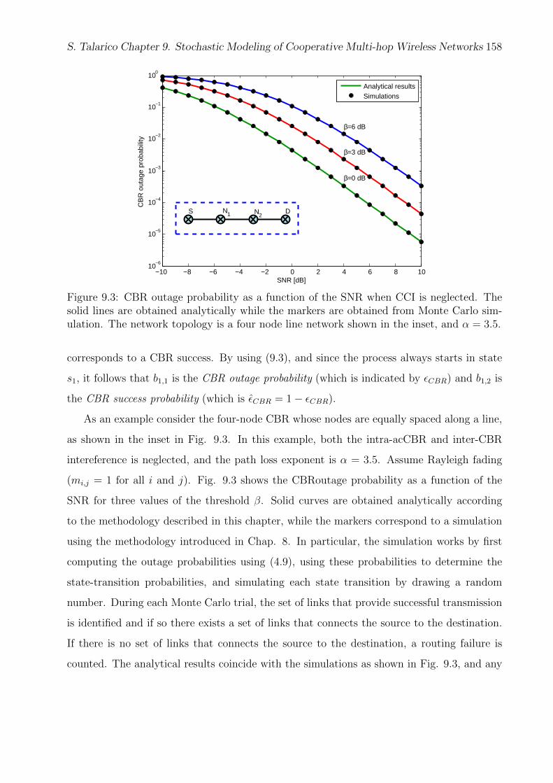
S. Talarico Chapter 9. Stochastic Modeling of Cooperative Multi-hop Wireless Networks 158
−10 −8 −6 −4 −2 0 2 4 6 8 1010
−6
10−5
10−4
10−3
10−2
10−1
100
SNR [dB]
CB
R o
utag
e pr
obab
ility
β=6 dB
β=3 dB
β=0 dB
S N1 N2D
Analytical resultsSimulations
Figure 9.3: CBR outage probability as a function of the SNR when CCI is neglected. Thesolid lines are obtained analytically while the markers are obtained from Monte Carlo sim-ulation. The network topology is a four node line network shown in the inset, and α = 3.5.
corresponds to a CBR success. By using (9.3), and since the process always starts in state
s1, it follows that b1,1 is the CBR outage probability (which is indicated by εCBR) and b1,2 is
the CBR success probability (which is εCBR = 1− εCBR).
As an example consider the four-node CBR whose nodes are equally spaced along a line,
as shown in the inset in Fig. 9.3. In this example, both the intra-acCBR and inter-CBR
intereference is neglected, and the path loss exponent is α = 3.5. Assume Rayleigh fading
(mi,j = 1 for all i and j). Fig. 9.3 shows the CBRoutage probability as a function of the
SNR for three values of the threshold β. Solid curves are obtained analytically according
to the methodology described in this chapter, while the markers correspond to a simulation
using the methodology introduced in Chap. 8. In particular, the simulation works by first
computing the outage probabilities using (4.9), using these probabilities to determine the
state-transition probabilities, and simulating each state transition by drawing a random
number. During each Monte Carlo trial, the set of links that provide successful transmission
is identified and if so there exists a set of links that connects the source to the destination.
If there is no set of links that connects the source to the destination, a routing failure is
counted. The analytical results coincide with the simulations as shown in Fig. 9.3, and any

S. Talarico Chapter 9. Stochastic Modeling of Cooperative Multi-hop Wireless Networks 159
discrepancy between the curves can be attributed to the finite number of Monte Carlo trials
(107 trials were executed per SNR point).
9.2.5 Inter-CBR Interference
This subsection focuses only on inter-CBR interference and assumes that the transmission
from a CBR’s source to its destination must take place within one radio frame or else an
outage occurs. Since each transmission requires one slot, the maximum number of slots per
radio frame is also N + 1. While variable-length frames could be supported, this would
complicate the synchronization of neighboring CBRs. It is thus assumed that all CBRs have
N interior nodes and F = N + 1.
Iterative method
Let Pk represent the transition matrix of the kth CBR. The transition probabilities in Pk
are computed using (4.9), which depend on the p(t)i associated with nodes in other CBRs.
However, each p(t)i represents the probability that node Xi transmits during time slot t, which
can be found from the Pk of the corresponding CBR. Thus, interference causes a linkage
between the transition probabilities in the given CBR and the transmission probabilities
of adjacent CBRs. While this linkage could be handled by considering the overall BRN
as one large Markov chain, this is a cumbersome solution as the number of states grows
exponentially with the number of nodes. A more efficient approach is an iterative one, which
alternates between computing the p(t)i and the Pk.
Let Si,t be the set of states associated with time slot t and labeled with a ‘1’ in the
position corresponding to Xi. These are the states for which Xi transmits during time slot
t. The probability p(t)i can be found by adding the probabilities of being in each of the states
in Si,t, given that the system starts from initial state s1. The probability of being in state
sj ∈ Si,t is found by multiplying the probabilities of all transitions in the Markov chain
leading from state s1 to state sj
Let P k[it] represent the state transition matrix for the kth CBR corresponding to iteration
it, and similarly let p(t)i [it] represent the transmission probability for the ith user during the

S. Talarico Chapter 9. Stochastic Modeling of Cooperative Multi-hop Wireless Networks 160
1 2 3 4 5 6
10−3
10−2
10−1
100
SNR = 0 dB
SNR = 10 dB
Number iterations
CB
R o
utag
e pr
obab
ility
α=3
α=3.5
α=4
Figure 9.4: CBR outage probability for the kth CBR as function of the number of iterationsused, when only the inter-CBR interference is considered. Set of curves at the top: SNR = 0dB. Set of curves at the bottom: SNR = 10 dB. Each set of curves is obtained using threevalues of α.
tth time slot corresponding to iteration it. The iterative method can be described as follows:
1. Initialization: Set it = 0 and initialize p(t)i [0] = 0,∀i, t, which corresponds to neglecting
interference. Then compute each P k[0] using the initial p(t)i [0].
2. Recursion: Increment it. Evaluate each P k[it] using the p(t)i [it−1] from the previous
iteration.
3. Decision: Halt the process if || (P k[it]− P k[it − 1]) ||F < ξ, ∀k, where the operator
|| · ||F is the Frobenius norm and ξ is a tolerance. Otherwise, go back to step 2.
The approach is further simplified if it is assumed that the BRN is comprised of an infinite
cascade of CBRs, all having identical topology. Otherwise, each CBR can be modeled by a
different Markov chain characterized by a specific Pk. Under the assumption of an infinite
cascade of identical CBRs, the Pk and the set of p(t)i will be the same in all active zones.
Because of this, performance can be described by a typical CBR.
As an illustrative example, assume that each CBR is composed of four nodes which are
configured as in the inset of Fig. 9.3. The typical CBR is analyzed assuming it receives

S. Talarico Chapter 9. Stochastic Modeling of Cooperative Multi-hop Wireless Networks 161
CCI from just the two closest adjacent active zones (the interference from distant zones is
neglected). Fig. 9.4 shows the CBR outage probability for a typical CBR as a function of
the number of iterations used in the algorithm described above. Curves are shown for two
values of SNR and three values of α. All six curves are obtained with β = 6 dB, α = 3.5
and under the assumption of Rayleigh faded channels. Fig. 9.4 shows that the CBR outage
probability increases as a function of the number of iterations, and that the iterative method
converges rapidly after very few iterations.
Network Optimization
In the context of a BRN, the ASE for a line network is
Sase = TdCBR (9.5)
where T is the throughput of the CBR and dCBR is the distance between the CBR’s source
and destination. From [?], the throughput can be written as
T =(1− εCBR)
FR (9.6)
where R is the code rate expressed in units of bits per channel use (bpcu).
Substituting (9.6) into (9.5), and relating the rate and the SINR threshold the Shannon
capacity for complex discrete-time AWGN channels, yields
Sase = dCBRεCBR
2 (N + 1)log2 (1 + β) (9.7)
where the factor 2 in the denominator is a consequence of the buffer nodes operating in
half-duplex mode, or, equivalently, due to alternating between active and silent zones
LetXk be a vector containing the position of the N relays in the kth CBR. The goal of the
network optimization is to determine the set Θ = Xk, R,N, dCBR that maximizes (9.7).
Because (9.7) is nonlinear in Θ and the search space is multi-dimensional, efficiently finding
a solution is a challenge. However, by initially using an exhaustive search, we have confirmed
that the optimization surface is convex over the set R,N, dCBR. Thus, the optimization
can be solved through a convex optimization over R,N, dCBR combined by a stochastic
optimization over Xk. It follows that an efficient approach to find the optimal set Θ is as
follows:

S. Talarico Chapter 9. Stochastic Modeling of Cooperative Multi-hop Wireless Networks 162
1. For each of the parameters N , R and dCBR, select a pair of endpoints and a midpoint
(33 = 27 points). The endpoints should initially be far enough apart to guarantee that
the optimal point lies within the endpoints.
2. Define a reference vector X ref (N, dCBR), which is a vector Xk for the pair (N, dCBR)
and a reference set X ref (N, dCBR) containing the reference vectors of all (N, dCBR)
considered by the algorithm. Create three vectors Xk for each pair of (N, dCBR).
When (N, dCBR) is chosen for the first time, the first vector of Xk is obtained by
placing the N relays on the length-dCBR line connecting the source and the destination
and this vector is added to the reference set, constituting X ref (N, dCBR) for the pair
(N, dCBR) chosen. The placement is done in such way that relays are separated by a
minimum distance rs = dCBR
3N, but are otherwise uniformly distributed along the line.
If the pair (N, dCBR) has been already used, the first vector of Xk is set to be equal
to X ref (N, dCBR). The other two vectors are obtained by mutating X ref (N, dCBR) as
follows:
(a) For each relay in X ref (N, dCBR), draw a Bernoulli random variable indicating if
the relay should be moved or if it should remain in its current location.
(b) If the node Xi is to be moved, the direction (right or left) of movement is selected
with equal probability. The new position is obtained by moving the current
position in the selected direction by a distance ∆ = dCBR
n∆N, where initially n∆ = 2.
3. Compute the ASE by (9.7) for the endpoints and the midpoints of the interval of one of
the parameters in the set R,N, d and for the different sets of locations of the relays.
For each pair (N, d) chosen, determine the vector Xk that provides the higher ASE
and replace the X ref (N, d) in the reference set with this vector.
4. For the same parameter of the set R,N, dCBR used in step 3, move the midpoint
of the interval towards the endpoint that gives higher ASE. For each pair (N, dCBR),
generate the three sets of positions as in step 2.
5. Repeat step 3 and 4 recursively for all the parameters in the set R,N, dCBR and

S. Talarico Chapter 9. Stochastic Modeling of Cooperative Multi-hop Wireless Networks 163
Table 9.1: Optimization results when inter-CBR interference is considered.
SNR (in dB) CCI R N dCBR Optimal nodes’ location for a line network Sopt
0 7 4.452 0 0.3
S D
0.490
3 4.421 5 1.2
R1 R2 R3 R4 R5S D
0.402
5 7 4.611 0 0.4
S D
0.683
3 4.452 5 1.7
R1 R2 R3 R4 R5S D
0.559
10 7 5.028 0 0.5
S D
0.951
3 4.547 5 2.3
R1 R2 R3 R4 R5S D
0.777
gradually reduce for one parameter at the time the range between the endpoints and
the midpoint until a certain tolerance is reached. If the optimal ASE remains the same
as in the previous iteration n∆ is increased by one, until a certain value is achieved.
6. If the optimal ASE remains the same as in the previous iteration, for all the parameters
in the set R,N, dCBR it is not possible to further reduce the range between the
endpoints and the midpoint, since a given tolerance is achieved, and n∆ reaches its
maximum value, the algorithm stops.
Using the methodology described above, optimization results were obtained under the
same assumptions that were used in the previous subsection. In particular, it is assumed that
the BRN extends infinitely and CBRs are composed of line networks with the same number
of relays which are all equally positioned. For each CBR the only CCI considered are the
ones from the two closest adjacent active zones (the interference from farther active zones
is neglected, since they are at least at 3dCBR distance away). Although these assumptions
can be relaxed using the analysis and methodology proposed along this chapter, in this
subsection they are used for simplicity of exposure.
Table 9.1 shows the optimal values of N , R, dCBR and the optimal location for the N
relays. Optimization results are provided for three values of Γ and when the CCI is neglected

S. Talarico Chapter 9. Stochastic Modeling of Cooperative Multi-hop Wireless Networks 164
as well as when they are taken into account. Vertical red lines indicate the optimal position
of the mobiles for SNR = 0 dB, and they are used to facilitate the graphical analysis and
comparison of the optimal location of the mobiles for different scenarios. For all scenarios
considered, the path loss exponent is fixed to α = 3.5. Table 9.1 emphasizes that when
there is no CCI, the optimal configuration for a cooperative BRN is to use short CBRs
characterized by a point-to-point conventional communication, while five relays distributed
over a larger CBR allow to achieve the optimal ASE Sopt when there is CCI from the adjacent
CBRs. As expected, the optimal ASE increases by increasing SNR, since the links experience
a more favorable channel. Furthermore, the optimal ASE increases going from a scenario in
which there is CCI to one in which CCI is neglected, and this is more prominent as SNR
increases since the network becomes more interference sensitive. In agreement with [154],
an increase in SNR produces a shift towards the source of the optimal position of the relays,
which increases the likelihood to cooperate among themselves. A more favorable condition
of the channel produces an increment in both the optimal code rate R and in the optimal
dimension of the CBR.
9.2.6 Intra-CBR Interference
While in the previous subsection, it is assumed that a time frame is sufficiently long
to ensure that a packet reaches the destination before a new packet is injected within a
CBR, this is not generally valid. In fact, in practice BRNs often employ a fixed frame
length of F = 4 and a fixed maximum number of relays that is greater than F [150]. In
such networks, spatial pipelining enables multiple packets, which will share the same radio
resources, to be active simultaneously within a given CBR. As previously mentioned, a new
packet is injected in a given CBR during the first time slot of each new radio frame, and
when multiple packets propagate with a given CBR, they interfere with each other. In order
to account for this source of interference within the aforementioned framework and in order
to account for the effect of correlation among packets an iterative method is introduced,
which is based on a Viterbi-like algorithm. Finally, similar to the previous subsection, an
optimization is performed for a line network subject to intra-CBR interference in order to

S. Talarico Chapter 9. Stochastic Modeling of Cooperative Multi-hop Wireless Networks 165
maximize its throughput by opportunely selecting the rate, the number of relays of which a
CBR is composed, as well as the number of time slots that compose the radio frame.
Iterative method
Let Pzk represent the transition matrix of the kth CBR for the zth packet. When the inter-
CBR interference is neglected, but multiple packets can simultaneously propagate within
the same CBR, there is a linkage between the transition probabilities for the zth packet Pzk
and the transmission probabilities of the nodes within the kth CBR that may be active in
letting other packets propagate during the interval of time the zth packet is broadcasted.
Furthermore, the probabilities of transmission for the zth packet during a given radio frame
depends also on the reciprocal interference produces by packets that have been propagating
or had propagated within the kth CBR since the very first transmission. These linkages could
be handled by considering a large Markov chain, which describes the full dynamics in time
of the kth CBR. However, this solution is in most cases computational infeasible. A more
appropriate approach is to use a Viterbi-like algorithm to iteratively update the transition
matrix of the kth CBR on a radio frame basis, alternating between the computation of the
Pzk and the p(t)
i,z, where p(t)i,z is the probability that ith node transmits the zth packet
during time slot t.
Let Z[f ] indicate the set of packets that might be active during the f th radio frame,
which are ordered based on when they are first injected. Let Z[f ](i) be the ith element of
the set Z[f ] and let Npk[f ] = |Z[f ]| is their number. Let P zk[it] represent the state transition
matrix for the kth CBR at iteration it for the zth packet, when it is active during the f th
radio frame, and similarly let p(t)i,z[it] represent the transmission probability at iteration it for
the ith user when it transmits the zth packet during the tth time slot of the f th radio frame.
Let If indicate the maximum number of iterations needed to evaluate the transition matrix
for the packet that is first transmitted during the f th radio frame. The iterative method can
be described as follows:
1. Initialization: Set f = 1 and it = 0. Find the set Z[1] of packets that might be active
during the first radio frame. Initialize p(t)i,z[0] = 0,∀i, t and z ∈ Z[1]. Note, that this

S. Talarico Chapter 9. Stochastic Modeling of Cooperative Multi-hop Wireless Networks 166
corresponds to neglecting interference within the kth CBR, during the duration of the
first radio frame. Furthermore, it allows the iterative method to start from the scenario
where the first packet injected within the kth CBR is not subject to any intra-CBR
interference, unless it is still propagating during one of the successive radio frames.
Compute P zk[0] using the initial p(t)
i,z[0] for all z ∈ Z[1].
2. Recursion:
(a) Increment it. Compute P zk[it] using the p(t)
i,z[it] from the previous iteration for
all z ∈ Z[f ].
(b) Go back to step 2a until || (P zk[it]− P z
k[it − 1]) ||F < ξ,∀z ∈ Z[f ], where the
operator || · ||F is the Frobenius norm and ξ is a tolerance.
3. Decision: Halt the process if both the following conditions are met:
•∣∣∣∣∣∣ (PZ[f ](i)
k [If ]− PZ[f−1](i)k [If−1]
) ∣∣∣∣∣∣F< ξ,∀i ∈ 1, · · · , Npk[f − 1];
• f 6= 1.
Otherwise,
(a) Increment f . Set it = 0. Evaluate the set Z[f ] of packets that might be active
during the f th radio frame.
(b) go back to step 2.
Note that this approach not only accounts for the reciprocal interference that different
packets produce to each other, but also for the effect of the correlation among them. As
an illustrative example, assume that a CBR is composed of four nodes (N = 2) which are
configured again as in the inset of Fig. 9.3. The CBR is analyzed by neglecting the inter-
CBR interference. Fig. 9.5 shows the CBR outage probability when the length of the radio
frame is varied within the set F = 1, 2 as function of the number of radio frames that
need to be considered in the aforementioned iterative method. Curves are shown for three
values of the path loss exponent. All curves are obtained with β = 6 dB, SNR = 0 dB, and
under the assumption of Rayleigh faded channels. Fig. 9.5 shows that the iterative method
converges very quickly.

S. Talarico Chapter 9. Stochastic Modeling of Cooperative Multi-hop Wireless Networks 167
0 5 10 15
10−1
100
Number radio frames
CB
R o
utag
e pr
obab
ility
F=1
F=2
α = 3
α = 3.5
α = 4
Figure 9.5: CBR outage probability for the kth CBR as function of the number of radioframes considered, when only the intra-CBR interference is taken into account.
Network Optimization
Using (9.5) and (9.6), and by relating again the rate and the SINR threshold by the
Shannon capacity for complex discrete-time AWGN channels, in this scenario the ASE can
be written as follows
Sase = dCBRεCBRF
log2 (1 + β) . (9.8)
As can be observed in (9.8), there is a tradeoff between the rate, the number of relays that
compose a CBR, and the number of time slots in a radio frame. Therefore, the goal of the
network optimization is to determine the set Θ = R,N, F that maximizes (9.8). While an
exhaustive search could be a good alternative to this type of non-linear optimization problem,
a more efficient method can be used. In particular, after finding that the optimization surface
is convex over R,N, F, a more efficient approach to find the optimal set Θ is as follows:
1. For each of the parameters N , R and F , select a pair of endpoints and a midpoint
(33 = 27 points). The endpoints should initially be far enough apart to guarantee that
the optimal point lies within the endpoints.

S. Talarico Chapter 9. Stochastic Modeling of Cooperative Multi-hop Wireless Networks 168
Table 9.2: Optimization results when intra-CBR interference is considered..
dCBR SNR (in dB) R N F Sopt
1 0 4.389 7 3 1.361
5 5.676 7 3 1.811
10 5.028 6 2 2.509
0.5 0 5.028 5 2 1.256
5 6.658 5 2 1.6615
10 8.309 5 2 2.062
2. Compute the ASE by (9.8) for the endpoints and the midpoints of the interval of one
of the parameters in the set R,N, F.
3. For the same parameter of the set R,N, F used in step 2, move the midpoint of the
interval towards the endpoint that gives higher ASE.
4. Repeat step 2 and 3 recursively for all the parameters in the set R,N, F and gradually
reduce for one parameter at the time the range between the endpoints and the midpoint
until a certain tolerance is reached. If the optimal ASE remains the same as in the
previous iteration, the algorithm stops.
Using the methodology described above, optimization results were obtained under the
assumption that the inter-CBR interference can be neglected3. A line network is considered,
which is composed of a CBR with nodes disposed at equal distance from each other.
Table 9.2 shows the optimal values of N , R, and F . Optimization results are provided for
three values of Γ. Two length for the CBR are considered. For all the scenarios considered,
the path loss is fixed to α = 3.5. Table 9.2 shows that as expected the optimal ASE increases
by increasing SNR. More importantly, as the SNR increases, it is possible to more frequently
inject new packets by reducing the length of the radio frame and slightly reduce the code
rate. As the length of the CBR is reduced, a fewer number of relays is required, and while
as expected the throughput increases, a lower ASE is achieved.
3Note that here for sake of simplicity the inter-CBR interference is neglected, but it can be taken intoaccount by jointly using the iterative method described in this subsection, together with the one describedin the previous subsection.

S. Talarico Chapter 9. Stochastic Modeling of Cooperative Multi-hop Wireless Networks 169
9.3 Chapter Summary
This chapter has presented a novel analytical framework to model and analyze coop-
erative multi-hop networks. The main advantage of this framework compared to those in
the literature is in the reduced computational effort required, since it builds on the anal-
ysis developed along this dissertation, which allows to evaluate the link outage probability
for diversity combining in closed-form and doesn’t require any averaging over the fading
gains. This framework is then applied to analyze and optimize unicast in a BRN. A BRN
is analyzed by describing the behavior of each constituent CBRs as a Markov chain and
the transition probabilities are computed by using a closed form expression for the outage
probability, which takes into account the path loss, Rayleigh fading, and interference. Both
inter-CBR and intra-CBR interference are considered. Both sources of interference cause
an interdependence between the transmission and transition probabilities, which is taken
into account by an iterative method. In the case of inter-CBR interference, the iterative
method updates the probability of collisions for each CBR at each iteration for each one of
the time slots. In contrast, intra-CBR is handled by using a Viterbi-like algorithm to iter-
atively update the transition probabilities on a radio frame basis, while still accounting for
the interdependence between packets that simultaneously propagate within a CBR and their
temporal correlation. The analysis and each iterative method have been used to perform
an optimization of a BRN by accounting individually for a single type of interference. First
only the inter-CBR interference are considered, and the aim has been to maximize the ASE
by finding the optimal number of relays that need to be used in the CBRs that compose the
BRN, their optimal placement, the optimal size of the CBRs and the optimal code rate at
which the nodes transmit. Finally, the effect of intra-CBR interference is studied and the
network is optimized for several different scenarios with the aim again of maximizing the
ASE by choosing opportunely the length of a radio frame, the code rate at which a node
transmits and the number of relays involved in the communication. While the analysis and
the model have been applied to study and optimize a BRN, this work could be extended to
different types of cooperative ad hoc networks.
170
Chapter 10
Conclusion
In this dissertation, the effect of interference and computational complexity has been
studied in the context of modern wireless communication systems. The first main contribu-
tion of this dissertation is the development of a novel analytical framework that captures the
effects of interference and fading by evaluating the outage probability for wireless networks
with interferers located according to a point process when the signal is subject to fading.
This framework is applied to a variety of cases in order to demonstrate its wide applicability
and benefits in modeling both conventional and cooperative networks (i.e., conventional and
cooperative cellular networks, and multi-hop ad hoc networks).
The second main contribution of the dissertation is the development of an analytical
framework to estimate the computational resources required to decode a signal under a given
performance constraint. This framework has been used to highlight the benefit of pooling
computational resources and centrally processing uplink signals as an alternative to a con-
ventional distributed approach. A better understanding of the interplay between available
computing resources and the required communications performance is provided. The disser-
tation developed computationally aware schedulers, in order to better manage the resources
available in systems such as Cloud-RANs, where the quality of communications is strongly
effected by the limited computational resources available for processing the communication
signals.
By leveraging its proposed analytical framework, the dissertation provided a novel method-
ology to optimize future-generation multiple-access networks, including FH systems, with the

S. Talarico Chapter 10. Conclusion 171
aim to further mitigate the effect of frequency-selective fading and prevent the near-far prob-
lem. The optimization accounts for the modulation format used, but also for the presence of
fading and interference effects, including CCI and ACI. This work has concluded by describ-
ing a more efficient and accurate method to stochastically model and study the performance
of cooperative multi-hop wireless networks in presence of interference, which was applied to
model and optimize a BRN.
10.1 Summary and Publications
After an introductory chapter, the discussion starts in Chap. 2, which builds an alterative
analytical framework to evaluate the outage probability of an arbitrarily shaped network sub-
ject to fading and with the location of the interferers distributed according to a point process.
In this chapter, the effect of spatial correlation of the interference has been also quantified.
The main contribution of this chapter lies in the fact that the common assumption of an
infinite network has been relaxed, and the analysis is broken into multiple steps, which help
to distinguish the effect of fading, shadowing and spatial distribution, which are mechanisms
that operate over different time scales. A closed-form expression is provided for the outage
probability averaged over the fading and conditioned on the topology of the network and
shadowing gains. This expression is particularly useful and results to be very efficient when
analytical untractable spatial models are adopted, or more sophisticated shadowing models
or path loss models want to be considered. In this case, the use of simulations is necessary,
but they are notably simplified since the effect of the small scale fading is already taken into
account. The analytical framework described in this chapter has been initially published and
presented at the 2012 Virginia Tech Symposium on Wireless Personal Communication [1]
under the simplified assumption of Rayleigh fading and a circular network, and then in IEEE
Communication Letters [2] for an arbitrarily shaped network. The work on the quantification
of the spatial correlation has been instead enclosed in a manuscript under preparation [3].
In order to prove the wide applicability of the framework introduced in Chap. 2, Chap.
3 applies it to model and analyze the performance of DS-CDMA cellular uplinks. The model
and the analysis, are very general and can handle a very large variety of MAC protocols

S. Talarico Chapter 10. Conclusion 172
and resource allocation policies. The main contribution of this chapter lies in the adoption
of a more accurate spatial model for both the BSs and UEs, which guarantees a minimum
separation among devices and mimics more closely the deployment of an actual cellular
network. Furthermore, the analysis allows to discharge the common assumptions of identical
fading conditions for each link and a distance dependent path loss model with a single slope.
The results contained in this chapter have been initially published and presented at the 2013
IEEE International Conference on Computing, Networking, and Communications [4] for the
downlink, and at the 2013 IEEE International Conference on Communication [5] for the
uplink. The work leading to this chapter has been also published on IEEE Transaction on
Communications [6].
The analytical framework built in Chap. 2 has been extended in Chap. 4 in order to
account for the case when a receiving device performs diversity combining of signals from
multiple source transmitters. In this case, the analysis is applied to model and analyze a
DS-CDMA downlink MCC and a MBSFN. The main contribution lies in the derivation of
a closed-form expression for the outage probability averaged over the fading, which allow
to adopt a more accurate spatial model, a distance dependent fading model and doesn’t
preclude the usage of a path loss model with multiple slopes. This work has been published
and presented at the 2013 IEEE Global Telecommunication Conference [7] and at the 2014
IEEE International Conference on Acoustic, Speech and Signal Processing [8].
Chap. 5 builts an analytical framework to estimate the required data processing resources
under a given performance constraint, which allows to underline the tradeoff between the
throughput and the computational complexity. In this chapter, the emphasis has been given
to the Cloud-RAN architecture, and the developed analytical framework is used to high-
light the benefits of pooling computational resources and centrally process uplink signals
from a group of BSs also by the introduction of novel metrics ( i.e., computational outage,
computational diversity and computational gain). As shown along Chap. 5, despite some
simplificative assumptions that have been made and which are necessary for the tractabil-
ity of the problem, the analytical framework is very accurate and provides a good match
with simulations obtained through a system level simulator compliant with the 3GPP LTE
standard. The analytical framework and the findings of this chapter have been published on

S. Talarico Chapter 10. Conclusion 173
IEEE Transaction on Wireless Communications [9].
Following from Chap. 5, Chap. 6 provides more insights on how the communications
performance are effected by the computational resources available. In this chapter, three
computational aware schedulers are designed for practical systems, which are able to signifi-
cantly reduce the computational effort required at the receiver by opportunely selecting the
MCS scheme to use for each uplink and improve the overall performance of the network by
reducing or eliminating the likelihood of computational outages. The first scheduler called
CAS chooses the MCS to adopt by opportunely backing-off from capacity with the aim to
reduce the computational complexity required at the receiver in order to reduce the proba-
bility of computational outage. The other two schedulers, SWF and SCC, are designed with
the aim to completely avoid computational outages while the objective is to maximize the
achieved sum-rate. SWF is based on a water-filling algorithm, while SCC is more intuitive
and simple and uses a complexity-cut-off approach. While the concepts of computational
outage and detailed performance evaluation of CAS have been published and presented at
the 2014 IEEE Global Telecommunication Conference [10], the remaining part of this chap-
ter will be presented in the 2015 venue [11]. The work discussed in both Chap. 5 and Chap.
6 will also appear on a book chapter [12].
Chap. 7 focuses on FH systems in general, and in particular on ad hoc networks which
uses a non-coherent CPFSK modulation. This modulation format depends on the modula-
tion index, the number of frequency channels in which the overall bandwidth is divided and
the fractional in-band power, which is the fraction of the signal power that lies within the
band of each frequency channel. These parameters are often chosen arbitrarily. However,
the chapter shows that under two different rate-allocation policies that optimally selecting
them together with the rate, it is possible to achieve a significant improvement of the perfor-
mance of the system. The results of this research have been published and presented at the
2012 IEEE Symposium on Military Communications [13], at the 2013 IEEE International
Conference on Communication [14], and at the 2015 IEEE Symposium on Military Commu-
nications [15]. Furthermore, a manuscript, which will be submitted to IEEE Transaction on
Communications [16] and summarizes all our results on the topic, is in preparation.
Chap. 8 introduces a new methodology to model and analyze the performance of multi-

S. Talarico Chapter 10. Conclusion 174
hop routing protocols in ad hoc networks which builds on the analytical framework intro-
duced in Chap. 2. This chapter accounts for the effect of the interference and their spatial
and temporal correlation and evaluates the performance of two representative geographic
routing protocols in order to gain perspective about their advantages and disadvantages.
The main contribution of this chapter is in proposed paradigm, which can be used for rapid
performance assessment of a large variety of routing protocols. The methodology proposed in
this chapter is able to discharge some of the common assumptions made in the related work in
the litterature, such as the independence of the success probabilities of path from the source
to the destination even when paths share the same links. This work has been published and
presented at the 2013 and 2014 IEEE Symposium on Military Communications [17,18] and
has been accepted to publication on IEEE Transactions on Communications [19].
Chap. 9 introduces an efficient method to stochastically model and study the perfor-
mance of cooperative multi-hop networks when accounting for CCI originated by multiple
packets that simultaneously propagate along the network, their temporal correlation and
interdependence. The dynamics of how a cooperative protocol evolves over time is described
through an absorbing Markov chain, which uses the analysis developed in Chap. 4 to evaluate
the transmission probability of each relay. This methodology differs from the ones existing
in the literature, since the end-to-end probability of success of a cooperative network is not
evaluated by starting from a single set of channel realizations (as it is usually done) and then
averaging over them, but through the channel outage framework developed along this disser-
tation. As already stated, this framework provides the channel outage probability already
averaged over the fading and in this context it drastically reduces the computational effort
to model and analyze a cooperative multi-hop network. As an example of its applicability,
this framework is used in this chapter to analyze the performance of a BRN and perform an
optimization of such a system over a set of parameters, which includes the code rate, and
the number of relays used. The work related to inter-CBR interference has been published
and presented at the 2014 IEEE Symposium on Military Communications [20], while the
remaining work has been enclosed in a recently submitted manuscript [21].

S. Talarico Chapter 10. Conclusion 175
10.2 Future Work
As already mentioned, the analytical frameworks proposed in this dissertation are very
general and they can be adopted to several other applications and case of studies. Suggestions
for future work and extensions of this work might include:
1. Cognitive Networks: The limited bandwidth available and the inefficient usage of the
spectrum has led in the past years a significant amount of research devoted to cognitive
radio. In a cognitive radio, a cognitive (secondary) user is allowed to share the spectrum
with a primary users, as long as its interference is below a certain threshold. In this
type of networks the geometry plays an important role and the analytical framework
developed in Chap. 2 can be actually used to analyze the interaction between primary
and secondary users.
2. Other diversity techniques: An attempt to expand the analytical framework devel-
oped in Chap. 2 for other diversity techniques can be made, which will open another
large set of interesting applications and optimization problems.
3. MmWave and device-to-device communication: Since the analysis developed in
Chap. 2 and Chap. 4 allows to consider non identical fading conditions at each link
and a multiple slope path loss model can be adopted, the methodology introduced in
Chap. 3 can be used to accurately model and analyze multi-antenna transmissions in
millimiter-wave heterogeneous cellular networks and device-to-device communication.
4. Computational requirements: channel outage and interference: One of the
weak points of the analytical framework developed in Chap. 5 is that the channel
outage is not explicitly taken into account. In a real system, the computational outage
and channel outage can both occur, in a non mutually exclusive manner, and they are
both equally important for the overall performance of the network. For instance, when a
channel outage occurs, the maximum computational complexity might be invested and
the data processing requirements might change. Therefore another possible extension
of this work might be to analytically account for the channel outage in the proposed
framework, in order to estimate more accurately the data processing requirements of

S. Talarico Chapter 10. Conclusion 176
the network. Furthermore, the effect of co-channel interference needs to be taken into
account, and bounds might be derived for the novel performance metrics introduced
in this chapter.

177
Appendix A
Conditional Outage Probability:
Derivation
This appendix provides details leading to (2.9). Let FZj
(z∣∣Ω) = 1−FZj
(z∣∣Ω) denote the
complementary CDF of Zj conditioned on Ω. Assuming that the Nakagami parameter m0,j
of the source’s channel is integer-valued, the CDF of Zj can be computed as follows [155]:
FZj(z∣∣Ω) = P[Zj > z
∣∣Ω] = P
[Sj > z +
M∑i
Yi,j
]=
∫...
∫RM
fY(y)FSj
(z +
∑yi
)dy (A.1)
where the integral is over M -dimensional real space. Taking into account the Nakagami
fading and the activity probability pi, the PDF of fY(y), which is the joint PDF of the
vector Y = Y1,j, ..., YM,j, is
fYi(y) = (1− pi) δ (y) + pi
(mi,j
Ωi,j
)mi,j ymi,j−1
Γ (mi,j)exp
(−mi,jy
Ωi,j
)u (y) (A.2)
where u (y) is the step function, δ (y) is the Dirac delta function, and
Γ (x) =
∫ ∞0
yx−1e−y dy. (A.3)
The gamma-distributed Sj with Nakagami parameter m0,j has a CDF, which is
FSj (s) = exp
(−βm0,js
Ω0,j
)m0,j−1∑µ=0
1
s!
[βm0,js
Ω0,j
]s. (A.4)

S. Talarico Appendix A 178
Substituting (A.4) into (A.1) and performing a few manipulations yields
FZj(z∣∣Ω) = exp
(−βm0,jz
Ω0,j
)m0,j−1∑µ=0
(βm0,jz)µ
Ωµ0,jµ!
×∫...
∫RM
fY(y) exp
(−βm0,j
Ω0,j
∑yi
)(1 + z−1
M∑i=1
yi
)µ
dy. (A.5)
Since µ is an integer, the binomial theorem gives the series expansion:(1 + z−1
M∑i=1
yi
)µ
=
µ∑t=0
(µ
t
)z−t
(M∑i=1
yi
)t
. (A.6)
A multinomial expansion yields(M∑i=1
yi
)t
= t!∑`i≥0∑Mi=1 `i=t
(M∏i=1
y`ii`i!
). (A.7)
Substituting (A.6) and (A.7) into (A.5), performing a few manipulations, and assuming that
the interfering channels fade independently,
FZj(z∣∣Ω) = exp
(−βm0,jz
Ω0,j
)m0,j−1∑µ=0
(βm0,jz)µ
Ωµ0,jµ!
µ∑t=0
z−t
(µ− t)!∑`i≥0∑Mi=1 `i=t
M∏i=1
G`i(Ωi,j) (A.8)
where
G`i(Ωi,j) =
∫R
exp
(−βm0,jy
Ω0,j
)y`i
`i!fYi,j(y) dy. (A.9)
Substituting (A.2) in (A.9),
G`i(Ωi,j) = (1− pi) δ`i +piΓ(`i +mi,j)
`i!Γ(mi,j)
(Ωi,j
mi,j
)`i (βm0,jΩi,j
mi,jΩ0,j
+ 1
)−(mi,j+`i)
. (A.10)
Finally, by substituting (A.10) into (A.8) and then into (2.8), (2.9) is obtained.

179
Appendix B
Asymptotic Outage Analysis
This appendix provides details leading to (2.50) through two approach: 1) direct approach
using classic probability theory; 2) stochastic geometry approach.
2.1 Direct Approach
Let A include the interferers on the entire plane R2. The outage probability can be
found by taking the limit of (2.49) as rin → 0 and rout →∞. Using (2.49), the limit may be
expressed as
εj = 1− exp
−βrα0,jSNR
+ πλp limx→∞
Φ (x)
(B.1)
where the right hand side follows from the continuity of the exponential function.
By performing the change of variables y =βrα0,jxα
and v = 1 + 2α
, the limit in (B.1) may
be written as
limx→∞
Φ (x) = limy→0
Φ
(β
1α r0,j
y1α
)= βv−1r2
0,j(v − 1) limy→0
y1−vφ (y)
(B.2)
where
φ(y) =1
vy2F 1
([1, v] ; v + 1,−y−1
)− 1
v − 1. (B.3)
From (2.24) and the functional equation Γ(1 + x) = xΓ(x),
φ(y) =1
y
∫ 1
0
tv−1
(1 +
t
y
)−1
dt− 1
v − 1. (B.4)

S. Talarico Appendix B 180
By splitting the integral at y and factoring the second integrand,
φ(y) =1
y
∫ y
0
tv−1
(1 +
t
y
)−1
dt
+
∫ 1
y
tv−2(
1 +y
t
)−1
dt− 1
v − 1. (B.5)
By substituting the Taylor series and then integrating term by term,
φ(y) =1
y
∞∑i=0
(−1)iyv
v + i+∞∑i=0
(−1)i (yi − yv−1)
v − 1− i− 1
v − 1. (B.6)
Simplifying the first series and dividing the second series into two series,
φ(y) =∞∑i=0
(−1)iyv−1
v + i+∞∑i=0
(−1)iyi
v − 1− i
−∞∑i=0
(−1)iyv−1
v − 1− i− 1
v − 1. (B.7)
Combining the first and third series, canceling the first term of the second series, and
multiplying both sides by y1−v,
φ(y)y1−v =∞∑i=0
(−1)i
v + i− (−1)i
v − 1− i
+∞∑i=1
(−1)iyi−v+1
v − 1− i. (B.8)
Taking the limit of (B.8) as y → 0
limy→0
∞∑i=0
(−1)i
v + i− (−1)i
v − 1− i
+∞∑i=1
(−1)iyi−v+1
v − 1− i
=∞∑i=0
(−1)i
v + i− (−1)i
v − 1− i
+∞∑i=1
(−1)i limy→0 yi−v+1
v − 1− i(B.9)
where the second line follows from the fact that the first series is independent of y and finite.
Since α > 2, and therefore v < 2, the exponent of yi−v+1 is always positive. Therefore, the
limit in (B.9) evaluates to zero, and
limy→0
φ(y)y1−v =∞∑i=0
(−1)i
v + i− (−1)i
v − 1− i
. (B.10)
Substituting (B.10) into (B.2)
limx→∞
Φ (x) = βv−1r20(v − 1)
∞∑i=0
(−1)i
v + i−∞∑i=0
(−1)i
v − 1− i
. (B.11)

S. Talarico Appendix B 181
Consider the first series in (B.11). By performing the change of variables i = −j − 1,
∞∑i=0
(−1)i
v + i=
−1∑j=−∞
(−1)−j−1
v − j − 1⇒ −
−1∑i=−∞
(−1)i
v − 1− i. (B.12)
Substituting (B.12) into (B.11), combining the two series, and replacing (v − 1) with 2/α,
limx→∞
Φ (x) = − 2
αβ2/αr2
0
∞∑i=−∞
(−1)i
2α− i
. (B.13)
The series in (B.13) can be written as
∞∑i=−∞
(−1)i
2α− i
=α
2+ 2
(2
α
) ∞∑i=1
(−1)i(2α
)2+ i2
= π csc
(2π
α
). (B.14)
where the last line follows from (4.22.5) of [156]. Substituting (B.14) into (B.13),
12α
+ i+
12α− i
=2(
2α
)(2α
)2+ i2
(B.15)
and combining the two series,
limx→∞
Φ (x) = −2β2/αr2
0,j
α
α
2+ 2
(2
α
) ∞∑i=1
(−1)i(2α
)2+ i2
. (B.16)
From (4.22.5) of [156],
limx→∞
Φ (x) = −2π
αβ2/αr2
0,j csc
(2π
α
). (B.17)
Finally, substituting (B.17) into (B.1) gives (2.50).

S. Talarico Appendix B 182
2.2 Stochastic Geometry Approach
Let Φ (λp) = Ωi denote the location of the interferers, which are distributed according
to a PPP with intensity λp. The outage probability is
εj = 1− P
[g0,jr
−α0,j
SNR−1 +∑
i∈Φ(λp) gi,jr−αi,j
> β
](B.18)
= 1− P
g0 >βrα0,jSNR
+ βrα0,j∑
i∈Φ(λp)
gi,jr−αi,j
(B.19)
(a)= 1− exp
−βrα0,jSNR
Eg,Φ
exp
s ∑i∈Φ(λp)
gi,jr−αi,j
s=βrα0,j
(B.20)
(b)= 1− exp
−βrα0,jSNR
EΦ
∏i∈Φ(λp)
Egi,j[exp
sgi,jr
−αi
]s=βrα0,j
(B.21)
where Egi,j [·] and EΦ [·] are the operator expectation evaluate respectively over the fading and
the spatial distribution of the interferers,(a)= follows due to the fact that g0,j is exponentially
distributed, while(b)= follows due to the fact that gi,j and ri,j are independent.
Since gi,j is exponentially distributed, the inner expectation in (B.21) is
Egi,j[exp
−sgi,jr−αi,j
]=
∫ ∞0
exp−gi,j
(sr−αi,j + 1
)dgi,j
=1
1 + sr−αi,j. (B.22)
Substituting (B.22) in (B.21), and using [157, proposition 2.12] for the PGFL of a PPP, the
outer expectation in (B.21) is
EΦ
∏i∈Φ(λp)
1
1 + sr−αi,j
= exp
−2πλp
∫ ∞0
sr−α
1 + sr−αr dr
. (B.23)
Performing the change of variables u = s−1α r and some algebraic manipulations, yields
EΦ
∏i∈Φ(λp)
1
1 + sr−αi,j
= exp
−2πλps2/α
∫ ∞0
u
1 + uαdu
= exp
−2πλps2/απ
αcsc
(2π
α
). (B.24)
Finally, recalling that s = βrα0,j, and substituting (B.24) in (B.21), (2.50) is obtained.

183
Appendix C
Correlation Coefficient in a BPP:
Derivation
This appendix provides details leading to (2.56), (2.57) and (2.58). The evaluation of the
three expressions requires the PDF of ri,j, which in this case is [48]
fr(r) =
2πr|A| for 0 ≤ r ≤ rout − r0
2r|A| arccos
(r2+r2
0−r2out
2r0r
)for rout − r0 ≤ r ≤ rout + r0
(C.1)
3.1 Spatially Averaged First Moment
The spatially averaged first moment of the outage probability is derived starting from
(7.9). In particular, substituting (C.1) in (7.9), yields
EΩ [εj (Ω) |M ] = 1−exp
(βrα0SNR
)[1−p+
2πp
|A|βrα0
∫ rout−r0
0
rα+1
1+rαβ−1r−α0
dr+Zi(rout, r0)
]M(C.2)
where
Zi (rout, r0) =
∫ rout+r0
rout−r0
riα+1
(βrα0 + rα)iarccos
(r2 + r2
0 − r2out
2r0r
)dr. (C.3)
Since the first integral in (C.2) is (2.19), which leads to (2.21), and after few algebraic
manipulations, (2.56) is obtained.

S. Talarico Appendix C 184
3.2 Spatially Averaged Second Moment
The spatially averaged second moment of the outage probability is derived starting from
(2.53) substituting in (2.10). Since Ω = r−α and the M interferers are independently and
uniformly distributed (i.u.d.) over A, yields
EΩ
[ε2j (Ω) |M
]= 1− 2 exp
(− βr
α0
SNR
)(1− p+ p
∫fr(r)
rα
βrα0 + rαdr
)M+ exp
(−2
βrα0SNR
)[∫fr(r)
(1− p+
prα
βrα0 + rα
)2
dr
]M. (C.4)
By substituting (C.1) in (C.4), from (2.19) and (C.3) the first integral in (C.4) is∫fr(r)
rα
βrα0 + rαdr =
2
|A|
[π
βrα0Ψ1 (rout − r0) + Z1 (rout, r0)
](C.5)
while after few algebraic manipulations the second integral is
S (rout, r0) =
∫fr(r)
(1−p+
prα
βrα0 +rα
)2
dr
= (1− p)2 +4
|A|(1− p) p
[π
βrα0Ψ1 (rout − r0) + Z1 (rout, r0)
]+
2p2
|A|[πG (rout − r0) + Z2 (rout, r0)] (C.6)
where Zi (rout, r0) is given by (C.3) and
G (x) =
∫ x
0
r2α+1
(βrα0 + rα)2 dr. (C.7)
By performing the change of variable r = yν1α ,
G (x) =x2α+2
(2 + 2α) β2r2α0 2
F1
([2,
2 + 2α
α
];2 + 3α
α;− xα
βrα0
). (C.8)
By substituting (C.5), (C.6) and (C.8), in (C.4), and by performing few algebraic ma-
nipulations (2.57) is obtained.
3.3 Spatially Averaged Joint First Moment
The spatially averaged joint first moment of the outage probability is derived starting
from (2.54). If polar coordinates are used to evaluate the distances between each interferer

S. Talarico Appendix C 185
and the jth receiver, then
r (ρ, φ, θ) = ||r0 exp (jθ) + rout√ρ exp (jφ)|| (C.9)
where ρ ∼ U (0, 1) and φ ∼ U (0, 2π). Since the M interferers are independently and uni-
formly distributed (i.u.d.) over A,
EΩ [ε1 (Ω) ε2 (Ω) |M ] = 1−exp
(− βr
α0
SNR
)(1−p+p
∫ ∫rα (ρ, φ, 0)
βrα0 +rα(ρ, φ, 0)fρ(ρ)fφ(φ) dρ dφ
)M− exp
(− βr
α0
SNR
)(1−p+p
∫ ∫rα (ρ, φ, θ)
βrα0 +rα(ρ, φ, θ)fρ(ρ)fφ(φ)dρ dφ
)M+ exp
(−2
βrα0SNR
)[∫ ∫ (1−p+
prα (ρ, φ, 0)
βrα0 + rα (ρ, φ, 0)
)×(
1− p+prα (ρ, φ, θ)
βrα0 + rα (ρ, φ, θ)
)fρ (ρ) fφ (φ) dρ dφ
]M. (C.10)
The first and second double integral in (C.10) are equivalent, since the first moment
of the outage probability is the same at the two receivers, which are equally distant from
the reference transmitter, and they coincide with (C.5). Performing the cross products and
several other algebraic manipulations in the last term of (C.10) and using the functions given
by (7.10) and (C.3), yields
W (rout, r0, θ) =
∫ ∫ (1− p+
prα (ρ, φ, 0)
βrα0 + rα (ρ, φ, 0)
)(1− p+
prα (ρ, φ, θ)
βrα0 + rα (ρ, φ, θ)
)dρ dφ
= (1−p)2+4
|A|(1−p) p[πΨ1(rout−r0)+Z1(rout, r0)]+p2X (rout, r0, θ) (C.11)
where
X (rout, r0, θ) =1
2π
∫ 1
0
∫ 2π
0
rα (ρ, φ, 0)
βrα0 + rα (ρ, φ, 0)
rα (ρ, φ, θ)
βrα0 + rα (ρ, φ, θ)dρ dφ. (C.12)
Finally, By substituting (C.11), and (C.12), in (C.10), and by performing few algebraic
manipulations (2.58) is obtained.

186
Appendix D
Conditional Outage Probability for
Diversity Combining: Derivation
This appendix provides details leading to (4.9). In the absence of interference, εj (Ω) =
FS
(SNR−1
∣∣Ω). Restricting the Nakagami parameters mk,j,∀k ∈ Gj, to be integer-valued,
but not necessarily identical, the CDF of S is found in [158] to be
FS
(s∣∣Ωj
)=
∑k∈Gj
mk,j∑n=1
[1− exp
(−βmk,js
Ωk,j
) n−1∑µ=0
(βmk,js)µ
Ωµk,jµ!
]
ΞNj
(k, n, mq,j∀q∈Gj ,
Ωq,j
βmq,j
∀q∈Gj
). (D.1)
The function ΞL
(k, n, rqLq=1 , ηq
Lq=1
)is
ΞL
(k, n, rqLq=1 , ηq
Lq=1
)=
rk∑l1=n
l1∑l2=n
· · ·lL−3∑
lL−2=n
[(−1)RL−rk ηnk∏L
h=1 ηrhh
(rk + r1+u(1−k) − l1 − 1
)!(
r1+u(1−k) − 1)! (rk − l1)!(
1
ηj− 1
η1+u(1−k)
)l1−rk−r1+u(1−k)(lL−2 + rL−1+u(L−1−k) − n− 1
)!(
rL−1+u(L−1−k) − 1)! (lL−2 − n)!(
1
ηk− 1
ηL−1+u(L−1−k)
)n−lL−2−rL−1+u(L−1−k) L−3∏s=1
(ls + rs+1+u(s+1−k) − ls+1 − 1
)!(
rs+1+u(s+1−k) − 1)! (ls − ls+1)!(
1
ηk− 1
ηs+1+u(s+1−k)
)ls+1−ls−rs+1+u(s+1−k)
](D.2)
where u(x) is the step function and
RL =L∑k=1
rk. (D.3)

S. Talarico Appendix D 187
The CDF of Zj can be computed as follows:
FZj(z∣∣Ω) = P [Zj < z] = P
Sj < z +∑i/∈Gj
Yi,j
=
∫...
∫RM−Nj
fY(y)FS
(z +
∑yi
)dy (D.4)
where the outer integral is over (M −Nj)-dimensional real space and fY(y) is the joint PDF
of the vector Y, where each element is gamma-distributed with Nakagami parameter mi,j.
Substituting (D.1) into (D.4) and performing a few manipulations yields
FZj(z∣∣Ω) =
∑k∈Gj
mk,j∑n=1
ΞNj
(k, n, mq,j∀q∈Gj ,
Ωq,j
βmq,j
∀q∈Gj
)1− exp
(−βmk,jz
Ωk,j
)n−1∑µ=0
(βmk,jz)µ
Ωµk,jµ!
∫...
∫RM−Nj
fY(y) exp
(−βmk,j
Ωk,j
∑yi
)1 + z−1∑i/∈Gj
yi
µ
dy
.(D.5)
Since µ is an integer, substituting (A.6) and (A.7) into (D.5), performing a few manipulations,
and assuming that the interfering channels fade independently, it follows that
FZj(z∣∣Ω) =
∑k∈Gj
mk,j∑n=1
ΞNj
(k, n, mq,j∀q∈Gj ,
Ωq,j
βmq,j
∀q∈Gj
)1− exp
(−βmk,jz
Ωk,j
)
×n−1∑µ=0
(βmk,jz)µ
Ωµk,jµ!
µ∑t=0
z−t
(µ− t)!∑`i≥0∑M−Nj
i=0 `i=t
∏i/∈Gj
(D.6)
where
G`i(Ωi,j) =
∫R
exp
(−βmk,jy
Ωk,j
)y`i
`i!fYi,j(y) dy. (D.7)
Substituting (A.2), in (D.7), it yields
G`i(Ωi,j) = (1− pi) δ`i +piΓ(`i +mi,j)
`i!Γ(mi,j)
(Ωi,j
mi,j
)`i(βmk,j
Ωk,j
Ωi,j
mi,j
+ 1
)−(mi,j+`i)
. (D.8)
Finally, by substituting (D.8) into (D.6), (4.9) is obtained.

188
Appendix E
Expectation and Variance of the
Decoding Complexity: Derivation
This appendix provides details leading to the expectation and the variance of the decoding
complexity, given respectively by (5.15) and (5.16).
5.1 Expectation of the Decoding Complexity
By knowing the PDF of the γ and by using the complexity model in Section 5.2.2, the
expected decoding complexity conditioned on the average SNR can be evaluated as follows
Eγi,∆γ|γCi =
∞∫0
Ci(γ,∆γ)fγi(γ)dγ
=
NR∑k=1
γRk+1∫γRk
Ci(γ,∆γ)fγi(γ)dγ. (E.1)
By substituting (5.14) and (5.3) into (E.1), the integral in (E.1) becomes
γRk+1∫γRk
Ci(γ,∆γ)fγi(γ)dγ =R(γRk ,∆γ
)log2 (ζ − 1)
[I1
(γRk+1, γ
Rk
)+ I2
(γRk+1, γ
Rk
)]. (E.2)

S. Talarico Appendix E 189
where
I1 (x1, x2) = log2
(ζ − 2
Kζ
) x1∫x2
1
γexp
(−γγ
)dγ
= − log2
(ζ − 2
Kζ
)exp
(−γγ
)∣∣∣∣x1
x2
(E.3)
I2 (x1, x2) =−2
γ
x1∫x2
log2 [lk(γ,Rk)] exp
(−γγ
)dγ (E.4)
with
lk(γ,Rk) = log2 (1 + γ)−R(γRk ,∆γ
). (E.5)
Eq. (E.4) cannot be solved in closed form. However, a piece-wise linearization of (E.5) can
be done, which leads to
lk(γ,Rk) ≈ ck(γ,Rk) = akγ + bk (E.6)
where
ak =lk(γ
Rk+1, Rk)− lk(γRk , Rk)
γRk+1 − γRk(E.7)
bk = lk(γRk , Rk)−
γRkγrk+1 − γRk
[lk(γ
Rk+1, Rk)− lk(γRk , Rk)
]. (E.8)
Substituting (E.6) into (E.4) and by integrating by parts yields
I2 (x1, x2) ≈ 2 log2 [ck(γ,Rk)] exp
(−γγ
)∣∣∣∣x1
x2
− I3 (x1, x2) (E.9)
where
I3 (x1, x2) = 2
x1∫x2
∂
∂γlog2 [lk(γ,Rk)]
exp
(−γγ
)dγ
=2
log (2)
x1∫x2
akakγ + bk
exp
(−γγ
)dγ. (E.10)

S. Talarico Appendix E 190
After few algebraic manipulations and using the change of variable γ =akt+ bkakγ
, (E.10)
becomes
I3 (x1, x2) =2
log (2)exp
(bkakγ
) ∞∫−τ(x1)
1
texp(−t)dt−
∞∫−τ(x2)
1
texp(−t)dt
(E.11)
where τ(x) =akx+ bkakγ
.
The integrals in (E.11) are exponential integrals, defined as (i.e, [112])
E1(x) =
∫ ∞x
e−t
tdt. (E.12)
By substituting (E.12) into (E.11), and (E.11) into (E.9) yields
I2 (x1, x2) ≈ 2 log2 [ck(γ,Rk)] exp
(−γγ
)∣∣∣∣x1
x2
+2
log (2)exp
(bkakγ
)E1 [τ(x)]
∣∣∣∣x1
x2
.(E.13)
Finally, an approximated closed form expression for the expected decoding complexity con-
ditioned over the average SNR is obtained by substituting (E.2), (E.3), and (E.13) into
(E.1).
5.2 Variance of the Decoding Complexity
The variance of the decoding complexity conditioned over the average SNR is
Varγi,∆γ|γ Ci = Eγi,∆γ|γ[Ci − Eγi,∆γ|γ Ci
]2= Eγi,∆γ|γ
C2i
− Eγi,∆γ|γ Ci
2 (E.14)
where Eγi,∆γ|γ Ci is given by (5.15) and
Eγi,∆γ|γC2i
=
∞∫0
C2i (γ,∆γ)fγi(γ)dγ
=
NR∑k=1
γRk+1∫γRk
C2i (γ,∆γ)fγi(γ)dγ. (E.15)
By substituting (5.14) and (5.3) into (E.15) yields
Eγi,∆γ|γC2i
=
NR∑k=1
[2R(γRk ,∆γ
)log2 (ζ − 1)
]2
I4
(γRk+1, γ
Rk
)(E.16)

S. Talarico Appendix E 191
where
I4 (x1, x2) =1
γ
x1∫x2
log2
log2 (1 + γ)−R (γ,∆γ)√ζ−2Kζ
2
exp
(−γγ
)dγ. (E.17)
The integral in (E.17) cannot be solved in closed form. However, a piece-wise linearization
of (E.5) can be done, and (E.17) becomes
I4 (x1, x2) ≈ 1
γ
x1∫x2
log2 (dkγ + ek)2 exp
(−γγ
)dγ (E.18)
where
dk =ak√ζ−2Kζ
(E.19)
ek =bk√ζ−2Kζ
. (E.20)
By integrating (E.18) by parts yields
I4 (x1, x2) ≈ − [log2 (dkγ + ek)]2 exp
(−γγ
)∣∣∣∣x1
x2
+ I5 (x1, x2) (E.21)
where
I5 (x1, x2) =
x1∫x2
exp
(−γγ
)∂
∂γ[log2 (dkγ + ek)]
2 dγ
=2
[log (2)]2
x1∫x2
exp
(−γγ
)dk
dkγ + eklog (dkγ + ek) dγ. (E.22)
After making the substitution t = dkγ + ek into (E.22) yields
I5 (x1, x2) =2
[log (2)]2exp
(ekdkγ
) dkx1+ek∫dkx2+ek
exp
(− t
dkγ
)log (t)
tdt. (E.23)
By integrating again by parts, (E.23) becomes
I5 (x1, x2) =2 exp
(ekdkγ
)[log (2)]2
[−E1
(t
dkγ
)log (t)
∣∣∣∣dkx1+ek
dkx2+ek
+ I6 (dkx1 + ek, dkx2 + ek)
](E.24)

S. Talarico Appendix E 192
where E1(·) is an exponential integral given as (E.12) and
I6 (x1, x2) =
x1∫x2
1
tE1
(t
dkγ
)dt. (E.25)
The integral (E.25) can be solved using the equality [159, Eq. (18), Sec. 4.1],∫ ∞b
E1 (ax)
xdx =
1
2
[γe + log (ab)]2 + ζ (2)
+∞∑n=1
(−ab)n
n!n2(E.26)
where γe is the Euler-Mascheroni constant and ζ (·) is the Riemann zeta function defined as
(i.e, [112])
ζ(x) =∞∑n=1
n−x. (E.27)
Furthermore, let use the identify
∞∑n=1
(−ax)n
n!n2= −x3F3
[1 1 1
2 2 2;x
](E.28)
where, by using the Pochhammer symbol (a)0 = 1 and (a)n = a(a+1)(a+2)...(a+n−1), n ≥
1, pFq(a1, . . . , ap; b1, . . . , bq; z) is the generalized hypergeometric function defined as (i.e, [112])
pFq
[a1 . . . apb1 . . . bq
;x
]=∞∑n=0
(a1)n . . . (ap)n(b1)n . . . (bq)n
xn
n!. (E.29)
By applying (E.26) and (E.28) into (E.25) yields
I6 (x1, x2) = −1
2
[γe + log
(t
dkγ
)]2
+ ζ (2)
∣∣∣∣x1
x2
+t
dkγ3F3
[1 1 1
2 2 2;− t
dkγ
]∣∣∣∣x1
x2
. (E.30)
While the generalized hypergeometric function is itself an infinite series as well as the Rie-
mann zeta function, they are widely known and they are implemented as a single function
call in most mathematical programming languages, including Matlab.
Finally, by substituting (E.24) and (E.30) into (E.21), by defining the function h (x) =
dkx+ ek and after few manipulations yields
I4 (x1, x2)≈− [log2 (t)]2 exp
(− tγ
)∣∣∣∣h(x1)
h(x2)
+2 exp
(ekdkγ
)[log (2)]2
[−E1
(t
dkγ
)log (t)
∣∣∣∣h(x1)
h(x2)
−1
2
[γe + log
(t
dkγ
)]2
+ ζ (2)
∣∣∣∣h(x1)
h(x2)
+t
dkγ3F3
[1 1 1
2 2 2;− t
dkγ
]∣∣∣∣h(x1)
h(x2)
].(E.31)

193
Appendix F
Max-Rate Optimization: Derivation
This appendix provides details leading to the solution of the optimization problem given
by (6.2). Since both (6.5) and the constrained functions in (6.2) have continuous first partial
derivatives, this problem can be solved through the method of Lagrange multipliers. Given
the Lagrange multipliers η and Θ = Θ1, ...,ΘNc, the Lagrangian can be written as follows
L(R, η,Θ) = −∑Rk∈R
Rk + η
[∑Rk∈R
Ck (γk,∆γ)−NcloudCmax
]− tr [Θdiag(Rk)] .
The partial derivative of the Lagrangian over Rk is
∂L(R, η,Θ)
∂Rk
= −1 + η∂Ck (γk,∆γ)
∂Rk
−Θ
= −1 + η (2υkRk + ok)−Θ. (F.1)
Using the Karush-Kuhn-Tucker conditions, it follows that
∀k :∂L(R, η,Θ)
∂Rk
= 0 =⇒ 1 + Θk = η (2αRk + ok) (F.2)∑Rk∈R
Ck (γk,∆γ) ≤ NcloudCmax =⇒ η≥ 0 (F.3)
∀k :Rk≥ 0 =⇒ ∀Θk≥ 0 : ΘkRk = 0. (F.4)
First, assume that Rk 6= 0 =⇒ Θk = 0, which follows from (F.4). Using (F.2) and
setting Θk = 0, yields
1 = η (2υkRk + ok) . (F.5)

S. Talarico Appendix F 194
From (F.5) using (F.3), it follows that (with η ≥ 0)
Rk =1
2υk
(1
η− ok
)+
. (F.6)
Now, let consider the case when Θk 6= 0 =⇒ Rk = 0, which again follows from (F.4).
Using (F.2) and setting Rk = 0, yields
1 + Θk = ηok. (F.7)
From (F.7) and since in this case Θk > 0, it follows that
η >1
ok. (F.8)
By combining (F.6) and (F.8), Theorem 6.2.1 is obtained.

195
References
[1] Qualcomm Technologies, “The 1000x Data Challenge,” 2014. Available online athttps://www.qualcomm.com/invention/technologies/1000x.
[2] J. G. Andrews, S. Buzzi, C. Wan, S. V. Hanly, A. Lozano, A. C. K. Soong, and J. C.Zhang, “What will 5G be?,” IEEE J. Select. Areas Commun., vol. 32, pp. 1065–1082,June 2014.
[3] P. Cardieri, “Modeling interference in wireless ad hoc networks,” IEEE Comm. Survey& Tuts., vol. 12, pp. 551–572, Fourth Quarter 2010.
[4] M. Haenggi, “Outage and throughput bounds for stochastic wireless networks,” in Proc.IEEE Int. Symp. on Inform. Theory (ISIT), (Adelaide, SA), September 2005.
[5] M. D. Yacoub, Foundations of Mobile Radio Engineering. New York: CRC Press, 1993.
[6] R. Rom and M. Sidi, Multiple Access Protocols. New York: Springer-Verlag, 1989.
[7] A. Krishna and R. LaMair, “A comparison of radio capture models and their effecton wireless LAN protocols,” Proc. IEEE Int. Conf. on Universal Personal Commun.(ICUPC), pp. 666–672, 1994.
[8] L. G. Roberts, “Aloha packet system with and without slots and capture broadcastchannels,” ACM SIGCOMM Comp. Comm. Rev., vol. 5, p. 2842, April 1975.
[9] A. Busson, G. Chelius, and J. M. Gorce, “Interference modeling in CSMA multi-hopwireless networks,” INRIA research report, No. 6624, 2009.
[10] F. Baccelli, B. B laszczyszyn, and P. Muhlethaler, “A spatial reuse Aloha MAC proto-col for multihop wireless mobile networks,” in Proc. Allerton Conf. Commun., Control,Computing, (Monticello, IL), Oct. 2003.
[11] H. ElSawy and E. Hossain, “A modified hard core point process for analysis of ran-dom CSMA wireless networks in general fading environments,” IEEE Trans. Commun.,vol. 61, pp. 1520–1534, Apr. 2013.
[12] S. Stoyan, W. Kendall, and J. Mecke, Stochastic Geometry and Its Applications. Wiley,1996.
[13] B. Matern, Spatial Variation. Springer Lecture Notes in Statistics, 1986.

REFERENCES 196
[14] F. Baccelli, B. B laszczyszyn, and P. Muhlethaler, “An Aloha protocol for multihopmobile wireless networks,” IEEE Trans. Inform. Theory, vol. 52, pp. 421–436, Feb. 2006.
[15] J. Zhang and J. Andrews, “Distributed antenna systems with randomness,” IEEETrans. Wireless Comm., vol. 7, pp. 3636–3646, September 2008.
[16] R. K. Ganti and M. Haenggi, “Interference and outage in clustered wireless ad hocnetworks,” IEEE Trans. Inform. Theory, vol. 55, pp. 4067–4086, May 2009.
[17] C. Bordenave and G. L. Torrisi, “Large deviations of Poisson cluster processes,” Stochas-tic Models, vol. 23, pp. 593–625, 2007.
[18] F. Baccelli and B. B laszczyszyn, Stochastic Geometry and Wireless Networks - VolumeI: Theory, vol. 3. Paris: Now, 2009.
[19] F. Baccelli and B. B laszczyszyn, Stochastic Geometry and Wireless Networks - VolumeII: Applications, vol. 4. Paris: Now, 2009.
[20] R. K. Ganti and M. Haenggi, Interference in Large Wireless Networks, vol. 3. Paris:Now, 2009.
[21] M. Haenggi, Stochastic Geometry for Wireless Networks. Cambridge University Press,2012.
[22] P. Gupta and P. R. Kumar, “The capacity of wireless networks,” IEEE Trans. Inform.Theory, vol. 46, pp. 388–404, Mar. 2000.
[23] A. Agarwal and P. R. Kumar, “Capacity bounds for ad hoc and hybrid wireless net-works,” ACM SIGCOMM Comp. Comm. Rev., vol. 34, pp. 71–81, April 2004.
[24] D. B. West, Introduction to Graph Theory. Prentice-Hall, 1996.
[25] I. Gronkvist and A. Hansson, “Comparison between graph-based and intereference basedSTDMA scheduling,” in ACM International Symposium Mobile Ad Hoc Netwing andComputing (MOBIHOC), (Long Beach, CA), Oct. 2001.
[26] T. Moscibroda, R. Wattenhofer, and Y. Weber, “Protocol design beyond graph-basedmodels,” in ACM Symposium on Parallelism in algorithms and architectures, (New York,NY), Aug. 2006.
[27] H. ElSawy, E. Hossain, and M. Haenggi, “Stochastic geometry for modeling, analysis,and design of a multi-tier and cognitive cellular wireless network: A survey,” IEEEComm. Survey & Tuts., vol. 15, pp. 996–1015, Third Quarter 2013.
[28] M. Di Renzo and P. Guan, “Stochastic geometry modeling of coverage and rate of cel-lular networks using the Gil-Pelaez inversion theorem,” IEEE Commun. Letters, vol. 18,pp. 1575–1578, Sept 2014.
REFERENCES 197
[29] S. Srinivasa and M. Haenggi, “Modeling interference in finite uniformly random net-works,” in Int. Workshop on Inform. Theory for Sensor Networks (WITS 2007), (SantaFe, NM), Jun. 2007.
[30] X. Wang, Y. Huang, C. Cui, K. Chen, and M. Chen, “C-RAN: Evolution toward GreenRadio Access Network,” China Communications, vol. 7, pp. 107–112, 2010.
[31] P. Rost, C. Bernardos, A. D. Domenico, M. D. Girolamo, M. Lalam, A. Maeder,D. Sabella, and D. Wubben, “Cloud technologies for flexible 5G radio access networks,”IEEE Commun. Magazine, vol. 52, May 2014.
[32] D. Wuebben, P. Rost, J. Bartelt, M. Lalam, V. Savin, M. Gorgoglione, A. Dekorsy, andG. Fettweis, “Benefits and impact of cloud computing on 5G signal processing,” IEEESignal Processing Magazine, vol. 31, pp. 35 – 44, Nov. 2014.
[33] M. Haenggi, J. Andrews, F. Baccelli, O.Dousse, and M. Franceschetti, “Stochastic ge-ometry and random graphs for the analysis and design of wireless networks,” IEEE J.Select. Areas Commun., vol. 27, pp. 1029–1046, Sept. 2009.
[34] M. Win, P. Pinto, and L. Shepp, “A mathematical theory of network interference andits applications,” Proc. IEEE, vol. 97, pp. 205–230, Feb. 2009.
[35] J. G. Andrews, R. K. Ganti, M. Haenggi, N. Jindal, and S. Weber, “A primer on spatialmodeling and analysis in wireless networks,” IEEE Commun. Magazine, pp. 156–163,Nov. 2010.
[36] Z. Zhu, Q. Wang, Y. Lin, P. Gupta, A. Sarangi, S. Kalyanaraman, and H. Franke,“Virtual base station pool: Towards a wireless network cloud for radio access networks,”in ACM International Conference on Computing Frontiers, (Ischia (Italy)), May 2011.
[37] C. W. M. Peng, V. Lau, and H. V. Poor, “Fronthaul-constrained cloud radio accessnetworks: insights and challenges,” vol. 22, Apr. 2015.
[38] R. K. Ganti and M. Haenggi, “Spatial and temporal correlation of the interference inALOHA ad hoc networks,” IEEE Commun. Letters, vol. 13, pp. 631–633, September2009.
[39] M. Haenggi, “Diversity loss due to intereference correlation,” IEEE Commun. Letters,vol. 16, pp. 1600–1603, October 2012.
[40] U. Schilcher, C. Bettstetter, and G. Brandner, “Temporal correlation of interference inwireless networks with Rayleigh block fading,” vol. 11, pp. 2109–2120, December 2012.
[41] C. E. Koksal, “An analysis of the temporal correlation of interference in extended wire-less networks,” (Austin, Texas), December 2013.
[42] M. Haenggi, “The local delay in Poisson networks,” IEEE Trans. Inform. Theory,vol. 59, pp. 1788–1802, March 2013.

REFERENCES 198
[43] Y. Zhong, W. Zhang, and M. Haenggi, “Managing interference correlation throughrandom medium access,” IEEE Trans. Wireless Comm., vol. 13, pp. 928–941, February2014.
[44] Z. Gong and M. Haenggi, “Interference and outage in mobile random networks: Expec-tation, distribution, and correlation,” vol. 13, pp. 337–349, February 2014.
[45] A. Hasan and J. G. Andrews, “The guard zone in wireless ad hoc networks,” IEEETrans. Wireless Comm., vol. 6, pp. 897–906, Mar. 2007.
[46] D. Torrieri and M. C. Valenti, “Exclusion and guard zones in DS-CDMA ad hoc net-works,” IEEE Trans. Commun., vol. 61, pp. 2468–2476, Jun. 2013.
[47] S. Talarico, M. C. Valenti, and D. Torrieri, “Analysis and optimization of a frequencyhopping ad hoc network in Rayleigh fading,” in Proc. Virginia Tech Symp. on WirelessPersonal Commun., (Blacksburg, VA), Jun. 2012.
[48] Z. Khalid and S. Durrani, “Distance distributions in regular polygons,” IEEE Trans.Veh. Tech., vol. 62, pp. 2363–2368, Jun. 2013.
[49] J. Guo, S. Durrani, and X. Zhou, “Outage probability in arbitrarily-shaped finite wire-less networks,” IEEE Trans. Commun., vol. 62, pp. 699–712, Feb. 2014.
[50] I. S. Gradshteyn and I. M. Ryzhik, Table of Integrals, Series, and Products. New York,NY: Academic Press, seventh ed., 1972.
[51] M. C. Valenti, D. Torrieri, and S. Talarico, “A direct approach to computing spatiallyaveraged outage probability,” IEEE Commun. Letters, vol. 18, pp. 1103–1106, July 2014.
[52] S. Weber, J. G. Andrews, and N. Jindal, “An overview of the transmission capacity ofwireless networks,” IEEE Trans. Commun., vol. 58, pp. 3593–3604, Dec. 2010.
[53] M. C. Valenti, D. Torrieri, and S. Talarico, “A new analysis of the DS-CDMA cellulardownlink under spatial constraints,” in Proc. IEEE Int. Conf. on Comp., Network. andCommun., (San Diego, CA), Jan. 2013.
[54] D. Torrieri, M. C. Valenti, and S. Talarico, “An analysis of the DS-CDMA cellular uplinkfor arbitrary and constrained topologies,” IEEE Trans. Commun., vol. 61, pp. 3318–3326,Aug. 2013.
[55] M. C. Valenti, D. Torrieri, and S. Talarico, “A new analysis of the DS-CDMA cel-lular uplink under spatial constraints,” in Proc. IEEE Int. Conf. on Commun. (ICC),(Budapest, Hungary), Jun. 2013.
[56] W. C. Y. Lee, “Elements of cellular mobile radio systems,” IEEE Trans. Veh. Tech.,vol. 35, pp. 48–56, May 1986.
[57] K. S. Gilhousen, I. M. Jacobs, R. Padovani, A. J. Viterbi, L. A. Weaver Jr., and C. E.Wheatley III, “On the capacity of a cellular CDMA system,” IEEE Trans. Veh. Tech.,vol. 40, pp. 303–312, May 1991.

REFERENCES 199
[58] A. J. Viterbi, CDMA Principles of Spread Spectrum Communication. Addison-Wesley,1995.
[59] M. Zorzi, “On the analytical computation of the interference statistics with applicationsto the performance evaluation of mobile radio systems,” IEEE Trans. Commun., vol. 45,pp. 103–109, Jan. 1997.
[60] T.-T. Vu, L. Decreusefond, and P. Martins, “An analytical model for evaluating outageand handover probability of cellular wireless networks,” in IEEE Wireless Pers. Multi-media Comm. (WPMC), (Monticello, IL), Sept. 2012.
[61] J. Andrews, F. Baccelli, and R. K. Ganti, “A tractable approach to coverage and ratein cellular networks,” IEEE Trans. Commun., vol. 59, pp. 3122–3134, Nov. 2011.
[62] H. S. Dhillon, R. K. Ganti, F. Baccelli, and J. G. Andrews, “Modeling and analysisof k-tier downlink heterogeneous cellular networks,” IEEE J. Select. Areas Commun.,vol. 30, Apr. 2012.
[63] H. S. Dhillon, T. D. Novlan, and J. G. Andrews, “Coverage probability of uplink cellularnetworks,” in Proc. IEEE Global Telecommun. Conf. (GLOBECOM), (Anaheim, CA),Dec. 2012.
[64] B. B laszczyszyn, M. K. Karray, and H. P. Keeler, “Using Poisson processes to modellattice cellular networks,” in Joint Conference IEEE Computer and CommunicationsSociety, (Turin, Italy), Apr. 2013.
[65] T. D. Novlan, H. S. Dhillon, and J. G. Andrews, “Analytical modeling of uplink cellularnetworks,” IEEE Trans. Wireless Comm., vol. 12, pp. 2669–2679, Jun. 2013.
[66] M. Di Renzo, A. Guidotti, and G. E. Corazza, “Average rate of downlink heterogeneouscellular networks over generalized fading channels: A stochastic geometry approach,”IEEE Trans. Commun., vol. 61, pp. 3050–3071, May 2013.
[67] X. Zhang and J. G. Andrews, “Downlink cellular network analysis with multi-slope pathloss models,” IEEE Trans. Commun., vol. 63, p. 18811894, May 2015.
[68] T. S. Rappaport, S. Sun, R. Mayzus, H. Zhao, Y. Azar, K. Wang, G. N. Wong, J. K.Schulz, M. Samimi, and F. Gutierrez, “Millimeter wave mobile communications for 5Gcellular: It will work!,” IEEE Access, vol. 1, p. 335349, May 2013.
[69] S. Rangan, T. S. Rappaport, and E. Erkip, “Millimeter-wave cellular wireless networks:Potentials and challenges,” Proc. IEEE, vol. 102, p. 366385, March 2014.
[70] L. Zhao and J. W. Mark, “Multi-step closed-loop power control using linear receivers forDS-CDMA systems,” IEEE Trans. Wireless Comm., vol. 3, pp. 2141–2155, Nov. 2004.
[71] C. C. Chai, T. T. Tjhung, and L. C. Leck, “Combined power and rate adaptation forwireless cellular systems,” IEEE Trans. Wireless Comm., vol. 4, pp. 6–13, Jan. 2005.

REFERENCES 200
[72] A. Subramanian and A. H. Sayed, “Joint rate and power control algorithms for wirelessnetworks,” IEEE Trans. Signal Proc., vol. 53, pp. 4204–4214, Nov. 2005.
[73] D. Torrieri, “Performance of direct-sequence systems with long pseudonoise sequences,”IEEE J. Select. Areas Commun., vol. 10, pp. 770–781, May 1992.
[74] D. Torrieri, Principles of Spread-Spectrum Communication Systems, 3nd ed. New York:Springer, 2015.
[75] S. Weber, X. Yang, J. Andrews, and G. de Veciana, “Transmission capacity of wireless adhoc networks with outage constraints,” IEEE Trans. Inform. Theory, vol. 51, pp. 4091–4102, Dec. 2005.
[76] T. Eng, K. Ning, and L. B. Milstein, “Comparison of diversity combining techniques forRayleigh-fading channels,” IEEE Trans. Commun., vol. 44, pp. 1117–1129, Sep. 1999.
[77] P. Marsch and G. P. Fettweis, Coordinated Multi-Point in Mobile Communications:From Theory to Practice. Cambridge University Press, 2011.
[78] V. Aalo and C. Chayawan, “Outage probability of cellular radio systems using maximalratio combining in rayleigh fading channel with multiple interferers,” Electronics Letters,vol. 36, pp. 1314–1315, Jul. 2000.
[79] A. Shah and A. M. Haimovich, “Performance analysis of maximal ratio combining andcomparison with optimum combining for mobile radio communications with cochannelinterference,” IEEE Trans. Veh. Tech., vol. 49, pp. 1454–1463, Jul. 2000.
[80] V. Aalo and J. Zhang, “Performance analysis of maximal ratio combining in the pres-ence of multiple equal-power cochannel interferers in a Nakagami fading channel,” IEEETrans. Veh. Tech., vol. 50, pp. 497–503, Mar. 2001.
[81] J. Pena-Martin and J. Romero-Jerez, “Outage probability with MRC in presence ofmultiple interferers under Rayleigh fading channels,” Electronics Letters, vol. 40, Sept.2004.
[82] V. Aalo, T. Piboongungon, and G. P. Efthymoglou, “Another look at the performance ofMRC schemes in nakagami-m fading channels with arbitrary parameters,” IEEE Trans.Commun., vol. 53, pp. 2002–2005, Dec. 2005.
[83] W. Choi and J. G. Andrews, “Improved performance analysis for maximal ratio com-bining in asynchronous cdma channels,” IEEE Trans. Wireless Comm., vol. 6, pp. 3297–3305, Sept. 2005.
[84] J. Romero-Jerez, J. Pena-Martin, and A. J. Goldsmith, “Outage probability of MRCwith arbitrary power cochannel interferers in Nakagami fading,” IEEE Trans. Commun.,vol. 55, pp. 1283–1286, Jul. 2007.
[85] R. Tanbourgi, H. S. Dhillon, J. G. Andrews, and F. K. Jondral, “Effect of spatialinterference correlation on the performance of maximum ratio combining,” IEEE Trans.Wireless Comm., vol. 13, pp. 3307–3316, Jun. 2014.

REFERENCES 201
[86] R. Tanbourgi, H. S. Dhillon, J. G. Andrews, and F. K. Jondral, “Dual-branch MRCreceivers under spatial interference correlation and Nakagami fading,” IEEE Trans. Com-mun., vol. 62, pp. 1830 – 1844, Jun. 2014.
[87] S. Talarico, M. C. Valenti, and D. Torrieri, “Analysis of multi-cell downlink cooperationwith a constrained spatial model,” in Proc. IEEE Global Telecommun. Conf. (GLOBE-COM), (Atlanta, GA), Dec. 2013.
[88] D. Gesbert, S. Hanly, H. Huang, S. Shitz, O. Simeone, and W. Yu, “Multi-cell MIMOcooperative networks: A new look at interference,” IEEE J. Select. Areas Commun.,vol. 28, pp. 1380–1408, Sep. 2010.
[89] O. Simeone, N. Levy, A. Sanderovich, O. Somekh, B. M. Zaidel, H. V. Poor, andS. Shitz, Cooperative Wireless Cellular Systems: An Information-Theoretic View. NOW:Foundations and Trends in Networking, 2011.
[90] R. Irmer, H. Droste, P. Marsch, M. Grieger, G. Fettweis, S. Brueck, H.-P. Mayer,L. Thiele, and V. Jungnickel, “Coordinated multipoint: Concepts, performance, andfield trial results,” IEEE Commun. Magazine, pp. 102–111, Feb. 2011.
[91] European Telecommunications Standards Institute, “LTE; Evolved universal terrestrialradio access network (E-UTRAN); X2 application protocol (X2AP),” 3GPP TS 136.423version 11.4.0, Mar. 2013.
[92] A. Lozano, R. W. Heath, and J. G. Andrew, “Fundamental limits of cooperation,” IEEETrans. Inform. Theory, vol. 59, pp. 5213–5226, Sept. 2013.
[93] M. K. Karakayali, G. J. Foschini, and R. A. Valenzuela, “Network coordination forspectrally efficient communications in cellular systems,” IEEE Trans. Wireless Comm.,vol. 13, pp. 56–61, Apr. 2006.
[94] H. Dahrouj and W. Yu, “Coordinated beamforming for the multicell multi antennawireless system,” IEEE Trans. Wireless Comm., vol. 9, pp. 1748–1759, May 2010.
[95] European Telecommunications Standards Institute, “Universal mobile telecommunica-tions system (UMTS); LTE; multimedia broadcast/multicast service (MBMS); protocolsand codecs,” 3GPP TS 126.346 version 11.4.0, Apr. 2013.
[96] A. Alexiou, C. Bouras, V. Kokkinos, A. Papazois, and G. Tsichritzis, “Spectral efficiencyperformance of MBSFN-enabled LTE networks,” (Niagara Falls, Canada), Oct. 2010.
[97] L. Rong, O. Haddada, and S. Elayoubi, “Analytical analysis of the coverage of a MB-SFN OFDMA network,” in Proc. IEEE Global Telecommun. Conf. (GLOBECOM), (NewOrleans, LA), Dec. 2008.
[98] A. Alexiou, C. Bouras, V. Kokkinos, and G. Tsichritzis, “Communication cost analysisof MBSFN in LTE,” in Proc. IEEE Personal Indoor and Mobile Radio Commun. Conf.,(Istanbul, Turkey), Sept. 2010.

REFERENCES 202
[99] A. Alexiou, C. Bouras, V. Kokkinos, and G. Tsichritzis, “Performance evaluation ofLTE for MBSFN transmissions,” Wireless Networks, vol. 18, pp. 227–240, Apr. 2012.
[100] S. Talarico and M. C. Valenti, “An accurate and efficient analysis of a MBSFN net-work,” (Florence, Italy), May 2014.
[101] E. Dahlman, S. Parkvall, and J. Skold, 4G LTE/LTE-Advanced for Mobile Broadband,Second Edition. Academic Press, 2013.
[102] M. Gudmundson, “Correlation model for shadow fading in mobile radio systems,”Electronics Letters, vol. 27, pp. 2145 – 2146, Nov. 1991.
[103] European Telecommunications Standards Institute, “Universal mobile telecommuni-cations system (UMTS); Selection procedures for the choice of radio transmission tech-nologies of the UMTS (UMTS 30.03),” TR 101 112, Apr. 1998.
[104] A. Checko, H. L. Christiansen, Y. Yan, L. Scolari, G. Kardaras, M. S. Berger, andL. Dittmann, “Cloud RAN for mobile networks - a technology overview,” IEEE Comm.Survey & Tuts., vol. PP, pp. 1–23, Sep. 2014.
[105] S. Bhaumik, S. P. Chandrabose, M. K. Jataprolu, G. Kumar, A. Muralidhar, P. Po-lakos, V. Srinivasan, and T. Woo, “CloudIQ: A framework for processing base stationsin a data center,” in 18th Annual Inter. Conf. on Mobile Computing and Networking(MobiCom), (Istanbul, Turkey), Aug. 2012.
[106] Eurecom, “Overview - Open Air Interface,” June 2014.
[107] European Telecommunications Standards Institute, “Radio access network; evolveduniversal terrestrial radio access; (E-UTRA); physical channels and modulation,” tech.rep., 3GPP TS 35.211 version 10.6, Dec. 2012.
[108] European Telecommunications Standards Institute, “Radio access network; evolveduniversal terrestrial radio access; (E-UTRA); physical channels and modulation,” tech.rep., 3GPP TS 35.211 version 11.1, Dec. 2012.
[109] P. Grover, K. A. Woyach, and A. Sahai, “Towards a communication-theoretic under-standing of system-level power consumption,” IEEE J. Select. Areas Commun., Septem-ber 2011.
[110] M. C. Valenti, S. Talarico, and P. Rost, “The role of computational outage in densecloud-based centralized radio access networks,” in Proc. IEEE Global Telecommun. Conf.(GLOBECOM), (Austin, TX), Dec. 2014.
[111] P. Rost, S. Talarico, and M. C. Valenti, “The complexity-rate tradeoff of centralizedradio access networks,” IEEE Trans. Wireless Comm., 2015. to appear.
[112] M. Abramowitz and I. A. Stegun, Handbook of Mathematical Functions: with Formulas,Graphs, and Mathematical Tables. New York, NY: Dover Publications, 1965.

REFERENCES 203
[113] M. Coupechoux and J. M. Kelif, “How to set the fractional power control compensationfactor in LTE?,” in IEEE Sarnoff Symposium, (Princeton, NJ), May. 2011.
[114] M. C. Valenti and J. Sun, “The UMTS turbo code and an efficient decoder imple-mentation suitable for software defined radios,” Int. J. Wireless Info. Networks, vol. 8,pp. 203–216, Oct. 2001.
[115] W. Yu and J. M. Cioffi, “On constant power water-filling,” in Proc. IEEE Int. Conf.on Commun. (ICC), (Helsinki, Finland), June 2001.
[116] P. Rost, A. Maeder, M. C. Valenti, and S. Talarico, “Computationally aware sum-rate optimal scheduling for centralized radio access networks,” in Proc. IEEE GlobalTelecommun. Conf. (GLOBECOM), (San Diego, CA), Dec. 2015.
[117] S. Weber, Y. Xiangying, G. de Veciana, and J. G. Andrews, “Transmission capacityof CDMA ad hoc networks,” in Proc. IEEE Int. Symp. on Spread Spectrum Techniquesand Applications (ISSSTA), (Sydney, Australia), Aug. 2004.
[118] J. Andrews, S. Weber, and M. Haenggi, “Ad hoc networks: To spread or not tospread?,” IEEE Commun. Magazine, vol. 45, pp. 84–91, Dec. 2007.
[119] M. C. Valenti, D. Torrieri, and S. Talarico, “Adjacent channel interference in frequency-hopping ad hoc networks,” in Proc. IEEE Int. Conf. on Commun. (ICC), (Budapest,Hungary), Jun. 2013.
[120] S. Cheng, R. I. Seshadri, M. Valenti, and D. Torrieri, “The capacity of noncoherentcontinuous-phase frequency shift keying,” in Proc. Conf. on Information Sciences andSystems (CISS), (Baltimore, MD), Mar. 2007.
[121] D. Torrieri, S. Cheng, and M. Valenti, “Robust frequency hopping for interference andfading channels,” IEEE Trans. Commun., vol. 56, pp. 1343–1351, Aug. 2008.
[122] J. G. Proakis and M. Salehi, Digital Communications. New York, NY: McGraw-Hill,Inc., fifth ed., 2008.
[123] S. Talarico, M. C. Valenti, and D. Torrieri, “Optimization of an adaptive frequency-hopping network,” in Proc. IEEE Military Commun. Conf. (MILCOM), (Tampa, FL),Oct. 2015.
[124] M. C. Valenti, D. Torrieri, and S. Talarico, “Optimization of a finite frequency-hoppingad hoc network in Nakagami fading,” in Proc. IEEE Military Commun. Conf. (MIL-COM), (Orlando, FL), Oct. 2012.
[125] J. C. Lagarias, J. A. Reeds, M. H. Wright, and P. E. Wright, “Convergence propertiesof the Nelder–Mead simplex method in low dimensions.,” SIAM J. Optim., vol. 9, no. 1,pp. 112–147, 1998.
[126] C. C. Wang and G. J. Pottie, “Variable bit allocation for FH-CDMA wireless commu-nication systems,” IEEE Trans. Commun., vol. 50, pp. 1637–1644, Dec. 2002.

REFERENCES 204
[127] Y. H. Lee and D. H. Kim, “Adaptive power and rate transmission in hybrid DS/FHCDMA communications over fading channels,” vol. 7, Sept. 2013.
[128] J. G. Andrews, S. Weber, M. Kountouris, and M. Haenggi, “Random access transportcapacity,” IEEE Trans. Wireless Comm., vol. 9, p. 21012111, Jun. 2010.
[129] R. Vaze, “Throughput-delay-reliability tradeoff with ARQ in wireless ad hoc net-works,” IEEE Trans. Wireless Comm., vol. 10, p. 21422149, Jul. 2011.
[130] P. H. J. Nardelli and M. Latva-aho, “Efficiency of wireless networks under differenthopping strategies,” IEEE Trans. Wireless Comm., vol. 11, pp. 15–20, Jan. 2012.
[131] P. H. J. Nardelli, M. Kaynia, P. Cardieri, and M. Latva-aho, “Optimal transmissioncapacity of ad hoc networks with packet retransmissions,” IEEE Trans. Wireless Comm.,vol. 11, pp. 2760–2766, Aug. 2012.
[132] I. Byun, J. G. Andrews, and K. S. Kim, “Delay-constrained random access transportcapacity,” IEEE Trans. Wireless Comm., vol. 12, pp. 1628–1639, Apr. 2013.
[133] Y. Chen and J. G. Andrews, “An upper bound on multihop transmission capacity withdynamic routing selection,” IEEE Trans. Inform. Theory, vol. 58, pp. 3751–3765, Jun.2012.
[134] A. Zanella, A. Bazzi, G. Pasolini, and B. M. Masini, “On the impact of routing strate-gies on the interference of ad hoc wireless networks,” IEEE Trans. Commun., vol. 61,pp. 4322–4333, Oct. 2013.
[135] D. Torrieri, S. Talarico, and M. C. Valenti, “Multihop routing in ad hoc networks,” inProc. IEEE Military Commun. Conf. (MILCOM), (San Diego, CA), Nov. 2013.
[136] D. Torrieri, S. Talarico, and M. C. Valenti, “Performance analysis of geographic routingprotocols in ad hoc networks,” in Proc. IEEE Military Commun. Conf. (MILCOM),(Baltimore, MD), Oct. 2014.
[137] D. Torrieri, S. Talarico, and M. C. Valenti, “Performance comparisons of geographicrouting protocols in mobile ad hoc networks,” IEEE Trans. Commun., 2015. to appear.
[138] F. Cadger, K. Curran, J. Santos, and S. Moffett, “A survey of geographical routingin wireless ad hoc networks,” IEEE Comm. Survey & Tuts., vol. 15, pp. 621–653, 2ndquarter 2013.
[139] E. Perkins and M. Royer, “Ad hoc on demand distance vector routing,” in Proc. IEEEMobile Computing Systems and Applications (WMCSA), (New Orleans, LA), Feb. 1999.
[140] K. Z. Ghafoor, K. A. Bakar, J. Lloret, R. H. Khokhar, and K. C. Lee, “Intelligent bea-conless geographical forwarding for urban vehicular environments,” Wireless Networks,vol. 19, pp. 345–362, Apr. 2013.
REFERENCES 205
[141] S. Ruhrup and I. Stojmenovic, “Optimizing communication overhead while reducingpath length in beaconless georouting with guaranteed delivery for wireless sensor net-works,” IEEE Trans. Computers, vol. 62, December 2013.
[142] C. Petrioli, M. Nati, P. Casari, M. Zorzi, and S. Basagni, “ALBA-R: Load-balancinggeographic routing around connectivity holes in wireless sensor networks,” IEEE Trans.Parallel and Distrib. Syst., vol. 25, pp. 529–539, March 2014.
[143] D. Torrieri and M. C. Valenti, “Exclusion and guard zones in DS-CDMA ad hocnetworks,” IEEE Trans. Commun., vol. 61, pp. 2468–2476, Jun. 2013.
[144] R. A. Brualdi, Introductory Combinatorics, 5th ed. Upper Saddle River,NJ: PearsonPrentice Hall, 2010.
[145] S. A. Hassan and M. A. Ingram, “A Quasi-Stationary Markov chain model of a coop-erative multi-hop linear network,” IEEE Trans. Wireless Comm., vol. 10, pp. 2306–2315,July 2011.
[146] N. Marchenko and C. Bettstetter, “Cooperative ARQ with relay selection: An analyt-ical framework using semi-Markov processes,” IEEE Trans. Veh. Tech., vol. 63, pp. 178–190, Jan. 2014.
[147] H. Jung and M. A. Ingram, “Multi-packet opportunistic large array transmission onstrip-shaped cooperative routes or networks,” IEEE Trans. Wireless Comm., vol. 13,pp. 144–158, Jan. 2014.
[148] S. Talarico, M. C. Valenti, and T. R. Halford, “Unicast barrage relay networks: Outageanalysis and optimization,” in Proc. IEEE Military Commun. Conf. (MILCOM), (Austin,TX), Oct. 2014.
[149] C. M. Grinstead and J. Laurie, Introduction to Probability. AMS Bookstore, 1997.
[150] T. R. Halford and K. M. Chugg, “Barrage relay networks,” in UCSD Inf. Theory andAppl. Workshop, (La Jolla, CA), Feb. 2010.
[151] T. R. Halford, T. A. Courtade, and K. A. Turck, “The user capacity of barrage relaynetworks,” in Proc. IEEE Military Commun. Conf. (MILCOM), (Orlando, FL), Nov.2012.
[152] D. K. Lee and K. M. Chugg, “A pragmatic approach to cooperative communication,”in Proc. IEEE Military Commun. Conf. (MILCOM), (Orlando, FL), Nov. 2006.
[153] T. R. Halford and K. M. Chugg, “The reliability multihop routes with autonomouscooperation,” in UCSD Inf. Theory and Appl. Workshop, (La Jolla, CA), Feb. 2011.
[154] A. Chattopadhyay, A. Sinha, M. Coupechoux, and A. Kumar, “Optimal capacity relaynode placement in a multi-hop network on a line,” in IEEE Model. & Opt. in Mob., AdHoc & Wireless Networks (WiOpt), (Paderborn, DE), pp. 452–459, May 2012.

REFERENCES 206
[155] D. Torrieri and M. C. Valenti, “The outage probability of a finite ad hoc network inNakagami fading,” IEEE Trans. Commun., vol. 60, pp. 3509–3518, Nov. 2012.
[156] F. W. J. Olver, D. W. Lozier, R. F. Boisvert, and C. W. Clark, NIST Handbookof Mathematical Functions. Cambridge University Press, 2010. Available online athttp://dlmf.nist.gov.
[157] S. Weber and J. G. Andrews, Transmission Capacity of Wireless Networks. Paris:Now, 2012.
[158] G. K. Karagiannidis, N. C. Sagias, and T. A. Tsiftsis, “Closed-form statistics forthe sum of squared Nakagami-m variates and its applications,” IEEE Trans. Commun.,vol. 45, pp. 1353–1359, Aug. 2006.
[159] M. Geller and W. N. Edward, “A table of integrals of the exponential integral,” Journalof Research of the National Bureau of Standards, vol. 71, p. 120, September 1969.

207
List of Publications
[1] S. Talarico, M. C. Valenti, and D. Torrieri, “Analysis and optimization of a frequencyhopping ad hoc network in Rayleigh fading,” in Proc. Virginia Tech Symp. on WirelessPersonal Commun., (Blacksburg, VA), Jun. 2012.
[2] M. C. Valenti, D. Torrieri, and S. Talarico, “A direct approach to computing spatiallyaveraged outage probability,” IEEE Commun. Letters, vol. 18, pp. 1103–1106, July.2014.
[3] S. Talarico and M. C. Valenti, “Outage correlation in finite wireless networks,” IEEEWireless Comm. Letters, 2015. in preparation.
[4] M. C. Valenti, D. Torrieri, and S. Talarico, “A new analysis of the DS-CDMA cellulardownlink under spatial constraints,” in Proc. IEEE Int. Conf. on Comp., Network.and Commun., (San Diego, CA), Jan. 2013.
[5] D. Torrieri, M. C. Valenti, and S. Talarico, “A new analysis of the DS-CDMA cellu-lar uplink under spatial constraints,” in Proc. IEEE Int. Conf. on Commun. (ICC),(Budapest, Hungary), Jun. 2013.
[6] D. Torrieri, M. C. Valenti, and S. Talarico, “An analysis of the DS-CDMA cellu-lar uplink for arbitrary and constrained topologies,” IEEE Trans. Commun., vol. 61,pp. 3318–3326, Aug. 2013.
[7] S. Talarico, M. C. Valenti, and D. Torrieri, “Analysis of multi-cell downlink cooper-ation with a constrained spatial model,” in Proc. IEEE Global Telecommun. Conf.(GLOBECOM), (Atlanta, GA), Dec. 2013.
[8] S. Talarico and M. C. Valenti, “An accurate and efficient analysis of a MBSFN net-work,” in Proc. IEEE Int. Conf. on Acoust., Speech and Signal Processing (ICASSP),(Florence, Italy), May 2014.
[9] P. Rost, S. Talarico, and M. C. Valenti, “The complexity-rate tradeoff of centralizedradio access networks,” IEEE Trans. Wireless Comm., 2015. to appear.
[10] M. C. Valenti, S. Talarico, and P. Rost, “The role of computational outage in densecloud-based centralized radio access networks,” in Proc. IEEE Global Telecommun.Conf. (GLOBECOM), (Austin, TX), Dec. 2014.

LIST OF PUBLICATIONS 208
[11] P. Rost, A. Maeder, M. C. Valenti, and S. Talarico, “Computationally aware sum-rate optimal scheduling for centralized radio access networks,” in Proc. IEEE GlobalTelecommun. Conf. (GLOBECOM), (San Diego, CA), Dec. 2015.
[12] P. Rost, M. C. Valenti, S. Talarico, and A. Maeder, Cloud Radio Access Networks:Principles, Technologies, and Applications, ch. Computational Complexity and Achiev-able Rates in Centralized RAN. Cambridge: Cambridge University Press, 2015. toappear.
[13] M. C. Valenti, D. Torrieri, and S. Talarico, “Optimization of a finite frequency-hoppingad hoc network in Nakagami fading,” in Proc. IEEE Military Commun. Conf. (MIL-COM), (Orlando, FL), Oct. 2012.
[14] M. C. Valenti, D. Torrieri, and S. Talarico, “Adjacent channel interference in frequency-hopping ad hoc networks,” in Proc. IEEE Int. Conf. on Commun. (ICC), (Budapest,Hungary), Jun. 2013.
[15] S. Talarico, M. C. Valenti, and D. Torrieri, “Optimization of an adaptive frequency-hopping network,” in Proc. IEEE Military Commun. Conf. (MILCOM), (Tampa, FL),Oct. 2015.
[16] S. Talarico, M. C. Valenti, and D. Torrieri, “Analysis and optimization of a frequency-hopping ad hoc network,” IEEE Trans. Commun., 2015. in preparation.
[17] D. Torrieri, S. Talarico, and M. C. Valenti, “Multihop routing in ad hoc networks,” inProc. IEEE Military Commun. Conf. (MILCOM), (San Diego, CA), Nov. 2013.
[18] D. Torrieri, S. Talarico, and M. C. Valenti, “Performance analysis of geographic routingprotocols in ad hoc networks,” in Proc. IEEE Military Commun. Conf. (MILCOM),(Baltimore, MD), Oct. 2014.
[19] D. Torrieri, S. Talarico, and M. C. Valenti, “Performance comparisons of geographicrouting protocols in mobile ad hoc networks,” IEEE Trans. Commun., 2015. to appear.
[20] S. Talarico, M. C. Valenti, and T. R. Halford, “Unicast barrage relay networks: Out-age analysis and optimization,” in Proc. IEEE Military Commun. Conf. (MILCOM),(Austin, TX), Oct. 2014.
[21] S. Talarico, M. C. Valenti, and T. R. Halford, “Stochastic modeling and analysis ofunicast barrage relay networks,” in IEEE Int. Conf. on Comp. Commun. (INFOCOM),2016. submitted.
[22] D. Torrieri, S. Talarico, and M. C. Valenti, “Performance analysis of fifth-generationcellular uplink,” in Proc. IEEE Military Commun. Conf. (MILCOM), (Tampa, FL),Oct. 2015.
[23] S. Talarico, N. A. Schmid, M. Alkhweldi, and M. C. Valenti, “Distributed estimation ofa parametric field: Algorithms and performance analysis,” IEEE Trans. Signal Proc.,vol. 62, pp. 1041–1053, Mar. 2014.