roi baer- accurate and efficient evolution of nonlinear schrodinger equations

8/3/2019 Roi Baer- Accurate and efficient evolution of nonlinear Schrodinger equations

http://slidepdf.com/reader/full/roi-baer-accurate-and-efficient-evolution-of-nonlinear-schrodinger-equations 1/7

Accurate and efficient evolution of nonlinear Schro ¨dinger equations

Roi Baer* Department of Physical Chemistry and The Lise Meitner Minerva-Center for Quantum Chemistry,

The Hebrew University of Jerusalem, Jerusalem 91904, Israel

Received 25 April 2000; published 13 November 2000

A numerical method is given for affecting nonlinear Schrodinger evolution on an initial wave function,

applicable to a wide range of problems, such as time-dependent Hartree, Hartree-Fock, density-functional, andGross-Pitaevskii theories. The method samples the evolving wave function at Chebyshev quadrature points of

a given time interval. This achieves an optimal degree of representation. At these sampling points, an implicit

equation, representing an integral Schrodinger equation, is given for the sampled wave function. Principles and

application details are described, and several examples and demonstrations of the method and its numerical

evaluation on the Gross-Pitaevskii equation for a Bose-Einstein condensate are shown.

PACS numbers: 03.75.Fi, 31.15.p, 42.65.k

I. INTRODUCTION

Nonlinear Hamiltonians and Schrodinger equations oftenarise when many-particle quantum dynamics are reduced to

effective one-particle quantum motion. Typical examples arethe time-dependent Hartree-Fock 1, Hartree 2, anddensity-functional theories 3, as well as the Gross-Pitaevskii 4 equation for the dynamics of a Bose-Einsteincondensate BEC. Typically, an initial value propagationproblem with (r,t 0) (r) is encountered,

i

t

2

22 V r W „r, t , t … , 1

where (t ) (r,t ) is the time-dependent wave function foran effective particle in an n-dimensional spatial vector r

typically, n1, 2, or 3; h /2 , where h is Planck’s con-

stant; and is the effective particle mass. The linear operatorV (r) represents an external potential usually a trap for con-fining the particles, while W „ (t ),r, t … is the term, whichincludes the nonlinear potential, resulting from the originalparticle-particle interactions, and any explicit time-dependent field applied on the system.

A numerical scheme for solving the nonlinear Schro-dinger equation must address the method of affecting timeevolution and the spatial representation of the wave functionand differential operators. These two topics are interrelated,and should be applied in a balanced way. Spatial representa-tions usually consist of equally spaced grid with finite-difference approximations of differential operators 5. Add-ing grid points is inefficient if high precision is needed.Instead, a global method, such as the Fourier-grid method6, needs to be applied. A matching high-precision timeevolution method must now follow.

The usual differential equation methods, such as adaptiveRunge-Kutta, and Adams-Bashforth-Moulton predictor-corrector schemes see Ref. 5 for references, as well asmore recent and specialized techniques 7– 9 are low orderin time steps. If one is going to use a Fourier representation,

as we plan to do in this paper, such a choice of temporalmethod yields an unbalanced overall treatment.

The widely used evolution method of Kosloff and co-workers 10–12 applicable only to the linear Schrodinger

equation, should set the standard for nonlinear evolution.Only a global evolution approach of this kind can match thehigh-quality spatial representation of the Fourier grid 13. Itis the purpose of this paper to show that this can be done.The Kosloff method exploits the existence of a closed formfor the evolution operator of the linear Schrodinger equation,

( t )e( i / ) Hit , which is expanded by a series of Cheby-shev polynomials. The resulting method is highly efficientand accurate. However, it cannot be used to treat explicitlytime-dependent and nonlinear Hamiltonians.

Extension of the Kosloff method to time-dependent Ham-iltonians has been made possible using a t t formalism14–16 or a Lanczos subspace propagation 17,18. How-

ever, these methods are expensive because physical time istreated on an equal global footing as the space degrees of freedom and auxiliary time ( t ) must be introduced to affectthe propagation.

In this paper, we present an evolution method which alsoexploits the power of the Chebyshev interpolation. However,this is done in such a way that a closed form for the evolu-tion operator is no longer needed, so that nonlinear and ex-plicitly time-dependent Hamiltonians can be treated. Weachieve this by performing the Chebyshev interpolation in

the time domain instead of the energy domain, as effectivelydone in the Kosloff method 12. This alternative treatmentis flexible enough to treat both time-dependent and nonlinearHamiltonians. We describe the method in Sec. II, and then,in Sec. III, show several examples of its use in the context of Bose-Einstein condensation, since this admits the simplestarchetype of nonlinear Schrodinger equations.

II. METHOD

The following integral equation is equivalent to theSchrodinger equation:

t i

0

t

H ˆ „ , … d , 2*FAX: 972-2-6513742. Email address: [email protected]

PHYSICAL REVIEW A, VOLUME 62, 063810

1050-2947/2000/626 /0638107 /$15.00 ©2000 The American Physical Societ62 063810-1



where H ˆ (2 /2)2V ˆ W ˆ . The crux of the method is

to perform the time evolution within an interval 0,T , onChebyshev sampling points. In order to understand what thismeans and why it is important, let us briefly outline the prin-ciples of Chebyshev approximation theory.

Suppose a function f (t ), defined in the time interval

0,T , is given, and we wish to construct a polynomial f N ( t )

of a given degree N 1, which is best in some sense over theinterval 0,T . For this purpose, we first transform the func-tion to an equivalent function defined in the interval x1,1 . This is done by the linear mapping x(2 t / T )

1 and f ( x) f 1/2T (1 x) . We now introduce theChebyshev polynomials 19 defined as C n( x)cos n ,where xcos , forming a family of orthogonal polynomialsover the interval:

2

1

1 C n x C m x

1 x2dx nm 1 n0. 3

We use Chebyshev polynomials to approximate the function

by a truncated expansion of N terms, forming a polynomialof degree N 1:

f x f N x k 0

N 1

F k C k x . 4

The expansion coefficients are defined as follows:

F k

2 k 0

1

1 f x C k x

1 x 2dx . 5

Thus, within the interval,

max x

f x f N x max x

f N 1 x f N x

F N max x

C N x F N . 6

The magnitude of F N approximately bounds the truncationerror of the approximation. It can be proved that this methodof generating the coefficients leads to the best convergingpolynomial approximation in the maximum norm 19. Thisresult is closely related to the fact that of all N -degree poly-nomials p N ( x) x N

a N 1 x N 1¯a0 , the polynomial

2 N C N ( x) is the smallest maximum normwise in the inter-val 1,1.

We then find that this procedure for approximating func-tions is a ‘‘best-fit technique.’’ We now add to this fact theconcept of the Gaussian quadrature, also called ‘‘quadratureof the highest degree of algebraic precision.’’ 20 This tech-nique is applied to the integrals that define the expansioncoefficients. The Gaussian quadrature theory implies that thefollowing rank- N quadrature rule is exact for all polynomialsof degree 2 N 1 20:

1

1 p x

1 x2dx

N n0

N 1

p x n, 7

where the points xn are the N roots of the N th Chebyshevpolynomial C N ( x):

x ncos n1

2

N , n0,1,..., N 1. 8

Applying the Gaussian quadrature to the orthogonal relations

of the Chebyshev polynomials Eq. 3 of order n N shows

2

N k 0

N 1

C n x k C m xk nm 1 n0 . 9

Thus the following reciprocal relations concerning f ( x) arevalid:

f x n0

N 1

F nC n x , 10

F k

2 k 0

N

n0

N 1

f x nC k x n. 11

We already noted that the Chebyshev approximation enjoysthe flavor of a best fit. Using Eq. 9, it is now evident thatsimultaneously it is also an interpolation, since it is exact on

the sampling points:

f xn k 0

N 1

F k C k x n. 12

In conclusion, the advantage of sampling a function at theroots of the N th Chebyshev polynomial is that the resultingrepresentation is exact at the sampling points as with any

interpolation and, concurrently, between the sampling pointsone is assured that the truncation error is uniformly spreadbest-fit flavor.

We summarize by writing the completeness and orthogo-nal properties of the Chebyshev polynomials on the N sam-pling points:

n0

N 1

C k xn C k x n

N

2 k ,0

k ,k . 13

k 0

N 12 k 0

N C k xn C k xn

n ,n. 14

Once the interpolation is implemented, integrals over the in-terpolated function can be performed analytically:

0

t

f d T

21

t

f xdx

T

2 k 0

N 1

F k 1

x

C k xdx

T

2 k 0

N 1

F k S k x 15

ROI BAER PHYSICAL REVIEW A 62 063810

063810-2



note that the transformation t 12 T (1 x) is used. With no-

tation xcos , it is straightforward to show that

Sk cos cos cos k 1k sin k sin

k 21 k 1 ,

16

S1 cos sin2

2 . 17

With this Chebyshev expansion, we write any time integraldirectly in terms of the function values at the samplingpoints,

0

t

f d T n0

N 1

f xn I n 2t

T 1 , 18

where

I n x

k 0

N 12 k 0

2 N

C k x nSk x . 19

Equations 18 and 19 are the central equations of themethod. They give the integral of a function of time as alinear combination of the function values at the Chebyshevsampling points. We underline once again the reason theseexpressions are essential. By increasing the number of sam-pling points, the underlying polynomial approximation is im-proved, not only because it is accurate on more samplingpoints but equally important because it is more accurate in

between them. This is not the case, for example, whenequally spaced points are used.

Using Eq. 19, we now return to the numerical solution

of the Schro¨

dinger equation. The integral Schro¨

dinger equa-tion Eq. 2 now becomes an implicit equation for (t n) atthe sampling points

t m iT

n0

N 1

H ˆ t n,t n t n I nm , 20

where, I n ,m I n( xm). This implicit equation can be solved by

setting 0( t n)ei H ˆ ( ) t n , and then performing thefollowing iteration to convergence:

L1 t m iT

n0

N 1

H ˆ L t n ,t n L t n I nm . 21

Once the self-consistent solution is obtained, the entire timedependence within the interval is determined by the Cheby-shev interpolation:

k

2 k 0

N

n0

N 1

t n C k 2t n

T 1 ,

22

t k 0

N 1

k C k 2t

T 1 .

Algorithm

Memory. The wave function at N different times n (t n) must be stored in RAM, and N 1 additional wavefunctions n and are needed as well in RAM.

1 Initial guess: For n0 . . . N 1, n .2 Set n0. For n0 . . . N 1, n .3 H ( n ,t n) n .

4 For n

0 . . . N

1: n

n

iT

I n ,n.5 If (n N ), nn1; go to 3.

6 For n0 to N 1, nn .7 Repeat from step 2, until converged self-consistent

functions are achieved.8 Once n are at hand, use Eq. 22 to determine ( t )

for any desired t 0,T .At this point, we should discuss how to estimate the re-

quired number of Chebyshev sampling points in the interval.A detailed discussion appears in the Appendix.

The method works well even for relatively large intervalsT . The size of the interval cannot be increased indefinitely,because the iterations start to converge slowly or even di-verge altogether. A more efficient iterative process is clearly

desirable; however, this issue will be addressed in futuredevelopments of the method. In this paper, we use shortenough interval lengths so that convergence is efficient. Aswill be shown in the examples, the use of short or longintervals does not affect the extremely high accuracy achiev-able with this method.

The cost in memory of the method depends on the lengthof the interval. It is found that a reasonable small intervalincludes between 3 and 5 sampling points, which means that7–11 auxiliary copies of the wave function are needed. Theamount of numerical work can be measured by the numberof Hamiltonian operations. This equals the number of sam-pling points times the number of iterations currently, be-

tween five and ten. Thus, at present, the method is about5–10 times more expensive than the Kosloff method be-cause of nonlinearity in terms of CPU and memory require-ments. While this means that the Kosloff method should bepreferred for the linear Schrodinger equation, this price hasto be paid for the nonlinear case, unless a substantial reduc-tion in the number of iterations can be achieved.

III. A BOSE-EINSTEIN CONDENSATE

We chose the simplest archetype of nonlinear Schrodingerequations, the Gross-Pitaevskii theory 4 of the weakly in-teracting BEC. This theory yields a simple yet illuminatingdescription of a BEC, where familiar quantum effects aredistorted by nonlinear artifacts 21.

The energy functional of an interacting Bose-Einsteincondensate within the Gross-Pitaevskii mean-field theory is

E P 2

2V r

1

2A r 2 , 23

where (r ) is the macroscopic coherent wave function, andV (r ) is an effective trap confining the condensate. We takethe condensate wave function normalized to 1.0, while thecondensate particle number, as well as the two-body interac-

ACCURATE AND EFFICIENT EVOLUTION OF . . . PHYSICAL REVIEW A 62 063810

063810-3



tion strength derived from the scattering length are ab-sorbed in the nonlinear constant A.

The Hamiltonian operator corresponding to this energyfunctional is obtained from the functional gradient

H r E

* r P 2

2V r A r 2 r .

24

For the purpose of demonstrating the time evolution method,here we study the ground state, the low-lying excitations, andthe aperture leakage of a one-dimensional 1D BEC.

A. 1D BEC ground state

The BEC is cooled to its ground state by evolving it inimaginary time. We start from an arbitrary state (r ) andpropagate the equation,

d

dt H „ t … t , 0 , 25

where , the norm conservation Lagrange multiplier, is ad- justed so as to keep the norm of equal to 1 since the exactimaginary time dynamics are not of interest, only the finalresult is important; this needs only be strictly required to-wards the last iterations. Because H is a gradient of theenergy, the resulting motion leads to a steepest-descent-typemethod, forcing the wave function to the minimum energy E ( ). We consider a harmonic trap,

V x 12

2 x2, 26

where we work in units of time and distance such that 1, 0.5, and 1. We also consider an anharmonic

potential, which for definiteness we take as a Morse form,

V x V 0 1e x2, 27

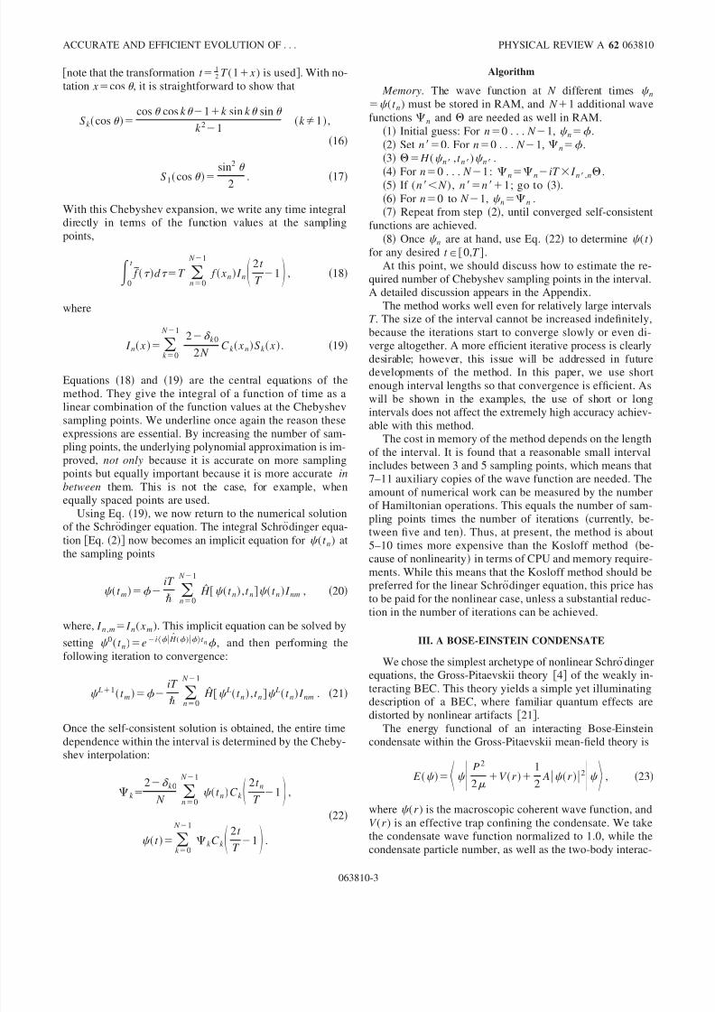
and, in the same units, V 06.25 and 0.2. This set of parameters leads to the same second derivative at the x0well minimum as that of the harmonic potential of Eq. 26.The ground-state energies we find for the 1D BEC in thesetraps are shown as a function of the nonlinear constant inFig. 1.

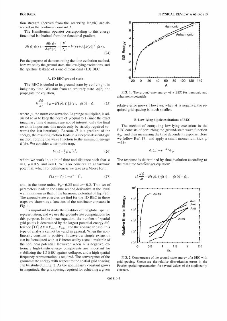
It is important to study the qualities of the global spatialrepresentation, and we use the ground-state computations forthis purpose. In the linear equation, the number of spatialgrid points is determined by the largest potential-energy dif-ference 11 V V maxV min . For the nonlinear case, thistype of analysis cannot be valid in general. When the non-linearity constant is positive, however, a simple extensioncan be formulated with V increased by a small multiple of the nonlinear potential. However, when A is negative, ex-tremely high-kinetic-energy components are important forstabilizing the 1D BEC against collapse, and a high spatialfrequency representation is required. The convergence of theground-state energy with respect to the spatial grid spacingcan be studied in Fig. 2. As the nonlinearity constant growsin magnitude, the grid spacing required for achieving a given

relative error grows. However, when A is negative, the re-quired grid spacing is much smaller.

B. Low-lying dipole excitations of BEC

The method of computing low-lying excitation in theBEC consists of perturbing the ground-state wave function gs , and then measuring the time dependent response. Herewe follow Ref. 7, and apply a small momentum kick p

k :

k x eik x gs .

The response is determined by time evolution according tothe real-time Schrodinger equation:

id

dt H „ t … t , 0 k .

FIG. 1. The ground-state energy of a BEC for harmonic and

anharmonic potentials.

FIG. 2. Convergence of the ground-state energy of a BEC with

grid spacing. Shown are the relative discretization errors in the

Fourier spatial representation for several values of the nonlinearity

constant.


063810-4



During this evolution in time, the position signal r ( t ) (t ) r ( t ) executes an intricate oscillatory motion, in-volving frequencies related to excitation energies of theBEC, which can be resolved by a Fourier analysis.

We first apply this method to a BEC in a harmonic trapEq. 26. We found that the condensate exhibits only asingle excitation energy, with the same frequency as a har-monic oscillator, 1. This was confirmed up to a largenonlinear constant 0 A128. Thus, in the ground state of aharmonic trap, the BEC ground-state dipole excitations areidentical to that of a simple harmonic oscillator.

Next, an anharmonic trap was examined Eq. 27. Thecomputation was performed using a spatial grid extendingfrom x 06, to x f 10, with a grid spacing x1. Thefrequency resolved spectra for several values of A are shownin Fig. 3, and the strong influence of the condensate nonlin-earity on the ground-state excitation spectrum is observed.

In order to appreciate the magnitude of the numerical er-rors incurred by evolution, we performed three computationsof the time dependent trajectory r ( t ) (t ) r ( t ) of theanharmonic oscillator, with A8. All three trajectories startfrom the same initial kicked ground state, and are computedusing 2000 time steps of size T 0.1, totaling to time T f

200. Each trajectory was computed using a different num-ber N of sampling points of the T interval with N 5, 10,

and 20 points used, respectively. The time propagation errorincurred in the first two trajectories can be estimated by thequantities e n(t )r n( t )r 3(t ) n1 and 2. The rate of er-ror accumulation en( t )/ t is plotted in Fig. 4. It is can beinferred that the time propagation error is readily eliminatedby increasing the number of sampling points N . Furthermore,the error grows only linearly with time.

C. Aperture leakage

When a hole is made in the confining potentials of a BEC,the gas can flow out. We affect such an aperture by coupling

to a repulsive potential. Suppose the confining potential isV ( x), and the repulsive potential is an exponential potential

V ex( x)Ke ( x xe) (K 0) ; then the coupling of the twotakes the following form see Fig. 5:

V A x V x V ex x

2 V x V ex x

2

2

C 21/2

.

28

The parameters for this numerical experiment are shown inTable I.

A negative imaginary potential is placed at the positive

grid boundary to absorb the outgoing BEC flux. This well-studied technique prevents spurious edge effects such as re-flection or wraparound 22. The resulting potential exhibitsa high potential barrier, so leakage through this barrier issmall. The time-dependent leaking wave packets for A0and 4 are shown in Figs. 6 and 7. Due to the self-repulsion,

FIG. 3. The ground-state excitation spectrum of a BEC in an

anharmonic trap for various values of the nonlinear constant. It is

seen that the spectrum shifts and new lines are formed as this con-

stant is varied.

FIG. 4. Time-propagation error accumulation. Shown is the rate

of numerical error accumulation, computed as discussed in the text.

The constant error accumulation rate is evident as is the drastic

reduction of the error by doubling the number of sampling points.

The time step is T 0.1.

FIG. 5. An aperture in the confining potential of the BEC, en-

abling tunneling.


063810-5



the condensate finds it easier to leak through the aperture asthe positive nonlinear constant becomes larger.

IV. SUMMARY

We have presented a highly accurate and efficient methodfor propagating the nonlinear time-dependent Schrodingerequation. The method combines an implicit approach withChebyshev interpolation in the time domain. In combinationwith a Fourier or plane-wave spatial representation it leads toan overall balanced numerical method. Although we haveshown only examples where the spatial part is one dimen-sional, the method is straightforwardly applicable to morespatial dimensions, since there is no direct dependence of thetime evolution and sampling points on the spatial grid. In-deed, the present method was recently implemented for elec-tronic structure 23, using a time-dependent formalism, andaccurate time evolution was achieved with no difficulty.

ACKNOWLEDGMENTS

I would like to express my gratitude to R. Kosloff for hisvaluable comments and suggestions regarding this work.This research was supported by Grant No. 9800108 from theUnited States–Israel Binational Science Foundation BSF,

Jerusalem, Israel. I also thank Santiago Alvarez from theUniversity of Barcelona where most of this work was con-ceived.

APPENDIX: DETERMINING THE REQUIRED NUMBER

OF CHEBYSHEV SAMPLING POINTS

Let us determine the number of Chebyshev samplingpoints required for representing a high-frequency component. This can be done by inspecting the Chebyshev coeffi-

cients of f (t )e it :

F k

2

e i1/2T

1

t e i 1/2Tx C k x

1 x 2dx

2ik e i 1/2T J k 1

2T . A1

The asymptotic properties of Bessel functions are wellknown 24, and it is established that, for large values of k ,

J k 1

2T 1

2 k eT

4k

4

A2

Thus, once k (e /4)T , the coefficients drop off exponen-tially fast, becoming zero to machine accuracy after a smallnumber of additional terms N r . Thus the number of sam-pling points is

FIG. 6. Tunnel leakage of a BEC with no interactions ( A0) .

At a time T 0 a hole is made in the confining potential see Eq.

28. As a result, a small tunneling current forms, and the conden-

sate leaks out.

FIG. 7. Same as Fig. 6, with A4. The tunneling rate is en-

hanced by the interparticle repulsion.

TABLE I. Parameters of the aperture.

Parameter Value

K 15

x0 1

1

C 0.2

TABLE II. Values of N r leading to maximum norm precisions

of 104 and 108 in the Chebyshev approximation of f ( x)

e i(1/2)Tx .

1

2 T N r units of 10

4

N r units of 10

8

1 5 8

2 5 9

4 6 11

8 6 12

16 6 13

32 6 14

64 6 15

128 6 15

256 6 15


063810-6



N e

4T N r A3

where N r is given in Table II.It is now important to estimate the maximal frequency in

the system. Also, it is important to arrange the Hamiltonianin a balanced way so as to minimize the maximal frequency,for example, for a time-independent linear Hermitian Hamil-

tonian with maximal eigenvalues E max and minimal eigen-values E min one can shift the Hamiltonian: H shifted H

( E max E min)/2, making the largest frequency equal to( E max E min)/2. For a nonlinear Hamiltonian, it is moreintricate to estimate what the highest frequencies are, how-ever, it is our experience that the nonlinearity does not buildtemporal frequencies beyond the ones taken into account bythe consideration above.

1 W. Negele, Rev. Mod. Phys. 54, 913 1986.

2 R. B. Gerber and M. A. Ratner, Adv. Chem. Phys. 70, 97

1988.

3 E. Runge and E. K. U. Gross, Phys. Rev. Lett. 52, 997 1984.

4 P. Nozieres and D. Pines, The Theory of Quantum Liquids,

Vol. II Addison-Wesley, Redwood City, CA, 1990.

5 W. H. Press, S. A. Teukolsky, W. T. Vetterling, and B. P.

Flannery, Numerical Recipes in C, 2nd ed. Cambridge Uni-

versity Press, Cambridge, 1992.

6 D. Kosloff and R. Kosloff, J. Comput. Phys. 52, 35 1983.7 K. Yabana and G. F. Bertsch, Phys. Rev. B 43, 4484 1996.

8 M. D. Feit, J. A. Fleck, and A. Steiger, J. Comput. Phys. 47,

412 1982.

9 H. Jiang and X. S. Zhao, Chem. Phys. Lett. 319, 555 2000.

10 H. Tal-Ezer and R. Kosloff, J. Chem. Phys. 81, 3967 1984.

11 R. Kosloff, J. Phys. Chem. 92, 2087 1988.

12 R. Kosloff, Annu. Rev. Phys. Chem. 45, 145 1994.

13 C. Leforestier, R. H. Bisseling, C. Cerjan, M. D. Feit, R.

Friesner, A. Guldberg, A. Hammerich, G. Jolicard, W. Karlein,

H.-D. Meyer, N. Lipkin, O. Roncero, and R. Kosloff, J. Com-

put. Phys. 94, 59 1991.

14 P. Pfeifer and R. D. Levine, J. Chem. Phys. 79, 5512 1983.

15 U. Peskin, R. Kosloff, and N. Moiseyev, J. Chem. Phys. 100,

8849 1994.

16 G. Yao and R. E. Wyatt, J. Chem. Phys. 101, 1904 1994.

17 G. Yao and R. E. Wyatt, Chem. Phys. Lett. 239, 207 1995.

18 C. S. Guiang and R. E. Wyatt, Int. J. Quantum Chem. 67, 273

1998.

19 T. J. Rivlin, Chebyshev Polynomials: From Approximation

Theory to Algebra and Numbers Theory Wiley, New York,1990.

20 V. I. Krylov, Approximate Calculation of Integrals, translated

by A. H. Stroud Macmillan, New York, 1962.

21 P. A. Ruprecht, M. J. Holland, K. Burnett, and M. Edwards,

Phys. Rev. A 51, 4704 1995.

22 D. Neuhauser and M. Baer, J. Chem. Phys. 90, 4351 1989.

23 R. Baer unpublished.

24 Handbook of Mathematical Functions, edited by N. Abramow-

itz and I. A. Stegan Dover, New York, 1972.


063810-7

roi baer- accurate and efficient evolution of nonlinear schrodinger equations

Documents