POSIVA OY

POSIVA 2002-05

Rock strength and deformation dependence on schistosity

Simulation of rock with PFC3D

Toivo Wanne

Saanio & Riekkola Oy

June 2002

Toolonkatu 4, FIN-00100 HELSINKI, FINLAND

Phone (09) 2280 30 (nat.), (+358-9-) 2280 30 (int.)

FAx 109) 2280 3719 {nat.), (+358-9-) 2280 3719 (int.)

sAANicr& RIEKKOLA OY a SAATE I 12. kesakuuta 2002

POSIVA-RAPORTIN I<ASIKIRJOITUKSEN TARKASTAMINEN JA HYVAKSYMINEN

TILAAJA

TILAUS

Posiva Oy Toolonkatu 4 001 00 Helsinki

9522/02/JPS

YHTEYSHENKILOT

Jukka-Pekka Salo Jorma Autio

Posiva Oy Saanio & Riekkola Oy

POSIVA-RAPORTTI POSIVA 2002-05

ROCK STRENGTH AND DEFORMATION DEPENDENCE ON SCHISTOSITY

TEKIJA . ----·z-~---z

DI Toivo Wanne Saanio & Riekkola Oy

TARKASTAJA 9~/ TkL Jorma Autio Saanio & Riekkola Oy

HYVAKSYJA ~,

/J /.1 ...... . ... /), / ., - '·

( .-~--?],) · .. ~ ~-~~ '~·Reijif"Riekkola Saanio & Riekkola Oy

toimitusjohtaja

11 JJ1 o ( ]fS) ~.-1Jchys-

1 //~ tL· lo·-

Tekija(t)- Author(s)

Toivo Wanne

Posiva-raportti - Posiva Report

Posiva Oy T6616nkatu 4, FIN-001 00 HELSINKI, FINLAND Puh. (09) 2280 30 -lnt. Tel. +358 9 2280 30

Toimeksiantaja(t)- Commissioned by

Saanio & Riekkola Oy Posiva Oy

Nimeke- Title

Raportin tunnus- Report code

POSIV A 2002-05

Julkaisuaika- Date

June 2002

ROCK STRENGTH AND DEFORMATION DEPENDENCE ON SCHISTOSITY Simulation of rock with PFC3D

Tiivistelma -Abstract

The objective of the work was to study the effect of anisotropy of the rock on strength and deformation properties by simulating a standard unconfined compression test with the PFC3D­program. Particle Flow Code (PFC) was selected to be used in the simulations because of its ability to model behavior of brittle rock material including fracture propagation. The schistosity was modeled in PFC3D intrinsically by generating an anisotropic particle structure consisting of matrix particles and oriented band particles. The approach was novel and no similar studies were found for references.

The model was generated and the results were compared to those of gneissic tonalite, which is a main rock type in the Research tunnel at Olkiluoto, Finland. The PFC3D simulated strength and deformation properties were found to be noticeably dependent on schistosity. The comparison to the laboratory results showed that the responses were similar. Damage formation observations made during the compression simulations indicated that the PFC3D modeling could simulate the events happening during the laboratory compression tests of rock samples by reproducing similar fracture generation and deformation. Furthermore it was noticed that the mechanical properties of the PFC3D model were dependent on the particle size and on the geometry of banding, but adding a third particle type, in addition to the previous two particle types, did not radically alter the behavior of the compression simulation.

A few topics have to be studied in more detail in order to improve the simulation process and the accuracy of a material model. These include the development of the PFC3D visualization tools of the fracturing process and the optimization of the particle size and simulation times.

Avainsanat- Keywords

PFC3D simulation, anisotropy, compression test, damage formation

ISBN ISSN

ISBN 951-652-112-6 ISSN 1239-3096

Sivumaara- Number of pages Kieli- Language

84 English

Tekija(t)- Author(s)

Toivo Wanne

Posiva-raportti - Posiva Report

Posiva Oy T6616nkatu 4, FIN-00100 HELSINKI, FINLAND Puh. (09) 2280 30 -lnt. Tel. +358 9 2280 30

Toimeksiantaja(t)- Commissioned by

Saanio & Riekkola Oy Posiva Oy

Nimeke- Title

Raportin tunnus- Report code

POSIV A 2002-05

Julkaisuaika- Date

Kesakuu 2002

KIVEN SUUNTAUTUNEISUUDEN VAIKUTUS LUJUUTEEN JA MUODONMUUTOKSIIN Kiven mallinnus PFC3D:lla

Tiivistelma - Abstract

Tyon tavoitteena oli tutkia kiven suuntautuneisuuden vaikutusta kiven lujuuteen ja muodon­muutosominaisuuksiin simuloimalla yksiaksiaalista puristuskoetta PFC3D-ohjelmalla. Tarkea osa sortumisen simuloinnissa on valitun mallinnusmenetelman kyky esittaa murtuman etenemista. Particle Flow Code (PFC) ohjelmisto valittiin kaytettavaksi simuloinneissa, koska menetelma pystyy mallintamaan hauraan kivimateriaalin kayttaytymista. Kiven suuntautuneisuutta mallinnet­tiin PFC3D:lla rakentamalla malli peruspartikkelimassasta ja suuntautuneista partikkeliryhmista. Lahestymistapa mallinnukseen oli uusi eika vastaavia tutkimuksia loydetty viitteeksi.

Puristuskokeen simulointituloksia verrattiin Olkiluodossa sijaitsevasta tutkimustunnelista otettu­jen gneissimaisen tonaliitin laboratoriokokeiden tuloksiin. Seka simulointi- etta laboratoriokokeet osoittivat kiven lujuus- ja muodonmuutosominaisuuksien olevan voimakkaasti riippuvaisia suuntauksesta. Tehdyssa vertailussa todettiin laboratoriokokeiden ja simulointien tulosten olevan samankaltaisia. Havainnot murtumisen kehityksesta simulointien aikana osoittavat, etta PFC3D mallinnus kykenee simuloimaan puristuskokeen aikaiset murtumistapahtumat aikaansaamalla samantapaisia rakojarjestelmia ja muodonmuutoksia PFC3D mallissa kuin laboratoriokokeiden naytteissa.

Herkkyystarkastelut osoittivat, etta PFC3D mallin on1inaisuudet ovat riippuvaisia mallin partikkelikoosta ja partikkeliryhmien geometriasta. Edelleen havaittiin, etta mallin kayttaytyminen ei muuttunut merkittavasti lisattaessa malliin kolmas partikkelityyppi aikaisempien kahden lisaksi.

Simulointimenetelman optimointia ja materiaalimallia tulee kehittaa, jotta menetelmalla pystyttai­siin mallintamaan tehokkaasti myos normaalien kalliotilojen kokoluokkaa olevien tilojen muodon­muutoksia. Yksi ratkaisu voisi olla FLAC3D:n ja PFC3D:n yhdistaminen suurissa mallinnuksissa. Talla hetkella suurehko ongelma on kolmiulotteisen murtumistapahtuman visualisointi. Mallin partikkelikoon seka kuormitusnopeuden vaikutusta simulointituloksiin tulisi myos tutkia tarkem­min.

Avainsanat- Keywords

PFC3D simulaatio, anisotropia, puristuskoe, murtuman syntyminen

ISBN ISSN

ISBN 951-652-112-6 ISSN 1239-3096

Sivumaara- Number of pages Kieli - Language

84 Englanti

PREFACE

The work has been carried out by Toivo Wanne of Consulting Engineers Saanio & Riekkola during the year 2001-02 in collaboration with POSIV A OY and Svensk Karnbdinslehantering AB (SKB).

The author wishes to thank the instructor Jorma Autio of Saanio & Riekkola and Jukka­Pekka Salo of POSIV A OY who acted as contact person.

Special acknowledgement to David Potyondy of Itasca Consulting Group for his valuable contribution concerning the Particle Flow Code modeling method.

1

TABLE OF CONTENTS

ABSTRACT

TIIVISTELMA

PREFACE

TABLE OF CONTENTS

LIST OF SYMBOLS AND NOTATIONS

LIST OF FIGURES

LIST OF TABLES

1

2

3

4

BACKGROUND AND INTRODUCTION

1.1 General 1.2 Numerical modeling

1.2.1 Modeling in general 1.2.2 Numerical modeling in rock mechanics

1.3 Principles of probability

DESCRIPTION OF UNCONFINED COMPRESSION TEST

2.1 Compression test 2.2 Anisotropy 2.3 Failure development during compression test 2.4 Gneissic tonalite

2.4.1 Igneous and metamorphic rock 2.4.2 Properties 2.4.3 Laboratory test results

PFC THEORY

3.1 Particle mechanics 3.2 Distinct Element Method 3.3 Calculation cycle 3.4 Contact models

PFC3D MODEL FOR ROCK

4.1 Modeling with PFC3D 4.2 Model generation and compression test simulation

4.2.1 Isotropic model generation in PFC3D 4.2.2 Particle band generation in PFC3D 4.2.3 Compression test simulation in PFC3D

1

3

4

6

7

7 8 8 9

10

13

13 14 17 19 19 20 20

23

23 23 24 24

25

25 25 26 26 29

5

6

7

8

2

RESULTS OF COMPRESSION TEST SIMULATIONS

5.1 Quantitative results 5.2 Qualitative study

5.2.1 Damage formation in PFC3D 5.2.2 Failure patterns

ANALYSIS OF RESULTS

6.1 Crack formation 6.2 Comparison against laboratory samples 6.3 Comparison to 2D modeling results

SENSITIVITY ANALYSIS

7.1 Resolution of the PFC model 7.1 .1 Effect of model resolution in 2D modeling 7.1.2 Effect of model resolution in 3D modeling

7.2 Geometry parameters 7.3 Three component model

CONCLUSION AND DISCUSSION

REFERENCES

APPENDIX 1: PFC MODEL FOR ROCK- PARAMETERS

Specimen genesis and material parameters Anisotropy installation parameters Unconfined compression test parameters Monitored parameters during testing

APPENDIX 2: CRACK PLOTS AND STRESS-STRAIN CURVES

33

33 38 38 38

51

51 53 55

57

57 57 58 61 64

65

67

69

69 70 70 71

72

3

LIST OF SYMBOLS AND NOTATIONS

~w E V

CDF DEM FISH OL

Angle of schistosity with respect to the vertical axis [0]

Crack-initiation stress [MPa] Unconfined I uniaxial compressive strength [MPa] Strain cotnponent, i=x,y,z Stress component, i=x,y,z [MPa] Friction angle of weakness plane [0

]

Young's tnodulus [Pa] Poisson's ratio

Cumulative distribution function Distinct -element method Built-in programming language ofPFC (and other Itasca codes) Olkiluoto

Pc Confining stress (in triaxial test) [P a] PDF Probability density function PFC2DI3D Particle Flow Code in 2 and 3 Dimensions Strain Stress ucs

Change in length per unit length, dimensionless Constraining force applied to a tnaterial, force per unit area [Pa] Unconfined I uniaxial compressive strength, peak strength [Pa]

4

LIST OF FIGURES

Figure 2-1. Schematic view of a compressional test arrangement. Uniaxial test: compression plates are placed on the bottom and top surfaces of the sample, the sides are unconstrained. In the Triaxial test, liquid is used to subject the sample to a confining pressure. (Department of Geological Sciences 2001.) 13

Figure 2-2. Left: definition of schistosity angle. Right: variation of peak strength with the angle of weakness plane (schistosity). 16

Figure 2-3. Slates, shales and sandstones exhibit strength anisotropy. Uniaxial and triaxial compression test results after Hoek & Brown ( 1982). 16

Figure 2-4. Failure modes for different types of rock sample stress-strain behavior. 1 -tensile splitting, 2- shear splitting, 3- 'barrel' -shape failure. (Geology for Engineers 2001.) 18

Figure 2-5. Average unconfined compressive strengths (with standard deviation) of gneissic tonalite specimens with respect to schistosity angle. Three different sample sizes were tested. (Autio et al. 2000.) 21

Figure 2-6. Average Young's modulus (with standard deviation) of gneissic tonalite specimens with respect to schistosity angle. Three different sample sizes were tested. (Autio et al. 2000.) 22

Figure 3-1. PFC calculation cycle. The velocities and accelerations are kept constant within each time ~· ~

Figure 4-1. Model generation steps in PFC3D. !-isotropic parallelpiped model, 2-anisotropic parallelpiped model, 3-anisotropic cylindrical model. 28

Figure 4-2. Band generation produces a group of five different samples for all nine schistosity angles. 28 Figure 4-3. Particle band generation produces an anisotropic model. Definitions of the geometry

parameters are shown. For illustrative purposes, the schemes on the left and in the center represent schistosity oriented parallel to the longitudinal axis of the model. 29

Figure 4-4. The pre-failure region (pre-peak stress) of the stress-strain curve obtained in an unconfined compression test and definitions of Young's modulus and peak strength. 31

Figure 5-1. Example of a stress-strain curve for a simulated unconfined compression test using PFC3D. Schistosity angle used in the model45°, Peak strength 97 MPa, Young's modulus 44 GPa. The unit of the vertical stress axis is Pascal [Pa]. 34

Figure 5-2. All results for simulation of Peak strength [MPa] (upper) and Young's modulus [GPa] (lower) are plotted with respect to schistosity angle [0

]. 35 Figure 5-3. Mean and standard deviations of simulation results plotted with respect to schistosity

angle [0]. Peak strength [MPa]- upper, Young's modulus [GPa] -lower. 35

Figure 5-4. Peak strength [MPa] of the laboratory tests and the PFC3D runs. The yellow transparent area encloses the laboratory results. Note that the vertical axis spans from 60- 180 MPa. 36

Figure 5-5. Young's modulus [GPa] of the laboratory tests and PFC3D runs. The yellow area encloses the laboratory results. Note that the vertical axis spans from 30- 90 GPa. 36

Figure 5-6. Simulated mean values for crack initiation stress [MPa] (above) and Poisson's Ratio (below) and their standard deviation with respect to the angle of schistosity [0

]. 37 Figure 5-7. Left: Presentation of tension-induced microcrack as a octagon. Right: Vertical and

horizontal sections. 39 Figure 5-8. Schematic illustration of the four phases of damage formation. 39 Figure 5-9. Damage formation at schistosity angle of 11°. 40 Figure 5-10. Damage formation at schistosity angle of 34°. 40 Figure 5-11. Damage formation at schistosity angle of 67.5°. 41 Figure 5-12. Damage formation at schistosity angle of 79°. 41

5

Figure 5-13. Model: sTx_mG_11c, schistosity angle 11°. Left: All cracks, time-dependent coloring (light= early, dark= late). Center: Cracks and displacements on the origo centered vertical section, time-dependent coloring (light= early, dark= late). Right: Cracks and modeled particles on the origo-centered vertical section, crack type coloring (red= tension, black= shear). Particle coloring: yellow = stronger matrix material, orange = weaker band material. 43

Figure 5-14. Model: sTx_mG_225d, schistosity angle 22.5°. Left: All cracks, time-dependent coloring (light= early, dark= late). Center: Cracks and displacements on the origo centered vertical section, time-dependent coloring (light = early, dark = late). Right: Cracks and modeled particles on the origo-centered vertical section, crack type coloring (red= tension, black = shear). Particle coloring: yellow = stronger matrix material, orange = weaker band material. 44

Figure 5-15. Model: sTx_mG_34d, schistosity angle 34°. Left: All cracks, time-dependent coloring (light= early, dark= late). Center: Cracks and displacements on the origo centered vertical section, time-dependent coloring (light= early, dark= late). Right: Cracks and modeled particles on the origo-centered vertical section, crack type coloring (red= tension, black= shear). Particle coloring: yellow= stronger matrix material, orange= weaker band material. 45

Figure 5-16. Model: sTx_mG_ 45a, schistosity angle 45°. Left: All cracks, time-dependent coloring (light= early, dark= late). Center: Cracks and displacements on the origo centered vertical section, time-dependent coloring (light= early, dark= late). Right: Cracks and modeled particles on the origo-centered vertical section, crack type coloring (red = tension, black = shear). Particle coloring: yellow = stronger matrix material, orange = weaker band material. 46

Figure 5-17. Model: sTx_mG_56c, schistosity angle 56°. Left: All cracks, time-dependent coloring (light= early, dark= late). Center: Cracks and displacements on the origo centered vertical section, time-dependent coloring (light= early, dark= late). Right: Cracks and modeled particles on the origo-centered vertical section, crack type coloring (red= tension, black= shear). Particle coloring: yellow= stronger matrix material, orange= weaker band material. 4 7

Figure 5-18. Model: sTx_mG_675e, schistosity angle 67.5°. Left: All cracks, time-dependent coloring (light= early, dark= late). Center: Cracks and displacements on the origo centered vertical section, time-dependent coloring (light = early, dark = late). Right: Cracks and modeled particles on the origo-centered vertical section, crack type coloring (red = tension, black = shear). Particle coloring: yellow = stronger matrix material, orange = weaker band material. 48

Figure 5-19. Model: sTx_mG_79c, schistosity angle 79°. Left: All cracks, time-dependent coloring (light= early, dark= late). Center: Cracks and displacements on the origo centered vertical section, time-dependent coloring (light= early, dark= late). Right: Cracks and modeled particles on the origo-centered vertical section, crack type coloring (red= tension, black= shear). Particle coloring: yellow = stronger matrix material, orange = weaker band material. 49

Figure 6-1. Horizontal cutting planes in two separate models. Left: schistosity angle 34°. Right: schistosity angle 45°. Red arrows show the direction of microcrack propagation. Sections shown are from the middle of the model. 52

Figure 6-2. Axial stress (uppermost black line), all cracks (black), tensile cracks (red) and shear cracks (blue) plotted against axial strain. The cracking increases after the peak strength and tensile cracking is predominant. Model sTx_mG34d, schistosity angle 34°, peak strength 99 MPa, Young's modulus 55 GPa, number of cracks at peak strength 820 pieces. 53

Figure 6-3. Laboratory samples (Autio et al. 2000) (upper) and PFC3D failure-pattern images (lower) from three different loading phases. Micro fracturing of laboratory samples is superimposed in red color. PFC3D crack coloring; red= tension-induced, blue= shear-induced. Only cracks in the origo centered section are shown. 54

6

Figure 7-1. Unconfined strength (UCS) and values for Young's modulus show a clear dependence on resolution. The relationship resembles a logarithmic dependence. 59

Figure 7-2. Damage patterns resulting from the use of different model resolutions. The numbers depict the average particle radius in the corresponding model. Crack coloring indicates the relative time when microcracks were formed [light= early, dark= late]. The models are isotropic. 60

Figure 7-3. Half of the models showing the three different geometries of the cases and the basic case (above). Cracks on the origo centered section are shown below. Yellow= matrix, red= weaker bands. In these models, the angle of schistosity is 22.5°. 62

Figure 7-4. Simulated peak strengths (upper diagram) and Young's modulus (lower diagram) of the three cases with different geometries and results from the basic case (Normal). The fitted spline lines which connect the observations are for clarification purposes only. 63

Figure 7-5. Left: Material structure in the three-particle model. Particles on the origo centered section are shown. Yellow = old matrix, red = bands, white = new matrix. Right: Mean simulated peak strength and Young's modulus with standard deviations. 64

LIST OF TABLES

Table 2-1. Average strengths and Young's modulus with respect to schistosity angle. Results from three different diameter samples ( 41, 54, 99 mm). (Autio et al. 2000.) 21

Table 4-1. Anisotropy installation parameters and their values. 27 Table 4-2. Unconfined compression test parameters for PFC3D. 30 Table 4-3. List of simulated compression tests with the corresponding chapter number. 31 Table 5-1. Mean values and standard deviations used for simulation of unconfined compression test. 34 Table 7-1. Results of the resolution test run. The dimensions of the specimens were 42 by 42 by 120

mm. A total of 17 runs were made; five for the reference model and four for each of the other specimens. Mean values are shown (E =Young's modulus [GPa], Sig_f= Unconfined compression strength [MPa]). 59

Table 7-2. The relationship between particle size, resolution and computing time. The dimensions of the specimens are 54 x 54 x 142 mm. (The values 51 hand 642 hare extrapolated assuming that the time-resolution relation is exponential [t=A Resotution*

8].) 60

Table 7-3. Geometric parameters for the three cases studied. 61

7

1 BACKGROUND AND INTRODUCTION

1.1 General

The objective of this work is to study the effect of anisotropy of the rock on strength and deformability by simulating a standard unconfined compression test with the PFC3D-program. A model is generated and the results obtained are compared to those obtained with gneissic tonalite, a main rock type in the Research tunnel at Olkiluoto, Finland (Autio et al. 1999).

The Finnish Parliament ratified in May 2001 the Government's positive Decision in Principle on Posiva's application to locate the repository for spent nuclear fuel at Olkiluoto. Olkiluoto is being investigated as a possible site for the final disposal of spent nuclear fuel from the Finnish nuclear power plants. The main rock types found in the area are mica gneiss and gneissic tonalite.

Assessing the stability of deep underground excavations is a subject of great importance in terms of both safety and constructability. Typical bedrock in many areas of Finland is gneissic and therefore anisotropic in nature. The anisotropy of mechanical properties such as strength and the effect of this anisotropy on the behavior and failure of rock around deep underground openings have not been studied in detail and the amount of data available is limited. The results of measurements on gneissic tonalite samples taken from the Research Tunnel at Olkiluoto showed that strength and deformation properties were significantly dependent on the orientation of schistosity.

Rock damage is produced by fracturing and this may eventually lead to instability. In crystalline rock, a significant component of progressive failure in deep underground openings is fracture propagation, and field observations have shown that in many cases this eventually reaches a stable state. For this reason, a key element in the simulation of a failure process is the ability to model fracture propagation.

While the development of computer software has made it possible to model fracture propagation in three dimensions, the number of methods available for the modeling of fracture generation and propagation is currently very limited. Particle Flow Code (PFC) was selected for use in this study because it is a well-documented and commercially available tool for modeling the behavior of brittle rock material including fracture propagation and mechanical stability in the near-field around underground openings. The PFC method has previously been used to model the behavior of gneissic tonalite in 2D (Potyondy & Autio 2001, Potyondy & Cundall 2000) and in several other studies (Li & Holt 2001, Kulatilake et al. 2001, Potyondy & Cundall 2001) with encouraging results.

Gneissic tonalite was chosen as the reference rock in this study because its anisotropy has been studied in detail and the behavior of laboratory samples has been simulated using PFC2D software.

The following chapters discuss topics of importance which concern modeling in general and the application of modeling in the field of rock mechanics. A short introduction to probability theory and its use in the study is also provided.

8

1.2 Numerical modeling

In a field such as geomechanics where data are not always available, numerical models can be useful in providing a picture of the mechanisms that may occur in particular physical systems. The following sections discuss some issues concerning modeling in general and its application in the field of rock mechanics.

1.2.1 Modeling in general

In an excellent paper on the mode ling of physical systems, Oreskes et al. ( 1994) make the observations presented in the following paragraphs. Modeling, or the use of a numerical model, contains usually closed mathematical components such as an algorithm within a computer program. These mathematical components may be subjected to verification because they are part of closed systems that include claims which are always true. However, the models that use these components are never closed systems, because they require input parameters that are incompletely known. The lack of complete knowledge of the system being modeled forces us to make inferences and assumptions about the real world. Many assumptions can be justified based on experience, but in a new study, the degree to which our assumptions hold can never be established a priori. The additional assumptions and input parameters required to make a model work are known as 'auxiliary hypotheses'. If verification of the problem fails, there is often no simple way to know whether the principal or auxiliary hypothesis is at fault. If we compare the response of a model with observational data and the comparison proves unacceptable, we know that something is wrong and we may or may not be able to define what it is. For this reason, the evaluation of a model should always be a step-by-step procedure. Typically, we continue to work on the model until it is an acceptable fit. When pursuing a good match, it should be remembered that more than one model construction can actually produce the same output. Another question for consideration is deciding on the point at which further modifications to the model are no longer considered acceptable.

When constructing a model we like to validate it to establish that the model or code does indeed reflect the behavior of the real world. In other words, that the model is a good representation of the actual processes that take place in a real system. The most common method of validation is a comparison of measurements from laboratory testing with the results obtained from computational models. However, an agreement between measurements and the output of numerical modeling in no way demonstrates that the model which produced the output is an exact representation of the real system. Validation is a process of building confidence in models, not provide validated models.

Numerical models are calibrated by manipulating the independent variables to obtain a match between the observed and simulated distributions of the dependent variables. As the goal of scientific theories is not truth but empirical adequacy, it could be said that a calibrated model is empirically adequate. On the other hand, as calibrated models often require refinement, this suggests that the adequacy of the models is forced. The availability of more data usually requires further adjustments. This requirement has a serious affect on the use of any calibrated model for predictive purposes such as estimating the long-term stability of an underground opening.

9

Models can confirm a hypothesis by offering evidence which strengthens what may have already been partly established by laboratory tests. Models can therefore be considered to be representations, useful for guiding further study. The philosopher N ancy Cartwright claimed that the models are like fiction. A model, like a novel, may resonate with nature but it is not a 'real' thing. The fundamental reason for carrying out the modeling process is a lack of full access to the phenomena of interest.

1.2.2 Numerical modeling in rock mechanics

Cundall & Starfield ( 1988) discuss the mode ling of problems in rock mechanics. Some of the issues they handle are presented here.

The lack of detail in rock mechanics was a primary stumbling block in the early days of modeling and the possibility of including additional detail was welcomed. Some ten years ago the focus in rock mechanics moved from measurement to computation. Models are constructed because the mechanical processes involved are too complex to be fully understood. Easy access to versatile, powerful and inexpensive computer packages has increased the extent to which models are employed. The computer tools themselves are not, however, an explicit solution, but rather a means to a solution.

Guidelines for modeling are given below.

- A model is a simplification of reality. It is an intellectual tool that must be chosen for a specific task.

- The design of a model should be driven by the question that the model is expected to answer rather than the details of the system actually being mode led.

- One should aim to gain confidence in a model to modify it as one uses it. - Be clear about the reasons for building a model and the questions that it should

answer. - Examine the mechanics of the problem. - Design the simplest possible model that will allow the mechanism being examined to

occur. - Implement the model, choose your simplest experiment, and run it. Once successful

runs have been carried out, proceed to experiments that are more complex. - Only run complex models once success has been achieved with simple ones. - Visualize and anticipate solutions before actually running a model. Attempt to

visualize the deformation of the structure under load and form an approximate picture of the deformations.

Modeling carried out in a cautious and considered manner leads either to new knowledge or improved understanding.

10

1.3 Principles of probability

Hoek et al. ( 1995) introduced the principles of probability in rock mechanics. In a rock mass, parameters such as the uniaxial compressive strength of rock specimens, the inclination and orientation of discontinuities, and the measured in-situ stresses do not have a single fixed value but may adopt any of a number of values. It is simply not possible to establish the exact value of any one of these parameters at any given point. These parameters can therefore be said to be random variables.

In research, it is desirable to include as many samples as possible in any set of studied observations but practical considerations limit the amount of data that can be collected. It is often necessary to make estimates on the basis of experience or by comparisons with results published by others.

Using a probability model does not allow prediction of the result of any individual experiment, but it does enable determination of the probability that a given outcome will fall inside a specific range of values.

A probability density function (PDF) describes the relative likelihood that a random variable will take a particular value. A PDF can be continuous (i.e. it can take all possible values) or it can be discrete. The same information can be presented in the form of a cumulative distribution function (CDF). A CDF yields the probability that the variable concerned will have a value that is less than or equal to the selected value.

For many applications it is useful to present only the most relevant summarizing parameters from the pile of information. Widely used parameters are the sample mean value (x), the sample variance (s2

), and the standard deviation (s).

The sample mean value (Eq. 1-1) indicates the center of gravity of a probability distribution. A test which yields the results x1, x2, ••• , Xn has a mean value of:

(1-1)

The sample variance is defined as the mean of the square of the difference between the values of Xi and the sample mean value. The standard deviation (Eq. 1-2) is the positive square root of the variance:

1 n 2

s= -L,(x;-x) n-1 i=l

(1-2)

Note that for a finite number of samples it can be shown that the denominator (n-1, instead of n) gives a better and unbiased estimate for the population variance.

In a normal distribution, approximately 95% of observations will fall within the range defined by the mean :t two standard deviations. If a result falls within these boundaries it is said that its deviation is "not significant". In this study, the range employed is

11

limited to the mean ::tone standard deviation. In a normal distribution, approximately 67.5% of the observations will fall within this range.

A normal (Gaussian) distribution is the most common type of probability distribution function. Normal distributions are a family of distributions that have the same general shape (sometimes described as "bell-shaped"), i.e. symmetric with scores more concentrated in the middle than in the tails. The shape of a normal distribution can be specified mathematically by using two parameters: the mean (x) and the standard deviation (s).

In geotechnical engineering, the normal distribution is generally used for probability studies unless there are good reasons for choosing a different distribution. It is typical for variables that arise as the sum of a number of random effects to be normally distributed.

12

13

2 DESCRIPTION OF UNCONFINED COMPRESSION TEST

This chapter provides a brief description of the laboratory-scale unconfined compression test, the anisotropy effect, and the development of failure in a rock sample subjected to compressive loading. Finally, gneissic tonalite and the results of laboratory tests are presented.

2.1 Compression test

The test most commonly performed on rock is uniaxial compression of cylindrical specimens prepared from drill cores (Figure 2-1 ). This test is used to determine the uniaxial or unconfined compressive strength, crc, and the elastic constants Young's modulus (E), and Poisson's ratio (v). The response observed will depend on the nature and composition of the rock, the geometry of the test specimen and the rate of loading. For rock with similar mineralogy, compressive strength will vary with varying properties. For example, strength will decrease as porosity and water content increase. Anisotropy in the microstructure (e.g. schistosity) will also affect the strength properties of specimens. The principles of compressive testing are presented and discussed by a variety of authors such as Brady & Brown (1985), Jaeger (1972) and Obert & Duvall (1967).

To standardize the tests employed and make the results obtained comparable, the International Society for Rock Mechanics (ISRM) provides (ISRM Commission 1979) suggested techniques for determining the uniaxial compressive strength and deformability properties of rock material. Some features of this testing regime are given below.

UNIAXIAL TRIAXIAL

Figure 2-1. Schematic view of a compressional test arrangement. Uniaxial test: compression plates are placed on the bottom and top surfaces of the sample, the sides are unconstrained. In the Triaxial test, liquid is used to subject the sample to a confining pressure. (Department of Geological Sciences 2001.)

14

- The test specimens should be circular cylinders having a height to diameter ratio of 2.5 -3.0.

- The specimen diameter should be at least 10 times the size of the largest grain in the rock.

- Load should be applied to the specimen at a constant stress rate of 0.5 - 1.0 MPals. - Axial load and axial and radial strains should be recorded throughout each test. - There should be at least five repetitions of each test.

During the test, the axial force is recorded and then divided by the initial cross-sectional area of the specimen to give the average axial stress, crz. This is then plotted against the overall axial strain, Ez. From this plot, it is possible to calculate a value for Young's modulus. Corresponding equations for calculating E and v are presented below after Jaeger (1972).

Computing E and v from a triaxial compression test. For an elastic material, all stress components are acting:

Ex = _!_ [a x - v( aY + a z ) ] E

EY =_!_[aY- v(az + ax)] E

t:, =~[a, -v(ax +ay)]

For the triaxial test:

-Strains ~Ex= ~Ey, ~Ez - Stresses ~crx = ~cry, ~crz - The z-axis is parallel to the loading axis.

(2-1)

We also assume that during a triaxial compression test, the axial strain is applied with a constant confining stress. Substituting these values in Equation (2-1) and solving forE (2-2) and v (2-3) yields the following:

E = ~a,z fl£z

(2-2)

(2-3)

These same equations also apply to an unconfined compression test because while in a triaxial test we assume that change in confining pressure is zero (~crx=~cry=O), in an unconfined test the change (and the values) are also zero.

2.2 Anisotropy

The behavior of many rocks is anisotropic because of some preferential orientation of the fabric or microstructure or the presence of bedding or cleavage. The taking of

15

samples and consequent stress release may also cause anisotropy by inducing microfracturing. In design, it is usual to employ only the simplest form of anisotropy, transverse isotropy. In transversely isotropic rock, peak strengths vary with respect to the orientation of the plane of weakness.

J aeger (Brady & Brown 1985) introduced a theory about how the strength of rock depends on the plane of weakness. The theoretical rock sample contains well-defined parallel planes of weakness. Each plane has a limiting shear strength, Equation (2-4). Slip along the weakness plane occurs when the shear stress ('t) on the plane is equal to the shear strength (s). The stress transformation equations in an unconfined situation give the normal {Equation (2-5)}, and shear {Equation (2-6)} stresses on a plane.

(2-4)

(j (j a = - 1 +-1 cos2f3

n 2 2 (2-5)

a 1 sin 2/3 r = __.:.. _ ___.;._ 2

(2-6)

where Cw is the cohesion of a plane, <1>w is the friction angle of the plane, B is the angle of weakness of planes with respect to the loading axis and cr1 is the compression stress (see Figure 2-2). Substituting Equation (2-5) in Equation (2-4), makings= 't and rearranging gives the criterion for slip on the plane of weakness as Equation (2-7).

2cw (jlS = ____ __...:..:.._ __ _ (1- tan tPw cot /3) sin 2/3 (2-7)

The compression stress required to produce slip tends to infinity as B~90° and as B~<!>w. Between these values of B [<!>w ... 90°], slip is possible. The stress at which slip actually occurs varies with B according to Equation (2-7). The strength - angle-of-plane -curve is U-shaped, and the minimum strength value (Eq. 2-8) occurs when:

J3 = 1! _ tPw 4 2 (2-8)

For values of B which are outside the range given above, slip on the plane cannot occur and so the peak strength of the specimen must be determined by some other mechanism.

In reality, the cr1 - B-curve does not take the theoretical shape as shown in Figure 2-2. In particular, the plateaus of constant strength in out-of-range sections of the curve are not always present in experimental strength data. This suggests that the theoretical model is an over-simplified representation of the variation of strength in anisotropic rocks. Results concerning rock strength and orientation of the schistosity plane are mainly available for sandstones, slates and shales (see Figure 2-3). These results show that minimum strength occurs when B is between 30 and 40 degrees. (Brady & Brown 1985.)

16

0 Schistosity angle ~

90

Figure 2-2. Left: definition of schistosity angle. Right: variation of peak strength with the angle of weakness plane (schistosity).

5

4

1 0

"'"" )(

~ 3 :c ;::.

Peak strength with respect to discontinuity angle

----+-Slate 1 (unconf)

---- Slate 2 (unconf)

--1:s- Slate 3 (conf)

~Sandstone (conf)

~Shale (conf)

0+-------------~------------~--------------~----------~ 0 22,5 45

Discontinuity angle r1 67,5 90

Figure 2-3. Slates, shales and sandstones exhibit strength anisotropy. Uniaxial and triaxial compression test results after Hoek & Brown (1982).

17

Autio et al. (2000) studied the effect of schistosity on the strength of hard crystalline rock by performing unconfined compression tests on gneissic tonalite (see Section 2.4 of this report - Gneissic tonalite). The anisotropy of strength was remarkable. Autio's conclusions concerning the test results were as follows:

- The uniaxial compressive strength, UCS, was at a maximum when the rock specimen was oriented parallel to the schistosity plane.

- The UCS was close to a minimum when orientation was perpendicular to the schistosity plane.

The main difference when comparing the results obtained by Autio to those presented in literature is that the strength of the rock specimens did not exhibit an increase when the orientation approached an angle perpendicular to the schistosity plane.

Peng and Johnson (1972) tested Chelmsford granite, mineralogically a quartz monzonite, which is homogeneous and does not exhibit schistosity or textural orientation. He concluded that the ultimate strength of the granite varied with the orientation of the specimen. Peng's tests were made on cylindrical samples cored from three different, perpendicular, directions (three sets of orthogonal cleavages) in a granite block. The ratio between the weakest and the strongest specimens ranged from 0.84 to 0.94.

2.3 Failure development during compression test

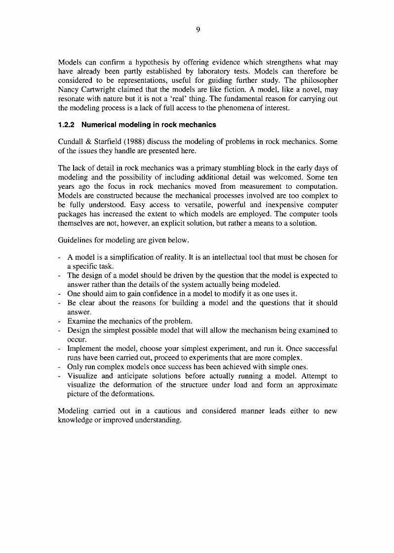
Geology lecture notes from the University of Saskatchewan (Department of Geological Sciences 2001) introduce general deformation behavior in rock. At high rates of strain, rocks act as brittle-elastic material (see Figure 2-4). At stresses up to approximately 70% of their strength rocks deform elastically, at higher stresses crack propagation becomes dominant and eventually failure occurs as cracks coalesce to form a large fracture or failure surface. At low confining pressures, shallow depths or close to free surfaces, vertical splitting ( 1) is one typical mode of failure. At higher confining pressures, a single shear plane may develop (2). At even higher confining pressures, a network of inclined shear faults is formed (3). At low strain rates and very high confining pressures, the stress-strain curve does not have a distinct maximum indicating failure. Samples show the continuous deformation under load which is characteristic of ductile-plastic materials. Failed cores have a characteristic "barrel" shape.

Hazzard et al. (2000) discussed crack formation during laboratory tests. The strength of brittle rocks under compression depends on the growth of cracks and how these cracks propagate and coalesce into larger shear faults. Laboratory observations of stressed rock samples have shown that most cracks which form during compression are tensile and parallel to the maximum compression stress. Observation has also shown that shear cracks cannot propagate in their own plane. Final failure of a sample therefore occurs by interaction of the tensile cracks to form a macro shear fault.

18

Continued strain

Typical ductile f; llure

A D Original -.u+- dimensions

t

+-Typical brittle failure Common forms:

1 2 3

Strain

Figure 2-4. Failure modes for different types of rock sample stress-strain behavior. 1-tensile splitting, 2- shear splitting, 3- 'barrel'-shape failure. (Geology for Engineers 2001.)

Another hypothesis by Hazzard et al. (2000) proposes that as a homogeneous rock is loaded to its peak stress, cracking is randomly-located and scattered. Once the peak stress is reached, a small zone of cracks forms near the sample edge. At this point the tensile cracks interact and more microcracks form in an unstable manner. This process zone then penetrates into the unfaulted sample and a macroshear fault develops.

The behavior of rock has been extensively studied by Martin (1994) as follows. Rock is a brittle heterogeneous material that exhibits inelastic deformation because of the existence and formation of the numerous microcracks. Under increasing load these microcracks close. Once the existing cracks are closed the rock is assumed to be a linear elastic material. The elastic properties of a specimen are determined from this point. As the load is increased, the growth of axial cracks is dominant and the specimen expands. These axial cracks are considered to be stable since an increase in load is required to cause additional cracking. When the load is increased further, unstable crack growth starts at an axial stress level which is 70- 85% of the rock's peak strength. At this point the mechanism of failure is a sliding of inclined surfaces. This is the most significant structural change in the sample, since the density of microcracks increases seven-fold. The peak strength of the material marks the beginning of post -peak behavior. In the first part of the post-peak region, major inclined shear fractures develop.

19

Peng and Johnson (1972) studied the fracture modes of Chelmsford granite subjected to laboratory compression tests. The conclusions of his observations are as follows:

- Cracks grow near the corners and in the center of the upper and lower half of the specimen.

- Cracks are aligned parallel to the axis of the specimen. - Specimens fail either by the formation of a cone at each end or by a single inclined

fault. - Many samples showed combinations of both failure modes. - The fault surface consists of small steps, in appearance similar to a staircase.

Wong (1982) studied the interaction and coalescing of microcracks into a macroscopic fault. He observed Westerly granite samples at different stages of the compression test with a scanning electron microscope. He concluded that a localized zone in a post­failure sample consisted of cracks inclined at angles of 15° - 45° to the maximum compression direction and that the cracks followed favorably-oriented grain boundaries. It should be noted that the four minerals in Westerly granite all behaved differently during faulting and that one dominant mechanism of brittle faulting could not be isolated.

Studies made with an AE instrumentations (Heo et al. 2001) give some hints about how microcracks are distributed in granite under triaxial loading with low confinement. Firstly, the microcracks are distributed randomly, then they start to concentrate at the center of the specimen. As the peak strength of the material is approached, the cracks are about to form one or more shear bands. As the compression stress increases, these shear bands extend. As the level of stress approaches the peak rock stress, macro cracks and shear fracture zones are formed by the growth and coalescing of cracks.

The studies reviewed primarily concerned isotropic rock samples. No other studies than that performed by Autio et al. (2000) were found in which the effect of orientation on strength in clearly anisotropic granitic rocks has been studied in detail.

2.4 Gneissic tonalite

2.4.1 Igneous and metamorphic rock

Press & Siever ( 1986) present the three main classes of rocks: igneous, metamorphic and sedimentary. Igneous rocks result from the solidification of molten or partly-molten magma. Metamorphic rocks are the special products of geological processes acting on the solid materials of the Earth. Metamorphism is a process in which already-existing rocks are altered by temperature and pressure. The textures of metamorphic rocks are the result of re-crystallization or the conversion of one mineral to another in the solid state. The most eye-catching textural feature is a set of parallel planes. Large crystals visible to the naked eye, accompanied by some segregation of minerals into lighter and darker bands, produces schistosity. The most pronounced banding of minerals is shown by gneisses, in which coarse bands of segregated light and dark minerals are prominent throughout the rock. Foliation, lineation, and other metamorphic textures are a product of the preferential orientation of crystals related to the directions of the compressional forces of deformation that are responsible for crystallization or recrystallization.

20

The main rock type found in the Research Tunnel at Olkiluoto in Finland is gneissic tonalite, sometimes referred as anisotropic tonalite, which is slightly-foliated, medium­grained, massive and sparsely fractured. The tonalite is gneissic, i.e. oriented, with the dominant dip and dip directions being 30° and 145° respectively. (Aikas & Sacklen 1993.) Despite the gneissic nature of tonalite, it is classified as an igneous rock based on its genesis processes.

2.4.2 Properties

Bates and Jackson (1990) describe tonalite as follows. Tonalite is a synonym for quartz diorite, a group of plutonic rocks having the composition of diorite but which contain a noticeable amount of quartz. The term gneissic describes the texture or structure typical of gneisses, with foliation that is more-widely-spaced, less-marked, and often more­discontinuous than that of rocks of a schistose texture.

Autio et al. (2000) provide following properties to tonalite. The main minerals in the gneissic tonalite from the Research Tunnel at Olkiluoto are plagioclase (45.3% ), biotite (26.4%), quartz (15.6%) and hornblende (8.2%). The grain size of the plagioclase is 2 - 3 mm. Biotite occurs as clusters of flaky grains that are 1 - 3 mm in size. The size of the quartz grains is between 0.3 and 0.5 mm. The gneissic tonalite exhibits schistosity, and this is evident from the visible banding which is a product of the oriented nature of the oblong grains of biotite and hornblende. The rock is solid with an average dry density of 2810 kg/m3 and intragranular fissures are sparse. The main minerals, which represent 96% of the total mineral content, have different values for stiffness and Poisson' s ratio.

2.4.3 Laboratory test results

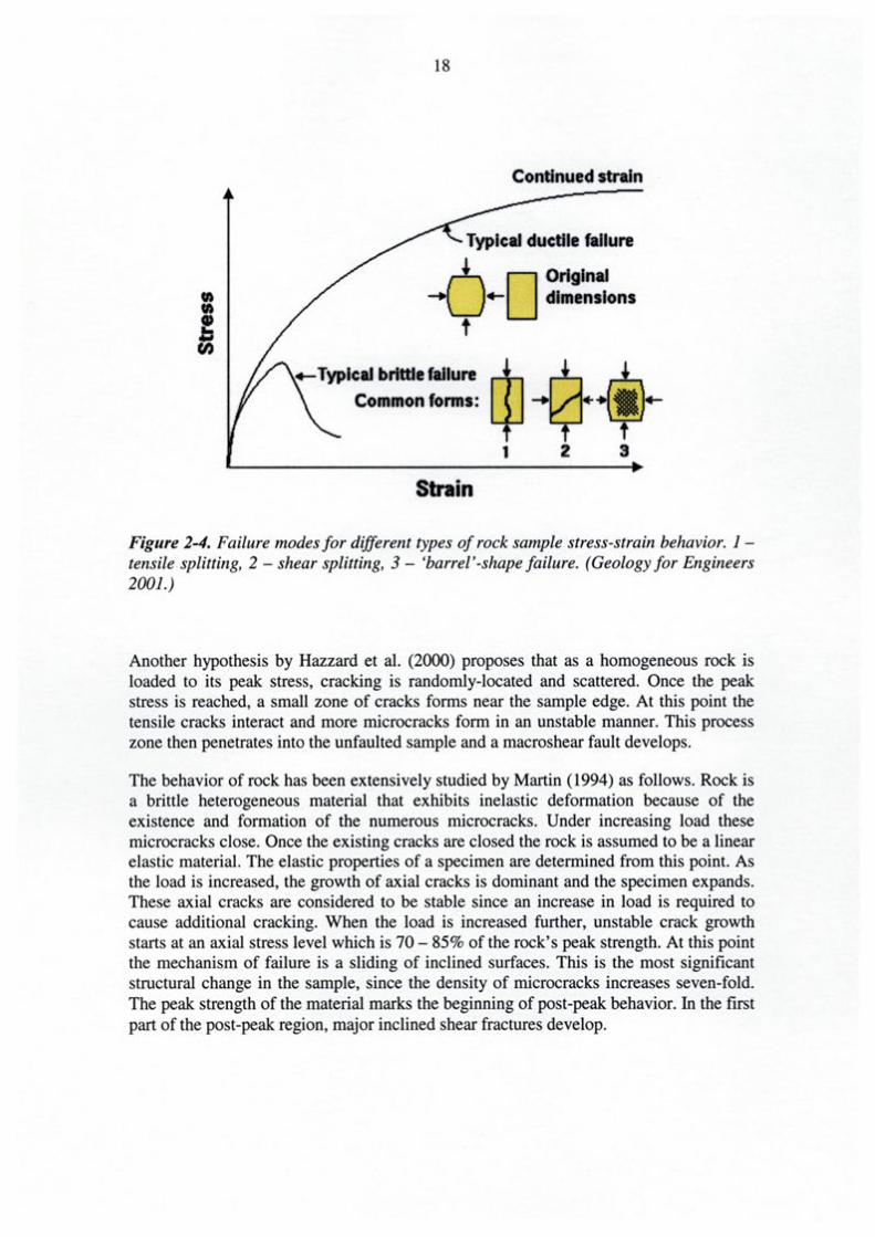
Tests made on samples of gneissic tonalite from the Research Tunnel at Olkiluoto (Autio et al. 2000) showed that the strength and deformation properties are significantly anisotropic and depend on the angle of schistosity in the test samples. Unconfined compression tests were performed for different schistosity angles to obtain Young's modulus, Poisson' s ratio and strength values. The strength and modulus results are summarized in Table 2-1 .

The uniaxial compressive strength as a function of specimen size and orientation is shown in Figure 2-5. Orientations were determined visually, with an estimated maximum error of± 10 degrees. A second order curve was fitted to the results.

The uniaxial strength is at a maximum when the sample is parallel to the schistosity plane (/3 = 0). When f3 is 38 - 43 degrees, measured strengths do not differ remarkably from values obtained with samples directed perpendicular to the plane (/3 = 90).

Measured values for Young's modulus exhibit similar behavior with respect to the schistosity angle as strength, while the effect of orientation on Poisson's ratio is not clear. Values for Young's modulus are at a maximum when a sample is oriented parallel to the schistosity plane, but drops to 20% of the maximum value when orientation is close to perpendicular, see Figure 2-6.

21

Table 2-1. Average strengths and Young's modulus with respect to schistosity angle. Results from three different diameter samples (41, 54, 99 mm). (Autio et al. 2000.)

5.8 11.1 11.5 33.7 38.6 43.0 70.0 75.5 84.2

160

140

~ 120 ~ ......

= en r::::: Q)

.b 100 (J)

80

78.2 141.8 74.6 126.4 77.2 127.1 68.1 98.1 66.0 97.1 61.4 94.2 62.0 93.4 59.4 97.8 66.3 97.8

Peak strength - laboratory samples Mean with std. dev.

o41mm o54mm o99mm

41.0 54.0 99.0 99.0 54.0 41.0 99.0 41.0 54.0

60+---------~----------~----------~--------~

0,0 22,5 45,0 Angle

67,5 90,0

Figure 2-5. Average unconfined compressive strengths (with standard deviation) of gneissic tonalite specimens with respect to schistosity angle. Three different sample sizes were tested. (Autio et al. 2000.)

100

90

80 (i 0. ~ t/J 70 ::::J "5 "C 0

::::E 60

50

40 0,0

22

Young's modulus -laboratory samples Mean with std. dev.

22,5 45,0 Angle

67,5

o41mm o54mm o99mm

90,0

Figure 2-6. Average Young 's modulus (with standard deviation) of gneissic tonalite specimens with respect to schistosity angle. Three different sample sizes were tested. (Autio et al. 2000.)

23

3 PFC THEORY

Particle Flow Code (PFC) models mechanical behavior by representing a solid as a bonded assembly of spherical particles. The modeling process is based on discrete­element (also called distinct-element) theory. PFC models are categorized as direct, damage-type numerical models in which the deformation is not a function of prescribed relationships between stresses and strains, but of changing microstructure.

The following sections describe general principles of the particle mechanics approach and the distinct element method and are based on PFC manuals published by ltasca (1999).

3.1 Particle mechanics

PFC2D and PFC3D (Particle Flow Code in 2 Dimensions and Particle Flow Code in 3 Dimensions) are programs for mode ling the movement and interaction of assemblies of arbitrarily-sized circular (2D) or spherical (3D) particles. The model is composed of distinct particles that displace independently from one another and interact only at contacts between the particles. Newton's laws of motion provide the fundamental relationship between particle motion and the forces causing the motion. Behavior that is more complex can be modeled by bonding the particles together at their contact points, and allowing the bond to break when the strength limit of the bond is exceeded. In addition to spherical particles, i.e. balls, the PFC model also includes 'walls'. The desired model is constructed from these two entities.

3.2 Distinct Element Method

PFC models the movement and interaction of particles using the distinct element method (DEM). PFC is classified as a discrete element code because it allows finite displacements and rotations of discrete bodies and because it recognizes new contacts automatically. The program is a simplified implementation of the distinct element method because of the restriction to rigid spherical particles.

In the distinct element method, interactions between particles are treated as a dynamic process. Dynamic behavior in PFC is represented in numerical terms by a time-stepping algorithm which requires repeated application of the laws of motion to each particle, a force-displacement law to each point of contact, and a constant updating of wall position. The use of an explicit numerical scheme makes it possible to simulate the non­linear interaction of a large number of particles without the requirement for the computer equipment being used to have extensive memory.

24

3.3 Calculation cycle

The PFC calculation cycle is shown in Figure 3-1. At the start of each time step, the set of contacts is updated from the known particle and wall positions. The force­displacement law is then applied to each contact to update the contact forces, and the law of motion is then applied to each particle to update its velocity and position.

3.4 Contact models

A contact model describes physical behavior at each contact. The constitutive model acting at a contact consists of a stiffness model, a slip model or a bonding model. The stiffness model is an elastic relationship between force and displacement. The slip model introduces friction into contact behavior. Particles may also be bonded together at a contact (the bonding model).

Two bonding models are supported in PFC. Both bonds can be described as the 'gluing together' of two particles. The contact-bond glue is of vanishingly-small size and acts only at the contact point. The parallel-bond glue has a finite size and acts over a circular cross-section positioned between the particles. The difference between the bonding models is that while the contact bond can only transmit a force, the parallel bond can also transmit a moment.

update particle+ wall positions and set of contacts

Law of motion (applied to each particle)

*resultant force & moment

contact forces

Force-Displacement law (applied to each contact)

*relative motion *constitutive law

Figure 3-1. P FC calculation cycle. The velocities and accelerations are kept constant within each time step.

25

4 PFC3D MODEL FOR ROCK

Some issues of importance concerning the modeling of rock with PFC3D are discussed in this chapter. The unconfined compression test procedure, specimen genesis and anisotropy installation processes are given particular emphasis because of the weight they carry in this study

4.1 Modeling with PFC3D

The modeling of rock behavior is challenging because rock is a complex anisotropic material made up of numerous grains cemented together. The mechanical behavior of rock involves crack growth which depends on the heterogeneous nature of local stress distribution within the material.

The fundamental element in PFC3D is a spherical particle. When the problem to be modeled concerns the interaction of spherical particles, the code can be applied in a straightforward way. On the other hand, when modeling solid material such as rock, the application process is more complex as particle properties cannot be determined directly - they have to be interpreted in an iterative manner from the results of standard laboratory tests. The parameters required are called micro-properties. They dictate how the model will respond and the kind of macro-properties that it will output. In rocks, the micro-properties that produce the known macro-properties and observed behavior are not usually known. Although the behavior of the PFC3D model is found to resemble that of rock, generally the particles in a PFC3D assembly are not associated with the minerals or grains in rock. (ltasca 1999.)

Calibration is the term used to describe the iterative process of determining and modifying the micro-properties for a PFC3D model. In the calibration process, the responses of the model are compared to the responses of the rock samples in the laboratory and the micro-properties of the model are modified in an iterative way to achieve good agreement. Comparisons can be at both laboratory and field scale. The laboratory-scale properties typically chosen for comparison are the elastic modulus (E), the crack-initiation stress ( O"ci), and the strength envelope ( crr = crr(P c), where Pc is the confining stress (Potyondy & Cundall 2000.) In this study, the properties chosen for calibration are Young's modulus (E) and the unconfined compressive strength ( crr). The laboratory response used as a target for calibration is presented in Section 2.4 Gneissic tonalite. In their excellent paper, Kulatilake et al. (200 1) discuss general issues concerning the calibration of micro-mechanical properties for an intact model material using PFC.

4.2 Model generation and compression test simulation

The PFC3D software package comes with prepared triaxial test procedures using the program's internal language (FISH). As this environment is somewhat limited in its scope, it was further developed to meet the requirements of this study. The primary areas of development were:

- Unconfined test procedures (rather than triaxial confined testing). - Altering the parallelpiped specimen shape used in the prepared package to a

cylindrical one.

26

- Introducing anisotropy (the prepared package environment is isotropic). - Developing the visualization tools used to visualize damage formation.

The following steps were performed when modeling with PFC3D:

1. The generation of an isotropic model that included particle generation, the compaction of these particles and internal stress reduction.

2. The introduction of anisotropy by adding banding in the specimen. 3. The simulation of a compression test.

A comprehensive description of model generation and the compression test can be found in the PFC3D manuals (ltasca 1999). The outcome of each step is illustrated in Figure 4-1.

4.2.1 Isotropic model generation in PFC3D

The procedure used to generate an isotropic model is made simpler by using a parallelpiped specimen shape. The final, cylindrical shape of the model is produced in Step 3. (Section 4.2). Firstly, bounding walls are created and the space (a parallelpiped box) is filled with spherical particles. The initial assembly is then compacted and internal isotropic stress is reduced. After additional steps, bonds between particles are introduced and the specimen is ready. Specimen dimensions are set in accordance with laboratory samples (Chapter 2.4 Gneissic tonalite). The specimen generation and material parameters are listed in Appendix 1. The specimen generation process produces an isotropic homogeneous model with given dimensions and micro-material properties.

4.2.2 Particle band generation in PFC3D

The schistosity of the gneissic tonalite is the result of oriented and clustered biotite grains. In PFC3D, an oriented rock sample is generated by running a random band generation procedure five different times at nine different schistosity angles to create bands of particles in the original isotropic packed model. This produces five different band formation for each schistosity angle, as illustrated in Figure 4-2. The final result is 45 different anisotropic models which are ready for further testing.

Potyondy & Cundall (2000) modeled anisotropy in 2-dimensions. Anisotropy was modeled here by using functions that they created. In this study, the functions were modified to be applicable in three dimensions. The following paragraphs explain the procedure used for band generation- which is partly based on the work by Potyondy & Cundall (2000).

Anisotropy is modeled by generating bands of particles within the matrix. Band particles are assigned micro-properties which are different to those possessed by the matrix particles. The procedure creates the joint-set, it marks the contacts as belonging to its joint -set. A sufficient number of joint planes are generated such that they cover the entire model. The joint planes are parallel to the schistosity planes, and their origin is at the center of the model bounding box. The thickness of each joint segment is set by first creating the joint segments via the JSET-command, and then expanding the contacts in the JSET to those that are adjacent to balls that are part of the original JSET. Input

27

parameters (with FISH-names) for establishing anisotropy are listed in Table 4-1 and in Appendix 1. The definitions used are shown in Figure 4-3. The geometry input parameters are expressed as multipliers of the average particle size used in the model.

The anisotropy geometry installation uses PFC3D JSET-command with aforementioned parameters. A joint-set is generated by assigning the joint-set ID number to all contacts between particles that lie upon opposite sides of each joint in the joint-set. Joints consist of a number of finite circular disks. The specified number of joint planes is generated, starting at the origin and then alternating on each side. Spacing is measured along the normal to the mean plane orientation. The parameters an2_rmult and an2_aratio define the area which the disks will occupy in the plane. The disks are placed at random locations within a square region of the joint plane that includes the whole model. Disks are generated until the ratio of the total disk area to the total square area equals the parameter set by an2_aratio. (ltasca 1999.)

The initial joint -set thickness is one particle. The expansion function expands the number of contacts that are part of the given joint-set. The function finds adjacent particles to the joint-set and adds them to the joint-set. This function is run given times to obtain wanted joint-set thickness. The used parameter value for this function expands the joint-set to have thickness of two particles.

After the geometry installation the micro-properties of the joint-set particles and bonds are modified. Two functions are used to modify the ball normal and shear stiffnesses and parallel-bond stiffnesses and strengths. The functions identify the particles and bonds that are part of the joint-set and apply the given factors to reduce the particle and bond stiffnesses and strengths, as it is assumed that the bands are softer and weaker than the matrix, resembling the properties of biotite.

Table 4-1. Anisotropy installation parameters and their values.

Description

Number of joint-sets to be created Seed of random-number generator Joint spacing will equal [an2_smult]*[particle_radius]*2 Number of expansions of joint-segment thickness Joint disk radius for joints will equal [an2_rmult]* [particle_radius] Joint area ration Schistosity angle [degrees] Ball stiffnesses reduction factor Parallel bond stiffnesses reduction factor (Ef) Parallel bond strength reduction factor (Sf)

FISH name

an2_isetnum an2_random an2_smult an2_stmult an2_rmult an2_aratio an2_stheta an2_efac an2_ebarfac an2_sigbarfac

Value

1 10001. .. 6 2 4 0.85 0 ... 90 0.05 0.05 0.2

28

1 2 3 Figure 4-1. Model generation steps in PFC3D. ]-isotropic parallelpiped model, 2-anisotropic parallelpiped model, ]-anisotropic cylindrical model.

Models with schistosity angle of 22.5 degrees. Each has different band formations. Models with schistosity angle of 67.5 degrees.

Each has different band formations.

Figure 4-2. Band generation produces a group of five different samples for all nine schistosity angles.

29

1 oint area ratio = Balls in joint (red) All balls in plane (red+ yellow)

Joint disk and its radius Joint spacin~ Joint thickness

Figure 4-3. Particle band generation produces an anisotropic model. Definitions of the geometry parameters are shown. For illustrative purposes, the schemes on the left and in the center represent schistosity oriented parallel to the longitudinal axis of the model.

4.2.3 Compression test simulation in PFC3D

The unconfined compression test is performed on a specimen with a circular cross­section. The cylindrical model is made out of a parallelpiped form by deleting particles which lie within the initial parallelpiped shaped model but outside the cylinder shape. As the test is an unconfined one, the first step in the test procedure is to remove the four separate side walls. The top and bottom walls act as loading platens.

At the start of the test, the platens are given a small velocity which is then gradually increased to the final compression-test velocity to maintain quasi-static conditions during the test. Induction of a compressive stress wave that will propagate through the model and produce impact loading must be avoided. The loading velocity is controlled throughout the test and is kept constant. Even though the velocity is quite large (0.05 m/s) the modeling environment is still in a near quasi-static condition because kinetic energy is being damped at a very high rate. Running simulations at a physical platen speed -1 MPa/s (see Section 2.1 Compression test) would have taken a very large number of simulation steps (and time) and would have produced much the same quasi-static results. One test was performed with the platen velocity of 0.025 mls. This showed that the modulus values were the same between the test with 'normal' platen

30

speed and the test with half the platen speed. The corresponding strength values deviated 2%.

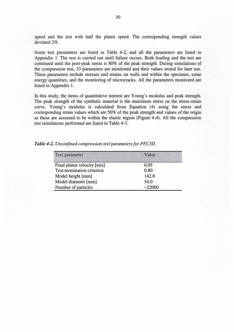
Some test parameters are listed in Table 4-2, and all the parameters are listed in Appendix 1. The test is carried out until failure occurs. Both loading and the test are continued until the post-peak stress is 80% of the peak strength. During simulations of the compression test, 33 parameters are monitored and their values stored for later use. These parameters include stresses and strains on walls and within the specimen, some energy quantities, and the monitoring of microcracks. All the parameters monitored are listed in Appendix 1.

In this study, the items of quantitative interest are Young's modulus and peak strength. The peak strength of the synthetic material is the maximum stress on the stress-strain curve. Young's modulus is calculated from Equation ( 4) using the stress and corresponding strain values which are 50% of the peak strength and values of the origin as these are assumed to be within the elastic region (Figure 4-4). All the compression test simulations performed are listed in Table 4-3.

Table 4-2. Unconfined compression test parameters for P FC3D.

Test parameter

Final platen velocity [m/s] Test-termination criterion Model height [mm] Model diameter [mm] Number of particles

Value

0.05 0.80 142.0 54.0 -22000

31

-AZ

Peak strength

z

Strain E

Figure 4-4. The pre-failure region (pre-peak stress) of the stress-strain curve obtained in an unconfined compression test and definitions of Young's modulus and peak strength.

Table 4-3. List of simulated compression tests with the corresponding chapter number.

0, 11, 22.5, 34, 45, 56, 67.5, 79,90

NIA 17 Ch. 7.1

0, 22.5, 45, 67.5, 90 35 Ch. 7.2

11,54, 79 9 Ch. 7.3

33

5 RESULTS OF COMPRESSION TEST SIMULATIONS

The results of compression test simulations are presented in this chapter. Firstly, numerical aspects of the modeling results are presented together with the appropriate laboratory results. After the quantitative presentation, the results of visual study are shown as well as failure patterns in the models. Finally, some observations are made about crack localization and crack evolution.

5.1 Quantitative results

As described in Section 4.2, the effect of schistosity was studied by carrying out a number of simulations with different schistosity angles from 0 to 90 degrees and an interval of approximately 11 degrees. r\t each schistosity angle, a total of five simulations were performed, resulting in a-total of 45 simulations. The height, diameter and average particle radius of the tested specimens were 142 mm, 54 mm and 1.3 mm, respectively. The vales for Young's modulus and peak strength obtained from the simulations are shown in Table 5-1 together with their standard deviations. An example of the axial stress versus axial strain curve at a schistosity angle of 45° is shown in Figure 5-1. The shapes of all the stress-strain curves in the other simulations are similar, but the positions of the curves differ slightly. More stress-strain curves can be found in Appendix 2. The values for peak strength and Young's modulus determined from each simulation are plotted with respect to schistosity angle in Figure 5-2. In Figure 5-3 the mean values of both peak strength and Young's modulus are shown. The peak strengths obtained in laboratory tests are plotted in Figure 5-4 together with the PFC3D results. Figure 5-5 shows values of Young's modulus determined from the simulations and values resulting from laboratory measurements.

The following conclusions were reached after comparing the laboratory results and the results obtained from the PFC3D simulations:

- The peak strength values obtained in simulations coincide with the values obtained from laboratory tests from 0 to approximately 65 degrees. From that point onwards, the results obtained in simulations are higher.

- If all the values obtained in simulations are shifted downwards by about 10 MP a, the two graphs (from simulations and laboratory tests) are almost similar - this is the standard calibration procedure described earlier. This suggests that the peak strength results are a qualitative match, and that if the calibration procedure were to be carried out again the model would also be quantitatively adequate.

A similar conclusion can be reached by comparing the values obtained for Young's modulus, shown in Figure 5-5.

- The shapes of the graphs are similar, but the levels of the modulus values differ by 10 - 20 GP a. This implies that re-calibration would superimpose the results.

A better matching of the reults can be achieved by re-calibration. In the process, four micro-properties can be scaled in order to achieve the required matching. The micro­properties are the particle-based ball-ball contact modulus, the parallel-bond modulus, the parallel-bond normal strength, and the parallel-bond shear strength.

34

The minimum peak strength occurs when the schistosity angle is 30 - 40 degrees. This angle is the same as the angle-of-failure plane in an isotropic rock model under uniaxial compression.

Table 5-l. Mean values and standard deviations used for simulation of unconfined compression test.

Schistosity angle Peak strength [MPa] Young's modulus [GPa] mean std.dev. mean std.dev.

0 149 2.7 74 0.6 11 137 2.3 69 1.6

22.5 104 5.7 60 2.0 34 93 5.6 51 2.9 45 96 5.1 47 1.5 56 103 2.5 44 1.7

67.5 112 3.3 44 2.0 79 111 3.9 43 2.6 90 112 2.7 44 2.4

Job Title: sT1_mG45b_tAOO

View Title: Axial stress vs. axial strain

X10"7

9 . 0

8.0

7 . 0

6 . 0

5 . 0

4 . 0

3 . 0

2.0

1 .0

0 . 0 -+--.--.....--.....-....-~-~~----r~------------.-~-------~--------....-.......--,.---.-~~--.-0 .0 0 . 5 1 . 0 1 . 5

x10A-3

2 . 0 2 . 5 3 . 0

Figure 5-1. Example of a stress-strain curve for a simulated unconfined compression test using PFC3D. Schistosity angle used in the model 45°, Peak strength 97 MPa, Young's modulus 44 GPa. The unit of the vertical stress axis is Pascal [Pa].

35

160. Peak strength and Young's modulus All values

140. I (i c. 120. G :f: ut . 2100· ; • $ :::s • I + "0

I I 0 ~ 80. ;:::.. (U

I c. ~ ..... 60· • .c -... C)

I c Cl)

40· ... .. I C/)

20.

0+---------------------~.~---------------------~.--------------------~.------------------------~. 45 67,5

Angle of s:histosity 0 22,5 90

Figure 5-2. All results for simulation of Peak strength [MPa] (upper) and Young 's modulus [GP a] (lower) are plotted with respect to schistosity angle [0

].

160.

140.

(i c. 120. G ..... 0 :::s '3100· "0 0

~ 80· (U

c. ~ 60· .c .. C) c ! 40· ... C/)

20.

Peak strength and Young's modulus Mean values with std .dev.

i

0+---------------------~.~---------------------~.--------------------~.------------------------~. 22,5 45

Angle of schistosity 67,5 90 0

Figure 5-3. Mean and standard deviations of simulation results plotted with respect to schistosity angle [0

}. Peak strength [MPa]- upper, Young's modulus [GPa] -lower.

180,0

160,0

140,0

= 120,0 m t: ~ -en

100,0

80,0

36

Peak strength- PFC and laboratory samples Mean values with std.dev.

Peak strength PFC3D

~ak strength LAB

60,0 +-------~---------.------.....,..------..... 0 22,5 45 67,5 90

Angle of schistosity

Figure 5-4. Peak strength [MPa] of the laboratory tests and the PFC3D runs. The yellow transparent area encloses the laboratory results. Note that the vertical axis spans from 60-180 MPa.

90,0

80,0

...... 70,0 ea c. ~ ~ 60,0 :; , 0 :E

50,0

40,0

Young's modulus- PFC and laboratory samples Mean values with std.dev.

Young's modulus LAB

Young's modulus PFC3D

30,0 +-------~-------r-------r----------. 0 22,5 45 67,5 90

Angle of schistosity

Figure 5-5. Young's modulus [GPa] of the laboratory tests and PFC3D runs. The yellow area encloses the laboratory results. Note that the vertical axis spans from 30-90GPa.

37

The crack-initiation stress corresponds to stress at which 1% of the total number of cracks existing at peak load has been formed. Poisson's Ratio (u) is calculated using Equation (5-1), where Ev is volumetric strain and Ez is strain in the specimen's z-direction.

V= _!_(1- fl.Cv ) 2 ~ez

(5-1)

Strain values are determined at a compression stress of 50% of the peak strength, see Figure 4-4. Crack initiation stress depends on the ratio of the standard deviation to the mean of the parallel-bond strengths. Poisson's Ratio depends on the ratio of the shear contact stiffness to the normal contact stiffness. (ltasca 1999.) Considering that the parameters were not focused on calibrating the model, the results obtained appear to correspond well with the work done by Autio et al. (2000). Figure 5-6 shows the crack initiation stress and values for Poisson' s Ratio with respect to schistosity angle.

Crack in it. stress 100•

80•

.. a. 60. i!. i i 40• UJ

20•

0 . . 0 22,5 45 67,5 90

Angle

Poisson's ratio 0,50

0,40

0,30 I I 0,20 I

0,10

0,00

0 22,5 45 67,5 90

Angle

Figure 5-6. Simulated mean values for crack initiation stress [MPa] (above) and Poisson 's Ratio (below) and their standard deviation with respect to the angle of schistosity [0

].

38

5.2 Qualitative study

Visual study of the damage formed during the compression test was carried out by looking at the damage patterns. All damage plots shown correspond to the final post­peak stage of simulations unless otherwise stated. Damage was studied in models in which the angle of schistosity angle was between 11° and 79°. Models with schistosity angles of 0° and 90° were not included in the detailed qualitative study because proper laboratory results for corresponding samples were not available.

5.2.1 Damage formation in PFC3D

The PFC3D model is constructed out of a number of particles which have been bonded together. As the model is loaded, forces build up and at some point a bond breaks. After the breaking of a bond, stress is redistributed and this may cause more cracks to form nearby. If the rock model is suitably stressed, these bond breakages may be localized into an inclined macro-fracture. Finally the model will fail. Rather than using constitutive laws in an indirect manner, deformations and fractures in the rock are modeled directly by allowing micro-mechanical damage to occur.

In the model, cracks are represented as colored octagons lying between two previously­bonded particles. The radius of the octagon is equal to the average radius of the two particles. Circular cracks are oriented perpendicular to the line joining the centers of the two particles (see Figure 5-7). Two ways of coloring the octagons are used. One way is to represent the cracks with respect to crack type as bi-colored octagons in which red represents tension-induced parallel-bond failure and black represents shear-induced parallel-bond failure. The second way is to illustrate cracks with respect to time by 16 gray-scale colors from white to black which indicate the time of crack formation; white= early, black= late.

5.2.2 Failure patterns

Study of damage was carried out by studying the damage patterns from different directions and in different sections (Figure 5-7), and by observing cracks at various phases of the simulation. In addition, an animation was made showing the generation of cracks during the simulated compression test. Based on observations made, failure patterns were divided into four groups based on the type of damage formation.

The four failure groups are as follows:

- Group A - models with a schistosity angle of 11 degrees, 5 simulations - Group B - models with a schistosity angle of 22.5 - 56 degrees, 20 simulations - Group C - models with a schistosity angle of 67.5 degrees, 5 simulations - Group D - models with a schistosity angle of 79 degrees, 5 simulations.

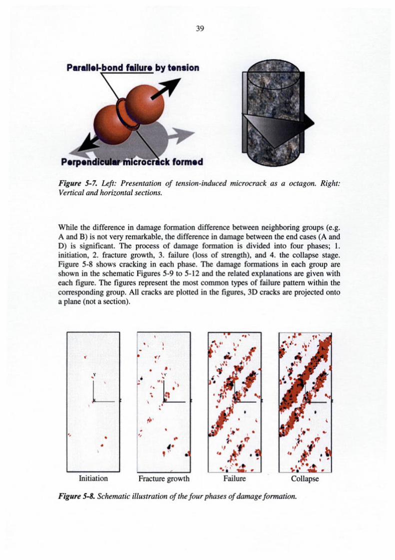
39

Par llel-:bond failur• by ten Ion

Figure 5-7. Left: Presentation of tension-induced microcrack . as a octagon. Right: Vertical and horizontal sections.

While the difference in damage formation difference between neighboring groups (e.g. A and B) is not very remarkable, the difference in damage between the end cases (A and D) is significant. The process of damage formation is divided into four phases; 1. initiation, 2. fracture growth, 3. failure (loss of strength), and 4. the collapse stage. Figure 5-8 shows cracking in each phase. The damage formations in each group are shown in the schematic Figures 5-9 to 5-12 and the related explanations are given with each figure. The figures represent the most common types of failure pattern within the corresponding group. All cracks are plotted in the figures, 3D cracks are projected onto a plane (not a section).

~.'

.. ~t

' • .I

L ,• ' Y

~

"'L_ .. ,., t ~

\; ·~ .....

,•

,:. I 4

• , " I •

• '; ' I .. 1• .rt

4• 11 ' •,• ., ~.

-r • Initiation Fracture growth Failure Collapse

Figure 5-8. Schematic illustration of the four phases of damage formation.

40

Group A, schistosity angle 11°

1. INITIATION The microcracks are forming evenly, mainly in the bands. It appears that there is slightly more cracking close to both ends of the model and around its perimeter than inside the model.

2. FRACTURE GROWTH Microcracking is, in general, concentrated in the bands and at the top of the model.

3. FAILURE The upper corner of the model is breaking (arrow) and a major fracture is localizing into one of the biotite bands.

4. COLLAPSE An extensive crushing region forms at one end of the model. The formation of macro-fracturing in the model resembles the shape of an hourglass.

Group B, schistosity angle 22.5°-56°

1. INITIATION

•

Figure 5-9. Damage formation at schistosity angle of 11°.

Microcracks start to form primarily within the biotite bands. 3 2. FRACTURE GROWTH Cracking is concentrating intensely in a single band. Weaker cracking is visible within parallel bands.

3. FAILURE A major fracture zone shears the model along the biotite band and forms two separated pieces. 1 4. COLLAPSE A zone of crushed rock forms around the shear fault. Arrows depict the splitting of the model.

Figure 5-10. Damage formation at schistosity angle of 34°.

41

Group C, schistosity angle 67.5°

1. INITIATION Microcracks start to form within the biotite bands and at the top of the model. Most of the cracks are located on the outer section of the model.

2. FRACTURE GROWTH Cracking increases within some biotite bands and at the top of the model.

3. FAILURE At peak stress, a major fracture zone is developing through the model which only partly follows the bands of biotite. The angle of the fracture plane is about 40 degrees with respect to the vertical axis while the biotite band is at an angle of 67.5 degrees. The upper corner is also splitting.

4. COLLAPSE Major crushing is taking place around the fracture and at the top of the model. Arrows show the movement of the fractured part.

Group D, schistosity angle 7~

1. INITIATION Most of the early cracking is located at both ends of the model.

2. FRACTURE GROWTH Cracking is increasing around the early cracking at one end and this starts to dominate the pattern of failure.

3. FAILURE Crushing at the top of the specimen. Small parts are cleaving off the model.

4. COLLAPSE Fractures are still expanding around the previous cracking. The end part is totally crushed.

1

Figure 5-11. Damage formation at schistosity angle of 67.5°.

f ... •

Figure 5-12. Damage formation at schistosity angle of7<f.

42

Simulated damage patterns for seven different values of schistosity angle are shown in Figures 5-13 to 5-19. The examples shown were selected to represent the most common types of failure generation. The method used to color cracks in these plots is time­dependent except in the case of the right-hand plots where the coloring indicates the type of cracking. In each case, the figure on the left shows all the cracks, the figure in the center shows cracks and displacements that lie in the Y -Z-section, and the figure on the right shows crack types and sample structure in the same section. In all cases, the viewing direction is parallel to the X -axis. More figures resulting from simulations can be found in Appendix 2. Most of the cracking seen in the figures (about 75%) forms after the peak stress has been reached, i.e. in the collapse stage, and does not affect the failure strength.

43

Figure 5-13. Model: sTx_mG_11 c, schistosity angle 11°. Left: All cracks, time­dependent coloring (light = early, dark = late). Center: Cracks and displacements on the origo centered vertical section, time-dependent coloring (light = early, dark = late). Right: Cracks and modeled particles on the origo-centered vertical section, crack type coloring (red = tension, black = shear). Particle coloring: yellow = stronger matrix material, orange = weaker band material.

•

' '

'

.. ,, ' .. . ' ,' "' ' •

44

Figure 5-14. Model: sTx_mG_225d, schistosity angle 22.5°. Left: All cracks, time­dependent coloring (light = early, dark = late). Center: Cracks and displacements on the origo centered vertical section, time-dependent coloring (light = early, dark = late). Right: Cracks and modeled particles on the origo-centered vertical section, crack type coloring (red = tension, black = shear). Particle coloring: yellow = stronger matrix material, orange = weaker band material.

45

' 'r,- •

Figure 5-15. Model: sTx_mG_34d, schistosity angle 34°. Left: All cracks, time­dependent coloring (light = early, dark = late). Center: Cracks and displacements on the origo centered vertical section, time-dependent coloring (light = early, dark = late). Right: Cracks and modeled particles on the origo-centered vertical section, crack type coloring (red = tension, black = shear). Particle coloring: yellow = stronger matrix material, orange = weaker band material.

'

46

• •• #!

,.~

' •I'

'

Figure 5-16. Model: sTx_mG_ 45a, schistosity angle 45°. Left: All cracks, time­dependent coloring (light = early, dark = late). Center: Cracks and displacements on the origo centered vertical section, time-dependent coloring (light= early, dark= late). Right: Cracks and modeled particles on the origo-centered vertical section, crack type coloring (red = tension, black = shear). Particle coloring: yellow = stronger matrix material, orange = weaker band material.

47

Figure 5-17. Model: sTx_mG_56c, schistosity angle 56°. Left: All cracks, time­dependent coloring (light = early, dark = late). Center: Cracks and displacements on the origo centered vertical section, time-dependent coloring (light= early, dark= late). Right: Cracks and modeled particles on the origo-centered vertical section, crack type coloring (red = tension, black = shear). Particle coloring: yellow = stronger matrix material, orange = weaker band material.

48

Figure 5-18. Model: sTx_mG_675e, schistosity angle 67.5°. Left: All cracks, time­dependent coloring (light = early, dark = late). Center: Cracks and displacements on the origo centered vertical section, time-dependent coloring (light = early, dark = late). Right: Cracks and modeled particles on the origo-centered vertical section, crack type coloring (red = tension, black = shear). Particle coloring: yellow = stronger matrix material, orange = weaker band material.

f ... ~

49

• * • I I 1

1 I I I 1 1 I

I a I I I a 1 i 1 . t!l •l' •• I . a,, •••

I I ·, I I . I 11 I li :

,, .•... f • f 0 .. , ... I I: :

• • # • • t .I •t • t t I t

'* • .. • # ... I t I • I f I I

• • • ~ _. • • I I • I

~ . "• . . •. :·.. . : .· ..... : . : .. ... .. : : . . . . . . ... . . . . y· .. : . . . : . . . . :· .: :,- .. : . : .... : ·.: · .. : ··.: ,; . ~ · .. · .....

• • • • ... • • t .. il ll •

.. ft .. . .. lil

Figure 5-19. Model: sTx_mG_79c, schistosity angle 7~. Left: All cracks, time­dependent coloring (light = early, dark = late). Center: Cracks and displacements on the origo centered vertical section, time-dependent coloring (light= early, dark= late). Right: Cracks and modeled particles on the origo-centered vertical section, crack type coloring (red = tension, black = shear). Particle coloring: yellow = stronger matrix material, orange = weaker band material.

51

6 ANALYSIS OF RESULTS

This chapter contains a discussion of important observations about failure development, a comparison of the results obtained from PFC3D simulations with results of laboratory tests, and comparison with results obtained in earlier work using 2D modeling.

6.1 Crack formation

The failure patterns in the different modeling simulations have some common features. The microcracks that form in an early stage of uniaxial compression are localized randomly throughout the specimen and within the biotite bands. In spite of the fact that the model is asymmetric and anisotropic, early microcracking is located in a quite symmetrical fashion. Early microcracks are primarily formed parallel to the direction of loading. At some point in time, microcracks begin to localize within the biotite bands, cracking in one band starts to become predominant, and in most cases the band-induced fracture zone propagates through the specimen. As the bands are not continuous in their geometry but are formed from distinct biotite sections aligned in a plane, fracture zones that form within a band are forced to jump to the next band section via the stronger matrix material in order to be able to continue cracking. This phenomenon is called "bridging". In models with schistosity angles from 11° to 67.5°, fracture propagation is more or less within a single biotite band (e.g. Appendix 2; Figures 45c and 675c). Minor fracturing also occurs parallel to the main fracture plane and this is evident in the damage plots. Major post -peak crushing regions are visible at the top and bottom of the specimens which have schistosity angles of 11° and 56° forward. In these models there is also more early-stage microcracking localized at the top and bottom ends of the model where the compressive load is exerted.

In some sections it was clear that microcracking proceeded from the outer cylindrical surface to the center of the model. In some models there was evidence that a microcrack was first formed inside a band and then spread in both directions along the band plane (Figure 6-1 is an example).

52

Figure 6-1. Horizontal cutting planes in two separate models. Left: schistosity angle 34°. Right: schistosity angle 45°. Red arrows show the direction of microcrack propagation. Sections shown are from the middle of the model.

Visual observation indicated that in some models there was more microcracking near the surface than in the center. To confirm this hypothesis radial distributions of cracks were calculated for each sample. The distributions showed that there might be slightly more cracking in the outer periphery of the samples than inside. A possible explanation for this could be that there is less internal cracking in the center of the model because the increased degree of constraint raises the strength of the matrix.

As can be seen from the time-dependent cumulative crack plot in Figure 6-2, most fracturing takes place in the post-peak stage. This figure also shows the stress-strain curve. It is clear that the number of cracks increases rapidly after peak stress is reached. The microcracks are either tensile- or shear-induced, and tensile cracking is clearly predominant as there is some five to ten times more tensile cracking than shear-induced cracking. All models demonstrated this behavior. The same crack-increasing phenomenon occurs when observing laboratory compression tests on an actual rock sample with an acoustic emission instrument (see for example Autio et al. 2000). In the model generation, the parallel bond tensile and shear strengths are set equal to one another. This produces more micro-tensile than micro-shear cracking to occur, as observed. This micro-property related effect was studied by Potyondy and Cundall (2000).

The results of simulations obtained using PFC3D clearly indicate that the method works advantageously. The results obtained show that the PFC3D results are related to corresponding laboratory results. The stress-strain curve obtained is similar in shape and the manner in which crack development takes place resembles many corresponding laboratory observations.

53

Job Till« aTt_m034d_tMO

at0'3

Figure 6-2. Axial stress (uppermost black line), all cracks (black), tensile cracks (red) and shear cracks (blue) plotted against axial strain. The cracking increases after the peak strength and tensile cracking is predominant. Model sTx_mG34d, schistosity angle 34°, peak strength 99 MPa, Young's modulus 55 GPa, number of cracks at peak strength 820 pieces.

6.2 Comparison against laboratory samples

Fracturing in 54 mm laboratory samples of gneissic tonalite and a PFC3D model are compared in Figure 6-3. The three photographic images show damage occurring during an unconfined laboratory compression test that was carried out in three different phases. The PFC3D images show cracking in the same phases. In spite of the relatively large particle size of the PFC3D model compared to actual grain size of the rock, some similarities can be found between the simulated failure patterns and failure in the laboratory test specimen. In the first phase, cracking is scattered around the sample and the amount is rather small even though the level of stress is only 10% below peak strength. At peak strength, cracking is primarily focused in a couple of inclined and parallel-oriented planes. After peak strength has been passed, cracking spreads along the planes. In the laboratory sample, post-peak cracking appears to have been spread more widely than in the PFC3D sample. In both cases, primary cracking takes place in the biotite (i.e. the PFC3D bands). The red dots in the photographic superposition images show cracking around the black biotite grains that has been confirmed by investigating laboratory samples with a scanning electron microscope (SEM). As can be seen in Figures 5-13 to 5-19, most of the cracking occurs in the PFC3D biotite sections.

'~

,, ' •• '>

y

•

Loading 10% less than peak strength (pre-peak)

54

• • •'t• " I I

' •' •' t.'

\ ~ y \

t L 1~~ ...

•r • ~ • '•

' j\ ' • •

•'t• \ . \

' •' ; ~ ' I

y •

1L •

' • ' •

Loading at peak strength Loading 5% less than peak strength (post-peak)

Figure 6-3. Laboratory samples (Autio et al. 2000) (upper) and PFC3D failure-pattern images (lower) from three different loading phases. Microfracturing of laboratory samples is superimposed in red color. P FC3D crack coloring; red = tension-induced, blue = shear-induced. Only cracks in the origo centered section are shown.

55

6.3 Comparison to 20 modeling results

Using PFC2D, Potyondy and Cundall (2000) modeled corresponding behavior of anisotropic rock. The results they obtained were compared with the results presented in this report.

Some differences between the results obtained from modeling in the two studies were observed. Most of the PFC2D models exhibited plastic-like behavior after peak loading whereas all of the PFC3D models showed brittle-like post-peak behavior (see for example Figure 6-2). Most of the PFC3D models showed secondary cracking parallel to the main cracking plane (see, for example, Figure 6-3) which was not as intense as in the PFC2D models. Some differences may arise from the fact that the PFC2D unconfined compression test were carried· out using a small confinement pressure ( -0.1 MPa) while the PFC3D simulations were performed without any confinement at all.

Several similarities between the results of modeling in the two studies were observed. Both methods showed a violent increase in cracking after the peak strength had been reached, with the main type of cracking being tensile-induced microcracking (see Figure 6-2). In both cases, pre-peak cracking was primarily located in biotite band segments and in bridging between these.

57

7 SENSITIVITY ANALYSIS

Three sensitivity analyses were performed: a study of the dependence of the PFC3D model on its macroscopic properties in relation to particle size, a study of the parameters related to the creation of anisotropic bands and a study of a three-particle­type model.

7.1 Resolution of the PFC model

The resolution of the model is defined as the number of particles across the model width (PFC2D) or the model diameter (PFC3D). If the dimensions of the model size are kept constant, reducing the particle size increases the model resolution and vice versa. The particle size is of interest because it has an effect on both the time required to complete simulations and the amount of computer memory required. Modeling with PFC is balancing between achieving a degree of resolution that is fine enough and the equipment resources that are available. The effect of the resolution was studied in both 2D and 3D.

7.1.1 Effect of model resolution in 20 modeling

Potyondy & Cundall (200 1) examined the effect of specimen resolution on macroscopic properties in 2D models with a height to width ratio of 2: 1. In the first set of tests they changed the width of the specimen while maintaining the same aspect ratio. In the second set of tests the particle sizes (i.e. radii) were changed. Specimen resolution increases when the specimen size is increased or the particle radius is reduced and vice versa. All other specimen properties were left untouched. The reference specimen for the PFC2D models was a specimen calibrated to fit the properties of Lac-du-Bonnet granite.

For both sets of tests, four different -sized specimens were generated, and for each of these specimens 10 repetitions of compression tests and Brazilian tests were performed. A total of 80 test-runs were executed.

The conclusions from the testing were as follows .

- As specimen resolution increases, <Jr, E and v tend towards a single mean value and the variations in value is reduced.

- Even the coarsest specimen, with 11 particles across the model width, produces average results that are very similar to those of the higher resolution specimens.

- Results achieved by altering specimen size and particle size are essentially the same.

At a macroscopic scale, strength properties can be divided into extensional or compressional conditions. The unconfined compressive strength results from compressional conditions, while the Brazilian tensile strength results from extensional conditions. While the resolution used does not affect compressional properties, it does affect extensional properties, and the Brazilian tensile strength decreased as specimen resolution increased.

58

7.1.2 Effect of model resolution in 3D modeling

The effect of particle size on the results of the PFC3D simulations was studied by performing compression test simulations with models employing different sizes of particle. Four different PFC3D specimens were constructed using different resolutions, with the alteration in resolution being achieved by changing the particle radius in each specimen. The reference material had a mean particle radius of 1.030 mm and a specimen cylinder size of 42 x 120 mm, giving a resolution (particle per width) of approximately 20 particles. The other specimens had particle sizes that were 1.5x, 2x, and 5x larger and the corresponding resolutions were 14, 11, and 4 particles respectively. A series of compression test were carried out and the strength and modulus values obtained were recorded.

The test results obtained using PFC3D were somewhat different from those obtained using PFC2D and showed a clear relationship between the resolution employed and the strength and modulus values obtained (see Figure 7-1 and Table 7-1). The effect of resolution appeared to be logarithmic in form. As the resolution increased, the values for strength and modulus obtained using the PFC3D simulation increased.

The conclusion here is that resolution affects macroscopic behavior and therefore the model has to be re-calibrated if the resolution used in the model is changed. It has more influence on the depiction of damage formation in specimens since the higher the resolution, the finer the structure of the specimen and the more detailed the damage formations that can result (see Figure 7-2). One major drawback to increasing the resolution is that models become too large to run in a standard PC (800 Mhz). Currently, an isotropic model with the resolution of 20 particles per width and the dimensions stated above (a total of 22,000 particles) requires 11 hours of computing time to running a single unconfined compression test simulation using PFC3D. Table 7-2 has values for the relationship between particle number, resolution and computer time required. Even though the specimen size used in obtaining these figures is different to that used in the resolution study, the relationship is essentially the same. As the resolution of the specimen is increased, the number of particles increases by the power of three and the computer time required to run one unconfined compression test using PFC3D increases exponentially.

59

Table 7-1. Results of the resolution test run. The dimensions of the specimens were 42 by 42 by 120 mm. A total of 17 runs were made; five for the reference model and four for each of the other specimens. Mean values are shown (E =Young's modulus [GPa], SigJ = Unconfined compression strength [MP a]).

Radius A vg. particle Resolution* Number of multiplier radius rmml r Particle/width l

xl.O 1.03 20 xl.5 1.54 14 x2.0 2.04 52 11 x5.0 4.94 38 4

*Resolution is defined as the number of particles across the model diameter.

Strength and modulus versus resolution

160

140

ea 120 D.

~ 1/)

-= 100 ::::J

"C 0 :E - 80 ea D.

~ 60 Young's modulus .s::::. -en c: Cl> ...

en 40

20

0 10 10

Resolution (particle/width)

Figure 7-1. Unconfined strength (UCS) and values for Young's modulus show a clear dependence on resolution. The relationship resembles a logarithmic dependence.

60

y

I z z

•

1.5mm 2.0mm 4.9mm

Figure 7-2. Damage patterns resulting from the use of different model resolutions. The numbers depict the average particle radius in the corresponding model. Crack coloring indicates the relative time when microcracks were formed [light = early, dark = late]. The models are isotropic.

Table 7-2. The relationship between particle size, resolution and computing time. The dimensions of the specimens are 54 x 54 x 142 mm. (The values 51 h and 642 h are

l d · h h · z · z · · · 1 [ AResolution*B} ) extrapo ate assumzng t at t e tzme-reso utzon re atzon zs exponentza t= .

Average particle radius rmml

2.0 1.5 1.3 1.03 0.8

Resolution* r particle/width 1

14 18 21 26 34

Number of particles

6500 15300 23600 47400

101100 *Resolution is defined as the number of particles across the model diameter.

Computer time rhoursl

1 4

11 (51)

(642)

61

7.2 Geometry parameters

Anisotropy was modeled by generating bands of particles as described in Section 4.2.2 Particle band generation in PFC3D. The sensitivity of the simulation results to changes in the band geometry parameters was studied by changing the band geometry but keeping all other material properties constant. Three cases were modeled and 35 simulations were performed. The parameters studied, joint area ratio and joint spacing (see Figure 4-3 for explanations), were changed so that the overall amount of band material in a model would be constant and identical to the basic case. In Case 1, the joint area ratio and joint spacing were reduced, producing a model in which the distinct band planes were no longer clearly visible. In Case 2, spacing was increased and the area of the weakness plane was filled with band particles to resemble a shale with very clear and visible continuous weakness planes. Case 3 was a modified version of Case 1, being geometrically between case 1 and the basic case. Table 7-3 is a list of the studied cases and the geometric parameters. Particle structures and damage patterns for the three cases are shown in Figure 7-3.

The results of the simulations show that cases 1 and 3 reduce the anisotropy of strength while Case 2 strengthens it. This can be seen in Figure 7-4 where peak strength and Young's modulus are shown with respect to the angle of schistosity. The weak anisotropy effect in cases 1 and 3 is almost identical - the shape of the curves remains the same only the absolute values deviate. The strengthened anisotropy in Case 2 is clear. Case 2 resembles slate in its anisotropy effect and its microstructure as described in Chapter 2.2 Anisotropy.

According to these results , the geometry of banding has a clear effect on strength and modulus anisotropy and is therefore essential input information in the modeling process.

Table 7-3. Geometric parameters for the three cases studied.

Joint area ratio Joint spacing # schistosity # simulations

Case 1 0.40 3 5 [0°, 22.5°, .. . ] 3x5 Case 2 1.00 12 5 [0°, 22.5°, .. . ] 1x5 Case 3 0.50 4 5 [0°, 22.5°, ... ] 3x5 Normal 0.85 6 9 [0°, 11 °, ... ] 9x5

• ')

t

•' •

Case 1

•

'

62

•

Case 2 Case 3 Basic case

Figure 7-3. Half of the models showing the three different geometries of the cases and the basic case (above). Cracks on the origo centered section are shown below. Yellow= matrix, red= weaker bands. In these models, the angle of schistosity is 22.5°.

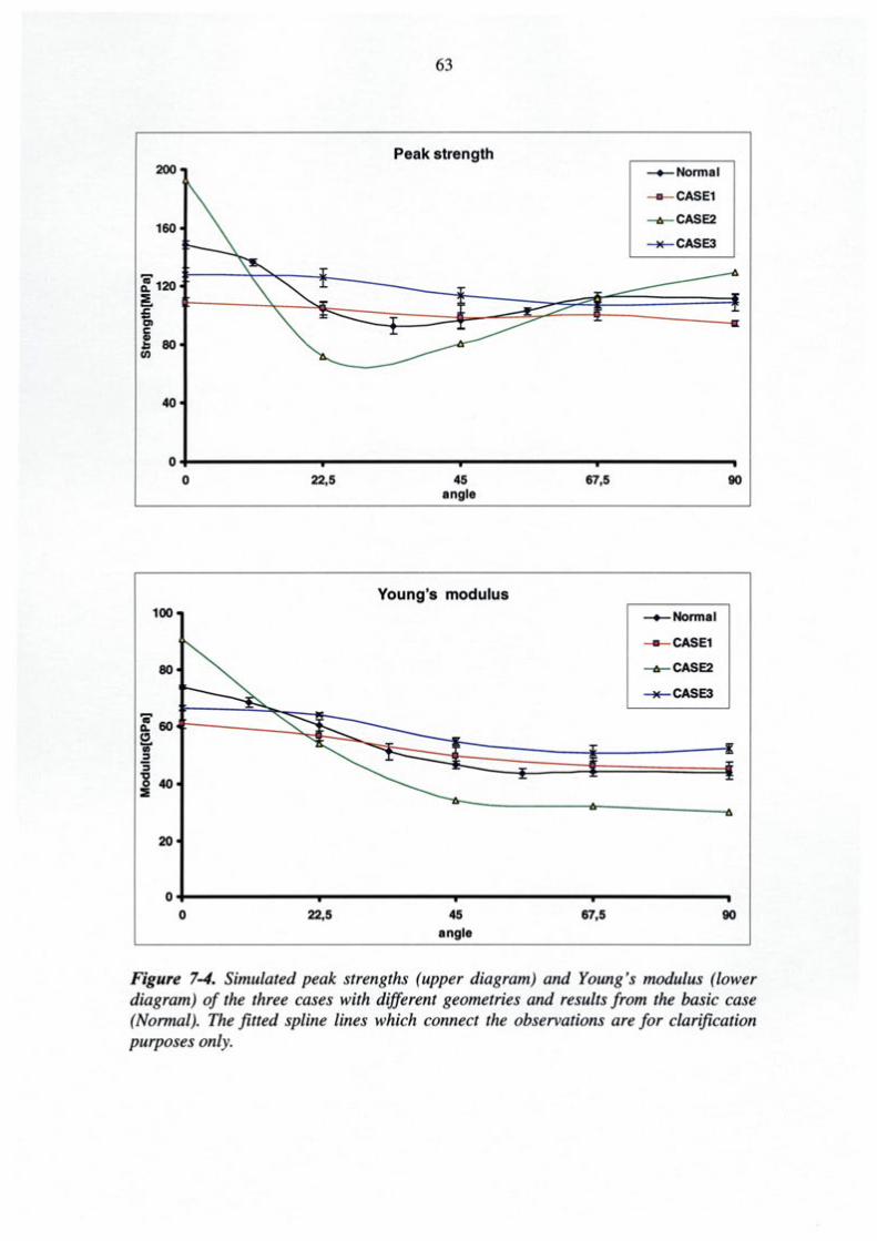
63

Peak strength 200

160

40

~Normal

CASE1

-1:r- CASE2

--*- CASE3

0+-------------~------------~------------~------------~ 0 22,5 45

angle

Young's modulus

67,5 90

~Normal

--cASE1

-1:r- CASE2

--*- CASE3

0+-------------~-------------r-------------.------------~ 0 22,5 45

angle

67,5 90

Figure 7-4. Simulated peak strengths (upper diagram) and Young's modulus (lower diagram) of the three cases with different geometries and results from the basic case (Normal). The fitted spline lines which connect the observations are for clarification purposes only.

64

7.3 Three component model

Gneissic tonalite consists of three main minerals: plagioclase, biotite and quartz. Simulations of the unconfined compression test were simplified by using two particle types to reduce the number of parameters. The model employed consisted of a matrix material and bands of particles that were weaker and less stiff (resembling biotite ). The behavior of a model that contained three different particle types was modeled to assess the significance of the third component. Band geometry and material properties were the same as in the basic two-particle model. The matrix material was divided between two different particle types. One of these particle types was the material already used as the matrix component in the basic case, the new third particle type was assigned strength and stiffness properties two times higher than the basic matrix particles. The structure of the third particle clusters was identified by performing the anisotropy installation procedure (Section 4.2.2) but with such a parameter values that no significant schistosity would occur in the modeL The particle structure of this model with a schistosity angle of 45 degrees is shown in Figure 7-5.

Three compression tests were simulated using three different angles of schistosity, i.e. nine simulations. The simulated peak strength and Young's modulus (see Figure 7-5), follow the results obtained with the two-particle model. In general, the strength and modulus values obtained when simulating the three-particle model are higher than in the two-particle model as the additional element (the new third particle) is both stronger and stiffer. The three-particle model was not calibrated to match the laboratory results because the main item of interest was the shape of the anisotropy curve, but the results obtained would probably coincide with the results obtained using the two-particle model if re-calibrated. It should be noted that the three-particle model does not radically alter the behavior of the compression simulation. According to these results, using a three­particle model would not produce results that are superior to those obtained using the two-particle model.

180• Peak strength and Young's modulus

160.

'i'140• A. CJ 'J120• :; '8 100 ~ .... 'i' 80 A. 11: I

• Strength I • Modulus

!. j,&O i J= 40 (/)

20

0

0 22,5

11

45 Angle

. 67,5

Figure 7-5. Left: Material structure in the three-particle model. Particles on the origo centered section are shown. Yellow = old matrix, red = bands, white = new matrix. Right: Mean simulated peak strength and Young 's modulus with standard deviations.

. 90

65

8 CONCLUSION AND DISCUSSION

The objective in this work was to study the effect of anisotropy in rock on strength and deformability by simulating a standard unconfined compression test with the PFC3D program. Anisotropy was modeled in 3D intrinsically by generating an anisotropic particle structure consisting of matrix particles and particles in oriented bands. The approach chosen is novel and no similar studies were found as references. The results obtained from the simulations were compared with corresponding laboratory test results. The comparison indicated that modeling using PFC3D can simulate the events which occur during laboratory compression tests of rock samples by reproducing similar fracture generation and deformation in both qualitative and quantitative terms.

Quantitative results for peak strength and Young's modulus obtained from the simulations resembled laboratory results. The exact values were close enough to conclude that the responses are similar. Fracture patterns produced by PFC3D modeling closely resembled the fracturing seen in laboratory test samples. PFC3D failure patterns showed features typical of brittle failure. Tensile cracking was dominant and most of the early microcracks formed in a direction parallel to the maximum compression stress. Initially located in a random manner, the tensile cracks began to interact and additional microcracks formed along the macroshear fault plane. The structural development of cracks during compression in PFC3D models and their evolution over time both resembled the corresponding damage events observed in actual rock samples.

Successful simulation of the behavior of a simple geometry makes it possible to proceed to the modeling of geometries that are more complicated such as well-defined problems associated with failure around underground openings in anisotropic rock. It would however be beneficial to study some topics in greater detail to optimize the simulation process and improve the accuracy of the material model. One of the current problems in the method is visualization of the cracking process in 3D. lllustration of the spatial and temporal processes using the visualization tools that are currently available is very difficult and radical improvement of these tools is undoubtedly required. Simulation takes a considerable amout of time and is related to the number of particles in a model and the number of particles is related to the particle size in a model. The topic of interest which is closely related to optimization of the material model is the effect of particle size on the simulation results.

A shortage of current empirical data and lack of understanding of the details of the failure processes in a rock matrix are factors which hamper use of the PFC method.

In terms of accuracy, the detailed reproduction of failure processes obtained by employing PFC3D software goes well beyond earlier results obtained by modeling with other methods. The method reported here has great future potential in the analysis of well-defined and clearly-focused problems.

66

67

REFERENCES

Autio, J., Johansson, E. & Sotnervuori, P. 1999. Modelling of an in-situ failure test in the Research Tunnel at Olkiluoto. Working report 99-74. POSIVA OY. Helsinki, Finland.

Autio, J., Johansson, E., Kirkkotnaki, T., Hakala, M. & Heikkila, E. 2000. In-situ failure test in the Research tunnel at Olkiluoto. Posiva report 2000-05. POSIV A OY. Helsinki, Finland.

Bates, R. L. & Jackson, J.A. 1990. Glossary of geology. 3rd edition. Atnerican geological institute, Alexandria, USA.

Brady, B.H.G. & Brown, E.T. 1985. Rock mechanics for underground Inining. George Alien & Unwin Ltd, London, Great Britain.

Cundall, P.A. & Starfield, A.M. 1988. Towards a methodology for rock mechanics 1nodeling. International journal of rock mechanics and mining sciences & geomechanics abstracts. 25(3). p. 99-106.

Departinent of Geological Sciences. 2001. Homepages for Depart1nent of Geological Sciences, University of Saskatchewan, Canada. June 261

h 2001. http://www. engr. us ask. ea/ dept/ geoe/

Hazzard, J.F., Young, R.P. & Maxwell, S.C. 2000. Micron1echanical modeling of cracking and failure in brittle rocks. Journal of geophysical research. Vol 105. No. B7, p. 16 683-16 697.

Heo, J .S., Cho, H.K. & Lee, C.I. 2001. Measureinent of acoustic einission and source location considering anisotropy of rock under triaxial compression. Rock mechanics - a challenge for society. Proceedings of the ISRM regional sy1nposiun1 Eurock 2001. A.A.Balkema. Netherlands.

Hock, E. & Brown, E.T. 1982. Underground excavations in rock. The Institution of Mining and Metallurgy. London, England.

Hoek, E., Kaiser, P.K. & Bawden, W.F. 1995. Support of underground excavations in hard rock. A.A.Balkema. Netherlands.

ISRM. International society for rock mechanics commiSSion on standardization of laboratory and field tests. 1979. Suggested 1nethods for determining the uniaxial cmnpressive strength and defonnability of rock Inaterials. International journal of rock mechanics and mining sciences & geomechanics abstracts. 16. p. 135-140.

Itasca Consulting Group, Inc. 1999. PFC3D (Particle Flow Code in 3 Dimensions). Version 2.0. Minneapolis, USA.

Jaeger, C. 1972. Rock mechanics and engineering. Cambridge University Press. Great Britain.

68

Li, L. & Holt, R.M. 2001. Simulation of granular matetial using particle tnodel with non-circularly shaped super-particles. Rock tnechanics - a challenge for society. Proceedings of the ISRM regional sytnposiwn Eurock 2001. Editors P. Sarkka & P. Eloranta. p. 511-516. Rotterdam: A. A. Balketna.

l(ulatilake, P.H.S.W., Malatna, B. & Wang, J. 2001. Physical and particle flow n1odeling of jointed rock block behavior under uniaxialloading. International journal of rock mechanics and mining sciences & geomechanics abstracts. 38. p. 641-657.

Martin, D. 1994. Proceedings of TVO/SKB/AECL Workshop on rock strength. Work report TEKA-94-07. Teollisuuden voitna Oy. Helsinki, Finland.

Obert, L. & Duvall, W. 1967. Rock tnechanics and the design of structures in rock. John Wiley & Sons, Inc. USA.

Oreskes, N., Shrader-Frechette, K. & Belitz, K. 1994. Verification, validation, and confirmation of numericaltnodels in the earth sciences. Science. Vol 263. p. 641-646

Peng, S. & Johnson, A. M. 1972. Crack growth and faulting in cylindrical specimens of Chehnsford granite. International journal of rock mechanics and mining sciences & geomechanics abstracts. 9. p. 37-86. Pergamon Press. Great Britain.

Potyondy, D. & Autio, J. Bonded-particle sitnulations of the In-situ failure test at Olkiluoto. 2001. In Proceedings of the 38th U.S. Rock Mechanics Symposium - DC Rocks 2001, Washington, D.C., July. 2001. Editors D. Elsworth, J.P. Tinucci & K.A. Heasley. p. 1553-1560. Rotterdam: A.A. Balketna.

Potyondy, D. & Cundall, P.A. 2000. Bonded-particle simulations of the in-situ failure test at Olkiluoto. Working report 2000-29. Posiva Oy. Helsinki, Finland.

Potyondy, D. & Cundall, P.A. 2001. The PFC model for rock: Predicting rock-tnass datnage at the underground research laboratory. Itasca Consulting Group, Inc. Atomic Energy of Canada Litnited (AECL). Issued as Ontario Hydro Nuclear Waste Managetnent Division Report No 06819-REP-01200-10061-ROO. Toronto, Canada.

Press, F. & Siever, R. 1986. Earth, 4th edition. W. H. Freeman and Company. New York, USA.

Wong, T.-F. 1982. Micromechanics of faulting in Westerly granite. International journal of rock mechanics and mining sciences & geomechanics abstracts. Vol. 19. p. 49-64. Pcrgamon Press. Great Britain.

Aikas, K. & Sacklen, N. 1993. Fracture tnapping in the research tunnel. Work report 93-01. TVO/Research tunnel. Helsinki, Finland.

69

APPENDIX 1: PFC MODEL FOR ROCK- PARAMETERS

The detailed desctiptions of each parameter listed here (excluding An isotropy installation parameters) are found in the PFC3D tnanual FISH in PFC3D (Itasca 1999).

Specimen genesis and material parameters

Sample width [tntn] Sample depth [tnm] Minin1 urn ball radius [mm] Ball size ratio, unifonn distribution Wall nonnal stiffness multiplier Requested value of isotropic stress [MP a] Requested tolerance for isotropic stress Stress reduction tnethod 1 (value=O) or 2 (value= I) Requested ratio of iso _ max over iso _min Run stress reduction this many steps Min. nutnber of contacts to be a non-floater

Young's modulus at each particle-particle contact [Pa] Ratio of particle normal to shear stiffness Ball friction coefficient

, generate Parallel-bond radius multiplier Young's tnodulus of each parallel bond [Pa] Ratio of parallel-bond nonnal to shear stiffness Mean value of parallel-bond normal strength [Pa] Std. deviation of nonnal strength [Pa] Mean value of parallel-bond shear strength [Pa] Std. deviation of shear strength [Pa]

et3 xlen et3 zlen et3 rlo et3 radius ratio

- -

tnd wEcfac tm _req_isostr ttn _req_isostr _tol tin _req_isostr2 tm _req_isostr _ratio tm _req_ steps flt def

-

md Ec md knoverks tnd fric

-

pb_radmult pb_Ec pb _knoverks pb _ sn _tnean pb_sn_sdev pb_ss_tnean pb_ss_sdev

54 54 2.5 1.66 1.1 -1.0 0.5 1

118.0e9 2.5 0.5

118.0e9 2.5 208.0e6 33.0e6 208.0e6 33.0e6

Anisotropy installation parameters

randmn-number generator Schistosity angle Joint spacing multiplier Joint-segment thickness tnultiplier Joint disk radius Joint area ratio

Parallel bond modulus reduction factor Parallel bond strength reduction factor

70

Unconfined compression test parameters

Lateral x-wa11 stiffness-reduction factor (triaxial-test) Lateral y-wall stiffness-reduction factor Lateral z-wall stiffness-reduction factor (triaxial-test) Target confining xx-stress [Pa] (triaxial-test) Target vertical stress [MP a] Target confining xx-stress [Pa] (triaxial-test) \V all-servo tolerance Final platen velocity [tn/s] Total cycles of platen acceleration Accelerate platens in this many stages Test-termination criterion Crack-initiation stress fraction

an2 SlTIUlt an2 stmult an2 nnult an2 aratio

an2 efac an2 ebarfac an2 _ sigbarfac

et3 knxfac et3_knyfac et3 knzfac et3 _ wsxx _req et3 _ wsyy _req et3 _ wszz _req et3 ws tol p_vel p_cyc p_stages et3 _peakfac pk_ci_fac

0 ... 90 6 2 4 0.85

0.05 0.05 0.2

N/A 1.000 N/A NIA 0.1 N/A 0.10 0.05 400 10 0.80 0.01

71

Monitored parameters during testing

nutn total number of contact bond failures in nonnal mode crk num cnf total nutnber of contact bond failures in shear mode crk nutn csf

- -

total number of parallel bond failures in nonnal crk _ nutn _pnf tnode total nutnber of parallel bond failures in shear mode

~~1E#~~:~n~~1!M~n~~~!i~~~,i~~r~iu§ wall-based strain in x-direction

wall-based volumetric strain specimen-based strain in x-direction

wan::aerlvea'stresse· · stress in x -direction

mean stress deviatoric stress

volumatric strain stress in x-direction

tnean stress deviatoric stress

1$~~~,<i~~n!i.~l work done by all walls total strain energy stored in the parallel bonds total energy dissipated by frictional sliding contacts total kinetic energy; translational and rotational total strain energy stored at contacts increment of strain energy

REFERENCES

at

et3 wexx et3_weyy et3 wezz et3 wevol et3 sexx et3_seyy et3 sezz et3 sevol

wsxx et3_wsyy et3 wszz et3 wsm et3 wsd

mexx et3_meyy et3 tnezz et3 mevol et3 msxx et3_tnsyy et3 mszz et3 msm et3 msd

energy energy bond energy frictional

energy kinetic energy strain et3 e delstrain

2 3 4

11 12 16 210 211 212 216

15 17 18

Ill 112 116 113 114 115 117 118

31 32

33 34 35

Itasca Consulting Group, Inc. 1999. PFC3D (Particle Flow Code in 3 Ditnensions). Version 2.0. Minneapolis, USA.

72

APPENDIX 2: CRACK PLOTS AND STRESS-STRAIN CURVES

In the pages 73-81 there are shown crack plots from all the si1nulations. The crack coloring is tin1e-dependent. All cracks are shown in a stage that corresponds the end of the test. Viewing direction is along the x-axis. So that the plots could fit the pages they have been rotated 90° anticlockwise.

Pages 82-84 show some stress-strain and crack nu1nber curves. Frmn each schistosity angle point one representative curve is shown. The plots are in sequence from 0 degrees to 90 degrees. The sample name and schistosity angle can be seen frmn THE JOB TITLE -

line of the corresponding plot.

For example: Job Title: sTJ mGOOa tAOO, where the number after the notation nzG, 00 - -

in this example, depicts the corresponding schistosity angle. (ex. 225=22.5°, 675 = 67. 5°, etc.)

73

Specimens sTl_ mGOOa .. .. e, schistosity angle 0 degrees, all cracks, time-dependent coloring

74

Specimens sT1_ mG 11 a ... e, schistosity angle 11 degrees, all cracks, time-dependent coloring

------------------------~=-----------~· E

75

Specimens sTl_ mG225a ... e, schistosity angle 22.5 degrees, all cracks, time-dependent coloring

. ., j --. •«• --- """- (#!

E

76

Specimens sTl_ mG34a ... e, schistosity angle 34 degrees, all cracks, time-dependent coloring

77

Specimens sTl_ mG45a ... e, schistosity angle 45 degrees, all cracks, titne-dependent coloring

•

~:.& J' f»P

-.;: -· .-. . ·.

~;·

.. tr~ ...

78

Specimens sTl_ mG56a ... e, schistosity angle 56 degrees, all cracks, time-dependent coloring

B

\ J <~ ......

~---~: #

79

Specimens sTl_ mG67 5a ... e, schistosity angle 67.5 degrees, all cracks, time-dependent coloring

80

Specimens sTl_mG79a ... e, schistosity angle 79 degrees, all cracks, time-dependent coloring

t , A i@l

~--------~.~~···· ·------------------------------~ c

81

Specimens sTl_ mG90a ... e, schistosity angle 90 degrees, all cracks, time-dependent coloring

~:.-.;(!if).@:»... ~~

* " "" @

E

82

/ 1 I I I I I

83

:.J.i

I

I I

/ I

i I I

/ /

/

;" /

/ ~

, ..... ~~·--

,/~ \ / / \I

~· !'\ I

/ /

~\/ / \,j

) I

/\ I \ I I

/ / I

/ I

/

_--'/

84

/~~/ / 0

/ !

/ I / I I ; I I

::/ -~( 1 ~;

J.3 Jci 'J

LIST OF REPORTS 1 (2)

POSIV A REPORTS 2002, situation 6/2002

POSIV A 2002-01

POSIV A 2002-02

POSIV A 2002-03

POSIV A 2002-04

Copper corrosion under expected conditions in a deep geologic repository Fraser King, Integrity Corrosion Consulting Ltd, Calgary, Canada Lasse Ahonen, Geological Survey of Finland Claes Taxen, Swedish Corrosion Institute, Stockholm, Sweden Ulla Vuorinen, VTT Chemical Technology Lars Werme, Svensk Kambranslehantering Ab, Stockholm, Sweden January 2002 ISBN 951-652-108-8

Estimation of rock movements due to future earthquakes at four candidate sites for a spent fuel repository in Finland Paul La Pointe Golder Associates Inc., Washington, USA Jan Hermanson Golder Associates AB, Sweden February 2002 ISBN 951-652-109-6

Fracture calcites at Olkiluoto- Evidence from Quaternary Infills for Palaeohydrogeology Seppo Gehor, Kivitieto Oy Juha Karhu, University of Helsinki Aulis Karki, Kivitieto Oy Jari Lofman, VTT Processes Petteri Pitkanen, VTT Building and Transport Paula Ruotsalainen, TUKES 0/avi Taikina-aho, Kivitieto Oy February 2002 ISBN 951-652-11 0-X

Structure and geological evolution of the bedrock of southern Satakunta, SW Finland Seppo Paulamaki, Markku Paananen, Seppo Elo Geological Survey of Finland February 2002 ISBN 951-652-111-8

POSIV A 2002-05

LIST OF REPORTS

Rock strength and deformation dependence on schistosity -Simulation of rock with PFC3D Toivo Wanne Saanio & Riekkola Oy June 2002 ISBN 951-652-112-6

2 (2)