Robust Parametric Tests of Constant Conditional Correlationin a MGARCH Model�

Wasel Shadatyz and Chris OrmeEconomics, School of Social Sciences, University of Manchester, UK

September 17, 2015

Abstract

This paper provides a rigorous asymptotic treatment of new and existing asymptotically validConditional Moment testing procedures of the Constant Conditional Correlation assumption in amultivariate GARCH model. Full and partial Quasi Maximum Likelihood Estimation frameworksare considered, as is the robustness of these tests to non-normality. In particular, the asymptoticvalidity of the LM procedure proposed by Tse (2000) is analyzed and new asymptotically robustversions of this test are proposed for both estimation frameworks. A Monte Carlo study suggeststhat a robust Tse test procedure exhibits good size and power properties, unlike the original variantwhich exhibits size distortion under non-normality.

JEL classi�cation: C12; C32Keywords: Multivariate GARCH; Constant Conditional Correlation; Conditional Moment Tests; Ro-bustness; Monte Carlo.

1 Introduction

Within a Multivariate GARCH (MGARCH) model, the conditional correlation approach has proved

popular amongst applied workers when modelling volatility. Initially, the Constant Conditional Corre-

lation (CCC) model was employed (see for example, Bollerslev (1990), Kroner and Claessens (1991),

Kroner and Sultan (1991, 1993), Park and Switzer (1995) and Lien and Tse (1998)), whilst recently

the Dynamic Conditional Correlation (DCC) model (Engle, 2002) has become more prevalent. Due to

the simplicity and computational advantages of the CCC model, on the one hand, but the increased

generality of the DCC approach, on the other, testing the adequacy of the CCC assumption within a

MGARCH model remains important from both a practical and, therefore, theoretical point of view.

Indeed, the most widely used test of the CCC assumption, among applied workers, is Tse�s (2000) LM

test (see, for example, Lien, Tse and Tsui (2002), Andreou and Ghysels (2003), Lee (2006), Aslanidis,

Osborn and Sensier (2008), among others) in preference to a number of other proposals in the literature

�An earlier version of the paper entitled �An Investigation of Parametric Tests of the Constant Conditional CorrelationAssumption�was presented at the European and Asian Meetings of the Econometric Society in Oslo (August 25-29, 2011)and Seoul (August 11-13, 2011). Detailed and exhaustive proofs are provided in a freely available on-line companionpaper, Shadat & Orme (2015). We are grateful for the insightful comments of the participants of these meetings and alsoto Ralf Becker, Alastair Hall and Len Gill. Two anonymous referees also provided constructive and insightful commentswhich were of enormous help in revising this paper. The standard disclaimer applies.

yCorresponding author: Dr Wasel Shadat, Economics, School of Social Science, University of Manchester, ManchesterM13 9PL, UK. e-mail: waselbin.Shadat@manchester.ac.uk

zThe �rst author�s research is part of his PhD thesis and was supported by a Commonwealth Scholarship and FellowshipPlan and a Manchester School Award; both of which are gratefully acknowledged.

1

(e.g., Bollerslev (1990), Longin and Solnik (1995) and Bera and Kim (2002)).1 Tse�s (2000) procedure,

unlike the information matrix test approach of Bera and Kim (2002), can be applied to high-dimensional

data but it is predicated on a Full Quasi Maximum Likelihood Estimation (FQMLE) approach, together

with an explicit assumption of normality when constructing the test statistic.

This paper addresses four inferential issues that emerge from Tse (2000): (i) Tse�s Outer Product

of the Gradient (OPG) version of the LM test is only guaranteed to be asymptotically valid under an

explicit normality assumption. (ii) Even under normality the OPG variant of a LM test may demonstrate

relatively poor �nite sample performance; see, for example, Davidson and MacKinnon (1983), Bera and

McKenzie (1986), Orme (1990), Chesher and Spady (1991). (iii) Tse�s test procedure may not be robust

to misspeci�cation of the individual volatility (GARCH) equations. (iv) It is still common practice,

when estimating a MGARCH model, to employ a two-stage or Partial Quasi Maximum Likelihood

Estimation (PQMLE) approach, where the volatility parameters in each equation are �rst estimated

using a univariate GARCH speci�cation and, second, the correlation parameters are then estimated

using these �rst-stage volatility parameter estimates (see Engle and Sheppard (2008), Hafner, Dijk

and Franses (2005), Billio, Caporin and Gobbo (2006), among others); however, within this PQMLE

framework, there appears to be no available test of the CCC assumption.

Thus, we propose, and provide a rigorous analysis of, asymptotically valid and non-normality robust

tests of the CCC assumption, based on a Conditional Moment (CM) approach. These tests will be

robust in the sense that their asymptotic validity does not depend on normality (unlike Tse (2002));

but they do require moment conditions which ensure standard asymptotic inferences can be applied.

Such tests can be employed following either FQMLE or PQMLE and robust versions of Tse�s test are

given particular attention. The required derivations require some straightforward, yet tedious, algebraic

results but lead to robust tests that are easy to implement. In our Monte Carlo study, with a moderate

number of assets/time-series (N = 5), these tests demonstrate satisfactory size properties in most

cases. Furthermore, whilst not addressed analytically, the Monte Carlo study also sheds some light

on the robustness of the various test statistics to GARCH misspeci�cations in the individual volatility

(GARCH) equations. From the panoply of procedures we consider, a robust version of Tse�s LM test

exhibits very good size and power properties under a variety of Data Generation Processes (DGPs).

The rest of this paper is organized as follows. The model, FQMLE, PQMLE and Tse�s original

LM test are reviewed in Section 2. In Section 3, a class of CM parametric tests is described, for both

estimation frameworks, and robust variants proposed. This is extended in Section 4 to provide robust

versions of Tse�s LM test that can be employed following either FQMLE or PQMLE. Section 5 reports

the �ndings of a Monte Carlo study and Section 6 concludes. The analysis follows standard �rst order

asymptotic theory, but to avoid obfuscating the main issues, technical (but fairly standard) assumptions

1Nakatani and Teräsvirta (2009) proposed another LM test for volatility interaction where the null model is CCCGARCH model against the alternative of Extended CCC (ECCC) GARCH model.

2

and proofs of the main results are relegated to an Appendix; with more detailed and exhaustive proofs

provided in an accompanying freely available on-line paper, Shadat and Orme (2015), which also contains

additional information concerning the Monte Carlo experiments undertaken.

The following notation is employed: the vec (:) operator stacks the N columns of a (M �N) ma-

trix as a (MN � 1) vector; vech (:) stacks the lower triangular portion of a (N �N) matrix as a�12N (N + 1)� 1

�vector; and, vecl (:) stacks the strictly lower triangular portion of a (N �N) ma-

trix as a�12N (N � 1)� 1

�vector. Correspondingly, sJN = f(i; j) : i = j; :::; N; j = 1; :::; N; and i

changing more quickly than jg de�nes the ordering of the elements of a (N �N) matrix A = faijg into

vech (A) and sCN = f(i; j) : i = j + 1; :::; N; j = 1; :::; N � 1; and i changing more quickly than jg the

corresponding ordering for the vecl (:) operator.

2 The CCC Model and Tse�s LM Test

We consider the following standard CCC-GARCH linear regression speci�cation

yit = w0it'i + "it; i = 1; :::; N t = 1; :::; T; (1)

to model the (N � 1) time-series vector yt = fyitg, with T large and N �xed/small, where wit =

(y0

i;t�1; d0it)0 is the (K � 1) vector of regressor variables, containing current and lagged exogenous vari-

ables (dit), and lagged dependent variables (yi;t�1) and 'i � <K is an unknown vector of regression

parameters. The volatility in the (N � 1) error vector "t = f"itg has a GARCH(p; q) speci�cation of

hit = �i0 +Pq

k=1 �ik"2i;t�k +

Ppj=1 �ijhi;t�j with �i = (�i0; �i1; :::; �iq; �i1; :::; �ip)

0 � <K�being an

unknown vector of volatility parameters. The CCC model is described by

"t = H1=2t �0t; and Ht = Dt�Dt; (2)

where the �0t are independently and identically distributed (iid) random vectors, with E [�0t] = 0 and

E��0t�

00t

�= IN , Dt = diag(h

1=2it ) a (N �N) diagonal matrix and � =

��ij; a (N �N) time invariant

symmetric positive de�nite matrix with �ii = 1; i = 1; :::; N: Thus, the conditional covariance matrix,

Ht; has elements hijt = h1=2it h

1=2jt �ij ; i; j = 1; :::; N:

To be more precise about the parameterization employed, de�ne �i = ('0i; �0i)0 � <K+K�

and ! =��0; �0

�0 2 � � <N�; where N� = N (K +K�) + 1

2N(N � 1) with � =��01; :::; �

0N

�0 � <N(K+K�) and

� = vecl(�):2 Then, "it = yit � w0it'i � "it('i) with hit � hit(�i); Dt � Dt(�), and Ht � Ht(!):

Letting !0 =��00; �

00

�0denote the true parameter vector, with �0 = vecl(�0), we have "0t = "t(�0);

2For example, for a AR(1) CCC speci�cation with N = 5 and individual GARCH (1,1) errors, we have K = 2; K� = 3and N� = 35:

3

D0t = Dt(�0); and H0t = Ht(!0) = D0t�0D0t so that E ["0tjFt�1] = 0; and E ["0t"00tjFt�1] = H0t,

where Ft�1 = �("0;t�1; "0;t�2; :::):3

Following Berkes, Horváth and Kokoszka (2003) and Ling and McAleer (2003), and given Assumption

A3(i)(ii), the process for hit has the representation h1it =P1

l=0 ilai;t�l; where, for all i; ait = �i0 +Pqk=1 �ik"

2i;t�k and il =

Ppj=1 �ij i;l�j with is = 0; s < 0; i0 = 1; il > 0; l > 0; and 0 <P1

l=0 il =�1�

Ppj=1 �ij

��1< 1: The coe¢ cients, il; decay exponentially fast, and there exist

constants �K > 0 and 0 < � < 1; independent of !; such that il � �K� l, for all i: Then, Assumption

A in the Appendix, ensures the identi�ability, stationarity and ergodicity of the process fyit;"0it; h0itg ;

where h0it � h1it (�i0) ; see Ling and McAleer (2003).

In the subsequent analyses, three alternative �transformed� error vectors are employed: volatility

adjusted errors (�t), �fully�standardized errors (�t) and (Tse�s) transformed standardized errors ("�t ).

These are, respectively,

�t � �t(�) = D�1t "t = f�it(�i)g (3)

�t � �t(!) = H�1=2t "t = f�it(!)g (4)

"�t � "�t (!) = ��1�t = �

�1D�1t "t = f"�it(!)g (5)

with �0t = �t(�0); �0t = �t(!0), "�0t = "�t (!0); and satisfying: (i) E [�0tjFt�1] = 0; E

��0t�

00tjFt�1

�= �0

(in the case of a CCC speci�cation); (ii) E [�0t] = 0; E��0t�

00t

�= IN ; from (2); and, (iii) E ["�0tjFt�1] = 0;

E ["�0t"�00tjFt�1] = ��10 . For some estimator ! = (�

0; �0)0 of !; the estimated counterparts of (3)-(5) will

be denoted �t � �t(�); �t � �t(!); "�t � "�t (!) and similarly �it; �it and "

�it: Finally, where there is

no ambiguity, this form of notation will be adopted for general functions of parameters mt(!); so that

mt � mt(!); m0t � mt(!0) and mt � mt(!); etc.

2.1 FQMLE and PQMLE Framework

Given (1) and (2), the quasi-conditional log-likelihood per observation, t; is given by

l�t (!) = � 12 ln j�j �

12

NXi=1

lnhit � 12�0t��1�t:

Assuming L�T (!) = T�1PT

t=1 l�t (!) is twice continuously di¤erentiable, and �g

�T (!) = T�1

PTt=1 g

�t (!) ;

where g�t (!) = @l�t (!)=@!; then the FQML estimator, ! = argmax! L�T (!); satis�es �g�T (!) = 0:

However, the observed l�t (!) is constructed conditional on available pre-sample values, because hit

needs to be constructed recursively given initial values, "+i0 =�"2i0; :::; "

2i;1�q; hi0; :::; hi;1�p

�0. In order

3Given the context, there should be no confusion between the random vector "0t; which has elements "0it; and theelements of "t; denoted "it; i = 1; :::; N; t = 1; ::::; T:

4

to simplify the algebra and asymptotic theory, it is assumed (in addition) that the required pre-sample

observations on wit are also available and that hit = 0 for all i and t � 0: The simpli�cations derive

from the fact that hit can then be expressed as hit =Pt�1

l=0 ilai;t�l; t = 1; :::; T; but the processes hit

and l�t (!) will not be stationary ergodic sequences.4

Replacing hit by h1it in l�t (!); throughout, provides an unobserved but stationary and ergodic log-

likelihood sequence

l1�t (!) = � 1

2 ln j�j �12

NXi=1

lnh1it � 12�10t ��1�1t ;

where �1t =�"it=

ph1it: Then, with N �nite and letting T ! 1; and under Assumptions A

and B1, B2 described in the Appendix, !p�! !0 and

pT (! � !0)

d�! N�0; J��10 ��ggJ

��10

�; where

J�0 = �E [@g1�t (!)=@!0]!=!0 and �

�gg = E [g1�

t (!0)g1�t (!0)

0] are both �nite and positive de�nite and

g1�t (!) = @l1�

t (!)=@!: That is to say, employing the recursively constructed hit (rather than the �true�

but unobserved h1it ) makes no di¤erence asymptotically.

Adopting a PQMLE approach, and following Engle (2002), we can write L�T (!) = LT (�) + LCT (!)

where LT (�) = 1T

PTt=1

PNi=1 lit(�i); with lit(�i) = � 1

2

�lnhit + h

�1it "

2it

and LCT (!) = 1

T

PTt=1 l

Ct (!);

with lCt (!) = � 12 ln j�j �

12�0t��1�t+

12�0t�t. Here,

1T

PTt=1 lit(�i) is the average log-likelihood for the i

th

univariate GARCH regression model (1) and lCt (!) models the CCC structure. This a¤ords a two-stage

PQMLE procedure where at stage one we obtain ~�i = argmax�i1T

PTt=1 lit(�i), the consistent univariate

GARCH QML estimators. Equivalently, ~� = argmax� LT (�); which satis�es �gT (~�) = 0; where �gT (�) =1T

PTt=1 gt(�) and gt(�) =

PNi=1 @lit(�i)=@�; which is, of course, gt(�) = (@l1t(�1)@�

01; :::; @lNt(�N )=@�

0N )

0.

For the second stage, we employ all the �rst stage PQML estimator ~� to obtain ~� = argmax� LCT (~�; �);

which satis�esPT

t=1

�~"�it~"

�jt � ~�ij

�= 0; j < i; where ��1 =

��ij: The resulting PQML estimator,

~! = (~�0; ~�0)0; is consistent, but asymptotically ine¢ cient relative to FQMLE.5 If we adopt Boller-

slev�s (1990) alternative parameterization of lit(�i); it transpires that the ensuing ~� has a closed form

expression satisfyingPT

t=1

�~�it~�jt � ~�ij

�= 0; j < i: Even without this alternative parameteriza-

tion, it is still the case that the simple estimator ~�ij =1T

PTt=1

~�it~�jt; j < i will be consistent

for the true correlation parameter value, and this will be the estimator, together with ~�i; that we

shall employ in the PQMLE framework. Moreover, it turns out that the limit distributions of the

various test indicators that we shall consider, obtained from PQMLE, are not in�uenced by this

choice of ~� and this leads to the construction of relatively simple asymptotically valid test statis-

tics. Thus, we just need the separate limit distributions ofpT�~�i � �i0

�and Assumptions A and

B1, B2, in the Appendix, implypT (~� � �0)

d! N(0; J�10 �ggJ�10 ) where the (block diagonal) matrix

4Note, that this is not the same start-up scheme employed by either Ling and McAleer (2003), who choose "+i0 = 0;Berkes et al (2003), or Francq and Zakoian (2004). In practice, and for all inferential procedures described in this paper,any constant value can be chosen for "+i0; in order to generate hit, t = 1; :::; T .

5Hafner and Herwartz (2008) provided an analytical expression for the asymptotic variance of the PQML estimator,for both the CCC and DCC models.

5

J0 = �E�@g1t (�0)=@�

0� = diag ��E �@2l1it (�i0)=@�i@�0i�� and �gg = E [g1t (�0)g1t (�0)

0] are both �nite

and positive de�nite, and g1t (�) =PN

i=1 @l1it (�i)=@� with l

1it (�i) = � 1

2

�lnh1it + "

2it=h

1it

; see, e.g.,

Halunga and Orme (2009, Theorem 1).

2.2 Tse�s LM Test of the CCC Assumption

For the purposes of constructing Tse�s test, a dynamic correlation structure of the form �ijt = �ij +

ij�i;t�1�j;t�1 is assumed, where ii = 0; ij = ji; even though �ijt is not a well-de�ned alternative

to the CCC since �t =��ijt

is not necessarily a positive de�nite matrix for all t. There are N(N�1)

2

additional parameters in DCC �alternative�model with the null hypothesis of CCC being H0 : ij = 0;

for all distinct i; j; and i > j. Tse (2000) employed the Lagrange Multiplier (LM) principle and proposed

an OPG variant of the LM test statistic which, in this case with test variables �t�1�0t�1, is

6

dLM�T = �0T �

����0��

��1��0�T ; (6)

where �� is a�T �N� + N(N�1)

2

�matrix, with rows equal to (g�0t ; vecl(("

�t "�0t � ��1)� �t�1�

0t�1)

0); �

denotes the Hadamard product, and �T is the (T � 1) column vector of ones.7 Under the usual regularity

conditions dLM�T is asymptotically distributed as �

2N(N�1)

2

:

The notation dLM�T is used to emphasize that (6) is constructed from ! and cannot be implemented

directly using ~!. Furthermore, the OPG construction advocated by Tse (2000) may be sensitive to

non-normality, and some evidence for this is provided by Tse (2000, Section 5). In the next section we

develop a Conditional Moment (CM) testing framework of the CCC assumption which accommodates

Tse�s Test. This framework provides, in Section 4, non-normality robust Tse test procedures for both the

FQMLE and PQMLE cases. However, for this particular choice of test variables, �i;t�1�j;t�1; a stronger

moment condition of E j"0itj8 <1 for all i; t, is then required in order to justify the asymptotic validity

of these robust tests.

3 A Class of Asymptotically Valid CM Test Procedures

If the CCC speci�cation is correct, then E��0t�

00t � �0jFt�1

�= 0 in which h0it = h1it (�i0). The diag-

onal elements of��t�

0t � �

�correspond to the individual GARCH (or volatility) speci�cations, whereas

the o¤-diagonal elements correspond to the CCC assumption. Also due to the symmetry there are

12N (N + 1) independent (distinct) restrictions in this moment condition; i.e., E

��J0tjFt�1

�= 0; where

�J0t = vech��0t�

00t � �0

�; the superscript J indicating joint testing of both the CCC and of the individual

6Here, cross-products of lagged standardised �residuals�, are employed as �test variables�which is feasible using theLM principle and, since this �alternative�is an arti�cial device simply employed to construct a test statistic, Silvennoinenand Teräsvirta (2009) interpreted this as a general misspeci�cation test.

7Details of g1�t (!); and hence g�t (!); are given in the Appendix, Proposition 6.

6

volatility speci�cations. The typical element of this moment condition can be written as

E��0;it�0;jt � �0;ij jFt�1

�= 0; i � j; i = 2; :::; N: (7)

When the underlying moment restriction is (7), the ensuing test will be referred as the Full CM (FCM)

test and can be treated as a joint misspeci�cation test of the complete MGARCH error speci�cation.

If we are only interested in testing the CCC assumption, the moment condition is E��C0tjFt�1

�= 0;

where �C0t = vecl��0t�

00t � �0

�and the superscript C denotes testing only the CCC assumption; i.e.,

E��0;it�0;jt � �0;ij jFt�1

�= 0; i > j; i = 2; :::; N: (8)

The ensuing test based on (8) will be referred to as the CCC CM (CCM) test.

The implication of (7) is that misspeci�cation tests of the CCC model can be constructed as tests

of the following moment conditions

E���0;it�0;jt � �0;ij

�rij;t(!0)

�= 0; (9)

where the (qij�1) vector rij;t(!0) is a Ft�1 measurable function, possibly depending upon the processes

h0it and h0jt:8 A CM test indicator vector can then be constructed, up to a knowledge of !; as �mT (!) =

1T

PTt=1mt(!) with the vector mt(!) constructed from the �stacked�sub-vectors

mij;t(!) = (�it�jt � �ij)rij;t = �ij;trij;t; (qij � 1) (10)

where �ij;t = (�it�jt � �ij); a scalar, and rij;t � rij;t(!): Note that the mij;t(!) are arranged in mt(!),

ordered by (i; j); according to either sJN (as in the vech(:) operator) or sCN (as in the vecl(:) operator).

In the former case, this will be denoted �mJT (!) =

1T

PTt=1m

Jt (!); q

J � 1, where qJ =P

i�j qij ; whilst

in the latter case it will be �mCT (!) =

1T

PTt=1m

Ct (!), q

C � 1; where qC =P

i>j qij = qJ �P

i qii: Then,

�mJT (!) will be referred to as the FCM test indicator, �mC

T (!) the CCM test indicator and both can be

constructed employing either the FQMLE, !; or the PQMLE, ~!:

The following specials cases emerge:

1. If rt is a common vector of test variables employed for all i; j; then �mJT (!) =

1T

PTt=1 �

Jt rt and

�mCT (!) =

1T

PTt=1 �

Ct rt; where �Jt = vech

��t�

0t � �

�and �Ct = vecl

��t�

0t � �

�:

2. If rij;t is a scalar, with �t = frij;tg ; (N �N) ; then �mJT (!) =

1T

PTt=1 �

Jt � rJt and �mC

T (!) =

1T

PTt=1 �

Ct � rCt , where rJt = vech(�t), rCt = vecl(�t).

8Although Ft�1 measurable, we write rij;t in de�ning rij;t(!0) rather than, say, rij;t�1: This is consistent with theusual notation h0it; which is also Ft�1 measurable.

7

Tse�s LM test can be interpreted as a test of the moment condition E�vecl

�"�0t"

�00t � ��10 jFt�1

��= 0;

where "�t is given in (5). Since "�t "�0t � ��1 = ��1(�t�

0t � �)��1; the (k; l)th element of this (N �N)

matrix is �k0��t�

0t � �

��l = vec

��k�l0

�0DN vech

��t�

0t � �

�, where �k is the kth column of ��1 and

DN is the�N2 � 1

2N(N + 1)�duplication matrix.9 Exploiting the properties of DN , we can write

"�kt"�lt � �kl = �0kl�

Jt , where �kl = vech

��k�l0 + �k�l0 � dg(�k�l0)

�; ( 12N(N + 1) � 1). For example, for

N = 2 we have �12 = �21 � �; say, and �021 � �0 = 1(1��2)2 [ �� 1 + �2 �� ]:

Since �0kl�Jt is a scalar, the (k; l)

th element of a Tse (LM test) indicator employing arbitrary test

variables, �kl;t; (qkl � 1), with indices (k; l) ordered according to sCN ; can be expressed as

�mLMkl;T (!) =

1

T

TXt=1

��0kl�

Jt

�kl;t = (�

0kl Iqkl) �mJ

(kl)T (!); (qkl � 1) (11)

where �mJ(kl)T (!) =

1T

PTt=1 �

Jt �kl;t, (

qkl2 N(N + 1) � 1); is a joint FCM test indicator vector, of the

form �mJT (!); but constructed with a common (qkl � 1) vector of test variables, �kl;t, for all elements

of �Jt : Therefore Tse�s test indicator is accommodated in this CM framework since its (k; l)th element

is simply the linear combination (through �0kl Iqkl) of ALL the FCM test indicators. Recall that in

Tse�s original test, Section 2.2, �kl;t = �k;t�1�l;t�1, and qkl = 1:

To construct asymptotically valid CM tests of the CCC hypothesis we need to establish the limit

distributions of the test indicator vectors. This is done in the following two sections for both the

FQMLE and PQMLE cases, for which we need to introduce some more notation. LetpT �mT (!) =

1pT

PTt=1mt(!) denote either

pT �mJ

T (!) orpT �mC

T (!); according to the test under consideration, where

mt � mt(!); (q � 1) denotes either mJt (!) or m

Ct (!) as de�ned above (with q = qJ ; or q = qC ; re-

spectively) and the vector �0t � �t(!0) will denote either �J0t; or �C0t: In particular, m0t � mt(!0) is

constructed from the stacked (qij � 1) sub-vectors, mij;t(!0). We shall also employ the following at var-

ious times: z0it =1hit

@hit@�0i

= (c0it; x0it); where c

0it =

1hit

@hit@'0i

and x0it =1hit

@hit@�0i

, and f 0it = (w0it=phit; 0

0K�);

where 0K� is the (K� � 1) vector of zeroes. Finally, and similarly to l1�t (!) and g1�

t (!); a superscript

of 1 signi�es that hit (and/or hjt) has been replaced by h1it (and/or h1jt ) where necessary.

3.1 Tests based on FQMLE

An asymptotically valid �2 test statistic, and test procedure, is justi�ed by the following results:

Proposition 1 Suppose Assumptions A and B, as described in the Appendix, hold. Then, �� =

E [u1�t (!0)u

1�t (!0)

0] is �nite, where u1�t (!)0 = (m1

t (!)0; g1�

t (!)0) : Furthermore:

(i) 1pT

PTt=1 u

1�t (!0)

d! N(0;��), where �� = E [u1�t (!0)u

1�t (!0)

0] is �nite; and,

9For A = A0; DN vech(A) = vec(A) whilst for any A; D0N vec(A) = vech(A + A0 � dg(A)); where dg(A) forms the

diagonal matrix from the diagonal elements of the square matrix A; see Magnus and Neudecker (1986).

8

(ii) 1T

PTt=1 u

�t (!)u

�t (!)

0 � �� = op(1); for any ! � !0 = op(1); where u�t (!)0 = (mt(!)

0; g�t (!)0) :

Remark 1 The choice of test variables rij;t ="i;t�1"j;t�1phi;t�1

phj;t�1

requires a strengthening of B1, in the

Appendix, to E j"0itj8 < 1: In the case of �mJT (!0); for example, �mm � E [m1

t (!0)m1t (!0)

0] is block

partitioned with (qij � qkl) blocks Eh�1ij;t�

1kl;tr

1ij;tr

10kl;t

i!=!0

; with both (i; j) and (k; l) ordered according

to sJN : The modi�cation is obvious for �mCT (!0) which simply removes all entries �

12ii;t r

1ii;tr

10ii;t, i = 1; :::; N;

from �mm: The following specials cases emerge:

1. If rt is the same vector of test variables employed for all i; j; then �mm = E [�10t�100t r10t r10

0t ] :

2. If rij;t is a scalar, with rt being either rJt or rCt ; as appropriate: Then, �mm = E [r10t r

100t � �10t�10

0t ] :

Proposition 2 Under the assumptions of Proposition 1,pT �mT (!)

d�! N (0; V �) ;where V � = A�0��A�00 ;

and A�0 =�Iq : �B�0J��10

�; with J�0 = �E

h@g1�

t (!0)@!0

i; positive de�nite, B�0 = �E

h@m1

t (!0)@!0

i; and Iq is

the (q � q) identity matrix:

In the case of �mJT (!); for example, B

�0 is block partitioned as B

�0 =

�B�0;ij

�; with blocks B�0;ij stacked

(vertically) ordered by (i; j); according to sJN ; and given by

B�0;ij = �E�r1ij;t

@(�1it �1jt � �ij)@!0

�!=!0

;

noting that @m1ij;t=@!

0 = r1ij;t(!)@�1ij;t=@!

0 + �1ij;t@r1ij;t(!)=@!

0; and E��1ij;t(!0)jFt�1

�= 0, so that

E��1ij;t@r

1ij;t(!)=@!

0jFt�1�!=!o

= 0: The modi�cation is obvious for �mCT (!) and simply removes all B

�ii

blocks, and in the special case that rt is the same vector of test variables employed for all i; j; then

B�0 = �E [@�1t (!0)=@!0 r10t ].

From Proposition 2, and provided V � is positive de�nite, the general form of the test statistic is

S�T = T �mT (!)0nV �T

o�1�mT (!); (12)

which has a limit �2q distribution, under the null, where V�T is any consistent estimator for V

�:

To construct asymptotically valid test statistics we need consistent estimators for V �: In doing so, we

consider the cases of Gaussian and non-Gaussian distributions, respectively, for the fully standardized

error process, �0t: The �rst case provides the well-known OPG covariance matrix estimator, denoted

V�(o)T : For the more general case, we develop a non-normality robust procedure, in the similar spirit

of Wooldridge (1990)10 , built on a robust variance-covariance matrix estimator denoted V�(r)T : This

estimator will be robust in the sense that its consistency asymptotic does not depend on normality, but

it does require moment conditions which ensure standard asymptotic inferences can be applied.

10Similar approach was employed by Halunga and Orme (2009).

9

3.1.1 The OPG-FQMLE Test

De�ne the (T � q) matrix M � M(!) to have rows mt(!)0 and G� � G�(!) is a (T �N�) matrix

with rows g�t (!)0=

@l�t (!)@!0 ; with the understanding that M � M (!) and G � G(!): By Proposition

6(ii) and (iv), Lemma 1 implies that a consistent estimator for �� is T�1U�0U� = 1T

PTt=1 u

�t (!)ut(!)

0;

where U� = (M; G�) has rows u�0t (!) = (m0t(!); g

�0t (!))

0. However, under the additional assumption

of normality, �0t � N (0; IN ) ; the generalized IM inequality holds (Newey, 1985) so that consistent

estimators of J�0 and B�0 will be T�1G�0G� and T�1G�0M; respectively: In this case, a consistent

estimator for V � can be obtained as

V�(o)T = T�1

�M 0M � M 0G�(G�0G�)�1G�0M

�: (13)

This provides the well-known OPG form formulation of (12) as

S�(o)T = �0T U

��U�0U�

��1U�0�T ; (14)

which is simply of the form T �R2u; where R2u is the (uncentred) R2 coe¢ cient following a regression of

�T on U�:

3.1.2 The Robust-FQMLE Test

Here we construct a (non-normality) robust estimator for V � = A�0��A�00 ; noting from above that

T�1U�0U���� = op(1), but without necessarily assuming normality. A robust estimator for A�0 requires

robust estimators of J�0 = �Eh@2l1�

t (!0)@!@!0

iand B�0 = �E

h@m1

t (!0)@!0

i: The strategy for construction

of such estimators follows, e.g., Nakatani and Teräsvirta (2009): de�ne the matrix J�T (!); which is

constructed as � 1T

PTt=1E

h@2l1�

t (!0)@!@!0

���Ft�1i but, once conditional expectations have been taken, !replaces !0 and hit replaces h1it . Similarly, B

�T (!) is constructed from � 1

T

PTt=1E

h@m1

t (!0)@!0

���Ft�1i inthe same way. We introduce the following additional notation: (i) Zi is a (T �K +K�) matrix having

rows z0it =1hit

@hit@�0i

= (c0it; x0it); (ii) Fi is the (T �K +K�) matrix with rows f 0it = (w0it=

phit; 0

0K�);

(iii) Rij is the (T � qij) matrix having rows r0ij;t; t = 1; :::; T ; (iv) Z = diag (Zi) and F = diag (Fi)

are (TN � N(K + K�)) block-diagonal matrices; (v) ei is the ith column of the IN ; the (N � N)

identity matrix, and eij = vecl((1� �ij) eie0j); so that eii is a vector of zeros, for all i = 1; :::; N ; EN

is the�N2 �N

�matrix; with columns ei ei and LN is the (N2 � 1

2N(N � 1)) matrix with columns

(ei ej) + (ej ei), ordered by (i; j) according to sCN ; (vi) �A = IN +���1 � �

�= �0A; (N �N) ; and,

(vii) P = IN ��1 + ��1 IN = P 0;�N2 �N2

�:

Then we have the following result:

Proposition 3 Under the Assumptions of Proposition 6, in the Appendix

10

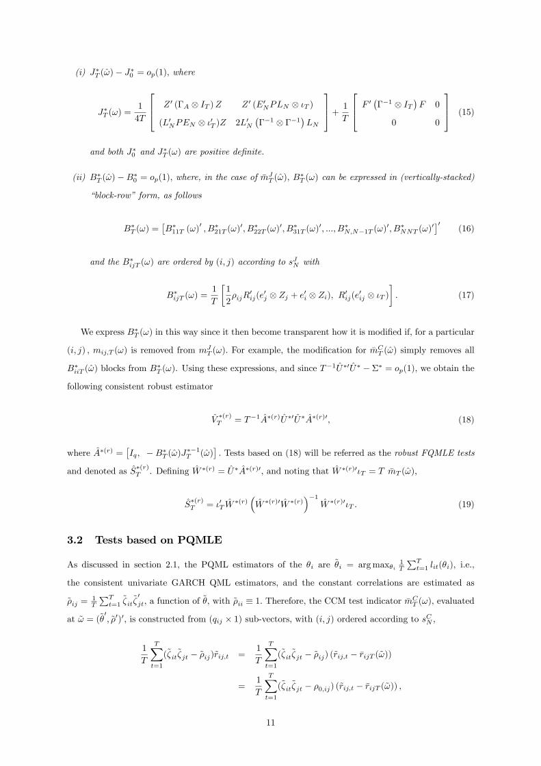
(i) J�T (!)� J�0 = op(1); where

J�T (!) =1

4T

264 Z 0 (�A IT )Z Z 0 (E0NPLN �T )

(L0NPEN �0T )Z 2L0N���1 ��1

�LN

375+ 1

T

264 F 0���1 IT

�F 0

0 0

375 (15)

and both J�0 and J�T (!) are positive de�nite.

(ii) B�T (!)�B�0 = op(1); where, in the case of �mJT (!); B

�T (!) can be expressed in (vertically-stacked)

�block-row� form, as follows

B�T (!) =�B�11T (!)

0; B�21T (!)

0; B�22T (!)0; B�31T (!)

0; :::; B�N;N�1T (!)0; B�NNT (!)

0�0 (16)

and the B�ijT (!) are ordered by (i; j) according to sJN with

B�ijT (!) =1

T

�1

2�ijR

0ij(e

0j Zj + e0i Zi); R0ij(e0ij �T )

�: (17)

We express B�T (!) in this way since it then become transparent how it is modi�ed if, for a particular

(i; j) ; mij;T (!) is removed from mJT (!): For example, the modi�cation for �m

CT (!) simply removes all

B�iiT (!) blocks from B�T (!). Using these expressions, and since T�1U�0U� � �� = op(1); we obtain the

following consistent robust estimator

V�(r)T = T�1A�(r)U�0U�A�(r)0; (18)

where A�(r) =�Iq; �B�T (!)J��1T (!)

�: Tests based on (18) will be referred as the robust FQMLE tests

and denoted as S�(r)T . De�ning W �(r) = U�A�(r)0; and noting that W �(r)0�T = T �mT (!);

S�(r)T = �0T W

�(r)�W �(r)0W �(r)

��1W �(r)0�T : (19)

3.2 Tests based on PQMLE

As discussed in section 2.1, the PQML estimators of the �i are ~�i = argmax�i1T

PTt=1 lit(�i), i.e.,

the consistent univariate GARCH QML estimators; and the constant correlations are estimated as

~�ij =1T

PTt=1

~�it~�0jt; a function of ~�; with ~�ii � 1: Therefore, the CCM test indicator �mC

T (!), evaluated

at ~! = (~�0; ~�0)0; is constructed from (qij � 1) sub-vectors, with (i; j) ordered according to sCN ;

1

T

TXt=1

(~�it~�jt � ~�ij)~rij;t =

1

T

TXt=1

(~�it~�jt � ~�ij) (~rij;t � �rijT (~!))

=1

T

TXt=1

(~�it~�jt � �0;ij) (~rij;t � �rijT (~!)) ;

11

where �rijT (~!) � 1T

PTt=1 ~rij;t: Note that we retain the notation �rijT (!) and �m

CT (!); for example, since it

is consistent with the FQMLE case; however both �rijT (~!) and �mCT (~!) are strictly speaking a function of

~�. This formulation considerably simpli�es the derivation of the limit distribution ofpT �mC

T (~!): In view

of this, and also to maintain simplicity in the construction of the various test statistics, we also employ

�de-meaned� test variables, ~rij;t � �rijT (~!); for the FCM test indicator, �mJT (~!): Thus, the (PQMLE)

FCM and CCM test indicators, respectively, are constructed from the following (qij � 1) sub-vectors,

with (i; j) ordered according to sJN and sCN ; respectively,

1

T

TXt=1

(~�it~�jt � ~�ij) (~rij;t � �rijT (~!)) ; i > j; (20)

1

T

TXt=1

(~�it~�jt � ~�ij) (~rij;t � �rijT (~!)) ; i > j: (21)

However, note that 1T

PTt=1(

~�2

it�1) 6= 0; so that 1T

PTt=1(

~�2

it�1) (~rii;t � �riiT (~!)) 6= 1T

PTt=1(

~�2

it�1)~rij;t:

Thus, in general, we consider the test indicator �mT (~!) =1T

PTt=1mt(~!) where mt(~!); (q � 1) ; is

constructed either from the (qij � 1) sub-vectors (20), for the FCM test indicator �mJT (~!), or (21) for

the CCM test indicator �mCT (~!): In order to treat either test indicator, let �n

1T (!) =

1T

PTt=1 n

1t (!)

constructed in the same way from the (qij � 1) sub-vectors

�n1ij;T (!) =1

T

TXt=1

(�1it �1jt � �0;ij)

�r1ij;t � �ij(!0)

�=

1

T

TXt=1

n1ij;t(!0);

where �ij(!0) = E�r1ij;t

�!=!0

and �ij(!0) <1; by Assumption B4 in the Appendix.

The following justi�es an asymptotically valid �2 test statistic, and procedure, based onpT �mT (~!) :

Proposition 4 Suppose, as described in the Appendix, Assumptions A and B, with B1 and B2, appro-

priately strengthened for the particular choice of rij;t; hold. Then, � = E [u1t (!0)u1t (!0)

0] is �nite,

where u1t (!)0 = (m1

t (!)0; g1t (�)

0) : Furthermore:

(i)pT �u1T (!)

d! N(0;�), where � = E [u1t (!0)u1t (!0)

0] is �nite; and,

(ii) 1T

PTt=1 ut(~!)ut(~!)

0 � � = op(1); for any ~! � !0 = op(1); where ut(!)0 = (mt(!)0; gt(�)

0) :

Remark 2 Again, for the choice of test variables rij;t ="i;t�1"j;t�1phi;t�1

phj;t�1

we will require E j"0itj8 < 1:

In the case of �mJT (!0); for example, �nn � E [n1t (!0)n

1t (!0)

0] is block partitioned in a similar way to

�mm; given in Remark 1, but with r1ij;t��ij(!0) replacing r1ij;t; throughout. The modi�cation is obvious

for �mCT (!0) which simply removes all i = j entries from �nn:

Some specials cases emerge, however, for either �mJT (!0) or �m

CT (!0) :

12

1. If rt is the same vector of test variables employed for all i; j; so that �ij � �; then �nn =

E [�0t�00t �rt(!0)�rt(!0)0] ; where �rt(!0) = rt(!0)� �(!0):

2. If rij;t is a scalar, let �t =�rij;t(!0)� �ij(!0)

; (N �N) and de�ne �rt(!0) to be either

vech(�t); in the case of �mJT (!0); or vecl(�t); in the case of �m

CT (!0):

Then �nn = E [�rt(!0)�rt(!0)0 � �0t�00t] :

Proposition 5 Under the assumptions of Proposition 4, and provided � is positive de�nite,pT �mT (~!)

d�!

N (0; V ) ; where V = A0�A00; A0 =

�Iq;�B0J�10

�; with J0 = �E

h@g1t (�0)@�0

i; B0 = �E

h@n1t (!0)@�0

i; and

Iq is the (q � q) identity matrix:

In the case of �mJT (~!); for example, B0 is block partitioned as B0 = [B0;ij ] ; with blocks B0;ij , stacked

(vertically) for i � j; i changing faster than j; and given by

B0;ij = �E�E

�@n1ij;t(!0)

@�0

����Ft�1�� = �E � �r1ij;t � �ij(!0)� @ ��1it �1jt �@�0

�!=!0

:

The modi�cation is obvious for �mCT (~!) and simply removes all B0;ii blocks from B0:

From Proposition 5, and provided V is positive de�nite, the general form of the test statistic is

~ST = T �mT (~!)0n~VT

o�1�mT (~!); (22)

which has a �2q limiting distribution, under the null, where ~VT = V + op(1):

Note that to obtain the right expression for the asymptotic variance estimator of the test indicator

one has to use vech(~�t~�0t� ~�) or vecl(~�t~�

0t� ~�)), rather than vech(~�t~�

0t) or vecl(~�t~�

0t); in the construction

of �mJT (~!) or �m

CT (~!) as given in (20) and (21), respectively. As earlier, ~V

(o)T and ~V (r)T will denote OPG

and robust variance-covariance matrix estimators, respectively, that we might use for ~VT :

3.2.1 The OPG-PQMLE Test

De�ne the (T � q) matrix M � M(!) to have rows m0t(!) with the understanding that ~M � M (~!) :

Also, let G = (G1; � � � ; GN ) and G�� = (G�1; � � � ; G�N ) ; where the Gi � G(�i) and G�i � G�i (!) are

(T �K +K�) matrices, i = 1; � � � ; N; with rows @lit(�i)@�0i

and@l�t (!)

@�0i; respectively.11 Then, G and G��

are (T � N (K +K�)) matrices with rows g0t(�) = (@l1t(�1)

@�01; :::;

@lNt(�N )

@�0N) and

@l�t (!)

@�0; respectively.

Firstly, and in general, T�1 ~U 0 ~U � � = op(1) by Proposition 4(ii), where ~U =h~M; ~G

i: Secondly, with

the additional normality assumption of �0t � N (0; IN ) ; the speci�cation of the log-likelihood for the

FQML estimation of parameters is correct. Thus, since E [gt(�0)] = 0; the generalized IM equality

11That is, Gi is the matrix having rows univariate GARCH scores; and is a function of �i; while the rows of G�i containsthe FQMLE scores; corresponding to the conditional mean and volatility parameters, �i, only, but is a function of !:

13

implies that

J0 = diag��E

h@2l1it (�0)@�i@�0i

i�= diag

�E

�@l1it (�i0)

@�i

@l1�t (!0)

@�0i

��;

whilst the blocks of B0 are

B0;ij = �E� �

r1ij;t � �ij(!0)� @ ��1it �1jt �

@�0

�!=!0

= E

�n1ij;t(!0)

@l1�t (!0)

@�0

�:

It then follows that, from Lemma 1, 6 and 7, in the Appendix, consistent estimators J0 and B0 can

be obtained as diag�T�1 ~G0i

~G�i

�and T�1 ~M 0 ~G��; respectively. Therefore, under normality, a consistent

estimator for V = A�A0 can be obtained as

~V(o)T = T�1 ~A(o) ~U 0 ~U ~A(o)0; (23)

where the matrix ~A(o) =hIq; � ~M 0 ~G�� � diag

�~G0i~G�i

�i. Again, exploiting the fact that ~G0�T � 0 so

that ~A(o) ~U 0�T � ~M 0�T = T �mT (~!); the test statistic can be expressed in a T � R2u form, but this time

following a regression of �T on ~W (o) = ~U ~A(o)0 :

~S(o)T = �0T ~W

(o)�~W (o)0 ~W (o)

��1~W (o)0�T : (24)

3.2.2 The Robust-PQMLE Test

To construct a robust (to non-normality) test of (22), �rst note that BT (~!) (the robust estimator for B0)

can be obtained using the results of Proposition 3, but replacing rij;t by ~rij;t � �rijT (~!); the demeaned

test variables. Thus, if eRij is the (T � qij) matrix having rows (~rij;t � �rijT (~!))0 ; t = 1; :::; T; then BT (~!)can be expressed in �block form�, but with a typical block now being

BijT (~!) =1

2T~�0ijeRij(e0j ~Zj + e

0i ~Zi); (25)

ordered by (i; j) according to sJN ; or sCN ; for �m

JT (~!); or �m

CT (~!); respectively. In addition, and as a

special case of Proposition 3(i) with N = 1; �ii = 1, �Eh@2l1it (�0)@�i@�0i

ican be consistently estimated by

JiT (~�i) =12T~Z 0i~Zi+

1T~F 0i~Fi; which is positive de�nite, so that JT (~�) = 1

2T~Z 0 ~Z+ 1

T~F 0 ~F ; see, for example,

Halunga and Orme (2009, Lemma 1).

Combining the above two results, we obtain the following expression for the robust consistent variance

estimator

~V(r)T = T�1 ~A(r) ~U 0 ~U ~A(r)0; (26)

where ~A(r) =hIq;�BT (~!)J�1T (~�)

i. Tests based on this estimator will be referred as the robust PQMLE

14

test and will be denoted as ~S(r)T and can be constructed as

~S(r)T = �0T

~W (r)�~W (r)0 ~W (r)

��1~W (r)0�T ; (27)

where ~W (r) = ~U ~A(r)0:

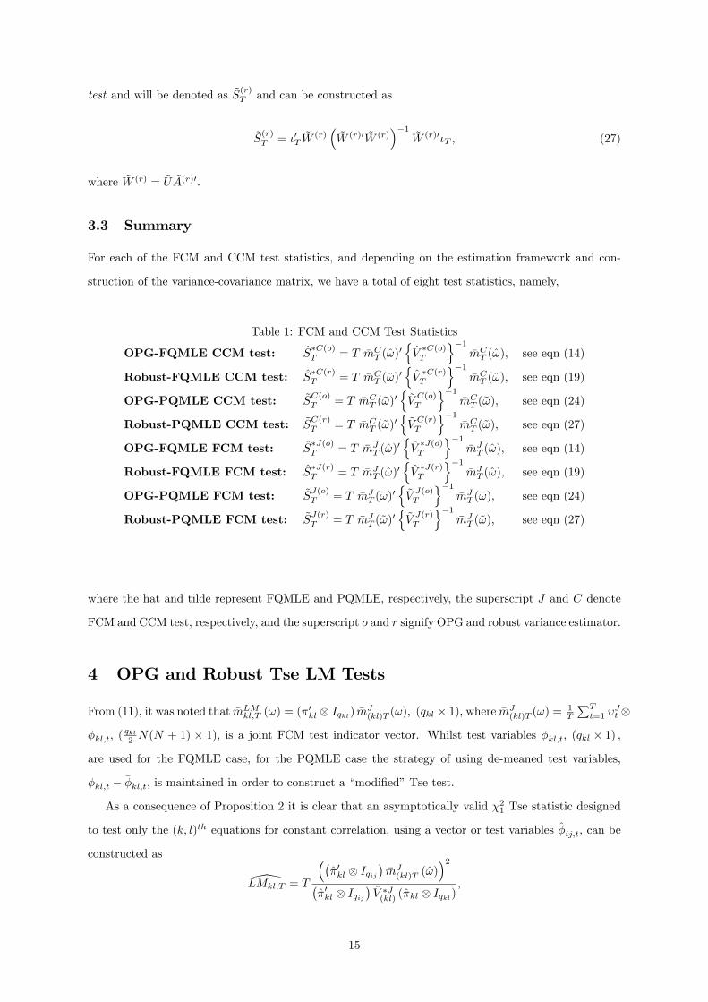
3.3 Summary

For each of the FCM and CCM test statistics, and depending on the estimation framework and con-

struction of the variance-covariance matrix, we have a total of eight test statistics, namely,

Table 1: FCM and CCM Test Statistics

OPG-FQMLE CCM test: S�C(o)T = T �mC

T (!)0nV�C(o)T

o�1�mCT (!); see eqn (14)

Robust-FQMLE CCM test: S�C(r)T = T �mC

T (!)0nV�C(r)T

o�1�mCT (!); see eqn (19)

OPG-PQMLE CCM test: ~SC(o)T = T �mC

T (~!)0n~VC(o)T

o�1�mCT (~!); see eqn (24)

Robust-PQMLE CCM test: ~SC(r)T = T �mC

T (~!)0n~VC(r)T

o�1�mCT (~!); see eqn (27)

OPG-FQMLE FCM test: S�J(o)T = T �mJ

T (!)0nV�J(o)T

o�1�mJT (!); see eqn (14)

Robust-FQMLE FCM test: S�J(r)T = T �mJ

T (!)0nV�J(r)T

o�1�mJT (!); see eqn (19)

OPG-PQMLE FCM test: ~SJ(o)T = T �mJ

T (~!)0n~VJ(o)T

o�1�mJT (~!); see eqn (24)

Robust-PQMLE FCM test: ~SJ(r)T = T �mJ

T (~!)0n~VJ(r)T

o�1�mJT (~!); see eqn (27)

where the hat and tilde represent FQMLE and PQMLE, respectively, the superscript J and C denote

FCM and CCM test, respectively, and the superscript o and r signify OPG and robust variance estimator.

4 OPG and Robust Tse LM Tests

From (11), it was noted that �mLMkl;T (!) = (�

0kl Iqkl) �mJ

(kl)T (!); (qkl � 1), where �mJ(kl)T (!) =

1T

PTt=1 �

Jt

�kl;t; (qkl2 N(N + 1) � 1); is a joint FCM test indicator vector. Whilst test variables �kl;t, (qkl � 1) ;

are used for the FQMLE case, for the PQMLE case the strategy of using de-meaned test variables,

�kl;t � ��kl;t; is maintained in order to construct a �modi�ed�Tse test.

As a consequence of Proposition 2 it is clear that an asymptotically valid �21 Tse statistic designed

to test only the (k; l)th equations for constant correlation, using a vector or test variables �ij;t; can be

constructed as

\LMkl;T = T

���0kl Iqij

��mJ(kl)T (!)

�2��0kl Iqij

�V �J(kl) (�kl Iqkl)

;

15

where either V �J(o)(kl) or V �J(r)(kl) can be employed, with the latter providing robustness to non-normality.

Similar manipulations can be used to construct joint Tse test statistics, but the following (equivalent)

procedures see more straightforward.

Obtain the (T � qC) matrix M �M(!); to have rows mLMt (!)0; where here qC =

Pk>l qkl: That is,

mLMt (!) is formed by stacking the (qkl�1) sub-vectors

�"�kt"

�lt � �kl

��kl;t = (�

0kl Iqkl) (�Jt �kl;t); for

the FQMLE case, or�"�kt"

�lt � �kl

�(�kl;t � ��kl;T ) = (�0kl Iqkl) (�Jt (�kl;t � ��kl;T )); for the PQMLE

case, with (k; l) ordered according to sCN . Then, with this de�nition of M and �mLMT = 1

T

PTt=1m

LMt (!);

the desired test statistic can be constructed as follows (with the �rst being just Tse�s original statistic):

1. The OPG-FQMLE Tse test statistic, dLM�(o)T .

Construct V �LM(o)T using (13) and S�(o)T as in (14) giving an equivalent expression to (6) as

dLM�(o)T = T �mLM

T (!)0nV�LM(o)T

o�1�mLMT (!): (28)

2. The Robust-FQMLE Tse test statistic, dLM�(r)T .

Obtain A�(r)LM =

�Iq; �D�

T (!)J��1T (!)

�, where the matrix D�

T (!) is constructed by vertically

stacking the matrices D�kl;T (!) =

��0kl Iqkl

�B�(kl)T (!); and B

�(kl)T (!) is de�ned in Proposition 3,

but where Rij is replaced R(kl); (T � qkl) ; having rows �0kl;t: Then construct V

�LM(r)T using (18)

and S�LM(r)T as in (19) giving

dLM�(r)T = T �mLM

T (!)0nV�LM(r)T

o�1�mLMT (!): (29)

3. The OPG-PQMLE Tse test statistic, gLM (o)

T .

Construct ~V LM(o)T using (23) and ~S(o)T as in (24) giving

gLM (o)

T = T �mLMT (~!)0

n~VLM(o)T

o�1�mLMT (~!): (30)

4. The Robust-FQMLE Tse test statistic, gLM (r)

T .

Obtain ~A(r)LM =hIq; �DT (~!)J

�1T (~�)

i, where the matrix DT (~!) is constructed by vertically stack-

ing the matrices Dkl;T (~!) = (�0kl Iqkl)B(kl)T (~!); and B(kl)T (~!) is de�ned by (25), but whereeRij is replaced by eR(kl); (T � qkl) ; having rows (~�kl;t � e�kl;T ): Then construct ~V LM(r)T using (26)

and S�LM(r)T as in (27) giving

gLM (r)

T = T �mLMT (~!)0

n~VLM(r)T

o�1�mLMT (~!): (31)

The above derivations also make it transparent how to construct a joint Tse test of a subset of the

16

constant conditional correlations, rather than for all 12N(N � 1): However, if all 12N(N � 1) constant

conditional correlations are to be tested, the derivations in the proof of Proposition 3 (see Shadat and

Orme, 2015) imply that D�T (!) and DT (!) can expressed as

D�T (!) =

1

4T

��0(L0NPEN IT )Z; 2�0(L0N

���1 ��1

�LN �T )

�;

DT (!) =1

4T

���0(L0NPEN IT )Z

�;

where � = diag(�kl);�T2N(N � 1)� qC

�with �kl; (T � qkl) having rows �kl;t; t = 1; :::; T; whilst

�� = diag(��kl);�T2N(N � 1)� qC

�with ��kl; (T � qkl) having rows �kl;t � ��kl;t; t = 1; :::; T:

5 Monte Carlo Evidence

In this section, we present Monte Carlo evidence on the �nite sample behaviour of the 12, for both

FQMLE and PQMLE procedures, for N = 5 equations: the 8 CM tests described in Table 1 and

the 4 Tse �LM�tests described in (28)-(31). The parameter values for the null and alternative Data

Generating Processes (DGPs), where possible, are taken from the existing literature (e.g., Engle and Ng

(1993), Tse (2000), Lundbergh and Teräsvirta (2002), Halunga and Orme (2009)). For each experiment,

two series of 1200 and 700 data realizations were generated with the �rst 200 observations being discarded

to avoid initialization e¤ects, yielding sample sizes of T = 1000 and 500; respectively. Each model is

replicated and estimated, 10; 000 times (to obtain empirical signi�cance levels) and 2000 times (for

robustness to non-normality and power experiments).

In practice, however, there is likely to be considerable uncertainty about the precise form of mis-

speci�cation in the MGARCH CCC structure and so that any �selected� alternative may often be

misspeci�ed, leading to an �incorrect� set of test variables. Thus, the primary purpose of the Monte

Carlo study, here, is to compare the �nite sample performance (empirical signi�cance levels, robustness

and power) of the various tests, each constructed with a common set of test variables, in order to see if

a ranking emerges. Following Tse (2000), the common scalar test variable employed for this purpose for

is rij;t(!) = �i;t�1�j;t�1, although in a demeaned form following PQMLE.12 All simulation experiments

are conducted in GAUSS programming language.

12Although not reported here, simulations were also carried out using �i;t�2�j;t�2 as test variables yielding qualitativelysimilar results. These are available from the authors upon request.

17

5.1 Empirical Signi�cance Levels

We employ AR(1)-CCC-GARCH (1,1) DGP for N = 5 as our null model; viz.,

yit = 'i0 + 'i1yi;t�1+"it; i = 1; � � � ; 5

V ar ("tjFt�1) = Ht ) E�"2itjFt�1

�= hit; "t = H

1=2t (!) �t; �t � N(0; I);

hi;t = �i0 + �i1"2i;t�1 + �i1hi;t�1;

Ht = Dt�Dt; Dt = diag�p

hit

�and

� =��ij; i; j = 1; � � � ; 5 with �ii = 1: (32)

Three experiments are considered E1, E2 and E3 (and the true parameter vectors employed are

given in Table A1 of Shadat and Orme (2015)). These provide models with relatively low (ranging

between 0.20 and 0.37), mixed (ranging between 0.30 and 0.80) and high (ranging between 0.62 and

0.80) correlation structure, respectively, for �. For all three DGPs the same true parameter values for

'0i and �0i = (�i0; �i1; �i1) are used: Note that the experiments considered various degrees of volatility

persistence; however, to save space, we report the results only for �1 + �1 = 0:85 since the results

are qualitatively similar in other cases. Tse (2000) also reports �correlations seem to play a role in

determining the rate of convergence to the nominal size. Models with low correlations are less subject to

over-rejection in small samples....the persistence of the conditional variance does not have much e¤ect�

(p. 115).

Table 2 reports the rejection frequencies when the null of the CCC is true under both Gaussian and

non-Gaussian errors. Apart from investigating the robustness of these tests under non-normality, where

the elements of �0t are iid as t(6); this also o¤ers some evidence on the robustness of the procedure

to violations of the underlying moment assumptions, since for this choice of test variables 8th order

moments are required. The results are reported for a nominal signi�cance level of 5%:

First, under Gaussian errors the original Tse test and other OPG-FQMLE type tests (dLM�(o)T ; S

�C(o)T

and S�J(o)T ) tend to over-reject, for all DGPs, even with T = 1000 (particularly S�J(o)T ). The robust

versions (dLM�(r)T ; S

�C(r)T and S�J(r)T ) are much superior. Interestingly, the OPG-PQMLE tests (gLM (o)

T ;

~SC(o)T and ~SJ(o)T ) perform better than the corresponding OPG-FQMLE tests, although, ~SC(o)T and ~SJ(o)T

are still oversized. However, the empirical signi�cance levels of their robust counterparts, both FQMLE

and PQMLE and including dLM�(r)T and gLM (r)

T ; are reasonably close to the nominal size of 5%, even when

T = 500. Second, in the case of experiments with mixed and high correlation structure (E2 and E3), the

size distortions of OPG-FQMLE tests are relatively higher compared to the low correlation structure

whilst the robust version of these statistics appears to correct this size distortion. On the other hand,

the rejection rates for OPG-PQMLE tests under low correlation structure (E1), in particular for ~SC(o)T

18

and ~SJ(o)T ; are higher than for E2 and E3, although their robust version again corrects this deformity.

The �nding from these experiments that size performance depends on correlation is in line with that of

Tse (2000) where the Monte Carlo experiments were performed for N = 2. Third, with �0t � t(6) all

OPG-FQMLE tests (dLM�(o)T , S�C(o)T and S�J(o)T ) over-reject under all correlation structures, but this

distortion is more severe in high and mixed correlation models. In particular, Tse�s original LM test

(dLM�(o)T ) is very sensitive to departures from normality. The robust-FQMLE version of all tests reduces

the over-rejection rate substantially. The empirical signi�cance levels of the robust versions of Tse�s test

(particularly gLM (r)

T ; as for the case with normal errors) and the robust CCM tests (S�C(r)T and ~SC(r)T ),

in general, are close to nominal level of 5% while the robust FCM tests (S�J(r)T and ~SJ(r)T ) can over or

under-reject.

In summary: the OPG-FCM tests over-reject; all test statistics perform better in low correlation ex-

periments; in general, the robust versions of tests perform better than the OPG; and, in particular,Tse�s

modi�ed robust PQMLE test and the robust CCM PQMLE tests (i.e., gLM (r)

T and ~SC(r)T ) provide quite

reliable signi�cance levels. All robust tests provide signi�cant size correction under non-normal errors.

5.2 Robustness to Misspeci�ed Univariate Volatility

In total,we consider 12 experiments (M1a-M1c, M2a-M2c, M3a-M3c and M4a-M4c), each within the

regression context to investigate, via Monte Carlo simulation, the impact of violations in the univariate

GARCH speci�cation, but when the true correlation structure for �0t is constant with Gaussian error.

The conditional mean parameters and the correlation structures remain the same as those previously em-

ployed, as detailed in Table A1 of Shadat and Orme (2015). For M1, M2 and M3 the univariate volatility

speci�cations of all �ve variables are governed by the GJR, higher order GARCH (i.e., GARCH(2,2))

and the EGARCH models, respectively whereas for M4 all 5 variables are subject to volatility spillover

via an ECCC model. The su¢ x a, b or c associated with these experiments indicate low, mixed and high

correlation structure, respectively, for �. Speci�cally, we employ the following DGPs, for i = 1; :::; 5 :

1. M1 (GJR): hit = ai0 + bi1[j"it�1j � bi2"it�1]2 + bi3hit�1;

with parameter vectors, for each i; (0:005; 0:23; 0:23; 0:70) ; (0:005; 0:30; 0:17; 0:70) ;

(0:005; 0:25; 0:20; 0:70) ; (0:005; 0:28; 0:15; 0:70) ; and (0:005; 0:20; 0:23; 0:70) :

2. M2 (GARCH(2; 2)): hit = ai0 + ai1"2i;t�1 + ai2"

2i;t�2 + bi1hi;t�1 + bi2hi;t�2;

with parameter vectors (0:01; 0:15; 0:05; 0:60; 0:15) ; (0:02; 0:25; 0:05; 0:50; 0:15) ;

(0:15; 0:10; 0:05; 0:70; 0:10) ; (0:05; 0:10; 0:01; 0:70; 0:14) ; and (0:05; 0:20; 0:05; 0:65; 0:05) :

3. M3 (EGARCH): log (hi;t) = ai0 + bi1 log (hi;t�1) + bi2����it�1��� bi3�it�1� ;

with parameter vectors, for each i; (�0:23; 0:90; 0:25; 0:30) ; (�0:20; 0:70; 0:25; 0:20) ;

(0:23; 0:60; 0:25; 0:20) ; (0:20; 0:80; 0:28; 0:15) ; and (�0:30; 0:90; 0:40; 0:15) :

19

4. M4 (ECCC): hit = �i0 + �i1"2i;t�1 + �iihi;t�1 +

Pj 6=i �ijhj;t�1;

with spillover parameter vectors, for each i; (0:01; 0:02; 0:015; 0:03) ; (0:02; 0:06; 0:03; 0:04) ;

(0:03; 0:01; 0:025; 0:015) ; (0:05; 0:03; 0:02; 0:01) ; and (0:002; 0:035; 0:04; 0:02) :

The GARCH parameters for the ECCC model remain the same as AR(1)-CCC-GARCH (1,1) null

model.

Although EGARCH and ECCC models are not formally within GARCH family of alternatives, as

the other DGPs considered here, they represent alternative misspeci�cations of volatility not captured

by GJR and GARCH(2,2). In order to conserve space, we report in Table 3 only the results for

experiments M1 (GJR) and M3 (EGARCH), since the results for M2 (GARCH(2; 2)) and M4 (ECCC)

are qualitatively similar to M1 (GJR), but summarise the main �ndings for all experiments. Full results

are provided in Shadat and Orme (2015). Rejection frequencies are based on both the 5% empirical

and nominal critical values (with the latter in the parenthesis) and with 2000 replications where the

data are generated with normal errors; i.e., in the former case, and for each test procedure, �size-

adjusted� rejection frequencies are reported, calculated using the empirical critical value that delivers

a 5% signi�cance level for the simulations reported in Section 5.1. All robust tests and PQMLE-OPG

tests are relatively insensitive to GJR, GARCH(2,2) and ECCC volatility spillover DGPs and for all

correlation structures; except joint tests ~S�J(r)T and ~S�J(o)T under the GARCH(2; 2) DGP. On the other

hand, the FQMLE-OPG versions, particularly S�J(o)T ; over-reject the null of CCC and the over-rejection

is substantially higher when we use the nominal signi�cance level. Since the FCM test indicator entails

the volatility moment condition, these tests display some power when this moment condition is violated.

In case of the EGARCH alternative, all tests, although to a much lesser extent dLM�(r)T and gLM (r)

T ; are

quite sensitive to the volatility misspec�cations embodied in M3b and M3c (i.e., with mixed and high

correlation). In these cases, all tests over-reject signi�cantly the null of CCC and the rejection rates are

similar for both empirical and nominal signi�cance level. However, for M3a (low correlation), all the

robust tests are less sensitive to univariate conditional variance misspeci�cation.

5.3 Power Results

To examine power, we consider three types of MGARCH models with time varying correlations. The

AR(1) conditional mean speci�cation, and parameters, remain as in (32) but now we examine three

alternative speci�cations for the conditional variance matrix Ht = V ar ("tjFt�1). The �rst is Engle�s

(2002) DCC-GARCH(1,1) model where the dynamic correlation matrix, �t; is given as

�t = (I �t)�1=2t (I �t)�1=2 = diag(t)�1=2t diag(t)�1=2;

t = (1� ~�� ~�)�� + e��t�1� 0t�1 + e�t�1; (33)

20

where ~� and ~� are nonnegative scalar parameters and � + � < 1 and �� is constant (time invariant)

5�5 symmetric positive de�nite matrix, with ones on the diagonal. Secondly, we consider the following

Varying Correlation (VC) model of Tse and Tsui (2002)

�t = (1� a� b) �� + a�t�1 + bt�1; (34)

where a and b are nonnegative scalar parameters, satisfying a + b � 1, and t�1 is the 5 � 5 sample

correlation matrix of��t�1; � � � ; �t�5

and its (i; j)th element is given by:

ij;t�1 =

P5m=1 �i;t�m�j;t�m�P5

m=1 �2i;t�m

�1=2 �P5m=1 �

2j;t�m

�1=2 :Finally we consider the BEKK model of Engle and Kroner (1995),

Ht = CB +A0B

�"t�1"

0t�1�AB +B

0BHt�1BB : (35)

In the following experiments the diagonal BEKK (DBEKK) model is employed where the parameter

matrices AB and BB are 5� 5 diagonal matrices.

Seven experiments are considered: P1, P2 and P3 follow the DCC DGP (33), P4 and P5 follow VC

DGP (34) and remaining two, P6 and P7, follow the DBEKK DGP (35). In all cases, the individual

volatility speci�cation for all variables is retained from earlier size experiment, whilst for the DCC and

VC DGPs the constant �� matrix is set to the previously de�ned mixed correlation structure (see Section

5.1). The remaining true parameter vectors are given in Shadat and Orme (2015).

Again, to conserve space, we only report detailed results for the DCC DGP, P1-P3, but summarise

the main �ndings for all experiments. Full results are provided in Shadat and Orme (2015). Table 4

presents the size-adjusted power (and nominal) results with 2000 replications, based on a 5% empirical

(respectively nominal) critical values and the data are generated assuming normality. As a measure

of the variability of the conditional correlation coe¢ cients, in experiments P1 to P7, we also report in

Shadat and Orme (2015) the average, maximum and minimum values of the true conditional correlation

coe¢ cients across the 2000 Monte Carlo replications of each T = 1000 sample.

When the true DGP is the DCC, P3 has the largest variability in correlations followed by P2 and

P1; i.e., variability increases as e� increases and e� decreases. In general, the FCM tests are found to

have higher power in all three DCC experiments. However, as the variability in correlation decreases

power decreases. The Tse and CCM tests also exhibit good power properties: even with T = 500, and

all tests have high power especially for the P2 and P3 DGPs. In case of the VC and BEKK DGPs

the conclusions are quite similar. P5 and P7 have larger variability in correlations than P4 and P6,

respectively, and the performance of all the tests re�ect that.

21

Although the OPG-FQMLE tests exhibit higher nominal power, in terms of the size-adjusted power

the robust-FQMLE and robust-PQMLE versions of these do not cost much in this respect, especially in

view of the lack of robustness to non-normality of the former.

6 Concluding Remarks

In this paper, we have considered a set of asymptotically valid Conditional Moment (CM) tests designed

to assess a constant correlation assumption and/or the individual GARCH speci�cations in a MGARCH

model. In particular, we consider both the FQMLE and PQMLE framework for the CCC model, noting

that there is very little in the existing literature for the latter case. These tests are very easy to

implement and include OPG versions - a popular variant in the applied literature but whose asymptotic

validity is based on an assumption of normality - and non-normality robust versions. In so doing, we

also provide a simple expression for a consistent estimator for the hessian in the FQMLE framework.

Our approach accommodates Tse�s (2000) LM test, originally proposed as a OPG-FQMLE type test,

so that we are able to provide the PQMLE and robust version of this popular test, as well.

We examine the �nite sample performance of these asymptotically valid tests via a small Monte Carlo

study, with N = 5 time series rather than the usual bivariate model, which indicates that, in general, all

tests have empirical signi�cance levels that are reasonably close to the nominal value of 5% but that the

robust versions are slightly preferred, even under normality. It also appears that, under the null, whilst

the degree of univariate volatility persistence has little detrimental e¤ect, low correlation is associated

with better empirical signi�cance levels. As anticipated, though, under non-normality (but otherwise

correct model speci�cation), the robust version of any particular test exhibits far superior �nite sample

behaviour relative to its OPG variant with all OPG-FQMLE tests over-rejecting. Interestingly, the

OPG-PQMLE based tests exhibit more robustness than the corresponding OPG-FQMLE tests. When

the GARCH error assumption of the null model is violated by introducing a volatility spillover e¤ect

the Monte Carlo evidence suggests that there is little impact on empirical signi�cance levels. When

there is no volatility spillover but simply one GARCH equation misspeci�ed, and a high correlation

structure, all tests experience increased empirical rejection rates. This is especially true in the case of

the EGARCH alternative with the FCM tests (which test jointly the individual volatility speci�cations

and the CCC assumption) being most sensitive, as one might expect. However, an important result that

emerges for applied workers is that although Tse�s original FQMLE test is also a¤ected, as it employs

all the indicators of the FCM tests, the modi�ed and robust PQMLE version developed in this paper

appears to be much less sensitive to univariate volatility misspeci�cation.

Turning to power, which depends on the variability of the true correlation parameter, it is found that

Tse�s test and FCM tests have good power, with the former being slightly more powerful, even in models

22

with less dispersed correlations. Furthermore, for both the Tse and FCM tests, there is comparability

across both FQMLE and PQMLE frameworks. Disappointingly, the CCM tests (designed only to assess

the CCC assumption) show comparatively lower power - particularly in models with less dispersed

correlations.

In conclusion, when testing the assumption CCC there appears to be little di¤erence between the

FQMLE and PQMLE approach and, in both cases, non-normality robust versions of the tests exhibit

reasonable �nite sample behaviour under the null. However, within the panoply of procedures considered

and with a common choice of test variable, the robust version of the Tse�s test, both for the FQMLE

and PQMLE, has very good empirical signi�cance level and power properties and would appear to

recommend itself, although it is not entirely robust, in general, to misspeci�ed volatility.

Appendix: Assumptions and Proofs

Unless stated otherwise all de�nitions are as in the main text, the Euclidean norm of a matrix A is

denoted kAk =ptr(A0A); and the properties of hit and h1it ; as discussed in Halunga and Orme (2009,

Appendix), are exploited. Whilst only brie�y discussed in this Appendix, exhaustive proofs of all results

are provided (freely on-line) in Shadat and Orme (2015).

Write w0it'i = 'i1(L)yit + d0it'i2 and hit = �i0 + Ai(L)"2it + Bi(L)hit = ait + Bi(L)hit; where

ait = �i0 + Ai(L)"2it = �i0 +

Pqk=1 �ik"

2i;t�k: As employed, for example, in Ling and McAleer (2003),

Berkes, Horváth and Kokoszka (2003) and Halunga and Orme (2009), the following assumptions ensure

the identi�ability, stationarity and ergodicity of the above process.13

Assumptions A

A1 The parameter space, �; is compact and !0 lies in the interior of �:

A2 The elements of d0it are strictly stationary and ergodic and all roots of 1� 'i1(L) = 1� 'i11L��i12L

2 � :::� �i1pLp = 0; �i1p 6= 0; p known, lie outside the unit circle, for all i.

A3 (i) All the roots of 1�Ai(z)�Bi (z) = 0 lie outside the unit circle.(ii) The parameter space is constrained such that 0 < � � mini;l f�ilg � maxi;l f�ilg < �;

l = 1; :::; p+ q + 1; where � and � are independent of !.

(iii) The polynomials Ai(z) and 1�Bi(z) are coprimes:

Ling and McAleer (2003), for example, required that E�"60t�< 1 to ensure asymptotic normality

of the QML estimator in the ARMA-GARCH model. This is also su¢ cient here, but with additional

moment restrictions on dit and the test variables rij;t; as follows:

Assumptions B

B1 E j"0itj6 <1 for all i; t:

B2 Ehkditk6

i<1; for all i; t:

B3PT

t=1E sup! j"it"jtjl r1ij;t � rij;t = O(1); at most, for all i; j; t and l = 0; 1:

B4 E sup! j"it"jtjl r1ij;t 2 <1 for all i; j; t; and l = 0; 1; 2:

13As discussed by Nelson and Cao (1992), although su¢ cient, A3(ii) is not necessary to ensure non-negative conditionalvariances.

23

B5 E sup! j"it"jtjl @r1ij;t@!

<1; at most, for all i; j; t and l = 0; 1:Remark 3 (i) A1, A2, B1 and B2 imply that E sup! j"itj

6< 1 uniformly in i; t; where "it = "0it �

w0it ('i � 'i0) ; and also that E jyitj6<1 for all i; t; so that E

hkwitk6

i<1; for all i; t. (ii) Extensions

of Halunga and Orme (2009, Proposition 4) imply that B3-B5 also hold with zit replacing rij;t. (iii)

Assumptions A, B1 and B2 are su¢ cient to establish the consistency and asymptotic normality of both

the FQMLE and PQMLE, and the consistency of variance estimators based on an OPG formulation.

(iv) Depending on the choice of rij;t; B1 and B2 may need strengthening, in view of the demands of

B4, in order to establish both the asymptotic normality of our test indicators and the consistency of the

various asymptotic variance estimators employed in constructing the �2 test statistics.

Case 1 For rij;t ="i;t�1"j;t�1phi;t�1

phj;t�1

, B3-B5 hold provided B1 and B2 are replaced by

B1* E j"0itj8 <1 for all i; t:

B2* Ehkditk8

i<1 for all i; t:

Proof. This follows from similar arguments to those employed by Halunga and Orme (2009).

We �rst establish some preliminary results that will be of use later.

Lemma 1 Let fxtgTt=1 be a sample of stationary ergodic random variables, such that the random vector

functions wt(!) � w(xt;!) and zt(!) � z(xt;!); t = 1; :::; T; satisfy 1pT

PTt=1 sup! kwt(!)� zt(!)k =

op(1):

(i) Then

sup!

1pT

TXt=1

wt(!)�1pT

TXt=1

zt(!)

= op(1):

(ii) If E sup! kw(x;!)k2<1; where ! 2 a compact set, then (in addition)

sup!

1TTXt=1

wt(!)wt(!)0 � 1

T

TXt=1

zt(!)zt(!)0

= op(1):

Proof. Follows from the properties of sup, the triangle inequality and Cauchy-Schwartz.

Remark 4 Under the conditions of Lemma 1, E sup! kw(x;!)k2< 1 so that E [wt(!0)wt(!0)0] is

�nite. Then, by a Uniform Law of Large Numbers and the triangle inequality, for any ! � !0 = op(1);1T

PTt=1 zt(!)zt(!)

0 � E [wt(!0)wt(!0)0] = op(1):

Proposition 6 Under Assumptions A and B1, B2:

(i) E sup! kg1�t (!)k2 <1;

(ii) 1pT

PTt=1 sup! kg1�

t (!)� g�t (!)k = op(1):

In addition, and adding B3 and B4:

(iii) E sup! km1t (!)k

2<1;

(iv)1pT

PTt=1 sup! km1

t (!)�mt(!)k = op(1):

24

Proof.(i) The scores are

@l1�t (!)=@�i = f1it "

1�it +

1

2(�1it "

1�it � 1) z1it ; (36)

@l1�t (!)=@�ij = "1�

it "1�jt � �ij ; i > j: (37)

The result follows from the arguments employed by Halunga and Orme (2009).

(ii) From (36),

1pT

TXt=1

sup!

@l1�t (!)@�i

� @l�t (!)@�i

� 1pT

TXt=1

sup!kf1it "1�

it � fit"�itk

+1

2

1pT

TXt=1

sup!k(�1it "1�

it � 1) z1it � (�it"�it � 1) zitk

= R1T +R2T :

Employing similar analysis to that of Halunga and Orme (2009), it can be shown that E [RjT ] = o(1); j =

1; 2; and the result follows by Markov�s Inequality. The result that 1pT

PTt=1 sup!

���@l1�t (!)@�ij

� @l�t (!)@�ij

��� =op(1) follows in a similar fashion.

(iii) E sup! km1t (!)k

2<1 provided E sup!

(�1it �1jt � �ij)r1ij;t 2 <1; for i; j; which it is by B4.(iv) Similar to (ii),

1pT

PTt=1E sup! km1

t (!)�mt(!k = o(1); and the result follows by Markov�s

inequality.

Proof of Proposition 1: �� is �nite by Proposition 6(i) and (iii). As in Ling and McAleer (2003,Lemma 5.2), (i) follows from a Martingale Central Limit Theorem. Part (ii), follows from Proposition

6 and Remark 4.�

Proof of Proposition 2: By Proposition 1,pT �mT (!) =

pT �m1

T (!) + op(1); so we work withpT �m1

T (!) whose limit distribution can be established more easily. Following Ling and McAleer (2003),

as adapted by Halunga and Orme (2009), it is straightforward to show that �rstly, !� !0 = op(1) and,

secondly, that E sup! @2l1�

t (!)@!@!0

< 1: Thus a Uniform of Large Numbers yields T�1PT

t=1@2l1�

t (~!)@!@!0 +

J�0 = op(1); for all ~! � !0 = op(1); and J�0 = �Eh@2l1�

t (!)@!!0

i!=!0

is �nite and positive de�nite by

Proposition 3, below. Furthermore, by Proposition 6,1pT

PTt=1 g

1�t (!) = op(1); so that a �rst order

asymptotic expansion of this quantity about !0 yieldspT (! � !0) = J��10

1pT

PTt=1 g

1�t (!0) + op(1);

which is Op(1). Next, it can be shown that E sup! @m1

t (!)@!

< 1, for general choice of r1ij;t; given

Assumptions B, so that @ �m1T (!T )@!0

p! �B�0 = Eh@m1

t (!0)@!0

i; for any sequence !T = !0+op(1); see Shadat

and Orme (2015). Thus a �rst order asymptotic expansion of �m1T (!) about !0 yields

pT �m1

T (!) =pT �m1

T (!0)�B�0pT (! � !0) + op (1)

= A�01pT

TXt=1

u1�t (!0) + op(1);

and, from Proposition 1,pT �mT (!)

d�! N(0; V �). �

Proof of Proposition 3(i) De�ne z1t = diag (z10

it ), the (N �N (K +K�)) block diagonal matrix with z10it , (1�K +K�) ;

forming the diagonal blocks, and f1t = diag (f10it ) ; (N �N (K +K�)) ; constructed in the same way:

25

Exploiting the properties of EN and LN ; J�0 can be obtained by direct di¤erentiation of the scores (36)

and (37) which can themselves can be expressed as

@l1�t (!)=@� = 1

4z10t (E0NP (�

1t �1t )� 2�N ) + f10

t ��1�1t ;

@l1�t (!)=@� = 1

2L0N

���1 ��1

�vec

��1t �

10t � �

�:

Now,

@(�1t �1t )=@�0 = @ vec��1t �

10t

�=@�0 = (�1t IN + IN �1t ) @�1t =@�0;

@�1t =@�0 = �f1t � 1

2

��10t IN

�ENz

1t ;

and, since E [�1t jFt�1]!=!0 = 0, E [IN �1t jFt�1]!=!0 = 0, E [E

0NP (�

1t �1t )� 2�N jFt�1]!=!0 = 0;

and E0NEN + E0N

���1 �

�EN = �A; we obtain

E�@2l1�

t (!0)=@�@�0jFt�1

�= � 1

4 [z10t �Az

1t ]

0!=!0

��f10t ��1f1t

�!=!0

:

Similarly,

E�@2l1�

t (!0)=@�@�0jFt�1

�= � 1

4 [L0NPENz

1t ]!=!0 ;

E�@2l1�

t (!0)=@�@�0jFt�1

�= � 1

2L0N

���1 ��1

�LN ;

since @ vec(�)=@�0 = LN : These then yield,

J�0 =14E

("z10t �Az

1t z10

t E0NPLN

L0NPENz1t 2L0N

���1 ��1

�LN

#)!=!0

+ E

"f10t ��1f1t 0

0 0

#!=!0

which is positive de�nite; see Shadat and Orme (2015)14 . This expression for J�0 concurs with Nakatani

and Teräsvirta (2009, p.151), but allowing for regression parameters, 'i.

From J�0 we obtain J�T (!) by: hit replacing h1it , ! replacing !0 and 1T

PTt=1 replacing �expecta-

tion�, throughout; and, noting that L0NPENPT

t=1 zt = L0NPEN (IN �0T )Z = (L0NPEN �0T )Z,PTt=1 zt

0�Azt = Z 0 (�A IT )Z andPT

t=1 f0t��1ft = F 0

���1 IT

�F: Thus J�T (!) is positive de�-

nite provided Z has full rank of N(K+K�). Consistency of J�T (!) follows from, e.g., Ling and McAleer

(2003) and is veri�ed in Orme and Shadat (2015).

(ii) B�0 = �E [@m1t (!0)=@!

0] ; is obtained as follows. First, f1it ; z1it , r

1ij;t and

@r1ij;t@�0k

and@r1ij;t@� are

all Ft�1 measurable. Second, E��120jt jFt�1

�= 1; E

��10jtf

10itjFt�1

�= E [�10itf

10itjFt�1] = 0; and

E��10it�

10jtjFt�1

�= �0ij : Then, from previous derivations we obtain

E�@m1

ij;t(!0)=@�0� = �1

2Eh�ijr

1ij;t

�ej z1jt + ei z1it

�0i!=!0

;

E�@m1

ij;t(!0)=@�0� = �E �r1ij;te0ij�!=!0 :

14Ling and McAleer (2003) require that �A � IN is positive semi-de�nite. But this seems to arise from an error intheir expression for the expected hessian (Ling and McAleer 2003, p.289). Speci�cally, the error arsises from writing(@ vec(�)=@�0)0

���1 ��1

�@ vec(�)=@�0as P 0P where, here, P = (IN ��1)@ vec(�)=@�0:

26

The corresponding partitions of B�T (!) are thus

B�ijT (!) =1

T

TXt=1

�1

2�ijrij;t

�e0j z0jt + e0i z0it

�; rij;te

0ij

�=

�12�ijR

0ij(e

0j Zj + e0i Zi); R0ij(e0ij �T )

�:

To establish consistency of B�T (!); de�ne q1ij;t =

�1; z10

it ; r10ij;t

�0; for any pair i > j, and correspondingly

qij;t =�1; z0it; r

0ij;t

�0: Then it is immediate from B4 and Remark 3(ii) that: (i) E sup!

q1ij;t 2 <1; and,(ii) 1p

T

PTt=1 sup!

q1ij;t � qij;t = op(1). The result then follows by Lemma 1.�

Proposition 7 De�ne �mT (!) = T�1PT

t=1mt(!) constructed from the (qij � 1) sub-vectors �mij;T (!) =1T

PTt=1(�it�jt � �ij) (rij;t � �rijT (!)) and �n1T (!) = T�1

PTt=1 n

1t (!) constructed from the (qij � 1)

sub-vectors �n1ij;T (!) =1T

PTt=1(�

1it �

1jt � �0;ij)

�r1ij;t � �ij(!0)

�; where �ij(!0) = E

�r1ij;t

�!=!0

and �ij(!) <1; by B4. Under Assumptions A and B1, B2:(i) E sup� kg1t (�)k

2<1;

(ii)1pT

PTt=1 sup� kg1t (�)� gt(�)k = op(1):

In addition, and adding B3 and B4:

(iii) E sup! kn1t (!)k2<1;

(iv)1pT

PTt=1 kn1t (~!)�mt(~!)k = op(1); where ~! is the PQML estimator described in Section 2.1.

Proof. It is readily shown that (i) and (ii) hold, and (iii) follows from Proposition 6(iii). For

(iv), let �m1ij;t(!) = (�1it �

1jt � �0;ij)r

1ij;t � (�it�jt � �0;ij)rij;t and write

pT��n1ij;T (~!)� �mij;T (~!)

�=

1pT

PTt=1 aij;t(~!); where

aij;t(!) = �m1ij;t(!) + (�it�jt � �0;ij)

��rijT (!)� �ij(!0)

����1it �

1jt � �it�jt

��ij(!0):

Similar to previous arguments, it can be shown that1pT

PTt=1 kaij;t(~!)k = op(1); so that

pT k�n1T (~!)� �mT (~!)k =

op(1):

Proof of Proposition 4: � is �nite by Proposition Proposition 7(i) and (iii). As in Ling and McAleer(2003, Lemma 5.2), (i) follows from a Martingale Central Limit Theorem. Part (ii), follows from

Proposition 7 and Remark 4.�

Proof of Proposition 5: By Proposition 7,pT �mT (~!) =

pT �n1T (~!) + op(1); and we work withp

T �n1T (~!). From the consistency and asymptotic normality of ~�;pT (~�� �0) = J�10

pT �g1T (�0) + op(1);

wherepT �g1T (�) =

pT �gT (�) + op(1), by Proposition 7: Similar to proof of Proposition 2, it is readily

shown that E sup! @n1t (!)@�

< 1: Thus, a Uniform Law of Large numbers and �rst order asymptotic

expansion ofpT �n1T (~!) about !0; yields

pT �n1T (~!) = A0

pT �u1T (!0) + op(1); and the result follows

from Proposition 4. �

References

Andreou, E., Ghysels, E. (2003). Tests for breaks in the conditional co-movements of asset returns.

Statistica Sinica 13(4):1045�1074.

27

Aslanidis, N., Osborn, D., Sensier, M. (2008). Co-movements between US and UK stock prices: the

roles of macroeconomic information and time-varying conditional correlations. Manchester Economics

Discussion Paper Series 0805.

Bera, A. K., Kim, S. (2002). Testing constancy of correlation and other speci�cations of the BGARCH

model with an application to international equity returns. Journal of Empirical Finance 9(2):171�195.

Bera, A. K., McKenzie, C. R. (1986). Alternative forms and properties of the score test. Journal of

Applied Statististics 13(1):13�25.

Berkes, I., Horváth, L., Kokoszka, P. (2003). GARCH processes: structure and estimation. Bernoulli

9(2): 201-227.

Billo, M., Caporin, M., Gobbo, M. (2006). Flexible dynamic conditional correlation multivariate GARCH

models for asset allocation. Applied Financial Economics Letters 2(2):123�130.

Bollerslev, T. (1990). Modeling the coherence in short-run nominal exchange rates: a multivariate

generalized ARCH model. Review of Economics and Statistics 72(3):498�505.

Chesher, A., Spady, R. (1991). Asymptotic expansions of the information matrix test statistics. Econo-

metrica 59(3):787�816.

Davidson, R., MacKinnon, J. G. (1983). Small sample properties of alternative forms of the Lagrange

multiplier test. Economics Letters 12(3-4):269�275.

Engle, R. F. (2002). Dynamic conditional correlation: a simple class of multivariate GARCH models.

Journal of Business and Economic Statistics 20(3):339�350.

Engle, R. F., Kroner, F. K. (1995). Multivariate simultaneous generalized ARCH. Econometric Theory

11(1):122�150.

Engle, R. F., Ng, V. K. (1993). Measuring and testing the impact of news on volatility. Journal of

Finance 48(5):1749�1778.

Engle, R. F., Sheppard, K. (2008). Evaluating the speci�cation of covariance models for large portfolios.

Working Paper, Department of Economics, University of Oxford.

Francq, C., Zakoian, J-M. (2004). Maximum likelihood estimation of pure GARCH and ARMA-GARCH

processes. Bernoulli 10(4): 605�637.

Hafner, C. M., van Dijk, D., Franses, P.H. (2005). Semi-parametric modelling of correlation dynamics.

In: Advances in Econometrics, vol. 20/A. Amsterdam: Elsevier Sciences, pp. 59�103.

Hafner, C. M., Herwartz, H. (2008). Analytical quasi maximum likelihood inference in multivariate

volatility models. Metrika 67(2):219-239.

Halunga. A. and Orme, C. D. (2009). First-order asymptotic theory for misspeci�cation tests of GARCH

models. Econometric Theory 25(2):364-410.

Kroner, K. F., Claessens, S. (1991). Optimal Dynamic Hedging Portfolios and the Currency Composition

of External Debt. Journal of International Money and Finance 10(1):131-148.

Kroner, K. F., Sultan, J. (1991). Exchange rate volatility and time varying hedge ratios. In: Paci�c-

Basin Capital Market Research, 2. Amsterdam: North-Holland, pp.397-412.

28

Kroner, K. F., Sultan, J. (1993). Time varying distribution and dynamic hedging with foreign currency

futures. Journal of Financial and Quantitative Analysis 28(4):535-551.

Lee, J. (2006). The comovement between output and prices: Evidence from a dynamic conditional

correlation GARCH model. Economics Letters 91(1):110-116.

Lien, D., Tse, Y. K. (1998). Hedging Time-Varying Downside Risk. Journal of Futures Markets

18(2):705-722.

Lien, D., Tse, Y. K., Tsui, A. K. C. (2002). Evaluating the hedging performance of the constant-

correlation GARCH model. Applied Financial Economics. 12(11):791-798.

Ling, S., McAleer, M. (2003). Asymptotic theory for a vector ARMA-GARCH model. Econometric

Theory 19(2):280�310.

Longin, F., Solnik, B. (1995). Is the correlation in international equity returns constant: 1960�1990?

Journal of International Money and Finance 14(1):3�26.

Lundbergh, S., Teräsvirta, T. (2002). Evaluating GARCH models. Journal of Econometrics 110(2):417�

435.

Magnus, J., Neudecker,H. (1986). Symmetry, 0-1 matrices and Jacobians: a review. Econometric Theory

2:157�190.

Nakatani, T. and Teräsvirta, T. (2009). Testing for volatility interactions in the Constant Conditional

Correlation GARCH model. Econometrics Journal 12(1):147-163.

Nelson, D.B., Cao, C.Q. (1992). Inequality constraints in the univariate GARCH model. Journal of

Business and Economic Statistics, 10(2):229-235.

Newey, W. K. (1985). Maximum likelihood speci�cation testing and conditional moment tests. Econo-

metrica 53(5):1047�1070.

Orme, C. (1990). The small-sample performance of the information-matrix test. Journal of Econometrics

46(3):309-331,

Park, T., Switzer, L. (1995). Time-varying distribution and the optimal hedge ratios for stock index

futures. Applied Financial Economics 5(3):131�137.

Silvennoinen, A., Teräsvirta, T. (2009). Multivariate GARCH models. In: Handbook of Financial Time

Series, Springer, pp. 201-229.

Tse, Y. K. (2000). A test for constant correlations in a multivariate GARCH model. Journal of Econo-

metrics 98 (1):107�127.

Tse, Y. K., Tsui, A. K. C. (2002). A multivariate GARCH model with time-varying correlations. Journal

of Business and Economic Statistics, 20(3):351-362.

Shadat, W., Orme, C. (2015). Robust Parametric Tests of Constant Conditional Correlation in a

MGARCH model: Full Monte Carlo and Detailed Proofs. University of Manchester, EScholarID:264022

(available at https://www.escholar.manchester.ac.uk/uk-ac-man-scw:264022).

Wooldridge, J. (1990). A uni�ed approach to robust, regression-based speci�cation tests. Econometric

Theory 6(1):17-43.

29

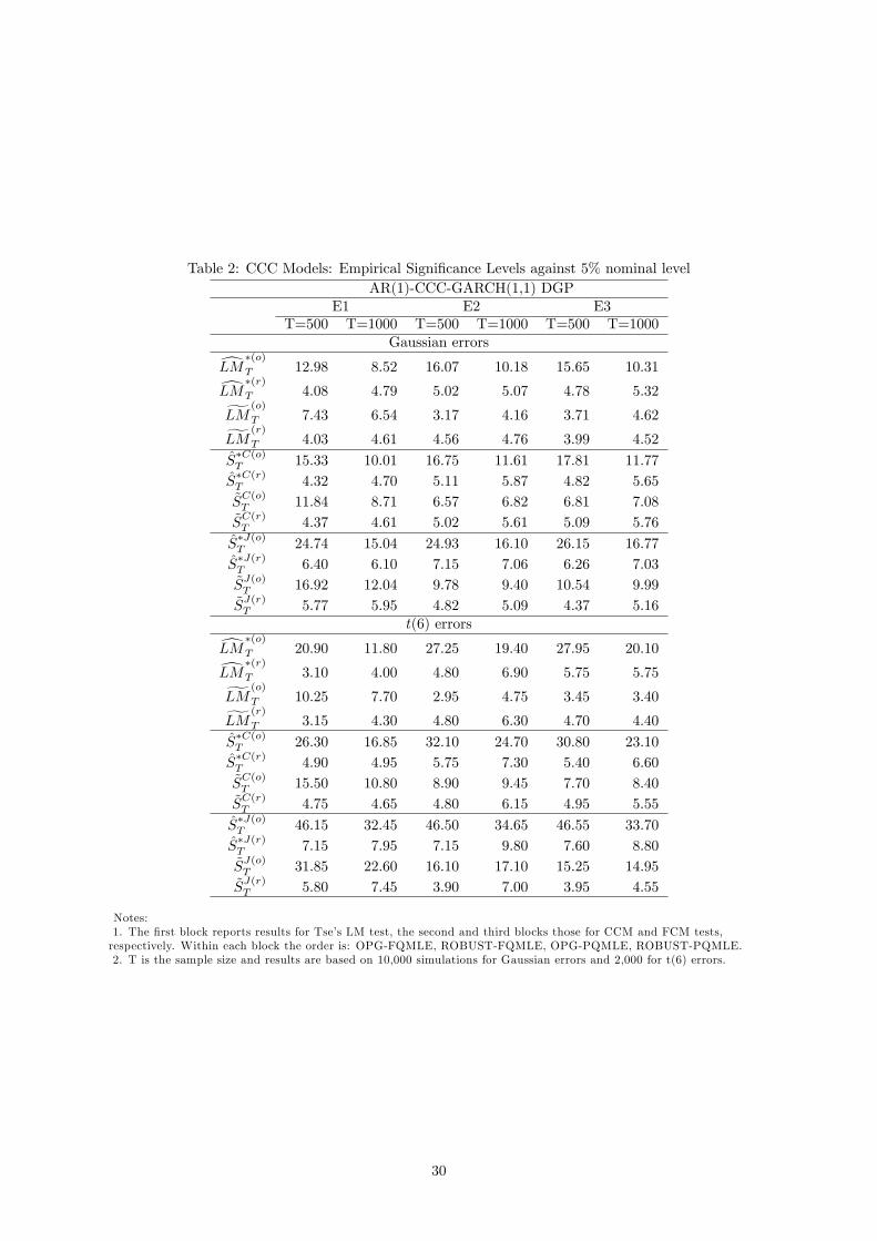
Table 2: CCC Models: Empirical Signi�cance Levels against 5% nominal levelAR(1)-CCC-GARCH(1,1) DGP

E1 E2 E3T=500 T=1000 T=500 T=1000 T=500 T=1000

Gaussian errorsdLM�(o)T 12.98 8.52 16.07 10.18 15.65 10.31dLM�(r)T 4.08 4.79 5.02 5.07 4.78 5.32gLM (o)

T 7.43 6.54 3.17 4.16 3.71 4.62gLM (r)

T 4.03 4.61 4.56 4.76 3.99 4.52

S�C(o)T 15.33 10.01 16.75 11.61 17.81 11.77S�C(r)T 4.32 4.70 5.11 5.87 4.82 5.65~SC(o)T 11.84 8.71 6.57 6.82 6.81 7.08~SC(r)T 4.37 4.61 5.02 5.61 5.09 5.76

S�J(o)T 24.74 15.04 24.93 16.10 26.15 16.77S�J(r)T 6.40 6.10 7.15 7.06 6.26 7.03~SJ(o)T 16.92 12.04 9.78 9.40 10.54 9.99~SJ(r)T 5.77 5.95 4.82 5.09 4.37 5.16

t(6) errorsdLM�(o)T 20.90 11.80 27.25 19.40 27.95 20.10dLM�(r)T 3.10 4.00 4.80 6.90 5.75 5.75gLM (o)

T 10.25 7.70 2.95 4.75 3.45 3.40gLM (r)

T 3.15 4.30 4.80 6.30 4.70 4.40

S�C(o)T 26.30 16.85 32.10 24.70 30.80 23.10S�C(r)T 4.90 4.95 5.75 7.30 5.40 6.60~SC(o)T 15.50 10.80 8.90 9.45 7.70 8.40~SC(r)T 4.75 4.65 4.80 6.15 4.95 5.55

S�J(o)T 46.15 32.45 46.50 34.65 46.55 33.70S�J(r)T 7.15 7.95 7.15 9.80 7.60 8.80~SJ(o)T 31.85 22.60 16.10 17.10 15.25 14.95~SJ(r)T 5.80 7.45 3.90 7.00 3.95 4.55

Notes:1. The �rst block reports results for Tse�s LM test, the second and third blocks those for CCM and FCM tests,respectively. Within each block the order is: OPG-FQMLE, ROBUST-FQMLE, OPG-PQMLE, ROBUST-PQMLE.2. T is the sample size and results are based on 10,000 simulations for Gaussian errors and 2,000 for t(6) errors.

30

Table3:Univariatevolatilitymisspeci�cationI:EmpiricalRejectionRatesagainst5%

empirical(nominal)criticalvalue

AR(1)-GJR-CCCDGP

AR(1)-EGARCH-CCCDGP

M1a

M1b

M1c

M3a

M3b

M3c

T=500

T=1000

T=500

T=1000

T=500

T=1000

T=500

T=1000

T=500

T=1000

T=500

T=1000

d LM�(o)

T5:70

5:25

6:05

5:20

5:90

4:70

19:45

12:05

77:35

86:30

78:30

86:00

(15:25)

(9:45)

(16:70)

(11:20)

(15:10)

(10:90)

(34:50)

(16:70)

(88:90)

(90:90)

(88:50)

(90:50)

d LM�(r)

T5:85

4:80

5:30

4:60

4:95

4:55

4:80

4:00

7:65

14:30

11:70

18:00

(4:85)

(4:55)

(4:70)

(4:70)

(4:75)

(5:05)

(4:10)

(3:70)

(7:75)

(14:50)

(11:25)

(20:00)

g LM(o)

T5:50

5:00

5:80

5:20

5:25

4:65

14:65

9:30

27:15

45:50

30:30

56:00

(8:15)

(6:60)

(4:60)

(4:15)

(4:10)

(4:50)

(18:80)

(11:30)

(22:20)

(42:15)

(26:30)

(51:00)

g LM(r)

T5:60

4:80

6:60

5:75

5:90

5:20

5:25

4:25

7:05

12:95

8:00

15:00

(4:75)

(4:40)

(5:60)

(5:40)

(4:85)

(4:85)

(4:20)

(3:85)

(6:60)

(12:40)

(6:85)

(13:00)

S�C(o)

T4:65

5:00

5:00

5:30

4:95

5:15

29:50

12:60

83:65

97:20

89:95

97:70

(15:90)

(9:75)

(18:00)

(11:55)

(18:70)

(12:45)

(48:70)

(18:95)

(92:35)

(98:40)

(96:15)

(99:10)

S�C(r)

T4:90

4:25

5:15

4:90

5:00

5:20

7:40

5:00

30:90

61:80

37:15

71:50

(4:25)

(4:10)

(5:55)

(6:00)

(4:90)

(5:80)

(6:30)

(4:65)

(31:60)

(65:35)

(36:60)

(77:00)

~ SC(o)

T3:95

3:80

4:95

4:65

5:30

4:90

18:65

9:05

55:80

85:30

68:95

95:00

(9:70)

(6:85)

(7:15)

(6:05)

(7:05)

(7:30)

(29:85)

(14:10)

(60:30)

(88:15)

(72:95)

(98:00)

~ SC(r)

T4:60

4:25

4:90

4:75

5:05

5:05

7:20

4:95

29:10

62:95

39:10

83:10

(4:15)

(3:95)

(5:05)

(5:40)

(5:05)

(5:95)

(6:50)

(4:60)

(29:25)

(64:35)

(39:50)

(85:00)

S�J(o)

T4:65

5:45

4:20

4:75

4:30

4:65

51:75

37:95

89:35

99:30

91:80

99:10

(25:15)

(15:40)

(23:80)

(14:50)

(25:80)

(15:65)

(80:65)

(58:15)

(98:15)

(99:90)

(98:20)

(99:95)

S�J(r)

T5:25

5:25

4:60

4:45

5:30

5:00

5:75

7:20

24:20

68:80

25:75

71:20

(6:40)

(6:35)

(6:70)

(6:65)

(6:75)

(6:70)

(7:60)

(9:70)

(30:25)

(76:35)

(31:30)

(79:00)

~ SJ(o)

T4:20

4:50

4:50

4:50

5:25

4:95

23:70

25:00

54:40

91:95

62:90

93:80

(15:60)

(11:45)

(11:90)

(9:30)

(11:15)

(9:45)

(52:25)

(41:85)

(67:95)

(95:25)

(74:00)

(97:00)

~ SJ(r)

T4:85

5:10

5:40

5:45

5:00

4:85

5:90

7:85

29:10

72:25

33:80

80:00

(5:30)

(6:20)

(4:75)

(5:70)

(4:15)

(5:10)

(6:40)

(9:50)

(28:40)

(72:80)

(31:15)

(81:00)

Notes:

1.Thesu¢xa,b,cdenotesthelow,mixed,highcorrelationstructure,respectively.

2.Tisthesamplesizeandresultsarebasedon2,000simulations.

3.Foreachtestthe�rst(second)rowreportrejectionratesusingempirical(nominal)criticalvalues;i.e.,�guresinthe�rstrowforecahteststatisticreportsize-adjustedrejectionrates.

31

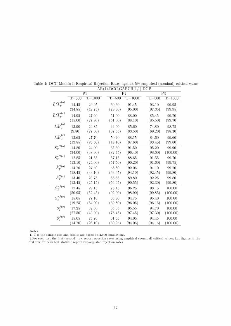
Table 4: DCC Models I: Empirical Rejection Rates against 5% empirical (nominal) critical valueAR(1)-DCC-GARCH(1,1) DGP

P1 P2 P3T=500 T=1000 T=500 T=1000 T=500 T=1000dLM�(o)

T 14:45 29:95 60:60 91:45 93:10 99:95(34:85) (42:75) (79:30) (95:00) (97:35) (99:95)dLM�(r)

T 14:95 27:60 51:00 88:00 85:45 99:70(15:00) (27:90) (51:00) (88:10) (85:50) (99:70)gLM (o)

T 13:90 24:85 44:00 85:60 74:80 98:75(9:80) (27:60) (37:55) (83:50) (69:20) (98:30)gLM (r)

T 13:65 27:70 50:40 88:15 84:60 99:60(12:85) (26:60) (49:10) (87:60) (83:45) (99:60)

S�C(o)T 14:80 24:00 65:60 91:50 95:20 99:90

(34:00) (38:90) (82:45) (96:40) (98:60) (100:00)

S�C(r)T 12:85 21:55 57:15 88:65 91:55 99:70

(13:10) (24:00) (57:50) (90:20) (91:60) (99:75)~SC(o)T 14:70 27:50 58:80 92:05 91:10 99:70

(18:45) (33:10) (63:65) (94:10) (92:45) (99:80)~SC(r)T 13:40 23:75 56:65 89:80 92:25 99:80

(13:45) (25:15) (56:65) (90:55) (92:30) (99:80)

S�J(o)T 17:45 29:15 73:45 96:25 98:15 100:00

(50:95) (52:45) (92:00) (98:90) (99:85) (100:00)

S�J(r)T 15:65 27:10 63:80 94:75 95:40 100:00

(19:25) (34:00) (69:80) (96:05) (96:15) (100:00)~SJ(o)T 17:25 32:30 65:35 95:55 94:70 100:00

(27:50) (43:90) (76:45) (97:45) (97:30) (100:00)~SJ(r)T 15:05 25:70 61:55 94:05 94:45 100:00

(14:70) (26:10) (60:95) (94:05) (94:15) (100:00)

Notes:1. T is the sample size and results are based on 2,000 simulations.2.For each test the �rst (second) row report rejection rates using empirical (nominal) critical values; i.e., �gures in the�rst row for ecah test statistic report size-adjusted rejection rates

32