Robust Investor Sentiment Indices

Liya ChuSingapore Management University

Qianqian DuSouthwestern University of Finance and Economics

Jun Tu∗Singapore Management University

First Version: October 2015

Current Version: February 2019

∗We are grateful to Doron Avramov, Phil Dybvig, Paul Pengjie Gao, Ning Gong, Hong Liu, Jingjun Liu, ZwetelinaIliewa (the EFA discussant), Neil Pearson, Nina Na Wang, Takeshi Yamada, Yuan Yu, Harold Zhang, Hong Zhang,Xiaoyan Zhang, Guofu Zhou, seminar participants at Australia National University, Deakin University, LuxembourgSchool of Finance, Sun Yat-sun University (Lingnan (University) College), Shanghai Jiao Tong University, ShenzhenUniversity (Shenzhen Audencia Business School), St. Louis University, Washington University, Wuhan University,and participants at the 2016 Asian Finance Association Annual Meeting, Singapore Management University FinanceSummer Research Camp 2016, the Annual Congress of the European Economic Association 2016, the 10th AnnualRisk Management Conference and the 2017 Annual Meeting of European Finance Association, for helpful comments.Jun Tu acknowledges that the study was funded through a research grant from Sim Kee Boon Institute for Finan-cial Economics. The usual disclaimer applies. We also thank Wurgler for kindly providing data on his web pages.The paper has been previously circulated under the title “Purging Investor Sentiment Index from Too Much Funda-mental Information”. Send correspondence to Jun Tu, Lee Kong Chian School of Business, Singapore ManagementUniversity, Singapore 178899; telephone: (+65) 6828 0764. E-mail: tujun@smu.edu.sg.

Robust Investor Sentiment Indices

Abstract

Market variables affected by not only investor sentiment, but also economic fun-damentals −such as the first-day returns of initial public offerings−have been used toconstruct investor sentiment indices that are widely used as behavioral bias indicators.However, we find that these sentiment indices could contain a large amount (50%to 60%) of fundamentals-related information, challenging their usage as behavioralvariables. By removing the more than 50% of fundamentals-related information, wepropose a robust investor sentiment index that performs better than these potentiallyfundamentals-related information dominated sentiment indices by capturing the senti-ment impact on cross-sectional stock returns, outperforming competing survey-basedsentiment indices, and predicting sentiment-related, equity-oriented mutual fund in-flows.

JEL classifications: C53, G02, G12, G14, G17

Keywords: Investor Sentiment, Principal components, Partial least squares, Cross-Sectional Returns

1. Introduction

Investor sentiment may drive prices away from their fundamental levels due to the psycho-

logical fact that people with high (low) sentiment tend to make overly optimistic (pessimistic)

judgments and choices (e.g., Keynes (1936), Shiller (1981, 2000), Neal and Weatley (1998), Hir-

shleifer (2001), Antoniou, Doukas and Subrahmanyam (2013)).1 Based on six market variables,

Baker and Wurgler (2006) construct a novel sentiment index (hereafter referred to as the BW in-

dex). Besides investor sentiment, the six market variables used to construct the BW index−such as

the monthly average first-day returns of initial public offerings−could also be affected by economic

fundamentals. Baker and Wurgler (2006) adjust the effect of economic fundamentals by removing

three business cycle variables from their BW index to obtain an orthogonalized version of the BW

index. Baker and Wurgler (2006) further show that the original BW index and the orthogonalized

version of the BW index are very similar to each other. Since the creation of the influential BW

index, numerous studies have adopted it as a behavioral variable in extensive applications.2

However, we find that an approximately 60% variation of the BW index is related to economic

fundamentals, while the three business cycle variables removed from the BW index account for

an approximately 3% variation of the BW index.3 Given that the index has been widely used as

a behavioral variable in the literature, it could be problematic to control for only a small amount

(3%) of economic fundamentals related information while allowing the majority amount of the

60% fundamentals-related information to remain in the (orthogonalized) BW index. To address

1De Long, Shleifer, Summers, and Waldmann (1990), Shleifer and Vishny (1997), Shleifer (2000), among others,provide further explanations for why sentiment can cause an asset price to deviate from its fundamental value in thepresence of limits of arbitrage even when informed traders recognize the opportunity.

2Those studies include, among others, risk-return trade-off in Yu and Yuan (2011), stock price response to earningsnews in Mian and Sankaraguruswamy (2012), asset pricing anomalies in Stambaugh, Yu and Yuan (2012), analysts’forecast error in Hribar and McInnis (2012), institutional/individual investors’ demand shocks in Devault, Sias andStarks (2016), the slope of security market line in Antoniou, Doukas and Subrahmanyam (2015), investments ofpublic and private firms in Badertscher, Shanthikumar and Teoh (2016), and hedge fund returns in Chen, Han and Pan(2016).

3Right after the creation of their novel sentiment index in Baker and Wurgler (2006), Baker and Wurgler (2007)have warned that the BW index could be significantly contaminated by economic fundamentals. For instance, on Page134 of Baker and Wurgler (2007), “This test is important, because sentiment measures may, despite our best efforts,be contaminated by economic fundamentals, ...”. And on Page 146 of Baker and Wurgler (2007), “Or, the sentimentindex may, despite our best efforts, be contaminated by economic fundamentals, ...”. Sibley, Wang, Xing and Zhang(2016) also find the BW index contains significant amount of fundamental information.

1

this concern, this study proposes a robust version of the BW index (hereafter referred to as the

BW-RB index) that controls for the effect of economic fundamentals much more thoroughly than

the existing sentiment indices.

To construct the BW-RB index, we first remove 14 economic fundamental factors from each

of the sentiment proxies. Firstly, we remove seven economic fundamental factors, which are the

principal components of seven groups of macroeconomic variables that are constructed from a

broad range of 109 macroeconomic variables and categorized into seven groups in Kyle, Ludvig-

son, and Ng (2015).4 Secondly, we remove two macroeconomic variables that are documented

in asset pricing literature as business cycle indicators but not included in the 109 variables: the

consumption-to-wealth ratio as in Lettau and Ludvigson (2001) and the GDP growth as in Lem-

mon and Portniaguina (2006). Furthermore, we remove three financial variables drawn from the

literature that are frequently used as indicators of business cycle: the yield on three-month Treasury

Bills, the default spread, and the term spread.5 Finally, we remove two risk factors: the dividend

yield of the value-weighted CRSP market portfolio (Campbell and Shiller, 1988a, 1988b) and the

liquidity risk factor that is measured as the percentage of stocks with zero returns ( Lee, 2011).

Second, the BW index, as the first principal component of the six investor sentiment prox-

ies, maximally represents the total variations of the proxies. However, the first principal compo-

nent may contain a substantial amount of common approximation errors among the six proxies

that are irrelevant to investor sentiment. Therefore, this study adopts the partial least squares

approach−which can control the issue of common approximation errors−to generate the BW-RB

index.6

We find that the BW-RB index has a better performance in capturing the sentiment impact on

cross-sectional stock returns than the BW index. Particularly, the BW-RB index demonstrates sig-

nificant forecasting power for the two portfolios based on tangibility characteristics (PPE/A port-

4The seven groups are (1) output and income, (2) labour market, (3) housing, (4) consumption, orders and inven-tories, (5) money and credit, (6) exchange rates, (7) inflation.

5Studies that use financial variables as business cycle indicators include Campbell (1987), Hodrick (1992), andChen, Roll and Ross (1986).

6The partial least squares approach is discussed in details later in the paper.

2

folio and RD/A portfolio) while the BW index does not. Out of their pool of 16 testing portfolios,

Baker and Wurgler (2006) declare that the PPE/A portfolio and the RD/A portfolio are suggested

by the referee of their paper. This gives rise to a potential data mining concern given that the BW

index does not work on these two referee-suggested types of out-of-sample testing assets. After

controlling for the fundamentals, the better performing BW-RB index, which may be considered

as an improved version of the BW index, is no longer affected by this data mining concern.

In addition, we compare the forecasting power of the BW index and the BW-RB index for cross-

sectional stock returns with four survey-based sentiment indices, namely, anxious index, consumer

sentiment index, individual investor sentiment index, and Gallup survey index. For the whole

sample, the BW sentiment index can predict the cross-sectional stock returns. However, the BW

index becomes unable to predict the cross-sectional stock returns for three of the four survey-based

sentiment indices for the four subsamples matching the sample periods of the four survey-based

sentiment indices, respectively. None of the four survey-based sentiment indices can predict the

cross-sectional stock returns. However, the BW-RB index can predict the cross-sectional stock

returns for the whole sample and for all four subsamples matching the sample periods of the four

survey-based sentiment indices. Therefore, the BW-RB index is more robust than the BW index

and can outperform three of the four survey-based sentiment measures while the BW index cannot.

Furthermore, we compare the influence of different investor sentiment indices on the inflows

into equity-oriented mutual funds, which reflect investor sentiment towards the stock market (Ben-

Rephael, Kandel and Wohl (2012)). We find that the BW-RB index is positively and significantly

correlated with contemporaneous equity-oriented mutual fund inflows and positively predicts the

inflows in the next period, while the BW index fails to do so. The findings indicate that the BW-RB

index is more consistent with investors’ actual behavior, suggesting that the BW-RB index reflects

widely shared investor beliefs.

Overall, after removing a large amount (approximately 60%) of fundamental related informa-

tion from the BW index, we propose the BW-RB index as a robust version of the BW index, which

performs better than the widely used BW index in terms of capturing the sentiment impact on cross-

3

sectional stock returns, outperforming competing survey-based sentiment indices, and predicting

sentiment-related equity-oriented mutual fund inflows.7

There may be one potential caveat. Fundamentals and sentiment can be correlated (e.g., An-

geletos and La’O (2013) and Benhabib, Liu, and Wang (2016)). Nevertheless, it could be too ex-

treme to treat fundamental variables and sentiment variables as the same class of variables. Hence,

it would be worthwhile to construct a robust version of the BW index with as much fundamental

information removed as possible, which may also have the effect of removing a certain amount of

fundamental-related sentiment information. However, the BW-RB index performs better than the

BW index. Therefore, the cost of removing the fundamental-related sentiment information appears

smaller than the benefit.

Moreover, we compare the BW-RB index with the newly proposed five-indicator BW index

(the BW(5) index) that drops one sentiment indicator, the average NYSE share turnover (TURN),

from the original set of six indicators. The BW(5) index still appears to be contaminated by a

large amount (more than 50%) of fundamental information while the BW-RB index is largely free

from this contamination issue. Therefore, it is not surprising that we find that just as the BW-RB

index improves the BW index, the BW-RB index can also significantly improve the BW(5) index

in terms of capturing the sentiment impact on cross-sectional stock returns, outperforming com-

peting survey-based sentiment indices, and predicting sentiment-related, equity-oriented mutual

fund inflows. Specifically, in terms of capturing the sentiment impact on cross-sectional stock re-

turns, the BW-RB index demonstrates significant forecasting power for the two portfolios based on

tangibility characteristics (PPE/A portfolio and RD/A portfolio), while the BW(5) index, like the

six-indicator BW index, is not able to predict the PPE/A portfolio and the RD/A portfolio. Similar

to the six-indicator BW index, the BW (5) index is still bothered by the data mining concern while

the BW-RB index is not.7Our analysis may be deemed as echoing the warning of Baker and Wurgler in some sense as well. Given that

their main goal is to create a novel sentiment measure, it seems acceptable for Baker and Wurgler (2006; 2007)to downplay the issue of the contamination of economic fundamentals by only taking out a small set of economicvariables. However, they issue their warning on this concern, which has been largely ignored by the literature butaddressed by this study.

4

In addition, the results of several existing studies using the BW index could be changed or even

overturned when the BW(5) index is used. For instance, when we follow Stambaugh, Yu and Yuan

(2012) to re-investigate the impact of sentiment on the 11 well-known anomalies, we find that many

claims in Stambaugh, Yu and Yuan (2012), which classify high and low sentiment periods based on

the six-indicator BW⊥ index (the orthogonalized version of the BW index), become much weaker

when they are based on the five-indicator BW (5)⊥ index (the orthogonalized version of the BW

(5) index). More specifically, under the new BW (5)⊥ index, the “total accruals” anomaly becomes

stronger following low sentiment than following high sentiment, with a significant t-statistics of

2.27. This is inconsistent with the claim in Stambaugh, Yu and Yuan (2012) that “the anomalies

should be stronger following high sentiment than following low sentiment.” Moreover, under the

new BW (5)⊥ index, 4 of the 11 long legs have significant and positive t-statistics. This is also

inconsistent with the claim in Stambaugh, Yu and Yuan (2012) that sentiment should not have an

appreciable effect on the long-leg returns. As a comparison, we also do the check using the BW-RB

index to classify high and low sentiment periods. We find that the results are still consistent with

the claims in Stambaugh, Yu and Yuan (2012). Therefore, the BW-RB index may be considered as

a more robust version of the BW index even when compared to the new BW(5) index.

In addition, the BW(5) index drops TURN while the BW-RB index keeps it. According to the

Jeffrey Wurgler’s website, the reason to drop TURN is that it seems no longer closely linked to

sentiment due to the explosion of institutional high-frequency trading and the migration of trading

to a variety of venues in recent years. We study the time-varying pattern of the loading of the TURN

indicator in the BW-RB index based on a rolling window approach. We find that the loading of

the TURN indicator is declining during the recent years, consistent with the above arguments that

TURN becomes less accurate as a sentiment indicator in recent years. However, we also find that

the loading of the TURN indicator is still sizable. This finding indicates that the TURN indicator

remains a relevant sentiment indicator. Therefore, we do not drop TURN in the BW-RB index.

Finally, we would like to explain why we focus on providing a robust version of the BW

sentiment index rather than robust versions of other sentiment measures. Baker and Wurgler

5

(2006) construct a novel investor sentiment index that aggregates the information from six market-

variable proxies.8 There are other sentiment indices, including the above mentioned survey-based

approaches (Brown and Cliff (2004), Lemmon and Portniaguina (2006)) and the search-based

sentiment indices (Da, Engelberg and Gao (2015)). Another type of sentiment measure focuses on

factors that could alter individuals’ moods or feelings (Kaplanski, Levy, Veld and Veld-Merkoulova

(2015)).9 Nevertheless, many of those non-market-variable measures are only available from re-

cent years, and some survey questions may not be answered carefully or truthfully. This could be

the reason for the popularity of the market-variable-based BW sentiment index with a long time-

series window dating back to 1960’s. Therefore, we choose to focus on the BW sentiment index

and use some of the other indices, such as the survey-based indices, only for additional checks.

The remainder of the paper is organized as follows. Section II discusses the construction of

the BW-RB index. Sections III explains the data and provides summary statistics. We present

the performances of the BW-RB index and comparing the BW-RB index with the BW indices and

survey based sentiment indices in Section IV. We conduct further analyses in Section V, VI, and

VII. Section VIII contains concluding remarks.

II. Construction of the robust sentiment index

A. Concerns about the BW index

Baker and Wurgler (2006) initiate an innovative sentiment index, which exerts significant ef-

fects on cross-sectional returns. Specifically, thd BW sentiment index is constructed by taking

the first principal component of six investor sentiment proxies: discount rate of closed-end fund

8There are many other studies employing sentiment measures based on market data. However, most of thesestudies use single proxy, such as retail investor trades, mutual fund flows, closed-end fund discounts and net equityissues (Kumar and Lee (2006), Ben-Rephael, Kandel and Wohl (2012), Lee, Shleifer, and Thaler (1991), Swaminathan(1996), Baker and Wurgler (2000)).

9For more examples, please see, weather related issues such as sunshine, clouds and temperature (e.g., Saunders(1993), Hirshleifer and Shumway (2003)), seasonal affective disorder arising from autumn and winter depression(Kamstra, Kramer, and Levi (2003)), and sports results or other abrupt events which could trigger investor sentiment(Edmans, Garcia, and Norli (2007), Kaplanski and Levy (2010a, 2010b)

6

(CEFD), average NYSE share turnover (TURN), the number of IPOs (NIPO), average first-day re-

turn (RIPO), the equity issuance (EQTI), and the log difference of market-to-book ratios between

dividend payers and nonpayers (PDND). Since the six raw investor sentiment proxies are highly

correlated with the business environment, Baker and Wurgler (2006) modify the sentiment index by

removing variables related to the business cycle from each proxy before the principal component

analysis (PCA). Specifically, they regress each proxy on growth in the industrial production index,

growth in consumer durables, nondurable and services, growth in employment and a dummy vari-

able for NBER recessions and use the residuals from the regressions as cleaner sentiment proxies

to construct a orthogonalized version of the Baker and Wurgler index, the BW⊥index.

We have two main concerns about the BW index. First, the BW index could be contaminated

by economic fundamentals. The six sentiment proxies that are used to construct the BW index

are closely correlated with the overall business environment. For instance, the number of IPOs

reflects investor sentiment, but it is inevitably determined by the economic condition. In Ritter and

Welch (2002)’s survey of the IPO literature, they conclude that ”market conditions are the most

important factor in the decision to go public.” The BW⊥ index has removed a few variables related

to business cycle and it possesses a 0.97 correlation with the original BW index. We find that the

BW index could be contaminated by a large amount (approximately 60%) of fundamental-related

information. As for the newly proposed five-indicator BW index, which drops the average NYSE

share turnover, it also contains a large amount (more than 50%) of fundamental-related informa-

tion. Given that the BW sentiment indices have been widely used as behavioral indicators in the

literature, it could be troublesome to control only a small amount (3%) of economic fundamentals

related information while allowing the majority amount of the 50% to 60% fundamental-related

information to remain in the BW indices. In this study, we control the effect of economic fun-

damentals more thoroughly than the existing sentiment indices by removing the 50% to 60% of

fundamental-related information.

Second, the BW index is the first principal component (PCA) of the six investor sentiment

proxies. Although econometrically the first principal component (PCA) is the best combination

7

of all the sentiment proxies that maximally represents the total variations of the proxies, the first

PCA may potentially contain a substantial amount of common approximation errors among the

six investor sentiment proxies that are irrelevant to investor sentiment. Additionally, the sentiment

irrelevant common approximation errors in the first PCA may reduce the forecasting performance

of the BW index. Due to these limitations, this study proposes a better method, the partial least

squares approach (PLS), to control the sentiment irrelevant common approximation errors as de-

tailed below.

B. Estimation of the robust sentiment index

To more effectively extract non-fundamental information from the six individual sentiment

proxies, we adopt the PLS to generate the purged sentiment index (the BW-RB index) and ap-

ply it to forecast portfolio returns. In this section, we outline our econometric methodology, which

is based on Kelly and Pruitt (2013, 2015), and Huang, Jiang, Tu and Zhou (2015).

B.1 Setup

First we set up the environment where we use the PLS method. We define the long-short com-

bined portfolio return ret as the mean return of 16 firm characteristics-based long-short portfolios

in Baker and Wurgler (2006). ret is composed of two parts: the conditional expectation plus an

unpredictable shock,

rett+1 = Et(rett+1)+ et+1, (1)

where rett+1 is the long-short combined portfolio return at time t+1 and et+1 is the unpredicted

shock.

We assume that conditioning on information at time t, the expected long-short combined port-

folio return is explained by unobservable investor sentiment Sentt ,

8

Et(rett+1) = β0 +β1Sentt . (2)

We rearrange equation (1) and obtain,

rett+1 = β0 +β1Sentt + et+1. (3)

We denote Vt = (v1,t , ...,vK,t)′ as an K×1 vector of purged individual sentiment proxies at time

period t. Each purged sentiment proxy is estimated as the regression residual of the individual

sentiment proxy in Baker and Wurgler (2006) on a wide range of economic fundamental variables.

Each purged sentiment proxy has a factor structure,

vi,t = λi,0 +λi,1 ∗Sentt +λi,2 ∗Cet + εi,t , for i = 1, ...,N. (4)

where λi,1 is the sensitivity of sentiment proxies vi,t to the movements in Sentt that is important

for forecasting the portfolio return, Cet is the common approximation error component of Vt that

is irrelevant to returns, and εi,t is the idiosyncratic noise.

B.2 Sentiment Estimator

Following Kelly and Pruitt (2013, 2015), and Huang, Jiang, Tu and Zhou (2015), PLS can be

implemented in two stages of OLS regression. In the first stage, for each sentiment proxy vi,t , which

is the residual component of the individual investor sentiment proxy after removing fundamental

information, we run a time-series regression on a constant and future long-short combined portfolio

return rett+1,

vi,t = µi,0 +µi ∗ rett+1 +υi,t , for t = 1, ...,T −1. (5)

9

The coefficient µi captures the sensitivity of each sentiment proxy vi,t to investor sentiment Sentt ,

proxied by the long-short combined portfolio return rett+1.10

In the second-stage, for each time period t, we run a cross-sectional regression of vi,t on the

corresponding estimated coefficient µ̂i from the first stage,

vi,t = ct +BW -RBt ∗ µ̂i +ωi,t , for i = 1, ...,K, (6)

where the coefficient BW -RBt is the estimated robust investor sentiment index.

In summary, the first-stage coefficient estimates map the purged sentiment proxies to the fore-

casting target rett+1, which is assumed to be driven by the unobservable investor sentiment Sentt ,

while second-stage regression use this map to back out estimates of the unobservable investor

sentiment Sentt at each point in time.

Huang, Jiang, Tu and Zhou (2015) discuss in detail the advantage of the PLS method used in

this study over the PCA method used in Baker and Wurgler (2006). In a nutshell, PCA maximally

represents the total co-movement of the six investor sentiment proxies including both Sentt and

Cet . In contrast, PLS can extract Sentt while excluding Cet , from the six investor sentiment proxies.

Based on Equations (3), (4) and (5), µi in Equation (5) is not affected by Cet . Based on Equation

(6), the BW -RBt derived from the PLS method is also not affected by Cet .11

10We have to admit that aside from the mean return of 16 firm characteristics-based long-short portfolios, alternativeportfolio returns could also serve as a proxy for investor sentiment Sentt . Nevertheless, the 16 firm characteristics-based long-short portfolios in Baker and Wurgler (2006) used here capture the sentiment impact via a large cross-sectional portfolios based on a broad range of characteristics including firm size, age, profitability, dividends, assettangibility, growth opportunities, and distress. It appears unclear that which alternative portfolio return can domi-nate the mean return of 16 firm characteristics-based long-short portfolios used in this study as a proxy for investorsentiment Sentt .

11Equation (3) assumes that rett+1 is not affected by Cet . We may relax this assumption and allow rett+1 to beaffected by the part of Cet that is related to systematic risk, which has not been fully offset by taking the differencebetween the long leg and the short leg in the 16 long-short spread portfolios. That is, rett+1 can be affected byboth sentiment Sentt and fundamental systematic risk that may be reflected by Cet to a certain degree. However, incomparison to PCA, which includes Cet fully, PLS can mostly likely eliminate a significant amount of Cet that isrelevant to the six sentiment proxies but is not related to fundamental systematic risk, and hence not relevant to rett+1.Thus PLS may still be a better method in terms of extracting the common co-movement related to sentiment Sentt whileat the same time minimizing the inclusion of common co-movement Cet that is not related to fundamental systematicrisk. In addition, even when the PLS derived BW -RBt contains fundamental systematic risk related information in Cetthat affects rett+1, the impact on the forecasting power of BW -RBt on rett+1 should be minimized after controllingFama French three factors and Carhart’s momentum factor in our predictive regression.

10

III. Data and summary statistics

A. BW index and purged sentiment proxies

We obtain BW index, BW⊥ index, BW (5) index, BW (5)⊥ index and six sentiment proxies that

are used to construct BW index from Wurgler’s website.12 The six individual sentiment proxies

are:

• Closed-end fund discount rate, CEFD: value-weighted average difference between the net

asset values of closed-end stock mutual fund shares and their market prices;

• Share turnover, TURN: log of the raw turnover ratio detrended by the past 5-year average,

where raw turnover ratio is the ratio of reported share volume to average shares listed from

the NYSE Fact Book;

• Number of IPOs, NIPO: monthly number of initial public offerings;

• First-day returns of IPOs, RIPO: monthly average first-day returns of initial public offerings;

• Dividend premium, PDND: log difference of the value-weighted average market-to-book

ratios of dividend payers and nonpayers; and

• Equity share in new issues, EQTI: gross monthly equity issuance divided by gross monthly

equity plus debt issuance.

Our sample period is from July 1965 to November 2014. All data are at a monthly frequency.

To construct the BW-RB index, we remove economic fundamental factors from each of the

sentiment proxies. Since there is an extensive list of economic fundamental variables, we first

construct the seven common factors from a broad range of macroeconomic variables. Follow-

12The data was previously be available on the website: http://people.stern.nyu.edu/jwurgler/. Since March of 2013,the data on TURN and the BW index based on 6 proxies have been removed from the website. The BW (5) index andother five sentiment proxies are currently available on this website. We collect TURN by ourselves and extend the BWindex to November 2014 following Baker and Wurgler(2006).

11

ing Kyle, Ludvigson, and Ng (2015),13 we use the information of 109 macroeconomic variables

that are categorized into seven groups, including: (1) output and income, (2) labour market, (3)

housing, (4) consumption, orders and inventories, (5) money and credit, (6) exchange rates, and

(7) inflation. We derive the first principal component from the macroeconomic variables in each

group, and then we remove the seven principal components from each of the sentiment proxies.

A full list of the 109 macroeconomic variables is provided in Online Appendix A.1. Second, we

remove two macroeconomic variables that are documented in asset pricing literature as business

cycle indicators but not included in the 109 variables:consumption-to-wealth ratio, as in Lettau

and Ludvigson (2001), and GDP growth, as in Lemmon and Portniaguina (2006). Furthermore,

we remove three financial variables drawn from the literature that are frequently used as indicators

of a business cycle: the yield on three-month Treasury Bills, the default spread that is measured

as the difference between the yields to maturity on Moody’s Baa-rated and Aaa-rated bonds, and

the term spread that is measured as the difference in yields between the ten-year Treasury bond

and the three-month Treasury Bill.14 Finally, we remove two risk factors: dividend yield of the

value-weighted CRSP market portfolio (Campbell and Shiller, 1988a, 1988b) and liquidity risk

factor that is measured as the percentage of stocks with zero returns ( Lee, 2011).15

As mentioned in the introduction, fundamentals may be related to sentiment. Particularly, the

percentage of stocks with zero returns is removed as a fundamental liquidity risk factor from the

BW index. On the one hand, market wide liquidity can affect expected returns of all securities

and may serve as a systematic risk factor (e.g., Pastor and Stambaugh (2003), Acharya and Ped-

ersen (2005), Korajczyk and Sadka (2008) and Lee (2011)). On the other hand, one may argue

that liquidity is closely related to sentiment (e.g., Baker and Stein (2004)) and hence should not

13Kyle, Ludvigson and Ng (2015) construct the latent common factors as the principal components from 132macroeconomic variables that are categorized into 8 groups and a detailed description of the 132 macroeconomicvariables is provided by the Fred-MD database. We construct the first principal components from each of the 7 groupsof macroeconomic variables, since the 8th group is about the stock market and we directly control the stock marketrisk separately. In the 6th group, we remove all bond related variables from that category , and we directly control the3-month treasury bill rate, term spread, and default spread later.

14Studies that use financial variables as business cycle indicators include Campbell (1987), Hodrick (1992), andChen, Roll and Ross (1986).

15We tried to remove different macro-economic variables, and still have consistent results. We will explain thedetails in the robustness check.

12

be removed. Nevertheless, to be safe, it is worth constructing a conservative type of sentiment

index with as much fundamental information removed as possible. In addition, the benefit seems

larger than the cost regarding the removal of the fundamental related sentiment information since a

conservative BW-RB index performs better than the BW index as indicated by the below empirical

results.

For each sentiment proxy, we remove all the 14 fundamental factors documented above in the

following regression:

vt = a+b′(Zt)+κt ,

where vt represents each sentiment proxy, Zt denotes the 14 fundamental variables and κt is the re-

gression residual. From those regerssions, we define the six residuals as purged sentiment proxies,

i.e., CEFDres, TURNres, NIPOres, RIPOres, PDNDres and EQTIres.

Panel A of Table 1 presents summary statistics of the BW index, the BW⊥ index, the BW (5)

index, the BW (5)⊥ index, and 14 fundamental factors.16 For each variable, we report the mean,

standard deviation, first-order autocorrelation (ρ(1)), correlation with the BW index and the data

source. Many of the fundamental factors possess a common feature of being highly persistent,

and this pattern is quite similar to the BW index and BW⊥ index. We find that the BW index is

significantly correlated with many of the fundamental factors, such as labour market employment,

housing, consumption, orders and inventory, consumption wealth ratio, GDP growth, three-month

Treasury bill, default spread, dividend yield and liquidity factor. Among these variables, three-

month treasury bill rate, GDP growth, consumption and liquidity have the highest correlations

with the BW sentiment index. This implies that a considerable proportion of BW sentiment index

is related to systematic risk. By contrast, although Baker and Wurlger (2006) have tried to remove

several business cycle variables from the original BW index to derive the BW⊥ index, the BW index

and the BW⊥ index are highly correlated (the correlation is 0.97). In addition, the BW (5) index

and the BW (5)⊥ index are highly correlated with the BW index (with correlations of 0.97 and 0.94

16BW (5)⊥ is constructed similarly to BW⊥. Compared to BW (5), a few economic variables are removed from thefive underlying sentiment proxies in BW (5)⊥.

13

respectively). Moreover, BW (5)⊥ seems unable to properly control the fundamental information

content given that it has a high correlation of 0.97 with BW (5).

In Panel B, we report the regression result of the BW index on the 14 fundamental factors.

We present the estimated coefficients, OLS t-statistics and Newey-West t-statistics that has been

adjusted for 12 lags. We find that adjusted R-squares for the BW index is about 62%, indicating

that the BW index contains a considerable portion of information related to economic fundamental

conditions. Moreover, we regress the BW(5) index on the 14 fundamental factors and achieve an

adjusted R-squares of around 52%, indicating that the BW(5) index is also significantly contami-

nated by economic fundamentals.17

Panels A and B in Table 2 provide summary statistics of the six raw sentiment proxies and the

six purged sentiment proxies. All the sentiment proxies are standardized to have zero mean and

unit variance. Each purged sentiment proxy is estimated as the regression residual of the raw sen-

timent proxy on 14 fundamental factors. Panel A presents the mean, standard deviation, first-order

autocorrelation (ρ(1)), as well as the minimum and maximum of the six raw sentiment proxies and

their correlations with BW sentiment index along with their correlation matrix. Four of the six sen-

timent proxies are positively correlated with the BW sentiment index, but not the closed-end fund

discount rate (CEFD) and dividend premium (PDND). Panel B presents summary statistics and

correlations of the six purged individual sentiment proxies. Since the common macroeconomic

variation has been removed from the purged sentiment proxies, it is not surprising that the six

purged sentiment proxies show a similar pattern but a smaller magnitude in terms of persistency

and correlation compared with raw sentiment proxies. Therefore, it would be more challenging to

efficiently extract the underlying commonality among the purged sentiment proxies.

17As detailed in the Online Appendix A.2, when we run the regression of each one of the six sentiment proxies onthe 14 fundamental factors, R-squares mostly range from approximately 30% to over 50%, indicating a considerableportion of the variation in each individual sentiment proxy can be explained by economic fundamentals.

14

B. Robust investor sentiment index

Following the two-steps of the estimation procedures of PLS, we obtain the BW-RB index from

the six purged individual sentiment indicators,

BW -RBt =−0.17∗CEFDrest +0.20∗TURNrest−12 +0.38∗NIPOrest

+0.29∗RIPOrest−12−0.49∗PDNDrest−12 +0.27∗EQT Irest

(7)

Since some proxies need a longer time to reveal the same sentiment (Huang, Jiang, Tu and

Zhou, 2015), the purged share turnover, purged average first-day return of IPO, and purged divi-

dend premium are taken as lagged 12 months relative to other three purged proxies.

We also detail the loadings of the six raw sentiment indicators when forming the BW index:

BWt =−0.28∗CEFDt +0.18∗TURNt−12 +0.07∗NIPOt

+0.10∗RIPOt−12−0.58∗PDNDt−12 +0.10∗EQT It(8)

Compared with the loadings of the raw sentiment indicators in the BW index, all the six purged

indicators have the same signs as the corresponding raw indicators in the BW index.18 In addition,

all of the six sentiment indicators are standardized with a mean of zero and a standard deviation of

one. Therefore, we can directly compare the magnitude of the estimates’ loadings of the indicators.

We find that the BW-RB index has a much smaller relative loading (in terms of the relative ranking

of the absolute value of the six loadings) on the TURN, than the BW index. For instance, although

the TURN is the third most important indicator among the six sentiment indicators in the BW

18To make an easy comparison with Baker and Wurgler (2006), the loadings presented here for both the BW indexandthe BW-RB index are based on in-sample regression, which are the same as in Baker and Wurgler (2006). Inaddition, the latter part of this study on predictive regression analyses are in-sample analysis as well, and the sameas in Baker and Wurgler (2006). We also conduct out-of-sample analysis based on rolling windows. The results aresimilar. Moreover, although the BW-RB index makes use of the information of the mean return of the 16 long-shortportfolios, its forecasting power is not driven by using the past or future information of the mean return of the 16long-short portfolios to forecast the future 16 long-short portfolios portfolio returns. First, we find that the past meanreturn of the 16 long-short portfolios cannot predict the future returns of the 16 long-short portfolios. Second, thefuture mean return of the 16 long-short portfolios is not used in our out-of-sample analysis, which has similar resultsas the in-sample analyses.

15

index, it becomes the second least important indicator in the BW-RB index.19,20

In addition, based on a rolling window approach, we study the time-varying pattern of the

loading of the TURN in the BW-RB index. We find that the loading of the TURN in the BW-

RB index appears to indeed trend down over recent years. However, the loading is still sizable.

This indicates that the TURN indicator may still be a relevant sentiment indicator. There could be

several reasons for this as detailed in the Online Appendix A.4. In addition, numerous studies have

produced influential results based on the old BW index, including the turnover indicator. Suddenly

dropping the turnover indicator completely may raise serious doubts about all of these studies.

Therefore, although the TURN may no longer serve as a strong sentiment indicator in recent years,

as argued by Wurgler’s website, it sappears too extreme to drop the turnover indicator completely

in the recently posted, new (five-indicator) BW index. The BW-RB index appears to be a relatively

better choice.

Furthermore, in contrast to the high correlation of 0.97 between Baker and Wurgler’s orthog-

onal sentiment index BW⊥ and their original sentiment index BW, the correlation between the

BW-RB index and the BW index is only 0.56. Figure 1 plots time series of the BW index and the

BW-RB index, showing that the BW-RB index captures almost all the same anecdotal accounts of

fluctuations as the BW index. Both sentiment indices are low at the beginning of the sample (after

the 1961 crash of growth stocks), and reach a spike in the electronic bubble in 1968 and 1969.

Sentiment declines subsequently until the middle of 1970s and rebounds from the late 1970s to

mid-1980s. During the late 1980s, sentiment falls and reaches a peak again in the Internet bubble

period from 1999 to 2001. The sentiment indices decrease during the subprime debt crisis from

19One possible explanation is that the TURN in the BW index may have a strong relationship with a commonfundamental economic component shared by all six indicators. In contrast, the TURN has a much weaker relationshipwith the other common component that is shared by all six indicators−the common sentiment component−than theother sentiment indicators. Indeed, we find that the TURN have much smaller correlations with the rest sentimentindicators after removing the fundamental related information in the BW sentiment index. More specifically, theweights on NIPO, RIPO and EQTI in the BW-RB index are increased significantly to be three to four times higherthan their loadings in the BW index, while the weight on TURN did not change much compared with their loadings inthe BW index.

20The relative importance of the CEFD has also dropped significantly in the BW-RB index, consistent with thedoubt against it as a sentiment indicator (e.g., Qiu and Welch (2004)). Although the CEFD and the TURN are thesecond and the third most important indicators among the six sentiment indicators in the BW index, they now becomethe two least important indicators in the BW-RB index.

16

2008 to 2009 and rebound in 2010. Although the two indices seem highly correlated, the BW-RB

index tends to be more volatile and appears to lead the BW index in some cases. Particularly, dur-

ing the periods after the financial crisis, roughly from year 2009 to 2014, the BW-RB index stays

slightly above the BW index, inferring that the robust sentiment index is not as dragged down by

bust fundamental conditions in the crisis.

We plot a time series of the six raw individual sentiment proxies and the six residual sentiment

proxies in Figure 2. On the one hand, the raw proxies and the residual proxies show comovement

during the entire sample period. On the other hand, the two types of sentiment proxies sometimes

deviate from each other. The only exception is the residual component in RIPO, which deviates

less from raw RIPO because the fundamental variables contribute less in explaining RIPO than in

explaining other sentiment proxies, making the two variables−RIPO and RIPOres−much closer.

C. Portfolio returns

To compare the BW-RB index with the original BW index, we use the same 16 testing portfolios

in Baker and Wurgler (2006), which are constructed based on firm characteristics including size,

age, dividend payment, earnings, tangible assets, R&D, sigma, external finance, sales growth, and

book-to-market ratio. The detailed description of these firm characteristics is contained in Online

Appendix A.3. We define the top three NYSE deciles as high, the firms in the bottom three NYSE

deciles as low, and the remaining middle four NYSE deciles as medium.

Baker and Wurgler (2006) document the conditional effect of sentiment on the spread portfolios

that buy the high group and sell the low group (high-low portfolio). For instance, a high-low

portfolio based on age has a higher return when BW sentiment is positive, and has a lower return

when BW sentiment is negative. However, the BW sentiment index has the opposite conditional

pattern on high-low portfolio based on sigma. For consistency, we construct long-short portfolios

on which the BW sentiment has the same direction of conditional effect. Specifically, we construct

the “high-low” portfolios, which have long legs in the top deciles (less exposed to sentiment) and

short legs in bottom deciles (more exposed to sentiment), according to size, age, dividend payment,

17

earnings, fixed assets, and book-to-market ratio. We construct low-high portfolios, which have the

long legs in the bottom deciles and short legs in top deciles in terms of R&D, sigma, external

finance, and sales growth. The relationships between sentiment and the variables related to growth

and distress-external finance, sales growth, and book-to-market ratioare not monotonic. Following

Baker and Wurgler (2006), we break external finance, sales growth, and book-to-market ratio into

medium-high and medium-low portfolios. In addition, we construct a combined portfolio, which

takes equal positions across the 16 firm characteristics-based portfolios.

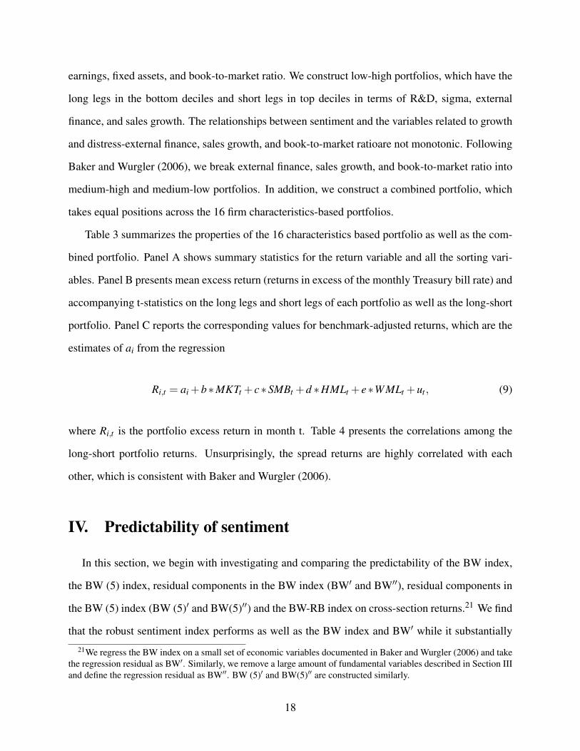
Table 3 summarizes the properties of the 16 characteristics based portfolio as well as the com-

bined portfolio. Panel A shows summary statistics for the return variable and all the sorting vari-

ables. Panel B presents mean excess return (returns in excess of the monthly Treasury bill rate) and

accompanying t-statistics on the long legs and short legs of each portfolio as well as the long-short

portfolio. Panel C reports the corresponding values for benchmark-adjusted returns, which are the

estimates of ai from the regression

Ri,t = ai +b∗MKTt + c∗SMBt +d ∗HMLt + e∗WMLt +ut , (9)

where Ri,t is the portfolio excess return in month t. Table 4 presents the correlations among the

long-short portfolio returns. Unsurprisingly, the spread returns are highly correlated with each

other, which is consistent with Baker and Wurgler (2006).

IV. Predictability of sentiment

In this section, we begin with investigating and comparing the predictability of the BW index,

the BW (5) index, residual components in the BW index (BW′ and BW′′), residual components in

the BW (5) index (BW (5)′ and BW(5)′′) and the BW-RB index on cross-section returns.21 We find

that the robust sentiment index performs as well as the BW index and BW′ while it substantially

21We regress the BW index on a small set of economic variables documented in Baker and Wurgler (2006) and takethe regression residual as BW′. Similarly, we remove a large amount of fundamental variables described in Section IIIand define the regression residual as BW′′. BW (5)′ and BW(5)′′ are constructed similarly.

18

outperforms BW′′. Furthermore, we analyze the predictability of the robust sentiment index on

future economic activities and investigate its relationship with the business cycle.

A. The predictability of the BW index

Panel A of Table 5 reports the results of using the BW index as the predictor for long-short

portfolio returns, long-leg returns and short-leg returns of 16 firm characteristics based portfo-

lios.22 After controlling for the Fama French three factors and Carhart’s momentum factor,23 the

BW index significantly predicts 11 of the 16 long-short portfolios. In terms of long- or short-leg

portfolio returns, the BW index can forecast 4 of the 16 long-leg returns, and 14 of the 16 short-

leg returns. We present the regression results for the long-short return spreads from column 3 to

column 6. We report the estimated coefficients and bootstrapped p-values to correct the bias of

autocorrelation (Stambaugh, 1999). The results are consistent with Baker and Wurgler (2006),

showing that the BW can predict most portfolio returns except for the portfolios based on PPE/A,

RD/A, BE/ME, EF/A, and GS, in which the predictive power disappears after controlling for the

Fama French three factors and Carhart’s momentum factor. The regression results illustrate the

significant U-shape pattern, which is also documented in Baker and Wurgler (2006), for portfolios

based on Medium-High, Medium-Low strategies of the growth and distress variables: external

finance, sales growth, and book-to-market ratio.

Stambaugh, Yu and Yuan (2012) argue that overpricing is more prevalent than underpricing due

to the short-sale constraint. Specifically, the short legs of the anomalies should be more profitable

following high sentiment, and sentiment should not exhibit any relation with the return of long

legs. Although the construction of our long-short portfolios is different from the anomalies in

Stambaugh, Yu and Yuan (2012), sentiment should have a stronger predictive power for the short

legs of portfolio returns since the short legs are set to be more exposed to sentiment. We report

the results of a predictive regression of the BW index for short legs of the portfolios from column

22We also consider the orthogonal Baker and Wurgler (2006) index BW⊥ and find similar results.23When the portfolio is formed based on SMB or HML, SMB or HML is not included as a control variable.

19

11 to column 14. Without controlling for the Fama French three factors and Carhart’s momentum

factor, the BW index significantly and negatively predicts all the short legs, and after controlling

for four factors, the BW index significantly predicts 14 of the 16 short legs. We report the results

of the predictive regression for long legs from column 7 to column 10, in which the BW index only

significantly predicts 4 of 16 portfolios controlling for the Fama French three factors and Carhart’s

momentum factor. The findings are consistent with Stambaugh, Yu and Yuan (2012)’s prediction

that sentiment exhibits asymmetric impacts on the long legs and short legs.

In Panel B of Table 5, we report the results of using the BW (5) index to predict long-short

portfolio returns, long-leg returns, and short-leg returns of 16 firm characteristics-based portfolios.

The predictability of the BW (5) index on the portfolio return shows a similar pattern to the BW

index, but the predictability is a bit weaker than the BW index. After controlling for the Fama

French three factors and Carhart’s momentum factor, the BW (5) index significantly predicts 11

of the 16 long-short portfolios, 1 of the 16 long-leg returns, and 10 of the 16 short-leg returns.

Consistent with the BW index, the BW (5) can predict most of the long-short portfolios returns

except the portfolios based on PPE/A, RD/A, BE/ME, EF/A and GS after controlling for the Fama

French three factors and Carhart’s momentum factor.

B. The predictability of BW′ and BW′′

Although the BW index can predict most of the portfolio returns, we cannot distinguish whether

the predictability is driven by investor sentiment or economic fundamental risks. In this section, we

try some straightforward methods to remove the fundamental factors from the BW index. First, we

directly remove six macroeconomic variables that are documented by Baker and Wurgler (2006)

from the BW index. We regress he BW index on the six macroeconomic variables−the growth of

industrial production, the growth of durable consumption, the growth of nondurable consumption,

the growth of service consumption, the growth of employment, and a dummy variable for NBER-

dated recessions−and define the regression residual BW′ as a new sentiment index. In Panel A of

Table 6, we report the regression results of using BW′ as an investor sentiment proxy to predict

20

cross-section returns. After controlling for the Fama French three factors and Carhart’s momentum

factor, BW′ significantly predicts 11 of the 16 long-short portfolio spreads, 5 of the 16 long-leg

returns, and 14 of the 16 short-leg returns. The predictability is comparable with the BW index,

but we are concerned that we fail to remove fundamental information completely.

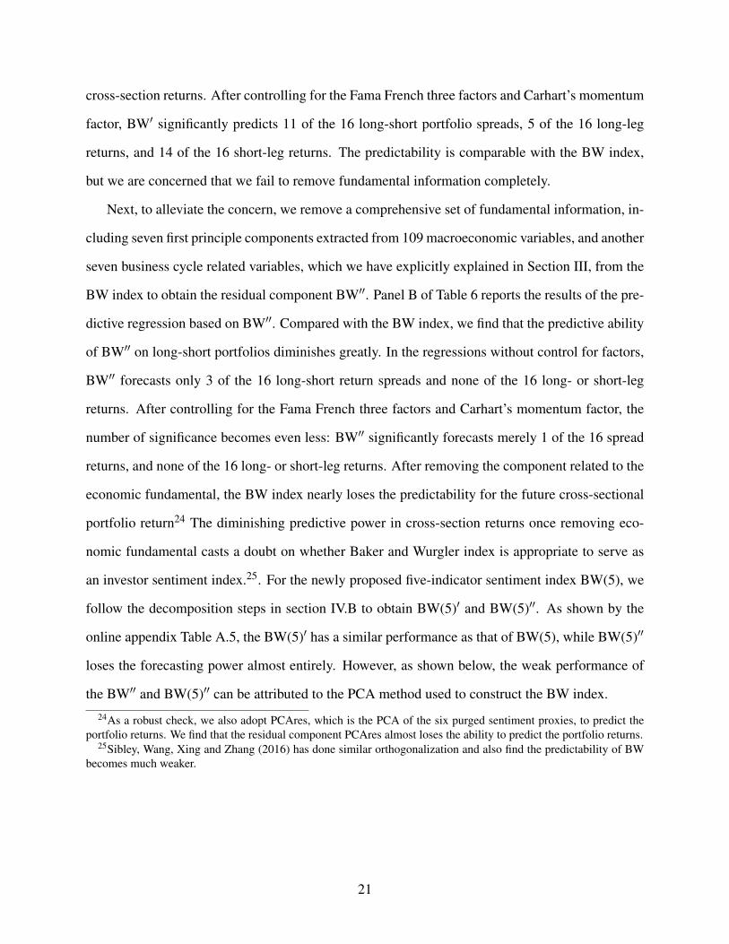
Next, to alleviate the concern, we remove a comprehensive set of fundamental information, in-

cluding seven first principle components extracted from 109 macroeconomic variables, and another

seven business cycle related variables, which we have explicitly explained in Section III, from the

BW index to obtain the residual component BW′′. Panel B of Table 6 reports the results of the pre-

dictive regression based on BW′′. Compared with the BW index, we find that the predictive ability

of BW′′ on long-short portfolios diminishes greatly. In the regressions without control for factors,

BW′′ forecasts only 3 of the 16 long-short return spreads and none of the 16 long- or short-leg

returns. After controlling for the Fama French three factors and Carhart’s momentum factor, the

number of significance becomes even less: BW′′ significantly forecasts merely 1 of the 16 spread

returns, and none of the 16 long- or short-leg returns. After removing the component related to the

economic fundamental, the BW index nearly loses the predictability for the future cross-sectional

portfolio return24 The diminishing predictive power in cross-section returns once removing eco-

nomic fundamental casts a doubt on whether Baker and Wurgler index is appropriate to serve as

an investor sentiment index.25. For the newly proposed five-indicator sentiment index BW(5), we

follow the decomposition steps in section IV.B to obtain BW(5)′ and BW(5)′′. As shown by the

online appendix Table A.5, the BW(5)′ has a similar performance as that of BW(5), while BW(5)′′

loses the forecasting power almost entirely. However, as shown below, the weak performance of

the BW′′ and BW(5)′′ can be attributed to the PCA method used to construct the BW index.24As a robust check, we also adopt PCAres, which is the PCA of the six purged sentiment proxies, to predict the

portfolio returns. We find that the residual component PCAres almost loses the ability to predict the portfolio returns.25Sibley, Wang, Xing and Zhang (2016) has done similar orthogonalization and also find the predictability of BW

becomes much weaker.

21

C. The predictability of the BW-RB index

Econometrically, the investor sentiment extracted from the PCA method may involve a sub-

stantial amount of common approximation errors that are irrelevant for forecasting cross-section

returns. Therefore, we use an improved econometric method PLS to construct the BW-RB index.

The BW-RB index has several desirable features. First, the BW-RB index is constructed from

purged sentiment proxies, from which fundamental information has been largely removed. Sec-

ond, the PLS estimation aligns the investor sentiment with the purpose of explaining the future

cross-sectional return and only extracts the information relevant for the forecasting target.

We report the predictability of the BW-RB index on portfolio returns in Panel A of Table 7. We

find that the BW-RB index can predict the cross-sectional stock returns remarkably well. Panel A

demonstrates that the BW-RB index significantly predicts 12 of the 16 long-short portfolio, 13 of

the 16 long-leg returns and all of the 16 short-leg returns. After controlling for Fama French three

factors and Carhart’s momentum factor, the BW-RB index is statistically significant in predicting

13 of the 16 long-short portfolio returns, 2 of the long-leg returns, and 10 of the short-leg returns.

In Panel A of Table 7, the first three rows show that when the BW-RB index is higher, returns

on small, young and high volatility firms are relatively lower in the next month. In terms of

economic magnitudes, for instance, the coefficient for predicting size portfolio indicates that a

one-unit increase in sentiment (which is equivalent to a one standard deviation increase because

the indices are standardized) is associated with a 0.5% higher monthly return on the large minus

small portfolio. For profitability and dividend payment, we find that the BW-RB index also has

significant predictive power for these portfolios and a higher BW-RB index forecasting relative to

lower returns on non-payers and unprofitable firms. The patterns of long-short and short leg are

consistent after controlling for the Fama French three factors and Carhart’s momentum factor.

In Baker and Wurgler (2006), the predictability of the BW index on long-short PPE/A and

RD/A portfolios is insignificant. However, the BW-RB index significantly predicts the tangibility

characteristics-based portfolios returns. From row 6 to row 7, we show that the BW-RB index

has significant predictive power for the PPE/A and RD/A portfolios. The higher the BW-RB, the

22

lower the future returns on low PPE/A stocks and high RD/A stocks. The findings are in line with

the theoretical prediction that the valuation of a firm with less tangible assets tends to be more

subjective, and thus its stock is affected more by the fluctuations of investor sentiment.

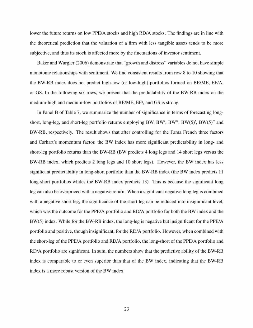
Baker and Wurgler (2006) demonstrate that “growth and distress” variables do not have simple

monotonic relationships with sentiment. We find consistent results from row 8 to 10 showing that

the BW-RB index does not predict high-low (or low-high) portfolios formed on BE/ME, EF/A,

or GS. In the following six rows, we present that the predictability of the BW-RB index on the

medium-high and medium-low portfolios of BE/ME, EF/, and GS is strong.

In Panel B of Table 7, we summarize the number of significance in terms of forecasting long-

short, long-leg, and short-leg portfolio returns employing BW, BW′, BW′′, BW(5)′, BW(5)′′ and

BW-RB, respectively. The result shows that after controlling for the Fama French three factors

and Carhart’s momentum factor, the BW index has more significant predictability in long- and

short-leg portfolio returns than the BW-RB (BW predicts 4 long legs and 14 short legs versus the

BW-RB index, which predicts 2 long legs and 10 short legs). However, the BW index has less

significant predictability in long-short portfolio than the BW-RB index (the BW index predicts 11

long-short portfolios whiles the BW-RB index predicts 13). This is because the significant long

leg can also be overpriced with a negative return. When a significant negative long leg is combined

with a negative short leg, the significance of the short leg can be reduced into insignificant level,

which was the outcome for the PPE/A portfolio and RD/A portfolio for both the BW index and the

BW(5) index. While for the BW-RB index, the long-leg is negative but insignificant for the PPE/A

portfolio and positive, though insignificant, for the RD/A portfolio. However, when combined with

the short-leg of the PPE/A portfolio and RD/A portfolio, the long-short of the PPE/A portfolio and

RD/A portfolio are significant. In sum, the numbers show that the predictive ability of the BW-RB

index is comparable to or even superior than that of the BW index, indicating that the BW-RB

index is a more robust version of the BW index.

23

D. The BW-RB index and business cycles

In this section, we examine whether the BW-RB index is correlated with business cycles. Figure

3 plots the peaks and troughs of the business cycle as defined by the NBER data along with the

contemporaneous BW-RB index. If the the BW-RB index is a proxy for an omitted macroeconomic

risk factor, we expect it to be procyclical. However, as shown in the figure, this does not appear to

be the case. Specifically, over the 14 reported business cycle peaks and troughs during our sample

period, he BW-RB index goes the opposite direction with the business cycle indicator for half of

the reported peak and trough dates. This evidence further indicates that the BW-RB index is less

likely to be related to the state of the macroeconomy.

E. Robustness checks

When we construct our purged sentiment proxies, we remove a wide range of fundamental in-

formation, including first principal components from seven groups of macroeconomic variables

and seven fundamental variables, and use PLS to extract the aligned investor sentiment. As ro-

bustness checks, we remove alternative sets of fundamental variables to derive purged sentiment

proxies. First, we extract seven common factors from more than 100 macroeconomic variables

using asymptotic principal component analysis. In this way, we summarize fundamental informa-

tion from a large number of macroeconomic time series into a small number of estimated common

factors.26 We remove the seven common factors along with the seven fundamental variables as

described in Section III. Second, we directly remove a wide range of raw fundamental variables:

130 macroeconomic variables from FRED-MD and five fundamental related variables, which are

consumption-to-wealth ratio, GDP growth, default spread, dividend yield, and liquidity risk fac-

tor.27 We present the predictability of the robust sentiment index constructed from PLS on alter-

native purged sentiment proxies in Panel A of Table 8. For instance, based on the first alternative

definition of fundamental variables, the robust sentiment index significantly predicts 12 out of 16

26To determine the number of common factors, we use BIC information criterion. (see Schwarz, 1978)27We delete the three-month Treasury Bill rate and term spread because of multicollinearity.

24

long-short return spreads, 2 of 16 long-leg portfolios and 12 of the 16 short-leg portfolios after

controlling for four factors.

In Panel B, we remove fundamental variables directly from the BW sentiment index. When the

Fama French three factors and Carhart’s momentum factor are included as control variables, the

residual component of BW sentiment based on the alternative 14 fundamental variables can predict

only 1 out of 16 long-short portfolio spreads, and none of the 16 long- and short-leg portfolios.

We remove fundamental variables directly from the BW (5) index and report the results in

Panel C of Table 8. The predicted results are similar to the results in Panel B. After controlling

for the Fama French three factors and Carhart’s momentum factor, the residual component of the

BW sentiment based on alternative 14 fundamental variables predicts 4 of 16 long-short portfolio

spreads, and none of the 16 long- and short-leg portfolios.

In Panel D, we use the PCA method to construct the residual sentiment index from the purged

sentiment proxies. Compared to applying PLS, the predictive performance of PCA on purged

sentiment proxies diminishes greatly. Specifically, we find that using the 14 fundamental vari-

ables illustrated in Section III, the residual sentiment based on PCA can forecast only 2 long-short

portfolio spread, none of the long-leg portfolio and 2 out of 16 short-leg portfolios. Using the

alternative 14 variables, the residual sentiment can forecast 4 of 16 long-short portfolio spreads,

none of the long-leg portfolio, and 3 of 16 short-leg portfolios.

In summary, the results show that the sentiment residual constructed on the alternative 14

variables performs similarly to the counterpart that was constructed based on the 14 fundamental

variables illustrated in Section III. We also have consistent results using 135 variables as funda-

mentals.

F. Survey-based alternative sentiment measures

Some studies, such as Brown and Cliff (2004), Lemmon and Portniaguina (2006), and Green-

wood and Shleifer (2014), indicate that survey-based investor expectations of stock returns may

negatively predict future returns. The evidence is consistent with Baker and Wurgler (2006)’s find-

25

ings that investor sentiment negatively affects cross-sectional stock returns and favors a behavioral

explanation. In this section, we compare stock rerun forecasting performances of the BW-RB index

and four survey-based sentiment indices.28

We obtain anxious index (AI) from the Federal Reserve Bank of Philadelphia that measures the

probability of a decline in real GDP, consumer sentiment index (ICS) from Michigan University,

individual investor sentiment index (AAII) from the American Association of Individual Investor

survey and rescaled Gallup investor index (GA) from the Galllup survey.29 We orthogonalize each

survey-based sentiment index to the 14 macroeconomic variables that we described in Section

IV. We take the fitted value as the fundamental component and the regression residual as the non-

fundamental component. After decomposing anxious index (AI), consumer sentiment index (ICS),

individual investor sentiment index (AAII), and rescaled Gallup investor index (GA) , we derive

AIres, ICSres, AAIIres and GAres respectively.

Panel A of Table 9 reports the univariate regressions of the relation between the BW-RB in-

dex and the contemporaneous survey-based sentiment indices respectively. We find that the non-

fundamental component in anxious index AIres is positively and significantly correlated with the

BW-RB index, with a Newey-West t-statistics of 2.29, while the relation between the BW-RB

index and other measures such as ICSres, AAIIres and GAres are much weaker.

Next, we investigate the predictive power of each survey-based sentiment index on the long-

short, long leg and short leg of the combined portfolio return in the next month. We report the

results from specifications (1) to (4) in Panels B, C and D respectively. All these predictors are

insignificant or weak under the conventional 5% significance level, and the only exception is using

GAres−the residual from the rescaled Gallup survey−to predict the long leg of the combined

portfolio return. GAres is positively correlated with the next month’s long-leg combined portfolio

28There are some other alternative sentiment measures, such as retail investor trades, mutual fund flows, closed-endfund discounts and net equity issues (Kumar and Lee (2006), Ben-Rephael, Kandel and Wohl (2012), Lee, Shleifer,and Thaler (1991), Swaminathan (1996), Baker and Wurgler (2000)). However, since these measures are also marketvariable based, like the BW index, but with only single sentiment indicator, it is not fair to compare them with themultiple indicator based BW index.

29We rescale Gallup investor index GA by projecting the stock return expectation (available between 1999 and2003) onto the raw Gallup series.

26

return with a Newey-West t-statistics of 2.42.

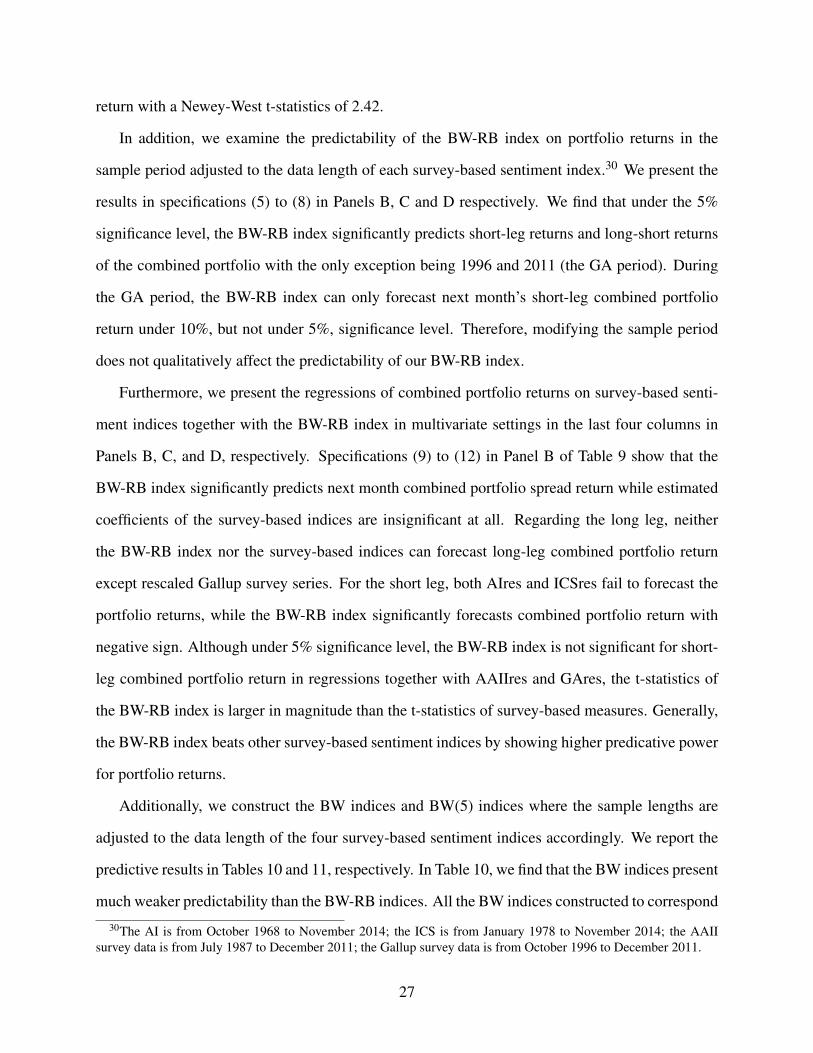
In addition, we examine the predictability of the BW-RB index on portfolio returns in the

sample period adjusted to the data length of each survey-based sentiment index.30 We present the

results in specifications (5) to (8) in Panels B, C and D respectively. We find that under the 5%

significance level, the BW-RB index significantly predicts short-leg returns and long-short returns

of the combined portfolio with the only exception being 1996 and 2011 (the GA period). During

the GA period, the BW-RB index can only forecast next month’s short-leg combined portfolio

return under 10%, but not under 5%, significance level. Therefore, modifying the sample period

does not qualitatively affect the predictability of our BW-RB index.

Furthermore, we present the regressions of combined portfolio returns on survey-based senti-

ment indices together with the BW-RB index in multivariate settings in the last four columns in

Panels B, C, and D, respectively. Specifications (9) to (12) in Panel B of Table 9 show that the

BW-RB index significantly predicts next month combined portfolio spread return while estimated

coefficients of the survey-based indices are insignificant at all. Regarding the long leg, neither

the BW-RB index nor the survey-based indices can forecast long-leg combined portfolio return

except rescaled Gallup survey series. For the short leg, both AIres and ICSres fail to forecast the

portfolio returns, while the BW-RB index significantly forecasts combined portfolio return with

negative sign. Although under 5% significance level, the BW-RB index is not significant for short-

leg combined portfolio return in regressions together with AAIIres and GAres, the t-statistics of

the BW-RB index is larger in magnitude than the t-statistics of survey-based measures. Generally,

the BW-RB index beats other survey-based sentiment indices by showing higher predicative power

for portfolio returns.

Additionally, we construct the BW indices and BW(5) indices where the sample lengths are

adjusted to the data length of the four survey-based sentiment indices accordingly. We report the

predictive results in Tables 10 and 11, respectively. In Table 10, we find that the BW indices present

much weaker predictability than the BW-RB indices. All the BW indices constructed to correspond

30The AI is from October 1968 to November 2014; the ICS is from January 1978 to November 2014; the AAIIsurvey data is from July 1987 to December 2011; the Gallup survey data is from October 1996 to December 2011.

27

to the ICSres, AAIIres and GAres sample periods fail to forecast the long-short combined portfolio

return significantly. In particular, only the BW index constructed according to the AIres sample

period can significantly forecast the long-short combined portfolio return in the next month. In

contrast, the BW-RB indices constructed in the four different sample periods show much stronger

predictive power in forecasting the long-short combined portfolio return than either the BW indices

or the four survey-based sentiment indices, with t-statistics ranging from 3.16 to 4.13 in Table 9. In

Table 11, we find that the performances of the BW(5) indices is similar to the BW indices, showing

much weaker predictability than the BW-RB index. Overall, the findings indicate that the BW-RB

index is a more robust version of the BW index.

G. Sentiment and equity-oriented mutual fund flows

In this section, we compare the influence of different investor sentiment indices on the inflows

into equity-oriented mutual funds, which reflects investor sentiment towards the stock market (Ben-

Rephael, Kandel and Wohl (2012)).31 In specifications (1) and (2) of Table 12, we find that the

BW-RB index is positively and significantly correlated with contemporaneous fund inflows with a

Newey-West t-statistics of 2.23. We also find the BW-RB index positively predicts next period’s

equity-oriented mutual fund inflows with t-statistics of 1.82. In contrast, the BW index in speci-

fications (3) and (4) is negatively correlated with contemporaneous fund inflows, and predicts the

next period fund inflows with an incorrect sign. In specifications (5) and (6), we use the newly pro-

posed five-indicator sentiment index BW(5) as the explanatory variable. We find that the BW(5)

index has no significant relationship with current or next period equity-oriented mutual fund in-

flows, which is consistent with prior findings in the literature (e.g., Ben-Rephael, Kandel and Wohl

(2012)). The evidence indicates that the BW-RB index is more consistent with investors’ actual31We obtain monthly data for equity-oriented mutual fund inflows from Investment Company Institute and scale

the net dollar inflows in each month by the aggregate capitalization of the U.S. stock market. Baker and Wurgler(2007) also show that their sentiment index is related to mutual fund flows. They find that after controlling for thegeneral demand of mutual funds, fund flows to more speculative categories, such as growth funds, are more sensitiveto the sentiment index than those flows to less speculative categories, such as income funds. However, we don’t havemonthly mutual fund inflow data of detailed categories. Due to the data constraint, we explore the relationship betweensentiment indices and inflows into equity-oriented mutual funds instead.

28

behavior, suggesting that the BW-RB index reflects widely shared investor beliefs.

V. Validation of the BW-RB index

Furthermore, we provide two validation tests for the BW-RB index. The first validation test

involves earnings announcement returns. Baker and Wurgler (2006) find that earnings announce-

ment returns are lower after high investor sentiment. Since investors are more likely to suffer errors

in valuation for stocks that are speculative and hard to arbitrage, we expect that earnings announce-

ment returns should be inversely related to the BW-RB index for speculative stocks. As detailed in

the Online Appendix A.6.1, The results are consistent with our expectation. The second validation

test involves mispricing component in Tobin’s Q. As detailed in the Online Appendix A.6.2, we

find that BW-RB captures mispricing information in Tobin’s Q and presents better predictability

for the portfolio returns than mispricing the component in Tobin’s Q.

VI. Economic explanations

In addition, it is of interest to investigate the economic driving force of the predictability of the

BW-RB index, i.e., whether the predictive power of the BW-RB index stems from time variations

in cash flows or discount rates. As detailed in the Online Appendix A.7, we find that the BW-RB

index significantly forecasts future dividend growth, which is a standard cash flow proxy, but in-

significantly forecasts future dividend price ratio, which is a common proxy of discount rates. The

evidence supports the claim that the cash flow channel is the source for predictability. Furthermore,

the ability of the BW-RB index to forecast the cross-section of stock returns is positively associ-

ated with its ability to also forecast the cross-section of future cash flows. Hence, our findings

are consistent with Baker and Wurgler (2007)’s findings that the lower stock return following high

investor sentiment periods appears to represent investors’ overly optimistic belief about future cash

flows that cannot be justified by subsequent economic fundamentals.

29

VII. The impact of sentiment on anomalies based on BW(5)⊥

In Panel A of Table 13, we investigate the impact of sentiment on the 11 well-known anomalies

and the combination strategy used in Stambaugh and Yu (2017) and Stambaugh, Yu and Yuan

(2012). The 11 anomalies are: O-score, distress, net stock issues, composite equity issues, total

accruals, net operating assets, momentum, gross profitability, asset growth, return on assets and

investment-to-assets. We extend the sample period of the data used in Stambaugh, Yu and Yuan

(2012), which ends in January 2008, to December 2014.

We use the BW (5)⊥ index to classify high and low sentiment periods.32 Interestingly, we find

that many claims in Stambaugh, Yu and Yuan (2012), which classifies high and low sentiment

periods based on the six-indicator BW⊥ index, become much weaker when based on the BW (5)⊥

index. For instance, in Table 3 of Stambaugh, Yu and Yuan (2012), the “total accruals” anomaly

is stronger following high sentiment than following low sentiment, although the difference is not

significant. In contrast, under the new BW (5)⊥ index, the “total accruals” anomaly now changes

its sign: it becomes stronger following low sentiment rather than following high sentiment, with a

significant t-statistics of -2.27.33 This is inconsistent with the claim in Stambaugh, Yu and Yuan

(2012): “the anomalies should be stronger following high sentiment than following low sentiment.”

Moreover, in Table 3 of Stambaugh, Yu and Yuan (2012), only one anomaly (net stock issues)

has a significant one-tailed t-statistic (1.69). Stambaugh, Yu and Yuan (2012) hence argue that

sentiment should not have an appreciable effect on the long-leg returns. However, using the new

BW (5)⊥ index, 4 out of the 11 long legs have significant and positive t-statistics, varying from

1.75 to 2.79. Therefore, if we classify high and low sentiment periods based on the BW (5)⊥ index,

the argument that sentiment should not have an appreciable effect on the long-leg returns seems

questionable.

32We follow Stambaugh, Yu and Yuan (2012) to use the orthogonal rather than the original Baker and Wurglersentiment index. The results are similar if we use the original BW(5) index.

33Based on our new sample extended to December 2014, when using the old BW⊥ index instead of the new BW (5)⊥

index, the “total accruals” anomaly is statistically not different across high sentiment and low sentiment with a t-valueof -0.52. Therefore, the difference across sentiment regime for the “total accruals” anomaly from not significantlydifferent from zero to significantly negative is likely due to the change of sentiment index from BW⊥ to BW (5)⊥ butnot due to the extension of the sample period to more recent years.

30

As a comparison, we also do the check by replacing the six-indicator BW⊥ index with the

BW-RB index. As shown in Panel B of Table 13, when we use BW-RB to classify high and low

sentiment periods, we find that “total accruals” becomes higher in high sentiment periods than in

low sentiment periods, consistent with the claim the anomalies should be stronger following high

sentiment than following low sentiment. In addition, we have only one long leg with significant

t-statistics based on the BW-RB index. This is consistent with the other claim of Stambaugh, Yu

and Yuan (2012) that sentiment should not have an appreciable effect on the long-leg returns.

Therefore, even though the TURN indicator may become a less relevant sentiment indicator

due to the reasons listed at Jeffrey Wurgler’s website, whether we should completely drop the

TURN indicator (as in the BW(5) index) or just reduce its relative weight in the total sentiment

index (as in the BW-RB index) is questionable.

VIII. Conclusion

The Baker and Wurgler (2006) sentiment index (the BW index) has been widely used as a be-

havioral bias indicator in extensive applications. However, the market variables used in construct-

ing the BW index are affected by not only investor sentiment but also economic fundamentals.

We find that an approximately 60% (or 50%) variation of the BW index (or the BW (5) index) is

related to economic fundamentals while the orthogonalized version of the BW index (or the or-

thogonalized version of the BW (5) index) removes only about 3% of variation of the BW index

(or the BW (5) index). Therefore, it could be problematic to control for only a small amount of

economic fundamentals related information while allowing the majority amount of the 60% (or

50%) fundamental information to remain in the (orthogonalized) BW (or BW (5)) index.

In this study, we propose a robust investor sentiment index, the BW-RB index, by control-

ling for the large amount (approximately 60%) of fundamental related information. The BW-RB

index performs better than both the original six-indicator BW index and the newly proposed five-

31

indicator BW (5) index, which may be contaminated by a large amount of fundamental informa-

tion, in terms of capturing the sentiment impact on cross-sectional stock returns, outperforming the

competing survey-based sentiment indices and predicting sentiment related equity-oriented mutual

fund inflows. Moreover, the results of several existing studies that use the original BW index will

be changed or possibly overturned when the five-indicator BW index (BW(5) index) is used, and

the results will hold when using the BW-RB index.

32

Reference

Ang, A., and G. Bekaert. 2007. Return predictability: Is it there? Review of Financial Studies 20,

651–707.

Angeletos. G., and J., La’O. 2013. Sentiments. Econometrica 81, 739 – 779.

Antoniou, C., J. A. Doukas, and A. Subrahmanyam. 2013. Cognitive dissonance, sentiment, and

momentum. Journal of Financial and Quantitative Analysis 48, 245–275.

Antoniou, C., J. A. Doukas, and A. Subrahmanyam. 2015. Investor Sentiment, Beta, and the Cost

of Equity Capital. Management Science 1–21.

Arif, S., and Charles M.C. Lee. 2014. Aggregate investment and investor sentiment. Review of

Financial Studies 27(11), 3241–3279.

Badertscher, B., D. Shanthikumar, and S. Teoh. 2016. Private firm investment and public peer

misvaluation. Working paper.

Baker, M., J. Wurgler. 2000. The equity share in new issues and aggregate stock returns. Journal

of Finance 55, 2219–2257.

Baker, M., and J. Wurgler. 2006. Investor sentiment and the cross-section of stock returns. Journal

of Finance 61, 1645–1680.

Baker, M., and J. Wurgler. 2007. Investor sentiment in the stock market. Journal of Economic

Perspectives 21, 129–152.

Benhabib, J., X. Liu, and P. Wang. 2016. Sentiments, Financial Markets, and Macroeconomic

Fluctuations. Journal of Financial Economics 120(2), 420–443.

Ben-Rephael, A., Kandel, S. and Wohl, A. 2012. Measuring investor sentiment with mutual fund

flows. Journal of Financial Economics 104, 363–382.

Brown, G. W., and Cliff, M. T. 2005. Investor sentiment and asset valuation. Journal of Business

78(2), 405–40.

Campbell, J. Y. 1987. Stock returns and the term structure. Journal of Financial Economics 18,

373–399.

Campbell, J. Y., and R. J. Shiller. 1988a. Stock prices, earnings and expected dividends. Journal

33

of Finance 43, 661–676.

Campbell, J. Y., and R. J. Shiller. 1988b. The dividend-price ratio and expectations of future

dividends and discount factors. Review of Financial Studies 1, 195–228.

Chen, N., Roll, R. and Ross, S. A. 1986. Economic forces and the stock market. Journal of

Business 59(3), 383–403.

Chen, Y., Han, B. and Pan, J. 2016. Sentiment risk, sentiment timing, and hedge fund returns.

Working paper.

Cochrane, J. H. 2008. The dog that did not bark: A defense of return predictability. Review of

Financial Studies 21, 1533–1575.

Cochrane, J. H. 2011. Presidential address: Discount rates. Journal of Finance 66, 1047–1108.

Da, Z., Engelberg, J. and Gao, P. 2015. The sum of ALL FEARS Investor sentiment and asset

prices. Review of Financial Studies 28, 1–32.

De Long, J. B., A. Shleifer, L. H. Summers, and R. Waldmann. 1990. Noise trader risk in financial

markets. Journal of Political Economy 98, 703–738.

Devault, L., Sias, R. and Starks, L. 2016. Who are the sentiment traders? Evidence from the

cross-section of stock returns and demand. Working paper.

Edmans, A., Garı́a, D. and Norli, O. 2007. Sports sentiment and stock returns. Journal of Finance

62, 1967–1998.

Fama, E. F., and K. R. French. 1988. Dividend yields and expected stock returns. Journal of

Financial Economics 22, 3–25.

Gao, Z., Ren, H. and Zhang, B. 2016. Googling investor sentiment around the world. Working

paper.

Garı́a, D. 2013. Sentiment during recessions. Journal of Finance 68, 1267–1300.

Greenwood, R. and Shleifer, A. 2014. Expectations of returns and expected returns. Review of

Financial Studies 27(3), 714–746.

Goetzmann, W. N., Kumar, A., Kim, D. and Wang, Q. 2014. Weather-induced mood, institutional

investors, and stock returns. Review of Financial Studies 28(1), 73–111.

34

Goyal, A., and I. Welch. 2008. A comprehensive look at the empirical performance of equity

premium prediction. Review of Financial Studies 21, 1455–508.

Goyenko, R. Y., Holden, C. W. and Trzcinka, C. A. 2009. Do liquidity measures measure liquidity?

Journal of Financial Economics 92, 153–181.

Han, B. 2008. Investor sentiment and option prices. Review of Financial Studies 21(1), 387–414.

Hirshleifer, D. 2001. Investor psychology and asset pricing. Journal of Finance 56(4), 1533–1597.

Hirshleifer, D. and Shumway, T. 2003. Good day sunshine: Stock returns and the weather. Journal

of Finance 58, 1009–1032.

Hodrick, R. J. 1992. Dividend yields and expected stock returns: Alternative procedures for infer-

ence and measurement. Review of Financial Studies 5(3), 357–386.

Hribar, P. and McInnis, J. 2007. Investor sentiment and analysts’ earnings forecast errors. Man-

agement Science 58(2), 293–307.

Huang, D., Jiang, F., Tu, J. and Zhou, G. 2015. Investor sentiment aligned: A powerful predictor

of stock returns Review of Financial Studies 28, 791–837.

Jiang, F., Lee, J., Martin, X. and Zhou, G. 2015. Manager sentiment and stock returns. Working

paper.

Kahneman, D., and A. Tversky. 1974. Judgment under uncertainty: Heuristics and biases. Science

185, 1124–1131.

Kamstra, M. J., Kramer, L. A. and Levi, M. D. 2003. Winter blues: A SAD stock market cycle.

American Economic Review 93, 324–343.

Kaplanski, G., Levy, H 2010a. Exploitable predictable irrationality: The FIFA World Cup effect

on the U.S. stock market. Journal of Financial and Quantitative Analysis 45(2), 535–553.

Kaplanski, G., Levy, H 2010b. Sentiment and stock prices: The case of aviation disasters. Journal

of Financial Economics 95(2), 174–201.

Kaplanski, G., Levy, H., Veld, C. and Veld-Merkoulova, Y. 2015. Do happy people make optimistic

investors? Journal of Financial and Quantitative Analysis 50, 145–168.

Kelly, B., and S. Pruitt. 2015. The three-pass regression filter: A new approach to forecasting

35

using many predictors. Journal of Econometrics 186(2), 294–316.

Kelly, B., and S. Pruitt. 2013. Market expectations in the cross-section of present values. Journal

of Finance, forthcoming.

Keynes, J. M. 1936. The General Theory of Employment, Interest and Money. London: Macmillan.

Kumar, A. and Lee, C. 2006. Retail investor sentiment and return comovements. Journal of

Finance 61(5), 2451–2486.

Kyle, J., Ludvigson, S. C., S. Ng. 2015. Measuring uncertainty. American Economic Review

105(3), 1177–1216.

Lee, C., Shleifer, A. and Thaler, R. H. 1991. Investor sentiment and the closed-end fund puzzle.

Journal of Finance 46, 75–109.

Lee, K. 2011. The world price of liquidity risk. Journal of Financial Economics 99, 136–161.

Lemmon, M., and E. Portniaquina. 2006. Consumer confidence and asset prices: Some empirical

evidence. Review of Financial Studies 19, 1499–1529.

Lettau, M., and S. Ludvigson. 2001. Resurrecting the (C)CAPM: A cross-sectional test when risk

premia are time-varying. Journal of Political Economy 109, 1238–1287.

Ludvigson, S. C., S. Ng. 2007. The empirical risk-return relation: A factor analysis approach.

Journal of Financial Economcis 83, 171–222.

McCracken, M. W., S. Ng. 2015. FRED-MD: A monthly database for macroeconomic research.

Working paper, Federal Reserve Bank of St. Louis.

Mian, G. M. and Sankaraguruswamy, S. 2012. Investor sentiment and stock market response to

earnings News. The Accounting Review 87(4), 1357–1384.

Neal, R., and S. Wheatley. 1998. Do measures of investor sentiment predict stock returns? Journal

of Financial and Quantitative Analysis 34, 523–547.

Papapostolou, N. C., Pouliasis, P. K., Nomikos, N. K. and Kyriakou, I. 2015. Real assets investor

sentiment and the predictability of stock returns. Working paper, City University London.

Qju, L. and Welch, I., 2004. Investor sentiment measures. Unpublished working paper, Brown

University.

36

Rhodes-Kropf, M., Robinson, R.M.D. and Viswanathan, S. 2005. Valuation waves and merger

activity: the empirical evidence. Journal of Financial Economics 77, 561–603.

Ritter, J. R. and Welch. I, 2002. A Review of IPO Activity, Pricing, and Allocations. Journal of

Finance 57, 1795–1828.

Saunders, E. M. 1993. Stock prices and wall street weather. American Economic Review 83,

1337–1345.

Schwarz, G. W. 1978. Estimating the dimension of a model. Annals of Statistics 6(2), 461–464.

Shiller, R. J. 1981. Do stock prices move too much to be justified by subsequent changes in

dividends? American Economic Review 71, 421–436.

Shiller, R. J. 2000. Irrational Exuberance Princeton UP, Princeton.

Shleifer, A. and R. W. Vishny. 1997. The limits of arbitrage. Journal of Finance 52, 35–55.

Shleifer, A. 2000. Inefficient markets. Oxford UP, Oxford

Sibley, S., Y. Wang, Y. Xing, and X. Zhang. 2016. The information content of the sentiment index.

Journal of Banking and Finance 62, 164–179.

Sohn, B. S. 2013. What does investor sentiment reflect: Animal spirits or risks? Working paper.

Spiegel, M. 2008. Forecasting the equity premium: Where we stand today. Review of Financial

Studies 21, 1453–1454.

Stambaugh, R. F. 1999. Predictive regressions. Journal of Financial Economics 54, 375–421.

Stambaugh, R. F., J. Yu, and Y. Yuan. 2012. The short of it: Investor sentiment and anomalies.

Journal of Financial Economics 104, 288–302.

Stambaugh, R. F. and Y. Yuan. 2017. Mispricing factors. Review of Financial Studies 30, 1270–

1315.

Swaminathan, B. 1996. Time-varying expected small firm returns and closed-end fund discounts.

Review of Financial Studies 9, 845–887.

Wold, H. 1966. Estimation of principal components and related models by iterative least squares.

In P. R. Krishnaiaah (eds.), Multivariate Analysis, 391–420. New York: Academic Press.

Wold, H. 1975. Path models with latent variables: The NIPALS approach. In H. M. Blalock, A.

37

Aganbegian, F. M. Borodkin, R. Boudon, and V. Cappecchi (eds.), Quantitative Sociology:

International Perspectives on Mathematical and Statistical Modeling. New York: Academic

Press.

Yu, J., and Y. Yuan. 2011. Investor sentiment and the mean-variance relation. Journal of Financial

Economics 100, 367–381.

38

Figure 1. Time series plot of the BW index and the BW-RB index.

This figure plots the BW index and the BW-RB index from July 1965 to November 2014. The solid black

line depicts the BW-RB index, while the blue dashed line plots the BW index. Both series are normalized to

have a mean of zero and a standard deviation of one.

39

Figure 2. Individual investor sentiment proxies.

The figures plot raw investor sentiment proxies and purged investor sentiment proxies. In each panel, the

solid black line depicts purged investor sentiment proxies, while the blue dashed line plots raw investor

sentiment proxies. The first panel shows the value-weighted average difference between the net asset values

of closed-end stock mutual fund shares and market prices. The second panel shows detrended log turnover.

Turnover is the ratio of reported share volume to average shares listed from the NYSE Fact Book. We de-

trend using the past five-year average. The third panel shows the monthly number of initial public offerings.

The fourth panel shows the average monthly first-day returns of initial public offerings. The fifth panel

shows the log ratio of the value-weighted average market-to-book ratios of dividend payers and nonpayers.

The sixth panel shows gross monthly equity issuance divided by gross monthly equity plus debt issuance.

Sample period is from July 1965 to November 2014.

40

Figure 3. NBER indicator of peaks and troughs and the BW-RB index

This figure plots NBER indicator of peaks and troughs (the solid bars) and the contemporaneous BW-RB

index (the clear bars). NBER indicator equals one when the economy is at peak and equals zero when it is

at trough. Sentiment indicator equals one when sentiment is above the medium level and equals zero when

it is below the medium level.

41

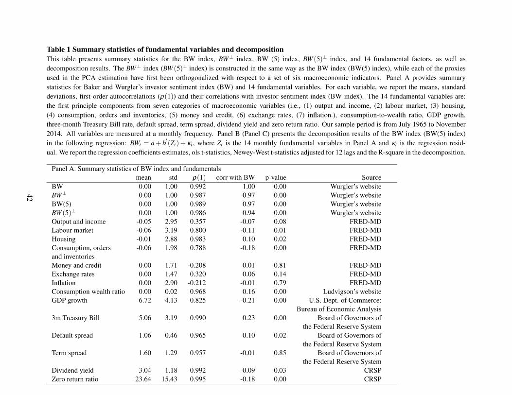
Table 1 Summary statistics of fundamental variables and decompositionThis table presents summary statistics for the BW index, BW⊥ index, BW (5) index, BW (5)⊥ index, and 14 fundamental factors, as well asdecomposition results. The BW⊥ index (BW (5)⊥ index) is constructed in the same way as the BW index (BW(5) index), while each of the proxiesused in the PCA estimation have first been orthogonalized with respect to a set of six macroeconomic indicators. Panel A provides summarystatistics for Baker and Wurgler’s investor sentiment index (BW) and 14 fundamental variables. For each variable, we report the means, standarddeviations, first-order autocorrelations (ρ(1)) and their correlations with investor sentiment index (BW index). The 14 fundamental variables are:the first principle components from seven categories of macroeconomic variables (i.e., (1) output and income, (2) labour market, (3) housing,(4) consumption, orders and inventories, (5) money and credit, (6) exchange rates, (7) inflation.), consumption-to-wealth ratio, GDP growth,three-month Treasury Bill rate, default spread, term spread, dividend yield and zero return ratio. Our sample period is from July 1965 to November2014. All variables are measured at a monthly frequency. Panel B (Panel C) presents the decomposition results of the BW index (BW(5) index)in the following regression: BWt = a+ b

′(Zt) + κt , where Zt is the 14 monthly fundamental variables in Panel A and κt is the regression resid-

ual. We report the regression coefficients estimates, ols t-statistics, Newey-West t-statistics adjusted for 12 lags and the R-square in the decomposition.

Panel A. Summary statistics of BW index and fundamentalsmean std ρ(1) corr with BW p-value Source

BW 0.00 1.00 0.992 1.00 0.00 Wurgler’s websiteBW⊥ 0.00 1.00 0.987 0.97 0.00 Wurgler’s websiteBW(5) 0.00 1.00 0.989 0.97 0.00 Wurgler’s websiteBW (5)⊥ 0.00 1.00 0.986 0.94 0.00 Wurgler’s websiteOutput and income -0.05 2.95 0.357 -0.07 0.08 FRED-MDLabour market -0.06 3.19 0.800 -0.11 0.01 FRED-MDHousing -0.01 2.88 0.983 0.10 0.02 FRED-MDConsumption, orders -0.06 1.98 0.788 -0.18 0.00 FRED-MDand inventoriesMoney and credit 0.00 1.71 -0.208 0.01 0.81 FRED-MDExchange rates 0.00 1.47 0.320 0.06 0.14 FRED-MDInflation 0.00 2.90 -0.212 -0.01 0.79 FRED-MDConsumption wealth ratio 0.00 0.02 0.968 0.16 0.00 Ludvigson’s websiteGDP growth 6.72 4.13 0.825 -0.21 0.00 U.S. Dept. of Commerce:

Bureau of Economic Analysis3m Treasury Bill 5.06 3.19 0.990 0.23 0.00 Board of Governors of

the Federal Reserve SystemDefault spread 1.06 0.46 0.965 0.10 0.02 Board of Governors of

the Federal Reserve SystemTerm spread 1.60 1.29 0.957 -0.01 0.85 Board of Governors of

the Federal Reserve SystemDividend yield 3.04 1.18 0.992 -0.09 0.03 CRSPZero return ratio 23.64 15.43 0.995 -0.18 0.00 CRSP

42

Panel B. Decomposition of BW Panel C. Decomposition of BW(5)Coef ols t-stat NW t-stat Coef ols t-stat NW t-stat

Intercept -0.52 -5.46 -2.21 -0.28 -2.53 -1.01Output and income -0.03 -2.32 -2.44 -0.03 -1.93 -1.98Labour market 0.04 2.60 1.30 0.04 2.45 1.28Housing 0.04 3.94 1.55 0.04 2.93 1.21Consumption,orders and inventories -0.02 -1.12 -0.59 -0.06 -2.42 -1.47Money and credit 0.00 0.06 0.08 -0.01 -0.34 -0.51Exchange rates 0.00 0.06 0.06 0.00 0.23 0.26Inflation 0.00 0.48 1.03 0.00 0.41 0.86Consumption wealth ratio 4.62 2.97 1.12 2.41 1.32 0.53GDP growth -0.06 -6.51 -3.61 -0.06 -5.87 -3.563m Treasury Bill 0.46 24.73 9.21 0.45 20.60 7.85Default spread -0.17 -1.96 -0.75 -0.38 -3.81 -1.39Term spread 0.46 15.04 7.29 0.51 14.20 6.58Dividend yield -0.15 -3.16 -1.13 -0.22 -3.95 -1.39Zero return ratio -0.07 -18.80 -5.30 -0.06 -13.66 -4.16R2 62.51% 52.88%Adj. R2 61.60% 51.74%

43

Table 2 Summary statistics of sentiment proxiesThis table reports summary statistics for raw investor sentiment proxies and purged sentiment proxies. Panel A presents the means, standard deviations,first-order autocorrelations (ρ(1)), as well as minimums and maximums of the six raw sentiment proxies and their correlations with the BW sentimentindex and correlation matrix. The first sentiment proxy (CEFD) is the value-weighted average difference between the net asset values of closed-endstock mutual fund shares and market prices. The second sentiment proxy (TURN) is detrended natural log turnover. Turnover is the ratio of reportedshare volume to average shares listed from the NYSE Fact Book. We detrend using the past five-year average. The third sentiment proxy (NIPO) isthe monthly number of initial public offerings. The fourth sentiment proxy (RIPO) is the average monthly first-day returns of initial public offerings.The fifth sentiment proxy (PDND) is the log difference of the value-weighted average market-to-book ratios of dividend payers and nonpayers. Thesixth sentiment proxy (EQTI) is gross monthly equity issuance divided by gross monthly equity plus debt issuance. Turnover, the average monthlyfirst-day IPO return, and the dividend premium are lagged one year relative to the other three measures. In Panel B, we present the summary statisticsand correlations of the six purged individual sentiment proxies. Purged sentiment proxies are the residuals from regressing corresponding sentimentproxies on 14 fundamental variables defined the same as in Table 1. Superscripts a, b, and c denote statistical significance at the 1%, 5%, and 10%level, respectively.

Panel A. Summary statistics and correlations of raw sentiment proxiescorrelation correlations

Mean Std ρ(1) min max with BW CEFD TURN NIPO RIPO PDND EQTI

CEFD 0.00 1.00 0.965 -2.77 2.29 −0.67a 1.00TURN 0.00 1.00 0.814 -2.91 3.08 0.47a −0.12a 1.00NIPO 0.00 1.00 0.862 -1.13 4.07 0.49a −0.29a 0.19a 1.00RIPO 0.00 1.00 0.653 -2.37 5.25 0.46a −0.17a 0.27a 0.17a 1.00PDND 0.00 1.00 0.976 -3.15 2.50 −0.90a 0.58a −0.32a −0.43a −0.39a 1.00EQTI 0.00 1.00 0.744 -1.46 4.22 0.13a 0.22a 0.21a 0.26a 0.11a -0.04 1.00

Panel B. Summary statistics and correlations of purged sentiment proxiescorrelation correlations

Mean Std ρ(1) min max with BW CEFDres TURNres NIPOres RIPOres PDNDres EQTIres

CEFDres 0.00 1.00 0.898 -3.11 2.80 −0.40a 1.00TURNres 0.00 1.00 0.709 -2.88 2.98 0.19a -0.01 1.00NIPOres 0.00 1.00 0.756 -1.96 4.83 0.23a −0.24a 0.00 1.00RIPOres 0.00 1.00 0.565 -2.04 5.33 0.30a -0.07 0.22a 0.13a 1.00PDNDres 0.00 1.00 0.841 -3.68 2.78 −0.53a 0.30a −0.14a −0.14a −0.40a 1.00EQTIres 0.00 1.00 0.512 -2.24 5.30 0.09b 0.09b 0.03 0.37a 0.09b 0.05 1.00

44

Table 3 The properties of the characteristics-based portfoliosThis table reports the properties of characteristics-based portfolios. The sample period spans from August 1965 to December 2014. PanelA summarizes six groups of variables: the returns variables; the size, age, and risk characteristics; profitability variables; dividend variables;tangibility measures; and variables used as proxies for growth opportunities and distress. Returns are measured monthly. For the four groups ofvariables regarding profitability, dividend policy, tangibility and growth opportunities and distress, accounting data from the fiscal year endingin t-1 are matched to monthly returns from July of year t through June of year t+1. All variables are winsorized at 99.5 and 0.5%. Panel Breports the means and t-statistics of excess returns for the 16 characteristics-based portfolios: firm size (ME), age, total risk (sigma), profitability(E/BE), dividends (D/BE), fixed assets (PPE/A), research and development (RD/A), book-to-market ratio (BE/ME), external finance over assets(EF/A), and sales growth decile (GS). We also construct a combination strategy of the 16 portfolios. Panel C reports the means and t-statisticsof benchmark-adjusted returns for the characteristics-based portfolios. Benchmark-adjusted average returns are estimates of ai in the followingregression: Ri,t = ai+bMKTt +cSMBt +dHMLt +eWMLt +ui,t , where Ri,t is excess return in month t for one of the characteristics-based portfolios.All t-statistics are based on the heteroskedasticity consistent standard errors of White (1980).

Panel A. Summary statisticsFull Sample

N Mean SD Min MaxReturns

Rt (%) 2185371 1.30 17.55 -98.13 2400.00Size, Age and Risk

MEt−1($M) 2185371 1157 4491 1 45205Aget (Years) 2185371 13.93 14.23 0.17 73.83Sigmat−1(%) 2184127 13.49 8.83 2.52 60.70

ProfitabilityE +/BEt−1(%) 2185371 10.22 10.26 0.00 68.97

Dividend PolicyD/BEt−1(%) 2184513 2.13 3.45 0.00 26.15

TangibilityPPE/At−1(%) 1969977 53.22 37.96 0.00 193.78RD/At−1(%) 2185359 3.27 8.22 0.00 62.60

Growth Opportunities and DistressBE/MEt−1(%) 2185371 0.87 0.73 0.03 5.17EF/At−1(%) 2157062 10.04 23.06 -69.27 123.86GSt−1(decile) 2126840 5.74 3.12 1.00 10.00

45

Panel B. Excess returns: Long-shortME Age Sigma E/BE D/BE PPE/A RD/A BE/ME EF/A GS BE/ME EF/A GS BE/ME EF/A GS Combine

M-L M-H M-H M-H M-L M-LLong leg (mean) 0.59 0.75 0.75 0.85 0.82 0.84 0.68 1.14 1.21 1.06 0.89 0.93 0.95 0.89 0.93 0.95 0.89Short leg (mean) 1.01 0.86 0.95 0.98 0.98 0.85 1.18 0.61 0.54 0.65 0.61 0.54 0.65 1.14 1.21 1.06 0.86Long minus short (mean) -0.42 -0.11 -0.20 -0.13 -0.16 -0.01 -0.50 0.53 0.67 0.41 0.28 0.39 0.30 -0.26 -0.28 -0.12 0.03Long leg (t-statistics) 2.88 3.86 4.99 3.89 4.16 4.14 2.88 5.11 5.08 4.23 3.91 4.41 4.59 3.91 4.41 4.59 4.28Short leg (t-statistics) 3.84 3.27 3.07 2.86 3.23 2.99 3.69 2.22 2.01 2.48 2.22 2.01 2.48 5.11 5.08 4.23 3.18Long minus short (t-statistics) -2.52 -0.82 -0.94 -0.71 -0.97 -0.05 -3.11 4.51 9.63 5.25 3.01 4.84 3.49 -4.94 -5.22 -1.39 0.28Panel C. Benchmark-adjusted returns: Long-short

ME Age Sigma E/BE D/BE PPE/A RD/A BE/ME EF/A GS BE/ME EF/A GS BE/ME EF/A GS CombineM-L M-H M-H M-H M-L M-L

Long leg (mean) 0.16 0.12 0.24 0.19 0.14 0.21 0.03 0.38 0.50 0.38 0.22 0.29 0.30 0.22 0.29 0.30 0.25Short leg (mean) 0.29 0.24 0.24 0.24 0.25 0.24 0.65 0.12 -0.05 0.05 0.12 -0.05 0.05 0.38 0.50 0.38 0.23Long minus short (mean) -0.13 -0.11 0.00 -0.06 -0.11 -0.04 -0.62 0.26 0.56 0.34 0.10 0.34 0.26 -0.16 -0.21 -0.08 0.02Long leg (t-statistics) 3.43 2.52 4.40 3.76 2.74 2.46 0.37 4.73 6.29 3.83 3.54 5.58 5.51 3.54 5.58 5.51 4.89Short leg (t-statistics) 2.90 2.59 1.98 1.35 2.17 2.40 4.71 1.30 -0.59 0.61 1.30 -0.59 0.61 4.73 6.29 3.83 2.42Long minus short (t-statistics) -1.14 -1.16 0.02 -0.35 -0.90 -0.39 -5.24 3.62 10.13 4.96 1.61 5.74 4.86 -3.52 -4.68 -1.03 0.36

46

Table 4 Correlations of long-short portfolio returnsThis table reports correlations among characteristics-based portfolios. The long−short portfolios are formed based on firm characteristics: firm size (ME), age,total risk (sigma), profitability (E/BE), dividends (D/BE), fixed assets (PPE/A), research and development (RD/A), book-to-market ratio (BE/ME), external financeover assets (EF/A), and sales growth decile (GS). High is defined as a firm in the top three NYSE deciles, low is defined as a firm in the bottom three NYSEdeciles, and medium is defined as a firm in the middle four NYSE deciles. We also construct a combination strategy of the 16 portfolios. Superscripts a, b, and cdenote statistical significance at the 1%, 5%, and 10% level, respectively.

Profitability, Growth OpportunitiesSize, Age and Risk Dividends Tangibility and Distress Growth Opportunities DistressME Age Sigma E/BE D/BE PPE/A RD/A BE/ME EF/A GS BE/ME EF/A GS BE/ME EF/A GS Combine

M-L M-H M-H M-H M-L M-LME H-L 1.00Age H-L 0.81a 1.00Sigma L-H 0.69a 0.87a 1.00E/BE > 0−< 0 0.73a 0.82a 0.84a 1.00D/BE > 0−= 0 0.75a 0.91a 0.94a 0.89a 1.00PPE/A H-L 0.61a 0.79a 0.77a 0.65a 0.78a 1.00RD/A L-H 0.45a 0.73a 0.70a 0.61a 0.72a 0.74a 1.00BE/ME H-L 0.05 0.49a 0.55a 0.36a 0.53a 0.51a 0.64a 1.00EF/A L-H 0.08c 0.45a 0.50a 0.30a 0.48a 0.51a 0.53a 0.71a 1.00GS L-H −0.21a 0.00 0.08b −0.22a 0.04 0.22a 0.15a 0.42a 0.66a 1.00BE/ME M-L 0.24a 0.65a 0.68a 0.57a 0.70a 0.61a 0.72a 0.91a 0.66a 0.28a 1.00EF/A M-H 0.53a 0.80a 0.87a 0.74a 0.86a 0.75a 0.67a 0.66a 0.76a 0.32a 0.76a 1.00GS M-H 0.46a 0.76a 0.85a 0.65a 0.83a 0.72a 0.69a 0.70a 0.75a 0.47a 0.76a 0.90a 1.00BE/ME M-H 0.32a 0.02 −0.05 0.18a 0.03 −0.08c −0.19a −0.67a −0.44a −0.47a −0.30a −0.15a −0.24a 1.00EF/A M-L 0.71a 0.64a 0.67a 0.72a 0.68a 0.47a 0.33a 0.08c −0.15a −0.39a 0.29a 0.53a 0.39a 0.34a 1.00GS M-L 0.66a 0.76a 0.78a 0.86a 0.79a 0.52a 0.56a 0.30a 0.13a −0.46a 0.50a 0.61a 0.57a 0.20a 0.75a 1.00Combine 0.72a 0.93a 0.95a 0.87a 0.97a 0.85a 0.81a 0.63a 0.58a 0.13a 0.78a 0.91a 0.88a −0.05 0.63a 0.77a 1.00

47

Table 5 The predictability of BW indexThis table presents the results of using Baker and Wurgeler’s investor sentiment index BW and the newly proposed five-indicator sentiment indexBW(5) to predict spread as well as long and short portfolio returns in Panels A and B respectively. The sample spans from August, 1965 to December,2014. The portfolios are formed based on firm characteristics: firm size (ME), age, total risk (Sigma), profitability (E/BE), dividends (D/BE), fixedassets (PPE/A), research and development (RD/A), book-to-market ratio (BE/ME), external finance over assets (EF/A), and sales growth decile (GS).High is defined as a firm in the top three NYSE deciles, low is defined as a firm in the bottom three NYSE deciles, and medium is defined as a firmin the middle four NYSE deciles. We provide results for the following two regressions respectively:

Ri,t = a+bBWt−1 +ui,t

Ri,t = a+bBWt−1 + cMKTt +dSMBt + eHMLt + fWMLt +ui,t

Variable Ri,t is the time t monthly return on the spread, long or short portfolio. SMB (HML) is not included as a control variable when SMB (HML)is the dependent variable. Both coefficient estimates and one-sided empirical p-values are reported. Number of significance in predicting long-short,long-leg and short-leg portfolio returns among the 16 individual portfolios using BW and BW(5) are also summarized.

long-short long leg short legno control FF(t) no control FF(t) no control FF(t)

Panel A. BW BW BW BW BW BWcoef p value coef p value coef p value coef p value coef p value coef p value

ME High-Low 0.562 0.001 0.539 0.001 -0.248 0.143 0.044 0.098 -0.810 0.002 -0.495 0.001Age High-Low 0.450 0.001 0.187 0.013 -0.324 0.062 -0.013 0.405 -0.774 0.003 -0.200 0.004Sigma Low-High 0.942 0.000 0.502 0.000 -0.085 0.303 0.149 0.004 -1.027 0.001 -0.353 0.000E/BE > 0−< 0 0.758 0.000 0.480 0.000 -0.493 0.016 -0.057 0.145 -1.251 0.000 -0.537 0.000D/BE > 0−= 0 0.768 0.000 0.447 0.000 -0.334 0.056 0.009 0.405 -1.102 0.000 -0.439 0.000PPE/A High-Low 0.363 0.010 0.084 0.220 -0.469 0.014 -0.122 0.058 -0.832 0.003 -0.205 0.008RD/A Low-High 0.319 0.040 0.058 0.369 -0.596 0.008 -0.146 0.035 -0.915 0.003 -0.205 0.067BE/ME High-Low 0.174 0.111 0.060 0.375 -0.572 0.008 -0.104 0.112 -0.746 0.005 -0.164 0.037EF/A Low-High 0.162 0.022 0.074 0.121 -0.623 0.006 -0.136 0.024 -0.784 0.003 -0.210 0.002GS Low-High 0.070 0.266 0.016 0.486 -0.695 0.004 -0.182 0.015 -0.766 0.003 -0.199 0.002BE/ME Med-Low 0.267 0.003 0.167 0.040 -0.480 0.024 0.002 0.439 -0.746 0.005 -0.164 0.037EF/A Med-High 0.374 0.000 0.223 0.000 -0.410 0.035 0.013 0.320 -0.784 0.003 -0.210 0.002GS Med-High 0.395 0.000 0.233 0.000 -0.370 0.048 0.034 0.172 -0.766 0.003 -0.199 0.002BE/ME Med-High 0.093 0.028 0.107 0.013 -0.480 0.024 0.002 0.439 -0.572 0.008 -0.104 0.112EF/A Med-Low 0.213 0.000 0.149 0.000 -0.410 0.035 0.013 0.320 -0.623 0.006 -0.136 0.024GS Med-Low 0.325 0.000 0.216 0.001 -0.370 0.048 0.034 0.172 -0.695 0.004 -0.182 0.015Combination 0.390 0.000 0.201 0.000 -0.435 0.025 -0.034 0.257 -0.825 0.002 -0.235 0.001Number of significance 14 11 12 4 16 14

48

Panel B. BW(5) BW(5) BW(5) BW(5) BW(5) BW(5)coef p value coef p value coef p value coef p value coef p value coef p value

ME High-Low 0.608 0.000 0.581 0.000 -0.228 0.213 0.051 0.080 -0.836 0.001 -0.530 0.000Age High-Low 0.482 0.000 0.165 0.028 -0.318 0.049 -0.011 0.407 -0.800 0.002 -0.176 0.010Sigma Low-High 0.998 0.000 0.494 0.000 -0.060 0.342 0.171 0.002 -1.058 0.000 -0.323 0.001E/BE > 0−< 0 0.757 0.000 0.434 0.001 -0.494 0.022 -0.034 0.293 -1.252 0.000 -0.468 0.001D/BE > 0−= 0 0.810 0.000 0.432 0.000 -0.325 0.068 0.023 0.301 -1.136 0.000 -0.408 0.000PPE/A High-Low 0.414 0.004 0.082 0.249 -0.449 0.020 -0.096 0.103 -0.863 0.002 -0.178 0.020RD/A Low-High 0.367 0.030 0.043 0.437 -0.576 0.012 -0.106 0.103 -0.942 0.006 -0.149 0.163BE/ME High-Low 0.212 0.073 0.093 0.286 -0.558 0.007 -0.047 0.279 -0.770 0.005 -0.140 0.077EF/A Low-High 0.191 0.010 0.089 0.084 -0.614 0.006 -0.095 0.086 -0.805 0.002 -0.183 0.007GS Low-High 0.107 0.152 0.044 0.358 -0.685 0.003 -0.135 0.052 -0.793 0.003 -0.179 0.004BE/ME Med-Low 0.286 0.002 0.177 0.037 -0.484 0.033 0.037 0.245 -0.770 0.005 -0.140 0.077EF/A Med-High 0.397 0.000 0.222 0.000 -0.408 0.050 0.039 0.155 -0.805 0.002 -0.183 0.007GS Med-High 0.429 0.000 0.240 0.000 -0.364 0.073 0.060 0.066 -0.793 0.003 -0.179 0.004BE/ME Med-High 0.074 0.072 0.084 0.036 -0.484 0.033 0.037 0.245 -0.558 0.007 -0.047 0.279EF/A Med-Low 0.206 0.000 0.133 0.000 -0.408 0.050 0.039 0.155 -0.614 0.006 -0.095 0.086GS Med-Low 0.321 0.000 0.196 0.002 -0.364 0.073 0.060 0.066 -0.685 0.003 -0.135 0.052Combination 0.416 0.000 0.193 0.000 -0.426 0.033 -0.008 0.492 -0.843 0.001 -0.201 0.004Number of significance 13 11 9 1 16 10

49

Table 6 The predictability of BW′ and BW′′

This table presents the results of using residual component in BW index (BW′ or BW′′) to predict spread portfolio returns, which is defined as theresidual from the decomposing regression

BWt = a+b′ECONt + et

where BWt is Baker and Wurgler’s investor sentiment index. In Panel A, ECONt represents fundamental variables in Baker and Wurgler (2006),including growth in industrial production, growth in durable consumption, nondurable consumption and service consumption, growth in employmentand NBER recession dummy. The derived residual component in the BW index is defined as BW′. In Panel B, ECONt represents 14 fundamentalvariables, including the first principle components from seven categories of macroeconomic variables ( (1) output and income, (2) labour market,(3) housing, (4) consumption, orders and inventories, (5) money and credit, (6) exchange rates, and (7) inflation), consumption-to-wealth ratio, GDPgrowth, three-month Treasury Bill rate, default spread, term spread, dividend yield and zero return ratio. The derived residual component of theBW index is defined as BW′′. The portfolios are formed based on firm characteristics: firm size (ME), age, total risk (Sigma), profitability (E/BE),dividends (D/BE), fixed assets (PPE/A), research and development (RD/A), book-to-market ratio (BE/ME), external finance over assets (EF/A), andsales growth decile (GS). High is defined as a firm in the top three NYSE deciles, low is defined as a firm in the bottom three NYSE deciles, andmedium is defined as a firm in the middle four NYSE deciles. We provide results for the following two regressions respectively:

Ri,t = a+bSt−1 +ui,t

Ri,t = a+bSt−1 + cMKTt +dSMBt + eHMLt + fWMLt +ui,t

Variable Ri,t is the time t monthly return on the spread, long or short portfolio, and St−1 represents residual component in investor sentiment BW′

(BW′′) at time t-1 in Panel A (B). The sample periods include monthly returns from August, 1965 to December, 2014. SMB (HML) is not includedas a control variable when SMB (HML) is the dependent variable. Both coefficient estimates and one-sided p-values are reported. Number ofsignificance in predicting long-short, long-leg and short-leg portfolio returns among the 16 individual portfolios using BW′ and BW′′ are alsosummarized.

50

long-short long leg short legno control FF(t) no control FF(t) no control FF(t)

Panel A. BW′ BW′ BW′ BW′ BW′ BW′

coef p value coef p value coef p value coef p value coef p value coef p valueME High-Low 0.581 0.001 0.560 0.001 -0.235 0.114 0.031 0.128 -0.817 0.001 -0.529 0.001Age High-Low 0.479 0.000 0.159 0.017 -0.313 0.040 -0.027 0.293 -0.792 0.001 -0.186 0.005Sigma Low-High 1.011 0.000 0.510 0.000 -0.055 0.271 0.159 0.005 -1.066 0.000 -0.352 0.000E/BE > 0−< 0 0.793 0.000 0.461 0.001 -0.486 0.011 -0.049 0.148 -1.279 0.000 -0.510 0.000D/BE > 0−= 0 0.802 0.000 0.422 0.000 -0.318 0.042 0.008 0.455 -1.120 0.000 -0.414 0.000PPE/A High-Low 0.396 0.007 0.062 0.268 -0.465 0.007 -0.133 0.026 -0.862 0.001 -0.195 0.009RD/A Low-High 0.388 0.020 0.070 0.324 -0.592 0.005 -0.143 0.030 -0.980 0.002 -0.213 0.051BE/ME High-Low 0.207 0.069 0.091 0.271 -0.560 0.005 -0.065 0.156 -0.767 0.002 -0.157 0.027EF/A Low-High 0.175 0.021 0.074 0.146 -0.627 0.004 -0.127 0.021 -0.803 0.001 -0.201 0.004GS Low-High 0.081 0.260 0.024 0.499 -0.702 0.002 -0.169 0.015 -0.783 0.001 -0.193 0.002BE/ME Med-Low 0.276 0.005 0.168 0.040 -0.491 0.013 0.011 0.523 -0.767 0.002 -0.157 0.027EF/A Med-High 0.391 0.000 0.213 0.000 -0.412 0.020 0.012 0.455 -0.803 0.001 -0.201 0.004GS Med-High 0.419 0.000 0.231 0.000 -0.365 0.029 0.037 0.273 -0.783 0.001 -0.193 0.002BE/ME Med-High 0.069 0.080 0.077 0.047 -0.491 0.013 0.011 0.523 -0.560 0.005 -0.065 0.156EF/A Med-Low 0.215 0.000 0.139 0.000 -0.412 0.020 0.012 0.455 -0.627 0.004 -0.127 0.021GS Med-Low 0.338 0.000 0.207 0.001 -0.365 0.029 0.037 0.273 -0.702 0.002 -0.169 0.015Combination 0.414 0.000 0.190 0.000 -0.431 0.016 -0.033 0.195 -0.844 0.001 -0.224 0.002Number of significance 13 11 14 5 16 14

51

Panel B. BW′′ BW′′ BW′′ BW′′ BW′′ BW′′

coef p value coef p value coef p value coef p value coef p value coef p valueME High-Low 0.209 0.045 0.192 0.147 -0.062 0.718 0.021 0.101 -0.271 0.118 -0.172 0.226Age High-Low 0.233 0.101 0.099 0.217 -0.046 0.268 0.044 0.304 -0.279 0.206 -0.055 0.300Sigma Low-High 0.397 0.063 0.196 0.091 0.015 0.522 0.080 0.109 -0.382 0.172 -0.116 0.181E/BE > 0−< 0 0.192 0.157 0.066 0.325 -0.126 0.225 0.030 0.382 -0.318 0.161 -0.036 0.372D/BE > 0−= 0 0.349 0.045 0.191 0.079 -0.040 0.262 0.067 0.249 -0.389 0.136 -0.124 0.144PPE/A High-Low 0.166 0.159 0.024 0.432 -0.128 0.324 -0.019 0.457 -0.294 0.226 -0.043 0.388RD/A Low-High 0.207 0.210 0.053 0.487 -0.147 0.351 0.008 0.393 -0.354 0.297 -0.045 0.563BE/ME High-Low 0.077 0.440 0.035 0.558 -0.165 0.233 0.021 0.481 -0.242 0.331 -0.014 0.600EF/A Low-High 0.117 0.082 0.070 0.125 -0.153 0.315 0.024 0.333 -0.270 0.224 -0.046 0.334GS Low-High 0.092 0.087 0.058 0.149 -0.188 0.302 0.000 0.415 -0.280 0.176 -0.058 0.209BE/ME Med-Low 0.115 0.243 0.074 0.355 -0.127 0.348 0.061 0.193 -0.242 0.331 -0.014 0.600EF/A Med-High 0.154 0.058 0.081 0.097 -0.116 0.356 0.035 0.205 -0.270 0.224 -0.046 0.334GS Med-High 0.204 0.014 0.123 0.013 -0.076 0.434 0.065 0.081 -0.280 0.176 -0.058 0.209BE/ME Med-High 0.038 0.193 0.040 0.153 -0.127 0.348 0.061 0.193 -0.165 0.233 0.021 0.481EF/A Med-Low 0.036 0.269 0.011 0.421 -0.116 0.356 0.035 0.205 -0.153 0.315 0.024 0.333GS Med-Low 0.112 0.121 0.065 0.222 -0.076 0.434 0.065 0.081 -0.188 0.302 0.000 0.415Combination 0.169 0.056 0.074 0.121 -0.105 0.356 0.032 0.225 -0.273 0.213 -0.042 0.357Number of significance 3 1 0 0 0 0

52

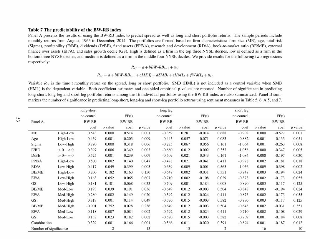
Table 7 The predictability of the BW-RB indexPanel A presents the results of using the BW-RB index to predict spread as well as long and short portfolio returns. The sample periods includemonthly returns from August, 1965 to December, 2014. The portfolios are formed based on firm characteristics: firm size (ME), age, total risk(Sigma), profitability (E/BE), dividends (D/BE), fixed assets (PPE/A), research and development (RD/A), book-to-market ratio (BE/ME), externalfinance over assets (EF/A), and sales growth decile (GS). High is defined as a firm in the top three NYSE deciles, low is defined as a firm in thebottom three NYSE deciles, and medium is defined as a firm in the middle four NYSE deciles. We provide results for the following two regressionsrespectively:

Ri,t = a+bBW -RBt−1 +ui,t

Ri,t = a+bBW -RBt−1 + cMKTt +dSMBt + eHMLt + fWMLt +ui,t

Variable Ri,t is the time t monthly return on the spread, long or short portfolio. SMB (HML) is not included as a control variable when SMB(HML) is the dependent variable. Both coefficient estimates and one-sided empirical p-values are reported. Number of significance in predictinglong-short, long-leg and short-leg portfolio returns among the 16 individual portfolios using the BW-RB index are also summarized. Panel B sum-marizes the number of significance in predicting long-short, long-leg and short-leg portfolio returns using sentiment measures in Table 5, 6, A.5, and 7.

long-short long leg short legno control FF(t) no control FF(t) no control FF(t)

Panel A. BW-RB BW-RB BW-RB BW-RB BW-RB BW-RBcoef p value coef p value coef p value coef p value coef p value coef p value

ME High-Low 0.543 0.000 0.514 0.001 -0.359 0.281 -0.014 0.688 -0.902 0.000 -0.527 0.001Age High-Low 0.439 0.001 0.203 0.009 -0.443 0.057 0.071 0.083 -0.882 0.001 -0.133 0.051Sigma Low-High 0.790 0.000 0.318 0.006 -0.275 0.067 0.056 0.161 -1.064 0.001 -0.263 0.008E/BE > 0−< 0 0.397 0.006 0.349 0.003 -0.660 0.012 0.002 0.353 -1.058 0.000 -0.347 0.005D/BE > 0−= 0 0.575 0.001 0.239 0.009 -0.509 0.021 0.043 0.161 -1.084 0.000 -0.197 0.030PPE/A High-Low 0.500 0.002 0.140 0.047 -0.478 0.021 -0.041 0.411 -0.978 0.002 -0.181 0.018RD/A Low-High 0.417 0.049 0.399 0.003 -0.639 0.009 0.001 0.563 -1.056 0.009 -0.398 0.002BE/ME High-Low 0.200 0.182 0.163 0.150 -0.648 0.002 -0.031 0.351 -0.848 0.003 -0.194 0.024EF/A Low-High 0.163 0.052 0.065 0.607 -0.710 0.002 -0.108 0.029 -0.873 0.002 -0.173 0.055GS Low-High 0.181 0.101 -0.068 0.033 -0.709 0.001 -0.184 0.008 -0.890 0.003 -0.117 0.125BE/ME Med-Low 0.198 0.039 0.191 0.036 -0.649 0.012 -0.003 0.504 -0.848 0.003 -0.194 0.024EF/A Med-High 0.280 0.002 0.149 0.020 -0.592 0.012 -0.024 0.411 -0.873 0.002 -0.173 0.055GS Med-High 0.319 0.001 0.114 0.049 -0.570 0.015 -0.003 0.582 -0.890 0.003 -0.117 0.125BE/ME Med-High -0.001 0.752 0.028 0.236 -0.649 0.012 -0.003 0.504 -0.648 0.002 -0.031 0.351EF/A Med-Low 0.118 0.007 0.084 0.002 -0.592 0.012 -0.024 0.411 -0.710 0.002 -0.108 0.029GS Med-Low 0.138 0.023 0.182 0.002 -0.570 0.015 -0.003 0.582 -0.709 0.001 -0.184 0.008Combination 0.329 0.001 0.166 0.001 -0.566 0.011 -0.020 0.391 -0.894 0.001 -0.187 0.012Number of significance 12 13 13 2 16 10

53

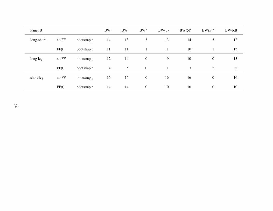
Panel B BW BW′ BW′′ BW(5) BW(5)′ BW(5)′′ BW-RB

long-short no FF bootstrap p 14 13 3 13 14 5 12

FF(t) bootstrap p 11 11 1 11 10 1 13

long leg no FF bootstrap p 12 14 0 9 10 0 13

FF(t) bootstrap p 4 5 0 1 3 2 2

short leg no FF bootstrap p 16 16 0 16 16 0 16

FF(t) bootstrap p 14 14 0 10 10 0 10

54

Table 8 Robustness checksThis table presents results for robustness checks. In Panel A, we present the predictability of the robust sentiment indices constructed from PLS onalternative purged sentiment proxies. Panel B reports the number of significance for the regression residuals of the BW index, where the residual isderived from decomposing the BW index directly from different sets of variables. Panel C reports number of significance for the regression residualsof the BW(5) index, where the residual is derived from decomposing BW(5) index directly from different sets of variables. We use the PCA methodto construct the residual sentiment index from the purged sentiment proxies and report the number of significance in Panel D. Significance is basedon one-sided p-value.

long-short long leg short leg16 spread portfolios 16 spread portfolios 16 spread portfolios

Panel A. BW-RB BW-RB BW-RBno FF 14 variables 12 13 16

alternative 14 variables 12 14 16135 variables 10 15 16

FF(t) 14 variables 13 2 10alternative 14 variables 12 2 12135 variables 7 2 12

Panel B. BW′′ BW′′ BW′′

no FF 14 variables 3 0 0alternative 14 variables 6 0 0135 variables 0 0 0

FF(t) 14 variables 1 0 0alternative 14 variables 1 0 0135 variables 1 0 0

Panel C. BW(5)′′ BW(5)′′ BW(5)′′

no FF 14 variables 5 0 0alternative 14 variables 8 0 2135 variables 0 0 0

FF(t) 14 variables 1 2 0alternative 14 variables 4 0 0135 variables 0 2 0

Panel D. PCAres PCAres PCAresFF(t) 14 variables 2 0 2

alternative 14 variables 4 0 3135 variables 3 2 0

55

Table 9 Comparing the BW-RB index with four survey-based sentiment indicesThis table compares the BW-RB index with four survey-based sentiment indices. Panel A presents resultsfor the time-series regressions of the BW-RB index as the dependent variable and four survey-basedsentiment indices as the explanatory variable. Panel B presents results for the time-series regressions oflong-short combination portfolio returns (L-S combine) as dependent variable and different sentimentmeasures as explanatory variable, controlling for the Fama French three factors and Carhart’s momentumfactor. Panel C presents results for the time-series regressions of long-leg combination portfolio returns (Lcombine) and different sentiment measures as the explanatory variable, controlling for four factors. PanelD presents results for the time-series regressions of short-leg combination portfolio returns (S combine)and different sentiment measures as the explanatory variable, controlling for four factors. AIres is theresidual component of anxious index. ICSres is the residual component in Michigan University consumersentiment. AAIIres is the residual component of individual investor sentiment. GAres is the residualcomponent in the rescaled Gallup survey data. Four BW-RB indices are constructed with the sample lengthadjusted to the data length of the four survey-based sentiment indices accordingly, and are compared withthe four survey-based sentiment indices in corresponding sample periods. The regression coefficients andNewey-West t-statistics are reported.

56

(1) (2) (3) (4) (5) (6) (7) (8) (9) (10) (11) (12)Panel A. BW-RBAIres 0.10

[2.29]ICSres -0.05

[-1.17]AAIIres -0.07

[-1.27]GAres 0.05

[0.65]Panel B. L-S combineAIres -0.03 -0.05

[-0.58] [-0.91]ICSres 0.02 0.04

[0.31] [0.55]AAIIres -0.14 -0.12

[-1.63] [-1.38]GAres 0.00 -0.02

[-0.01] [-0.18]BW-RB(AI) 0.19 0.19

[3.68] [3.73]BW-RB(ICS) 0.27 0.28

[4.13] [4.11]BW-RB(AAII) 0.32 0.32

[3.16] [3.06]BW-RB(GA) 0.41 0.41

[3.31] [3.32]

Panel C. L combineAIres 0.03 0.03

[0.57] [0.62]ICSres 0.02 0.02

[0.32] [0.29]AAIIres 0.10 0.10

[1.56] [1.54]GAres 0.22 0.22

[2.42] [2.37]BW-RB(AI) -0.03 -0.03

[-0.56] [-0.62]BW-RB(ICS) -0.03 -0.02

[-0.41] [-0.39]BW-RB(AAII) -0.01 0.00

[-0.11] [-0.02]BW-RB(GA) 0.06 0.05

[0.56] [0.48]

Panel D. S combineAIres 0.06 0.08

[0.73] [0.97]ICSres 0.00 -0.02

[-0.03] [-0.19]AAIIres 0.24 0.22

[1.92] [1.75]GAres 0.22 0.24

[1.34] [1.44]BW-RB(AI) -0.21 -0.22

[-2.87] [-2.90]BW-RB(ICS) -0.30 -0.30

[-2.84] [-2.82]BW-RB(AAII) -0.33 -0.32

[-2.06] [-1.94]BW-RB(GA) -0.34 -0.35

[-1.75] [-1.82]

57

Table 10 Comparing the BW index with four survey-based sentiment indicesThis table compares the BW index with four survey-based sentiment indices. Panel A presents resultsfor the time-series regressions of long-short combination portfolio returns (L-S combine) as dependentvariable and different sentiment measures as the explanatory variable, controlling for the Fama French threefactors and Carhart’s momentum factor. Panel B presents results for the time-series regressions of long-legcombination portfolio returns (L combine) and different sentiment measures as the explanatory variable,controlling for four factors. Panel C presents results for the time-series regressions of short-leg combinationportfolio returns (S combine) and different sentiment measures as explanatory variable, controlling forfour factors. AIres is residual component of anxious index. ICSres is residual component in MichiganUniversity consumer sentiment. AAIIres is the residual component of individual investor sentiment. GAresis the residual component in the rescaled Gallup survey data. The sample length of the four BW-RB indicesare adjusted to the data length of the four survey-based sentiment indices accordingly, and the four BW-RBindices are compared with the four survey-based sentiment indices in corresponding sample periods. Theregression coefficients and Newey-West t-statistics are reported.

58

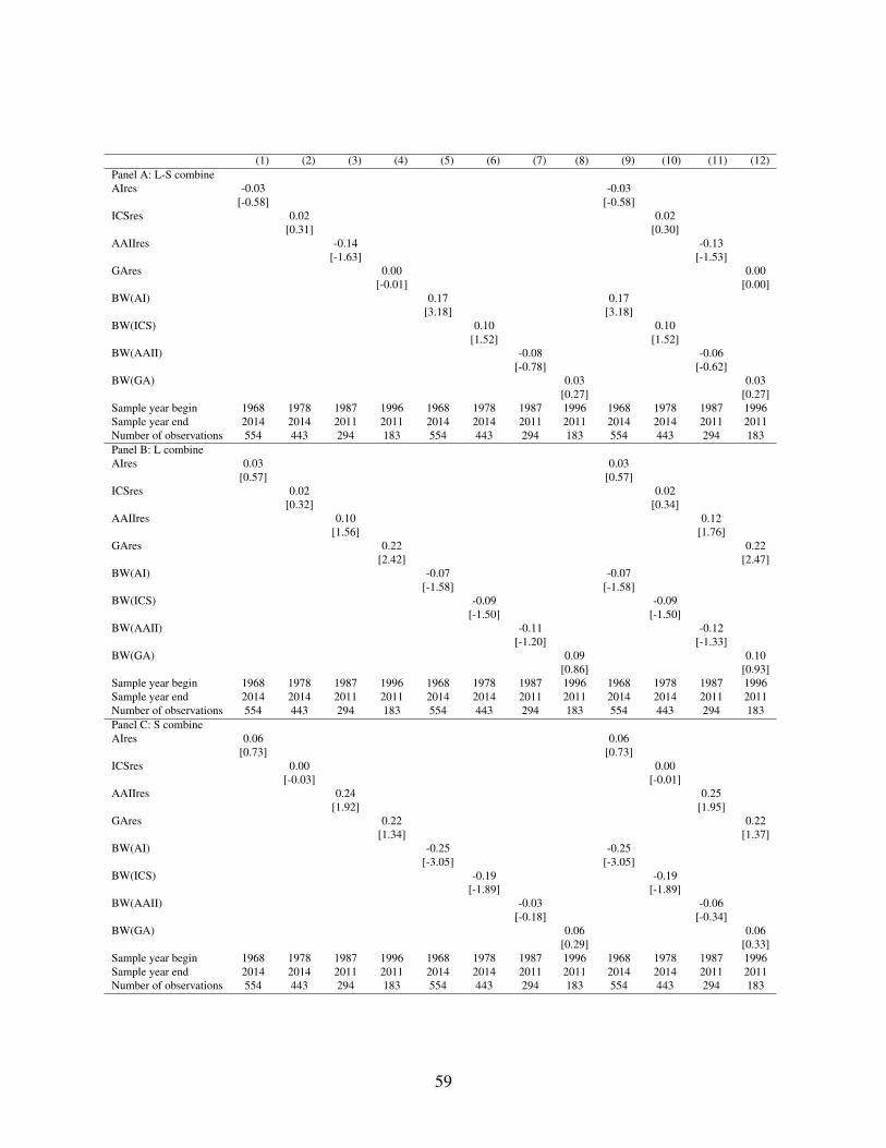
(1) (2) (3) (4) (5) (6) (7) (8) (9) (10) (11) (12)Panel A: L-S combineAIres -0.03 -0.03

[-0.58] [-0.58]ICSres 0.02 0.02

[0.31] [0.30]AAIIres -0.14 -0.13

[-1.63] [-1.53]GAres 0.00 0.00

[-0.01] [0.00]BW(AI) 0.17 0.17

[3.18] [3.18]BW(ICS) 0.10 0.10

[1.52] [1.52]BW(AAII) -0.08 -0.06

[-0.78] [-0.62]BW(GA) 0.03 0.03

[0.27] [0.27]Sample year begin 1968 1978 1987 1996 1968 1978 1987 1996 1968 1978 1987 1996Sample year end 2014 2014 2011 2011 2014 2014 2011 2011 2014 2014 2011 2011Number of observations 554 443 294 183 554 443 294 183 554 443 294 183Panel B: L combineAIres 0.03 0.03

[0.57] [0.57]ICSres 0.02 0.02

[0.32] [0.34]AAIIres 0.10 0.12

[1.56] [1.76]GAres 0.22 0.22

[2.42] [2.47]BW(AI) -0.07 -0.07

[-1.58] [-1.58]BW(ICS) -0.09 -0.09

[-1.50] [-1.50]BW(AAII) -0.11 -0.12

[-1.20] [-1.33]BW(GA) 0.09 0.10

[0.86] [0.93]Sample year begin 1968 1978 1987 1996 1968 1978 1987 1996 1968 1978 1987 1996Sample year end 2014 2014 2011 2011 2014 2014 2011 2011 2014 2014 2011 2011Number of observations 554 443 294 183 554 443 294 183 554 443 294 183Panel C: S combineAIres 0.06 0.06

[0.73] [0.73]ICSres 0.00 0.00

[-0.03] [-0.01]AAIIres 0.24 0.25

[1.92] [1.95]GAres 0.22 0.22

[1.34] [1.37]BW(AI) -0.25 -0.25

[-3.05] [-3.05]BW(ICS) -0.19 -0.19

[-1.89] [-1.89]BW(AAII) -0.03 -0.06

[-0.18] [-0.34]BW(GA) 0.06 0.06

[0.29] [0.33]Sample year begin 1968 1978 1987 1996 1968 1978 1987 1996 1968 1978 1987 1996Sample year end 2014 2014 2011 2011 2014 2014 2011 2011 2014 2014 2011 2011Number of observations 554 443 294 183 554 443 294 183 554 443 294 183

59

Table 11 Comparing the BW(5) index with four survey-based sentiment indicesThis table compares the BW(5)index with four survey-based sentiment indices. Panel A presents resultsfor the time-series regressions of long-short combination portfolio returns (L-S combine) as the dependentvariable and different sentiment measures as the explanatory variable, controlling for the Fama French threefactors and Carhart’s momentum factor. Panel B presents results for the time-series regressions of long-legcombination portfolio returns (L combine) and different sentiment measures as the explanatory variable,controlling for four factors. Panel C presents results for the time-series regressions of short-leg combinationportfolio returns (S combine) and different sentiment measures as the explanatory variable, controllingfor four factors. AIres is the residual component of anxious index. ICSres is the residual componentin Michigan University consumer sentiment. AAIIres is the residual component of individual investorsentiment. GAres is the residual component in the rescaled Gallup survey data. Four BW(5) indices areconstructed for which the sample length is adjusted to the data length of the four survey-based sentimentindices accordingly, and compared with the four survey-based sentiment indices in corresponding sampleperiods. The regression coefficients and Newey-West t-statistics are reported.

60

(1) (2) (3) (4) (5) (6) (7) (8) (9) (10) (11) (12)Panel A: L-S combineAIres -0.03 -0.03

[-0.58] [-0.53]ICSres 0.02 0.02

[0.31] [0.32]AAIIres -0.14 -0.14

[-1.63] [-1.58]GAres 0.00 0.00

[-0.01] [0.00]BW5(AI) 0.16 0.16

[2.85] [2.85]BW5(ICS) 0.07 0.07

[0.90] [0.90]BW5(AAII) -0.05 -0.03

[-0.55] [-0.39]BW5(GA) 0.04 0.04

[0.31] [0.31]Sample year begin 1968 1978 1987 1996 1968 1978 1987 1996 1968 1978 1987 1996Sample year end 2014 2014 2011 2011 2014 2014 2011 2011 2014 2014 2011 2011Number of observations 554 443 294 183 554 443 294 183 554 443 294 183Panel B: L combineAIres 0.03 0.03

[0.57] [0.55]ICSres 0.02 0.02

[0.32] [0.31]AAIIres 0.10 0.11

[1.56] [1.75]GAres 0.22 0.22

[2.42] [2.45]BW5(AI) -0.06 -0.06

[-1.24] [-1.23]BW5(ICS) -0.08 -0.08

[-1.28] [-1.27]BW5(AAII) -0.11 -0.12

[-1.44] [-1.58]BW5(GA) 0.09 0.09

[0.89] [0.95]Sample year begin 1968 1978 1987 1996 1968 1978 1987 1996 1968 1978 1987 1996Sample year end 2014 2014 2011 2011 2014 2014 2011 2011 2014 2014 2011 2011Number of observations 554 443 294 183 554 443 294 183 554 443 294 183Panel C: S combineAIres 0.06 0.06

[0.73] [0.67]ICSres 0.00 0.00

[-0.03] [-0.04]AAIIres 0.24 0.25

[1.92] [1.98]GAres 0.22 0.22

[1.34] [1.36]BW5(AI) -0.21 -0.21

[-2.59] [-2.59]BW5(ICS) -0.15 -0.15

[-1.34] [-1.34]BW5(AAII) -0.06 -0.09

[-0.43] [-0.60]BW5(GA) 0.05 0.06

[0.26] [0.30]Sample year begin 1968 1978 1987 1996 1968 1978 1987 1996 1968 1978 1987 1996Sample year end 2014 2014 2011 2011 2014 2014 2011 2011 2014 2014 2011 2011Number of observations 554 443 294 183 554 443 294 183 554 443 294 183

61

Table 12 Sentiment and mutual fund flowsThis table reports regression results of mutual fund flow on sentiment variables. We estimate time-seriesregressions of the form

Flowt = a+bSENTt + cControlt + et

Flowt = a+bSENTt−1 + cControlt−1 + et

where the dependent variable Flow measures the inflows into equity-oriented mutual funds scaled bythe aggregate capitalization of the U.S. stock market in each month; SENT represents the BW-RB indexfor specifications (1) and (2), the BW index for specifications (3) and (4), and the BW(5) index forspecifications (5) and (6); control variables are the 14 representative fundamental variables includingthe first principle components from seven categories of macroeconomic variables ( output and income,labour market, housing, consumption, orders and inventories, money and credit, exchange rates, inflation),consumption-to-wealth ratio, GDP growth, three-month Treasury Bill rate, default spread, term spread,dividend yield and zero return ratio. Specifications (1), (3) and (5) provide relations between fund flow andcontemporaneous sentiment variables while specifications (2), (4), and (6) summarize relations betweenfund flow and lagged sentiment variables. The regression slopes, Newey-West t -statistics, as well as R2sare reported. The sample period is from January, 1984 to December 2014.

(1) (2) (3) (4) (5) (6)BW-RB(t) 0.16

[2.23]BW-RB(t-1) 0.14

[1.82]BW(t) -0.17

[-2.14]BW(t-1) -0.17

[-1.95]BW5(t) 0.03

[0.38]BW5(t-1) 0.03

[0.37]Sample year begin 1984 1984 1984 1984 1984 1984Sample year end 2014 2014 2014 2014 2014 2014Number of observations 371 371 371 371 371 371R2(%) 40.35 31.15 39.96 31.03 39.15 30.27

62

Table 13 Anomalies during periods of high and low investor sentimentThis table presents average benchmark-adjusted returns following high and low levels of investor sentiment, as classified based on the median level oftwo investor sentiment measures: BW (5)⊥ in Panel A and BW-RB in Panel B. The average returns in high- and low- sentiment periods are estimatesof aH and aL in the regression

Ri,t = aHdH,t +aLdL,t +bMKTt + cSMBt +dHMLt + εi,t

where dH,t and dL,t are dummy variables indicating high- and low- sentiment periods, and Ri,t is the excess return in month t on either the long leg,the short leg, or the difference. Also reported are returns on a strategy that equally combines the strategies available within a given month. ForDistress anomaly, data begins in Novermber, 1973, Total accruals anomaly begins in June 1966, Return on assets starts from Novermber 1971,and the sample period for other anomalies is from August, 1965 to December 2014. All t-statistics are based on the heteroskedasticity-consistentstandard errors of White (1980).

63

Anomaly Long leg Short leg Long-shortPanel A: High Low High High Low High High Low HighBW (5)⊥ sentiment sentiment - low sentiment sentiment - low sentiment sentiment - lowO-score 0.28 0.13 0.14 -0.48 -0.01 -0.47 0.75 0.14 0.61

2.88 1.45 1.11 -4.38 -0.07 -3.15 5.01 0.90 2.92Distress 0.36 0.11 0.25 -1.38 -0.46 -0.92 1.74 0.57 1.17

2.16 0.88 1.15 -6.00 -2.05 -2.97 5.03 1.92 2.58Net stock issues 0.24 0.09 0.16 -0.59 -0.42 -0.17 0.83 0.50 0.33

3.77 1.38 1.75 -5.84 -3.72 -1.17 6.16 3.67 1.74Composite equity issues 0.10 0.10 0.00 -0.52 -0.26 -0.25 0.62 0.36 0.26

0.98 0.96 0.03 -5.19 -2.54 -1.79 4.06 2.45 1.25Total accruals -0.02 0.42 -0.44 -0.22 -0.36 0.14 0.20 0.78 -0.59

-0.15 3.03 -2.38 -1.87 -2.67 0.83 1.09 3.98 -2.27Net operating assets 0.28 -0.03 0.31 -0.61 -0.22 -0.40 0.90 0.19 0.71

2.55 -0.25 1.98 -6.15 -1.88 -2.62 5.17 1.07 2.89Momentum 0.54 0.63 -0.09 -1.17 -0.83 -0.34 1.72 1.46 0.25

3.02 3.48 -0.34 -4.42 -3.72 -0.97 4.31 3.99 0.46Gross profitability 0.57 0.13 0.44 -0.29 -0.36 0.07 0.86 0.49 0.37

4.87 1.20 2.79 -2.33 -2.31 0.35 5.08 2.66 1.53Asset growth 0.03 0.11 -0.08 -0.39 -0.07 -0.32 0.42 0.18 0.24

0.24 1.03 -0.56 -3.78 -0.64 -2.22 2.55 1.16 1.07Return on assets 0.47 0.17 0.30 -0.76 -0.34 -0.42 1.23 0.51 0.73

4.89 1.75 2.22 -4.52 -1.76 -1.74 5.77 2.22 2.40Investment-to-assets 0.15 0.18 -0.03 -0.39 -0.18 -0.22 0.54 0.36 0.18

1.58 1.73 -0.24 -3.00 -1.26 -1.17 3.43 2.17 0.82Combination 0.27 0.20 0.07 -0.60 -0.32 -0.29 0.87 0.51 0.36

5.55 4.88 1.12 -8.43 -4.26 -2.85 8.59 5.53 2.62

64

Anomaly Long leg Short leg Long-shortPanel B: High Low High High Low High High Low HighBW-RB sentiment sentiment - low sentiment sentiment - low sentiment sentiment - lowO-score 0.20 0.21 -0.01 -0.35 -0.13 -0.21 0.55 0.34 0.21

2.08 2.28 -0.05 -3.27 -1.23 -1.44 3.53 2.22 0.97Distress 0.31 0.17 0.14 -1.28 -0.59 -0.69 1.60 0.77 0.83

1.87 1.38 0.67 -5.29 -2.80 -2.20 4.47 2.71 1.85Net stock issues 0.22 0.10 0.12 -0.63 -0.37 -0.26 0.86 0.48 0.38

3.48 1.66 1.32 -5.88 -3.53 -1.75 6.22 3.54 1.98Composite equity issues 0.17 0.03 0.14 -0.53 -0.25 -0.28 0.70 0.28 0.42

1.64 0.29 0.97 -4.97 -2.58 -2.00 4.46 1.92 2.02Total accruals 0.19 0.21 -0.01 -0.37 -0.21 -0.16 0.56 0.42 0.14

1.31 1.64 -0.07 -2.80 -1.72 -0.89 2.72 2.42 0.54Net operating assets 0.25 0.00 0.25 -0.56 -0.28 -0.28 0.81 0.27 0.53

2.23 -0.01 1.61 -5.03 -2.55 -1.84 4.41 1.62 2.17Momentum 0.54 0.63 -0.09 -1.16 -0.84 -0.32 1.70 1.48 0.23

2.89 3.65 -0.34 -4.48 -3.84 -0.94 4.21 4.20 0.43Gross profitability 0.40 0.30 0.10 -0.39 -0.26 -0.14 0.79 0.56 0.24

3.25 2.79 0.62 -2.69 -1.88 -0.72 4.26 3.26 0.95Asset growth 0.25 -0.11 0.36 -0.35 -0.11 -0.24 0.60 -0.01 0.61

2.21 -1.08 2.40 -3.28 -1.04 -1.68 3.82 -0.04 2.75Return on assets 0.39 0.26 0.13 -0.80 -0.30 -0.50 1.18 0.56 0.63

3.98 2.65 0.91 -4.48 -1.62 -2.03 5.14 2.57 2.01Investment-to-assets 0.21 0.12 0.09 -0.31 -0.26 -0.05 0.52 0.38 0.14

2.20 1.16 0.64 -2.28 -1.89 -0.27 3.29 2.29 0.63Combination 0.29 0.18 0.10 -0.59 -0.32 -0.27 0.88 0.50 0.37

5.98 4.45 1.67 -7.73 -4.73 -2.66 8.31 5.78 2.73

65

Online Appendix

“Robust Investor Sentiment Indices”

A.1 A full list of the 109 macroeconomic variables

We use the information of 109 macroeconomic variables that are categorized into seven groups, includ-

ing: (1) output and income, (2) labour market, (3) housing, (4) consumption, orders and inventories, (5)

money and credit, (6) exchange rates, and (7) inflation. A full data list for the macroenomic variables is

provided below. For the detailed description and construction of the variables, please refer to McCracken

and Ng (2015).

Group (1) has 17 variables related to output and income, including: Real Personal Income, Real personal

income ex transfer receipts, IP Index, IP: Final Products and Nonindustrial Supplies, IP: Final Products

(Market Group), IP: Consumer Goods, IP: Durable Consumer Goods, IP: Nondurable Consumer Goods,

IP: Business Equipment, IP: Materials, IP: Durable Materials, IP: Nondurable Materials, IP: Manufacturing

(SIC), IP: Residential Utilities, IP: Fuels, ISM Manufacturing: Production Index, Capacity Utilization:

Manufacturing.

Group (2) has 32 variables related to labour market, including: Help-Wanted Index for United States,

Ratio of Help Wanted/No. Unemployed, Civilian Labor Force, Civilian Employment, Civilian Unemploy-

ment Rate, Average Duration of Unemployment (Weeks), Civilians Unemployed - Less Than 5 Weeks,

Civilians Unemployed for 5-14 Weeks, Civilians Unemployed - 15 Weeks, Civilians Unemployed for 15-

26 Weeks, Civilians Unemployed for 27 Weeks and Over Initial Claims, All Employees: Total nonfarm,

All Employees: Goods-Producing Industries, All Employees: Mining and Logging, All Employees: Con-

struction, All Employees: Manufacturing, All Employees: Durable goods, All Employees: Nondurable

goods, All Employees: Service-Providing Industries, All Employees: Trade, Transportation, All Employ-

ees: Wholesale Trade, All Employees: Retail Trade, All Employees: Financial Activities All Employees:

Government, Average Weekly Hours: Goods-Producing, Average Weekly Overtime Hours: Manufactur-

ing, Average Weekly Hours: Manufacturing, ISM Manufacturing: Employment Index, Average Hourly

Earnings: Goods-Producing, Average Hourly Earnings: Construction, Average Hourly Earnings: Manufac-

turing.

66

Group (3) has 10 variables related to housing, including: Housing Starts(Total New Privately Owned),

Housing Starts (Northeast), Housing Starts (Midwest), Housing Starts (South), Housing Starts (West), New

Private Housing Permits (SAAR), New Private Housing Permits(Northeast), New Private Housing Permits

(Midwest), New Private Housing Permits(South), New Private Housing Permits(West).

Group (4) has 14 variables related to consumption, orders and inventories, including: Real personal

consumption expenditures, Real Manu. and Trade Industries Sales, Retail and Food Services Sales, ISM:

PMI Composite Index, ISM: New Orders Index, ISM: Supplier Deliveries Index, ISM: Inventories Index,

New Orders for Consumer Goods, New Orders for Durable Goods, New Orders for Nondefense Capital

Goods, Unfilled Orders for Durable Goods, Total Business Inventories, Total Business: Inventories to Sales

Ratio, Consumer Sentiment Index.

Group (5) has 14 variables related to money and credit, including: M1 Money Stock, M2 Money Stock,

Real M2 Money Stock, St. Louis Adjusted Monetary Base, Total Reserves of Depository Institutions, Re-

serves Of Depository Institutions, Commercial and Industrial Loans, Real Estate Loans at All Commercial

Banks Total Nonrevolving Credit, Nonrevolving consumer credit to Personal Income, MZM Money Stock,

Consumer Motor Vehicle Loans Outstanding, Total Consumer Loans and Leases Outstanding, Securities in

Bank Credit at All Commercial Banks.

Group (6) has 5 variables related to exchange rates, including: Trade Weighted U.S. Dollar Index: Major

Currencies, Switzerland / U.S. Foreign Exchange Rate, Japan / U.S. Foreign Exchange Rate, U.S. / U.K.

Foreign Exchange Rate, Canada / U.S. Foreign Exchange Rate.

Group (7) has 21 variables related to inflation, including: PPI: Finished Goods, PPI: Finished Con-

sumer Goods, PPI: Intermediate Materials, PPI: Crude Materials, Crude Oil and Spliced WTI, PPI: Metals

and metal products, ISM Manufacturing: Prices Index, CPI: All Items, CPI: Apparel, CPI: Transportation,

CPI: Medical Care, CPI: Commodities, CPI: Durables, CPI: Services, CPI: All Items Less Food, CPI: All

items less shelter, CPI: All items less medical care, Personal Consumption Expenditure: Chain Index, Per-

sonal Consumption Expenditure: Durable goods, Personal Consumption Expenditure: Nondurable goods,

Personal Consumption Expenditure: Services.

67

A.2 Decomposition regression results for each individual sentiment proxy

We present the decomposition regression results for each individual sentiment proxy in this section. As

shown in the below table A.2, for each decomposition, R-squares range from approximately 30% to over

50% except the first-day returns of IPOs (RIPO) with a relatively low R-square, indicating a considerable

portion of the variation in each sentiment proxy can be explained by economic fundamentals. Specifically,

for close-end fund discount rate (CEFD) and dividend premium (PDND), a large proportion of R-square

is due to the contribution of three-month treasury bill rate, term spread and liquidity risk. Moreover, the

contribution of the fundamental variables varies in different sentiment proxies. For example, housing related

variables and liquidity risk factor contribute most for share turnover (TURN), while labour market related

variables show up with high explanatory power alongside with three-month treasury bill rate and term spread

for number of IPOs (NIPO).

68

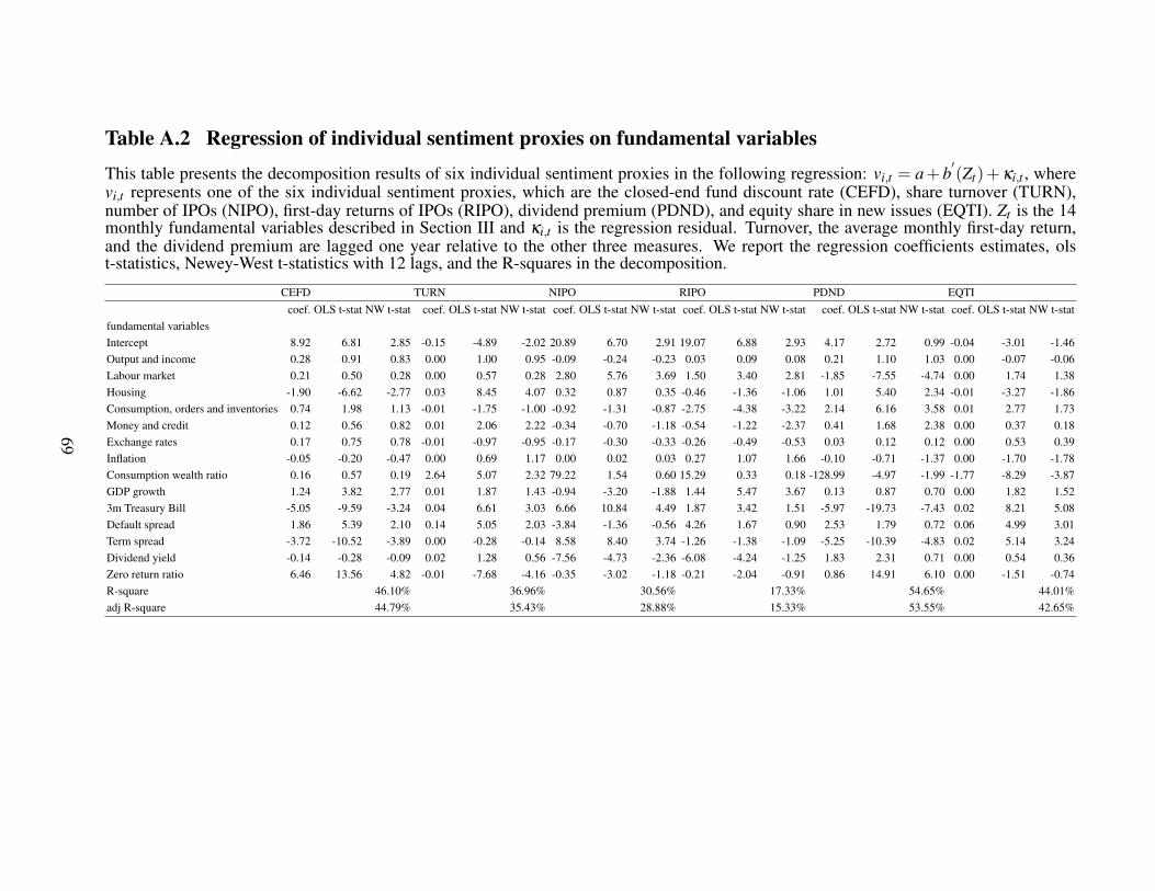
Table A.2 Regression of individual sentiment proxies on fundamental variables

This table presents the decomposition results of six individual sentiment proxies in the following regression: vi,t = a+b′(Zt)+κi,t , where

vi,t represents one of the six individual sentiment proxies, which are the closed-end fund discount rate (CEFD), share turnover (TURN),number of IPOs (NIPO), first-day returns of IPOs (RIPO), dividend premium (PDND), and equity share in new issues (EQTI). Zt is the 14monthly fundamental variables described in Section III and κi,t is the regression residual. Turnover, the average monthly first-day return,and the dividend premium are lagged one year relative to the other three measures. We report the regression coefficients estimates, olst-statistics, Newey-West t-statistics with 12 lags, and the R-squares in the decomposition.

CEFD TURN NIPO RIPO PDND EQTIcoef. OLS t-stat NW t-stat coef. OLS t-stat NW t-stat coef. OLS t-stat NW t-stat coef. OLS t-stat NW t-stat coef. OLS t-stat NW t-stat coef. OLS t-stat NW t-stat

fundamental variablesIntercept 8.92 6.81 2.85 -0.15 -4.89 -2.02 20.89 6.70 2.91 19.07 6.88 2.93 4.17 2.72 0.99 -0.04 -3.01 -1.46Output and income 0.28 0.91 0.83 0.00 1.00 0.95 -0.09 -0.24 -0.23 0.03 0.09 0.08 0.21 1.10 1.03 0.00 -0.07 -0.06Labour market 0.21 0.50 0.28 0.00 0.57 0.28 2.80 5.76 3.69 1.50 3.40 2.81 -1.85 -7.55 -4.74 0.00 1.74 1.38Housing -1.90 -6.62 -2.77 0.03 8.45 4.07 0.32 0.87 0.35 -0.46 -1.36 -1.06 1.01 5.40 2.34 -0.01 -3.27 -1.86Consumption, orders and inventories 0.74 1.98 1.13 -0.01 -1.75 -1.00 -0.92 -1.31 -0.87 -2.75 -4.38 -3.22 2.14 6.16 3.58 0.01 2.77 1.73Money and credit 0.12 0.56 0.82 0.01 2.06 2.22 -0.34 -0.70 -1.18 -0.54 -1.22 -2.37 0.41 1.68 2.38 0.00 0.37 0.18Exchange rates 0.17 0.75 0.78 -0.01 -0.97 -0.95 -0.17 -0.30 -0.33 -0.26 -0.49 -0.53 0.03 0.12 0.12 0.00 0.53 0.39Inflation -0.05 -0.20 -0.47 0.00 0.69 1.17 0.00 0.02 0.03 0.27 1.07 1.66 -0.10 -0.71 -1.37 0.00 -1.70 -1.78Consumption wealth ratio 0.16 0.57 0.19 2.64 5.07 2.32 79.22 1.54 0.60 15.29 0.33 0.18 -128.99 -4.97 -1.99 -1.77 -8.29 -3.87GDP growth 1.24 3.82 2.77 0.01 1.87 1.43 -0.94 -3.20 -1.88 1.44 5.47 3.67 0.13 0.87 0.70 0.00 1.82 1.523m Treasury Bill -5.05 -9.59 -3.24 0.04 6.61 3.03 6.66 10.84 4.49 1.87 3.42 1.51 -5.97 -19.73 -7.43 0.02 8.21 5.08Default spread 1.86 5.39 2.10 0.14 5.05 2.03 -3.84 -1.36 -0.56 4.26 1.67 0.90 2.53 1.79 0.72 0.06 4.99 3.01Term spread -3.72 -10.52 -3.89 0.00 -0.28 -0.14 8.58 8.40 3.74 -1.26 -1.38 -1.09 -5.25 -10.39 -4.83 0.02 5.14 3.24Dividend yield -0.14 -0.28 -0.09 0.02 1.28 0.56 -7.56 -4.73 -2.36 -6.08 -4.24 -1.25 1.83 2.31 0.71 0.00 0.54 0.36Zero return ratio 6.46 13.56 4.82 -0.01 -7.68 -4.16 -0.35 -3.02 -1.18 -0.21 -2.04 -0.91 0.86 14.91 6.10 0.00 -1.51 -0.74R-square 46.10% 36.96% 30.56% 17.33% 54.65% 44.01%adj R-square 44.79% 35.43% 28.88% 15.33% 53.55% 42.65%

69

A.3 Description of characteristics that are used to construct the 16 testing

portfolios

• Firm size (ME): Measured as the log value of price times shares outstanding.

• Age: Constructed as the number of years since the firm’s first appearance on CRSP.

• Total risk (sigma): Measured as the annual standard deviation in monthly returns for the 12 months

ending in June of year t.

• Profitability (E/BE): Earnings to book equity, defined as earnings (E) divided by the book value of

equity (BE). Earnings (E) is defined as income before extraordinary items plus income statement

deferred taxes minus preferred dividends. Book equity (BE) is defined as shareholders equity plus

balance sheet deferred taxes.

• Dividends (D/BE): Dividends to book equity, measured as dividends (D) divided by the book value of

equity (BE). Dividends (D) are equal to dividends per share at the ex date times shares outstanding.

Book equity (BE) is defined as shareholders equity plus balance sheet deferred taxes.

• Fixed assets (PPE/A): Measured as the ratio of property, plant, and equipment to total assets.

• Research and development (RD/A): Measured as the ratio of research and development expense to

total assets.

• Book-to-market ratio (BE/ME): Measured as the ratio of book equity to market equity.

• External finance over assets (EF/A): Measured as external finance (EF) divided by assets. External

finance (EF) is equal to the change in assets minus the change in retained earnings.

• Sales growth decile (GS): Measured as the decile of firm’s sales growth in the prior year relative to

NYSE firms’ decile breakpoints, while sales growth is the change in net sales divided by prior-year

net sales.

70

A.4 Reasons why the NYSE turnover (TURN) indicator may still be a rele-

vant sentiment indicator

First, the given reason on Jeffrey Wurgler’s website to drop TURN is: ”Turnover does not mean what it

once did, given the explosion of institutional high-frequency trading and the migration of trading to a variety

of venues.” The relocations of trading across various venues may reduce but is unlikely to completely destroy

the power of the TURN as a sentiment indicator. This is because that the TURN indicator is based on the

NYSE turnover. Given that the NYSE is still a dominating trading hub, its turnover is likely to be highly

correlated the aggregated total trading activities.

Second, the sharp increase in institutional high-frequency trading is likely to be driven by the increase

in arbitrating or speculating but not (independent) hedging. Hedging is costly and not likely to make money

by itself. Therefore, to institutional traders, hedging is normally used to reduce the risk exposure resulting

from arbitrating or speculating positions. Without a sharp increase in arbitrating or speculating, it is unlikely

to have a stand alone sharp increase in hedging. As for the arbitrating, it is essentially driven by mispricing,

which should be highly correlated with the investor sentiment. As for the speculating, it is largely driven

by non-fundamental information or technical analysis, which is also related to investor sentiment. Even the

speculating may be partially based on fundamental analysis or economic variables, the BW-RB index should

be able to purge the TURN indicator of the fundamental information. Thus the residual part of the TURN

indicator should still be related to sentiment.

In addition, institutional high-frequency trading for arbitrating or speculating purposes can also be the

result of insider information. Now, institutional trading is no longer relevant to sentiment. The inside in-

formation is also not able to be purged from the TURN indicator given that the insider information is not

publicly available. Therefore, if the increase of the sentiment is unrelated to trading based on insider infor-

mation, which outweighs such sentiment related trading reflected in the recent sharp increase of institutional

high-frequency trading, the TURN indicator can become a weaker sentiment indicator. Nevertheless, this

is unlikely to be the case. Given the improved corporate governance and market regulations environments

(e.g., the Regulation Fair Disclosure 2000), we should expect to have a smaller and not a larger amount of

insider information available for institutional traders in recent years. Therefore, the weakened power of the

TURN variable as a sentiment indicator in recent years is unlikely to be driven by an increase in sentiment

71

unrelated to institutional trading based on insider information.

Moreover, the recent decline in the power of the TURN indicator may be a result of temporary reasons.

For example, the recent sharp increase of institutional high-frequency trading may be potentially due to a

sharp decrease in trading frictions (both the explicit and the hidden ones). Since the decrease in trading

frictions cannot be significantly related to investor sentiment, the link between the TURN indicator and the

sentiment may be sharply weakened. However, this may be only a temporary phenomenon. When the impact

of trading frictions is smoothed out over time, the once weakened link may be quickly restored. Basically, we

may have recently had a regime shift for the TURN indicator to switch from a strong sentiment indicator to

a weak one. However, the TURN indicator may undergo another regime shift to return as a strong sentiment

indicator in the future once the weakened link has been restored. This type of regime shifts appear to have

occurred at other places. For example, the size effect has been documented to disappear for some years yet

but returns again in later years.

72

A.5 The predictability of BW(5)′ and BW(5)′′

For the newly proposed five-indicator sentiment index BW(5), we follow the decomposition steps in the

section IV.B to remove the fundamental factors directly. First, we remove six macroeconomic variables and

obtain the regression residual BW(5)′. In Panel A of Table A.5, we report the regression results of using

BW(5)′ as the investor sentiment proxy to predict cross-section returns. We find that the predictability of

BW(5)′ on portfolio returns is comparable with the BW index and BW′.

Second, to alleviate the concern that BW(5)′ fails to remove the fundamental information thoroughly, we

further remove seven first-principle components extracted from 109 macroeconomic variables and another

seven business cycle related variables that we have explicitly explained in Section III. We report the pre-

dictability results of using BW(5)′′ as the investor sentiment proxy in Table A.5 Panel B. In the regressions

without control factors, BW(5)′′ significantly forecasts 5 of the 16 long-short return spreads and 0 of the

16 long- or short-leg returns. After controlling for the Fama French three factors and Carhart’s momentum

factor, BW(5)′′ significantly forecasts merely one out of the 16 spread returns, 2 of 16 long-leg return, and

none of the 16 short-leg returns. After removing comprehensive economic fundamental information, the

diminishing predictive power of the BW(5) index in cross-section returns is similar to the BW index, which

reinforces our concerns about whether the BW index is a sentiment index.

73

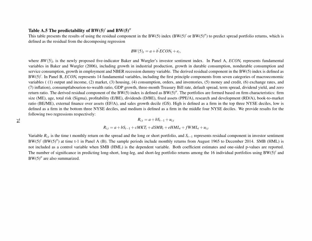
Table A.5 The predictability of BW(5)′ and BW(5)′′This table presents the results of using the residual component in the BW(5) index (BW(5)′ or BW(5)′′) to predict spread portfolio returns, which isdefined as the residual from the decomposing regression

BW (5)t = a+b′ECONt + et ,

where BW (5)t is the newly proposed five-indicator Baker and Wurgler’s investor sentiment index. In Panel A, ECONt represents fundamentalvariables in Baker and Wurgler (2006), including growth in industrial production, growth in durable consumption, nondurable consumption andservice consumption, growth in employment and NBER recession dummy variable. The derived residual component in the BW(5) index is defined asBW(5)′. In Panel B, ECONt represents 14 fundamental variables, including the first principle components from seven categories of macroeconomicvariables ( (1) output and income, (2) market, (3) housing, (4) consumption, orders, and inventories, (5) money and credit, (6) exchange rates, and(7) inflation), consumptlabourion-to-wealth ratio, GDP growth, three-month Treasury Bill rate, default spread, term spread, dividend yield, and zeroreturn ratio. The derived residual component of the BW(5) index is defined as BW(5)′′. The portfolios are formed based on firm characteristics: firmsize (ME), age, total risk (Sigma), profitability (E/BE), dividends (D/BE), fixed assets (PPE/A), research and development (RD/A), book-to-marketratio (BE/ME), external finance over assets (EF/A), and sales growth decile (GS). High is defined as a firm in the top three NYSE deciles, low isdefined as a firm in the bottom three NYSE deciles, and medium is defined as a firm in the middle four NYSE deciles. We provide results for thefollowing two regressions respectively:

Ri,t = a+bSt−1 +ui,t

Ri,t = a+bSt−1 + cMKTt +dSMBt + eHMLt + fWMLt +ui,t

Variable Ri,t is the time t monthly return on the spread and the long or short portfolio, and St−1 represents residual component in investor sentimentBW(5)′ (BW(5)′′) at time t-1 in Panel A (B). The sample periods include monthly returns from August 1965 to December 2014. SMB (HML) isnot included as a control variable when SMB (HML) is the dependent variable. Both coefficient estimates and one-sided p-values are reported.The number of significance in predicting long-short, long-leg, and short-leg portfolio returns among the 16 individual portfolios using BW(5)′ andBW(5)′′ are also summarized.

74

long-short long leg short legno control FF(t) no control FF(t) no control FF(t)

Panel A. BW(5)′ BW(5)′ BW(5)′ BW(5)′ BW(5)′ BW(5)′

coef p value coef p value coef p value coef p value coef p value coef p valueME High-Low 0.610 0.000 0.586 0.000 -0.214 0.195 0.063 0.054 -0.824 0.001 -0.523 0.001Age High-Low 0.473 0.001 0.171 0.032 -0.312 0.067 0.011 0.423 -0.785 0.003 -0.159 0.023Sigma Low-High 0.948 0.000 0.459 0.000 -0.084 0.311 0.163 0.003 -1.032 0.001 -0.296 0.001E/BE > 0−< 0 0.745 0.000 0.424 0.002 -0.485 0.018 -0.015 0.464 -1.230 0.000 -0.439 0.002D/BE > 0−= 0 0.759 0.000 0.398 0.000 -0.334 0.057 0.034 0.241 -1.093 0.000 -0.364 0.000PPE/A High-Low 0.422 0.006 0.115 0.171 -0.428 0.018 -0.056 0.229 -0.850 0.003 -0.171 0.033RD/A Low-High 0.387 0.027 0.104 0.278 -0.553 0.011 -0.071 0.207 -0.940 0.004 -0.176 0.136BE/ME High-Low 0.157 0.178 0.040 0.480 -0.574 0.007 -0.069 0.205 -0.731 0.007 -0.108 0.168EF/A Low-High 0.172 0.026 0.089 0.093 -0.611 0.006 -0.076 0.143 -0.783 0.004 -0.165 0.019GS Low-High 0.082 0.240 0.037 0.379 -0.682 0.004 -0.119 0.089 -0.764 0.004 -0.156 0.013BE/ME Med-Low 0.245 0.014 0.137 0.099 -0.486 0.021 0.028 0.274 -0.731 0.007 -0.108 0.168EF/A Med-High 0.382 0.000 0.221 0.000 -0.400 0.039 0.056 0.080 -0.783 0.004 -0.165 0.019GS Med-High 0.400 0.000 0.228 0.000 -0.364 0.050 0.072 0.040 -0.764 0.004 -0.156 0.013BE/ME Med-High 0.087 0.034 0.097 0.021 -0.486 0.021 0.028 0.274 -0.574 0.007 -0.069 0.205EF/A Med-Low 0.211 0.000 0.133 0.000 -0.400 0.039 0.056 0.080 -0.611 0.006 -0.076 0.143GS Med-Low 0.318 0.000 0.191 0.004 -0.364 0.050 0.072 0.040 -0.682 0.004 -0.119 0.089Combination 0.400 0.000 0.191 0.000 -0.424 0.028 0.008 0.359 -0.823 0.002 -0.183 0.010Number of significance 14 10 10 3 16 10

75

Panel B. BW(5)′′ BW(5)′′ BW(5)′′ BW(5)′′ BW(5)′′ BW(5)′′

coef p value coef p value coef p value coef p value coef p value coef p valueME High-Low 0.293 0.016 0.267 0.057 -0.037 0.739 0.030 0.079 -0.330 0.075 -0.237 0.095Age High-Low 0.281 0.051 0.085 0.258 -0.047 0.264 0.047 0.301 -0.327 0.147 -0.038 0.356Sigma Low-High 0.468 0.028 0.192 0.085 0.031 0.469 0.101 0.055 -0.437 0.125 -0.091 0.233E/BE > 0−< 0 0.203 0.127 0.029 0.383 -0.151 0.197 0.044 0.289 -0.354 0.128 0.015 0.544D/BE > 0−= 0 0.398 0.019 0.172 0.080 -0.055 0.254 0.068 0.232 -0.453 0.075 -0.104 0.150PPE/A High-Low 0.242 0.078 0.043 0.383 -0.104 0.325 0.022 0.378 -0.346 0.176 -0.021 0.473RD/A Low-High 0.279 0.122 0.052 0.524 -0.125 0.352 0.060 0.207 -0.404 0.256 0.008 0.271BE/ME High-Low 0.094 0.355 0.044 0.531 -0.178 0.226 0.060 0.339 -0.272 0.267 0.016 0.295EF/A Low-High 0.137 0.061 0.078 0.116 -0.170 0.265 0.055 0.216 -0.307 0.192 -0.024 0.454GS Low-High 0.123 0.057 0.079 0.113 -0.202 0.251 0.037 0.300 -0.325 0.148 -0.042 0.293BE/ME Med-Low 0.122 0.181 0.070 0.363 -0.150 0.337 0.086 0.116 -0.272 0.267 0.016 0.295EF/A Med-High 0.174 0.037 0.079 0.108 -0.134 0.339 0.055 0.113 -0.307 0.192 -0.024 0.454GS Med-High 0.236 0.006 0.127 0.011 -0.088 0.426 0.085 0.041 -0.325 0.148 -0.042 0.293BE/ME Med-High 0.028 0.231 0.025 0.208 -0.150 0.337 0.086 0.116 -0.178 0.226 0.060 0.339EF/A Med-Low 0.037 0.223 0.000 0.463 -0.134 0.339 0.055 0.113 -0.170 0.265 0.055 0.216GS Med-Low 0.113 0.094 0.048 0.255 -0.088 0.426 0.085 0.041 -0.202 0.251 0.037 0.300Combination 0.202 0.027 0.068 0.133 -0.111 0.336 0.054 0.119 -0.313 0.166 -0.015 0.468Number of significance 5 1 0 2 0 0

76

A.6 Validation of the BW-RB index

In this section, we further apply two tests to validate the BW-RB index: earnings annoucment returns,

and non-fundamental component in Tobin’s Q.

A.6.1 BW-RB and earnings announcement returns

The first validation test involves earnings announcement returns. La Porta, Lakonishok, Shleifer and

Vishny (1997) argue that earnings announcement returns reflect investors’ correction of their errors in earn-

ings’ expectation. Since investors tend to make errors in the firms that are difficult to value, we expect that

earnings announcement returns would be lower for difficult- to-value firms after a high sentiment period.

For each quarterly earnings announcement, we calculate the three-day cumulative abnormal return around

the report date (CAR(-1,1)). The portfolios are constructed the same as in Section III.C. We define firms

in the top three NYSE deciles as high, the bottom three NYSE deciles as low, and remaining middle four

NYSE deciles as medium, based on firm characteristics: firm size (ME), age, total risk (Sigma), fixed assets

(PPE/A), research and development (RD/A), book-to-market ratio (BE/ME), external finance over assets

(EF/A), and sales growth decile (GS) respectively. Portfolios formed on profitability (E/BE) and dividend

(D/BE) are divided into two groups: profitable/unprofitable firms, and dividend payers and non-payers.

We average CAR (-1,1) within each characteristic portfolio per month, and run the following regression to

examine the relationship between the BW-RB index and earnings announcement returns:

CARi,t = a+b∗BW -RBt−1 + εi,t , (10)

where CARi,t is the average of CARs around quarterly earnings announcements within each characteristic

portfolio in month t, and BW -RBt−1 is the BW-RB index in month t-1.34

Table A.3 reports the coefficient estimates for each characteristic portfolio using the BW-RB index

from column 3 to column 5. In general, the coefficients of the BW-RB index are negative, indicating

that earnings announcement effects are lower following high sentiment periods. Moreover, the earnings

announcement effects are much stronger for uncertain or difficult-to-value stocks that are usually more

34To eliminate the noise from individual stocks, we require that the number of CARs used to calculateCARXit=H/M/L,t in month t is larger than a critical value of 15.

77

sensitive to sentiment: heteroskedasticity-robust t-statistics of the coefficients of the BW-RB index are larger

for small stocks, young stocks, high volatility stocks, non-dividend paying stocks, and also stocks with low

PPE and high R&D. Particularly, the stronger earnings announcement effects for stocks with low PPE and

high R&D are consistent with our findings in Section IV.C that the BW-RB index is more significant for

portfolio returns based on firms with less tangible assets.

We also summarize the coefficient estimates based on the BW index from column 6 to column 8 in

Table A.3 for comparison. Among all cases, the difference between high and low based on ME, RD/A, and

D/BE is larger for the BW-RB index than for the BW index. For BE/ME, EF/A, and GS, we compare the

difference between high and medium and between low and medium: for BE/ME, the difference between

high and medium and between low and medium is larger for BW-RB than for BW; for GS, the difference is

similar for the BW-RB index and the BW index; for EF/A, only the difference between low and medium are

smaller for the BW-RB index than the BW index while the difference between high and medium are similar

for the BW-RB index and the BW index. Thus, regarding 5 of the total 16 cases: ME, RD/A, D/BE, and

BE/ME (H-M; M-L), the difference is larger for BW-RB than for BW. Only for two case− EF/A ()M-L)

and E/BE−the difference is smaller for the BW-RB index than for the BW index. Regarding the remaining

nine cases, the difference are similar for the BW-RB index and the BW index. Therefore, the BW-RB index

is comparable to, or better than, the BW index in predicting CAR.

Overall, the results support the view that investors are more likely to suffer errors in earnings expecta-

tions for stocks that are more sensitive to sentiment, which further validates the BW-RB index as a proxy

for investor sentiment with behavioral explanation.

78

Table A.6.1 Earnings announcement returns and the BW-RB indexThis table reports the results of the regression of average monthly earnings announcement returns on laggedthe BW-RB index:

CARXi,t=H/M/L,t = a+b∗BW -RBt−1 + εi,t

where CARXi,t=H/M/L,t is the average of CARs around quarterly earnings announcements of each character-istic portfolio in month t, BW -RBt−1 is the BW-RB index in month t-1. The portfolios are formed based onfirm characteristics: firm size (ME), age, total risk (Sigma), profitability (E/BE), dividends (D/BE), fixedassets (PPE/A), research and development (RD/A), book-to-market ratio (BE/ME), external finance overassets (EF/A), and sales growth decile (GS). Portfolios formed on earnings are divided into two groups:unprofitable firms and profiable firms. Portfolios formed on dividends are divided into two groups: nondividend paying firms and dividend paying firms. For other firm characteristics, high (H) is defined as afirm in the top three NYSE deciles, low (L) is defined as a firm in the bottom three NYSE deciles, andmedium (M) is defined as a firm in the middle four NYSE deciles. We report the regression slopes andheteroskedasticity-robust t-statistics for each characteristic portfolio based on the BW-RB index and theBW index respectively. The sample period is from January 1973 to December 2014.

BW-RB BWL M H L M H

ME coef -0.11 -0.06 0.00 -0.11 -0.04 -0.05t-stat -2.67 -1.82 -0.09 -2.71 -1.09 -1.61

Age coef -0.07 -0.09 -0.06 -0.08 -0.06 -0.06t-stat -1.87 -2.50 -1.43 -2.17 -1.65 -1.76

Sigma coef 0.01 -0.07 -0.13 0.02 -0.08 -0.11t-stat 0.47 -2.24 -2.62 0.62 -2.29 -2.42

PPE/A coef -0.11 -0.06 -0.05 -0.11 -0.07 -0.04t-stat -2.60 -1.69 -1.28 -2.52 -1.86 -1.15

RD/A coef -0.01 -0.17 -0.14 -0.12 -0.18 -0.12t-stat -0.23 -3.04 -2.52 -2.17 -3.49 -2.24

BE/ME coef -0.06 -0.10 -0.08 -0.05 -0.07 -0.08t-stat -1.66 -3.10 -1.76 -1.25 -2.20 -1.93

EF/A coef -0.07 -0.07 -0.10 -0.03 -0.07 -0.11t-stat -1.74 -2.22 -2.41 -0.80 -2.20 -2.76

GS coef -0.10 -0.06 -0.08 -0.09 -0.08 -0.04t-stat -2.25 -2.04 -2.13 -2.00 -2.81 -1.28

<= 0 > 0 <= 0 > 0E/BE coef -0.14 -0.07 -0.17 -0.05

t-stat -1.97 -2.74 -2.17 -1.82D/BE coef -0.14 -0.05 -0.11 -0.06

t-stat -3.02 -1.68 -2.07 -2.32

79

A.6.2 Non-fundamental component in Tobin’s Q

The second validation test involves a non-fundamental component of Tobin’s Q. We follow Rhodes-

Kropf, Robinson and Viswanathan (2005) and decompose Tobin’s Q into fundamental component and non-

fundamental component, which captures firm’s growth opportunities and mispricing in Tobin’s Q respec-

tively. We use the mispricing part in Tobin’s Q (mQ) as a proxy for investor sentiment and compare its

predictability on portfolio returns.

Panel A of Table A.6.2 shows the regression of the BW-RB index on the contemporaneous mispricing

component in Tobin’s Q (mQ). The relation between BW-RB and mQ is positive and significant, with a

Newey-West t-statistics of 4.90, indicating that the BW-RB index captures relevant mispricing information

in Tobins Q. In Panel B of Table A.4, we investigate the predictability of mQ on long-short, long- and short-

leg combined portfolio returns respectively. We find that mQ fails to significantly forecast portfolio returns

in the next month. Panel C further test the forecasting ability of BW-RB on portfolio returns controlling for

mQ. The results show that BW-RB significantly forecasts combined portfolio returns while the predictability

of mQ is weak, suggesting BW-RB better captures investor sentiment in mispricing than the mispricing part

in Tobin’s Q.

80

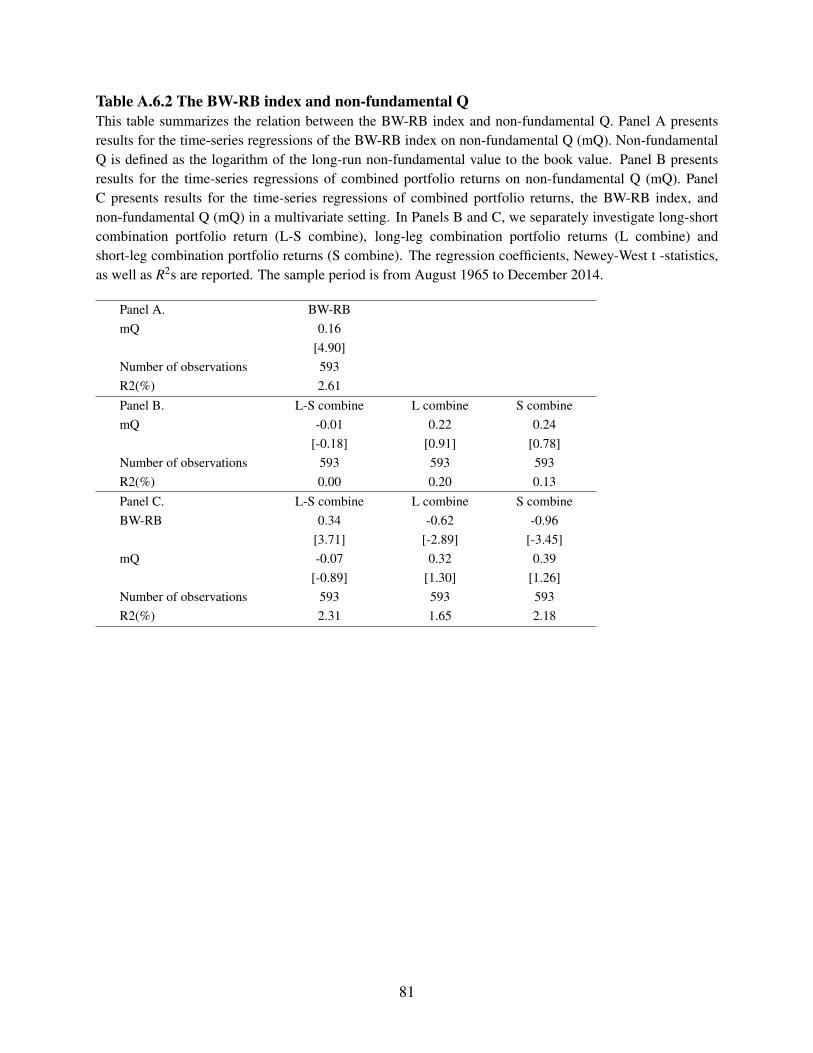
Table A.6.2 The BW-RB index and non-fundamental QThis table summarizes the relation between the BW-RB index and non-fundamental Q. Panel A presentsresults for the time-series regressions of the BW-RB index on non-fundamental Q (mQ). Non-fundamentalQ is defined as the logarithm of the long-run non-fundamental value to the book value. Panel B presentsresults for the time-series regressions of combined portfolio returns on non-fundamental Q (mQ). PanelC presents results for the time-series regressions of combined portfolio returns, the BW-RB index, andnon-fundamental Q (mQ) in a multivariate setting. In Panels B and C, we separately investigate long-shortcombination portfolio return (L-S combine), long-leg combination portfolio returns (L combine) andshort-leg combination portfolio returns (S combine). The regression coefficients, Newey-West t -statistics,as well as R2s are reported. The sample period is from August 1965 to December 2014.

Panel A. BW-RBmQ 0.16

[4.90]Number of observations 593R2(%) 2.61Panel B. L-S combine L combine S combinemQ -0.01 0.22 0.24

[-0.18] [0.91] [0.78]Number of observations 593 593 593R2(%) 0.00 0.20 0.13Panel C. L-S combine L combine S combineBW-RB 0.34 -0.62 -0.96

[3.71] [-2.89] [-3.45]mQ -0.07 0.32 0.39

[-0.89] [1.30] [1.26]Number of observations 593 593 593R2(%) 2.31 1.65 2.18

81

A.7 Economic explanations

In this section, we investigate the economic driving force of the predictability of the BW-RB index, i.e.,

whether the predictive power of the BW-RB index stems from time variations in cash flows or discount rates.

Stocks are priced by discounting their future cash flow at a discount rate. Campbell and Shiller (1988b)

develop a convenient framework to analyze cash flow and discount rate, in which they establish a loglinear

approximate identity

rt+1 ≈ k+ρ pt+1 +(1−ρ)dt+1− pt , (11)

where rt+1 ≡ log(Pt+1 +Dt+1)− log(Pt), and ρ is a positive log-linearization constant. P denotes price,

D denotes dividend, and lowercase letters indicate the log transforms. Following Cochrane (2011), we

rearrange the approximate identity and derive

rt+1 ≈ k+∆dt+1−ρd pt+1 +d pt , (12)

where ∆dt+1 is the log dividend growth rate and d pt+1 is the log dividend price ratio. (12) implies that

the predictability of the BW-RB index on portfolio returns should stem either from cash flow channel or

discount rate channel. In this section, we explore through which channel the BW-RB index influences

portfolio returns by testing the predictability of the BW-RB index on future cash flow and discount rate.

Dividend growth is widely used as the proxy for cash flow in the previous asset pricing literatures (e.g.,

Campbell and Shiller (1988b), Cochrane ( 2008, 2011)), therefore we use dividend growth of the portfolio

as our cash flow proxy. Cochrane (2008, 2011) documents that the variation from discount rate is largely

driven by dividend price ratio, hence, we use dividend price ratio of the portfolio as the proxy for discount

rate. We focus on the short legs of the portfolios on which our sentiment index has a more pronounced effect

and use the following bivariate predictive regression model:

yt+1 = α +βBW -RBt +ϕd pt +ωt+1,y = ∆dt+1 or d pt+1 (13)

where ∆dt+1 is the annual log dividend growth rate on the short leg of the portfolio from July of year t to

June of year t+1, d pt+1 is the log dividend price ratio on the short leg of the portfolio in June of year t+1,

and BW -RBt is the BW-RB index in June of year t. Following the literature, we use annual data to avoid

82

spurious predictability arising from seasonality.

Table A.6 reports the estimation results for the predictability regression. In Panel A, ∆dt+1 and d pt+1

are constructed based on the short leg of the combined portfolio and used as the dependent variables respec-

tively. The estimated coefficient of BW -RBt for ∆dt+1 is -6.65 with t-statistics of -3.38, while the estimated

coefficient of BW -RBt for d pt+1 is close to zero and insignificant. The lagged dividend price ratio d pt has

strong forecasting power for future dividend price ratio d pt+1 with a mean reverting coefficient of around

0.9, whereas its forecasting ability for dividend growth rate is much weaker, consistent with Cochrane (2008,

2011), showing dividend price ratio capture time variation in discount rate.

In Panel B, ∆dt+1 and d pt+1 are constructed based on the short legs of individual characteristics portfo-

lios respectively. We find consistent results as in Panel A that BW -RBt significantly and negatively predicts

∆dt+1 while BW -RBt has no significant predictability under conventional 5% significance level for d pt+1 in

portfolios formed on various firm characteristics, such as age, volatility, dividend, tangibility, etc. The nega-

tive coefficients of BW -RBt for ∆dt+1 (β ) further confirms the negative coefficients of BW -RBt for short-leg

portfolio returns rt+1 documented in Section IV.

Since dividend growth rate and dividend price ratio represent cash flow channel and discount rate chan-

nel separately, the results indicate that the negative predictability of the BW-RB indexfor short legs of port-

folio returns comes from the cash flow channel, i.e, the higher investor sentiment leads to the overoptimistic

opinion towards future cash flow, and when the realized cash flow is lower than the investors’ expectation,

the future return decreases.

83

Table A.7 Economic explanationThis table reports estimation results for the bivariate predictive regressions

yt+1 = α +βBW -RBt +ϕd pt +ωt+1,y = ∆dt+1 or d pt+1

where d pt+1 is the annual log dividend-price ratio for each short leg of characteristics based portfolios,∆dt+1 is the annual log dividend-growth rate for each short leg of characteristics based portfolios from Julyof year t to June of year t+1 (in percentage), BW -RBt is the BW-RB index in June of year t. ∆dt+1 and d pt+1

are constructed following Cochrane (2008, 2011). We report the regression slopes, Newey-West t-statistics,as well as R2s. The sample period is from August, 1965 to December, 2014.

yt+1 β t-stat ϕ t-stat R2(%)Panel A. Combination portfoliod p 0.04 1.51 0.89 14.54 82.78∆d(%) -6.65 -3.38 -12.82 -2.47 27.93Panel B. Individual portfolioMEd p 0.05 2.02 0.92 19.78 87.8∆d(%) -5.40 -2.38 -9.82 -2.09 14.6aged p 0.04 1.44 0.92 19.93 88.2∆d(%) -7.88 -3.49 -8.95 -1.85 18.7sigmad p 0.06 1.67 0.91 16.92 87.3∆d(%) -6.61 -2.01 -11.87 -2.24 13.4D/BEd p -0.02 -0.30 0.68 7.06 50.2∆d(%) -17.30 -2.90 -36.82 -3.92 28.2PPE/Ad p 0.05 1.78 0.92 20.28 88.8∆d(%) -8.02 -2.67 -11.72 -2.04 9.4RD/Ad p 0.02 0.59 0.91 16.95 86.4∆d(%) -7.73 -2.52 -10.07 -1.94 15.7BE/MEd p -0.01 -0.18 0.91 19.36 87.7∆d(%) -13.62 -3.90 -13.77 -2.90 34.0

84