robust inventory control under demand and lead time

Robust inventory control under demand and lead time uncertainty

Authors: Andreas Thorsen & Tao Yao

The final publication is available at Springer via http://dx.doi.org/10.1007/s10479-015-2084-1.

Thorsen, Andreas, and Tao Yao. "Robust inventory control under demand and lead time uncertainty." Annals of Operations Research (December 2015): 1-30. DOI: 10.1007/s10479-015-2084-1

Made available through Montana State University’s ScholarWorks scholarworks.montana.edu

http://scholarworks.montana.edu/

http://scholarworks.montana.edu/

https://dx.doi.org/10.1007/s10479-015-2084-1

https://dx.doi.org/10.1007/s10479-015-2084-1

Annals of Operations Research manuscript No.(will be inserted by the editor)

Robust Inventory Control Under Demand and LeadTime Uncertainty

Andreas Thorsen · Tao Yao

Received: date / Accepted: date

Abstract In this paper a general methodology is proposed based on robust op-timization for an inventory control problem subject to uncertain demands anduncertain lead times. Several lead time uncertainty sets are proposed based on thebudget uncertainty set, and a set based on the central limit theorem (CLT). Robustoptimization models are developed for a periodic review, finite horizon inventorycontrol problem subject to uncertain demands and uncertain lead times. We de-velop an approach based on Benders’ decomposition to compute optimal robust(i.e., best worst-case) policy parameters. The proposed approach does not assumedistributional knowledge, makes no assumption regarding order crossovers, and istractable in a practical sense. Comparing the new approach to an epigraph re-formulation method, we demonstrate that the epigraph reformulation approach isoverly conservative even when costs are stationary. The approach is benchmarkedagainst the sample average approximation (SAA) method. Computational resultsindicate that the approach provides more stable and robust solutions compared toSAA in terms of standard deviation and worst-case solution, especially when therealized distribution is different than the sampled distribution.

Keywords robust optimization · inventory control · lead time uncertainty ·demand uncertainty

1 Introduction

In supply chain systems where supply and demand are uncertain it is importantto calculate optimal inventory ordering policies to reduce costs while maintaininghigh customer service levels. Future demand may be difficult to predict and lead

A. ThorsenJake Jabs College of Business & Entrepreneurship, Montana State University, 302 Jabs Hall,Bozeman MT 59717, USAE-mail: [email protected]

T. YaoHarold and Inge Marcus Department of Industrial and Manufacturing Engineering, Pennsyl-vania State University, 310 Leonhard Building, University Park, PA 16801, USA

1 2 3 4 5 6 7 8 9 10 11 12 13 14 15 16 17 18 19 20 21 22 23 24 25 26 27 28 29 30 31 32 33 34 35 36 37 38 39 40 41 42 43 44 45 46 47 48 49 50 51 52 53 54 55 56 57 58 59 60 61 62 63 64 65

2 Andreas Thorsen, Tao Yao

times may be uncertain because of reasons such as variable processing times at thesupplier or transportation delays. There is a rich body of literature dealing withinventory control under demand uncertainty, and there is a much smaller body ofliterature concerning inventory control under lead time uncertainty.

Formulating an inventory control problem under lead time uncertainty is dif-ficult because of a phenomenon called “order crossover”, which is the arrival oforders in a sequence different than the sequence they were placed (He et al. 1998).Order crossover distorts the lead time distribution which complicates the analysis.

Many results in the literature rely on the assumption that order crossovers donot occur and that orders are independent and identically distributed (i.i.d) but thei.i.d. assumption is contradictory and this assumption will not always hold (Hayyaet al. 2008). In fact, crossovers are likely to occur more frequently in the futurefor several reasons. Riezebos (2006) examines the changes in modern supply chainmanagement and concludes that some of the reasons for the increasing frequencyof order crossovers are “a reduction of the time between issuing an order, moresuppliers, more frequent ordering, larger distances between supplier and firm, moresupply options with different lead time consequences, and dependable but morevariable total lead times.”

Many policies have been proposed for inventory problems under stochasticdemand and constant lead time. For example, the basestock policy (also calledthe “order-up-to” policy), which involves placing an order for S − x units whenthe inventory position x falls below S, was initially proven to be optimal forserial supply chains when demand follows a known distribution by Clark andScarf (1960) and it has been shown to be optimal for more general systems sincethen (the reader is referred to Zipkin (2000) where many extensions can be found).Due to its simplicity, the basestock policy has been widely adopted in industry.Stochastic dynamic programming (SDP) is often used to compute the optimalpolicy parameters. However, SDP is intractable for large problems as it suffersfrom “the curse of dimensionality” (Zipkin 2000). Another downside of SDP isthat for many real world problems the true probability distribution may not beknown.

An alternate approach to handle uncertainty is using uncertainty sets in a ro-bust optimization (RO) framework. RO has been studied in supply chain problemsshowing promising computational results for problems under demand uncertainty(e.g., see Ben-Tal et al. 2005, Bertsimas and Thiele 2006, Bienstock and Ozbay2008). In these papers robust optimization is cast as a distribution-free approachthat does not take into account information about probability distributions oravailable data on past parameter realizations. In the above papers involving de-mand uncertainty, the supply-side is assumed to be deterministic and order leadtimes are assumed to be either zero or fixed. There have been far fewer RO pa-pers on supply uncertainty, and they mainly deal with yield uncertainty and rawmaterial supply uncertainty. These papers are discussed in Section 2.

In this paper a general methodology is proposed based on robust optimizationfor an inventory control problem subject to uncertain lead times as well as uncer-tain demand. Prior research has examined this problem using stochastic dynamicprogramming under the assumption of no order crossovers and full distributionalknowledge of lead times. Important characteristics of the proposed approach isthat it does not assume distributional knowledge, it makes no assumption regard-

1 2 3 4 5 6 7 8 9 10 11 12 13 14 15 16 17 18 19 20 21 22 23 24 25 26 27 28 29 30 31 32 33 34 35 36 37 38 39 40 41 42 43 44 45 46 47 48 49 50 51 52 53 54 55 56 57 58 59 60 61 62 63 64 65

Robust Inventory Control Under Demand and Lead Time Uncertainty 3

ing order crossovers, and it is tractable in a practical sense. The contributions ofthis paper are as follows:

– We propose a RO model for an inventory control problem under uncertaindemand and lead time. While there are several results in the literature forrobust inventory control under uncertain demand, this is the first that jointlyconsiders uncertain demand and uncertain lead time from an RO perspective.We present a new budget-type lead time uncertainty set as well as a CLT-basedlead time uncertainty set.

– We use a Benders’ decomposition approach to handle robust optimization prob-lems under CLT-based uncertainty sets. The Benders’ approach has been shownto produce less conservative solutions than the alternative method in the lit-erature of robustifying the epigraph formulation of inventory control prob-lems (Gorissen and Den Hertog 2013).

– Using a computational study for an inventory control problem we compare theperformance of several uncertainty set modeling approaches (budget and CLT).This is the first attempt to compare the performance of these uncertainty setsin this setting. The numerical results indicate that our approach compares wellto Sample Average Approximation (SAA).

In Section 2 we discuss relevant literature. In Section 3 we describe the ROmethodology including several modeling approaches for uncertainty sets. We presentthe robust inventory problem in Section 4. The solution approach is described inSection 5. In Section 6, we extend the approach to involve more general lead timeuncertainty sets. Computational results follow in Section 7. Finally, concludingremarks are made in Section 8.

2 Literature Review

2.1 Robust Optimization

Robust optimization (RO) is a methodology used to solve optimization problemsthat involve uncertainty in the parameter values without considering probabil-ity distributions. Typically, the objective of robust optimization is to find the bestworst-case solution over an uncertainty set specified by the modeler. The set-basedrobust optimization is significantly different than the scenario-based robust opti-mization developed in Mulvey et al. (1995). In scenario-based robust optimizationa finite set of scenarios are considered and the solution may violate the constraintsinvolving these scenarios; a penalty function is included in the objective to ac-count for the violations. For the remainder of the paper, when we write RO weare referring to set-based robust optimization.

The downside of the RO approach is that the solutions are usually more conser-vative than solutions generated using complementary methods such as stochasticoptimization, although the conservatism can be controlled somewhat by the designof the uncertainty sets (Ben-Tal et al. 2009). The main advantage of robust opti-mization over alternative methods (e.g., stochastic dynamic programming) is thatthe approach is computationally tractable (i.e., polynomially solvable) for manycases. For example, a robust linear program with an ellipsoidal uncertainty set canbe reformulated as a second-order cone problem which is tractably solvable using

1 2 3 4 5 6 7 8 9 10 11 12 13 14 15 16 17 18 19 20 21 22 23 24 25 26 27 28 29 30 31 32 33 34 35 36 37 38 39 40 41 42 43 44 45 46 47 48 49 50 51 52 53 54 55 56 57 58 59 60 61 62 63 64 65


interior-point methods (Ben-Tal and Nemirovski 1999), and a robust linear pro-gram with polyhedral uncertainty can be reformulated as a (slightly larger) linearprogram (Bertsimas and Sim 2004). However, these reformulations are possiblebecause of an approach using duality to handle subproblems involving uncertainparameters in the constraints of the optimization problems. Therefore, uncertaintysets which are row-wise dependent are considered. We refer the reader to Gabrelet al. (2014), a recent survey paper on applications of robust optimization, whichdescribes this reformulation approach. When uncertainty is dependent within thecolumns (as is the case for the lead time models presented in this paper), thisreformulation tactic does not work (see section Differences with Bertsimas andSim’s Approach in Minoux (2009)).

Widely cited as the first paper considering RO, Soyster (1973) considers amodel using column-wise uncertainty sets for linear programming problems wherethe uncertainty sets are ellipsoids. The author shows that if each column of theconstraint matrix belongs to a convex set, then solving the problem amounts tosolving a linear program with the matrix coefficients equal to their worst-casevalue. While this is beautifully simple, it is also an extremely conservative mod-eling approach. The formulation by Soyster was largely dismissed for many yearsbecause of its extreme conservatism. Ben-Tal and Nemirovski (1999) formulatea robust optimization model for a linear program where the uncertainty is row-wise and ellipsoidal. They show that their model can be reformulated as a conicquadratic program. Bertsimas and Sim (2004) formulate an alternative robustoptimization model using a row-wise and polyhedral uncertainty set in which abudget parameter is used to control the conservatism of the model. The main ad-vantage of this method is that the robust counterpart of a linear program underbudget uncertainty remains a (slightly larger) linear program, while the robustcounterpart of a linear program under the Ben-Tal and Nemirovski uncertaintyset becomes a conic quadratic program. Bandi and Berstimas (2012) develop anew approach to constructing uncertainty sets using conclusions from probabil-ity. The approach incorporates distributional information which can be estimatedwith historical data and the CLT is assumed to hold which is used to constructthe uncertainty sets.

The models discussed above are static models where all decisions are “hereand now” decisions that are made before uncertainties are realized. Ben-Tal et al.(2004) present a dynamic approach called adjustable RO (ARO) approach where“wait and see” decisions are made after uncertainty realizations occur. This ap-proach can produce less conservative solutions than the static approach but it maybe computationally intractable. The authors formulate an affinely adjustable RO(AARO) approach (this is also called the linear decision rule approach in the lit-erature) by restricting the decisions to be affine function of uncertain data whichis shown to be tractable for certain cases.

With the exception of Soyster (1973), the papers previously discussed haveconsidered row-wise uncertainty sets. However, column-based uncertainty sets arestill important since they can represent uncertainty in processes (Soyster and Mur-phy 2013). Since it is straightforward that the dual formulation corresponding toa robust problem with row-wise uncertainty has column-based uncertainty, therehas been a stream of research investigating this relationship. Minoux (2009) con-siders robust linear programming with right-hand side uncertainty, a special caseof column-wise uncertainty. The main results are that the dual of the robust model

1 2 3 4 5 6 7 8 9 10 11 12 13 14 15 16 17 18 19 20 21 22 23 24 25 26 27 28 29 30 31 32 33 34 35 36 37 38 39 40 41 42 43 44 45 46 47 48 49 50 51 52 53 54 55 56 57 58 59 60 61 62 63 64 65


is not equivalent to the robust version of the dual, and the formulation of a two-stage approach produces less conservative solutions for column-wise robust prob-lems than the Soyster model. Beck and Ben-Tal (2009) show that the dual of therobust counterpart is the same as the optimistic counterpart of the dual, where theoptimistic counterpart is defined as a solution to a problem that satisfies the con-straints for at least one realization in the uncertainty set. Minoux (2011) furtherinvestigates the two-stage approach to robust linear programming under right-hand side uncertainty which is shown to be NP-hard for the general case and theauthor shows several polynomially solvable special cases.

A robust optimization problem can be solved using either a direct reformu-lation approach or what is called an adversarial approach. First we describe thevarious solution approaches utilizing a direct reformulation. Soyster (1973) showsthat the robust counterpart of a linear program under column-wise, ellipsoidal un-certainty is a linear program. Ben-Tal and Nemirovski (1999) show that the robustcounterpart of a linear program under row-wise, ellipsoidal uncertainty is a conicquadratic program. Bertsimas and Sim (2004) show that the robust counterpartunder budget uncertainty (polyhedral) remains a linear program.

A cutting plane approach is proposed in Bienstock and Ozbay (2008) whichinvolves solving the robust problem over a finite set of uncertainty scenarios. Theworst-case uncertainty scenario for that problem is then identified by solving anadversarial problem and added to the set and then the problem is re-solved usingthe updated set of uncertainty scenarios. This process continues in an iterativefashion until the robust solution is obtained.

2.2 RO: Supply Chain Applications Under Demand Uncertainty

A large proportion of the literature on RO applied to supply chain problemsdeals with demand uncertainty. For example, Ben-Tal et al. (2005) solves thetwo-echelon, multi-period retailer-supplier flexible commitment contract problemunder demand uncertainty using the AARO approach. Also using the AARO ap-proach, Ang et al. (2012) examine the storage assignment problem in unit-loadwarehouses under demand uncertainty. Zhang (2011) shows that two-stage min-imax regret robust uncapacitated lot-sizing problems are polynomially solvablewhen demand uncertainty is characterized using interval uncertainty sets.

Over the past decade there have been many papers that have applied ROto problems in inventory control. Bertsimas and Thiele (2006) develop an RO ap-proach for inventory control where demand is uncertain using a budget uncertaintyset first derived in Bertsimas and Sim (2004). The approach involves applying ROto a reformulation of the inventory problem. Recently, Gorissen and Den Hertog(2013) discuss the conservatism of such a formulation. Despite the conservatismmany papers take this approach in applying RO to problems in operations man-agement (e.g., Ben-Tal et al. 2005, Jose Alem and Morabito 2012, Wei et al.2011, Aouam and Brahimi 2013). Bienstock and Ozbay (2008) alleviate this con-servatism for an inventory problem under demand uncertainty and solve it usinga Benders’ decomposition approach. Rikun (2011) extends this by considering amulti-echelon system with more cost structure as well as a polyhedral uncertaintyset motivated by the CLT.

1 2 3 4 5 6 7 8 9 10 11 12 13 14 15 16 17 18 19 20 21 22 23 24 25 26 27 28 29 30 31 32 33 34 35 36 37 38 39 40 41 42 43 44 45 46 47 48 49 50 51 52 53 54 55 56 57 58 59 60 61 62 63 64 65


Wei et al. (2011) formulate a robust production planning problem with un-certain demands and returns using a RO model with budget uncertainty sets.Jose Alem and Morabito (2012) examine a production planning problem for a fur-niture company with uncertain costs and demands using a RO model with budgetuncertainty sets. Aouam and Brahimi (2013) formulate a static RO model for aproduction planning problem with order acceptance decisions under demand un-certainty using the budget uncertainty set approach. Carlsson et al. (2014) studythe distribution and inventory planning problem for a large pulp producer usinga RO model with budget uncertainty sets.

2.3 RO: Supply Chain Applications Under Supply Uncertainty

In the above papers involving demand uncertainty, the supply-side is assumedto be deterministic and order lead times are assumed to be either zero or fixed.There have been far fewer papers on robust optimization with supply uncertainty,and they mainly deal with yield uncertainty and raw material supply uncertainty.Bohle et al. (2010) develop a static RO model using the budget uncertainty setapproach for wine grape harvesting scheduling where productivity of the manualharvesting method (i.e., yield) is uncertain. Alvarez and Vera (2011) formulatea static RO model for a sawmill planning problem with yield uncertainty usingthe budget uncertainty set approach. Similarly, Varas et al. (2014) formulate astatic RO model for a sawmill planning problem under demand and raw materialsupply uncertainty using the budget uncertainty set approach. Movahed and Zhang(2013) present a scenario-based robust approach to compute (s, S) parameters foran inventory problem under demand and lead time uncertainty, and we emphasizethat the modeling approach (scenario-based RO) is based on Mulvey et al. (1995),which is a different methodology than the set-based RO approach considered inthis paper.

In this paper, we develop several RO models for a multi-period inventory prob-lem under both demand and lead time uncertainty (which lies in the recourse ma-trix) where the uncertainty set is binary and we develop a solution method basedon Benders’ decomposition to solve it.

3 Robust Optimization

In this section we describe the RO methodology and several uncertainty sets thatare used in this paper. Consider the following nominal linear program:

minx

c>x

subject to

Ax ≤ b

(1)

1 2 3 4 5 6 7 8 9 10 11 12 13 14 15 16 17 18 19 20 21 22 23 24 25 26 27 28 29 30 31 32 33 34 35 36 37 38 39 40 41 42 43 44 45 46 47 48 49 50 51 52 53 54 55 56 57 58 59 60 61 62 63 64 65


where the decision variable is x ∈ Rn, and parameters are A ∈ Rm×n, c ∈ Rn,and b ∈ Rm. The robust version of Formulation (1) is the following:

minx

max(A,b,c)∈U

c>x

subject to

Ax ≤ b ∀(A,b, c) ∈ U

(2)

where U is an uncertainty set. The solution to Formulation (2) remains feasiblefor any realization of data uncertainty within U, and it achieves the best worst-case objective value. This is a semi-infinite optimization problem because there areinfinitely many constraints, however for many uncertainty sets the problem can bereformulated to be tractably solvable (these reformulations are often called “robustcounterparts” in the literature). Next, several uncertainty sets are described.

3.1 Budget uncertainty sets

Budget uncertainty sets were first introduced in Bertsimas and Sim (2004). With-out loss of generality, consider a problem where the only uncertain parameters arethe elements of A where aij ∈ [aij − aij , aij + aij ]. Define the scaled deviationfrom the nominal value as zij = (aij − aij)/aij , so that |zij | ≤ 1. The cumulativedeviation from the nominal value for each row i is bounded by a budget parameter,that is,

∑nj=1 zij ≤ Γi. The budget uncertainty set is the following:

Ubi = (ai1, . . . , ain) : |zij | ≤ 1 ∀j,n∑j=1

zij ≤ Γi i = 1, . . . ,m (3)

An advantage of this uncertainty set is that the robust counterpart of a linearprogram can be reformulated as a linear program (see Bertsimas and Sim (2004)for details). A disadvantage of this method is that it is unclear what value Γishould take. One approach is to show the full spectrum of setting the budget fromΓi = 0 (which is equivalent to the nominal formulation) to Γi = Ji, where Jiis the maximum number of parameters in row i that may vary using sensitivityanalysis (Bertsimas and Thiele 2006, Jose Alem and Morabito 2012). This allowsthe decision maker to examine the robustness tradeoff, or “the price of robust-ness” (Bertsimas and Sim 2004). Another approach is to set the upper and lowerbounds of the aij parameters according to a (1−α)% confidence interval and thenset the budget parameter to a low value if the confidence interval is very widesince it is unlikely that many of the aij ’s will reach their bounds, or set the budgetparameter high if the confidence interval is narrower (Denton et al. 2010).

As a remark, this approach does not require distributional information or pastdata, and if these are available it is not straightforward how to use such informa-tion.

3.2 Central limit theorem-based uncertainty sets

The CLT-based uncertainty set is introduced in Bandi and Berstimas (2012) wherethe authors replace the axioms of probability theory and the concept of random

1 2 3 4 5 6 7 8 9 10 11 12 13 14 15 16 17 18 19 20 21 22 23 24 25 26 27 28 29 30 31 32 33 34 35 36 37 38 39 40 41 42 43 44 45 46 47 48 49 50 51 52 53 54 55 56 57 58 59 60 61 62 63 64 65


variables with uncertainty sets derived from conclusions of probability, in partic-ular the Central Limit Theorem. Consider i.i.d. random variables Xi, i = 1, . . . , nwith mean µ and variance σ2, and define the sum Yn =

∑ni=1Xi. The Central

Limit Theorem states that, as n → ∞, (Yn − nµ)/σ√n is asymptotically dis-

tributed as a standard normal variable. The CLT-based uncertainty set is basedon the z-test where the inputs to this z-test are the uncertainty realizations. TheCLT-based uncertainty set is the following:

UCLT = (X1, . . . , Xn) : |n∑i=1

Xi − nµ| ≤ Γσ√n (4)

Using standard normal tables we can find probabilities, e.g.,

P(|(Yn − nµ)/σ√n| ≤ 2) ≈ 0.95

so the Γ parameter can be specified by the modeler to satisfy some asymptoticprobability guarantee (e.g., in this example Γ = 2, satisfies a 95% guarantee).This property is the main advantage of this uncertainty set. Also, like the budgetuncertainty set, the CLT-based uncertainty set is polyhedral which allows therobust counterpart of a linear program to be formulated as a linear program. Thedisadvantage of this method is that the modeler must assume the data belongs toa specific probability distribution, and furthermore, the approach does not providea finite-sample probability guarantee.

Also note that the budget uncertainty set is directly applied to the A ma-trix of the uncertain problem while the CLT-based uncertainty set is applied toparameters which behave like a sequence of i.i.d. random variables. While thisapproach can easily be applied to problems such as the inventory control problemin this paper where there is a sequence of demands and lead times, it will not beapplicable in general, as is the budget approach.

4 Robust Multi-Period Inventory Model

The problem setup is as follows. We consider a periodic review inventory controlproblem for a single facility over a finite time horizon of T time periods. Theplanner places an order, ui, at the beginning of the time period i which incurs avariable cost c. Then demand, di, occurs during the period. Then order ui arrivesif the lead time is zero; if the lead time is LT (i), then ui arrives in LT (i) periods.At the end of each period costs are incurred for holding positive inventory (holdingcost, h), or for negative inventory (backorder cost, b). The initial inventory levelis x0.

The lead time parameter δik is defined as follows:

Definition 1

δik =

0 LT (i) > k − i1 otherwise

(5)

where LT (i) represents the lead time (measured in integer number of periods) ofthe order in period i, where i = 1, . . . , T and k ≥ i. If δik = 1, the order placed inperiod i has arrived by period k. If δik = 0, the order placed in period i has notyet arrived by period k.

1 2 3 4 5 6 7 8 9 10 11 12 13 14 15 16 17 18 19 20 21 22 23 24 25 26 27 28 29 30 31 32 33 34 35 36 37 38 39 40 41 42 43 44 45 46 47 48 49 50 51 52 53 54 55 56 57 58 59 60 61 62 63 64 65


Assuming fixed demand and fixed lead time, the inventory level at the end ofperiod t is xt+1, and the inventory balance constraints are the following:

xt+1 = x0 +

t∑i=1

(δitui − di) (6)

The inventory problem is to minimize the total cost Z which can be expressed asfollows:

Z = minu≥0T∑t=1

(cut + maxhxt+1,−bxt+1

) (7)

Problem (7) is nonlinear because of the max function in the objective. It isequivalent to the following linear program (called the epigraph formulation):

Z = minu,yT∑t=1

(cut + yt

)

subject to

yt ≥ h(x0 +

t∑i=1

(δitui − di)), t = 1, . . . , T

yt ≥ −b(x0 +

t∑i=1

(δitui − di)), t = 1, . . . , T

ut ≥ 0, t = 1, . . . , T

(8)

The solution of this problem when demand is known and lead times are zero istrivial where ut is set to dt for each time period t. However, when lead timesand demand are uncertain the solution is unclear. In this paper we model theuncertainty by allowing the demand and lead time of each order to belong touncertainty sets and solving a min-max problem.

4.1 Demand uncertainty sets

We model demand using the budget uncertainty set as follows:

Dbt = d ∈ Rt, z ∈ Rt : di = di + zidi, i = 1, . . . , t;

− 1 ≤ zi ≤ 1, i = 1, . . . , t;

t∑i=1

|zi| ≤ Γt, t = 1, . . . , T

(9)

The budget parameter Γt is set to αt where α ∈ [0, 1]. When α = 0 the uncertaintyset is reduced to dt = dt for all t. When α = 1 the demand uncertainty set is mostconservative, allowing all demands to reach their worst-case values simultaneously.

1 2 3 4 5 6 7 8 9 10 11 12 13 14 15 16 17 18 19 20 21 22 23 24 25 26 27 28 29 30 31 32 33 34 35 36 37 38 39 40 41 42 43 44 45 46 47 48 49 50 51 52 53 54 55 56 57 58 59 60 61 62 63 64 65


4.2 Lead time uncertainty sets

For our first model of lead time uncertainty of the order placed at time period t,we use the following uncertainty set:

Lt = δt ∈ RT−t : 0 ≤ δti ≤ 1, i = t, . . . , T ;

δti ≤ δt,i+1, i = 1, . . . , T − t− 1;

δt,t+LTmax= 1 t = 1, . . . , T

(10)

where δt := (δtt, . . . , δtT ). Combining the lead time uncertainty sets for all timeperiods, the lead time uncertainty set can be stated as

L = δt ∈ Lt : t = 1, . . . , T (11)

The uncertainty set allows the possible realizations of uncertain order leadtimes at time period t to be between zero and LTmax. A major structural differencebetween this uncertainty set and the demand budget uncertainty set is that Ltis a column-wise set, while the demand uncertainty set is row-wise. As anotherremark about the set Lt, note that this uncertainty set relaxes the binary structureof the δij terms (as originally defined in Definition 1). The implication of thisrelaxation is that partial orders may be delivered. For example, δ11 = 0.5 meansthat half of the order that was placed in period 1 is delivered with zero lead time.In many supply chains partial deliveries may occur if a supplier cannot fulfill theentire order on time and ships a portion early or if a supplier has longer leadtimes and the customer uses an alternative supplier to satisfy immediate needs. Inorder to use standard robust optimization techniques involving duality to derive arobust counterpart it is required that the uncertainty sets are convex. Therefore,we introduce the lead time parameter relaxation into the uncertainty set insteadof imposing binary values.

4.3 Robust Counterpart of Inventory Control Problem Under Uncertain Demandand Lead Time

The robust problem involves solving the epigraph formulation where the con-straints must hold for any realization of uncertainty:

Z = minu,yT∑t=1

(cut + yt

)

subject to

yt ≥ h(x0 +

t∑i=1

(δitui − di)), t = 1, . . . , T ; ∀d ∈ Dbt , ∀δi ∈ Li, i = 1, . . . , t

yt ≥ −b(x0 +t∑i=1

(δitui − di)), t = 1, . . . , T ; ∀d ∈ Dbt , ∀δi ∈ Li, i = 1, . . . , t

ut ≥ 0, t = 1, . . . , T(12)

We now show that the inventory problem under demand uncertainty and leadtime uncertainty can also be formulated as a linear program.

1 2 3 4 5 6 7 8 9 10 11 12 13 14 15 16 17 18 19 20 21 22 23 24 25 26 27 28 29 30 31 32 33 34 35 36 37 38 39 40 41 42 43 44 45 46 47 48 49 50 51 52 53 54 55 56 57 58 59 60 61 62 63 64 65


Proposition 1 The robust counterpart of Model (12) is the following linear pro-gram:

Z = minu,yT∑t=1

(cut + yt

)

subject to

yk ≥ h(x0 −

k∑i=1

di +

k∑i=1

sHik −∑

i≤k−LTmax

vHik + Γkqk +

k∑i=1

rik

), k = 1, . . . , T

yk ≥ −b(x0 −

k∑i=1

di −k∑i=1

sBik +∑

i≤k−LTmax

vBik − Γkqk −k∑i=1

rik

), k = 1, . . . , T

qk + rik ≥ di, k = 1, . . . , T, i = 1, . . . , k

sHik − vHik ≥ ui, k = 1, . . . , T, i ≤ k − LTmaxsHik ≥ ui, k = 1, . . . , T, i > k − LTmaxsBik − vBik ≥ −ui, k = 1, . . . , T, i ≤ k − LTmaxsBik ≥ −ui, k = 1, . . . , T, i > k − LTmaxqk, uk ≥ 0, k = 1, . . . , T

vHik, vBik ≥ 0, k = 1, . . . , T, i ≤ k − LTmax

sHik, sBik, rik ≥ 0, k = 1, . . . , T, i = 1, . . . , k

(13)

Proof In order for the holding constraint in Model (12) at time period k to befeasible for any demand or lead time realization within the respective uncertaintyset, it must satisfy

yk ≥ maxd∈Db

k, δ∈Lh(x0 +

k∑i=1

(δikui − di))

= hx0 + h(maxδ∈L

k∑i=1

(δikui) + maxd∈Db

k

k∑i=1

(−di))

(14)

= h(x0 −k∑i=1

di) + h(maxδ∈L

k∑i=1

(δikui) + maxd∈Db

k

k∑i=1

(−zidi

) )

Bertsimas and Thiele (2006) show that the robust inventory problem underdemand uncertainty (using budget uncertainty sets) can be formulated as a linearprogram by applying principles of duality to the demand subproblem. The demandsubproblem for this holding constraint k is the following linear program (dualvariables in parentheses):

1 2 3 4 5 6 7 8 9 10 11 12 13 14 15 16 17 18 19 20 21 22 23 24 25 26 27 28 29 30 31 32 33 34 35 36 37 38 39 40 41 42 43 44 45 46 47 48 49 50 51 52 53 54 55 56 57 58 59 60 61 62 63 64 65


maxz

k∑i=1

zidi

subject to

zi ≤ 1, i = 1, . . . , k (rik)

k∑i=1

zi ≤ Γk (qk)

zi ≥ 0, i = 1, . . . , k

(15)

Its dual is the following:

minq,r

Γkqk +

k∑i=1

rik

subject to

qk + rik ≥ di, i = 1, . . . , k

qk ≥ 0, rik ≥ 0, i = 1, . . . , k;

(16)

Similarly, the lead time subproblem for holding constraint k is the followinglinear program (dual variables in parentheses).

maxδ

k∑i=1

δikui

subject to

δik ≤ 1, i = 1, . . . , k (sHik)

−δik ≤ −1, i ≤ k − LTmax (vHik)

δik ≥ 0, i = 1, . . . , k

(17)

Formulation (17) involves the lead time parameters δ1k, . . . , δkk. Thus the con-straints of type δti ≤ δt,i+1 from the lead time uncertainty set (10) are not involvedin this subproblem. The dual of this problem is

mins,v

( k∑i=1

(sik)−∑

i≤k−LTmax

(vik))

subject to

sHik − vHik ≥ ui, i ≤ k − LTmaxsHik ≥ ui, i > k − LTmaxvHik ≥ 0, i ≤ k − LTmaxsHik ≥ 0, i = 1, . . . , k

(18)

The lead time subproblem for backorder constraint k is similar. We substitutethe duals for these subproblems back into the original problem and obtain therobust counterpart, Formulation (13).

1 2 3 4 5 6 7 8 9 10 11 12 13 14 15 16 17 18 19 20 21 22 23 24 25 26 27 28 29 30 31 32 33 34 35 36 37 38 39 40 41 42 43 44 45 46 47 48 49 50 51 52 53 54 55 56 57 58 59 60 61 62 63 64 65


5 Solution Methods

Two approaches are used to solve this problem in this paper. First, the epigraphreformulation (ER) approach involves solving Model (13) directly using an opti-mization solver such as CPLEX or GUROBI which can be solved quickly since itis a linear programming problem. However, it may produce solutions that are tooconservative. Recall that Model (13) is equivalent to Model (12), which is just theepigraph formulation of Model (7) under uncertainty. As discussed by Gorissenand Den Hertog (2013), the conservatism occurs because of the structure of theepigraph reformulation which bring the sum terms from Model (7) to the con-straints. Then, the worst-case values of each of the terms in the sum from theoriginal objective function (Model (7)) can occur at different realizations of theuncertain parameter.

To find less conservative solutions we solve the “true min-max problem” usingthe Adversarial approach. The “true min-max problem” is the following:

minu≥0 maxδ∈L,d∈Db

T∑t=1

(cut + maxhxt,−bxt

) (19)

where δ := δij : i = 1, ..., T, j = i, ..., T and xt = x0 +t∑i=1

(δitui − di)

This “true min-max problem” solves the unreformulated problem, Model (7),under uncertainty. Model (19) is clearly nonconvex, as it involves maximizing aconvex function over a convex set, in contrast to Model (13), which is a linearprogram. Model (19) is solved under two ordering policies: static (called staticbecause the ordering decisions for the entire time horizon are determined at timezero), and basestock. For the basestock, the ordering policy is restricted to theform

ui =

σ − xi xi < σ

0 otherwise(20)

where σ is the order-up-to level, and xi is the inventory position at time i.

The Adversarial approach involves maintaining a finite list of lead time anddemand scenarios and minimizing the maximum cost over these scenarios in theDecision Maker Subproblem (DM). Worst-case lead time and demand scenariosare generated in the Adversarial subproblem (AP), which are used as cuts in theDM.

Algorithm 1 is a high level description of the approach. For the problem dis-cussed in this paper, the DM is formulated as a linear program for the static policyand a mixed-integer linear program (MILP)for the basestock policy, and the APis formulated as a MILP program for both static and basestock policies.

The number of cuts needed to converge is critical and there is no guaranteesince in theory, all extreme points of the uncertainty set could be required to begenerated before convergence. However, we present numerical results in Section 7that show that instances can be solved in a reasonable time for time horizons upto T = 40.

1 2 3 4 5 6 7 8 9 10 11 12 13 14 15 16 17 18 19 20 21 22 23 24 25 26 27 28 29 30 31 32 33 34 35 36 37 38 39 40 41 42 43 44 45 46 47 48 49 50 51 52 53 54 55 56 57 58 59 60 61 62 63 64 65


Algorithm 1 Adversarial Approach

1. Initialization Step:

Set Ω = ∅.Choose initial lead time and demand scenario Ω0 and add it to ΩSet i = 0, L = 0, and U =∞2. Decision Maker Subproblem:

Set L = Objective value from DM formulationFor static policy problem: Set u = Solution from DM formulationFor basestock policy problem: Set σ = solution from DM formulation

3. Adversarial Subproblem:

Set U = minU,Objective value from AP FormulationSet (δ, d) = Solution from AP Formulation with order vector u, and set Ωi+1 = (δ, d)

4. Terminate if U − L < ε

Otherwise, add Ωi+1 to Ω, set i = i+ 1, and return to Step 2.

5.1 Benders’ Subproblems for Static Policy

For the static policy, the explicit formulations of the Decision Maker Subproblemand Adversarial Subproblem are the following. The Decision Maker Subproblemfor the static policy is the following linear program:

min Z

s.t. Z ≥T∑i=1

(cui + yi,ω) ω = 0, . . . , |Ω|

yi,ω ≥ h

(x0 +

t∑i=1

(δωitui − dωi )

)i = 1, . . . , T, ω = 0, . . . , |Ω|

yi,ω ≥ −b

(x0 +

t∑i=1

(δωitui − dωi )

)i = 1, . . . , T, ω = 0, . . . , |Ω|

ui ≥ 0 i = 1, . . . , T.

(21)

The Adversarial Subproblem for the static policy is the following MILP:

maxδ,I,B,p,d

T∑i=1

(cui + Ii +Bi) (22)

s.t. Ik ≥ h

(x0 +

k∑i=1

(δikui − di)

)k = 1, . . . , T

Ik ≤ h

(x0 +

k∑i=1

(δikui − di)

)+Mk(1− pk) k = 1, . . . , T

Ik ≤Mk(pk) k = 1, . . . , T

Bk ≥ −b

(x0 +

k∑i=1

(δikui − di)

)k = 1, . . . , T

1 2 3 4 5 6 7 8 9 10 11 12 13 14 15 16 17 18 19 20 21 22 23 24 25 26 27 28 29 30 31 32 33 34 35 36 37 38 39 40 41 42 43 44 45 46 47 48 49 50 51 52 53 54 55 56 57 58 59 60 61 62 63 64 65


Bk ≤ −b

(x0 +

k∑i=1

(δikui − di)

)+Mk(pk) k = 1, . . . , T

Bk ≤Mk(1− pk) k = 1, . . . , T

δik ∈ L i = 1, . . . , T, k ≥ i

di ∈ Dbi , i = 1, . . . , T

pk ∈ 0, 1

where Mk is a sufficiently large constant. Mk should be set to a value which isalways as large as xk can become, and as large as −xk can become. Therefore wecan set Mk = maxX,X, where

X = x0 +

k∑i=1

(ui −

(di − di

))X = −

(x0 +

k∑i=LTmax+1

(ui−LTmax)−

k∑i=1

(di + di)

) (23)

X represents the case where all demand realizations reach their lower boundsand all orders are received on time, maximizing the on-hand inventory, and Xrepresents the case where all demands reach their upper bounds and orders areoutstanding.

5.2 Benders’ Subproblems for Basestock Policy

For the basestock policy, the explicit formulations of the Decision Maker Subprob-lem and Adversarial Subproblem are the following. The Decision Maker Subprob-lem for the basestock policy is the following MILP:

min Z

s.t. Z ≥T∑i=1

(cuωi + yi,ω) ω = 0, . . . , |Ω|

yi,ω ≥ h

(x0 +

t∑i=1

(δωituωi − dωi )

)i = 1, . . . , T, ω = 0, . . . , |Ω|

yi,ω ≥ −b

(x0 +

t∑i=1

(δωituωi − dωi )

)i = 1, . . . , T, ω = 0, . . . , |Ω|

uωi ≥ 0 i = 1, . . . , T, ω = 0, . . . , |Ω|uωi ≤Mzi,ω i = 1, . . . , T, ω = 0, . . . , |Ω|σ − xωi ≤ uωi ≤ σ − xωi +M(1− zi,ω) i = 1, . . . , T, ω = 0, . . . , |Ω|

xωk+1 = x0 +k∑i=1

uωi −k∑i=1

dωi k = 1, . . . , T, ω = 0, . . . , |Ω|

zi,ω ∈ 0, 1 i = 1, . . . , T, ω = 0, . . . , |Ω|

(24)

1 2 3 4 5 6 7 8 9 10 11 12 13 14 15 16 17 18 19 20 21 22 23 24 25 26 27 28 29 30 31 32 33 34 35 36 37 38 39 40 41 42 43 44 45 46 47 48 49 50 51 52 53 54 55 56 57 58 59 60 61 62 63 64 65


In Formulation (24), where both lead time and demand are uncertain, the ordersui at each period i are indexed by the uncertainty realization ω. This is because thebasestock policy, defined by Equation (20), is a dynamic policy based on inventoryposition which is a function of demand.

The Adversarial Subproblem for the basestock policy is the following MILP:

maxδ,I,B,p,d

T∑i=1

(cui + Ii +Bi)

s.t. ut ≤ σ −∑i<t

(ui − di) +M1t (1− ξt) , t = 1, . . . , T

ut ≥ σ −∑i<t

(ui − di) , t = 1, . . . , T

ut ≤M1t (ξt), t = 1, . . . , T

xk+1 = x0 +

k∑i=1

(uik − di), k = 1, . . . , T

utk ≤ ut, t = 1, . . . , T, k = t, . . . , t+ LTmax − 1

utk ≥ ut −M1t (1− δtk), t = 1, . . . , T, k = t, . . . , t+ LTmax − 1

utk = ut, t = 1, . . . , T, k = t+ LTmax, . . . , T

Ik ≥ h (xk+1) k = 1, . . . , T

Ik ≤ h (xk+1) +M2k (1− pk) k = 1, . . . , T

Ik ≤M2k (pk) k = 1, . . . , T

Bk ≥ −b (xk+1) k = 1, . . . , T

Bk ≤ −b (xk+1) +M2k (pk) k = 1, . . . , T

Bk ≤M2k (1− pk) k = 1, . . . , T

δik ∈ L i = 1, . . . , T k ≥ i

di ∈ Dbi , i = 1, . . . , T

uk, uik, Ik, Bk, xk ≥ 0, i = 1, . . . , T, k = 1, . . . , T

pk ∈ 0, 1, k = 1, . . . , T

ξk ∈ 0, 1, k = 1, . . . , T

(25)

where M1t , and M2

t are sufficiently large constants. The first, second, and thirdconstraints are Big M constraints to force the orders to follow a basestock policy.We set M1

t = σ+∑i<t(di+ di) for t = 1, . . . , T , since ut cannot exceed this value.

Recall that the inventory level follows Equation (6), which involves δtkut terms.As long as δtk is binary, the inventory level xt at each period t can be expressedby the fourth through seventh constraints which determine the inventory level, xtat each period t, where the lead time parameter δtk acts as an indicator variable.Notice in the sixth constraint that when δtk is zero, then utk is forced to zero aslong as M1

t ≥ ut. Thus, the value of M1t mentioned above is a good choice for this

constraint as well.

1 2 3 4 5 6 7 8 9 10 11 12 13 14 15 16 17 18 19 20 21 22 23 24 25 26 27 28 29 30 31 32 33 34 35 36 37 38 39 40 41 42 43 44 45 46 47 48 49 50 51 52 53 54 55 56 57 58 59 60 61 62 63 64 65


The next two sets of constraints determine the inventory holding cost or back-order cost that is incurred at each time period t. The value of the constant M2

t

is set in a similar fashion to the constant from Model (22). The next constraintsenforce that the lead time parameters must belong to the lead time uncertaintyset, the demand parameters must belong to the lead time uncertainty set, and thevariables pk and ξk are binary.

5.3 On Overconservatism of the Epigraph Reformulation Approach

We use a small problem instance to illustrate the differences between the solutionsobtained with the ER approach and the Adversarial approach. Our results showthat the ER approach can produce overly conservative results compared to theAdversarial approach in several ways. The results show that ER conservativenessincreases for instances with nonstationary demand, increases as maximum leadtime increases, and increases as the critical ratio (b/(h+ b)) increases.

To illustrate the differences between the solutions obtained with the ER ap-proach and the Adversarial approach, we use the following small problem instance(using a time horizon T = 10). The problem instance is described as follows: De-mand uncertainty is characterized using the budget demand uncertainty set Db

where the average demand dt = 15 and dt = 5 at each time period t. The costsare h = 5, b = 10, and c = 1.

First consider the case where lead time is fixed at zero and the demand uncer-tainty budget is at the most conservative level, Γt = t. The second column of Table1 shows the ER solution (calculated by solving Formulation (13)), and the cor-responding costs for each period are shown in the third column. The Adversarialsolution is shown in the fourth column, which is calculated by applying Algorithm1 for the static policy where the Decision Maker Subproblem is Formulation (21)and Adversarial Subproblem is Formulation (22). Algorithm 1 solves this prob-lem instance in two iterations. The two demand scenarios that were generatedby Algorithm 1 are shown in the next two columns. The costs of the Adversarialsolution for the two demand scenarios are shown in the next two columns. In thefinal column we show the cost for using the optimal Adversarial solution in theER model.

The total cost for the ER solution (2000) is only 2.2% higher than the totalcost for the Adversarial solution (1957.5), which is not surprising. Bertsimas andThiele (2006) show that the ER approach works well for an inventory problemunder demand uncertainty, when costs are stationary as they are in this example.However, the solutions themselves are quite different. In the ER approach, a con-stant amount is ordered per period, while in the Adversarial approach a higheramount is ordered in earlier periods tapering off in the last few periods.

Table 1 also illustrates how the ER approach can produce overly conservativesolutions. By decoupling the terms of the objective function for each time periodinto separate constraints, the ER approach allows different realizations of uncer-tainty to produce the worst-case for each term. This is revealed in the last columnin Table 1 which shows costs from the ER model using the optimal Adversarialsolution as input. Notice that the cost of each time period is equal to the max-imum costs of the two uncertainty realizations (D1 and D2), producing a totalcost (3120) significantly higher than the total cost computed by the Adversarial

1 2 3 4 5 6 7 8 9 10 11 12 13 14 15 16 17 18 19 20 21 22 23 24 25 26 27 28 29 30 31 32 33 34 35 36 37 38 39 40 41 42 43 44 45 46 47 48 49 50 51 52 53 54 55 56 57 58 59 60 61 62 63 64 65


Table 1 Comparing the ER (Formulation (13)) and Adversarial solution approaches for aninstance with demand uncertainty and fixed lead time of zero. The Adversarial approach iscomprised of the Decision Maker Subproblem (Formulation (21)) and the Adversarial Sub-problem (Formulation (22))

t ER ER Adv Scen Scen Adv Adv ER cost usingsoln cost soln D1 D2 Cost D1 Cost D2 Adv soln

1 16.67 33.33 20 20 10 0 50 502 16.67 66.67 20 20 10 0 100 1003 16.67 100 20 20 10 0 150 1504 16.67 133.33 20 20 10 0 200 2005 16.67 166.67 20 20 10 0 250 2506 16.67 200 20 20 10 0 300 3007 16.67 233.33 4.1667 20 10 158.33 270.83 270.838 16.67 266.67 0 20 10 358.33 220.83 358.339 16.67 300 0 20 10 558.33 170.83 558.3310 16.67 333.33 0 20 10 758.33 120.83 758.33Total 2000 1957.5 1957.5 3120.00

approach (1957.5). It is clear that these two uncertainty realizations cannot occursimultaneously.

Figure 1 shows the percentage increase in the worst-case cost of the ER ap-proach over the Adversarial approach for the same example for the full range of αwhen lead time uncertainty is also present. We characterize lead time uncertaintyusing the lead time uncertainty set Lt for each period t and vary the parameterLTmax between zero and three. When costs and demands are stationary the ERsolution may overestimate the worst-case solution by close to 25% when lead timesare between zero and three periods. These numerical results demonstrate that thedirect reformulation approach is overly conservative even when costs are station-ary. The overconservatism of the ER is increased when average demand is timevarying, as shown in Figure 2 which is for an example with average demand dtgenerated from a discrete uniform distribution, U(5, 25).

Next, we examine an instance with parameters T = 20, c = 1, h = 10, d = 20,and d = 10, and we vary lead times (LTmax), uncertainty budget (α), and criticalratio (b/b + h). Table 2 shows that the overconservatism may also be relatedto the critical ratio (b/(h + b)) (Zipkin 2000). The last column reveals that ERconservativeness increases on average as the critical ratio increases.

6 Extension to More General Uncertainty Sets

6.1 Lead Time Uncertainty Sets: A Budget Approach

The uncertainty sets described so far for the multi-period inventory problem in-clude a budget-type demand uncertainty set and a lead time uncertainty set. Thebenefit of budget uncertainty sets is the ability to control the conservatism byvarying the degree of uncertainty from the nominal case (without uncertainty) tothe worst-case (high uncertainty). The lead time uncertainty set Lt for the orderlead time at period t does not involve budget-like constraints.

It is not straightforward how to develop a budget-type lead time uncertaintyset when using the ER approach. Budget constraints require a sum of deviations

1 2 3 4 5 6 7 8 9 10 11 12 13 14 15 16 17 18 19 20 21 22 23 24 25 26 27 28 29 30 31 32 33 34 35 36 37 38 39 40 41 42 43 44 45 46 47 48 49 50 51 52 53 54 55 56 57 58 59 60 61 62 63 64 65


Fig. 1 The percentage of increase of ER solution over Adversarial solution for an instancewith stationary demand

Fig. 2 The percentage of increase of ER solution over Adversarial solution for an instancewith time varying demands

to be less than or equal to some budget parameter. In lead time uncertainty setLt, lead times can deviate from zero to LTmax. Let us denote Xt as the lead timeof an order placed in period t. We remark that Xt is equal to

∑LTmax

j=0 (1− δt,t+j).However, Formulation (17), the subproblem for time period k, involves only leadtime parameters δik, . . . , δkk which represents whether orders at periods 1, . . . , khave arrived at period k. Within the holding or backorder constraint for time t,there is not information available pertaining to the actual arrival period of previousorders. Therefore a ‘budget’ on a sum of deviations for (X1, . . . , Xk) is not directlyimplementable for the ER approach.

1 2 3 4 5 6 7 8 9 10 11 12 13 14 15 16 17 18 19 20 21 22 23 24 25 26 27 28 29 30 31 32 33 34 35 36 37 38 39 40 41 42 43 44 45 46 47 48 49 50 51 52 53 54 55 56 57 58 59 60 61 62 63 64 65


Table 2 Percent increase of ER solution over Adversarial solution for instances with param-eters T = 20, c = 1, h = 10, d = 20, and d = 10, varying lead times (LTmax), uncertaintybudget (α), and critical ratio (b/b+h). The final column computes the average percent increaseover all instances within the row.

α

LTmaxb

(b+h)0 0.1 0.2 0.3 0.4 0.5 0.6 0.7 0.8 0.9 1.0 Avg

1

1/2 0.0 0.5 0.6 0.6 0.6 0.6 0.6 0.6 0.5 0.5 0.5 0.52/3 0.0 2.2 3.4 4.0 4.2 4.1 4.3 4.2 4.1 4.0 3.8 3.55/6 1.9 4.6 6.2 7.3 8.0 8.8 9.1 8.3 7.9 7.7 7.2 7.010/11 2.2 5.5 8.2 10.2 11.4 12.6 12.5 12.0 11.5 11.1 10.6 9.8

2

1/2 0.0 0.2 0.4 0.4 0.4 0.4 0.4 0.4 0.4 0.4 0.3 0.32/3 0.0 1.4 2.2 2.6 3.0 3.2 3.5 3.8 4.2 4.7 4.9 3.05/6 0.6 2.3 3.9 5.0 5.8 6.3 7.1 8.1 8.8 9.9 10.8 6.210/11 1.1 7.7 4.9 6.3 7.7 9.1 10.1 11.4 13.2 15.5 17 9.5

3

1/2 0.0 0.1 0.2 0.3 0.3 0.3 0.3 0.3 0.3 0.3 0.3 0.22/3 0.0 0.7 1.5 1.9 2.0 2.3 2.6 3.0 3.7 5.1 6.6 2.75/6 0.2 1.0 2.1 3.0 3.8 4.3 5.1 6.3 8.1 10.1 14.3 5.310/11 0.4 2.8 3.8 3.7 4.7 5.9 7.5 9.4 11.6 15.3 18.9 7.6

However, next we present a budget-type lead time uncertainty set which canbe used in the Adversarial approach since the Adversarial approach considers alluncertainties simultaneously.

Definition 2 The following is a budget-type lead time uncertainty set:

Lb = δt ∈ Lt t = 1, . . . , T :

τ∑t=1

t+bLTmax2 c−1∑j=t

δtj ≤ Γ τ , τ = 1, . . . , T

τ∑t=1

t+LTmax−1∑j=t+bLTmax

2 c(1− δtj) ≤ Γ τ , τ = 1, . . . , T

(26)

where δt := (δtt, . . . , δtT ) and Γ τ , Γ τ are budget parameters.

For simplicity, we assume that the nominal lead time value is the integer value⌊LTmax

2

⌋. For the nominal case (without uncertainty), per Definition 1, all values

of δti are set to zero for i <⌊LTmax

2

⌋+ t, and set to one for i ≥

⌊LTmax

2

⌋+ t.

The roles of the budget parameters Γ τ and Γ τ are to adjust the conserva-tiveness of the model, as it may be unlikely that all uncertainties will reach theirbounds simultaneously. The number of lead time uncertainty realizations smallerthan the nominal lead time are controlled using Γ τ , and the number of lead timeuncertainty realizations larger than the nominal lead time are controlled using Γ τ .In this study, we set Γ τ = βτ

⌊LTmax

2

⌋and Γ τ = βτ(LTmax −

⌊LTmax

2

⌋) where

0 ≤ β ≤ 1. The implication is that when β = 0, all lead time parameters areforced to their nominal values. When β = 1, then the uncertainty set allows allorder lead times to reach their maximum values. The major value of budget un-certainty sets is to allow the decision maker to make tradeoffs between worst-casecost and robustness.

1 2 3 4 5 6 7 8 9 10 11 12 13 14 15 16 17 18 19 20 21 22 23 24 25 26 27 28 29 30 31 32 33 34 35 36 37 38 39 40 41 42 43 44 45 46 47 48 49 50 51 52 53 54 55 56 57 58 59 60 61 62 63 64 65


6.2 Uncertainty Sets: A Central Limit Theorem Based Approach

So far, we have not used distributional information in constructing the lead timeuncertainty sets. In practice, there is often historical data that can be used toestimate the distribution of orders. While stochastic optimization methods aim touse the assumed probability distribution directly, we follow the ideas set forth inBandi and Berstimas (2012) to use conclusions of probability theory, specificallythe CLT, to model the lead time uncertainty set.

The CLT states that if Xi, i = 1, . . . , n are i.i.d. random variables with mean

µ and variance σ2, for a sufficiently large n, the random variable Z =n∑i=1

Xi is

distributed as a standard normal. We can use standard normal tables to computeP(|Z| ≤ Γ ) for a given Γ parameter (For example, P(|Z| ≤ 2) = 0.95). Then theCLT-uncertainty set is defined as

Uε = (X1, . . . , Xn) | − Γσ√n ≤

n∑i=1

Xi − nµ ≤ Γσ√n (27)

First, we examine the case where the assumed distribution of lead times is discreteuniform on the interval [θ, θ]. The mean and variance of the discrete uniform

distribution are µ = θ+θ2 and σ2 = (θ−θ+1)2−1

12 respectively.

Definition 3 The following is a CLT-based uncertainty set for random variablesZi ∼ U [0, LTmax], where 1 ≤ i ≤ T :

ULTε = (Z1, . . . , ZT ) |T µ− σ√TΓLTε ≤

T∑i=1

Zi ≤ T µ+ σ√TΓLTε (28)

where Zi is the lead time of order i, µ = LTmax/2, σ =

√LT 2

max+2LTmax

12 , and

ΓLTε is chosen empirically.

Using the lead time parameter of our model, we define

Zi =

minT,i+LTmax−1∑j=i

(1− δij) (29)

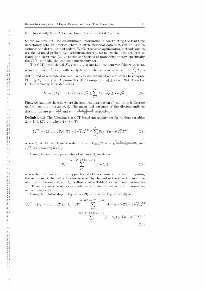
where the min function in the upper bound of the summation is due to imposingthe requirement that all orders are received by the end of the time horizon. Therelationship between Zi and δij is illustrated in Table 3 for lead time parametersδij . There is a one-to-one correspondance of Zi to the values of δij parametersunder binary δij ’s.

Using the relationship in Equation (29), we rewrite Equation (28) as

ULTε = δij i = 1, . . . , T j = i, . . . , T |minT,i+LTmax−1∑

j=i

(1− δij) ≥ T µ− σ√TΓLTε

minT,i+LTmax−1∑j=i

(1− δij) ≤ T µ+ σ√TΓLTε

(30)

1 2 3 4 5 6 7 8 9 10 11 12 13 14 15 16 17 18 19 20 21 22 23 24 25 26 27 28 29 30 31 32 33 34 35 36 37 38 39 40 41 42 43 44 45 46 47 48 49 50 51 52 53 54 55 56 57 58 59 60 61 62 63 64 65


Table 3 Zi, defined in Equation (29) for various realizations of δij

δi,i δi,i+1 δi,i+2 ... δi,i+LTmax−2 δi,i+LTmax−1 δi,i+LTmax Zi1 1 1 ... 1 1 1 00 1 1 ... 1 1 1 10 0 1 ... 1 1 1 20 0 0 ... 0 1 1 LTmax − 10 0 0 ... 0 0 1 LTmax

Thus, we define the CLT-based lead time uncertainty set as LCLT = L ∩ ULTε .Similarly, the following is a demand uncertainty set based on the CLT.

Udε = (d1, . . . , dT ) |T µd − σd√TΓ dε ≤

T∑i=1

di ≤ T µd + σd√TΓ dε (31)

where di is the demand at time t, µd and σd are the mean and standard deviationof demand, respectively, and Γ dε is chosen empirically.

7 Computational Results

First we study the computational performance of the Benders’ decomposition al-gorithm for calculating static and basestock inventory policies. All computationswere carried out on a 3.5 GHz desktop with 32 GB memory, and the subproblemswere solved using CPLEX 12.6. From Algorithm 1, the termination criteria usedwas ε = 0.01, representing a 1% optimality gap. For the first experiment we con-sidered time horizons of 10, 20, and 40 periods, and maximum lead times of 2, 4,6, and 8 periods, with minimum lead time equal to zero in all scenarios. We ran 50instances for each combination of time horizon/lead time scenario, and the compu-tation times and iteration counts are shown in Tables 4 and 5. Other parameterswere set as follows: Average demand (dt) was sampled from a discrete uniformdistribution from 20 to 40; dt was sampled from a discrete uniform distributionfrom 5 to 20; ordering cost (c) was sampled from a uniform distribution from 0to 10; holding cost (h) was sampled from a discrete uniform distribution from 10to 10; and backorder cost (b) was sampled from a discrete uniform distributionfrom 10 to 100. The budgeted lead time and demand models were solved, whereα = β = 1. Basestock models are solved with far fewer iterations, however the DMsubproblem for basestock models can be computationally burdensome for longertime horizons (T = 40) resulting in higher solve time per iteration, since DM is aMILP for the basestock model, and an LP for the static model.

7.1 Results for Budget Uncertainty

We examine the effect of changing the budget for demand (α) and the budgetfor lead times (β) for the static model in an example where T = 10, demanduncertainty is characterized using the budget demand uncertainty set Db wherethe average demand dt = 15 and dt = 5 at each time period t. The costs are h = 5,b = 10, and c = 1. The surface plots in Figures 3, 4, and 5 show for a given α (resp.,

1 2 3 4 5 6 7 8 9 10 11 12 13 14 15 16 17 18 19 20 21 22 23 24 25 26 27 28 29 30 31 32 33 34 35 36 37 38 39 40 41 42 43 44 45 46 47 48 49 50 51 52 53 54 55 56 57 58 59 60 61 62 63 64 65


Table 4 Computational results for solving the static problem using budget uncertainty setswhere (α = β = 1) using Benders’ decomposition including computation time (in seconds) andnumber of iterations

T LTmax Avg Time Min Time Max Time Avg Iter Min Iter Max Iter

10

2 3.8 1.7 8.9 13.7 6 304 2.9 0.9 9.1 10.3 3 306 1.7 0.7 3.4 6.3 3 128 2.0 0.5 4.0 7.0 2 14

20

2 21.5 6.5 137.4 40.7 14 2194 24.7 11.2 167.7 44.8 22 2406 21.3 6.9 123.2 39.4 14 1848 15.2 2.3 61.1 28.4 5 95

40

2 96.8 13.0 484.3 78.9 14 3024 342.9 35.2 1760.9 193.8 36 6876 408.7 62.3 3694.2 204 61 9718 417.9 63.2 5022.8 182.5 60 998

Table 5 Computational results for solving the basestock problem using budget uncertaintysets where (α = β = 1) using Benders’ decomposition including computation time (in seconds)and number of iterations

T LTmax Avg Time Min Time Max Time Avg Iter Min Iter Max Iter

10

2 1.7 1.0 2.3 4.2 3 54 1.6 1.0 2.3 3.8 3 56 1.3 0.9 2.7 3.2 3 58 1.1 0.6 1.9 3.0 2 4

20

2 3.5 2.2 5.5 4.2 3 54 3.6 2.1 5.7 3.8 3 56 3.6 2.0 7.8 3.6 3 58 3.5 1.8 6.9 3.4 3 4

40

2 10.3 4.9 21.1 4.4 3 74 13.9 4.3 26.5 4.0 3 66 39.7 5.6 1019.9 3.8 3 58 72.4 5.0 1031.9 3.7 3 5

β), how the worst-case cost changes according to β (resp., α) for instances wherethe maximum order lead time (LTmax) equals one, two, or three periods. Table 6shows several numerical results corresponding to Figures 3, 4, and 5. For the caseof LTmax = 1, fixing β to 0.5 while increasing α from 0 to 1 increases worst-casecost by 287.3%, while the worst-case cost only increases by 43.8% when α is fixedto 0.5 while β was increased from 0 to 1. However for LTmax=3, the percentageincrease in these two situations are similar (97.0% and 107.7%, respectively). Thiscan be visualized by noticing the increasing slope of the β-axis from Figure 3 to 5.

It is important to note that the worst-case costs determined by the optimizationmodel shown in Figures 3, 4, and 5 could be significantly higher if the uncertaintybudgets underestimate the realized uncertainty levels.

7.2 Robust Optimization vs. Sampling Based Stochastic Programming

Sample Average Approximation (SAA) is a stochastic programming method tominimize the expected value of a stochastic program by generating random samplesand solving a deterministic program to optimize the sample average objective

1 2 3 4 5 6 7 8 9 10 11 12 13 14 15 16 17 18 19 20 21 22 23 24 25 26 27 28 29 30 31 32 33 34 35 36 37 38 39 40 41 42 43 44 45 46 47 48 49 50 51 52 53 54 55 56 57 58 59 60 61 62 63 64 65


Fig. 3 Surface plot where budget for demand and lead time uncertainty budgets are varied


value. We compare our robust optimization-based approach to the SAA approach.In the SAA approach, we select N samples (ξ1, . . . , ξN ), where ξn represents thenth realization of lead times (δnij , where i = 1, . . . , T, j = i, . . . , T ) and demands(dni , where i = 1, . . . , T ) for the full time horizon. The following is the SAAformulation for the static policy:

1 2 3 4 5 6 7 8 9 10 11 12 13 14 15 16 17 18 19 20 21 22 23 24 25 26 27 28 29 30 31 32 33 34 35 36 37 38 39 40 41 42 43 44 45 46 47 48 49 50 51 52 53 54 55 56 57 58 59 60 61 62 63 64 65



Table 6 Worst-case costs for specific instances from the example used for Figures 3, 4, and 5where α (resp. β) are fixed at 0.5 and β (resp. α) are varied from 0 to 1

Worst Case Costs Worst Case CostsModel 1 Model 2 % increase from Model 3 Model 4 % increase from

LTmax α = 0.5, α = 0.5, Model 1 to 2 α = 0, α = 1, Model 3 to 4β = 0 β = 1 β = 0.5 β = 0.5

1 1050.4 1511.0 43.8 566.6 2194.5 287.32 1201.2 1924.4 60.2 940.7 2495.9 165.33 1201.2 2366.9 97.0 1326.5 2755.0 107.7

minimize1

N

( N∑n=1

T∑i=1

(cui + yi,n))

yi,n ≥ h

(x0 +

t∑i=1

(δnitui − dni )

)i = 1, . . . , T, n = 1, . . . , N

yi,n ≥ −b

(x0 +

t∑i=1

(δnitui − dni )

)i = 1, . . . , T, n = 1, . . . , N

ui ≥ 0 i = 1, . . . , T.

(32)

where N is the number of samples. We implement SAA in the following way.For our comparison, we draw 500 samples of demands and lead times for the fulltime horizon where the demands belong to a uniform distribution between 20 and30, and the lead times belong to a discrete uniform distribution between 0 and3. Then we take the ordering decisions from the SAA problem, and run a MonteCarlo simulation using 100 new samples, using several distributions. The demand

1 2 3 4 5 6 7 8 9 10 11 12 13 14 15 16 17 18 19 20 21 22 23 24 25 26 27 28 29 30 31 32 33 34 35 36 37 38 39 40 41 42 43 44 45 46 47 48 49 50 51 52 53 54 55 56 57 58 59 60 61 62 63 64 65


distributions used are Uniform(20,30) and Beta(5,1) with a lower bound of 20and an upper bound of 30, and the lead time distributions used are Uniform(0,3),Two-point (where P(LT=0)=0.25, and P(LT=3)=0.75), and Triangular (whereP(LT=0)=P(LT=3)=0.1, P(LT=1)=P(LT=2)=0.4). Tables 7, 8, and 9 show theresults from the Monte Carlo simulation for an example using the following pa-rameters: h=5, b=10, c=1, and T=10.

Since the robust optimization problem is solved for the full range of 0 ≤ α ≤ 1and 0 ≤ β ≤ 1 in increments of 0.1, we have 11 ∗ 11 = 121 solutions to eachproblem. In the following tables, we report the lowest, median, and highest valuesto have a comparison to the SAA problem. The numbers highlighted in bold inTables 7, 8, and 9 are the objective values of the robust solutions that are smallerthan the SAA results.

Table 7 Average Cost from Monte Carlo simulation (100 replications) for Robust Optimiza-tion Problem and SAA Problem where demands and lead times are drawn from uniform dis-tributions. Numbers highlighted in bold are the objective values of the robust solutions thatare smaller than the SAA results

Lead Time Distribution Uniform 2-point TriangularDemand Distr Uni Beta Uni Beta Uni Beta

SAA 1142 2258 1420 2896 1146 2384Robust(lowest) 1178 1842 990 1561 1118 1799Robust(median) 1373 2101 1412 1975 1360 2367Robust(highest) 1933 2942 2068 2327 1969 3252

Table 8 Maximum Cost from Monte Carlo simulation (100 replications) for Robust Opti-mization Problem and SAA Problem where demands and lead times are drawn from uniformdistributions. Numbers highlighted in bold are the objective values of the robust solutions thatare smaller than the SAA results


SAA 3269 3441 2963 4203 2474 3236Robust(lowest) 1178 2715 1844 2357 2010 2716Robust(median) 1373 3147 2220 3317 2402 3256Robust(highest) 1933 4205 2603 4305 3461 4247

Table 7 shows that the RO solution performs well compared to SAA for severalranges of the budget parameters even though SAA explicitly minimizes averagecost while the RO objective is to minimize the maximum cost. SAA dominates ROin terms of average cost under the uniform lead time, uniform demand scenario.This is not surprising since these are the distributions from which SAA was sam-pled. Tables 8 and 9 indicate that RO provides more stable and robust solutionscompared to SAA in terms of standard deviation and worst case solution.

Table 10 shows two specific robust optimization solutions compared to SAA.SAA is generated using uniform demand and uniform lead time distributions.RO(α = β = 0.3) is a RO model with low uncertainty budget, while RO(α =β = 0.9) is a RO model where a high uncertainty budget is chosen. In the top

1 2 3 4 5 6 7 8 9 10 11 12 13 14 15 16 17 18 19 20 21 22 23 24 25 26 27 28 29 30 31 32 33 34 35 36 37 38 39 40 41 42 43 44 45 46 47 48 49 50 51 52 53 54 55 56 57 58 59 60 61 62 63 64 65


Table 9 Standard Deviation of Cost from Monte Carlo simulation (100 replications) for Ro-bust Optimization Problem and SAA Problem where demands and lead times are drawn fromuniform distributions. Numbers highlighted in bold are the objective values of the robustsolutions that are smaller than the SAA results


SAA 364.2 550.8 248.8 627.4 315.9 420.3Robust(lowest) 215.8 243.1 183.7 155.7 180.9 271.3Robust(median) 296.0 437.4 257.6 368.9 258.7 358.7Robust(highest) 532.2 618.1 395.3 688.4 512.4 482.1

section of the table, the out-of-sample distribution is the same as the in-sampleSAA distribution. We see that RO (α = β = 0.3) performs similarly to SAA withslightly increased average cost, and decreased maximum cost and better stability.The average cost of RO (α = β = 0.9) is 54.6% higher than SAA, but the maximumcost is much lower, and the stability is higher.

In the second set of results from Table 10 , the out-of-sample distributionis Beta for demand, and same as in-sample for lead time. Both RO solutionsoutperform SAA in all three performance measures. In particular, the stability forRO (α = β = 0.9) is better.

In the third set of results from Table 10, the out-of-sample distribution issame as in-sample for demand, and Two-Point for lead time. RO (α = β = 0.9)has better stability than SAA, and lower maximum cost, with the tradeoff ofincreased average cost (20% higher). RO (α = β = 0.3) has higher average costand maximum cost than SAA. This may be due to the under-estimate for budget.

Finally, when the out-of-sample distribution is Beta for demand, and Two-Point for lead time, both RO solutions have good performance compared to SAAin this case.

Table 10 Comparison of two RO solutions to SAA

Out-Of Sample Dist. Measure SAA RO RO(α = β = 0.3) (α = β = 0.9)

d ∼ Uniform, Avg Cost 1142 1238 (8.4%) 1765(54.6%)LT ∼ Uniform Max Cost 3269 2762(-15.5%) 2463(-24.7%)

Std. Dev 364.2 326.7(-10.3%) 257.9(-26.7%)d ∼ Beta, Avg Cost 2258 2103(-6.9%) 2035(-9.9%)

LT ∼ Uniform Max Cost 3341 3172(-5.1%) 2821(-15.6%)Std. Dev 550.8 512.6(-6.9%) 257.0(-53.3%)

d ∼ Uniform, Avg Cost 1420 1572(10.7%) 1704(20.0%)LT ∼ Two− Point Max Cost 2963 3575(20.6%) 2407(-18.8%)

Std. Dev 469.5 441.8(-5.9%) 246.5(-52.5%)d ∼ Beta, Avg Cost 2896 2908(0.4%) 2259(-22.0%)

LT ∼ Two− Point Max Cost 4203 4103(-2.3%) 2922(-30.5%)Std. Dev 627.4 640.8(2.1%) 350.8(-44.1%)

In Table 11 we show the ranges of budget parameters (α and β) that allowRO to outperform SAA in the previous Monte Carlo simulation. RO has a bettermaximum cost compared to SAA on a wide range of budget parameters for all

1 2 3 4 5 6 7 8 9 10 11 12 13 14 15 16 17 18 19 20 21 22 23 24 25 26 27 28 29 30 31 32 33 34 35 36 37 38 39 40 41 42 43 44 45 46 47 48 49 50 51 52 53 54 55 56 57 58 59 60 61 62 63 64 65


demand/lead time distribution combinations. The average cost of RO can outper-form SAA on wide range of parameters when the demand is simulated from a Betadistribution, however under uniformly distributed demand the average cost onlyoutperformed SAA over a narrow range of parameters where α and β were usuallysmall.

Table 11 Ranges of α and β where RO outperforms SAA with respect to average cost andmaximum cost from a Monte Carlo simulation (100 replications)

Demand Lead time Range where RO outperforms Range where RO outperformsdistr. distr. SAA wrt Avg Cost SAA wrt Maximum Cost

Uniform

Uniform Noneα ∈ [0.4, 1], ∀β ;β ∈ [0.3, 1], ∀α

Two-pointα ∈ [0.2, 1] where β ∈ [0, 0.2] ;

113/121 cases outperform SAAα ∈ [0.1, 0.4] where β ∈ [0.2, 0.5]

Triangular23/121 cases outperform SAA; α ∈ [0.6, 1], ∀β ;discontinuous range of α and β β ∈ [0.3, 1], ∀α

Beta

Uniformα ∈ [0.1, 1] where β ∈ [0.3, 1]

α ∈ [0.1, 1] where β ∈ [0.3, 1]α ∈ [0.8, 1], ∀β

Two-point ∀α, ∀β 118/121 cases outperform SAA

Triangularα ∈ [0.7, 1], ∀β ; α ∈ [0.7, 1], ∀β ;β ∈ [0.4, 1], ∀α β ∈ [0.4, 1], ∀α

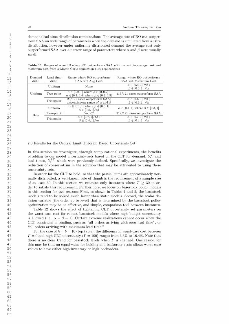
7.3 Results for the Central Limit Theorem Based Uncertainty Set

In this section we investigate, through computational experiments, the benefitsof adding to our model uncertainty sets based on the CLT for demand, Udε , andlead times, ULTε which were previously defined. Specifically, we investigate thereduction of conservatism in the solution that may be attributed to using theseuncertainty sets.

In order for the CLT to hold, so that the partial sums are approximately nor-mally distributed, a well-known rule of thumb is the requirement of a sample sizeof at least 30. In this section we examine only instances where T ≥ 30 in or-der to satisfy this requirement. Furthermore, we focus on basestock policy modelsin this section for two reasons: First, as shown in Tables 4 and 5, the basestockmodels tend to be solved much faster than static models. Second, the scalar de-cision variable (the order-up-to level) that is determined by the basestock policyoptimization may be an effective, and simple, comparison tool between instances.

Table 12 shows the effect of tightening CLT uncertainty set parameters onthe worst-case cost for robust basestock models where high budget uncertaintyis allowed (i.e., α = β = 1). Certain extreme realizations cannot occur when theCLT constraint is binding, such as “all orders arriving with zero lead time”, or“all orders arriving with maximum lead time.”

For the case of h = b = 10 (top table), the difference in worst-case cost betweenΓ = 0 and high CLT uncertainty (Γ = 100) ranges from 6.3% to 16.4%. Note thatthere is no clear trend for basestock levels when Γ is changed. One reason forthis may be that an equal value for holding and backorder costs allows worst-casevalues to have either high inventory or high backorders.

1 2 3 4 5 6 7 8 9 10 11 12 13 14 15 16 17 18 19 20 21 22 23 24 25 26 27 28 29 30 31 32 33 34 35 36 37 38 39 40 41 42 43 44 45 46 47 48 49 50 51 52 53 54 55 56 57 58 59 60 61 62 63 64 65


Table 12 Objective values (WC is the best worst-case solution) and corresponding basestocklevels (BS) for the solutions. Gamma=100 corresponds to relaxing the CLT uncertainty set soit is non-binding. (Note: Γ refers to the parameter setting for both ΓLT and Γd)

T=30, c=3, h=10, b=10, α = β = 1LTmax = 2 LTmax = 4 LTmax = 6 LTmax = 8

Gamma WC BS WC BS WC BS WC BS100 9060 36 15250 57 21440 77 27630 974 9043 31 15107 46 21068 61 26928 763 9021 29 15052 44 20984 59 26703 372 8979 28 14981 43 20560 31 25290 431 8918 20 14449 26 19514 34 24209 440 8480 20 13782 32 18619 41 23108 52





For the case of h = 10, b = 50 (middle table), the trend for basestock levelsis more clear. As the solution becomes less conservative (i.e., worst-case cost de-creases) the basestock level increases. The same trend holds for the bottom tablewhere h = 10, b = 100 (bottom table). The difference in worst-case cost betweenΓ = 0 and high CLT uncertainty (Γ = 100) for these two instances ranges fromabout 3-13%.

8 Concluding Remarks

In this paper, several robust optimization models for inventory control under un-certain demand and uncertain lead time are proposed. We describe several ap-proaches for robust optimization, including budget uncertainty sets and CLT-baseduncertainty sets.

Our numerical results indicate that standard robust optimization methods us-ing epigraph reformulations are overly conservative for the multi-period inventorycontrol problem under demand and lead time uncertainty due to their inherentoverestimation of total cost even when costs and demands are stationary. This isdue to the decoupling of the robust optimization subproblems that are solved. We

1 2 3 4 5 6 7 8 9 10 11 12 13 14 15 16 17 18 19 20 21 22 23 24 25 26 27 28 29 30 31 32 33 34 35 36 37 38 39 40 41 42 43 44 45 46 47 48 49 50 51 52 53 54 55 56 57 58 59 60 61 62 63 64 65


present new budget-type lead time uncertainty sets and CLT-type uncertainty setsto handle demand and lead time uncertainty.

We compare our demand and lead time budget RO approach to the sampling-based SAA method. The RO solution performs well compared to SAA for severalranges of the budget parameters even though SAA explicitly minimizes averagecost while the RO objective is to minimize the maximum cost. The computationalresults indicate that RO provides more stable and robust solutions compared toSAA in terms of standard deviation and worst case solutions, especially when therealized distribution is different than the sampled distribution.

The research presented in this paper can be considered the start of a frame-work for modeling lead time uncertainty using robust optimization. Future workcan involve extending this approach to a more general setting: for example includ-ing fixed costs, and considering multi-echelon supply chains. Using this approach,it would be interesting to consider adaptive policies that explicitly consider thenumber and age of outstanding orders in the ordering decisions.

References

Alvarez, P. P. and Vera, J. R. (2011). Application of robust optimization to thesawmill planning problem. Annals of Operations Research, pages 1–19.

Ang, M., Lim, Y. F., and Sim, M. (2012). Robust storage assignment in unit-loadwarehouses. Management Science, 58(11):2114–2130.

Aouam, T. and Brahimi, N. (2013). Integrated production planning and order ac-ceptance under uncertainty: A robust optimization approach. European Journalof Operational Research, 228(3):501–515.

Bandi, C. and Berstimas, D. (2012). Tractable stochastic analysis in high dimen-sions via robust optimization. Mathematical Programming, 134(1):23–70.

Beck, A. and Ben-Tal, A. (2009). Duality in robust optimization: Primal worstequals dual best. Operations Research Letters, 37(1):1–6.

Ben-Tal, A., El Ghaoui, L., and Nemirovski, A. (2009). Robust optimization.Princeton University Press.

Ben-Tal, A., Golany, B., Nemirovski, A., and Vial, J. (2005). Retailer-supplierflexible commitments contracts: a robust optimization approach. Manufacturingand Service Operations Management, 7(3):248–271.

Ben-Tal, A., Goryashko, A., Guslitzer, E., and Nemirovski, A. (2004). Adjustablerobust solutions of uncertain linear programs. Mathematical Programming,99(2):351–376.

Ben-Tal, A. and Nemirovski, A. (1999). Robust solutions of uncertain linear pro-grams. Operations Research Letters, 25(1):1–13.

Bertsimas, D. and Sim, M. (2004). The price of robustness. Operations Research,52(1):35–53.

Bertsimas, D. and Thiele, A. (2006). A robust optimization approach to inventorytheory. Operations Research, 54(1):150–168.

Bienstock, D. and Ozbay, N. (2008). Computing robust basestock levels. DiscreteOptimization, 5(2):389–414.

Bohle, C., Maturana, S., and Vera, J. (2010). A robust optimization approach towine grape harvesting scheduling. European Journal of Operational Research,200(1):245–252.

1 2 3 4 5 6 7 8 9 10 11 12 13 14 15 16 17 18 19 20 21 22 23 24 25 26 27 28 29 30 31 32 33 34 35 36 37 38 39 40 41 42 43 44 45 46 47 48 49 50 51 52 53 54 55 56 57 58 59 60 61 62 63 64 65


Carlsson, D., Flisberg, P., and Ronnqvist, M. (2014). Using robust optimizationfor distribution and inventory planning for a large pulp producer. Computers &Operations Research, 44:214–225.

Clark, A. and Scarf, H. (1960). Optimal policies for a multi-echelon inventoryproblem. Management Science, 6(4):475–490.

Denton, B. T., Miller, A. J., Balasubramanian, H. J., and Huschka, T. R. (2010).Optimal allocation of surgery blocks to operating rooms under uncertainty. Op-erations Research, 58(4):802–816.

Gabrel, V., Murat, C., and Thiele, A. (2014). Recent advances in robust optimiza-tion: An overview. European Journal of Operational Research, 235(3):471–483.

Gorissen, B. L. and Den Hertog, D. (2013). Robust counterparts of inequalitiescontaining sums of maxima of linear functions. European Journal of OperationalResearch, 227(1):30–43.

Hayya, J., Bagchi, U., Kim, J., and Sun, D. (2008). On static stochastic ordercrossover. International Journal of Production Economics, 114:404–413.

He, X., Xu, S., and Ord, J. (1998). An inventory model with order crossover.Operations Research, 46(3):S112–S119.

Jose Alem, D. and Morabito, R. (2012). Production planning in furniture settingsvia robust optimization. Computers & Operations Research, 39(2):139–150.

Minoux, M. (2009). Robust linear programming with right-hand-side uncertainty,duality, and applications. In Floudas, L. and Pardolas, P., editors, Encyclopediaof Optimization, 2nd edn. Springer, Boston, US.

Minoux, M. (2011). On two-stage robust LP with RHS uncertainty: complexityresults and applications. Journal of Global Optimization, 49(3):521–537.

Movahed, K. K. and Zhang, Z.-H. (2013). Robust design of (s, s) inventory policyparameters in supply chains with demand and lead time uncertainties. Interna-tional Journal of Systems Science, (ahead-of-print):1–11.

Mulvey, J. M., Vanderbei, R. J., and Zenios, S. A. (1995). Robust optimization oflarge-scale systems. Operations Research, 43(2):264–281.

Riezebos, J. (2006). Inventory order crossovers. International Journal of Produc-tion Economics, 104(2):666–675.

Rikun, A. (2011). Applications of Robust Optimization to Queueing and InventorySystems. PhD thesis, Massachusetts Institute of Technology.

Soyster, A. (1973). Convex programming with set-inclusive constraints and appli-cations to inexact linear programming. Operations Research, 21(5):1154–1157.

Soyster, A. and Murphy, F. (2013). A unifying framework for duality and modelingin robust linear programs. Omega, 41(6):984–997.

Varas, M., Maturana, S., Pascual, R., Vargas, I., and Vera, J. (2014). Schedulingproduction for a sawmill: A robust optimization approach. International Journalof Production Economics, 150:37–51.

Wei, C., Li, Y., and Cai, X. (2011). Robust optimal policies of production andinventory with uncertain returns and demand. International Journal of Produc-tion Economics, 134(2):357–367.

Zhang, M. (2011). Two-stage minimax regret robust uncapacitated lot-sizing prob-lems with demand uncertainty. Operations Research Letters, 39(5):342–345.

Zipkin, P. (2000). Foundations of Inventory Management. McGraw-Hill.

1 2 3 4 5 6 7 8 9 10 11 12 13 14 15 16 17 18 19 20 21 22 23 24 25 26 27 28 29 30 31 32 33 34 35 36 37 38 39 40 41 42 43 44 45 46 47 48 49 50 51 52 53 54 55 56 57 58 59 60 61 62 63 64 65

robust inventory control under demand and lead time

Documents