FEDERAL RESERVE BANK OF SAN FRANCISCO

WORKING PAPER SERIES

Working Paper 2005-20 http://www.frbsf.org/publications/economics/papers/2005/wp05-20bk.pdf

The views in this paper are solely the responsibility of the authors and should not be interpreted as reflecting the views of the Federal Reserve Bank of San Francisco or the Board of Governors of the Federal Reserve System.

Robust Control with Commitment: A Modification to Hansen-Sargent

Richard Dennis Federal Reserve Bank of San Francisco

December 2006

Robust Control with Commitment: A Modi�cationto Hansen-Sargent�

Richard Dennisy

Federal Reserve Bank of San Francisco

December, 2006

Abstract

This paper examines the Hansen and Sargent (2003) formulation of the robust Stackel-berg problem and shows that their method of constructing the approximating equilibrium,which is central to any robust control exercise, is generally invalid. The paper then turnsto the Hansen and Sargent (2007) treatment, which, responding to the problems raisedin this paper, changes subtly, but importantly, how the robust Stackelberg problem isformulated. This paper proves, �rst, that their method for obtaining the approximat-ing equilibrium is now equivalent to the one developed in this paper, and, second, thatthe worst-case speci�cation errors are not subject to a time-inconsistency problem. An-alyzing robust monetary policy in two New Keynesian business cycle models, the paperdemonstrates that a robust central bank should primarily fear that the supply side of itsapproximating model is misspeci�ed and that attenuation characterizes robust policymak-ing. Depending on how the robust Stackelberg problem is formulated, this paper showsthat the Hansen-Sargent approximating equilibrium can be dynamically unstable and thatrobustness can be irrelevant, i.e., that the robust policy can coincide with the rationalexpectations policy.

Keywords: Robust control, Robust Stackelberg games, Approximating equilibrium.

JEL Classi�cation: E52, E62, C61.

�I would like to thank Tom Sargent for discussions on robust control and Eric Swanson and Carl Walsh forcomments on an earlier draft of this paper. The views expressed in this paper do not necessarily re�ect thoseof the Federal Reserve Bank of San Francisco or the Federal Reserve System.

yAddress for Correspondence: Economic Research, Mail Stop 1130, Federal Reserve Bank of San Francisco,101 Market St, CA 94105, USA. Email: richard.dennis@sf.frb.org.

1 Introduction

Uncertainty of one form or another is a problem that all decisionmakers must confront, and

it is an issue that is clearly important for policy institutions such as the Federal Reserve.

In the words of former Federal Reserve chairman Greenspan, �Uncertainty is not just an

important feature of the monetary policy landscape; it is the de�ning characteristic of that

landscape�(Greenspan, 2003). Recognizing the impact that uncertainty can have on behavior,

Hansen and Sargent and coauthors show how economic agents can use robust control theory

to make decisions while guarding against the uncertainty that they fear.1 Building on and

extending rational expectations, robust control allows a concern for model misspeci�cation,

or pessimism, to distort how expectations are formed, and thereby alter decisions. Although

decisionmakers may possess a �good� model of the economy (their approximating model),

fears of misspeci�cation are operationalized by assuming that expectations are formed and

decisions are made in the context of a model distorted strategically by speci�cation errors.

The distorted model twists the approximating model according to the worst fears of that

particular agent.2 Importantly, although it is common to assume that all agents share the

same approximating model, there can be as many distorted models as there are agents in the

economy, with each distorted model re�ecting the concerns of that particular agent.

It is important to appreciate, however, that although agents may fear that their model is

misspeci�ed, speci�cation errors need not actually be present. For this reason, the concept

of an approximating equilibrium is central to any robust control exercise. In the approxi-

mating equilibrium, although the approximating model is correctly speci�ed, agents that seek

robustness apply decision rules that guard against their worst-case speci�cation error. The ap-

proximating equilibrium is distinct from the rational expectations equilibrium, in which agents

do not fear misspeci�cation, and from an agent�s worst-case equilibrium, in which that agent�s

worst fears materialize. For robust Stackelberg games, Hansen and Sargent (2003) describe

a procedure to recover the approximating equilibrium from a pessimistic agent�s worst-case

equilibrium. However, complicating the analysis of robust Stackelberg games is the fact that

the leader�s commitment to its policy means that shadow prices, or Lagrange multipliers on

1 In their manuscript Robustness, Hansen and Sargent (2007) provide a sweeping analysis of how robustcontrol can be applied to economic decisionmaking.

2 Insomuch as in equilibrium they each involve probabilities being distorted, or slanted, toward unfavorablepayo¤s, there are ties between robust control, risk sensitive control (Whittle, 1990), uncertainty aversion (Ep-stein and Wang, 1994), disappointment aversion (Gul, 1991), and the latter�s generalization (Routledge andZin, 2003).

1

implementability conditions, enter the solution.3

In this paper, I show that although the method that Hansen and Sargent (2003) use cor-

rectly locates the approximating equilibrium for planning problems in which private agents

are not forward-looking (Sargent, 1999; Hansen and Sargent, 2001a), it fails for the very

class of robust Stackelberg games that they sought to analyze. After demonstrating why

their method fails, I show how to recover the approximating equilibrium correctly. Unlike

Hansen and Sargent (2003), when recovering the approximating equilibrium, I recognize that

the shadow prices that arise in the solution when followers are forward-looking are a com-

ponent of the optimal policy, they re�ect the history dependence of the leader�s policy and

are intended to induce particular behavior from the followers. Therefore, when constructing

the approximating equilibrium, both the leader�s decision rule and the law of motion for the

shadow prices should re�ect the leader�s fear of misspeci�cation.

To understand the nature of robust monetary policy, I employ two New Keynesian (NK)

business cycle models. The �rst model is the canonical NK model (Clarida, Galí, and Gertler,

1999), which forms the basis of numerous nonrobust optimal policy studies.4 The second

model is the sticky price/sticky wage model developed by Erceg, Henderson, and Levin (2000),

which provides the foundation for many modern NK business cycle models. Introducing the

speci�cation errors as per Hansen and Sargent (2003), I show that the central bank in the

canonical NK model will fear mainly that its approximating model understates the persis-

tence of the shock processes. I also show that, although the Hansen-Sargent approximating

equilibrium produces counterintuitive behavior from the central bank and private agents, this

unusual behavior will not be brought to light using detection-error methods.5 For the sticky

price/sticky wage model, I show that a pessimistic central bank will fear primarily that its

approximating model understates the persistence of the technology shock. And I show that

the Hansen-Sargent approximating equilibrium can produce oscillatory behavior or instabil-

ity, even while both the rational expectations equilibrium and the worst-case equilibrium are

stable and non-oscillatory.

After I informed them of these problems,6 Hansen and Sargent (2007, chapter 16) modi�ed

3 In this respect, there is a clear parallel between the solution of robust Stackelberg games and nonrobustStackelberg games, in which shadow prices also serve as state variables (Kydland and Prescott, 1980).

4Giordani and Söderlind (2004) also used this model to investigate robust monetary policy. However,discretionary policymaking was their main focus, and their analysis employing commitment was conductedusing the Hansen and Sargent (2003) approximating equilibrium.

5A detection error occurs when an econometrician observing equilibrium outcomes mistakenly infers whichof two models generated the data.

6After writing the �rst version of this paper (April 2005), I sent copies to Lars Hansen and Tom Sargent.

2

the class of robust Stackelberg games that they analyze; this is an important contribution of

this paper. In addition to speci�cation errors residing in the predetermined block of the model,

they now allow the Stackelberg leader to fear distortions to private-agent expectations, similar

to Woodford (2005). For this alternative formulation of the robust Stackelberg problem, I

prove the worst-case distortions are una¤ected by the Stackelberg leader�s promises about

future policy. I also prove that, conditional on the Stackelberg leader�s robust decision rule,

the worst-case distortions do not a¤ect the worst-case law of motion for the shadow prices.

As a consequence, simply setting the worst-case distortions to zero does not alter the law

of motion for the shadow prices, and, for this reason, the approximating equilibrium that

results is equivalent to the one obtained using my procedure. It follows that, whether interest

centers on the robust control problem analyzed in Hansen and Sargent (2003) or on that

analyzed in Hansen and Sargent (2007, chapter 16), the method I propose returns the correct

approximating equilibrium.

Returning to the two NK business cycle models, allowing the central bank to fear distor-

tions to private-agent expectations, I show that the robust policy in the canonical NK model

coincides with the rational expectations policy. In other words, strikingly, the central bank�s

fear of misspeci�cation has no e¤ect on monetary policy, no e¤ect on economic outcomes, and

no e¤ect on welfare. This robustness-irrelevance result arises because the central bank�s abil-

ity to manipulate expectations allows it to craft a policy that entirely insulates the economy

from misspeci�cation. Perhaps fortunately, this robustness-irrelevance result does not carry

over to the sticky price/sticky wage model. For that model, I �nd that the central bank�s

desire for robustness primarily a¤ects the promises it makes regarding future policy. Across

the two models and across the two formulations of the robust control problem, common themes

are that the central bank fears distortions to supply shocks and that its desire for robustness

does not elicit aggressive policy interventions.

The remainder of the paper is organized as follows. In the following section, I summarize

some related literature. In section 3, I introduce the general structure of the approximat-

ing model and outline how Hansen and Sargent (2003) formulate the optimization problem

confronting a Stackelberg leader who fears misspeci�cation. section 4 shows how control

methods developed by Backus and Dri¢ ll (1986) can be employed to solve for the worst-case

Subsequently, they acknowledged the error, changed the nature of the distortions that the Stackelberg leaderfears, and revised the relevant chapters of their manuscript. As a consequence, I do not believe that thetreatment that Hansen and Sargent currently provide in their manuscript, Robustness, is in error. Indeed, Ishow that their method of constructing the approximating equilibrium is now equivalent to mine.

3

equilibrium.7 Two methods for constructing the approximating equilibrium are presented

and explained in section 5. section 6 clari�es how and why the approximating equilibrium

developed in section 5 di¤ers from Hansen and Sargent (2003). section 7 describes and ana-

lyzes the Hansen and Sargent (2007) revised formulation of the robust Stackelberg problem.

section 8 examines robust monetary policy using two NK business cycle models. section 9

concludes. Appendices contain technical material.

2 Related literature

Prominent applications of robust control have examined how uncertainty a¤ects asset prices.

For example, Hansen, Sargent, and Tallarini (1999) study consumption behavior and the price

of risk using a model in which a representative consumer, facing a linear production technology

and an exogenous endowment process, has a preference for robustness. They show that a

preference for robustness operates on asset prices like a change in the discount factor, with

expressions for consumption and investment unchanged from the usual permanent income

formulas. Hansen, Sargent, and Wang (2002) build on Hansen, Sargent, and Tallarini (1999)

by assuming that part of the state vector is unobserved and by introducing robust �ltering.

Exploiting a separation principle that allows consumers to �rst estimate the state and then

apply robust control as if the state were known, they show that the consumer�s �ltering problem

does not add to the price of risk for a given detection error probability. Cagetti, Hansen,

Sargent, and Williams (2002) extend the analysis in Hansen, Sargent, and Wang (2002) to

a continuous-time nonlinear stochastic growth model in which technology follows a two-state

Markov process.

Where the studies outlined above all employ single-agent robust decision theory, Hansen

and Sargent (2003) consider a multi-agent environment, focusing on robust Stackelberg games

in which the leader and the follower(s) may each express a preference for robustness separately.

To illustrate their approach, Hansen and Sargent (2003) solve a model in which a monopoly

leads a competitive fringe. Naturally, robust Stackelberg games can also be applied to multi-

agent economies in which a �scal or a monetary authority seeks to conduct policy while

expressing distrust in its model. Taking this path, Giordani and Söderlind (2004) analyze

monetary policy in an economy consisting of households, �rms, and a central bank. They study

robust Stackelberg games (commitment equilibria) and robust Markov-perfect Stackelberg

7Backus and Dri¢ ll (1986) build on earlier work by Oudiz and Sachs (1985). See also Currie and Levine(1985, 1993).

4

games (discretionary equilibria) in which the central bank formulates policy while fearing

misspeci�cation. In recent work, Hansen and Sargent (2007, chapter 15) consider Markov-

perfect equilibria in multi-agent economies, allowing each agent to seek robustness.

3 The benchmark robust Stackelberg game

In this section, I describe a linear-quadratic control problem in which a Stackelberg leader

commits to a policy while expressing concern that its model may be misspeci�ed. For sim-

plicity, I focus on an environment in which only one agent � the Stackelberg leader � fears

misspeci�cation, and, consistent with Hansen and Sargent (2003), I assume that the speci�ca-

tion errors that the Stackelberg leader fears reside in the �predetermined block�of the model.8

An alternative assumption is to allow the speci�cation errors to distort both the conditional

mean and the conditional volatility of the shock processes (Dennis, Leitemo, and Söderström,

2006a). In section 7, I consider the case where the Stackelberg leader also fears that speci�-

cation errors will distort private-agent expectations, expanding on Hansen and Sargent (2007,

chapter 16).

The economic environment is one in which an n � 1 vector of endogenous variables, zt,consisting of n1 predetermined variables, xt, and n2 (n2 = n�n1) non-predetermined variables,yt, evolves over time according to

xt+1 = A11xt +A12yt +B1ut +C1"xt+1; (1)

Etyt+1 = A21xt +A22yt +B2ut; (2)

where ut is a p�1 vector of policy control variables, "xt � iid [0; Is] is an s�1 (s � n1) vectorof white-noise innovations, and Et is the private sector�s mathematical expectations operator

conditional upon period t information. Equations (1) and (2) describe the approximating

model, the model that the leader and private agents (the followers) believe comes closest to

describing the data generating process. The matrices A11, A12, A21, A22, B1, and B2 are

conformable with xt, yt, and ut and contain the structural parameters that govern preferences

and technology. The matrix C1 is determined to ensure that "xt has the identity matrix as

its variance-covariance matrix.

In a rational expectations world, the control problem is for the leader to choose the control

8Note that Giordani and Söderlind (2004), Dennis, Leitemo, and Söderström (2006a,b), and numerous otherrobust control applications model the speci�cation errors this way.

5

variables futg10 to minimize

E01Xt=0

�thz0tWzt + z

0tUut + u

0tU

0zt + u

0tRut

i; (3)

where � 2 (0; 1) is the discount factor, subject to equations (1) and (2). The weighting

matrices,W and R, are assumed to be positive semide�nite and positive de�nite, respectively.

However, the leader is concerned that its approximating model may be misspeci�ed. To

accommodate this concern, distortions, or speci�cation errors, vt+1, are introduced and the

approximating model is surrounded by a class of models of the form

xt+1 = A11xt +A12yt +B1ut +C1 (vt+1 + "xt+1) ; (4)

Etyt+1 = A21xt +A22yt +B2ut: (5)

Equations (4) and (5) describe the �distorted� model, the approximating model distorted

by speci�cation errors. Because private agents know that the leader is concerned about

misspeci�cation, the distorted model can be written more compactly as

zt+1 = Azt +But +Cvt+1 + eC"t+1; (6)

where C ��C10

�, eC � � C1 0

0 I

�, and "t+1 �

�"xt+1"yt+1

�in which "yt+1 � yt+1� Etyt+1 is a

Martingale di¤erence sequence; these expectation errors are determined as part of equilibrium.

Assume that the pair (A, B) is stabilizable (Kwakernaak and Sivan, 1972, chapter 6) and

that the sequence of speci�cation errors, fvt+1g10 , satis�es the boundedness condition

E01Xt=0

�t+1v0t+1vt+1 � �; (7)

where � 2 [0; �). It is the satisfaction of this boundedness condition that de�nes the sense inwhich the approximating model, shown in equations (1) and (2), is a �good�one. Note that

in the special case in which � = 0, the nonrobust control problem is restored.

To guard against the misspeci�cations that it fears, the leader formulates policy subject

to the distorted model with the mind-set that the speci�cation errors will be as damaging

as possible, a view that is operationalized through the metaphor that fvt+1g10 is chosen

by a �ctitious evil agent whose objectives are diametrically opposed to those of the leader.

Applying Luenberger�s (1969) Lagrange multiplier theorem, Hansen and Sargent (2001b) show

that the constraint problem, in which equation (3) is minimized with respect to futg10 and

6

maximized with respect to fvt+1g10 , subject to equations (6) and (7), can be replaced withan equivalent multiplier problem, in which

E01Xt=0

�thz0tWzt + z

0tUut + u

0tU

0zt + u

0tRut � ��v

0t+1vt+1

i; (8)

� 2 [�;1), is minimized with respect to futg10 and maximized with respect to fvt+1g10 ,

subject to equation (6). With the following de�nitions eut � �utvt+1

�, eB � �

B C�,

eU � � U 0�, and eR � � R 0

0 ���I

�, the robust problem can be expressed as9

minfutg10

maxfvt+1g10

E01Xt=0

�thz0tWzt + z

0teUeut + eu0t eU0

zt + eu0t eReuti ; (9)

subject to the distorted model

zt+1 = Azt + eBeut + eC"t+1: (10)

4 The worst-case equilibrium

The problem facing a Stackelberg leader that must conduct policy while fearing that its model

is misspeci�ed is described by equations (9) and (10). The solution to this problem returns the

leader�s worst-case equilibrium, the decision rules, and the law of motion for the state variables

that govern the economy�s behavior according to the leader�s worst-case fears. Because

the control problem is linear-quadratic, the leader�s worst-case equilibrium can be obtained

by applying the Backus and Dri¢ ll (1986) solution method, developed originally to solve

problems with rational expectations, which formulates the optimization problem as a dynamic

program.10

Since the control problem is linear-quadratic, the value function takes the form V (zt) =

z0tVzt + d and the dynamic program can be written as

z0tVzt + d � minut maxvt+1

hz0tWzt + z

0teUeut + eu0t eU0

zt + eu0t eReut + �Et �z0t+1Vzt+1 + d�i ; (11)

subject to

zt+1 = Azt + eBeut + eC"t+1: (12)

9 In moving from the constraint problem to the multiplier problem, the assumptions that the pair (A, B)is stabilizable and the sequence fvt+1g10 is bounded are replaced with the assumptions that the pair (A, eB)is stabilizable and that �I � eC0

VeC is positive de�nite, where V is de�ned implicitly by equation (11). Thesecond of these two assumptions determines the lower bound, �, that � must exceed.10Alternatively, this robust control problem can be solved using a Lagrangian, or by applying the recursive

saddle-point theorem (Marcet and Marimon, 1999).

7

To keep the paper self-contained, I describe the Backus-Dri¢ ll solution method in Appen-

dix A, where I show that in the worst-case equilibrium the law of motion for the state variables

is �xt+1pt+1

�= T (A�BFu �CFv)T�1

�xtpt

�+C"xt+1; (13)

p0 = 0, where pt is an n2 � 1 vector of shadow prices of the non-predetermined variables,

yt. These shadow prices, pt, are predetermined variables that enter the equilibrium as

state variables to give private agents the necessary incentives to form expectations and to

make decisions that conform with the unique stable rational expectations equilibrium that

is consistent with the leader�s chosen policy. An alternative way of thinking about these

shadow prices is that they encode the history dependence of the leader�s policy, a history

dependence arising from the leader�s commitment to its policy. The matrix T provides the

mapping between the state variables, xt and pt, and the endogenous variables, zt, and is given

by T =�

I 0V21 V22

�, where V21 and V22 are submatrices of V, conformable with xt and yt

(see Appendix A).

Together with the law of motion for the state variables, the solution for the non-predetermined

variables is

yt =�V�122 V21 V�1

22

� � xtpt

�; (14)

while the robust decision rule(s) for the leader and the worst-case distortions are given by�utvt+1

�= �

�FuFv

�T�1

�xtpt

�: (15)

The leader�s worst-case fear is that the approximating model is distorted by the speci�cation

errors contained within equation (15).

5 The approximating equilibrium

The approximating equilibrium describes the economy�s behavior under robust decisionmak-

ing but in the absence of misspeci�cation.11 Although the worst-case equilibrium and the

approximating equilibrium di¤er, because the distorted model is a device the leader employs

to achieve robustness, the approximating equilibrium and the leader�s worst-case equilibrium

11Here the Stackelberg leader is the only agent seeking robustness and, as a consequence, there is a single set ofworst-case distortions and a single worst-case equilibrium. More generally, with multiple decisionmakers thereis a set of worst-case distortions and a worst-case equilibrium for each agent seeking robustness. Nevertheless,even when multiple agents seek robustness, provided all agents share the same approximating model, there isa single shared approximating equilibrium.

8

are closely connected. To construct the approximating equilibrium, I begin by taking the

worst-case equilibrium, equations (13) �(15) and writing it out in terms of states as

xt+1 = M11xt +M12pt +C1"xt+1; (16)

pt+1 = M21xt +M22pt; (17)

yt = H21xt +H22pt; (18)

ut = eFu1xt + eFu2pt; (19)

vt+1 = eFv1xt + eFv2pt; (20)

where H21 � V�122 V21, H22 � V�1

22 ,h eFu1 eFu2 i � �FuT�1, h eFv1 eFv2 i � �FvT�1, and

M =

�M11 M12

M21 M22

�� T (A�BFu �CFv)T�1.

With the worst-case equilibrium given by equations (16) �(20), identical representations

of the approximating equilibrium can be derived by working with either the approximating

model or the distorted model. Building up from the approximating model, the �rst step

is to set aside the worst-case distortions (the evil agent�s decision rules) by setting eFv1 = 0

and eFv2 = 0 in equation (20). The second step is to substitute equations (18) and (19)

into the approximating model, equation (1). With these substitutions, in the approximating

equilibrium the predetermined variables, xt, evolve over time according to

xt+1 = A11xt +A12yt +B1ut +C1"xt+1;

= A11xt +A12 (H21xt +H22pt) +B1

�eFu1xt + eFu2pt�+C1"xt+1;=

�A11 +A12H21 +B1eFu1�xt + �A12H22 +B1eFu2�pt +C1"xt+1; (21)

with the remainder of the approximating equilibrium given by equations (17) �(19).

Alternatively, simplifying down from the distorted model, substituting equations (18) �

(20) into the distorted model, equation (4), yields

xt+1 = A11xt +A12yt +B1ut +C1vt+1 +C1"xt+1;

= A11xt +A12 (H21xt +H22pt) +B1

�eFu1xt + eFu2pt�+C1 �eFv1xt + eFv2pt�+C1"xt+1;=

�A11 +A12H21 +B1eFu1 +C1eFv1�xt + �A12H22 +B1eFu2 +C1eFv2�pt +C1"xt+1:(22)

Then, zeroing-out the distortions by setting eFv1 = 0 and eFv2 = 0 in equation (22), producesxt+1 =

�A11 +A12H21 +B1eFu1�xt + �A12H22 +B1eFu2�pt +C1"xt+1; (23)

9

with the remainder of the system behaving according to equations (17) �(19). Equation (23)

is, of course, identical to equation (21).

Importantly, in the approximating equilibrium, the non-predetermined variables, yt, the

leader�s decision variables, ut, and the shadow prices of the non-predetermined variables, pt,

all respond to the state variables as they do in the worst-case equilibrium. The approximating

equilibrium and the worst-case equilibrium di¤er solely because the absence of misspeci�cation

alters the law of motion for the predetermined variables, xt.

6 The Hansen-Sargent approximating equilibrium

In contrast to the approach above, Hansen and Sargent (2003) derive the approximating

equilibrium as follows. Given the leader�s worst-case equilibrium, Hansen and Sargent (2003,

p. 592) set Fv = 0 in equations (13) and (15) to obtain what I will term the �Hansen-Sargent

approximating equilibrium.� With this simpli�cation, the law of motion for the state variables

becomes �xt+1pt+1

�= T (A�BFu)T�1

�xtpt

�+C"xt+1; (24)

(see Hansen and Sargent, 2003, equation (3.21a)), while the non-predetermined variables and

the leader�s decision rule(s) continue to be given by equations (18) and (19), respectively.

According to the Hansen-Sargent approximating equilibrium, the decision rules for private

agents and for the Stackelberg leader are formulated to guard against the leader�s worst-

case misspeci�cation, but the law of motion for the state variables � the predetermined

variables and the shadow prices of the non-predetermined variables � is modi�ed because the

speci�cation errors that the leader fears are absent.

On a mechanical level, the di¤erence between the approximating equilibrium presented in

section 5 and the Hansen-Sargent approximating equilibrium described by equation (24) is

that, whereas I zero out the speci�cation errors by setting eFv1 = 0 and eFv2 = 0 in equations(20) and (22), Hansen and Sargent (2003) zero out the speci�cation errors by setting Fv = 0

in equations (13) and (15). But whereas eFv1 and eFv2 represent coe¢ cients on the statevariables (the predetermined variables and the shadow prices) in the evil agent�s decision rule,

Fv describes how the evil agent�s decision variables relate to the predetermined variables,

xt, and the non-predetermined variables, yt. It is apparent from equation (13) that setting

Fv = 0 can change the behavior of both xt and pt, allowing the absence of misspeci�cation to

alter the law of motion for the shadow prices even while the decision rules for private agents

10

and the leader are unaltered.

Unfortunately, the method that Hansen and Sargent (2003) propose will return an incorrect

solution when setting Fv = 0 changes the law of motion for the shadow prices. The method is

generally inappropriate because it treats the shadow prices as if they are physical states, rather

than recognizing that they enter the equilibrium to induce private agents to behave in a manner

consistent with the equilibrium desired by the Stackelberg leader. Since the Stackelberg leader

fears misspeci�cation, and this fear does not depend on whether the approximating model is

actually misspeci�ed, in the approximating equilibrium the shadow prices, which encode the

history dependence of the leader�s robust policy, should respond to the state variables as they

do in the worst-case equilibrium.

7 An alternative robust Stackelberg game

Responding to the issues raised in this paper, Hansen and Sargent (2007, chapter 16) change

how they formulate the robust Stackelberg problem; the change is subtle, but important. In

this section, I describe and interpret this alternative formulation. Then I prove, �rst, that,

conditional on the Stackelberg leader�s worst-case decision rule, the worst-case law of motion

for the shadow prices of the non-predetermined variables does not depend on the worst-case

distortions and, second, that the Stackelberg leader cannot in�uence the worst-case distortions

through its promises about future policy. The former result implies that Hansen and Sargent�s

(2003) approach to constructing the approximating equilibrium would have been correct had

it been applied to the Hansen and Sargent (2007) formulation of the problem. The latter

result implies that the trade-o¤s confronting the metaphorical evil agent are very simple,

unencumbered by promises about future policy. As a consequence, the solution is invariant

to whether the worst-case distortions are determined once and for all or period by period.

Recall that the approximating model is

xt+1 = A11xt +A12yt +B1ut +C1"xt+1; (25)

Etyt+1 = A21xt +A22yt +B2ut; (26)

where the expectation operator in equation (26) re�ects expectations formed by private agents.

Introducing the expectational error, "yt+1 � yt+1� Etyt+1, the approximating model can be

11

written in terms of realized values

xt+1 = A11xt +A12yt +B1ut +C1"xt+1; (27)

yt+1 = A21xt +A22yt +B2ut + "yt+1: (28)

Recognizing that in equilibrium the expectational errors will be a linear function of the

shocks, "yt = C2"xt, equations (27) and (28) can be written more compactly as

zt+1 = Azt +But +C"xt+1; (29)

where C ��C1C2

�. With C2 yet to be determined, Hansen and Sargent (2007, chapter 16)

introduce speci�cation errors to equation (29) and write the distorted model as

zt+1 = Azt +But +Cvt+1 +C"xt+1; (30)

where the speci�cation errors are, of course, constrained to satisfy equation (7).

Conditional on C2, the dynamic program for this robust control problem is

z0tVzt + d � minut maxvt+1

hz0tWzt + z

0teUeut + eu0t eU0

zt + eu0t eReut + �Et �z0t+1Vzt+1 + d�i ; (31)

subject to

zt+1 = Azt +But +Cvt+1 +C"xt+1: (32)

To obtain the worst-case equilibrium, the approach is to conjecture a solution for C2 and

use the method described in Appendix A to solve the dynamic programming problem. The

conjecture for C2 is then updated according to C2 �V�122 V21C1, see equation (A11), and

the procedure is iterated until convergence.12

How does this formulation of the robust Stackelberg problem di¤er from the one described

in section 3? The di¤erence lies in how the speci�cation errors distort the economy. In the

benchmark formulation described in section 3, the Stackelberg leader fears speci�cation errors

that reside in the predetermined block of the model (equation (1)). In contrast, in this section

the Stackelberg leader also fears distortions to private-agent expectations, i.e., the Stackelberg

leader fears that the expectations that private agents form will be slanted in a direction that

makes its stabilization problem more di¢ cult. Put di¤erently, here the Stackelberg leader

fears that the followers will use the distorted model to form expectations, and formulates

policy accordingly, whereas in section 3 the Stackelberg leader understands that the followers12Although it is not obvious that this procedure will necessarily converge, I did not encounter any di¢ culties

with it in this paper.

12

will use the approximating model to form expectations, and formulates policy accordingly. Of

course, because the solution to this problem involves repeated application of the same method

used in section 4, the worst-case equilibrium still takes the form of equations (13) �(15), with

the worst-case speci�cation errors distorting the conditional mean of the shock processes.

Lemma 1: Conditional on the Stackelberg leader�s robust decision rule, the worst-case

law of motion for the shadow prices of the non-predetermined variables does not depend on

the worst-case distortions.

Proof: The shadow prices of the non-predetermined variables are given by

pt+1 =�V21 V22

�zt+1; (33)

=�V21 V22

� �Azt +But +Cvt+1 +C"xt+1

�: (34)

However, the coe¢ cient on the speci�cation errors in this law of motion is given by�V21 V22

�C =

�V21 V22

� � C1�V�1

22 V21C1

�= 0: � (35)

An immediate implication of Lemma 1 is that the law of motion for the shadow prices of

the non-predetermined variables is una¤ected by whether the approximating model is misspec-

i�ed or not, the essential property emphasized in this paper. It follows that the procedures

described in sections 5 and 6 will deliver the same approximating equilibrium.

Lemma 2: The worst-case distortions do not depend on the non-predetermined variables,

precluding the Stackelberg leader from in�uencing the worst-case distortions through promises

about future policy.

Proof: The easiest way to see this important feature of the solution is to reformulate the

robust control problem in terms of a Lagrangian and to exploit the relationship between the

two optimization problems.

The Lagrangian for the robust Stackelberg game is

L = E01Xt=0

�t[z0tWzt + z

0tUut + u

0tU

0zt + u

0tRut � ��v

0t+1vt+1

+�0t+1

�Azt +But +Cvt+1 +C"xt+1 � zt+1

�]; (36)

where futg10 is chosen to minimize equation (36) and fvt+1g10 is chosen to maximize equation

(36) and where �t+1 �h�x

0t+1 �y

0

t+1

i0is a vector of Lagrange multipliers. Focusing on the

maximization problem, the �rst-order condition associated with vt+1 is13

@L

@vt+1= �2��vt+1 +C

0Et�t+1 = 0: (37)

13Since the constraints are linear and � > 0, this �rst-order condition is associated with a maximum.

13

As is well known, the Lagrange multipliers in equation (36) are equivalent to the shadow

prices on zt in the dynamic program, equations (31) and (32). Therefore,14��xt+1�yt+1

�= 2

�V11 V12V21 V22

� �xt+1yt+1

�: (38)

Substituting equation (38) into equation (37), this �rst-order condition can be written as

@L

@vt+1= ���vt+1 +C

0�V11 V12V21 V22

�Et

�xt+1yt+1

�= 0; (39)

= ���vt+1 +�C

01V11 +C

02V21

�Etxt+1 +

�C

01V12 +C

02V22

�Etyt+1 = 0: (40)

The next step is to recognize that C2 = �V�122 V21C1 in equilibrium. Therefore, equation

(40) becomes

@L

@vt+1= ���vt+1 +C

01

�V11 �V

021V

�122 V21

�Etxt+1 +C

01

�V12 �V

021

�Etyt+1 = 0; (41)

which, because V is symmetric (see equation (A7)), collapses to

@L

@vt+1= ���vt+1 +C

01

�V11 �V

021V

�122 V21

�Etxt+1 = 0: (42)

Making vt+1 the subject, equation (42) implies

vt+1 =1

��C

01

�V11 �V

021V

�122 V21

�Etxt+1; (43)

establishing that the worst-case distortions do not depend on Etyt+1 and therefore do not

depend on Et�yt+1 (Etpt+1).

15 �Lemma 2 has several important implications. First, equation (43) establishes that when

determining how to distort the model the �ctitious evil agent need only consider the e¤ect

its distortions have on the natural state variables. Second, equation (42) shows that when

distorting the model the �ctitious evil agent equates the marginal cost of a change in its

14Note that the �2� in equation (38) is simply a scale factor that is sometimes accommodated by placing a�2� in front of the Lagrange multipliers in equation (36) (which makes the Lagrange multipliers equal to halfthe shadow prices). Naturally, both approaches yield the same answer.15 If this last point is unclear, simply note that the state variables are given by�

xt�yt

�=

�I 0V21 V22

� �xtyt

�;

and that equation (43) can therefore also be written as

vt+1 =1

��

hC

01

�V11 �V

021V

�122 V21

�0i � I 0

�V�122 V21 V�1

22

� �Etxt+1Et�

yt+1

�:

14

instrument(s) to the marginal bene�t, where the marginal bene�t comes in two forms: a

direct e¤ect on the loss function of a change in Etxt+1 and an indirect e¤ect through the

e¤ect the change in this expectation has on the non-predetermined variables. Third, because

its �rst-order condition holds for all t > 0 and does not depend on the non-predetermined

variables, the �ctitious evil agent is not subject to a time-inconsistency problem. Therefore,

the solution to the game in which the Stackelberg leader and the �ctitious evil agent both make

decisions once-and-for-all is also the solution to the game in which the Stackelberg leader makes

decisions once-and-for-all, but the �ctitious evil agent makes decisions sequentially.

8 Robust monetary policy

With the solution apparatus behind us, in this section I analyze robust monetary policy in

terms of the canonical NK business cycle model (Clarida, Galí, and Gertler, 1999) and the

sticky price/sticky wage business cycle model developed by Erceg, Henderson, and Levin

(2000). For each model, I formulate the robust Stackelberg game �rst as per section 3 and

then as per section 7. To prevent confusion, when presenting the results I will refer to the

optimization problems described in sections 3 and 7 as �problem one� and �problem two,�

respectively.

8.1 The canonical NK model

The canonical NK business cycle model consists of equations for consumption and aggregate

in�ation. The model is one in which �rms are monopolistically competitive and nominal prices

are �sticky�due to Calvo-contracts (Calvo, 1983). Households maximize utility de�ned over

consumption (a Dixit-Stiglitz aggregate of the �rms�outputs) and leisure, subject to a budget

constraint in which households can transfer income through time by holding either (one-period)

nominal bonds or nominal money balances. The labor market is perfectly competitive and

labor is the only factor in a constant-returns-to-scale production function. When log-linearized

about a zero-in�ation steady state, the model has the form

ct = Etct+1 � (it � Et�t+1) + e1t (44)

�t = �Et�t+1 + �ct + e2t (45)

e1t = �1e1t�1 + �"1"1t (46)

e2t = �2e2t�1 + �"2"2t; (47)

15

where 2 (0;1) is the elasticity of intertemporal substitution, � 2 (0; 1) is the subjectivediscount factor, and � 2 (0;1) represents the slope of the (short-run) Phillips curve anddepends on the price rigidity and the discount factor. In the model, ct denotes consumption,

�t denotes aggregate in�ation, and it denotes the short-term nominal interest rate. The

consumption Euler equation is shifted by a consumption preference shock, e1t, and the Phillips

curve is shifted by a markup shock, e2t, with each shock following an AR(1) process with white

noise innovations. The parameters in the two shock processes satisfy f�1; �2g 2 (�1; 1) andf�"1; �"2g 2 (0;1). Subject to equations (44) � (47), the central bank (the Stackelberg

leader) chooses fitg10 to optimize the loss function,

Loss [0;1] = E01Xt=0

�t��2t + �c

2t + �i

2t

�: (48)

8.1.1 Problem one

When the model is written in state-space form, it is straightforward to solve for the rational

expectations equilibrium. By adding the speci�cation errors (the controls of the �ctitious

evil agent), I can easily obtain the worst-case equilibrium, the approximating equilibria, and

the Hansen-Sargent approximating equilibrium. For reasons that will shortly become clear,

the robustness parameter, �, is set to 38:967.16 Solving for the worst-case equilibrium, the

worst-case distortions are

v"1t+1 = 0:040e1t + 0:003e2t � 0:002p�t � 0:005pct (49)

v"2t+1 = �0:002e1t + 0:088e2t � 0:007p�t + 0:015pct; (50)

where pct and p�t are the shadow prices associated with consumption and in�ation, respectively.

Equations (49) and (50) reveal that the distortions that the central bank fears are those that

increase the persistence of the shocks, particularly the persistence of the markup shock. These

fears are easily rationalized because persistent shocks make it more di¢ cult for the central bank

to stabilize the economy. Moreover, persistent markup shocks are especially damaging because

they force the central bank to raise interest rates � lowering current-period consumption �

in order to unwind the in�ationary e¤ects of the shock.

How does the central bank�s fear of misspeci�cation a¤ect the approximating equilibrium?

16The remaining parameters were assigned the values reported in Giordani and Söderlind (2004). Speci�cally,I set � = 0:99; = 0:5; � = 0:645; �1 = �2 = 0:8; and �"1 = �"2 = 1, with the loss function parameters set to� = 0:5 and � = 0:2.

16

In the approximating equilibrium, the law of motion for the state variables is2664e1t+1e2t+1p�t+1pct+1

3775 =2664

0:8 0 0 00 0:8 0 0

�0:302 �0:630 0:458 �0:253�0:355 0:035 0:053 0:396

37752664e1te2tp�tpct

3775+26641 00 10 00 0

3775� "1t+1"2t+1

�; (51)

with in�ation, consumption, and the nominal interest rate determined according to

�t = 0:124e1t + 0:647e2t + 0:568p�t + 0:452pct; (52)

ct = 0:544e1t � 0:904e2t + 0:452p�t + 0:633pct; (53)

it = 0:879e1t � 0:086e2t � 0:132p�t � 0:981pct: (54)

By way of contrast, if the approximating equilibrium were constructed using the Hansen-

Sargent method, then the law of motion for the state variables would become2664e1t+1e2t+1p�t+1pct+1

3775 =2664

0:8 0 0 00 0:8 0 0

�0:357 �0:173 0:424 �0:171�0:278 �0:414 0:086 0:312

37752664e1te2tp�tpct

3775+26641 00 10 00 0

3775� "1t+1"2t+1

�; (55)

with the behavior of in�ation, consumption, and the nominal interest rate still given by equa-

tions (52) �(54). Comparing equations (51) and (55), it is clear that the main di¤erences

reside in how the shadow prices respond to the shocks, particularly in how they respond to

the markup shock.

Figure 1 illustrates how the model, with robust monetary policy, behaves following an

adverse 1 percent markup shock, and clari�es why � was set to 38:967. Panel A maps out the

relationship between the (log of the) robustness parameter, �, and the probability of making

a �detection error,�given a sample of 200 observations. A detection-error probability is the

probability that an econometrician observing equilibrium outcomes would infer incorrectly

whether the approximating equilibrium or the worst-case equilibrium generated the data.

Among other factors, detection-error probabilities depend on the available sample size. A

method for calculating detection-error probabilities is described in Appendix B.17

As � increases (� falls), the distortions become smaller and the probability of making

a detection error rises. In fact, in the limit as � " 1 (� # 0), the central bank�s risingcon�dence in its model means that the speci�cation errors are so severely constrained that

the approximating equilibrium and the worst-case equilibrium each converge to the rational

expectations equilibrium, and the detection-error probability converges to 0:5. Panel A shows17See also Hansen, Sargent, and Wang (2002) or Hansen and Sargent (2006, chapter 9).

17

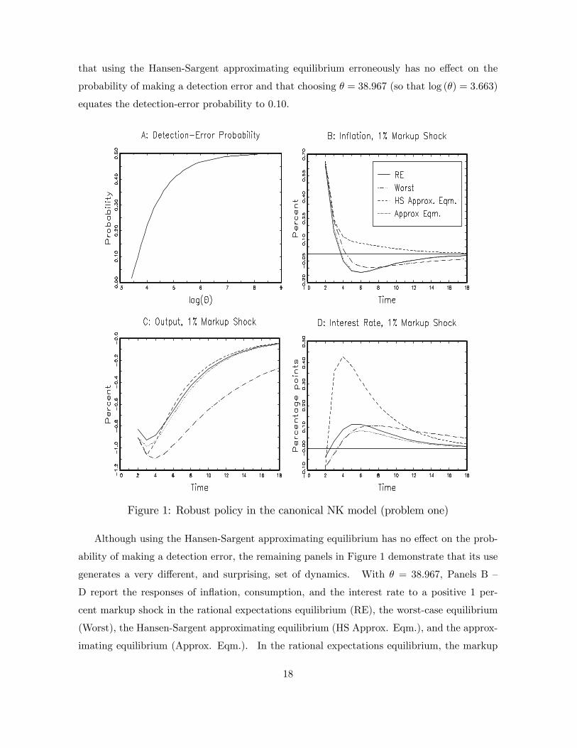
that using the Hansen-Sargent approximating equilibrium erroneously has no e¤ect on the

probability of making a detection error and that choosing � = 38:967 (so that log (�) = 3:663)

equates the detection-error probability to 0:10.

Figure 1: Robust policy in the canonical NK model (problem one)

Although using the Hansen-Sargent approximating equilibrium has no e¤ect on the prob-

ability of making a detection error, the remaining panels in Figure 1 demonstrate that its use

generates a very di¤erent, and surprising, set of dynamics. With � = 38:967, Panels B �

D report the responses of in�ation, consumption, and the interest rate to a positive 1 per-

cent markup shock in the rational expectations equilibrium (RE), the worst-case equilibrium

(Worst), the Hansen-Sargent approximating equilibrium (HS Approx. Eqm.), and the approx-

imating equilibrium (Approx. Eqm.). In the rational expectations equilibrium, the markup

18

shock causes in�ation to rise, with interest rates (after an initial decline) rising in response.

The higher interest rate lowers consumption, placing downward pressure on in�ation. As

in�ation begins to decline, the interest rate falls and consumption rises. In the worst-case

equilibrium, in�ation is more persistent, with the e¤ects of the shock dissipating less rapidly

than under rational expectations. To counter this in�ation persistence, the central bank

commits to a gradual, but sustained, rise in interest rates. In the approximating equilibrium,

the economy�s initial responses are the same as those for the worst-case equilibrium. Subse-

quently, however, interest rates rise by less than they do in the worst-case equilibrium and the

economy�s behavior more closely resembles that of the rational expectations equilibrium.

However, where the responses for the rational expectations, the worst-case, and the ap-

proximating equilibria are all relatively similar, the responses for the Hansen-Sargent approx-

imating equilibrium are very di¤erent. For example, in�ation�s response is systematically

higher than it is for the other equilibria. In fact, the Hansen-Sargent approximating equilib-

rium does not show in�ation falling below baseline, a hallmark of commitment policies in NK

models. With higher in�ation, the central bank raises interest rates more, generating a larger

decline in consumption. Notice that where the Hansen-Sargent approximating equilibrium

suggests that the central bank should respond aggressively to the shock, the approximating

equilibrium actually suggests attenuation, with the robust policy responding less aggressively

to the shock than under the rational expectations policy.

Finally, an obvious question raised by Figure 1 is why using the Hansen-Sargent approx-

imating equilibrium has no e¤ect on the probability of making a detection error when it has

such important implications for the behavior of in�ation, consumption, and the interest rate.

Setting aside the fact that the probability of making a detection error depends on both shocks,

not just the markup shock, it is important to recognize that detection-error probabilities de-

pend on the behavior of the shock processes and not on the behavior of the shadow prices,

the decision variables, or the endogenous variables (see Appendix B). As a consequence, the

unattractive behavior of in�ation, consumption, and the interest rate exhibited in Figure 1

holds no implication for the probability of making a detection error. Clearly, one must be

cautious when using detection-error probabilities to measure the �distance�between two mod-

els, because behavioral di¤erences that are quantitatively and qualitatively important can be

masked.

19

8.1.2 Problem two

When I formulate the optimization problem as per section 7, setting � = 30:829 (log (�) =

3:428) so that the detection-error probability equals 0:1, the worst-case distortions are

v"1t+1 = 0:042e1t + 0:004e2t; (56)

v"2t+1 = 0:004e1t + 0:091e2t: (57)

Notice that, unlike problem one, the worst-case distortions depend only on the shocks. Nev-

ertheless, the speci�cation errors that the central bank fears are those that increase the per-

sistence of the markup shock. The law of motion for the state variables in the approximating

equilibrium is2664e1t+1e2t+1p�t+1pct+1

3775 =2664

0:8 0 0 00 0:8 0 0

�0:292 �0:610 0:456 �0:251�0:346 0:016 0:054 0:393

37752664e1te2tp�tpct

3775+26641 00 10 00 0

3775� "1t+1"2t+1

�; (58)

with in�ation, consumption, and the nominal interest rate determined according to

�t = 0:119e1t + 0:618e2t + 0:570p�t + 0:448pct; (59)

ct = 0:531e1t � 0:829e2t + 0:448p�t + 0:644pct; (60)

it = 0:855e1t � 0:040e2t � 0:133p�t � 0:973pct: (61)

Figure 2 illustrates how the model behaves following an adverse 1 percent markup shock

and can be compared directly to Figure 1. Of course, the rational expectations responses

are the same in the two �gures, however, in the worst-case equilibrium, consumption declines

by less in Figure 2 than in Figure 1 and, therefore, the interest rate response in Figure 2

shows the central bank responding more aggressively to the shock than in Figure 1. Turning

to the model�s behavior in the approximating equilibrium, a striking result in Figure 2 is

that the approximating equilibrium is identical to the rational expectations equilibrium. In

practical terms, the central bank�s fear of misspeci�cation and the intensity with which it

fears misspeci�cation have no policy implications. In fact, it is straightforward to verify

that equations (58) � (61) are the same as rational expectations, implying that the central

bank�s preference for robustness, because it does not a¤ect policy, does not a¤ect economic

outcomes more generally. Strikingly, according to this formulation of the robust control

problem, robustness is irrelevant.

20

Figure 2: Robust policy in the canonical NK model (problem two)

8.2 A sticky price/sticky wage model

I now turn to the sticky price/sticky wage NK business cycle model developed by Erceg,

Henderson, and Levin (2000), a model increasingly re�ective of those used to study optimal

policymaking. Similar to the canonical NK model, the production technology is linear in labor

and prices are subject to a Calvo-style nominal price rigidity. Here, however, nominal wages

are also rigid (Calvo wages) with monopolistically competitive �rms hiring a Dixit-Stiglitz

labor aggregate. In addition to a consumption preference shock, the model contains a leisure

preference shock and a serially correlated technology shock.

21

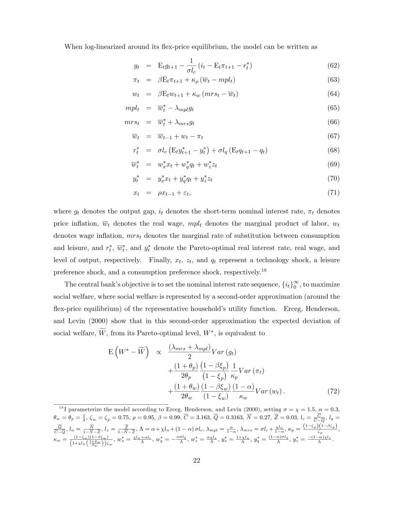
When log-linearized around its �ex-price equilibrium, the model can be written as

gt = Etgt+1 �1

�lc(it � Et�t+1 � r�t ) (62)

�t = �Et�t+1 + �� (wt �mplt) (63)

wt = �Etwt+1 + �w (mrst � wt) (64)

mplt = w�t � �mplgt (65)

mrst = w�t + �mrsgt (66)

wt = wt�1 + wt � �t (67)

r�t = �lc�Ety�t+1 � y�t

�+ �lq (Etqt+1 � qt) (68)

w�t = w�xxt + w�qqt + w

�zzt (69)

y�t = y�xxt + y�qqt + y

�zzt (70)

xt = �xt�1 + "t; (71)

where gt denotes the output gap, it denotes the short-term nominal interest rate, �t denotes

price in�ation, wt denotes the real wage, mplt denotes the marginal product of labor, wt

denotes wage in�ation, mrst denotes the marginal rate of substitution between consumption

and leisure, and r�t , w�t , and y

�t denote the Pareto-optimal real interest rate, real wage, and

level of output, respectively. Finally, xt, zt, and qt represent a technology shock, a leisure

preference shock, and a consumption preference shock, respectively.18

The central bank�s objective is to set the nominal interest rate sequence, fitg10 , to maximizesocial welfare, where social welfare is represented by a second-order approximation (around the

�ex-price equilibrium) of the representative household�s utility function. Erceg, Henderson,

and Levin (2000) show that in this second-order approximation the expected deviation of

social welfare, fW , from its Pareto-optimal level, W �, is equivalent to

E�W � �fW� / (�mrs + �mpl)

2V ar (gt)

+(1 + �p)

2�p

�1� ��p

��1� �p

� 1

�pV ar (�t)

+(1 + �w)

2�w

(1� ��w)(1� �w)

(1� �)�w

V ar (wt) : (72)

18 I parameterize the model according to Erceg, Henderson, and Levin (2000), setting � = � = 1:5; � = 0:3;�w = �p =

13; �w = �p = 0:75; � = 0:95; � = 0:99; C = 3:163; Q = 0:3163; N = 0:27; Z = 0:03; lc =

C

C�Q ; lq =

Q

C�Q ; ln =N

1�N�Z ; lz =Z

1�N�Z ; � = �+�ln+(1� �)�lc; �mpl =�

1�� ; �mrs = �lc+�ln1�� ; �p =

(1��p)(1���p)�p

;

�w =(1��w)(1���w)�1+�ln

�1+�w�w

���w; w�x =

�ln+�lc�

; w�q = ���lq�; w�z =

��lz�; y�x =

1+�ln�

; y�q =(1��)�lq

�; y�z =

�(1��)�lz�

:

22

Because social welfare cannot exceed the Pareto-optimal level, the central bank�s optimization

problem is to minimize equation (72) subject to equation (7) and equations (62) �(71).

8.2.1 Problem one

As discussed earlier, after adding the speci�cation errors, the only parameter that remains

to be determined is the robustness parameter, �. I set the detection-error probability to

0:1, which implies � = 4:75 (so that log (�) = 1:558), and with this parameterization the

speci�cation errors that the central bank fears are

vxt+1 = 0:107xt + 0:001zt � 0:270wt�1 � 0:006pwt � 0:001pgt + 0:016p�t; (73)

vqt+1 = �0:001xt + 0:002wt�1; (74)

vzt+1 = 0:003xt � 0:006wt�1 + 0:001p�t: (75)

Clearly, the central bank is most concerned with speci�cation errors that distort the tech-

nology shock, equation (73), and is relatively unconcerned about misspeci�cation of the other

shock processes. Because the technology shock plays the same role in this model as the

markup shock does in the canonical NK model, this �nding is consistent across the two mod-

els. Interestingly, the autoregressive coe¢ cient in the worst-case shock process for technology

is greater than one. However, stability of the worst-case equilibrium is preserved through

feedback among the worst-case shock processes, the real wage, and the shadow prices.

Paralleling Figure 1, Figure 3 (Panel A) plots the relationship between (log) � and the

probability of making a detection error. With � = 4:75, Figure 3 (Panels B �D) also displays

the responses of in�ation, output, and the interest rate to a positive 1 percent technology

shock for the rational expectations equilibrium, the worst-case equilibrium, and the approxi-

mating equilibrium. Focusing �rst on the rational expectations equilibrium, Figure 3 shows

that in�ation and the interest rate fall while the output gap rises in response to a 1 percent

technological innovation. The positive technology shock lowers the cost of producing a unit

of output (real marginal costs), which, through competitive forces, causes prices and in�ation

(due to sticky prices) to fall. With in�ation falling, the central bank cuts interest rates,

stimulating demand and opening up a positive output gap. As the e¤ects of the shock begin

to dissipate, and as the demand stimulus exerts upward pressure on in�ation, both in�ation

and interest rates begin to rise, causing the output gap to fall. In the worst-case equilibrium,

in�ation falls by more than under rational expectations and the central bank responds aggres-

sively, cutting interest rates and opening up a larger output gap. Last, the robust policy in

23

the approximating equilibrium initially cuts interest rates by more than when expectations

are rational to guard against a sustained and persistent decline in in�ation, but then raises

interest rates quickly as in�ationary pressures begin to build. The central bank�s fear of

misspeci�cation reveals itself most prominently in how the central bank initially responds to

the shock.

Figure 3: Robust policy in the sticky price/sticky wage model (problem one)

Now consider what happens if the Hansen-Sargent approximating equilibrium is used.

Figure 4 reports the responses of in�ation, output, and the interest rate, allowing � to take on

three di¤erent values. For a reason that will become clear, these three values for � are all much

larger than the value used in Figure 3 and correspond to detection-error probabilities that are

all greater than 0:49. The fact that the impulse responses associated with the Hansen-Sargent

24

approximating equilibrium are unusual can be seen immediately in the behavior of the output

gap and the interest rate. Where the in�ation responses are similar to rational expectations,

these in�ation paths are associated with an unusual spike in interest rates and the output gap

when � = 500, damped oscillations in interest rates and the output gap when � = 380, and

explosive oscillations in interest rates and the output gap when � = 356.19 Notice that these

explosive oscillations have no e¤ect on the detection-error probability because the instability

does not stem from the shock processes.

Setting the oscillatory behavior aside, the fact that the Hansen-Sargent approximating

equilibrium is unstable with � = 356 is telling, because it demonstrates that the equilibrium

does not minimize the maximum loss for distortion sequences that satisfy equation (7). Specif-

ically, the loss associated with the sequence fvtg10 = f0g10 is greater than the loss associated

with the sequence of worst-case distortions.

19To see the source of this instability, notice that, although the spectral radius of T (A�BFu �CFv)T�1

must be less than one (because the worst-case equilibrium is stable), this does not imply that the spectralradius of T (A�BFu)T�1 is less than one.

25

Figure 4: The Hansen-Sargent approximating equilibrium (problem one)

8.2.2 Problem two

I set the detection-error probability to 0:1, which implies � = 3:077 (log (�) = 1:124), and with

this parameterization the speci�cation errors that the central bank fears are

vxt+1 = 0:122xt + 0:001qt � 0:003zt � 0:319wt�1 � 0:005pgt; (76)

vqt+1 = �0:001xt + 0:001wt�1; (77)

vzt+1 = 0:002xt � 0:004wt�1: (78)

As shown earlier, the central bank is most concerned with speci�cation errors that distort

26

the technology shock process, equation (76).

Figure 5: Robust policy in the sticky price/sticky wage model (problem two)

Depicting the economy�s response to a technology shock, Figure 5 shows that robustness

primarily e¤ects the behavior of output. In this economy, output and consumption are equal,

so output is a non-predetermined variable whose behavior is governed partly by central bank

promises about future policy. Indeed, comparing the behavior of the robust and the nonrobust

economies, the main di¤erences reside in the laws-of-motion for the shadow prices (not shown),

particularly those of wage growth and in�ation. In e¤ect, although robustness has little e¤ect

on the central bank�s interest rate decision rule, the central bank�s desire for robustness is

manifest in the promises it makes about future policy, and these promises assert themselves

in the behavior of output. In this respect, Figures 3 and 5 are qualitatively similar. Notably,

27

the interest rate responses in Figure 5 also display a form of attenuation.

9 Conclusion

This paper analyzes decisionmaking in economies where a Stackelberg leader formulates policy

under commitment while seeking robustness to model misspeci�cation. The paper�s �rst

important contribution is to show that the Hansen and Sargent (2003) solution to this class of

robust control problems is generally incorrect. As is by now well-known, shadow prices enter

the solution of control problems in which the leader commits. These shadow prices encode

the history dependence of the optimal policy and direct private agents toward the equilibrium

the Stackelberg leader desires. This paper shows that the approximating equilibrium that

Hansen and Sargent (2003) develop is generally incorrect because their method for obtaining

it fails to appreciate the role these shadow prices play in determining equilibrium. The paper

then shows how the approximating equilibrium can be constructed correctly, establishing as a

general principle that the shadow prices must evolve in the approximating equilibrium as they

do in the worst-case equilibrium.

Having shown how to construct the approximating equilibrium, this paper analyzes robust

monetary policy in two NK business cycle models. An important result that emerges from

these applications is that a robust central bank should fear that its approximating model

understates the persistence of supply-side shocks, such as markup shocks and technology

shocks. Distortions to these shock processes are feared because they are di¢ cult for the central

bank to counteract. With the approximating equilibrium constructed correctly, this paper

further shows that attenuation does generally characterize robust monetary policy, contrary

to popular belief. Further, these applications illustrate that counterintuitive oscillations or

even instability can be produced if the Hansen-Sargent approximating equilibrium is used, and

that these problems will not be brought to light by detection-error probabilities.

Next the paper considers the treatment of robust Stackelberg games given in Hansen and

Sargent (2007), which, due to the issues raised in this paper, di¤ers importantly from Hansen

and Sargent (2003). The paper shows that in the solution to this more general formulation

of the robust Stackelberg game, conditional on the leader�s robust decision rule, the law of

motion for the shadow prices is una¤ected by the worst-case distortions. As a consequence, the

method Hansen and Sargent (2007) use to construct the approximating equilibrium coincides

with that developed in this paper because it satis�es the principle that the law of motion

for shadow prices must be the same in the approximating equilibrium as it is in the worst-

28

case equilibrium. Further, the paper shows that the �rst-order condition determining the

worst-case distortions does not depend on the non-predetermined variables. Therefore, the

worst-case distortions are una¤ected by promises about future policy and are also not subject

to a time-inconsistency problem.

Returning to the two NK business cycle models, but with the robust Stackelberg game

formulated according to Hansen and Sargent (2007), the paper �nds that in the canonical NK

model the approximating equilibrium coincides with the rational expectations equilibrium for

all values of the robustness parameter. Simply put, in this model the central bank�s desire

for robustness has no implications for monetary policy, for economic outcomes, or for welfare.

Fortunately, this stark conclusion does not carry over to the sticky price/sticky wage model,

however the main results concerning robust monetary policy do. Speci�cally, a central bank

that seeks robustness should primarily fear speci�cation errors that raise the persistence of

supply-side shocks. Finally, although robust control is often associated with aggressive policy

responses, for the models analyzed in this paper, and perhaps more generally, attenuation

characterizes robust monetary policy.

Appendix A - Worst-case equilibrium

With the optimization problem written as

minfutg

maxfvt+1g

E01Xt=0

�thz0tWzt + z

0teUeut + eu0t eU0

zt + eu0t eReuti ;subject to

zt+1 = Azt + eBeut + eC"t+1; (A1)

the policy problem conforms to the standard linear-quadratic framework studied and solvedby Backus and Dri¢ ll (1986). To obtain the optimal policy, Backus and Dri¢ ll (1986) �rsttake z0 as given and write the optimization problem recursively as

z0tVzt + d � minut maxvt+1

hz0tWzt + z

0teUeut + eu0t eU0

zt + eu0t eReut + �Et �z0t+1Vzt+1 + d�i ; (A2)

subject tozt+1 = Azt + eBeut + eC"t+1: (A3)

Using dynamic programming they obtain the standard solution

zt+1 = (A� eBF)zt + eC"t+1 (A4)eut = �Fzt; (A5)

29

where

F =�� eB0

VeB+ eR��1 �� eB0VA+ eU� (A6)

V = ��A� eBF�0V �A� eBF�+W � eUF� eU0

F0+ F

0 eRF (A7)

d =�tr

heC0VeCE�"t+1"0t+1�i1� � : (A8)

Since y0 is not predetermined and the expectation errors are not exogenous, the Stackelbergleader also chooses y0 and f"ytg11 to minimize the value function

z00Vz0 + d =

�x00 y

00

� � V11 V12V21 V22

� �x0y0

�+ d; (A9)

obtaining

y0 = �V�122 V21x0 (A10)

"yt = �V�122 V21C1"xt: (A11)

In the equilibrium that the leader desires, in the initial period the non-predeterminedvariables relate to the predetermined variables according to equation (A10) and in each periodthe expectational errors relate to the innovations according to equation (A11). To achievethis equilibrium, the leader represents its policy as a function of a vector of shadow pricesof the non-predetermined variables with the shadow prices inducing private agents to formexpectations that are consistent with the desired equilibrium. Thus, introducing a vector ofshadow prices of the non-predetermined variables

pt ��V21 V22

� � xtyt

�(A12)

and noting that pt is predetermined (implied by equation (A11)) with initial value p0 = 0(implied by equation (A10)), the dynamics of xt and pt are given by�

xt+1pt+1

�= T

�A� eBF�T�1 � xt

pt

�+TeC"t+1 (A13)

= T�A� eBF�T�1 � xt

pt

�+

�C10

�"xt+1 (A14)

where

T =

�I 0V21 V22

�: (A15)

Finally, yt and eut are determined according toyt =

�V�122 V21 V�1

22

� � xtpt

�(A16)

and

eut = �FT�1 � xtpt�; (A17)

respectively.Equations (A14), (A16), and (A17) describe the state-contingent behavior of the predeter-

mined variables, xt and pt, the non-predetermined variables, yt, and the decision variables, eut,in the unique stable worst-case equilibrium in which the leader sets policy with commitment.

30

Appendix B - Detection-error probability

Let A denote the approximating model and B denote the worst-case model; then, assigningequal prior weight to each model and assuming that model selection is based on the likelihoodratio principle, Hansen, Sargent, and Wang (2002) show that detection-error probabilities arecalculated according to

p (�) =prob (AjB) + prob(BjA)

2; (B1)

where prob(AjB) (prob(BjA)) represents the probability that the econometrician erroneouslychooses A (B) when B (A) generated the data. Let fzBt gT1 denote a �nite sequence of economicoutcomes (the shocks, the shadow prices, the endogenous variables, and the followers� andleader�s decision variables) generated by the worst-case equilibrium, and let LAB and LBBdenote the likelihood associated with models A and B, respectively; then the econometricianchooses A over B if log(LBB=LAB) < 0. Generating M independent sequences fzBt gT1 ,prob (AjB) can be calculated according to

prob (AjB) � 1

M

MXm=1

I�log

�LmBBLmAB

�< 0

�; (B2)

where I[log (LmBB=LmAB) < 0] is the indicator function that equals one when its argument is

satis�ed and equals zero otherwise; prob(BjA) is calculated analogously using data generatedfrom the approximating model.

Let

zt+1 = HAzt +G"t+1 (B3)zt+1 = HBzt +G"t+1 (B4)

govern equilibrium outcomes under the approximating equilibrium and the worst-case equilib-rium, respectively. Using the Moore-Penrose inverse,

b"ijjt+1 = �G0G��1

G0�zjt+1 �Hiz

jt

�; fi; jg 2 fA;Bg (B5)

are the inferred innovations in period t + 1 when model i is �tted to data fzjtgT1 generatedfrom model j, and let b�ijj be the associated estimates of the innovation variance-covariancematrices. Note that the Moore-Penrose inverse picks out the shock process from among thevariables in zt.

Assuming that the innovations are normally distributed, it is easy to show that

log

�LAALBA

�=

1

2tr�b�BjA � b�AjA� (B6)

log

�LBBLAB

�=

1

2tr�b�AjB � b�BjB� : (B7)

Given equations (B6) and (B7), equation (B2) is used to estimate prob(AjB) and (similarly)prob(BjA), which are needed to construct the detection-error probability, as per equation (B1).The robustness parameter, �, is then determined by selecting a detection-error probability andinverting equation (B1). This inversion can be performed numerically by constructing themapping between � and the detection-error probability for a given sample size. Note thatany sequence of speci�cation errors that satis�es equation (7) will be at least as di¢ cult todistinguish from the approximating model as is a sequence that satis�es equation (7) withequality; as such, p(�) represents a lower bound on the probability of making a detectionerror.

31

References[1] Backus, D., and J. Dri¢ ll, (1986), �The Consistency of Optimal Policy in Stochastic

Rational Expectations Models,�Centre for Economic Policy Research Discussion Paper#124.

[2] Cagetti, M., Hansen, L., Sargent, T., and N. Williams, (2002), �Robustness and Pricingwith Uncertain Growth,�The Review of Financial Studies, 15, 2, pp363-404.

[3] Calvo, G., (1983), �Staggered Contracts in a Utility-Maximising Framework,�Journal ofMonetary Economics, 12, pp383-398.

[4] Clarida, R., J. Galí and M. Gertler, (1999), �The Science of Monetary Policy: A NewKeynesian Perspective,�Journal of Economic Literature, 37, 4, pp1661-1707.

[5] Currie, D., and P. Levine, (1985), �Macroeconomic policy design in an interdependentworld,�in Buiter, W. and R. Marston (eds) International Economic Policy Coordination,Cambridge University Press, Cambridge.

[6] Currie, D., and P. Levine, (1993), Rules, Reputation and Macroeconomic Policy Coordi-nation, Cambridge University Press, Cambridge.

[7] Dennis, R., Leitemo, K., and U. Söderström, (2006a), �Methods for Robust Control,�Federal Reserve Bank of San Francisco Working Paper # 2006-10.

[8] Dennis, R., Leitemo, K., and U. Söderström, (2006b), �Monetary Policy in a Small OpenEconomy with a Preference for Robustness,� Federal Reserve Bank of San Francisco,mimeo.

[9] Epstein, L., and T. Wang, (1994), �Intertemporal Asset Pricing Under Knightian Uncer-tainty,�Econometrica, 62, 3, pp283-322.

[10] Erceg, C., Henderson, D., and A. Levin, (2000), �Optimal Monetary Policy with StaggeredWage and Price Contracts,�Journal of Monetary Economics, 46, pp281-313.

[11] Giordani, P., and P. Söderlind, (2004), �Solution of Macro-Models with Hansen-SargentRobust Policies: Some Extensions,� Journal of Economic Dynamics and Control, 28,pp2367-2397.

[12] Greenspan, A., (2003), Opening Remarks at �Monetary Policy Under Uncertainty,�sym-posium sponsored by the Federal Reserve Bank of Kansas City, Jackson Hole, Wyoming.

[13] Gul, F. (1991), �A Theory of Disappointment Aversion,�Econometrica, 59, 3, pp667-686.

[14] Hansen, L., and T. Sargent, (2001a), �Acknowledging Misspeci�cation in MacroeconomicTheory,�Review of Economic Dynamics, 4, pp519-535.

[15] Hansen, L., and T. Sargent, (2001b), �Robust Control and Model Uncertainty,�AmericanEconomic Review, Papers and Proceedings, 91, 2, pp60-66.

[16] Hansen, L., and T. Sargent, (2003), �Robust Control of Forward-Looking Models,�Jour-nal of Monetary Economics, 50, pp581-604.

[17] Hansen, L., and T. Sargent, (2007), Robustness, Princeton University Press, forthcoming,(version dated December 5, 2006).

[18] Hansen, L., Sargent, T., and T. Tallarini, (1999), �Robust Permanent Income and Pric-ing,�The Review of Economic Studies, 66, 4, pp873-907.

32

[19] Hansen, L., Sargent, T., and N. Wang, (2002), �Robust Permanent Income and Pricingwith Filtering,�Macroeconomic Dynamics, 6, pp40-84.

[20] Kwakernaak, H., and R. Sivan, (1972), Linear Optimal Control Systems,Wiley Press, NewYork.

[21] Kydland, F., and E. Prescott, (1980), �Dynamic Optimal Taxation, Rational Expecta-tions and Optimal Control,�Journal of Economic Dynamics and Control, 2, pp79-91.

[22] Luenberger, D., (1969), Optimization by Vector Space Methods, Wiley Press, New York.

[23] Marcet, A., and R. Marimon, (1999), �Recursive Contracts,�University of Pompeu Fabra,mimeo.

[24] Oudiz, G., and J. Sachs, (1985), �International policy coordination in dynamic macro-economic models,� in Buiter, W. and R. Marston (eds) International Economic PolicyCoordination, Cambridge University Press, Cambridge, pp275-319.

[25] Routledge, B., and S. Zin, (2003), �Generalized Disappointment Aversion and Assetprices,�National Bureau of Economic Research Working Paper #10107.

[26] Sargent, T., (1999), �Comment: Policy Rules for Open Economies,� in Taylor, J. (ed),Monetary Policy Rules, University of Chicago Press, Chicago.

[27] Whittle, P., (1990), Risk Sensitive Optimal Control, Wiley Press, New York.

[28] Woodford, M., (2005), �Robustly Optimal Monetary Policy with Near-Rational Expec-tations,�University of Columbia, mimeo, (version dated December 13, 2005).

33