AVEC’08

Robust control to suppress clutch judder

Gerrit Nausa, Menno Beenakkersa, Rudolf Huismanb,Rene van de Molengrafta, Maarten Steinbucha.

aDept. of Mechanical Engineering, Eindhoven University of Technology, The Netherlands.bProduct Development, DAF Trucks N.V., Eindhoven, The Netherlands.

PO Box 513, 5600 MB, Eindhoven, THE NETHERLANDSPhone: +31 (0) 40 247 4092

Fax: +31 (0) 40 246 1418E-mail: g.j.l.naus@tue.nl

Judder is a well-known phenomenon occurring in dry clutches. Especially during drive-off, clutchjudder induces undesired driveline oscillations. This paper presents the design and implementationof a robust control concept to actively damp judder in a clutch system. A DK-iteration procedure,combining H∞ controller synthesis and µ-analysis is adopted for robust controller design.Simulations are performed for validation of the control concept.

Powertrain & Drivetrain Control (12), Truck & Heavy Duty Vehicle (24), Vehicle Dynamics (1)

1. INTRODUCTION

Focus of this research lies on the powertrain ofHeavy Duty Vehicles (HDVs) incorporating an Auto-mated Manual Transmission (AMT). An AMT typicallyincorporates a gearbox in combination with a dry plateor lock-up clutch system. The clutch transmits torquefrom the engine to the rest of the driveline (see Fig. 1).The driveline in combination with the engine will bereferred to as the powertrain.

engine

clutch

gearbox differential

drive shaftswheel

and tireAMT

Fig. 1. Schematic representation of a typical HDV powertrain.

Oscillations in the driveline specifically originatingfrom the clutch, are referred to as clutch (engagement)judder [4]. Judder is a friction-induced vibration be-tween masses with sliding contact and is a well-knownphenomenon in dry clutches [6], [12]. The resultingoscillations inherit the first resonance frequency of thedriveline. These oscillations introduce undesired dy-namic loads, increase slip and wear effects in the clutchand reduce driver comfort [2].

Generally speaking, two main causes of clutch jud-der can be distinguished [12]. Firstly, variation in the

friction characteristics of the clutch facings materialand secondly, mechanical tolerances and misalignmentin the driveline. The effect of judder may be solvedby i) changing vehicle driveline properties by meansof mechanical adjustments, e.g. increasing damping andstiffness of the shafts or improving the characteristics ofthe clutch facings material, or ii) application of controlto actively damp the oscillations in the driveline. Thisresearch focuses on the design of a controller.

Much research regarding active damping of drivelineoscillations focuses on control of the engine output, asthe engine can be regarded as an easy-to-use actua-tor (e.g. [3]). Judder however, occurs in the slippingclutch phase, when the engine is decoupled from thedriveline. Hence, this research focuses on the design ofa controller utilizing the clutch actuator. This actuatorprovides the clamping force to close the clutch. Forexample [12], [11] propose such control algorithms tocounteract the judder phenomenon. These algorithms,however, are based on a learning feedforward filter. Assoon as the judder phenomenon is detected, the filteris initialized and the oscillations are opposed by theresulting feedforward signal. Although some successfulresults are reported, the controller is unable to stabilizethe driveline in all working conditions. This can beattributed to the lack of feedback control, which resultsin a non-robust system.

The contribution of this paper comprises the designof a robustly stable feedback controller to actively dampjudder-induced driveline oscillations [1]. The controlconcept is tested in simulations.

AVEC’08

2. MODELING

2.1 Modeling of the clutch systemThe clutch consists of several plates, which are

clamped together. The plate facings are covered with amaterial with a high friction coefficient µ. The clampingforce Fn is provided by the clutch actuator. Frictioninduced judder models typically comprise a combinationof static µst and viscous µkin friction, [6], [4]

µ = sign(ωsl) µst + µkin ωsl (1)

where ωsl = ωe−ωg (see Fig. 2). For simplicity, assumefocusing on driving-off on a flat road, starting fromstandstill. This implies ωe > ωg and hence

µ = µst + µkin ωsl (2)

Assuming constant pressure across the surface of theclutch plates, the torque transmitted by the clutch isgiven by

Tcl = FnRmnclµ (3)

with constants Rm and ncl the mean clutch radius andthe number of clutch plates respectively, µ as defined in(2) and Fn ≥ 0 the clamping force.

Combining (2) and (3) shows that FnRmnclµkin canbe regarded as a damping term. The values of µst andµkin may vary as a function of temperature, wear, moist,etc. [12]. For µkin < 0, this may thus induce instabilitieswhich will be referred to as clutch judder.

Jg

Je

ωe ωg

µ

Fn

ds

ks

Te

Jv

ωvde

Tcl

Fig. 2. Mass-spring-damper model of the HDV powertrain. Allinertias and rotations are lumped, taking into account the gearboxand differential ratios. The engine torque Te and the force Fn withwhich the clutch plates are clamped together are considered as inputs.Indicated are the engine, gearbox and vehicle inertias, Je, Jg , Jv (thelatter one includes all external loads) and their corresponding rotationalspeeds ωe, ωg and ωv respectively, the damping and stiffness of thedrive shafts, ds and ks respectively, the engine damping de and thefriction coefficient of the clutch plates facings µ. Tcl indicates thetorque transmitted by the clutch.

2.2 Modeling of the powertrainIn Fig. 2, a mass-spring-damper model of the pow-

ertrain including the main variables and parametersis shown. Correspondingly, a nonlinear, MIMO modeldescription Σnl is derived.

Σnl :

Jeωe = Te − deωe − Tcl

Jgωg = Tcl + ksθ + dsθ

Jvωv = −ksθ − dsθ

θ = ωv − ωg

(4)

where θ represents the winding of the drive shafts, i.e.θ = ωv − ωg . Defining µ∗st = Rmnclµst, µ∗kin =

Rmnclµkin and combining (3) and (4) yields

Σnl :

Jeωe = Te − deωe − Fnµ∗st + . . .. . . + Fnµ∗kin(ωg − ωe)

Jgωg = −dsωg + ksθ + dsωv + . . .. . . + Fn (µ∗kin(ωe − ωg) + µ∗st)

Jvωv = −ksθ − ds(ωv − ωg)θ = ωv − ωg

(5)

The goal is to damp oscillations in the driveline whiledriving-off. The gearbox rotational speed ωg is directlylinked to the clutch and provides a measurement inwhich the driveline oscillations due to clutch judder arewell observable. As discussed in the introduction, Fn

will be used to control ωg . To assure the engine keepson running while driving-off, the engine output Te willbe used to control the engine rotational speed ωe.

Define the state x = (ωe, ωg, ωv, θ)T , the input vectoru = (Te, Fn)T and the output vector y = (ωe, ωg)T .Consider linearisation of (5) around nominal workingconditions x = x, u = u and y = y. Focusing on (small)perturbations around the nominal working conditionsx = δx, u = δu and y = δy, this yields the linearmodel

Σl :{ ˙x = A(ξ1)x + B(ξ2)u

y = Cx + Du(6)

where

A(ξ1) =

−de−ξ1

Je

ξ1Je

0 0ξ1Jg

−ds−ξ1Jg

ds

Jg

ks

Jg

0 ds

Jv

−ds

Jv

−ks

Jv

0 −1 1 0

B(ξ2) =

1Je

−ξ2−µ∗st

Je

0 ξ2+µ∗st

Jg

0 00 0

(7)

C =[I2×2, 02×2

], D =

[02×2

]and ξ1 = Fnµ∗kin, ξ2 = ωslµ

∗kin with Fn and ωsl

nominal values of Fn and ωsl respectively.

2.3 Sensor, actuator and communication dynamicsCompared to practice, the theoretical models Σnl and

Σl lack actuator, sensor and communication dynamics.For the sake of simplicity, these additional dynamics arenot taken into account in the calculations. The resultsas well as the final robust controller design however, doincorporate these dynamics. See e.g. Fig. 3, in which anadditional time-delay is clearly visible.

Following [5] and utilizing measurement results, lim-ited bandwidth of the actuators as well as limited reso-lution of the sensors is accounted for via correspondinglow-pass filters. Furthermore, a time-delay is modeledusing a Pade approximation.

AVEC’08

2.4 Model validationFor a powertrain with closed clutch, ωe = ωg holds,

reducing the order of the model (4). The resulting modelΣp : Te 7→ ωe is linear.

Σp :

(Je + Jg)ωe = Te − deωe + ksθ + dsθ

Jvωv = −ksθ − dsθ

θ = ωv − ωg

(8)The model described by (8) is compared to experimentalmeasurement results, utilizing frequency response mea-surement techniques [7]. On the basis of these measure-ments, the actual parameter values of Σp are estimatedby fitting the model onto the measurement results, seeFig. 3. These values are then used in the models Σnl

and Σl, incorporating the powertrain including a slippingclutch.

10−1

100

101

−20

0

20

40

mag

nitu

de [d

B]

10−1

100

101

−400

−200

0

frequency [Hz]

phas

e [d

eg]

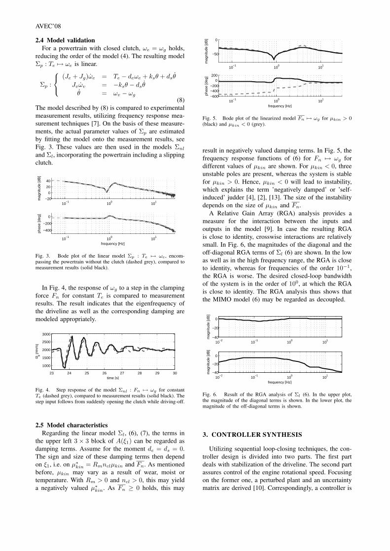
Fig. 3. Bode plot of the linear model Σp : Te 7→ ωe, encom-passing the powertrain without the clutch (dashed grey), compared tomeasurement results (solid black).

In Fig. 4, the response of ωg to a step in the clampingforce Fn for constant Te is compared to measurementresults. The result indicates that the eigenfrequency ofthe driveline as well as the corresponding damping aremodeled appropriately.

23 24 25 26 27 28 29 30

1000

1500

2000

2500

3000

time [s]

ω g [rev

/s]

Fig. 4. Step response of the model Σnl : Fn 7→ ωg for constantTe (dashed grey), compared to measurement results (solid black). Thestep input follows from suddenly opening the clutch while driving-off.

2.5 Model characteristicsRegarding the linear model Σl, (6), (7), the terms in

the upper left 3× 3 block of A(ξ1) can be regarded asdamping terms. Assume for the moment de = ds = 0.The sign and size of these damping terms then dependon ξ1, i.e. on µ∗kin = Rmnclµkin and Fn. As mentionedbefore, µkin may vary as a result of wear, moist ortemperature. With Rm > 0 and ncl > 0, this may yielda negatively valued µ∗kin. As Fn ≥ 0 holds, this may

10−1

100

101

−50

0

mag

nitu

de [d

B]

10−1

100

101

−600

−400−200

0200

frequency [Hz]

phas

e [d

eg]

Fig. 5. Bode plot of the linearized model Fn 7→ ωg for µkin > 0(black) and µkin < 0 (grey).

result in negatively valued damping terms. In Fig. 5, thefrequency response functions of (6) for Fn 7→ ωg fordifferent values of µkin are shown. For µkin < 0, threeunstable poles are present, whereas the system is stablefor µkin > 0. Hence, µkin < 0 will lead to instability,which explains the term ’negatively damped’ or ’self-induced’ judder [4], [2], [13]. The size of the instabilitydepends on the size of µkin and Fn.

A Relative Gain Array (RGA) analysis provides ameasure for the interaction between the inputs andoutputs in the model [9]. In case the resulting RGAis close to identity, crosswise interactions are relativelysmall. In Fig. 6, the magnitudes of the diagonal and theoff-diagonal RGA terms of Σl (6) are shown. In the lowas well as in the high frequency range, the RGA is closeto identity, whereas for frequencies of the order 10−1,the RGA is worse. The desired closed-loop bandwidthof the system is in the order of 100, at which the RGAis close to identity. The RGA analysis thus shows thatthe MIMO model (6) may be regarded as decoupled.

10−2

10−1

100

101

−40

−20

0

mag

nitu

de [d

B]

10−2

10−1

100

101

−40

−20

0

frequency [Hz]

mag

nitu

de [d

B]

Fig. 6. Result of the RGA analysis of Σl (6). In the upper plot,the magnitude of the diagonal terms is shown. In the lower plot, themagnitude of the off-diagonal terms is shown.

3. CONTROLLER SYNTHESIS

Utilizing sequential loop-closing techniques, the con-troller design is divided into two parts. The first partdeals with stabilization of the driveline. The second partassures control of the engine rotational speed. Focusingon the former one, a perturbed plant and an uncertaintymatrix are derived [10]. Correspondingly, a controller is

AVEC’08

designed using a DK-iteration scheme. This approachenables robust stability and performance analysis.

3.1 Sequential loop-closingBased on the RGA analysis (Sect. 2.5), a decentralized

diagonal controller K(s) = diag (Ke(s),Kg(s)) insteadof a full MIMO controller is designed. Sequential Loop-closing (SQL) techniques are adopted for the design [8].In this way, off-diagonal interaction terms are accountedfor.

Transforming the state-space representation Σl to atransfer function H(s) yields[

ωe

ωg

]=

[H11 H12

H21 H22

] [Te

Fn

](9)

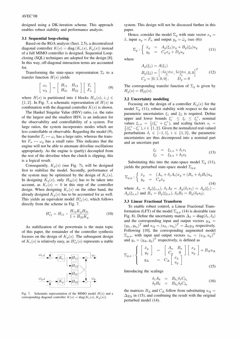
where H(s) is partitioned into 4 blocks Hij(s), i, j ∈{1, 2}. In Fig. 7, a schematic representation of H(s) incombination with the diagonal controller K(s) is shown.

The Hankel Singular Value (HSV) ratio, i.e. the ratioof the largest and the smallest HSV, is an indicator forthe observability and controllability of a system. Forlarge ratios, the system incorporates modes which areless controllable or observable. Regarding the model (9),the transfer Te 7→ ωe has a large ratio, whereas the trans-fer Fn 7→ ωg has a small ratio. This indicates that theengine will not be able to attenuate driveline oscillationsappropriately. As the engine is (partly) decoupled fromthe rest of the driveline when the clutch is slipping, thisis a logical result.

Consequently, Kg(s) (see Fig. 7), will be designedfirst to stabilize the model. Secondly, performance ofthe system may be optimized by the design of Ke(s).In designing Kg(s), only H22(s) has to be taken intoaccount, as Ke(s) = 0 in this step of the controllerdesign. When designing Ke(s) on the other hand, thealready designed Kg(s) has to be accounted for as well.This yields an equivalent model H∗

11(s), which followsdirectly from the scheme in Fig. 7.

H∗11 = H11 −

H12KgH21

1 + H22Kg(10)

As stabilization of the powertrain is the main topicof this paper, the remainder of the controller synthesisfocuses on the design of Kg(s). The subsequent designof Ke(s) is relatively easy, as H∗

11(s) represents a stable

ωg,d ωg

H11ωe,d

H12

H21

H22

Ke

Kg

− ωe

−

Fig. 7. Schematic representation of the MIMO model H(s) and acorresponding diagonal controller K(s) = diag(Ke(s), Kg(s)).

system. This design will not be discussed further in thispaper.

Hence, consider the model Σg with state vector xg =x, input ug = Fn and output yg = ωg (see (6))

Σg :{

xg = Ag(ξ1)xg + Bg(ξ2)ug

yg = Cgxg + Dgug(11)

where

Ag(ξ1) = A(ξ1)

Bg(ξ2) =[−ξ2−µst

Je, ξ2+µst

Jg, 0, 0

]T

Cg = [0, 1, 0, 0] , Dg = 0

(12)

The corresponding transfer function of Σg is given byHg(s) = H22(s).

3.2 Uncertainty modelingFocusing on the design of a controller Kg(s) for the

model Σg (11), robust stability with respect to the realparametric uncertainties ξ1 and ξ2 is required. Defineupper and lower bounds ξ−i ≤ ξi ≤ ξ+

i , nominalvalues ξi,n = 1

2 (ξ−i + ξ+i ), and scaling factors si =

12 (ξ+

i −ξ−i ), i ∈ {1, 2}. Given the normalized real-valuedperturbations δi ∈ [−1, 1], i ∈ {1, 2}, the parametricuncertainties are thus decomposed into a nominal partand an uncertain part

ξ1 = ξ1,n + δ1s1

ξ2 = ξ2,n + δ2s2(13)

Substituting this into the state-space model Σg (11),yields the perturbed state-space model Σg,p

Σg,p :{

xg = (An + δ1Aδ)xg + (Bn + δ2Bδ)ug

yg = Cgxg

(14)where An = Ag(ξ1,n), δ1Aδ = Ag(δ1s1) = Ag(ξ1) −Ag(ξ1,n) and Bn = Bg(ξ2,n), δ2Bδ = Bg(δ2s2).

3.3 Linear Fractional TransformTo enable robust control, a Linear Fractional Trans-

formation (LFT) of the model Σg,p (14) is desirable (seeFig. 8). Define the uncertainty matrix ∆δ = diag(δ1, δ2)and the corresponding input and output vectors y∆ =(yδ1 , yδ2)

T and u∆ = (uδ1 , uδ2)T = ∆δy∆ respectively.

Following [10], the corresponding augmented modelΣg,a, with input and output vectors ua = (u∆, ug)T

and ya = (y∆, yg)T respectively, is defined as

Σg,a :

[

xg

yg

]=

[An Bn

Cg 0

] [xg

ug

]+ B∆u∆

y∆ = C∆

[xg

ug

](15)

Introducing the scalings

δ1Aδ = Bδ1δ1Cδ1

δ2Bδ = Bδ2δ2Cδ2

(16)

the matrices B∆ and C∆ follow from substituting u∆ =∆y∆ in (15), and combining the result with the originalperturbed model (14).

AVEC’08

Bδ1

Bδ2

Bn An

1/s

Cg

Cδ1

Cδ2

Wp

∆δ

H∗g,a

Kg

Hg,ayδ1

yδ2

yK

z

uδ1

uδ2

ug

r

y∆

yK

zz

u∆

ug

r

−

H∗g,a

yg

(a) (b)

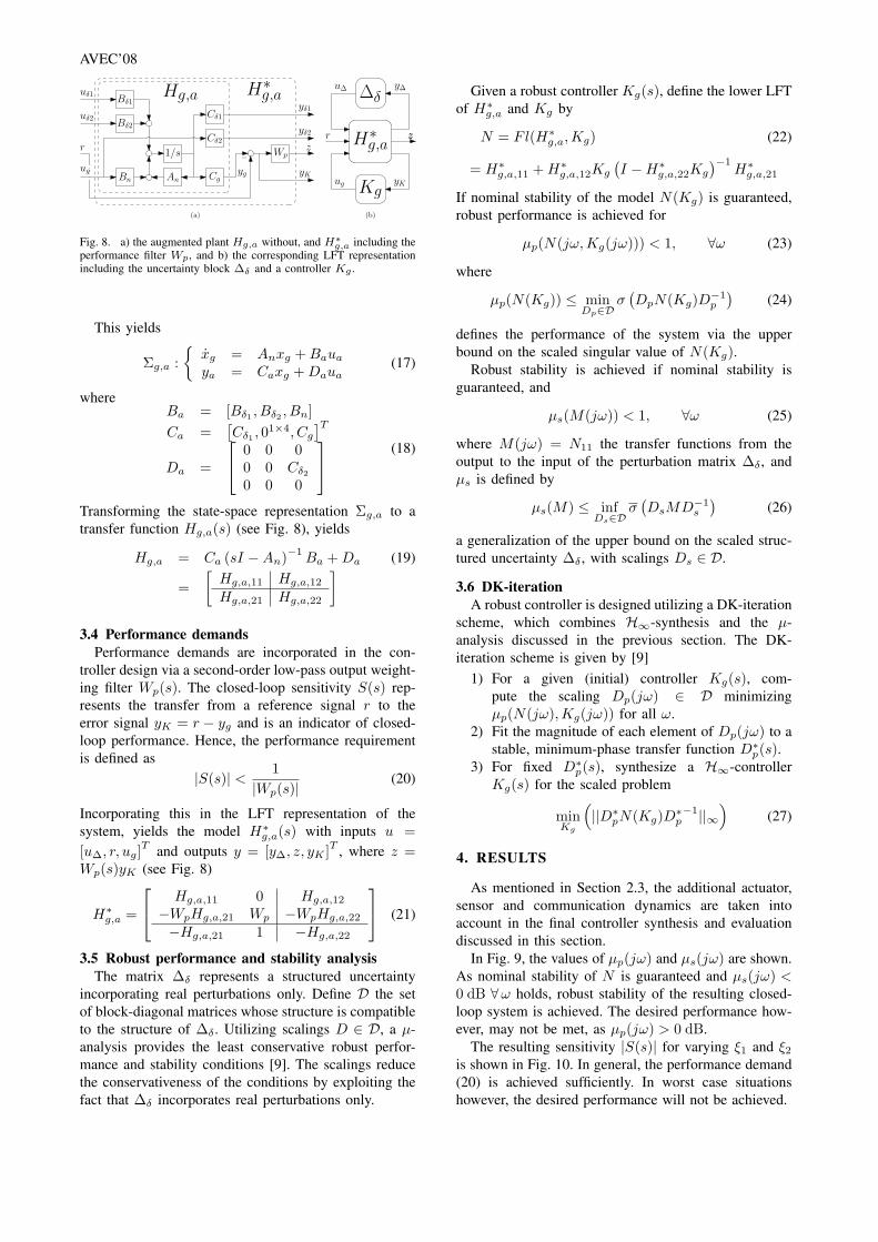
Fig. 8. a) the augmented plant Hg,a without, and H∗g,a including the

performance filter Wp, and b) the corresponding LFT representationincluding the uncertainty block ∆δ and a controller Kg .

This yields

Σg,a :{

xg = Anxg + Baua

ya = Caxg + Daua(17)

whereBa = [Bδ1 , Bδ2 , Bn]Ca =

[Cδ1 , 0

1×4, Cg

]T

Da =

0 0 00 0 Cδ2

0 0 0

(18)

Transforming the state-space representation Σg,a to atransfer function Hg,a(s) (see Fig. 8), yields

Hg,a = Ca (sI −An)−1Ba + Da (19)

=[

Hg,a,11 Hg,a,12

Hg,a,21 Hg,a,22

]3.4 Performance demands

Performance demands are incorporated in the con-troller design via a second-order low-pass output weight-ing filter Wp(s). The closed-loop sensitivity S(s) rep-resents the transfer from a reference signal r to theerror signal yK = r − yg and is an indicator of closed-loop performance. Hence, the performance requirementis defined as

|S(s)| < 1|Wp(s)|

(20)

Incorporating this in the LFT representation of thesystem, yields the model H∗

g,a(s) with inputs u =[u∆, r, ug]

T and outputs y = [y∆, z, yK ]T , where z =Wp(s)yK (see Fig. 8)

H∗g,a =

Hg,a,11 0 Hg,a,12

−WpHg,a,21 Wp −WpHg,a,22

−Hg,a,21 1 −Hg,a,22

(21)

3.5 Robust performance and stability analysisThe matrix ∆δ represents a structured uncertainty

incorporating real perturbations only. Define D the setof block-diagonal matrices whose structure is compatibleto the structure of ∆δ . Utilizing scalings D ∈ D, a µ-analysis provides the least conservative robust perfor-mance and stability conditions [9]. The scalings reducethe conservativeness of the conditions by exploiting thefact that ∆δ incorporates real perturbations only.

Given a robust controller Kg(s), define the lower LFTof H∗

g,a and Kg by

N = Fl(H∗g,a,Kg) (22)

= H∗g,a,11 + H∗

g,a,12Kg

(I −H∗

g,a,22Kg

)−1H∗

g,a,21

If nominal stability of the model N(Kg) is guaranteed,robust performance is achieved for

µp(N(jω, Kg(jω))) < 1, ∀ω (23)

where

µp(N(Kg)) ≤ minDp∈D

σ(DpN(Kg)D−1

p

)(24)

defines the performance of the system via the upperbound on the scaled singular value of N(Kg).

Robust stability is achieved if nominal stability isguaranteed, and

µs(M(jω)) < 1, ∀ω (25)

where M(jω) = N11 the transfer functions from theoutput to the input of the perturbation matrix ∆δ , andµs is defined by

µs(M) ≤ infDs∈D

σ(DsMD−1

s

)(26)

a generalization of the upper bound on the scaled struc-tured uncertainty ∆δ , with scalings Ds ∈ D.

3.6 DK-iterationA robust controller is designed utilizing a DK-iteration

scheme, which combines H∞-synthesis and the µ-analysis discussed in the previous section. The DK-iteration scheme is given by [9]

1) For a given (initial) controller Kg(s), com-pute the scaling Dp(jω) ∈ D minimizingµp(N(jω),Kg(jω)) for all ω.

2) Fit the magnitude of each element of Dp(jω) to astable, minimum-phase transfer function D∗

p(s).3) For fixed D∗

p(s), synthesize a H∞-controllerKg(s) for the scaled problem

minKg

(||D∗

pN(Kg)D∗p−1||∞

)(27)

4. RESULTS

As mentioned in Section 2.3, the additional actuator,sensor and communication dynamics are taken intoaccount in the final controller synthesis and evaluationdiscussed in this section.

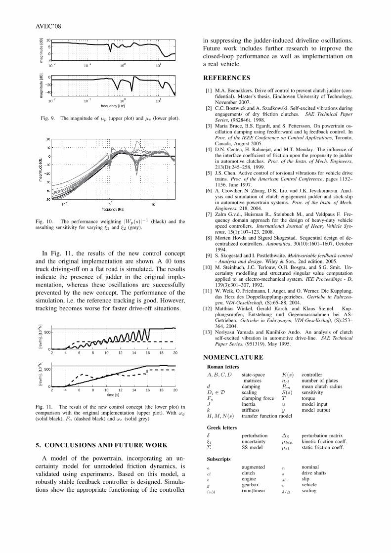
In Fig. 9, the values of µp(jω) and µs(jω) are shown.As nominal stability of N is guaranteed and µs(jω) <0 dB ∀ω holds, robust stability of the resulting closed-loop system is achieved. The desired performance how-ever, may not be met, as µp(jω) > 0 dB.

The resulting sensitivity |S(s)| for varying ξ1 and ξ2

is shown in Fig. 10. In general, the performance demand(20) is achieved sufficiently. In worst case situationshowever, the desired performance will not be achieved.

AVEC’08

10−2

10−1

100

101

−5

0

5

10m

agni

tude

[dB

]

10−2

10−1

100

101

−40

−20

0

frequency [Hz]

mag

nitu

de [d

B]

Fig. 9. The magnitude of µp (upper plot) and µs (lower plot).

Fig. 10. The performance weighting |Wp(s)|−1 (black) and theresulting sensitivity for varying ξ1 and ξ2 (grey).

In Fig. 11, the results of the new control conceptand the original implementation are shown. A 40 tonstruck driving-off on a flat road is simulated. The resultsindicate the presence of judder in the original imple-mentation, whereas these oscillations are successfullyprevented by the new concept. The performance of thesimulation, i.e. the reference tracking is good. However,tracking becomes worse for faster drive-off situations.

2 4 6 8 10 12 14 16 18 200

500

[rev

/m],

[10 2

N]

2 4 6 8 10 12 14 16 18 200

500

time [s]

[rev

/m],

[10 2

N]

Fig. 11. The result of the new control concept (the lower plot) incomparison with the original implementation (upper plot). With ωg

(solid black), Fn (dashed black) and ωe (solid grey).

5. CONCLUSIONS AND FUTURE WORK

A model of the powertrain, incorporating an un-certainty model for unmodeled friction dynamics, isvalidated using experiments. Based on this model, arobustly stable feedback controller is designed. Simula-tions show the appropriate functioning of the controller

in suppressing the judder-induced driveline oscillations.Future work includes further research to improve theclosed-loop performance as well as implementation ona real vehicle.

REFERENCES

[1] M.A. Beenakkers. Drive off control to prevent clutch judder (con-fidential). Master’s thesis, Eindhoven University of Technology,November 2007.

[2] C.C. Bostwick and A. Szadkowski. Self-excited vibrations duringengagements of dry friction clutches. SAE Technical PaperSeries, (982846), 1998.

[3] Maria Bruce, B.S. Egardt, and S. Pettersson. On powertrain os-cillation damping using feedforward and lq feedback control. InProc. of the IEEE Conference on Control Applications, Toronto,Canada, August 2005.

[4] D.N. Centea, H. Rahnejat, and M.T. Menday. The influence ofthe interface coefficient of friction upon the propensity to judderin automotive clutches. Proc. of the Instn. of Mech. Engineers,213(D):245–258, 1999.

[5] J.S. Chen. Active control of torsional vibrations for vehicle drivetrains. Proc. of the American Control Conference, pages 1152–1156, June 1997.

[6] A. Crowther, N. Zhang, D.K. Liu, and J.K. Jeyakumaran. Anal-ysis and simulation of clutch engagement judder and stick-slipin automotive powertrain systems. Proc. of the Instn. of Mech.Engineers, 218, 2004.

[7] Zalm G.v.d., Huisman R., Steinbuch M., and Veldpaus F. Fre-quency domain approach for the design of heavy-duty vehiclespeed controllers. International Journal of Heavy Vehicle Sys-tems, 15(1):107–123, 2008.

[8] Morten Hovda and Sigurd Skogestad. Sequential design of de-centralized controllers. Automatica, 30(10):1601–1607, October1994.

[9] S. Skogestad and I. Postlethwaite. Multivariable feedback control- Analysis and design. Wiley & Son., 2nd edition, 2005.

[10] M. Steinbuch, J.C. Terlouw, O.H. Bosgra, and S.G. Smit. Un-certainty modelling and structured singular value computationapplied to an electro-mechanical system. IEE Proceedings - D,139(3):301–307, 1992.

[11] W. Weik, O. Friedmann, I. Anger, and O. Werner. Die Kupplung,das Herz des Doppelkupplungsgetriebes. Getriebe in Fahrzeu-gen, VDI-Gesellschaft, (S):65–88, 2004.

[12] Matthias Winkel, Gerald Karch, and Klaus Steinel. Kup-plungsrupfen, Entstehung und Gegenmassnahmen bei AS-Getrieben. Getriebe in Fahrzeugen, VDI-Gesellschaft, (S):253–364, 2004.

[13] Noriyasu Yamada and Kunihiko Ando. An analysis of clutchself-excited vibration in automotive drive-line. SAE TechnicalPaper Series, (951319), May 1995.

NOMENCLATURERoman lettersA, B, C, D state-space K(s) controller

matrices ncl number of platesd damping Rm mean clutch radiusDi ∈ D scaling S(s) sensitivityFn clamping force T torqueJ inertia u model inputk stiffness y model outputH, M, N(s) transfer function model

Greek lettersδ perturbation ∆δ perturbation matrixξi uncertainty µkin kinetic friction coeff.Σ SS model µst static friction coeff.

Subscriptsa augmented n nominalcl clutch s drive shaftse engine sl slipg gearbox v vehicle(n)l (non)linear δ/∆ scaling