Robust Classification of Objects, Faces and Flowers using Natural

Image Statistics

CVPR 2011Christopher KananGarrison CottrellDept. of Computer Sc., Univ. Of California, San Diego

Presented bySk. Mohammadul Haque

Elec. Engineering DepartmentIndian Institute of Science,Bangalore

Outline

Introduction & Motivation Natural Image Statistics Visual Attention and Saliency Saccades - Fixations - Spatial pooling

LMS Color Space ICA The Algorithm

Image Preprocessing ICA Features Saliency Map Computation Fixations and Spatial Pooling Dimension Reduction using PCA Training/ Classification: NN-KDE

Results as in the Paper References

Introduction & Motivation

Human Visual Perception is an amazingly magical process by which we acquire knowledge about environmental objects and events by extracting information from the light the objects emit or reflect, in an effortless and almost reliable way, in our daily environment.

We are simply not aware of the whole computational process going on in our brains, rather we experience only the result of that computation.

When we try to model or implement it, vision becomes an exceptionally difficult computational task.

Introduction & Motivation

But, it is natural that computer vision scientists have tried to draw inspiration from biology and succeeded to an extent.

Many image processing sytems try to mimic the processing that is known to occur in the early parts of the biological visual system. However, beyond the very early stages, little is actually known about the representations used in the brain. Thus, there is actually not much to guide computer vision research at the present.

On the other hand, the importance of prior information in our vision leads us to the Statistical Model of the Visual System which comes up with the natural image statistics.

Natural Image Statistics

Natural Image: Natural image(s) is a small subset of all possible color/intensity combination that we believe has similar statistical structure to that which the visual system is adapted to.

Random Image: Very much unnatural.

Natural images has a structure, more precisely a statistical structure which acts as a prior to our vision system.

Natural Image Statistics

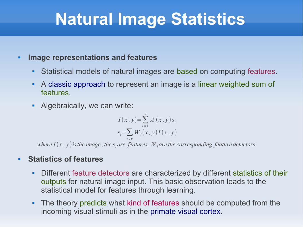
Image representations and features

Statistical models of natural images are based on computing features.

A classic approach to represent an image is a linear weighted sum of features.

Algebraically, we can write:

Statistics of features

Different feature detectors are characterized by different statistics of their outputs for natural image input. This basic observation leads to the statistical model for features through learning.

The theory predicts what kind of features should be computed from the incoming visual stimuli as in the primate visual cortex.

I ( x , y)=∑i=1

n

A i(x , y ) si

si=∑x , y

W i (x , y ) I (x , y )

where I (x , y ) is the image , the si are features ,W i are the corresponding feature detectors.

Visual Attention and Saliency

The surrounding world contains a tremendous amount of visual information, which the visual system cannot fully process. The visual system thus faces the problem of how to allocate its processing resources to focus on important aspects of a scene.

Visual saliency is the distinct subjective perceptual quality which makes some items in the world stand out from their neighbours and immediately grab our attention.

Visual Attention and Saliency

Bayesian framework for saliency and SUN (Saliency Using Natural statistics)

Goal of the visual system is to find potential targets that are important to survival.

The visual system must actively estimate the probability of a target at every location given the visual features observed. This probability defines visual saliency.

Let the binary random variable, C, denote whether a point belongs to a target class, let the random variable, L, denote the location of a point, and let the random variable, F, denote the visual features of a point. Saliency of a point z is then defined as p(C = 1|F = f

z , L = l

z),

where fz represents the feature values observed at z and l

z represents the location (pixel

coordinates) of z.

If we assume for simplicity that features and location are independent and conditionally independent, given C = 1, this probability can be calculated using Bayes’ rule:

SUN uses only bottom-up saliency.

s z= p (C=1∣F= f z , L=l z)=1

p (F= f z)⏟bottom−up saliency

⋅p (F= f z∣C=1)⏟likelihood

⋅p (C=1∣L=l z)⏟location prior

⇔ log ( s z)=−log p (F= f z)⏟self information

+log p(F= f z∣C=1)⏟log likelihood

+log p(C=1∣L=l z)⏟location prior

Saccades-Fixations-Spatial Pooling

Since the visual system cannot fully process the tremendous amount of visual information all at once, sampled by discontinuous fixations, we experience a seamless, continuous world.

Saccades are quick, simultaneous movements of both eyes in the same direction, which helps in the sampling of visual data in a sequential manner.

Attentional and oculomotor processes are greatly intertwined in the brain. Visual modulation of microsaccades is the by-product of attentional modulation driven by visual inputs.

Invariances to scale, location, rotation and viewpoint variations are required for object recognition. Spatial pooling is a model technique to induce scale-invarince, while other methods like MAX operations over neighbouring regions and over neighbouring orientations of retinal filters induces location and rotation invariances respectively.

LMS Color Space

LMS is a color space represented by the response of the three types of cones of the human eye, named after their responsivity (sensitivity) at long, medium and short wavelengths.

It is common to use the LMS color space when performing chromatic adaptation (estimating the appearance of a sample under a different illuminant).

This helps in a non-linear(logarithmic) compression of the bandwidth of huge intensity range.

Independent Component Analysis

Signals are believed to be linear mixtures of some independent components or "latent variables".

We want to estimate sj and a

ji' s under the constraint that s

j's are

maximally independent.

ICA finds the independent components by maximizing the statistical independence of the estimated components.

Maximization of non-Gaussianity (Kurtosis, Negentropy)

Minimization of Mutual Information

Applications – Source separation, finding hidden factors in financial data, noise reduction, independent feature extraction, etc.

x j=a j1 s1+a j2 s2+...+a jn sn , for j=1,2,... , N ,where , {x j} j=1N are the observed signals

Independent Component Analysis

Preprocessing

Centering and Whitening

FastICA

uses the criterion for maximizing the non-Gaussianity using negentropy.

based on fixed point iteration.

For one component, y=wTx

1. Choose initial (random) weight vector, w

2. Let w+ = E[xg(wTx)]- E[g'(wTx)]w, where, g=G'

3. Let w = w+/||w+||

4. If not converged, go to step 2.

For, multiple components, yi , the corresponding weights, w

i, are estimated sequentially and to maintain

independence Gram-Schmidt orthogonalization is used.

The weights are simultaneously updated as

maximizey

{Negentropy , J ( y )∝[E {G( y)}−E {G(ν)}]2}

⇒ J ' ( y )∝[E {G( y)}−E {G (ν)}]⋅E {G' ( y )}=0where , ν is a zero−meanGaussian r.v.with same variance as y

W=W+D[diag (− β i)+E g ( y ) y ]Wwhere , y=W z , β i=E y i g ( y i) ,D=diag (1/( β i−E g ′ ( y i)))

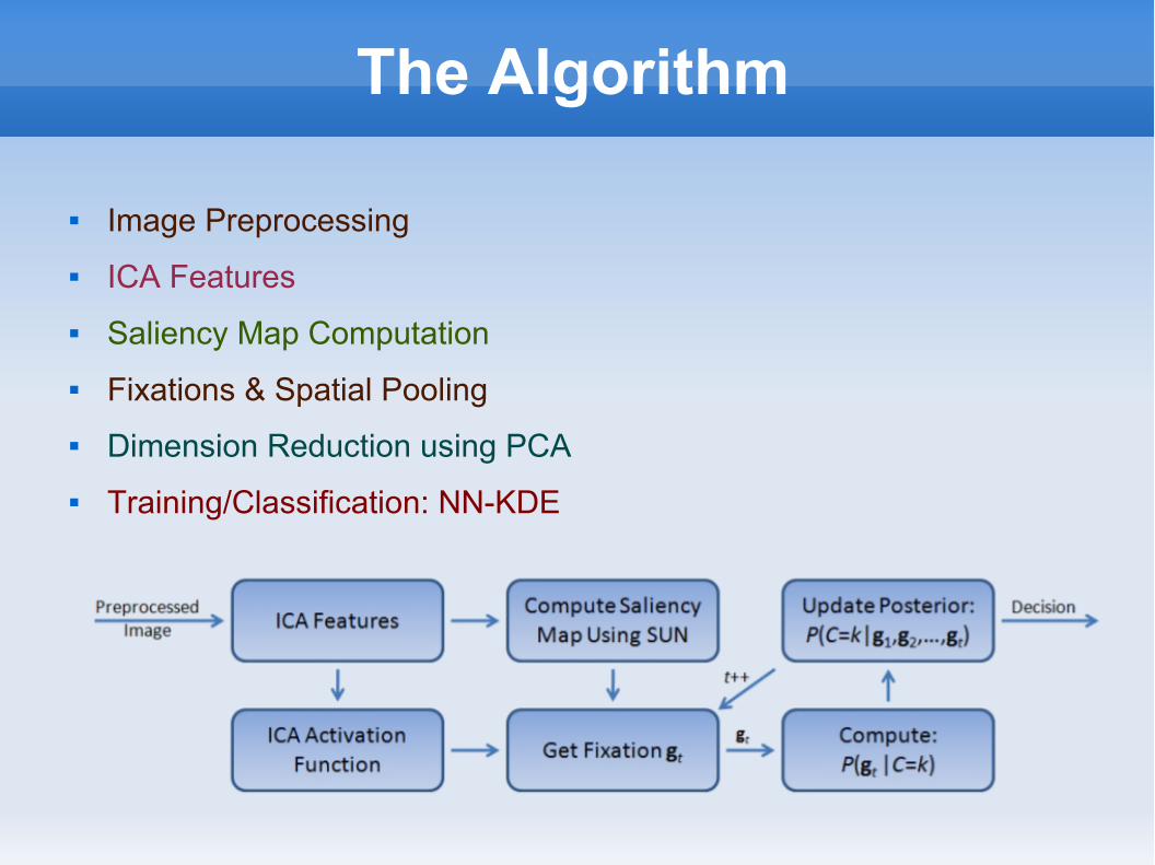
The Algorithm

Image Preprocessing

ICA Features

Saliency Map Computation

Fixations & Spatial Pooling

Dimension Reduction using PCA

Training/Classification: NN-KDE

Image Preprocessing

Images are resized to standard size without altering the aspect ratio.

They are converted from sRGB to LMS color space.

Then, the color values are globally normalized as

To cope with enormous variance as in the biological vision system, the color values are non-linearly processed as

r lineari

(x , y)=c i( x , y)−min

i , x , yc i(x , y)

maxi , x , y

ci (x , y)

r non−lineari

(x , y)=log (ε )−log (r linear

i(x , y)+ε)

log (ε )−log (1+ε )where , ε≈0.05

ICA Features

Feature detectors or filters are learned from image patches of size m x n x 3 obtained from numerous natural images.

These filters are sparse and are similar to the simple cells in primate visual cortex.

ICA is applied to those natural image patches after dimension reduction to d-dimension and discarding the 1st component (corresponds mainly to change in brightness).

d statistically independent gabor-like filters of size m x n x 3 are obtained.

Best parameter values were found as 192 filters of size 24 x 24.

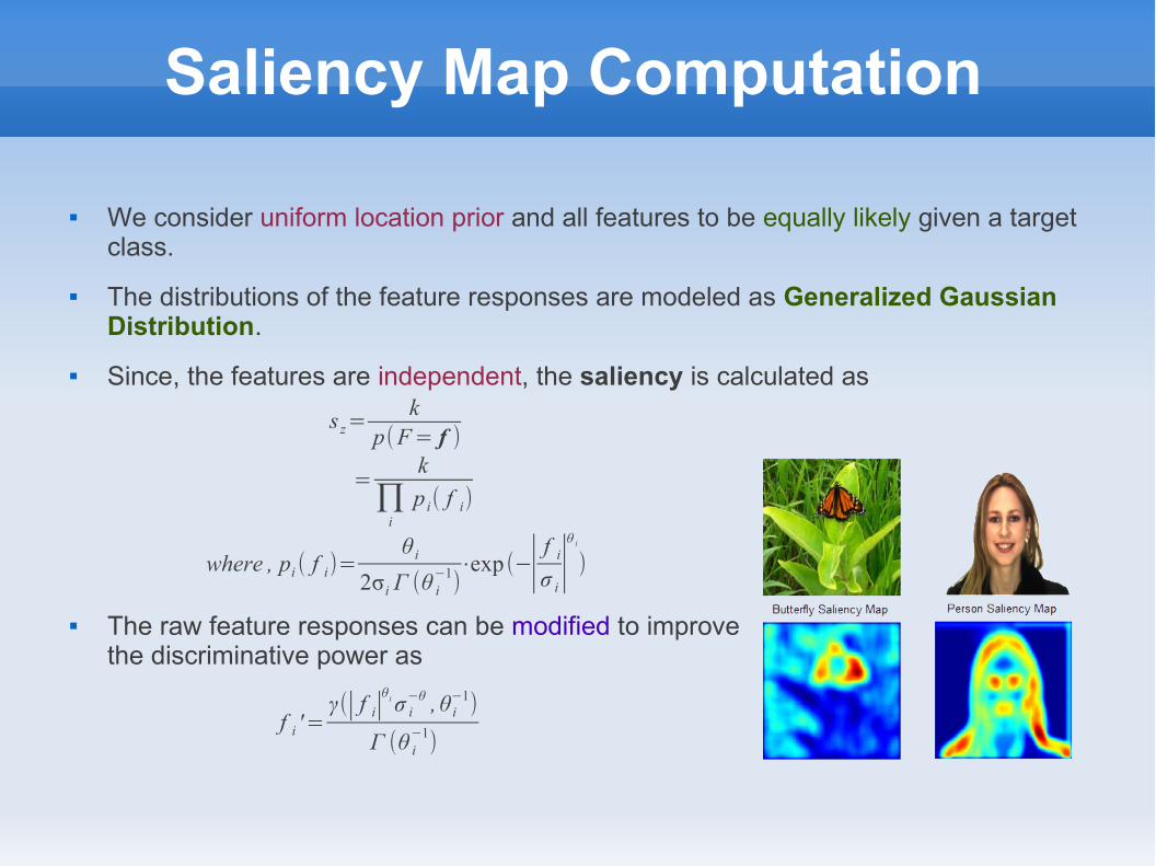
Saliency Map Computation

We consider uniform location prior and all features to be equally likely given a target class.

The distributions of the feature responses are modeled as Generalized Gaussian Distribution.

Since, the features are independent, the saliency is calculated as

The raw feature responses can be modified to improve the discriminative power as

s z=k

p(F= f )

=k

∏i

p i( f i)

where , pi ( f i)=θ i

2σi Γ (θ i−1

)⋅exp (−∣ f i

σ i∣θ i

)

f i '=γ(∣ f i∣

θ iσ i−θ , θ i

−1)

Γ (θ i−1

)

T fixations at locations lt are randomly chosen according to the saliency

map, where, T=100.

Centred at each location, lt, a w x w x d stack of filter responses are given a

target class, where, w=51.

The spatial pooling creates a pyramid of height 3 with sizes 1 x 1, 2 x 2 and 4 x 4 from top to bottom by spatial averaging the filter responses and normalizing each of them.

This reduces the dimension from 512d to 21d.

Further only 500 first principal components are retained and then whitened.

Fixations & Spatial Pooling

Training/Classification: NN-KDE

Classification is done using NIMBLE: an NN-KDE method to model P(g

t|C=k), where, g

t is the vector of fixations features acquired at time

t and k is one of the classes in the training.

Using Naive Bayes' assumption, we have

For each class,

Since, NN is used, the class is assigned as

P ({g t }1T∣C=k )=∏

t=1

T

P ( g t∣C=k )

P (C=k∣{g t }1T )∝P (C=k )⋅∏

t=1

T

P (g t∣C=k )

P (g t∣C=k )∝maxi

1

∥wk , i−g t∥2

2+α∥vk , i−l t∥2

2+ε

where ,wk , i is ith examplar of class k ,vk , i is normalized fixation centre of the same ,α=0.5, ε≈10−4

C=argmaxk

P(C=k∣{g t }1T)

Results as in the Paper

References

Christopher Kanan and Garrison Cottrell, Robust Classification of Objects, Faces and Flower using Natural Image Statistics, CVPR 2010

Aapo Hyvarinen, Jarmo Hurri and Patrik O. Hoyer, Natural Image Statistics-A probabilistic approach to early computational vision, February 27, 2009, Springer

Maximilian Riesenhuber, HMAX, MAXLab, The Laboratory for Computational Cognitive Neuroscience, http://riesenhuberlab.neuro.georgetown.edu/hmax.html

M. Fairchild, Color appearance models, Wiley Inter-science, 2nd edition, 2005

D. J. Field, What is the goal of sensory coding?, Neural Computation, 6:559–601, 1994.

M. Riesenhuber and T. Poggio, Hierarchical models of object recognition in cortex, Nature Neuroscience, 2:1019–1025, 1999

L. Zhang, M. H. Tong, T. K. Marks, H. Shan and G. W. Cottrell, SUN: A Bayesian framework for saliency using natural statistics, Journal of Vision, 8:1–20, 2008

Aapo Hyvärinen and Erkki Oja, Independent Component Analysis: Algorithms and Applications, Neural Networks, 13(4-5):411-430, 2000

Pierre Comos, Independent component analysis, A new concept?, Signal Processing 36 (1994), 287-314

James T. Fulton, Processes in Biological Vision, Vision Concepts, August 1, 2000, http://neuronresearch.net/vision/

LMS color space, http://en.wikipedia.org/wiki/LMS_color_space

Visual system, http://en.wikipedia.org/wiki/Visual_system

Luke Barrington, Tim K. Marks and Garrison W. Cottrell, NIMBLE: A Kernel Density Model of Saccade-Based Visual Memory, Annual Cognitive Science Conference, Nashville, Tennessee

Susana M., S. L. Macknik and David H. Hubel, The role of fixational eye movements in visual perception, Nature Reviews, Neuroscience, Vol. 5, March 2004