robust and efficient estimation of the mode...
TRANSCRIPT
D. R. Bickel, submitted to InterStat. 1
ROBUST AND EFFICIENT ESTIMATIONOF THE MODE OF CONTINUOUS DATA:
THE MODE AS A VIABLE MEASURE OF CENTRAL TENDENCY
David R. BickelMedical College of Georgia
Office of Biostatistics and Bioinformatics1120 Fifteenth St., AE-3037
Augusta, GA 30912-4900URL: http://www.mcg.edu/research/biostat/bickel.htmlE-mail: [email protected], [email protected]
Key words: Robust estimation; robust mode; mode estimator; average value;measure of location; asymmetry; transformation; efficiency.
ABSTRACT. Although a natural measure of the central tendency of a sample ofcontinuous data is its mode (the most probable value), the mean and median arethe most popular measures of location due to their simplicity and ease ofestimation. The median is often used instead of the mean for asymmetric databecause it is closer to the mode and is insensitive to extreme values in the sample.However, the mode itself can be reliably estimated by first transforming the datainto approximately normal data by raising the values to a real power, and thenestimating the mean and standard deviation of the transformed data. With thismethod, two estimators of the mode of the original data are proposed: a simpleestimator based on estimating the mean by the sample mean and the standarddeviation by the sample standard deviation, and a more robust estimator based onestimating the mean by the median and the standard deviation by the standardizedmedian absolute deviation.
Both of these mode estimators were tested using simulated data drawnfrom normal (symmetric), lognormal (asymmetric), and Pareto (very asymmetric)distributions. The latter two distributions were chosen to test the generality of themethod since they are not power transforms of the normal distribution. Each ofthe proposed estimators of the mode has a much lower variance than the mean andmedian for the two asymmetric distributions. When outliers were added to thesimulations, the more robust of the two proposed mode estimators had a lowerbias and variance than the median for the asymmetric distributions, especiallywhen the level of contamination approached the 50% breakdown point. It isconcluded that the mode is often a more reliable measure of location than themean or median for asymmetric data. The proposed estimators also performedwell relative to previous estimators of the mode. While different estimators arebetter under different conditions, the proposed robust estimator is reliable for awide variety of distributions and contamination levels.
D. R. Bickel, submitted to InterStat. 2
1. INTRODUCTION
Although many measures of location have been developed in recent years,
researchers still mostly use the mean and median to describe the location or
“average” value of continuous data, largely because those measures are easy to
understand and estimate. The concept of the mode is also easily understood and is
attractive as the most probable value, but reliable methods of estimating the mode
of continuous data are not widely known. Most investigators describe the average
of continuous data by the mean except when the data are highly skewed, highly
kurtotic, or contaminated with outliers, in which case the median is often used.
The median is indeed a good choice in the latter two cases, when the mean is very
unreliable or even undefined. In the case of asymmetric data, the median is
preferred to the mean, often since the median is almost always closer to the mode,
but a better approach would be to estimate the mode itself in many cases.
(Dharmadhikari and Joag-dev (1988) give the conditions under which the median
is between the mode and the mean.) The mode is the most intuitive measure of
central tendency since the mode represents the most typical value of the data.
However, previous estimators of the mode have suffered from high bias, low
efficiency (high variance), or a sensitivity to outliers, and these limitations have
probably contributed to the neglect of the mode as a description of the central
tendency. To enable a wider use of the mode, it will be demonstrated herein that
the mode can be estimated with lower bias and even higher efficiency and
robustness to outliers than the median for asymmetric, continuous data.
The mean, median, and mode are all measures of location µ X( ) of a
continuous random variable X in the sense that they satisfy
∀a> 0,b
µ aX + b( )= aµ X( ) + b , µ −X( )= −µ X( ), and X ≥ 0 ⇒ µ X( ) ≥ 0 (Staudte and
Sheather 1990). The sample mean and sample median are simple nonparametric
estimators of the mean and median of the underlying continuous distribution. For
symmetric distributions, the sample mean and sample median estimate the same
D. R. Bickel, submitted to InterStat. 3
estimand since the mean and median are equal in this case. For asymmetric
distributions, the sample mean and sample median estimate different, but known,
estimands. The mode, however, has no natural estimator. In this paper, previous
estimators of the mode are compared with estimators designed to have low
variance.
The proposed strategy of mode estimation consists of the following steps:
1. transform the data such that the transformed data is approximately normal;
2. estimate the mean and standard deviation of the transformed data;
3. assuming that the transformed data were drawn from a normal distribution,
use the estimated mean and standard deviation of the transformed data to
estimate the mode of the original data.
The transformation used herein is the simple power transformation: y x;α( )= xα ,
where y is called the transformed variable, x is called the original variable, and α
is a nonzero real constant. We require that x > 0, but the transformation can be
generalized by y x;α,β( ) = x + β( )α to allow negative values of x (Box & Tiao
1992). Thus, given a data set xi{ }i =1
n, the transformed data set is yi α( ){ }
i =1
n, where
yi α( )= xiα . The value of α is chosen to make the transformed data as close as
possible to normally-distributed data. Although y is not exactly normal, it is
constructed to be approximately normal through the choice of α , so it can be
considered normal for the purpose of estimation. If y is normally distributed with
parameters y and σ , then the probability density function (PDF) of y is
fy y; y ,σ( )= 2πσ( )−1
exp −y − y ( )2
2σ 2
(1)
and thus the PDF of x is
fx x; y ,σ,α( ) = fy xα ; y ,σ( )∂y∂x
= 2πσ( )−1
α xα −1 exp −xα − y ( )2
2σ 2
. (2)
D. R. Bickel, submitted to InterStat. 4
Many distributions can be approximated by Eq. (2), in which α quantifies the
skewness, with 1=α for zero skewness. The mode of x, denoted by M, is the
value of x that maximizes its PDF. Requiring that ( )[ ] 0,,; =∂∂=Mxx xyxf ασ , we
find that
( )α
αασ
12
2 14
2
1
−++= yyM . (3)
(Note that 1=α implies that yM = , as expected from the fact that the mode of a
normal distribution equals its mean.) Therefore, M can be estimated by replacing
y and σ with estimates of the mean and standard deviation from the transformed
sample ( ){ }n
iiy 1=α . If α is positive and so low that the argument of the square root
is negative, as sometimes occurs for small samples with high skewness, then the
estimate of the mode is the minimum value of the sample. This method of
estimating the mode is described in detail in Section 2. Its bias, efficiency, and
resistance to outliers were studied by simulation, as reported in Section 3.
2. ESTIMATORS OF THE MODE
2.1 Standard parametric estimator
A simple implementation of the mode estimation technique of Section 1 is
the following algorithm:
1. transform the data using the value of α that maximizes the standard
correlation coefficient between the ordered transformed data and the expected
order statistics for a normal distribution;
2. estimate the mean and standard deviation of the transformed data using the
sample mean and sample standard deviation;
D. R. Bickel, submitted to InterStat. 5
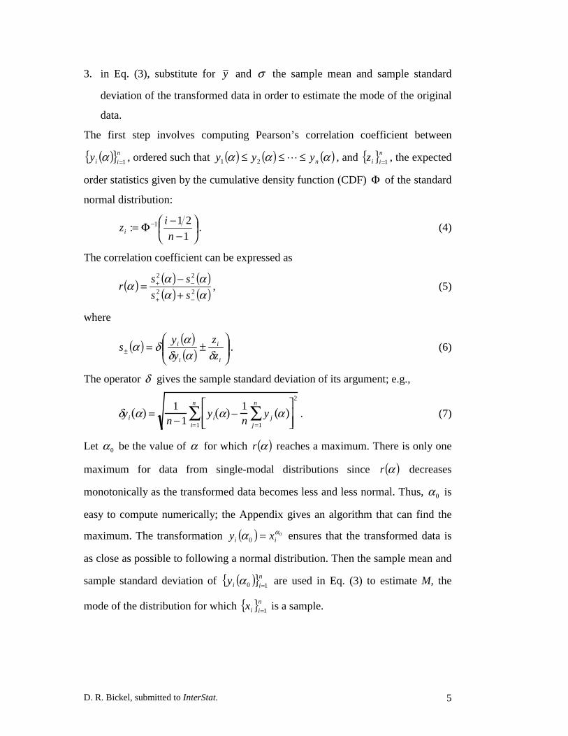
3. in Eq. (3), substitute for y and σ the sample mean and sample standard
deviation of the transformed data in order to estimate the mode of the original
data.
The first step involves computing Pearson’s correlation coefficient between
( ){ }n
iiy 1=α , ordered such that ( ) ( ) ( )ααα nyyy ≤≤≤ �21 , and { }n
iiz 1= , the expected
order statistics given by the cumulative density function (CDF) Φ of the standard
normal distribution:
−−Φ= −
1
21: 1
n
izi . (4)
The correlation coefficient can be expressed as
( ) ( ) ( )( ) ( )αα
ααα22
22
−+
−+
+−
=ss
ssr , (5)
where
( ) ( )( )
±=±
i
i
i
i
z
z
y
ys
δαδαδα . (6)
The operator δ gives the sample standard deviation of its argument; e.g.,
δyi α( ) =1
n −1yi α( )−
1n
y j α( )j =1
n
∑
2
i=1
n
∑ . (7)
Let 0α be the value of α for which ( )αr reaches a maximum. There is only one
maximum for data from single-modal distributions since ( )αr decreases
monotonically as the transformed data becomes less and less normal. Thus, 0α is
easy to compute numerically; the Appendix gives an algorithm that can find the
maximum. The transformation ( ) 00
αα ii xy = ensures that the transformed data is
as close as possible to following a normal distribution. Then the sample mean and
sample standard deviation of ( ){ }n
iiy 10 =α are used in Eq. (3) to estimate M, the
mode of the distribution for which { }n
iix 1= is a sample.

D. R. Bickel, submitted to InterStat. 6
This estimator of the mode, called the standard parametric mode (SPM),
has advantages in its simplicity and its efficiency in the case that ( ){ }n
iiy 10 =α is
approximately normal. However, it is not robust to outliers since if the value of a
single ix is sufficiently large, then 0α can be brought past any bound and the
estimation can thereby be rendered worthless. The next subsection modifies the
algorithm to make it resistant to outliers.
2.2 Robust parametric estimator
The steps in Section 1 for computing the mode become highly robust to
contamination in the data when they take this form:
1. transform the data using the value of α that maximizes a robust correlation
coefficient between the ordered transformed data and the expected order
statistics for a normal distribution;
2. estimate the mean and standard deviation of the transformed data using the
median and standardized median absolute deviation (MAD);
3. in Eq. (3), substitute for y and σ the median and MAD of the transformed
data in order to estimate the mode of the original data.
The robust correlation coefficient is based on a generalization of the linear
correlation coefficient (Huber, 1981), with the δ of Eq. (6) denoting a general
measure of dispersion or scale, rather than the standard deviation. Again assuming
that ( ) ( ) ( )ααα nyyy ≤≤≤ �21 , we use the correlation coefficient given by
( ) ( ) ( )( ) ( )αα
ααα22
22
−+
−+
+−
=SS
SSR , (8)
where
( ) ( )( )
∆
±∆
∆=±i
i
i
i
z
z
y
yS
ααα . (9)
Here, the operator ∆ yields MAD, normalized such that σ=∆y if y is normally
distributed with standard deviation σ . For example,

D. R. Bickel, submitted to InterStat. 7
∆yi α( )= 1 Φ−1 3 4( )[ ]med yi α( )− medyi α( )≈1.4826med yi α( )− med yi α( )
, (10)
where med is the sample median operator, so that ( )αiymed is the median of
( ){ }n
iiy 1=α . Since ( )αR quantifies the normality of the transformed data, the value
0α is found that maximizes ( )αR , i.e., ( ) ( )ααα
RR max0 = . For a normal
distribution, the mean is equal to the median and the standard deviation is equal to
MAD, so ( )0med αiy and ( )0αiy∆ are substituted for y and σ in Eq. (3) to
estimate the mode M.
The robustness of this estimator of the mode, termed the robust
parametric mode (RPM), can be quantified by its finite-sample breakdown point,
the minimum proportion of outliers in a sample that could make an estimator
unbounded (Donoho and Huber 1983). For example, for a sample of size n, the
breakdown point of the median is ( ) ( )nn 21+ for odd n or 21 for even n since at
least half of the points in the sample would have to be replaced with sufficiently
high or sufficiently low values before the median would be higher or lower than
any bound. Being based on the median, the mode estimator described in this
subsection has the same breakdown point, which is the highest breakdown point
possible for a measure of location. The mode estimator of Section 2.1, on the
other hand, is less robust, since the sample mean and sample standard deviation
each has a breakdown point of only n1 , entailing that a single outlier can make
them arbitrarily large.
2.3 Grenander’s estimators
The estimators of the mode introduced above are called parametric
estimators since they make use of the parameters of the family of normal
distributions. A simple class of nonparametric estimators is Grenander’s (1965)
family of estimators of the mode of { }n
iix 1= , with nxxx ≤≤≤ �21 :
D. R. Bickel, submitted to InterStat. 8
( ) ( )
( )kp
xx
xxxxM
kn
i
piki
kn
i
pikiiki
kp <<−
−+=
∑
∑−
=+
−
=++
∗ 1,1
2
1
1
1, , (11)
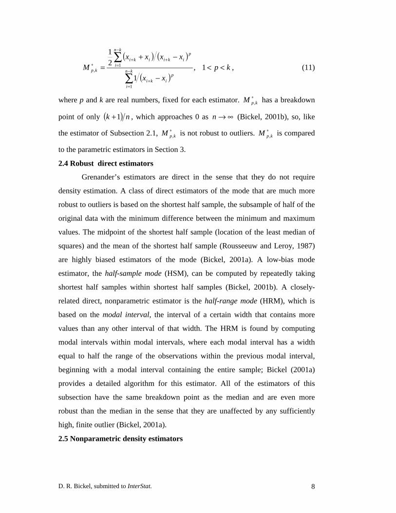
where p and k are real numbers, fixed for each estimator. ∗kpM , has a breakdown
point of only ( ) nk 1+ , which approaches 0 as ∞→n (Bickel, 2001b), so, like
the estimator of Subsection 2.1, ∗kpM , is not robust to outliers. ∗
kpM , is compared
to the parametric estimators in Section 3.
2.4 Robust direct estimators
Grenander’s estimators are direct in the sense that they do not require
density estimation. A class of direct estimators of the mode that are much more
robust to outliers is based on the shortest half sample, the subsample of half of the
original data with the minimum difference between the minimum and maximum
values. The midpoint of the shortest half sample (location of the least median of
squares) and the mean of the shortest half sample (Rousseeuw and Leroy, 1987)
are highly biased estimators of the mode (Bickel, 2001a). A low-bias mode
estimator, the half-sample mode (HSM), can be computed by repeatedly taking
shortest half samples within shortest half samples (Bickel, 2001b). A closely-
related direct, nonparametric estimator is the half-range mode (HRM), which is
based on the modal interval, the interval of a certain width that contains more
values than any other interval of that width. The HRM is found by computing
modal intervals within modal intervals, where each modal interval has a width
equal to half the range of the observations within the previous modal interval,
beginning with a modal interval containing the entire sample; Bickel (2001a)
provides a detailed algorithm for this estimator. All of the estimators of this
subsection have the same breakdown point as the median and are even more
robust than the median in the sense that they are unaffected by any sufficiently
high, finite outlier (Bickel, 2001a).
2.5 Nonparametric density estimators

D. R. Bickel, submitted to InterStat. 9
The nonparametric estimators of Sections 2.3 and 2.4 are direct, but there
are also nonparametric estimators of the mode that depend on estimation of the
probability density. Grenander (1965) and Dharmadhikari and Joag-dev (1988)
note that the mode can be estimated as the argument for which a smoothed
empirical density function (EDF), an estimate of the PDF, reaches a maximum.
The EDF based on a normal kernel function is
ˆ f x( ) =1
nh 2πexp −
12
x − xi
h
2
i =1
n
∑ . (12)
Smaller values of the smoothing parameter h yield lower biases, but higher
variances, in the mode estimates. Based on optimal estimates of the PDF,
Silverman (1986) recommended setting h equal to 0.9( )S , where S is the
minimum of the sample standard deviation and the normal-consistent interquartile
range. This recommendation is followed in the simulations below, except that the
interquartile range is replaced with the MAD, made consistent with the normal
distribution by multiplying by 1.4826. The MAD is preferred for these studies
with large numbers of outliers since its asymptotic breakdown point is twice that
of the interquartile range (Rousseeuw and Croux, 1993). The mode is estimated
by the empirical density function mode (EDFM), denoted by ′ M and defined such
that ˆ f ′ M ( )= maxx
ˆ f x( ).
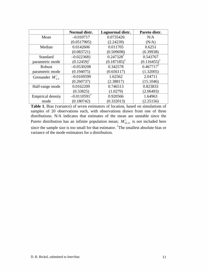
3. SIMULATIONS
The methods of Section 2 were used to estimate the mode for samples
generated from a normal distribution, which is symmetric (zero skewness), a
lognormal distribution, which is moderately asymmetric (finite positive
skewness), and a Pareto distribution, which is extremely asymmetric (infinite
skewness). The normal distribution has a mean parameter of 6 and a standard
deviation parameter of 1, with a median of 6 and a mode of 6; the lognormal
distribution has a mean parameter of 1 and a standard deviation parameter of 1,

D. R. Bickel, submitted to InterStat. 10
with a median of 72.2≈e and a mode of 1; the Pareto distribution has a PDF of
( )2321 x for 1≥x and 0 for 1<x , with a median of 4 and a mode of 1. From
each of these distributions, 100 samples, each of n random numbers, were
generated for n = 20, 100, and 1000. For each sample, the mode was estimated by
the SPM of Subsection 2.1, by the RPM of Subsection 2.2, by ∗3,2M and ∗
21,10M of
Subsection 2.3, by the HRM of Subsection 2.4, and by the EDFM of Subsection
2.5. The sample means and medians were also computed for comparison. The
bias, defined as the mean of the estimates minus the value of the estimand (e.g., 6
for the mode of the normal distribution), and the variance of the estimates are
displayed in Tables 1-3 for each estimator and sample size, based on the
simulations without contamination.
D. R. Bickel, submitted to InterStat. 11
Normal distr. Lognormal distr. Pareto distr.Mean –0.010717
(0.0517905)0.0735426(2.24239)
N/A(N/A)
Median 0.0142606(0.083721)
0.011705(0.509698)
0.6251(6.39938)
Standardparametric mode
–0.0223681(0.12459)†
0.247328†
(0.187185)†0.543767
(0.116455)†
Robustparametric mode
–0.0530208(0.194075)
0.342578(0.656117)
0.467717†
(1.32005)Grenander ∗
3,2M –0.0169599(0.260737)
1.62562(2.38817)
2.04711(15.1046)
Half-range mode 0.0162209(0.33825)
0.746513(1.0279)
0.823833(2.06493)
Empirical densitymode
–0.0110591†
(0.180742)0.920566
(0.332013)1.64963
(2.25156)Table 1. Bias (variance) of seven estimators of location, based on simulations ofsamples of 20 observations each, with observations drawn from one of threedistributions. N/A indicates that estimates of the mean are unstable since thePareto distribution has an infinite population mean; ∗
21,10M is not included here
since the sample size is too small for that estimator. †The smallest absolute bias orvariance of the mode estimators for a distribution.
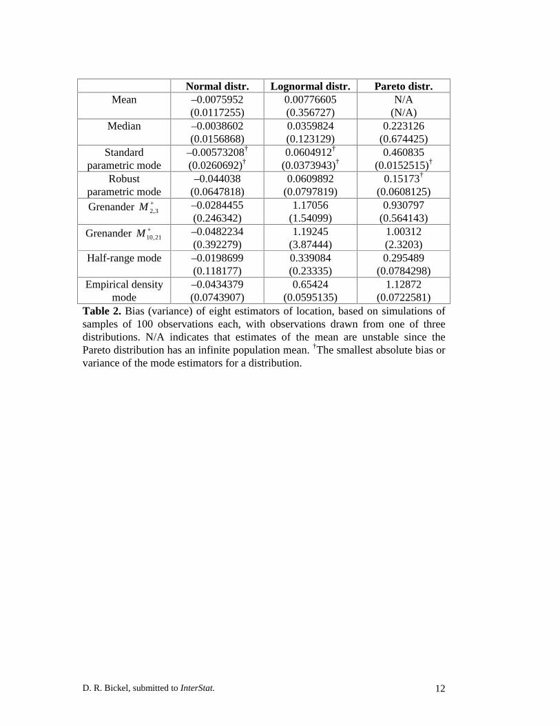
D. R. Bickel, submitted to InterStat. 12
Normal distr. Lognormal distr. Pareto distr.Mean –0.0075952
(0.0117255)0.00776605(0.356727)
N/A(N/A)
Median –0.0038602(0.0156868)
0.0359824(0.123129)
0.223126(0.674425)
Standardparametric mode
–0.00573208†
(0.0260692)†0.0604912†
(0.0373943)†0.460835
(0.0152515)†
Robustparametric mode
–0.044038(0.0647818)
0.0609892(0.0797819)
0.15173†
(0.0608125)Grenander ∗
3,2M –0.0284455(0.246342)
1.17056(1.54099)
0.930797(0.564143)
Grenander ∗21,10M –0.0482234
(0.392279)1.19245
(3.87444)1.00312(2.3203)
Half-range mode –0.0198699(0.118177)
0.339084(0.23335)
0.295489(0.0784298)
Empirical densitymode
–0.0434379(0.0743907)
0.65424(0.0595135)
1.12872(0.0722581)
Table 2. Bias (variance) of eight estimators of location, based on simulations ofsamples of 100 observations each, with observations drawn from one of threedistributions. N/A indicates that estimates of the mean are unstable since thePareto distribution has an infinite population mean. †The smallest absolute bias orvariance of the mode estimators for a distribution.

D. R. Bickel, submitted to InterStat. 13
Normal distr. Lognormal distr. Pareto distr.Mean –0.00326734
(0.000951839)0.00903911(0.0355888)
N/A(N/A)
Median 0.00131511(0.00174824)
0.020602(0.0126342)
0.000485909(0.0627678)
Standardparametric mode
–0.000506764†
(0.00294714)†0.000228966†
(0.00292074)†0.438992
(0.00109655)†
Robustparametric mode
–0.00243254(0.00818409)
0.0141563(0.00662873)
0.133249(0.0123286)
Grenander ∗3,2M –0.0372012
(0.220012)1.00229
(0.93199)0.907745(1.55889)
Grenander ∗21,10M 0.0375113
(0.359484)1.33723
(3.87184)1.08314
(4.83415)Half-range mode 0.0152163
(0.0642674)0.159715
(0.0892078)0.115442†
(0.00732768)Empirical density
mode–0.0479948(0.0401846)
0.357288(0.00675236)
0.778715(0.00432567)
Table 3. Bias (variance) of eight estimators of location, based on simulations ofsamples of 1000 observations each, with observations drawn from one of threedistributions. N/A indicates that estimates of the mean are unstable since thePareto distribution has an infinite population mean. †The smallest absolute bias orvariance of the mode estimators for a distribution.
Because of their high breakdown points, the median, RPM, HRM, and
EDFM have meaning even in the presence of many outliers, so they were applied
to samples generated as described above with four levels of contamination: 5%,
10%, 15%, and 20% for n = 20 and n =100, and 10%, 20%, 30%, and 40% for
n =1000. The level of contamination is the probability that a given value in the
sample was replaced by a value drawn from a normal distribution with a mean
equal to the 99.99th percentile of the main distribution (normal, lognormal, or
Pareto) and with a standard deviation equal to a hundredth of the interquartile
range of the main distribution divided by the interquartile range of the standard
normal distribution. Thus, the normal distribution was contaminated by
N 9.71902, 0.01( )2( ), the lognormal distribution by N 112.058, 0.0292913( )2( ), and
the Pareto distribution by N 108, 0.105429( )2( ). Higher levels of contamination

D. R. Bickel, submitted to InterStat. 14
could not be used for the smaller sample sizes because that would sometimes lead
to more than half of the values of a sample drawn from the outlier distribution,
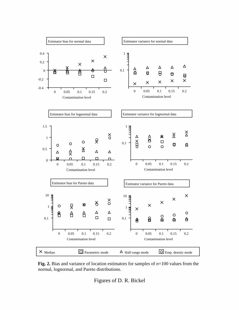
which would break down any estimator. The bias and variance in the estimators
for each contamination level and each main distribution are displayed in Fig. 1
n = 20( ), Fig. 2 n = 100( ), and Fig. 3 n = 1000( ).
Figs. 4-6 display the PDFs estimated from a sample of 1000 values from
each distribution and the same sample with 40% contamination. The PDFs were
estimated by Eq. (2), using the parameters α , y , and σ estimated as described in
Section 2.2. The value of x yielding the maximum value of each estimated PDF is
the RPM.

D. R. Bickel, submitted to InterStat. 15
4. DISCUSSION
The bias and variance of the two proposed parametric estimators of the
mode were low for all three distributions, even though the lognormal and Pareto
distributions cannot be converted into a normal distribution by the simple power
transformation. For the contaminated normal and lognormal distributions and for
the Pareto distribution with and without contamination, Figs. 4-6 show large
discrepancies between the theoretical distributions and the distributions estimated
using Eq. (2). The fact that the estimates of the mode were affected little by those
discrepancies suggests that the parametric estimators can be successfully applied
not only to power transforms of the normal distribution, but also to a much more
general class of contaminated single-modal distributions.
Tables 1-3 give an indication of the relative performance of the location
estimators considered in the absence of contamination. The two mode estimators
of Grenander (1965) have the highest bias and variance of the mode estimators for
all distributions considered. The SPM performs consistently better than the other
estimators of the mode, except that the RPM and HRM tend to be less biased for
the Pareto distribution, and, at n=20, the EDFM has a lower bias for the normal
distribution. Based on these results, the SPM is a good choice of a mode estimator
for uncontaminated data, except when the distribution of the data has extreme
skewness or long tails, in which cases the RPM or HRM would be better.
When a particular data set may be contaminated with outliers, the selection
of an estimator of the mode for that data can be informed by the estimator
properties displayed in Figs. 1-3. While the EDFM has the lowest absolute bias
for the contaminated normal distribution, the RPM has the best bias for the other
two distributions, except for the Pareto distribution at n=1000 (Fig. 3), in which
case the HRM has a lower bias and variance. Thus, the RPM is appropriate for
many cases of data with outliers and moderate to high skewness. The HRM is
better in some instances of high sample size and very high skewness, but in these
D. R. Bickel, submitted to InterStat. 16
cases, the computation speed of HRM is slow and similar results can instead be
obtained using the HSM, which can be computed very quickly. The EDFM
appears to work well for contaminated normal distributions.
The RPM is recommended as a general-purpose estimator of the mode
since it was often the best mode estimator and when it was not, it never performed
much worse than the best mode estimator in the simulations of this study, except
for the uncontaminated normal distribution. If the data are known to be
approximately normal and uncontaminated, then the sample mean would have the
lowest bias and variance and would be approximately equal to the mode since the
normal distribution is symmetric. Without this knowledge, the RPM is a safe
estimator of the mode: although it has less efficiency in some cases, it has low
bias and variance in many cases and is never affected much by outliers when the
number of outliers is less than the number of good values.
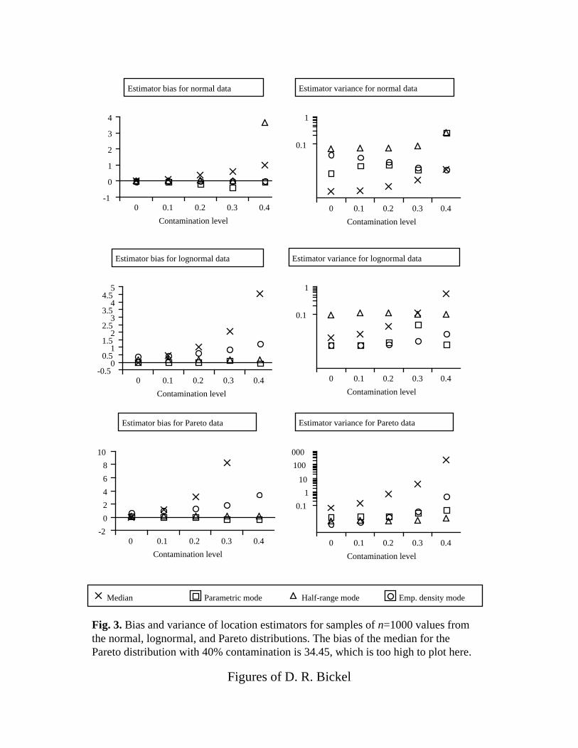
Its much greater resistance to high levels of outliers makes the mode a
viable alternative to the median as a robust measure of central tendency: the bias
and variance of the sample median consistently increase with the level of
contamination, a reflection of the fact that the median does not reject outliers,
unlike robust estimators of the mode (Bickel, 2001a) such as RPM. Figs. 1-3
show that the median can be much less reliable than RPM for contaminated,
skewed distributions.
Modifications of the SPM and RPM may lead to improved estimation; I
make three suggestions:
1. Using a trimmed mean to estimate the mean of transformed data would
have better efficiency in the uncontaminated normal case than using the
median and better robustness to outliers than using the mean, so the
resulting estimator of the mode would have characteristics intermediate to
those of the SPM and RPM.
2. The method of Section 1 can be implemented with criteria for selecting the
transformation exponent other than those proposed in Section 2, e.g., α0

D. R. Bickel, submitted to InterStat. 17
could be defined as the value of α for which the Kolmogorov-Smirnov
distance (Press et al., 1996) between the EDF of the transformed data and
a normal distribution is minimized.
3. The power transformation was chosen for its simplicity, but other
transformations to approximate normality could give better results.
Exploring the properties of these modified estimators and other generalizations of
the proposed technique requires further research.
BIBLIOGRAPHY
Bickel, D. R. (2001a) “Robust estimators of the mode and skewness of continuousdata,” Computational Statistics and Data Analysis (in press); available frompreprint server:http://www.mathpreprints.com/math/Preprint/bickel/20010705.1/3/
Bickel, D. R. (2001b), “Simple estimator of the mode for continuousdistributions: The mode as a more robust measure of location,” under review.
Box, G. E. P. and G. C. Tiao (1992), Bayesian Inference in Statistical Analysis,John Wiley and Sons (New York).
Dharmadhikari, S. and K. Joag-dev (1988), Unimodality, Convexity, andApplications, Academic Press (New York).
Donoho, D. L. and P. J. Huber (1983), “The notion of a breakdown point,” inFetschrift for Erich L. Lehmann, edited by P. J. Bickel, K. A. Doksum, J. L.Hodges Jr., Wadsworth: Belmont, CA.
Grenander, U. (1965), “Some direct estimates of the mode,” Annals ofMathematical Statistics 36, 131-138.
Huber, P. J. (1981), Robust Statistics, John Wiley & Sons (New York).Press, W. H., S. A. Teukolsky, W. T. Vetterling, B. P. Flannery (1996), Numerical
Recipes in C, Cambridge University Press: Cambridge.Rousseeuw, P. J. and C. Croux (1993) Alternatives to the median absolute
deviation Journal of the American Statistical Association 88, 1273-1283.Silverman, B. W. (1986) Density Estimation for Statistics and Data Analysis,
Chapman and Hall (New York).Staudte, R. G. and S. J. Sheather (1990), Robust Estimation and Testing, Wiley-
Interscience: New York, 1990.
D. R. Bickel, submitted to InterStat. 18
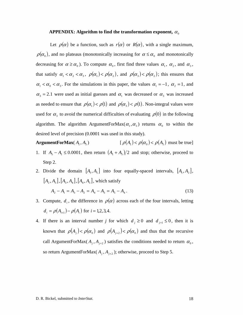
APPENDIX: Algorithm to find the transformation exponent, 0α
Let ( )αρ be a function, such as ( )αr or ( )αR , with a single maximum,
( )0αρ , and no plateaus (monotonically increasing for 0αα ≤ and monotonically
decreasing for 0αα ≥ ). To compute 0α , first find three values 1α , 2α , and 3α ,
that satisfy 321 ααα << , ( ) ( )21 αραρ < , and ( ) ( )23 αραρ < ; this ensures that
301 ααα << . For the simulations in this paper, the values 11 −=α , 12 =α , and
1.23 =α were used as initial guesses and 1α was decreased or 3α was increased
as needed to ensure that ( ) ( )11 ραρ < and ( ) ( )13 ραρ < . Non-integral values were
used for 3α to avoid the numerical difficulties of evaluating ( )0ρ in the following
algorithm. The algorithm ArgumentForMax( 1α , 3α ) returns 0α to within the
desired level of precision (0.0001 was used in this study).
ArgumentForMax( 1A , 5A ) [ ( ) ( ) ( )501 AA ραρρ << must be true]
1. If 0001.015 ≤− AA , then return ( ) 251 AA + and stop; otherwise, proceed to
Step 2.
2. Divide the domain [ ]51 , AA into four equally-spaced intervals, [ ]21, AA ,
[ ]32 , AA , [ ]43 , AA , [ ]54 , AA , which satisfy
45342312 AAAAAAAA −=−=−=− . (13)
3. Compute, id , the difference in ( )αρ across each of the four intervals, letting
( ) ( )iii AAd ρρ −= +1 for i = 1,2,3,4.
4. If there is an interval number j for which 0≥jd and 01 ≤+jd , then it is
known that ( ) ( )0αρρ <jA and ( ) ( )02 αρρ <+jA and thus that the recursive
call ArgumentForMax( jA , 2+jA ) satisfies the conditions needed to return 0α ,
so return ArgumentForMax( jA , 2+jA ); otherwise, proceed to Step 5.
D. R. Bickel, submitted to InterStat. 19
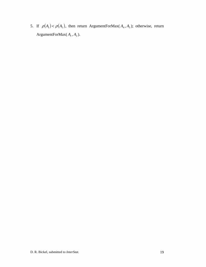
5. If ( ) ( )51 AA ρρ < , then return ArgumentForMax( 4A , 5A ); otherwise, return
ArgumentForMax( 1A , 2A ).

Figures of D. R. Bickel
Fig. 1. Bias and variance of location estimators for samples of n=20 values from thenormal, lognormal, and Pareto distributions.
Median Parametric mode Half-range mode Emp. density mode
1.5
1
0.5
0
Contamination level
0 0.05 0.1 0.15 0.2
Estimator bias for lognormal data
10
1
0.1
Contamination level
0 0.05 0.1 0.15 0.2
Estimator variance for lognormal data
0.4
0.2
0
-0.2
Contamination level
0 0.05 0.1 0.15 0.2
Estimator bias for normal data
1
0.1
Contamination level
0 0.05 0.1 0.15 0.2
Estimator variance for normal data
1000
100
10
1
Contamination level
0 0.05 0.1 0.15 0.2
Estimator bias for Pareto data
100000001000000
10000010000
1000100
101
0.1
Contamination level
0 0.05 0.1 0.15 0.2
Estimator variance for Pareto data
Figures of D. R. Bickel
Fig. 2. Bias and variance of location estimators for samples of n=100 values from thenormal, lognormal, and Pareto distributions.
Median Parametric mode Half-range mode Emp. density mode
0.4
0.2
0
-0.2
-0.4
Contamination level
0 0.05 0.1 0.15 0.2
Estimator bias for normal data
1
0.1
Contamination level
0 0.05 0.1 0.15 0.2
Estimator variance for normal data
1.5
1
0.5
0
Contamination level
0 0.05 0.1 0.15 0.2
Estimator bias for lognormal data
1
0.1
Contamination level
0 0.05 0.1 0.15 0.2
Estimator variance for lognormal data
10
1
0.1
Contamination level
0 0.05 0.1 0.15 0.2
Estimator bias for Pareto data
10
1
0.1
Contamination level
0 0.05 0.1 0.15 0.2
Estimator variance for Pareto data
Figures of D. R. Bickel
Fig. 3. Bias and variance of location estimators for samples of n=1000 values fromthe normal, lognormal, and Pareto distributions. The bias of the median for thePareto distribution with 40% contamination is 34.45, which is too high to plot here.
Median Parametric mode Half-range mode Emp. density mode
4
3
2
1
0
-1
Contamination level
0 0.1 0.2 0.3 0.4
Estimator bias for normal data
1
0.1
Contamination level
0 0.1 0.2 0.3 0.4
Estimator variance for normal data
54.5
43.5
32.5
21.5
10.5
0-0.5
Contamination level
0 0.1 0.2 0.3 0.4
Estimator bias for lognormal data
1
0.1
Contamination level
0 0.1 0.2 0.3 0.4
Estimator variance for lognormal data
1000
100
10
1
0.1
Contamination level
0 0.1 0.2 0.3 0.4
Estimator variance for Pareto data
10
8
6
4
2
0
-2
Contamination level
0 0.1 0.2 0.3 0.4
Estimator bias for Pareto data