Robust Adaptive Control of Manipulators

Kim Doang Nguyen, Harry DankowiczDepartment of Mechanical Science and Engineering

University of Illinois at Urbana-Champaign

January 9, 2014

Abstract

This paper develops an adaptive controller for robot manipulators. The design decouples the system’sadaptation and control loops to allow for fast estimation rates, while guaranteeing robustness. The controlscheme is tested in different manipulation scenarios, namely, (i) trajectory tracking where the desiredjoint motions are predefined and (ii) command following where the desired motions are not knowna priori and instead inferred using measurements and inverse kinematics. We consider, in addition,an operating modality in which the control scheme switches between command following and staticpositioning, for which the predefined desired joint motions are constant in time and identical to themanipulator angles at the time of switching. The simulation results illustrate the performance of theproposed control algorithm and its ability to deal with unmodeled dynamics, measurement noise, andtime delay, while maintaining smooth control signals.

1 IntroductionRobot manipulators are widely used in industry and have long been considered as testbeds for researchin nonlinear control theory. Early work on adaptive control of manipulators was mostly based on model-reference adaptive-control architectures, which drive the system response to a reference model via adaptiveestimation of unknown parameters [1, 2, 3]. In [4], the authors present a model-based controller that employsa parameter-adaptation scheme to eliminate the contributions of nonlinearities to the equations of motiongoverning a robotic arm, and to reject disturbances. However, this control scheme requires accelerationmeasurements and access to the inverse of the mass matrix. The control architecture in [5], which eliminatesthose disadvantages, is composed of a proportional-derivative feedback loop together with adaptation laws tocompensate for nonlinearities and to estimate the unknown parameters in the system model. The controllerexploits the dynamic structure and the passivity property of rigid robot dynamics in the absence of friction.It decouples the nonlinearity into a regression matrix and a vector of unknown parameters and implementsan adaptive scheme to estimate these parameters.

The formulation proposed in [5] was further exploited in [6] for the development of repetitive and adap-tive control strategies without the need for velocity measurements; in back-stepping design [7]; in the con-text of adaptive Jacobian tracking [8]; for image-based visual servoing control of manipulators [9]; and forspace-robot control with optimal sensor architecture [10]. In these papers, the manipulator control adap-tively adjusts the system energy to obtain the control objective, while preserving the passivity of the roboticmechanism. Such a control design philosophy, based on dynamic passivity, led to several important papersin robot control [12, 13, 14, 15, 16, 17]. Disturbance observers were designed for manipulator control in[18, 19, 20, 21]. In these control schemes, the filtered system states are used for the inversion of the robot

1

dynamics. Joint torques/forces are treated as disturbances and compensated for by the controller design.This eliminates the need for torque/force sensors, while keeping the desirable tracking performance. How-ever, these controllers may suffer from inversion errors, since they perform filtering before plant inversionand therefore require accurate system modeling. A modification to disturbance-observer structure was pro-posed in [22] to alleviate the dependence on the accuracy of plant modeling. Disturbance observers werealso applied with a force estimator in the scenario of human-robot comanipulation [23].

The work in [24] proposed a systematic method for integrating sliding-mode control in a model-referenceadaptive controller to drive a robot arm to track certain trajectories. Following this work, robust adaptivecontrol schemes with semi-strict feedback forms were developed for single-input-single-output [25] systemsand multi-input-multi-output systems [26]. Recently, sliding-mode control has been employed to design anobserver-based adaptive controller for servo actuators with friction. Adaptation laws compensate for the un-certain friction and load torque with the estimated friction state [27]. The main disadvantage of this controlformulation comes from the property of the sliding mode: the control law is discontinuous across the slidingsurface. In practice, therefore, a resultant chattering control signal may excite unmodeled high-frequencydynamics and seriously damage the system’s robustness. The architecture can be modified to improve therobustness, but with the sacrifice of tracking accuracy and asymptotic stability [28, 29]. In addition, thebounds of the unknown parameters and disturbances must be known to design an adaptive sliding-modecontroller for robustness and convergence [30].

In the context of robot manipulators, all existing control architectures in the presence of an estimationloop share the structural property that the control loop and the estimation loop are coupled. As a result,in order to maintain desirable performance in the presence of disturbances or unmodeled dynamics, theadaptation rate must be increased. This, in turn, will make the control signal oscillate with high frequencyand high amplitude, deteriorating the system’s tolerance to time delays [31]. Furthermore, as in [5], it mustbe possible to decouple the nonlinearities in terms of a matrix product of a regression matrix and a vectorof unknown parameters, where the regression matrix is known. Any uncertainty in the dynamic structure ormeasurement noise will degrade the system performance [32].

The so-called L1 control architecture has been developed to enable fast adaptation, while guaranteeingrobustness with time-delay margin bounded away from zero, as well as maintaining clean control channels[33, 34]. The performance of L1 control has been demonstrated in numerous aerospace applications [35,36, 37, 38]. Inspired by this work, this paper proposes a controller for robot manipulators, which does notrequire measurement of accelerations and eliminates the need to compute the inverse of the inertia matrix.Moreover, a low-pass filter in the feedback channel decouples the estimation loop from the control loop, andwith that facilitates the increase of estimation rates without sacrificing robustness. Tuning of the filter alsoallows for shaping the nominal response and enhancing the time-delay margin.

The adaptive controller is developed for manipulators in two scenarios: 1) tracking predefined jointtrajectories and 2) following unknown command movements when interacting with a user. The first task isused to assess the performance of most algorithms for robot control. The second task was studied in [39]and [40] with a hybrid control scheme to make a lower-limb exoskeleton follow human movement whilesupporting a payload. Unlike that work, the proposed controller in this paper is able to adaptively estimatethe robot nonlinearity, which are hard to model, with guaranteed robustness. A switching strategy betweenthese two scenarios is also presented. The control schemes’ performance is demonstrated with a typicalthree-degree-of-freedom robotic arm.

The remainder of this paper is organized as follows. The dynamic model of manipulators is discussed inSec. 2, in which the robot dynamics is converted to a relevant form. The adaptive controller for manipula-tors is designed and analyzed in Sec. 3. Section 4 presents the simulation results of a robot arm performingtrajectory tracking tasks, including the presence of base-motion disturbances and actuator delay. Section 5

2

couples the control architecture with an additional estimation loop in order to support the task of commandfollowing, and demonstrates this concept in the context of a switching strategy between command follow-ing and static positioning, for which the predefined joint trajectory is constant in time. Finally, the paperconcludes in Sec. 6 with a discussion.

2 Dynamic Model of Manipulators

Let a superscribed dot denote differentiation with respect to time t. The dynamics of an n-link robot manip-ulator are governed by the following equations of motion

M(q)q + Vm

(q, q)q +G

(q)

+ F(q)

+D = uT , (1)

where the n generalized coordinates contained in the column vector q describe relative joint angles, thesquare matrix Vm

(q, q)

contains Coriolis and centripetal effects, the column vector G(q)

represents theeffects of gravity and other conservative forces, the column vector F

(q)

represents dissipative, velocity-dependent mechanisms, for example associated with friction, and the column vectors uT and D are thetime-dependent control input torque and bounded unknown disturbances, respectively. The inertia matrixM(q)

is assumed to be positive-definite, symmetric, and bounded, i.e., such that µ1I ≤ M(q)≤ µ2I, for

all q and for some positive scalars µ1 and µ2, where I denotes the identity matrix.Inspired by the sliding control formulation in [5], we introduce the new variable

r = (q − qd) + Λ(q − qd), (2)

where qd represents desired trajectories for the joint angles and Λ is a symmetric, positive-definite matrixof design parameters, so that (2) is a stable system. This means that as long as the controller maintains abounded r(t), the joint trajectories q(t) can be solved for in terms of r(t) and are also bounded. In addition,since −Λ is Hurwitz, (2) is finite-gain L-stable (see [41]). Therefore, from Lemma A.7.1 in [42], we have

q(s) = (sI + Λ)−1r(s) + qd(s) + (sI + Λ)−1(q(0)− qd(0)

)⇒ ‖qt‖L∞ ≤ ‖(sI + Λ)−1‖L1‖rt‖L∞ + ‖qd(s) + (sI + Λ)−1

(q(0)− qd(0)

)‖L∞ , (3)

where the subscript t restricts attention to the time interval [0, t]. Because (sI + Λ)−1 is a proper and stabletransfer function, ‖(sI + Λ)−1‖L1 and ‖qd(s) + (sI + Λ)−1

(q(0) − qd(0)

)‖L∞ exist and are bounded by

positive numbers Q1 and Q2 respectively. In other words,

‖qt‖L∞ ≤ Q1‖rt‖L∞ +Q2. (4)

Consider the decompositionuT (t) = u(t) +Amr(t) (5)

of the control input in terms of an adaptive control input u(t) and a Hurwitz matrix Am that is introduced toshape the transient response of the system dynamics. Substitution of (1) and (5) into the time derivative of(2) then yields

r(t) = Amr(t) + u(t)− f(t, ζ(t)

), r(0) = r0, (6)

where ζT =[rT , qT

]and f

(t, ζ(t)

)lumps all the unknown nonlinearities and disturbances.

In the next section, an adaptive controller is designed to estimate this unknown nonlinear function inevery computation loop, as well as to control the manipulator to accurately track certain prescribed jointtrajectories.

3

3 A robust adaptive controller

This section develops the control scheme for controlling the robot dynamics presented in the form of (6),the detailed knowledge of the robot model is unknown. The control architecture is depicted in Figure 1(cf. [42]). Here, the controller’s objective is to drive the state r to the desired state rd = 0. The variabler represents a predictor for r. Similarly, the variables θ and σ denote adaptive estimates for two unknownquantities θ and σ, introduced below.

Figure 1: Block diagram of the proposed control system for the manipulator dynamics.

3.1 Parameterization of the nonlinear robot function

Let the unknown nonlinear robot function f(t, ζ) : R× R2n → Rn satisfy the following assumptions:

• There exists a constant Z > 0 such that ‖f(t, 0)‖∞ ≤ Z for all t ≥ 0.

• The nonlinear function f(t, ζ) is continuous in its arguments. For arbitrary δ, there exist dft(δ) > 0and dfζ (δ) > 0 independent of time, such that for all ‖ζ‖∞ ≤ δ, the partial derivatives of f(t, ζ) withrespect to t and ζ are piecewise continuous and bounded:∥∥∥∥∂f(t, ζ)

∂t

∥∥∥∥∞≤ dft(δ);

∥∥∥∥∂f(t, ζ)∂ζ

∥∥∥∥∞≤ dfζ (δ). (7)

Now suppose that r(t) is continuous and (piecewise)-differentiable for all t ≥ 0, and that ‖rτ‖L∞ ≤ ρand ‖rτ‖L∞ ≤ dr, for a given τ ≥ 0 and in terms of some positive constants ρ and dr. Finally, let

ρ(ρ) , max{ρ+ γ,Q1(ρ+ γ) +Q2}, Lρ ,ρ(ρ)ρdfζ(ρ(ρ)

)(8)

for some arbitrary γ > 0. It follows that ρ < ρ(ρ) and, consequently, dfζ(ρ(ρ)

)< Lρ. Taking (4)

into account, it follows from Lemma A.9.2 in [42] that there exist differentiable functions θ(t) ∈ Rn andσ(t) ∈ Rn such that the nonlinear function f

(t, ζ(t)

)can be parameterized in θ(t) and σ(t) using ‖rt‖L∞

as a regressor:

f(t, ζ(t)

)= θ(t)‖rt‖L∞ + σ(t), ∀t ∈ [0, τ ]. (9)

4

In particular, for t ∈ [0, τ ], the functions θ and σ and their first derivatives are bounded:

||θ(t)||∞ < θb ||θ(t)||∞ < dθ ||σ(t)||∞ < σb ||σ(t)||∞ < dσ. (10)

where θb , Lρ, σb , LρQ2+Z+ε, in which ε is an arbitrary positive constant and dθ and dσ are computablebounds.

For t ∈ [0, τ ], it follows that (6) can be written in the following form:

r(t) = Amr(t) + u(t)−(θ(t)‖rt‖L∞ + σ(t)

), r(0) = r0. (11)

3.2 State Predictor

A predictor r for the state r is now constructed as follows:

˙r(t) = Amr(t) + u(t)−(θ(t)‖rt‖L∞ + σ(t)

)−Kspr(t), r(0) = r0, (12)

where the prediction error r(t) , r(t)− r(t), and Ksp is a matrix of loop-shaping parameters that is tunedto reject oscillations caused by high-frequency disturbances or noise.

3.3 Adaptation Laws

Let the adaptive estimates θ(t) and σ(t) in (12) be governed by the following projection-based laws (cf. [43]):

˙θ(t) = ΓProj(θ(t), P r‖rt‖L∞), θ(0) = θ0, (13)˙σ(t) = ΓProj(σ(t), P r), σ(0) = σ0. (14)

Here, Γ ∈ R+ is the adaptation gain and the matrix P = P T > 0 is the solution to the Lyapunov equationATmP + PAm = −Q, for some arbitrary Q = QT > 0. The projection operator Proj(·, ·) ensures that‖θ(t)‖∞ ≤ θb and ‖σ(t)‖∞ ≤ σb provided that θ0 and σ0 satisfy the same bounds. In each of the simulationsin Secs. 4 and 5, θ0 = σ0 = 0.

3.4 Control Law

Next, let the adaptive control torque in (11) be obtained from the output of the following system

u(s) = C(s)η(s), (15)

where η(s) is the Laplace transform of η(t) , θ(t)‖rt‖L∞ + σ(t). Here, C(s) is a diagonal matrix ofBIBO-stable and strictly proper transfer functions with DC gain C(0) = 1, assuming zero initializationfor its state-space realization. This filter structure decouples the estimation loop from the control loop andallows for arbitrarily large values of the adaptation gain (limited only by available hardware), without hurtingthe system’s robustness.

3.5 Error dynamics

From the previous definitions, the prediction error dynamics are now governed by

˙r(t) = (Am −Ksp)r(t)−(θ(t)‖rt‖L∞ + σ(t)

), r(0) = 0, (16)

where the estimation errors θ(t) = θ(t) − θ(t), and σ(t) = σ(t) − σ(t) (note that the initial condition r0of r(t) and r(t) is assumed to be known). One of the objectives of the control design is now to choose Am,Ksp, Γ, Q and the matrix of filters C(s) in order to achieve desirable performance bounds on the error r. Inthe numerical analysis in the next section, we always set Q = I.

5

3.6 Reference system

In order to obtain design criteria in terms of bounds on the predictability of the state and control input, weconstruct the closed-loop reference system:

qref (t) = qd(t) + rref (t)− Λ (qref (t)− qd(t)) , qref (0) = q0 (17)

rref (t) = Amrref (t) + uref (t)− f(t, ζref (t)), rref (0) = r0, (18)

uref (s) = C(s)ηref (s), (19)

where ζTref = [rTref , qTref ], and ηref (s) is the Laplace transform of the signal ηref (t) , f(t, ζref (t)).

We sketch the proof of the following theorem in Appendix A.

Theorem 1 Let ρref denote a positive number, chosen such that

ρref > ‖H(s)r0‖L∞ . (20)

Suppose that ‖r0‖∞ < ρref and that C(s) is chosen such that the following condition holds:

‖H(s)(C(s)− I

)‖L1 <

ρref − ‖H(s)r0‖L∞Lρrefρref + Z

, (21)

where Lρref and Z were introduced in the characterization of the nonlinear robot function f . The state ofthe reference system is then bounded for all time:

‖rref‖L∞ < ρref . (22)

Moreover,‖uref‖L∞ < ‖C(s)‖L1

(Lρrefρref + Z

), ρu,ref . (23)

3.7 Performance bounds

Suppose that the conditions of Theorem 1 are satisfied by the value of ρref , the matrix C(s), and the initialvalue r0. We seek to formulate design conditions that guarantee that

‖r‖L∞ ≤ γ0 (24)

‖rref − r‖L∞ ≤ γ1, (25)

‖uref − u‖L∞ ≤ γ2, (26)

for suitably defined bounds γ0, γ1, and γ2. We sketch the proof of the following theorem in Appendix B.

Theorem 2 Let γ∗ denote the value of γ used in the definition of ρref (ρref ) and suppose that γ0 and β arechosen such that

γ1 ,‖H(s)C(s)H−1(s)‖L1

1− ‖H(s)(C(s)− I

)‖L1LρrefQm

γ0 + β < γ∗, (27)

where Qm , max{1, Q1} and H(s) , (sI−Am +Ksp)−1. Moreover, let

γ2 , ‖C(s)‖L1LρrefQmγ1 + ‖C(s)H−1(s)‖L1γ0. (28)

The bounds (24)-(26) then hold, provided that the adaptive gain Γ satisfies the design constraint

Γ ≥ θmλmin(P )γ2

0

, (29)

in terms of a computable coefficient θm.

We note that one can achieve arbitrarily small performance bounds γ0, γ1 and γ2 by increasing the adaptivegain Γ.

6

3.8 Simulation model

We restrict attention in the remainder of this paper to a typical pick-and-place manipulator, as shown inFig. 2, in which q1, q2, and q3 are the relative joint angles between the homogeneous links and (xb, yb, zb)represents the time-dependent position of the manipulator base, treated as an unknown disturbance in theanalysis below. Here, gravity is assumed to act along the negative z-axis. In the numerical results reportedbelow, and in a set of consistent units (the SI system is used throughout the paper), the link lengths, themasses of the three links, the payload at the end-effector, and the acceleration of gravity are given byL1 = 0.25; L2 = 0.2; L3 = 0.1; m1 = 1.25; m2 = 1; m3 = 0.25; me = 1.25; g = 9.81.

Figure 2: Typical pick-and-place manipulator with moving base.

4 Trajectory tracking

We begin by illustrating the performance of the control design when the joint angles are tasked to trackpredefined

• step reference inputs with q1,d(t) = q2,d(t) = q3,d(t) ≡ α, for values ofα ∈ [0, 2], with q0 = q0 = (0, 0, 0)T

and

• sinusoidal reference inputs with q1,d(t) = q2,d(t) = sin 23 t and q3,d(t) = cos 2

3 t with q0 = (0, 0, 1)T

and q0 = (0, 0, 0)T .

In the simulations in this paper, the control parameters and the filter are tuned to the following controlobjectives:

• In the case of the step reference inputs, achieve a response settling time (the time required for theresponse to reach and stay within 2% of the final value) of less than 5 s, with zero overshoot.

• In the case of the sinusoidal reference inputs, achieve a root-mean-square (RMS) tracking error of lessthan 0.07 under various disturbances including time delay, base motion, and measurement noise.

7

To this end, the filter matrix in (2) is here set to equal Λ = I, the adaptive gain Γ is set to 105, and thetransient response characteristics are governed by the design matrix Am = −5I. A second-order filterC(s) = ω2

c/(s2 + 2ξωcs+ω2

c ) with bandwidth of ωc = 12 and damping factor of ξ = 0.7 is employed. Werely on the result in [44] to set the matrix of loop-shaping parameters Ksp in the state-predictor design (12)to 6√

ΓI +Am.The numerical results below were obtained from a Simulink-based implementation of the manipulator

equations of motion and the L1 control architecture, described above. Default Simulink tolerances andsettings were used throughout.

4.1 Performance in ideal working conditions

Figure 3 and 4 show the response of the manipulator to the L1 control actuation in the case of step referenceinputs with different values of α and the sinusoidal reference input, respectively. As seen in the bottompanels, for both types of reference inputs, the L1 control signals are smooth and clean, in spite of the use ofhigh-rate estimation to accommodate nonlinearity and model uncertainty while retaining small predictionerrors. For the step reference input, no overshoot is observed, and the maximum settling time is 4.45 s. Asseen in Figure 3, the system response scales approximately uniformly with the size of the step referenceinput. For the sinusoidal reference input, the maximum RMS tracking error is 0.0589.

Figure 3: Performance of the proposed controller in ideal working conditions with various step referenceinputs: The top row shows the actual joint angles q(t) (solid) together with the desired joint trajectoriesqd(t) (dashed) as a function of time t. The bottom row displays the components of the control input u(t)and the prediction error r(t).

8

Figure 4: Performance of the proposed controller in ideal working conditions with sinusoidal referenceinputs: The top row shows the actual joint angles q(t) (solid) together with the desired joint trajectoriesqd(t) (dashed). The bottom row displays the components of the control input u(t) and the prediction errorr(t).

4.2 Robustness

We proceed to analyze the robustness of the L1 control system by investigating its performance in thepresence of time delays at the plant input. Specifically, we define the critical time delay as the maximumactuator time delay, for which the controller is able to maintain bounded performance, for a given choice ofsystem parameters and desired trajectory qd(t).

For the current set of parameters and the sinusoidal input reference, with a time delay of 150 ms or less,the controller gives almost the same performance as that obtained without delay in Fig. 4. When a timedelay of 180 ms is introduced in the system, the tracking performance of the proposed controller remainsdesirable, as illustrated in Fig. 5 with a maximum RMS tracking error of 0.0675. For this time delay,however, oscillations begin to appear in the control signals. These oscillations can be largely eliminatedby introducing a time delay in the state predictor (see [45]). Such a systematic modification to the statepredictor by incorporating known delays hence improves the system robustness. As the actuator time delayis increased further, the system performance deteriorates gradually, and an unbounded response is obtainedfor a delay of 233 ms. In the L1 control architecture, it is possible to improve the critical time delay bysuitable tuning of the filter C(s). For instance, with a filter bandwidth of 8 and the same damping factor of0.7, the critical time delay is increased to 275 ms.

9

Figure 5: Performance of the proposed controller with actuator time delay of 180 ms without re-tuning: Thetop row shows the actual joint angles q(t) (solid) together with the desired joint trajectories qd(t) (dashed).The bottom row displays the components of the control input u(t) and the prediction error r(t).

4.3 Control performance under base motion

We consider next the response of the control system to base motion acceleration of the formxb = 0.8 sin 20t,yb = 0.8 cos 20t,zb = 0.8 cos 20t.

(30)

The desired trajectories and initial conditions remain unchanged as in the previous sections. The unknownbase movement in (30) can be thought of as unmodeled dynamics or a disturbance. As shown in Fig. 6, thereis minimal effect on the tracking performance of the controller with the maximum RMS tracking error of0.0605. Although the control signal contains the additional frequency component associated with the baseacceleration, it remains smooth and implementable.

4.4 Control performance with measurement noise

Finally, we consider the performance of the control system in the presence of velocity measurement noise.To this end, unfiltered, uniformly distributed noise in the range [−0.1, 0.1] rad/s and with sample time of0.01 s was added to the angular velocity measurements. As seen in Fig. 7, without any further tuning, theproposed controller successfully rejects the noise. The control scheme still maintains desirable trackingperformance with the maximum RMS tracking error of 0.0599. In addition, the control signals are relativelyclean and implementable.

10

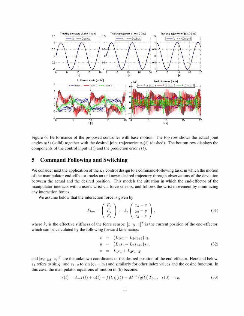
Figure 6: Performance of the proposed controller with base motion: The top row shows the actual jointangles q(t) (solid) together with the desired joint trajectories qd(t) (dashed). The bottom row displays thecomponents of the control input u(t) and the prediction error r(t).

5 Command Following and Switching

We consider next the application of the L1 control design to a command-following task, in which the motionof the manipulator end-effector tracks an unknown desired trajectory through observations of the deviationbetween the actual and the desired position. This models the situation in which the end-effector of themanipulator interacts with a user’s wrist via force sensors, and follows the wrist movement by minimizingany interaction forces.

We assume below that the interaction force is given by

Fhm =

FxFyFz

:= ks

xd − xyd − yzd − z

, (31)

where ks is the effective stiffness of the force sensor; [x y z]T is the current position of the end-effector,which can be calculated by the following forward kinematics:

x =(L1s1 + L2s1+2

)c3,

y =(L1s1 + L2s1+2

)s3, (32)

z = L1c1 + L2c1+2;

and [xd yd zd]T are the unknown coordinates of the desired position of the end-effector. Here and below,s1 refers to sin q1 and s1+2 to sin (q1 + q2) and similarly for other index values and the cosine function. Inthis case, the manipulator equations of motion in (6) become:

r(t) = Amr(t) + u(t)− f(t, ζ(t)

)+M−1

(q(t)

)Thm, r(0) = r0, (33)

11

Figure 7: Performance of the proposed controller in the presence of velocity measurement noise in therange [−0.1, 0.1] rad/s and with sample time of 0.01 s: The top row shows the actual joint angles q(t)(solid) together with the desired joint trajectories qd(t) (dashed). The bottom row displays the componentsof the control input u(t).

12

where Thm represents a column vector of generalized forces that can be obtained from Fhm as follows:

Thm =

(L1c1 + L2c1+2)c3 (L1c1 + L2c1+2)s3 −(L1s1 + L2s1+2)L2c1+2c3 L2c1+2s3 −L2s1+2

−(L1s1 + L2s1+2)s3 (L1s1 + L2s1+2)c3 0

Fhm. (34)

The same control architecture with predictor dynamics (12), adaptation laws (13) and (14), and controlinput (15) are used to control this system. Here, we construct a reference trajectory on the fly, by requiringthat qd satisfy the following constitutive relation

qd∂h

∂qd(qd, t) +

∂h

∂t(qd, t) + Ψh(qd, t) = 0, qd(0) = q0, (35)

where Ψ is a diagonal matrix of positive constants;

h(qd, t) ,

(L1 sin qd1 + L2 sin(qd1 + qd2)) cos qd3 − xd(t)(L1 sin qd1 + L2 sin(qd1 + qd2)) sin qd3 − yd(t)

L1 cos qd1 + L2 cos(qd1 + qd2)− zd(t)

; (36)

and xd(t), yd(t), zd(t), and their time derivatives are obtained from (31) using filtered measurements of theinteraction force and forward kinematics of the measured joint angles.

Now let static positioning be defined as a special case of trajectory tracking in which the predefineddesired joint motions are constant and equal to the actual joint angles at the onset of tracking. We considerbelow a strategy for switching between static positioning and command following, in which qd(t) is contin-uous everywhere except at moments corresponding to a switch to static positioning. It follows that at such amoment, the initial condition r0 must be set to equal the value of q.

Let Fcr and Vcr denote preset critical values of the magnitude of the interaction force and the speed of themanipulator end-effector, respectively. We associate the case of static positioning to a phase during whichthe magnitude of the measured interaction force is less than Fcr and the measured speed of the manipulatorend-effector is less than Vcr. Similarly, we associate the case of command following to a phase during whicheither the measured interaction force exceeds Fcr or the measured end-effector speed exceeds Vcr. A switchfrom static positioning to command following then occurs when either the force or the velocity exceed thecorresponding critical value. Similarly, a switch from command following to static positioning occurs whenboth the force and velocity fall below the corresponding critical values. In practice the interaction force willexceed Fcr before the end-effector speed exceeds Vcr, given a phase of static positioning.

To simulate a practical scenario, the manipulator is initialized by following step reference inputs froma resting configuration to a desired position. After the manipulator stabilizes around the desired position att = 5, the control algorithm is switched to a phase of static positioning, during which a user starts interactingwith the manipulator’s end-effector and interaction forces are measured. At t = 6.5, the user’s wrist startsmoving. The controller uses the proposed strategies to decide when to switch to command following. Here,we let Fcr = 0.05 and Vcr = 0.05. The former is equivalent to an effective displacement of 0.01 betweenthe position of the human wrist and that of the manipulator’s end-effector, given a sensor stiffness of ks = 5.The desired path is equivalent to the following time histories (cf. Fig. 9).

xd(t) = 0.0625 + 0.05 cos(t),yd(t) = 0.125 + 0.0625 sin(t), (37)

zd(t) = 0.0125t,

13

Figure 8: Performance of the switching task: The top row shows the actual joint angles q(t) (solid) togetherwith the desired joint trajectories qd(t) (dashed) with zoomed-in figures of the switching interval. The filledcircles in each of these figure indicate the onset and termination of wrist motion, in each case followed bythe controller switching from static positioning to command following, and vice versa. The panels in thebottom row display the components and magnitude of the measured interaction force and magnitude and themeasured velocity of the end-effector, respectively.

As stated previously, the desired path is not known a priori to the controller. Instead, the locus of the user’swrist is estimated in every loop based on the joint angle and force measurements. In the numerical results,these measurements are filtered through a first-order filter with bandwidth 100 prior to further processing(e.g., differentiation). In the L1 controller, the same control parameters and filter C(s) as in the previoussections are employed. The diagonal matrix Ψ in (35) is set equal to 5I. At t = 22, the user stops moving,and the controller switches back to static positioning when both the interaction force and the end-effector’sspeed fall below the corresponding critical values. Figure 8 shows the performance of the L1 controlstrategy, using the parameter values given in Sec. 4, combined with the switching strategy described above,in the absence of measurement noise and base motion, but with model uncertainty and nonlinearity. Thetop row shows the joint trajectories vs. the desired trajectories; the bottom row shows the interaction forceand the end-effector speed. Initialization occurs during the first five seconds. The manipulator’s restingconfiguration is assumed to be q = (0.4, 2, 0.8)T . Static positioning of the end-effector begins at t = 5and is maintained until the measured interaction force exceeds the critical value following the onset of wristmotion at t = 6.5. The controller then switches to the command-following strategy, where the desired pathis inferred from the interaction force measurements, in order to follow the desired path of the user’s wrist.When the speed of the manipulator end-effector and the interaction force both fall below the correspondingcritical values, the controller switches back to the static positioning control scheme (in the last four seconds).It is observed that at the onset of static positioning, qd exhibits a jump discontinuity, such that qd equals theactual joint angles following the jump. Figure 9 illustrates the end-effector’s path and the desired path of

14

Figure 9: End-effector path in physical space during the control task described in Sec. 5 using the proposedcontrol architecture and the switching scheme between command following and static positioning.

the user’s wrist in space. After the initial phase of static positioning, the manipulator end-effector’s path[x y z]T quickly settles to a smooth curve that closely follows the desired path [xd yd zd]T . The maximalFhm experienced during the command-following task clearly depends on the numerical values of the controlparameters, as well as the filters’ bandwidth.

6 Conclusion

This paper has described a robust adaptive controller based on the L1 control architecture for robot ma-nipulators. As evidenced by fundamental theoretical results on the existence of computable performancebounds, this framework successfully separates the adaptation loop from the control loop, thereby allowingfor arbitrary increases in the adaptation rate (bounded only by hardware constraints) without sacrificing thesystem’s robustness, and allows for a predictable transient response with smooth and implementable controlsignals. With the introduction of a variable transformation, inspired by earlier work in [5], and an innovativecontrol design, the formulation is able to compensate for the nonlinearity and uncertainties in the dynamicmodel without the need for the inversion of inertia matrix.

Numerical simulations were used to illustrate the control paradigm in the context of a trajectory trackingtask imposed on a three-degree-of-freedom robot arm, for a known reference input, as well as in the caseof one inferred on the fly using end-effector measurements and inverse kinematics. The results demonstratedesirable tracking performance and clean and smooth control input with different types of disturbances,including intense base motion, measurement noise, and time delay. A switching strategy between static po-sitioning (constant desired joint angles) and command following (inferred desired joint angles) was also pre-sented and successfully tested. This opens the promising opportunity of L1 control in robotic applications,where time delay or unmodeled dynamics are unavoidable, for example teleoperation, mobile manipulation,and bioassistive devices.

The successful design of the adaptive control architecture relies upon a key parameterization of thenonlinear contribution to the robot equations of motion in two time-varying parameters with the L∞-normof the state as a regressor. The controller further employs projection operators in the adaptive laws to impose

15

bounds on the parameter estimates, and uses filters in the control input to keep the control-signal frequenciesbelow the available control-system bandwidth. In this case, Theorem 2 implies close agreement between thesystem response and the control input, on the one hand, and the corresponding time histories for a suitablyformulated reference system, on the other hand, provided that the adaptive gain is chosen sufficiently large.The deviation between the system response and the desired trajectory observed in the numerical results maybe traced to the need to maintain a finite filter bandwidth, in order to guarantee robustness. This is the designtrade-off between performance and robustness of the proposed control architecture.

We finally comment on the observations made regarding the critical time delay during the two trajectorytracking tasks considered above. As seen in [42] in the linear case, the basic L1 control architecture supportsthe formulation of theoretical lower bounds on the time delay margin, through the use of a suitably formu-lated equivalent LTI system. Some degree of robustness is therefore guaranteed provided that the adaptationgain is sufficiently large. Work is currently underway [45] to adapt these theoretical results to the manipu-lator context. For static and periodic reference inputs, a systematic analysis of the dependence on the actualcritical time delay on the control parameters may be obtained, for example, using techniques of numericalcontinuation. We will return to these considerations in a future publication.

Acknowledgement

This work was partially supported by AFOSR and a NASA SBIR Phase I contract, order no. NNX12CE97P,awarded to CU Aerospace, L.L.C. We would like to thank Evgeny Kharisov for his support in the simulationof the proposed control algorithm.

A Proof of Theorem 1

The reference system in (18) may be expressed in the Laplace domain in terms of the matrixH(s) , (sI−Am)−1

of proper transfer functions:

rref (s) = H(s)(C(s)− I

)ηref (s) +H(s)r0. (38)

If (22) is not true, there exists some τ > 0 such that

‖rref τ‖L∞ = ρref , (39)

and, since ‖rref (0)‖∞ = ‖r0‖∞ < ρref ,

‖rref (t)‖∞ < ρref ∀t ∈ [0, τ), and ‖rref (τ)‖∞ = ρref . (40)

It follows that

‖ζref τ‖L∞ ≤ max{‖rref τ‖L∞ , Q1‖rref τ‖L∞ +Q2} < ρref (ρref ), (41)

where ρref is given by (8) in terms of some arbitrary positive constant γ.The uniform boundedness of the partial derivatives of f(t, ζ) in assumption (7) now implies that

‖(f(t, ζref )− f(t, 0)

)τ‖L∞ ≤ dfζ

(ρref (ρref )

)‖ζref τ‖L∞

⇒ ‖ηref τ‖L∞ < Lρrefρref + Z. (42)

16

It follows from (38) and Lemma A.7.1 in [42] that

‖rref τ‖L∞ ≤ ‖H(s)(C(s)− I

)‖L1‖ηref τ‖L∞ + ‖H(s)r0‖L∞ . (43)

Substitution of (42) and the stability condition (21) in (43) yields ‖rref τ‖L∞ < ρref , in contradiction to(39).

From (22), it follows that (42) holds for arbitrary τ . The bound in (23) is obtained by applying (42) tothe norm inequality of the control input in (19):

‖uref‖L∞ ≤ ‖C(s)‖L1‖ηref‖L∞ . (44)

B Proof of Theorem 2

Suppose that the bounds in (25) and (26) are not true. Because ‖rref (0)−r(0)‖ = 0 < γ1 and ‖uref (0)− u(0)‖ = 0 < γ2,and since rref (t), r(t), uref (t) and u(t) are continuous functions, there exists τ > 0 such that

‖rref (t)− r(t)‖∞ < γ1, ‖uref (t)− u(t)‖∞ < γ2, ∀t ∈ [0, τ), (45)

and‖rref (τ)− r(τ)‖∞ = γ1 or ‖uref (τ)− u(τ)‖∞ = γ2. (46)

This means at least one of the following inequalities is true:

‖(rref − r)τ‖L∞ = γ1 or ‖(uref − u)τ‖L∞ = γ2. (47)

Let

ρ∗ , ρref + γ∗, (48)

ρu , ρu,ref + γ2. (49)

It follows from Theorem 1 that

‖rτ‖L∞ ≤ ρ∗, ‖uτ‖L∞ ≤ ρu (50)

and thus that

‖ζτ‖L∞ ≤ max{‖rτ‖L∞ , Q1‖rτ‖L∞ +Q2} ≤ max{ρ∗, Q1ρ∗ +Q2}

= max{ρref + γ∗, Q1(ρref + γ∗) +Q2} = ρref (ρref ) . (51)

By considering the following Lyapunov function candidate

V(r(t), θ(t), σ(t)

)= rT (t)P r(t) +

1Γ(θ2(t) + σ2(t)

), (52)

one can prove in the same way as in [42] that

‖rτ‖ ≤

√θm

λmin(P )Γ, (53)

17

where

θm , 4θ2b + 4σ2

b + 4λmax(P )λmin(Q)

(θbdθ + σbdσ

). (54)

Hence, if Γ is selected to satisfy the design constraint in (29), then

‖rτ‖ ≤ γ0. (55)

It follows from (4) and (17) that

‖(qref − q)τ‖L∞ ≤ Q1‖(rref − r)τ‖L∞ . (56)

Together with (41) and (51), the uniform boundedness of the partial derivatives of f(t, ζ) in assumption (7)then implies that

‖(ηref − η)τ‖L∞ ≤ dfζ(ρref (ρref )

)‖(ζref − ζ)τ‖L∞

≤ LρrefQm‖(rref − r)τ‖L∞ , (57)

where η(t) , f (t, ζ(t)). Now let H(s) ,(sI−Am +Ksp

)−1. From (6), (16), and (18), we obtain

rref (s)− r(s) = H(s)(C(s)− I

)(ηref (s)− η(s)

)+H(s)C(s)H−1(s)r(s)

⇒ ‖(rref − r)τ‖L∞ ≤ ‖H(s)(C(s)− I

)‖L1LρrefQm‖(rref − r)τ‖L∞ + ‖H(s)C(s)H−1(s)‖L1γ0

⇒ ‖(rref − r)τ‖L∞ ≤ ‖H(s)C(s)H−1(s)‖L1

1− ‖H(s)(C(s)− I

)‖L1LρrefQm

γ0 = γ1 − β < γ1. (58)

Furthermore, it follows from (15) and (19) that

uref (s)− u(s) = C(s)(ηref (s)− η(s)

)+ C(s)H−1(s)r(s)

⇒ ‖(uref − u)τ‖L∞ ≤ ‖C(s)‖L1LρrefQm(γ1 − β) + ‖C(s)H−1(s)‖L1γ0 < γ2 (59)

As the results in (58) and (59) contradict each of the equalities in (47), the bounds in (25) and (26) mustfollow. Consequently, the bounds in (50) hold uniformly for all time. From here one can use the sameLyapunov function in (52) to prove that the bounds in (53) and (55) hold uniformly for all time providedthat Γ is chosen appropriately.

References

[1] Dubowsky S, DesForges DT. The application of model reference adaptive control to robotic manipula-tors. Journal of Dynamic Systems, Measurement and Control 1979; 101:193-200.

[2] Nicosia S, Tomei P. Model reference adaptive control algorithms for industrial robots. Automatica 1984;20(5):635-644.

[3] Horowitz R, Tomizuka M. An Adaptive Control Scheme for Mechanical Manipulators - Compensationof Nonlinearity and Decoupling Control. Journal of Dynamic Systems, Measurement, and Control 1986;108:127-136.

[4] Craig JJ, Hsu P, Sastry SS. Adaptive Control of Mechanical Manipulators. International Journal ofRobotics Research 1987; 6(2):16-28.

18

[5] Slotine JJE, Li W. On the adaptive control of robot manipulators. International Journal of RoboticsResearch 1987; 6(3):49-59.

[6] Kaneko K, Horowitz R. Repetitive and adaptive control of robot manipulators with velocity estimation.IEEE Transactions on Robotics and Automation 1997; 13(2):204-217

[7] Sirouspour MR, Salcudean SE. Nonlinear control of hydraulic robots. IEEE Transactions on Roboticsand Automation 2001; 17(2):173-182.

[8] Cheah CC, Liu C, Slotine, JJE. Adaptive Jacobian tracking control of robots with uncertainties in kine-matic, dynamic and actuator models. IEEE Transactions on Automatic Control 2006, 51(6):1024-1029.

[9] Wang H, Liu YH, Zhou D. Adaptive Visual Servoing Using Point and Line Features With an Uncali-brated Eye-in-Hand Camera. IEEE Transactions on Robotics 2008; 24(4):843-857.

[10] Boning P, Dubowsky S. A Kinematic Approach to Determining the Optimal Actuator Sensor Archi-tecture for Space Robots. The International Journal of Robotics Research 2011; 30(9):1194-1204.

[11] Ortega R, Spong MW. Adaptive motion control of rigid robots: A tutorial. Automatica 1989;25(6):877-888, .

[12] Brogliato B, Landau ID, Lozano-Leal R. Adaptive motion control of robot manipulators: A unifiedapproach based on passivity. The International Journal Robust and Nonlinear Control 1991; 1:187-202.

[13] Niemeyer G, Slotine JJE. Stable adaptive teleoperation. IEEE Journal of Oceanographic Engineering1991; 16(1):152-162.

[14] Berghuis H, Nijmeijer H. A passivity approach to controller-observer design for robots. IEEE Trans-actions on Robotics and Automation 1993; 9(6):740-754.

[15] Ortega R and van de Schaft AJ, Maschke B, Escobar G. Interconnection and damping assignmentpassivity-based control of port-controlled Hamiltonian systems. Automatica 2002, 38(4):585-596.

[16] Albu-Schffer A, Ott C, Hirzinger G. A Unified Passivity-based Control Framework for Position, Torqueand Impedance Control of Flexible Joint Robots. International Journal of Robotics Research 2007;26(1):23-39.

[17] Fujita M, Kawai H, Spong MW. Passivity-Based Dynamic Visual Feedback Control for Three-Dimensional Target Tracking: Stability and L2-Gain Performance Analysis. IEEE Transactions onControl Systems Technology 2007; 15(1):40-52.

[18] Murakami T, Yu F, Ohnishi K. Torque sensorless control in multidegree-of-freedom manipulator. IEEETransactions on Industrial Electronics 1993; 40(2):259-265.

[19] Chan SP. A disturbance observer for robot manipulators with application to electronic componentsassembly. IEEE Transactions on Industrial Electronics 1995; 42(5):487-493.

[20] Komada S, Machii N, Hori T. Control of redundant manipulators considering order of disturbanceobserver. IEEE Transactions on Industrial Electronics 2000; 47(2):413-420

[21] Chen WH, Ballance DJ, Gawthrop PJ, O’Reilly J. A nonlinear disturbance observer for robotic manip-ulators. IEEE Transactions on Industrial Electronics 2000; 47(4):932-938

19

[22] Kolhe JP, Shaheed M, Chandar TS, Talole SE. Robust control of robot manipulators based on uncer-tainty and disturbance estimation. The International Journal of Robust and Nonlinear Control 2013;23:104-122.

[23] Lichiardopol S, van de Wouw N, Nijmeijer H. Robust disturbance estimation for humanrobotic coma-nipulation. The International Journal of Robust and Nonlinear Control 2013.

[24] Yao B, Tomizuka M. Smooth robust adaptive sliding mode control of robot manipulators with guaran-teed transient performance. Proceedings of American Control Conference 1994; 1176-1180.

[25] Yao B, Tomizuka M. Adaptive robust control of SISO nonlinear systems in a semi-strict feedbackform. Automatica 1997; 33(5):893-900.

[26] Yao B, Tomizuka M. Adaptive robust control of MIMO nonlinear systems in semi-strict-feedbackforms. Automatica 2001; 37(9):1305-1321.

[27] Xie WF. Sliding-Mode-Observer-Based Adaptive Control for Servo Actuator With Friction. IEEETransactions on Industrial Electronics 2007; 54(3):1517-1527.

[28] Slotine JJE. The robust control of robot manipulators. International Journal of Robotics Research1985; 4(2):49-63.

[29] Swaroop D, Hedrick JK, Yip PP, Gerdes JC. Dynamic surface control for a class of nonlinear systems.IEEE Transactions on Automatic Control 2000; 45(10):1893-1899.

[30] Young KD, Utkin VI, Ozguner U. A control engineers guide to sliding mode control. IEEE Transac-tions on Control Systems Technology 1999, 7(3):328-342.

[31] Hovakimyan N, Cao C, Kharisov E, Xargay E, Gregory IM. L1 adaptive control for safety-criticalsystems: Guaranteed robustness with fast adaptation. IEEE Control Systems Magazine 2011; 5:54-106.

[32] Yao B. Adaptive robust control of nonlinear systems with application to control of mechanical systems.Ph.D.thesis, Mechanical Engineering Department, University of California at Berkeley, Berkeley, USA,January 1996.

[33] Cao C, Hovakimyan N. Design and Analysis of a Novel L1 Adaptive Control Architecture With Guar-anteed Transient Performance. IEEE Transactions on Automatic Control 2008; 53(2):586-591.

[34] Cao C, Hovakimyan N. Stability Margins of L1 Adaptive Control Architecture. IEEE Transactions onAutomatic Control 2010; 55(2):480-487.

[35] Cao C, Hovakimyan N. L1 Adaptive Output-Feedback Controllers for Non-Strictly-Positive-Real Ref-erence Systems: Missile Longitudinal Autopilot Design. Journal of Guidance, Control, and Dynamics2009; 32(3):717-726.

[36] Kaminer I, Pascoal A, Xargay E, Cao C, Hovakimyan N, Dobrokhodov V. Path Following for Un-manned Aerial Vehicles Using L1 Adaptive Augmentation of Commercial Autopilots. AIAA Journal ofGuidance, Control and Dynamics 2010; 33(2):550-564.

[37] Wang J, Hovakimyan N, Cao C. Verifiable Adaptive Flight Control: Unmanned Combat Aerial Vehicleand Aerial Refueling. AIAA Journal of Guidance, Control, and Dynamics 2010; 33(1):75-87.

20

[38] Dobrokhodov V, Kaminer I, Kitsios I, Xargay E, Hovakimyan N, Cao C, Gregory I, Valavani L. Exper-imental Validation of Adaptive Control: Rohrs’ Counterexample in Flight. AIAA Journal of Guidance,Control and Dynamics 2011; 34(5):1311-1328.

[39] Kazerooni H, Steger R, Huang L. Hybrid Control of the Berkeley Lower Extremity Exoskeleton. TheInternational Journal of Robotics Research 2006; 25(5-6):561-573.

[40] Kazerooni H, Chu A, Steger R. That which does not stabilize, will only make us stronger. The Inter-national Journal of Robotics Research 2007; 26(1):75-89.

[41] Khalil HK. Nonlinear Systems. Prentice-Hall, 2002.

[42] Hovakimyan N., Cao C. L1 Adaptive Control Theory: Guaranteed Robustness with Fast Adaptation.Philadelphia, PA: SIAM, 2010.

[43] Pomet JB, Praly L. Adaptive nonlinear regulation: estimation from the Lyapunov equation. IEEETransactions on Automatic Control 1992; 376:729-740.

[44] Kharisov E, Hovakimyan N, Astrom K. Comparison of Several Adaptive Controllers According toTheir Robustness Metrics, Proceedings of AIAA Guidance, Navigation and Control Conference 2010;AIAA-2010-8047, Toronto, Canada.

[45] Nguyen KD, Dankowicz H, Hovakimyan N. Marginal Stability in L1-Adaptive Control of Manipula-tors. Proceedings of the 9th International Conference on Multibody Systems, Nonlinear Dynamics, andControl 2013; DETC2013-12744, Portland, Oregon.

21