NBER WORKING PAPER SERIES

ROBOTS, TRADE, AND LUDDISM:A SUFFICIENT STATISTIC APPROACH TO OPTIMAL TECHNOLOGY REGULATION

Arnaud CostinotIván Werning

Working Paper 25103http://www.nber.org/papers/w25103

NATIONAL BUREAU OF ECONOMIC RESEARCH1050 Massachusetts Avenue

Cambridge, MA 02138September 2018

We thank Pol Antràs, Matt Grant, Marc Melitz, Andrés Rodriguez-Clare, Uwe Thuemmel and seminar and conference participants at Berkeley, MIT, Harvard, BFI, Copenhagen, Oslo, Princeton, NBER, and BU for helpful comments. Masao Fukui, Mary Gong and Martina Uccioli provided excellent research assistance. Finally, we thank HAL for its unrelenting discouragement. The views expressed herein are those of the authors and do not necessarily reflect the views of the National Bureau of Economic Research.

NBER working papers are circulated for discussion and comment purposes. They have not been peer-reviewed or been subject to the review by the NBER Board of Directors that accompanies official NBER publications.

© 2018 by Arnaud Costinot and Iván Werning. All rights reserved. Short sections of text, not to exceed two paragraphs, may be quoted without explicit permission provided that full credit, including © notice, is given to the source.

Robots, Trade, and Luddism: A Sufficient Statistic Approach to Optimal Technology Regulation Arnaud Costinot and Iván WerningNBER Working Paper No. 25103September 2018JEL No. F11,F13,H0,H2,H21

ABSTRACT

Technological change, from the advent of robots to expanded trade opportunities, tends to create winners and losers. How should government policy respond? And how should the overall welfare impact of technological change on society be valued? We provide a general theory of optimal technology regulation in a second best world, with rich heterogeneity across households, linear taxes on the subset of firms affected by technological change, and a nonlinear tax on labor income. Our first results consist of three optimal tax formulas, with minimal structural assumptions, involving sufficient statistics that can be implemented using evidence on the distributional impact of new technologies, such as robots and trade. Our second result is a comparative static exercise illustrating that while distributional concerns create a rationale for non-zero taxes on robots and trade, the magnitude of these taxes may decrease as the process of automation and globalization deepens and inequality increases. Our final result shows that, despite limited tax instruments, technological progress is always welcome and valued in the same way as in a first best world.

Arnaud CostinotDepartment of Economics, E52-534MIT77 Massachusetts AvenueCambridge MA 02142and NBERcostinot@mit.edu

Iván WerningDepartment of Economics, E52-536MIT77 Massachusetts AvenueCambridge, MA 02139and NBERiwerning@mit.edu

1 Introduction

Robots and artificial intelligence technologies are on the rise. So are imports from China

and other developing countries. These changes create opportunities for some workers,

destroy opportunities for others, and generate significant distributional consequences, as

documented in the recent empirical work of Autor, Dorn and Hanson (2013) and Ace-

moglu and Restrepo (2017b) for the United States.

Should any policy response be in place? Should we become more luddites as ma-

chines become more efficient or more protectionist as trade opportunities expand? And,

ultimately, how should we value the overall welfare impact of technological progress on

society? The goal of this paper is to provide a general second-best framework to help

address these and other related questions.

Answers to these questions necessarily depend on the range of available policy in-

struments. At one extreme, if lump-sum transfers are available, as in the Second Welfare

Theorem, or if linear taxes are available on all goods and factors, as in Diamond and

Mirrlees (1971a,b) and Dixit and Norman (1980), then distribution can be done without

distorting production. In such cases, production efficiency implies the optimality of zero

taxes on robots and free trade. At another extreme, in the absence of any policy instru-

ment, whenever technological progress creates at least one loser, a welfare criterion must

be consulted and the status quo may be preferred.

Here, we focus on a more realistic intermediate situation where tax instruments are

available, but are more limited than those ensuring production efficiency. We consider

two sets of technologies, which we refer to as old and new. For instance, firms using

the new technology may be producers of robots or traders that export some goods in

exchange for others. Since we are interested in the optimal regulation of the new tech-

nology, we do not impose any restriction on the taxation of firms using that technology,

e.g. taxes on robots or trade. In contrast, we restrict the set of taxes that can be imposed

on households’ labor supply to a non-linear income tax, as in Mirrlees (1971). In the eco-

nomic environment that we consider, the after-tax wage structure can be influenced by

tax policy, but not completely controlled, which creates a meaningful trade-off between

redistribution and efficiency.

Our first set of results characterizes the structure of optimal taxes on new technology

firms. In a two-type environment, Naito (1999) has proven that governments seeking to

redistribute income from high- to low-skill workers may have incentives to depart from

production efficiency. Doing so manipulates relative wages, which cannot be taxed di-

rectly, and relaxes incentive compatibility constraints. Our general analysis goes beyond

1

this qualitative insight by allowing for rich heterogeneity across households and deriving

optimal tax formulas expressed in terms of sufficient statistics that are, at least in princi-

ple, empirically measurable.

Specifically, we provide three novel optimal tax formulas. Each formula provides dif-

ferent insights and involves its own set of sufficient statistics, but they all give a central

role to the impact on the wage distribution. Although the response of wages to robots

or trade is of obvious empirical interest for descriptive reasons, our formulas show how

it also provides a sufficient statistic for optimal policy design. Given knowledge of this

statistic, the specific structure of the economy leading to a change in wages can be left in

the background. For example, it is not necessary to take a stand on how robots and work-

ers may be combined to perform different tasks, or on how production processes may get

fragmented across countries. While these features may be critical in shaping the impact

of new technologies on wages, all that is needed according to our formulas is knowledge

of this impact, not how it comes about.

We illustrate the usefulness of our approach by exploring the magnitude of optimal

taxes on robots and trade. We focus on the third of our formulas, which can be imple-

mented without taking a stand on preferences for redistribution, since it does not involve

social welfare weights. Using the reduced-form evidence of Acemoglu and Restrepo

(2017b) on the impact of robots in the United States, we find efficient taxes on robots

ranging from 1% to 3.7%. In contrast, the evidence of Chetverikov, Larsen and Palmer

(2016) on the impact of Chinese imports on U.S. inequality points towards much smaller

efficient tariffs, between 0.03% to 0.11%. While the estimated impact of robots and Chi-

nese imports on wages is of similar magnitude, robots account for a much smaller share

of the U.S. economy. According to our third formula, this calls for a much larger tax on

robots than trade.

Our second result is a comparative static exercise that asks: as progress in Artificial

Intelligence and other areas makes for cheaper and better robots, should we tax them

more? Or in a trade context, does hyper-globalization call for hyper-protection? We do

so by constructing a simple economy in which the government has Rawlsian preferences

and cheaper machines, either robots or imported machines from China, increase in in-

equality. In spite of both the government’s extreme preference for redistribution and the

negative impact of technological progress on inequality, we show that improvements in

new technologies are associated with lower taxes on firms using those technologies. Thus,

as the process of automation and globalization deepens, more inequality may best be met

with lower Luddism and less protectionism.

Our final result focuses on the welfare impact of new technologies under the assump-

2

tion that constrained, but optimal policies are in place. We offer a novel envelope result

that generalizes the evaluation of productivity shocks in first-best environments, as in

Solow (1957) and Hulten (1978), to distorted economies. Because of restrictions on the set

of available tax instruments, marginal rates of substitution may not be equalized across

agents and marginal rates of transformation may not be equalized between new and old

technology firms. Yet, “Immiserizing Growth,” as in Bhagwati (1958), never arises. Pro-

vided that governments are free to tax new technology firms, the welfare impact of tech-

nological progress can be measured in the exact same way as in first best environments,

despite not being first best.

A direct implication of our envelope result is that even if new technologies tend to

have a disproportionate effect on the wages of less skilled workers, and one cares about

redistribution, this does not create any new rationale for taxes and subsidies on innova-

tion, that is, no reason to distort technology adoption by firms.

Related Literature

Our paper makes three distinct contributions to the existing literature. The first one is a

general characterization of the structure of optimal taxes in environments with restricted

factor income taxation. In so doing, we fill a gap between the general analysis of Diamond

and Mirrlees (1971a,b) and Dixit and Norman (1980), which assumes that linear taxes on

all factors are available, and specific examples, typically with two goods and two factors,

in which only income taxation is available, as in the original work of Naito (1999), and

subsequent work by Guesnerie (1998), Spector (2001), Naito (2006), and Jacobs (2015).1 On

the broad spectrum of restrictions on available policy instruments, one can also view our

analysis as an intermediate step between the work of Diamond and Mirrlees (1971a,b) and

Dixit and Norman (1980) and the trade policy literature where it is common to assume

that the only instruments available for redistribution are trade taxes. In fact, one of our

three formulas is a strict generalization of the formulas reviewed by Helpman (1997),

including Grossman and Helpman’s (1994) tariff formula.

Our second contribution is to offer a more specific application of our general formulas

to the taxation of robots and trade. In recent work, Guerreiro, Rebelo and Teles (2017)

and Thuemmel (2018) have studied a model with both heterogeneous workers as well as

1In the first three papers, like in Dixit and Norman (1980), the new technology is international trade.In another related trade application, Feenstra and Lewis (1994) study an environment where governmentscannot subject different worker types to different taxes, but can offer subsidies to workers moving from oneindustry to another in response to trade. They provide conditions under which such a trade adjustmentassistance program are sufficient to guarantee Pareto gains from trade, as in Dixit and Norman (1980).

3

robots. Assuming factor-specific taxes are unavailable, they find a non-zero tax on robots

to be generally optimal, in line with Naito (1999). Although we share the same rationale

for finding nonzero taxes on robots, based on Naito (1999), our main goal is not to sign

the tax on robots, nor to explore a particular production structure, but instead to offer

tax formulas highlighting key sufficient statistics needed to determine the level of taxes,

with fewer structural assumptions. In this way, our formulas provide a foundation for

empirical work as well as the basis for novel comparative static results. In another recent

contribution, Hosseini and Shourideh (2018) analyze a multi-country Ricardian model

of trade with input-output linkages and imperfect mobility of workers across sectors.

Although sector-specific taxes on labor are not explicitly allowed, these missing taxes can

be perfectly mimicked by the available tax instruments. By implication, their economy

provides an alternative implementation but fits Diamond and Mirrlees (1971b,a) and Dixit

and Norman (1980, 1986), where households face a complete set of linear taxes, including

sector-specific taxes on labor. Production efficiency and free trade then follow, just as they

did in Diamond and Mirrlees (1971a,b).2

Our third contribution is a new perspective on the welfare impact of technological

progress in the presence of distortions. In a first best world, the impact of small pro-

ductivity shocks can be evaluated, absent any restriction on preferences and technology,

using a simple envelope argument as in Solow (1957) and Hulten (1978). With distortions,

evaluating the welfare impact of productivity shocks, in general, requires additional in-

formation about whether such shocks aggravate or alleviate underlying distortions. In

an environment with markups, for instance, this boils down to whether employment is

reallocated towards goods with higher or lower markups, as in Baeqee and Farhi (2017).

If the aggravation of distortions is large enough, technological progress may even lower

welfare, as discussed by Bhagwati (1971). Here, we follow a different approach. Our

analysis builds on the idea that while economies may be distorted and tax instruments

may be limited, the government may still have access to policy instruments to regulate

the new technology. If so, we show that the envelope results of Solow (1957) and Hulten

(1978) still hold, with direct implications for the taxation of innovation and the valuation

of new technologies.

2A separate line of work, e.g. Itskhoki (2008), Antras, de Gortari and Itskhoki (2017) and Tsyvinski andWerquin (2018), studies technological changes such as trade or robots, without considering taxes on thesenew technologies, but instead focusing on how the income tax schedule may respond to these changes.

4

2 Environment

We consider an economy with an arbitrary number of goods and a continuum of hetero-

geneous households supplying labor. Households have the same preferences, but differ

in their skills. We allow this heterogeneity to be multi-dimensional, unlike the classical

one-dimensional Mirrleesian model. For instance, a household may be more productive

at some tasks, but less productive at others, as in a Roy model. Households sell their

labor in competitive labor markets and pay nonlinear taxes on their earnings to the gov-

ernment. Production is carried out by competitive firms. The government may linearly

taxes transactions between firms and households as well as the transactions that take

place between firms, inducing production inefficiency. This is the focus of our analysis.

2.1 Preferences

All households have identical and weakly separable preferences between goods and la-

bor. The utility of household θ is given by

U(θ) = u(C(θ), n(θ)),

C(θ) = v(c(θ)),

where C(θ) is the sub-utility that household θ derives from consuming goods, n(θ) is her

labor supply, c(θ) ≡ ci(θ) is her vector of good consumption, and u and v are quasi-

concave and strictly increasing utility functions.

2.2 Technology

Households are distinguished by their skill θ ∈ Θ ⊆ Rn with distribution F. Each skill

type θ provides a distinct labor input for use in production. We assume that, for at least

one of the elements of θ = (θ1, θ2, . . . , θn), higher values are associated with higher pro-

ductivity (thus, commanding higher wages).

We divide technologies into two types, which we refer to as old and new, each associ-

ated with a distinct production set. In our applications, the old technology is how most

production takes place, while the new technology captures either trade with the rest of

the world or the production of machines, like robots. The dichotomy between old and

new technologies is what allows us to consider the taxation of transactions between firm,

robots or trade in our applications, and the resulting aggregate production inefficiency.

5

Without such taxation we could consolidate technology into a single aggregate produc-

tion set.

Old Technology. Let y ≡ yi denote the vector of total net output by old technology

firms and let n ≡ n(θ) denote the schedule of their total labor demand. Positive values

for yi represent output, while negative yi represent inputs. The production set associated

with the old technology corresponds to all production plans (y, n) such that

G(y, n) ≤ 0,

where G is some convex and homogeneous function of (y, n). Homogeneity of G implies

constant returns to scale.

Except for constant returns to scale, we impose no restriction on the old technology.

This allows for arbitrary production networks and global supply chains. For instance, old

technology firms may be able to produce a final good by executing a continuum of tasks,

with each task chosen to be performed by either workers or robots, as in Acemoglu and

Restrepo (2017a), or by domestic or foreign workers, as in Grossman and Rossi-Hansberg

(2008). In such environments, the production possibility frontier G can be derived from a

subproblem that solves the optimal assignment of workers and other inputs to tasks. The

commodity vector y then consists of the final good produced and the intermediate goods

demanded, i.e., the robots or foreign labor services supplied by new technology firms,

but omits tasks as they become subsumed in the definition of G. Appendix B.1 provides

the formal mapping between production functions that explicitly model tasks and our

general production possibility frontier G.

New Technology. Let y∗ ≡ y∗i denote the vector of total net output by new tech-

nology firms. The production set associated with the new technology corresponds to all

production plans y∗ such that

G∗(y∗; φ) ≤ 0,

where G∗ is some convex and homogeneous function of y∗ and φ > 0 is a productivity

parameter. We assume that G∗ is decreasing in φ so that an increase in φ corresponds to

an improvement in the new technology.

Unlike the old technology, the new technology does not employ labor directly. This

assumption fits well our applications to robots and trade. In the first case, new technol-

ogy firms may be robot-producers that transform a composite of all other goods in the

economy, call it gross output, into robots. This is the standard way to model capital accu-

6

mulation in a neoclassical growth model.3 In the second case, new technology firms may

be traders who export and import goods,

G∗(y∗; φ) = p(φ) · y∗,

where p(φ) ≡ pi(φ) denotes the vector of world prices, and · denotes the inner product

of two vectors. An increase in φ corresponds to a positive terms-of-trade shock that may

be due to a change in transportation costs or productivity in the rest of the world.

Abstracting from labor in the new technology is convenient, as it implies that wages

are determined by the old technology. New technology has an effect on wages, through its

effect on the structure of production within the old technology, but not directly through

employment. For a fixed value of φ, this restriction is without loss of generality since

the new technology sector can always be defined as the last stage of production where

taxation is imposed, as described in Appendix B.2. For comparative static exercises, the

omission of labor from G∗ implicitly restricts attention to changes in φ that are labor-

neutral in the sense that that they do not induce changes in wages for given prices faced

by the old technology firms.

Resource Constraint. For all goods, the demand by households is equal to the supply

by old and new technology firms,

ˆ

c(θ)dF(θ) = y + y∗.

2.3 Prices and Taxes

Factors. Let w ≡ w(θ) denote the schedule of wages faced by firms. Because of in-

come taxation, a household with ability θ and labor earnings w(θ)n(θ) retains

w(θ)n(θ)− T(w(θ)n(θ)),

where T(w(θ)n(θ)) denotes its total tax payment. Crucially, the income tax schedule T is

the same for all households. This rules out agent-specific lump-sum transfers, in contrast

to the Second Welfare Theorem, as well as factor-specific linear taxes, in contrast to the

analysis of Diamond and Mirrlees (1971a,b) and Dixit and Norman (1980).

3Due to constant returns to scale, profits are zero for the owners of new technology firms. In ourframework, one can capture windfall gains of initial owners by introducing endowments of robots. Thisleads to issues similar to those found in the literature on capital taxation, with the optimum possibly callingfor expropriatory levels of taxation of such initial wealth.

7

Goods. Let p∗ ≡ p∗i denote the vector of good prices faced by new technology firms.

Because of ad-valorem taxes t∗ ≡ t∗i , these prices may differ from the vector of good

prices p ≡ pi faced by old technology firms and households,

pi = (1 + t∗i )p∗i , for all i.

Production inefficiency arises if t∗ 6= 0 because of the wedge created between the two

technologies. In the robot context the tax in question might be a tax on robots produced

by the new technology and employed in the old technology. In a trade context, an import

tariff or an export subsidy on good i corresponds to t∗i > 0, whereas an import subsidy or

an export tax corresponds to t∗i < 0. Since demand and supply only depend on relative

prices, we can normalize prices and taxes such that p1 = p∗1 = 1 and t∗1 = 0. We maintain

this normalization throughout.4

3 Equilibrium, Social Welfare, and Government Problem

We now define the equilibrium for this economy, introduce our general social welfare

criterion, and describe the government problem.

3.1 Equilibrium

An equilibrium consists of an allocation, c ≡ c(θ), n ≡ n(θ), C ≡ C(θ), y ≡ yi,

and y∗ ≡ y∗i , prices and wages, p ≡ pi, p∗ ≡ p∗i , and w ≡ w(θ), as well as

an income tax schedule, T, and taxes on new technology firms, t∗ ≡ t∗i , such that: (i)

households maximize their utility, (ii) firms maximize profits, (iii) markets clear, and (iv)

prices satisfy the non-arbitrage condition, as described in Appendix C.

The equilibrium determination of wages is central to our analysis. As shown in Ap-

pendix C, profit maximization by old technology firms implies a wage schedule

w(p, n; θ)

that depends on prices p and labor n. By affecting the labor demand of old technology

firms, changes in p affect wages. Given the limited ability of the government to tax dif-

ferent factors differently, this creates a pecuniary motive for taxing goods. This is the key

4Section 4.3 discusses the generalization of our results to environments where ad-valorem taxes onold technology firms, t ≡ ti, are also available. In such case, the government may also create a wedgebetween the prices p ≡ pi faced by old technology firms and those faced by consumers, q ≡ qi.

8

mechanism at play in our optimal tax formulas.

3.2 Social Welfare

We consider a general social welfare criterion that depends on the distribution of indi-

vidual well-beings, not the particular well-being of certain agents. Any consumption

and labor supply schedule (c, n) ≡ c(θ), n(θ) is associated with a utility schedule

U ≡ U(θ). This, in turn, induces a cumulative distribution over utilities, summa-

rized by the utility level U(z) associated with each quantile z ∈ [0, 1]. The social welfare

objective is assumed to be a strictly increasing function W of this induced distribution,

W(U).

When θ is one dimensional and higher-θ households achieve higher utility, as in the

standard Mirrleesian setup, this nests the special case of a weighted utilitarian objective.

When θ is multidimensional, our assumption about W only restricts Pareto weights to be

the same for all households θ earning the same wage, since they obtain the same utility.

3.3 Government Problem

The government problem is to select a competitive equilibrium with taxes that maximizes

social welfare. A compact statement of the government problem is as follows:

max(c,n,y,y∗,p,p∗,w,T,t∗,U)∈Ω

W(U)

subject to

G∗(y∗; φ) ≤ 0,

where the feasible set Ω imposes all equilibrium conditions except the resource constraint

associated with the new technology, G∗(y∗; φ) ≤ 0, as also described in Appendix C.

4 Optimal Technology Regulation

Our first set of results characterizes the structure of taxes on new technology firms. Specif-

ically, we provide optimal tax formulas expressed in terms of sufficient statistics and us-

ing minimal structural assumptions.

9

4.1 The Trade-off Between Efficiency and Redistribution

Our tax formulas are derived by starting from an initial equilibrium with taxes (t∗, T) and

engineering marginal changes δt∗ in the taxes on the new technology firms, potentially

accompanied by changes in the nonlinear tax schedule δT, such that all the equilibrium

conditions are met except G∗(y∗; φ) ≤ 0. These marginal tax changes, in turn, induce

equilibrium marginal adjustments in prices δp, wages δw, quantities δy∗, labor δn, and,

ultimately, social welfare. Our three formulas differ in whether the nonlinear tax is ad-

justed and how it is adjusted.

We start with an intermediate result that encompasses all cases, providing a condition

that the marginal tax changes δt∗ and δT as well as the marginal adjustments δp, δw, δy∗

and δn must satisfy so that welfare is not improved by the variation. For any household

at the quantile z ∈ [0, 1] of both the utility and wage distribution, let w(z), n(z), x(z), and

c(z) denote the common wage, labor supply, earnings, and consumption vector, respec-

tively, and let τ(z) ≡ T′(x(z)) denote the marginal income tax rate. Using the previous

notation, our first optimal tax result can be stated as follows.

Lemma 1. Optimal taxes satisfy

(p∗ − p) · δy∗ −

ˆ

τ(z)w(z)δn(z) dz

=

ˆ

[λ(z)− 1][(1 − τ(z))n(z) δw(z)− c(z) · δp − δT(z)] dz, (1)

where λ(z) measures the social marginal benefit of allocating income to households at quantile z,

as described in Appendix D.1.

Lemma 1 captures the trade-off between efficiency and redistribution. It states that for

a marginal change in taxes not to improve welfare, its marginal costs in terms of efficiency

should be equal to its marginal benefit in terms of redistribution.

Efficiency considerations are reflected in two fiscal externalities on the left-hand side

of equation (1). The first term represents the change in revenues from the linear tax t∗,

also equal to the marginal increase in the deadweight burden or “Harberger triangle”;

the second term captures the change in revenue from the non-linear income tax schedule.

These changes in revenue are not internalized by private agents and thus represent a

change in efficiency.

Distributional considerations are represented by the right-hand side. It evaluates the

change in utility in monetary terms directly perceived by a household, weighted by

λ(z) − 1. By an envelope argument, the marginal change in real income for z is given

10

by (1 − τ(z))n(z) δw(z)− c(z) · δp − δT(z). The first two terms, (1 − τ(z))n(z) δw(z)−

δT(z), capture the change in income, due to both the change in before-tax income as well

as the change in the tax schedule. The term −c(z) · δp adjusts this change in income by a

household-specific measure of inflation.

It is also important to note that all variables and adjustments in equation (1) are ex-

pressed in terms of the percentile z, not the underlying skills θ. This implies that one can

collapse heterogeneity and proceed as if there were of a single dimension of heterogene-

ity. For empirical purposes, this aspect is crucial. It implies that researchers can focus

measurement on the wage distribution, as is often done in practice, without modeling

underlying rich sources of heterogeneity.

4.2 Three Tax Formulas

We now explore three feasible tax variations, each leading to a novel optimal tax formula.

All variations lead to changes in y∗ in any desired direction, but differ with respect to the

nonlinear labor income tax schedule. In particular, we consider variations with

i. no change in income taxes, δT = 0;

ii. no change in (the distribution of) labor supply, δn = 0;

iii. no change in (the distribution of) utility, δU = 0.

To obtain a formula for the tax on good i in each of these cases, we focus on a marginal

changes with δy∗i 6= 0 and δy∗j = 0 for j 6= i. For notational convenience, all formulas are

expressed in terms of the price gap pi − p∗i between old and new technology firms.

No change in income taxes. Our first variation leaves the labor income tax schedule

unchanged. Hence, the last term in equation (1) vanishes. In addition, the change in

labor supply simply equals the change in wage times an uncompensated elasticity of

labor supply.

Formula 1 (δT = 0). Optimal taxes satisfy

pi − p∗i = −

ˆ

[

(λ(z)−1)(δw(z)

δy∗i|δT=0 − c(z)

δp

δy∗i|δT=0

)

+ τ(z)εu(z)n(z))δw(z)

δy∗i|δT=0

]

dz,

where εu(z) is an uncompensated elasticity of labor supply.

11

Our first formula stresses the need to combine the changes in wages—evaluating

both their direct distributional impact and their indirect incentive effects on fiscal rev-

enues—with the changes in prices faced by consumers. It offers a strict generalization of

the tax formulas found in the political economy of trade literature, as reviewed in Help-

man (1997). Compared to that earlier literature, we allow for endogenous labor supply,

nonlinear income taxation, as well as general preferences and technology. In the special

case with inelastic labor supply and without labor income taxation, our formula becomes

pi − p∗i = −

ˆ

(λ(z)−1)(δw(z)

δy∗i|δT=0 − c(z)

δp

δy∗i|δT=0

)

dz.

If one further assumes quasi-linear preferences and a specific-factor model, with a discrete

number of factors and z levels, so thatδw(j)δy∗i

= 0 for j 6= i, one obtains

pi − p∗i = −(λ(i)−1)δw(i)

δy∗i,

which corresponds to the tariff formula derived by Helpman (1997) for various political-

economy models, including the lobbying model of Grossman and Helpman (1994).5

No change in (the distribution of) labor supply. Our second variation engineers a

change in the income tax schedule that keeps the distribution of labor supply unchanged.

Because there is a continuum of ways to do this we also maintain resource feasibility. In

the canonical Mirrleesian case, where θ is one dimensional, this variation ensures that la-

bor supply is unchanged for each household. When θ is multidimensional, there are not

enough instruments to ensure this, but still enough instruments to keep the distribution

unchanged.

Formula 2 (δn = 0). Optimal taxes satisfy

pi − p∗i =

ˆ

ψ(z)(1 − τ(z))w(z)n(z)δω(z)

δy∗i|δn=0 dz,

where ω(z) = w′(z)/w(z) and the coefficient ψ(z) depends only on household preferences and

social weights, not technology, as described in Appendix D.2. When household preferences are

quasilinear, it simplifies to ψ(z) = Λ(z)− z with Λ(z) ≡ (´ z

0 λ(z)dz)/(´

λ(z)dz).

5Of course, different political-economy models—direct democracy (Mayer, 1984), political supportfunction (Hillman, 1982), tariff formation function (Findlay and Wellisz, 1982), electoral competition (Mageeet al., 1989), and influence-driven contributions (Grossman and Helpman, 1994)—lead to different socialweights, λ(i). Our analysis here is agnostic about those.

12

Formula 2 only features one distributional term on the right-hand side. Because the

distribution of labor is unchanged, the labor fiscal externality is not present. Although

the expression is simple, who wins and who loses is no longer mechanical, as it now

incorporates the adjustment in the income tax schedule required to keep the distribution

of labor supply unchanged.

One interesting difference between Formula 1 and Formula 2 is the complete absence

of the adjustment in real income due to price changes. Intuitively, when the income tax

schedule is modified to keep labor unchanged, it must offset these price changes. After all,

labor supply decisions depend on real income, the tradeoff between n and the attainable

aggregate consumption C. Note also that the elasticity of labor supply does not enter

Formula 2; again, this is due to the fact that the distribution of labor is kept unchanged.

Compared to Formula 1, only changes in relative wages, as captured by δω appear,

weighted by distributional concerns summarized in ψ(z). Note that it is the change in

the growth rate ω(z) = w′(z)/w(z) rather than the level w(z) immediately implies that a

zero tax is optimal if the proportional impact on wages is uniform across z. This reflects

the fact that only relative wages matter for incentives. To see this more formally, consider

the incentive compatibility constraints that hold at any equilibrium

u(C(z), n(z)) ≥ u(C(z′), n(z′) w(z′)w(z)

),

where C(z) is the indirect utility from consumption, given income w(z)n(z)−T(w(z)n(z))

and prices p. In Formula 2, ω(z) is the local counterpart to w(z′)w(z)

. It captures the fact that

a household of type z that earns the same amount as one of type z′ must work n(z, z′)

where w(z)n(z, z′) = w(z′)n(z′). Hence, changes in relative wages may tighten or loosen

incentive compatibility constraints, not changes in the overall wage level.

No change in (the distribution of) utility. Our third variation engineers a change in the

income tax schedule to keep the distribution of utility unchanged.

Formula 3 (δU = 0). Optimal taxes satisfy

pi − p∗i =

ˆ

τ(z)w(z)n(z)ε(z)

ε(z) + 1

1

ω(z)

δω(z)

δy∗i|δU=0 dz,

where ε(z) is a consumption-compensated elasticity of labor supply.

Unlike our two previous formulas, Formula 3 does not require any information on

the welfare weights λ(z). This is because, by construction, the distribution of utility is

13

unaffected by our variation; thus, social welfare is unaffected. As a result, distributional

considerations vanish and only efficiency considerations remain, captured by the labor

fiscal externality. Remarkably, tedious calculations relegated in Appendix D.2 show that

the fiscal externality takes a very simple form, with the change in labor given by

δn(z) =ε(z)

ε(z) + 1

1

ω(z)δω(z).

For purposes of implementation, the fact that welfare weights do not enter Formula 3

must be welcomed. It opens up the possibility of a purely empirical evaluation, without

any subjective choice over the social welfare objective. Our formula effectively rules out a

first-order dominant improvement in the distribution of utilities. Our general strategy is

reminiscent of the one used by Dixit and Norman (1986) to show the existence of Pareto

gains from trade by constructing commodity taxes such that all households are kept at the

same utility level under free trade, while simultaneously increasing the fiscal revenues of

the government. Here, we show that unless Formula 3 holds, one can also construct

changes in taxes that increase fiscal revenues, while holding utility fixed at all quantiles

of the wage distribution.

The existence of a nonlinear income tax schedule T plays a crucial role, as evidenced

by the presence of the marginal tax rates τ(z) in the formula. Everything else being equal,

higher marginal taxes τ(z) potentiate fiscal externalities and demand larger t∗i . To take an

extreme case, if marginal taxes were zero, τ(z), then the formula immediately implies t∗i =

0. This should come as no surprise: the First Welfare Theorem holds in our environment,

so the absence of taxation leads to a Pareto optimum that cannot be improved upon.

4.3 Discussion

Limited Factor Taxation and Wage Manipulation. Despite their differences, all three

formulas give center stage to the change in the wage schedule, as either captured by the

change in the wage level w, as in Formula 1, or wage growth ω, as in Formulas 2 and 3.

Our formulas make clear that changes in the wage schedule, which may be of empirical

interest for descriptive reasons, is actually a sufficient statistic for optimal policy design.

Given knowledge of this statistic, the underlying structure of the economy leading to the

change in wages can be left in the background.

Unlike in Diamond and Mirrlees (1971a,b) and Dixit and Norman (1980), the govern-

ment here cannot achieve its distributional objectives by taxing workers of different types

at different rates. To achieve the same objectives, it is now forced to manipulate wages

14

before taxes, which it can do by influencing, through taxes t∗, the prices p that firms face,

and, in turn, their demand for workers of different types, as in Naito (1999).

Taxes on Old and New Technology Firms. Our three formulas have assumed that only

taxes on new technology firms were available. What if taxes on old technology firms

were available as well? In a trade context, this would mean the possibility of imposing

production taxes rather than import tariffs or export taxes. We now describe how our

results extend to environments with ad-valorem taxes on old technology firms t ≡ ti.

If taxes on both old and new technology firms are available, the government can create

wedges between the prices faced by old technology firms, p ≡ pi, the prices faced by

new technology firms, p∗ ≡ p∗i , and the prices faced by consumers, q ≡ qi, with

qi = (1+ ti)pi and qi = (1+ t∗i )pi. In such environments, the trade-off between efficiency

and redistribution described in Lemma 1 generalizes to

(p∗ − q) · δc − (p∗ − p) · δy −

ˆ

τ(z)w(z)δn(z) dz

=

ˆ

[λ(z)− 1][(1 − τ(z))n(z) δw(z)− c(z) · δq − δT(z)] dz. (2)

Compared to equation (1), the first term on the left-hand side is now split into two, reflect-

ing the fact the fiscal externality associated with changes in consumption and output are

now different. In addition, the price deflator on the right-hand side is now given c(z) · δq,

reflecting the fact that consumer prices are now given by q rather than p.

Using the standard Atkinson and Stiglitz’s (1976) logic, one can show that for a feasible

variation not to improve welfare, q and p∗ should be equalized. That is, there should be

no taxes on new technology firms. One can view the fact that the government would only

tax old technology firms as an expression of the Targeting Principle. Since wages depend

on the labor demand of those firms, redistribution through wage manipulation is best

achieved by taxing them, without introducing any additional consumption distortion.6

Given the equality between q and p∗, one can use the same steps as in Section 4.2 to go

from equation (2) to each of our formulas. The only difference between our old formulas

and the new ones is that the differentials on the right-hand side should now be taken

with respect to δy rather than δy∗, reflecting again the fact that only the output of old

6Mayer and Riezman (1987) establish a similar result in a trade context with inelastic factor supply andno income taxation. If both producer and consumer taxes are available, they show that only the formershould be used. This result, however, requires preferences to be homothetic, as discussed in Mayer andRiezman (1989). Our result does not require this restriction. This reflects the fact that we have access to non-linear income taxation and that preferences are weakly separable. Hence, absent the wage manipulationmotive, there is no rationale for commodity taxation, as in Atkinson and Stiglitz (1976).

15

technology firms is being distorted, not the consumption of households.7

Full versus Partial Optimality. All our formulas must coincide and hold at an optimum,

for any given welfare function. Away from an optimum, each formula instead highlights

an alternative way to increase welfare through a different marginal change in taxes. In this

way, our formulas do not require the income tax schedule T to be optimized conditional

on the taxes on new technology firms t∗.

Absent full optimality, however, a given formula may fail to detect welfare-improving

changes in t∗. To see this more clearly, consider again the extreme case where τ(z) =

0. In this situation, Formula 3 leads to t∗i = 0. But suppose that the government has

Rawlsian preferences, so that the absence of labor income taxation is undesirable. In

this case, the government enjoys many ways of improving welfare. It could change the

nonlinear tax schedule only, or it could also change the linear tax t∗, along the lines of

Formula 1, or change both using Formula 2. In this case, these two formulas may detect

an improvement, even if Formula 3 does not.

Although there is no reason for our three formulas to coincide in general, the fact that

they do coincide at an optimum can be used to provide an alternative perspective on the

absence of social weights in Formula 3. At an optimum, this absence can be thought of as

reflecting a revealed preference on the part of the government. Intuitively, the underlying

social preferences for the utility of different groups of households, as measured by λ(z),

get revealed by the marginal tax rate τ(z) after controlling for the distortionary cost of

redistribution, as measured by the labor supply elasticity ε(z).8

A Pigouvian Interpretation. Interestingly, all three formulas provide a direct expres-

sion for the tax rate. This differs from the optimal linear tax literature (e.g. Diamond and

Mirrlees, 1971b), which usually derives a system of simultaneous equations, with the en-

tire set of tax rates on the left hand side. Although we could have stated our formulas in

such forms—with the matrix of derivatives of y∗ with respect to p on the left-hand side

and the vector of derivatives of w(z) with respect to p on the right-hand side—our final

expression is more akin to the Pigouvian tax literature, which provides an explicit expres-

sion for the tax on each good in terms of its externality. Indeed, we favor a Pigouvian

interpretation of our three formulas, as correcting for distributional and fiscal externali-

7The counterpart of Formula 1 provides a strict generalization—to an environment with endogenouslabor supply, nonlinear income taxation, as well as general preferences and technology—of the optimalproduction taxes in Dixit (1996).

8This is the idea behind Werning’s (2007) test of whether an income tax schedule is Pareto optimal.Namely, it is if the inferred Pareto weights are all positive.

16

ties: if an extra unit of y∗i is increased, then this has an impact on the wage schedule that,

in turn, affects distribution and social welfare, as well the resources in the hands of the

government; the tax asks agents to pay for these marginal effects.

4.4 Quantitative Examples

We now illustrate through two examples, robots and trade, how our theoretical results can

be combined with existing reduced-form evidence to provide estimates of optimal taxes.

We restrict attention to Formula 3, which allows us to dispense with any assumption on

welfare weights. According to this formula, the ad-valorem tax t∗m on either robots or

imports must satisfy

t∗m =

ˆ

τ(z)w(z)n(z)

p∗my∗m

ǫ(z)

ǫ(z) + 1

δ ln ω(z)

δ ln y∗m|δU=0 dz. (3)

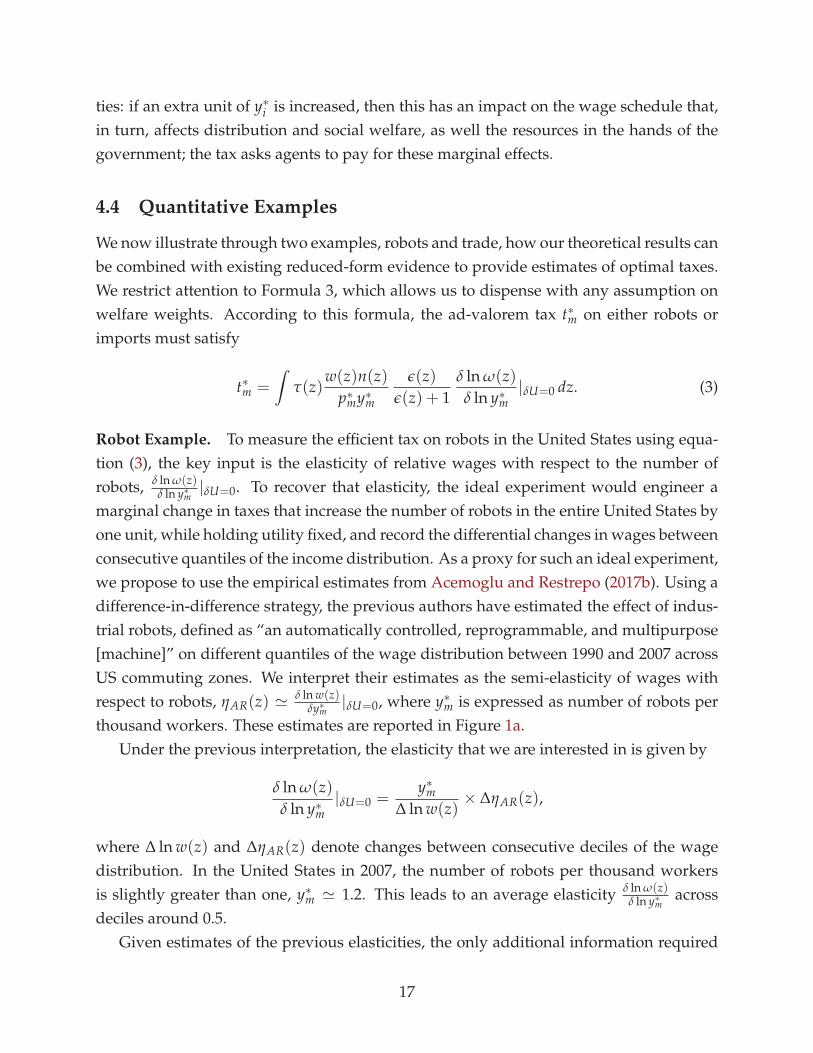
Robot Example. To measure the efficient tax on robots in the United States using equa-

tion (3), the key input is the elasticity of relative wages with respect to the number of

robots, δ ln ω(z)δ ln y∗m

|δU=0. To recover that elasticity, the ideal experiment would engineer a

marginal change in taxes that increase the number of robots in the entire United States by

one unit, while holding utility fixed, and record the differential changes in wages between

consecutive quantiles of the income distribution. As a proxy for such an ideal experiment,

we propose to use the empirical estimates from Acemoglu and Restrepo (2017b). Using a

difference-in-difference strategy, the previous authors have estimated the effect of indus-

trial robots, defined as “an automatically controlled, reprogrammable, and multipurpose

[machine]” on different quantiles of the wage distribution between 1990 and 2007 across

US commuting zones. We interpret their estimates as the semi-elasticity of wages with

respect to robots, ηAR(z) ≃δ ln w(z)

δy∗m|δU=0, where y∗m is expressed as number of robots per

thousand workers. These estimates are reported in Figure 1a.

Under the previous interpretation, the elasticity that we are interested in is given by

δ ln ω(z)

δ ln y∗m|δU=0 =

y∗m∆ ln w(z)

× ∆ηAR(z),

where ∆ ln w(z) and ∆ηAR(z) denote changes between consecutive deciles of the wage

distribution. In the United States in 2007, the number of robots per thousand workers

is slightly greater than one, y∗m ≃ 1.2. This leads to an average elasticity δ ln ω(z)δ ln y∗m

across

deciles around 0.5.

Given estimates of the previous elasticities, the only additional information required

17

(a) Robots (Acemoglu and Restrepo, 2017b) (b) Chinese Imports (Chetverikov, Larsen and Palmer, 2016)

Figure 1: Semi-Elasticity of wages, d ln w(z)dym

× 100, acrossquantiles of US wage distribution.

to evaluate the optimal tax on robots given by equation (3) is: (i) total spending on robots,

p∗my∗m, which we obtain Graetz and Michaels (2018); (ii) labor earnings, w(z)n(z), which

we compute from the World Wealth and Income Database; (iii) marginal income tax rates,

τ(z), which we compute from Guner, Kaygusuz and Ventura (2014); and (iv) labor supply

elasticities, ǫ(z), which we obtain Chetty (2012).

For a labor supply elasticity of ǫ = 0.1, in the low range of the micro-estimates re-

viewed in Chetty (2012), equation (3) leads to an optimal tax on robots equal to t∗m = 1%.

For higher labor supply elasticities of ǫ = 0.3 or ǫ = 0.5, the previous tax goes up to

t∗m = 2.7% and t∗m = 3.7%, respectively.

Trade Example. Our second example focuses on Chinese imports. Again, we propose to

use estimates obtained from a difference-in-difference strategy as a proxy for the elasticity

that we are interested in, δ ln ω(z)δ ln y∗m

|δU=0. Using the same empirical strategy as in Autor,

Dorn and Hanson (2013), Chetverikov, Larsen and Palmer (2016) have estimated the effect

on log wages of a $1,000 increase in Chinese imports per worker at different percentiles

of the wage distribution, as described in Figure 1b. Following the same approach as in

the case of robots, we can transform the previous semi-elasticities into elasticities using

y∗m ≃ 2.2 as the value of Chinese imports, in thousands of US dollars, per worker for the

United States in 2007.

Interestingly, the average value of the relative wage elasticity, d ln ωd ln y∗m

, is of the same or-

der of magnitude as the one implied by the estimates of Acemoglu and Restrepo (2017b),

around 0.5. Compared to the robot example, however, the ratio of total labor earnings to

total Chinese imports in 2007 is only 26.4, an order of magnitude smaller than the ratio to

18

total spending on robots, around 245.9 This leads to an optimal tax on Chinese imports

that is much smaller than the tax on robots: t∗m = 0.03% for ǫ = 0.1, 0.08% for ǫ = 0.3, and

0.11% for ǫ = 0.5.

5 Comparative Statics

Our second result focuses on comparative static issues. By way of a simple example,

we propose to tackle the following question: If improvements in new technologies raise

inequality, should taxes on firms using these technologies be raised further as well?

5.1 A Simple Economy

Consider a special case of the environment presented in Section 3. There is one final good,

indexed by f , and one intermediate good, indexed by m, which could be either robots that

are produced domestically or machines that are imported from abroad. Households have

quasi-linear preferences,

U(θ) = C(θ)−(n(θ))1+1/ǫ

1 + 1/ǫ, (4)

with C(θ) the consumption of the unique final good, which we use as our numeraire, p f =

p∗f = 1, and ǫ the constant labor supply elasticity. Skill heterogeneity is one-dimensional,

θ ∈ [θ, θ].

Old technology firms produce the final good, y f ≥ 0, using workers, n ≡ n(θ), and

machines, ym ≤ 0, as an input. Their production set is given by

G(y f , ym, n) = y − maxym(θ)

ˆ

g(ym(θ), n(θ); θ)dF(θ)|

ˆ

ym(θ)dF(θ) ≤ −ym, (5)

with g(ym(θ), n(θ); θ) a Cobb-Douglas production function,

g(ym(θ), n(θ); θ) = exp(α(θ)) · (ym(θ)

β(θ))β(θ)(

n(θ)

1 − β(θ))1−β(θ), (6)

where ym(θ) represents the number of machines combined with workers of type θ to

produce the final good, α(θ) ≡ α ln(1−θ)β ln(1−θ)−1

, and β(θ) ≡ β ln(1−θ)β ln(1−θ)−1

, with α, β > 0. New

technology firms produce machines, y∗m ≥ 0, using the final good, y∗f ≤ 0,

G∗(y∗f , y∗m; φ) = φy∗f + y∗m, (7)

9Graetz and Michaels (2018) estimate the share of robots in total capital services to be around 0.64%.

19

where φ measures the productivity of machine producers.

Let pm and p∗m denote the price of robots faced by old and new technology firms. Profit

maximization by new technology firms implies

p∗m = 1/φ,

whereas profit maximization by old technology firms implies

w(pm; θ) = (1 − θ)−1/γ(pm),

with γ(pm) ≡ 1/(α − β ln pm). Under the restriction that γ(pm) > 0, which we maintain

throughout, wages are increasing in θ and Pareto distributed with shape parameter equal

to γ(pm) and lower bound equal to 1. By construction, more skilled workers tend to

use machines relatively more, since β(θ) is increasing in θ. So an increase in the price of

machines tends to lower their wages relatively more, which decreases inequality,

d ln ω(θ)

d ln pm= −

d ln γ(pm)

d ln pm= −βγ(pm) < 0.

Here, because of additive separability in production, machines directly affect inequality

by affecting the relative marginal products of workers of different skills, but not indirectly

through further changes in their relative labor supply, as in Stiglitz (1982).

5.2 Technological Progress, Greater Inequality, and Lower Taxes

In the spirit of keeping this example as simple as possible, we propose to study how t∗mvaries with φ in the case of a government with extreme preferences for redistribution.

Namely, we assume that the government has Rawlsian preferences, which corresponds

to the weighted utilitarian objective of Section 3.2, with the distribution of Pareto weights

Λ being a Dirac at θ.

For comparative static purposes, a limitation of our three formulas is that they involve

the entire schedule of marginal income tax rates. These are themselves endogenous ob-

jects that will respond to changes in φ. In Appendix E, we demonstrate how to solve for

τ(θ) and obtain the following formula for the optimal Rawlsian tax,

t∗m1 + t∗m

=

ǫǫ+1

d ln ωd ln y∗m

τ∗

1 − ǫǫ+1

d ln ωd ln y∗m

τ∗

1 − sm

sm, (8)

20

where the elasticity of relative wages, d ln ωd ln y∗m

≡ −βγ(pm)∂ ln pm

∂ ln |ym(pm,n)|, is now constant

across agents; τ∗ ≡ ǫ+1ǫ+1+ǫγ(pm)

corresponds to the optimal marginal tax rate that would

be imposed in the absence of a tax on machines, as in Diamond (1998), Saez (2001), and

Scheuer and Werning (2017); and sm ≡ pmy∗m´

x(θ)dF(θ)+pmy∗mmeasures the share of machines in

gross output. After expressing the three previous statistics, d ln ωd ln y∗m

, τ∗, and sm, as functions

of t∗m and φ, we can apply the Implicit Function Theorem to determine the monotonicity

of the optimal tax, as we do in Appendix E. This leads to the following proposition.

Proposition 1. In a simple economy where equations (4)-(7) hold, the optimal Rawlsian tax t∗m is

decreasing with the productivity φ of new technology firms.

By construction, more machines always increase inequality in this simple economy,d ln ωd ln y∗m

> 0. So one should always tax new technology firms. For comparative static pur-

poses, however, the relevant question is whether this effect gets exacerbated as the new

technology improves. Here, one can check that ∂∂φ

d ln ωd ln y∗m

< 0 both because relative wages

are becoming less responsive to the price of machines, ∂∂φ |

d ln ωd ln y∗m

| < 0, and because the

demand for machines is becoming more elastic, ∂∂φ |

∂ ln pm

∂ ln |ym(pm,n)|| < 0, due to the increase

in the labor supply of high-skilled workers whose demand for machines is more elastic.

One can also check that these two effects dominate the increase in the marginal tax rate,∂τ∗

∂φ > 0, in response to greater inequality. For a given share of machines sm, this im-

plies that the total fiscal externality associated with new machines decreases. Since the

share of machines increase with improvements in the new technology, ∂sm∂φ > 0, the fiscal

externality per machine a fortiori decreases and so does the tax on machines.

As this simple example illustrates, cheaper robots may lead to a higher share of robots

in the economy, more inequality, but a lower optimal tax on robots. Likewise, more im-

ports and more inequality, in spite of the government having extreme distributional con-

cerns and imports causing inequality, may be optimally met with less trade protection.

This does not occur because redistribution is becoming more costly as the economy gets

more open.10 Here, the elasticity of labor supply is fixed and the marginal tax rate τ∗

increases with φ. This also does not occur because redistribution through income taxa-

tion is becoming more attractive. Everything else being equal, an increase in τ∗ raises the

tax on imports. Rather the decrease in the tax on imports captures a standard Pigouvian

intuition: as φ increases, the total fiscal externality associated with imports increases, but

the marginal impact does not, leading to a lower value for the optimal tax.

10This is the point emphasized by Itskhoki (2008) and Antras, de Gortari and Itskhoki (2017) in an econ-omy where entrepreneurs can decide whether to export or not. This makes labor supply decisions moreelastic in an open economy, which may reduce redistribution at the optimum.

21

6 The Valuation of Technological Change

Our final result focuses on the welfare impact of new technologies under the assumption

that constrained, but optimal policies are in place. In the presence of distortions, it is well-

known that technological progress may lower welfare. This is what Edgeworth (1884)

and Bhagwati (1958) refer to as “Economic Damnification” and “Immesirizing Growth”.

Since we have established that governments may want to depart from production effi-

ciency in order to achieve their distributional objectives, one might expect the previous

phenomenon to arise here as well. We now demonstrate that this is not the case.

6.1 An Envelope Result

Let V(φ) denote the value function associated with the government problem. As shown

in Appendix F.1, it is also equal to the value function of the relaxed problem,

V(φ) = max(c,N,n,y,y∗,p,p∗,w,T,t∗,U)∈ΩR

W(U)

subject to

G∗(y∗; φ) ≤ 0,

with ΩR ⊂ Ω requiring utility maximization by households, profit maximization by old

technology firms, and market clearing, but not profit maximization by new technology

firms. Crucially, this implies that ΩR is independent of φ.

Now consider a small productivity shock from φ to φ + dφ. The Envelope Theorem

immediately impliesdV

dφ= −γ

∂G∗

∂φ, (9)

with γ > 0 the Lagrange multiplier associated with the constraint G∗(y∗; φ) ≤ 0.11

This envelope condition can be thought of as a generalized version of Hulten’s (1978)

Theorem. In spite of the economy not being first-best, the welfare impact of technological

progress can be measured in the exact same way as in first-best environments. This leads

to our next proposition.

Proposition 2. Technological change increases social welfare, dV/dφ > 0, if and only if it ex-

pands the production possibility of new technology firms, that is, if and only if ∂G∗/∂φ < 0.

11In general, the Lagrange multiplier γ could be equal to zero if preferences were satiated or if the gov-ernment was unable, or unwilling due to distributional concerns, to transfer extra income to households.The assumption that u, v, and W are strictly increasing rules out the first issue. Appendix F.2 shows thatthe availability of non-linear income taxation makes the second issue irrelevant as well.

22

The critical assumption here is not that there are no distortions or, equivalently, that

our planner has enough tax instruments to target any underlying distortion. In fact, the

planning problem described above would also hold in an environment with externalities

and other market imperfections, such as price and wage rigidities leading to labor market

distortions. Proposition 2 instead follows from the assumption that, in spite of distortions

and restrictions on the set of available instruments, our planner still has a tax instruments

t∗ to control the new technology firms, which is where technological change occurs.

In the case of international trade, for which G∗(y∗; φ) = ∑i=1 pi(φ)y∗i , equation (9)

implies that a country gains from a terms-of-trade shock if and only if it raises the value

of its net exports, evaluated at the initial quantities,

∑i=1

p′i(φ)(−y∗i ) ≥ 0.

Intuitively, whenever world prices p(φ) fluctuate, the government has the option to main-

tain domestic prices p unchanged by adjusting the (specific) tax on each good i by − p′i(φ).

The sole impact of this adjustment is to change tax revenues by −∑i=1 p′i(φ)y∗i . Although

this may not be the optimal response, the possibility of such a response is sufficient to

evaluate the welfare impact of a terms-of-trade shock at the margin.12

6.2 Regulation of Innovation (Not!)

Our envelope result has direct implications for the regulation of innovation. To see this,

suppose that there exists a set of feasible new technologies, Φ, that can be restricted by

the government. The profit maximization problem of new technology firms is given by

y∗, φ ∈ maxy∗,φ∈Φ

p∗ · y∗|G∗(y∗; φ) ≤ 0,

where Φ ⊂ Φ is the set of technologies allowed by the government. The government’s

problem, in turn, takes the general form,

max(c,n,y,y∗,p,p∗,w,T,t∗,U)∈Ω,φ∈Φ

W(c, n)

subject to

G∗(y∗; φ) ≤ 0.

12The previous observation does not depend on whether the country is a small open economy or not.The same result holds when international prices depend on y∗.

23

By equation (9), the optimal technology φ∗ simply satisfies

∂G∗(y∗; φ∗)

∂φ= 0.

Provided that taxes of new technology firms, t∗, have been set such that they find it op-

timal to produce y∗, conditional on φ∗, they will also find it optimal to choose φ∗ , if

allowed to do so. It follows that the government does not need to affect the direction of

innovation, in spite of its potential distributional implications. More generally, there may

be externalities across firms that directly call for subsidizing, or taxing, innovation. In

such environments, the implication of our envelope result is that distributional concerns

do not add a new motive for taxing, or subsidizing, innovation.

7 Conclusion

Our paper has focused on two broad questions. First, how should government policy

respond to technological change? Second, how should we valuate the overall welfare

impact of technological change?

Our answer to the first question is that in second best environments—where income

taxation is available, but taxes on specific factors are not—there is a general case for taxing

new technology firms, with each of our three formulas offering a precise answer to what

optimal taxes on new technology firms should be as a function of a few sufficient statistics.

Perhaps surprisingly, we have also provided an example showing that more robots or

more trade may go hand in hand with more inequality and lower taxes, despite robots

or trade being responsible for the rise in inequality, and governments having extreme

preferences for redistribution.

Our answer to the second question is that in such second best environments, tech-

nological change can still be evaluated using a simple envelope argument. The critical

assumption behind this result is not the absence of any distortion, like in a first best envi-

ronment, but rather that the government has enough instruments to control the behavior

of new technology firms, which are the only ones directly subject to technological change.

This offers a new perspective on technological change that stands in sharp contrast with

the existing results of a large literature concerned with distortions and welfare. It implies,

in particular, that innovation should not be distorted because of distributional concerns.

More broadly, our envelope result suggests that provided that governments have

access to a full set of trade policy instruments, the general law of comparative advan-

tage (Deardorff, 1980) may remain valid in economies subject to imperfect competition,

24

political-economy forces, and various distortions; the only rationale for trade agreements

in all these economies may remain to correct terms-of-trade externalities (Bagwell and

Staiger, 1999, 2001, 2012a,b); and that in spite of distributional concerns and various labor

market imperfections, the welfare gains from trade may still be given by the integral be-

low the import demand curve (Costinot and Rodríguez-Clare, 2018). We leave a formal

analysis of these matters for future research.

25

References

Acemoglu, Daron and Pascual Restrepo, “The Race Between Machine and Man: Impli-

cations of Technology for Growth, Factor Shares and Employment,” NBER Work. Pap.

22252, 2017.

and , “Robots and Jobs: Evidence from US Local Labor Markets,” mimeo MIT, 2017.

Antras, Pol, Alonso de Gortari, and Oleg Itskhoki, “Globalization, Inequality and Wel-

fare,” Journal of International Economics, 2017, 108, 387–412.

Atkinson, A.B. and J.E. Stiglitz, “The Design of Tax Structure: Direct versus Indirect

Taxation,” Journal of Public Economics, 1976, 6, 55–75.

Autor, D., D. Dorn, and G. Hanson, “The China syndrom: Local labor market effects of

import competition in the United States,” American Economic Review, 2013, 103, 2121–

2168.

Baeqee, David and Emmanuel Farhi, “Productivity and Misallocation in General Equi-

librium,” mimeo Harvard University, 2017.

Bagwell, Kyle and Robert W. Staiger, “An Economic Theory of GATT,” American Eco-

nomic Review, 1999, 89 (1), 215–248.

and , “Domestic Policies, National Sovereignty, and International Economic Institu-

tions,” Quarterly Journal of Economics, 2001, 116 (2), 519–562.

and , “The Economics of Trade Agreements in the Linear Cournot Delocation

Model,” Journal of International Economics, 2012, 88 (1), 32–46.

and , “Profit Shifting and Trade Agreements in Imperfectly Competitive Markets,”

International Economic Review, 2012, 53 (4), 1067–1104.

Bhagwati, Jagdish N., “Immesirizing Growth: A Geometrical Note,” Review of Economic

Studies, 1958, 25.

, The Generalized Theory of Distortions and Welfare, Vol. Trade, Balance of Payments, and

Growth: Papers in International Economics in Honor of Charles P. Kindleberger, Ams-

terdam: North-Holland, 1971.

Chetty, Raj, “Bounds on Elasticities with Optimization Frictions: A Synthesis of Micro

and Macro Evidence on Labor Supply,” Econometrica, 2012, 80 (3), 969–1018.

26

Chetverikov, Denis, Bradley Larsen, and Christopher John Palmer, “IV Quantile Re-

gression for Group-Level Treatments, with an Application to the Effects of Trade on the

Distribution of Wage,” Econometrica, 2016, 84 (2), 809–833.

Costinot, Arnaud and Andres Rodríguez-Clare, “The US Gains from Trade: Valuation

Using the Demand for Foreign Factor Services,” Journal of Economic Perspectives, 2018,

32 (2), 3–24.

Deardorff, Alan V., “The General Validity of the Law of Comparative Advantage,” Jour-

nal of Political Economy, 1980, 88 (55), 941–957.

Diamond, Peter A., “Optimal Income Taxation: An Example with a U-Shaped Pattern of

Optimal Marginal Tax Rates,” American Economic Review, 1998, 88 (1), 83–95.

and James A. Mirrlees, “Optimal Taxation and Public Production I: Production Effi-

ciency,” American Economic Review, 1971, 61 (1), 8–27.

and , “Optimal Taxation and Public Production II: Tax Rules,” American Economic

Review, 1971, 61 (3), 261–278.

Dixit, Avinash and Victor Norman, “Gains from Trade without Lump-Sum Compensa-

tion,” Journal of Intermational Economics, 1986, 21, 111–122.

Dixit, Avinash K., “Special-Interest Lobbying and Endogenous Commodity Taxation,”

Eastern Economic Journal, 1996, 22 (4), 375–388.

and Victor Norman, Theory of International Trade, Cambridge University Press, 1980.

Edgeworth, F.Y., “The theory of international values,” Economic Journal, 1884, 4, 35–50.

Feenstra, Robert C. and Tracy R. Lewis, “Trade adjustment assistance and Pareto gains

from trade,” Journal of International Economics, 1994, 36, 201–222.

Findlay, Ronald and Stanislaw Wellisz, Endogenous tariffs, the political economy of trade

restrictions, and welfare Import Competition and Response, Chicago: University of

Chicago Press, 1982.

Graetz, Georg and Guy Michaels, “Robots at Work,” mimeo LSE, 2018.

Grossman, Gene M. and Elhanan Helpman, “Protection for Sale,” American Economic

Review, 1994, 84 (4), 833–850.

27

and Esteban Rossi-Hansberg, “Trading Tasks: A Simple Theory of Offshoring,” Amer-

ican Economic Review, 2008, 98 (5), 1978–1997.

Guerreiro, Joao, Sergio Rebelo, and Pedro Teles, “Should Robots Be Taxed?,” mimeo

Northwestern University, 2017.

Guesnerie, Roger, “Peut-on toujours redistribuer les gains a la specialisation et a

l’echange? Un retour en pointille sur Ricardo et Heckscher-Ohlin,” Revue Economique,

1998, 49 (3), 555–579.

Guner, Nezih, Remzi Kaygusuz, and Gustavo Ventura, “Income Taxation of U.S. House-

holds: Facts and Parametric Estimates,” Review of Economic Dynamics, 2014, 17 (4), 559–

581.

Helpman, Elhanan, Politics and Trade Policy Advances in Economics and Econometrics:

Theory and Applications, New York: Cambridge University Press, 1997.

Hillman, Arye L., “Declining Industries and Political-Support Protectionist Motives,”

American Economic Review, 1982, 72 (1180-1187).

Hosseini, Roozbeh and Ali Shourideh, “Inequality, Redistribution, and Optimal Trade

Policy: A Public Finance,” mimeo Carnegie Mellon University, 2018.

Hulten, Charles R., “Growth Accounting with Intermediate Inputs,” The Review of Eco-

nomic Studies, 1978, 45 (3), 511–518.

Itskhoki, Oleg, “Optimal Redistribution in an Open Economy,” mimeo Princeton Univer-

sity, 2008.

Jacobs, Bas, “Optimal Inefficient Production,” mimeo Erasmus University, 2015.

Magee, Stephen P., William A. Brock, and Leslie Young, Black Hole Tariffs and Endogenous

Policy Formation, Cambridge: MIT Press, 1989.

Mayer, Wolfgang, “Endogenous Tariff Formation,” American Economic Review, 1984, 74,

970–985.

and Raymond G. Riezman, “Endogenous Choice of Trade Policy Instruments,” Journal

of Intermational Economics, 1987, 23, 377–381.

and , “Tariff Formation in a Multidimensional Voting Model,” Economics and Politics,

1989, 61-79.

28

Mirrlees, J.A., “An Exploration in the Theory of Optimum Income Taxation,” Review of

Economic Studies, 1971, 38 (2), 175–208.

Naito, Hisairo, “Re-examination of uniform commodity taxes under non-linear income

tax system and its implications for production efficiency,” Journal of Public Economics,

1999, 1 (2), 65–88.

, “Redistribution, production inefficiency and decentralized efficiency,” International

Tax Public Finance, 2006, 13, 625–640.

Saez, Emmanuel, “Using Elasticities to Derive Optimal Income Tax Rates,” Review of Eco-

nomic Studies, 2001, 68 (1), 205–229.

Scheuer, Florion and Ivan Werning, “The Taxation of Superstars,” Quarterly Journal of

Economics, 2017, 132, 211–270.

Solow, Robert, “Technical Change and the Aggregate Production Function,” The Review

of Economics and Statistics, 1957, 39 (3), 312–320.

Spector, David, “Is it possible to redistribute the gains from trade using income taxa-

tion?,” Journal of International Economics, 2001, 55, 441–460.

Stiglitz, Joseph E., “Self-selection and Pareto efficient taxation,” Journal of Public Eco-

nomics, 1982, 17 (2), 213–240.

Thuemmel, Uwe, “Optimal Taxation of Robots,” mimeo University of Zurich, 2018.

Tsyvinski, Aleh and Nicolas Werquin, “Generalized Compensation Principle,” mimeo

Yale University, 2018.

Werning, Ivan, “Pareto Efficient Income Taxation,” mimeo MIT, 2007.

29

A Notation

Consider a function h : Rn → R

m such that

h(x1, ..., xn) = (h1(x1, ..., xn), ..., hm(x1, ..., xn)).

Throughout our appendix, we use the following notation

hxi(x1, ..., xn) ≡

∂h(x1, ..., xn)

∂xifor all i = 1, ..., n,

hj,xi(x1, ..., xn) ≡

∂hj(x1, ..., xn)

∂xifor all i = 1, ..., n and j = 1, ..., m,

Whenever there is no risk of confusion, we also drop arguments from functions so that, for in-

stance, h implicitly stands for h(x1, ..., xn).

B Section 2

B.1 Tasks in Old Technology

Our environment nests economies in which a final good is produced using a continuum of tasks.

To see this formally, consider an economy that produces a final good f using a continuum of tasks

indexed by j,

y f = g f (y(j)),

with y(j) ≥ 0 the output of task j and g f a constant returns to scale production function. Each task,

in turn, is produced using domestic workers and robots, as in Acemoglu and Restrepo (2017a), or

domestic and foreign workers, as in Grossman and Rossi-Hansberg (2008),

y(j) = gj(ym(j), n(θ, j)), for all j,

with ym(j) ≥ 0 the number of robots or foreign workers used to perform task j, n(θ, j) ≥ 0 the

number of domestic workers, and gj a constant return to scale production function. The produc-

tion possibility frontier is then given by

G(y f , ym, n) = maxy(j),ym(j),n(θ,j)

g f (y(j))

30

subject to

y(j) ≤ gj(ym(j), n(θ, j)), for all j,

n(θ) ≥

ˆ

n(θ, j)dj, for all θ,

−ym ≥

ˆ

ym(j)dj,

with y f ≥ 0 the output of the final good and ym ≤ 0 the total amount of robots or foreign workers

demanded by old technology firms.

B.2 Labor in New Technology

In Section 2, we have argued that it is without loss of generality to assume the new technology G∗

does not employing labor. Here, we provide the formal argument.

Suppose that the production sets associated with the old and new technology are such that

G(y, n) ≤ 0,

G∗(y∗, n∗) ≤ 0.

First, define

y =

(

y

y∗

)

Next, define G so that the set of (y, n) satisfying G(y, n) ≤ 0 coincides with the set of (y, n) for

which there exists n and n∗ such that

G(y, n) ≤ 0,

G∗(y∗, n∗) ≤ 0,

n + n∗ = n.

Last, define G∗ such that G∗(y∗) ≤ 0 is satisfied if and only if

y∗ =

(

y

y∗

)

is such that y ≤ −y∗.

31

C Section 3

C.1 Competitive Equilibrium with Taxes

We provide a formal definition of a competitive equilibrium with taxes.

Demand. Households maximize utility taking prices p and the income tax schedule T as given.

Since preferences are weakly separable, the demand of any household θ is given by the two-step

problem

c(θ) ∈ argmaxc(θ)v(c(θ))|p · c(θ) ≤ w(θ)n(θ)− T(w(θ)n(θ)), (C.1)

n(θ) ∈ argmaxn(θ)u(C(p, w(θ)n(θ)− T(w(θ)n(θ))), n(θ)), (C.2)

with C(p, R(θ)) ≡ maxc(θ)v(c(θ))|p · c(θ) ≤ R(θ) the indirect utility function of an household

with after-tax earnings R(θ) ≡ w(θ)n(θ)− T(w(θ)n(θ)).

Supply. Firms maximize profits taking prices p and p∗ as given,

y, n ∈ argmaxy,np · y −

ˆ

w(θ)n(θ)dF(θ) | G(y, n) ≤ 0, (C.3)

y∗ ∈ argmaxy∗p∗ · y∗| G∗(y∗; φ) ≤ 0. (C.4)

Market Clearing. Demand equals supply for all goods,

ˆ

ci(θ)dF(θ) = yi + y∗i for all i. (C.5)

Linear Taxation. Prices satisfy

pi = (1 + t∗i )p∗i for all i. (C.6)

Equilibrium. A competitive equilibrium with taxes (T, t∗) is an allocation c ≡ c(θ), n ≡

n(θ), y ≡ yi, y∗ ≡ y∗i , prices and wages p ≡ pi, p∗ ≡ p∗i , and w ≡ w(θ), such that:

i. households maximize their utility, condition (C.1) and (C.2);

ii. firms maximize their profits, conditions (C.3) and (C.4);

iii. good markets clear, condition (C.5);

iv. prices satisfy the non-arbitrage condition (C.6).

32

C.2 Wage Schedule

Let y(p, n) denote the supply of old technology firms, that is the solution to

maxyp · y | G(y, n) ≤ 0.

The first-order conditions of (C.3) imply a wage schedule w(p, n) ≡ w(p, n; θ) such that

w(θ) = −Gn(θ)(y(p, n), n)/Gy1(y(p, n), n) for all θ.

C.3 Government Problem

For any vector of consumption and labor supply, c ≡ c(θ) and n ≡ n(θ), the utility of quantile

z ∈ [0, 1] is given byˆ

u(v(c(θ)),n(θ))≤U(z)dF(θ) = z. (C.7)

For any y∗, construct p∗ such that

p∗i = G∗y∗i(y∗; φ)/G∗

y∗1(y∗; φ) for all i. (C.8)

Define the feasible set

Ω = (c, n, y, y∗, p, p∗, w, T, t∗, U) such that equations (C.1)-(C.3) and (C.5)-(C.8) hold.

The problem of selecting a competitive equilibrium with taxes that maximizes social welfare can

then be expressed as

max(c,n,y,y∗,p,p∗,w,T,t∗,U)∈Ω

W(U)

subject to

G∗(y∗; φ) ≤ 0.

D Section 4

D.1 Lemma 1

Preliminaries. The next lemma will be used to reduce the dimensionality from θ to the per-

centile z in our optimality conditions.

Lemma 2. Suppose θ ∈ Θ ⊆ Rn, ǫ ∈ R and the function w(θ, ǫ) is a.e. differentiable and increasing in

θn, define

Z(W, ǫ) =

ˆ

w(θ,ǫ)≤WdF(θ)

33

and let w(z, ǫ) denote the inverse of Z with respect to W. Then

wǫ(z, ǫ) = E[wǫ(θ, ǫ) | w(θ, ǫ) = w(z, ǫ)].

Proof. Denote the inverse of W = w(θ, ǫ) for θn as θ(θ−n, W, ǫ). Then

Z(W, ǫ) =

ˆ

F(θ(θ−n, W, ǫ) | θ−n) dF(θ−n). (D.1)

Since w(θ−n, θ(θ−n, W, ǫ), ǫ) = W it follows that

θW(θ−n, W, ǫ) =1

wθn(θ−n, θ(θ−n, W, ǫ), ǫ)

θǫ(θ−n, W, 0) = −wǫ(θ−n, θ(θ−n, W, ǫ), ǫ)

wθn(θ−n, θ(θ−n, W, ǫ), ǫ)

Since w(Z(W, ǫ), ǫ) = W it follows that

wǫ(z, ǫ) = −wz(z, ǫ)Zǫ(w(z, ǫ), ǫ) = −1

ZW(w(z, ǫ), ǫ)Zǫ(w(z, ǫ), ǫ)

Using these expressions and differentiating (D.1) gives

wǫ(z, ǫ) =1

´ f (θ(θ−n,w(z,ǫ),ǫ)|θ−n)

wθn (θ−n,θ(θ−n,w(z,ǫ),ǫ),ǫ)dF(θ−n)

×

ˆ

f (θ(θ−n, w(z, ǫ), ǫ) | θ−n)

wθn(θ−n, θ(θ−n, w(z, ǫ), ǫ), ǫ)

wǫ(θ−n, θ(θ−n, w(z, ǫ), ǫ), ǫ) dF(θ−n).

To see that this establishes the desired equality, define

G(W | θ−n) = F(θ(θ−n, W, ǫ) | θ−n)

the c.d.f. for W = w(θ, ǫ) conditional on θ−n; differentiating, one sees that

g(W | θ−n) =f (θ(θ−n, W, ǫ) | θ−n)

wθn(θ−n, θ(θ−n, W, ǫ), ǫ)

represents the associated conditional density. Noting that

g(θ−n | W) =g(W | θ−n)dF(θ−n)´

g(W | θ−n)dF(θ−n)

the result then follows: wǫ(z, ǫ) = E[wǫ(θ, ǫ) | w(θ, ǫ) = w(z, ǫ)].

The following simple corollary will be employed below, for any differentiable function N(w, ǫ)

34

define n(θ, ǫ) = N(w(θ, ǫ), ǫ) and n(z, ǫ) = N(w(z, ǫ), ǫ) then

nǫ(z, ǫ) = E[nǫ(θ, ǫ) | w(θ, ǫ) = w(z, ǫ)].

Proof of Lemma 1. We shall engineer variations that ensure all the equilibrium conditions are

met except G∗(y∗; φ) ≤ 0. We must evaluate how the variation affects welfare W(U) and G∗(y∗; φ).

To do so, define the Lagrangian

L = W(U)− γG∗(y∗; φ)

with Lagrange multiplier γ > 0.13 At an optimum the variation in L must be set to zero.

The new tax schedule is given by

t∗i (ǫ) = t∗i + ǫt∗i for all i,

T(x, ǫ) = T(x) + ǫT(x) for all x ≥ 0,

for some arbitrary vector new technology taxes, t∗, income tax schedule, T, and ǫ ∈ R. We let

c(θ, ǫ), n(θ, ǫ), y(ǫ) ≡ yi(ǫ), and y∗(ǫ) ≡ y∗i (ǫ) denote the associated equilibrium allo-

cation and we let p(ǫ) ≡ pi(ǫ), p∗(ǫ) ≡ p∗i (ǫ) and w(θ, ǫ) denote the associated prices and

wages. They are given by conditions (C.1)-(C.3) and (C.5)-(C.8). The only equilibrium condition

that is not imposed is G∗(y∗(ǫ); φ) = 0.

Let W(U(z, ǫ)) denote the social welfare associated with a given value of ǫ. Since house-

holds have identical preferences, all households of a given quantile z of the utility distribution

have wage w(z, ǫ) and achieve utility

U(z, ǫ) = maxn(θ)u(C(p(ǫ), R(w(z, ǫ)n(θ), ǫ)), n(θ)),

with labor supply n(z, ǫ), consumption, c(z, ǫ), and earnings, x(z, ǫ) ≡ w(z, ǫ)n(z, ǫ). Let Uǫ(z, ǫ) ≡

∂U(z, ǫ)/∂ǫ denote the marginal change in utility at quantile z. The Envelope Theorem implies

Uǫ(z, ǫ) = uC(z, ǫ) CR(z, ǫ) [Rx(z, ǫ)n(z, ǫ)wǫ(z, ǫ) + Rǫ(z, ǫ)− c(z, ǫ) · pǫ],

with

uC(z, ǫ) ≡ uC(C, n)|C=C(p(ǫ),R(z,ǫ)),n=n(z,ǫ) ,

CR(z, ǫ) ≡ CR(p, R)|p=p(ǫ),R=R(z,ǫ) ,

R(z, ǫ) ≡ R(x(z, ǫ), ǫ),

Rx(z, ǫ) ≡ Rx(x, ǫ)|x=x(z,ǫ),ǫ ,

Rǫ(z, ǫ) ≡ Rǫ(x, ǫ)|x=x(z,ǫ),ǫ .

13The formal argument establishing that γ cannot be equal to zero is given in Appendix F.2.

35

This further implies

dW(U(z, ǫ))

dǫ= (D.2)ˆ

∂W

∂U(z)uC(z, ǫ) CR(z, ǫ) [Rx(z, ǫ)n(z, ǫ)wǫ(z, ǫ)− c(z, ǫ) · pǫ + Rǫ(z, ǫ)] dz.

Now consider the change in the cost of resources used by the new technology,

dG∗(y∗(ǫ); φ)

dǫ= ∑

i

G∗y∗i

y∗i,ǫ +

ˆ

G∗n∗(θ)n

∗ǫ(θ, ǫ)dF(θ).

Using equation (C.8), this can be rearranged as

dG∗(y∗(ǫ); φ)

dǫ= G∗

y1(p∗ − p) · y∗ǫ + p ·

ˆ

cǫ(θ, ǫ)dF(θ)− p · yǫ. (D.3)

From the first-order conditions associated with (C.3), we know that

p ·∂y(p, n)

∂pi= 0 for all i,

p ·∂y(p, n)

∂n(θ)= w(θ) for all θ.

It follows that

p · yǫ = p · [∑i

∂y(p, n)

∂pipi,ǫ +

ˆ

∂y(p, n)

∂n(θ)nǫ(θ, ǫ)dF(θ)] =

ˆ

w(θ)nǫ(θ, ǫ)dF(θ), (D.4)

From the budget constraint associated with (C.1), we also know that

d

dǫ[p(ǫ) ·

ˆ

c(θ, ǫ)dF(θ)] =dR(w(θ, ǫ)n(θ, ǫ), ǫ)

dǫ.

It follows that

p ·

ˆ

cǫ(θ, ǫ)dF(θ) =−

ˆ

pǫ · c(θ, ǫ)dF(θ) +

ˆ

[Rǫ(w(θ, ǫ)n(θ, ǫ), ǫ) (D.5)

+ Rx(w(θ, ǫ)n(θ, ǫ), ǫ)(

wǫ(θ, ǫ)n(θ, ǫ) + w(θ, ǫ)nǫ(θ, ǫ))]

dF(θ).

Combining (D.3)-(D.5) and using w(θ, ǫ)n(θ, ǫ) = x(θ, ǫ), we get

dG∗(y∗(ǫ); φ)

dǫ= G∗

y1

(p∗ − p) · y∗ǫ −

ˆ

pǫ · c(θ, ǫ)dF(θ)ˆ

[Rǫ(x(θ, ǫ), ǫ) + Rx(x(θ, ǫ), ǫ)wǫ(θ, ǫ)n(θ, ǫ)− (1 − Rx(x(θ, ǫ), ǫ))w(θ, ǫ)nǫ(θ, ǫ))]dF(θ)

.

36

Applying the corollary of Lemma 2, we have

nǫ(z, ǫ) =

ˆ

nǫ(θ, ǫ) f (θ|w(θ, ǫ) = w(z, ǫ))dθ.

Thus we can rearrange the previous expression as

dG∗(y∗(ǫ); φ)

dǫ= G∗

y1(p∗ − p) · y∗ǫ +

ˆ

[Rǫ(z, ǫ) + Rx(z, ǫ)n(z, ǫ)wǫ(z, ǫ)− c(z, ǫ) · pǫ]dz

−

ˆ

(1 − Rx(z, ǫ))w(z, ǫ)nǫ(z, ǫ)]dz. (D.6)

A necessary condition for a feasible variation not to improve welfare is that

dW(U(z, ǫ))

dǫ

∣

∣

∣

∣

ǫ=0

− γdG∗(y∗(ǫ); φ)

dǫ

∣

∣

∣

∣

ǫ=0

= 0.

Combining equations (D.2) and (D.6), this implies

ˆ

[λ(z)− 1][(1 − τ(z))n(z)wǫ(z)− c(z) · pǫ − Tǫ(z)]dz

= (p∗ − p) · y∗ǫ −

ˆ

τ(z)w(z)nǫ(z)dz,

with

λ(z) ≡(∂W/∂U(z))|ǫ=0 uC(z, 0) CR(z, 0))

γG∗y1(y∗(0))

,

τ(z) ≡ 1 − Rx(z, 0),

Tǫ(z) ≡ −Rǫ(z, 0),

as well as the obvious short hand notation, n(z) ≡ n(z, 0) etc.

D.2 Proposition 1

Preliminaries. We introduce the following definitions,

C(x, ǫ) ≡ C(R(x, ǫ), p(ǫ)),

MRS(C, n) ≡ −un(C, n)

uC(C, n).

37

For the household at the quantile z of the utility distribution, we then have

U(z, ǫ) =u(C(x(z, ǫ), ǫ), n(z, ǫ))], (D.7)

MRS(C(x(z, ǫ), ǫ), n(z, ǫ)) = w(z, ǫ)Cx(x(z, ǫ), ǫ), (D.8)

x(z, ǫ) = w(z, ǫ)n(z, ǫ), (D.9)

where the second equation corresponds to the first-order condition associated with C.2.

Differentiating equations (D.7)-(D.9) with respect to ǫ implies

Uǫ = uC(Cxnwǫ + Cǫ), (D.10)

nǫ =(Cxxwn + Cx)wǫ + Cxǫw − MRSC(Cxnwǫ + Cǫ)

(MRSCCxw + MRSn − Cxxw2)(D.11)

Below we use equations (D.10) and (D.11) to construct variations such that nǫ = 0 and Uǫ = 0.

Variation δT = 0. Consider a first variation such that

t∗i (ǫ) = t∗i + ǫt∗i for all i,

T(x, ǫ) = T(x) for all x ≥ 0,

From Lemma 1, if Tǫ = 0, then

(p∗ − p) · y∗ǫ −

ˆ

τ(z)w(z)nǫ(z) dz =

ˆ

(λ(z)− 1)((1 − τ(z))n(z) wǫ(z)− c(z) · pǫ) dz. (D.12)

Pick t∗ ≡ t∗i such that y∗1,ǫ, y∗i,ǫ 6= 0 and y∗j,ǫ = 0 for all j 6= 1, i. This implies

pi − p∗i = −

ˆ

(

(λ(z)− 1)(1 − τ(z)) + τ(z) εu(z))

n(z)δw(z)

δy∗i|δT=0 dz−

ˆ

(λ(z)− 1)c(z) ·δp

δy∗i|δT=0 dz,

where εu(z) ≡ w(z)n(z)

δn(z)δw(z)

denotes the uncompensated labor supply elasticity.

Variation δn = 0. Consider a variation

t∗i (ǫ) = t∗i + ǫt∗i for all i,

T(x, ǫ) = T(x) + ǫT(x) for all x ≥ 0,

such that nǫ = 0 and (dG∗(y∗(ǫ))/dǫ)ǫ=0 = 0. From Lemma 1, we know that if nǫ(z) = 0 for all z,

then

(p∗ − p) · y∗ǫ =

ˆ

[λ(z)− 1][Rx(z)n(z)wǫ(z)− c(z) · pǫ + Rǫ(z)]dz.

38

By definition of C(x, ǫ) ≡ C(R(x, ǫ), p(ǫ)), we must also have

Cx(x(z), 0) = CR(z)Rx(z), (D.13)

Cǫ(x(z), 0) = CR(z)[Rǫ − c(z) · pǫ]. (D.14)

Thus, we can rearrange the previous expression as

(p∗ − p) · y∗ǫ =

ˆ

[Cx(x(z), 0)n(z)wǫ(z) + Cǫ(x(z), 0)][λ(z)− 1]

CR(z)dz. (D.15)

Let us now compute Cǫ. By equation (D.11), for nǫ = 0, Cǫ must solve

Cxǫ(x(z), 0)− ρ(z)Cǫ(x(z), 0) = g(z),

with

ρ(z) ≡MRSC(C(x(z), 0), n(z))

w(z)(D.16)

g(z) ≡ −wǫ(z)

w(z)Cx(x(z), 0)[1 +

Cxx(x(z), 0)w(z)n(z)

Cx(x(z), 0)] + ρ(z)Cx(x(z), 0)n(z)wǫ(z). (D.17)

The general solution to this ODE is

Cǫ(x(z), 0) =

ˆ z

0exp[

ˆ z

zρ(v)dx(v)]g(z)dx(z) + exp[

ˆ z

0ρ(v)dx(v)]Cǫ(x(0), 0). (D.18)

The initial condition Cǫ(x(0), 0), in turn, is given by the requirement that (dG∗(y∗(ǫ))/dǫ)ǫ=0 = 0.

Using equations (D.6), (D.13), and (D.14), we can rearrange this requirement as

(p∗ − p) · y∗ǫ +

ˆ

[Cx(x(z), 0)n(z)wǫ(z) + Cǫ(x(z), 0)]1

CR(z)dz = 0.

Combining this expression with equation (D.18) leads to

Cǫ(x(0), 0) =(p − p∗) · y∗ǫ −

´

[Cx(x(z), 0)n(z)wǫ(z) +´ z

0 exp[´ z

z ρ(v)dx(v)]g(z)dx(z)] 1CR(z)

dz´

exp[´ z

0 ρ(v)dx(v)] 1CR(z)

dz.

(D.19)

Next, substituting for Cǫ in (D.15) using (D.18) and (D.19), we obtain

(p∗− p) · y∗ǫ =

ˆ

[Cx(x(z), 0)n(z)wǫ(z) exp[−

ˆ z

0ρ(v)dx(v)]+

ˆ z

0exp[−

ˆ z

0ρ(v)dx(v)]g(z)dx(z)]dΥ(z),

39

with

dΥ(z) ≡

´

exp[´ z

0 ρ(v)dx(v)] 1CR(z)

dz´

exp[´ z

0 ρ(v)dx(v)] λ(z)CR(z)

dzλ(z)− 1

exp[´ z

0 ρ(v)dx(v)]

CR(z)dz.

Integrating by parts, we get

(p∗ − p) · y∗ǫ =−

ˆ

ξ(z)Cxx xz(z)wǫn + Cxwǫzn + Cxwǫnz − ρ(z)xz(z)Cxwǫn + g(z)xzdz.

with ξ(z) ≡ exp[−´ z

0 ρ(v)dx(v)]´ z

0 dΥ(z). Substituting for g(z) using (D.17) implies

(p∗ − p) · y∗ǫ = −

ˆ

ξ(z)Cx−wǫ

wxz(z) + wǫzn + wǫnzdz.

Using the fact that xz(z) = wzn + wnz , one can further check that

−wǫ

wxz(z) + wǫzn + wǫnz = (wn)ωǫ,

with ω ≡ d ln wdz . This leads to

(p∗ − p) · y∗ǫ =−

ˆ

ψ(z)(1 − τ(z))w(z)n(z)ωǫ(z)dz

with

ψ(z) ≡

ˆ z

0

´

exp[´ z′

0 ρ(v)dx(v)] λ(z)CR(z′)

dz′

´

exp[´ z′

0 ρ(v)dx(v)] λ(z′)CR(z′)

dz′− 1

CR(z)

CR(z)exp[

ˆ z

zρ(v)dx(v)]

dz.

Pick T and t∗ ≡ t∗i such that, in addition to nǫ = 0, Cǫ(x(0), 0) = −κ and y∗1,ǫ, y∗i,ǫ 6= 0 and

y∗j,ǫ = 0 for all j 6= 1, i. Then

pi − p∗i =

ˆ

ψ(z)(1 − τ(z))w(z)n(z)δω

δy∗i|δn=0 dz.

Variation δU = 0. Consider a variation

t∗i (ǫ) = t∗i + ǫt∗i for all i,

T(x, ǫ) = T(x) + ǫT(x) for all x ≥ 0,

40

such that Uǫ = 0. From Lemma 1, we know that

(p∗ − p) · y∗ǫ −

ˆ

τ(z)w(z)nǫ(z) dz

=

ˆ

(λ(z)− 1)[(1 − τ(z))n(z) wǫ(z)− c(z) · pǫ − Tǫ(z)] dz.

In the proof of Lemma 1, we have already established that

Uǫ(z) = uC(z) CR(z)[(1 − τ(z))n(z) wǫ(z)− c(z) · pǫ − Tǫ(z)].

It follows that if Uǫ = 0, then

(p∗ − p) · y∗ǫ =

ˆ

τ(z)w(z)nǫ(z) dz. (D.20)

Let us now compute nǫ(z). By equation (D.10), Uǫ = 0 implies

Cx(x(z), 0)n(z)wǫ(z) + Cǫ(x(z), 0) = 0. (D.21)

Differentiating with respect to z implies

(

Cǫx + Cxxwǫn)

(nzw + nwz) + Cxwǫzn + Cxwǫnz = 0. (D.22)

Differentiating (D.8) with respect to z further implies

nz =Cxxwn + Cx − MRSCCxn

MRSCCxw + MRSn − Cxxw2wz.

Substituting for nz in equation (D.22), we get

(

Cǫx + Cxxwǫn) (

Cxw + MRSnn)

wz

+(

MRSCCxw + MRSn − Cxxw2)

Cxwǫzn + Cxwǫ

(

Cxxwn + Cx − MRSCCxn)

wz = 0.

Let ε(z) ≡ MRS(C(x(z),0),n(z))MRSn(C(x(z),0),n(z))n(z)

denote the consumption-compensated elasticity of labor supply.

Using equation (D.8), the previous expression can be rearranged as

Cǫx = −Cxxwǫn −ε(

MRSCCxwn + MRSnn − Cxxw2n)

1 + ε

wǫz

wzw

+ε(

MRSCCxwn − Cxw − Cxxw2n)

1 + ε

wǫ

w2.

41

Together with equation (D.21), equation (D.11) further implies

nǫ =(Cxxwn + Cx)wǫ + Cxǫw

(MRSCCxw + MRSn − Cxxw2).

Substituting for Cǫx leads to

nǫ =Cxwǫ −

ε1+ε

(

(

MRSCCxw + MRSn − Cxxw2)

n wǫzwz

−(

MRSCCxnw − Cxw − Cxxw2n)

wǫw

)

(MRSCCxw + MRSn − Cxxw2).

Differentiating ω ≡ d ln wdz with respect to ǫ also implies

ωǫ

ω=

1wzw

∂

∂ǫ

(

wz

w

)

=1wzw

(

wzǫ

w−

wzwǫ

w2

)

=wzǫ

wz−

wǫ

w.

Combining the two previous expressions we obtain

nǫ =Cxwǫ1+ε − ε

1+ε nMRSnwǫzwz

− ε1+ε n ωǫ

ω

(

MRSCCxw − Cxxw2)

(MRSCCxw + MRSn − Cxxw2).

By equation (D.8), we know that

Cxwǫ

1 + ε=

MRS

1 + ε

wǫ

w=

ε

1 + εnMRSn

wǫ

w.

It follows that

nǫ = −ε

1 + εn

ωǫ

ω.

Substituting for nǫ into (D.20), we obtain

(p∗ − p) · y∗ǫ = −

ˆ

τ(z)w(z)n(z)ε(z)

1 + ε(z)

ωǫ(z)

ω(z)dz.

Pick T and t∗ ≡ t∗i such that, in addition to Uǫ = 0, y∗1,ǫ, y∗i,ǫ 6= 0 and y∗j,ǫ = 0 for all j 6= 1, i. Then

pi − p∗i =

ˆ

τ(z)w(z)n(z)ǫ(z)

ǫ(z) + 1

1

ω(z)

δω(z)

δy∗i|δU=0 dz.

E Section 5

E.1 Preliminaries

Government Problem. Suppose, as in Section 5, that skill heterogeneity is one-dimensional so

that we can write social welfare as a function of the utility of each skill type, W(U(θ)). Using

42

the revelation principle, we can express the government problem as

maxU,n,p

W(U(θ))

subject to

θ ∈ argmaxθu

(

C(n(θ), U(θ)), n(θ)w(p, n; θ)

w(p, n; θ)

)

,

G∗(c(p, n, U)− y(p, n); φ) ≤ 0,

where C(n(θ), U(θ)) is the aggregate consumption required to achieve utility U(θ) given labor

supply n(θ), that is the solution to u(C, n(θ)) = U(θ), and c(p, n, U) =´

c(p, C(n(θ), U(θ)))dF(θ)

is the total demand for goods conditional on prices, p, labor supply, n ≡ n(θ), and utility levels,

U ≡ U(θ), with c(p, C) the solution to minc(θ)p · c|v(c) ≥ C.

The envelope condition associated with the Incentive Compatibility constraint gives

U′(θ) = −un(C(n(θ), U(θ)), n(θ))n(θ)ω(p, n; θ)

with ω(p, n; θ) ≡ wθ(p,n;θ)w(p,n;θ)

. For piecewise differentiable allocations, the envelope condition and

monotonicity of the mapping from wages, w(p, n; θ), to before-tax earnings, w(p, n; θ)n(θ) is equiv-

alent to incentive compatibility. We will focus on cases where w(p, n; θ) is increasing in θ, which

for a given allocation can be interpreted as a normalization or ordering of θ. Under the previous

conditions, we can rearrange our planning problem as

maxU,n,p

W(U(θ))

subject to

U′(θ) = −un(C(n(θ), U(θ)), n(θ))n(θ)ω(p, n; θ),

G∗(c(p, n, U)− y(p, n); φ) ≤ 0.

Under the functional-form assumptions of Section 5 this simplifies further into

maxU,n,pm

ˆ

U(θ)dΛ(θ) (E.1a)

subject to

U′(θ) = h′(n(θ))n(θ)ω(pm; θ), (E.1b)

φ[

ˆ

(U(θ) + h(n(θ)))dF(θ)− y f (pm, n)]− ym(pm, n) ≤ 0, (E.1c)

43

with h(n(θ)) ≡ (n(θ))1+1/ǫ

1+1/ǫ and Λ(θ) = 1 for all θ, that is full weight at θ.

Lagrangian. The Lagrangian associated with the planner’s problem (E.1) is given by

L =

ˆ

U(θ)dΛ(θ) +

ˆ

µ(θ)(

U′(θ)− h′(n(θ))n(θ)ω(pm; θ))

dθ

− γ[φ[

ˆ

(U(θ) + h(n(θ)))dF(θ)− y f (pm, n)]− ym(pm, n)].

Integrating by parts, we get

L =

ˆ

U(θ)dΛ(θ)−

ˆ

µ′(θ)U(θ)dθ + U(θ)µ(θ)− U(θ)µ(θ)

−

ˆ

µ(θ)h′(n(θ))n(θ)ω(pm; θ)dθ

− γ[φ[

ˆ

(U(θ) + h(n(θ)))dF(θ)− y f (pm, n)]− ym(pm, n)].

Since U(θ) and U(θ) are free we must have

µ(θ) = µ(θ) = 0.

First-order Conditions: U(θ). The first-order condition with respect to U(θ) leads to

λ(θ)− µ′(θ)− γφ f (θ) = 0.

Since µ(θ) = 0, integrating between θ and θ, we get

µ(θ) = Λ(θ)− γφF(θ).

Since µ(θ) = 0, we must also have

1 − γφ = 0.

Combining the two previous observations, we obtain

µ(θ)

γφ= Λ(θ)− F(θ). (E.2)

First-order Conditions: n(θ). The first-order condition with respect to n(θ) is given by

γφ[y f ,n(θ)(pm, n)− h′(n(θ)) +1

φym,n(θ)(pm, n] f (θ) (E.3)

= µ(θ)[h′′(n(θ))n(θ) + h′(n(θ))]ω(pm; θ),

44

with y f ,n(θ) ≡ ∂y f /∂n(θ) and ym,n(θ) ≡ ∂ym/∂n(θ). The first-order conditions of old technology

firms, new technology firms, and households imply

y f ,n(θ)(pm, n) + pmym,n(θ)(pm, n) = w(θ),

p∗m = 1/φ,

h′(n(θ)) = w(θ)(1 − τ(θ)).

Thus, we can rearrange equation (E.3) into

γφ[w(θ)τ(θ) + (p∗m − pm)ym,n(θ)] f (θ) = µ(θ)h′(n(θ))[ǫ(θ) + 1

ǫ(θ)]ω(pm; θ), (E.4)

with ǫ(θ) ≡ d ln(n(θ))/d ln h′(n(θ))).

First-order Conditions: pm. The first-order condition with respect to pm is given by

γφ(p∗m − pm)ym,pm =

ˆ

µ(θ)h′(n(θ))n(θ)ωpm(pm; θ)dθ, (E.5)

with ym,pm ≡ ∂ym/∂pm and ωpm ≡ ∂ω/∂pm.

Optimal Tax on Machines Using equation (E.4) to substitute for µ(θ)h′(n(θ))/γ in equation

(E.5) and noting that ∂ ln ym(pm, n(θ); θ)/∂ ln n(θ) = 1,14 we obtain

pm − p∗m =

´ ǫ(θ)ǫ(θ)+1

· d ln ω(θ)d ln |ym|

· τ(θ) · x(θ)dF(θ)

|ym|[1 −´ ǫ(θ)

ǫ(θ)+1· d ln ω(θ)

d ln |ym|· ym(θ)

|ym|dF(θ)]

,

with d ln ω(θ)d ln |ym|

= ∂ ln pm

∂ ln |ym(pm,n)|d ln ω(pm;θ)

d ln pm. Using y∗m = |ym| and t∗m = pm/p∗m − 1, this implies

t∗m =

´ ǫ(θ)ǫ(θ)+1

d ln ω(θ)d ln y∗m

τ(θ)x(θ)dF(θ)

p∗my∗m[1 −´ ǫ(θ)

ǫ(θ)+1d ln ω(θ)d ln y∗m

ym(θ)y∗m

dF(θ)]. (E.6)

Optimal Income Tax. Equations (E.2) and (E.4) imply

[w(θ)τ(θ) + (p∗m − pm)ym,n(θ)] =[Λ(θ)− F(θ)]

f (θ)h′(n(θ))[

ǫ(θ) + 1

ǫ(θ)]ω(pm; θ).

14Recall that ym(pm, n(θ); θ) is implicitly defined as the solution to pm = ∂g(ym(θ), n(θ); θ)/∂ym(θ).Since g(·, ·; θ) is homogeneous of degree one, this is equivalent to pm = ∂g(ym(θ)/n(θ), 1; θ)/∂ym(θ). Dif-ferentiating, we therefore get ∂ ln ym(pm, n(θ); θ)/∂ ln n(θ) = 1.

45

Using again the fact that ∂ ln ym(pm, n(θ); θ)/∂ ln n(θ) = 1 and h′(n(θ)) = w(θ)(1 − τ(θ)), from

the first-order condition of the household’s utility maximization problem, this leads to

τ(θ) = τ∗(θ)−pm − p∗m

pm

pmym(θ)

x(θ)(1 − τ∗(θ)), (E.7)

with

τ∗(θ) ≡1

1 + ǫ(θ)ǫ(θ)+1

· f (θ)(Λ(θ)−F(θ))ω(pm;θ)

.

Equation (8). Combining equations (E.6) and (E.7), we obtain

t∗m1 + t∗m

=

´ ǫ(θ)ǫ(θ)+1

· d ln ω(θ)d ln y∗m

· τ∗(θ) · x(θ)dF(θ)

pmy∗m[1 −´ ǫ(θ)

ǫ(θ)+1· d ln ω(θ)

d ln y∗m· τ∗(θ) · ym(θ)

y∗mdF(θ)]

(E.8)

In the parametric example of Section (5), we have assumed

ǫ(θ) = ǫ for all θ, (E.9)

Λ(θ) = 1 for all θ, (E.10)

f (θ) = 1 for all θ, (E.11)

F(θ) = θ for all θ. (E.12)

We therefore immediately get

τ∗(θ, pm) =1

1 + ǫǫ+1 ·

1(1−θ)ω(pm;θ)

. (E.13)

In Section 5, we have also established that

w(pm; θ) = (1 − θ)−1/γ(pm),

which implies

ω(pm; θ) =1

γ(pm)·

1

1 − θ.

Substituting into equation (E.13), we therefore get

τ∗(θ) =1

1 + ǫǫ+1 γ(pm)

≡ τ∗. (E.14)

In Section (5), we have also established that

d ln ω(pm; θ)

d ln pm= −βγ(pm),

46

which impliesd ln ω(θ)

d ln |ym|= −βγ(pm)

d ln pm

d ln |ym(pm, n)|=

d ln ω

d ln y∗m. (E.15)

Combining equations (E.8), (E.9), (E.14) and (E.15), we obtain

t∗m1 + t∗m

=

ǫǫ+1

d ln ωd ln y∗m

τ∗

1 − ǫǫ+1

d ln ωd ln y∗m

τ∗(θ, pm)

´

x(θ)dF(θ)

pmy∗m, (E.16)

Letting sm ≡ pmy∗m´

x(θ)dF(θ)+pmy∗m, this leads to equation (8).

E.2 Proposition 1

From equation (8), we know that

t∗m1 + t∗m

=

ǫǫ+1

d ln ωd ln y∗m

τ∗

1 − ǫǫ+1

d ln ωd ln y∗m

τ∗

1 − sm

sm,

with

d ln ω

d ln |ym|= −βγ(pm)

d ln pm

d ln |ym(pm, n)|,

τ∗ =1

1 + ǫǫ+1 γ(pm)

,

sm =pm|ym(pm, n)|

´

x(θ)dF(θ) + pm|ym(pm, n)|,

This expression can be rearranged as

t∗m1 + t∗m

=Φ

ρ − Φ

1 − sm

sm(E.17)

with

Φ = −ǫβγ(pm)

(ǫ + 1) + ǫγ(pm), (E.18)

ρ =∂ ln |ym(pm, n)|

∂ ln pm.

We first demonstrate that Φ, sm, and ρ can be expressed as functions of t∗m and φ.

Using the fact that pm = (1 + t∗m)/φ, we can immediately rearrange equation (E.18) as

Φ = −ǫβγ((1 + t∗m)/φ)

(ǫ + 1) + ǫγ((1 + t∗m)/φ)≡ Φ(t∗m, φ). (E.19)

To express sm and ρ as a function of t∗m and φ, we further need to solve for the optimal labor supply

47

of each agent, n(θ), which itself depends on the marginal income tax rates, τ(θ). Together with

equations (E.14), equation (E.7) implies

τ(θ) =ǫ + 1 − t∗m

1+t∗m

pmym(θ)x(θ)

ǫγ(pm)

ǫ + 1 + ǫγ(pm).

From the first-order condition of the old technology firms, we know that

pmym(θ)

x(θ)= −β ln(1 − θ), (E.20)

which leads to

τ(θ) =ǫ + 1 + t∗m

1+t∗mβǫγ(pm) ln(1 − θ)

ǫ + 1 + ǫγ(pm). (E.21)

The optimal labor supply is given by the agent’s first-order condition

n(θ) = ((1 − τ(θ))w(θ))ǫ. (E.22)

Combining equations (E.21) and (E.22) with the fact that w(pm; θ) = (1 − θ)−1/γ(pm), we get

n(θ) = (ǫγ(pm)

ǫ + 1 + ǫγ(pm))ǫ(1 −

t∗m1 + t∗m

β ln(1 − θ))ǫ(1 − θ)−ǫ/γ(pm),

and in turn,

ˆ

w(θ)n(θ)dθ = (ǫγ(pm)

ǫ + 1 + ǫγ(pm))ǫ

ˆ

(1 −t∗m

1 + t∗mβ ln(1 − θ))ǫ(1 − θ)

− 1+ǫγ(pm) dθ

Using equation (E.20), we further get

pmym(pm, n(θ); θ) = −β ln(1 − θ)(ǫγ(pm)

ǫ + 1 + ǫγ(pm))ǫ(1 −

t∗m1 + t∗m

β ln(1 − θ))ǫ(1 − θ)− 1+ǫ

γ(pm) , (E.23)

and in turn,

pm|y(pm, n)| = −β(ǫγ(pm)

ǫ + 1 + ǫγ(pm))ǫ

ˆ

ln(1 − θ)(1 −t∗m

1 + t∗mβ ln(1 − θ))ǫ(1 − θ)

− 1+ǫγ(pm) dθ. (E.24)

The aggregate share of robots is therefore given by

sm =

´

β ln(1 − θ)(1 − t∗m1+t∗m

β ln(1 − θ))ǫ(1 − θ)− 1+ǫ

γ((1+t∗m)/φ) dθ

´

(β ln(1 − θ)− 1)(1 − t∗m1+t∗m

β ln(1 − θ))ǫ(1 − θ)− 1+ǫ

γ((1+t∗m)/φ) dθ≡ sm(t

∗m, φ), (E.25)

where we have again used pm = (1+ t∗m)/φ. The elasticity ρ can be computed in a similar manner.

48

From equation (E.20) and the fact that w(pm; θ) = (1 − θ)−1/γ(pm), we get

pmy(pm, n(θ); θ) = −β ln(1 − θ)n(θ)(1 − θ)−1/γ(pm).

Using the previous expression with the definition of ρ ≡ ∂ ln |ym(pm,n)|∂ ln pm

, we get

ρ =

ˆ

y(pm, n(θ); θ)

|ym(pm, n)|

d ln w(pm; θ)

d ln pmdθ − 1.

Combining the previous expressions with equations (E.23), (E.24), and using the fact thatd ln w(pm;θ)

d ln pm=

β ln(1 − θ) and pm = (1 + t∗m)/φ, we get

ρ =

´

(β ln(1 − θ)− 1) ln(1 − θ)(1 − t∗m1+t∗m

β ln(1 − θ))ǫ(1 − θ)− 1+ǫ

γ((1+t∗m)/φ) dθ

´

ln(1 − θ)(1 − t∗m1+t∗m

β ln(1 − θ))ǫ(1 − θ)− 1+ǫ

γ((1+t∗m)/φ) dθ≡ ρ(t∗m, φ). (E.26)

At this point, we have established that the three statistics in equation (E.17) can be expressed

as Φ(t∗m, φ), ρ(t∗m, φ), and sm(t∗m, φ). We can therefore rearrange equation (E.17) as

H(t∗m, Φ(t∗m, φ), ρ(t∗m, φ), sm(t∗m, φ)) = 0,

with

H(t∗m, Φ, ρ, sr) ≡Φ

ρ − Φ·

1 − sm

sm−

t∗m1 + t∗m

.

By the Implicit Function Theorem, we have

dt∗mdφ

= −dH/dφ

dH/dt∗m. (E.27)

Since the tax on robots is chosen to maximize welfare, the second derivative of the government’s

value function, expressed as a function of t∗m only, must be negative. Noting that H corresponds

to its first derivative—which is equal to zero at the optimal tax—we therefore obtain

dH/dt∗m < 0. (E.28)

Since γ(·) is a strictly increasing function, equation (E.19) implies

∂Φ(t∗m, φ)

∂φ> 0. (E.29)

To establish the monotonicity of sm and ρ with respect to φ, it is convenient to introduce the fol-

49

lowing function:

d(t∗m, φ, ζ; θ) = (1 − βt∗m

1 + t∗mln(1 − θ))ǫ(1 − θ)

− 1+ǫγ((1+t∗m)/φ) (ln(1 − θ))−ζ .

By construction, d is log-supermodular in (φ, ζ, θ). Since log-supermodularity is preserved by

integration, the following function,

D(φ, ζ) =

ˆ

d(t∗m, φ, ζ; θ)dθ,

is also log-supermodular. It follows that

D(φ, ζ = 0)

D(φ, ζ = −1)=

´

(1 − β t∗m1+t∗m

ln(1 − θ))ǫ(1 − θ)− 1+ǫ

γ((1+t∗m)/φ) dθ

´

(ln(1 − θ))(1 − β t∗r1+t∗r

ln(1 − θ))ǫ(1 − θ)− 1+ǫ

γ((1+t∗m)/φ) dθis increasing in φ,

D(φ, ζ = −2)

D(φ, ζ = −1)=

´

(ln(1 − θ))2(1 − β t∗m1+t∗m

ln(1 − θ))ǫ(1 − θ)− 1+ǫ

γ((1+t∗m)/φ) dθ

´

(ln(1 − θ))(1 − β t∗r1+t∗m

ln(1 − θ))ǫ(1 − θ)− 1+ǫ

γ((1+t∗m)/φ) dθis decreasing in φ.

Noting that

sm =1

1 − 1β

D(φ,ζ=0)D(φ,ζ=−1)

,

ρ = βD(φ, ζ = −2)

D(φ, ζ = −1)− 1,

we obtain that

∂sm(t∗m, φ)

∂φ> 0, (E.30)

∂ρ(t∗m, φ)

∂φ< 0. (E.31)

Since ∂H∂Φ

< 0, ∂H∂sm

< 0, and ∂H∂ρ > 0, inequalities (E.29)-(E.31) imply

dH

dφ=

∂H

∂Φ

∂Φ

∂φ+

∂H

∂sm

∂sm

∂φ+

∂H

∂ρ

∂ρ

∂φ< 0.

Combining this observation with equation (E.27) and (E.28), we conclude that dt∗m/dφ > 0.

50

F Section 6

F.1 Relaxed Problem

Define the feasible set

ΩR = (c, N, n, y, y∗, p, p∗, w, T, t∗, U) such that equations (C.1)-(C.3), (C.5), and (C.7) hold ⊂ Ω.

Consider the value function VR(φ) associated with the relaxed version of the government problem

VR(φ) = max(c,N,n,y,y∗,p,p∗,w,T,t∗,U)∈ΩR

W(U)

subject to

G∗(y∗; φ) ≤ 0.

Since Ω ⊂ ΩR, we must have

VR(φ) ≥ V(φ).

Conversely, take a solution (c, N, n, y, y∗, p, p∗, w, T, t∗, U) of the relaxed problem. Construct p∗

and t∗ such that

p∗i = G∗y∗i(y∗)/G∗

y∗1(y∗) for all i,

t∗i = pi/p∗i − 1 for all i.

Since (c, N, n, y, y∗, p, p∗, w, T, t∗, U) ∈ Ω, we must have

VR(φ) ≤ V(φ).

This establishes that V(φ) = VR(φ), as argued in Section 6.

F.2 Lagrange Multiplier is Strictly Positive

In the proof of Lemma 1, we have focused on the case γ > 0. In Footnote 11, we have discussed the

reasons why γ might, in general, be equal to zero. We now provide the formal argument showing

that γ cannot be equal to zero at an optimum in our environment.

Start with γ ≥ 0. Following the same steps as in the proof of Lemma 1, one can show that for

any variation that satisfies all the equilibrium conditions except G∗(y∗; φ) ≤ 0, we must have

ˆ

[λ(z)− γ][(1 − τ(z))n(z)wǫ(z)− c(z) · pǫ − Tǫ(z)]dz

= γ[(p∗ − p) · y∗ǫ −

ˆ

τ(z)w(z)nǫ(z)dz],

51

with

λ(z) ≡(∂W/∂U(z))|ǫ=0 uC(z, 0) CR(z, 0))

G∗y1(y∗(0))

.

Now construct a variation in the taxes on old technology firms and the income tax schedule,

t∗i (ǫ) = t∗i + ǫt∗i for all i,

T(x, ǫ) = T(x) + ǫT(x) for all x ≥ 0,

such that nǫ = 0, pǫ = 0, and, in turn, wǫ = 0. For any such variation, the same steps as in the

proof our second formula leads to the counterpart of equation (D.15),

γ[(p∗ − p) · y∗ǫ +

ˆ

Cǫ(x(z), 0)

CR(z)dz] =

ˆ

Cǫ(x(z), 0)λ(z)

CR(z)dz, (F.1)

with C(x, ǫ) ≡ C(R(x, ǫ), p(ǫ)) the indirect utility of households with earnings x.

By equation (D.11), for nǫ = 0 and wǫ = 0, the change in indirect utility Cǫ must solve

Cxǫ(x(z), 0)− ρ(z)Cǫ(x(z), 0) = 0,

with

ρ(z) ≡MRSC(C(x(z), 0), n(z))

w(z).

The solution to this ODE is

Cǫ(x(z), 0) = exp[

ˆ z

0ρ(v)dx(v)]Cǫ(x(0), 0). (F.2)

Now, pick T(0) such that Cǫ(x(0), 0) > 0. By equation (F.2), we therefore have Cǫ(x(z), 0) > 0 for

all z. For such a variation, the right-hand side of equation (F.1) is strictly positive. So the left-hand

side must be strictly positive as well. This establishes that γ cannot be zero.

52