9378 2021

October 2021

Robots, Marriageable Men, Family, and Fertility Massimo Anelli, Osea Giuntella, Luca Stella

Impressum:

CESifo Working Papers ISSN 2364-1428 (electronic version) Publisher and distributor: Munich Society for the Promotion of Economic Research - CESifo GmbH The international platform of Ludwigs-Maximilians University’s Center for Economic Studies and the ifo Institute Poschingerstr. 5, 81679 Munich, Germany Telephone +49 (0)89 2180-2740, Telefax +49 (0)89 2180-17845, email office@cesifo.de Editor: Clemens Fuest https://www.cesifo.org/en/wp An electronic version of the paper may be downloaded · from the SSRN website: www.SSRN.com · from the RePEc website: www.RePEc.org · from the CESifo website: https://www.cesifo.org/en/wp

CESifo Working Paper No. 9378

Robots, Marriageable Men, Family, and Fertility

Abstract Robots have radically changed the demand for skills and the role of workers in production. This phenomenon has replaced routine and mostly physical work of blue collar workers, but it has also created positive employment spillovers in other occupations and sectors that require more social interaction and managing skills. This study examines how the exposure to robots and its heterogeneous effects on the labor market opportunities of men and women affected demographic behavior. We focus on the United States and find that in regions that were more exposed to robots, gender gaps in income and labor force participation declined, reducing the relative economic stature of men. Regions affected by intense robot penetration experienced also an increase in both divorce and cohabitation and a decline –albeit non-significant– in the number of marriages. While there was no change in the overall fertility rate, marital fertility declined, and there was an increase in nonmarital births. Our findings provide support to the hypothesis that changes in labor market structures that affect the absolute and relative prospects of men may reduce their marriage-market value and affect marital and fertility behavior. JEL-Codes: J120, J130, J210, J230, J240. Keywords: automation, marriage market, divorce, cohabitation, fertility, gender.

Massimo Anelli

Carlo F. Dondena Centre for Research on Social Dynamics and Public Policy Bocconi University / Milan / Italy

massimo.anelli@unibocconi.it

Osea Giuntella Department of Economics

University of Pittsburgh / PA / USA osea.giuntella@pitt.edu

Luca Stella Free University Berlin / Germany

luca.stella@fu-berlin.de October 20, 2021 This project has received funding from the European Research Council under the European Union’s Horizon 2020 research and innovation program (grant agreement n. 694262), project DisCont - Discontinuities in Household and Family Formation. We thank the Editor, Tara Watson, and two anonymous referees for their helpful comments and suggestions. We are grateful to Caitlin Myers for generously sharing the data on family policies, Kelly Jones and Mayra Pineda-Torres for publicly sharing the data on TRAP laws, and Dario Sansone for sharing the data on same-sex marriages and civil unions legislation in the United States. We are grateful to the participants at the 2nd IZA/CREA Workshop: Exploring the Future of Work in Bonn, the TASKS V Conference on “Robotics, Artificial Intelligence and the Future of Work” in Bonn, the Population Association of America in Austin, the Alpine Population Conference in La Thuile and at seminars at Ifo in Munich, Bocconi University, the University of Verona, the John F. Kennedy Institute at Free University in Berlin, the Centre for Fertility and Health in Oslo, and at the Discont Meeting organized at the University of Oxford for comments and suggestions.

1 Introduction

Millions of workers across the world feel the increasing pressure and fear of machines replac-

ing their jobs. Artificial intelligence (AI), machine learning, robots, and the Internet have already

transformed the nature of jobs and will continue to change our labor markets rapidly. The debate

on the effects that the development of robotics and automation will have on the future of jobs

has been lively (Brynjolfsson and McAfee, 2014; Autor et al., 2015; Graetz and Michaels, 2018;

Dauth et al., 2019; Frey and Osborne, 2017; Acemoglu and Restrepo, 2020). However, despite the

growing interest in the labor market effects of automation, we know very little about how these

structural economic changes are reshaping key life-course choices. Previous studies investigated

the effects of labor market shocks on fertility and family formation. Our study adds to this

literature by examining how the exposure to robots and its effects on relative gender economic

opportunities and the declining economic stature of blue collar male workers have affected demo-

graphic behavior (Shenhav, 2020; Schaller, 2016; Kearney and Wilson, 2018; Matysiak et al., 2020;

Wilson, 1996). Unlike economic recessions or other temporary labor market shocks, the adoption

of robots and automation systems permanently change the economic prospects of individuals,

and thus, are likely to have long-lasting effects on family and fertility behavior.

We focus on the United States (US) context and exploit the information on marriage, cohabi-

tation, divorce, marital, and non-marital fertility drawn from the American Community Survey

(ACS) data covering the 2005 to 2016 period. We construct a measure of regional exposure to

robots following Acemoglu and Restrepo (2020) and using data from the International Federa-

tion of Robotics (IFR). The adoption of robots could be correlated with other demographic trends

within an industry or a local labor market. To mitigate the concern, we rely on variation in the

historical sectoral distribution of employment across commuting zones.1 combined with national

changes in the adoption of robots across industries over time. Furthermore, we instrument the

latter with the industry-level spread of robots in Europe. This variation should capture the exoge-

nous trends in automatability of certain sectors driven by the advancements in the technological1Commuting zones are geographical units corresponding to regional labor markets characterized by intense daily

commuting of workers, as defined by David and Dorn (2013)

2

frontier, which are plausibly independent of the US demographic trends.

Using this empirical strategy, we investigate the effects of this shock on the absolute labor

market outcomes of men and women, on the relative gender-gaps, on the marriage market, and

fertility. The analysis of labor market outcomes shows that robot exposure had differential effects

on the labor market opportunities of men and women: one standard deviation increase in robot

exposure penalized to a larger extent employment and earnings of men. This, in turn, reduced

the gender income gap by 4.2% and the gender gap in labor force participation by 2.1%, pointing

at a reduction of both the absolute and relative value of men and at a greater bargaining power of

women. Consistently with these labor market effects, commuting zones that were more exposed

to robot penetration experienced a reduction –albeit non-significant– in the marriage rate and a

statistically significant increase in divorce and cohabitation. A one standard deviation increase

in robot exposure was associated with a 1% reduction in the marriage rate, a 9% increase in

divorces, and a 10% increase in cohabitations. While we find a null effect of robots on the overall

fertility, this result masks substantial heterogeneous effects. Indeed, we show that commuting

zones that were more exposed to robots’ penetration exhibit a 12% reduction in marital fertility

and a 15% increase in the nonmarital fertility rate.

We discuss the typical challenges of a Bartik-type instrumental variable approach (Goldsmith-

Pinkham et al., 2020), and reassuringly, we document no evidence of significant pre-trends in the

outcomes of interest. The electronics sector has, by far, the highest Rotemberg weight throughout

the period under investigation. We show that the results are substantially unchanged when

removing the electronics sector or controlling for area-specific trends across quartiles of the share

of employment in the electronics sector. Furthermore, as the automotive sector was driving

the adoption of robots in the period under study, we show that our results are robust to the

inclusion of specific time trends across areas with different initial shares of automotive sector

employment. Finally, we show that our results are robust to controlling for differential exposure

to trade liberalization.

Overall, our findings suggest that a decrease in the relative marriage-market value of men

may be a relevant transmission mechanism of the impact of robot penetration on marriage and

marital fertility rates (Shenhav, 2020; Schaller, 2016; Autor et al., 2019; Kearney and Wilson, 2018).

The rest of the paper is organized as follows. Section 2 reviews the relevant literature on

3

technology, gender-specific labor demand shocks, marital behavior and fertility, and discusses

the conceptual framework. Section 3 describes the data used and explains our empirical strategy.

Results are presented in Section 4. Section 5 includes a set of robustness checks and heterogeneity

analyses. Section 6 concludes.

2 Technology, Gender-Specific Labor Demand Shocks, Marital Behav-

ior and Fertility

Our study contributes to three important strands of the literature analyzing family and fertil-

ity choices. First, many seminal papers have documented the massive impact of technology on

family and fertility decisions. Previous literature shows how the advancements in contraceptive

technology played a major role in the radical change in reproductive patterns during the past cen-

tury, that is, the “Second Demographic Transition” (Lesthaeghe, 2010) and favored human capital

investments and labor force participation of women (Goldin and Katz, 2002; Bailey, 2006). An

additional dimension of technological change affecting the role of women within the household

includes the diffusion of household appliances in the US between 1930 and 1950, which was a key

driver of the increase in the labor market participation of women during that period and beyond

(Greenwood et al., 2005; de V. Cavalcanti and Tavares, 2008). The technological progress in the

medical field, such as the improvement in maternal and infant health, also plays an important

role. This medical progress has allowed women to reconcile work and motherhood, thereby con-

tributing to an increase in their fertility rate and participation in the labor market (Albanesi and

Olivetti, 2016). Recently, technological change has also taken the form of the “digital revolution.”

Many studies have analyzed the impact of broadband Internet on a large array of demographic

and health outcomes, including marriage decisions (Bellou, 2015), fertility behavior (Billari et al.,

2019; Guldi and Herbst, 2017), bodyweight (DiNardi et al., 2017), and sleep (Billari et al., 2018).

Both Bailey and DiPrete (2016) and Greenwood et al. (2017) provide comprehensive surveys of the

literature modelling female labor force participation, marriage, divorce, fertility, and the role of

technological changes and economic opportunities in determining life-course choices. Our study

contributes to this discussion by focusing on a more recent wave of technological change—the

development of robotics and automation—that, instead of directly affecting fertility and family

4

choices, might disrupt them by profoundly changing employment opportunities for both women

and men.

Second, our study adds to the literature on the decline in the relative and absolute marriage-

value of men, and more generally, of partnership formation. In his classical framework, Becker

(1973) predicts that a reduction in the gender wage gap would reduce the marriage option value

for women because of a reduced scope for intra-household specialization. While Becker focused

on the role of relative income, in the sociological literature, William Julius Wilson argued that the

absolute fall in the economic stature of men due to the decline in the US blue-collared employ-

ment reduced the value of marriage for women, and thus, affected partnership formation and

fertility (Wilson et al., 1986; Wilson, 1987, 1996). Testing these hypotheses empirically has proven

to be a challenging task because of the many confounding factors that could be correlated both

with male economic opportunities as well as other trends in marriage and family formation be-

havior. Yet, a handful of studies have attempted to shed light on the causal effects of labor market

shocks on marital and fertility behavior. Black et al. (2003) provided empirical support to Wilson’s

thesis that the availability of high-paying manufacturing jobs for low-skilled workers may be an

important contributor to explain trends in marriage markets and fertility behavior. Exploiting the

effects of the Appalachian coal boom (the 1970s) and bust (the 1980s), they provide evidence that

the expansion in high-wage jobs for low-skilled workers increased marriage rates and reduced

the incidence of female-headed households. In a follow-up paper, Black et al. (2013) show that the

coal boom also led to an increase in fertility within marriage and a decrease in the non-marital

birth rate. Kearney and Wilson (2018) examined the effects of the more recent fracking boom

and found that while the positive shock to the income of low-skilled men led to higher fertility,

marital patterns were not affected. Changes in social norms may explain the differences for the

observations by Black et al. (2013) examining coal boom and bust of the 1970s and 1980s. Consis-

tent with Becker’s model, Schaller (2016) documents that while improvements in the men’s labor

market conditions are associated with increases in fertility rates, improvements in the women’s

labor market conditions have smaller negative effects. Further support to the predictions of the

Becker’s model of household specialization is provided by Autor et al. (2019), who examine how

the gender-specific components of labor market shocks induced by the increased competition

with international manufacturing imports affected the relative economic stature of men versus

5

women, and in turn, marital and fertility behavior. They find that—consistent with the prediction

of the Becker’s model of household specialization—a negative shock to male’s earnings reduced

marriage and fertility. In a related work, Shenhav (2020) uses gender-specific shocks and gender

differences in occupational choice to predict changes in relative gender earnings, demonstrating

that a higher female-to-male wage ratio increases the quality of women’s mates, reduces mar-

riage rates, and raises the number of hours worked by women. These results are also consistent

with previous evidence by Watson and McLanahan (2011) who find that low-income men are less

likely to be married if they live in a high-income metropolis, and that half of the marriage gap

between high- and low-income men is determined by relative—rather than absolute—income.

Watson and McLanahan (2011) suggest that low-income couples’ decisions to marry are affected

by their expectation of achieving a certain economic status, which, in turn, is determined relative

to the income of their reference group. We offer two main contributions to this literature. To

the best of our knowledge, this is the first study to provide empirical evidence of the effects of

robots’ penetration on marital and fertility choices. Second, we examine the differential effect

of robots on the labor market opportunities of men and women—and thus, the impact on both

the absolute economic outcomes of men and their relative marriage-market value—as the poten-

tial mechanism. Similar to the observations by Autor et al. (2019) when analyzing the relative

exposure to import penetration, men are more likely to be employed in industries exposed to

robot penetration. We thus expect that employment opportunities and earnings may decrease

in these male-dominated sectors. At the same time, there is evidence that the increase in pro-

ductivity triggered by robotization has translated into increases in employment opportunities in

the service sector (Dauth et al., 2019). Contrary to manufacturing jobs, service jobs tend to be

more gender-neutral and require interpersonal and social skills for which women might have

a comparative advantage. These dynamics are likely to impact both the absolute and relative

economic stature of men negatively.

In a Beckerian type model (Shenhav, 2020; Bertrand et al., 2016), as the difference between

the income of the household and the income of the single woman erodes, the pecuniary gains

from marriage decline. Similarly, as female relative wage increases, the child-rearing gains to

marriage decline because of higher returns to labor market activity. More women may choose to

remain single to pursue their career and higher relative wages. Unmarried couples may respond

6

to these incentives by choosing less costly forms of commitment (i.e., cohabitation). Married

couples may be induced to divorce in the face of lower returns to marriage. Consistent with

previous evidence on the importance of relative gender earnings in marital and fertility behavior

(Shenhav, 2020; Watson and McLanahan, 2011; Schaller, 2016), we, therefore, expect that reduced

economic stature of men may lead to a reduction in marriages and an increase in divorce and

cohabitation rates. These effects may contribute to a decline in marital fertility but potentially

lead to an increase in nonmarital fertility (Autor et al., 2019; Black et al., 2013). As in Autor

et al. (2019), our empirical setting does not allow us to distinguish between the role of relative

economic stature within the couple (Becker hypothesis) and the role of men’s (women’s) absolute

economic stature (Wilson hypothesis). As the adoption of robots generates both an absolute fall

in the employment and earnings of men and a decline in their relative economic stature, we

cannot cleanly distinguish between the two hypotheses.

The third strand of the demographic literature on which we build our work focuses on the

effects of economic downturns and uncertainty on fertility choices. Several studies have docu-

mented fertility declines following economic recessions and rising unemployment rates (Cherlin

et al., 2013; Sobotka et al., 2011; Ozcan et al., 2010; Lanzieri, 2013). More recent studies have fo-

cused on the latest “Great Recession” and have confirmed previous findings on the pro-cyclicality

of fertility (Goldstein et al., 2013; Currie and Schwandt, 2014; Matysiak et al., 2020). Recent work

shows that exposure to robots may increase economic uncertainty following the dynamics of

economic recessions. Acemoglu and Restrepo (2020) find significant negative effects of robot

exposure on wages and employment. In an earlier study, Graetz and Michaels (2018) used varia-

tion in the adoption of industrial robots across six industries in different countries to estimate the

effects of automation on productivity and wages. They find that robots had positive effects on

productivity and wages, but negatively affected the employment of low-skilled workers. Dauth

et al. (2019) estimate that robots accounted for almost 23% of the overall decline in manufactur-

ing employment in Germany between 1994 and 2014, although this loss was offset by the jobs

created in the service sector. Anelli et al. (2019) show that the structural economic changes in-

duced by robotization in Europe have increased both actual and perceived economic uncertainty

of individuals, which, in turn, have boosted voting for nationalist and radical right parties. While

robotization generates effects on employment and wages that are potentially similar to those of

7

an economic recession, it does have peculiar characteristics that differ from classical economic

downturns. For instance, there is evidence that the impact of the increased economic uncer-

tainty triggered by economic recessions on fertility is the result of both lower completed fertility

rates (i.e., quantum) and postponement of fertility decisions (i.e., tempo) (Orsal and Goldstein,

2010; Comolli and Bernardi, 2015). Therefore, part of the temporary fall in total fertility rates

determined by economic downturns is not translated into lower completed fertility rates but is

“recuperated” after the end of the economic downturns. This phenomenon is strictly connected

to the cyclical nature of economic recessions. Unlike economic recessions, the economic uncer-

tainty caused by robotization of industrial production is not cyclical in nature and is likely to

change the economic prospects of the affected workers permanently. It is costly and implausible

for adults and young adults displaced by robots to retrain and become complementary to this

new technology. Therefore, it is unclear a priori whether we should expect the effect of robotiza-

tion on family choices and fertility to be comparable to those of standard economic recessions.

Finally, by focusing on the period 2005–2016, we provide new evidence on the effects of

robots on the US labor market outcomes relative to the study by Acemoglu and Restrepo (2020),

which considered the pre-recession period. A longer-term perspective on the effects of robotiza-

tion allows us to capture the long-term economic and human capital adjustments, which might

counteract the short-term negative impact estimated by Acemoglu and Restrepo (2020).

3 Data and Methods

To document the relationship between robot exposure and demographic outcomes, we merge

data from two main sources: the ACS and IFR.

3.1 American Community Survey

The ACS is an ongoing survey conducted annually by the US Census Bureau since 2000. The

survey gathers information previously contained only in the long form of the decennial census,

such as ancestry, citizenship, educational attainment, income, language proficiency, migration,

disability, employment, and housing characteristics. It collects information on approximately

8

295,000 households monthly (or 3.5 million per year). Several features of the ACS data make

them particularly attractive for the present analysis. First, they collect information on household

structure, marital status, fertility in the previous year, and the number of children. We use this

information to create our main outcomes of interest. Second, the large sample sizes of the ACS

allow us to conduct analyses at the granular geographical level. Finally, our dataset contains

information on individuals’ labor market behavior, such as their income and employment. Given

that we expect robot exposure to affect the labor market outcomes, these variables enable us to

shed some light on the potential mechanisms through which robot exposure affects marital and

fertility behavior.

Our working sample is constructed as follows. We consider the survey years 2005–2016 and

restrict attention to individuals aged 16–50 during the years in which outcomes were measured.2

We then aggregate the data at the commuting zone3 and year level, the level of variation in our

measure of exposure to robots. We obtain a final longitudinal sample containing 7,410 commut-

ing zone-year observations resulting from 741 commuting zones.

Table A.1 in the Appendix reports descriptive statistics on the main variables used in the

analysis at the commuting zone-level. The fertility rate is derived by dividing the number of

women reporting a birth in the previous year by the number of women aged between 16 and

50 residing in a commuting zone in a given year. To measure (non-)marital fertility rate, we

restrict the numerator to (un)married women reporting a birth in the previous year, while we

keep the denominator constant. The effect estimated on these two outcomes has the advantage

of capturing both the increase/decrease in (non-)marital fertility due to the changing family

formation patterns and the one induced by the change in fertility rates within married and

unmarried women. In the Appendix (see Table A.2), we replicated our analysis, focusing either

only on the fertility rates within (un)married women or using the share of births born to married

or unmarried women. Results are consistent with our baseline measure.

The average fertility rate in a given commuting zone and year is about 6% (3.4% marital

fertility and 2% nonmarital fertility). One of the limitations of the ACS data is that we do not

have information on the number of people married or divorced in the previous year for the

22005 is the first year in which demographic outcomes were collected in the ACS data.3Commuting zones can be regarded as local labor market areas.

9

entire period under investigation. Thus, we can only analyze changes in the share of married

and divorced individuals over time. The proportion of married and divorced people is 41% and

10%, respectively. Approximately, 4% of individuals are cohabiting.4 The average income by

commuting zone and year is $23,388, roughly 75% of individuals are in the labor force, and 69%

are employed.

3.2 Robots Data

The data on the stock of robots by industry, country, and year are sourced from the IFR, a

professional organization of robot suppliers established in 1987 to promote the robotics indus-

try worldwide. Specifically, the IFR conducts an annual survey among its members collecting

information on the number of robots that have been sold in a given industry and country. This

survey reports data on the stock of robots for 70 countries over the period from 1993 to 2016,

covering more than 90% of the world robots market. This dataset has been employed before

by Acemoglu and Restrepo (2020) for the US, Dauth et al. (2019) for Germany, Giuntella et al.

(2019) for China, Anelli et al. (2019) for Europe, and by Graetz and Michaels (2018) in a cross-

country analysis. The IFR data provide the operational stock of “industrial robots,” which are

defined as “automatically controlled, reprogrammable, and multipurpose machines” (IFR, 2016).

In practice, these industrial robots are autonomous machines not operated by humans that can

be programmed for several tasks, such as welding, painting, assembling, carrying materials, or

packaging. Single-purpose machines, such as coffee machines, elevators, and automated storage

systems are, by contrast, not robots in this definition, because they cannot be programmed to

perform other tasks, require a human operator, or both.

However, the IFR robot data present some limitations. First, the information on the number

of industrial robots by sectors is limited to a sub-sample of countries for the period 1990–2003.

For example, the IFR dataset for the US provides details on the industry background only since

2004, although we do have information on the total stock of industrial robots in the US since 1993.

Second, while the information is broken down at the industry-level, industry classifications are

coarse. Within manufacturing, we have data on the operational stock of robots for 13 industrial

sectors (roughly at the three-digit level), namely, food and beverages (1), textiles (2), wood and

4Cohabitation is defined as living with an unmarried partner.

10

furniture (3), paper (4), plastic and chemicals (5), glass and ceramics (6), basic metals (7), metal

products (8), metal machinery (9), electronics (10), automotive (11), other vehicles (12), and other

manufacturing industries (13). For non-manufacturing sectors, data on the operational stock

of robots are restricted to six broad categories, namely, agriculture, forestry and fishing (1),

mining (2), utilities (3), construction (4), education, research and development (5), and other non-

manufacturing industries (e.g., services and entertainment) (6). Furthermore, approximately a

third of the robots are not classified. Following Acemoglu and Restrepo (2020), we allocate the

unclassified robots in the same proportion as in the classified data. An additional limitation of

the IFR data is the lack of geographical information on the within-country distribution of robots

(i.e., the smallest geographical unit for which robot data are available is at the country level). To

construct a metric of robot penetration in the US labor market, we follow Acemoglu and Restrepo

(2020) and use the variation in the pre-existing distribution of employment across commuting

zones and industries to redistribute the number of robots by sectors across commuting zones (see

Section 3.3 for further details). The pattern that emerges is that despite the slowdown caused by

the Great Recession, the number of robots per thousand workers has rapidly increased between

2005 and 2016, going from 1.3 to 2.4 robots per thousand workers (+78%).

We aggregate our measure of exposure to robots at the commuting zone-level because their

adoption in a plant in a given regional labor market affects employment opportunities of all indi-

viduals that can potentially commute to that factory to work. Focusing on a smaller geographical

unit would introduce substantial measurement errors.

3.3 Empirical Strategy

To examine how robot exposure affects the family behavior, we estimate the following linear

regression model:

Yct = α + β(Exposure to Robots)USc,t−2 + λXct + τt + ηc ++εct (1)

where the subscript ct denotes a commuting zone c in a given year t. Yct represents one of

our outcomes of interest, including, for instance, marriage, divorce, cohabitation, fertility (i.e.,

overall, marital and nonmarital fertility), the logarithm of income, labor force participation, and

11

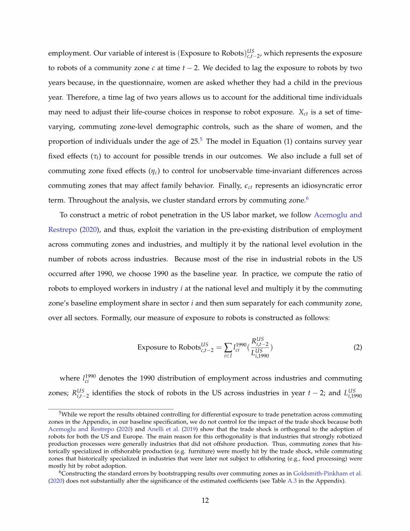
employment. Our variable of interest is (Exposure to Robots)USc,t−2, which represents the exposure

to robots of a community zone c at time t− 2. We decided to lag the exposure to robots by two

years because, in the questionnaire, women are asked whether they had a child in the previous

year. Therefore, a time lag of two years allows us to account for the additional time individuals

may need to adjust their life-course choices in response to robot exposure. Xct is a set of time-

varying, commuting zone-level demographic controls, such as the share of women, and the

proportion of individuals under the age of 25.5 The model in Equation (1) contains survey year

fixed effects (τt) to account for possible trends in our outcomes. We also include a full set of

commuting zone fixed effects (ηc) to control for unobservable time-invariant differences across

commuting zones that may affect family behavior. Finally, εct represents an idiosyncratic error

term. Throughout the analysis, we cluster standard errors by commuting zone.6

To construct a metric of robot penetration in the US labor market, we follow Acemoglu and

Restrepo (2020), and thus, exploit the variation in the pre-existing distribution of employment

across commuting zones and industries, and multiply it by the national level evolution in the

number of robots across industries. Because most of the rise in industrial robots in the US

occurred after 1990, we choose 1990 as the baseline year. In practice, we compute the ratio of

robots to employed workers in industry i at the national level and multiply it by the commuting

zone’s baseline employment share in sector i and then sum separately for each community zone,

over all sectors. Formally, our measure of exposure to robots is constructed as follows:

Exposure to RobotsUSc,t−2 = ∑

i∈Il1990ci (

RUSi,t−2

LUSi,1990

) (2)

where l1990ci denotes the 1990 distribution of employment across industries and commuting

zones; RUSi,t−2 identifies the stock of robots in the US across industries in year t − 2; and LUS

i,1990

5While we report the results obtained controlling for differential exposure to trade penetration across commutingzones in the Appendix, in our baseline specification, we do not control for the impact of the trade shock because bothAcemoglu and Restrepo (2020) and Anelli et al. (2019) show that the trade shock is orthogonal to the adoption ofrobots for both the US and Europe. The main reason for this orthogonality is that industries that strongly robotizedproduction processes were generally industries that did not offshore production. Thus, commuting zones that his-torically specialized in offshorable production (e.g. furniture) were mostly hit by the trade shock, while commutingzones that historically specialized in industries that were later not subject to offshoring (e.g., food processing) weremostly hit by robot adoption.

6Constructing the standard errors by bootstrapping results over commuting zones as in Goldsmith-Pinkham et al.(2020) does not substantially alter the significance of the estimated coefficients (see Table A.3 in the Appendix).

12

Figure 1: Industrial Robots across the US, ∆2004−2016

Notes - Data are drawn from the International Federation of Robotics. While we use county-level boundaries, the variation in ourmeasure of robot exposure is at the commuting zone level.

represents the total number of individuals (in thousands) employed in sector i in 1990.

Figure 1 illustrates the intensity of robot penetration across commuting zones between 2004

and 2016 based on the above metric.7 While the increase in the use of industrial robots was

widespread across the US, Figure 1 depicts the substantial variation in the penetration of robots

across commuting zones and over time. Our analysis leverages these variations in exposure to

robots across commuting zones and over time.

While this measure of exposure to robots can be considered already as a Bartik instrument

per se—given that most of its variation relies on employment shares measured well before the

advent of automation—some concerns about the endogeneity of the stock RUSi of robots in the

US may still arise. For instance, there may exist confounding factors correlated with both the

industry-level adoption of robots in the US and family or fertility behavior. To address these

potential concerns, we robustify our measure of exposure as proposed by Acemoglu and Restrepo

(2020). We use the industry-level robot installations in other economies, which are meant to proxy

7While the borders of geographical units in the map refer to counties, coloring refers to the commuting zonevariation. This is because commuting zones either correspond to counties or are a sum of counties. Hence, allcounties within a commuting zone in the map will share the same color gradient and robot penetration measure.

13

improvements in the world technology frontier of robots, as our instrument for the adoption of

robots in the US. Specifically, we use the average robot exposure at the industry-level in the

nine European countries that are available in the IFR data over the same period.8 Therefore, we

leverage only the variation in the increase in robot adoption across industries of other countries.

Formally, our instrument for the adoption of robots in the US can be written in the following

form:

Exposure to RobotsIVc,t−2 = ∑

i∈Il1970ci (

Rp30,EUi,t−2

LEUi,1990

) (3)

where the sum runs over all industries available in the IFR data, l1970ci represents the 1970

share of employment in commuting zone c and industry i, as calculated from the 1970 Census,

andRp30,EU

i,t−2

LEUi,1990

denotes the 30th percentile of robot exposure among the above-mentioned European

countries in industry i and year t− 2.9 10

A concern with our identification strategy is that our estimates may reflect specific trends in

sectors that may be playing a primary role in our identifying variation. These sectors may have

been subject to specific economic trends, and this may confound our estimates and cast doubts

on a causal interpretation of our results. To partially alleviate this concern, we first show that

marital behavior and fertility rates are largely uncorrelated with future trends in the adoption

of robots in Europe (i.e., our instrumental variable) and if anything some of the outcomes were

trending in the opposite direction. Second, we follow Goldsmith-Pinkham et al. (2020), and find

that the electronics sector plays a predominant role in driving the variation of the instrument (i.e.,

it has, by far, the highest Rotemberg weight in the identification). In our robustness analyses,

we show that reassuringly, the results are substantially unchanged when removing the stock of

robots in the electronics sector from the computation of the robot exposure measure or controlling

for specific time trends across areas with different initial employment shares in the electronics

industry.11 Similarly, we show that results are unchanged when controlling for specific time

8France, Denmark, Finland, Italy, Germany, Norway, Spain, Sweden, and the United Kingdom.9Following Acemoglu and Restrepo (2020), we used the 30th percentile as the US robot adoption closely follow

the 30th percentile of the EU robot adoption distribution.10We use the 1970 share of employment following Acemoglu and Restrepo (2020). However, using 1990 as a base

year yields similar results.11In practice, we include as controls interactions of year dummies with quartiles of the share of employment in the

electronics sector as of 1990.

14

trends across areas with different initial employment shares in the automotive sector, which is by

far the leading sector in terms of industrial robots’ adoption.

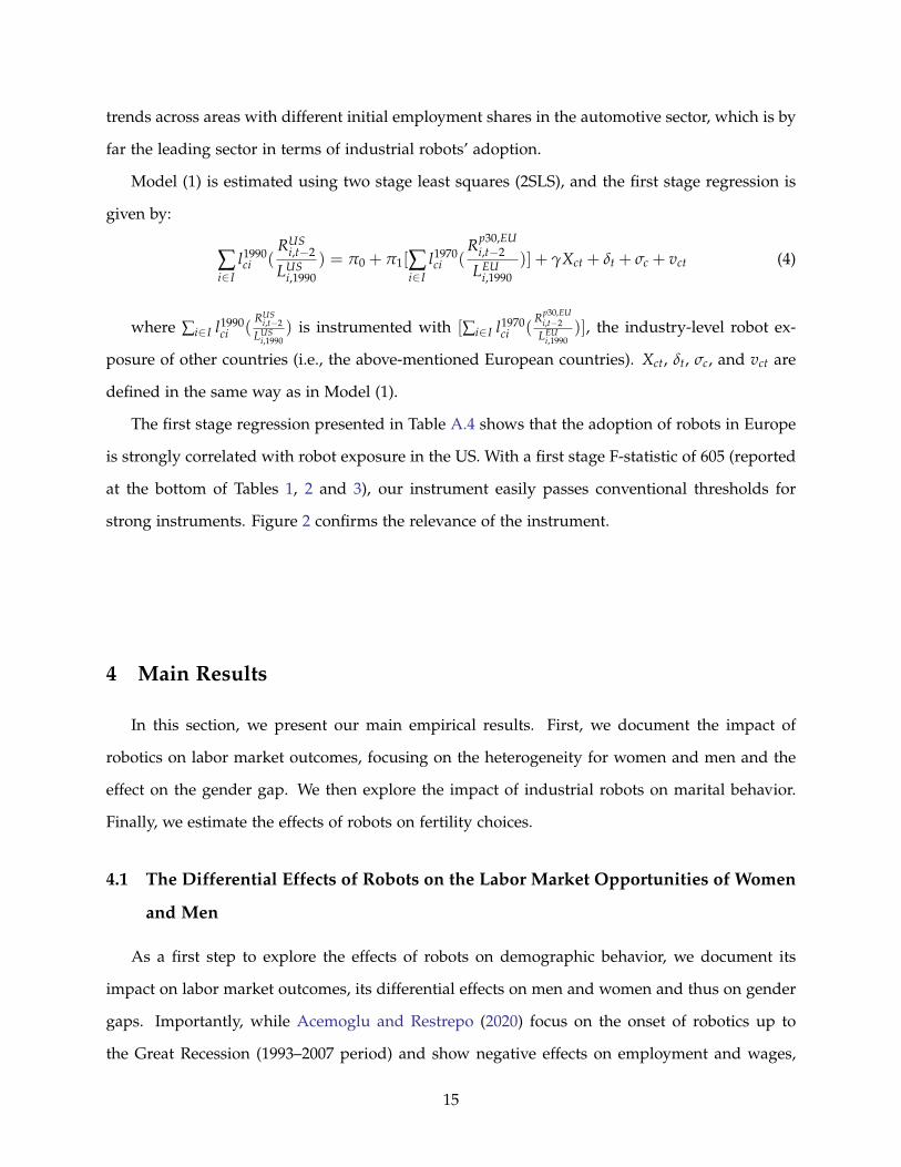
Model (1) is estimated using two stage least squares (2SLS), and the first stage regression is

given by:

∑i∈I

l1990ci (

RUSi,t−2

LUSi,1990

) = π0 + π1[∑i∈I

l1970ci (

Rp30,EUi,t−2

LEUi,1990

)] + γXct + δt + σc + vct (4)

where ∑i∈I l1990ci (

RUSi,t−2

LUSi,1990

) is instrumented with [∑i∈I l1970ci (

Rp30,EUi,t−2

LEUi,1990

)], the industry-level robot ex-

posure of other countries (i.e., the above-mentioned European countries). Xct, δt, σc, and vct are

defined in the same way as in Model (1).

The first stage regression presented in Table A.4 shows that the adoption of robots in Europe

is strongly correlated with robot exposure in the US. With a first stage F-statistic of 605 (reported

at the bottom of Tables 1, 2 and 3), our instrument easily passes conventional thresholds for

strong instruments. Figure 2 confirms the relevance of the instrument.

4 Main Results

In this section, we present our main empirical results. First, we document the impact of

robotics on labor market outcomes, focusing on the heterogeneity for women and men and the

effect on the gender gap. We then explore the impact of industrial robots on marital behavior.

Finally, we estimate the effects of robots on fertility choices.

4.1 The Differential Effects of Robots on the Labor Market Opportunities of Women

and Men

As a first step to explore the effects of robots on demographic behavior, we document its

impact on labor market outcomes, its differential effects on men and women and thus on gender

gaps. Importantly, while Acemoglu and Restrepo (2020) focus on the onset of robotics up to

the Great Recession (1993–2007 period) and show negative effects on employment and wages,

15

Figure 2: First Stage: Robot Exposure in the US and Europe

Notes - Data are drawn from the International Federation of Robotics.

16

we think it is important to extend their analysis by focusing on the recent decades to document

whether the pre-2008 dynamics have persisted also in later years, those for which we are going

to study demographic outcomes.

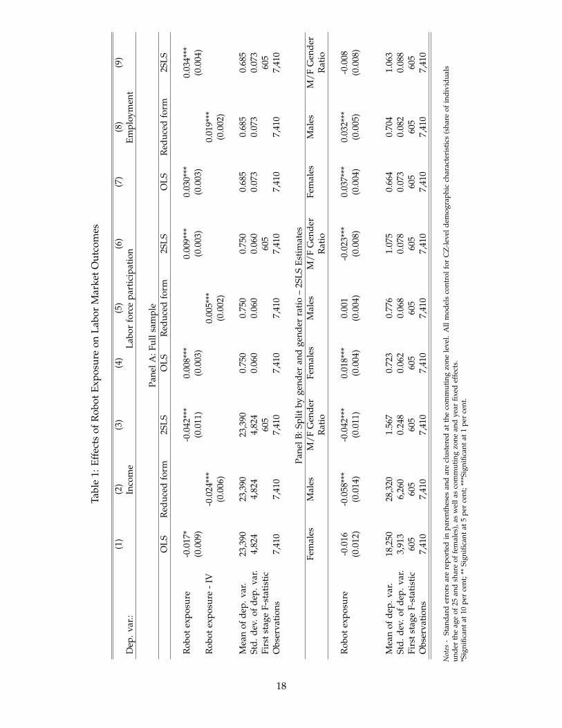
In Table 1, we rely on the identification strategy presented in Section 3.3 to estimate the im-

pact of robot exposure on three labor market indicators: income, labor force participation, and

employment.12 Columns 1–3 in Panel A illustrate the impact of robot exposure on income and

present an OLS specification (see column 1), a reduced form one (see column 2), and the 2SLS

estimation (see column 3). Focusing on the IV estimate of column 3, a one standard deviation

increase in robot exposure (1.90 robots per 1,000 workers) decreases income by 4.2%. The effect

for the IV estimate is larger than the one for the OLS estimate. This is not surprising because

we expect the OLS estimates to be biased downward by the pro-cyclicality of robot adoption,

that is, more robots are installed in periods of economic growth, which, in turn, is also asso-

ciated with better labor market outcomes, on average. Columns 4–9 report a positive effect on

labor force participation and employment. These results are consistent with empirical evidence

showing that robots reduce employment in traditional well-paid manufacturing sectors but boost

employment—through productivity spillovers—in service sectors with lower income and slower

career progression (Dauth et al., 2019). Importantly, with respect to Acemoglu and Restrepo

(2020), our results suggest that contrary to the earlier periods, the overall effect of robotics on US

employment might have turned positive in the recent years, while the negative impact on income

appears robust in both the short- and long-run.13

In Panel B of Table 1, we turn to study the effect of robot exposure on labor market outcomes

separately for men and women and the gender gap in those same outcomes. Columns 1–3 show

that the effect of robots on male income (-5.8%, see column 2) is substantially larger than that

on female income (-1.6%, see column 1). This drives the gender income-gap (defined as the ratio

between male and female income) down by 4.2% in areas that were more exposed to robot pene-

tration.14 In columns 4–6, we provide the corresponding results of robot exposure on labor force

12As detailed in the Empirical Strategy section, in each regression, we include a set of commuting zone-leveldemographic controls, year dummies, and commuting zone FEs.

13A similar pattern has been observed by Bloom et al. (2019) when analyzing the effects of trade on labor marketoutcomes and by David and Dorn (2013) when expanding the analysis to the post-recession period .

14Our results on the gender income-gap complement recent empirical evidence by Aksoy et al. (2019) for Europeancountries. In the context of Eastern European countries with higher baseline levels of gender inequality, the authorsfind that automation has increased the gender earning gap with this effect driven by middle-skill workers. This

17

Tabl

e1:

Effe

cts

ofR

obot

Expo

sure

onLa

bor

Mar

ket

Out

com

es

(1)

(2)

(3)

(4)

(5)

(6)

(7)

(8)

(9)

Dep

.var

.:In

com

eLa

bor

forc

epa

rtic

ipat

ion

Empl

oym

ent

Pane

lA:F

ulls

ampl

eO

LSR

educ

edfo

rm2S

LSO

LSR

educ

edfo

rm2S

LSO

LSR

educ

edfo

rm2S

LS

Rob

otex

posu

re-0

.017

*-0

.042

***

0.00

8***

0.00

9***

0.03

0***

0.03

4***

(0.0

09)

(0.0

11)

(0.0

03)

(0.0

03)

(0.0

03)

(0.0

04)

Rob

otex

posu

re-

IV-0

.024

***

0.00

5***

0.01

9***

(0.0

06)

(0.0

02)

(0.0

02)

Mea

nof

dep.

var.

23,3

9023

,390

23,3

900.

750

0.75

00.

750

0.68

50.

685

0.68

5St

d.de

v.of

dep.

var.

4,82

44,

824

4,82

40.

060

0.06

00.

060

0.07

30.

073

0.07

3Fi

rst

stag

eF-

stat

isti

c60

560

560

5O

bser

vati

ons

7,41

07,

410

7,41

07,

410

7,41

07,

410

7,41

07,

410

7,41

0

Pane

lB:S

plit

byge

nder

and

gend

erra

tio

–2S

LSEs

tim

ates

Fem

ales

Mal

esM

/FG

ende

rFe

mal

esM

ales

M/F

Gen

der

Fem

ales

Mal

esM

/FG

ende

rR

atio

Rat

ioR

atio

Rob

otex

posu

re-0

.016

-0.0

58**

*-0

.042

***

0.01

8***

0.00

1-0

.023

***

0.03

7***

0.03

2***

-0.0

08(0

.012

)(0

.014

)(0

.011

)(0

.004

)(0

.004

)(0

.008

)(0

.004

)(0

.005

)(0

.008

)

Mea

nof

dep.

var.

18,2

5028

,320

1.56

70.

723

0.77

61.

075

0.66

40.

704

1.06

3St

d.de

v.of

dep.

var.

3,91

36,

260

0.24

80.

062

0.06

80.

078

0.07

30.

082

0.08

8Fi

rst

stag

eF-

stat

isti

c60

560

560

560

560

560

560

560

560

5O

bser

vati

ons

7,41

07,

410

7,41

07,

410

7,41

07,

410

7,41

07,

410

7,41

0

Not

es-

Stan

dard

erro

rsar

ere

port

edin

pare

nthe

ses

and

are

clus

tere

dat

the

com

mut

ing

zone

leve

l.A

llm

odel

sco

ntro

lfor

CZ

-lev

elde

mog

raph

icch

arac

teri

stic

s(s

hare

ofin

divi

dual

sun

der

the

age

of25

and

shar

eof

fem

ales

),as

wel

las

com

mut

ing

zone

and

year

fixed

effe

cts.

*Sig

nific

ant

at10

per

cent

;**

Sign

ifica

ntat

5pe

rce

nt;*

**Si

gnifi

cant

at1

per

cent

.

18

participation. The estimates reported in columns 4 and 5 reveal significant differences between

male and female labor force participation. Robot exposure has a relatively small impact on male

labor force participation. Conversely, an increase in robot exposure has a positive and highly

significant effect on female labor force participation. As a result, the gender gap in labor force

participation decreases by 2.1% (with respect to the mean) in response to more robot adoption in

the US (see column 6). Finally, the effect on the gender gap in employment is negative, although

not statistically significant (see column 9).

In Table A.5 in the Appendix, we build an empirical bridge between the labor market evi-

dence and family formation/fertility decisions, by documenting the association of income, labor

force participation, and employment gender gaps with marital and fertility behavior in cross-

commuting zone, fixed-effect (FE) regressions. This descriptive evidence shows that higher male

to female gaps are positively associated with higher marriage and marital fertility rates and neg-

atively associated with divorce and nonmarital fertility rates. Despite its descriptive nature, it is

reassuring that this empirical evidence is consistent with the classical Becker model of household

specialization and with recent evidence by Schaller (2016).

This first set of results captures three main dynamics triggered by the consequences of au-

tomation: first, the absolute economic stature of men as measured by income has been substan-

tially lessened; second, women have seen an improvement in their employment opportunities;

third, the relative economic position of men relative to women has substantially declined. All

three impacts might reduce the gains from household specialization, reduce the pecuniary and

child-rearing gains to marriage (Shenhav, 2020), increase the divorce “threat point” (Lundberg

and Pollak, 1996), and therefore increase divorce, with a potential consequential shift from mari-

tal towards nonmarital fertility.

4.2 Effects on Marital Behavior

In Table 2, we test whether it is the case that, by reducing labor market gender gaps, robot

exposure tend to lessen the value of marriage (Wilson, 1987; Becker et al., 1974), relying on the

identification strategy described in the Empirical Strategy section. Panel A displays the results for

marriage, whereas Panels B and C report the estimates for divorce and cohabitation, respectively.

suggests that the impact of automation on the gender gap may be context-specific.

19

In Panel A, the OLS (see column 1) and the reduced-form (see column 2) estimates suggest that

one standard deviation increase in robot exposure (1.90 robots per 1,000 workers) decreases the

probability of being married by 0.5% relative to the mean outcome. The 2SLS estimate in column

3 presents a larger coefficient, although not statistically significant.

When considering divorce rates and cohabitation as the dependent variable (see Panels B and

C, respectively), we find a positive relationship. The 2SLS coefficient shows that a one standard

deviation increase in robot exposure leads to a 9% increase in divorce (see column 3 of Panel B)

and to a 10% increase in the likelihood of cohabitation (see column 3 of Panel C).15

Consistent with the evidence on absolute and relative economic opportunities of men and

women, these results show that the consequences of automation have impacted marriage on

both the extensive (returns to marriage) and intensive (intra-marriage bargaining) margin. With

respect to the extensive margin, women compare their potential income in a married house-

hold with their income as single women (Shenhav, 2020). As their relative wage increases, the

pecuniary and child-rearing gains to marriage decline, and hence the woman’s threshold for

acceptable husband quality rises. In this framework, these dynamics lead to fewer marriages

and higher-quality husbands among those that do marry. This prediction is consistent with our

evidence of a negative, albeit not precisely estimated, effect on marriage (see column 3 of Panel

A of Table 2) and a larger negative, precisely estimated, effect obtained among women aged 30+

(see Tables A.6–A.8 in the Appendix). We also test the prediction on the effects on matching

quality and find that among married and cohabiting couples, robot exposure leads to an increase

in the share of women married or cohabiting with a higher-educated partner (see Table A.9 in

the Appendix). This effect is particularly large for cohabitation (+20% with respect to the mean),

suggesting an overall increase in the quality of women’s mates (Shenhav, 2020). Our results for

cohabitation also suggest that the exposure to the shock may yield unmarried couples to opt

for less costly forms of commitment. Regarding the intensive margin, the increase in divorces

in response to the automation shock are consistent with a rise in the “threat-point” of divorce

(Lundberg and Pollak, 1996) – i.e., the maximum available utility outside of marriage –, thereby

15The fact that our IV coefficients are slightly larger in magnitude compared to the OLS ones suggests once againthat the potential endogenous bias was driven by the pro-cyclicality of robot adoption, namely, more robots areinstalled during periods of economic growth, which is likely correlated with a higher (lower) incidence of marriage(divorce) relative to economic downturns.

20

Table 2: Effects of Robot Exposure on Marital Behavior

(1) (2) (3)OLS Reduced form 2SLS

Panel A: Dep. var.: Marriage

Robot exposure -0.002 -0.004(0.003) (0.004)

Robot exposure - IV -0.002(0.002)

Mean of dep. var. 0.412 0.412 0.412Std. dev. of dep. var. 0.061 0.061 0.061First stage F statistic 605

Panel B: Dep. var.: Divorce

Robot exposure 0.007*** 0.009***(0.002) (0.002)

Robot exposure - IV 0.005***(0.001)

Mean of dep. var. 0.098 0.098 0.098Std. dev. of dep. var. 0.021 0.021 0.021First stage F statistic 605

Panel C: Dip. var.: Cohabitation

Robot exposure 0.001 0.004***(0.001) (0.001)

Robot exposure - IV 0.003***(0.001)

Mean of dep. var. 0.039 0.039 0.039Std. dev. of dep. var. 0.012 0.012 0.012First stage F statistic 605

Observations 7,410 7,410 7,410

Notes - Standard errors are reported in parentheses and are clustered at the commuting zone level. All models control for CZ-leveldemographic characteristics (share of individuals under the age of 25 and share of females), as well as commuting zone and yearfixed effects.*Significant at 10 per cent; ** Significant at 5 per cent; ***Significant at 1 per cent.

21

increasing the intra-marriage bargaining power of women, triggered by the improved earnings

and employment opportunities of women relative to men.

One natural concern is that when jobs disappear because of robots, people might move away

to find new jobs or people who would have moved might not any more. As certain types of

individuals might be better able/more likely to adjust on this margin, this could change the

composition of the population. Therefore, we re-estimated our baseline regression restricting the

analysis to individuals who did not change the place of residence in the previous year (see Table

A.10 in the Appendix), and to individuals who currently reside in their state of birth (see Table

A.11 in the Appendix). Results remain substantially unchanged, suggesting that our findings

are not driven by compositional effects. Similarly, including controls for the share of individuals

changing residence with respect to the previous year or for the share of individuals who were

born in their current state of residence does not significantly affect the results (see Tables A.12

and A.13 in the Appendix, respectively).

While the inclusion of CZ FEs does control for the time-invariant differences across com-

muting zones, one remaining source of concern about our regression specification is linked to

the possibility that robot adoption was somehow correlated with (or the result of) pre-existing

trends in family outcomes. To dispel this concern, we test whether the change in robot adoption

captured by our IV is correlated with commuting zone trends in demographic outcomes that

occurred before the advent of robotics. Data on demographic outcomes are drawn from the 1980

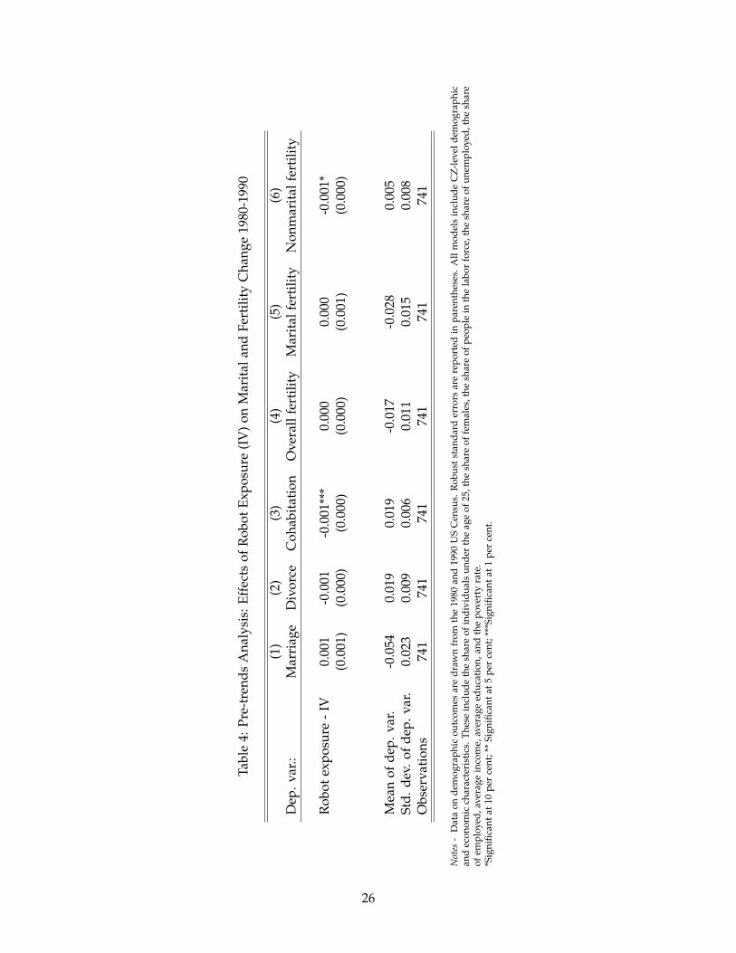
and 1990 US Census. The results of this analysis are reported in Table 4. If anything, 1980–1990

trends in marital behavior were opposite to the patterns observed between 2005 and 2016 (see

columns 1–3). Furthermore, the coefficients are all relatively small and statistically significant

only for cohabitation (see column 3).16

4.3 Effects on Fertility Behavior

In Table 3, we analyze the impact of automation on fertility behavior. We focus on women

because the ACS surveys only women on whether they had a child in the previous year.

Panel A considers overall fertility as the outcome. We estimate that the effect of robot expo-

16As shown in Figure A.1 in the Appendix, already in the 1990s there was a positive trend in the adoption ofindustrial robots across the US. For this reason, we considered pre-trends for the years 1980-1990.

22

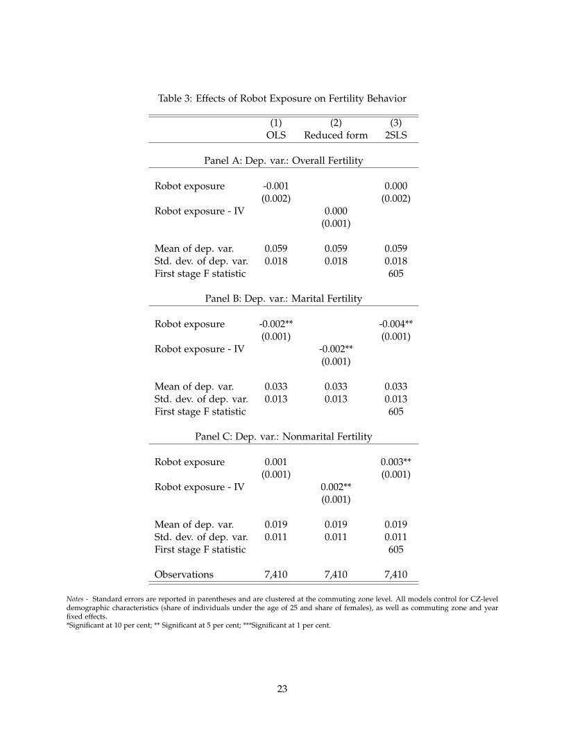
Table 3: Effects of Robot Exposure on Fertility Behavior

(1) (2) (3)OLS Reduced form 2SLS

Panel A: Dep. var.: Overall Fertility

Robot exposure -0.001 0.000(0.002) (0.002)

Robot exposure - IV 0.000(0.001)

Mean of dep. var. 0.059 0.059 0.059Std. dev. of dep. var. 0.018 0.018 0.018First stage F statistic 605

Panel B: Dep. var.: Marital Fertility

Robot exposure -0.002** -0.004**(0.001) (0.001)

Robot exposure - IV -0.002**(0.001)

Mean of dep. var. 0.033 0.033 0.033Std. dev. of dep. var. 0.013 0.013 0.013First stage F statistic 605

Panel C: Dep. var.: Nonmarital Fertility

Robot exposure 0.001 0.003**(0.001) (0.001)

Robot exposure - IV 0.002**(0.001)

Mean of dep. var. 0.019 0.019 0.019Std. dev. of dep. var. 0.011 0.011 0.011First stage F statistic 605

Observations 7,410 7,410 7,410

Notes - Standard errors are reported in parentheses and are clustered at the commuting zone level. All models control for CZ-leveldemographic characteristics (share of individuals under the age of 25 and share of females), as well as commuting zone and yearfixed effects.*Significant at 10 per cent; ** Significant at 5 per cent; ***Significant at 1 per cent.

23

sure on the overall fertility rate is zero. However, these zero fertility effects may mask important

heterogeneity along two dimensions of fertility behavior: marital and nonmarital fertility.

Indeed, Panels B and C document opposite trends for marital and nonmarital fertility. Specif-

ically, column 1 of Panel B reports the relationship between our measure of robot exposure across

commuting zones and the share of married women reporting that they had a child in the past

year. According to the OLS and reduced-form specification (see columns 1 and 2), a one standard

deviation increase in the exposure to robots is associated with a 6% decrease in marital fertility

with respect to the mean outcome (0.034). The 2SLS estimate in column 3 is larger than the OLS

and reduced-form estimates in absolute value, suggesting that the exposure to robot penetration

may be negatively correlated with unobserved determinants of marital fertility. A one standard

deviation increase in the exposure to robots decreases marital fertility in the previous year by

12% or .3 standard deviations. This effect is consistent with the changes observed in marital

behavior discussed in the previous section.

Panel C examines the impact of robot exposure on nonmarital fertility. The OLS and reduced-

form estimates imply that a one standard deviation increase in robot exposure raises nonmarital

fertility by 5% and 10%, respectively (see columns 1 and 2), although the former effect is not pre-

cisely estimated. The 2SLS estimate is larger in absolute value and indicates that a one standard

deviation increase in robot exposure leads to a 15% increase in nonmarital fertility (see column

3). In Table A.2, we replicated the analysis using alternative metrics for marital and non-marital

fertility, that is, focusing either only on the fertility rates within (un)married women or using

the share of births born to married or unmarried women. Panel A replicates our baseline results

as reference. In Panel B, we calculated the fertility rate among married (see column 2) and un-

married women (see column 3). The results show that the change in the number of births from

(un)married women is not driven only by the changing number of women getting married or

divorcing (see Table A.2, Panel B). Following Autor et al. (2019) and Kearney and Wilson (2018),

we also replicated our analysis using the share of all births from married and unmarried women

as outcomes (see Table A.2, Panel C). The estimated effects are substantially similar with respect

to our baseline.

Similar to what observed for marriage patterns, estimates are robust to restricting the analysis

to individuals who did not change the place of residence in the previous year (see Table A.14 in

24

the Appendix) or to individuals who currently reside in their state of birth (see Table A.15 in the

Appendix). Results are also unchanged when we include controls for the share of individuals

changing residence with respect to the previous year or for the share of individuals who were

born in their current state of residence (see Tables A.16 and A.17, respectively).

Reassuringly, columns 4–6 of Table 4 further corroborate the causal interpretation of the esti-

mates, because 1980–1990 trends in fertility behavior are not correlated with exposure to robots,

as measured by our IV. Specifically, there is no evidence of pre-trends in marital fertility, and, if

anything, a negative (opposite) trend in nonmarital fertility.

5 Robustness Checks and Heterogeneity Analyses

5.1 Robustness Checks

In this section, we conduct several robustness checks. First, we show that the 2SLS results

obtained using a long-difference specification tend in the same direction and remain statistically

significant (see Table A.18 in the Appendix). In practice, we regress the change in our outcomes

between 2005-07 and 2014-16 on the change in robot exposure over the same period. We find

that a one standard deviation increase in robot exposure reduces the gender income gap by

0.126 standard deviations, the labor force participation gap by 0.129 standard deviations, and

the gender gap in employment by 0.119 standard deviations (see, respectively, columns 1 to 3

of Panel A). Turning to marital behavior, a one standard deviation increase in robot exposure

is associated with a 0.064 standard deviations reduction in the marriage rate, a 0.098 standard

deviations increase in divorces, and a 0.061 standard deviations increase in cohabitations (see,

respectively, columns 1 to 3 of Panel B). Considering fertility behavior, robot exposure leads to a

0.083 standard deviations reduction in marital fertility and a 0.164 standard deviations increase

in nonmarital fertility (see, respectively, columns 2 to 3 of Panel C). Using this long-difference

approach, we also demonstrate that the 2SLS results are unchanged when controlling for pre-

trends from 1980-1990 in the respective outcome of interest (see Table A.19 in the Appendix).

Second, to address the concern that our identification may be subject to differential trends

experienced by some industries driving the results, and to better understand the source of vari-

ation underlying our identification strategy, we calculated the Rotemberg weights by sector and

25

Tabl

e4:

Pre-

tren

dsA

naly

sis:

Effe

cts

ofR

obot

Expo

sure

(IV

)on

Mar

ital

and

Fert

ility

Cha

nge

1980

-199

0

(1)

(2)

(3)

(4)

(5)

(6)

Dep

.var

.:M

arri

age

Div

orce

Coh

abit

atio

nO

vera

llfe

rtili

tyM

arit

alfe

rtili

tyN

onm

arit

alfe

rtili

ty

Rob

otex

posu

re-

IV0.

001

-0.0

01-0

.001

***

0.00

00.

000

-0.0

01*

(0.0

01)

(0.0

00)

(0.0

00)

(0.0

00)

(0.0

01)

(0.0

00)

Mea

nof

dep.

var.

-0.0

540.

019

0.01

9-0

.017

-0.0

280.

005

Std.

dev.

ofde

p.va

r.0.

023

0.00

90.

006

0.01

10.

015

0.00

8O

bser

vati

ons

741

741

741

741

741

741

Not

es-

Dat

aon

dem

ogra

phic

outc

omes

are

draw

nfr

omth

e19

80an

d19

90U

SC

ensu

s.R

obus

tst

anda

rder

rors

are

repo

rted

inpa

rent

hese

s.A

llm

odel

sin

clud

eC

Z-l

evel

dem

ogra

phic

and

econ

omic

char

acte

rist

ics.

Thes

ein

clud

eth

esh

are

ofin

divi

dual

sun

der

the

age

of25

,the

shar

eof

fem

ales

,the

shar

eof

peop

lein

the

labo

rfo

rce,

the

shar

eof

unem

ploy

ed,t

hesh

are

ofem

ploy

ed,a

vera

gein

com

e,av

erag

eed

ucat

ion,

and

the

pove

rty

rate

.*S

igni

fican

tat

10pe

rce

nt;*

*Si

gnifi

cant

at5

per

cent

;***

Sign

ifica

ntat

1pe

rce

nt.

26

year following the methodology described in Goldsmith-Pinkham et al. (2020). Table A.20 in the

Appendix presents these weights averaged by sector throughout the period under study, and

indicates that the electronics industry has, by far, the highest Rotemberg weight in the iden-

tification, with an average weight of 0.32 throughout the period under investigation (ranging

between 0.07 and 0.76).17 We first show that our main results for marital and fertility behavior

are robust to the exclusion of the stock of robots in the electronics sector from the computation

of the robot exposure measure (see Tables A.21 and A.22 in the Appendix). Second, we show

that the estimates are similar to the baseline specification (see Tables 2 and 3) when controlling

for differential trends across commuting zones in different quartiles of the 1990 share of employ-

ment in the electronics sector (see Tables A.23 and A.24 in the Appendix). Third, we show no

evidence of a significant correlation between the change in the outcomes between 1980 and 1990

and the share of employment in the electronics industry in 1970 (see Panel A of Table A.25 in the

Appendix). Additionally, as the automotive sector was still by far the largest robot adopter in

the US, we conduct similar tests for the automotive sector, and overall confirm our main results

(see Tables A.26, A.27, and Panel B of Table A.25 in the Appendix). These findings lend further

support to a causal interpretation of the effect of robot exposure on marital and fertility behavior.

Fourth, we show that our results are largely unchanged when controlling for exposure to

trade penetration. To measure trade penetration, we followed Pierce and Schott (2020), and

computed exposure to Chinese imports by looking at the difference between tariff rates set by

the Smoot-Hawley Tariff Act and the corresponding NTR (normal trade relations) tariffs. In

2000, the US passed a bill granting normal trade relations to China. This trade liberalization

affected differentially US regions depending on their industry structure. A larger difference

between the non-NTR rates and the NTR rates implied a larger potential for Chinese exporters

increasing import competition for US producers in a given sector. Consistent with Pierce and

Schott (2020), we calculated the commuting zone-level exposure to import penetration using the

labor-share-weighted average NTR gaps of the industries active within a commuting zone in 1990.

We then interacted this commuting zone-level measure of exposure to trade with year dummies.

Reassuringly, in Table A.28 in the Appendix we obtain similar 2SLS results for marital and fertility

17Instead, all the other industries play a less relevant role in the identification, with the average weights beingbelow 0.05.

27

behavior relative to the benchmark specification (see Tables 2 and 3). As a further check, in Table

A.29 in the Appendix we demonstrate that our 2SLS results are robust to the inclusion of time-

specific trends interacted with the 1990 share of employment in total manufacturing.

Another relevant concern is that our estimates may be capturing the effect of the different

implementation of family and reproductive policies over time across the US. To dispel this con-

cern, we include in our analysis a large array of state-year control variables for various policies

related to access to family planning services. Specifically, we used the data constructed by Myers

(2021) including the following state and year-level policies: mandatory delay for abortion, which

indicates whether a state requires a mandatory delay for women seeking abortions; parental-

involvement laws, which measures the fraction of a year that a parental involvement law for

minors seeking abortion was in place, where parental involvement is defined as a requirement

of notification and/or consent; mandated insurance coverage for contraception, which requires

that private insurance plans that cover prescription drugs also provide coverage for any FDA-

approved contraceptive; emergency contraception available, which indicates whether a state per-

mitted over-the-counter access to emergency contraception; medicaid expansion, which indicates

that a state has expanded Medicaid eligibility for family planning services; and the poverty

threshold for family planning Medicaid expansion eligibility. In column 1 of Tables A.30 and

A.31, we show that the 2SLS results for marital and fertility behavior are robust to the inclusion

of the above-mentioned controls for family policies. In addition, we collected contextual infor-

mation on abortion rules (i.e., TRAP laws) from the work by Jones and Pineda-Torres (2020), and

added them to our model. As shown in column 2 of Tables A.30 and A.31, the results remain

substantially unaffected by this inclusion. Finally, in column 3 we added to our model controls

for both family policies and TRAP laws, and obtained remarkably similar estimates compared

to those obtained in the baseline specification. Taken together, this evidence suggests that our

results are not distorted by family policies that happened during the sample period under inves-

tigation.

28

5.2 Heterogeneity Analyses

In what follows, we present some heterogeneity analyses along several dimensions. First, we

explore the heterogeneity of the effects by age groups (see Tables A.6– A.8 in the Appendix).

Taken together, we find evidence that the effect of robot exposure on marital fertility is mainly

driven by older individuals (i.e., 30-50 years old), while the effect on nonmarital fertility is larger

(in absolute value) among younger age groups (i.e., younger than 30 years old).18

Second, we examine whether the adoption of robots differentially affected fertility choice

on the extensive and on the intensive margin. Panels A and B of Table A.32 in the Appendix

suggest that the fertility effects are present both on the extensive – defined as the likelihood of

having a first child– and on the intensive margin– defined as the likelihood of having a second or

higher-order child. The impact of robots on nonmarital fertility is fairly similar on the extensive

and on the intensive margin (+17% vs. +14% with respect to the mean). At the same time, the

effects on marital fertility are marginally stronger on the extensive rather than on the intensive

margin: a one standard deviation increase in robot exposure increases marital fertility on the

extensive margin by 17% compared to a 11% increase on the intensive margin. In Panel C of

Table A.32, we further explored the effect of robot exposure on the intensive margin of fertility

by considering the number of children as the dependent variable. In line with the evidence

above, we find a negative effect on marital fertility and a positive effect on nonmarital fertility.

We also explored the heterogeneity of the results on marital behavior by the presence of children

and age of the youngest child (see Table A.33 in the Appendix). If anything, the presence of

children is associated with a larger negative effect on marriage (see Panel A). Similarly, we detect

a slightly larger effect on divorce among families with children, although the impacts tend to

be smaller (in absolute value) among families with younger children (see Panel B). The positive

effects of exposure to robots on cohabitation tend to be instead slightly higher among families

with children, regardless of the child’s age (see Panel C). These results suggest that the shocks

induced by robot exposure may both reduce the propensity to marriage and the propensity

18We note that the effects may vary by cohort. Older cohorts may be more entrenched in their career and furtheralong on the lifecycle when robots come on the scene. While it would be interesting to examine the heterogeneityof the effects by birth cohorts, our data–and the limited window of time for which we have information on robots’adoption–does not allow us to isolate cohort from age effects. Future research using longer panels may shed furtherlight on this point.

29

divorce, but increase cohabitation.

Third, in Table A.34 in the Appendix, we examine completed fertility, which reflects the actual

number of children per woman measured after the reproductive age (i.e., aged 45 and older). We

find consistent evidence of a significant negative effect of robot exposure on marital fertility and a

positive effect on nonmarital fertility. Our estimates reveal that a one standard deviation increase

in robot exposure is associated with a 3.7% reduction in the number of children among married

women, and a 21% increase in the number of children among unmarried women. Because our

dataset does not contain information on marital histories and we lack longitudinal data, these

results should be interpreted with caution. However, these estimates are suggestive that robot

exposure did not only affect period fertility rates but also completed (or cohort) fertility. Taken

together, in response to robot exposure, the short-term changes in period fertility result in a

long-term effect on completed fertility, signalling a limited role for recuperation effects in the

long-run.

Fourth, combining information available in our dataset on women’s fertility, marital status,

and cohabitation, we constructed two additional measures of fertility: nonmarital fertility among

women who are not married but are cohabiting, and nonmarital fertility among women who

are neither married nor cohabiting. In Table A.35 in the Appendix, we explore the differential

fertility effects between unmarried but cohabiting and unmarried not cohabiting women using

these two measures of fertility as alternative outcome variables. We find that the effect of robots

on nonmarital fertility is largely driven by unmarried women who are not cohabiting (see column

3). This result is consistent with the findings of previous work analyzing the impact of economic

shocks on fertility and finding an increase in the fraction of children living in single-headed

households (Autor et al., 2019; Black et al., 2003).

Finally, we investigated the effects of robot exposure among same-sex couples (see Table A.36

in the Appendix). Previous studies suggest that specialization may be less pronounced in same-

sex couples (Badgett, 2009; Jepsen and Jepsen, 2015; Giddings et al., 2014). Thus, the implications

of automation for same-sex couples may be very different compared to those obtained in hetero-

sexual couples. Restricting attention to same-sex couples, we estimate a close to null effect on

fertility behavior, and no significant impact on divorce and cohabitation (see Panel A). Interest-

ingly, we detect a negative and significant impact of robot exposure on same-sex marriages (see

30

column 1). As shown in Table A.37, this negative effect is larger among male same-sex marriages,

which may be consistent with men being less likely to commit given their exposure to worse la-

bor market conditions. However, given the small fraction of same-sex couples in our sample

(approximately 1% throughout the period), we do not think that much can be inferred from this

specific result. Excluding same-sex couples from our sample yields substantially identical results

relative to the benchmark specification (see Panel B). Furthermore, we demonstrate that our 2SLS

results for marital and fertility behavior are unchanged when controlling for the timing of the

introduction of legal same-sex marriages across US states (see Panel C).19

6 Conclusion

The impact of automation, robots, and artificial intelligence on labor markets has produced

fundamental shifts in our daily lives. A handful of pioneering studies have examined the impact

of robots on labor markets (Acemoglu and Restrepo, 2020; Graetz and Michaels, 2018). Yet, we

know little about how these labor market shocks may affect gender differences in labor market

opportunities, and, in turn, family and fertility decisions. This study estimates the impact of

exposure to industrial robots on life-course choices, such as marriage, divorce, cohabitation, and

fertility. In areas that were more exposed to robot penetration, marriage rates decreased, while

divorce rates and cohabitation increased. We then show that exposure to robots reduced marital

fertility but increased nonmarital fertility. Looking at potential mechanisms, we show that robot

penetration has different effects on the labor market opportunities of men and women, reducing

the gender gap in income. Male income fell at a substantially higher rate than female income,

decreasing the gender income gap. Moreover, robot exposure has increased female labor force

participation significantly while leaving the labor force participation of men unchanged.

While our empirical setting does not allow us to distinguish between the role of absolute

(Wilson hypothesis) and relative income (Becker hypothesis), we argue that robots have both

worsened the absolute economic stature of men as measured by their earning opportunities, and

lowered the relative position of men on the marriage market. This, in turn, has contributed to

reducing women’s willingness to long-term commitments, such as marrying. At the same time,19We draw data on the variation in the timing of legalization of same-sex marriage across states relying on the

works by Hansen et al. (2020); Carpenter and Sansone (2021).

31

the lower marriage-market value of men has increased the value of nonmarital fertility options

for women and the share of children born to single-headed households.

Given the concerns that cohabitation may reduce children’s well-being (Manning, 2015),

developing more encompassing family policies that cover married and cohabitating couples

more homogenously could be an effective response to the implications of robotics on life-course

choices. Future research exploiting longitudinal data or matched employer-employee data may

shed further light on these mechanisms and the impact of automation on children’s well-being as

well as trying to distinguish the Becker hypothesis on relative economic stature from the Wilson’s

thesis emphasizing men’s absolute economic stature.

32

References

Acemoglu, Daron and Pascual Restrepo, “Robots and jobs: Evidence from US labor markets,”

Journal of Political Economy, 2020, 128 (6), 2188–2244.

Aksoy, Cevat Giray, Ozkan Berkay, and Philip Julia, “Robots and the Gender Pay Gap: Evidence

from Europe,” LSE Mimeo, 2019.

Albanesi, Stefania and Claudia Olivetti, “Gender roles and medical progress,” Journal of Political

Economy, 2016, 124 (3), 650–695.

Anelli, Massimo, Italo Colantone, and Piero Stanig, “We were the robots: Automation and

voting behavior in western europe,” BAFFI CAREFIN Centre Research Paper, 2019, (2019-115).

Autor, David, David Dorn, and Gordon Hanson, “When work disappears: Manufacturing de-

cline and the falling marriage market value of young men,” American Economic Review: Insights,

2019, 1 (2), 161–78.

Autor, David H, David Dorn, and Gordon H Hanson, “Untangling trade and technology: Evi-

dence from local labour markets,” The Economic Journal, 2015, 125 (584), 621–646.

Badgett, MV Lee, When gay people get married, New York University Press, 2009.

Bailey, Martha J, “More power to the pill: the impact of contraceptive freedom on women’s life

cycle labor supply,” The Quarterly Journal of Economics, 2006, 121 (1), 289–320.

and Thomas A DiPrete, “Five decades of remarkable but slowing change in US women’s

economic and social status and political participation,” RSF: The Russell Sage Foundation Journal

of the Social Sciences, 2016, 2 (4), 1–32.

Becker, Gary S, “A theory of marriage: Part I,” Journal of Political economy, 1973, 81 (4), 813–846.

, H Gregg Lewis, and Theodore W Schultz, Economics of the Family: Marriage, Children, and

Human Capital, University of Chicago press Chicago, IL, 1974.

Bellou, Andriana, “The impact of Internet diffusion on marriage rates: evidence from the broad-

band market,” Journal of Population Economics, 2015, 28 (2), 265–297.

33

Bertrand, Marianne, Patricia Cortes, Claudia Olivetti, and Jessica Pan, “Social norms, labor

market opportunities, and the marriage gap for skilled women,” Technical Report, National

Bureau of Economic Research 2016.

Billari, Francesco C, Osea Giuntella, and Luca Stella, “Broadband internet, digital temptations,

and sleep,” Journal of Economic Behavior & Organization, 2018, 153, 58–76.

, , and , “Does broadband Internet affect fertility?,” Population Studies, 2019, pp. 1–20.

Black, Dan A, Natalia Kolesnikova, Seth G Sanders, and Lowell J Taylor, “Are children “nor-

mal”?,” The Review of Economics and Statistics, 2013, 95 (1), 21–33.

, Terra G McKinnish, and Seth G Sanders, “Does the availability of high-wage jobs for low-

skilled men affect welfare expenditures? Evidence from shocks to the steel and coal industries,”

Journal of Public Economics, 2003, 87 (9-10), 1921–1942.

Bloom, Nicholas, Kyle Handley, Andre Kurman, and Phillip Luck, “The impact of Chinese

trade on US Employment: The Good, the Bad, and the Debatable,” Unpublished draft, 2019.

Brynjolfsson, Erik and Andrew McAfee, The second machine age: Work, progress, and prosperity in

a time of brilliant technologies, WW Norton & Company, 2014.

Carpenter, Christopher S and Dario Sansone, “Cigarette taxes and smoking among sexual mi-

nority adults,” Journal of Health Economics, 2021, 79, 102492.

Cherlin, Andrew, Erin Cumberworth, S Philip Morgan, and Christopher Wimer, “The effects

of the Great Recession on family structure and fertility,” The ANNALS of the American Academy

of Political and Social Science, 2013, 650 (1), 214–231.

Comolli, Chiara Ludovica and Fabrizio Bernardi, “The causal effect of the great recession on

childlessness of white American women,” IZA Journal of Labor Economics, 2015, 4 (1), 21.

Currie, Janet and Hannes Schwandt, “Short-and long-term effects of unemployment on fertility,”

Proceedings of the National Academy of Sciences, 2014, 111 (41), 14734–14739.

Dauth, Wolfgang, Sebastian Findeisen, Jens Suedekum, and Nicole Woessner, “The Adjust-

ment of Labor Markets to Robots,” University of Wurzburg, 2019.

34

David, H and David Dorn, “The growth of low-skill service jobs and the polarization of the US

labor market,” American Economic Review, 2013, 103 (5), 1553–97.

de V. Cavalcanti, Tiago V and Jose Tavares, “Assessing the “Engines of Liberation”: home

appliances and female labor force participation,” The Review of Economics and Statistics, 2008, 90

(1), 81–88.

DiNardi, Michael, Melanie Guldi, and David Simon, “Body weight and Internet access: evi-

dence from the rollout of broadband providers,” Journal of Population Economics, 2017, pp. 1–37.

Frey, Carl Benedikt and Michael A. Osborne, “The future of employment: How susceptible are

jobs to computerisation?,” Technological Forecasting and Social Change, 2017, 114, 254 – 280.

Giddings, Lisa, John M Nunley, Alyssa Schneebaum, and Joachim Zietz, “Birth cohort and

the specialization gap between same-sex and different-sex couples,” Demography, 2014, 51 (2),

509–534.

Giuntella, Osea, Lu Yi, and Tianyi Wang, “Is an Army of Robots Marching on Chinese Jobs?,”

IZA Discussion Paper, 2019.

Goldin, Claudia and Lawrence F Katz, “The power of the pill: Oral contraceptives and women’s

career and marriage decisions,” Journal of Political Economy, 2002, 110 (4), 730–770.

Goldsmith-Pinkham, Paul, Isaac Sorkin, and Henry Swift, “Bartik instruments: What, when,

why, and how,” American Economic Review, 2020, 110 (8), 2586–2624.

Goldstein, Joshua, Michaela Kreyenfeld, Aiva Jasilioniene, and Deniz Dilan Karaman Orsal,

“Fertility reactions to the” Great Recession” in Europe: Recent evidence from order-specific

data,” Demographic Research, 2013, 29, 85–104.

Graetz, Georg and Guy Michaels, “Robots at work,” Review of Economics and Statistics, 2018, 100

(5), 753–768.

Greenwood, Jeremy, Ananth Seshadri, and Mehmet Yorukoglu, “Engines of liberation,” The

Review of Economic Studies, 2005, 72 (1), 109–133.

35

, Nezih Guner, and Guillaume Vandenbroucke, “Family economics writ large,” Journal of

Economic Literature, 2017, 55 (4), 1346–1434.

Guldi, Melanie and Chris M Herbst, “Offline effects of online connecting: the impact of broad-

band diffusion on teen fertility decisions,” Journal of Population Economics, 2017, 30 (1), 69–91.

Hansen, Mary Eschelbach, Michael E Martell, and Leanne Roncolato, “A labor of love: The

impact of same-sex marriage on labor supply,” Review of Economics of the Household, 2020, 18

(2), 265–283.

Jepsen, Christopher and Lisa K Jepsen, “Labor-market specialization within same-sex and

difference-sex couples,” Industrial Relations: A Journal of Economy and Society, 2015, 54 (1), 109–

130.

Jones, Kelly M and Mayra Pineda-Torres, “Targeted Regulations on Abortion Providers: Impacts

on Women’s Education and Future Income,” 2020.

Kearney, Melissa S and Riley Wilson, “Male earnings, marriageable men, and nonmarital fertil-

ity: Evidence from the fracking boom,” Review of Economics and Statistics, 2018, 100 (4), 678–690.

Lanzieri, Giampaolo, “Towards a ‘baby recession’in Europe?,” Europe (in million), 2013, 16

(16.655), 16–539.

Lesthaeghe, Ron, “The unfolding story of the second demographic transition,” Population and

Development Review, 2010, 36 (2), 211–251.

Lundberg, Shelly and Robert A Pollak, “Bargaining and distribution in marriage,” Journal of

economic perspectives, 1996, 10 (4), 139–158.

Manning, Wendy D, “Cohabitation and child wellbeing,” The Future of children/Center for the

Future of Children, the David and Lucile Packard Foundation, 2015, 25 (2), 51.

Matysiak, Anna, Tomas Sobotka, and Daniele Vignoli, “The Great Recession and fertility in

Europe: A sub-national analysis,” European Journal of Population, 2020, pp. 1–36.

Myers, Caitlin Knowles, “Cooling off or Burdened? The Effects of Mandatory Waiting Periods

on Abortions and Births,” 2021.

36

Orsal, Deniz Dilan Karaman and Joshua R Goldstein, “The increasing importance of economic

conditions on fertility,” in “Annual Meeting of the Population Association of America, Dallas,

Texas” 2010.

Ozcan, Berkay, Karl Ulrich Mayer, and Joerg Luedicke, “The impact of unemployment on the

transition to parenthood,” Demographic Research, 2010, 23, 807–846.

Pierce, Justin R and Peter K Schott, “Trade liberalization and mortality: evidence from US

counties,” American Economic Review: Insights, 2020, 2 (1), 47–64.

Schaller, Jessamyn, “Booms, Busts, and Fertility Testing the Becker Model Using Gender-Specific

Labor Demand,” Journal of Human Resources, 2016, 51 (1), 1–29.

Shenhav, Na’ama, “Lowering Standards to Wed? Spouse Quality, Marriage, and Labor Market

Responses to the Gender Wage Gap,” Review of Economics and Statistics, 2020, pp. 1–45.

Sobotka, Tomas, Vegard Skirbekk, and Dimiter Philipov, “Economic Recession and Fertility in

the Developed World,” Population and Development Review, 2011, 37 (2), 267–306.

Watson, Tara and Sara McLanahan, “Marriage meets the joneses relative income, identity, and

marital status,” Journal of Human Resources, 2011, 46 (3), 482–517.

Wilson, William Julius, The truly disadvantaged: The inner city, the underclass, and public policy,

University of Chicago Press, 1987.

, When work disappears: The world of the new urban poor 1996.

, Kathryn Neckerman, Sheldon Danziger, and Daniel Weinberg, “Poverty and family struc-

ture: The widening gap between evidence and public policy issues,” Fighting poverty: What

works and what doesn’t, 1986.

37

Appendix A: Supplemental Figures and Tables

Figure A.1: Evolution of the Stocks of Robots, 1993-2016

Notes - Data are drawn from the International Federation of Robotics over the period 1993-2016.

38

Table A.1: Descriptive Statistics - Commuting Zone-Year Observations: 7,410

Mean Std. dev. Min Max

Panel A: Outcome variablesFertility 0.059 0.018 0.003 0.160Marital fertility 0.034 0.014 0 0.117Nonmarital fertility 0.020 0.012 0 0.084Married 0.412 0.061 0.214 0.662Divorced 0.099 0.021 0.037 0.187Cohabiting 0.040 0.012 0.005 0.110Income 23,388 4,824 12,105 51,834Labor Force Participation 0.750 0.060 0.534 0.907Employed 0.685 0.073 0.434 0.871

Panel B: CovariatesRobot exposure 1.841 1.963 0.123 20.508Robot exposure - IV 1.233 0.935 0.244 10.815Age under 25 0.289 0.037 0.166 0.555Female 0.489 0.018 0.391 0.557

Notes - Data are drawn from the American Community Survey and the International Federation of Robotics over the period 2005-2016.

39

Table A.2: Effects of Robot Exposure on Fertility Behavior - Alternative Outcomes (2SLS Esti-mates)

(1) (2) (3)

Panel A: Baseline SpecificationDep. var.: Overall fertility Marital fertility Nonmarital fertility

Robot exposure 0.000 -0.004** 0.003**(0.002) (0.001) (0.001)

Mean of dep. var. 0.059 0.033 0.019Std. dev. of dep. var. 0.018 0.013 0.011First stage F statistic 605 605 605

Panel B: Fertility Rates Among Married and Unmarried WomenDep. var.: Overall fertility Marital fertility rate Nonmarital fertility rate

Robot exposure 0.000 -0.009*** 0.010***(0.002) (0.003) (0.003)

Mean of dep. var. 0.059 0.075 0.049Std. dev. of dep. var. 0.018 0.025 0.028First stage F statistic 605 605 605

Panel C: Share of BirthsDep. var.: Overall fertility Share of births Share of births

born to married mothers born to unmarried mothers

Robot exposure 0.000 -0.045*** 0.029**(0.002) (0.014) (0.014)

Mean of dep. var. 0.059 0.572 0.326Std. dev. of dep. var. 0.018 0.154 0.145First stage F statistic 605 605 605

Observations 7,410 7,410 7,410

Notes - Standard errors are reported in parentheses and are clustered at the commuting zone level. All models control for CZ-leveldemographic characteristics (share of individuals under the age of 25 and share of females), as well as commuting zone and yearfixed effects.*Significant at 10 per cent; ** Significant at 5 per cent; ***Significant at 1 per cent.

40

Table A.3: Effects of Robot Exposure on Labor Market Outcomes, Marital and Fertility Behavior,Bootstrapped Standard Errors – 2SLS Estimates

(1) (2) (3)

Robot exposureDep. var.: Coefficient Standard p-value Corrected p-value

Income - M/F gender ratio -0.042 0.003 0.007Labor force participation - M/F gender ratio -0.023 0.003 0.003Employment - M/F gender ratio -0.008 0.299 0.324Marriage -0.004 0.354 0.350Divorce 0.009 0.000 0.000Cohabitation 0.004 0.000 0.000Overall fertility 0.000 0.803 0.829Marital fertility -0.004 0.011 0.008Nonmarital fertility 0.003 0.015 0.013

Observations 7,410

Notes - The table reports the coefficient of robot exposure derived by regressions of the outcome listed in in each row on robotexposure. All models control for CZ-level demographic characteristics (share of individuals under the age of 25 and share offemales), as well as commuting zone and year fixed effects. Standard p-values as well as bootstrapped p-values are reported.

41

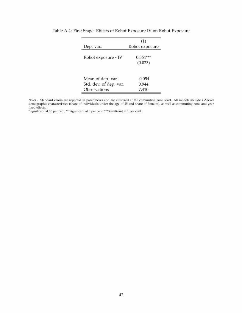
Table A.4: First Stage: Effects of Robot Exposure IV on Robot Exposure

(1)Dep. var.: Robot exposure

Robot exposure - IV 0.564***(0.023)

Mean of dep. var. -0.054Std. dev. of dep. var. 0.944Observations 7,410

Notes - Standard errors are reported in parentheses and are clustered at the commuting zone level. All models include CZ-leveldemographic characteristics (share of individuals under the age of 25 and share of females), as well as commuting zone and yearfixed effects.*Significant at 10 per cent; ** Significant at 5 per cent; ***Significant at 1 per cent.

42

Table A.5: Effects of Labor Market Status on Marital and Fertility Behavior - Fixed-Effect Esti-mates

(1) (2) (3) (4) (5) (6)Dep. var.: Fertility

Marriage Divorce Cohabitation Overall Marital Nonmarital

Income - M/F Gender Ratio 0.026*** -0.014*** -0.001 -0.001 0.003** -0.003**(0.003) (0.002) (0.001) (0.002) (0.001) (0.001)

LFP - M/F Gender Ratio 0.052*** -0.017*** 0.000 0.012*** 0.018*** -0.009***(0.006) (0.003) (0.002) (0.004) (0.003) (0.003)

Employment - M/F Gender Ratio 0.051*** -0.018*** -0.001 0.006* 0.013*** -0.007***(0.005) (0.003) (0.002) (0.003) (0.002) (0.002)

Mean of dep. var. 0.412 0.098 0.039 0.059 0.033 0.019Std. dev. of dep. var. 0.061 0.021 0.012 0.018 0.013 0.011Observations 7,410 7,410 7,410 7,410 7,410 7,410

Notes - Standard errors are reported in parentheses and are clustered at the commuting zone level. All models control for CZ-leveldemographic characteristics (share of individuals under the age of 25 and share of females), as well as commuting zone and yearfixed effects.*Significant at 10 per cent; ** Significant at 5 per cent; ***Significant at 1 per cent.

43

Table A.6: Effects of Robot Exposure on Marital Behavior, by Age Group – 2SLS Estimates

(1) (2) (4)Marriage Divorce Cohabitation

Panel A: Individuals aged 16-29

Robot exposure 0.009* 0.002 -0.001(0.005) (0.001) (0.002)

Mean of dep. var. 0.175 0.023 0.044Std. dev. of dep. var. 0.057 0.013 0.018

Panel B: Individuals aged 30-50

Robot exposure -0.013** 0.013*** 0.008***(0.006) (0.004) (0.001)

Mean of dep. var. 0.588 0.154 0.036Std. dev. of dep. var. 0.069 0.029 0.013

Panel C: Individuals aged 15-44

Robot exposure -0.014*** 0.003* 0.005***(0.005) (0.002) (0.001)

Mean of dep. var. 0.353 0.076 0.041Std. dev. of dep. var. 0.058 0.020 0.013

Panel D: Individuals aged 15-19

Robot exposure 0.007*** 0.001** 0.001(0.002) (0.000) (0.001)

Mean of dep. var. 0.008 0.001 0.007Std. dev. of dep. var. 0.013 0.003 0.011

First stage F statistic 605 605 605Observations 7,410 7,410 7,410

Notes - Standard errors are reported in parentheses and are clustered at the commuting zone level. All models control for CZ-leveldemographic characteristics (share of individuals under the age of 25 and share of females), as well as commuting zone and yearfixed effects.*Significant at 10 per cent; ** Significant at 5 per cent; ***Significant at 1 per cent.

44

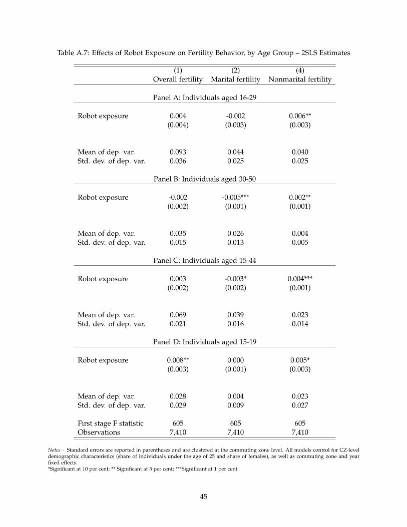
Table A.7: Effects of Robot Exposure on Fertility Behavior, by Age Group – 2SLS Estimates

(1) (2) (4)Overall fertility Marital fertility Nonmarital fertility

Panel A: Individuals aged 16-29

Robot exposure 0.004 -0.002 0.006**(0.004) (0.003) (0.003)

Mean of dep. var. 0.093 0.044 0.040Std. dev. of dep. var. 0.036 0.025 0.025

Panel B: Individuals aged 30-50

Robot exposure -0.002 -0.005*** 0.002**(0.002) (0.001) (0.001)

Mean of dep. var. 0.035 0.026 0.004Std. dev. of dep. var. 0.015 0.013 0.005

Panel C: Individuals aged 15-44

Robot exposure 0.003 -0.003* 0.004***(0.002) (0.002) (0.001)

Mean of dep. var. 0.069 0.039 0.023Std. dev. of dep. var. 0.021 0.016 0.014

Panel D: Individuals aged 15-19

Robot exposure 0.008** 0.000 0.005*(0.003) (0.001) (0.003)

Mean of dep. var. 0.028 0.004 0.023Std. dev. of dep. var. 0.029 0.009 0.027

First stage F statistic 605 605 605Observations 7,410 7,410 7,410

Notes - Standard errors are reported in parentheses and are clustered at the commuting zone level. All models control for CZ-leveldemographic characteristics (share of individuals under the age of 25 and share of females), as well as commuting zone and yearfixed effects.*Significant at 10 per cent; ** Significant at 5 per cent; ***Significant at 1 per cent.

45

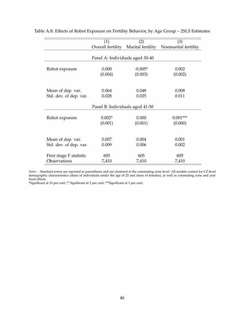
Table A.8: Effects of Robot Exposure on Fertility Behavior, by Age Group – 2SLS Estimates

(1) (2) (3)Overall fertility Marital fertility Nonmarital fertility

Panel A: Individuals aged 30-40

Robot exposure 0.000 -0.005* 0.002(0.004) (0.003) (0.002)

Mean of dep. var. 0.064 0.048 0.008Std. dev. of dep. var. 0.028 0.025 0.011

Panel B: Individuals aged 41-50

Robot exposure 0.002* 0.000 0.001***(0.001) (0.001) (0.000)

Mean of dep. var. 0.007 0.004 0.001Std. dev. of dep. var. 0.009 0.006 0.002

First stage F statistic 605 605 605Observations 7,410 7,410 7,410

Notes - Standard errors are reported in parentheses and are clustered at the commuting zone level. All models control for CZ-leveldemographic characteristics (share of individuals under the age of 25 and share of females), as well as commuting zone and yearfixed effects.*Significant at 10 per cent; ** Significant at 5 per cent; ***Significant at 1 per cent.

46

Table A.9: Effects of Robot Exposure on Match Quality in Couples – 2SLS Estimates

(1) (2) (3)Dep. var.: Spouse Education, Relative to Own More More More

among married among cohabiting

Robot exposure 0.011** 0.008 0.048***(0.005) (0.005) (0.016)

Mean of dep. var. 0.188 0.184 0.232Std. dev. of dep. var. 0.0378 0.0386 0.131First stage F statistic 605 605 605Observations 7,410 7,410 7,410

Notes - Standard errors are reported in parentheses and are clustered at the commuting zone level. All models control for CZ-leveldemographic characteristics (share of individuals under the age of 25 and share of females), as well as commuting zone and yearfixed effects.*Significant at 10 per cent; ** Significant at 5 per cent; ***Significant at 1 per cent.

47

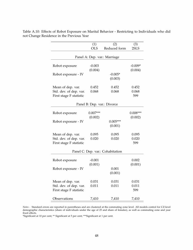
Table A.10: Effects of Robot Exposure on Marital Behavior - Restricting to Individuals who didnot Change Residence in the Previous Year

(1) (2) (3)OLS Reduced form 2SLS

Panel A: Dep. var.: Marriage

Robot exposure -0.003 -0.009*(0.004) (0.004)

Robot exposure - IV -0.005*(0.003)

Mean of dep. var. 0.452 0.452 0.452Std. dev. of dep. var. 0.068 0.068 0.068First stage F statistic 599

Panel B: Dep. var.: Divorce

Robot exposure 0.007*** 0.008***(0.002) (0.002)

Robot exposure - IV 0.005***(0.001)

Mean of dep. var. 0.095 0.095 0.095Std. dev. of dep. var. 0.020 0.020 0.020First stage F statistic 599

Panel C: Dep. var.: Cohabitation

Robot exposure -0.001 0.002(0.001) (0.001)

Robot exposure - IV 0.001(0.001)

Mean of dep. var. 0.031 0.031 0.031Std. dev. of dep. var. 0.011 0.011 0.011First stage F statistic 599

Observations 7,410 7,410 7,410

Notes - Standard errors are reported in parentheses and are clustered at the commuting zone level. All models control for CZ-leveldemographic characteristics (share of individuals under the age of 25 and share of females), as well as commuting zone and yearfixed effects.*Significant at 10 per cent; ** Significant at 5 per cent; ***Significant at 1 per cent.

48

Table A.11: Effects of Robot Exposure on Marital Behavior - Restricting to Individuals who Residein the Same State as the Place of Birth

(1) (2) (3)OLS Reduced form 2SLS

Panel A: Dep. var.: Marriage

Robot exposure -0.002 -0.003(0.004) (0.005)

Robot exposure - IV -0.001(0.003)

Mean of dep. var. 0.389 0.389 0.389Std. dev. of dep. var. 0.072 0.072 0.072First stage F statistic 600

Panel B: Dep. var.: Divorce

Robot exposure 0.006*** 0.007***(0.002) (0.002)

Robot exposure - IV 0.004***(0.001)

Mean of dep. var. 0.094 0.094 0.094Std. dev. of dep. var. 0.023 0.023 0.023First stage F statistic 600

Panel C: Dep. var.: Cohabitation

Robot exposure 0.002* 0.004***(0.001) (0.001)

Robot exposure - IV 0.002***(0.001)

Mean of dep. var. 0.038 0.038 0.038Std. dev. of dep. var. 0.013 0.013 0.013First stage F statistic 600

Observations 7,410 7,410 7,410

Notes - Standard errors are reported in parentheses and are clustered at the commuting zone level. All models control for CZ-leveldemographic characteristics (share of individuals under the age of 25 and share of females), as well as commuting zone and yearfixed effects.*Significant at 10 per cent; ** Significant at 5 per cent; ***Significant at 1 per cent.

49

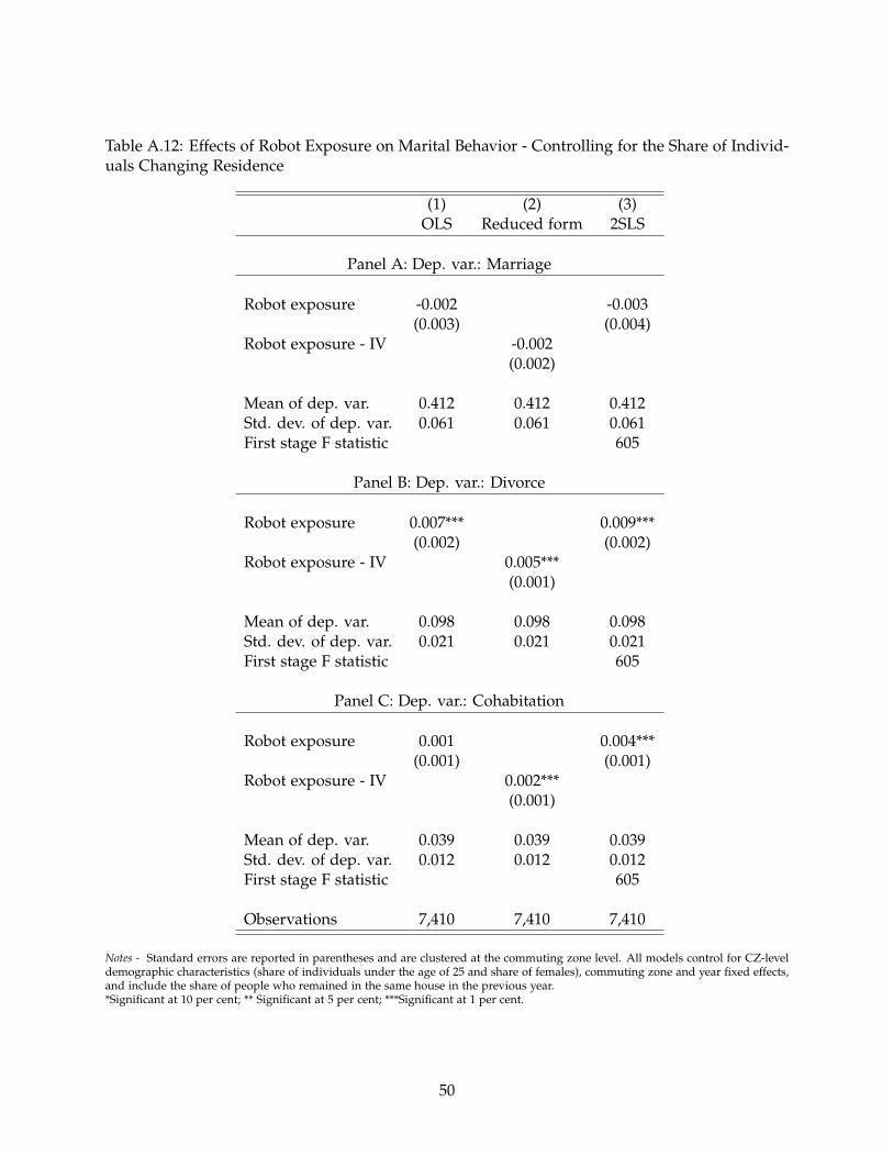
Table A.12: Effects of Robot Exposure on Marital Behavior - Controlling for the Share of Individ-uals Changing Residence

(1) (2) (3)OLS Reduced form 2SLS

Panel A: Dep. var.: Marriage

Robot exposure -0.002 -0.003(0.003) (0.004)

Robot exposure - IV -0.002(0.002)

Mean of dep. var. 0.412 0.412 0.412Std. dev. of dep. var. 0.061 0.061 0.061First stage F statistic 605

Panel B: Dep. var.: Divorce

Robot exposure 0.007*** 0.009***(0.002) (0.002)

Robot exposure - IV 0.005***(0.001)

Mean of dep. var. 0.098 0.098 0.098Std. dev. of dep. var. 0.021 0.021 0.021First stage F statistic 605

Panel C: Dep. var.: Cohabitation

Robot exposure 0.001 0.004***(0.001) (0.001)

Robot exposure - IV 0.002***(0.001)

Mean of dep. var. 0.039 0.039 0.039Std. dev. of dep. var. 0.012 0.012 0.012First stage F statistic 605

Observations 7,410 7,410 7,410

Notes - Standard errors are reported in parentheses and are clustered at the commuting zone level. All models control for CZ-leveldemographic characteristics (share of individuals under the age of 25 and share of females), commuting zone and year fixed effects,and include the share of people who remained in the same house in the previous year.*Significant at 10 per cent; ** Significant at 5 per cent; ***Significant at 1 per cent.

50

Table A.13: Effects of Robot Exposure on Marital Behavior - Controlling for the Share of Individ-uals Residing in their State of Birth

(1) (2) (3)OLS Reduced form 2SLS

Panel A: Dep. var.: Marriage

Robot exposure -0.002 -0.003(0.003) (0.004)

Robot exposure - IV -0.002(0.002)

Mean of dep. var. 0.412 0.412 0.412Std. dev. of dep. var. 0.061 0.061 0.061First stage F statistic 605

Panel B: Dep. var.: Divorce

Robot exposure 0.007*** 0.009***(0.002) (0.002)

Robot exposure - IV 0.005***(0.001)

Mean of dep. var. 0.098 0.098 0.098Std. dev. of dep. var. 0.021 0.021 0.021First stage F statistic 605

Panel C: Dep. var.: Cohabitation

Robot exposure 0.001 0.005***(0.001) (0.001)

Robot exposure - IV 0.003***(0.001)

Mean of dep. var. 0.039 0.039 0.039Std. dev. of dep. var. 0.012 0.012 0.012First stage F statistic 605

Observations 7,410 7,410 7,410

Notes - Standard errors are reported in parentheses and are clustered at the commuting zone level. All models control for CZ-leveldemographic characteristics (share of individuals under the age of 25 and share of females), commuting zone and year fixed effects,and include the share of people whose current state of residence is the same as their state of birth.*Significant at 10 per cent; ** Significant at 5 per cent; ***Significant at 1 per cent.

51

Table A.14: Effects of Robot Exposure on Fertility Behavior - Restricting to Individuals who didnot Change Residence in the Previous Year

(1) (2) (4)OLS Reduced form 2SLS

Panel A: Dep. var.: Overall Fertility

Robot exposure -0.002 -0.001(0.002) (0.002)

Robot exposure - IV -0.001(0.001)

Mean of dep. var. 0.053 0.053 0.053Std. dev. of dep. var. 0.017 0.017 0.017First stage F statistic 599

Panel B: Dep. var.: Marital Fertility

Robot exposure -0.005*** -0.006***(0.001) (0.002)

Robot exposure - IV -0.004***(0.001)

Mean of dep. var. 0.033 0.033 0.033Std. dev. of dep. var. 0.014 0.014 0.014First stage F statistic 599

Panel C: Dep. var.: Nonmarital Fertility

Robot exposure 0.003*** 0.004***(0.001) (0.001)

Robot exposure - IV 0.002***(0.001)

Mean of dep. var. 0.015 0.015 0.015Std. dev. of dep. var. 0.011 0.011 0.011First stage F statistic 599

Observations 7,410 7,410 7,410

Notes - Standard errors are reported in parentheses and are clustered at the commuting zone level. All models control for CZ-leveldemographic characteristics (share of individuals under the age of 25 and share of females), as well as commuting zone and yearfixed effects.*Significant at 10 per cent; ** Significant at 5 per cent; ***Significant at 1 per cent.

52

Table A.15: Effects of Robot Exposure on Fertility Behavior - Restricting to Individuals whoReside in the Same State as the Place of Birth

(1) (2) (4)OLS Reduced form 2SLS

Panel A: Dep. var.: Overall Fertility

Robot exposure 0.002 0.006**(0.002) (0.002)

Robot exposure - IV 0.003**(0.001)

Mean of dep. var. 0.060 0.060 0.060Std. dev. of dep. var. 0.021 0.021 0.021First stage F statistic 600

Panel B: Dep. var.: Marital Fertility

Robot exposure -0.003* -0.003*(0.002) (0.002)

Robot exposure - IV -0.002*(0.001)

Mean of dep. var. 0.032 0.032 0.032Std. dev. of dep. var. 0.015 0.015 0.015First stage F statistic 600

Panel C: Dep. var.: Nonmarital Fertility

Robot exposure 0.004*** 0.007***(0.001) (0.002)

Robot exposure - IV 0.004***(0.001)

Mean of dep. var. 0.022 0.022 0.022Std. dev. of dep. var. 0.015 0.015 0.015First stage F statistic 600

Observations 7,410 7,410 7,410

Notes - Standard errors are reported in parentheses and are clustered at the commuting zone level. All models control for CZ-leveldemographic characteristics (share of individuals under the age of 25 and share of females), as well as commuting zone and yearfixed effects.*Significant at 10 per cent; ** Significant at 5 per cent; ***Significant at 1 per cent.

53

Table A.16: Effects of Robot Exposure on Fertility Behavior - Controlling for the Share of Indi-viduals Changing Residence

(1) (2) (4)OLS Reduced form 2SLS

Panel A: Dep. var.: Overall Fertility

Robot exposure -0.001 0.000(0.002) (0.002)

Robot exposure - IV 0.000(0.001)

Mean of dep. var. 0.059 0.059 0.059Std. dev. of dep. var. 0.018 0.018 0.018First stage F statistic 605

Panel B: Dep. var.: Marital Fertility

Robot exposure -0.002* -0.004**(0.001) (0.001)

Robot exposure - IV -0.002**(0.001)

Mean of dep. var. 0.033 0.033 0.033Std. dev. of dep. var. 0.013 0.013 0.013First stage F statistic 605

Panel C: Dep. var.: Nonmarital Fertility

Robot exposure 0.001 0.003**(0.001) (0.001)

Robot exposure - IV 0.002**(0.001)

Mean of dep. var. 0.019 0.019 0.019Std. dev. of dep. var. 0.011 0.011 0.011First stage F statistic 605

Observations 7,410 7,410 7,410

Notes - Standard errors are reported in parentheses and are clustered at the commuting zone level. All models control for CZ-leveldemographic characteristics (share of individuals under the age of 25 and share of females), commuting zone and year fixed effects,and include the share of people who remained in the same house in the previous year.*Significant at 10 per cent; ** Significant at 5 per cent; ***Significant at 1 per cent.

54

Table A.17: Effects of Robot Exposure on Fertility Behavior - Controlling for the Share of Indi-viduals Residing in their State of Birth

(1) (2) (4)OLS Reduced form 2SLS

Panel A: Dep. var.: Overall Fertility

Robot exposure -0.001 0.001(0.002) (0.002)

Robot exposure - IV 0.000(0.001)

Mean of dep. var. 0.059 0.059 0.059Std. dev. of dep. var. 0.018 0.018 0.018First stage F statistic 605

Panel B: Dep. var.: Marital Fertility

Robot exposure -0.002** -0.004**(0.001) (0.001)

Robot exposure - IV -0.002**(0.001)

Mean of dep. var. 0.033 0.033 0.033Std. dev. of dep. var. 0.013 0.013 0.013First stage F statistic 605

Panel C: Dep. var.: Nonmarital Fertility

Robot exposure 0.001 0.003**(0.001) (0.001)

Robot exposure - IV 0.002**(0.001)

Mean of dep. var. 0.019 0.019 0.019Std. dev. of dep. var. 0.011 0.011 0.011First stage F statistic 605

Observations 7,410 7,410 7,410

Notes - Standard errors are reported in parentheses and are clustered at the commuting zone level. All models control for CZ-leveldemographic characteristics (share of individuals under the age of 25 and share of females), commuting zone and year fixed effects,and include the share of people whose current state of residence is the same as their state of birth.*Significant at 10 per cent; ** Significant at 5 per cent; ***Significant at 1 per cent.

55

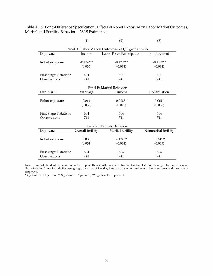
Table A.18: Long-Difference Specification: Effects of Robot Exposure on Labor Market Outcomes,Marital and Fertility Behavior – 2SLS Estimates

(1) (2) (3)

Panel A: Labor Market Outcomes - M/F gender ratioDep. var.: Income Labor Force Participation Employment

Robot exposure -0.126*** -0.129*** -0.119***(0.035) (0.034) (0.034)

First stage F statistic 604 604 604Observations 741 741 741

Panel B: Marital BehaviorDep. var.: Marriage Divorce Cohabitation

Robot exposure -0.064* 0.098** 0.061*(0.036) (0.041) (0.036)

First stage F statistic 604 604 604Observations 741 741 741

Panel C: Fertility BehaviorDep. var.: Overall fertility Marital fertility Nonmarital fertility

Robot exposure 0.039 -0.083** 0.164***(0.031) (0.034) (0.035)

First stage F statistic 604 604 604Observations 741 741 741

Notes - Robust standard errors are reported in parentheses. All models control for baseline CZ-level demographic and economiccharacteristics. These include the average age, the share of females, the share of women and men in the labor force, and the share ofemployed.*Significant at 10 per cent; ** Significant at 5 per cent; ***Significant at 1 per cent.

56

Table A.19: Long-Difference Specification: Effects of Robot Exposure on Marital and FertilityBehavior - Including Controls for Pre-trends (from 1980-1990) – 2SLS Estimates

(1) (2) (3) (4) (5) (6)Dep. var.: Marriage Divorce Cohabitation Overall fertility Marital fertility Nonmarital fertility

Robot exposure -0.074** 0.121*** 0.045 0.046 -0.064* 0.160***(0.037) (0.041) (0.037) (0.031) (0.034) (0.035)

First stage F statistic 599 603 613 586 584 607Observations 741 741 741 741 741 741

Notes - Robust standard errors are reported in parentheses. All models control for baseline CZ-level demographic and economiccharacteristics. These include the average age, the share of females, the share of women and men in the labor force and the share ofemployed. All models further include controls for pre-trends (from 1980-1990) in the outcome of interest.*Significant at 10 per cent; ** Significant at 5 per cent; ***Significant at 1 per cent.

57

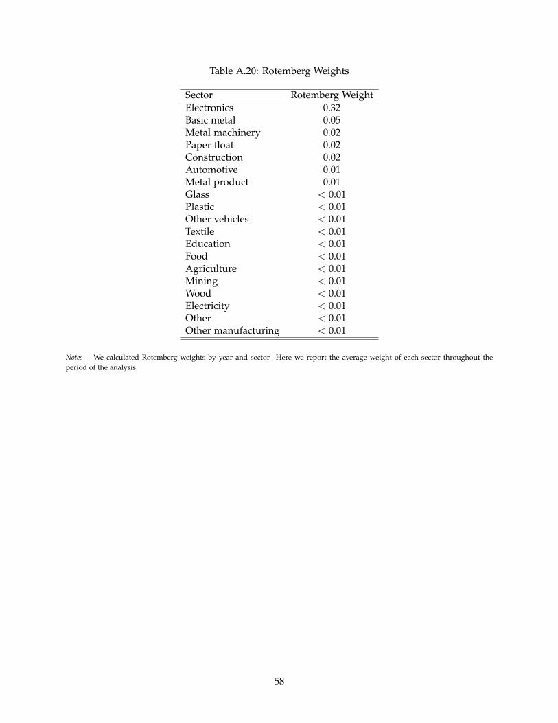
Table A.20: Rotemberg Weights

Sector Rotemberg WeightElectronics 0.32Basic metal 0.05Metal machinery 0.02Paper float 0.02Construction 0.02Automotive 0.01Metal product 0.01Glass < 0.01Plastic < 0.01Other vehicles < 0.01Textile < 0.01Education < 0.01Food < 0.01Agriculture < 0.01Mining < 0.01Wood < 0.01Electricity < 0.01Other < 0.01Other manufacturing < 0.01

Notes - We calculated Rotemberg weights by year and sector. Here we report the average weight of each sector throughout theperiod of the analysis.

58

Table A.21: Effects of Robot Exposure on Marital Behavior – Excluding Robots in the ElectronicsSector

(1) (2) (3)OLS Reduced form 2SLS

Panel A: Marriage

Robot exposure -0.004 -0.004(0.004) (0.004)

Robot exposure - IV -0.002(0.002)

Mean of dep. var. 0.412 0.412 0.412Std. dev. of dep. var. 0.061 0.061 0.061First stage F statistic 588

Panel B: Divorce

Robot exposure 0.008*** 0.009***(0.002) (0.002)

Robot exposure - IV 0.005***(0.001)

Mean of dep. var. 0.098 0.098 0.098Std. dev. of dep. var. 0.021 0.021 0.021First stage F statistic 588

Panel C: Cohabitation

Robot exposure 0.002** 0.005***(0.001) (0.001)

Robot exposure - IV 0.003***(0.001)

Mean of dep. var. 0.039 0.039 0.039Std. dev. of dep. var. 0.012 0.012 0.012First stage F statistic 588

Observations 7,410 7,410 7,410

Notes - Standard errors are reported in parentheses and are clustered at the commuting zone level. All models control for CZ-leveldemographic characteristics (share of individuals under the age of 25 and share of females), as well as commuting zone and yearfixed effects. All models exclude the stock of robots in the electronics sector from the computation of the robot exposure measure.*Significant at 10 per cent; ** Significant at 5 per cent; ***Significant at 1 per cent.

59

Table A.22: Effects of Robot Exposure on Fertility Behavior – Excluding Robots in the ElectronicsSector

(1) (2) (4)OLS Reduced form 2SLS

Panel A: Overall Fertility

Robot exposure -0.002 0.001(0.002) (0.002)

Robot exposure - IV 0.000(0.001)

Mean of dep. var. 0.059 0.059 0.059Std. dev. of dep. var. 0.018 0.018 0.018First stage F statistic 588

Panel B: Marital Fertility

Robot exposure -0.003** -0.004**(0.001) (0.001)

Robot exposure - IV -0.002**(0.001)

Mean of dep. var. 0.033 0.033 0.033Std. dev. of dep. var. 0.013 0.013 0.013First stage F statistic 588

Panel C: Nonmarital Fertility

Robot exposure 0.001 0.003**(0.001) (0.001)

Robot exposure - IV 0.002**(0.001)

Mean of dep. var. 0.019 0.019 0.019Std. dev. of dep. var. 0.011 0.011 0.011First stage F statistic 588

Observations 7,410 7,410 7,410

Notes - Standard errors are reported in parentheses and are clustered at the commuting zone level. All models control for CZ-leveldemographic characteristics (share of individuals under the age of 25 and share of females), as well as commuting zone and yearfixed effects. All models exclude the stock of robots in the electronics sector from the computation of the robot exposure measure.*Significant at 10 per cent; ** Significant at 5 per cent; ***Significant at 1 per cent.

60

Table A.23: Effects of Robot Exposure on Marital Behavior – Including Controls for Specific TimeTrends by Initial Share of Employment in the Electronics Sector

(1) (2) (3)OLS Reduced form 2SLS

Panel A: Marriage

Robot exposure -0.010** -0.010*(0.004) (0.006)

Robot exposure - IV -0.005*(0.003)

Mean of dep. var. 0.412 0.412 0.412Std. dev. of dep. var. 0.061 0.061 0.061First stage F statistic 438

Panel B: Divorce

Robot exposure 0.006*** 0.006**(0.002) (0.002)

Robot exposure - IV 0.003**(0.001)

Mean of dep. var. 0.098 0.098 0.098Std. dev. of dep. var. 0.021 0.021 0.021First stage F statistic 438

Panel C: Cohabitation

Robot exposure 0.004*** 0.008***(0.001) (0.001)

Robot exposure - IV 0.004***(0.001)

Mean of dep. var. 0.039 0.039 0.039Std. dev. of dep. var. 0.012 0.012 0.012First stage F statistic 438

Observations 7,410 7,410 7,410

Notes - Standard errors are reported in parentheses and are clustered at the commuting zone level. All models control for CZ-leveldemographic characteristics (share of individuals under the age of 25 and share of females), commuting zone and year fixed effects,and include specific time trends across areas in different quartiles of the initial share of employment in the electronics sector. Inpractice, we include controls interacting year dummies with quartiles of the share of employment in the electronics sector as of 1990.*Significant at 10 per cent; ** Significant at 5 per cent; ***Significant at 1 per cent.

61

Table A.24: Effects of Robot Exposure on Fertility Behavior – Including Controls for Specific TimeTrends by Initial Share of Employment in the Electronics Sector

(1) (2) (4)OLS Reduced form 2SLS

Panel A: Overall Fertility

Robot exposure -0.005** -0.001(0.002) (0.002)

Robot exposure - IV -0.001(0.001)

Mean of dep. var. 0.059 0.059 0.059Std. dev. of dep. var. 0.018 0.018 0.018First stage F statistic 438

Panel B: Marital Fertility

Robot exposure -0.003** -0.004**(0.001) (0.002)

Robot exposure - IV -0.002**(0.001)

Mean of dep. var. 0.033 0.033 0.033Std. dev. of dep. var. 0.013 0.013 0.013First stage F statistic 438

Panel C: Nonmarital Fertility

Robot exposure -0.001 0.001(0.001) (0.001)

Robot exposure - IV 0.001(0.001)

Mean of dep. var. 0.019 0.019 0.019Std. dev. of dep. var. 0.011 0.011 0.011First stage F statistic 438

Observations 7,410 7,410 7,410

Notes - Standard errors are reported in parentheses and are clustered at the commuting zone level. All models control for CZ-leveldemographic characteristics (share of individuals under the age of 25 and share of females), commuting zone and year fixed effects,and include specific time trends across areas in different quartiles of the initial share of employment in the electronics sector. Inpractice, we include controls interacting year dummies with quartiles of the share of employment in the electronics sector as of 1990.*Significant at 10 per cent; ** Significant at 5 per cent; ***Significant at 1 per cent.

62

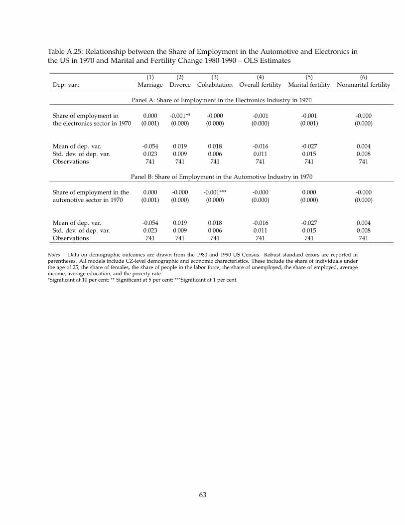
Table A.25: Relationship between the Share of Employment in the Automotive and Electronics inthe US in 1970 and Marital and Fertility Change 1980-1990 – OLS Estimates

(1) (2) (3) (4) (5) (6)Dep. var.: Marriage Divorce Cohabitation Overall fertility Marital fertility Nonmarital fertility

Panel A: Share of Employment in the Electronics Industry in 1970

Share of employment in 0.000 -0.001** -0.000 -0.001 -0.001 -0.000the electronics sector in 1970 (0.001) (0.000) (0.000) (0.000) (0.001) (0.000)

Mean of dep. var. -0.054 0.019 0.018 -0.016 -0.027 0.004Std. dev. of dep. var. 0.023 0.009 0.006 0.011 0.015 0.008Observations 741 741 741 741 741 741

Panel B: Share of Employment in the Automotive Industry in 1970

Share of employment in the 0.000 -0.000 -0.001*** -0.000 0.000 -0.000automotive sector in 1970 (0.001) (0.000) (0.000) (0.000) (0.000) (0.000)

Mean of dep. var. -0.054 0.019 0.018 -0.016 -0.027 0.004Std. dev. of dep. var. 0.023 0.009 0.006 0.011 0.015 0.008Observations 741 741 741 741 741 741

Notes - Data on demographic outcomes are drawn from the 1980 and 1990 US Census. Robust standard errors are reported inparentheses. All models include CZ-level demographic and economic characteristics. These include the share of individuals underthe age of 25, the share of females, the share of people in the labor force, the share of unemployed, the share of employed, averageincome, average education, and the poverty rate.*Significant at 10 per cent; ** Significant at 5 per cent; ***Significant at 1 per cent.

63

Table A.26: Effects of Robot Exposure on Marital Behavior - Including Controls for Specific TimeTrends by Initial Share of Employment in the Automotive Sector.

(1) (2) (3)OLS Reduced form 2SLS

Panel A: Dep. var.: Marriage

Robot exposure -0.006 -0.009(0.005) (0.007)

Robot exposure - IV -0.004(0.003)

Mean of dep. var. 0.412 0.412 0.412Std. dev. of dep. var. 0.061 0.061 0.061First stage F statistic 200

Panel B: Dep. var.: Divorce

Robot exposure 0.003 0.006*(0.002) (0.003)

Robot exposure - IV 0.002*(0.001)

Mean of dep. var. 0.098 0.098 0.098Std. dev. of dep. var. 0.021 0.021 0.021First stage F statistic 200

Panel C: Dep. var.: Cohabitation

Robot exposure 0.003** 0.009***(0.001) (0.002)

Robot exposure - IV 0.004***(0.001)

Mean of dep. var. 0.039 0.039 0.039Std. dev. of dep. var. 0.012 0.012 0.012First stage F statistic 200

Observations 7,410 7,410 7,410

Notes - Standard errors are reported in parentheses and are clustered at the commuting zone level. All models control for CZ-leveldemographic characteristics (share of individuals under the age of 25 and share of females), commuting zone and year fixed effects,and include specific time trends across areas in different quartiles of the initial share of employment in the automotive sector. Inpractice, we include controls interacting year dummies with quartiles of the share of employment in the automotive sector as of 1990.*Significant at 10 per cent; ** Significant at 5 per cent; ***Significant at 1 per cent.

64

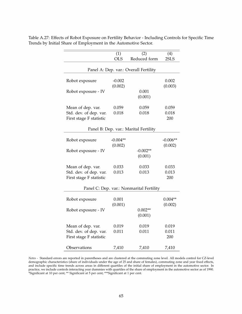
Table A.27: Effects of Robot Exposure on Fertility Behavior - Including Controls for Specific TimeTrends by Initial Share of Employment in the Automotive Sector.

(1) (2) (4)OLS Reduced form 2SLS

Panel A: Dep. var.: Overall Fertility

Robot exposure -0.002 0.002(0.002) (0.003)

Robot exposure - IV 0.001(0.001)

Mean of dep. var. 0.059 0.059 0.059Std. dev. of dep. var. 0.018 0.018 0.018First stage F statistic 200

Panel B: Dep. var.: Marital Fertility

Robot exposure -0.004** -0.006**(0.002) (0.002)

Robot exposure - IV -0.002**(0.001)

Mean of dep. var. 0.033 0.033 0.033Std. dev. of dep. var. 0.013 0.013 0.013First stage F statistic 200

Panel C: Dep. var.: Nonmarital Fertility

Robot exposure 0.001 0.004**(0.001) (0.002)

Robot exposure - IV 0.002**(0.001)

Mean of dep. var. 0.019 0.019 0.019Std. dev. of dep. var. 0.011 0.011 0.011First stage F statistic 200

Observations 7,410 7,410 7,410

Notes - Standard errors are reported in parentheses and are clustered at the commuting zone level. All models control for CZ-leveldemographic characteristics (share of individuals under the age of 25 and share of females), commuting zone and year fixed effects,and include specific time trends across areas in different quartiles of the initial share of employment in the automotive sector. Inpractice, we include controls interacting year dummies with quartiles of the share of employment in the automotive sector as of 1990.*Significant at 10 per cent; ** Significant at 5 per cent; ***Significant at 1 per cent.

65

Table A.28: Effects of Robot Exposure on Marital and Fertility Behavior – Including Controls forExposure to Trade – 2SLS Estimates

(1) (2) (3) (4) (5) (6)Dep. var.: Marriage Divorce Cohabitation Overall fertility Marital fertility Nonmarital fertility

Robot exposure -0.004 0.008*** 0.004*** -0.000 -0.004*** 0.002**(0.004) (0.002) (0.001) (0.002) (0.001) (0.001)

Mean of dep. var. 0.412 0.098 0.039 0.059 0.033 0.019Std. dev. of dep. var. 0.061 0.021 0.012 0.018 0.013 0.011First stage F statistic 589 589 589 589 589 589Observations 7,410 7,410 7,410 7,410 7,410 7,410

Notes - Standard errors are reported in parentheses and are clustered at the commuting zone level. All models control for CZ-leveldemographic characteristics (share of individuals under the age of 25 and share of females), as well as commuting zone and yearfixed effects. All models further include the CZ-level measure of exposure to trade (detailed in Section 5.1) interacted with yeardummies.*Significant at 10 per cent; ** Significant at 5 per cent; ***Significant at 1 per cent.

66

Table A.29: Effects of Robot Exposure on Marital and Fertility Behavior - Including Controls forTrends in the Manufacturing Sector – 2SLS Estimates

(1) (2) (3) (4) (5) (6)Dep. var.: Marriage Divorce Cohabitation Overall fertility Marital fertility Nonmarital fertility

Robot exposure -0.004 0.008*** 0.004*** -0.000 -0.004*** 0.002**(0.004) (0.002) (0.001) (0.002) (0.001) (0.001)

Mean of dep. var. 0.412 0.098 0.039 0.059 0.033 0.019Std. dev. of dep. var. 0.061 0.021 0.012 0.018 0.013 0.011First stage F statistic 590 590 590 590 590 590Observations 7,410 7,410 7,410 7,410 7,410 7,410

Notes - Standard errors are reported in parentheses and are clustered at the commuting zone level. All models control for CZ-leveldemographic characteristics (share of individuals under the age of 25 and share of females), commuting zone and year fixed effects,and include controls interacting year dummies with the share of employment in total manufacturing as of 1990.*Significant at 10 per cent; ** Significant at 5 per cent; ***Significant at 1 per cent.

67

Table A.30: Effects of Robot Exposure on Marital Behavior– Including Controls for Family PolicyEnvironment – 2SLS Estimates

(1) (2) (3)Family controls TRAP laws Family controls

and TRAP laws

Panel A: Dep. var.: Marriage

Robot exposure -0.004 -0.004 -0.004(0.004) (0.004) (0.004)

Mean of dep. var. 0.412 0.412 0.412Std. dev. of dep. var. 0.061 0.061 0.061First stage F statistic 639 619 647

Panel B: Dep. var.: Divorce

Robot exposure 0.009*** 0.009*** 0.009***(0.002) (0.002) (0.002)

Mean of dep. var. 0.098 0.098 0.098Std. dev. of dep. var. 0.021 0.021 0.021First stage F statistic 639 619 647

Panel C: Dep. var.: Cohabitation

Robot exposure 0.004*** 0.004*** 0.004***(0.001) (0.001) (0.001)

Mean of dep. var. 0.039 0.039 0.039Std. dev. of dep. var. 0.012 0.012 0.012First stage F statistic 639 619 647

Observations 7,410 7,410 7,410

Notes - Standard errors are reported in parentheses and are clustered at the commuting zone level. All models control for CZ-leveldemographic characteristics (share of individuals under the age of 25 and share of females), as well as commuting zone and yearfixed effects. Furthermore, column 1 includes controls for family policies (see Section 5.1 for details), column 2 adds TRAP laws, andcolumn 3 includes controls for both family policies and TRAP laws.*Significant at 10 per cent; ** Significant at 5 per cent; ***Significant at 1 per cent.

68

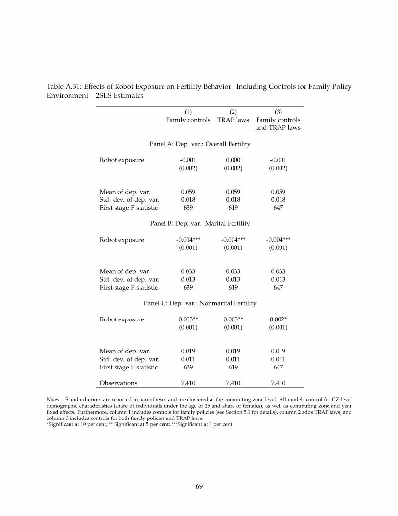
Table A.31: Effects of Robot Exposure on Fertility Behavior– Including Controls for Family PolicyEnvironment – 2SLS Estimates

(1) (2) (3)Family controls TRAP laws Family controls

and TRAP laws

Panel A: Dep. var.: Overall Fertility

Robot exposure -0.001 0.000 -0.001(0.002) (0.002) (0.002)

Mean of dep. var. 0.059 0.059 0.059Std. dev. of dep. var. 0.018 0.018 0.018First stage F statistic 639 619 647

Panel B: Dep. var.: Marital Fertility

Robot exposure -0.004*** -0.004*** -0.004***(0.001) (0.001) (0.001)

Mean of dep. var. 0.033 0.033 0.033Std. dev. of dep. var. 0.013 0.013 0.013First stage F statistic 639 619 647

Panel C: Dep. var.: Nonmarital Fertility

Robot exposure 0.003** 0.003** 0.002*(0.001) (0.001) (0.001)

Mean of dep. var. 0.019 0.019 0.019Std. dev. of dep. var. 0.011 0.011 0.011First stage F statistic 639 619 647

Observations 7,410 7,410 7,410

Notes - Standard errors are reported in parentheses and are clustered at the commuting zone level. All models control for CZ-leveldemographic characteristics (share of individuals under the age of 25 and share of females), as well as commuting zone and yearfixed effects. Furthermore, column 1 includes controls for family policies (see Section 5.1 for details), column 2 adds TRAP laws, andcolumn 3 includes controls for both family policies and TRAP laws.*Significant at 10 per cent; ** Significant at 5 per cent; ***Significant at 1 per cent.

69

Table A.32: Effects of Robot Exposure on Fertility Behavior, Extensive and Intensive Margin –2SLS Estimates

(1) (2) (4)Overall fertility Marital fertility Nonmarital fertility

Panel A: Extensive Margin of Fertility (Share of Women Having at Least One Child)

Robot exposure 0.001 -0.003*** 0.003**(0.002) (0.001) (0.002)

Mean of dep. var. 0.0402 0.0174 0.0185Std. dev. of dep. var. 0.0173 0.0101 0.0131

Panel B: Intensive Margin of Fertility (Share of Women Having More than One Child)

Robot exposure -0.002 -0.007*** 0.004**(0.003) (0.003) (0.002)

Mean of dep. var. 0.102 0.0637 0.0289Std. dev. of dep. var. 0.0288 0.0247 0.0172

Panel C: Intensive Margin of Fertility (Number of Children)

Robot exposure -0.000 -0.073*** 0.055***(0.010) (0.015) (0.012)

Mean of dep. var. 1.019 1.556 0.374Std. dev. of dep. var. 0.135 0.185 0.146

First stage F statistic 605 605 605Observations 7,410 7,410 7,410

Notes - Standard errors are reported in parentheses and are clustered at the commuting zone level. All models control for CZ-leveldemographic characteristics (share of individuals under the age of 25 and share of females), as well as commuting zone and yearfixed effects.*Significant at 10 per cent; ** Significant at 5 per cent; ***Significant at 1 per cent.

70

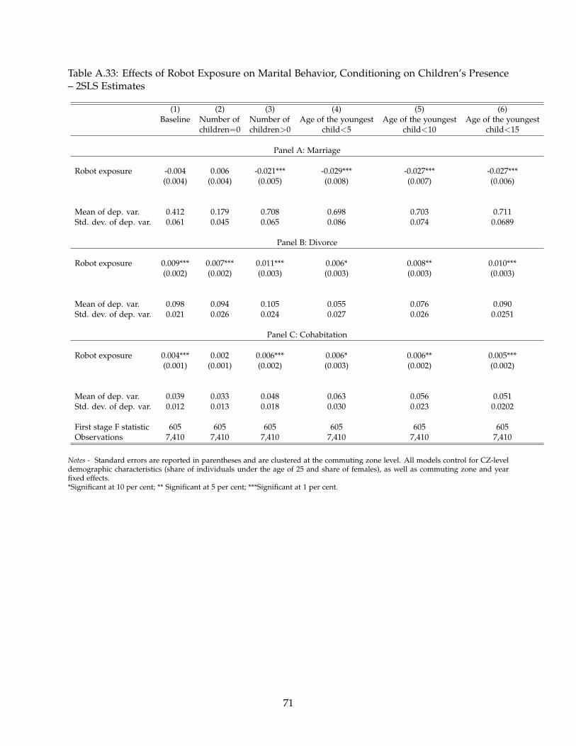
Table A.33: Effects of Robot Exposure on Marital Behavior, Conditioning on Children’s Presence– 2SLS Estimates

(1) (2) (3) (4) (5) (6)Baseline Number of Number of Age of the youngest Age of the youngest Age of the youngest

children=0 children>0 child<5 child<10 child<15

Panel A: Marriage

Robot exposure -0.004 0.006 -0.021*** -0.029*** -0.027*** -0.027***(0.004) (0.004) (0.005) (0.008) (0.007) (0.006)

Mean of dep. var. 0.412 0.179 0.708 0.698 0.703 0.711Std. dev. of dep. var. 0.061 0.045 0.065 0.086 0.074 0.0689

Panel B: Divorce

Robot exposure 0.009*** 0.007*** 0.011*** 0.006* 0.008** 0.010***(0.002) (0.002) (0.003) (0.003) (0.003) (0.003)

Mean of dep. var. 0.098 0.094 0.105 0.055 0.076 0.090Std. dev. of dep. var. 0.021 0.026 0.024 0.027 0.026 0.0251

Panel C: Cohabitation

Robot exposure 0.004*** 0.002 0.006*** 0.006* 0.006** 0.005***(0.001) (0.001) (0.002) (0.003) (0.002) (0.002)

Mean of dep. var. 0.039 0.033 0.048 0.063 0.056 0.051Std. dev. of dep. var. 0.012 0.013 0.018 0.030 0.023 0.0202

First stage F statistic 605 605 605 605 605 605Observations 7,410 7,410 7,410 7,410 7,410 7,410

Notes - Standard errors are reported in parentheses and are clustered at the commuting zone level. All models control for CZ-leveldemographic characteristics (share of individuals under the age of 25 and share of females), as well as commuting zone and yearfixed effects.*Significant at 10 per cent; ** Significant at 5 per cent; ***Significant at 1 per cent.

71

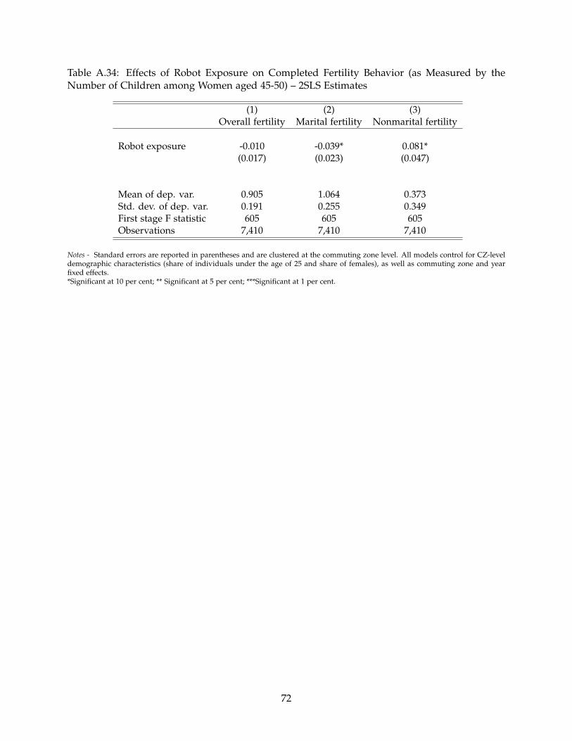
Table A.34: Effects of Robot Exposure on Completed Fertility Behavior (as Measured by theNumber of Children among Women aged 45-50) – 2SLS Estimates

(1) (2) (3)Overall fertility Marital fertility Nonmarital fertility

Robot exposure -0.010 -0.039* 0.081*(0.017) (0.023) (0.047)

Mean of dep. var. 0.905 1.064 0.373Std. dev. of dep. var. 0.191 0.255 0.349First stage F statistic 605 605 605Observations 7,410 7,410 7,410

Notes - Standard errors are reported in parentheses and are clustered at the commuting zone level. All models control for CZ-leveldemographic characteristics (share of individuals under the age of 25 and share of females), as well as commuting zone and yearfixed effects.*Significant at 10 per cent; ** Significant at 5 per cent; ***Significant at 1 per cent.

72

Table A.35: Effects of Robot Exposure on Nonmarital Fertility among Cohabiting and Non-cohabiting Women – 2SLS Estimates

(1) (2) (3)Dep. var.: Nonmarital fertility Nonmarital fertility - Nonmarital fertility -

cohabiting women non-cohabiting women

Robot exposure 0.003** 0.000 0.003**(0.001) (0.000) (0.001)

Mean of dep. var. 0.019 0.003 0.017Std. dev. of dep. var. 0.011 0.004 0.011First stage F statistic 605 605 605Observations 7,410 7,410 7,410

Notes - Standard errors are reported in parentheses and are clustered at the commuting zone level. All models control for CZ-leveldemographic characteristics (share of individuals under the age of 25 and share of females), as well as commuting zone and yearfixed effects.*Significant at 10 per cent; ** Significant at 5 per cent; ***Significant at 1 per cent.

73

Table A.36: Effects of Robot Exposure on Marital and Fertility Behavior among Same-Sex Couples– 2SLS Estimates

(1) (2) (3) (4) (5) (6)Marriage Divorce Cohabitation Overall fertility Marital fertility Nonmarital fertility

Panel A: Focusing on Same-Sex Couples

Robot exposure -0.001*** 0.000 0.000 -0.000 -0.000 0.000(0.000) (0.000) (0.000) (0.000) (0.000) (0.000)

Mean of dep. var. 0.001 0.001 0.002 0.000 0.000 0.000Std. dev. of dep. var. 0.002 0.001 0.002 0.001 0.001 0.000First stage F statistic 597 597 597 597 597 597

Panel B: Baseline that excludes Same-Sex Couples

Robot exposure -0.003 0.009*** 0.004*** 0.000 -0.004** 0.003**(0.004) (0.002) (0.001) (0.002) (0.001) (0.001)

Mean of dep. var. 0.413 0.0982 0.0382 0.0595 0.0338 0.0196Std. dev. of dep. var. 0.0616 0.0212 0.0119 0.0180 0.0136 0.0117First stage F statistic 604 604 604 604 604 604

Panel C: Baseline that includes Legislation of Same-Sex Marriage

Robot exposure -0.003 0.009*** 0.005*** 0.000 -0.004*** 0.003**(0.004) (0.002) (0.001) (0.002) (0.001) (0.001)

Mean of dep. var. 0.412 0.0986 0.0398 0.0594 0.0337 0.0196Std. dev. of dep. var. 0.0612 0.0213 0.0120 0.0180 0.0135 0.0116First stage F statistic 597 597 597 597 597 597

Observations 7,410 7,410 7,410 7,410 7,410 7,410

Notes - Standard errors are reported in parentheses and are clustered at the commuting zone level. All models control for CZ-leveldemographic characteristics (share of individuals under the age of 25 and share of females), as well as commuting zone and yearfixed effects.*Significant at 10 per cent; ** Significant at 5 per cent; ***Significant at 1 per cent.

74

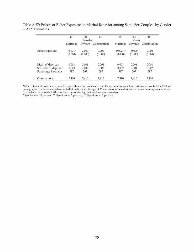
Table A.37: Effects of Robot Exposure on Marital Behavior among Same-Sex Couples, by Gender– 2SLS Estimates

(1) (2) (3) (4) (5) (6)Females Males

Marriage Divorce Cohabitation Marriage Divorce Cohabitation

Robot exposure -0.001* 0.000 0.000 -0.002*** -0.000 0.000(0.000) (0.000) (0.000) (0.000) (0.000) (0.000)

Mean of dep. var. 0.001 0.001 0.002 0.001 0.001 0.001Std. dev. of dep. var. 0.003 0.002 0.002 0.002 0.001 0.002First stage F statistic 597 597 597 597 597 597

Observations 7,410 7,410 7,410 7,410 7,410 7,410

Notes - Standard errors are reported in parentheses and are clustered at the commuting zone level. All models control for CZ-leveldemographic characteristics (share of individuals under the age of 25 and share of females), as well as commuting zone and yearfixed effects. All models further include controls for legislation of same-sex marriage.*Significant at 10 per cent; ** Significant at 5 per cent; ***Significant at 1 per cent.

75