roberto’s notes on linear algebra chapter 6: lines, … · linear algebra chapter 6: lines,...

Linear Algebra Chapter 6: Lines, planes and other straight objects Section 1: Equations of lines in 2

Roberto’s Notes on Linear Algebra

Chapter 6: Lines, planes and other straight objects Section 1

Equations of lines in 2

What you need to know already: What you can learn here:

The dot product.

The correspondence between equations and

graphs.

General concepts related to linear functions.

How to describe a line in the Cartesian plane

by using linear algebra notation and

operations.

Both in high school and in the calculus course you have worked extensively

with lines in the Cartesian plane.

Tell me about it!

So, you have seen the connections that exists between the equation of a line and

its graph, especially its slope and its position in the plane.

And the intercepts and the other stuff.

It is now time to explore more deeply these connections between lines and the

linear equations we have encountered so far. We shall do that by using several of the

tools that we have developed so far and by constructing several other ways to

describe a line algebraically.

Hence “linear algebra!”

Exactly! You may remember that, at the most elementary level, a line is

described as a “straight” curve, that is, a curve with constant slope. This property

allows us to construct several types of equations that identify or describe a line.

Here is a reminder of the forms that are most commonly used and that we have most

likely seen in the past.

Knot on your finger

The slope-intercept equation of a line:

Is of the form y mx b .

Is called this way because it includes the slope m

and the y-intercept b explicitly.

Applies only to non-vertical lines.

Is also called functional equation, since it is

given in the form y f x .


Knot on your finger

The point-slope equation of a line:

Is of the form 0 0y y m x x .

Is called this way because it includes the slope m

and one point 0 0,x y explicitly.

Applies only to non-vertical lines.

Knot on your finger

The two-point equation of a line:

Can be written in one of the two forms

1 2 1 1 2 1y y x x x x y y

2 11 1

2 1

y yy x x y

x x

Is called this way because it includes two

different points 1 1,x y and 2 2,x y explicitly.

Applies to all lines, at least in the first form.

Knot on your finger

The general equation of a line:

Is of the form ax by c or 0ax by c .

Is called this way because it can be constructed

from any suitable information.

Applies to all lines.

Example: 2 3y x

This line has slope 2m and y-intercept

0, 3 , as clearly visible in the formula.

By using some basic algebra we can

change this form into the general equation:

2 3 2 3y x x y

From either equation, we can see that the

point 2, 1 is also on the line, so we can

use this point and the slope we already

know to construct the point-slope form:

1 2 2y x

Again some simple algebra can change this back to the general form.

Also, we can use the points 2, 1 and 3, 3 to get the two-points equation:

1 3 2 2 3 1y x

This also turns into the general forms in two easy steps.

2,1

3, 3


This example illustrates what we can do for equations of lines that have a slope.

But we have much fewer options for those lines that don’t have a slope, namely

vertical lines.

Example: 3x

The vertical line through the point 3, 2

does not have a slope and hence we can only

use the general or two-point form. But how

do we construct either?

By observing that any point on the vertical

line we are seeking must have the same x-

coordinate, that is, it must have 3x . But

this is the general equation, with

1, 0, 3a b c !

Alternatively, the same observation implies that the point 3, 0 is also on

the same line and we can use the two-point form:

2 0 0 3 0 2 0 6 2y x x

A little rearrangement will give us again the form 3x .

Yeah, yeah! Will we learn anything new in this section?

Of course, my impatient padawan! It turns out that a line can also be defined in

terms of vectors, instead of points and slopes, thus giving rise to yet more forms of

the equation.

And why do we need more forms: aren’t the ones we know enough?

The new forms of the equation of a line will open several new doors for new or

more efficient uses. For instance:

they will provide efficient and/or effective ways of developing certain

types of applications

they can be used to extend the content of “straight” to higher dimensions

and, with that, of lots of nice properties of lines

they will give us the possibility to use matrices in relation to lines and

other straight objects.

Show me!

Let’s begin with a new definition of a line that shies away from the self-

referential concept of straight. This approach is related to the earlier observation

that using the slope is cumbersome when working with vectors, especially in higher

dimensions.

Definition

The line containing a

point 0 0,P x y and

having direction vector

1 2d dd consists of all

points ,X x y such

that the vector PX x p

is parallel to d.

That is, this line consists

of all points that satisfy the equation:

k x p d or 0 0 1 2x x y y kd kd

Notice that, as usual, in this definition the points ,X x y and 0 0,P x y

are identified with the vectors x yx and 0 0x yp respectively.

Example: 3 4 2x y k k

This line contains the point 3, 4 and has direction 1 2 . So, for

instance, the point 6,10 is on it: just let k=3.

P

X

d


Is this equivalent to the usual definition?

Excellent question! Although the picture suggests clearly that it should be, in

mathematics we better check these important details. So, for your satisfaction, I will

let you find that out in the Learning questions.

What I want to show you instead, is how we can use this definition to construct

several other formulae that can be useful and/or informative.

Technical fact

The line containing 0 0,P x y and with direction

1 2d dd can be written in the following forms:

0 1

0 2

x dxk

y dy

k x p d

0 1

0 2

x kdx

y kdy

Proof

We only need to fiddle with the defining formula and use some basic vector

operation:

0 0 1 2x x y y kd kd

0 0 1 2x y x y k d d

0 01 1

0 02 2

x xd dx xk k

y yd dy y

This is the first form claimed. If we go back to the names of the vectors

involved, we obtain:

0 1

0 2

x dxk k

y dy

x p d

If we compute the linear combination on the right we get the last form:

0 0 11

0 0 22

x x kddx xk

y y kddy y

Just as the previous forms of the equation of a line have their own name, so do

these ones.

Definitions

The equation:

0 1

0 2

x dxk k

y dy

x p d

is the vector equation of the line containing

0 0,P x y and with direction 1 2d dd .

In this equation:

x yx is the variable vector

0 0x yp is the reference vector

k is the parameter

1 2d dd is the direction vector.


Interesting, but rather abstract.

True, so here is a picture to make it more

visual. Remember that we identify the point

0 0,P x y with the reference vector

0 0x yp and similarly for the variable point

and vector.

What the vector equation tells us is that to reach

the point X from the origin, we first reach the point P

by using the vector p, then travel in the direction of d

with a suitable multiple of it.

And before giving you the customary examples, here is another definition

closely related to the vector equation of a line.

Definition

If we write the vector equation of a line with each

component as a separate equation, we obtain the

parametric equations of the line:

0 1

0 22

0 1

0

x x kd

y y

x dx

kd dk

yy

Notice that the parametric equations of a line may be viewed as the solutions of

a system with x and y as leading variables and k as a free variable. But more on this

later.

Example: 3 1

4 2

xk

y

This line contains 3, 4 and has direction

1 2 . Therefore, above you have its

vector equation, while its parametric

equations are:

3

4 2

x k

y k

Example: 3x

This is the vertical line through the point

3, 2 and parallel to 0 2 . Therefore

we can write its vector equation as:

3 0

2 2

xk

y

Also, its parametric equation are:

3

2 2

x

y k

Notice that the second equation does not really give any information, since k

can take any value and is not used for x. Therefore, the first equation is all we

need, but that is again 3x .

To construct each of these equations you picked one point and one vector, so what happens if we pick different ones?

P

Xd

kdp x


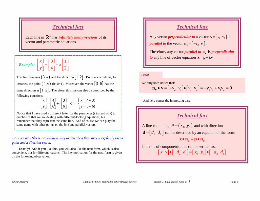
Technical fact

Each line in 2

has infinitely many versions of its

vector and parametric equations.

Example: 3 1

4 2

xk

y

This line contains 3, 4 and has direction 1 2 . But it also contains, for

instance, the point 4, 6 (let k=1). Moreover, the vector 3 6 has the

same direction as 1 2 . Therefore, this line can also be described by the

following equations:

4 3 4 3

6 6 6 6

x x tt

y y t

Notice that I have used a different letter for the parameter (t instead of k) to

emphasize that we are dealing with different-looking equations, but

remember that they represent the same line. And of course we can play the

same game with other points on the line and parallel vectors.

I can see why this is a convenient way to describe a line, since it explicitly uses a point and a direction vector.

Exactly! And if you like this, you will also like the next form, which is also

convenient, but for different reasons. The key motivation for the next form is given

by the following observation:

Technical fact

Any vector perpendicular to a vector 1 2v vv is

parallel to the vector 2 1v v vn .

Therefore, any vector parallel to vn is perpendicular

to any line of vector equation k x p v .

Proof

We only need notice that:

2 1 1 2 2 1 1 2 0v v v v v v v v vn v

And here comes the interesting part.

Technical fact

A line containing 0 0,P x y and with direction

1 2d dd can be described by an equation of the form:

d dx n p n

In terms of components, this can be written as:

2 1 0 0 2 1x y d d x y d d


Proof

We need to check two things:

Every point on the line satisfies the given equation.

Every point that satisfies the given equation is on the line.

For the first item, if ,X x y is a point on the line, then there is a value of

k for which k x p d . If we dot product both sides by the perpendicular

vector dn we get:

0k k d d d d dx n p d n p n d n p n

This shows that the given equation is satisfied.

On the other hand, if x yx satisfies the given equation, then, by using

the distributivity of the dot product we can see that:

0 d d dx n p n x p n

This means that the vector x-p is perpendicular to the perpendicular vector

and hence is parallel to d. Therefore:

k k x p d x p d

so that the point X is on the line.

This deserves a definition.

Definition

The equation d dx n p n is called the normal

equation of the line containing 0 0x yp and

with direction 1 2d dd .

Example: 3 1

4 2

xk

y

This line contains 3, 4 and has direction 1 2 . Therefore, its normal

equation is:

2 3 2

1 4 1

x

y

This looks like a shrinking illusion: the equations are getting smaller!

That is part of the beauty of the normal equation: its being so short and its

hiding so much information behind it. For instance, the normal equation hides a

good old friend:

Technical fact

If 0 0x y a b x y a b is the normal

equation of a line, then its general equation is:

0 0 0ax by ax by

If 0ax by c is the general equation of a line,

then its normal equation can be written as:

0 /x y a b c b a b if 0b

or as:

/ 0x y a b c a a b if 0a


Proof

The first statement is clear once we compute the dot products involved.

For the second, if 0b , so that the line is not vertical, we can change the

general form to the slope-intercept form:

a cy x

b b

This means that its slope is a

b and hence its direction vector can be

chosen to be b a . But this means that the normal vector is a b .

Moreover, the point 0,c

b

is on the line and the normal equation

follows. A similar argument proves the second case.

This leads to a useful connection.

Knot on your finger

The coefficients of the general equation of a line are

the components of a vector normal to the line.

Example: 2

7 35

y x

This line contains 3, 7 , has slope 2

5m and slope-intercept form:

2 6 2 297

5 5 5 5y x x

Therefore, its general form is:

5 2 29 2 5 29y x x y

This means that one of its normal forms is

2 5 3 7 2 5x y

I see that the normal form is not unique either, eh?

Of course, since there are lots of options available when picking the reference

point and the normal vector.

To finish, let’s see a neat geometrical use of these equations.

Do you know how to compute the distance from a point to a line in 2

?

Let’s see, I can find the minimum of the distance function by using calculus…

You certainly can and there are other convoluted ways of doing it, but here is a

very simple method based on the linear algebra formulae we have seen so far.

Technical fact

The distance from a point 0 0,P x y to a line

0ax by c is given by:

0 0

2 2

ax by cd

a b

Proof

The distance from 0 0,P x y to the line is, by definition, the length of

the perpendicular segment from P to the line, as shown in the following

picture.


But if we pick a point ,Q x y on the line – any point – and compute the

scalar projection of the vector v from Q to P onto the vector normal to the

line we get exactly such length. Here is the picture:

We know that 0 0x x y y v and that a bn . Therefore:

0 0

2 2proj

x x y y a b

a b

n

v nv

n

0 0

2 2

ax ax by by

a b

Since Q is on the line we know that:

0ax by c c ax by

and therefore:

0 0 0 0

2 2 2 2proj

ax by ax by ax by c

a b a b

nv

as claimed.

Example: 3 5y x

To find the distance from the point (2, 4) to this line we first rewrite it in

general form as 3 5 0x y and then apply the formula:

0 0

2 2 22

3 2 1 4 5 7

103 1

ax by cd

a b

Cool, but what does this all have to do with systems and matrices?

Lots: the connections become more apparent in higher dimensions, but they

start here. Remember that a system is obtained by considering several linear

equations at the same time. Well, what happens when we consider several lines at

the same time?

Knot on your finger

Given n lines in 2

of general equations:

,1i i ia x b y c i n

their common points of intersection are exactly the

solutions of the system whose augmented matrix is:

1 1 1

... ... ...

n n n

a b c

a b c

QP

n

v

P


Well, of course!

Maybe, but you may want to check that you are clear on this by addressing the

Learning question that asks you to explain why this is true. And here is the first

important consequence: this correspondence provides a first connection between

lines and systems.

Technical fact

The set consisting of the points of intersection of n

lines in 2

contains either:

no point, or

a single point, or

infinitely many points

Proof

This follows immediately from what we know about the number of solutions

of a system.

Here are some examples that highlight the correspondence between the number

of solutions of the system and the geometrical relation between the lines.

Example: 3 2 4x y and 2 14x y

The lines have one point of intersection, as is confirmed by checking the

number of solution of the system

1 2

3 2 4 3 2 4 1 2 14

2 14 1 2 14 3 2 4

x y

x y

R R

2 1

1 2 143

0 8 38

R R

Since the augmented matrix and the matrix

of coefficients have the same rank and this

equals the number of variables, there is a

unique solution, as expected.

We can clearly see this in the graph as well

Can you find the coordinates of this

intersection?

Example: 3 5 5, 3 3 52 1, 05 0x y xx yy

The graph of these three lines suggests that

they are parallel and their slopes confirm

this. The matrix of coefficients has three

equal rows, two of which can be eliminated

when using Gauss-Jordan, but the constants

are not the same, thus creating a leading

coefficient in the last column: no solutions,

as expected.

However, let us consider these three

equations, which are very similar to the

previous ones:

3 5 5, 6 10 10, 5 3 5x y x y y x

This time we notice that the equations are multiples of each other and hence

identify the same line. The augmented matrix of the corresponding system

has an REF with a single non-zero row, hence one free variable and infinitely

many solutions: all the points of the line! This is a degenerate case, but it will

become more meaningful in higher dimensions.

But now, let us look at a different situation, which contains a detail that tends ot

trick some students into error.


Example: 3 528 432, 1 0, 2x yx y x y

These equations identify the three lines shown here.

The augmented matrix is as follows:

2 1

3 1

1 8 32 1 8 32

1 2 14 0 6 183

3 5 20 0 29 116

R R

R R

The last two rows are not multiples of each other and hence will generate a

leading coefficient in the last column: no solutions.

But wait a minute: don’t we see three points of intersection? CAREFUL!

We are looking for points that are common to ALL lines, not just two of

them. And there is no point that belongs to all three lines.

That’s enough material for one section: make sure to digest it properly before

moving on to the next one and some interesting generalizations.

Summary

By using vector notation, we can devise additional ways to identify a line through an equation.

There are several such notations (especially vector, normal and parametric) and each of them highlights a particular feature of the line.

By using linear systems, we can identify the points of intersection that are common to a set of lines.

Common errors to avoid

Make sure to distinguish among the different types of equations of lines and their visible features. Mixing them up can easily lead to errors of interpretation and computation.


Learning questions for Section LA 6-1

Review questions:

1. Describe the different types of equations for a line in 2 .

2. Identify the features of a line that are explicitly present in each

type of equation of a line.

3. For each type of equation, identify one advantage and one

disadvantage.

4. Explain the relation between the components of the normal vector

of a line and the coefficients of the general equation of that line.

Memory questions:

1. What is the general form of the slope-intercept equation of a line in 2 ?

2. What is the general form of the point-slope equation of a line in 2 ?

3. What is the general form of the two-point equation of a line in 2 ?

4. What is the general form of the general equation of a line in 2 ?

5. What is the general form of the vector equation of a line in 2 ?

6. What is the general form of the parametric equation of a line in 2 ?

7. What is the general form of the normal equation of a line in 2 ?

Computation questions:

1. For the line containing the point 2, 5 and having slope 4

3, construct:

a) The point-slope equation

b) The general equation

c) The normal equation

d) The vector equation

e) The parametric equations

2. Given the line of equations 1

2 42

y x , determine:

a) The coordinates of a point p on the line

b) The components of a direction vector d

c) The value of the coefficient k for which 8, 7 k p d

3. Find the intersection of the lines 3 2 1x y and 3 5x y


4. For each of the following systems, describe the geometric interpretation of each

equation and of the solution set of the system.

a) 5 2 8

3 6 2

x y

x y

b) 5 2 8

5 2 2

x y

x y

c) 5 2 8

10 4 16

x y

x y

5. Use a linear algebra method to compute the distance from the point 2,1 to

the line 3 2y x .

Theory questions:

1. When two equations represent two non-parallel lines in R2, what does the

solution of the system consisting of those equations represent?

2. When two equations represent two parallel lines in R2, what does the solution of

the system consisting of those equations represent?

3. When two equations representing two lines in R2 are multiples of each other,

what do the solutions of the system consisting of those equations represent?

4. Why are the slope-intercept and the point-slope equations not suitable for

vertical lines?

Proof questions:

1. Prove that the equations of a line provided in this section are consistent with the usual definition of a line, in the sense that the slope between any two points that satisfy any

one of those equations is always the same.


Templated questions:

1. Pick a point and a direction vector and construct the equation of the

corresponding line in all forms seen in this section.

2. Construct the general equations of two lines and find their point of intersection,

if any.

3. Pick a point and a line and compute the distance between the two.

4. Construct the equation of a line in any of the forms seen in this section and from

it construct the other forms.

What questions do you have for your instructor?

roberto’s notes on linear algebra chapter 6: lines, … · linear algebra chapter 6: lines,...

Documents