robert j. vanderbei linear programmingmath.uchicago.edu/.../vanderbei_linear-programming... ·...
TRANSCRIPT

International Series in Operations Research & Management Science
Robert J. Vanderbei
Foundations and Extensions
Fourth Edition
Linear Programming

International Series in OperationsResearch & Management Science
Volume 196
Series Editor
Frederick S. HillierStanford University, CA, USA
Special Editorial Consultant
Camille C. PriceStephen F. Austin State University, TX, USA
For further volumes:http://www.springer.com/series/6161

Robert J. Vanderbei
Linear Programming
Foundations and Extensions
Fourth Edition
123

Robert J. VanderbeiDepartment of Operations Research
and Financial EngineeringPrinceton UniversityPrinceton, New Jersey, USA
ISSN 0884-8289ISBN 978-1-4614-7629-0 ISBN 978-1-4614-7630-6 (eBook)DOI 10.1007/978-1-4614-7630-6Springer New York Heidelberg Dordrecht London
Library of Congress Control Number: 2013939593
© Springer Science+Business Media New York 2014This work is subject to copyright. All rights are reserved by the Publisher, whether the whole or part ofthe material is concerned, specifically the rights of translation, reprinting, reuse of illustrations, recitation,broadcasting, reproduction on microfilms or in any other physical way, and transmission or informationstorage and retrieval, electronic adaptation, computer software, or by similar or dissimilar methodologynow known or hereafter developed. Exempted from this legal reservation are brief excerpts in connectionwith reviews or scholarly analysis or material supplied specifically for the purpose of being enteredand executed on a computer system, for exclusive use by the purchaser of the work. Duplication ofthis publication or parts thereof is permitted only under the provisions of the Copyright Law of thePublisher’s location, in its current version, and permission for use must always be obtained from Springer.Permissions for use may be obtained through RightsLink at the Copyright Clearance Center. Violationsare liable to prosecution under the respective Copyright Law.The use of general descriptive names, registered names, trademarks, service marks, etc. in this publica-tion does not imply, even in the absence of a specific statement, that such names are exempt from therelevant protective laws and regulations and therefore free for general use.While the advice and information in this book are believed to be true and accurate at the date of pub-lication, neither the authors nor the editors nor the publisher can accept any legal responsibility for anyerrors or omissions that may be made. The publisher makes no warranty, express or implied, with respectto the material contained herein.
Printed on acid-free paper
Springer is part of Springer Science+Business Media (www.springer.com)

To Krisadee,Marisa and Diana

Preface
This book is about constrained optimization. It begins with a thorough treat-ment of linear programming and proceeds to convex analysis, network flows, integerprogramming, quadratic programming, and convex optimization. Along the way,dynamic programming and the linear complementarity problem are touched on aswell.
The book aims to be a first introduction to the subject. Specific examples andconcrete algorithms precede more abstract topics. Nevertheless, topics covered aredeveloped in some depth, a large number of numerical examples are worked outin detail, and many recent topics are included, most notably interior-point methods.The exercises at the end of each chapter both illustrate the theory and, in some cases,extend it.
Prerequisites. The book is divided into four parts. The first two parts assumea background only in linear algebra. For the last two parts, some knowledge ofmultivariate calculus is necessary. In particular, the student should know how to useLagrange multipliers to solve simple calculus problems in 2 and 3 dimensions.
Associated software. It is good to be able to solve small problems by hand,but the problems one encounters in practice are large, requiring a computer for theirsolution. Therefore, to fully appreciate the subject, one needs to solve large (prac-tical) problems on a computer. An important feature of this book is that it comeswith software implementing the major algorithms described herein. At the time ofwriting, software for the following five algorithms is available:
• The two-phase simplex method as shown in Figure 6.1.• The self-dual simplex method as shown in Figure 7.1.• The path-following method as shown in Figure 18.1.• The homogeneous self-dual method as shown in Figure 22.1.• The long-step homogeneous self-dual method as described in Exercise
22.4.
The programs that implement these algorithms are written in C and can beeasily compiled on most hardware platforms. Students/instructors are encouragedto install and compile these programs on their local hardware. Great pains havebeen taken to make the source code for these programs readable (see Appendix A).In particular, the names of the variables in the programs are consistent with thenotation of this book.
vii
viii PREFACE
There are two ways to run these programs. The first is to prepare the input ina standard computer-file format, called MPS format, and to run the program usingsuch a file as input. The advantage of this input format is that there is an archiveof problems stored in this format, called the NETLIB suite, that one can downloadand use immediately (a link to the NETLIB suite can be found at the web site men-tioned below). But, this format is somewhat archaic and, in particular, it is not easyto create these files by hand. Therefore, the programs can also be run from within aproblem modeling system called AMPL. AMPL allows one to describe mathemat-ical programming problems using an easy to read, yet concise, algebraic notation.To run the programs within AMPL, one simply tells AMPL the name of the solver-program before asking that a problem be solved. The text that describes AMPL,Fourer et al. (1993) makes an excellent companion to this book. It includes a dis-cussion of many practical linear programming problems. It also has lots of exercisesto hone the modeling skills of the student.
Several interesting computer projects can be suggested. Here are a few sugges-tions regarding the simplex codes:
• Incorporate the partial pricing strategy (see Section 8.7) into the two-phase simplex method and compare it with full pricing.
• Incorporate the steepest-edge pivot rule (see Section 8.8) into the two-phase simplex method and compare it with the largest-coefficient rule.
• Modify the code for either variant of the simplex method so that it cantreat bounds and ranges implicitly (see Chapter 9), and compare the per-formance with the explicit treatment of the supplied codes.
• Implement a “warm-start” capability so that the sensitivity analyses dis-cussed in Chapter 7 can be done.
• Extend the simplex codes to be able to handle integer programming prob-lems using the branch-and-bound method described in Chapter 23.
As for the interior-point codes, one could try some of the following projects:
• Modify the code for the path-following algorithm so that it implementsthe affine-scaling method (see Chapter 21), and then compare the twomethods.
• Modify the code for the path-following method so that it can treat boundsand ranges implicitly (see Section 20.3), and compare the performanceagainst the explicit treatment in the given code.
• Modify the code for the path-following method to implement the higher-order method described in Exercise 18.5. Compare.
• Extend the path-following code to solve quadratic programming problemsusing the algorithm shown in Figure 24.3.
• Further extend the code so that it can solve convex optimization problemsusing the algorithm shown in Figure 25.2.
And, perhaps the most interesting project of all:
• Compare the simplex codes against the interior-point code and decide foryourself which algorithm is better on specific families of problems.
PREFACE ix
The software implementing the various algorithms was developed using consistentdata structures and so making fair comparisons should be straightforward. The soft-ware can be downloaded from the following web site:
http://www.princeton.edu/∼rvdb/LPbook/
If, in the future, further codes relating to this text are developed (for example, aself-dual network simplex code), they will be made available through this web site.
Features. Here are some other features that distinguish this book from others:
• The development of the simplex method leads to Dantzig’s parametricself-dual method. A randomized variant of this method is shown to beimmune to the travails of degeneracy.
• The book gives a balanced treatment to both the traditional simplex methodand the newer interior-point methods. The notation and analysis is de-veloped to be consistent across the methods. As a result, the self-dualsimplex method emerges as the variant of the simplex method with mostconnections to interior-point methods.
• From the beginning and consistently throughout the book, linear program-ming problems are formulated in symmetric form. By highlighting sym-metry throughout, it is hoped that the reader will more fully understandand appreciate duality theory.
• By slightly changing the right-hand side in the Klee–Minty problem, weare able to write down an explicit dictionary for each vertex of the Klee–Minty problem and thereby uncover (as a homework problem) a simple,elegant argument why the Klee-Minty problem requires 2n − 1 pivots tosolve.
• The chapter on regression includes an analysis of the expected numberof pivots required by the self-dual variant of the simplex method. Thisanalysis is supported by an empirical study.
• There is an extensive treatment of modern interior-point methods, includ-ing the primal–dual method, the affine-scaling method, and the self-dualpath-following method.
• In addition to the traditional applications, which come mostly from busi-ness and economics, the book features other important applications suchas the optimal design of truss-like structures and L1-regression.
Exercises on the Web. There is always a need for fresh exercises. Hence, I havecreated and plan to maintain a growing archive of exercises specifically created foruse in conjunction with this book. This archive is accessible from the book’s website:
http://www.princeton.edu/∼rvdb/LPbook/
The problems in the archive are arranged according to the chapters of this book anduse notation consistent with that developed herein.
Advice on solving the exercises. Some problems are routine while others arefairly challenging. Answers to some of the problems are given at the back of the book.

x PREFACE
In general, the advice given to me by Leonard Gross (when I was a student) shouldhelp even on the hard problems: follow your nose.
Audience. This book evolved from lecture notes developed for my introductorygraduate course in linear programming as well as my upper-level undergraduatecourse. A reasonable undergraduate syllabus would cover essentially all of Part 1(Simplex Method and Duality), the first two chapters of Part 2 (Network Flowsand Applications), and the first chapter of Part 4 (Integer Programming). At thegraduate level, the syllabus should depend on the preparation of the students. For awell-prepared class, one could cover the material in Parts 1 and 2 fairly quickly andthen spend more time on Parts 3 (Interior-Point Methods) and 4 (Extensions).
Dependencies. In general, Parts 2 and 3 are completely independent of eachother. Both depend, however, on the material in Part 1. The first Chapter in Part 4(Integer Programming) depends only on material from Part 1, whereas the remainingchapters build on Part 3 material.
Acknowledgments. My interest in linear programming was sparked by RobertGarfinkel when we shared an office at Bell Labs. I would like to thank him forhis constant encouragement, advice, and support. This book benefited greatly fromthe thoughtful comments and suggestions of David Bernstein and Michael Todd. Iwould also like to thank the following colleagues for their help: Ronny Ben-Tal,Leslie Hall, Yoshi Ikura, Victor Klee, Irvin Lustig, Avi Mandelbaum, Marc Meke-ton, Narcis Nabona, James Orlin, Andrzej Ruszczynski, and Henry Wolkowicz. Iwould like to thank Gary Folven at Kluwer and Fred Hillier, the series editor, forencouraging me to undertake this project. I would like to thank my students forfinding many typos and occasionally more serious errors: John Gilmartin, JacintaWarnie, Stephen Woolbert, Lucia Wu, and Bing Yang. My thanks to Erhan Cınlarfor the many times he offered advice on questions of style. I hope this book re-flects positively on his advice. Finally, I would like to acknowledge the support ofthe National Science Foundation and the Air Force Office of Scientific Researchfor supporting me while writing this book. In a time of declining resources, I amespecially grateful for their support.
Princeton, NJ, USA Robert J. Vanderbei
Preface to 2nd Edition
For the 2nd edition, many new exercises have been added. Also I have workedhard to develop online tools to aid in learning the simplex method and duality theory.These online tools can be found on the book’s web page:
http://www.princeton.edu/∼rvdb/LPbook/
and are mentioned at appropriate places in the text. Besides the learning tools, I havecreated several online exercises. These exercises use randomly generated problemsand therefore represent a virtually unlimited collection of “routine” exercises thatcan be used to test basic understanding. Pointers to these online exercises are in-cluded in the exercises sections at appropriate points.
Some other notable changes include:
• The chapter on network flows has been completely rewritten. Hopefully,the new version is an improvement on the original.
• Two different fonts are now used to distinguish between the set of basicindices and the basis matrix.
• The first edition placed great emphasis on the symmetry between the pri-mal and the dual (the negative transpose property). The second editioncarries this further with a discussion of the relationship between the basicand nonbasic matrices B and N as they appear in the primal and in thedual. We show that, even though these matrices differ (they even havedifferent dimensions), B−1N in the dual is the negative transpose of thecorresponding matrix in the primal.
• In the chapters devoted to the simplex method in matrix notation, the col-lection of variables z1, z2, . . . , zn, y1, y2, . . . , ym was replaced, in the firstedition, with the single array of variables y1, y2, . . . , yn+m. This causedgreat confusion as the variable yi in the original notation was changedto yn+i in the new notation. For the second edition, I have changed thenotation for the single array to z1, z2, . . . , zn+m.
• A number of figures have been added to the chapters on convex analysisand on network flow problems.
• The algorithm refered to as the primal–dual simplex method in the firstedition has been renamed the parametric self-dual simplex method in ac-cordance with prior standard usage.
xi

xii PREFACE TO 2ND EDITION
• The last chapter, on convex optimization, has been extended with a dis-cussion of merit functions and their use in shortenning steps to make someotherwise nonconvergent problems converge.
Acknowledgments. Many readers have sent corrections and suggestions forimprovement. Many of the corrections were incorporated into earlier reprintings.Only those that affected pagination were accrued to this new edition. Even thoughI cannot now remember everyone who wrote, I am grateful to them all. Some sentcomments that had significant impact. They were Hande Benson, Eric Denardo,Sudhakar Mandapati, Michael Overton, and Jos Sturm.
Princeton, NJ, USA Robert J. Vanderbei

Preface to 3rd Edition
It has been almost 7 years since the 2nd edition appeared and the publisher isitching for me to finish a new edition. The previous edition had very few typos. Ihave fixed them all! Of course, I’ve also added some new material and who knowshow many new typos I’ve introduced. The most significant new material is con-tained in a new chapter on financial applications, which discusses a linear program-ming variant of the portfolio selection problem and option pricing. I am grateful toAlex d’Aspremont for pointing out that the option pricing problem provides a niceapplication of duality theory. Finally, I’d like to acknowledge the fact that half (fourout of eight) of the typos were reported to me by Trond Steihaug. Thanks Trond!
Princeton, NJ, USA Robert J. Vanderbei
xiii

Preface to 4th Edition
Besides the ongoing tweaking and refining of the language and presentation ofthe material, this edition also features new material in Chapters 4 and 12 on theaverage performance of the simplex method.
I’d like to thank Cagin Ararat and Firdevs Ulus for carefully reviewing andcommenting on this new material.
Princeton, NJ, USA Robert J. Vanderbei
xv
Contents
Preface vii
Preface to 2nd Edition xi
Preface to 3rd Edition xiii
Preface to 4th Edition xv
Part 1. Basic Theory: The Simplex Method and Duality 1
Chapter 1. Introduction 31. Managing a Production Facility 32. The Linear Programming Problem 5Exercises 7Notes 9
Chapter 2. The Simplex Method 111. An Example 112. The Simplex Method 143. Initialization 164. Unboundedness 185. Geometry 19Exercises 20Notes 23
Chapter 3. Degeneracy 251. Definition of Degeneracy 252. Two Examples of Degenerate Problems 253. The Perturbation/Lexicographic Method 284. Bland’s Rule 315. Fundamental Theorem of Linear Programming 336. Geometry 33Exercises 36Notes 37
xvii

xviii CONTENTS
Chapter 4. Efficiency of the Simplex Method 391. Performance Measures 392. Measuring the Size of a Problem 393. Measuring the Effort to Solve a Problem 404. Worst-Case Analysis of the Simplex Method 415. Empirical Average Performance of the Simplex Method 44Exercises 50Notes 52
Chapter 5. Duality Theory 531. Motivation: Finding Upper Bounds 532. The Dual Problem 543. The Weak Duality Theorem 554. The Strong Duality Theorem 575. Complementary Slackness 636. The Dual Simplex Method 647. A Dual-Based Phase I Algorithm 668. The Dual of a Problem in General Form 679. Resource Allocation Problems 6910. Lagrangian Duality 72Exercises 73Notes 79
Chapter 6. The Simplex Method in Matrix Notation 811. Matrix Notation 812. The Primal Simplex Method 833. An Example 864. The Dual Simplex Method 905. Two-Phase Methods 926. Negative Transpose Property 93Exercises 95Notes 97
Chapter 7. Sensitivity and Parametric Analyses 991. Sensitivity Analysis 992. Parametric Analysis and the Homotopy Method 1023. The Parametric Self-Dual Simplex Method 105Exercises 107Notes 109
Chapter 8. Implementation Issues 1111. Solving Systems of Equations: LU -Factorization 1112. Exploiting Sparsity 1153. Reusing a Factorization 1194. Performance Tradeoffs 1235. Updating a Factorization 124
CONTENTS xix
6. Shrinking the Bump 1277. Partial Pricing 1288. Steepest Edge 129Exercises 131Notes 132
Chapter 9. Problems in General Form 1331. The Primal Simplex Method 1332. The Dual Simplex Method 135Exercises 140Notes 140
Chapter 10. Convex Analysis 1411. Convex Sets 1412. Caratheodory’s Theorem 1433. The Separation Theorem 1444. Farkas’ Lemma 1465. Strict Complementarity 147Exercises 149Notes 150
Chapter 11. Game Theory 1511. Matrix Games 1512. Optimal Strategies 1533. The Minimax Theorem 1554. Poker 157Exercises 161Notes 163
Chapter 12. Regression 1651. Measures of Mediocrity 1652. Multidimensional Measures: Regression Analysis 1673. L2-Regression 1684. L1-Regression 1705. Iteratively Reweighted Least Squares 1716. An Example: How Fast Is the Simplex Method? 173Exercises 178Notes 183
Chapter 13. Financial Applications 1851. Portfolio Selection 1852. Option Pricing 190Exercises 194Notes 195

xx CONTENTS
Part 2. Network-Type Problems 197
Chapter 14. Network Flow Problems 1991. Networks 1992. Spanning Trees and Bases 2023. The Primal Network Simplex Method 2064. The Dual Network Simplex Method 2115. Putting It All Together 2146. The Integrality Theorem 215Exercises 216Notes 224
Chapter 15. Applications 2251. The Transportation Problem 2252. The Assignment Problem 2273. The Shortest-Path Problem 2284. Upper-Bounded Network Flow Problems 2315. The Maximum-Flow Problem 233Exercises 235Notes 239
Chapter 16. Structural Optimization 2411. An Example 2412. Incidence Matrices 2433. Stability 2444. Conservation Laws 2455. Minimum-Weight Structural Design 2496. Anchors Away 250Exercises 252Notes 254
Part 3. Interior-Point Methods 255
Chapter 17. The Central Path 257Warning: Nonstandard Notation Ahead 2571. The Barrier Problem 2572. Lagrange Multipliers 2593. Lagrange Multipliers Applied to the Barrier Problem 2624. Second-Order Information 2645. Existence 264Exercises 266Notes 267
CONTENTS xxi
Chapter 18. A Path-Following Method 2691. Computing Step Directions 2692. Newton’s Method 2703. Estimating an Appropriate Value for the Barrier Parameter 2724. Choosing the Step Length Parameter 2725. Convergence Analysis 274Exercises 279Notes 283
Chapter 19. The KKT System 2851. The Reduced KKT System 2852. The Normal Equations 2863. Step Direction Decomposition 288Exercises 290Notes 291
Chapter 20. Implementation Issues for Interior-Point Methods 2931. Factoring Positive Definite Matrices 2932. Quasidefinite Matrices 2963. Problems in General Form 302Exercises 307Notes 307
Chapter 21. The Affine-Scaling Method 3091. The Steepest Ascent Direction 3092. The Projected Gradient Direction 3113. The Projected Gradient Direction with Scaling 3124. Convergence 3165. Feasibility Direction 3176. Problems in Standard Form 319Exercises 320Notes 321
Chapter 22. The Homogeneous Self-Dual Method 3231. From Standard Form to Self-Dual Form 3232. Homogeneous Self-Dual Problems 3243. Back to Standard Form 3344. Simplex Method vs. Interior-Point Methods 336Exercises 339Notes 341
Part 4. Extensions 343
Chapter 23. Integer Programming 3451. Scheduling Problems 345

xxii CONTENTS
2. The Traveling Salesman Problem 3463. Fixed Costs 3494. Nonlinear Objective Functions 3505. Branch-and-Bound 351Exercises 361Notes 362
Chapter 24. Quadratic Programming 3631. The Markowitz Model 3632. The Dual 3673. Convexity and Complexity 3704. Solution via Interior-Point Methods 3735. Practical Considerations 374Exercises 376Notes 378
Chapter 25. Convex Programming 3791. Differentiable Functions and Taylor Approximations 3792. Convex and Concave Functions 3803. Problem Formulation 3804. Solution via Interior-Point Methods 3815. Successive Quadratic Approximations 3826. Merit Functions 3837. Parting Words 385Exercises 385Notes 388
Erratum E1
Appendix A. Source Listings 3891. The Self-Dual Simplex Method 3902. The Homogeneous Self-Dual Method 393
Answers to Selected Exercises 395
Bibliography 399
Index 407
Part 1
Basic Theory: The Simplex Methodand Duality

We all love to instruct, though we can teach onlywhat is not worth knowing. — J. Austen

CHAPTER 1
Introduction
This book is mostly about a subject called Linear Programming. Before definingwhat we mean, in general, by a linear programming problem, let us describe a fewpractical real-world problems that serve to motivate and at least vaguely to definethis subject.
1. Managing a Production Facility
Consider a production facility for a manufacturing company. The facility iscapable of producing a variety of products that, for simplicity, we enumerate as1, 2, . . . , n. These products are constructed/manufactured/produced out of certainraw materials. Suppose that there are m different raw materials, which again wesimply enumerate as 1, 2, . . . ,m. The decisions involved in managing/operating thisfacility are complicated and arise dynamically as market conditions evolve aroundit. However, to describe a simple, fairly realistic optimization problem, we considera particular snapshot of the dynamic evolution. At this specific point in time, thefacility has, for each raw material i = 1, 2, . . . ,m, a known amount, say bi, onhand. Furthermore, each raw material has at this moment in time a known unitmarket value. We denote the unit value of the ith raw material by ρi.
In addition, each product is made from known amounts of the various raw ma-terials. That is, producing one unit of product j requires a certain known amount,say aij units, of raw material i. Also, the jth final product can be sold at the knownprevailing market price of σj dollars per unit.
Throughout this section we make an important assumption:
The production facility is small relative to the market as a wholeand therefore cannot through its actions alter the prevailing mar-ket value of its raw materials, nor can it affect the prevailingmarket price for its products.
We consider two optimization problems related to the efficient operation of thisfacility (later, in Chapter 5, we will see that these two problems are in fact closelyrelated to each other).
1.1. Production Manager as Optimist. The first problem we wish to consideris the one faced by the company’s production manager. It is the problem of how touse the raw materials on hand. Let us assume that she decides to produce xj unitsof the jth product, j = 1, 2, . . . , n. The revenue associated with the production ofone unit of product j is σj . But there is also a cost of raw materials that must be
R.J. Vanderbei, Linear Programming, International Series in Operations Research& Management Science 196, DOI 10.1007/978-1-4614-7630-6 1,© Springer Science+Business Media New York 2014
3

4 1. INTRODUCTION
considered. The cost of producing one unit of product j is∑m
i=1 ρiaij . Therefore,the net revenue associated with the production of one unit is the difference betweenthe revenue and the cost. Since the net revenue plays an important role in our model,we introduce notation for it by setting
cj = σj −m∑
i=1
ρiaij , j = 1, 2, . . . , n.
Now, the net revenue corresponding to the production of xj units of product j issimply cjxj , and the total net revenue is
(1.1)n∑
j=1
cjxj .
The production planner’s goal is to maximize this quantity. However, there are con-straints on the production levels that she can assign. For example, each productionquantity xj must be nonnegative, and so she has the constraints
(1.2) xj ≥ 0, j = 1, 2, . . . , n.
Secondly, she can’t produce more product than she has raw material for. The amountof raw material i consumed by a given production schedule is
∑nj=1 aijxj , and so
she must adhere to the following constraints:
(1.3)n∑
j=1
aijxj ≤ bi i = 1, 2, . . . ,m.
To summarize, the production manager’s job is to determine production values xj ,j = 1, 2, . . . , n, so as to maximize (1.1) subject to the constraints given by (1.2) and(1.3). This optimization problem is an example of a linear programming problem.This particular example is often called the resource allocation problem.
1.2. Comptroller as Pessimist. In another office at the production facilitysits an executive called the comptroller. The comptroller’s problem (among others)is to assign a value to the raw materials on hand. These values are needed foraccounting and planning purposes to determine the cost of inventory. There arerules about how these values can be set. The most important such rule (and the onlyone relevant to our discussion) is the following:
The company must be willing to sell the raw materials shouldan outside firm offer to buy them at a price consistent with thesevalues.
Let wi denote the assigned unit value of the ith raw material, i = 1, 2, . . . ,m.That is, these are the numbers that the comptroller must determine. The lost oppor-tunity cost of having bi units of raw material i on hand is biwi, and so the total lostopportunity cost is
(1.4)m∑
i=1
biwi.
2. THE LINEAR PROGRAMMING PROBLEM 5
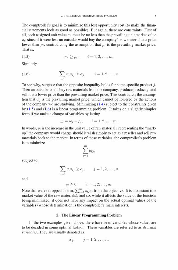
The comptroller’s goal is to minimize this lost opportunity cost (to make the finan-cial statements look as good as possible). But again, there are constraints. First ofall, each assigned unit value wi must be no less than the prevailing unit market valueρi, since if it were less an outsider would buy the company’s raw material at a pricelower than ρi, contradicting the assumption that ρi is the prevailing market price.That is,
(1.5) wi ≥ ρi, i = 1, 2, . . . ,m.
Similarly,
(1.6)m∑
i=1
wiaij ≥ σj , j = 1, 2, . . . , n.
To see why, suppose that the opposite inequality holds for some specific product j.Then an outsider could buy raw materials from the company, produce product j, andsell it at a lower price than the prevailing market price. This contradicts the assump-tion that σj is the prevailing market price, which cannot be lowered by the actionsof the company we are studying. Minimizing (1.4) subject to the constraints givenby (1.5) and (1.6) is a linear programming problem. It takes on a slightly simplerform if we make a change of variables by letting
yi = wi − ρi, i = 1, 2, . . . ,m.
In words, yi is the increase in the unit value of raw material i representing the “mark-up” the company would charge should it wish simply to act as a reseller and sell rawmaterials back to the market. In terms of these variables, the comptroller’s problemis to minimize
m∑
i=1
biyi
subject tom∑
i=1
yiaij ≥ cj , j = 1, 2, . . . , n
andyi ≥ 0, i = 1, 2, . . . ,m.
Note that we’ve dropped a term,∑m
i=1 biρi, from the objective. It is a constant (themarket value of the raw materials), and so, while it affects the value of the functionbeing minimized, it does not have any impact on the actual optimal values of thevariables (whose determination is the comptroller’s main interest).
2. The Linear Programming Problem
In the two examples given above, there have been variables whose values areto be decided in some optimal fashion. These variables are referred to as decisionvariables. They are usually denoted as
xj , j = 1, 2, . . . , n.

6 1. INTRODUCTION
In linear programming, the objective is always to maximize or to minimize somelinear function of these decision variables
ζ = c1x1 + c2x2 + · · ·+ cnxn.
This function is called the objective function. It often seems that real-world prob-lems are most naturally formulated as minimizations (since real-world planners al-ways seem to be pessimists), but when discussing mathematics it is usually nicer towork with maximization problems. Of course, converting from one to the other istrivial both from the modeler’s viewpoint (either minimize cost or maximize profit)and from the analyst’s viewpoint (either maximize ζ or minimize −ζ). Since thisbook is primarily about the mathematics of linear programming, we usually take theoptimist’s view of maximizing the objective function.
In addition to the objective function, the examples also had constraints. Someof these constraints were really simple, such as the requirement that some decisionvariable be nonnegative. Others were more involved. But in all cases the constraintsconsisted of either an equality or an inequality associated with some linear combi-nation of the decision variables:
a1x1 + a2x2 + · · ·+ anxn
⎧⎨
⎩
≤=≥
⎫⎬
⎭b.
It is easy to convert constraints from one form to another. For example, aninequality constraint
a1x1 + a2x2 + · · ·+ anxn ≤ b
can be converted to an equality constraint by adding a nonnegative variable, w,which we call a slack variable:
a1x1 + a2x2 + · · ·+ anxn + w = b, w ≥ 0.
On the other hand, an equality constraint
a1x1 + a2x2 + · · ·+ anxn = b
can be converted to inequality form by introducing two inequality constraints:
a1x1 + a2x2 + · · ·+ anxn ≤ b
a1x1 + a2x2 + · · ·+ anxn ≥ b.
Hence, in some sense, there is no a priori preference for how one poses the con-straints (as long as they are linear, of course). However, we shall also see that, froma mathematical point of view, there is a preferred presentation. It is to pose theinequalities as less-thans and to stipulate that all the decision variables be nonnega-tive. Hence, the linear programming problem, as we study it, can be formulated asfollows:
maximize c1x1 + c2x2 + · · ·+ cnxn
subject to a11x1 + a12x2 + · · ·+ a1nxn ≤ b1a21x1 + a22x2 + · · ·+ a2nxn ≤ b2
...am1x1 + am2x2 + · · ·+ amnxn ≤ bm
x1, x2, . . . xn ≥ 0.
EXERCISES 7
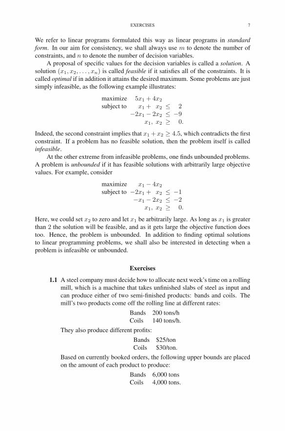
We refer to linear programs formulated this way as linear programs in standardform. In our aim for consistency, we shall always use m to denote the number ofconstraints, and n to denote the number of decision variables.
A proposal of specific values for the decision variables is called a solution. Asolution (x1, x2, . . . , xn) is called feasible if it satisfies all of the constraints. It iscalled optimal if in addition it attains the desired maximum. Some problems are justsimply infeasible, as the following example illustrates:
maximize 5x1 + 4x2
subject to x1 + x2 ≤ 2−2x1 − 2x2 ≤ −9
x1, x2 ≥ 0.
Indeed, the second constraint implies that x1+x2 ≥ 4.5, which contradicts the firstconstraint. If a problem has no feasible solution, then the problem itself is calledinfeasible.
At the other extreme from infeasible problems, one finds unbounded problems.A problem is unbounded if it has feasible solutions with arbitrarily large objectivevalues. For example, consider
maximize x1 − 4x2
subject to −2x1 + x2 ≤ −1−x1 − 2x2 ≤ −2
x1, x2 ≥ 0.
Here, we could set x2 to zero and let x1 be arbitrarily large. As long as x1 is greaterthan 2 the solution will be feasible, and as it gets large the objective function doestoo. Hence, the problem is unbounded. In addition to finding optimal solutionsto linear programming problems, we shall also be interested in detecting when aproblem is infeasible or unbounded.
Exercises
1.1 A steel company must decide how to allocate next week’s time on a rollingmill, which is a machine that takes unfinished slabs of steel as input andcan produce either of two semi-finished products: bands and coils. Themill’s two products come off the rolling line at different rates:
Bands 200 tons/hCoils 140 tons/h.
They also produce different profits:
Bands $25/tonCoils $30/ton.
Based on currently booked orders, the following upper bounds are placedon the amount of each product to produce:
Bands 6,000 tonsCoils 4,000 tons.

8 1. INTRODUCTION
Given that there are 40 h of production time available this week, the prob-lem is to decide how many tons of bands and how many tons of coilsshould be produced to yield the greatest profit. Formulate this problemas a linear programming problem. Can you solve this problem by inspec-tion?
1.2 A small airline, Ivy Air, flies between three cities: Ithaca, Newark, andBoston. They offer several flights but, for this problem, let us focus onthe Friday afternoon flight that departs from Ithaca, stops in Newark, andcontinues to Boston. There are three types of passengers:(a) Those traveling from Ithaca to Newark.(b) Those traveling from Newark to Boston.(c) Those traveling from Ithaca to Boston.
The aircraft is a small commuter plane that seats 30 passengers. The air-line offers three fare classes:(a) Y class: full coach.(b) B class: nonrefundable.(c) M class: nonrefundable, 3-week advanced purchase.
Ticket prices, which are largely determined by external influences (i.e.,competitors), have been set and advertised as follows:
Ithaca–Newark Newark–Boston Ithaca–BostonY 300 160 360B 220 130 280M 100 80 140
Based on past experience, demand forecasters at Ivy Air have determinedthe following upper bounds on the number of potential customers in eachof the nine possible origin-destination/fare-class combinations:
Ithaca–Newark Newark–Boston Ithaca–BostonY 4 8 3B 8 13 10M 22 20 18
The goal is to decide how many tickets from each of the nine origin/destination/fare-class combinations to sell. The constraints are that theplane cannot be overbooked on either of the two legs of the flight and thatthe number of tickets made available cannot exceed the forecasted maxi-mum demand. The objective is to maximize the revenue. Formulate thisproblem as a linear programming problem.
1.3 Suppose that Y is a random variable taking on one of n known values:
a1, a2, . . . , an.
Suppose we know that Y either has distribution p given by
P(Y = aj) = pj

NOTES 9
or it has distribution q given by
P(Y = aj) = qj .
Of course, the numbers pj , j = 1, 2, . . . , n are nonnegative and sum toone. The same is true for the qj’s. Based on a single observation of Y , wewish to guess whether it has distribution p or distribution q. That is, foreach possible outcome aj , we will assert with probability xj that the dis-tribution is p and with probability 1−xj that the distribution is q. We wishto determine the probabilities xj , j = 1, 2, . . . , n, such that the probabilityof saying the distribution is p when in fact it is q has probability no largerthan β, where β is some small positive value (such as 0.05). Furthermore,given this constraint, we wish to maximize the probability that we say thedistribution is p when in fact it is p. Formulate this maximization problemas a linear programming problem.
Notes
The subject of linear programming has its roots in the study of linear inequal-ities, which can be traced as far back as 1826 to the work of Fourier. Since then,many mathematicians have proved special cases of the most important result in thesubject—the duality theorem. The applied side of the subject got its start in 1939when L.V. Kantorovich noted the practical importance of a certain class of linearprogramming problems and gave an algorithm for their solution—see Kantorovich(1960). Unfortunately, for several years, Kantorovich’s work was unknown in theWest and unnoticed in the East. The subject really took off in 1947 when G.B.Dantzig invented the simplex method for solving the linear programming problemsthat arose in U.S. Air Force planning problems. The earliest published accountsof Dantzig’s work appeared in 1951 (Dantzig 1951a,b). His monograph (Dantzig1963) remains an important reference. In the same year that Dantzig invented thesimplex method, T.C. Koopmans showed that linear programming provided the ap-propriate model for the analysis of classical economic theories. In 1975, the RoyalSwedish Academy of Sciences awarded the Nobel Prize in economic science toL.V. Kantorovich and T.C. Koopmans “for their contributions to the theory of opti-mum allocation of resources.” Apparently the academy regarded Dantzig’s workas too mathematical for the prize in economics (and there is no Nobel Prize inmathematics).
The textbooks by Bradley et al. (1977), Bazaraa et al. (1977), and Hillier andLieberman (1977) are known for their extensive collections of interesting practicalapplications.
CHAPTER 2
The Simplex Method
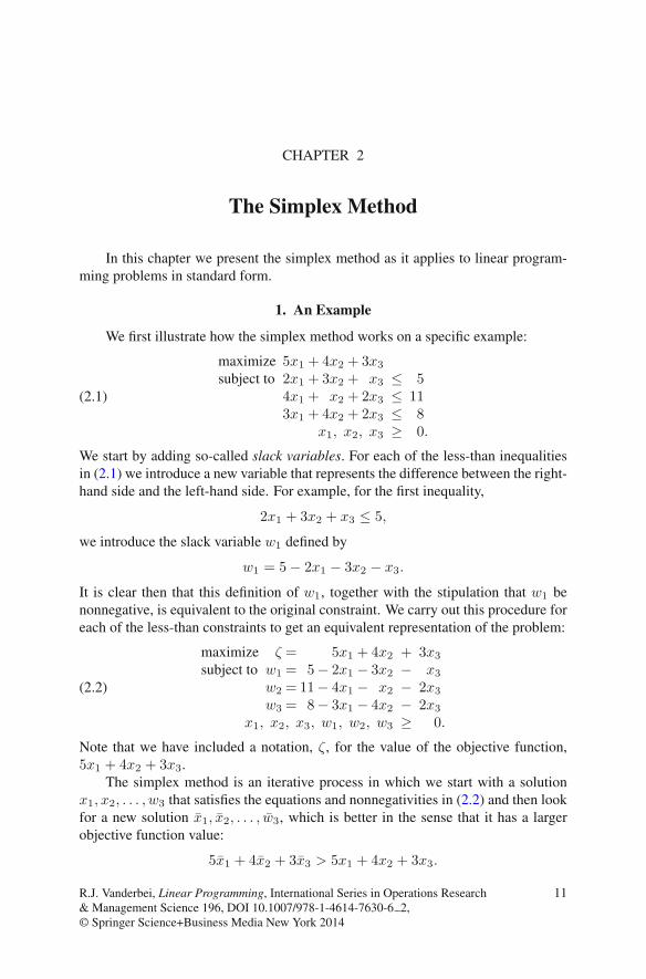
In this chapter we present the simplex method as it applies to linear program-ming problems in standard form.
1. An Example
We first illustrate how the simplex method works on a specific example:
(2.1)
maximize 5x1 + 4x2 + 3x3
subject to 2x1 + 3x2 + x3 ≤ 54x1 + x2 + 2x3 ≤ 113x1 + 4x2 + 2x3 ≤ 8
x1, x2, x3 ≥ 0.
We start by adding so-called slack variables. For each of the less-than inequalitiesin (2.1) we introduce a new variable that represents the difference between the right-hand side and the left-hand side. For example, for the first inequality,
2x1 + 3x2 + x3 ≤ 5,
we introduce the slack variable w1 defined by
w1 = 5− 2x1 − 3x2 − x3.
It is clear then that this definition of w1, together with the stipulation that w1 benonnegative, is equivalent to the original constraint. We carry out this procedure foreach of the less-than constraints to get an equivalent representation of the problem:
(2.2)
maximize ζ = 5x1 + 4x2 + 3x3
subject to w1 = 5− 2x1 − 3x2 − x3
w2 = 11− 4x1 − x2 − 2x3
w3 = 8− 3x1 − 4x2 − 2x3
x1, x2, x3, w1, w2, w3 ≥ 0.
Note that we have included a notation, ζ, for the value of the objective function,5x1 + 4x2 + 3x3.
The simplex method is an iterative process in which we start with a solutionx1, x2, . . . , w3 that satisfies the equations and nonnegativities in (2.2) and then lookfor a new solution x1, x2, . . . , w3, which is better in the sense that it has a largerobjective function value:
5x1 + 4x2 + 3x3 > 5x1 + 4x2 + 3x3.
R.J. Vanderbei, Linear Programming, International Series in Operations Research& Management Science 196, DOI 10.1007/978-1-4614-7630-6 2,© Springer Science+Business Media New York 2014
11

12 2. THE SIMPLEX METHOD
We continue this process until we arrive at a solution that can’t be improved. Thisfinal solution is then an optimal solution.
To start the iterative process, we need an initial feasible solution x1, x2, . . . , w3.For our example, this is easy. We simply set all the original variables to zero anduse the defining equations to determine the slack variables:
x1 = 0, x2 = 0, x3 = 0, w1 = 5, w2 = 11, w3 = 8.
The objective function value associated with this solution is ζ = 0.We now ask whether this solution can be improved. Since the coefficient of
x1 in the objective function is positive, if we increase the value of x1 from zero tosome positive value, we will increase ζ. But as we change its value, the values ofthe slack variables will also change. We must make sure that we don’t let any ofthem go negative. Since x2 and x3 are currently set to 0, we see that w1 = 5− 2x1,and so keeping w1 nonnegative imposes the restriction that x1 must not exceed5/2. Similarly, the nonnegativity of w2 imposes the bound that x1 ≤ 11/4, andthe nonnegativity of w3 introduces the bound that x1 ≤ 8/3. Since all of theseconditions must be met, we see that x1 cannot be made larger than the smallest ofthese bounds: x1 ≤ 5/2. Our new, improved solution then is
x1 =5
2, x2 = 0, x3 = 0, w1 = 0, w2 = 1, w3 =
1
2.
This first step was straightforward. It is less obvious how to proceed. Whatmade the first step easy was the fact that we had one group of variables that wereinitially zero and we had the rest explicitly expressed in terms of these. This prop-erty can be arranged even for our new solution. Indeed, we simply must rewrite theequations in (2.2) in such a way that x1, w2, w3, and ζ are expressed as functions ofw1, x2, and x3. That is, the roles of x1 and w1 must be swapped. To this end, weuse the equation for w1 in (2.2) to solve for x1:
x1 =5
2− 1
2w1 −
3
2x2 −
1
2x3.
The equations for w2, w3, and ζ must also be doctored so that x1 does not appearon the right. The easiest way to accomplish this is to do so-called row operations onthe equations in (2.2). For example, if we take the equation for w2 and subtract twotimes the equation for w1 and then bring the w1 term to the right-hand side, we get
w2 = 1 + 2w1 + 5x2.
Performing analogous row operations for w3 and ζ, we can rewrite the equationsin (2.2) as
(2.3)
ζ = 12.5− 2.5w1 − 3.5x2 + 0.5x3
x1 = 2.5− 0.5w1 − 1.5x2 − 0.5x3
w2 = 1+ 2w1 + 5x2
w3 = 0.5 + 1.5w1 + 0.5x2 − 0.5x3.

1. AN EXAMPLE 13
Note that we can recover our current solution by setting the “independent” variablesto zero and using the equations to read off the values for the “dependent” variables.
Now we see that increasing w1 or x2 will bring about a decrease in the ob-jective function value, and so x3, being the only variable with a positive coef-ficient, is the only independent variable that we can increase to obtain a furtherincrease in the objective function. Again, we need to determine how much thisvariable can be increased without violating the requirement that all the dependentvariables remain nonnegative. This time we see that the equation for w2 is not af-fected by changes in x3, but the equations for x1 and w3 do impose bounds, namelyx3 ≤ 5 and x3 ≤ 1, respectively. The latter is the tighter bound, and so the newsolution is
x1 = 2, x2 = 0, x3 = 1, w1 = 0, w2 = 1, w3 = 0.
The corresponding objective function value is ζ = 13.Once again, we must determine whether it is possible to increase the objective
function further and, if so, how. Therefore, we need to write our equations withζ, x1, w2, and x3 written as functions of w1, x2, and w3. Solving the last equationin (2.3) for x3, we get
x3 = 1 + 3w1 + x2 − 2w3.
Also, performing the appropriate row operations, we can eliminate x3 from the otherequations. The result of these operations is
(2.4)
ζ = 13− w1 − 3x2 − w3
x1 = 2− 2w1 − 2x2 + w3
w2 = 1+ 2w1 + 5x2
x3 = 1+ 3w1 + x2 − 2w3.
We are now ready to begin the third iteration. The first step is to identify anindependent variable for which an increase in its value would produce a correspond-ing increase in ζ. But this time there is no such variable, since all the variables havenegative coefficients in the expression for ζ. This fact not only brings the simplexmethod to a standstill but also proves that the current solution is optimal. The reasonis quite simple. Since the equations in (2.4) are completely equivalent to those in(2.2) and, since all the variables must be nonnegative, it follows that ζ ≤ 13 forevery feasible solution. Since our current solution attains the value of 13, we seethat it is indeed optimal.
1.1. Dictionaries, Bases, Etc. The systems of equations (2.2), (2.3), and (2.4)that we have encountered along the way are called dictionaries. With the excep-tion of ζ, the variables that appear on the left (i.e., the variables that we have beenreferring to as the dependent variables) are called basic variables. Those on theright (i.e., the independent variables) are called nonbasic variables. The solutionswe have obtained by setting the nonbasic variables to zero are called basic feasiblesolutions.

14 2. THE SIMPLEX METHOD
2. The Simplex Method
Consider the general linear programming problem presented in standard form:
maximizen∑
j=1
cjxj
subject ton∑
j=1
aijxj ≤ bi i = 1, 2, . . . ,m
xj ≥ 0 j = 1, 2, . . . , n.
Our first task is to introduce slack variables and a name for the objective functionvalue:
(2.5)
ζ =
n∑
j=1
cjxj
wi = bi −n∑
j=1
aijxj i = 1, 2, . . . ,m.
As we saw in our example, as the simplex method proceeds, the slack variables be-come intertwined with the original variables, and the whole collection is treated thesame. Therefore, it is at times convenient to have a notation in which the slack vari-ables are more or less indistinguishable from the original variables. So we simplyadd them to the end of the list of x-variables:
(x1, . . . , xn, w1, . . . , wm) = (x1, . . . , xn, xn+1, . . . , xn+m).
That is, we let xn+i = wi. With this notation, we can rewrite (2.5) as
ζ =
n∑
j=1
cjxj
xn+i = bi −n∑
j=1
aijxj i = 1, 2, . . . ,m.
This is the starting dictionary. As the simplex method progresses, it moves from onedictionary to another in its search for an optimal solution. Each dictionary has mbasic variables and n nonbasic variables. Let B denote the collection of indices from{1, 2, . . . , n+m} corresponding to the basic variables, and let N denote the indicescorresponding to the nonbasic variables. Initially, we have N = {1, 2, . . . , n} andB = {n+ 1, n+ 2, . . . , n+m}, but this of course changes after the first iteration.Down the road, the current dictionary will look like this:
(2.6)
ζ = ζ +∑
j∈Ncjxj
xi = bi −∑
j∈Naijxj i ∈ B.
Note that we have put bars over the coefficients to indicate that they change as thealgorithm progresses.

2. THE SIMPLEX METHOD 15
Within each iteration of the simplex method, exactly one variable goes fromnonbasic to basic and exactly one variable goes from basic to nonbasic. We saw thisprocess in our example, but let us now describe it in general.
The variable that goes from nonbasic to basic is called the entering variable. Itis chosen with the aim of increasing ζ; that is, one whose coefficient is positive: pickk from {j ∈ N : cj > 0}. Note that if this set is empty, then the current solutionis optimal. If the set consists of more than one element (as is normally the case),then we have a choice of which element to pick. There are several possible selectioncriteria, some of which will be discussed in the next chapter. For now, suffice it tosay that we usually pick an index k having the largest coefficient (which again couldleave us with a choice).
The variable that goes from basic to nonbasic is called the leaving variable. Itis chosen to preserve nonnegativity of the current basic variables. Once we havedecided that xk will be the entering variable, its value will be increased from zeroto a positive value. This increase will change the values of the basic variables:
xi = bi − aikxk, i ∈ B.We must ensure that each of these variables remains nonnegative. Hence, we requirethat
(2.7) bi − aikxk ≥ 0, i ∈ B.Of these expressions, the only ones that can go negative as xk increases are thosefor which aik is positive; the rest remain fixed or increase. Hence, we can restrictour attention to those i’s for which aik is positive. And for such an i, the value ofxk at which the expression becomes zero is
xk = bi/aik.
Since we don’t want any of these to go negative, we must raise xk only to thesmallest of all of these values:
xk = mini∈B:aik>0
bi/aik.
Therefore, with a certain amount of latitude remaining, the rule for selecting theleaving variable is pick l from {i ∈ B : aik > 0 and bi/aik is minimal}.
The rule just given for selecting a leaving variable describes exactly the processby which we use the rule in practice. That is, we look only at those variables forwhich aik is positive and among those we select one with the smallest value of theratio bi/aik. There is, however, another, entirely equivalent, way to write this rulewhich we will often use. To derive this alternate expression we use the conventionthat 0/0 = 0 and rewrite inequalities (2.7) as
1
xk≥ aik
bi, i ∈ B
(we shall discuss shortly what happens when one of these ratios is an indeterminateform 0/0 as well as what it means if none of the ratios are positive). Since we wishto take the largest possible increase in xk, we see that

16 2. THE SIMPLEX METHOD
xk =
(
maxi∈B
aikbi
)−1
.
Hence, the rule for selecting the leaving variable is as follows: pick l from {i ∈ B :aik/bi is maximal}.
The main difference between these two ways of writing the rule is that in onewe minimize the ratio of aik to bi whereas in the other we maximize the reciprocalratio. Of course, in the minimize formulation one must take care about the signof the aik’s. In the remainder of this book we will encounter these types of ratiosoften. We will always write them in the maximize form since that is shorter to write,acknowledging full well the fact that it is often more convenient, in practice, to doit the other way.
Once the leaving-basic and entering-nonbasic variables have been selected, themove from the current dictionary to the new dictionary involves appropriate rowoperations to achieve the interchange. This step from one dictionary to the next iscalled a pivot.
As mentioned above, there is often more than one choice for the entering andthe leaving variables. Particular rules that make the choice unambiguous are calledpivot rules.
3. Initialization
In the previous section, we presented the simplex method. However, we onlyconsidered problems for which the right-hand sides were all nonnegative. Thisensured that the initial dictionary was feasible. In this section, we discuss whatto do when this is not the case.
Given a linear programming problem
maximizen∑
j=1
cjxj
subject ton∑
j=1
aijxj ≤ bi i = 1, 2, . . . ,m
xj ≥ 0 j = 1, 2, . . . , n,
the initial dictionary that we introduced in the preceding section was
ζ =n∑
j=1
cjxj
wi = bi −n∑
j=1
aijxj i = 1, 2, . . . ,m.
The solution associated with this dictionary is obtained by setting each xj to zeroand setting each wi equal to the corresponding bi. This solution is feasible if andonly if all the right-hand sides are nonnegative. But what if they are not? We handlethis difficulty by introducing an auxiliary problem for which

3. INITIALIZATION 17
(1) A feasible dictionary is easy to find and(2) The optimal dictionary provides a feasible dictionary for the original prob-
lem.
The auxiliary problem is
maximize −x0
subject ton∑
j=1
aijxj − x0 ≤ bi i = 1, 2, . . . ,m
xj ≥ 0 j = 0, 1, . . . , n.
It is easy to give a feasible solution to this auxiliary problem. Indeed, we simplyset xj = 0, for j = 1, . . . , n, and then pick x0 sufficiently large. It is also easyto see that the original problem has a feasible solution if and only if the auxiliaryproblem has a feasible solution with x0 = 0. In other words, the original problemhas a feasible solution if and only if the optimal solution to the auxiliary problemhas objective value zero.
Even though the auxiliary problem clearly has feasible solutions, we have notyet shown that it has an easily obtained feasible dictionary. It is best to illustratehow to obtain a feasible dictionary with an example:
maximize −2x1 − x2
subject to −x1 + x2 ≤ −1−x1 − 2x2 ≤ −2
x2 ≤ 1x1, x2 ≥ 0.
The auxiliary problem is
maximize −x0
subject to −x1 + x2 − x0 ≤ −1−x1 − 2x2 − x0 ≤ −2
x2 − x0 ≤ 1x0, x1, x2 ≥ 0.
Next we introduce slack variables and write down an initial infeasible dictionary:
ξ = − x0
w1 =−1 + x1 − x2 + x0
w2 =−2 + x1 + 2x2 + x0
w3 = 1 − x2 + x0.
This dictionary is infeasible, but it is easy to convert it into a feasible dictionary. Infact, all we need to do is one pivot with variable x0 entering and the “most infeasiblevariable,” w2, leaving the basis:
ξ =−2 + x1 + 2x2 −w2
w1 = 1 − 3x2 +w2
x0 = 2− x1 − 2x2 +w2
w3 = 3− x1 − 3x2 +w2.

18 2. THE SIMPLEX METHOD
Note that we now have a feasible dictionary, so we can apply the simplex method asdefined earlier in this chapter. For the first step, we pick x2 to enter and w1 to leavethe basis:
ξ =−1.33 + x1 − 0.67w1 − 0.33w2
x2 = 0.33 − 0.33w1 + 0.33w2
x0 = 1.33− x1 + 0.67w1 + 0.33w2
w3 = 2− x1 + w1 .
Now, for the second step, we pick x1 to enter and x0 to leave the basis:
ξ = 0− x0
x2 = 0.33 − 0.33w1 + 0.33w2
x1 = 1.33− x0 + 0.67w1 + 0.33w2
w3 = 0.67 + x0 + 0.33w1 − 0.33w2.
This dictionary is optimal for the auxiliary problem. We now drop x0 from theequations and reintroduce the original objective function:
ζ = −2x1 − x2 = −3− w1 − w2.
Hence, the starting feasible dictionary for the original problem is
ζ = −3− w1 − w2
x2 = 0.33− 0.33w1 + 0.33w2
x1 = 1.33 + 0.67w1 + 0.33w2
w3 = 0.67 + 0.33w1 − 0.33w2.
As it turns out, this dictionary is optimal for the original problem (since the coef-ficients of all the variables in the equation for ζ are negative), but we can’t expectto be this lucky in general. All we normally can expect is that the dictionary so ob-tained will be feasible for the original problem, at which point we continue to applythe simplex method until an optimal solution is reached.
The process of solving the auxiliary problem to find an initial feasible solutionis often referred to as Phase I, whereas the process of going from a feasible solutionto an optimal solution is called Phase II.
4. Unboundedness
In this section, we discuss how to detect when the objective function value isunbounded.
Let us now take a closer look at the “leaving variable” computation: pick l from{i ∈ B : aik/bi is maximal}. We avoided the issue before, but now we must facewhat to do if a denominator in one of these ratios vanishes. If the numerator isnonzero, then it is easy to see that the ratio should be interpreted as plus or minusinfinity depending on the sign of the numerator. For the case of 0/0, the correctconvention (as we’ll see momentarily) is to take this as a zero.
What if all of the ratios, aik/bi, are nonpositive? In that case, none of the basicvariables will become zero as the entering variable increases. Hence, the enteringvariable can be increased indefinitely to produce an arbitrarily large objective value.

5. GEOMETRY 19
In such situations, we say that the problem is unbounded. For example, consider thefollowing dictionary:
ζ = 5+ x3 − x1
x2 = 5+ 2x3 − 3x1
x4 = 7 − 4x1
x5 = x1.
The entering variable is x3 and the ratios are
−2/5, −0/7, 0/0.
Since none of these ratios is positive, the problem is unbounded.In the next chapter, we will investigate what happens when some of these ratios
take the value + ∞.
5. Geometry
When the number of variables in a linear programming problem is three or less,we can graph the set of feasible solutions together with the level sets of the objectivefunction. From this picture, it is usually a trivial matter to write down the optimalsolution. To illustrate, consider the following problem:
maximize 3x1 + 2x2
subject to −x1 + 3x2 ≤ 12x1 + x2 ≤ 82x1 − x2 ≤ 10
x1, x2 ≥ 0.
Each constraint (including the nonnegativity constraints on the variables) is a half-plane. These half-planes can be determined by first graphing the equation oneobtains by replacing the inequality with an equality and then asking whether or not
1 2 3 4 5 600
1
2
3
4
5
6
x1
x2
−x1+3x2=12 x1+x2=8
3x1+2x2=113x1+2x2=22
2x1−x2=10
FIGURE 2.1. The set of feasible solutions together with level setsof the objective function.

20 2. THE SIMPLEX METHOD
some specific point that doesn’t satisfy the equality (often (0, 0) can be used) satis-fies the inequality constraint. The set of feasible solutions is just the intersection ofthese half-planes. For the problem given above, this set is shown in Figure 2.1. Alsoshown are two level sets of the objective function. One of them indicates points atwhich the objective function value is 11. This level set passes through the middleof the set of feasible solutions. As the objective function value increases, the corre-sponding level set moves to the right. The level set corresponding to the case wherethe objective function equals 22 is the last level set that touches the set of feasiblesolutions. Clearly, this is the maximum value of the objective function. The optimalsolution is the intersection of this level set with the set of feasible solutions. Hence,we see from Figure 2.1 that the optimal solution is (x1, x2) = (6, 2).
Exercises
Solve the following linear programming problems. If you wish, you may checkyour arithmetic by using the simple online pivot tool:
www.princeton.edu/∼rvdb/JAVA/pivot/simple.html
2.1 maximize 6x1 + 8x2 + 5x3 + 9x4
subject to 2x1 + x2 + x3 + 3x4 ≤ 5x1 + 3x2 + x3 + 2x4 ≤ 3
x1, x2, x3, x4 ≥ 0 .
2.2 maximize 2x1 + x2
subject to 2x1 + x2 ≤ 42x1 + 3x2 ≤ 34x1 + x2 ≤ 5x1 + 5x2 ≤ 1x1, x2 ≥ 0 .
2.3 maximize 2x1 − 6x2
subject to −x1 − x2 − x3 ≤ −22x1 − x2 + x3 ≤ 1
x1, x2, x3 ≥ 0 .
2.4 maximize −x1 − 3x2 − x3
subject to 2x1 − 5x2 + x3 ≤ −52x1 − x2 + 2x3 ≤ 4
x1, x2, x3 ≥ 0 .
2.5 maximize x1 + 3x2
subject to −x1 − x2 ≤ −3−x1 + x2 ≤ −1x1 + 2x2 ≤ 4x1, x2 ≥ 0 .
EXERCISES 21
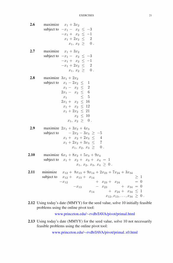
2.6 maximize x1 + 3x2
subject to −x1 − x2 ≤ −3−x1 + x2 ≤ −1x1 + 2x2 ≤ 2
x1, x2 ≥ 0 .
2.7 maximize x1 + 3x2
subject to −x1 − x2 ≤ −3−x1 + x2 ≤ −1−x1 + 2x2 ≤ 2
x1, x2 ≥ 0 .
2.8 maximize 3x1 + 2x2
subject to x1 − 2x2 ≤ 1x1 − x2 ≤ 22x1 − x2 ≤ 6x1 ≤ 52x1 + x2 ≤ 16x1 + x2 ≤ 12x1 + 2x2 ≤ 21
x2 ≤ 10x1, x2 ≥ 0 .
2.9 maximize 2x1 + 3x2 + 4x3
subject to − 2x2 − 3x3 ≥ −5x1 + x2 + 2x3 ≤ 4x1 + 2x2 + 3x3 ≤ 7
x1, x2, x3 ≥ 0 .
2.10 maximize 6x1 + 8x2 + 5x3 + 9x4
subject to x1 + x2 + x3 + x4 = 1x1, x2, x3, x4 ≥ 0 .
2.11 minimize x12 + 8x13 + 9x14 + 2x23 + 7x24 + 3x34
subject to x12 + x13 + x14 ≥ 1−x12 + x23 + x24 = 0
−x13 − x23 + x34 = 0x14 + x24 + x34 ≤ 1
x12, x13, . . . , x34 ≥ 0 .
2.12 Using today’s date (MMYY) for the seed value, solve 10 initially feasibleproblems using the online pivot tool:
www.princeton.edu/∼rvdb/JAVA/pivot/primal.html
2.13 Using today’s date (MMYY) for the seed value, solve 10 not necessarilyfeasible problems using the online pivot tool:
www.princeton.edu/∼rvdb/JAVA/pivot/primal x0.html

22 2. THE SIMPLEX METHOD
2.14 Consider the following dictionary:
ζ = 3 + x1 + 6x2
w1 = 1 + x1 − x2
w2 = 5 − 2x1 − 3x2 .
Using the largest coefficient rule to pick the entering variable, computethe dictionary that results after one pivot.
2.15 Show that the following dictionary cannot be the optimal dictionary forany linear programming problem in which w1 and w2 are the initial slackvariables:
ζ = 4 − w1 − 2x2
x1 = 3 − 2x2
w2 = 1 + w1 − x2 .
Hint: if it could, what was the original problem from whence it came?
2.16 Graph the feasible region for Exercise 2.8. Indicate on the graph the se-quence of basic solutions produced by the simplex method.
2.17 Give an example showing that the variable that becomes basic in one iter-ation of the simplex method can become nonbasic in the next iteration.
2.18 Show that the variable that becomes nonbasic in one iteration of the sim-plex method cannot become basic in the next iteration.
2.19 Solve the following linear programming problem:
maximizen∑
j=1
pjxj
subject ton∑
j=1
qjxj ≤ β
xj ≤ 1 j = 1, 2, . . . , nxj ≥ 0 j = 1, 2, . . . , n.
Here, the numbers pj , j = 1, 2, . . . , n, are positive and sum to one. Thesame is true of the qj’s:
n∑
j=1
qj = 1
qj > 0.
Furthermore (with only minor loss of generality), you may assume that
p1q1
<p2q2
< · · · < pnqn
.
Finally, the parameter β is a small positive number. See Exercise 1.3 forthe motivation for this problem.

NOTES 23
Notes
The simplex method was invented by G.B. Dantzig in 1949. His monograph(Dantzig 1963) is the classical reference. Most texts describe the simplex methodas a sequence of pivots on a table of numbers called the simplex tableau. Follow-ing Chvatal (1983), we have developed the algorithm using the more memorabledictionary notation.

CHAPTER 3
Degeneracy
In the previous chapter, we discussed what it means when the ratios computedto calculate the leaving variable are all nonpositive (the problem is unbounded). Inthis chapter, we take up the more delicate issue of what happens when some of theratios are infinite (i.e., their denominators vanish).
1. Definition of Degeneracy
We say that a dictionary is degenerate if bi vanishes for some i ∈ B. A de-generate dictionary could cause difficulties for the simplex method, but it might not.For example, the dictionary we were discussing at the end of the last chapter,
ζ = 5+ x3 − x1
x2 = 5+ 2x3 − 3x1
x4 = 7 − 4x1
x5 = x1,
is degenerate, but it was clear that the problem was unbounded and therefore nomore pivots were required. Furthermore, had the coefficient of x3 in the equationfor x2 been −2 instead of 2, then the simplex method would have picked x2 for theleaving variable and no difficulties would have been encountered.
Problems arise, however, when a degenerate dictionary produces degeneratepivots. We say that a pivot is a degenerate pivot if one of the ratios in the calculationof the leaving variable is +∞; i.e., if the numerator is positive and the denominatorvanishes. To see what happens, let’s look at a few examples.
2. Two Examples of Degenerate Problems
Here is an example of a degenerate dictionary in which the pivot is alsodegenerate:
(3.1)ζ = 3− 0.5x1 + 2x2 − 1.5w1
x3 = 1− 0.5x1 − 0.5w1
w2 = x1 − x2 + w1.
For this dictionary, the entering variable is x2 and the ratios computed to determinethe leaving variable are 0 and +∞. Hence, the leaving variable is w2, and the factthat the ratio is infinite means that as soon as x2 is increased from zero to a positive
The original version of this chapter was revised. An erratum to this chapter can be found at DOI10.1007/978-1-4614-7630-6 26
R.J. Vanderbei, Linear Programming, International Series in Operations Research& Management Science 196, DOI 10.1007/978-1-4614-7630-6 3,© Springer Science+Business Media New York 2014
25
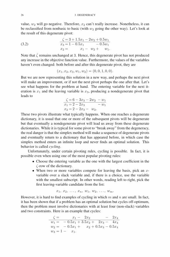
26 3. DEGENERACY
value, w2 will go negative. Therefore, x2 can’t really increase. Nonetheless, it canbe reclassified from nonbasic to basic (with w2 going the other way). Let’s look atthe result of this degenerate pivot:
(3.2)ζ = 3+ 1.5x1 − 2w2 + 0.5w1
x3 = 1− 0.5x1 − 0.5w1
x2 = x1 − w2 + w1.
Note that ζ remains unchanged at 3. Hence, this degenerate pivot has not producedany increase in the objective function value. Furthermore, the values of the variableshaven’t even changed: both before and after this degenerate pivot, they are
(x1, x2, x3, w1, w2) = (0, 0, 1, 0, 0).
But we are now representing this solution in a new way, and perhaps the next pivotwill make an improvement, or if not the next pivot perhaps the one after that. Let’ssee what happens for the problem at hand. The entering variable for the next it-eration is x1 and the leaving variable is x3, producing a nondegenerate pivot thatleads to
ζ = 6− 3x3 − 2w2 −w1
x1 = 2− 2x3 −w1
x2 = 2− 2x3 − w2.
These two pivots illustrate what typically happens. When one reaches a degeneratedictionary, it is usual that one or more of the subsequent pivots will be degeneratebut that eventually a nondegenerate pivot will lead us away from these degeneratedictionaries. While it is typical for some pivot to “break away” from the degeneracy,the real danger is that the simplex method will make a sequence of degenerate pivotsand eventually return to a dictionary that has appeared before, in which case thesimplex method enters an infinite loop and never finds an optimal solution. Thisbehavior is called cycling.
Unfortunately, under certain pivoting rules, cycling is possible. In fact, it ispossible even when using one of the most popular pivoting rules:
• Choose the entering variable as the one with the largest coefficient in theζ-row of the dictionary.
• When two or more variables compete for leaving the basis, pick an x-variable over a slack variable and, if there is a choice, use the variablewith the smallest subscript. In other words, reading left to right, pick thefirst leaving-variable candidate from the list:
x1, x2, . . . , xn, w1, w2, . . . , wm.
However, it is hard to find examples of cycling in which m and n are small. In fact,it has been shown that if a problem has an optimal solution but cycles off-optimum,then the problem must involve dictionaries with at least four (non-slack) variablesand two constraints. Here is an example that cycles:
ζ = x1 − 2x2 − 2x4
w1 = − 0.5x1 + 3.5x2 + 2x3 − 4x4
w2 = − 0.5x1 + x2 + 0.5x3 − 0.5x4
w3 = 1 − x1.

2. TWO EXAMPLES OF DEGENERATE PROBLEMS 27
And here is the sequence of dictionaries the above pivot rules produce. For the firstpivot, x1 enters and w1 leaves bringing us to:
ζ = − 2w1 + 5x2 + 4x3 − 10x4
x1 = − 2w1 + 7x2 + 4x3 − 8x4
w2 = w1 − 2.5x2 − 1.5x3 + 3.5x4
w3 = 1 + 2w1 − 7x2 − 4x3 + 8x4 .
For the second iteration, x2 enters and w2 leaves bringing us to:
ζ = − 2w2 + x3 − 3x4
x1 = 0.8w1 − 2.8w2 − 0.2x3 + 1.8x4
x2 = 0.4w1 − 0.4w2 − 0.6x3 + 1.4x4
w3 = 1 − 0.8w1 + 2.8w2 + 0.2x3 − 1.8x4 .
For the third iteration, x3 enters and x1 leaves:
ζ = 4w1 − 16w2 − 5x1 + 6x4
x3 = 4w1 − 14w2 − 5x1 + 9x4
x2 = − 2w1 + 8w2 + 3x1 − 4x4
w3 = 1 − x1.
For the fourth iteration, x4 enters and x2 leaves:
ζ = w1 − 4w2 − 0.5x1 − 1.5x2
x3 = − 0.5w1 + 4w2 + 1.75x1 − 2.25x2
x4 = − 0.5w1 + 2w2 + 0.75x1 − 0.25x2
w3 = 1 − x1.
In the fifth iteration, w1 enters and x3 leaves:
ζ = − 2x3 + 4w2 + 3x1 − 6x2
w1 = − 2x3 + 8w2 + 3.5x1 − 4.5x2
x4 = x3 − 2w2 − x1 + 2x2
w3 = 1 − x1.
Lastly, for the sixth iteration, w2 enters and x4 leaves:
ζ = − 2x4 + x1 − 2x2
w1 = 2x3 − 4x4 − 0.5x1 + 3.5x2
w2 = 0.5x3 − 0.5x4 − 0.5x1 + x2
w3 = 1 − x1.
Note that we have come back to the original dictionary, and so from here onthe simplex method simply cycles through these six dictionaries and never makesany further progress toward an optimal solution. As bad as cycling is, the followingtheorem tells us that nothing worse can happen:
THEOREM 3.1. If the simplex method fails to terminate, then it must cycle.
PROOF. A dictionary is completely determined by specifying which variablesare basic and which are nonbasic. There are only
(n+mm
)
=(n+m)!
n!m!
28 3. DEGENERACY
different possibilities. This number is big, but it is finite. If the simplex method failsto terminate, it must visit some of these dictionaries more than once. Hence, thealgorithm cycles. �
Note that, if the simplex method cycles, then all the pivots within the cyclemust be degenerate. This is easy to see, since the objective function value neverdecreases. Hence, it follows that all the pivots within the cycle must have the sameobjective function value, i.e., all of the these pivots must be degenerate.
In practice, degeneracy is common because a zero right-hand side value cropsup frequently in real-world problems. Cycling is not as common, but it can happenand therefore must be addressed. Computer implementations of the simplex methodin which numbers are represented as integers or as simple rational numbers are atrisk of cycling and one of the techniques described in the following sections mustbe used to avoid the problem. But, most implementations of the simplex methodare written with floating point numbers (the computer approximation to a full set ofreal numbers). With floating point computation there is inevitable round-off error.Hence, a zero appearing as a right-hand side value generally shows up not as anexact zero but rather as a very small number. The result is that the dictionary appearsto be slightly off from actually being degenerate and therefore cycling is usuallyavoided.
3. The Perturbation/Lexicographic Method
As we have seen, there is not just one algorithm called the simplex method.Instead, the simplex method is a whole family of related algorithms from whichwe can pick a specific instance by specifying what we have been referring to aspivoting rules. We have also seen that, using a very natural pivoting rule, the sim-plex method can fail to converge to an optimal solution by occasionally cyclingindefinitely through a sequence of degenerate pivots associated with a nonoptimalsolution.
So this raises a natural question: are there pivoting rules for which the simplexmethod will, with certainty, either reach an optimal solution or prove that no suchsolution exists? The answer to this question is yes, and we shall present two choicesof such pivoting rules.
The first method is based on the observation that degeneracy is sort of an ac-cident. That is, a dictionary is degenerate if one or more of the bi’s vanish. Ourexamples have generally used small integers for the data, and in this case it doesn’tseem too surprising that sometimes cancellations occur and we end up with a de-generate dictionary. But each right-hand side could in fact be any real number, andin the world of real numbers the occurrence of any specific number, such as zero,seems to be quite unlikely. So how about perturbing a given problem by addingsmall random perturbations independently to each of the right-hand sides? If theseperturbations are small enough, we can think of them as insignificant and hence notreally changing the problem. If they are chosen independently, then the probabilityof an exact cancellation is zero.

3. THE PERTURBATION/LEXICOGRAPHIC METHOD 29
Such random perturbation schemes are used in some implementations, but whatwe have in mind as we discuss perturbation methods is something a little bit differ-ent. Instead of using independent identically distributed random perturbations, let usconsider using a fixed perturbation for each constraint, with the perturbation gettingmuch smaller on each succeeding constraint. Indeed, we introduce a small positivenumber ε1 for the first constraint and then a much smaller positive number ε2 forthe second constraint, etc. We write this as
0 < εm � · · · � ε2 � ε1 � all other data.
The idea is that each εi acts on an entirely different scale from all the other εi’s andthe data for the problem. What we mean by this is that no linear combination ofthe εi’s using coefficients that might arise in the course of the simplex method canever produce a number whose size is of the same order as the data in the problem.Similarly, each of the “lower down” εi’s can never “escalate” to a higher level.Hence, cancellations can only occur on a given scale. Of course, this completeisolation of scales can never be truly achieved in the real numbers, so instead ofactually introducing specific values for the εi’s, we simply treat them as abstractsymbols having these scale properties.
To illustrate what we mean, let’s look at a specific example. Consider the fol-lowing degenerate dictionary:
ζ = 6 x1 + 4 x2
w1 = 0+ 9 x1 + 4 x2
w2 = 0− 4 x1 − 2 x2
w3 = 1 − x2.
The first step is to introduce symbolic parameters
0 < ε3 � ε2 � ε1
to get a perturbed problem:
ζ = 6 x1 + 4 x2
w1 = 0+ ε1 + 9 x1 + 4 x2
w2 = 0 + ε2 − 4 x1 − 2 x2
w3 = 1 + ε3 − x2.
This dictionary is not degenerate. The entering variable is x1 and the leaving vari-able is unambiguously w2. The next dictionary is
ζ = 1.5 ε2 − 1.5w2 + x2
w1 = 0+ ε1 + 2.25 ε2 − 2.25w2 − 0.5 x2
x1 = 0 + 0.25 ε2 − 0.25w2 − 0.5 x2
w3 = 1 + ε3 − x2.
For the next pivot, the entering variable is x2 and, using the fact that ε2 � ε1, wesee that the leaving variable is x1. The new dictionary is

30 3. DEGENERACY
ζ = 2 ε2 − 2w2 − 2 x1
w1 = 0+ ε1 + 2 ε2 − 2w2 + x1
x2 = 0 + 0.5 ε2 − 0.5w2 − 2 x1
w3 = 1 − 0.5 ε2 + ε3 + 0.5w2 + 2 x1.
This last dictionary is optimal. At this point, we simply drop the symbolic εiparameters and get an optimal dictionary for the unperturbed problem:
ζ = − 2w2 − 2 x1
w1 = 0− 2w2 + x1
x2 = 0− 0.5w2 − 2 x1
w3 = 1+ 0.5w2 + 2 x1.
When treating the εi’s as symbols, the method is called the lexicographicmethod. Note that the lexicographic method does not affect the choice of enteringvariable but does amount to a precise prescription for the choice of leaving variable.
It turns out that the lexicographic method produces a variant of the simplexmethod that never cycles:
THEOREM 3.2. The simplex method always terminates provided that the leavingvariable is selected by the lexicographic rule.
PROOF. It suffices to show that no degenerate dictionary is ever produced. Aswe’ve discussed before, the εi’s operate on different scales and hence can’t cancelwith each other. Therefore, we can think of the εi’s as a collection of independentvariables. Extracting the ε terms from the first dictionary, we see that we start withthe following pattern:
ε1ε2
. . .εm.
And, after several pivots, the ε terms will form a system of linear combinations, say,
r11ε1 + r12ε2 . . . + r1mεmr21ε1 + r22ε2 . . . + r2mεm
......
. . ....
rm1ε1 + rm2ε2 . . . + rmmεm.
Since this system of linear combinations is obtained from the original system bypivot operations and, since pivot operations are reversible, it follows that the rankof the two systems must be the same. Since the original system had rank m, we seethat every subsequent system must have rank m. This means that there must be atleast one nonzero rij in every row i, which of course implies that none of the rowscan be degenerate. Hence, no dictionary can be degenerate. �

4. BLAND’S RULE 31
4. Bland’s Rule
The second pivoting rule we consider is called Bland’s rule. It stipulates thatboth the entering and the leaving variable be selected from their respective sets ofchoices by choosing the variable xk with the smallest index k.
THEOREM 3.3. The simplex method always terminates provided that both theentering and the leaving variable are chosen according to Bland’s rule.
The proof may look rather involved, but the reader who spends the time tounderstand it will find the underlying elegance most rewarding.
PROOF. It suffices to show that such a variant of the simplex method nevercycles. We prove this by assuming that cycling does occur and then showing thatthis assumption leads to a contradiction. So let’s assume that cycling does occur.Without loss of generality, we may assume that it happens from the beginning. LetD0, D1, . . . , Dk−1 denote the dictionaries through which the method cycles. Thatis, the simplex method produces the following sequence of dictionaries:
D0, D1, . . . , Dk−1, D0, D1, . . . .
We say that a variable is fickle if it is in some basis and not in some other basis.Let xt be the fickle variable having the largest index and let D denote a dictionaryin D0, D1, . . . , Dk−1 in which xt leaves the basis. Again, without loss of generalitywe may assume that D = D0. Let xs denote the corresponding entering variable.Suppose that D is recorded as follows:
ζ = v +∑
j∈Ncjxj
xi = bi −∑
j∈Naijxj i ∈ B.
Since xs is the entering variable and xt is the leaving variable, we have that s ∈ Nand t ∈ B.
Now let D∗ be a dictionary in D1, D2, . . . , Dk−1 in which xt enters the basis.Suppose that D∗ is recorded as follows:
(3.3)
ζ = v∗ +∑
j∈N∗
c∗jxj
xi = b∗i −∑
j∈N∗
a∗ijxj i ∈ B∗.
Since all the dictionaries are degenerate, we have that v∗ = v, and therefore we canwrite the objective function in (3.3) as
(3.4) ζ = v +
n+m∑
j=1
c∗jxj ,
where we have extended the notation c∗j to all variables (both original and slack) bysetting c∗j = 0 for j ∈ B∗.
32 3. DEGENERACY
Ignoring for the moment the possibility that some variables could go negative,consider the solutions obtained by letting xs increase while holding all other vari-ables in N at zero:
xs = y,
xj = 0, j ∈ N \ {s},xi = bi − aisy, i ∈ B.
The objective function at this point is given by
ζ = v + csy.
However, using (3.4), we see that it is also given by
ζ = v + c∗sy +∑
i∈Bc∗i (bi − aisy).
Equating these two expressions for ζ, we see that(
cs − c∗s +∑
i∈Bc∗i ais
)
y =∑
i∈Bc∗i bi.
Since this equation must be an identity for every y, it follows that the coefficientmultiplying y must vanish (as must the right-hand side):
cs − c∗s +∑
i∈Bc∗i ais = 0.
Now, the fact that xs is the entering variable in D implies that
cs > 0.
Recall that xt is the fickle variable with the largest index. Since xs is also fickle, wesee that s < t. Since xs is not the entering variable in D∗ (as xt is), we see that
c∗s ≤ 0.
From these last three displayed equations, we get∑
i∈Bc∗i ais < 0.
Hence, there must exist an index r ∈ B for which
(3.5) c∗rars < 0.
Consequently, c∗r �= 0 and r ∈ N ∗. Hence, xr is fickle and therefore r ≤ t. Infact, r < t, since c∗tats > 0. To see that this product is positive, note that both itsfactors are positive: c∗t is positive, since xt is the entering variable in D∗, and ats ispositive, since xt is the leaving variable in D.
The fact that r < t implies that c∗r ≤ 0 (otherwise, according to the smallestindex criteria, r would be the entering variable for D∗). Hence, (3.5) implies that
ars > 0.
Now, since each of the dictionaries in the cycle describe the same solution, it followsthat every fickle variable is zero in all these dictionaries (since it is clearly zero in

6. GEOMETRY 33
a dictionary in which it is nonbasic). In particular, xr = 0. But in D, xr is basic.Hence,
br = 0.
These last two displayed equations imply that xr was a candidate to be the leavingvariable in D, and since r < t, it should have been chosen over xt. This is thecontradiction we have been looking for. �
5. Fundamental Theorem of Linear Programming
Now that we have a Phase I algorithm and a variant of the simplex method thatis guaranteed to terminate, we can summarize the main points of this chapter in thefollowing theorem:
THEOREM 3.4. For an arbitrary linear program in standard form, the followingstatements are true:
(1) If there is no optimal solution, then the problem is either infeasible orunbounded.
(2) If a feasible solution exists, then a basic feasible solution exists.(3) If an optimal solution exists, then a basic optimal solution exists.
PROOF. The Phase I algorithm either proves that the problem is infeasible orproduces a basic feasible solution. The Phase II algorithm either discovers that theproblem is unbounded or finds a basic optimal solution. These statements depend,of course, on applying a variant of the simplex method that does not cycle, whichwe now know to exist. �
6. Geometry
As we saw in the previous chapter, the set of feasible solutions for a problemin two dimensions is the intersection of a number of halfplanes, i.e., a polygon.In three dimensions, the situation is similar. Consider, for example, the followingproblem:
(3.6)
maximize x1 + 2x2 + 3x3
subject to x1 + 2x3 ≤ 3x2 + 2x3 ≤ 2
x1, x2, x3 ≥ 0 .
The set of points satisfying x1 + 2x3 = 3 is a plane. The inequality x1 + 2x3 ≤ 3therefore consists of all points on one side of this plane; that is, it is a halfspace.The same is true for each of the other four inequalities. The feasible set consistsof those points in space that satisfy all five inequalities, i.e., those points lying inthe intersection of these halfspaces. This set is the polyhedron shown in Figure 3.1.This polyhedron is bordered by five facets, each facet being a portion of one of theplanes that was defined by replacing a constraint inequality with an equation. Forexample, the “front” facet in the figure is a portion of the plane x1 + 2x3 = 3.

34 3. DEGENERACY
x2
x3
x1
x1+2x3=3
x2+2x3=2x2=0
FIGURE 3.1. The set of feasible solutions for the problem givenby (3.6).
The facets acquire a particularly simple description if we introduce slack variablesinto the problem:
w1 = 3 − x1 − 2x3
w2 = 2 − x2 − 2x3 .
Indeed, each facet corresponds precisely to some variable (either original or slack)vanishing. For instance, the front facet in the figure corresponds to w1 = 0 whereasthe “left” facet corresponds to x2 = 0.
The correspondences can be continued. Indeed, each edge of the polyhedroncorresponds to a pair of variables vanishing. For example, the edge lying at theinterface of the left and the front facets in the figure corresponds to both w1 = 0 andx2 = 0.
Going further yet, each vertex of the polyhedron corresponds to three variablesvanishing. For instance, the vertex whose coordinates are (1, 0, 1) corresponds tow1 = 0, x2 = 0, and w2 = 0.
Now, let’s think about applying the simplex method to this problem. Everybasic feasible solution involves two basic variables and three nonbasic variables.Furthermore, the three nonbasic variables are, by definition, zero in the basic fea-sible solution. Therefore, for this example, the basic feasible solutions stand in
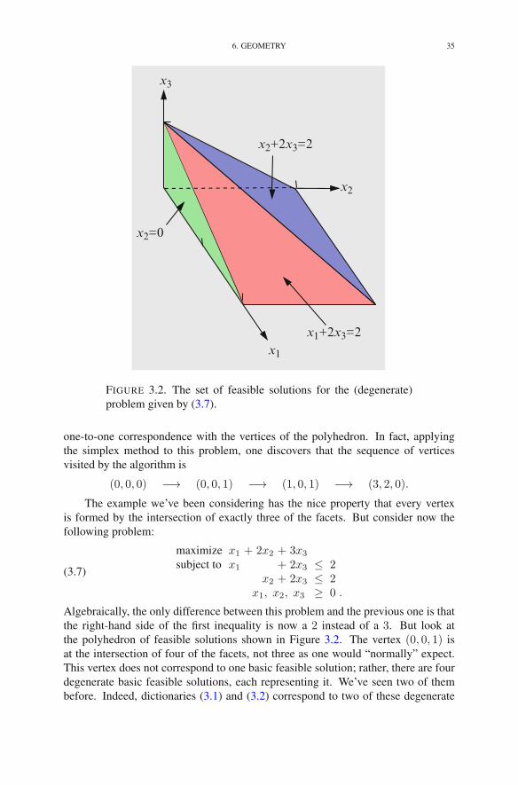
6. GEOMETRY 35
1x2
x3
x1
x2=0
x2+2x3=2
x1+2x3=2
FIGURE 3.2. The set of feasible solutions for the (degenerate)problem given by (3.7).
one-to-one correspondence with the vertices of the polyhedron. In fact, applyingthe simplex method to this problem, one discovers that the sequence of verticesvisited by the algorithm is
(0, 0, 0) −→ (0, 0, 1) −→ (1, 0, 1) −→ (3, 2, 0).
The example we’ve been considering has the nice property that every vertexis formed by the intersection of exactly three of the facets. But consider now thefollowing problem:
(3.7)
maximize x1 + 2x2 + 3x3
subject to x1 + 2x3 ≤ 2x2 + 2x3 ≤ 2
x1, x2, x3 ≥ 0 .
Algebraically, the only difference between this problem and the previous one is thatthe right-hand side of the first inequality is now a 2 instead of a 3. But look atthe polyhedron of feasible solutions shown in Figure 3.2. The vertex (0, 0, 1) isat the intersection of four of the facets, not three as one would “normally” expect.This vertex does not correspond to one basic feasible solution; rather, there are fourdegenerate basic feasible solutions, each representing it. We’ve seen two of thembefore. Indeed, dictionaries (3.1) and (3.2) correspond to two of these degenerate

36 3. DEGENERACY
dictionaries (in fact, dictionary (3.1) is the dictionary one obtains after one pivot ofthe simplex method applied to problem (3.7)).
We end by considering the geometric effect of the perturbation method for re-solving degeneracy. By perturbing the right-hand sides, one moves the planes thatdetermine the facets. If the moves are random or chosen with vastly different mag-nitudes (all small), then one would expect that each vertex in the perturbed problemwould be determined by exactly three planes. That is, degenerate vertices from theoriginal problem get split into multiple nearby vertices in the perturbed problem.For example, problem (3.6) can be thought of as a perturbation of degenerate prob-lem (3.7) (the perturbation isn’t small, but it also isn’t so large as to obscure theeffect). Note how the degenerate vertex in Figure 3.2 appears as two vertices inFigure 3.1.
Exercises
3.1 Solve the following linear program using the perturbation method to re-solve degeneracy:
maximize 10x1 − 57x2 − 9x3 − 24x4
subject to 0.5x1 − 5.5x2 − 2.5x3 + 9x4 ≤ 00.5x1 − 1.5x2 − 0.5x3 + x4 ≤ 0
x1 ≤ 1x1, x2, x3, x4 ≥ 0 .
Note: The simple pivot tool with the Lexicographic labels can be used tocheck your arithmetic:
www.princeton.edu/∼rvdb/JAVA/pivot/simple.html
3.2 Solve the following linear program using Bland’s rule to resolve degener-acy:
maximize 10x1 − 57x2 − 9x3 − 24x4
subject to 0.5x1 − 5.5x2 − 2.5x3 + 9x4 ≤ 00.5x1 − 1.5x2 − 0.5x3 + x4 ≤ 0
x1 ≤ 1x1, x2, x3, x4 ≥ 0 .
3.3 Using today’s date (MMYY) for the seed value, solve 10 possibly degen-erate problems using the online pivot tool:
www.princeton.edu/∼rvdb/JAVA/pivot/lexico.html
3.4 Consider the linear programming problems whose right-hand sides areidentically zero:
maximizen∑
j=1
cjxj
subject ton∑
j=1
aijxj ≤ 0 i = 1, 2, . . . ,m
xj ≥ 0 j = 1, 2, . . . , n.

NOTES 37
Show that either xj = 0 for all j is optimal or else the problem isunbounded.
3.5 Consider the following linear program:
maximize x1 + 3x2
subject to −2x1 ≤ −5x1 ≥ 0.
Show that this problem has feasible solutions but no vertex solutions. Howdoes this reconcile with the fundamental theorem of linear programming(Theorem 3.4)?
3.6 Suppose that a linear programming problem has the following property:its initial dictionary is not degenerate and, when solved by the simplexmethod, there is never a tie for the choice of leaving variable.(a) Can such a problem have degenerate dictionaries? Explain.(b) Can such a problem cycle? Explain.
3.7 Consider the following dictionary:
ζ = 5 + 2x2 − 2x3 + 3x5
x6 = 4 − 2x2 − x3 + x5
x4 = 2 − x2 + x3 − x5
x1 = 6 − 2x2 − 2x3 − 3x5 .
(a) List all pairs (xr, xs) such that xr could be the entering variable andxs could be the leaving variable.
(b) List all such pairs if the largest-coefficient rule for choosing the en-tering variable is used.
(c) List all such pairs if Bland’s rule for choosing the entering and leav-ing variables is used.
Notes
The first example of cycling was given by Hoffman (1953). The fact that anylinear programming problem that cycles must have at least six variables and threeconstraints was proved by Marshall and Suurballe (1969).
Early proofs of the fundamental theorem of linear programming (Theorem 3.4)were constructive, relying, as in our development, on the existence of a variant ofthe simplex method that works even in the presense of degeneracy. Hence, findingsuch variants occupied the attention of early researchers in linear programming. Theperturbation method was first suggested by A. Orden and developed independentlyby Charnes (1952). The essentially equivalent lexicographic method first appearedin Dantzig et al. (1955). Theorem 3.3 was proved by Bland (1977).
For an extensive treatment of degeneracy issues see Gal (1994).
CHAPTER 4
Efficiency of the Simplex Method
In the previous chapter, we saw that the simplex method (with appropriatepivoting rules to guarantee no cycling) will solve any linear programming prob-lem for which an optimal solution exists. In this chapter, we investigate just howfast it will solve a problem of a given size.
1. Performance Measures
Performance measures can be broadly divided into two types:
• Worst case• Average case.
As its name implies, a worst-case analysis looks at all problems of a given “size” andasks how much effort is needed to solve the hardest of these problems. Similarly,an average-case analysis looks at the average amount of effort, averaging over allproblems of a given size. Worst-case analyses are generally easier than average-caseanalyses. The reason is that, for worst-case analyses, one simply needs to give anupper bound on how much effort is required and then exhibit a specific example thatattains this bound. However, for average-case analyses, one must have a stochasticmodel of the space of “random linear programming problems” and then be able tosay something about the solution effort averaged over all the problems in the samplespace. There are two serious difficulties here. The first is that it is not clear at all howone should model the space of random problems. Secondly, given such a model, onemust be able to evaluate the amount of effort required to solve every problem in thesample space.
Therefore, worst-case analysis is more tractable than average-case analysis, butit is also less relevant to a person who needs to solve real problems. In this chapter,we will start by giving a detailed worst-case analysis of the simplex method usingthe largest-coefficient rule to select the entering variable. We will then present anddiscuss the results of some empirical studies in which millions of linear program-ming problems were generated randomly and solved by the simplex method. Suchstudies act as a surrogate for a true average-case analysis.
2. Measuring the Size of a Problem
Before looking at worst cases, we must discuss two issues. First, how do wespecify the size of a problem? Two parameters come naturally to mind: m and n.Often, we simply use these two numbers to characterize the size a problem. How-ever, we should mention some drawbacks associated with this choice. First of all,
R.J. Vanderbei, Linear Programming, International Series in Operations Research& Management Science 196, DOI 10.1007/978-1-4614-7630-6 4,© Springer Science+Business Media New York 2014
39

40 4. EFFICIENCY OF THE SIMPLEX METHOD
it would be preferable to use only one number to indicate size. Since the data fora problem consist of the constraint coefficients together with the right-hand sideand objective function coefficients, perhaps we should use the total number of dataelements, which is roughly mn.
The product mn isn’t bad, but what if many or even most of the data elementsare zero? Wouldn’t one expect such a problem to be easier to solve? Efficient im-plementations do indeed take advantage of the presence of lots of zeros, and so ananalysis should also account for this. Hence, a good measure might be simply thenumber of nonzero data elements. This would definitely be an improvement, but onecan go further. On a computer, floating-point numbers are all the same size and canbe multiplied in the same amount of time. But if a person is to solve a problem byhand (or use unlimited precision computation on a computer), then certainly multi-plying 23 by 7 is a lot easier than multiplying 23,453.2352 by 86,833.245643. Soperhaps the best measure of a problem’s size is not the number of data elements, butthe actual number of bits needed to store all the data on a computer. This measureis popular among most computer scientists and is usually denoted by L.
However, with a little further abstraction, the size of the data, L, is seen to beambiguous. As we saw in Chapter 1, real-world problems, while generally largeand sparse, usually can be described quite simply and involve only a small amountof true input data that gets greatly expanded when setting the problem up with aconstraint matrix, right-hand side, and objective function. So should L representthe number of bits needed to specify the nonzero constraint coefficients, objectivecoefficients, and right-hand sides, or should it be the number of bits in the originaldata set plus the number of bits in the description of how this data represents a linearprogramming problem? No one currently uses this last notion of problem size, butit seems fairly reasonable that they should (or at least that they should seriouslyconsider it). Anyway, our purpose here is merely to mention that these importantissues are lurking about, but, as stated above, we shall simply focus on m and n tocharacterize the size of a problem.
3. Measuring the Effort to Solve a Problem
The second issue to discuss is how one should measure the amount of workrequired to solve a problem. The best answer is the number of seconds of computertime required to solve the problem, using the computer sitting on one’s desk. Un-fortunately, there are (hopefully) many readers of this text, not all of whom use theexact same computer. Even if they did, computer technology changes rapidly, anda few years down the road everyone would be using something entirely different.It would be nice if the National Institute of Standards and Technology (the govern-ment organization in charge of setting standards, such as how many threads/inch astandard light bulb should have) would identify a standard computer for the purposeof benchmarking algorithms, but, needless to say, this is not very likely. So thetime needed to solve a problem, while the most desirable measure, is not the mostpractical one here. Fortunately, there is a fairly reasonable substitute. Algorithmsare generally iterative processes, and the time to solve a problem can be factored

4. WORST-CASE ANALYSIS OF THE SIMPLEX METHOD 41
into the number of iterations required to solve the problem times the amount of timerequired to do each iteration. The first factor, the number of iterations, does notdepend on the computer and so is a reasonable surrogate for the actual time. Thissurrogate is useful when comparing various algorithms within the same general classof algorithms, in which the time per iteration can be expected to be about the sameamong the algorithms; however, it becomes meaningless when one wishes to com-pare two entirely different algorithms. For now, we shall measure the amount ofeffort to solve a linear programming problem by counting the number of iterations,i.e. pivots, needed to solve it.
4. Worst-Case Analysis of the Simplex Method
How bad can the simplex method be in the worst case? Well, we have alreadyseen that for some pivoting rules it can cycle, and hence the worst-case solutiontime for such variants is infinite. However, what about noncycling variants of thesimplex method? Since the simplex method operates by moving from one basicfeasible solution to another without ever returning to a previously visited solution,an upper bound on the number of iterations is simply the number of basic feasiblesolutions, of which there can be at most
(n+mm
)
.
For a fixed value of the sum n + m, this expression is maximized when m = n.And how big is it? It is not hard to show that
1
2n22n ≤
(2nn
)
≤ 22n
(see Exercise 4.9). It should be noted that, even though typographically compact,the expression 22n is huge even when n is not very big. For example, for n = 25,we have 250 = 1.1259× 10¹⁵.
Our best chance for finding a bad example is to look at the case where m = n.In 1972, V. Klee and G.J. Minty were the first to discover an example in which thesimplex method using the largest coefficient rule requires 2n − 1 iterations to solve.The example is quite simple to state:
(4.1)
maximizen∑
j=1
10n−jxj
subject to 2
i−1∑
j=1
10i−jxj + xi ≤ 100i−1 i = 1, 2, . . . , n
xj ≥ 0 j = 1, 2, . . . , n.
It is instructive to look closely at the constraints. The first three constraints are
x1 ≤ 120x1 + x2 ≤ 100200x1 + 20x2 + x3 ≤ 10,000.
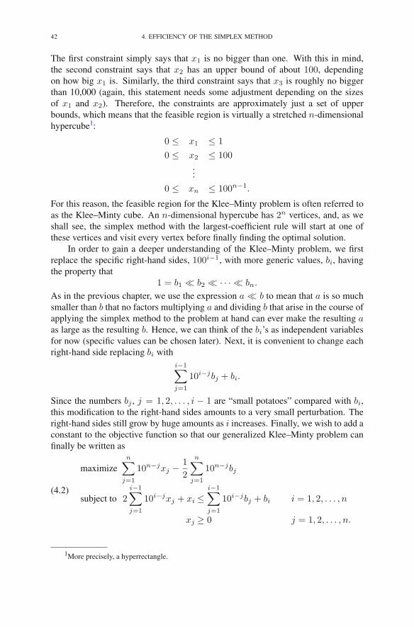
42 4. EFFICIENCY OF THE SIMPLEX METHOD
The first constraint simply says that x1 is no bigger than one. With this in mind,the second constraint says that x2 has an upper bound of about 100, dependingon how big x1 is. Similarly, the third constraint says that x3 is roughly no biggerthan 10,000 (again, this statement needs some adjustment depending on the sizesof x1 and x2). Therefore, the constraints are approximately just a set of upperbounds, which means that the feasible region is virtually a stretched n-dimensionalhypercube1:
0 ≤ x1 ≤ 1
0 ≤ x2 ≤ 100
...
0 ≤ xn ≤ 100n−1.
For this reason, the feasible region for the Klee–Minty problem is often referred toas the Klee–Minty cube. An n-dimensional hypercube has 2n vertices, and, as weshall see, the simplex method with the largest-coefficient rule will start at one ofthese vertices and visit every vertex before finally finding the optimal solution.
In order to gain a deeper understanding of the Klee–Minty problem, we firstreplace the specific right-hand sides, 100i−1, with more generic values, bi, havingthe property that
1 = b1 � b2 � · · · � bn.
As in the previous chapter, we use the expression a � b to mean that a is so muchsmaller than b that no factors multiplying a and dividing b that arise in the course ofapplying the simplex method to the problem at hand can ever make the resulting aas large as the resulting b. Hence, we can think of the bi’s as independent variablesfor now (specific values can be chosen later). Next, it is convenient to change eachright-hand side replacing bi with
i−1∑
j=1
10i−jbj + bi.
Since the numbers bj , j = 1, 2, . . . , i − 1 are “small potatoes” compared with bi,this modification to the right-hand sides amounts to a very small perturbation. Theright-hand sides still grow by huge amounts as i increases. Finally, we wish to add aconstant to the objective function so that our generalized Klee–Minty problem canfinally be written as
(4.2)
maximizen∑
j=1
10n−jxj −1
2
n∑
j=1
10n−jbj
subject to 2
i−1∑
j=1
10i−jxj + xi ≤i−1∑
j=1
10i−jbj + bi i = 1, 2, . . . , n
xj ≥ 0 j = 1, 2, . . . , n.
1More precisely, a hyperrectangle.

4. WORST-CASE ANALYSIS OF THE SIMPLEX METHOD 43
In Exercise 4.7, you are asked to prove that this problem takes 2n − 1 iterations.To start to get a handle on the proof, here are the seven iterations that one gets withn = 3. The initial dictionary is
ζ =− 1002 b1 − 10
2 b2 − 12b3 + 100x1 + 10x2 + x3
w1 = b1 − x1
w2 = 10b1 + b2 − 20x1 − x2
w3 = 100b1 + 10b2 + b3 − 200x1 − 20x2 − x3,
which is feasible. Using the largest coefficient rule, the entering variable is x1. Fromthe fact that each subsequent bi is huge compared with its predecessor it follows thatw1 is the leaving variable. After the first iteration, the dictionary reads
ζ = 1002 b1 − 10
2 b2 − 12b3 − 100w1 + 10x2 + x3
x1 = b1 − w1
w2 = −10b1 + b2 + 20w1 − x2
w3 =−100b1 + 10b2 + b3 + 200w1 − 20x2 − x3.
Now, x2 enters and w2 leaves, so after the second iteration we get:
ζ =− 1002 b1 +
102 b2 − 1
2b3 + 100w1 − 10w2 + x3
x1 = b1 − w1
x2 = −10b1 + b2 + 20w1 − w2
w3 = 100b1 − 10b2 + b3 − 200w1 + 20w2 − x3.
After the third iteration
ζ = 1002 b1 +
102 b2 − 1
2b3 − 100x1 − 10w2 + x3
w1 = b1 − x1
x2 = 10b1 + b2 − 20x1 − w2
w3 =−100b1 − 10b2 + b3 + 200x1 + 20w2 − x3.
After the fourth iteration
ζ = − 1002 b1 − 10
2 b2 +12b3 + 100x1 + 10w2 −w3
w1 = b1 − x1
x2 = 10b1 + b2 − 20x1 − w2
x3 =−100b1 − 10b2 + b3 + 200x1 + 20w2 −w3.
After the fifth iteration
ζ = 1002 b1 − 10
2 b2 +12b3 − 100w1 + 10w2 −w3
x1 = b1 − w1
x2 =−10b1 + b2 + 20w1 − w2
x3 = 100b1 − 10b2 + b3 − 200w1 + 20w2 −w3.
After the sixth iteration
ζ = − 1002 b1 +
102 b2 +
12b3 + 100w1 − 10x2 −w3
x1 = b1 − w1
w2 = −10b1 + b2 + 20w1 − x2
x3 =−100b1 + 10b2 + b3 + 200w1 − 20x2 −w3.

44 4. EFFICIENCY OF THE SIMPLEX METHOD
And, finally, after the seventh iteration, we get
ζ = 1002 b1 +
102 b2 +
12b3 − 100x1 − 10x2 −w3
w1 = b1 − x1
w2 = 10b1 + b2 − 20x1 − x2
x3 = 100b1 + 10b2 + b3 − 200x1 − 20x2 −w3,
which is, of course, optimal.A few observations should be made. First, every pivot is the swap of an xj with
the corresponding wj . Second, every dictionary looks just like the first one with theexception that the wi’s and the xi’s have become intertwined and various signs havechanged (see Exercise 4.6).
Also note that the final dictionary could have been reached from the initialdictionary in just one pivot if we had selected x3 to be the entering variable. Butthe largest-coefficient rule dictated selecting x1. It is natural to wonder whether thelargest-coefficient rule could be replaced by some other pivot rule for whichthe worst-case behavior would be much better than the 2n behavior of the largest-coefficient rule. So far no one has found such a pivot rule. However, no one hasproved that such a rule does not exist either.
Finally, we mention that one desirable property of an algorithm is that it bescale invariant. This means that should the units in which one measures the decisionvariables in a problem be changed, the algorithm would still behave in exactly thesame manner. The simplex method with the largest-coefficient rule is not scaleinvariant. To see this, consider changing variables in the Klee–Minty problem byputting
xj = 100j−1xj .
In the new variables, the initial dictionary for the n = 3 Klee–Minty problembecomes
ζ =− 1002 b1 − 10
2 b2 − 12b3 + 100x1 + 1000x2 + 10000x3
w1 = b1 − x1
w2 = 10b1 + b2 − 20x1 − x2
w3 = 100b1 + 1000b2 + b3 − 200x1 − 2000x2 − 10000x3.
Now, the largest-coefficient rule picks variable x3 to enter. Variable w3 leaves, andthe method steps to the optimal solution in just one iteration. There exist pivot rulesfor the simplex method that are scale invariant. But Klee–Minty-like examples havebeen found for most proposed alternative pivot rules (whether scale invariant or not).In fact, it is an open question whether there exist pivot rules for which one can provethat no problem instance requires an exponential number of iterations (as a functionof m or n).
5. Empirical Average Performance of the Simplex Method
To investigate the empirical average case performance of the simplex method,we generated a large number of random linear programming problems and solvedeach of them using the simplex method. There are many ways to generate randomproblems. In this section, we consider one such method and analyze the results.

5. EMPIRICAL AVERAGE PERFORMANCE OF THE SIMPLEX METHOD 45
As we have so dramatically seen, the number of iterations can depend on thespecific choice of pivot rule. In the code discussed below, we choose the enteringvariable to be the one with the largest coefficient. The way we generate randomproblems makes it unlikely that there will be ties in the choice of largest coeffi-cient (at least after the first pivot). So, even though the program makes a choice,it is not terribly important to articulate what that choice is. Similarly, there is littlechance for a tie when choosing a leaving variable, so we do not dwell on this mattereither.
We list below the source code. The program is written in a language calledMATLAB—a widely used language whose source code is fairly easy to read, evenfor those not familiar with the language. So, to get started, here’s how we initializethe data describing a linear programming problem:
m = round(10*exp(log(100)*rand()));n = round(10*exp(log(100)*rand()));
sigma = 10;A = round(sigma*(randn(m,n)));b = round(sigma*abs(randn(m,1)));c = round(sigma*randn(1,n));
Here, rand() generates a (pseudo) random number uniformly distributed onthe interval [0, 1] and round() simply rounds a number to its nearest integer value.The formulas for m and n produce numbers between 10 and 1,000. The formulamay seem more complicated than one would expect. For example, one might sug-gest this simpler formula: m = round(10 + 990*rand()). There is a goodreason for the more complicated version. We would like about half of the problemsto be between 10 and 100 and the other half to be between 100 and 1,000. Using thesimple scheme suggested above, only about 10% of the numbers would be between10 and 100. The vast majority would be between 100 and 1,000. So, what we wantis to have our numbers uniformly distributed when viewed on a logarithmic scale.Our formula for m and n achieves this logarithmically-uniform distribution.
The vector c of objective function coefficients is generated using the functionrandn(). This function is like rand() but, instead of generating numbers with auniform distribution, it generates numbers with a Gaussian (aka “normal”) distribu-tion with mean 0 and standard deviation 1. Multiplying such a variable by sigma,which is set to 10, increases the standard deviation to 10. The arguments (1,n)passed to randn() tells the random number generator not to produce just one suchnumber but rather to produce a 1 × n matrix, i.e. a row vector, of independentinstances of these random variables. There is no particular reason to round the co-efficients in the row vector c to be integers. The only reason this was done was tomake the random problems seem slightly more realistic since many/most real-worldproblems involve data that is mostly integer-valued. The matrix A and the right-hand side vector b are generated in a manner similar to how c is generated. But,note that the formula for b involves the abs() which returns absolute values sothat all elements of b are non-negative. This minor, but important, twist is done toensure that the starting dictionary is feasible. Here’s the main pivot loop:

46 4. EFFICIENCY OF THE SIMPLEX METHOD
iter = 0;while max(c) > eps,
% pick largest coefficient[cj, col] = max(c);Acol = A(:,col);
% select leaving variableif sum(Acol<-eps) == 0,
opt = -1; % unbounded’unbounded’break;
endnums = b.*(Acol<-eps);dens = -Acol.*(Acol<-eps);[t, row] = min(nums./dens);Arow = A(row,:);
a = A(row,col); % pivot element
A = A - Acol*Arow/a;A(row,:) = -Arow/a;A(:,col) = Acol/a;A(row,col) = 1/a;
brow = b(row);b = b - brow*Acol/a;b(row) = -brow/a;
ccol = c(col);c = c - ccol*Arow/a;c(col) = ccol/a;
iter = iter+1;end
In this code, the expression max(c) computes the maximum value of the elementsof the vector c. It returns both the maximum value and the index at which this valuewas attained (the first such index if there are more than one). So, cj is the maximalcoefficient and col is the index at which this maximum is attained. Hence colis the entering column. Given the matrix A, the expression A(:,col) denotesthe column vector consisting of the elements from the col column of A. Hence,Acol denotes the column of the dictionary associated with the entering variable.The next lines of this short code selects the leaving variable, which is in the rowcalled row. Given the entering column and the leaving row, all that remains is toupdate the coefficients in the objective function, the right-hand side, and the arrayof coefficients A. The last few lines encode exactly what one needs to do to carryout a pivot.
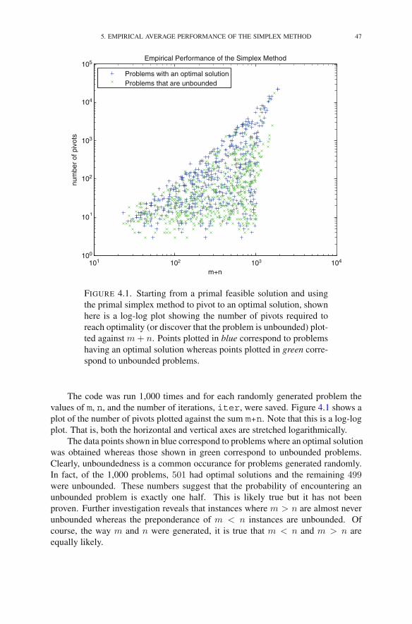
5. EMPIRICAL AVERAGE PERFORMANCE OF THE SIMPLEX METHOD 47
101 102 103 104100
101
102
103
104
105Empirical Performance of the Simplex Method
m+n
num
ber
of p
ivot
sProblems with an optimal solutionProblems that are unbounded
FIGURE 4.1. Starting from a primal feasible solution and usingthe primal simplex method to pivot to an optimal solution, shownhere is a log-log plot showing the number of pivots required toreach optimality (or discover that the problem is unbounded) plot-ted against m+ n. Points plotted in blue correspond to problemshaving an optimal solution whereas points plotted in green corre-spond to unbounded problems.
The code was run 1,000 times and for each randomly generated problem thevalues of m, n, and the number of iterations, iter, were saved. Figure 4.1 shows aplot of the number of pivots plotted against the sum m+n. Note that this is a log-logplot. That is, both the horizontal and vertical axes are stretched logarithmically.
The data points shown in blue correspond to problems where an optimal solutionwas obtained whereas those shown in green correspond to unbounded problems.Clearly, unboundedness is a common occurance for problems generated randomly.In fact, of the 1,000 problems, 501 had optimal solutions and the remaining 499were unbounded. These numbers suggest that the probability of encountering anunbounded problem is exactly one half. This is likely true but it has not beenproven. Further investigation reveals that instances where m > n are almost neverunbounded whereas the preponderance of m < n instances are unbounded. Ofcourse, the way m and n were generated, it is true that m < n and m > n areequally likely.
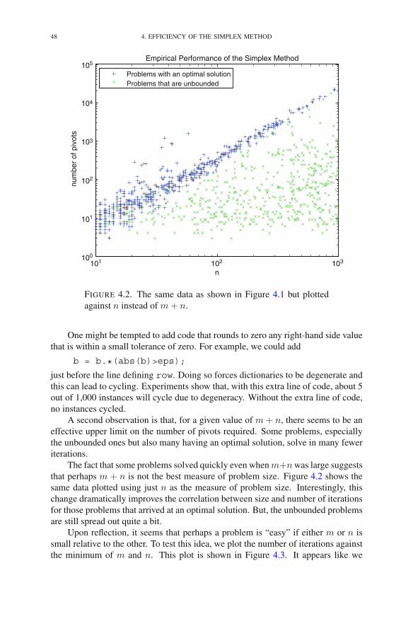
48 4. EFFICIENCY OF THE SIMPLEX METHOD
101 102 103100
101
102
103
104
105Empirical Performance of the Simplex Method
n
num
ber
of p
ivot
sProblems with an optimal solutionProblems that are unbounded
FIGURE 4.2. The same data as shown in Figure 4.1 but plottedagainst n instead of m+ n.
One might be tempted to add code that rounds to zero any right-hand side valuethat is within a small tolerance of zero. For example, we could add
b = b.*(abs(b)>eps);
just before the line defining row. Doing so forces dictionaries to be degenerate andthis can lead to cycling. Experiments show that, with this extra line of code, about 5out of 1,000 instances will cycle due to degeneracy. Without the extra line of code,no instances cycled.
A second observation is that, for a given value of m + n, there seems to be aneffective upper limit on the number of pivots required. Some problems, especiallythe unbounded ones but also many having an optimal solution, solve in many feweriterations.
The fact that some problems solved quickly even when m+n was large suggeststhat perhaps m + n is not the best measure of problem size. Figure 4.2 shows thesame data plotted using just n as the measure of problem size. Interestingly, thischange dramatically improves the correlation between size and number of iterationsfor those problems that arrived at an optimal solution. But, the unbounded problemsare still spread out quite a bit.
Upon reflection, it seems that perhaps a problem is “easy” if either m or n issmall relative to the other. To test this idea, we plot the number of iterations againstthe minimum of m and n. This plot is shown in Figure 4.3. It appears like we
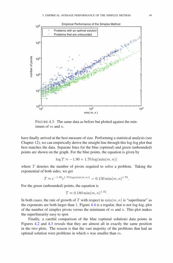
5. EMPIRICAL AVERAGE PERFORMANCE OF THE SIMPLEX METHOD 49
101 102 103100
105
104
103
102
101
Empirical Performance of the Simplex Method
min( m, n )
num
ber
of p
ivot
sProblems with an optimal solutionProblems that are unbounded
FIGURE 4.3. The same data as before but plotted against the min-imum of m and n.
have finally arrived at the best measure of size. Performing a statistical analysis (seeChapter 12), we can empirically derive the straight line through this log-log plot thatbest matches the data. Separate lines for the blue (optimal) and green (unbounded)points are shown on the graph. For the blue points, the equation is given by
log T ≈ −1.90 + 1.70 log(min(m,n))
where T denotes the number of pivots required to solve a problem. Taking theexponential of both sides, we get
T ≈ e−1.90e1.70 log(min(m,n)) = 0.150min(m,n)1.70.
For the green (unbounded) points, the equation is
T ≈ 0.180min(m,n)1.42.
In both cases, the rate of growth of T with respect to min(m,n) is “superlinear” asthe exponents are both larger than 1. Figure 4.4 is a regular, that is not log-log, plotof the number of simplex pivots versus the minimum of m and n. This plot makesthe superlinearity easy to spot.
Finally, a careful comparison of the blue (optimal solution) data points inFigures 4.2 and 4.3 reveals that they are almost all in exactly the same positionin the two plots. The reason is that the vast majority of the problems that had anoptimal solution were problems in which n was smaller than m.

50 4. EFFICIENCY OF THE SIMPLEX METHOD
0 100 200 300 400 500 600 700 800 900 10000
0.5
1
1.5
2
2.5x 10⁴ Empirical Performance of the Simplex Method
min( m, n )
num
ber
of p
ivot
sProblems with an optimal solutionProblems that are unbounded
FIGURE 4.4. The same comparison as in Figure 4.3 but plot lin-early rather than log-log. This version makes clear that the num-ber of pivots grows faster than linearly.
Exercises
In solving the following problems, the simple pivot tool can be used to checkyour arithmetic:
www.princeton.edu/∼rvdb/JAVA/pivot/simple.html
4.1 Compare the performance of the largest-coefficient and the smallest-indexpivoting rules on the following linear program:
maximize 4x1 + 5x2
subject to 2x1 + 2x2 ≤ 9x1 ≤ 4
x2 ≤ 3x1, x2 ≥ 0 .
4.2 Compare the performance of the largest-coefficient and the smallest-indexpivoting rules on the following linear program:
maximize 2x1 + x2
subject to 3x1 + x2 ≤ 3x1, x2 ≥ 0 .

EXERCISES 51
4.3 Compare the performance of the largest-coefficient and the smallest-indexpivoting rules on the following linear program:
maximize 3x1 + 5x2
subject to x1 + 2x2 ≤ 5x1 ≤ 3
x2 ≤ 2x1, x2 ≥ 0 .
4.4 Solve the Klee–Minty problem (4.1) for n = 3.
4.5 Solve the four variable Klee-Minty problem using the online pivot tool:
www.princeton.edu/∼rvdb/JAVA/pivot/kleeminty.html
4.6 Consider the dictionary
ζ = −n∑
j=1
εj10n−j
(1
2bj − xj
)
wi =
i−1∑
j=1
εiεj10i−j(bj − 2xj) + (bi − xi) i = 1, 2, . . . , n,
where the bi’s are as in the Klee–Minty problem (4.2) and where each εiis ±1. Fix k and consider the pivot in which xk enters the basis and wk
leaves the basis. Show that the resulting dictionary is of the same form asbefore. How are the new εi’s related to the old εi’s?
4.7 Use the result of the previous problem to show that the Klee–Minty prob-lem (4.2) requires 2n − 1 iterations.
4.8 Consider the Klee–Minty problem (4.2). Suppose that bi = βi−1 for someβ > 1. Find the greatest lower bound on the set of β’s for which the thisproblem requires 2n − 1 iterations.
4.9 Show that, for any integer n,
1
2n22n ≤
(2nn
)
≤ 22n.
4.10 Consider a linear programming problem that has an optimal dictionaryin which exactly k of the original slack variables are nonbasic. Showthat by ignoring feasibility preservation of intermediate dictionariesthis dictionary can be arrived at in exactly k pivots. Don’t forget toallow for the fact that some pivot elements might be zero. Hint: seeExercise 2.15.
4.11 (MATLAB required.) Modify the MATLAB code posted at
www.princeton.edu/∼rvdb/LPbook/complexity/primalsimplex.m
so that data elements in A, b, and c are not rounded off to integers. Runthe code and compare the results to those shown in Figure 4.3.

52 4. EFFICIENCY OF THE SIMPLEX METHOD
4.12 (MATLAB required.) Modify the MATLAB code posted at
www.princeton.edu/∼rvdb/LPbook/complexity/primalsimplex.m
so that the output is a log-log plot of the number of pivots versus theproduct m times n. Run the code and compare the results to those shownin Figure 4.3.
Notes
The first example of a linear programming problem in n variables and n con-straints taking 2n − 1 iterations to solve was published by Klee and Minty (1972).Several researchers, including Smale (1983), Borgwardt (1982, 1987a), Adler andMegiddo (1985), and Todd (1986), have studied the average number of iterations.For a survey of probabilistic methods, the reader should consult Borgwardt (1987b).
Roughly speaking, a class of problems is said to have polynomial complexityif there is a polynomial p for which every problem of “size” n in the class can besolved by some algorithm in at most p(n) operations. For many years it was un-known whether linear programming had polynomial complexity. The Klee–Mintyexamples show that, if linear programming is polynomial, then the simplex methodis not the algorithm that gives the polynomial bound, since 2n is not dominated byany polynomial. In 1979, Khachian gave a new algorithm for linear programming,called the ellipsoid method, which is polynomial and therefore established once andfor all that linear programming has polynomial complexity. The collection of allproblem classes having polynomial complexity is usually denoted by P . A class ofproblems is said to belong to the class NP if, given a (proposed) solution, one canverify its optimality in a number of operations that is bounded by some polynomialin the “size” of the problem. Clearly, P ⊂ NP (since, if we can solve from scratchin a polynomial amount of time, surely we can verify optimality at least that fast).An important problem in theoretical computer science is to determine whether ornot P is a strict subset of NP .
The study of how difficult it is to solve a class of problems is called complexitytheory. Readers interested in pursuing this subject further should consult Garey andJohnson (1977).

CHAPTER 5
Duality Theory
Associated with every linear program is another called its dual. The dual of thisdual linear program is the original linear program (which is then referred to as theprimal linear program). Hence, linear programs come in primal/dual pairs. It turnsout that every feasible solution for one of these two linear programs gives a boundon the optimal objective function value for the other. These ideas are important andform a subject called duality theory, which is the topic of this chapter.
1. Motivation: Finding Upper Bounds
We begin with an example:
maximize 4x1 + x2 + 3x3
subject to x1 + 4x2 ≤ 13x1 − x2 + x3 ≤ 3
x1, x2, x3 ≥ 0.
Our first observation is that every feasible solution provides a lower bound on theoptimal objective function value, ζ∗. For example, the solution (x1, x2, x3) =(1, 0, 0) tells us that ζ∗ ≥ 4. Using the feasible solution (x1, x2, x3) = (0, 0, 3), wesee that ζ∗ ≥ 9. But how good is this bound? Is it close to the optimal value? Toanswer, we need to give upper bounds, which we can find as follows. Let’s multiplythe first constraint by 2 and add that to 3 times the second constraint:
2 (x1 + 4x2 ) ≤ 2(1)+3 (3x1 − x2 + x3) ≤ 3(3)
11x1 + 5x2 + 3x3 ≤ 11.
Now, since each variable is nonnegative, we can compare the sum against the ob-jective function and notice that
4x1 + x2 + 3x3 ≤ 11x1 + 5x2 + 3x3 ≤ 11.
Hence, ζ∗ ≤ 11. We have localized the search to somewhere between 9 and 11.These bounds leave a gap (within which the optimal solution lies), but they are betterthan nothing. Furthermore, they can be improved. To get a better upper bound, weagain apply the same upper bounding technique, but we replace the specific numberswe used before with variables and then try to find the values of those variablesthat give us the best upper bound. So we start by multiplying the two constraints
R.J. Vanderbei, Linear Programming, International Series in Operations Research& Management Science 196, DOI 10.1007/978-1-4614-7630-6 5,© Springer Science+Business Media New York 2014
53

54 5. DUALITY THEORY
by nonnegative numbers, y1 and y2, respectively. The fact that these numbers arenonnegative implies that they preserve the direction of the inequalities. Hence,
y1( x1 + 4x2 ) ≤ y1+y2( 3x1 − x2 + x3) ≤ 3y2
(y1 + 3y2)x1 + (4y1 − y2)x2 + (y2)x3 ≤ y1 + 3y2.
If we stipulate that each of the coefficients of the xi’s be at least as large as thecorresponding coefficient in the objective function,
y1 + 3y2 ≥ 44y1 − y2 ≥ 1
y2 ≥ 3 ,
then we can compare the objective function against this sum (and its bound):
ζ = 4x1 + x2 + 3x3
≤ (y1 + 3y2)x1 + (4y1 − y2)x2 + (y2)x3
≤ y1 + 3y2.
We now have an upper bound, y1 + 3y2, which we should minimize in our effortto obtain the best possible upper bound. Therefore, we are naturally led to thefollowing optimization problem:
minimize y1 + 3y2subject to y1 + 3y2 ≥ 4
4y1 − y2 ≥ 1y2 ≥ 3
y1, y2 ≥ 0 .
This problem is called the dual linear programming problem associated with thegiven linear programming problem. In the next section, we will define the duallinear programming problem in general.
2. The Dual Problem
Given a linear programming problem in standard form,
(5.1)
maximizen∑
j=1
cjxj
subject ton∑
j=1
aijxj ≤ bi i = 1, 2, . . . ,m
xj ≥ 0 j = 1, 2, . . . , n,

3. THE WEAK DUALITY THEOREM 55
the associated dual linear program is given by
minimizem∑
i=1
biyi
subject tom∑
i=1
yiaij ≥ cj j = 1, 2, . . . , n
yi ≥ 0 i = 1, 2, . . . ,m.
Since we started with (5.1), it is called the primal problem. Our first order ofbusiness is to show that taking the dual of the dual returns us to the primal. Tosee this, we first must write the dual problem in standard form. That is, we mustchange the minimization into a maximization and we must change the first set ofgreater-than-or-equal-to constraints into less-than-or-equal-to. Of course, we musteffect these changes without altering the problem. To change a minimization into amaximization, we note that to minimize something it is equivalent to maximize itsnegative and then negate the answer:
minm∑
i=1
biyi = −max
(
−m∑
i=1
biyi
)
.
To change the direction of the inequalities, we simply multiply through by minusone. The resulting equivalent representation of the dual problem in standard formthen is
−maximizem∑
i=1
(−bi)yi
subject tom∑
i=1
(−aij)yi ≤ (−cj) j = 1, 2, . . . , n
yi ≥ 0 i = 1, 2, . . . ,m.
Now we can take its dual:
−minimizen∑
j=1
(−cj)xj
subject ton∑
j=1
(−aij)xj ≥ (−bi) i = 1, 2, . . . ,m
xj ≥ 0 j = 1, 2, . . . , n,
which is clearly equivalent to the primal problem as formulated in (5.1).
3. The Weak Duality Theorem
As we saw in our example, the dual problem provides upper bounds for theprimal objective function value. This result is true in general and is referred to asthe Weak Duality Theorem:

56 5. DUALITY THEORY
] [Gap
]
Primal Values Dual Values
Primal Values Dual Values
No Gap
[
FIGURE 5.1. The primal objective values are all less than the dualobjective values. An important question is whether or not there isa gap between the largest primal value and the smallest dual value.
THEOREM 5.1. If (x1, x2, . . . , xn) is feasible for the primal and (y1, y2,. . . , ym) is feasible for the dual, then
∑
j
cjxj ≤∑
i
biyi.
PROOF. The proof is a simple chain of obvious inequalities:
∑
j
cjxj ≤∑
j
(∑
i
yiaij
)
xj
=∑
ij
yiaijxj
=∑
i
⎛
⎝∑
j
aijxj
⎞
⎠ yi
≤∑
i
biyi,
where the first inequality follows from the fact that each xj is nonnegative and eachcj is no larger than
∑i yiaij . The second inequality, of course, holds for similar
reasons. �
Consider the subset of the real line consisting of all possible values for theprimal objective function, and consider the analogous subset associated with thedual problem. The weak duality theorem tells us that the set of primal values liesentirely to the left of the set of dual values. As we shall see shortly, these sets areboth closed intervals (perhaps of infinite extent), and the right endpoint of the primalset butts up against the left endpoint of the dual set (see Figure 5.1). That is, there isno gap between the optimal objective function value for the primal and for the dual.The lack of a gap between primal and dual objective values provides a convenienttool for verifying optimality. Indeed, if we can exhibit a feasible primal solution

4. THE STRONG DUALITY THEOREM 57
(x∗1, x
∗2, . . . , x
∗n) and a feasible dual solution (y∗1 , y
∗2 , . . . , y
∗m) for which
∑
j
cjx∗j =
∑
i
biy∗i ,
then we may conclude that each of these solutions is optimal for its respective prob-lem. To see that the primal solution is optimal, consider any other feasible solution(x1, x2, . . . , xn). By the weak duality theorem, we have that
∑
j
cjxj ≤∑
i
biy∗i =
∑
j
cjx∗j .
Now, since (x∗1, x
∗2, . . . , x
∗n) was assumed to be feasible, we see that it must be
optimal. An analogous argument shows that the dual solution is also optimal forthe dual problem. As an example, consider the solutions x = (0, 0.25, 3.25) andy = (1, 3) in our example. Both these solutions are feasible, and both yield anobjective value of 10. Hence, the weak duality theorem says that these solutions areoptimal.
4. The Strong Duality Theorem
The fact that for linear programming there is never a gap between the primaland the dual optimal objective values is usually referred to as the Strong DualityTheorem:
THEOREM 5.2. If the primal problem has an optimal solution,
x∗ = (x∗1, x
∗2, . . . , x
∗n),
then the dual also has an optimal solution,
y∗ = (y∗1 , y∗2 , . . . , y
∗m),
such that
(5.2)∑
j
cjx∗j =
∑
i
biy∗i .
Carefully written proofs, while attractive for their tightness, sometimes obfus-cate the main idea. In such cases, it is better to illustrate the idea with a simpleexample. Anyone who has taken a course in linear algebra probably already appre-ciates such a statement. In any case, it is true here as we explain the strong dualitytheorem.
The main idea that we wish to illustrate here is that, as the simplex methodsolves the primal problem, it also implicitly solves the dual problem, and it does soin such a way that (5.2) holds.
To see what we mean, let us return to the example discussed in Section 5.1.We start by introducing variables wi, i = 1, 2, for the primal slacks and zj , j =1, 2, 3, for the dual slacks. Since the inequality constraints in the dual problem aregreater-than constraints, each dual slack is defined as a left-hand side minus thecorresponding right-hand side. For example,
z1 = y1 + 3y2 − 4.
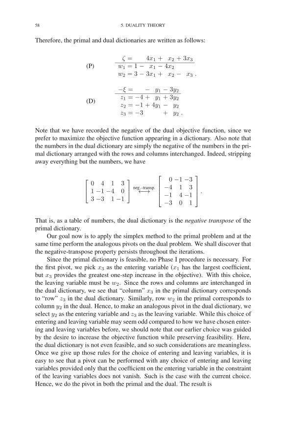
58 5. DUALITY THEORY
Therefore, the primal and dual dictionaries are written as follows:
(P)ζ = 4x1 + x2 + 3x3
w1 = 1 − x1 − 4x2
w2 = 3 − 3x1 + x2 − x3 .
(D)
−ξ = − y1 − 3y2z1 = −4 + y1 + 3y2z2 = −1 + 4y1 − y2z3 = −3 + y2 .
Note that we have recorded the negative of the dual objective function, since weprefer to maximize the objective function appearing in a dictionary. Also note thatthe numbers in the dual dictionary are simply the negative of the numbers in the pri-mal dictionary arranged with the rows and columns interchanged. Indeed, strippingaway everything but the numbers, we have
⎡
⎣0 4 1 31 −1 −4 03 −3 1 −1
⎤
⎦ neg.–transp.←→
⎡
⎢⎢⎣
0 −1 −3−4 1 3−1 4 −1−3 0 1
⎤
⎥⎥⎦ .
That is, as a table of numbers, the dual dictionary is the negative transpose of theprimal dictionary.
Our goal now is to apply the simplex method to the primal problem and at thesame time perform the analogous pivots on the dual problem. We shall discover thatthe negative-transpose property persists throughout the iterations.
Since the primal dictionary is feasible, no Phase I procedure is necessary. Forthe first pivot, we pick x3 as the entering variable (x1 has the largest coefficient,but x3 provides the greatest one-step increase in the objective). With this choice,the leaving variable must be w2. Since the rows and columns are interchanged inthe dual dictionary, we see that “column” x3 in the primal dictionary correspondsto “row” z3 in the dual dictionary. Similarly, row w2 in the primal corresponds tocolumn y2 in the dual. Hence, to make an analogous pivot in the dual dictionary, weselect y2 as the entering variable and z3 as the leaving variable. While this choice ofentering and leaving variable may seem odd compared to how we have chosen enter-ing and leaving variables before, we should note that our earlier choice was guidedby the desire to increase the objective function while preserving feasibility. Here,the dual dictionary is not even feasible, and so such considerations are meaningless.Once we give up those rules for the choice of entering and leaving variables, it iseasy to see that a pivot can be performed with any choice of entering and leavingvariables provided only that the coefficient on the entering variable in the constraintof the leaving variables does not vanish. Such is the case with the current choice.Hence, we do the pivot in both the primal and the dual. The result is

4. THE STRONG DUALITY THEOREM 59
(P)ζ = 9 − 5x1 + 4x2 − 3w2
w1 = 1 − x1 − 4x2
x3 = 3 − 3x1 + x2 − w2 .
(D)
−ξ = −9 − y1 − 3z3z1 = 5 + y1 + 3z3z2 = −4 + 4y1 − z3y2 = 3 + z3 .
Note that these two dictionaries still have the property of being negative-transposesof each other. For the next pivot, the entering variable in the primal dictionary is x2
(this time there is no choice) and the leaving variable is w1. In the dual dictionary,the corresponding entering variable is y1 and the leaving variable is z2. Doing thepivots, we get
(P)ζ = 10 − 6x1 − w1 − 3w2
x2 = 0.25 − 0.25x1 − 0.25w1
x3 = 3.25 − 3.25x1 − 0.25w1 − w2 .
(D)
−ξ = −10 − 0.25z2 − 3.25z3z1 = 6 + 0.25z2 + 3.25z3y1 = 1 + 0.25z2 + 0.25z3y2 = 3 + z3 .
This primal dictionary is optimal, since the coefficients in the objective row are allnegative. Looking at the dual dictionary, we see that it is now feasible for the anal-ogous reason. In fact, it is optimal too. Finally, both the primal and dual objectivefunction values are 10.
The situation should now be clear. Given a linear programming problem, whichis assumed to possess an optimal solution, first apply the Phase I procedure to geta basic feasible starting dictionary for Phase II. Then apply the simplex method tofind an optimal solution. Each primal dictionary generated by the simplex methodimplicitly defines a corresponding dual dictionary as follows: first write down thenegative transpose and then replace each xj with a zj and each wi with a yi. As longas the primal dictionary is not optimal, the implicitly defined dual dictionary will beinfeasible. But once an optimal primal dictionary is found, the corresponding dualdictionary will be feasible. Since its objective coefficients are always nonpositive,this feasible dual dictionary is also optimal. Furthermore, at each iteration, thecurrent primal objective function value coincides with the current dual objectivefunction value.
To see why the negative transpose property is preserved from one dictionaryto the next, let’s observe the effect of one pivot. To keep notations uncluttered, weconsider only four generic entries in a table of coefficients: the pivot element, whichwe denote by a, one other element on the pivot element’s row, call it b, one otherin its column, call it c, and a fourth element, denoted d, chosen to make these fourentries into a rectangle. A little thought (and perhaps some staring at the examplesabove) reveals that a pivot produces the following changes:
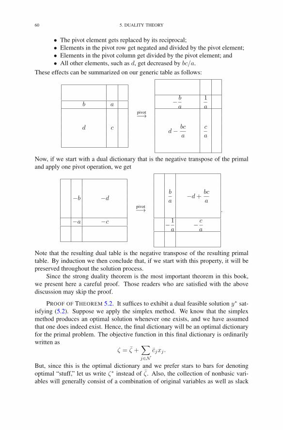
60 5. DUALITY THEORY
• The pivot element gets replaced by its reciprocal;• Elements in the pivot row get negated and divided by the pivot element;• Elements in the pivot column get divided by the pivot element; and• All other elements, such as d, get decreased by bc/a.
These effects can be summarized on our generic table as follows:
b a
d c
pivot−→
− b
a
1
a
d− bc
a
c
a
Now, if we start with a dual dictionary that is the negative transpose of the primaland apply one pivot operation, we get
−b −d
−a −c
pivot−→
b
a−d+
bc
a
−1
a− c
a
.
Note that the resulting dual table is the negative transpose of the resulting primaltable. By induction we then conclude that, if we start with this property, it will bepreserved throughout the solution process.
Since the strong duality theorem is the most important theorem in this book,we present here a careful proof. Those readers who are satisfied with the abovediscussion may skip the proof.
PROOF OF THEOREM 5.2. It suffices to exhibit a dual feasible solution y∗ sat-isfying (5.2). Suppose we apply the simplex method. We know that the simplexmethod produces an optimal solution whenever one exists, and we have assumedthat one does indeed exist. Hence, the final dictionary will be an optimal dictionaryfor the primal problem. The objective function in this final dictionary is ordinarilywritten as
ζ = ζ +∑
j∈Ncjxj .
But, since this is the optimal dictionary and we prefer stars to bars for denotingoptimal “stuff,” let us write ζ∗ instead of ζ. Also, the collection of nonbasic vari-ables will generally consist of a combination of original variables as well as slack
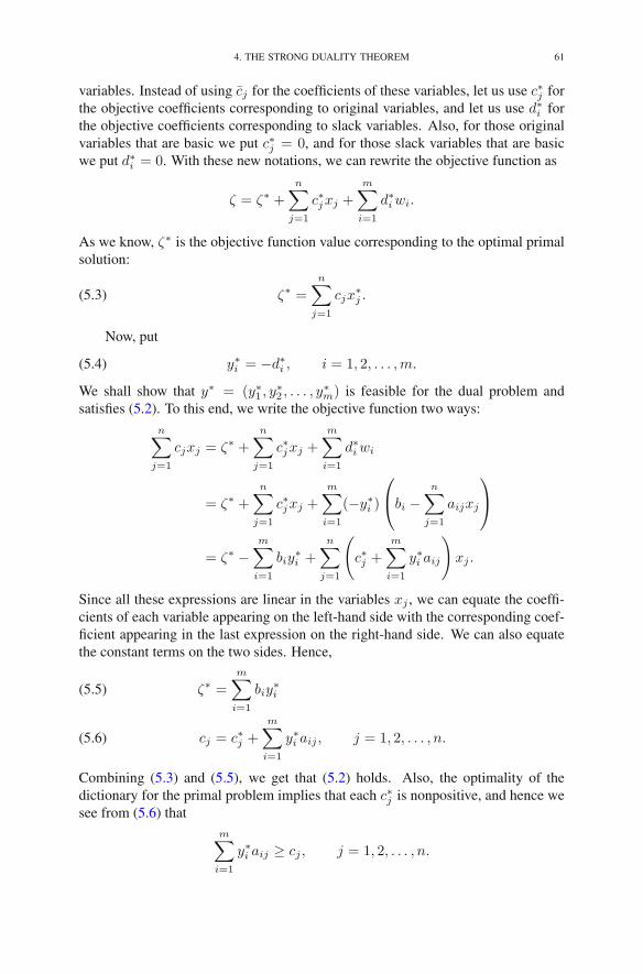
4. THE STRONG DUALITY THEOREM 61
variables. Instead of using cj for the coefficients of these variables, let us use c∗j forthe objective coefficients corresponding to original variables, and let us use d∗i forthe objective coefficients corresponding to slack variables. Also, for those originalvariables that are basic we put c∗j = 0, and for those slack variables that are basicwe put d∗i = 0. With these new notations, we can rewrite the objective function as
ζ = ζ∗ +n∑
j=1
c∗jxj +
m∑
i=1
d∗iwi.
As we know, ζ∗ is the objective function value corresponding to the optimal primalsolution:
(5.3) ζ∗ =
n∑
j=1
cjx∗j .
Now, put
(5.4) y∗i = −d∗i , i = 1, 2, . . . ,m.
We shall show that y∗ = (y∗1 , y∗2 , . . . , y
∗m) is feasible for the dual problem and
satisfies (5.2). To this end, we write the objective function two ways:n∑
j=1
cjxj = ζ∗ +n∑
j=1
c∗jxj +
m∑
i=1
d∗iwi
= ζ∗ +n∑
j=1
c∗jxj +
m∑
i=1
(−y∗i )
⎛
⎝bi −n∑
j=1
aijxj
⎞
⎠
= ζ∗ −m∑
i=1
biy∗i +
n∑
j=1
(
c∗j +m∑
i=1
y∗i aij
)
xj .
Since all these expressions are linear in the variables xj , we can equate the coeffi-cients of each variable appearing on the left-hand side with the corresponding coef-ficient appearing in the last expression on the right-hand side. We can also equatethe constant terms on the two sides. Hence,
ζ∗ =m∑
i=1
biy∗i(5.5)
cj = c∗j +m∑
i=1
y∗i aij , j = 1, 2, . . . , n.(5.6)
Combining (5.3) and (5.5), we get that (5.2) holds. Also, the optimality of thedictionary for the primal problem implies that each c∗j is nonpositive, and hence wesee from (5.6) that
m∑
i=1
y∗i aij ≥ cj , j = 1, 2, . . . , n.

62 5. DUALITY THEORY
By the same reasoning, each d∗i is nonpositive, and so we see from (5.4) that
y∗i ≥ 0, i = 1, 2, . . . ,m.
These last two sets of inequalities are precisely the conditions that guarantee dualfeasibility. This completes the proof. �
The strong duality theorem tells us that, whenever the primal problem has anoptimal solution, the dual problem has one also and there is no duality gap. But whatif the primal problem does not have an optimal solution? For example, suppose thatit is unbounded. The unboundedness of the primal together with the weak dualitytheorem tells us immediately that the dual problem must be infeasible. Similarly,if the dual problem is unbounded, then the primal problem must be infeasible. Itis natural to hope that these three cases are the only possibilities, because if theywere we could then think of the strong duality theorem holding globally. That is,even if, say, the primal is unbounded, the fact that then the dual is infeasible is likesaying that the primal and dual have a zero duality gap sitting out at +∞. Similarly,an infeasible primal together with an unbounded dual could be viewed as a pair inwhich the gap is zero and sits at −∞.
But it turns out that there is a fourth possibility that sometimes occurs—it canhappen that both the primal and the dual problems are infeasible. For example,consider the following problem:
maximize 2x1 − x2
subject to x1 − x2 ≤ 1−x1 + x2 ≤ −2
x1, x2 ≥ 0 .
It is easy to see that both this problem and its dual are infeasible. For these problems,one can think of there being a huge duality gap extending from −∞ to +∞.
Duality theory is often useful in that it provides a certificate of optimality. Forexample, suppose that you were asked to solve a really huge and difficult linearprogram. After spending weeks or months at the computer, you are finally ableto get the simplex method to solve the problem, producing as it does an optimaldual solution y∗ in addition to the optimal primal solution x∗. Now, how are yougoing to convince your boss that your solution is correct? Do you really want to askher to verify the correctness of your computer programs? The answer is probablynot. And in fact it is not necessary. All you need to do is supply the primal andthe dual solution, and she only has to check that the primal solution is feasible forthe primal problem (that’s easy), the dual solution is feasible for the dual problem(that’s just as easy), and the primal and dual objective values agree (and that’s eveneasier). Certificates of optimality have also been known to dramatically reduce theamount of time certain underpaid professors have to devote to grading homeworkassignments!
As we’ve seen, the simplex method applied to a primal problem actually solvesboth the primal and the dual. Since the dual of the dual is the primal, applyingthe simplex method to the dual also solves both the primal and the dual problem.

5. COMPLEMENTARY SLACKNESS 63
Sometimes it is easier to apply the simplex method to the dual, for example, if thedual has an obvious basic feasible solution but the primal does not. We take up thistopic in the next chapter.
5. Complementary Slackness
Sometimes it is necessary to recover an optimal dual solution when only anoptimal primal solution is known. The following theorem, known as the Comple-mentary Slackness Theorem, can help in this regard.
THEOREM 5.3. Suppose that x = (x1, x2, . . . , xn) is primal feasible and thaty = (y1, y2, . . . , ym) is dual feasible. Let (w1, w2, . . . , wm) denote the correspond-ing primal slack variables, and let (z1, z2, . . . , zn) denote the corresponding dualslack variables. Then x and y are optimal for their respective problems if and only if
xjzj = 0, for j = 1, 2, . . . , n,
wiyi = 0, for i = 1, 2, . . . ,m.(5.7)
PROOF. We begin by revisiting the chain of inequalities used to prove the weakduality theorem:
∑
j
cjxj ≤∑
j
(∑
i
yiaij
)
xj(5.8)
=∑
i
⎛
⎝∑
j
aijxj
⎞
⎠ yi
≤∑
i
biyi.(5.9)
Recall that the first inequality arises from the fact that each term in the left-handsum is dominated by the corresponding term in the right-hand sum. Furthermore,this domination is a consequence of the fact that each xj is nonnegative and
cj ≤∑
i
yiaij .
Hence, inequality (5.8) will be an equality if and only if, for every j = 1, 2, . . . , n,either xj = 0 or cj =
∑i yiaij . But since
zj =∑
i
yiaij − cj ,
we see that the alternative to xj = 0 is simply that zj = 0. Of course, the state-ment that at least one of these two numbers vanishes can be succinctly expressed bysaying that the product vanishes.
An analogous analysis of inequality (5.9) shows that it is an equality if and onlyif (5.7) holds. This then completes the proof. �
Suppose that we have a nondegenerate primal basic optimal solution
x∗ = (x∗1, x
∗2, . . . , x
∗n)
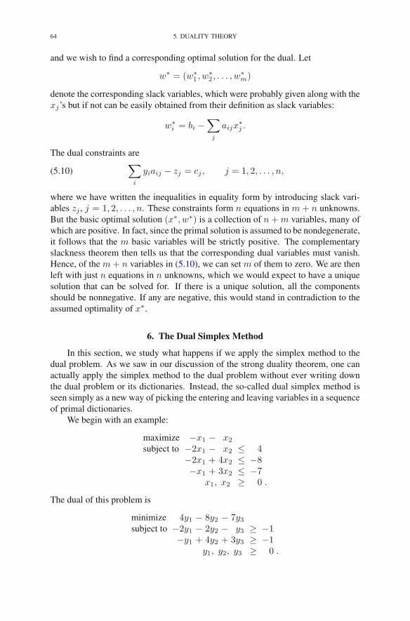
64 5. DUALITY THEORY
and we wish to find a corresponding optimal solution for the dual. Let
w∗ = (w∗1 , w
∗2 , . . . , w
∗m)
denote the corresponding slack variables, which were probably given along with thexj’s but if not can be easily obtained from their definition as slack variables:
w∗i = bi −
∑
j
aijx∗j .
The dual constraints are
(5.10)∑
i
yiaij − zj = cj , j = 1, 2, . . . , n,
where we have written the inequalities in equality form by introducing slack vari-ables zj , j = 1, 2, . . . , n. These constraints form n equations in m + n unknowns.But the basic optimal solution (x∗, w∗) is a collection of n+m variables, many ofwhich are positive. In fact, since the primal solution is assumed to be nondegenerate,it follows that the m basic variables will be strictly positive. The complementaryslackness theorem then tells us that the corresponding dual variables must vanish.Hence, of the m+ n variables in (5.10), we can set m of them to zero. We are thenleft with just n equations in n unknowns, which we would expect to have a uniquesolution that can be solved for. If there is a unique solution, all the componentsshould be nonnegative. If any are negative, this would stand in contradiction to theassumed optimality of x∗.
6. The Dual Simplex Method
In this section, we study what happens if we apply the simplex method to thedual problem. As we saw in our discussion of the strong duality theorem, one canactually apply the simplex method to the dual problem without ever writing downthe dual problem or its dictionaries. Instead, the so-called dual simplex method isseen simply as a new way of picking the entering and leaving variables in a sequenceof primal dictionaries.
We begin with an example:
maximize −x1 − x2
subject to −2x1 − x2 ≤ 4−2x1 + 4x2 ≤ −8−x1 + 3x2 ≤ −7
x1, x2 ≥ 0 .
The dual of this problem is
minimize 4y1 − 8y2 − 7y3subject to −2y1 − 2y2 − y3 ≥ −1
−y1 + 4y2 + 3y3 ≥ −1y1, y2, y3 ≥ 0 .
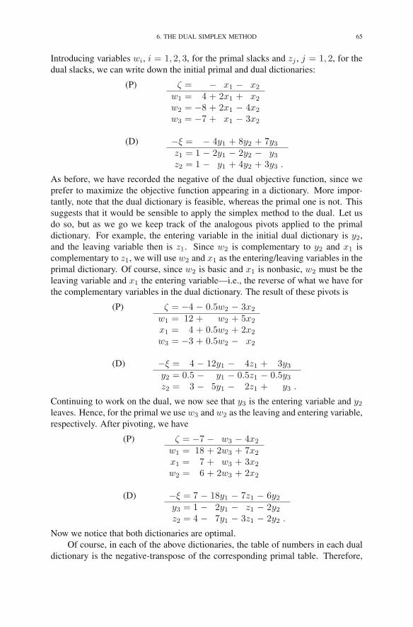
6. THE DUAL SIMPLEX METHOD 65
Introducing variables wi, i = 1, 2, 3, for the primal slacks and zj , j = 1, 2, for thedual slacks, we can write down the initial primal and dual dictionaries:
(P) ζ = − x1 − x2
w1 = 4 + 2x1 + x2
w2 = −8 + 2x1 − 4x2
w3 = −7 + x1 − 3x2
(D) −ξ = − 4y1 + 8y2 + 7y3z1 = 1 − 2y1 − 2y2 − y3z2 = 1 − y1 + 4y2 + 3y3 .
As before, we have recorded the negative of the dual objective function, since weprefer to maximize the objective function appearing in a dictionary. More impor-tantly, note that the dual dictionary is feasible, whereas the primal one is not. Thissuggests that it would be sensible to apply the simplex method to the dual. Let usdo so, but as we go we keep track of the analogous pivots applied to the primaldictionary. For example, the entering variable in the initial dual dictionary is y2,and the leaving variable then is z1. Since w2 is complementary to y2 and x1 iscomplementary to z1, we will use w2 and x1 as the entering/leaving variables in theprimal dictionary. Of course, since w2 is basic and x1 is nonbasic, w2 must be theleaving variable and x1 the entering variable—i.e., the reverse of what we have forthe complementary variables in the dual dictionary. The result of these pivots is
(P) ζ = −4 − 0.5w2 − 3x2
w1 = 12 + w2 + 5x2
x1 = 4 + 0.5w2 + 2x2
w3 = −3 + 0.5w2 − x2
(D) −ξ = 4 − 12y1 − 4z1 + 3y3y2 = 0.5 − y1 − 0.5z1 − 0.5y3z2 = 3 − 5y1 − 2z1 + y3 .
Continuing to work on the dual, we now see that y3 is the entering variable and y2leaves. Hence, for the primal we use w3 and w2 as the leaving and entering variable,respectively. After pivoting, we have
(P) ζ = −7 − w3 − 4x2
w1 = 18 + 2w3 + 7x2
x1 = 7 + w3 + 3x2
w2 = 6 + 2w3 + 2x2
(D) −ξ = 7 − 18y1 − 7z1 − 6y2y3 = 1 − 2y1 − z1 − 2y2z2 = 4 − 7y1 − 3z1 − 2y2 .
Now we notice that both dictionaries are optimal.Of course, in each of the above dictionaries, the table of numbers in each dual
dictionary is the negative-transpose of the corresponding primal table. Therefore,
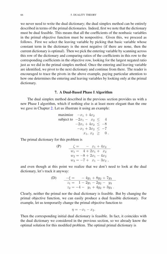
66 5. DUALITY THEORY
we never need to write the dual dictionary; the dual simplex method can be entirelydescribed in terms of the primal dictionaries. Indeed, first we note that the dictionarymust be dual feasible. This means that all the coefficients of the nonbasic variablesin the primal objective function must be nonpositive. Given this, we proceed asfollows. First we select the leaving variable by picking that basic variable whoseconstant term in the dictionary is the most negative (if there are none, then thecurrent dictionary is optimal). Then we pick the entering variable by scanning acrossthis row of the dictionary and comparing ratios of the coefficients in this row to thecorresponding coefficients in the objective row, looking for the largest negated ratiojust as we did in the primal simplex method. Once the entering and leaving variableare identified, we pivot to the next dictionary and continue from there. The reader isencouraged to trace the pivots in the above example, paying particular attention tohow one determines the entering and leaving variables by looking only at the primaldictionary.
7. A Dual-Based Phase I Algorithm
The dual simplex method described in the previous section provides us with anew Phase I algorithm, which if nothing else is at least more elegant than the onewe gave in Chapter 2. Let us illustrate it using an example:
maximize −x1 + 4x2
subject to −2x1 − x2 ≤ 4−2x1 + 4x2 ≤ −8−x1 + 3x2 ≤ −7
x1, x2 ≥ 0 .
The primal dictionary for this problem is
(P) ζ = − x1 + 4x2
w1 = 4 + 2x1 + x2
w2 = −8 + 2x1 − 4x2
w3 = −7 + x1 − 3x2 ,
and even though at this point we realize that we don’t need to look at the dualdictionary, let’s track it anyway:
(D) −ξ = − 4y1 + 8y2 + 7y3z1 = 1 − 2y1 − 2y2 − y3z2 = −4 − y1 + 4y2 + 3y3 .
Clearly, neither the primal nor the dual dictionary is feasible. But by changing theprimal objective function, we can easily produce a dual feasible dictionary. Forexample, let us temporarily change the primal objective function to
η = −x1 − x2.
Then the corresponding initial dual dictionary is feasible. In fact, it coincides withthe dual dictionary we considered in the previous section, so we already know theoptimal solution for this modified problem. The optimal primal dictionary is

8. THE DUAL OF A PROBLEM IN GENERAL FORM 67
η = −7 − w3 − 4x2
w1 = 18 + 2w3 + 7x2
x1 = 7 + w3 + 3x2
w2 = 6 + 2w3 + 2x2 .
This primal dictionary is optimal for the modified problem but not for the originalproblem. However, it is feasible for the original problem, and we can now simplyreinstate the intended objective function and continue with Phase II. Indeed,
ζ = −x1 + 4x2
= −(7 + w3 + 3x2) + 4x2
= −7− w3 + x2.
Hence, the starting dictionary for Phase II is
ζ = −7 − w3 + x2
w1 = 18 + 2w3 + 7x2
x1 = 7 + w3 + 3x2
w2 = 6 + 2w3 + 2x2 .
The entering variable is x2. Looking for a leaving variable, we discover that thisproblem is unbounded. Of course, more typically one would expect to have to doseveral iterations of Phase II to find the optimal solution (or show unboundedness).Here we just got lucky that the game ended so soon.
It is interesting to note how we detect infeasibility with this new Phase I algo-rithm. The modified problem is guaranteed always to be dual feasible. It is easy tosee that the primal problem is infeasible if and only if the modified problem is dualunbounded (which the dual simplex method will detect just as the primal simplexmethod detects primal unboundedness).
The two-phase algorithm we have just presented can be thought of as a dual–primal algorithm, since we first apply the dual simplex method to a modified dualfeasible problem and then finish off by applying the primal simplex method to theoriginal problem, starting from the feasible dictionary produced by Phase I. Onecould consider turning this around and doing a primal–dual two-phase algorithm.Here, the right-hand side of the primal problem would be modified to produce anobvious primal feasible solution. The primal simplex method would then be applied.The optimal solution to this primal problem will then be feasible for the originaldual problem but will not be optimal for it. But then the dual simplex method canbe applied, starting with this dual feasible basis until an optimal solution for the dualproblem is obtained.
8. The Dual of a Problem in General Form
In Chapter 1, we saw that linear programming problems can be formulated ina variety of ways. In this section, we derive the form of the dual when the primalproblem is not necessarily presented in standard form.
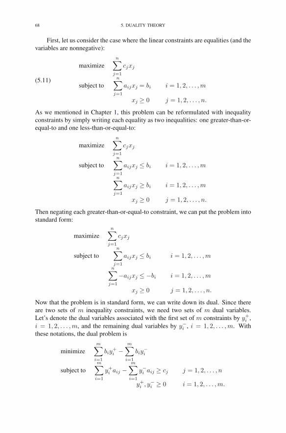
68 5. DUALITY THEORY
First, let us consider the case where the linear constraints are equalities (and thevariables are nonnegative):
(5.11)
maximizen∑
j=1
cjxj
subject ton∑
j=1
aijxj = bi i = 1, 2, . . . ,m
xj ≥ 0 j = 1, 2, . . . , n.
As we mentioned in Chapter 1, this problem can be reformulated with inequalityconstraints by simply writing each equality as two inequalities: one greater-than-or-equal-to and one less-than-or-equal-to:
maximizen∑
j=1
cjxj
subject ton∑
j=1
aijxj ≤ bi i = 1, 2, . . . ,m
n∑
j=1
aijxj ≥ bi i = 1, 2, . . . ,m
xj ≥ 0 j = 1, 2, . . . , n.
Then negating each greater-than-or-equal-to constraint, we can put the problem intostandard form:
maximizen∑
j=1
cjxj
subject ton∑
j=1
aijxj ≤ bi i = 1, 2, . . . ,m
n∑
j=1
−aijxj ≤ −bi i = 1, 2, . . . ,m
xj ≥ 0 j = 1, 2, . . . , n.
Now that the problem is in standard form, we can write down its dual. Since thereare two sets of m inequality constraints, we need two sets of m dual variables.Let’s denote the dual variables associated with the first set of m constraints by y+i ,i = 1, 2, . . . ,m, and the remaining dual variables by y−i , i = 1, 2, . . . ,m. Withthese notations, the dual problem is
minimizem∑
i=1
biy+i −
m∑
i=1
biy−i
subject tom∑
i=1
y+i aij −m∑
i=1
y−i aij ≥ cj j = 1, 2, . . . , n
y+i , y−i ≥ 0 i = 1, 2, . . . ,m.

9. RESOURCE ALLOCATION PROBLEMS 69
Primal Dual
Equality constraint Free variableInequality constraint Nonnegative variable
Free variable Equality constraintNonnegative variable Inequality constraint
TABLE 5.1. Rules for forming the dual.
A moment’s reflection reveals that we can simplify this problem. If we put
yi = y+i − y−i , i = 1, 2, . . . ,m,
the dual problem reduces to
minimizem∑
i=1
biyi
subject tom∑
i=1
yiaij ≥ cj j = 1, 2, . . . , n.
This problem is the dual associated with (5.11). Note what has changed from whenwe were considering problems in standard form: now the dual variables are notrestricted to be nonnegative. And that is the message: equality constraints in theprimal yield unconstrained variables (also referred to as free variables) in the dual,whereas inequality constraints in the primal yield nonnegative variables in the dual.Employing the symmetry between the primal and the dual, we can say more: freevariables in the primal yield equality constraints in the dual, whereas nonnegativevariables in the primal yield inequality constraints in the dual. These rules aresummarized in Table 5.1.
9. Resource Allocation Problems
Let us return to the production facility problem studied in Chapter 1. Recallthat this problem involves a production facility that can take a variety of raw ma-terials (enumerated i = 1, 2, . . . ,m) and turn them into a variety of final products(enumerated j = 1, 2, . . . , n). We assume as before that the current market value ofa unit of the ith raw material is ρi, that the current market price for a unit of the jthproduct is σj , that producing one unit of product j requires aij units of raw materiali, and that at the current moment in time the facility has on hand bi units of the ithraw material.
The current market values/prices are, by definition, related to each other by theformulas
σj =∑
i
ρiaij , j = 1, 2, . . . , n.
These equations hold whenever the market is in equilibrium. (Of course, it iscrucial to assume here that the collection of “raw materials” appearing on the right-hand side is exhaustive, including such items as depreciation of fixed assets and
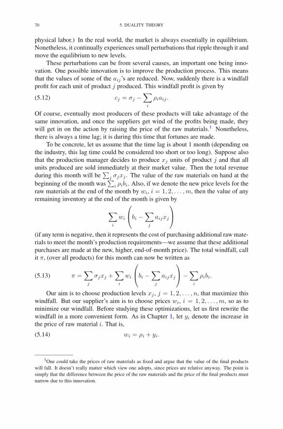
70 5. DUALITY THEORY
physical labor.) In the real world, the market is always essentially in equilibrium.Nonetheless, it continually experiences small perturbations that ripple through it andmove the equilibrium to new levels.
These perturbations can be from several causes, an important one being inno-vation. One possible innovation is to improve the production process. This meansthat the values of some of the aij’s are reduced. Now, suddenly there is a windfallprofit for each unit of product j produced. This windfall profit is given by
(5.12) cj = σj −∑
i
ρiaij .
Of course, eventually most producers of these products will take advantage of thesame innovation, and once the suppliers get wind of the profits being made, theywill get in on the action by raising the price of the raw materials.1 Nonetheless,there is always a time lag; it is during this time that fortunes are made.
To be concrete, let us assume that the time lag is about 1 month (depending onthe industry, this lag time could be considered too short or too long). Suppose alsothat the production manager decides to produce xj units of product j and that allunits produced are sold immediately at their market value. Then the total revenueduring this month will be
∑j σjxj . The value of the raw materials on hand at the
beginning of the month was∑
i ρibi. Also, if we denote the new price levels for theraw materials at the end of the month by wi, i = 1, 2, . . . ,m, then the value of anyremaining inventory at the end of the month is given by
∑
i
wi
⎛
⎝bi −∑
j
aijxj
⎞
⎠
(if any term is negative, then it represents the cost of purchasing additional raw mate-rials to meet the month’s production requirements—we assume that these additionalpurchases are made at the new, higher, end-of-month price). The total windfall, callit π, (over all products) for this month can now be written as
(5.13) π =∑
j
σjxj +∑
i
wi
⎛
⎝bi −∑
j
aijxj
⎞
⎠−∑
i
ρibi.
Our aim is to choose production levels xj , j = 1, 2, . . . , n, that maximize thiswindfall. But our supplier’s aim is to choose prices wi, i = 1, 2, . . . ,m, so as tominimize our windfall. Before studying these optimizations, let us first rewrite thewindfall in a more convenient form. As in Chapter 1, let yi denote the increase inthe price of raw material i. That is,
(5.14) wi = ρi + yi.
1One could take the prices of raw materials as fixed and argue that the value of the final productswill fall. It doesn’t really matter which view one adopts, since prices are relative anyway. The point issimply that the difference between the price of the raw materials and the price of the final products mustnarrow due to this innovation.
9. RESOURCE ALLOCATION PROBLEMS 71
Substituting (5.14) into (5.13) and then simplifying notations using (5.12), we seethat
(5.15) π =∑
j
cjxj +∑
i
yi
⎛
⎝bi −∑
j
aijxj
⎞
⎠ .
To emphasize that π depends on each of the xj’s and on the yi’s, we sometimeswrite it as π(x1, . . . , xn, y1, . . . , ym).
Now let us return to the competing optimizations. Given xj for j = 1, 2, . . . , n,the suppliers react to minimize π(x1, . . . , xn, y1, . . . , ym). Looking at (5.15), wesee that for any resource i in short supply, that is,
bi −∑
j
aijxj < 0,
the suppliers will jack up the price immensely (i.e., yi = ∞). To avoid this obvi-ously bad situation, the production manager will be sure to set the production levelsso that ∑
j
aijxj ≤ bi, i = 1, 2, . . . ,m.
On the other hand, for any resource i that is not exhausted during the windfall month,that is,
bi −∑
j
aijxj > 0,
the suppliers will have no incentive to change the prevailing market price (i.e.,yi =0). Therefore, from the production manager’s point of view, the problem re-duces to one of maximizing
∑
j
cjxj
subject to the constraints that∑
j
aijxj ≤ bi, i = 1, 2, . . . ,m,
xj ≥ 0, j = 1, 2, . . . , n.
This is just our usual primal linear programming problem. This is the problem thatthe production manager needs to solve in anticipation of adversarial suppliers.
Now let us look at the problem from the suppliers’ point of view. Rearrangingthe terms in (5.15) by writing
(5.16) π =∑
j
(
cj −∑
i
yiaij
)
xj +∑
i
yibi,
we see that if the suppliers set prices in such a manner that a windfall remains onthe jth product even after the price adjustment, that is,
cj −∑
i
yiaij > 0,
72 5. DUALITY THEORY
then the production manager would be able to generate for the facility an arbitrarilylarge windfall by producing a huge amount of the jth product (i.e., xj = ∞). Weassume that this is unacceptable to the suppliers, and so they will determine theirprice increases so that
∑
i
yiaij ≥ cj , j = 1, 2, . . . , n.
Also, if the suppliers set the price increases too high so that the production facilitywill lose money by producing product j, that is,
cj −∑
i
yiaij < 0,
then the production manager would simply decide not to engage in that activity.That is, she would set xj = 0. Hence, the first term in (5.16) will always be zero,and so the optimization problem faced by the suppliers is to minimize
∑
i
biyi
subject to the constraints that∑
i
yiaij ≥ cj , j = 1, 2, . . . , n,
yi ≥ 0, i = 1, 2, . . . ,m.
This is precisely the dual of the production manager’s problem!As we’ve seen earlier with the strong duality theorem, if the production man-
ager’s problem has an optimal solution, then so does the suppliers’ problem, andthe two objectives agree. This means than an equilibrium can be reestablished bysetting the production levels and the price hikes according to the optimal solutionsto these two linear programming problems.
10. Lagrangian Duality
The analysis of the preceding section is an example of a general technique thatforms the foundation of a subject called Lagrangian duality, which we shall brieflydescribe.
Let us start by summarizing what we did. It was quite simple. The analysisrevolved around a function
π(x1, . . . , xn, y1, . . . , ym) =∑
j
cjxj −∑
i
∑
j
yiaijxj +∑
i
yibi.
To streamline notations, let x stand for the entire collection of variables x1, x2,. . . , xn and let y stand for the collection of yi’s so that we can write π(x, y) inplace of π(x1, . . . , xn, y1, . . . , ym). Written with these notations, we showed in theprevious section that
maxx≥0
miny≥0
π(x, y) = miny≥0
maxx≥0
π(x, y).

EXERCISES 73
We also showed that the inner optimization could in both cases be solved explicitly,that the max–min problem reduced to a linear programming problem, and that themin–max problem reduced to the dual linear programming problem.
One could imagine trying to carry out the same program for functions π thatdon’t necessarily have the form shown above. In the general case, one needs toconsider each step carefully. The max–min problem is called the primal problem,and the min–max problem is called the dual problem. However, it may or may notbe true that these two problems have the same optimal objective values. In fact, thesubject is interesting because one can indeed state specific, verifyable conditionsfor which the two problems do agree. Also, one would like to be able to solve theinner optimizations explicitly so that the primal problem can be stated as a puremaximization problem and the dual can be stated as a pure minimization problem.This, too, is often doable. There are various ways in which one can extend thenotions of duality beyond the context of linear programming. The one just describedis referred to as Lagrangian duality. It is perhaps the most important such extension.
Exercises
In solving the following problems, the advanced pivot tool can be used to checkyour arithmetic:
www.princeton.edu/∼rvdb/JAVA/pivot/advanced.html
5.1 What is the dual of the following linear programming problem:
maximize x1 − 2x2
subject to x1 + 2x2 − x3 + x4 ≥ 04x1 + 3x2 + 4x3 − 2x4 ≤ 3−x1 − x2 + 2x3 + x4 = 1
x2, x3 ≥ 0.
5.2 Illustrate Theorem 5.2 on the problem in Exercise 2.9.
5.3 Illustrate Theorem 5.2 on the problem in Exercise 2.1.
5.4 Illustrate Theorem 5.2 on the problem in Exercise 2.2.
5.5 Consider the following linear programming problem:
maximize 2x1 + 8x2 − x3 − 2x4
subject to 2x1 + 3x2 + 6x4 ≤ 6−2x1 + 4x2 + 3x3 ≤ 1.53x1 + 2x2 − 2x3 − 4x4 ≤ 4
x1, x2, x3, x4 ≥ 0 .
Suppose that, in solving this problem, you have arrived at the followingdictionary:
ζ = 3.5 − 0.25w1 + 6.25x2 − 0.5w3 − 1.5x4
x1 = 3.0 − 0.5w1 − 1.5x2 − 3.0x4
w2 = 0.0 + 1.25w1 − 3.25x2 − 1.5w3 + 13.5x4
x3 = 2.5 − 0.75w1 − 1.25x2 + 0.5w3 − 6.5x4 .
74 5. DUALITY THEORY
(a) Write down the dual problem.(b) In the dictionary shown above, which variables are basic? Which are
nonbasic?(c) Write down the primal solution corresponding to the given dictio-
nary. Is it feasible? Is it degenerate?(d) Write down the corresponding dual dictionary.(e) Write down the dual solution. Is it feasible?(f) Do the primal/dual solutions you wrote above satisfy the comple-
mentary slackness property?(g) Is the current primal solution optimal?(h) For the next (primal) pivot, which variable will enter if the largest
coefficient rule is used? Which will leave? Will the pivot be degen-erate?
5.6 Solve the following linear program:
maximize −x1 − 2x2
subject to −2x1 + 7x2 ≤ 6−3x1 + x2 ≤ −19x1 − 4x2 ≤ 6x1 − x2 ≤ 1
7x1 − 3x2 ≤ 6−5x1 + 2x2 ≤ −3
x1, x2 ≥ 0 .
5.7 Solve the linear program given in Exercise 2.3 using the dual–primal two-phase algorithm.
5.8 Solve the linear program given in Exercise 2.4 using the dual–primal two-phase algorithm.
5.9 Solve the linear program given in Exercise 2.6 using the dual–primal two-phase algorithm.
5.10 Using today’s date (MMYY) for the seed value, solve 10 problems usingthe dual phase I primal phase II simplex method:
www.princeton.edu/∼rvdb/JAVA/pivot/dp2phase.html
5.11 Using today’s date (MMYY) for the seed value, solve 10 problems usingthe primal phase I dual phase II simplex method:
www.princeton.edu/∼rvdb/JAVA/pivot/pd2phase.html
5.12 For x and y in R, compute
maxx≥0
miny≥0
(x− y) and miny≥0
maxx≥0
(x− y)
and note whether or not they are equal.

EXERCISES 75
5.13 Consider the following process. Starting with a linear programming prob-lem in standard form,
maximizen∑
j=1
cjxj
subject ton∑
j=1
aijxj ≤ bi i = 1, 2, . . . ,m
xj ≥ 0 j = 1, 2, . . . , n,
first form its dual:
minimizem∑
i=1
biyi
subject tom∑
i=1
yiaij ≥ cj j = 1, 2, . . . , n
yi ≥ 0 i = 1, 2, . . . ,m.
Then replace the minimization in the dual with a maximization to get anew linear programming problem, which we can write in standard formas follows:
maximizem∑
i=1
biyi
subject tom∑
i=1
−yiaij ≤ −cj j = 1, 2, . . . , n
yi ≥ 0 i = 1, 2, . . . ,m.
If we identify a linear programming problem with its data, (aij , bi, cj),the above process can be thought of as a transformation T on the space ofdata defined by
(aij , bi, cj)T−→ (−aji,−cj , bi).
Let ζ∗(aij , bi, cj) denote the optimal objective function value of thestandard-form linear programming problem having data (aij , bi, cj).By strong duality together with the fact that a maximization dominatesa minimization, it follows that
ζ∗(aij , bi, cj) ≤ ζ∗(−aji,−cj , bi).
Now if we repeat this process, we get
(aij , bi, cj)T→ (−aji,−cj , bi)
T→ (aij ,−bi,−cj)
T→ (−aji, cj ,−bi)
T→ (aij , bi, cj)
76 5. DUALITY THEORY
and hence that
ζ∗(aij , bi, cj) ≤ ζ∗(−aji,−cj , bi)
≤ ζ∗(aij ,−bi,−cj)
≤ ζ∗(−aji, cj ,−bi)
≤ ζ∗(aij , bi, cj).
But the first and the last entry in this chain of inequalities are equal. There-fore, all these inequalities would seem to be equalities. While this out-come could happen sometimes, it certainly isn’t always true. What is theerror in this logic? Can you state a (correct) nontrivial theorem that fol-lows from this line of reasoning? Can you give an example where the fourinequalities are indeed all equalities?
5.14 Consider the following variant of the resource allocation problem:
(5.17)
maximizen∑
j=1
cjxj
subject ton∑
j=1
aijxj ≤ bi i = 1, 2, . . . ,m
0 ≤ xj ≤ uj j = 1, 2, . . . , n.
As usual, the cj’s denote the unit prices for the products and the bi’s denotethe number of units on hand for each raw material. In this variant, the uj’sdenote upper bounds on the number of units of each product that can besold at the set price. Now, let’s assume that the raw materials have notbeen purchased yet and it is part of the problem to determine the bi’s. Letpi, i = 1, 2, . . . ,m denote the price for raw material i. The problem thenbecomes an optimization over both the xj’s and the bi’s:
maximizen∑
j=1
cjxj −m∑
i=1
pibi
subject ton∑
j=1
aijxj − bi ≤ 0 i = 1, 2, . . . ,m
0 ≤ xj ≤ uj j = 1, 2, . . . , nbi ≥ 0 i = 1, 2, . . . ,m.
(a) Show that this problem always has an optimal solution.(b) Let y∗i (b), i = 1, 2, . . . ,m, denote optimal dual variables for the
original resource allocation problem (5.17). Note that we’ve explic-itly indicated that these dual variables depend on the b’s. Also, weassume that problem (5.17) is both primal and dual non-degenerateso the y∗i (b) is uniquely defined. Show that the optimal value of thebi’s, call them b∗i ’s, satisfy
y∗i (b∗) = pi.

EXERCISES 77
Hint: You will need to use the fact that, for resource allocation prob-lems, we have aij ≥ 0 for all i, and all j.
5.15 Consider the following linear program:
maximizen∑
j=1
pjxj
subject ton∑
j=1
qjxj ≤ β
xj ≤ 1 j = 1, 2, . . . , nxj ≥ 0 j = 1, 2, . . . , n.
Here, the numbers pj , j = 1, 2, . . . , n are positive and sum to one. Thesame is true of the qj’s:
n∑
j=1
qj = 1
qj > 0.
Furthermore, assume thatp1q1
<p2q2
< · · · < pnqn
and that the parameter β is a small positive number. Let k = min{j :qj+1 + · · ·+ qn ≤ β}. Let y0 denote the dual variable associated with theconstraint involving β, and let yj denote the dual variable associated withthe upper bound of 1 on variable xj . Using duality theory, show that theoptimal values of the primal and dual variables are given by
xj =
⎧⎨
⎩
0 j < kβ−qk+1−···−qn
qkj = k
1 j > k
yj =
⎧⎪⎨
⎪⎩
pk
qkj = 0
0 0 < j ≤ k
qj
(pj
qj− pk
qk
)j > k
See Exercise 1.3 for the motivation for this problem.
5.16 Diet Problem. An MIT graduate student was trying to make ends meet ona very small stipend. He went to the library and looked up theNational Research Council’s publication entitled “Recommended DietaryAllowances” and was able to determine a minimum daily intake quantityof each essential nutrient for a male in his weight and age category. Let mdenote the number of nutrients that he identified as important to his diet,and let bi for i = 1, 2, . . . ,m denote his personal minimum daily require-ments. Next, he made a list of his favorite foods (which, except for pizzaand due mostly to laziness and ineptitude in the kitchen, consisted almost

78 5. DUALITY THEORY
entirely of frozen prepared meals). He then went to the local grocery storeand made a list of the unit price for each of his favorite foods. Let us de-note these prices as cj for j = 1, 2, . . . , n. In addition to prices, he alsolooked at the labels and collected information about how much of the crit-ical nutrients are contained in one serving of each food. Let us denote byaij the amount of nutrient i contained in food j. (Fortunately, he was ableto call his favorite pizza delivery service and get similar information fromthem.) In terms of this information, he formulated the following linearprogramming problem:
minimizen∑
j=1
cjxj
subject ton∑
j=1
aijxj ≥ bi i = 1, 2, . . . ,m
xj ≥ 0 j = 1, 2, . . . , n.
Formulate the dual to this linear program. Can you introduce anotherperson into the above story whose problem would naturally be to solvethe dual?
5.17 Saddle points. A function h(y) defined for y ∈ R is called strongly convexif• h′′(y) > 0 for all y ∈ R,• limy→−∞ h′(y) = −∞, and• limy→∞ h′(y) = ∞.
A function h is called strongly concave if −h is strongly convex. Letπ(x, y), be a function defined for (x, y) ∈ R
2 and having the followingform
π(x, y) = f(x)− xy + g(y),
where f is strongly concave and g is strongly convex. Using elementarycalculus
1. Show that there is one and only one point (x∗, y∗) ∈ R2 at which the
gradient of π,
∇π =
[∂π/∂x∂π/∂y
]
,
vanishes. Hint: From the two equations obtained by setting thederivatives to zero, derive two other relations having the form x =φ(x) and y = ψ(y). Then study the functions φ and ψ to show thatthere is one and only one solution.
2. Show that
maxx∈R
miny∈R
π(x, y) = π(x∗, y∗) = miny∈R
maxx∈R
π(x, y),
NOTES 79
where (x∗, y∗) denotes the “critical point” identified in Part 1 above.(Note: Be sure to check the signs of the second derivatives for boththe inner and the outer optimizations.)
Associated with each strongly convex function h is another function, calledthe Legendre transform of h and denoted by Lh, defined by
Lh(x) = maxy∈R
(xy − h(y)), x ∈ R.
3. Using elementary calculus, show that Lh is strongly convex.4. Show that
maxx∈R
miny∈R
π(x, y) = maxx∈R
(f(x)− Lg(x))
and that
miny∈R
maxx∈R
π(x, y) = miny∈R
(g(y) + L−f (−y)).
5. Show that the Legendre transform of the Legendre transform of afunction is the function itself. That is,
LLh(z) = h(z) for all z ∈ R.
Hint: This can be proved from scratch but it is easier to use the resultof Part 2 above.
Notes
The idea behind the strong duality theorem can be traced back to conversationsbetween G.B. Dantzig and J. von Neumann in the fall of 1947, but an explicit state-ment did not surface until the paper of Gale et al. (1951). The term primal problemwas coined by G.B. Dantzig’s father, T. Dantzig. The dual simplex method was firstproposed by Lemke (1954).
The solution to Exercise 5.13 (which is left to the reader to supply) suggests thata random linear programming problem is infeasible with probability 1/4, unboundedwith probability 1/4, and has an optimal solution with probability 1/2.

CHAPTER 6
The Simplex Method in Matrix Notation
So far, we have avoided using matrix notation to present linear programmingproblems and the simplex method. In this chapter, we shall recast everything intomatrix notation. At the same time, we will emphasize the close relations betweenthe primal and the dual problems.
1. Matrix Notation
As usual, we begin our discussion with the standard-form linear programmingproblem:
maximizen∑
j=1
cjxj
subject ton∑
j=1
aijxj ≤ bi i = 1, 2, . . . ,m
xj ≥ 0 j = 1, 2, . . . , n.
In the past, we have generally denoted slack variables by wi’s but have noted thatsometimes it is convenient just to string them onto the end of the list of originalvariables. Such is the case now, and so we introduce slack variables as follows:
xn+i = bi −n∑
j=1
aijxj , i = 1, 2, . . . ,m.
With these slack variables, we now write our problem in matrix form:
maximize cTxsubject to Ax= b
x≥ 0,
where
(6.1) A =
⎡
⎢⎢⎢⎣
a11 a12 . . . a1n 1a21 a22 . . . a2n 1
......
.... . .
am1 am2 . . . amn 1
⎤
⎥⎥⎥⎦,
R.J. Vanderbei, Linear Programming, International Series in Operations Research& Management Science 196, DOI 10.1007/978-1-4614-7630-6 6,© Springer Science+Business Media New York 2014
81
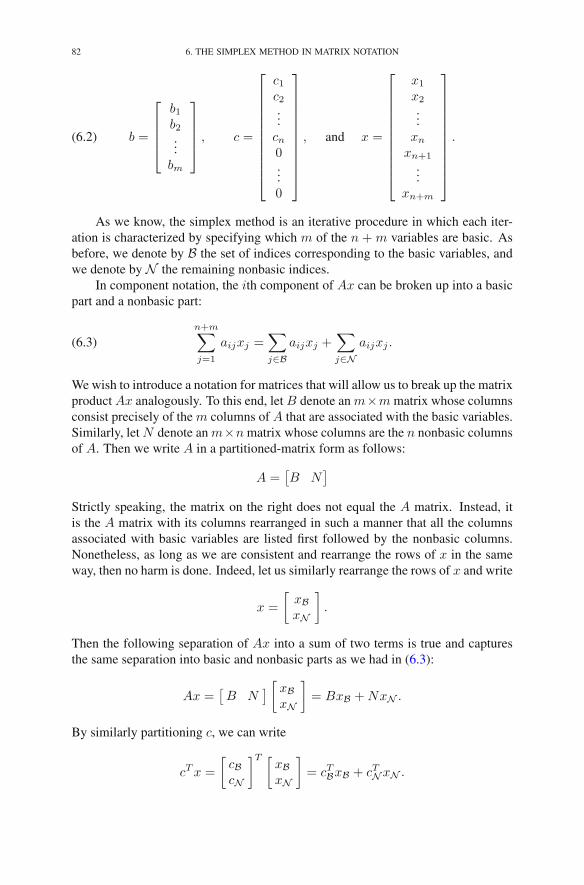
82 6. THE SIMPLEX METHOD IN MATRIX NOTATION
(6.2) b =
⎡
⎢⎢⎢⎣
b1b2...bm
⎤
⎥⎥⎥⎦, c =
⎡
⎢⎢⎢⎢⎢⎢⎢⎢⎢⎢⎣
c1c2...cn0...0
⎤
⎥⎥⎥⎥⎥⎥⎥⎥⎥⎥⎦
, and x =
⎡
⎢⎢⎢⎢⎢⎢⎢⎢⎢⎢⎣
x1
x2
...xn
xn+1
...xn+m
⎤
⎥⎥⎥⎥⎥⎥⎥⎥⎥⎥⎦
.
As we know, the simplex method is an iterative procedure in which each iter-ation is characterized by specifying which m of the n +m variables are basic. Asbefore, we denote by B the set of indices corresponding to the basic variables, andwe denote by N the remaining nonbasic indices.
In component notation, the ith component of Ax can be broken up into a basicpart and a nonbasic part:
(6.3)n+m∑
j=1
aijxj =∑
j∈Baijxj +
∑
j∈Naijxj .
We wish to introduce a notation for matrices that will allow us to break up the matrixproduct Ax analogously. To this end, let B denote an m×m matrix whose columnsconsist precisely of the m columns of A that are associated with the basic variables.Similarly, let N denote an m×n matrix whose columns are the n nonbasic columnsof A. Then we write A in a partitioned-matrix form as follows:
A =[B N
]
Strictly speaking, the matrix on the right does not equal the A matrix. Instead, itis the A matrix with its columns rearranged in such a manner that all the columnsassociated with basic variables are listed first followed by the nonbasic columns.Nonetheless, as long as we are consistent and rearrange the rows of x in the sameway, then no harm is done. Indeed, let us similarly rearrange the rows of x and write
x =
[xBxN
]
.
Then the following separation of Ax into a sum of two terms is true and capturesthe same separation into basic and nonbasic parts as we had in (6.3):
Ax =[B N
][xBxN
]
= BxB +NxN .
By similarly partitioning c, we can write
cTx =
[cBcN
]T [xBxN
]
= cTBxB + cTNxN .

2. THE PRIMAL SIMPLEX METHOD 83
2. The Primal Simplex Method
A dictionary has the property that the basic variables are written as functions ofthe nonbasic variables. In matrix notation, we see that the constraint equations
Ax = b
can be written asBxB +NxN = b.
The fact that the basic variables xB can be written as a function of the nonbasicvariables xN is equivalent to the fact that the matrix B is invertible, and hence,
(6.4) xB = B−1b−B−1NxN .
(The fact that B is invertible means that its m column vectors are linearly indepen-dent and therefore form a basis for Rm—this is why the basic variables are calledbasic, in case you were wondering.) Similarly, the objective function can be writtenas
ζ = cTBxB + cTNxN(6.5)
= cTB(B−1b−B−1NxN
)+ cTNxN
= cTBB−1b−
((B−1N)T cB − cN
)TxN .
Combining (6.5) and (6.4), we see that we can write the dictionary associatedwith basis B as
(6.6) ζ = cTBB−1b −
((B−1N)T cB − cN
)TxN
xB = B−1b − B−1NxN .
Comparing against the component-form notation of Chapter 2 (see (2.6)), we makethe following identifications:
cTBB−1b = ζ
cN − (B−1N)T cB = [cj ]
B−1b =[bi]
B−1N = [aij ] ,
where the bracketed expressions on the right denote vectors and matrices with theindex i running over B and the index j running over N . The basic solution associ-ated with dictionary (6.6) is obtained by setting xN equal to zero:
x∗N = 0,
x∗B = B−1b.(6.7)
As we saw in the last chapter, associated with each primal dictionary there isa dual dictionary that is simply the negative-transpose of the primal. However, tohave the negative-transpose property, it is important to correctly associate comple-mentary pairs of variables. So first we recall that, for the current discussion, wehave appended the primal slack variables to the end of the original variables:
(x1, . . . , xn, w1, . . . , wm) −→ (x1, . . . , xn, xn+1, . . . , xn+m).

84 6. THE SIMPLEX METHOD IN MATRIX NOTATION
Also recall that the dual slack variables are complementary to the original primalvariables and that the original dual variables are complementary to the primal slackvariables. Therefore, to maintain the desired complementarity condition betweenlike indices in the primal and the dual, we need to relabel the dual variables andappend them to the end of the dual slacks:
(z1, . . . , zn, y1, . . . , ym) −→ (z1, . . . , zn, zn+1, . . . , zn+m).
With this relabeling of the dual variables, the dual dictionary corresponding to(6.6) is
−ξ = −cTBB−1b− (B−1b)T zB
zN = (B−1N)T cB − cN + (B−1N)T zB.
The dual solution associated with this dictionary is obtained by setting zB equal tozero:
z∗B = 0,
z∗N = (B−1N)T cB − cN .(6.8)
Using (6.7) and (6.8) and introducing the shorthand
(6.9) ζ∗ = cTBB−1b,
we see that we can write the primal dictionary succinctly as
(6.10)ζ = ζ∗ − z∗N
TxNxB = x∗
B −B−1NxN .
The associated dual dictionary then has a very symmetric appearance:
(6.11)−ξ =−ζ∗ − (x∗
B)T zB
zN = z∗N + (B−1N)T zB.
The (primal) simplex method can be described briefly as follows. The startingassumptions are that we are given
(1) A partition of the n+m indices into a collection B of m basic indices anda collection N of n nonbasic ones with the property that the basis matrixB is invertible,
(2) An associated current primal solution x∗B ≥ 0 (and x∗
N = 0), and(3) An associated current dual solution z∗N (with z∗B = 0)
such that the dictionary given by (6.10) represents the primal objective function andthe primal constraints. The simplex method then produces a sequence of steps to“adjacent” bases such that the current value ζ∗ of the objective function ζ increasesat each step (or, at least, would increase if the step size were positive), updatingx∗B and z∗N along the way. Two bases are said to be adjacent to each other if they
differ in only one index. That is, given a basis B, an adjacent basis is determinedby removing one basic index and replacing it with a nonbasic index. The index thatgets removed corresponds to the leaving variable, whereas the index that gets addedcorresponds to the entering variable.
One step of the simplex method is called an iteration. We now elaborate furtheron the details by describing one iteration as a sequence of specific steps.

2. THE PRIMAL SIMPLEX METHOD 85
Step 1. Check for Optimality. If z∗N ≥ 0, stop. The current solution is optimal.To see this, first note that the simplex method always maintains primal feasibilityand complementarity. Indeed, the primal solution is feasible, since x∗
B ≥ 0 andxN = 0 and the dictionary embodies the primal constraints. Also, the fact thatx∗N = 0 and z∗B = 0 implies that the primal and dual solutions are complementary.
Hence, all that is required for optimality is dual feasibility. But by looking at theassociated dual dictionary (6.11), we see that the dual solution is feasible if and onlyif z∗N ≥ 0.
Step 2. Select Entering Variable. Pick an index j ∈ N for which z∗j < 0.Variable xj is the entering variable.
Step 3. Compute Primal Step Direction ΔxB. Having selected the enteringvariable, it is our intention to let its value increase from zero. Hence, we let
xN =
⎡
⎢⎢⎢⎢⎢⎢⎢⎢⎢⎢⎣
0...0t0...0
⎤
⎥⎥⎥⎥⎥⎥⎥⎥⎥⎥⎦
↖= tej ,
jth position
where we follow the common convention of letting ej denote the unit vector thatis zero in every component except for a one in the position associated with index j(note that, because of our index rearrangement conventions, this is not generally thejth element of the vector). Then from (6.10), we have that
xB = x∗B −B−1Ntej .
Hence, we see that the step direction ΔxB for the primal basic variables is given by
ΔxB = B−1Nej .
Step 4. Compute Primal Step Length. We wish to pick the largest t ≥ 0 forwhich every component of xB remains nonnegative. That is, we wish to pick thelargest t for which
x∗B ≥ tΔxB.
Since, for each i ∈ B∗, x∗i ≥ 0 and t ≥ 0, we can divide both sides of the above
inequality by these numbers and preserve the sense of the inequality. Therefore,doing this division, we get the requirement that
1
t≥ Δxi
x∗i
, for all i ∈ B.
We want to let t be as large as possible, and so 1/t should be made as small as pos-sible. The smallest possible value for 1/t that satisfies all the required inequalitiesis obviously
1
t= max
i∈B
Δxi
x∗i
.
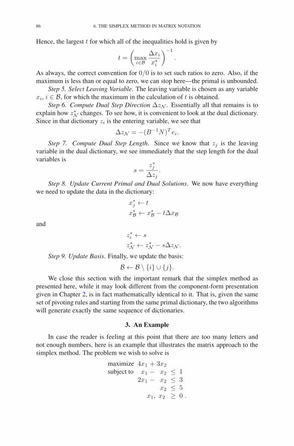
86 6. THE SIMPLEX METHOD IN MATRIX NOTATION
Hence, the largest t for which all of the inequalities hold is given by
t =
(
maxi∈B
Δxi
x∗i
)−1
.
As always, the correct convention for 0/0 is to set such ratios to zero. Also, if themaximum is less than or equal to zero, we can stop here—the primal is unbounded.
Step 5. Select Leaving Variable. The leaving variable is chosen as any variablexi, i ∈ B, for which the maximum in the calculation of t is obtained.
Step 6. Compute Dual Step Direction ΔzN . Essentially all that remains is toexplain how z∗N changes. To see how, it is convenient to look at the dual dictionary.Since in that dictionary zi is the entering variable, we see that
ΔzN = −(B−1N)T ei.
Step 7. Compute Dual Step Length. Since we know that zj is the leavingvariable in the dual dictionary, we see immediately that the step length for the dualvariables is
s =z∗jΔzj
.
Step 8. Update Current Primal and Dual Solutions. We now have everythingwe need to update the data in the dictionary:
x∗j ← t
x∗B ← x∗
B − tΔxB
and
z∗i ← s
z∗N ← z∗N − sΔzN .
Step 9. Update Basis. Finally, we update the basis:
B ← B \ {i} ∪ {j}.We close this section with the important remark that the simplex method as
presented here, while it may look different from the component-form presentationgiven in Chapter 2, is in fact mathematically identical to it. That is, given the sameset of pivoting rules and starting from the same primal dictionary, the two algorithmswill generate exactly the same sequence of dictionaries.
3. An Example
In case the reader is feeling at this point that there are too many letters andnot enough numbers, here is an example that illustrates the matrix approach to thesimplex method. The problem we wish to solve is
maximize 4x1 + 3x2
subject to x1 − x2 ≤ 12x1 − x2 ≤ 3
x2 ≤ 5x1, x2 ≥ 0 .
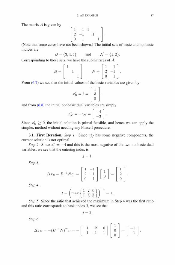
3. AN EXAMPLE 87
The matrix A is given by ⎡
⎣1 −1 12 −1 10 1 1
⎤
⎦ .
(Note that some zeros have not been shown.) The initial sets of basic and nonbasicindices are
B = {3, 4, 5} and N = {1, 2}.Corresponding to these sets, we have the submatrices of A:
B =
⎡
⎣1
11
⎤
⎦ N =
⎡
⎣1 −12 −10 1
⎤
⎦ .
From (6.7) we see that the initial values of the basic variables are given by
x∗B = b =
⎡
⎣135
⎤
⎦ ,
and from (6.8) the initial nonbasic dual variables are simply
z∗N = −cN =
[−4−3
]
.
Since x∗B ≥ 0, the initial solution is primal feasible, and hence we can apply the
simplex method without needing any Phase I procedure.
3.1. First Iteration. Step 1. Since z∗N has some negative components, thecurrent solution is not optimal.
Step 2. Since z∗1 = −4 and this is the most negative of the two nonbasic dualvariables, we see that the entering index is
j = 1.
Step 3.
ΔxB = B−1Nej =
⎡
⎣1 −12 −10 1
⎤
⎦[
10
]
=
⎡
⎣120
⎤
⎦ .
Step 4.
t =
(
max
{1
1,2
3,0
5
})−1
= 1.
Step 5. Since the ratio that achieved the maximum in Step 4 was the first ratioand this ratio corresponds to basis index 3, we see that
i = 3.
Step 6.
ΔzN = −(B−1N)T ei = −[
1 2 0−1 −1 1
]⎡
⎣100
⎤
⎦ =
[−11
]
.

88 6. THE SIMPLEX METHOD IN MATRIX NOTATION
Step 7.
s =z∗jΔzj
=−4
−1= 4.
Step 8.
x∗1 = 1, x∗
B =
⎡
⎣135
⎤
⎦− 1
⎡
⎣120
⎤
⎦ =
⎡
⎣015
⎤
⎦ ,
z∗3 = 4, z∗N =
[−4−3
]
− 4
[−11
]
=
[0
−7
]
.
Step 9. The new sets of basic and nonbasic indices are
B = {1, 4, 5} and N = {3, 2}.Corresponding to these sets, we have the new basic and nonbasic submatrices of A,
B =
⎡
⎣12 10 1
⎤
⎦ N =
⎡
⎣1 −10 −10 1
⎤
⎦ ,
and the new basic primal variables and nonbasic dual variables:
x∗B =
⎡
⎣x∗1
x∗4
x∗5
⎤
⎦ =
⎡
⎣115
⎤
⎦ z∗N =
[z∗3z∗2
]
=
[4
−7
]
.
3.2. Second Iteration. Step 1. Since z∗N has some negative components, thecurrent solution is not optimal.
Step 2. Since z∗2 = −7, we see that the entering index is
j = 2.
Step 3.
ΔxB = B−1Nej =
⎡
⎣12 10 1
⎤
⎦
−1 ⎡
⎣1 −10 −10 1
⎤
⎦[
01
]
=
⎡
⎣−111
⎤
⎦ .
Step 4.
t =
(
max
{−1
1,1
1,1
5
})−1
= 1.
Step 5. Since the ratio that achieved the maximum in Step 4 was the secondratio and this ratio corresponds to basis index 4, we see that
i = 4.
Step 6.
ΔzN = −(B−1N)T ei
= −[
1 0 0−1 −1 1
]⎡
⎣1 2 0
11
⎤
⎦
−1 ⎡
⎣010
⎤
⎦ =
[2
−1
]
.

3. AN EXAMPLE 89
Step 7.
s =z∗jΔzj
=−7
−1= 7.
Step 8.
x∗2 = 1, x∗
B =
⎡
⎣115
⎤
⎦− 1
⎡
⎣−111
⎤
⎦ =
⎡
⎣204
⎤
⎦ ,
z∗4 = 7, z∗N =
[4
−7
]
− 7
[2
−1
]
=
[−10
0
]
.
Step 9. The new sets of basic and nonbasic indices are
B = {1, 2, 5} and N = {3, 4}.Corresponding to these sets, we have the new basic and nonbasic submatrices of A,
B =
⎡
⎣1 −1 02 −1 00 1 1
⎤
⎦ N =
⎡
⎣1 00 10 0
⎤
⎦ ,
and the new basic primal variables and nonbasic dual variables:
x∗B =
⎡
⎣x∗1
x∗2
x∗5
⎤
⎦ =
⎡
⎣214
⎤
⎦ z∗N =
[z∗3z∗4
]
=
[−10
7
]
.
3.3. Third Iteration. Step 1. Since z∗N has some negative components, thecurrent solution is not optimal.
Step 2. Since z∗3 = −10, we see that the entering index is
j = 3.
Step 3.
ΔxB = B−1Nej =
⎡
⎣1 −1 02 −1 00 1 1
⎤
⎦
−1 ⎡
⎣1 00 10 0
⎤
⎦[
10
]
=
⎡
⎣−1−22
⎤
⎦ .
Step 4.
t =
(
max
{−1
2,−2
1,2
4
})−1
= 2.
Step 5. Since the ratio that achieved the maximum in Step 4 was the third ratioand this ratio corresponds to basis index 5, we see that
i = 5.
Step 6.
ΔzN = −(B−1N)T ei
= −[1 0 00 1 0
]⎡
⎣1 2 0
−1 −1 10 0 1
⎤
⎦
−1 ⎡
⎣001
⎤
⎦ =
[−21
]
.
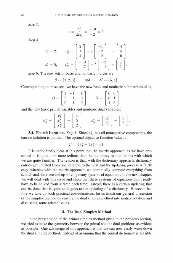
90 6. THE SIMPLEX METHOD IN MATRIX NOTATION
Step 7.
s =z∗jΔzj
=−10
−2= 5.
Step 8.
x∗3 = 2, x∗
B =
⎡
⎣214
⎤
⎦− 2
⎡
⎣−1−22
⎤
⎦ =
⎡
⎣450
⎤
⎦ ,
z∗5 = 5, z∗N =
[−10
7
]
− 5
[−21
]
=
[02
]
.
Step 9. The new sets of basic and nonbasic indices are
B = {1, 2, 3} and N = {5, 4}.Corresponding to these sets, we have the new basic and nonbasic submatrices of A,
B =
⎡
⎣1 −1 12 −1 00 1 0
⎤
⎦ N =
⎡
⎣0 00 11 0
⎤
⎦ ,
and the new basic primal variables and nonbasic dual variables:
x∗B =
⎡
⎣x∗1
x∗2
x∗3
⎤
⎦ =
⎡
⎣452
⎤
⎦ z∗N =
[z∗5z∗4
]
=
[52
]
.
3.4. Fourth Iteration. Step 1. Since z∗N has all nonnegative components, thecurrent solution is optimal. The optimal objective function value is
ζ∗ = 4x∗1 + 3x∗
2 = 31.
It is undoubtedly clear at this point that the matrix approach, as we have pre-sented it, is quite a bit more tedious than the dictionary manipulations with whichwe are quite familiar. The reason is that, with the dictionary approach, dictionaryentries get updated from one iteration to the next and the updating process is fairlyeasy, whereas with the matrix approach, we continually compute everything fromscratch and therefore end up solving many systems of equations. In the next chapter,we will deal with this issue and show that these systems of equations don’t reallyhave to be solved from scratch each time; instead, there is a certain updating thatcan be done that is quite analogous to the updating of a dictionary. However, be-fore we take up such practical considerations, let us finish our general discussionof the simplex method by casting the dual simplex method into matrix notation anddiscussing some related issues.
4. The Dual Simplex Method
In the presentation of the primal simplex method given in the previous section,we tried to make the symmetry between the primal and the dual problems as evidentas possible. One advantage of this approach is that we can now easily write downthe dual simplex method. Instead of assuming that the primal dictionary is feasible

4. THE DUAL SIMPLEX METHOD 91
(x∗B ≥ 0), we now assume that the dual dictionary is feasible (z∗N ≥ 0) and perform
the analogous steps:Step 1. Check for Optimality. If x∗
B ≥ 0, stop. The current solution is optimal.Note that for the dual simplex method, dual feasibility and complementarity aremaintained from the beginning, and the algorithm terminates once a primal feasiblesolution is discovered.
Step 2. Select Entering Variable. Pick an index i ∈ B for which x∗i < 0.
Variable zi is the entering variable.Step 3. Compute Dual Step Direction ΔzN . From the dual dictionary, we see
thatΔzN = −(B−1N)T ei.
Step 4. Compute Dual Step Length. We wish to pick the largest s ≥ 0 for whichevery component of zN remains nonnegative. As in the primal simplex method, thiscomputation involves computing the maximum of some ratios:
s =
(
maxj∈N
Δzjz∗j
)−1
.
If s is not positive, then stop here—the dual is unbounded (implying, of course, thatthe primal is infeasible).
Step 5. Select Leaving Variable. The leaving variable is chosen as any variablezj , j ∈ N , for which the maximum in the calculation of s is obtained.
Step 6. Compute Primal Step Direction ΔxB. To see how x∗B changes in the
dual dictionary, it is convenient to look at the primal dictionary. Since in that dictio-nary xj is the entering variable, we see that
ΔxB = B−1Nej .
Step 7. Compute Primal Step Length. Since we know that xi is the leavingvariable in the primal dictionary, we see immediately that the step length for theprimal variables is
t =x∗i
Δxi.
Step 8. Update Current Primal and Dual Solutions. We now have everythingwe need to update the data in the dictionary:
x∗j ← t
x∗B ← x∗
B − tΔxB.
and
z∗i ← s
z∗N ← z∗N − sΔzN
Step 9. Update Basis. Finally, we update the basis:
B ← B \ {i} ∪ {j}.To further emphasize the similarities between the primal and the dual simplex
methods, Figure 6.1 shows the two algorithms side by side.

92 6. THE SIMPLEX METHOD IN MATRIX NOTATION
Primal Simplex
Suppose x∗B ≥ 0
while (z∗N �≥ 0) {pick j ∈ {j ∈ N : z∗j < 0}ΔxB = B−1Nej
t =
⎛
⎜⎝maxi∈B
Δxi
x∗i
⎞
⎟⎠
−1
pick i ∈ argmaxi∈BΔxi
x∗i
ΔzN = −(B−1N)T ei
s =z∗jΔzj
x∗j ← t
x∗B ← x∗
B − tΔxBz∗i ← sz∗N ← z∗N − sΔzNB ← B \ {i} ∪ {j}
}
Dual Simplex
Suppose z∗N ≥ 0while (x∗
B �≥ 0) {pick i ∈ {i ∈ B : x∗
i < 0}ΔzN = −(B−1N)T ei
s =
⎛
⎜⎝maxj∈N
Δzjz∗j
⎞
⎟⎠
−1
pick j ∈ argmaxj∈NΔzjz∗j
ΔxB = B−1Nej
t =x∗i
Δxix∗j ← t
x∗B ← x∗
B − tΔxBz∗i ← sz∗N ← z∗N − sΔzNB ← B \ {i} ∪ {j}
}
FIGURE 6.1. The primal and the dual simplex methods.
5. Two-Phase Methods
Let us summarize the algorithm obtained by applying the dual simplex methodas a Phase I procedure followed by the primal simplex method as a Phase II. Initially,we set
B = {n+ 1, n+ 2, . . . , n+m} and N = {1, 2, . . . , n}.
Then from (6.1) we see that A =[N B
], where
N =
⎡
⎢⎢⎢⎣
a11 a12 . . . a1na21 a22 . . . a2n
......
...am1 am2 . . . amn
⎤
⎥⎥⎥⎦, B =
⎡
⎢⎢⎢⎣
11
. . .1
⎤
⎥⎥⎥⎦,
and from (6.2) we have
cN =
⎡
⎢⎢⎢⎣
c1c2...cn
⎤
⎥⎥⎥⎦
and cB =
⎡
⎢⎢⎢⎣
00...0
⎤
⎥⎥⎥⎦.

6. NEGATIVE TRANSPOSE PROPERTY 93
Substituting these expressions into the definitions of x∗B, z∗N , and ζ∗, we find that
x∗B = B−1b = b
z∗N = (B−1N)T cB − cN = −cN
ζ∗ = 0.
Hence, the initial dictionary reads:
ζ = cTNxNxB = b − NxN .
If b has all nonnegative components and cN has all nonpositive components,then this dictionary is optimal—the problem was trivial. Suppose, however, that oneof these two vectors (but not both) has components of the wrong sign. For exam-ple, suppose that b is okay (all nonnegative components) but cN has some positivecomponents. Then this dictionary is primal feasible, and we can start immediatelywith the primal simplex method. On the other hand, suppose that cN has all non-positive components but b has some negative ones. Then the starting dictionary isdual feasible, and we can commence immediately with the dual simplex algorithm.
The last, and most common, case is where both b and cN have components ofthe wrong sign. In this case, we must employ a two-phase procedure. There are twochoices. We could temporarily replace cN with another vector that is nonpositive.Then the modified problem is dual feasible, and so we can apply the dual simplexmethod to find an optimal solution of this modified problem. After that, the originalobjective function could be reinstated. With the original objective function, theoptimal solution from Phase I is most likely not optimal, but it is feasible, andtherefore the primal simplex method can be used to find the optimal solution to theoriginal problem.
The other choice would be to modify b instead of cN , thereby obtaining a primalfeasible solution to a modified problem. Then we would use the primal simplexmethod on the modified problem to obtain its optimal solution, which will then bedual feasible for the original problem, and so the dual simplex method can be usedto finish the problem.
6. Negative Transpose Property
In our discussion of duality in Chapter 5, we emphasized the symmetry be-tween the primal problem and its dual. This symmetry can be easily summarizedby saying that the dual of a standard-form linear programming problem is the neg-ative transpose of the primal problem. Now, in this chapter, the symmetry appearsto have been lost. For example, the basis matrix is an m×m matrix. Why m×mand not n × n? It seems strange. In fact, if we had started with the dual problem,added slack variables to it, and introduced a basis matrix on that side it would be ann × n matrix. How are these two basis matrices related? It turns out that they arenot themselves related in any simple way, but the important matrix B−1N is stillthe negative transpose of the analogous dual construct. The purpose of this sectionis to make this connection clear.

94 6. THE SIMPLEX METHOD IN MATRIX NOTATION
Consider a standard-form linear programming problem
maximize cTxsubject to Ax≤ b
x≥ 0,
and its dualminimize bT y
subject to AT y ≥ cy ≥ 0.
Let w be a vector containing the slack variables for the primal problem, let z be aslack vector for the dual problem, and write both problems in equality form:
maximize cTxsubject to Ax+ w= b
x, w≥ 0,
andminimize bT y
subject to AT y − z = cy, z ≥ 0.
Introducing three new notations,
A =[A I
], c =
[c0
]
, and x =
[xw
]
,
the primal problem can be rewritten succinctly as follows:
maximize cT xsubject to Ax= b
x≥ 0.
Similarly, using “hats” for new notations on the dual side,
A =[−I AT
], b =
[0b
]
, and y =
[zy
]
,
the dual problem can be rewritten in this way:
minimize bT y
subject to Ay = cy ≥ 0.
Note that the matrix A = [A I ] is an m× (n+m) matrix. The first n columnsof it are the initial nonbasic variables and the last m columns are the initial basiccolumns. After doing some simplex pivots, the basic and nonbasic columns getjumbled up but we can still write the equality
[A I
]=
[N B
]
with the understanding that the equality only holds after rearranging the columnsappropriately.
On the dual side, the matrix A = [−I AT ] is an n× (n+m) matrix. The firstn columns of it are the initial basic variables (for the dual problem) and the last m

EXERCISES 95
columns are the initial nonbasic columns. If the same set of pivots that were appliedto the primal problem are also applied to the dual, then the columns get rearrangedin exactly the same way as they did for the primal and we can write
[−I AT
]=
[B N
]
again with the proviso that the columns of one matrix must be rearranged in a spe-cific manner to bring it into exact equality with the other matrix.
Now, the primal dictionary involves the matrix B−1N whereas the dual dictio-nary involves the matrix B−1N . It probably doesn’t seem at all obvious that thesetwo matrices are negative transposes of each other. To see that it is so, considerwhat happens when we multiply A by AT in both the permuted notation and theunpermuted notation:
AAT =[N B
][BT
NT
]
= NBT + BNT
and
AAT =[A I
][−IA
]
= −A+A = 0.
These two expressions obviously must agree so we see that
NBT + BNT = 0.
Putting the two terms on the opposite sides of the equality sign and multiplying onthe right by the inverse of BT and on the left by the inverse of B, we get that
B−1N = −(B−1N
)T
,
which is the property we wished to establish.
Exercises
6.1 Consider the following linear programming problem:
maximize −6x1 + 32x2 − 9x3
subject to −2x1 + 10x2 − 3x3 ≤ −6x1 − 7x2 + 2x3 ≤ 4
x1, x2, x3 ≥ 0 .
Suppose that, in solving this problem, you have arrived at the followingdictionary:
ζ = −18 − 3x4 + 2x2
x3 = 2 − x4 + 4x2 − 2x5
x1 = 2x4 − x2 + 3x5 .
(a) Which variables are basic? Which are nonbasic?(b) Write down the vector, x∗
B, of current primal basic solution values.(c) Write down the vector, z∗N , of current dual nonbasic solution values.(d) Write down B−1N .(e) Is the primal solution associated with this dictionary feasible?
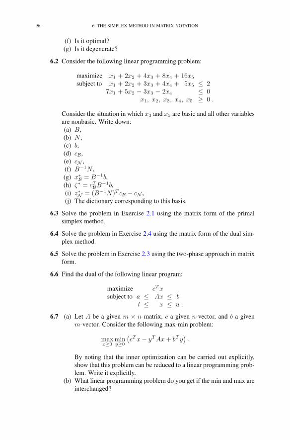
96 6. THE SIMPLEX METHOD IN MATRIX NOTATION
(f) Is it optimal?(g) Is it degenerate?
6.2 Consider the following linear programming problem:
maximize x1 + 2x2 + 4x3 + 8x4 + 16x5
subject to x1 + 2x2 + 3x3 + 4x4 + 5x5 ≤ 27x1 + 5x2 − 3x3 − 2x4 ≤ 0
x1, x2, x3, x4, x5 ≥ 0 .
Consider the situation in which x3 and x5 are basic and all other variablesare nonbasic. Write down:(a) B,(b) N ,(c) b,(d) cB,(e) cN ,(f) B−1N ,(g) x∗
B = B−1b,(h) ζ∗ = cTBB
−1b,(i) z∗N = (B−1N)T cB − cN ,(j) The dictionary corresponding to this basis.
6.3 Solve the problem in Exercise 2.1 using the matrix form of the primalsimplex method.
6.4 Solve the problem in Exercise 2.4 using the matrix form of the dual sim-plex method.
6.5 Solve the problem in Exercise 2.3 using the two-phase approach in matrixform.
6.6 Find the dual of the following linear program:
maximize cTxsubject to a ≤ Ax ≤ b
l ≤ x ≤ u .
6.7 (a) Let A be a given m × n matrix, c a given n-vector, and b a givenm-vector. Consider the following max-min problem:
maxx≥0
miny≥0
(cTx− yTAx+ bT y
).
By noting that the inner optimization can be carried out explicitly,show that this problem can be reduced to a linear programming prob-lem. Write it explicitly.
(b) What linear programming problem do you get if the min and max areinterchanged?
NOTES 97
Notes
In this chapter, we have accomplished two tasks: (1) we have expressed thesimplex method in matrix notation, and (2) we have reduced the information wecarry from iteration to iteration to simply the list of basic variables together withcurrent values of the primal basic variables and the dual nonbasic variables. Inparticular, it is not necessary to calculate explicitly all the entries of the matrixB−1N .
What’s in a name? There are times when one thing has two names. So far inthis book, we have discussed essentially only one algorithm: the simplex method(assuming, of course, that specific pivot rules have been settled on). But this onealgorithm is sometimes referred to as the simplex method and at other times it isreferred to as the revised simplex method. The distinction being made with this newname has nothing to do with the algorithm. Rather it refers to the specifics of an im-plementation. Indeed, an implementation of the simplex method that avoids explicitcalculation of the matrix B−1N is referred to as an implementation of the revisedsimplex method. We shall see in Chapter 8 why it is beneficial to avoid computingB−1N .

CHAPTER 7
Sensitivity and Parametric Analyses
In this chapter, we consider two related subjects. The first, called sensitiv-ity analysis (or postoptimality analysis) addresses the following question: havingfound an optimal solution to a given linear programming problem, how much canwe change the data and have the current partition into basic and nonbasic variablesremain optimal? The second subject addresses situations in which one wishes tosolve not just one linear program, but a whole family of problems parametrized bya single real variable.
We shall study parametric analysis in a very specific context in which we wishto find the optimal solution to a given linear programming problem by starting froma problem whose solution is trivially known and then deforming this problem backto the original problem, maintaining as we go optimality of the current solution.The result of this deformation approach to solving a linear programming problemis a new variant of the simplex method, which is called the parametric self-dualsimplex method. We will see in later chapters that this variant of the simplex methodresembles, in certain respects, the interior-point methods that we shall study.
1. Sensitivity Analysis
One often needs to solve not just one linear programming problem but severalclosely related problems. There are many reasons that this need might arise. Forexample, the data that define the problem may have been rather uncertain and onemay wish to consider various possible data scenarios. Or perhaps the data are knownaccurately but change from day to day, and the problem must be resolved for eachnew day. Whatever the reason, this situation is quite common. So one is led toask whether it is possible to exploit the knowledge of a previously obtained optimalsolution to obtain more quickly the optimal solution to the problem at hand. Ofcourse, the answer is often yes, and this is the subject of this section.
We shall treat a number of possible situations. All of them assume that a prob-lem has been solved to optimality. This means that we have at our disposal the final,optimal dictionary:
ζ = ζ∗ − z∗TN xNxB = x∗
B − B−1NxN .
Suppose we wish to change the objective coefficients from c to, say, c. It is natural toask how the dictionary at hand could be adjusted to become a valid dictionary for thenew problem. That is, we want to maintain the current classification of the variables
R.J. Vanderbei, Linear Programming, International Series in Operations Research& Management Science 196, DOI 10.1007/978-1-4614-7630-6 7,© Springer Science+Business Media New York 2014
99

100 7. SENSITIVITY AND PARAMETRIC ANALYSES
into basic and nonbasic variables and simply adjust ζ∗, z∗N , and x∗B appropriately.
Recall from (6.7) to (6.9) that
x∗B = B−1b,
z∗N = (B−1N)T cB − cN ,
ζ∗ = cTBB−1b.
Hence, the change from c to c requires us to recompute z∗N and ζ∗, but x∗B remains
unchanged. Therefore, after recomputing z∗N and ζ∗, the new dictionary is stillprimal feasible, and so there is no need for a Phase I procedure: we can jump straightinto the primal simplex method, and if c is not too different from c, we can expectto get to the new optimal solution in a relatively small number of steps.
Now suppose that instead of changing c, we wish to change only the right-handside b. In this case, we see that we need to recompute x∗
B and ζ∗, but z∗N remainsunchanged. Hence, the new dictionary will be dual feasible, and so we can applythe dual simplex method to arrive at the new optimal solution fairly directly.
Therefore, changing just the objective function or just the right-hand side resultsin a new dictionary having nice feasibility properties. What if we need/want tochange some (or all) entries in both the objective function and the right-hand sideand maybe even the constraint matrix too? In this case, everything changes: ζ∗,z∗N , x∗
B. Even the entries in B and N change. Nonetheless, as long as the newbasis matrix B is nonsingular, we can make a new dictionary that preserves the oldclassification into basic and nonbasic variables. The new dictionary will most likelybe neither primal feasible nor dual feasible, but if the changes in the data are fairlysmall in magnitude, one would still expect that this starting dictionary will get us toan optimal solution in fewer iterations than simply starting from scratch. While thereis no guarantee that any of these so-called warm-starts will end up in fewer iterationsto optimality, extensive empirical evidence indicates that this procedure often makesa substantial improvement: sometimes the warm-started problems solve in as littleas 1 % of the time it takes to solve the original problem.
1.1. Ranging. Often one does not wish to solve a modification of the originalproblem, but instead just wants to ask a hypothetical question:
If I were to change the objective function by increasing or de-creasing one of the objective coefficients a small amount, howmuch could I increase/decrease it without changing the optimal-ity of my current basis?
To study this question, let us suppose that c gets changed to c + tΔc, where t is areal number and Δc is a given vector (which is often all zeros except for a one in asingle entry, but we don’t need to restrict the discussion to this case). It is easy tosee that z∗N gets incremented by
tΔzN ,
where
(7.1) ΔzN = (B−1N)TΔcB −ΔcN .

1. SENSITIVITY ANALYSIS 101
Hence, the current basis will remain dual feasible as long as
(7.2) z∗N + tΔzN ≥ 0.
We’ve manipulated this type of inequality many times before, and so it should beclear that, for t > 0, this inequality will remain valid as long as
t ≤(
maxj∈N
−Δzjz∗j
)−1
.
Similar manipulations show that, for t < 0, the lower bound is
t ≥(
minj∈N
−Δzjz∗j
)−1
.
Combining these two inequalities, we see that t must lie in the interval(
minj∈N
−Δzjz∗j
)−1
≤ t ≤(
maxj∈N
−Δzjz∗j
)−1
.
Let us illustrate these calculations with an example. Consider the followinglinear programming problem:
maximize 5x1 + 4x2 + 3x3
subject to 2x1 + 3x2 + x3 ≤ 54x1 + x2 + 2x3 ≤ 113x1 + 4x2 + 2x3 ≤ 8x1, x2, x3 ≥ 0 .
The optimal dictionary for this problem is given by
ξ = 13− 3x2 − x4 − x6
x3 = 1+ x2 + 3x4 − 2x6
x1 = 2− 2x2 − 2x4 + x6
x5 = 1+ 5x2 + 2x4 .
The optimal basis is B = {3, 1, 5}. Suppose we want to know how much the coef-ficient of 5 on x1 in the objective function can change without altering the optimalityof this basis. From the statement of the problem, we see that
c =[
5 4 3 0 0 0]T
.
Since we are interested in changes in the first coefficient, we put
Δc =[
1 0 0 0 0 0]T
.
We partition c according to the final (optimal) basis. Hence, we have
ΔcB =
⎡
⎣010
⎤
⎦ and ΔcN =
⎡
⎣000
⎤
⎦ .
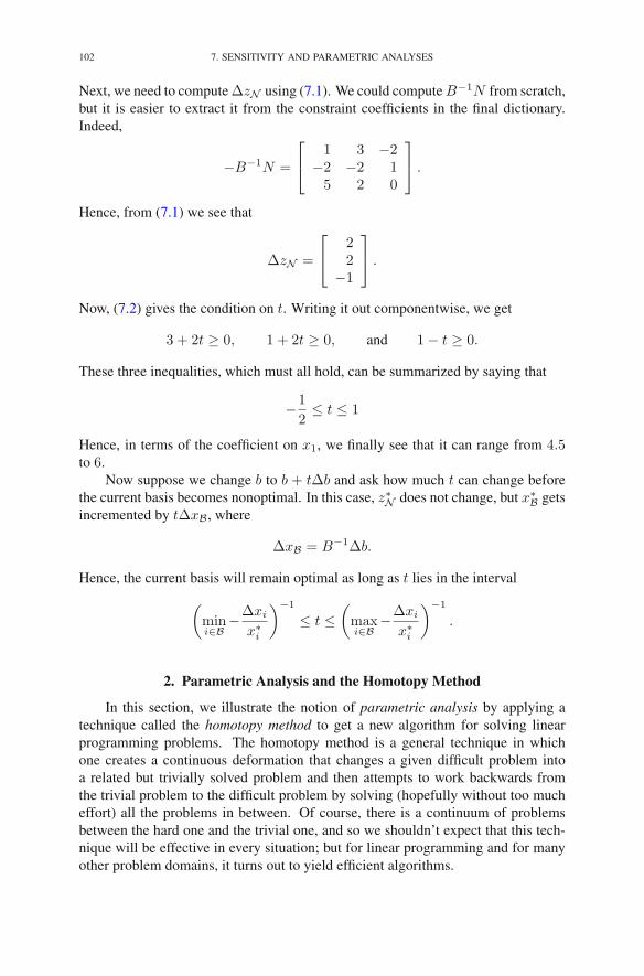
102 7. SENSITIVITY AND PARAMETRIC ANALYSES
Next, we need to compute ΔzN using (7.1). We could compute B−1N from scratch,but it is easier to extract it from the constraint coefficients in the final dictionary.Indeed,
−B−1N =
⎡
⎣1 3 −2
−2 −2 15 2 0
⎤
⎦ .
Hence, from (7.1) we see that
ΔzN =
⎡
⎣22
−1
⎤
⎦ .
Now, (7.2) gives the condition on t. Writing it out componentwise, we get
3 + 2t ≥ 0, 1 + 2t ≥ 0, and 1− t ≥ 0.
These three inequalities, which must all hold, can be summarized by saying that
−1
2≤ t ≤ 1
Hence, in terms of the coefficient on x1, we finally see that it can range from 4.5to 6.
Now suppose we change b to b + tΔb and ask how much t can change beforethe current basis becomes nonoptimal. In this case, z∗N does not change, but x∗
B getsincremented by tΔxB, where
ΔxB = B−1Δb.
Hence, the current basis will remain optimal as long as t lies in the interval
(
mini∈B
−Δxi
x∗i
)−1
≤ t ≤(
maxi∈B
−Δxi
x∗i
)−1
.
2. Parametric Analysis and the Homotopy Method
In this section, we illustrate the notion of parametric analysis by applying atechnique called the homotopy method to get a new algorithm for solving linearprogramming problems. The homotopy method is a general technique in whichone creates a continuous deformation that changes a given difficult problem intoa related but trivially solved problem and then attempts to work backwards fromthe trivial problem to the difficult problem by solving (hopefully without too mucheffort) all the problems in between. Of course, there is a continuum of problemsbetween the hard one and the trivial one, and so we shouldn’t expect that this tech-nique will be effective in every situation; but for linear programming and for manyother problem domains, it turns out to yield efficient algorithms.

2. PARAMETRIC ANALYSIS AND THE HOMOTOPY METHOD 103
We start with an example. Suppose we wish to solve the following linear pro-gramming problem:
maximize −2x1 + 3x2
subject to −x1 + x2 ≤ −1−x1 − 2x2 ≤ −2
x2 ≤ 1x1, x2 ≥ 0 .
The starting dictionary is
ζ = − 2x1 − (−3)x2
x3 =−1 + x1 − x2
x4 =−2 + x1 + 2x2
x5 = 1 − x2 .
This dictionary is neither primal nor dual feasible. Let’s perturb it by adding apositive real number μ to each right-hand side and subtracting it from each objectivefunction coefficient. We now arrive at a family of dictionaries, parametrized by μ:
(7.3)
ζ = − (2 + μ)x1 − (−3 + μ)x2
x3 =−1 + μ+ x1 − x2
x4 =−2 + μ+ x1 + 2x2
x5 = 1+ μ − x2 .
Clearly, for μ sufficiently large, specifically μ ≥ 3, this dictionary is both primaland dual feasible. Hence, the associated solution x = [0, 0,−1 + μ,−2 + μ, 1 + μ]is optimal. Starting with μ large, we reduce it as much as we can while keepingdictionary (7.3) optimal. This dictionary will become nonoptimal as soon as μ < 3,since the associated dual variable y∗2 = −3 + μ will become negative. In otherwords, the coefficient of x2, which is 3 − μ, will become positive. This change ofsign on the coefficient of x2 suggests that we make a primal pivot in which x2 entersthe basis. The usual ratio test (using the specific value of μ = 3) indicates that x3
must be the leaving variable. Making the pivot, we get
ζ = −3 + 4μ − μ2 − (−1 + 2μ)x1 − (3− μ)x3
x2 = −1 + μ + x1 − x3
x4 = −4 + 3μ + 3x1 − 2x3
x5 = 2 − x1 + x3.
This dictionary is optimal as long as
−1 + 2μ ≥ 0, 3− μ ≥ 0,
−1 + μ ≥ 0, −4 + 3μ ≥ 0.
These inequalities reduce to4
3≤ μ ≤ 3.
So now we can reduce μ from its current value of 3 down to 4/3. If we reduce itbelow 4/3, the primal feasibility inequality, −4 + 3μ ≥ 0, becomes violated. This
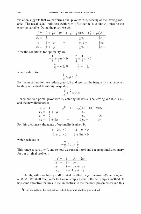
104 7. SENSITIVITY AND PARAMETRIC ANALYSES
violation suggests that we perform a dual pivot with x4 serving as the leaving vari-able. The usual (dual) ratio test (with μ = 4/3) then tells us that x1 must be theentering variable. Doing the pivot, we get
ζ =− 53 + 1
3μ+ μ2 − (− 13 + 2
3μ)x4 − ( 73 + 13μ)x3
x2 =13 + 1
3x4 − 13x3
x1 =43 − μ + 1
3x4 +23x3
x5 =23 + μ − 1
3x4 +13x3 .
Now the conditions for optimality are
−1
3+
2
3μ ≥ 0,
7
3+
1
3μ ≥ 0,
4
3− μ ≥ 0,
2
3+ μ ≥ 0,
which reduce to1
2≤ μ ≤ 4
3.
For the next iteration, we reduce μ to 1/2 and see that the inequality that becomesbinding is the dual feasibility inequality
−1
3+
2
3μ ≥ 0.
Hence, we do a primal pivot with x4 entering the basis. The leaving variable is x5,and the new dictionary is
ζ = −1 − μ2 − (1− 2μ)x5 − (2 + μ)x3
x2 = 1 + μ − x5
x1 = 2 − x5 + x3
x4 = 2 + 3μ − 3x5 + x3.
For this dictionary, the range of optimality is given by
1− 2μ ≥ 0, 2 + μ ≥ 0,
1 + μ ≥ 0, 2 + 3μ ≥ 0,
which reduces to
−2
3≤ μ ≤ 1
2.
This range covers μ = 0, and so now we can set μ to 0 and get an optimal dictionaryfor our original problem:
ζ = −1 − x5 − 2x3
x2 = 1 − x5
x1 = 2 − x5 + x3
x4 = 2 − 3x5 + x3.
The algorithm we have just illustrated is called the parametric self-dual simplexmethod.1 We shall often refer to it more simply as the self-dual simplex method. Ithas some attractive features. First, in contrast to the methods presented earlier, this
1In the first edition, this method was called the primal–dual simplex method.

3. THE PARAMETRIC SELF-DUAL SIMPLEX METHOD 105
algorithm does not require a separate Phase I procedure. It starts with any problem,be it primal infeasible, dual infeasible, or both, and it systematically performs pivots(whether primal or dual) until it finds an optimal solution.
A second feature is that a trivial modification of the algorithm can avoid en-tirely ever encountering a degenerate dictionary. Indeed, suppose that, instead ofadding/subtracting μ from each of the right-hand sides and objective coefficients,we add/subtract a positive constant times μ. Suppose further that the positive con-stant is different in each addition/subtraction. In fact, suppose that they are chosenindependently from, say, a uniform distribution on [1/2, 3/2]. Then with probabilityone, the algorithm will produce no primal degenerate or dual degenerate dictionaryin any iteration. In Chapter 3, we discussed perturbing the right-hand side of a linearprogramming problem to avoid degeneracy in the primal simplex method, but backthen the perturbation changed the problem. The present perturbation does not in anyway affect the problem that is solved.
With the above randomization trick to resolve the degeneracy issue, the analy-sis of the convergence of the algorithm is straightforward. Indeed, let us consider aproblem that is feasible and bounded (the questions regarding feasibility and bound-edness are addressed in Exercise 7.10). For each nondegenerate pivot, the next valueof μ will be strictly less than the current value. Since each of these μ values is de-termined by a partition of the variables into basics and nonbasics and there are onlya finite number of such partitions, it follows that the method must reach a partitionwith a negative μ value in a finite number of steps.
3. The Parametric Self-Dual Simplex Method
In the previous section, we illustrated on an example a new algorithm for solv-ing linear programming problems, called the parametric self-dual simplex method.In this section, we shall lay out the algorithm in matrix notation.
Our starting point is an initial dictionary as written in (6.10) and transcribedhere for convenience:
ζ = ζ∗ − z∗NTxN
xB = x∗B − B−1NxN ,
where
x∗B = B−1b
z∗N = (B−1N)T cB − cN
ζ∗ = cTBx∗B = cTBB
−1b.
Generally speaking, we don’t expect this dictionary to be either primal or dual fea-sible. So we perturb it by adding essentially arbitrary perturbations xB and zN tox∗B and z∗N , respectively:
ζ = ζ∗ − (z∗N + μzN )TxNxB = (x∗
B + μxB) − B−1NxN .
We assume that the perturbations are all strictly positive,
xB > 0 and zN > 0,

106 7. SENSITIVITY AND PARAMETRIC ANALYSES
so that by taking μ sufficiently large the perturbed dictionary will be optimal. (Ac-tually, to guarantee optimality for large μ, we only need to perturb those primal anddual variables that are negative in the initial dictionary.)
The parametric self-dual simplex method generates a sequence of dictionarieshaving the same form as the initial one—except, of course, the basis B will change,and hence all the data vectors (z∗N , zN , x∗
B, and xB) will change too. Additionally,the current value of the objective function ζ∗ will, with the exception of the firstdictionary, depend on μ.
One step of the self-dual simplex method can be described as follows. First, wecompute the smallest value of μ for which the current dictionary is optimal. Lettingμ∗ denote this value, we see that
μ∗ = min{μ : z∗N + μzN ≥ 0 and x∗B + μxB ≥ 0}.
There is either a j ∈ N for which z∗j +μ∗zj = 0 or an i ∈ B for which x∗i +μ∗xi =
0 (if there are multiple choices, an arbitrary selection is made). If the blockingconstraint corresponds to a nonbasic index j ∈ N , then we do one step of theprimal simplex method. If, on the other hand, it corresponds to a basic index i ∈ B,then we do one step of the dual simplex method.
Suppose, for definiteness, that the blocking constraint corresponds to an indexj ∈ N . Then, to do a primal pivot, we declare xj to be the entering variable, andwe compute the step direction for the primal basic variables as the jth column ofthe dictionary. That is,
ΔxB = B−1Nej .
Using this step direction, we find an index i ∈ B that achieves the maximal value ofΔxi/(x
∗i +μ∗xi). Variable xi is the leaving variable. After figuring out the leaving
variable, the step direction vector for the dual nonbasic variables is just the negativeof the ith row of the dictionary
ΔzN = −(B−1N)T ei.
After computing the primal and dual step directions, it is easy to see that the steplength adjustments are given by
t =x∗i
Δxi, t =
xi
Δxi,
s =z∗jΔzj
, s =zjΔzj
.
And from these, it is easy to write down the new solution vectors:
x∗j ← t, xj ← t, z∗i ← s, zi ← s,
x∗B ← x∗
B − tΔxB, xB ← xB − tΔxB,
z∗N ← z∗N − sΔzN , zN ← zN − sΔzN .
Finally, the basis is updated by adding the entering variable and removing the leav-ing variable
B ← B \ {i} ∪ {j}.

EXERCISES 107
Compute μ∗ = max
⎛
⎝maxj∈Nzj>0
−z∗jzj
,maxi∈Bxi>0
−x∗i
xi
⎞
⎠
While (μ∗ > 0) {
If max is achieved byj ∈ N :
ΔxB = B−1Nej
pick i ∈ argmaxi∈BΔxi
x∗i + μ∗xi
ΔzN = −(B−1N)T ei
i ∈ B :ΔzN = −(B−1N)T ei
pick j ∈ argmaxj∈NΔzj
z∗j + μ∗zjΔxB = B−1Nej
t =x∗i
Δxit =
xi
Δxi
s =z∗jΔzj
s =zjΔzj
x∗j ← t xj ← t
z∗i ← s zi ← s
x∗B ← x∗
B − tΔxB xB ← xB − tΔxBz∗N ← z∗N − sΔzN zN ← zN − sΔzN
B ← B \ {i} ∪ {j}Recompute μ∗ as above
}
FIGURE 7.1. The parametric self-dual simplex method.
The algorithm is summarized in Figure 7.1.
Exercises
In solving the following problems, the advanced pivot tool can be used to checkyour arithmetic:
www.princeton.edu/∼rvdb/JAVA/pivot/advanced.html
7.1 The final dictionary for
maximize x1 + 2x2 + x3 + x4
subject to 2x1 + x2 + 5x3 + x4 ≤ 82x1 + 2x2 + 4x4 ≤ 123x1 + x2 + 2x3 ≤ 18
x1, x2, x3, x4 ≥ 0
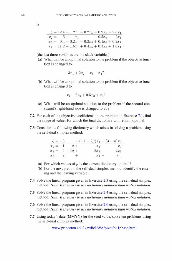
108 7. SENSITIVITY AND PARAMETRIC ANALYSES
is
ζ = 12.4 − 1.2x1 − 0.2x5 − 0.9x6 − 2.8x4
x2 = 6 − x1 − 0.5x6 − 2x4
x3 = 0.4 − 0.2x1 − 0.2x5 + 0.1x6 + 0.2x4
x7 = 11.2 − 1.6x1 + 0.4x5 + 0.3x6 + 1.6x4 .
(the last three variables are the slack variables).(a) What will be an optimal solution to the problem if the objective func-
tion is changed to
3x1 + 2x2 + x3 + x4?
(b) What will be an optimal solution to the problem if the objective func-tion is changed to
x1 + 2x2 + 0.5x3 + x4?
(c) What will be an optimal solution to the problem if the second con-straint’s right-hand side is changed to 26?
7.2 For each of the objective coefficients in the problem in Exercise 7.1, findthe range of values for which the final dictionary will remain optimal.
7.3 Consider the following dictionary which arises in solving a problem usingthe self-dual simplex method:
ζ = −3 − (−1 + 2μ)x1 − (3− μ)x3
x2 = −1 + μ + x1 − x3
x4 = −4 + 3μ + 3x1 − 2x3
x5 = 2 + x1 + x3.
(a) For which values of μ is the current dictionary optimal?(b) For the next pivot in the self-dual simplex method, identify the enter-
ing and the leaving variable.
7.4 Solve the linear program given in Exercise 2.3 using the self-dual simplexmethod. Hint: It is easier to use dictionary notation than matrix notation.
7.5 Solve the linear program given in Exercise 2.4 using the self-dual simplexmethod. Hint: It is easier to use dictionary notation than matrix notation.
7.6 Solve the linear program given in Exercise 2.6 using the self-dual simplexmethod. Hint: It is easier to use dictionary notation than matrix notation.
7.7 Using today’s date (MMYY) for the seed value, solve ten problems usingthe self-dual simplex method:
www.princeton.edu/∼rvdb/JAVA/pivot/pd1phase.html
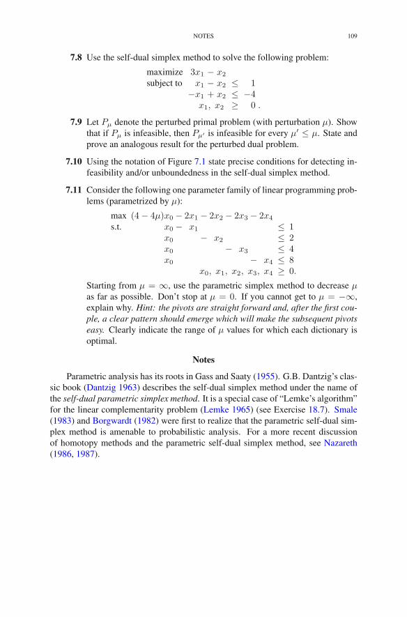
NOTES 109
7.8 Use the self-dual simplex method to solve the following problem:
maximize 3x1 − x2
subject to x1 − x2 ≤ 1−x1 + x2 ≤ −4
x1, x2 ≥ 0 .
7.9 Let Pμ denote the perturbed primal problem (with perturbation μ). Showthat if Pμ is infeasible, then Pμ′ is infeasible for every μ′ ≤ μ. State andprove an analogous result for the perturbed dual problem.
7.10 Using the notation of Figure 7.1 state precise conditions for detecting in-feasibility and/or unboundedness in the self-dual simplex method.
7.11 Consider the following one parameter family of linear programming prob-lems (parametrized by μ):
max (4− 4μ)x0 − 2x1 − 2x2 − 2x3 − 2x4
s.t. x0 − x1 ≤ 1x0 − x2 ≤ 2x0 − x3 ≤ 4x0 − x4 ≤ 8
x0, x1, x2, x3, x4 ≥ 0.
Starting from μ = ∞, use the parametric simplex method to decrease μas far as possible. Don’t stop at μ = 0. If you cannot get to μ = −∞,explain why. Hint: the pivots are straight forward and, after the first cou-ple, a clear pattern should emerge which will make the subsequent pivotseasy. Clearly indicate the range of μ values for which each dictionary isoptimal.
Notes
Parametric analysis has its roots in Gass and Saaty (1955). G.B. Dantzig’s clas-sic book (Dantzig 1963) describes the self-dual simplex method under the name ofthe self-dual parametric simplex method. It is a special case of “Lemke’s algorithm”for the linear complementarity problem (Lemke 1965) (see Exercise 18.7). Smale(1983) and Borgwardt (1982) were first to realize that the parametric self-dual sim-plex method is amenable to probabilistic analysis. For a more recent discussionof homotopy methods and the parametric self-dual simplex method, see Nazareth(1986, 1987).

CHAPTER 8
Implementation Issues
In the previous chapter, we rewrote the simplex method using matrix notation.This is the first step toward our aim of describing the simplex method as one wouldimplement it as a computer program. In this chapter, we shall continue in this direc-tion by addressing some important implementation issues.
The most time-consuming steps in the simplex method are the computations
ΔxB = B−1Nej and ΔzN = −(B−1N)T ei,
and the difficulty in these steps arises from the B−1. Of course, we don’t everactually compute the inverse of the basis matrix. Instead, we calculate, say, ΔxB bysolving the following system of equations:
(8.1) BΔxB = aj ,
whereaj = Nej
is the column of N associated with nonbasic variable xj .Similarly, the calculation of ΔzN is also broken into two steps:
BT v = ei,(8.2)
ΔzN = −NT v.
Here, the first step is the solution of a large system of equations, this time involvingBT instead of B, and the second step is the comparatively trivial task of multiplyinga vector on the left by the matrix −NT .
Solving the systems of equations (8.1) and (8.2) is where most of the com-plexity of a simplex iteration lies. We discuss solving such systems in the first twosections. In the second section, we look at the effect of sparsity on these systems.The next few sections explain how to reuse and/or update the computations of oneiteration in subsequent iterations. In the final sections, we address a few other issuesthat affect the efficiency of an implementation.
1. Solving Systems of Equations: LU -Factorization
In this section, we discuss solving systems of equations of the form
Bx = b,
where B is an invertible m×m matrix and b is an arbitrary m-vector. (Analysis ofthe transpose BTx = b is left to Exercise 8.4.) Our first thought is to use Gaussian
R.J. Vanderbei, Linear Programming, International Series in Operations Research& Management Science 196, DOI 10.1007/978-1-4614-7630-6 8,© Springer Science+Business Media New York 2014
111

112 8. IMPLEMENTATION ISSUES
elimination. This idea is correct, but to explain how Gaussian elimination is actuallyimplemented, we need to take a fresh look at how it works. To explain, let usconsider an example:
B =
⎡
⎢⎢⎢⎢⎣
2 4 −23 1 1
−1 −1 −2−1 −6
1 4
⎤
⎥⎥⎥⎥⎦.
(Note that, to emphasize the importance of sparsity, zero entries are simply leftblank.) In Gaussian elimination, one begins by subtracting appropriate multiplesof the first row from each subsequent row to get zeros in the first column belowthe diagonal. For our specific example, we subtract 3/2 times the first row fromthe second row and we subtract −1/2 times the first row from the third row. Theresult is
⎡
⎢⎢⎢⎢⎣
2 4 −21 −6 1 3
1 −3−1 −6
1 4
⎤
⎥⎥⎥⎥⎦.
Shortly, we will want to remember the values of the nonzero elements in the firstcolumn. Therefore, let us agree to do the row operations that are required to elimi-nate nonzeros, but when we write down the result of the elimination, we will leavethe nonzeros there. With this convention, the result of the elimination of the firstcolumn can be written as
⎡
⎢⎢⎢⎢⎣
2 4 −23 1 −6 1 3
−1 1 −3−1 −6
1 4
⎤
⎥⎥⎥⎥⎦.
Note that we have drawn a line to separate the eliminated top/left parts of the matrixfrom the uneliminated lower-right part.
Next, we eliminate the nonzeros below the second diagonal (there’s only one)by subtracting an appropriate multiple of the second row from each subsequent row.Again, we write the answer without zeroing out the eliminated elements:
⎡
⎢⎢⎢⎢⎣
2 4 −23 1 −6 1 3
−1 1 −3−1 −6 1 −3
1 4
⎤
⎥⎥⎥⎥⎦.

1. SOLVING SYSTEMS OF EQUATIONS: LU -FACTORIZATION 113
After eliminating the third column, we get⎡
⎢⎢⎢⎢⎣
2 4 −23 1 −6 1 3
−1 1 −3−1 −6 1 −21
1 7
⎤
⎥⎥⎥⎥⎦.
Now, the remaining uneliminated part is already an upper triangular matrix, andhence no more elimination is required.
At this point, you are probably wondering how this strangely produced matrixis related to the original matrix B. The answer is both simple and elegant. First, takethe final matrix and split it into three matrices: the matrix consisting of all elementson or below the diagonal, the matrix consisting of just the diagonal elements, andthe matrix consisting of all elements on or above the diagonal. It is amazing buttrue that B is simply the product of the resulting lower triangular matrix times theinverse of the diagonal matrix times the upper triangular matrix:
B =
⎡
⎢⎢⎢⎢⎣
23 1
−1 1−1−6 1
1 7
⎤
⎥⎥⎥⎥⎦
⎡
⎢⎢⎢⎢⎣
21
11
7
⎤
⎥⎥⎥⎥⎦
−1 ⎡
⎢⎢⎢⎢⎣
2 4 −21 −6 1 3
1 −31 −21
7
⎤
⎥⎥⎥⎥⎦.
(If you don’t believe it, multiply them and see.) Normally, the product of the lowertriangular matrix and the diagonal matrix is denoted by L,
L =
⎡
⎢⎢⎢⎢⎣
23 1
−1 1−1−6 1
1 7
⎤
⎥⎥⎥⎥⎦
⎡
⎢⎢⎢⎢⎣
21
11
7
⎤
⎥⎥⎥⎥⎦
−1
=
⎡
⎢⎢⎢⎢⎢⎣
132 1
− 12 1−1−6 1
1 1
⎤
⎥⎥⎥⎥⎥⎦
,
and the upper triangular matrix is denote by U :
U =
⎡
⎢⎢⎢⎢⎣
2 4 −21 −6 1 3
1 −31 −21
7
⎤
⎥⎥⎥⎥⎦.
The resulting representation,
B = LU,
is called an LU -factorization of B. Finding an LU -factorization is equivalent toGaussian elimination in the sense that multiplying B on the left by L−1 has theeffect of applying row operations to B to put it into upper-triangular form U .

114 8. IMPLEMENTATION ISSUES
The value of an LU -factorization is that it can be used to solve systems ofequations. For example, suppose that we wish to solve equation (8.1), where B isas above and
(8.3) aj =
⎡
⎢⎢⎢⎢⎣
7−2030
⎤
⎥⎥⎥⎥⎦.
First, we substitute LU for B so that the system becomes
LUΔxB = aj .
Now, if we let y = UΔxB, then we can solve
Ly = b
for y, and once y is known, we can solve
UΔxB = y
for ΔxB. Because L is lower triangular, solving Ly = b is easy. Indeed, writing thesystem out,
⎡
⎢⎢⎢⎢⎣
132 1
− 12 1−1 −6 1
1 1
⎤
⎥⎥⎥⎥⎦
⎡
⎢⎢⎢⎢⎣
y1y2y3y4y5
⎤
⎥⎥⎥⎥⎦=
⎡
⎢⎢⎢⎢⎣
7−2030
⎤
⎥⎥⎥⎥⎦,
we notice immediately that y1 = 7. Then, given y1, it becomes clear from thesecond equation that y2 = −2− (3/2)y1 = −25/2. Continuing in this way, we findthat
⎡
⎢⎢⎢⎢⎣
y1y2y3y4y5
⎤
⎥⎥⎥⎥⎦=
⎡
⎢⎢⎢⎢⎢⎢⎣
7− 25
2
72
232
− 72
⎤
⎥⎥⎥⎥⎥⎥⎦
.
The process of successively solving for the elements of the vector y starting withthe first and proceeding to the last is called forward substitution.
Of course, solving UΔxB = y is easy too, since U is upper triangular. Thesystem to solve is given by
⎡
⎢⎢⎢⎢⎣
2 4 −21 −6 1 3
1 −31 −21
7
⎤
⎥⎥⎥⎥⎦
⎡
⎢⎢⎢⎢⎣
Δx1
Δx2
Δx3
Δx4
Δx5
⎤
⎥⎥⎥⎥⎦=
⎡
⎢⎢⎢⎢⎢⎢⎣
7− 25
2
72
232
− 72
⎤
⎥⎥⎥⎥⎥⎥⎦
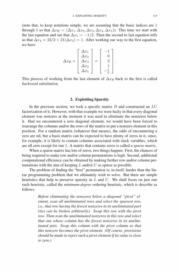
2. EXPLOITING SPARSITY 115
(note that, to keep notations simple, we are assuming that the basic indices are 1through 5 so that ΔxB = (Δx1,Δx2,Δx3,Δx4,Δx5)). This time we start withthe last equation and see that Δx5 = −1/2. Then the second to last equation tellsus that Δx4 = 23/2 + 21(Δx5) = 1. After working our way to the first equation,we have
ΔxB =
⎡
⎢⎢⎢⎢⎣
Δx1
Δx2
Δx3
Δx4
Δx5
⎤
⎥⎥⎥⎥⎦=
⎡
⎢⎢⎢⎢⎣
−1021
− 12
⎤
⎥⎥⎥⎥⎦.
This process of working from the last element of ΔxB back to the first is calledbackward substitution.
2. Exploiting Sparsity
In the previous section, we took a specific matrix B and constructed an LUfactorization of it. However, with that example we were lucky in that every diagonalelement was nonzero at the moment it was used to eliminate the nonzeros belowit. Had we encountered a zero diagonal element, we would have been forced torearrange the columns and/or the rows of the matrix to put a nonzero element in thisposition. For a random matrix (whatever that means), the odds of encountering azero are nil, but a basis matrix can be expected to have plenty of zeros in it, since,for example, it is likely to contain columns associated with slack variables, whichare all zero except for one 1. A matrix that contains zeros is called a sparse matrix.
When a sparse matrix has lots of zeros, two things happen. First, the chances ofbeing required to make row and/or column permutations is high. Second, additionalcomputational efficiency can be obtained by making further row and/or column per-mutations with the aim of keeping L and/or U as sparse as possible.
The problem of finding the “best” permutation is, in itself, harder than the lin-ear programming problem that we ultimately wish to solve. But there are simpleheuristics that help to preserve sparsity in L and U . We shall focus on just onesuch heuristic, called the minimum-degree ordering heuristic, which is describe asfollows:
Before eliminating the nonzeros below a diagonal “pivot” el-ement, scan all uneliminated rows and select the sparsest row,i.e., that row having the fewest nonzeros in its uneliminated part(ties can be broken arbitrarily). Swap this row with the pivotrow. Then scan the uneliminated nonzeros in this row and selectthat one whose column has the fewest nonzeros in its unelim-inated part. Swap this column with the pivot column so thatthis nonzero becomes the pivot element. (Of course, provisionsshould be made to reject such a pivot element if its value is closeto zero.)

116 8. IMPLEMENTATION ISSUES
As a matter of terminology, the number of nonzeros in the uneliminated part ofa row/column is called the degree of the row/column. Hence, the name of theheuristic.
Let’s apply the minimum-degree heuristic to the LU -factorization of the matrixB studied in the previous section. To keep track of the row and column permuta-tions, we will indicate original row indices on the left and original column indicesacross the top. Hence, we start with:
B =
1 2 3 4 512345
⎡
⎢⎢⎢⎢⎣
2 4 −23 1 1
−1 −1 −2−1 −6
1 4
⎤
⎥⎥⎥⎥⎦
.
To begin, row 4 has the fewest nonzeros, and within row 4, the −1 in column 2belongs to the column with the fewest nonzeros. Hence, we swap rows 1 and 4 andwe swap columns 1 and 2 to rewrite B as
B =
2 1 3 4 542315
⎡
⎢⎢⎢⎢⎣
−1 −61 3 1
−1 −1 −22 4 −2
1 4
⎤
⎥⎥⎥⎥⎦
.
Now, we eliminate the nonzeros under the first diagonal element (and, as before, weleave the eliminated nonzeros as they were). The result is
2 1 3 4 542315
⎡
⎢⎢⎢⎢⎣
−1 −61 3 1 −6
−1 −1 −22 4 −2
1 4
⎤
⎥⎥⎥⎥⎦
.
Before doing the elimination associated with the second diagonal element, wenote that row 5 is the row with minimum degree, and within row 5, the element 1 incolumn 3 has minimum column degree. Hence, we swap rows 2 and 5 and we swapcolumns 1 and 3 to get
2 3 1 4 545312
⎡
⎢⎢⎢⎢⎣
−1 −61 4
−1 −1 −24 2 −2
1 3 1 −6
⎤
⎥⎥⎥⎥⎦
.
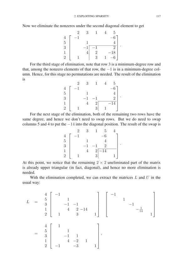
2. EXPLOITING SPARSITY 117
Now we eliminate the nonzeros under the second diagonal element to get
2 3 1 4 545312
⎡
⎢⎢⎢⎢⎣
−1 −61 4
−1 −1 24 2 −18
1 3 1 −6
⎤
⎥⎥⎥⎥⎦
.
For the third stage of elimination, note that row 3 is a minimum-degree row andthat, among the nonzero elements of that row, the −1 is in a minimum-degree col-umn. Hence, for this stage no permutations are needed. The result of the eliminationis
2 3 1 4 545312
⎡
⎢⎢⎢⎢⎣
−1 −61 4
−1 −1 24 2 −14
1 3 1
⎤
⎥⎥⎥⎥⎦
.
For the next stage of the elimination, both of the remaining two rows have thesame degree, and hence we don’t need to swap rows. But we do need to swapcolumns 5 and 4 to put the −14 into the diagonal position. The result of the swap is
2 3 1 5 445312
⎡
⎢⎢⎢⎢⎣
−1 −61 4
−1 −1 24 2 −14
1 3 1
⎤
⎥⎥⎥⎥⎦
.
At this point, we notice that the remaining 2 × 2 uneliminated part of the matrixis already upper triangular (in fact, diagonal), and hence no more elimination isneeded.
With the elimination completed, we can extract the matrices L and U in theusual way:
L =
45312
⎡
⎢⎢⎢⎢⎣
−11
−1 −14 2 −14
1 3 1
⎤
⎥⎥⎥⎥⎦
⎡
⎢⎢⎢⎢⎣
−11
−1− 1
141
⎤
⎥⎥⎥⎥⎦
=
45312
⎡
⎢⎢⎢⎢⎣
11
−1 14 −2 1
−1 −3 1
⎤
⎥⎥⎥⎥⎦
,

118 8. IMPLEMENTATION ISSUES
and
U =
2 3 1 5 4⎡
⎢⎢⎢⎢⎣
−1 −61 4
−1 2−14
1
⎤
⎥⎥⎥⎥⎦
.
(Note that the columns of L and the rows of U do not have any “original” indicesassociated with them, and so no permutation is indicated across the top of L or downthe left side of U .)
This LU -factorization has five off-diagonal nonzeros in L and three off-diagonalnonzeros in U for a total of eight off-diagonal nonzeros. In contrast, the LU fac-torization from the previous section had a total of 12 off-diagonal nonzeros. Hence,the minimum-degree ordering heuristic paid off for this example by reducing thenumber of nonzeros by 33 %. While such a reduction may not seem like a big dealfor small matrices such as our 5 × 5 example, for large matrices the difference canbe dramatic.
The fact that we have permuted the rows and columns to get this factoriza-tion has only a small impact on how one uses the factorization to solve systems ofequations. To illustrate, let us solve the same system that we considered before:BΔxB = aj , where aj is given by (8.3). The first step in solving this system is topermute the rows of aj so that they agree with the rows of L and then to use forwardsubstitution to solve the system Ly = aj . Writing it out, the system looks like this:
45312
⎡
⎢⎢⎢⎢⎣
11
−1 14 −2 1
−1 −3 1
⎤
⎥⎥⎥⎥⎦
⎡
⎢⎢⎢⎢⎣
y1y2y3y4y5
⎤
⎥⎥⎥⎥⎦=
45312
⎡
⎢⎢⎢⎢⎣
3007
−2
⎤
⎥⎥⎥⎥⎦
The result of the forward substitution is that
(8.4)
⎡
⎢⎢⎢⎢⎣
y1y2y3y4y5
⎤
⎥⎥⎥⎥⎦=
⎡
⎢⎢⎢⎢⎣
30071
⎤
⎥⎥⎥⎥⎦.
The next step is to solve the system UΔxB = y. Writing this system out, we get
2 3 1 5 4⎡
⎢⎢⎢⎢⎣
−1 −61 4
−1 2−14
1
⎤
⎥⎥⎥⎥⎦
23154
⎡
⎢⎢⎢⎢⎣
Δx2
Δx3
Δx1
Δx5
Δx4
⎤
⎥⎥⎥⎥⎦=
⎡
⎢⎢⎢⎢⎣
30071
⎤
⎥⎥⎥⎥⎦.

3. REUSING A FACTORIZATION 119
Using backward substitution, we see that
23154
⎡
⎢⎢⎢⎢⎣
Δx2
Δx3
Δx1
Δx5
Δx4
⎤
⎥⎥⎥⎥⎦=
⎡
⎢⎢⎢⎢⎣
02
−1− 1
21
⎤
⎥⎥⎥⎥⎦.
Finally, we rewrite the solution listing the elements of ΔxB in their original order:
ΔxB =
⎡
⎢⎢⎢⎢⎣
Δx1
Δx2
Δx3
Δx4
Δx5
⎤
⎥⎥⎥⎥⎦=
⎡
⎢⎢⎢⎢⎣
−1021
− 12
⎤
⎥⎥⎥⎥⎦.
Of course, the answer obtained here agrees with the one obtained at the end of theprevious section.
Even with good fill-in minimizing heuristics such as minimum-degree, the LU -factorization remains a significant computational bottleneck. To see why, considerfor the moment dense matrices. If we were to write a subroutine to carry out anLU -factorization, we would find that the main body of the routine would have a bigtriply nested loop:
for each column index j {for each remaining row index i {
for each remaining column index k {update the (i,k) entry in accordance withthe aim to make the (i,j) entry be zero
}}
}
Since each of these loops involves approximately m steps, the LU -factorizationroutine requires about m3 operations and hence is called an order m3 algorithm.Similar considerations tell us that the forward and backward substitutions are bothorder m2 algorithms. This means that forward and backward substitution can bedone much faster than LU -factorization. Indeed, if m = 5,000, then factorizationtakes a couple of 1,000 times longer than a forward or backward substitution. Ofcourse, this argument is for dense matrices. But for sparse matrices a similar, if lessdramatic, effect is seen. Typically, for sparse matrices, one expects that factorizationwill take from 10 to 100 times longer than substitution. Therefore, it is important toperform as few LU -factorizations as possible. This is the subject of the next section.
3. Reusing a Factorization
In the previous two sections, we showed how to use an LU -factorization of Bto solve the system of equations
BΔxB = aj

120 8. IMPLEMENTATION ISSUES
for the primal step direction ΔxB. Since the basis matrix doesn’t change much fromone iteration of the simplex method to the next (columns get replaced by new onesone at a time), we ask whether the LU -factorization of B from the current iterationmight somehow be used again to solve the systems of equations that arise in the nextiteration (or even the next several iterations).
Let B denote the current basis (for which a factorization has already been com-puted) and let B denote the basis of the next iteration. Then B is simply B withthe column that holds the column vector ai associated with the leaving variable xi
replaced by a new column vector aj associated with the entering variable xj . Thisverbal description can be converted into a formula:
(8.5) B = B + (aj − ai)eTi .
Here, as before, ei denotes the vector that is all zeros except for a one in the positionassociated with index i—to be definite, let us say that this position is the pth positionin the vector. To see why this formula is correct, it is helpful to realize that a columnvector, say a, times eTi produces a matrix that is all zero except for the pth column,which contains the column vector a.
Since the basis B is invertible, (8.5) can be rewritten as
B = B(I +B−1(aj − ai)e
Ti
).
Denote the matrix in parentheses by E. Recall that aj = Nej , since it is the columnvector from A associated with the entering variable xj . Hence,
B−1aj = B−1Nej = ΔxB,
which is a vector we need to compute in the current iteration anyway. Also,
B−1ai = ei,
since ai is the column of B associated with the leaving variable xi. Therefore, wecan write E more simply as
E = I + (ΔxB − ei)eTi .
Now, if E has a simple inverse, then we can use it together with the LU -factorizationof B to provide an efficient means of solving systems of equations involving B. Thefollowing proposition shows that E does indeed have a simple inverse.
PROPOSITION 8.1. Given two column vectors u and v for which 1 + vTu �= 0,
(I + uvT )−1 = I − uvT
1 + vTu.
PROOF. The proof is trivial. We simply multiply the matrix by its supposedinverse and check that we get the identity:
(I + uvT
)(
I − uvT
1 + vTu
)
= I + uvT − uvT
1 + vTu− uvTuvT
1 + vTu
= I + uvT(
1− 1
1 + vTu− vTu
1 + vTu
)
= I,
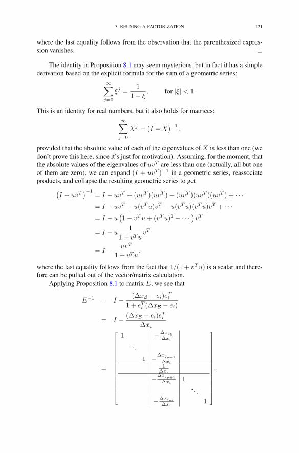
3. REUSING A FACTORIZATION 121
where the last equality follows from the observation that the parenthesized expres-sion vanishes. �
The identity in Proposition 8.1 may seem mysterious, but in fact it has a simplederivation based on the explicit formula for the sum of a geometric series:
∞∑
j=0
ξj =1
1− ξ, for |ξ| < 1.
This is an identity for real numbers, but it also holds for matrices:
∞∑
j=0
Xj = (I −X)−1
,
provided that the absolute value of each of the eigenvalues of X is less than one (wedon’t prove this here, since it’s just for motivation). Assuming, for the moment, thatthe absolute values of the eigenvalues of uvT are less than one (actually, all but oneof them are zero), we can expand (I + uvT )−1 in a geometric series, reassociateproducts, and collapse the resulting geometric series to get
(I + uvT
)−1= I − uvT + (uvT )(uvT )− (uvT )(uvT )(uvT ) + · · ·= I − uvT + u(vTu)vT − u(vTu)(vTu)vT + · · ·= I − u
(1− vTu+ (vTu)2 − · · ·
)vT
= I − u1
1 + vTuvT
= I − uvT
1 + vTu,
where the last equality follows from the fact that 1/(1 + vTu) is a scalar and there-fore can be pulled out of the vector/matrix calculation.
Applying Proposition 8.1 to matrix E, we see that
E−1 = I − (ΔxB − ei)eTi
1 + eTi (ΔxB − ei)
= I − (ΔxB − ei)eTi
Δxi
=
⎡
⎢⎢⎢⎢⎢⎢⎢⎢⎢⎢⎢⎢⎣
1 −Δxj1
Δxi
. . .
1 −Δxjp−1
Δxi1
Δxi
−Δxjp+1
Δxi1
. . .
−Δxjm
Δxi1
⎤
⎥⎥⎥⎥⎥⎥⎥⎥⎥⎥⎥⎥⎦
.

122 8. IMPLEMENTATION ISSUES
Now, let’s look at the systems of equations that need to be solved in the nextiteration. Using tildes to denote items associated with the next iteration, we see thatwe need to solve
BΔxB = aj and BT v = ei
(actually, we should probably put the tilde on the j instead of the aj and on the iinstead of the ei, but doing so seems less aesthetically appealing, even though it’smore correct). Recalling that B = BE, we see that the first system is equivalent to
BEΔxB = aj ,
which can be solved in two stages:
Bu = aj ,
EΔxB = u.
Of course, the second system (involving E) is trivial, since we have an explicitformula for the inverse of E:
ΔxB = E−1u
= u− ui
Δxi(ΔxB − ei)
(where, in keeping with our tradition, we have used ui to denote the element of uassociated with the basic variable xi—that is, ui is the pth entry of u).
The system involving BT is handled in the same manner. Indeed, first werewrite it as
ETBT v = ei
and then observe that it too can be solved in two steps:
ETu = ei,
BT v = u.
This time, the first step is the trivial one1:
u = E−T ei
= ei − ei(ΔxB − ei)
T eiΔxi
.
Note that the fraction in the preceding equation is a scalar, and so this final expres-sion for u shows that it is a vector with at most two nonzeros—that is, the result isutterly trivial even if the formula looks a little bit cumbersome.
We end this section by returning briefly to our example. Suppose that B is Bwith column 3 replaced by the vector aj given in (8.3). Suppose that
aj =[
5 0 0 0 −1]T
.
To solve BΔxB = aj , we first solve Bu = aj using our LU -factorization of B.The result of the forward and backward substitutions is
1Occasionally we use the superscript −T for the transpose of the inverse of a matrix. Hence,E−T = (E−1)T .
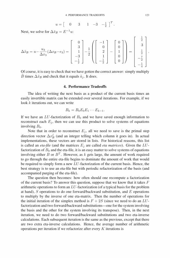
4. PERFORMANCE TRADEOFFS 123
u =[
0 3 1 −3 − 12
]T.
Next, we solve for ΔxB = E−1u:
ΔxB = u− u3
Δx3(ΔxB−e3) =
⎡
⎢⎢⎢⎢⎣
031
−3− 1
2
⎤
⎥⎥⎥⎥⎦− 1
2
⎛
⎜⎜⎜⎜⎝
⎡
⎢⎢⎢⎢⎣
−1021
− 12
⎤
⎥⎥⎥⎥⎦−
⎡
⎢⎢⎢⎢⎣
00100
⎤
⎥⎥⎥⎥⎦
⎞
⎟⎟⎟⎟⎠
=
⎡
⎢⎢⎢⎢⎢⎢⎢⎣
12
3
12
− 72
− 14
⎤
⎥⎥⎥⎥⎥⎥⎥⎦
.
Of course, it is easy to check that we have gotten the correct answer: simply multiplyB times ΔxB and check that it equals aj . It does.
4. Performance Tradeoffs
The idea of writing the next basis as a product of the current basis times aneasily invertible matrix can be extended over several iterations. For example, if welook k iterations out, we can write
Bk = B0E0E1 · · ·Ek−1.
If we have an LU -factorization of B0 and we have saved enough information toreconstruct each Ej , then we can use this product to solve systems of equationsinvolving Bk.
Note that in order to reconstruct Ej , all we need to save is the primal stepdirection vector Δxj
B (and an integer telling which column it goes in). In actualimplementations, these vectors are stored in lists. For historical reasons, this listis called an eta-file (and the matrices Ej are called eta matrices). Given the LU -factorization of B0 and the eta-file, it is an easy matter to solve systems of equationsinvolving either B or BT . However, as k gets large, the amount of work requiredto go through the entire eta-file begins to dominate the amount of work that wouldbe required to simply form a new LU -factorization of the current basis. Hence, thebest strategy is to use an eta-file but with periodic refactorization of the basis (andaccompanied purging of the eta-file).
The question then becomes: how often should one recompute a factorizationof the current basis? To answer this question, suppose that we know that it takes Farithmetic operations to form an LU -factorization (of a typical basis for the problemat hand), S operations to do one forward/backward substitution, and E operationsto multiply by the inverse of one eta-matrix. Then the number of operations forthe initial iteration of the simplex method is F + 2S (since we need to do an LU -factorization and two forward/backward substitutions—one for the system involvingthe basis and the other for the system involving its transpose). Then, in the nextiteration, we need to do two forward/backward substitutions and two eta-inversecalculations. Each subsequent iteration is the same as the previous, except that thereare two extra eta-inverse calculations. Hence, the average number of arithmeticoperations per iteration if we refactorize after every K iterations is

124 8. IMPLEMENTATION ISSUES
T (K) =1
K((F + 2S) + 2(S + E) + 2(S + 2E)
+ · · ·+ 2(S + (K − 1)E))
=1
KF + 2S + (K − 1)E.
Treating K as a real variable for the moment, we can differentiate this expressionwith respect to K, set the derivative equal to zero, and solve for K to get an estimatefor the optimal choice of K:
K =
√F
E.
As should be clear from our earlier discussions, E is of order m and, if the basismatrix is dense, F is of order m3. Hence, for dense matrices, our estimates wouldindicate that refactorizations should take place every m iterations or so. However,for sparse matrices, F will be substantially less that m3—more like a constant timesm2—which would indicate that refactorizations should occur on the order of every√m iterations. In practice, one typically allows the value of K to be a user-settable
parameter whose default value is set to something like 100.
5. Updating a Factorization
There is an important alternative to the eta-matrix method for reusing an LU -factorization, which we shall describe in this section and the next. As always, itis easiest to work with an example, so let’s continue with the same example we’vebeen using throughout this chapter.
Recall that the matrix B is simply B with its third column replaced by thevector aj given in (8.3):
B =
1 2 3 4 512345
⎡
⎢⎢⎢⎢⎣
2 7 −23 1 −2 1
−1 −2−1 3 −6
4
⎤
⎥⎥⎥⎥⎦
=
2 3 1 5 445312
⎡
⎢⎢⎢⎢⎣
−1 3 −64
−1 −27 2 −2
1 −2 3 1
⎤
⎥⎥⎥⎥⎦
.
(Note that we’ve highlighted the new column by putting a box around it.)Since L−1B = U and B differs from B in only one column, it follows that
L−1B coincides with U except for the column that got changed. And, since thiscolumn got replaced by aj , it follows that this column of L−1B contains L−1aj ,which we’ve already computed and found to be given by (8.4). Hence,
(8.6) L−1B =
2 3 1 5 412345
⎡
⎢⎢⎢⎢⎣
−1 3 −64
−1 27 −141 1
⎤
⎥⎥⎥⎥⎦
.

5. UPDATING A FACTORIZATION 125
As we saw before, the columns of L have no “original” indices to relate back to, andso one can simply take them to be numbered in natural order. The same is then truefor the rows of L−1 and hence for the rows of L−1B. That is why the rows shownabove are numbered as they are. We’ve shown these numbers explicitly, since theyare about to get permuted.
The boxed column in (8.6) is called a spike, since it has nonzeros below thediagonal. The 4 × 4 submatrix constructed from rows 2 through 5 and columns 3,1, 5, and 4 is called the bump. To get this matrix back into upper-triangular form,one could do row operations to eliminate the nonzeros in the spike that lie below thediagonal. But such row operations could create fill-in anywhere in the bump. Suchfill-in would be more than one would like to encounter. However, consider whathappens if the spike column is moved to the rightmost column of the bump, shiftingthe other columns left one position in the process, and if the top row of the bump(i.e., row 2) is moved to the bottom of the bump, shifting the other bump rows upby one. The result of these permutations is
L−1B =
2 1 5 4 313452
⎡
⎢⎢⎢⎢⎣
−1 −6 3−1 2
−14 71 1
4
⎤
⎥⎥⎥⎥⎦
.
(For future reference, we’ve boxed the bump.) In general, the effect of this permu-tation is that the column spike gets replaced by a row spike along the bottom row ofthe bump:
⎡⎢⎢⎢⎢⎢⎢⎢⎢⎢⎢⎢⎢⎢⎢⎣
∗ ∗ ∗ ∗ ∗ ∗ ∗ ∗ ∗ ∗ ∗∗ ∗ ∗ ∗ ∗ ∗ ∗ ∗ ∗ ∗
∗ ∗ ∗ ∗ ∗ ∗ ∗ ∗ ∗∗ ∗ ∗ ∗ ∗ ∗ ∗ ∗ ∗∗ ∗ ∗ ∗ ∗ ∗ ∗ ∗∗ ∗ ∗ ∗ ∗ ∗ ∗∗ ∗ ∗ ∗ ∗ ∗∗ ∗ ∗ ∗ ∗∗ ∗ ∗ ∗
∗ ∗∗
⎤⎥⎥⎥⎥⎥⎥⎥⎥⎥⎥⎥⎥⎥⎥⎦
−→
⎡⎢⎢⎢⎢⎢⎢⎢⎢⎢⎢⎢⎢⎢⎢⎣
∗ ∗ ∗ ∗ ∗ ∗ ∗ ∗ ∗ ∗ ∗∗ ∗ ∗ ∗ ∗ ∗ ∗ ∗ ∗ ∗
∗ ∗ ∗ ∗ ∗ ∗ ∗ ∗ ∗∗ ∗ ∗ ∗ ∗ ∗ ∗ ∗
∗ ∗ ∗ ∗ ∗ ∗ ∗∗ ∗ ∗ ∗ ∗ ∗
∗ ∗ ∗ ∗ ∗∗ ∗ ∗ ∗
∗ ∗ ∗ ∗ ∗ ∗ ∗ ∗ ∗∗ ∗
∗
⎤⎥⎥⎥⎥⎥⎥⎥⎥⎥⎥⎥⎥⎥⎥⎦
.
Now any fill-in produced by row operations is confined to the spike row. In ourexample, there is only one nonzero in the spike row, and to eliminate it we need toadd 2/7 times row 4 to it. This row operation can be represented algebraically asmultiplication on the left by the matrix
E =
⎡
⎢⎢⎢⎢⎣
11
11
27 1
⎤
⎥⎥⎥⎥⎦.
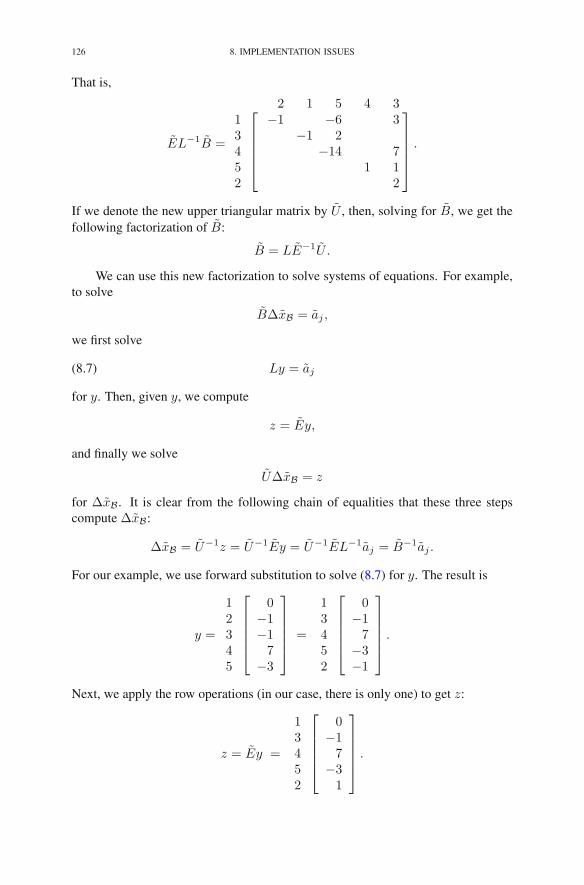
126 8. IMPLEMENTATION ISSUES
That is,
EL−1B =
2 1 5 4 313452
⎡
⎢⎢⎢⎢⎣
−1 −6 3−1 2
−14 71 1
2
⎤
⎥⎥⎥⎥⎦
.
If we denote the new upper triangular matrix by U , then, solving for B, we get thefollowing factorization of B:
B = LE−1U .
We can use this new factorization to solve systems of equations. For example,to solve
BΔxB = aj ,
we first solve
(8.7) Ly = aj
for y. Then, given y, we compute
z = Ey,
and finally we solve
UΔxB = z
for ΔxB. It is clear from the following chain of equalities that these three stepscompute ΔxB:
ΔxB = U−1z = U−1Ey = U−1EL−1aj = B−1aj .
For our example, we use forward substitution to solve (8.7) for y. The result is
y =
12345
⎡
⎢⎢⎢⎢⎣
0−1−17
−3
⎤
⎥⎥⎥⎥⎦
=
13452
⎡
⎢⎢⎢⎢⎣
0−17
−3−1
⎤
⎥⎥⎥⎥⎦.
Next, we apply the row operations (in our case, there is only one) to get z:
z = Ey =
13452
⎡
⎢⎢⎢⎢⎣
0−17
−31
⎤
⎥⎥⎥⎥⎦.
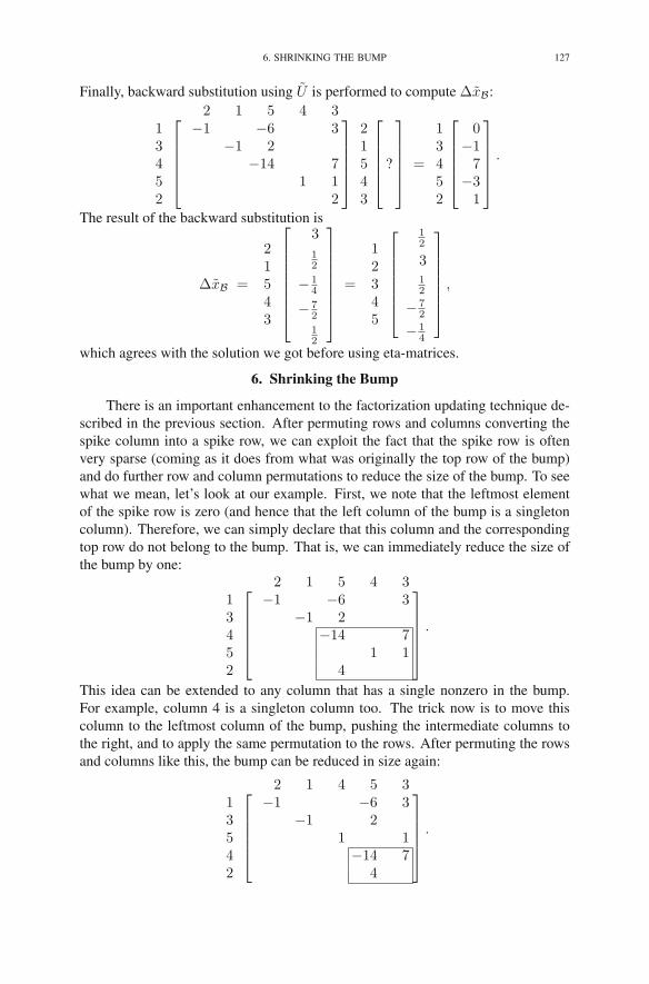
6. SHRINKING THE BUMP 127
Finally, backward substitution using U is performed to compute ΔxB:2 1 5 4 3
13452
⎡
⎢⎢⎢⎢⎣
−1 −6 3−1 2
−14 71 1
2
⎤
⎥⎥⎥⎥⎦
21543
⎡
⎢⎢⎢⎢⎣
?
⎤
⎥⎥⎥⎥⎦
=
13452
⎡
⎢⎢⎢⎢⎣
0−17
−31
⎤
⎥⎥⎥⎥⎦
.
The result of the backward substitution is
ΔxB =
21543
⎡
⎢⎢⎢⎢⎢⎢⎢⎣
3
12
− 14
− 72
12
⎤
⎥⎥⎥⎥⎥⎥⎥⎦
=
12345
⎡
⎢⎢⎢⎢⎢⎢⎣
12
312
− 72
− 14
⎤
⎥⎥⎥⎥⎥⎥⎦
,
which agrees with the solution we got before using eta-matrices.
6. Shrinking the Bump
There is an important enhancement to the factorization updating technique de-scribed in the previous section. After permuting rows and columns converting thespike column into a spike row, we can exploit the fact that the spike row is oftenvery sparse (coming as it does from what was originally the top row of the bump)and do further row and column permutations to reduce the size of the bump. To seewhat we mean, let’s look at our example. First, we note that the leftmost elementof the spike row is zero (and hence that the left column of the bump is a singletoncolumn). Therefore, we can simply declare that this column and the correspondingtop row do not belong to the bump. That is, we can immediately reduce the size ofthe bump by one:
2 1 5 4 313452
⎡
⎢⎢⎢⎢⎣
−1 −6 3−1 2
−14 71 1
4
⎤
⎥⎥⎥⎥⎦
.
This idea can be extended to any column that has a single nonzero in the bump.For example, column 4 is a singleton column too. The trick now is to move thiscolumn to the leftmost column of the bump, pushing the intermediate columns tothe right, and to apply the same permutation to the rows. After permuting the rowsand columns like this, the bump can be reduced in size again:
2 1 4 5 313542
⎡
⎢⎢⎢⎢⎣
−1 −6 3−1 2
1 1−14 7
4
⎤
⎥⎥⎥⎥⎦
.
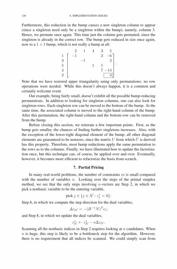
128 8. IMPLEMENTATION ISSUES
Furthermore, this reduction in the bump causes a new singleton column to appear(since a singleton need only be a singleton within the bump), namely, column 3.Hence, we permute once again. This time just the column gets permuted, since thesingleton is already in the correct row. The bump gets reduced in size once again,now to a 1× 1 bump, which is not really a bump at all:
2 1 4 3 513542
⎡
⎢⎢⎢⎢⎣
−1 3 −6−1 2
1 17 −14
4
⎤
⎥⎥⎥⎥⎦
.
Note that we have restored upper triangularity using only permutations; no rowoperations were needed. While this doesn’t always happen, it is a common andcertainly welcome event.
Our example, being fairly small, doesn’t exhibit all the possible bump-reducingpermutations. In addition to looking for singleton columns, one can also look forsingleton rows. Each singleton row can be moved to the bottom of the bump. At thesame time, the associated column is moved to the right-hand column of the bump.After this permutation, the right-hand column and the bottom row can be removedfrom the bump.
Before closing this section, we reiterate a few important points. First, as thebump gets smaller, the chances of finding further singletons increases. Also, withthe exception of the lower-right diagonal element of the bump, all other diagonalelements are guaranteed to be nonzero, since the matrix U from which U is derivedhas this property. Therefore, most bump reductions apply the same permutation tothe rows as to the columns. Finally, we have illustrated how to update the factoriza-tion once, but this technique can, of course, be applied over and over. Eventually,however, it becomes more efficient to refactorize the basis from scratch.
7. Partial Pricing
In many real-world problems, the number of constraints m is small comparedwith the number of variables n. Looking over the steps of the primal simplexmethod, we see that the only steps involving n-vectors are Step 2, in which wepick a nonbasic variable to be the entering variable,
pick j ∈ {j ∈ N : z∗j < 0};Step 6, in which we compute the step direction for the dual variables,
ΔzN = −(B−1N)T ei;
and Step 8, in which we update the dual variables,
z∗N ← z∗N − sΔzN .
Scanning all the nonbasic indices in Step 2 requires looking at n candidates. Whenn is huge, this step is likely to be a bottleneck step for the algorithm. However,there is no requirement that all indices be scanned. We could simply scan from
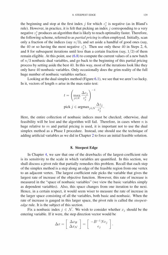
8. STEEPEST EDGE 129
the beginning and stop at the first index j for which z∗j is negative (as in Bland’srule). However, in practice, it is felt that picking an index j corresponding to a verynegative z∗j produces an algorithm that is likely to reach optimality faster. Therefore,the following scheme, referred to as partial pricing is often employed. Initially, scanonly a fraction of the indices (say n/3), and set aside a handful of good ones (say,the 40 or so having the most negative z∗j ). Then use only these 40 in Steps 2, 6,and 8 for subsequent iterations until less than a certain fraction (say, 1/2) of themremain eligible. At this point, use (6.8) to compute the current values of a new batchof n/3 nonbasic dual variables, and go back to the beginning of this partial pricingprocess by setting aside the best 40. In this way, most of the iterations look like theyonly have 40 nonbasic variables. Only occasionally does the grim reality of the fullhuge number of nonbasic variables surface.
Looking at the dual simplex method (Figure 6.1), we see that we aren’t so lucky.In it, vectors of length n arise in the max-ratio test:
t =
(
maxj∈N
Δzjz∗j
)−1
pick j ∈ argmaxj∈NΔzjz∗j
.
Here, the entire collection of nonbasic indices must be checked; otherwise, dualfeasibility will be lost and the algorithm will fail. Therefore, in cases where n ishuge relative to m and partial pricing is used, it is important not to use the dualsimplex method as a Phase I procedure. Instead, one should use the technique ofadding artificial variables as we did in Chapter 2 to force an initial feasible solution.
8. Steepest Edge
In Chapter 4, we saw that one of the drawbacks of the largest-coefficient ruleis its sensitivity to the scale in which variables are quantified. In this section, weshall discuss a pivot rule that partially remedies this problem. Recall that each stepof the simplex method is a step along an edge of the feasible region from one vertexto an adjacent vertex. The largest coefficient rule picks the variable that gives thelargest rate of increase of the objective function. However, this rate of increase ismeasured in the “space of nonbasic variables” (we view the basic variables simplyas dependent variables). Also, this space changes from one iteration to the next.Hence, in a certain respect, it would seem wiser to measure the rate of increase inthe larger space consisting of all the variables, both basic and nonbasic. When therate of increase is gauged in this larger space, the pivot rule is called the steepest-edge rule. It is the subject of this section.
Fix a nonbasic index j ∈ N . We wish to consider whether xj should be theentering variable. If it were, the step direction vector would be
Δx =
[ΔxBΔxN
]
=
[−B−1Nej
ej
]
.

130 8. IMPLEMENTATION ISSUES
This vector points out along the edge corresponding to the pivot that would resultby letting xj enter the basis. As we know, the objective function is
f(x) = cTx = cTBxB + cTNxN .
The derivative of f(x) in the direction of Δx is given by
∂f
∂Δx= cT
Δx
‖Δx‖ =cTBΔxB + cTNΔxN
‖Δx‖ .
The numerator is easy (and familiar):
cTBΔxB + cTNΔxN = cj − cTBB−1Nej
=(cN − (B−1N)T cB
)j
= −z∗j .
The denominator is more troublesome:
‖Δx‖2 = ‖ΔxB‖2 + 1 = ‖B−1Nej‖2 + 1.
To calculate B−1Nej for every j ∈ N is exactly the same as computing the matrixB−1N , which (as we’ve discussed before) is time consuming and therefore a com-putation we wish to avoid. But it turns out that we can compute B−1Nej for everyj ∈ N once at the start (when B is essentially, if not identically, an identity matrix)and then update the norms of these vectors using a simple formula, which we shallnow derive.
Letνk = ‖B−1Nek‖2, k ∈ N .
Suppose that we know these numbers, we use them to perform one step of the sim-plex method, and we are now at the beginning of the next iteration. As usual, letus denote quantities in this next iteration by putting tildes on them. For example,B denotes the new basis matrix. As we’ve seen before, B is related to B by theequation B = BE, where
E−1 = I − (ΔxB − ei)eTi
Δxi.
Now, let’s compute the new ν values:
νk = aTk B−T B−1ak
= aTkB−TE−TE−1B−1ak
= aTkB−T
(
I − ei(ΔxB − ei)T
Δxi
)(
I − (ΔxB − ei)eTi
Δxi
)
B−1ak.(8.8)
Recall from (8.2) that we must compute
v = B−T ei
in the course of the old iteration. If, in addition, we compute
w = B−TΔxB
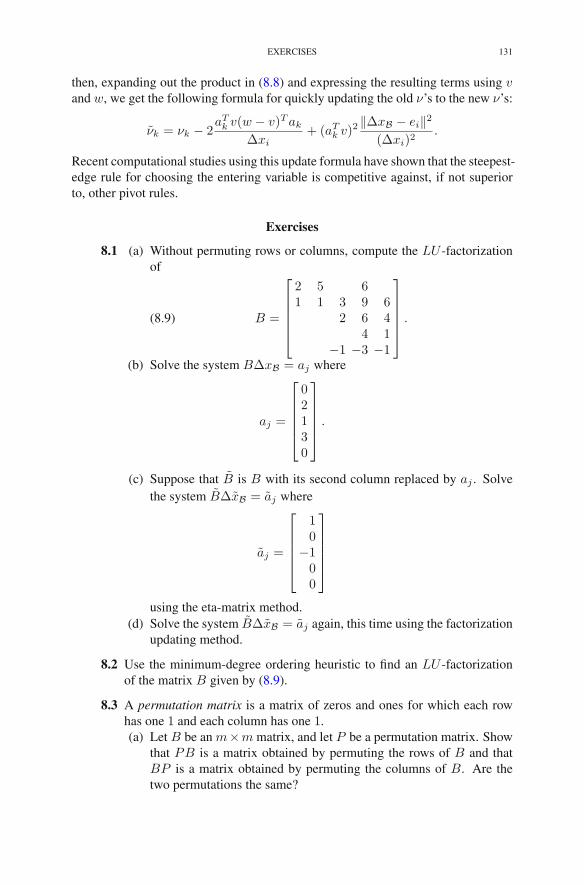
EXERCISES 131
then, expanding out the product in (8.8) and expressing the resulting terms using vand w, we get the following formula for quickly updating the old ν’s to the new ν’s:
νk = νk − 2aTk v(w − v)Tak
Δxi+ (aTk v)
2 ‖ΔxB − ei‖2(Δxi)2
.
Recent computational studies using this update formula have shown that the steepest-edge rule for choosing the entering variable is competitive against, if not superiorto, other pivot rules.
Exercises
8.1 (a) Without permuting rows or columns, compute the LU -factorizationof
(8.9) B =
⎡
⎢⎢⎢⎢⎣
2 5 61 1 3 9 6
2 6 44 1
−1 −3 −1
⎤
⎥⎥⎥⎥⎦.
(b) Solve the system BΔxB = aj where
aj =
⎡
⎢⎢⎢⎢⎣
02130
⎤
⎥⎥⎥⎥⎦.
(c) Suppose that B is B with its second column replaced by aj . Solvethe system BΔxB = aj where
aj =
⎡
⎢⎢⎢⎢⎣
10
−100
⎤
⎥⎥⎥⎥⎦
using the eta-matrix method.(d) Solve the system BΔxB = aj again, this time using the factorization
updating method.
8.2 Use the minimum-degree ordering heuristic to find an LU -factorizationof the matrix B given by (8.9).
8.3 A permutation matrix is a matrix of zeros and ones for which each rowhas one 1 and each column has one 1.(a) Let B be an m×m matrix, and let P be a permutation matrix. Show
that PB is a matrix obtained by permuting the rows of B and thatBP is a matrix obtained by permuting the columns of B. Are thetwo permutations the same?

132 8. IMPLEMENTATION ISSUES
(b) Show that every permutation of the rows of a matrix B correspondsto multiplying B on the left by a permutation matrix.
(c) Show that for any permutation matrix P ,
P−1 = PT .
8.4 Explain how to use the factorization B = LU to solve
BTx = b.
Notes
Techniques for exploiting sparsity in matrix factorization have their roots in thepaper by Markowitz (1957). A few standard references on matrix factorization arethe books of Duff et al. (1986), Golub and VanLoan (1989), and Gill et al. (1991).The eta-matrix technique given in Section 8.3 for using an old basis to solve systemsof equations involving the current basis was first described by Dantzig and Orchard-Hayes (1954). The factorization updating technique described in Section 8.5 is themethod given by Forrest and Tomlin (1972). The bump reduction techniques ofSection 8.6 were first introduced by Saunders (1973) and Reid (1982). The steepest-edge pivoting rule is due to Goldfarb and Reid (1977). A similar rule, known asDevex, was given by Harris (1973).
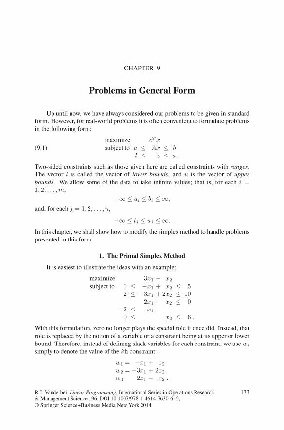
CHAPTER 9
Problems in General Form
Up until now, we have always considered our problems to be given in standardform. However, for real-world problems it is often convenient to formulate problemsin the following form:
(9.1)maximize cTxsubject to a ≤ Ax ≤ b
l ≤ x ≤ u .
Two-sided constraints such as those given here are called constraints with ranges.The vector l is called the vector of lower bounds, and u is the vector of upperbounds. We allow some of the data to take infinite values; that is, for each i =1, 2, . . . ,m,
−∞ ≤ ai ≤ bi ≤ ∞,
and, for each j = 1, 2, . . . , n,
−∞ ≤ lj ≤ uj ≤ ∞.
In this chapter, we shall show how to modify the simplex method to handle problemspresented in this form.
1. The Primal Simplex Method
It is easiest to illustrate the ideas with an example:
maximize 3x1 − x2
subject to 1 ≤ −x1 + x2 ≤ 52 ≤ −3x1 + 2x2 ≤ 10
2x1 − x2 ≤ 0−2 ≤ x1
0 ≤ x2 ≤ 6 .
With this formulation, zero no longer plays the special role it once did. Instead, thatrole is replaced by the notion of a variable or a constraint being at its upper or lowerbound. Therefore, instead of defining slack variables for each constraint, we use wi
simply to denote the value of the ith constraint:
w1 = −x1 + x2
w2 = −3x1 + 2x2
w3 = 2x1 − x2 .
R.J. Vanderbei, Linear Programming, International Series in Operations Research& Management Science 196, DOI 10.1007/978-1-4614-7630-6 9,© Springer Science+Business Media New York 2014
133

134 9. PROBLEMS IN GENERAL FORM
The constraints can then be interpreted as upper and lower bounds on these vari-ables. Now when we record our problem in a dictionary, we will have to keepexplicit track of the upper and lower bound on the original xj variables and the newwi variables. Also, the value of a nonbasic variable is no longer implicit; it couldbe at either its upper or its lower bound. Hence, we shall indicate which is the caseby putting a box around the relevant bound. Finally, we need to keep track of thevalues of the basic variables. Hence, we shall write our dictionary as follows:
l −2 0
u ∞ 6ζ = 3x1 − x2 = −6
1 5 w1 = −x1 + x2 = 22 10 w2 = −3x1 + 2x2 = 6
−∞ 0 w3 = 2x1 − x2 = −4 .
Since all the wi’s are between their upper and lower bounds, this dictionary is fea-sible. But it is not optimal, since x1 could be increased from its present value atthe lower bound, thereby increasing the objective function’s value. Hence, x1 shallbe the entering variable for the first iteration. Looking at w1, we see that x1 can beraised only 1 unit before w1 hits its lower bound. Similarly, x1 can be raised by 4/3units, at which point w2 hits its lower bound. Finally, if x1 were raised 2 units, thenw3 would hit its upper bound. The tightest of these constraints is the one on w1, andso w1 becomes the leaving variable—which, in the next iteration, will then be at itslower bound. Performing the usual row operations, we get
l 1 0
u 5 6ζ = −3w1 + 2x2 = −3
−2 ∞ x1 = −w1 + x2 = −12 10 w2 = 3w1 − x2 = 3
−∞ 0 w3 = −2w1 + x2 = −2 .
Note, of course, that the objective function value has increased (from −6 to −3).For the second iteration, raising x2 from its lower bound will produce an increasein ζ. Hence, x2 is the entering variable. Looking at the basic variables (x1, w2, andw3), we see that w2 will be the first variable to hit a bound, namely, its lower bound.Hence, w2 is the leaving variable, which will become nonbasic at its lower bound:
l 1 2u 5 10
ζ = 3w1 − 2w2 = −1−2 ∞ x1 = 2w1 − w2 = 00 6 x2 = 3w1 − w2 = 1
−∞ 0 w3 = w1 − w2 = −1 .
For the third iteration, w1 is the entering variable, and w3 is the leaving vari-able, since it hits its upper bound before any other basic variables hit a bound.The result is
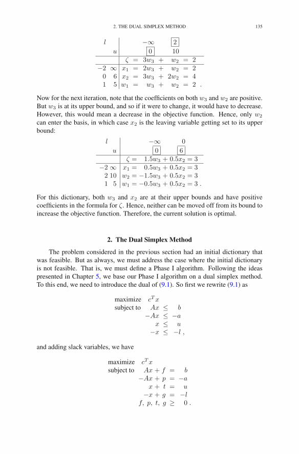
2. THE DUAL SIMPLEX METHOD 135
l −∞ 2
u 0 10ζ = 3w3 + w2 = 2
−2 ∞ x1 = 2w3 + w2 = 20 6 x2 = 3w3 + 2w2 = 41 5 w1 = w3 + w2 = 2 .
Now for the next iteration, note that the coefficients on both w3 and w2 are positive.But w3 is at its upper bound, and so if it were to change, it would have to decrease.However, this would mean a decrease in the objective function. Hence, only w2
can enter the basis, in which case x2 is the leaving variable getting set to its upperbound:
l −∞ 0
u 0 6ζ = 1.5w3 + 0.5x2 = 3
−2 ∞ x1 = 0.5w3 + 0.5x2 = 32 10 w2 = −1.5w3 + 0.5x2 = 31 5 w1 = −0.5w3 + 0.5x2 = 3 .
For this dictionary, both w3 and x2 are at their upper bounds and have positivecoefficients in the formula for ζ. Hence, neither can be moved off from its bound toincrease the objective function. Therefore, the current solution is optimal.
2. The Dual Simplex Method
The problem considered in the previous section had an initial dictionary thatwas feasible. But as always, we must address the case where the initial dictionaryis not feasible. That is, we must define a Phase I algorithm. Following the ideaspresented in Chapter 5, we base our Phase I algorithm on a dual simplex method.To this end, we need to introduce the dual of (9.1). So first we rewrite (9.1) as
maximize cTxsubject to Ax ≤ b
−Ax ≤ −ax ≤ u
−x ≤ −l ,
and adding slack variables, we have
maximize cTxsubject to Ax + f = b
−Ax + p = −ax + t = u
−x + g = −lf, p, t, g ≥ 0 .
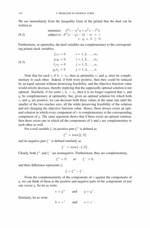
136 9. PROBLEMS IN GENERAL FORM
We see immediately from the inequality form of the primal that the dual can bewritten as
(9.2)minimize bT v − aT q + uT s− lThsubject to AT (v − q)− (h− s) = c
v, q, s, h ≥ 0 .
Furthermore, at optimality, the dual variables are complementary to the correspond-ing primal slack variables:
(9.3)
fivi = 0 i = 1, 2, . . . ,m,
piqi = 0 i = 1, 2, . . . ,m,
tjsj = 0 j = 1, 2, . . . , n,
gjhj = 0 j = 1, 2, . . . , n.
Note that for each i, if bi > ai, then at optimality vi and qi must be comple-mentary to each other. Indeed, if both were positive, then they could be reducedby an equal amount without destroying feasibility, and the objective function valuewould strictly decrease, thereby implying that the supposedly optimal solution is notoptimal. Similarly, if for some i, bi = ai, then it is no longer required that vi andqi be complementary at optimality; but, given an optimal solution for which bothvi and qi are positive, we can decrease both these values at the same rate until thesmaller of the two reaches zero, all the while preserving feasibility of the solutionand not changing the objective function value. Hence, there always exists an opti-mal solution in which every component of v is complementary to the correspondingcomponent of q. The same argument shows that if there exists an optimal solution,then there exists one in which all the components of h and s are complementary toeach other as well.
For a real variable ξ, its positive part ξ+ is defined as
ξ+ = max{ξ, 0}and its negative part ξ− is defined similarly as
ξ− = max{−ξ, 0}.Clearly, both ξ+ and ξ− are nonnegative. Furthermore, they are complementary,
ξ+ = 0 or ξ− = 0,
and their difference represents ξ:
ξ = ξ+ − ξ−.
From the complementarity of the components of v against the components ofq, we can think of them as the positive and negative parts of the components of justone vector y. So let us write:
v = y+ and q = y−.
Similarly, let us writeh = z+ and s = z−.

2. THE DUAL SIMPLEX METHOD 137
If we impose these complementarity conditions not just at optimality but also fromthe start, then we can eliminate v, q, s, and h from the dual and write it simply as
(9.4)minimize bT y+ − aT y− + uT z+ − lT z−
subject to AT y − z = c ,
where the notation y+ denotes the componentwise positive part of y, etc. This prob-lem is an example from the class of problems called piecewise linear programs.Usually, piecewise linear programs are solved by converting them into linear pro-grams. Here, however, we wish to go in the other direction. We shall present analgorithm for (9.4) that will serve as an algorithm for (9.2). We will call this algo-rithm the dual simplex method for problems in general form.
To economize on the presentation, we shall present the dual simplex methodin the context of a Phase I algorithm for linear programs in general form. Also,to avoid cumbersome notations, we shall present the algorithm with the followingexample:
(9.5)
maximize 2x1 − x2
subject to 0 ≤ x1 + x2 ≤ 62 ≤ −x1 + 2x2 ≤ 10
x1 − x2 ≤ 0−2 ≤ x1
1 ≤ x2 ≤ 5 .
The piecewise linear formulation of the dual is
minimize 6y+1 + 10y+2 + 2z+1 − z+2− 2y−2 + ∞y−3 + ∞z−1 + 5z−2
subject to y1 − y2 + y3 − z1 = 2y1 + 2y2 − y3 − − z2 = −1 .
Note that the objective function has coefficients that are infinite. The correctconvention is that infinity times a variable is plus infinity if the variable is positive,zero if the variable is zero, and minus infinity if the variable is negative.
Since the objective function is nonlinear (taking positive and negative parts ofvariables is certainly a nonlinear operation), we will not be able to do the usual rowoperations on the objective function. Therefore, in each iteration, we simply studyit as is. But as usual, we prefer to think in terms of maximization, and so we recordthe negative of the objective function:
(9.6)−ξ = −6y+1 − 10y+2 − 2z+1 + z+2
+ 2y−2 − ∞y−3 − ∞z−1 − 5z−2 .
We can of course perform row operations on the two constraints, so we set upthe usual sort of dictionary for them:
(9.7)z1 = −2 + y1 − y2 + y3z2 = 1 + y1 + 2y2 − y3 .
For the dual problem, all the action takes place at zero. That is, slopes in the objec-tive function change when a variable goes from negative to positive. Since nonbasic

138 9. PROBLEMS IN GENERAL FORM
variable are supposed to be set where the action is, we associate a current solutionwith each dictionary by setting the nonbasic variables to zero. Hence, the solutionassociated with the initial dictionary is
(y1, y2, y3, z1, z2) = (0, 0, 0,−2, 1).
The fact that z1 is negative implies that z−1 is a positive number and hence that theobjective function value associated with this solution is minus infinity. Wheneverthe objective function value is minus infinity, we say that the solution is infeasible.We also refer to the associated dictionary as infeasible. Hence, the initial dictionarygiven in (9.7) is infeasible.
The dual simplex method must start with a dual feasible solution. But since weintend to use the dual simplex method simply to find a feasible solution for (9.5), weare free to change the objective function in (9.5) any way we please. In particular,we can change it from
ζ = 2x1 − x2
toη = −2x1 − x2.
Making that change to the primal leaves the dual objective function unchanged, butproduces a feasible dual dictionary:
(9.8)z1 = 2 + y1 − y2 + y3z2 = 1 + y1 + 2y2 − y3 .
For comparison purposes, let us also record the corresponding primal dictio-nary. It is easy to write down the equations defining the wi’s, but how do we knowwhether the xj’s are supposed to be at their upper or their lower bounds? The an-swer comes from the requirement that the primal and dual satisfy the complemen-tarity conditions given in (9.3). Indeed, from the dual dictionary we see that z1 = 1.Hence, z+1 = 1. But since z+1 is just a surrogate for h1, we see that h1 is positiveand hence that g1 must be zero. This means that x1 must be at its lower bound. Sim-ilarly, for the sake of complementarity, x2 must also be at its lower bound. Hence,the primal dictionary is
l −2 1
u ∞ 5η = −x1 − x2 = 1
0 6 w1 = x1 + x2 = −12 10 w2 = −x1 + 2x2 = 4
−∞ 0 w3 = x1 − x2 = −3 .
Note that it is infeasible, since w1 is not between its upper and lower bounds.We are now ready to describe the first iteration of the dual simplex method.
To this end, we ask whether we can improve the dual objective function value bymoving one of the nonbasic variables (y1, y2, or y3) away from zero. Of course,each of these three variables can be moved either to the positive or the negative sideof zero; we must analyze these six cases individually. First of all, note that sincez1 is positive at the current solution, it follows that z+1 = z1 and z−1 = 0 in a

2. THE DUAL SIMPLEX METHOD 139
neighborhood of the current solution. A similar statement can be made for z2, andso we can rewrite (9.6) locally around the current solution as
−ξ = −6y+1 − 10y+2 − 2z1 + z2+ 2y−2 − ∞y−3 .
Now, as y1 is increased from zero, the rate of increase of −ξ is simply the derivativeof the right-hand side with respect to y1, where we must keep in mind that z1 and z2are functions of y1 via the dictionary (9.8). Hence, the rate of increase is −6− 2 +1 = −7; i.e., the objective function decreases at a rate of 7 units per unit increaseof y1. If, on the other hand, y2 is decreased from zero into negative territory, thenthe rate of increase of −ξ is the negative of the derivative of the right-hand side. Inthis case we get no contribution from y−1 but we do get something from z1 and z2for a total of 2 − 1 = 1. Hence, the rate of increase as we move in this direction isone unit increase per unit move. We can analyze changes to y2 and y3. The entiresituation can be summarized as follows:
y1 ↗ −6 − 2 + 1 = −7y1 ↘ 0 + 2 − 1 = 1y2 ↗ −10 + 2 + 2 = −6y2 ↘ 2 − 2 − 2 = −2y3 ↗ 0 − 2 − 1 = −3y3 ↘ −∞ + 2 + 1 = −∞ .
Of these six cases, the only one that brings about an increase in −ξ is the one inwhich y1 is sent negative. Hence, y1 shall be our entering variable, and it will gonegative. To find the leaving variable, we must ask: as y1 goes negative, which ofz1 and z2 will hit zero first? For the current dictionary, z2 gets to zero first andso becomes the leaving variable. Performing the usual row operations, the newdictionary for the dual problem is
z1 = 1 + z2 − 3y2 + 2y3y1 = −1 + z2 − 2y2 − y3 .
Let us have a look at the new primal dictionary. The fact that y1 was the enteringvariable in the dual dictionary implies that w1 is the leaving variable in the primal.Furthermore, the fact that y1 has gone negative implies that y−1 is now positive, andso complementarity then demands that q1 be zero; i.e., w1 should go to its lowerbound. The fact that z2 was the leaving variable in the dual dictionary implies thatx2 is the entering variable in the primal. Hence, the new primal dictionary is
l −2 0
u ∞ 6η = −x1 − w1 = 2
1 5 x2 = −x1 + w1 = 22 10 w2 = −3x1 + 2w1 = 6
−∞ 0 w3 = 2x1 − w1 = −4 .
We are now ready to begin the second iteration. Therefore, we ask which non-basic variable should be moved away from zero (and in which direction). As before,we first note that z1 positive implies that z+1 = z1 and z−1 = 0 and that y1 negative

140 9. PROBLEMS IN GENERAL FORM
implies that y+1 = 0 and y−1 = −y1. Hence, the objective function can be writtenlocally around the current solution as
−ξ = − 10y+2 − 2z1 + z+2+ 2y−2 − ∞y−3 − 5z−2 .
We now summarize the possibilities in a small table:z2 ↗ 1 − 2 = −1z2 ↘ −5 + 2 = −3y2 ↗ −10 + 6 = −4y2 ↘ 2 − 6 = −4y3 ↗ 0 − 4 = −4y3 ↘ −∞ + 4 = −∞ .
Note that all the changes are negative, meaning that there are no possibilities toincrease the objective function any further. That is, the current dual solution isoptimal. Of course, this also could have been deduced by observing that the primaldictionary is feasible (which is what we are looking for, after all).
Even though this example of the dual simplex method has terminated after onlyone iteration, it should be clear how to proceed had it not terminated.
Now that we have a feasible solution for the primal, we could solve the problemto optimality by simply reinstating the original objective function and proceedingby applying the primal simplex method in a Phase II procedure to find the optimalsolution. Since the primal simplex method has already been discussed, we stop hereon this problem.
Exercises
Solve the following linear programming problems:
9.1 maximize −x1 + x2
subject to −x1 + x2 ≤ 5x1 − 2x2 ≤ 90 ≤ x1 ≤ 60 ≤ x2 ≤ 8 .
9.2 maximize −3x1 − x2 + x3 + 2x4 − x5 + x6 − x7 − 4x8
subject to x1 + 4x3 + x4 − 5x5 − 2x6 + 3x7 − 6x8 = 7x2 − 3x3 − x4 + 4x5 + x6 − 2x7 + 5x8 = −3
0 ≤ x1 ≤ 80 ≤ x2 ≤ 60 ≤ x3 ≤ 100 ≤ x4 ≤ 150 ≤ x5 ≤ 20 ≤ x6 ≤ 100 ≤ x7 ≤ 40 ≤ x8 ≤ 3.
Notes
Dantzig (1955) was the first to consider variants of the simplex method thathandle bounds and ranges implicitly.
CHAPTER 10
Convex Analysis
This book is mostly about linear programming. However, this subject, impor-tant as it is, is just a subset of a larger subject called convex analysis. In this chapter,we shall give a brief introduction to this broader subject. In particular, we shall provea few of the fundamental results of convex analysis and see that their proofs dependon some of the theory of linear programming that we have already developed.
1. Convex Sets
Given a finite set of points, z1, z2, . . . , zn, in Rm, a point z in R
m is called aconvex combination of these points if1
z =
n∑
j=1
tjzj ,
where tj ≥ 0 for each j and∑n
j=1 tj = 1. It is called a strict convex combination ifnone of the tj’s vanish. For n = 2, the set of all convex combinations of two pointsis simply the line segment connecting them.
A subset S of Rm is called convex if, for every x and y in S, S also contains allpoints on the line segment connecting x and y. That is, tx+(1− t)y ∈ S, for every0 < t < 1. See Figure 10.1.
Certain elementary properties of convex sets are trivial to prove. For example,the intersection of an arbitrary collection of convex sets is convex. Indeed, let Sα,α ∈ I , denote a collection of convex sets indexed by some set I . Then the claim isthat ∩α∈ISα is convex. To see this, consider an arbitrary pair of points x and y inthe intersection. It follows that x and y are in each Sα. By the convexity of Sα itfollows that Sα contains the line segment connecting x and y. Since each of thesesets contains the line segment, so does their intersection. Hence, the intersection isconvex.
Here is another easy one:
THEOREM 10.1. A set C is convex if and only if it contains all convex combina-tions of points in C.
1Until now we’ve used subscripts for the components of a vector. In this chapter, subscripts will beused to list sequences of vectors. Hopefully, this will cause no confusion.
R.J. Vanderbei, Linear Programming, International Series in Operations Research& Management Science 196, DOI 10.1007/978-1-4614-7630-6 10,© Springer Science+Business Media New York 2014
141

142 10. CONVEX ANALYSIS
x
FIGURE 10.1. The set on the left is convex—for any pair of pointsin the set, the line segment connecting the two points is also con-tained in the set. The set on the right is not convex—there existspairs of points, such as the x and y shown, for which the connect-ing line segment is not entirely in the set.
PROOF. Let C be a convex set. By definition, C contains all convex combina-tions of pairs of points in C. The first nontrivial step is to show that C contains allconvex combinations of triples of points in C. To see this, fix z1, z2, and z3 in Cand consider
z = t1z1 + t2z2 + t3z3,
where tj ≥ 0 for each j and∑3
j=1 tj = 1. If any of the tj’s vanish, then z is reallyjust a convex combination of two points and so belongs to C. Hence, suppose thateach of the tj’s is strictly positive. Rewrite z as follows:
z = (1− t3)
(t1
1− t3z1 +
t21− t3
z2
)
+ t3z3
= (1− t3)
(t1
t1 + t2z1 +
t2t1 + t2
z2
)
+ t3z3.
Since C contains all convex combinations of pairs of points, it follows thatt1
t1 + t2z1 +
t2t1 + t2
z2 ∈ C.
Now, since z is a convex combination of the two points t1t1+t2
z1 +t2
t1+t2z2 and z3,
both of which belong to C, it follows that z is in C. It is easy to see (pun intended)that this argument can be extended to an inductive proof that C contains all convexcombinations of finite collections of points in C. Indeed, one must simply show thatthe fact that C contains all convex combinations of n points from C implies that itcontains all convex combinations of n + 1 points from C. We leave the details tothe reader.
Of course, proving that a set is convex if it contains every convex combinationof its points is trivial: simply take convex combinations of pairs to get that it isconvex. �
For each set S in Rm (not necessarily convex), there exists a smallest convex
set, which we shall denote by conv(S), containing S. It is defined, quite simply,as the intersection of all convex sets containing S. From our discussion about in-tersections, it follows that this set is convex. The set conv(S) is called the convexhull of S. This definition can be thought of as a definition from the “outside,” since
2. CARATHEODORY’S THEOREM 143
it involves forming the intersection of a collection of sets that contain S. Our nexttheorem gives a characterization of convex sets from the “inside”:
THEOREM 10.2. The convex hull conv(S) of a set S in Rm consists precisely of
the set of all convex combinations of finite collections of points from S.
PROOF. Let H denote the set of all convex combinations of finite sets of pointsin S:
H =
⎧⎨
⎩z =
n∑
j=1
tjzj : n ≥ 1, zj ∈ S and tj > 0 for all j, andn∑
j=1
tj = 1
⎫⎬
⎭.
It suffices to show that (1) H contains S, (2) H is convex, and (3) every convex setcontaining S also contains H .
To see that H contains S, just take n = 1 in the definition of H .To see that H is convex, fix two points x and y in H and a real number 0 < t <
1. We must show that z = tx + (1 − t)y ∈ H . The fact that x ∈ H implies thatx =
∑rj=1 pjxj , for some r ≥ 1, where pj > 0 for j = 1, 2, . . . , r,
∑rj=1 pj = 1,
and xj ∈ S for j = 1, 2, . . . , r. Similarly, the fact that y is in H implies thaty =
∑sj=1 qjyj , for some s ≥ 1, where qj > 0 for j = 1, 2, . . . , s,
∑sj=1 qj = 1,
and yj ∈ S for j = 1, 2, . . . , s. Hence,
z = tx+ (1− t)y =r∑
j=1
tpjxj +s∑
j=1
(1− t)qjyj .
Since the coefficients (tp1, . . . , tpr, (1 − t)q1, . . . , (1 − t)qs) are all positive andsum to one, it follows that this last expression for z is a convex combination of r+spoints from S. Hence, z is in H . Since x and y were arbitrary points in H and twas an arbitrary real number between zero and one, the fact that z ∈ H implies thatH is convex.
It remains simply to show that H is contained in every convex set containingS. Let C be such a set (i.e., convex and containing S). From Theorem 10.1 and thefact that C contains S, it follows that C contains all convex combinations of pointsin S. Hence, C contains H . �
2. Caratheodory’s Theorem
In the previous section, we showed that the convex hull of a set S can be con-structed by forming all convex combinations of finite sets of points from S. In 1907,Caratheodory showed that it is not necessary to use all finite sets. Instead, m + 1points suffice:
THEOREM 10.3. The convex hull conv(S) of a set S in Rm consists of all convex
combinations of m+ 1 points from S:
conv(S) =
⎧⎨
⎩z =
m+1∑
j=1
tjzj : zj ∈ S and tj ≥ 0 for all j, and∑
j
tj = 1
⎫⎬
⎭.

144 10. CONVEX ANALYSIS
PROOF. Let H denote the set on the right. From Theorem 10.2, we see that His contained in conv(S). Therefore, it suffices to show that every point in conv(S)belongs to H . To this end, fix a point z in conv(S). By Theorem 10.2, there ex-ists a collection of, say, n points z1, z2, . . . , zn in S and associated nonnegativemultipliers t1, t2, . . . , tn summing to one such that
(10.1) z =
n∑
j=1
tjzj .
Let A denote the matrix consisting of the points z1, z2, . . . , zn as the columns of A:
A =[z1 z2 · · · zn
].
Also, let x∗ denote the vector consisting of the multipliers t1, t2, . . . , tn:
x∗ =
⎡
⎢⎢⎢⎣
t1t2...tn
⎤
⎥⎥⎥⎦.
Finally, let b = z. Then from (10.1), we see that x∗ is feasible for the followinglinear programming problem:
(10.2)
maximize cTxsubject to Ax = b
eTx = 1x ≥ 0 .
The fundamental theorem of linear programming (Theorem 3.4) tells us that ev-ery feasible linear program has a basic feasible solution. For such a solution, onlythe basic variables can be nonzero. The number of basic variables in (10.2) co-incides with the number of equality constraints; that is, there are at most m + 1variables that are nonzero. Hence, this basic feasible solution corresponds to a con-vex combination of just m+ 1 of the original n points. (See Exercise 10.5.) �
It is easy to see that the number m + 1 is the best possible. For example, thepoint (1/(m+ 1), 1/(m+ 1), . . . , 1/(m+ 1)) in R
m belongs to the convex hull ofthe m+ 1 points e1, e2, . . . , em, 0 but is not a convex combination of any subset ofthem.
3. The Separation Theorem
We shall define a halfspace of Rn to be any set given by a single (nontrivial)linear inequality:
(10.3) {x ∈ Rn :
n∑
j=1
ajxj ≤ b}, (a1, a2, . . . , an) �= 0.
Every halfspace is convex. To see this, suppose that x = (x1, x2, . . . , xn) andy = (y1, y2, . . . , yn) both satisfy the linear inequality in (10.3). Fix t betweenzero and one. Then both t and 1 − t are nonnegative, and so multiplying by them
3. THE SEPARATION THEOREM 145
preserves the direction of inequality. Therefore, multiplying∑
j ajxj ≤ b by t and∑
j ajyj ≤ b by 1− t and then adding, we get
∑
j
aj (txj + (1− t)yj) ≤ b.
That is, tx+ (1− t)y also satisfies the inequality defining the halfspace.If we allow the vector of coefficients (a1, a2, . . . , an) in the definition of a
halfspace to vanish, then we call the set so defined a generalized halfspace. It iseasy to see that every generalized halfspace is simply a halfspace, all of Rn, or theempty set. Also, every generalized halfspace is clearly convex.
A polyhedron is defined as the intersection of a finite collection of generalizedhalfspaces. That is, a polyhedron is any set of the form
⎧⎨
⎩x ∈ R
n :n∑
j=1
aijxj ≤ bi, i = 1, 2, . . . ,m
⎫⎬
⎭.
Every polyhedron, being the intersection of a collection of convex sets, is convex.The following theorem is called the Separation Theorem for polyhedra.
THEOREM 10.4. Let P and P be two disjoint nonempty polyhedra in Rn. Then
there exist disjoint halfspaces H and H such that P ⊂ H and P ⊂ H .
PROOF. Suppose that P and P are given by the following systems ofinequalities:
P = {x : Ax ≤ b},P = {x : Ax ≤ b}.
The disjointness of P and P implies that there is no solution to the system
(10.4)
[A
A
]
x ≤[b
b
]
.
To continue the proof, we need a result known as Farkas’ Lemma, which says thatAx ≤ b has no solutions if and only if there is an m-vector y such that
AT y = 0
y ≥ 0
bT y < 0.
We shall prove this result in the next section. For now, let us apply Farkas’ Lemmato the situation at hand. Indeed, the fact that there are no solutions to (10.4) impliesthat there exists a vector, which we shall write in block form as
[yy
]
,

146 10. CONVEX ANALYSIS
such that
[AT AT
][yy
]
= AT y + AT y = 0(10.5)[yy
]
≥ 0(10.6)
[bT bT
][yy
]
= bT y + bT y < 0.(10.7)
From the last condition, we see that either bT y < 0 or bT y < 0 (or both). Withoutloss of generality, we may assume that
bT y < 0.
Farkas’ Lemma (this time applied in the other direction) together with the nonempti-ness of P now implies that
AT y �= 0.
Put
H ={x : (AT y)Tx ≤ bT y
}and H =
{x : (AT y)Tx ≥ −bT y
}.
These sets are clearly halfspaces. To finish the proof, we must show that they aredisjoint and contain their corresponding polyhedra.
First of all, it follows from (10.7) that H and H are disjoint. Indeed, supposethat x ∈ H . Then (AT y)Tx ≤ bT y < −bT y, which implies that x is not in H .
To show that P ⊂ H , fix x in P . Then Ax ≤ b. Since y ≥ 0 (as we know from(10.6)), it follows then that yTAx ≤ yT b. But this is exactly the condition that saysthat x belongs to H . Since x was an arbitrary point in P , it follows that P ⊂ H .
Showing that P is a subset of H is similar. Indeed, suppose that x ∈ P . ThenAx ≤ b. Multiplying on the left by −yT and noting that y ≥ 0, we see that−yT Ax ≥ −yT b. But from (10.5) we see that −yT Ax = yTAx, and so this lastinequality is exactly the condition that x ∈ H . Again, the arbitrariness of x ∈ Pimplies that P ⊂ H , and the proof is complete. �
4. Farkas’ Lemma
The following result, known as Farkas’ Lemma, played a fundamental role inthe proof of the separation theorem of the preceding section (Theorem 10.4). In thissection, we state it formally as a lemma and give its proof.
LEMMA 10.5. The system Ax ≤ b has no solutions if and only if there is a ysuch that
AT y = 0
y ≥ 0(10.8)
bT y < 0.

5. STRICT COMPLEMENTARITY 147
PROOF. Consider the linear program
maximize 0subject to Ax ≤ b
and its dualminimize bT ysubject to AT y = 0
y ≥ 0 .
Clearly, the dual is feasible (just take y = 0). So if the primal is feasible, then thedual is bounded. Also, if the primal is infeasible, the dual must be unbounded. Thatis, the primal is infeasible if and only if the dual is unbounded. To finish the proof,we claim that the dual is unbounded if and only if there exists a solution to (10.8).Indeed, suppose that the dual is unbounded. The dual simplex method is guaranteedto prove that it is unbounded, and it does so as follows. At the last iteration, a stepdirection Δy is computed that preserves feasibility, i.e.,
ATΔy = 0,
is a descent direction for the objective function, i.e.,
bTΔy < 0,
and is a direction for which the step length is unbounded, i.e.,
Δy ≥ 0.
But these three properties show that Δy is the solution to (10.8) that we were lookingfor. Conversely, suppose that there is a solution to (10.8). Call it Δy. It is easy tosee that starting from y = 0, this step direction provides an unbounded decrease inthe objective function. This completes the proof. �
5. Strict Complementarity
In this section, we consider the usual inequality-form linear programming prob-lem, which we write with its slack variables shown explicitly:
(10.9)maximize cTxsubject to Ax+ w= b
x, w≥ 0.
As we know, the dual can be written as follows:
(10.10)minimize bT y
subject to AT y − z = cy, z ≥ 0.
In our study of duality theory in Chapter 5, we saw that every pair of optimal solu-tions to these two problems possesses a property called complementary slackness. If(x∗, w∗) denotes an optimal solution to the primal and (y∗, z∗) denotes an optimalsolution to the dual, then the complementary slackness theorem says that, for eachj = 1, 2, . . . , n, either x∗
j = 0 or z∗j = 0 (or both) and, for each i = 1, 2, . . . ,m,either y∗i = 0 or w∗
i = 0 (or both). In this section, we shall prove that there areoptimal pairs of solutions for which the parenthetical “or both” statements don’t

148 10. CONVEX ANALYSIS
happen. That is, there are optimal solutions for which exactly one member of eachpair (x∗
j , z∗j ) vanishes and exactly one member from each pair (y∗i , w
∗i ) vanishes.
In such cases, we say that the optimal solutions are strictly complementary to eachother. The strictness of the complementary slackness is often expressed by sayingthat x∗ + z∗ > 0 and y∗ + w∗ > 0.2
As a warm-up, we prove the following theorem.
THEOREM 10.6. If both the primal and the dual have feasible solutions, thenthere exists a primal feasible solution (x, w) and a dual feasible solution (y, z) suchthat x+ z > 0 and y + w > 0.
PROOF. If there is a feasible primal solution x for which xj > 0, then it doesn’tmatter whether there is a feasible dual solution whose jth slack variable is strictlypositive. But what about indices j for which xj = 0 for every feasible solution? Letj be such an index. Consider the following linear programming problem:
(10.11)maximize xj
subject to Ax≤ bx≥ 0.
This problem is feasible, since its constraints are the same as for the original primalproblem (10.9). Furthermore, it has an optimal solution (the corresponding objectivefunction value is zero). The dual of (10.11) is:
minimize bT y
subject to AT y ≥ ejy ≥ 0.
By the strong duality theorem, the dual has an optimal solution, say y′. Letting z′
denote the corresponding slack variable, we have that
AT y′ − z′ = ej
y′, z′ ≥ 0.
Now, let y be any feasible solution to (10.10) and let z be the corresponding slackvariable. Then the above properties of y′ and z′ imply that y + y′ is feasible for(10.10) and its slack is z + z′ + ej . Clearly, for this dual feasible solution we havethat the jth component of its vector of slack variables is at least 1. To summa-rize, we have shown that, for each j, there exists a primal feasible solution, call it(x(j), w(j)), and a dual feasible solution, call it (y(j), z(j)), such that x(j)
j +z(j)j > 0.
In the same way, one can exhibit primal and dual feasible solutions for which eachindividual dual variable and its corresponding primal slack add to a positive number.To complete the proof, we now form a strict convex combination of these n + mfeasible solutions. Since the feasible region for a linear programming problem isconvex, these convex combinations preserve primal and dual feasibility. Since theconvex combination is strict, it follows that every primal variable and its dual slackadd to a strictly positive number as does every dual variable and its primal slack. �
2Given any vector ξ, we use the notation ξ > 0 to indicate that every component of ξ is strictlypositive: ξj > 0 for all j.

EXERCISES 149
A variable xj that must vanish in order for a linear programming problem tobe feasible is called a null variable. The previous theorem says that if a variable isnull, then its dual slack is not null.
The following theorem is called the Strict Complementary Slackness Theorem
THEOREM 10.7. If a linear programming problem has an optimal solution, thenthere is an optimal solution (x∗, w∗) and an optimal dual solution (y∗, z∗) such thatx∗ + z∗ > 0 and y∗ + w∗ > 0.
We already know from the complementary slackness theorem (Theorem 5.1)that x∗ and z∗ are complementary to each other as are y∗ and w∗. This theoremthen asserts that the complementary slackness is strict.
PROOF. The proof is much the same as the proof of Theorem 10.6 except thistime we look at an index j for which xj vanishes in every optimal solution. We thenconsider the following problem:
(10.12)
maximize xj
subject to Ax≤ bcTx≥ ζ∗
x≥ 0,
where ζ∗ denotes the objective value of the optimal solution to the original problem.In addition to the dual variables y corresponding to the Ax ≤ b constraints, thereis one more dual variable, call it t, associated with the constraint cTx ≥ ζ∗. Theanalysis of problem (10.12) is similar to the analysis given in Theorem 10.6 exceptthat one must now consider two cases: (a) the optimal value of t is strictly positiveand (b) the optimal value of t vanishes. The details are left as an exercise (seeExercise 10.6). �
Exercises
10.1 Is Rn a polyhedron?
10.2 For each b ∈ Rm, let ξ∗(b) denote the optimal objective function value
for the following linear program:
maximize cTxsubject to Ax≤ b
x≥ 0.
Suppose that ξ∗(b) < ∞ for all b. Show that the function ξ∗(b) is concave(a function f on R
m is called concave if f(tx+(1− t)y) ≥ tf(x)+ (1−t)f(y) for all x and y in R
m and all 0 < t < 1). Hint: Consider the dualproblem.
10.3 Describe how one needs to modify the proof of Theorem 10.4 to get aproof of the following result:

150 10. CONVEX ANALYSIS
Let P and P be two disjoint polyhedra in Rn. Then there exist
disjoint generalized halfspaces H and H such that P ⊂ H andP ⊂ H .
10.4 Find a strictly complementary solution to the following linear program-ming problem and its dual:
maximize 2x1 + x2
subject to 4x1 + 2x2 ≤ 6x2 ≤ 1
2x1 + x2 ≤ 3x1, x2 ≥ 0 .
10.5 There is a slight oversimplification in the proof of Theorem 10.3. Can youspot it? Can you fix it?
10.6 Complete the proof of Theorem 10.7.
10.7 Interior solutions. Prove the following statement: If a linear programmingproblem has feasible solutions and the set of feasible solutions is bounded,then there is a strictly positive dual feasible solution: y > 0 and z > 0.Hint. It is easier to prove the equivalent statement: if a linear program-ming problem has feasible solutions and the dual has null variables, thenthe set of primal feasible solutions is an unbounded set.
Notes
Caratheodory (1907) proved Theorem 10.3. Farkas (1902) proved Lemma 10.5.Several similar results were discovered by many others, including Gordan (1873),Stiemke (1915), Ville (1938), and Tucker (1956). The standard reference on convexanalysis is Rockafellar (1970).

CHAPTER 11
Game Theory
In this chapter, we shall study if not the most practical then certainly an elegantapplication of linear programming. The subject is called game theory, and we shallfocus on the simplest type of game, called the finite two-person zero-sum game, orjust matrix game for short. Our primary goal shall be to prove the famous MinimaxTheorem, which was first discovered and proved by John von Neumann in 1928.His original proof of this theorem was rather involved and depended on anotherbeautiful theorem from mathematics, the Brouwer Fixed-Point Theorem. However,it eventually became clear that the solution of matrix games could be found bysolving a certain linear programming problem and that the Minimax Theorem isjust a fairly straightforward consequence of the Duality Theorem.
1. Matrix Games
A matrix game is a two-person game defined as follows. Each person firstselects, independently of the other, an action from a finite set of choices (the twoplayers in general will be confronted with different sets of actions from which tochoose). Then both reveal to each other their choice. If we let i denote the firstplayer’s choice and j denote the second player’s choice, then the rules of the gamestipulate that the first player will pay the second player aij dollars. The array ofpossible payments
A = [aij ]
is presumed known to both players before the game begins. Of course, if aij isnegative for some pair (i, j), then the payment goes in the reverse direction—fromthe second player to the first. For obvious reasons, we shall refer to the first player asthe row player and the second player as the column player. Since we have assumedthat the row player has only a finite number of actions from which to choose, wecan enumerate these actions and assume without loss of generality that i is simplyan integer selected from 1 to m. Similarly, we can assume that j is simply an indexranging from 1 to n (in its real-world interpretation, row action 3 will generallyhave nothing to do with column action 3—the number 3 simply indicates that it isthe third action in the enumerated list of choices).
Let us look at a specific familiar example. Namely, consider the game everychild knows, called Paper–Scissors–Rock. To refresh the memory of older readers,this is a two-person game in which at the count of three each player declares eitherPaper, Scissors, or Rock. If both players declare the same object, then the round is a
R.J. Vanderbei, Linear Programming, International Series in Operations Research& Management Science 196, DOI 10.1007/978-1-4614-7630-6 11,© Springer Science+Business Media New York 2014
151

152 11. GAME THEORY
draw. But Paper loses to Scissors (since scissors can cut a piece of paper), Scissorsloses to Rock (since a rock can dull scissors), and finally Rock loses to Paper (sincea piece of paper can cover up a rock—it’s a weak argument but that’s the way thegame is defined). Clearly, for this game, if we enumerate the actions of declaringPaper, Scissors, or Rock as 1, 2, 3, respectively, then the payoff matrix is
⎡
⎣0 1 −1
−1 0 11 −1 0
⎤
⎦ .
With this matrix, neither player has an obvious (i.e., deterministic) winning strategy.If the column player were always to declare Paper (hoping that the row player willdeclare Rock), then the row player could counter by always declaring Scissors andguaranteeing herself a winning of one dollar in every round. In fact, if the columnplayer were to stick to any specific declaration, then the row player would eventuallyget wise to it and respond appropriately to guarantee that she wins. Of course, thesame logic applies to the row player. Hence, neither player should employ the samedeclaration over and over. Instead, they should randomize their declarations. In fact,due to the symmetry of this particular game, both players should make each of thethree possible declarations with equal likelihood.
But what about less trivial games? For example, suppose that the payoffs in thePaper–Scissors–Rock game are altered so that the payoff matrix becomes
A =
⎡
⎣0 1 −2
−3 0 45 −6 0
⎤
⎦ .
This new game still has the property that every deterministic strategy can be foiledby an intelligent opponent. Hence, randomized behavior remains appropriate. Butthe best probabilities are no longer uniformly 1/3. Also, who has the edge in thisgame? Since the total of the payoffs that go from the row player to the column playeris 10 whereas the total of the payoffs that go to the row player is 11, we suspect thatthe row player might have the edge. But this is just a guess. Is it correct? If it iscorrect, how much can the row player expect to win on average in each round? Ifthe row player knows this number accurately and the column player does not, thenthe row player could offer to pay the column player a small fee for playing eachround. If the fee is smaller than the expected winnings, then the row player can stillbe confident that over time she will make a nice profit. The purpose of this chapteris to answer these questions precisely.
Let us return now to the general setup. Consider the row player. By a random-ized strategy, we mean that, at each play of the game, it appears (from the columnplayer’s viewpoint) that the row player is making her choices at random accordingto some fixed probability distribution. Let yi denote the probability that the rowplayer selects action i. The vector y composed of these probabilities is called a sto-chastic vector. Mathematically, a vector is a stochastic vector if it has nonnegativecomponents that sum up to one:
y ≥ 0 and eT y = 1,

2. OPTIMAL STRATEGIES 153
where e denotes the vector consisting of all ones. Of course, the column player mustalso adopt a randomized strategy. Let xj denote the probability that the columnplayer selects action j, and let x denote the stochastic vector composed of theseprobabilities.
The expected payoff to the column player is computed by summing over allpossible outcomes the payoff associated with that outcome times the probabilityof the outcome. The set of possible outcomes is simply the set of pairs (i, j) asi ranges over the row indices (1, 2, . . . ,m) and j ranges over the column indices(1, 2, . . . , n). For outcome (i, j) the payoff is aij , and, assuming that the row andcolumn players behave independently, the probability of this outcome is simplyyixj . Hence, the expected payoff to the column player is
∑
i,j
yiaijxj = yTAx.
2. Optimal Strategies
Suppose that the column player adopts strategy x (i.e., decides to play in accor-dance with the stochastic vector x). Then the row player’s best defense is to use thestrategy y∗ that achieves the following minimum:
(11.1)minimize yTAx
subject to eT y = 1y ≥ 0.
From the fundamental theorem of linear programming, we know that this problemhas a basic optimal solution. For this problem, the basic solutions are simply yvectors that are zero in every component except for one, which is one. That is, thebasic optimal solutions correspond to deterministic strategies. This is fairly obviousif we look again at our example. Suppose that
x =
⎡
⎣1/31/31/3
⎤
⎦ .
Then
Ax =
⎡
⎣−1/31/3
−1/3
⎤
⎦ ,
and so the row player’s best choice is to select either i = 1 (Paper) or i = 3 (Rock)or any combination thereof. That is, an optimal solution is y∗ = (1, 0, 0) (it is notunique).
Since for any given x the row player will adopt the strategy that achieves theminimum in (11.1), it follows that the column player should employ a strategy x∗
that attains the following maximum:
(11.2) maxx
miny
yTAx,
where the max and the min are over all stochastic vectors (of the appropriatedimension).

154 11. GAME THEORY
The question then becomes: how do we solve (11.2)? It turns out that thisproblem can be reformulated as a linear programming problem. Indeed, we havealready seen that the inner optimization (the minimization) can be taken over justthe deterministic strategies:
miny
yTAx = mini
eTi Ax,
where we have used ei to denote the vector of all zeros except for a one in positioni. Hence, the max-min problem given in (11.2) can be rewritten as
maximize(mini e
Ti Ax
)
subject ton∑
j=1
xj = 1
xj ≥ 0 j = 1, 2, . . . , n.
Now, if we introduce a new variable, v, representing a lower bound on the eTi Ax’s,then we see that the problem can be recast as a linear program:
maximize vsubject to v ≤ eTi Ax i = 1, 2, . . . ,m
n∑
j=1
xj = 1
xj ≥ 0 j = 1, 2, . . . , n.
Switching back to vector notation, the problem can be written as
maximize vsubject to ve−Ax≤ 0
eTx= 1x≥ 0.
Finally, writing in block-matrix form, we get
(11.3)
maximize[0 1
][xv
]
subject to
[−A eeT 0
] [xv
]≤=
[01
]
x≥ 0v free.
Now let’s turn it around. By symmetry, the row player seeks a strategy y∗ thatattains optimality in the following min-max problem:
miny
maxx
yTAx,
which can be reformulated as the following linear program:
minimize u
subject to ue−AT y ≥ 0eT y = 1
y ≥ 0.
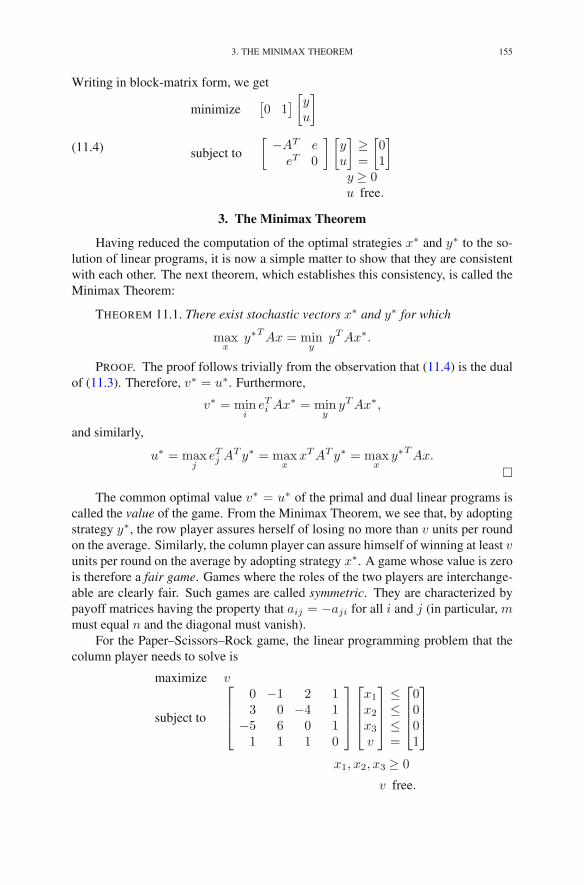
3. THE MINIMAX THEOREM 155
Writing in block-matrix form, we get
(11.4)
minimize[0 1
][yu
]
subject to
[−AT e
eT 0
] [yu
]≥=
[01
]
y ≥ 0u free.
3. The Minimax Theorem
Having reduced the computation of the optimal strategies x∗ and y∗ to the so-lution of linear programs, it is now a simple matter to show that they are consistentwith each other. The next theorem, which establishes this consistency, is called theMinimax Theorem:
THEOREM 11.1. There exist stochastic vectors x∗ and y∗ for which
maxx
y∗TAx = miny
yTAx∗.
PROOF. The proof follows trivially from the observation that (11.4) is the dualof (11.3). Therefore, v∗ = u∗. Furthermore,
v∗ = mini
eTi Ax∗ = min
yyTAx∗,
and similarly,
u∗ = maxj
eTj AT y∗ = max
xxTAT y∗ = max
xy∗TAx.
�
The common optimal value v∗ = u∗ of the primal and dual linear programs iscalled the value of the game. From the Minimax Theorem, we see that, by adoptingstrategy y∗, the row player assures herself of losing no more than v units per roundon the average. Similarly, the column player can assure himself of winning at least vunits per round on the average by adopting strategy x∗. A game whose value is zerois therefore a fair game. Games where the roles of the two players are interchange-able are clearly fair. Such games are called symmetric. They are characterized bypayoff matrices having the property that aij = −aji for all i and j (in particular, mmust equal n and the diagonal must vanish).
For the Paper–Scissors–Rock game, the linear programming problem that thecolumn player needs to solve is
maximize v
subject to
⎡
⎢⎢⎣
0 −1 2 13 0 −4 1
−5 6 0 11 1 1 0
⎤
⎥⎥⎦
⎡
⎢⎢⎣
x1
x2
x3
v
⎤
⎥⎥⎦
≤≤≤=
⎡
⎢⎢⎣
0001
⎤
⎥⎥⎦
x1, x2, x3 ≥ 0
v free.
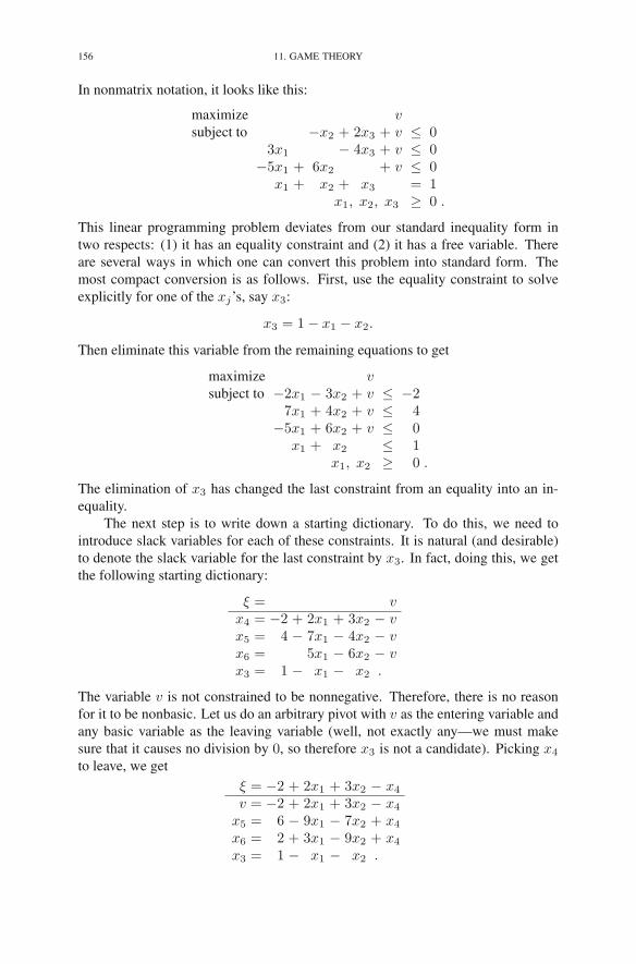
156 11. GAME THEORY
In nonmatrix notation, it looks like this:
maximize vsubject to −x2 + 2x3 + v ≤ 0
3x1 − 4x3 + v ≤ 0−5x1 + 6x2 + v ≤ 0
x1 + x2 + x3 = 1x1, x2, x3 ≥ 0 .
This linear programming problem deviates from our standard inequality form intwo respects: (1) it has an equality constraint and (2) it has a free variable. Thereare several ways in which one can convert this problem into standard form. Themost compact conversion is as follows. First, use the equality constraint to solveexplicitly for one of the xj’s, say x3:
x3 = 1− x1 − x2.
Then eliminate this variable from the remaining equations to get
maximize vsubject to −2x1 − 3x2 + v ≤ −2
7x1 + 4x2 + v ≤ 4−5x1 + 6x2 + v ≤ 0
x1 + x2 ≤ 1x1, x2 ≥ 0 .
The elimination of x3 has changed the last constraint from an equality into an in-equality.
The next step is to write down a starting dictionary. To do this, we need tointroduce slack variables for each of these constraints. It is natural (and desirable)to denote the slack variable for the last constraint by x3. In fact, doing this, we getthe following starting dictionary:
ξ = vx4 = −2 + 2x1 + 3x2 − vx5 = 4 − 7x1 − 4x2 − vx6 = 5x1 − 6x2 − vx3 = 1 − x1 − x2 .
The variable v is not constrained to be nonnegative. Therefore, there is no reasonfor it to be nonbasic. Let us do an arbitrary pivot with v as the entering variable andany basic variable as the leaving variable (well, not exactly any—we must makesure that it causes no division by 0, so therefore x3 is not a candidate). Picking x4
to leave, we getξ = −2 + 2x1 + 3x2 − x4
v = −2 + 2x1 + 3x2 − x4
x5 = 6 − 9x1 − 7x2 + x4
x6 = 2 + 3x1 − 9x2 + x4
x3 = 1 − x1 − x2 .

4. POKER 157
Since v is free of sign constraints, it will never leave the basis (since a leavingvariable is, by definition, a variable that hits its lower bound—v has no such bound).Therefore, we may as well remove it from the dictionary altogether; it can alwaysbe computed at the end. Hence, we note that
v = −2 + 2x1 + 3x2 − x4,
or better yet thatv = ξ,
and the dictionary now becomes
ξ = −2 + 2x1 + 3x2 − x4
x5 = 6 − 9x1 − 7x2 + x4
x6 = 2 + 3x1 − 9x2 + x4
x3 = 1 − x1 − x2 .
At last, we are in a position to apply the simplex method. Two (tedious) iterationsbring us to the optimal dictionary. Since it involves fractions, we multiply eachequation by an integer to make each number in the dictionary an integer. Indeed,after multiplying by 102, the optimal dictionary is given by
102ξ = −16 − 27x5 − 13x6 − 62x4
102x1 = 40 − 9x5 + 7x6 + 2x4
102x2 = 36 − 3x5 − 9x6 + 12x4
102x3 = 26 + 12x5 + 2x6 − 14x4 .
From this dictionary, it is easy to read off the optimal primal solution:
x∗ =
⎡
⎣40/10236/10226/102
⎤
⎦ .
Also, since x4, x5, and x6 are complementary to y1, y2, and y3 in the dual problem,the optimal dual solution is
y∗ =
⎡
⎣62/10227/10213/102
⎤
⎦ .
Finally, the value of the game is
v∗ = ξ∗ = −16/102 = −0.15686275,
which indicates that the row player does indeed have an advantage and can expectto make on the average close to 16 cents per round.
4. Poker
Some card games such as poker involve a round of bidding in which the play-ers at times bluff by increasing their bid in an attempt to coerce their opponentsinto backing down, even though if the challenge is accepted they will surely lose.Similarly, they will sometimes underbid to give their opponents false hope. In this

158 11. GAME THEORY
section, we shall study a simplified version of poker (the real game is too hard toanalyze) to see if bluffing and underbidding are justified bidding strategies.
Simplified poker involves two players, A and B, and a deck having three cards,1, 2, and 3. At the beginning of a round, each player “antes up” $1 and is dealt onecard from the deck. A bidding session follows in which each player in turn, startingwith A, either (a) bets and adds $1 to the “kitty” or (b) passes. Bidding terminateswhen
a bet is followed by a bet,a pass is followed by a pass, ora bet is followed by a pass.
In the first two cases, the winner of the round is decided by comparing cards, andthe kitty goes to the player with the higher card. In the third case, bet followed bypass, the player who bet wins the round independently of who had the higher card(in real poker, the player who passes is said to fold).
With these simplified betting rules, there are only five possible bettingscenarios:
A passes, B passes: $1 to holder of higher cardA passes, B bets, A passes: $1 to BA passes, B bets, A bets: $2 to holder of higher cardA bets, B passes: $1 to AA bets, B bets: $2 to holder of higher card
After being dealt a card, player A will decide to bet along one of three lines:
1. Pass. If B bets, pass again.2. Pass. If B bets, bet.3. Bet.
Similarly, after being dealt a card, player B can bet along one of four lines:
1. Pass no matter what.2. If A passes, pass, but if A bets, bet.3. If A passes, bet, but if A bets, pass.4. Bet no matter what.
To model the situation as a matrix game, we must identify each player’s pure strate-gies. A pure strategy is a statement of what line of betting a player intends to followfor each possible card that the player is dealt. Hence, the players’ pure strategiescan be denoted by triples (y1, y2, y3), where yi is the line of betting that the playerwill use when holding card i. (For player A, the yi’s can take values 1, 2, and 3,whereas for player B, they can take values 1, 2, 3, and 4.)
Given a pure strategy for both players, one can compute the average paymentfrom, say, A to B. For example, suppose that player A adopts strategy (3, 1, 2) and

4. POKER 159
player B adopts strategy (3, 2, 4). There are six ways in which the cards can bedealt, and we can analyze each of them as follows:
card dealt betting session paymentA B A to B1 2 A bets, B bets 21 3 A bets, B bets 22 1 A passes, B bets, A passes 12 3 A passes, B bets, A passes 13 1 A passes, B bets, A bets −23 2 A passes, B passes −1
Since each of the six deals are equally likely, the average payment from A to B is(2 + 2 + 1 + 1− 2− 1)/6 = 0.5.
The calculation of the average payment must be carried out for every combi-nation of pairs of strategies. How many are there? Player A has 3 × 3 × 3 = 27pure strategies and player B has 4 × 4 × 4 = 64 pure strategies. Hence, there are27×64 = 1,728 pairs. Calculating the average payment for all these pairs is a daunt-ing task. Fortunately, we can reduce the number of pure strategies (and hence thenumber of pairs) that need to be considered by making a few simple observations.
The first observation is that a player holding a 1 should never answer a bet witha bet, since the player will lose regardless of the answering bet and will lose less bypassing. This logic implies that, when holding a 1,
player A should refrain from betting along line 2;player B should refrain from betting along lines 2 and 4.
More clearly improvable strategies can be ruled out when holding the highestcard. For example, a player holding a 3 should never answer a bet with a pass, sinceby passing the player will lose, but by betting the player will win. Furthermore,when holding a 3, a player should always answer a pass with a bet, since in eithercase the player is going to win, but answering with a bet opens the possibility ofthe opponent betting again and thereby increasing the size of the win for the playerholding the 3. Hence, when holding a 3,
player A should refrain from betting along line 1;player B should refrain from betting along lines 1, 2, and 3.
Eliminating from consideration the above lines of betting, we see that playerA now has 2 × 3 × 2 = 12 pure strategies and player B has 2 × 4 × 1 = 8 purestrategies. The number of pairs has therefore dropped to 96—a significant reduction.Not only do we eliminate these “bad” strategies from the mathematical model butalso we assume that both players know that these bad strategies will not be used.That is, player A can assume that player B will play intelligently, and player Bcan assume the same of A. This knowledge then leads to further reductions. For
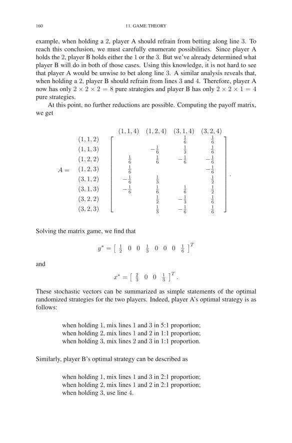
160 11. GAME THEORY
example, when holding a 2, player A should refrain from betting along line 3. Toreach this conclusion, we must carefully enumerate possibilities. Since player Aholds the 2, player B holds either the 1 or the 3. But we’ve already determined whatplayer B will do in both of those cases. Using this knowledge, it is not hard to seethat player A would be unwise to bet along line 3. A similar analysis reveals that,when holding a 2, player B should refrain from lines 3 and 4. Therefore, player Anow has only 2 × 2 × 2 = 8 pure strategies and player B has only 2 × 2 × 1 = 4pure strategies.
At this point, no further reductions are possible. Computing the payoff matrix,we get
A =
(1, 1, 4) (1, 2, 4) (3, 1, 4) (3, 2, 4)(1, 1, 2)
(1, 1, 3)
(1, 2, 2)
(1, 2, 3)
(3, 1, 2)
(3, 1, 3)
(3, 2, 2)
(3, 2, 3)
⎡
⎢⎢⎢⎢⎢⎢⎢⎢⎢⎢⎢⎢⎢⎣
16
16
− 16
13
16
16
16 − 1
6 − 16
16 − 1
6
− 16
13
12
− 16
16
16
12
12 − 1
316
13 − 1
616
⎤
⎥⎥⎥⎥⎥⎥⎥⎥⎥⎥⎥⎥⎥⎦
.
Solving the matrix game, we find that
y∗ =[
12 0 0 1
3 0 0 0 16
]T
and
x∗ =[
23 0 0 1
3
]T.
These stochastic vectors can be summarized as simple statements of the optimalrandomized strategies for the two players. Indeed, player A’s optimal strategy is asfollows:
when holding 1, mix lines 1 and 3 in 5:1 proportion;when holding 2, mix lines 1 and 2 in 1:1 proportion;when holding 3, mix lines 2 and 3 in 1:1 proportion.
Similarly, player B’s optimal strategy can be described as
when holding 1, mix lines 1 and 3 in 2:1 proportion;when holding 2, mix lines 1 and 2 in 2:1 proportion;when holding 3, use line 4.

EXERCISES 161
Note that it is optimal for player A to use line 3 when holding a 1 at least some ofthe time. Since line 3 says to bet, this bet is a bluff. Player B also bluffs some-times, since betting line 3 is sometimes used when holding a 1. Clearly, the optimalstrategies also exhibit some underbidding.
Exercises
11.1 Players A and B each hide a nickel or a dime. If the hidden coins match,player A gets both; if they don’t match, then B gets both. Find the opti-mal strategies. Which player has the advantage? Solve the problem forarbitrary denominations a and b.
11.2 Players A and B each pick a number between 1 and 100. The game is adraw if both players pick the same number. Otherwise, the player whopicks the smaller number wins unless that smaller number is one less thanthe opponent’s number, in which case the opponent wins. Find the optimalstrategy for this game.
11.3 We say that row r dominates row s if arj ≥ asj for all j = 1, 2, . . . , n.Similarly, column r is said to dominate column s if air ≥ ais for alli = 1, 2, . . . ,m. Show that(a) If a row (say, r) dominates another row, then the row player has an
optimal strategy y∗ in which y∗r = 0.(b) If a column (say, s) is dominated by another column, then the column
player has an optimal strategy x∗ in which x∗s = 0.
Use these results to reduce the following payoff matrix to a 2× 2 matrix:⎡
⎢⎢⎣
−6 2 −4 −7 −50 4 −2 −9 −1
−7 3 −3 −8 −22 −3 6 0 3
⎤
⎥⎥⎦ .
11.4 Solve simplified poker assuming that antes are $2 and bets are $1.
11.5 Give necessary and sufficient conditions for the rth pure strategy of therow and the sth pure strategy of the column player to be simultaneouslyoptimal.
11.6 Use the Minimax Theorem to show that
maxx
miny
yTAx = miny
maxx
yTAx.
11.7 Bimatrix Games. Consider the following two-person game defined interms of a pair of m × n matrices A and B: if the row player selectsrow index i and the column player selects column index j, then the rowplayer pays aij dollars and the column player pays bij dollars. Stochasticvectors x∗ and y∗ are said to form a Nash equilibrium if
y∗TAx∗ ≤ yTAx∗ for all yy∗TBx∗ ≤ y∗TBx for all x.

162 11. GAME THEORY
The purpose of this exercise is to relate Nash equilibria to the problem offinding vectors x and y that satisfy
(11.5)
[0 −A
−BT 0
] [yx
]
+
[wz
]
=
[−e−e
]
,
yiwi = 0, for all i,xjzj = 0, for all j,
x, w, y, z ≥ 0
(vectors w and z can be thought of as being defined by the matrix equal-ity). Problem (11.5) is called a linear complementarity problem.(a) Show that there is no loss in generality in assuming that A and B
have all positive entries.(b) Assuming that A and B have all positive entries, show that, if (x∗, y∗)
is a Nash equilibrium, then
x′ =x∗
y∗TAx∗ , y′ =y∗
y∗TBx∗
solves the linear complementarity problem (11.5).(c) Show that, if (x′, y′) solves the linear complementarity problem
(11.5), then
x∗ =x′
eTx′ , y∗ =y′
eT y′
is a Nash equilibrium.(An algorithm for solving the linear complementarity problem is devel-oped in Exercise 18.7.)
11.8 The Game of Morra. Two players simultaneously throw out one or twofingers and call out their guess as to what the total sum of the outstretchedfingers will be. If a player guesses right, but his opponent does not, hereceives payment equal to his guess. In all other cases, it is a draw.(a) List the pure strategies for this game.(b) Write down the payoff matrix for this game.(c) Formulate the row player’s problem as a linear programming prob-
lem. (Hint: Recall that the row player’s problem is to minimize themaximum expected payout.)
(d) What is the value of this game?(e) Find the optimal randomized strategy.
11.9 Heads I Win—Tails You Lose. In the classical coin-tossing game, playerA tosses a fair coin. If it comes up heads player B pays player A $2 butif it comes up tails player A pays player B $2. As a two-person zero-sum game, this game is rather trivial since neither player has anything todecide (after agreeing to play the game). In fact, the matrix for this gameis a 1 × 1 matrix with only a zero in it, which represents the expectedpayoff from player A to B.
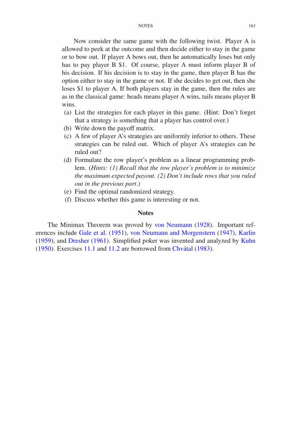
NOTES 163
Now consider the same game with the following twist. Player A isallowed to peek at the outcome and then decide either to stay in the gameor to bow out. If player A bows out, then he automatically loses but onlyhas to pay player B $1. Of course, player A must inform player B ofhis decision. If his decision is to stay in the game, then player B has theoption either to stay in the game or not. If she decides to get out, then sheloses $1 to player A. If both players stay in the game, then the rules areas in the classical game: heads means player A wins, tails means player Bwins.(a) List the strategies for each player in this game. (Hint: Don’t forget
that a strategy is something that a player has control over.)(b) Write down the payoff matrix.(c) A few of player A’s strategies are uniformly inferior to others. These
strategies can be ruled out. Which of player A’s strategies can beruled out?
(d) Formulate the row player’s problem as a linear programming prob-lem. (Hints: (1) Recall that the row player’s problem is to minimizethe maximum expected payout. (2) Don’t include rows that you ruledout in the previous part.)
(e) Find the optimal randomized strategy.(f) Discuss whether this game is interesting or not.
Notes
The Minimax Theorem was proved by von Neumann (1928). Important ref-erences include Gale et al. (1951), von Neumann and Morgenstern (1947), Karlin(1959), and Dresher (1961). Simplified poker was invented and analyzed by Kuhn(1950). Exercises 11.1 and 11.2 are borrowed from Chvatal (1983).
CHAPTER 12
Regression
In this chapter, we shall study an application of linear programming to an areaof statistics called regression. As a specific example, we shall use size and iteration-count data collected from a standard suite of linear programming problems to derivea regression estimate of the number of iterations needed to solve problems of agiven size.
1. Measures of Mediocrity
We begin our discussion with an example. Here are the midterm exam scoresfor a linear programming course:
28, 62, 80, 84, 86, 86, 92, 95, 98.
Let m denote the number of exam scores (i.e., m = 9) and let bi, i = 1, 2, . . . ,m,denote the actual scores (arranged in increasing order as above). The most naivemeasure of the “average” score is just the mean value, x, defined by
x =1
m
m∑
i=1
bi = 79.0.
This is an example of a statistic, which, by definition, is a function of a set ofdata. Statistics are computed so that one does not need to bother with reportinglarge tables of raw numbers. (Admittedly, the task of reporting the above list ofnine exam scores is not very onerous, but this is just an example.) Now, supposethe professor in question did not report the scores but instead just gave summarystatistics. Consider the student who got an 80 on the exam. This student surelydidn’t feel great about this score but might have thought that at least it was betterthan average. However, as the raw data makes clear, this student really did worsethan average1 on the exam (the professor confesses that the exam was rather easy).In fact, out of the nine students, the one who got an 80 scored third from the bottomof the class. Furthermore, the student who scored worst on the exam did so badlythat one might expect this student to drop the course, thereby making the 80 lookeven worse.
Any statistician would, of course, immediately suggest that we report themedian score instead of the mean. The median score is, by definition, that score
1“Average” is usually taken as synonymous with “mean” but in this section we shall use it in animprecise sense, employing other technically defined terms for specific meanings.
R.J. Vanderbei, Linear Programming, International Series in Operations Research& Management Science 196, DOI 10.1007/978-1-4614-7630-6 12,© Springer Science+Business Media New York 2014
165

166 12. REGRESSION
FIGURE 12.1. The objective function whose minimum occurs atthe median.
which is worse than half of the other scores and better than the other half. In otherwords, the median x is defined as
x = b(m+1)/2 = 86.
(Here and in various places in this chapter, we shall assume that m is odd so thatcertain formulas such as this one remain fairly simple.) Clearly, the 86 gives a moreaccurate indication of what the average score on the exam was.
There is a close connection between these statistical concepts and optimization.For example, the mean x minimizes, over all real numbers x, the sum of the squareddeviations between the data points and x itself. That is,
x = argminx∈R
m∑
i=1
(x− bi)2.
To verify this claim, we let f(x) =∑m
i=1(x − bi)2, differentiate with respect to x,
and set the derivative to zero to get
f ′(x) =m∑
i=1
2(x− bi) = 0.
Solving this equation for the critical point2 x, we see that
x =1
m
m∑
i=1
bi = x.
The fact that this critical point is a minimum rather than a maximum (or a saddlepoint) follows from the fact that f ′′(x) > 0 for all x ∈ R.
2Recall from calculus that a critical point is any point at which the derivative vanishes or fails toexist.

2. MULTIDIMENSIONAL MEASURES: REGRESSION ANALYSIS 167
The median x also enjoys a close connection with optimization. Indeed, it isthe point that minimizes the sum of the absolute values of the difference betweeneach data point and itself. That is,
x = argminx∈R
m∑
i=1
|x− bi|.
To see that this is correct, we again use calculus. Let
f(x) =
m∑
i=1
|x− bi|.
This function is continuous, piecewise linear, and convex (see Figure 12.1). How-ever, it is not differentiable at the data points. Nonetheless, we can look at itsderivative at other points to see where it jumps across zero. The derivative, forx �∈ {b1, b2, . . . , bm}, is
f ′(x) =m∑
i=1
sgn(x− bi),
where
sgn(x) =
⎧⎨
⎩
1 if x > 00 if x = 0
−1 if x < 0.
Hence, we see that the derivative at x is just the number of data points to the left ofx minus the number of data points to the right. Clearly, this derivative jumps acrosszero at the median, implying that the median is the minimum.
In this chapter, we shall discuss certain generalizations of means and medi-ans called regressions. At the end, we will consider a specific example that is ofparticular interest to us: the empirical average performance of the simplex method.
2. Multidimensional Measures: Regression Analysis
The analysis of the previous section can be recast as follows. Given a “random”observation b, we assume that it consists of two parts: a fixed, but unknown, partdenoted by x and a random fluctuation about this fixed part, which we denote by ε.Hence,
b = x+ ε.
Now, if we take several observations and index them as i = 1, 2, . . . ,m, the b’s andthe ε’s will vary, but x is assumed to be the same for all observations. Therefore, wecan summarize the situation by writing
bi = x+ εi, i = 1, 2, . . . ,m.
We now see that the mean is simply the value of x that minimizes the sum of thesquares of the εi’is. Similarly, the median is the value of x that minimizes the sumof the absolute values of the εi’s.
Sometimes one wishes to do more than merely identify some sort of “average.”For example, a medical researcher might collect blood pressure data on thousands

168 12. REGRESSION
of patients with the aim of identifying how blood pressure depends on age, obesity(defined as weight over height), sex, etc. So associated with each observation b ofa blood pressure are values of these control variables. Let’s denote by a1 the ageof a person, a2 the obesity, a3 the sex, etc. Let n denote the number of differentcontrol variables being considered by the researcher. In (linear) regression analysis,we assume that the response b depends linearly on the control variables. Hence, weassume that there are (unknown) numbers xj , j = 1, 2, . . . , n, such that
b =
n∑
j=1
ajxj + ε.
This equation is referred to as the regression model. Of course, the researcher col-lects data from thousands of patients, and so the data items, b and the aj’s, must beindexed over these patients. That is,
bi =
n∑
j=1
aijxj + εi, i = 1, 2, . . . ,m.
If we let b denote the vector of observations, ε the vector of random fluctuations,and A the matrix whose ith row consists of the values of the control variables forthe ith patient, then the regression model can be expressed in matrix notation as
(12.1) b = Ax+ ε.
In regression analysis, the goal is to find the vector x that best explains theobservations b. Hence, we wish to pick values that minimize, in some sense, thevector ε’s. Just as for the mean and median, we can consider minimizing eitherthe sum of the squares of the εi’s or the sum of the absolute values of the εi’s. Thereare even other possibilities. In the next two sections, we will discuss the range ofpossibilities and then give specifics for the two mentioned above.
3. L2-Regression
There are several notions of the size of a vector. The most familiar one is theEuclidean length
‖y‖2 = (∑
i
y2i )1/2.
This notion of length corresponds to our physical notion (at least when the dimen-sion is low, such as 1, 2, or 3). However, one can use any power inside the sumas long as the corresponding root accompanies it on the outside of the sum. For1 ≤ p < ∞, we get then the so-called Lp-norm of a vector y
‖y‖p = (∑
i
ypi )1/p.
Other than p = 2, the second most important case is p = 1 (and the third mostimportant case corresponds to the limit as p tends to infinity).
Measuring the size of ε in (12.1) using the L2-norm, we arrive at the L2-regression problem, which is to find x that attains the minimum L2-norm for the

3. L2-REGRESSION 169
difference between b and Ax. Of course, it is entirely equivalent to minimize thesquare of the L2-norm, and so we get
x = argminx‖b−Ax‖22.Just as for the mean, there is an explicit formula for x. To find it, we again rely onelementary calculus. Indeed, let
f(x) = ‖b−Ax‖22 =∑
i
(
bi −∑
j
aijxj
)2
.
In this multidimensional setting, a critical point is defined as a point at which thederivative with respect to every variable vanishes. So if we denote a critical pointby x, we see that it must satisfy the following equations:
∂f
∂xk(x) =
∑
i
2(bi −
∑
j
aij xj
)(−aik) = 0, k = 1, 2, . . . , n.
Simplifying these equations, we get∑
i
aikbi =∑
i
∑
j
aikaij xj , k = 1, 2, . . . , n.
In matrix notation, these equations can be summarized as follows:
AT b = ATAx.
In other words, assuming that ATA is invertible, we get
(12.2) x = (ATA)−1AT b.
This is the formula for L2-regression. It is also commonly called least squaresregression. In Section 12.6, we will use this formula to solve a specific regressionproblem.
Example. The simplest and most common regression model arises when onewishes to describe a response variable b as a linear function of a single input variablea. In this case, the model is
b = ax1 + x2.
The unknowns here are the slope x1 and the intercept x2. Figure 12.2 shows a plotof three pairs (a, b) through which we want to draw the “best” straight line. At firstglance, this model does not seem to fit the regression paradigm, since regressionmodels (as we’ve defined them) do not involve a term for a nonzero intercept. Butthe model here can be made to fit by introducing a new control variable, say, a2,which is always set to 1. While we’re at it, let’s change our notation for a to a1 sothat the model can now be written as
b = a1x1 + a2x2.
The three data points can then be summarized in matrix notation as⎡
⎣12.53
⎤
⎦ =
⎡
⎣0 12 14 1
⎤
⎦[
x1
x2
]
+
⎡
⎣ε1ε2ε3
⎤
⎦ .

170 12. REGRESSION
a
b
0 1 2 3 40
1
2
3
4
FIGURE 12.2. Three data points for a linear regression.
For this problem,
ATA =
[0 2 41 1 1
]⎡
⎣0 12 14 1
⎤
⎦ =
[20 66 3
]
and
AT b =
[0 2 41 1 1
]⎡
⎣12.53
⎤
⎦ =
[176.5
]
.
Hence,
x =
[x1
x2
]
=1
24
[3 −6−6 20
] [176.5
]
=
[1/27/6
]
.
4. L1-Regression
Just as the median gives a more robust estimate of the “average value” of acollection of numbers than the mean, L1-regression is less sensitive to outliers thanleast squares regression is. It is defined by minimizing the L1-norm of the deviationvector in (12.1). That is, the problem is to find x as follows:
x = argminx‖b−Ax‖1.
Unlike for least squares regression, there is no explicit formula for the solution tothe L1-regression problem. However, the problem can be reformulated as a linearprogramming problem. Indeed, it is easy to see that the L1-regression problem,

5. ITERATIVELY REWEIGHTED LEAST SQUARES 171
minimize∑
i
∣∣∣∣∣∣bi −
∑
j
aijxj
∣∣∣∣∣∣,
can be rewritten as
minimize∑
i ti
subject to ti −∣∣∣bi −
∑j aijxj
∣∣∣ = 0, i = 1, 2, . . . ,m,
which is equivalent to the following linear programming problem:
(12.3)minimize
∑i ti
subject to −ti ≤ bi −∑
j aijxj ≤ ti, i = 1, 2, . . . ,m.
Hence, to solve the L1-regression problem, it suffices to solve this linear program-ming problem. In the next section, we shall present an alternative algorithm forcomputing the solution to an L1-regression problem.
Example. Returning to the example of the last section, the L1-regression prob-lem is solved by finding the optimal solution to the following linear programmingproblem:
minimize t1 +t2 +t3subject to −x2−t1 ≤ −1
−2x1−x2 −t2 ≤ −2.5−4x1−x2 −t3 ≤ −3
x2−t1 ≤ 12x1+x2 −t2 ≤ 2.54x1+x2 −t3 ≤ 3
t1, t2, t3 ≥ 0.
The solution to this linear programming problem is
x =
[0.51
]
,
which clearly indicates that the point (2, 2.5) is viewed by the L1-regression as anoutlier, since the regression line passes exactly through the other two points.
5. Iteratively Reweighted Least Squares
Even though calculus cannot be used to obtain an explicit formula for thesolution to the L1-regression problem, it can be used to obtain an iterative procedurethat, when properly initialized, converges to the solution of the L1-regression prob-lem. The resulting iterative process is called iteratively reweighted least squares. Inthis section, we briefly discuss this method. We start by considering the objectivefunction for L1-regression:

172 12. REGRESSION
f(x) = ‖b−Ax‖1
=∑
i
∣∣∣∣∣∣bi −
∑
j
aijxj
∣∣∣∣∣∣.
Differentiating this objective function is a problem, since it involves absolute values.However, the absolute value function
g(z) = |z|is differentiable everywhere except at one point: z = 0. Furthermore, we can usethe following simple formula for the derivative, where it exists:
g′(z) =z
|z| .
Using this formula to differentiate f with respect to each variable, and setting thederivatives to zero, we get the following equations for critical points:
(12.4)∂f
∂xk=
∑
i
bi −∑
j aijxj
|bi −∑
j aijxj |(−aik) = 0, k = 1, 2, . . . , n.
If we introduce the following shorthand notation for the deviations,
εi(x) =
∣∣∣∣∣∣bi −
∑
j
aijxj
∣∣∣∣∣∣,
we see that we can rewrite (12.4) as∑
i
aikbiεi(x)
=∑
i
∑
j
aikaijxj
εi(x), k = 1, 2, . . . , n.
Now, if we let Ex denote the diagonal matrix containing the vector ε(x) on thediagonal, we can write these equations in matrix notation as follows:
ATE−1x b = ATE−1
x Ax.
This equation can’t be solved for x as we were able to do in L2-regression becauseof the dependence of the diagonal matrix on x. But let us rearrange this system ofequations by multiplying both sides by the inverse of ATE−1
x A. The result is
x =(ATE−1
x A)−1
ATE−1x b.
This formula suggests an iterative scheme that hopefully converges to a solution.Indeed, we start by initializing x0 arbitrarily and then use the above formula tosuccessively compute new approximations. If we let xk denote the approximationat the kth iteration, then the update formula can be expressed as
xk+1 =(ATE−1
xk A)−1
ATE−1xk b.
Assuming only that the matrix inverse exists at every iteration, one can show thatthis iteration scheme converges to a solution to the L1-regression problem.

6. AN EXAMPLE: HOW FAST IS THE SIMPLEX METHOD? 173
6. An Example: How Fast Is the Simplex Method?
In Chapter 4, we discussed the worst-case behavior of the simplex method andstudied the Klee–Minty problem that achieves the worst case. We also discussed theimportance of empirical studies of algorithm performance. In this section, we shallintroduce a model that allows us to summarize the results of these empirical studies.
We wish to relate the number of simplex iterations T required to solve a lin-ear programming problem to the number of constraints m and/or the number ofvariables n in the problem (or some combination of the two). As any statisticianwill report, the first step is to introduce an appropriate model.3 Hence, we beginby asking: how many iterations, on average, do we expect the simplex method totake if the problem has m constraints and n variables? To propose an answer tothis question, consider the initial dictionary associated with a given problem. Thisdictionary involves m values, x∗
B, for the primal basic variables, and n values, y∗N ,for the dual nonbasic variables. We would like each of these m + n variables tohave nonnegative values, since that would indicate optimality. If we assume thatthe initial dictionary is nondegenerate, then one would expect on the average that(m + n)/2 of the values would be positive and the remaining (m + n)/2 valueswould be negative.
Now let’s look at the dynamics of the simplex method. Each iteration focuseson exactly one of the negative values. Suppose, for the sake of discussion, that thenegative value corresponds to a dual nonbasic variable, that is, one of the coeffi-cients in the objective row of the dictionary. Then the simplex method selects thecorresponding primal nonbasic variable to enter the basis, and a leaving variable ischosen by a ratio test. After the pivot, the variable that exited now appears as anonbasic variable in the same position that the entering variable held before. Fur-thermore, the coefficient on this variable is guaranteed to be positive (since we’veassumed nondegeneracy). Hence, the effect of one pivot of the simplex method isto correct the sign of one of the negative values from the list of m + n values ofinterest. Of course, the pivot also affects all the other values, but there seems noreason to assume that the situation relative to them will have any tendency to getbetter or worse, on the average. Therefore, we can think of the simplex method asstatistically reducing the number of negative values by one at each iteration.
Since we expect on the average that an initial dictionary will have (m + n)/2negative values, it follows that the simplex method should take (m + n)/2 itera-tions, on average. Of course, these expectations are predicated on the assumptionthat degenerate dictionaries don’t arise. As we saw in Section 7.2, the self-dual sim-plex method initialized with random perturbations will, with probability one, neverencounter a degenerate dictionary. Hence, we hypothesize that this variant of thesimplex method will, on average, take (m+ n)/2 iterations. It is important to notethe main point of our hypothesis; namely, that the number of iterations is linear inm+ n as opposed, say, to quadratic or cubic.
3In the social sciences, a fundamental difficulty is the lack of specific arguments validating theappropriateness of the models commonly introduced.

174 12. REGRESSION
We can test our hypothesis by first supposing that T can be approximated by afunction of the form
2α(m+ n)β
for a pair of real numbers α and β. Our goal then is to find the value for theseparameters that best fits the data obtained from a set of empirical observations.(We’ve written the leading constant as 2α simply for symmetry with the otherfactor—there is no fundamental need to do this.) This multiplicative representationof the number of iterations can be converted into an additive (in α and β) represen-tation by taking logarithms. Introducing an ε to represent the difference between themodel’s prediction and the true number of iterations, we see that the model can bewritten as
log T = α log 2 + β log(m+ n) + ε.
Now, suppose that several observations are made. Using subscripts to distinguishthe various observations, we get the following equations:
⎡
⎢⎢⎢⎣
log T1
log T2
...log Tk
⎤
⎥⎥⎥⎦=
⎡
⎢⎢⎢⎣
log 2 log(m1 + n1)log 2 log(m2 + n2)
......
log 2 log(mk + nk)
⎤
⎥⎥⎥⎦
[αβ
]
+
⎡
⎢⎢⎢⎣
ε1ε2...εk
⎤
⎥⎥⎥⎦.
If we let b denote the vector on the left, A the matrix on the right, x the vectormultiplied by A, and ε the vector of deviations, then the model can be expressed as
b = Ax+ ε,
where A and b are given. As we’ve seen, this is just a regression model, which wecan solve as an L1-regression or as an L2-regression.
Given real data, we shall solve this model both ways. Table 12.1 shows specificdata obtained by running the self-dual simplex method described in Chapter 7 (withrandomized initial perturbations) against most of the problems in a standard suiteof test problems (called the NETLIB suite Gay 1985). Some problems were too bigto run on the workstation used for this experiment, and others were formulated withfree variables that the code was not equipped to handle.
Using (12.2) to solve the problem as an L2-regression, we get[
αβ
]
=
[−1.035611.05152
]
.
Or, in other words,T ≈ 0.488(m+ n)1.052.
This is amazingly close to our hypothesized formula, (m+n)/2. Figure 12.3 showsa log–log plot of T vs. m + n with the L2-regression line drawn through it. It isclear from this graph that a straight line (in the log–log plot) is a good model forfitting this data.
Using (12.3) to solving the problem, we get[
αβ
]
=
[−0.95081.0491
]
.

6. AN EXAMPLE: HOW FAST IS THE SIMPLEX METHOD? 175
Name m n iters Name m n iters25fv47 777 1,545 5,089 nesm 646 2,740 5,82980bau3b 2,021 9,195 10,514 recipe 74 136 80adlittle 53 96 141 sc105 104 103 92afiro 25 32 16 sc205 203 202 191agg2 481 301 204 sc50a 49 48 46agg3 481 301 193 sc50b 48 48 53bandm 224 379 1,139 scagr25 347 499 1,336beaconfd 111 172 113 scagr7 95 139 339blend 72 83 117 scfxm1 282 439 531bnl1 564 1,113 2,580 scfxm2 564 878 1,197bnl2 1,874 3,134 6,381 scfxm3 846 1,317 1,886boeing1 298 373 619 scorpion 292 331 411boeing2 125 143 168 scrs8 447 1,131 783bore3d 138 188 227 scsd1 77 760 172brandy 123 205 585 scsd6 147 1,350 494czprob 689 2,770 2,635 scsd8 397 2,750 1,548d6cube 403 6,183 5,883 sctap1 284 480 643degen2 444 534 1,421 sctap2 1,033 1,880 1,037degen3 1,503 1,818 6,398 sctap3 1,408 2,480 1,339e226 162 260 598 seba 449 896 766etamacro 334 542 1,580 share1b 107 217 404fffff800 476 817 1,029 share2b 93 79 189finnis 398 541 680 shell 487 1,476 1,155fit1d 24 1,026 925 ship04l 317 1,915 597fit1p 627 1,677 15,284 ship04s 241 1,291 560forplan 133 415 576 ship08l 520 3,149 1,091ganges 1,121 1,493 2,716 ship08s 326 1,632 897greenbea 1,948 4,131 21,476 ship12l 687 4,224 1,654grow15 300 645 681 ship12s 417 1,996 1,360grow22 440 946 999 sierra 1,212 2,016 793grow7 140 301 322 standata 301 1,038 74israel 163 142 209 standmps 409 1,038 295kb2 43 41 63 stocfor1 98 100 81lotfi 134 300 242 stocfor2 2,129 2,015 2,127maros 680 1,062 2,998
TABLE 12.1. Number of iterations for the self-dual simplex method.
In other words,
T ≈ 0.517(m+ n)1.049.
The fact that this regression formula agrees closely with the L2-regression indicatesthat the data set contains no outliers. In Section 12.6.1, we will consider randomlygenerated problems and see at least one example where the L1 and L2 regressionlines differ significantly.
6.1. Random Problems. Now, let’s consider random problems generated in amanner similar to the way we did it back in Chapter 4. We do, however, introducesome changes. First of all, the problems in Chapter 4 were generated in such amanner as to guarantee primal feasibility but dual feasibility was left to chance—that is, many (half) of the problems were unbounded. The problems we wish toconsider now will be assumed to have optimal solutions (real-world problems areoften, but not always, known to have an optimal solution because of the underlyingphysical model and therefore primal or dual infeasibility is often an indicator ofdata and/or modeling errors). To guarantee the existence of an optimal solution, we

176 12. REGRESSION
102 103 104101
102
103
104
Parametric Self−Dual Simplex Method
m+n
num
ber
of p
ivot
s
DataLeast SquaresLeast Absolute Deviation
FIGURE 12.3. A log–log plot of T vs. m+ n and the L1 and L2
regression lines.
generate random optimal primal and dual solutions and associated random optimalslack/surplus variables. Here’s the MATLAB code for that:
x = round(sigma*rand(n,1)).*(rand(n,1)>0.5);y = round(sigma*rand(1,m)).*(rand(1,m)>0.5);z = round(sigma*rand(1,n)).*(rand(1,n)>0.5);w = round(sigma*rand(m,1)).*(rand(m,1)>0.5);
(as in Chapter 4, sigma is a constant initialized to 10). We then define A, b, and cas problem data consistent with these optimal solutions:
A = round(sigma*(randn(m,n))).*(rand(m,n)>0.5);b = A*x + w;c = y*A - z;
Note that we have made one other key change from before—we have randomlyforced about half of the optimal values of the variables and about half of the con-straint matrix coefficients to be zero. This change makes the problems slightly morerealistic as real-world problems often have much sparsity.
Next, we need to initialize a right-hand side perturbation and an objective func-tion perturbation:
b0 = rand(m,1);c0 = -rand(1,n);

6. AN EXAMPLE: HOW FAST IS THE SIMPLEX METHOD? 177
There are just three relatively simple changes to the code defining the simplexmethod itself to convert it from a primal-simplex algorithm to the parametric self-dual method. The first is to change the line of code that checks if the problem hasbeen solved. Before, we only needed to check if all of the objective coefficients hadbecome negative (dual feasibility) because primal feasibility was built in. Now, wehave to check both primal and dual feasibility:
while max(c) > eps || min(b) < -eps,
Secondly, the choice of enter/leaving variables must be updated as it is now basedon minimizing the perturbation parameter:
[mu_col, col] = max( (-c./c0).*(c0<-eps));[mu_row, row] = max( (-b./b0).*(b0> eps));if mu_col >= mu_row,
mu = mu_col;Acol = A(:,col);[t, row] = max(-Acol./(b+mu*b0));
elsemu = mu_row;Arow = A(row,:);[s, col] = max(-Arow./(c+mu*c0));
end
Finally, as part of every pivot we have to update b0 and c0:
brow = b0(row);b0 = b0 - brow*Acol/a;b0(row) = -brow/a;
ccol = c0(col);c0 = c0 - ccol*Arow/a;c0(col) = ccol/a;
The code was run 1,000 times. Figure 12.4 shows the number of pivots plottedagainst the sum m+n. Just as we saw with the primal simplex method in Chapter 4,m+ n does not seem to be a good measure of problem size as many problems of agiven size solve much more quickly than the more typical cases. Hence, there area number of “outliers.” Overlayed on the scatter plot are the L1 and L2 regressionlines. While neither regression line follows what appears to be an upper line ofpoints that seems to dominate the results, the L1 is closer to that than is the L2 line.
The result of the L1-regression is:
T ≈ e−0.722e1.12 log(m+n) = 0.486(m+ n)1.12.
The result of the L2-regression is:
T ≈ e−0.606e1.05 log(m+n) = 0.546(m+ n)1.05.
Finally, as in Chapter 4, min(m,n) is a better measure of problem size for theserandomly generated problems. Figure 12.5 shows the same data plotted againstmin(m,n).
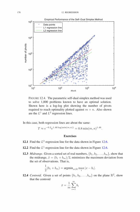
178 12. REGRESSION
105
104
103
102
101
101 102 103 104
Empirical Performance of the Self−Dual Simplex Method
m+n
num
ber
of p
ivot
sData pointsL1 regression lineL2 regression line
FIGURE 12.4. The parametric self-dual simplex method was usedto solve 1,000 problems known to have an optimal solution.Shown here is a log-log plot showing the number of pivotsrequired to reach optimality plotted against m + n. Also shownare the L1 and L2 regression lines.
In this case, both regression lines are about the same:
T ≈ e−0.2e1.46 log(min(m,n)) = 0.8min(m,n)1.46.
Exercises
12.1 Find the L2-regression line for the data shown in Figure 12.6.
12.2 Find the L1-regression line for the data shown in Figure 12.6.
12.3 Midrange. Given a sorted set of real numbers, {b1, b2, . . . , bm}, show thatthe midrange, x = (b1 + bm)/2, minimizes the maximum deviation fromthe set of observations. That is,
1
2(b1 + bm) = argminx∈R
maxi
|x− bi|.
12.4 Centroid. Given a set of points {b1, b2, . . . , bm} on the plane R2, show
that the centroid
x =1
m
m∑
i=1
bi

EXERCISES 179
101 102 103101
102
103
104
105Empirical Performance of the Self−Dual Simplex Method
min( m, n )
num
ber
of p
ivot
sData pointsL1 regression lineL2 regression line
FIGURE 12.5. The parametric self-dual simplex method was usedto solve 1,000 problems known to have an optimal solution.Shown here is a log-log plot showing the number of pivotsrequired to reach optimality plotted against min(m,n). In thiscase, the L1 and L2 regression lines are almost exactly on top ofeach other.
minimizes the sum of the squares of the distance to each point in the set.That is, x solves the following optimization problem:
minimizem∑
i=1
‖x− bi‖22
Note: Each data point bi is a vector in R2 whose components are denoted,
say, by bi1 and bi2, and, as usual, the subscript 2 on the norm denotes theEuclidean norm. Hence,
‖x− bi‖2 =√
(x1 − bi1)2 + (x2 − bi2)2.
12.5 Facility Location. A common problem is to determine where to locatea facility so that the distance from its customers is minimized. That is,given a set of points {b1, b2, . . . , bm} on the plane R
2, the problem is tofind x = (x1, x2) that solves the following optimization problem:
minimizem∑
i=1
‖x− bi‖2.
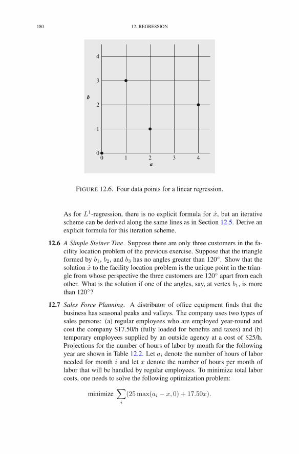
180 12. REGRESSION
a
b
0 1 2 3 40
1
2
3
4
FIGURE 12.6. Four data points for a linear regression.
As for L1-regression, there is no explicit formula for x, but an iterativescheme can be derived along the same lines as in Section 12.5. Derive anexplicit formula for this iteration scheme.
12.6 A Simple Steiner Tree. Suppose there are only three customers in the fa-cility location problem of the previous exercise. Suppose that the triangleformed by b1, b2, and b3 has no angles greater than 120◦. Show that thesolution x to the facility location problem is the unique point in the trian-gle from whose perspective the three customers are 120◦ apart from eachother. What is the solution if one of the angles, say, at vertex b1, is morethan 120◦?
12.7 Sales Force Planning. A distributor of office equipment finds that thebusiness has seasonal peaks and valleys. The company uses two types ofsales persons: (a) regular employees who are employed year-round andcost the company $17.50/h (fully loaded for benefits and taxes) and (b)temporary employees supplied by an outside agency at a cost of $25/h.Projections for the number of hours of labor by month for the followingyear are shown in Table 12.2. Let ai denote the number of hours of laborneeded for month i and let x denote the number of hours per month oflabor that will be handled by regular employees. To minimize total laborcosts, one needs to solve the following optimization problem:
minimize∑
i
(25max(ai − x, 0) + 17.50x).
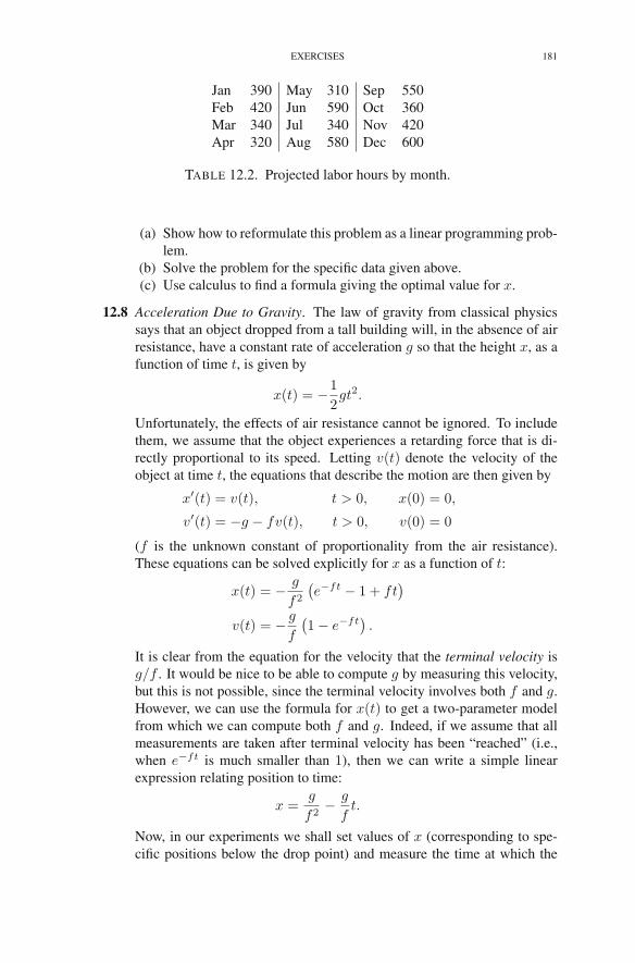
EXERCISES 181
Jan 390 May 310 Sep 550Feb 420 Jun 590 Oct 360Mar 340 Jul 340 Nov 420Apr 320 Aug 580 Dec 600
TABLE 12.2. Projected labor hours by month.
(a) Show how to reformulate this problem as a linear programming prob-lem.
(b) Solve the problem for the specific data given above.(c) Use calculus to find a formula giving the optimal value for x.
12.8 Acceleration Due to Gravity. The law of gravity from classical physicssays that an object dropped from a tall building will, in the absence of airresistance, have a constant rate of acceleration g so that the height x, as afunction of time t, is given by
x(t) = −1
2gt2.
Unfortunately, the effects of air resistance cannot be ignored. To includethem, we assume that the object experiences a retarding force that is di-rectly proportional to its speed. Letting v(t) denote the velocity of theobject at time t, the equations that describe the motion are then given by
x′(t) = v(t), t > 0, x(0) = 0,
v′(t) = −g − fv(t), t > 0, v(0) = 0
(f is the unknown constant of proportionality from the air resistance).These equations can be solved explicitly for x as a function of t:
x(t) = − g
f2
(e−ft − 1 + ft
)
v(t) = − g
f
(1− e−ft
).
It is clear from the equation for the velocity that the terminal velocity isg/f . It would be nice to be able to compute g by measuring this velocity,but this is not possible, since the terminal velocity involves both f and g.However, we can use the formula for x(t) to get a two-parameter modelfrom which we can compute both f and g. Indeed, if we assume that allmeasurements are taken after terminal velocity has been “reached” (i.e.,when e−ft is much smaller than 1), then we can write a simple linearexpression relating position to time:
x =g
f2− g
ft.
Now, in our experiments we shall set values of x (corresponding to spe-cific positions below the drop point) and measure the time at which the

182 12. REGRESSION
Obs. Position Timenumber (m) (s)
1 −10 3.722 −20 7.063 −30 10.464 −10 3.715 −20 7.006 −30 10.487 −10 3.678 −20 7.089 −30 10.33
TABLE 12.3. Time at which a falling object passes certain points.
object passes these positions. Since we prefer to write regression mod-els with the observed variable expressed as a linear function of the controlvariables, let us rearrange the above expression so that t appears as a func-tion of x:
t =1
f− f
gx.
Using this regression model and the data shown in Table 12.3, do anL2-regression to compute estimates for 1/f and −f/g. From these es-timates derive an estimate for g. If you have access to linear program-ming software, solve the problem using an L1-regression and compareyour answers.
12.9 Iteratively Reweighted Least Squares. Show that the sequence of iteratesin the iteratively reweighted least squares algorithm produces a monoton-ically decreasing sequence of objective function values by filling in thedetails in the following outline. First, recall that the objective function forL1-regression is given by
f(x) = ‖b−Ax‖1 =
m∑
i=1
εi(x),
where
εi(x) =
∣∣∣∣∣∣bi −
n∑
j=1
aijxj
∣∣∣∣∣∣.
Also, the function that defines the iterative scheme is given by
T (x) =(ATE−1
x A)−1
ATE−1x b,
where Ex denotes the diagonal matrix with the vector ε(x) on its diagonal.Our aim is to show that
f(T (x)) < f(x).
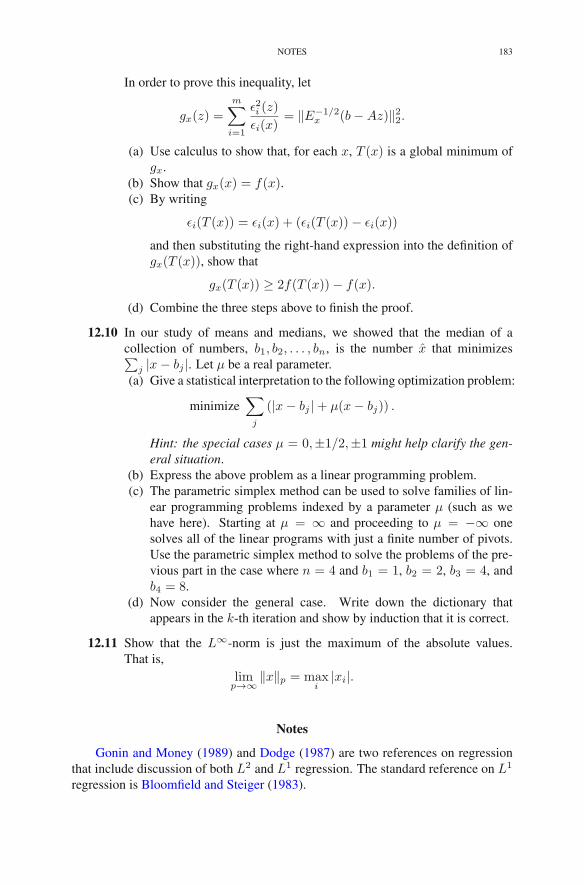
NOTES 183
In order to prove this inequality, let
gx(z) =m∑
i=1
ε2i (z)
εi(x)= ‖E−1/2
x (b−Az)‖22.
(a) Use calculus to show that, for each x, T (x) is a global minimum ofgx.
(b) Show that gx(x) = f(x).(c) By writing
εi(T (x)) = εi(x) + (εi(T (x))− εi(x))
and then substituting the right-hand expression into the definition ofgx(T (x)), show that
gx(T (x)) ≥ 2f(T (x))− f(x).
(d) Combine the three steps above to finish the proof.
12.10 In our study of means and medians, we showed that the median of acollection of numbers, b1, b2, . . . , bn, is the number x that minimizes∑
j |x− bj |. Let μ be a real parameter.(a) Give a statistical interpretation to the following optimization problem:
minimize∑
j
(|x− bj |+ μ(x− bj)) .
Hint: the special cases μ = 0,±1/2,±1 might help clarify the gen-eral situation.
(b) Express the above problem as a linear programming problem.(c) The parametric simplex method can be used to solve families of lin-
ear programming problems indexed by a parameter μ (such as wehave here). Starting at μ = ∞ and proceeding to μ = −∞ onesolves all of the linear programs with just a finite number of pivots.Use the parametric simplex method to solve the problems of the pre-vious part in the case where n = 4 and b1 = 1, b2 = 2, b3 = 4, andb4 = 8.
(d) Now consider the general case. Write down the dictionary thatappears in the k-th iteration and show by induction that it is correct.
12.11 Show that the L∞-norm is just the maximum of the absolute values.That is,
limp→∞
‖x‖p = maxi
|xi|.
Notes
Gonin and Money (1989) and Dodge (1987) are two references on regressionthat include discussion of both L2 and L1 regression. The standard reference on L1
regression is Bloomfield and Steiger (1983).

184 12. REGRESSION
Several researchers, including Smale (1983), Borgwardt (1982, 1987a), Adlerand Megiddo (1985), and Todd (1986), have studied the average number of itera-tions of the simplex method as a function of m and/or n. The model discussed inthis chapter is similar to the sign-invariant model introduced by Adler and Berenguer(1981).
CHAPTER 13
Financial Applications
In this chapter, we shall study some applications of linear programming toproblems in quantitative finance.
1. Portfolio Selection
Every investor, from the individual to the professional fund manager, must de-cide on an appropriate mix of assets to include in his or her investment portfolio.Given a collection of potential investments (indexed, say, from 1 to n), let Rj denotethe return in the next time period on investment j, j = 1, . . . , n. In general, Rj is arandom variable, although some investments may be essentially deterministic.
A portfolio is determined by specifying what fraction of one’s assets to put intoeach investment. That is, a portfolio is a collection of nonnegative numbers xj ,j = 1, . . . , n, that sum to one. The return (on each dollar) one would obtain using agiven portfolio is given by
R =∑
j
xjRj .
The reward associated with such a portfolio is defined as the expected return1:
ER =∑
j
xjERj .
If reward were the only issue, then the problem would be trivial: simply put ev-erything in the investment with the highest expected return. But unfortunately, in-vestments with high reward typically also carry a high level of risk. That is, eventhough they are expected to do very well in the long run, they also tend to be erraticin the short term. There are many ways to define risk, some better than others. Wewill define the risk associated with an investment (or, for that matter, a portfolio ofinvestments) to be the mean absolute deviation from the mean (MAD):
1In this chapter, we assume a modest familiarity with the ideas and notations of probability: thesymbol E denotes expected value, which means that, if R is a random variable that takes valuesR(1), R(2), . . . , R(T ) with equal probability, then
ER =1
T
T∑
t=1
R(t).
R.J. Vanderbei, Linear Programming, International Series in Operations Research& Management Science 196, DOI 10.1007/978-1-4614-7630-6 13,© Springer Science+Business Media New York 2014
185

186 13. FINANCIAL APPLICATIONS
E|R− ER| = E
∣∣∣∣∣∣
∑
j
xj(Rj − ERj)
∣∣∣∣∣∣
= E
∣∣∣∣∣∣
∑
j
xjRj
∣∣∣∣∣∣,
where Rj = Rj − ERj . One would like to maximize the reward while at the sametime not incur excessive risk. Whenever confronted with two (or more) competingobjectives, it is necessary to consider a spectrum of possible optimal solutions asone moves from putting most weight on one objective to the other. In our port-folio selection problem, we form a linear combination of the reward and the risk(parametrized here by μ) and maximize that:
(13.1)
maximize μ∑
j
xjERj − E
∣∣∣∣∣∣
∑
j
xjRj
∣∣∣∣∣∣
subject to∑
j
xj = 1
xj ≥ 0 j = 1, 2, . . . , n.
Here, μ is a positive parameter that represents the importance of risk relative toreward: high values of μ tend to maximize reward regardless of risk, whereas lowvalues attempt to minimize risk.
It is important to note that by diversifying (that is, not putting everything intoone investment), it might be possible to reduce the risk without reducing the reward.To see how this can happen, consider a hypothetical situation involving two invest-ments A and B. Each year, investment A either goes up 30 % or goes down 10 %,but unfortunately, the ups and downs are unpredictable (that is, each year is inde-pendent of the previous years and is an up year with probability 1/2). InvestmentB is also highly volatile. In fact, in any year in which A goes up 30 %, investmentB goes down 10 %, and in the years in which A goes down 10 %, B goes up 30 %.Clearly, by putting half of our portfolio into A and half into B, we can create a port-folio that goes up 10 % every year without fail. The act of identifying investmentsthat are negatively correlated with each other (such as A and B) and dividing theportfolio among these investments is called hedging. Unfortunately, it is fairly diffi-cult to find pairs of investments with strong negative correlations. But such negativecorrelations do occur. Generally speaking, they can be expected to occur when thefortunes of both A and B depend on a common underlying factor. For example, ahot, rainless summer is good for energy but bad for agriculture.
Solving problem (13.1) requires knowledge of the joint distribution of the Rj’s.However, this distribution is not known theoretically but instead must be estimatedby looking at historical data. For example, Table 13.1 shows monthly returns over arecent 2-year period for one bond fund (3-year Treasury Bonds) and eight differentsector index funds: Materials (XLB), Energy (XLE), Financial (XLF), Industrial(XLI), Technology (XLK), Staples (XLP), Utilities (XLU), and Healthcare (XLV).
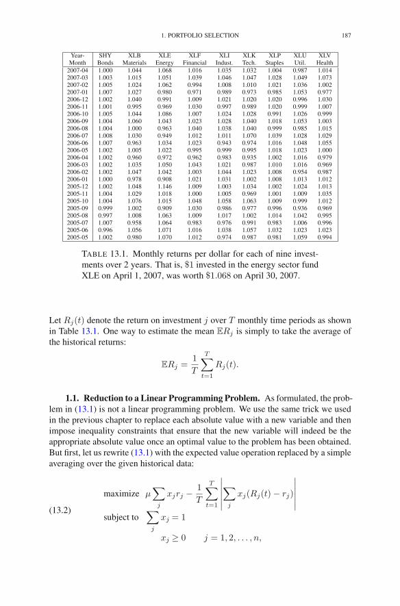
1. PORTFOLIO SELECTION 187
Year- SHY XLB XLE XLF XLI XLK XLP XLU XLVMonth Bonds Materials Energy Financial Indust. Tech. Staples Util. Health
2007-04 1.000 1.044 1.068 1.016 1.035 1.032 1.004 0.987 1.0142007-03 1.003 1.015 1.051 1.039 1.046 1.047 1.028 1.049 1.0732007-02 1.005 1.024 1.062 0.994 1.008 1.010 1.021 1.036 1.0022007-01 1.007 1.027 0.980 0.971 0.989 0.973 0.985 1.053 0.9772006-12 1.002 1.040 0.991 1.009 1.021 1.020 1.020 0.996 1.0302006-11 1.001 0.995 0.969 1.030 0.997 0.989 1.020 0.999 1.0072006-10 1.005 1.044 1.086 1.007 1.024 1.028 0.991 1.026 0.9992006-09 1.004 1.060 1.043 1.023 1.028 1.040 1.018 1.053 1.0032006-08 1.004 1.000 0.963 1.040 1.038 1.040 0.999 0.985 1.0152006-07 1.008 1.030 0.949 1.012 1.011 1.070 1.039 1.028 1.0292006-06 1.007 0.963 1.034 1.023 0.943 0.974 1.016 1.048 1.0552006-05 1.002 1.005 1.022 0.995 0.999 0.995 1.018 1.023 1.0002006-04 1.002 0.960 0.972 0.962 0.983 0.935 1.002 1.016 0.9792006-03 1.002 1.035 1.050 1.043 1.021 0.987 1.010 1.016 0.9692006-02 1.002 1.047 1.042 1.003 1.044 1.023 1.008 0.954 0.9872006-01 1.000 0.978 0.908 1.021 1.031 1.002 1.008 1.013 1.0122005-12 1.002 1.048 1.146 1.009 1.003 1.034 1.002 1.024 1.0132005-11 1.004 1.029 1.018 1.000 1.005 0.969 1.001 1.009 1.0352005-10 1.004 1.076 1.015 1.048 1.058 1.063 1.009 0.999 1.0122005-09 0.999 1.002 0.909 1.030 0.986 0.977 0.996 0.936 0.9692005-08 0.997 1.008 1.063 1.009 1.017 1.002 1.014 1.042 0.9952005-07 1.007 0.958 1.064 0.983 0.976 0.991 0.983 1.006 0.9962005-06 0.996 1.056 1.071 1.016 1.038 1.057 1.032 1.023 1.0232005-05 1.002 0.980 1.070 1.012 0.974 0.987 0.981 1.059 0.994
TABLE 13.1. Monthly returns per dollar for each of nine invest-ments over 2 years. That is, $1 invested in the energy sector fundXLE on April 1, 2007, was worth $1.068 on April 30, 2007.
Let Rj(t) denote the return on investment j over T monthly time periods as shownin Table 13.1. One way to estimate the mean ERj is simply to take the average ofthe historical returns:
ERj =1
T
T∑
t=1
Rj(t).
1.1. Reduction to a Linear Programming Problem. As formulated, the prob-lem in (13.1) is not a linear programming problem. We use the same trick we usedin the previous chapter to replace each absolute value with a new variable and thenimpose inequality constraints that ensure that the new variable will indeed be theappropriate absolute value once an optimal value to the problem has been obtained.But first, let us rewrite (13.1) with the expected value operation replaced by a simpleaveraging over the given historical data:
(13.2)
maximize μ∑
j
xjrj −1
T
T∑
t=1
∣∣∣∣∣∣
∑
j
xj(Rj(t)− rj)
∣∣∣∣∣∣
subject to∑
j
xj = 1
xj ≥ 0 j = 1, 2, . . . , n,

188 13. FINANCIAL APPLICATIONS
where
rj =1
T
T∑
t=1
Rj(t)
denotes the expected reward for asset j. Now, replace∣∣∣∑
j xj(Rj(t)− rj)∣∣∣ with a
new variable yt and rewrite the optimization problem as
(13.3)
maximize μ∑
j
xjrj −1
T
T∑
t=1
yt
subject to −yt ≤∑
j
xj(Rj(t)− rj)≤ yt t = 1, 2, . . . , T,
∑j xj = 1
xj ≥ 0 j = 1, 2, . . . , nyt ≥ 0 t = 1, 2, . . . , T.
As we’ve seen in other contexts before, at optimality one of the two inequalitiesinvolving yt must actually be an equality because if both inequalities were strictthen it would be possible to further increase the objective function by reducing yt.
1.2. Solution via Parametric Simplex Method. The problem formulationgiven by (13.3) is a linear program that can be solved for any particular value ofμ using the methods described in previous chapters. However, we can do much bet-ter than this. The problem is a parametric linear programming problem, where theparameter is the risk aversion parameter μ. If we can give a value of μ for which abasic optimal solution is obvious, then we can start from this basic solution and usethe parametric simplex method to find the optimal solution associated with each andevery value of μ. It is easy to see that for μ larger than some threshold, the optimalsolution is to put all of our portfolio into a single asset, the one with the highestexpected reward rj . Let j∗ denote this highest reward asset:
rj∗ ≥ rj for all j.
We need to write (13.3) in dictionary form. To this end, let us introduce slackvariables w+
t and w−t :
maximize μ∑
j
xjrj −1
T
T∑
t=1
yt
subject to −yt −∑
j
xj(Rj(t)− rj) + w−t = 0 t = 1, 2, . . . , T,
−yt +∑
j xj(Rj(t)− rj) + w+t = 0 t = 1, 2, . . . , T,
∑j xj = 1
xj ≥ 0 j = 1, 2, . . . , n,yt, w
+t , w
−t ≥ 0 t = 1, 2, . . . , T.
We have 3T + n nonnegative variables and 2T + 1 equality constraints. Hence, weneed to find 2T + 1 basic variables and T + n − 1 nonbasic variables. Since weknow the optimal values for each of the allocation variables, xj∗ = 1 and the rest of

1. PORTFOLIO SELECTION 189
the xj’s vanish, it is straightforward to figure out the values of the other variables aswell. We can then simply declare any variable that is positive to be basic and declarethe rest to be nonbasic. With this prescription, the variable xj∗ must be basic. Theremaining xj’s are nonbasic. Similarly, all of the yt’s are nonzero and hence basic.For each t, either w−
t or w+t is basic and the other is nonbasic. To say which is
which, we need to introduce some additional notation. Let
Dtj = Rj(t)− rj .
Then it is easy to check that w−t is basic if Dtj∗ > 0 and w+
t is basic if Dtj∗ < 0(the unlikely case where Dtj∗ = 0 can be decided arbitrarily). Let
T+ = {t : Dtj∗ > 0} and T− = {t : Dtj∗ < 0}
and let
εt =
{1, for t ∈ T+
−1, for t ∈ T−.
It’s tedious, but here’s the optimal dictionary:
ζ = 1T
T∑
t=1
εtDtj∗ − 1T
∑
j �=j∗
T∑
t=1
εt(Dtj −Dtj∗)xj − 1T
∑
t∈T−
w−t − 1
T
∑
t∈T+
w+t
+ μrj∗ + μ∑
j �=j∗(rj − rj∗)xj
yt = − Dtj∗ −∑
j �=j∗(Dtj −Dtj∗)xj +w−
t t ∈ T−
w−t = 2 Dtj∗ + 2
∑
j �=j∗(Dtj −Dtj∗)xj +w+
t t ∈ T+
yt = Dtj∗ +∑
j �=j∗(Dtj −Dtj∗)xj +w+
t t ∈ T+
w+t =−2 Dtj∗ − 2
∑
j �=j∗(Dtj −Dtj∗)xj +w−
t t ∈ T−
xj∗ = 1 −∑
j �=j∗xj
We can now check that, for large μ, this dictionary is optimal. Indeed, the objectivecoefficients on the w−
t and w+t variables in the first row of the objective function
are negative. The coefficients on the xj’s in the first row can be positive or negativebut for μ sufficiently large, the negative coefficients on the xj’s in the second rowdominate and make all coefficients negative after considering both rows. Similarly,the fact that all of the basic variables are positive follows immediately from thedefinitions of T+ and T−.
A few simple inequalities determine the μ-threshold above which the givendictionary is optimal. The parametric simplex method can then be used to system-atically reduce μ to zero. Along the way, each dictionary encountered correspondsto an optimal solution for some range of μ values. Hence, in one pass we havesolved the portfolio selection problem for every investor from the bravest to themost cautious. Figure 13.1 shows all of the optimal portfolios. The set of all risk–reward profiles that are possible is shown in Figure 13.2. The lower-right boundary
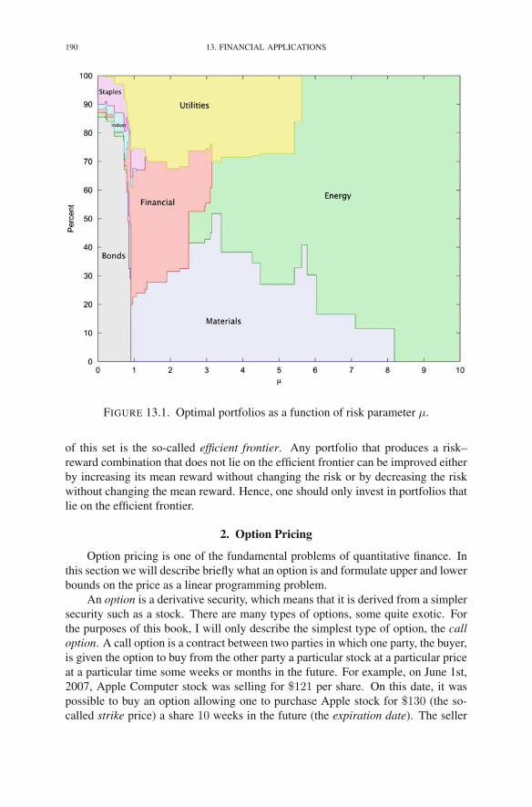
190 13. FINANCIAL APPLICATIONS
FIGURE 13.1. Optimal portfolios as a function of risk parameter μ.
of this set is the so-called efficient frontier. Any portfolio that produces a risk–reward combination that does not lie on the efficient frontier can be improved eitherby increasing its mean reward without changing the risk or by decreasing the riskwithout changing the mean reward. Hence, one should only invest in portfolios thatlie on the efficient frontier.
2. Option Pricing
Option pricing is one of the fundamental problems of quantitative finance. Inthis section we will describe briefly what an option is and formulate upper and lowerbounds on the price as a linear programming problem.
An option is a derivative security, which means that it is derived from a simplersecurity such as a stock. There are many types of options, some quite exotic. Forthe purposes of this book, I will only describe the simplest type of option, the calloption. A call option is a contract between two parties in which one party, the buyer,is given the option to buy from the other party a particular stock at a particular priceat a particular time some weeks or months in the future. For example, on June 1st,2007, Apple Computer stock was selling for $121 per share. On this date, it waspossible to buy an option allowing one to purchase Apple stock for $130 (the so-called strike price) a share 10 weeks in the future (the expiration date). The seller

2. OPTION PRICING 191
FIGURE 13.2. The efficient frontier.
was offering this contract for a price of $3.20. Where does this price come from?The simple answer is that it is determined solely by the marketplace, since optioncontract themselves can be bought and sold up until their expiration date. But, astechnical folks, we seek an analytical formula that tells us what a fair price ought tobe. This we can do.
To explain how to price the option, we need to think a little bit more about thevalue of the option on the date of expiration. If Apple stock does well over thenext 10 weeks and ends up at $140 per share, then on the day of expiration I canexercise the contract and buy the stock for $130. I can then immediately sell thestock for $140 and pocket the $10 difference. Of course, I paid $3.20 for the rightto do this. Hence, my net profit is $6.80. Now, suppose instead of rising to $140per share, the stock only climbs to $132 per share. In this case, I will still want toexercise the option because I can pocket a $2 difference. But, after subtracting thecost of the option, I’ve actually lost a modest $1.20 per share. Finally, suppose thatthe stock only goes up to $125 per share. In this case, I will let the option expirewithout exercising it. I will have lost only the $3.20 that I originally paid for theoption. Finally, consider the case where in the intervening 10 weeks some reallybad news surfaces that drives Apple stock down to $100 per share. Had I actuallybought Apple stock, I would now be out $21 per share, which could be a substantialamount of money if I had bought lots of shares. But, by buying the option, I’m only

192 13. FINANCIAL APPLICATIONS
100 110 120 130 140 150 160-5
0
5
10
15
20
25
30
FIGURE 13.3. A graph of the value of the option at expiration asa function of stock price. In this example, the strike price is $130.
out $3.20 per share. This is the attraction of call options. They allow an investorwho is optimistic about the economy (or a particular company) to take a chancewithout risking much on the down side. Figure 13.3 shows a plot of the net profitper share as a function of the share price at expiration.
Let s0 denote the (known) current stock price and let S1 denote the (not yetknown, i.e., random) stock price at expiration. A key feature of options is that theirvalue at the expiration date is given by a specific function h(S1) of the stock priceat expiration. For the specific call option discussed above, the function h(S1) isthe “hockey-stick” shaped function shown in Figure 13.3. If we think we know thedistribution of the random variable S1, then we could compute its expected valueand, if we ignore the discounting for inflation, we could use this to price the option:
p = Eh(S1).
Unfortunately, we generally don’t know the distribution of S1.We can, however, make some indirect inferences based on “market wisdom”
that constrain the possible values for p and thereby implicitly tell us somethingabout the distribution of S1. Specifically, let us imagine that there are already anumber of options being traded in the market that are based on the same underlyingstock and have the same expiration date. Let us suppose that there are already noptions being traded in the market with known prices. That is, there are specificfunctions hj(S1), j = 1, 2, . . . , n, for which there are already known prices pj .One can think of the underlying stock itself as the simplest possible option. Sincethe stock is traded, it too provides some information about the future. We assume

2. OPTION PRICING 193
that this trivial asset is the j = 1 option in the collection of known priced options.For this option, we have h1(S1) = S1 and p1 = s0. To these n options, we add onemore: cash. One dollar today will be worth one dollar on the expiration date (again,we are ignoring here the time value of money). In a sense, this is also and option.
The problem we wish to consider is how to price a new option whose payoutfunction we denote by g(S1). Consider building a portfolio of the available optionsconsisting of x0 “shares” of dollars, x1 shares of the underlying stock, and xj sharesof option j (j = 2, . . . , n). Today, this portfolio costs
x0 + x1s0 +
n∑
j=2
xjpj .
At the expiration date, the portolio’s value will be
x0 + x1S1 +
n∑
j=2
xjhj(S1).
Suppose that no matter how S1 turns out, the value of the new option dominates thatof the portfolio:
x0 + x1S1 +n∑
j=2
xjhj(S1) ≤ g(S1).
Then, it must be the case that the price p of the new option today must also dominatethe cost of this portfolio:
x0 + x1s0 +n∑
j=2
xjpj ≤ p.
This is called a no-arbitrage condition. This no-arbitrage condition implies a lowerbound p on the price of the new option, which we can maximize:
maximize x0 + x1s0 +
n∑
j=2
xjpj
subject to x0 + x1S1 +n∑
j=2
xjhj(S1)≤ g(S1).
This problem actually has an infinite number of constraints because the inequalitymust hold no matter what value S1 takes on. It can be made into a linear program-ming problem by introducing a finite set of possible values, say s1(1), s1(2), . . . ,s1(m). The resulting linear programming problem can thus be written as
(13.4)
maximize p = x0 + x1s0 +n∑
j=2
xjpj
subject to x0 + x1s1(i) +
n∑
j=2
xjhj(s1(i))≤ g(s1(i)), i = 1, . . . ,m.
In a completely analogous manner we can find a tight upper bound p for p by solvinga minimization problem:
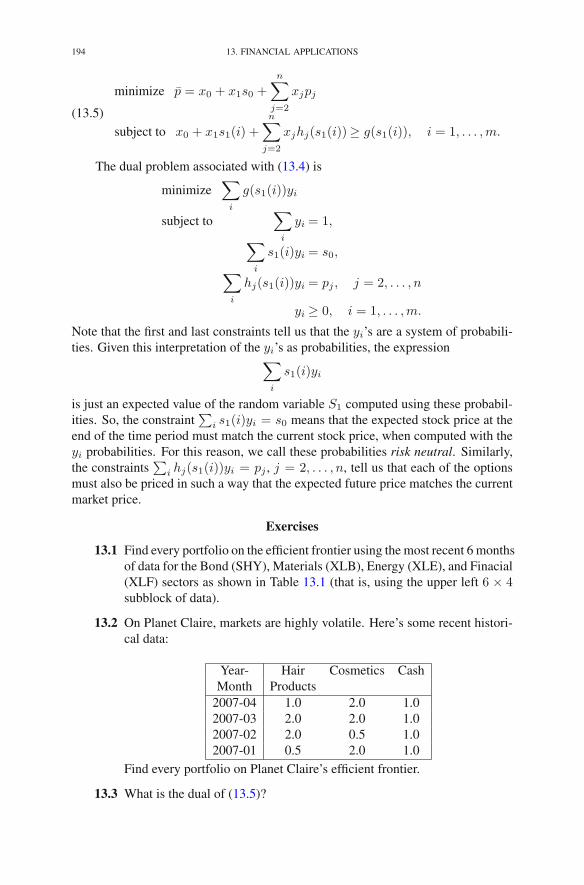
194 13. FINANCIAL APPLICATIONS
(13.5)
minimize p = x0 + x1s0 +
n∑
j=2
xjpj
subject to x0 + x1s1(i) +
n∑
j=2
xjhj(s1(i))≥ g(s1(i)), i = 1, . . . ,m.
The dual problem associated with (13.4) is
minimize∑
i
g(s1(i))yi
subject to∑
i
yi = 1,
∑
i
s1(i)yi = s0,
∑
i
hj(s1(i))yi = pj , j = 2, . . . , n
yi ≥ 0, i = 1, . . . ,m.
Note that the first and last constraints tell us that the yi’s are a system of probabili-ties. Given this interpretation of the yi’s as probabilities, the expression
∑
i
s1(i)yi
is just an expected value of the random variable S1 computed using these probabil-ities. So, the constraint
∑i s1(i)yi = s0 means that the expected stock price at the
end of the time period must match the current stock price, when computed with theyi probabilities. For this reason, we call these probabilities risk neutral. Similarly,the constraints
∑i hj(s1(i))yi = pj , j = 2, . . . , n, tell us that each of the options
must also be priced in such a way that the expected future price matches the currentmarket price.
Exercises
13.1 Find every portfolio on the efficient frontier using the most recent 6 monthsof data for the Bond (SHY), Materials (XLB), Energy (XLE), and Finacial(XLF) sectors as shown in Table 13.1 (that is, using the upper left 6 × 4subblock of data).
13.2 On Planet Claire, markets are highly volatile. Here’s some recent histori-cal data:
Year- Hair Cosmetics CashMonth Products
2007-04 1.0 2.0 1.02007-03 2.0 2.0 1.02007-02 2.0 0.5 1.02007-01 0.5 2.0 1.0
Find every portfolio on Planet Claire’s efficient frontier.
13.3 What is the dual of (13.5)?

NOTES 195
Notes
The portfolio selection problem originates with Markowitz (1959). He won the1990 Nobel prize in Economics for this work. In its original formulation, risk ismodeled by the variance of the portfolio’s value rather than the absolute deviationfrom the mean considered here. We will discuss the quadratic formulation later inChapter 24.
The MAD risk measure we have considered in this chapter has many nice prop-erties the most important of which is that it produces portfolios that are guaranteednot to be stochastically dominated (to second order) by other portfolios. Many riskmeasures fail to possess this important property. See Ruszczynski and Vanderbei(2003) for details.

Part 2
Network-Type Problems

Allow me to say, . . . , that the arguments withwhich you have supported this extraordinary
application have been as frivolous as theapplication was ill-judged. — J. Austen

CHAPTER 14
Network Flow Problems
Many linear programming problems can be viewed as a problem of minimizingthe “transportation” cost of moving materials through a network to meet demandsfor material at various locations given sources of material at other locations. Suchproblems are called network flow problems. They form the most important specialclass of linear programming problems. Transportation, electric, and communicationnetworks provide obvious examples of application areas. Less obvious, but justas important, are applications in facilities location, resource management, financialplanning, and others.
In this chapter we shall formulate a special type of linear programming problemcalled the minimum-cost network flow problem. It turns out that the simplex methodwhen applied to this problem has a very simple description and some important spe-cial properties. Implementations that exploit these properties benefit dramatically.
1. Networks
A network consists of two types of objects: nodes and arcs. We shall let Ndenote the set of nodes. We let m denote the number of nodes (i.e., the cardinalityof the set N ).
The nodes are connected by arcs. Arcs are assumed to be directed. This meansthat an arc connecting node i to node j is not the same as an arc connecting node jto node i. For this reason, we denote arcs using the standard mathematical notationfor ordered pairs. That is, the arc connecting node i to node j is denoted simply as(i, j). We let A denote the set of all arcs in the network. This set is a subset of theset of all possible arcs:
A ⊂ {(i, j) : i, j ∈ N , i �= j}.In typical networks, the set A is much smaller than the set of all arcs. In fact, usuallyeach node is only connected to a handful of “nearby” nodes.
The pair (N ,A) is called a network. It is also sometimes called a graph ora digraph (to emphasize the fact that the arcs are directed). Figure 14.1 shows anetwork having 7 nodes and 14 arcs.
To specify a network flow problem, we need to indicate the supply of (or de-mand for) material at each node. So, for each i ∈ N , let bi denote the amountof material being supplied to the network at node i. We shall use the convention
The original version of this chapter was revised. An erratum to this chapter can be found at DOI10.1007/978-1-4614-7630-6 26
R.J. Vanderbei, Linear Programming, International Series in Operations Research& Management Science 196, DOI 10.1007/978-1-4614-7630-6 14,© Springer Science+Business Media New York 2014
199

200 14. NETWORK FLOW PROBLEMS
a e
d
c b
f g5
−2
−6
−6
9
FIGURE 14.1. A network having 7 nodes and 14 arcs. The num-bers written next to the nodes denote the supply at the node (neg-ative values indicate demands; missing values indicate no supplyor demand).
that negative supplies are in fact demands. Hence, our problem will be to move thematerial that sits at the supply nodes over to the demand nodes. The movementsmust be along the arcs of the network (and adhering to the directions of the arcs).Since, except for the supply and demand, there is no other way for material to enteror leave the system, it follows that the total supply must equal the total demand forthe problem to have a feasible solution. Hence, we shall always assume that
∑
i∈Nbi = 0.
To help us decide the paths along which materials should move, we assumethat each arc, say, (i, j), has associated with it a cost cij that represents the cost ofshipping one unit from i to j directly along arc (i, j). The decision variables thenare how much material to ship along each arc. That is, for each (i, j) ∈ A, xij willdenote the quantity shipped directly from i to j along arc (i, j). The objective is tominimize the total cost of moving the supply to meet the demand:
minimize∑
(i,j)∈Acijxij .
As we mentioned before, the constraints on the decision variables are that theyensure flow balance at each node. Let us consider a fixed node, say, k ∈ N . Thetotal flow into node k is given by
∑
i:(i,k)∈A
xik.

1. NETWORKS 201
a e
d
c b
f g
10
56
108 48
24
33
19
7387
48
15
65
28
FIGURE 14.2. The costs on the arcs for the network in Figure 14.1.
Similarly, the total flow out from node k is∑
j:(k,j)∈A
xkj .
The difference between these two quantities is the net inflow, which must be equalto the demand at the node. Hence, the flow balance constraints can be written as
∑
i:(i,k)∈A
xik −∑
j:(k,j)∈A
xkj = −bk, k ∈ N .
Finally, the flow on each arc must be nonnegative (otherwise it would be going inthe wrong direction):
xij ≥ 0, (i, j) ∈ A.
Figure 14.2 shows cost information for the network shown in Figure 14.1. Inmatrix notation, the problem can be written as follows:
(14.1)minimize cTxsubject to Ax= −b
x≥ 0,
wherexT =
[xac xad xae xba xbc xbe xdb xde xfa xfb xfc xfg xgb xge
],
A=
⎡
⎢⎢⎢⎢⎢⎢⎢⎢⎣
−1 −1 −1 1 1−1 −1 −1 1 1 1
1 1 11 −1 −1
1 1 1 1−1 −1 −1 −1
1 −1 −1
⎤
⎥⎥⎥⎥⎥⎥⎥⎥⎦
, b =
⎡
⎢⎢⎢⎢⎢⎢⎢⎢⎣
00
−6−6−295
⎤
⎥⎥⎥⎥⎥⎥⎥⎥⎦
,
cT =[
48 28 10 7 65 7 38 15 56 48 108 24 33 19].

202 14. NETWORK FLOW PROBLEMS
In network flow problems, the constraint matrix A is called the node–arc inci-dence matrix.
The network flow problem differs from our usual standard form linear pro-gramming problem in two respects: (1) it is a minimization instead of a maximiza-tion and (2) the constraints are equalities instead of inequalities. Nonetheless, wehave studied before how duality applies to problems in nonstandard form. The dualof (14.1) is
maximize −bT y
subject to AT y + z = cz ≥ 0.
Written in network notation, the dual is
maximize −∑
i∈Nbiyi
subject to yj − yi + zij = cij , (i, j) ∈ Azij ≥ 0, (i, j) ∈ A.
Finally, it is not hard to check that the complementarity conditions (to be satisfiedby an optimal primal–dual solution pair) are
xijzij = 0, (i, j) ∈ A.
We shall often refer to the primal variables as primal flows.
2. Spanning Trees and Bases
Network flow problems can be solved efficiently because the basis matriceshave a special structure that can be described nicely in terms of the network. Inorder to explain this structure, we need to introduce a number of definitions.
First of all, an ordered list of nodes (n1, n2, . . . , nk) is called a path in the net-work if each adjacent pair of nodes in the list is connected by an arc in the network.It is important to note that we do not assume that the arcs point in any particulardirection. For example, for nodes ni and ni+1, there must be an arc in the network.It could run either from ni to ni+1 or from ni+1 to ni. (One should think aboutone-way roads—even though cars can only go one way, pedestrians are allowed towalk along the path of the road in either direction.) A network is called connected ifthere is a path connecting every pair of nodes (see Figure 14.3). For the remainderof this chapter, we make the following assumption:
Assumption. The network is connected.
For any arc (i, j), we refer to i as its tail and j as its head.A cycle is a path in which the last node coincides with the first node. A network
is called acyclic if it does not contain any cycles (see Figure 14.4).A network is a tree if it is connected and acyclic (see Figure 14.5). A network
(N , A) is called a subnetwork of (N ,A) if N ⊂ N and A ⊂ A. A subnetwork(N , A) is a spanning tree if it is a tree and N = N . Since a spanning tree’s nodeset coincides with the node set of the underlying network, it suffices to refer to aspanning tree by simply giving its arc set.

2. SPANNING TREES AND BASES 203
FIGURE 14.3. The network on the left is connected whereas theone on the right is not.
FIGURE 14.4. The network on the left contains a cycle whereasthe one on the right is acyclic.
FIGURE 14.5. The network on the left is a tree whereas the twoon the right not—they fail in the first case by being disconnectedand in the second by containing a cycle.
Given a network flow problem, any selection of primal flow values that satisfiesthe balance equations at every node will be called a balanced flow. It is important tonote that we do not require the flows to be nonnegative to be a balanced flow. Thatis, we allow flows to go in the wrong direction. If all the flows are nonnegative,then a balanced flow is called a feasible flow. Given a spanning tree, a balancedflow that assigns zero flow to every arc not on the spanning tree will be called atree solution. Consider, for example, the tree shown in Figure 14.6. The num-bers shown on the arcs of the spanning tree give the tree solution corresponding tothe supplies/demands shown in Figure 14.1. They were obtained by starting at the
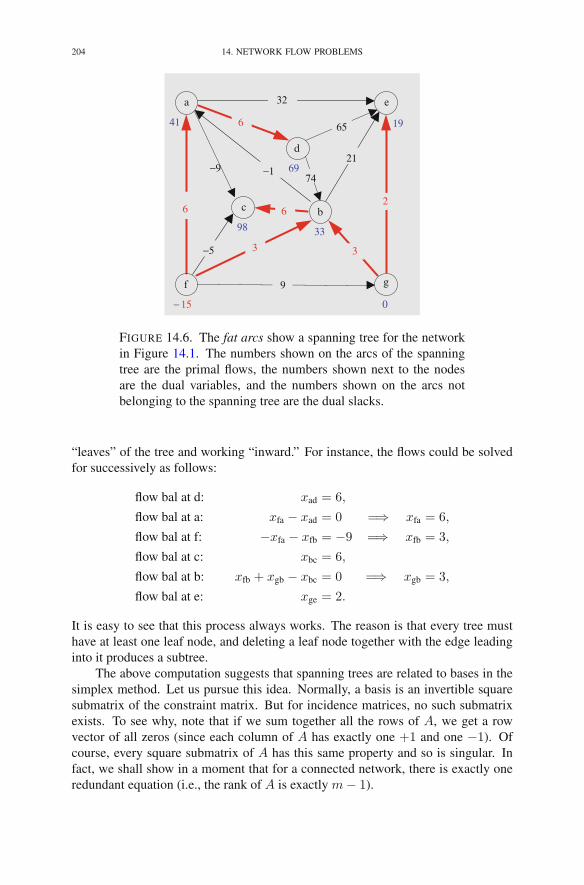
204 14. NETWORK FLOW PROBLEMS
a e
d
c b
f g
6
−5 3 3
2
21−1−9
6
641
− 15
98
19
0
33
6974
32
9
65
FIGURE 14.6. The fat arcs show a spanning tree for the networkin Figure 14.1. The numbers shown on the arcs of the spanningtree are the primal flows, the numbers shown next to the nodesare the dual variables, and the numbers shown on the arcs notbelonging to the spanning tree are the dual slacks.
“leaves” of the tree and working “inward.” For instance, the flows could be solvedfor successively as follows:
flow bal at d: xad = 6,
flow bal at a: xfa − xad = 0 =⇒ xfa = 6,
flow bal at f: −xfa − xfb = −9 =⇒ xfb = 3,
flow bal at c: xbc = 6,
flow bal at b: xfb + xgb − xbc = 0 =⇒ xgb = 3,
flow bal at e: xge = 2.
It is easy to see that this process always works. The reason is that every tree musthave at least one leaf node, and deleting a leaf node together with the edge leadinginto it produces a subtree.
The above computation suggests that spanning trees are related to bases in thesimplex method. Let us pursue this idea. Normally, a basis is an invertible squaresubmatrix of the constraint matrix. But for incidence matrices, no such submatrixexists. To see why, note that if we sum together all the rows of A, we get a rowvector of all zeros (since each column of A has exactly one +1 and one −1). Ofcourse, every square submatrix of A has this same property and so is singular. Infact, we shall show in a moment that for a connected network, there is exactly oneredundant equation (i.e., the rank of A is exactly m− 1).
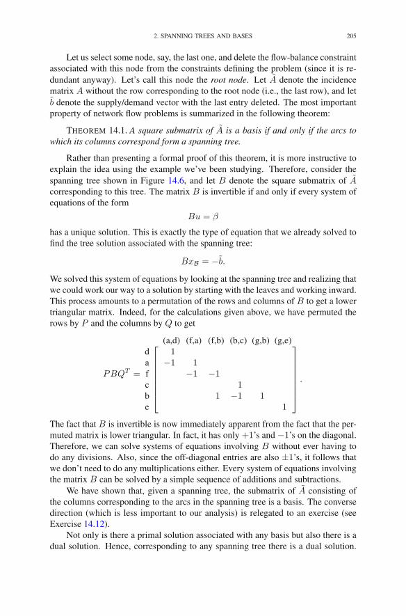
2. SPANNING TREES AND BASES 205
Let us select some node, say, the last one, and delete the flow-balance constraintassociated with this node from the constraints defining the problem (since it is re-dundant anyway). Let’s call this node the root node. Let A denote the incidencematrix A without the row corresponding to the root node (i.e., the last row), and letb denote the supply/demand vector with the last entry deleted. The most importantproperty of network flow problems is summarized in the following theorem:
THEOREM 14.1. A square submatrix of A is a basis if and only if the arcs towhich its columns correspond form a spanning tree.
Rather than presenting a formal proof of this theorem, it is more instructive toexplain the idea using the example we’ve been studying. Therefore, consider thespanning tree shown in Figure 14.6, and let B denote the square submatrix of Acorresponding to this tree. The matrix B is invertible if and only if every system ofequations of the form
Bu = β
has a unique solution. This is exactly the type of equation that we already solved tofind the tree solution associated with the spanning tree:
BxB = −b.
We solved this system of equations by looking at the spanning tree and realizing thatwe could work our way to a solution by starting with the leaves and working inward.This process amounts to a permutation of the rows and columns of B to get a lowertriangular matrix. Indeed, for the calculations given above, we have permuted therows by P and the columns by Q to get
PBQT =
(a,d) (f,a) (f,b) (b,c) (g,b) (g,e)dafcbe
⎡
⎢⎢⎢⎢⎢⎢⎣
1−1 1
−1 −11
1 −1 11
⎤
⎥⎥⎥⎥⎥⎥⎦
.
The fact that B is invertible is now immediately apparent from the fact that the per-muted matrix is lower triangular. In fact, it has only +1’s and −1’s on the diagonal.Therefore, we can solve systems of equations involving B without ever having todo any divisions. Also, since the off-diagonal entries are also ±1’s, it follows thatwe don’t need to do any multiplications either. Every system of equations involvingthe matrix B can be solved by a simple sequence of additions and subtractions.
We have shown that, given a spanning tree, the submatrix of A consisting ofthe columns corresponding to the arcs in the spanning tree is a basis. The conversedirection (which is less important to our analysis) is relegated to an exercise (seeExercise 14.12).
Not only is there a primal solution associated with any basis but also there is adual solution. Hence, corresponding to any spanning tree there is a dual solution.
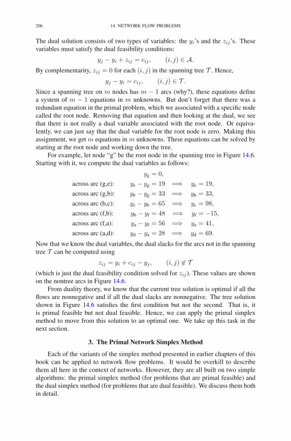
206 14. NETWORK FLOW PROBLEMS
The dual solution consists of two types of variables: the yi’s and the zij’s. Thesevariables must satisfy the dual feasibility conditions:
yj − yi + zij = cij , (i, j) ∈ A.
By complementarity, zij = 0 for each (i, j) in the spanning tree T . Hence,
yj − yi = cij , (i, j) ∈ T .
Since a spanning tree on m nodes has m − 1 arcs (why?), these equations definea system of m − 1 equations in m unknowns. But don’t forget that there was aredundant equation in the primal problem, which we associated with a specific nodecalled the root node. Removing that equation and then looking at the dual, we seethat there is not really a dual variable associated with the root node. Or equiva-lently, we can just say that the dual variable for the root node is zero. Making thisassignment, we get m equations in m unknowns. These equations can be solved bystarting at the root node and working down the tree.
For example, let node “g” be the root node in the spanning tree in Figure 14.6.Starting with it, we compute the dual variables as follows:
yg = 0,
across arc (g,e): ye − yg = 19 =⇒ ye = 19,
across arc (g,b): yb − yg = 33 =⇒ yb = 33,
across arc (b,c): yc − yb = 65 =⇒ yc = 98,
across arc (f,b): yb − yf = 48 =⇒ yf = −15,
across arc (f,a): ya − yf = 56 =⇒ ya = 41,
across arc (a,d): yd − ya = 28 =⇒ yd = 69.
Now that we know the dual variables, the dual slacks for the arcs not in the spanningtree T can be computed using
zij = yi + cij − yj , (i, j) �∈ T(which is just the dual feasibility condition solved for zij). These values are shownon the nontree arcs in Figure 14.6.
From duality theory, we know that the current tree solution is optimal if all theflows are nonnegative and if all the dual slacks are nonnegative. The tree solutionshown in Figure 14.6 satisfies the first condition but not the second. That is, itis primal feasible but not dual feasible. Hence, we can apply the primal simplexmethod to move from this solution to an optimal one. We take up this task in thenext section.
3. The Primal Network Simplex Method
Each of the variants of the simplex method presented in earlier chapters of thisbook can be applied to network flow problems. It would be overkill to describethem all here in the context of networks. However, they are all built on two simplealgorithms: the primal simplex method (for problems that are primal feasible) andthe dual simplex method (for problems that are dual feasible). We discuss them bothin detail.
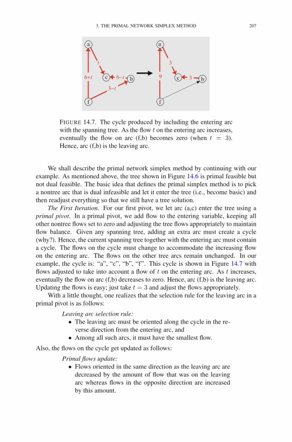
3. THE PRIMAL NETWORK SIMPLEX METHOD 207
a
c b
f
6+t
t
6−t
a
c b
f
9
3
3
3−t
FIGURE 14.7. The cycle produced by including the entering arcwith the spanning tree. As the flow t on the entering arc increases,eventually the flow on arc (f,b) becomes zero (when t = 3).Hence, arc (f,b) is the leaving arc.
We shall describe the primal network simplex method by continuing with ourexample. As mentioned above, the tree shown in Figure 14.6 is primal feasible butnot dual feasible. The basic idea that defines the primal simplex method is to picka nontree arc that is dual infeasible and let it enter the tree (i.e., become basic) andthen readjust everything so that we still have a tree solution.
The First Iteration. For our first pivot, we let arc (a,c) enter the tree using aprimal pivot. In a primal pivot, we add flow to the entering variable, keeping allother nontree flows set to zero and adjusting the tree flows appropriately to maintainflow balance. Given any spanning tree, adding an extra arc must create a cycle(why?). Hence, the current spanning tree together with the entering arc must containa cycle. The flows on the cycle must change to accommodate the increasing flowon the entering arc. The flows on the other tree arcs remain unchanged. In ourexample, the cycle is: “a”, “c”, “b”, “f”. This cycle is shown in Figure 14.7 withflows adjusted to take into account a flow of t on the entering arc. As t increases,eventually the flow on arc (f,b) decreases to zero. Hence, arc (f,b) is the leaving arc.Updating the flows is easy; just take t = 3 and adjust the flows appropriately.
With a little thought, one realizes that the selection rule for the leaving arc in aprimal pivot is as follows:
Leaving arc selection rule:• The leaving arc must be oriented along the cycle in the re-
verse direction from the entering arc, and• Among all such arcs, it must have the smallest flow.
Also, the flows on the cycle get updated as follows:
Primal flows update:• Flows oriented in the same direction as the leaving arc are
decreased by the amount of flow that was on the leavingarc whereas flows in the opposite direction are increasedby this amount.

208 14. NETWORK FLOW PROBLEMS
a e
d
c b
f g
?
?
??
?
3
2
21?
??
?
?
6?
?
98
19
0
33
?
FIGURE 14.8. The two disjoint trees. Primal and dual values thatremained unchanged are shown, whereas those that need to beupdated are shown as question marks.
The next issue is how to update the dual variables. To this end, note that ifwe delete the leaving arc from the spanning tree (without concurrently adding theentering arc), we disconnect it into two disjoint trees. In our example, one treecontains nodes “a”, “d” and “f” while the second tree contains the other nodes.Figure 14.8 shows the two disjoint trees. Recalling that the dual variables are calcu-lated starting with the root node and working up the spanning tree, it is clear that thedual variables on the subtree containing the root node remain unchanged, whereasthose on the other subtree must change. For the current pivot, the other subtreeconsists of nodes “a”, “d”, and “f”. They all get incremented by the same fixedamount, since the only change is that the arc by which we bridged from the root-containing tree to this other tree has changed from the leaving arc to the enteringarc. Looking at node “a” and using tildes to denote values after being changed, wesee that
ya = yc − cac
= yc − cac,
whereaszac = ya + cac − yc.
Combining these two equations, we get
ya = ya − zac.
That is, the dual variable at node “a” gets decremented by zac = −9. Of course,all of the dual variables on this subtree get decremented by this same amount. Ingeneral, the dual variable update rule can be stated as follows:

3. THE PRIMAL NETWORK SIMPLEX METHOD 209
a e
d
c b
f g
41
9
4 9
18
3
2
21
83−103
74
3
650
−6
98
19
0
33
78
FIGURE 14.9. The tree solution at the end of the first iteration.
Dual variables update:• If the entering arc crosses from the root-containing tree to
the non-root-containing tree, then increase all dual vari-ables on the non-root-containing tree by the dual slack ofthe entering arc.
• Otherwise, decrease these dual variables by this amount.
Finally, we must update the dual slacks. The only dual slacks that change arethose that span across the two trees since, for these nodes, either the head or the taildual variable changes, while the other does not. Those that span the two subtreesin the same direction as the entering arc must be decreased by zac, whereas thosethat bridge the two trees in the opposite direction must be increased by this amount.For our example, six nontree arcs, (f,g), (f,b), (f,c), (d,b), (d,e), and (a,e), span inthe same direction as the entering arc. They all must be decreased by −9. That is,they must be increased by 9. For example, the dual slack on arc (f,c) changes from−5 to 4. Only one arc, (b,a), spans in the other direction. It must be decreased by9. The updated solution is shown in Figure 14.9. The general rule for updating thedual slacks is as follows:
Dual slacks update:• The dual slacks corresponding to those arcs that bridge in
the same direction as the entering arc get decremented bythe old dual slack on the entering arc, whereas those thatcorrespond to arcs bridging in the opposite direction getincremented by this amount.
The Second Iteration. The tree solution shown in Figure 14.9 has only oneremaining infeasibility: zba = −10. Arc (b,a) must therefore enter the spanningtree. Adding it, we create a cycle consisting of nodes “a”, “b”, and “c”. The leaving
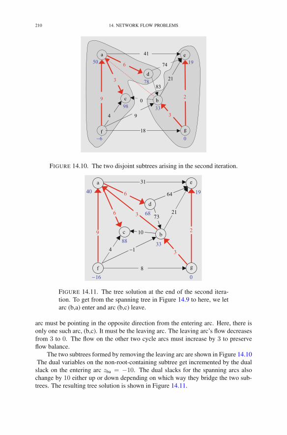
210 14. NETWORK FLOW PROBLEMS
83
a e
d
c b
f g
41
9
4 9
18
3
2
213
74
0
650
−6
98
19
0
33
78
FIGURE 14.10. The two disjoint subtrees arising in the second iteration.
a e
d
c b
f g
9
4
8
3
2
2136
640
−16
88
19
0
33
68
64
31
10
73
−1
FIGURE 14.11. The tree solution at the end of the second itera-tion. To get from the spanning tree in Figure 14.9 to here, we letarc (b,a) enter and arc (b,c) leave.
arc must be pointing in the opposite direction from the entering arc. Here, there isonly one such arc, (b,c). It must be the leaving arc. The leaving arc’s flow decreasesfrom 3 to 0. The flow on the other two cycle arcs must increase by 3 to preserveflow balance.
The two subtrees formed by removing the leaving arc are shown in Figure 14.10The dual variables on the non-root-containing subtree get incremented by the dual
slack on the entering arc zba = −10. The dual slacks for the spanning arcs alsochange by 10 either up or down depending on which way they bridge the two sub-trees. The resulting tree solution is shown in Figure 14.11.

4. THE DUAL NETWORK SIMPLEX METHOD 211
a e
d
c b
f g
1
5 9 3
2
21126
640
− 15
88
19
0
33
68
31
10
9
73
64
FIGURE 14.12. The tree solution at the end of the third iteration.To get from the spanning tree in Figure 14.11 to here, we let arc(f,b) enter and arc (f,a) leave. This tree solution is the optimalsolution to the problem.
The Third and Final Iteration. The tree solution shown in Figure 14.11 hasone infeasibility: zfb = −1. Hence, arc (f,b) must enter the spanning tree. Theleaving arc must be (f,a). Leaving the details of updating to the reader, the resultingtree solution is shown in Figure 14.12. It is both primal and dual feasible—henceoptimal.
4. The Dual Network Simplex Method
In the previous section, we developed simple rules for the primal network sim-plex method, which is used in situations where the tree solution is primal feasiblebut not dual feasible. When a tree solution is dual feasible but not primal feasible,then the dual network simplex method can be used. We shall define this methodnow. Consider the tree solution shown in Figure 14.13. It is dual feasible but notprimal feasible (since xdb < 0). The basic idea that defines the dual simplex methodis to pick a tree arc that is primal infeasible and let it leave the spanning tree (i.e.,become nonbasic) and then readjust everything to preserve dual feasibility.
The First Iteration. For the first iteration, we need to let arc (d,b) leave thespanning tree using a dual pivot, which is defined as follows. Removing arc (d,b)disconnects the spanning tree into two disjoint subtrees. The entering arc must beone of the arcs that spans across the two subtrees so that it can reconnect them intoa spanning tree. That is, it must be one of
(a,e), (a,d), (b,e), or (g,e).
See Figure 14.14. To see how to decide which it must be, we need to considercarefully the impact of each possible choice.

212 14. NETWORK FLOW PROBLEMS
a e
d
c b
f g
1
5 9 5
9
30−8
66
27340
−15
88
10
0
33
10
−5
9
40
FIGURE 14.13. A tree solution that is dual feasible but not primal feasible.
a e
d
c b
f g
1
5 9 5
9
3066
27340
−15
88
10
0
33
−5
9
40
10
FIGURE 14.14. The two subtrees for the first pivot of the dualsimplex method.
To this end, let us consider the general situation. As mentioned above, the span-ning tree with the leaving arc removed consists of two disjoint trees. The enteringarc must reconnect these two trees.
First, consider a reconnecting arc that connects in the same direction as theleaving arc. When we add flow to this prospective entering arc, we will have todecrease flow on the leaving arc to maintain flow balance. Therefore, the leaving

4. THE DUAL NETWORK SIMPLEX METHOD 213
a e
d
c b
f g
31
1
5 9
9
−3
8
21966
−6
10
6440
−15
88
19
0
33
4
FIGURE 14.15. The tree solution after the first pivot.
arc’s flow, which is currently negative, can’t be raised to zero. That is, the leavingarc can’t leave. This is no good.
Now suppose that the reconnecting arc connects in the opposite direction. Ifit were to be the entering arc, then its dual slack would drop to zero. All otherreconnecting arcs pointing in the same direction would drop by the same amount.To maintain nonnegativity of all the others, we must pick the one that drops theleast. We can summarize the rule as follows:
Entering arc selection rule:• The entering arc must bridge the two subtrees in the oppo-
site direction from the leaving arc, and• Among all such arcs, it must have the smallest dual slack.
In our example, all bridging arcs point in the opposite direction from the leavingarc. The one with the smallest dual slack is (g,e) whose slack is zge = 9. This arcmust be the entering arc.
We have now determined both the entering and leaving arcs. Hence, the newspanning tree is determined and therefore, in principle, all the variables associatedwith this new spanning tree can be computed. Furthermore, the rules for determin-ing the new values by updating from the previous ones are the same as in the primalnetwork simplex method. The resulting tree solution is shown in Figure 14.15.
The Second Iteration. For the second pivot, there are two choices for the leavingarc: (g,b) and (d,e). Using the most infeasible, we choose (d,e). We remove this arcfrom the spanning tree to produce two subtrees. One of the subtrees consists of justthe node “d” all by itself while the other subtree consists of the rest of the nodes.Remembering that the reconnecting arc must bridge the two subtrees in the oppositedirection, the only choice is (a,d). So this arc is the entering arc. Making the pivot,we arrive at the optimal tree solution shown in Figure 14.12.
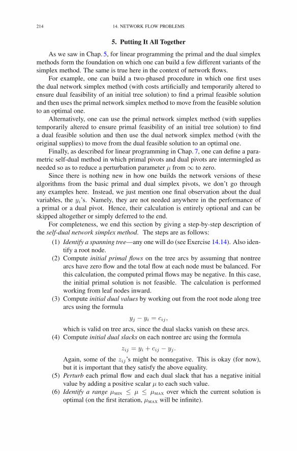
214 14. NETWORK FLOW PROBLEMS
5. Putting It All Together
As we saw in Chap. 5, for linear programming the primal and the dual simplexmethods form the foundation on which one can build a few different variants of thesimplex method. The same is true here in the context of network flows.
For example, one can build a two-phased procedure in which one first usesthe dual network simplex method (with costs artificially and temporarily altered toensure dual feasibility of an initial tree solution) to find a primal feasible solutionand then uses the primal network simplex method to move from the feasible solutionto an optimal one.
Alternatively, one can use the primal network simplex method (with suppliestemporarily altered to ensure primal feasibility of an initial tree solution) to finda dual feasible solution and then use the dual network simplex method (with theoriginal supplies) to move from the dual feasible solution to an optimal one.
Finally, as described for linear programming in Chap. 7, one can define a para-metric self-dual method in which primal pivots and dual pivots are intermingled asneeded so as to reduce a perturbation parameter μ from ∞ to zero.
Since there is nothing new in how one builds the network versions of thesealgorithms from the basic primal and dual simplex pivots, we don’t go throughany examples here. Instead, we just mention one final observation about the dualvariables, the yi’s. Namely, they are not needed anywhere in the performance ofa primal or a dual pivot. Hence, their calculation is entirely optional and can beskipped altogether or simply deferred to the end.
For completeness, we end this section by giving a step-by-step description ofthe self-dual network simplex method. The steps are as follows:
(1) Identify a spanning tree—any one will do (see Exercise 14.14). Also iden-tify a root node.
(2) Compute initial primal flows on the tree arcs by assuming that nontreearcs have zero flow and the total flow at each node must be balanced. Forthis calculation, the computed primal flows may be negative. In this case,the initial primal solution is not feasible. The calculation is performedworking from leaf nodes inward.
(3) Compute initial dual values by working out from the root node along treearcs using the formula
yj − yi = cij ,
which is valid on tree arcs, since the dual slacks vanish on these arcs.(4) Compute initial dual slacks on each nontree arc using the formula
zij = yi + cij − yj .
Again, some of the zij’s might be nonnegative. This is okay (for now),but it is important that they satisfy the above equality.
(5) Perturb each primal flow and each dual slack that has a negative initialvalue by adding a positive scalar μ to each such value.
(6) Identify a range μMIN ≤ μ ≤ μMAX over which the current solution isoptimal (on the first iteration, μMAX will be infinite).
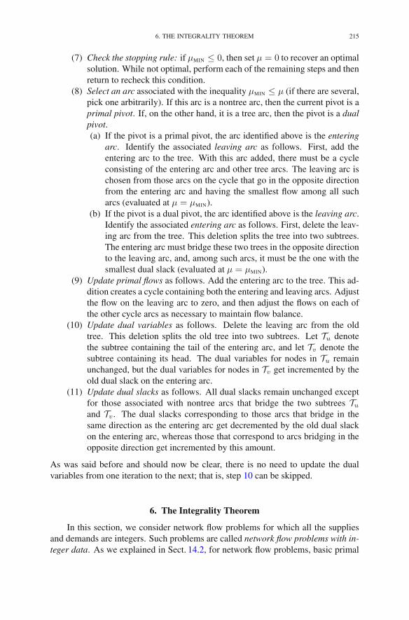
6. THE INTEGRALITY THEOREM 215
(7) Check the stopping rule: if μMIN ≤ 0, then set μ = 0 to recover an optimalsolution. While not optimal, perform each of the remaining steps and thenreturn to recheck this condition.
(8) Select an arc associated with the inequality μMIN ≤ μ (if there are several,pick one arbitrarily). If this arc is a nontree arc, then the current pivot is aprimal pivot. If, on the other hand, it is a tree arc, then the pivot is a dualpivot.(a) If the pivot is a primal pivot, the arc identified above is the entering
arc. Identify the associated leaving arc as follows. First, add theentering arc to the tree. With this arc added, there must be a cycleconsisting of the entering arc and other tree arcs. The leaving arc ischosen from those arcs on the cycle that go in the opposite directionfrom the entering arc and having the smallest flow among all sucharcs (evaluated at μ = μMIN).
(b) If the pivot is a dual pivot, the arc identified above is the leaving arc.Identify the associated entering arc as follows. First, delete the leav-ing arc from the tree. This deletion splits the tree into two subtrees.The entering arc must bridge these two trees in the opposite directionto the leaving arc, and, among such arcs, it must be the one with thesmallest dual slack (evaluated at μ = μMIN).
(9) Update primal flows as follows. Add the entering arc to the tree. This ad-dition creates a cycle containing both the entering and leaving arcs. Adjustthe flow on the leaving arc to zero, and then adjust the flows on each ofthe other cycle arcs as necessary to maintain flow balance.
(10) Update dual variables as follows. Delete the leaving arc from the oldtree. This deletion splits the old tree into two subtrees. Let Tu denotethe subtree containing the tail of the entering arc, and let Tv denote thesubtree containing its head. The dual variables for nodes in Tu remainunchanged, but the dual variables for nodes in Tv get incremented by theold dual slack on the entering arc.
(11) Update dual slacks as follows. All dual slacks remain unchanged exceptfor those associated with nontree arcs that bridge the two subtrees Tuand Tv. The dual slacks corresponding to those arcs that bridge in thesame direction as the entering arc get decremented by the old dual slackon the entering arc, whereas those that correspond to arcs bridging in theopposite direction get incremented by this amount.
As was said before and should now be clear, there is no need to update the dualvariables from one iteration to the next; that is, step 10 can be skipped.
6. The Integrality Theorem
In this section, we consider network flow problems for which all the suppliesand demands are integers. Such problems are called network flow problems with in-teger data. As we explained in Sect. 14.2, for network flow problems, basic primal

216 14. NETWORK FLOW PROBLEMS
solutions are computed without any multiplication or division. The following im-portant theorem follows immediately from this property:
THEOREM 14.2. Integrality Theorem. For network flow problems with integerdata, every basic feasible solution and, in particular, every basic optimal solutionassigns integer flow to every arc.
This theorem is important because many real-world network flow problemshave integral supplies/demands and require their solutions to be integral too. Thisintegrality restriction typically occurs when one is shipping indivisible units througha network. For example, it wouldn’t make sense to ship one third of a car from anautomobile assembly plant to one dealership with the other two thirds going to an-other dealership.
Problems that are linear programming problems with the additional stipulationthat the optimal solution values must be integers are called integer programmingproblems. Generally speaking, these problems are much harder to solve than linearprogramming problems (see Chap. 23). However, if the problem is a network flowproblem with integer data, it can be solved efficiently using the simplex methodto compute a basic optimal solution, which the integrality theorem tells us will beinteger valued.
6.1. Konig’s Theorem. In addition to its importance in real-world optimiza-tion problems, the integrality theorem also has many applications to the branch ofmathematics called combinatorics. We illustrate with just one example.
THEOREM 14.3. Konig’s Theorem. Suppose that there are n girls and n boys,that every girl knows exactly k boys, and that every boy knows exactly k girls. Thenn marriages can be arranged with everybody knowing his or her spouse.
Before proving this theorem it is important to clarify its statement by sayingthat the property of “knowing” is symmetric (for example, knowing in the biblicalsense). That is, if a certain girl knows a certain boy, then this boy also knows thisgirl.
PROOF. Consider a network with nodes g1, g2, . . . , gn, b1, b2, . . . , bn and anarc from gi to bj if girl i and boy j know each other. Assign one unit of supply toeach girl node and a unit of demand to each boy node. Assign arbitrary objectivecoefficients to create a well-defined network flow problem. The problem is guaran-teed to be feasible: just put a flow of 1/k on each arc (the polygamists in the groupmight prefer this nonintegral solution). By the integrality theorem, the problem hasan integer-valued solution. Clearly, the flow on each arc must be either zero or one.Also, each girl node is the tail of exactly one arc having a flow of one. This arcpoints to her intended mate. �
Exercises
In solving the following problems, the network pivot tool can be used to checkyour arithmetic:
www.princeton.edu/∼rvdb/JAVA/network/nettool/netsimp.html
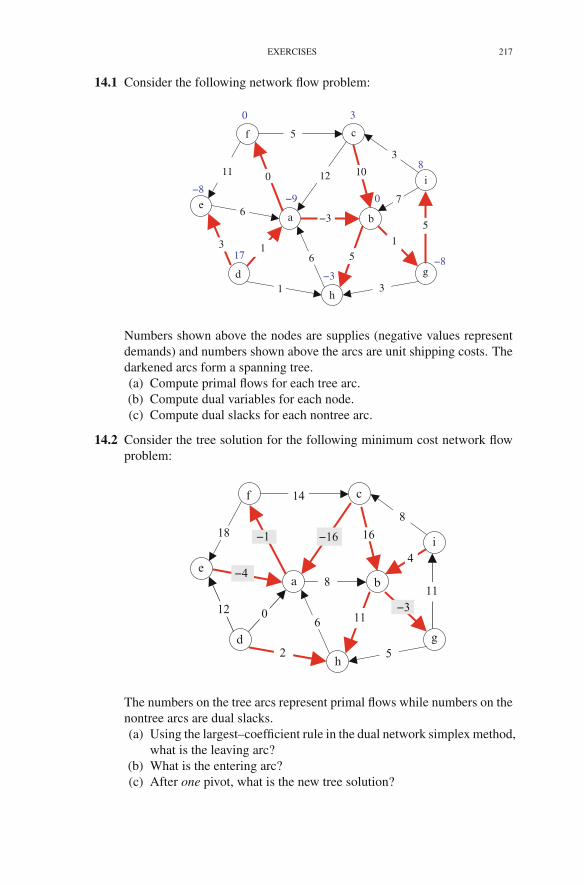
EXERCISES 217
14.1 Consider the following network flow problem:
f
0
e
d
a
c
b
h
g
i11
5
0
6
3
1
−3
12 103
5
15
3
1
7
6
−8
3
8
17
−3−8
−9 0
Numbers shown above the nodes are supplies (negative values representdemands) and numbers shown above the arcs are unit shipping costs. Thedarkened arcs form a spanning tree.(a) Compute primal flows for each tree arc.(b) Compute dual variables for each node.(c) Compute dual slacks for each nontree arc.
14.2 Consider the tree solution for the following minimum cost network flowproblem:
f
e
d
a
c
b
h
g
i18
14
−1
−4
12
2
8
−16 168
11
0 11
5
−3
4
6
The numbers on the tree arcs represent primal flows while numbers on thenontree arcs are dual slacks.(a) Using the largest–coefficient rule in the dual network simplex method,
what is the leaving arc?(b) What is the entering arc?(c) After one pivot, what is the new tree solution?
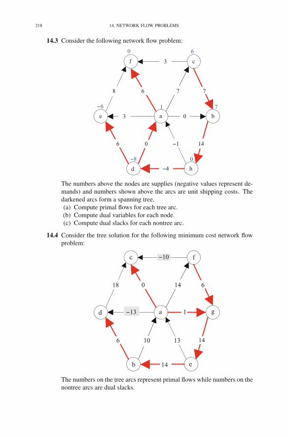
218 14. NETWORK FLOW PROBLEMS
14.3 Consider the following network flow problem:
f
e
d
a
c
b
h
8
3
6
3
6
−4
0
7 7
0 14−1
−6
0
1 7
0 6
−8
The numbers above the nodes are supplies (negative values represent de-mands) and numbers shown above the arcs are unit shipping costs. Thedarkened arcs form a spanning tree.(a) Compute primal flows for each tree arc.(b) Compute dual variables for each node.(c) Compute dual slacks for each nontree arc.
14.4 Consider the tree solution for the following minimum cost network flowproblem:
c
d
b
a
f
g
e
−10
0
−13
6
14
1
14 6
10 14
18
13
The numbers on the tree arcs represent primal flows while numbers on thenontree arcs are dual slacks.
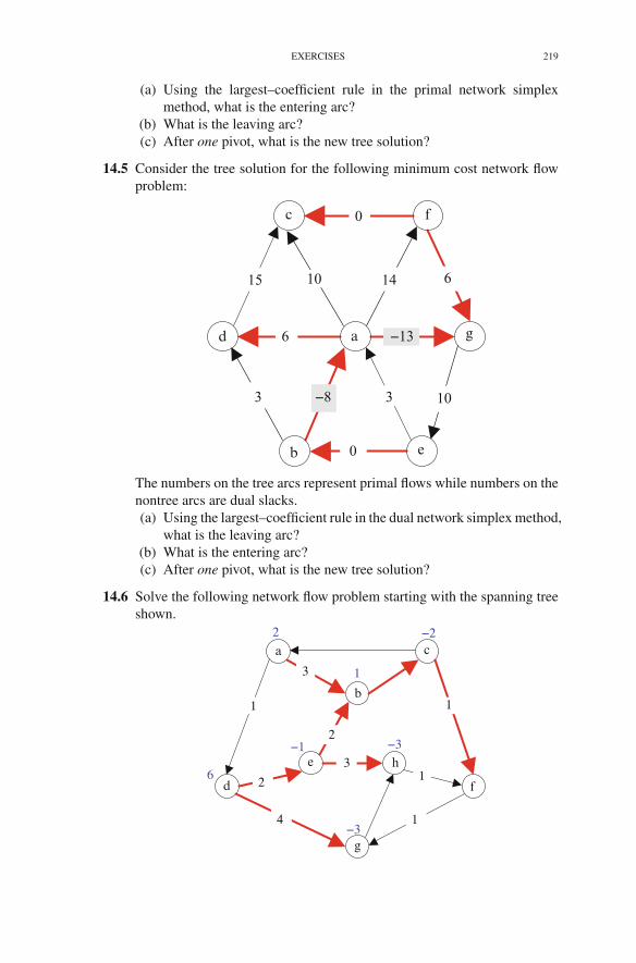
EXERCISES 219
(a) Using the largest–coefficient rule in the primal network simplexmethod, what is the entering arc?
(b) What is the leaving arc?(c) After one pivot, what is the new tree solution?
14.5 Consider the tree solution for the following minimum cost network flowproblem:
c
d
b
a
f
g
e
0
10
6
3
0
−13
14 6
−8 10
15
3
The numbers on the tree arcs represent primal flows while numbers on thenontree arcs are dual slacks.(a) Using the largest–coefficient rule in the dual network simplex method,
what is the leaving arc?(b) What is the entering arc?(c) After one pivot, what is the new tree solution?
14.6 Solve the following network flow problem starting with the spanning treeshown.
c2
b
e h
d
g
f
a
3
1
2
4
3
2
1
1
1
−2
−3−1
6
−3
1
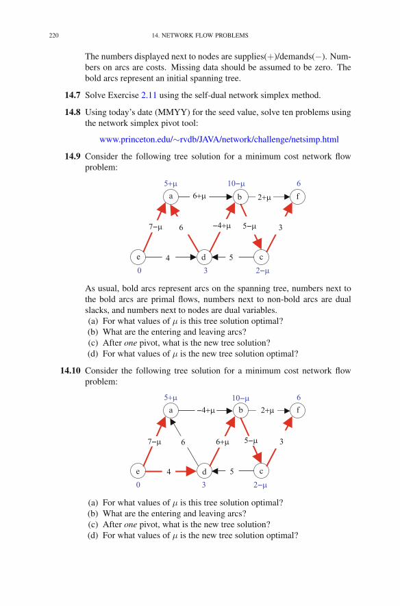
220 14. NETWORK FLOW PROBLEMS
The numbers displayed next to nodes are supplies(+)/demands(−). Num-bers on arcs are costs. Missing data should be assumed to be zero. Thebold arcs represent an initial spanning tree.
14.7 Solve Exercise 2.11 using the self-dual network simplex method.
14.8 Using today’s date (MMYY) for the seed value, solve ten problems usingthe network simplex pivot tool:
www.princeton.edu/∼rvdb/JAVA/network/challenge/netsimp.html
14.9 Consider the following tree solution for a minimum cost network flowproblem:
a
e d
b
c
f
7−μ
6+μ
6
4 5
−4+μ 5−μ 3
0 3 2−μ
5+μ 10−μ 6
2+μ
As usual, bold arcs represent arcs on the spanning tree, numbers next tothe bold arcs are primal flows, numbers next to non-bold arcs are dualslacks, and numbers next to nodes are dual variables.(a) For what values of μ is this tree solution optimal?(b) What are the entering and leaving arcs?(c) After one pivot, what is the new tree solution?(d) For what values of μ is the new tree solution optimal?
14.10 Consider the following tree solution for a minimum cost network flowproblem:
a
e d
b
c
f
7−μ
−4+μ
6
4 5
6+μ 5−μ 3
2+μ
0 3
5+μ 10−μ 6
2−μ
(a) For what values of μ is this tree solution optimal?(b) What are the entering and leaving arcs?(c) After one pivot, what is the new tree solution?(d) For what values of μ is the new tree solution optimal?

EXERCISES 221
14.11 Consider the following minimum cost network flow problem
a
d c
b
−2
3
−9
−7
1 −1
−1 1
As usual, the numbers on the arcs represent the flow costs and numbersat the nodes represent supplies (demands are shown as negative supplies).The arcs shown in bold represent a spanning tree. If the solution cor-responding to this spanning tree is optimal prove it, otherwise find anoptimal solution using this tree as the initial spanning tree.
14.12 Suppose that a square submatrix of A is invertible. Show that the arcscorresponding to the columns of this submatrix form a spanning tree.
14.13 Show that a spanning tree on m nodes must have exactly m− 1 arcs.
14.14 Define an algorithm that takes as input a network and either finds a span-ning tree or proves that the network is not connected.
14.15 Give an example of a minimum-cost network flow problem with all arccosts positive and the following counterintuitive property: if the supplyat a particular source node and the demand at a particular sink node aresimultaneously reduced by one unit, then the optimal cost increases.
14.16 Consider a possibly disconnected network (N ,A). Two nodes i and j inN are said to be connected if there is a path from i to j (recall that pathscan traverse arcs backwards or forwards). We write i ∼ j if i and j areconnected.(a) Show that “∼” defines an equivalence relation. That is, it has the
following three properties:(i) (Reflexivity) for all i ∈ N , i ∼ i;
(ii) (Symmetry) for all i, j ∈ N , i ∼ j implies that j ∼ i;(iii) (Transitivity) for all i, j, k ∈ N , i ∼ j and j ∼ k implies that
i ∼ k.Using the equivalence relation, we can partition N into a collection ofsubsets of equivalence classes N1,N2, . . . ,Nk such that two nodes areconnected if and only if they belong to the same subset. The number k iscalled the number of connected components.(b) Show that the rank of the node–arc incidence matrix A is exactly
m− k (recall that m is the number of rows of A).

222 14. NETWORK FLOW PROBLEMS
df
e
ab
c
B
C
D
A
1
11
2
4
2
5 15−3
−2
1
−1
FIGURE 14.16. The primal network has nodes “a” through “f”.The corresponding dual network has nodes “A” through “D” (node“A” is “at infinity”). A primal spanning tree is shown. It con-sists of five arcs: (a,b), (f,b), (b,e), (e,d), and (c,d). The corre-sponding dual spanning tree consists of three arcs: (B,A), (A,C),and (D,A). Primal costs are shown along the primal arcs and sup-plies/demands are shown at the primal nodes.
14.17 One may assume without loss of generality that every node in a minimumcost network flow problem has at least two arcs associated with it. Why?
14.18 The sum of the dual slacks around any cycle is a constant. What is thatconstant?
14.19 Planar Networks. A network is called planar if the nodes and arcs can belaid out on the two-dimensional plane in such a manner that no two arcscross each other (it is allowed to draw the arcs as curves if necessary). Allof the networks encountered so far in this chapter have been planar. Asso-ciated with each planar network is a geometrically defined dual network.The purpose of this problem is to establish the following interesting fact:
A dual network simplex pivot is precisely a primal network sim-plex method applied to the dual network.Viewed geometrically, the nodes of a planar graph are called vertices
and the arcs are called edges. Consider a specific connected planar net-work. If one were to delete the vertices and the edges from the plane,one would be left with a disjoint collection of subsets of the plane. Thesesubsets are called faces. Note that there is one unbounded face. It is aface just like the other bounded ones. An example of a connected planarnetwork with its faces labeled A through D is shown in Figure 14.16.

EXERCISES 223
Dual nodes. Associated with each connected planar network is a dualnetwork defined by interchanging vertices and faces. That is, place a dualvertex in the center of each primal face. Note: the dual vertex corre-sponding to the unbounded primal face could be placed anywhere in theunbounded face but we choose to put it at infinity. In this way, dual edges(defined next) that have a head or a tail at this node can run off to infinityin any direction.
Dual arcs. Connect with a dual edge any pair of dual nodes whosecorresponding primal faces share an edge. Each dual edge crosses exactlyone primal edge. The directionality of the dual edge is determined asfollows: first, place a vector along the corresponding primal edge pointingin the direction of the primal arc, and then rotate it counterclockwise untilit is tangent to the dual edge. The vector now defines the direction for thedual arc.
Dual spanning tree. Consider a spanning tree on the primal networkand suppose that a primal–dual tree solution is given. We define a span-ning tree on the dual network as follows. A dual edge is on the dualnetwork’s spanning tree if and only if the corresponding primal edge isnot on the primal network’s spanning tree.
Dual flows and dual dual-slacks. The numerical arc data for the dualnetwork is inherited directly from the primal. That is, flows on the dualtree arcs are exactly equal to the dual slacks on the associated primal non-tree arcs. And, the dual slacks on the dual nontree arcs are exactly equalto the primal flows on the associated primal tree arcs. Having specifiednumerical data on the arcs of the dual network, it is fairly straightforwardto determine values for supplies/demands at the nodes and shipping costsalong the arcs that are consistent with these numerical values.
(a) Which of the following networks are planar:
a
be
d c
aa
bb
cc
d
d
a b c
(b) A network is called complete if there is an arc between every pairof nodes. If a complete network with m nodes is planar, then everynetwork with m nodes is planar. Prove it.
(c) Show that a nonplanar network must have five or more nodes.(d) As always, let m denote the number of nodes and let n denote the
number of arcs in a network. Let f denote the number of faces in aplanar network. Show by induction on f that m = n− f + 2.

224 14. NETWORK FLOW PROBLEMS
(e) Show that the dual spanning tree defined above is in fact a spanningtree.
(f) Show that a dual pivot for a minimum cost network flow problemdefined on the primal network is precisely the same as a primal pivotfor the corresponding network flow problem on the dual network.
(g) Using the cost and supply/demand information given for the primalproblem in Figure 14.16, write down the primal problem as a linearprogramming problem.
(h) Write down the dual linear programming problem that one derivesalgebraically from the primal linear programming problem.
(i) Using the spanning tree shown in Figure 14.16, compute the primalflows, dual variables, and dual slacks for the network flow problemassociated with the primal network.
(j) Write down the flow and slacks for the network flow problem asso-ciated with the dual network.
(k) Find arc costs and node supplies/demands for the dual network thatare consistent with the flows and slacks just computed.
(l) Write down the linear programming problem associated with the net-work flow problem on the dual network.
Notes
The classical reference is Ford and Fulkerson (1962). More recent works includethe books by Christofides (1975), Lawler (1976), Bazaraa et al. (1977),Kennington and Helgason (1980), Jensen and Barnes (1980), Bertsekas (1991), andAhuja et al. (1993).
The two “original” algorithms for solving minimum-cost network flow problemsare the network simplex method developed by Dantzig (1951a) and the primal–dualmethod developed by Ford and Fulkerson (1958). The self-dual algorithm describedin this chapter is neither of these. In fact, it resembles the “out-of-kilter” methoddescribed by Ford and Fulkerson (1962).
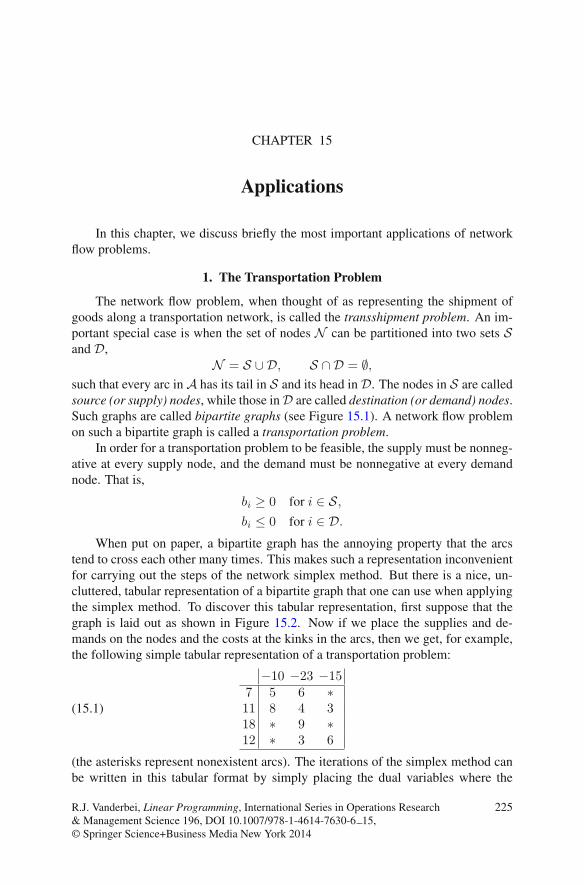
CHAPTER 15
Applications
In this chapter, we discuss briefly the most important applications of networkflow problems.
1. The Transportation Problem
The network flow problem, when thought of as representing the shipment ofgoods along a transportation network, is called the transshipment problem. An im-portant special case is when the set of nodes N can be partitioned into two sets Sand D,
N = S ∪ D, S ∩ D = ∅,such that every arc in A has its tail in S and its head in D. The nodes in S are calledsource (or supply) nodes, while those in D are called destination (or demand) nodes.Such graphs are called bipartite graphs (see Figure 15.1). A network flow problemon such a bipartite graph is called a transportation problem.
In order for a transportation problem to be feasible, the supply must be nonneg-ative at every supply node, and the demand must be nonnegative at every demandnode. That is,
bi ≥ 0 for i ∈ S,bi ≤ 0 for i ∈ D.
When put on paper, a bipartite graph has the annoying property that the arcstend to cross each other many times. This makes such a representation inconvenientfor carrying out the steps of the network simplex method. But there is a nice, un-cluttered, tabular representation of a bipartite graph that one can use when applyingthe simplex method. To discover this tabular representation, first suppose that thegraph is laid out as shown in Figure 15.2. Now if we place the supplies and de-mands on the nodes and the costs at the kinks in the arcs, then we get, for example,the following simple tabular representation of a transportation problem:
(15.1)
−10 −23 −157 5 6 ∗11 8 4 318 ∗ 9 ∗12 ∗ 3 6
(the asterisks represent nonexistent arcs). The iterations of the simplex method canbe written in this tabular format by simply placing the dual variables where the
R.J. Vanderbei, Linear Programming, International Series in Operations Research& Management Science 196, DOI 10.1007/978-1-4614-7630-6 15,© Springer Science+Business Media New York 2014
225
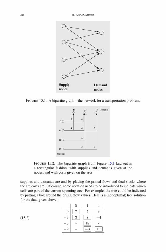
226 15. APPLICATIONS
Supplynodes
Demandnodes
FIGURE 15.1. A bipartite graph—the network for a transportation problem.
Supplies
Demands
7
11
18
12
−10 −23 −15
9
5 6
8 4 3
3 6
FIGURE 15.2. The bipartite graph from Figure 15.1 laid out ina rectangular fashion, with supplies and demands given at thenodes, and with costs given on the arcs.
supplies and demands are and by placing the primal flows and dual slacks wherethe arc costs are. Of course, some notation needs to be introduced to indicate whichcells are part of the current spanning tree. For example, the tree could be indicatedby putting a box around the primal flow values. Here is a (nonoptimal) tree solutionfor the data given above:
(15.2)
5 1 4
0 7 5 ∗−3 3 8 −4
−8 ∗ 18 ∗−2 ∗ −3 15
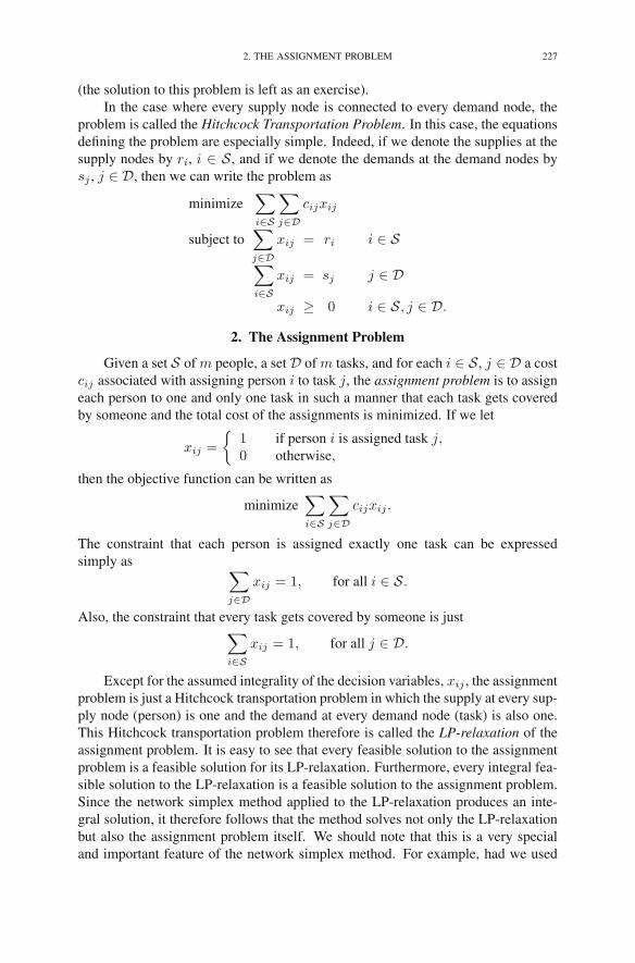
2. THE ASSIGNMENT PROBLEM 227
(the solution to this problem is left as an exercise).In the case where every supply node is connected to every demand node, the
problem is called the Hitchcock Transportation Problem. In this case, the equationsdefining the problem are especially simple. Indeed, if we denote the supplies at thesupply nodes by ri, i ∈ S , and if we denote the demands at the demand nodes bysj , j ∈ D, then we can write the problem as
minimize∑
i∈S
∑
j∈Dcijxij
subject to∑
j∈Dxij = ri i ∈ S
∑
i∈Sxij = sj j ∈ D
xij ≥ 0 i ∈ S, j ∈ D.
2. The Assignment Problem
Given a set S of m people, a set D of m tasks, and for each i ∈ S , j ∈ D a costcij associated with assigning person i to task j, the assignment problem is to assigneach person to one and only one task in such a manner that each task gets coveredby someone and the total cost of the assignments is minimized. If we let
xij =
{1 if person i is assigned task j,0 otherwise,
then the objective function can be written as
minimize∑
i∈S
∑
j∈Dcijxij .
The constraint that each person is assigned exactly one task can be expressedsimply as ∑
j∈Dxij = 1, for all i ∈ S.
Also, the constraint that every task gets covered by someone is just∑
i∈Sxij = 1, for all j ∈ D.
Except for the assumed integrality of the decision variables, xij , the assignmentproblem is just a Hitchcock transportation problem in which the supply at every sup-ply node (person) is one and the demand at every demand node (task) is also one.This Hitchcock transportation problem therefore is called the LP-relaxation of theassignment problem. It is easy to see that every feasible solution to the assignmentproblem is a feasible solution for its LP-relaxation. Furthermore, every integral fea-sible solution to the LP-relaxation is a feasible solution to the assignment problem.Since the network simplex method applied to the LP-relaxation produces an inte-gral solution, it therefore follows that the method solves not only the LP-relaxationbut also the assignment problem itself. We should note that this is a very specialand important feature of the network simplex method. For example, had we used

228 15. APPLICATIONS
the primal–dual interior-point method to solve the LP-relaxation, there would beno guarantee that the solution obtained would be integral (unless the problem has aunique optimal solution, in which case any LP solver would find the same, integralanswer—but typical assignment problems have alternate optimal solutions, and aninterior-point method will report a convex combination of all of them).
3. The Shortest-Path Problem
Roughly speaking, the shortest-path problem is to find, well, the shortest pathfrom one specific node to another in a network (N ,A). In contrast to earlier usage,the arcs connecting successive nodes on a path must point in the direction of travel.Such paths are sometimes referred to as directed paths. To determine a shortest path,we assume that we are given the length of each arc. To be consistent with earliernotations, let us assume that the length of arc (i, j) is denoted by cij . Naturally, weassume that these lengths are nonnegative.
To find the shortest path from one node (say, s) to another (say, r), we willsee that it is necessary to compute the shortest path from many, perhaps all, othernodes to r. Hence, we define the shortest-path problem as the problem of findingthe shortest path from every node in N to a specific node r ∈ N . The destinationnode r is called the root node.
3.1. Network Flow Formulation. The shortest-path problem can be formu-lated as a network flow problem. Indeed, put a supply of one unit at each nonrootnode, and put the appropriate amount of demand at the root (to meet the total sup-ply). The cost on each arc is just the length of the arc. Suppose that we’ve solvedthis network flow problem. Then the shortest path from a node i to r can be foundby simply following the arcs from i to r on the optimal spanning tree. Also, thelength of the shortest path is y∗r − y∗i .
While the network simplex method can be used to solve the shortest-path prob-lem, there are faster algorithms designed especially for it. To describe these algo-rithms, let us denote the distance from i to r by vi. These distances (or approxima-tions thereof) are called labels in the networks literature. Some algorithms computethese distances systematically in a certain order. These algorithms are called label-setting algorithms. Other algorithms start with an estimate for these labels and theniteratively correct the estimates until the optimal values are found. Such algorithmsare called label-correcting algorithms.
Note that if we set y∗r to zero in the network flow solution, then the labels aresimply the negative of the optimal dual variables. In the following subsections, weshall describe simple examples of label-setting and label-correcting algorithms.
3.2. A Label-Correcting Algorithm. To describe a label-correctingalgorithm, we need to identify a system of equations that characterize the shortest-path distances. First of all, clearly
vr = 0.

3. THE SHORTEST-PATH PROBLEM 229
What can we say about the labels at other nodes, say, node i? Suppose that we selectan arc (i, j) that leaves node i. If we were to travel along this arc and then, fromnode j, travel along the shortest path to r, then the distance to the root would becij + vj . So, from node i, we should select the arc that minimizes these distances.This selection will then give the shortest distance from i to r. That is,
(15.3) vi = min{cij + vj : (i, j) ∈ A}, i �= r.
The argument we have just made is called the principle of dynamic programming,and equation (15.3) is called Bellman’s equation. Dynamic programming is a wholesubject of its own—we shall only illustrate some of its basic ideas by our study ofthe shortest-path problem. In the dynamic programming literature, the set of vi’sviewed as a function defined on the nodes is called the value function (hence thenotation).
From Bellman’s equation, it is easy to identify the arcs one would travel on ina shortest-path route to the root. Indeed, these arcs are given by
T = {(i, j) ∈ A : vi = cij + vj}.
This set of arcs may contain alternate shortest paths to the root, and so the set is notnecessarily a tree. Nonetheless, any path that follows these arcs will get to the rooton a shortest-path route.
3.2.1. Method of Successive Approximation. Bellman’s equation is an implicitsystem of equations for the values vi, i ∈ N . Implicit equations such as this arisefrequently and beg to be solved by starting with a guess at the solution, using thisguess in the right-hand side, and computing a new guess by evaluating the right-hand side. This approach is called the method of successive approximations. Toapply it to the shortest-path problem, we initialize the labels as follows:
v(0)i =
{0 i = r∞ i �= r.
Then the updates are computed using Bellman’s equation:
v(k+1)i =
{0 i = r
min{cij + v(k)j : (i, j) ∈ A} i �= r.
3.2.2. Efficiency. The algorithm stops when an update leaves all the vi’s un-changed. It turns out that the algorithm is guaranteed to stop in no more than m
iterations. To see why, it suffices to note that v(k)i has a very simple description:it is the length of the shortest path from i to r that has k or fewer arcs in the path.(It is not hard to convince yourself with an induction on k that this is correct, buta pedantic proof requires introducing a significant amount of added notation thatwe wish to avoid.) Hence, the label-correcting algorithm cannot take more than miterations, since every shortest path can visit each node at most once. Since eachiteration involves looking at every arc of the network, it follows that the numberof additions/comparisons needed to solve a shortest-path problem using the label-correcting algorithm is about nm.
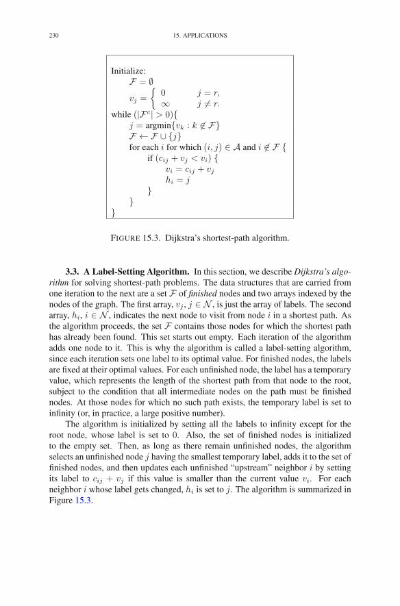
230 15. APPLICATIONS
Initialize:F = ∅vj =
{0 j = r,∞ j �= r.
while (|Fc| > 0){j = argmin{vk : k �∈ F}F ← F ∪ {j}for each i for which (i, j) ∈ A and i �∈ F {
if (cij + vj < vi) {vi = cij + vjhi = j
}}
}
FIGURE 15.3. Dijkstra’s shortest-path algorithm.
3.3. A Label-Setting Algorithm. In this section, we describe Dijkstra’s algo-rithm for solving shortest-path problems. The data structures that are carried fromone iteration to the next are a set F of finished nodes and two arrays indexed by thenodes of the graph. The first array, vj , j ∈ N , is just the array of labels. The secondarray, hi, i ∈ N , indicates the next node to visit from node i in a shortest path. Asthe algorithm proceeds, the set F contains those nodes for which the shortest pathhas already been found. This set starts out empty. Each iteration of the algorithmadds one node to it. This is why the algorithm is called a label-setting algorithm,since each iteration sets one label to its optimal value. For finished nodes, the labelsare fixed at their optimal values. For each unfinished node, the label has a temporaryvalue, which represents the length of the shortest path from that node to the root,subject to the condition that all intermediate nodes on the path must be finishednodes. At those nodes for which no such path exists, the temporary label is set toinfinity (or, in practice, a large positive number).
The algorithm is initialized by setting all the labels to infinity except for theroot node, whose label is set to 0. Also, the set of finished nodes is initializedto the empty set. Then, as long as there remain unfinished nodes, the algorithmselects an unfinished node j having the smallest temporary label, adds it to the set offinished nodes, and then updates each unfinished “upstream” neighbor i by settingits label to cij + vj if this value is smaller than the current value vi. For eachneighbor i whose label gets changed, hi is set to j. The algorithm is summarized inFigure 15.3.

4. UPPER-BOUNDED NETWORK FLOW PROBLEMS 231
4. Upper-Bounded Network Flow Problems
Some real-world network flow problems involve upper bounds on the amountof flow that an arc can handle. There are modified versions of the network simplexmethod that allow one to handle such upper bounds implicitly, but we shall simplyshow how to reduce an upper-bounded network flow problem to one without upperbounds.
Let us consider just one arc, (i, j), in a network flow problem. Suppose thatthere is an upper bound of uij on the amount of flow that this arc can handle. Wecan express this bound as an extra constraint:
0 ≤ xij ≤ uij .
Introducing a slack variable, tij , we can rewrite these bound constraints as
xij + tij = uij
xij , tij ≥ 0.
If we look at the flow balance constraints and focus our attention on the variablesxij and tij , we see that they appear in only three constraints: the flow balanceconstraints for nodes i and j and the upper bound constraint,
· · · −xij · · · = −bi· · · xij · · · =−bj
xij +tij = uij .
If we subtract the last constraint from the second one, we get
· · · −xij · · · = −bi· · · · · · −tij =−bj − uij
xij +tij = uij .
Note that we have restored a network structure in the sense that each column againhas one +1 and one −1 coefficient. To make a network picture, we need to createa new node (corresponding to the third row). Let us call this node k. The networktransformation is shown in Figure 15.4.
We can use the above transformation to derive optimality conditions for upper-bounded network flow problems. Indeed, let us consider an optimal solution tothe transformed problem. Clearly, if xik is zero, then the corresponding dual slackzik = yi + cij − yk is nonnegative:
(15.4) yi + cij − yk ≥ 0.
Furthermore, the back-flow xjk must be at the upper bound rate:
xjk = uij .

232 15. APPLICATIONS
i j
bi
cij
bjuij
xij
ki j
bi −uij
cij 0
bj+uij
xij tij
FIGURE 15.4. Adding a new node, k, to accommodate an arc(i, j) having an upper bound uij on its flow capacity.
Hence, by complementarity, the corresponding dual slack must vanish:
(15.5) zjk = yj − yk = 0.
Combining (15.4) with (15.5), we see that
yi + cij ≥ yj .
On the other hand, if the flow on arc (i, k) is at the capacity value, then the back-flowon arc (j, k) must vanish. The complementarity conditions then say that
zik = yi + cij − yk = 0
zjk = yj − yk ≥ 0.
Combining these two statements, we get
yi + cij ≤ yj .
Finally, if 0 < xij < uij , then both slack variables vanish, and this implies that
yi + cij = yj .
These properties can then be summarized as follows:
xij = 0 =⇒ yi + cij ≥ yj
xij = uij =⇒ yi + cij ≤ yj(15.6)
0 < xij < uij =⇒ yi + cij = yj .
While upper-bounded network flow problems have important applications, weadmit that our main interest in them is more narrowly focused. It stems from their

5. THE MAXIMUM-FLOW PROBLEM 233
st
C
cts= −1
FIGURE 15.5. A cut set C for a maximum flow problem.
relation to an important theorem called the Max-Flow Min-Cut Theorem. We shallstate and prove this theorem in the next section. The only tool we need to prove thistheorem is the above result giving the complementarity conditions when there areupper bounds on arcs. So on with the show.
5. The Maximum-Flow Problem
The subject of this section is the class of problems called maximum-flow prob-lems. These problems form an important topic in the theory of network flows. Thereare very efficient algorithms for solving them, and they appear as subproblems inmany algorithms for the general network flow problem. However, our aim is rathermodest. We wish only to expose the reader to one important theorem in this subject,which is called the Max-Flow Min-Cut Theorem.
Before we can state this theorem we need to set up the situation. Suppose thatwe are given a network (N ,A), a distinguished node s ∈ N called the source node,a distinguished node t ∈ N called the sink node, and upper bounds on the arcs ofthe network uij , (i, j) ∈ A. For simplicity, we shall assume that the upper boundsare all finite (although this is not really necessary). The objective is to “push” asmuch flow from s to t as possible.
To solve this problem, we can convert it to an upper-bounded network flowproblem as follows. First, let cij = 0 for all arcs (i, j) ∈ A, and let bi = 0 for everynode i ∈ N . Then add one extra arc (t, s) connecting the sink node t back to thesource node s, put a negative cost on this arc (say, cts = −1), and let it have infinitecapacity uts = ∞. Since the only nonzero cost is actually negative, it follows thatwe shall actually make a profit by letting more and more flow circulate through thenetwork. But the upper bound on the arc capacities limits the amount of flow that itis possible to push through.
In order to state the Max-Flow Min-Cut Theorem, we must define whatwe mean by a cut. A cut, C, is a set of nodes that contains the source node butdoes not contain the sink node (see Figure 15.5). The capacity of a cut is defined as
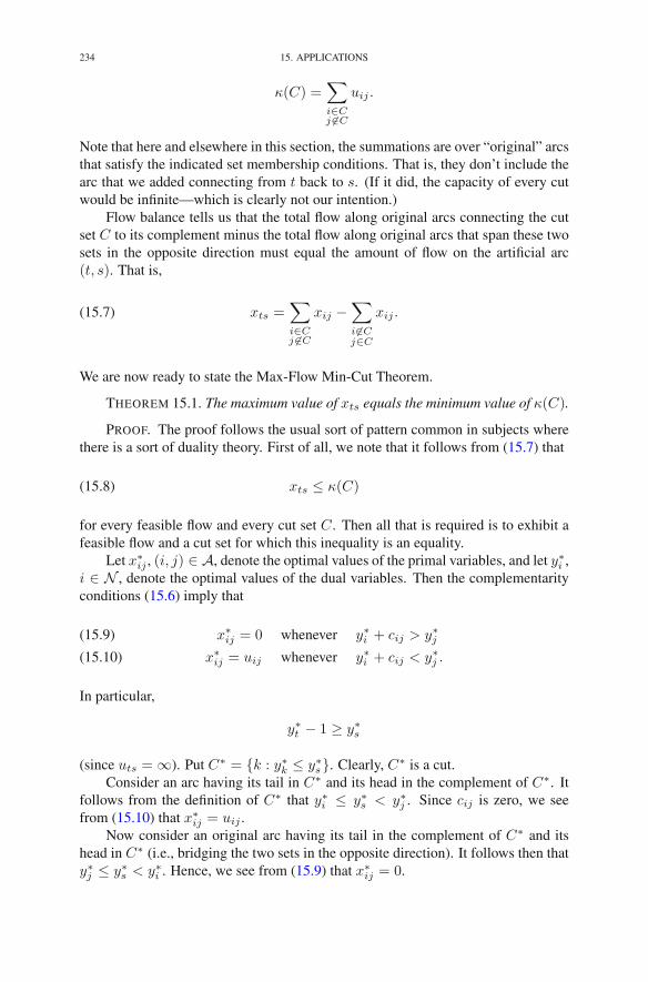
234 15. APPLICATIONS
κ(C) =∑
i∈Cj ∈C
uij .
Note that here and elsewhere in this section, the summations are over “original” arcsthat satisfy the indicated set membership conditions. That is, they don’t include thearc that we added connecting from t back to s. (If it did, the capacity of every cutwould be infinite—which is clearly not our intention.)
Flow balance tells us that the total flow along original arcs connecting the cutset C to its complement minus the total flow along original arcs that span these twosets in the opposite direction must equal the amount of flow on the artificial arc(t, s). That is,
(15.7) xts =∑
i∈Cj ∈C
xij −∑
i∈Cj∈C
xij .
We are now ready to state the Max-Flow Min-Cut Theorem.
THEOREM 15.1. The maximum value of xts equals the minimum value of κ(C).
PROOF. The proof follows the usual sort of pattern common in subjects wherethere is a sort of duality theory. First of all, we note that it follows from (15.7) that
(15.8) xts ≤ κ(C)
for every feasible flow and every cut set C. Then all that is required is to exhibit afeasible flow and a cut set for which this inequality is an equality.
Let x∗ij , (i, j) ∈ A, denote the optimal values of the primal variables, and let y∗i ,
i ∈ N , denote the optimal values of the dual variables. Then the complementarityconditions (15.6) imply that
x∗ij = 0 whenever y∗i + cij > y∗j(15.9)
x∗ij = uij whenever y∗i + cij < y∗j .(15.10)
In particular,
y∗t − 1 ≥ y∗s
(since uts = ∞). Put C∗ = {k : y∗k ≤ y∗s}. Clearly, C∗ is a cut.Consider an arc having its tail in C∗ and its head in the complement of C∗. It
follows from the definition of C∗ that y∗i ≤ y∗s < y∗j . Since cij is zero, we seefrom (15.10) that x∗
ij = uij .Now consider an original arc having its tail in the complement of C∗ and its
head in C∗ (i.e., bridging the two sets in the opposite direction). It follows then thaty∗j ≤ y∗s < y∗i . Hence, we see from (15.9) that x∗
ij = 0.

EXERCISES 235
Combining the observations of the last two paragraphs with (15.7), we see that
x∗ts =
∑
i∈Cj ∈C
uij = κ(C∗).
In light of (15.8), the proof is complete. �
Exercises
15.1 Solve the transportation problem given in (15.1), using (15.2) for the start-ing tree solution.
15.2 Solve the following linear programming problem:
maximize 7x1 − 3x2 + 9x3 + 2x4
subject to x1 + x2 ≤ 1x3 + x4 ≤ 1
x1 + x3 ≥ 1x2 + x4 ≥ 1x1, x2, x3, x4 ≥ 0.
(Note: there are two greater-than-or-equal-to constraints.)
15.3 Bob, Carol, David, and Alice are stranded on a desert island. Bob andDavid each would like to give their affection to Carol or to Alice. Foodis the currency of trade for this starving foursome. Bob is willing to payCarol 7 clams if she will accept his affection. David is even more keenand is willing to give Carol 9 clams if she will accept it. Both Bob andDavid prefer Carol to Alice (sorry Alice). To quantify this preference,David is willing to pay Alice only 2 clams for his affection. Bob is evenmore averse: he says that Alice would have to pay him for it. In fact,she’d have to pay him 3 clams for his affection. Carol and Alice, beingproper young women, will accept affection from one and only one of thetwo guys. Between the two of them they have decided to share the clamsequally between them and hence their objective is simply to maximizethe total number of clams they will receive. Formulate this problem as atransportation problem. Solve it.
15.4 Project Scheduling.This problem deals with the creation of a project sched-ule; specifically, the project of building a house. The project has beendivided into a set of jobs. The problem is to schedule the time at whicheach of these jobs should start and also to predict how long the projectwill take. Naturally, the objective is to complete the project as quickly aspossible (time is money!). Over the duration of the project, some of thejobs can be done concurrently. But, as the following table shows, certainjobs definitely can’t start until others are completed.

236 15. APPLICATIONS
Duration Must beJob (weeks) preceded by
0. Sign contract with buyer 0 –1. Framing 2 02. Roofing 1 13. Siding 3 14. Windows 2.5 35. Plumbing 1.5 36. Electrical 2 2,47. Inside finishing 4 5,68. Outside painting 3 2,49. Complete the sale to buyer 0 7,8
One possible schedule is the following:
Job Start time0. Sign contract with buyer 01. Framing 12. Roofing 43. Siding 64. Windows 105. Plumbing 96. Electrical 137. Inside finishing 168. Outside painting 149. Complete the sale to buyer 21
With this schedule, the project duration is 21 weeks (the differencebetween the start times of jobs 9 and 0).
To model the problem as a linear program, introduce the followingdecision variables:
tj = the start time of job j.
(a) Write an expression for the objective function, which is to minimizethe project duration.
(b) For each job j, write a constraint for each job i that must precedej; the constraint should ensure that job j doesn’t start until job i isfinished. These are called precedence constraints.
15.5 Continuation. This problem generalizes the specific example of the pre-vious problem. A project consists of a set of jobs J . For each job j ∈ Jthere is a certain set Pj of other jobs that must be completed before job jcan be started. (This is called the set of predecessors of job j.) One of thejobs, say s, is the starting job; it has no predecessors. Another job, say t,is the final (or terminal) job; it is not the predecessor of any other job. Thetime it will take to do job j is denoted dj (the duration of the job).

EXERCISES 237
The problem is to decide what time each job should begin so thatno job begins before its predecessors are finished, and the duration of theentire project is minimized. Using the notations introduced above, writeout a complete description of this linear programming problem.
15.6 Continuation. Let xij denote the dual variable corresponding to the prece-dence constraint that ensures job j doesn’t start until job i finishes.(a) Write out the dual to the specific linear program in Problem 15.4.(b) Write out the dual to the general linear program in Problem 15.5.(c) Describe how the optimal value of the dual variable xij can be inter-
preted.
15.7 Continuation. The project scheduling problem can be represented on adirected graph with arc weights as follows. The nodes of the graph corre-spond to the jobs. The arcs correspond to the precedence relations. Thatis, if job i must be completed before job j, then there is an arc pointingfrom node i to node j. The weight on this arc is di.(a) Draw the directed graph associated with the example in Problem 15.4,
being sure to label the nodes and write the weights beside the arcs.(b) Return to the formulation of the dual from Problem 15.6(a). Give
an interpretation of that dual problem in terms of the directed graphdrawn in Part (a).
(c) Explain why there is always an optimal solution to the dual problemin which each variable xij is either 0 or 1.
(d) Write out the complementary slackness condition corresponding todual variable x26.
(e) Describe the dual problem in the language of the original projectscheduling model.
15.8 Continuation. Here is an algorithm for computing optimal start times tj :1. List the jobs so that the predecessors of each job come
before it in the list.2. Put t0 = 0.3. Go down the list of jobs and for job j put tj = max{ti +
di : i is a predecessor of j}.(a) Apply this algorithm to the specific instance from Problem 15.4.
What are the start times of each of the jobs? What is the projectduration?
(b) Prove that the solution found in Part (a) is optimal by exhibiting acorresponding dual solution and checking the usual conditions foroptimality (Hint: The complementary slackness conditions may helpyou find a dual solution.).
15.9 Currency Arbitrage. Consider the world’s currency market. Given twocurrencies, say the Japanese Yen and the US Dollar, there is an exchangerate between them (currently about 110 Yen to the Dollar). It is always

238 15. APPLICATIONS
true that, if you convert money from one currency to another and thenback, you will end up with less than you started with. That is, the productof the exchange rates between any pair of countries is always less thanone. However, it sometimes happens that a longer chain of conversionsresults in a gain. Such a lucky situation is called an arbitrage. One canuse a linear programming model to find such situations when they exist.
Consider the following table of exchange rates (which is actual datafrom the Wall Street Journal on Nov 10, 1996):
param rate:USD Yen Mark Franc :=
USD . 111.52 1.4987 5.0852Yen .008966 . .013493 .045593Mark .6659 73.964 . 3.3823Franc .1966 21.933 .29507 .;
It is not obvious, but the USD→Yen→Mark→USD conversion actuallymakes $0.002 on each initial dollar.
To look for arbitrage possibilities, one can make a generalized net-work model, which is a network flow model with the unusual twist that aunit of flow that leaves one node arrives at the next node multiplied by ascale factor—in our example, the currency conversion rate. For us, eachcurrency is represented by a node. There is an arc from each node to ev-ery other node. A flow of one unit out of one node becomes a flow of adifferent magnitude at the head node. For example, one dollar flowing outof the USD node arrives at the Franc node as 5.0852 Francs.
Let xij denote the flow from node (i.e. currency) i to node j. Thisflow is measured in the currency of node i.
One node is special; it is the home node, say the US Dollars (USD)node. At all other nodes, there must be flow balance.
(a) Write down the flow balance constraints at the 3 non-home nodes(Franc, Yen, and Mark).
At the home node, we assume that there is a supply of one unit (to getthings started). Furthermore, at this node, flow balance will not be satis-fied. Instead one expects a net inflow. If it is possible to make this inflowgreater than one, then an arbitrage has been found. Let f be a variablethat represents this inflow.
(b) Using variable f to represent net inflow to the home node, write aflow balance equation for the home node.
NOTES 239
Of course, the primal objective is to maximize f .
(c) Using yi to represent the dual variable associated with the primalconstraint for currency i, write down the dual linear program. (Re-gard the primal variable f as a free variable.)
Now consider the general case, which might involve hundreds of curren-cies worldwide.
(d) Write down the model mathematically using xij for the flow leavingnode i heading for node j (measured in the currency of node i), rijfor the exchange rate when converting from currency i to currency j,and f for the net inflow at the home node i∗.
(e) Write down the dual problem.(f) Can you give an interpretation for the dual variables? Hint: It might
be helpful to think about the case where rji = 1/rij for all i, j.(g) Comment on the conditions under which your model will be un-
bounded and/or infeasible.
Notes
The Hitchcock problem was introduced by Hitchcock (1941). Dijkstra’s algo-rithm was discovered by Dijkstra (1959).
The Max-Flow Min-Cut Theorem was proved independently by Elias et al.(1956), by Ford and Fulkerson (1956) and, in the restricted case where the upperbounds are all integers, by Kotzig (1956). Fulkerson and Dantzig (1955) also provedthe Max-Flow Min-Cut Theorem. Their proof uses duality, which is particularly rel-evant to this chapter.
The classic references for dynamic programming are the books by Bellman(1957) and Howard (1960). Further discussion of label-setting and label-correctingalgorithms can be found in the book by Ahuja et al. (1993).

CHAPTER 16
Structural Optimization
This final chapter on network-type problems deals with finding the best designof a structure to support a specified load at a fixed set of points. The topology of theproblem is described by a graph where each node represents a joint in the structureand each arc represents a potential member.1 We shall formulate this problem asa linear programming problem whose solution determines which of the potentialmembers to include in the structure and how thick each included member must beto handle the load. The optimization criterion is to find a minimal weight structure.As we shall see, the problem bears a striking resemblance to the minimum-costnetwork flow problem that we studied in Chapter 14.
1. An Example
We begin with an example. Consider the graph shown in Figure 16.1. Thisgraph represents a structure consisting of five joints and eight possible membersconnecting the joints. The five joints and their coordinates are given as follows:
Joint Coordinates1 (0.0 , 0.0)2 (6.0 , 0.0)3 (0.0 , 8.0)4 (6.0 , 8.0)5 (3.0 , 12.0)
Since joints are analogous to nodes in a network, we shall denote the set of jointsby N and denote by m the number of joints. Also, since members are analogous toarcs in network flows, we shall denote the set of them by A. For the structure shownin Figure 16.1, the set of members is
A = {{1, 2}, {1, 3}, {1, 4}, {2, 3}, {2, 4}, {3, 4}, {3, 5}, {4, 5}} .Note that we enclosed the pairs of endjoints in braces to emphasize that their orderis irrelevant. For example, {2, 3} and {3, 2} refer to one and the same memberspanning between joints 2 and 3. In network flows, the graphs we considered weredirected graphs. Here, they are undirected. Also, the graphs here are embeddedin a d-dimensional Euclidean space (meaning that every node comes with a set ofcoordinates indicating its location in d-dimensional space). No such embedding was
1Civil engineers refer to beams as members.
R.J. Vanderbei, Linear Programming, International Series in Operations Research& Management Science 196, DOI 10.1007/978-1-4614-7630-6 16,© Springer Science+Business Media New York 2014
241
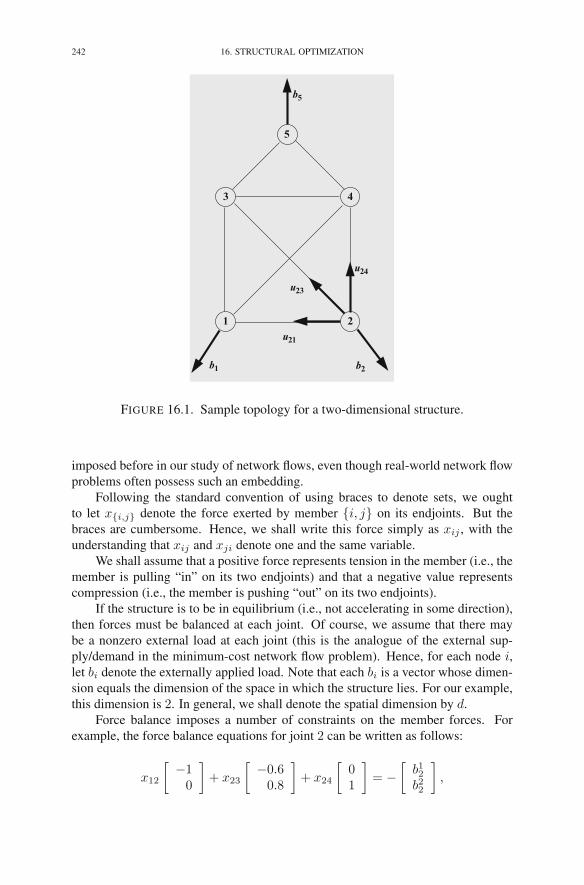
242 16. STRUCTURAL OPTIMIZATION
3
1 2
4
5
b1 b2
b5
u21
u24
u23
FIGURE 16.1. Sample topology for a two-dimensional structure.
imposed before in our study of network flows, even though real-world network flowproblems often possess such an embedding.
Following the standard convention of using braces to denote sets, we oughtto let x{i,j} denote the force exerted by member {i, j} on its endjoints. But thebraces are cumbersome. Hence, we shall write this force simply as xij , with theunderstanding that xij and xji denote one and the same variable.
We shall assume that a positive force represents tension in the member (i.e., themember is pulling “in” on its two endjoints) and that a negative value representscompression (i.e., the member is pushing “out” on its two endjoints).
If the structure is to be in equilibrium (i.e., not accelerating in some direction),then forces must be balanced at each joint. Of course, we assume that there maybe a nonzero external load at each joint (this is the analogue of the external sup-ply/demand in the minimum-cost network flow problem). Hence, for each node i,let bi denote the externally applied load. Note that each bi is a vector whose dimen-sion equals the dimension of the space in which the structure lies. For our example,this dimension is 2. In general, we shall denote the spatial dimension by d.
Force balance imposes a number of constraints on the member forces. Forexample, the force balance equations for joint 2 can be written as follows:
x12
[−10
]
+ x23
[−0.60.8
]
+ x24
[01
]
= −[
b12b22
]
,

2. INCIDENCE MATRICES 243
where b12 and b22 denote the components of b2. Note that the three vectors appearingon the left are unit vectors pointing out from joint 2 along each of the correspondingmembers.
2. Incidence Matrices
If, for each joint i, we let pi denote its position vector, then the unit vectorspointing along the arcs can be written as follows:
uij =pj − pi‖pj − pi‖
, {i, j} ∈ A.
It is important to note that uji = −uij , since the first vector points from j towardsi, whereas the second points from i towards j. In terms of these notations, the forcebalance equations can be expressed succinctly as
(16.1)∑
j:{i,j}∈A
uijxij = −bi i = 1, 2, . . . ,m.
These equations can be written in matrix form as
(16.2) Ax = −b
where x denotes the vector consisting of the member forces, b denotes the vectorwhose elements are the applied load vectors, and A is a matrix containing the unitvectors pointing along the appropriate arcs. For our example, we have
xT =[
x12 x13 x14 x23 x24 x34 x35 x45]
A =
1
2
3
4
5
⎡
⎢⎢⎢⎢⎢⎢⎢⎢⎢⎢⎢⎢⎢⎣
[10
] [01
] [.6.8
]
[−10
] [−.6.8
] [01
]
[0
−1
] [.6
−.8
] [10
] [.6.8
]
[−.6−.8
] [0
−1
] [−10
] [−.6.8
]
[−.6−.8
] [.6
−.8
]
⎤
⎥⎥⎥⎥⎥⎥⎥⎥⎥⎥⎥⎥⎥⎦
, b =
⎡
⎢⎢⎢⎢⎢⎢⎢⎢⎢⎢⎢⎢⎢⎢⎢⎣
b11b21b12b22b13b23b14b24b15b25
⎤
⎥⎥⎥⎥⎥⎥⎥⎥⎥⎥⎥⎥⎥⎥⎥⎦
.
Note that we have written A as a matrix of 2-vectors by putting “inner” brack-ets around appropriate pairs of entries. These inner brackets could of course bedropped—they are included simply to show how the constraints match up with(16.1).
In network flows, an incidence matrix is characterized by the property that everycolumn of the matrix has exactly two nonzero entries, one +1 and one −1. Here, thematrix A is characterized by the property that, when viewed as a matrix of d-vectors,every column has two nonzero entries that are unit vectors pointing in oppositedirections from each other. Generically, matrix A can be written as follows:

244 16. STRUCTURAL OPTIMIZATION
{i, j}↓
A =i →
j →
⎡
⎢⎢⎢⎢⎣
uij
uji
⎤
⎥⎥⎥⎥⎦
where, for each {i, j} ∈ A,uij , uji ∈ R
d,
uij = −uji,
and‖uij‖ = ‖uji‖ = 1.
By analogy with network flows, the matrix A is called an incidence matrix. Thisdefinition is a strict generalization of the definition we had before, since, for d =1, the current notion reduces to the network flows notion. Incidence matrices fornetwork flows enjoy many useful properties. In the following sections, we shallinvestigate the extent to which these properties carry over to our generalized notion.
3. Stability
Recall that for network flows, the sum of the rows of the incidence matrix van-ishes and that if the network is connected, this is the only redundancy. For d > 1,the situation is similar. Clearly, the sum of the rows vanishes. But is this the onlyredundancy? To answer this question, we need to look for nonzero row vectors yT
for which yTA = 0. The set of all such row vectors is a subspace of the set of allrow vectors. Our aim is to find a basis for this subspace and, in particular, to identifyits dimension. To this end, first write y in component form as yT = [ yT1 · · · yTm ]where each of the entries yi, i = 1, 2, . . . ,m, are d-vectors (transposed to makethem into row vectors). Multiplying this row vector against each column of A, wesee that yTA = 0 if and only if
(16.3) yTi uij + yTj uji = 0, for all {i, j} ∈ A.
There are many choices of y that yield a zero row combination. For example, wecan take any vector v ∈ R
d and put
yi = v, for every i ∈ N .
Substituting this choice of yi’s into the left-hand side of (16.3), we get
yTi uij + yTj uji = vTuij + vTuji = vTuij − vTuij = 0.
This set of choices shows that the subspace is at least d-dimensional.But there are more! They are defined in terms of skew symmetric matrices. A
matrix R is called skew symmetric if RT = −R. A simple but important propertyof skew symmetric matrices is that, for every vector ξ,
(16.4) ξTRξ = 0
4. CONSERVATION LAWS 245
(see Exercise 16.1). We shall make use of this property shortly. Now, to give morechoices of y, let R be a d× d skew symmetric matrix and put
yi = Rpi, for every i ∈ N(recall that pi denotes the position vector for joint i). We need to check (16.3).Substituting this definition of the y’s into the left-hand side in (16.3), we see that
yTi uij + yTj uji = pTi RTuij + pTj R
Tuji
= −pTi Ruij − pTj Ruji
= (pj − pi)TRuij .
Now substituting in the definition of uij , we get
(pj − pi)TRuij =
(pj − pi)TR(pj − pi)
‖pj − pi‖.
Finally, by putting ξ = pj − pi and using property (16.4) of skew symmetric matri-ces, we see that the numerator on the right vanishes. Hence, (16.3) holds.
How many redundancies have we found? For d = 2, there are two independentv-type redundancies and one more R-type. The following two vectors and a matrixcan be taken as a basis for these redundancies
[10
]
,
[01
]
,
[0 −11 0
]
.
For d = 3, there are three independent v-type redundancies and three R-type. Hereare three vectors and three matrices that can be taken as a basis for the space ofredundancies: ⎡
⎣100
⎤
⎦ ,
⎡
⎣010
⎤
⎦ ,
⎡
⎣001
⎤
⎦ ,
(16.5)
⎡
⎣0 −1 01 0 00 0 0
⎤
⎦ ,
⎡
⎣0 0 −10 0 01 0 0
⎤
⎦ ,
⎡
⎣0 0 00 0 −10 1 0
⎤
⎦ .
In general, there are d+ d(d− 1)/2 = d(d+ 1)/2 independent redundancies.There could be more. But just as for network flows, where we showed that thereis one redundancy if and only if the network is connected, further redundanciesrepresent a defect in the underlying graph structure. In fact, we say that the graph isstable if the rank of the incidence matrix A is exactly md − d(d + 1)/2, that is, ifand only if the above redundancies account for the entire rank deficiency of A.
4. Conservation Laws
Recall that for network flows, not all choices of supplies/demands yield feasibleflows. For connected networks, it is necessary and sufficient that the total supplyequals the total demand. The situation is similar here. The analogous question is:which external loads give rise to solutions to (16.2)? We have already identifiedseveral row vectors yT for which yTA = 0. Clearly, in order to have a solution
246 16. STRUCTURAL OPTIMIZATION
to (16.2), it is necessary that yT b = 0 for all these row vectors. In particular forevery v ∈ R
d, we see that b must satisfy the following condition:∑
i
vT bi = 0.
Bringing the sum inside of the product, we get
vT
(∑
i
bi
)
= 0.
Since this must hold for every d-vector v, it follows that∑
i
bi = 0.
This condition has a simple physical interpretation: the loads, taken in total, mustbalance.
What about the choices of yT arising from skew symmetric matrices? We shallshow that these choices impose the conditions necessary to prevent the structurefrom spinning around some axis of rotation. To show that this is so, let us firstconsider the two-dimensional case. For every 2 × 2 skew symmetric matrix R, theload vectors bi, i ∈ N , must satisfy
(16.6)∑
i
(Rpi)T bi = 0.
This expression is a sum of terms of the form (Rp)T b, where p is the position vectorof a point and b is a force applied at this point. We claim that (Rp)T b is preciselythe torque about the origin created by applying force b at location p. To see thisconnection between the algebraic expression and its physical interpretation, firstdecompose p into the product of its length r times a unit vector v pointing in thesame direction and rewrite the algebraic expression as
(Rp)T b = r(Rv)T b.
Now, without loss of generality, we may assume that R is the “basis” matrix for thespace of skew symmetric matrices,
R =
[0 −11 0
]
.
This matrix has the additional property that its two columns are unit vectors that areorthogonal to each other. That is, RTR = I . Hence,
‖Rv‖2 = ‖v‖2 = 1.
Furthermore, property (16.4) tells us that Rv is orthogonal to v. Therefore, theproduct (Rv)T b is the length of the projection of b in the direction of Rv, and sor(Rv)T b is the distance from the origin (of the coordinate system) to p, which iscalled the moment arm, times the component of the force that is orthogonal to themoment arm in the direction of Rv (see Figure 16.2). This interpretation for eachsummand in (16.6) shows that it is exactly the torque around the rotation axis pass-ing through the origin of the coordinate system caused by the force bi applied to
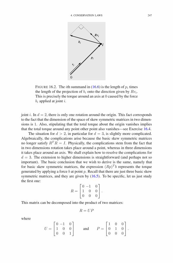
4. CONSERVATION LAWS 247
bi
pi
Rvi
vi
0
i
FIGURE 16.2. The ith summand in (16.6) is the length of pi timesthe length of the projection of bi onto the direction given by Rvi.This is precisely the torque around an axis at 0 caused by the forcebi applied at joint i.
joint i. In d = 2, there is only one rotation around the origin. This fact correspondsto the fact that the dimension of the space of skew symmetric matrices in two dimen-sions is 1. Also, stipulating that the total torque about the origin vanishes impliesthat the total torque around any point other point also vanishes—see Exercise 16.4.
The situation for d > 2, in particular for d = 3, is slightly more complicated.Algebraically, the complications arise because the basic skew symmetric matricesno longer satisfy RTR = I . Physically, the complications stem from the fact thatin two dimensions rotation takes place around a point, whereas in three dimensionsit takes place around an axis. We shall explain how to resolve the complications ford = 3. The extension to higher dimensions is straightforward (and perhaps not soimportant). The basic conclusion that we wish to derive is the same, namely thatfor basic skew symmetric matrices, the expression (Rp)T b represents the torquegenerated by applying a force b at point p. Recall that there are just three basic skewsymmetric matrices, and they are given by (16.5). To be specific, let us just studythe first one:
R =
⎡
⎣0 −1 01 0 00 0 0
⎤
⎦ .
This matrix can be decomposed into the product of two matrices:
R = UP
where
U =
⎡
⎣0 −1 01 0 00 0 1
⎤
⎦ and P =
⎡
⎣1 0 00 1 00 0 0
⎤
⎦ .

248 16. STRUCTURAL OPTIMIZATION
vq
p
b
r
x1
x2
x3
Uv(Uv)Tb
FIGURE 16.3. The decomposition of (Rp)T b into the product ofa moment arm r times the component of b in the direction Uvshows that it is precisely the torque around the third axis.
The matrix U has the property that R had before, namely,
UTU = I.
Such matrices are called unitary. The matrix P is a projection matrix. If we let
q = Pp,
v =q
‖q‖ ,
and
r = ‖q‖,
then we can rewrite (Rp)T b as
(Rp)T b = r(Uv)T b.
Since v is a unit vector and U is unitary, it follows that Uv is a unit vector. Hence,(Uv)T b represents the scalar projection of b onto the direction determined by Uv.Also, it is easy to check that Uv is orthogonal to v. At this point, we can consultFigure 16.3 to see that r is the moment arm for the torque around the third coordinateaxis and (Uv)T b is the component of force in the direction of rotation around thisaxis. Therefore, the product is precisely the torque around this axis. As we know,for d = 3, there are three independent axes of rotation, namely, pitch, roll, andyaw. These axes correspond to the three basis matrices for the space of 3× 3 skewsymmetric matrices (the one we have just studied corresponds to the yaw axis).
Finally, we note that (16.6) simply states that the total torque around each axisof rotation must vanish. This means that the forces cannot be chosen to make thesystem spin.
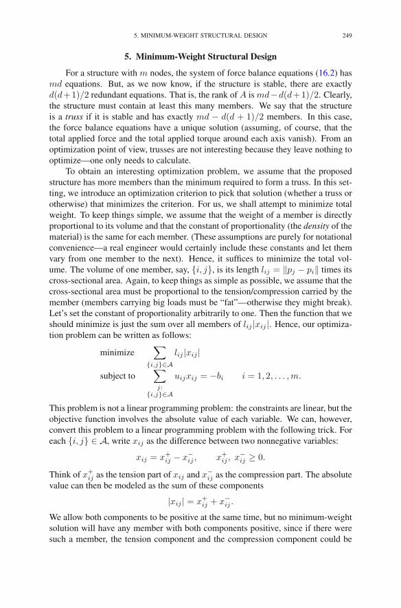
5. MINIMUM-WEIGHT STRUCTURAL DESIGN 249
5. Minimum-Weight Structural Design
For a structure with m nodes, the system of force balance equations (16.2) hasmd equations. But, as we now know, if the structure is stable, there are exactlyd(d+1)/2 redundant equations. That is, the rank of A is md−d(d+1)/2. Clearly,the structure must contain at least this many members. We say that the structureis a truss if it is stable and has exactly md − d(d + 1)/2 members. In this case,the force balance equations have a unique solution (assuming, of course, that thetotal applied force and the total applied torque around each axis vanish). From anoptimization point of view, trusses are not interesting because they leave nothing tooptimize—one only needs to calculate.
To obtain an interesting optimization problem, we assume that the proposedstructure has more members than the minimum required to form a truss. In this set-ting, we introduce an optimization criterion to pick that solution (whether a truss orotherwise) that minimizes the criterion. For us, we shall attempt to minimize totalweight. To keep things simple, we assume that the weight of a member is directlyproportional to its volume and that the constant of proportionality (the density of thematerial) is the same for each member. (These assumptions are purely for notationalconvenience—a real engineer would certainly include these constants and let themvary from one member to the next). Hence, it suffices to minimize the total vol-ume. The volume of one member, say, {i, j}, is its length lij = ‖pj − pi‖ times itscross-sectional area. Again, to keep things as simple as possible, we assume that thecross-sectional area must be proportional to the tension/compression carried by themember (members carrying big loads must be “fat”—otherwise they might break).Let’s set the constant of proportionality arbitrarily to one. Then the function that weshould minimize is just the sum over all members of lij |xij |. Hence, our optimiza-tion problem can be written as follows:
minimize∑
{i,j}∈Alij |xij |
subject to∑
j:{i,j}∈A
uijxij = −bi i = 1, 2, . . . ,m.
This problem is not a linear programming problem: the constraints are linear, but theobjective function involves the absolute value of each variable. We can, however,convert this problem to a linear programming problem with the following trick. Foreach {i, j} ∈ A, write xij as the difference between two nonnegative variables:
xij = x+ij − x−
ij , x+ij , x
−ij ≥ 0.
Think of x+ij as the tension part of xij and x−
ij as the compression part. The absolutevalue can then be modeled as the sum of these components
|xij | = x+ij + x−
ij .
We allow both components to be positive at the same time, but no minimum-weightsolution will have any member with both components positive, since if there weresuch a member, the tension component and the compression component could be

250 16. STRUCTURAL OPTIMIZATION
decreased simultaneously at the same rate without changing the force balance equa-tions but reducing the weight. This reduction contradicts the minimum-weight as-sumption.
We can now state the linear programming formulation of the minimum weightstructural design problem as follows:
minimize∑
{i,j}∈A(lijx
+ij + lijx
−ij)
subject to∑
j:{i,j}∈A
(uijx+ij − uijx
−ij) = −bi i = 1, 2, . . . ,m
x+ij , x
−ij ≥ 0 {i, j} ∈ A.
In terms of the incidence matrix, each column must now be written down twice,once as before and once as the negative of before.
6. Anchors Away
So far we have considered structures that are free floating in the sense thateven though loads are applied at various joints, we have not assumed that any ofthe joints are anchored to a large object such as the Earth. This setup is fine forstructures intended for a rocket or a space station, but for Earth-bound applicationsit is generally desired to anchor some joints. It is trivial to modify the formulationwe have already given to cover the situation where some of the joints are anchored.Indeed, the d force balance equations associated with an anchored joint are simplydropped as constraints, since the Earth supplies whatever counterbalancing force isneeded. Of course, one can consider dropping only some of the d force balanceequations associated with a particular joint. In this case, the physical interpretationis quite simple. For example, in two dimensions it simply means that the joint isallowed to roll on a track that is aligned with one of the coordinate directions but isnot allowed to move off the track.
If enough “independent” constraints are dropped (at least three in two dimen-sions and at least six in three dimensions), then there are no longer any limitations onthe applied loads—the structure will be sufficiently well anchored so that the Earthwill apply whatever forces are needed to prevent the structure from moving. This isthe most typical scenario under which these problems are solved. It makes settingup the problem much easier, since one no longer needs to worry about supplyingloads that can’t be balanced.
We end this chapter with one realistic example. Suppose the need exists todesign a bracket to support a hanging load at a fixed distance from a wall. Thisbracket will be molded out of plastic, which means that the problem of finding anoptimal design belongs to the realm of continuum mechanics. However, we can getan idea of the optimal shape by modeling the problem discretely (don’t tell anyone).That is, we define a lattice of joints as shown in Figure 16.4 and introduce a setof members from which the bracket can be constructed. Each joint has membersconnecting it to several nearby joints. Figure 16.5 shows the members connected toone specific joint. Each joint in the structure has this connection “topology” with,
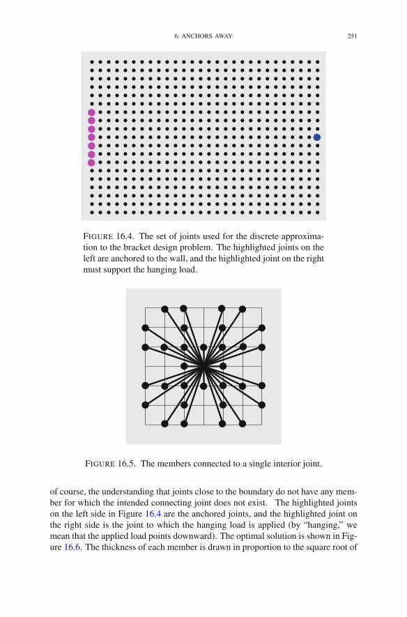
6. ANCHORS AWAY 251
FIGURE 16.4. The set of joints used for the discrete approxima-tion to the bracket design problem. The highlighted joints on theleft are anchored to the wall, and the highlighted joint on the rightmust support the hanging load.
FIGURE 16.5. The members connected to a single interior joint.
of course, the understanding that joints close to the boundary do not have any mem-ber for which the intended connecting joint does not exist. The highlighted jointson the left side in Figure 16.4 are the anchored joints, and the highlighted joint onthe right side is the joint to which the hanging load is applied (by “hanging,” wemean that the applied load points downward). The optimal solution is shown in Fig-ure 16.6. The thickness of each member is drawn in proportion to the square root of
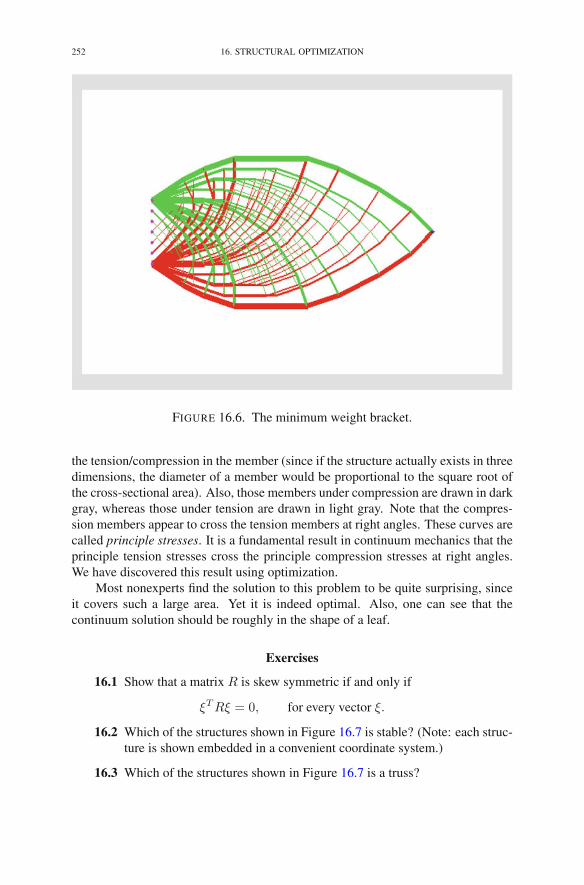
252 16. STRUCTURAL OPTIMIZATION
FIGURE 16.6. The minimum weight bracket.
the tension/compression in the member (since if the structure actually exists in threedimensions, the diameter of a member would be proportional to the square root ofthe cross-sectional area). Also, those members under compression are drawn in darkgray, whereas those under tension are drawn in light gray. Note that the compres-sion members appear to cross the tension members at right angles. These curves arecalled principle stresses. It is a fundamental result in continuum mechanics that theprinciple tension stresses cross the principle compression stresses at right angles.We have discovered this result using optimization.
Most nonexperts find the solution to this problem to be quite surprising, sinceit covers such a large area. Yet it is indeed optimal. Also, one can see that thecontinuum solution should be roughly in the shape of a leaf.
Exercises
16.1 Show that a matrix R is skew symmetric if and only if
ξTRξ = 0, for every vector ξ.
16.2 Which of the structures shown in Figure 16.7 is stable? (Note: each struc-ture is shown embedded in a convenient coordinate system.)
16.3 Which of the structures shown in Figure 16.7 is a truss?

EXERCISES 253
a b
c d
e f
FIGURE 16.7. Structures for Exercises 16.2 and 16.3.
16.4 Assuming that the total applied force vanishes, show that total torque istranslation invariant. That is, for any vector ξ ∈ R
d,∑
i
(R(pi − ξ))T bi =∑
i
(Rpi)T bi.
16.5 In 3-dimensions there are 5 regular (Platonic) solids. They are shown inFigure 16.8 and have the following number of vertices and edges:
vertices edgestetrahedron 4 6cube 8 12octahedron 6 12dodecahedron 20 30icosahedron 12 30

254 16. STRUCTURAL OPTIMIZATION
FIGURE 16.8. The five regular solids.
If one were to construct pin-jointed wire-frame models of these solids,which ones would be stable?
Notes
Structural optimization has its roots in Michell (1904). The first paper in whichtruss design was formulated as a linear programming problem is Dorn et al. (1964).A few general references on the subject include Hemp (1973), Rozvany (1989),Bendsøe et al. (1994), and Recski (1989).

Part 3
Interior-Point Methods

There is, I believe, in every disposition atendency to some particular evil—a natural
defect, which not even the best educationcan overcome.—J. Austen

CHAPTER 17
The Central Path
In this chapter, we begin our study of an alternative to the simplex method forsolving linear programming problems. The algorithm we are going to introduce iscalled a path-following method. It belongs to a class of methods called interior-pointmethods. The path-following method seems to be the simplest and most natural ofall the methods in this class, so in this book we focus primarily on it. Before wecan introduce this method, we must define the path that appears in the name of themethod. This path is called the central path and is the subject of this chapter. Beforediscussing the central path, we must lay some groundwork by analyzing a nonlin-ear problem, called the barrier problem, associated with the linear programmingproblem that we wish to solve.
Warning: Nonstandard Notation Ahead
Starting with this chapter, given a lower-case letter denoting a vector quantity,we shall use the upper-case form of the same letter to denote the diagonal matrixwhose diagonal entries are those of the corresponding vector. For example,
x =
⎡
⎢⎢⎢⎣
x1
x2
...xn
⎤
⎥⎥⎥⎦
=⇒ X =
⎡
⎢⎢⎢⎣
x1
x2
. . .xn
⎤
⎥⎥⎥⎦.
This notation is nonstandard in mathematics at large, but has achieved a certainamount of acceptance in the interior-point-methods community.
1. The Barrier Problem
In this chapter, we consider the linear programming problem expressed, asusual, with inequality constraints and nonnegative variables:
maximize cTxsubject to Ax≤ b
x≥ 0.
The corresponding dual problem is
minimize bT y
subject to AT y ≥ cy ≥ 0.
R.J. Vanderbei, Linear Programming, International Series in Operations Research& Management Science 196, DOI 10.1007/978-1-4614-7630-6 17,© Springer Science+Business Media New York 2014
257
258 17. THE CENTRAL PATH
As usual, we add slack variables to convert both problems to equality form:
(17.1)maximize cTxsubject to Ax+ w= b
x, w≥ 0
andminimize bT y
subject to AT y − z = cy, z ≥ 0.
Given a constrained maximization problem where some of the constraints areinequalities (such as our primal linear programming problem), one can considerreplacing any inequality constraint with an extra term in the objective function. Forexample, in (17.1) we could remove the constraint that a specific variable, say, xj ,is nonnegative by adding to the objective function a term that is negative infinitywhen xj is negative and is zero otherwise. This reformulation doesn’t seem to beparticularly helpful, since this new objective function has an abrupt discontinuitythat, for example, prevents us from using calculus to study it. However, suppose wereplace this discontinuous function with another function that is negative infinitywhen xj is negative but is finite for xj positive and approaches negative infinity asxj approaches zero. In some sense this smooths out the discontinuity and perhapsimproves our ability to apply calculus to its study. The simplest such function isthe logarithm. Hence, for each variable, we introduce a new term in the objectivefunction that is just a constant times the logarithm of the variable:
(17.2)maximize cTx+ μ
∑j log xj + μ
∑i logwi
subject to Ax+ w = b.
This problem, while not equivalent to our original problem, seems not too differenteither. In fact, as the parameter μ, which we assume to be positive, gets small, itappears that (17.2) becomes a better and better stand-in for (17.1). Problem (17.2)is called the barrier problem associated with (17.1). Note that it is not really oneproblem, but rather a whole family of problems indexed by the parameter μ. Each ofthese problems is a nonlinear programming problem because the objective functionis nonlinear. This nonlinear objective function is called a barrier function or, morespecifically, a logarithmic barrier function.
It is instructive to have in mind a geometric picture of the barrier function. Re-call that, for problems expressed in standard form, the set of feasible solutions isa polyhedron with each face being characterized by the property that one of thevariables is zero. Hence, the barrier function is minus infinity on each face of thepolyhedron. Furthermore, it is finite in the interior of the polyhedron, and it ap-proaches minus infinity as the boundary is approached. Figure 17.1 shows somelevel sets for the barrier function for a specific problem and a few different choicesof μ. Notice that, for each μ, the maximum is attained at an interior point, and asμ gets closer to zero this interior point moves closer to the optimal solution of theoriginal linear programming problem (which is at the top vertex). Viewed as a func-tion of μ, the set of optimal solutions to the barrier problems forms a path through

2. LAGRANGE MULTIPLIERS 259
μ= 8
μ=1
μ=0.01
μ=∞ μ=1
μ=0.01 central path
a b
c d
FIGURE 17.1. Parts (a) through (c) show level sets of the barrierfunction for three values of μ. For each value of μ, four level setsare shown. The maximum value of the barrier function is attainedinside the innermost level set. The drawing in part (d) shows thecentral path.
the interior of the polyhedron of feasible solutions. This path is called the centralpath. Our aim is to study this central path. To this end, we need to develop somemachinery, referred to as Lagrange multipliers.
2. Lagrange Multipliers
We wish to discuss briefly the general problem of maximizing a function sub-ject to one or more equality constraints. Here, the functions are permitted to benonlinear, but are assumed to be smooth, say, twice differentiable.
For the moment, suppose that there is a single constraint equation so that theproblem can be formally stated as
maximize f(x)subject to g(x) = 0.
In this case, the geometry behind the problem is compelling (see Figure 17.2). Thegradient of f , denoted ∇f , is a vector that points in the direction of most rapidincrease of f . For unconstrained optimization, we would simply set this vector equalto zero to determine the so-called critical points of f , and the maximum, if it exists,would have to be included in this set. However, given the constraint, g(x) = 0, it isno longer correct to look at points where the gradient vanishes. Instead, the gradientmust be orthogonal to the set of feasible solutions {x : g(x) = 0}. Of course, ateach point x in the feasible set, ∇g(x), is a vector that is orthogonal to the feasible

260 17. THE CENTRAL PATH
g=0x* Δf
FIGURE 17.2. The concentric rings illustrate a few level sets off . Clearly, at the optimal solution, x∗, the gradient must be per-pendicular to the feasible set.
set at this point x. Hence, our new requirement for a point x∗ to be a critical pointis that it is feasible and that ∇f(x∗) be proportional to ∇g(x∗). Writing this out asa system of equations, we have
g(x∗) = 0
∇f(x∗) = y∇g(x∗).
Here, y is the proportionality constant. Note that it can be any real number, ei-ther positive, negative, or zero. This proportionality constant is called a Lagrangemultiplier.
Now consider several constraints:maximize f(x)subject to g1(x) = 0
g2(x) = 0...
gm(x) = 0.
In this case, the feasible region is the intersection of m hypersurfaces (see Fig-ure 17.3). The space orthogonal to the feasible set at a point x is no longer a one-dimensional set determined by a single gradient, but is instead a higher-dimensionalspace (typically m), given by the span of the gradients. Hence, we require that∇f(x∗) lie in this span. This yields the following set of equations for a criticalpoint:
g(x∗) = 0
∇f(x∗) =m∑
i=1
yi∇g(x∗).(17.3)
The derivation of these equations has been entirely geometric, but there is also asimple algebraic formalism that yields the same equations. The idea is to introducethe so-called Lagrangian function

2. LAGRANGE MULTIPLIERS 261
g1=0
x*
g2=0
Δg2
Δg1
Δf
Δf
FIGURE 17.3. The feasible set is the curve formed by the inter-section of g1 = 0 and g2 = 0. The point x∗ is optimal, since thegradient of f at that point is perpendicular to the feasible set.
L(x, y) = f(x)−∑
i
yigi(x)
and to look for its critical points over both x and y. Since this is now an uncon-strained optimization problem, the critical points are determined by simply settingall the first derivatives to zero:
∂L
∂xj=
∂f
∂xj−
∑
i
yi∂gi∂xj
= 0, j = 1, 2, . . . , n,
∂L
∂yi= −gi = 0, i = 1, 2, . . . ,m.
Writing these equations in vector notation, we see that they are exactly the same asthose derived using the geometric approach. These equations are usually referred toas the first-order optimality conditions.
Determining whether a solution to the first-order optimality conditions is indeeda global maximum as desired can be difficult. However, if the constraints are alllinear, the first step (which is often sufficient) is to look at the matrix of secondderivatives:
Hf(x) =
[∂2f
∂xi∂xj
]
.
This matrix is called the Hessian of f at x. We have
THEOREM 17.1. If the constraints are linear, a critical point x∗ is a local max-imum if
(17.4) ξTHf(x∗)ξ < 0
262 17. THE CENTRAL PATH
for each ξ �= 0 satisfying
(17.5) ξT∇gi(x∗) = 0, i = 1, 2, . . . ,m.
PROOF. We start with the two-term Taylor series expansion of f about x∗:
f(x∗ + ξ) = f(x∗) +∇f(x∗)T ξ +1
2ξTHf(x∗)ξ + o(‖ξ‖2).
The vector ξ represents a displacement from the current point x∗. The only displace-ments that are relevant are those that lie in the feasible set. Hence, let ξ be a directionvector satisfying (17.5). From (17.3) and (17.5), we see that ∇f(x∗)T ξ = 0, and so
f(x∗ + ξ) = f(x∗) +1
2ξTHf(x∗)ξ + o(‖ξ‖2).
Employing (17.4) finishes the proof. �
It is worth remarking that if (17.4) is satisfied not just at x∗ but at all x, then x∗
is a unique global maximum.In the next section, we shall use Lagrange multipliers to study the central path
defined by the barrier problem.
3. Lagrange Multipliers Applied to the Barrier Problem
In this section, we shall use the machinery of Lagrange multipliers to study thesolution to the barrier problem. In particular, we will show that (subject to somemild assumptions) for each value of the barrier parameter μ, there is a unique solu-tion to the barrier problem. We will also show that as μ tends to zero, the solution tothe barrier problem tends to the solution to the original linear programming problem.In the course of our study, we will stumble naturally upon the central path for thedual problem. Taken together, the equations defining the primal and the dual centralpaths play an important role, and so we will introduce the notion of a primal–dualcentral path.
We begin by recalling the barrier problem:
maximize cTx+ μ∑
j log xj + μ∑
i logwi
subject to Ax+ w = b.
This is an equality-constrained optimization problem, and so it is a problem to whichwe can apply the Lagrange multiplier tools developed in the previous section. TheLagrangian for this problem is
L(x,w, y) = cTx+ μ∑
j
log xj + μ∑
i
logwi + yT (b−Ax− w).
3. LAGRANGE MULTIPLIERS APPLIED TO THE BARRIER PROBLEM 263
Taking derivatives with respect to each variable and setting them to zero, we get thefirst-order optimality conditions:
∂L
∂xj= cj + μ
1
xj−
∑
i
yiaij = 0, j = 1, 2, . . . , n,
∂L
∂wi= μ
1
wi− yi = 0, i = 1, 2, . . . ,m.
∂L
∂yi= bi −
∑
j
aijxj − wi = 0, i = 1, 2, . . . ,m.
Writing these equations in matrix form, we get
AT y − μX−1e = c
y = μW−1e
Ax+ w = b.
Here, as warned at the beginning of the chapter, X denotes the diagonal matrixwhose diagonal entries are the components of x, and similarly for W . Also, recallthat we use e to denote the vector of all ones.
Introducing an extra vector defined as z = μX−1e, we can rewrite the first-order optimality conditions like this:
Ax+ w = b.
AT y − z = c
z = μX−1e
y = μW−1e.
Finally, if we multiply the third equation through by X and the fourth equation byW , we arrive at a primal–dual symmetric form for writing these equations:
(17.6)
Ax+ w= bAT y − z = c
XZe= μeYWe= μe.
Note that the first equation is the equality constraint that appears in the primal prob-lem, while the second equation is the equality constraint for the dual problem. Fur-thermore, writing the third and fourth equations out componentwise,
xjzj = μ j = 1, 2, . . . , n
yiwi = μ i = 1, 2, . . . ,m,
we see that they are closely related to our old friend: complementarity. In fact, ifwe set μ to zero, then they are exactly the usual complementarity conditions thatmust be satisfied at optimality. For this reason, we call these last two equations theμ-complementarity conditions.
The first-order optimality conditions, as written in (17.6), give us 2n + 2mequations in 2n + 2m unknowns. If these equations were linear, they could be

264 17. THE CENTRAL PATH
solved using Gaussian elimination, and the entire subject of linear programmingwould be no more difficult than solving systems of linear equations. But alas, theyare nonlinear—but just barely. The only nonlinear expressions in these equationsare simple multiplications such as xjzj . This is about the closest to being linearthat one could imagine. Yet, it is this nonlinearity that makes the subject of linearprogramming nontrivial.
We must ask both whether a solution to (17.6) exists and if so is it unique. Weaddress these questions in reverse order.
4. Second-Order Information
To show that the solution, if it is exists, must be unique, we use second-orderinformation on the barrier function:
(17.7) f(x,w) = cTx+ μ∑
j
log xj + μ∑
i
logwi.
The first derivatives are∂f
∂xj= cj +
μ
xj, j = 1, 2, . . . , n,
∂f
∂wi=
μ
wi, i = 1, 2, . . . ,m,
and the pure second derivatives are
∂2f
∂x2j
= − μ
x2j
, j = 1, 2, . . . , n,
∂2f
∂w2i
= − μ
w2i
, i = 1, 2, . . . ,m.
All the mixed second derivatives vanish. Therefore, the Hessian is a diagonal matrixwith strictly negative entries. Hence, by Theorem 17.1, there can be at most onecritical point and, if it exists, it is a global maximum.
5. Existence
So, does a solution to the barrier problem always exist? It might not. Consider,for example, the following trivial optimization problem on the nonnegative half-line:
maximize 0subject to x ≥ 0.
For this problem, the barrier function is
f(x) = μ log x,
which doesn’t have a maximum (or, less precisely, the maximum is infinity whichis attained at x = ∞). However, such examples are rare. For example, considermodifying the objective function in this example to make x = 0 the unique optimalsolution:
maximize −xsubject to x ≥ 0.

5. EXISTENCE 265
In this case, the barrier function is
f(x) = −x+ μ log x,
which is a function whose maximum is attained at x = μ.In general, we have the following result:
THEOREM 17.2. There exists a solution to the barrier problem if and only ifboth the primal and the dual feasible regions have nonempty interior.
PROOF. The “only if” part is trivial and less important to us. Therefore, we onlyprove the “if” part. To this end, suppose that both the primal and the dual feasibleregions have nonempty interior. This means that there exists a primal feasible point(x, w) with x > 0 and w > 0 and there exists a dual feasible point (y, z) with y > 0and z > 0.1 Now, given any primal feasible point (x,w), consider the expressionzTx + yTw. Replacing the primal and dual slack variables with their definitions,we can rewrite this expression as follows:
zTx+ yTw =(AT y − c
)Tx+ yT (b−Ax)
= bT y − cTx.
Solving this equation for the primal objective function cTx, we get that
cTx = −zTx− yTw + bT y.
Therefore, the barrier function f defined in equation (17.7) can be written as fol-lows:
f(x,w) = cTx+ μ∑
j
log xj + μ∑
i
logwi
=∑
j
(−zjxj + μ log xj)
+∑
i
(−yiwi + μ logwi)
+ bT y.
Note that the last term is just a constant. Also, each summand in the two sums is afunction of just one variable. These functions all have the following general form:
h(ξ) = −aξ + μ log ξ, 0 < ξ < ∞,
where a > 0. Such functions have a unique maximum (at μ/a) and tend to −∞ asξ tends to ∞. From these observations, it is easy to see that, for every constant c,the set {
(x,w) ∈ Rn+m : f(x,w) ≥ c
}
is bounded.Put
f = f(x, w)
1Recall that we write ξ > 0 to mean that ξj > 0 for all j.

266 17. THE CENTRAL PATH
and let
P = {(x,w) : Ax+ w = b, x ≥ 0, w ≥ 0, f(x,w) ≥ f}.Clearly, P is nonempty, since it contains (x, w). From the discussion above, we seethat P is a bounded set.
This set is also closed. To see this, note that it is the intersection of three sets,
{(x,w) : Ax+ w = b} ∩ {(x,w) : x ≥ 0, w ≥ 0} ∩ {(x,w) : f(x,w) ≥ f}.
The first two of these sets are obviously closed. The third set is closed because it isthe inverse image of a closed set, [f ,∞], under a continuous mapping f . Finally,the intersection of three closed sets is closed.
In Euclidean spaces, a closed bounded set is called compact. A well-knowntheorem from real analysis about compact sets is that a continuous function on anonempty compact set attains its maximum. This means that there exists a pointin the compact set at which the function hits its maximum. Applying this theoremto f on P , we see that f does indeed attain its maximum on P , and this implies itattains its maximum on all of {(x,w) : x > 0, w > 0}, since P was by definitionthat part of this domain on which f takes large values (bigger than f , anyway). Thiscompletes the proof. �
We summarize our main result in the following corollary:
COROLLARY 17.3. If a primal feasible set (or, for that matter, its dual) has anonempty interior and is bounded, then for each μ > 0 there exists a unique solution
(xμ, wμ, yμ, zμ)
to (17.6).
PROOF. Follows immediately from the previous theorem and Exercise 10.7.�
The path {(xμ, wμ, yμ, zμ) : μ > 0} is called the primal–dual central path.It plays a fundamental role in interior-point methods for linear programming. Inthe next chapter, we define the simplest interior-point method. It is an iterativeprocedure that at each iteration attempts to move toward a point on the central paththat is closer to optimality than the current point.
Exercises
17.1 Compute and graph the central trajectory for the following problem:
maximize −x1 + x2
subject to x2 ≤ 1−x1 ≤ −1
x1, x2 ≥ 0 .
Hint: The primal and dual problems are the same—exploit this symmetry.
NOTES 267
17.2 Let θ be a fixed parameter, 0 ≤ θ ≤ π2 , and consider the following prob-
lem:maximize (cos θ)x1 + (sin θ)x2
subject to x1 ≤ 1x2 ≤ 1
x1, x2 ≥ 0.
Compute an explicit formula for the central path (xμ, wμ, yμ, zμ), andevaluate limμ→∞ xμ and limμ→0 xμ.
17.3 Suppose that {x : Ax ≤ b, x ≥ 0} is bounded. Let r ∈ Rn and s ∈ R
m bevectors with positive elements. By studying an appropriate barrier func-tion, show that there exists a unique solution to the following nonlinearsystem:
Ax+ w= bAT y − z = c
XZe= rY We= s
x, y, z, w > 0.
17.4 Consider the linear programming problem in equality form:
(17.8)
maximize∑
j cjxj
subject to∑
j
ajxj = b
xj ≥ 0, j = 1, 2, . . . , n,where each aj is a vector in R
m, as is b. Consider the change of variables,
xj = ξ2j ,
and the associated maximization problem:
(17.9)maximize
∑j cjξ
2j
subject to∑
j ajξ2j = b
(note that the nonnegativity constraints are no longer needed). Let V de-note the set of basic feasible solutions to (17.8), and let W denote the setof points (ξ21 , ξ
22 , . . . , ξ
2n) in R
n for which (ξ1, ξ2, . . . , ξn) is a solutionto the first-order optimality conditions for (17.9). Show that V ⊂ W .What does this say about the possibility of using (17.9) as a vehicle tosolve (17.8)?
Notes
Research into interior-point methods has its roots in the work of Fiacco andMcCormick (1968). Interest in these methods exploded after the appearance ofthe seminal paper Karmarkar (1984). Karmarkar’s paper uses clever ideas fromprojective geometry. It doesn’t mention anything about central paths, which havebecome fundamental to the theory of interior-point methods. The discovery thatKarmarkar’s algorithm has connections with the primal–dual central path introducedin this chapter can be traced to Megiddo (1989). The notion of central points can be

268 17. THE CENTRAL PATH
traced to pre-Karmarkar times with the work of Huard (1967). D.A. Bayer and J.C.Lagarias, in a pair of papers (Bayer and Lagarias 1989a,b), give an in-depth studyof the central path.
Deriving optimality conditions and giving conditions under which they are nec-essary and sufficient to guarantee optimality is one of the main goals of nonlin-ear programming. Standard texts on this subject include the books by Luenberger(1984), Bertsekas (1995), and Nash and Sofer (1996).
CHAPTER 18
A Path-Following Method
In this chapter, we define an interior-point method for linear programming thatis called a path-following method. Recall that for the simplex method we requireda two-phase solution procedure. The path-following method is a one-phase method.This means that the method can begin from a point that is neither primal nor dualfeasible and it will proceed from there directly to the optimal solution. Hence,we start with an arbitrary choice of strictly positive values for all the primal anddual variables, i.e., (x,w, y, z) > 0, and then iteratively update these values asfollows:
(1) Estimate an appropriate value for μ (i.e., smaller than the “current” valuebut not too small).
(2) Compute step directions (Δx,Δw,Δy,Δz) pointing approximately atthe point (xμ, wμ, yμ, zμ) on the central path.
(3) Compute a step length parameter θ such that the new point
x = x+ θΔx, y = y + θΔy,
w = w + θΔw, z = z + θΔz
continues to have strictly positive components.(4) Replace (x,w, y, z) with the new solution (x, w, y, z).
To fully define the path-following method, it suffices to make each of these foursteps precise. Since the second step is in some sense the most fundamental, we startby describing that one after which we turn our attention to the others.
1. Computing Step Directions
Our aim is to find (Δx,Δw,Δy,Δz) such that the new point (x + Δx,w +Δw, y+Δy, z+Δz) lies approximately on the primal–dual central path at the point(xμ, wμ, yμ, zμ). Recalling the defining equations for this point on the central path,
Ax+ w = b
AT y − z = c
XZe = μe
YWe = μe,
we see that the new point (x + Δx,w + Δw, y + Δy, z + Δz), if it were to lieexactly on the central path at μ, would be defined by
R.J. Vanderbei, Linear Programming, International Series in Operations Research& Management Science 196, DOI 10.1007/978-1-4614-7630-6 18,© Springer Science+Business Media New York 2014
269
270 18. A PATH-FOLLOWING METHOD
A(x+Δx) + (w +Δw) = b
AT (y +Δy)− (z +Δz) = c
(X +ΔX)(Z +ΔZ)e = μe
(Y +ΔY )(W +ΔW )e = μe.
Thinking of (x,w, y, z) as data and (Δx,Δw,Δy,Δz) as unknowns, we rewritethese equations with the unknowns on the left and the data on the right:
AΔx+Δw = b−Ax− w =: ρ
ATΔy −Δz = c−AT y + z =: σ
ZΔx+XΔz +ΔXΔZe = μe−XZe
WΔy + YΔw +ΔYΔWe = μe− YWe.
Note that we have introduced abbreviated notations, ρ and σ, for the first two right-hand sides. These two vectors represent the primal infeasibility and the dual infea-sibility, respectively.
Now, just as before, these equations form a system of nonlinear equations (thistime for the “delta” variables). We want to have a linear system, so at this point wesimply drop the nonlinear terms to arrive at the following linear system:
AΔx+Δw = ρ(18.1)
ATΔy −Δz = σ(18.2)
ZΔx+XΔz = μe−XZe(18.3)
WΔy + YΔw = μe− YWe.(18.4)
This system of equations is a linear system of 2n + 2m equations in 2n + 2munknowns. We will show later that this system is nonsingular (under the mild as-sumption that A has full rank) and therefore that it has a unique solution that definesthe step directions for the path-following method. Chapters 19 and 20 are devotedto studying methods for efficiently solving systems of this type.
If the business of dropping the nonlinear “delta” terms strikes you as bold, letus remark that this is the most common approach to solving nonlinear systems ofequations. The method is called Newton’s method. It is described briefly in the nextsection.
2. Newton’s Method
Given a function
F (ξ) =
⎡
⎢⎢⎢⎣
F1(ξ)F2(ξ)
...FN (ξ)
⎤
⎥⎥⎥⎦, ξ =
⎡
⎢⎢⎢⎣
ξ1ξ2...ξN
⎤
⎥⎥⎥⎦,
from RN into R
N , a common problem is to find a point ξ∗ ∈ RN for which
F (ξ∗) = 0. Such a point is called a root of F . Newton’s method is an iterativemethod for solving this problem. One step of the method is defined as follows.

2. NEWTON’S METHOD 271
Given any point ξ ∈ RN , the goal is to find a step direction Δξ for which F (ξ +
Δξ) = 0. Of course, for a nonlinear F it is not possible to find such a step direction.Hence, it is approximated by the first two terms of its Taylor’s series expansion,
F (ξ +Δξ) ≈ F (ξ) + F ′(ξ)Δξ,
where
F ′(ξ) =
⎡
⎢⎢⎢⎢⎢⎢⎢⎢⎢⎢⎣
∂F1
∂ξ1∂F1
∂ξ2· · · ∂F1
∂ξN
∂F2
∂ξ1∂F2
∂ξ2· · · ∂F2
∂ξN
......
...
∂FN
∂ξ1∂FN
∂ξ2· · · ∂FN
∂ξN
⎤
⎥⎥⎥⎥⎥⎥⎥⎥⎥⎥⎦
.
The approximation is linear in Δξ. Hence, equating it to zero gives a linear systemto solve for the step direction:
F ′(ξ)Δξ = −F (ξ).
Given Δξ, Newton’s method updates the current solution ξ by replacing it withξ+Δξ. The process continues until the current solution is approximately a root (i.e.,F (ξ) ≈ 0). Simple one-dimensional examples given in every elementary calculustext illustrate that this method works well, when it works, but it can fail if F is notwell behaved and the initial point is too far from a solution.
Let’s return now to the problem of finding a point on the central path. Letting
ξ =
⎡
⎢⎢⎣
xwyz
⎤
⎥⎥⎦
and
F (ξ) =
⎡
⎢⎢⎣
Ax+ w − bAT y − z − cXZe− μeYWe− μe
⎤
⎥⎥⎦ ,
we see that the set of equations defining (xμ, wμ, yμ, zμ) is a root of F . The matrixof derivatives of F is given by
F ′(ξ) =
⎡
⎢⎢⎣
A I 0 00 0 AT −IZ 0 0 X0 Y W 0
⎤
⎥⎥⎦ .
Noting that
Δξ =
⎡
⎢⎢⎣
ΔxΔwΔyΔz
⎤
⎥⎥⎦ ,

272 18. A PATH-FOLLOWING METHOD
it is easy to see that the Newton direction coincides with the direction obtained bysolving equations (18.1)–(18.4).
3. Estimating an Appropriate Value for the Barrier Parameter
We need to say how to pick μ. If μ is chosen to be too large, then the sequencecould converge to the analytic center of the feasible set, which is not our intention.If, on the other hand, μ is chosen to be too small, then the sequence could stray toofar from the central path and the algorithm could jam into the boundary of the fea-sible set at a place that is suboptimal. The trick is to find a reasonable compromisebetween these two extremes. To do this, we first figure out a value that represents,in some sense, the current value of μ and we then choose something smaller thanthat, say a fixed fraction of it.
We are given a point (x,w, y, z) that is almost certainly off the central path.If it were on the central path, then there are several formulas by which we couldrecover the corresponding value of μ. For example, we could just compute zjxj forany fixed index j. Or we could compute yiwi for any fixed i. Or, perverse as it mayseem, we could average all these values:
(18.5) μ =zTx+ yTw
n+m.
This formula gives us exactly the value of μ whenever it is known that (x,w, y, z)lies on the central path. The key point here then is that we will use this formula toproduce an estimate for μ even when the current solution (x,w, y, z) does not lie onthe central path. Of course, the algorithm needs a value of μ that represents a pointcloser to optimality than the current solution. Hence, the algorithm takes this “par”value and reduces it by a certain fraction:
μ = δzTx+ yTw
n+m,
where δ is a number between zero and one. In practice, one finds that setting δ toapproximately 1/10 works quite well, but for the sake of discussion we will alwaysleave it as a parameter.
4. Choosing the Step Length Parameter
The step directions, which were determined using Newton’s method, were de-termined under the assumption that the step length parameter θ would be equal toone (i.e., x = x + Δx, etc.). But taking such a step might cause the new solutionto violate the property that every component of all the primal and the dual variablesmust remain positive. Hence, we may need to use a smaller value for θ. We need toguarantee, for example, that
xj + θΔxj > 0, j = 1, 2, . . . , n.

4. CHOOSING THE STEP LENGTH PARAMETER 273
initialize (x,w, y, z) > 0while (not optimal) {
ρ = b−Ax− wσ = c−AT y + zγ = zTx+ yTw
μ = δγ
n+msolve:
AΔx+Δw = ρATΔy −Δz = σZΔx+XΔz = μe−XZeWΔy + YΔw = μe− YWe
θ = r
(
maxij
{
−Δxj
xj,−Δwi
wi,−Δyi
yi,−Δzj
zj
})−1
∧ 1
x ← x+ θΔx, w ← w + θΔw
y ← y + θΔy, z ← z + θΔz
}
FIGURE 18.1. The path-following method.
Moving the Δxj term to the other side and then dividing through by θ and xj , bothof which are positive, we see that θ must satisfy
1
θ> −Δxj
xj, j = 1, 2, . . . , n.
Of course, a similar inequality must be satisfied for the w, y, and z variables too.Putting it all together, the largest value of θ would be given by
1
θ= max
ij
{
−Δxj
xj,−Δwi
wi,−Δyi
yi,−Δzj
zj
}
,
where we have abused notation slightly by using the maxij to denote the maximumof all the ratios in the indicated set. However, this choice of θ will not guaranteestrict inequality, so we introduce a parameter r, which is a number close to butstrictly less than one, and we set1
(18.6) θ = r
(
maxij
{
−Δxj
xj,−Δwi
wi,−Δyi
yi,−Δzj
zj
})−1
∧ 1.
This formula may look messy, and no one should actually do it by hand, but it istrivial to program a computer to do it. Such a subroutine will be really fast (requiringonly on the order of 2n+ 2m operations).
A summary of the algorithm is shown in Figure 18.1. In the next section, weinvestigate whether this algorithm actually converges to an optimal solution.
1For compactness, we use the notation a ∧ b to represent the minimum of the two numbers a and b.
274 18. A PATH-FOLLOWING METHOD
5. Convergence Analysis
In this section, we investigate the convergence properties of the path-followingalgorithm. Recall that the simplex method is a finite algorithm (assuming that stepsare taken to guard against cycling). For interior-point methods, the situation is dif-ferent. Every solution produced has all variables strictly positive. Yet for a solutionto be optimal generally requires many variables to vanish. This vanishing can onlyhappen “in the limit.” This raises questions, the most fundamental of which arethese: does the sequence of solutions produced by the path-following method con-verge? If so, is the limit optimal? How fast is the convergence? In particular, ifwe set “optimality tolerances,” how many iterations will it take to achieve thesetolerances? We will address these questions in this section.
In this section, we will need to measure the size of various vectors. There aremany choices. For example, for each 1 ≤ p < ∞, we can define the so-calledp-norm of a vector x as
‖x‖p =
⎛
⎝∑
j
|xj |p⎞
⎠
1p
.
The limit as p tends to infinity is also well defined, and it simplifies to the so-calledsup-norm:
‖x‖∞ = maxj
|xj |.
5.1. Measures of Progress. Recall from duality theory that there are threecriteria that must be met in order that a primal–dual solution be optimal:
(1) Primal feasibility,(2) Dual feasibility, and(3) Complementarity.
For each of these criteria, we introduce a measure of the extent to which they fail tobe met.
For the primal feasibility criterion, we use the 1-norm of the primal infeasibilityvector
ρ = b−Ax− w.
For the dual feasibility criterion, we use the 1-norm of the dual infeasibility vector
σ = c−AT y + z.
For complementarity, we use
γ = zTx+ yTw.
5.2. Progress in One Iteration. For the analysis in the section, we prefer tomodify the algorithm slightly by having it take shorter steps than specified before.Indeed, we let

5. CONVERGENCE ANALYSIS 275
θ = r
(
maxi,j
{∣∣∣∣Δxj
xj
∣∣∣∣ ,
∣∣∣∣Δwi
wi
∣∣∣∣ ,
∣∣∣∣Δyiyi
∣∣∣∣ ,
∣∣∣∣Δzjzj
∣∣∣∣
})−1
∧ 1
=r
max(‖X−1Δx‖∞, . . . , ‖Z−1Δz‖∞)∧ 1.(18.7)
Note that the only change has been to replace the negative ratios with the absolutevalue of the same ratios. Since the maximum of the absolute values can be largerthan the maximum of the ratios themselves, this formula produces a smaller valuefor θ. In this section, let x, y, etc., denote quantities from one iteration of thealgorithm, and put a tilde on the same letters to denote the same quantity at the nextiteration of the algorithm. Hence,
x = x+ θΔx, y = y + θΔy,
w = w + θΔw, z = z + θΔz.
Now let’s compute some of the other quantities. We begin with the primalinfeasibility:
ρ = b−Ax− w
= b−Ax− w − θ(AΔx+Δw).
But b − Ax − w equals the primal infeasibility ρ (by definition) and AΔx + Δwalso equals ρ, since this is precisely the first equation in the system that defines the“delta” variables. Hence,
(18.8) ρ = (1− θ)ρ.
Similarly,
σ = c−AT y + z
= c−AT y + z − θ(AΔy −Δz)
= (1− θ)σ.(18.9)
Since θ is a number between zero and one, it follows that each iteration produces adecrease in both the primal and the dual infeasibility and that this decrease is betterthe closer θ is to one.
The analysis of the complementarity is a little more complicated (after all, thisis the part of the system where the linearization took place):
γ = zT x+ yT w
= (z + θΔz)T (x+ θΔx) + (y + θΔy)T (w + θΔw)
= zTx+ yTw
+ θ(zTΔx+ΔzTx+ yTΔw +ΔyTw)
+ θ2(ΔzTΔx+ΔyTΔw).
276 18. A PATH-FOLLOWING METHOD
We need to analyze each of the θ terms separately. From (18.3), we see that
zTΔx+ΔzTx = eT (ZΔx+XΔz)
= eT (μe− ZXe)
= μn− zTx.
Similarly, from (18.4), we have
yTΔw +ΔyTw = eT (YΔw +WΔy)
= eT (μe− YWe)
= μm− yTw.
Finally, (18.1) and (18.2) imply that
ΔzTΔx+ΔyTΔw =(ATΔy − σ
)TΔx+ΔyT (ρ−AΔx)
= ΔyT ρ− σTΔx.
Substituting these expressions into the last expression for γ, we get
γ = zTx+ yTw
+ θ(μ(n+m)− (zTx+ yTw)
)
+ θ2(ΔyT ρ− σTΔx
).
At this point, we recognize that zTx+ yTw = γ and that μ(n+m) = δγ. Hence,
γ = (1− (1− δ)θ) γ + θ2(ΔyT ρ− σTΔx
).
We must now abandon equalities and work with estimates. Our favorite tool forestimation is the following inequality:
|vTw| = |∑
j
vjwj |
≤∑
j
|vj ||wj |
≤ (maxj
|vj |)(∑
j
|wj |)
= ‖v‖∞‖w‖1.This inequality is the trivial case of Holder’s inequality. From Holder’s inequality,we see that
|ΔyT ρ| ≤ ‖ρ‖1‖Δy‖∞ and |σTΔx| ≤ ‖σ‖1‖Δx‖∞.
Hence,
γ ≤ (1− (1− δ)θ) γ + θ (‖ρ‖1‖θΔy‖∞ + ‖σ‖1‖θΔx‖∞) .
Next, we use the specific choice of step length θ to get a bound on ‖θΔy‖∞ and‖θΔx‖∞. Indeed, (18.7) implies that
θ ≤ r
‖X−1Δx‖∞≤ xj
|Δxj |for all j.
5. CONVERGENCE ANALYSIS 277
Hence,‖θΔx‖∞ ≤ ‖x‖∞.
Similarly,‖θΔy‖∞ ≤ ‖y‖∞.
If we now assume that, along the sequence of points x and y visited by the algorithm,‖x‖∞ and ‖y‖∞ are bounded by a large real number M , then we can estimate thenew complementarity as
(18.10) γ ≤ (1− (1− δ)θ) γ +M‖ρ‖1 +M‖σ‖1.
5.3. Stopping Rule. Let ε > 0 be a small positive tolerance, and let M < ∞be a large finite tolerance. If ‖x‖∞ gets larger than M , then we stop and declare theproblem primal unbounded. If ‖y‖∞ gets larger than M , then we stop and declarethe problem dual unbounded. Finally, if ‖ρ‖1 < ε, ‖σ‖1 < ε, and γ < ε, thenwe stop and declare the current solution to be optimal (at least within this smalltolerance).
Since γ is a measure of complementarity and complementarity is related to theduality gap, one would expect that a small value of γ should translate into a smallduality gap. This turns out to be true. Indeed, from the definitions of γ, σ, and ρ,we can write
γ = zTx+ yTw
= (σ +AT y − c)Tx+ yT (b−Ax− ρ)
= bT y − cTx+ σTx− ρT y.
At this point, we use Holder’s inequality to bound some of these terms to get anestimate on the duality gap:
|bT y − cTx| ≤ γ + |σTx|+ |yT ρ|≤ γ + ‖σ‖1‖x‖∞ + ‖ρ‖1‖y‖∞.
Now, if γ, ‖σ‖1, and ‖ρ‖1 are all small (and ‖x‖∞ and ‖y‖∞ are not too big),then the duality gap will be small. This estimate shows that one shouldn’t expectthe duality gap to get small until the primal and the dual are very nearly feasible.Actual implementations confirm this expectation.
5.4. Progress Over Several Iterations. Now let ρ(k), σ(k), γ(k), θ(k), etc.,denote the values of these quantities at the kth iteration. We have the followingresult about the overall performance of the algorithm:
THEOREM 18.1. Suppose there is a real number t > 0, a real number M < ∞,and an integer K such that for all k ≤ K,
θ(k) ≥ t,
‖x(k)‖∞ ≤ M,
‖y(k)‖∞ ≤ M.
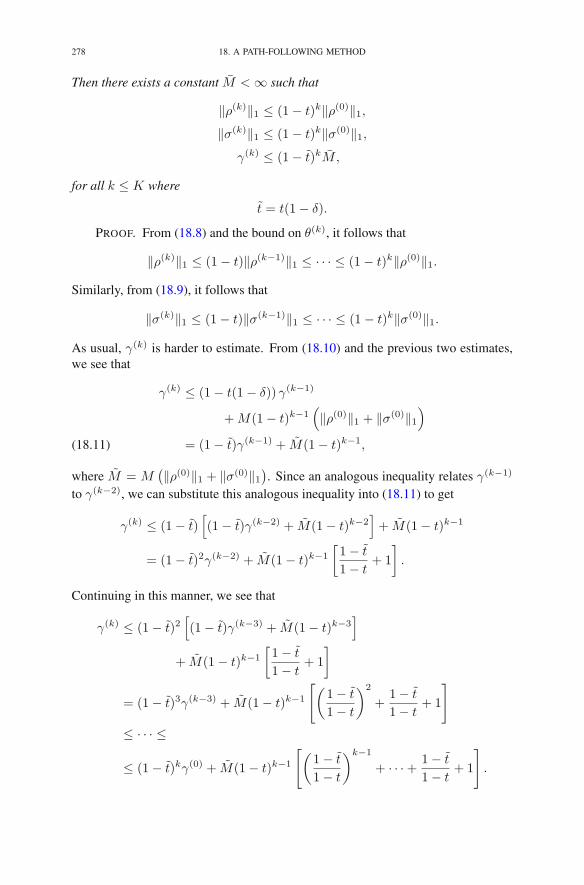
278 18. A PATH-FOLLOWING METHOD
Then there exists a constant M < ∞ such that
‖ρ(k)‖1 ≤ (1− t)k‖ρ(0)‖1,‖σ(k)‖1 ≤ (1− t)k‖σ(0)‖1,
γ(k) ≤ (1− t)kM,
for all k ≤ K where
t = t(1− δ).
PROOF. From (18.8) and the bound on θ(k), it follows that
‖ρ(k)‖1 ≤ (1− t)‖ρ(k−1)‖1 ≤ · · · ≤ (1− t)k‖ρ(0)‖1.
Similarly, from (18.9), it follows that
‖σ(k)‖1 ≤ (1− t)‖σ(k−1)‖1 ≤ · · · ≤ (1− t)k‖σ(0)‖1.
As usual, γ(k) is harder to estimate. From (18.10) and the previous two estimates,we see that
γ(k) ≤ (1− t(1− δ)) γ(k−1)
+M(1− t)k−1(‖ρ(0)‖1 + ‖σ(0)‖1
)
= (1− t)γ(k−1) + M(1− t)k−1,(18.11)
where M = M(‖ρ(0)‖1 + ‖σ(0)‖1
). Since an analogous inequality relates γ(k−1)
to γ(k−2), we can substitute this analogous inequality into (18.11) to get
γ(k) ≤ (1− t)[(1− t)γ(k−2) + M(1− t)k−2
]+ M(1− t)k−1
= (1− t)2γ(k−2) + M(1− t)k−1
[1− t
1− t+ 1
]
.
Continuing in this manner, we see that
γ(k) ≤ (1− t)2[(1− t)γ(k−3) + M(1− t)k−3
]
+ M(1− t)k−1
[1− t
1− t+ 1
]
= (1− t)3γ(k−3) + M(1− t)k−1
[(1− t
1− t
)2
+1− t
1− t+ 1
]
≤ · · · ≤
≤ (1− t)kγ(0) + M(1− t)k−1
[(1− t
1− t
)k−1
+ · · ·+ 1− t
1− t+ 1
]
.

EXERCISES 279
Now we sum the bracketed partial sum of a geometric series to get
(1− t)k−1
[(1− t
1− t
)k−1
+ · · ·+ 1− t
1− t+ 1
]
= (1− t)k−1
1−(1− t
1− t
)k
1− 1− t
1− t
=(1− t)k − (1− t)k
t− t.
Recalling that t = t(1− δ) and dropping the second term in the numerator, we get
(1− t)k − (1− t)k
t− t≤ (1− t)k
δt.
Putting this all together, we see that
γ(k) ≤ (1− t)k
(
γ(0) +M
δt
)
.
Denoting the parenthesized expression by M completes the proof. �
Theorem 18.1 is only a partial convergence result because it depends on theassumption that the step lengths remain bounded away from zero. To show that thestep lengths do indeed have this property requires that the algorithm be modifiedand that the starting point be carefully selected. The details are rather technical andhence omitted (see the Notes at the end of the chapter for references).
Also, before we leave this topic, note that the primal and dual infeasibilities godown by a factor of 1− t at each iteration, whereas the duality gap goes down by asmaller amount 1 − t. The fact that the duality gap converges more slowly that theinfeasibilities is also readily observed in practice.
Exercises
18.1 Starting from (x,w, y, z) = (e, e, e, e), and using δ = 1/10, and r =9/10, compute (x,w, y, z) after one step of the path-following methodfor the problem given in(a) Exercise 2.3.(b) Exercise 2.4.(c) Exercise 2.5.(d) Exercise 2.10.
18.2 Let {(xμ, wμ, yμ, zμ) : μ ≥ 0} denote the central trajectory. Show that
limμ→∞
bT yμ − cTxμ = ∞.
Hint: look at (18.5).
18.3 Consider a linear programming problem whose feasible region is boundedand has nonempty interior. Use the result of Exercise 18.2 to show thatthe dual problem’s feasible set is unbounded.

280 18. A PATH-FOLLOWING METHOD
18.4 Scale invariance. Consider a linear program and its dual:
(P )
max cTxs.t. Ax+ w = b
x, w ≥ 0
(D)
min bT y
s.t. AT y − z = c
y, z ≥ 0.
Let R and S be two given diagonal matrices having positive entries alongtheir diagonals. Consider the scaled reformulation of the original problemand its dual:
(P )
max (Sc)T xs.t. RASx+ w = Rb
x, w ≥ 0
(D)
min (Rb)T y
s.t. SATRy − z = Sc
y, z ≥ 0.
Let (xk, wk, yk, zk) denote the sequence of solutions generated by theprimal–dual interior-point method applied to (P )–(D). Similarly, let(xk, wk, yk, zk) denote the sequence of solutions generated by the primal–dual interior-point method applied to (P )–(D). Suppose that we have thefollowing relations among the starting points:
x0 = S−1x0, w0 = Rw0, y0 = R−1y0, z0 = Sz0.
Show that these relations then persist. That is, for each k ≥ 1,
xk = S−1xk, wk = Rwk, yk = R−1yk, zk = Szk.
18.5 Homotopy method. Let x, y, z, and w be given componentwise positive“initial” values for x, y, z, and w, respectively. Let t be a parameterbetween 0 and 1. Consider the following nonlinear system:
(18.12)
Ax+ w= tb+ (1− t)(Ax+ w)AT y − z = tc+ (1− t)(AT y − z)
XZe= (1− t)XZeY We= (1− t)Y W e
x, y, z, w > 0.(a) Use Exercise 17.3 to show that this nonlinear system has a unique
solution for each 0 ≤ t < 1. Denote it by (x(t), y(t), z(t), w(t)).(b) Show that (x(0), y(0), z(0), w(0)) = (x, y, z, w).(c) Assuming that the limit
(x(1), y(1), z(1), w(1)) = limt→1
(x(t), y(t), z(t), w(t))
exists, show that it solves the standard-form linear programming prob-lem.
(d) The family of solutions (x(t), y(t), z(t), w(t)), 0 ≤ t < 1, describesa curve in “primal–dual” space. Show that the tangent to this curve att = 0 coincides with the path-following step direction at (x, y, z, w)computed with μ = 0; that is,

EXERCISES 281
(dx
dt(0),
dy
dt(0),
dz
dt(0),
dw
dt(0)
)
= (Δx,Δy,Δz,Δw),
where (Δx,Δy,Δz,Δw) is the solution to (18.1)–(18.4).
18.6 Higher-order methods. The previous exercise shows that the path-follow-ing step direction can be thought of as the direction one gets by approxi-mating a homotopy path with its tangent line:
x(t) ≈ x(0) +dx
dt(0)t.
By using more terms of the Taylor’s series expansion, one can get a betterapproximation:
x(t) ≈ x(0) +dx
dt(0)t+
1
2
d2x
dt2(0)t2 + · · ·+ 1
k!
dkx
dtk(0)tk.
(a) Differentiating the equations in (18.12) twice, derive a linear systemfor (d2x/dt2(0), d2y/dt2(0), d2z/dt2(0), d2w/dt2(0)).
(b) Can the same technique be applied to derive linear systems for thehigher-order derivatives?
18.7 Linear Complementarity Problem. Given a k×k matrix M and a k-vectorq, a vector x is said to solve the linear complementarity problem if
−Mx+ z = qXZe = 0x, z ≥ 0
(note that the first equation can be taken as the definition of z).(a) Show that the optimality conditions for linear programming can be
expressed as a linear complementarity problem with
M =
[0 −AAT 0
]
.
(b) The path-following method introduced in this chapter can be ex-tended to cover linear complementarity problems. The main step inthe derivation is to replace the complementarity condition XZe = 0with a μ-complementarity condition XZe = μe and then to useNewton’s method to derive step directions Δx and Δz. Carry outthis procedure and indicate the system of equations that define Δxand Δz.
(c) Give conditions under which the system derived above is guaranteedto have a unique solution.
(d) Write down the steps of the path-following method for the linearcomplementarity problem.
(e) Study the convergence of this algorithm by adapting the analysisgiven in Section 18.5.

282 18. A PATH-FOLLOWING METHOD
18.8 Consider again the L1-regression problem:
minimize ‖b−Ax‖1.
Complete the following steps to derive the step direction vector Δx asso-ciated with the primal–dual affine-scaling method for solving this problem.(a) Show that the L1-regression problem is equivalent to the following
linear programming problem:
(18.13)minimize eT (t+ + t−)subject to Ax+ t+ − t− = b
t+, t− ≥ 0.(b) Write down the dual of (18.13).(c) Add slack and/or surplus variables as necessary to reformulate the
dual so that all inequalities are simple nonnegativities of variables.(d) Identify all primal–dual pairs of complementary variables.(e) Write down the nonlinear system of equations consisting of: (1) the
primal equality constraints, (2) the dual equality constraints, (3) allcomplementarity conditions (using μ = 0 since we are looking foran affine-scaling algorithm).
(f) Apply Newton’s method to the nonlinear system to obtain a linearsystem for step directions for all of the primal and dual variables.
(g) We may assume without loss of generality that both the initial primalsolution and the initial dual solution are feasible. Explain why.
(h) The linear system derived above is a 6× 6 block matrix system. Butit is easy to solve most of it by hand. First eliminate those step di-rections associated with the nonnegative variables to arrive at a 2× 2block matrix system.
(i) Next, solve the 2× 2 system. Give an explicit formula for Δx.(j) How does this primal–dual affine-scaling algorithm compare with
the iteratively reweighted least squares algorithm defined in Sec-tion 12.5?
18.9 (a) Let ξj , j = 1, 2, . . . , denote a sequence of real numbers between zeroand one. Show that
∏j(1− ξj) = 0 if
∑j ξj = ∞.
(b) Use the result of part a to prove the following convergence result: ifthe sequences ‖x(k)‖∞, k = 1, 2, . . . , and ‖y(k)‖∞, k = 1, 2, . . . ,are bounded and
∑k θ
(k) = ∞, then
limk→∞
‖ρ(k)‖1 = 0
limk→∞
‖σ(k)‖1 = 0
limk→∞
γ(k) = 0.

NOTES 283
Notes
The path-following algorithm introduced in this chapter has its origins in a pa-per by Kojima et al. (1989). Their paper assumed an initial feasible solution andtherefore was a true interior-point method. The method given in this chapter doesnot assume the initial solution is feasible—it is a one-phase algorithm. The simpleyet beautiful idea of modifying the Kojima–Mizuno–Yoshise primal–dual algorithmto make it into a one-phase algorithm is due to Lustig (1990).
Of the thousands of papers on interior-point methods that have appeared inthe last decade, the majority have included convergence proofs for some versionof an interior-point method. Here, we only mention a few of the important pa-pers. The first polynomial-time algorithm for linear programming was discoveredby Khachian (1979). Khachian’s algorithm is fundamentally different from any al-gorithm presented in this book. Paradoxically, it proved in practice to be inferior tothe simplex method. N.K. Karmarkar’s pathbreaking paper (Karmarkar 1984) con-tained a detailed convergence analysis. His claims, based on preliminary testing,that his algorithm is uniformly substantially faster than the simplex method sparkeda revolution in linear programming. Unfortunately, his claims proved to be exag-gerated, but nonetheless interior-point methods have been shown to be competitivewith the simplex method and usually superior on very large problems. The con-vergence proof for a primal–dual interior-point method was given by Kojima et al.(1989). Shortly thereafter, Monteiro and Adler (1989) improved on the convergenceanalysis. Two recent survey papers, Todd (1995) and Anstreicher (1996), give niceoverviews of the current state of the art. Also, a soon-to-be-published book byWright (1996) should prove to be a valuable reference to the reader wishing moreinformation on convergence properties of these algorithms.
The homotopy method outlined in Exercise 18.5 is described in Nazareth (1986,1996). Higher-order path-following methods are described (differently) in Carpen-ter et al. (1993).

CHAPTER 19
The KKT System
The most time-consuming aspect of each iteration of the path-following methodis solving the system of equations that defines the step direction vectors Δx, Δy,Δw, and Δz:
AΔx+Δw = ρ(19.1)
ATΔy −Δz = σ(19.2)
ZΔx+XΔz = μe−XZe(19.3)
WΔy + YΔw = μe− YWe.(19.4)
After minor manipulation, these equations can be written in block matrix form asfollows:
(19.5)
⎡
⎢⎢⎣
−XZ−1 −IA I
−I AT
I Y W−1
⎤
⎥⎥⎦
⎡
⎢⎢⎣
ΔzΔyΔxΔw
⎤
⎥⎥⎦ =
⎡
⎢⎢⎣
−μZ−1e+ xρσ
μW−1e− y
⎤
⎥⎥⎦ .
This system is called the Karush–Kuhn–Tucker system, or simply the KKT system.It is a symmetric linear system of 2n + 2m equations in 2n + 2m unknowns. Onecould, of course, perform a factorization of this large system and then follow thatwith a forward and backward substitution to solve the system. However, it is betterto do part of this calculation “by hand” first and only use a factorization routine tohelp solve a smaller system. There are two stages of reductions that one could apply.After the first stage, the remaining system is called the reduced KKT system, andafter the second stage it is called the system of normal equations. We shall discussthese two systems in the next two sections.
1. The Reduced KKT System
Equations (19.3) and (19.4) are trivial (in the sense that they only involve diag-onal matrices), and so it seems sensible to eliminate them right from the start. Topreserve the symmetry that we saw in (19.5), we should solve them for Δz and Δw,respectively:
Δz = X−1(μe−XZe− ZΔx)
Δw = Y −1(μe− YWe−WΔy).
R.J. Vanderbei, Linear Programming, International Series in Operations Research& Management Science 196, DOI 10.1007/978-1-4614-7630-6 19,© Springer Science+Business Media New York 2014
285

286 19. THE KKT SYSTEM
Substituting these formulas into (19.1) and (19.2), we get the so-called reduced KKTsystem:
AΔx− Y −1WΔy = ρ− μY −1e+ w(19.6)
ATΔy +X−1ZΔx = σ + μX−1e− z.(19.7)
Substituting in the definitions of ρ and σ and writing the system in matrix notation,we get
[−Y −1W A
AT X−1Z
] [ΔyΔx
]
=
[b−Ax− μY −1ec−AT y + μX−1e
]
.
Note that the reduced KKT matrix is again a symmetric matrix. Also, the right-handside displays symmetry between the primal and the dual. To reduce the system anyfurther, one needs to break the symmetry that we have carefully preserved up to thispoint. Nonetheless, we forge ahead.
2. The Normal Equations
For the second stage of reduction, there are two choices: we could either (1)solve (19.6) for Δy and eliminate it from (19.7) or (2) solve (19.7) for Δx andeliminate it from (19.6). For the moment, let us assume that we follow the latterapproach. In this case, we get from (19.7) that
(19.8) Δx = XZ−1(c−AT y + μX−1e−ATΔy),
which we use to eliminate Δx from (19.6) to get
−(Y −1W +AXZ−1AT )Δy = b−Ax− μY −1e(19.9)
−AXZ−1(c−AT y + μX−1e).
This last system is a system of m equations in m unknowns. It is called the systemof normal equations in primal form. It is a system of equations involving the matrixY −1W + AXZ−1AT . The Y −1W term is simply a diagonal matrix, and so thereal meat of this matrix is contained in the AXZ−1AT term.
Given that A is sparse (which is generally the case in real-world linear pro-grams), one would expect the matrix AXZ−1AT to be likewise sparse. However,we need to investigate the sparsity of AXZ−1AT (or lack thereof) more closely.Note that the (i, j)th element of this matrix is given by
(AXZ−1AT )ij =
n∑
k=1
aikxk
zkajk.
That is, the (i, j)th element is simply a weighted inner product of rows i and j ofthe A matrix. If these rows have disjoint nonzero patterns, then this inner product isguaranteed to be zero, but otherwise it must be treated as a potential nonzero. Thisis bad news if A is generally sparse but has, say, one dense column:

2. THE NORMAL EQUATIONS 287
∗ ∗ ∗∗ ∗ ∗∗ ∗ ∗∗ ∗ ∗∗ ∗
∗∗∗∗∗∗∗∗
∗ ∗ ∗ ∗ ∗∗ ∗
∗∗∗
∗ ∗∗
∗
=
∗ ∗ ∗ ∗ ∗∗ ∗ ∗ ∗ ∗∗ ∗ ∗ ∗ ∗∗ ∗ ∗ ∗ ∗∗ ∗ ∗ ∗ ∗
.
But don’t forget that we didn’t have to go the primal normal equations route.Instead, we could have chosen the other alternative of solving (19.6) for Δy,
Δy = −YW−1(b−Ax− μY −1e−AΔx),
and eliminating it from (19.7):
(ATYW−1A+X−1Z)Δx = c−AT y + μX−1e(19.10)
+ATYW−1(b−Ax− μY −1e).
The system defined by (19.10) is a system of n equations in n unknowns. It is calledthe system of normal equations in dual form. Note that dense columns do not posea problem for these equations. Indeed, for the example given above, we now get
∗ ∗ ∗ ∗ ∗∗ ∗
∗∗∗
∗ ∗∗
∗
∗∗∗∗∗
∗ ∗ ∗∗ ∗ ∗∗ ∗ ∗∗ ∗ ∗∗ ∗
=
∗ ∗ ∗ ∗ ∗ ∗ ∗ ∗∗ ∗ ∗ ∗∗ ∗ ∗∗ ∗ ∗∗ ∗ ∗∗ ∗ ∗∗ ∗ ∗∗ ∗ ∗
.
While this system is larger than the one before, it is also sparse, and sparsity almostalways is more important than matrix dimensions. In this example, the dense matrixassociated with the primal normal equations requires 65 arithmetic operations tofactor, whereas the larger, sparser matrix associated with the dual normal equationsrequires just 60. This is a small difference, but these are small matrices. As thematrices involved get large, factoring a dense matrix takes on the order of n3 oper-ations, whereas a very sparse matrix might take only on the order of n operations.Clearly, as n gets large, the difference between these becomes quite significant.
It would be great if we could say that it is always best to solve the primal normalequations or the dual normal equations. But as we’ve just seen, dense columns in Aare bad for the primal normal equations and, of course, it follows that dense rowsare bad for the dual normal equations. Even worse, some problems have constraintmatrices A that are overall very sparse but contain some dense rows and some densecolumns. Such problems are sure to run into trouble with either sets of normal equa-tions. For these reasons, it is best to factor the matrix in the reduced KKT systemdirectly. Then it is possible to find pivot orders that circumvent the difficulties posedby both dense columns and dense rows.

288 19. THE KKT SYSTEM
3. Step Direction Decomposition
In the next chapter, we shall discuss factorization techniques for symmetricmatrices (along with other implementation issues). However, before we embark onthat discussion, we end this chapter by taking a closer look at the formulas for thestep direction vectors. To be specific, let us look at Δx. From the primal normalequations (19.9), we can solve for Δy and then substitute the solution into (19.8) toget an explicit formula for Δx:
Δx =(D2 −D2AT (E−2 +AD2AT )−1AD2
)(c−AT y + μX−1e)(19.11)
+D2AT (E−2 +AD2AT )−1(b−Ax− μY −1e),
where we have denoted by D the positive diagonal matrix defined by
D2 = XZ−1
and we have denoted by E the positive diagonal matrix defined by
E2 = YW−1
(defining these matrices by their squares is possible, since the squares have positivediagonal entries). However, using the dual normal equations, we get
Δx =(ATE2A+D−2
)−1(c−AT y + μX−1e)(19.12)
+(ATE2A+D−2
)−1ATE2(b−Ax− μY −1e).
These two expressions for Δx look entirely different, but they must be the same,since we know that Δx is uniquely defined by the reduced KKT system. They areindeed the same, as can be shown directly by establishing a certain matrix identity.This is the subject of Exercise 19.1. There are a surprising number of publishedresearch papers on interior-point methods that present supposedly new algorithmsthat are in fact identical to existing methods. These papers get published becausethe equivalence is not immediately obvious (such as the one we just established).
We can gain further insight into the path-following method by looking moreclosely at the primal step direction vector. Formula (19.11) can be rearranged asfollows:
Δx =(D2 −D2AT (E−2 +AD2AT )−1AD2
)c
+ μ(D2 −D2AT (E−2 +AD2AT )−1AD2
)X−1e
− μD2AT (E−2 +AD2AT )−1Y −1e
+D2AT (E−2 +AD2AT )−1(b−Ax)
−D2AT(I − (E−2 +AD2AT )−1AD2AT
)y.
For comparison purposes down the road, we prefer to write the Y −1e that appears inthe second term containing μ as E−2W−1e. Also, using the result of Exercise 19.2,we can rewrite the bulk of the last line as follows:
(I − (E−2 +AD2AT )−1AD2AT
)y = (E−2 +AD2AT )−1E−2y
= (E−2 +AD2AT )−1w.

3. STEP DIRECTION DECOMPOSITION 289
Putting this all together, we get
Δx =(D2 −D2AT (E−2 +AD2AT )−1AD2
)c
+ μ(D2 −D2AT (E−2 +AD2AT )−1AD2
)X−1e
− μD2AT (E−2 +AD2AT )−1E−2W−1e
+D2AT (E−2 +AD2AT )−1ρ
= ΔxOPT + μΔxCTR +ΔxFEAS,
where
ΔxOPT =(D2 −D2AT (E−2 +AD2AT )−1AD2
)c,
ΔxCTR =(D2 −D2AT (E−2 +AD2AT )−1AD2
)X−1e
−D2AT (E−2 +AD2AT )−1E−2W−1e,
andΔxFEAS = D2AT (E−2 +AD2AT )−1ρ.
In Chapter 21, we shall show that these components of Δx have important connec-tions to the step directions that arise in a related interior-point method called theaffine-scaling method. For now, we simply establish some of their properties asthey relate to the path-following method. Our first result is that ΔxOPT is an ascentdirection.
THEOREM 19.1. cTΔxOPT ≥ 0.
PROOF. We use the result of Exercise 19.1 (with the roles of E and D switched)to see that
ΔxOPT = (ATE2A+D−2)−1c.
Hence,cTΔxOPT = cT (ATE2A+D−2)−1c.
We claim that the right-hand side is obviously nonnegative, since the matrix sand-wiched between c and its transpose is positive semidefinite.1 Indeed, the claimfollows from the definition of positive semidefiniteness: a matrix B is positive semi-definite if ξTBξ ≥ 0 for all vectors ξ. To see that the matrix in question is in factpositive semidefinite, we first note that ATE2A and D−2 are positive semidefinite:
ξTATE2Aξ = ‖EAξ‖2 ≥ 0 and ξTD−2ξ = ‖D−1ξ‖2 ≥ 0.
Then we show that the sum of two positive semidefinite matrices is positive semi-definite and finally that the inverse of a symmetric positive semidefinite matrix ispositive semidefinite. To verify closure under summation, suppose that B(1) andB(2) are positive semidefinite, and then compute
ξT (B(1) +B(2))ξ = ξTB(1)ξ + ξTB(2)ξ ≥ 0.
To verify closure under forming inverses of symmetric positive semidefinite matri-ces, suppose that B is symmetric and positive semidefinite. Then
1In fact, it’s positive definite, but we don’t need this stronger property here.
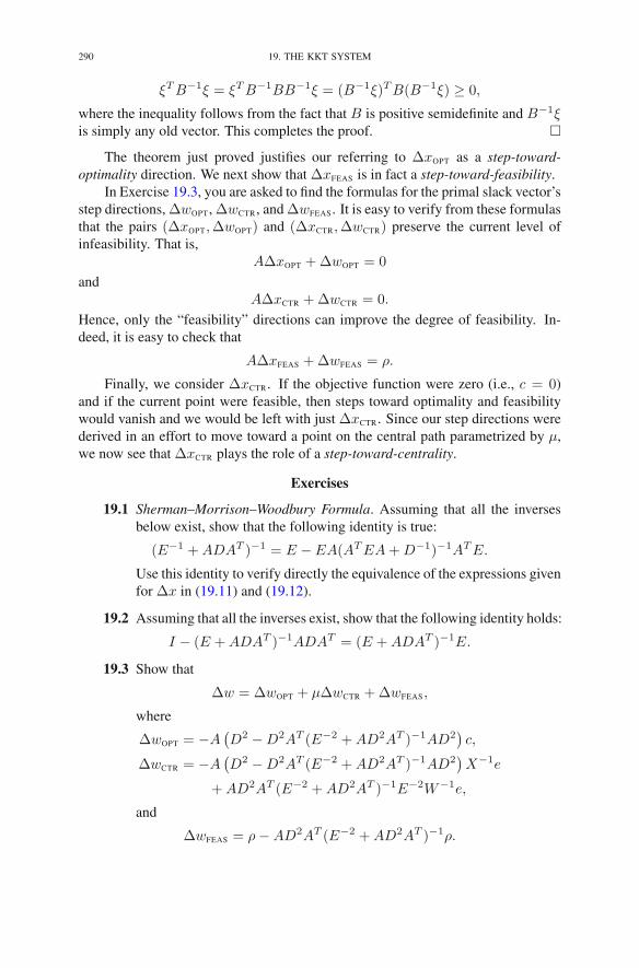
290 19. THE KKT SYSTEM
ξTB−1ξ = ξTB−1BB−1ξ = (B−1ξ)TB(B−1ξ) ≥ 0,
where the inequality follows from the fact that B is positive semidefinite and B−1ξis simply any old vector. This completes the proof. �
The theorem just proved justifies our referring to ΔxOPT as a step-toward-optimality direction. We next show that ΔxFEAS is in fact a step-toward-feasibility.
In Exercise 19.3, you are asked to find the formulas for the primal slack vector’sstep directions, ΔwOPT, ΔwCTR, and ΔwFEAS. It is easy to verify from these formulasthat the pairs (ΔxOPT,ΔwOPT) and (ΔxCTR,ΔwCTR) preserve the current level ofinfeasibility. That is,
AΔxOPT +ΔwOPT = 0
andAΔxCTR +ΔwCTR = 0.
Hence, only the “feasibility” directions can improve the degree of feasibility. In-deed, it is easy to check that
AΔxFEAS +ΔwFEAS = ρ.
Finally, we consider ΔxCTR. If the objective function were zero (i.e., c = 0)and if the current point were feasible, then steps toward optimality and feasibilitywould vanish and we would be left with just ΔxCTR. Since our step directions werederived in an effort to move toward a point on the central path parametrized by μ,we now see that ΔxCTR plays the role of a step-toward-centrality.
Exercises
19.1 Sherman–Morrison–Woodbury Formula. Assuming that all the inversesbelow exist, show that the following identity is true:
(E−1 +ADAT )−1 = E − EA(ATEA+D−1)−1ATE.
Use this identity to verify directly the equivalence of the expressions givenfor Δx in (19.11) and (19.12).
19.2 Assuming that all the inverses exist, show that the following identity holds:
I − (E +ADAT )−1ADAT = (E +ADAT )−1E.
19.3 Show that
Δw = ΔwOPT + μΔwCTR +ΔwFEAS,
where
ΔwOPT = −A(D2 −D2AT (E−2 +AD2AT )−1AD2
)c,
ΔwCTR = −A(D2 −D2AT (E−2 +AD2AT )−1AD2
)X−1e
+AD2AT (E−2 +AD2AT )−1E−2W−1e,
and
ΔwFEAS = ρ−AD2AT (E−2 +AD2AT )−1ρ.

NOTES 291
Notes
The KKT system for general inequality constrained optimization problems wasderived by Kuhn and Tucker (1951). It was later discovered that W. Karush hadproven the same result in his 1939 master’s thesis at the University of Chicago(Karush 1939). John (1948) was also an early contributor to inequality-constrainedoptimization. Kuhn’s survey paper (Kuhn 1976) gives a historical account of thedevelopment of the subject.

CHAPTER 20
Implementation Issues for Interior-Point Methods
In this chapter, we discuss implementation issues that arise in connection withthe path-following method.
The most important issue is the efficient solution of the systems of equationsdiscussed in the previous chapter. As we saw, there are basically three choices,involving either the reduced KKT matrix,
(20.1) B =
[−E−2 AAT D−2
]
,
or one of the two matrices associated with the normal equations:
(20.2) AD2AT + E−2
or
(20.3) ATE2A+D−2.
(Here, E−2 = Y −1W and D−2 = X−1Z.)In the previous chapter, we explained that dense columns/rows are bad for the
normal equations and that therefore one might be better off solving the system in-volving the reduced KKT matrix. But there is also a reason one might prefer towork with one of the systems of normal equations. The reason is that these matri-ces are positive definite. We shall show in the first section that there are importantadvantages in working with positive definite matrices. In the second section, weshall consider the reduced KKT matrix and see to what extent the nice propertiespossessed by positive definite matrices carry over to these matrices.
After finishing our investigations into numerical factorization, we shall take upa few other relevant tasks, such as how one extends the path-following algorithm tohandle problems with bounds and ranges.
1. Factoring Positive Definite Matrices
As we saw in the proof of Theorem 19.1, the matrix (20.2) appearing in the pri-mal normal equations is positive semidefinite (and so is (20.3), of course). In fact, itis even better—it’s positive definite. A matrix B is positive definite if ξTBξ > 0 forall vectors ξ �= 0. In this section, we will show that, if we restrict our row/column re-ordering to symmetric reorderings, that is, reorderings where the rows and columnsundergo the same permutation, then there is no danger of encountering a pivot
R.J. Vanderbei, Linear Programming, International Series in Operations Research& Management Science 196, DOI 10.1007/978-1-4614-7630-6 20,© Springer Science+Business Media New York 2014
293

294 20. IMPLEMENTATION ISSUES FOR INTERIOR-POINT METHODS
element whose value is zero. Hence, the row/column permutation can be selectedahead of time based only on the aim of maintaining sparsity.
If we restrict ourselves to symmetric permutations, each pivot element is a diag-onal element of the matrix. The following result shows that we can start by pickingan arbitrary diagonal element as the first pivot element:
THEOREM 20.1. If B is positive definite, then bii > 0 for all i.
The proof follows trivially from the definition of positive definiteness:
bii = eTi Bei > 0.
The next step is to show that after each stage of the elimination process, the remain-ing uneliminated matrix is positive definite. Let us illustrate by breaking out thefirst row/column of the matrix and looking at what the first step of the eliminationprocess does. Breaking out the first row/column, we write
B =
[a bT
b C
]
.
Here, a is the first diagonal element (a scalar), b is the column below a, and C is thematrix consisting of all of B except the first row/column. One step of elimination(as described in Chapter 8) transforms B into
[a bT
b C − bbT
a
]
.
The following theorem tells us that the uneliminated part is positive definite:
THEOREM 20.2. If B is positive definite, then so is C − bbT /a.
PROOF. The fact that B is positive definite implies that
(20.4)[x yT
][a bT
b C
] [xy
]
= ax2 + 2yT bx+ yTCy
is positive whenever the scalar x or the vector y is nonzero (or both). Fix a vectory �= 0, and put x = − 1
abT y. Using these choices in (20.4), we get
0 <1
ayT bbT y − 2
1
ayT bbT y + yTCy = yT
(
C − bbT
a
)
y.
Since y was an arbitrary nonzero vector, it follows that C−bbT /a is positive definite.�
Hence, after one step of the elimination, the uneliminated part is positive def-inite. It follows by induction then that the uneliminated part is positive definite atevery step of the elimination.
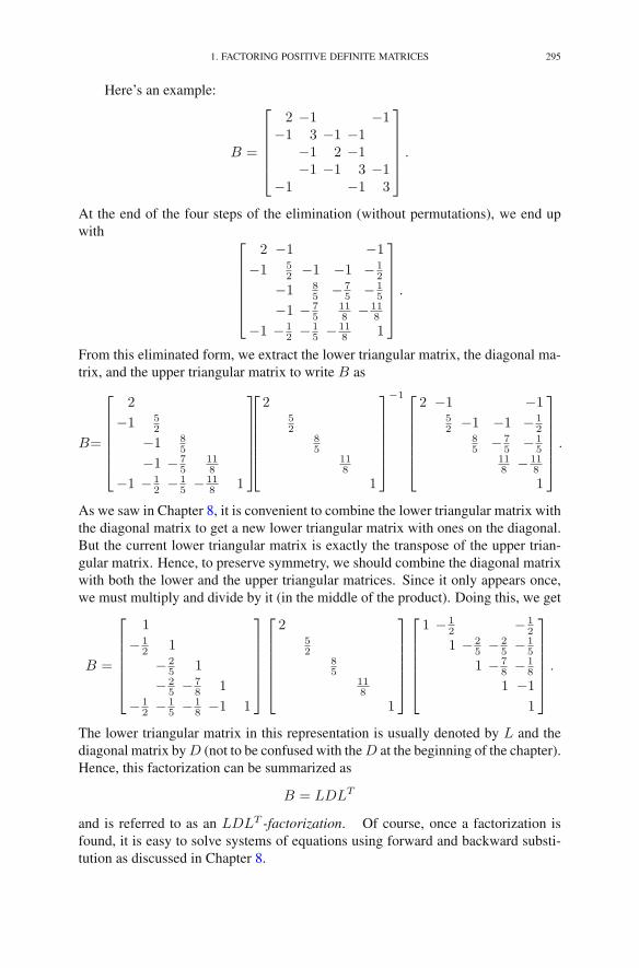
1. FACTORING POSITIVE DEFINITE MATRICES 295
Here’s an example:
B =
⎡
⎢⎢⎢⎢⎣
2 −1 −1−1 3 −1 −1
−1 2 −1−1 −1 3 −1
−1 −1 3
⎤
⎥⎥⎥⎥⎦.
At the end of the four steps of the elimination (without permutations), we end upwith
⎡
⎢⎢⎢⎢⎢⎣
2 −1 −1
−1 52 −1 −1 − 1
2
−1 85 − 7
5 − 15
−1 − 75
118 − 11
8
−1 − 12 − 1
5 − 118 1
⎤
⎥⎥⎥⎥⎥⎦
.
From this eliminated form, we extract the lower triangular matrix, the diagonal ma-trix, and the upper triangular matrix to write B as
B=
⎡
⎢⎢⎢⎢⎢⎣
2
−1 52
−1 85
−1 − 75
118
−1 − 12 − 1
5 − 118 1
⎤
⎥⎥⎥⎥⎥⎦
⎡
⎢⎢⎢⎢⎢⎣
252
85
118
1
⎤
⎥⎥⎥⎥⎥⎦
−1 ⎡
⎢⎢⎢⎢⎢⎣
2 −1 −152 −1 −1 − 1
285 − 7
5 − 15
118 − 11
8
1
⎤
⎥⎥⎥⎥⎥⎦
.
As we saw in Chapter 8, it is convenient to combine the lower triangular matrix withthe diagonal matrix to get a new lower triangular matrix with ones on the diagonal.But the current lower triangular matrix is exactly the transpose of the upper trian-gular matrix. Hence, to preserve symmetry, we should combine the diagonal matrixwith both the lower and the upper triangular matrices. Since it only appears once,we must multiply and divide by it (in the middle of the product). Doing this, we get
B =
⎡
⎢⎢⎢⎢⎢⎣
1
− 12 1
− 25 1
− 25 − 7
8 1
− 12 − 1
5 − 18 −1 1
⎤
⎥⎥⎥⎥⎥⎦
⎡
⎢⎢⎢⎢⎢⎣
252
85
118
1
⎤
⎥⎥⎥⎥⎥⎦
⎡
⎢⎢⎢⎢⎢⎣
1 − 12 − 1
2
1 − 25 − 2
5 − 15
1 − 78 − 1
8
1 −1
1
⎤
⎥⎥⎥⎥⎥⎦
.
The lower triangular matrix in this representation is usually denoted by L and thediagonal matrix by D (not to be confused with the D at the beginning of the chapter).Hence, this factorization can be summarized as
B = LDLT
and is referred to as an LDLT -factorization. Of course, once a factorization isfound, it is easy to solve systems of equations using forward and backward substi-tution as discussed in Chapter 8.

296 20. IMPLEMENTATION ISSUES FOR INTERIOR-POINT METHODS
1.1. Stability. We began our discussion of factoring positive definite matriceswith the comment that a symmetric permutation can be chosen purely with the aimof preserving sparsity, since it is guaranteed that no pivot element will ever vanish.However, the situation is even better than that—we can show that whenever a pivotelement is small, so is every other nonzero in the uneliminated part of the samerow/column. Before saying why, we need to set down a few technical results.
THEOREM 20.3. If bii denotes a diagonal element in the uneliminated subma-trix at some stage of an elimination and bii denotes the original value of that diag-onal element, then 0 < bii ≤ bii.
PROOF. The positivity of bii follows from the fact the uneliminated submatrixis positive definite. The fact that it is bounded above by bii follows from the factthat each step of the elimination can only decrease diagonal elements, which can beseen by looking at the first step of the elimination. Using the notation introducedjust after Theorem 20.1,
cii −b2ia
≤ cii.
�THEOREM 20.4. If B is symmetric and positive definite, then |bij | <
√biibjj
for all i �= j.
PROOF. Fix i �= j and let ξ = rei + ej . That is, ξ is the vector that’s all zeroexcept for the ith and jth position, where it’s r and 1, respectively. Then,
0 < ξTBξ = biir2 + 2bijr + bjj ,
for all r ∈ R. This quadratic expression is positive for all values of r if and only ifit is positive at its minimum, and it’s easy to check that it is positive at that point ifand only if |bij | <
√biibjj . �
These two theorems, together with the fact that the uneliminated submatrixis symmetric and positive definite, give us bounds on the off-diagonal elements.Indeed, consider the situation after a number of steps of the elimination. Using barsto denote matrix elements in the uneliminated submatrix and letting M denote anupper bound on the diagonal elements before the elimination process began (which,without loss of generality, could be taken as 1), we see that, if bjj < ε, then
(20.5) bij <√εM.
This bound is exceedingly important and is special to positive definite matrices.
2. Quasidefinite Matrices
In this section, we shall study factorization techniques for the reduced KKTmatrix (20.1). The reduced KKT matrix is an example of a quasidefinite matrix.A symmetric matrix is called quasidefinite if it can be written (perhaps after a sym-metric permutation) as
B =
[−E AAT D
]
,
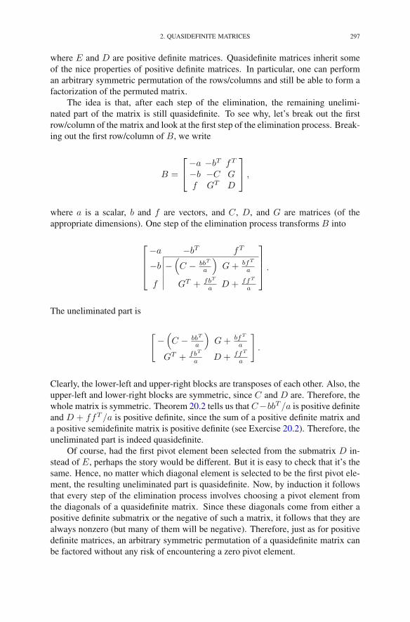
2. QUASIDEFINITE MATRICES 297
where E and D are positive definite matrices. Quasidefinite matrices inherit someof the nice properties of positive definite matrices. In particular, one can performan arbitrary symmetric permutation of the rows/columns and still be able to form afactorization of the permuted matrix.
The idea is that, after each step of the elimination, the remaining unelimi-nated part of the matrix is still quasidefinite. To see why, let’s break out the firstrow/column of the matrix and look at the first step of the elimination process. Break-ing out the first row/column of B, we write
B =
⎡
⎣−a −bT fT
−b −C Gf GT D
⎤
⎦ ,
where a is a scalar, b and f are vectors, and C, D, and G are matrices (of theappropriate dimensions). One step of the elimination process transforms B into
⎡
⎢⎢⎣
−a −bT fT
−b −(C − bbT
a
)G+ bfT
a
f GT + fbT
a D + ffT
a
⎤
⎥⎥⎦ .
The uneliminated part is
[−
(C − bbT
a
)G+ bfT
a
GT + fbT
a D + ffT
a
]
.
Clearly, the lower-left and upper-right blocks are transposes of each other. Also, theupper-left and lower-right blocks are symmetric, since C and D are. Therefore, thewhole matrix is symmetric. Theorem 20.2 tells us that C−bbT /a is positive definiteand D + ffT /a is positive definite, since the sum of a positive definite matrix anda positive semidefinite matrix is positive definite (see Exercise 20.2). Therefore, theuneliminated part is indeed quasidefinite.
Of course, had the first pivot element been selected from the submatrix D in-stead of E, perhaps the story would be different. But it is easy to check that it’s thesame. Hence, no matter which diagonal element is selected to be the first pivot ele-ment, the resulting uneliminated part is quasidefinite. Now, by induction it followsthat every step of the elimination process involves choosing a pivot element fromthe diagonals of a quasidefinite matrix. Since these diagonals come from either apositive definite submatrix or the negative of such a matrix, it follows that they arealways nonzero (but many of them will be negative). Therefore, just as for positivedefinite matrices, an arbitrary symmetric permutation of a quasidefinite matrix canbe factored without any risk of encountering a zero pivot element.
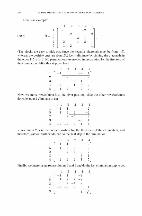
298 20. IMPLEMENTATION ISSUES FOR INTERIOR-POINT METHODS
Here’s an example:
(20.6) B =
1 2 3 4 512345
⎡
⎢⎢⎢⎢⎣
−1 −2 1−2 2
−3 1−2 1 21 2 1
⎤
⎥⎥⎥⎥⎦.
(The blocks are easy to pick out, since the negative diagonals must be from −E,whereas the positive ones are from D.) Let’s eliminate by picking the diagonals inthe order 1, 5, 2, 4, 3. No permutations are needed in preparation for the first step ofthe elimination. After this step, we have
1 2 3 4 512345
⎡
⎢⎢⎢⎢⎣
−1 −2 1−2 2
−3 1−2 1 6 −21 2 −2 2
⎤
⎥⎥⎥⎥⎦.
Now, we move row/column 5 to the pivot position, slide the other rows/columnsdown/over, and eliminate to get
1 5 2 3 415234
⎡
⎢⎢⎢⎢⎣
−1 1 −21 2 2 −2
2 −4 2−3 1
−2 −2 2 1 4
⎤
⎥⎥⎥⎥⎦.
Row/column 2 is in the correct position for the third step of the elimination, andtherefore, without further ado, we do the next step in the elimination:
1 5 2 3 415234
⎡
⎢⎢⎢⎢⎣
−1 1 −21 2 2 −2
2 −4 2−3 1
−2 −2 2 1 5
⎤
⎥⎥⎥⎥⎦.
Finally, we interchange rows/columns 3 and 4 and do the last elimination step to get
1 5 2 4 3
15243
⎡
⎢⎢⎢⎢⎣
−1 1 −21 2 2 −2
2 −4 2−2 −2 2 5 1
1 − 165
⎤
⎥⎥⎥⎥⎦.

2. QUASIDEFINITE MATRICES 299
From this final matrix, it is easy to extract the LDLT -factorization of the permuta-tion of B:
B =
1 5 2 4 315243
⎡
⎢⎢⎢⎢⎣
−1 1 −21 1 2
2 −2−2 2 1
1 −3
⎤
⎥⎥⎥⎥⎦
=
15243
⎡
⎢⎢⎢⎢⎣
1−1 1
1 12 −1 − 1
2 115 1
⎤
⎥⎥⎥⎥⎦
⎡
⎢⎢⎢⎢⎣
−12−4
5− 16
5
⎤
⎥⎥⎥⎥⎦
1 5 2 4 3⎡
⎢⎢⎢⎢⎣
1 −1 21 1 −1
1 − 121 1
51
⎤
⎥⎥⎥⎥⎦
.
As always, the factorization is computed so that one can solve systems of equations.Given the factorization, all that is required is a forward substitution, a backwardsubstitution, a scaling, and two permutations.
2.1. Instability. We have shown that an arbitrary symmetric permutation ofthe rows/columns of a quasidefinite matrix can be factored into LDLT . That is,mathematically none of the pivot elements will be zero. But they can be small, andtheir smallness can cause troubles not encountered with positive definite matrices.To explain, let’s look at an example. Consider the linear programming problem
maximize x1 + x2
subject to x1 + 2x2 ≤ 12x1 + x2 ≤ 1
x1, x2 ≥ 0
and its dual
minimize y1 + y2subject to y1 + 2y2 ≥ 1
2y1 + y2 ≥ 1y1, y2 ≥ 0 .
Drawing pictures, it is easy to see that the optimal solution is
x∗1 = x∗
2 = y∗1 = y∗2 =1
3z∗1 = z∗2 = w∗
1 = w∗2 = 0.
Therefore, as the optimal solution is approached, the diagonal elements in X−1Zand Y −1W approach zero. Therefore, at late stages in the path-following method,one is faced with the problem of factoring the following reduced KKT matrix:
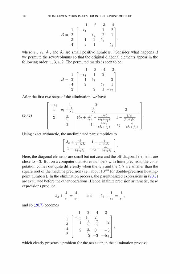
300 20. IMPLEMENTATION ISSUES FOR INTERIOR-POINT METHODS
B =
1 2 3 41234
⎡
⎢⎢⎣
−ε1 1 2−ε2 2 1
1 2 δ12 1 δ2
⎤
⎥⎥⎦ ,
where ε1, ε2, δ1, and δ2 are small positive numbers. Consider what happens ifwe permute the rows/columns so that the original diagonal elements appear in thefollowing order: 1, 3, 4, 2. The permuted matrix is seen to be
B =
1 3 4 21342
⎡
⎢⎢⎣
−ε1 1 21 δ1 22 δ2 1
2 1 −ε2
⎤
⎥⎥⎦ .
After the first two steps of the elimination, we have
(20.7)
⎡
⎢⎢⎢⎢⎢⎣
−ε1 1 21 δ1 +
1ε1
2ε1
2
2 2ε1
(δ2 +4ε1)− 4/ε21
(δ1+1ε1
)1− 4/ε1
(δ1+1ε1
)
2 1− 4/ε1(δ1+
1ε1
)−ε2 − 4
(δ1+1ε1
)
⎤
⎥⎥⎥⎥⎥⎦
.
Using exact arithmetic, the uneliminated part simplifies to[δ2 +
4δ11+ε1δ1
1− 41+ε1δ1
1− 41+ε1δ1
−ε2 − 4ε11+ε1δ1
]
.
Here, the diagonal elements are small but not zero and the off-diagonal elements areclose to −3. But on a computer that stores numbers with finite precision, the com-putation comes out quite differently when the εi’s and the δi’s are smaller than thesquare root of the machine precision (i.e., about 10−8 for double-precision floating-point numbers). In the elimination process, the parenthesized expressions in (20.7)are evaluated before the other operations. Hence, in finite precision arithmetic, theseexpressions produce
δ2 +4
ε1=
4
ε1and δ1 +
1
ε1=
1
ε1,
and so (20.7) becomes
1 3 4 2
1342
⎡
⎢⎢⎢⎣
−ε1 1 21 1
ε12ε1
2
2 2ε1
0 −3
2 −3 −4ε1
⎤
⎥⎥⎥⎦,
which clearly presents a problem for the next step in the elimination process.
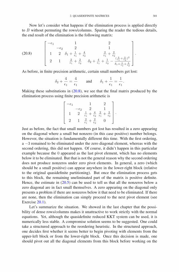
2. QUASIDEFINITE MATRICES 301
Now let’s consider what happens if the elimination process is applied directlyto B without permuting the rows/columns. Sparing the reader the tedious details,the end result of the elimination is the following matrix:
(20.8)
⎡
⎢⎢⎢⎢⎣
−ε1 1 2−ε2 2 1
1 2 δ1 +1ε1
+ 4ε2
2ε1
+ 2ε2
2 1 2ε1
+ 2ε2
δ2 +4ε1
+ 1ε2
−( 2ε1
+ 2ε2
)2
δ1+1ε1
+ 4ε2
⎤
⎥⎥⎥⎥⎦.
As before, in finite precision arithmetic, certain small numbers get lost:
δ2 +4
ε1=
4
ε1and δ1 +
1
ε1=
1
ε1.
Making these substitutions in (20.8), we see that the final matrix produced by theelimination process using finite precision arithmetic is
⎡
⎢⎢⎢⎣
−ε1 1 2−ε2 2 1
1 2 1ε1
+ 4ε2
2ε1
+ 2ε2
2 1 2ε1
+ 2ε2
0
⎤
⎥⎥⎥⎦.
Just as before, the fact that small numbers got lost has resulted in a zero appearingon the diagonal where a small but nonzero (in this case positive) number belongs.However, the situation is fundamentally different this time. With the first ordering,a −3 remained to be eliminated under the zero diagonal element, whereas with thesecond ordering, this did not happen. Of course, it didn’t happen in this particularexample because the 0 appeared as the last pivot element, which has no elementsbelow it to be eliminated. But that is not the general reason why the second orderingdoes not produce nonzeros under zero pivot elements. In general, a zero (whichshould be a small positive) can appear anywhere in the lower-right block (relativeto the original quasidefinite partitioning). But once the elimination process getsto this block, the remaining uneliminated part of the matrix is positive definite.Hence, the estimate in (20.5) can be used to tell us that all the nonzeros below azero diagonal are in fact small themselves. A zero appearing on the diagonal onlypresents a problem if there are nonzeros below it that need to be eliminated. If thereare none, then the elimination can simply proceed to the next pivot element (seeExercise 20.1).
Let’s summarize the situation. We showed in the last chapter that the possi-bility of dense rows/columns makes it unattractive to work strictly with the normalequations. Yet, although the quasidefinite reduced KKT system can be used, it isnumerically less stable. A compromise solution seems to be suggested. One couldtake a structured approach to the reordering heuristic. In the structured approach,one decides first whether it seems better to begin pivoting with elements from theupper-left block or from the lower-right block. Once this decision is made, oneshould pivot out all the diagonal elements from this block before working on the

302 20. IMPLEMENTATION ISSUES FOR INTERIOR-POINT METHODS
other block, with the exception that pivots involving dense rows/columns be de-ferred to the end of the elimination process. If no dense columns are identified, thisstrategy mimics the normal equations approach. Indeed, after eliminating all thediagonal elements in the upper-left block, the remaining uneliminated lower-rightblock contains exactly the matrix for the system of dual normal equations. Similarly,had the initial choice been to pivot out all the diagonal elements from the lower-rightblock, then the remaining uneliminated upper-left block becomes the matrix for thesystem of primal normal equations.
With this structured approach, if no dense rows/columns are identified and de-ferred, then the elimination process is numerically stable. If, on the other hand,some dense rows/columns are deferred, then the factorization is less stable. But inpractice, this approach seems to work well. Of course, one could be more carefuland monitor the diagonal elements. If a diagonal element gets small (relative to theother uneliminated nonzeros in the same row/column), then one could flag it andthen calculate a new ordering in which such pivot elements are deferred to the endof the elimination process.
3. Problems in General Form
In this section, we describe how to adapt the path-following algorithm to solv-ing problems presented in the following general form:
(20.9)maximize cTxsubject to a ≤ Ax ≤ b
l ≤ x ≤ u.
As in Chapter 9, some of the data elements are allowed to take on infinite values.However, let us consider first the case where all the components of a, b, l, and u arefinite. Infinities require special treatment, which shall be discussed shortly.
Following the derivation of the path-following method that we introduced inChapter 18, the first step is to introduce slack variables as appropriate to replace allinequality constraints with simple nonnegativity constraints. Hence, we rewrite theprimal problem (20.9) as follows:
maximize cTxsubject to Ax + f = b
−Ax + p = −ax + t = u
−x + g = −lf, p, t, g ≥ 0.
In Chapter 9, we showed that the dual problem is given by
minimize bT v − aT q + uT s− lThsubject to AT (v − q)− (h− s) = c
v, q, s, h ≥ 0,

3. PROBLEMS IN GENERAL FORM 303
and the corresponding complementarity conditions are given by
fivi = 0 i = 1, 2, . . . ,m,
piqi = 0 i = 1, 2, . . . ,m,
tjsj = 0 j = 1, 2, . . . , n,
gjhj = 0 j = 1, 2, . . . , n.
The next step in the derivation is to introduce the primal–dual central path,which we parametrize as usual by a positive real parameter μ. Indeed, for eachμ > 0, we define the associated central-path point in primal–dual space as theunique point that simultaneously satisfies the conditions of primal feasibility, dualfeasibility, and μ-complementarity. Ignoring nonnegativity (which is enforced sep-arately), these conditions are
Ax+ f = bf + p= b− ax+ t= u
−x+ g =−l
AT y + s− h= cy + q − v = 0
FV e= μePQe= μeTSe= μeGHe= μe.
Note that we have replaced the primal feasibility condition, −Ax + p = −a, withthe equivalent condition that f + p = b − a, and we have introduced into the dualproblem new variables y defined by y = v − q. The reason for these changes isto put the system of equations into a form in which A and AT appear as little aspossible (so that solving the system of equations for the step direction will be asefficient as possible).
The last four equations are the μ-complementarity conditions. As usual, eachupper case letter that appears on the left in these equations denotes the diagonal ma-trix having the components of the corresponding lower-case vector on its diagonal.The system is a nonlinear system of 5n + 5m equations in 5n + 5m unknowns.It has a unique solution in the strict interior of the following subset of primal–dualspace:
(20.10) {(x, f, p, t, g, y, v, q, s, h) : f, p, t, g, v, q, s, h ≥ 0}.This fact can be seen by noting that these equations are the first-order optimalityconditions for an associated strictly convex barrier problem.
As μ tends to zero, the central path converges to the optimal solution to both theprimal and dual problems. The path-following algorithm is defined as an iterativeprocess that starts from a point in the strict interior of (20.10), estimates at eachiteration a value of μ representing a point on the central path that is in some sense
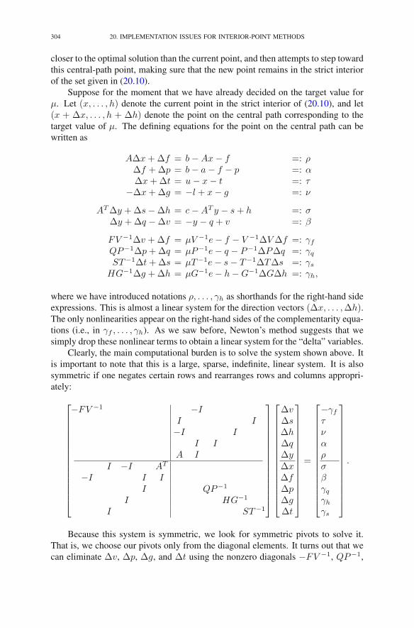
304 20. IMPLEMENTATION ISSUES FOR INTERIOR-POINT METHODS
closer to the optimal solution than the current point, and then attempts to step towardthis central-path point, making sure that the new point remains in the strict interiorof the set given in (20.10).
Suppose for the moment that we have already decided on the target value forμ. Let (x, . . . , h) denote the current point in the strict interior of (20.10), and let(x + Δx, . . . , h + Δh) denote the point on the central path corresponding to thetarget value of μ. The defining equations for the point on the central path can bewritten as
AΔx+Δf = b−Ax− f =: ρΔf +Δp = b− a− f − p =: αΔx+Δt = u− x− t =: τ
−Δx+Δg = −l + x− g =: ν
ATΔy +Δs−Δh = c−AT y − s+ h =: σΔy +Δq −Δv = −y − q + v =: β
FV −1Δv +Δf = μV −1e− f − V −1ΔVΔf =: γfQP−1Δp+Δq = μP−1e− q − P−1ΔPΔq =: γqST−1Δt+Δs = μT−1e− s− T−1ΔTΔs =: γs
HG−1Δg +Δh = μG−1e− h−G−1ΔGΔh =: γh,
where we have introduced notations ρ, . . . , γh as shorthands for the right-hand sideexpressions. This is almost a linear system for the direction vectors (Δx, . . . ,Δh).The only nonlinearities appear on the right-hand sides of the complementarity equa-tions (i.e., in γf , . . . , γh). As we saw before, Newton’s method suggests that wesimply drop these nonlinear terms to obtain a linear system for the “delta” variables.
Clearly, the main computational burden is to solve the system shown above. Itis important to note that this is a large, sparse, indefinite, linear system. It is alsosymmetric if one negates certain rows and rearranges rows and columns appropri-ately:
⎡
⎢⎢⎢⎢⎢⎢⎢⎢⎢⎢⎢⎢⎢⎢⎣
−FV −1 −II I−I I
I IA I
I −I AT
−I I II QP−1
I HG−1
I ST−1
⎤
⎥⎥⎥⎥⎥⎥⎥⎥⎥⎥⎥⎥⎥⎥⎦
⎡
⎢⎢⎢⎢⎢⎢⎢⎢⎢⎢⎢⎢⎢⎢⎣
ΔvΔsΔhΔqΔyΔxΔfΔpΔgΔt
⎤
⎥⎥⎥⎥⎥⎥⎥⎥⎥⎥⎥⎥⎥⎥⎦
=
⎡
⎢⎢⎢⎢⎢⎢⎢⎢⎢⎢⎢⎢⎢⎢⎣
−γfτναρσβγqγhγs
⎤
⎥⎥⎥⎥⎥⎥⎥⎥⎥⎥⎥⎥⎥⎥⎦
.
Because this system is symmetric, we look for symmetric pivots to solve it.That is, we choose our pivots only from the diagonal elements. It turns out that wecan eliminate Δv, Δp, Δg, and Δt using the nonzero diagonals −FV −1, QP−1,

3. PROBLEMS IN GENERAL FORM 305
HG−1, and ST−1, respectively, in any order without causing any nondiagonal fill-in. Indeed, the equations for Δv, Δp, Δg, and Δt are
Δv = V F−1(γf −Δf)
Δp = PQ−1(γq −Δq)(20.11)
Δg = GH−1(γh −Δh)
Δt = TS−1(γs −Δs),
and after elimination from the system, we get⎡
⎢⎢⎢⎢⎢⎢⎣
−TS−1 I−GH−1 −I
−PQ−1 IA I
I −I AT
I I V F−1
⎤
⎥⎥⎥⎥⎥⎥⎦
⎡
⎢⎢⎢⎢⎢⎢⎣
ΔsΔhΔqΔyΔxΔf
⎤
⎥⎥⎥⎥⎥⎥⎦
=
⎡
⎢⎢⎢⎢⎢⎢⎣
τναρσ
β
⎤
⎥⎥⎥⎥⎥⎥⎦
,
where again we have introduced abbreviated notations for the components of theright-hand side:
τ = τ − TS−1γs
ν = ν −GH−1γh
α = α− PQ−1γq
β = β + V F−1γf .
Next we use the pivot elements −TS−1, −GH−1, and −PQ−1 to solve forΔs, Δh, and Δq, respectively:
Δs = −ST−1(τ −Δx)
Δh = −HG−1(ν +Δx)(20.12)
Δq = −QP−1(α−Δf).
After eliminating these variables, the system simplifies to⎡
⎣A I
AT DI E
⎤
⎦
⎡
⎣ΔyΔxΔf
⎤
⎦ =
⎡
⎣ρσ + ST−1τ −HG−1ν
β +QP−1α.
⎤
⎦ ,
where
D = ST−1 +HG−1
and
E = V F−1 +QP−1.
Finally, we use the pivot element E to solve for Δf ,
(20.13) Δf = E−1(β +QP−1α−Δy),

306 20. IMPLEMENTATION ISSUES FOR INTERIOR-POINT METHODS
which brings us to the reduced KKT equations:
(20.14)
[ −E−1 A
AT D
] [Δy
Δx
]
=
[ρ− E−1(β +QP−1α)
σ + ST−1τ −HG−1ν
]
.
initialize (x, f, p, t, g, y, v, q, s, h) such that f, p, t, g, v, q, s, h > 0while (not optimal) {
ρ = b−Ax− w
σ = c−AT y + z
γ = fT v + pT q + tT s+ gTh
μ = δγ
n+m
γf = μV −1e− f
γq = μP−1e− q
γs = μT−1e− s
γh = μG−1e− h
τ = u− x− t− TS−1γs
ν = −l + x− g −GH−1γh
α = b− a− f − p− PQ−1γq
β = −y − q + v + V F−1γf
D = ST−1 +HG−1
E = V F−1 +QP−1
solve:
[−E−1 AAT D
] [ΔyΔx
]
=
[ρ− E−1(β +QP−1α)σ + ST−1τ −HG−1ν
]
compute: Δf using (20.13), Δs, Δh, Δq using (20.12),and Δv, Δp, Δg, Δt using (20.11)
θ = r
(
maxij
{
−Δfjfj
,−Δpipi
,−Δtiti
,−Δgjgj
,
−Δvjvj
,−Δqiqi
,−Δsisi
,−Δhj
hj
})−1
∧ 1
x ← x+ θΔx, y ← y + θΔy, f ← f + θΔf, v ← v + θΔv
p ← p+ θΔp, q ← q + θΔq, t ← t+ θΔt, s ← s+ θΔs
g ← g + θΔg, h ← h+ θΔh}
FIGURE 20.1. The path-following method—general form.

NOTES 307
Up to this point, none of the eliminations have produced any off-diagonal fill-in. Also, the matrix for system given in (20.14) is a symmetric quasidefinite matrix.Hence, the techniques given in Section 19.2 for solving such systems can be used.The algorithm is summarized in Figure 20.1.
Exercises
20.1 The matrix
B =
⎡
⎢⎢⎢⎢⎣
2 −21 −1
−2 2−1 2 −1
−1 2
⎤
⎥⎥⎥⎥⎦
is not positive definite but is positive semidefinite. Find a factorizationB = LDLT , where L is lower triangular with ones on the diagonal andD is a diagonal matrix with nonnegative diagonal elements. If such a fac-torization exists for every symmetric positive semidefinite matrix, explainwhy. If not, give a counterexample.
20.2 Show that the sum of a positive definite matrix and a positive semidefinitematrix is positive definite.
20.3 Permute the rows/columns of the matrix B given in (20.6) so that thediagonal elements from B appear in the order 2, 3, 4, 5, 1. Compute anLDLT -factorization of this matrix.
20.4 Show that, if B is symmetric and positive semidefinite, then |bij | ≤√biibjj for all i, j.
Notes
Most implementations of interior-point methods assume the problem to be for-mulated with equality constraints. In this formulation, Lustig et al. (1994) give agood overview of the performance of interior-point algorithms compared with thesimplex method.
The suggestion that it is better to solve equations in the KKT form instead ofnormal form was offered independently by a number of researchers (Gill et al. 1992;Turner 1991; Fourer and Mehrotra 1991; Vanderbei and Carpenter 1993).
The advantages of the primal–dual symmetric formulation were first reportedin Vanderbei (1994). The basic properties of quasidefinite matrices were first givenin Vanderbei (1995).

CHAPTER 21
The Affine-Scaling Method
In the previous chapter, we showed that the step direction for the path-followingmethod can be decomposed into a linear combination of three directions: a directiontoward optimality, a direction toward feasibility, and a direction toward centrality. Itturns out that these directions, or minor variants of them, arise in all interior-pointmethods.
Historically, one of the first interior-point methods to be invented, analyzed,and implemented was a two-phase method in which Phase I uses only the feasibil-ity direction and Phase II uses only the optimality direction. This method is calledaffine scaling. While it is no longer considered the method of choice for practi-cal implementations, it remains important because its derivation provides valuableinsight into the nature of the three basic directions mentioned above.
In this chapter, we shall explain the affine-scaling principle and use it to derivethe step toward optimality and step toward feasibility directions. As always, ourmain interest lies in problems presented in standard form. But for affine scaling,it is easier to start by considering problems in equality form. Hence, we begin byassuming that the linear programming problem is given as
(21.1)maximize cTxsubject to Ax= b
x≥ 0.
We shall begin with the Phase II algorithm. Hence, we assume that we have afeasible initial starting point, x0. For the affine-scaling method, it is important thatthis starting point lie in the strict interior of the feasible set. That is, we assume that
Ax0 = b and x0 > 0.
1. The Steepest Ascent Direction
Since the affine-scaling principle is fundamentally geometric, it is useful tokeep a picture in mind. A typical picture for m = 1 and n = 3 is shown inFigure 21.1. The ultimate goal is, of course, to move from x0 to the optimal so-lution x∗. However, the short-term goal is to move from x0 in some direction Δxthat improves the objective function. Such a direction is called an ascent direction.You probably recall from elementary calculus that the best, i.e., steepest, ascentdirection is given by the gradient of the objective function. However, as we see inFigure 21.1, there is no reason a priori for the gradient to “lie in” the feasible region.
R.J. Vanderbei, Linear Programming, International Series in Operations Research& Management Science 196, DOI 10.1007/978-1-4614-7630-6 21,© Springer Science+Business Media New York 2014
309

310 21. THE AFFINE-SCALING METHOD
x1
x2
x3
x0
level sets of cTx
Feasible region
x*
Pc
c
FIGURE 21.1. A typical feasible region when the problem is inequality form, m = 1, and n = 3. The lines drawn on the feasibleset represent level sets of the objective function, and x0 representsthe starting point for the affine-scaling method.
Hence, the steepest ascent direction will almost surely cause a move to infeasiblepoints. This is also clear algebraically. Indeed,
A(x0 +Δx) = Ax0 +AΔx = b+Ac �= b
(unless Ac = 0 which is not likely).To see how to find a better direction, let us first review in what sense the gradient
is the steepest ascent direction. The steepest ascent direction is defined to be thedirection that gives the greatest increase in the objective function subject to theconstraint that the displacement vector has unit length. That is, the steepest ascentdirection is the solution to the following optimization problem:
(21.2)maximize cT (x0 +Δx)subject to ‖Δx‖2 = 1.
We can solve this problem using Lagrange multipliers. Indeed, if we let λ denotethe Lagrange multiplier for the constraint, the problem becomes
maxΔx,λ
cT (x0 +Δx)− λ(ΔxTΔx− 1).
Differentiating with respect to Δx and setting the derivative to zero, we get
c− 2λΔx = 0,
which implies that
Δx =1
2λc ∝ c.
2. THE PROJECTED GRADIENT DIRECTION 311
Then differentiating the Lagrangian with respect to λ and setting that derivative tozero, we see that
‖Δx‖2 − 1 = 0,
which implies that‖Δx‖ = ±1.
Hence, the steepest ascent direction points in the direction of either c or its negative.Since the negative is easily seen not to be an ascent direction at all, it follows thatthe steepest ascent direction points in the direction of c.
2. The Projected Gradient Direction
The problem with the steepest ascent direction is that it fails to preserve feasi-bility. That is, it fails to preserve the equality constraints Ax = b. To remedy thisproblem, let’s add these constraints to (21.2) so that we get the following optimiza-tion problem:
maximize cT (x0 +Δx)subject to ‖Δx‖2 = 1
A(x0 +Δx) = b.
Again, the method of Lagrange multipliers is the appropriate tool. As before, let λdenote the Lagrange multiplier for the norm constraint, and now introduce a vectory containing the Lagrange multipliers for the equality constraints. The resultingunconstrained optimization problem is
maxΔx,λ,y
cT (x0 +Δx)− λ(ΔxTΔx− 1)− yT (A(x0 +Δx)− b).
Differentiating this Lagrangian with respect to Δx, λ, and y and setting these deriva-tives to zero, we get
c− 2λΔx−AT y = 0
‖Δx‖2 − 1 = 0
A(x0 +Δx)− b = 0.
The second equation tells us that the length of Δx is one. Since we are interestedin the direction of Δx and are not concerned about its length, we ignore this secondequation. The first equation tells us that Δx is proportional to c− AT y, and again,since we aren’t concerned about lengths, we put λ = 1/2 so that the first equationreduces to
(21.3) Δx = c−AT y.
Since Ax0 = b, the third equation says that
AΔx = 0.
Substituting (21.3) into this equation, we get
Ac−AAT y = 0,
which, assuming that AAT has full rank (as it should), can be solved for y to get
y = (AAT )−1Ac.
312 21. THE AFFINE-SCALING METHOD
Now, substituting this expression into (21.3), we see that
Δx = c−AT (AAT )−1Ac.
It is convenient to let P be the matrix defined by
P = I −AT (AAT )−1A.
With this definition, Δx can be expressed succinctly as
Δx = Pc.
We claim that P is the matrix that maps any vector, such as c, to its orthogonalprojection onto the null space of A. To justify this claim, we first need to define someof the terms we’ve used. The null space of A is defined as {d ∈ R
n : Ad = 0}. Weshall denote the null space of A by N(A). A vector c is the orthogonal projectionof c onto N(A) if it lies in the null space,
c ∈ N(A),
and if the difference between it and c is orthogonal to every other vector in N(A).That is,
dT (c− c) = 0, for all d ∈ N(A).
Hence, to show that Pc is the orthogonal projection of c onto the null space of A,we simply check these two conditions. Checking the first, we see that
APc = Ac−AAT (AAT )−1Ac,
which clearly vanishes. To check the second condition, let d be an arbitrary vectorin the null space, and compute
dT (c− Pc) = dTAT (AAT )−1Ac,
which also vanishes, since dTAT = (Ad)T = 0. The orthogonal projection Pc isshown in Figure 21.1.
3. The Projected Gradient Direction with Scaling
The orthogonal projection of the gradient gives a good step direction in thesense that among all feasibility-preserving directions, it gives the largest rate ofincrease of cTx per unit step length. This property is nice as long as the currentpoint x0 is well inside the feasible set. But if it is close to a “wall,” the overallincrease in one step will be small, since even though the rate is large the actualstep length will be small, yielding a small overall increase. In fact, the increasewill become arbitrarily small as the point x0 is taken closer and closer to a “wall.”Hence, to get a reasonable algorithm, we need to find a formula for computing stepdirections that steers away from walls as they get close.
The affine-scaling algorithm achieves this affect as follows: scale the variablesin the problem so that the current feasible solution is far from the walls, compute thestep direction as the projected gradient in the scaled problem, and then translate thisdirection back into the original system. The idea of scaling seems too simple to doany good, and this is true if one tries the most naive scaling—just multiplying everyvariable by one large number (such as the reciprocal of the smallest component of
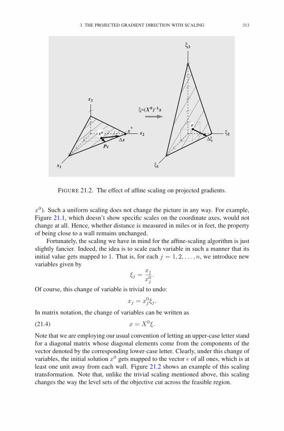
3. THE PROJECTED GRADIENT DIRECTION WITH SCALING 313
Δx
x*
Pc
x1
x3
ξ1
x2 ξ2
ξ3
x0
e
Δξ
ξ=(X 0)–1x
FIGURE 21.2. The effect of affine scaling on projected gradients.
x0). Such a uniform scaling does not change the picture in any way. For example,Figure 21.1, which doesn’t show specific scales on the coordinate axes, would notchange at all. Hence, whether distance is measured in miles or in feet, the propertyof being close to a wall remains unchanged.
Fortunately, the scaling we have in mind for the affine-scaling algorithm is justslightly fancier. Indeed, the idea is to scale each variable in such a manner that itsinitial value gets mapped to 1. That is, for each j = 1, 2, . . . , n, we introduce newvariables given by
ξj =xj
x0j
.
Of course, this change of variable is trivial to undo:
xj = x0jξj .
In matrix notation, the change of variables can be written as
(21.4) x = X0ξ.
Note that we are employing our usual convention of letting an upper-case letter standfor a diagonal matrix whose diagonal elements come from the components of thevector denoted by the corresponding lower-case letter. Clearly, under this change ofvariables, the initial solution x0 gets mapped to the vector e of all ones, which is atleast one unit away from each wall. Figure 21.2 shows an example of this scalingtransformation. Note that, unlike the trivial scaling mentioned above, this scalingchanges the way the level sets of the objective cut across the feasible region.
314 21. THE AFFINE-SCALING METHOD
Making the change of variables given by (21.4) in (21.1), we find that the prob-lem in the scaled space is
maximize cTX0ξsubject to AX0ξ = b
ξ ≥ 0.
Clearly, it is a linear programming problem in standard form with constraint matrixAX0 and vector of objective function coefficients (cTX0)T = X0c. Letting Δξdenote the projected gradient of the objective function in this scaled problem, wesee that
Δξ =(I −X0AT (AX02AT )−1AX0
)X0c.
Ignore step length worries for the moment, and consider moving from the currentsolution ξ0 = e to the following new point in the scaled problem:
ξ1 = ξ0 +Δξ.
Then transforming this new point back into the original unscaled variables, we geta new point x1 given by
x1 = X0ξ1 = X0(e+Δξ) = x0 +X0Δξ.
Of course, the difference between x1 and x0 is the step direction in the originalvariables. Denoting this difference by Δx, we see that
Δx = X0(I −X0AT (AX02AT )−1AX0
)X0c
=(D −DAT (ADAT )−1AD
)c,(21.5)
where
D = X02.
The expression for Δx given by (21.5) is called the affine-scaling step direction.Of course, to construct the affine-scaling algorithm out of this formula for a stepdirection, one simply needs to choose step lengths in such a manner as to ensure“strict” feasibility of each iterate.
We end this section by illustrating some of the calculations on the followingtrivial example:
maximize 2x1 + 3x2 + 2x3
subject to x1 + x2 + 2x3 = 3x1, x2, x3 ≥ 0 .
This is precisely the problem shown in Figure 21.2. As in the figure, let us assumethat
x0 =
⎡
⎢⎣
13214
⎤
⎥⎦ .
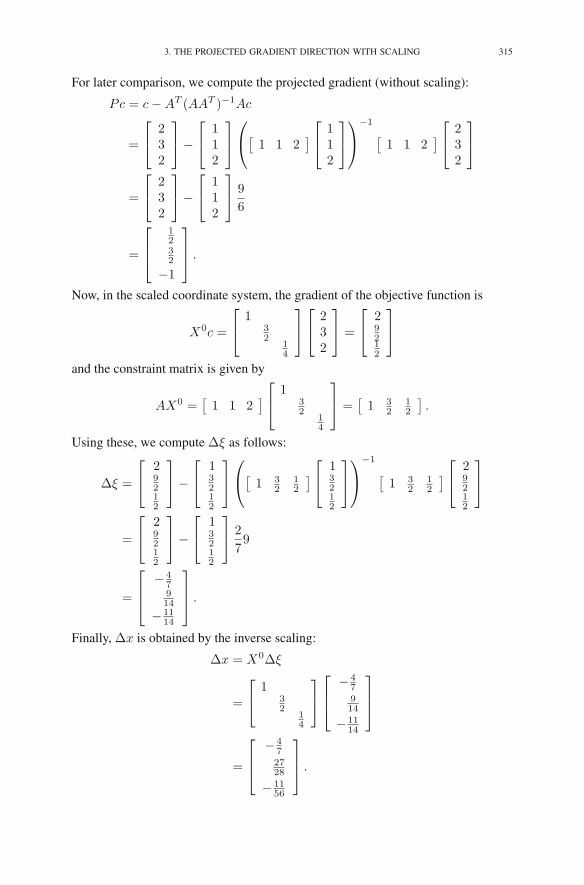
3. THE PROJECTED GRADIENT DIRECTION WITH SCALING 315
For later comparison, we compute the projected gradient (without scaling):
Pc = c−AT (AAT )−1Ac
=
⎡
⎣232
⎤
⎦−
⎡
⎣112
⎤
⎦
⎛
⎝[1 1 2
]⎡
⎣112
⎤
⎦
⎞
⎠
−1
[1 1 2
]⎡
⎣232
⎤
⎦
=
⎡
⎣232
⎤
⎦−
⎡
⎣112
⎤
⎦ 9
6
=
⎡
⎢⎣
1232
−1
⎤
⎥⎦ .
Now, in the scaled coordinate system, the gradient of the objective function is
X0c =
⎡
⎣1
32
14
⎤
⎦
⎡
⎣232
⎤
⎦ =
⎡
⎣29212
⎤
⎦
and the constraint matrix is given by
AX0 =[1 1 2
]⎡
⎣1
32
14
⎤
⎦ =[1 3
212
].
Using these, we compute Δξ as follows:
Δξ =
⎡
⎣29212
⎤
⎦−
⎡
⎣13212
⎤
⎦
⎛
⎝[1 3
212
]⎡
⎣13212
⎤
⎦
⎞
⎠
−1
[1 3
212
]⎡
⎣29212
⎤
⎦
=
⎡
⎣29212
⎤
⎦−
⎡
⎣13212
⎤
⎦ 2
79
=
⎡
⎢⎣
− 47914
− 1114
⎤
⎥⎦ .
Finally, Δx is obtained by the inverse scaling:
Δx = X0Δξ
=
⎡
⎣1
32
14
⎤
⎦
⎡
⎢⎣
− 47914
− 1114
⎤
⎥⎦
=
⎡
⎢⎣
− 472728
− 1156
⎤
⎥⎦ .

316 21. THE AFFINE-SCALING METHOD
In the next section, we discuss the convergence properties of the affine-scaling al-gorithm.
4. Convergence
In the previous section, we derived the affine-scaling step direction Δx. Tomake an algorithm, we need to introduce an associated step length. If the stepwere chosen so that the new point were to lie exactly on the boundary of the fea-sible region, then the multiplier for Δx, which as usual we denote by θ, would begiven by
θ =
(
maxj
{
−Δxj
xj
})−1
.
But as always, we need to shorten the step by introducing a parameter 0 < r < 1and setting
θ = r
(
maxj
{
−Δxj
xj
})−1
.
With this choice of θ, the iterations of the affine-scaling algorithm are defined by
x ← x+ θΔx.
It turns out that the analysis of the affine-scaling algorithm is more delicatethan the analysis of the path-following algorithm that we discussed in Chapter 18.Hence, we simply state without proof the main results.
THEOREM 21.1.
(a) If the problem and its dual are nondegenerate, then for every r < 1, thesequence generated by the algorithm converges to the optimal solution.
(b) For r ≤ 2/3, the sequence generated by the algorithm converges to anoptimal solution (regardless of degeneracy).
(c) There exists an example and an associated r < 1 for which the algorithmconverges to a nonoptimal solution.
There is only one example currently known for which the affine-scaling algo-rithm fails by converging to a nonoptimal solution. For this example, the failureoccurs only for all r > 0.995. It is not known whether there are examples of thealgorithm failing for all r > 2/3, although such a worst-case example seems likelyto exist.
Convergence is only the first question. Once convergence is established, thefollow-up question is: how fast? For example, given a fixed tolerance, does theaffine-scaling algorithm produce a solution within this tolerance of optimality ina number of iterations that is bounded by a polynomial in n? Some variants ofthe path-following method have this desirable property, so one would hope that theaffine-scaling method would share it. Unfortunately, while no one has written downa detailed example yet, there is strong evidence that the affine-scaling method doesnot have this property.
To explain the evidence, consider letting the step lengths in the affine-scalingalgorithm be extremely short, even infinitesimally short. In this case, the algorithm
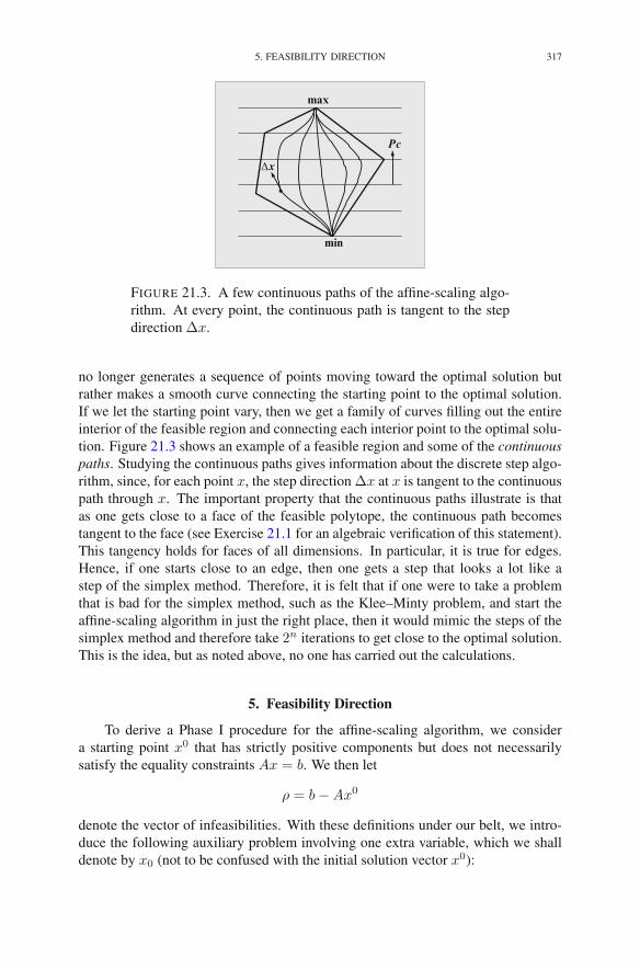
5. FEASIBILITY DIRECTION 317
Pc
min
max
Δx
FIGURE 21.3. A few continuous paths of the affine-scaling algo-rithm. At every point, the continuous path is tangent to the stepdirection Δx.
no longer generates a sequence of points moving toward the optimal solution butrather makes a smooth curve connecting the starting point to the optimal solution.If we let the starting point vary, then we get a family of curves filling out the entireinterior of the feasible region and connecting each interior point to the optimal solu-tion. Figure 21.3 shows an example of a feasible region and some of the continuouspaths. Studying the continuous paths gives information about the discrete step algo-rithm, since, for each point x, the step direction Δx at x is tangent to the continuouspath through x. The important property that the continuous paths illustrate is thatas one gets close to a face of the feasible polytope, the continuous path becomestangent to the face (see Exercise 21.1 for an algebraic verification of this statement).This tangency holds for faces of all dimensions. In particular, it is true for edges.Hence, if one starts close to an edge, then one gets a step that looks a lot like astep of the simplex method. Therefore, it is felt that if one were to take a problemthat is bad for the simplex method, such as the Klee–Minty problem, and start theaffine-scaling algorithm in just the right place, then it would mimic the steps of thesimplex method and therefore take 2n iterations to get close to the optimal solution.This is the idea, but as noted above, no one has carried out the calculations.
5. Feasibility Direction
To derive a Phase I procedure for the affine-scaling algorithm, we considera starting point x0 that has strictly positive components but does not necessarilysatisfy the equality constraints Ax = b. We then let
ρ = b−Ax0
denote the vector of infeasibilities. With these definitions under our belt, we intro-duce the following auxiliary problem involving one extra variable, which we shalldenote by x0 (not to be confused with the initial solution vector x0):

318 21. THE AFFINE-SCALING METHOD
maximize −x0
subject to Ax+ x0ρ= bx ≥ 0, x0 ≥ 0.
Clearly, the vector[
x0
1
]
is a strictly positive feasible solution to the auxiliary problem. Hence, we can applythe affine-scaling algorithm to the auxiliary problem. If the optimal solution hasx∗0 > 0, then the original problem is infeasible. If, on the other hand, the optimal
solution has x∗0 = 0, then the optimal solution to the auxiliary problem provides
a feasible starting solution to the original problem (it may not be a strictly interiorfeasible solution, but we shall ignore such technicalities in the present discussion).
Let us now derive a specific formula for the step direction vector in the auxiliaryproblem. The vector of objective coefficients is
[0
−1
]
,
the constraint matrix is[A ρ
],
and the “current” solution can be denoted as[
xx0
]
.
Substituting these three objects appropriately into (21.5), we get[
ΔxΔx0
]
=
([X2
x20
]
−[
X2
x20
] [AT
ρT
]
([A ρ
][X2
x20
] [AT
ρT
])−1
[A ρ
][X2
x20
])[0
−1
]
.
Exploiting heavily the fact that all the coefficients in the objective vector are zeroexcept for the last, we can write a fairly simple expression for Δx:
Δx = X2AT(AX2AT + x2
0ρρT)−1
ρx0.
The final simplification comes from applying the Sherman–Morrison–Woodburyformula (see Exercise 19.1) to the inverted expression above to discover that thevector (AX2AT + x2
0ρρT )−1ρ points in the same direction as (AX2AT )−1ρ. That
is, there is a positive scalar α such that
(AX2AT + x20ρρ
T )−1ρ = α(AX2AT )−1ρ
6. PROBLEMS IN STANDARD FORM 319
(see Exercise 21.3). Since vector lengths are irrelevant, we can define the affine-scaling feasibility step direction as
(21.6) Δx = X2AT(AX2AT
)−1ρ.
6. Problems in Standard Form
We return now to problems in standard form:
maximize cTxsubject to Ax≤ b
x≥ 0.
Introducing slack variables w, we can write the problem equivalently as
(21.7)
maximize
[c0
]T [xw
]
subject to[A I
][
xw
]
= b[xw
]
≥ 0.
Writing down the affine-scaling step direction for this problem, we get[
ΔxΔw
]
=
([X2
W 2
]
−[
X2
W 2
] [AT
I
]
([A I
][X2
W 2
] [AT
I
])−1
[A I
][X2
W 2
])[c0
]
,
which simplifies to[
ΔxΔw
]
=
[X2c0
]
−[
X2AT
W 2
](AX2AT +W 2
)−1AX2c.
Therefore, in particular
Δx = X2c−X2AT (AX2AT +W 2)−1AX2c.
Note that this formula for Δx matches the formula for ΔxOPT given in Section 19.3,except that the diagonal matrix X2 replaces XZ−1 and W 2 replaces WY −1. Thesediagonal matrices are referred to as scaling matrices. Hence, the formula for Δxgiven above is often called the affine-scaling step direction with primal scaling,whereas ΔxOPT is referred to as the affine-scaling step direction with primal–dualscaling.
Similar connections can be established between the Phase I step direction de-rived in this section and ΔxFEAS from Section 19.3. Indeed, from (21.6), we see that

320 21. THE AFFINE-SCALING METHOD
the feasibility step direction for (21.7) is[
ΔxΔw
]
=
[X2
W 2
] [AT
I
]([A I
][X2
W 2
] [AT
I
])−1
(
b−[A I
][
xw
])
.
Again, looking just at the formula for Δx, we see that
Δx = X2AT (AX2AT +W 2)−1(b−Ax− w),
which coincides with ΔxFEAS except that X2 replaces XZ−1 and W 2
replaces WY −1.
Exercises
21.1 Step direction becomes tangent to each facet. Let Δx denote the affine-scaling step direction given by
Δx =(X2 −X2AT (AX2AT )−1AX2
)c.
This step direction is clearly a function of x. Fix j. Show that the limit asxj tends to zero of Δx is a vector whose jth component vanishes. That is,
limxj→0
Δxj = 0.
21.2 Dual Estimates. Consider the following function, defined in the interiorof the polytope of feasible solutions {x : Ax = b, x > 0} by
y(x) = (AX2AT )−1AX2c.
Consider a partition of the columns of A =[B N
]into a basic part B
and a nonbasic part N , and, as we did in our study of the simplex method,partition the n-vectors analogously. Show that
limxN→0
y(x) = (BT )−1cB.
21.3 Let A be an m × n matrix having rank m, and let ρ be an arbitrary m-vector. Use the identity proved in Exercise 19.1 to show that there existsa scalar α such that
(AAT + ρρT )−1ρ = α(AAT )−1ρ.
Hint: Be mindful of which matrices are invertible.
21.4 (So-called) Dual Affine-Scaling Method. Compute the affine-scaling step-direction vector Δx for problems in the following form:
maximize cTxsubject to Ax ≤ b.

NOTES 321
Notes
The affine-scaling algorithm was first suggested by Dikin (1967). He sub-sequently published a convergence analysis in Dikin (1974). Dikin’s work wentlargely unnoticed for many years until several researchers independently rediscov-ered the affine-scaling algorithm as a simple variant of Karmarkar’s algorithm (Kar-markar 1984). Of these independent rediscoveries, only two papers offered a con-vergence analysis: one by Barnes (1986) and the other by Vanderbei et al. (1986). Itis interesting to note that Karmarkar himself was one of the independent rediscov-erers, but he mistakenly believed that the algorithm enjoyed the same convergenceproperties as his algorithm (i.e., that it would get within any fixed tolerance of opti-mality within a specific number of iterations bounded by a polynomial in n).
Theorem 21.1(a) was proved by Vanderbei et al. (1986). Part (b) of the Theoremwas proved by Tsuchiya and Muramatsu (1992) who also show that the result issharp. A sharper sharpness result can be found in Hall and Vanderbei (1993). Part(c) of the Theorem was established by Mascarenhas (1997).
The first derivation of the affine-scaling feasibility step direction was given byVanderbei (1989). The simple derivation given in Section 21.5 is due to M. Meketon.
A recent book by Saigal (1995) contains an extensive treatment of affine-scalingmethods.

CHAPTER 22
The Homogeneous Self-Dual Method
In Chapter 18, we described and analyzed an interior-point method called thepath-following algorithm. This algorithm is essentially what one implements inpractice but as we saw in the section on convergence analysis, it is not easy (andperhaps not possible) to give a complete proof that the method converges to anoptimal solution. If convergence were completely established, the question wouldstill remain as to how fast is the convergence. In this chapter, we shall present asimilar algorithm for which a complete convergence analysis can be given.
1. From Standard Form to Self-Dual Form
As always, we are interested in a linear programming problem given in standardform
(22.1)maximize cTx
subject to Ax≤ bx≥ 0
and its dual
(22.2)minimize bT y
subject to AT y ≥ cy ≥ 0.
As we shall show, these two problems can be solved by solving the followingproblem, which essentially combines the primal and dual problems into one problem:
(22.3)
maximize 0subject to − AT y + cφ ≤ 0,
Ax − bφ ≤ 0,−cTx + bT y ≤ 0,
x, y, φ ≥ 0.
Note that, beyond combining the primal and dual into one big problem, one newvariable (φ) and one new constraint have been added. Hence, the total number ofvariables in (22.3) is n +m + 1 and the total number of constraints is n +m + 1.Furthermore, the objective function and the right-hand sides all vanish. Problemswith such right-hand sides are called homogeneous. Also, the constraint matrixfor problem (22.3) is skew symmetric. That is, it is equal to the negative of itstranspose. Homogeneous linear programming problems having a skew symmetricconstraint matrix are called self-dual.
R.J. Vanderbei, Linear Programming, International Series in Operations Research& Management Science 196, DOI 10.1007/978-1-4614-7630-6 22,© Springer Science+Business Media New York 2014
323
324 22. THE HOMOGENEOUS SELF-DUAL METHOD
In the next section, we shall give an algorithm for the solution of homogeneousself-dual linear programming problems. But first, let’s note that a solution to (22.3)in which φ > 0 can be converted into solutions for (22.1) and (22.2). Indeed, let(x, y, φ) be an optimal solution to problem (22.3). Suppose that φ > 0. (The algo-rithm given in the next section will guarantee that this property is satisfied whenever(22.1) and (22.2) have optimal solutions.1) Put
x∗ = x/φ and y∗ = y/φ.
Then the constraints in (22.3) say that
− AT y∗ + c ≤ 0,Ax∗ − b ≤ 0,
−cTx∗ + bT y∗ ≤ 0.
Also, x∗ and y∗ are both nonnegative. Therefore, x∗ is feasible for (22.1) and y∗ isfeasible for (22.2). From the weak duality theorem together with the third inequalityabove, we get
cTx∗ = bT y∗.
Therefore, x∗ is optimal for the primal problem (22.1) and y∗ is optimal for thedual problem (22.2). As we will see later, the case where φ = 0 corresponds toinfeasibility of either the primal or the dual problem (or both).
2. Homogeneous Self-Dual Problems
Consider a linear programming problem in standard form
maximize cTxsubject to Ax≤ b
x≥ 0
and its dualminimize bT y
subject to AT y ≥ cy ≥ 0.
Such a linear programming problem is called self-dual if m = n, A = −AT , andb = −c. The reason for the name is that the dual of such a problem is the same asthe primal. To see this, rewrite the constraints as less-thans and then use the definingproperties for self-duality to get
AT y ≥ c ⇔ −AT y ≤ −c ⇔ Ay ≤ b.
Similarly, writing the objective function as a maximization, we get
min bT y = −max−bT y = −max cT y.
Hence, ignoring the (irrelevant) fact that the dual records the negative of the objec-tive function, the primal and the dual are seen to be the same. A linear programmingproblem in which the right-hand side vanishes is called a homogeneous problem.
1The astute reader might notice that setting all variables to 0 produces an optimal solution.

2. HOMOGENEOUS SELF-DUAL PROBLEMS 325
It follows that if a problem is homogeneous and self-dual, then its objective func-tion must vanish too.
For the remainder of this section, we assume that the problem under consider-ation is homogeneous and self-dual. Since the case m = n = 1 is trivial (A = 0in this case), we assume throughout this section that n ≥ 2. Also, since the dual isthe same problem as the primal, we prefer to use the letter z for the primal slacks(instead of the usual w). Hence, the primal can be written as
(22.4)maximize 0subject to Ax+ z = 0
x, z ≥ 0.
The following theorem establishes some of the important properties of homo-geneous self-dual problems.
THEOREM 22.1. For homogeneous self-dual problem (22.4), the followingstatements hold:
(1) It has feasible solutions and every feasible solution is optimal.(2) The set of feasible solutions has empty interior. In fact, if (x, z) is feasible,
then zTx = 0.
PROOF. (1) The trivial solution, (x, z) = (0, 0), is feasible. Since the objectivefunction is zero, every feasible solution is optimal.
(2) Suppose that (x, z) is feasible for (22.4). The fact that A is skew symmetricimplies that ξTAξ = 0 for every vector ξ (see Exercise 16.1). In particular, xTAx =0. Therefore, multiplying Ax+z = 0 on the left by xT , we get 0 = xTAx+xT z =xT z. This completes the proof. �
Part (2) of the previous Theorem tells us that homogeneous self-dual problemsdo not have central paths.
2.1. Step Directions. As usual, the interior-point method we shall derive willhave the property that the intermediate solutions it produces will be infeasible.Hence, let
ρ(x, z) = Ax+ z
denote the infeasibility of a solution (x, z). Also, let
μ(x, z) =1
nxT z.
The number μ(x, z) measures the degree of noncomplementarity between x and z.When x and z are clear from context, we shall simply write ρ for ρ(x, z) and μ forμ(x, z).
Step directions (Δx,Δz) are chosen to reduce the infeasibility and noncomple-mentarity of the current solution by a given factor δ, 0 ≤ δ ≤ 1. Hence, we considerthe nonlinear system that would make the infeasibility and noncomplementarity of(x+Δx, z +Δz) be δ times that of (x, z):

326 22. THE HOMOGENEOUS SELF-DUAL METHOD
A(x+Δx) + (z +Δz) = δ(Ax+ z),
(X +ΔX)(Z +ΔZ)e = δμ(x, z)e.
As usual, this system is nonlinear in the “delta” variables. Dropping the nonlinearterm (appearing only in the second equation), we get the following linear system ofequations for the step directions:
AΔx+Δz = −(1− δ)ρ(x, z),(22.5)
ZΔx+XΔz = δμ(x, z)e−XZe.(22.6)
With these step directions, we pick a step length θ and step to a new point:
x = x+ θΔx, z = z + θΔz.
We denote the new ρ-vector by ρ and the new μ-value by μ:
ρ = ρ(x, z) and μ = μ(x, z).
The following theorem establishes some of the properties of these step directions.
THEOREM 22.2. The following relations hold:
(1) ΔzTΔx = 0.(2) ρ = (1− θ + θδ)ρ.(3) μ = (1− θ + θδ)μ.(4) XZe− μe = (1− θ)(XZe− μe) + θ2ΔXΔZe.
PROOF. (1) We start by multiplying both sides of (22.5) on the left by ΔxT :
(22.7) ΔxTAΔx+ΔxTΔz = −(1− δ)ΔxT ρ.
The skew symmetry of A (i.e., A = −AT ) implies that ΔxTAΔx = 0 (see Exer-cise 16.1). Hence, the left-hand side of (22.7) simplifies nicely:
ΔxTAΔx+ΔxTΔz = ΔxTΔz.
Substituting the definition of ρ into the right-hand side of (22.7), we get
−(1− δ)ΔxT ρ = −(1− δ)ΔxT (Ax+ z).
Next, we use the skew symmetry of A to rewrite ΔxTAx as follows:
ΔxTAx = (Ax)TΔx = xTATΔx = −xTAΔx.
Assembling what we have so far, we see that
(22.8) ΔxTΔz = −(1− δ)(−xTAΔx+ zTΔx).
To proceed, we use (22.5) to replace AΔx with −(1− δ)ρ−Δz. Therefore,
−xTAΔx+ zTΔx = xT ((1− δ)ρ+Δz) + zTΔx
= (1− δ)xT ρ+ xTΔz + zTΔx.(22.9)
Again using the definition of ρ and the skew symmetry of A, we see that
xT ρ = xT (Ax+ z) = xT z.

2. HOMOGENEOUS SELF-DUAL PROBLEMS 327
The last two terms in (22.9) can be simplified by multiplying both sides of (22.6) onthe left by eT and then using the definition of μ to see that
zTΔx+ xTΔz = δμn− xT z = (δ − 1)xT z.
Making these substitutions in (22.9), we get
−xTAΔx+ zTΔx = (1− δ)xT z + (δ − 1)xT z = 0.
Hence, from (22.8), we see that ΔxTΔz vanishes as claimed.(2) From the definitions of x and z, we see that
ρ = A(x+ θΔx) + (z + θΔz)
= Ax+ z + θ(AΔx+Δz)
= (1− θ + θδ)ρ.
(3) From the definitions of x and z, we see that
xT z = (x+ θΔx)T (z + θΔz)
= xT z + θ(zTΔx+ xTΔz) + θ2ΔzTΔx.
From part (1) and (22.6), we then get
xT z = xT z + θ(δμn− xT z).
Therefore,
μ =1
nxT z = (1− θ)μ+ θδμ.
(4) From the definitions of x and z together with part (3), we see that
XZe− μe = (X + θΔX)(Z + θΔZ)e− (1− θ + θδ)μe
= XZe+ θ(ZΔx+XΔz) + θ2ΔXΔZe− (1− θ + θδ)μe.
Substituting (22.6) into the second term on the right and recollecting terms, we getthe desired expression. �
2.2. Predictor-Corrector Algorithm. With the preliminaries behind us, weare now ready to describe an algorithm. We shall be more conservative than we werein Chapter 18 and define the algorithm in such a way that it keeps the componentsof XZe close to each other. Indeed, for each 0 ≤ β ≤ 1, let
N (β) = {(x, z) > 0 : ‖XZe− μ(x, z)e‖ ≤ βμ(x, z)} .Shortly, we will only deal with N (1/4) and N (1/2) but first let us note generallythat β < β′ implies that N (β) ⊂ N (β′). Hence, as a function of β, the N (β)’sform an increasing family of sets. Also, N (0) is precisely the set of points (x, z)for which XZe has all equal components.
The algorithm alternates between two types of steps. On the first iterationand subsequently on every other iteration, the algorithm performs a predictor step.Before a predictor step, one assumes that
(x, z) ∈ N (1/4).
328 22. THE HOMOGENEOUS SELF-DUAL METHOD
Then step directions are computed using δ = 0 (i.e., with no centering) and the steplength is calculated so as not to go outside of N (1/2):
(22.10) θ = max{t : (x+ tΔx, z + tΔz) ∈ N (1/2)}.
On the even iterations, the algorithm performs a corrector step. Before a correctorstep, one assumes that
(x, z) ∈ N (1/2)
(as is guaranteed by the predictor step’s step length). Then step directions are com-puted using δ = 1 (i.e., pure centering) and the step length parameter θ is set to 1.
The following theorem shows that the result of each step satisfies the precondi-tion for the next step of the algorithm and that μ decreases on predictor steps whileit stays the same on corrector steps.
THEOREM 22.3. The following statements are true:
(1) After a predictor step, (x, z) ∈ N (1/2) and μ = (1− θ)μ.(2) After a corrector step, (x, z) ∈ N (1/4) and μ = μ.
PROOF OF PART (1). The formula for μ follows from part (3) of Theorem 22.2by putting δ = 0. The fact that (x, z) ∈ N (1/2) is an immediate consequence ofthe choice of θ. �
Before proving Part (2) of the Theorem, we need to introduce some notationand prove a few technical results. Let
p = X−1/2Z1/2Δx,
q = X1/2Z−1/2Δz,
r = p+ q
= X−1/2Z−1/2(ZΔx+XΔz)
= X−1/2Z−1/2(δμe−XZe).(22.11)
The technical results are summarized in the following lemma.
LEMMA 22.4. The following statements are true:
(1) ‖PQe‖ ≤ 12‖r‖2.
(2) If δ = 0, then ‖r‖2 = nμ.(3) If δ = 1 and (x, z) ∈ N (β), then ‖r‖2 ≤ β2μ/(1− β).
PROOF. (1) First note that pT q = ΔxTΔz = 0 by Theorem 22.2(1). Hence,
‖r‖2 = ‖p+ q‖2 = pT p+ 2pT q + qT q =∑
j
(p2j + q2j ).

2. HOMOGENEOUS SELF-DUAL PROBLEMS 329
Therefore,
‖r‖4 =
⎛
⎝∑
j
(p2j + q2j )
⎞
⎠
2
≥∑
j
(p2j + q2j )2
=∑
j
((p2j − q2j )
2 + 4p2jq2j
)
≥ 4∑
j
p2jq2j
= 4‖PQe‖2.Taking square roots yields the desired inequality.
(2) Putting δ = 0 in (22.11), we see that r = −X1/2Z1/2e. Therefore, ‖r‖2 =zTx = nμ.
(3) Suppose that (x, z) ∈ N (β). Whenever the norm of a vector is smaller thansome number, the magnitude of each component of the vector must also be smallerthan this number. Hence, |xjzj − μ| ≤ βμ. It is easy to see that this inequality isequivalent to
(22.12) (1− β)μ ≤ xjzj ≤ (1 + β)μ.
Now putting δ = 1 in (22.11), we get
‖r‖2 =∑
j
(xjzj − μ)2
xjzj.
Therefore, using the lower bound given in (22.12), we get the following upperbound:
‖r‖2 ≤ 1
(1− β)μ
∑
j
(xjzj − μ)2.
Finally, since (x, z) ∈ N (β), we see that the above sum is bounded by β2μ2. Thisgives the claimed inequality. �
PROOF OF THEOREM 22.3(2). Since θ = 1 in a corrector step, it follows fromTheorem 22.2(4) that XZe− μe = ΔXΔZe = PQe. Therefore, parts (1) and (3)of Lemma 22.4 imply that
‖XZe− μe‖ = ‖PQe‖
≤ 1
2‖r‖2
≤ 1
2
(1/2)2
1− 1/2μ
=1
4μ.(22.13)
330 22. THE HOMOGENEOUS SELF-DUAL METHOD
We also need to show that (x, z) > 0. For 0 ≤ t ≤ 1, let
x(t) = x+ tΔx, z(t) = z + tΔz, and μ(t) = μ(x(t), z(t)).
Then from part (4) of Theorem 22.2, we have
X(t)Z(t)e− μ(t)e = (1− t)(XZe− μe) + t2ΔXΔZe.
The right-hand side is the sum of two vectors. Since the length of the sum of twovectors is less than the sum of the lengths (i.e., by the triangle inequality), it followsthat
(22.14) ‖X(t)Z(t)e− μ(t)e‖ ≤ (1− t)‖XZe− μe‖+ t2‖ΔXΔZe‖
(note that we’ve pulled the scalars out of the norms). Now, since (x, z) ∈ N (1/2),we have ‖XZe−μe‖ ≤ μ/2. Furthermore, from (22.13) we have that ‖ΔXΔZe‖ =‖PQe‖ ≤ μ/4. Replacing the norms in (22.14) with these upper bounds, we getthe following bound:
(22.15) ‖X(t)Z(t)e− μ(t)e‖ ≤ (1− t)μ
2+ t2
μ
4≤ μ
2
(the second inequality follows from the obvious facts that t2 ≤ t and μ/4 ≤ μ/2).Now, consider a specific component j. It follows from (22.15) that
xj(t)zj(t)− μ(t) ≥ −μ
2.
Since δ = 1, part (3) of Theorem 22.2 tells us that μ(t) = μ for all t. Therefore theprevious inequality can be written as
(22.16) xj(t)zj(t) ≥μ
2> 0.
This inequality then implies that xj(t) > 0 and zj(t) > 0 for all 0 ≤ t ≤ 1(since they could only become negative by passing through 0, which is ruled out by(22.16)). Putting t = 1, we get that xj > 0 and zj > 0. Since the component j wasarbitrary, it follows that (x, z) > 0. Therefore (x, z) ∈ N (1/4). �
2.3. Convergence Analysis. The previous theorem showed that the predictor-corrector algorithm is well defined. The next theorem gives us a lower bound on theprogress made by each predictor step.
THEOREM 22.5. In each predictor step, θ ≥ 12√n
.
PROOF. Using the same notation as in the proof of Theorem 22.3, we have theinequality:
‖X(t)Z(t)e− μ(t)e‖ ≤ (1− t)‖XZe− μe‖(22.17)
+ t2‖ΔXΔZe‖.
This time, however, (x, z) ∈ N (1/4) and δ = 0. Hence,
‖XZe− μe‖ ≤ μ
4
2. HOMOGENEOUS SELF-DUAL PROBLEMS 331
and, from parts (1) and (2) of Lemma 22.4,
‖ΔXΔZe‖ = ‖PQe‖ ≤ 1
2‖r‖2 =
1
2nμ.
Using these two bounds in (22.17), we get the following bound:
‖X(t)Z(t)e− μ(t)e‖ ≤ (1− t)μ
4+ t2
nμ
2.
Now, fix a t ≤ (2√n)−1. For such a t, we have t2n/2 ≤ 1/8. Therefore, using the
fact that t ≤ 1/2 for n ≥ 2, we get
‖X(t)Z(t)e− μ(t)e‖ ≤ (1− t)μ
4+
μ
8
≤ (1− t)μ
4+ (1− t)
μ
4
= (1− t)μ
2
=μ(t)
2.
Hence, as in the previous theorem, (x(t), z(t)) ∈ N (1/2). Since t was an arbitrarynumber less than (2
√n)−1, it follows that θ ≥ (2
√n)−1. �
Let (x(k), z(k)) denote the solution after the kth iteration and let
ρ(k) = ρ(x(k), z(k)) and μ(k) = μ(x(k), z(k)).
The algorithm starts with x(0) = z(0) = e. Therefore, μ(0) = 1. Our aim is toshow that μ(k) and ρ(k) tend to zero as k tends to infinity. The previous theoremtogether with Theorem 22.3 implies that, after an even number of iterations, say 2k,the following inequality holds:
μ(2k) ≤(
1− 1
2√n
)k
.
Also, since the corrector steps don’t change the value of μ, it follows that
μ(2k−1) = μ(2k).
From these two statements, we see that
limk→∞
μ(k) = 0.
Now, consider ρ(k). It follows from parts (2) and (3) of Theorem 22.2 that thereduction in infeasibility tracks the reduction in noncomplementarity. Hence,
ρ(k) = μ(k)ρ(0).
Therefore, the fact that μ(k) tends to zero implies the same for ρ(k).In fact, more can be said:
THEOREM 22.6. The limits x∗ = limk→∞ x(k) and z∗ = limk→∞ z(k) existand (x∗, z∗) is optimal. Furthermore, the vectors x∗ and z∗ are strictly comple-mentary to each other. That is, for each j, x∗
jz∗j = 0 but either x∗
j > 0 or z∗j > 0.

332 22. THE HOMOGENEOUS SELF-DUAL METHOD
The proof is fairly technical, and so instead of proving it, we prove the followingtheorem, which captures the main idea.
THEOREM 22.7. There exist positive constants c1, c2, . . . , cn such that (x, z) ∈N (β) implies that xj + zj ≥ cj > 0 for each j = 1, 2, . . . , n.
PROOF. Put μ = μ(x, z) and ρ = ρ(x, z) = μρ(0). Let (x∗, z∗) be a strictlycomplementary feasible solution (the existence of which is guaranteed by Theorem10.6). We begin by studying the expression zTx∗ +xT z∗. Since Ax∗ + z∗ = 0, wehave that
zTx∗ + xT z∗ = zTx∗ − xTAx∗
= (−ATx+ z)Tx∗.
By the skew-symmetry of A, we see that −ATx + z = Ax + z = ρ. And, sinceρ = μρ(0), we get
(22.18) zTx∗ + xT z∗ = μρ(0)Tx∗.
The factor ρ(0)Tx∗ is a constant (i.e., it does not depend on x or z). Let us denote it
by M . Since all the terms in the two products on the left in (22.18) are nonnegative,it follows that each one is bounded by the right-hand side. So if we focus on aparticular index j, we get the following bounds:
(22.19) zjx∗j ≤ μM and xjz
∗j ≤ μM.
Now, we use the assumption that (x, z) ∈ N (β) to see that
xjzj ≥ (1− β)μ.
In other words, μ ≤ xjzj/(1− β), and so the inequalities in (22.19) become
zjx∗j ≤ M
1− βzjxj and xjz
∗j ≤ M
1− βxjzj .
Since xj and zj are strictly positive, we can divide by them (and the constants) toget
1− β
Mx∗j ≤ xj and
1− β
Mz∗j ≤ zj .
Putting
cj =1− β
M(x∗
j + z∗j ),
we get the desired lower bound on xj + zj . �
2.4. Complexity of the Predictor-Corrector Algorithm. Of course, in prac-tice we don’t run an infinite number of iterations. Instead, we set a priori a thresholdand stop when μ(k) falls below it. The threshold is usually denoted by 2−L whereL is some number. Typically, we want the threshold to be about 10−8, which corre-sponds to L ≈ 26.

2. HOMOGENEOUS SELF-DUAL PROBLEMS 333
As we saw before, after an even number of iterations, say 2k, the μ-value isbounded by the following inequality:
μ(2k) ≤(
1− 1
2√n
)k
.
Hence, it suffices to pick a k big enough to have
(
1− 1
2√n
)k
≤ 2−L.
Taking logarithms of both sides and solving for k, we see that any
k ≥ L
− log(1− 12√n)
will do. Since − log(1− x) ≥ x, we get
2L√n ≥ L
− log(1− 12√n).
Therefore, any k ≥ 2L√n will do. In particular, k = 2L
√n rounded up to the
nearest integer will suffice. Since k represents half the number of iterations, it fol-lows that it will take at most 4L
√n iterations for the μ-value to fall below the
threshold of 2−L. This bound implies that the method is a polynomial algorithm,since it says that any desired precision can be obtained in a number of iterations thatis bounded above by a polynomial in n (here, 4L
√n is not itself a polynomial but
is bounded above by say a linear function in n for n ≥ 2).
2.5. The KKT System. We end this section on homogeneous self-dual prob-lems by briefly discussing the KKT system (22.5)–(22.6). Solving this system ofequations is the most time consuming step within each iteration of the predictor-corrector algorithm. There are several ways in which one can organize the compu-tation. The approach that most parallels what we have done before is first to solve(22.6) for Δz,
Δz = X−1(−ZΔx+ δμe−XZe)(22.20)
= −X−1ZΔx+ δμX−1e− z,
and then to eliminate it from (22.5) to get the following reduced KKT system:
(A−X−1Z)Δx = −(1− δ)ρ+ z − δμX−1e.
In the next section, we apply the algorithm developed in this section to the homoge-neous self-dual problem given by (22.3).

334 22. THE HOMOGENEOUS SELF-DUAL METHOD
3. Back to Standard Form
We return now to the setup in Section 1. Let z, w, and ψ denote the slackvariables for the constraints in problem (22.3):
(22.21)
maximize 0subject to − AT y + cφ + z = 0,
Ax − bφ + w = 0,−cTx + bT y + ψ = 0,
x, y, φ, z, w, ψ ≥ 0.
We say that a feasible solution (x, y, φ, z, w, ψ) is strictly complementary if xj +zj > 0 for all j, yi + wi > 0 for all i, and φ + ψ > 0. Theorem 10.6 ensures theexistence of such a solution (why?).
The following theorem summarizes and extends the motivating discussion givenin Section 1.
THEOREM 22.8. Suppose that (x, y, φ, z, w, ψ) is a strictly complementaryfeasible (hence, optimal) solution to (22.21).
(1) If φ > 0, then x∗ = x/φ is optimal for the primal problem (22.1) andy∗ = y/φ is optimal for its dual (22.2).
(2) If φ = 0, then either cT x > 0 or bT y < 0.(a) If cT x > 0, then the dual problem is infeasible.(b) If bT y < 0, then the primal problem is infeasible.
PROOF. Part (1) was proved in Section 1. For part (2), suppose that φ = 0. Bystrict complementarity, ψ > 0. Hence, x and y satisfy
AT y ≥ 0,
Ax ≤ 0,(22.22)
bT y < cT x.
From the last inequality, we see that it is impossible to have bT y ≥ 0 and cT x ≤ 0.That is, either cT x > 0 or bT y < 0 (or both). Suppose, without loss of generality,that cT x > 0. We will prove by contradiction that the dual problem is infeasible.To this end, suppose that there exists a vector y0 ≥ 0 such that
(22.23) AT y0 ≥ c.
Since x ≥ 0, we can multiply by it without changing the direction of an inequality.So multiplying (22.23) on the left by xT , we get
xTAT y0 ≥ xT c.
Now, the right-hand side is strictly positive. But inequality (22.22) together with thenonnegativity of y0 implies that the left-hand side is nonpositive:
xTAT y0 = (Ax)T y0 ≤ 0.
This is a contradiction and therefore the dual must be infeasible. �

3. BACK TO STANDARD FORM 335
3.1. The Reduced KKT System. The right-hand side in the reduced KKTsystem involves the vector of infeasibilities. We partition this vector into three partsas follows:⎡
⎣σργ
⎤
⎦ =
⎡
⎣−AT c
A −b−cT bT
⎤
⎦
⎡
⎣xyφ
⎤
⎦+
⎡
⎣zwψ
⎤
⎦ =
⎡
⎣−AT y + cφ+ zAx− bφ+ w
−cTx+ bT y + φ
⎤
⎦ .
The reduced KKT system for (22.3) is given by
(22.24)
⎡
⎣−X−1Z −AT c
A −Y −1W −b−cT bT −ψ/φ
⎤
⎦
⎡
⎣ΔxΔyΔφ
⎤
⎦ =
⎡
⎣σργ
⎤
⎦ ,
where ⎡
⎣σργ
⎤
⎦ =
⎡
⎣−(1− δ)σ + z − δμX−1e−(1− δ)ρ+ w − δμY −1e−(1− δ)γ + ψ − δμ/φ
⎤
⎦ .
This system is not symmetric. One could use a general purpose equation solverto solve it, but its special structure would be mostly ignored by such a solver. Toexploit the structure, we solve this system in two stages. We start by using the firsttwo equations to solve simultaneously for Δx and Δy in terms of Δφ:
[ΔxΔy
]
=
[−X−1Z −AT
A −Y −1W
]−1 ([σρ
]
−[
c−b
]
Δφ
)
.
Introducing abbreviating notations, we can write
(22.25)
[ΔxΔy
]
=
[fxfy
]
−[
gxgy
]
Δφ,
where the vectors
f =
[fxfy
]
and g =
[gxgy
]
are found by solving the following two systems of equations:[
−X−1Z −AT
A −Y −1W
] [fxfy
]
=
[σρ
]
and[
−X−1Z −AT
A −Y −1W
] [gxgy
]
=
[c
−b
]
.
Then we use (22.25) to eliminate Δx and Δy from the last equation in (22.24):
[−cT bT
]([
fxfy
]
−[
gxgy
]
Δφ
)
− ψ
φΔφ = γ.
We then solve for Δφ:
Δφ =cT fx − bT fy + γ
cT gx − bT gy − ψ/φ.
336 22. THE HOMOGENEOUS SELF-DUAL METHOD
Given Δφ, (22.25) determines Δx and Δy. Once these vectors are known, (22.20)is used to compute the step directions for the slack variables:
Δz = −X−1ZΔx+ δμX−1e− z
Δw = −Y −1WΔy + δμY −1e− w
Δψ = −ψ
φΔφ+ δμ/φ− ψ.
We now see that the reduced KKT system can be solved by solving two sys-tems of equations for f and g. These two systems both involve the same matrix.Furthermore, these systems can be formulated as quasidefinite systems by negatingthe first equation and then reordering the equations appropriately. For example, thequasidefinite system for g is
[−Y −1W A
AT X−1Z
] [gygx
]
=
[−b−c
]
.
Therefore, the techniques developed in Chapter 20 can be used to solve these sys-tems of equations. In particular, to solve the two systems, the quasidefinite matrixonly needs to be factored once. Then the two systems can be solved by doing twoforward and two backward substitutions. Since factorization requires more com-putation than forward and backward substitutions, one would expect to be able tosolve these two systems in much less time than if they were each being solved fromscratch. In fact, it is often the case that one can solve two systems involving thesame quasidefinite matrix in little more time than is required to solve just one suchsystem.
The full homogeneous self-dual method is summarized in Figure 22.1.
4. Simplex Method vs. Interior-Point Methods
Finally, we compare the performance of interior-point methods with the sim-plex method. For this comparison, we have chosen the homogeneous self-dualmethod described in this chapter and the self-dual simplex method (see Figure 7.1).In the interest of efficiency certain liberties have been taken with the implementa-tions. For example, in the homogeneous self-dual method, (18.6) is used to com-pute “long” step lengths instead of the more conservative “short” step lengths in(22.10). The code fragments implementing each of these two algorithms are shownin Appendix A.
A standard collection of test problems, the so-called NETLIB suite, were usedin the comparison. Problems in this collection are formulated with bounds andranges:
minimize cTxsubject to b ≤ Ax ≤ b+ r
l ≤ x ≤ u.
However, to keep the algorithms as simple as possible, they were implemented onlyfor problems in our standard inequality form. Therefore, the problems from theNETLIB suite were converted to standard form as follows:
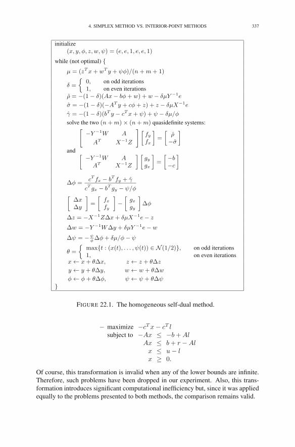
4. SIMPLEX METHOD VS. INTERIOR-POINT METHODS 337
initialize(x, y, φ, z, w, ψ) = (e, e, 1, e, e, 1)
while (not optimal) {μ = (zTx+ wT y + ψφ)/(n+m+ 1)
δ =
{0, on odd iterations1, on even iterations
ρ = −(1− δ)(Ax− bφ+ w) + w − δμY −1e
σ = −(1− δ)(−AT y + cφ+ z) + z − δμX−1e
γ = −(1− δ)(bT y − cTx+ ψ) + ψ − δμ/φ
solve the two (n+m)× (n+m) quasidefinite systems:[
−Y −1W A
AT X−1Z
] [fyfx
]=
[ρ−σ
]
and [−Y −1W A
AT X−1Z
] [gygx
]=
[−b−c
]
Δφ =cT fx − bT fy + γ
cT gx − bT gy − ψ/φ[
ΔxΔy
]=
[fxfy
]−
[gxgy
]Δφ
Δz = −X−1ZΔx+ δμX−1e− z
Δw = −Y −1WΔy + δμY −1e− w
Δψ = −ψφΔφ+ δμ/φ− ψ
θ =
{max{t : (x(t), . . . , ψ(t)) ∈ N (1/2)}, on odd iterations1, on even iterations
x ← x+ θΔx, z ← z + θΔz
y ← y + θΔy, w ← w + θΔw
φ ← φ+ θΔφ, ψ ← ψ + θΔψ
}
FIGURE 22.1. The homogeneous self-dual method.
− maximize −cTx− cT lsubject to −Ax ≤ −b+Al
Ax ≤ b+ r −Alx ≤ u− lx ≥ 0.
Of course, this transformation is invalid when any of the lower bounds are infinite.Therefore, such problems have been dropped in our experiment. Also, this trans-formation introduces significant computational inefficiency but, since it was appliedequally to the problems presented to both methods, the comparison remains valid.

338 22. THE HOMOGENEOUS SELF-DUAL METHOD
The results of our experiment are shown in Table 22.1. The most obviousobservation is that the simplex method is generally faster and that, for many prob-lems, the slower method is not more than 3 or 4 times slower. For problems in thissuite, these results are consistent with results reported in the literature. However, itmust be noted that the problems in this suite range only from small to medium insize. The largest problem, fit2p, has about 3,000 constraints and about 14,000 vari-ables. By today’s standards, this problem is considered of medium size. For largerproblems, reports in the literature indicate that interior point methods tend to besuperior although the results are very much dependent on the specific class of prob-lems. In the remaining chapters of this book we shall consider various extensionsof the linear programming model. We shall see that the simplex method is partic-ularly well suited for solving integer programming problems studied in Chapter 23whereas interior point methods are more appropriate for extensions into the qua-dratic and convex programming problems studied in Chapters 24 and 25. Theseconsiderations are often more important than speed. There are, of course, excep-tions. For example, the interior-point method is about 900 times faster than thesimplex method on problem fit2p. Such a difference cannot be ignored.
When comparing algorithms it is always tempting to look for ways to improvethe slower method. There are obvious enhancements to the interior-point methodused in this implementation. For example, one could use the same LDLT factoriza-tion to compute both the predictor and the corrector directions. When implementedproperly, this enhancement alone can almost halve the times for this method.
Of course, the winning algorithm can also be improved (but, significant overallimprovements such as the one just mentioned for the interior-point method are not atall obvious). Looking at the table, we note that the interior-point method solved bothfit2p and fit2d in roughly the same amount of time. These two problems are duals ofeach other and hence any algorithm that treats the primal and the dual symmetricallyshould take about the same time to solve them. Now, look at the simplex method’sperformance on these two problems. There is a factor of 36 difference betweenthem. The reason is that, even though we have religiously adhered to primal-dualsymmetry in our development of the simplex method, an asymmetry did creep in. Tosee it, note that the basic matrix is always a square submatrix of
[A I
]. That is,
it is an m×m matrix. If we apply the algorithm to the dual problem, then the basismatrix is n × n. Hence, even though the sequence of iterates generated should beidentical with the two problems, the computations involved in each iteration can bevery different if m and n are not about the same. This is the case for the fit2p/fit2dpair. Of course, one can easily think up schemes to overcome this difficulty. Buteven if the performance of the simplex method on fit2p can be brought in line withits performance on fit2d, it will still be about 25 times slower than the interior-pointon this problem—a difference that remains significant.

EXERCISES 339
Name Time Name TimeSimplex Interior Simplex Interiormethod point method point
25fv47 2 min 55.70 s 3 min 14.82 s maros 1 min 0.87 s 3 min 19.43 s80bau3b 7 min 59.57 s 2 min 34.84 s nesm 1 min 40.78 s 6 min 21.28 sadlittle 0 min 0.26 s 0 min 0.47 s pilot87 * *afiro 0 min 0.03 s 0 min 0.11 s pilotnov * 4 min 15.31 sagg 0 min 1.09 s 0 min 4.59 s pilots * 32 min 48.15 sagg2 0 min 1.64 s 0 min 21.42 s recipe 0 min 0.21 s 0 min 1.04 sagg3 0 min 1.72 s 0 min 26.52 s sc105 0 min 0.28 s 0 min 0.37 sbandm 0 min 15.87 s 0 min 9.01 s sc205 0 min 1.30 s 0 min 0.84 sbeaconfd 0 min 0.67 s 0 min 6.42 s sc50a 0 min 0.09 s 0 min 0.17 sblend 0 min 0.40 s 0 min 0.56 s sc50b 0 min 0.12 s 0 min 0.15 sbnl1 0 min 38.38 s 0 min 46.09 s scagr25 0 min 12.93 s 0 min 4.44 sbnl2 3 min 54.52 s 10 min 19.04 s scagr7 0 min 1.16 s 0 min 1.05 sboeing1 0 min 5.56 s 0 min 9.14 s scfxm1 0 min 4.44 s 0 min 7.80 sboeing2 0 min 0.80 s 0 min 1.72 s scfxm2 0 min 14.33 s 0 min 18.84 sbore3d 0 min 1.17 s 0 min 3.97 s scfxm3 0 min 28.92 s 0 min 28.92 sbrandy 0 min 5.33 s 0 min 8.44 s scorpion 0 min 3.38 s 0 min 2.64 sczprob 0 min 50.14 s 0 min 41.77 s scrs8 0 min 7.15 s 0 min 9.53 sd2q06c * 1 h 11 min 1.93 s scsd1 0 min 0.86 s 0 min 3.88 sd6cube 2 min 46.71 s 13 min 44.52 s scsd6 0 min 2.89 s 0 min 9.31 sdegen2 0 min 17.28 s 0 min 17.02 s scsd8 0 min 28.87 s 0 min 16.82 sdegen3 5 min 55.52 s 3 min 36.73 s sctap1 0 min 2.98 s 0 min 3.08 sdfl001 8 h 55 min 33.05 s ** sctap2 0 min 7.41 s 0 min 12.03 se226 0 min 4.76 s 0 min 6.65 s sctap3 0 min 11.70 s 0 min 17.18 setamacro 0 min 17.94 s 0 min 43.40 s seba 0 min 27.25 s 0 min 11.90 sfffff800 0 min 10.07 s 1 min 9.15 s share1b 0 min 2.07 s 0 min 10.90 sfinnis 0 min 4.76 s 0 min 6.17 s share2b 0 min 0.47 s 0 min 0.71 sfit1d 0 min 18.15 s 0 min 11.63 s shell 0 min 16.12 s 0 min 29.45 sfit1p 7 min 10.86 s 0 min 16.47 s ship04l 0 min 3.82 s 0 min 13.60 sfit2d 1 h 3 min 14.37 s 4 min 27.66 s ship04s 0 min 3.48 s 0 min 10.81 sfit2p 36 h 31 min 31.80 s 2 min 35.67 s ship08l 0 min 17.83 s 0 min 39.06 sforplan 0 min 3.99 s * ship08s 0 min 8.85 s 0 min 19.64 sganges 0 min 44.27 s 0 min 34.89 s ship12l 0 min 26.55 s 1 min 8.62 sgfrdpnc 0 min 11.51 s 0 min 8.46 s ship12s 0 min 16.75 s 0 min 30.33 sgreenbea 22 min 45.49 s 43 min 4.32 s sierra 0 min 10.88 s 0 min 42.89 sgrow15 0 min 8.55 s 0 min 58.26 s standata 0 min 0.57 s 0 min 6.60 sgrow22 0 min 11.79 s 2 min 0.53 s standmps 0 min 2.41 s 0 min 13.44 sgrow7 0 min 3.61 s 0 min 13.57 s stocfor1 0 min 0.22 s 0 min 0.92 sisrael 0 min 1.83 s 0 min 2.66 s stocfor2 0 min 45.15 s 0 min 40.43 skb2 0 min 0.15 s 0 min 0.34 s wood1p 0 min 14.15 s 7 min 18.47 slotfi 0 min 0.81 s 0 min 3.36 s woodw 1 min 48.14 s 8 min 53.92 smaros-r7 * 1 h 31m12.06 s
(*) Denotes numerical difficulties(**) Denotes insufficient memory
TABLE 22.1. Comparison between the self-dual simplex methodand the homogeneous self-dual interior-point method.
Exercises
22.1 When n = 1, the set N (β) is a subset of R2. Graph it.
22.2 Suppose there is an algorithm for which one can prove that
μ(k) ≤(
1− a
f(n)
)k
,
for every k ≥ 1, where f(n) denotes a specific function of n, such asf(n) = n2, and a is a constant. In terms of a and f and the “precision”L, give a (tight) upper bound on the number of iterations that would besufficient to guarantee that
μ(k) ≤ 2−L.

340 22. THE HOMOGENEOUS SELF-DUAL METHOD
22.3 In Section 3 of Chapter 20, we extended the primal-dual path-followingmethod to treat problems in general form. Extend the homogeneous self-dual method in the same way.
22.4 Long-step variant. Let
M(β) = {(x, z) : minXZe ≥ (1− β)μ(x, z)}.(The notation minXZe denotes the scalar that is the minimum of all thecomponents of the vector XZe. Throughout this problem, given any vec-tor v, the notation min v (max v) will denote the minimum (maximum) ofthe components of v.) Fix 1
2 < β < 1 (say β = 0.95). A long-step variantof the homogeneous self-dual method starts with an initial (x, z) ∈ M(β)and in every iteration uses
δ = 2(1− β)
andθ = max{t : (x+ tΔx, z + tΔz) ∈ M(β)}.
The goal of this exercise is to analyze the complexity of this algorithm bycompleting the following steps.(a) Show that N (β) ⊂ M(β) ⊂ M(1) = {(x, z) > 0}.(b) Show that max(−PQe) ≤ ‖r‖2/4. Hint: Start by writing
pjqj ≥∑
i:piqi<0
piqi
and then use the facts that pT q = 0, pi + qi = ri, and that for anytwo real numbers a and b, (a+ b)2 ≥ 4ab (prove this).
(c) Show that if (x, z) ∈ M(β), then ‖r‖2 ≤ nμ. Hint: Use (22.11) towrite ‖r‖2 =
∑j(xjzj − δμ)2/xjzj . Expand the numerator, use the
definitions of μ and δ to simplify, and then use the assumption that(x, z) ∈ M(β) to take care of the remaining denominator.
(d) Show that if (x, z) ∈ M(β), then
θ ≥ min{1,− βδμ
minPQe} ≥ 4βδ
n.
Hint: Using the same notation as in the proof of Theorem 22.3, fixt ≤ min{1,−βδμ/minPQe}, write
xj(t)zj(t)− μ(t) = (1− t)(xjzj − μ) + t2ΔxjΔzj ,
and then replace the right-hand side by a lower bound that isindependent of j. From there, follow your nose until you get thefirst inequality. The second inequality follows from parts (b) and (c).
(e) As usual letting μ(k) denote the μ value associated with the solutionon the kth iteration of the algorithm, show that
μ(k) ≤(
1− 4βδ
n(1− δ)
)k
.
NOTES 341
(f) Give an upper bound on the number of iterations required to getμ(k) ≤ 2−L.
(g) Show that θ can be computed by solving n (univariate) quadraticequations.
(h) A robust implementation of a quadratic equation solver uses theformula
x =
⎧⎨
⎩
−b−√b2−4ac2a , b ≥ 0,
2c−b+
√b2−4ac
, b < 0,
for one of the two roots to ax2 + bx + c = 0 (a similar formula isused for the other one). Show that the two expressions on the rightare mathematically equal and suggest a reason to prefer one over theother in the particular cases indicated.
Notes
The first study of homogeneous self-dual problems appeared in Tucker (1956).This chapter is based on the papers Mizuno et al. (1993), Ye et al. (1994), andXu et al. (1993). The step length formula (22.10) forces the algorithm studied inthis chapter to take much shorter steps than those in Chapter 18. In general, algo-rithms that are based on steps that confine the iterates to N (β) are called short-stepmethods. A long-step variant of the algorithm can be obtained by enlarging the setN (β). Such a variant is the subject of Exercise 22.4. For this method, a worstcase analysis shows that it takes on the order of n steps to achieve a given level ofprecision. Xu et al. (1993) describes an efficient implementation of the long-stepvariant.
The predictor–corrector method is a standard technique used in the numeri-cal solution of ordinary differential equations. Mehrotra (1992) (see also Mehrotra1989) was the first to apply this technique in the context of interior-point methods,although the related notion of forming power series approximations was suggestedearlier by N.K. Karmarkar and is described in Adler et al. (1989).

Part 4
Extensions

It’s hard. But it’s harder to ignore it. — C. Stevens

CHAPTER 23
Integer Programming
Many real-world problems could be modeled as linear programs except thatsome or all of the variables are constrained to be integers. Such problems are calledinteger programming problems. One might think that these problems wouldn’t bemuch harder than linear programming problems. For example, we saw in Chapter 14that for network flow problems with integer data, the simplex method automaticallyproduces integer solutions. But that was just luck. In general, one can’t expect toget integer solutions; in fact, as we shall see in this chapter, integer programmingproblems turn out to be generally much harder to crack than linear ones.
There are many important real-world problems that can be formulated as integerprogramming problems. The subject is so important that several monographs aredevoted entirely to it. In this chapter, we shall just present a few favorite applicationsthat can be modeled as integer programming problems and then we will discuss onetechnique for solving problems in this class, called branch-and-bound.
1. Scheduling Problems
There are many problems that can be classified as scheduling problems. Weshall consider just two related problems of this type: the equipment scheduling andcrew scheduling problems faced by large airlines. Airlines determine how to routetheir planes as follows. First, a number of specific flight legs are defined based onmarket demand. A leg is by definition one flight taking off from somewhere at sometime and landing somewhere else (hopefully). For example, a leg could be a flightfrom New York directly to Chicago departing at 7:30 A.M. Another might be a flightfrom Chicago to San Francisco departing at 1:00 P.M. The important point is thatthese legs are defined by market demand, and it is therefore not clear a priori howto put these legs together in such a way that the available aircraft can cover all ofthem. That is, for each airplane, the airline must put together a route that it will fly.A route, by definition, consists of a sequence of flight legs for which the destinationof one leg is the origin of the next (and, of course, the final destination must be theorigin of the first leg, forming a closed loop).
The airline scheduling problems are generally tackled in two stages. First, rea-sonable routes are identified that meet various regulatory and temporal constraints(you can’t leave somewhere before you’ve arrived there—time also must be reservedfor dropping off and taking on passengers). This route-identification problem is byno means trivial, but it isn’t our main interest here, so we shall simply assume thata collection of reasonable routes has already been identified. Given the potential
R.J. Vanderbei, Linear Programming, International Series in Operations Research& Management Science 196, DOI 10.1007/978-1-4614-7630-6 23,© Springer Science+Business Media New York 2014
345

346 23. INTEGER PROGRAMMING
routes, the second stage is to select a subset of them with the property that each legis covered by exactly one route. If the collection of potential routes is sufficientlyrich, we would expect there to be several feasible solutions. Therefore, as always,our goal is to pick an optimal one, which in this case we define as one that minimizesthe total cost. To formulate this problem as an integer program, let
xj =
{1 if route j is selected,0 otherwise,
aij =
{1 if leg i is part of route j,0 otherwise,
andcj = cost of using route j.
With these notations, the equipment scheduling problem is to
minimizen∑
j=1
cjxj
subject ton∑
j=1
aijxj = 1 i = 1, 2, . . . ,m,
xj ∈ {0, 1} j = 1, 2, . . . , n.
This model is often called a set-partitioning problem, since the set of legs getsdivided, or partitioned, among the various routes.
The flight crews do not necessarily follow the same aircraft around a route. Themain reason is that the constraints that apply to flight crews differ from those for theaircraft (for example, flight crews need to sleep occasionally). Hence, the problemhas a different set of potential routes. Also, it is sometimes reasonable to allowcrews to ride as passengers on some legs with the aim of getting in position for asubsequent flight. With these changes, the crew scheduling problem is
minimizen∑
j=1
cjxj
subject ton∑
j=1
aijxj ≥ 1 i = 1, 2, . . . ,m,
xj ∈ {0, 1} j = 1, 2, . . . , n.
This model is often referred to as a set-covering problem, since the crews are as-signed so as to cover each leg.
2. The Traveling Salesman Problem
Consider a salesman who needs to visit each of n cities, which we shall enu-merate as 0, 1, . . . , n − 1. His goal is to start from his home city, 0, and make atour visiting each of the remaining cities once and only once and then returning tohis home. We assume that the “distance” between each pair of cities, cij , is known(distance does not necessarily have to be distance—it could be travel time or, even

2. THE TRAVELING SALESMAN PROBLEM 347
0
1
2
3
4
5
6
FIGURE 23.1. A feasible tour in a seven-city traveling salesman problem.
better, the cost of travel) and that the salesman wants to make the tour that min-imizes the total distance. This problem is called the traveling salesman problem.Figure 23.1 shows an example with seven cities. Clearly, a tour is determined bylisting the cities in the order in which they will be visited. If we let si denote the ithcity visited, then the tour can be described simply as
s0 = 0, s1, s2, . . . , sn−1.
The total number of possible tours is equal to the number of ways one can permutethe n − 1 cities, i.e., (n − 1)!. Factorials are huge even for small n (for example,50! = 3.041 × 1064). Hence, enumeration is out of the question. Our aim is toformulate this problem as an integer program that can be solved more quickly thanby using enumeration.
It seems reasonable to introduce for each (i, j) a decision variable xij that willbe equal to one if the tour visits city j immediately after visiting city i; otherwise,it will be equal to zero. In terms of these variables, the objective function is easy towrite:
minimize∑
i
∑
j
cijxij .
The tricky part is to formulate constraints to guarantee that the set of nonzero xij’scorresponds exactly to a bonafide tour. Some of the constraints are fairly obvious.For example, after the salesman visits city i, he must go to one and only one citynext. We can write these constraints as
(23.1)∑
j
xij = 1, i = 0, 1, . . . , n− 1
(we call them the go-to constraints). Similarly, when the salesman visits a city, hemust have come from one and only one prior city. That is,
(23.2)∑
i
xij = 1, j = 0, 1, . . . , n− 1

348 23. INTEGER PROGRAMMING
0
1
2
3
4
5
6
FIGURE 23.2. Two disjoint subtours in a seven-city travelingsalesman problem.
(by analogy we call these the come-from constraints). If the go-to and the come-from constraints are sufficient to ensure that the decision variables represent a tour,the traveling salesman problem would be quite easy to solve because it would justbe an assignment problem, which can be solved efficiently by the simplex method.But unfortunately, these constraints are not sufficient, since they do not rule out thepossibility of forming disjoint subtours. An example is shown in Figure 23.2.
We need to introduce more constraints to guarantee connectivity of the graphthat the tour represents. To see how to do this, consider a specific tour
s0 = 0, s1, s2, . . . , sn−1.
Let ti for i = 0, 1, . . . , n be defined as the number of the stop along the tour at whichcity i is visited; i.e., “when” city i is visited along the tour. From this definition, wesee that t0 = 0, ts1 = 1, ts2 = 2, etc. In general,
tsi = i, i = 0, 1, . . . , n− 1,
so that we can think of the tj’s as being the inverse of the si’s. For a bonafide tour,
tj = ti + 1, if xij = 1.
Also, each ti is an integer between 0 and n − 1, inclusive. Hence, tj satisfies thefollowing constraints:
tj ≥{
ti + 1− n if xij = 0,ti + 1 if xij = 1.
(Note that by subtracting n in the xij = 0 case, we have effectively made thecondition always hold.) These constraints can be written succinctly as
(23.3) tj ≥ ti + 1− n(1− xij), i ≥ 0, j ≥ 1, i �= j.
Now, these constraints were derived based on conditions that a bonafide tour satis-fies. It turns out that they also force a solution to be a bonafide tour. That is, they
3. FIXED COSTS 349
rule out subtours. To see this, suppose to the contrary that there exists a solutionto (23.1), (23.2), and (23.3) that consists of at least two subtours. Consider a sub-tour that does not include city 0. Let r denote the number of legs on this subtour.Clearly, r ≥ 2. Now, sum (23.3) over all arcs on this subtour. On the left, we get thesum of the tj’s over each city visited by the subtour. On the right, we get the samesum plus r. Cancelling the sums from the two sides, we get that
0 ≥ r,
which is a contradiction. Hence, the traveling salesman problem can be formulatedas the following integer programming problem:
minimize∑
i,j
cijxij
subject ton∑
j=1
xij = 1, i = 0, 1, . . . , n− 1,
n∑
i=1
xij = 1, j = 0, 1, . . . , n− 1,
tj ≥ ti + 1− n(1− xij), i ≥ 0, j ≥ 1, i �= j,t0 = 0,xij ∈ {0, 1},ti ∈ {0, 1, 2, . . .}.
Note that, for the n-city problem, there are n2 + n variables in this formulation.
3. Fixed Costs
The terms in an objective function often represent costs associated with engag-ing in an activity. Until now, we’ve always assumed that each of these terms is alinear function such as cx. However, it is sometimes more realistic to assume thatthere is a fixed cost for engaging in the activity plus a linear variable cost. That is,one such term might have the form
c(x) =
{0 if x = 0K + cx if x > 0.
If we assume that there is an upper bound on the size of x, then it turns out that sucha function can be equivalently modeled using strictly linear functions at the expenseof introducing one integer-valued variable. Indeed, suppose that u is an upper boundon the x variable. Let y denote a {0, 1}-valued variable that is one when and onlywhen x > 0. Then
c(x) = Ky + cx.
Also, the condition that y is one exactly when x > 0 can be guaranteed by introduc-ing the following constraints:
x ≤ uy
x ≥ 0
y ∈ {0, 1}.

350 23. INTEGER PROGRAMMING
Of course, if the objective function has several terms with associated fixed costs,then this trick must be used on each of these terms.
4. Nonlinear Objective Functions
Sometimes the terms in the objective function are not linear at all. For example,one such term could look like the function shown in Figure 23.3. In Chapter 25, wewill discuss efficient algorithms that can be used in the presence of nonlinear objec-tive functions—at least when they have appropriate convexity/concavity properties.In this section, we will show how to formulate an integer programming approxi-mation to a general nonlinear term in the objective function. The first step is toapproximate the nonlinear function by a continuous piecewise linear function.
The second step is to introduce integer variables that allow us to represent thepiecewise linear function using linear relations. To see how to do this, first wedecompose the variable x into a sum,
x = x1 + x2 + · · ·+ xk,
where xi denotes how much of the interval [0, x] is contained in the ith linear seg-ment of the piecewise linear function (see Figure 23.4). Of course, some of theinitial segments will lie entirely within the interval [0, x], one segment will lie par-tially in and partially out, and then the subsequent segments will lie entirely outsideof the interval. Hence, we need to introduce constraints to guarantee that the initialxi’s are equal to the length of their respective segments and that after the straddlingsegment the subsequent xi’s are all zero. A little thought reveals that the followingconstraints do the trick:
Ljwj ≤ xj ≤ Ljwj−1 j = 1, 2, . . . , k
w0 = 1
wj ∈ {0, 1} j = 1, 2, . . . , k
xj ≥ 0 j = 1, 2, . . . , k.
FIGURE 23.3. A nonlinear function and a piecewise linear ap-proximation to it.
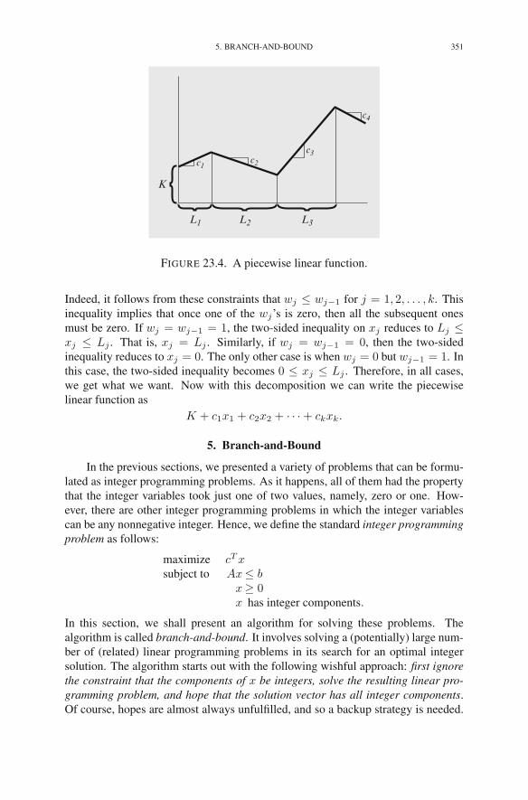
5. BRANCH-AND-BOUND 351
K
L1 L2 L3
c1 c2c3
c4
FIGURE 23.4. A piecewise linear function.
Indeed, it follows from these constraints that wj ≤ wj−1 for j = 1, 2, . . . , k. Thisinequality implies that once one of the wj’s is zero, then all the subsequent onesmust be zero. If wj = wj−1 = 1, the two-sided inequality on xj reduces to Lj ≤xj ≤ Lj . That is, xj = Lj . Similarly, if wj = wj−1 = 0, then the two-sidedinequality reduces to xj = 0. The only other case is when wj = 0 but wj−1 = 1. Inthis case, the two-sided inequality becomes 0 ≤ xj ≤ Lj . Therefore, in all cases,we get what we want. Now with this decomposition we can write the piecewiselinear function as
K + c1x1 + c2x2 + · · ·+ ckxk.
5. Branch-and-Bound
In the previous sections, we presented a variety of problems that can be formu-lated as integer programming problems. As it happens, all of them had the propertythat the integer variables took just one of two values, namely, zero or one. How-ever, there are other integer programming problems in which the integer variablescan be any nonnegative integer. Hence, we define the standard integer programmingproblem as follows:
maximize cTxsubject to Ax≤ b
x≥ 0x has integer components.
In this section, we shall present an algorithm for solving these problems. Thealgorithm is called branch-and-bound. It involves solving a (potentially) large num-ber of (related) linear programming problems in its search for an optimal integersolution. The algorithm starts out with the following wishful approach: first ignorethe constraint that the components of x be integers, solve the resulting linear pro-gramming problem, and hope that the solution vector has all integer components.Of course, hopes are almost always unfulfilled, and so a backup strategy is needed.

352 23. INTEGER PROGRAMMING
1 2 3 4 5 600
1
2
3
4
5
6
x1
x2
10x1+7x2=40
17x1+12x2=68.33
x1+x2=5
Optimal Solution to LP-relaxation
=z0
FIGURE 23.5. An integer programming problem. The dots repre-sent the feasible integer points, and the shaded region shows thefeasible region for the LP-relaxation.
The simplest strategy would be to round each resulting solution value to its nearestinteger value. Unfortunately, this naive strategy can be quite bad. In fact, the inte-ger solution so obtained might not even be feasible, which shouldn’t be surprising,since we know that the solution to a linear programming problem is at a vertex ofthe feasible set and so it is quite expected that naive movement will go outside ofthe feasible set.
To be concrete, consider the following example:
maximize 17x1 + 12x2
subject to 10x1 + 7x2 ≤ 40x1 + x2 ≤ 5
x1, x2 ≥ 0x1, x2 integers.
The linear programming problem obtained by dropping the integrality constraint iscalled the LP-relaxation. Since it has fewer constraints, its optimal solution providesan upper bound ζ0 on the the optimal solution ζ∗ to the integer programming prob-lem. Figure 23.5 shows the feasible points for the integer programming problem aswell as the feasible polytope for its LP-relaxation. The solution to the LP-relaxationis at (x1, x2) = (5/3, 10/3), and the optimal objective value is 205/3 = 68.33.Rounding each component of this solution to the nearest integer, we get (2, 3),which is not even feasible. The feasible integer solution that is closest to the LP-optimal solution is (1, 3), but we can see from Figure 23.5 that this solution is notthe optimal solution to the integer programming problem. In fact, it is easy to seefrom the figure that the optimal integer solution is either (1, 4) or (4, 0). To make the

5. BRANCH-AND-BOUND 353
0
1
2
3
4
5
6
x11 2 3 4 5 60
x2
P1
P2
FIGURE 23.6. The feasible subregions formed by the first branch.
problem interesting, we’ve chosen the objective function to make the more distantpoint (4, 0) be the optimal solution.
Of course, we can solve only very small problems by the graphical method: tosolve larger problems, an algorithm is required, which we now describe. Considervariable x1 in the optimal solution to the LP-relaxation. Its value is 5/3. In theoptimal solution to the integer programming problem, it will be an integer. Hence,it will satisfy either x1 ≤ 1 or x1 ≥ 2. We consider these two cases separately.Let P1 denote the linear programming problem obtained by adding the constraintx1 ≤ 1 to the LP-relaxation, and let P2 denote the problem obtained by includingthe other possibility, x1 ≥ 2. The feasible regions for P1 and P2 are shown inFigure 23.6. Let us study P1 first. It is clear from Figure 23.6 that the optimalsolution is at (x1, x2) = (1, 4) with an objective value of 65. Our algorithm hasfound its first feasible solution to the integer programming problem. We record thissolution as the best-so-far. Of course, better ones may (in this case, will) comealong later.
Now let’s consider P2. Looking at Figure 23.6 and doing a small amount ofcalculation, we see that the optimal solution is at (x1, x2) = (2, 20/7). In this case,the objective function value is 478/7 = 68.29. Now if this value had turned out tobe less than the best-so-far value, then we’d be done, since any integer solution thatlies within the feasible region for P2 would have a smaller value yet. But this is notthe case, and so we must continue our systematic search. Since x2 = 20/7 = 2.86,we divide P2 into two subproblems, one in which the constraint x2 ≤ 2 is addedand one with x2 ≥ 3 added.
Before considering these two new cases, note that we are starting to develop atree of linear programming subproblems. This tree is called the enumeration tree.The tree as far as we have investigated is shown in Figure 23.7. The double box
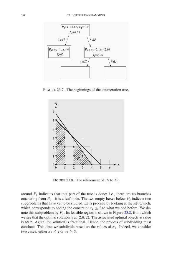
354 23. INTEGER PROGRAMMING
P0: x1=1.67, x2=3.33
ζ
x1<1 x1>2
x2>3
P1: x1=1, x2=4
ζ
P2 : x1=2, x2=2.86
ζ=
x2<2
FIGURE 23.7. The beginnings of the enumeration tree.
1 2 3 4 5 600
1
2
3
4
5
6
x1
x2
P1
P3
FIGURE 23.8. The refinement of P2 to P3.
around P1 indicates that that part of the tree is done: i.e., there are no branchesemanating from P1—it is a leaf node. The two empty boxes below P2 indicate twosubproblems that have yet to be studied. Let’s proceed by looking at the left branch,which corresponds to adding the constraint x2 ≤ 2 to what we had before. We de-note this subproblem by P3. Its feasible region is shown in Figure 23.8, from whichwe see that the optimal solution is at (2.6, 2). The associated optimal objective valueis 68.2. Again, the solution is fractional. Hence, the process of subdividing mustcontinue. This time we subdivide based on the values of x1. Indeed, we considertwo cases: either x1 ≤ 2 or x1 ≥ 3.

5. BRANCH-AND-BOUND 355
ζ =68.33
x1>2
ζ=65
P0: x1=1.67, x2=3.33
x1<1
P1: x1=1, x2=4 P2: x1=2, x2=2.86
x2>3x2<2
P3: x1=2.6, x2=2
x1<2 x1>3
FIGURE 23.9. The enumeration tree after solving P3.
Figure 23.9 shows the enumeration tree as it now stands. At this juncture, thereare three directions in which we could proceed. We could either study the otherbranch under P2 or work on one of the two branches sitting under P3. If we wereto systematically solve all the problems on a given level of the tree before goingdeeper, we would be performing what is referred to as a breadth-first search. Onthe other hand, going deep before going wide is called a depth-first search. Forreasons that we shall explain later, it turns out to be better to do a depth-first search.And, to be specific, let us always choose the left branch before the right branch (inpractice, there are much better rules that one can employ here). So our next linearprogramming problem is the one that we get by adding the constraint that x1 ≤ 2 tothe constraints that defined P3. Let us call this new problem P4. Its feasible regionis shown in Figure 23.10. It is easy to see that the optimal solution to this problemis (2, 2), with an objective value of 58. This solution is an integer solution, so it isfeasible for the integer programming problem. But it is not better than our best-so-far. Nonetheless, we do not need to consider any further subproblems below thisone in the enumeration tree.
Since problem P4 is a leaf in the enumeration tree, we need to work back upthe tree looking for the first node that has an unsolved problem sitting under it. Forthe case at hand, the unsolved problem is on the right branch underneath P3. Letus call this problem P5. It too is depicted in Figure 23.10. The optimal solutionis (3, 1.43), with an optimal objective function value of 68.14. Since this objective
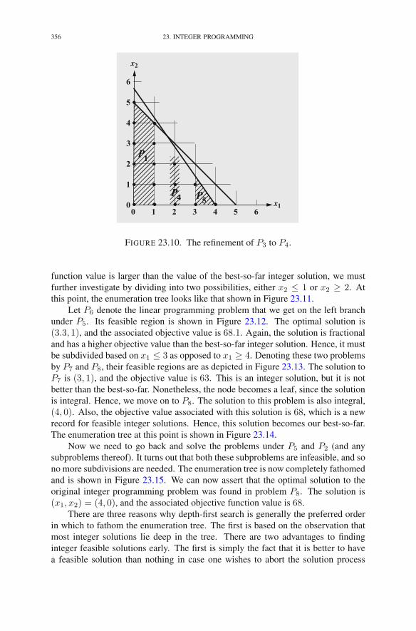
356 23. INTEGER PROGRAMMING
1 2 3 4 5 600
1
2
3
4
5
6
x1
x2
P1
P5P4
FIGURE 23.10. The refinement of P3 to P4.
function value is larger than the value of the best-so-far integer solution, we mustfurther investigate by dividing into two possibilities, either x2 ≤ 1 or x2 ≥ 2. Atthis point, the enumeration tree looks like that shown in Figure 23.11.
Let P6 denote the linear programming problem that we get on the left branchunder P5. Its feasible region is shown in Figure 23.12. The optimal solution is(3.3, 1), and the associated objective value is 68.1. Again, the solution is fractionaland has a higher objective value than the best-so-far integer solution. Hence, it mustbe subdivided based on x1 ≤ 3 as opposed to x1 ≥ 4. Denoting these two problemsby P7 and P8, their feasible regions are as depicted in Figure 23.13. The solution toP7 is (3, 1), and the objective value is 63. This is an integer solution, but it is notbetter than the best-so-far. Nonetheless, the node becomes a leaf, since the solutionis integral. Hence, we move on to P8. The solution to this problem is also integral,(4, 0). Also, the objective value associated with this solution is 68, which is a newrecord for feasible integer solutions. Hence, this solution becomes our best-so-far.The enumeration tree at this point is shown in Figure 23.14.
Now we need to go back and solve the problems under P5 and P2 (and anysubproblems thereof). It turns out that both these subproblems are infeasible, and sono more subdivisions are needed. The enumeration tree is now completely fathomedand is shown in Figure 23.15. We can now assert that the optimal solution to theoriginal integer programming problem was found in problem P8. The solution is(x1, x2) = (4, 0), and the associated objective function value is 68.
There are three reasons why depth-first search is generally the preferred orderin which to fathom the enumeration tree. The first is based on the observation thatmost integer solutions lie deep in the tree. There are two advantages to findinginteger feasible solutions early. The first is simply the fact that it is better to havea feasible solution than nothing in case one wishes to abort the solution process

5. BRANCH-AND-BOUND 357
ζ=68.33
P0: x1=1.67, x2=3.33
x1>2
ζ=65
P1: x1=1, x2=4 P2: x1=2, x2=2.86
ζ=68.29
x2<2
x2<1
x2>3
x2>2
ζ=68.2
ζ=68.14ζ=58
P3: x1=2.6, x2=2
P5: x1=3, x2=1.43P4: x1=2, x2=2
x1<2 x1>3
x1<1
FIGURE 23.11. The enumeration tree after solving P5. The dou-ble box around P4 indicates that it is a leaf in the tree.
early. But more importantly, identifying an feasible integer solution can result insubsequent nodes of the enumeration tree being made into leaves simply becausethe optimal objective function associated with that node is lower than the best-so-far integer solution. Making such nodes into leaves is called pruning the tree andcan account for tremendous gains in efficiency.
A second reason to favor depth-first search is the simple fact that it is very easyto code the algorithm as a recursively defined function. This may seem trite, but oneshouldn’t underestimate the value of code simplicity when implementing algorithmsthat are otherwise quite sophisticated, such as the one we are currently describing.
The third reason to favor depth-first search is perhaps the most important. Itis based on the observation that as one moves deeper in the enumeration tree, eachsubsequent linear programming problem is obtained from the preceding one by sim-ply adding (or refining) an upper/lower bound on one specific variable. To see whythis is an advantage, consider for example problem P2, which is a refinement of P0.The optimal dictionary for problem P0 is recorded as

358 23. INTEGER PROGRAMMING
1 2 3 4 5 600
1
2
3
4
5
6
x1
x2
P1
P6P4
FIGURE 23.12. The refinement of P5 to P6.
1 2 3 4 5 600
1
2
3
4
5
6
x1
x2
P1
P7P5 P8
FIGURE 23.13. The refinement of P6 to P7 and P8.
ζ = 2053 − 5
3w1 − 13w2
x1 = 53 − 1
3w1 + 73w2
x2 = 103 + 1
3w1 − 103 w2.
Problem P2 is obtained from P0 by adding the constraint that x1 ≥ 2. Introducing avariable, g1, to stand for the difference between x1 and this lower bound and usingthe dictionary above to write x1 in terms of the nonbasic variables, we get

5. BRANCH-AND-BOUND 359
ζ=68.33
P0: x1=1.67, x2=3.33
x1<1 x1>2
x2>3x2<2
P1: x1=1, x2=4
ζ=65P2: x1=2, x2=2.86
ζ=68.29
x1>3x1<2
x2<1
x1<3 x1>4
x2>2
P3: x1=2.6, x2=2
ζ=68.2
P4: x1=2, x2=2
ζ=58
P6: x1=3.3, x2=1
ζ=68.1
P5: x1=3, x2=1.43
ζ=68.14
P8: x1=4, x2=0ζ=68
P7: x1=3, x2=1
ζ=63
FIGURE 23.14. The enumeration tree after solving P6, P7, and P8.
g1 = x1 − 2 = −1
3− 1
3w1 +
7
3w2.
Therefore, we can use the following dictionary as a starting point for the solution ofP2:
ζ = 2053 − 5
3w1 − 13w2
x1 =53 − 1
3w1 +73w2
x2 =103 + 1
3w1 − 103 w2
g1 =− 13 − 1
3w1 +73w2.

360 23. INTEGER PROGRAMMING
ζ=58
ζ=63
P0: x1=1.67, x2=3.33
ζ=68.33
x1<1
x2<2
x1<2
x2<1
x1<3 x1>4
x2>2
x1>3
x2>3
x1>2
P1: x1=1, x2=4
ζ=65P2: x1=2, x2=2.86
ζ=68.29
P9: Infeasible
P10: Infeasible
P3: x1=2.6, x2=2ζ=68.2
P4: x1=2, x2=2 P5: x1=3, x2=1.43
ζ=68.14
P6: x1=3.3, x2=1
ζ=68.1
P7: x1=3, x2=1 P8: x1=4, x2=0ζ=68
FIGURE 23.15. The complete enumeration tree.
This dictionary is dual feasible but primal infeasible. Therefore, the dual simplexmethod is likely to find a new optimal solution in very few iterations. Accordingto the dual simplex method, variable g1 is the leaving variable and w2 is the corre-sponding entering variable. Making the pivot, we get the following dictionary:
ζ = 4787 − 12
7 w1 − 17g1
x1 = 2 + g1
x2 =207 − 1
7w1 − 107 g1
w2 =17 + 1
7w1 +37g1.

EXERCISES 361
This dictionary is optimal for P2. In general, the dual simplex method will takemore than one iteration to reoptimize, but nonetheless, one does expect it to get to anew optimal solution quickly.
We end this chapter by remarking that many real problems have the propertythat some variables must be integers but others can be real valued. Such problemsare called mixed integer programming problems. It should be easy to see how tomodify the branch-and-bound technique to handle such problems as well.
Exercises
23.1 Knapsack Problem. Consider a picnicker who will be carrying a knapsackthat holds a maximum amount b of “stuff.” Suppose that our picnickermust decide what to take and what to leave behind. The jth thing thatmight be taken occupies aj units of space in the knapsack and will bringcj amount of “enjoyment.” The knapsack problem then is to maximizeenjoyment subject to the constraint that the stuff brought must fit into theknapsack:
maximizen∑
j=1
cjxj
subject ton∑
j=1
ajxj ≤ b
xj ∈ {0, 1} j = 1, 2, . . . , n.
This apparently simple problem has proved difficult for general-purposebranch-and-bound algorithms. To see why, analyze the special case inwhich each thing contributes the same amount of enjoyment, i.e., cj = cfor all j, and takes up exactly two units of space, i.e., aj = 2 for all j.Suppose also that the knapsack holds n units of stuff.(a) What is the optimal solution when n is even? when n is odd?(b) How many subproblems must the branch-and-bound algorithm con-
sider when n is odd?
23.2 Vehicle Routing. Consider the dispatching of delivery vehicles (for exam-ple, mail trucks, fuel-oil trucks, newspaper delivery trucks, etc.). Typi-cally, there is a fleet of vehicles that must be routed to deliver goods froma depot to a given set of n drop-points. Given a set of feasible deliv-ery routes and the cost associated with each one, explain how to formu-late the problem of minimizing the total delivery cost as a set-partitioningproblem.
23.3 Explain how to modify the integer programming reformulation of contin-uous piecewise linear functions so that it covers piecewise linear functionshaving discontinuities at the junctions of the linear segments. Can fixedcosts be handled with this approach?

362 23. INTEGER PROGRAMMING
Notes
Standard references for integer programming include the classic text byGarfinkel and Nemhauser (1972) and the more recent text by Nemhauser and Wolsey(1988). Bill Cook’s recent book Cook (2012) on the traveling salesman prob-lem gives an entertaining historical and mathematical perspective on this particularapplication of integer programming.

CHAPTER 24
Quadratic Programming
In Chapter 23, we studied a generalization of the linear programming problemin which variables were constrained to take on integer values. In this chapter, weconsider a generalization of a different kind. Namely, we shall study the class ofproblems that would be linear programs except that the objective function is permit-ted to include terms involving products of pairs of variables. Such terms are calledquadratic terms, and the problems we shall study are called quadratic programmingproblems.
We have two reasons for being interested in quadratic programming problems.First, on the practical side, there are many real-world optimization problems thatfall into this category. This is so because most real-world applications have an ele-ment of uncertainty to them and that uncertainty is modeled by including a sum ofsquares deviation, i.e. variance, as a measure of the robustness of the solution. Itis often possible to arrange it so that these quadratic robustness terms appear onlyin the objective function. The quadratic version of the portfolio selection prob-lem studied in Chapter 13 is one such example—there are many others. The sec-ond reason for our interest in quadratic programming problems is that they form abridge to the much broader subject of convex programming that we shall take up inChapter 25.
We begin this chapter with a quadratic variant of the portfolio selection problem.
1. The Markowitz Model
Harry Markowitz received the 1990 Nobel Prize in Economics for his port-folio optimization model in which the tradeoff between risk and reward is explic-itly treated. We shall briefly describe this model in its simplest form. We start byreintroducing the basic framework of the problem. Those who have read Chap-ter 13 will note that the first few paragraphs here are a repeat of what was writtenthere.
Given a collection of potential investments (indexed, say, from 1 to n), letRj denote the return in the next time period on investment j, j = 1, . . . , n. Ingeneral, Rj is a random variable, although some investments may be essentiallydeterministic.
A portfolio is determined by specifying what fraction of one’s assets to put intoeach investment. That is, a portfolio is a collection of nonnegative numbers xj ,
R.J. Vanderbei, Linear Programming, International Series in Operations Research& Management Science 196, DOI 10.1007/978-1-4614-7630-6 24,© Springer Science+Business Media New York 2014
363
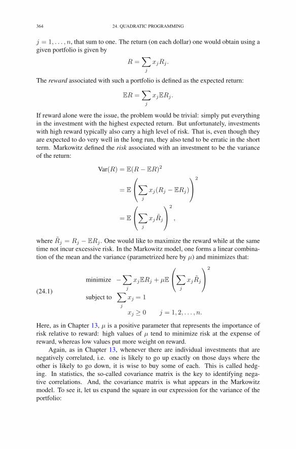
364 24. QUADRATIC PROGRAMMING
j = 1, . . . , n, that sum to one. The return (on each dollar) one would obtain using agiven portfolio is given by
R =∑
j
xjRj .
The reward associated with such a portfolio is defined as the expected return:
ER =∑
j
xjERj .
If reward alone were the issue, the problem would be trivial: simply put everythingin the investment with the highest expected return. But unfortunately, investmentswith high reward typically also carry a high level of risk. That is, even though theyare expected to do very well in the long run, they also tend to be erratic in the shortterm. Markowitz defined the risk associated with an investment to be the varianceof the return:
Var(R) = E(R− ER)2
= E
⎛
⎝∑
j
xj(Rj − ERj)
⎞
⎠
2
= E
⎛
⎝∑
j
xjRj
⎞
⎠
2
,
where Rj = Rj − ERj . One would like to maximize the reward while at the sametime not incur excessive risk. In the Markowitz model, one forms a linear combina-tion of the mean and the variance (parametrized here by μ) and minimizes that:
(24.1)
minimize −∑
j
xjERj + μE
⎛
⎝∑
j
xjRj
⎞
⎠
2
subject to∑
j
xj = 1
xj ≥ 0 j = 1, 2, . . . , n.
Here, as in Chapter 13, μ is a positive parameter that represents the importance ofrisk relative to reward: high values of μ tend to minimize risk at the expense ofreward, whereas low values put more weight on reward.
Again, as in Chapter 13, whenever there are individual investments that arenegatively correlated, i.e. one is likely to go up exactly on those days where theother is likely to go down, it is wise to buy some of each. This is called hedg-ing. In statistics, the so-called covariance matrix is the key to identifying nega-tive correlations. And, the covariance matrix is what appears in the Markowitzmodel. To see it, let us expand the square in our expression for the variance of theportfolio:

1. THE MARKOWITZ MODEL 365
E
⎛
⎝∑
j
xjRj
⎞
⎠
2
= E
(∑
i
xiRi
)⎛
⎝∑
j
xjRj
⎞
⎠
= E
⎛
⎝∑
i
∑
j
xixjRiRj
⎞
⎠
=∑
i
∑
j
xixjE(RiRj)
=∑
i
∑
j
xixjCi,j ,
whereCi,j = E(RiRj)
is the covariance matrix. Hence, problem (24.1) can be rewritten as
(24.2)
minimize −∑
j
rjxj + μ∑
i
∑
j
xixjCi,j
subject to∑
j
xj = 1
xj ≥ 0 j = 1, 2, . . . , n,
where we have introduced rj = ERj for the mean return on investment j.Solving problem (24.2) requires an estimate of the mean return for each of
the investments as well as an estimate of the covariance matrix. However, thesequantities are not known theoretically but instead must be estimated by looking athistorical data. For example, Table 24.1 shows annual returns from 1973 to 1994 foreight different possible investments: U.S. 3-Month T-Bills, U.S. Government LongBonds, S&P 500, Wilshire 5000 (a collection of small company stocks), NASDAQComposite, Lehman Brothers Corporate Bonds Index, EAFE (a securities index forEurope, Asia, and the Far East), and Gold. Let Rj(t) denote the return on investmentj in year 1972+ t. One way to estimate the mean ERj is simply to take the averageof the historical returns:
rj = ERj =1
T
T∑
t=1
Rj(t).
There are two drawbacks to this simple formula. First, whatever happened in 1973certainly has less bearing on the future than what happened in 1994. Hence, givingall the past returns equal weight puts too much emphasis on the distant past at theexpense of the recent past. A better estimate is obtained by using a discounted sum:
ERj =
∑Tt=1 p
T−tRj(t)∑T
t=1 pT−t
.
Here, p is a discount factor. Putting p = 0.9 gives a weighted average that puts moreweight on the most recent years. To see the effect of discounting the past, considerthe Gold investment. The unweighted average return is 1.129, whereas the weighted

366 24. QUADRATIC PROGRAMMING
Year US US S&P Wilshire NASDAQ Lehman EAFE Gold3-Month Gov. 500 5000 Composite Bros.
T-Bills Long Corp.Bonds Bonds
1973 1.075 0.942 0.852 0.815 0.698 1.023 0.851 1.6771974 1.084 1.020 0.735 0.716 0.662 1.002 0.768 1.7221975 1.061 1.056 1.371 1.385 1.318 1.123 1.354 0.7601976 1.052 1.175 1.236 1.266 1.280 1.156 1.025 0.9601977 1.055 1.002 0.926 0.974 1.093 1.030 1.181 1.2001978 1.077 0.982 1.064 1.093 1.146 1.012 1.326 1.2951979 1.109 0.978 1.184 1.256 1.307 1.023 1.048 2.2121980 1.127 0.947 1.323 1.337 1.367 1.031 1.226 1.2961981 1.156 1.003 0.949 0.963 0.990 1.073 0.977 0.6881982 1.117 1.465 1.215 1.187 1.213 1.311 0.981 1.0841983 1.092 0.985 1.224 1.235 1.217 1.080 1.237 0.8721984 1.103 1.159 1.061 1.030 0.903 1.150 1.074 0.8251985 1.080 1.366 1.316 1.326 1.333 1.213 1.562 1.0061986 1.063 1.309 1.186 1.161 1.086 1.156 1.694 1.2161987 1.061 0.925 1.052 1.023 0.959 1.023 1.246 1.2441988 1.071 1.086 1.165 1.179 1.165 1.076 1.283 0.8611989 1.087 1.212 1.316 1.292 1.204 1.142 1.105 0.9771990 1.080 1.054 0.968 0.938 0.830 1.083 0.766 0.9221991 1.057 1.193 1.304 1.342 1.594 1.161 1.121 0.9581992 1.036 1.079 1.076 1.090 1.174 1.076 0.878 0.9261993 1.031 1.217 1.100 1.113 1.162 1.110 1.326 1.1461994 1.045 0.889 1.012 0.999 0.968 0.965 1.078 0.990
TABLE 24.1. Returns per dollar for each of eight investments overseveral years. That is, $1 invested in US 3-Month T-Bills onJanuary 1, 1973, was worth $1.075 on December 31, 1973.
average is 1.053. Most experts in 1995 felt that a 5.3% return represented a morerealistic expectation than a 12.9% return. In the results that follow, all expectationsare estimated by computing weighted averages using p = 0.9.
The second issue concerns the estimation of means (not variances). An invest-ment that returns 1.1 one year and 0.9 the next has an (unweighted) average returnof 1, that is, no gain or loss. However, one dollar invested will actually be worth(1.1)(0.9) = 0.99 at the end of the second year. While a 1% error is fairly small,consider what happens if the return is 2.0 one year and then 0.5 the next. Clearly,the value of one dollar at the end of the 2 years is (2.0)(0.5) = 1, but the averageof the two returns is (2.0 + 0.5)/2 = 1.25. There is a very significant differencebetween an investment that is flat and one that yields a 25% return in 2 years. Thisis obviously an effect for which a correction is required. We need to average 2.0 and0.5 in such a way that they cancel out—and this cancellation must work not only for2.0 and 0.5 but for every positive number and its reciprocal. The trick is to averagethe logarithm of the returns (and then exponentiate the average). The logarithm hasthe correct effect of cancelling a return r and its reciprocal:
log r + log1
r= 0.
Hence, we estimate means from Table 24.1 using
ERj = exp
(∑Tt=1 p
T−t logRj(t)∑T
t=1 pT−t
)
.
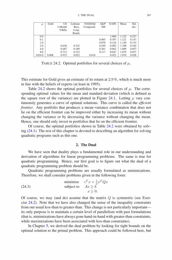
2. THE DUAL 367
μ Gold US Lehman NASDAQ S&P EAFE Mean Std.3-Month Bros. Composite 500 dev.
T-Bills Corp.Bonds
0.0 1.000 1.122 0.2270.1 0.603 0.397 1.121 0.1471.0 0.876 0.124 1.120 0.1332.0 0.036 0.322 0.549 0.092 1.108 0.1024.0 0.487 0.189 0.261 0.062 1.089 0.0578.0 0.713 0.123 0.117 0.047 1.079 0.037
1024.0 0.008 0.933 0.022 0.016 0.022 1.070 0.028
TABLE 24.2. Optimal portfolios for several choices of μ.
This estimate for Gold gives an estimate of its return at 2.9%, which is much morein line with the beliefs of experts (at least in 1995).
Table 24.2 shows the optimal portfolios for several choices of μ. The corre-sponding optimal values for the mean and standard deviation (which is defined asthe square root of the variance) are plotted in Figure 24.1. Letting μ vary con-tinuously generates a curve of optimal solutions. This curve is called the efficientfrontier. Any portfolio that produces a mean–variance combination that does notlie on the efficient frontier can be improved either by increasing its mean withoutchanging the variance or by decreasing the variance without changing the mean.Hence, one should only invest in portfolios that lie on the efficient frontier.
Of course, the optimal portfolios shown in Table 24.2 were obtained by solv-ing (24.1). The rest of this chapter is devoted to describing an algorithm for solvingquadratic programs such as this one.
2. The Dual
We have seen that duality plays a fundamental role in our understanding andderivation of algorithms for linear programming problems. The same is true forquadratic programming. Hence, our first goal is to figure out what the dual of aquadratic programming problem should be.
Quadratic programming problems are usually formulated as minimizations.Therefore, we shall consider problems given in the following form:
(24.3)minimize cTx+ 1
2xTQx
subject to Ax≥ bx≥ 0.
Of course, we may (and do) assume that the matrix Q is symmetric (see Exer-cise 24.2). Note that we have also changed the sense of the inequality constraintsfrom our usual less-than to greater-than. This change is not particularly important—its only purpose is to maintain a certain level of parallelism with past formulations(that is, minimizations have always gone hand-in-hand with greater-than constraints,while maximizations have been associated with less-than constraints).
In Chapter 5, we derived the dual problem by looking for tight bounds on theoptimal solution to the primal problem. This approach could be followed here, but

368 24. QUADRATIC PROGRAMMING
Wilshire5000 μ=0.1
μ=1
1.08 1.09 1.10 1.11 1.12 1.131.07
2
6
8
10
12
14
16
18
20
22
24
4 T−Bills
Corp.Bonds
LongBonds
S&P 500
NASDAQComposite
Gold
EAFE
μ=8
μ=4
μ=2
μ=0
μ=1024
FIGURE 24.1. The efficient frontier.
it seems less compelling in the context of quadratic programming. A more directapproach stems from the connection between duality and the first-order optimalityconditions for the barrier problem that we examined in Chapter 17. Indeed, let usstart by writing down the barrier problem associated with (24.3). To this end, weintroduce a nonnegative vector w of surplus variables and then subtract a barrierterm for each nonnegative variable to get the following barrier problem:
minimize cTx+ 12x
TQx− μ∑
j log xj − μ∑
i logwi
subject to Ax− w = b.
Next, we introduce the Lagrangian:
f(x,w, y) = cTx+1
2xTQx− μ
∑
j
log xj − μ∑
i
logwi
+ yT (b−Ax+ w).
The first-order optimality conditions for the barrier problem are obtained bydifferentiating the Lagrangian with respect to each of its variables and setting thesederivatives to zero. In vector notation, setting to zero the derivative with respect tothe x variables gives
c+Qx− μX−1e−AT y = 0.

2. THE DUAL 369
Similarly, setting to zero the derivatives with respect to the w and y variables gives
−μW−1e+ y = 0
b−Ax+ w = 0,
respectively. As we did in our study of linear programming problems, we nowintroduce a new vector z given by
z = μX−1e.
With this definition, the first-order optimality conditions can be summarized as
AT y + z −Qx = c
Ax− w = b
XZe = μe
YWe = μe.
From the last two conditions, we see that the dual problem involves an n-vectorof variables z that are complementary to the primal variables x and an m-vector ofvariables y that are complementary to the primal slack variables w. Because of thesecomplementarity conditions, we expect that the variables y and z are constrained tobe nonnegative in the dual problem. Also, to establish the proper connection be-tween the first-order optimality conditions and the dual problem, we must recognizethe first condition as a dual constraint. Hence, the constraints for the dual prob-lem are
AT y + z −Qx = c
y, z ≥ 0.
It is interesting to note that the dual constraints involve an n-vector x that seems asif it should belong to the primal problem. This may seem odd, but when understoodproperly it turns out to be entirely harmless. The correct interpretation is that thevariable x appearing in the dual has, in principle, no connection to the variable xappearing in the primal (except that, as we shall soon see, at optimality they will beequal).
The barrier problem has helped us write down the dual constraints, but it doesnot shed any light on the dual objective function. To see what the dual objectivefunction should be, we look at what it needs to be for the weak duality theorem tohold true. In the weak duality theorem, we assume that we have a primal feasiblesolution (x,w) and a dual feasible solution (x, y, z). We then follow the obviouschains of equalities:
yT (Ax) = yT (b+ w) = bT y + yTw
and
(AT y)Tx = (c− z +Qx)Tx = cTx− zTx+ xTQx.
370 24. QUADRATIC PROGRAMMING
Now, since yT (Ax) = (AT y)Tx, we see that
0 ≤ yTw + zTx = cTx+ xTQx− bT y
= (cTx+1
2xTQx)− (bT y − 1
2xTQx).
From this inequality, we see that the dual objective function is bT y − 12x
TQx.Hence, the dual problem can be stated now as
maximize bT y − 12x
TQx
subject to AT y + z −Qx= cy, z ≥ 0.
For linear programming, the fundamental connection between the primal and dualproblems is summarized in the Complementary Slackness Theorem. In the nextsection, we shall derive a version of this theorem for quadratic programming.
3. Convexity and Complexity
In linear programming, the dual problem is important because it provides a cer-tificate of optimality as manifest in the Complementary Slackness Theorem. Undercertain conditions, the same is true here. Let us start by deriving the analogue ofthe Complementary Slackness Theorem. The derivation begins with a reiteration ofthe derivation of the Weak Duality Theorem. Indeed, let (x,w) denote a feasiblesolution to the primal problem and let (x, y, z) denote a feasible solution to the dualproblem (we have put a bar on the dual x to distinguish it from the one appearing inthe primal). The chain of equalities that form the backbone of the proof of the WeakDuality Theorem are, as always, obtained by writing yTAx two ways, namely,
yT (Ax) = (AT y)Tx,
and then producing the obvious substitutions
yT (Ax) = yT (b+ w) = bT y + yTw
and(AT y)Tx = (c− z +Qx)Tx = cTx− zTx+ xTQx.
Comparing the ends of these two chains and using the fact that both yTw and zTxare nonnegative, we see that
(24.4) 0 ≤ yTw + zTx = cTx+ xTQx− bT y.
So far, so good.Now, what about the Complementary Slackness Theorem? In the present con-
text, we expect this theorem to say roughly the following: given a solution (x∗, w∗)that is feasible for the primal and a solution (x∗, y∗, z∗) that is feasible for the dual,if these solutions make inequality (24.4) into an equality, then the primal solution isoptimal for the primal problem and the dual solution is optimal for the dual problem.
Let’s try to prove this. Let (x,w) be an arbitrary primal feasible solution. Weakduality applied to (x,w) on the primal side and (x∗, y∗, z∗) on the dual side saysthat
cTx+ x∗TQx− bT y∗ ≥ 0.

3. CONVEXITY AND COMPLEXITY 371
But for the specific primal feasible solution (x∗, w∗), this inequality is an equality:
cTx∗ + x∗TQx∗ − bT y∗ = 0.
Combining these, we get
cTx∗ + x∗TQx∗ ≤ cTx+ x∗TQx.
This is close to what we want, but not quite it. Recall that our aim is to show thatthe primal objective function evaluated at x∗ is no larger than its value at x. That is,
cTx∗ +1
2x∗TQx∗ ≤ cTx+
1
2xTQx.
It is easy to get from the one to the other. Starting from the desired left-hand side,we compute as follows:
cTx∗ +1
2x∗TQx∗ = cTx∗ + x∗TQx∗ − 1
2x∗TQx∗
≤ cTx+ x∗TQx− 1
2x∗TQx∗
= cTx+1
2xTQx− 1
2xTQx+ x∗TQx− 1
2x∗TQx∗
= cTx+1
2xTQx− 1
2(x− x∗)TQ(x− x∗).
The last step in the derivation is to drop the subtracted term on the right-hand side ofthe last expression. We can do this if the quantity being subtracted is nonnegative.But is it? In general, the answer is no. For example, if Q were the negative of theidentity matrix, then the expression (x − x∗)TQ(x − x∗) would be negative ratherthan nonnegative.
So it is here that we must impose a restriction on the class of quadratic pro-gramming problems that we study. The correct assumption is that Q is positivesemidefinite. Recall from Chapter 19 that a matrix Q is positive semidefinite if
ξTQξ ≥ 0 for all ξ ∈ Rn.
With this assumption, we can finish the chain of inequalities and conclude that
cTx∗ +1
2x∗TQx∗ ≤ cTx+
1
2xTQx.
Since x was an arbitrary primal feasible point, it follows that x∗ (together with w∗)is optimal for the primal problem. A similar analysis shows that y∗ (together withx∗ and z∗) is optimal for the dual problem (see Exercise 24.4).
A quadratic programming problem of the form (24.3) in which the matrix Qis positive semidefinite is called a convex quadratic programming problem. Thediscussion given above can be summarized in the following theorem:
THEOREM 24.1. For convex quadratic programming problems, given a solution(x∗, w∗) that is feasible for the primal and a solution (x∗, y∗, z∗) that is feasible forthe dual, if these solutions make inequality (24.4) into an equality, then the primalsolution is optimal for the primal problem and the dual solution is optimal for thedual problem.

372 24. QUADRATIC PROGRAMMING
x1
x2
FIGURE 24.2. The objective function for (24.5) in the case wheren = 2.
To see how bad things are when Q is not positive semidefinite, consider thefollowing example:
(24.5)minimize
∑j xj(1− xj) +
∑j cjxj
subject to 0 ≤ xj ≤ 1, j = 1, 2, . . . , n.
We assume that the coefficients, cj , j = 1, 2, . . . , n, are small. To be precise, weassume that
|cj | < 1, j = 1, 2, . . . , n.
Let f(x) denote the value of the objective function at point x. Setting the gradientto zero,
∇f(x) = e− 2x+ c = 0,
we see that there is one interior critical point. It is given by
x = (e+ c)/2
(the assumption that c is small guarantees that this x lies in the interior of the feasibleset: 0 < x < 1). However, this critical point is a local maximum, since the ma-trix of second derivatives is −2I . The algebraic details are tedious, but if we lookat Figure 24.2, it is easy to be convinced that every vertex of the feasible set is alocal minimum. While this particular problem is easy to solve explicitly, it doesindicate the essential difficulty associated with nonconvex quadratic programmingproblems—namely, for such problems one may need to check every vertex individ-ually, and there may be an exponential number of such vertices.
The situation for convex quadratic programming problems is much better, sincethey inherit most of the properties that made linear programs efficiently solvable.Indeed, in the next section, we derive an interior-point method for quadratic pro-gramming problems.

4. SOLUTION VIA INTERIOR-POINT METHODS 373
4. Solution via Interior-Point Methods
In this section, we derive an interior-point method for quadratic programmingproblems. We start from the first-order optimality conditions, which we saw in thelast section are given by
AT y + z −Qx = c
Ax− w = b
XZe = μe
YWe = μe.
Following the derivation given in Chapter 18, we replace (x,w, y, z) with(x + Δx,w + Δw, y + Δy, z + Δz) to get the following nonlinear system in(Δx,Δw,Δy,Δz):
ATΔy +Δz −QΔx = c−AT y − z +Qx =: σ
AΔx−Δw = b−Ax+ w =: ρ
ZΔx+XΔz +ΔXΔZe = μe−XZe
WΔy + YΔw +ΔYΔWe = μe− YWe.
Next, we drop the nonlinear terms to get the following linear system for the stepdirections (Δx,Δw,Δy,Δz):
ATΔy +Δz −QΔx = σ
AΔx−Δw = ρ
ZΔx+XΔz = μe−XZe
WΔy + YΔw = μe− YWe.
Following the reductions of Chapter 19, we use the last two equations to solve forΔz and Δw to get
Δz = X−1(μe−XZe− ZΔx)
Δw = Y −1(μe− YWe−WΔy).
We then use these expressions to eliminate Δz and Δw from the remaining twoequations in the system. After elimination, we arrive at the following reduced KKTsystem:
ATΔy − (X−1Z +Q)Δx = σ − μX−1e+ z(24.6)
AΔx+ Y −1WΔy = ρ+ μY −1e− w.(24.7)
Substituting in the definitions of ρ and σ and writing the system in matrixnotation, we get
[−(X−1Z +Q) AT
A Y −1W
] [ΔxΔy
]
=
[c−AT y − μX−1e+Qx
b−Ax+ μY −1e
]
.
A summary of the algorithm is shown in Figure 24.3. It should be clear thatthe quadratic term in the objective function plays a fairly small role. In fact, the

374 24. QUADRATIC PROGRAMMING
initialize (x,w, y, z) > 0
while (not optimal) {ρ = b−Ax+ wσ = c−AT y − z +Qxγ = zTx+ yTw
μ = δγ
n+msolve:[
−(X−1Z +Q) AT
A Y −1W
] [ΔxΔy
]
=
[c−AT y − μX−1e+Qx
b−Ax+ μY −1e
]
.
Δz = X−1(μe−XZe− ZΔx)Δw = Y −1(μe− YWe−WΔy)
θ = r
(
maxij
{
−Δxj
xj,−Δwi
wi,−Δyi
yi,−Δzj
zj
})−1
∧ 1
x ← x+ θΔx, w ← w + θΔw
y ← y + θΔy, z ← z + θΔz
}
FIGURE 24.3. The path-following method for quadratic program-ming problems.
convergence analysis given in Chapter 18 can be easily adapted to yield analogousresults for quadratic programming problems (see Exercise 24.6).
5. Practical Considerations
For practical implementations of interior-point algorithms, we saw in Chap-ter 19 that the difficulties created by dense rows/columns suggest that we solve thereduced KKT system using an equation solver that can handle symmetric indefinitesystems (such as those described in Chapter 20). Quadratic programming problemsgive us even more reason to prefer the reduced KKT system. To see why, let usreduce the system further to get a feel for the normal equations for quadratic pro-gramming.
If we use (24.6) to solve for Δx and then eliminate it from (24.7), we get
Δx = −(X−1Z +Q)−1(c−AT y +Qx− μX−1e−ATΔy
)
and the associated system of normal equations (in primal form):(A(X−1Z +Q)−1AT + Y −1W
)Δy = b−Ax+ μY −1e
+A(X−1Z +Q)−1(c−AT y +Qx− μX−1e
).
As we saw in Chapter 19, the most significant disadvantage of the normal equationsis that they could involve a dense matrix even when the original constraint matrixis sparse. For quadratic programming, this disadvantage is even more pronounced.Now the matrix of normal equations has the nonzero pattern of A(D + Q)−1AT ,

5. PRACTICAL CONSIDERATIONS 375
where D is a diagonal matrix. If Q is a diagonal matrix, then this matrix appearingbetween A and AT is diagonal, and the system has the same structure as we saw forlinear programming. But if Q is not a diagonal matrix, then all hope for any sparsityin A(D +Q)−1AT is lost.
Fortunately, however, the dual form of the normal equations is likely to retainsome sparsity. Indeed, to derive the dual form, we use (24.7) to solve for Δy andthen eliminate it from (24.6). The result is
Δy = YW−1(b−Ax+ μY −1e−AΔx
)
and
−(X−1Z +Q+ATYW−1A
)Δx = c−AT y +Qx− μX−1e
−ATYW−1(b−Ax+ μY −1e
).
Now the matrix has a nonzero pattern of ATA+Q. This pattern is much more likelyto be sparse than the pattern we had above.
As mentioned earlier, there is significantly less risk of fill-in if Q is diagonal.A quadratic programming problem for which Q is diagonal is called a separablequadratic programming problem. It turns out that every nonseparable quadratic pro-gramming problem can be replaced by an equivalent separable version, and some-times this replacement results in a problem that can be solved dramatically fasterthan the original nonseparable problem. The trick reveals itself when we remindourselves that the problems we are studying are convex quadratic programs, and sowe ask the question: how do we know that the matrix Q is positive semidefinite? Or,more to the point, how does the creator of the model know that Q is positive semi-definite? There are many equivalent characterizations of positive semidefiniteness,but the one that is easiest to check is the one that says that Q is positive semidefiniteif and only if it can be factored as follows:
Q = FTDF.
Here F is a k × n matrix and D is a k × k diagonal matrix having all nonnegativediagonal entries. In fact, the model creator often started with F and D and thenformed Q by multiplying. In these cases, the matrix F will generally be less densethan Q. And if k is substantially less than n, then the following substitution is almostguaranteed to dramatically improve the solution time. Introduce new variables y bysetting
y = Fx.
With this definition, the nonseparable quadratic programming problem (24.3) canbe replaced by the following equivalent separable one:
minimize cTx+ 12y
TDy
subject to Ax≥ b
Fx− y = 0
x≥ 0.
376 24. QUADRATIC PROGRAMMING
The cost of separation is the addition of k new constraints. As we said before, if kis small and/or F is sparse, then we can expect this formulation to be solved moreefficiently.
To illustrate this trick, let us return to the Markowitz model. Recall that thequadratic terms in this model come from the variance of the portfolio’s return, whichis given by
Var(R) = E(∑
j
xjRj)2
=
T∑
t=1
p(t)
⎛
⎝∑
j
xjRj(t)
⎞
⎠
2
.
Here,
p(t) =pT−t
∑Ts=1 p
T−s
for t = 1, 2, . . . , T , and
Rj(t) = Rj(t)−T∑
t=1
p(t)Rj(t).
If we introduce the variables,
y(t) =∑
j
xjRj(t), t = 1, 2, . . . , T,
then we get the following separable version of the Markowitz model:
maximize∑
j
xjERj − μT∑
t=1
p(t)y(t)2
subject to∑
j
xj = 1
y(t) =∑
j xjRj(t), t = 1, 2, . . . , T,
xj ≥ 0 j = 1, 2, . . . , n.
Using specific data involving 500 possible investments and 20 historical time peri-ods, the separable version solves 60 times faster than the nonseparable version usinga QP-solver called LOQO.
Exercises
24.1 Show that the gradient of the function
f(x) =1
2xTQx
is given by∇f(x) = Qx.
24.2 Suppose that Q is an n × n matrix that is not necessarily symmetric. LetQ = 1
2 (Q+QT ). Show that

EXERCISES 377
(a) xTQx = xT Qx, for every x ∈ Rn, and
(b) Q is symmetric.
24.3 Penalty Methods.(a) Consider the following problem:
minimize 12x
TQx
subject to Ax = b,
where Q is symmetric, positive semidefinite, and invertible (theselast two conditions are equivalent to saying that Q is positive def-inite). By solving the first-order optimality conditions, give an ex-plicit formula for the solution to this problem.
(b) Each equality constraint in the above problem can be replaced by apenalty term added to the objective function. Penalty terms should besmall when the associated constraint is satisfied and become rapidlylarger as it becomes more and more violated. One choice of penaltyfunction is the quadratic function. The quadratic penalty problem isdefined as follows:
minimize1
2xTQx+
λ
2(b−Ax)T (b−Ax),
where λ is a large real-valued parameter. Derive an explicit formulafor the solution to this problem.
(c) Show that, in the limit as λ tends to infinity, the solution to thequadratic penalty problem converges to the solution to the originalproblem.
24.4 Consider a convex quadratic programming problem. Suppose that (x∗, w∗)is a feasible solution for the primal and that (x∗, y∗, z∗) is a feasiblesolution for the dual. Suppose further that these solutions make inequal-ity (24.4) into an equality. Show that the dual solution is optimal for thedual problem.
24.5 A real-valued function f defined on Rn is called convex if, for every x, y ∈
Rn, and for every 0 < t < 1,
f(tx+ (1− t)y) ≤ tf(x) + (1− t)f(y).
Show that the function
f(x) = cTx+1
2xTQx, x ∈ R
n,
is convex if Q is positive semidefinite.
24.6 Extend the convergence analysis given in Chapter 18 so that it applies toconvex quadratic programming problems, and identify in particular anysteps that depend on Q being positive semidefinite.

378 24. QUADRATIC PROGRAMMING
24.7 Consider the quadratic programming problem given in the following form:
minimize cTx+ 12x
TQxsubject to Ax ≥ b,
(i.e., without assuming nonnegativity of the x vector). Show that theformulas for the step directions Δx and Δy are given by the followingreduced KKT system:
(24.8)
[−Q AT
A WY −1
] [ΔxΔy
]
=
[c−AT y +Qxb−Ax+ μY −1e
]
.
Notes
The portfolio optimization model presented in Section 24.1 was first introducedby Markowitz (1959). He received the 1990 Nobel Prize in Economics for this work.
Quadratic programming is the simplest class of problems from the subjectcalled nonlinear programming. Two excellent recent texts that cover nonlinear pro-gramming are those by Bertsekas (1995) and Nash and Sofer (1996). The first paperthat extended the path-following method to quadratic programming was Monteiroand Adler (1989). The presentation given here follows Vanderbei (1999).
CHAPTER 25
Convex Programming
In the last chapter, we saw that small modifications to the primal–dualinterior-point algorithm allow it to be applied to quadratic programming problemsas long as the quadratic objective function is convex. In this chapter, we shall gofurther and allow the objective function to be a general (smooth) convex function.In addition, we shall allow the feasible region to be any convex set given by a finitecollection of convex inequalities.
1. Differentiable Functions and Taylor Approximations
In this chapter, all nonlinear functions will be assumed to be twice differen-tiable, and the second derivatives will be assumed continuous. We begin by reiter-ating a few definitions and results that were briefly touched on in Chapter 17. Firstof all, given a real-valued function f defined on a domain in R
n, the vector
∇f(x) =
⎡
⎢⎢⎢⎢⎣
∂f∂x1
(x)∂f∂x2
(x)...
∂f∂xn
(x)
⎤
⎥⎥⎥⎥⎦
is called the gradient of f at x. The matrix
Hf(x) =
⎡
⎢⎢⎢⎢⎢⎣
∂2f∂x2
1(x) ∂2f
∂x1∂x2(x) · · · ∂2f
∂x1∂xn(x)
∂2f∂x2∂x1
(x) ∂2f∂x2
2(x) · · · ∂2f
∂x2∂xn(x)
......
...∂2f
∂xn∂x1(x) ∂2f
∂xn∂x2(x) · · · ∂2f
∂x2n(x)
⎤
⎥⎥⎥⎥⎥⎦
is called the Hessian of f at x. In dimensions greater than one, the gradient and theHessian are the analogues of the first and second derivatives of a function in onedimension. In particular, they appear in the three-term Taylor series expansion of fabout the point x:
f(x+Δx) = f(x) +∇f(x)TΔx+1
2ΔxTHf(x)Δx+ rx(Δx).
The last term is called the remainder term. The value of this expansion lies in thefact that this remainder is small when Δx is small. To be precise, the remainder hasthe following property:
R.J. Vanderbei, Linear Programming, International Series in Operations Research& Management Science 196, DOI 10.1007/978-1-4614-7630-6 25,© Springer Science+Business Media New York 2014
379

380 25. CONVEX PROGRAMMING
limΔx→0
rx(Δx)
‖Δx‖2 = 0.
This result follows immediately from the one-dimensional three-term Taylor seriesexpansion applied to g(t) = f(x+ tΔx) and the chain rule (see Exercise 25.8).
2. Convex and Concave Functions
There are several equivalent definitions of convexity of a function. The defini-tion that is most expedient for our purposes is the multidimensional generalizationof the statement that a function is convex if its second derivative is nonnegative.Hence, we say that a real-valued function defined on a domain in R
n is convex ifits Hessian is positive semidefinite everywhere in its domain. A function is calledconcave if its negation is convex.
3. Problem Formulation
We shall study convex optimization problems posed in the following form:
minimize c(x)subject to ai(x) ≥ bi, i = 1, 2, . . . ,m.
Here, the real-valued function c(·) is assumed to be convex, and the m real-valuedfunctions ai(·) are assumed to be concave. This formulation is the natural exten-sion of the convex quadratic programming problem studied in the previous chapter,except that we have omitted the nonnegativity constraints on the variables. Thisomission is only a matter of convenience since, if a given problem involves non-negative variables, the assertion of their nonnegativity can be incorporated as partof the m nonlinear inequality constraints. Also note that once we allow for generalconcave inequality constraints, we can take the right-hand sides to be zero by sim-ply incorporating appropriate shifts into the nonlinear constraint functions. Hence,many texts on convex optimization prefer to formulate the constraints in the formai(x) ≥ 0. We have left the constants bi on the right-hand side for later comparisonswith the quadratic programming problem of the previous chapter. Finally, note thatmany convex and concave functions become infinite in places and therefore have anatural domain that is a strict subset of Rn. This issue is important to address whensolving practical problems, but since this chapter is just an introduction to convexoptimization, we shall assume that all functions are finite on all of Rn.
At times it will be convenient to use vector notation to consolidate the m con-straints into a single inequality. Hence, we sometimes express the problem as
minimize c(x)subject to A(x) ≥ b,
where A(·) is a function from Rn into R
m and b is a vector in Rm. As usual, we let
w denote the slack variables that convert the inequality constraints to equalities:
minimize c(x)subject to A(x)− w= b
w≥ 0.
4. SOLUTION VIA INTERIOR-POINT METHODS 381
4. Solution via Interior-Point Methods
In this section, we derive an interior-point method for convex programmingproblems. We start by introducing the associated barrier problem:
minimize c(x)− μ∑
i logwi
subject to ai(x)− wi = bi, i = 1, 2, . . . ,m.
The Lagrangian for this problem is given by
L(x,w, y) = c(x)− μ∑
i
logwi +∑
i
yi(bi − ai(x) + wi).
Equating to zero the derivative of L with respect to each of its variables, we get thefollowing set of first-order optimality conditions:
∂L
∂xj=
∂c
∂xj(x)−
∑
i
yi∂ai∂xj
(x) = 0, j = 1, 2, . . . , n,
∂L
∂wi= − μ
wi+ yi = 0, i = 1, 2, . . . ,m,
∂L
∂yi= bi − ai(x) + wi = 0, i = 1, 2, . . . ,m.
The next step is to multiply the ith equation in the middle set by wi and then replacex with x+Δx, y by y +Δy, and w by w +Δw to get the following system:
∂c
∂xj(x+Δx)−
∑
i
(yi +Δyi)∂ai∂xj
(x+Δx) = 0, j = 1, 2, . . . , n,
−μ+ (wi +Δwi)(yi +Δyi) = 0, i = 1, 2, . . . ,m,
bi − ai(x+Δx) + wi +Δwi = 0, i = 1, 2, . . . ,m.
Now we view this set of equations as a nonlinear system in the “delta” variablesand linearize it by replacing each nonlinear function with its two-term Taylor seriesapproximation. For example, ∂c/∂xj(x+Δx) gets replaced with
∂c
∂xj(x+Δx) ≈ ∂c
∂xj(x) +
∑
k
∂2c
∂xj∂xk(x)Δxk.
Similarly, ∂ai/∂xj(x+Δx) gets replaced with
∂ai∂xj
(x+Δx) ≈ ∂ai∂xj
(x) +∑
k
∂2ai∂xj∂xk
(x)Δxk.

382 25. CONVEX PROGRAMMING
Writing the resulting linear system with the delta-variable terms on the left andeverything else on the right, we get
∑
k
(
− ∂2c
∂xj∂xk+
∑
i
yi∂2ai
∂xj∂xk
)
Δxk +∑
i
∂ai∂xj
Δyi =∂c
∂xj−
∑
i
yi∂ai∂xj
yiΔwi + wiΔyi = μ− wiyi∑
k
∂ai∂xk
Δxk −Δwi = bi − ai + wi.
(Note that we have omitted the indication that the functions c, ai, and their deriva-tives are to be evaluated at x.)
As usual, the next step is to solve the middle set of equations for the Δwi’s andthen to eliminate them from the system. The reduced system then becomes
∑
k
(
− ∂2c
∂xj∂xk+
∑
i
yi∂2ai
∂xj∂xk
)
Δxk +∑
i
∂ai∂xj
Δyi =∂c
∂xj−
∑
i
yi∂ai∂xj
∑
k
∂ai∂xk
Δxk +wi
yiΔyi = bi − ai +
μ
yi,
and the equations for the Δwi’s are
Δwi = −wi
yiΔyi +
μ
yi− wi, i = 1, 2, . . . ,m.
At this point it is convenient to put the equations into matrix form. If we generalizeour familiar gradient notation by letting ∇A(x) denote the m × n matrix whose(i, j)th entry is ∂ai/∂xj(x), then we can write the above system succinctly as fol-lows:(25.1)[
−Hc(x) +∑
i yiHai(x) ∇A(x)T
∇A(x) WY −1
] [ΔxΔy
]
=
[∇c(x)−∇A(x)T yb−A(x) + μY −1e
]
.
Now that we have step directions, the algorithm is easy to describe—just com-pute step lengths that preserve strict positivity of the wi’s and the yi’s, step to a newpoint, and iterate.
5. Successive Quadratic Approximations
It is instructive to notice the similarity between the system given above and theanalogous system for the quadratic programming problem posed in the analogousform (see Exercise 24.7). Indeed, a careful matching of terms reveals that the stepdirections derived here are exactly those that would be obtained if one were to forma certain quadratic approximation at the beginning of each iteration of the interior-point algorithm. Hence, the interior-point method can be thought of as a successivequadratic programming algorithm. In order to write this quadratic approximationneatly, let x and y denote the current primal and dual variables, respectively. Thenthe quadratic approximation can be written as
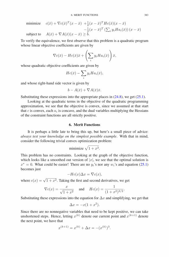
6. MERIT FUNCTIONS 383
minimize c(x) +∇c(x)T (x− x) + 12 (x− x)THc(x)(x− x)
− 12 (x− x)T (
∑i yiHai(x)) (x− x)
subject to A(x) +∇A(x)(x− x) ≥ b.
To verify the equivalence, we first observe that this problem is a quadratic programwhose linear objective coefficients are given by
∇c(x)−Hc(x)x+
(∑
i
yiHai(x)
)
x,
whose quadratic objective coefficients are given by
Hc(x)−∑
i
yiHai(x),
and whose right-hand side vector is given by
b−A(x) +∇A(x)x.
Substituting these expressions into the appropriate places in (24.8), we get (25.1).Looking at the quadratic terms in the objective of the quadratic programming
approximation, we see that the objective is convex, since we assumed at that startthat c is convex, each ai is concave, and the dual variables multiplying the Hessiansof the constraint functions are all strictly positive.
6. Merit Functions
It is perhaps a little late to bring this up, but here’s a small piece of advice:always test your knowledge on the simplest possible example. With that in mind,consider the following trivial convex optimization problem:
minimize√
1 + x2.
This problem has no constraints. Looking at the graph of the objective function,which looks like a smoothed out version of |x|, we see that the optimal solution isx∗ = 0. What could be easier! There are no yi’s nor any wi’s and equation (25.1)becomes just
−Hc(x)Δx = ∇c(x),
where c(x) =√1 + x2. Taking the first and second derivatives, we get
∇c(x) =x√
1 + x2and Hc(x) =
1
(1 + x2)3/2.
Substituting these expressions into the equation for Δx and simplifying, we get that
Δx = −x(1 + x2).
Since there are no nonnegative variables that need to be kept positive, we can takeunshortened steps. Hence, letting x(k) denote our current point and x(k+1) denotethe next point, we have that
x(k+1) = x(k) +Δx = −(x(k))3.

384 25. CONVEX PROGRAMMING
That is, the algorithm says to start at any point x(0) and then replace this point withthe negative of its cube, replace that with the negative of its cube, and so on.
The question is: does this sequence converge to zero? It is easy to see thatthe answer is yes if |x(0)| < 1 but no otherwise. For example, if we start withx(0) = 1/2, then the sequence of iterates is
k x(k)
0 0.500000001 −0.125000002 0.001953133 −0.00000001
If, on the other hand, we start at x(0) = 2, then we get the following wildly divergentsequence:
k x(k)
0 21 −82 5123 −134,217,728
Here is what goes wrong in this example. For problems without constraints, ouralgorithm has an especially simple description:
From the current point, use the first three terms of a Taylorseries expansion to make a quadratic approximation to the ob-jective function. The next point is the minimum of this quadraticapproximation function.
Figure 25.1 shows a graph of the objective function together with the quadraticapproximation at x(0) = 2. It is easy to see that the next iterate is at −8. Also, thefurther from zero that one starts, the more the function looks like a straight line andhence the further the minimum will be to the other side.
How do we remedy this nonconvergence? The key insight is the observationthat the steps are always in the correct direction (i.e, a descent direction) but theyare too long—we need to shorten them. A standard technique for shortening stepsin situations like this is to introduce a function called a merit function and to shortensteps as needed to ensure that this merit function is always monotonically decreas-ing. For the example above, and in fact for any unconstrained optimization problem,we can use the objective function itself as the merit function. But, for problems withconstraints, one needs to use something a little different from just the objective func-tion. For example, one can use the logarithmic barrier function plus a constant timesthe square of the Euclidean norm of the infeasibility vector:
Ψ(x,w) := c(x)−∑
i
log(wi) + β‖b−A(x) + w‖2.
Here, β is a positive real number. One can show that for β sufficiently large the stepdirections are always descent directions for this merit function.
A summary of the algorithm is shown in Figure 25.2.

EXERCISES 385
-4
-2
0
2
4
6
8
10
12
14
-10 -5 0 5 10
sqrt(x**2 + 1)
sqrt(5)+2*(x-2)/sqrt(5)+(x-2)**2/(2*sqrt(5)**3)
FIGURE 25.1. The function c(x) =√1 + x2 and its quadratic
approximation at x = 2.
7. Parting Words
A story is never over, but every book must have an end. So, we stop heremindful of the fact that there are many interesting things left unsaid and topics un-explored. We hope we have motivated the reader to pursue the story further withoutour assistance—by reading other books and/or research papers and even perhapsmaking his or her own contributions. Cheers.
Exercises
25.1 Piecewise Linear Approximation. Given real numbers b1 < b2 < · · · <bk, let f be a continuous function on R that is linear on each interval[bi, bi+1], i = 0, 1, . . . , k (for convenience we let b0 = −∞ and bk+1 =∞). Such a function is called piecewise linear and the numbers bi arecalled breakpoints. Piecewise linear functions are often used to approxi-mate (continuous) nonlinear functions. The purpose of this exercise is toshow how and why.(a) Every piecewise linear function can be written as a sum of a constant
plus a linear term plus a sum of absolute value terms:
f(x) = d+ a0x+k∑
i=1
ai|x− bi|.
Let ci denote the slope of f on the interval [bi, bi+1]. Derive anexplicit expression for each of the aj’s (including a0) in terms ofthe ci’s.

386 25. CONVEX PROGRAMMING
initialize (x,w, y) so that (w, y) > 0
while (not optimal) {set up QP subproblem:
A = ∇A(x)b = b−A(x) +∇A(x)xc = ∇c(x)−Hc(x)x+ (
∑i yiHai(x))x
Q = Hc(x)−∑
i yiHai(x)ρ = b−Ax+ wσ = c−AT y +Qxγ = yTw
μ = δγ
n+msolve:[
−Q AT
A Y −1W
] [ΔxΔy
]
=
[c−AT y +Qxb−Ax− μY −1e
]
Δw = Y −1(μe− YWe−WΔy)
θ = r
(
maxij
{
−Δxj
xj,−Δwi
wi,−Δyi
yi
})−1
∧ 1
do {xnew = x+ θΔx,
wnew = w + θΔw
ynew = y + θΔyθ ← θ/2
}while ( Ψ(xnew, wnew) ≥ Ψ(x,w) )}
FIGURE 25.2. The path-following method for convex program-ming problems.
(b) In terms of the ci’s, give necessary and sufficient conditions for f tobe convex.
(c) In terms of the aj’s, give necessary and sufficient conditions for f tobe convex.
(d) Assuming that f is convex and is a term in the objective functionfor a linearly constrained optimization problem, derive an equivalentlinear programming formulation involving at most k extra variablesand constraints.
(e) Repeat the first four parts of this problem using max(x − bi, 0) inplace of |x− bi|.
25.2 Let f be the function of 2 real variables defined by
f(x, y) = x2 − 2xy + y2.
Show that f is convex.

EXERCISES 387
25.3 A function f of 2 real variables is called a monomial if it has the form
f(x, y) = xmyn
for some nonnegative integers m and n. Which monomials are convex?
25.4 Let φ be a convex function of a single real variable. Let f be a functiondefined on R
n by the formula
f(x) = φ(aTx+ b),
where a is an n-vector and b is a scalar. Show that f is convex.
25.5 Which of the following functions are convex (assume that the domain ofthe function is all of Rn unless specified otherwise)?(a) 4x2 − 12xy + 9y2
(b) x2 + 2xy + y2
(c) x2y2
(d) x2 − y2
(e) ex−y
(f) ex2−y2
(g) x2
y on {(x, y) : y > 0}
25.6 Given a symmetric square matrix A, the quadratic form xTAx =∑
i,j
aijxixj generalizes the notion of the square of a variable. The generaliza-tion of the notion of the fourth power of a variable is an expression of theform
f(x) =∑
i,j,k,l
aijklxixjxkxl.
The four-dimensional array of numbers A = {aijkl : 1 ≤ i ≤ n, 1 ≤j ≤ n, 1 ≤ k ≤ n, 1 ≤ l ≤ n} is called a 4-tensor. As with quadraticexpressions, we may assume that A is symmetric:
aijkl = ajkli = · · · = alkij
(i.e., given i, j, k, l, all 4! = 24 premutations must give the same value forthe tensor).(a) Give conditions on the 4-tensor A to guarantee that f is convex.(b) Suppose that some variables, say yi’s, are related to some other vari-
ables, say xj’s, in a linear fashion:
yi =∑
j
fijxj .
Express∑
i y4i in terms of the xj’s. In particular, give an explicit
expression for the 4-tensor and show that it satisfies the conditionsderived in part (a).
25.7 Consider the problem
minimize ax1 + x2
subject to√
ε2 + x21 ≤ x2.

388 25. CONVEX PROGRAMMING
where −1 < a < 1.(a) Graph the feasible set:
{(x1, x2) :
√ε2 + x2
1 ≤ x2
}. Is the problem
convex?(b) Following the steps in the middle of p. 391 of the text, write down the
first-order optimality conditions for the barrier problem associatedwith barrier parameter μ > 0.
(c) Solve explicitly the first-order optimality conditions. Let (x1(μ),x2(μ)) denote the solution.
(d) Graph the central path, (x1(μ), x2(μ)), as μ varies from 0 to ∞.
25.8 Multidimensional Taylor’s series expansion. Given a function g(t)defined for real values of t, the three-term Taylor’s series expansion withremainder is
g(t+Δt) = g(t) + g′(t)Δt+1
2g′′(t)Δt2 + rt(Δt).
The remainder term satisfies
limΔt→0
rt(Δt)
Δt2= 0.
Let f be a smooth function defined on Rn. Apply the three-term Taylor’s
series expansion to g(t) = f(x+ tΔx) to show that
f(x+Δx) = f(x) +∇f(x)TΔx+1
2ΔxTHf(x)Δx+ rx(Δx).
25.9 Consider the following convex programming problem:
minimize x2
subject to x21 + x2
2 ≤ 1.
(a) Find the quadratic subproblem if the current primal solution is(x1, x2) = (1/2,−2/3) and the current dual solution is y = 2.
(b) Show that for arbitrary current primal and dual solutions, the feasi-ble set for the convex programming problem is contained within thefeasible set for the quadratic approximation.
Notes
Interior-point methods for nonlinear programming can be traced back to thepioneering work of Fiacco and McCormick (1968). For more on interior-point meth-ods for convex programming, see Nesterov and Nemirovsky (1993) or den Hertog(1994).
The fact that the step directions are descent directions for the merit function Ψis proved in Vanderbei and Shanno (1999).

ERRATUM
Linear Programming
Robert J. Vanderbei
R.J. Vanderbei, Linear Programming, International Series in Operations Research& Management Science 196, DOI 10.1007/978-1-4614-7630-6,© Springer Science+Business Media New York 2014
DOI 10.1007/978-1-4614-7630-6 26
The publisher regrets the errors published in the print and online versions of thisbook, corrections to Chapter 3, page 29, and Chapter 14, page 211, have beenupdated and can be found on the next pages.
10.1007/978-1-4614-7630-6
R.J. Vanderbei, Linear Programming, International Series in Operations Research& Management Science 196, DOI 10.1007/978-1-4614-7630-6 26,© Springer Science+Business Media New York 2017
E1
The updated original online version for this book can be found at DOI
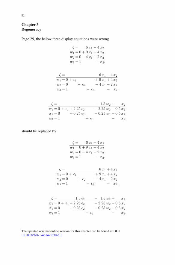
E2
Chapter 3Degeneracy
Page 29, the below three display equations were wrong
ζ = 6 x1 − 4 x2
w1 = 0+ 9 x1 + 4 x2
w2 = 0− 4 x1 − 2 x2
w3 = 1 − x2.
ζ = 6 x1 − 4 x2
w1 = 0+ ε1 + 9 x1 + 4 x2
w2 = 0 + ε2 − 4 x1 − 2 x2
w3 = 1 + ε3 − x2.
ζ = − 1.5w2 + x2
w1 = 0+ ε1 + 2.25 ε2 − 2.25w2 − 0.5 x2
x1 = 0 + 0.25 ε2 − 0.25w2 − 0.5 x2
w3 = 1 + ε3 − x2.
should be replaced by
ζ = 6 x1 + 4 x2
w1 = 0+ 9 x1 + 4 x2
w2 = 0− 4 x1 − 2 x2
w3 = 1 − x2.
ζ = 6 x1 + 4 x2
w1 = 0+ ε1 + 9 x1 + 4 x2
w2 = 0 + ε2 − 4 x1 − 2 x2
w3 = 1 + ε3 − x2.
ζ = 1.5 ε2 − 1.5w2 + x2
w1 = 0+ ε1 + 2.25 ε2 − 2.25w2 − 0.5 x2
x1 = 0 + 0.25 ε2 − 0.25w2 − 0.5 x2
w3 = 1 + ε3 − x2.
10.1007/978-1-4614-7630-6 3The updated original online version for this chapter can be found at DOI

E3
Chapter 14Network Flow Problems
Page 211, “Hence, arc (f,c) must enter the spanning tree” should read “Hence,arc (f,b) must enter the spanning tree”.
10.1007/978-1-4614-7630-6 14The updated original online version for this chapter can be found at DOI
APPENDIX A
Source Listings
The algorithms presented in this book have all been implemented and are pub-licly available from the author’s web site:
http://www.princeton.edu/∼rvdb/LPbook/
There are two variants of the simplex method: the two-phase method as shownin Figure 6.1 and the self-dual method as shown in Figure 7.1. The simplex codesrequire software for efficiently solving basis systems. There are two options: the eta-matrix approach described in Section 8.3 and the refactorization approach describedin Section 8.5. Each of these “engines” can be used with either simplex method.Hence, there are in total four possible simplex codes that one can experiment with.
There are three variants of interior-point methods: the path-following methodas shown in Figure 18.1, the homogeneous self-dual method shown in Figure 22.1(modified to take long steps), and the long-step homogeneous self-dual method de-scribed in Exercise 22.4 of Chapter 22.
The source code that implements the algorithms mentioned above share asmuch common code as possible. For example, they all share the same input andoutput routines (the input routine, by itself, is a substantial piece of code). Theyalso share code for the common linear algebra functions. Therefore, the differencebetween two methods is limited primarily to the specific function that implementsthe method itself.
The total number of lines of code used to implement all of the algorithms isabout 9,000. That is too many lines to reproduce all of the code here. But theroutines that actually lay out the particular algorithms are fairly short, only about300 lines each. The relevant part of the self-dual simplex method is shown startingon the next page. It is followed by a listing of the relevant part of the homogeneousself-dual method.
R.J. Vanderbei, Linear Programming, International Series in Operations Research& Management Science 196, DOI 10.1007/978-1-4614-7630-6,© Springer Science+Business Media New York 2014
389

390 A. SOURCE LISTINGS
1. The Self-Dual Simplex Method
/***************************************************************** Main loop *****************************************************************/
for (iter=0; iter<MAX_ITER; iter++) {
/************************************************************** STEP 1: Find mu **************************************************************/
mu = -HUGE_VAL;col_in = -1;for (j=0; j<n; j++) {
if (zbar_N[j] > EPS2) {if ( mu < -z_N[j]/zbar_N[j] ) {
mu = -z_N[j]/zbar_N[j];col_in = j;
}}
}col_out = -1;for (i=0; i<m; i++) {
if (xbar_B[i] > EPS2) {if ( mu < -x_B[i]/xbar_B[i] ) {
mu = -x_B[i]/xbar_B[i];col_out = i;col_in = -1;
}}
}if ( mu <= EPS3 ) { /* OPTIMAL */
status = 0;break;
}
if ( col_out >= 0 ) {
/************************************************************** -1 T ** STEP 2: Compute dz = -(B N) e ** N i ** where i = col_out **************************************************************/
vec[0] = -1.0;ivec[0] = col_out;nvec = 1;
btsolve( m, vec, ivec, &nvec );
Nt_times_z( N, at, iat, kat, basicflag, vec, ivec, nvec,dz_N, idz_N, &ndz_N );
/************************************************************** STEP 3: Ratio test to find entering column **************************************************************/
col_in = ratio_test( dz_N, idz_N, ndz_N, z_N, zbar_N, mu );
if (col_in == -1) { /* INFEASIBLE */status = 2;break;
}
/************************************************************** -1 ** STEP 4: Compute dx = B N e ** B j ** **************************************************************/
j = nonbasics[col_in];

1. THE SELF-DUAL SIMPLEX METHOD 391
for (i=0, k=ka[j]; k<ka[j+1]; i++, k++) {dx_B[i] = a[k];
idx_B[i] = ia[k];}ndx_B = i;
bsolve( m, dx_B, idx_B, &ndx_B );
} else {
/************************************************************** -1 ** STEP 2: Compute dx = B N e ** B j **************************************************************/
j = nonbasics[col_in];for (i=0, k=ka[j]; k<ka[j+1]; i++, k++) {
dx_B[i] = a[k];idx_B[i] = ia[k];
}ndx_B = i;
bsolve( m, dx_B, idx_B, &ndx_B );
/************************************************************** STEP 3: Ratio test to find leaving column **************************************************************/
col_out = ratio_test( dx_B, idx_B, ndx_B, x_B, xbar_B, mu );
if (col_out == -1) { /* UNBOUNDED */status = 1;break;
}
/************************************************************** -1 T ** STEP 4: Compute dz = -(B N) e ** N i ** **************************************************************/
vec[0] = -1.0;ivec[0] = col_out;nvec = 1;
btsolve( m, vec, ivec, &nvec );
Nt_times_z( N, at, iat, kat, basicflag, vec, ivec, nvec,dz_N, idz_N, &ndz_N );
}
/************************************************************** ** STEP 5: Put t = x /dx ** i i ** _ _ ** t = x /dx ** i i ** s = z /dz ** j j ** _ _ ** s = z /dz ** j j **************************************************************/
for (k=0; k<ndx_B; k++) if (idx_B[k] == col_out) break;
t = x_B[col_out]/dx_B[k];tbar = xbar_B[col_out]/dx_B[k];
for (k=0; k<ndz_N; k++) if (idz_N[k] == col_in) break;
s = z_N[col_in]/dz_N[k];

392 A. SOURCE LISTINGS
sbar = zbar_N[col_in]/dz_N[k];
/************************************************************** _ _ _ ** STEP 7: Set z = z - s dz z = z - s dz ** N N N N N N ** _ _ ** z = s z = s ** i i ** _ _ _ ** x = x - t dx x = x - t dx ** B B B B B B ** _ _ ** x = t x = t ** j j **************************************************************/
for (k=0; k<ndz_N; k++) {j = idz_N[k];z_N[j] -= s *dz_N[k];zbar_N[j] -= sbar*dz_N[k];
}
z_N[col_in] = s;zbar_N[col_in] = sbar;
for (k=0; k<ndx_B; k++) {i = idx_B[k];x_B[i] -= t *dx_B[k];xbar_B[i] -= tbar*dx_B[k];
}
x_B[col_out] = t;xbar_B[col_out] = tbar;
/************************************************************** STEP 8: Update basis **************************************************************/
i = basics[col_out];j = nonbasics[col_in];basics[col_out] = j;nonbasics[col_in] = i;basicflag[i] = -col_in-1;basicflag[j] = col_out;
/************************************************************** STEP 9: Refactor basis and print statistics **************************************************************/
from_scratch = refactor( m, ka, ia, a, basics, col_out, v );
if (from_scratch) {primal_obj = sdotprod(c,x_B,basics,m) + f;printf("%8d %14.7e %9.2e \n", iter, primal_obj, mu );fflush(stdout);
}}

2. THE HOMOGENEOUS SELF-DUAL METHOD 393
2. The Homogeneous Self-Dual Method
/***************************************************************** Main loop *****************************************************************/
for (iter=0; iter<MAX_ITER; iter++) {
/************************************************************** STEP 1: Compute mu and centering parameter delta.
*************************************************************/
mu = (dotprod(z,x,n)+dotprod(w,y,m)+phi*psi) / (n+m+1);
if (iter%2 == 0) {delta = 0.0;
} else {delta = 1.0;
}
/************************************************************** STEP 1: Compute primal and dual objective function values.
*************************************************************/
primal_obj = dotprod(c,x,n);dual_obj = dotprod(b,y,m);
/************************************************************** STEP 2: Check stopping rule.
*************************************************************/
if ( mu < EPS ) {if ( phi > EPS ) {
status = 0;break; /* OPTIMAL */
}elseif ( dual_obj < 0.0) {
status = 2;break; /* PRIMAL INFEASIBLE */
}elseif ( primal_obj > 0.0) {
status = 4;break; /* DUAL INFEASIBLE */
}else{
status = 7; /* NUMERICAL TROUBLE */break;
}}
/************************************************************** STEP 3: Compute infeasibilities.
*************************************************************/
smx(m,n,A,kA,iA,x,rho);for (i=0; i<m; i++) {
rho[i] = rho[i] - b[i]*phi + w[i];}normr = sqrt( dotprod(rho,rho,m) )/phi;for (i=0; i<m; i++) {
rho[i] = -(1-delta)*rho[i] + w[i] - delta*mu/y[i];}
smx(n,m,At,kAt,iAt,y,sigma);for (j=0; j<n; j++) {
sigma[j] = -sigma[j] + c[j]*phi + z[j];}norms = sqrt( dotprod(sigma,sigma,n) )/phi;for (j=0; j<n; j++) {
sigma[j] = -(1-delta)*sigma[j] + z[j] - delta*mu/x[j];}

394 A. SOURCE LISTINGS
gamma = -(1-delta)*(dual_obj - primal_obj + psi) + psi - delta*mu/phi;
/************************************************************** Print statistics.
*************************************************************/
printf("%8d %14.7e %8.1e %14.7e %8.1e %8.1e \n",iter, primal_obj/phi+f, normr,
dual_obj/phi+f, norms, mu );fflush(stdout);
/************************************************************** STEP 4: Compute step directions.
*************************************************************/
for (j=0; j<n; j++) { D[j] = z[j]/x[j]; }for (i=0; i<m; i++) { E[i] = w[i]/y[i]; }
ldltfac(n, m, kAt, iAt, At, E, D, kA, iA, A, v);
for (j=0; j<n; j++) { fx[j] = -sigma[j]; }for (i=0; i<m; i++) { fy[i] = rho[i]; }
forwardbackward(E, D, fy, fx);
for (j=0; j<n; j++) { gx[j] = -c[j]; }for (i=0; i<m; i++) { gy[i] = -b[i]; }
forwardbackward(E, D, gy, gx);
dphi = (dotprod(c,fx,n)-dotprod(b,fy,m)+gamma)/(dotprod(c,gx,n)-dotprod(b,gy,m)-psi/phi);
for (j=0; j<n; j++) { dx[j] = fx[j] - gx[j]*dphi; }for (i=0; i<m; i++) { dy[i] = fy[i] - gy[i]*dphi; }
for (j=0; j<n; j++) { dz[j] = delta*mu/x[j] - z[j] - D[j]*dx[j]; }for (i=0; i<m; i++) { dw[i] = delta*mu/y[i] - w[i] - E[i]*dy[i]; }dpsi = delta*mu/phi - psi - (psi/phi)*dphi;
/************************************************************** STEP 5: Compute step length (long steps).
*************************************************************/
theta = 0.0;for (j=0; j<n; j++) {
if (theta < -dx[j]/x[j]) { theta = -dx[j]/x[j]; }if (theta < -dz[j]/z[j]) { theta = -dz[j]/z[j]; }
}for (i=0; i<m; i++) {
if (theta < -dy[i]/y[i]) { theta = -dy[i]/y[i]; }if (theta < -dw[i]/w[i]) { theta = -dw[i]/w[i]; }
}theta = MIN( 0.95/theta, 1.0 );
/************************************************************** STEP 6: Step to new point
*************************************************************/
for (j=0; j<n; j++) {x[j] = x[j] + theta*dx[j];z[j] = z[j] + theta*dz[j];
}for (i=0; i<m; i++) {
y[i] = y[i] + theta*dy[i];w[i] = w[i] + theta*dw[i];
}phi = phi + theta*dphi;psi = psi + theta*dpsi;
}

Answers to Selected Exercises
1.3: See Exercise 2.19.2.1: (x1, x2, x3, x4) = (2, 0, 1, 0), ζ = 17.2.2: (x1, x2) = (1, 0), ζ = 2.2.3: (x1, x2, x3) = (0, 0.5, 1.5), ζ = −3.2.4: (x1, x2, x3) = (0, 1, 0), ζ = −3.2.5: (x1, x2) = (2, 1), ζ = 5.2.6: Infeasible.2.7: Unbounded.2.8: (x1, x2) = (4, 8), ζ = 28.2.9: (x1, x2, x3) = (1.5, 2.5, 0), ζ = 10.5.2.10: (x1, x2, x3, x4) = (0, 0, 0, 1), ζ = 9.2.11: (x12, x13, x14, x23, x24, x34) = (1, 0, 0, 1, 0, 1), ζ = 6.7.1: (1) x∗ = (2, 4, 0, 0, 0, 0, 8), ξ∗ = 14. (2) x∗ unchanged, ξ∗ = 12.2. (3)
x∗ = (0, 8, 0, 0, 0, 10, 10), ξ∗ = 16.7.2: Δc1 ∈ (−∞, 1.2], Δc2 ∈ [−1.2,∞), Δc3 ∈ [−1, 9], Δc4 ∈ (−∞, 2.8].9.1: (x1, x2) = (0, 5).9.2: (x1, x2, x3, x4, x5, x6, x7, x8) = (0, 6, 1, 15, 2, 1, 0, 0).10.5: The fundamental theorem was proved only for problems in standard form.
The LP here can be reduced to standard form.11.1: A should hide a or b with probabilities b/(a+ b) and a/(a+ b), respectively.
B should hide a or b with equal probability.11.3:
[2 −4
−3 6
]
12.1: Slope = 2/7, intercept = 1.12.2: Slope = 1/2, intercept = 0.12.7: (2) 340. (3) x∗ is chosen so that the number of months in which extra work-
ers will be used is equal to the number of months in the cycle (12) times theinhouse employee cost ($17.50) divided by the outhouse employee cost ($25)rounded down to the nearest integer.
12.8: Using L1, g = 8.951. With L2, g = 8.924.
R.J. Vanderbei, Linear Programming, International Series in Operations Research& Management Science 196, DOI 10.1007/978-1-4614-7630-6,© Springer Science+Business Media New York 2014
395
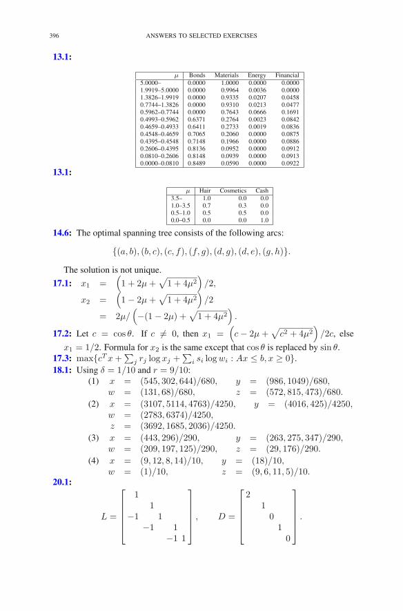
396 ANSWERS TO SELECTED EXERCISES
13.1:
μ Bonds Materials Energy Financial5.0000– 0.0000 1.0000 0.0000 0.00001.9919–5.0000 0.0000 0.9964 0.0036 0.00001.3826–1.9919 0.0000 0.9335 0.0207 0.04580.7744–1.3826 0.0000 0.9310 0.0213 0.04770.5962–0.7744 0.0000 0.7643 0.0666 0.16910.4993–0.5962 0.6371 0.2764 0.0023 0.08420.4659–0.4933 0.6411 0.2733 0.0019 0.08360.4548–0.4659 0.7065 0.2060 0.0000 0.08750.4395–0.4548 0.7148 0.1966 0.0000 0.08860.2606–0.4395 0.8136 0.0952 0.0000 0.09120.0810–0.2606 0.8148 0.0939 0.0000 0.09130.0000–0.0810 0.8489 0.0590 0.0000 0.0922
13.1:
μ Hair Cosmetics Cash3.5– 1.0 0.0 0.01.0–3.5 0.7 0.3 0.00.5–1.0 0.5 0.5 0.00.0–0.5 0.0 0.0 1.0
14.6: The optimal spanning tree consists of the following arcs:
{(a, b), (b, c), (c, f), (f, g), (d, g), (d, e), (g, h)}.
The solution is not unique.
17.1: x1 =(1 + 2μ+
√1 + 4μ2
)/2,
x2 =(1− 2μ+
√1 + 4μ2
)/2
= 2μ/(−(1− 2μ) +
√1 + 4μ2
).
17.2: Let c = cos θ. If c �= 0, then x1 =(c− 2μ+
√c2 + 4μ2
)/2c, else
x1 = 1/2. Formula for x2 is the same except that cos θ is replaced by sin θ.17.3: max{cTx+
∑j rj log xj +
∑i si logwi : Ax ≤ b, x ≥ 0}.
18.1: Using δ = 1/10 and r = 9/10:(1) x = (545, 302, 644)/680, y = (986, 1049)/680,
w = (131, 68)/680, z = (572, 815, 473)/680.
(2) x = (3107, 5114, 4763)/4250, y = (4016, 425)/4250,w = (2783, 6374)/4250,z = (3692, 1685, 2036)/4250.
(3) x = (443, 296)/290, y = (263, 275, 347)/290,w = (209, 197, 125)/290, z = (29, 176)/290.
(4) x = (9, 12, 8, 14)/10, y = (18)/10,w = (1)/10, z = (9, 6, 11, 5)/10.
20.1:
L =
⎡
⎢⎢⎢⎢⎣
11
−1 1−1 1
−1 1
⎤
⎥⎥⎥⎥⎦, D =
⎡
⎢⎢⎢⎢⎣
21010
⎤
⎥⎥⎥⎥⎦.

ANSWERS TO SELECTED EXERCISES 397
20.3:
L =
⎡
⎢⎢⎢⎢⎣
11
− 13 1
−1 1− 6
713 1
⎤
⎥⎥⎥⎥⎦, D =
⎡
⎢⎢⎢⎢⎣
−2−3
73
3− 64
21
⎤
⎥⎥⎥⎥⎦.
Bibliography
Adler, I., & Berenguer, S. (1981). Random linear programs (Techincal Report 81-4).Operations Research Center Report, U.C. Berkeley. 184
Adler, I., & Megiddo, N. (1985). A simplex algorithm whose average number ofsteps is bounded between two quadratic functions of the smaller dimension. Jour-nal of the ACM, 32, 871–895. 52, 184
Adler, I., Karmarkar, N., Resende, M., & Veiga, G. (1989). An implementationof Karmarkar’s algorithm for linear programming. Mathematical Programming,44, 297–335. 341
Ahuja, R., Magnanti, T., & Orlin, J. (1993). Network flows: Theory, algorithms, andapplications. Englewood Cliffs: Prentice Hall. 224, 239
Anstreicher, K. (1996). Potential reduction algorithms (Technical Report). Depart-ment of Management Sciences, University of Iowa. 283
Barnes, E. (1986). A variation on Karmarkar’s algorithm for solving linear program-ming problems. Mathematical Programming, 36, 174–182. 321
Bayer, D., & Lagarias, J. (1989a). The nonlinear geometry of linear programming. I.Affine and projective scaling trajectories. Transactions of the AMS, 314, 499–525.268
Bayer, D., & Lagarias, J. (1989b). The nonlinear geometry of linear programming.II. Legendre transform coordinates and central trajectories. Transactions of theAMS, 314, 527–581. 268
Bazaraa, M., Jarvis, J., & Sherali, H. (1977). Linear programming and networkflows (2nd ed.). New York: Wiley. 9, 224
Bellman, R. (1957). Dynamic programming. Princeton: Princeton University Press.239
Bendsøe, M., Ben-Tal, A., & Zowe, J. (1994). Optimization methods for truss ge-ometry and topology design. Structural Optimization, 7, 141–159. 254
Bertsekas, D. (1991). Linear network optimization. Cambridge: MIT. 224Bertsekas, D. (1995). Nonlinear programming. Belmont: Athena Scientific. 268,
378Bland, R. (1977). New finite pivoting rules for the simplex method. Mathematics of
Operations Research, 2, 103–107. 37Bloomfield, P., & Steiger, W. (1983). Least absolute deviations: Theory, applica-
tions, and algorithms. Boston: Birkhauser. 183
R.J. Vanderbei, Linear Programming, International Series in Operations Research& Management Science 196, DOI 10.1007/978-1-4614-7630-6,© Springer Science+Business Media New York 2014
399

400 Bibliography
Borgwardt, K. -H. (1982). The average number of pivot steps required by thesimplex-method is polynomial. Zeitschrift fur Operations Research, 26, 157–177.52, 109, 184
Borgwardt, K. -H. (1987a). Probabilistic analysis of the simplex method. In Oper-ations research proceedings, 16th DGOR meeting, Springer-Verlag, New York,USA (pp. 564–576). 52, 184
Borgwardt, K. -H. (1987b). The simplex method—A probabilistic approach.Berlin/Heidelberg/New York: Springer. 52
Bradley, S., Hax, A., & Magnanti, T. (1977). Applied mathematical programming.Reading: Addison Wesley. 9
Caratheodory, C. (1907). Uber den variabilitatsbereich der koeffizienten von poten-zreihen, die gegebene werte nicht annehmen. Mathematische Annalen, 64, 95–115. 150
Carpenter, T., Lustig, I., Mulvey, J., & Shanno, D. (1993). Higher order predictor-corrector interior point methods with application to quadratic objectives. SIAMJournal on Optimization, 3, 696–725. 283
Charnes, A. (1952). Optimality and degeneracy in linear programming. Economet-rica, 20, 160–170. 37
Christofides, N. (1975). Graph theory: An algorithmic approach. New York: Aca-demic. 224
Chvatal, V. (1983). Linear programming. New York: Freeman. 23, 163Cook, W. (2012). In pursuit of the traveling salesman. Princeton: Princeton Univer-
sity Press. 362Dantzig, G. (1951a). Application of the simplex method to a transportation problem.
In T. Koopmans (Ed.), Activity analysis of production and allocation (pp. 359–373). New York: Wiley. 9, 224
Dantzig, G. (1951b). A proof of the equivalence of the programming problem andthe game problem. In T. Koopmans (Ed.), Activity analysis of production andallocation (pp. 330–335). New York: Wiley. 9
Dantzig, G. (1955). Upper bounds, secondary constraints, and block triangularity inlinear programming. Econometrica, 23, 174–183. 140
Dantzig, G. (1963). Linear programming and extensions. Princeton: Princeton Uni-versity Press. 9, 23, 109
Dantzig, G., & Orchard-Hayes, W. (1954). The product form for the inverse in thesimplex method. Mathematical Tables and Other Aids to Computation, 8, 64–67.132
Dantzig, G., Orden, A., & Wolfe, P. (1955). The generalized simplex method forminimizing a linear form under linear inequality constraints. Pacific Journal ofMathematics, 5, 183–195. 37
den Hertog, D. (1994). Interior point approach to linear, quadratic, and convexprogramming. Dordrecht: Kluwer. 388
Dijkstra, E. (1959). A note on two problems in connexion with graphs. NumerischeMathematik, 1, 269–271. 239
Dikin, I. (1967). Iterative solution of problems of linear and quadratic programming.Soviet Mathematics Doklady, 8, 674–675. 321

Bibliography 401
Dikin, I. (1974). On the speed of an iterative process. Upravlyaemye Sistemi, 12,54–60. 321
Dodge, Y. (Ed.). (1987). Statistical data analysis based on the L1-norm and relatedmethods. Amsterdam: North-Holland. 183
Dorn, W., Gomory, R., & Greenberg, H. (1964). Automatic design of optimal struc-tures. Journal de Mecanique, 3, 25–52. 254
Dresher, M. (1961). Games of strategy: Theory and application. Englewood Cliffs:Prentice-Hall. 163
Duff, I., Erisman, A., & Reid, J. (1986). Direct methods for sparse matrices. Oxford:Oxford University Press. 132
Elias, P., Feinstein, A., & Shannon, C. (1956). Note on maximum flow through anetwork. IRE Transactions on Information Theory, 2, 117–119. 239
Farkas, J. (1902). Theorie der einfachen Ungleichungen. Journal fur die reine undangewandte Mathematik, 124, 1–27. 150
Fiacco, A., & McCormick, G. (1968). Nonlinear programming: Sequential uncon-strained minimization techniques. McLean: Research Analysis Corporation. Re-published in 1990 by SIAM, Philadelphia. 267, 388
Ford, L., & Fulkerson, D. (1956). Maximal flow through a network. Canadian Jour-nal of Mathematics, 8, 399–404. 239
Ford, L., & Fulkerson, D. (1958). Constructing maximal dynamic flows from staticflows. Operations Research, 6, 419–433. 224
Ford, L., & Fulkerson, D. (1962). Flows in networks. Princeton: Princeton Univer-sity Press. 224
Forrest, J., & Tomlin, J. (1972). Updating triangular factors of the basis to main-tain sparsity in the product form simplex method. Mathematical Programming,2, 263–278. 132
Fourer, R., & Mehrotra, S. (1991). Solving symmetric indefinite systems in an inte-rior point method for linear programming. Mathematical Programming, 62, 15–40. 307
Fourer, R., Gay, D., & Kernighan, B. (1993). AMPL: A modeling language formathematical programming. Belmont: Duxbury Press. viii
Fulkerson, D., & Dantzig, G. (1955). Computation of maximum flow in networks.Naval Research Logistics Quarterly, 2, 277–283. 239
Gal, T. (1994). Postoptimal analyses, parametric programming, and related topics:degeneracy, multicriteria decision making, redundancy. de Gruyter 37
Gale, D., Kuhn, H., & Tucker, A. (1951). Linear programming and the theory ofgames. In T. Koopmans (Ed.), Activity analysis of production and allocation(pp. 317–329). New York: Wiley. 79, 163
Garey, M., & Johnson, D. (1977). Computers and intractability. San Francisco:W.H. Freeman. 52
Garfinkel, R., & Nemhauser, G. (1972). Integer programming. New York: Wiley.362
Gass, S., & Saaty, T. (1955). The computational algorithm for the parametric objec-tive function. Naval Research Logistics Quarterly, 2, 39–45. 109

402 Bibliography
Gay, D. (1985). Electronic mail distribution of linear programming test problems.Mathematical Programming Society COAL Newslettter, 13, 10–12. 174
Gill, P., Murray, W., & Wright, M. (1991). Numerical linear algebra and optimiza-tion (Vol. 1). Redwood City: Addison-Wesley. 132
Gill, P., Murray, W., Ponceleon, D., & Saunders, M. (1992). Preconditioners forindefinite systems arising in optimization. SIAM Journal on Matrix Analysis andApplications, 13(1), 292–311. 307
Goldfarb, D., & Reid, J. (1977). A practicable steepest-edge simplex algorithm.Mathematical Programming, 12, 361–371. 132
Golub, G., & VanLoan, C. (1989). Matrix computations (2nd ed.). Baltimore: TheJohns Hopkins University Press. 132
Gonin, R., & Money, A. (1989). Nonlinear Lp-norm estimation. New York/Basel:Marcel Dekker. 183
Gordan, P. (1873). Uber die Auflosung linearer Gleichungen mit reelen coefficien-ten. Mathematische Annalen, 6, 23–28. 150
Hall, L., & Vanderbei, R. (1993). Two-thirds is sharp for affine scaling. OR Letters,13, 197–201. 321
Harris, P. (1973). Pivot selection methods of the Devex LP code. Mathematical Pro-gramming, 5, 1–28. 132
Hemp, W. (1973). Optimum structures. Oxford: Clarendon Press. 254Hillier, F., & Lieberman, G. (1977). Introduction to mathematical programming
(2nd ed.). New York: McGraw-Hill. 9Hitchcock, F. (1941). The distribution of a produce from several sources to numer-
ous localities. Journal of Mathematical Physics, 20, 224–230. 239Hoffman, A. (1953). Cycling in the simplex algorithm (Techincal Report 2974).
National Bureau of Standards. 37Howard, R. (1960). Dynamic programming and Markov processes. New York: Wi-
ley. 239Huard, P. (1967). Resolution of mathematical programming with nonlinear con-
straints by the method of centers. In J. Abadie (Ed.), Nonlinear programming(pp. 209–219). Amsterdam: North-Holland. 268
Jensen, P., & Barnes, J. (1980). Network flow programming. New York: Wiley. 224John, F. (1948). Extremum problems with inequalities as subsidiary conditions. In
K. Fredrichs, O. Neugebauer, & J. Stoker (Eds.), Studies and essays: Courantanniversary volume (pp. 187–204). New York: Wiley. 291
Kantorovich, L. (1960). Mathematical methods in the organization and planning ofproduction. Management Science, 6, 550–559. Original Russian version appearedin 1939. 9
Karlin, S. (1959). Mathematical methods and theory in games, programming, andeconomics (Vols. 1 and 2). Reading: Addison-Wesley. 163
Karmarkar, N. (1984). A new polynomial time algorithm for linear programming.Combinatorica, 4, 373–395. 267, 283, 321
Karush, W. (1939). Minima of functions of several variables with inequalities as sideconditions (Technical report, M.S. thesis) Department of Mathematics, Universityof Chicago. 291

Bibliography 403
Kennington, J., & Helgason, R. (1980). Algorithms for network programming. NewYork: Wiley. 224
Khachian, L. (1979). A polynomial algorithm in linear programming. DokladyAcademiia Nauk SSSR, 244, 191–194 (in Russian) (English translation: SovietMathematics Doklady, 20, 191–194) 52, 283
Klee, V., & Minty, G. (1972). How good is the simplex algorithm? In O. Shisha(Ed.), Inequalities–III (pp. 159–175). New York: Academic. 52
Kojima, M., Mizuno, S., & Yoshise, A. (1989). A primal-dual interior point algo-rithm for linear programming. In N. Megiddo (Ed.), Progress in mathematicalprogramming (pp. 29–47). New York: Springer. 283
Kotzig, A. (1956). Suvislost’ a Pravidelina Suvislots’ Konecnych Grafov (TechincalReport). Bratislava: Vysoka Skola Ekonomicka. 239
Kuhn, H. (1950). A simplified two-person poker. Annals of Mathematics Studies,24, 97–103. 163
Kuhn, H. (1976). Nonlinear prgramming: A historical view. In R. Cottle &C. Lemke (Eds.), Nonlinear programming, SIAM-AMS proceedings (Vol. 9,pp. 1–26). Providence: American Mathetical Society. 291
Kuhn, H., & Tucker, A. (1951). Nonlinear prgramming. In J. Neyman (Ed.), Pro-ceedings of the second Berkeley symposium on mathematical statistics and prob-ability (pp. 481–492). Berkeley: University of California Press. 291
Lawler, E. (1976). Combinatorial optimization: Networks and matroids. New York:Holt, Rinehart and Winston. 224
Lemke, C. (1954). The dual method of solving the linear programming problem.Naval Research Logistics Quarterly, 1, 36–47. 79
Lemke, C. (1965). Bimatrix equilibrium points and mathematical programming.Management Science, 11, 681–689. 109
Luenberger, D. (1984). Introduction to linear and nonlinear programming. Reading:Addison-Wesley. 268
Lustig, I. (1990). Feasibility issues in a primal-dual interior-point method for linearprogramming. Mathematical Programming, 49(2), 145–162. 283
Lustig, I., Marsten, R., & Shanno, D. (1994). Interior point methods for linear pro-gramming: Computational state of the art. ORSA Journal on Computing, 6, 1–14.307
Markowitz, H. (1957). The elimination form of the inverse and its application tolinear programming. Management Science, 3, 255–269. 132
Markowitz, H. (1959). Portfolio selection: Efficient diversification of investments.New York: Wiley. 195, 378
Marshall, K., & Suurballe, J. (1969). A note on cycling in the simplex method.Naval Research Logistics Quarterly, 16, 121–137. 37
Mascarenhas, W. (1997). The affine scaling algorithm fails for λ = 0.999. SIAMJournal on Optimization, 7, 34–46. 321
Megiddo, N. (1989). Pathways to the optimal set in linear programming. InN. Megiddo (Ed.), Progress in mathematical programming (pp. 131–158). NewYork: Springer. 267

404 Bibliography
Mehrotra, S. (1989). Higher order methods and their performance (Techincal Re-port TR 90-16R1) Department of Industrial Engineering and Management Sci-ences, Northwestern University, Evanston. Revised July 1991. 341
Mehrotra, S. (1992). On the implementation of a (primal-dual) interior pointmethod. SIAM Journal on Optimization, 2, 575–601. 341
Michell, A. (1904). The limits of economy of material in frame structures. Philo-sophical Magazine Series, 8, 589–597. 254
Mizuno, S., Todd, M., & Ye, Y. (1993). On adaptive-step primal-dual interior-point algorithms for linear programming. Mathematics of Operations Research,18, 964–981. 341
Monteiro, R., & Adler, I. (1989). Interior path following primal-dual algorithms:Part i: Linear programming. Mathematical Programming, 44, 27–41. 283, 378
Nash, S., & Sofer, A. (1996). Linear and nonlinear programming. New York:McGraw-Hill. 268, 378
Nazareth, J. (1986). Homotopy techniques in linear programming. Algorithmica,1, 529–535. 109, 283
Nazareth, J. (1987). Computer solutions of linear programs. Oxford: Oxford Uni-versity Press. 109
Nazareth, J. (1996). The implementation of linear programming algorithms basedon homotopies. Algorithmica, 15, 332–350. 283
Nemhauser, G., & Wolsey, L. (1988). Integer and combinatorial optimization. NewYork: Wiley. 362
Nesterov, Y., & Nemirovsky, A. (1993). Interior point polynomial methods in convexprogramming: Theory and algorithms. Philadelphia: SIAM. 388
Recski, A. (1989). Matroid theory and its applications in electric network theoryand in statics. Berlin/Heidelberg/New York: Springer. 254
Reid, J. (1982). A sparsity-exploiting variant of the Bartels-Golub decompositionfor linear programming bases. Mathematical Programming, 24, 55–69. 132
Rockafellar, R. (1970). Convex analysis. Princeton: Princeton University Press. 150Rozvany, G. (1989). Structural design via optimality criteria. Dordrecht: Kluwer.
254Ruszczynski, A., & Vanderbei, R. (2003). Frontiers of stochastically nondominated
portfolios. Econometrica, 71(4), 1287–1297. 195Saigal, R. (1995). Linear programming. Boston: Kluwer. 321Saunders, M. (1973). The complexity of LU updating in the simplex method. In
R. Andersen & R. Brent (Eds.), The complexity of computational problem solving(pp. 214–230). Brisbane: University of Queensland Press. 132
Smale, S. (1983). On the average number of steps of the simplex method of linearprogramming. Mathematical Programming, 27, 241–262. 52, 109, 184
Stiemke, E. (1915). Uber positive Losungen homogener linearer Gleichungen.Mathematische Annalen, 76, 340–342. 150
Todd, M. (1986). Polynomial expected behavior of a pivoting algorithm for linearcomplementarity and linear programming. Mathematical Programming, 35, 173–192. 52, 184

Bibliography 405
Todd, M. (1995). Potential-reduction methods in mathematical programming (Tech-incal Report 1112). SORIE, Cornell University, Ithaca. 283
Tsuchiya, T., & Muramatsu, M. (1992). Global convergence of a long-step affinescaling algorithm for degenerate linear programming problems. SIAM Journal onOptimization, 5(3), 525–551. 321
Tucker, A. (1956). Dual systems of homogeneous linear equations. Annals of Math-ematics Studies, 38, 3–18. 150, 341
Turner, K. (1991). Computing projections for the Karmarkar algorithm. Linear Al-gebra and Its Applications, 152, 141–154. 307
Vanderbei, R. (1989). Affine scaling for linear programs with free variables. Math-ematical Programming, 43, 31–44. 321
Vanderbei, R. (1994). Interior-point methods: Algorithms and formulations. ORSAJournal on Computing, 6, 32–34. 307
Vanderbei, R. (1995). Symmetric quasi-definite matrices. SIAM Journal on Opti-mization, 5(1), 100–113. 307
Vanderbei, R. (1999). LOQO: An interior point code for quadratic programming.Optimization Methods and Software, 12, 451–484. 378
Vanderbei, R., & Carpenter, T. (1993). Symmetric indefinite systems for interior-point methods. Mathematical Programming, 58, 1–32. 307
Vanderbei, R., & Shanno, D. (1999). An interior-point algorithm for nonconvexnonlinear programming. Computational Optimization and Applications, 13, 231–252. 388
Vanderbei, R., Meketon, M., & Freedman, B. (1986). A modification of Karmarkar’slinear programming algorithm. Algorithmica, 1, 395–407. 321
Ville, J. (1938). Sur la theorie general des jeux ou intervient l’habilete des jouers.In E. Borel (Ed.), Traite du Calcul des probabilites et des ses applications. Paris:Gauthiers-Villars. 150
von Neumann, J. (1928). Zur Theorie der Gesselschaftschpiele. Mathematische An-nalen, 100, 295–320. 163
von Neumann, J., & Morgenstern, O. (1947). Theory of games and economic be-havior (2nd ed.). Princeton: Princeton University Press. 163
Wright, S. (1996). Primal-dual interior-point methods. Philadelphia: SIAM. 283Xu, X., Hung, P., & Ye, Y. (1993). A simplified homogeneous and self-dual linear
programming algorithm and its implementation (Techincal Report). College ofBusiness Administration, University of Iowa. To appear in Annals of OperationsResearch. 341
Ye, Y., Todd, M., & Mizuno, S. (1994). An o(√nl)-iteration homogeneous and
self-dual linear programming algorithm. Mathematics of Operations Research,19, 53–67. 341

Index
LDLT−factorization, 295Lp−norm, 168L2−regression, 168LU-factorization, 113
AAcyclic network, 202Adler and Berenguer (1981), 184, 427Adler and Megiddo (1985), 52, 184, 427Adler et al. (1989), 341, 427Affine-scaling algorithm, 309Ahuja et al. (1993), 224, 239, 427Algorithm
affine-scaling, 309Dijkstra’s, 230dual simplex, 92homogeneous, self-dual interior-point, 337parametric self-dual simplex, 107path-following, 273
convex programming, 386general form, 306quadratic programming, 374
primal simplex, 92self-dual network simplex, 214self-dual parametric simplex, 109successive quadratic programming, 382
Anstreicher (1996), 283, 427Arbitrage, 193Arc, 199
head of, 202Ascent direction, 309Assignment problem, 227Auxiliary problem, 16Average-case analysis, 44Axes, pitch, roll, and yaw, 248
BBackward substitution, 115
Balanced flow, 203Barnes (1986), 321, 427Barrier function, 258Barrier problem, 257, 258Basic feasible solution, 13Basic variables, 13Bayer and Lagarias (1989a), 268, 427Bayer and Lagarias (1989b), 268, 427Bazaraa et al. (1977), 9, 224, 427Bellman (1957), 239, 427Bellman’s equation, 229Bendsøe et al. (1994), 254, 427Ben-Tal, A., xBernstein, D.H., xBertsekas (1991), 224, 427Bertsekas (1995), 268, 378, 427Bimatrix games, 161Bipartite graph, 225Bland (1977), 37, 427Bland’s rule, 31Bloomfield and Steiger (1983), 183, 427Bluffing, 157Borgwardt (1982), 52, 109, 184, 428Borgwardt (1987a), 52, 184, 428Borgwardt (1987b), 52, 428Bradley et al. (1977), 9, 428Branch-and-bound, 345, 351Breadth-first search, 355Bump, 125
CCapacity
cut, 233Caratheodory (1907), 150, 428Carpenter et al. (1993), 283, 428Central path, 257, 259, 266Centroid, 178Certificate of optimality, 62Charnes (1952), 37, 428
R.J. Vanderbei, Linear Programming, International Series in Operations Research& Management Science 196, DOI 10.1007/978-1-4614-7630-6,© Springer Science+Business Media New York 2014
407

408 INDEX
Christofides (1975), 224, 428Chvatal (1983), 23, 163, 428Cınlar, E., xColumn dominance, 161Come-from, 348Complementarity, 263
strict, 147, 148Complementary slackness theorem, 63Complexity
predictor-corrector algorithm, 332Complexity theory, 52Concave function, 149, 380Connected, 202, 221Connected components, 221Conservation laws, 245Continuous paths, 317Convergence, 274, 316, 330Convex analysis, 141Convex combination, 141Convex function, 377, 380Convex hull, 142Convex programming, 379
interior-point method for, 381Convex quadratic programming problem, 371Convex set, 141Cook (2012), 362, 428Corrector step, 328Cost
lost opportunity, 4Crew scheduling problem, 346Critical point(s), 166, 259Cut set, 233Cycle, 202Cycling, 26
DDantzig (1951a), 9, 224, 428Dantzig (1951b), 9, 428Dantzig (1955), 140, 428Dantzig (1963), 9, 23, 109, 428Dantzig and Orchard-Hayes (1954), 132, 428Dantzig et al. (1955), 37, 428Dantzig, G.B., 9, 23, 79Dantzig, T., 79Decision variables, 5Degeneracy, 25
geometry, 33Degenerate dictionary, 25Degenerate pivot, 25Demand node, 225den Hertog (1994), 388, 428Depth-first search, 355Destination node, 225
Devex, 132Dictionary, 13Diet problem, 77Digraph, 199Dijkstra (1959), 239, 428Dijkstra’s algorithm, 230Dikin (1967), 321, 428Dikin (1974), 321, 428Directed paths, 228Dodge (1987), 183, 429Dorn et al. (1964), 254, 429Dresher (1961), 163, 429Dual estimates, 320Duality theory, 53Dual network simplex method, 211Dual pivot, 211, 215Dual problem, 55
general form, 67Dual simplex method, 64, 90, 135, 137Duff et al. (1986), 132, 429Dynamic programming, 229
EEdge, 34Efficiency
simplex method, 39, 173Efficient frontier, 190, 367Elias et al. (1956), 239, 429Ellipsoid method, 52Entering arc, 215Entering variable, 15, 85, 91Enumeration tree, 353Equilibrium
Nash, 161Equivalence classes, 221Equivalence relation, 221Eta-file, 123Eta matrix, 123
FFacet, 33Facility location, 179FactorizationLDLT , 295LU , 113instability and quasidefinite matrices, 299stability and positive definite matrices, 296
Fair game, 155Farkas (1902), 150, 429Farkas’ lemma, 146Feasible flow, 203Feasible solution, 7Fiacco and McCormick (1968), 267, 388, 429

INDEX 409
Fixed costs, 349Flow balance constraints, 201Folven, G., xFord and Fulkerson (1956), 239, 429Ford and Fulkerson (1958), 224, 429Ford and Fulkerson (1962), 224, 429Forrest and Tomlin (1972), 132, 429Forward substitution, 114Fourer and Mehrotra (1991), 307, 429Fourer et al. (1993), viii, 429Fourer, R., viiiFourier, 9Fulkerson and Dantzig (1955), 239, 429Function
barrier, 258concave, 149, 380
strongly, 78convex, 377, 380
strongly, 78objective, 6
GGal (1993), 37, 429Gale et al. (1951), 79, 163, 429Games
bimatrix, 161zero-sum, 151
Game theory, 151Garey and Johnson (1977), 52, 429Garfinkel and Nemhauser (1972), 362, 429Garfinkel, R.S., xGass and Saaty (1955), 109, 429Gay (1985), 174, 429Gay, D.M., viiiGill et al. (1991), 132, 430Gill et al. (1992), 307, 430Gilmartin, J., xGoldfarb and Reid (1977), 132, 430Golub and VanLoan (1989), 132, 430Gonin and Money (1989), 183, 430Gordan (1873), 150, 430Go-to, 347Gradient, 379Graph, 199Gravity, acceleration due to, 181Gross, L., x
HHalfspace, 33, 144
generalized, 145Hall and Vanderbei (1993), 321, 430Hall, L.A., xHarris (1973), 132, 430
Hedging, 186Hemp (1973), 254, 430Hessian, 261, 379Higher-order methods, 281Hillier and Lieberman (1977), 9, 430Hitchcock (1941), 239, 430Hitchcock transportation problem, 227Hoffman (1953), 37, 430Holder’s inequality, 276Homogeneous problem, 323, 324Homogeneous self-dual method, 323Homotopy method, 102, 280Howard (1960), 239, 430Huard (1967), 268, 430
IIkura, Y., xIncidence matrix, 244Infeasibility, 7, 138, 270Infeasible dictionary, 17Initialization
dual-based, 66Integer programming, 216Integer programming problem, 345, 351Integrality theorem, 216Interior-point methods, 257
affine-scaling, 309homogeneous, self-dual, 337path-following, 273
convex programming, 386general form, 306quadratic programming, 374
Inventory, cost of, 4Iteratively reweighted least squares, 171Iterative reweighted least squares, 182
JJensen and Barnes (1980), 224, 430John (1948), 291, 430Joint, 241
KKantorovich (1960), 9, 430Karlin (1959), 163, 430Karmarkar (1984), 267, 283, 321, 430Karmarkar, N.K., 283Karush (1939), 291, 430Karush–Kuhn–Tucker (KKT) system, 285,
333Karush, W., 285, 291, 305, 373Kennington and Helgason (1980), 224, 430Kernighan, B., 429

410 INDEX
Khachian (1979), 52, 283, 431Klee and Minty (1972), 52, 431Klee, V., xKnapsack problem, 361Kojima et al. (1989), 282, 283, 431Konig’s theorem, 216Koopmans, T.C., 9Kotzig (1956), 239, 431Kuhn (1950), 163, 431Kuhn (1976), 291, 431Kuhn and Tucker (1951), 291, 431Kuhn, H.W., 285, 305, 373
LLabel-correcting algorithm, 228Labels, 228Label-setting algorithm, 228Lagrange multipliers, 259, 260Lagrangian, 261Lagrangian duality, 72Lawler (1976), 224, 431Least squares, 169Leaving arc, 215Leaving variable, 15, 86, 91Legendre transform, 79Legs, 345Lemke (1954), 79, 431Lemke (1965), 109, 431Lemma
Farkas’, 146Lexicographic method, 28, 30, 37Linear complementarity problem, 162, 281Linear program
standard form, 7Logarithmic barrier function, 258Long-step method, 340, 341Lower bounds, 133LP-relaxation, 227, 352Luenberger (1984), 268, 431Lustig (1990), 283, 431Lustig et al. (1994), 307, 431Lustig, I.J., x
MMandelbaum, A., xMarkowitz (1957), 132, 431Markowitz (1959), 195, 378, 431Markowitz model, 363Marshall and Suurballe (1969), 37, 431Mascarenhas (1997), 321, 431Matrix
notation, 81
positive definite, 293quasidefinite, 296sparse, 115
Matrix game, 151Maximum-flow problem, 233Mean, 165Median, 165Mediocrity, measures thereof, 165Megiddo (1989), 267, 431Mehrotra (1989), 341, 432Mehrotra (1992), 341, 432Meketon, M.S., xMember, 241Method
affine-scaling, 309dual network simplex, 211dual simplex, 64, 90, 92, 135higher-order, 281homogeneous self-dual, 323homogeneous, self-dual interior-point, 337homotopy, 280lexicographic, 28long-step, 340, 341Newton’s, 270out-of-kilter, 224parametric self-dual simplex, xi, 104, 105,
107path-following, 257, 269, 273
convex programming, 386general form, 306quadratic programming, 374
perturbation, 28predictor-corrector, 327primal–dual simplex, xi, 104primal network simplex, 206primal simplex, 83, 92, 133self-dual network simplex, 214self-dual parametric simplex, 109short-step, 341simplex, 11two phase, 92
Michell (1904), 254, 432Midrange, 178Minimum-cost network flow problem, 199Minimum-degree ordering, 115Minimum operator ∧, 273Minimum-weight structural design problem,
249Mixed integer programming problem, 361Mizuno et al. (1993), 341, 432Moment arm, 246Monteiro and Adler (1989), 283, 378, 432
INDEX 411
NNabona, N., xNash and Sofer (1996), 268, 378, 432Nash equilibrium, 161Nazareth (1986), 109, 283, 432Nazareth (1987), 109, 432Nazareth (1996), 283, 432Negative transpose, 58Nemhauser and Wolsey (1988), 362, 432Nesterov and Nemirovsky (1993), 388, 432Network, 199
acyclic, 202complete, 223connected, 202
Network flow problems, 199Network simplex method, 224Newton’s method, 270Node, 199Node-arc incidence matrix, 202Nonbasic variables, 13Nonlinear objective function, 350Nonlinear programming, 268Normal equations, 286, 287Null space, 312Null variable, 149
OObjective function, 6Onion skin, 317Optimality
check for, 85, 91Optimality conditions
first-order, 261, 263, 303, 368, 369, 373,381
Optimal solution, 7Option pricing, 190Orden, A., 37Orlin, J.B., xOrthogonal projection, 312Out-of-Kilter method, 224
PParametric analysis, 102Parametric self-dual simplex method, 104,
105Partial pricing, 129Path, 202Path-following method, 257, 269Penalty function, 377Perturbation method, 28, 37Phase I, 18
dual-based, 66Phase II, 18
Piecewise linear function, 385Pivot, 16Pivot rule, 16Planar network, 222Poker, 157Polyhedron, 33, 145Polynomial algorithm, 333Polynomial complexity, 52Portfolio optimization, 185, 363Portfolio selection, 185Positive definite matrix, 293Positive semidefinite matrix, 289, 371
closure under inversion, 289closure under summation, 289
Predictor-corrector algorithm, 327complexity, 332
Predictor step, 327Primal–dual network simplex method, 224Primal–dual scaling, 319Primal–dual simplex method, 104Primal flow, 202Primal network simplex method, 206Primal pivot, 207, 215Primal problem, 55Primal scaling, 319Primal simplex method, 83, 133Principle stresses, 252Probability
of infeasibility, 79of unboundedness, 79
Problemassignment, 227auxiliary, 16barrier, 257, 258convex quadratic programming, 371crew scheduling, 346diet, 77dual, 55equipment scheduling, 346Hitchcock transportation, 227homogeneous linear programming, 324homogeneous self-dual, 323integer programming, 345, 351knapsack, 361linear complementarity, 162, 281linear programming
general form, 133, 302maximum-flow, 233minimum-cost network, 199minimum-weight structural design, 249mixed integer programming, 361network flows, 199primal, 55quadratic penalty, 377

412 INDEX
quadratic programming, 363scheduling, 345self-dual linear programming, 324separable quadratic programming, 375set-covering, 346set-partitioning, 346shortest path, 228transportation, 225transshipment, 225traveling salesman, 347upper-bounded network flow, 231
Programmingnonlinear, 268
Projected gradient direction, 311scaled, 312
Projection, 312Projective geometry, 267Pruning, 357
QQuadratic form, 387Quadratic penalty problem, 377Quadratic programming problem, 363
convex, 370dual, 367interior-point method for, 373
Quasidefinite matrix, 296
RRanges, 133Recski (1989), 254, 432Reduced KKT system, 286, 333, 373Regression, 165Regression model, 168Reid (1982), 132, 432Resource allocation, 4, 69Revised simplex method, 97Reward, 185, 364Risk, 185, 364Rockafellar (1970), 150, 432Root
of a function, 270Root node, 205, 228Roses,Route, 345Row dominance, 161Row operations, 12Rozvany (1989), 254, 432Ruszczynski, A, xRuszczynski and Vanderbei (2003), 195, 432
SSaddle points, 78Saigal (1995), 321, 432Sailing, 250Sales force planning, 180Saunders (1973), 132, 432Scale invariance, 280Scaling matrices, 319Scheduling problem, 345Second-order conditions, 264Self-dual linear program, 324Self-dual parametric simplex method, 109Self-dual problem, 323Self-dual simplex method, 104Sensitivity analysis, 99Separable quadratic programming problem,
375Separation theorem, 145Set-covering problem, 346Set-partitioning problem, 346Sherman–Morrison–Woodbury formula, 290Shortest-path problem, 228Short-step method, 341Simplex method, 11
average-case analysis, 44dual, 92geometry, 19initialization, 16
dual-based, 66parametric self-dual, xi, 107primal, 92primal–dual, xirevised, 97self-dual network, 214unboundedness, 18worst-case analysis, 41
Sink node, 233Skew symmetric matrix, 244Slack variable, 6, 11Smale (1983), 52, 109, 184, 432Solution, 7
basic feasible, 13feasible, 7optimal, 7tree, 203
Source node, 225, 233Spanning tree, 202Sparse matrix, 115Sparsity, 115Spike column, 125Stability, 244
INDEX 413
Stable structure, 245Steepest ascent, 310Steepest edge, 129Steiner tree, 180Step direction, 85, 271
affine-scaling, 314dual, 86, 91primal, 91
Step direction decomposition, 288Step length, 85, 86, 91Stiemke (1915), 150, 432Stochastic vector, 152Strategy
randomized, 152Strict complementarity, 147, 148Strictly positive vector (>), 148, 265Strong duality theorem, 57Strongly concave function, 78Strongly convex function, 79Structural optimization, 241Subnetwork, 202Substitution
backward, 115forward, 114
Successive approximations, 229Successive quadratic programming algorithm,
382Supply node, 225Supremum norm, 274Symmetric games, 155
TTableau
simplex, 23Tail of an arc, 202Taylor’s series, 388Tensor, 387Theorem
ascent direction, 289Bland’s rule, 31Caratheodory, 143central path, 265complementary slackness, 63convergence of affine-scaling, 316convergence of simplex method, 27convex hull, 143efficiency of interior-point method, 277integrality, 216Konig, 216lexicographic rule, 30linear programming, fundamental, 33local maximum, 261max-flow min-cut, 234
minimax, 155optimality for convex quadratic programs,
371separating hyperplane, 145spanning tree, 205strict complementary slackness, 149strong duality, 57weak duality, 56
Todd (1986), 52, 184, 432Todd (1995), 283, 432Todd, M.J., xTopology, 241Transportation problem, 225Transshipment problem, 225Traveling salesman problem, 347Tree, 202
solution, 203spanning, 202
Triangle inequality, 330Truss, 249Tsuchiya and Muramatsu (1992), 321, 433Tucker (1956), 150, 341, 433Tucker, A.W., 285, 305, 373Turner (1991), 307, 433Two-phase methods, 92
UUnboundedness, 7, 19Underbidding, 157Unitary matrix, 248Upper-bounded network flow problem, 231Upper bounds, 133
VValue, 155Value function, 229Vanderbei (1989), 321, 433Vanderbei (1994), 307, 433Vanderbei (1995), 307, 433Vanderbei (1999), 378, 433Vanderbei and Carpenter (1993), 307, 433Vanderbei and Shanno (1999), 388, 433Vanderbei et al. (1986), 321, 433Variable
basic, 13decision, 5entering, 15, 85, 91leaving, 15, 86, 91nonbasic, 13null, 149slack, 6, 11
Vector norms, 274Vehicle routing, 361

414 INDEX
Vertex, 34Ville (1938), 150, 433von Neumann (1928), 163, 433von Neumann and Morgenstern (1947), 163,
433von Neumann, J., 79
WWarnie, J., xWeak duality theorem, 55Wolkowicz, H., x
Woolbert, S., xWorst-case analysis, 41Wright (1996), 283, 433Wu, L., x
XXu et al. (1993), 341, 433
YYang, B., xYe et al. (1994), 341, 433