riverbank protection with groynes, numerical simulation 1d
TRANSCRIPT

2020, Instituto Mexicano de Tecnología del Agua
Open Access bajo la licencia CC BY-NC-SA 4.0 (https://creativecommons.org/licenses/by-nc-sa/4.0/)
Tecnología y ciencias del agua, ISSN 2007-2422, 11(1), 342-374. DOI: 10.24850/j-tyca-2020-01-09
342
DOI: 10.24850/j-tyca-2020-01-09
Articles
Riverbank protection with groynes, numerical
simulation 1D
Protección marginal con espigones, simulación
numérica 1D
Fabián Rivera-Trejo1
Ayuxi Hernández-Cruz2
1Universidad Juárez Autónoma de Tabasco, Villahermosa, Tabasco,
Mexico, [email protected], ORCID: 0000-0002-6722-0869
2Universidad Juárez Autónoma de Tabasco, Villahermosa, Tabasco,
Mexico, [email protected]
Correspondence author: Fabián Rivera-Trejo, [email protected]
Abstract
Riverbank protections are essential when carrying out river channeling
or redirection works. Predicting its proper functioning is the
responsibility of the designers and agencies in charge of safeguarding

2020, Instituto Mexicano de Tecnología del Agua
Open Access bajo la licencia CC BY-NC-SA 4.0 (https://creativecommons.org/licenses/by-nc-sa/4.0/)
Tecnología y ciencias del agua, ISSN 2007-2422, 11(1), 342-374. DOI: 10.24850/j-tyca-2020-01-09
343
the safety of the population surrounding them. The numerical simulation
is one of the tools that allow these forecasts to be made. In this work,
we used HEC-RAS 1D to evaluate its capacity to reproduce adequately
the hydraulic behavior of riverbank protection based on seven groynes.
The numerical model was calibrated with experimental measurements
made in a reduced physical model, 1:40 scale. Three ways to input the
geometry of the groins were tested: i) as a barrier, with dimensions of
height, width, and average length; ii) as a set of stepped obstructions
and iii) as part of the natural terrain. The barrier was the optimal
geometry. The numerical results reproduced satisfactorily the effects
measured in the physical model. From this calibration, two alternatives
were tested, finding that an arrangement of four groynes combined with
a marginal revetment could have the same effect as the full
arrangement of seven groynes but with a smaller volume of work.
Although the phenomenon under study presents 2D characteristics, the
key in numerical modeling 1D is in the quality of the data with which it
is calibrated. Also, the 1D models are faster and have fewer instabilities
than the 2D and 3D models, which allows analyzing different design
conditions in less time.
Keywords: HEC-RAS, riverbank protections, physical models.
Resumen
Las protecciones marginales son esenciales cuando se realizan obras de
encauzamiento o redirección del flujo en ríos. Pronosticar su adecuado

2020, Instituto Mexicano de Tecnología del Agua
Open Access bajo la licencia CC BY-NC-SA 4.0 (https://creativecommons.org/licenses/by-nc-sa/4.0/)
Tecnología y ciencias del agua, ISSN 2007-2422, 11(1), 342-374. DOI: 10.24850/j-tyca-2020-01-09
344
funcionamiento es responsabilidad de los diseñadores y organismos
encargados de salvaguardar la seguridad de la población aledaña a los
mismos. La simulación numérica es una de las herramientas que
permiten realizar tales pronósticos. En este trabajo se empleó el
software HEC-RAS 1D con el objetivo de evaluar su capacidad para
reproducir de manera adecuada el funcionamiento hidráulico de una
protección marginal con base en siete espigones. El modelo numérico
fue calibrado con mediciones experimentales realizadas en un modelo
físico reducido, escala 1:40. Se probaron tres formas de ingresar la
geometría de los espigones: a) como una barrera, con dimensiones de
altura, ancho y longitud promedio; b) como un conjunto de
obstrucciones escalonadas, y c) como parte del terreno natural. La
barrera fue la geometría óptima. Los resultados, obtenidos
numéricamente, reprodujeron de modo satisfactorio los efectos medidos
en el modelo físico. A partir de esta calibración, se probaron alternativas
de solución, encontrando que un arreglo de cuatro espigones
combinados con recubrimiento marginal podría tener el mismo efecto
que los siete espigones, pero con un menor volumen de obra. Aunque el
fenómeno en estudio evidentemente presenta características 2D, la
clave en la modelación numérica 1D está en la calidad de los datos con
lo que se calibra. Además, los modelos 1D son más rápidos y presentan
menos inestabilidades que los modelos 2D y 3D, lo que permite analizar
diferentes condiciones de diseño en menor tiempo.
Palabras clave: HEC-RAS, protección marginal, modelos físicos.
2020, Instituto Mexicano de Tecnología del Agua
Open Access bajo la licencia CC BY-NC-SA 4.0 (https://creativecommons.org/licenses/by-nc-sa/4.0/)
Tecnología y ciencias del agua, ISSN 2007-2422, 11(1), 342-374. DOI: 10.24850/j-tyca-2020-01-09
345
Received: 14/01/2015
Accepted: 31/04/2019
Introduction
Bank protections in rivers are an essential and costly component on
flood protection systems. The most common protections are revetments,
dikes, and groynes, where the objective of these works is to redirect the
flow in such way that avoids the interaction between the high-velocity
flow and the material from the banks (Nguyen, Vo, & Gourbesville,
2018; Qin, Zhong, Wu, & Wu, 2017; Sukhodolov, 2014). In the
particular case of groynes, these structures are placed within the
channel, perpendicular or with a particular inclination angle to respect to
the bank. Its purpose is to redirect and move out the current lines that
affect the bank, avoiding problems of erosion and drag of material.
Several studies reported the hydraulic functioning of groynes, from
numerical simulations (Mawandha, Wignyosukarto, & Jayadi, 2018;
McCoy, Constantinescu, & Weber, 2007a; McCoy, Constantinescu, &
Weber, 2008) to laboratory studies (Kang, Yeo, Kim, & Ji, 2011;
Weitbrecht, Socolofsky, & Jirka, 2008; Zhang et al., 2017). The most of

2020, Instituto Mexicano de Tecnología del Agua
Open Access bajo la licencia CC BY-NC-SA 4.0 (https://creativecommons.org/licenses/by-nc-sa/4.0/)
Tecnología y ciencias del agua, ISSN 2007-2422, 11(1), 342-374. DOI: 10.24850/j-tyca-2020-01-09
346
these researches are limited to study groynes that emerge from the free
surface water and are placed perpendicular to the bank; being lack
studied, the submerged and those oriented at a certain angle McCoy,
McCoy, Constantinescu, & Weber, 2007b; Jiménez-León, Mendiola-
Lizárraga, Rivera-Trejo, Nungaray-Núñez, & Díaz-Arcos, 2017 ).
Currently, a significant number of these structures have been designed
to the judgment and builder’s experience, instead of following a specific
norm or criteria (Minor, Rennie, & Townsend, 2007). In Mexico, as in
many Latin American countries, the primary reference is the Rivers
Engineering Manual, from the Engineering Institute, UNAM (Maza-
Alvarez, García-Flores, & Olvera-Salgado, 1996); however, due to every
river presents hydraulic conditions that make it unique, is necessary to
study the sizing, spacing and orientation of the groynes for every
particular case. That is why, in this work, we use HEC-RAS (Brunner,
2016) to simulate numerically an arrangement of seven groynes
oriented at a certain angle from the bank and partially submerged. Its
design followed the methodology proposed by Maza-Alvarez, García-
Flores and Olvera-Salgado (1996), and it’s hydraulically behavior was
tested by a physical model. The studies in physical models are
expensive, and with particular exceptions, the most common is to do
numerical simulation. However, numerical simulation is not an easy task
and involves experience not only in the analysis and interpretation of
results; but also, in the way to introduce the data and propose the
boundary conditions. Besides in the simulations there is not a rule about
the best way to model the groynes geometry, in this work we tried three

2020, Instituto Mexicano de Tecnología del Agua
Open Access bajo la licencia CC BY-NC-SA 4.0 (https://creativecommons.org/licenses/by-nc-sa/4.0/)
Tecnología y ciencias del agua, ISSN 2007-2422, 11(1), 342-374. DOI: 10.24850/j-tyca-2020-01-09
347
alternatives: 1) as a barrier, 2) as a set of stepped obstructions and 3)
as part of the natural terrain. We found that the hydraulic profiles
generated by the three options presented a similar behavior compared
with the measurements did in the physical model. Therefore, we chose
the barrier option due at is the easiest and fastest way. Finally, from the
numerical simulations, we analyzed two alternatives trying to get the
same hydraulic behavior but with the fewer volume of work. The optimal
result was the combination between a bank revetment and four groynes.
By the other hand, the computational models developed to study
the hydraulic behavior or a channel design, vary due to the complexity
of its computational algorithm, its degree of sophistication and
reliability. The different models are defined as models of one (1D), two
(2D) or three (3D) dimensions. The 1D models consider that the main
component of the velocity profile is along the x coordinate axis;
therefore, unlike two-dimensional (2D) and three-dimensional (3D)
models, the velocity components on y and z coordinate axes are
neglected. These models consider the average elevation of the water
surface in y and z directions; they are trendy since they are less
computationally demanding (Rau-Lavado, 2007) and require less
information to compile than 2D and 3D models. These characteristics
have given them extended use over more complex models. Examples of
1D models are HEC-RAS (Brunner, 2016), Mike11 (DHI, 2016) and Iber
(Bladé et al., 2014), among others. In this work, used the HEC-RAS
software, which is a free access program, and is continuously developed
and updated by the Hydrological Engineering Center of the US Army

2020, Instituto Mexicano de Tecnología del Agua
Open Access bajo la licencia CC BY-NC-SA 4.0 (https://creativecommons.org/licenses/by-nc-sa/4.0/)
Tecnología y ciencias del agua, ISSN 2007-2422, 11(1), 342-374. DOI: 10.24850/j-tyca-2020-01-09
348
Corps of Engineers. It presents a natural environment, so the data is
easy to edit, modify, and visualize on screen. Although HEC-RAS has the
possibility of considering sediment transport, in this particular was not
used because the physical model did not reproduce it. HEC-RAS is a
validated program in North America, Mexico, and many Latin American
countries. In Mexico, it is required by government agencies at the
federal, state and municipal levels to carry out hydraulic modeling of
open channels, rivers, and artificial canals.
Materials and methods
Study case
To protect the city of Villahermosa, Tabasco against floods (Rivera-
Trejo, Soto-Cortés, & Barajas-Fernández, 2009), in 2010 it was
proposed to build a series of diversion channels on the main rivers that
drain into the city. The objective was to reduce the flow of these rivers
and reduce the risk of overflow and flooding toward to Villahermosa. The

2020, Instituto Mexicano de Tecnología del Agua
Open Access bajo la licencia CC BY-NC-SA 4.0 (https://creativecommons.org/licenses/by-nc-sa/4.0/)
Tecnología y ciencias del agua, ISSN 2007-2422, 11(1), 342-374. DOI: 10.24850/j-tyca-2020-01-09
349
diversion channels are branches that are open up in rivers to divert part
of their flow to another place. In the case of Villahermosa, the diversion
channels direct the flow to areas of natural regulation. These works are
usually placed in curves of rivers to maximize the flow derived, leaving
the banks susceptible to erosion, so they must be protected.
The case analyzed considers bank protection located downstream
of the Sabanillas diversion channel, located in the municipality of
Centro, Villahermosa, Tabasco, coordinates 512627 E, 1979777 N. The
protection consists of an arrangement of seven rock groynes as shown
in Figure 1.
Figure 1. Sabanillas, Municipality of Centro, Villahermosa, Tabasco, derivation channel
and the right bank protection based on seven rock groynes.

2020, Instituto Mexicano de Tecnología del Agua
Open Access bajo la licencia CC BY-NC-SA 4.0 (https://creativecommons.org/licenses/by-nc-sa/4.0/)
Tecnología y ciencias del agua, ISSN 2007-2422, 11(1), 342-374. DOI: 10.24850/j-tyca-2020-01-09
350
Physical model
In order to determine the hydraulic functioning of the diversion channel,
was constructed a physical model Esc 1:40 (Figure 2). In the model,
were measured experimentally: a) Water surface levels on the curve
and the diversion channel, b) The flow discharge.
Figure 2. Prototype and physical model of the Sabanillas diversion channel, located in
the Municipality of Centro, Villahermosa, Tabasco, México.
The physical model was instrumented with dynamic level meters
distributed along the curve of the river and the channel (Figure 3a). The
derived flow (Figure 3b) was measured through triangular weirs; while
the velocities in the channel were measured with a low-velocity micro

2020, Instituto Mexicano de Tecnología del Agua
Open Access bajo la licencia CC BY-NC-SA 4.0 (https://creativecommons.org/licenses/by-nc-sa/4.0/)
Tecnología y ciencias del agua, ISSN 2007-2422, 11(1), 342-374. DOI: 10.24850/j-tyca-2020-01-09
351
propeller (Figure 3c). The topography was calibrated by a Wallingford
topographic bed profiler with a tolerance of 0.001 m (Figure 3d). The
instrumentation of the physical model, and the quality of the data,
allowed to achieve a proper calibration of the numerical model.
Figure 3. Instrumentation: a) dynamic level meter, b) derivation channel; c) low-
velocity micro-propeller; d) topographic bed profiler.
In the experimental model, we studied: a) the hydraulic behavior
of a single groin located on the right bank of the river where the
diversion channel ends and b) the arrangement of seven groynes

2020, Instituto Mexicano de Tecnología del Agua
Open Access bajo la licencia CC BY-NC-SA 4.0 (https://creativecommons.org/licenses/by-nc-sa/4.0/)
Tecnología y ciencias del agua, ISSN 2007-2422, 11(1), 342-374. DOI: 10.24850/j-tyca-2020-01-09
352
distributed along the right margin. Both experiments were numerically
simulated, and its values used for calibration purposes of the model.
Numerical simulation
The first step in the numerical simulation was to determine the way to
input the geometry of the groynes to the model. This is because it can
be done in several ways, each of which differs in the degree of
complexity. The physical and geometric elements used as variables that
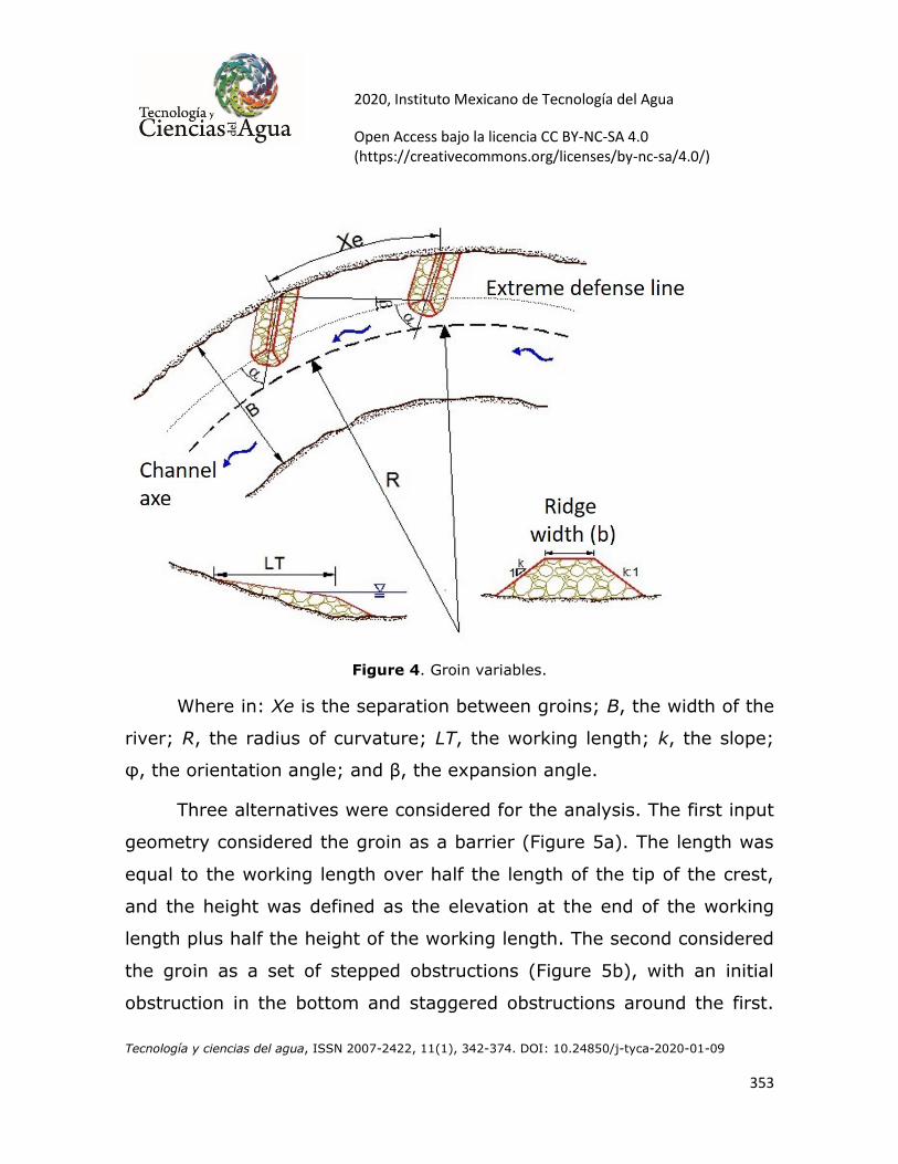
characterize the groynes are shown in Figure 4.
2020, Instituto Mexicano de Tecnología del Agua
Open Access bajo la licencia CC BY-NC-SA 4.0 (https://creativecommons.org/licenses/by-nc-sa/4.0/)
Tecnología y ciencias del agua, ISSN 2007-2422, 11(1), 342-374. DOI: 10.24850/j-tyca-2020-01-09
353
Figure 4. Groin variables.
Where in: Xe is the separation between groins; B, the width of the
river; R, the radius of curvature; LT, the working length; k, the slope;
φ, the orientation angle; and β, the expansion angle.
Three alternatives were considered for the analysis. The first input
geometry considered the groin as a barrier (Figure 5a). The length was
equal to the working length over half the length of the tip of the crest,
and the height was defined as the elevation at the end of the working
length plus half the height of the working length. The second considered
the groin as a set of stepped obstructions (Figure 5b), with an initial
obstruction in the bottom and staggered obstructions around the first.

2020, Instituto Mexicano de Tecnología del Agua
Open Access bajo la licencia CC BY-NC-SA 4.0 (https://creativecommons.org/licenses/by-nc-sa/4.0/)
Tecnología y ciencias del agua, ISSN 2007-2422, 11(1), 342-374. DOI: 10.24850/j-tyca-2020-01-09
354
The ridge width initially proposed in the groin was equivalent to the
working length, and the height was defined as the elevation at the end
of the working length plus half the height. The rest of the obstructions
were distributed in such a way as to cover the surface of the original
groin. The third option was to model the groin as a part of the natural
terrain (Figure 5c). The topography was modified, and Digital Terrain
Model DTM was generated. The construction of the digital terrain model
(DTM) was carried out from topographic data collected in the field.
Figure 5. Alternatives: A) physical barrier; b) stepped barriers, c) natural terrain.

2020, Instituto Mexicano de Tecnología del Agua
Open Access bajo la licencia CC BY-NC-SA 4.0 (https://creativecommons.org/licenses/by-nc-sa/4.0/)
Tecnología y ciencias del agua, ISSN 2007-2422, 11(1), 342-374. DOI: 10.24850/j-tyca-2020-01-09
355
Calibration
The numerical model was calibrated with the inlet, outlet, and derived
flow rates measured in the physical model, and the free surface water
levels measured at six sampling points h0-h6 (Figure 6). The roughness
coefficient was varied until the results of the numerical modeling
reproduced acceptably the results measured experimentally in the
physical model.
Figure 6. Variables measurement at the physical model: Qin, Input discharge; Qout,
output discharge; Qder, derivate discharge, h0 –h6, level meter samplers.
2020, Instituto Mexicano de Tecnología del Agua
Open Access bajo la licencia CC BY-NC-SA 4.0 (https://creativecommons.org/licenses/by-nc-sa/4.0/)
Tecnología y ciencias del agua, ISSN 2007-2422, 11(1), 342-374. DOI: 10.24850/j-tyca-2020-01-09
356
Once the model has been calibrated, we analyzed the differences
between the water surface levels measured experimentally and those
simulated numerically with the geometry options (barrier, stepped, and
natural terrain).
Choose the best way to input the geometry of the groynes, the full
arrangement was built (Figure 7), and was compared with the
experimental and the simulated hydraulics behavior.

2020, Instituto Mexicano de Tecnología del Agua
Open Access bajo la licencia CC BY-NC-SA 4.0 (https://creativecommons.org/licenses/by-nc-sa/4.0/)
Tecnología y ciencias del agua, ISSN 2007-2422, 11(1), 342-374. DOI: 10.24850/j-tyca-2020-01-09
357
Figure 7. Physical model and detail of the full groynes arrangement.
An alternative of the groynes arrangement

2020, Instituto Mexicano de Tecnología del Agua
Open Access bajo la licencia CC BY-NC-SA 4.0 (https://creativecommons.org/licenses/by-nc-sa/4.0/)
Tecnología y ciencias del agua, ISSN 2007-2422, 11(1), 342-374. DOI: 10.24850/j-tyca-2020-01-09
358
In addition to checking the numerical simulation of the arrangement of
groynes, it was decided to apply the numerical model for design
purposes. Therefore, the groynes design criteria considered in the Rivers
Engineering Manual (Maza-Alvarez et al., 1996) were revised, in terms
of the angle of expansion and orientation, the separation between
breakwaters and a working length of them. The objective was to
evaluate the possibility of using another kind of protection work that had
the same effect but could reduce the volume of work. The proposed
options were: a) the placement of a bank revetment (Figure 8a) and b)
combination of bank revetment with a minor arrangement of groynes
(Figure 8b). Both alternatives were modeled in HEC-RAS, and the
hydraulic profiles obtained, as well as the operating curves of the
derivation channel.
Figure 8. A) Bank revetment, b) Bank revetment + four groynes.

2020, Instituto Mexicano de Tecnología del Agua
Open Access bajo la licencia CC BY-NC-SA 4.0 (https://creativecommons.org/licenses/by-nc-sa/4.0/)
Tecnología y ciencias del agua, ISSN 2007-2422, 11(1), 342-374. DOI: 10.24850/j-tyca-2020-01-09
359
Results
Modeling natural conditions
Table 1 shows the proposed value of Manning (n), the numerical results,
and the experimental measurements under natural conditions.
Table 1. Calibration of the Manning roughness coefficient.
Roughness coefficient
“n”
Discharge
m3/s
Level
(masl)
0.025 1305 6.63
0.024 1357 6.61
0.023 1417 6.61
0.023 y 0.0226 downstream. 1438 6.59
Physical model 1450 6.60

2020, Instituto Mexicano de Tecnología del Agua
Open Access bajo la licencia CC BY-NC-SA 4.0 (https://creativecommons.org/licenses/by-nc-sa/4.0/)
Tecnología y ciencias del agua, ISSN 2007-2422, 11(1), 342-374. DOI: 10.24850/j-tyca-2020-01-09
360
Therefore, was chosen a Manning coefficient of 0.023 for the bend,
and 0.0226 for the output. Also, because both the curve and the
derivation channel were constructed with the same material, a Manning
coefficient of 0.023 was used in the derivation channel.
Geometrical input of the groynes
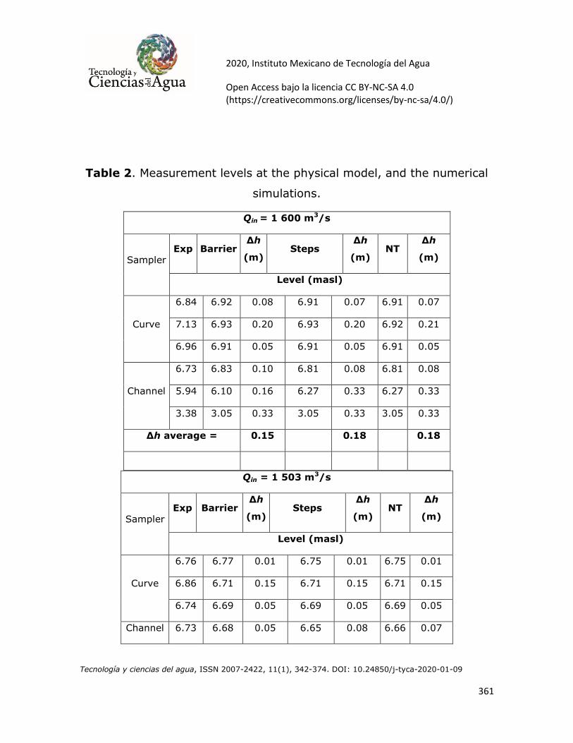
The hydraulic profiles measured in the physical model were compared
against the numerical simulations with the different ways of input the
geometry of the groynes. Table 2 shows the measured levels and those
generated from the numerical modeling at the sampler points in the
curve (h0, h3, and h4) and the derivation channel (h1, h5, and h6). In the
simulation, the three options of the geometry of the groynes were
considered: a) barrier, b) set of stepped obstructions (steps), and c)
natural terrain (NT). The range of the flows is from the moment in which
the channel starts to derive (1 000 m3/s), up to the overflow flow (1 600
m3/s).
2020, Instituto Mexicano de Tecnología del Agua
Open Access bajo la licencia CC BY-NC-SA 4.0 (https://creativecommons.org/licenses/by-nc-sa/4.0/)
Tecnología y ciencias del agua, ISSN 2007-2422, 11(1), 342-374. DOI: 10.24850/j-tyca-2020-01-09
361
Table 2. Measurement levels at the physical model, and the numerical
simulations.
Qin = 1 600 m3/s
Sampler Exp Barrier
Δh
(m) Steps
Δh
(m) NT
Δh
(m)
Level (masl)
Curve
6.84 6.92 0.08 6.91 0.07 6.91 0.07
7.13 6.93 0.20 6.93 0.20 6.92 0.21
6.96 6.91 0.05 6.91 0.05 6.91 0.05
Channel
6.73 6.83 0.10 6.81 0.08 6.81 0.08
5.94 6.10 0.16 6.27 0.33 6.27 0.33
3.38 3.05 0.33 3.05 0.33 3.05 0.33
Δh average = 0.15 0.18 0.18
Qin = 1 503 m3/s
Sampler Exp Barrier
Δh
(m) Steps
Δh
(m) NT
Δh
(m)
Level (masl)
Curve
6.76 6.77 0.01 6.75 0.01 6.75 0.01
6.86 6.71 0.15 6.71 0.15 6.71 0.15
6.74 6.69 0.05 6.69 0.05 6.69 0.05
Channel 6.73 6.68 0.05 6.65 0.08 6.66 0.07

2020, Instituto Mexicano de Tecnología del Agua
Open Access bajo la licencia CC BY-NC-SA 4.0 (https://creativecommons.org/licenses/by-nc-sa/4.0/)
Tecnología y ciencias del agua, ISSN 2007-2422, 11(1), 342-374. DOI: 10.24850/j-tyca-2020-01-09
362
5.81 5.97 0.16 6.11 0.30 6.11 0.30
3.69 2.93 0.76 2.93 0.76 2.93 0.76
Δh average = 0.20 0.23 0.22
Qin = 1 450 m3/s
Sampler Exp Barrier
Δh
(m) Steps
Δh
(m) NT
Δh
(m)
Level (masl)
Curve
6.64 6.70 0.06 6.68 0.04 6.68 0.04
6.79 6.62 0.17 6.62 0.17 6.62 0.17
6.57 6.60 0.03 6.60 0.03 6.60 0.03
Channel
6.50 6.61 0.11 6.59 0.09 6.59 0.09
5.62 5.92 0.30 6.05 0.43 6.05 0.43
2.61 2.89 0.28 2.89 0.28 2.89 0.28
Δh average = 0.16 0.17 0.17
Qin = 1 397 m3/s
Sampler Exp Barrier
Δh
(m) Steps
Δh
(m) NT
Δh
(m)
Level (masl)
Curve
6.66 6.59 0.07 6.56 0.10 6.57 0.09
6.62 6.47 0.15 6.47 0.15 6.47 0.15
6.50 6.45 0.05 6.45 0.05 6.45 0.05
Channel 6.57 6.50 0.07 6.47 0.10 6.48 0.09

2020, Instituto Mexicano de Tecnología del Agua
Open Access bajo la licencia CC BY-NC-SA 4.0 (https://creativecommons.org/licenses/by-nc-sa/4.0/)
Tecnología y ciencias del agua, ISSN 2007-2422, 11(1), 342-374. DOI: 10.24850/j-tyca-2020-01-09
363
5.54 5.85 0.31 5.97 0.43 5.97 0.43
3.42 2.82 0.60 2.82 0.60 2.82 0.60
Δh average = 0.21 0.24 0.24
Qin = 1 307 m3/s
Sampler Exp Barrier
Δh
(m) Steps
Δh
(m) NT
Δh
(m)
Level (masl)
Curve
6.57 6.48 0.09 6.45 0.12 6.46 0.11
6.48 6.32 0.16 6.32 0.16 6.32 0.16
6.33 6.30 0.03 6.30 0.03 6.30 0.03
Channel
6.4 6.4 0.00 6.37 0.03 6.37 0.03
5.53 5.75 0.22 5.84 0.31 5.84 0.31
3.31 2.73 0.58 2.73 0.58 2.73 0.58
Δh average= 0.18 0.21 0.20
Qin = 1 199 m3/s
Sampler Exp Barrier
Δh
(m) Steps
Δh
(m) NT
Δh
(m)
Level (masl)
Curve
6.40 6.50 0.10 6.29 0.11 6.30 0.10
6.24 6.32 0.08 6.13 0.11 6.13 0.10
6.10 6.30 0.20 6.10 0.00 6.10 0.00

2020, Instituto Mexicano de Tecnología del Agua
Open Access bajo la licencia CC BY-NC-SA 4.0 (https://creativecommons.org/licenses/by-nc-sa/4.0/)
Tecnología y ciencias del agua, ISSN 2007-2422, 11(1), 342-374. DOI: 10.24850/j-tyca-2020-01-09
364
Channel
6.33 6.43 0.10 6.22 0.11 6.22 0.11
5.31 5.62 0.31 5.70 0.39 5.70 0.39
3.13 2.62 0.51 2.62 0.51 2.62 0.51
Δh average= 0.22 0.21 0.20
Qin = 1 102 m3/s
Sampler Exp Barrier
Δh
(m) Steps
Δh
(m) NT
Δh
(m)
Level (masl)
Curve
6.28 6.18 0.10 6.14 0.14 6.15 0.13
6.00 5.93 0.07 5.93 0.07 5.93 0.07
5.96 5.90 0.06 5.90 0.06 5.90 0.06
Channel
6.10 6.11 0.01 6.07 0.03 6.08 0.02
5.15 5.48 0.33 5.53 0.38 5.53 0.38
3.04 2.51 0.53 2.51 0.53 2.51 0.20
Δh average = 0.18 0.20 0.14
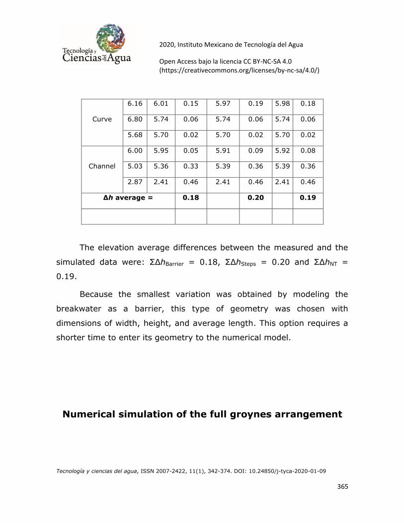
Qin = 1 000 m3/s
Sampler Exp Barrier
Δh
(m) Steps
Δh
(m) NT
Δh
(m)
Level (masl)
2020, Instituto Mexicano de Tecnología del Agua
Open Access bajo la licencia CC BY-NC-SA 4.0 (https://creativecommons.org/licenses/by-nc-sa/4.0/)
Tecnología y ciencias del agua, ISSN 2007-2422, 11(1), 342-374. DOI: 10.24850/j-tyca-2020-01-09
365
Curve
6.16 6.01 0.15 5.97 0.19 5.98 0.18
6.80 5.74 0.06 5.74 0.06 5.74 0.06
5.68 5.70 0.02 5.70 0.02 5.70 0.02
Channel
6.00 5.95 0.05 5.91 0.09 5.92 0.08
5.03 5.36 0.33 5.39 0.36 5.39 0.36
2.87 2.41 0.46 2.41 0.46 2.41 0.46
Δh average = 0.18 0.20 0.19
The elevation average differences between the measured and the
simulated data were: ΣΔhBarrier = 0.18, ΣΔhSteps = 0.20 and ΣΔhNT =
0.19.
Because the smallest variation was obtained by modeling the
breakwater as a barrier, this type of geometry was chosen with
dimensions of width, height, and average length. This option requires a
shorter time to enter its geometry to the numerical model.
Numerical simulation of the full groynes arrangement

2020, Instituto Mexicano de Tecnología del Agua
Open Access bajo la licencia CC BY-NC-SA 4.0 (https://creativecommons.org/licenses/by-nc-sa/4.0/)
Tecnología y ciencias del agua, ISSN 2007-2422, 11(1), 342-374. DOI: 10.24850/j-tyca-2020-01-09
366
Once determined the way to input the groin geometry at the model, the
next step was to input the full arrangement of the seven groynes. Due
to the effect produced by the whole groynes arrangement is mainly
reflected in the curve (sampler point h1), it was taken as a reference to
compare the experimental measurements against the numerical
simulations. Table 3 shows the experimental levels measured (Exp) and
those generated from the numerical modeling (Full). Column Δh listed
the levels difference between both results and the Δh average.
Table 3. Results of the levels at the derivation, with the full groynes arrangement.
Discharge h derived
Δh
(m) Qin Qder Exp Full
(m3/s) (masl)
1 438 639 6.94 6.86 0.08
1 397 596 6.89 6.76 0.13
1 309 500 6.76 6.68 0.08
1 204 385 6.57 6.59 0.02
1 102 294 6.42 6.46 0.04
1 001 223 6.28 6.31 0.03
Δh average = 0.06
It was observed that the variation between the measured and
the numerically simulated results averaged 0.06 m. It was considered
that this result is acceptable, and therefore, the numerical model
2020, Instituto Mexicano de Tecnología del Agua
Open Access bajo la licencia CC BY-NC-SA 4.0 (https://creativecommons.org/licenses/by-nc-sa/4.0/)
Tecnología y ciencias del agua, ISSN 2007-2422, 11(1), 342-374. DOI: 10.24850/j-tyca-2020-01-09
367
simulated the functioning of the derivation structure adequately. The
next step was to model an alternative that reproduced the same effect
caused by the arrangement of seven groynes, but with smaller work
volume.
Alternative to the arrangement of seven groynes
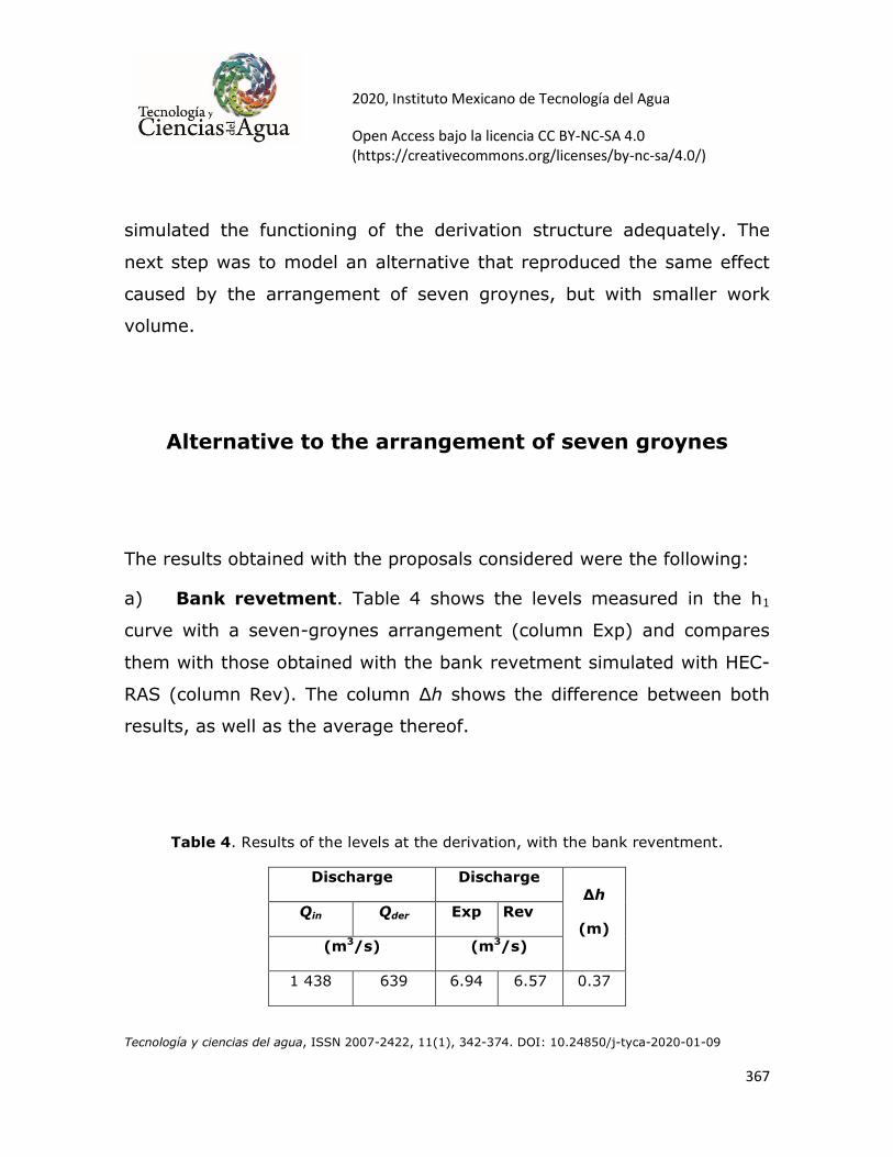
The results obtained with the proposals considered were the following:
a) Bank revetment. Table 4 shows the levels measured in the h1
curve with a seven-groynes arrangement (column Exp) and compares
them with those obtained with the bank revetment simulated with HEC-
RAS (column Rev). The column Δh shows the difference between both
results, as well as the average thereof.
Table 4. Results of the levels at the derivation, with the bank reventment.
Discharge Discharge
Δh
(m) Qin Qder Exp Rev
(m3/s) (m3/s)
1 438 639 6.94 6.57 0.37

2020, Instituto Mexicano de Tecnología del Agua
Open Access bajo la licencia CC BY-NC-SA 4.0 (https://creativecommons.org/licenses/by-nc-sa/4.0/)
Tecnología y ciencias del agua, ISSN 2007-2422, 11(1), 342-374. DOI: 10.24850/j-tyca-2020-01-09
368
1 397 596 6.89 6.44 0.45
1 309 500 6.76 6.33 0.43
1 204 385 6.57 6.19 0.38
1 102 294 6.42 6.03 0.39
1 001 223 6.28 5.86 0.42
Δh average = 0.41
It was observed that the average difference in the free surface
water between both configurations was 0.41 m. That is to say, that with
the marginal revetment it is not possible to adequately reproduce the
derivation effect.
b) Revetment and four groynes. Table 5 shows the levels measured in
the curve (h1) with the seven-groynes arrangement (column Exp) and
compares them against those obtained with the numerical modeling of
the revetment and proposes four-groynes arrangement (column Rev +
4G). In the column Δh, the difference in level between the results of the
numerical modeling and the experimental results is shown.
Table 5. Results of the levels at the derivation, with the bank reventment + four
groynes.
Discharge Discharge Δh
Qin Qder Exp Rev+4G Rev+4GH

2020, Instituto Mexicano de Tecnología del Agua
Open Access bajo la licencia CC BY-NC-SA 4.0 (https://creativecommons.org/licenses/by-nc-sa/4.0/)
Tecnología y ciencias del agua, ISSN 2007-2422, 11(1), 342-374. DOI: 10.24850/j-tyca-2020-01-09
369
(m3/s) (m3/s) m
1 438 639 6.94 6.81 0.13
1 397 596 6.89 6.70 0.19
1 309 500 6.76 6.62 0.14
1 204 385 6.57 6.52 0.05
1 102 294 6.42 6.39 0.03
1 001 223 6.28 6.24 0.04
Δh average = 0.10
It was observed that between the results of the experimental
measurements and the numerical modeling of the proposed alternative,
the average variation in the water sheet is 0.10 m, and the difference
between the results obtained with the modeling of the seven groynes
and the modeling of the combined the bank revetment with the
arrangement of four breakwaters is 0.04 m. It is considered that this
variation is not significant, so this alternative can adequately reproduce
the derivation effect.
Volume of work

2020, Instituto Mexicano de Tecnología del Agua
Open Access bajo la licencia CC BY-NC-SA 4.0 (https://creativecommons.org/licenses/by-nc-sa/4.0/)
Tecnología y ciencias del agua, ISSN 2007-2422, 11(1), 342-374. DOI: 10.24850/j-tyca-2020-01-09
370
Table 6 shows for comparative purposes, the estimated volume of work
required by each alternative.
Tabla 6. Comparison of the volume of work.
Original volume (m3)
A full arrangement of seven groynes 12 687.21
Alternative volume (m3)
Bank revetment 4 948.16
Arrangement of four groynes 6 024.28
Total = 10 972.44
Difference = 1 714.77
It was estimated a reduction in the volume of work of around 1
700 m3, which in economic terms represent a significant saving.
Conclusions

2020, Instituto Mexicano de Tecnología del Agua
Open Access bajo la licencia CC BY-NC-SA 4.0 (https://creativecommons.org/licenses/by-nc-sa/4.0/)
Tecnología y ciencias del agua, ISSN 2007-2422, 11(1), 342-374. DOI: 10.24850/j-tyca-2020-01-09
371
In the numerical simulations, the HEC-RAS software was used, which is
a hydraulic numerical model that can work in 1D or 2D. The objective
was to perform a hydraulic analysis on a river in which a diversion
channel was made, and marginal protection at a base of groynes was
built. The hydraulic phenomenon is evident three-dimensional (3D), so it
is thought that the use of 1D software, could be limited. HEC-RAS 1D
was used here, and its performance was contrasted against the
experimental data in a reduced physical model, taking into account the
acceptable results. It was found that the best way to model the groynes,
in this case, was also a barrier, as well as the numerical results
compared against the average the least difference (0.06 m). This option
requires a shorter time to enter the geometry in the model numerical.
There is also a mode of alternative protection consisting of a bank
revetment and four groynes, to find an arrangement to reproduce the
original effect for the arrangement of seven groynes, but with a smaller
volume of work. In this study was used the free surface level as a
parameter of comparison and calibration, found that HEC-RAS 1D
showed excellent performance for the hydraulic analysis of groynes in
curves. However, it is recommended once the 1D analysis has been
carried out and the final design has been chosen, to use a 2D model,
and carry out a sensibility analysis and contrast the results with those
obtained with the 1D model.

2020, Instituto Mexicano de Tecnología del Agua
Open Access bajo la licencia CC BY-NC-SA 4.0 (https://creativecommons.org/licenses/by-nc-sa/4.0/)
Tecnología y ciencias del agua, ISSN 2007-2422, 11(1), 342-374. DOI: 10.24850/j-tyca-2020-01-09
372
References
Bladé, E., Cea, L., Corestein, G., Escolano, E., Puertas, J., Vázquez-
Cendón, E., Dolz, J., & Coll, A. (2014). Iber: herramienta de
simulación numérica del flujo en ríos. Revista Internacional de
Métodos Numéricos para Cálculo y Diseño en Ingeniería, 30, 1-10.
Recovered from https://doi.org/10.1016/j.rimni.2012.07.004
Brunner, G. W. (2016). HEC-RAS 5.0 Users Manual.pdf. Davis, USA: US
Army Corps of Engineers, Institute of Water Resources, Hydrologic
Engineer Center. Recovered fromhttps://www.hec.usace.army.mil/
software/hec-ras/documentation/HEC-RAS% 205.0%20 Reference
%20 Manual.pdf
DHI. (2016). Mike 11. Hørsholm, Denmark: DHI.
Jiménez-León, E., Mendiola-Lizárraga, L., Rivera-Trejo, F., Nungaray-
Núñez, A., Díaz-Arcos, J. (2017). Cambio hidrodinámico y
evolución del fondo en ríos de planicie por espigones. Epistemus,
11, 27-35.
Kang, J., Yeo, H., Kim, S., & Ji, U. (2011). Experimental investigation on
the local scour characteristics around groynes using a hydraulic
model. Water and Environment Journal, 25, 181-191. Recovered
from https://doi.org/10.1111/j.1747-6593.2009.00207.x
Mawandha, H. G., Wignyosukarto, B. S., & Jayadi, R. (2018). Mini
polders as alternative flood management in the lower Bengawan
Solo river, Indonesia. Irrigation and Drainage, 67, 72-80.

2020, Instituto Mexicano de Tecnología del Agua
Open Access bajo la licencia CC BY-NC-SA 4.0 (https://creativecommons.org/licenses/by-nc-sa/4.0/)
Tecnología y ciencias del agua, ISSN 2007-2422, 11(1), 342-374. DOI: 10.24850/j-tyca-2020-01-09
373
Recovered from https://doi.org/10.1002/ird.2198
Maza-Alvarez, J. A., García-Flores, M., & Olvera-Salgado, R. (1996).
Estabilización y rectificación de ríos. Cap. 14. En: Manual de
ingeniería de ríos. México, DF, México: nstituto de ngenier a,
niversidad acional ut noma de xico
McCoy, A., Constantinescu, G., & Weber, L. (2007a). A numerical
investigation of coherent structures and mass exchange processes
in channel flow with two lateral submerged groynes. Water
Resources Research, 43. Recovered from
https://doi.org/10.1029/2006WR005267
McCoy, A., Constantinescu, G., & Weber, L. (2007b). Hydrodynamics of
flow in a channel with two lateral submerged groynes. World
Environmental and Water Resources Congress 2007 (pp. 1-11),
American Society of Civil Engineers, Reston, USA. Recovered from
https://doi.org/10.1061/40927(243)118
McCoy, A., Constantinescu, G., & Weber, L. J. (2008). Numerical
investigation of flow hydrodynamics in a channel with a series of
groynes. Journal of Hydraulic Engineering, 134, 157-172.
Recovered from https://doi.org/10.1061/(ASCE)0733-
9429(2008)134:2(157)
Minor, B., Rennie, C. D., & Townsend, R. D. (2007) “Barbs” for river
bend bank protection: Application of a three-dimensional
numerical model. Canadian Journal of Civil Engineering, 34, 1087-
1095. Recovered from https://doi.org/10.1139/l07-088

2020, Instituto Mexicano de Tecnología del Agua
Open Access bajo la licencia CC BY-NC-SA 4.0 (https://creativecommons.org/licenses/by-nc-sa/4.0/)
Tecnología y ciencias del agua, ISSN 2007-2422, 11(1), 342-374. DOI: 10.24850/j-tyca-2020-01-09
374
Nguyen, Q. B., Vo, N. D., & Gourbesville, P. (2018). Flow around
groynes modelling in different numerical schemes. 13th
International Conference on Hydroinformatics, HIC 2018 (pp.
1513-1502), Palermo, Italy, July, 1-6. Recovered from
https://doi.org/10.29007/2nlb
Qin, J., Zhong, D., Wu, T., & Wu, L. (2017). Advances in water
resources sediment exchange between groin fields and main-
stream. Advances in Water Resources, 108, 44-54. Recovered
from https://doi.org/10.1016/j.advwatres.2017.07.015
Rau-Lavado, P. C. (2007). Comparación de modelos unidimensionales y
bidimensionales en la simulación hidráulica de ríos. Aplicación al
río Majes-sector Querulpa-Tomaca. Lima, Perú: Universidad
Nacional de Ingeneiría.
Rivera-Trejo, F., Soto-Cortés, G., & Barajas-Fernández, J. (2009). The
2007 flooding in Tabasco, Mexico: Evolution of water levels.
Ingenieria Hidraulica en México, 24(4), 159-166.
Sukhodolov, A. N. (2014). Hydrodynamics of groyne fields in a straight
river reach: Insight from field experiments hydrodynamics of
groyne fields in a straight river reach: Insight from field
experiments. Journal of Hydraulic Research, 1, 105-120.
Recovered from https://doi.org/10.1080/00221686.2014.880859
Weitbrecht, V., Socolofsky, S. A., & Jirka, G. H. (2008). Experiments on
mass exchange between groin fields and main stream in rivers.
Journal of Hydraulic Engineering, 134, 173-183. Recovered from

2020, Instituto Mexicano de Tecnología del Agua
Open Access bajo la licencia CC BY-NC-SA 4.0 (https://creativecommons.org/licenses/by-nc-sa/4.0/)
Tecnología y ciencias del agua, ISSN 2007-2422, 11(1), 342-374. DOI: 10.24850/j-tyca-2020-01-09
375
https://doi.org/10.1061/(asce)0733-9429(2008)134:2(173)
Zhang, Y., Chen, G., Hu, J., Chen, X., Yang, W., & Tao, A. (2017).
Experimental study on mechanism of sea-dike failure due to wave
overtopping. Physics Procedia, 68, 171-181. Recovered from
https://doi.org/10.1016/j.apor.2017.08.009