risk sharing among large and small countries

Introduction Model Edgeworth Box Welfare Two-factor model Conclusions

Risk Sharing among Large and Small Countries

Giancarlo CorsettiUniversity of Cambridge and CEPR

Anna LipinskaFederal Reserve Board

November 10 2017

The views expressed here should not be interpreted as reflecting the views ofthe Federal Reserve System.


The Question• Ongoing debate on the degree of international risk sharing

between countries and how to increase it.

• globally: performance of capital markets in achieving risksharing among countries (Fratzscher and Imbs 2009) andreform of international institutions.

• in Europe: what policies should be implemented to enhancerisk sharing? (e.g. Fatas 1998, or more recently Farhi andWerning 2017, Beblavy et al 2015).

• Countries differ in size and risk profile:What are the macroeconomic implications/effects ofarrangements that improve sharing of macroeconomic riskamong asymmetric countries?

• To what extent can these implications hamper integration, byraising political economy and distributional issues?

• Asymmetry challenges macro modelling.


This Paper

• We present a stylized analysis of risk sharing arrangements(operating either via capital market integration orinstitutions), with the goal of deriving broad implications forpolicy and empirical studies.

• For simplicity:

• two-period model.• risk is only fundamental, output process is exogenous

(endowment economies).• one good model (PPP holds, RER=1).• no frictions, except for possibility of market incompleteness.

• In our setup, barring risk sharing (status quo), countries wouldhave identical per capita income on average....but can differ in size and stochastic properties of businesscycle.


Main Message

• Relative income and aggregate demand changes whencountries enter either risk or income sharing arrangements (viamarket integration or institution).

• The shadow price of domestic (state-contingent) output maydiffer across borders: in an equilibrium with perfect risksharing, the value of output flows at market prices may rise orfall.

• Perfect risk sharing involves an implicit efficient transfer(redistribution) reflecting the ”pecuniary” effects of priceadjustment.

• Key: enhancing risk sharing, the level of national demandmay thus rise or fall relative to the status quo.


Implications (1)Political Economy

• Asymmetries between regions affect political equilibrium andthus degree of risk sharing provided by regional publictransfers (e.g. Persson and Tabellini (1996)).

• Because of asymmetries across countries, schemes pursuingincome pooling (i.e. redistribution targeting average incomeacross borders) will generally lead to allocations that differfrom complete-market, and may not be Pareto improving.


Implications (2)Quantitative and Empirical Studies

• In quantitative models, approximation around non-stochasticsteady state fails to take into account the equilibrium price ofrisk.• Up to first order, asymmetry among countries does not matter

and thus income pooling is equivalent to complete markets.

• Up to second order, neglecting the effect of asymmetry on thesteady state may lead to spurious “welfare reversals”.

• Measure of risk sharing focused on equalization of (RERadjusted) consumption growth rates may be confounded bystep adjustment in consumption levels at time of regimechanges (capital market reforms).

• Consumption growth rates may not be equalised at the time ofof a risk-sharing enhancing reform.


Literature

• Theoretical discussion in quantitative studies see Cole andObstfeld (1991), Kim and Kim (2003), Chari et al (2002),Tille and Pesenti (2004).

• Gains from financial integration depend on the stochasticproperties, size and degree of financial development ofcountries (Rey et al (2016)).

• Discussion of institutions that could enhance risk sharing inthe European Union (EU Commission Reflection Paper(2017)).

• A vast literature on estimating level of risk sharing (Asdrubaliet al (1996), Bayoumi and Klein (1997), Furceri andZdzienicka (2015), Sala-i-Martin and Sachs (1991), Sorensenand Yosha (1998), von Hagen and Hepp (2013)).


Outline

• Model (one factor).

• Different Risk Sharing Arrangements: Complete Markets,Income Pooling and Financial Autarky.

• Edgeworth box and country size.

• Welfare.

• Generalization (two factors).


Analytical Framework

• Two-period endowment model with two countries (H and F)differing in size and output process.

• First example: Asymmetric volatility—a single global shockwith different factor loadings for each country.• In second example we show that results generalize to

country-specific shocks.

• We contrast three different arrangements:

1. complete markets (CM),2. income pooling (IP) (equalisation of home and foreign

consumption),3. financial autarky (FA).

• Welfare analysis under the second order approximation withlog utility, U(Ci ) = log(Ci ) where i = H,F .


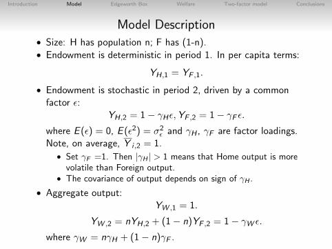
Model Description• Size: H has population n; F has (1-n).• Endowment is deterministic in period 1. In per capita terms:

YH,1 = YF ,1.

• Endowment is stochastic in period 2, driven by a commonfactor ε:

YH,2 = 1− γHε,YF ,2 = 1− γF ε.where E (ε) = 0, E (ε2) = σ2ε and γH , γF are factor loadings.Note, on average, Y i ,2 = 1.

• Set γF =1. Then |γH | > 1 means that Home output is morevolatile than Foreign output.

• The covariance of output depends on sign of γH .

• Aggregate output:YW ,1 = 1.

YW ,2 = nYH,2 + (1− n)YF ,2 = 1− γW ε.where γW = nγH + (1− n)γF .


Complete Markets Allocation

• Consumption growth rates in each country are equalisedacross all states of nature.

• In levels, consumption in each country is a fraction of theworld endowment (see e.g. Obstfeld and Rogoff (1996)):

Ci ,t = µiYW ,t .

where µi =

Yi,1YW ,1

+βE

(Yi,2YW ,2

)1+β .

• Up to second order approx, E(

YH,2

YW ,2

)≈ 1 + (γW − γH)γWσ

2ε .

• Home and Foreign consumption shares:

µH = 1 +βγW (γW − γH)

1 + βσ2ε , µF = 1 +

βγW (γW − γF )

1 + βσ2ε .


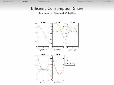
Efficient Consumption ShareAnalytical Representation

µi = 1 +βγW (γW − γi )

1 + βσ2ε

where i = H,F and γW = nγH + (1− n)γF .

• Up to first order, µi = 1 implying that CH,t = CF ,t , wheret = 1, 2.

• Up to second order, µi can be higher or lower than 1:

• Home and Foreign consumption share increase in the difference(γW − γi ).

• γi can be negative which can result in negative γW .

• γW is a function of the size of the country: the larger thecountry the larger its influence on the world output and γW .


Efficient Consumption ShareAsymmetric Size and Volatility


Consumption: Levels vs Growth ratesunder different risk-sharing arrangements

• consumption LEVELS are equalized under IP:

CH,t = CF ,t where t = 1, 2.:

...as well as (by construction in our example) under FA inperiod 1:

CH,1 = 1 = CF ,1

(recall: CH,2 = 1− γHε 6= CF ,2 yet CH = CF = 1.)

• may not be equalized under CM, because of the endogenousadjustment of income to the price of risk:

CH,1 = µH ,CH,2 = µHYH,2 with CH = µH .

• Consumption GROWTH RATES instead are equalizedunder both CM and IP, not under FA.


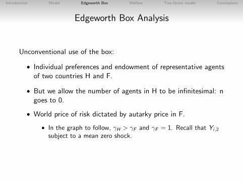
Edgeworth Box Analysis

Unconventional use of the box:

• Individual preferences and endowment of representative agentsof two countries H and F.

• But we allow the number of agents in H to be infinitesimal: ngoes to 0.

• World price of risk dictated by autarky price in F.

• In the graph to follow, γH > γF and γF = 1. Recall that Yi,2

subject to a mean zero shock.


Edgeworth BoxFinancial Autarky

E

H

FPreference and endowment of representative agents in country H and F

output in state 2

output in state 1

output in state 1

output in state 2


Edgeworth BoxBudget Constraint and Autarky World Prices

E

then FFA prices=world prices.

H

F

FAH

world prices

Size of H ->0; size of F->1


Edgeworth BoxComplete Markets

E

CMH

Clearly, at the complete market prices, Home gains: CMH>FAH

H

F

FAH

Agents in the large country keep consuming their endowment


Edgeworth BoxIncome Pooling

E=IPF

CMH

H

F

FAH

Now, suppose H and F ''pool income"

From the vantage point of H, IPH mirrors IPF

All agents consume the same average income in F: E=IPF

IPH


Comparing Risk Sharing ArrangementsIP is a good deal for Home: case of high volatility of output with γH = 2

E=IPF

IPH

CMH

IPH>CMH>FAH

H

F

FAH

The price of risk is equalised worldwide at FFA prices


Comparing Risk Sharing ArrangementsBut income pooling may also be a bad deal for Home

output variance high but covariance negative γH = −2, (γF = 1)

γH=-2 implies CMH>IPH>FAH

IPH

CMH

E=IPF

H

F


Comparing Risk Sharing ArrangementsHome may even be better off in FA

volatility of output not too high, e.g. γH = 0.5, (γF = 1)

IPH

ECMH

γH=.5 implies CMH>FAH>IPH

H

F


Welfare analysis in the general caseSecond Order Approximation

We now reconsider welfare ranking using:

E (log(CH)) = E (log(CH) +1

CH

E (CH − CH)− 1

C2H

E (CH − CH)2

Home loss under different risk sharing arrangements:

• FA: LFAH = β2γ

2Hσ

2ε .

• CM: LCMH = −β(γW − γH)γWσ2ε + β

2γ2Wσ

2ε .

• IP: LIPH = β2γ

2Wσ

2ε .


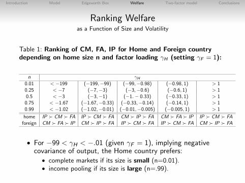
Ranking Welfareas a Function of Size and Volatility

Table 1: Ranking of CM, FA, IP for Home and Foreign countrydepending on home size n and factor loading γH (setting γF = 1):

n γH0.01 < −199 (−199,−99) (−99,−0.98) (−0.98, 1) > 10.25 < −7 (−7,−3) (−3,−0.6) (−0.6, 1) > 10.5 < −3 (−3,−1) (−1.− 0.33) (−0.33, 1) > 1

0.75 < −1.67 (−1.67,−0.33) (−0.33,−0.14) (−0.14, 1) > 10.99 < −1.02 (−1.02,−0.01) (−0.01,−0.005) (−0.005, 1) > 1

home IP � CM � FA IP � CM � FA CM � IP � FA CM � FA � IP IP � CM � FAforeign CM � FA � IP CM � IP � FA IP � CM � FA IP � CM � FA CM � IP � FA

• For −99 < γH < −.01 (given γF = 1), implying negativecovariance of output, the Home country prefers:• complete markets if its size is small (n=0.01).• income pooling if its size is large (n=.99).


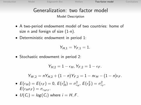
Generalization: two factor modelModel Description

• A two-period endowment model of two countries: home ofsize n and foreign of size (1-n).

• Deterministic endowment in period 1:

YH,1 = YF ,1 = 1.

• Stochastic endowment in period 2:

YH,2 = 1− εH ,YF ,2 = 1− εF .

YW ,2 = nYH,2 + (1− n)YF ,2 = 1− nεH − (1− n)εF .

• E (εH) = E (εF ) = 0, E (ε2H) = σ2εH , E (ε2F ) = σ2εF ,E (εHεF ) = σεHεF .

• U(Ci ) = log(Ci ) where i = H,F .


Complete Market allocationin the two-factor model

• Consumption in each country is a fraction of the world

endowment with µi =

Yi,1YW ,1

+βE

(Yi,2YW ,2

)1+β .

• E(

YH,2

YW ,2

)≈ 1 + n(n− 1)σ2εH + (1− n)2σ2εF + 2n(1− n)σεHεF .

• Home consumption share:

µH = 1 +β(1− n)(n(σεHεF − σ2εH )− (1− n)(σεHεF − σ2εF ))

1 + β.

• if n→ 0 then µH = 1 +β(σ2

εF−σεH εF )1+β .

• In general, ∂µH∂σ2εH

= −β(1−n)n1+β and ∂µH

∂σεH εF= β(1−n)(2n−1)

1+β .


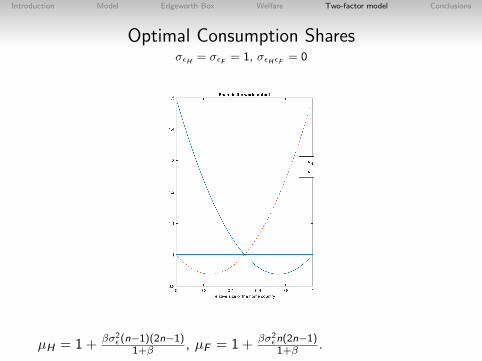
Optimal Consumption SharesσεH = σεF = 1, σεHεF = 0

µH = 1 + βσ2ε(n−1)(2n−1)

1+β , µF = 1 + βσ2εn(2n−1)1+β .


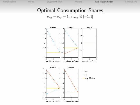
Optimal Consumption SharesσεH = σεF = 1, σεHεF ∈ [−1, 1]


What do we learn?

• Countries that are ex ante identical but for size, may end upwith a different level of (consumption) demand with full risksharing.

• Smaller countries gain. Intuitively, the equilibrium price of riskis close to the FA prices of the larger country.

• The gains are larger, the more negative the covariance ofoutput is.


Consumption LevelTwo-factor model

1. By construction, we have an example in which consumptionlevels in period 1 are equalized under financial autarky.

CH,1 = 1,CH,2 = 1− εH ,CH = 1.

2. as well as with income pooling:

CH,t = CF ,t where t = 1, 2.:

CH,1 = 1,CH,2 = (1− nεH − (1− n)εF ),CH = 1.

3. Under complete markets, however, because of the endogenousadjustment of income to the price of risk, Consumption is notequalized in period 1.

CH,1 = µH ,CH,2 = µH(1− nεH − (1− n)εF ),CH = µH .


WelfareTwo-factor model

Home loss under different risk sharing arrangements:

• FA: LFAH = β2σ

2εH

.

• CM: LCMH = −β(1− n)(n(σεHεF − σ2εH )− (1− n)(σεHεF −σ2εF )) + β

2 (n2σ2εH + (1− n)2σ2εF + 2n(1− n)σεHεF ).

• IP: LIPH = β2 (n2σ2εH + (1− n)2σ2εF + 2n(1− n)σεHεF ).


Welfare Rankingas a Function of Size and Volatility

Table 2: Ranking of CM, IP, FA for Home and Foreign countrydepending on home size n and σ2

εH(σεF = 1 and σεHεF = 0)

n σ2εH0.01 < 0.98 (0.98, 99) (99, 199) > 1990.25 < 0.6 (0.6, 3) (3, 7) > 70.5 < 0.33 (0.33, 1) (1, 3) > 3

0.75 < 0.14 (0.14, 0.33) (0.33, 1.67) > 1.670.99 < 0.005 (0.005, 0.01) (0.01, 1.02) > 1.02

home CM � FA � IP CM � IP � FA IP � CM � FA IP � CM � FAforeign IP � CM � FA IP � CM � FA CM � IP � FA CM � FA � IP

• For 0.01 < σ2εH < 99 (given σεF = 1) Home country prefers:• complete markets if its size is small (n=0.01).• income pooling if its size is large (n=.99).


Conclusions

• We reconsider the implications of risk sharing arrangementsamong countries that differ in size and business cycle.

• As the shadow price of future contingent output differs acrossborders, reforms that enhance risk-sharing necessarily lead toa change in relative income and (consumption) demandvis-a-vis the status quo.

• Potential implications for the political economy of institutionalreform and capital market integration.• large countries would prefer arrangement implementing income

pooling while small countries would prefer complete markets.

• Macro modeling of risk sharing:• Asymmetries among countries underline importance of second

order approximation around the stochastic steady state.


Research Directions

• Modeling risk sharing among asymmetric countries.

• Portfolio adjustment as a function of risk sharingarrangements.

• Unemployment and labor income risk insurance.

• Interaction of financial frictions with other distortions.• In our examples, pecuniary externalities from moving to

complete markets are efficient (since there are no distortionsother than incomplete markets).For an example in which these externalities may lower welfare(because of nominal rigidities and single monetary policy), seeAuray and Equyem (2014).

.


AppendixComplete Markets: Utility Maximisation

maxU(CH) = u(CH,1) +S∑

s=1

βπ(s)u(CH,2(s))

subject to:

CH,1 +S∑

s=1

p(s)

1 + rCH,2(s) = YH,1 +

S∑s=1

p(s)

1 + rYH,2(s)

Home and Foreign Euler equations:

CH,2(s) =

[π(s)β

(1 + r)

p(s)

] 1ρ

CH,1;CF ,2(s) =

[π(s)β

(1 + r)

p(s)

] 1ρ

CF ,1

risk sharing among large and small countries

Documents