risk, return and cash flow characteristics of ... · risk, return and cash flow characteristics of...

Risk, Return and Cash Flow Characteristics of

Infrastructure Fund Investments∗

Florian Bitsch†

Axel Buchner‡

Christoph Kaserer§

November 1, 2010

∗The authors would like to thank Nico Engel, Christian Figge, Christian Fingerle and the participantsof the ERSA Summer School 2010 for helpful comments. Financial support by the European InvestmentBank through the EIBURS programme as well as support by Timo Valila is also gratefully acknowledged.Any errors remain those of the authors. The findings, interpretations and conclusions presented in thisarticle are entirely those of the authors and should not be attributed in any manner to the EuropeanInvestment Bank.†Florian Bitsch ([email protected]) is research assistant at the Center for Entrepreneurial

and Financial Studies (CEFS), TUM Business School, Technische Universitat Munchen.‡Axel Buchner ([email protected]) is postdoctoral researcher at Technische Universitat

Munchen and consultant at the Center of Private Equity Research (CEPRES).§Christoph Kaserer ([email protected]) is full professor at Technische Universitat

Munchen and is holding the chair for Financial Management and Capital Markets. He is also co-headof the Center for Entrepreneurial and Financial Studies (CEFS).

Risk, Return and Cash Flow Characteristics of

Infrastructure Fund Investments

Abstract

We analyze the risk, return and cash flow characteristics of infrastructure invest-

ments by using a unique dataset of deals done by private-equity-like investment

funds. We show that infrastructure deals have a performance that is higher than

that of non-infrastructure deals, despite lower default frequencies. However, we

do not find that infrastructure deals offer more stable cash flows. Our paper of-

fers some evidence in favour of the hypothesis that higher infrastructure returns

could be driven by higher market risk. In fact, these investments appear to be

highly levered and their returns are positively correlated to public equity markets,

but uncorrelated to GDP growth. Our results also indicate that returns could

be influenced by the regulatory framework as well as by defective privatization

mechanisms. By contrast, returns are neither linked to inflation nor subject to the

‘money chasing deals’ phenomenon.

JEL Classification: G23, G24

1 Introduction

In this paper, we analyze the risk, return and cash flow characteristics of infrastructure

investments and compare them to non-infrastructure investments. It is generally argued

in the literature that infrastructure investments offer typical characteristics such as long-

term, stable and predictable, inflation-linked returns with low correlation to other assets

(Inderst 2009, p. 7). However, these characteristics attributed to infrastructure in-

vestments have not yet been proven empirically. The goal of this paper is to fill this

gap and provide a more thorough understanding of infrastructure returns and cash flow

characteristics.

One of the main obstacles in infrastructure research has been the lack of available

data. In this paper we make use of a unique and novel dataset of global infrastructure and

non-infrastructure investments done by unlisted funds. Overall, we have information on

363 fully-realized infrastructure and 11,223 non-infrastructure deals. The special feature

of the data is that they contain the full history of cash flows for each deal. This enables

us to study the risk, return and cash flow characteristics of infrastructure investments

and to draw comparisons between infrastructure and non-infrastructure investments.

Our results indicate that infrastructure deals have a performance that is uncorrelated

to macroeconomic development and that is higher than that of non-infrastructure deals

despite lower default frequencies. However, we do not find that infrastructure deals offer

cash flows that are more stable, longer term, inflation-linked or uncorrelated to public

equity markets. To measure ‘stability’, we introduce a measure of the variability of cash

outflows from the portfolio company to the fund. We also find evidence that infrastruc-

ture assets are higher levered but that they have not been exposed to overinvestment

as often stated. Finally, we offer some evidence that higher returns might be driven by

higher market risk or higher political risk. However, returns in the infrastructure sector

might also be driven by defective privatization mechanisms.

This article contributes to the emerging literature on infrastructure financing. Recent

publications in this area include Newell and Peng (2007; 2008), Dechant and Finken-

zeller (2009) or Sawant (2010a). These previous studies exclusively focus on data from

listed infrastructure stocks, indices of unlisted infrastructure investments or infrastruc-

ture project bonds. In contrast, we are the first to use data of unlisted infrastructure

1

fund investments.

The article is structured as follows. Section 2 highlights the importance and need

for infrastructure assets and summarizes what forms of infrastructure investments are

available for investors. Section 3 describes the main investment characteristics that are

assumed to be infrastructure-specific and derives the hypotheses on infrastructure fund

investments to be tested in this paper. Section 4 describes our database and sample

selection. Section 5 presents and discusses the empirical results. Section 6 summarizes

the findings and gives an outlook on future research in this area.

2 Infrastructure investments

2.1 The infrastructure investment gap

Several studies estimate that in the course of the 21st century, increasing amounts of

money need to be spent on infrastructure assets globally. In this context, infrastructure

is generally understood as assets in the transportation, telecommunication, electricity

and water sectors (OECD 2007, p. 21). Sometimes other energy-related assets such as

oil and gas transportation and storage or social institutions such as hospitals, schools or

prisons are included as well.

These estimates are based on an increasing need for such assets in developing coun-

tries due to population growth but also economic development. More people need more of

the existing infrastructure but they also need new infrastructure, such as better telecom-

munication or transportation systems when entering globalized markets. But also the

developed markets will show an increasing demand for infrastructure assets based on

these studies: despite a rather decreasing population, existing but aging infrastructure

systems need to be replaced. Moreover, technological progress is an important factor for

emerging and developed countries alike as it enables and partly requires more spending

on infrastructure assets. This is the case when, for example, upgrading the power grids

to match the special requirements of the newly installed offshore wind energy parks.

Taken together, needs of worldwide infrastructure investments between 2005 and 2030

could be as high as USD 70,000 billion according to the OECD (OECD 2007, p. 22 and

p. 97).

2

Although high needs and future demands for infrastructure assets are generally rec-

ognized, the factor that typically constrains the provision of these goods is the lack

of financing resources: The governments of the emerging countries often have not yet

established the capabilities to finance and administer the high number and volumes of

projects targeted, whereas the governments of the developed countries are struggling

with rising social expenditures - partly due to an ageing population - and thus limited

budgets for infrastructure (OECD 2007, p. 24). While infrastructure assets have histor-

ically been, and still are to a large extent, financed by the public sector, this traditional

financing source is unlikely to cover the large estimated investment needs (OECD 2007,

p. 29). This gap between the projected needs for infrastructure assets and the supply

thereof has found a popular description as the ‘infrastructure investment gap’ (OECD

2007, p. 14).

A natural idea to solve this problem is to make the infrastructure sectors more ac-

cessible for private investors to cover a fraction of the investment needed. Considering

assets under management of about USD 25,000 billion (OECD 2010, p. 2) or a weighted

average asset-to-GDP ratio for pension funds of 67.1 percent in 2009 (OECD 2010, p.

8) in the funded-pension markets of OECD countries only, suggests that institutional

investors, such as pension funds or insurance companies, could narrow the infrastruc-

ture investment gap to a large extent if they invested a proportion of their assets in

infrastructure assets. Some pension funds have already started doing this with some

individual funds showing an infrastructure share of over 10 percent (Inderst 2009, p. 3

and p. 13; Beeferman 2008, p. 16). Nevertheless, only a small proportion of overall

pension assets are allocated to infrastructure (OECD 2010, p. 37).

Whatever the amount of capital that could be invested by institutional investors, it

is not even clear yet to what extent infrastructure assets are suitable investments for

private investors. To analyze this, we next give an overview of the forms of investment

into infrastructure that are available to investors.

2.2 Forms of investment

Investors not only have to decide on the optimal share of infrastructure assets in their

portfolio but also on the form of investment within the infrastructure sector. The various

3

forms of investment have different profiles regarding minimum-capital requirement or

time horizon on the one hand and the various risks associated, such as liquidity or

political risk, on the other hand. Figure 1 gives a schematic overview.1

[Insert Figure 1 about here]

Making direct investments into infrastructure assets such as toll roads or power

plants usually requires the longest time horizon for an investor since infrastructure as-

sets have a long life of up to 60 years on average (Rickards 2008). Some concessions

can even last as long as 99 years (Beeferman 2008, p. 7). Due to the physical nature of

these assets, direct investments cannot easily be sold on and thus bear a high liquidity

risk as well. Since infrastructure assets are, on average, very capital-intensive, there are

also large capital requirements for single investors as well as the (usually small) group

of co-investors. Furthermore, committing a high amount of capital over a long period of

time into a single infrastructure asset exposes the investor to high political and regula-

tory risk. In case a country in which the asset is located changes the legal framework or

even attempts an expropriation, investors can hardly react flexibly. Overall, only a few

investors like insurance companies or pension funds would be capable of making invest-

ments with such characteristics and only recently have these investments become more

popular with them (Inderst 2009, p. 3). There are special forms of direct infrastructure

investments, the most prominent being those using Public Private Partnerships (PPPs)

or project finance structures (see Valila 2005 and Esty 2003 and 2010, respectively, for

overviews of these forms of investment).

The disadvantage of a high capital requirement can be eliminated to a large extent

by investing in direct and indirect listed securities of companies that operate in sectors

relevant to infrastructure, where the amount of capital committed can be set almost ar-

bitrarily. This makes portfolio diversification easier, reducing exposure to single-country

political and regulatory risk. Moreover, the high fungibility of listed securities reduces

the liquidity risk. Also, the time horizon is lower for listed securities, typically a couple

of years. Indexes of listed infrastructure securities and listed infrastructure funds inher-

ently provide for an even better diversification of the business risk of a single company.

1For an overview of additional categories refer to Beeferman (2008, pp. 18-23).

4

Unlisted infrastructure funds also provide less concentrated business risk through

diversification effects and enable smaller investors to participate in unlisted infrastruc-

ture assets through a smaller minimum capital requirement than for unlisted direct

investments. Starting with the launch of the first fund of this kind in 1993, this form of

investment has become one of the most specialized and rapidly growing ones, comprising

over 70 funds with an average fund size of USD 3.3 billion in 2008 (Preqin 2008; Orr

2007; and Inderst 2009, p. 11).

Such funds are usually structured as Limited Partnerships like in the private-equity

industry. The fund manager - called General Partner - collects money from investors,

the Limited Partners, and invests it in portfolio companies on their behalf over a spec-

ified period of time. The committed capital is returned to the investor in the form of

distributions (cash outflows from the point of view of the fund manager) once portfolio

companies could be sold off at prices above those at which they were originally bought.

In the following, we refer to ‘deal’ as a single investment by the fund through which the

fund participates in the underlying portfolio company. Thereby the deal size can range

between 0 percent and 100 percent of the asset value. However, cash flows between

portfolio companies and the fund usually differ from cash flows between the fund and

investors for at least two reasons: first, a fund participates in more than one investment;

and second, the manager receives fees for administration and management of the fund

which are deducted from the fund’s assets.

In our analysis, we concentrate on single deals by such funds and on the cash flow

between the portfolio company and the fund. To the best of our knowledge, we are the

first to provide empirical evidence on this form of investment from an academic point of

view.

Almost all forms of investment mentioned before can be carried out using debt or

equity financing. Our sample of infrastructure fund investments contains only equity

investments since in this way the risk profile of infrastructure investments can be better

traced.2 Equity funds dominate the market for infrastructure fund investments. Debt

financing through private investment vehicles is still quite uncommon.

2Infrastructure funds also use mezzanine or debt financing for their assets. The latter is primarilylent by banks and not provided by the funds themselves. The first infrastructure fund that investsexclusively in infrastructure debt was launched in 2009 (Sawant 2010b, p. 93).

5

From a theoretical perspective, however, infrastructure projects are expected to be

debt-financed to a significant extent as ceteris paribus, the agency cost of debt is lower

compared to non-infrastructure projects. According to the Free Cash Flow Hypothe-

sis, a high level of debt has a disciplinary effect on managers and prevents them from

investing in negative net-present-value (NPV) projects (Jensen 1986). Sawant (2010b,

pp. 73-81) argues that this mechanism is particularly relevant for infrastructure assets.

First, they allegedly provide stable cash flows that can be used to cover a higher level

of debt obligations. Second, infrastructure assets have fewer growth options. This fur-

ther hinders management from over-investing in negative NPV projects, as investment

decisions can be monitored more easily by external claimholders.

In the next section we propose eight hypotheses on allegedly infrastructure-specific

characteristics that we will test with our data of equity fund investments in Section 5.

3 Hypotheses

When analyzing equity infrastructure fund investments we question whether this form

of investment offers alleged infrastructure-specific investment characteristics. So far,

infrastructure is often referred to as a new asset class in the context of asset al location.

For example, large investors such as pension funds have dedicated specific allocation

targets for infrastructure, be it separately or within the budget of real assets, inflation-

sensitive investments or alternative investments (Orr 2007, p. 81, Beeferman 2008, p.

15). But there is a large variance in how to practically treat these assets in a portfolio

context even disregarding the fact that there is no academic consensus on the exact

definition of an ‘asset class’ and its constituting characteristics.

We therefore do not take a stance on the question of an asset class for the reasons

mentioned above.3

However, what most publications and comments on infrastructure investments agree

on is that such investments exhibit special investment characteristics. Therefore, it is

the goal of this paper to analyze whether the most commonly postulated characteristics

can be observed empirically at the deal level.

3For a discussion on infrastructure investments as an asset class, see Inderst (2010).

6

Infrastructure companies often operate in monopolistic markets or show properties

of natural monopolies. Following from here, it is intuitive that such companies also

exhibit specific financing and investment characteristics based on their special economic

characteristics. We group our eight infrastructure-specific hypotheses (H1, H2, ... , H8 )

into three classes: asset characteristics, risk-return profile, and performance drivers.

3.1 Asset characteristics

H1: Infrastructure investments have a longer time horizon than non-infrastructure

investments.

This intuitive hypothesis is based on the aforementioned long life spans of the underlying

infrastructure assets (see Section 2.2). Thus we expect that on average, investors hold

infrastructure investments for longer than non-infrastructure investments to mimic the

long-term asset characteristic.

H2: Infrastructure investments require more capital than non-infrastructure

investments.

Infrastructure assets are large and require a high amount of capital when being acquired

(Sawant 2010b). Therefore one would expect that on average, investments in such assets

require a high amount of capital, too. Specifically, we expect that investors commit more

capital per infrastructure deal than per non-infrastructure deal.

3.2 Risk-return profile

H3: Infrastructure investments provide stable cash flows.

The special economic characteristics result in inelastic and stable demand for infrastruc-

ture services (Sawant 2010b, p. 35). This intuitively supports the claim that infrastruc-

ture assets are bond-like investments with stable and thus predictable cash flows. We

would like to stress that the economic characteristics of infrastructure assets also imply

special regulatory and legal characteristics. For example, a regulated natural monopoly

7

with rate-of-return regulation may provide stable cash flows and returns by law (Helm

and Tindall 2009, p. 414). A similar case is that of a contract-led project, for example

for a power plant, whereby a long-term power purchase agreement enables the operator

of the plant to forecast output and cash flows well ahead (Haas 2005, p. 8). Of course,

this stability only holds if the contract partner does not default and if the legal or regu-

latory conditions do not change. This shows the inherently high degree of political risk

of infrastructure assets.

H4: Infrastructure investments are low-risk and low-return investments.

Despite high political risk, it is often stated that infrastructure investments have low risk

from an investor‘s point of view and thus low default rates (Inderst 2009, p. 7). Due to

low risk, investors require a low return in compensation. We measure risk by historical

default frequency since an investment is risky if the probability of a large decrease in

value or failure of the project is high. The multiple and total internal rates of return

(IRR) are applied as measures of return. Therefore, we expect lower default frequencies

and lower multiples and IRRs for infrastructure deals than for non-infrastructure deals.

H5: Within infrastructure investments there is a different risk-return profile

between greenfield and brownfield investments.

This is because greenfield investment assets face a relatively high level of business risk,

including construction risk, uncertain demand, and specific risks in the early years after

privatizations. For development projects or projects in emerging markets, total return

consists mostly of capital growth with a premium for associated risk factors. Investment

in the construction phase of a toll road is one example of a development stage infras-

tructure asset, with initial investors taking construction and, possibly, traffic demand

risk.

In contrast, brownfield investments - referring to infrastructure assets that are estab-

lished businesses with a history of consistent and predictable cash flows - are perceived to

be the lowest-return and lowest-risk sector of infrastructure investing. Demand patterns,

regulatory conditions and industry dynamics are well understood or at least predictable.

An existing toll road is a good example of this kind of infrastructure investments. Once

8

it has been in operation for two or three years, it is likely to have an established, steady

traffic profile (Buchner et al. 2008, p. 46). Therefore we expect brownfield investments

to offer lower default frequencies as well as lower returns on average.

3.3 Performance drivers

H6: Overinvestment has lowered returns on infrastructure investments.

There is empirical evidence for an effect called ‘money chasing deals’ in private-equity

investments at the deal level (Gompers and Lerner 2000) as well as at the fund level

(Diller and Kaserer 2009). It means that private equity can be subject to overinvest-

ment, so that asset prices go up and performance goes down. Since the infrastructure

deals in our data are made by private-equity funds, we expect that overinvestment in

the broader private equity market entails overinvestment for infrastructure deals. We

therefore expect that capital inflows into the private equity market lower the subsequent

returns not only of non-infrastructure but also of infrastructure deals.

H7: Infrastructure investments provide inflation-linked returns.

Owners or operators of infrastructure assets often implement ex ante an inflation-linked

revenue component. This enables them to quickly pass through cost increases to the

users of the infrastructure assets and thus maintain profit margins and levels of returns.

If non-infrastructure companies do so less quickly, we expect infrastructure deals to be

more positively influenced by the level of inflation. In the case of natural monopolies,

pricing power can also be a source of inflation-linked returns (Martin 2010, p. 23).

However, due to regulation it is not totally clear to what extent infrastructure providers

are allowed to adjust prices for inflation or exert market power.

H8: Infrastructure investments provide returns uncorrelated with the macroe-

conomic environment.

Due to the stable demand for infrastructure services outlined in H3 above, revenues from

infrastructure services are not correlated to fluctuations in economic growth. Therefore

9

we expect infrastructure investments to provide returns that are less correlated with

macroeconomic developments than non-infrastructure investments. As a corollary, we

expect infrastructure investments to be uncorrelated to the performance of other asset

classes such as public equity markets. The latter correlation also gives an indication

of the market risk of the investment. The sensitivity of returns to a market index as

a proxy for the overall investable market is an important parameter in the choice of

financial portfolios. Once again, regulation can influence both relationships, though it

is not clear in what direction.

3.4 Other performance drivers

Apart from infrastructure-specific hypotheses we also examine differences in regions of

investment and industry sectors. Within the infrastructure sector, these variables can,

for example, show the differing regional characteristics of the infrastructure market or

show how homogenous the sector is across infrastructure assets. Since infrastructure

assets have special economic characteristics, we also expect that these and other factors

show different impacts on performance compared to non-infrastructure assets.

4 Data

Before testing our hypotheses as well as regional and sectoral characteristics, we give a

comprehensive overview of the underlying data.

4.1 Data source

The dataset used for the empirical analysis is provided by the Center for Private Equity

Research (CEPRES), a private consulting firm established in 2001 as a spin-off from the

University of Frankfurt. Today it is supported by Technische Universitat Munchen and

Deutsche Bank Group. A unique feature of CEPRES is the collection of information on

the monthly cash flows generated by private equity deals.

CEPRES obtains data from private-equity firms that make use of a service called ‘The

Private Equity Analyzer’. Participating firms sign a contract that stipulates that they

10

are giving the correct cash flows (before fees) generated for each investment they have

made in the past. In return, the firm receives statistics such as risk-adjusted performance

measures. These statistics are used by the firm internally for various purposes like

bonus payments or strengths/weaknesses analysis. Importantly, and unlike other data

collectors, CEPRES does not benchmark private equity firms to peer groups. This

improves data accuracy and representativeness as it eliminates incentives to manipulate

cash flows or cherry-pick past investments. In 2010, this programme has reached coverage

of around 1,200 private-equity funds including more than 25,000 equity and mezzanine

deals worldwide.

Earlier versions of this dataset have been utilized in previous studies.4 For this paper,

CEPRES granted us access to all liquidated investments in their database as of Septem-

ber 2009. We thus have access to a comprehensive and accurate panel of total cash flow

streams generated by infrastructure and non-infrastructure private-equity investments.

This unique feature enables us to construct precise measures of the investment perfor-

mance, which is essential for comparing the risk, return and cash flow characteristics of

infrastructure and non-infrastructure investments.

4.2 Sample selection

We eliminate mezzanine deals and all deals that are not fully realized yet. By doing

this we can concentrate on cash flows of pure equity deals that actually occurred and

do not have to question the validity of valuations for deals that have not had their exit

yet. Our data contain deals that have had their initial investment and final exit between

January 1971 and September 2009.5 We split the remaining sample into infrastructure

and non-infrastructure deals according to an infrastructure definition following Bitsch et

al. (2010). Hereby, infrastructure deals are defined as investments in physical networks

within the sectors Transport (including aviation, railway, road and marine systems),

Telecommunication (including data transmission and navigation systems), Natural re-

4A subset of the database covering mainly venture capital investments is used by Cumming et al.(2009), Cumming and Walz (2009), and Krohmer et al. (2009). A subset covering buyout investmentsis used by Franzoni et al. (2010).

5The sample also contains infrastructure deals by funds that are not exclusively dedicated to infras-tructure investments. This explains why deals are included that had their initial date of investmentbefore the emergence of specialized infrastructure funds in the 1990s.

11

sources and energy (including oil, gas, tele-heating and electricity) and Renewable en-

ergy (renewable electricity). Social infrastructure such as schools, hospitals etc. are not

included in our definition.

4.3 Variables

Table 1 gives an overview of the most important variables included in the analysis. A

full list and description of variables used in the regressions can be found in Table 2.

Table 1 also summarizes which hypotheses the variables serve to test and what outcome

is expected based on the corresponding hypothesis.

[Insert Tables 1 and 2 about here]

4.4 Descriptive statistics

After the sample selection process, the final sample contains 363 infrastructure and

11,223 non-infrastructure deals. As Franzoni et al. (2010) point out, the total CEPRES

database can be considered representative for the global private-equity market. Dif-

ferences between the infrastructure and non-infrastructure sample could thus reveal

specifics of the infrastructure market.

[Insert Table 3 about here]

Table 3 above and Table 4 below give information on industry sectors, stages of

investment and regions of investment. Table 3 shows that within the infrastructure sub-

sample, the sector Telecommunication dominates (58.7 percent) followed by Natural

resources & energy (24.8 percent), Transport (12.9 percent), whereas the number of

Alternative energy deals is rather marginal (3.6 percent).


Table 4 shows a slight majority of venture capital (VC) over private equity (PE)6

deals (52.9 percent versus 47.1 percent) in the infrastructure sample. The dominance

6In the following, we refer to ‘Venture Capital’ as assets that are classified being in the Seed, StartUp, Early, Expansion, Later or Unspecified VC stage. We refer to ‘Private Equity’ as assets that

12

of venture capital is stronger in the non-infrastructure sectors (58.1 percent versus 41.9

percent). From Table 4 we also see that for the infrastructure market, European deals

are as frequent as North American deals in our sample, whereas North-American deals

clearly outnumber European deals in the non-infrastructure sub-sample. For comparison,

the most comprehensive publicly-available private equity datasets Thomson Venture

Expert and Capital IQ show that the overall private-equity market is largely dominated

by North American deals (Lopez de Silanes et al. 2009, p. 9). Compared to that,

European deals occur relatively more frequently in the infrastructure market as shown

in Table 4, which reflects that the European market for infrastructure is more mature

than the US market (OECD 2007, p. 32).

Finally, Figure 2 shows the frequencies of deals per year as a percentage of the total

number of deals, thereby distinguishing between infrastructure and non-infrastructure

deals.

[Insert Figure 2 about here]

5 Empirical results

We now turn to the empirical results. We use the data described above to test the

hypotheses outlined in Section 3.

5.1 Asset characteristics

H1 : In order to test the hypothesis that infrastructure investments have longer time

horizons, we look at the differences in duration of the deals. We expect that infrastruc-

ture deals have longer average durations compared to the non-infrastructure deals. The

results in Table 5 show, however, that this is not the case, so we reject the hypothesis.

We even find a shorter average duration for infrastructure deals (48.90 months) than for

non-infrastructure deals (50.83 months) but the difference is not statistically significant.

The finding that the time horizon of infrastructure deals is generally no longer than

are classified being in the Growth, Management buy-out/Management buy-in (MBO/MBI), Recapital-ization, Leveraged buy-out (LBO), Acquisition Financing, Public to Private, Spin-Off or UnspecifiedBuyout stage.

13

that of non-infrastructure deals also holds for the median. It also holds across stages of

investment as illustrated in Table 6.


This finding is surprising, considering the long average life span of infrastructure

assets (Rickards 2008). In this regard, it is worth pointing out that our sample contains

deals done by private-equity-type funds which typically have a duration of 10 to 12 years

(Metrick and Yasuda 2010, p. 2305), constraining the time horizon of the investment.

Typically, the life of an infrastructure asset will continue after the exit of the fund and

thus can be much longer. Nevertheless, our finding is important. As most infrastructure

funds raised nowadays have a typical private equity-type construction, the average dura-

tion of infrastructure deals of around four years shows that these funds do not typically

incorporate the longevity of infrastructure assets.

H2 : As frequently stated, infrastructure assets require large and often up-front in-

vestments (Sawant 2010b, p. 32). As we do not have information on the total size of the

infrastructure assets in our data, we approximate capital requirement by deal size of the

investments. Thereby, deal size measures the sum of all cash injections of a fund into

the portfolio company between the initial investment and the exit. This is not equal to

the size of the whole infrastructure asset. It just measures the size of the stake a single

fund takes in the asset. Deal size provides a good indication for capital requirement

assuming that on average, deal size increases with the size of an asset.

The results in Tables 7 and 8 show that infrastructure deals are, on average, almost

five times the size of non-infrastructure deals.7 The larger size of infrastructure deals

holds individually in each stage sub-sample, i.e., for venture capital and private equity

deals. We therefore do not reject the hypothesis that infrastructure deals are larger than

non-infrastructure deals.


7The median size of infrastructure deals is almost twice the size of non-infrastructure deals, whichshows that the average size of infrastructure deals is inflated by outliers.

14

5.2 Risk-return profile

H3 : We now turn to the analysis of the variability of the infrastructure and non-

infrastructure deal cash flows. In general, it is argued that infrastructure assets are

bond-like investments that provide stable and predictable cash flows. Therefore, we

would expect the sub-sample of infrastructure deals to exhibit lower cash flow variabil-

ity than the non-infrastructure deals.

In order to analyze this hypothesis, we first need to construct an appropriate measure

of cash flow variability. A very simple approach would be to measure cash flow variability

by the volatility of cash outflows of an investment (see e.g. Cumming and Walz 2009).

However, this simple approach would neglect the fact that cash outflows of infrastructure

and non-infrastructure deals are typically not identically distributed over time.

This is illustrated in Figures 3a and 3b by the S-shaped structure of the average

cumulated capital outflows of the infrastructure and non-infrastructure deals over time.

This S-shaped structure implies that average capital outflows are not stable over time;

otherwise the function would be linear. Therefore, the dispersion around a constant

mean is not an appropriate measure of cash flow variability.

[Insert Figures 3a and 3b about here]

A more appropriate measure of variability must account for the time-dependent

means. We do this by measuring the cash flow volatility by the dispersion of the deal

cash flows around the average structures given in Figures 3a and 3b.8 We do this by

using the infrastructure-specific average structure for calculating the variability of cash

flows of infrastructure deals and using the non-infrastructure-specific average structure

for non-infrastructure deals. This approach is only valid if the average structures shown

in Figures 3a and 3b are representative of the sample deals. We verify this by a bootstrap

simulation. The simulation results show that the mean structures can be measured with

high precision, as indicated by the confidence bounds in Figures 4a and 4b.

[Insert Figures 4a and 4b about here]

8At first glance, Figures 3a and 3b seem to suggest that infrastructure deals provide slightly fasteroutflows than non-infrastructure deals. However, these differences are not statistically significant.

15

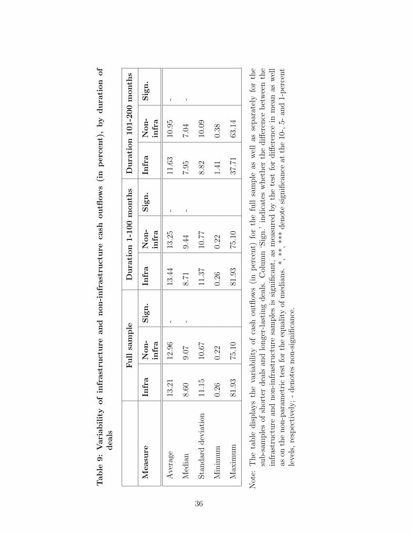
Table 9 shows the empirical results. To account for the different durations of our

sample deals, we construct two different cases: 1-100 denotes sample deals that have

a duration between 1 and 100 months; 101-200 denotes sample deals with a duration

between 101 and 200 months. Using our measure of cash flow variability introduced

above, we calculate the cash flow volatility for each of the deals in our samples. The

cross-sectional means reported in Table 9 do not indicate that infrastructure investments

offer more stable (in the sense of predictable) cash (out-) flows than non-infrastructure

investments. In fact, the average and median variability of the infrastructure deals is

even slightly higher for most sub-samples. But these differences are not statistically

significant. Also, in a regression with the measure of variability as dependent variable,

we could not find evidence for a statistically significant difference between infrastructure

and non-infrastructure deals. Therefore, we reject the hypothesis that infrastructure

fund investments offer more stable cash flows than non-infrastructure fund investments.


H4 : Infrastructure assets are generally regarded as investments that exhibit low

levels of risk. We analyze this hypothesis by comparing the default frequencies of infras-

tructure investments with those of non-infrastructure investments. We measure default

frequencies by the fraction of sample deals with a multiple equal to zero and by the frac-

tion of deals with a multiple smaller than one.9 The first variable gives the proportion

of complete write-off deals in the samples. The second variable indicates the proportion

of deals where money was lost, i.e., the cash return from the investment was smaller

than the cash the fund had injected into the portfolio company.


Overall, our results suggest that infrastructure deals show lower default frequencies.

Table 10 reveals that there is a significant difference in default rates between infras-

tructure and non-infrastructure deals for both measures applied. In addition, Table

11 shows that this is also the case for sub-samples of venture capital and private eq-

uity deals. These findings support the hypothesis that infrastructure investments show

relatively low default rates (Inderst 2009, p. 7).

9The multiple of a transaction, in the context of this paper, measures the cumulated distributionsreturned to the investors as a proportion of the cumulative paid-in capital.

16

As infrastructure deals show relatively low levels of risk compared to non-infrastructure

deals, the traditional view is that their returns tend to be lower, too. Interestingly, the

descriptive statistics in Tables 12 and 13 show higher average and median returns for

the infrastructure deals, as measured by the investment multiples and internal rates of

return (IRR).10 This result also holds for each of the VC and PE sub-samples, and most

differences are statistically highly significant.


To further scrutinize these findings on differences in risk and return, we perform

a regression of the IRR (Table 14, Model 1) and of the dummy variable DEFAULT

(Table 14, Model 2) on several fund- and deal-specific variables as well as macroeconomic

factors. For this purpose we eliminate deals at and above the 95th percentile of the IRR

due to the high dispersion as can be seen in Tables 12 and 13. The reasoning is that

these outliers might be subject to data errors. Both regressions meet the standard OLS

conditions and have high explanatory power with an R2 of 34.70 percent and a Pseudo

R2 of 48.95 percent, respectively.


Model 1 confirms that infrastructure deals significantly outperform non-infrastructure

deals, as can be seen in the positive coefficient of variable INFRA. In turn, Model 2 con-

firms that the likelihood of default is significantly smaller for infrastructure deals than

for non-infrastructure deals (negative coefficient of variable INFRA).11

One reason why we find higher return and lower risk might be that, in our analyses,

we apply total cash flows and not operating cash flows and thus, we measure equity

and not asset risk. As we will show later, there is evidence that infrastructure assets

have higher leverage than non-infrastructure assets. Higher leverage, in turn, implies

increased market risk and thus requires higher equity returns. However, as we do not

10The IRR, sometimes also called money-weighted rate of return, is defined as a measure that cal-culates the rate of return at which cash flows are discounted so that the net present value amounts tozero.

11This result is robust to applying a Tobit regression or taking the dummy variable PAR-TIAL DEFAULT as dependent variable.

17

know deal-specific leverage levels, we cannot infer whether the higher returns observed

for infrastructure deals are just a fair compensation for higher market risk or whether

they indicate true out-performance. It is nevertheless striking that we find higher returns

and lower stand-alone risk for infrastructure investments.

H5 : After having seen significant differences in risk and return between infrastructure

and non-infrastructure deals, we now test whether greenfield and brownfield investments

within the infrastructure universe exhibit different risk and return profiles. Our data

do not contain the explicit information whether a portfolio company is a greenfield or

brownfield investment. We approximate this by using the information whether a deal is a

venture capital or private equity deal. Venture capital typically refers to deals involving

portfolio companies at an early development stage. In contrast, private equity refers to

deals involving portfolio companies at a later development stage. This approximation

matches the typical descriptions of greenfield and brownfield investments (see Section

3 above). Beeferman (2008, p. 6) even defines greenfield and brownfield investments

as early and late-stage investments, which makes the analogy to venture capital and

private equity even more obvious. Therefore, taking VC and PE as an approximation

for greenfield and brownfield seems to be a reasonable assumption.

We find that brownfield investments are less risky than greenfield investments. This is

expressed by consistently and significantly lower default frequencies across sub-samples

in Tables 10 and 11 above. In addition, it is interesting to observe the significant

difference in performance between greenfield and brownfield investments, as shown in

Tables 12 and 13 above. Brownfield investments show higher average and median per-

formance, regardless whether measured by IRR or the multiple. The differences are

statistically significant across sub-samples, too. These findings are consistent with other

studies on private equity (e.g. the studies at fund level by Kaplan and Schoar 2005 and

Ljungqvist and Richardson 2003). Similar to the comparison between infrastructure and

non-infrastructure deals above, we find higher returns for the assets with lower risk.

The regression analysis in Table 14 enables us to check whether these significant

differences remain when controlling for a number of deal, fund and macroeconomic

characteristics. Model 1 confirms that PE deals significantly outperform VC deals,

as reflected by the positive coefficient of variable PE. Likewise, Model 2 confirms that

the likelihood of default is significantly smaller for PE deals than for VC deals (negative

18

coefficient of variable PE).12

5.3 Performance drivers

As shown in Sub-section 5.2, we find significant differences in the performance of in-

frastructure and non-infrastructure deals. We now turn to the question which variables

drive these results and how the drivers of performance differ between the infrastruc-

ture and non-infrastructure sub-samples. In order to address these questions, we again

eliminate deals at the 95th percentile of the IRR and regress the IRR on several fund-

and deal-specific variables as well as macroeconomic factors. However, we now perform

separate regressions for the infrastructure and non-infrastructure sub-samples. For each

sub-sample we include infrastructure- and non-infrastructure-specific dummy variables

that control for the sector. The results of this exercise are shown in Models 3 and 4 in

Table 15. Both regressions meet the standard OLS conditions and have high explanatory

power with an R2 of 46.2 percent and 34.6 percent, respectively.


H6 : It has been shown in the literature that a high inflow of capital into the market

for private equity at the time of investment drives up asset prices because of the increased

competition for attractive deals. This, in turn, results in a poor performance of the deals,

an effect that is often referred to as the money chasing deals phenomenon (Gompers and

Lerner 2000; Diller and Kaserer 2009). In our regressions, capital inflows are measured

by the variable LN COMMITTED CAP. Interestingly, the regression results indicate

a clear difference between the two sub-samples. In particular, the coefficient for non-

infrastructure deals (-13.30) is highly significant and negative, whereas the coefficient

for infrastructure deals (3.82) is not significantly different from zero. This confirms that

the capital inflows into private equity markets at the time of initial investment have a

strong adverse influence on the performance of non-infrastructure deals. Since the same

does not hold for infrastructure deals, we do not observe overinvestment in infrastructure

fund investments caused by capital inflows into the private-equity market.

12This result is also robust when applying a Tobit regression or taking the dummy variable PAR-TIAL DEFAULT as dependent variable.

19

H7 : It is commonly argued that infrastructure investments provide inflation-linked

returns. The coefficient of the variable INFLATION is positive for the infrastructure

sample (3.29) whereas it is negative for the non-infrastructure sample (-1.73). This would

indicate evidence in favour of the hypothesis that infrastructure fund investments would

provide a better inflation-linkage of returns than non-infrastructure investments. How-

ever, neither coefficient is statistically significant. This is in line with Sawant (2010b)

who does not find a significant correlation between inflation and return for listed infras-

tructure stocks either. By contrast, Martin (2010, p. 24) finds that infrastructure can

provide a long-term hedge against inflation for an investor provided the ongoing cash

flows are at least partially linked to the price level.

H8 : We can clearly reject the hypothesis that returns on infrastructure fund invest-

ments are uncorrelated to the performance of public equity markets. Models 3 and 4 in

Table 15 show that the coefficient of the variable PUBL MKT PERF is positive (0.13)

and statistically significant for the infrastructure sub-sample, whereas it is negative and

not statistically significant for the non-infrastructure sub-sample. Therefore, the hypoth-

esis of returns uncorrelated to equity markets would rather hold for non-infrastructure

deals. A special diversification benefit of infrastructure fund investments in the context

of financial portfolio choice can thus not be confirmed.

On the other hand, the coefficient of the variable GDP is not statistically signif-

icant (albeit positive at 1.74) for the infrastructure sub-sample (Model 3) while it is

positive (2.09) and statistically significant for the non-infrastructure sample (Model 4).

This supports the hypothesis that infrastructure fund investments offer returns that are

uncorrelated to the macroeconomic development.

5.4 Other performance drivers

Having tested all our infrastructure-specific hypotheses stated in Section 3, we now

outline several other interesting findings from our regressions in Table 15.

Interest rate sensitivity. We find a negative influence of the short-term interest

rate at the date of investment on performance. The coefficients for the variable RISK-

FREERATE are negative and statistically highly significant for both samples. This

negative relationship has also been pointed out in earlier studies (e.g. Ljungqvist and

20

Richardson 2003). In addition, we find that the coefficient for the infrastructure sample

(-4.92) is more negative compared with that of the non-infrastructure sample (-3.96).

That is, the performance of infrastructure deals reacts more sensitive to interest rate

changes.

A possible explanation for this is that infrastructure investments have higher lever-

age ratios than non-infrastructure investments. This is intuitive since the cost of debt

is usually directly related to the risk-free rate while this may not necessarily be true for

the cost of equity. A higher cost of debt implies a higher cost of capital for a levered

portfolio company, which implies a lower return, expressed by a lower IRR in our re-

gression. Unfortunately, we do not have explicit information on leverage ratios in our

data. However, the view that the higher regression coefficient for infrastructure deals

reflects higher leverage ratios is supported by several other studies. For example, Bucks

(2003) reports an average leverage of up to 83 percent in the water and energy sectors

compared with 57 percent in other sectors in 2003. Ramamurti and Doh (2004, p. 161)

report leverage of up to 75 percent in the infrastructure sector in general and Beeferman

(2008, p. 9) lists average leverage ranging from 50 percent for toll roads and airports to

65 percent for utilities and even 90 percent for social infrastructure, all of which refer to

the level of individual assets. Orr (2007, p. 7) reports an additional leverage of up to 80

percent at fund level whereby the source of returns comes, to a large proportion, from

financial structuring. Helm and Tindall (2009, p. 415) identify the late 1990s as a time

where the scale of leverage and financial engineering peaked, especially in the utilities

sector. The following time of historically low interest rates combined with the benefit

of tax shield effects and thus, a lower weighted average cost of capital also benefited the

use of debt.

Fund manager experience. At fund level, the variable LN GENERATION mea-

sures the number of funds the investment manager has operated prior to the current

fund that invests in the specific deal. It may be seen as a proxy for the experience of the

investment manager, which may be an important performance driver as several studies

on private equity suggest (Achleitner et al. 2010). In contrast, our regression results

reveal that the experience of the investment manager has no significant influence on

either of the sub-samples in Models 3 and 4 in Table 15.

Duration of deals. At deal level, we can see that the duration of deals has

21

a significant effect on returns in both sub-samples. The coefficients of the variable

LN DURATION are significant, positive and similarly large in value. The economic ra-

tionale behind this result is that badly-performing deals are typically exited more quickly

than well-performing deals, such that deals with a longer duration also show a higher

IRR (Buchner et al. 2010; Krohmer et al. 2009).

Number of financing rounds. A similar result is found for the variable LN NUMBER.

This variable measures the total number of cash injections a portfolio company has re-

ceived from the fund and may be seen as a proxy for the number of financing rounds.

In our regression, the number of financing rounds has a significantly negative influence

on performance in both sub-samples, i.e., the more often the fund manager invests ad-

ditional equity into a deal, the lower the IRR. This is referred to as ‘staging’ and is

extensively discussed in the literature (Sahlmann 1990; Krohmer et al. 2009). Consis-

tent with our results, Krohmer et al. (2009) argue that badly-performing companies

need to ‘gamble for resurrection’ more often in order to get additional cash injections

from fund managers. Therefore, there is a negative relationship between number of

financing rounds and performance.

Deal size. Models 3 and 4 in Table 15 show that the size of a non-infrastructure

deal has a significant positive influence on its IRR, despite controlling for the fund size,

whereas this is not the case for infrastructure deals. This is shown by a highly signif-

icant coefficient for LN SIZE of 2.81 for the non-infrastructure and by an insignificant

coefficient of 2.24 for the infrastructure sub-sample. Also Franzoni et al. (2010) find a

positive influence of deal size on performance. They explain this effect with an illiquidity

premium that is increasing in deal size. From a theoretical perspective, it is unclear why

deal size should have an impact on performance. In this paper we cannot control for the

illiquidity premium hypothesis mentioned by Franzoni et al. (2010). Furthermore, we

cannot control to what extent deal size is a proxy for other performance-related variables

such as deal risk or management experience. Hence, we can hardly explain this finding.

Still, it is noteworthy that the size effect is not present in infrastructure deals.

Regional differences. In terms of regional influences, we observe that deals made in

Europe - one of the most mature infrastructure markets besides Australia and Canada

(OECD 2007, p. 32) - significantly outperform deals in other regions. Infrastructure

deals show an even larger spread, with European infrastructure deals, on average, having

22

an IRR that is 35.40 percentage points higher than in other regions as indicated by the

dummy variable EUROPE. This effect is much smaller for European non-infrastructure

deals with 19.57 percentage points. Lopez de Silanes et al. (2009) also report a higher

performance for private-equity deals in Europe excluding the UK.

A rationale for this difference might be that Europe has seen the largest volume in

privatizations, especially in the infrastructure sectors (e.g. Brune et al. 2004; Clifton

et al. 2006, pp. 745-751). Therefore, the proportion of deals involving privatization

is likely to be much higher in the sub-sample of European infrastructure deals than in

the other sub-samples. Three explanations why such sales of assets from the public

to private investors could have delivered higher returns include that i) a government

or municipality might not have the objective to maximize the sale price of an asset,

but instead tries to make the sale succeed in the first place; ii) management of newly

privatized companies often negotiated large capital and operational expenditures with

regulators before privatization but cut these expenditures back afterwards (Helm and

Tindall 2009, pp. 420-421); and iii) after the formerly state-owned companies with low

leverage were privatized, the new owners increased the leverage to lower the weighted

average cost of capital and thus the return on the asset instead of using it for real capital

investments (Helm 2009, p. 319).

Privatizations usually take place via private placements, tenders or fixed-price sales.

Regarding the latter, there is empirical evidence that under-pricing is larger at priva-

tizations than at private-company IPOs and larger in regulated than in unregulated

industries (Dewenter and Malatesta 1997). These empirical and theoretical findings

support the idea that there are higher returns for privatizations of infrastructure assets

in Europe in general.

The same line of argument might also hold for our empirical finding of high returns

of private equity-type infrastructure deals. Hall (2006, p. 8) points out the increasing

importance of private equity and infrastructure funds as buyers of privatized companies

in Europe, strengthening the link between our empirical findings and the mechanisms

of privatization mentioned above.

Differences in returns within the infrastructure sector. The highly significant

and positive coefficient of the variable TRANSPORT in Model 3 reveals that transport

infrastructure assets (e.g. airports, marine ports or toll roads) exhibit IRRs above

23

the average - and by a wide margin - while assets in Natural resources and energy

do not. On average, deals in the transportation sector yield an IRR that is 24.32

percentage points higher than other infrastructure deals. The reason for this might be

that the transportation sector is subject to a high degree of government intervention

and thus, discretionary power (Yarrow et al. 1986, p. 340), while at the same time

being less subject to independent regulation than other infrastructure sectors such as

utilities. Indeed, Egert et al. (2009, p. 70) show in a survey that independent regulators

are far less common in the transportation sector than in the electricity, gas, water or

even telecommunication sectors. Less stability and credibility given by a regulatory

framework, in turn, leads to higher investment uncertainty - including higher price and

quantity risk - for which an investor requires a higher rate of return (Egert et al. 2009,

pp. 31-32). The latter is in line with our empirical finding.

Within the non-infrastructure sample, we can see that a wider range of industries has

a significantly higher IRR as shown by the variable INDUSTRIAL in Model 4. However,

the coefficient is economically rather small.

6 Summary

We have scrutinized the risk- and return profile of unlisted infrastructure investments

and have compared them to non-infrastructure investments. It is widely believed that

infrastructure investments offer some typical financial characteristics such as long-term,

stable and predictable, inflation-linked returns with low correlation to other assets. To

some extent, our findings corroborate this view. However, we also document some results

that are not in accordance with parts of this perception.

By using a unique dataset of infrastructure and non-infrastructure deals made by

private-equity-like investment funds, we have come up with the following results. First,

in terms of risk differences between infrastructure and non-infrastructure deals, results

are a bit mixed. We do not find any evidence supporting the hypothesis that infrastruc-

ture investments offer more stable cash (out-) flows than non-infrastructure investments.

It appears to be true, however, that default risk - or downside risk more generally - is

significantly lower in infrastructure investments than in non-infrastructure investments.

24

Second, as far as returns are concerned, we do find higher average and median re-

turns for infrastructure deals, as measured by the investment multiples and internal

rates of return. This result also holds when separating the sample into venture capital

and private-equity deals, and most differences are statistically significant. This is an

interesting finding as it contradicts the traditional view that infrastructure investments

exhibit low levels of risk and, consequently, provide only moderate returns.

Third, there is some evidence that the higher average returns reflect higher market

risk. For one thing, our sample contains only equity investments, and leverage ratios of

infrastructure portfolio companies are higher than for their non-infrastructure counter-

parts. For another, returns to infrastructure fund investments are more strongly corre-

lated with the performance of public-equity markets than returns to non-infrastructure

fund investments.

Fourth, European infrastructure investments are found to have consistently higher re-

turns than their non-European counterparts. We hypothesize that this might be related

to the fact that Europe has seen the largest volume of privatizations, especially in the in-

frastructure sectors. It could well be that the ex ante return expectation in privatization

transactions is higher, either because of defective privatization mechanisms or because

of higher political risk. Concerning the latter, we find some evidence that the regulatory

environment has an impact on returns. Specifically, deals in the transportation sector

have significantly higher returns than those in other infrastructure sectors, probably re-

flecting less independent regulation and hence, higher political risk in transportation as

compared to the utilities or energy sectors.

Fifth, our empirical results do not support some other claims made in the literature.

In particular, returns to infrastructure deals are not linked to inflation and do not depend

on management experience, and their cash flow durations are not any different from

those of non-infrastructure deals. It is also interesting to see that, unlike venture capital

and private-equity transactions at large, infrastructure investments do not appear to be

subject to the so-called money chasing deals phenomenon.

Thus, the allegedly bond-like characteristics of infrastructure deals have not been

confirmed. This is shown by the fact that infrastructure investments do not offer longer-

term or more stable cash flows than non-infrastructure investments. The returns showing

a positive correlation to public-equity markets and no inflation linkage also point to

25

equity-like rather than bond-like characteristics.

Summing up, our paper supports the perception that infrastructure investments do

have special characteristics that are of interest for institutional investors. Lower down-

side risk is certainly an important feature in this context. However, it is unlikely that

the infrastructure market offers a free lunch. Even though it is true that returns have

been attractive in the past, it cannot be ruled out that these returns are driven by higher

market risk. Our results, at least, offer some evidence in favour of this hypothesis. But a

more general picture of the infrastructure market is still needed. Especially the influence

of regulatory and political risk needs to be better understood. In this regard, our paper

offers some limited evidence that can be used as a starting point for future research.

26

Tables

Table 1: Empirical variables and their expected results

Level Variable Description Hypo-thesis

Expected result

Deal Duration Number of months be-tween initial investmentand exit

H1 Longer average duration for infradeals

Deal Size Dealsize measured in USD H2 Larger size for infra deals

Deal Variability Volatility of cash outflows H3 Lower variability for infra deals

Deal (PARTIAL )DEFAULT (Partial) default rate H4 Lower default rate for infra deals

H5 Lower default rate for brownfielddeals

Deal IRR Internal rate of return H4 Lower performance for infradeals

H5 Lower performance for brown-field deals

Deal Multiple Cumulative paid-out rela-tive to cumulative paid-incapital

H4 Lower performance for infradeals

H5 Lower performance for brown-field deals

Macro LN COMMITTED CAP Committed capital in theoverall private equity mar-ket

H6 Negative influence on perfor-mance of infra deals

Macro INFLATION Average inflation rate H7 Positive influence on perfor-mance of infra deals

Macro PUBL MKT PERF Average growth of publicequity market index

H8 Non-positive influence on perfor-mance of infra deals

Macro GDP Average GDP growth H8 Non-positive influence on perfor-mance of infra deals

Note: Column ‘Level’ shows if the variable refers to a deal characteristic or if it is a macroeconomicvariable. Column ‘Hypothesis’ states which of the eight hypotheses outlined in Section 3 eachvariable serves to test. ‘Expected result’ specifies the expected results based on the hypotheses.‘Infra’ and ‘non-infra’ refer to infrastructure and non-infrastructure deals, respectively.

27

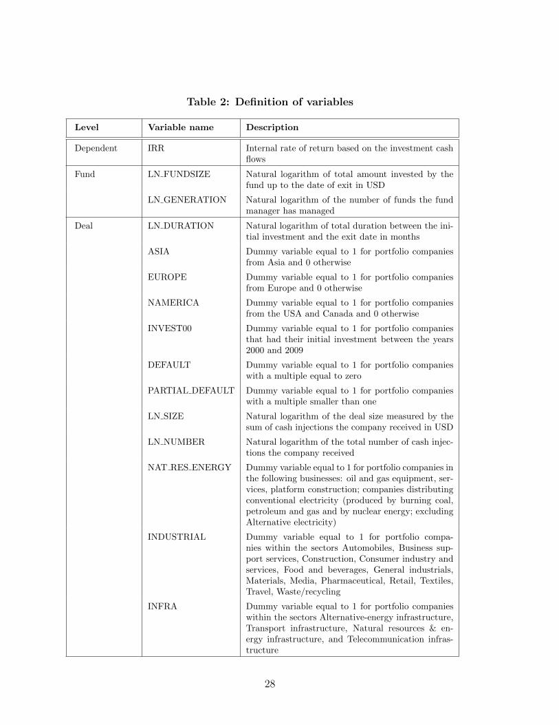
Table 2: Definition of variables

Level Variable name Description

Dependent IRR Internal rate of return based on the investment cashflows

Fund LN FUNDSIZE Natural logarithm of total amount invested by thefund up to the date of exit in USD

LN GENERATION Natural logarithm of the number of funds the fundmanager has managed

Deal LN DURATION Natural logarithm of total duration between the ini-tial investment and the exit date in months

ASIA Dummy variable equal to 1 for portfolio companiesfrom Asia and 0 otherwise

EUROPE Dummy variable equal to 1 for portfolio companiesfrom Europe and 0 otherwise

NAMERICA Dummy variable equal to 1 for portfolio companiesfrom the USA and Canada and 0 otherwise

INVEST00 Dummy variable equal to 1 for portfolio companiesthat had their initial investment between the years2000 and 2009

DEFAULT Dummy variable equal to 1 for portfolio companieswith a multiple equal to zero

PARTIAL DEFAULT Dummy variable equal to 1 for portfolio companieswith a multiple smaller than one

LN SIZE Natural logarithm of the deal size measured by thesum of cash injections the company received in USD

LN NUMBER Natural logarithm of the total number of cash injec-tions the company received

NAT RES ENERGY Dummy variable equal to 1 for portfolio companies inthe following businesses: oil and gas equipment, ser-vices, platform construction; companies distributingconventional electricity (produced by burning coal,petroleum and gas and by nuclear energy; excludingAlternative electricity)

INDUSTRIAL Dummy variable equal to 1 for portfolio compa-nies within the sectors Automobiles, Business sup-port services, Construction, Consumer industry andservices, Food and beverages, General industrials,Materials, Media, Pharmaceutical, Retail, Textiles,Travel, Waste/recycling

INFRA Dummy variable equal to 1 for portfolio companieswithin the sectors Alternative-energy infrastructure,Transport infrastructure, Natural resources & en-ergy infrastructure, and Telecommunication infras-tructure

28

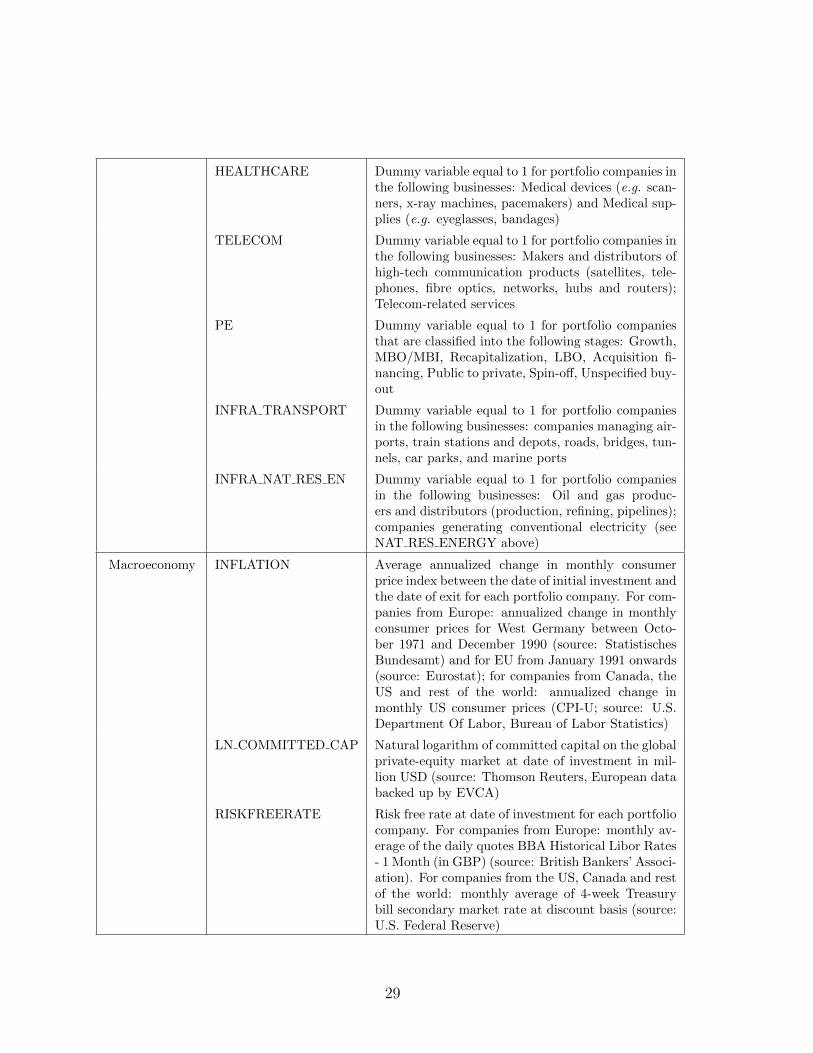
HEALTHCARE Dummy variable equal to 1 for portfolio companies inthe following businesses: Medical devices (e.g. scan-ners, x-ray machines, pacemakers) and Medical sup-plies (e.g. eyeglasses, bandages)

TELECOM Dummy variable equal to 1 for portfolio companies inthe following businesses: Makers and distributors ofhigh-tech communication products (satellites, tele-phones, fibre optics, networks, hubs and routers);Telecom-related services

PE Dummy variable equal to 1 for portfolio companiesthat are classified into the following stages: Growth,MBO/MBI, Recapitalization, LBO, Acquisition fi-nancing, Public to private, Spin-off, Unspecified buy-out

INFRA TRANSPORT Dummy variable equal to 1 for portfolio companiesin the following businesses: companies managing air-ports, train stations and depots, roads, bridges, tun-nels, car parks, and marine ports

INFRA NAT RES EN Dummy variable equal to 1 for portfolio companiesin the following businesses: Oil and gas produc-ers and distributors (production, refining, pipelines);companies generating conventional electricity (seeNAT RES ENERGY above)

Macroeconomy INFLATION Average annualized change in monthly consumerprice index between the date of initial investment andthe date of exit for each portfolio company. For com-panies from Europe: annualized change in monthlyconsumer prices for West Germany between Octo-ber 1971 and December 1990 (source: StatistischesBundesamt) and for EU from January 1991 onwards(source: Eurostat); for companies from Canada, theUS and rest of the world: annualized change inmonthly US consumer prices (CPI-U; source: U.S.Department Of Labor, Bureau of Labor Statistics)

LN COMMITTED CAP Natural logarithm of committed capital on the globalprivate-equity market at date of investment in mil-lion USD (source: Thomson Reuters, European databacked up by EVCA)

RISKFREERATE Risk free rate at date of investment for each portfoliocompany. For companies from Europe: monthly av-erage of the daily quotes BBA Historical Libor Rates- 1 Month (in GBP) (source: British Bankers’ Associ-ation). For companies from the US, Canada and restof the world: monthly average of 4-week Treasurybill secondary market rate at discount basis (source:U.S. Federal Reserve)

29

GDP Average GDP growth rates between the date of ini-tial investment and the date of exit for each portfo-lio company. For companies from Europe: averageannualized percentage change in quarterly (West)German GDP between October 1971 and Decem-ber 1995 (seasonally adjusted, source: StatistischesBundesamt). Average annualized percentage changein quarterly EU GDP from January 1996 onwards(seasonally adjusted, source: Eurostat). For com-panies from Canada, US and rest of the world: av-erage annualized percentage change in quarterly USGDP (seasonally adjusted, source: U.S. Departmentof Commerce, Bureau of Economic Analysis)

PUBL MKT PERF Total return of benchmark stock index between thedate of initial investment and the date of exit foreach portfolio company. For companies from Europe:MSCI Europe Total Return Index. For companiesfrom Canada and USA: MSCI USA Total ReturnIndex. For companies from Asia: MSCI World TotalReturn between October 1971 and December 1987,MSCI AC Asia Pacific Total Return from January1988 onwards. For companies from rest of the world:MSCI World Total Return Index.

Note: Column ‘Level’ shows if the variable refers to a deal or fund characteristic or if it is a macroeco-nomic variable.

30

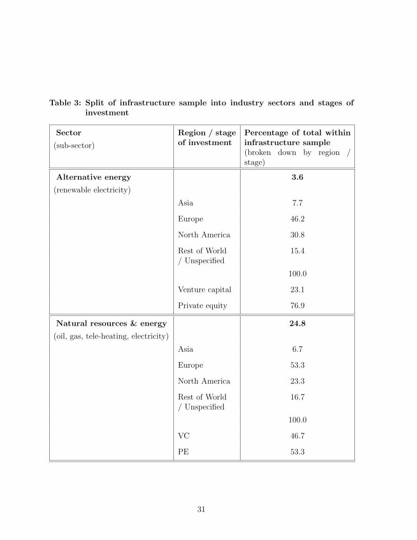
Table 3: Split of infrastructure sample into industry sectors and stages ofinvestment

Sector

(sub-sector)

Region / stageof investment

Percentage of total withininfrastructure sample(broken down by region /stage)

Alternative energy

(renewable electricity)

3.6

Asia 7.7

Europe 46.2

North America 30.8

Rest of World/ Unspecified

15.4

100.0

Venture capital 23.1

Private equity 76.9

Natural resources & energy

(oil, gas, tele-heating, electricity)

24.8

Asia 6.7

Europe 53.3

North America 23.3


16.7

100.0

VC 46.7

PE 53.3

31

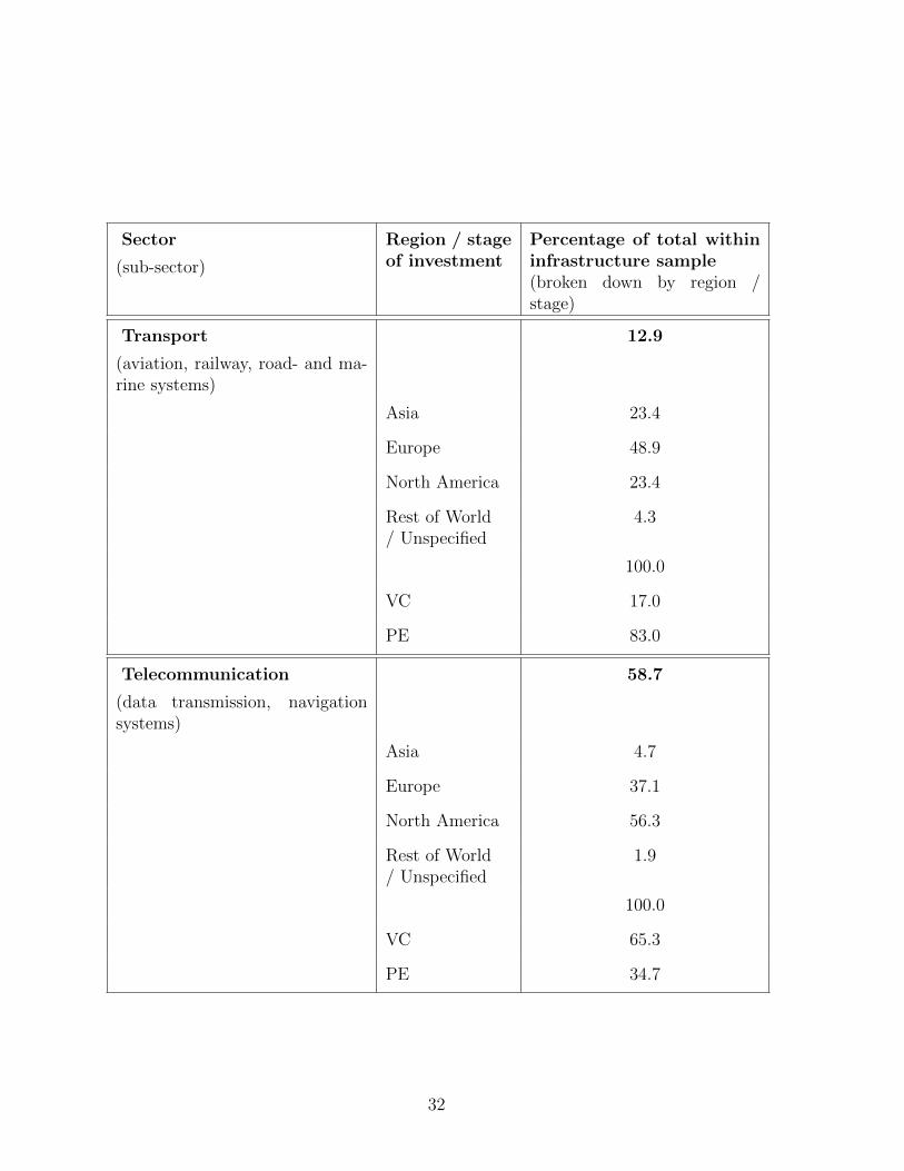
Sector

(sub-sector)

Region / stageof investment

Percentage of total withininfrastructure sample(broken down by region /stage)

Transport

(aviation, railway, road- and ma-rine systems)

12.9

Asia 23.4

Europe 48.9

North America 23.4


4.3

100.0

VC 17.0

PE 83.0

Telecommunication

(data transmission, navigationsystems)

58.7

Asia 4.7

Europe 37.1

North America 56.3


1.9

100.0

VC 65.3

PE 34.7

32

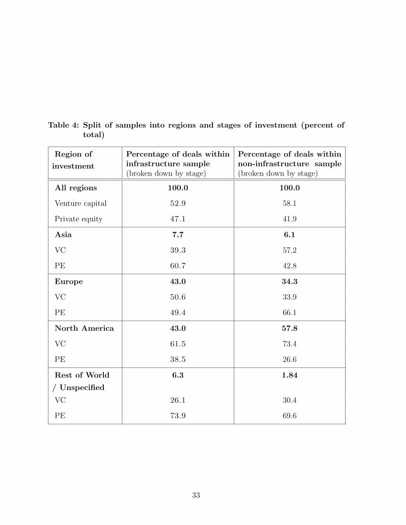
Table 4: Split of samples into regions and stages of investment (percent oftotal)

Region of

investment

Percentage of deals withininfrastructure sample(broken down by stage)

Percentage of deals withinnon-infrastructure sample(broken down by stage)

All regions 100.0 100.0

Venture capital 52.9 58.1

Private equity 47.1 41.9

Asia 7.7 6.1

VC 39.3 57.2

PE 60.7 42.8

Europe 43.0 34.3

VC 50.6 33.9

PE 49.4 66.1

North America 43.0 57.8

VC 61.5 73.4

PE 38.5 26.6

Rest of World

/ Unspecified

6.3 1.84

VC 26.1 30.4

PE 73.9 69.6

33

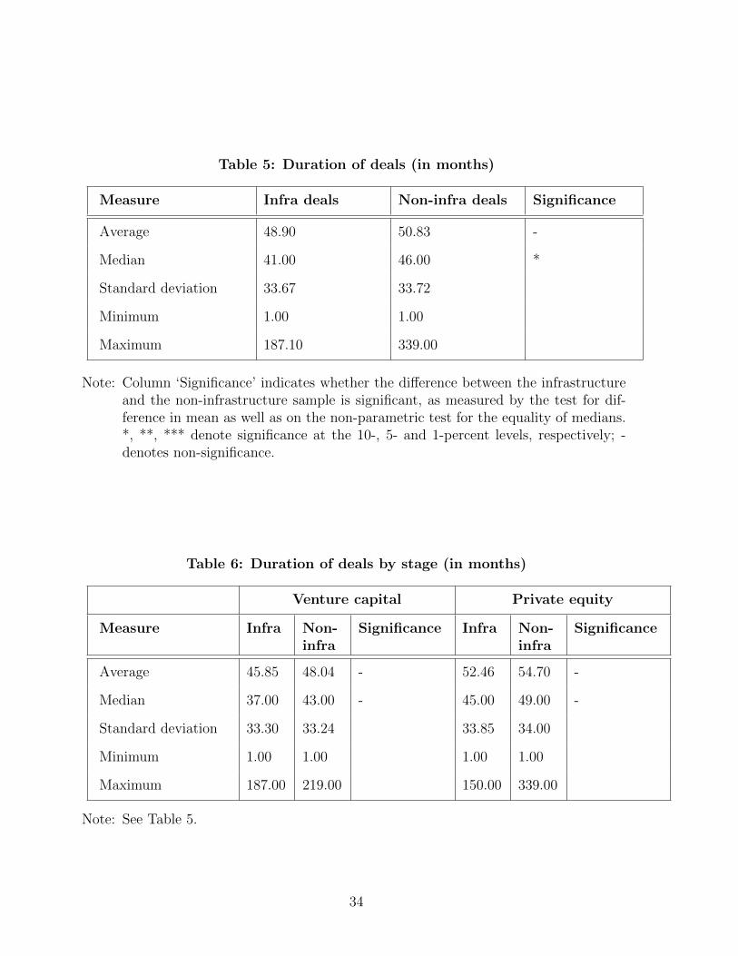
Table 5: Duration of deals (in months)

Measure Infra deals Non-infra deals Significance

Average 48.90 50.83 -

Median 41.00 46.00 *

Standard deviation 33.67 33.72

Minimum 1.00 1.00

Maximum 187.10 339.00

Note: Column ‘Significance’ indicates whether the difference between the infrastructureand the non-infrastructure sample is significant, as measured by the test for dif-ference in mean as well as on the non-parametric test for the equality of medians.*, **, *** denote significance at the 10-, 5- and 1-percent levels, respectively; -denotes non-significance.

Table 6: Duration of deals by stage (in months)

Venture capital Private equity

Measure Infra Non-infra

Significance Infra Non-infra

Significance

Average 45.85 48.04 - 52.46 54.70 -

Median 37.00 43.00 - 45.00 49.00 -

Standard deviation 33.30 33.24 33.85 34.00

Minimum 1.00 1.00 1.00 1.00

Maximum 187.00 219.00 150.00 339.00

Note: See Table 5.

34

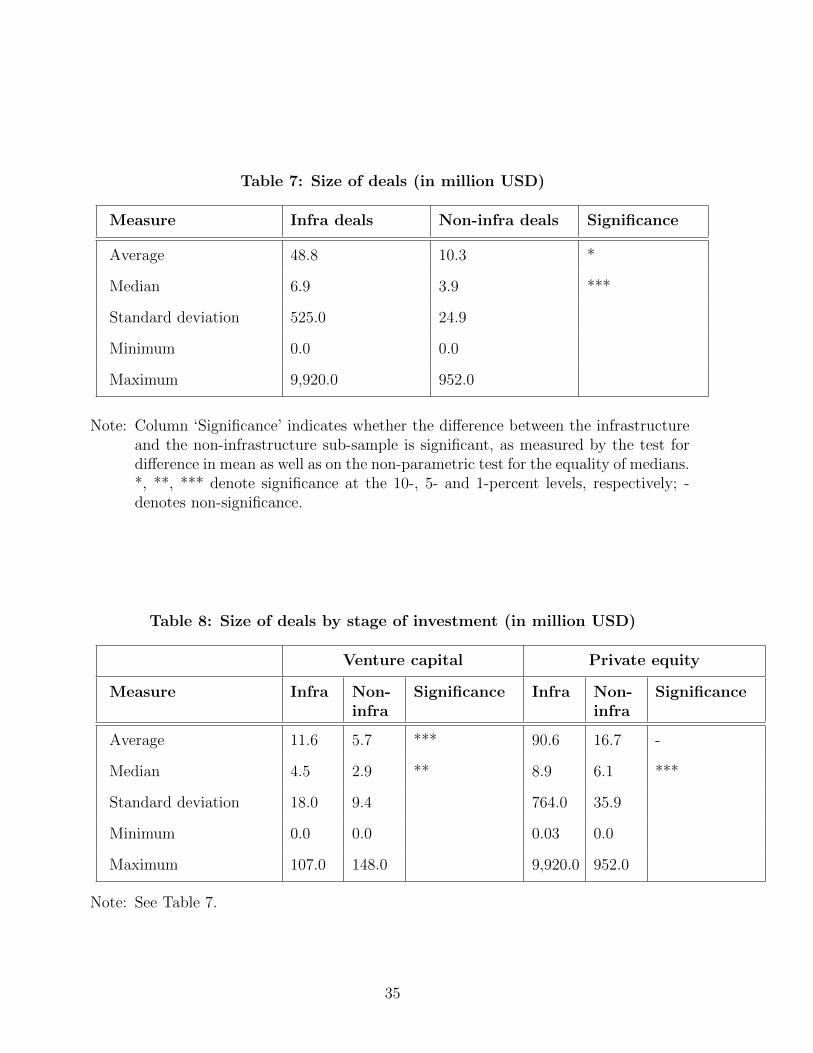
Table 7: Size of deals (in million USD)

Measure Infra deals Non-infra deals Significance

Average 48.8 10.3 *

Median 6.9 3.9 ***

Standard deviation 525.0 24.9

Minimum 0.0 0.0

Maximum 9,920.0 952.0

Note: Column ‘Significance’ indicates whether the difference between the infrastructureand the non-infrastructure sub-sample is significant, as measured by the test fordifference in mean as well as on the non-parametric test for the equality of medians.*, **, *** denote significance at the 10-, 5- and 1-percent levels, respectively; -denotes non-significance.

Table 8: Size of deals by stage of investment (in million USD)

Venture capital Private equity

Measure Infra Non-infra

Significance Infra Non-infra

Significance

Average 11.6 5.7 *** 90.6 16.7 -

Median 4.5 2.9 ** 8.9 6.1 ***


Minimum 0.0 0.0 0.03 0.0

Maximum 107.0 148.0 9,920.0 952.0

Note: See Table 7.

35

Table

9:

Vari

abil

ity

of

infr

ast

ruct

ure

and

non-i

nfr

ast

ruct

ure

cash

outfl

ow

s(i

np

erc

ent)

,by

du

rati

on

of

deals

Full

sam

ple

Dura

tion

1-1

00

month

sD

ura

tion

101-2

00

month

s

Measu

reIn

fra

Non-

infr

aSig

n.

Infr

aN

on-

infr

aSig

n.

Infr

aN

on

-in

fra

Sig

n.

Ave

rage

13.2

112

.96

-13

.44

13.2

5-

11.6

310

.95

-

Med

ian

8.60

9.07

-8.

719.

44-

7.95

7.04

-

Sta

ndar

ddev

iati

on11

.15

10.6

711

.37

10.7

78.

8210

.09

Min

imum

0.26

0.22

0.26

0.22

1.41

0.38

Max

imum

81.9

375

.10

81.9

375

.10

37.7

163

.14

Not

e:T

he

table

dis

pla

ys

the

vari

abilit

yof

cash

outfl

ows

(in

per

cent)

for

the

full

sam

ple

asw

ell

asse

par

atel

yfo

rth

esu

b-s

ample

sof

shor

ter

dea

lsan

dlo

nge

r-la

stin

gdea

ls.

Col

um

n‘S

ign.’

indic

ates

whet

her

the

diff

eren

ceb

etw

een

the

infr

astr

uct

ure

and

non

-infr

astr

uct

ure

sam

ple

sis

sign

ifica

nt,

asm

easu

red

by

the

test

for

diff

eren

cein

mea

nas

wel

las

onth

enon

-par

amet

ric

test

for

the

equal

ity

ofm

edia

ns.

*,**

,**

*den

ote

sign

ifica

nce

atth

e10

-,5-

and

1-p

erce

nt

leve

ls,

resp

ecti

vely

;-

den

otes

non

-sig

nifi

cance

.

36

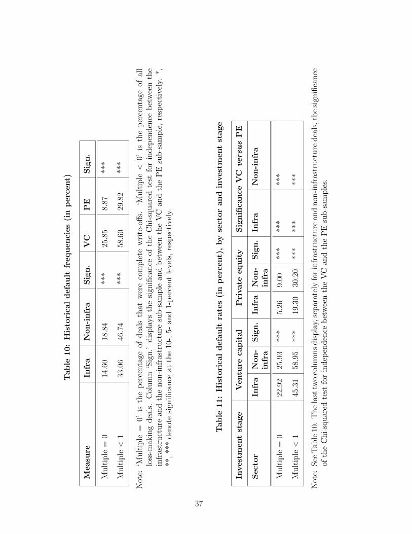
Table

10:

His

tori

cal

defa

ult

frequenci

es

(in

perc

ent)

Measu

reIn

fra

Non-i

nfr

aSig

n.

VC

PE

Sig

n.

Mult

iple

=0

14.6

018

.84

***

25.8

58.

87**

*

Mult

iple

<1

33.0

646

.74

***

58.6

029

.82

***

Not

e:‘M

ult

iple

=0’

isth

ep

erce

nta

geof

dea

lsth

atw

ere

com

ple

tew

rite

-off

s.‘M

ult

iple

<0’

isth

ep

erce

nta

geof

all

loss

-mak

ing

dea

ls.

Col

um

n‘S

ign.’

dis

pla

ys

the

sign

ifica

nce

ofth

eC

hi-

squar

edte

stfo

rin

dep

enden

ceb

etw

een

the

infr

astr

uct

ure

and

the

non

-infr

astr

uct

ure

sub-s

ample

and

bet

wee

nth

eV

Can

dth

eP

Esu

b-s

ample

,re

spec

tive

ly.

*,**

,**

*den

ote

sign

ifica

nce

atth

e10

-,5-

and

1-p

erce

nt

leve

ls,

resp

ecti

vely

.

Table

11:

His

tori

cal

defa

ult

rate

s(i

np

erc

ent)

,by

sect

or

and

invest

ment

stage

Invest

ment

stage

Ventu

reca

pit

al

Pri

vate

equit

ySig

nifi

cance

VC

versus

PE

Sect

or

Infr

aN

on-

infr

aSig

n.

Infr

aN

on-

infr

aSig

n.

Infr

aN

on-i

nfr

a

Mult

iple

=0

22.9

225

.93

***

5.26

9.00

***

***

***

Mult

iple

<1

45.3

158

.95

***

19.3

030

.20

***

***

***

Not

e:See

Tab

le10

.T

he

last

two

colu

mns

dis

pla

y,se

par

atel

yfo

rin

fras

truct

ure

and

non

-infr

astr

uct

ure

dea

ls,th

esi

gnifi

cance

ofth

eC

hi-

squar

edte

stfo

rin

dep

enden

ceb

etw

een

the

VC

and

the

PE

sub-s

ample

s.

37

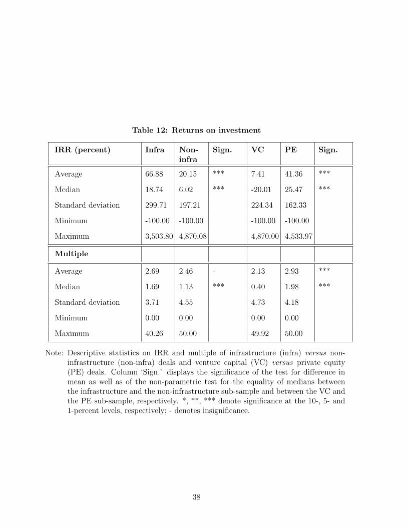
Table 12: Returns on investment

IRR (percent) Infra Non-infra

Sign. VC PE Sign.

Average 66.88 20.15 *** 7.41 41.36 ***

Median 18.74 6.02 *** -20.01 25.47 ***


Minimum -100.00 -100.00 -100.00 -100.00

Maximum 3,503.80 4,870.08 4,870.00 4,533.97

Multiple

Average 2.69 2.46 - 2.13 2.93 ***

Median 1.69 1.13 *** 0.40 1.98 ***


Minimum 0.00 0.00 0.00 0.00

Maximum 40.26 50.00 49.92 50.00

Note: Descriptive statistics on IRR and multiple of infrastructure (infra) versus non-infrastructure (non-infra) deals and venture capital (VC) versus private equity(PE) deals. Column ‘Sign.’ displays the significance of the test for difference inmean as well as of the non-parametric test for the equality of medians betweenthe infrastructure and the non-infrastructure sub-sample and between the VC andthe PE sub-sample, respectively. *, **, *** denote significance at the 10-, 5- and1-percent levels, respectively; - denotes insignificance.

38

Table

13:

Retu

rns

on

invest

ment

by

sect

or

and

invest

ment

stage

Ventu

reca

pit

al

Pri

vate

equit

ySig

nifi

can

ceV

Cversus

PE

IRR

(perc

ent)

Infr

aN

on-

infr

aSig

n.

Infr

aN

on-

infr

aSig

n.

Infr

aN

on

-in

fra

Ave

rage

45.7

36.

27*

90.6

839

.54

***

***

Med

ian

5.00

-21.

94**

*36

.06

25.1

6**

***

***

*

Sta

ndar

ddev

iati

on30

5.93

221.

3929

1.64

155.

28

Min

imum

-100

.00

-100

.00

-100

.00

-100

.00

Max

imum

2,22

4.88

4,87

0.08

3,50

3.79

4,53

3.97

Mult

iple

Ave

rage

2.17

2.13

-3.

272.

92*

***

***

Med

ian

1.15

0.38

***

2.47

1.96

****

***

*

Sta

ndar

ddev

iati

on4.

144.

753.

034.

21

Min

imum

0.00

0.00

0.00

0.00

Max

imum

40.2

649

.92

22.7

850

.00

Not

e:See

Tab

le12

.T

he

last

two

colu

mns

dis

pla

y,se

par

atel

yfo

rin

fras

truct

ure

and

non

-infr

astr

uct

ure

dea

ls,th

esi

gnifi

cance

ofth

ete

sts

for

diff

eren

cein

mea

nan

dfo

rth

eeq

ual

ity

ofm

edia

ns

bet

wee

nth

eV

Can

dth

eP

Esu

b-s

ample

.

39

Table 14: Regression results: All deals

Model 1 OLS (all deals) Model 2 Probit (all deals)

Dependent variable IRR Dependent variable DEFAULT

Variable Coefficient

(t-statistic)


(z-statistic)

LN GENERATION 0.67 LN GENERATION 0.02

(0.91) (0.93)

LN FUNDSIZE -1.64 ** LN FUNDSIZE -0.06 **

(-2.47) (-2.49)

PE 22.27 *** PE -0.42 ***

(14.30) (-7.73)

LN NUMBER -31.58 *** LN NUMBER 1.22 ***

(-35.35) (32.92)

LN DURATION 26.74 *** LN GENERATION -1.23 ***

(52.25) (-38.90)

LN SIZE 2.85 *** LN SIZE 0.01

(4.91) (0.77)

ASIA 4.86 * ASIA -0.19 **

(1.87) (-2.15)

EUROPE 20.77 *** EUROPE -0.45 ***

(10.17) (-6.48)

INFRA 12.15 *** INFRA -0.36 ***

(3.76) (-6.48)

INFLATION -1.89 INFLATION 0.01

(-1.42) (0.16)

40

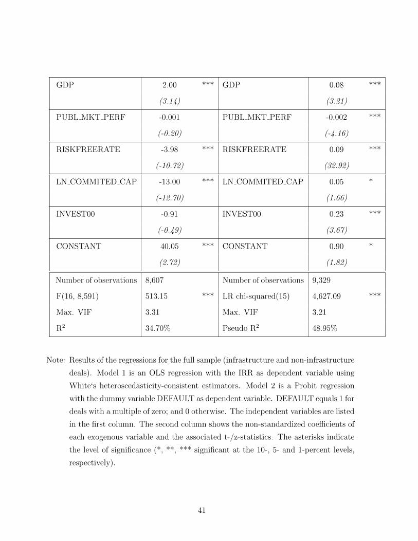
GDP 2.00 *** GDP 0.08 ***

(3.14) (3.21)

PUBL MKT PERF -0.001 PUBL MKT PERF -0.002 ***

(-0.20) (-4.16)

RISKFREERATE -3.98 *** RISKFREERATE 0.09 ***

(-10.72) (32.92)

LN COMMITED CAP -13.00 *** LN COMMITED CAP 0.05 *

(-12.70) (1.66)

INVEST00 -0.91 INVEST00 0.23 ***

(-0.49) (3.67)

CONSTANT 40.05 *** CONSTANT 0.90 *

(2.72) (1.82)

Number of observations 8,607 Number of observations 9,329

F(16, 8,591) 513.15 *** LR chi-squared(15) 4,627.09 ***

Max. VIF 3.31 Max. VIF 3.21

R2 34.70% Pseudo R2 48.95%

Note: Results of the regressions for the full sample (infrastructure and non-infrastructure

deals). Model 1 is an OLS regression with the IRR as dependent variable using

White‘s heteroscedasticity-consistent estimators. Model 2 is a Probit regression

with the dummy variable DEFAULT as dependent variable. DEFAULT equals 1 for

deals with a multiple of zero; and 0 otherwise. The independent variables are listed

in the first column. The second column shows the non-standardized coefficients of

each exogenous variable and the associated t-/z-statistics. The asterisks indicate

the level of significance (*, **, *** significant at the 10-, 5- and 1-percent levels,

respectively).

41

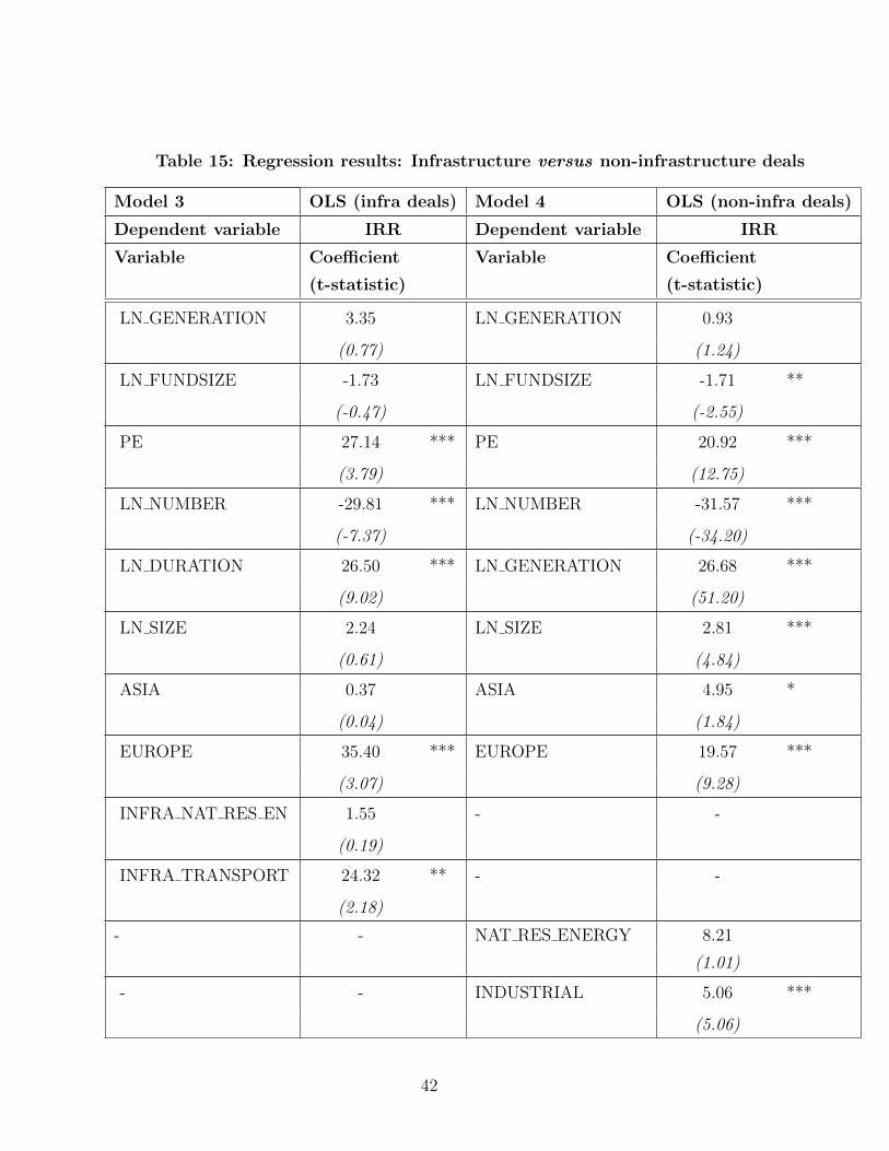
Table 15: Regression results: Infrastructure versus non-infrastructure deals

Model 3 OLS (infra deals) Model 4 OLS (non-infra deals)

Dependent variable IRR Dependent variable IRR


(t-statistic)


(t-statistic)

LN GENERATION 3.35 LN GENERATION 0.93

(0.77) (1.24)

LN FUNDSIZE -1.73 LN FUNDSIZE -1.71 **

(-0.47) (-2.55)

PE 27.14 *** PE 20.92 ***

(3.79) (12.75)

LN NUMBER -29.81 *** LN NUMBER -31.57 ***

(-7.37) (-34.20)

LN DURATION 26.50 *** LN GENERATION 26.68 ***

(9.02) (51.20)

LN SIZE 2.24 LN SIZE 2.81 ***

(0.61) (4.84)

ASIA 0.37 ASIA 4.95 *

(0.04) (1.84)

EUROPE 35.40 *** EUROPE 19.57 ***

(3.07) (9.28)

INFRA NAT RES EN 1.55 - -

(0.19)

INFRA TRANSPORT 24.32 ** - -

(2.18)

- - NAT RES ENERGY 8.21

(1.01)

- - INDUSTRIAL 5.06 ***

(5.06)

42

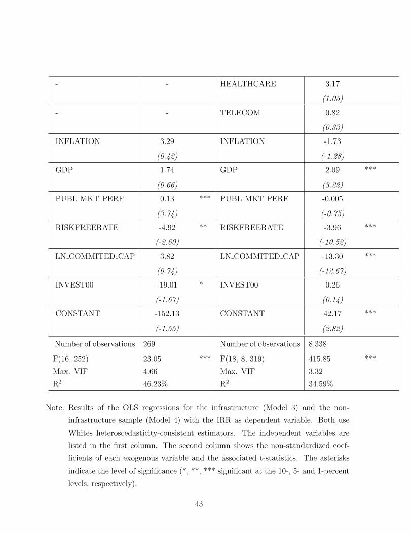
- - HEALTHCARE 3.17

(1.05)

- - TELECOM 0.82

(0.33)

INFLATION 3.29 INFLATION -1.73

(0.42) (-1.28)

GDP 1.74 GDP 2.09 ***

(0.66) (3.22)

PUBL MKT PERF 0.13 *** PUBL MKT PERF -0.005

(3.74) (-0.75)

RISKFREERATE -4.92 ** RISKFREERATE -3.96 ***

(-2.60) (-10.52)

LN COMMITED CAP 3.82 LN COMMITED CAP -13.30 ***

(0.74) (-12.67)

INVEST00 -19.01 * INVEST00 0.26

(-1.67) (0.14)

CONSTANT -152.13 CONSTANT 42.17 ***

(-1.55) (2.82)

Number of observations 269 Number of observations 8,338

F(16, 252) 23.05 *** F(18, 8, 319) 415.85 ***

Max. VIF 4.66 Max. VIF 3.32

R2 46.23% R2 34.59%

Note: Results of the OLS regressions for the infrastructure (Model 3) and the non-

infrastructure sample (Model 4) with the IRR as dependent variable. Both use

Whites heteroscedasticity-consistent estimators. The independent variables are

listed in the first column. The second column shows the non-standardized coef-

ficients of each exogenous variable and the associated t-statistics. The asterisks

indicate the level of significance (*, **, *** significant at the 10-, 5- and 1-percent

levels, respectively).

43

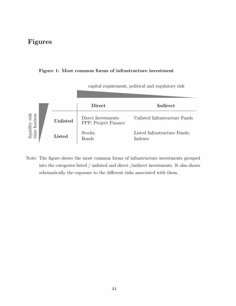
Figures

capital requirement, political and regulatory risk

liquidityrisk

timehorizon

Unlisted

Listed

Direct Indirect

Direct InvestmentsPPP; Project Finance

Stocks;

Bonds

Unlisted Infrastructure Funds

Listed Infrastructure Funds;

Indexes

Figure 1: Most common forms of infrastructure investment

Note: The figure shows the most common forms of infrastructure investments grouped

into the categories listed / unlisted and direct /indirect investments. It also shows

schematically the exposure to the different risks associated with them.

44

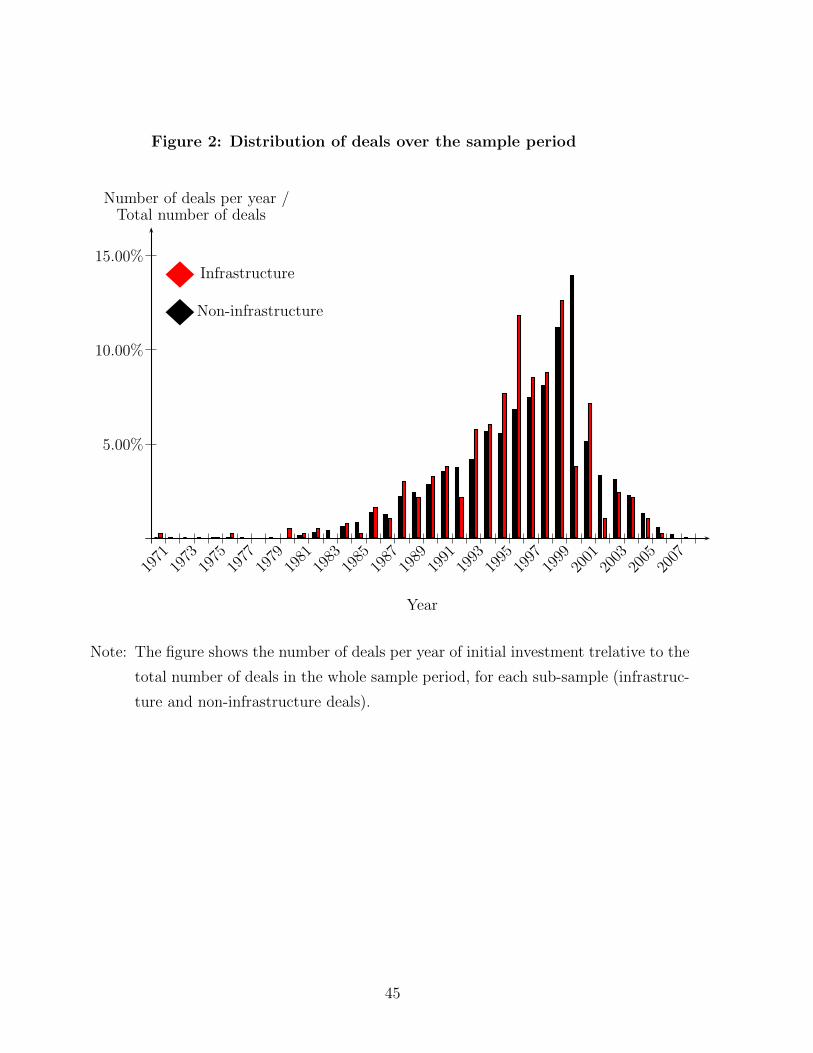
Figure 2: Distribution of deals over the sample period

Infrastructure

Non-infrastructure

5.00%

10.00%

15.00%

Number of deals per year /Total number of deals

1971

1973

1975

1977

1979

1981

1983

1985

1987

1989

1991

1993

1995

1997

1999

2001

2003

2005

2007

Year

Note: The figure shows the number of deals per year of initial investment trelative to the

total number of deals in the whole sample period, for each sub-sample (infrastruc-

ture and non-infrastructure deals).

45

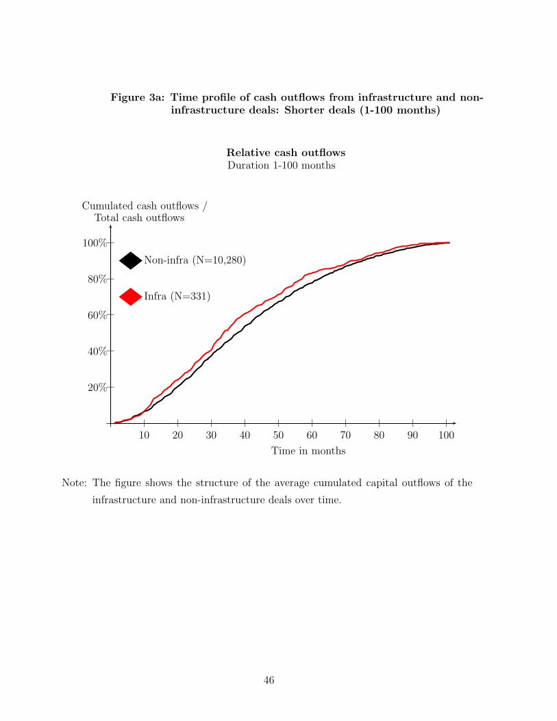
10 20 30 40 50 60 70 80 90 100

Figure 3a: Time profile of cash outflows from infrastructure and non-infrastructure deals: Shorter deals (1-100 months)

Relative cash outflowsDuration 1-100 months

Cumulated cash outflows /Total cash outflows

Non-infra (N=10,280)

Infra (N=331)

20%

40%

60%

80%

100%

Time in months

Note: The figure shows the structure of the average cumulated capital outflows of the

infrastructure and non-infrastructure deals over time.

46

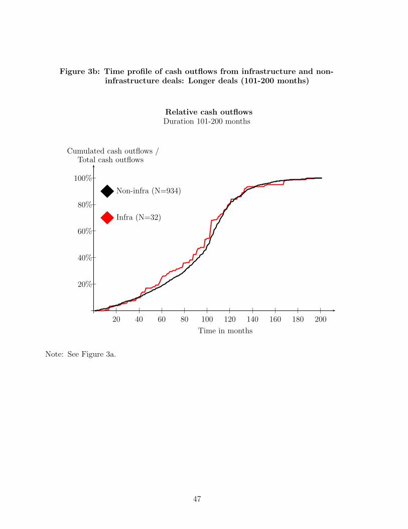
20 40 60 80 100 120 140 160 180 200

Figure 3b: Time profile of cash outflows from infrastructure and non-infrastructure deals: Longer deals (101-200 months)

Relative cash outflowsDuration 101-200 months


Non-infra (N=934)

Infra (N=32)

20%

40%

60%

80%

100%

Time in months

Note: See Figure 3a.

47

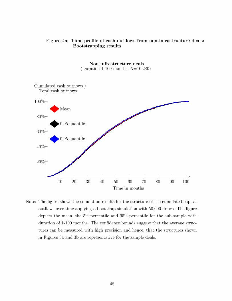
10 20 30 40 50 60 70 80 90 100

Figure 4a: Time profile of cash outflows from non-infrastructure deals:Bootstrapping results

Non-infrastructure deals(Duration 1-100 months, N=10,280)


Mean

0.05 quantile

0.95 quantile

20%

40%

60%

80%

100%

Time in months

Note: The figure shows the simulation results for the structure of the cumulated capital

outflows over time applying a bootstrap simulation with 50,000 draws. The figure

depicts the mean, the 5th percentile and 95th percentile for the sub-sample with

duration of 1-100 months. The confidence bounds suggest that the average struc-

tures can be measured with high precision and hence, that the structures shown

in Figures 3a and 3b are representative for the sample deals.

48

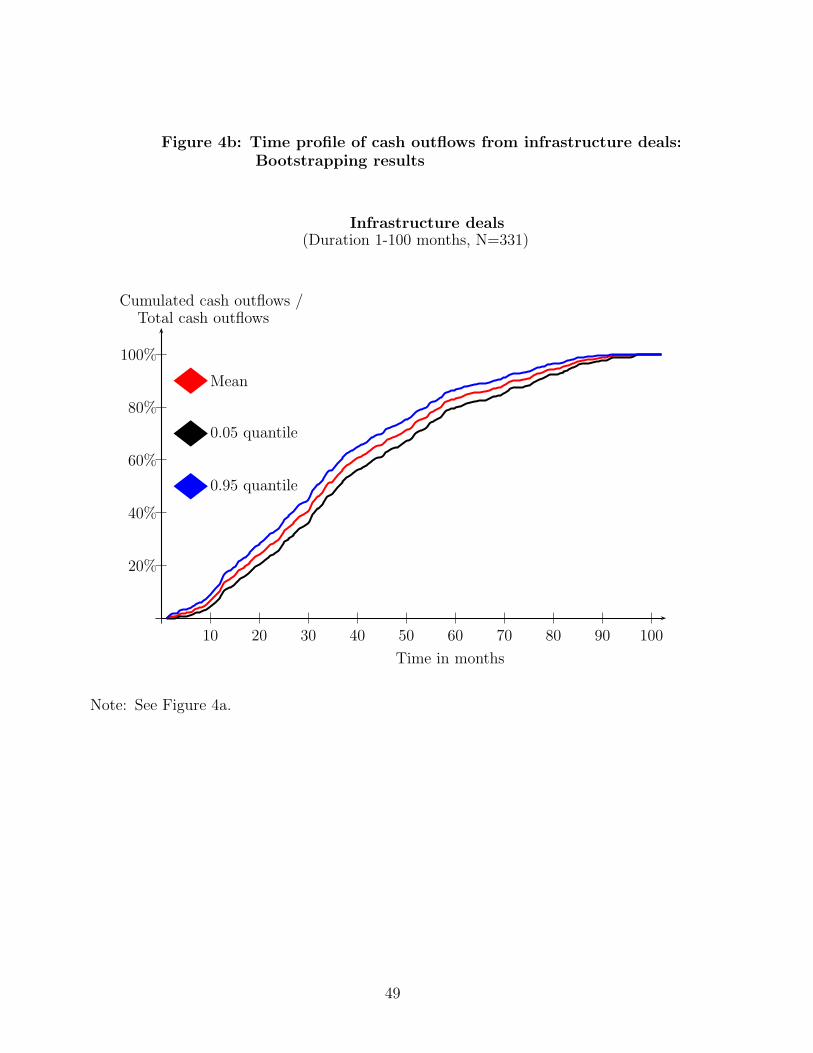
10 20 30 40 50 60 70 80 90 100

Figure 4b: Time profile of cash outflows from infrastructure deals:Bootstrapping results

Infrastructure deals(Duration 1-100 months, N=331)


Mean

0.05 quantile

0.95 quantile

20%

40%

60%

80%

100%

Time in months

Note: See Figure 4a.

49

References

Achleitner, A.-K., Braun, R. and Engel, N. (2010), ‘Value Creation and Pricing

in Buyouts: Empirical Evidence from Europe and North America’, Technische Uni-

versitat Munchen - Center for Entrepreneurial and Financial Studies, CEFS Working

Paper.

Beeferman, L. (2008), ‘Pension Fund Investment in Infrastructure: A Resource Pa-

per’, Occasional Paper Series No. 3, pp. 1-78.

Bitsch, F., Kaserer, C. and Kasper, E. (2010), ‘Infrastructure - An Approach

Towards an Economic Based Definition’, Technische Universitat Munchen - Center for

Entrepreneurial and Financial Studies, CEFS Working Paper.

Brune, N., Garrett, G. and Kogut, B. (2004), ‘The International Monetary Fund

and the Global Spread of Privatization’, IMF Staff Papers, (51:2), pp. 195-219.

Buchner, A., Kaserer, C. and Schmidt, D. (2008), ‘Infrastructure Private Equity’,

Center of Private Equity Research, Discussion Paper.

Buchner, A., Krohmer, P., Schmidt, D. and Wahrenburg, M. (2010), ‘Pro-

jection of Private Equity Fund Performance: A Simulation Approach’ in: Cumming,

D. (ed.), Private Equity - Funds Types, Risks, Returns and Regulation, pp. 197-228,

Wiley & Sons, Hoboken, NJ, USA.

Bucks, P. (2003), ‘Financial Leverage and the Regulator’, The Utilities Journal, (6:10),

pp. 38-39.

Clifton, J., Comin, F. and Fuentes, D. (2006), ‘Privatizing Public Enterprises

in the European Union 1960-2002: Ideological, Pragmatic, Inevitable?’, Journal of

European Public Policy, (13:5), pp. 736-756.

Cumming, D., Schmidt, D. and Walz, U. (2009), ‘Private Equity Returns and

Disclosure Around the World’, Journal of Business Venturing, forthcoming.

Cumming, D. and Walz, U. (2009), ‘Private Equity Returns and Disclosure Around

the World’, Journal of International Business Studies, (41:4), pp. 727-754.

50

Dechant, T. and Finkenzeller, K. (2009), ‘Infrastructure - A New Dimension of

Real Estate? An Asset Allocation Analysis’, ERES Conference 2009, Conference

Paper.

Dewenter, K. and Malatesta, P. (1997), ‘Public Offerings of State-Owned and

Privately-Owned Enterprises: An International Comparison’, The Journal of Finance,

(52:4), pp. 1659-1679.

Diller, C. and Kaserer, C. (2009), ‘What Drives Private Equity Returns? - Fund

Inflows, Skilled GPs, and/or Risk?’, European Financial Management, (15:3), pp.

643-675.

Egert, B., Kozluk, T. and Sutherland, D. (2009), ‘Infrastructure Investment:

Links to Growth and the Role of Public Policies’, OECD Economics Department

Working Papers, No. 686.

Esty, B. (2003), ‘The Economic Motivations for Using Project Finance’, Harvard

Business School, mimeo.

Esty, B. (2010), ‘An Overview of Project Finance and Infrastructure Finance - 2009

Update’, Harvard Business School Case No. 210-061.

Franzoni, F., Nowak, E. and Phalippou, L. (2010), ‘Private Equity Performance

and Liquidity Risk’, Swiss Finance Institute, Research Paper No.09-43.

Gompers, P. and Lerner, J. (2000), ‘Money chasing deals? The Impact of Fund

Inflows on Private Equity Valuation’, Journal of Financial Economics, (55:2), pp.

281-325.

Haas, C. (2005), Vertragsstrukturen privat finanzierter Infrastrukturprojekte, Peter

Lang - Euopaischer Verlag der Wissenschaften, Frankfurt am Main, Germany.

Hall, D. (2006), ‘Private Equity and Infrastructure Funds in Public Services and

Utilities’, University of Greenwich, PSIRU Working Paper.

Helm, D. (2009), ‘Infrastructure Investment, the Cost of Capital, and Regulation: an

Assessment’, Oxford Review of Economic Policy, (25:3), pp. 307-326.

51

Helm, D. and Tindall, T. (2009), ‘The Evolution of Infrastructure and Utility

Ownership and its Implications’, Oxford Review of Economic Policy, (25:3), pp. 411-

434.

Inderst, G. (2009), ‘Pension Fund Investment in Infrastructure’, OECD Working

Papers on Insurance and Private Pensions, No. 32.

Inderst, G. (2010), ‘Infrastructure as an Asset Class’, EIB Papers, (15:1), forthcoming.

Jensen, M. (1986), ‘Agency Costs of Free Cash Flow, Corporate Finance, and the

Market for Corporate Control’, American Economic Review, (76:2), pp. 323-329.

Kaplan, S. and Schoar, A. (2005), ‘Private Equity Performance: Returns, Persis-

tence, and Capital Flows’, The Journal of Finance, (60:4), pp. 1791-1823.

Krohmer, P., Lauterbach, R. and Calanog, V. (2009), ‘The Bright and Dark Side

of Staging: Investment Performance and the Varying Motivations of Private Equity’,

Journal of Banking and Finance, (33:9), pp. 1597-1609.

Ljungqvist, A. and Richardson, M. (2003), ‘The Investment Behavior of Private

Equity Fund Managers’, London School of Economics, RICAFE Working Paper No.

005.

Lopez de Silanes, F., Phalippou, L. and Gottschalg, O. (2009), ‘Giants at the

Gate: Diseconomies of Scale in Private Equity’, AFA 2010 Atlanta Meetings Paper;

EFA 2009 Bergen Meetings Paper.

Martin, G. (2010), ‘The Long-Horizon Benefits of Traditional and New Real Assets in

the Institutional Portfolio’, The Journal of Alternative Investments, (13:1), pp. 6-29.

Metrick, A. and Yasuda, A. (2010), ‘The Economics of Private Equity Funds’,

Review of Financial Studies, (23:6), pp. 2303-2341.

Newell, G. and Peng, H. (2007), ‘The Significance of Infrastructure in Investment

Portfolios’, Pacific Rim Real Estate Society Conference 2007, Conference Paper.

Newell, G. and Peng, H. (2008), ‘The Role of U.S. Infrastructure in Investment

Portfolios’, Journal of Real Estate Portfolio Management, (14:1), pp. 21-32.

52

OECD (2007), Infrastructure to 2030, Volume 2, Mapping Policy for Electricity, Water

and Transport, Organisation for Economic Co-operation and Development, Paris.

OECD (2010), ‘Pension Markets in Focus’, Issue 7, Organisation for Economic Co-

operation and Development, Paris.

Orr, R. (2007), ‘The Rise of Infra Funds’, in Project Finance International - Global

Infrastructure Report 2007, Supplement, pp. 2-12, Project Finance International, Zell

am Harmersbach, Germany.

Prequin (2008), ‘Preqin Infrastructure Review: An Examination of the Unlisted In-

frastructure Fund Market’, Prequin, London.

Ramamurti, R. and Doh, J. (2004), ‘Rethinking Foreign Infrastructure Investment

in Developing Countries’, Journal of World Business, (39:2), pp. 151-167.

Rickards, D. (2008), ‘Global Infrastructure - A Growth Story’, in Davis, H. (ed.),

Infrastructure Finance: Trends and Techniques, pp. 1-47, Euromoney Books, London,

UK.

Sahlmann, W. (1990), ‘The Structure and Governance of Venture-Capital Organiza-

tions’, Journal of Financial Economics, (27), pp. 473 - 522.

Sawant, R. (2010a), ‘Emerging Market Infrastructure Project Bonds: Their Risks and

Returns’, The Journal of Structured Finance, (15:4), pp. 75-83.

Sawant, R. (2010b), Infrastructure Investing: Managing Risks & Rewards for Pen-

sions, Insurance Companies & Endowments, John Wiley and Sons, Hoboken, NJ,

USA.

Valila, T. (2005), ‘How Expensive are Cost Savings? On the Economics of Public-

Private Partnerships’, EIB Papers, (10:1), pp. 94-119.

Yarrow, G., King, M., Mairesse, J. and Melitz, J. (1986), ‘Privatization in

Theory and Practice’, Economic Policy, (1:2), pp. 323-377.

53

risk, return and cash flow characteristics of ... · risk, return and cash flow characteristics of...

Documents