risk premia harvesting through dual momentum · 1 risk premia harvesting through dual momentum gary...
TRANSCRIPT

1
Risk Premia Harvesting Through Dual Momentum
Gary Antonacci
Portfolio Management Associates, LLC1
First version: April 18, 2012
This version: January 28, 2013
Abstract
Momentum is the premier market anomaly. It is nearly universal in its applicability. This paper
examines multi-asset momentum with respect to what can make it most effective for momentum
investors. We consider price volatility as a value-adding factor. We show that both absolute and
relative momentum can enhance returns, but that absolute momentum does far more to lessen
volatility and drawdown. We see that combining absolute and relative momentum gives the best
results. Finally, we show how asset modules can serve as diversification building blocks that
allow us to easily combine relative with absolute momentum and capture risk premia profits.
1 http://www.optimalmomentum.com An earlier version of this paper with a different title was the first place
winner of the 2012 NAAIM Wagner Awards for Advancements in Active Investment Management. The author
wishes to thank Tony Cooper, Wesley Gray, and Akindynos-Nikolaos Baltas for their helpful comments.

2
1. Introduction
Momentum is the tendency of investments to persist in their performance. Assets that
perform well over a 6 to 12 month period tend to continue to perform well into the future. The
momentum effect of Jegadeesh and Titman (1993) is one of the strongest and most pervasive
financial phenomena. Researchers have verified its existence in U.S. stocks (Jegadeesh and
Titman (1993), Asness (1994)), industries (Moskowitz and Grinblatt (1999), Asness, Porter and
Stevens (2000)), foreign stocks (Rouwenhorst (1998), Chan, Hameed and Tong (2000), Griffen,
Ji and Martin (2005)), emerging markets (Rouwenhorst (1999)), equity indices (Asness, Liew
and Stevens (1997), Bhojraj and Swaminathan (2006), Hvidkjaer (2006)), commodities (Pirrong
(2005), Miffre and Rallis (2007)), currencies (Menkoff et al (2011)), global government bonds
(Asness, Moskowitz and Pedersen (2012)), corporate bonds (Jostova, Nikolova and Philipov
(2010)), and residential real estate (Beracha and Skiba (2011)). Since its first publication,
momentum has been shown to work out-of-sample going forward in time (Grundy and Martin
(2001), Asness, Moskowitz and Pedersen (2012)) and back to the year 1866 (Chabot, Ghysels
and Jagannathan (2009)). Momentum works well across asset classes, as well as within them
(Blitz and Vliet (2008), Asness, Moskowitz and Pedersen (2012)).
In addition to cross-sectional or relative strength momentum, in which an asset's
performance relative to other assets predicts its future relative performance, momentum also
works well on an absolute, or time series, basis, in which an asset's own past return predicts its
future performance (Moskowitz, Ooi and Pedersen (2012)). Absolute momentum appears to be
just as robust and universally applicable as cross-sectional momentum. It holds up well across
multiple asset classes and back in time to the turn of the century (Hurst, Ooi, and Pedersen
(2012)). Trend following absolute momentum may also benefit relative strength momentum,
3
since there is evidence that relative strength profits depend on the state of the market (Cooper,
Guiterrez, and Hameed (2004)). Fama and French (2008) call momentum "the center stage
anomaly of recent years…an anomaly that is above suspicion…the premier market anomaly."
They observe that the abnormal returns associated with momentum are pervasive. Schwert
(2003) explored all known market anomalies and declared momentum as the only one that has
been persistent and has survived since publication.
Yet despite an abundance of momentum research and acceptance, no one is sure why it
works. The rational risk-based explanation is that momentum profits represent risk premia
because winners are riskier than losers. (Berk, Green and Naik (1999), Johnson (2002), Ahn,
Conrad and Dittmar (2003), Sagi and Seashales (2007), Liu and Zhang (2008)). The most
common explanations, however, of both relative and absolute momentum, have to do with
behavioral factors, such as anchoring, herding, and the disposition effect. (Tversky and
Kahneman (1974), Barberis, Shleifer, and Vishny (1998), Daniel, Hirshleifer, and
Subrahmanyam (1998), Hong and Stein (1999), Frazzini (2006)). Such behavioral biases are
unlikely to disappear, which may explain why momentum profits have persisted, and may
continue to persist, as a strong anomaly.
Zhang (2006) argues that stock price continuation is due to under-reaction to public
information by investors, and that investors will under-react even more in the case of greater
information uncertainty. One of his proxies for information uncertainty is return volatility. When
information uncertainty and price volatility are high, we can expect abnormal returns to be
higher.
In addition to extensive study of momentum across countries and asset classes, there has
also been considerable study of exogenous factors that influence momentum. Bandarchuk, Pavel
4
and Hilscher (2011) reexamine some of the factors that have previously been shown to impact
momentum in the equities market. These include analyst coverage, illiquidity, price level, age,
size, analyst forecast dispersion, credit rating, R2, market-to-book, and turnover. The authors
show that these factors are proxies for extreme past returns and high volatility. Greater
momentum profits come from assets that are more volatile or that have extreme past returns.
With respect to fixed income, Jostova, Niklova and Philipov (2010) show that momentum
strategies are highly profitable among non-investment grade corporate bonds. High yield, non-
investment grade corporate bonds have, by far, the highest volatility among bonds of similar
maturity. This may point toward high volatility as also a proxy for credit default risk.
The real estate market and long-term Treasury bonds are subject to high volatility due to
their high sensitivity to interest rate risk and economic uncertainty. Gold is also subject to high
volatility due to its response to economic and political turmoil.
Before proceeding, we need to distinguish clearly between relative and absolute
momentum. When we consider two assets, momentum is positive on a relative basis if one asset
has appreciated more than the other has. However, momentum is negative on an absolute basis if
both assets have declined in value over time. It is possible for an asset to have positive relative
and negative absolute momentum. Positive absolute momentum exists when the excess return of
an asset is positive over the look back period, regardless of its performance relative to other
assets.
Cross sectional momentum researchers use long and short positions applied to both the
long and short side of a market simultaneously. They are therefore only concerned with relative
momentum. It makes little difference whether the studied markets go up or down, since short
momentum positions hedge long ones, and vice versa.
5
When looking only at long side momentum, however, it is desirable to be long only when
both absolute and relative momentum are positive, since long-only momentum results are highly
regime dependent. One way to determine absolute momentum is to see if an asset has had a
positive excess return by outperforming Treasury bills over the past year. Since Treasury bill
returns should remain positive over time, if our chosen asset has outperformed Treasury bills,
then it too is likely to continue showing a positive future return by virtue of the transitive
property. In absolute momentum, there is significant positive auto-covariance between an asset's
excess return next month and its lagged one-year return (Moskowitz, Ooi, and Pedersen (2012)).
In our momentum match ups, we use a two-stage selection process. First, we choose
between our module's non-Treasury bill assets using relative strength momentum. If our selected
asset does not also show positive momentum with respect to Treasury bills (meaning it does not
have positive absolute momentum), we select Treasury bills as an alternative proxy investment
until our selected asset is stronger than Treasury bills. Treasury bill returns thus serve as both a
hurdle rate before we can invest in other assets, as well as an alternative investment, until our
assets can show both relative and absolute positive momentum.
Besides incorporating a safe alternative investment when market conditions are not
favorable, our module approach has another important benefit. It imposes diversification on our
momentum portfolio.
With only absolute momentum, this would not be a problem, since one could construct a
well-diversified permanent portfolio. With relative strength momentum, however, some assets
may drop out of the active portfolio. If one were to toss all assets into one large pot, as is often
the case with momentum investing, and then select the top momentum candidates, even with
covariance-based position sizing, all or most of the positions could be highly correlated with one

6
another. Modules help ensure that diversified asset classes receive portfolio representation under
a dual momentum framework, without having to use historic covariances, that may be unstable,
or historic variances, that may be non-stationary (Tsay (2010)).
2. Data and Methodology
All monthly return data begins in January 1974, unless otherwise noted, and includes
interest and dividends. For equities, we use the MSCI US, MSCI EAFE, and MSCI ACWI ex US
indices. These are free float adjusted market capitalization weightings of large and midcap
stocks. The MSCI EAFE Europe, Australia and Far East Index includes twenty-two major
developed market countries, excluding the U.S. and Canada. The MSCI ACWI ex US, i.e., MSCI
All Country World Index ex US, includes twenty-three developed market countries and twenty-
one emerging market countries. MSCI ACWI ex US data begins in January 1988. We create a
composite data series called EAFE+ that is comprised of the MSCI EAFE Index until December
1987 and the MSCI ACWI ex US after its formation in December 1987.2
The Bank of America Merrill Lynch U.S. Cash Pay High Yield Index we use begins in
November 1984. Data prior to that is from Steele System’s mutual find database of the Corporate
Bond High Yield Average, adjusted for expenses. For Treasury bills, we use the Bank of
America Merrill Lynch 3-Month Treasury bill Index. All other bond indices are from Barclays
Capital. The Barclays Capital Aggregate Bond Index begins in January 1976. REIT data is from
the FTSE NAREIT U.S. Real Estate Indices of the National Association of Real Estate
Investment Trusts (NAREIT). The S&P GSCI (formally Goldman Sachs Commodities Index) is
from Standard and Poor's. Gold returns using the London PM gold fix are from the World Gold
Council.
2 Since these indices are based on capitalization, the MSCI ACWI ex US receives only a modest influence from
emerging markets. Our results do not change significantly if we use only the MSCI EAFE Index.

7
There have been no deductions for transaction costs. The average number of switches per
year for our modules are 1.4 for foreign/U.S. equities, 1.2 for high yield/credit bonds, 1.6 for
equity/mortgage REITs, and 1.6 for gold/Treasuries. Therefore, additional transaction costs from
the use of momentum are minor.
Most momentum studies use either a six or a twelve-month formation (look back) period.
Since twelve months is more common and has lower transaction costs, we will use that
timeframe.3 With equity returns, one often skips the most recent month during the formation
period in order to disentangle the momentum effect from the short-term reversal effect related to
liquidity or microstructure issues. Non-equity assets suffer less from liquidity issues. Because we
are dealing with gold, fixed income and real estate, as well as equities, for consistency reasons,
we adjust all our positions monthly without skipping a month.
We first apply relative and absolute momentum to the MSCI U.S. and EAFE+ stock market
indices in order to create our equities momentum module. We then match High Yield Bonds with
the Barclays Capital U.S. Intermediate Credit Bond Index, the next most volatile intermediate
term fixed income index, to form our credit risk module.
Real estate has the highest volatility over the past five years looking at the eleven U.S.
equity market sectors tracked by Morningstar. Real Estate Investment Trusts (REITs) make up
most of this sector. The Morningstar real estate sector index has both mortgage and equity based
REITs. We similarly use both to create our REIT module.
Our final high volatility risk factor focuses on economic stress and uncertainty. For this,
we use the Barclays Capital U.S. Treasury 20+ year bond index and physical gold. Investors
generally hold these as safe haven alternatives to equities and non-government, fixed income
3 The four long-only momentum products available to the public also use a twelve-month look back period (three of
the four skip the last month, which can be helpful with individual stocks). AQR Funds, QuantShares, State Street
Global Advisors, and Summerhaven Index Management are the fund sponsors.
8
securities. Maximum drawdown here is the greatest peak-to-valley equity erosion on a month
end basis.
3. Equity/Sovereign Risk
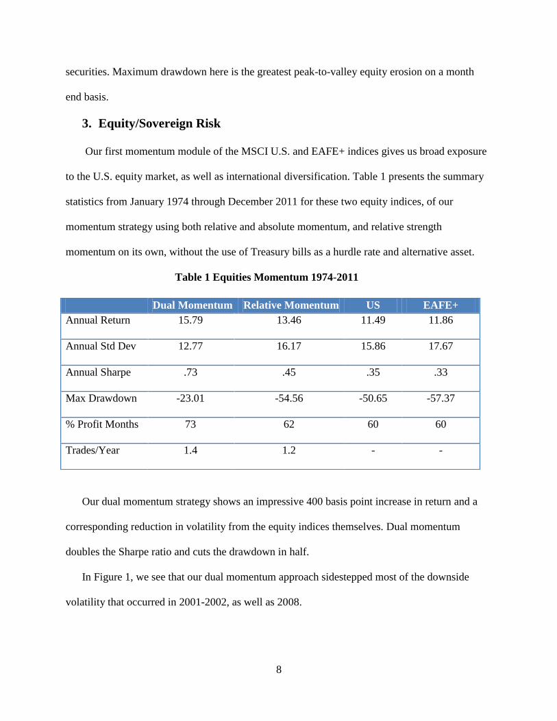
Our first momentum module of the MSCI U.S. and EAFE+ indices gives us broad exposure
to the U.S. equity market, as well as international diversification. Table 1 presents the summary
statistics from January 1974 through December 2011 for these two equity indices, of our
momentum strategy using both relative and absolute momentum, and relative strength
momentum on its own, without the use of Treasury bills as a hurdle rate and alternative asset.
Table 1 Equities Momentum 1974-2011
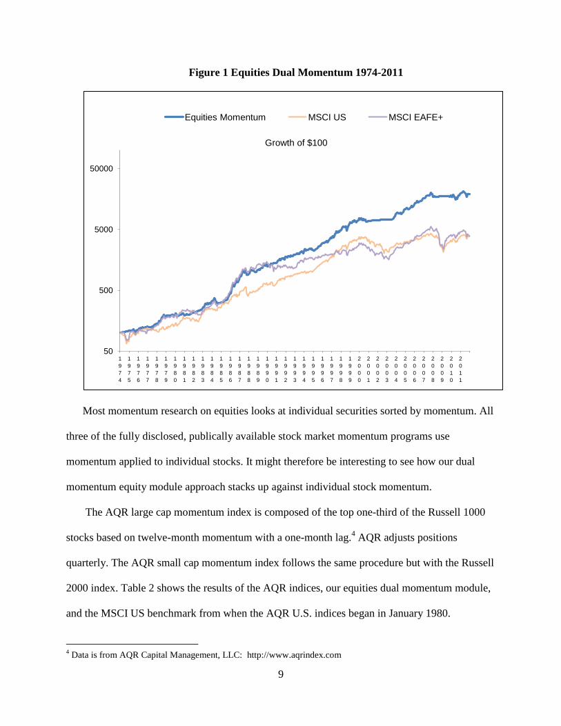
Our dual momentum strategy shows an impressive 400 basis point increase in return and a
corresponding reduction in volatility from the equity indices themselves. Dual momentum
doubles the Sharpe ratio and cuts the drawdown in half.
In Figure 1, we see that our dual momentum approach sidestepped most of the downside
volatility that occurred in 2001-2002, as well as 2008.
Dual Momentum Relative Momentum US EAFE+
Annual Return 15.79 13.46 11.49 11.86
Annual Std Dev 12.77 16.17 15.86 17.67
Annual Sharpe .73 .45 .35 .33
Max Drawdown -23.01 -54.56 -50.65 -57.37
% Profit Months 73 62 60 60
Trades/Year 1.4 1.2 - -
9
Figure 1 Equities Dual Momentum 1974-2011
Most momentum research on equities looks at individual securities sorted by momentum. All
three of the fully disclosed, publically available stock market momentum programs use
momentum applied to individual stocks. It might therefore be interesting to see how our dual
momentum equity module approach stacks up against individual stock momentum.
The AQR large cap momentum index is composed of the top one-third of the Russell 1000
stocks based on twelve-month momentum with a one-month lag.4 AQR adjusts positions
quarterly. The AQR small cap momentum index follows the same procedure but with the Russell
2000 index. Table 2 shows the results of the AQR indices, our equities dual momentum module,
and the MSCI US benchmark from when the AQR U.S. indices began in January 1980.
4 Data is from AQR Capital Management, LLC: http://www.aqrindex.com
50
500
5000
50000
1
9
7
4
1
9
7
5
1
9
7
6
1
9
7
7
1
9
7
8
1
9
7
9
1
9
8
0
1
9
8
1
1
9
8
2
1
9
8
3
1
9
8
4
1
9
8
5
1
9
8
6
1
9
8
7
1
9
8
8
1
9
8
9
1
9
9
0
1
9
9
1
1
9
9
2
1
9
9
3
1
9
9
4
1
9
9
5
1
9
9
6
1
9
9
7
1
9
9
8
1
9
9
9
2
0
0
0
2
0
0
1
2
0
0
2
2
0
0
3
2
0
0
4
2
0
0
5
2
0
0
6
2
0
0
7
2
0
0
8
2
0
0
9
2
0
1
0
2
0
1
1
Growth of $100
Equities Momentum MSCI US MSCI EAFE+
10
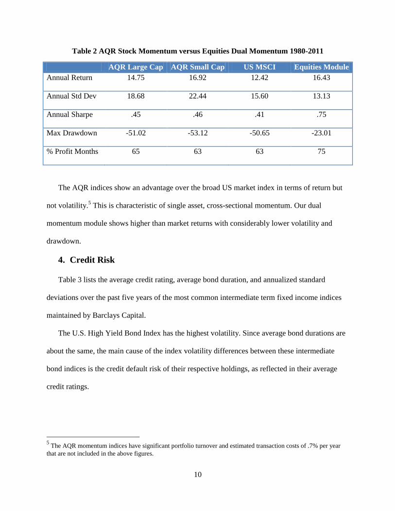
Table 2 AQR Stock Momentum versus Equities Dual Momentum 1980-2011
AQR Large Cap AQR Small Cap US MSCI Equities Module
Annual Return 14.75 16.92 12.42 16.43
Annual Std Dev 18.68 22.44 15.60 13.13
Annual Sharpe .45 .46 .41 .75
Max Drawdown -51.02 -53.12 -50.65 -23.01
% Profit Months 65 63 63 75
The AQR indices show an advantage over the broad US market index in terms of return but
not volatility.5 This is characteristic of single asset, cross-sectional momentum. Our dual
momentum module shows higher than market returns with considerably lower volatility and
drawdown.
4. Credit Risk
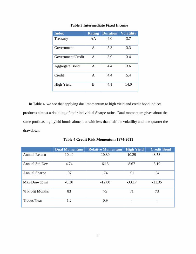
Table 3 lists the average credit rating, average bond duration, and annualized standard
deviations over the past five years of the most common intermediate term fixed income indices
maintained by Barclays Capital.
The U.S. High Yield Bond Index has the highest volatility. Since average bond durations are
about the same, the main cause of the index volatility differences between these intermediate
bond indices is the credit default risk of their respective holdings, as reflected in their average
credit ratings.
5 The AQR momentum indices have significant portfolio turnover and estimated transaction costs of .7% per year
that are not included in the above figures.
11
Table 3 Intermediate Fixed Income
Index Rating Duration Volatility
Treasury AA 4.0 3.7
Government A 5.3 3.3
Government/Credit A 3.9 3.4
Aggregate Bond A 4.4 3.6
Credit A 4.4 5.4
High Yield B 4.1 14.0
In Table 4, we see that applying dual momentum to high yield and credit bond indices
produces almost a doubling of their individual Sharpe ratios. Dual momentum gives about the
same profit as high yield bonds alone, but with less than half the volatility and one-quarter the
drawdown.
Table 4 Credit Risk Momentum 1974-2011
Dual Momentum Relative Momentum High Yield Credit Bond
Annual Return 10.49 10.39 10.29 8.53
Annual Std Dev 4.74 6.13 8.67 5.19
Annual Sharpe .97 .74 .51 .54
Max Drawdown -8.20 -12.08 -33.17 -11.35
% Profit Months 83 75 71 73
Trades/Year 1.2 0.9 - -
12
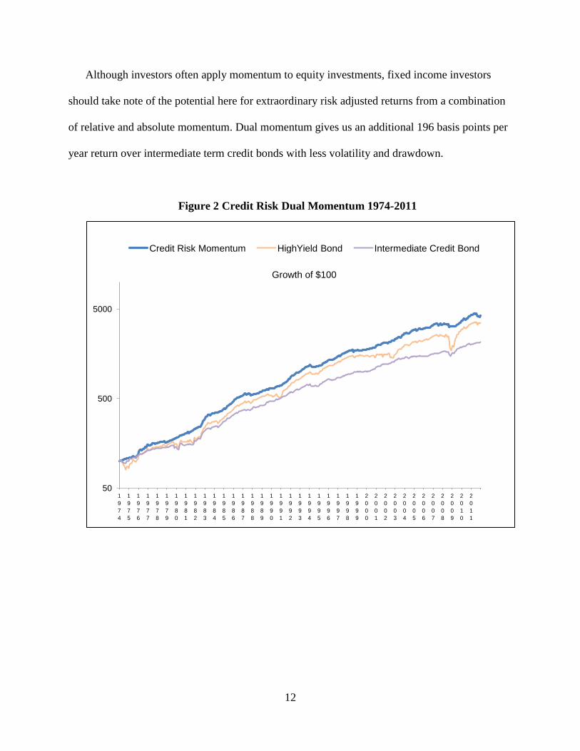
Although investors often apply momentum to equity investments, fixed income investors
should take note of the potential here for extraordinary risk adjusted returns from a combination
of relative and absolute momentum. Dual momentum gives us an additional 196 basis points per
year return over intermediate term credit bonds with less volatility and drawdown.
Figure 2 Credit Risk Dual Momentum 1974-2011
50
500
5000
1
9
7
4
1
9
7
5
1
9
7
6
1
9
7
7
1
9
7
8
1
9
7
9
1
9
8
0
1
9
8
1
1
9
8
2
1
9
8
3
1
9
8
4
1
9
8
5
1
9
8
6
1
9
8
7
1
9
8
8
1
9
8
9
1
9
9
0
1
9
9
1
1
9
9
2
1
9
9
3
1
9
9
4
1
9
9
5
1
9
9
6
1
9
9
7
1
9
9
8
1
9
9
9
2
0
0
0
2
0
0
1
2
0
0
2
2
0
0
3
2
0
0
4
2
0
0
5
2
0
0
6
2
0
0
7
2
0
0
8
2
0
0
9
2
0
1
0
2
0
1
1
Growth of $100
Credit Risk Momentum HighYield Bond Intermediate Credit Bond
13
5. Real Estate Risk
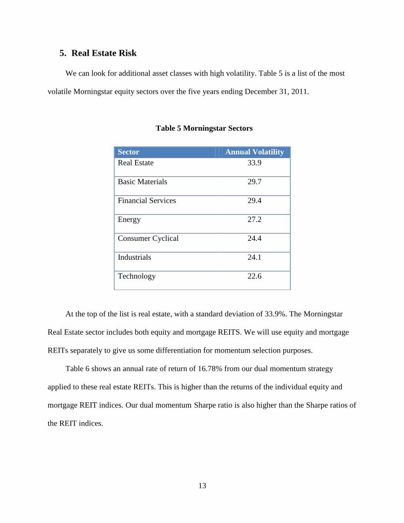
We can look for additional asset classes with high volatility. Table 5 is a list of the most
volatile Morningstar equity sectors over the five years ending December 31, 2011.
Table 5 Morningstar Sectors
At the top of the list is real estate, with a standard deviation of 33.9%. The Morningstar
Real Estate sector includes both equity and mortgage REITS. We will use equity and mortgage
REITs separately to give us some differentiation for momentum selection purposes.
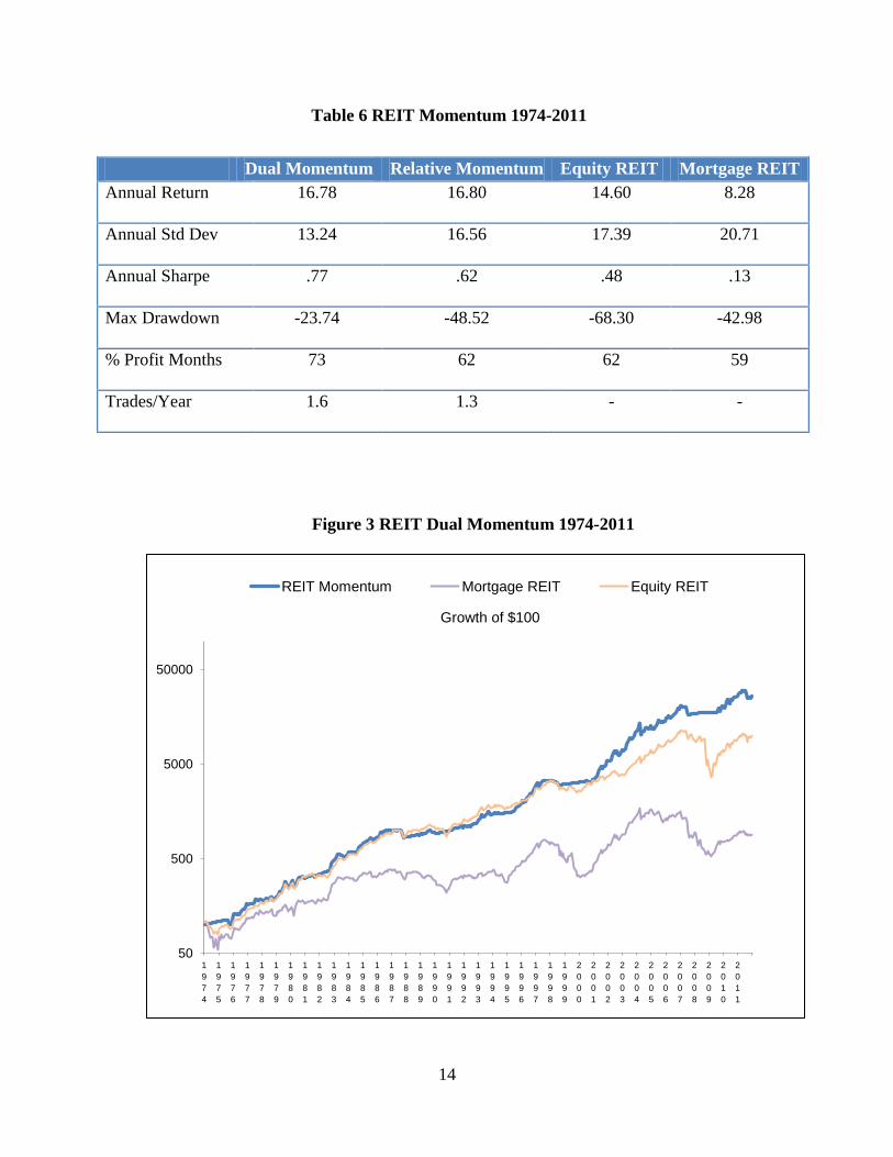
Table 6 shows an annual rate of return of 16.78% from our dual momentum strategy
applied to these real estate REITs. This is higher than the returns of the individual equity and
mortgage REIT indices. Our dual momentum Sharpe ratio is also higher than the Sharpe ratios of
the REIT indices.
Sector Annual Volatility
Real Estate 33.9
Basic Materials 29.7
Financial Services 29.4
Energy 27.2
Consumer Cyclical 24.4
Industrials 24.1
Technology 22.6
14
Table 6 REIT Momentum 1974-2011
Figure 3 REIT Dual Momentum 1974-2011
50
500
5000
50000
1
9
7
4
1
9
7
5
1
9
7
6
1
9
7
7
1
9
7
8
1
9
7
9
1
9
8
0
1
9
8
1
1
9
8
2
1
9
8
3
1
9
8
4
1
9
8
5
1
9
8
6
1
9
8
7
1
9
8
8
1
9
8
9
1
9
9
0
1
9
9
1
1
9
9
2
1
9
9
3
1
9
9
4
1
9
9
5
1
9
9
6
1
9
9
7
1
9
9
8
1
9
9
9
2
0
0
0
2
0
0
1
2
0
0
2
2
0
0
3
2
0
0
4
2
0
0
5
2
0
0
6
2
0
0
7
2
0
0
8
2
0
0
9
2
0
1
0
2
0
1
1
Growth of $100
REIT Momentum Mortgage REIT Equity REIT
Dual Momentum Relative Momentum Equity REIT Mortgage REIT
Annual Return 16.78 16.80 14.60 8.28
Annual Std Dev 13.24 16.56 17.39 20.71
Annual Sharpe .77 .62 .48 .13
Max Drawdown -23.74 -48.52 -68.30 -42.98
% Profit Months 73 62 62 59
Trades/Year 1.6 1.3 - -
15
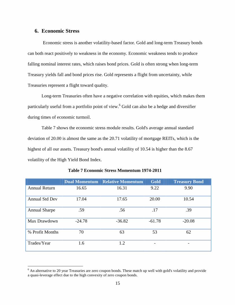
6. Economic Stress
Economic stress is another volatility-based factor. Gold and long-term Treasury bonds
can both react positively to weakness in the economy. Economic weakness tends to produce
falling nominal interest rates, which raises bond prices. Gold is often strong when long-term
Treasury yields fall and bond prices rise. Gold represents a flight from uncertainty, while
Treasuries represent a flight toward quality.
Long-term Treasuries often have a negative correlation with equities, which makes them
particularly useful from a portfolio point of view.6 Gold can also be a hedge and diversifier
during times of economic turmoil.
Table 7 shows the economic stress module results. Gold's average annual standard
deviation of 20.00 is almost the same as the 20.71 volatility of mortgage REITs, which is the
highest of all our assets. Treasury bond's annual volatility of 10.54 is higher than the 8.67
volatility of the High Yield Bond Index.
Table 7 Economic Stress Momentum 1974-2011
6 An alternative to 20 year Treasuries are zero coupon bonds. These match up well with gold's volatility and provide
a quasi-leverage effect due to the high convexity of zero coupon bonds.
Dual Momentum Relative Momentum Gold Treasury Bond
Annual Return 16.65 16.31 9.22 9.90
Annual Std Dev 17.04 17.65 20.00 10.54
Annual Sharpe .59 .56 .17 .39
Max Drawdown -24.78 -36.82 -61.78 -20.08
% Profit Months 70 63 53 62
Trades/Year 1.6 1.2 - -
16
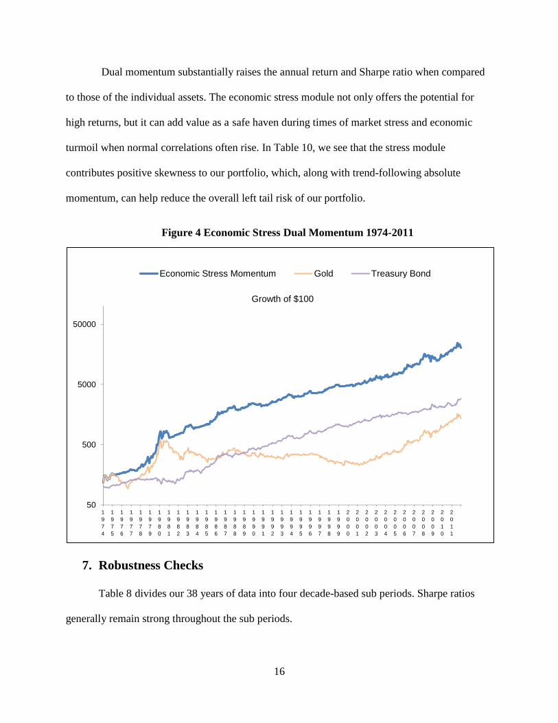
Dual momentum substantially raises the annual return and Sharpe ratio when compared
to those of the individual assets. The economic stress module not only offers the potential for
high returns, but it can add value as a safe haven during times of market stress and economic
turmoil when normal correlations often rise. In Table 10, we see that the stress module
contributes positive skewness to our portfolio, which, along with trend-following absolute
momentum, can help reduce the overall left tail risk of our portfolio.
Figure 4 Economic Stress Dual Momentum 1974-2011
7. Robustness Checks
Table 8 divides our 38 years of data into four decade-based sub periods. Sharpe ratios
generally remain strong throughout the sub periods.
50
500
5000
50000
1
9
7
4
1
9
7
5
1
9
7
6
1
9
7
7
1
9
7
8
1
9
7
9
1
9
8
0
1
9
8
1
1
9
8
2
1
9
8
3
1
9
8
4
1
9
8
5
1
9
8
6
1
9
8
7
1
9
8
8
1
9
8
9
1
9
9
0
1
9
9
1
1
9
9
2
1
9
9
3
1
9
9
4
1
9
9
5
1
9
9
6
1
9
9
7
1
9
9
8
1
9
9
9
2
0
0
0
2
0
0
1
2
0
0
2
2
0
0
3
2
0
0
4
2
0
0
5
2
0
0
6
2
0
0
7
2
0
0
8
2
0
0
9
2
0
1
0
2
0
1
1
Growth of $100
Economic Stress Momentum Gold Treasury Bond
17
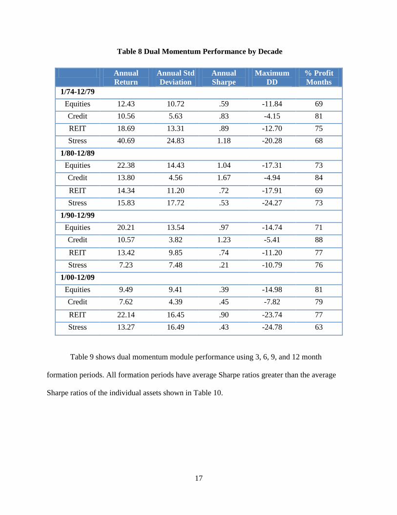
Table 8 Dual Momentum Performance by Decade
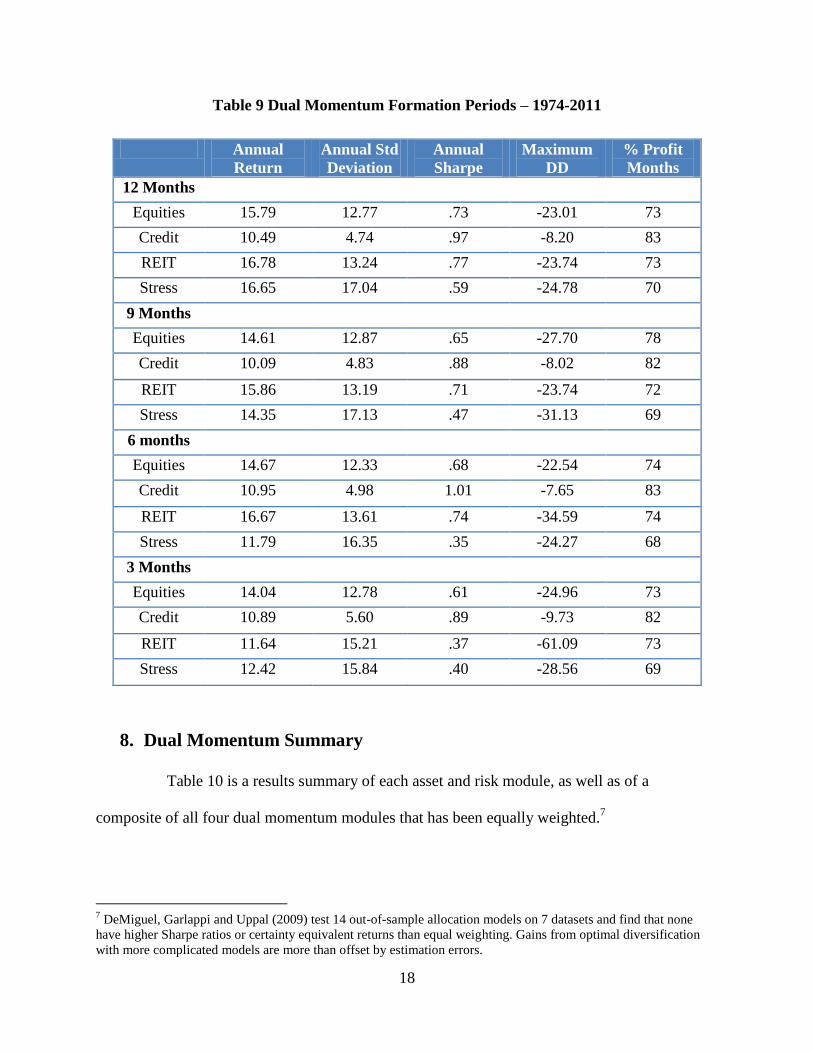
Table 9 shows dual momentum module performance using 3, 6, 9, and 12 month
formation periods. All formation periods have average Sharpe ratios greater than the average
Sharpe ratios of the individual assets shown in Table 10.
Annual
Return
Annual Std
Deviation
Annual
Sharpe
Maximum
DD
% Profit
Months
1/74-12/79
Equities 12.43 10.72 .59 -11.84 69
Credit 10.56 5.63 .83 -4.15 81
REIT 18.69 13.31 .89 -12.70 75
Stress 40.69 24.83 1.18 -20.28 68
1/80-12/89
Equities 22.38 14.43 1.04 -17.31 73
Credit 13.80 4.56 1.67 -4.94 84
REIT 14.34 11.20 .72 -17.91 69
Stress 15.83 17.72 .53 -24.27 73
1/90-12/99
Equities 20.21 13.54 .97 -14.74 71
Credit 10.57 3.82 1.23 -5.41 88
REIT 13.42 9.85 .74 -11.20 77
Stress 7.23 7.48 .21 -10.79 76
1/00-12/09
Equities 9.49 9.41 .39 -14.98 81
Credit 7.62 4.39 .45 -7.82 79
REIT 22.14 16.45 .90 -23.74 77
Stress 13.27 16.49 .43 -24.78 63
18
Table 9 Dual Momentum Formation Periods – 1974-2011
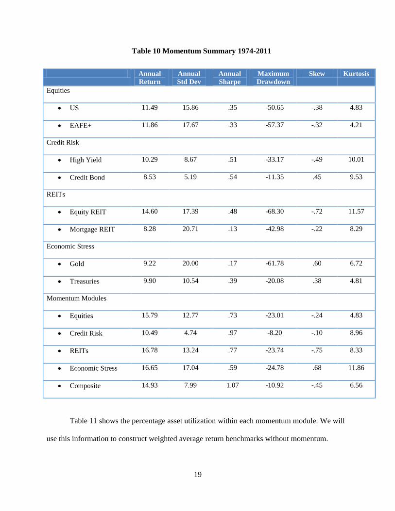
8. Dual Momentum Summary
Table 10 is a results summary of each asset and risk module, as well as of a
composite of all four dual momentum modules that has been equally weighted.7
7 DeMiguel, Garlappi and Uppal (2009) test 14 out-of-sample allocation models on 7 datasets and find that none
have higher Sharpe ratios or certainty equivalent returns than equal weighting. Gains from optimal diversification
with more complicated models are more than offset by estimation errors.
Annual
Return
Annual Std
Deviation
Annual
Sharpe
Maximum
DD
% Profit
Months
12 Months
Equities 15.79 12.77 .73 -23.01 73
Credit 10.49 4.74 .97 -8.20 83
REIT 16.78 13.24 .77 -23.74 73
Stress 16.65 17.04 .59 -24.78 70
9 Months
Equities 14.61 12.87 .65 -27.70 78
Credit 10.09 4.83 .88 -8.02 82
REIT 15.86 13.19 .71 -23.74 72
Stress 14.35 17.13 .47 -31.13 69
6 months
Equities 14.67 12.33 .68 -22.54 74
Credit 10.95 4.98 1.01 -7.65 83
REIT 16.67 13.61 .74 -34.59 74
Stress 11.79 16.35 .35 -24.27 68
3 Months
Equities 14.04 12.78 .61 -24.96 73
Credit 10.89 5.60 .89 -9.73 82
REIT 11.64 15.21 .37 -61.09 73
Stress 12.42 15.84 .40 -28.56 69
19
Table 10 Momentum Summary 1974-2011
Table 11 shows the percentage asset utilization within each momentum module. We will
use this information to construct weighted average return benchmarks without momentum.
Annual
Return
Annual
Std Dev
Annual
Sharpe
Maximum
Drawdown
Skew Kurtosis
Equities
US 11.49 15.86 .35 -50.65 -.38 4.83
EAFE+ 11.86 17.67 .33 -57.37 -.32 4.21
Credit Risk
High Yield 10.29 8.67 .51 -33.17 -.49 10.01
Credit Bond 8.53 5.19 .54 -11.35 .45 9.53
REITs
Equity REIT 14.60 17.39 .48 -68.30 -.72 11.57
Mortgage REIT 8.28 20.71 .13 -42.98 -.22 8.29
Economic Stress
Gold 9.22 20.00 .17 -61.78 .60 6.72
Treasuries 9.90 10.54 .39 -20.08 .38 4.81
Momentum Modules
Equities 15.79 12.77 .73 -23.01 -.24 4.83
Credit Risk 10.49 4.74 .97 -8.20 -.10 8.96
REITs 16.78 13.24 .77 -23.74 -.75 8.33
Economic Stress 16.65 17.04 .59 -24.78 .68 11.86
Composite 14.93 7.99 1.07 -10.92 -.45 6.56

20
Table 11 Weighted Average Return Benchmarks 1974-2011
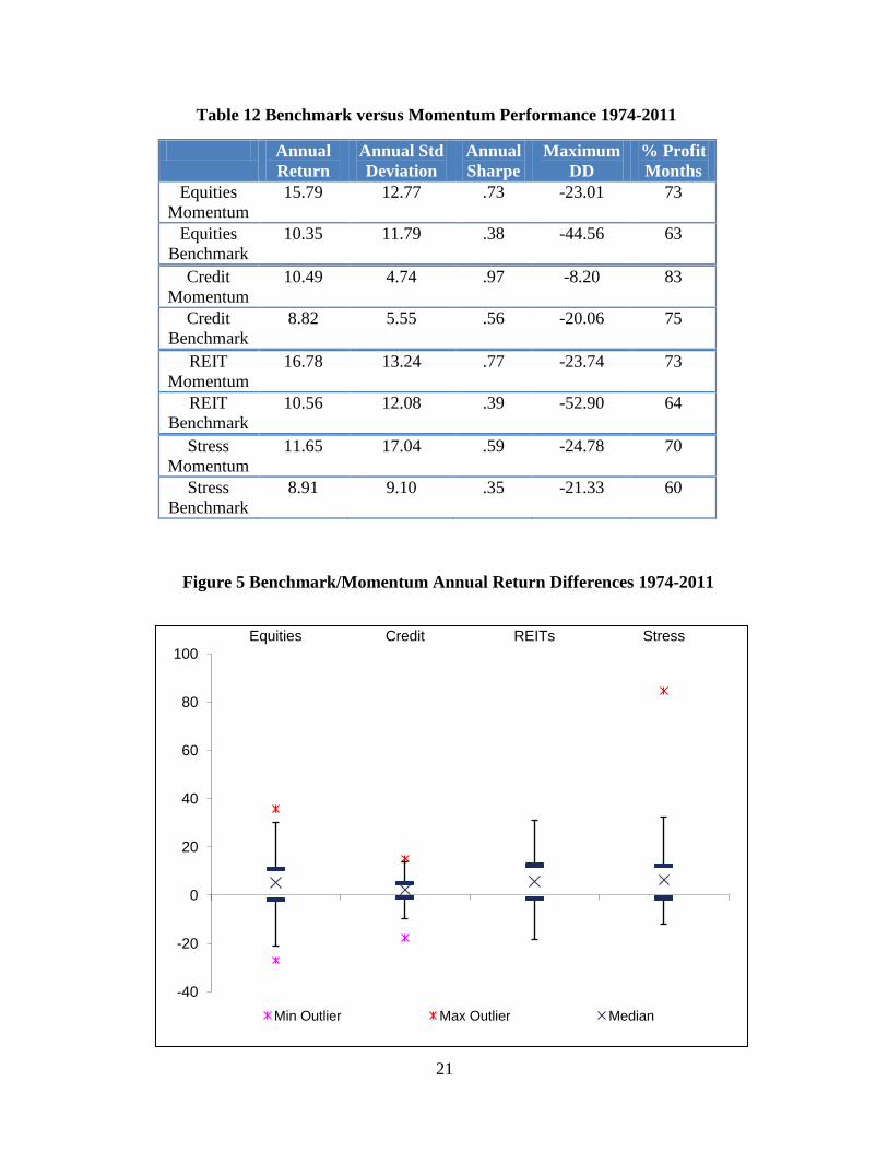
Table 12 compares dual momentum module performance with the weighted average
return benchmarks from Table 11. Figure 5 is an inter quartile box plot of the differences in
annual return between the weighted average benchmarks and the dual momentum modules
covering our 38 years of data.
8 The entire portfolio is simultaneously in Treasury bills 3.5% of the time. Three of the four modules are
simultaneously in Treasury bills 6.8% of the time, while two of the four modules are simultaneously in Treasury
bills 8.3% of the time.
Asset Return % of Time
Utilized8
Weighted Average
Return Benchmark
Equities U.S. 11.49 37.7
EAFE+ 11.86 39.7
T Bill 5.89 22.6 10.35
Credit Risk Credit 8.53 19.5
Hi Yield 10.29 55.3
T Bill 5.89 25.2 8.82
REITs Equity 14.60 46.9
Mortgage 8.28 26.8
T Bill 5.89 26.3 10.56
Stress Gold 9.02 39.0
Treasuries 9.90 43.2
T Bill 5.89 17.8 8.91
21
Table 12 Benchmark versus Momentum Performance 1974-2011
Annual
Return
Annual Std
Deviation
Annual
Sharpe
Maximum
DD
% Profit
Months
Equities
Momentum
15.79 12.77 .73 -23.01 73
Equities
Benchmark
10.35 11.79 .38 -44.56 63
Credit
Momentum
10.49 4.74 .97 -8.20 83
Credit
Benchmark
8.82 5.55 .56 -20.06 75
REIT
Momentum
16.78 13.24 .77 -23.74 73
REIT
Benchmark
10.56 12.08 .39 -52.90 64
Stress
Momentum
11.65 17.04 .59 -24.78 70
Stress
Benchmark
8.91 9.10 .35 -21.33 60
-40
-20
0
20
40
60
80
100
Equities Credit REITs Stress
Min Outlier Max Outlier Median
Figure 5 Benchmark/Momentum Annual Return Differences 1974-2011
22
9. Module Characteristics
We might find additional high volatility assets by further segmenting a market or asset class.
For example, we could split equities into individual countries or regions. However, greater
segmentation would reduce the diversification benefits we get from using broader asset classes.
Our module approach imposes a framework of portfolio diversification, which reduces
portfolio volatility. Our trend following, absolute momentum Treasury bill overlay further
reduces potential downside volatility. These two elements of our dual momentum approach are
desirable from a portfolio risk point of view.
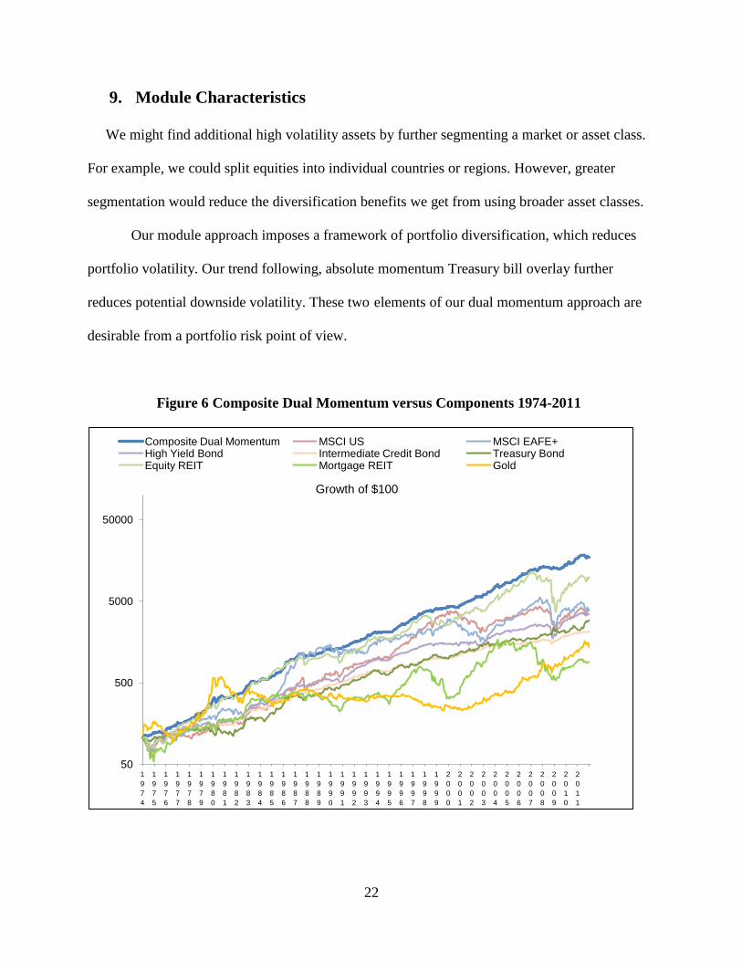
Figure 6 Composite Dual Momentum versus Components 1974-2011
50
500
5000
50000
1
9
7
4
1
9
7
5
1
9
7
6
1
9
7
7
1
9
7
8
1
9
7
9
1
9
8
0
1
9
8
1
1
9
8
2
1
9
8
3
1
9
8
4
1
9
8
5
1
9
8
6
1
9
8
7
1
9
8
8
1
9
8
9
1
9
9
0
1
9
9
1
1
9
9
2
1
9
9
3
1
9
9
4
1
9
9
5
1
9
9
6
1
9
9
7
1
9
9
8
1
9
9
9
2
0
0
0
2
0
0
1
2
0
0
2
2
0
0
3
2
0
0
4
2
0
0
5
2
0
0
6
2
0
0
7
2
0
0
8
2
0
0
9
2
0
1
0
2
0
1
1
Growth of $100
Composite Dual Momentum MSCI US MSCI EAFE+ High Yield Bond Intermediate Credit Bond Treasury Bond Equity REIT Mortgage REIT Gold
23
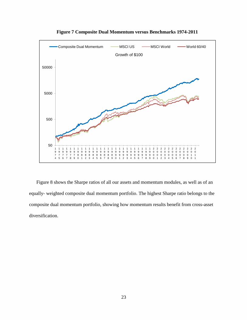
Figure 7 Composite Dual Momentum versus Benchmarks 1974-2011
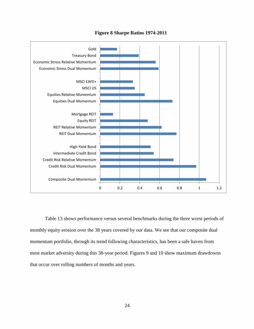
Figure 8 shows the Sharpe ratios of all our assets and momentum modules, as well as of an
equally- weighted composite dual momentum portfolio. The highest Sharpe ratio belongs to the
composite dual momentum portfolio, showing how momentum results benefit from cross-asset
diversification.
50
500
5000
50000
1
9
7
4
1
9
7
5
1
9
7
6
1
9
7
7
1
9
7
8
1
9
7
9
1
9
8
0
1
9
8
1
1
9
8
2
1
9
8
3
1
9
8
4
1
9
8
5
1
9
8
6
1
9
8
7
1
9
8
8
1
9
8
9
1
9
9
0
1
9
9
1
1
9
9
2
1
9
9
3
1
9
9
4
1
9
9
5
1
9
9
6
1
9
9
7
1
9
9
8
1
9
9
9
2
0
0
0
2
0
0
1
2
0
0
2
2
0
0
3
2
0
0
4
2
0
0
5
2
0
0
6
2
0
0
7
2
0
0
8
2
0
0
9
2
0
1
0
2
0
1
1
Growth of $100
Composite Dual Momentum MSCI US MSCI World World 60/40
24
Figure 8 Sharpe Ratios 1974-2011
Table 13 shows performance versus several benchmarks during the three worst periods of
monthly equity erosion over the 38 years covered by our data. We see that our composite dual
momentum portfolio, through its trend following characteristics, has been a safe haven from
most market adversity during this 38-year period. Figures 9 and 10 show maximum drawdowns
that occur over rolling numbers of months and years.
0 0.2 0.4 0.6 0.8 1 1.2
Composite Dual Momentum
Credit Risk Dual Momentum
Credit Risk Relative Momentum
Intermediate Credit Bond
High Yield Bond
REIT Dual Momentum
REIT Relative Momentum
Equity REIT
Mortgage REIT
Equities Dual Momentum
Equities Relative Momentum
MSCI US
MSCI EAFE+
Economic Stress Dual Momentum
Economic Stress Relative Momentum
Treasury Bond
Gold

25
Table 13 Largest Bear Market Drawdowns 1974-2011
Date MSCI US MSCI World World 60/40 Composite
Momentum
3/74 - 9/74 -33.3 -30.8 -19.0 +2.1
9/00 – 9/01 -30.9 -31.7 -15.9 +17.1
4/02 - 9/02 -29.1 -25.6 -11.9 +7.5
11/07 - 2/09 -50.6 -53.6 -32.8 -2.8
World 60/40 is composed of 60% MSCI World Index and 40% Barclays Intermediate Treasury Index.
Figure 9 Rolling 1-12 Month Maximum Drawdowns 1974-2011
-50
-45
-40
-35
-30
-25
-20
-15
-10
-5
0
MSCI US MSCI World World 60/40 Composite Momentum
1 Month 3 Month 6 Month 12 Month

26
Figure 10 Rolling 5 Year Maximum Drawdowns 1979-2011
10. Absolute Momentum
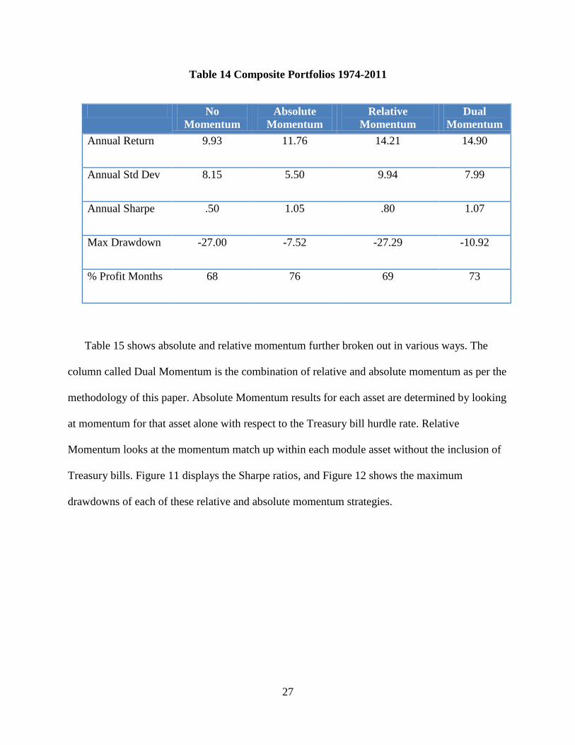
Table 14 shows equal-weighted composite portfolios with and without absolute momentum.
The first column is all nine assets without any momentum. The second column shows the same
assets with an absolute momentum overlay applied to each asset. The third column shows our
four modules with relative momentum, but not absolute momentum. The final column is our dual
momentum module-based portfolio. We see that absolute momentum enhances performance
considerably, both with and without relative momentum.
-60
-50
-40
-30
-20
-10
0
1
9
7
9
1
9
8
0
1
9
8
1
1
9
8
2
1
9
8
3
1
9
8
4
1
9
8
5
1
9
8
6
1
9
8
7
1
9
8
8
1
9
8
9
1
9
9
0
1
9
9
1
1
9
9
2
1
9
9
3
1
9
9
4
1
9
9
5
1
9
9
6
1
9
9
7
1
9
9
8
1
9
9
9
2
0
0
0
2
0
0
1
2
0
0
2
2
0
0
3
2
0
0
4
2
0
0
5
2
0
0
6
2
0
0
7
2
0
0
8
2
0
0
9
2
0
1
0
2
0
1
1
Composite Momentum MSCI US MSCI World World 60/40
27
Table 14 Composite Portfolios 1974-2011
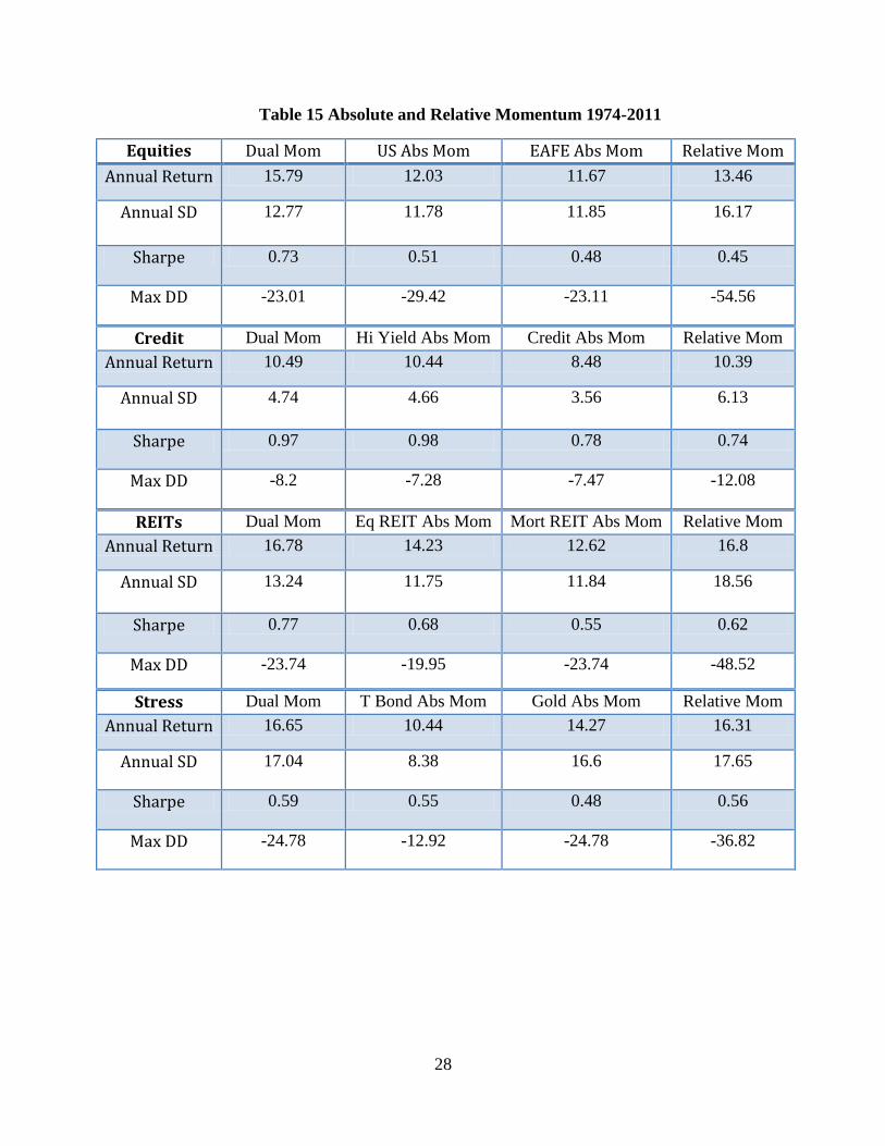
Table 15 shows absolute and relative momentum further broken out in various ways. The
column called Dual Momentum is the combination of relative and absolute momentum as per the
methodology of this paper. Absolute Momentum results for each asset are determined by looking
at momentum for that asset alone with respect to the Treasury bill hurdle rate. Relative
Momentum looks at the momentum match up within each module asset without the inclusion of
Treasury bills. Figure 11 displays the Sharpe ratios, and Figure 12 shows the maximum
drawdowns of each of these relative and absolute momentum strategies.
No
Momentum
Absolute
Momentum
Relative
Momentum
Dual
Momentum
Annual Return 9.93 11.76 14.21 14.90
Annual Std Dev 8.15 5.50 9.94 7.99
Annual Sharpe .50 1.05 .80 1.07
Max Drawdown -27.00 -7.52 -27.29 -10.92
% Profit Months 68 76 69 73
28
Table 15 Absolute and Relative Momentum 1974-2011
Equities Dual Mom US Abs Mom EAFE Abs Mom Relative Mom
Annual Return 15.79 12.03 11.67 13.46
Annual SD 12.77 11.78 11.85 16.17
Sharpe 0.73 0.51 0.48 0.45
Max DD -23.01 -29.42 -23.11 -54.56
Credit Dual Mom Hi Yield Abs Mom Credit Abs Mom Relative Mom
Annual Return 10.49 10.44 8.48 10.39
Annual SD 4.74 4.66 3.56 6.13
Sharpe 0.97 0.98 0.78 0.74
Max DD -8.2 -7.28 -7.47 -12.08
REITs Dual Mom Eq REIT Abs Mom Mort REIT Abs Mom Relative Mom
Annual Return 16.78 14.23 12.62 16.8
Annual SD 13.24 11.75 11.84 18.56
Sharpe 0.77 0.68 0.55 0.62
Max DD -23.74 -19.95 -23.74 -48.52
Stress Dual Mom T Bond Abs Mom Gold Abs Mom Relative Mom
Annual Return 16.65 10.44 14.27 16.31
Annual SD 17.04 8.38 16.6 17.65
Sharpe 0.59 0.55 0.48 0.56
Max DD -24.78 -12.92 -24.78 -36.82

29
Figure 11 Momentum Sharpe Ratios 1974-2011
0
0.1
0.2
0.3
0.4
0.5
0.6
0.7
0.8
0.9
1
Dual AbsCr AbsHY Relative Credit HiYld
Credit
0
0.1
0.2
0.3
0.4
0.5
0.6
0.7
0.8
0.9
1
Dual AbsUS AbsEAFE Relative US EAFE
Equities
0
0.1
0.2
0.3
0.4
0.5
0.6
0.7
0.8
0.9
1 REITs
0
0.1
0.2
0.3
0.4
0.5
0.6
0.7
0.8
0.9
1 Stress
30
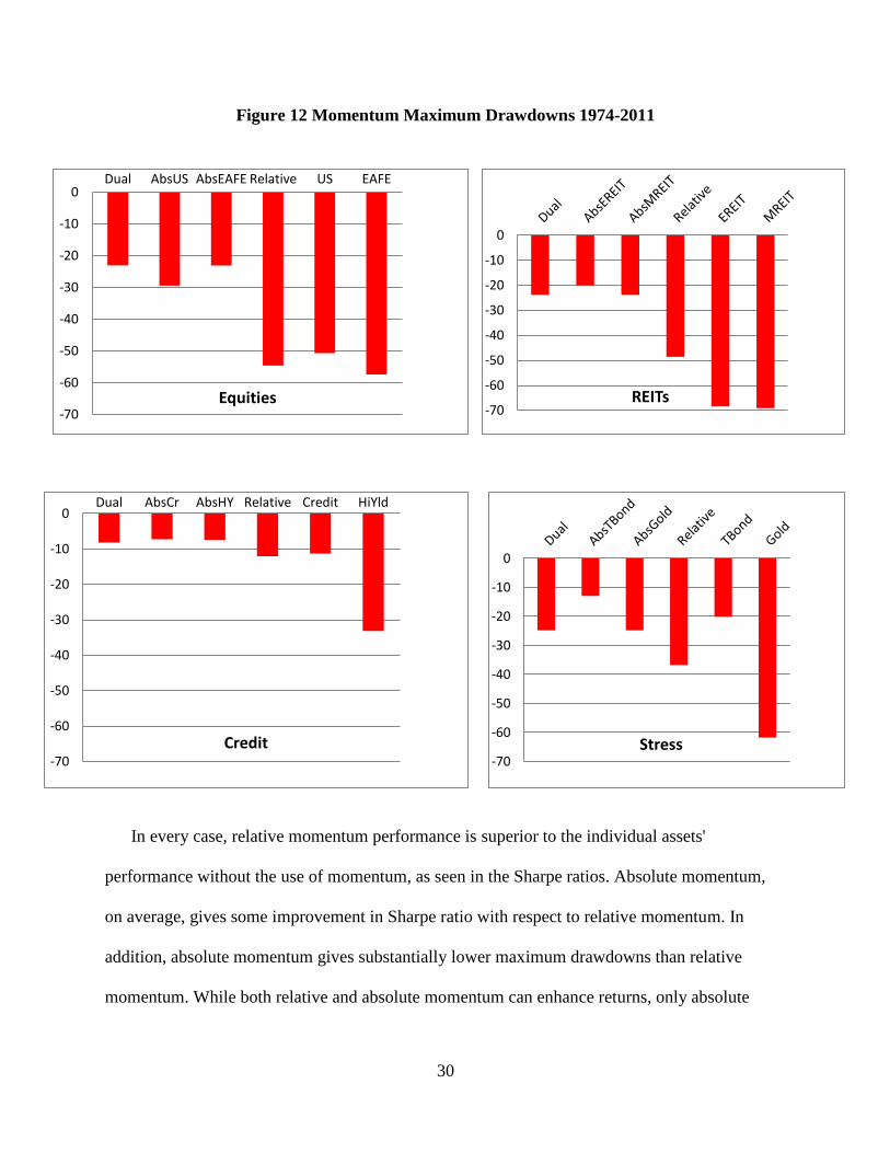
Figure 12 Momentum Maximum Drawdowns 1974-2011
In every case, relative momentum performance is superior to the individual assets'
performance without the use of momentum, as seen in the Sharpe ratios. Absolute momentum,
on average, gives some improvement in Sharpe ratio with respect to relative momentum. In
addition, absolute momentum gives substantially lower maximum drawdowns than relative
momentum. While both relative and absolute momentum can enhance returns, only absolute
-70
-60
-50
-40
-30
-20
-10
0 Dual AbsUS AbsEAFE Relative US EAFE
Equities -70
-60
-50
-40
-30
-20
-10
0
REITs
-70
-60
-50
-40
-30
-20
-10
0 Dual AbsCr AbsHY Relative Credit HiYld
Credit
-70
-60
-50
-40
-30
-20
-10
0
Stress
31
momentum substantially reduces volatility and drawdown. The best results, however, come from
dual momentum, our combination of absolute and relative momentum.
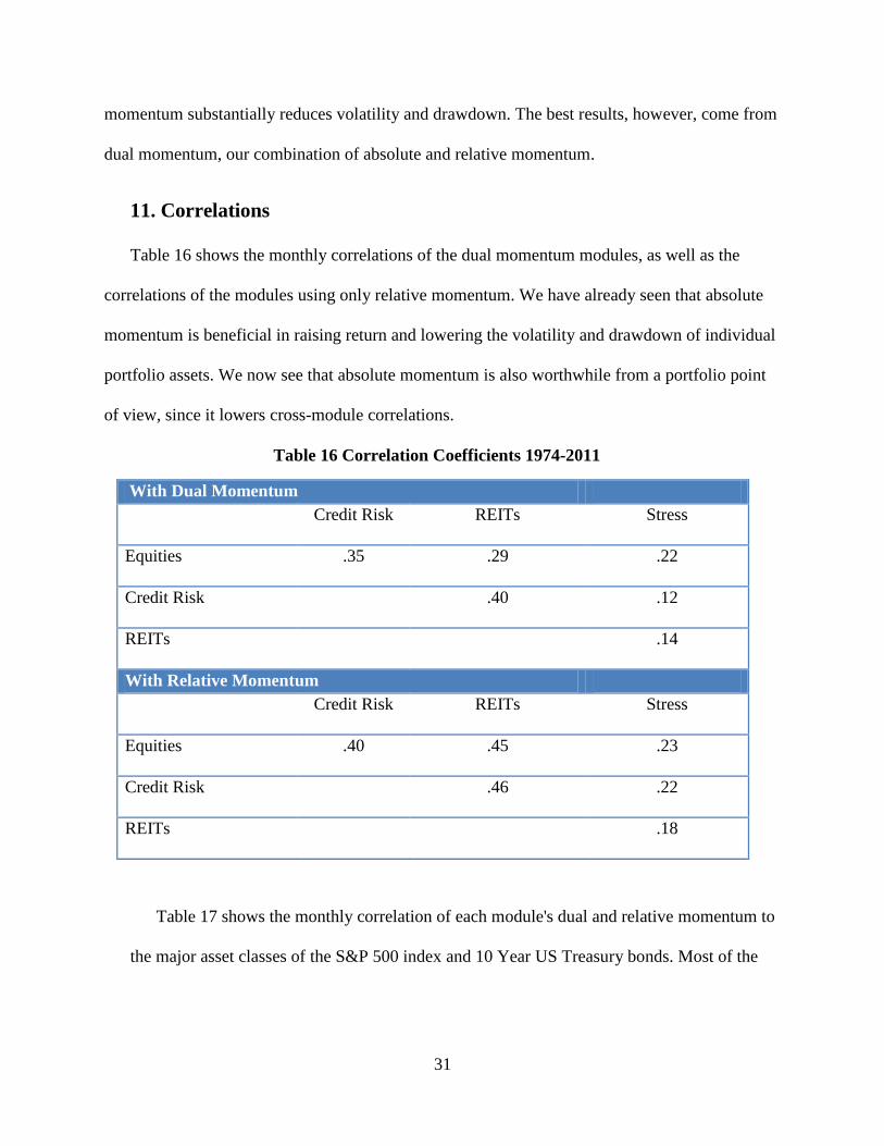
11. Correlations
Table 16 shows the monthly correlations of the dual momentum modules, as well as the
correlations of the modules using only relative momentum. We have already seen that absolute
momentum is beneficial in raising return and lowering the volatility and drawdown of individual
portfolio assets. We now see that absolute momentum is also worthwhile from a portfolio point
of view, since it lowers cross-module correlations.
Table 16 Correlation Coefficients 1974-2011
With Dual Momentum
Credit Risk REITs Stress
Equities .35 .29 .22
Credit Risk .40 .12
REITs .14
With Relative Momentum
Credit Risk REITs Stress
Equities .40 .45 .23
Credit Risk .46 .22
REITs .18
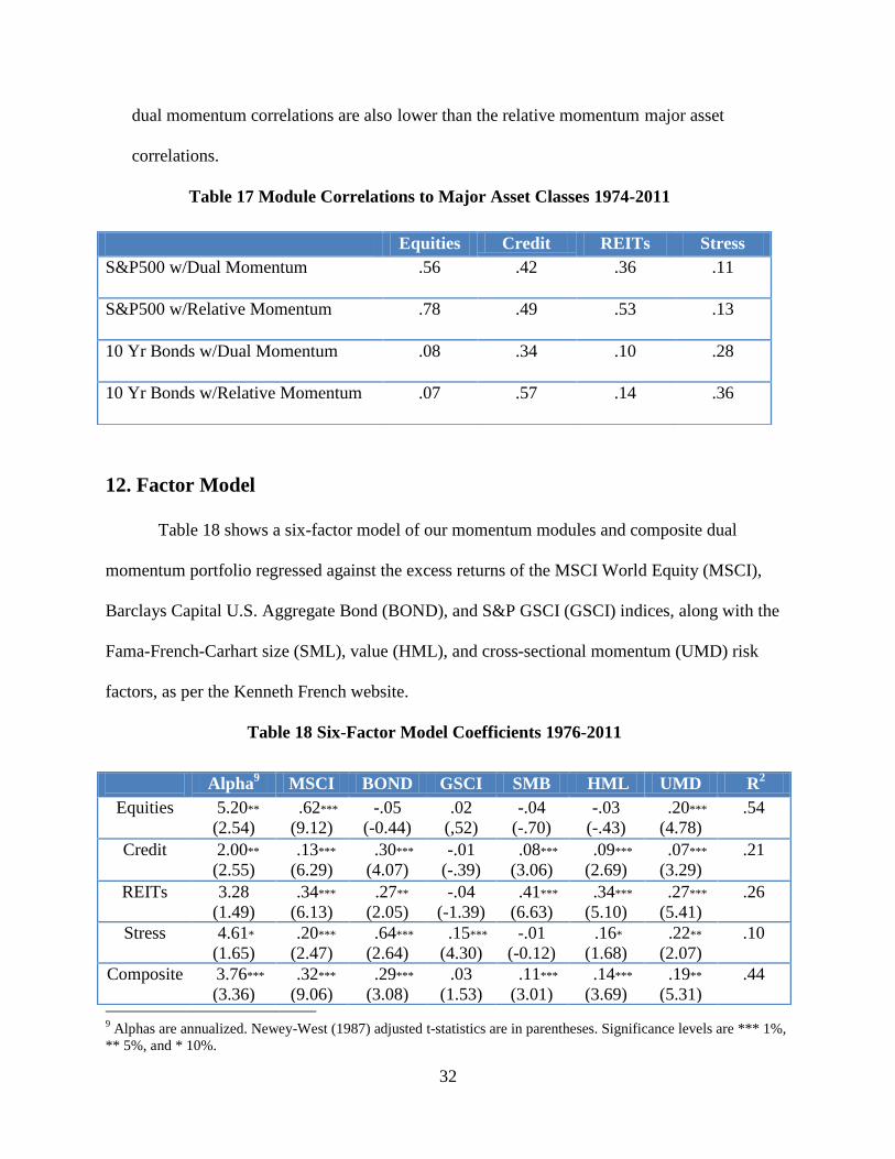
Table 17 shows the monthly correlation of each module's dual and relative momentum to
the major asset classes of the S&P 500 index and 10 Year US Treasury bonds. Most of the
32
dual momentum correlations are also lower than the relative momentum major asset
correlations.
Table 17 Module Correlations to Major Asset Classes 1974-2011
12. Factor Model
Table 18 shows a six-factor model of our momentum modules and composite dual
momentum portfolio regressed against the excess returns of the MSCI World Equity (MSCI),
Barclays Capital U.S. Aggregate Bond (BOND), and S&P GSCI (GSCI) indices, along with the
Fama-French-Carhart size (SML), value (HML), and cross-sectional momentum (UMD) risk
factors, as per the Kenneth French website.
Table 18 Six-Factor Model Coefficients 1976-2011
9 Alphas are annualized. Newey-West (1987) adjusted t-statistics are in parentheses. Significance levels are *** 1%,
** 5%, and * 10%.
Equities Credit REITs Stress
S&P500 w/Dual Momentum .56 .42 .36 .11
S&P500 w/Relative Momentum .78 .49 .53 .13
10 Yr Bonds w/Dual Momentum .08 .34 .10 .28
10 Yr Bonds w/Relative Momentum .07 .57 .14 .36
Alpha9 MSCI BOND GSCI SMB HML UMD R
2
Equities 5.20**
(2.54)
.62***
(9.12)
-.05
(-0.44)
.02
(,52)
-.04
(-.70)
-.03
(-.43)
.20***
(4.78)
.54
Credit 2.00**
(2.55)
.13***
(6.29)
.30***
(4.07)
-.01
(-.39)
.08***
(3.06)
.09***
(2.69)
.07***
(3.29)
.21
REITs 3.28
(1.49)
.34***
(6.13)
.27**
(2.05)
-.04
(-1.39)
.41***
(6.63)
.34***
(5.10)
.27***
(5.41)
.26
Stress 4.61*
(1.65)
.20***
(2.47)
.64***
(2.64)
.15***
(4.30)
-.01
(-0.12)
.16*
(1.68)
.22**
(2.07)
.10
Composite 3.76***
(3.36)
.32***
(9.06)
.29***
(3.08)
.03
(1.53)
.11***
(3.01)
.14***
(3.69)
.19**
(5.31)
.44

33
We see significant positive alphas in our equities and credit, and stress modules, as well as our
dual momentum composite. As expected, cross-sectional momentum loadings are positive and
significant across all modules and the composite.
13. Conclusions
Our results have important implications for momentum investors. Using thirty-eight years
of past performance data, dual momentum modules show significant performance improvements
in all four areas we have examined - equities, credit risk, real estate, and economic stress, as well
as with an equally-weighted composite portfolio of all the modules. The ancillary conclusions we
reach are as follows:
1) Long side momentum works best when one uses a combination of absolute
momentum and relative strength momentum. Trend determination with absolute momentum can
help mitigate downside risk and take advantage of regime persistence, while both relative
strength and absolute momentum can enhance expected returns. Portfolios also benefit from the
low correlations that accompany dual momentum, making multi-asset momentum portfolios
desirable.
2) Investors generally wish to avoid high volatility. There is now, in fact, a propensity
toward low volatility investment portfolios. However, what is undesirable is downside
variability, rather than total volatility. Absolute momentum can help investors harness volatility
and convert it into extraordinary returns while reducing the potential drawdowns that are usually
associated with high volatility.
3) Focused modules can isolate and target specific risk factors. They facilitate the effective
use of a hurdle rate/safe harbor alternative asset. Modules provide flexibility and diversification

34
on a non-parametric basis, making it simple and easy to implement dual momentum-based
portfolios.
The combination of relative and absolute momentum makes diversification more efficient
by selectively utilizing assets only when both their relative and absolute momentum are positive,
and these assets are more likely to appreciate. A dual momentum approach bears market risk
when it makes the most sense, i.e., when there is positive absolute, as well as relative,
momentum. Module-based dual momentum, serving as a strong alpha overlay, can help capture
risk premia from volatile assets, while at the same time, defensively adapting to regime change.
35
References
Ahn, Dong-Hyu., Jennifer Conrad, and Robert Dittmar (2003), “Risk Adjustment and Trading
Strategies,” Review of Financial Studies 16 ( 2), 459-485
Asness, Clifford S., 1994, “Variables that Explain Stock Returns," Ph.D. Dissertation, University
of Chicago
Asness, Clifford S., Burt Porter, and Ross Stevens, 2000, "Predicting Stock Returns Using
Industry Relative Firm Characteristics," working paper, AQR Capital Management
Asness, Clifford S., John Liew, and Ross Stevens, 1997, “Parallels Between the Cross-Sectional
Predictability of Stock and Country Returns,” The Journal of Portfolio Management, 23, 79-87
Asness, Clifford S., Tobias J. Moskowitz, and Lasse J. Pedersen, 2012, “Value and Momentum
Everywhere,” Journal of Finance, forthcoming
Bandarchuk, Pavel and Jena Hilscher, 2011, “Sources of Momentum Profits: Evidence on the
Irrelevance of Characteristics,” working paper
Barberis, Nicholas, Shleifer, A., Vishny, R., 1998, "A Model of Investor Sentiment," Journal of
Financial Economics 49, 307–343
Beracha, Eli and Hilla Skiba, 2011, “Momentum in Residential Real Estate,” Journal of Real
Estate Finance and Economics 43, 299-320
Berk, Jonathan, Robert Green and Vasant Naik, 1999, “Optimal Investment, Growth Options and
Security Returns,” Journal of Finance 54, 1153-1608
Bhojraj, Sanjeev and Bhaskaran Swaminathan, 2006, “Macromomentum: Returns Predictability
in International Equity Indices,” Journal of Business 79, 429–451
Chabot, Benjamin R., Eric Ghysels, and Ravi Jagannathan, 2009, “Price Momentum in Stocks:
Insights from Victorian Age Data,” working paper, National Bureau of Economic Research
Blitz, David C and Pim Van Vliet, 2008, "Global Tactical Cross-Asset Allocation: Applying
Value and Momentum Across Asset Classes," Journal of Portfolio Management 35 (1), 23-38
Chan, Kalak, Allaudeen Hameed and Wilson H.S. Tong, 2000, “Profitability of Momentum
Strategies in International Equity Markets,” Journal of Financial and Quantitative Analysis 35,
153-175
Cooper, Michael J, Roberto C Guiterrez, Jr, and Allaudeen Hameed, 2004, "Market States and
Momentum," Journal of Finance 59, 1345-1365
36
Daniel, Kent, Hirshleifer, D., Subrahmanyam, A., 1998, "Investor Psychology and Security
Market Under- and Over-Reactions." Journal of Finance 53, 1839–1886
DeMiguel, Victor, Lorenzo Garlappi and Raman Uppal, 2009, "Optimal Versus Naïve
Diversification: How Inefficient is the 1/N Portfolio Strategy?" Review of Financial Studies 22
(5), 1915-1953
Fama, Eugene F. and Kenneth R. French, 2008, “Dissecting Anomalies,” Journal of Finance 63,
1653-1678
Frazzini, Andrea, 2006, "The Disposition Effect and Underreaction to News," Journal of
Finance 61, 2017-2046
Griffin, John, Xiuquing Ji, and J. Spencer Martin, 2005, “Global Momentum Strategies: A
Portfolio Perspective,” Journal of Portfolio Management 31, 23-39
Grundy, Bruce D and J Spencer Martin, 2001, “Understanding the Nature of the Risks and the
Sources of the Rewards to Momentum Investing,” Review of Financial Studies 14, 29-78
Hong, Harrison and Jeremy Stein, 1999, "A Unified Theory of Underreaction, Momentum
Trading, and Overreaction in Asset Markets," Journal of Finance 54, 2143-2184
Hvidkjaer, Soeren, 2006,. "A Trade-based Analysis of Momentum.” Review of Financial Studies
19 (2), 457–491
Hurst, Brian, Yao Hua Ooi, and Lasse H Pedersen, 2012, "A Century of Evidence onTrend-
Following Investing," AQR Capital Management, LLC
Jegadeesh, Narasimhan and Sheridan Titman, 1993, “Returns to Buying Winners and Selling
Losers: Implications for Stock Market Efficiency,” Journal of Finance 48, 65-91
Johnson, Timothy, 2002, “Rational Momentum Effects,” Journal of Finance 57, 585-608.
Jostova, Gergana, Stanislova Nikolova, Alexander Philipov, and Christof W Stahel, 2010,
“Momentum in Corporate Bond Returns,” working paper
Liu, Laura Xiaolei and Lu Zhang, 2008, “Momentum Profits, Factor Pricing, and
Macroeconomic Risk,” Review of Financial Studies 21 (6), 2417-2448
Menkoff, Lukas, Lucio Sarno, Maik Schmeling and Andreas Schrimpf, 2011, "Currency
Momentum Strategies," working paper
Miffre, Joelle and Georgios Rallis, 2007, “Momentum Strategies in Commodity Futures
Markets,” Journal of Banking and Finance 31, 1863-1886
37
Moskowitz, Tobias J. and Mark Grinblatt, 1999, "Do Industries Explain Momentum?" Journal of
Finance 54, 1249–1290
Moskowitz, Tobias J., Yao Hua Ooi, and Lasse Heje Pedersen, 2012, "Time Series Momentum,"
Journal of Financial Economics 104, 228-250
Newey, Whitney K. and Kenneth D. West, 1987, "A Simple, Positive Semi-Definite,
Heteroskedasticity and Autocorrelation Consistent Covariance Matrix," Econometrica 55(3),
703–708
Pirrong, Craig, 2005, “Momentum in Futures Markets,” working paper
Rouwenhorst, K. Geert, 1998, “International Momentum Strategies,” Journal of Finance 53,
267-284
Rouwenhorst, K. Geet, 1999, “Local Return Factors and Turnover in Emerging Stock Markets,”
Journal of Finance 54, 1439-1464
Sagi, Jacob, and Mark Seasholes, 2007, “Firm-specific Attributes and the Cross-section of
Momentum,” Journal of Financial Economics 84 (2), 389-434
Schwert, G. William, 2002, “Anomolies and Market Efficiency,” working
paper, National Bureau of Economic Research
Tsay, Ruey S, 2010, Analysis of Financial Time Series, John Wiley & Sons, Inc, Hoboken, NJ
Tversky, Amos and Daniel Kahneman, 1974, "Judgment under Uncertainty: Heuristics and
Biases," Science 185, 1124-1131
Zhang, X Frank, 2006, "Information Uncertainty and Stock Returns," Journal of Finance
61,105–136