risk pooling, commitment, and information: an experimental test … · 2019-06-17 · 2 risk...

Risk Pooling, Commitment, and Information:

An experimental test of two fundamental assumptions*

CSAE WPS/2003-05

Abigail Barr**

Centre for the Study of African Economies

University of Oxford

June 2003

* This research was funded by the Department for International Development under ESCOR grant number R7650. ** Corresponding author:- Abigail Barr, Centre for the Study of African Economies, Department of Economics, University of Oxford, Manor Road, Oxford, OX1 3UQ, United Kingdom. E-mail address: [email protected]

Risk Pooling, Commitment and Information: An experimental test of

two fundamental assumptions

Abstract

This paper presents rigorous and direct tests of two assumptions relating to limited

commitment and asymmetric information that underpin current models of risk

pooling. A specially designed economic experiment involving 678 subjects across 23

Zimbabwean villages is used to solve the problems of observability and quantification

that have frustrated previous attempts to conduct such tests. I find that more extrinsic

commitment is associated with more risk pooling, but that more information is

associated with less risk pooling. The first of these results accords with our

expectations and assumptions. The second does not. I offer two explanations as to the

origin of the second result and discuss their implications for how we view the

assumptions made elsewhere in the literature. I also conduct a test of the relevance or

external validity of the experimental results to our understanding of real risk pooling

behaviour. In four out of the five villages for which the test could be conducted the

networks of risk pooling contracts constructed during the experiment and the

networks existing in real life were significantly correlated.

JEL Classifications: C93; D81; O12.

Keywords: Field experiment; Asymmetric information; Limited commitment;

Villages; Economic development; Risk; Insurance.

.

2

Risk Pooling, Commitment and Information: An experimental test of

two fundamental assumptions

1. Introduction

Over four fifths of the world’s population do not have access to formal insurance

against income and consumption shocks (Holtzmann, Packard & Cuesta, (2000)).

Recent insights into how these people prepare for and cope with such shocks are

based on the application of game and contract theory to informal risk pooling

arrangements, informal credit, and reciprocal gift giving (e.g., Coate and Ravallion

(1993), Fafchamps (1998)) and on the increasingly innovative empirical studies

motivated by the resulting theoretical models. From these empirical studies we have

learnt that full risk pooling is rare (e.g., Ravallion and Dearden (1988), Morduch

(1991), Ravallion and Chaudhuri (1991), Alderman and Paxson (1992), Townsend

(1994), Ligon (1998)), that some types of shocks are more likely to be informally

insured than others, that risk pooling is associated with certain forms of relationship

(e.g., Grimaud (1997), Fafchamps and Lund (1997), De Weerdt (2002), Dekker

(2003)), and that some theoretical models explain the data more effectively than

others (Ligon, Thomas and Worrall (2002)).

But are our insights well founded? There are a series of assumptions

underpinning all of this work that have yet to be explored and tested directly. These

relate to: the origins and extent of commitment and its effects on risk pooling; and the

degree to which information is asymmetric and the effects of this asymmetry on risk

pooling. If these assumptions are ill founded so may be the insights and conclusions

we have drawn from the analyses cited above.

3

The assumption that limited commitment leads to less risk pooling is true by

definition if, following Platteau (1994a, 1994b), Fafchamps (1992, 1996), Posner and

Rasmusen (1999), Kreps (1997) and others, we acknowledge that both extrinsic

incentives, especially the sanctions that can credibly be threatened, and intrinsic

motivations, altruism, inequality aversion and reciprocal kindness, can act as bases for

commitment. However, theoretical models of risk pooling focus exclusively on the

former and we have yet to distinguish effectively between the two empirically.

Kinship, co-ethnicity, shared clan membership, and religious co-affiliation are all

statistically associated with flows of assistance (Grimaud (1997), Fafchamps and

Lund (1997), De Weerdt (2002), Dekker (2003)), but is this because such

relationships facilitate the effective use of extrinsic incentives or because they are

associated with relation-specific forms of intrinsic motivation?

This ambiguity is problematic. For policy-makers the relative importance of

extrinsic incentives and intrinsic motivations as determinants of behaviour has

implications for the potential success of certain interventions. A carefully planned

reform of an informal, grass-roots institution, that is predicted to improve welfare

under the assumption that people respond to extrinsic incentives, could crowd out

cooperative behaviour and lead to reductions in welfare if, in fact, people are

primarily intrinsically motivated (Cardenas, Stranlund, and Willis (2000), Bohnet,

Frey, and Huck (2001)). For theorists and empirical researchers the relative

importance of extrinsic and intrinsic bases for commitment may also have

implications for the effect of information asymmetries on the extent to which risk is

pooled. If flows of assistance in times of need are intrinsically motivated is irrelevant

and information asymmetries will have no bearing on levels of risk pooling.

4

Even if extrinsic incentives are required to support risk pooling arrangements,

it is possible to conceive of scenarios under which more rather than less information

leads to less risk pooling. Suppose that, as the experiments of Falk, Fehr, and

Fischbacher (2000), Bowles, Carpenter and Gintis (2001), and Barr (2002) show,

social or shame-based sanctions can be used to enhance commitment and that such

sanctions are commonly threatened and applied. Also suppose that people can be and

know that they can be tempted into behaving in a manner that will attract such

sanctions when the immediate individual returns to doing so are high enough, but also

know that they will suffer regret if they are tempted, exposed, and shamed in this way.

Then, an increased likelihood of detection or exposure could lead to less risk pooling

as it is only by not entering into such arrangements that people can ensure that they

will not be tempted to renege and suffer the shameful consequences. Using Elster’s

(1984) terminology, choosing not to enter into risk pooling arrangements could be a

form of pre-commitment.

Alternatively suppose that, instead of questioning their own willpower and

fearing shame and regret, people are conflict averse, in much the same way that

Harowitz (2001) assumes countries to be. They fear reneging by others because they

suffer not only the material consequences of being cheated but also the psychological

consequences of conflict. If the second concern dominates, an increased likelihood of

detection could lead to less risk pooling as not entering into such arrangements is the

only way to ensure that one will not end up in conflict with a renegade. Such conflict

aversion might also cause people to put less effort into gathering information even

when it is relatively easy or costless to do so. In other words, they might choose to

‘turn a blind eye’. But this, along with the recent work of Boozer and Goldstein

(2003) on information asymmetries within households, calls into question the

5

assumption often made by theorists, that within the tightly knit social groups that are

likely to engage in risk pooling, information is unlimited.

The reason why these assumptions have not been fully explored and directly

tested relates to problems of observability and quantification. Such an analysis

requires data on how much risk is pooled, the degree of asymmetry in information, the

extent to which extrinsic commitment is limited, and maybe even the incidence and

content of intrinsic motivations. It has proven very difficult to generate these data,

especially relating to commitment, using a survey-based approach. Here, I solve these

problems by running an economic experiment that is novel in two regards. First, it is

designed specifically for the task, making it the first risk pooling experiment to be run

anywhere. And second, it is designed to support a formal test of its own external

validity, i.e., its relevance to our understanding of real risk pooling behaviour.

Within the experiment, subjects were invited to pool risk under three

treatments that varied with respect to the degree to which information is asymmetric

and extrinsic commitment is limited. (Section 2 provides a detailed description of the

experimental design.) The data generated during the experiment was used to test two

hypotheses: (1) that when extrinsic commitment is limited less risk pooling occurs;

and (2) that when information is asymmetric less risk pooling occurs. The results of

the experiment support hypothesis (1). However, even though there is more reneging

on pooling agreements when information is asymmetric, hypothesis (2) is rejected.

Information asymmetries lead to more rather than less risk pooling. (Section 3

presents the analysis.)

To maximize the external validity of the experiment two unusual steps were

taken: first, the experimental subjects were sub-Saharan villagers rather than students

at a western university; and second, the risk pooling decisions within the experiment

6

were made not anonymously with strangers via computer terminals or pencils and

paper but face-to-face with fellow villagers. These steps also prepared the way for the

test of external validity, to the author’s knowledge, the first formal test of external

validity ever to be carried out. The test, which was conducted in five out of the 23

villages, involved a comparison of the networks of risk pooling contracts formed

within the context of the game with the networks of risk pooling contracts in real life.

Using a technique developed by social network analysts I found that in four out of the

five villages the experimental and real risk pooling networks were significantly

correlated. (Section 4 describes the test, the data used, and the results.)

The paper concludes with a review of the assumptions commonly made by

researchers working on risk pooling in the light of the experimental results (section 5).

2. Experimental Design

The experimental design has four components; the first is the choice of the subjects;

the second involves the creation of a risky decision-making environment; the third is

the provision of an opportunity to pool risk; and the fourth involves varying the

degrees to which information and commitment are limited across subjects.

Choice of subjects

Most economic experiments are conducted in specially designed laboratories

with university students as subjects. Usually, the subjects are assumed not to know

one another and, often, their identity is kept private throughout the experiment. But

here my objective is to simulate key aspects of the situations within which people in

developing countries often but not always choose to pool risk. This objective can best

be met by working with people in developing countries within the social groupings

7

that are most relevant to their usual risk pooling endeavours. Thus, instead of

university students my subjects are Zimbabwean villagers and instead of calling the

subjects to a laboratory I take the experiment to their village meeting places. The

results presented below relate to experimental sessions in 23 villages. A total of 678

subjects were involved in the experiment, although only 642 took part in the second,

more interesting round and only 618 took part in both the first and second round. This

attrition and replacement occurred because in each village the experiment took place

over two days and some of the subjects were called away on unforeseen business on

the second day.

Creating a risky decision-making environment

I created a risky decision-making environment by conducting a near-

replication of Binswanger’s (1980) risk aversion experiment. Each subject was

confronted with a choice of six gambles. Every gamble yielded either a high or low

payoff each with probability 0.5. Whichever gamble was chosen, the payoff was

determined by playing a game that involved guessing which of the researcher’s hands

contained a blue rather than a yellow counter.1 If the subject found the blue counter he

or she received the high payoff associated with the gamble of his or her choice. If he

or she found the yellow counter, he or she received the low payoff associated with

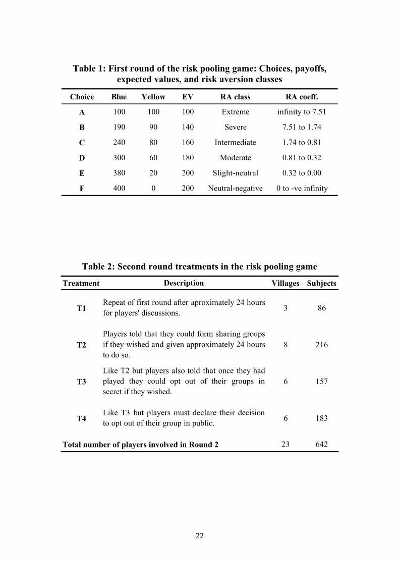
that gamble. The six gambles, drawn from Binswanger’s set of eight, are presented in

Table 1.2 Each is associated with a letter used to identify it during both play and the

analysis. In Table 1, the column labelled ‘Blue’ shows the high payoffs associated

1 Binswanger used coin tossing as the randomising device. However, in Zimbabwe women did not know how to toss and many men thought they could cheat and focused on this rather than on other aspects of the game. The which-hand-is-it-in game, known as Chigigaro in Shona, is played by grandmothers with their grandchildren and by children together throughout Zimbabwe. Thus, we can reasonably assume that the probabilities in the game are well understood. 2 The two inefficient gambles, introduced by Binswanger in order to explore subject’s understanding of the game, were left out.

8

with each gamble in Zimbabwean dollars. The column labelled ‘Yellow’ shows the

corresponding low payoffs, also in Zimbabwean dollars. The expected values, risk

aversion classes as defined by Binswanger and ranges of partial relative risk aversion

coefficients associated with each gamble are also shown. The gambles were presented

to the subjects, many of whom were illiterate, as pictures on a specially designed card

(see Figure 1). Each gamble was depicted as two piles of money, one (the high

payoff) on a blue background and the other (the low payoff) on a yellow background.

The subject had to pick the hand that had the blue counter in order to secure the high

payoff on the blue background.

At the time of the experiment, one day of casual labour would have earned a

villager approximately 200 Zimbabwean dollars, although, such work opportunities

were scarce. The official exchange rate was 50 Zimbabwean dollars to one US dollar.

In each village the subjects were called to a meeting, having been told that this

was to be the first of two meetings to be held on consecutive days. Once the research

team had been introduced, each subject met one of four research assistants in private.

They were taught the gamble choice game, their comprehension was tested, and then

they played. They were paid and then asked to sit separately from those who had not

yet played to await further instructions. Tea and snacks were served. Once everyone

had played, the next stage of the experiment was explained.

Introducing the possibility of risk pooling

The instructions then issued to the subjects varied across the villages (see

Table 2). In three of the villages the subjects were told that during the meeting

scheduled for the next day, they would be playing the same game once again. They

9

were given copies of Figure 1 to aid any discussions they wished to hold and told the

arrangements for the following day. This treatment is referred to as T1 below.

In eight of the villages, having been told that they would be playing the same

game once again, they were informed that they could, if they wished, form ‘sharing

groups’ within which all winnings from the game would be shared equally. It was left

up to the subjects whether or not they joined a group and, if they did, how large the

group was to be. The monetary implications of sharing-group-formation were

explained with the aid of simple examples. Once again the subjects were given copies

of Figure 1 to aid any discussions they wished to hold and told the arrangements for

the following day. This treatment is referred to as T2 below.

Varying the asymmetry of information and the limits on extrinsic commitment

Under T2 the subjects could not renege on the risk pooling arrangements they made

amongst themselves prior to the second round of games, i.e., extrinsic commitment

was perfect. In contrast, in treatments T3 and T4 reneging is possible, i.e., extrinsic

commitment was limited, and information was variably asymmetric. In six villages,

having been told that they could form sharing groups, the subjects were told that they

could, if they wished, opt out of their sharing groups in secret after they knew the

outcome of their own gamble. Once again the subjects were given copies of Figure 1

and told the arrangements for the following day. Under this treatment, T3 below,

commitment is limited and information is asymmetric. In the remaining six villages,

the subjects were told that they could opt out of their sharing groups after they knew

the outcome of their own gamble, but only if they were prepared to do so by raising

their hand in front of the whole meeting when the question was asked. Under this

treatment, T4 below, information is less asymmetric than under T3.

10

The data

The experiment generates two indicators of the amount of risk pooling that the

subjects are undertaking. One relates to the subject’s decisions about group formation.

If a subject joins a group containing n subjects in total, he or she is making n-1 risk

pooling contracts. The other relates to their choice of gamble. Ceteris paribus, if the

members of a sharing group select more risky gambles, they can be said to be pooling

more risk in anticipation of a higher expected return. By comparing these two

indicators across treatments we can investigate the effects of limited extrinsic

commitment and asymmetric information on risk pooling.

3. Results

Do subjects renege when commitment is limited?

Before turning to the analysis of risk pooling, it is useful to look at reneging

behaviour in the two treatments under which it is possible. Caution is required here as

subjects could only renege if they were socially selected into a sharing group: a

subject might not be selected if he or she is expected to renege. Thus, the statistics

presented will be subject to selection bias.

Figure 2 describes the decisions made by those subjects that chose to join

groups under T3 and T4. Under T3, 64 of 157 subjects joined sharing groups. Of

these, 32 won high payoffs on the gambles of their choosing and of these 7 (22

percent) reneged by opting out of their sharing group in private. All of the subjects

who won low payoffs stayed in their groups. Under T4, 66 of 183 subjects joined

sharing groups. Of these 34 won high payoffs on the gambles of their choosing and of

these only one (three percent) reneged by opting out of her sharing group in public.

11

All of the subjects who won low payoffs stayed in their groups. The proportion of

renegades among high payoff winning group members differs significantly (five

percent level) between the treatments, being lower when the reneging has to be done

publicly. This suggests that subjects do fear social sanctioning when information is

less limited.

Group formation

Figure 3 graphs the size of groups that each of the subjects in T2, T3, and T4

joined prior to the second round of the game. To aid comparisons between the

treatments, relative frequencies are shown. A group size of one indicates that the

subject played solo, i.e., not in a sharing group. Thus, a direct comparison of the bars

relating to each of the treatments on the far left of the figure is highly informative.

Only 31 percent of subjects did not join sharing groups under T2 as compared to 59

and 68 percent under T3 and T4 respectively. Turning to group size, it is in T2 that we

see the largest group, a group of twelve. Groups of ten are a focal point due to the

examples given during the instruction of the subjects. We see groups of 10 under both

T2 and T3. It is under T4 that group size is most restricted. No groups of more than

five were formed under this treatment.

In order to test the statistical significance of these variations, while controlling

for other factors that may have influenced the subjects’ decisions, I conduct a

regression analysis. Table 3 presents the results of a probit analysis of whether

subjects joined a group and then a linear regression analysis of group size conditional

on group membership. In each case the standard errors are corrected to take account

of the potential non-independence of errors within villages due to group formation

being a social process.

12

In the first column of the table, the dichotomous variable that takes the value

one if the subject joined a sharing group and zero otherwise is regressed on the

following: two treatment dummies (T2 is the basis for comparison); five dummies

relating to the choice of gamble that the subject made in the first round, included to

control for how risk averse the subject is; a dummy indicating whether the subject

won the high payoff in the first round; the number of households in the village, which

corresponds to the maximum number of subjects attending the session; two dummies

relating to the geographical area within which the subjects’ village falls, and one

dummy distinguishing resettled villages from non-resettled villages. Only the

coefficients on the two treatment dummies are significant and only these survive a

general to specific process of elimination taking the ten percent level of significance

as a cut-off. Under both T3 and T4 subjects are significantly less likely to join a group

than under T2.

If the size of the group that the subject joins is regressed on the same set of

explanatory variables only one of the treatment dummies, the one relating to T4, is

significant. The coefficient on this dummy variable is also significantly different from

the one on the treatment dummy relating to T3. In addition, three of the other

variables are significant in this model. First, subjects who won the high payoff

associated with their choice of gamble in the first round joined smaller groups.3

Second, subjects in resettled villages formed larger groups. And third, subjects in

Area 2, which has the poorest soil and least reliable rainfall, form larger groups,

3 This is not an income effect. When used in place of the high payoff dummy, actual winnings from the first round were not significant in the group formation regressions. Many of those who won high payoffs in the first round described how they avoided forming groups with those who received only low payoffs, while many of those who won low payoffs in the first round expressed a desire to be in groups with high payoff winners and disappointment at having to settle for being in a group of ‘loosers’ even though this was preferable to playing solo. This suggests that the subjects did not see the two rounds of gambles as independent probabilistic events. Such failures of expected utility theory have been observed in many contexts and should not come as a surprise here.

13

although the area dummies did not survive in the general to specific process of

variable elimination.

Choice of gamble

Figure 4 depicts the cumulative frequencies for the subjects’ choices of

gamble under T1, T2, T3, and T4. The most striking feature of these plots is the

greater tendency for subjects under T2 to choose the riskier gambles. Over one quarter

of the subjects under T2 chose gambles E or F as compared to between 10 and 13

percent of subjects under the other treatments. Further, only seven percent of subjects

under T2 chose gambles A or B as compared to between 14 and 17 of subjects under

the other treatments.

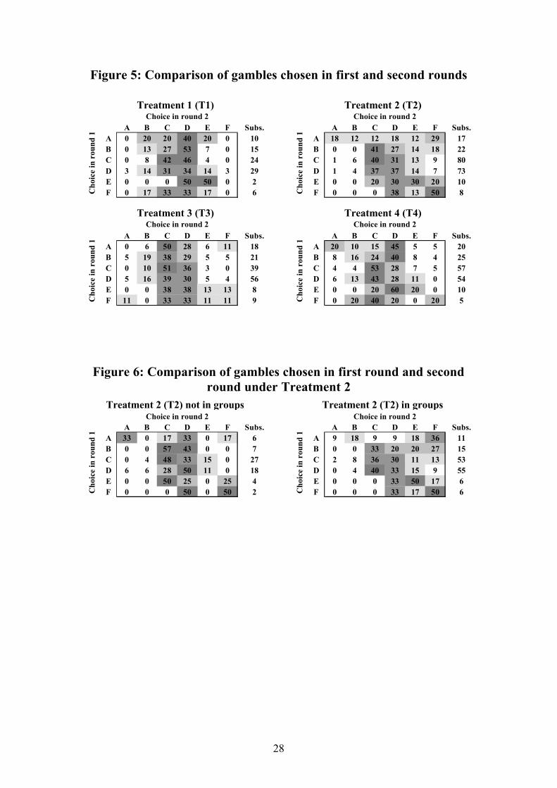
A more careful analysis of gamble choice under the four treatments must take

account of each subject’s decision in the first round, thereby allowing us to focus on

the extra risk that the subjects take on when pooling is an option. Figure 5 contains

four transition matrices, one for each of the treatments. The numbers within the

matrices are percentages. The ijth element of a matrix is the percentage of those

subjects who chose gamble i in the first round and gamble j in the second round. The

frequencies associated with the first round choices are shown beside the matrices. To

aid the reader the cells of the matrices have been shaded in accordance with the

percentage they contain. Darker cells contain higher percentages. When the high

percentages are concentrated down the principle diagonal it indicates that most

subjects chose the same gamble in both rounds. When the high percentages are

concentrated in the middle two columns it indicates that the subjects tended towards

the middle-of-the-range gambles in the second round regardless of their choices in the

first round. If there are medium to high percentages in the bottom left-hand corner of

14

a matrix it indicates that subjects chose less risky gambles in the second round. And if

there are medium to high percentages in the top right-hand corner of a matrix it

indicates that subjects chose riskier gambles in the second round.

The matrices for T1, T3, and T4 display quite dominant principle diagonals

combined, to varying degrees, with dominant middle columns. The option to risk pool

under T3 and T4 appears not to be causing subjects to choose riskier gambles. In

contrast, the matrix for T2 is shaded in the top right-hand corner indicating that a

considerable proportion of subjects chose riskier gambles in the second round. In

Figure 6 the matrix for T2 is further sub-divided into those who did and did not join

groups. It is in the former that we see the concentration in the top right-hand corner.

Once again, we can use a regression analysis to test the significance of these

regularities in the data, while controlling for other factors that might have influenced

the subjects’ decisions. Here, I run a tobit regression that takes account of the fact that

the gamble choice sorts the subjects into intervals according to how much risk they

are prepared to take on. The tobit was set up with reference to the bounds on the risk

aversion coefficients associated with each gamble and presented in Table 1. Thus, if

an explanatory variable bears a significant negative coefficient it indicates that an

increase in that variable is associated with an increase in the riskiness of the chosen

gamble. The results of the analysis are presented in Table 4. In the first column the

subjects’ choices in the second round are regressed on a set of five dummy variables

indicating their choices of gamble in the first round (A is the base for comparison),

their winnings from the first round,4 and a set of six dummies indicating which

treatment the decision was made under and whether they opted to be in a group or

play solo (T1 is the base for comparison). All standard errors are adjusted to take

4 The large coefficient on the winnings variable may be indicative of an income effect or may relate to the perceived non-independence of gambles described in footnote 3.

15

account of the potential non-independence of errors due to the social context within

which the decisions were made.

The dummies relating to choice of gamble in the first round are jointly, highly

significant. Those who won more in the first round assume greater risks in the second.

The dummies relating to being in a group under T2, T3, or T4 are jointly significant,

while those relating to playing solo under T2, T3, or T4 are not significant. A careful

general to specific process yields the regression presented in the second column of

Table 4. In this regression, of the treatment-group dummies, only the one identifying

those who belonged to a group under T2 survives. The choices made under T3 and T4

or by solo players under T2 were indistinguishable from those made under T1.

4. A Test of External Validity

While this experiment was underway, Dekker (2002) was conducting an in-

depth study of flows of assistance between households in five of the 23 villages. As

part of her fieldwork Dekker asked every household in these villages to name the

households in their village to whom they had given assistance and from whom they

had received assistance. Here, I use Dekker’s data to investigate whether the groups

formed during the experiment bear any resemblance to real risk pooling networks

within these five villages.5

Dekker’s data takes the form of relational matrices. The ijth element in the

‘assistance given’ matrix for a particular village takes the value one if household i

reported giving assistance to household j and zero otherwise. Similarly, the ijth

5 There is no reason to expect that the five villages in Dekker’s study represent a biased sample of the 23 included in the experiment. In her choice of villages, Dekker’s aim was to capture as much social diversity as possible while controlling for access to roads, other infrastructure and social services. There is a possibility that Dekker presence in the villages could have biased behaviour in the experiments. However, Dekker had not yet started work in two out of the three villages at the time when the experiments were conducted.

16

element in the ‘assistance received’ matrix for a particular village takes the value one

if household i reported receiving assistance from household j and zero otherwise.

With no measurement error, one of these matrices should equal the transpose of the

other. This is not the case and, consistent with there being a stigma associated with

needing or receiving assistance and/or high status associate with giving assistance,

many more relations involving the giving of assistance are reported, i.e., there are

many more ones in the ‘assistance given’ matrix than in the ‘assistance received’

matrix. For this reason, and because there is no way of telling which of the two

matrices is a better reflection of the actual pattern of transfers, the procedure

described below is repeated twice for each village, once using the ‘assistance

received’ matrix, and once using the ‘assistance given’ matrix.

To facilitate the analysis another matrix relating to group formation within the

experiment is constructed for each of the five villages. In these matrices the ijth

element takes the value one if the representative from household i in the experiment

was in the same group as the representative from household j and zero otherwise.

Then, the statistical correlations between the experimental group formation matrix

and the corresponding ‘assistance given’ and ‘assistance received’ matrices are

calculated. A standard correlation assuming independence is not appropriate as each

matrix represents a fully enumerated and interrelated social system. Instead, the

following two-stage procedure was used. First, a simple matching coefficient between

corresponding cells in the two data matrices is calculated. Second, the rows and

columns of one matrix are randomly but synchronously permutated and the

correlation recomputed every time. 10,000 permutations are carried out and the

proportion of times that the match between the one observed and one permutated

matrix is greater than or equal to the match between both observed matrices is

17

calculated. This proportion is reported as the level of significance or p-value of the

correlation.

The test is subject to two sources of bias both of which may suppress the

significance of a correlation and thereby render the test conservative. First, in

Dekker’s data an actual flow of assistance is observed only if one household is in

need and another is both willing and able to respond, whereas in the experiment only

the condition of willingness needs to be met in order for two subjects to become

linked by group membership. Dekker’s data implies an ex post flows of assistance

while experimental co-group membership implies an ex ante informal contract

relating to a flow of assistance if unequal payoffs arise. Thus, the experimental group

matrices are likely to contain many more ones than either of the ‘assistance’ matrices.

This suppresses the significance of the correlations and renders it more likely that the

denser ‘assistance given’ matrices will yield the significant results.

The second potential source of bias arises if the subjects in the experiment and

those making real life risk pooling decisions are distinct. Out of the five villages for

which the test was conducted there was one in which this bias may have arisen. In

Pedzanhamo a large proportion of the experimental subjects were young dependents

rather than senior household members.

The results of the correlation exercise are reported in Table 5. In three out of

the five villages, Moturamhepo, Zvataida, and Mudzinge, the correlation between

group formation in the game and patterns of assistance reported as given is

significant. For one of the other villages, Muringamombe, the correlation between

group formation in the game and patterns of assistance reported as received is

significant. For the fifth village, Pedzanhamo, no correlation is found between

reported assistance, given or received, and group formation in the game.

18

5. Discussion

The results indicate that more risk pooling takes place when extrinsic

commitment is unlimited; under T2 more subjects join sharing groups and group

members take on greater risk. However, even then a considerable proportion of

subjects choose not to join groups. One possible explanation is that these subjects are

risk loving, although if this were the case we would expect to see significant

coefficients on the choice of gamble dummies in the probit regressions. An alternative

explanation is that they are being punished by exclusion for previous misdemeanours.

When extrinsic commitment is limited and information is asymmetric less risk

pooling takes place; in T3 and T4 a smaller proportion of subjects join groups and

group members take on no more risk than solo players. This result supports the

commonly made assumption that limited extrinsic commitment reduces risk pooling.

However, note that some subjects are not deterred from forming groups under such

conditions suggesting that intrinsic motivations may be a sufficient basis for

commitment for some agent dyads.

Not in accordance with commonly made assumptions is the finding that

asymmetric information is associated with more rather than less risk pooling; the

information asymmetries are greatest in T3 but it is under T4 that the lowest

proportion of subjects join groups and that the smallest groups are formed. This

finding suggests that individual responses to socially sensitive information might be

more complex than we usually acknowledge. People may be conflict averse or may be

highly motivated by anticipated shame and may not always trust themselves to act in

way that minimises their likelihood of attracting shame. While the current experiment

was not designed to distinguish between these hypotheses, it suggests that they might

be usefully explored. Further, the result suggests that the full information within

19

social groups such as villages is ill founded, that given the opportunity people may

actually shy away from information, and that there might be a negative relationship

between information and commitment. Knowing when people renege may make

relations too difficult, there may be value in being able to give people the benefit of

the doubt in some circumstances. This challenges the verisimilitude of many of our

theoretical models and the conclusions based on the related empirical work.

References

Alderman and Paxson (1992), ‘Do the poor insure? A synthesis of the literature on

risk and consumption in developing countries,’ World Bank Policy Research

Working Paper.

Bala, V. and S. Goyal (2000), ‘A non-cooperative model of network formation,’

Econometrica 68, 1181-1229.

Binswanger, H. P. (1980), ‘Attitudes toward risk: Experimental Measurement in rural

India,’ American Journal of Agricultural Economics.

Bohnet, I., B. Frey, and S. Huck (2001), ‘More Order with less law: On contract

enforcement, trust, and crowding,’ American Political Science Review, 95(1),

131-143.

Boozer, M. and M. Goldstein (2003), ‘Poverty Measurement and Dynamics,’ mimeo

Yale University.

Bowles, S. J. Carpenter, and H. Gintis (2001), ‘Mutual monitoring in teams: The

effects of residual claimancy and reciprocity,’ mimeo University of

Massachusetts.

Cardenas, J. C., J. Stranlund, and C. Willis (2000), ‘Local Environmental Control and

Institutional,’ World-Development 28(10), 1719-33

20

Coate, S. and M. Ravallion (1993), ‘Reciprocity without commitment:

Characterisations and performance of informal risk-sharing arrangements,’

Journal of Development Economics 40, 1-24.

Dekker, M. (2002), ‘Risk sharing relations in a village’, mimeo, Department of

General and Development Economics, Free University, Amsterdam.

De Weerdt, J (2002), Social networks, transfers and insurance in developing

countries, Ph.D., KULeuven.

Elster, J (1984), Ulysses and the Sirens: Studies in Rationality and Irrationality,

Cambridge University Press, Cambridge.

Fafchamps, M. (1998), ‘Risk sharing and quasi-credit,’ Journal of International Trade

and Development 8, 257-278.

Fafchamps, M. and Lund, S. (forthcoming), ‘Risk-sharing networks in rural

Philippines,’ Journal of Development Economics.

Falk, A., E. Fehr, and U. Fischbacher (2000) ‘Informal Sanctions,’ Institute for

Empirical Research in Economics, University of Zurich, Working Paper Series,

ISSN 1424-0459.

Grimaud, F. (1997), ‘Household consumption smoothing through ethnic ties:

Evidence for Côte d’Ivoire,’ Journal of Development Economics 53, 391-421.

Harowitz, S. (2001), ‘The Balance of Power: Formal Perfection and Practical Flaws,’

Journal of Peace Research 38(6), 705-22.

Holtzmann, R., T. Packard, and J. Cuesta, (2000), ‘Extending coverage in multi-pillar

pension systems: Constraints and hypotheses, preliminary evidence and future

research agenda,’ Social Protection Working Paper, World Bank.

Ligon, E. (1998), ‘Risk-sharing and information in villages economies,’ Review of

Economic Studies 65, 847-864.

21

Ligon, E., J. P. Thomas, and T. Worrall (2002), ‘Informal Insurance Arrangements

with Limited Commitment: Theory and Evidence from Village Economies’,

Review of Economic Studies 69(1), 209-44.

Morduch, J. (1991), ‘Consumption smoothing across space: Tests for village-level

responses to risk,’ Harvard University mimeo.

Platteau, J. P. (1994a), >Behind the Market Stage Where Real Societies Exist - Part I:

The Role of Public and Private Order Institutions=, Journal of Development

Studies 30(3), 533-577.

Platteau, J. P. (1994b), >Behind the Market Stage Where Real Societies Exist - Part II:

The Role of Moral Norms=, Journal of Development Studies 30(3), 753-817.

Posner, R. A. and E. B. Rasmusen (1999) ‘Creating and Enforcing Norms, with

Special Reference to Sanctions,’ International Review of Law and Economics

19, 369-82.

Rosenzweig, M. R. and O. Stark (1989), ‘Consumption smoothing, migration, and

marriage: Evidence from rural India,’ Journal of Political Economics 101, 223-

244.

Ravallion, M. and S. Chaudhuri (1991), ‘Testing risk-sharing in three Indian villages,’

World Bank mimeo.

Ravallion, M. and L. Dearden (1988), ‘Social security in a “moral economy”: An

empirical analysis for Java,’ Review of Economics and Statistics 70, 36-44.

Townsend, R. M. (1994), ‘Risk and insurance in village India,’ Econometrica 62,

539-591.

Udry, C. (1994), ‘Risk and Insurance in a Rural Credit Market: An Empirical

Investigation in Northern Nigeria,’ Review of Economic Studies 61, 495-526.

22

Table 1: First round of the risk pooling game: Choices, payoffs, expected values, and risk aversion classes

Choice Blue Yellow EV RA class RA coeff.

A 100 100 100 Extreme infinity to 7.51

B 190 90 140 Severe 7.51 to 1.74

C 240 80 160 Intermediate 1.74 to 0.81

D 300 60 180 Moderate 0.81 to 0.32

E 380 20 200 Slight-neutral 0.32 to 0.00

F 400 0 200 Neutral-negative 0 to -ve infinity

Table 2: Second round treatments in the risk pooling game

Treatment Villages Subjects

T1 3 86

T2 8 216

T3 6 157

T4 6 183

Total number of players involved in Round 2 23 642

Repeat of first round after aproximately 24 hoursfor players' discussions.

Players told that they could form sharing groupsif they wished and given approximately 24 hoursto do so.

Like T2 but players also told that once they hadplayed they could opt out of their groups insecret if they wished.

Description

Like T3 but players must declare their decisionto opt out of their group in public.

23

Table 3: Group membership and group size Dependent variables = dummy taking the value 1 if in a group and number of group members

Coef. s.e. Coef. s.e. Coef. s.e. Coef. s.e.Constant 0.430 0.670 0.625 0.165 *** 2.934 1.556 * 4.514 0.811 ***

T3 -0.891 0.417 ** -0.859 0.391 ** -0.428 0.623 -0.244 0.776T4 -0.984 0.204 *** -0.982 0.212 *** -3.737 0.515 *** -3.287 0.575 ***

B (round 1) 0.297 0.257 -0.266 0.386C (round 1) -0.102 0.255 -0.003 0.462D (round 1) 0.182 0.266 0.239 0.426E (round 1) 0.375 0.411 1.040 0.978F (round 1) 0.034 0.353 0.239 0.980Blue in round 1 -0.166 0.146 -0.457 0.244 * -0.400 0.234 *

H'holds in village -0.002 0.012 0.042 0.031Area 2 0.450 0.276 1.811 0.857 *

Area 3 0.389 0.260 0.964 0.687Resettled 0.053 0.371 1.686 0.432 *** 1.396 0.444 *

Joint significance of round 1 choice 0.155 0.766Joint significance of areas 0.200 0.120R2 0.117 0.091 0.350 0.328Obs. 568 592 260 260

Probit of group formation Group size conditional on formation

Note: Reported standard errors have been adjusted to take account of potential non-independence within villages/sessions. * significant at 10% level, ** significant at 5% level, *** significant at 1% level.

24

Table 4: Choice of gamble in second round Dependent variable = riskiness of gamble as indicated by corresponding coefficient of partial relative risk aversion

Coef. s.e. Coef. s.e.Constant 1.700 0.318 *** 1.942 0.368 ***

Winnings in round 1 -0.003 6.02e-4*** -0.003 5.84e-4

***

B (game 1) -0.267 0.318 -0.269 0.317C (game 1) -0.287 0.334 -0.306 0.332D (game 1) -0.058 0.368 -0.061 0.372E (game 1) -0.911 0.350 *** -0.864 0.334 ***

F (game 1) -0.530 0.527 -0.571 0.539Treatment 2 & in group -0.346 0.236 -0.579 0.268 **

Treatment 3 & in group 0.308 0.194Treatment 4 & in group 0.597 0.402Treatment 2 & solo 0.110 0.251Treatment 3 & solo 0.197 0.181Treatment 4 & solo 0.260 0.160

1.512 0.142 1.521 0.145Joint sig of game 1 choice 0.000 0.000Joint sig of treatment & in a group dummies 0.056Joint sig of treatment & solo dummies 0.364Wald 70.59 64.32Obs. 618 618

2χ

σ

Note: Reported standard errors have been adjusted to take account of potential non-independence within villages/sessions. * significant at 10% level, ** significant at 5% level, *** significant at 1% level.

Table 5: Correlations between experimental and real

risk pooling networks

VillageCorrelation with reported

assistance given (p-value)

Correlation with reported assistance received

(p-value)Pedzanhamo 0.786 0.631Moturamhepo 0.056 0.956Zvataida 0.053 0.310Muringamombe 0.151 0.099Mudzinge 0.065 0.268

25

Figure 1: Presentation of the gambles to the experimental subjects

A B

$100 $190

$100 $90

C D

$240 $300

$80 $60

E F

$380 $400

$20 $0

26

Figure 2: Limited commitment and renegades in Treatments 3 and 4

Joined groups under T364

low payoff high payoff32 32

stay in opt out stay in opt out32 0 25 (78%) 7 (22%)

Joined groups under T466

low payoff high payoff32 34

stay in opt out stay in opt out32 0 33 (97%) 1 (3%)

Figure 3: Group formation in second round of the risk pooling game

0

10

20

30

40

50

60

70

1 2 3 4 5 6 7 8 9 10 12

Group size

Rel

ativ

e fr

eque

ncy

(%)

T2T3T4

27

Figure 4: Choice of gamble in second round of the risk pooling game

0

20

40

60

80

100

A B C D E FChoice of gamble

Cum

ulat

ive

freq

uenc

y (%

)

T1T2T3T4

28

Figure 5: Comparison of gambles chosen in first and second rounds

Treatment 1 (T1) Treatment 2 (T2)

A B C D E F Subs. A B C D E F Subs.A 0 20 20 40 20 0 10 A 18 12 12 18 12 29 17B 0 13 27 53 7 0 15 B 0 0 41 27 14 18 22C 0 8 42 46 4 0 24 C 1 6 40 31 13 9 80D 3 14 31 34 14 3 29 D 1 4 37 37 14 7 73E 0 0 0 50 50 0 2 E 0 0 20 30 30 20 10F 0 17 33 33 17 0 6 F 0 0 0 38 13 50 8

Treatment 3 (T3) Treatment 4 (T4)


Choice in round 2

Choice in round 2

Cho

ice

in r

ound

1

Choice in round 2

Cho

ice

in r

ound

1

Choice in round 2

Cho

ice

in r

ound

1

Cho

ice

in r

ound

1

Figure 6: Comparison of gambles chosen in first round and second round under Treatment 2

Treatment 2 (T2) not in groups Treatment 2 (T2) in groups


Choice in round 2

Cho

ice

in r

ound

1

Choice in round 2

Cho

ice

in r

ound

1

risk pooling, commitment, and information: an experimental test … · 2019-06-17 · 2 risk...

Documents