risk modelling in hazardous material transport · risk modelling in hazardous material transport...

Risk Modelling in Hazardous Material Transport

Edward Austin, Supervisor: Christina Wright

Edward Austin Risk Modelling in Hazmat Transport 1 / 21

1 Motivation

2 Modelling Risk

3 Lancaster-Preston Network

4 Model Comparison

5 Questioning Assumptions

6 Conclusion


Motivation


Traditional Risk

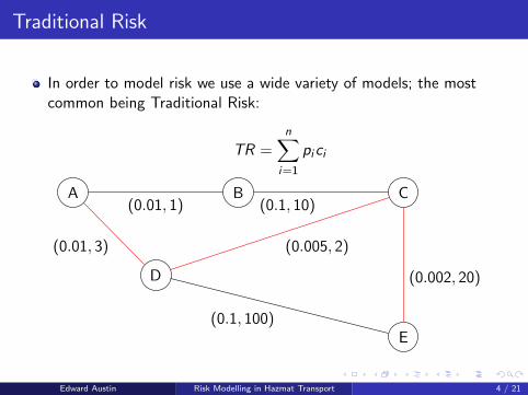
In order to model risk we use a wide variety of models; the mostcommon being Traditional Risk:

TR =n∑

i=1

pici

A B C

D

E

(0.01, 1) (0.1, 10)

(0.01, 3) (0.005, 2)

(0.1, 100)

(0.002, 20)


Modelling Consequence

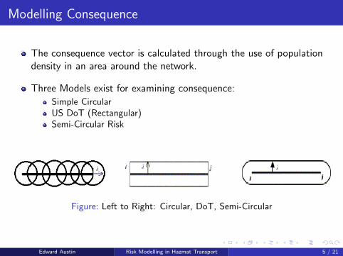
The consequence vector is calculated through the use of populationdensity in an area around the network.

Three Models exist for examining consequence:

Simple CircularUS DoT (Rectangular)Semi-Circular Risk

Figure: Left to Right: Circular, DoT, Semi-Circular


Double Counting

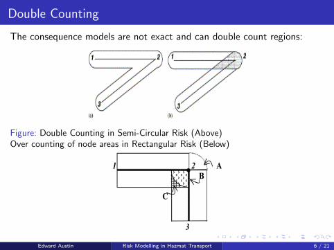
The consequence models are not exact and can double count regions:

Figure: Double Counting in Semi-Circular Risk (Above)Over counting of node areas in Rectangular Risk (Below)


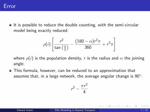
Error

It is possible to reduce the double counting, with the semi-circularmodel being exactly reduced:

ρ(i)

[r2

tan(α2

) − (180− α)r2π

360+ r2π

]

where ρ(i) is the population density, r is the radius and α the joiningangle.

This formula, however, can be reduced to an approximation thatassumes that, in a large network, the average angular change is 90◦:

r2 − πr2

4


Modelling an Example Network

We can model four routes between Lancaster and Preston usinghalf-mile intervals, as seen below:

Figure: Clockwise: Route 1, Route 2, Route 4, Route 3


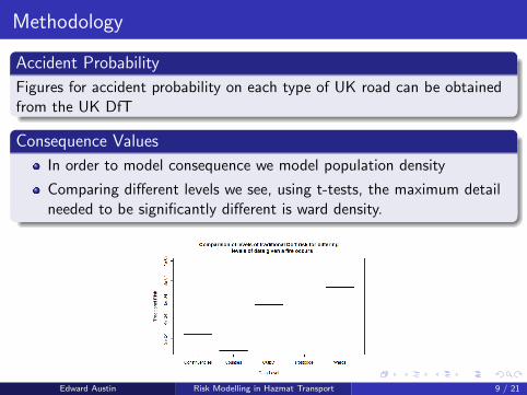
Methodology

Accident Probability

Figures for accident probability on each type of UK road can be obtainedfrom the UK DfT

Consequence Values

In order to model consequence we model population density

Comparing different levels we see, using t-tests, the maximum detailneeded to be significantly different is ward density.


Comparing Consequence Methods

The highest, and so best, risk representation is given by semi-circularrisk.

As such we propose to use Semi-Circular Risk with averaged error andward population density for our future modelling work.


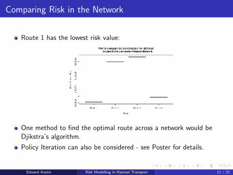
Comparing Risk in the Network

Route 1 has the lowest risk value:

One method to find the optimal route across a network would beDjikstra’s algorithm.

Policy Iteration can also be considered - see Poster for details.


Questioning Assumptions

Assumes that all road types have different accident probabilities

Assumes all accidents will be equally severe, and that all causedamage

Assumes injuring people is the only form of consequence


Do Different Road Types Have a Different AccidentFrequency?

We can use ANOVA to test the difference in the datasets:

H0 : µMotorway = µRural = µUrban H1 : µMotorway 6= µRural 6= µUrban

Pairwise t-testing suggests Rural and Urban are similar but that theyare significantly different from motorways.


Do Accidents Always Cause Damage?

There is the assumption in the model that accidents lead to damages,however is it the case that more frequent accidents cause an increase?

Figure: MBLM is a Median Based Linear Model


Is Population Density an effective statistic?

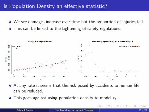
We see damages increase over time but the proportion of injuries fall.

This can be linked to the tightening of safety regulations.

At any rate it seems that the risk posed by accidents to human lifecan be reduced.

This goes against using population density to model ci .


Forecasting Accident and Injury Probability

Using the data we can attempt to quantify what is meant by a‘severe’ accident.

Namely this is one that leads to injury, or a fatality.


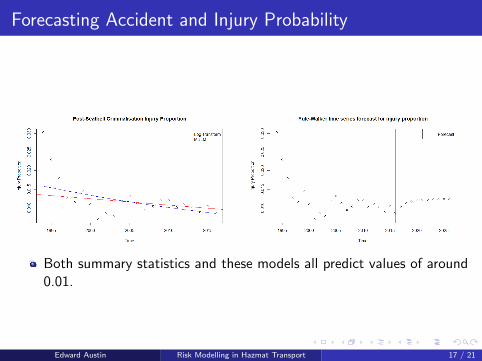
Forecasting Accident and Injury Probability

Both summary statistics and these models all predict values of around0.01.


Conclusion

Different road types do need modelling, however the type of roadalone is not enough

The severity of accidents varies

It may also be helpful to consider the financial cost as well as humancost for the consequence value


Further Work

Further explore methods to predict accident and injury probability ina network

Create a model that represents the location of the accident, perhapsusing a Poisson Process

Investigate the relationship between the weather, time of year andother climate factors on accident probability.

Explore how these factors could be worked into a new risk model


References

1 Erhan Erkut, Vedat Verter, (1998) Modelling of Transport Risk forHazardous Materials. Operations Research 46(5):625− 642

2 B.Y. Kara, E. Erkut, V. Verter, (2008) Accurate calculation ofhazardous materials transport risks, Operations Research Letters31(4):285− 292

3 Faraway, J. (2005). Linear models with R (Texts in statistical science; v. 63). Boca Raton, Fla.: Chapman & Hall/CRC.

4 Chatfield, C. (2004). The analysis of time series : An introduction(6th ed., Texts in statistical science). Boca Raton, Fla.: Chapman &Hall/CRC


Thanks For Listening!

Any Questions?

Figure: Perhaps our model needs to include height..?


risk modelling in hazardous material transport · risk modelling in hazardous material transport...

Documents