risk matters: studies in finance, trade and politics · pdf filetv$ stockholm school of...
TRANSCRIPT

Risk Matters:
Studies in Finance, Trade and Politics

$ STOCKHOLM SCHOOL OF ECONOMICStv EPI, THE ECONOMIC RESEARCH INSTITUTE
EFIMissionEFI, the Economic Research Institute at the Stockholm School of Economics, is a scientificinstitution which works independently of economic, political and sectional interests. It conductstheoretical and empirical research in management and economic sciences, including selectedrelated disciplines. The Institute encourages and assists in the publication and distribution of itsresearch findings and is also involved in the doctoral education at the Stockholm School ofEconomics.EFI selects its projects based on the need for theoretical or practical development of a researchdomain, on methodological interests, and on the generality of a problem.
Research OrganizationThe research activities are organized in twenty Research Centers within eight Research Areas.Center Directors are professors at the Stockholm School of Economics.
ORGANIZATIONAND MANAGEMENTManagement and Organisation; (A)Center for Ethics and Economics; (CEE)Center for Entrepreneurship and Business Creation; (E)Public Management; (F)Information Management; (I)Center for People and Organization; (PMO)Center for Innovation and Operations Management; (T)
ECONOMIC PSYCHOLOGYCenter for Risk Research; (CFR)Economic Psychology; (P)
MARKETINGCenter for Information and Communication
Research; (CIC)Center for Consumer Marketing; (CCM)Marketing, Distribution and Industrial
Dynamics; (D)ACCOUNTING, CONTROL AND CORPORATE FINANCE
Accounting and Managerial Finance; (B)Managerial Economics; (C)
FINANCEFinance; (FI)
ECONOMICSCenter for Health Economics; (CHE)International Economics and Geography; (lEG)Economics; (S)
ECONOMICS STATISTICSEconomic Statistics; (ES)
LAWLaw; (RV)
Prof Sven-Erik SjostrandAdj Prof Hans de GeerProf Carin HolmquistProfNils BrunssonProf Mats LundebergProf Jan LowstedtProf Christer Karlsson
Prof Lennart SjobergProf Guje Sev6n
Adj Prof Bertil ThorngrenActing Prof Magnus Soderlund
Prof Lars-Gunnar Mattsson
ProfLars OstmanProfPeter Jennergren
Prof Clas Bergstrom
Prof Bengt JonssonProfMats LundahlProfLars Bergman
Prof Anders Westlund
Prof Erik Nerep
Chairman o/the Board: ProfHakan Lindgren. Director: Associate ProfBo Sellstedt.
AdressEFI, Box 6501, S-113 83 Stockholm, Sweden • Internet: www.hhs.se/efi/Telephone: +46(0)8-736 90 00 • Fax: +46(0)8-31 62 70 • E-mail [email protected]

RISK MATTERS:
STUDIES IN FINANCE, TRADE AND POLITICS
Jonas Vlachos
tll STOCKHOLM SCHOOL OF ECONOMICS~~J~ EFI, THE ECONOMIC RESEARCH INSTITUTE
t1Ft, Dissertation for the Degree of Doctor of Philosophy, Ph.D.u'S'm"*,"+" Stockholm School of Economics, 2002
© EFI and the author
ISBN 91-7258-591-9
Keywords:Con1parative advantage, financial intermediation, financial markets, financial systems, labormarket risk, panel data, public employment, public sector size, redistribution, regionalintegration, risk sharing, secession, spatial econon1etrics, specialization patterns, trade policy
Chapter 1 is forthcoming in Journal ofInternational Economics © Elsevier Science (2001) andappears here with permission from Elsevier Science.Chapter 2 is additionally available as SWOPEC Working Paper No. 449.
Cover design by Karin Bergvall
Distributed by:EFI, The Econon1ic Research InstituteStockholm School of EconomicsP.O. Box 6501, S-113 83 Stockholm, Swedenwww.hhs.se/efi/
Printed by:Elanders Gotab, Stockholm 2001

to Karin and Elias


CONTENTS
Acknowledgements
Introduction and Summary
ix
Xl
Chapter 1
Chapter 2
Chapter 3
Chapter 4
Markets for Risk and Openness to Trade: How are They Related? 1
Financial Markets, the Pattern of Specialization, and 39Conlparative Advantage: Evidence from OECD Countries.
Who Wants Political Integration? Evidence from the Swedish 79ED-Membership Referendum.
Does Labor Market Risk Increase the Size of the Public Sector? 111Evidence from Swedish Municipalities.
vii

II
III
IIII
II
I
IIII
I
II
III
I
III
I
I
II
III
I
III
III
I
III
II
I
I
III
I
III
II
I
IIII
I
II
IIII
III
II

ACKNOWLEDGMENTS
In the corridors of the doctoral students' center at Saltmatargatan the rumor goes that
whatever your field of interest is, Tore Ellingsen is better read than you are. Having
had Tore as my supervisor for three years, I can basically confirm this rumor. For
someone with as wide interests as I (or should I say, lack of focus), this has proven to
be an invaluable asset. Whenever I approached Tore with an idea, however vague, he
was always been able to point me in the right direction. Moreover, he has done so
with an irresistible enthusiasm that has made me stick to ideas that I would otherwise
have discarded far too easily. Even more importantly, Tore has made me realize that
the world is so full of unsolved mysteries that ideas for research should never be a
problem. Although it is a cliche, I can honestly say that this thesis had never been
written without him.
When still at Handels, Marcus Asplund, my co-supervisor, gave me very useful
advice on all aspects of empirical work. Without Marcus, it is probable that I would
still struggle to get data into the software packages. Karolina Ekholm was always
willing to discuss trade-related issues, which has improved this thesis substantially. I
am also grateful to Torsten Persson, partly for reading some of the papers with such
scrutiny and always asking the right questions, but also for being an excellent teacher.
Among my fellow PhD-students, Helena Svaleryd, the co-author of two of the papers
included here, is the one who has influenced this thesis the most. Thank you for
balancing my swings between hubris and despair and for not minding to be forced to
work all the way into labor-pains. Lars Frisell, my roommate for several years,
deserves gratitude for showing me why two agents in a room is the key to understand
econonlics. Fredrik Heynlan not only taught me the trick of differential equations, but
has also been my closest ally in the battle between STATA and LIMDEP. Malin
Adolfson has helped nle with Gauss and been relentless in her efforts to show the rest
of us the world outside Saltis. Unfortunately, these efforts largely failed, as did her
attempts to explain the essence of inflation. Patrik Gustavsson has played a crucial
role for two of the papers, but I am not sure he even knows that himself. Thanks
Patrik!
ix

Raana and Gisela are two other colleagues who are very dear to me, not the least
because they were more than willing to talk about babies. The lunch gang: Erik, Nina,
Daniel, Andreas, Therese, Niklas, Magnus, Bjorn, David, Martin and Katariina,
managed to create the unthinkable - something like a sense of community in the
academic world. I will miss the debates around the lunch table. The secretaries: Carin
Blanksvard, Britt-Marie Eisler, Pirjo Furtenbach, Ritva Kiviharju, Kerstin Niklasson
and Ingrid Nilsson have all been very helpful during the years at Handels. Financial
support from the Swedish Research Council (then called HSFR), the Swedish Institute
of Banking Research, the Stockholnl School of Economics and the Swedish
Government is gratefully acknowledged.
My friends outside the academia have been very supportive in both good and bad
times. Rather than risking the possibility of forgetting a name, I take the easy way out
and thank all of you. I am also grateful to my father for practically breastfeeding me
with economics, and to my mother and brother for not doing likewise.
My little family, Karin and Elias, are of course the ones who mean the most to me and
they have both played an essential role during my studies. Karin somehow managed
to keep her faith in nle regardless of my stress levels, while the arrival of Elias made
nle write with unprecedented speed. I love you both more than you can possibly
imagine.
Stockholm, November 2001
Jonas Vlachos
x

Introduction and Summary
INTRODUCTION AND SUMMARY
This thesis consists of four self-contained empirical essays. The simple idea
underlying three of the four papers is that risk and uncertainty affect political choice.
Indeed, most people would have to be hard pressed to argue otherwise. This idea does,
however, have some interesting implications; in particular, it means that the existence,
or the development, of different types of insurance should affect the political agenda.
For exanlpIe, we rarely hear political demands for government intervention in the
home-insurance industry - most likely because home-insurance markets are relatively
efficient. Unemployment insurance, on the other hand, is usually high on the
electorate's list of political priorities. Although this can partly be explained by a
preference for redistribution, the severe moral hazard and adverse selection problems
affecting private insurance for human capital, naturally raise demand for public
insurance of this kind.
How far this point can be taken naturally depends on what types of markets and
insurance we are analyzing. Since the focus of the essays is political choice at the
macro level (openness to trade, regional integration, and the size of the public sector),
two of the largest and nl0st important markets in a modem economy, namely the
financial sector and the labor market, are considered. The everyday importance of the
labor market is self-evident, as is the fact that labor markets differ in the level of risk
to which they are subject. The financial sector specializes in the handling of financial
risks and is a large contributor to GDP in most developed countries. l If an important
effect of the insurance characteristics of these markets on policy cannot be
documented empirically, the starting point of this thesis is likely to be just a
theoretical curiosity.
Although the questions and hypotheses investigated here only constitute a small sub
set of all possible links from markets handling risk to policy, the results indicate that
these links can be important. Broadly speaking, this gives support for theories such as
Persson and Tabellini (1996) who discuss the risk-sharing aspects of regional
integration, and Fernandez and Rodrik (1991) who denl0nstrate how individual-
I Demirgiic-Kunt and Levine (1996) present estimates of the size of the financial sector..Thecontribution to GDP in 1990 was around five percent in the USA, and around nine percent in Japan.
xi

Introduction and Summary
specific uncertainty can create a bias away from welfare enhancing economic refomls.
At a more general level, it can be argued that political choices affecting the
functioning of nlarkets are likely to change the tradeoffs faced by political actors,
thereby also influencing the political agenda. Similar nlechanisms have been
considered in the literature on endogenous choice of policy instruments. Rodrik
(1986), for example, demonstrates that although a production subsidy is more efficient
than a tariff, the electorate would, if possible, pre-commit to tariff protection only.
The reason is that lobbying for tariffs generates more free-riding between interest
groups and hence, smaller distortions. Although the point that policy can influence the
political game itself is easily made, it can severely complicate the analysis of
economic and political reforms. Therefore, plenty of empirical work needs to be
undertaken to better understand the strength and scope of these mechanisms.
FINANCIAL DEVELOPMENT
Whenever econonlic research leaves the world of theory, there is an attempt to put
numbers on theoretical phenomena. This is always tricky, and especially so when
dealing with macro-level indicators of various kinds. In two of the papers included in
this volume, numbers are used to indicate the degree of development in the financial
sector. These numbers are supposed to measure how well the financial sector
mobilizes savings, allocates credit across time and space, exerts corporate control, as
well as how efficient are the hedging, pooling, and pricing of risks. The fact that
indicators similar to the ones used here are commonly used in the literature (starting
with King and Levine, 1993), does not reduce the problems involved in attaching a
single number to these complex institutions and markets.2
This problem is dealt with by using a variety of indicators of financial development.
When the results are consistent across indicators, we put greater faith in them. To
further conlplicate matters, however, financial systems have developed along different
paths in different countries. The various indicators of financial development therefore
supposedly also measure different aspects of the financial system. Traditionally,
researchers have classified financial systems as either bank: based (e.g. in Japan and
2 This criticism naturally extends to other indicators such as "democratic development", "lawenforcement", "corruption", and "social capital", commonly used in economic research.
xii

Introduction and Summary
Gennany) or market based (e.g. in the United States and the United Kingdom). This
division partly emerged due to the different regulatory systems created as responses to
financial crises during the early phases of industrialization (see the account in Allen
and Gale, 2000). Since there is considerable variation in the way the financial sector is
regulated and in company law even within these two subgroups, there is a continuing
debate on to what extent this grouping adds to the understanding of different financial
systems. Moreover, recent research has failed to document that the classification can
contribute to the understanding of economic performance at the aggregate (Levine,
2001) or industry (Beck and Levine, 2001) level. For these reasons, results for
individual indicators should be interpreted with care.
Rather than focusing on the differences between bank- and market-based financial
systems, there is a growing consensus that the legal environment - for example,
protection of minority shareholders and creditors, and rules for infonnation
dissemination - is what matters for financial development (see e.g. La Porta et aI.,
1998). According to this view, financial contracts are upheld by more or less efficient
law enforcement. Other mechanisnls can substitute for weak regulation in one area,
and ,vhat ultimately counts is the overall performance of the legal system. An
important insight from this literature is that deeply rooted legal traditions play a
central role in shaping a financial system. In particular, common-law legal systems
seenl to offer better protection of investors than civil-law systems. Since the legal
tradition of a society is not easily changed, one possible implication of this theory is
that financial development cannot be generated without encompassing legal reforms.
The relative ease with which countries can be divided into different legal traditions
can explain the wide spread use of this approach. The approach is not unproblematic,
however. Countries in the same legal tradition do, for example, find themselves at
very different levels of financial development. Further, the development of the
financial sector has not been monotonic over time. Rather, both expansions and
reversals have characterized the pattern of development during the last century. These
facts bring into question theories stressing the importance of the legal tradition, which
is time-invariant by nature. In contrast, Rajan and Zingales (2001) argue that poorly
developed financial markets can benefit industry incumbents by restricting the
availability of financial capital to new entrants. If competition in goods and/or
xiii

Introduction and Summary
financial markets increases for exogenous reasons (for example through a trade
reform), the relative benefit of holding back financial development is decreased.
Coffee (2001) is another dissenting voice, questioning the mechanism through which
the legal traditions have affected the financial systems. He argues that strong
securities markets created a constituency demanding a stricter legal protection of
investors. The legal tradition played a role through the early separation of the private
sector from central government control in several comnl0n-Iaw countries. This
separation generated self-regulatory mechanisms of securities nlarkets that, in tum,
facilitated the development of dispersed ownership. According to Coffee's view, the
important difference between civil- and common law countries does not lie so much
in the formal rules as in the structure of law-making.
These objections highlight some of the difficulties involved in the methodology
employed in this dissertation. In order to fully comprehend the mechanisms at work,
both case studies and time series research are needed.
CHAPTER!
In "Markets for Risk and Openness to Trade: How are They Related?" (with Helena
Svaleryd), we ask if there is an empirical relationship between financial development
and openness to trade. Numerous theoretical papers have noted that trade policies can
be used as an insurance against shocks from international markets. It follows that the
development of markets for risk should reduce the incentives to rely on trade policy
for insurance purposes. Feeney and Hillman (2001) explicitly demonstrate how asset
market incompleteness can affect trade policy in a model where trade policy is
determined by the lobbying of interest groups. If risk can be fully diversified, special
interest groups have no incentive to lobby for protection, and free trade will prevail.
Likewise, trade liberalization might increase the demand for financial services,
thereby spurring the development of financial markets.
Using several indicators of both openness to trade and financial development, we find
an economically significant relation between the two. In particular, the relation holds
when using the well known, although criticized (Rodriguez and Rodrik 1999), Sachs
Warner index, and structurally adjusted trade, as indicators of openness. For tariff
xiv

Introduction and Summary
levels and non-tariff barriers, the results hold only for relatively rich countries.
Causality seems to be running both from openness to financial development and the
other way around, depending on which indicator and methodology are used.
CHAPTER 2
Due to underlying technological differences, industries differ in their need for external
financing (Rajan and Zingales, 1998). Since services provided by the financial sector
are largely immobile across countries (Pagano et aI., 2001), the pattern of
specialization should be influenced by the degree of financial development. In the
second essay, "Financial Markets, the Pattern of Specialization, and Comparative
Advantage: Evidence from DECD Countries" (with Helena Svaleryd), we find this
effect to be strong. In fact, the financial sector has an even greater impact on the
pattern of specialization among DECD countries than differences in human- and
physical capital. Further, the financial sector gives rise to comparative advantage in a
way consistent with the Hecksher-Dhlin-Vanek model. Large and active stock
markets, as well as the degree of concentration in the banking sector, produce the
strongest and most consistent effects. The results also support the view that the quality
accounting standards and the legal protection of creditors affect the pattern of industry
specialization, while the depth of the financial system (measured by the amount of
liquidity in an economy) is a source of comparative advantage.
CHAPTER 3
The third essay, "Who Wants Political Integration? Evidence from the Swedish EU
Membership Referendum" looks directly at the detenninants of political attitudes
towards regional integration and separation. More precisely, the regional voting
pattern of the 1994- Swedish ED-membership referendum is analyzed. To explain this
variation, an empirical investigation based on the extensive theoretical literature
analyzing the detenninants of regional economic and political integration is
undertaken. Since enhanced possibilities of inter-regional risk sharing is one of the
main gains from integration discussed in the literature (e.g Persson and Tabellini,
1996), special attention is given to this issue.
xv
Introduction and Summary
The enlpirical results show that individuals living in labor markets exposed to a high
degree of risk were nlore negative towards ED-membership than those living in safe
ones. It is also shown that inhabitants of high-income labor markets, with a high level
of schooling and small receipts of central government transfers were relatively
positive towards the ED-membership. Given the restrictive regulations limiting
discretionary policies within the ED, these results suggest that inhabitants of safe and
rich regions voted in favor of secession from the Swedish transfer system, rather than
in favor of European integration.
CHAPTER 4
In the final essay, "Does Labor Market Risk Increase the Size of the Public Sector?
Evidence From Swedish Municipalities", I study if a high degree of private labor
market risk is related to a larger public sector in Swedish municipalities. The
theoretical hypothesis is based on Rodrik (1998), who argues (and shows enlpirically)
that countries exposed to a high degree of external risk also tend to have larger
governments. The safe public sector is expanded at the expense of risky sectors and
hence provides insurance against income volatility. Several problems related to data
availability and comparability that apply to cross-country studies are circumvented by
using data on Swedish municipalities. Further, there is no need to aggregate the public
sector across different levels of governance: local risk is directly related to the size of
the local public sector.
The paper is not a conlplete parallel to Rodrik's study, however. Several alternative
insurance mechanisnls that do not exist between countries are available between
municipalities. For example, the central govemnlent provides insurance against
individual-specific risk such as unenlployment and illness, private capital nlarkets are
better integrated within than between countries, and the central governnlent can hand
out grants to municipalities. Despite these mitigating factors, local labor-market risk is
found to have a substantial impact on municipal public employment. It is also found
that shocks increasing the size of the public sector across all municipalities tend to
generate a larger increase in risky locations. For municipal public spending and
taxation the results are, however, much weaker. Hence, labor-market risk affects the
labor intensity of the municipal public sector, rather than its size.
xvi

Introduction and Summary
REFERENCES
Allen, F. and D. Gale (2000) Comparing Financial Systems, MIT Press, Cambridge:MA.
Beck, T. and R. Levine (2001) "Industry Growth and Capital Allocation: Does Havinga Market- or Bank-Based System Matter?", forthcoming Journal of FinancialEconomics.
Coffee, J.C. (2001) "The Rise of Dispersed Ownership: The Roles of Law and State inthe Separation of Ownership and Control", forthconling Yale Law Journal.
Demirgiic-Kunt, A. and R. Levine (1996) "Stock Market Development and FinancialIntermediaries: Stylized Facts", World Bank Economic Review, 10:2, 291-321.
Feeney, J. and A. Hillman (2001) "Trade Liberalization and Asset Markets", mimeoUniversity of Albany.
Fernandez, R. and D. Rodrik (1991) "Resistance to Reform: Status Quo Bias in thePresence of Individual-Specific Uncertainty", American Economic Review, 81 :5,1146-1155.
King, R. and R. Levine (1993) "Finance and Growth: Schumpeter Might be Right",Quarterly Journal ofEconomics, CVIII (3),681-737.
La Porta, R., F. Lopez-de-Silanes, A. Shleifer, R. Vislmy (1998) "Law and Finance",Journal ofPolitical Economy, 106:6, 1113-1155.
Levine, R. (2001) "Bank-Based or Market-Based Financial Systems: Which isBetter?", mimeo University ofMinnesota.
Pagano, M., O. Rand!, A. Roell, J., J. Zechner (2001) "What Makes Stock-ExchangesSucceed? Evidence from Cross-Listing Decisions", European Economic Review, 45,770-782.
Persson, T. and G. Tabellini (1996a) "Federal Fiscal Constitutions: Risk Sharing andRedistribution", Journal ofPolitical Economy, 104:5, 979-1009.
Rajan, R. and L. Zingales (1998) "Financial Dependence and Growth", AmericanEconomic Review, 88, 559-586.
Rajan, R. and L. Zingales (2001) "The Great Reversals: The Politics ofFinancialDevelopment in the 20th Century", mimeo University of Chicago.
Rodriguez, F. and D. Rodrik (1999) "Trade Policy and Economic Growth: ASkeptic's Guide to Cross-National Evidence", NBER Working Paper #7081.
xvii

Introduction and Summary
Rodrik, D. (1986) "Tariffs, Subsidies, and Welfare with Endogenous Policy", JournalofInternational Economics, 21, 285-299.
Rodrik, D. (1998) "Why Do More Open Economies Have Bigger Governments?",Journal ofPolitical Economy, 1065:5,997-1031.
xviii

CHAPTER!
MARKETS FOR RISK AND OPENNESS TO TRADE: How ARE THEY RELATED?*
Helena Svaleryd+ and Jonas Vlachos++
Abstract
If protectionist trade policies aim to insure domestic industries against swings in
world market prices, the development of financial markets could lead to trade
liberalization. Likewise, trade liberalization could lead to the development of
financial markets that help agents diversify the added risks. In this paper, we
empirically address the hypothesis that there is a positive interdependence
between financial development and liberal trade policies. We find a positive and
economically significant relationship between the two, with causation running
in both directions. The results are, however, somewhat dependent on the
measure of trade policy being used.
JEL Classification: F13; G20
Keywords: Financial markets; Trade policy; Panel data
II< This paper is forthcoming in Journal ofInternationa1Economics © Elsevier Science (2001) andappears here with permission from Elsevier Science. We thank Marcus Asplund, Tore Ellingsen, LarsFrisell, JoAnne Feeney, Almas Heshmati, Fredrik Heyman, Torsten Persson, two anonymous refereesand seminar participants at the Stockholm School of Economics and Stockholm University for helpfulsuggestions. Mark Blake has provided excellent editorial assistance. Karen Lewis, Dani Rodrik andRomain Wacziarg have generously shared their data with us. Svaleryd thanks the Ahlstrom andTerserus Foundation, Vlachos thanks HSFR and the Swedish Institute for Banking Research forfinancial support.+ Department of Economics, Stockholm University, 106 91 Stockholm, Sweden. Email: [email protected].++ Corresponding author: Department of Economics, Stockholm School ofEconomics, Box 6501, 11383 Stockholm, Sweden. Email: [email protected].

Chapter 1
1. Introduction
It has long been argued that trade restrictions can be motivated by insurance
considerations in the absence of full risk diversification. Examples are Corden (1974),
Hillman (1977), Cassing (1980), Newbery and Stiglitz (1984), Eaton and Grossman
(1985), Cassing et al. (1986).2 It follows that the development of institutions for risk
diversification, e.g. financial markets, might reduce barriers to trade. Given the
abundance of theoretical models, it is surprising that no empirical work has brought
this hypothesis to the data. In this paper, we address the issue empirically and show
that there exists a positive relation between opemless to trade and the degree of
financial sector development.
International trade brings about substantial changes in competition, technology, prices
of intermediary and final goods, and in the long run even in factor endowments and
the institutional features of a society. The exact outcome of trade liberalization for
different individuals is therefore uncertain. Rodrik (1998) provides evidence that
openness to trade also increases the permanent degree of income volatility in an
econonly.3 The theoretical papers mentioned above argue that trade barriers can be
welfare enhancing if private markets fail to pool such risks. Feeney and Hillman
(2001a) explicitly denlonstrate how asset market incompleteness can affect trade
policy in a positive theory of trade liberalization. In their model, the degree of
portfolio diversification determines the protectionist lobbying effort conducted by
owners of sector specific capital. If risk can be fully diversified, special interest
groups have no incentive to lobby for protection and free trade will prevail. This
model suggests a causal effect from financial development to trade liberalization.
Another possibility is that the demand for insurance increases after liberalization, thus
promoting the development of the financial sector.
In the light of this literature, we ask the question whether institutions allowing for
better insurance possibilities and risk diversification within a country are positively
2 Dixit (1987, 1989ab) is a dissenting voice in this literature. When explicitly modeling the reasonsbehind the absence of insurance markets, he finds the scope for government intervention to be limited.3 Traca (2000) shows theoretically that we have reasons to expect trade to increase income volatility.Further empirical evidence for this view is given in Gottschalk and Moffit (1994), and Ghosh and Wolf(1997).
2

Markets for Risk and Openness to Trade
related to a liberal trade regime. In particular, we investigate whether the development
of domestic financial markets is systenlatically related to trade policy. Moreover,
since openness to trade increases aggregate income volatility, we expect international
financial integration to reduce the demand for trade protection. This hypothesis is also
brought to the data. Due to the difficulties involved in measuring trade restrictions, we
employ a number of different measures. The expected positive relation between
financial development, both domestic and international, and openness to trade appears
clearly for some indicators. For other measures, the results are weaker and only seem
to apply to relatively rich countries. Causality is an inlportant issue, albeit a difficult
one to fully resolve using cross-national evidence. We find some support for a causal
link· from financial development to openness for trade, and some support for the
opposite. These results are conditional on the indicator we use.
This paper is organized as follows. Section 2 provides an extensive theoretical and
empirical motivation for the study. Section 3 outlines the empirical methodology,
while Section 4 describes the data. Special attention is given to the measurement of
trade policy and financial sector development. Section 5 presents the results and
Section 6 concludes.
2. Theoretical and empirical motivation
As mentioned in the introduction, a number of papers deal with trade policy as an
insurance device within a social planner framework. Feeney and Hillman (2001a),
however, provide a positive theory of trade policy. Specifically, they model a two
sector economy with independent productivity shocks that determine which sector
will be exporting and import competing. Ex post the import competing sector can
choose to lobby for protection and policy makers respond by implementing a tariff.
The tariff increases the price for the import-competing good, but it also induces a
consumption distortion in the economy thereby lowering aggregate welfare. In the
standard case, when no portfolio diversification is possible, the equilibrium tariff will
always be positive since the income gain from lobbying is larger than the
consunlption distortion for the import competing sector.
3

Chapter 1
Next, domestic asset markets are introduced into this framework. Suppose that before
the uncertainty regarding productivity is revealed, specific factor owners can trade in
the asset markets. In the case when asset markets work without friction, the incentive
for lobbying disappears since specific factor owners will optimally hold a fully
diversified portfolio with specific capital from both sectors, and therefore only care
about aggregate welfare. Suppose instead that the agents can only trade with a subset
of capital. They may then be unable to reach a perfectly pooled equilibrium. The
extent of lobbying and consequently tariffs will be detennined by the difference
between the income gain and the consumption distortion. Compared to the model
without any trade in sector-specific capital, even limited access to capital markets
reduces the payoff from protectionist policies. Thus, the degree of asset market
incompleteness affects the lobby pressure for the imposition of tariffs and
consequently how liberal a country's trade policies will be. Regardless of how
susceptible the political sector is to private demand for protection, this effect will
always be present. Given this setup, the empirical prediction would be a causal effect
from financial development to trade liberalization. Another possibility is that the
demand for financial services increases when the volatility of income goes up. In this
case causality would run from openness to financial development.
The nlain focus of the Feeney-Hillman model is on domestic diversifiable risk and the
functioning of domestic financial markets. The productivity shocks that hit the two
sectors are independent inlplying that the risk can be domestically diversified.4 The
assumption that a significant share of the risk facing the agents can be domestically
diversified receives suppol1 in studies ofoutput shocks and volatility. Ghosh and Wolf
(1997) use US data to show that shocks to output growth in a particular industry in a
particular state is mainly driven by shocks to the sector, and that these shocks are only
slightly correlated across sectors. Hence there is scope for risk diversification between
industries within a country using domestic financial markets. Using international data,
Clark and Shin (2000) provide further support for this view by showing that the main
source of variation in output and employment for an industry in a country is due to
shocks to that industry in that country (as opposed to shocks conmlon to the whole
4 In some cases, access to international asset markets can reduce lobbying pressure in the FeeneyHillman model. For this to happen, an asymmetry of assets that can be traded must be present between
4

Markets for Risk and Openness to Trade
country or industry). By showing that shocks to the traded goods sector are larger than
shocks to the non-traded goods sector, Ghosh and Wolf (1997) also provide indirect
evidence that trade increase the volatility of output, i.e. support for the underlying
assumption in the models mentioned in the beginning of this section.
The higher volatility of the tradable sector, compared to the non-tradable sector, is
given a theoretical explanation in Traca (2000).5 In his model, productivity shocks hit
both sectors. The tradable sector is also subject to price shocks, uncorrelated to the
productivity shocks. When shocks hit the non-traded goods sector, prices move to
offset the volatility of aggregate income. Since world market prices are given, no such
offsetting mechanism is at work in the traded goods sector. Hence volatility in this
sector is higher.
Although the main focus of this paper is the impact of domestic financial development
on trade policy, it is obvious that an international dimension exists as well. If trade
raises aggregate risk, as Rodrik (1998) argues, it is not possible to diversify this risk in
purely domestic financial markets. Therefore, the amount of international risk sharing
should also have a positive impact on openness to trade. In addition, Feeney and
Hillman (2001b) observe that internationally open financial markets eliminate, or
reduce, the interest in strategic trade policy. This being said, the literature on
international risk sharing indicates that this effect is likely to be small. When
summarizing the evidence, Lewis (1995) shows that the amount of consumption
smoothing that takes place internationally is limited and that this amount is quite
persistent over time.6 Moreover, there is a strong 'home-bias' in equity holdings,
suggesting that portfolios are not optinlally diversified.7 One reason for this could be
the blurred distinction between international and domestic financial markets. Due to
the presence of internationally active corporations and the cross-listing of companies,
it is possible that international diversification can be achieved within the domestic
sectors. If we interpret the share of tradable capital as the degree of financial development, theassumption of asymmetries between sectors is quite odd.S Traca cites empirical evidence by Gottschalk and Moffit (1994) to motivate his model.6 The last point is important because if international risk sharing is constant over time, this effect willbe captured by the country specific fixed effects when running panel regressions.7 Stulz (1999) finds more recent evidence that globalization has so far had quite a limited impact on thecost of capital to fmns. Kraay et al. (2000) show that countries' foreign asset positions have been verypersistent over time and have mainly taken the form of loans rather than equity during the 1966-1997period. Both these papers indicate that international capital markets are not yet well integrated.
5
Chapter 1
market. It is clear that whatever measures we use to capture the degree of domestic
financial development, they will also capture this effect.
Another issue regarding international financial integration is concerned with the
timing of liberalization events. The Feeney-Hillman model suggests that financial
integration should precede trade liberalization. Generally, however, trade
liberalization seenlS to precede or be simultaneous with international financial
liberalization.8 In practice, it is difficult to separate trade and financial liberalization
from each other. As shown by Tamirisa (1999), capital controls can effectively work
as an impediment to trade. Thus, nleasures of financial openness, rather than
explaining trade policy, may be part of what we wish to explain. Since trade and
financial liberalization can be part of the same policy, questions concerning the timing
between the two types of events are hard to sort out.9
3. From Theory to Estimation
There are, of course, other determinants of trade policy besides the concern for
insurance. The optimal tariff argument makes it clear that countries (economically)
large enough to affect international goods prices can increase their welfare by the
introduction of a tariff. In a related vein, Alesina and Wacziarg (1998) argue that the
cost of self-sufficiency is lower for large than for small countries. Countries with
large markets should therefore be less open to trade than countries with small
domestic markets. As the demand for variety in the choice of goods is likely to
increase with wealth, per capita GDP is another probable determinant of trade
policy. 10 This leaves us with the following basic trade policy equation to estimate:
Trade Policy = f(Market Size, GDP, Financial Development)
8 We thank an anonymous referee for making this point.9 There are of course other factors that can explain financial liberalization. One is that the gains fromthe removal of capital restrictions can increase after an increase in trade since the volume ofinternational transactions has gone up. Another reason (not related to trade) is that governmentsrunning deficits might want to free capital movements in order to get access to international credit morecheaply.10 The inclusion ofper capita GDP in the trade policy equation can be motivated by other arguments aswell: Industrial specialization and dependence on imported intermediate goods are just some factorslikely to increase with GDP.
6

Markets for Risk and Openness to Trade
Since the institutional environment is roughly the same for all sectors within a
country, and risk diversification is essentially an inter-sector activity, the natural level
of comparison is between countries. It is of course possible that the need and the
opportunities for risk diversification differ between industries. However, since it is
unclear in what way industries differ, we argue that the most suitable approach is to
use country level data. Thus, we analyze how aggregate measures of financial
development affect the aggregate trade policy choices made in a country.
Due to the level of aggregation, it is possible neither to discriminate between different
sources of uncertainty, nor to be explicit about the mechanism that causes financial
development to affect openness to trade. What is possible, however, is to control both
for aggregate risk caused by openness and for aggregate income uncertainty. This is
of inlportance since domestic asset markets cannot diversify aggregate risk.
A standard cross-section approach has the disadvantage of being a static approach to
the essentially dynamic problem of financial development and trade policy. To allow
for a time dimension, we make extensive use of panel data. Panel data has a number
of advantages compared to both cross-section and time-series analysis, the most
obvious being the ability to control for time and country specific fixed effects. In
addition, the panel approach allows us to undertake causality tests, which are not
possible in a cross-section setting.
4. Measurement issues and data
We now tum to the problem ofhow to measure trade policy and financial sectors with
the available data.
4.1. Measuring trade policy
There is a huge literature discussing the pros and cons of different aggregate measures
of the restrictiveness of trade policy (see e.g. Harrison 1996). The conclusion to be
drawn from these studies is that no fully satisfactory measure is available. For our
purpose, the measures should be objectively comparable across countries and time.
7

Chapter 1
A popular direct measure of trade policy is the Sachs-Warner (1995) index. In their
study of the period between 1950-94, a cOlmtry is judged as open when it does not
fulfill anyone of the following criteria: (i) average tariffs are higher than 40%, (ii)
non-tariff trade barriers cover more than 40% of imports, (iii) the economic system is
considered socialist, (iv) major exports are nlonopolized by the state, and (v) the black
market exchange rate premium exceeded 20%. The fraction of years between 1950-94
when the country is judged as open is then used to construct the index. A problem
with the Sachs-Warner indicator is that it only considers the discrete nature of trade
policy and not the degree of restrictiveness. Moreover, the different criteria might not
be equivalent when evaluating the protectionist impact of trade policy. A more serious
criticism of the Sachs-Warner index is put forward by Rodriguez and Rodrik (1999).
They argue that the index serves as proxy for a wide range of policy and institutional
differences and not only of trade policy. Despite these criticisms we will make use of
the index, since it attempts to handle the problem of aggregating and cOITlbining
different aspects of trade policy coherently across countries and tinle.
The second indicator of trade policy to be used is openness, measured as the ratio of
the sunl of imports and exports to GDP. Openness itself is not a measure of trade
policy since trade is determined by other factors than policy. Lee (1993) constructs a
simple measure of free trade openness, which controls for distance to the world's
major trading economies and land area. The main advantage compared to the
incidence measures is that all relevant trade restrictions are captured in a single,
aggregate measure. The most obvious shortcoming here is the hypothetical
counterfactual under free trade, making the measure sensitive to misspecifications of
the trade equation. Despite these limitations, we will follow Lee and control for
structural features of the economy and use trade share to GDP as a measure of trade
policy (OPEN in this paper).
In addition to the measures described above we make some use of other indicators of
trade policy. First, the ratio of inlport duty revenue to the value of total inlports
(IMPDUT) is used as a proxy for effective import tariffs. The main problem with the
import duty ratio is that it does not have a linear relation to the effective degree of
protection. If tariffs are prohibitive, they will not show up in this measure. Further,
especially in poor countries, trade taxes are an important source of government
8

Markets for Risk and Openness to Trade
revenue. Finally, a drawback with all measures based on tariffs is that many
restrictions on trade are not tariff-based. The second additional measure of trade
policy, the pre Uruguay round non-tariff trade barriers (NTB), tries to remedy this
problem. This is not unproblematic since it disregards the use of tariffs as
impediments to trade. Moreover, the cover ratio is just an indicator of the share of all
traded goods that are subject to quotas and similar restrictions. This means that
nothing can be said about whether these restrictions are binding or not.
4.2. Measuring financial development
The purpose of the paper is to investigate whether the financial system, in its role as
an insurance mechanism, is correlated with trade openness. Thus, we need a measure
describing the financial systems ability to hedge, diversify, and pool risks.
The possible proxies for financial development can be divided into three different
categories: the size of financial sector, the financial systems ability to allocate credit,
and the real interest rate. Since the real interest rate is largely affected by
macroeconomic factors, it will not be used in this study. A general problem with size
based measures is that the size of the financial sector does not necessarily measure its
capacity to diversify risk.
The most popular measure for size of financial sector is the ratio of liquid liabilities to
GDP, labeled LLY in this paper. A potential problem with this nleasure is that it can
be too high in countries with undeveloped financial markets, since no other value
keeping asset than money exists. To allocate credit is a nlajor function of the financial
sector, especially the banking industry. Proxies focusing of the financial system's
ability to allocate credits have been developed by for example King and Levine
(1993). Since we are interested in the financial system's ability to diversify private
sector risk, we will use credit issued to private enterprises divided by GDP, and label
it DC.
Another measure focuses on the stock market. Levine and Zervos (1998) measure
stock market capitalization by the value of listed companies on the stock market as
share of GDP in a given year (here labeled MCAP). Although large nlarkets do not
9

Chapter 1
necessarily function effectively, many researchers use capitalization as an indicator of
stock market development. Compared to the other measures, MCAP is intuitively
better related to the underlying idea of portfolio diversification than LLY and DC.
Unfortunately, this variable is not available prior to 1975, and the number of countries
for which MCAP is available is also more limited than for LLY and DC. The
correlations between LLY, DC, MCAP, and GDP (among other variables) are
presented in Table A2. 11
4.3. Measuring the possibilities of international risk-sharing
In their report Exchange Arrangements and Exchange Restrictions, the IMF annually
summarizes the restrictions on international capital markets that each country
imposes. These indicators are given the number one if a certain restriction is imposed,
and zero otherwise. Although the binary nature of these indicators makes them less
than ideal, they are the only available measure for a wide range of countries over time
(we have data from between 1967-1993). Moreover, they have been found to have
significant explanatory power on international consumption risk sharing (Lewis
1996), thus making them suitable for our purposes. In order to account for the
differences in the degree of restrictiveness between countries, the simple annual
average of four indicators is calculated and labeled CAPCONT. 12 These annual
averages are then converted into five-year averages in order to fit the rest of the data.
4.4. Scope of the data set
The panel in this study is constructed for the years 1960-1994. To smooth short-tenn
fluctuations, and to fill gaps in the series, all time varying variables are averages over
five year periods. The selection of countries is based on the widely used Barro-Lee
(1994) data set, which contains data for 138 countries. Data availability restricts the
sample for some regressions to around 80 countries (for more details on the data, see
11 In Table A2, the correlations in the 1990-94 cross section are presented. The results are essentiallyunchanged when considering the full sample of observations.12 The indicators are 'Bilateral payments', 'Restrictions for payments on capital transactions','Restrictions for payments on current account transactions', and 'Proscribed currency/payment arrears' .See Lewis (1996) for a thorough discussion of the data. Using alternate versions of this index does notaffect the results to any significant degree. However, when using the widest measure (capital
10

Markets for Risk and Openness to Trade
Table Al in the Appendix). When running panel regressions, we first remove
countries for which one or more variables are available for one (or no) time periods.
This procedure allows us to make better comparisons between fixed and random
effects estimations. We also check for outliers and in the panel study remove Hong
Kong and Singapore in the regressions with OPEN as dependent variable. This is
done because these countries display an extreme degree of trade, which largely
consists of transit trade.
5. Results
Now we are ready to formulate the specifications we would like to estimate. Theory
predicts that there will be a positive relation between well developed financial
nlarkets and openness to trade, even when controlling for other deternlinants of trade
policy.
5.1. The Sachs-Warner index
We begin by looking at the Sachs-Warner index. Given the discussion in Section 2,
we use land area and population as proxies for country size, and GDP per capita as a
measure of wealth. According to theory, the size proxies should have a negative effect
and GDP a positive effect on openness. Moreover, we include dummies for
geographical region (DEeD, East Asia, Latin America and Sub-Saharan Africa) and
proxies for financial development in the regression. In line with our hypothesis, we
expect the proxies for financial development to enter with a positive sign. Since the
Sachs-Warner index is an aggregate index based on the fraction of years a country has
been open since 1950, we can not take the tinle variation of the variables into account.
Since it is not obvious which time period to use in OLS regressions, we use the
average of the explanatory variables to estimate the following equation:
Sachs-Warneri = a + /31AREA; + /32POPi + /33GDPi + /3FDi +/3sRegioni + 8i
transactions) by itself, this variable loses its significance. Since most countries have some restrictionson international transactions, this should be ofno surprise.
11

Chapter 1
where FDi is one of our measures of financial development. The results from the
estimations are presented in Table 1. The coefficients on LLY and DC are positive
and significantly different from zero, as expected. MCAP, however, is not significant
on conventional levels. One possible explanation is that the MCAP sample mainly
includes relatively rich countries, which score high on the Sachs-Warner index. Per
capita GDP is positive, but not statistically significant. Population enters, as expected,
negatively into the regressions although not always statistically significant. The other
proxy for size - area is never significant. Due to the construction of the index, the
interpretation of the coefficient values of 0.52 and 0.37 is not fully clear. In the full
sample of observations, the medians of LLY and DC are around 29 and 22, with
standard deviations of24 and 26, respectively. The median of the Sachs-Warner index
is 17. An increase in LLY or DC by approximately one standard deviation (25
percentage points) would yield an increase in the index by about 10 points. For a
country around the median of the Sachs-Warner scale (Philippines), an increase of 10
points means getting ahead of 12 countries in the openness ranking. Thus, the results
indicate a strong positive relationship between openness and financial development.
(Table 1 here)
As discussed in Section 2, we would like to control for international financial
openness. The measures at hand, however, partly overlap with the Sachs-Warner
index and should thus not be included in the regressions. However, if we nevertheless
include the measure CAPCONT, the results remain virtually unchanged.
As mentioned in Section 2, causality may run either from financial development to
trade liberalization or the other way around if the demand for insurance increases after
the switch of trade regime. Since the Sachs-Warner measure is constructed as an
average over the period 1950-1994, it is not obvious how to investigate the question
of causality between financial development and trade liberalization using this index.
In Table 2, we show the percentage change in financial development for the five-year
periods preceding and succeeding the actual date of liberalization (most countries just
liberalize once and then remain open).13 The first two rows indicate that after an
economy moved from closed to open according to the Sachs-Warner index, financial
12

Markets for Risk and Openness to Trade
development accelerated. From the bottom two rows, however, we read that the
countries that are open during the whole period have a higher initial level of financial
development than closed countries. Investigating in this way shows that the direction
of causality seems to run from trade liberalization to financial development. This
indicates that the demand for the services provided by the financial sector increases
after trade liberalization. Another possibility is that Rodriguez and Rodrik (1999) are
correct when criticizing the Sachs-Warner index for reflecting a general switch to
market friendly practices. 14
(Table 2 here)
5.2. Openness: cross-sectional results
The other approach chosen to investigate whether financial markets affect trade policy
is to use the direct measure of trade, i.e. OPEN. Since actual trade is not a measure of
trade policy, we control for structural factors such as population and area. Not only
does country size affect trade policy, it also affects the country's propensity to trade.
This assumption is based on gravity models, which show that, everything else being
equal, large countries will tend to trade less than smaller ones. GDP per capita is
included given the reasons presented in Section 3. We use the measure of aggregate
distance as a proxy for transportation costs, since high transportation costs are likely
to decrease trade by making it less profitable. Finally, regional dummies are included.
This gives us the following baseline cross-section specification:
The results from cross-sectional regressions on 1990-94 data are presented in Table 3.
We estimate the baseline regression both with and without the inclusion of measures
of financial development. In the presented regressions, all variables are in logs. We
can motivate a log specification on theoretical grounds: it is reasonable to assume that
the risk reducing effect is more important when starting from a low degree of
13 The results are qualitatively the same when using a 10-year period rather than a five-year period.
13

Chapter 1
financial development. 15 The results, however, are not contingent on the log
specification. In the baseline opelmess equation (column 2), population and distance
indeed come out with the expected negative sign. Moreover, the proxy for financial
markets, LLY, is statistically significant and positive as predicted by theory~ In
columns 3 and 4, we show that this relationship holds for both DC and MCAP as well.
Comparing columns 2 and 3, we see that the adjusted R2 increases by 8 percentage
points when adding LLY to the openness equation, implying that multicollinearity
between GDP and LLY is not what is driving the results. I6 Further, we see that the
point estimates vary quite a bit between the proxies, making it difficult to judge the
effect of the development of financial markets on trade. Moreover, it must be
remembered that we are dealing with proxies, making the interpretation of the slope
coefficients slightly unclear. However, if we consider the point estimate of 0.412,17
then an increase in LLY by 10 percent of GDP would imply an increase in the trade to
GDP ratio by 4 percentage points. To get some further intuition about the size of this
effect, note that the median values of LLY and OPEN in the period 1990-94 are
around 40 and 60, with a standard deviation of 27 and 41, respectively. Increasing
LLY by one standard deviation would then be associated with an increase in the trade
to GDP ratio by 11 percentage points. For the country with median openness, this is
an increase in the trade share of GDP by 18 percent. Repeating this exercise for DC
and MCAP shows that an increase by one standard deviation in the respective variable
would increase OPEN by 7 and 5 percentage points respectively. All in all, these
estimates indicate that an increase by one standard deviation in financial development
increases openness to trade by between 8-18 percent for a country with median
openness.
(Table 3 here)
14 It is also possible that investments increase after liberalization (Wacziarg 1998), and that the proxiesof financial development are related to investments. However, controlling for the investment share ofGDP does not affect the results.15 This argument does not apply to the special case of CARA utility.16 For the log-specifications, the adjusted R2 without the proxies for financial development are 0.55,0.55, and 0.74, for the respective sample. This means that the increase in explanatory power fromadding financial proxies is between 4 and 8 percentage points.17 The point estimate is higher in 1990 than any other time period. The coefficients on DC and MCAPare more stable over time.
14
Markets for Risk and Openness to Trade
The relationship between LLY and OPEN holds for all cross-sections except the
1960-64 period. For DC, the result is somewhat weaker, although still pretty strong. In
1985-89, the effect is borderline significant (p-value 0.115) and it fails to hold in
1960-64 and 1965-69. MCAP is strongly significant, both in the 1980-84, 1985-89
and 1990-94 periods. In the first period of availability, 1975-79, MCAP is not
significant. In this period, the very small sample of countries is likely to be part of the
explanation. Since MCAP is the proxy closest to our idea of portfolio diversification,
it is encouraging for the hypothesis that it remains significant at the 1% level in the
three last tinle periods.
Aggregate vs. diversifiable risk
In Section 2, the difference between domestically diversifiable risk and aggregate risk
was discussed. Domestic insurance markets calmot diversify aggregate risk - access
to international insurance markets is necessary for that purpose. In Table 4, we show
the result of some tests for LLY and MCAP that consider these issues. 18 In the first'
column we add the index of international financial openness. The sign of this variable
is negative (although not significant) as we would expect it to be if access to
international financial nlarkets helps facilitate an open trade policy. Including the
variable CAPCONT does not affect the estimates of LLY and MCAP. In the next two
columns, we control for variables likely to increase aggregate external risk. The first
of these variables is an index on the product concentration of exports, CI,19 the second
the share of primary exports of all exports, PRIMSH. It is reasonable to assume that a
high value on either of these variables will increase aggregate income volatility
caused by price movements on the international markets. Since domestic risk nlarkets
cannot diversify aggregate risk, controlling for external risk is the equivalent to
controlling for non-diversifiable risk. The inclusion of these variables does not affect
the results for LLY or MCAP. In the last column we include the share of foreign
direct investments to GDP, FDI, in order to account for the possibility of a spurious
18 The results are essentially the same for DC. The reason why both LLY and MCAP are presented isthat the sample differs quite a bit between the variables.19 The Gini-Hirschman index of concentration over 239 three-digit SITC export categories, calculatedbyUNCTAD.
15

Chapter 1
correlation between financial development and trade.2o It is plausible that FDI is
positively related to both trade and financial development. This inclusion does not
affect the basic results.
(Table 4 here)
5.3. Openness: panel results
By using a panel of data, we can go beyond the simple cross-section approach,
controlling also for time and country specific effects, as well as bringing time into the
analysis. The baseline panel specification is:
OPENit = a + PAREAi + P2POPit + P:lJISTi + P~DPit
+ PsFDit + Pflegioni + At + Vi + Sit
Where At is a time-specific effect, constant over countries, Vi is a country-specific
effect, constant over time, and Sit is the usual residual. AREA and DIST will not be
included in fixed effects estimations since these variables are time-invariant and can
hence not be distinguished from the country specific effects. We introduce further
variables later on.
The baseline panel results are presented in Table 5. The results are very similar to the
ones in the cross-country setting, although the point estimates on our proxies for
financial development are somewhat smaller. We have also run random effects
regressions, but since these results are similar to the fixed effect estimations, we do
not present them.21 More generally, the fixed effects approach is an attempt to account
for the changes in opemless which have occurred between 1960-94. To account for
these changes, we would need nlore (time varying) explanatory variables than the
20 We have also controlled for the investment share to GDP, human capital, and population density butthis does not affect the results. This is further evidence that the measures of financial development arenot proxies for investments (compare note 14).21 The great exception in the difference in explanatory power - the 'within' R2 that applies to fixedeffect estimations and the 'overall' R2 applYing to random effects. The overall R2 is between 0.7-0.8depending on sample and specification. Since some of our control variables for trade are time invariant(DIST, AREA, regional dummies), it should be ofno surprise that the within R2 is much lower than theoverall R2
•
16

Markets for Risk and Openness to Trade
ones we have included in the baseline regressions. However, the result that financial
development is positively related to openness, even after controlling for both fixed
country effects and time-specific events, is encouraging for our basic hypothesis.
(Table 5 here)
Aggregate risk, once again
To check the robustness of the panel results, especially with respect to aggregate and
domestically non-diversifiable risk, we continue our study by including additional
control variables. The results from these regressions are reported in Table 6.22 The
first variable we include is CAPCONT, the index capital controls. As we would
suspect, the sign of the coefficient is negative, although the statistical significance
varies between specifications. The negative sign gives support for the hypothesis that
international risk sharing is an important determinant of trade policy. In Section 2 we
mentioned some caveats with this measure. Most importantly, capital controls can
effectively work as trade restrictions, thus belonging on the left-hand side of the
regression. However, regardless of the exact mechanism involved, the sign should be
negative. Domestic financial markets still have a positive and significant impact on
trade in all specifications. Hence we can conclude that the basic result is not due to a
correlation between international financial restrictions and financial development.
Both the development of domestic asset markets and the integration on international
financial markets have independent effects on openness to trade.
(Table 6 here)
Next, we include TOT, tenns of trade shocks. TOT is defined as the growth rate of
export prices minus the growth rate of import prices. We would expect the sign of this
coefficient to be positive: a country is likely to trade more if export prices are rising
and import prices are falling (or growing at a slower rate). This prediction is
supported by the data and the inclusion of TOT does not affect the point estimates of
22 All specifications have been estimated for DC as well. These regressions are virtually identical to theLLY-regressions so we do not present the results.
17
Chapter 1
LLY and MCAP (TOT is not included in the baseline specification since it is not
available for the full time period).
In the cross-section regressions we had to rely on export concentration, CI, and the
share of primary resources in exports, PRIMSH, as proxies for aggregate external risk.
The panel setting allows for more direct ways of approaching this problem. In
columns 5 and 6 of Table 6, we control for total aggregate risk as measured by the
standard deviation of per capita GDP during the period 1960-92. The variable is not
significant and does not affect the coefficients on LLY or MCAP. In the last two
columns, we control for aggregate external risk, measured by the standard deviation
of terms of trade n1ultiplied by average openness. Given its construction, it is of no
surprise that this variable is positively related to openness. Since the key estimates are
not affected by these inclusions, we conclude that the effect of financial markets on
openness is not caused by a correlation with external risk. Rather, the stability of the
coefficient even after the inclusion of aggregate risk measures indicates that domestic
risk sharing is what matters for openness. As our controls for aggregate risk are time
invariant, we must use the random effects estimator for the last four regressions.23 For
these estimations, we perform the Hausman specification test. If the en1pirical n10del
is correctly specified, and the Hausman test returns a significant result, this can be
interpreted as evidence that the individual specific effects and the regressors are
correlated and hence that fixed effects estimation should be used. As can be seen in
the last row of Table 6, the Hausman test indicates that the random effects estimator is
appropriate for the LLY regressions, but not for the MCAP regressions. Despite this
limitation, we conclude that domestic asset markets have an independent positive
relation with openness to trade, and that access to international asset seems to have a
positive impact on trade, although this result is somewhat weaker.
5.4. Alternative measures of openness
As discussed above, there are many possible, but no ideal, measures of openness that
have been used in the literature. Before moving on to issues regarding causality and
23 It should also be noted that the effect of aggregate risk, measured in these ways, is captured in thecountry specific fixed effects when running fixed effects estimations.
18

Markets for Risk and Openness to Trade
simultaneity, we take a look at the measures IMPDUT and NTB's.24 Although direct
indicators of trade policy, these measures suffer from drawbacks mentioned in Section
4.1. For these reasons, and for the lack of very interesting results, this section is kept
brief.
There are good reasons to expect the use of these barriers to vary between rich and
poor countries. Therefore, we split the sample according to average per capita GDP
(for the relevant time period). Since no significant effects are found for the full sample
of countries for any of the trade policy indicators, Table 7 only includes the sub
sample regressions. When using the proxy LLY for financial development, no
significant results are found in any specification (the same is true when using DC).
When using MCAP, our favored measure, we see from columns one and three that the
variable enters with the predicted sign in the sub-sample of relatively rich countries.
The absence of results for poor countries could reflect their reliance on trade taxes as
a source of government revenue. Since trade-related risk may also be diversified on
international markets, we also include the measure of international financial
integration, CAPCONT, to the regressions (not presented). NTB-cover ratios are not
affected by this inclusion. We do find support for the hypothesis in rich countries,
when inlport duties is used as a measure of trade policy. However, when both
CAPCONT and MCAP are included in the regressions, the latter loses its
significance.
It must be kept in nlind that these results only apply for a sub-section of the sample
and that they are quite weak. Despite this, they do point in the direction suggested by
theory. The weak concordance with the results for OPEN and the Sachs-Warner index
partly reflects the difficulties in putting a single number on a country's aggregate
trade policy. However, it also suggests that financial development has a stronger link
to trade than to trade policy.
(Table 7)
24 A combined measure of import- and export duty ratios is also constructed: TARIFFS =(1+IMPDUT)(1+EXPDUT)-1), as suggested in Rodriguez and Rodrik (1999). This measure is highlycorrelated with IMPDUT and hence, the results are essentially equivalent.
19
Chapter 1
5.5. Causality
So far, we have established a strong relationship between our proxies for financial
development and openness to trade, but have not mentioned issues of causality and
simultaneity in relation to the variable OPEN. Finding a causal link from financial
development to trade would lend specific support for the Feeney and Hillman (2001a)
hypothesis. The reverse causality, from trade to financial development, would not,
however, contradict the underlying theoretical reasoning. Increased exposure to the
fluctuations of the international market could increase the demand for portfolio
diversification. Finally, one can easily imagine political decisions affecting both
variables simultaneously.
In order to explore the causality aspects, we first tum to the concept of Granger
causality tests~ The Granger test amounts to checking whether the lagged independent
variables are jointly significant in a regression of the dependent variable on its own
lagged values, i.e. a regression of the following kind:
n n
Yit = a 0 +L a r Yit - r + L f3 r Xit - r + Vi + Cit
r=1 r=1
The inclusion of the lagged dependent variable on the RHS creates a dynanlic panel
data problem: the lagged dependent variable is correlated with the fixed effect. To
eliminate the bias caused by the presence of fixed effects, the equation is estimated in
first differences. Since first the differentiation induces MA(1) residuals, the lagged
difference of the dependent variable has to be instrumented for. This will be done
using the twice-lagged difference and the twice-lagged level of the dependent variable
as instruments.25
The estimates presented in Table 8 include only one lag, since 5-year averages make
the time series rather short. Columns 1 and 2 show that the causality runs both ways.
LLY and DC do Granger-cause openness, but there is also an effect of openness on
the two proxies for financial development. MCAP, however, does not Granger-cause
OPEN instead the causality clearly runs in the opposite direction. Thus, which
25 The dynamic panel data problem and its solutions are discussed in Baltagi (1995), chapter 8.
20
Markets for Risk and Openness to Trade
conclusion to draw depends on which proxy is used. Judging by the result for DC and
LLY, there is an effect of financial markets on trade, while MCAP shows that there is
no such effect. It should be kept in mind that we have very few time-periods available
when testing for causality using MCAP.
(Table 8)
5.6. Simultaneity
In order to take into account the possible simultaneity, we use instruments for
financial development to see if the exogenous component of each of the proxies is
significant. Finding instruments for financial development that are not correlated with
trade policy is not an easy task. LaPorta et al. (1997) have, however, come up with a
number variables that could possibly serve our purposes. Unfol1unately, these
variables are all time-invariant, making panel regressions in1possible.26 Instead we
limit our focus to the 1990-94 cross-section and attempt to instrument for our three
proxies of financial development. The instruments we use are: (i) an index ofminority
shareholder protection that takes a value between 0-6 with a higher value indicating
stronger minority rights, (ii) a 'rule of law' index constructed by the risk rating agency
International Country Risk (ICR) that assesses the law and order tradition of a country
and ranges between 0-10, with lower scores for less tradition of law and order, and
(iii) the number of assassinations per million inhabitants. We use these instruments in
order to capture the ideas that the protection of shareholders, an effective legal
system, and a relatively safe environment are crucial elements for the development of
financial markets. Why these instruments should have a relation to trade policy is less
clear, and below we test for an independent effect of the instnlments on openness to
trade. Using these instruments limits the number of observations, and we end up with
36-38 countries in the regressions. Even though the sample is limited, we see in Table
9 that LLY, DC, and MCAP are all significant with the expected sign. The level of
significance in a bit lower than in the OLS-estin1ations, but this should be of no
surprise since we lose efficiency by using instrumental variables. Compared to the
26 As explained above, all time-invariant variables are captured in the country specific fixed effects.
21
Chapter 1
OLS-estinlates in Table 3, all point estimates are much larger, suggesting elasticities
between 0.2-0.6.27
(Table 9 here)
In order to account for the validity of the instruments, we also report the test statistics
from the Hansen over-identification test in Table 9.28 Since the 10% critical value
equals 4.61, all three IV-regressions pass the test by a wide margin.
Using the instrumental variables of financial development on the Sachs-Warner index
does not yield any significant results. One reason could be that the instruments are
from the late 1980's or the early 1990's, while the Sachs-Warner index is an average
between 1950-1994. Thus, even if the results had been significant, we would have had
reasons to question the exogeneity of the instruments.
These results are broadly consistent with the results on Granger causality. LLY and
DC Granger cause OPEN, and have an exogenous effect on OPEN when using
instrumental variables. MCAP seems to have an exogenous effect on openness, even
though the Granger tests tell a different story.
Finally, we consider the possibility that both openness and financial development are
simultaneously caused by the same underlying variable, not yet included in the
regressions. One obvious possibility is that market friendly policies in general could
affect both financial development and trade policies. To control for this, an index of
"regulatory burden" described in Kaufmann et.a!. (1999) is added to the regressions.
This index is a combination of measures of market unfriendly practices. Further,
dummy variables of a country's legal origin as described in LaPorta et.a!. (1997) are
included on the right hand side of the regressions. The inclusion of these variables
does not affect the results and the regressions are not presented.
27 In the IV-samples, the OLS-estimates for LLY, DC, and MCAP are 0.23, 0.15, and 0.21 respectively.28 This test assesses if the instruments have an independent effect of openness to trade beyond theirability to explain cross-country variation in financial development. The test statistic is obtained byrunning the residuals from the second stage regression on the instruments and multiplYing the R2 fromthis regression with the number of observations. Under the null-hypothesis that the instruments are notcorrelated with the error term, the test is distributed X2 with (j-k) degrees of freedom, where j is thenumber of instruments, and k the number of variables instrumented for.
22

Markets for Risk and Openness to Trade
6. Conclusion
Previous work on the relation between trade policy and financial markets has been
purely theoretical. This paper is a first attempt to empirically investigate the
interdependence between financial development and openness to trade. Our major
finding is that there does exist an economically significant relationship between these
variables. In addition, the degree of integration on international financial markets has
an independent effect on openness to trade. However, the results are somewhat
dependent on the measure of trade policy that is used.
The positive relation is shown to hold both when the Sachs-Warner index and when
structurally adjusted trade are used as measures of openness. The results are robust for
a variety of specifications and econometric techniques. For proxies of tariff levels and
non-tariff trade barriers the results are weaker and only hold for relatively rich
countries. Evidence of simultaneity between trade and financial development is found,
and the direction of causality seems to be running both from financial development to
the volunle of trade and in the opposite direction. Considering the possible
simultaneity, we find support for an exogenous effect of financial markets on
opelmess to trade using instrumental variables. However, when looking at trade
liberalization according to the Sachs-Warner index, we find that financial
development is stronger after, rather than before, the liberalization event. Despite our
efforts to establish causality the results are inconclusive and hence the exact
mechanism behind the effect is not revealed in this study. This is perhaps not
surprising since issues concerning causality are notoriously difficult to settle using
cross-national panel data.
This paper can be seen as a complenlent to the recent literature suggesting that risk
reducing policies and trade policy is interdependent. In an oft-quoted paper, Rodrik
(1998) presents theoretical and empirical arguments that countries more open to trade
show greater fluctuations in income, and that the government sector is expanded in
order to reduce these fluctuations. Since risk is aggregate in his model, private risk
diversification within a country is not possible. Rodrik argues informally and shows
empirically, however, that policies that reduce risk between groups within a country
are also an important response to openness to trade. Agell (1999) follows the same
23
Chapter 1
line of thought when showing that open countries are more prone to provide insurance
through labor market regulations than closed ones. The common theme in these two
papers is that risk-increasing policies can be optimally combined with policies
reducing risk. Our paper makes the point that there may be interdependence between
opportunities for private risk diversification and risk-increasing policies. This point
should apply to other areas than trade policy and is of interest when discussing,
among other issues, the timing and political feasibility ofpolicy reform.
Our results qualify some conclusions drawn in the recent literature. Both Agell (1999)
and Rodrik (1997) warn that the current trend towards globalization of economic
activity leads to a greater exposure to risk, and thus greater denland for risk-reducing
refonns, while simultaneously reducing the scope for government interventions
especially through taxation and labor-market regulations. However, globalization also
encompasses financial markets. If domestic asset markets and the integration of
international asset markets facilitate liberal trade policies, as our results suggest, better
domestic and international financial markets may well alleviate the negative effects of
globalization pointed out by Agell and Rodrik.
24
Markets for Risk and Openness to Trade
Table AI. Descri tive statisticsDescription Source Mean Standard Nobs
deviation
Number of assassinations p.er World 0.261 0.474 70million inhabitants Bank1Land area in km2 WDI 761052 1693138 134
Restrictions index on inter- IMF 0.503 0.301 757national capital movementsExport concentration index, UNCTAD 0.401 0.247 122defmed in textFinancial resources to IMF-IFS 30.809 26.148 797private sector, % ofGDPDistance to 20 major trading Barro-Lee 5.953 2.311 90economiesForeign direct investment, WDI 1.798 2.997 126net inflow, % of GDP% tariff revenue to value of WDI 12.52 9.435 459imports.(Log of) real per capita GDP PWT 7.685 1.027 853
Liquid liabilities, % of GDP IMF-IFS 36.534 24.461 783
Value of listed companies, World 26.975 40.976 217%ofGDP BanklIndex of minority share World 2.441 1.231 41holder protection Bank1Non-tariff trade barrier cover Wacziarg 13.269 13.094 113ratio (1998)Exports + imports, % of WDI 63.960 37.196 811GDPThousands of inhabitants WDI 28941 101986 880
Variable(years available)
AssassinationsAREA(1960-94)
CAPCONT(1967-92)
CI(1990)
DC(1960-94)
DIST(1960-94)
FDI(1990-94)
IMPDUT(1975-94)
Log(GDP)(1960-92)
LLY(1960-94)
MCAP(1987-94)
Minority(1990)
NTB(1985)
OPEN(1960-94)
POP(1960-94)
PRIMSH(1990)
Regburd(1990)
Rule-of-Iaw(1990)
Sachs-Warner(1950-94)
TOT(1965-92)
Share of primary exports intotal exportsIndex ofmarket unfriendlypracticesICR index of law and ordertraditionIndex of openness,Defined in textGrowth ofmerchandiseexport prices minus growthof im ort rices
WDI
WorldBank2WorldBank1
SW
Wacziarg(1998)
0.657
0.137
7.072
36.928
-0.0067
0.313
0.795
2.618
41.373
0.066
116
124
41
110
803
PWT stands for Penn World Tables 5.6; WDI for World Bank, World Development Indicators;World Bank1 for the Financial Structure and Economic Development Database; World Bank2 forthe World Bank Governance Indicators described in Kaufmann et.al. (1999); UNCTAD forHandbook of International Trade and Development Statistics of UNCTAD; IFC for Internation~lFinance Corporation, Emerging Stock Market Factbook; IMF for the IMP's Exchange arrangementand Exchange Restrictions; IMF-IFS for IMF's International Finance Statistics; Barro-Lee forBarro and Lee (1994); SW for Sachs and Warner (1995). SW, PWT and Barro-Lee are available athttp://www.nuff.ox.ac.ukJEconomics/Growth/datasets.htm. The Financial Structure and EconomicDevelopment Database and the Governance Indicators are available athttp://www.worldbank.org/research.
25

N Table A2. Correlation between main variables of interest (1990-94 cross sectiont) Q0\
OPEN AREA DIST POP SW LLY DC MCAP IMPD. NTB {i~~
.......
GDP I 0.164* 0.190** -0.516*** -0.043 0.750*** 0.577*** 0.752*** 0.394*** -0.619*** -0.090(107) (107) (80) (109) (106) (104) (106) (69) (81) (113)
OPEN I -0.291 *** -0.038 -0.209*** 0.342*** 0.459*** 0.221 *** 0.504*** -0.064 -0.005(130) (90) (130) (120) (125) (127) (76) (96) (107)
AREA I 0.099 0.542*** 0.018 0.003 0.167** 0.003 -0.110 -0.032(91) (136) (122) (128) (130) (76) (97) (111)
DIST I 0.104 -0.409*** -0.302*** -0.297*** -0.054 0.430**'" 0.158(92) (91) (86) (88) (61) (68) (86)
POP I -0.095 0.116 0.143* -0.068 0.028 0.128(124) (128) (130) (76) (97) (109)
Sachs-
I
0.572*** 0.641 *** 0.436*** -0.609*** -0.086Warner (116) (118) (75) (80) (105)LLY 0.737*** 0.512*** -0.306*** 0.083
(128) (73) (95) (102)DC I 0.622*** -0.539*** -0.025
(75) (97) (104)MCAP I -0.289** -0.205
(67) (52)IMPDUT I 0.192*
(89)
*** Indicate significance at 1%-level, ** at 5%-level, * at 10%-level. Figures in parentheses are number of observations. Note that theabove correlations are virtually the same for the full sample of observations. a) The correlations between NTB and the other variablesare for the 1985-89 period.

Markets for Risk and Openness to Trade
References
Agell, J., 1999. On the benefits from rigid labor markets: nonns, market failures, and
social insurance. Economic Journal 109, FI43--F164.
Alesina, A., Wacziarg, R., 1998. Openness, country size and government. Journal of
Public Economics 69.305--321.
Baltagi, B., 1995. Econometric Analysis ofPanel Data. Wiley, Chichester.
Barro, R., Lee, J-W., 1994. Data set for a panel of 138 countries. Minleo Harvard
University.
Cassing, J., 1980. Alternatives to protectionism, in: Levenson, J., Wheeler, J.W.
(Eds.), Western Economies in Transition. Westview Press, Boulder.
Cassing, J., Hillman, A., Long, N., 1986. Risk aversion, tenns of trade uncertainty and
social-consensus trade policy. Oxford Economic Papers 38, 234-242.
Clark, T., Shin, K., 2000. The sources of fluctuations within and across countries, in:
Hess, G.D. (Ed.) Intranational Economics. Cambridge University Press: Cambridge.
Corden, M., 1974. Trade Policy and Economic Welfare. Clarendon Press, Oxford.
Dixit, A., 1987. Trade and insurance with moral hazard. Journal of International
Economics 23, 201--220.
Dixit, A., 1989a. Trade and insurance with adverse selection. Review of Econonlic
Studies 56, 235--248.
Dixit, A., 1989b. Trade and insurance with imperfectly observed outconles. Quarterly
Journal of Economics 104, 195--203.
Eaton, J., Grossman, G., 1985. Tariffs as insurance: optimal commercial policy when
domestic markets are incomplete. Canadian Journal ofEconomics 18, 258--272.
Feeney, J., Hillman, A., 2001a. Trade liberalization and asset markets. University of
Albany Working Paper.
Feeney, J., Hillman, A., 2001b. Privatization and the political economy of strategic
trade policy. International Economic Review 42, 535--556.
Ghosh, A., Wolf, H., 1997. Geographical and sectoral shocks in the U.S. business
cycle. NBER Working Paper #6180.
Gottschalk, P., Moffit, R., 1994. The growth of earnings instability on the US labor
nlarket. Brookings Papers on Economic Activity 2, 217--254.
Harrison, A., 1996., Openness and growth: a time-series, cross-country analysis for
developing economies. Journal ofDevelopment Economics 48, 419--447.
27

Chapter 1
Hillman, A., 1977. The case for terminal protection for declining industries. Southern
Economic Journal 44, 155--160.
Kaufinann, D., Kraay, A. Zoido-Lobaton, P., 1999. Governance matters. World Bank
Working Paper #2196.
King, R., Levine, R., 1993. Finance and growth: Schumpeter nlight be right. Quarterly
Journal of Economics 108,717--737.
Kraay, A., Loayza, N., Serven, L., Ventura, J., 2000. Country portfolios. Mimeo
World Bank.
LaPorta, R., Lopez-de-Silanes, F., Schleifer, A., Vishny, R., 1997. Legal determinants
of external finance. Journal ofFinance 52,1131--1150.
Lee, J-W., 1993. International trade, distortions, and long-run economic growth. IMP
Staff Papers 40, 299--328.
Levine, R., Zervos, S., 1998. Stock markets, banks, and economic growth. American
Economic Review 88, 537-58.
Lewis, K., 1995. Puzzles in international financial markets, in: Grossman, G., Rogoff,
K. (Eds.) Handbook of International Economics Vo1.3. North-Holland: Amsterdam.
Lewis, K., 1996. What can explain the apparent lack of international consumption risk
sharing? Journal ofPolitical Economy 104, 267--297.
Newbery, D., Stiglitz, J., 1984. Pareto inferior trade. Review ofEconomic Studies 51,
1--12.
Rodriguez, F., Rodrik, D., 1999. Trade policy and economic growth: a skeptic's guide
to cross-national evidence. NBER Working Paper #7081.
Rodrik, D., 1997. Trade, social insurance, and the limits to globalization. NBER
Working paper #5905.
Rodrik, D., 1998. Why do more open economies have bigger governments? Journal of
Political Economy 106, 997--1032.
Sachs, J., Warner, A., 1995. Economic reform and the process of global integration.
Brookings Papers of Economic Activity 1, 1--118.
Stulz, R., 1999. Globalization of equity markets and the cost of capital. NBER
Working Paper #7021.
Tamirisa, N., 1999. Exchange and capital controls as barriers to trade. IMF Staff
Papers 46, 69--88.
Traca, D., 2000. Globalization, wage volatility and the welfare of workers. Mimeo
INSEAD.
28

Markets for Risk and Openness to Trade
Wacziarg, R., 1998. Measuring the dynamic gains from trade. World Bank Policy
Research Paper #2001.
29
Chapter 1
Table 1. Sachs-Warner indexSW SW SW
Constant 0.529 20.784* 14.197(0.053) (1.926) (1.463)
LLY 0.522***(2.655)
MCAP 0.241(1.245)
DC 0.376**(2.351)
GDP 0.001 0.002 0.001(0.637) (0.689) (0.637)
AREA -0.004 -0.015 -0.010(-0.306) (-1.262) (-0.829)
POP -0.326 -0.238 -0.386*(-1.6272 (-1.149) (-1.7202
OECD 49.708 ** 50.733*** 44.112 **(3.672) (2.661) (2.929)
LAAM 10.692 7.436 2.195(1.174) (0.620) (0.219)
SAFRICA -3.167 -1.344 -11.689(-0..346) (-0.081) (-1.158)
EASIA 38.483*** 42.415*** 34.026**(2.558) (2.441) (2.169)
N Countries 105 68 107
Adj. R2 0.612 0.522 0.607
*** Indicate significance at 1%-level, ** at 5%-level,* at 10%-level. t-statistics based on robust standard errors inparentheses.
30

Table 2. Before and after liberalizationLLY DC MCAP
Markets for Risk and Openness to Trade
% Changebefore lib.% Change afterlib.lnitiallevel:a
>
always openlnitiallevel:a
)
always closed
9.5(37)16.3(23)49.4(19)13.6(17)
21.7(35)38.2(21)37.9(16)11.1(13)
75.6(11)
306.1(8)
23.1(19)3.6(3)
Number of observations in parenthesis. a) 1960 for LLY andDC, 1980 for MCAP.
31
Chapter 1
Table 3. Baseline cross section 1990-94Log(OPEN) Log(OPEN) Log(OPEN) Log(OPEN)
Log(LLY) 0.412*"'·(3.988)
Log(DC) 0.197·"(2.789)
Log(MCAP) 0.138"·(4.784)
Log(AREA) -0.030 -0.017 -0.025 -0.017(-0.845) (-0.551) (-0.774) (-0.709)
Log(DIST) -0.289"· -0.343"''' -0.335*"'· -0.486***(-2.801) (-3.150) (-0.335) (-5.161)
Log(POP) -0.223*** -0.208*** -0.223*** -0.252***(-4.683) (-5.315) (-5.608) (-7.790)
Log(GDP) 0.065 -0.052 -0.052 -0.176**(0.759) (-0.658) (-0.593) (-2.180)
OECD -0.352** -0.265 -0.357** -0.273*(-2.178) (-1.558) (-2.037) (-1.650)
LAAM -0.298** -0.010 -0.229"'* -0.205*(-2.355) (-0.064) (-1.666) (-1.677)
SAFRICA -0.99 0.220 0.009 0.183(0.560) (1.289) (0.055) (1.170)
EASIA 0.525*** 0.610"* 0.458*** 0.533***(3.274) (3.737) (2.684) (4.079)
Constant 6.602*** 5.628*** 6.851 *** 8.669***(7.252) (7.427) (9.127) (11.250)
Nobs. 77 75 77 55
Adj. R2 0.552 0.635 0.592 0.793
*** Indicate significance at 1%-level, ** at 5%-level, * at 10%-level.t-statistics based on robust standard errors in parentheses.
32
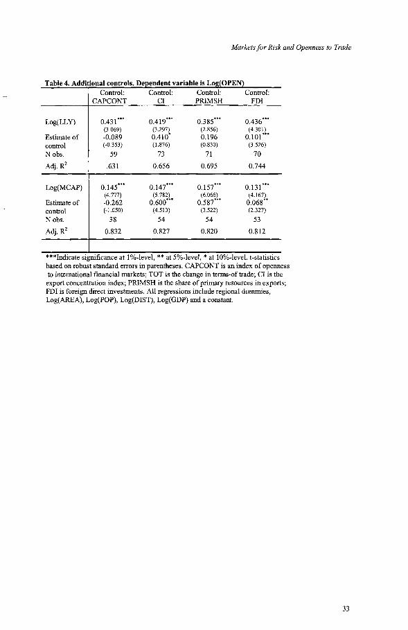
Marketsfor Risk and Openness to Trade
Table 4. Additional controls. Dependent variable is Log(OPEN)Control: Control: Control: Control:
CAPCONT CI PRIMSH FDI
Log(LLY) 0.431*""" 0.419......... 0.385 ......... 0.436"'*'"(3.069) (3.297) (2.856) (4.301)
Estimate of -0.089 0.410'" 0.196 0.101 M'"
control (-0.353) (1.876) (0.830) (3.526)
Nobs. 59 73 71 70
Adj. R2 .631 0.656 0.695 0.744
Log(MCAP) 0.145......... 0.147......... 0.157......... 0.131 .........(4.777) (5.782) (6.066) (4.167)
Estimate of -0.262 0.600"""'" 0.587"''''''' 0.068 ......
control (-1.050) (4.513) (3.522) (2.327)
Nobs. 38 54 54 53
Adj. R2 0.832 0.827 0.820 0.812
***Indicate significance at 1%-level, ** at 5%-level, * at 10%-level. t-statisticsbased on robust standard errors in parentheses. CAPCONT is an index of opennessto international financial markets; TOT is the change in terms-of trade; CI is theexport concentration index; PRIMSH is the share of primary resources in exports;FDI is foreign direct investments. All regressions include regional dummies,Log(AREA), Log(POP), Log(DIST), Log(GDP) and a constant.
33

Chapter 1
Table 5. Panel, LLY and DC 1960-94, MCAP 1975-94.Log(OPEN) Log(OPEN) Log(OPEN)
FE FE FE
Log(LLY)
Log(DC)
Log(MCAP)
Log(POP)
Log(GDP)
Nobs
N countries
Within R2
0.185***(5.410)
-0.202"'*(-2.244)
0.191'''**(4.434)
694
121
0.316
0.099***(4.269)
0.060***(2.701)
-0.088 0.352*(-1.032) (1.782)
0.167'"** -0.096(4.269) (-0.977)
706 199
123 68
0.302 0.261
*** Indicate significance at 1%-level, ** at 5%-level, * at 10%level. t-statistics based on robust standard errors in parentheses.All regressions include time-period dummies and country-specificfixed effects that are jointly significant.
34

Table 6. Additional tests. Dependent variable is Log(OPEN)Fixed Fixed Fixed Fixed Random Random Random Random
Effects Effects Effects Effects Effects Effects Effects Effects
Log(LLY)
I
0.167*** 0.15t'** 0.139*** 0.159***(4.273) (3.990) (3.203) (3.698)
Log(MCAP) 0.051 ** 0.050** 0.061 *** 0.071***(1.996) (1.969) (3.019) (3.753)
CAPCONT
I-0.126** -0.174 -0.150** -0.166 -0.198*** -0.236** -0.185*** -0.171(-1.917) (-1.191) (-2.241) (-1.107) (-2.808) (-2.024) (-2.664) (1.600)
TOT 0.512*** 0.134 0.594*"'* -0.037 0.624*** 0.321(3.900) (0.322) (3.653) (-0.093) (3.753) (0.812)
cr(GDP)60_92 0.447 0.327(1.395) (0.938)
cr(TOT)71-90 0.022*...... 0.027"'**
x OPEN6o-9o (3.920) (3.583)
Nobs. 596 175 579 173 431 154 420 151~
N countries 116 62 115 61 81 52 79 52 ""I!
rtWithin R2 0.316 0.254 0.320 0.255
~
~Overall R2 0.716 0.848 0.760 0.873
""I!
~
Hausmana)
f;;'6.82 18.63 11.80 1786.87 ~
~
[p-value] [0.74_]_ [0.017] [0.299] [0.000] ~
l::4.
~~
*** Indicate significance at 1%-level, ** at 5%-level, * at 10%-level. t-statistics based on robust standard errors in parentheses. All regressions ~~
include Log(POP), Log(GDP) and time period dummies. The random effects estimates also include regional dummies, Log(AREA), and ~~
Log(DIST). cr(GDP)60-92 is the standard deviation ofGDP 1960-92, cr(TOT)71-9o is the standard deviation of log differences in terms of trade S1971-90, OPEN6o-9o is average openness 1960-90. a) The Hausman test statistics is X2 distributed with the same degrees of freedom as the ~
w number of explanatory variables. The p-value indicates at which probability we can reject the hypothesis that the fixed effects and the regressors ~Vlare correlated.

Chapter 1
Table 7. Alternative measures of openness.IMPDUT IMPDlJT NTB NTB> mean <mean > mean <meanGDP/pc. GDP/pc. GDP/pc. GDP/pc.
Log(LLY) -1.376 2.270 -3.437 6.337(-0.934) (1.111) (-0.753) (1.233)
Log(MCAP) -1.473** 1.508 -3.075· 0.850(-2.191) (0.743) (-1.790) (0.428)
***Indicate significance at 1%-level, ** at 5%-level, * at 10%-level. tstatistics based on robust standard errors in parentheses. In columns oneand two, Log(POP), Log(GDP), time period and country specific fixed effectsare also part of the regressions. In columns three and four, Log(AREA),
Log(POP), Log(GDP), and continent dummies are also part of the regression.
36
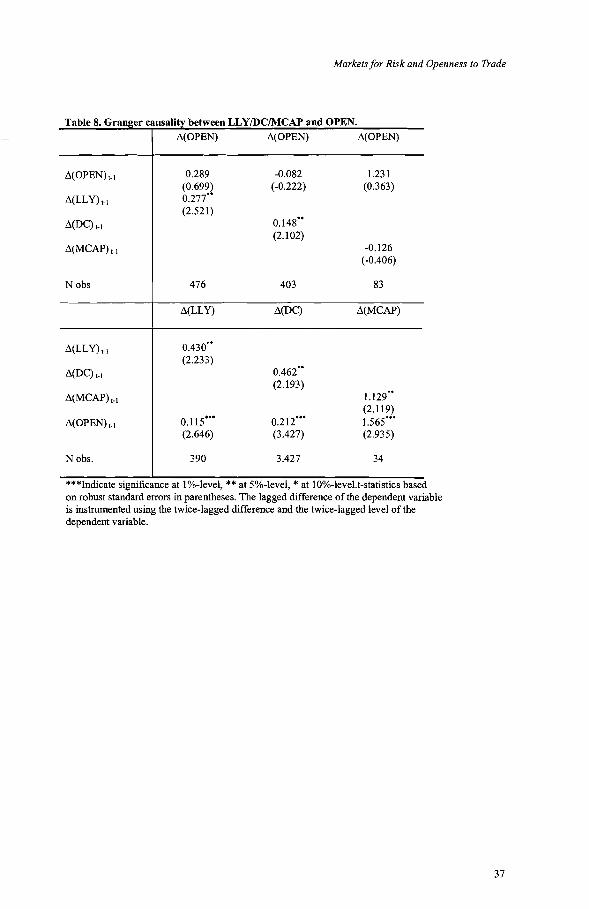
Markets for Risk and Openness to Trade
Table 8. Granger causality between LLY/DCIMCAP and OPEN.~(OPEN) ~(OPEN) ~(OPEN)
~(OPEN)t_1 0.289 -0.082 1.231(0.699) (-0.222) (0.363)
~(LLY)t-1 0.277**(2.521)
~(DC)t-1 0.148**(2.102)
~(MCAP)t.1 -0.126(-0.406)
Nobs 476 403 83
~(LLY) ~(DC) ~(MCAP)
~(LLY)t.1 0.430**(2.233)
~(DC)t-1 0.462**(2.193)
~(MCAP)t-l 1.129**(2.119)
~(OPEN)t-l 0.115*** 0.212*** 1.565***(2.646) (3.427) (2.935)
Nobs. 390 3.427 34
***Indicate significance at l%-level, ** at 5%-level, * at 10%-leve1.t-statistics basedon robust standard errors in parentheses. The lagged difference of the dependent variableis instrumented using the twice-lagged difference and the twice-lagged level of thedependent variable.
37

Chapter 1
Table 9. Instrumental variables 1990-94Log(OPEN) Log(OPEN) Log(OPEN)
Log(LLY) 0.606··(1.993)
Log(DC) 0.606u
(2.011)Log(MCAP) 0.276·
(1.866)
Nobs. 36 38 37
R2 of residuals 0.004 0.0001 0.053on instrumentsOIR-testa) 0.144 0.004 1.961
*** Indicate significance at 1%-level, ** at 5%-level, * at 10%-level.t-statistics based on robust standard errors in parentheses. Regressionsinclude constant, Log(GDP), Log(AREA), Log(DIST), Log(POP), andregional dummies. Instruments are an index of minority shareholder rights,the 'rule of law' index by feR, and the number of assassinations per nrillioninhabitants. a) The null hypothesis of the overidentification test is that theinstruments are not correlated with the residuals from the second stageregression. Critical values for the test (2 d.f.): 10%=4.61, 5%=5.99.
38

CHAPTER 2
FINANCIAL MARKETS, THE PATTERN OF SPECIALIZATION AND COMPARATIVE
ADVANTAGE.
EVIDENCE FROM OECD COUNTRIES.a
Helena Svaleryd* and Jonas Vlachos**
Abstract
Due to underlying technological differences, industries differ in their need for
external finance. Since services provided by the financial sector are largely
immobile across countries, the pattern of specialization should be influenced by
the degree of financial developnlent. We find this effect to be strong. In fact, the
financial sector has an even greater impact on the pattern of specialization
among OECD countries than differences in human- and physical capital
endownlent. Further, it gives rise to comparative advantage in a way consistent
with the Hecksher-Ohlin-Vanek model. Results on which aspects of financial
systems that are of importance for specialization are also presented.
JEL classification: F14; G20; 016
Keywords: Financial intermediation; Financial systems; Specialization patterns;
Comparative advantage
aWe thank Thorsten Beck, Karolina Ekholm, Tore Ellingsen, Rickard Forslid, Patrik Gustavsson,Torsten Persson, Daniel Waldenstrom and seminar participants at the European Economic AssociationConference in Lausanne, Nordic International Trade Seminars in Copenhagen, Stockholm Universityand the Stockholm School of Economics for helpful suggestions. Financial support from the Ahlstromand Terserus Foundation (Svaleryd) and the Swedish Institute for Banking Research (Vlachos) isgratefully acknowledged. All remaining errors are our own.... Department of Economics, Stockholm University. Email: [email protected].** Corresponding author. Department of Economics, Stockholm School of Economics, P.O. Box 6501,11383 Stockholm, Sweden. Fax: +46-8-313207. Email: [email protected].

Chapter 2
1. Introduction
In a modem economy, financial markets and financial intermediaries play an
important role by mobilizing savings, allocating credit, and facilitating the hedging,
pooling and pricing of risks. l That a well-functioning financial sector has strong,
positive effects on a country's aggregate growth opportunities has been shown by, for
example, Levine et al. (2000). Since the need for external financing through financial
markets differs depending on in which type of activity firms are involved, it would be
surprising if the growth effect was completely symmetric across sectors and firms.
Resent research (Rajan and Zingales 1998, Demirguc-Kunt and Maksimovic 1998,
Beck and Levine 2001) has actually found evidence that firms and industries heavily
dependent on external financing grow faster in countries with well-developed
financial systems. Given these empirical results, it is only natural to expect trading
and specialization patters to be influenced by the financial sector. This paper adds to
earlier research, first by reporting that differences in financial development among
OBeD countries have an even greater impact on the pattern of specialization than
differences in human or physical capital. Second, we find that well-developed
financial intermediaries and markets have a positive effect on the content of external
financing in net trade. In other words, the financial sector gives rise to conlparative
advantages in a way consistent with the Heckscher-Ohlin-Vanek (HOV) model.
When discussing financial development, it is important to keep in mind that the
financial sector has developed along different lines in different countries.
Consequently, there has been an intense debate on the relative merits of the different
systems, traditionally divided into bank-based versus market-based systems. By using
a variety of indicators of financial development, we attempt to assess the relative
importance of different aspects of the financial system on specialization patterns and
the strength of comparative advantage. Our findings indicate that large and active
stock markets, and the degree of competition in the banking sector, have the strongest
effect on both specialization patterns and the trade content of external financing.
Further, there is support for the view that the quality of investor information and the
1 The contribution of the financial sector to GDP is large. Demirguc-Kunt and Levine (1996) presentestimates varying from around 5% ofGDP in the US to 9% in Japan during the years around 1990.
40
Financial Markets, the Pattern ofSpecialization, and Comparative Advantage
legal protection of creditors affect the pattern of industry specialization, while the
depth of the financial system is a source of comparative advantage.
An obvious prediction of the standard Heckscher-Ohlin-Vanek (HOV) model is that a
country well endowed with institutions of relatively high quality should tend to
specialize in the production of goods relatively intense in the use of services provided
by these institutions. This study treats financial markets and intermediaries as factors
in the production of goods and services. A necessary condition for a production factor
to give rise to comparative advantage is that it is immobile across countries. If
financial intermediation were internationally mobile, however, we would not expect
the strong growth effect of domestic financial development that is found in the
empirical growth literature. Moreover, Jayrathne and Strahan (1996) show that the
services provided by the financial sector are indeed highly immobile geographically,
even within the USA.
This paper belongs to the small empirical literature investigating the effects of
institutions on trade. In Svaleryd and Vlachos (2001), we find an economically
significant relation between the degree of financial development and aggregate
openness to trade. Anderson and Marcouiller (1999) find corruption and inlperfect
contract enforcement to be important determinants of aggregate bilateral trading
volumes. To our knowledge, the present paper is the first to analyze empirically how
financial markets affect industry specialization patterns and international
competitiveness.2 More broadly speaking, this is the first paper documenting that the
institutional features of a society can give rise to conlparative advantage. It also
contributes to the literature on financial market and growth by focusing on absolute
levels of production rather than growth rates. Finally, we provide new, indirect
evidence to the debate on the relative merits of different financial systems to generate
capital.
The paper is organized as follows. In Section 2, we start by discussing different
aspects of the financial sector. Section 3 describes our measures and data of financial
2 After the completion of this paper, the independent work by Beck (2001) was released. Beckaddresses the same questions, using basically the same methods. He does not, however, control for a
41
Chapter 2
intermediation and other variables. Sections 4 and 5 present the results for industry
specialization and factor content ofnet trade, respectively, and Section 6 concludes.
2. The financial sector
2.1. The financial sector as an endowment
What do we mean by our claim that the financial sector effectively works as an
internationally immobile factor endowment? The question is important since Wood
(1994) has shown that the inclusion of internationally mobile production factors in
studies of the factor content of trade can yield incorrect predictions. Especially, he
argues that since capital mobility has (more or less) equalized real interest rates across
countries, capital cannot be a source of comparative advantage. This line of reasoning
abstracts from the well-known imperfections of financial n1arkets arising from
informational asymmetries and conflicting interests between creditors and debtors
however (see, for example, Stiglitz and Weiss 1981).
These problems have given rise to financial intermediaries specializing in project
evaluation and monitoring and information dissemination, thereby mitigating the
negative effects of market imperfections. Two countries with the same real interest
rate, but with financial sectors of differing quality, are thus, in practice, differently
endowed with financial capital. Alternatively, the problem can be seen from the
perspective of the firm or industry: Industries heavily involved in projects subject to
especially strong informational problems stand to gain most from the development of
financial intermediaries, even if this development does not affect market interest rates.
There is a huge literature on the underlying causes of, and possible remedies to, these
problems. The degree of project uncertainty (Huang and Xu 1999) and the share of
investments in intangible assets (Myers and Majuf 1984) are just two of the factors
that make financial intermediation more important. Hence, it should be clear that
financial intermediaries do not just raise money for financing investments in physical
capital. In fact, it is difficult to have a clear prior on the factor content of the
investments made with financial capital, which makes us draw the conclusion that the
wider range of production factors. Hence, he cannot relate the size of the effect of financial markets onthe pattern of specialization to the effect of other factors.
42
Financial Markets, the Pattern ofSpecialization, and Comparative Advantage
financial sector is best viewed as a type of human or organizational capital,
specialized in overcoming market distortions in financing.
But are not the services provided by the financial sector internationally tradable,
thereby erasing this source of con1parative advantage? Several results in the empirical
growth literature suggest otherwise. In a recent study, Levine et al. (2000)
demonstrate that the domestic level of financial development is an important
determinant of its economic growth. Following La Porta et al. (1997, 1998), they also
show that a country's legal origin and the legal environment have strong effects on the
development of the financial sector. Wurgler (2000) shows that more capital is
allocated to growing industries, and less to declining industries, in countries with
well-developed financial systems compared to other countries. This improved
allocation of capital can explain why Beck et al. (2000) find that the development of
financial intermediaries has a positive effect on total factor productivity growth.
Several micro-oriented studies also present results indicating the non-tradable
character of financial services. Demirgiic-Kunt and Maksimovic (1998) show that
firms highly dependent on external finance, located in countries with efficient
financial and legal systems, tend to grow faster than similar firms in other countries.
In an influential study, Rajan and Zingales (1998) show that the same result applies at
the industry level. Giannetti (2000) presents evidence that the ease with which finns
investing in intangible assets obtain loans depends on the legal system and the level of
financial development. More direct evidence is found in Jayaratne and Strahan (1996),
who show that financial services are difficult to trade geographically even within a
country. In those US states that experienced relaxation in bank branch restrictions, the
quality of bank loans improved and per capita income grew compared to those
without banking deregulation. Finally, by investigating companies' cross-listing
decisions, Pagano et al. (2001) conclude that geography is still of importance for
financing.
All these studies demonstrate that the use of financial capital that, admittedly, is
internationally mobile, to a large extent depends on the immobile institutional features
of a society, summarized in measures of financial development. The problems pointed
out by Wood (1994) when including measures of internationally traded physical
43

Chapter 2
capital in HOV-studies, hence do not apply to the endowment of financial
intennediaries. It is therefore reasonable to expect countries with well-functioning
financial markets to have a comparative advantage in the production of financial
services, and to specialize in industries highly dependent on external financing.
2.2. Views of the financial system
Although the above discussion is quite straightforward, it is also abstract. In reality,
the financial system is not an entity that develops linearly along a single dimension;
rather, there are intrinsic differences between different systems. Naturally, there is
also a huge literature on the pros and cons of these different systems. Traditionally,
the debate has been focused on bank-based versus market-based financial systems.
Recently, however, new perspectives based on the overall efficiency of the financial
sector, and its legal environment, have widened the debate.
Hardly anyone doubts that banks play an important role in the nlodem economy, by
specializing in monitoring and screening firms, and by building long-term
relationships with firms. Thereby, banks mitigate the informational problems between
borrowers and lenders and allow them to provide financing for firms. Competitive
equity markets could, however, potentially perform exactly the same functions as by
banks, although Stiglitz (1985) argues that information disseminates quickly on well
developed markets. Hence, the individual investor has small incentives to acquire
information in the market-based system, whereas the long-term relationships
characterizing bank-based systems may mitigate this problem. Schleifer and Vishny
(1986) present a similar argument i.e. that the easy by which the individual owner can
sell their shares on a well-developed market reduces the incentives to exercise
corporate control. All in all, it may well be that banks are better at assessing and
controlling firms and managers, and hence at and providing financing.
Several objections have been raised to this negative view of markets. First of all, a
well-developed stock market aggregates information about both firms and markets in
a way not possible for an individual bank. Even though information spreads fast, there
are large and quick gains to be nlade from acquiring superior information, possibly
nlaking markets better informed than banks. Second, corporate control may be
44

Financial Markets, the Pattern ofSpecialization, and Comparative Advantage
facilitated by stock markets through compensation schemes linked to stock market
performance. Further, Hellwig (1991) argues that rent extraction by banks can reduce
manager incentives for profitable investments due to their inside information. It is also
likely that banks that issue debt have an incentive to be biased against high-risk
projects, which can explain why Allen and Gale (2000) find that riskier industries
attract more external funding in market-based economies. Another explanation for this
might be that a well functioning stock market also expands the possibilities for risk
diversification, thereby making high-risk projects more attractive for the individual
investor.
Another possibility expressed by, for example, Huybens and Smith (1999) is that
markets and banks are complements rather than substitutes. Then, it is the efficiency
of the financial sector as a whole that is of importance, not whether the system is
primarily based on markets or banks. Finally, as La Porta et al. (2000) have stressed,
the legal system is a key determinant of the workings of the financial system.
Especially, the legal system protects creditors and minority shareholders against
expropriation by majority shareholders and managers. Legal investor protection is
therefore associated with effective corporate governance and hence, constitutes a
better staring point for cross-country comparisons of financial systems than the bank
versus market framework.
Thus, there are four main views of the financial sector: the market based and the bank
based views, the view that it is the overall size and efficiency that is of importance,
and the view that it is the legal protection of creditors and shareholders that is of
importance. In the next section, the different measures employed in this study are
presented and related to these views.
3. Measurement issues and data
3.1. Financial dependence
The basic premise of this paper is that there are intrinsic technological reasons why
industries differ in their dependence on external financing, and that these differences
persist across countries. In the empirical trade literature, such assumptions are quite
45

Chapter 2
standard regarding other production factors such as human and physical capital. It is
even standard procedure to assunle the inter-industry ranking of intensity in factor
usage to be stable over tinle. Making this assumption for financial dependence might
therefore be more enlpirically than conceptually difficult.
In an innovative paper, Rajan and Zingales (1998) tackle exactly the problem of how
to measure industry differences in financial dependence.3 This is achieved by noting
that when financial markets work relatively without friction, the supply of external
financing will be very elastic. Differences in the actual use of external financing in
such an economy will hence mainly reflect differences in demand for this type of
funding. By arguing that the U.S. financial markets are the most advanced in the
world, Rajan and Zingales use data on the actual external financing pattern of U.S.
finns to calculate their measure of financial dependence. More precisely, their
measure is defined as capital expenditures minus cash flow from operations divided
by capital expenditures. To smooth fluctuations, they use data on the finn's external
financing and capital expenditure over a 10-year period. In order to prevent that
excessive weight from being given to large firms, industry values for each of the
industries in their study are calculated as medians rather than means. According to
this indicator, drug and medicines (ISIC 3522) constitute the most financially
dependent industry, while the tobacco industry (ISIC 314) is the least so.
3.2. Financial development
Ideally, a measure of how well developed the financial sector is should gauge how
effectively financial internlediaries and markets manage to nl0bilize and allocate
capital. Thus, the ideal measure of financial development should be related to the
variety of internlediaries and nlarkets available, the efficiency with which they
evaluate and monitor firms, and the legal and regulatory framework assuring
performance. Although there are no perfect measures available, the recently
developed indicators in Beck et al. (1999) proxy for the different aspects of the
financial system outlined in Section 2.2.
3 Beck and Levine (2001) basically employ the same methodology as Rajan and Zingales, when askingif a bank-based or a market-based financial system is most conductive to the growth of fmanciallydependent industries.
46

Financial Markets, the Pattern ofSpecialization, and Comparative Advantage
The first couple of proxies are related to the size and activity of the stock market, and
are hence related to the market-based view of the financial system. We use the stock
market capitalization to GDP ratio (MCAP) which equals the value of listed shares to
GDP, as an indicator of the size of the stock market. Second, the total value of stock
market trade to GDP (STRADE) is used to proxy for the activity of the stock market.
Both these indicators suffer from the potential problem of capturing the forward
looking expectations of the economic agents, however if, for example, high growth
and hence, high profits are anticipated, both MCAP and STRADE will increase.
Although this could result in severe problems when considering the effect of these
variables on growth as in Levine and Zervos (1998), it is not a problem since we here
study within country and across industry differences. Another potential problem is
that none of these measures reflect the amount of financing actually obtained by
firms.
A commonly used proxy for the degree of overall financial development is the liquid
liabilities to GDP ratio (LLY). This proxy is usually employed as an indicator of
financial depth and has the advantage ofbeing available for a wide range of countries.
It is not, however, a direct measure of the financial sector's capacity to generate funds
and may be most appropriate when other indicators are not available. A more direct
aggregate indicator of the activity of financial intermediaries is the amount of credit
given in an economy. More precisely, we use the ratio of private credit by deposit
money banks and other financial institutions (DC) to GDP to proxy for this. One
virtue of this measure is that it isolates credit issued to the private sector from the
private sector. These two indicators are used to investigate the argument that the
overall size and efficiency of the financial system is what is of importance for
generating capital.
Next, we include indicators of the efficiency and market structure of commercial
banks. A potential measure of the efficiency with which commercial banks channel
funds fronl savers to investors is the net interest margin, i.e. the accounting value of a
bank's net interest revenue as share of its total assets (MARGIN). This indicator
serves as a proxy for the wedge between the prices faced by the parties on either side
of a loan transaction. We define (CONC) as the ratio of the three largest banks' assets
47

Chapter 2
to total banking sector assets, as an indicator of the market structure. A highly
concentrated banking sector might be less competitive and hence less efficient than a
competitive one.4
The next set of proxies is nlore related to regulatory efficiency and hence to the
potential of raising funds, rather than the actual outconle. For this purpose, we (again)
follow Rajan and Zingales and use the accounting standards for each country in 1990
(ACSTAN). International comparisons of accounting standards are made by the
Center for International Financial Analysis and Research. This proxy is supposed to
reflect the potential for obtaining financing by reducing information cost. Hence, it
can be considered as an overall indicator of the quality of information available to
investors. As a check for the consistency of this index, we also make use of the 1983
accounting standards (ACSTAN83).5 Finally, we tum to indicators of the legal rights
of creditors and minority shareholders. MINORITY is an index from zero to six of
how well protected minority shareholders are. The higher is the value of this index,
the better the legal protection against expropriation. CREDITOR is an index between
zero and four, increasing in the legal rights of creditors relative to management and
other stakeholders.
3.3. Data on other endowments and intensities
In order to measure the input requirements of human capital, we use the share of
workers with post-secondary education in each industry, weighted by the relative size
of the respective industry. The average number of years of secondary schooling in the
population above 25 is used as a proxy for the national endowments ofhuman capital.
Whether or not to include physical capital in the analysis is an open question. The
answer is contingent on the mobility of physical capital; if it is a mobile resource, it
should not be included. We choose to follow the convention and include physical
capital, especially since we want to ensure that the indicators of financial dependence
and endowments do not proxy for any other type of production factors. Physical
4 As will be discussed later, competition in the banking sector can have both positive and negativeeffects for the generation of external financing to firms.5 The correlation between ACSTAN and ACSTAN83 is 0.70. ACSTAN83 is not available for Mexico.
48

Financial Markets, the Pattern ofSpecialization, and Comparative Advantage
capital intensities are calculated as the OECD-averaged capital formation to value
added ratio, while the physical capital per workers measure capital endowments. 6 In
order to capture the effect of natural resource endowments, the stock of agricultural
and forestland per worker is also employed. The intensity of the fonner is just a
dummy for food production, whereas the latter is calculated using Swedish input
output data. For further details on all variables and sources, see the appendix.
3.4. Trade data
Production and trade data by three and four-digit ISIC industry codes for the OECD
countries are obtained fronl the OECD/STAN database. Since we are forced to
combine different data sources, our final data set includes data on 32 manufacturing
industries in 20 countries. In other words, it must be kept in mind that trade in
services and raw materials is not included in this study.
4. The pattern of specialization
We first approach the question of how different countries' factor endowments affect
international trade by considering the pattern of industrial specialization. The
hypothesis is that the international competitiveness of an industry in a certain country
depends on the resource endownlents of that country and the input requirements of the
industry. Balassa pioneered this approach in a couple of influential papers (Balassa
1979, 1986).
One obvious candidate as an indicator of international competitiveness and industrial
specialization is the ratio between production and consumption as suggested by
Gustavsson et al (1999),
(4.1)Qij Cij+Xj-Mij 1 Xij-Mij
rij=-= = + ,Cij Cij Cij
6 There are alternative ways ofmeasuring both human- and physical capital intensities andendowments. We have employed several (see appendix) as checks on the robustness of the results.
49

Chapter 2
where Qij is production, Cij is consumption, Mij is imports, and Xij exports of good i in
country j. It should be clear that when rij is greater than one, country j is a net exporter
of good i, whereas a value lower than one indicates that the country is a net importer.
In the analysis, rij is regressed on a set of variables constructed by interacting the
input requirenlents of each industry i with the country characteristics of each country
j. The larger the value of rij, the more specialized is country j in industry i.
In order to pick up fixed industry and country effects, a set of industry and country
dummies is added to the regression. We take the logarithm of rij to ensure that the
trade imbalances end up in the country fixed effects. To see this, consider the case of
balanced trade. It must then be true that
For each country j there exists a parameter f3J such that
By scaling each element in the production vector by (1 +fJJ), a hypothetical value of
production under balanced trade is derived. The relationship between the measure of
specialization under balanced and unbalanced trade can then be expressed as
By taking the logarithms of (4.4), it should be clear that the country-fixed effects
capture the trade imbalance parameter (1 +fJJ).
An alternative measure of industry specialization would be the one used by Balassa
(1986), namely
50

Financial Markets, the Pattern ofSpecialization, and Comparative Advantage
The main difference between this measure and rij is that it can take on a negative
value. Thus, it cannot be adjusted for trade imbalances by taking on logarithms.
Although the approach behind (4.1) and (4.5) is inspired by the HOV-theory, it should
not be considered as a fonnal test of the HOV-theory. Leamer and Levinsohn (1995)
raise theoretical objections to this type of studies when the number of goods is larger
than the number of production factors. Bowen and Sveikauskas (1992) demonstrate,
however, that these theoretical objections are of little practical importance in actual
empirical analysis. The patterns of industry specialization are shown to be consistent
with the net exports of factor services, especially for broad aggregates of production
factors. What is important, though, is to adjust the dependent variable for trade
imbalances. For this reason, we will n1ainly focus on rij, and keep the Balassa
measure for testing the robustness of the results.7
4.1. Estimation and Data
In order to estimate the impact of financial development on the pattern of industry
specialization, we use data on industry factor input requirements and country-factor
endowments. The expected sign of the interaction variables is usually positive, which
means that a country well endowed with a certain factor will specialize in the
industries with large input requirements of that factor. Exceptions are when net
interest margin and bank industry concentration are used as proxies of efficiency and
competition in the banking sector. Since higher values of these variables imply lower
efficiency and competition, we expect the interaction between financial dependence
and MARGIN and CONC to be negative.
This means that we estin1ate the following relationship:
(4.6) lnr.. =~~ PI·D. +"~ P2·D. +"m P3k(a'k xEND.k)+8 .. ,u L.",=l I , L.J j =l j j L."k=l ' j 1J
where i is the industry index, j is the country index, k is the factor index, Di is a
dummy for industry i, Dj is a dummy for country j, aik is the input requirement of
7 The correlation between the two indicators of specialization is 0.69.
51

Chapter 2
factor k in sector i, ENDjk is the endowment of factor k in country j, and Bij is the error
term.
4.2. Results
Table 1 shows the results from the estimation of (4.6). Seven of the ten interactions
between financial dependence and financial development are statistically si~ificant
and all have the expected signs. Further, all other interaction variables are positive as
expected, but the interaction of agricultural inputs is not significant. Given the highly
regulated agricultural sector in most OEeD-countries, it might not be surprising that
natural advantage is not a key determinant of the pattern of agricultural production.
Establishing statistical significance is a first step, but is the effect of financial markets
on the pattern of specialization of economic significance? In column one, we see that
the coefficient on the interaction tenn between financial dependence and the market
capitalization ratio takes the value of 0.194. In order to interpret the economic
n1agnitude of this coefficient, the following experiment is helpful: Consider that the
industry at the 75th percentile of financial dependence was located in the country at
the 75th percentile of financial development, rather that in the country at the 25th
percentile of financial development. Further, consider the same switch of locations for
the industry at the 25th percentile of financial development. How much larger would
the industry of high dependence be in the high development country compared to the
low-dependence industry, given that all other variables take on their average values?8
In specification (1), this exercise leads to an increase in In(rij) by 0.103. For all
industries, the average value of In(rij) is -0.164. Hence, the switch of countries would
lead to a 10.8 percent increase in rij, compared to the average value. For the other
(statistically significant) proxies of financial development, the same number is 12.2,
5.4, 7.0, 6.1, 8.7, and 8.5 percent. In comparison, the same thought experiment with
respect to human and physical capital gives an increase in rij by around 5 and 6
percent, respectively. The impact of the financial system on the pattern of
specialization must thus be considered as very large.
8 This thought experiment is from Rajan and Zingales (1998). Mathematically, this means the followingcalculation:COEFFx {FINDEP75 x (FINDEV75-FINDEV25) - FINDEP25 x (FINDEV75-FINDEV25)}
52
Financial Markets, the Pattern ofSpecialization, and Comparative Advantage
When turning to the specific indicators of financial development, we see that both
stock market indicators (MCAP, STRADE) are statistically significant. Moreover, the
size-effect of these variables is the largest among all interaction terms. This shows
that a well-developed stock nlarket is the most important source of competitive
advantage among financially dependent industries. In other words, we have indirect
support for the view that a market-based financial system is the most efficient.
Neither of the aggregate indicators of financial-sector development, LLY and DC,
seem to be of much importance for the pattern of specialization. The liquid liabilities
ratio is not even close to statistical significance, while the credit ratio is weakly
significant. The effect ofDC is also among the smallest (although still large compared
to the effect of human- and physical capital). One way of interpreting this is that the
aggregate size of the financial sector is of less inlportance for raising funds, at least
among OECD-countries. Thus, we have indirect evidence suggesting that the type of
financial system is of importance.
Turning to the efficiency of the banking sector, the net interest margin (MARGIN)
does not affect the pattern of specialization. The concentration index (CONe), which
proxies for the degree of competition in the banking sector is, however, of
importance. The result for banking concentration is interesting since it indirectly
suggests that financially dependent industries have better access to credit when the
banking industry is competitive. This contradicts Petersen and Rajan (1995) who
show that competition in the credit market can be detrimental to the formation of
firm-creditor relationships. The reason is that when creditors cannot hold equity
claims, and the market is competitive, the creditor is forced to break even every
period. For high-risk projects, this implies a very high interest rate that can distort the
firms' incentives. In a monopolistic market, on the other hand, the creditor can cross
subsidy the firm over time - to the nlutual benefit ofboth creditor and lender.9 Rather,
the result in column 5 constitutes indirect support of the view put forward by Rajan
9 Petersen and Rajan (1995) also provide empirical evidence from the US, supporting this view. Usingthe same methodology as Rajan and Zingales (1998), Cetorelli and Gambera (2001) fmd that aconcentrated banking sector supports the growth of fmancially dependent industries.
53

Chapter 2
(1992). There, he suggests banks with market power extract rents and hence, reduce
the firms' incentives to invest.
Accounting standards (ACSTAN, ACSTAN83), the indicators of the aggregate
quality of information available to investors, are also significant - both statistically
and economically. Given the severe infonnational problems in the financial markets,
it should not be a surprise that good information has a positive effect on the
generation of external financing.
Finally, the results concerning the view that the legal protection of outsiders against
expropriation attempts by insiders are mixed. Minority shareholder protection
(MINORITY) does not seem to affect the pattern of specialization, while the
protection of creditors (CREDITOR) does.
[Table 1 here]
4.3. Sensitivity analysis
There are many different ways of measuring most variables in of regression 4.6. Since
we want to ensure that the results presented above are not due to our choice of
indicators, we perform a number of sensitivity tests. Each cell of Table 2 refers to an
individual regression, and shows the estimates of the interaction terms between
financial dependence and financial development.
In row 1, we replace Ln(rij) with the Balassa (1986) nleasure of industry
specialization: (Xij -Mij)/(Xij +Mij). The results are remarkably consistent with the
ones in Table 1. Accounting standards for 1990 lose their significance, as does the
index of creditor rights. The indicators of financial depth and domestic credit, on the
other hand, now gain statistical significance. Making the same analysis for the size of
the effect as for In(rij), we obtain an increase in the dependent variable by 0.075,
0.090, 0.031, 0.062, 0.063, 0.052, and 0.044 for each of the significant interaction
terms. For human capital, the size-effect is around 0.06 and for physical capital 0.025.
54

Financial Markets, the Pattern ofSpecialization, and Comparative Advantage
Thus, the large effect on the pattern of specialization previously found is not due to
the choice of dependent variable.
In row 2, we instrument for financial development using each country's legal origin as
instrument, as suggested by La Porta et al. (1998).10 These instruments are a set of
dummy variables taking the value one if a country is of British, Scandinavian,
German, and French legal origin, respectively. To this set of instruments, we add the
"rule of law" index produced by Business International Corporation. Although these
instruments have successfully been used in other studies (e.g. Rajan and Zingales,
1998), we have some worries that there is too little variation in these variables since
the analysis is limited to the OECD. However, the results from Table 1 are quite
robust to the instrunlentation, although the significance levels of the variables are
generally sonlewhat lower. One exception is that CREDITOR gains both in statistical
significance and size: the point estimate increases from 0.07 to 0.25. If we were to
take this estimate seriously, an increase in the creditor rights' index fronl 1 to 3 would
imply an increase in rij by 23 percent.
In row 3, the human capital indicator is now replaced by an interaction term where the
number of scientists per worker in each country is used as country endowment of
human capital. 11 In this specification, all interactions between financial dependence
and financial development except the one based on financial depth (LLY) are
statistically significant. The point estimates are very similar to the ones in Table 1. If
we calculate the size-effect for this indicator of human capital, we get a value of
around 6 percent, roughly the same as when secondary schooling is used. 12
In row 4, physical capital intensities are replaced by the British industry level capital
stock to value added ratio, which is done to verify that the results are not contingent
to The evolution and persistence of the French and British legal traditions are discussed theoretically inGlaeser and Shleifer (2001).11 The correlation between SECSCH and SCIENW is 0.53.12 Hanushek and Kimko (2000) measure labor force quality by using international mathenlatics andscience test scores. They can thereby avoid the unrealistic assumption that schooling is of equal qualityin different countries. Moreover, the use of test scores reduces the likelihood ofproxying for generaldevelopment effects rather than human capital. Using their indicator (HCQl) rather than quantity basedindicators such as SECSCH and SCIENW does not alter the results in this paper. The size effect ofHCQl is 4.8 percent (results available upon request).
55

Chapter 2
upon the flow-measure previously used. 13 The size-effect for this indicator is around
2 percent and hence, we can once again verify the results from Table 1.
In row 5, we exclude the US from the regression since the indicator of financial
dependence is based on calculations on US firms. 14 This exclusion leaves the results
unchanged.
Finally, we include interaction terms between industry intensity and country
abundance of electricity and steel. Although these inputs are tradable, and hence
should arguably be excluded from the regression, we include them to verify that the
results for financial development are not spurious (similar production factors are also
included by e.g. Ellison and Glaeser 1999, and Gustavsson et al. 1999). Both new
variables are positive and significant but, as can be seen, the basic results are, if
anything, strengthened by their inclusion.
[Table 2 here]
5. The factor content of trade
A different approach to the question of how financial development affects the pattern
of trade between countries is to consider at the factor content of net trade. Basically,
this approach amounts to investigating if the financial system can be a source of
comparative advantage. Traditionally, the sources of comparative advantages have
been analyzed within the framework of the Heckscher-Ohlin-Vanek (HOV) model. If
we consider of financial intermediaries as immobile factor endowments, the
prediction of the HOV-model is that a country endowed with well-developed financial
markets will be a net exporter of external finance.
13 The correlation between eVAI and CAPVA is -0.07 (not significant). That the two measures are notcorrelated is of course naturally a matter of concern. evAI, however, is highly correlated with electricintensity, sometimes used as a proxy for capital intensity. This leads us to put more trust in themeasure.14 It is by no means obvious why this should force us to exclude the US from the analysis. Rajan andZingales do that in their paper, however, so we follow their example.
56

Financial Markets, the Pattern ofSpecialization, and Comparative Advantage
5.1. Estimation and data
The way to derive an empirical measure of the factor content of net trade, somewhat
consistent with the HOV-theory though relaxing the assumption of balanced trade, has
been shown in for example Leamer and Levinsohn (1995). In the present paper, we
modify the Leamer-Levinsohn measure in the same way as Lundberg and Wilmer
(1997). More precisely, we calculate the following nleasure
where xi} is the share of exports of sector i in country j, my is the share of imports of
sector i in country j, andfik is the input-requirement of factor k in sector i. Regardless
of the trade balance, the ratio carries infomlation about the relative factor content of
exports to imports. Specifically, if 4k >1 exports are more concentrated to k-intensive
goods than imports (Lundberg and Wikner 1997).15
We use the Rajan and Zingales (1998) indicator of financial dependence as a proxy
for the industry-requirements of external financing, as discussed previously
(FINDEP). Likewise, we use the same indicators of financial development as before
to proxy for the country endowment of financial intermediation. In this section, as
well as before, we hope to be able to discrinlinate between what aspects of the
financial system that are of importance for comparative advantage. This is done by
studying at a whole series of indicators. All the measures are thoroughly described in
Section 3.
The reason why we do not use exactly the sanle measure of factor content of net trade
as suggested by Leamer and Levinsohn (1995) is that this would require data on world
factor endowment of financial intermediation. The meaning of this is conceptually
difficult to grasp. Rather than tackling these conceptual difficulties, we use the qk of
15Equation (5.1) can thus be read as the factor content ratio under the restriction that balanced trade isachieved without a change in the composition of trade. The export (import) expansion needed to get ridof a trade deficit (surplus) is, in other words, assumed to be proportional across goods.
57

Chapter 2
equation (5.1), which is very much In the spirit of the Leamer and Levinsohn
measure. 16
When constructing 0k, we have not taken the services of production factors in input
goods into account. Thus, the net trade of external financing is calculated using only
the direct and not the indirect input of services of financial markets.
5.2. Results
Japan has the largest net export of external financing according to definition (5.1).
Other countries with high values in the Zfd measure are Germany, Denmark and the
U.K. At the bottom of the list, we find countries such as New Zealand, Australia and
Greece.
When turning to regression analysis, indicators of human- and physical capital
endowments, as well as the endowments of forest- and agricultural land, are included
in the regressions. The reason is twofold. First, an industry's dependence on external
financing may be a proxy for its human or physical capital intensity, for example,
while a country's endowment of financial intennediation may be a proxy for its
endowment in these production factors. To ensure that the results are not only an
artifact of spurious correlation we control for the endowment of human and physical
capital. Second, the exchange of external financing embodied in trade in services and
raw material is not included, since the data covers manufacturing only. This may give
a distorted picture of the factor content of trade for countries where raw material or
services account for a large proportion of trade. Suppose that the external financing
requirement in a sector not included in the data is very high (low). Then, the
endowment figures will overstate (understate) the supply of external financing
available for the manufacturing industry in countries where this particular sector is
large. For this reason, it is necessary to include measures of the endowment of other
production factors.
16 The Leamer and Levinsohn measure, under the balanced trade restriction, would take the form:
(jjk =LXij(L eijhk - Lmijhk ) / V}k =1- S j / a jk , where ~j is the export of good i fromiii
countryj, Jjk is countryj's endowment of factor k and ajk is countryj's share of world endowments offactor k.
58

Financial Markets, the Pattern ofSpecialization, and Comparative Advantage
Table 3 presents results where the measure of factor content of net trade (Zfd) is
regressed on country endowment variables. There is definitely support for the
hypothesis that the financial sector is a source of comparative advantage. The
measures of stock market size (MCAP) and activity (STRADE) both positively enter
the regression. The same is true for the proxy for the liquidity, or financial depth
measure, of the financial sector (LLY), and the conlpetition indicator of the banking
sector (CONC). However, DC and the other proxy regarding the functioning of the
bank sector (MARGIN) are not statistically significant. Moreover, there is no P9sitive
effect of a country's accounting standards or its legal framework on the net factor
trade of external financing.
Thus, the effects of the endowment of financial intermediaries on a country's pattern
of specialization and comparative advantage in trade are roughly the sanle. Notably,
the size and activity of the stock market and the concentration of the banking system
have a significant effect on both variables.
Admittedly, it is not easy to judge the economic effects of being endowed with well
developed financial intermediaries, since we deal with proxies of what we attempt to
measure. To investigate the effect in the different proxies for financial intermediation,
imagine an increase of, for example, STRADE by one standard deviation. This
induces an increase in Zfd by 23 percent from the mean. The impact of the other
significant proxies is around 20 percent, or around 60 percent of one standard
deviation. Another way of assessing the effect of the financial service endowment is
to see what happens if it is excluded. Column 1 reveals that removing the proxy for
financial internlediation reduces the adjusted R2 from about 0.45 to 0.03. Thus, the
statistically significant proxies have a remarkable effect on the fit of the regression.
[Table 3 here]
5.3. Sensitivity
As checks for robustness, we have replaced SECSCH with the test-based labor force
quality indicator (HCQl, results are not presented), but this has no effect on the
59

Chapter 2
results presented in Table 3. We also include other control variables in the
regressions. First, it may be the case that the indicators of financial development
capture some aspect of economic development not accounted for by the other
endowment variables. We therefore include GDP per capita, but the results remain
unchanged. Second, the public sector is likely to be financed in other ways than
through the private financial markets. Thus, for a country with a large public sector,
the true endowment of financial intermediation available for private manufacturing
may be larger than in a country with smaller public employment. Including the share
of public employment does not, however, affect the results.
Finally, we run all specifications in Table 3 on an alternative measure of factor
content of net trade. This measure is constructed as the ratio of factor content in net
trade, corrected for trade imbalance, to factor content in consumption. Specifically,
(5.2)
where fik is the input-requirement of factor k in sector i, X;j the exports of sector i in
country j, Mij the imports of sector i in country j, Bj country j's the trade imbalance
and Cij country j's consumption of good i. QiwlGDPw is the share of world output of
good i in world GDP. Once more this has little effect on the results presented in Table
3. All results remain qualitatively the same, except in the specification including LLY,
where LLY is no longer statistically significant on conventional levels.
So far, the results show strong support for the hypothesis that the financial system can
give rise to comparative advantage. Specifically, countries endowed with large and
active financial intermediaries are nlore likely to have a larger net export of the
services provided by the financial sector. To obtain a greater understanding of the
impact, we derive'a similar measure for net trade of human capital. The purpose of
this paper is neither to test the validity of the HOV-model, nor to study the effect of a
country's human capital endowment on the trade pattern. Nevertheless, it may be
60
Financial Markets, the Pattern ofSpecialization, and Comparative Advantage
enlightening to look at the equivalent measure of comparative advantage for human
capital, mainly for two reasons. First, it might indicate whether the proxies used for
human capital intensity and human capital endowment are valid. Second, it may make
us more comfortable with our measure of net factor trade. Keep in mind, however,
that the HOV-model has found limited support in the empirical trade literature.
A common procedure when studying the empirical support for the HOV-model is to
conduct rank and sign tests (Leamer and Levinsohn 1995). According to the HOV
model, a country's ranking in net trade of a specific factor should correspond to its
ranking in terms of endowment. We use the measure of net trade in factors as defined
in equation 5.1. Table 4 shows the Kendall's rank test for the two production factors
financial intermediation and human capital. We use the share of workers with post
secondary education, weighted by the relative size of that industry, as input
requirements ofhuman capital.
The results for the different proxies for financial intermediation are in line with the
regression results presented in Table 3. All correlations, except for accounting
standards, carry the expected sign and four are statistically significant. The
correlations between our measure of the net trade of services of hunlan capital and
endownlents of human capital are also positive (and significant in two cases out of
three). In light of the fact that empirical research finds linlited support for the HOV
model, we consider these results to be satisfactory.
[Table 4 here]
6. Conclusions
The main finding of this paper is that countries with well-functioning financial
systems tend to specialize in industries highly dependent on external financing.
Although this might not be surprising in itself: the size of the effect is. In fact,
differences in financial systems are more important determinants of the pattern of
specialization between GECD-countries than differences in human or physical capital.
One plausible explanation for this phenomenon is that the differences in human- and
physical capital within the OECD are fairly small. Hence, the relative size of the
61

Chapter 2
effect might be smaller in a wider selection of countries. Whether this is true is a
question left for future research. We also show that the financial system gives rise to
comparative advantage in way consistent with the Heckscher-Ohlin-Vanek model.
Another way of studying this paper is as a robustness test of the Rajan and Zingales
(1998) result that financially dependent industries grow faster in countries with well
developed financial nlarkets. However, we approach this question by studying levels
rather than growth rates. Given that Rajan and Zingales find strong signs of
conditional convergence among industries (initially large industries tend to grow
slower than initially small industries), it is by no nleans obvious that their result
should carryover from growth rates to levels.
Especially strong results are found for indicators of stock market size and activity, as
well as for competition in the banking sector. The latter result thus gives support to
theories suggesting that banking concentration limit the amount of capital raised by
firms (e.g. Rajan 1992).17 The quality of a country's accounting standards and the
legal protection given to creditors are also important determinants of the pattern of
specialization. Financial depth and the aggregate amount of credit in an economy give
rise to comparative advantage, but the results for the pattenl of specialization for these
indicators are mixed.
Since this is one of the first papers approaching the question at hand, we have aimed
at simplicity and clarity in the empirical analysis. One extension of this study would
be to allow for other amendments common in the empirical HOV-analysis. These
amendments might be to allow for cross-country technological and demand
differences as suggested by Trefler (1993), Davis and Weinstein (1996), and Harrigan
(1997). Another interesting extension is to analyze the potential effects of the
financial market on the choice of technology. Since financial markets are supposed
(and shown) to solve information problems in the market place, they are likely to
affect the choice of technology. Carlin and Mayer (1999) take a first step in this
direction by showing that the financial system affects R&D. To get a better
understanding of its effect on technology, we would also need a better grasp of why
17 The finding that banking sector concentration is conductive for the growth of fmancially dependentindustries reported in Cetorelli and Gambera (2001) also hinges on conditional convergence.
62
Financial Markets, the Pattern ofSpecialization, and Comparative Advantage
some industries are more dependent on external financing than others are. This might
be a fruitful area for future research with implications for the literature on growth as
well as international trade. Incorporating other institutional factors is another
extension along these lines. As long as industries differ in their use of the services
provided by these institutions (and the services are non-tradable), we would expect the
pattern of specialization to be deternlined by institutional factors. I8
Finally, there are at least two reasons for expecting the pattern in this paper to
disappear over time. First, multinational corporations are supposedly insensitive to
local financing conditions. To the extent that MNC:s continue to increase their share
of international trade, local financial markets should exert a continuously smaller
inlpact on the pattern of trade. The same applies if financial markets effectively
become better integrated across countries over time. I9 Hence, extending the analysis
along the time dimension might be fruitful.
18 Naturally, measuring input requirements of institutional factors, and institutional quality is difficult.That wage-setting institutions compressing the wage distribution can affect the industrial compositionis supported by evidence in Davis and Henrekson (2000).19 Petersen and Rajan (2001) document an increase in the physical distance between small firms andlenders in the US over time. This increase is correlated with higher bank productivity and hence,constitutes evidence that financial development reduces the need for proximity between borrowers andlenders.
63

0'\"J::.. Appendix
Table At. Correlations and summary statistics: Endowments
Mcap Strade Uy Dc Cone Margin Acstan Aestan Credi- Mino- Seesch Scienw HCQI Kapwl Agrilw Rwood Elecw Steelw83 tor rity w
Mcap 1Strade 0.80·" 1Lty 0.72·" 0.68··· IDc 0.74··· 0.75··· 0.72··· IConc -0.36· -0.50·· -0.47·· -0.18 IMargin -0.46·· -0.50·· -0.43·· -0.68··· -0.11 1Acstan 0.39· 0.16 0.00 0.43· 0.24 -0.37* IAcstan83 0.48·· 0.35 0.01 0.50·· -0.02 -0.49·· 0.70··· ICreditor 0.27 0.33 0.20 0.20 0.03 -0.36 0.08 -0.01 1Minority 0.49·· 0.36 0.31 0.51·· -0.06 -0.25 0.45·· 0.29 0.16 ISccsch 0.15 0.38· 0.17 0.45·· -0.11 -0.46·· 0.31 0.31 0.30 0.45·· IScienw 0.62''''' 0.81"· 0.38·· 0.71··· -0.23 -0.66··· 0.42· 0.67·" 0.30 0.34 0.53"· 1HCQI 0.42· 0.53" 0.54··· 0.47·· -0.19 -0.61··· 0.03 0.05 0.61··· 0.07 0.33 0.57··· IKapwl 0.28 0.33 0.21 0.54·· -0.05 -0.68··· 0.63··· 0.56·· 0.11 0.43· 0.63"· 0.70·" 0.34 IAgrilw -0.02 -0.13 -0.12 -0.07 0.15 0.00 0.27 0.03 -0.39· 0.40· 0.11 -0.07 -0.45·· 0.23 IRwoodw -0.15 -0.28 -0.20 0.07 0.49·· -0.24 0.50·· 0.24 0-.16 0.28 0.27 0.00 -0.18 0.40· 0.20 IElecw 0.01 -0.04 -0.17 0.20 0.38· -0.26 0.59··· 0.40· -0.04 0.41· 0.37· 0.33 -0.06 0.63··· 0.19 0.60··· 1Stee1w -0.08 -0.12 -0.07 0.02 0.27 -0.30 0.25 0.12 -0.12 -0.09 -0.08 0.05 0.01 0.31 -0.03 0.59··· 0.05 IMean 0.38 0.16 0.67 0.83 0.61 0.029 66 65 1.86 2.29 2.7 4.9 50,2 44.3 1.0 3752 18.7 1581Stdev 0.27 0.15 0.30 0.42 0.23 0.013 10 II 1.06 1.42 1.1 2.4 5,8 12.5 1.4 4725 12.1 329275th perc. 0.48 0.21 0.75 1.09 0.46 0.018 74 73 3 4 3.1 6.5 54,2 53.0 -25th perc. 0.15 0.04 0.50 0.49 0.87 0.044 61 61 I I 1.9 2.7 44,6 39.9 - -*** indicates significance at the l%-level, ** at the 5%-level, and * at the 10%-level. The last two rows display the values of the observations belonging to the 75th and the 25th percentilerespectively.
Q~~l"-,)

Financial Markets, the Pattern ofSpecialization, and Comparative Advantage
Table A2. Correlations and summary statistics: Intensities
Findep Ahi Cvai Capva Wood- Land- Elintl Ironintint use
Findep 1Ahi 0.36** 1Cvai 0.14 0.10 1Capva 0.05 -0.13 -0.07 1Woodint -0.06 -0.09 0.13 -0.11 1Landuse -0.09 0.31* -0.03 -0.13 -0.04 1Elintl -0.19 -0.22 0.54*** -0.02 0.21 -0.05 1Ironint -0.11 -0.06 0.20 -0.02 0.04 -0.03 0.14 1Mean 0.34 0.07 0.15 0.41 1.7 0.03 185 0.03Stdev 0.42 0.06 0.07 0.25 6.8 0.18 285 0.1875th perc. 0.47 0.09 0.20 0.42 - - - -25th perc. 0.06 0.02 0.11 0.26 - - - -*** indicates significance at the 1%-level, ** at the 5%-level, and * at the 10%-level. The last tworows display the values of the observations belonging to the 75th and the 25th percentile respectively.
65

Chapter 2
Table A3. Correlations and summary statistics: Dependent variables
Mean Stdev CorrelationsLn(rij) -0.164 0.482 1 -Balassa -0.210 0.431 0.69"""* 1
Zfd 0.84 0.29 1 -Wfd -0.12 0.19 0.74*** 1
Zhc 0.98 0.52 - -*** mdIcates sigmficance at the 1%-leve1, ** at the 5%-level, and * at the 1Q°,/o-level.
66

Financial Markets, the Pattern ofSpecialization, and Comparative Advantage
Table A4. Industries and countries included
ISIC Sectors Countries
3110 Food Australia
3130 Beverages Austria
3140 Tobacco Belgium
3210 Wearing Apparel Canada
3220 Textiles, Apparel & Denmark
3230 Leather & Products Finland
3240 Footwear France
3310 Wood Products Germany
3320 Furnitures & Fixtures Greece
3410 Paper & Products Italy
3420 Printing & Publishing Japan
3520 Other Chemicals Mexico1
3522 Drugs & Medicines Netherlands
3530 Petroleum Refineries New Zealand
3540 Petroleum & Coal Pr Norway
3550 Rubber Products Portugal
3560 Plastic Products, n Spain
3610 Pottery, China etc Sweden
3620 Glass & Products UK
3690 Non-Metallic Products USA
3710 Iron & Steel
3720 Non-Ferrous Metals
3810 Metal Products
3820 Non-Electrical Mach
3825 Office & Computing
3830 Electrical Machinery
3832 Radio, TV &Communication
3840 Transport Equipment
3841 Shipbuilding & Repair
3843 Motor Vehicles
3850 Professional Goods
3900 Other Manufacturing
1 Accountmg standards from 1983 are missmg for Mexico.
67

Chapter 2
Data description
Dependent variables
rij = Qij/Cij = Qi/(Qij + Mij - )(), where Qij is the production, Cij is the consumption, Mij are the imports
from the rest of the world, )(j are the exports to the rest of the world, of industry i in country j. Average
values 1989-91. Source: STAN. The defInition is from Gustavsson et al. (1999).
Balassa = (Xij - ~j) / (Xij +~). Source: STAN.
Zik = Li xijhk /Limijhk ' where xij and mij are the shares of exports (imports) of sector i from (to)
country j, and fik is the input requirement of factor k in sector i. The measure is called Zfd when using
external financing requirements and Zhc when using human capital requirements. Source: xij and mi are
constructed from STAN average values in 1989-91,hk for external financing is FINDEP (Rajan and
Zingales (1998» and human capital intensity is ARI. The defmition is from Lundberg and Wikner
(1997).
Lfik(Xij-Mij-Bj~)J¥jk = i GDPw ,where fik is the input-requirement of factor k in sector i, X;j the
LfikCiji
exports of sector i in country}, Mij the imports of sector i in country}, Bj is country}'s trade imbalance
and Cij countryj's consumption of good i. QiulGDPw is the share of world output of good i in world
GDP. The measure is called njd when using external finance requirements. Source:)(j, Mij and Cij
from STAN average values 1989-91.hk for external finance is FINDEP. Qiw the sum ofproduction
over the 22 countries included in the study and GDPw is the sum ofGDP for the countries in the study.
Bj = total export-total import ofgoods and services for 1990 from World Development Indicators.
Financial variables
External finance dependence:
FINDEP. Capital expenditure minus cash flows from operations divided by capital expenditures. Data
source: Rajan and Zingales (1998).
Financial sector development:
MCAP: Stock ma~ket capitalization to GDP, average 1989-91. Source: Beck et al (1999).
STRADE: Stock market total value traded to GDP, average 1989-91. Source: Beck et al (1999).
LLY: Liquid liabilities to GDP, average 1989-91. Source: Beck et al (1999).
DC: Private credit by deposit money banks and other financial institutions to GDP, average 1989-91.
Source: Beck et al (1999).
CONC: Market share of the three largest banks. Source: Beck et al (1999).
MARGIN: Net interest margin to total assets. Source: Beck et al (1999).
ACSTAN: Accounting standards 1990. Source: Rajan and Zingales (1998).
ACSTAN83: Accounting standards 1983. Source: Rajan and Zingales (1998).
Legal variables:
MINORITY: Index of minority share holder rights, range 0-6. Source: La Porta et.a!. (1998).
CREDITOR: Index of creditor rights. Range 0-4. Source: La Porta et.a!. (1998).
68

Financial Markets, the Pattern ofSpecialization, and Comparative Advantage
RULELAW: International Country Risk (ICR) index of law and order tradition. Source: La Porta et.al.
(1998).
SCAND, GERMAN, FRENCH, ENGL: Dummies of legal origin. Source: La Porta et.al. (1998).
Human capital
Human capital intensities:
POSTSEC: The share of post-secondary schooling in total employment, 1990, Swedish industries.
Source: SCB Regional Labor Statistics, unpublished.
ARI: Lj{(EMPLOYMENTij / WORKERS j) x POSTSECi } / number ofcountries. Source:
EMPLOYMENT from STAN average 1989-91, WORKERS from Penn World Tables 5.6.
Human capital endowment:
SECSCH: Average years of secondary schooling in the population over 25. Average 1985-90. Source:
Barro and Lee (2000).
SCIENW: Number of scientists and engineers per worker. Year 1990 or the closest available (1988
93). Source: United Nations Statistical Yearbook.
HCQ1: Indicator of labor force quality, based on international mathematics and science test scores.
Based on fixed world average test score. Source: Hanushek and Kimko (2000)
Physical capital
Physical capital intensities:
CVAI = Ljcapita/formatiOnij /Ljvalue addedij ,Average 1989-91. Source: STAN.
CAPVA = Capital stock! Value added in UK. Average 1993-95. Source: OECD Statistical
Compendium, Industry, Science and Technology, Industrial Structure Statistics - Industrial Surveys.
Physical capital endowment:
KAPW1: KSTOCK/WORKERS. Capital per worker, thousands of dollars. Average 1988-90. Source:
KSTOCK: Real net capital stock in millions ofUS dollars. This is the accumulated, depreciated, and
deflated series (15 years, 13.33% depreciation rate) of gross fixed capital formation in each country.
Investment deflators were taken from Summers and Heston. Average 1988-90. From the Factor
endowments database, (FEDB) compiled by Maskus and Poterba.
Natural resources
Natural resource intensities:
LANDUSE: Agricultural land intensities: Dummy for food production (ISIC 311/2).
WOODINT: Defmition: Millions of SEK worth of input of forestry products divided by millions of
SEK worth of production (times 100). Source: SCB (1992).
IRONINT: Use of iron ore. Dummy for iron & steel production (ISIC 3710).
ELINT1: Defmition: Total amount ofpurchased electrical energy in megawatt hours divided by total
number of thousands ofhours worked. Average value 1990/1991. Source: SCB Industristatistik.
69
Chapter 2
Natural resources endowment:
FORLANDW: FORLANDIWORKERS. FORLAND: Area of forests and woodland measured in
thousands of hectares. Source: The Production Yearbook of the FAO. Average 1988-90. FEDB.
RWOODW: RWOODIWORKERS. RWOOD: Round wood production, cubic meters. Average 1989
91. Source: United Nations Statistical Yearbook.
AGRILW: AGRILANDIWORKERS. AGRILAND: Area of arable land and land under pennanent
crops or permanent pasture in thousands of hectares. Source: The Production Yearbook of the FAO.
Average 1988-90. FEDB.
ELECW: ELECIWORKERS. ELEC: Indigenous production of electricity (Gwh). Average 1989-91.
Source: OECD Basic Energy Statistics, various issues.
STEELW: STEELIWORKERS. STEEL: Crude steel and pig iron production in metric tons. Average
1989-91. Source: United Nations Statistical Yearbook.
General country factors
GDPPC: GDP per capita. Average 1988-90. Source: Penn World Tables 5.6.
GDPPW: GDP per worker. Average 1988-90. Source: Penn World Tables 5.6.
POP: Population in thousands. Average 1988-90. Source: Penn World Tables 5.6.
WORKERS: Workforce in thousands. Average 1988-90. Source: Own calculations
GDPPC*POP/GDPPW.
GDP: Total GDP. Average 1988-90. Source: Own calculations GDPPC*POP.
TOTEXP: Total manufacturing export value in dollars. Average 1989-91. Source: STAN.
TOTIMP: Total manufacturing import value in dollars. Average 1989-91. Source: STAN.
GOVSH: Government share of employment. Defined as government employment/WORKERS.
Average value 1989-91. Source: OEeD Economic Outlook.
70
Financial Markets, the Pattern ofSpecialization, and Comparative Advantage
References
Allen, F. and D. Gale (2000), Comparing Financial Systems, MIT Press: Cambridge.
Anderson, 1. and D. Marcouiller (1999), "Trade, Insecurity, and Home Bias: An
Enlpirical Investigation", NBER working paper #7000.
Balassa, B. (1979), "The Changing Pattern of Comparative Advantage in
Manufactured Goods", Review ofEconomics and Statistics, 61, 259-266.
Balassa, B. (1986), "Comparative Advantage in Manufactured Goods: A
Reappraisal", Review ofEconomics and Statistics, 61, 315-319.
Beck, T. (2001) "Financial Dependence and International Trade", World Bank
Working Paper #2609.
Beck, T. A. Demirgiic-Kunt, and R. Levine (1999), "A New Database on Financial
Development and Structure", World Bank Working Paper #2146.
Beck, T., and R. Levine (2001) "Industry Growth and the Allocation of capital: Does
Having a Market- or Bank-Based System Matter?", forthcoming Journal of
Financial Economics.
Beck, T., R. Levine, and N. Loayza (2000), "Finance and the Sources of Growth",
Journal ofFinancial Economics, 58,261-300.
Bowen, H., E. Leamer, and L. Sveikauskas (1987), "Multicountry, Multifactor tests of
the Factor Abundance Theory", American Economic Review, December, 791
809.
Bowen, H. and L. Sveikauskas (1992), "Judging Factor Abundance", Quarterly
Journal ofEconomics, May, 599-620.
Carlin, W. and C. Mayer (1999), "Finance, Investnlent and Growth", CEPR
Discussion Paper #2233.
Cetorelli, N. and M. Ganlbera (2001) "Banking Market Structure, Financial
Dependence and Growth: International Evidence from Industry Data", Journal
ofFinance, LVI:2, 617-648.
Davis, D. and D. Weinstein (1996), "Does Economic Geography Matter for
International Specialization?", NBER WP #5706.
Davis, S. and M. Henrekson (2000) "Wage-setting Institutions as Industrial Policy",
SWOPEC Working Paper #352.
Demirgiic-Kunt, A. and R. Levine (1996) "Stock Market Developnlent and Financial
Intennediaries: Stylized Facts", World Bank Economic Review, 10:2,291-321.
71

Chapter 2
Demirgiic-Kunt, A. and V. Maksimovic (1998), "Law, Finance, and Firm Growth",
Journal of Finance, 53, 2107-2137.
Ellison, G. and E. Glaeser (1999), "The Geographic Concentration of Industry: Does
Natural Advantage Explain Agglomeration?", American Economic Review
Papers and Proceedings, May, 311-316.
Giannetti, M. (2000), "Do Better Institutions Mitigate Agency Problems? Evidence
from Corporate Finance Choices", mimeo SITE.
Glaeser, E. and A. Shleifer (2001), "Legal Origins", NBER Working Paper #8272.
Gustavsson, P., Hansson, P. and Lundberg, L., (1999), "Technology, Resources,
Endowments and International Competitiveness", European Economic
Review, 43, August, 1501-1530.
Harrigan, J. (1997), "Technology, Factor Supplies, and International Specialization:
Estimating the Neoclassical Model", American Economic Review, September,
475-494.
Hellwig, M. (1991), "Banking, Financial Intermediation, and Corporate Finance", in:
A. Giovanni and C. Mayer (Eds.) European Financial Intermediation,
Cambridge University Press: Cambridge.
Huang, H. and C. Xu (1999), "Institutions, Innovations, and Growth", American
Economic Review Papers and Proceedings, 89, 438-43.
Hanushek, E. and D. Kimko (2000), "Schooling Labor-Force Quality, and the Growth
ofNations", American Economic Review, 90, 1184-1208.
Huybens, E. and B. Smith (1999), "Inflation, Financial Markets and Long-Run Real
Activity", Journal ofMonetary Economics, 43, 283-315.
Jayaratne, J. and P. Strahan (1996), "The Finance-Growth Nexus: Evidence from
Bank Branch Deregulation", Quarterly Journal ofEconomics, 111, 639-670.
La Porta, R., F. Lopez-de-Silanes, A. Schleifer, and R. Vishny (1997), "Legal
Determinants ofExternal Finance", Journal ofFinance, 52, 1131-1150.
La Porta, R., F. Lopez-de-Silanes, A. Schleifer, and R. Vishny (1998), "Law and
Finance", Journal ofPolitical Economy, 106,1113-1155.
La Porta, R., F. Lopez-de-Silanes, A. Schleifer, and R. Vishny (2000), "Investor
Protection and Corporate Governance", Journal ofFinancial Economics, 58,
3-27.
Leamer, E. and J. Levinsohn (1995), "International Trade Theory: The Evidence", in
Grossman and Rogoff (eds.), Handbook ofInternational Economics, Vol. 3.
72

Financial Markets, the Pattern ofSpecialization, and Comparative Advantage
Amsterdam: North-Holland.
Levine, R., N. Loayza, and T. Beck (2000), "Financial Intermediation and Growth:
Causality and Causes", Journal ofMonetary Economics, 46, 31-77.
Levine, R. and S. Zervos (1998), "Stock markets, banks, and economic growth",
American Economic Review, June, 537-558.
Lundberg, L. and P. Wiker (1997), "Skilled labor and international specialization in
OECD countries", International Review ofApplied Economics, Vol. 11, No 3,
P 369-385.
Maskus, K., C. Sveikauskas, and A. Webster (1994) "The Composition of the Human
Capital Stock and its Relation to International Trade: Evidence from the US
and Britain", Weltwirtschaftliches Archiv, 130, 50-76.
Myers, S. and S. Majluf(1984), "Corporate Financing and Investment Decisions
When Firms Have Information Investors Do Not Have", Journal ofFinancial
Economics, 13, 187-221.
Pagano, M., O. Randl, A. Roell, J. and J. Zechner (2001) "What Makes Stock
Exchanges Succeed? Evidence from Cross-Listing Decisions", European
Economic Review, 45, 770-782.
Petersen, M. and R. Rajan (1995), "The Effect of Credit Market Competition on
Lending Relationships", Quarterly Journal ofEconomics, 110, 407-443.
Petersen, M. and R. Rajan (2001), "Does Distance Still Matter: The Information
Revolution in Small Business Lending", mimeo University of Chicago.
Rajan, R. (1992), "Insiders and Outsiders: The Choice Between Informed and Arms
Length Debt", Journal ofFinance, 47, 1367-1400.
Rajan, R. and L. Zingales (1998), "Financial dependence and growth", American
Economic Review, June, 559-586.
Shleifer, A. and R. Vishny (1986), "Large Shareholders and Corporate Control",
Journal ofPolitical Economy, 96,461-488.
Stiglitz,1. (1985), "Credit Markets and the Control of Capital", Journal ofMoney,
Credit and Banking, 17, 133-152.
Stiglitz, J. and A. Weiss (1981), "Credit Rationing in Markets with Imperfect
Information", American Economic Review, June, 393-410.
Svaleryd, H. and J. Vlachos (2001), "Markets for Risk and Openness to Trade: How
are they Related?", forthcon1ing Journal ofInternational Economics.
Trefler, D. (1993), "International Factor Price Differences: LeontiefWas Right!",
73

Chapter 2
Journal o/Political Economy, 101,961-987.
Wood, A. (1994), "Give Heckscher and Ohlin a Chance!", Weltwirtschaftliches
Archiv, 130, 20-49.
Wurgler, J. (2000), "Financial Markets and the Allocation of Capital", Journal of
Financial Economics, 58, 187-214.
74

Table 1. Dependent variable is Ln(rij)
(1) (2) (3) (4) (5) (6) (7) (8) (9) (10)
FINDEPxLn(MCAP) 0.218***(3.12)
FINDEPxLn(STRADE) 0.165***(2.86)
FINDEPx Ln(LLY) -0.002(-0.020)
FINDEPxLn(DC) 0.161* ~(1.89)
~~
FINDEPxCONC -0.407** ~(":)
(-2.40) ~FINDEPxMARGIN I -5.592 ~(-1.46)
*FINDEPxACSTAN I 0.012"'** (tl
(2.53)'o~
FINDEPxACSTAN83
I0.017*** S.
(tl
(3.39) ;;pFINDEPxMINORITY 0.014 ~
(0.51)0.066**
~FINDEPxCREDITOR I ~
1.505*** 1.344*** 1.782*** 1.469*** 1.744*** 1.552***(2.00) ~
AHlxLn(SECSCH) 1.494*** 1.441*** 1.729*** 1.650*** (tl(":)
(3.15) (2.73) (3.82) (2.93) (3.76) (3.13) (3.17) (2.50) (3.69) (3.54) SS·CVAlxLn(KAPW1) 2.223*** 2.241 *** 2.375*** 2.231 *** 2.366*** 2.266*** 2.186·** 3.319*** 2.356*** 2.350*** EF
(2.73) (2.76) (2.89) (2.72) (2.90) (2.77) (2.68) (2.88) (2.87) (2.87)~g.
LANDUSExLn(AGRIW) 0.024 0.022 0.031 0.026 0.027 0.026 0.035 0.027 0.032 0.024 ~
(0.44) (0.40) (0.53) (0.46) (0.50) (0.45) (0.61) (0.47) (0.55) (0.42) ~
FORESTxLn(RWOODW) 0.008*** 0.008*** 0.008*** 0.008*" 0.008*** 0.008*** 0.008*** 0.008*** 0.008*** 0.008*** ~~
8.22 8.26 8.12 8.27 8.35 (8.24) 8.33) 8.40 8.31 8.25 9% increase in fij 10.8 12.2 - 5.4 7.0 - 6.1 8.7 - 8.5 ~ADJR2 0.300 0.300 0.281 0.289 0.290 0.286 0.295 0.330 0.282 0.285 ~
#OBS. 619 619 619 619 619 619 619 587 619 619 ~
Robust t-values in parenthesis. *** indicates significance at the 1%-level, ** at the 5%-level, and * at the 10%-level. Regressions include industry and country~.(tl
fixed effects. I The interpretation of this value is given in the text. ::t..~~~
-.....JS
O'QUl (tl
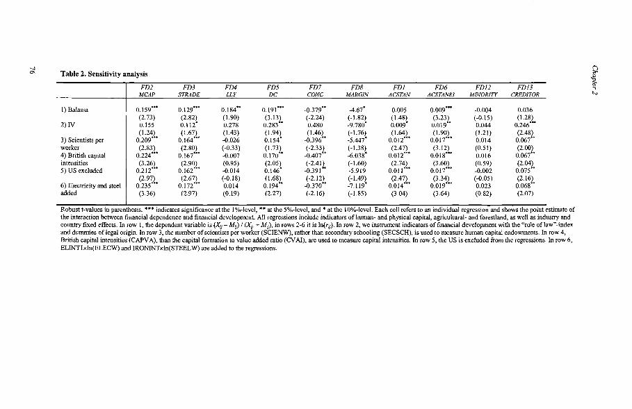
-.....J Q0'\ Table 2. Sensitivity analysis~
FD2 FD3 FD4 FD5 FD7 FD8 FDl FD6 FD12 FD13 ~""Il
MCAP STRAJJE LLY DC CONC MARGIN ACSTAN ACSTAN83 MINORITY CREDITOR ~
1) Balassa 0.159*** 0.129*** 0.184** 0.191 *** -0.379** -4.67* 0.005 0.009*** -0.004 0.036(2.73) (2.82) (1.90) (3.13) (-2.24) (-1.82) (1.48) (3.23) (-0.15) (1.28)
2) IV 0.155 0.112* 0.278 0.283** 0.480 -9.780* 0.009* 0.019** 0.044 0.246***(1.24) (1.67) (1.43) (1.94) (1.46) (-1.76) (1.64) (1.90) (1.21) (2.48)
3) Scientists per 0.209*** 0.164*** -0.026 0.154* -0.396** -5.447* 0.012*** 0.017*** 0.014 0.067**worker (2.83) (2.80) (-0.33) (1.73) (-2.33) (-1.38) (2.47) (3.12) (0.51) (2.00)4) British capital 0.224*** 0.167*** -0.007 0.170** -0.407** -6.038* 0.012*** 0.018*** 0.016 0.067**intensities (3.26) (2.90) (0.95) (2.05) (-2.41) (-1.60) (2.74) (3.60) (0.59) (2.04)5) US excluded 0.212*** 0.162*** -0.014 0.146* -0.391 ** -5.919 0.011 *** 0.017*** -0.002 0.075**
(2.97) (2.67) (-0.18) (1.68) (-2.12) (-1.49) (2.47) (3.34) (-0.05) (2.16)6) Electricity and steel 0.235*** 0.172*** 0.014 0.194*'" -0.370** -7.119* 0.014*** 0.019*** 0.023 0.068**added (3.36) (2.97) (0.19) (2.27) (-2.16) (-1.85) (3.04) (3.64) (0.82) (2.07)
Robust t-values in parenthesis. *** indicates significance at the 1%-level, ** at the 5%-level, and * at the 10%-level. Each cell refers to an individual regression and shows the point estimate ofthe interaction between financial dependence and financial development. All regressions include indicators ofhuman- and physical capital, agricultural- and forestland, as well as industry andcountry fixed effects. In row 1, the dependent variable is (Xij - Mij) / (Xij + Mij), in rows 2-6 it is In(rij)' In row 2, we instrument indicators of financial development with the "rule of law"-indexand dummies of legal origin. In row 3, the number of scientists per worker (SCIENW), rather than secondary schooling (SECSCH), is used to measure human capital endowments. In row 4,British capital intensities (CAPVA), than the capital formation to value added ratio (CVAI), are used to measure capital intensities. In row 5, the US is excluded from the regressions. In row 6,ELINTI xln(ELECW) and IRONINTxln(STEELW) are added to the regressions.

Table 3. Factor content of net trade (defined as in equation 5.1 Z/d). Basic regressions.
Zed Zfd
MCAP I 0.620**(2.59)
~STRADE I 1.278***(3.08)
~~
LLY I 0.578*** ~~
(3.47) §.:DC I 0.352 ~
(l.40) *'MARGIN I -4.091 ~
'"~(-0.57)S-CONC I -0.681 ** ~
(-2.22) ~ACSTAN
I-0.859 ~
xl000 (-0.17) ""':~
CREDITOR -0.014 ~(-0.29) ~
MINORITY I -0.002 ~~
(-0.04) 5'KAPWI I 0.005 -0.000 0.001 -0.000 -0.002 0.002 0.003 0.005 0.005 0.005 ~
~
(0.74) (-0.02) (0.27) (-0.07) (-0.39) (0.36) (0.75) (0.62) (0.72) (0.75) 5'SECSCH I 0.030 0.039 -0.023 0.034 0.013 0.028 0.015 0.029 0.035 0.031 ~
(0.73) (1.05) (-0.46) (0.91) (0.25) (0.60) (0.34) (0.62) (0.84) (0.562) ~~
FORLANDW I -12.032 -9.894 -2.735 -6.353 -5.719 -13.206 -0.346 -11.749 -12.313 -11.979 ~
xl000 (-1.19) (-1.18) (-0.36) (-0.96) (-0.52) (-1.13) (-0.05) (-1.20) (-1.15) (-1.17) gAGRILW -0.050 -0.046 -0.054 -0.039 -0.043 -0.040 -0.065 -0.050 -0.053 -0.049 .§
(-1.20) (-1.24) (-1.63) (-1.19) (-1.13) (-0.92) (-1.53) (-1.18) (-1.41) (-0.87) ~
Constant I 0.667*** 0.614*** 0.751*** 0.453* 0.695*** 0.908* 1.185*** 0.705*** 0.684*** 0.668*** ~~.
(4.58) (4.37) (6.72) (1.88) (4.86) (2.14) (5.53) (3.70) (4.80) (4.45) ~~
~
Adj R2 0.037 0.448 0.467 0.463 0.221 -0.005 0.381 -0.031 -0.024 -0.032 ~~
N.obs 20 20 20 20 20 20 20 20 20 20 ~
S*** Indicate significance at 1%-level, ** at 5%-level, * at 10%-level. t-statistics based on robust standard errors in parentheses. O'Q
-.l ~
-.l

Chapter 2
Human capital SECSCH 0.238HCQI 0.408***SCIENW 0.295*
*** Indicate significance at 1%-level, ** at 5%-level, * at 10%-level
78

CHAPTER 3
WHO WANTS POLITICAL INTEGRATION?
EVIDENCE FROM THE SWEDISH ED-MEMBERSHIP REFERENDUM*
Jonas Vlachost
AbstractThe political determinants of regional integration and separation have beenanalyzed in much theoretical, but little empirical work. From a local perspective,the Swedish 1994 EU-men1bership referendun1 can be described as the choicebetween two different unions - Sweden and the EU. In this particular case,membership implies less discretion to handle income shocks. Local industrydiversity is shown to have been an important determinant of the voting pattern.Further, high-income regions were more prone to vote in favor of membership. Areasonable interpretation is that safe and rich regions voted in favor of secessionfrom Sweden, rather than integration with Europe.
JEL Classification: F15, Hll, H70Keywords: Regional integration; Secession; Risk sharing; Redistribution; Spatialeconometrics.
* I thank Malin Adolfson, Tore Ellingsen, Lars Frisell, Patrik Gustavsson, Fredrik Heyman, andseminar participants at the Stockholm School of Economics for helpful comments and suggestions.Financial support from HSFR and Bankforskningsinstitutet is gratefully acknowledged.t Department of Economics, Stockholm School of Economics, P.G Box 6501, 113 83 Stockholm,Sweden. Phone: +46-8-7369649, Fax: +46-8-313207, Email: [email protected].

Chapter 3
1. Introduction
During the last decade, the political economy of regional integration and
disintegration has been under theoretical scrutiny (for surveys, see Alesina et al. 1995,
and Bolton et al. 1996). Although there is a huge empirical literature on various
aspects of regional integration (e.g Hess and van Wincoop, 2000), little enlpirical
work has directly analyzed political attitudes toward the integration process. In this
paper, the regional voting pattern in the Swedish 1994 ED-membership referendum is
used to gain insights on the regional characteristics detennining political preferences
regarding integration.
Although enhanced possibilities of inter-regional risk sharing constitute one of the
main themes in the literature discussing the possible gains from regional integration
(e.g. Persson and Tabellini 1996ab), the European Union has chosen a constitution
limiting the national discretionary powers to handle economic shocks in several
dimensions. 1 This constitution is the starting point of the simple framework guiding
the empirical analysis of the paper: by joining the ED, national governments renounce
the freedonl to deal with local income volatility.2 Add to this that migration between
regions is costly. A lower degree of local industry diversity hence implies higher costs
ofjoining the EU. Consistent with this hypothesis, it is found that individuals in risky
locations - in a standard portfolio sense - were significantly more negative towards
ED-membership than those in safe ones. It is also shown that inhabitants of high
income labor markets, with a high level of schooling and small receipts of central
government transfers were more positive towards ED-membership. Taken together,
these results suggest that inhabitants of safe and rich regions voted in favor of
1 Although an interesting issue in itself, no attempt is made to explain why the ED is less willing toallow for insurance-type transfers than national governments. One possibility is that the distribution ofindustry aid is more difficult to supervise at a more aggregate level, another that there is less solidaritybetween people living in different countries. Both effects suggest that moral hazard problems would bemore severe within the ED than in individual nations, making it rational to limit the degree ofdiscretion when creating a union. Persson and Tabellini (1996b) discuss federal risk sharing underdifferent constitutions when subject to local government moral hazard.2 Since 1994, national support to manufacturing industries in the Euro-12 area has continuouslydeclined from around 40 to around 28 billion Euro (ED 2000). This suggests that the attempts by theED to limit govenunent intervention at the industry level are (at least to some extent) successful. Thefunds handed out at the ED-level are mainly directed to agriculture and regions suffering frompermanent economic backwardness. Further, ED rules on monetary policy, fiscal policy, competition,and public procurement all restrict the degree of national discretion.
80
Who Wants Political Integration?
secession from the Swedish transfer system, rather than In favor of European
integration.
There is relatively little empirical work with which to contrast the results, and what
there is, is based on cross-country data. Panizza (1999) shows that country size, per
capita income, ethnic fractionalization, and denlocracy are all negatively related to the
degree of fiscal federalism (defined as the percentage of revenues or expenditure of
the central government out of total revenues or expenditure).3 Alesina et al. (2000)
focus on the relation between political and economic integration. They find that
openness to trade mediates the economic benefits of country size, and that open trade
reginles tend to generate secessions. This paper has two main advantages compared to
previous studies. First, it looks directly at voter preferences on the decision to
integrate (or secede) and second, by exploiting regional data, it circumvents some of
the well-known problems with cross-country studies. More observations are available,
problems of data comparability are much less severe and, perhaps most important, the
variation between unobservables (or hard-to-observables), such as institutional
quality, is usually lower within a country than between countries.
Whereas most of the theoretical literature tends to identify, implicitly or explicitly, a
"region" with a "nation", the present paper suggests that a local labor market
perspective can be fruitful. This is due to the fact that the local labor market is usually
a place of residence from which exit is costly, both for social and economic reasons.
Since tax revenue and hence, public services, are partly determined locally, it is
obvious that every inhabitant is affected by whatever happens to his/her local market.
Likewise, housing values are largely driven by local demand characteristics. From the
viewpoint of the individual, what is usually portrayed as the choice between
unification and separation of regions - as well as fiscal centralization or
decentralization - could therefore well be described as the choice between different
types ofunification and centralization.
3 These indicators are subject to several problems, especially when exploiting cross-national data. (i)Different levels of local governments should be weighted in different ways. (ii) Local governmentsmay collect taxes without having autonomy in deciding the tax amount, or how to allocate theexpenditures. (iii) Intergovernmental grants are not captured in the data.
81

Chapter 3
This paper is organized as follows: In section 2, the theoretical argunlent guiding this
study is presented. In section 3, the data is described, with special focus on the
construction of an index of labor market risk, and some results are shown. Section 4
describes the problenl that mightd be encountered when using spatial data and the
estinlates when taking these problems into consideration are presented. Section 5
concludes.
2. The theoretical argument
Although economic integration could foster market-based risk sharing between
regions (see e.g. Asdrubali et al. 1996, and Melitz and Zumer 1999), this paper
highlights the political aspects of risk reduction. Entering the European Union
involves renouncing national discretion along several dimensions. The Maastricht
treaty entails the complete loss of monetary autonomy and caps on government
borrowing during temporary shocks. Further, joining the ED would also mean joining
a customs union, leaving Sweden with no discretionary trade policy towards third
countries. Finally, the inner market builds on strict rules regarding industrial
subsidies, competition policy and public procurement, leaving national governments
with little discretion in times of industrial crises.4 That the attempts to limit the
interventions by national governments in the economy have been successful can be
verified by the 30 percent decline in national state aid to industries since 1994 in the
Euro-12 area (ED 2000). Since Sweden joined the EU, Swedish employment aid has
declined by almost 50 percent and regional aid by more than 20 percent (NUTEK
2000).5
Based on these stylized facts, the binary choice between two different types of unions
is studied. Specifically, one alternative is to vote in favor of membership in the
4 An example related to Sweden is the policy to differentiate electricity tax rates depending on industryelectricity consumption. The policy, which has been used to shield electricity dependent industry fromprice shocks, is now under heavy attack from the European Commission since it is claimed to distortcompetition. The ED-rules regulating state aid are summarized in ED (1999).5 As a share of total value added in industry, state aid has been reduced by about 27 percent from 1995to 1999 according to the NUTEK (2000) study. Calculating the full extent of different subsidies is acomplicated task and the results largely depend on which definitions have been used. In Sweden, oneestimate of the value of industrial support in 1994 was around 50 billion Swedish kronor (about 5billion Euro). The same year, corporate income taxation aggregated to 20 billion kronor (2 billion
82

Who Wants Political Integration?
European Union - with the loss of national powers this implies. The other alternative
is to vote for continued autonomy.6 Within the ED, the national government is
assumed to have no discretionary power to compensate for industry-specific shocks,
whereas there are no restrictions on these policies when being a non-member. An
obvious objection to this extreme setup is that the European Union itself transfers
resources between regions and industries. Although this is true, these transfers are
mainly directed to industries and regions with permanent, rather than temporary,
problems. Moreover, except in the case of agriculture, the transferable funds available
at the ED-level are minute compared to the national budgets. Thus, it is fair to say that
the ED prevents national governments from using many types of insurance
mechanisms, while at the same time offering little replacement.7
Mathematically, the argument can be described in the following way. In a local
market, c, labor is employed in sectors s=1,2, ...n. Every period, each sector is hit by a
normally distributed productivity shock, Ss '" (0, as2). The share of labor in each city
sector is ssc=Lse/Le, where Lse is the number of employed in sector s in labor market c,
and Le is total employment in this market. Leaving a local labor market is assumed to
be prohibitively expensive,8 and there are no opportunities for private insurance across
individuals or regions. Each individual gets an equal share of the total revenue to all
industries in a local market. If Sweden joins the ED, the revenue of each industry
changes by ms and the national government is not allowed to insure against industry
shocks. This means that total revenue in c in case ofnlenlbership is:
Euro) (Barkman and FoIster 1995). To the best ofmy knowledge, no estimates employing the samemethodology have been produced at a later date.6 Naturally, it can be questioned how real the Swedish autonomy would be outside the ED. The EESagreement regulating trade between the ED and Sweden did imply that many of the ED regulationswould automatically apply to Sweden, being members or not. That autonomy would be greater outsideof the ED is quite obvious, however.7 This point is also made by Sorensen and Yosha (1998) who show that only a small fraction of shocksto ED-countries are smoothed by international transfers. Likewise, private markets (still) offer limitedinsurance. Given the importance of the national government in consumption and income smoothing,they argue that the strict fiscal discipline imposed by the Maastricht treaty should be relaxed.8 This assumption is less restrictive than what appears at a first glance. One could easily imagine thathouseholds own an immobile asset (say a house) that has a value proportional to the aggregate incomeof a region. The basic argument would hold even for this case.
83

Chapter 3
The expected value ofjoining the ED is then given by
and the total variance of returns is
where Cist is the variance/covariance of shocks. The inhabitants of a local market do
not only care about this monetary revenue, but also have preferences over the election
outcome for other reasons. If Sweden joins the ED, an individual i in labor market c
receives utility u j (R:) +YP where Yi captures individual preferences over the
membership. Agents are risk averse and hence, the utility function satisfies: u'(Rc) >
0, and u"(Rc) < o. Since the shocks are assumed to be nornlally distributed, a two
term Taylor's series of the expected utility can be approximated by
(2.4) ui(R:) +1/2u/'(R:)Var(R:) + Yi.
It is obvious that the expected utility decreases with the volatility of income. If
Sweden does not join the ED, the national government has full discretion to deal with
the industry-specific shocks. Assuming that the government is maximizing total
utility, this means that the marginal utility between cities will be equalized in every
period. In this extreme setup, full insurance against idiosyncratic shocks, as well as
full redistribution, is, in other words, provided. Total revenue will be equalized across
locations:
where ts is the tax (subsidy) paid (received) by the respective industry. The volatility
of income is equalized across cities to aggregate national volatility:
84

Who Wants Political Integration?
Given that an individual receives utility ni if Sweden stays out, the utility of each
individual can be approximated by:
(2.7) ui(R) +1/2u/'(R)Var(R)+ni.
A voter will cast his or her vote in favor ofmembership whenever (2.4) is greater than
(2.7):
(2.8) Ui( R:) - u;{ R )+ 1/2 {u/'( R:)Var( R:) - u/'( R )Var( R )} ~ ni - Yi.
It should be clear that those who stand the most to gain from joining the ED are the
inhabitants of relatively rich and stable regions, since they are no longer forced to
participate in the transfer schemes towards poor and unstable regions. Hence, a "yes"
vote could best be described as a vote in favor of secession from Sweden, rather than
a vote in favor ofnlembership itself.
At a first glance, this result appears to contrast with the results in Persson and
Tabellini (1996a), and Bolton and Roland (1997). In these models, the risky and poor
regions have greater incentives to join the larger union in order to exploit the greater
opportunities of risk sharing and redistribution within the larger economic entity. The
difference is superficial, however. Joining the ED is here claimed to imply leaving a
system of regional transfers, whereas unification in the above papers implies the
creation of a regional transfer scheme. Had the ED and Sweden shared the same
policies regarding redistribution and risk sharing, the results in this paper would have
been reversed.
3. Empirics
Most of the data in this paper has been collected from Statistics Sweden, although the
unemployment statistics are from AMS, the central body of the Swedish labor market
authorities. Except when otherwise indicated, data refers to the election year, i.e.
85

Chapter 3
1994. The units of analysis are the 109 local labor markets (LLM) that exist in
Sweden. An LLM is an analytical (and not administrative) unit created by Statistics
Sweden based upon the observed commuting pattern.9 Since most variables are not
available at the LLM-Ievel, data has been aggregated using infoffilation from
Sweden's 288 municipalities. Although the LLM:s are constructed in accordance with
commuting patterns, it is possible that the conditions on one LLM affect choices made
in a neighboring LLM. In other words, there is a possibility that LLM:s cannot be
treated as independent observation units. In Section 4, I will describe - and attempt to
correct for - the problems these spatial aspects induce to the econometric analysis.
3.1. Measuring Labor Market Risk
To construct the indicator of local labor market risk, the portfolio-theoretic approach
used by Conroy (1975) and Diamond and Simon (1990) is followed. They derive what
can best be described as an augmented Herfindahl index. This concept is borrowed
from the literature on financial economics: each local market is viewed as a portfolio
of industries, each industry is subject to random fluctuations. The total degree of labor
market risk ofa labor market is the weighted average of the variances and covariances
of these fluctuations. The total variance in city c equals
n n n
(3.1) RISKe =LS;cO";s + LLsscsucO"su ,S:# U,c =1,...,109s s u
where Sse is the employment share of sector s in labor market c, OSs is the variance of
employment in sector s, and O"su the covariance of employment in industries sand u. 10
Specifically, the variance/covariance matrix is constructed as follows: The variance
elenlent, OSs, is the variance in the rate of national employment growth in sector s,
while the covariance elements, OSu, equal the covariance between growth rates. To
capture the degree of unexpected volatility, the employment growth rate of each
industry was de-trended by taking the first differences of employment on the national
level. The logarithms of the first differences were then regressed on a time trend. For
9 See Statistics Sweden (1998) for a closer description of the LLM subdivisions.10 In the nl0del, volatility is due to revenue fluctuations, rather than employment fluctuations. Revenue,however, is likely to fluctuate much less than employment, due to the public unemployment insurance.
86

Who Wants Political Integration?
each regression, the residuals were used to construct the variance/covariance matrix. 11
In order to calculate the variance/covariance matrix, sectoral employnlent data at the
national level for 43 industries between 1985-1997 was used. I2 This amounts to the
assumption that industries are subject to the same fluctuations, regardless of their
geographical location. Obviously, this assumption is not a perfect description of
reality, but it is necessary in order to capture both the within and between industry
fluctuations in a systematic manner. 13
In Table 1, the ten least and most risky markets are listed. It is obvious that markets in
the north of Sweden had a large representation of unstable industries, which is in line
with popular beliefs on this issue. It is not surprising that Stockholm, the largest labor
market by far, finds its place among the least risky ones. Some of the labor markets
are less obvious members of the low risk group. It should be kept in nlind, however,
that the measure of risk is derived using fluctuations around a trend. Local markets
with a large share of steadily shrinking (or expanding) industries will be regarded as
"safe" in this study. This does not imply that the labor market situation is good in any
other sense of the word. Hallefors (the eighth safest market), for example, had an
unenlployment rate of 18 percent at the time of the referendum. 14
At this point, it is appropriate to ask why local unemployment fluctuations are not
used rather than the derived measure of industry risk. There are two main reasons for
this. First, the theoretical argument is that industries, rather than geographical areas,
are hit by shocks. It is possible that safe local markets (in the portfolio sense) actually
experienced large employment fluctuations in the relevant time period. This does not
mean, however, that rational agents should update their beliefs about the future
riskiness of their local market. An analogy is that ex ante safe financial portfolios may
very well exhibit larger fluctuations, ex post, than risky ones. Second, even though
moving is prohibitively expensive in the model, it is not so in the real world. If people
11 It can be noted that under the very strong assumptions of independently and identically distributedgrowth rates, the portfolio diversification index is equivalent to the well known Herfmdahl index.12 This period is the longest possible for which industry data is consistent at the municipal level. Thesectoral division is based on Statistics Sweden's "limited level". Industries are described in theappendix.13 Clark (1998) shows that industry shocks constitute an important part of the total variation in regionaloutput.14 This said, note that the correlation between RISK and unemployment is 0.38.
87

Chapter 3
do move in response to local employment shocks, the unemployn1ent statistics will
misrepresent true labor market risk.
3.2. Empirical Specification
The dependent variable is the percentage of votes in favor of EU-membership, labeled
YES. In addition to the RISK-variable, INCOME is added to the regression. Given the
argument in Section 2, we would expect richer regions to be more prone to enter the
ED (or rather, leave the Swedish transfer system).15 Several control variables are also
used. Average years of schooling, SCHOOL, are added to the regressions since the
benefits of the ED-membership might possibly benefit the well educated more than
the less educated. Investment in general human capital makes individuals less
sensitive to industry-specific shocks, making the loss of national discretion less
important for this group. In n10st studies discussing the referendun1, a clear north
south voting patten1 is described, but not explained (see e.g. Gilljam 1996). In this
paper, the north-south dimension is accounted for by creating a "trend" variable
nun1bering the local markets, depending on the distance to Copenhagen, i.e. the
nearest major ED-city. This ordering is then squared to take into account that labor
markets increase in geographical size (and hence the distance to ED is increased)
when moving north in Sweden. 16 Alesina and Spolaore (1997) give one possible
interpretation of the trend variable. In their model, agents living far from the center
stand the most to lose from political integration. Although this interpretation might be
too literal, the expected sign of the variable TREND is negative. 17
Since the nationwide Swedish political parties played a major role in the campaign
prior to the referendum, it is likely that voters were influenced by the opinion of
"their" party. In order to account for this effect, I use the percentage share of votes in
the 1991 n1unicipal election for the Social Democratic party, SAP, and the
15 INCOME is defined as average income per working family. Alternative measures would bedisposable income per fanlily or per capita income, but the choice of income measure does not affectthe results to any significant degree.16 Using the squared ordering markedly improves the fit of the regressions compared to using a simplesouth-north ordering of labor markets.17 One possibility is that one of the major advantages of the EU membership is the increased possibilityof cross-border trade (especially in highly taxed goods such as alcohol). Naturally, the benefits fromcross-border trade decreases (more than proportionately) with the distance from the border.
88

Who Wants Political Integration?
Conservative party, MODERAT, respectively. IS The reason for using voting data from
the 1991 rather than the 1994 election is that the 1991 election did not concern the
EU-question. This way, the underlying political preferences are captured, and we rule
out the possibility that the voters' attitudes towards the EU affected the voting pattern
in the county election rather than the other way around. Since both the Social
Democratic and the Conservative parties were strongly in favor of membership in the
European Union, the expected signs on both SAP and MODERAT are positive.
The voter turnout ratio, TURNOUT, defined as the share of voters casting their votes
in the referendum, is also included in the regressions. Although it is difficult to have a
clear theoretical prior on the sign of this variable, it is possible that the willingness to
vote varied systematically with the attitudes towards EU-men1bership. In US
elections, a high turnout implies that a larger share of poor people with low education
vote. In the present context, this type of effect would lead to a negative sign. 19
However, if the hypothesis of this paper is correct, then it is likely that the willingness
to vote also varies systematically with LLM-risk. In other words, sonle of the effect
that should be attributed to local market risk will be captured by TURNOUT. To
account for this problem, TURNOUT will be instrumented for by using the turnout
ratio of the 1991 and 1994 parliamentary elections. 20
The referendum has commonly been described as large vs. small cities. For this
reason, population size is included in the regressions. The sector most strongly
affected by EU membership is probably agriculture. Due to the huge agricultural
subsidies handed out by ~he ED, we would expect the share of agricultural employees,
AGRI, to be positively related to the share of yes votes.
What is not yet controlled for is the expected sectoral impact of the ED nlembership
(other than agriculture for which there is a clear prior). In other words, how do we
control for the permanent change in sectoral revenue due to the menlbership (i.e. me of
equation 2.2)? One possibility would be to consider actual changes in aggregate
18 An attempt is also made to use voting shares of other parties, but these results are not significant.19 The correlation between TURNOUT and INCOME is 0.50, and between TURNOUT and SCHOOL0.35.20 The correlation between the turnout ratio of the referendum and the 1991 and 1994 elections turnoutratios is 0.65 and 0.61, respectively.
89

Chapter 3
sectoral employment since 1994 which would mean that all changes in employment
that have occurred since 1994 are explained by the EU membership. Although this is
obviously incorrect, this variable could give us some indication of the magnitude of
me. Formally, we control for
(3.2)
(3.3) dLs == [(Ls,1995 + Ls,1996 + Ls,1997) / 3 - Ls,1994 )].
L s ,1994
Ls,t is the national employment in sector s at time t. This variable is labeled
AVGCH9497. All in all, we have the following baseline equation to estimate21
(3.4) YESc= CONSTc + P1RISKc + ,82RISK~ + ,83INCOMEc
+ ,84SCHOOLc + ,8sTRENDc + P6MODERATc + P7SAPc
+ ,88TURNOUTc + P9POPc + PloAG~ + ,811AVGCH9497 + Ec·
3.3. Results
Several interesting results are revealed just by inspecting the correlation matrix in the
appendix. First of all, the correlation between YES and RISK is -0.46. A scatter plot
of the variables is shown in Figure 1. This strong correlation is an indication that
increased labor market risk did indeed contribute to making people less prone to vote
in favor of membership in the EU. Second, the correlation between RISK and
MODERAT is -0.39, while the correlation between RISK and SAP is 0.29 which
suggests that political sympathies vary systenlatically with local market risk: the
larger the risk, the nlore government intervention is asked for. Finally, the idea that
recipients of large central government grants worried about the future of these
transfers is given some support by the strong negative (-0.82) correlation with the
share of yes-votes.
90

Who Wants Political Integration?
[Figure 1 about here]
In Table 2, column 1, the baseline estimate of equation (3.4) is presented. The fit is
very good, with an adjusted R2 of 0.86. As can be seen, all significant variables have
the expected sign. TREND and TURNOUT are negative, suggesting that the further to
the north, and the larger the share of people who used their right to vote, the more
negative people in the respective labor market were towards the EU. A higher average
income, more average schooling, a larger share of workers in the agricultural sector,
and a larger share of Social Democratic or conservative supporters all seem to result
in a more positive attitude towards the ED. Neither population size, nor the measure
of expected change of employment, is significant (AVGCH9497 even has the
incorrect sign). The main variables of interest, RISK and RISK2, also have the
expected (and statistically significant) signs, thereby giving support to the hypothesis
that living and working in a riskier labor market did indeed make people less prone to
vote in favor of ED-membership. All regressions are estimated using White's
heteroskedasticty consistent standard errors. A Jarque-Bera test of nornlality of this
first specification (which has a X2 distribution with two degrees of freedom under the
null hypothesis ofnonnally distributed errors) has a value of 1.60, which amounts to a
probability value of0.45. Thus, the null hypothesis cannot be rejected.
In column 2, the turnout ratios from the 1991 and 1994 parliamentary elections are
used as instruments for TURNOUT in a standard 2SLS-regression. This is done to
account for the possibility that TURNOUT itself is affected by labor market risk.
Despite the high correlations between the instruments and TURNOUT (0.65 and
0.60), and the fairly good fit of the first stage regression (0.57), the point estimate of
TURNOUT drops sharply and loses its statistical significance. The point estimate of
RISK is, on the other hand, almost doubled. The size of the point estimates and the
statistical significance of the political variables MODERAT and SAP also increase. In
columns 3 and 4, the insignificant variables are dropped from the specification but the
results remain stable.
21 The term RISK2 is entered since the fit of the regressions is found to be better using thisspecification. Actually, there are no reasons to expect the relationship to be linear.
91

Chapter 3
Although the normality test indicates that outliers do not drive the results, I
experiment by excluding labor markets with more than 50 percent yes-votes. As can
be seen in column 5 (only 2SLS estimates are reported for the sake of brevity), this
exclusion - if anything - strengthens the results for RISK. AGRI, MODERAT, and
SAP lose some of their significance in this specification. Since OLS-estimates can be
sensitive to outliers, column 6 reports the results from a median regression (that
estimates the median of the dependent variable). The estimates are similar to the
previous ones. Upon close inspection of the explanatory variables, it can be found that
four labor n1arkets display such a large labor market risk so large that they can be
considered as outliers in the box-plot sense of the word. In an unreported set of
regressions, these labor markets are excluded from the san1ple. This exclusion results
in an increase in the point estimates of RISK (-0.37 and -0.64 in the OLS- and 2SLS
specifications, respectively), but otherwise the results are stable.
One possible problem with the model specification is that the dependent variable is
bounded between zero and one. The problem is likely to be of minor importance,
however, since the minimum value of YES is 17.7 and the maximum is 65.3. The
standard procedure of dealing with bounded dependent variables converts it to the
fOffi1 Log(YES/100-YES). This conversion does not affect the results to any
substantial degree, either statistically or economically (the point estimates for RISK
and RISK2 are both significant at the 5-percent level). In the last colunm of Table 2,
Log(YES/100-YES) is used as the dependent variable while all regressors are entered
in logarithms. Now, the instrumented point estimate for TURNOUT is even positive
(although not significant). Moreover, the SAP coefficient is not significant.
Establishing statistical significance is a first step; the next question is whether the
effect is economically significantt. The point estimate of RISK is around -0.27 and
that of RISK2 0.0034 when using OLS, and around -0.42 and 0.0053 respectively
when using 2SLS. Since the standard deviation of RISK is 13.3, an increase in RISK
by one standard deviation implies a decrease in YES by 3 percentage points when
considering the OLS-estimates and 4.6 percentage points when looking at the 2SLS
estimates. Here, it is also interesting to consider the first-stage regression (not shown).
In this, the coefficient on RISK is 0.11 and on RISK2 -0.0014 (both are significant at
the 5%-level). An increase in RISK by one standard deviation would then imply an
92
Who Wants Political Integration?
increase in TURNOUT by 1.19. Since the coefficient on TURNOUT is -1.31 in the
OLS-specification, an increase in TURNOUT by 1.19 implies a decrease in YES by
1.56 percentage points. Thus, the total effect of a one standard deviation increase in
RISK is around -4.6 percentage points, in the 2SLS-specification as well as in the
OLS-specification.22 Given that the mean of YES across local labor markets is 41.8,
the effect is indeed substantial.
These calculations raise a potentially serious concern. In the sanlpIe, RISK ranges
from around 14 to 72. The coefficients on RISK and RISK2 indicate that the point at
which the quadratic function turns from negative to positive is 39.8 (OLS
specification). This would mean that among the LLM:s with above average risk,
increased risk is associated with a more positive attitude towards membership.
Although not implausible, this result is highly dependent on the precision with which
the coefficient of RISK2 is estinlated. By moving towards the lower bound of the 95
percent confidence interval of the point estimate, the turning point moves to 3608.
Moving to the upper bound results in a turning point at 20. Thus, even minor errors in
the estimate easily push the turning point far outside the relevant interval. Since the
logarithmic specification produces highly significant negative point estimates, it is
reasonable to expect the turning point to actually be above 72.
For the other statistically significant variables, increasing the independent variables by
one standard deviation gives the following impact on the share of yes-votes (columns
3 and 4, respectively). SCHOOL: 4 and 3.4 percentage points. INCOME: 3.6 and 2.9
percentage points. AGRI: 1.8 and 2.0 percentage points. MODERAT: 0.8 and 1.3
percentage points. SAP: 1.5 and 1.9 percentage points. TREND: 7.2 percentage
points. Altogether, the results presented in this section point in the direction suggested
by theory. The results concerning the political variables do not appear to be very
robust, however.
In Table 3, some further robustness tests are performed in order to exclude the
possibility that the results are driven by an omitted variable (only 2SLS-estinlates are
shown). In column 1, the average age of the population in each labor nlarket is
22 The first-stage regression is obviously not specified to capture all variation in TURNOUT. However,
93

Chapter 3
entered. Column 2 contains per capita welfare spending and column 3 the
unemployment rate. Column 4 shows the results when population density and column
5 when the share of public employment is entered, respectively. These inclusions add
very little to our understanding of the voting pattern.23 In colunm 6, however, per
capita grants from the central government to municipalities are added to the
regression. The coefficient of this variable is negative and highly significant, which is
in line with the hypothesis that those receiving large redistributive grants are less
willing to join the ED. The point estimates of RISK, RISK2, and INCOME are
somewhat reduced, but still statistically significant in this specification.24
4. The Spatial Dimension
As mentioned above, some special econometric problems might arise when using
geographical data of the type used in this study. Basically, the problems are due to the
fact that the units of analysis, LLM:s, are not completely closed off from each other.
Not only do people commute across imaginary borders; income, schooling, etc. are
more similar between nearby regions than between distant ones. If this is the case, the
attitudes towards ED-membership can "spill over" between labor markets. Using a
different terminology, we have a problem of spatial autocorrelation. Formally, this
type of spillovers would result in a systematic correlation between the dependent
variable across regions, i.e. the so-called space lag case
where Q is a weight matrix of dimension cxc, where c is the number of geographical
units used in the study. r is the coefficient of Q in the regression. The elements in the
weight matrix take the value of one if two regions are neighbors and zero otherwise. If
since the fit of the regression is fairly good (adj.R2=0.51), these calculations are quite informative.23 Ringdal and Valen (1998) fmd that population density in the area of residence is an importantdeterminant of the individual voting pattern. In the present data set, the correlation between populationdensity and RISK is -0.32. In a specification including both variables, RISK is significant whilepopulation density is not. Thus, the fact that diversified labor markets also tend to be densely populatedmight be what drives Ringdal and Valen's results.24 When all six new control variables are entered simultaneously, the point estimates and significancelevels ofRISK, RISK2
, and INCOME are roughly the same as in column six.
94

Who Wants Political Integration?
4.1 describes the true model, then corr[yi ,Yj] "# 0 which would yield biased estimates
using OLS.
Another possibility is that the true model is described by equation 4.2 - the so-called
space error case. In this case, the error temlS are systematically correlated across
regions, but it is not the voting pattern per se that is behind the correlation. Formally,
this takes the form:
In this case, corr[&i , lj] "* 0 but 17 is iid. and the OLS-estinlates will be inconsistent.
Just as the model 4.1, a weight matrix is necessary to properly estimate 4.2. Since the
autoregressive coefficient Ais not known, a full maximum likelihood estimation nlust
be carried out.
The first issue at hand when taking the spatial structure into consideration is the
construction of the weight matrix Q. Given the nature of the problem, different
specifications can be called for. In this paper, the simplest possible weight matrix,
consisting solely of zeroes and ones, will be used. Q will then be a 109x 109 matrix,
where the elements take the value one if two LLM:s are neighbors, and zero if they
are not. Given the size of each LLM, it is not likely that any significant amount of
movement takes place between LLM:s that are not neighbors. Each row in the matrix
is nonnalized so that it sunlS to one, which means that the assumed impact of each
labor market on its neighbors is decreasing in the number of neighbors of this labor
market.
The baseline specification, without the insignificant variables, is reproduced in Table
4, column 1 for ease of comparison. The only difference fronl Table 2 is that the
Akaike information criterion (AIC) rather than the adjusted R2 is used. Since the
spatial regressions are estimated using nlaximunl likelihood, a more general measure
of fit than the adjusted R2 must be used. The regression is re-estimated using Q to
check for the different types of spatial autocorrelation. First, when testing for a spatial
lag structure, the Lagrange Multiplier test suggested by Anselin (1988) is used. The
95
Chapter 3
test yields a X2-distributed test statistic equal to 14.407 (one degree of freedom) with a
probability value of 0.00, which means that the null hypothesis of no spatial lags can
be finnly rejected. Second, the LM-test for a spatial error structure suggested by
Burridge (1980) is performed. The test statistic is X2 -distributed with one degree of
freedom. This test statistic has the value 13.33, with a probability value of 0.00.
Hence, the null hypothesis of no spatial errors is also rejected. Based on this
information alone, we cannot conclude whether the spatial lag or the spatial error
model is the correct one to use. That spatial correlation should be taken into account is
obvious, however.
Now, this regression is re-estimated assuming a spatial lag structure (i.e. equation
4.1). In other words, QYES is entered on the right-hand side of the equation and r
(GAMMA in Table 4) is estimated. r is highly significant and the drop in the Ale,
from 637 to 625, suggests that the spatially lagged variable captures a considerable
part of the previously unexplained variation in YES. The point estinlate of 0.24
implies that an increase in the number of yes-votes in a neighboring labor market by
one percentage point increases the number of yes-votes by 0.24 percentage points.
When inspecting the coefficients and significance levels of the other explanatory
variables, some interesting changes can be found. First of all, the significance levels
of RISK and RISK2 are somewhat reduced. The point estimates are stable, however.
Second, the point estimate and the significance level of MODERAT are both
dramatically reduced. Thus, the effect of this variable seems to have been an artifact
of the spatial structure of the data. Finally, the LM-test for spatial errors indicates that
some spatial structure in the error terms is still present. In column 3, the results from a
spatially lagged N -estimation are shown. Two main differences can be found: first
the instrumented variable TURNOUT is now (weakly) significant with a point
estimate of-0.62 and second, the test for spatial errors is now barely significant.
Next, the spatial error structure is taken into consideration by re-estimating the
regression specified according to equation 4.2. The variable LAMBDA is the A of
equation 4.2. As can be seen, this variable is highly significant, so obviously the
weight matrix captures some of the variation previously unaccounted for, or attributed
to other variables. The Ale now takes a value of 618, i.e. even lower than in the
96

Who Wants Political Integration?
spatial lag case. When conducting the LM-test for a spatial lag structure on this
specification, the test is not significant.25 Thus, the spatial error specification seems to
be the one best describing the data. Some further tests are performed on this model: a
spatial Breusch-Pagan test indicates that heteroskedasticity is not a problem,26 and a
likelihood ratio test shows that it was indeed appropriate to correct for spatial errors.27
Compared to the regression in column 1, some interesting differences can be found.
First of all, RISK and RISK2 are stable to the inclusion, although some of their
significance is lost Gust as in the space lag case). INCOME and SCHOOL are also
robust towards the change in the specification. The party variables MODERAT and
SAP, however, lose all their significance and the point estimates are sharply reduced.
The point estimates of the rest of the variables are somewhat changed, but the basic
relation between them and YES is robust. All in all, the results in this section show
that the space error model is the one best describing the data. The coefficient on
LAMBDA of around 0.6 tells us that when the expected number of YES votes is
exceeded by one percentage point in one LLM, then YES will also increase by 0.6
percentage points in the neighboring LLM.
5. Conclusions and discussion
The ain1 of this paper has been to give some empirical input to the largely theoretical
debate on the political economy of regional integration and secession. Using the
regional voting pattern from the Swedish 1994 EU-men1bership referendum, it is
found that regions with a well diversified industrial structure, high average income
and educational levels, close to the ED-center (i.e. in the south of Sweden), and a
large agricultural sector were more positive to ED-membership than other regions.
Further, the inhabitants of municipalities receiving large central government grants
were less willing to join the EU.
Superficially, these results appear to contradict both Persson and Tabellini (1996a)
and Bolton and Roland (1997). The former show that regions subject to large
25 Ho: No spatial lag dependence. 1 degree of freedom; value 0.96; probability 0.33.26 Spatial B-P: Ho: No heteroskedastiticy. 9 degrees of freedom; value 7.86; probability 0.55.27 LR-test: 1 degree of freedom; value 44.76; probability 0.00.
97

Chapter 3
idiosyncratic shocks have stronger incentives to join a union than stable regions. The
latter present a model where poor regions are more prone to integrate since they stand
more to gain from inter-regional transfer schemes. Based on the strict regulations
regarding discretionary policies within the European Union, however, a more
reasonable interpretation is available. From the individuals' viewpoint, joining the ED
could well be described as leaving a system of transfers at the national level, whereas
unification in the above-mentioned models implies the creation of an inter-regional
transfer scheme. The inhabitants of stable and rich regions receiving little central
government assistance could, in other words, be said to have voted for secession from
Sweden rather than for integration with the EU. This interpretation highlights the
importance of defining what "regions" and "unions" actually are, especially in models
based on individual political choice. Further, it demonstrates that it is the actual
institutional arrangements that are of importance for political choice - which is
exactly the point made by Persson and Tabellini, as well as Bolton and Roland. The
suggested interpretation offers an interesting potential explanation ofwhy the political
leadership was so much more positive towards EU-membership than the population as
a whole. 28 From a national - rather than regional - perspective, greater risk sharing
between nations could very well be encouraged by membership, even though this
comes at the expense of less risk sharing between regions. Once again, what is safe
and what is risky all depends on the perspective
Fernandez and Rodrik (1991) offer an alternative explanation to (some of) the
empirical results in this paper. They show that uncertainty of gains and losses from an
economic reform creates a bias towards the status quo. Joining the EU can be seen as
undertaking an encompassing economic and political reform. To the extent that the
uncertainty about gainers and losers depends on the insurance characteristics of the
local industry structure, we would expect safe regions to be more prone to vote in
favor ofmembership.
The basic relation between local industry diversity and voting behavior is interesting
for several reasons. That the local market can act as an insurance mechanism adds a
new dimension both to future empirical investigations in the field of political
28 More than 80 percent of the members ofparliament, compared to 52 percent of the electorate, were
98

Who Wants Political Integration?
economy, as well as to policy analysis. Second, political preferences can be expected
to be conditional upon labor market diversity. The basic pattern of correlations
indicates that people living on diversified markets vote nlore "right-wing" than people
on less diversified ones. This suggests some degree of substitutability between
insurance on the market and social safety nets.29 Another open question is the
generality of the results. Obviously, the cost of moving can differ both between and
within countries. The effect of local conditions on voting behavior can be expected to
decrease if relocation costs are reduced. Another possible extension of this work
would he to decompose the sources of local lahor-market risk into their national,
regional, and industry-specific components. Since the optimal local policy response
depends on the sources of risk, the different components can then be related to the
referendum results.
in favor of the membership.29 In Vlachos (2001) it is shown that LLM-risk has a positive impact on municipal public employmentin Sweden.
99

Chapter 3
References
Alesina, A., R. Perotti, E. Spolaore (1995) "Together or Separately. Issues on theCosts and Benefits of Political and Fiscal Unions", European Economic Review, 39,751-758.
Alesina, A. and E. Spolaore (1997) "On the Number and Size of Nations", QuarterlyJournal ofEconomics, 112:4, 1027-1056.
Alesina, A. E. Spolaore, R. Wacziarg (2000) "Economic Integration and PoliticalDisintegration", American Economic Review, 90:3, 1276-1296.
Anselin, L. (1988) "Lagrange Multiplier Test Diagnostics for Spatial Dependence andSpatial Heterogeneity", Geographical Analysis, 20, 1-17.
Asdrubali, P., B. Sorensen, O. Yosha (1996) "Channels of Interstate Risk Sharing:United States 1963-1990", Quarterly Journal ofEconomics, 111, 1081-1110.
Barkman, C. and S. FoIster (1995), "Foretagsstodet - vad kostar det egentligen?",Report from ESO DsFi 1995:14.
Bolton, P. and G. Roland (1997) "The Breakup of Nations: A Political EconomyAnalysis", Quarterly Journal ofEconomics, 112:4, 1057-1090.
Bolton, P., G. Roland, and E. Spolaore (1996) "Economic Theories of the Break-Upand Integration ofNations", European Economic Review, 40, 697-705.
Burridge, P. (1980) "On the Cliff-Ord Test for Spatial Autocorrelation", Journal ofthe Royal Statistical Society, B 42, 107-108.
Clark, T. (1998) "Employment Fluctuations in the U.S. Regions and Industries: TheRoles of National, Region-Specific, and Industry-Specific Shocks", Journal ofLaborEconomics, 16, 202-229.
Comoy, M. (1975) "The Concept and Measuren1ent of Regional IndustrialDiversification", Southern Economic Journal, 41, 492-505.
Diamond and Simon (1990) "Industrial Specialization and the Returns to Labor",Journal ofLabor Economics, 8:2,175-201.
EU (1999) "Vademecum - Community Rules on State Aid". To be found athttp://europa.eu.int/comm/competition/state_aid/others.
EU (2000) "Eight Survey on State Aid in the EU", COM (205). To be found athttp://europa.eu.int/comn1lcon1petition/state_aid/others.
Fernandez, R. and D. Rodrik (1991) "Resistance to Reform: Status Quo Bias in thePresence of Individual-Specific Uncertainty", American Economic Review, 81 :5,1146-1155.
100

Who Wants Political Integration?
Gilljam, M (1996) "Det kluvna Sverige? (The Divided Sweden?)" in Gilljam, M. andS. Holmberg (eds.) Ett knappt ja till EU: Viiljarna och folkomrostningen 1994,Nordstedts, Stockholm.
Hess, G. and E. van Wincoop (eds.) (2000) Intranational Economics, CanlbridgeUniversity Press: Cambridge
Melitz, J. and F. Zumer (1999) "Interregional and International Risk-Sharing andLessons for EMU", Carnegie-Rochester Conference Series on Public Policy, 51, 149188.
NUTEK (2000), "Swedish Industry and Industrial Policy 2000", NUTEK Report InfoNumber 043-2000. To be found at http://www.itps.nu/sv-nliv.htnl1.
Panizza, U. (1999) "On the Determinants of Fiscal Centralization: Theory andEvidence", Journal ofPublic Economics, 74, 97-139.
Persson, T. and G. Tabellini (1996a) "Federal Fiscal Constitutions: Risk Sharing andRedistribution", Journal ofPolitical Economy, 104:5,979-1009.
Persson, T. and G. Tabellini (1996b) "Federal Fiscal Constitutions: Risk Sharing andMoral Hazard", Econometrica, 64:3, 623-646.
Ringdal, K. and H. Valen (1998) "Structural Divisions in the EU Referendums" inJenssen, T., P. Pesonen, and M. Gilljam (eds.) To Join or Not to Join: Three NordicReferendums on Membership in the European Union, Scandinavian University Press,Olso.
Sorensen, B. and O. Yosha (1998) "International Risk Sharing and EuropeanMonetary Unification", Journal ofInternational Economics, 45,211-238.
Statistics Sweden (1998) "Regionala koder enligt indelningen den 1 januari 1998(Numerical codes by region for various Swedish subdivisions)", MIS 1998:2.
Vlachos, J. (2001) "Does Labor Market Risk Increase the Size of the Public Sector?Evidence from Swedish Municipalities", mimeo, Stockholm School ofEcononlics.
101

Chapter 3
Table AI: Descriptive statistics:
YES RISK TREND SCH- IN- POP TURN- MODER SAP AGRI PUB- POP- GRANT UEMPOOL COME OUT AT LIC DENS
Mean 41.79 31.81 4015 10.66 156.02 80884 82.59 16.18 41.53 0.02 0.35 30.09 7339 13.07Media 43.31 29.14 3025 10.62 156.70 27642 82.96 16.78 41.02 0.02 0.35 16.19 6455 12.86Max 65.28 72.83 11881 11.70 184.50 1.8xl06 86.90 32.79 60.54 0.09 0.56 169.32 17638 20.69Min 17.70 14.24 1 10.16 138.50 3424 74.30 3.73 23.92 0.00 0.14 0.28 -1001 4.99Std. 10.50 13.36 3589.02 0.32 8.83 199226 2.08 5.73 7.87 0.02 0.07 36.29 3738 2.80Dev.
102

Who Wants Political Integration?
Table A2: Correlation matrix:!
YES RISK TREND SCH- IN- POP TURN- MOD- SAP AGRI PUB- POP- UEMP AGEDOL COME OUT ERAT LIC DENS
RISK -0.46(0.00)
TREND -0.72 0.67(0.00) (0.00)
SCH- 0.46 0.04 0.02DOL (0.00) (0.71) (0.80)IN- 0.63 -0.13 -0.34 0.52
COME (0.00) (0.17) (0.00) (0.00)POP 0.68 -0.26 -0.35 0.80 0.61
(0.00) (0.01) (0.00) (0.00) (0.00)TURN- 0.25 -0.18 -0.34 0.35 0.50 0.38
OUT (0.01) (0.07) (0.00) (0.00) (0.00) (0.00)MOD- 0.68 -0.39 -0.59 0.41 0.46 0.60 0.29ERAT (0.00) (0.00) (0.00) (0.00) (0.00) (0.00) (0.00)SAP -0.38 0.29 0.59 -0.07 -0.23 -0.22 -0.31 -0.56
(0.00) (0.00) (0.00) (0.47) (0.02) (0.02) (0.00) (0.00)AGRI 0.16 -0.04 -0.25 -0.09 -0.17 -0.02 -0.01 0.14 -0.39
(0.08) (0.65) (0.01) (0.35) (0.07) (0.84) (0.92) (0.14) (0.00)PUB- -0.26 0.40 0.50 0.37 -0.31 0.05 -0.19 -0.12 0.26 0.04LIe (0.01) (0.00) (0.00) (0.00) (0.00) (0.63) (0.04) (0.23) (0.00) (0.69)
POP- 0.63 -0.32 -0.47 0.46 0.42 0.63 0.21 0.54 -0.24 0.09 -0.05DENS (0.00) (0.00) (0.00) (0.00) (0.00) (0.00) (0.03) (0.00) (0.01) (0.34) (0.58)UEMP -0.53 0.38 0.60 -0.17 -0.56 -0.34 -0.49 -0.48 0.47 -0.09 0.48
(0.00) (0.00) (0.00) (0.07) (0.00) (0.00) (0.00) (0.00) (0.00) (0.35) (0.00)AGE -0.55 0.09 0.28 -0.60 -0.76 -0.63 -0.46 -0.51 0.42 -0-07 0.16
(0.00) (0.33) (0.00) (0.00) (0.00) (0.00) (0.00) (0.00) (0.00) (0.47) (0.10)GRANT -0.82 0.56 0.69 -0.41 -0.73 -0.33 -0.45 -0.60 0.34 0.05 0.38
0.00 0.00 0.00 0.00 0.00 0.00 0.00 0.00 0.00 0.57 0.001) Probability values in parenthesis.
103

Chapter 3
Table A3: Industry classification according to Statistics Sweden's "limited level"
Industry Description Created Industry Description Creatednumber from number from
(NACE)l (NACE)l
00 Unspecified 00, blank 22 Wholesale trade 5101 Agriculture 01 23 Retail trade 5202 Forestry 02 24 Transports 60.-6303 Fishing 05 25 Postal services and 64
telephony04 Mining and mineral 10-14 26 Banks and credit 65,67.1
extraction institutions05 Foodstuff 15-16 27 Insurance 66, 67.206 Textile and 17-19 28 Real estate services 70
clothing07 Wood 20 29 Staffing and 71
recruitment08 Paper and pulp 21 30 Computer 72
consultants andservices
09 Publishing and 22 31 Other corporate 74graphical printing services
10 Chemicals 23-24 32 Education 8011 Rubber and plastics 25 33 Research and 73
development12 Dirt and rocks 26 34 Health care 85.1,85.213 Steel and metal 27 35 Child care 85.321,
plants 85.32214 Metals 28 36 Elderly care 85.311,
85.32315 Machinery 29 37 Other care 85.312-
85.315,85.325
16 Electric and optical 30-33 38 Hotels and 55appliances restaurants
17 Transport 34-35 39 Interest 91equipment organizations
18 Other 36-37 40 Recreation, culture, 92manufacturing and sports
19 Energy, water and 40-41, 90 41 Other services 93,95disposals
20 Construction 45 42 Public 75,99administration
21 Motor vehicle sales 50and gas stations
1) Standard for Swedish mdustry claSSification.
104

Who Wants Political Integration?
Figure 1
80
60
RISK40
20
oo
oo 0 0
o 00 ~ 0 0 8 l6o COoo 0
00 0 0
d' 00
0 0 '5%o :0 ~t 8 0: o~ 00
o 0 0 0 0 0 00
706050403020O--l;---..,.....--..,.....---.----..,.....---r----~
10
YES
105

Chapter 3
Table 1: The least and most risky local markets.
MARKET RISK SOUTH-NORTHORDERING
Karlskoga 14.24 51ArbogalKoping 14.36 57Filipstad 15.30 60Arvika/Saffle 15.74 41Avesta/Sater 15.79 71Mora 16.63 76Vastervik 16.64 36Hallefors 17.17 62Stockholm 17.98 56Norrkoping 18.07 44
Gallivare 49.59 103Solleftea 50.02 85Stomman 59.02 96Overtomea 60.09 107Kalix 60.22 105Overkalix 60.88 104Jokkmokk 67.16 102Haparanda 69.35 106Pajala 72.69 108Boden 72.83 101
106

Who Wants Political Integration?
Table 2
(1) (2) (3) (4) (5) (6) (7)OLS 2SLS OLS 2SLS 2SLS 2SLS 2SLS
RISK -0.277 -0.417 -0.265 -0.414 -0.473 -0.451 -0.309(0.044) (0.014) (0.046) (0.010) (0.009) (0.057) (0.001 )
RISK2 0.003 0.005 0.003 0.005 0.006 0.006(0.061) (0.025) (0.063) (0.021) (0.015) (0.040)
TURNOUT -1.314 -0.204 -1.308 -0.203 -0.984 0.478 4.572(0.000) (0.755) (0.000) (0.751) (0.984) (0.506) (0.211 )
SCHOOL 12.843 10.269 12.472 10.649 8.793 10.749 2.588(0.000) (0.002) (0.000) (0.000) (0.000) (0.000) (0.013)
INCOME 0.416 0.329 0.408 0.326 0.303 0.236 1.912(0.000) (0.000) (0.000) (0.000) (0.000) (0.032) (0.038)
POP -0.209 0.066(0.793) (0.760)
AVCH9497 -41.438 -36.808(0.726) (0.760)
AGRI 89.028 96.360 91.401 98.868 52.895 84.77 0.115(0.002) (0.003) (0.001 ) (0.002) (0.158) (0.094) (0.009)
MOD 0.158 0.231 0.149 0.230 0.115 0.222 0.260(0.111) (0.027) (0.115) (0.023) (0.328) (0.212) (0.021 )
SAP 0.192 0.236 0.194 0.242 0.168 0.329 0.317(0.014) (0.006) (0.008) (0.004) (0.063) (0.006) (0.130)
TREND -0.002 -0.002 -0.002 -0.002 -0.002 -0.002 -0.151(0.000) (0.000) (0.000) (0.000) (0.000) (0.000) (0.000)
CaNST -48.743 -103.99 -46.536 -107.33 -93.831 -153.30 -36.148(0.054) (0.017) (0.017) (0.011 ) (0.054) (0.001) (0.006)
ADJ. R2 0.86 0.82 0.86 0.83 0.70 0.59 0.61
#OBS 109 109 109 109 84 109 109
White's standard errors have been used. P-values in parenthesis. Instruments for TURNOUT are the turnout ratiosfrom the 1991 and the 1994 parliamentary elections. In columns (1)-(6), the dependent variable is YES. In column(5), labor markets with more than 50% yes-votes are dropped from the sample. In column (6), median regressionrather than OLS is used, and in column (7), the dependent variable is Log(YES/1 00-YES) and all variables areentered in logarithms.
107

Chapter 3
Table 3
(1) (2) (3) (4) (5) (6)2SLS 2SLS 2SLS 2SLS 2SLS 2SLS
WEL- POP-CONTROL AGE FARE UEMP DENS PUBLIC GRANT
RISK -0.416 -0.408 -0.389 -0.408 -0.424 -0.347(0.009) (0.009) (0.020) (0.011) (0.015) (0.029)
RISK2 0.005 0.005 0.005 0.005 0.006 0.005(0.019) (0.018) (0.038) (0.021 ) (0.025) (0.026)
INCOME 0.355 0.323 0.343 0.318 0.303 0.186(0.000) (0.000) (0.000) (0.000) (0.001) (0.034)
EST. OF 0.232 1.665 0.106 0.021 -0.127 -0.788CONTROL (0.744) (0.346) (0.655) (0.244) (0.244) (0.001)
ADJ. R2 0.83 0.83 0.83 0.82 0.82 0.84
White's standard errors have been used. P-values in parenthesis. SCHOOL, TURNOUT, AGRl, MODERAT,SAP, TREND, and a constant are included in the regressions. Instruments for TURNOUT are the turnout ratiosfrom the 1991 and the 1994 parliamentary elections.
108
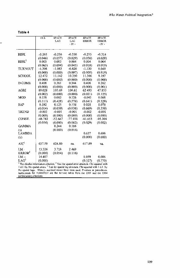
Table 4
OLS SPACE SPACE SPACE SPACELAG LAG ERROR ERROR
- IV- - IV-
RISK -0.265 -0.256 -0.330 -0.253 -0.314(0.046) (0.057) (0.029) (0.056) (0.028)
RISK2 0.003 0.003 0.004 0.004 0.004(0.063) (0.094) (0.045) (0.018) (0.019)
TlTRNOUT -1.308 -1.083 -0.620 -1.130 0.049(0.000) (0.000) (0.097) (0.000) (0.919)
SCHOOL 12.472 11.142 10.350 11.366 9.197(0.000) (0.000) (0.000) (0.000) (0.000)
INCOME 0.408 0.361 0.344 0.406 0.262(0.000) (0.000) (0.000) (0.000) (0.001)
AGRI 89.028 105.69 106.81 62.493 47.853(0.002) (0.000) (0.000) (0.031) (0.125)
MOD 0.158 0.083 0.126 -0.045 0.068(0.111) (0.428) (0.276) (0.641 ) (0.529)
SAP 0.192 0.125 0.156 0.028 0.070(0.014) (0.059) (0.036) (0.669) (0.350)
TREND -0.002 -0.001 -0.001 -0.002 -0.001(0.000) (0.000) (0.000) (0.000) (0.000)
CONST. -48.743 -52.667 -77.938 -41.653 -95.304(0.054) (0.000) (0.002) (0.029) (0.002)
GAMMA 0.244 0.186(y) (0.000) (0.016)LAMBDA 0.637 0.686(A) (0.000) (0.000)
AIC I 637.59 624.80 na. 617.89 na.
LM- 13.326 3.718 2.469ERROR2 (0.000) (0.054) (0.116)LM- 14.407 0.959 0.086LA03 0.000) 0.327 0.770
The Akaike information criterion. Test for spatial error structure. Chi-squared with1 d.f. Ho: No spatial errors. 3 Test for spatial lag structure. Chi-squared with 1 d.f. Ho:No spatial lags. White's standard errors have been used. P-values in parenthesis.Instruments for TURNOUT are the turnout ratios from the 1991 and the 1994parliamentary elections.
Who Wants Political Integration?
109

CHAPTER 4
DOES LABOR MARKET RISK INCREASE THE SIZE OF THE PUBLIC SECTOR?
EVIDENCE FROM SWEDISH MUNICIPALITIES.·
Jonas Vlachos·
Abstract
It has been argued that the public sector is an insurance against otherwise uninsurable
risks. If that is the case, it is reasonable to expect the public sector to be larger in
regions where the private labor-market is risky. Using data fronl Swedish
municipalities, this paper reports that labor-nlarket risk has a substantial impact on
public employment. The results for aggregate spending and taxation are, however,
much weaker and labor-market risk thus affects the lahor intensity of the municipal
public sector.
JEL Classification: C23; HI!; H40; J45
Keywords: Public sector size; Public employment; Labor market risk; Panel data
... Tore Ellingsen, seminar participants at the Economic Council of Sweden, FIEF, Stockholm School ofEconomics and, especially, Helena Svaleryd have given many helpful suggestions. Matz Dahlberg, EvaJohansson and Per Pettersson-Lidbom have generously shared their data with me.* Department of Economics, Stockholm School of Economics, P.O. Box 6501, 11383 Stockholm,Sweden. Email: [email protected].

Chapter 4
1. Introduction
In a pair of influential papers, Rodrik (1998, 2000) shows that open economies tend to
have larger public sectors. He also presents evidence in favor of a plausible
explanation for this phenomenon: International trade raises the volatility of income,
which can be decreased by the public sector. Optimally, an open trade regime
therefore goes hand in hand with a larger government, when other insurance
mechanisms are not available. Agell (1999) has subsequently argued that the
globalization of economic activity increases labor market instability and hence,
political demand for labor market rigidities. Although Alesina and Wacziarg (1998)
have questioned the link fronl trade-induced risk to government size, the theoretical
argument still has considerable appeal. hldeed, it would be surprising if the resources
spent by the public sector were completely independent of the need for insurance.
Here, the hypothesis that private sector risk increases the size of the public sector is
addressed using data from Swedish municipalities. Several problems related to cross
country data availability and comparability are therefore circumvented. 1 The fact that
there is no need to aggregate public spending across different levels of governance
might be most important: local aggregate risk is directly related to the size of the local
public sector.
The indicator of private-sector risk in local labor nlarkets is found to have a
substantial impact on municipal public employment. It is also found that shocks
increasing the size of the public sector across all nlunicipalities tend to generate larger
increas~s in risky locations. While some of the results hold even for aggregate
nlunicipal spending and the rate of taxation, on balance the hypothesis can be rej ected
for these variables. Hence, labor-market risk affects the labor intensity of the
municipal public sector, rather than its size.
By using municipal data, several well-known problems with cross-country data can be
circumvented. First of all, data might not be comparable across countries. Second,
institutional and cultural factors are not easily controlled for in a cross-country setting.
Finally, there are plainly not enough comparable countries. Researchers are thus
112

Labor Market Risk and Public Sector Size
forced to compare countries of very different degrees of development, hence
aggravating the problems mentioned above. For these reasons, several researchers
have successfully used municipal (or regional) data to test the predictions of different
political-economy related models. The appeal of such an approach is obvious. Using
municipal data in this study does not come without cost, however. There are three
main reasons for expecting the effect of market-induced risk on government size to be
smaller in Swedish municipalities than between countries. First of all, the Swedish
central government provides insurance against individual-specific labor nlarket risk
through the unemployment insurance. No such mechanism exists between countries.
Second, despite the international nlobility of capital, private capital markets do not
(yet) provide nluch risk sharing between countries (see e.g. Lewis 1995). These
markets are therefore poor providers of insurance against aggregate country-specific
shocks. Within a country, however, capital markets can certainly provide some
insurance against municipal-specific risks. Sorensen and Yosha (2000) verify this by
showing that interregional credit markets are highly integrated whereas the same is
not true between DEeD-countries. Finally, the Swedish central government has the
means and power to transfer funds directly to the municipalities. Since we can find an
economically significant effect of labor-market risk on local government size, despite
these mitigating factors, this should be read as support for Rodrik's (1998, 2000)
argument.2
A key issue in this paper is the indicator of labor-market risk, which is based on the
industry structure of local labor markets; hence taking commuting patterns into
explicit consideration. The behavioral consequences of local labor market risk have
mainly been analyzed in the field of labor economics. Simon (1988) shows that
frictional unemployment is higher in less diversified local labor markets and thus
provides evidence that industrial shocks are less costly to people working in well
diversified cities. Diamond and Simon (1990) probe deeper into the differences in
unemployment risk between local labor markets. By building on a portfolio theoretic
1 Swedish municipalities enjoy a constitutional right of self-governance, thereby making themappropriate units of analysis for questions regarding government size. Self-governance has given rise toconsiderable variation in the dependent variables used in this study.2 This said, countries have both monetary and fiscal policy instruments at their disposal to smoothtemporary fluctuations. To some extent, Swedish municipalities can also use fiscal policy to this end(Dahlberg and Lindstrom, 1998). In fact, Pettersson-Lidbom (2001) even fmds that municipalities usedebt to strategically influence future policy makers.
113

Chapter 4
view of labor markets pioneered by Conroy (1975), they show that cities with a more
diversified industrial structure have both a lower probability of unemployment and
lower wages. The reason is that a diversified labor market creates a portfolio effect for
the individual worker, thereby making the aggregate risk lower compared to a
specialized city. Thus, everything else equal, a worker is willing to accept lower mean
wages on a diversified than on a specialized local labor market. All models used in
local labor market analysis are based on the interplay between costly migration and
local labor market conditions. Given the everyday importance of local markets, it
should be of no surprise if political attitudes are also influenced by the insurance
properties of different locations.
The paper is organized as follows. In Section 2, Rodrik's (1998) argument is
presented. In Section 3, the data is described, with special attention given to the
indicator of labor-market risk. Section 4 discusses the empirical specification, while
the results are presented in Section 5. Section 6 concludes. In the appendix, all
variables and data sources are described in detail.
2. Rodrik's model
Following Rodrik (1998), an economy with a fixed supply x of a manufactured good,
not consumed within the economy, is considered. The manufactured good is traded
for an import good at price 1l. In addition, there is a publicly and a privately produced
good and the productivity ofprivate production is enhanced by the import good. Since
trade is continuously balanced, the economy can afford Xll of the import good. The
private sector enlploys (I-A) of the total labor supply (which is normalized to one).
Assuming that the production of the private good is linear, total production is xJZ(l
A). The supply of the publicly produced good is h(A), where h '>0 and h "<0. The size
of the public sector, A, is detennined before the realization of llis known. Assuming
that the public and the private good are perfect substitutes, the government's problem
is to maximize V(A) = E[u(h(A) + xJZ(l-A»] with respect to A. u() is the utility
function of a representative household, displaying standard properties. If the mean of
1l equals 1lm, and the variance equals cl, the Taylor expansion of V(A) gives the
following expression (after taking expectations)
114

Labor Market Risk and Public Sector Size
(2.1) V(A) ~ U(h(A) + xn(l-A)) + Y2 u"(h(A) + xJrm(1-A))(1-A)2x2d.
The first-order condition of this expression is then (ifz = xa),
As long as households display prudence (u "'>0), the first term is positive.3 Then, the
larger the aggregate risk z, the larger is the optimal level of A. To see this, consider an
economy, A, with zero aggregate external risk (ZA = 0). The first-order condition is
then reduced to h '(AA) = Xlrm. In another economy, B, risk is positive (ZB > 0) and
hence h '(AB) < Xlrm. Since h' '<0, it must be that AB >AA. In other words, a relocation
of resources to the safe public sector is the optimal response to a higher level of
aggregate manufacturing risk.
Naturally, the providing a safety net would be the ideal way of insuring against
aggregate risk. Swedish municipalities do not, however, have the power to directly
redistribute income between households: this task is performed by the central
government. Given that the local government wants to provide further insurance for
its inhabitants, it must do this in less direct ways.
It should be noted that the issue here is not whether counter-cyclical policies can
reduce inconle volatility, but whether the size of the public sector can do SO.4 The
answer to this question is not obvious and ultimately, it is empirical. Fatas and Mihov
(2001) document a strong negative correlation between government size output
volatility across DEeD countries, as well as across US states. Their study explicitly
deals with several conceptual and econometric problems alising when investigating
the proposed effect. In Table 1, the standardized variance of the pre-tax municipal per
capita income for the period 1985-1999 is regressed on the 1985 values of municipal
employment, spending, and tax rate, respectively (all variables are in logarithms). Per
3 For a discussion of prudence in a macro context, see e.g. Romer (1996), chapter 7. In a micro context,see e.g. Menezes et al. (1980).
115

Chapter 4
capita income and a dummy for municipalities performing tasks usually performed at
county level (see footnote 5) are added as control variables in this regression.
Admittedly, this is a very crude way of analyzing the relation between public sector
size and income volatility, and the results should therefore be read as indicative rather
than conclusive. As Rodrik (1998, p. 1023) notes, the coefficient on government size
is downward biased in this regression if the hypothesis presented here is true. Despite
this, a substantial negative effect on income volatility can be found for all three
indicators ofpublic sector size, however.
[Table 1]
3. Data
The constitutional right of self governance enjoyed by Swedish municipalities makes
them appropriate units of analysis when studying the determinants of government
size. In total, there are at present 289 Swedish municipalities. Nine of which are
removed from the sample because they are either split or created in the time period
1983-1999.5 The local tax rate, per capita municipal spending, and the share of
inhabitants employed by the municipality will be used as dependent variables. There
is considerable variation in these variables: The tax rate ranges from 9.7 to 23.6
percent, per capita spending from 20400 to 61500 SEK, and the share of municipal
employment from 2.1 to 9.7 percent.6
When measuring the degree of labor n1arket risk, con1IDuting and other spillovers
make the use of data on the municipal level unreasonable. Rather, data on the "local
labor market"-level is used. Local labor markets are analytical, and not administrative,
units of analysis whose boundaries are based on actual commuting patterns within and
between municipalities. In total, there are 109 local labor markets in Sweden and data
4 Sorensen et al. (2001) fmd that strongly procyclical revenue and weakly procyclical spending lead toprocyclical budget surpluses in U.S. state and local governments. Dahlberg and Lindstrom (1998) fmdthat Swedish local governments act to intertemporally smooth income.5 Three municipalities (Malmo, Gotland, and Goteborg) also perform tasks normally undertaken at thecounty (landsting) level. Whether these municipalities should be included in the sample is an openquestion. Here, they are included since they constitute a substantial share of the Swedish population.Further, the municipal specific fixed effects should capture the difference in responsibilities acrossmunicipalities. Excluding them has a miniscule effect on the results.6 These figures do not include municipalities with county-level responsibilities.
116

Labor Market Risk and Public Sector Size
is available biannually between 1985-1999.7 All in all, the data set covers 280
municipalities over eight time periods, giving a total of 2240 observations. The
dependent variables from 1983 are included in order to reduce the loss of time periods
when estimating dynamic specifications. All variables are entered in logarithms and
the monetary variables are expressed in 1995 prices.
To construct the indicator of private aggregate local labor market risk, we follow the
portfolio-theoretic approach used by Conroy (1975) and Diamond and Simon (1990)
to derive what can best be described as an augnlented Herfindahl index. The concept
is borrowed fronl the literature on financial economics: each local market is viewed as
a portfolio of industries, each of which is subject to random fluctuations. The total
degree of labor nlarket risk in a region is the weighted average of the variances and
covariances of these fluctuations. The total variance in city c equals
where Sse is the enlployment share of sector S in labor market c, ass is the variance of
employment in sector s, and asu is the covariance of employment in industries sand u.
Specifically, the variance/covariance matrix is constructed as follows: The variance
element, ass, is the variance in the rate of national employment growth in sector s at
time t, while the covariance elements, asu, equal the covariance between growth rates.
In order to capture the degree of unexpected volatility, the employment growth rate of
each industry was de-trended by taking the first differences of employment on the
national level. The logarithms of the first differences were then regressed on a time
trend. For each regression, the residuals were used to construct the
variance/covariance matrix and thus the risk index at each point in time provides an
7 See Statistics Sweden (1998) for a closer description of the LLM subdivisions. That the indicator ofrisk is constructed at a different level of aggregation than the dependent variables potentially induces adownward bias in the standard errors (Moulton 1990). Here, there are, on average, only 2.6municipalities per local labor market, which means that the problem is of little practical relevance.Allowing for possible cluster effects between municipalities in the same labor market yields an increasein the standard errors, but this effect is very small.
117

Chapter 4
indication of the need for insurance against labor market induced risk. It can be noted
that under the very strong assumptions of independently and identically distributed
growth rates, the portfolio diversification index is equivalent to the well known
Herfindahl index.
In order to calculate the variance/covariance matrix, sectoral employment data at the
national level between 1985-1999 is used. This procedure amount to the assumptions
that industries are subject to the same fluctuations, regardless of their geographical
location, and that the pattern of fluctuations is stable over time. Obviously, these
assumptions are not a perfect description of reality, but they are necessary to capture
both the within and between industry fluctuations in a systematic manner. Another
important question is which industries should be included in the study. To mainly
capture the effects of economic fluctuations from outside the local market, the sample
consists of all manufacturing and a few business-cycle sensitive service industries,
making a total of 21 industries. 8
4. Specification of the empirical model
The shares of population between 0-6,7-9,10-19,65-79, and 80+, respectively are
used as control variables. This division of groups is based on the cost differences
between age groups.9 Population density is also included to account for cost
differences between municipalities. Per capita income is included in all specifications,
while the average wage in the municipal sector is included when municipal
employment is the dependent variable. As further controls, a dummy variable for left
wing majority and a dummy for undefined political majority are sometimes included
as checks ofrobustness. It must be kept in mind that these political variables are likely
to be affected by the degree of labor market risk (given that labor market risk is an
important detenninant of policy). The central government redistributes resources both
8 The industry classification is based on Statistics Sweden's "limited level". A description of theindustries is available in the appendix. The 21 industries constitute 35 percent of total employment and52 percent of total private employment. Minor changes in the sample of industries do not change theresults.
118

Labor Market Risk and Public Sector Size
directly to, as well as between, municipalities. However, the system of redistribution
has changed during the relevant time period, making it difficult to con1pare the impact
of government grants on the size of the local government over time (see Bergstron1 et
al. 1998). This problem is further accentuated because of changes in grants-variable
definitions over time. Another problem with central government grants is that for part
of the period, they were mainly matching grants. 10 Hence, they are likely to be
endogenous to the fiscal decisions taken in the municipalities. For these reasons, per
capita grants will only be included to check for robustness. Since grants can be
negative, they cannot be entered as a separate regressor in a logarithmic specification.
Rather, they are added to per capita income. ll In addition to these variables, I have
also experimented by using the share of non-Swedish citizens, the share of women,
the share ofwelfare recipients, and changes in aggregate employment at the municipal
level. None of these variables has significant explanatory power, and their inclusion
does not change the other estimates in any substantial way.
The general specification of the empirical model is then
(4.1) Yit =f3 Zit +yXit + At + Vi + 8it,
where Yit denotes a particular measure of govenm1ent size in a municipality in a
specific year, Zit is the indicator of labor n1arket risk, and Xit the vector of control
variables mentioned above. As concerns the remaining variables, At is a time-specific
effect, constant over municipalities, Vi is a municipal-specific effect, constant over
time, and 8it is the usual residual.
The advantage of using fixed municipal- and time effects is that they account for a
large number of uncontrollable factors affecting the size of government. The time
specific effects, for example, control for business-cycle movements that could affect
public spending. Since the fixed effects may be falsely attributed to changes in
government size that should really be accounted for by other variables, this advantage
9 Swedish Government Official Reports (1993).10 Aronsson and Wikstrom (1996) and Bergstrom et al. (1998) provide descriptions of the Swedishgrants system.11 In fact, a different effect on spending from grants than from tax revenue is not supported by anyutility function (Dahlberg and Jacob 2000).
119

Chapter 4
comes at a cost, however. An attempt to account for these problems will be made in
Sections 5.3 and 5.4.
5. Results
5.1. Fixed effects estimates
Table 2 shows the basic results for both the base and the full conditioning set of
control variables. 12 The explanatory power is very good for the employment and
taxation specifications (adjusted R2 = 0.93), and quite good for spending (0.69). The
indicator of labor market risk is highly significant when municipal employment is
used as the dependent variable. In the base specification for per capita spending, labor
market risk is weakly significant (at the ten percent level), but not in the full
specification. The municipal tax rate, on the other hand, seems to be independent of
labor market risk. A high per capita income increases the size of the public sector
while population density has a negative effect. Municipalities where the public wage
rate is high tend to have a lower number of employees and most of the demographic
variables display a high level of statistical significance.
[Table 2]
The point estimates are not very large: 0.09 and 0.08 for the employment equation.
There is, however, considerable variation in labor market risk. One standard deviation
increase from the mean of this variable implies a change in the dependent variable by
4 percent. As a comparison, one standard deviation change in employment equals a 28
percent deviation from the mean of this variable. Some calculations show this effect
to be somewhat larger than the effect of having a left-wing rather than a right-wing
political majority in the municipality (see Pettersson-Lidbom 2000 for a thorough
discussion of this topic).
12 The full set includes central government grants (added to per capita income), a dummy for left-wingpolitical majority, and a dummy for undefined political majority.
120
Labor Market Risk and Public Sector Size
5.2. Dynamic specification. GMM.
Several studies (e.g. Bergstrom et.al 1998 and Pettersson-Lidbom 2000) of Swedish
local governments have found that dynamics are important. Further, in a study of the
demand for local public services, Dahlberg and Jacob (2000) have shown that the
explanatory variables used in this paper are not strictly exogenous. I3 Since the fixed
effects estimator is biased and inconsistent in a dynamic set-up, the Arellano and
Bond (1991) GMM-estimator is used when introducing a lagged dependent variable to
the specifications. This estimator is based on the use of lagged levels of the dependent
and endogenous variables, while strictly exogenous regressors are estimated in
differences. In order to check the model specification and the validity of the
instruments, the Sargan over identification test is used. Since this test tends to over
reject in the presence of heteroskedaticity, two-step estimates are used to judge the
model specification. The reported coefficients are, however, based on (robust) first
step estimates, since Arellano and Bond show that the two-step standard errors tend to
be downward biased. In order to save space, only the specifications where all
regressors are treated as endogenous are presented. I4 The Arellano-Bond method is
only valid if second-order autocorrelation is not present. For this reason, the test
statistics of an AR(2) test (null hypothesis ofno autocorrelation) are also presented.
[Table 3]
As shown in Table 3, the lagged dependent variables are highly significant in all
specifications for all three dependent variables. Allowing for dynanlics and
endogeneity results in an increase of the point estimates of the risk variable by almost
100 percent (0.14-0.18). A 44 percent increase in labor market risk then implies an
increase in municipal employment by 6-8 percent, which is indeed substantial. This is
just the short-run effect, however. The long-run elasticity is calculated by dividing the
coefficient on labor market risk by one minus the coefficient on the lagged dependent
variable, which yields an elasticity of 0.52-0.72, i.e. very large indeed. Column 3
shows that the point estimate in the spending equation is now statistically significant
13 The reason can be Tiebout-migration, causing both income and the demographic structure to beendogenous.14 The Sargan test rejects all specifications where the regressors are treated as strictly exogenous.
121

Chapter 4
and large (short-run elasticity 0.2, long-run 0.33). This result is somewhat sensitive to
the model specification, and when using the full conditioning set, statistical
significance falls just short of the 10-percent level. Interestingly, labor-market risk has
a snlall and nlarginally significant negative effect on the tax rate in these dynamic
specifications. The reason could be that there is relatively little variation over time in
this variable, and that tax increases were illegal during the first half of the 1990's.
5.3. Response to unobservable shocks. NLS.
One problem with the estimates presented in Sections 5.1 and 5.2 is that there is less
variation over time in the degree of labor market risk within labor markets compared
to the variation between labor markets. More precisely, the range of the risk variable
within labor nlarkets is 0.15-0.42, while the range between labor markets is 0.17-1.61.
Since both the fixed effect- and the GMM-estimators mainly exploit the short-run
time variation in the data, it is possible that some of the effects that should be
attributed to labor market diversity are actually captured by the fixed effects. In
particular, it is plausible that municipalities respond differently to similar shocks,
depending on how well diversified their labor markets are. In all regressions, the time
effects are highly significant, indicating that some set of common shocks has
influenced (i.e. increased) the size of the municipal sector in Sweden. These shocks
may, for example, include business cycle effects, changes in preferences, and changes
in the municipalities' responsibilities. Since we do not exactly know what shocks are
captured by the time-effects, it is not obvious how to estimate their interrelation with
labor-market risk. Blanchard and Wolfers (2000), however, suggest a method for
dealing with this type of problem. In a study of the effect of labor market institutions
on unemployment, they interact nleasures of country-specific institutions with shocks
common to all countries in their study. Persson and Tabellini (2001) employ the same
methodology when investigating the effects of political institutions on economic
policy.
Following Blanchard and Wolfers, equation 4.1 is re-specified as
122

Labor Market Risk and Public Sector Size
As above, Yit is the measure of government size, Zit is the indicator of labor nlarket
risk, Xit is the same vector of control variables as in the previous sections and Vi is the
municipality specific effect. As before, the set of year dunmlies is used to estimates
the effect of common events. Now, the effect of common events At is proportional to
17( Zit - Zt), where Zt is the year average across municipalities. In other words, I measure
whether the same unobservable shock has a different effect in municipalities deviating
from average labor market risk. Because of the fonn of the specification, the variable
17 must be estimated using non-linear least square. An additional problem is that the
lagged dependent variable cannot be included in these regressions since that would
yield biased and inconsistent estimates. IS
[Table 4]
In Table 4, results are presented that indeed support this hypothesis. The time effects
on the size of the public sector and the interaction tenn 17 are highly significant in the
employment and taxation equations, although no such effect can be found on
spending. This means that any undefined shock increasing the size of the public sector
is associated with a larger effect in risky labor markets than in safe ones.
To understand the size of this effect, the cumulative time-effect is calculated by
subtracting the coefficient of the 1999 time-period dummy from the 1985 dummy (lfJ99
- lfJ85)' The time effect is then multiplied by the interaction term 17~ and by 44 percent
(a one standard deviation increase from the mean in the risk variable), resulting in a
cumulative effect of around 4 percent. As seen in the top row of Table 4, the point
estimate of labor market risk (jJ) is around 0.1 in this specification. Altogether, these
results suggest that two municipalities with the same per capita number of employees
in 1985, going through the same sequence of shocks with a 44 percent difference in
labor market risk, display a 8.5 percent difference in per capita employment in 1999.
15 When only entering the lagged dependent variable in a fixed effects setting, the point estimates oflabor market risk are insignificant for all specifications. As has been seen, however, when using theGMM-estimator to properly address the dynamic econometric problems, labor market risk does indeed
123

Chapter 4
5.4. Response to observable shocks
The above results show that the response to common shocks indeed differs with labor
market risk. Naturally, some curiosity arises as to what types of shocks are
considered. We can, for example, expect the public sector to expand more during a
temporary economic downturn when the private labor nlarket is risky than when it is
well diversified. To investigate this hypothesis, the GDP growth rate is interacted with
the indicator of labor nlarket risk. The interaction term is expected to be negative
since risky labor markets have a greater incentive than safe ones to expand the public
sector when the growth rate is low. The same reasoning applies when using the
interaction between the total change in employment (at the local labor market level)
and labor market risk. In other words: a negative (positive) point estimate indicates
that the public sector is expanded to a relatively small (large) extent in risky labor
markets when employment growth is high. 16
[Table 5]
These predictions do find some support in Table 5, although the results are somewhat
dependent on the type of shock. Interpreting the point estimates is quite difficult, but
they carry the general message that labor market risk is one determinant as to how
growth and employment shocks are handled at the municipal level.
5.5 Some additional tests
On average, staff costs constitute about 50 percent of total spending. In the full
sample this ratio varies from 26 to 68 percent. So far, the results indicate that
municipalities subject to large labor market risk tend to increase the number of
employees rather than the size of the public sector per se, which implies that the
public sector is relatively labor intensive in risky locations. A direct way of testing
this hypothesis is to regress the ratio between total municipal labor costs and total
come out significant. When including the lagged dependent variable in the NLS-specifications, theresults are considerably weakened.16 Entering employment change as an independent variable does not change any results, and its pointestinlate is not statistically significant. The high correlation between changes in GDP and changes inlocal employment (0.86) nlakes it likely that the time-period dummies capture any direct effects.
124

Labor Market Risk and Public Sector Size
expenditures on the indicator of labor market risk. In the first two columns of Table 6,
the results from fixed effect estimates, as well as NLS-estimates using an interaction
term between unobservable shocks and the indicator of labor market risk (as in
Equation 5.1) are presented. As can be seen, there is indeed support for this
hypothesis. The point estimates are similar to those in Table 2 and 4, indicating that
the increase in labor intensity is roughly similar to the increase in public employment.
One might also worry about the possibility that safe municipalities have a greater
propensity to have services provided by private entrepreneurs. If that were the case,
municipal spending would be constant, while municipal enlployment would be lower
in these municipalities. The results in Table 6 are, however, a strong indication
against this possibility.
[Table 6]
As an additional check of robustness, the ratio ofpublic employees to the working age
population (ages 20-64) is used as the dependent variable, rather than the per capita
ratio used before. As can be seen in the last two columns of Table 6, the results are
similar to the previous ones.
6. Conclusions
Consider two municipalities that only differ in the degree of aggregate private labor
market risk. More precisely, one labor market is one standard deviation above the
mean (44 percent) riskier than the other. These nlunicipalities go through the same
sequence of shocks to the size of the public sector between 1985-1999. The findings
in this paper indicate that per capita public employment is between 8 (lower bound)
and 30 (upper bound) percent higher in the risky relative to the safe municipality at
the end of this period. Surprisingly, given these results, labor market risk does not
seem to be an important detenninant of aggregate municipal spending or taxation.
Rather, the public sector in municipalities with a substantial representation of risky
private industries is relatively labor intensive.
A reasonable interpretation of these results is that municipalities attempt to provide an
insurance against unemployment risk, rather than income insurance per se. Since
125

Chapter 4
income insurance is largely provided for by the central government, this may very
well be an optimal policy. Support for this interpretation is given by the reduction in
point estimates on risk in the spending equations that occur when central government
grants are controlled for. In other words, these transfers seem to mitigate the adverse
effects of a risky private labor market.
In this paper, only the risk due to the local composition of private industries has been
considered. Although Clark (1998) has shown that industry shocks constitute a
substantial share of the total variation of regional output, it would be interesting to
include other sources of variation in the analysis. One possible extension of this work
would therefore be to decompose local labor market risk into its national, regional,
and industry-specific components. Since the optimal local policy response depends on
the sources of volatility, the different components can then be related to policy
choices both at the local and central levels. The greatest challenge of such an
undertaking would be to construct indicators that capture risk, rather than fluctuations
per se. So far, most of the research on regional output and income volatility has only
dealt with the latter issue (see e.g. Clark and Shin, 2000).
126

Labor Market Risk and Public Sector Size
Appendix. Data description and variables
Split (Boras (1490), Nykoping (480), Sodertalje (181), Orebro (1880» and new (Bollebygd (1443),Gnesta (461), Lekeberg (1814), Nykvam (140), Trosa (488» municipalities are removed from thesample.
The industry classification is based on Statistics Sweden's "limited level" which, in turn, is constructedusing the MIS standard of Swedish industry classification. The following industries are included in thesample: fishery, transport equipment, agriculture, metals, rubber and plastics, textiles and clothing,wood, other manufacturing, mining and minerals, forestry, dirt and rocks, electric and opticalappliances, steel and metal products, construction, machinery, telephone and postal services, publishingand graphical printing, paper and pulp, foodstuf:f, insurance, chemicals. The following industries arenot included: Energy- water- and garbage disposals, motor vehicle sales and gas stations, wholesaletrade, retail trade, transports and storage, real estate services, recruitment and staffing services,computer consultants and services, other corporate services, education, research and development,health care, child care, elderly care, other care, hotels and restaurants, interest groups, recreation andsports, other services, public administration, unspecified activities. The included industries are listedaccording to their variance (variance measure described in text), the most volatile come frrst.
The ten least risky (definition in text) labor markets in 1991 were: Sundsvall, Timra, Karlstad,Stockholm, Hylte, Ange, Gavle, Sandviken, Avesta, Borlange. The ten most risky labor markets in1991 were: Olofstrom, Trollhattan, Arboga, Tidaholm, Dorotea, Gnosjo, Gislaved, Oskarshamn,Skovde, Gullspang.
The data is biannual, and all monetary variables are expressed in 1995 prices after being deflated by theGDP-deflator.
RISK: Labor market risk measure calculated according to the portfolio measure described in the text.Source: Statistics Sweden "Registerbaserad arbetsmarknadsstatistik". Mean: 0.289. Std: 0.129.
INCOME: Total taxable personal income, lagged one period (due to delay in payments), divided bytotal population (at the end of the year). Sources: Statistics Sweden "Arsbok for Sveriges kommuner"and "Vad kostar verksamheten i din kommun?". Mean: 76870. Std: 15445.
INCOME (grants adjusted): Total taxable personal income, lagged one period (due to delay inpayments), plus net grants and redistribution to the central government divided by total population (atthe end of the year). Sources: Statistics Sweden "Arsbok for Sveriges kommuner" and "Vad kostarverksamheten i din kommun?". Mean: 80637. Std: 16062.
POPlTLATION DENSITY: Total population (at the end of the year) divided by area. Source: StatisticsSweden "Vad kostar verksamheten i din kommun?". Mean: 111.04. Std: 376.58.
SHARE -6: Share of population between 0-6 years of age (x 100). Source: Statistics Sweden "Sverigesofficiella statistik". Mean: 8.67. Std: 1.11
SHARE 7-9: Share of population between 7-9 years of age (x 100). Source: Statistics Sweden "Sverigesofficiella statistik". Mean: 3.89. Std: 0.55.
SHARE 10-19: Share of population between 10-19 years of age (x 100). Source: Statistics Sweden"Sveriges officiella statistik". Mean: 13.91. Std: 1.68
SHARE 65-79: Share of population between 65-79 years of age (x 100). Source: Statistics Sweden"Sveriges officiella statistik". Mean: 13.91. Std: 2.95.
SHARE 80+: Share of population above 80 years of age (x 100). Source: Statistics Sweden "Sverigesofficiella statistik". Mean: 4.59. Std: 1.35.
LEFT-WING MAJORITY: 1 if SAP + VP obtains more than 50% of the valid votes, 0 otherwise.Source: Statistics Sweden "Sveriges officiella statistik". Mean: 0.396. Std: 0.489.
127

Chapter 4
RIGHT-WING MAJORITY: 1 if MOD + KD + FP + CP obtains than 50 % of the valid votes, 0otherwise. Source: Statistics Sweden "Sveriges officiella statistik". Mean: 0.360. Std: 0.480.
UNDEFINED MAJORITY: 1 if LEFT-WING and RIGHT-WING MAJORITY both equal 0, 0otherwise. Source: Statistics Sweden "Sveriges officiella statistik". Mean: 0.245. Std: 0.430.
WAGE: Implicit unit labor cost, derived by dividing the total municipal labor costs (wages, employertaxes and fees) with total municipal employment. Sources: Kommunforbundet "Kommunal Personal"and Statistics Sweden "Vad kostar verksamheten i din kommun?". A few missing observations for1995 have been replaced by the average of 1994 and 1996. Mean: 307894. Std: 45330.
EMPLOYMENT: Municipal full-time equivalent employees as a share of the population (x 100).Source: Kommunforbundet "Kommunal Personal". A few missing observations for 1995 have beenreplaced by the average of 1994 and 1996. Mean: 5.46. Std: 1.54.
EMPLOYMENT PER WORKING AGE POPULATION: Municipal full-time equivalent employees asa share of the population aged 20-64. Calculated as EMPLOYMENT/(I-[SHARE-6]-[SHARE7-9]SHARE[10-19]-[SHARE65-79]-[SHARE80+]). Mean: 9.88. Std: 2.94.
SPENDING: Total municipal expenditure divided by total population. Source: Statistics Sweden "Vadkostar verksamheten i din kommun" och "Arsbok for Sveriges kommuner". Nine missing values for1995 have been replaced by the average of 1994 and 1996. Mean: 32820. Std: 5984.
STAFF COST SHARE OF TOTAL EXPENDITURE: Total municipal labor costs (wages, employertaxes and fees) divided by total expenditures. Sources: Kommunforbundet "Kommunal Personal" andStatistics Sweden "Vad kostar verksamheten i din kommun?". A few missing observations for 1995have been replaced by the average of 1994 and 1996. Mean: 0.50. Std: 0.05.
TAX RATE: The municipal income tax rate (in percent). Source: Statistics Sweden "Sveriges officiellastatistik". Mean: 18.04. Std: 2.30.
EMPLOYMENT SHOCK: The percentage change in total employment at the local labor market levelbetween t-l and 1. Source: Statistics Sweden "Registerbaserad arbetsmarknadsstatistik". Mean: -1.54.Std: 5.87.
GROWTH SHOCK: Growth rate of real Swedish GDP between t-l and 1. Source: Statistics Sweden"Nationalrakenskapema". Mean: 4.07. Std: 3.63.
DEFLATOR: The ratio between nominal GDP and GDP in 1995 year prices. Source: Statistics Sweden"Nationalrakenskapema".
128

Labor Market Risk and Public Sector Size
References
Agell, J. (1999) "On the Benefits From Rigid Labor Markets: Nonns, MarketsFailures, and Social Insurance", Economic Journal, 109, F143-F164.
Alesina, A. and R. Wacziarg (1998) "Openness, Country Size and Government",Journal ofPublic Economics, 69, 305-321.
Arellano, M. and S. Bond (1991) "Some Tests of Specification for Panel Data: MonteCarlo Evidence and an Application to Employment Equations", Review ofEconomicStudies, 58, 277-297.
Aronsson, T. and M. Wikstrom (1996) "Local Public Expenditure in Sweden. AModel where the Median Voter is not Necessarily Decisive", European EconomicReview, 40, 1705-1716.
Bergstrom, P., M. Dahlberg, E. Johansson (1998) "Municipal Labor Demand. Sweden1988-1995", mimeo Department of Economics, Uppsala University.
Blanchard, O. and J. Wolfers (2000) "The Role of Shocks and Institutions in the Riseof European Unemployment: The Aggregate Evidence", Economic Journal, 110, C1C33.
Clark, T. (1998) "Employment Fluctuations in the U.S. Regions and Industries: TheRoles of National, Region-Specific, and Industry-Specific Shocks", Journal ofLaborEconomics, 16, 202-229.
Clark, T. and K. Shin (2000) "The Sources of Fluctuations Within and AcrossCountries", in Hess and van Wincoop (2000).
Conroy, M. (1975) "The Concept and Measurement of Regional IndustrialDiversification", Southern Economic Journal, 41, 492-505.
Dahlberg, M. and J. Jacob (2000) "Sluggishness, Endogeneity and the Demand forLocal Public Services", mimeo Department of Economics, Uppsala University.
Dahlberg, M. and T. Lindstrom (1998) "Are Local Governments Governed byForward Looking Decision Makers? An Investigation of Spending Patterns inSwedish Municipalities", Journal ofUrban Economics, 44, 254-271.
Diamond, C. and C. Simon (1990) "Industrial Specialization and the Returns toLabor", Journal ofLabor Economics, 8:2, 175-201.
Fatas, A. and 1. Mihov (2001) "Government Size and Automatic Stabilizers:International and Intranational Evidence", Journal ofInternational Economics, 55:1,3-28.
Hess, G. and E. van Wincoop (Eds.) (2000) Intranational Economics. CambridgeUniversity Press: Cambridge.
129

Chapter 4
Lewis, K. (1995) "Puzzles in International Financial Markets", in Handbook ofInternational Economics, vol. 3, edited by Grossman, G. and K. Rogoff. Amsterdam:North-Holland.
Menezes, C., C. Geiss, J. Tressler (1980) "Increasing Downside Risk", AmericanEconomic Review, 70:5, 921-932.
Moulton, B. (1990) "An Illustration of a Pitfall in Estimating the Effects ofAggregateVariables on Micro Unit", Review ofEconomics and Statistics, 72:2, 334-338.
Persson, T. and G. Tabellini (2001) "Political Institutions and Policy Outcomes: Whatare the Stylized Facts?", mimeo lIES.
Pettersson-Lidbom, P. (2000) "Do Parties Matter for Fiscal Policy Choice", mimeolIES.
Petterson-Lidbom, P. (2001) "An Empirical Investigation of the Strategic Use ofDebt", Journal ofPolitical Economy, 109, 570-583.
Rodrik, D. (1998) "Why Do More Open Economies Have Bigger Governments?",Journal ofPolitical Economy, 106:5,997-1031.
Rodrik, D. (2000) "What Drives Public Employment in Developing Countries",Review ofDevelopment Economics, 4:3,229-243.
Romer, D. (1996) Advanced Macroeconomics, McGraw-Hill, New York.
Simon, C. (1988) "Frictional Unemployment and the Role of Industrial Diversity",Quarterly Journal ofEconomics, 103,715-728.
Sorensen, B., L. Wu, O. Yosha (2001) "Output Fluctuations and Fiscal Policy: U.S.State and Local Governments 1978-1994, European Economic Review, 45, 12711310.
Sorensen, B. and O. Yosha (2000) "Intranational and International Credit MarketIntegration: Evidence from Regional Income and Consumption Patterns", in Hess andvan Wincoop (2000).
Statistics Sweden (1998) "Regionala koder enligt indelningen den 1 januari 1998(Nunlerical codes by region for various Swedish subdivisions)", MIS 1998:2.
Swedish Government Official Reports (1993), 1993:53. Allma-nna Forlaget.
130
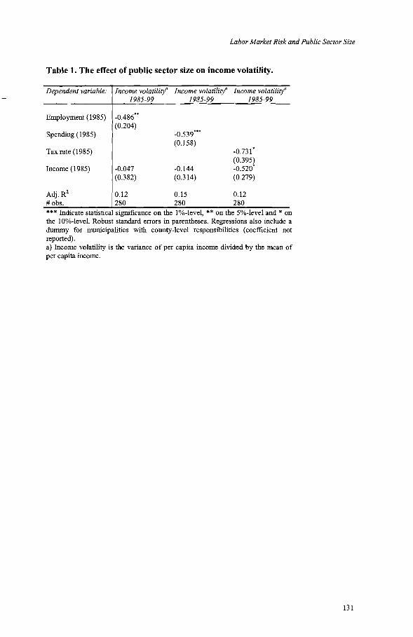
Labor Market Risk and Public Sector Size
Table 1. The effect of public sector size on income volatility.
Dependent variable: Income volatilitya Income volatilitya Income volatilitya1985-99 1985-99 1985-99
Employment (1985) -0.486**(0.204)
Spending (1985) -0.539***(0.158)
Tax rate (1985) -0.731*(0.395)
Income (1985) -0.047 -0.144 -0.520·(0.382) (0.314) (0.279)
Adj. R2 0.12 0.15 0.12# obs. 280 280 280*** Indicate statistical significance on the 1%-level, ** on the 5%-level and * onthe 10%-level. Robust standard errors in parentheses. Regressions also include adummy for municipalities with county-level responsibilities (coefficient notreported).a) Income volatility is the variance of per capita income divided by the mean ofper capita income.
131
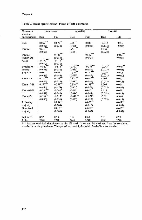
Chapter 4
Table 2. Basic specification. Fixed effects estimates
Dependent Employment Spending Tax ratevariable:S ecification: Base Full Base Full Base Full
Risk 0.091*** 0.075*** 0.061 * 0.049 -0.012 -0.017(0.032) (0.031) (0.035) (0.035) (0.145) (0.014)
Income 0.609*** 0.571 *** 0.089"''''*(0.062) (0.067) (0.028)
Income 0.729*** 0.552*** 0.089**'"(grants adj.) (0.058) (0.064) (0.026)Wage -0.790**'" -0.779***
(0.030) (0.030)Population -0.860**'" -0.818*** -0.377**'" -0.353"'** -0.043* -0.049*'"density (0.051) (0.050) (0.055) (0.056) (0.023) (0.023)Share-6 0.034 0.048 0.226"'*'" 0.207"'** -0.014 -0.015
(0.046) (0.044) (0.050) (0.049) (0.021) (0.020)Share 7-9 0.117*** 0.101 *"'* 0.104**'" 0.084*"'* 0.004 0.000
(0.029) (0.028) (0.031) (0.031) (0.013) (0.013)Share 10-19 0.297*** 0.251 "'** 0.266*** 0.198*"'* 0.006 0.004
(0.056) (0.053) (0.061) (0.059) (0.025) (0.024)Share 65-79 -0. 140**'" -0.146*"'* -0.013 0.015 0.023 0.021
(0.041) (0.040) (0.044) (0.044) (0.018) (0.018)Share 80+ -0.241 *** -0.217*** -0.090*"'* -0.078** -0.011 -0.004
(0.030) (0.030) (0.033) (0.033) (0.013) (0.013)Left-wing 0.034*** 0.026*** 0.019**'"majority (0.009) (0.010) (0.004)Undefined 0.018"'** 0.018*"'* 0.015"'**majority (0.006) (0.007) (0.003)
Within R2 0.93 0.93 0.69 0.69 0.93 0.93#obs. 2240 2240 2240 2240 2240 2240
*** Indicate statistical significance on the 1%-level, ** on the 5%-level and * on the 10%-level.Standard errors in parentheses. Time-period and municipal-specific fixed effects are included.
132

Labor Market Risk and Public Sector Size
Table 3. Dynamic specification. GMM-estimates
Dependent Employment Spending Tax ratevariable:S ecification: Base Full Base Full Base Full
Risk 0.180"''''''' 0.147.... 0.204"'* 0.153 -0.069'" -0.070'"(0.069) (0.068) (0.102) (0.101) (0.037) (0.039)
Lagged dep. 0.751"''''''' 0.726.... '" 0.405....• 0.410....• 0.625"''' 0.631"'''''''Variable (0.070) (0.069) (0.041) (0.041) (0.123) (0.124)
Sargan testa 474.00 477.44 337.63 398.98 560.65 558.99(one-step) (0.000) (0.000) (0.000) (0.000) (0.000) (0.000)Sargan testa 256.74 255.50 222.37 224.71 246.13 248.88(two-step) (0.563) (0.550) (0.713) (0.638) (0.265) (0.223)AR(2) testb 0.16 0.74 1.38 -1.18 -0.83 -0.61(one-step) (0.876) (0.459) (0.168) (0.238) (0.401) (0.541)
# obs. 1680 1680 1680 1680 1680 1680*** Indicate statistical significance on the 1%-level, ** on the 5%-level and * on the 10%-level.Standard errors in parentheses. All point estimates are (robust) two-step. The same sets of controlvariables as in Table 2 are used.a) Sargan gives the test statistic and p-value of the Sargan test for over-identifying restrictions. Both thetest statistics from the first and second step estimations are presented since the test statistic from thefust-step has been shown to over-reject in the presence ofheteroscedasticity. The null hypothesis is thatthe instruments are valid/the model is correctly specified.b) AR2 is the test statistic and p-value for no second-order correlation. The null hypothesis is that thereis no second-order serial correlation.
133

Chapter 4
Table 4. Unobservable shocks. NLS-estimates.
Dependent variable: Employment Spending
S ecification: Base Full Base Full
Risk [,B] 0.106"""* 0.093*** 0.061 0.043(0.032) (0.032) (0.035) (0.036)
Risk deviation from mean x 0.341 *** 0.365*** 0.000 -0.156time dummies [17] (0.054) (0.064) (0.130) (0.186)Cumulative time effect 85-99 0.283 0.23 0.10 0.07[ tp99 - tp85]
Cumulative time effect in 4.2% 3.7% O%a _0.5%amunicipality with labormarket risk 44% above mean.17[ tp99 - tp85] x 44%b
Tax rate
Base Full
-0.012 -0.015(0.014) (0.014)0.069*** 0.064***(0.025) (0.025)0.22 0.22
0.7% 0.6%
Adj. R2 0.94 0.94 0.82 0.82 0.95 0.95# obs. 2240 2240 2240 2240 2240 2240*** Indicate statistical significance on the 1%-level, ** on the 5%-level and * on the 10%-level.Standard errors in parenthesis. The same sets of control variables as in Table 2 are used.a) Not significant.b) One standard deviation is 44 percent above the mean of the risk variable.
134
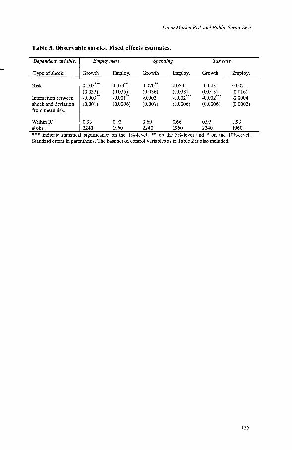
Labor Market Risk and Public Sector Size
Table 5. Observable shocks. Fixed effects estimates.
Dependent variable: Employment Spending Tax rate
T e of shock: Growth Em 10 . Growth Em 10 . Growth Em 10 .
Risk 0.105"''''''' 0.079""" 0.070""" 0.059 -0.003 0.002(0.033) (0.035) (0.036) (0.038) (0.015) (0.016)
Interaction between -0.003** -0.001 ** -0.002 -0.002"""'" -0.002"'...... -0.0004shock and deviation (0.001) (0.0006) (0.001) (0.0006) (0.0006) (0.0002)from mean risk.
Within R2 0.93 0.92 0.69 0.66 0.93 0.93# obs. 2240 1960 2240 1960 2240 1960*** Indicate statistical significance on the 1%-level, ** on the 5%-level and * on the 10%-level.Standard errors in parenthesis. The base set of control variables as in Table 2 is also included.
135

Chapter 4
Table 6. Additional robustness tests
Dependent variable: Staffcost share oftotalcosts
Public employment perworking age population
Estimation method: FE NLS FE NLS
Risk 0.093*** 0.090*** 0.097*** 0.112***(0.036) (0.036) (0.033) (0.032)
Risk deviation from mean x 0.384*** 0.356***time dummies (0.084) (0.055)Cumulative time effect 85-99 0.18 0.29
Cumulative tinle effect in 3.0% 4.4%municipality with labor marketrisk 44% above mean.a
R2 0.29 0.49 0.93 0.94(within) (adjusted) (within) (adjusted)
# obs. 2240 2240 2240 2240*** Indicate statistical significance on the 1%-level, ** on the 5%-level and * on the 10%level. Standard errors in parentheses. The municipal wage rate, the population shares of agegroups 0-6, 7-9, 10-19, 65-79, 80+, time-period and municipal-specific fixed effectsare included in columns 1 and 2. In columns 3 and 4, the same controls as in Table 2 areincluded. a) 44 percent is one standard deviation above the mean.
136

EFIThe Economic Research Institute
Reports since 1995A complete publication list can be found at www.hhs.se/efi
Published in the language indicated by the title
2001Adolfson, M., Monetary Policy and Exchange Rates - Breakthrough of Pass-Through.Andersson, P., Expertise in Credit Granting: Studies on Judgment and DecisionMaking behavior.Bjorklund, C., Work Motivation - Studies of its Determinants and Outcomes.Center for Management and Organization 50 (1951-2001).Charpentier, C., Uppfoljning av kultur- och fritidsforvaltningen efter stadsdelsnfunndsreformen.Dahlen, M., Marketing on the Web - Empirical Studies ofAdvertising and PromotionEffectiveness.Ekelund, M., Competition and Innovation in the Swedish Pharmaceutical Market.Ericsson, D., Kreativitetsmysteriet - Ledtradar till arbetslivets kreativisering ocllskrivandets metafysik.Eriksson, R., Price Responses to Changes in Costs and Demand.Frisell, L., Information and Politics.Giordani, P., Essays in Monetary Economics and Applied Econometrics.Gustavsson, P., Essays on Trade, Growth and Applied Econometrics.Hedlund, A., Konsumentens erfarenhet - och dess inverkan pa livsmedelsinkop paInternet.Hill, M., Essays on Environmental Policy Analysis: Computable General EquilibriumApproaches Applied to Sweden.Hvenmark, J.,Varfor slocknar elden? Om utbrandhet bland chefer i ideellaorganisationer.Hagglund, P.B., Foretaget som investeringsobjekt - Hur placerare och analytikerarbetar med att ta fram ett investeringsobjekt.Hook, P., Stridspiloter i vida kjolar, om ledarutveckling ochjamsUilldhet.Johansson, C., Styrning for sanlordning.Kjellberg, H., Organising Distribution - Hakonbolaget and the efforts to rationalisefood distribution, 1940-1960.Lange, F. oeh Wahlund, R., Category Management - Nar konsumenten ar manager.Liljenberg, A., Customer-geared competition - A socio-Austrian explanation of TertiusGaudens.Lindkvist, B., Kunskapsoverforing meUan produktutvecklingsprojekt.Ljunggren, U., Nyckeltal i grundskolan i Stockholms stad fore och efter stadsdelsnfunndsreformen.Lakemedel- Kostnad eller resurs fdr sjukvarden? (red. Jonsson, B.,).Lof, M., On Seasonality and Cointegration.Martensen, K., Essays on Entry Externalities and Market Segmentation.Matros, A., Stochastic Stability and Equilibrium Selection in Games.Mirtensson, P., Management Processes - An Infomlation Perspective on ManagerialWork.Nilsson, A., Market Transparency.

Norberg, P., Finansmarknadens amoralitet och det kalvinska kyrkorummet - En studiei ekonomisk mentalitet och etik.Persson, B., Essays on Altruism and Health Care Markets.Skoglund, J., Essays on Random Effects Models and GARCH.Strand, N., Empirical Studies of Pricing.Thoren, B., Stadsdelsnamndsreformen och det ekonomiska styrsystemet - Om budgetavvikelser.
2000Berg-Suurwee, D., Styrning fore och efter stadsdelsnfunndsreform inom kulturoch fritid - Resultat fran intervjuer och enkat.Bergkvist, L., Advertising Effectiveness Measurement: Intermediate Constructsand Measures.Brodin, B., Lundkvist, L., Sjostrand, S-E., Ostman, L., Koncernchefen och agama.Bornefalk, A., Essays on Social Conflict and Reform.Charpentier, C., Samuelson, L.A., Effekter av en sjukvardsreform.Edman, J., Information Use and Decision Making in Groups.Emling, E., Svenskt familjeforetagande.Ericson, M., Strategi, kalkyl, kansla.Gunnarsson, J., Wahlund, R., Flink, H., Finansiella strategier i forandring: segmentoch beteenden bland svenska hushaH.Hellman, N., Investor Behaviour - An Empirical Study of How Large SwedishInstitutional Investors Make Equity Investment Decisions.Hyll, M., Essays on the Term Structure of Interest Rates.Hakansson, P., Beyond Private Label- The Strategic View on Distributor OwnBrands.I huvudet pa kunden. Soderlund, M., (red).Karlsson Stider, A., Familjen oeh firman.Ljunggren, D., Styrning av grundskolan i Stockholms stad fore och efterstadsdelsnfunndsreformen - Resultat fran intervjuer och enkat.Ludvigsen, J., The International Networking between European Logistical Operators.Nittmar, H., Produktutveckling i samarbete - Strukturforandring vid inforande av nyaInformationssystem.Robertsson, G., International Portfolio Choice and Trading Behavior.Schwarz, B., Weinberg, S., Serviceproduktion och kostnader - att soka orsaker tillkommunala skiHnader.Stenstrom, E., Konstiga foretag.Styrning av team och processer - Teoretiska perspektiv och fallstudier.Bengtsson, L., Lind, J., Samuelson, L.A., (red).Sweet, S., Industrial Change Towards Environmental Sustainability - The Case ofReplacing Chloroflouoroearbons.Tamm Hallstrom, K., Kampen for auktoritet - Standardiseringsorganisationer iarbete.
1999Adler, N., Managing Complex Product Development.Allgulin, M., Supervision and Monetary Incentives.Andersson, P., Experto Credite: Three Papers on Experienced Decision Makers.Ekman, G., Fran text till batong - Om poliser, busar och svennar.Eliasson, A-C., Smooth Transitions in Macroeconomic Relationships.Flink, H., Gunnarsson, J., Wahlund, R., Svenska hushallens sparande ochskuldsattning- ett konsumentbeteende-perspektiv.Gunnarsson, J., Portfolio-Based Segmentation and Consumer Behavior: EmpiricalEvidence and Methodological Issues.

Hamrefors, S., Spontaneous Environmental Scanning.Helgesson, C-F., Making a Natural Monopoly: The Configuration of a TechnoEconomic Order in Swedish Telecommunications.Japanese Production Management in Sunrise or Sunset. Karlsson, C., (red).Jonsson, B., Jonsson, L., Kobelt, G., Modelling Disease Progression And the Effect ofTreatment in Secondary Progressive MS. Research Report.Linde, J., Essays on the Effects of Fiscal and Monetary Policy.Ljunggren, U., Indikatorer i grundskolan i Stockholms stad fore stadsdelsnamndsreformen - en kartHiggning.Ljunggren, U., En utvardering av metoder for art mata produktivitet och effektivitet iskolan - Med tillampning i Stockholms stads grundskolor.Lundbergh, S., Modelling Economic High-Frequency Time Series.Magi, A., Store Loyalty? An Empirical Study of Grocery Shopping.Molleryd, B.G., Entrepreneurship in Technological Systems - the Development ofMobile Telephony in Sweden.Nilsson, K., Ledtider for ledningsinformation.Osynlig Foretagsledning. Sjostrand, S-E., Sandberg, 1., Tyrstrup, M., (red).Rognes, J., Telecommuting - Organisational Impact of Home Based - Telecommuting.Sandstrom, M., Evaluating the Benefits and Effectiveness of Public Policy.Skalin, J., Modelling Macroeconomic Time Series with Smooth TransitionAutoregressions.Spagnolo, G., Essays on Managerial Incentives and Product-Market Competition.Strauss, T., Governance and Structural Adjustment Programs: Effects on Investment,Growth and Income Distribution.Svedberg Nilsson, K., Effektiva foretag? En studie av hur privatiserade organisationerkonstrueras.Soderstrom, U., Monetary Policy under Uncertainty.Werr, A., The Language of Change The Roles of Methods in the Work of ManagementConsultants.Wijkstrom, F., Svenskt organisationsliv - Framvaxten av en ideell sektor.
1998Andersson, M., On Testing and Forecasting in Fractionally Integrated Time SeriesModels.Berg-Suurwee, U., Styming av kultur- och fritidsforvaltnillg innan stadsdelsnamndsreformen.Berg-Suurwee, U., Nyckeltal avseende kultur- och fritidsforvaltning innan stadsdelsnfunndsreformen.Bergstrom, F., Essays on the Political Economy of Industrial Policy.Bild, M., Valuation of Takeovers.Charpentier, C., Samuelson, L.A., Effekter av en sjukvardsreform - en allalys avStockholmsmodellen.Eriksson-Skoog, G., The Soft Budget Constraint: The Emergence, Persistence andLogic of an Institution. The Case of Tanzania 1967-1992.Gredenhoff, M., Bootstrap Inference in Time Series Econometrics.Joannidis, D., I nationens tjanst? Strategisk handling i politisk miljo - en nationellteleoperators interorganisatoriska, strategiska utveckling.Johansson, S., Savings Investment, and Economic Reforms in Developing Countries.Levin, J., Essays in Conlpany Valuation.Ljunggren, U., Styrning av grundskolan i Stockholms stad innan stadsdelsnamndsreformen.Mattsson, S., Fran stat till marknad - effekter pa natverksrelationer vid en bolagiseringsreform.Nyberg, A., Innovation in Distribution Channels - An Evolutionary Approach.

Olsson, P., Studies in Company Valuation.Reneby, J., Pricing Corporate Securities.Roszbach, K., Essays on Banking Credit and Interest Rates.Runsten, M., The Association Between Accounting Information and Stock Prices.Model developnlent and empirical tests based on Swedish Data.Segendorff, B., Essays on Bargaining and Delegation.Sjoberg, L., Bagozzi, R., Ingvar, D.H., Will and Economic Behavior.Sjogren, A., Perspectives on Human Capital: Economic Growth, Occupational Choiceand Intergenerational Mobility.Studier i kostnadsintaktsanalys. Jennergren, P., (red)Soderholm, J., Malstyrning av decentraliserade organisationer. Styming mot finansiellaoch icke-finansiella mal.Thorburn, K., Cash Auction Bankruptcy and Corporate RestructuringWijkstrom, F., Different Faces of Civil Society.Zethraeus, N., Essays on Econonlic Evaluation in Health Care. Evaluation of HormoneReplacement Therapy and Uncertainty in Economic Evaluations.
1997Alexius, A., Essays on Exchange Rates, Prices and Interest Rates.Andersson, B., Essays on the Swedish Electricity Market.Berggren, N., Essays in Constitutional Economics.Ericsson, J., Credit Risk in Corporate Securities and Derivatives. Valuation andOptimal Capital Structure Choice.Charpentier, C., Budgeteringens roller, aktorer och effekter. En studie av budgetprocesserna i en offentlig organisation.De Geer, H., Silfverberg, G., Citizens'Trust and Authorities' Choices, A Report fromThe Fourth International Conference on Ethics in the Public Service, Stockholm June15-18, 1994.Friberg, R., Prices, Profits and Exchange Rates.Fran optionsprissattning till konkurslagstiftning. Bergstrom, C., Bjork, T., (red)Hagerud, G.E., A New Non-Linear GARCH Model.Haksar, A., Environmental Effects of Economywide Policies: Case Studies of CostaRica and Sri Lanka.He, C., Statistical Properties of Garch Processes.Holmgren, M., Datorbaserat kontrollrum inom processindustrin; erfarenheter i etttidsperspektiv.Jennergren, P., Tutorial on the McKinsey Model for Valuation of Companies.Lagerlof, J., Essays on Political Economy, Information, and Welfare.Lange, F., Wahlund, R., Planerade och oplanerade kop - Konsumenternas planeringoch kop av dagligvaror.Lothgren, M., Essays on Efficiency and Productivity; Contributions on Bootstrap, DEAand Stochastic Frontier Models.Nilsson, H.E., Using Conceptual Data Modelling in Management Accounting: A CaseStudy.Sjoberg, L., Ramsberg, J., En analys av en samhallsekonomisk bedomning av andradesakerhetsforeskrifter rorande heta arbeten.Safvenblad, P., Price Formation in Multi-Asset Securities Markets.Sillstrom, S., On the Dynamics of Price Quality.Sodergren, B., Pa vag mot en horisontell organisation? Erfarenheter fran naringslivet avdecentralisering och darefter.Tambour, M., Essays on Performance Measurement in Health Care.Thoren, B., Berg-Surwee, U., Omradesarbete i Ostra Hokarangen - ett forsok attstudera effekter av decentralisering.Zhang Gang., Chinese Rural Enterprises Between Plan and Market.

Ahlstrom, P., Sequences in the Profess ofAdopting Lean Production.Akesson, G., Foretagsledning i strategiskt vakuum. Onl aktorer och forandringsprocesser.Asbrink, S., Nonlinearities and Regime Shifts in Financial Time Series.
1996Advancing your Business. People and Information Systems in Concert.Lundeberg, M., Sundgren, B (red).Att :fora verksamheten framat. Manniskor och informationssystem i samverkan.red. Lundeberg, M., Sundgren, B.Andersson, P., Concurrence, Transition and Evolution - Perspectives of IndustrialMarketing Change Processes.Andersson, P., The Emergence and Change ofPharmacia Biotech 1959-1995. ThePower of the Slow Flow and the Drama of Great Events.Asplund, M., Essays in Industrial Economics.Delmar, F., Entrepreneurial Behavior & Business Performance.Edlund, L., The Marriage Market: How Do You Compare?Gunnarsson, J., Three Studies of Financial Behavior. Research Report.Hedborg, A., Studies of Framing, Judgment and Choice.Holgersson, C., Hook, P., Ledarutveckling for kvinnor - Uppfoljning av en satsning paVolvo - Research Report.Holmberg, C., Stores and Consumers - Two Perspectives on Food Purchasing.Hakansson, P., Wahlund, R., Varumarken. Fran teori till praktik.Karlsson, A., The Family Business as an Heirloom. Research Report.Linghag, S., Man ar handelsstudent. Research Report.Molin, J., Essays on Corporate Finance and Governance.Magi, A., The French Food Retailing Industry - A Descriptive Study.Molleryd, B., Sa byggdes en varldsindustri - Entreprenorskapets betydelse for svensknl0biltelefoni. Research Report.Nielsen, S., Omkostningskalkulation for avancerede produktions-omgivelser - ensammenligning af stokastiske og deterministiske omkost-ningskalkulationsmodeller.Normark, P., Danielsson, L., Larsson, A., Lundblad, P., Kooperativa nyckelta1.Research Report.Sandin, R., Heterogeneity in Oligopoly: Theories and Tests.Sanden-Hakansson, U., Fran kampanjmal till mediemix - en studie avsamarbete mellan annonsorer, reklambyraer och mediebyraer. Research Report.Stein, J., Soderlund, M., Framgang i arbetet, strategier for att utfora arbetsuppgifterna,arbetsuppgiftemas karaktar och utbildningskvalitet. En empirisk studie av civilekonomer. Research Report.Stromberg, P., Thorburn, K., An Empirical Investigation of Swedish Corporations inLiquidation Bankruptcy. Research Report.Soderlund, M., Och ge oss den nojda kunden. En studie av kundtillfredsstallelse ochdess orsaker och effekter. Research Report.Thodenius, B., Anvandningen av ledningsinformationssystem i Sverige: Lagesbild1995. Research Report.Ulfsdotter, U., Intemationalisering for expansion eller hemmamarknadsforsvar? Denordiska marknadema for fruktyoghurt 1982-1994.Westelius, A., A Study of Patterns of Communication in Management Accounting andControl Projects.Wijkstrom, F., Den svenska ideella sektom och pengama. Research Report.Ortendahl, M., Health and Time - A Problem of Discounting.
