risk loads how they started where they are where they’re going presentation to cane by glenn...
TRANSCRIPT
Risk LoadsHow they startedWhere they are
Where they’re going
Presentation to CANE
by
Glenn Meyers
September 18, 1998
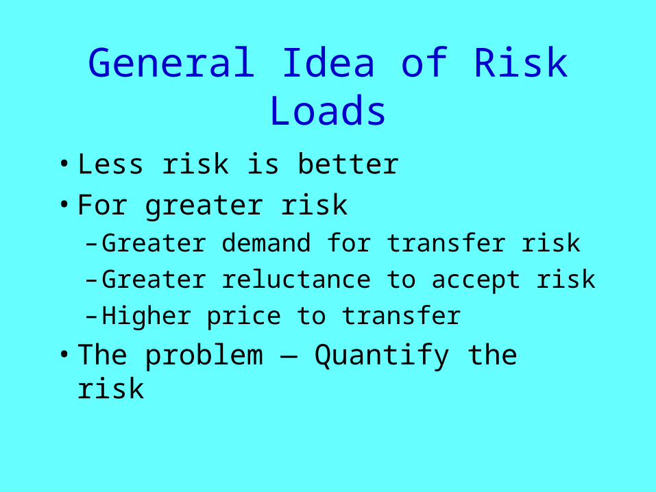
General Idea of Risk Loads
• Less risk is better
• For greater risk– Greater demand for transfer risk
– Greater reluctance to accept risk
– Higher price to transfer
• The problem — Quantify the risk
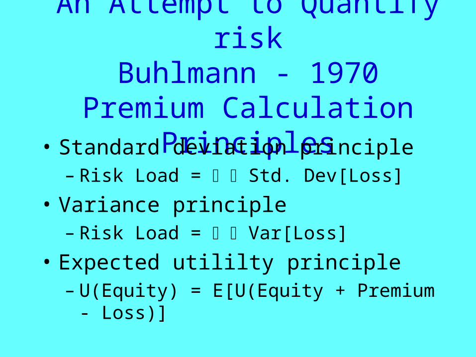
An Attempt to Quantify riskBuhlmann - 1970
Premium Calculation Principles• Standard deviation principle
– Risk Load = Std. Dev[Loss]
• Variance principle– Risk Load = Var[Loss]
• Expected utililty principle– U(Equity) = E[U(Equity + Premium - Loss)]

An Early (Late 70’s) Use of a Mathematical Formula
• ISO Increased Limits Ratemaking
• Used the Variance Principle
– Reference — Miccolis (PCAS 1977)– Replaced judgmental risk loads.
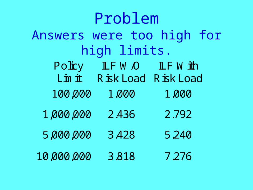
ProblemAnswers were too high for high limits.
PolicyLimit
ILF W/ORisk Load
ILF WithRisk Load
100,000 1.000 1.000
1,000,000 2.436 2.792
5,000,000 3.428 5.240
10,000,000 3.818 7.276
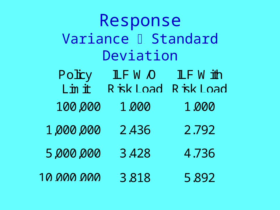
ResponseVariance Standard Deviation
PolicyLimit
ILF W/ORisk Load
ILF WithRisk Load
100,000 1.000 1.000
1,000,000 2.436 2.792
5,000,000 3.428 4.736
10,000,000 3.818 5.892

Capital Asset Pricing Model
• Designed for pricing securities
Where:
E R R R Rf M f a fR turn on the urity
R Risk free return
R Market return
Cov R R
Var R
f
M
M
M
Re sec
,
[ ]

Interpretation of CAPM
• If Cov[R,RM] = 0, then E[R] = Rf
• The market does not reward one for taking diversifiable risks.
• Systematic risk is taken when Cov[R,RM] > 0
• The market only rewards those who take on systematic risk.
• My reaction --
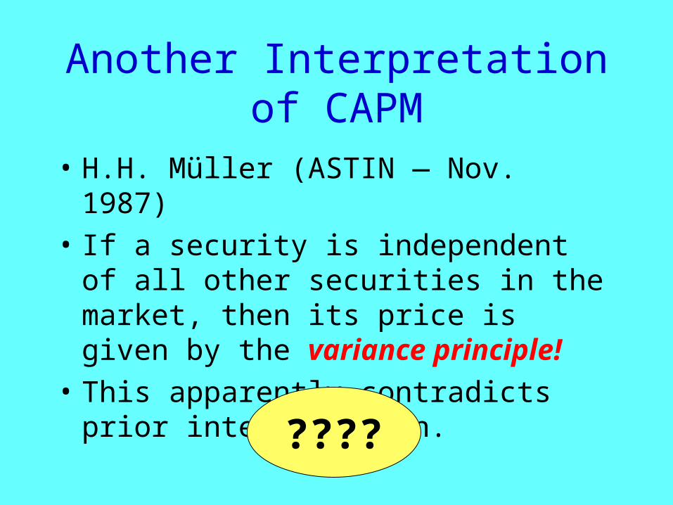
Another Interpretation of CAPM
• H.H. Müller (ASTIN — Nov. 1987)
• If a security is independent of all other securities in the market, then its price is given by the variance principle!
• This apparently contradicts prior interpretation.
????
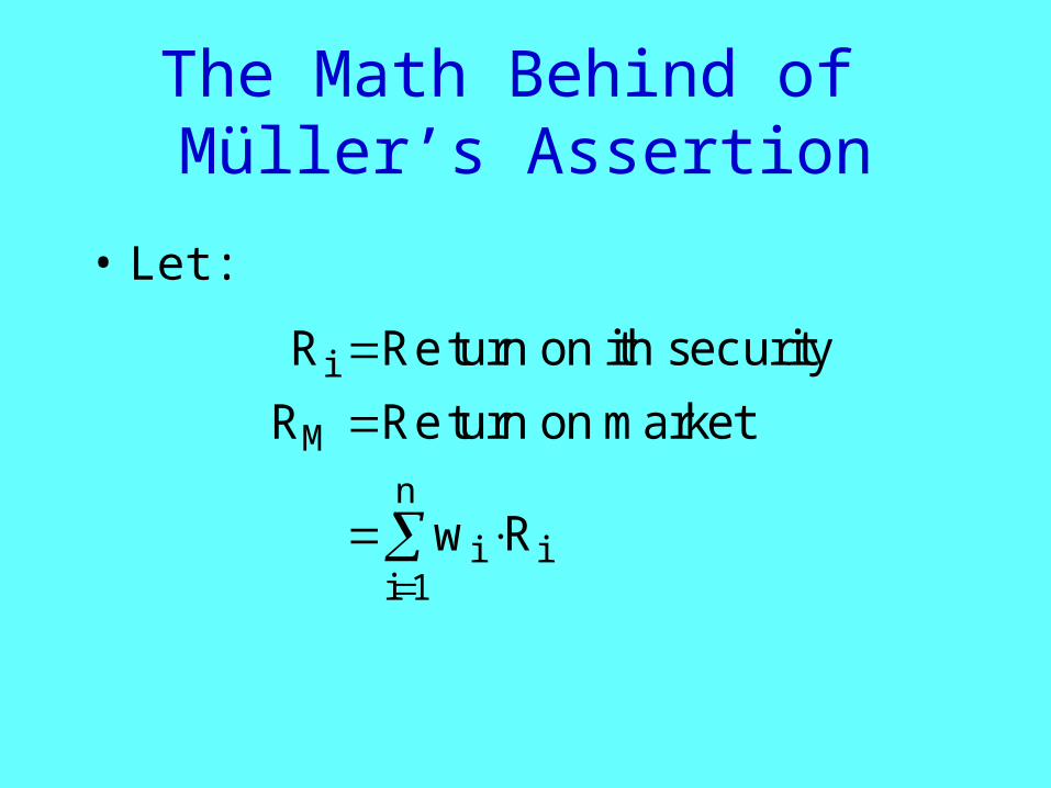
The Math Behind of Müller’s Assertion
• Let:
R turn on ith urity
R turn on market
w R
i
M
i ii
n
Re sec
Re
1
The Math Behind of Müller’s Assertion
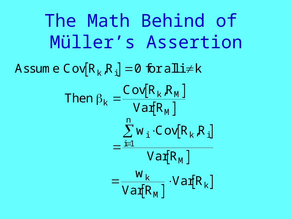
Assume Cov R R for all i kk i, 0
w
Var RVar Rk
Mk
w Cov R R
Var R
i k ii
n
M
,1
ThenCov R R
Var Rkk M
M
,
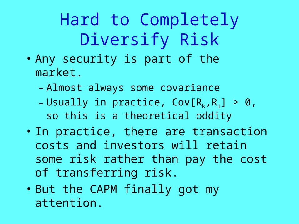
Hard to Completely Diversify Risk
• Any security is part of the market.– Almost always some covariance
– Usually in practice, Cov[Rk,Ri] > 0, so this is a theoretical oddity
• In practice, there are transaction costs and investors will retain some risk rather than pay the cost of transferring risk.
• But the CAPM finally got my attention.
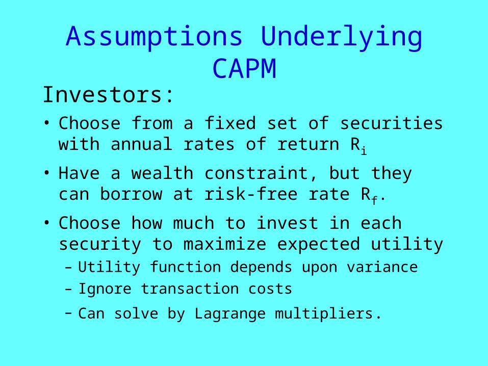
Assumptions Underlying CAPM
Investors:• Choose from a fixed set of securities with
annual rates of return Ri
• Have a wealth constraint, but they can borrow at risk-free rate Rf.
• Choose how much to invest in each security to maximize expected utility– Utility function depends upon variance– Ignore transaction costs
– Can solve by Lagrange multipliers.
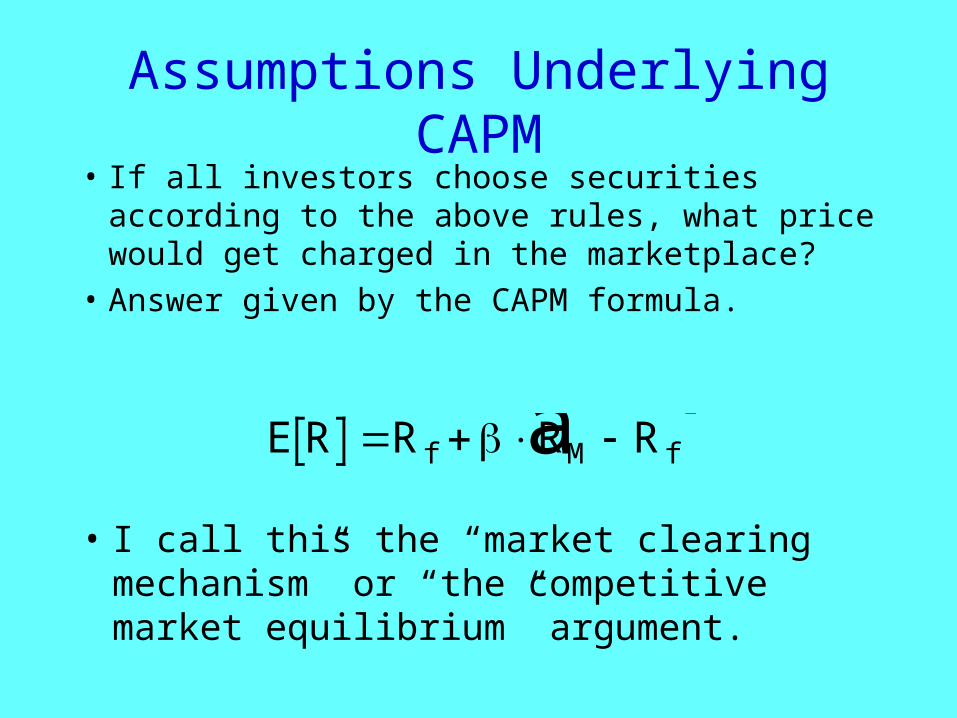
Assumptions Underlying CAPM• If all investors choose securities according
to the above rules, what price would get charged in the marketplace?
• Answer given by the CAPM formula.
• I call this the “market clearing mechanism” or “the competitive market equilibrium” argument.
E R R R Rf M f a f
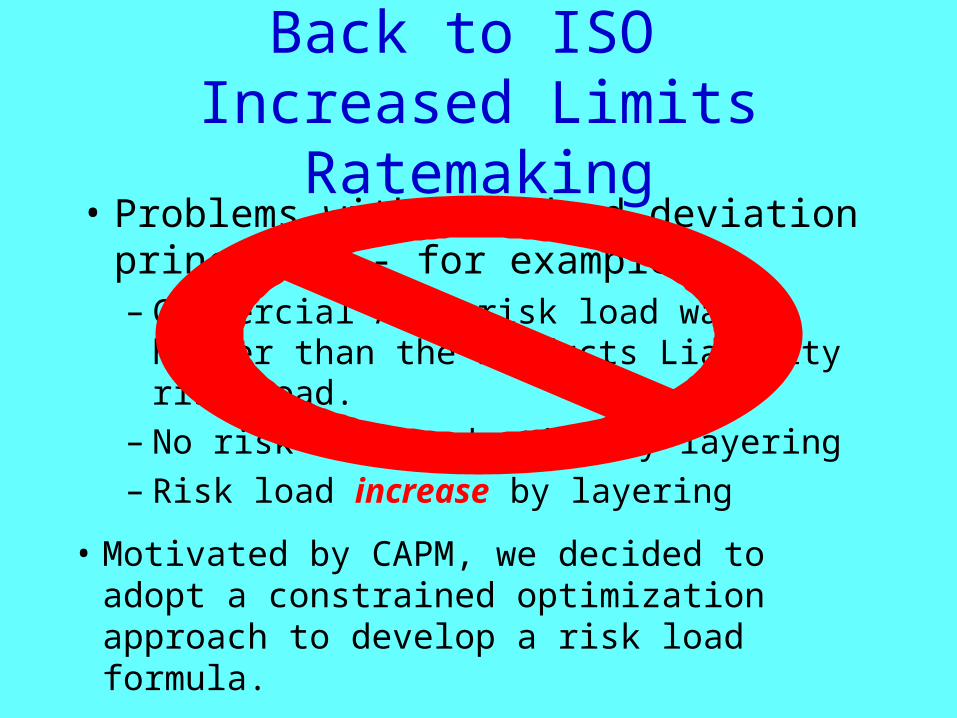
Back to ISO Increased Limits Ratemaking
• Problems with standard deviation principle -- for example:– Commercial Auto risk load was higher than
the Products Liability risk load.– No risk load reduction by layering– Risk load increase by layering
• Motivated by CAPM, we decided to adopt a constrained optimization approach to develop a risk load formula.
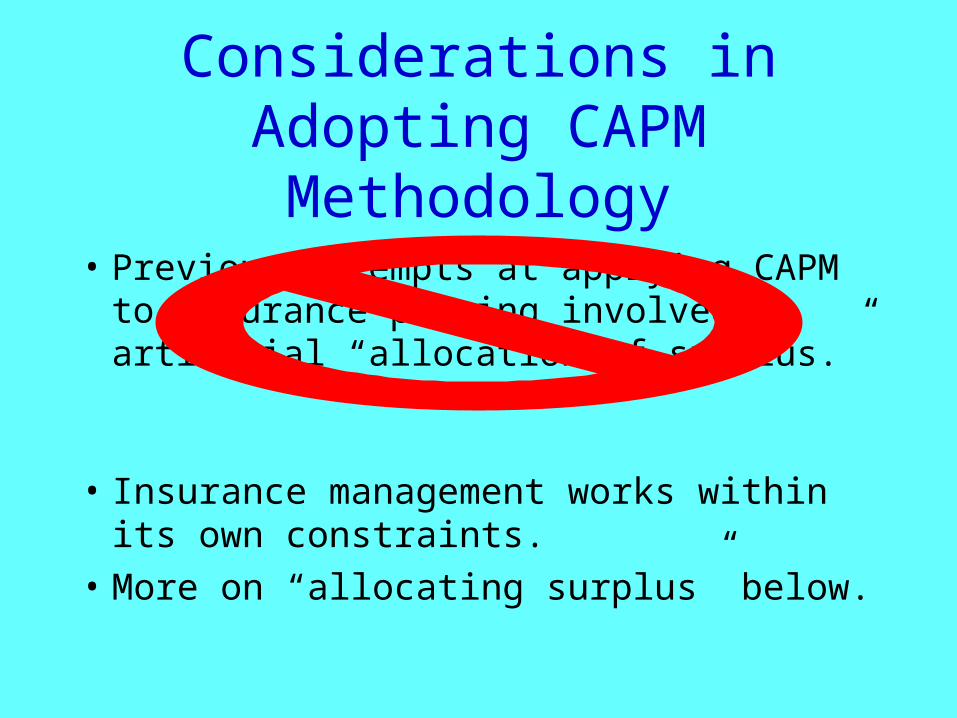
Considerations in Adopting CAPM Methodology
• Previous attempts at applying CAPM to insurance pricing involved an artificial “allocation of surplus.”
• Insurance management works within its own constraints.
• More on “allocating surplus” below.
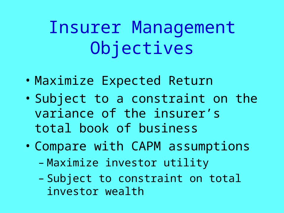
Insurer Management Objectives
• Maximize Expected Return
• Subject to a constraint on the variance of the insurer’s total book of business
• Compare with CAPM assumptions– Maximize investor utility– Subject to constraint on total investor
wealth
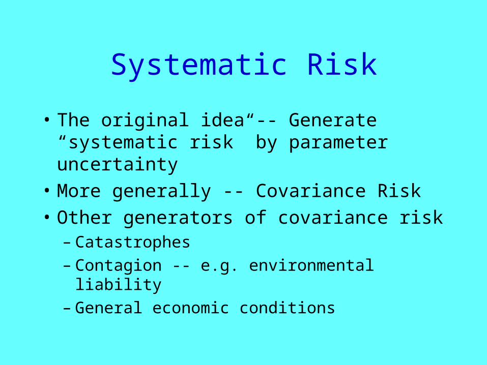
Systematic Risk
• The original idea -- Generate “systematic risk” by parameter uncertainty
• More generally -- Covariance Risk• Other generators of covariance risk
– Catastrophes– Contagion -- e.g. environmental liability– General economic conditions
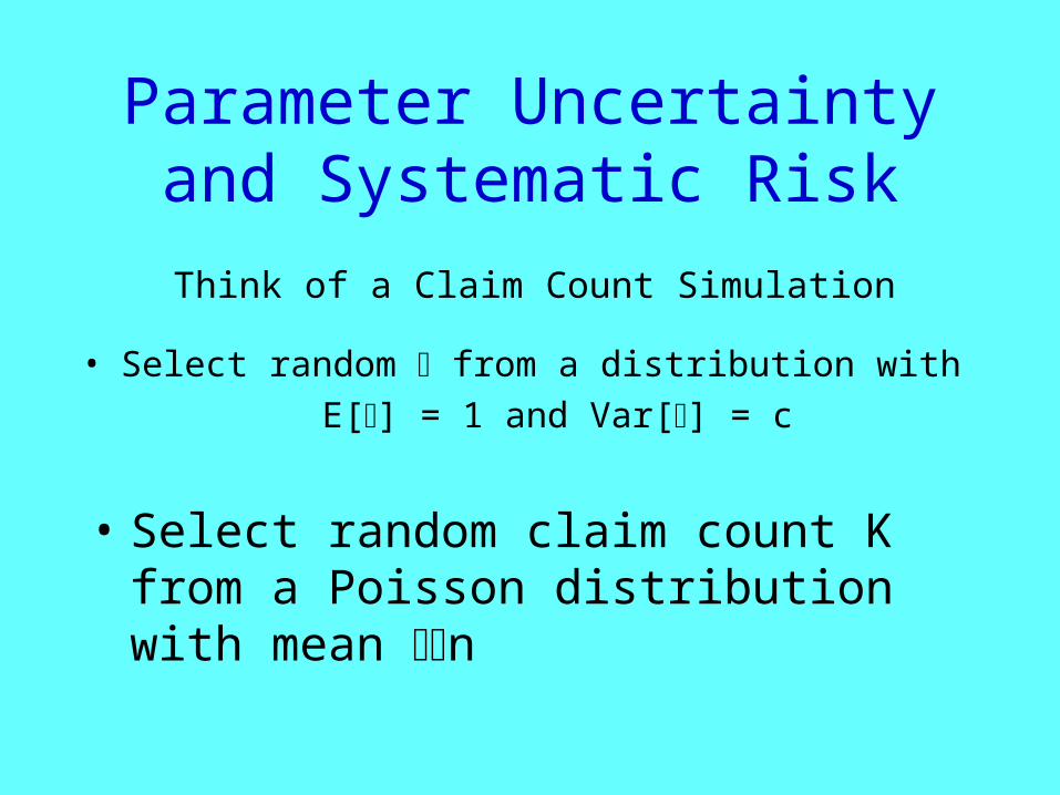
Parameter Uncertainty and Systematic Risk
• Select random from a distribution with
E[] = 1 and Var[] = c
• Select random claim count K from a Poisson distribution with mean n
Think of a Claim Count Simulation
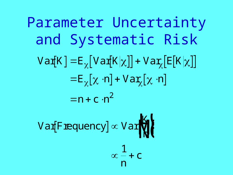
Parameter Uncertainty and Systematic Risk
Var K E Var K Var E K
E n Var n
n c n
2
Var Frequency VarKn
nc
LNMOQP
1
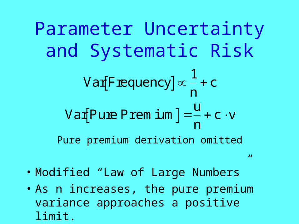
Parameter Uncertainty and Systematic Risk
Pure premium derivation omitted
• Modified “Law of Large Numbers”
• As n increases, the pure premium variance approaches a positive limit.
Var Frequencyn
c 1
Var Pure emiumun
c vPr
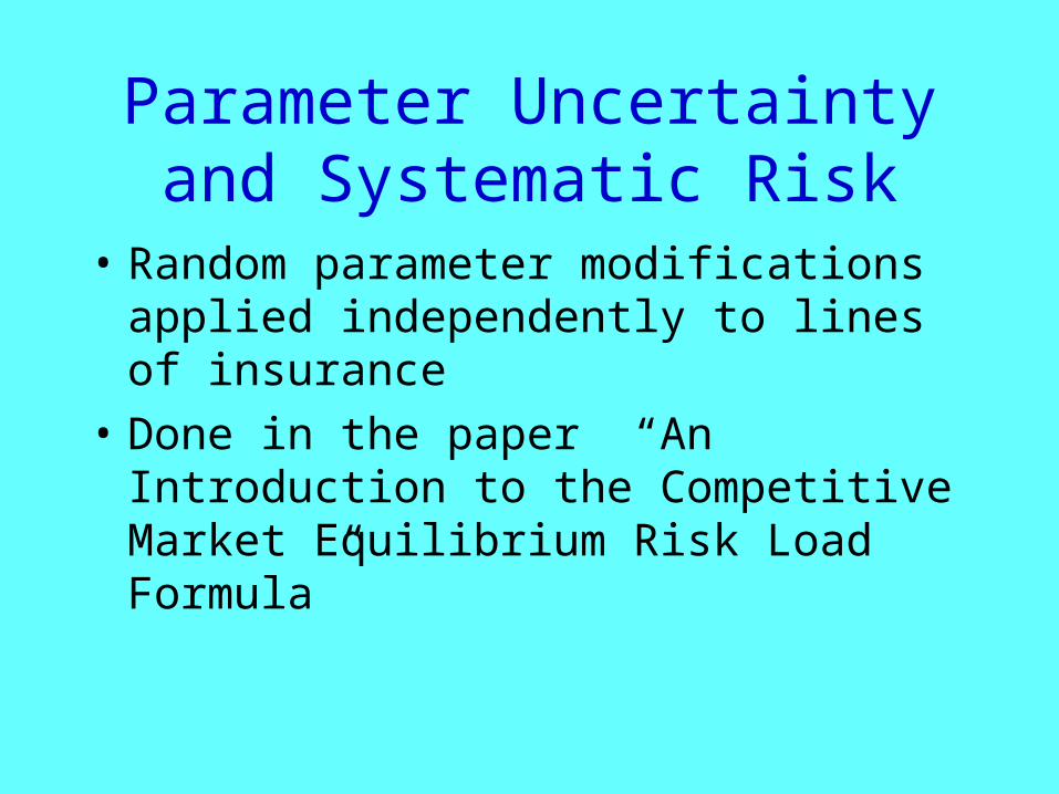
Parameter Uncertainty and Systematic Risk
• Random parameter modifications applied independently to lines of insurance
• Done in the paper “An Introduction to the Competitive Market Equilibrium Risk Load Formula”
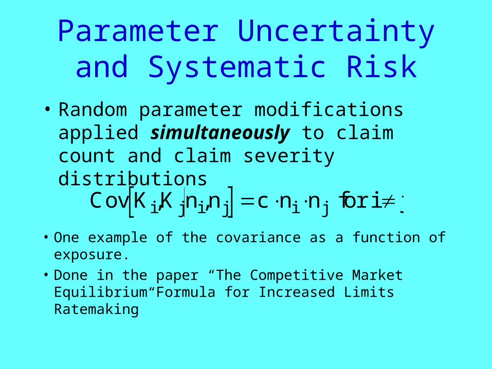
Parameter Uncertainty and Systematic Risk
• Random parameter modifications applied simultaneously to claim count and claim severity distributions
• One example of the covariance as a function of exposure.
• Done in the paper “The Competitive Market Equilibrium Formula for Increased Limits Ratemaking”
Cov K K n n c n n for i ji j i j i j, ,
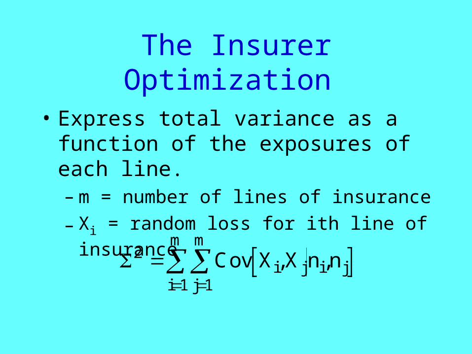
The Insurer Optimization
• Express total variance as a function of the exposures of each line.– m = number of lines of insurance
– Xi = random loss for ith line of insurance
2
11
Cov X X n ni j i jj
m
i
m
, ,

The Insurer Optimization
Subject to the constraint that:
2
11
Cov X X n ni j i jj
m
i
m
, ,
Maximize total expected return:
n ri ii
m
1
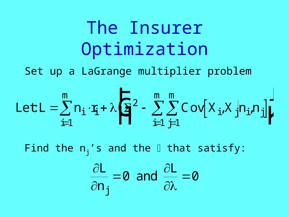
The Insurer Optimization
Set up a LaGrange multiplier problem
Let L n r Cov X X n ni i i j i jj
m
i
m
i
m
: , , FHG
IKJ
2
111
Find the nj’s and the that satisfy:
Ln
andL
j0 0

Solution for Independent Lines
The message:
These equations are solvable.
n
ru
vi
ii
i
12
rv
uv
i
ii
m
i
ii
m
2
1
22
1
4
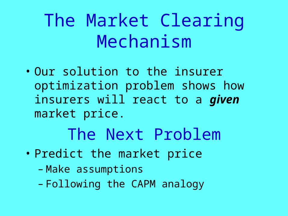
The Market Clearing Mechanism
• Our solution to the insurer optimization problem shows how insurers will react to a given market price.
The Next Problem• Predict the market price
– Make assumptions– Following the CAPM analogy
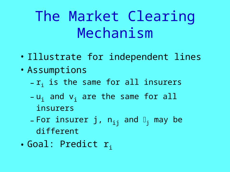
The Market Clearing Mechanism
• Illustrate for independent lines
• Assumptions– ri is the same for all insurers
– ui and vi are the same for all insurers
– For insurer j, nij and j may be different
• Goal: Predict ri
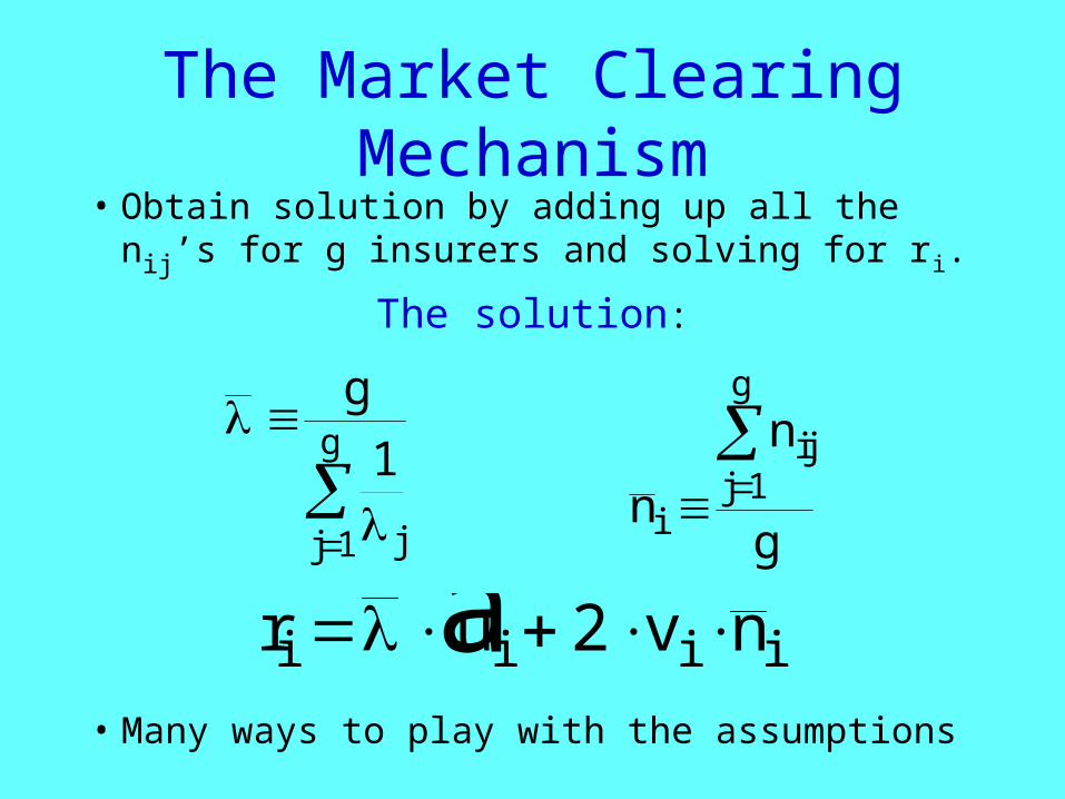
The Market Clearing Mechanism
• Obtain solution by adding up all the nij’s
for g insurers and solving for ri.
The solution:
g
jj
g 1
1n
n
gi
ijj
g
1
r u v ni i i i 2a f• Many ways to play with the assumptions
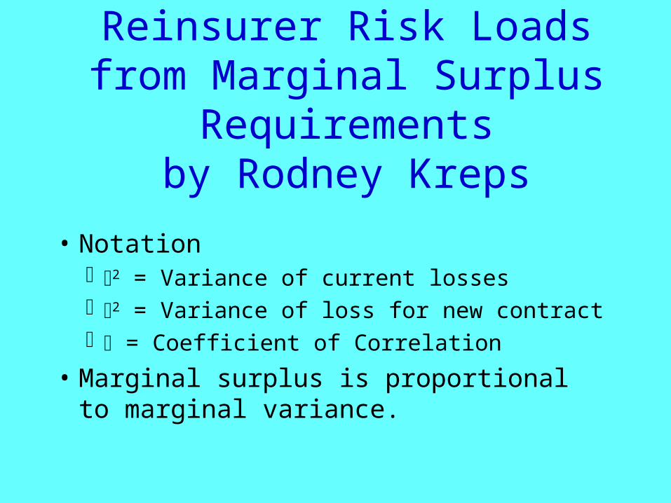
Reinsurer Risk Loads from Marginal Surplus Requirements
by Rodney Kreps
• Notation 2 = Variance of current losses 2 = Variance of loss for new contract = Coefficient of Correlation
• Marginal surplus is proportional to marginal variance.
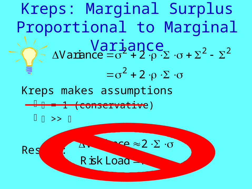
Kreps: Marginal Surplus Proportional to Marginal Variance
Kreps makes assumptions = 1 (conservative) >>
Result:
Variance
2 2 2
2
2
2
Variance
Risk Load
2 R
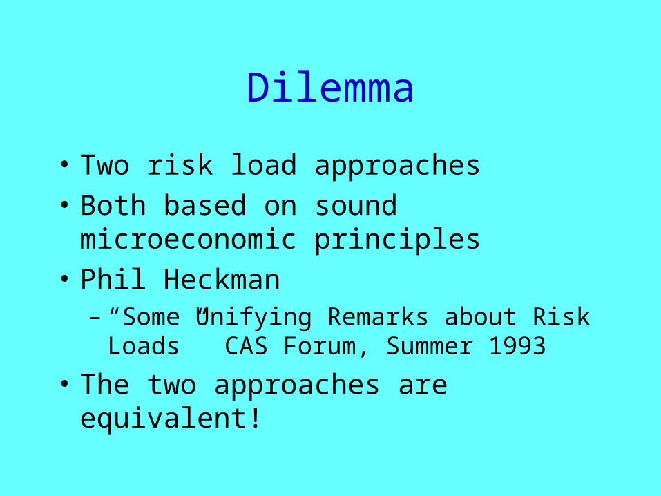
Dilemma
• Two risk load approaches
• Both based on sound microeconomic principles
• Phil Heckman– “Some Unifying Remarks about Risk
Loads” CAS Forum, Summer 1993
• The two approaches are equivalent!
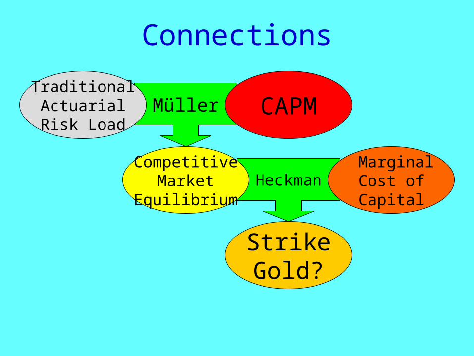
Connections
StrikeGold?
MüllerTraditional Actuarial Risk Load
CAPM
HeckmanCompetitive
Market Equilibrium
MarginalCost ofCapital

Joining Two Rich Traditions
Stochastic Models• Collective Risk Model
– Claim Frequency– Claim Severity– Parameter Risk– Process Risk
• Catastrophe Models• Covariance Structures
Financial Models• Time value of money• Make comparisons
with non-insurance risks
• Additional risk financing Instruments– Reinsurance– Securitization
ActuarialTheory of Risk
Cost ofCapitalDFA
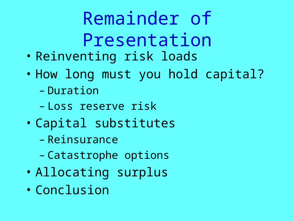
Remainder of Presentation
• Reinventing risk loads
• How long must you hold capital?– Duration– Loss reserve risk
• Capital substitutes– Reinsurance– Catastrophe options
• Allocating surplus
• Conclusion
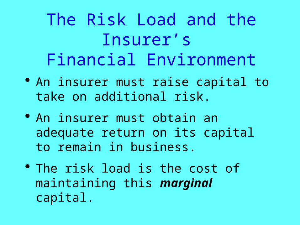
The Risk Load and the Insurer’s Financial Environment
An insurer must raise capital to take on additional risk.
An insurer must obtain an adequate return on its capital to remain in business.
The risk load is the cost of maintaining this marginal capital.
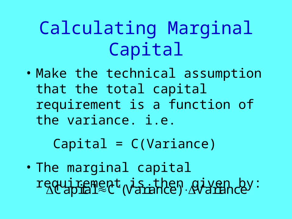
Calculating Marginal Capital
• Make the technical assumption that the total capital requirement is a function of the variance. i.e.
Capital = C(Variance)
• The marginal capital requirement is then given by:
Capital C Variance Variance ( )
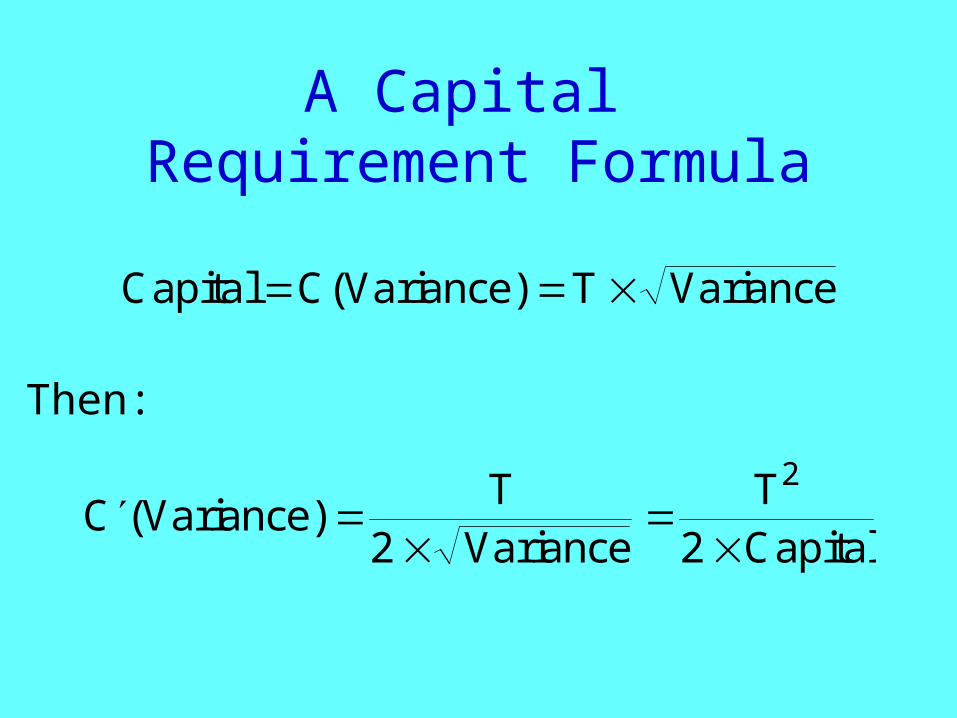
A Capital Requirement Formula
Then:
Capital C Variance T Variance ( )
C VarianceT
VarianceTCapital
( )2 2
2
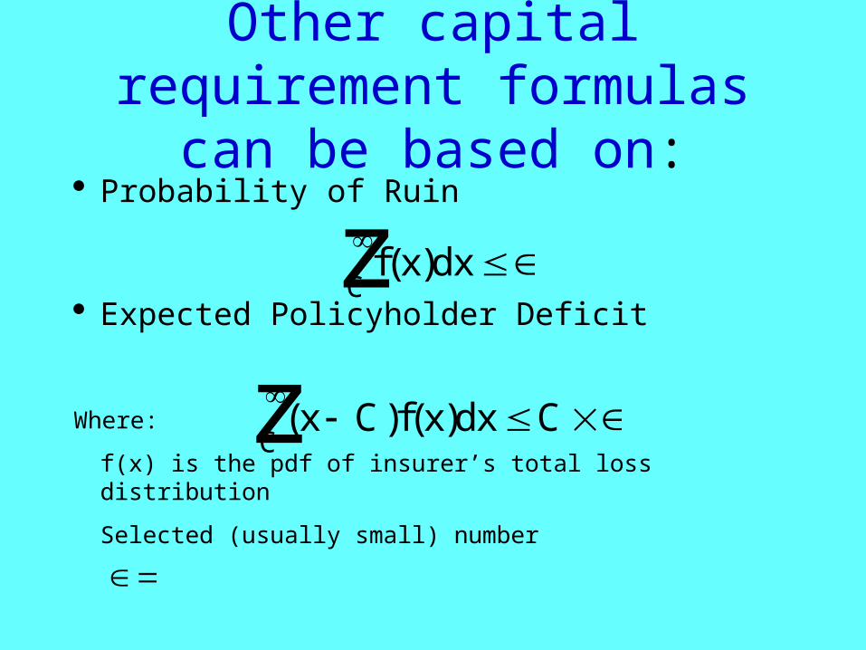
Other capital requirement formulas can be based on:
Probability of Ruin
Expected Policyholder Deficit
Where:
f(x) is the pdf of insurer’s total loss distribution
Selected (usually small) number
f x dxC
( )z
( ) ( )x C f x dx CC
z
Marginal Variance
Cov X X Cov X X
Cov X X Cov X X
n
n n n
1 1 1
1
, ,
, ,
Cov Y X Cov Y Xn, ,1
Cov X Y
Cov X Yn
1,
,
Cov Y Y,
Original Variance
Cov X Xi jj
n
i
n
,
11
Variance
Var Y Cov X Yii
n
[ ] , 2
1
{X}’s - Current Contracts Y - New Contract

Variance Depends on Existing Business
• If Y is the loss on the first contract
Variance = Var[Y]
• If Y is the loss on the second contract
Variance = Var[Y] + 2 Cov[X1,Y]
• If Y is the loss on the nth contract
Variance = Var[Y] + 2 Cov X Yi
n
i
1
1
[ , ]
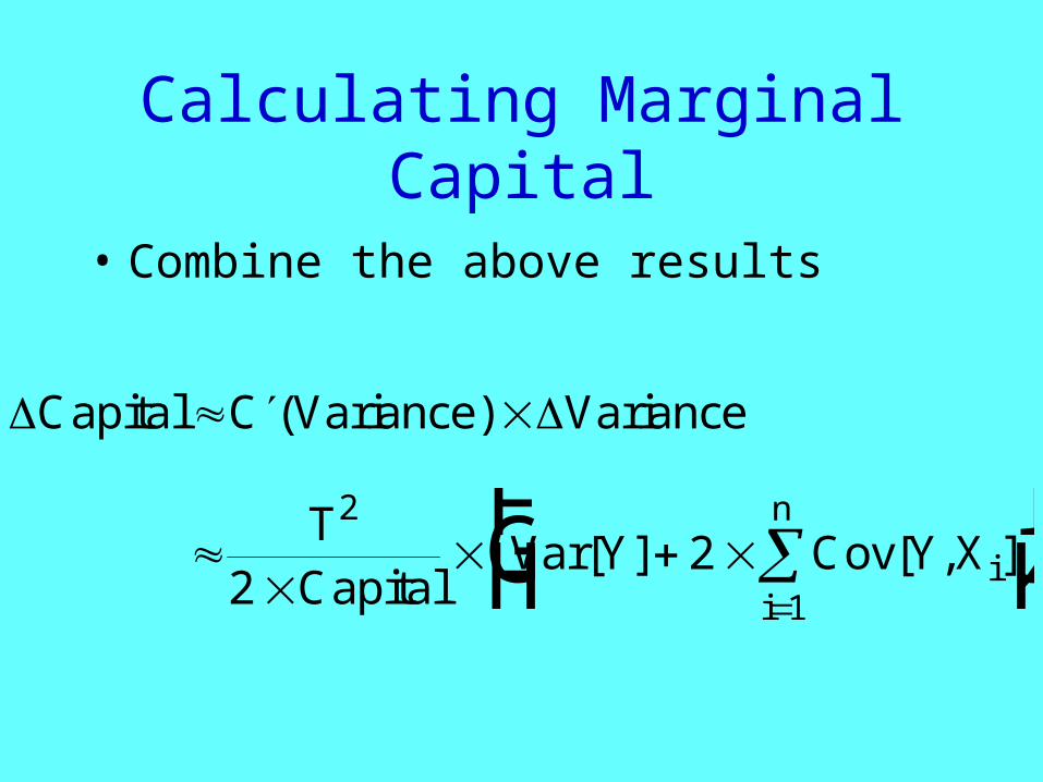
Calculating Marginal Capital
• Combine the above results
Capital C Variance Variance ( )
FHG
IKJ
TCapital
Var Y Cov Y Xii
n2
122[ ] [ , ]
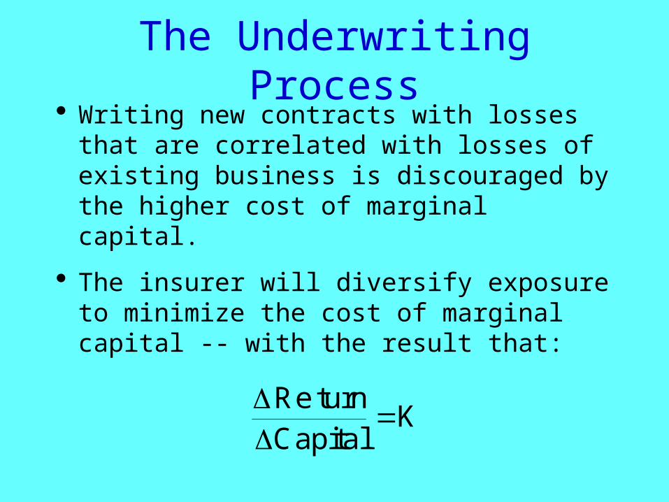
The Underwriting Process Writing new contracts with losses that
are correlated with losses of existing business is discouraged by the higher cost of marginal capital.
The insurer will diversify exposure to minimize the cost of marginal capital -- with the result that:
ReturnCapital
K
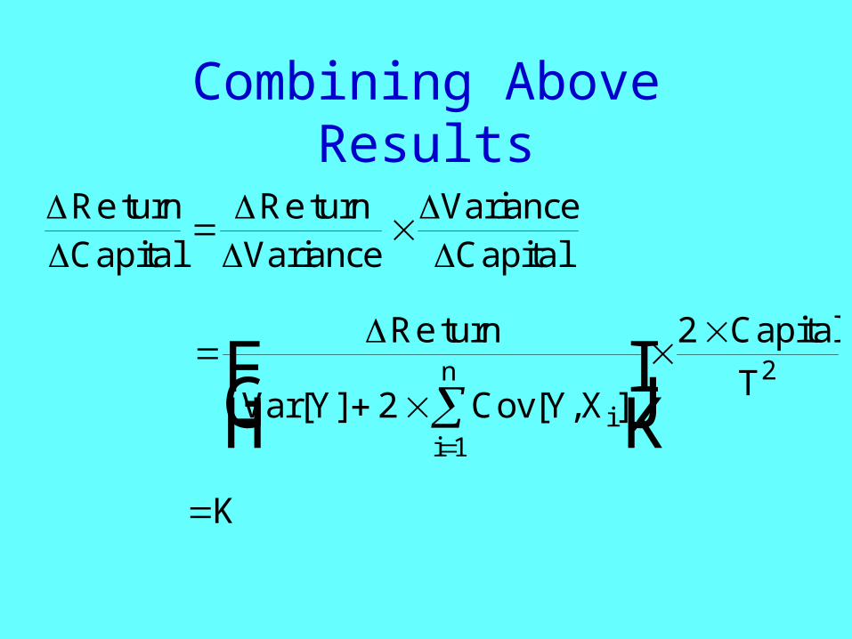
Combining Above Results
K
FHG
IKJ
Re
[ ] [ , ]
turn
Var Y Cov Y X
Capital
Ti
i
n
2
2
1
2
Re ReturnCapital
turnVariance
VarianceCapital

Continuing the Math
Risk Load turn
KTCapital
Var Y Cov Y X
Var Y Cov Y X
Where Risk Load Multiplier
ii
n
ii
n
FHG
IKJ
FHG
IKJ
Re
[ ] [ , ]
[ ] [ , ]
2
1
1
22
2
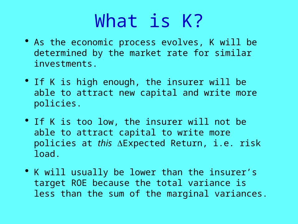
What is K? As the economic process evolves, K will be
determined by the market rate for similar investments.
If K is high enough, the insurer will be able to attract new capital and write more policies.
If K is too low, the insurer will not be able to attract capital to write more policies at this Expected Return, i.e. risk load.
K will usually be lower than the insurer’s target ROE because the total variance is less than the sum of the marginal variances.
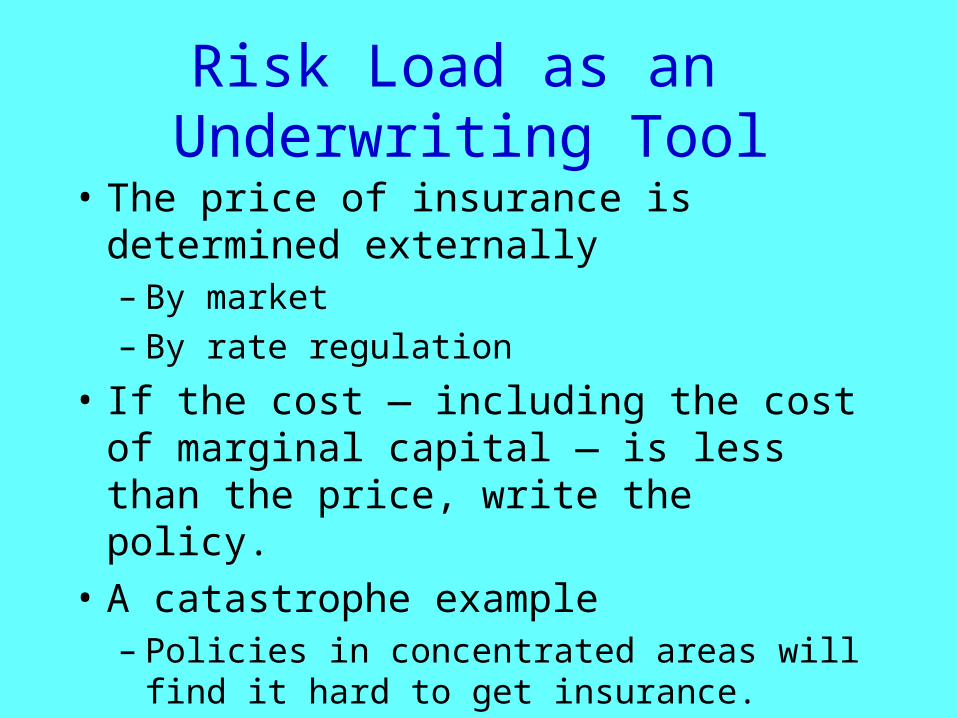
Risk Load as an Underwriting Tool
• The price of insurance is determined externally– By market– By rate regulation
• If the cost — including the cost of marginal capital — is less than the price, write the policy.
• A catastrophe example– Policies in concentrated areas will find it
hard to get insurance.
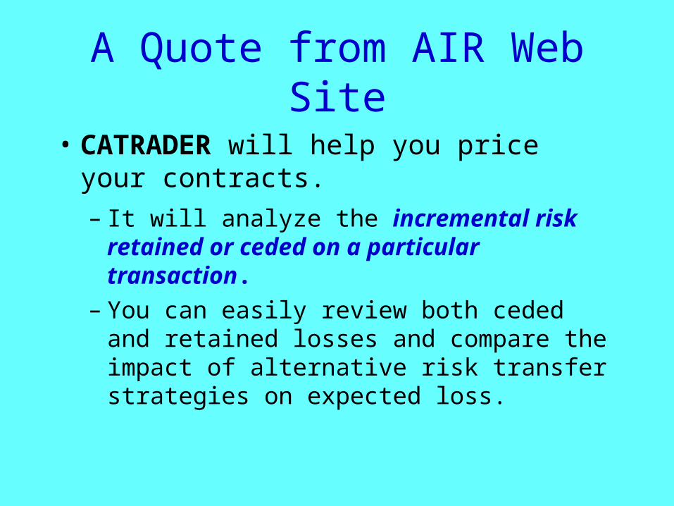
A Quote from AIR Web Site
• CATRADER will help you price your contracts.
– It will analyze the incremental risk retained or ceded on a particular transaction.
– You can easily review both ceded and retained losses and compare the impact of alternative risk transfer strategies on expected loss.
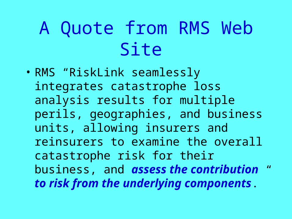
A Quote from RMS Web Site
• RMS “RiskLink seamlessly integrates catastrophe loss analysis results for multiple perils, geographies, and business units, allowing insurers and reinsurers to examine the overall catastrophe risk for their business, and assess the contribution to risk from the underlying components.”
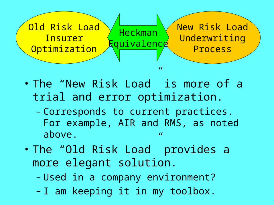
• The “New Risk Load” is more of a trial and error optimization.– Corresponds to current practices. For
example, AIR and RMS, as noted above.
• The “Old Risk Load” provides a more elegant solution.– Used in a company environment?– I am keeping it in my toolbox.
New Risk LoadUnderwriting
Process
Old Risk LoadInsurer
Optimization
HeckmanEquivalence
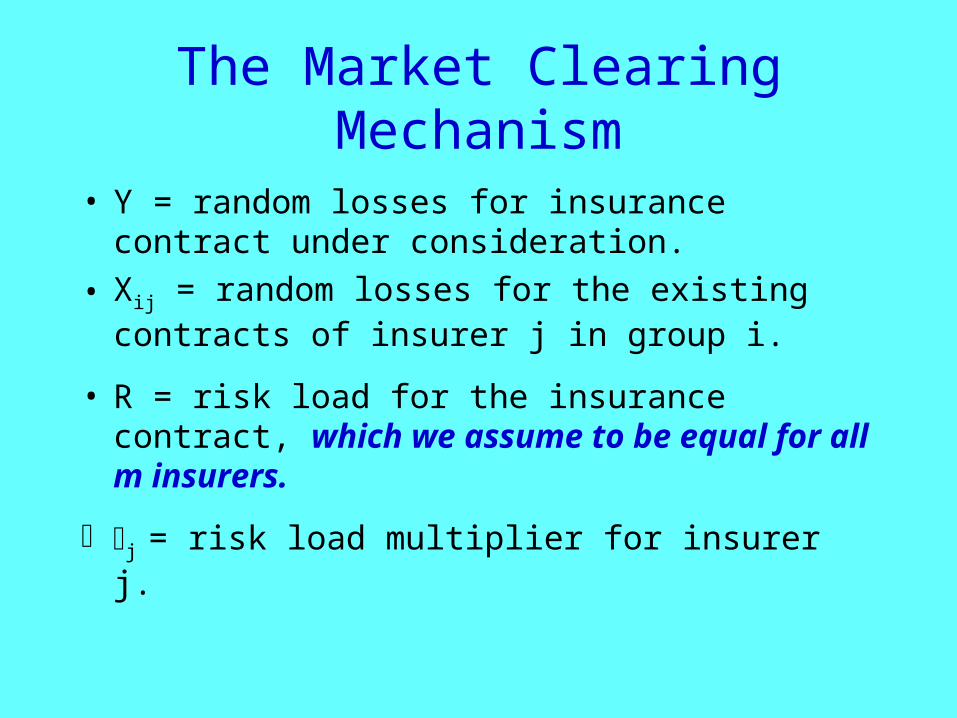
The Market Clearing Mechanism
• Y = random losses for insurance contract under consideration.
• Xij = random losses for the existing contracts of insurer j in group i.
• R = risk load for the insurance contract, which we assume to be equal for all m insurers.
j = risk load multiplier for insurer j.
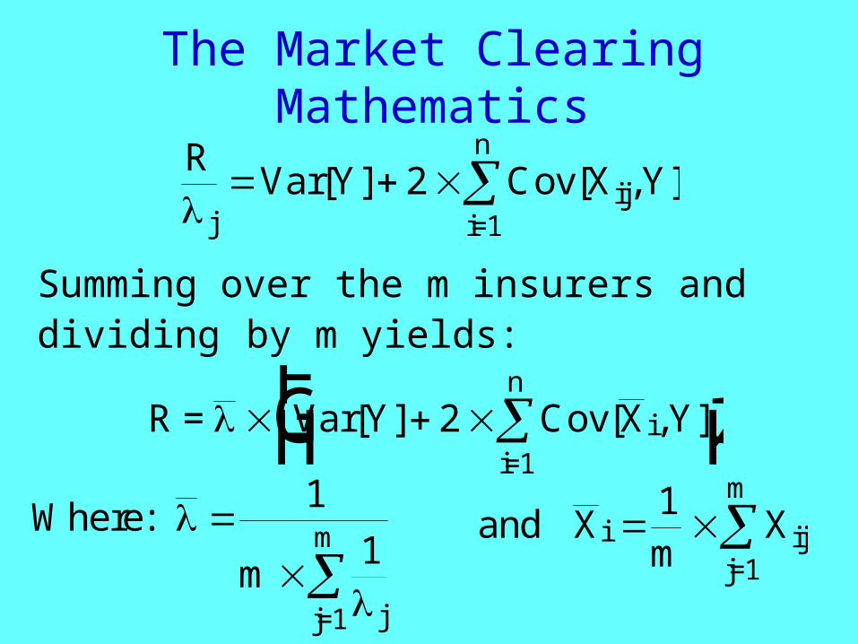
The Market Clearing Mathematics
RVar[ Cov[
jij
i=1
n
Y X Y] , ]2
R = Var[ Cov[ ii=1
n
FHG
IKJY X Y] , ]2
Where
m
:
1
1
jj=1
m and X Xi ijj=1
m
m 1
Summing over the m insurers and dividing by m yields:

Some comments about the market clearing concept
• It came from the CAPM• It is probably about as good as the
CAPM is in predicting security prices.• It fails to account for relevant facts.
– Capital must be held longer for some lines of insurance.
– Risk can be transferred — at a cost
• I am keeping it in my toolbox.
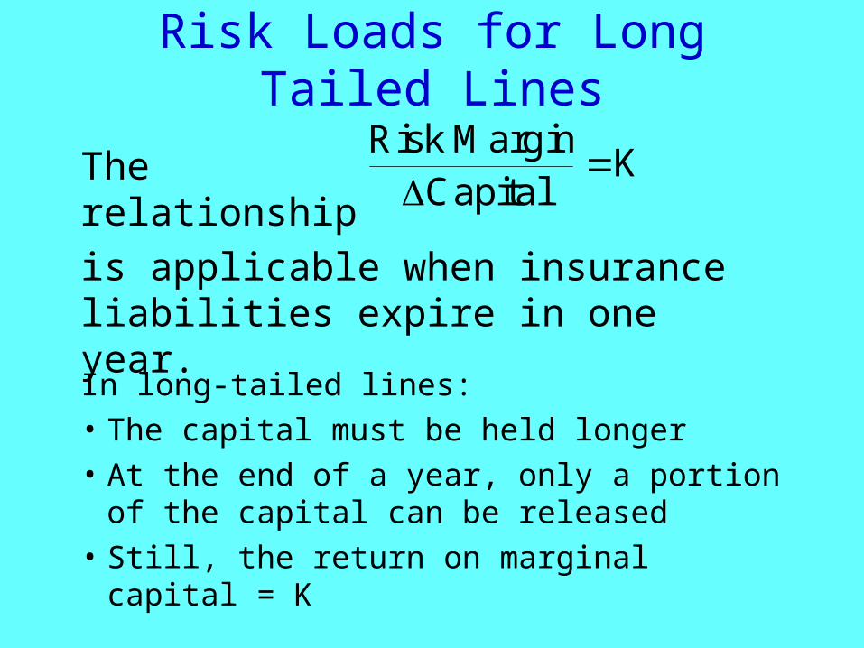
Risk Loads for Long Tailed Lines
Risk M inCapital
Karg
The relationship
is applicable when insurance liabilities expire in one year.
In long-tailed lines:
• The capital must be held longer
• At the end of a year, only a portion of the capital can be released
• Still, the return on marginal capital = K
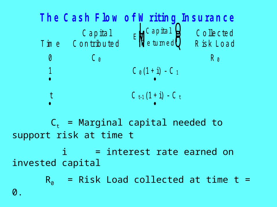
T h e C a s h F l o w o f W r i t i n g I n s u r a n c e
T im eC a p i t a l
C o n t r ib u t e dE
C a p i t a l
t u r n e dR e
LNM
OQP
C o l le c t e dR is k L o a d
0 C 0 R 0
1 C 0 ( 1 + i ) - C 1
t C t - 1 ( 1 + i ) - C t
Ct = Marginal capital needed to support risk at time t
i = interest rate earned on invested capital
R0 = Risk Load collected at time t = 0.
Choose R0 so that
C0 = R0 + Present Value (E[Capital Returned] ) at rate K
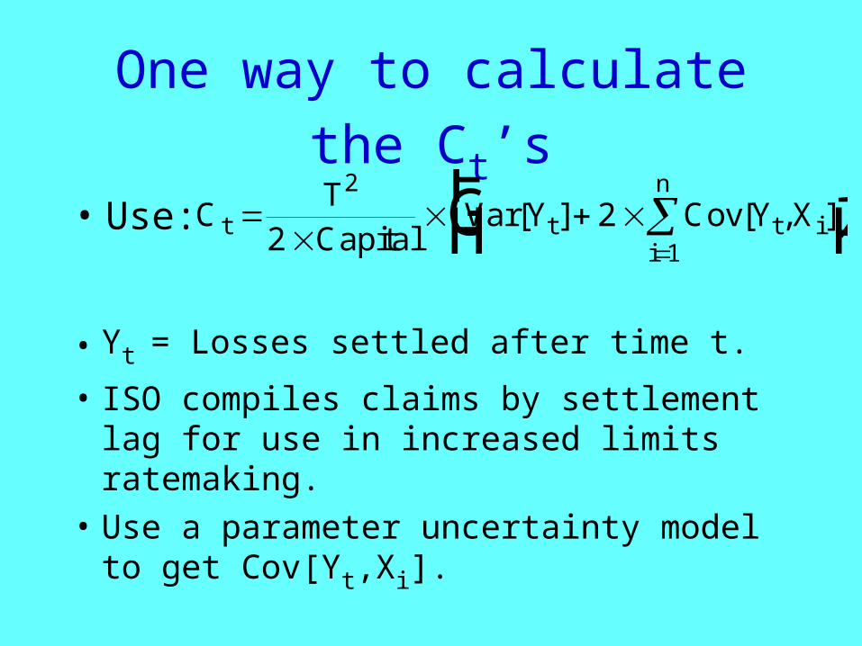
One way to calculate the Ct’s
• Use:
• Yt = Losses settled after time t.
• ISO compiles claims by settlement lag for use in increased limits ratemaking.
• Use a parameter uncertainty model to get Cov[Yt,Xi].
CTCapital
Var Y Cov Y Xt t t ii
n
FHG
IKJ
2
122[ ] [ , ]
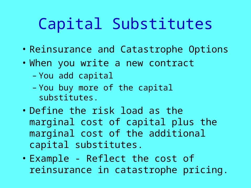
• Reinsurance and Catastrophe Options
• When you write a new contract– You add capital– You buy more of the capital substitutes.
• Define the risk load as the marginal cost of capital plus the marginal cost of the additional capital substitutes.
• Example - Reflect the cost of reinsurance in catastrophe pricing.
Capital Substitutes
Capital Substitutes
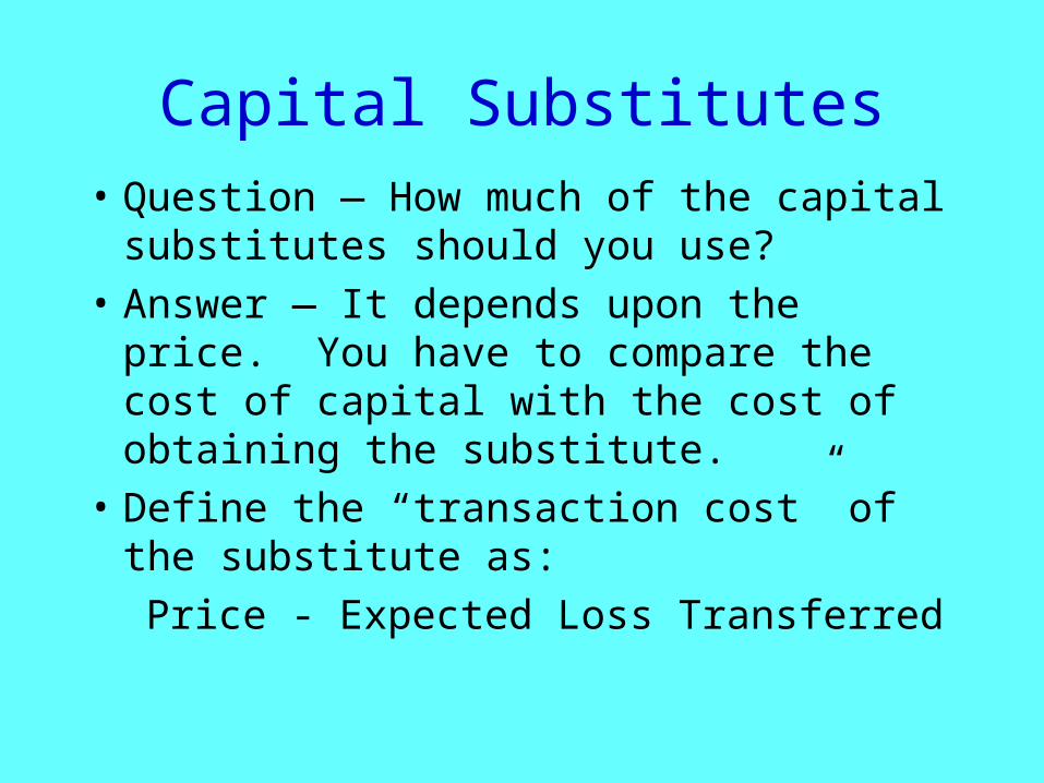
• Question — How much of the capital substitutes should you use?
• Answer — It depends upon the price. You have to compare the cost of capital with the cost of obtaining the substitute.
• Define the “transaction cost” of the substitute as:
Price - Expected Loss Transferred
Current State of Affairs
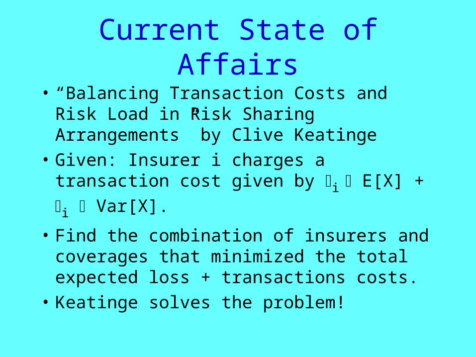
• “Balancing Transaction Costs and Risk Load in Risk Sharing Arrangements” by Clive Keatinge
• Given: Insurer i charges a transaction cost given by i E[X] + i Var[X].
• Find the combination of insurers and coverages that minimized the total expected loss + transactions costs.
• Keatinge solves the problem!
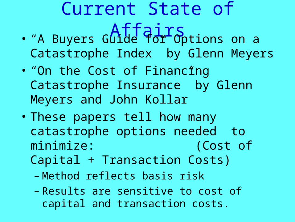
Current State of Affairs• “A Buyers Guide for Options on a
Catastrophe Index” by Glenn Meyers
• “On the Cost of Financing Catastrophe Insurance” by Glenn Meyers and John Kollar
• These papers tell how many catastrophe options needed to minimize: (Cost of Capital + Transaction Costs)– Method reflects basis risk– Results are sensitive to cost of capital and
transaction costs.
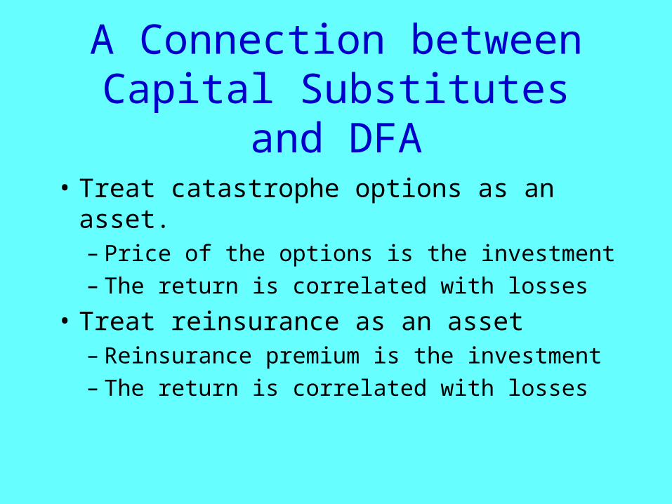
A Connection between Capital Substitutes and DFA
• Treat catastrophe options as an asset.– Price of the options is the investment– The return is correlated with losses
• Treat reinsurance as an asset– Reinsurance premium is the investment– The return is correlated with losses
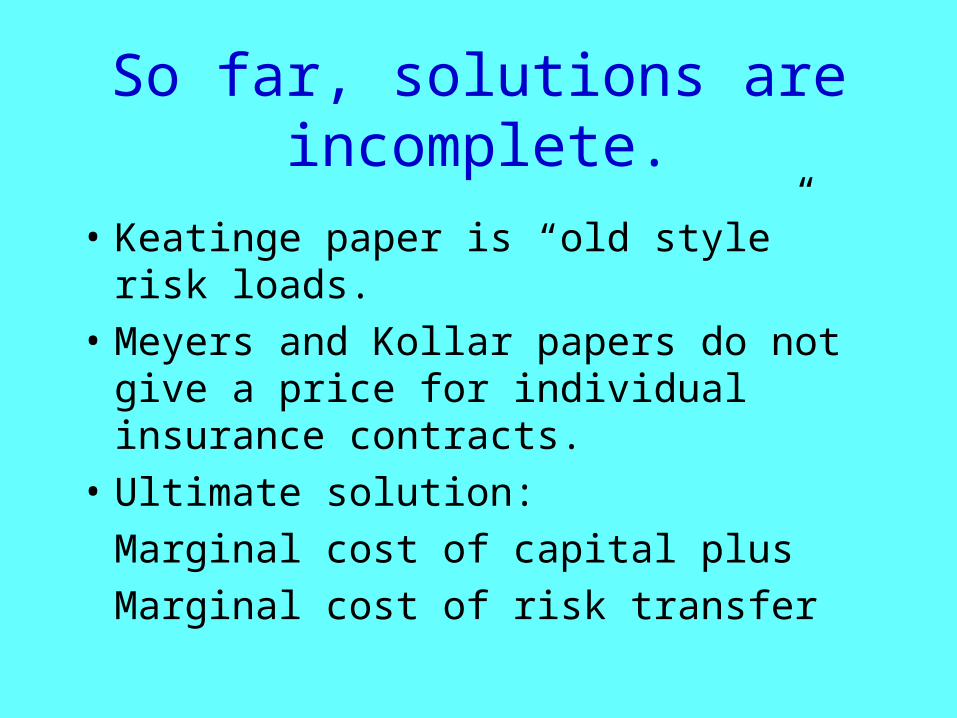
So far, solutions are incomplete.
• Keatinge paper is “old style” risk loads.
• Meyers and Kollar papers do not give a price for individual insurance contracts.
• Ultimate solution:
Marginal cost of capital plus
Marginal cost of risk transfer
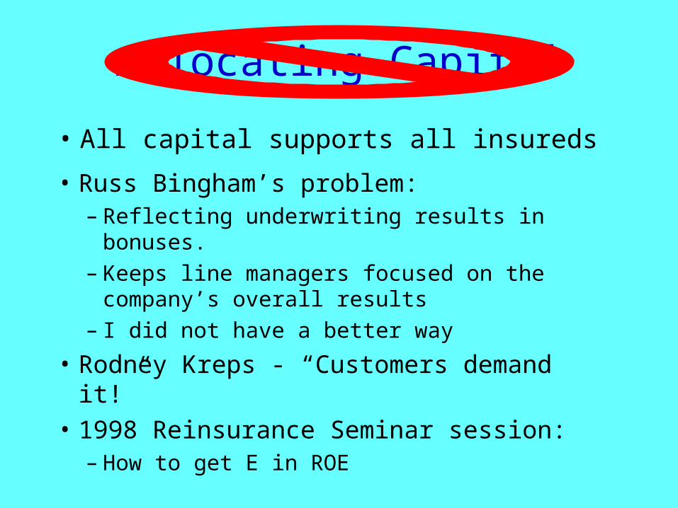
Allocating Capital
• All capital supports all insureds
• Russ Bingham’s problem:– Reflecting underwriting results in bonuses.– Keeps line managers focused on the
company’s overall results– I did not have a better way
• Rodney Kreps - “Customers demand it!”
• 1998 Reinsurance Seminar session:– How to get E in ROE
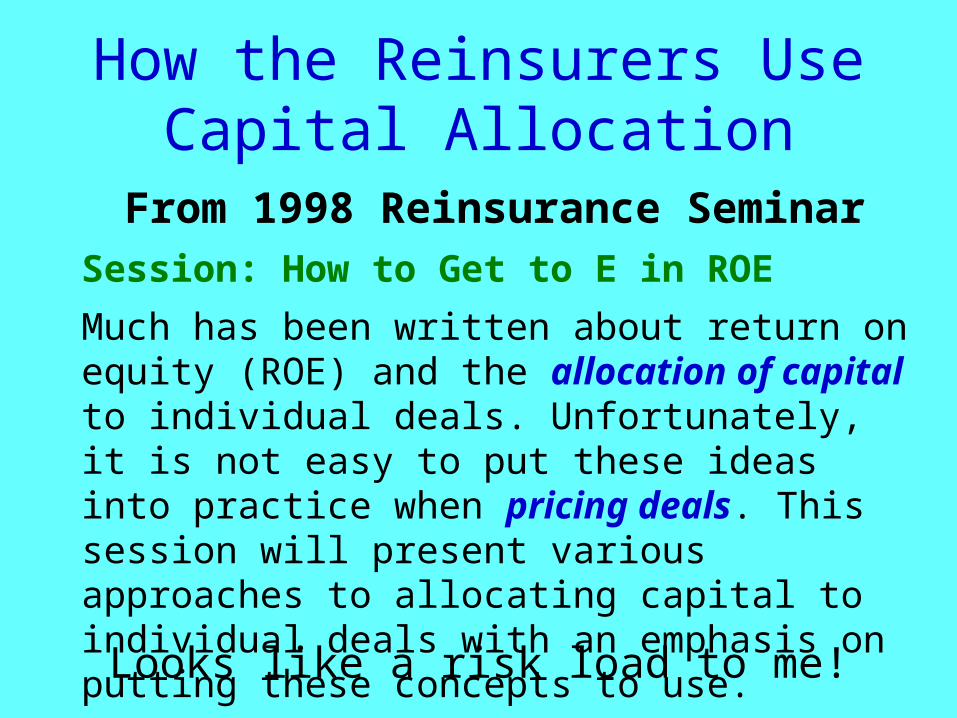
How the Reinsurers Use Capital Allocation
From 1998 Reinsurance SeminarSession: How to Get to E in ROE
Much has been written about return on equity (ROE) and the allocation of capital to individual deals. Unfortunately, it is not easy to put these ideas into practice when pricing deals. This session will present various approaches to allocating capital to individual deals with an emphasis on putting these concepts to use.
Looks like a risk load to me!
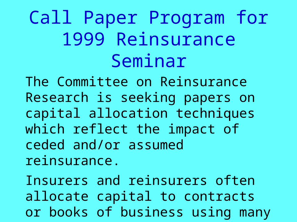
Call Paper Program for 1999 Reinsurance Seminar
The Committee on Reinsurance Research is seeking papers on capital allocation techniques which reflect the impact of ceded and/or assumed reinsurance.
Insurers and reinsurers often allocate capital to contracts or books of business using many different risk measures as the basis for making those allocations.

(Continued)Possible areas the papers could
address include but are not limited to:
• How long capital is allocated for and how it is released over time
• Cost of the allocated capital
• Alternative forms of capital
• The impact on pricing decisions
• How correlation is reflected
• Others
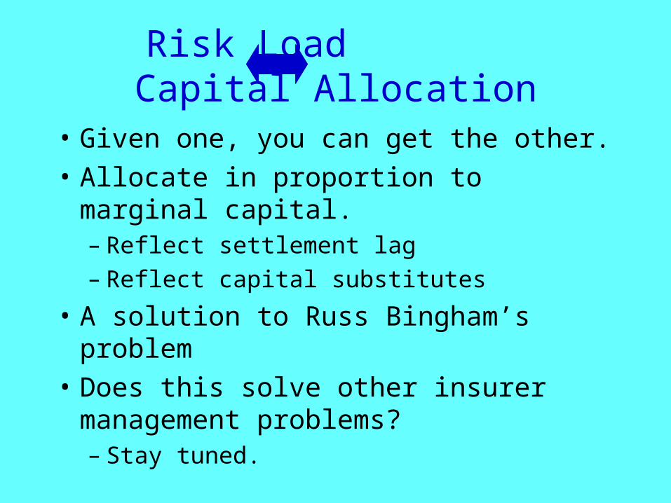
Risk Load Capital Allocation
• Given one, you can get the other.
• Allocate in proportion to marginal capital.– Reflect settlement lag– Reflect capital substitutes
• A solution to Russ Bingham’s problem
• Does this solve other insurer management problems?– Stay tuned.
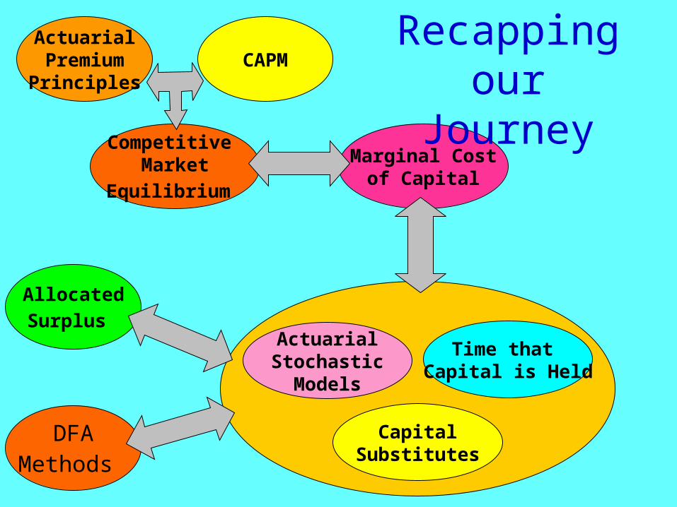
CAPMActuarialPremiumPrinciples
Competitive Market
Equilibrium
Marginal Costof Capital
Allocated
Surplus Actuarial
StochasticModels
Time that Capital is Held
CapitalSubstitutes
Recapping our Journey
DFAMethods