risk factors of in ation-indexed and conventional

Risk Factors of Inflation-Indexed and

Conventional Government Bonds and the APT

Andreas Reschreiter∗

July 14, 2003

∗Department of Economics and Finance, Institute for Advanced Studies, Stumpergasse56, A-1060 Vienna, Austria; e-mail: [email protected] I would like to thank DavidBarr, David Blake and Ian Garrett for comments. Any remaining errors are my responsi-bility.

Risk Factors of Inflation-Indexed and Conventional

Government Bonds and the APT

Abstract

This paper models UK fixed income security returns of various

bond types and maturities with Ross’s (1976) Arbitrage Pricing The-

ory. We extract statistical risk factors from the return covariance ma-

trix and analyze their relation with economic news. The following

five economic and financial risk factors are related to the orthogonal

principal components: unexpected inflation, changes in the slopes of

the real and nominal term structure, growth in retail sales and the

stock market excess return. The stock market excess return is used

as a proxy for any unobserved residual risk. We use Hansen’s (1982)

Generalized Method of Moments (GMM) to estimate the APT with

macroeconomic and financial risk factors as a constrained time series

regression model. The five factor APT model explains the time series

and cross section of returns very well. Two bond characteristics are

important for expected bond returns, the maturity of the bond and

whether the bond is indexed or not. We compare the performance

of the five factor APT model with three single factor models: the

stock market index CAPM, a bond market index CAPM and a lin-

earized consumption CAPM. The APT model fits the cross-section of

expected bond returns much better than the single factor models.

JEL: G12, E43

Keywords: APT, inflation-indexed, government bonds, fixed-income,

term structure

1

1 Introduction

The purpose of this paper is to specify the factors driving UK fixed income

security returns and to explain expected bond returns. This is important for

several reasons. First, the UK bond market incorporates the world’s largest

and most liquid market for inflation indexed debt. Multifactor models have

yet to be applied to price inflation-indexed bonds. Second, estimating and

testing multifactor asset pricing models has become a major research topic

in financial economics, but bond markets have received rather little atten-

tion compared to stock markets despite their size and economic significance.1

Third, we can use the APT to model the relation between bond returns and

macroeconomic news. This allows us to identify economic risk factors in the

bond market. Fourth, when the risk factors are economic variables, then

investors can adjust their portfolios according to their perception of likely

future movements in these risk factors. Portfolio managers can decrease or

increase the exposure to specific economic risk factors and form portfolios,

which are exposed to the risk factors according to their needs. Fifth, the APT

reveals the costs and rewards of changes in the factor exposures through the

changes in expected returns. This includes a change from conventional to

inflation-indexed. Thus, we can investigate the difference between the ex-

pected excess returns of conventional and inflation-indexed bonds.

Litterman and Scheinkman (1991) and Knez, Litterman and Scheinkman

(1994) estimate linear factor models for returns on US zero coupon bonds.

Similarly, Rebonato (1996) decomposes changes in UK nominal yields. These

studies find that that three implicit factors explain most of the time series

variation of bond returns, however, they do not assess the cross-sectional

restrictions of the APT on expected returns. Gultekin and Rogalski (1985)

estimate the APT for US-Treasury securities with factor analysis and Elton,

Gruber and Blake (1995) use constrained time series regressions to estimate

the APT for US fixed income security indices with economic and financial

news. This paper links the research on statistical risk factors with macroeco-

1Antoniou, Garrett and Priestley (1998), Clare and Thomas (1994) and Priestley (1996)are recent applications of the APT to the UK stock market.

2

nomic risk factors. We derive return principal components for various bond

types and maturities and relate them to macroeconomic and financial risk

factors. We use this to identify the prespecified risk factors.

After we have identified the macroeconomic and financial risk factors

driving UK bond returns, we estimate the APT as a system of constrained

time series regressions. Our investigation differs in at least three aspects

from Elton et al. (1995). First, we put more emphasis on the maturity of

the bonds. Second, we incorporate index-linked gilts into the analysis and,

third, we investigate the UK bond market. To our knowledge this is the first

investigation of the UK bond market with the Arbitrage Pricing Theory.

The rest of the paper is organised as follows. Section 2 outlines the multi-

factor model and Arbitrage Pricing Theory. Section 3 explores financial and

macroeconomic variables as likely risk factors. Section 4 investigates the is-

sues arising from investigating bond returns. In section 5 we examine the

relation between the statistical and macroeconomic risk factors and in sec-

tion 6 we estimate the APT with macroeconomic and financial risk factors

as a system of constrained time series regressions. Section 8 summarises our

findings and conclusions.

2 Multifactor Models and the Arbitrage Pric-

ing Theory

With the Arbitrage Pricing Theory (APT) the mean variance framework of

the Capital Asset Pricing Model (CAPM) is replaced by the return gener-

ating process. Investors homogeneously believe that a linear K-factor model

generates returns

Rit = E(Rit) +K

∑

j=1

βijfjt + uit. (1)

Rit is the return on asset i at time t and E(Rit) is the expected return of

asset i at time t. The factor loadings or factor betas, βij, are the sensitivities

of the i = 1, .., N asset returns to movements in the j = 1, .., K risk factors

fjt, which are by definition unpredictable and mean zero. The unsystematic

3

or idiosyncratic return, uit, is the return of asset i not explained by the

factors at time t. The expected return and the betas are fixed coefficients

from the linear projection of returns on the K-factors, which implies that

E(uit) = E(uitfjt) = 0 for all i = 1, .., N assets and j = 1, .., K factors.

The contribution of the APT is to derive a description of equilibrium for

multifactor models. Ross (1976) derives the APT for a strict factor model,

which assumes that the error covariance matrix is diagonal, E(uitujt) = 0

for any i 6= j. Any equilibrium is characterised by the absence of arbitrage

opportunities, which implies the cross-sectional APT pricing equation

E(Rit) = λ0t +K

∑

j=1

βijλj (2)

where λj is the risk premiums associated with factor j. An asset with zero

betas to all risk factors is risk free and therefore λ0t is equal to the risk free

interest rate, Rft. The factor risk premiums are constant with this static

specification of the APT. In equilibrium expected returns are equal to the

risk free rate plus the sum of K-products of factor betas and factor risk

premiums. This gives the cost or reward of changes in the exposure to the

factors.2

When we substitute the expected return equation (2) into the factor

model (1) and deduct the risk free rate Rft from both sides we get for the

APT in excess returns

rit =K

∑

j=1

βij(fjt + λj) + vit,

where rit = Rit−Rft is the excess return of asset i at time t. The no arbitrage

condition holds for any well-diversified subset of securities. Thus, the APT

is not subject to Roll’s (1977) critique, because there is no need to proxy for

the market portfolio like with the CAPM.

2Ross’s (1976) derivation of the APT does not imply that all risk premiums, λj forj = 1, ..,K, have to be different from zero. It only requires that the expected return vectoris linearly dependent to the constant and sensitivity vectors. This is satisfied if it is linearlydependent to at least one of these vectors, i.e. there has to be at least one nonzero riskpremium.

4

The strict factor assumption of Ross (1976) is not necessary for the deriva-

tion of the APT. Idiosyncratic returns are correlated within industries and

uncorrelated across industries with an approximate factor structure. This

generates a block-diagonal idiosyncratic return covariance matrix. The sub-

matrices along the diagonal are within-industry covariance matrices. This

is an important generalisation of the APT, because shocks to idiosyncratic

returns may affect several assets.3

2.1 Principal Components Analysis

We investigate the unconditional or static version of the APT, for which the

betas and risk premiums are time invariant. The expected return of any asset

is equal to the safe rate plus the sum of K products of factor sensitivities

and risk premiums. The expected return is constant when we assume that

the short rate is constant

Rit − R̄it =K

∑

j=1

βijfjt + uit.

Principal component analysis yields K orthogonal factor time series and the

matrix of factor loadings of the N -assets to the K-factors. We can avoid the

assumption that the short rate is constant when we analyze excess returns.

Excess returns also have to be demeaned, because principal component anal-

ysis requires that the variables are mean zero. The results for returns and

excess returns are only identical if the safe rate is constant, which is gen-

erally not the case in empirical applications. Roll and Ross (1980) analyze

returns and Knez et al. (1994) investigate excess returns. The econometrics

of principal component analysis is summarized for example in Theil (1974).

3Chamberlain (1983) and Chamberlain and Rothschild (1983) derive the APT for anapproximate factor model with an asymptotic statistical framework. In their model theidiosyncratic risk is diversifiable with an infinite sequence of assets, but factor risk is notdiversifiable. The K-largest eigenvalues of the covariance matrix of returns go to infinityas the number of assets goes to infinity and the K+1 largest eigenvalue is bounded forany number of assets.

5

2.2 Constrained Time Series Regressions

We estimate the unconditional multifactor pricing models with prespecified

factors as a seemingly unrelated regression model (SURM), which simultane-

ously estimates the factor betas and risk premiums. We implement this via

Hansen’s (1982) Generalised Method of Moments (GMM) technique. This al-

lows for non-normally distributed errors, conditional heteroskedasticity, and

errors which are correlated across the return equations of different assets,

i.e., for an approximate factor structure.

The data vector is assumed to be generated by a strictly stationary and

ergodic stochastic process, which implies that the variables have to be sta-

tionary. We use the contemporaneous values of the K-factors and a vector of

ones as instruments. We have N -equations (GMM constituencies) and K +1

information variables. To ensure that the model is identified we may have at

most N(K +1) unknown coefficients. Thus, we use the excess return form of

the APT and estimate only the factor risk premiums and factor loadings.

We allow for a K-factor model with J-tradable (factor mimicking) port-

folios and K−J economic factors. The return of a factor mimicking portfolio

is equal to the sum of the factor and factor risk premium, rjt = fjt + λjt.

Common risk premiums across the securities imply nonlinear cross-equation

restrictions as long as the number of assets is strictly larger than the number

of factors. We get for the APT in excess returns the following equation

rit =K−J∑

j=1

βij(fjt + λj) +K

∑

j=K−J+1

βijrjt + vit.

This restricts the intercept of the excess return factor model to be equal to

the sum of the products of risk premiums and betas of the economic factors

rit = αi +K−J∑

j=1

βijfjt +K

∑

j=K−J+1

βijrjt + vit

where

αi =K−J∑

j=1

βijλj.

6

When we use only factor mimicking returns then the intercept is restricted

to zero. The restriction on the intercept of the factor model can be used to

test the APT. The N(K + 1) orthogonality conditions state that none of

the i = 1, .., N idiosyncratic returns is predictable with the constant vector,

E(uit) = 0, any of the economic factors, E(uitfjt) = 0, or the factor mim-

icking returns, E(uitrjt) = 0. This restriction only holds if we have correctly

specified the return generating process (i.e. the factor model is valid) and

if the APT restrictions on the factor model hold. Thus, the APT is tested

jointly with the return generating process. We use Hansen’s J-test of overiden-

tifying restrictions to test whether the APT residuals are predictable. When

the imposed model structure is valid then the residual is not predictable. We

only need to estimate the restricted model to test the APT restrictions with

Hansen’s J-test.

3 Macroeconomic and Financial Risk Factors

The main advantage of using financial and economic variables as risk fac-

tors is the economic interpretability of the factors generating returns and

risk premiums. However, the APT does not specify the macroeconomic and

financial factors that affect the prices of financial assets. Chen, Roll and Ross

(1986) pioneered in their seminal paper the specification of macroeconomic

and financial variables as risk factors. The empirical determination of the

economic state variables generating returns is a main area of APT research.

Macroeconomic sources of asset price movements are non-diversifiable sys-

tematic sources of investment risk. The net present value model is frequently

employed to guide the selection of economic and financial risk factors. It

postulates that the price of an asset is equal to its discounted sum of ex-

pected future payments. Unexpected returns are associated with unantici-

pated movements in general economic state variables, which either alter the

discount factors or future payoffs.

Payments to bondholders are fixed in real terms for index-linked gilts and

in nominal terms for conventional gilts. Thus, unexpected movements in bond

prices are associated with unexpected movements in the discount rate. The

7

vast majority of research on the APT risk factors investigates common stock

returns. However, to the extend that the risk factors identified in these studies

price equities through the discount rate, they should also price fixed income

securities. Thus, some of the risk factors identified for common stocks may

also be important for bond returns. Table 1 summarises the factor candidates

we investigate for the bond market.

[Table 1 about here.]

3.1 Inflation Factors

Inflation has attracted a lot of attention in the economics literature. Barr and

Pesaran (1997) model the difference between conventional and index-linked

gilts in terms of the log-linear model of Campbell and Shiller (1988). This

suggests that revisions in expected future inflation is an important macroeco-

nomic risk factor. Moreover, as cross-sectional differences in expected returns

are attributed to different exposures of the assets to the risk factors, revisions

to expected inflation is likely to be a priced factor. We follow the Kalman Fil-

ter approach of Burmeister, Wall and Hamilton (1986) to extract unobserved

expected inflation rates from observed nominal interest rates and inflation

rates. The change in expected inflation risk factor (DEI) is the difference be-

tween the one month ahead expected inflation rate today and one month ago.

To account for the publication lag of inflation figures we lead the inflation

variables by one month.

Unanticipated price level changes will have a systematic influence on pric-

ing assets in real terms. The level of unexpected inflation is likely to reflect

the general uncertainty about future inflation, which may cause investors to

adjust their inflation risk premium. Thus, in addition to revisions in inflation

expectations we also investigate the extent to which unexpected inflation af-

fects returns on fixed income securities. The unexpected inflation risk factor

(UEI) is defined as the difference between the ex-post realised rate of inflation

and its expected value from the previous period. We additionally investigate

the contemporaneous change in the inflation rate (DI) as a proxy for changes

in expected inflation and unexpected inflation.

8

3.2 Term Structure Factors

The rate at which future dividends are discounted in is an average of rates

and, thus, not only affected by the level of interest rates but also by the term-

structure spread across different maturities. Unanticipated changes in the

term structure are frequently employed as APT risk factors. The factor (DTS)

is the difference between the return on long term and short term government

bonds.4 We also investigate a corresponding term structure measure obtained

from the index-linked gilts market. The real term structure (DTR) factor is

the difference between the return on long term and short-term index-linked

gilts.

The difference between these two term structure measures becomes clear

when we analyse their determinants with the log-linear model of Campbell

and Ammer (1993) and Barr and Pesaran (1997) for nominal and index-linked

gilts. The return difference between two conventional bonds (DTS) reflects

revisions in expected real interest rates and inflation rates from the shorter

bond’s maturity to the maturity of the longer bond. The empirical finance

literature supports the view that nominal interest rate differentials are related

to expected future inflation rates (e.g. Mishkin 1990). Thus, changes in the

nominal term structure may be mainly due to revisions in expected future

inflation rates.

Now, let us investigate the determinants of the difference between the

returns of two index-linked gilts of different maturity. Index-linked gilts are

only exposed to revisions in inflation expectations due to their inflation in-

dexation lag. This different inflation exposure is also reflected in their return

difference. The difference between the return of two index-linked gilts with

different maturities reflects revisions in expected real rates and excess returns

(risk premiums) rather than revisions to expected future inflation rates.

4One can also use the difference between the return on long-term UK government bondsand the one-month Treasury-Bill rate. We find that both lead to very similar results.

9

3.3 Default Risk Premium

Default risk is another frequently employed prespecified APT risk factor. It

reflects changes in the general business risk compensation. In terms of the

log-linear model of Campbell and Shiller (1988) it reflects changes in expected

future excess returns. It is usually measured as the difference between the

return on corporate and government bonds. However, we are limited to an

UK corporate bond yield series. The risk premium factor (DPR) is the change

in the log difference of the yield on UK-corporate and government bonds.5

We use the residual from an AR(1) process to generate unexpected changes.

For each period we estimate the first order autoregressive coefficient over the

previous 60 months.

3.4 Economic Activity

The level of real activity is likely to reflect the level of returns on physical

investments. Changes in inflation may trigger shifts in tastes with respect to

current and future consumption and ultimately alter the level of industrial

activity. The level of industrial activity is also likely to vary with general

business risk. Thus, changes in economic activity may proxy for changes in

real rates, inflation rates and risk premiums.

We investigate two measures of economic activity. The industrial pro-

duction growth rate factor (GIP) is the difference between the logarithm of

industrial production this period and one year ago. The second variable is

the annual growth rate in retail sales (GRS). We use annual growth rates for

two distinct reasons. First, annual growth rates may proxy for more infor-

mation than monthly growth rates, as they cover a longer period. Financial

market participants are forward looking and take long term information into

account. Second, we can calculate annual growth rates from seasonally un-

adjusted data, which has the advantage that we can use data which has not

undergone any pre-processing. Both, industrial production and retail sales

5This yield ratio is less exposed to general interest rate changes than the yield spreadbetween corporate and governmental bonds. Thus, the yield ratio is more likely to reflectchanges in risk compensations than the yield spread.

10

measure flows rather than stocks and therefore they measure changes lagged

by at least a partial month. Thus, similar to Chen et al. (1986), we lead

both series by one month. This also accounts for a potential lag in their

publication.

3.5 Other Factors

The main disadvantage of the APT is that it does not specify the factors. We

cannot assume that the above economic and financial risk factors account for

all relevant sources of risk. For example, several studies investigating the UK

stock market include factors accounting for money supply and exchange rate

risk (see for example Clare and Thomas 1994, Priestley 1996, Antoniou et al.

1998). It may be important to including an exchange rate factor to account for

the UK’s ’small open-economy’ characteristic. Similarly, unexpected money

supply may alter the market’s expectation about future inflation.

Fama and French (1993) investigate factors based on accounting mea-

sures. They employ the difference between returns on portfolios of stocks

with high and low book to market ratios and portfolios of stocks with small

and large market capitalisation as risk factors. Although they found that

these factors have little impact on common return variations of investment

grade bonds in the US, they could still be important sources of risk in the

UK.

This demonstrates the need for a framework that allows for omitted risk

factors. McElroy and Burmeister (1988) use the residual in the regression

of the market return on the other factors as a proxy for an unobserved risk

factor. In Burmeister and McElroy (1988) they employ the returns on indices

comprising shares, corporate bonds and government bonds to proxy for up

to three unobserved risk factors. We include the stock market excess return

(SMX) to allow for one omitted risk factor.


11

3.6 Macroeconomic Factor Statistics

Macroeconomic time series are frequently correlated with each other and may

have measurement problems, especially over short intervals. Moreover, many

time series are highly autocorrelated, but by definition only the unpredictable

part of the macroeconomic variable is related to unexpected returns. Table 2

shows that the autocorrelation coefficients are small, except for the two mea-

sures of economic activity. When an economic time series is autocorrelated

then the residual from a fitted expectation model may be used to measure

unanticipated innovations in the economic variable. However, different expec-

tation models can be used to derive expected values, which in turn produce

different factor time series and alter the inference (see Priestley 1996, Chen

and Jordan 1993, Connor 1995). Moreover, the failure to adequately filter

out expected movements in the variables may introduce an additional error.

The error in describing expected movements has to be traded off against the

error of measuring the economic factor without removing its predictable part.

Moreover, by definition only the unexpected part of the factor measure can

be related to unexpected returns. Thus, we are not attempting to remove the

predictable part from the variables.

The strongest correlation between the factors is found for the three infla-

tion measures. Revisions in expected inflation and unexpected inflation have

a correlation coefficient of 0.85 and both are approximated by the change

in the inflation rate. The two industrial activity measures (GIP, GRS) have

a moderate correlation coefficient of 0.29, which suggests that they reflect

different influences. They are both positively correlated with unexpected in-

flation and changes in expected inflation. This may reflect price increases

due to increases in demand. The four factors derived from financial variables

(DTR, DTS, DPR, SMX) are positively correlated with each other. The two

term structure measures are correlated because the real term structure also

affects the nominal term structure. Changes in the risk premium are corre-

lated with both term structure measures and the stock market excess return,

which in turn is related to the term structure factors.

12

4 Bond Returns

The factor sensitivity of a default free bond is proportional to the duration

of the bond and also depends on the covariance of interest rate and factor

movements. The factor sensitivity of an individual bond is nonstationary, be-

cause its duration is a function of time to maturity. It decreases over time as

the bond gets closer to maturity and reaches zero at maturity. Thus, for the

estimation of factor models we have to take into account that the betas of

individual bonds decrease over time. Blake, Elton and Gruber (1993) point

out that the sensitivity of bond i to factor j is equal to βij = (Dij/Dj)Xij,

where Dj is the duration of a factor j mimicking portfolio, Xij is the propor-

tion of risk exposure to factor j of bond i and Dij is the duration of the risk

exposure to factor j of bond i. The ratio of the factor loadings for two bonds

(or bond funds) which differ only in their duration is equal to the ratio of

their durations.


The estimation of the APT assumes constant betas. Two different ap-

proaches exist to achieve this. Knez et al. (1994) calculate returns from yield

curve changes for certain maturities and Elton et al. (1995) use constant

maturity portfolios to avoid the nonstationarity of the factor betas. Bond

indices have fairly stable durations as continuously new bonds are issued and

old bonds expire. Table 3 summarises the bond indices employed for the es-

timation of the APT. These indices are maintained and provided by Barclay

Capitals, London. Only bonds with an issue size of at least £75 million (£150

million for gilts) are included in the indices. Interest payments are reinvested

in the index.

We use bond indices with three different maturity ranges for the estima-

tion of the APT. The short maturity range indices include bonds expiring

within the next 5 years. Bonds with less than three months to maturity are

excluded from the calculation. The medium range indices include bonds with

5 to 15 years to maturity and bonds in the long maturity indices have at least

15 years left to maturity. We use two categories of government bonds, conven-

tional and index-linked. A separate category of indices is calculated for bonds

13

issued by sovereigns and supranationals. We also employ two categories of

corporate bond indices. One for corporate eurosterling and unsecured loan

stocks and another for secured corporate bonds. For secured corporate bonds

we only have an over 15 years to maturity segment.

4.1 Bond Return Statistics

Table 4 shows some descriptive statistics of the bond return indices. For each

type of bond the average return increases with maturity, which also implies

that excess returns increase with maturity. Average returns of conventional

bonds are approximately by 17%, 30% and 38% larger than returns on index-

linked gilts for the up to five, 5 to 15 and over 15 years to maturity segments,

respectively. This suggests that the indexation influence is stronger the higher

the maturity of the bond. Returns on bonds with over 15 years to maturity

are approximately by 50% larger than returns on bonds with up to 5 years to

maturity. For index-linked gilts it is only about 27% larger. Index-linked gilts

yield on average the lowest returns for any maturity segment and returns on

non-governmental bonds are larger than returns on government bonds for

any of the three maturity segments.


The return standard deviations increase with the maturity of the bonds.

Quite surprisingly the standard deviation of the return on index-linked gilts is

the largest for each of the three maturity segments. This suggests that index-

linked gilts have similar time series variations as conventional gilts, but they

require lower risk compensations because they are inflation indexed.

The modified duration entries in Table 4 are monthly averages. For the

medium and long maturity segments the duration of indexed gilts is consid-

erably larger than for non-indexed gilts. Nominal payments on index-linked

gilts increase over time as the price level increases. As a result, the duration

of indexed gilts is larger than the duration of conventional gilts with sim-

ilar maturities. The other bond indices have similar modified durations as

conventional government bonds.

14

The correlation coefficients within a bond sector reveal comovements be-

tween returns of the same type of bonds for different maturity segments.

Returns on the long and medium maturity indices have correlation coeffi-

cients larger than 0.92. The correlation between returns on the short and

medium maturity range are slightly less strong and range between 0.86 and

0.91. Returns on the short and long maturity indices have the lowest correla-

tion coefficients, which vary between 0.66 and 0.73. The return correlations

of different maturity segments are very similar for the four different bond

types.

Now let us investigate the correlation between returns of different types of

gilts. The smallest correlation coefficient is 0.44 for returns on short maturity

indexed and long maturity conventional gilts. Generally, the largest correla-

tion coefficients are found between indices of the same maturity range. None

of the returns on indexed gilts has a correlation coefficient larger than 0.79

with any of the other bond returns. The correlation coefficients between re-

turns of different types of bonds of the same maturity segment are around

0.7 for indexed gilts and larger than 0.97 otherwise.

5 Statistical and Macroeconomic Factors

In this section we employ principal component analysis to derive statistical

factors. To investigate whether our proposed measures of economic news

explain the extracted principal components we project the statistical factors

on the economic risk factors.

5.1 Extracted Principal Components

The factor loadings of the bond indices to the extracted principal components

are shown in Table 5. The bond indices cover the whole maturity range in

three segments. The factor sensitivities and durations of the different indices

reveal the influence of the factors on the yield curve. When the ratio of the

duration of two indices is equal to the ratio of their factor loadings, then the

factor measures shifts in the yield curve.

15


The factor loadings of the indices with the first principal component are

positive and increase as the duration of the indices increases. Thus, the first

principal component covers shifts in the yield. As conventional and indexed

bonds have similar factor loadings it measures a common random influence

on bond returns. The first principal component explains on average 84.24 %

of the return variation.

The factor loadings of the second principal component with the indices

are negative for short maturities, close to zero for the medium maturity

indices and positive for the long maturity indices. The factor loadings of

indexed-gilts are an exception to this, as they are negative for any maturity

and become more negative with increasing maturity. The second principal

component affects the slope of the yield curve and explains more than two

thirds of the return variation not explained by the first principal component.

The third principal component explains around 3% of the overall return

variance, which leaves little return variation unexplained. Generally, the short

and medium maturity segments have approximately equal loadings to the

third factor, whereas the long maturity indices have opposite signs. This al-

ters the curvature of the yield curve. The other principal components explain

little return variation and might reflect bond specific variations. These results

for the statistical factor model are similar to the results in Litterman and

Scheinkman (1991) and Knez et al. (1994) for the US and Rebonato (1996)

for the UK.

The sensitivities of the bond indices have the same sign for the first prin-

cipal component. It reflects a general bond return influence, which may be in-

terpreted as a general bond market component. Different types of bonds have

different sensitivity signs to the second principal component. Thus, it reflects

a bond sector specific influence. Whether the bond is inflation indexed or not

is an important bond sector distinction. The estimates of the sensitivities to

the first principal components are quite similar for conventional and index-

linked gilts, but for the second principal component they differ substantially.

From the log-linear model of Campbell and Shiller (1988) we know that in-

16

dexed gilts are not exposed to changes is expected future inflation rates. This

suggests that the second principal component is an inflation-related factor.

5.2 Cross-sectional Regressions

In the second step of the Fama and MacBeth (1973) two-step procedure the

returns of the bond indices are regressed on the estimated factor loadings

from the first step at each point in time. This yields a time series of cross

sectional estimates of the sum of risk premium and factor movements. For

period t we get the following cross-sectional regression over the N assets

R1t

...

RNt

= λ0t + (λ1t + f1t)

β11

...

βN1

+ · · · + (λKt + fKt)

β1K

...

βNK

+

e1t

...

eNt

Figure 1 shows the time series of the coefficient estimates from the cross-

sectional regression of returns on a constant and the factor sensitivities. The

time series averages are equal to the factor risk premiums and indicated with

dashed lines. The results are derived from cross sectional regressions of the

returns on the first seven principal components, although Figure 1 only shows

the estimates for the intercept and the first three principal components. The

dates of the graphs correspond to the first day of the month.

[Figure 1 about here.]

Only the second principal component has a negative peak in Septem-

ber 1992. Thus, Britain’s exit from the ERM has affected the steepness of

the yield curve rather than the level of interest rates. The second principal

component reflects a bond sector specific influence as index-linked and con-

ventional bonds respond differently. The return sensitivity of indexed gilts

is negative for each of the three maturity segments. The other indices have

negative loadings for short maturities and positive loadings for long maturi-

ties. Thus, the prices of indexed gilts of any maturity have benefited from the

ERM exit and the prices of long maturity conventional bonds have suffered.

17

The main difference between indexed gilts and conventional bonds is that

the former is not exposed to inflation. Fixing the sterling deutsche mark

exchange rate may have been perceived to lock the UK economy to low infla-

tion rates, as the Bundesbank was independent and obliged by law to price

stability in Germany. A negative shock to the second principal component

widens the difference between nominal and real yields at the long end of

the maturity range, which is likely to reflect an increase in expected future

inflation rates. Barr and Campbell (1997) show that the difference between

nominal and real yields is related to future expected inflation rates. This

suggests that the second largest principal component is related to inflation.

The second principal component accounts for about 10% of the time series

variations of bond returns.

The risk premium estimate for the second factor is positive, and therefore,

investors demand a risk compensation for a positive exposure to the second

factor. For index-linked gilts the exposure is negative and thus investors

are willing to forego some return in exchange for the inflation indexation of

index-linked gilts.

With exception of the fifth and seventh principal component the risk

premium estimates are positive. The t-test of the null hypothesis that the

risk premium of factor j is zero is

tj = T1

2

E(λj)

σ(λj),

where T is the number of observations, E(λj) is the sample mean and σ(λj)

is the standard deviation of the cross sectional risk premium estimates. The

first, second, fifth and sixth risk premiums have t-ratios larger than one.

5.3 The Principal Components and Prespecified Fac-

tors

The extracted statistical factors can produce models with a good fit of the

return data, but the extracted factors have no economic interpretation or

intuition. We find that similar statistical factors explain the time series of

18

bond returns as in Litterman and Scheinkman (1991) and Knez et al. (1994).

They concentrate on the time series of returns and do not investigate a

potential relation between returns and economic news. In the following we

use the extracted statistical factors from the previous section to investigate

whether asset prices adjust to news associated with our proposed economic

state variables.

The extracted statistical factors from the return covariance matrix can

be interpreted as portfolios capturing common movements in returns. Chen

et al. (1986) point out that an economic variable is only significantly related

to return movements if and only if it is significantly related to at least one of

the common statistical factors. We follow this approach and select the APT

factors on their ability to explain the principal components.6


Table 6 reports the results of regressing the extracted principal compo-

nents on the macroeconomic and financial factor candidates. The reported

test statistics are based on Hansen’s (1982) generalised method of moments.

The null hypothesis for each proposed factor states that its regression coef-

ficients across the equations for the principal components are jointly equal

to zero. The Wald test of this hypothesis is rejected at the 1% level for the

unexpected inflation, real term structure, nominal term structure, retail sales

growth rate and stock market excess return factors. None of the other factors

is significantly related to the principal components.7

Unexpected inflation is the best measure of the inflation impact on returns

out of the three proposed inflation factors. This supports the use of the

Kalman Filter approach of Burmeister et al. (1986) to extract unexpected

inflation from measured inflation and the safe rate. The default risk factor

may be insignificant, because we look predominantly at risk free bonds. Out

6Chen et al. (1986) find in regressions of the extracted factors from factor analysis ontheir proposed state variables that the economic state variables explain the statisticallyidentified factors, but they do not provide the empirical results of this in their paper.

7We also looked at the results when the principal components are extracted from theexcess return covariance matrix instead of the return covariance matrix and find that thesame five factors are overall significant.

19

of the two measures for economic activity only the growth rate in retail

sales is related to bond returns. Industrial production may be smoothed by

adjustments in the level of stocks and therefore convey little information.

With exception of the unexpected inflation factor each of the identified

overall significant factors has at least two significant coefficients with the

principal components. The unexpected inflation factor is significantly related

to the third principal component when we delete the insignificant factors. The

second principal component reflects movements in opposite directions of the

nominal and real term structure. This suggests that the second principal

component is inflation related, as Barr and Campbell (1997) find that the

difference between the nominal and real term structure is a proxy for future

inflation.

To examine how may of the orthogonal principal components are signifi-

cantly related to economic news, we investigate for each principal component

the hypothesis of zero coefficients across the factors. The Wald test for this

hypothesis is rejected at the 1% level for the first four principal components.

For the sixth principal component the hypothesis is also rejected, but the test

statistic is not significant when the principal components are extracted from

excess returns instead of returns. Similarly, when the insignificant factors are

excluded from the regression, then the Wald test for the sixth principal com-

ponent becomes insignificant. The explained time series variation of the sixth

principal component is less than 1%. This indicates that the sixth principal

component may reflect an idiosyncratic return component rather than the

influence of a general economic state variable on returns.8

Economic news explains a large proportion of the time series variation

of the first two principal components and a considerable amount for the

third and fourth principal components. From the results of the regressions

of the principal components on the hypothesised economic state variables we

conclude that the first four orthogonal principal components are related to

economic news.

8The number of principal components has no effect on the test statistics whether a prin-cipal component is explained with the economic factors, because the principal componentsare orthogonal to each other.

20

5.4 Interest Rate Risk and the Identified Factors

Unexpected bond returns are associated with unexpected interest rate move-

ments. The nominal m-period interest rate can be broken down into four

components, its real interest rate, inflation rate, liquidity premium and mar-

ket risk premium, i.e.

ym = rm + πm + lm + σm.

Interest rate risk comprises the risk of unexpected movements in any of these

four components. Consequently, unexpected interest rate movements are as-

sociated with unexpected movements in at least one of the four interest rate

components.

Some of the components of the m-period interest rate may cointegrate.

For example, if the real interest rate and inflation cointegrate, then the error-

correction-mechanism associated with such a cointegration relationship could

be employed to model their expected movements. The unexpected change,

which in turn leads to unexpected returns, is just the difference between

the actual and expected change. However, this modelling approach requires

measures of the interest rate components, which are not readily available.

Moreover, the APT risk factors ’only’ have to capture unexpected movements

in the components of the interest rate, but not the interest rate itself or its

components.

This raises the question whether the five identified risk factors are likely

to account for unexpected movements in each of these four components. The

retail sale and real term structure factors should capture movements in the

real interest rate. The unexpected inflation factor clearly represents the in-

flation component in interest rates. Movements in inflation rates should also

be reflected in the difference between the nominal and real term structure

factors. Bonds with longer term to maturity are exposed to greater amounts

of interest rate risk. Short-term bonds will be redeemed in the near future,

which makes them less vulnerable to interest rate movements. As a result

of this, investors prefer to lend for short periods and accept lower yields for

short-term bonds. On the other hand, borrowers prefer long-term contracts

21

to avoid the risk of rolling over short-term contracts at unfavourable rates.

Borrowers are willing to pay a liquidity premium (also known as term pre-

mium or horizon premium) for long-term bonds. The liquidity premium is

not related to specific bond issues, it characterises a feature of the yield curve.

Lutz (1940) argues that the liquidity premium is positive and increases with

maturity. The nominal and real term structure incorporate yields of different

maturities and should therefore reflect movements in the liquidity premium.

Finally, the stock market excess return should account for movements in the

risk premium.

6 The Cross Section of Bond Returns

The selection of the factors into the macroeconomic factor model is based on

their ability to explain the principal components. To investigate whether the

economic risk factors are priced and to test the APT we impose the APT

cross-sectional pricing restrictions on the factor model.

6.1 Macroeconomic Factor Model


Table 7 reports the results of estimating the factor model with the five

economic factors, which are significantly related to the principal components.

A factor is useful in explaining returns if its betas are different from zero. We

have to distinguish the time series and cross-sectional explanatory power of a

factor. A factor can have low correlations with asset returns, but it may have

an important average risk premium. However, when the factor loadings of a

factor are insignificantly different from zero in the factor model regression,

then the factor is neither useful in explaining random returns nor expected

returns. Thus, it is important to test that each factor significantly explains

the time series of returns before we impose the APT restrictions on the factor

model. Table 7 reports for each of the factors the result of the Wald test of

the hypothesis that the factor betas across the assets are jointly equal to

22

zero. The hypothesis is strongly rejected at the 1% level for each of the five

factors.

The betas of a factor can be significantly different from zero, but they can

still be insignificantly different from each other. Cross-sectional differences

in returns are attributed to differences in the factor sensitivities of the as-

sets. Thus, a factor is only priced cross-sectionally if its beta estimates vary

across the assets. The last two rows in Table 7 report the results of the null

hypothesis that the factor betas across the assets are constant. The Wald

test is rejected at the 1% level for each of five factors.

All betas of the real term structure factor are positive and significantly

different from zero. With exception of the index-linked gilts sector, the beta

estimates for the retail sales factor are negative and highly significant. Simi-

larly, for the stock market excess return the betas for index-linked gilts have

the lowest t-ratios. None of the betas for the unexpected inflation factor has

a significant t-ratio, and only for the short maturity segment are the betas

significantly different from zero at the 10% level. The support for the inflation

factor is considerably weaker from the t-test statistics than from the Wald

tests.

Short maturity index-linked gilts have the lowest R̄2 with 25.5%. For the

other indices it is larger than 57.1%. The higher the maturity of the index,

the better the five factors describe the time series of excess returns. Thus,

the five factors describe the time series of bond returns very well. The sample

mean of the factors is equal to zero and therefore the intercept is equal to the

expected excess returns of the bond indices. Index-linked and short maturity

bonds have insignificant average excess returns and the other bond indices

earn significant positive risk compensations.

6.2 Arbitrage Pricing Theory

Table 8 summarises the results of the factor model estimation with the APT

restriction imposed. The constrained time series regression technique imposes

the APT restriction on the factor model and jointly estimates the factor

23

sensitivities and factor risk premia.9


The beta estimates are quite similar to the estimates from the unrestricted

factor model. The largest deviations between the beta estimates from the re-

stricted and unrestricted factor model are found for the unexpected inflation

factor. The significance of the t-tests generally increases and in particular

for the unexpected inflation factor. With exception of the index-linked gilts

sector, the betas of the unexpected inflation factor become significant for the

short and medium maturity segments. The adjusted R̄2 are very similar for

the unrestricted and restricted factor model.

The risk premiums of the unexpected inflation and change in real term

structure factors are both positive and significantly different from zero. The

other three risk factors have insignificant risk premiums, but only the stock

market excess return factor has a t-ratio smaller than one.

The contribution of the APT is to derive a description of equilibrium

for multifactor models, which states that expected returns are equal to the

sum of K products of factor sensitivities and factor risk premiums. We test

this hypothesis with Hansen’s J-test of overidentifying restrictions and accept

that the APT restrictions hold.

6.3 Expected Bond Returns


As we have accepted the APT restrictions on expected returns, we can

further analyse the expected return predictions of the APT. Figure 2 plots

the average excess returns of the assets against their APT predictions. The

straight line is the 45◦ line and all assets should be close to it. The graph

indicates that the five factors APT model explains the cross-section of ex-

pected returns very well. The model generally assigns slightly too large risk

compensations.

9We use the GMM programs written by Hansen, Heaton and Ogaki in Gauss under theNational Science Foundation Grant number SES-8512371. We employ iterative GMM asFerson and Foerster (1994) find that iterated GMM has better small sample properties.

24

Following Elton et al. (1995) we calculate the model’s ability to explain

cross-sectional variations in expected returns. The explained excess return

variation is calculated as 1 minus the sum of the squared differences between

average excess returns and predicted average excess returns divided by the

sum of squared differences between average excess returns and the mean of

the average excess returns, i.e.

1 −

∑Ni=1

(

r̄i −∑K

j=1 β̂ijλ̂j

)2

∑Ni=1 (r̄i − ¯̄ri)

2

This is equivalent to the (unadjusted) R2 of the cross-sectional regression

(without a constant) of average excess returns on predicted average excess

returns. This is a general measure of how well the model explains the cross-

section of returns. In terms of this measure the APT explains 99.44% of the

cross-sectional excess return variations.

To investigate the cross-sectional importance of the factors we analyse

the contribution of the factors to the expected return predictions. Table 9

summarises the expected return contributions of the five factors. The table

entries are based on the absolute value of the product of factor sensitivity

and factor risk premium divided through the sum of these values across the

factors, i.e.|β̂ijλ̂j|

∑Kj=1 |β̂ijλ̂j|

These figures are averaged across all assets, across the assets in the same

bond category and across the assets in the same maturity segment.


Considering all assets, we find that the growth rate in retail sales con-

tributes the largest portion to expected returns. Around two thirds of the

variability in expected returns is derived from the two macroeconomic vari-

ables. The remaining variability is mainly due to the term structure variables.

The contribution of the stock market excess return is less than 1%.

Now let us investigate the contribution of the factors to expected returns

for different types of bonds. The real term structure is the largest contributor

25

to expected returns on index-linked gilts and the importance of the nominal

term structure drops to an average of 3.14%. Leaving aside the index-linked

gilts sector, the results do not vary greatly for different types of bonds.

The expected return contribution of the unexpected inflation factor and

nominal term structure factor to expected returns varies considerably with

the maturity of the bonds. The influence of the unexpected inflation factor

decreases and the importance of the nominal term structure factor increases

with maturity. This suggests that the unexpected inflation factor reflects

short horizon inflation and the nominal term structure factor proxies for

long horizon inflation.

The result indicates that two bond characteristics are important for ex-

pected returns. Firstly, whether the bond is index-linked or not and, secondly,

the maturity of the bond.

7 Single Factor Models

It is an important issue to investigate the relative performance of the APT

to alternative asset pricing models. The usefulness of a model is generally

judged on its practical applications and policy implications. This suggests

the need for a comparative analysis of the model to specific alternatives such

as the CAPM, a bond index CAPM and the Consumption CAPM.

7.1 The Equity Market CAPM

The capital asset pricing model is based on the mean variance efficiency of the

market portfolio. This implies a linear relation between the excess return on

any asset with the excess return on the market portfolio. The CAPM beta of

asset i, βi, is the regression coefficient of asset i’s excess returns on the excess

return of the market portfolio. The CAPM predicts that asset i’s expected

excess return is linearly related to the expected excess return on the market

portfolio via the asset’s beta, E(rit) = βiE(rmt). We implement the CAPM

into the APT framework with the market excess return as the only factor.

The Sharpe (1964) and Lintner (1965) standard version of the CAPM places

26

the restriction αi = 0 on the factor model regression, rit = αi + βirmt + vit.

Thus, the market excess return is used as a factor mimicking portfolio return

and only the CAPM betas are estimated.


The estimation results of the CAPM are shown in the second and third

column of Table 10. The market portfolio of risky assets is not observable and

therefore a broad stock market index is frequently employed as a proxy for

the market portfolio. We use the return on the FT-all share index in excess of

the one-month Treasury-Bill rate as measure for the market excess return. All

CAPM beta estimates are positive and highly significant. Bond indices of the

same maturity segment have similar beta estimates, which increase with the

maturity of the bonds. The short maturity indices have considerably lower

CAPM betas than the medium and long maturity indices.10 This assigns

larger risk compensations to longer maturity bonds. The CAPM explains

reasonably large portions of the time series variance of excess returns. With

exception of the index-linked gilts sector, the R̄2s are larger than 0.3. Only

for the return on short maturity index-linked gilts is the explained portion

of the time series variance quite low with a value of 8.6%.


Shiller and Beltratti (1992) find a similar strong relation between UK

bond and stock market excess returns for the period from 1918 to 1989 with

a correlation coefficient of 0.6. Hansen’s J-test rejects the hypothesis that

average excess returns are equal to the product of CAPM beta and market

excess return. Thus, the unconditional mean variance efficiency of the stock

market index is rejected at the 5% level. Gultekin and Rogalski (1985) report

a similar rejection of the CAPM for the US bond market.11

10In the regressions of the extracted principal components on the stock market excessreturn we find that only the first principal component is significantly related to the stockmarket excess return with a t-ratio of 7.00, which explains 38% of the time series variationof the first principal component. As a result of this the relative size of the beta estimatesstrongly resemble the factor loadings of the first principal component.

11We also looked at the result when the demeaned market excess return is used asfactor surprise, fmt = rmt − E(rmt). Then the market risk premium is estimated and the

27

Figure 3 shows the predicted and actual cross-section of average returns

for the CAPM. The model explains 43.23% of the cross-sectional variation

in expected excess returns.12 The predicted mean excess returns range in a

narrow band between 0.06% and 0.22% per month whereas the actual values

vary in a considerable wider range. As a result of this the predicted excess

return is too low for bonds with above average excess returns and too large for

bonds with below average excess returns. The model has obvious problems to

fit the negative sample average excess returns for index-linked gilts, because it

cannot fit negative expected excess returns with positive betas and a positive

market risk premium.

7.2 The Bond Market CAPM

In the following we estimate a bond market version of the CAPM. The CAPM

states that the excess return on any risky asset is linearly related to the excess

return of the market portfolio, which is the portfolio of all risky assets. A

proxy for the market portfolio has to be employ in empirical applications of

the CAPM, as the portfolio of all risky assets is unobservable. A stock market

index is commonly employed to proxy for the market portfolio. This may be

entirely inappropriate to the pricing of fixed income securities, because a

stock market index as proxy for the market portfolio entirely omits fixed

income securities.13 The same argument applies to a bond market index, as

it neither describes the whole set of risky securities. However, in the following

we look at the performance of a fixed income security index as a proxy for

restriction αi = βiλm is imposed on the factor model rit = αi + βi(rmt − E(rmt)) + vit.This model is less restrictive than the CAPM as the market risk premium is not restrictedto the average of the market access return. Estimating the risk premia may improve thefit of the model and reveals how close the estimated risk premium is to the average ofthe market excess return. This model is also rejected at the 5% level and differs onlymarginally from the CAPM as its risk premium estimate of 0.893% per month is quiteclose to the average market excess return of 0.740% per month.

12See section 6.3 for the definition of the explained cross-sectional return variation.13This is the very heart of Roll’s (1977) critique. It is based on the necessity to proxy

for the market portfolio, as the true market portfolio is unobservable. If the proxy for themarket portfolio is not mean variance efficient then the CAPM is empirically rejected,but the ’true’ market portfolio could be mean variance efficient and the CAPM a validdescription of security returns.

28

the market portfolio.


Column four and five of Table 10 summarise the estimation results when

we proxy for the market portfolio with the FT-all government bonds index

in excess of the one-month Treasury Bill rate. All beta estimates are again

positive and highly significant. The beta estimates are quite similar for bond

indices of the same maturity segment.14 The explained variation in the time

series of bond returns is naturally larger with a bond index than with a stock

market index. However, the explained cross-sectional variation in returns

has decreased to 20.65%. The predicted and actual bond excess returns are

shown in Figure 4. For most of the assets the predicted average excess returns

are too high. The restriction that expected excess return are described by

the product of factor sensitivities and expected bond index excess return is

rejected at the 1% level.15

7.3 The Consumption CAPM

The consumption capital asset pricing model (CCAPM) is regarded as the

theoretically superior model to the CAPM. It is based on investors (i.e. a rep-

resentative investor) who maximise their lifetime utility of consumption. In

equilibrium the marginal utility of current consumption equals the marginal

utility of consumption in any future period. Through the real return from

investments a higher amount of real consumption is achieved in future peri-

ods, which ensures that the marginal utility of current consumption equals

14The bond market excess return only explains the first principal component. Its coeffi-cient has a t-ratio of 40.65 and explains 94% of the variance of the first principal compo-nent. The beta estimates reflect the factor loadings of the assets with the first principalcomponent.

15When the bond index excess return is not used as a factor mimicking portfolio then weget a risk premium estimate of 0.152%, which is less than have the size of the average bondindex excess return. This decreases the average excess return predictions and increases theexplained cross-sectional return variation to 31.55%. However, the APT restrictions arestill rejected at the 5% level.

29

the marginal utility of future consumption.16

The CCAPM may be useful to price UK fixed income securities in the

sense that index-linked gilts ensure future real consumption. We estimate

a linear version of the CCAPM, rit = αi + βi∆ct + wt, which relates asset

excess returns, rit, to the growth rate of real consumption of non-durables

and services, ∆ct. Thus, the growth rate of real consumption is specified to

be the only return factor (see for example Cochrane 1996).

We are limited to quarterly consumption data. Various approaches exist to

derive monthly consumption data from quarterly consumption observations.

We interpolate monthly consumption values with cubic splines from quarterly

observations.17


Figure 5 shows the predicted average returns for the CCAPM. It suggests

that the CCAPM describes the cross section of bonds better than the CAPM.

However, this result has to be interpreted with caution, as Table 10 indicates

only a very weak relation between consumption growth and bond returns.

8 Conclusions

This paper investigates the usefulness and empirical contents of the APT

for different types of bonds and various maturities. We derive statistical risk

16Chen et al. (1986) find that changes in real per capita consumption growth are notsignificantly related to expected stock returns in the US in conjunction with their APTfactors.

17Breeden (1979) shows that the CCAPM can be restated and tested in terms of a max-imum correlation portfolio (MCP). The MCP is designed to have maximum correlationwith aggregate consumption growth and is used instead of the consumption data to esti-mate the CCAPM. The weights of the risky assets in the maximum correlation portfolioare proportional to the multiple regression coefficient of consumption on the risky assetreturns (see Breeden, Gibbons and Litzenberger 1989). Asset returns are measured morefrequently than consumption. Thus, the monthly returns on the MCP can be used to es-timate the CCAPM on a monthly basis with quarterly consumption data. The simplestapproach to derive a monthly series is to use a monthly retail sales series instead of con-sumption. Alternatively, one can use the Kalman Filter to estimate a model for aggregateddata. We find that these two latter approaches lead to similar results.

30

factors, which describe the time series of returns very well. The first prin-

cipal component shifts the yield curve up and down and explains 84.24%

of the bond return variance. Besides this general bond return index a bond

sector component explains an additional 10.89% of the total return variance.

Indexed and conventional bonds are differently exposed to this second prin-

cipal component, which affects the slope of the yield curve. In the regression

of the second principal component on macroeconomic and financial news,

we find that it describes opposite movements in the real and nominal term

structure. The empirical results indicate that this second factor is inflation

related.

The first four principal components are related to financial and economic

news, which explain large proportions of the time series variance of the first

three principal components. Unexpected inflation, the real and nominal term

structure, retail sales growth and the stock market excess return are signif-

icantly related to the principal components. These five macroeconomic and

financial risk factors explain the time series and cross section of bond returns

very well. Two distinct bond characteristics are important for the cross sec-

tion of bond returns, namely whether the bond is inflation indexed and the

maturity of the bond.

We compare the performance of this five factor APT model with three

single factor models. The CAPM based on stock and bond market indexes

describe the time series of bond returns quite well. For the consumption

CAPM we find that the growth rate in real consumption is hardly related

to bond returns. The five-factor model describes the cross-section of bond

returns considerably better than the single factor models.

Possible areas of further research include the relation of fixed income

security returns with alternative factor measures. Fama and French (1992)

investigate size and the book to market ratio for the US, whereas Cochrane

(1996) looks at a production based asset pricing model and uses investment

returns as factors to model US stock returns.

Intertemporal asset pricing models based on consumption data are subject

to continuous refinements, see for example Campbell and Cochrane (1999),

but they are predominately concerned with stock market data or with bond

31

market data in conjunction with stock market data.

32

References

Antoniou, A., Garrett, I. and Priestley, R. (1998), ‘Macroeconomic variables

as common pervasive risk factors and the empirical content of the arbi-

trage pricing theory’, Journal of Empirical Finance 5(3), 221–240.

Barr, D. G. and Campbell, J. Y. (1997), ‘Inflation, real interest rates and

the bond market: A study of UK nominal and index-linked government

bond prices’, Journal of Monetary Economics 39, 361–383.

Barr, D. G. and Pesaran, B. (1997), ‘An assessment of the relative impor-

tance of real interest rates, inflation, and term premiums in determining

the prices of real and nominal U.K. bonds’, Review of Economics and

Statistics 99, 362–366.

Blake, C. R., Elton, E. J. and Gruber, M. J. (1993), ‘The performance of

bond mutual funds’, Journal of Business 66(3), 371–403.

Breeden, D. (1979), ‘An intertemporal asset pricing model with stochastic

consumption and investment opportunities’, Journal of Financial Eco-

nomics 7, 265–296.

Breeden, D., Gibbons, M. and Litzenberger, R. (1989), ‘Empirical tests of

the consumption-oriented CAPM’, Journal of Finance 44, 231–262.

Burmeister, E. and McElroy, M. B. (1988), ‘Joint estimation of factor sen-

sitivities and risk premia for the arbitrage pricing theory’, Journal of

Finance 43(3), 721–735.

Burmeister, E., Wall, K. D. and Hamilton, J. D. (1986), ‘Estimation of un-

observed expected monthly inflation using Kalman filtering’, Journal of

Business and Economic Statistics 4(2), 147–160.

Campbell, J. Y. and Ammer, J. (1993), ‘What moves the stock and bond

markets? A variance decomposition for long-term asset returns’, Journal

of Finance 48(1), 3–37.

33

Campbell, J. Y. and Cochrane, J. H. (1999), ‘By force of habit: A consump-

tion based explanation of aggregate stock market behavior’, Journal of

Political Economy 107(2), 205–251.

Campbell, J. Y. and Shiller, R. J. (1988), ‘Stock prices, earnings, and ex-

pected dividends’, Journal of Finance 43(3), 661–676.

Chamberlain, G. (1983), ‘Funds, factors, and diversification in arbitrage pric-

ing models’, Econometrica 51(5), 1305–1323.

Chamberlain, G. and Rothschild, M. (1983), ‘Arbitrage, factor structure,

and mean-variance analysis on large asset markets’, Econometrica

51(5), 1281–1304.

Chen, N.-F., Roll, R. and Ross, S. (1986), ‘Economic forces and the stock

market’, Journal of Business 59(3), 383–403.

Chen, S. and Jordan, D. B. (1993), ‘Some empirical tests in the arbitrage

pricing theory; macrovariables vs. derived factors’, Journal of Banking

and Finance 17, 65–89.

Clare, A. D. and Thomas, S. H. (1994), ‘Macroeconomic factors, the APT

and the UK stockmarket’, Journal of Business Finance and Accounting

21(3), 309–330.

Cochrane, J. H. (1996), ‘A cross-sectional test of an investment-based asset

pricing model’, Journal of Political Economy 104(3), 572–621.

Connor, G. (1995), ‘The three types of factor models: A comparison of their

explanatory power’, Financial Analysts Journal, May-June pp. 42–46.

Elton, E. J., Gruber, M. J. and Blake, C. R. (1995), ‘Fundamental economic

variables, expected returns and bond fund performance’, Journal of Fi-

nance 50(4), 1229–1256.

Fama, E. F. and French, K. R. (1992), ‘The cross-section of expected returns’,

Journal of Finance 47, 427–65.

34

Fama, E. F. and French, K. R. (1993), ‘Common risk factors in the returns

on stocks and bonds’, Journal of Financial Economics 33, 3–56.

Fama, E. F. and MacBeth, J. D. (1973), ‘Risk, return, and equilibrium: Em-

pirical tests’, Journal of Political Economy 81, 607–635.

Ferson, W. E. and Foerster, S. R. (1994), ‘Finite sample properties of the gen-

eralized method of moments in tests of conditional asset pricing models’,

Journal of Financial Economics 36, 29–55.

Gultekin, N. B. and Rogalski, R. J. (1985), ‘Government bond returns, mea-

surement of interest rate risk, and the arbitrage pricing theory’, Journal

of Finance 40(1), 43–61.

Hansen, L. P. (1982), ‘Large sample properties of generalized method of mo-

ments estimation’, Econometrica 50(4), 1029–1054.

Knez, P. J., Litterman, R. and Scheinkman, J. (1994), ‘Explorations into fac-

tors explaining money market returns’, Journal of Finance 49(5), 1861–

82.

Lintner, J. (1965), ‘The valuation of risky assets and the selection of risky in-

vestments in stock portfolios and capital budgets’, Review of Economics

and Statitics 47, 13–37.

Litterman, R. and Scheinkman, J. (1991), ‘Common factors affecting bond

returns’, Journal of Fixed Income 1(1), 54–61.

Lutz, F. (1940), ‘The structure of interest rates’, Quarterly Journal of Eco-

nomics 55, 36–63.

McElroy, M. B. and Burmeister, E. (1988), ‘Arbitrage pricing theory as a

restricted nonlinear multivariate regression model’, Journal of Business

and Economic Statistics 6, 29–42.

Mishkin, F. S. (1990), ‘What does the term structure tell us about future

inflation?’, Journal of Monetary Economics 25, 77–95.

35

Priestley, R. (1996), ‘The arbitrage pricing theory, macroeconomic and finan-

cial factors, and expectations generating processes’, Journal of Banking

and Finance 20(5), 869–890.

Rebonato, R. (1996), Interest rate option models: A critical survey, in

C. Alexander, ed., ‘The Handbook of Risk Management and Analysis’,

John Wiley & Sons Ltd.

Roll, R. (1977), ‘A critique of the asset pricing theory’s tests’, Journal of

Financial Economics 4, 129–176.

Roll, R. and Ross, A. (1980), ‘An empirical investigation of the arbitrage

pricing theory’, Journal of Finance 35(5), 1073–1102.

Ross, A. (1976), ‘The arbitrage theory of capital asset pricing’, Journal of

Economic Theory 13, 341–360.

Sharpe, W. (1964), ‘Capital asset prices: A theory of market equilibrium

under conditions of risk’, Journal of Finance 19, 425–442.

Shiller, R. J. and Beltratti, A. E. (1992), ‘Stock prices and bond yields:

Can their comovements be explained in terms of present value models?’,

Journal of Monetary Economics 30, 25–46.

Theil, H. (1974), Principles of Econometrics, John Wiley & Sons, New York.

White, H. (1980), ‘A heteroskedasticity-consistent covariance matrix estima-

tor and a direct test for heteroskedasticity’, Econometrica 48(4), 817–

838.

36

Table 1: Prespecified Factor Definitions

The table summarises the definitions of the macroeconomic and financial risk factors.Basic Series

Corporate yield YCB Yield on UK corporate bondsGovernment yield YGB Yield on UK government bondsUK inflation rate πt Annual change in the UK retail price indexOne month interest IB One month UK interbank rateReturn on short bonds CRS Return on under 5 years FTA government bonds indexReturn on long bonds CRL Return on over 15 years FTA government bonds indexReturn short indexed IRS Return on under 5 years FTA index-linked gilts indexReturn long indexed IRL Return on over 5 years FTA index-linked gilts indexIndustrial production IP Volume of UK industrial production not seasonally ad-

justedRetail sales SALE Volume of UK retail sales not seasonally adjustedStock market return SMR Return on the FTA all shares indexExpected inflation πe

t Expected inflation derived at time t−1 from state spacemodel of measured inflation and the interbank rate.

Factor time seriesChange in expectedinflation

DEI First difference in expected one month ahead inflation:DEIt+1 = πe

t+1 − πet .

Unexpected inflation UEI Actual inflation at time t minus expected inflation onemonth ago: UEIt+1 = πt − πe

t .Change in inflationrate

DI First difference in ex post inflation rates: DIt+1 = πt −πt−1.

Real term structurechange

DTR Difference between the return on over five years index-linked gilts and under five years index-linked gilts:DTRt = IRLt − IRSt.

Nominal term struc-ture change

DTS Difference between the return on over 15 years govern-ment gilts gilts and under five years government gilts:DTSt = CRLt − CRSt.

Risk premium changes DPR Residual of the AR(1) model of the first difference of thelogarithm of the yield on UK corporate and governmentbonds.

Growth rate in indus-trial production

GIP Annual difference in the logarithm of industrial produc-tion: GIPt = ln(IPt) − ln(IPt−12). This series has beenlead by one month.

Growth rate in retailsales

GRS Annual change in the logarithm of UK retail sales:GRSt = ln(SALEt) − ln(SALEt−12). This series hasbeen lead by one month.

Stock market excessreturn

SMX Excess return on the FTA all shares index: SMRt −IBt−1

Source: Datastream

37

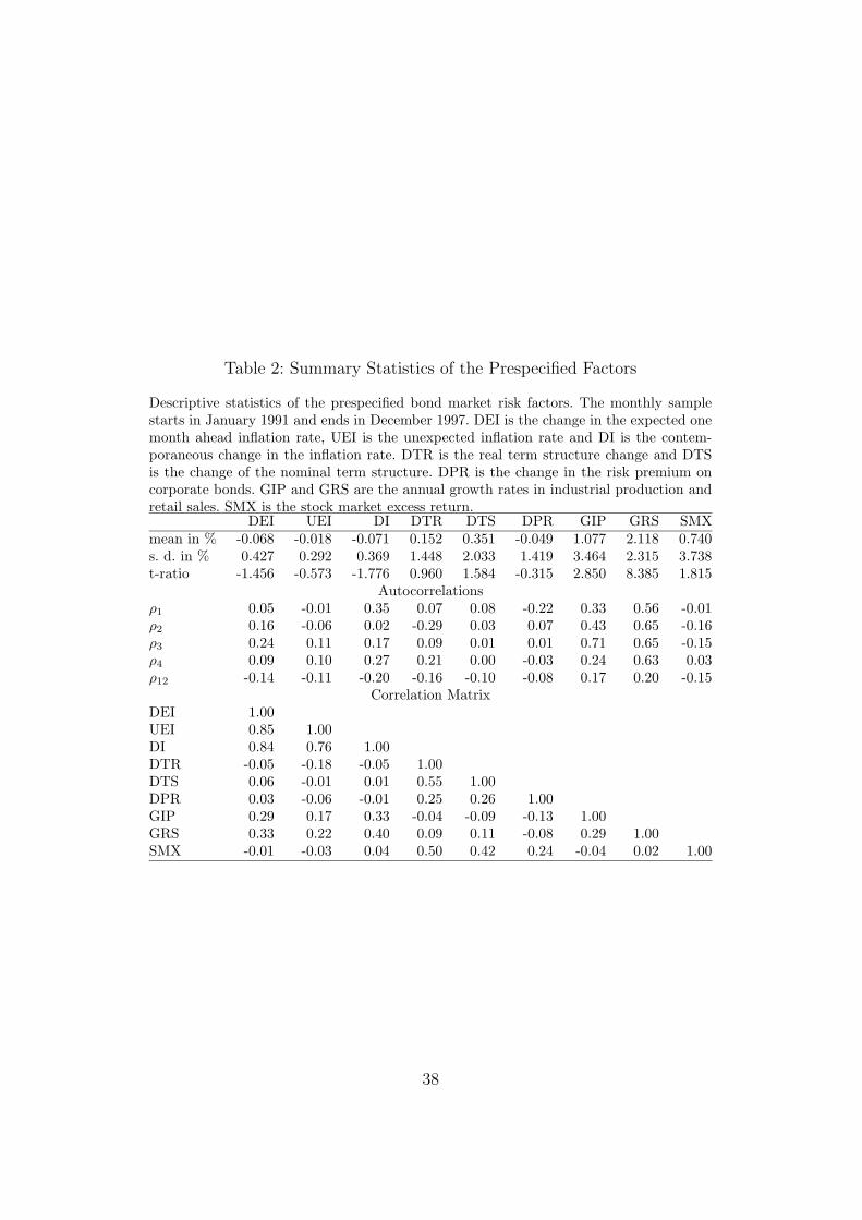
Table 2: Summary Statistics of the Prespecified Factors

Descriptive statistics of the prespecified bond market risk factors. The monthly samplestarts in January 1991 and ends in December 1997. DEI is the change in the expected onemonth ahead inflation rate, UEI is the unexpected inflation rate and DI is the contem-poraneous change in the inflation rate. DTR is the real term structure change and DTSis the change of the nominal term structure. DPR is the change in the risk premium oncorporate bonds. GIP and GRS are the annual growth rates in industrial production andretail sales. SMX is the stock market excess return.

DEI UEI DI DTR DTS DPR GIP GRS SMXmean in % -0.068 -0.018 -0.071 0.152 0.351 -0.049 1.077 2.118 0.740s. d. in % 0.427 0.292 0.369 1.448 2.033 1.419 3.464 2.315 3.738t-ratio -1.456 -0.573 -1.776 0.960 1.584 -0.315 2.850 8.385 1.815

Autocorrelationsρ1 0.05 -0.01 0.35 0.07 0.08 -0.22 0.33 0.56 -0.01ρ2 0.16 -0.06 0.02 -0.29 0.03 0.07 0.43 0.65 -0.16ρ3 0.24 0.11 0.17 0.09 0.01 0.01 0.71 0.65 -0.15ρ4 0.09 0.10 0.27 0.21 0.00 -0.03 0.24 0.63 0.03ρ12 -0.14 -0.11 -0.20 -0.16 -0.10 -0.08 0.17 0.20 -0.15

Correlation MatrixDEI 1.00UEI 0.85 1.00DI 0.84 0.76 1.00DTR -0.05 -0.18 -0.05 1.00DTS 0.06 -0.01 0.01 0.55 1.00DPR 0.03 -0.06 -0.01 0.25 0.26 1.00GIP 0.29 0.17 0.33 -0.04 -0.09 -0.13 1.00GRS 0.33 0.22 0.40 0.09 0.11 -0.08 0.29 1.00SMX -0.01 -0.03 0.04 0.50 0.42 0.24 -0.04 0.02 1.00

38

Table 3: Bond Indices

Bond Category under 5 years 5 to 15 years over 15 yearsConventional gilts GOVS GOVM GOVLIndex-linked gilts INDS INDM INDLSovereign & Supranational bonds SOVS SOVM SOVLCorporate eurosterling & unsecured CEUS CEUM CEULSecured corporate bonds - - SECLSource: Barclays Capital, London

39

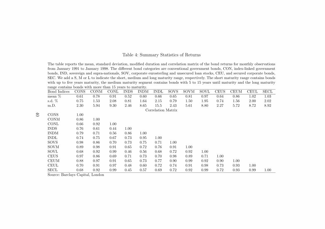
Table 4: Summary Statistics of Returns

The table reports the mean, standard deviation, modified duration and correlation matrix of the bond returns for monthly observationsfrom January 1991 to January 1998. The different bond categories are conventional government bonds, CON, index-linked governmentbonds, IND, sovereign and supra-nationals, SOV, corporate eurosterling and unsecured loan stocks, CEU, and secured corporate bonds,SEC. We add a S, M or L to indicate the short, medium and long maturity range, respectively. The short maturity range contains bondswith up to five years maturity, the medium maturity segment contains bonds with 5 to 15 years until maturity and the long maturityrange contains bonds with more than 15 years to maturity.Bond Indices CONS CONM CONL INDS INDM INDL SOVS SOVM SOVL CEUS CEUM CEUL SECLmean % 0.61 0.78 0.91 0.52 0.60 0.66 0.65 0.81 0.97 0.64 0.86 1.02 1.03s.d. % 0.75 1.53 2.08 0.81 1.64 2.15 0.79 1.50 1.95 0.74 1.56 2.00 2.02m.D. 2.30 5.94 9.30 2.46 8.65 15.5 2.43 5.61 8.80 2.27 5.72 8.72 8.92

Correlation MatrixCONS 1.00CONM 0.86 1.00CONL 0.66 0.92 1.00INDS 0.76 0.61 0.44 1.00INDM 0.79 0.71 0.56 0.86 1.00INDL 0.74 0.75 0.67 0.73 0.95 1.00SOVS 0.98 0.86 0.70 0.73 0.75 0.71 1.00SOVM 0.89 0.98 0.91 0.65 0.72 0.76 0.91 1.00SOVL 0.68 0.92 0.99 0.46 0.56 0.68 0.72 0.92 1.00CEUS 0.97 0.86 0.69 0.71 0.73 0.70 0.98 0.89 0.71 1.00CEUM 0.88 0.97 0.91 0.65 0.73 0.77 0.90 0.99 0.92 0.90 1.00CEUL 0.70 0.91 0.97 0.48 0.60 0.72 0.74 0.91 0.98 0.73 0.93 1.00SECL 0.68 0.92 0.99 0.45 0.57 0.69 0.72 0.92 0.99 0.72 0.93 0.99 1.00Source: Barclays Capital, London

40

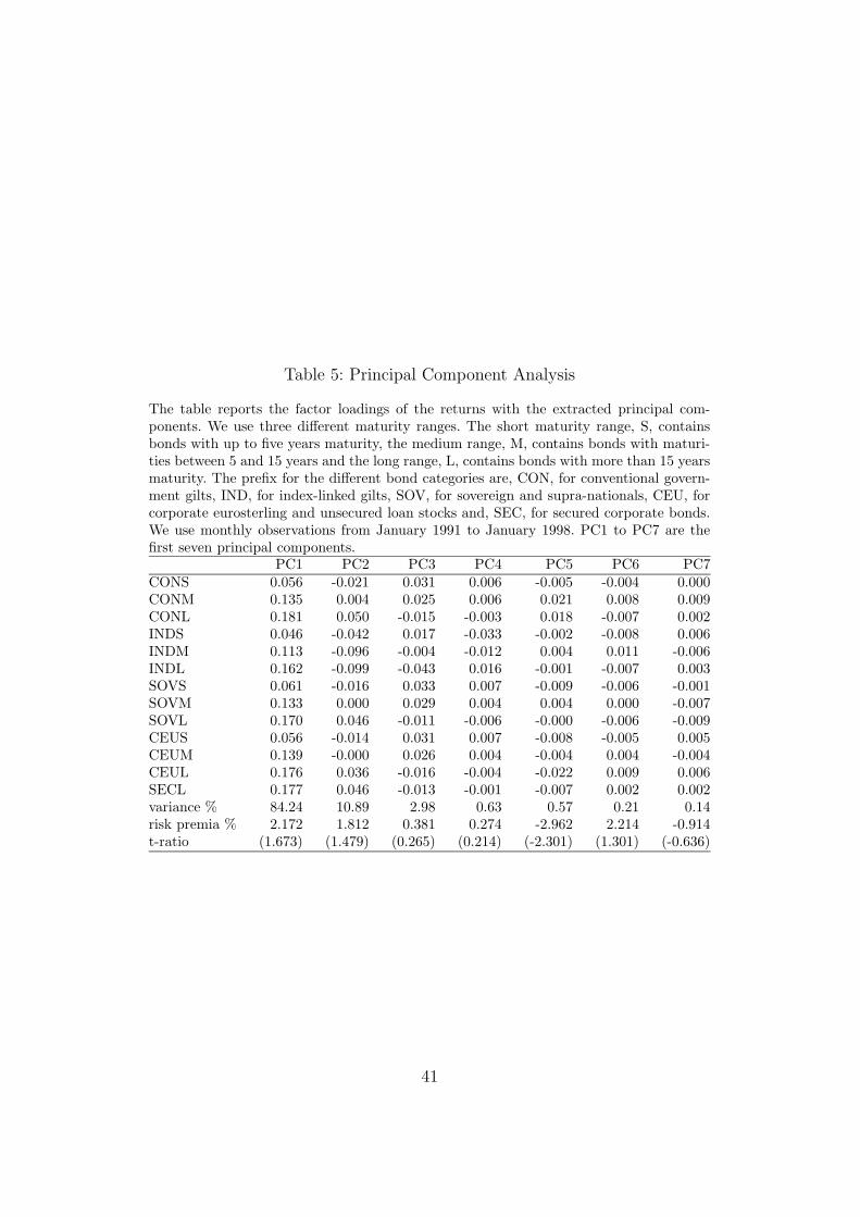
Table 5: Principal Component Analysis

The table reports the factor loadings of the returns with the extracted principal com-ponents. We use three different maturity ranges. The short maturity range, S, containsbonds with up to five years maturity, the medium range, M, contains bonds with maturi-ties between 5 and 15 years and the long range, L, contains bonds with more than 15 yearsmaturity. The prefix for the different bond categories are, CON, for conventional govern-ment gilts, IND, for index-linked gilts, SOV, for sovereign and supra-nationals, CEU, forcorporate eurosterling and unsecured loan stocks and, SEC, for secured corporate bonds.We use monthly observations from January 1991 to January 1998. PC1 to PC7 are thefirst seven principal components.

PC1 PC2 PC3 PC4 PC5 PC6 PC7CONS 0.056 -0.021 0.031 0.006 -0.005 -0.004 0.000CONM 0.135 0.004 0.025 0.006 0.021 0.008 0.009CONL 0.181 0.050 -0.015 -0.003 0.018 -0.007 0.002INDS 0.046 -0.042 0.017 -0.033 -0.002 -0.008 0.006INDM 0.113 -0.096 -0.004 -0.012 0.004 0.011 -0.006INDL 0.162 -0.099 -0.043 0.016 -0.001 -0.007 0.003SOVS 0.061 -0.016 0.033 0.007 -0.009 -0.006 -0.001SOVM 0.133 0.000 0.029 0.004 0.004 0.000 -0.007SOVL 0.170 0.046 -0.011 -0.006 -0.000 -0.006 -0.009CEUS 0.056 -0.014 0.031 0.007 -0.008 -0.005 0.005CEUM 0.139 -0.000 0.026 0.004 -0.004 0.004 -0.004CEUL 0.176 0.036 -0.016 -0.004 -0.022 0.009 0.006SECL 0.177 0.046 -0.013 -0.001 -0.007 0.002 0.002variance % 84.24 10.89 2.98 0.63 0.57 0.21 0.14risk premia % 2.172 1.812 0.381 0.274 -2.962 2.214 -0.914t-ratio (1.673) (1.479) (0.265) (0.214) (-2.301) (1.301) (-0.636)

41

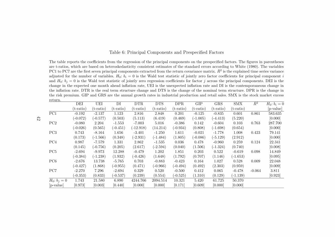
Table 6: Principal Components and Prespecified Factors

The table reports the coefficients from the regression of the principal components on the prespecified factors. The figures in parenthesesare t-ratios, which are based on heteroskedasticity consistent estimates of the standard errors according to White (1980). The variablesPC1 to PC7 are the first seven principal components extracted from the return covariance matrix. R̄2 is the explained time series varianceadjusted for the number of variables. H0: bi = 0 is the Wald test statistic of jointly zero factor coefficients for principal component i

and H0: bj = 0 is the Wald test statistic of jointly zero regression coefficients for factor j across the principal components. DEI is thechange in the expected one month ahead inflation rate, UEI is the unexpected inflation rate and DI is the contemporaneous change inthe inflation rate. DTR is the real term structure change and DTS is the change of the nominal term structure. DPR is the change inthe risk premium. GIP and GRS are the annual growth rates in industrial production and retail sales. SMX is the stock market excessreturn.

DEI UEI DI DTR DTS DPR GIP GRS SMX R̄2 H0: bi = 0(t-ratio) (t-ratio) (t-ratio) (t-ratio) (t-ratio) (t-ratio) (t-ratio) (t-ratio) (t-ratio) [p-value]

PC1 -0.192 -2.137 1.123 2.816 2.848 0.201 -0.125 -0.835 0.601 0.861 583.635(-0.072) (-0.577) (0.503) (5.113) (6.419) (0.469) (-1.005) (-4.413) (5.220) [0.000]

PC2 -0.080 2.204 -1.553 -7.003 5.016 -0.386 0.142 -0.604 0.103 0.763 287.700(-0.026) (0.565) (-0.451) (-12.918) (14.214) (-0.934) (0.808) (-1.698) (0.654) [0.000]

PC3 0.743 -8.164 1.656 -3.401 -1.250 1.611 -0.021 -1.778 1.008 0.423 79.141(0.173) (-1.566) (0.348) (-2.931) (-1.484) (1.805) (-0.086) (-5.129) (2.912) [0.000]

PC4 0.987 -7.579 1.331 2.862 -1.535 0.036 0.478 -0.960 0.259 0.124 22.341(0.145) (-0.756) (0.205) (2.617) (-2.594) (0.040) (1.506) (-1.324) (0.740) [0.008]

PC5 -2.694 -9.973 12.288 -0.479 1.202 1.851 0.203 0.522 -0.619 0.098 14.849(-0.384) (-1.238) (1.932) (-0.426) (1.648) (1.792) (0.707) (1.146) (-1.653) [0.095]

PC6 -2.676 13.738 -5.765 0.703 -0.883 -0.423 0.164 1.027 0.528 0.009 22.048(-0.427) (1.868) (-0.955) (0.471) (-0.966) (-0.494) (0.492) (2.303) (0.959) [0.009]

PC7 -2.270 7.296 -2.694 0.329 0.520 -0.500 0.412 0.065 -0.478 -0.064 3.811(-0.353) (0.833) (-0.537) (0.239) (0.554) (-0.525) (1.310) (0.129) (-1.139) [0.923]

H0: bj = 0 1.743 21.580 6.890 4244.766 2094.514 10.321 5.420 61.725 50.370[p-value] [0.973] [0.003] [0.440] [0.000] [0.000] [0.171] [0.609] [0.000] [0.000]

42

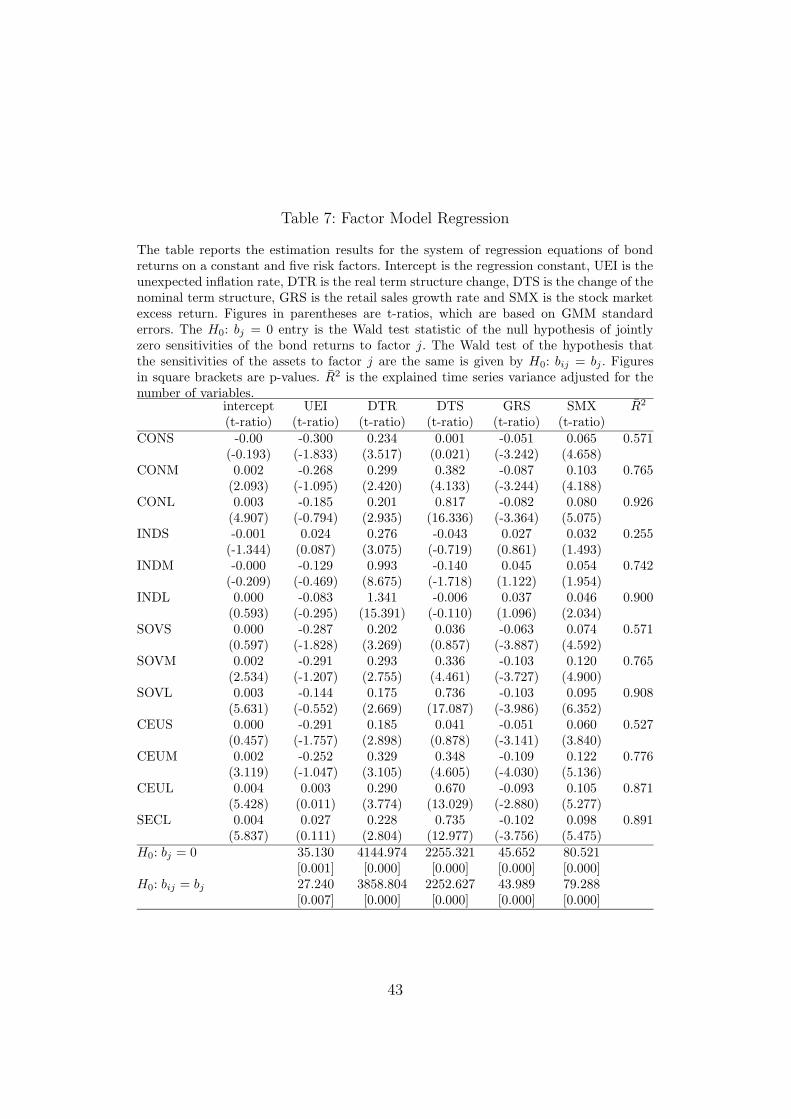
Table 7: Factor Model Regression

The table reports the estimation results for the system of regression equations of bondreturns on a constant and five risk factors. Intercept is the regression constant, UEI is theunexpected inflation rate, DTR is the real term structure change, DTS is the change of thenominal term structure, GRS is the retail sales growth rate and SMX is the stock marketexcess return. Figures in parentheses are t-ratios, which are based on GMM standarderrors. The H0: bj = 0 entry is the Wald test statistic of the null hypothesis of jointlyzero sensitivities of the bond returns to factor j. The Wald test of the hypothesis thatthe sensitivities of the assets to factor j are the same is given by H0: bij = bj . Figuresin square brackets are p-values. R̄2 is the explained time series variance adjusted for thenumber of variables.

intercept UEI DTR DTS GRS SMX R̄2

(t-ratio) (t-ratio) (t-ratio) (t-ratio) (t-ratio) (t-ratio)CONS -0.00 -0.300 0.234 0.001 -0.051 0.065 0.571

(-0.193) (-1.833) (3.517) (0.021) (-3.242) (4.658)CONM 0.002 -0.268 0.299 0.382 -0.087 0.103 0.765

(2.093) (-1.095) (2.420) (4.133) (-3.244) (4.188)CONL 0.003 -0.185 0.201 0.817 -0.082 0.080 0.926

(4.907) (-0.794) (2.935) (16.336) (-3.364) (5.075)INDS -0.001 0.024 0.276 -0.043 0.027 0.032 0.255

(-1.344) (0.087) (3.075) (-0.719) (0.861) (1.493)INDM -0.000 -0.129 0.993 -0.140 0.045 0.054 0.742

(-0.209) (-0.469) (8.675) (-1.718) (1.122) (1.954)INDL 0.000 -0.083 1.341 -0.006 0.037 0.046 0.900

(0.593) (-0.295) (15.391) (-0.110) (1.096) (2.034)SOVS 0.000 -0.287 0.202 0.036 -0.063 0.074 0.571

(0.597) (-1.828) (3.269) (0.857) (-3.887) (4.592)SOVM 0.002 -0.291 0.293 0.336 -0.103 0.120 0.765

(2.534) (-1.207) (2.755) (4.461) (-3.727) (4.900)SOVL 0.003 -0.144 0.175 0.736 -0.103 0.095 0.908

(5.631) (-0.552) (2.669) (17.087) (-3.986) (6.352)CEUS 0.000 -0.291 0.185 0.041 -0.051 0.060 0.527

(0.457) (-1.757) (2.898) (0.878) (-3.141) (3.840)CEUM 0.002 -0.252 0.329 0.348 -0.109 0.122 0.776

(3.119) (-1.047) (3.105) (4.605) (-4.030) (5.136)CEUL 0.004 0.003 0.290 0.670 -0.093 0.105 0.871

(5.428) (0.011) (3.774) (13.029) (-2.880) (5.277)SECL 0.004 0.027 0.228 0.735 -0.102 0.098 0.891

(5.837) (0.111) (2.804) (12.977) (-3.756) (5.475)H0: bj = 0 35.130 4144.974 2255.321 45.652 80.521

[0.001] [0.000] [0.000] [0.000] [0.000]H0: bij = bj 27.240 3858.804 2252.627 43.989 79.288

[0.007] [0.000] [0.000] [0.000] [0.000]

43

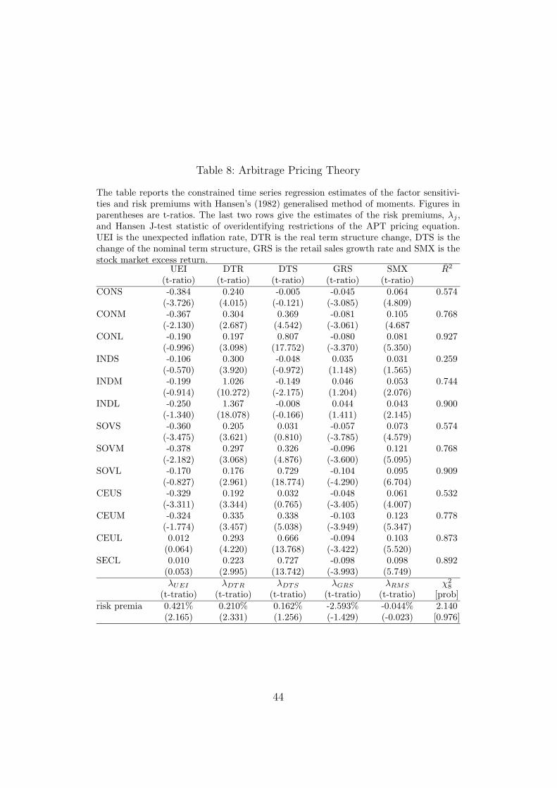
Table 8: Arbitrage Pricing Theory

The table reports the constrained time series regression estimates of the factor sensitivi-ties and risk premiums with Hansen’s (1982) generalised method of moments. Figures inparentheses are t-ratios. The last two rows give the estimates of the risk premiums, λj ,and Hansen J-test statistic of overidentifying restrictions of the APT pricing equation.UEI is the unexpected inflation rate, DTR is the real term structure change, DTS is thechange of the nominal term structure, GRS is the retail sales growth rate and SMX is thestock market excess return.

UEI DTR DTS GRS SMX R̄2

(t-ratio) (t-ratio) (t-ratio) (t-ratio) (t-ratio)CONS -0.384 0.240 -0.005 -0.045 0.064 0.574

(-3.726) (4.015) (-0.121) (-3.085) (4.809)CONM -0.367 0.304 0.369 -0.081 0.105 0.768

(-2.130) (2.687) (4.542) (-3.061) (4.687CONL -0.190 0.197 0.807 -0.080 0.081 0.927

(-0.996) (3.098) (17.752) (-3.370) (5.350)INDS -0.106 0.300 -0.048 0.035 0.031 0.259

(-0.570) (3.920) (-0.972) (1.148) (1.565)INDM -0.199 1.026 -0.149 0.046 0.053 0.744

(-0.914) (10.272) (-2.175) (1.204) (2.076)INDL -0.250 1.367 -0.008 0.044 0.043 0.900

(-1.340) (18.078) (-0.166) (1.411) (2.145)SOVS -0.360 0.205 0.031 -0.057 0.073 0.574

(-3.475) (3.621) (0.810) (-3.785) (4.579)SOVM -0.378 0.297 0.326 -0.096 0.121 0.768

(-2.182) (3.068) (4.876) (-3.600) (5.095)SOVL -0.170 0.176 0.729 -0.104 0.095 0.909

(-0.827) (2.961) (18.774) (-4.290) (6.704)CEUS -0.329 0.192 0.032 -0.048 0.061 0.532

(-3.311) (3.344) (0.765) (-3.405) (4.007)CEUM -0.324 0.335 0.338 -0.103 0.123 0.778

(-1.774) (3.457) (5.038) (-3.949) (5.347)CEUL 0.012 0.293 0.666 -0.094 0.103 0.873

(0.064) (4.220) (13.768) (-3.422) (5.520)SECL 0.010 0.223 0.727 -0.098 0.098 0.892

(0.053) (2.995) (13.742) (-3.993) (5.749)λUEI λDTR λDTS λGRS λRMS χ2

8

(t-tratio) (t-tratio) (t-tratio) (t-tratio) (t-tratio) [prob]risk premia 0.421% 0.210% 0.162% -2.593% -0.044% 2.140

(2.165) (2.331) (1.256) (-1.429) (-0.023) [0.976]

44

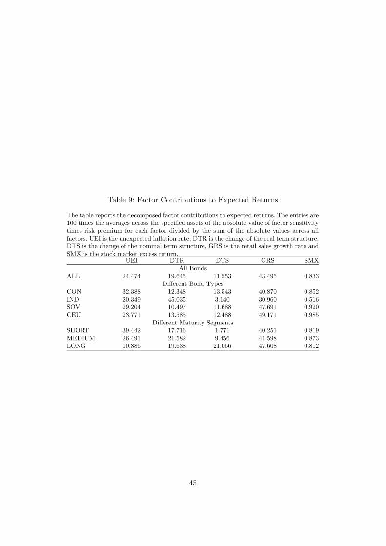
Table 9: Factor Contributions to Expected Returns

The table reports the decomposed factor contributions to expected returns. The entries are100 times the averages across the specified assets of the absolute value of factor sensitivitytimes risk premium for each factor divided by the sum of the absolute values across allfactors. UEI is the unexpected inflation rate, DTR is the change of the real term structure,DTS is the change of the nominal term structure, GRS is the retail sales growth rate andSMX is the stock market excess return.

UEI DTR DTS GRS SMXAll Bonds

ALL 24.474 19.645 11.553 43.495 0.833Different Bond Types

CON 32.388 12.348 13.543 40.870 0.852IND 20.349 45.035 3.140 30.960 0.516SOV 29.204 10.497 11.688 47.691 0.920CEU 23.771 13.585 12.488 49.171 0.985

Different Maturity SegmentsSHORT 39.442 17.716 1.771 40.251 0.819MEDIUM 26.491 21.582 9.456 41.598 0.873LONG 10.886 19.638 21.056 47.608 0.812

45

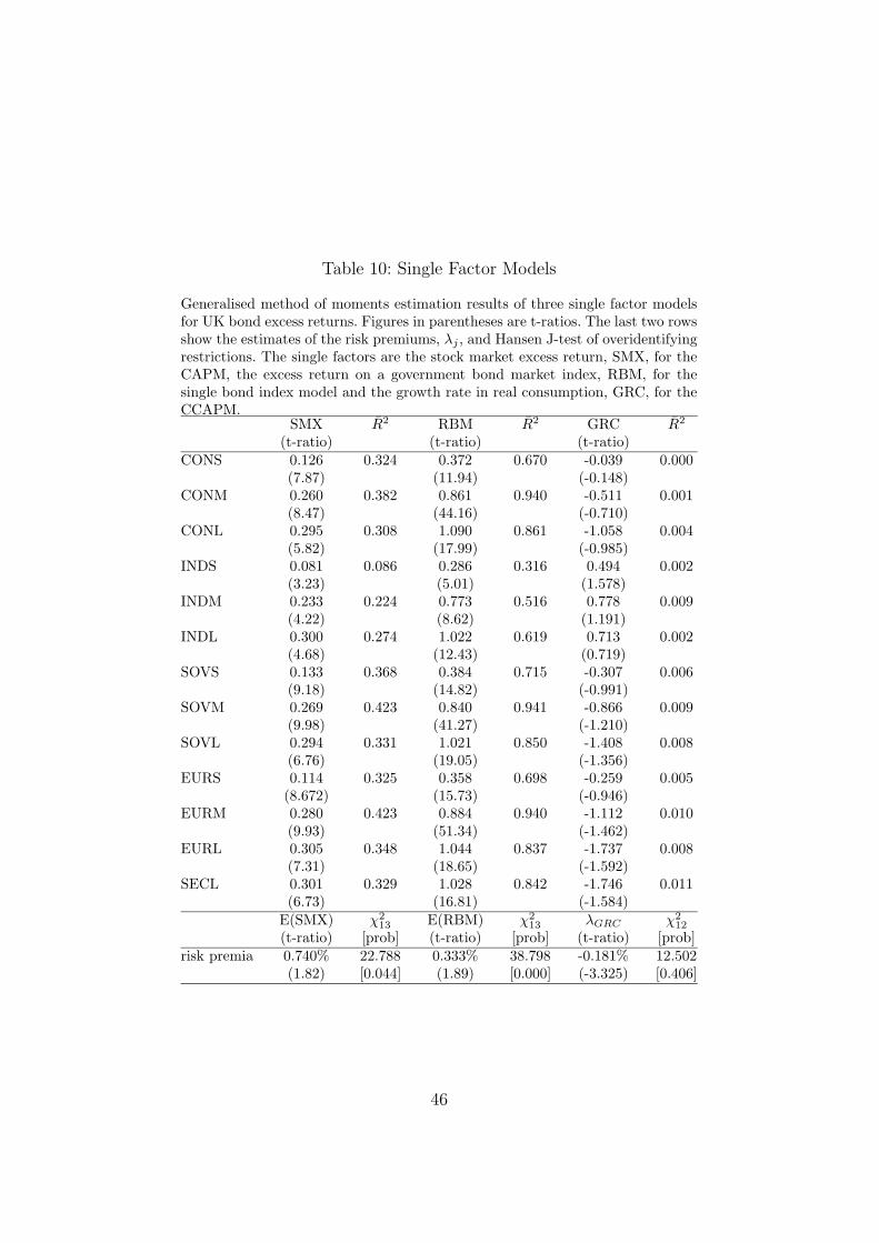
Table 10: Single Factor Models

Generalised method of moments estimation results of three single factor modelsfor UK bond excess returns. Figures in parentheses are t-ratios. The last two rowsshow the estimates of the risk premiums, λj , and Hansen J-test of overidentifyingrestrictions. The single factors are the stock market excess return, SMX, for theCAPM, the excess return on a government bond market index, RBM, for thesingle bond index model and the growth rate in real consumption, GRC, for theCCAPM.

SMX R̄2 RBM R̄2 GRC R̄2

(t-ratio) (t-ratio) (t-ratio)CONS 0.126 0.324 0.372 0.670 -0.039 0.000

(7.87) (11.94) (-0.148)CONM 0.260 0.382 0.861 0.940 -0.511 0.001

(8.47) (44.16) (-0.710)CONL 0.295 0.308 1.090 0.861 -1.058 0.004

(5.82) (17.99) (-0.985)INDS 0.081 0.086 0.286 0.316 0.494 0.002

(3.23) (5.01) (1.578)INDM 0.233 0.224 0.773 0.516 0.778 0.009

(4.22) (8.62) (1.191)INDL 0.300 0.274 1.022 0.619 0.713 0.002

(4.68) (12.43) (0.719)SOVS 0.133 0.368 0.384 0.715 -0.307 0.006

(9.18) (14.82) (-0.991)SOVM 0.269 0.423 0.840 0.941 -0.866 0.009

(9.98) (41.27) (-1.210)SOVL 0.294 0.331 1.021 0.850 -1.408 0.008

(6.76) (19.05) (-1.356)EURS 0.114 0.325 0.358 0.698 -0.259 0.005

(8.672) (15.73) (-0.946)EURM 0.280 0.423 0.884 0.940 -1.112 0.010

(9.93) (51.34) (-1.462)EURL 0.305 0.348 1.044 0.837 -1.737 0.008

(7.31) (18.65) (-1.592)SECL 0.301 0.329 1.028 0.842 -1.746 0.011

(6.73) (16.81) (-1.584)E(SMX) χ2

13 E(RBM) χ213 λGRC χ2

12

(t-ratio) [prob] (t-ratio) [prob] (t-ratio) [prob]risk premia 0.740% 22.788 0.333% 38.798 -0.181% 12.502

(1.82) [0.044] (1.89) [0.000] (-3.325) [0.406]

46

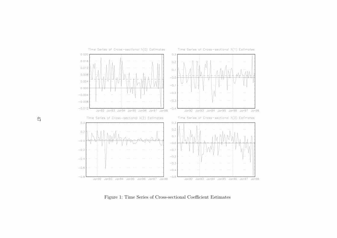
Figure 1: Time Series of Cross-sectional Coefficient Estimates

47

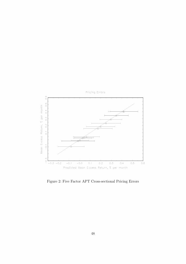
Figure 2: Five Factor APT Cross-sectional Pricing Errors

48

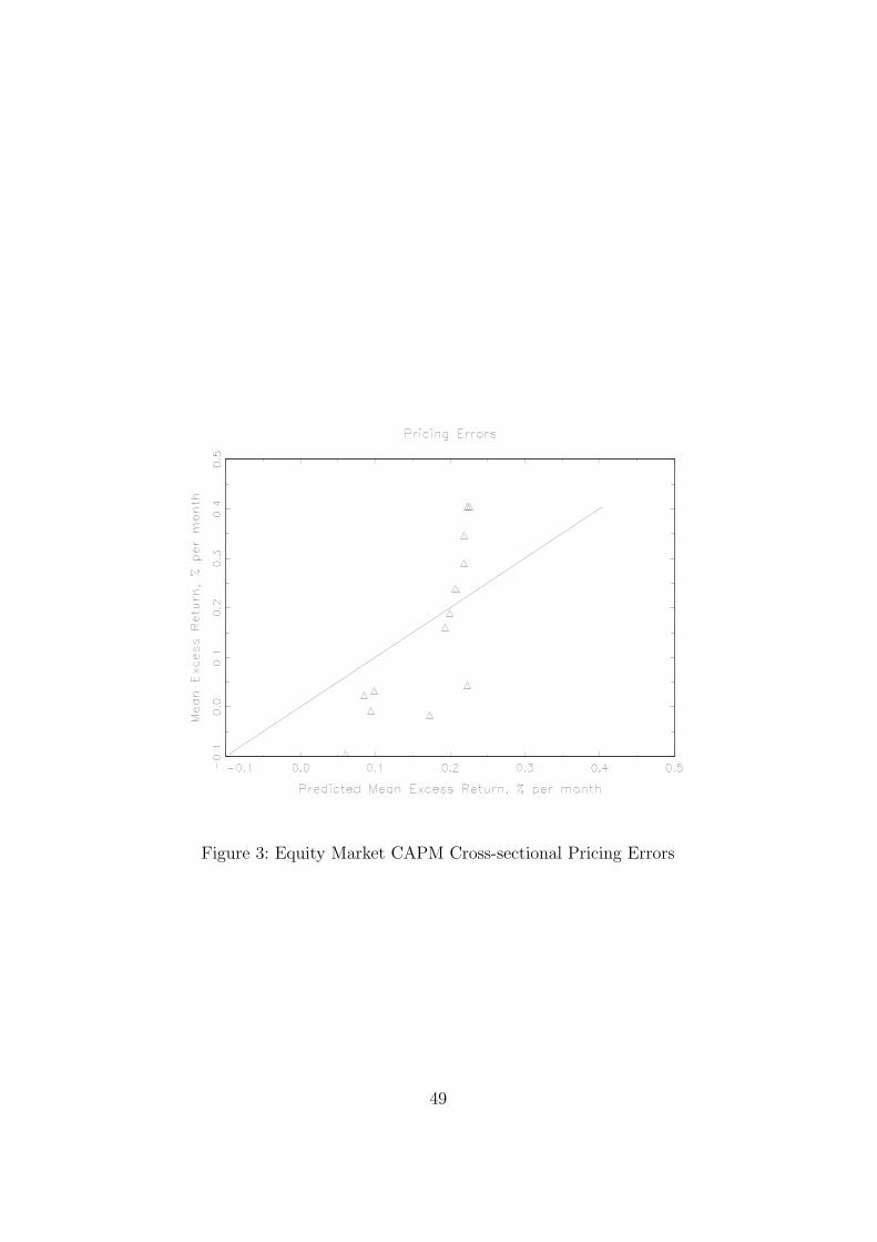
Figure 3: Equity Market CAPM Cross-sectional Pricing Errors

49

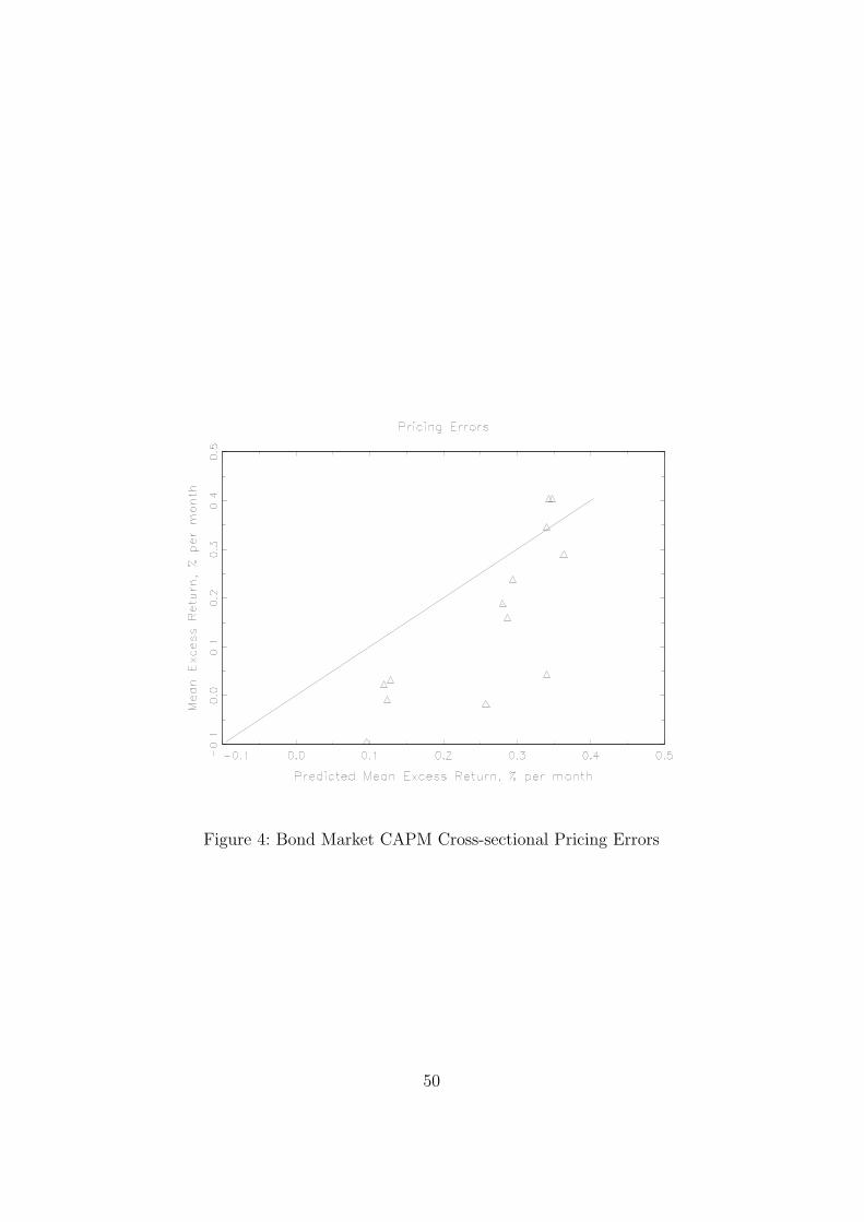
Figure 4: Bond Market CAPM Cross-sectional Pricing Errors

50

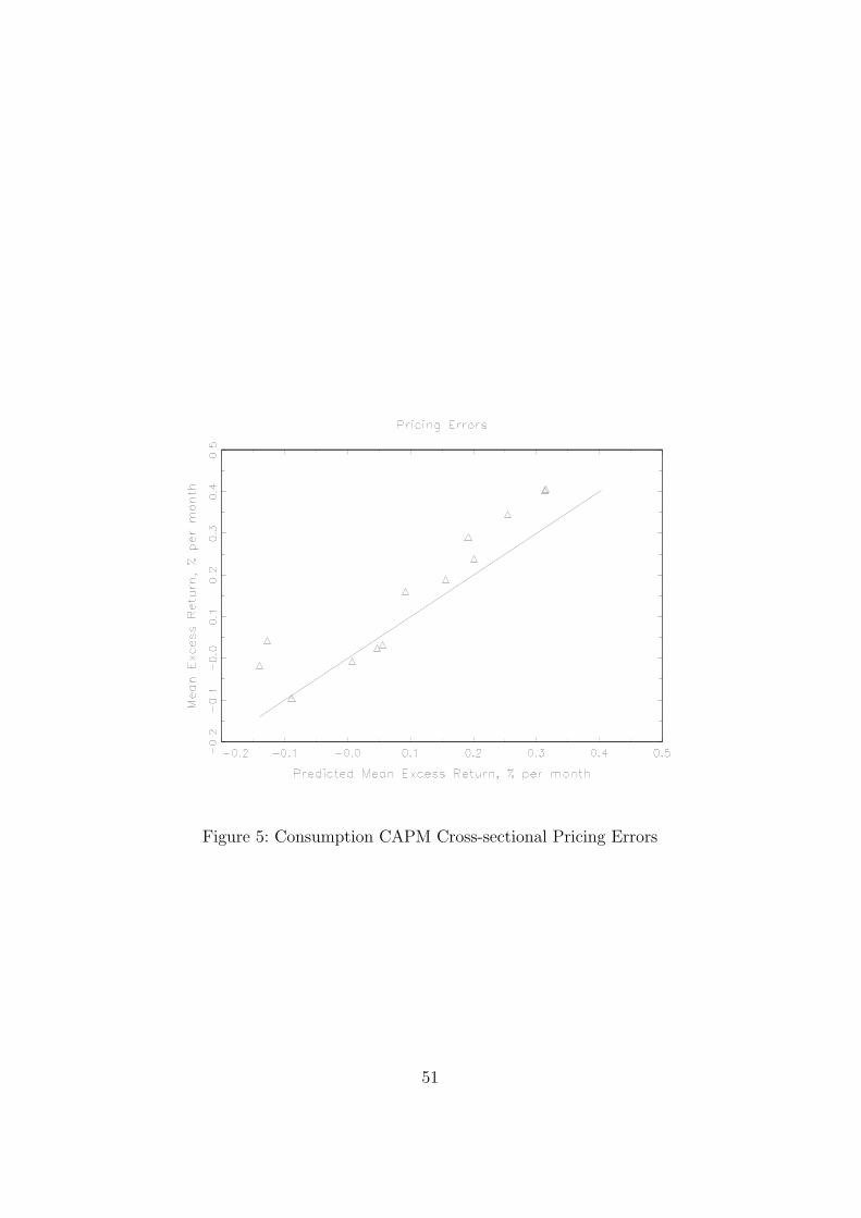
Figure 5: Consumption CAPM Cross-sectional Pricing Errors

51

risk factors of in ation-indexed and conventional

Documents