Risk Assessment of Heating, Ventilating, and Air-Conditioning Strategies in Low-Load Homes Andrew Poerschke IBACOS, Inc.

February 2016

NOTICE

This report was prepared as an account of work sponsored by an agency of the United States government. Neither the United States government nor any agency thereof, nor any of their employees, subcontractors, or affiliated partners makes any warranty, express or implied, or assumes any legal liability or responsibility for the accuracy, completeness, or usefulness of any information, apparatus, product, or process disclosed, or represents that its use would not infringe privately owned rights. Reference herein to any specific commercial product, process, or service by trade name, trademark, manufacturer, or otherwise does not necessarily constitute or imply its endorsement, recommendation, or favoring by the United States government or any agency thereof. The views and opinions of authors expressed herein do not necessarily state or reflect those of the United States government or any agency thereof.

Available electronically at SciTech Connect http:/www.osti.gov/scitech

Available for a processing fee to U.S. Department of Energy and its contractors, in paper, from:

U.S. Department of Energy Office of Scientific and Technical Information P.O. Box 62 Oak Ridge, TN 37831-0062 OSTI http://www.osti.gov Phone: 865.576.8401 Fax: 865.576.5728 Email: reports@osti.gov

Available for sale to the public, in paper, from: U.S. Department of Commerce National Technical Information Service 5301 Shawnee Road Alexandria, VA 22312 NTIS http://www.ntis.gov Phone: 800.553.6847 or 703.605.6000 Fax: 703.605.6900 Email: orders@ntis.gov

iii

Risk Assessment of Heating, Ventilating, and Air-Conditioning Strategies in Low-Load Homes

Prepared for:

The National Renewable Energy Laboratory

On behalf of the U.S. Department of Energy’s Building America Program

Office of Energy Efficiency and Renewable Energy

15013 Denver West Parkway

Golden, CO 80401

NREL Contract No. DE-AC36-08GO28308

Prepared by:

Andrew Poerschke

IBACOS, Inc.

2214 Liberty Avenue

Pittsburgh, PA 15222

NREL Technical Monitor: Stacey Rothgeb

Prepared under Subcontract No. KNDJ-0-40341-05

February 2016

iv

The work presented in this report does not represent performance of any product relative to regulated minimum efficiency requirements. The laboratory and/or field sites used for this work are not certified rating test facilities. The conditions and methods under which products were characterized for this work differ from standard rating conditions, as described. Because the methods and conditions differ, the reported results are not comparable to rated product performance and should only be used to estimate performance under the measured conditions.

v

Acknowledgments

The author would like to acknowledge Thermal Energy System Specialists, Inc. and John Holton for their help with this project.

vi

Contents Acknowledgments ...................................................................................................................................... v List of Figures ........................................................................................................................................... vii List of Tables ............................................................................................................................................ viii Definitions ................................................................................................................................................... ix Executive Summary .................................................................................................................................... x 1 Introduction and Background ............................................................................................................. 1

1.1 Background ..........................................................................................................................1 1.2 Research Questions ..............................................................................................................2

2 Mathematical and Modeling Methods ................................................................................................. 3 2.1 Variable Parameters .............................................................................................................7

2.1.1 Geometry..................................................................................................................7 2.1.2 Heating, Ventilating, and Air-Conditioning System..............................................11 2.1.3 Control Strategy .....................................................................................................11 2.1.4 Internal Gains .........................................................................................................11

2.2 Computational Fluid Dynamics .........................................................................................14 3 Research/Experimental Methods ...................................................................................................... 15 4 Results ................................................................................................................................................. 16

4.1 Computational Fluid Dynamics .........................................................................................21 5 Discussion ........................................................................................................................................... 24 6 Conclusions ........................................................................................................................................ 25

6.1 Integration Opportunities ...................................................................................................26 References ................................................................................................................................................. 27 Appendix: Select Simulation Data ........................................................................................................... 29

vii

List of Figures Figure 1. House 1—Single-story ranch house on a crawl space. .......................................................... 8 Figure 2. House 2—Two-story house on a slab. ...................................................................................... 9 Figure 3. House 3—Two-story house with a basement. ....................................................................... 10 Figure 4. An example histogram. The bar color represents additional variables (e.g., season). ..... 16 Figure 5. Histogram plot of all models. ................................................................................................... 17 Figure 6. Stacked histogram plot dividing seasonal data. ................................................................... 19 Figure 7. Stacked histogram plot dividing each house by room. ........................................................ 20 Figure 8. Summary of ASHRAE Standard 55 cycle and drift analysis. ............................................... 21 Figure 9. Cooling simulation after 10 min of operation, initial air temperature 76°F and inlet

air temperature 56°F. .......................................................................................................................... 22 Figure 10. Heating simulation after 10 min of operation, initial air temperature 71°F and inlet

air temperature 110°F. ........................................................................................................................ 22 Figure 11. Heating simulation after 10 min of operation, partition door closed. ................................ 23 Figure 12. Simulation temperature data for the two-story house over a basement, climate

zone 5, hot days. ................................................................................................................................. 29 Figure 13. Simulation temperature data for the case of the two-story house on a slab, climate

zone 5, hot days. ................................................................................................................................. 30

Unless otherwise noted, all figures and photos were created by IBACOS.

viii

List of Tables Table 1. Overview of Maximum Simulation Parameters. ........................................................................ 3 Table 2. Reduced Number of Simulations: Case Numbers. ................................................................... 4 Table 3. Parameter Matrix for Base Houses. ............................................................................................ 6 Table 4. TRNSYS Model Parameters. ........................................................................................................ 7 Table 5. HVAC System Overview. ............................................................................................................ 11 Table 6. Control Strategy Overview. ....................................................................................................... 11 Table 7. Example Hourly Internal Gain Profile for One Day. ................................................................. 13 Table 8. Internal Gain Monthly Multipliers. ............................................................................................. 14 Table 9. Limited Set of Simulations. ....................................................................................................... 14

Unless otherwise noted, all tables were created by IBACOS.

ix

Definitions

ACCA Air Conditioning Contractors of America

ACH50 Air changes per hour at 50 Pascals

ACHnat Air changes per hour under typical pressure differentials

BEopt™ Building Energy Optimization (software)

Btu British thermal units

Btu/h British thermal units per hour

CFD Computational fluid dynamics

CFM Cubic feet per minute

DOE U.S. Department of Energy

HVAC Heating, ventilating and air conditioning

SHGC Solar heat gain coefficient

TRNSYS Transient System Simulation Tool (software)

ZERH Zero Energy Ready Home

x

Executive Summary

Modern and energy-efficient homes that conform to the U.S. Department of Energy’s (DOE’s) Zero Energy Ready Home (ZERH) requirements are being constructed at an increasing rate. ZERH requirements closely align with the International Energy Conservation Code (ICC 2012). One challenge that faces these homes in the marketplace, however, is the risk that traditional heating, ventilating, and air-conditioning (HVAC) systems will not provide adequate comfort. DOE’s Building America Research team IBACOS found that low-load homes (ZERHs) have differing room-to-room load densities and highly variable load densities throughout the day and year based on solar gains and internal gains (Poerschke and Stecher 2014). Current engineering guidelines for air-based space-conditioning systems use a methodology that was developed more than 50 years ago, which was based on the concept that buildings are dominated by externally driven shell loads (Straub 1956). Significant advances in thermal enclosure performance mean that peak loads that are still externally dominated can be strongly influenced by internal gains, hourly loads in different rooms, and thermal lag—all of which require rethinking the traditional space-conditioning system. Homeowners want to live in durable, comfortable, and efficient homes. Such homes are achievable with appropriate care in the design and construction phases. This project provides valuable insight into design techniques for maximizing comfort in an efficient home. Homebuilders need solutions that will ensure occupant comfort and achieve the high level of energy efficiency demanded by modern standards.

To identify cases in which comfort standards may be compromised and to identify strategies to mitigate this concern, IBACOS used detailed TRNSYS (TESS 2015) models (Version 17) to simulate three different house geometries in three climate zones. Each house was simulated with a traditional HVAC system, a high-velocity HVAC system, and a multihead mini-split system. As appropriate for each respective system, different control strategies were evaluated for their effectiveness in maintaining thermal uniformity in the house.

These simulations enabled IBACOS to identify which strategies work best for particular climate zones or house geometries and to propose solutions that homebuilders can implement to reduce the risk of occupant discomfort in individual rooms.

The results of this study indicate that the control strategy and ideal system type vary with house type and climate. Single-story homes with centralized open layouts can be adequately conditioned with a single thermostat in all the simulated climate zones. Two-story homes with a high window-to-wall ratio on the southern and western exposures need multiple thermostats to provide adequate comfort. In these cases, continuous fan operation does not significantly improve comfort; a discretely zoned approach is necessary to prevent undercooling of some zones.

1

1 Introduction and Background

The U.S. Department of Energy’s (DOE’s) Building America research team IBACOS found that low-load homes (zero energy ready homes [ZERHs]) have differing room-to-room load densities and highly variable load densities throughout the day and year because of solar gains and internal gains (Stecher and Poerschke 2014). IBACOS defines low load as a house with a thermal enclosure that yields a maximum space heating and cooling load of less than 10 Btu/h per square foot of conditioned floor area (31.5 W/m2 [1,200 ft2/ton]). These variations present a challenge to homebuilders, who face the risk of thermal discomfort by using traditional heating, ventilating, and air-conditioning (HVAC) systems that are designed with a methodology that was developed more than 50 years ago. This methodology was based on the concept that buildings are dominated by externally driven shell loads (Straub 1956). Although peak loads are still externally dominated, significant advances in thermal enclosure performance mean that peak loads can be strongly influenced by internal gains, hourly loads in different rooms, and thermal lag—all of which require rethinking the traditional space-conditioning system. Homebuilders need cost-effective and simple solutions to ensure occupant comfort in these low-load homes.

The goal of this project was to identify cases in which comfort standards may be compromised and then to determine the effect the HVAC system alone can have to mitigate these concerns. IBACOS used detailed TRNSYS (TESS 2015) models (Version 17) to simulate three different house geometries in three climate zones. Each house was simulated with a traditional HVAC system, a high-velocity HVAC system, and a multihead mini-split system. As appropriate for each respective system, different control strategies were evaluated for their effectiveness in maintaining thermal uniformity in the house, with respect to Air Conditioning Contractors of America (ACCA) Manual RS (Rutkowski 1997) and ASHRAE Standard 55-2013 comfort standards (ASHRAE 2013).

These simulations enabled IBACOS to identify which strategies work best for particular climate zones or house geometries and to propose solutions that homebuilders can implement to ensure occupant comfort in individual rooms.

1.1 Background Advances in the thermal enclosure performance of low-load homes have created a need to rethink the way space-conditioning and control systems are designed for these homes in order to maintain acceptable occupant comfort levels. Findings from two unoccupied test houses (Stecher and Poerschke 2014; Poerschke and Stecher 2014) indicate that some form of distribution to each room is beneficial for occupant comfort but that a traditional “right-sized system” may not guarantee comfort in all rooms because of closed doors and internal/solar loads imposed on specific rooms. Greater room-to-room interaction of air and temperatures is needed than a traditional single-zone thermostat model can provide. The results of this work were used to assess the viability of the variable-volume airflow small-diameter duct system in the tested climates and house geometries.

The difficulty with creating central space-conditioning systems (design, balancing, operation, supply outlet locations, and fan operation strategies) for low-load homes has been well documented through modeling and field measurements (IBACOS 2006a, 2006b, 2007; Rittelmann 2008; Broniek 2008). Aldrich (2009) documented the significant impact that internal

2

gains of occupants and residential electronics can have on a house during the heating season in houses with single-point heating systems and traditional distribution systems. For example, hourly temperature readings in energy-efficient and sun-tempered houses on Martha’s Vineyard, Massachusetts, showed significant temperature fluctuations in the first-floor main space (predominantly where the south-facing windows were located) and the upstairs bedrooms with only east- or west-facing windows (Stecher et al. 2012).

IBACOS studied individual thermostatic controls in each room connected to a centrally ducted distribution. The thermostat in each room can turn on the air handling unit fan and circulate air throughout the entire house whenever that room is out of the acceptable temperature range (Rittelmann 2008). This strategy maintained uniform temperatures between individual rooms and the thermostatically controlled airspace more effectively than a single-zone thermostat. This report looks at the impact of continuous fan operation as an upper boundary limit; if continuous operation could not significantly improve comfort, any shorter duration would have little effect.

IBACOS also studied passive air transfer from the main space of the house to bedrooms with both opened and closed doors in two unoccupied test houses—one in Pittsburgh, Pennsylvania (Poerschke and Stecher 2014), and one in Fresno, California (Stecher and Poerschke 2014). Even with passive air inlets installed in partition doors, limited airflow resulted in room-to-room temperature differences beyond ACCA Manual RS recommendations (Rutkowski 1997). Measured data (Aldrich 2010) indicated that limited fan-forced supply from the first-floor main space to the second-floor bedrooms with doors closed generally could maintain comfortable conditions from a single source of heating or cooling in the main living space in a cold climate during the heating season. Aldrich (2010) and Townsend et al. (2009) indicate that some level of active air mixing throughout the house also is necessary to ensure fresh ventilation air reaches all spaces.

1.2 Research Questions The following research questions will be addressed by the research project of this report.

• What are the magnitude and range of climate impact on the operating parameters of a small-diameter duct HVAC system in a low-load house?

• What are the magnitude and range of climate impact on the operating parameters of discretely zoned (e.g., one or two spaces with doors isolating them from the remainder of the house) ducted and ductless mini-splits or hydronic air handling units in a low-load house?

• What is the operational impact of single- or multizoned control strategies?

• Can such systems create superior occupant comfort while maintaining or reducing energy consumption compared to a traditional centrally ducted and controlled system?

3

2 Mathematical and Modeling Methods

To answer the research questions, IBACOS used a battery of simulations to predict the environmental and operating conditions that result in the greatest risk of occupant comfort complaints. Given correct input values, HVAC simulation models can simulate the operations of multizone buildings quite accurately. For each case, a multizone building model was created using TRNSYS Version 17 to allow a variety of parameters to be modified. The Type 56 building model was used to create a multizone simulation. This approach allowed the team to rapidly test many scenarios, which would not be feasible in a test house approach. A relatively small number of base models grew rapidly when considering each climate zone, building orientation, and control strategy, as listed in Table 1.

Table 1. Overview of Maximum Simulation Parameters

Parameter Variations Climate Zone 3

Design Geometry 3 HVAC System 3

Control Strategy 6 Orientation 4

Maximum Total* 648 *Simplification will reduce this total number.

Completing this multitude of simulations was not reasonable for the scope of this project. The number of simulations was greatly reduced by removing irrational and excessive combinations. The team determined that considering only the case with the maximum load was sufficient because other factors did not significantly affect the results. Also, when using a mini-split system, using only a single-zone/single-thermostat control strategy is reasonable because the approach employs several systems to satisfy the thermal requirements of all rooms of a house. Doing this made the number of simulations (99) more manageable (Table 2). The team was able to generate a complete set of results for the 99 cases, which would be nearly impossible using actual test houses. Because of the consistent data set using perfectly matching weather, the team could draw many comparisons that would not have been practical with actual test houses.

4

Table 2. Reduced Number of Simulations: Case Numbers

Single-Story Ranch Two-Story Slab Two-Story Basement

Orlando (CZ1)

Fresno (CZ3)

Denver (CZ5)

Orlando (CZ1)

Fresno (CZ3)

Denver (CZ5)

Orlando (CZ1)

Fresno (CZ3)

Denver (CZ5)

Mini-Split Heat Pump 1 2 3 4 5 6 7 8 9

Traditional

1 zone, 1 thermostat 10 15 20 25 30 35 40 45 50

1 zone, 2 thermostats 11 16 21 26 31 36 41 46 51

2 systems, 2 thermostats 12 17 22 27 32 37 42 47 52

Continuous fan 13 18 23 28 33 38 43 48 53

Responsive thermostat 14 19 24 29 34 39 44 49 54

Small-Diameter

1 zone, 1 thermostat 55 60 65 70 75 80 85 90 95

1 zone, 2 thermostats 56 61 66 71 76 81 86 91 96

2 systems, 2 thermostats 57 62 67 72 77 82 87 92 97

Continuous fan 58 63 68 73 78 83 88 93 98

Responsive thermostat 59 64 69 74 79 84 89 94 99

5

To efficiently process the multitude of simulation results, the scripting language Python (Python Software Foundation 2015) was employed. The team used the data series package pandas (pandas 2015) and the plotting package Matplotlib (Hunter 2007) to import and analyze the results in a way that would have been time consuming and nonreproducible using traditional methods such as Excel. Also, the team was able to directly read compressed .zip files, which allowed for efficient use of storage space.

Each base house was designed to the ZERH standard, which uses the 2012 International Energy Conservation Code as a basis (ICC 2012). Table 3 outlines the parameters for each base house. Each house geometry and system type will be explained in detail in later sections of this report. Load calculations from Wrightsoft Corporation (2015) also are included, which serve as a starting point for system capacity sizing.

6

Table 3. Parameter Matrix for Base Houses

Single-Story over Crawl Space (1) Two-Story on Slab (2) Two-Story over Basement (3)

Hot Mixed Cold Hot Mixed Cold Hot Mixed Cold Climate Zone (International Energy Conservation Code) CZ1 CZ3 CZ5 CZ1 CZ3 CZ5 CZ1 CZ3 CZ5

City Orlando Fresno Denver Orlando Fresno Denver Orlando Fresno Denver Heating Design Temperature 42°F 34°F 7°F 42°F 34°F 7°F 42°F 34°F 7°F Cooling Design Temperature 92°F 101°F 92°F 92°F 101°F 92°F 92°F 101°F 92°F

Basement/Crawl Space Vented crawl space

Conditioned crawl space

Conditioned crawl space – – – Piered vented

crawl space Conditioned

basement Conditioned

basement Bedrooms 3 3 3 5 5 5 4 4 4

Crawl Space Ceiling/Walls R-13 ceiling R-13 batt R-19 batt – – – R-13 ceiling – –

Basement Floor/Slab – – – – – R-10 2-ft

perimeter of slab

– R-5 cont. R-5 cont.

Walls R-13 cavity R-13 cavity, R-5 cont.

R-13 cavity, R-5 cont. R-13 cavity R-13 cavity,

R-5 cont. R-13 cavity,

R-5 cont. R-13 cavity R-13 cavity, R-5 cont.

R-13 cavity, R-5 cont.

Ceiling R-30, vented

attic, no radiant barrier

R-38, no radiant

barrier

R-50, no radiant

barrier

R-30, vented attic, no radiant

barrier

R-38, no radiant

barrier

R-50, no radiant

barrier

R-30 vented attic, no

radiant barrier

R-38, no radiant

barrier

R-50, no radiant

barrier Garage Ceiling R-13 R-19 R-30 R-13 R-19 R-30 R-13 R-19 R-30

Windows U-0.4, SHGC 0.25

U-0.3, SHGC 0.27

U-0.27, SHGC 0.27

U-0.4, SHGC 0.25

U-0.3, SHGC 0.27

U-0.27, SHGC 0.27

U-0.4, SHGC 0.25

U-0.3, SHGC 0.27

U-0.27, SHGC 0.27

Doors U-0.19 U-0.19 U-0.19 U-0.19 U-0.19 U-0.19 U-0.19 U-0.19 U-0.19

Leakage 0.15

ACHnat (3.0 ACH50)

0.125 ACHnat

(2.5 ACH50)

0.10 ACHnat

(2.0 ACH50)

0.15 ACHnat

(3.0 ACH50)

0.125 ACHnat

(2.5 ACH50)

0.10 ACHnat

(2.0 ACH50)

0.15 ACHnat

(3.0 ACH50)

0.125 ACHnat

(2.5 ACH50)

0.10 ACHnat

(2.0 ACH50) Heating Load (Btu/h)* 10,867 18,364 26,766 25,407 16,995 36,078 24,753 27,970 35,883

Cooling Sensible Load (Btu/h)* 16,687 14,015 11,681 29,146 18,835 22,057 26,316 24,522 21,566 Latent Cooling (Btu/h)* 2,634 646 0 5,069 696 0 3,211 704 0 House Square Footage 1,512 1,512 1,512 2,128 2,128 2,128 3,399 3,399 3,399

Window-to-Wall Ratio (South Face) 18% (1st)\ NA (2nd) 20% (1st)\ 30% (2nd) 22% (1st)\ 14% (2nd) ACH50 is air changes per hour at 50 Pascals. ACHnat is air changes per hour under typical pressure differentials. SHGC is solar heat gain coefficient.

*Values calculated using Wrightsoft.

7

Initially, each base model was created with unique building geometry and HVAC system types. After the team verified that the results from this initial test were within expectations, each base model underwent the specified parametric iterations to determine the effect of the control strategy. Table 4 summarizes the TRNSYS model parameters that were kept constant for each model.

Table 4. TRNSYS Model Parameters

Airflow Model CONTAM (NIST 2013), assuming open interior doors

Building Model Type 56, with geometry created using SketchUp (Trimble Navigation Limited 2015) plug-in

Basement/Slab Simple conduction model, assuming greater levels of insulation to ground

Energy Recovery Ventilator ASHRAE Standard 62.2 ventilation rate, standard efficiency (ASHRAE 2010)

Radiation Mode Three-dimensional geometry Infiltration Model CONTAM

Time Step 5 min A number of other assumptions were also made in the simulation software. Interzonal air coupling was computed by the CONTAM model based on adjacent zone temperature differences and assumed airflow during system operation. Specific heat capacity of wall components was handled on a per-layer-and-material basis. Additional heat capacity of 6 kJ/K per cubic meter of room volume was assumed to account for room furnishings. This value is typical of residential building simulation and does not overly dampen temperature swings.

2.1 Variable Parameters

2.1.1 Geometry To have the greatest impact and relevance to Building America goals, IBACOS chose three house plans that correlate to houses IBACOS has monitored in past studies. Although the simulation results could not be calibrated against measured data because of small differences in the floor plans, building envelope parameters, and climate zones, the team made comparisons to verify that the models captured any dynamic or abnormal behaviors.

Figure 1 through Figure 3 show each of the three floor plans. Figure 1, a single-story ranch-style house over a crawl space, was chosen for its simplified floor plan. The corresponding occupied test house (House 1) is conditioned by a traditional system with floor-mounted registers and is located in Rehoboth, Delaware (Imm and Wayne 2013). The floor plan shown in Figure 2 is based on an occupied test house (House 2) that IBACOS is monitoring in San Antonio, Texas (Rapport and Paul 2014). This house is conditioned with ducted and ductless mini-split units. The house plan shown in Figure 3 is based on the Pittsburgh, Pennsylvania, unoccupied test house (House 3), which has had extensive monitoring performed for traditional ductwork and high-velocity systems with high sidewall registers (Poerschke and Stecher 2014). In these floor plans, W.A. stands for window area, and W.W.R. stands for window-to-wall ratio. Simulated thermostat locations have been marked with “T-1” and “T-2.”

8

Figure 1. House 1—Single-story ranch house on a crawl space

9

Figure 2. House 2—Two-story house on a slab

10

Figure 3. House 3—Two-story house with a basement

11

2.1.2 Heating, Ventilating, and Air-Conditioning System In addition to matching the simulated geometry to actual houses, each simulated HVAC system was based on actual systems in the test houses. The team used real-world room temperature data to ensure that the models captured any dynamic behaviors associated with the various HVAC strategies. Table 5 outlines the HVAC systems that the team simulated in each house.

Table 5. HVAC System Overview

Mini-Split Typical mini-split layout with a mixture of ducted and ductless head units

Centrally Ducted Gas furnace, direct expansion coil (different annual fuel utilization efficiency/seasonal energy efficiency

ratio per climate zone)

High-Velocity Duct

Lower volume, higher temperature rise, gas furnace, direct expansion coil (different annual fuel

utilization efficiency/seasonal energy efficiency ratio per climate zone)

2.1.3 Control Strategy The team evaluated several control strategies to determine the most effective method to maintain acceptable thermal uniformity in each zone. For the evaluation of mini-split heat pumps, only a case in which there was one thermostat to each indoor head unit was considered. Table 6 summarizes the control strategies. Control strategy 4 was selected as an upper boundary for fan operation. Any less frequent operation would have a lesser impact and should be considered only if continuous fan operation keeps all zones comfortable. Control strategy 5 was considered as an alternative to continuous fan operation; the fan operates only during unbalanced load conditions.

Table 6. Control Strategy Overview

1 Single zone, single thermostat Standard set points: 71°F heating, 76°F cooling

2 Single zone, two thermostats

The system runs if one thermostat calls for conditioning. Determine the ideal location for the second thermostat (e.g., south bedroom,

west bedroom).

3 Two zone, two thermostats Determine the ideal location for the second thermostat (e.g., south bedroom, west bedroom).

4 Single zone, single thermostat, fan on

Constant fan operation, conditioning supplied only as called for by the thermostat.

5 Clever thermostat

The thermostat reads the weather forecast at the top of each hour and cycles the fan during conditions that typically would result in

asymmetric loads (e.g., sunny midseason day). 2.1.4 Internal Gains The research team generated the internal gains hourly schedules based on the Building America House Simulation Protocols (Hendron and Engebrecht 2010). By default, Building Energy Optimization software (BEopt™) Version 2.3 (NREL n.d.) includes internal gains profiles that adhere to the standard. To input equivalent profiles into the TRNSYS simulations, the team used

12

the Building America analysis spreadsheet for new construction to generate hourly numbers that could be fed into the simulations—one for each of the three houses. The spreadsheet calculates hourly load distributions and monthly multipliers to adjust the internal gains according to fluctuations caused by, for example, exterior conditions, domestic hot water distribution type, and number of occupants.

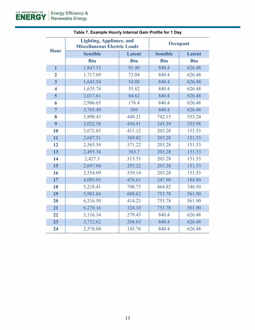
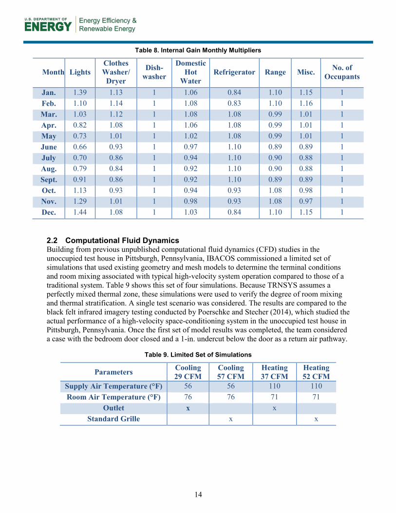
Table 7 illustrates an example hourly gain profile for a single day. This profile represents internal gains, sensible, and latent, added to the conditioned space per hour. Table 8 shows monthly multipliers to adjust the hourly values up or down, depending on the month. For example, summer months correspond with higher refrigerator use because of increased differences between the temperature in the refrigerator and the temperature in the conditioned space. No interpolation was completed to smooth between months; the same daily profile was used for every day in each month; discrete jumps occurred between months. The internal gain latent and sensible energy was distributed across each zone in the house, weighted based on floor area. This was to minimize any effect various distributions and particular occupant behaviors might have on the results of the simulations so clear comparisons could be made between the system types, control strategies, climate zones, and house geometry.

To verify that assuming an evenly weighted distribution of internal gains would not oversimplify the results, the team ran nine simulations (a single house in a single climate zone) to gauge the impact on the comparative conclusion between system and control strategies.

Internal gains were distributed among the thermal zones of the model according to the following reasoning. Gains from appliances were attributed to zones in which they were located; for example, the refrigerator and range were associated with the kitchen. Miscellaneous, lighting, and occupant thermal loads were distributed according to the presumed level of occupancy for each zone with bedrooms (e.g., receiving the highest occupant load). Detailed distributions according to specific lighting fixture and plug loads counts were not determined. Domestic hot water loads were associated only with spaces containing hot water fixtures, the bathrooms, laundry, and kitchen. Weights were assigned to each internal gain source per zone, and the whole-house loads calculated from the lighting, appliance, and miscellaneous electric load spreadsheet were divided among the zones according to the weights.

The results of this analysis show that distributing internal gains based on use areas has minimal impact on the final conclusions of the report. The two-story house over a basement in Denver, with mini-split heat pumps, showed a change of 82.8% passing rate to 84.5% passing by distributing loads according to usage zone. Across the set of two-story houses in Denver, there was a change of 1.7% to 5.3%, but the overall ranking of performance did not change for any control strategy.

13

Table 7. Example Hourly Internal Gain Profile for 1 Day

Hour

Lighting, Appliance, and Miscellaneous Electric Loads Occupant

Sensible Latent Sensible Latent Btu Btu Btu Btu

1 1,847.33 91.49 840.4 626.48 2 1,717.69 73.04 840.4 626.48 3 1,643.54 54.88 840.4 626.48 4 1,635.74 55.82 840.4 626.48 5 2,017.61 84.62 840.4 626.48 6 2,986.65 176.4 840.4 626.48 7 3,765.49 369 840.4 626.48 8 3,898.43 448.21 742.15 553.24 9 3,022.58 430.91 343.39 255.98 10 2,672.83 411.12 203.28 151.53 11 2,607.51 369.82 203.28 151.53 12 2,565.54 371.22 203.28 151.53 13 2,493.34 363.7 203.28 151.53 14 2,427.3 313.35 203.28 151.53 15 2,697.04 293.22 203.28 151.53 16 2,554.09 339.14 203.28 151.53 17 4,005.05 476.61 247.90 184.80 18 5,218.41 708.73 464.82 346.50 19 5,981.84 608.62 753.78 561.90 20 6,316.50 414.23 753.78 561.90 21 6,270.16 324.10 753.78 561.90 22 5,116.14 279.43 840.4 626.48 23 3,712.62 204.63 840.4 626.48 24 2,578.04 145.76 840.4 626.48

14

Table 8. Internal Gain Monthly Multipliers

Month Lights Clothes Washer/

Dryer

Dish-washer

Domestic Hot

Water Refrigerator Range Misc. No. of

Occupants

Jan. 1.39 1.13 1 1.06 0.84 1.10 1.15 1 Feb. 1.10 1.14 1 1.08 0.83 1.10 1.16 1 Mar. 1.03 1.12 1 1.08 1.08 0.99 1.01 1 Apr. 0.82 1.08 1 1.06 1.08 0.99 1.01 1 May 0.73 1.01 1 1.02 1.08 0.99 1.01 1 June 0.66 0.93 1 0.97 1.10 0.89 0.89 1 July 0.70 0.86 1 0.94 1.10 0.90 0.88 1 Aug. 0.79 0.84 1 0.92 1.10 0.90 0.88 1 Sept. 0.91 0.86 1 0.92 1.10 0.89 0.89 1 Oct. 1.13 0.93 1 0.94 0.93 1.08 0.98 1 Nov. 1.29 1.01 1 0.98 0.93 1.08 0.97 1 Dec. 1.44 1.08 1 1.03 0.84 1.10 1.15 1

2.2 Computational Fluid Dynamics Building from previous unpublished computational fluid dynamics (CFD) studies in the unoccupied test house in Pittsburgh, Pennsylvania, IBACOS commissioned a limited set of simulations that used existing geometry and mesh models to determine the terminal conditions and room mixing associated with typical high-velocity system operation compared to those of a traditional system. Table 9 shows this set of four simulations. Because TRNSYS assumes a perfectly mixed thermal zone, these simulations were used to verify the degree of room mixing and thermal stratification. A single test scenario was considered. The results are compared to the black felt infrared imagery testing conducted by Poerschke and Stecher (2014), which studied the actual performance of a high-velocity space-conditioning system in the unoccupied test house in Pittsburgh, Pennsylvania. Once the first set of model results was completed, the team considered a case with the bedroom door closed and a 1-in. undercut below the door as a return air pathway.

Table 9. Limited Set of Simulations

Parameters Cooling 29 CFM

Cooling 57 CFM

Heating 37 CFM

Heating 52 CFM

Supply Air Temperature (°F) 56 56 110 110 Room Air Temperature (°F) 76 76 71 71

Outlet x x Standard Grille x x

15

3 Research/Experimental Methods

The success or failure of each simulation permutation was judged based on the ACCA Manual RS standard on thermal uniformity (Rutkowski 1997) and ASHRAE Standard 55-2013, Section 5.3.5: Temperature Variations with Time (ASHRAE 2013).

ACCA Manual RS states that each room should be within 2°F of the thermostat set point temperature in heating mode and within 3°F of the set point temperature in cooling mode. IBACOS made calculations to indicate the success or failure of a room to meet this standard at each time step, as well as the magnitude of each excursion. The results of this analysis are valuable because for a given set point temperature and with no other significant effects (e.g., radiation, air speed, stratification), an occupant is assumed to consider the entire house to be comfortable if the house is conditioned within this temperature range. Previous research indicates that for a well-designed low-load home (Broniek 2008), stratification and radiation imbalances from walls are below levels that might impact comfort.

ASHRAE Standard 55, Section 5.3.5, suggests that over a given time interval, the temperature in a particular zone should remain relatively constant. According to the standard, the temperature in a zone should not change by more than 2°F in 0.25 h, 3°F in 0.5 h, 4°F in 1 h, 5°F in 2.0 h, and 6.0°F in 4 h.

IBACOS performed the analysis for an entire year’s worth of simulated data to provide an accurate likelihood that temperatures would fall outside the desired parameters. ASHRAE Standard 55 specifies that the thermal uniformity analysis should be performed at certain conditions that are representative of the design load (ASHRAE 2013).

16

4 Results

Results from all 99 models are summarized later in Figure 5 through Figure 8. In these figures, the deviation of the temperature in each room from the thermostat set point is binned and summed for each house. However, a sample of a single histogram first is presented in Figure 4 with descriptive labels. Each histogram is combined into a small multiples plot to easily assess the success or failure of each system in each house and climate zone. In addition to a histogram for each case, the average percentage of time each room was within the ACCA Manual RS comfort band (±2°F heating, ±3°F cooling), standard deviation, and mean has also been printed. The best-performing cases are highlighted with green text in Figure 5.

Figure 4. An example histogram. The bar color represents additional variables (e.g., season).

17

Figure 5. Histogram plot of all models

18

A winter in climate zone 1 has many days during which the ambient temperature rises higher than the indoor set point. Conversely, climate zone 5 has summer nightly swings during which the ambient temperature drops lower than the cooling set point. During these periods, the temperature in each room of a house can drop significantly lower than the cooling set point without dropping lower than the heating set point. The ACCA Manual RS analysis (Rutkowski 1997) flags these periods as comfort failures; however, a homeowner probably would not deem the home uncomfortable. This trend lowers the overall passing rate of a case and is most pronounced in climate zone 1 and climate zone 5.

Many of the thermal deviations are season specific. Figure 6 captures room deviations from the set point during different seasons. In this case, each season is divided into a stacked bar plot; the total height represents the percentage of time the house was within a specific bin.

A final summary plot is presented in Figure 7. In this case, the histogram is broken down by individual rooms. Figure 7 indicates the rooms that are the typical outliers.

Looking at overall home pass or failure rates may be somewhat misleading. Typically, only one or two rooms pose comfort problems in low-load homes. When summed with all other zones in a house, the overall weight of an individual room failing decreases based on the total number of rooms. With 10 rooms in a home, if a particularly uncomfortable room fails 50% of the time, this equates to only a 5% change in the total house failure rate. As such, further analysis has been conducted in select rooms.

To summarize and highlight the significant results of the ASHRAE Standard 55 cycle and drift analysis (ASHRAE 2013), a heat-map plot is presented as Figure 8. The color of cells indicates the percentage of time a room fails in a cycle or drift. The cycle or drift mode is indicated on the right axis. Figure 8 is organized similarly to the previous summary figures; data are set into a column for each room, and individual rows correspond to particular failure modes. Additionally, heating, cooling, and shoulder periods are plotted on sets of rows. Areas highlighted in color show periods of more significant failure. Failure rates lower than 10% have been filtered out to show only the most significant deviations.

19

Figure 6. Stacked histogram plot dividing seasonal data

20

Figure 7. Stacked histogram plot dividing each house by room

21

Figure 8. Summary of ASHRAE Standard 55 cycle and drift analysis

4.1 Computational Fluid Dynamics Results from each of the four CFD simulations are presented in Figure 9 and Figure 10. The team also thought the impact of closing the master bedroom door on thermal stratification was interesting to consider. Figure 9 and Figure 10 show a side-view snapshot of indoor air

22

temperatures after 10 min of simulation. The slice was taken directly in the middle of the air outlet, which corresponds closely to the center of the room. As a comparison, the typical inlet air temperature during heating mode for the TRNSYS model was 115°F. The rectangle visible in the right third of each frame is the outline of the master bathroom door.

Figure 9. Cooling simulation after 10 min of operation, initial air temperature 76°F, and inlet air temperature 56°F

Figure 10. Heating simulation after 10 min of operation, initial air temperature 71°F, and inlet air

temperature 110°F

To consider the alternative case of doors closed, the team ran the simulation with identical parameters in heating and cooling modes with modified geometry. The results are presented in Figure 11.

23

Figure 11. Heating simulation after 10 min of operation, partition door closed

24

5 Discussion

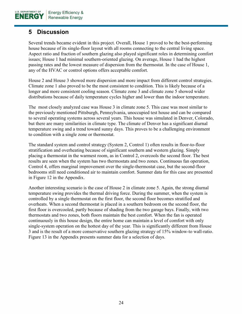
Several trends became evident in this project. Overall, House 1 proved to be the best-performing house because of its single-floor layout with all rooms connecting to the central living space. Aspect ratio and fraction of southern glazing also played significant roles in determining comfort issues; House 1 had minimal southern-oriented glazing. On average, House 1 had the highest passing rates and the lowest measure of dispersion from the thermostat. In the case of House 1, any of the HVAC or control options offers acceptable comfort.

House 2 and House 3 showed more dispersion and more impact from different control strategies. Climate zone 1 also proved to be the most consistent to condition. This is likely because of a longer and more consistent cooling season. Climate zone 3 and climate zone 5 showed wider distributions because of daily temperature cycles higher and lower than the indoor temperature.

The most closely analyzed case was House 3 in climate zone 5. This case was most similar to the previously mentioned Pittsburgh, Pennsylvania, unoccupied test house and can be compared to several operating systems across several years. This house was simulated in Denver, Colorado, but there are many similarities in climate type. The climate of Denver has a significant diurnal temperature swing and a trend toward sunny days. This proves to be a challenging environment to condition with a single zone or thermostat.

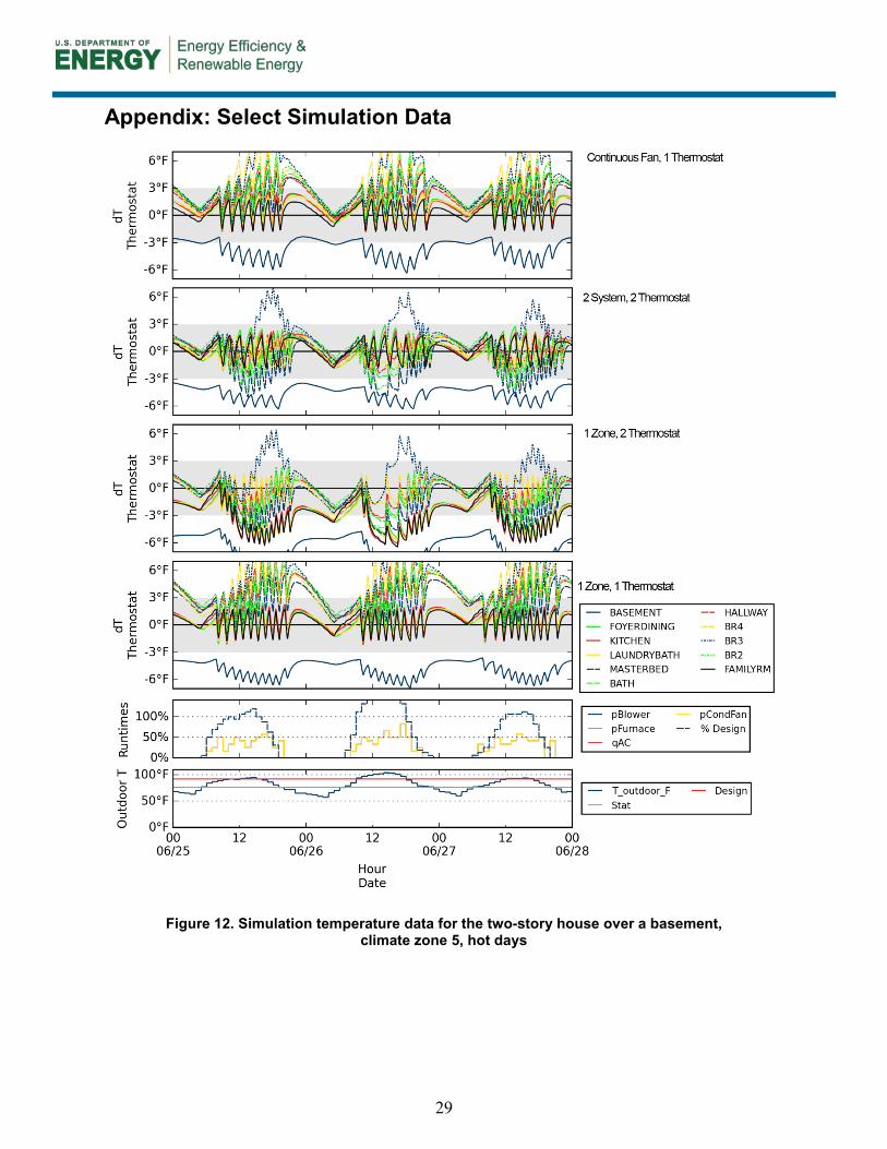
The standard system and control strategy (System 2, Control 1) often results in floor-to-floor stratification and overheating because of significant southern and western glazing. Simply placing a thermostat in the warmest room, as in Control 2, overcools the second floor. The best results are seen when the system has two thermostats and two zones. Continuous fan operation, Control 4, offers marginal improvement over the single-thermostat case, but the second-floor bedrooms still need conditioned air to maintain comfort. Summer data for this case are presented in Figure 12 in the Appendix.

Another interesting scenario is the case of House 2 in climate zone 5. Again, the strong diurnal temperature swing provides the thermal driving force. During the summer, when the system is controlled by a single thermostat on the first floor, the second floor becomes stratified and overheats. When a second thermostat is placed in a southern bedroom on the second floor, the first floor is overcooled, partly because of shading from the two garage bays. Finally, with two thermostats and two zones, both floors maintain the best comfort. When the fan is operated continuously in this house design, the entire home can maintain a level of comfort with only single-system operation on the hottest day of the year. This is significantly different from House 3 and is the result of a more conservative southern glazing strategy of 15% window-to wall-ratio. Figure 13 in the Appendix presents summer data for a selection of days.

25

6 Conclusions

Designers of HVAC systems have the goal of providing thermal comfort to occupants. ASHRAE Standard 55 defines thermal comfort as a subjective matter (ASHRAE 2013). No single formula is guaranteed to provide comfort. Furthermore, with residences the question of occupancy also should be considered. If a room is not occupied, a discussion can take place about whether it needs to fall within the thermal comfort boundaries. Some control strategies may provide perfect comfort in all rooms but unnecessarily use significantly more energy. For this report, however, the team assumed all zones were occupied at all times.

The following research questions were addressed in this report:

• What are the magnitude and range of climate impact on the operating parameters of a small-diameter duct HVAC system in a low-load house?

• What are the magnitude and range of climate impact on the operating parameters of discretely zoned (e.g., one or two spaces with doors isolating them from the remainder of the house) ducted and ductless mini-splits or hydronic air handlers in a low-load house?

• What is the operational impact of single- or multizoned control strategies?

• Can such systems create superior occupant comfort while maintaining or reducing energy consumption compared to a traditional, centrally ducted and controlled system?

The results of this work indicate several significant trends concerning climate, control strategies, and system type. Climate and latitude must be taken into account when considering the ideal control strategy for a particular HVAC system. Regions of higher latitude show a higher susceptibility to overheating southern rooms because of solar heat gains—even during the summer season. Building design also must be carefully considered. Generally, simplified building geometry with a central connecting zone and low aspect ratio can be adequately conditioned with a single thermostat. House 1 is an example of simple building geometry; a single story and all zones connect directly to the central living space with no extended hallways. Buildings with multiple floors and distant separated rooms require more complex control strategies.

In the case of the single-floor ranch house, a more complicated control strategy provides only minimal improvement. The central open zone to which each room connects allows adequate mixing to each zone. The raw data indicate the heating system may be oversized and result in some ASHRAE Standard 55 cycling failure.

The two-story house on a slab offers a more significant conditioning challenge. In this case, dual thermostats alone are not enough to ensure comfort because of the significant disparity between the load on second-floor south-facing rooms and the first-floor north-facing rooms. During the cooling season, if a thermostat is placed in the second floor, the first floor will be overcooled. The best solution is to provide two thermostats or discretely zoned mini-split heat pump head units. In the case of climate zone 1, the house can maintain 100% of the rooms within 3°F of the thermostat regardless of the system or control strategy in the summer. During the winter, however, the home does not maintain a consistent temperature because of warmer days with

26

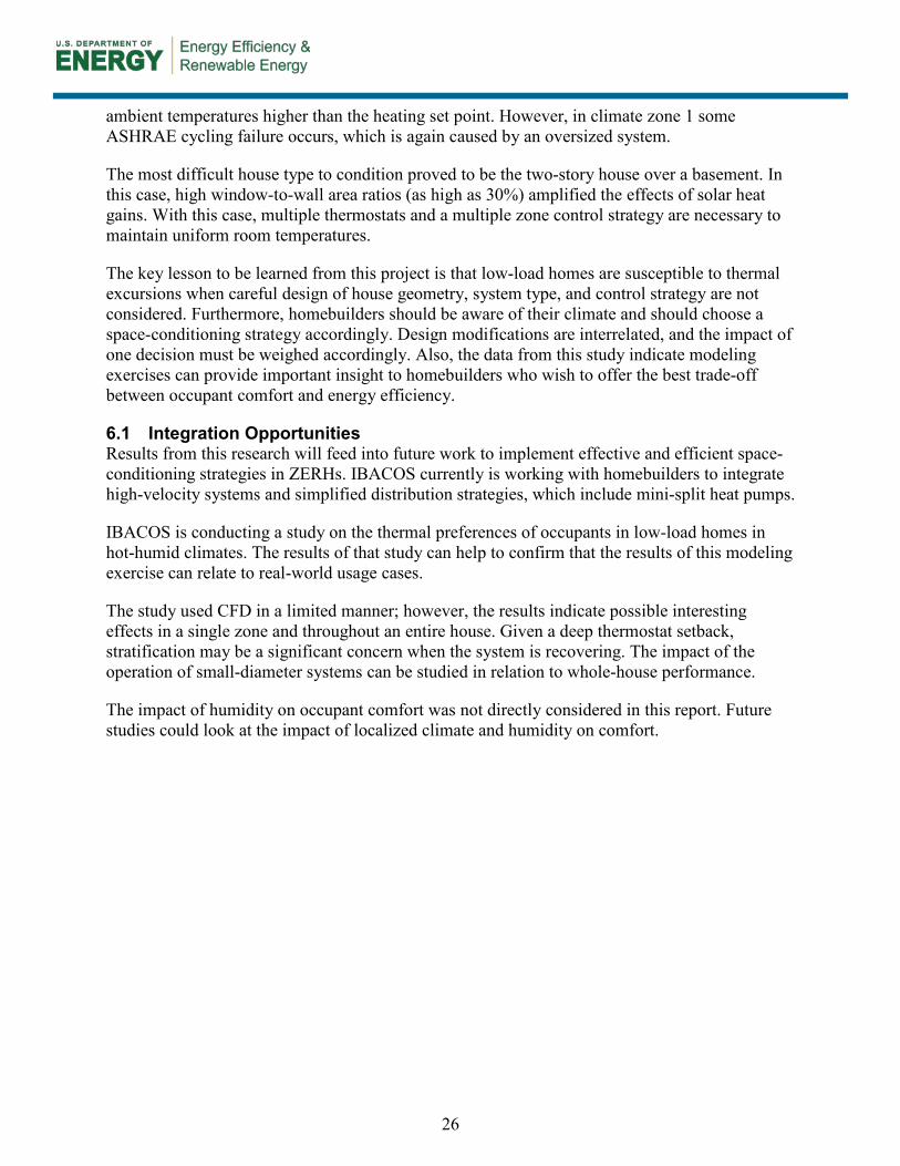
ambient temperatures higher than the heating set point. However, in climate zone 1 some ASHRAE cycling failure occurs, which is again caused by an oversized system.

The most difficult house type to condition proved to be the two-story house over a basement. In this case, high window-to-wall area ratios (as high as 30%) amplified the effects of solar heat gains. With this case, multiple thermostats and a multiple zone control strategy are necessary to maintain uniform room temperatures.

The key lesson to be learned from this project is that low-load homes are susceptible to thermal excursions when careful design of house geometry, system type, and control strategy are not considered. Furthermore, homebuilders should be aware of their climate and should choose a space-conditioning strategy accordingly. Design modifications are interrelated, and the impact of one decision must be weighed accordingly. Also, the data from this study indicate modeling exercises can provide important insight to homebuilders who wish to offer the best trade-off between occupant comfort and energy efficiency.

6.1 Integration Opportunities Results from this research will feed into future work to implement effective and efficient space-conditioning strategies in ZERHs. IBACOS currently is working with homebuilders to integrate high-velocity systems and simplified distribution strategies, which include mini-split heat pumps.

IBACOS is conducting a study on the thermal preferences of occupants in low-load homes in hot-humid climates. The results of that study can help to confirm that the results of this modeling exercise can relate to real-world usage cases.

The study used CFD in a limited manner; however, the results indicate possible interesting effects in a single zone and throughout an entire house. Given a deep thermostat setback, stratification may be a significant concern when the system is recovering. The impact of the operation of small-diameter systems can be studied in relation to whole-house performance.

The impact of humidity on occupant comfort was not directly considered in this report. Future studies could look at the impact of localized climate and humidity on comfort.

27

References

Aldrich, R. 2009. “Efficient Houses with Minimal HVAC.” Presented at the Northeast Sustainable Energy Association’s Building Energy 2011 Conference, Boston, MA, March 2011. http://www.nesea.org/buildingenergy/bepresentations/.

Aldrich, R. 2010. Point-Source Heating Systems in Cold-Climate Homes: Wisdom Way Solar Village. Norwalk, CT: Steven Winter Associates, Inc.

ASHRAE. 2010. ANSI/ASHRAE Standard 62.2 – 2010. Ventilation and Acceptable Indoor Air Quality in Low-Rise Residential Buildings. Atlanta, GA: ASHRAE.

ASHRAE. 2013. ANSI/ASHRAE Standard 55-2013. Thermal Environmental Conditions for Human Occupancy. Atlanta, GA: ASHRAE.

Broniek, J. 2008. “Could a European Super Energy Efficient Standard Be Suitable for the U.S.?” Presented at the BEST1 Conference, Minneapolis, MN, June 2008. http://best1.thebestconference.org/program.htm.

Hendron, R., and Engebrecht, C. 2010. Building America House Simulation Protocols (Technical Report). Golden, CO: National Renewable Energy Laboratory, NREL/TP-550-49426.

Hunter, J.D. 2007. “Matplotlib: A 2D Graphics Environment.” Computing in Science & Engineering 9:3.

IBACOS. 2006a. “Evaluation of Advanced Systems Research Plan.” Pittsburgh, PA: IBACOS, KAAX-3-33410-11.A.2 (unpublished).

IBACOS. 2006b. “Evaluation of Advanced Systems Research Plan.” Pittsburgh, PA: IBACOS, KAAX-3-33410-11.B.1 (unpublished).

IBACOS. 2007. “Evaluation of Advanced Systems Research Plan.” Pittsburgh, PA: IBACOS, KAAX-3-33410-14.B.1 (unpublished).

ICC. 2012. 2012 International Energy Conservation Code. Washington, DC: International Code Council.

Imm, C., and Wayne, M. 2013. “Dual-Fuel Air Source Heat Pump Field Performance Evaluation.” Golden, CO: National Renewable Energy Laboratory (unpublished).

NIST. 2013. CONTAM. National Institute of Standards and Technology, accessed July 24, 2015: http://www.nist.gov/el/building_environment/contam_software.cfm.

NREL. n.d. BEopt Building Energy Optimization software, Version 2.3. National Renewable Energy Laboratory, accessed July 24, 2015: http://beopt.nrel.gov/.

pandas. 2015. pandas software, Version 0.15.0, accessed July 24, 2015: http://pandas.pydata.org/.

28

Poerschke, A., and Stecher, D. 2014. Simplified Space Conditioning in Low-Load Homes: Results from Pittsburgh, Pennsylvania, New Construction Unoccupied Test House (Subcontractor Report). Golden, CO: National Renewable Energy Laboratory, NREL/SR-5500-62122.

Python Software Foundation. 2015. Python software, Version 2.7. Python Software Foundation, accessed July 24, 2015: https://www.python.org.

Rapport, A., and Paul. A. 2014. “Test Plan: Imagine Homes Mini-Split Heat Pump Evaluation and ZERH Support.” Golden, CO: National Renewable Energy Laboratory (unpublished).

Rittelmann, W. 2008. “Thermal Comfort Performance—Field Investigation of a Residential Forced-Air Heating and Cooling System with High Sidewall Supply Air Outlets.” Presented at the BEST1 Conference, Minneapolis, MN, June 2008. http://best1.thebestconference.org/pdfs/045.pdf.

Rutkowski, H. 1997. Manual RS—Comfort, Air Quality, and Efficiency by Design. Arlington, VA: Air Conditioning Contractors of America.

Stecher, D., Allison, K., and Prahl, D. 2012. Long-Term Results from Evaluation of Advanced New Construction Packages in Test Homes: Martha’s Vineyard (Subcontractor Report). Golden, CO: National Renewable Energy Laboratory. www.nrel.gov/docs/fy13osti/54382.pdf.

Stecher, D., and Poerschke, A. 2014. Simplified Space Conditioning in Low-Load Homes: Results from Fresno, California, Retrofit Unoccupied Test House (Subcontractor Report). Golden, CO: National Renewable Energy Laboratory, NREL/SR-5500-60712. http://www.nrel.gov/docs/fy14osti/60712.pdf.

Straub, H.E. 1956. Distribution of Air Within a Room for Year-Round Air Conditioning, Part 1. University of Illinois at Urbana Champaign, College of Engineering, accessed July 24, 2015: http://www.ideals.illinois.edu/handle/2142/4438.

TESS. 2015. TRNSYS. Transient System Simulation Tool, Version 17. Thermal Energy Simulation Specialists, Inc., accessed July 24, 2015: http://www.trnsys.com/.

Townsend, A., Rudd, A., and Lstiburek, J. 2009. “A Method for Modifying Ventilation Airflow Rates to Achieve Equivalent Occupant Exposure.” Somerville, MA: Building Science Corporation. http://www.buildingscience.com/documents/reports/rr-0908-ashrae-modifying-ventilation-airflow.

Trimble Navigation Limited. 2015. SketchUp. Trimble Navigation Limited, accessed July 24, 2015: http://www.sketchup.com/.

Wrightsoft Corporation. 2015. Wrightsoft Right-Suite Universal, Version 13.0.10. Wrightsoft Corporation, accessed July 24, 2015: http://www.wrightsoft.com/.

29

Appendix: Select Simulation Data

Figure 12. Simulation temperature data for the two-story house over a basement, climate zone 5, hot days

30

Figure 13. Simulation temperature data for the case of the two-story house on a slab, climate zone 5, hot days

buildingamerica.gov

DOE/GO-102016-4711 ▪ February 2016