1

RISK AND SUSTAINABLE MANAGEMENT GROUP WORKING PAPER SERIES

TITLE:

Analogy Based Valuation of Commodity Options

AUTHOR:

Hammad Siddiqi

Working Paper: F15_1

2011

FINANCE

Schools of Economics and Political Science

The University of Queensland

St Lucia

Brisbane

Australia 4072

Web: www.uq.edu.au

2015

1

Analogy Based Valuation of Commodity Options

Hammad Siddiqi

h.siddiqi@uq.edu.au

University of Queensland

This version: January 2015

Typically, three types of implied volatility smiles are seen in commodity options: the reverse skew, the smile, and the forward skew. I put forward an economic explanation for all three types of implied volatility smiles based on the idea that a commodity call option is valued in analogy with its underlying futures contract, where the underlying futures price follows geometric Brownian motion. Closed form solutions for commodity calls and puts exist in the presence of transaction costs. Analogy based jump diffusion model is also developed. The smiles are steeper with jump diffusion when compared with smiles with geometric Brownian motion.

JEL Classification: G13

Keywords: Implied Volatility Smile, Implied Volatility Skew, Reverse Skew, Forward Skew, Analogy Making, Commodity Call Option, Commodity Futures Contract

2

Analogy based Valuation of Commodity Options

Commodity options are different from equity options as, unlike equity options, they typically do not

offer spot delivery of the underlying on exercise. Instead, the underlying instrument delivered upon

exercise is a commodity futures contract. Black (1976) extends the classic Black-Scholes replication

argument to commodity options: under certain simplifying assumptions (in particular, no transaction

costs), a portfolio consisting of continuously adjusted proportions of an option and its underlying

futures contract perfectly replicates a risk free bond. Hence, by no-arbitrage, it should offer the risk-

free rate of return. Existence of a unique no-arbitrage price of the option follows from this

argument, and the resulting option pricing formula is known in the literature as Black-76. Black-76

differs from the famous Black-Scholes option pricing formula because no initial outlay (ignoring

margin requirements) is required at the time of entering into a futures contract. Arguably, Black-76 is

the most popular commodity option pricing model among traders today.

The existence of the implied volatility smile where the implied volatility varies with the strike

price is considered a major shortcoming of Black-76 (see Fackler and King (1990), and Sherrick et al

(1996) among others). In general, three broad shapes are generated. Typically, for base metals,

precious metals, and crude oil, either a smile or a skew is generated. Smile refers to the shape of the

implied volatility curve when in-the-money and out-of-the-money options are more expensive than

at-the-money options. The skew refers to the shape where implied volatility falls monotonically with

strike. The third category, typically observed for agricultural commodities like wheat and soybean, is

known as the forward skew, in which implied volatility rises monotonically with strike.

Just like for equity options, the commodity option pricing literature has responded to the

challenge of explaining the behavior of implied volatility by focusing on finding the right

distributional properties of terminal (futures) prices (by allowing for jump diffusion, stochastic

volatility, mean-reversion, seasonality etc in the stochastic processes of futures prices). This literature

includes Kang and Brorsen (1995), Hilliard and Reis (1998), Hilliard and Reis (1999), Ji and Brorsen

(2009), and Trolle and Schwartze (2009) among others. These explanations are primarily statistical in

nature as they identify miss-specified distributional properties of terminal futures prices in Black-76

as the root cause of this phenomenon.

3

In this article, I put forward an economic explanation for the implied volatility smile based

on the idea that commodity call options are valued in analogy with the underlying commodity

futures contract. Specifically, an analogy maker expects the same gain from a call option as she

(subjectively) expects to get from the underyling futures contract. With analogy making, all three

types of implied volatility smiles mentioned earlier, are generated even when the distributional

properties are assumed to be exactly identical to Black-76. That is, the reverse skew, the smile, as

well as the forward skew are generated even when the underlying futures price is assumed to follow

geometric Brownian motion.

Black-76 ignores transaction costs to arrive at a unique no-arbitrage price. With transaction

costs, no matter how small, Black-76 does not hold, as the total cost of replication grows without

bound. Hence, there is no non-trivial replicating portfolio and the argument underlying Black-76

fails. See Soner, Shreve, and Cvitanic (1995). In contrast, with analogy making, transaction costs are

easily incorporated and appear as parameters in the option pricing formula. In other words, with

transaction costs, analogy makers cannot be arbitraged away as Black-76 does not hold.

Furthermore, a closed-from solution still exists for analogy based option pricing even with

transaction costs.

The idea of analogy making is complementary to other explanations of the skew such as the

jump diffusion model of Bates (1991) and Merton (1976). After all, the notion of analogy making is

not tied to a specific distribution for the underlying, and can be integrated with any assumed

stochastic process for the underlying commodity futures price. In this article, I also put forward an

analogy based option pricing formula which is applicable when the underlying commodity futures

price follows the jump diffusion process as in Bates (1991) and Merton (1976). In contrast with the

models in Bates (1991) and Merton (1976), the analogy based jump diffusion model generates the

skew even when jumps are symmetric (the mean jump size is zero).

It has been argued in cognitive science and psychology literature that analogy making is the

core of cognition and the fuel and fire of thinking (see Hofstadter and Sander (2013)). When faced

with a new situation, people instinctively search their memories for a similar situation they have

encountered before, and the repertoire of information relevant to the familiar situation is accessed to

form judgments regarding the new situation. Such way of thinking, termed analogy making, is not

new to economic literature. Some examples include the coarse thinking model of Mullainathan et al

4

(2008), case based decision theory of Gilboa and Schmeidler (2001), and the analogy based

expectations equilibrium of Jeheil (2005). A commodity call option is defined over a futures contract

and derives its payoffs from the payoffs of the underlying futures contract. When faced with the task

of valuing a commodity call option, it seems natural to form an analogy with the underlying futures

contract.

Analogy making has been extensively tested for equity options in laboratory experiments and

has been found to matter for equity option pricing (see Rockenbach (2004), Siddiqi (2011), and

Siddiqi (2012)). The implications of analogy making for equity option prices have been explored in

Siddiqi (2014a), Siddiqi (2014b), and Siddiqi (2014c). Siddiqi (2014a) puts forward an analogy based

option pricing formula when the underlying instrument is an equity index option. In this model, an

analogy maker expects a return from a call option, which is equal to her subjective assessment of the

return available from the underlying index. The model generates the observed implied volatility skew

in equity index options. Siddiqi (2014b) empirically tests two prediction of the analogy model

developed in Siddiqi (2014a) and finds strong support with nearly 25 years of options data. Siddiqi

(2014c) looks at the risk management implications of analogy making for equity index options.

As the market value of a futures contract is taken to be zero at the time of contracting, the

concept of expected return (expected gain divided by price) is not relevant for a commodity futures

contract. Instead of equating expected returns, here I assume that an analogy maker values a

commodity call option by equating the gains she expects from the call option to her subjective

assessment of the gains available from the underlying futures contract. In continuous time, this leads

to a partial differential equation which can be converted into an inhomogeneous heat equation. The

relevant inhomogeneous heat equation can be solved with the application of Duhamel’s principle.

Hence, a closed form solution exists. If the prices are determined in accordance with the analogy

based commodity option pricing formula, and Black-76 is used to back out implied volatility, all

three types of smiles are observed.

This article is organized as follows. Section 1 discusses the relevance of analogy making for

option pricing. Section 2 illustrates the key ideas with a numerical example. Section 3 puts forward

an analogy based commodity call option pricing formula in continuous time. Section 4 shows that if

prices are determined in accordance with the analogy formula and Black-76 is used to back out

5

implied volatility, the smile is observed. Section 5 puts forward a jump diffusion analogy formula for

commodity options and discusses implications for implied volatility. Section 6 concludes.

1. The Relevance of Analogy Making for Option Pricing

An equity call option is commonly considered a surrogate for the underlying stock. A popular

strategy among market professionals is stock replacement strategy in which stocks are replaced with

corresponding call options as they are considered equity surrogates.1 A series of controlled

laboratory experiments on equity options have found that subjects consider a call option to be a

stock surrogate (see Rockenbach (2004), Siddiqi (2011), and Siddiqi (2012)). In these experiments,

subjects valued a call option in analogy with its underlying stock. Specifically, they valued a call

option by equating the expected return from the call option to the expected return available from

the underlying stock. The consequences of such analogy making for equity options are explored in

Siddiqi (2014a), Siddiqi (2014b), and Siddiqi (2014c).

A call option on a commodity futures contract is a slightly different instrument than a call

option on a stock. The major difference is that one can buy a futures contract without any initial

cash outlay, whereas purchasing a stock requires a cash outlay. That is, a stock has a market price

that must be paid to purchase it, whereas a futures contract does not have a market price that must

be paid to enter as a buyer. The lack of market price implies that the notion of expected return is not

relevant for a futures contract. If an analogy maker wants to value a call option on a futures contract,

how would she do it? The corresponding relevant quantity for a long futures contract is expected

dollar gain from the long position. In this article, I assume that an analogy maker values a call option

by equating the expected dollar gain from the call option with the expected dollar gain from a long

position in the underlying futures contract. I put forward an analogy based commodity call option

1 As illustrative examples of this advice generated by investment professionals, see the following: http://finance.yahoo.com/news/stock-replacement-strategy-reduce-risk-142949569.html http://ezinearticles.com/?Call-Options-As-an-Alternative-to-Buying-the-Underlying-Security&id=4274772, http://www.investingblog.org/archives/194/deep-in-the-money-options/ http://www.triplescreenmethod.com/TradersCorner/TC052705.asp, http://daytrading.about.com/od/stocks/a/OptionsInvest.htm

6

pricing formula (the formula for put option is deduced via put-call parity)2, and show that all three

types of smiles are generated within the framework of geometric Brownian motion.

How important is analogy making to human thinking process? It has been argued that when

faced with a new situation, people instinctively search their memories for something similar they

have seen before, and mentally co-categorize the new situation with the similar situations

encountered earlier. This way of thinking, termed analogy making, is considered the core of

cognition and the fuel and fire of thinking by prominent cognitive scientists and psychologists (see

Hofstadter and Sander (2013)). Hofstadter and Sander (2013) write, “[…] at every moment of our lives,

our concepts are selectively triggered by analogies that our brain makes without letup, in an effort to make sense of the

new and unknown in terms of the old and known.”

(Hofstadter and Sander (2013), Prologue page1).

The analogy making argument has been made in the economic literature previously in

various contexts. Prominent examples that appeal to analogy making in different contexts include

the coarse thinking model of Mullainathan et al (2008), the case based decision theory of Gilboa and

Schmeidler (2001), and the analogy based expectations equilibrium of Jehiel (2005). This article adds

another dimension to this literature by exploring the implications of analogy making for commodity

option valuation. Clearly, a commodity call option’s payoffs directly depend on the payoffs from the

underlying futures contract over which it is defined. Given the importance of analogy making to

human thinking in general, it seems natural to consider the possibility that such a call option is

valued in analogy with its underlying futures contract. This article carefully explores the implications

of such analogy making, and shows that analogy making provides a new explanation for the implied

volatility puzzle.

2. Analogy Making: A Numerical Example

Suppose there is a commodity futures contract with a given expiration date and one can either go

long or short on it at a futures price of $100. To the party going long, such a contract creates an

obligation to buy the (specified amount of) underlying commodity at a price of $100 on expiry, and

2 As commodity call options trade much more heavily than commodity put options, analogy making is likely to influence them directly, with the corresponding put prices following from the model-free restriction of put-call parity.

7

to the party going short; the obligation is to sell at $100, with no money changing hands at the time

of entering into the contract. For simplicity, I ignore margin requirements in this illustration.

As the futures contract is settled and re-written everyday at the prevailing futures price, each

party to the contract either gains or loses money depending on what position has been taken earlier.

Suppose tomorrow, the futures price could either be $110 (red state) or $90 (blue state). This means

that the buyer gains $10 (the seller loses $10) in the red state and loses $10 (the seller gains $10) in

the blue state. For simplicity, assume that the risk free rate of borrowing or lending is zero, and

everyone can borrow or lend at that rate.

Suppose a new asset is introduced with two possible outcomes: either it pays $10 tomorrow

in the red state or it pays nothing tomorrow in the blue state. How much should one be willing to

pay for this asset?

If one buys the futures contract, one can either gain or lose $10 depending on which state is

realized, without paying anything upfront. Instead, if one buys the new asset, one gains $10 in the

red state; however, there is no corresponding loss in the blue state. The payoff is simply equal to

zero in the blue state with the new asset. It seems that the new asset should be valuable to a person

worried about losing money in the blue state with the futures contract. That is, one should be willing

to pay a price upfront for the new asset as it eliminates the downside of the futures contract.

Suppose there is an investor who assigns an equal chance (subjectively of course) to either

state. To her, the expected gain from entering into the futures contract is zero (0.5 × 10 + 0.5 ×

−10). Such an investor may reason as follows: My expected gain from buying the futures contract is

zero, and I pay nothing upfront for it. The new asset eliminates the downside of the futures

contract, so I should be willing to pay something for it. The new asset is very similar to the futures

contract. It pays more ($10) when the futures contract pays more ($10). It pays less (0) when the

futures contract pays less (-$10). So, by analogy, I should be willing to pay a price for it that leaves

me with at least the same expected gain as the futures contract. That price is: 0.5(10 − 𝐶) +

0.5(0 − 𝐶) = 0 => 𝐶 = $5. That is, the analogy maker is willing to pay up to $5 for the new asset.

Note that the new asset is equivalent to a call option on the futures contract with a striking price of

$100.

8

By applying the no-arbitrage argument underlying Black-76, one can also calculate the no-

arbitrage price for this call option. By lending $5 (at the assumed interest rate of zero) and buying

0.5 unit of the futures contract, one creates a portfolio that perfectly replicates the call option. In the

red state, 0.5 unit of the futures contract pays $5 and one receives $5 on account of lending this

amount earlier to give a total of $10, which is equal to the call’s payoff in the red state. In the blue

state, 0.5 unit of the futures contract requires one to pay $5, and one receives $5 on account of

earlier lending, resulting in a net payoff of zero, which is equal to the call’s payoff in the blue state.

Hence, the no-arbitrage price of this call option is also equal to $5, which is the cost of setting up

the replicating portfolio. This is not a coincidence. In fact, I show in section 3 that the analogy price

is always equal to the no-arbitrage price if the expected gain from the underlying futures contract is

zero, the risk free rate of borrowing or lending is also zero, and there are no transaction costs.

Now, consider a bullish analogy maker, who assigns a probability of 0.55 to the red state and

a probability of 0.45 to the blue state. By using the same analogy argument that was used earlier, she

should be willing to pay up to $4.5 for the call option.3 Similarly, we can imagine a bearish analogy

maker, who assigns probabilities of 0.45 and 0.55 to red and blue states respectively. Such an analogy

maker is willing to pay up to $5.5 for the call option.

Shouldn’t rational arbitrageurs make money at the expense of such analogy makers? In

reality, such arbitraging is very difficult, if not impossible, in the presence of transaction costs.

Entering into a futures contract entails significant transaction costs as one is required to put up

maintenance margin up front and margin calls are generated frequently based on futures price

fluctuations. And if one takes the route of a forward contract, buying and storing the underlying

commodity entails significant financing and storage costs. So, practically, there is no risk-free

arbitrage available here, for a wide range of option prices.

In the example considered, the arbitrage profits disappear even if we allow for a proportional

transaction cost as small as only 1% of the price. First consider the possibility of arbitraging the

bullish analogy maker. Recall, she values the option at $4.5, whereas the rational price is $5. An

arbitrageur would attempt to buy the call and short the replicating portfolio to finance the purchase.

3 As one gets more and more bullish, the analogy price of call falls. When the implied price of call becomes negative, it is equated to zero, as call prices cannot be negative. Clearly, for a very bullish analogy maker, the downside in a futures contract has such a low chance that it is not worthwhile to pay money to buy a call option to eliminate the downside.

9

The transaction costs involved in shorting the replicating portfolio (0.5 unit of futures+$5) are $0.50

for shorting futures (futures price is $100) and 5 cents for borrowing $5. Hence, the total transaction

cost exceeds the potential gain of $0.50 from the arbitrage attempt. It is easy to see that the bearish

analogy maker cannot be arbitraged away either in this example.

In the next section, analogy based pricing is considered in continuous time, and the

corresponding commodity call option pricing formula is put forward. In continuous time, no matter

how small the transaction cost is, the total transaction cost involved in setting up a replicating

portfolio and continuously adjusting it grows without bound. Hence, in Black-76, one has no choice

but to impose a rather strong condition that the transaction costs are exactly zero. With analogy

making, the presence of transaction costs leads to a modification of the analogy option pricing

formula, however, a closed form solution exists even with transaction costs, as the next section

shows.

3. Analogy based Commodity Option Pricing

As this article considers only a single short term futures contract, the link between stochastic

processes of different maturities is not modeled. That is, the term structure of futures prices is not

considered here. All the assumptions of Black-76 are maintained except one. The one exception is

that, in this article, transaction costs are assumed to be non-zero. With non-zero transaction costs,

the replication argument in Black-76 does not hold as the total transaction costs grow without

bound. See Soner, Shreve, and Cvitanic (1995). Hence, analogy makers cannot be arbitraged away in

this case.

I assume proportional and symmetric transaction costs for simplicity. If 𝐶 is the price of a

call option then both the buyer and the writer pay ∅𝑐 ∙ 𝐶 in transaction costs, where ∅𝑐 is a small

and positive fraction. In a futures contract, at the time of contracting, the market value is zero, and

nothing needs to be paid by either party. However, there are margin requirements as each party is

required to furnish a maintenance margin. I assume that the present value of the cost of furnishing

and maintaining the margin can be expressed as a percentage of the futures price. That is, both the

buyer and the seller pay ∅𝐹 .𝐹 in transaction costs, where ∅𝐹 is a small and positive fraction. Note,

that ∅𝑐 and ∅𝐹 can take different values. An analogy maker values a call option by equating the gain

10

she expects from the call option to her subjective assessment of the expected gain available from the

underlying commodity futures contract (expected gain can be zero, positive, or negative) over a time

interval 𝑑𝑑:

𝐸[𝑑𝐶] − ∅𝑐 ∙ 𝐶 = 𝐸[𝑑𝐹] − ∅𝐹 ∙ 𝐹 (1)

As in Black-76, I assume that the underlying commodity futures price follows geometric

Brownian motion.

𝑑𝐹𝑡 = 𝑢𝐹𝑡𝑑𝑑 + 𝜎𝐹𝑡𝑑𝑊𝑡 (2)

Where 𝑢 (percentage drift) and 𝜎 (percentage volatility) are constants, and 𝑊𝑡 is a Wiener process.

Proposition 1 presents the partial differential equation that a commodity call option must

satisfy under analogy making.

Proposition 1 If the price of a European commodity call option is determined in analogy

with the underlying commodity futures contract, and there are proportional and symmetric

transaction costs, then the following partial differential equation must be satisfied:

𝝏𝝏𝝏𝝏

+ 𝒖𝒖𝝏𝝏𝝏𝒖

+𝟏𝟐𝝈𝟐𝒖𝟐

𝝏𝟐𝝏𝝏𝒖𝟐

= (𝒖 − ∅𝒖)𝒖 + ∅𝒄𝝏 (𝟑)

With the boundary condition:

𝝏(𝒖,𝑻) = 𝒎𝒎𝒎(𝒖 −𝑲,𝟎)

Proof.

See Appendix A.

▄

Unlike the Black-Scholes model, the PDE in (3) cannot be transformed into a homogeneous heat

equation; however, it can be converted into an inhomogeneous heat equation with appropriate

variable transformations. The inhomogeneous heat equation is then solvable with the application of

Duhamel’s principal.

11

Proposition 2 puts forward an option pricing formula which is obtained by finding a closed

form solution to the PDE in (3)

Proposition 2 Under analogy making, the price of a European Call option on a commodity

futures contract with a striking price of 𝑲 is given by:

𝝏 = 𝒎𝒎𝒎{𝝏∗,𝟎}

𝝏∗(𝒖, 𝝏) = 𝒖𝒆(𝒖−∅𝒄)(𝑻−𝝏) �𝑵(𝒅𝟏) − �𝒓� − ∅𝒖�� ∙𝟏𝑸

(𝒆𝑸𝑸 − 𝟏)� − 𝑲𝒆−∅𝒄(𝑻−𝝏)𝑵(𝒅𝟐) (𝟒)

𝒓� =𝟐𝒖𝝈𝟐

; ∅𝒖� =𝟐∅𝒖𝝈𝟐

;𝑸 =(𝒓� − 𝟏)𝟐

𝟒+ ∅�𝒄; 𝑸 =

𝝈𝟐

𝟐(𝑻 − 𝝏); ∅𝒄� =

𝟐∅𝒄𝝈𝟐

𝒅𝟏 =𝒍𝒍 �𝒖𝑲�+ �𝒖 + 𝝈𝟐

𝟐 � (𝑻 − 𝝏)

𝝈√𝑻 − 𝝏

𝒅𝟐 =𝒍𝒍 �𝒖𝑲�+ �𝒖 − 𝝈𝟐

𝟐 � (𝑻 − 𝝏)

𝝈√𝑻 − 𝝏

Proof.

See Appendix B.

▄

Corollary 2.1 If the transaction costs (as a percentage of price) of trading in calls, puts, and

risk-free bonds are equal, and the underlying futures contract is cash settled, then the

analogy based price of a European put option on a commodity futures contract is g iven by:

𝑷𝒖𝝏 = 𝒖𝒆(𝒖−∅𝒄)(𝑻−𝝏) �𝑵(𝒅𝟏) − �𝒓� − ∅𝒖�� ∙𝟏𝑸

(𝒆𝑸𝑸 − 𝟏)� − 𝑲𝒆−∅𝒄(𝑻−𝝏)𝑵(𝒅𝟐)

+ (𝑲− 𝒖)𝒆−𝒓(𝑻−𝝏) −∅𝒖

(𝟏 + ∅𝒄)𝒖 𝒊𝒊 𝝏 > 0 (𝟓)

𝑷𝒖𝝏 = (𝑲− 𝒖)𝒆−𝒓(𝑻−𝝏) − ∅𝒖

(𝟏 + ∅𝒄)𝒖 𝒊𝒊 𝝏 = 𝟎

12

Proof.

Follows from put-call parity

▄

It is interesting to note that the formulas in (4) and (5) are equal to Black-76 when the drift rate,

transaction costs, and the risk free rate are zero. This is exactly what we saw in the numerical

example discussed in section 2.

4. The Behavior of Implied Volatility

If the prices are determined in accordance with the analogy formula (given in (4) and (5)) and Black-

76 is used to back out implied volatility, then all three types of smiles (reverse skew, smile, and

forward skew) arise for various parameter values.

There are six broad categories of interest:

1) 𝑢 = 0; ∅𝑐 = 0; ∅𝐹 = 0

2) 𝑢 = 0; ∅𝑐 > 0; ∅𝐹 > 0

3) 𝑢 > 0; ∅𝑐 = 0; ∅𝐹 = 0

4) 𝑢 < 0; ∅𝑐 = 0; ∅𝐹 = 0

5) 𝑢 > 0; ∅𝑐 > 0; ∅𝐹 > 0

6) 𝑢 < 0; ∅𝑐 > 0; ∅𝐹 > 0

In category 1, the drift rate (𝑢) as well as transaction costs (∅𝑐,∅𝐹) are zero. It is easy to

verify that in this case, if the risk free rate is also assumed to be zero, the analogy formula is exactly

identical to Black-76. Hence, the analogy formula contains Black-76 as a special case. With non-zero

risk free rate, Black-76 differs from the analogy formula only due to a present value factor.

In category 2, the drift rate is zero implying that the marginal call investor neither expects a

gain nor a loss from a long position in the underlying futures contract. The transaction costs,

13

however, are allowed. In this case, a volatility smile arises as figure 1 shows. The smile gets steeper as

time to expiry gets closer.

Implied volatility smile steepens as expiry approaches (from 0.08 year to 0.02 year)

(Other parameter values: 𝐹 = 100; 𝜎 = 20%;𝑢 = 0; ∅𝑐 = 0.01; ∅𝐹 = 0.01)

Figure 1

Even when initially the skew has a shape of a forward skew, as in agricultural commodities, or a

reverse skew, as in crude oil, closer to expiry, it typically converts into a smile shape. It’s interesting

to see that a smile shape can arise within the framework of geometric Brownian motion in analogy

based valuation with non-zero transaction costs. One wonders what impact changes in transaction

costs have on the shape of the smile. It turns out that the impact depends on whether the change is

taking place in the transaction cost associated with a call option or in the transaction cost associated

with its underlying futures contract.

15.0000%

17.0000%

19.0000%

21.0000%

23.0000%

25.0000%

27.0000%

29.0000%

31.0000%

33.0000%

35.0000%

0.80 0.85 0.90 0.95 1.00 1.05 1.10 1.15 1.20

IV-0.08

IV-0.04

IV-0.02

Implied Volatility

K/F

14

If ∅𝑐 (call transaction cost) increases then the implied volatility curve shifts downwards.

However, the implied volatility curve shifts upwards with increases in ∅𝐹(transaction cost associated

with the underlying futures contract), as figure 2 shows.

Implied Volatility shifts up as the futures transaction cost increases (from 0.01 to 0.03)

(Other parameter values: 𝐹 = 100; 𝜎 = 20%;𝑢 = 0; ∅𝑐 = 0.01; (T − t) = 0.04year)

Figure 2

In category 3, the marginal call investor expects a gain from a long position in the underlying

futures contract, however, the transaction costs are assumed to be zero. Under such conditions, if

the prices are determined in accordance with the analogy formula, and Black-76 is used to back out

implied volatility, the reverse skew arises, in which implied volatility falls monotonically with strike.

15.0000%

17.0000%

19.0000%

21.0000%

23.0000%

25.0000%

27.0000%

29.0000%

31.0000%

33.0000%

0.85 0.90 0.95 1.00 1.05 1.10 1.15

IV-0.01

IV-0.02

IV-0.03

Implied Volatility

K/F

15

Figure 3 shows a representative shape of this category.

The Reverse Implied Volatility Skew

(Parameter values: 𝑢 = 2%; 𝐹 = 100; 𝜎 = 20%;𝑢 = 0; ∅𝑐 = 0; ∅𝐹 = 0; (T − t) = 0.04year)

Figure 3

A particularly puzzling feature of agricultural commodity options is the emergence of

forward implied volatility skew in which implied volatility rises as the striking price increases. This is

in sharp contrast with equities and other commodities in which typically a reverse skew or a smile is

observed. A commonly given practitioner explanation of the phenomenon of forward skew is as

follows: Businesses who are worried about not being able to secure supply bid up the prices of out-

of-the-money calls giving rise to the forward skew.

It turns out that analogy based pricing provides a theoretical foundation to the above

mentioned practitioner explanation for forward skew. Businesses that require agricultural

commodities such as wheat as inputs for their processed food products are willing to pay a high

futures price to secure supply. At high futures prices, on average, they expect to lose money in the

0.15

0.17

0.19

0.21

0.23

0.25

0.27

0.29

0.31

0.85 0.90 0.95 1.00 1.05 1.10 1.15

Implied Volatility

K/F

16

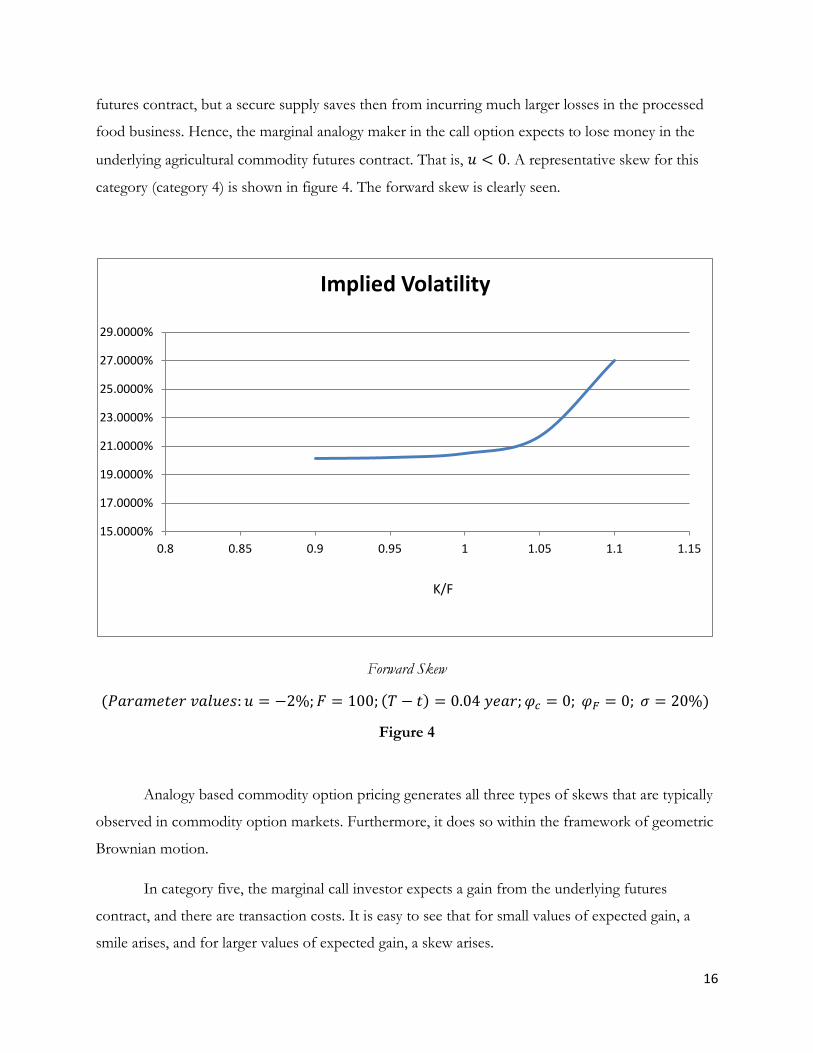
futures contract, but a secure supply saves then from incurring much larger losses in the processed

food business. Hence, the marginal analogy maker in the call option expects to lose money in the

underlying agricultural commodity futures contract. That is, 𝑢 < 0. A representative skew for this

category (category 4) is shown in figure 4. The forward skew is clearly seen.

Forward Skew

(𝑃𝑃𝑃𝑃𝑃𝑃𝑑𝑃𝑃 𝑣𝑃𝑣𝑢𝑃𝑣:𝑢 = −2%;𝐹 = 100; (𝑇 − 𝑑) = 0.04 𝑦𝑃𝑃𝑃;𝜑𝑐 = 0; 𝜑𝐹 = 0; 𝜎 = 20%)

Figure 4

Analogy based commodity option pricing generates all three types of skews that are typically

observed in commodity option markets. Furthermore, it does so within the framework of geometric

Brownian motion.

In category five, the marginal call investor expects a gain from the underlying futures

contract, and there are transaction costs. It is easy to see that for small values of expected gain, a

smile arises, and for larger values of expected gain, a skew arises.

15.0000%

17.0000%

19.0000%

21.0000%

23.0000%

25.0000%

27.0000%

29.0000%

0.8 0.85 0.9 0.95 1 1.05 1.1 1.15

Implied Volatility

K/F

17

In category six, the marginal call investor expects to lose money in the underlying futures

contract, and there are transaction costs. For a small expected loss, a smile is seen, and for large

expected losses, a forward skew arises.

Next, the analogy approach is extended to the jump diffusion framework of Bates (1991)

and Merton (1976).

5. Analogy based Option Pricing with Jump Diffusion

The idea of analogy making does not depend on the specific distributional assumptions that are

made regarding the behavior of the underlying futures price.

In this section, the idea of analogy making is combined with the distributional assumptions

of Bates (1991) and Merton (1976). It is assumed that the futures price follows a mixture of

geometric Brownian motion and Poisson-driven jumps:

𝑑𝐹 = (𝜇 − 𝛾𝛾)𝐹𝑑𝑑 + 𝜎𝐹𝑑𝜎 + 𝑑𝑑

Where 𝑑𝜎 is a standard Guass-Weiner process, and 𝑑(𝑑) is a Poisson process. 𝑑𝜎 and 𝑑𝑑 are

assumed to be independent. 𝛾 is the mean number of jump arrivals per unit time, 𝛾 = 𝐸[𝑌 − 1]

where 𝑌 − 1 is the random percentage change in the futures price if the Poisson event occurs, and

𝐸 is the expectations operator over the random variable 𝑌. If 𝛾 = 0 (hence, 𝑑𝑑 = 0) then the

futures price dynamics are identical to those assumed in Black-76. For simplicity, assume that

𝐸[𝑌] = 1.

The futures price then follows:

𝑑𝐹 = 𝜇𝐹𝑑𝑑 + 𝜎𝐹𝑑𝜎 + 𝑑𝑑 (6)

Clearly, with jump diffusion, Black-76 no-arbitrage technique cannot be employed as there is

no portfolio consisting of a futures contract and corresponding option which is risk-free. Equation

(6) describes the actual process followed by the futures price, so if (6) is used to calculate the payoffs

from the option then these payoffs need to be discounted at a rate that includes a premium for risk.

Another way is to adjust (6) for risk. Payoffs generated by the risk adjusted process can be

18

discounted at the risk free rate. Typically, a general equilibrium model with restrictions on

technology and preference is proposed for this purpose. Bates (1991) is one such model. In contrast,

an analogy maker, by definition, expects the same gain from the call option as he expects to get from

the underlying futures contract; this allows the option to be priced without explicitly modeling

preferences.

If analogy making determines the price of the call option when the underlying futures price

dynamics are a mixture of geometric Brownian motion and Poisson jumps as described earlier, then

the following partial differential equation must be satisfied (see Appendix C for the derivation):

𝜕𝐶𝜕𝑑

+ 𝑢𝐹𝜕𝐶𝜕𝐹

+12𝜎2𝐹2

𝜕2𝐶𝜕𝐹2

+ 𝛾𝐸[𝐶(𝐹𝑌, 𝑑) − 𝐶(𝐹, 𝑑)] = (𝑢 − ∅𝐹)𝐹 + ∅𝑐𝐶 (7)

If the distribution of 𝑌 is assumed to log-normal with a mean of 1 (assumed for simplicity)

and a variance of 𝑣2 then by using an argument analogous to Merton (1976), the following analogy

based option pricing formula for the case of jump diffusion follows (proof available from author):

𝐶𝑃𝑣𝑣 = �𝑃−𝛾(𝑇−𝑡)�𝛾(𝑇 − 𝑑)�

𝑗

𝑗!

∞

𝑗=0

𝐶𝑃𝑣𝑣𝐴𝐴�𝐹, (𝑇 − 𝑑),𝐾,𝑢,∅𝑐,∅𝐹,𝜎𝑗� (8)

Where 𝐶𝑃𝑣𝑣𝐴𝐴 is given in (4), and 𝜎𝑗 = �𝜎2 + 𝑣2 � 𝑗𝑇−𝑡

�

It is easy to see that when 𝑢,∅𝑐,𝑃𝑎𝑑 ∅𝐹 are zero, and the risk free rate is also zero, (8) generates the

symmetric implied volatility smile. This is in contrast with the corresponding case without jumps,

where the call price converges to Black-76. The reverse skew is seen at larger positive values of 𝑢

and the forward skew is seen at larger negative values of 𝑢. Hence, all three types of shapes are

generated with analogy based jump diffusion. Unsurprisingly, the presence of jumps makes the smile

curves steeper.

6. Conclusions

Commodity options are typically options on futures contracts. The most intriguing phenomenon in

the commodity options markets is the presence of the implied volatility smile. In general, three types

19

of shapes are seen: the reverse skew and the smile are typically seen in base metals and precious

metals, and the forward skew is typically seen in agricultural commodities. Typically, attempts to

explain these shapes have taken the direction of appropriately modifying the terminal distribution of

futures prices. In sharp contrast, in this article, an economic explanation has been put forward based

on the notion that a call option is valued in analogy with its underlying futures contract and there are

transaction costs. It is shown that such analogy based valuation generates all three types of smiles

even when the underlying futures price follows geometric Brownian motion. Hence, the presence of

the smile does not automatically imply that one needs to abandon the simple framework of

geometric Brownian motion.

As the notion of analogy making is not tied to a particular distribution for the underlying

futures price, it can easily be extended to other distributions of terminal futures price. That is, even

though with analogy making, one does not need to abandon the framework of geometric Brownian

motion to generate the smile, other frameworks can easily be incorporated. In this article, an analogy

based jump diffusion model is also put forward. Such a model generates similar though steeper

smiles when compared with the smiles generates in the geometric Brownian motion framework.

20

References

Bates (1991), “The crash of 87: Was it expected? The evidence from options markets”, Journal of Finance, 46, pp. 1009-1044. Black, F. (1976), “The pricing of commodity contract”, Journal of Financial Economics, 3, 167-79. Fackler, P.L., and R.P. King, (1990) "Calibration of Option-Based Probability Assessments in Agricultural Commodity Markets." American Journal of Agricultural Economics 72(1):73-83. Gilboa, I., Schmeidler, D. (2001), “A Theory of Case Based Decisions”. Publisher: Cambridge University Press.

Hilliard and Reis (1999), “Jump processes in commodity futures prices and option pricing”, American Journal of Agricultural Economics, pp. 273-286.

Hilliard and Reis (1998), “Valuation of commodity futures and options under stochastic convenience yield, interest rates, and jump diffusion in the spot”, The Journal of Financial and Quantitative Analysis, 33(1), pp. 61-86.

Hofstadter, D., and Sander, E. (2013), “Surfaces and Essences: Analogy as the fuel and fire of thinking”, Published by Basic Books, April.

Jehiel, P. (2005), “Analogy based Expectations Equilibrium”, Journal of Economic Theory, Vol. 123, Issue 2, pp. 81-104.

Ji and Brorsen (2009), "A relaxed lattice option pricing model: implied skewness and kurtosis." Agricultural Finance Review 69(3):268-283. Kang and Brorsen (1995), “Conditional heteroskedasticity, asymmetry, and option prices”, Journal of Futures Markets, 15(8), pp. 901-928.

Merton, R. C. (1976), “Option Pricing when underlying stock returns are discontinuous”, Journal of Financial Economics, 3, pp. 125-44. Mullainathan, S., Schwartzstein, J., & Shleifer, A. (2008) “Coarse Thinking and Persuasion”. The Quarterly Journal of Economics, Vol. 123, Issue 2 (05), pp. 577-619. Rockenbach, B. (2004), “The Behavioral Relevance of Mental Accounting for the Pricing of Financial Options”. Journal of Economic Behavior and Organization, Vol. 53, pp. 513-527.

Sherrick, B.J., P. Garcia, and V. Tirupattur (1996), "Recovering probabilistic information from option markets: Tests of distributional assumptions." Journal of Futures Markets 16(5):545-560. Siddiqi, H. (2011), “Does Coarse Thinking Matter for Option Pricing? Evidence from an Experiment” IUP Journal of Behavioral Finance, Vol. VIII, No.2. pp. 58-69

Siddiqi, H. (2012), “The Relevance of Thinking by Analogy for Investors’ Willingness to Pay: An Experimental Study”, Journal of Economic Psychology, Vol. 33, Issue 1, pp. 19-29.

Siddiqi, H. (2014a), “Analogy making and the structure of implied volatility skew”, University of Queensland Working Paper # F14_7, available at: SSRN: http://ssrn.com/abstract=2465738 or http://dx.doi.org/10.2139/ssrn.2465738

21

Siddiqi, H. (2014b), “Analogy making and the puzzles of index option returns and implied volatility skew: Theory and Empirical Evidence”, University of Queensland Working Paper #F14_4, available at: SSRN: http://ssrn.com/abstract=2435791 or http://dx.doi.org/10.2139/ssrn.2435791

Siddiqi, H. (2014c), “Managing option trading risk when analogy making influences prices”, Journal of Risk (Forthcoming)

Soner, H.M., S. Shreve, and J. Cvitanic, (1995), “There is no nontrivial hedging portfolio for option pricing with transaction costs”, Annals of Applied Probability 5, 327–355.

Trolle and Schwartz (2009), “Unspanned stochastic volatility and the pricing of commodity derivatives”, Review of Financial Studies, 22, 4423-4461.

22

Appendix A

Analogy making implies that over a time interval, 𝑑𝑑, the following holds:

𝐸[𝑑𝐶] − ∅𝑐 ∙ 𝐶 = 𝐸[𝑑𝐹] − ∅𝐹 ∙ 𝐹 (A1)

We know that:

𝐸[𝑑𝐶] = �𝜕𝜕𝜕𝑡

+ 𝑢𝐹 𝜕𝜕𝜕𝐹

+ 𝜎2𝐹2

𝜕2𝜕𝜕𝐹2

� (A2)

And:

𝐸[𝑑𝐹] = 𝑢𝐹 (A3)

Substituting A2 and A3 in A1 and re-arranging leads to:

𝜕𝜕𝜕𝑡

+ 𝑢𝐹 𝜕𝜕𝜕𝐹

+ 12𝜎2𝐹2 𝜕

2𝜕𝜕𝐹2

= (𝑢 − 𝜑𝐹)𝐹 + 𝜑𝑐𝐶 (A4)

The boundary condition is:

𝐶(𝐹,𝑇) = 𝑃𝑃𝑚(𝐹 − 𝐾, 0)

Appendix B

Start by making the following variable transformations:

𝜏 =𝜎2

2(𝑇 − 𝑑)

𝑚 = 𝑣𝑎𝐹𝐾

=> 𝐹 = 𝐾𝑃𝑥

𝐶(𝐹, 𝑑) = 𝐾 ∙ 𝑐(𝑚, 𝜏) = 𝐾 ∙ 𝑐 �𝑣𝑎 �𝐹𝐾� ,𝜎2

2(𝑇 − 𝑑)�

It follows,

𝜕𝜕𝜕𝑡

= 𝐾 ∙ 𝜕𝑐𝜕𝜕∙ 𝜕𝜕𝜕𝑡

= 𝐾 ∙ 𝜕𝑐𝜕𝜕∙ �− 𝜎2

2� (B1)

23

𝜕𝜕𝜕𝐹

= 𝐾 ∙ 𝜕𝑐𝜕𝑥∙ 𝜕𝑥𝜕𝐹

= 𝐾 ∙ 𝜕𝑐𝜕𝑥∙ 1𝐹 (B2)

𝜕2𝜕𝜕𝐹2

= 𝐾 ∙ 1𝐹2∙ 𝜕

2𝜕𝜕𝑥2

− 𝐾 ∙ 1𝐹2

𝜕𝜕𝜕𝑥

(B3)

Substituting (B1), (B2), and (B3) in (A4) and writing �̃� = 2𝑢𝜎2

, ∅𝐹� = 2∅𝐹𝜎2

, and ∅𝑐� = 2∅𝑐𝜎2

, we get:

𝜕𝑐𝜕𝜕

= 𝜕2𝑐𝜕𝑥2

+ (�̃� − 1) 𝜕𝑐𝜕𝑥− ∅𝑐�𝑐 − ��̃� − ∅𝐹��𝑃𝑥 (B4)

Make a further variable transformation:

𝑐(𝑚, 𝜏) = 𝑃𝛼𝑥+𝛽𝜕𝑢(𝑚, 𝜏)

It follows,

𝜕𝑐𝜕𝑚

= 𝛼𝑃𝛼𝑥+𝛽𝜕𝑢 + 𝑃𝛼𝑥+𝛽𝜕𝜕𝑢𝜕𝑚

𝜕2𝑐𝜕𝑚2

= 𝛼2𝑃𝛼𝑥+𝛽𝜕𝑢 + 2𝛼𝑃𝛼𝑥+𝛽𝜕𝜕𝑢𝜕𝑚

+ 𝑃𝛼𝑥+𝛽𝜕𝜕2𝑢𝜕𝑚2

𝜕𝑐𝜕𝜏

= 𝛾𝑃𝛼𝑥+𝛽𝜕𝑢 + 𝑃𝛼𝑥+𝛽𝜕𝜕𝑢𝜕𝜏

Substituting the above transformations in (B4), we get:

𝜕𝑢𝜕𝜕

= 𝜕2𝑢𝜕𝑥2

+ �𝛼2 + 𝛼(�̃� − 1) − ∅𝑐� − 𝛾�𝑢 + �2𝛼 + (�̃� − 1)� 𝜕𝑢𝜕𝑥− ��̃� − ∅𝐹��𝑃𝑥 (B5)

Choosing = − (�̃�−1)2

, and 𝛾 = − (�̃�−1)2

4− ∅𝑐� in (B5) lead to:

𝜕𝑢𝜕𝜕

= 𝜕2𝑢𝜕𝑥2

− ��̃� − ∅𝐹��𝑃𝑥 (B6)

With the initial condition: 𝑢(𝑚, 0) = 𝑃𝑃𝑚�𝑃(1−𝛼)𝑥 − 𝑃−𝛼𝑥, 0�

(B6) is an inhomogeneous heat equation which can be solved by using Duhamel’s principle:

𝑢(𝑚, 𝜏) = 𝑢ℎ(𝑚, 𝜏) + 𝐺(𝑚, 𝜏) (B7)

24

𝑢ℎ(𝑚, 𝜏) is a solution to the associated homogeneous problem:

𝜕𝑢ℎ

𝜕𝜕= 𝜕2𝜇ℎ

𝜕𝑥2 (B8)

With the initial condition: 𝑢(𝑚, 0) = 𝑃𝑃𝑚�𝑃(1−𝛼)𝑥 − 𝑃−𝛼𝑥, 0�

And,

𝐺(𝑚, 𝜏) = � 𝑔(𝑚, 𝜏: 𝑣)𝜕

0𝑑𝑣

𝜕𝜕𝜕𝜕

= 𝜕2𝜕𝜕𝑥2

(B9)

With the initial condition: (𝑚, 𝜏: 𝑣) = −��̃� − ∅𝐹��𝑃(1−𝛼)𝑥−𝛽𝛽 ; 𝜏 = 𝑣

(B8) and (B9) can be solved by exploiting the standard solution of the heat equation.

Solving (B8) yields:

𝑢ℎ(𝑚, 𝜏) = 𝑃𝑚𝑁(𝑑1) − 𝑃𝑛𝑁(𝑑2) (B10)

𝑃 = ��̃�+12� 𝑚 + (�̃�+1)2

4𝜏, 𝑎 = ��̃�−1

2� 𝑚 + (�̃�−1)2

4𝜏

𝑑1 = 𝑥√2𝜋

+ �𝜕2

(�̃� + 1), 𝑑2 = 𝑥√2𝜋

+ �𝜕2

(�̃� − 1)

𝑁(∙) is the cumulative standard normal distribution.

From (B9), it follows that,

𝐺(𝑚, 𝜏) = −��̃� − ∅𝐹�� ∙ 𝑃(1−𝛼)2𝜕+(1−𝛼)𝑥 ∙ 1𝑄

{𝑃𝑄𝜕 − 1} (B11)

Where 𝑄 = (�̃�−1)2

4+ ∅𝑐�

Substituting (B11) and (B10) in (B7), recovering original variables, and imposing the condition that

the price cannot be negative leads to the following formula for a European call option on a

commodity futures contract:

25

𝐶 = 𝑃𝑃𝑚{𝐶∗, 0}

𝐶∗(𝐹, 𝑑) = 𝐹𝑃(𝑢−∅𝑐)(𝑇−𝑡) �𝑁(𝑑1) − ��̃� − ∅𝐹�� ∙1𝑄

(𝑃𝑄𝜕 − 1)� − 𝐾𝑃−∅𝑐(𝑇−𝑡)𝑁(𝑑2) (𝐵12)

�̃� = 2𝑢𝜎2

; ∅𝐹� = 2∅𝐹𝜎2

;𝑄 = (�̃�−1)2

4+ ∅�𝑐; 𝜏 = 𝜎2

2(𝑇 − 𝑑); ∅�𝑐 = 2∅𝑐

𝜎2

𝑑1 =𝑙𝑛�𝐹𝐾�+�𝑢+

𝜎2

2 �(𝑇−𝑡)

𝜎√𝑇−𝑡 , 𝑑2 =

𝑙𝑛�𝐹𝐾�+�𝑢−𝜎2

2 �(𝑇−𝑡)

𝜎√𝑇−𝑡

Appendix C

Analogy making implies that over a time interval, 𝑑𝑑, the following holds:

𝐸[𝑑𝐶] − ∅𝑐 ∙ 𝐶 = 𝐸[𝑑𝐹] − ∅𝐹 ∙ 𝐹 (C1)

We know that with jump diffusion:

𝐸[𝑑𝐶] = 𝜕𝜕𝜕𝑡

+ 𝑢𝐹 𝜕𝜕𝜕𝐹

+ 12𝜎2𝐹2 𝜕

2𝜕𝜕𝐹2

+ 𝛾𝐸[𝐶(𝐹𝑌, 𝑑) − 𝐶(𝐹, 𝑑)] (C2)

And:

𝐸[𝑑𝐹] = 𝑢𝐹 (C3)

Substituting C2 and C3 in C1 and re-arranging leads to:

𝜕𝜕𝜕𝑡

+ 𝑢𝐹 𝜕𝜕𝜕𝐹

+ 12𝜎2𝐹2 𝜕

2𝜕𝜕𝐹2

+ 𝛾𝐸[𝐶(𝐹𝑌, 𝑑) − 𝐶(𝐹, 𝑑)] = (𝑢 − ∅𝐹)𝐹 + ∅𝑐𝐶 (C4)

The boundary condition is:

𝐶(𝐹,𝑇) = 𝑃𝑃𝑚(𝐹 − 𝐾, 0)

26

PREVIOUS WORKING PAPERS IN THE SERIES

FINANCE

F12_1 Government Safety Net, Stock Market Participation and Asset Prices by Danilo Lopomo Beteto (2012).

F12_2 Government Induced Bubbles by Danilo Lopomo Beteto (2012).

F12_3 Government Intervention and Financial Fragility by Danilo Lopomo Beteto (2012).

F13_1 Analogy Making in Complete and Incomplete Markets: A New Model for Pricing Contingent Claims by Hammad Siddiqi (September, 2013).

F13_2 Managing Option Trading Risk with Greeks when Analogy Making Matters by Hammad Siddiqi (October, 2012).

F14_1 The Financial Market Consequences of Growing Awareness: The Cased of Implied Volatility Skew by Hammad Siddiqi (January, 2014).

F14_2 Mental Accounting: A New Behavioral Explanation of Covered Call Performance by Hammad Siddiqi (January, 2014).

F14_3 The Routes to Chaos in the Bitcoins Market by Hammad Siddiqi (February, 2014).

F14_4 Analogy Making and the Puzzles of Index Option Returns and Implied Volatility Skew: Theory and Empirical Evidence by Hammad Siddiqi (July, 2014).

F14_5 Network Formation and Financial Fragility by Danilo Lopomo Beteto Wegner (May 2014).

F14_6 A Reinterpretation of the Gordon and Barro Model in Terms of Financial Stability by Danilo Lopomo Beteto Wegner (August, 2014).

F14_7 Analogy Making and the Structure of Implied Volatility Skew by Hammad Siddiqi (October, 2014).

F15_1 Analogy based Valuation of Commodity Options by Hammad Siddiqi (January, 2015)