risk and return in convertible arbitrage: evidence from the convertible bond market

Journal of Empirical Finance 18 (2011) 175–194

Contents lists available at ScienceDirect

Journal of Empirical Finance

j ourna l homepage: www.e lsev ie r.com/ locate / jempf in

Risk and return in convertible arbitrage: Evidence from the convertiblebond market

Vikas Agarwal a,b,1, William H. Fung c,2, Yee Cheng Loon d,3, Narayan Y. Naik c,⁎a Georgia State University, J. Mack Robinson College of Business, Atlanta, GA, USAb Centre for Financial Research (CFR), University of Cologne, Germanyc London Business School, London, UKd Binghamton University, School of Management, Binghamton, NY, USA

a r t i c l e i n f o

⁎ Corresponding author. London Business School, SuE-mail addresses: [email protected] (V. Agarwal),

1 Tel.: +1 404 413 7326; fax: +1 404 413 7312.2 Tel.: +44 20 7000 8227; fax: +44 20 7000 8201.3 Tel.: +1 607 777 2376; fax: +1 607 777 4422.

0927-5398/$ – see front matter © 2010 Elsevier B.V.doi:10.1016/j.jempfin.2010.11.008

a b s t r a c t

Article history:Received 5 May 2009Received in revised form 20 August 2010Accepted 29 November 2010Available online 24 December 2010

In this paper, we identify and document the empirical characteristics of the key driversof convertible arbitrage as a strategy and how they impact the performance of convertiblearbitrage hedge funds. We show that the returns of a buy-and-hedge strategy involving takinga long position in convertible bonds (“CBs”) while hedging the equity risk alone explains asubstantial amount of these funds' return dynamics. In addition, we highlight the importanceof non-price variables such as extreme market-wide events and the supply of CBs onperformance. Out-of-sample tests provide corroborative evidence on our model's predictions.At a more micro level, larger funds appear to be less dependent on directional exposure to CBsand more active in shorting stocks to hedge their exposure than smaller funds. They are alsomore vulnerable to supply shocks in the CB market. These findings are consistent witheconomies of scale that large funds enjoy in accessing the stock loan market. However, thefriction involved in adjusting the stock of risk capital managed by a large fund can negativelyimpact performance when the supply of CBs declines. Taken together, our findings areconsistent with convertible arbitrageurs collectively being rewarded for playing an interme-diation role of funding CB issuers whilst distributing part of the equity risk of CBs to the equitymarket.

© 2010 Elsevier B.V. All rights reserved.

JEL classification:G10G19G23

Keywords:Hedge fundsConvertible bondsConvertible arbitrageSupplyRisk factors

1. Introduction

At the turn of the century, capitalization of the global convertible bond (“CB”) market stood at just under $300 billion while theUS equity market wasmore than 50 times higher at over $1.5 trillion. Yet during the difficult market conditions between 2000 and2002 (with events such as end to the dotcom bubble, September 11, and the accounting scandals at Worldcom and Enron), thenew issues in both these markets were of similar orders of magnitude—close to $300 billion. Even during the financial crisis of

ssex Place, Regent's Park, London NW1 4SA, UK. Tel.: +44 20 7000 8223; fax: +44 20 7000 [email protected] (W.H. Fung), [email protected] (Y.C. Loon), [email protected] (N.Y. Naik).

All rights reserved.

http://dx.doi.org/10.1016/j.jempfin.2010.11.008

mailto:[email protected]




http://dx.doi.org/10.1016/j.jempfin.2010.11.008

http://www.sciencedirect.com/science/journal/09275398

176 V. Agarwal et al. / Journal of Empirical Finance 18 (2011) 175–194

2007–2008, firmsmanaged to raise about $118 billion in the US CBmarket.4 This underscores the importance of the CBmarket as asource of capital for corporations during adverse economic conditions.5

To smooth the placement of such a large-scale issuance of CBs, economic agents willing to assume the inventory risk are clearlyneeded. Coincident to these macro events, the last decade has witnessed a rapid growth of convertible arbitrage (“CA”) hedgefunds. In spite of the rapid growth, assets employed by the convertible arbitrage strategy averaged around 4.51% of assets across allhedge fund strategies between December 1993 and June 2007 (Lipper-TASS Asset Flow Report). On the other hand, Mitchell et al.(2007) point out that convertible arbitrage and other hedge funds make up about 75% of the convertible market. Accounts in thefinancial press support this view; for example, Pulliam (2004) notes that in 2003, CA hedge funds purchased about 80% of newlyissued convertible bonds. Brown et al. (2010) document that a large fraction of convertible issues are sold to hedge funds byissuers with greater stock volatility and higher probability of financial distress thereby avoiding high costs of issuing equity—coststhat are likely to rise during poor market condition. Although CA funds are typically not among the largest hedge funds in terms ofassets under management (being naturally limited by the supply of CBs in the market), CA hedge funds do play a significant role infunding the convertible bond market.

In this paper, we posit that a typical CA hedge fund manager assumes the role of an intermediary—financing the CB issuerswhile distributing part of the equity risk of CB ownership to the equity market through delta hedging. To test our hypothesis, weexplicitlymodel a commonly used trading strategy that gives us direct insight into the performance of CA hedge funds. Specifically,we assume that CA hedge funds take a long position in the CBs and mitigate the inherent equity risk by shorting the equity of theCB issuers. We demonstrate empirically that such a model explains a substantial amount of CA hedge funds' return dynamics.

More specifically, our model encompasses both passive and active CB trading styles. The passive component is similar to the“buy-and-hold” strategy commonly used by mutual funds, while the active component resembles the “buy-and-hedge” strategyused by hedge funds. The passive component differs from the active component in two dimensions—leverage and riskmanagement. Since mutual funds rarely use leverage (e.g., Almazán et al. (2004)), the amount of liquidity they provide to CBissuers is limited to the amount of assets they manage. In contrast, through the use of leverage, CA hedge funds can purchase aquantity of CBs well in excess of their capital and therefore can provide greater liquidity to the CB issuers.6 From a riskmanagement perspective, unlike CB mutual funds that typically do not short securities, CA hedge funds can hedge the equity riskembedded in the CBs by shorting stocks. Thus, unlike mutual funds, CA hedge funds can use leverage and provide much moreliquidity to CB issuers at only moderate levels of overall portfolio risk. We capture these two dimensions by specifying a “buy-and-hedge” strategy, which involves buying CBs at issuance and holding them until maturity (or till the end of our sample period,whichever is earlier) and shorting the shares of the CB issuers to hedge the equity risk.7

As a funding intermediary for CB issuers, a convertible arbitrageur's performance depends on the supply of CBs as well asdiscrete liquidity events such as the Long Term Capital Management (LTCM) crisis. The supply of CBs will affect the investmentopportunities and therefore profitability of CA funds. Liquidity events can negatively impact CA funds' ability to borrow short-termcapital from brokers and raise long-term capital from investors thereby adversely affecting their ability to effectively implementthe CA strategy. Therefore, liquidity events can also affect the risk appetite of arbitrageurs. We test these hypotheses byincorporating the impact of changes in supply conditions and major market events while modeling the return of CA hedge funds.

Using the daily prices of 1646 US CBs from January 1993 to April 2003, we have five major findings. First, we show that acombination of buy-and-hold and buy-and-hedge strategies explains a significant proportion of the variation in CA hedge fundreturns. In addition, we show empirically that the returns of CA hedge funds are positively related to the supply of CBs. Second,responding to adverse liquidity events, we show that after the LTCM crisis, CA hedge funds do reduce their reliance on the buy-and-hold strategy thereby paring their directional exposure to the CBmarket. Third, combining both supply conditions andmarketevents, we find alpha on average to be either insignificantly different from zero or significantly negative. At first glance, persistentnegative alphas appear to be at odds with the growth in CA funds. We show empirically that these observed negative alphasdepend on the assumption underlying the monetization of specific measures of CB supply. Put differently, conventional measuresof alpha can be associated with the reward for providing liquidity to issuers of CBs. Fourth, we find that larger funds rely more onthe buy-and-hedge factor relative to the buy-and-hold factor, and are affected more by supply shocks. This is consistent witheconomies of scale that large funds enjoy in accessing the stock loan market. However, the friction involved in adjusting the stockof risk capital managed by a large fund can negatively impact performance when the supply of CBs declines. Finally, going beyond

4 Equity data are from Federal Reserve Bulletin (various issues). We thank Jeff Wurgler for making it available on his website http://pages.stern.nyu.edu/~jwurgler/. CB estimate is from the public and private proceeds of convertible debt from Thomson Reuters Financial's SDC Platinum database, which we also uselater on for our out-of-sample analysis.

5 Apart from being a useful source of liquidity to issuers during adverse market conditions, the issuance of CBs depends also on the costs and benefitscompared to other forms of securities issuance. Firms selling CBs incur costs including issuance costs (e.g., underwriter fees and discounts) and dilution ofexisting stockholders' interest upon conversion. Firms can also enjoy certain benefits from issuing CBs. These include reduction in the agency cost of debt (Green,1984; Jensen and Meckling, 1976), mitigation of underinvestment problem due to adverse selection (Brennan and Kraus, 1987; Brennan and Schwartz, 1988;Constantinides and Grundy, 1989), avoidance of high costs of direct equity sales (Brown et al., 2010; Stein, 1992), and reduction of the costs of sequentialfinancing while controlling overinvestment incentives (Mayers, 1998). Firms will only issue CBs if these benefits exceed the costs of issuing CBs.

6 Anecdotal evidence suggests that some CA hedge funds employ a leverage ratio of up to $5 borrowing to $1 equity (Zuckerman, 2008). Gupta and Liang(2005) apply the Value-at-Risk Approach to evaluate the capital adequacy of hedge funds and find that convertible arbitrage funds are better capitalized thanfunds in emerging markets, long/short equity, and managed futures categories.

7 Since we cannot directly observe the extent to which CA hedge funds actively hedge the equity risk as opposed to buying and holding CBs, we allow for boththe passive and active components in our model and empirically estimate their relative importance in determining the CA funds' performance.

http://pages.stern.nyu.edu/~jwurgler/

http://pages.stern.nyu.edu/~jwurgler/

177V. Agarwal et al. / Journal of Empirical Finance 18 (2011) 175–194

the data used to calibrate our model which ended in April 2003, we are able to corroborate the in-sample results by using adifferent out-of-sample data source spanning the period May 2003 to June 2007.

Our paper contributes to the growing literature on identifying risk factors that drive different hedge fund strategies' returnssuch as trend-following strategy (Fung and Hsieh (2001)), merger arbitrage strategy (Mitchell and Pulvino (2001)), equity-oriented hedge fund strategies (Agarwal and Naik (2004)), equity pairs trading strategy (Gatev et al. (2006)), and fixed incomearbitrage strategy (Duarte et al. (2007); Fung and Hsieh (2004)). Our empirical findings complement the recent work of Choi et al.(2009, 2010). Choi et al. (2009) find that short selling of equity securities by CA hedge funds improves stock liquidity but does notaffect price efficiency after CB issuance. Choi et al. (2010) analyze how the supply of capital from CA funds affects CB issuanceactivity. In this paper, we show in an integrated framework that CA hedge funds short stocks as part of their risk managementprocess, as distinct from speculative motives, and that the supply of CB issuance in turn impacts these funds' performance.

The rest of the paper is organized as follows. Section 2 describes the data. Section 3 outlines themodels of CA strategies used byCA hedge funds. Section 4 provides a description of our empirical methodology and our findings during the sample period.Section 5 discusses the results from fund level regressions. Section 6 describes findings from our out-of-sample analysis andSection 7 concludes the paper.

2. Data

The initial sample of daily CB data comprises 2243 US dollar-denominated CBs kindly provided to us by Albourne Partners,London.8 From this data set we are able to recover 1646 CBs over the sample period from January 1993 to April 2003 that havecomplete contractual information and daily closing prices needed for our empirical analysis. Table 1 provides descriptive statisticsof our sample. Panel A shows that there are 1224 firms issuing a total of 1646 CBs with a majority of the firms having a single CBissue. Panel B reports statistics on issue size. The mean and median issue sizes are $323 million and $175 million, respectively.Panel C tracks the growth in the number of CB issues in our sample. The issuance activity in the US increased steadily from 91issues in 1993 to 179 issues in 2002, reaching the peak of 211 issues and 265 issues in 1997 and 2001 respectively.9 This variationin the supply of CBs has important implications for the investment opportunity of CA hedge funds—an issue we explore inSection 4.2 of the paper.

3. A model of convertible arbitrage strategies

In order to capture the dynamic nature of hedge fund strategies, Fung and Hsieh (1997) put forward a model where a portfolioof hedge funds can be represented as a linear combination of a set of basic, synthetic hedge fund strategies. Ideally, these synthetichedge fund strategies are rule-based constructs involving only observable asset prices, and are similar in concept to the familiarCarhart (1997) and Fama and French (1993) long–short factors used in conventional asset pricingmodels. Ourmodel is a variationof this approach adapted for CA hedge funds. However, our research application is in a market in which transaction costs need tobe incorporated. This departure from previous research methodology is described in the next section where we specify thestructure of our model.

3.1. A buy-and-hedge strategy—the X factor

In the spirit of Fung and Hsieh (2001, 2004), we construct a single asset-based-style (ABS) factor using all new CB issues tocreate a hedged CB portfolio over time. This involves forming an issue-size-weighted portfolio of CBs by buying each CB at the firstavailable price and holding it till its natural maturity or till the end of the sample, whichever comes first.10 This simplified modelhas the benefit of having well-defined entry and exit points for the arbitrageurs and avoids complex and often costly secondarymarket trading strategies. Equity risk is estimated by computing the daily return on an issue-size-weighted portfolio of theunderlying stocks associated with each CB in the portfolio—denoted as EQt.

The idea behind using issue-size-weighting is two-fold. First, in terms of transaction costs, issue-size-weighting avoids thefrequent and prohibitively expensive rebalancing induced by daily bond price changes in an equally-(dollar-) weighted portfolio.Second, issue-size-weighting gives more weight to larger issues reflecting the impact of CB availability on arbitrageurs' returns.Note that our approach differs from a market-value weighted portfolio with a constant amount of capital invested. By increasingthe invested capital of the hedged CB portfolio as new issues arrive, we avoid the need to sell existing holdings to make room fornew issues that a fixed capital method entails. There is, however, an implicit assumption that CA hedge fund managers, inaggregate, are able to absorb new CB issues through capital infusion from their investors, through increased leverage, or both.

8 In an earlier version of our paper, we had conducted the entire analysis using Japanese CB data as well. Our results were similar for Japan but for the sake ofbrevity, we focus only on the analysis with the US bonds here. It would be interesting to examine the structural differences between different CB markets byincluding Europe too. These issues are part of our ongoing research agenda.

9 Since our sample period ends in April 2003, the issuance figures for 2003 are not comparable to the other years.10 By natural maturity, we mean the point at which either the bond was converted to equity or redeemed by the issuer. In either case, there will be an exit pricerecorded in our data sample as in the case of a maturing bond where the initial principal is returned to the bond holder.

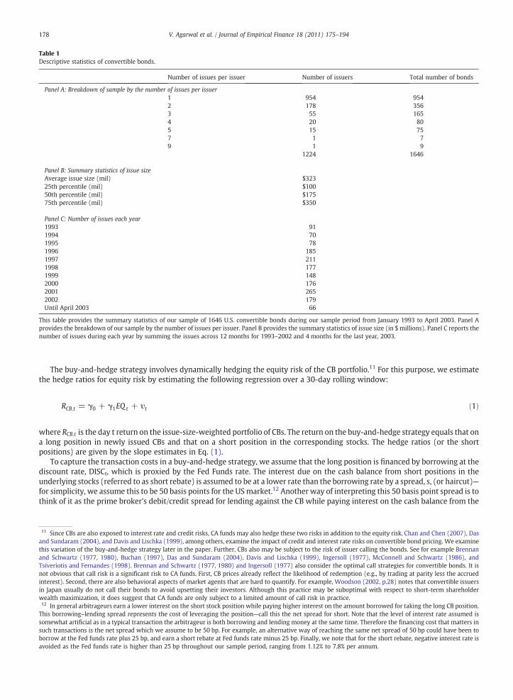
Table 1Descriptive statistics of convertible bonds.

Number of issues per issuer Number of issuers Total number of bonds

Panel A: Breakdown of sample by the number of issues per issuer1 954 9542 178 3563 55 1654 20 805 15 757 1 79 1 9

1224 1646

Panel B: Summary statistics of issue sizeAverage issue size (mil) $32325th percentile (mil) $10050th percentile (mil) $17575th percentile (mil) $350

Panel C: Number of issues each year1993 911994 701995 781996 1851997 2111998 1771999 1482000 1762001 2652002 179Until April 2003 66

This table provides the summary statistics of our sample of 1646 U.S. convertible bonds during our sample period from January 1993 to April 2003. Panel Aprovides the breakdown of our sample by the number of issues per issuer. Panel B provides the summary statistics of issue size (in $ millions). Panel C reports thenumber of issues during each year by summing the issues across 12 months for 1993–2002 and 4 months for the last year, 2003.


The buy-and-hedge strategy involves dynamically hedging the equity risk of the CB portfolio.11 For this purpose, we estimatethe hedge ratios for equity risk by estimating the following regression over a 30-day rolling window:

11 Sincand Sunthis varand SchTsiverionot obvinterestin Japanwealth12 In gThis bosomewsuch traborrowavoided

RCB;t = γ0 + γ1EQ t + υt ð1Þ

RCB;t is the day t return on the issue-size-weighted portfolio of CBs. The return on the buy-and-hedge strategy equals that on
wherea long position in newly issued CBs and that on a short position in the corresponding stocks. The hedge ratios (or the shortpositions) are given by the slope estimates in Eq. (1).
To capture the transaction costs in a buy-and-hedge strategy, we assume that the long position is financed by borrowing at thediscount rate, DISCt, which is proxied by the Fed Funds rate. The interest due on the cash balance from short positions in theunderlying stocks (referred to as short rebate) is assumed to be at a lower rate than the borrowing rate by a spread, s, (or haircut)—for simplicity, we assume this to be 50 basis points for the US market.12 Another way of interpreting this 50 basis point spread is tothink of it as the prime broker's debit/credit spread for lending against the CB while paying interest on the cash balance from the

e CBs are also exposed to interest rate and credit risks, CA funds may also hedge these two risks in addition to the equity risk. Chan and Chen (2007), Dasdaram (2004), and Davis and Lischka (1999), among others, examine the impact of credit and interest rate risks on convertible bond pricing. We examineiation of the buy-and-hedge strategy later in the paper. Further, CBs also may be subject to the risk of issuer calling the bonds. See for example Brennanwartz (1977, 1980), Buchan (1997), Das and Sundaram (2004), Davis and Lischka (1999), Ingersoll (1977), McConnell and Schwartz (1986), andtis and Fernandes (1998). Brennan and Schwartz (1977, 1980) and Ingersoll (1977) also consider the optimal call strategies for convertible bonds. It isious that call risk is a significant risk to CA funds. First, CB prices already reflect the likelihood of redemption (e.g., by trading at parity less the accrued). Second, there are also behavioral aspects of market agents that are hard to quantify. For example, Woodson (2002, p.28) notes that convertible issuersusually do not call their bonds to avoid upsetting their investors. Although this practice may be suboptimal with respect to short-term shareholder

maximization, it does suggest that CA funds are only subject to a limited amount of call risk in practice.eneral arbitrageurs earn a lower interest on the short stock position while paying higher interest on the amount borrowed for taking the long CB position.rrowing–lending spread represents the cost of leveraging the position—call this the net spread for short. Note that the level of interest rate assumed ishat artificial as in a typical transaction the arbitrageur is both borrowing and lending money at the same time. Therefore the financing cost that matters innsactions is the net spread which we assume to be 50 bp. For example, an alternative way of reaching the same net spread of 50 bp could have been toat the Fed funds rate plus 25 bp, and earn a short rebate at Fed funds rate minus 25 bp. Finally, we note that for the short rebate, negative interest rate isas the Fed funds rate is higher than 25 bp throughout our sample period, ranging from 1.12% to 7.8% per annum.


short sale. This way, the reference level of interest rate cancels and the net cost to the CA hedge fund is this debit/credit spread of50 basis points.13

After adjusting for these financing and transaction costs in this manner, the return corresponding to hedging the equity riskis EQ t−(DISCt−s). We denote this cost-adjusted return by XEQt. The returns for our buy-and-hedge factor, X, is thereforegiven by

13 Althmarketswell bemarket14 It shcollaterhigher t15 Fromfund apa final s$1 billio

Xt = RCB;t−DISCt

� �−γ̂1XEQ t ð2Þ

Xt is day t return on following the convertible arbitrage strategy, RCB;t−DISCt� �

is the day t return on the bond portfolio
whereadjusted for borrowing cost DISCtð Þ associated with funding the long position in the hedged CB portfolio.
3.2. Descriptive statistics of buy-and-hedge strategies

Table 2 reports the descriptive statistics of the X factor. Panel A shows that there are 411 CBs, on average, in the issue-size-weighted CB portfolio. These bonds have an average current yield of 13%, an average parity of 69%, and an average age (time sinceissuance) of 2.4 years.

Although the X factor has daily returns spanning the sample period from January 1993 to April 2003, we can only observeCA hedge fund returns on a monthly basis. Thus, we compound the daily returns on the X factor into monthly returns for ourstatistical analyses. Table 2 Panel B provides the descriptive statistics of these monthly returns over our sample period. TheX factor has average monthly return of 0.17% during the sample period.14 Although the average monthly return is positive,the factor return is quite volatile. The sample standard deviation of the X factor is about six times its monthly average return(1.01% vs. 0.17%).

3.3. Buy-and-hold component of CA hedge fund returns

We use the returns of the Vanguard Convertible Securities mutual fund (VG), one of the largest mutual funds investing in U.S.dollar denominated CBs, to proxy the performance of the passive buy-and-hold component for US CBs. Our choice of usingVanguard fund returns instead of a CB index to proxy for buy-and-hold returns is driven by the fact that Vanguard returns accountfor the costs associated with acquiring and carrying a long position in the CB market. Further, in contrast to a CB index, theVanguard fund is investable.

Panel A of Table 3 reports the descriptive statistics of the returns on the passive buy-and-hold strategy. Comparing the resultsin Tables 2 and 3, we observe that the mean monthly return of VG (X) is 0.32% (0.17%) with a standard deviation of 3.72% (1.01%).These comparisons suggest that the buy-and-hedge strategy offers a better risk-return tradeoff than the buy-and-hold strategy inthe CB market. For example, the ratio of mean return to sample standard deviation is 0.168 (0.086) for X (VG).

3.4. Representative portfolios of the CA hedge fund universe

Since many hedge funds report solely to one database and there is little overlap between different databases (see Agarwal et al.(2009)), in order to construct a broad and more representative sample of CA hedge funds, we use data on individual hedge fundsfrom three different databases the Centre for International Securities and Derivative Markets (CISDM), CS Tremont (CT) (nowLipper TASS), and Hedge Fund Research (HFR). Specifically, we create two CA portfolios (equally-weighted (EW) and value-weighted (VW)) from the 155 unique funds out of a total of 207 funds that are classified as CA hedge funds spanning the sampleperiod January 1993 to April 2003.15 For the sake of completeness, we also repeat our analysis using easily available and widelyused CA indexes based on these three databases. It is important to note that hedge fund indexes are generally constructed fromwidely diverging samples employing different index construction methods. For example, CISDM uses returns of the median fund,HFR uses equally-weighted returns, and CT employs value-weighted returns. Given the differences in index construction anddifferent index inclusion requirements for funds, throughout the paper, we focus primarily on the results for our two CA portfolios(EW and VW), which are constructed using the union of these three databases. We also briefly discuss the results with the CISDM,CT, and HFR indexes.

ough it is quite possible that when liquidity conditions in the market is poor, this funding spread can rise. However, it is not clear that when creditare at extreme whether leverage will continue to be available at higher prices or simply dries up. Therefore, under normal market conditions, there maysmall variations to this simple assumption of 50 basis points funding spread the effect of which is unlikely to be material to our conclusions. Extremeconditions are perhaps better modeled as discrete events separately and we do address this point separately in this paper.ould be noted that in theory, these returns only require an amount of equity margin pledged with the CA hedge funds' prime brokers in order toalize the long/short transactions. Therefore, depending on the implicit leverage used by a CA hedge fund, the return on equity margin can be significantlyhan the reported figures.the 207 CA hedge funds from the three databases, we identify duplicates by matching funds by name and by comparing their return histories. When a

pears in more than one database, we select the fund from the database that has the longest return history for that fund. Eliminating duplicate funds yieldsample of 155 distinct CA hedge funds. The universe of CA hedge funds has grown substantially over our sample period from 29 funds managing just undern at the beginning of 1993 to 119 funds managing about $1 billion at the end of 2002.

Table 2Descriptive statistics of the buy-and-hedge factor.

Panel A: Bonds used to construct X factorAverage number of bonds 411Current yield (%) 13Parity (%) 69Age of bonds (in years) 2.4

Panel B: Summary statistics of the monthly returns of X factorMean (%) 0.17Median (%) 0.22SD (%) 1.01Min. (%) −1.78Max. (%) 1.95Skew −0.14Kurt −0.48

We report descriptive statistics of the buy-and-hedge factor, X. Panel A provides the daily average ofthe number of convertible bonds, current yield, parity, and age of convertible bonds in the portfoliogenerating the X factor. Current yield is computed using a full year's coupon divided by the bond'sprice (which incorporates accrued interest). Parity is the bond's conversion value as a percentage ofthe par value. Age is the number of years since the bond was issued. Panel B provides summarystatistics of the buy-and-hedge factor's monthly returns during our sample period from January 1993to April 2003.


Panel A of Table 3 reports the descriptive statistics of monthly returns of the two CA portfolios (EW and VW) and the three CAindexes. The mean (median) monthly returns for these indexes and portfolios range from 0.47% to 0.61% (0.68% to 0.79%) whilethe standard deviations (SDs) range from 0.67% to 1.38%. As expected, the broad-based variables targeting the central tendency ofCA hedge funds' performance (EW, VW, CISDM, CT, and HFR) fall within a small range.

Panel B reports the correlations among the CA portfolios, the three CA indexes, VG, and the X factor. Not surprisingly, the CAportfolios and CA indexes are highly correlated with each other (correlations ranging from 0.80 to 0.93). Their correlations withVG are positive but lower in magnitude; the correlations range from a low of 0.34 (CT) to a high of 0.60 (EW). The CA portfoliosand CA indexes are all positively correlated to the X factor, consistent with the use of the buy-and-hedge strategy by CA hedgefunds.

Next we conduct a multivariate analysis of CA fund returns using a two-factor model consisting of both buy-and-hedge andbuy-and-hold factors.

Table 3Descriptive statistics of the long-biased convertible bond portfolio and the convertible arbitrage portfolios.

Panel A: Summary statistics

Mean (%) Median (%) SD (%) Min. (%) Max. (%) Skew Kurt

VG 0.32 0.22 3.72 −13.25 10.11 −0.43 1.33EW 0.56 0.68 1.03 −4.00 2.55 −1.08 2.51VW 0.50 0.74 1.28 −4.66 3.04 −1.24 2.59CISDM 0.61 0.74 0.67 −2.35 2.20 −1.36 3.98CT 0.47 0.79 1.38 −5.10 3.07 −1.69 4.55HFR 0.57 0.71 0.98 −3.65 2.93 −1.39 3.99

Panel B: Correlations between VG, the two CA portfolios, the three CA indexes and the X factor

VG EW VW CISDM CT HFR X

VG 1.00EW 0.60⁎⁎⁎ 1.00VW 0.49⁎⁎⁎ 0.90⁎⁎⁎ 1.00CISDM 0.55⁎⁎⁎ 0.92⁎⁎⁎ 0.83⁎⁎⁎ 1.00CT 0.34⁎⁎⁎ 0.81⁎⁎⁎ 0.85⁎⁎⁎ 0.80⁎⁎⁎ 1.00HFR 0.51⁎⁎⁎ 0.90⁎⁎⁎ 0.84⁎⁎⁎ 0.93⁎⁎⁎ 0.80⁎⁎⁎ 1.00X 0.39⁎⁎⁎ 0.62⁎⁎⁎ 0.58⁎⁎⁎ 0.61⁎⁎⁎ 0.48⁎⁎⁎ 0.60⁎⁎⁎ 1.00

Panel A of this table provides the descriptive statistics of the monthly returns of the Vanguard Convertible Securities mutual fund (VG), equally-weighted andvalue-weighted portfolios of all CA hedge funds (EW and VW) and three convertible arbitrage (CA) indexes (CISDM, CT, and HFR) from January 1993 to April 2003with the exception of the CT index, which starts in 1994. The descriptive statistics include mean, median, standard deviation (SD), minimum (Min.), maximum(Max.), skewness (Skew), and kurtosis (Kurt). Panel B provides the correlations among the above return series and the buy-and-hedge factor, X. ⁎, ⁎⁎, and ⁎⁎⁎

indicate that the coefficient is significantly different from zero at the 10, 5, and 1% levels respectively.

Table 4Regression analysis with the buy-and-hedge and buy-and-hold factors.

CA portfolios CA indexes

EW VW CISDM CT HFR

Coeff t-stat Coeff t-stat Coeff t-stat Coeff t-stat Coeff t-stat

Intercept 0.004⁎⁎⁎ (4.756) 0.004⁎⁎⁎ (2.654) 0.005⁎⁎⁎ (8.505) 0.004⁎⁎ (2.339) 0.005⁎⁎⁎ (5.135)X 0.465⁎⁎⁎ (4.969) 0.581⁎⁎⁎ (3.952) 0.311⁎⁎⁎ (5.079) 0.558⁎⁎⁎ (3.600) 0.453⁎⁎⁎ (4.562)VG 0.118⁎⁎⁎ (5.499) 0.108⁎⁎⁎ (3.866) 0.066⁎⁎⁎ (4.279) 0.065⁎ (1.902) 0.087⁎⁎⁎ (3.588)Adj-R2 52.82% 41.50% 48.18% 24.20% 43.96%

This table provides the results of the following OLS regression during our sample period from January 1993 to April 2003:

CAt = θ0 + θ1Xt + θ2VGt + ψt

where, CAt are the excess returns (in excess of risk-free rate, i.e., US Fed Funds rate) during month t on the equally-weighted and value-weighted indexes of allthe CA funds in our sample (EW and VW) or on the convertible arbitrage (CA) hedge fund indexes (CISDM, CT, or HFR), Xt is the return during month t on the buy-and-hedge factor and VGt is the excess return during month t on the Vanguard Convertible Securities mutual fund. Coeff are regression estimates and t-stat aret-statistics computed with Newey and West (1987) standard errors. ⁎, ⁎⁎, and ⁎⁎⁎ indicate that the coefficient is significantly different from zero at the 10, 5,and 1% levels respectively.


4. Empirical methodology and results

4.1. A model of CA hedge fund returns

Our analysis begins with the following regression model16:

16 Unlvalues f17 It ison the bin the p18 To fthe hed(2004)30%, wh19 We

CAt = θ0 + θ1Xt + θ2VGt + ψt : ð3Þ

Here the time series of monthly returns for each CA portfolio and index, denoted by CAt, are regressed against the monthlyreturns of the buy-and-hedge and buy-and-hold strategies. Since we cannot directly observe the extent to which CA hedge fundsactively hedge the equity risk as opposed to buying and holding CBs, we allow for both the passive and active components in ourmodel and empirically estimate their relative importance in determining the CA funds' performance.

The results in Table 4 show that the two CA portfolios (EW and VW) have significant exposures to X and VG, which is consistentwith both buy-and-hedge and buy-and-hold strategies contributing to the CA returns. We also observe a significant intercept (oralpha) of 40 basis points per month for both EW and VW.17 The adjusted-R2 for the EW and VW portfolios are 52.82% and 41.50%,respectively, suggesting that our simple model of using two asset-based strategies (buy-and-hedge and buy-and-hold) does agood job of explaining the dynamics of CA fund returns.18 The results for the three CA indexes are qualitatively similar to those forthe two CA portfolios. We consistently observe significant loadings on X and VG, with explanatory power ranging from 24.20% to48.18%.

As a robustness check, we repeat our analysis using only CBs that mature within the sample period to construct an alternativeversion of the buy-and-hedge factor.19 The results (not reported in the table) are qualitatively similar. Both the buy-and-hedgefactor and the buy-and-hold factor continue to be positively related to CA returns; the coefficient of the buy-and-hedge factor isstatistically significant in all cases but one and the coefficient of VG is always statistically significant. The two-factor modelproduces adjusted-R2s ranging from 11% to 39% but lower than those reported in Table 4. This suggests that the buy-and-hedgefactor that uses all CBs does a better job of explaining CA returns during our sample period.

Since CBs are also exposed to interest rate risk and credit risk, in theory, CA funds may also hedge these two risks in addition tothe equity risk. However, the extent to which they do so in practice must depend on the costs and benefits of hedging these riskswhich is an empirical question. To answer this question, we repeat our analysis using an alternative buy-and-hedge factor, XA,which hedges all three sources of risk (interest, credit and equity). XA is constructed as follows. Equity risk is captured in EQt,as in the case of factor X. The impact of credit risk inherent in CBs is proxied by the daily change in the spread between the

ess otherwise stated, we use Newey and West (1987) heteroskedasticity-and-autocorrelation consistent standard errors to compute t-statistics and p-or regression coefficients.important to note that this specification assumes constant factor loadings through the sample period. Arguably, hedge funds may change their weightsuy-and-hold and buy-and-hedge strategies in response to changes in investment opportunities and market conditions, an issue we explore in detail, lateraper.urther highlight the economic importance of the X factors, we also compare the adjusted-R2 from our model with adjusted-R2s from other models used inge fund literature including the Carhart (1997) model augmented with out-of-the-money call and put options on S&P 500 index as in Agarwal and Naikand the Fung and Hsieh (2004) seven-factor model. The results in Appendix A show that the explanatory power from these models ranges from 7% toich is substantially lower than the range of 24% to 53% obtained with our more parsimonious model.thank the referee for suggesting this possibility.

Table 5Results with the alternative buy-and-hedge factor, XA.


EW VW CISDM CT HFR


Intercept 0.003⁎⁎⁎ (2.884) 0.002 (1.327) 0.005⁎⁎⁎ (5.783) 0.003 (1.214) 0.004⁎⁎⁎ (2.961)XA 0.345⁎⁎⁎ (3.886) 0.447⁎⁎⁎ (3.271) 0.226⁎⁎⁎ (3.915) 0.405⁎⁎⁎ (2.693) 0.361⁎⁎⁎ (4.036)VG 0.115⁎⁎⁎ (4.281) 0.102⁎⁎⁎ (3.015) 0.065⁎⁎⁎ (3.385) 0.059 (1.423) 0.081⁎⁎⁎ (2.858)Adj-R2 43.68% 32.75% 38.05% 16.51% 35.73%


CAt = η0 + η1XAt + η2VGt + πt

where, CAt are the excess returns (in excess of risk-free rate, i.e., US Fed Funds rate) during month t on the equally-weighted and value-weighted indexes of all theCA funds in our sample (EW and VW) or on the convertible arbitrage (CA) hedge fund indexes (CISDM, CT, or HFR), XA

t is the return during month t on thealternative-X factor where all the three risks are hedged, i.e., long convertible bonds and short the equity, credit, and interest rate risks and VGt is the excess returnduring month t on the Vanguard Convertible Securities mutual fund. We proxy the credit risk in CBs by the daily change in the spread between the yield on Baacorporate bonds and the yield on 10-year U.S. Treasury bonds. We capture the interest rate risk in CBs through the daily yield on 5-year U.S. Treasury bonds. Coeffare regression estimates and t-stat are t-statistics computedwith Newey andWest (1987) standard errors. ⁎, ⁎⁎, and ⁎⁎⁎ indicate that the coefficient is significantlydifferent from zero at the 10, 5, and 1% levels respectively.


yields of Baa corporate bonds and 10-year U.S. Treasury bonds. To incorporate the impact of interest rate risk, we use the dailyyield of 5-year U.S. Treasury bonds. 20 The risks of the portfolio of CBs are hedged using the following regression model:

20 We21 Theweighti

RCB;t = γ0 + γ1EQt + γ2IRt + γ3CRt + ηt : ð4Þ

Here RCB;t is the day t return on the issue-size-weighted portfolio of CBs, EQt is the day t return on the issue-size-weightedportfolio of underlying stocks, IRt is the day t interest rate proxy, and CRt is the day t credit risk proxy. The return to the strategythat hedges all three risks follows that of a portfolio comprising a long position in the issue-size-weighted portfolio of CBs, a shortposition in the issue-size-weighted portfolio of the corresponding stocks, a short position in government bonds, and a shortposition in the spread between corporate and government bonds.21 The short quantities are obtained from the slope estimates inEq. (4).

After adjusting for financing and transaction costs, the returns corresponding to hedging the equity, credit, and interest raterisks are EQ t−(DISCt−s), CRt−(DISCt−s), and IRt−(DISCt−s) respectively. We denote these cost-adjusted returns by XEQt,XCRt, and XIRt. The cost-adjusted returns from the alternative buy-and-hedge factor, XA, is given by

XAt = RCB;t−DISCt

� �−γ̂1XEQ t−γ̂2XIRt−γ̂3XCRt ð5Þ

XAt is day t return on following the convertible arbitrage strategy, RCB;t−DISCt

� �is the day t return on the bond portfolio
where
adjusted for borrowing cost DISCtð Þ associated with funding the long position in the CB portfolio, and XEQ t ;XCRt ; and XIRt are asdefined above.

Table 5 reports the results from the regressionmodel of Eq. (3), re-estimated using VG and XA. We observe that the loadings onthe two factors are similar to those in Table 4. However, using the alternative buy-and-hedge factor lowers explanatory poweracross all CA portfolios and indexes. For example, for the EW CA portfolio, the two-factor model with the original buy-and-hedgefactor (X) achieves an adjusted-R2 of 52.82%, but the two-factor model with the alternative buy-and-hedge factor (XA) produces alower adjusted-R2 of 43.68%. This suggests that our specification of hedging equity risk alone is a better characterization of thebuy-and-hedge strategy used by CA hedge funds in practice. Therefore, in the following analyses, our buy-and-hedge strategyinvolves taking a long position in CBs and delta hedging the equity risk.

These empirical results suggest that CA hedge funds behave in a manner consistent with that of an intermediary who providesfunding to the CB issuers while acting as an equity-risk transfer agent distributing risk from the CB to the equity market.

4.2. How does the supply of CBs affect convertible arbitrageurs?

Viewed as a funding and risk intermediary for CB issuers, a convertible arbitrageur's performance in month t should depend onthe supply of new CB issues available for tradingmonth t, NIt . However, simply relying on CB issuance dates recorded in databasesproduces an inaccurate measure of NIt as these bonds often trade in the “when-issued” (WI) market—which exists between the

obtain these from the Federal Reserve Board website and Datastream.stocks in the stock portfolio receive the same weight as the corresponding CBs. The interest rate and credit variables are indexes. Hence, there is nong for these variables.

Table 6Information content of supply.

Announcement month is No. of convertible bond issues Percent (%)

Same as issuance month 63 67.741 month before issuance month 22 23.662 months before issuance month 6 6.454 months before issuance month 1 1.085 months before issuance month 1 1.08Total 93 100

We randomly sample 100 US convertible bonds and hand collect the earliest announcement date from Factiva news search supplementedwith searches on SEC EDGAR and Google. Announcement dates are successfully collected for 93 of the 100 bonds. For these bonds, we comparethe announcement month and the issuance month to determine the extent to which the announcement date precedes reported issuance date.We report the frequency distribution of the announcement month relative to the issuance month.


announcement date of a new issue and ends on the issuance date that can be severalmonths hence.22 The existence of theWImarketmeans that the profit/loss effect of a new CB issue can enter into a CA fund's performance well before the recorded issuance date ofnewly issued CBs as WI CB positions are marked to market for accounting purposes. The combination of when issued trading and apotentially long settlement period between announcement and issuance dates give rise to a measurement problem if one usesissuance dates to construct a supply proxy. In other words, NIt contains bonds with issuance dates in months t+1, t+2, or beyond.Therefore, thefirst step to constructing anaccurate proxyof CB supply is to gaugehow far in timeCBdeals are announced in advanceofeventual issuance. To that end, we randomly sample (without replacement) 100 CBs that are issued during our sample period andmanually collect the earliest announcement date from Factiva news search supplemented with searches on the SEC EDGAR databaseand Google.23 Ninety-three of the 100 randomly selected bonds have complete information.

Table 6 displays the frequency distribution of the announcement month relative to the issuance month. About two-thirds ofthe announcements are made in the same month as the issuance month while the remaining announcements are made beforethe issuance month. In particular, about 24% of the CB deals are announced 1 month before the issuance month and another6% are announced 2 months before. Of the two remaining CB issues, one is announced 4 months before issuance while another isannounced 5 months before issuance. This distribution suggests that a reasonable proxy of NIt includes CBs with issuance dates inmonths t+1 and t+2. Accordingly, we construct our month t supply variable, LDealt, as

22 ChaNyborgAuthori23 Oursampled24 For25 Webetwee

LDealt = log 1 + CBt+1 + CBt+2� � ð6Þ

log(.) is the natural logarithm function, and CBt+1 (CBt+2) is the number of CB issues with issuance dates in month t+1
where(t+2).24 To test whether supply conditions affect CA performance, we estimate the following regression model:
CAt = α + β1Xt + β2VGt + γLDealt + χt ð7Þ

LDealt is the supply variable in month t and the other variables are as in Eq. (3).
whereTable 7 reports the results from applying Eq. (7) to the two CA portfolios and the three CA indexes. The coefficients for X and VG
with respect to the two CA portfolios, EW and VW, remain positive and statistically significant. In addition, the new supply variableLDeal has a positive and highly significant coefficient for both the portfolios. After accounting for supply effects via the LDeal variable,both CA portfolios exhibit significant negative alphas. This is in sharp contrast to the positive alphas previously reported in Table 4before the supply effects of CBs are incorporated into our model. Furthermore, despite the reduction in the degrees of freedom, theintroduction of the supply variable leads to an improvement in the explanatory power of our model—adjusted-R2 increases from52.82% to 59.70% for EW, and from 41.50% to 55.26% for VW. The results for the three CA indexes are qualitatively similar. Takentogether, the evidence highlights the importance of changing investment opportunities on the performance of CA hedge funds.

At first glance, the occurrence of significant negative alphas appears to be at odd with the growth in CA hedge funds. To explorethis phenomenon, we examine alternative ways of incorporating the effect of the WI market on the LDeal variable. Unlike otherfactors in our model, LDeal is a non-price construct and is not directly investable. The monetization of LDeal's effect onperformance is imprecise. The possibility exists that we may have over compensated for the when-issued trading effect of theLDeal variable. Short of precisely quantifying the exact announcement dates of thousands of bonds manually, there is no obviousway to accurately assess this possibility. Here we report our results based on a measure of LDeal that errs on the side ofconservatism. Overall, without the LDeal variable, one observes positive alpha. Using a conservative estimate of LDeal leads to theobserved negative alpha. Both sets of results point to the presence of a supply effect.25

cko et al. (2005) study the determinants of liquidity in the US corporate bond market using a dataset of when-issued and secondary market trades.and Sundaresan (1996), among others, study when-issued trading in the US Treasury market. In private correspondence, a Financial Industry Regulatoryty (FINRA) representative confirms the existence of when-issued trading in convertible bonds.CB data set from Albourne Partners contains the issuance dates, but not the announcement dates. In unreported work, we find that the distribution ofbonds across years is similar to the distribution for the entire sample of 1646 bonds.

robustness, we repeat our tests using the logarithm of the number of CB issues in month t, and find our results to be qualitatively similar.repeat our analyses using a version of LDeal that is based only on supply in month t+1 (i.e., LDeal=log (CBt+1)) and find that the estimated alphas falln the alphas we currently report and the alphas based only on supply in month t.

Table 7Regression analysis allowing for supply.


EW VW CISDM CT HFR


Intercept −0.010⁎⁎ (2.169) −0.022⁎⁎⁎ (4.078) −0.005 (1.432) −0.026⁎⁎⁎ (3.197) −0.011⁎⁎ (2.236)X 0.442⁎⁎⁎ (5.279) 0.535⁎⁎⁎ (4.396) 0.294⁎⁎⁎ (5.622) 0.453⁎⁎⁎ (3.696) 0.427⁎⁎⁎ (4.800)VG 0.099⁎⁎⁎ (5.994) 0.074⁎⁎⁎ (3.444) 0.053⁎⁎⁎ (4.179) 0.030 (1.015) 0.068⁎⁎⁎ (3.248)LDealt 0.005⁎⁎⁎ (3.415) 0.008⁎⁎⁎ (5.033) 0.003⁎⁎⁎ (3.360) 0.010⁎⁎⁎ (3.910) 0.005⁎⁎⁎ (3.516)Adj-R2 59.70% 55.26% 55.44% 39.19% 51.90%


CAt = α + β1Xt + β2VGt + γLDealt + χt

where CAt are the excess returns (in excess of risk-free rate—US Fed Funds rate) during month t on the equally-weighted and value-weighted indexes of all the CAfunds in our sample (EW and VW) or on the convertible arbitrage (CA) hedge fund indexes (CISDM, CT, or HFR), Xt is the return during month t on the buy-and-hedge factor and VGt is the excess return during month t on the Vanguard Convertible Securities mutual fund. LDealt is the natural log of one plus the numberof convertible issues in months t+1 and t+2. Coeff are regression estimates and t-stat are t-statistics computed with Newey and West (1987) standard errors.⁎, ⁎⁎, and ⁎⁎⁎ indicate that the coefficient is significantly different from zero at the 10, 5, and 1% levels respectively.


Thus far the empirical analyses indicate that convertible arbitrageurs benefit from providing funding to CB issuers whilesimultaneously offsetting the bond's equity risk utilizing the liquidity of the equity markets. However, for CA hedge funds toperform this function effectively they have to secure funding, and sometimes have to leverage their portfolio to purchase the CBs.The ability of CA hedge funds to borrow short-term capital from prime brokers as well as to attract longer term capital from theirinvestors will in turn depend on prevailing liquidity conditions in the market place. In this context, the question arises as to howconvertible arbitrageurs respond to market upheavals that interrupt their ability to fund their portfolios? To gain insight into thisquestion, we examine how CA hedge funds manage extreme events such as the LTCM crisis.

Table 8Structural break model after allowing for supply of convertible bonds.


EW VW CISDM CT HFR


Pre-LTCM period D1 −0.011⁎⁎ (2.085) −0.027⁎⁎⁎ (4.643) −0.005 (1.359) −0.032⁎⁎⁎ (4.321) −0.012⁎⁎ (2.344)D1×X 0.349⁎⁎⁎ (3.557) 0.420⁎⁎⁎ (2.911) 0.235⁎⁎⁎ (3.841) 0.282⁎⁎ (2.347) 0.293⁎⁎⁎ (3.083)D1×VG 0.154⁎⁎⁎ (5.152) 0.129⁎⁎⁎ (3.563) 0.085⁎⁎⁎ (3.913) 0.067 (1.336) 0.128⁎⁎⁎ (4.473)D1×LDeal t 0.005⁎⁎⁎ (3.117) 0.010⁎⁎⁎ (5.418) 0.003⁎⁎⁎ (3.062) 0.011⁎⁎⁎ (5.058) 0.005⁎⁎⁎ (3.570)

Post-LTCM period D2 −0.003 (0.644) −0.007 (0.811) −0.001 (0.158) −0.010 (0.568) 0.0001 (0.010)D2×X 0.552⁎⁎⁎ (6.228) 0.683⁎⁎⁎ (5.231) 0.376⁎⁎⁎ (6.773) 0.694⁎⁎⁎ (4.269) 0.643⁎⁎⁎ (6.029)D2×VG 0.075⁎⁎⁎ (4.160) 0.050⁎ (1.873) 0.039⁎⁎⁎ (2.936) 0.017 (0.429) 0.041⁎ (1.809)D2×LDeal t 0.002⁎ (1.814) 0.004 (1.496) 0.002 (1.564) 0.005 (0.954) 0.002 (0.782)Adj-R2 69.29% 62.40% 75.49% 45.52% 65.70%

Test of differences of coefficientsF-value p-value F-value p-value F-value p-value F-value p-value F-value p-value

D1=D2=0 3.44⁎⁎ 0.035 11.07⁎⁎⁎ 0.000 1.37 0.259 12.10⁎⁎⁎ 0.000 3.49⁎⁎ 0.034D1×X=D2×X 2.68 0.104 2.24 0.138 2.84⁎ 0.095 3.70⁎ 0.057 6.34⁎⁎ 0.013D1×VG=D2×VG 3.72⁎ 0.056 2.61 0.109 2.96⁎ 0.088 0.37 0.544 5.09⁎⁎ 0.026D1×LDealt=D2×LDealt 1.39 0.240 3.97⁎⁎ 0.049 0.62 0.434 1.43 0.234 1.87 0.175


CAt = D1 ω0 + ω1XUSt + ω2VGt + LDealt

� �+ D2 ω0 + ω3X

USt + ω4VGt + LDealt

� �+ κt

where, CAt are the excess returns during month t on the equally-weighted and value-weighted indexes of all the CA funds in our sample (EW and VW) or on theconvertible arbitrage (CA) hedge fund indexes (CISDM, CT, or HFR), Xt are the return during month t on the buy-and-hedge factor and VGt is the excess returnduring month t on the Vanguard Convertible Securities mutual fund. LDealt is natural log of one plus the number of convertible issues in month t+1 and t+2. Thepre-LTCM (post-LTCM) period dummy, D1 (D2), takes the value of 1 (0) before (after) the LTCM crisis in September 1998 and equals 0 (1) otherwise. There is nointercept term as the regression includes both the dummies. Coeff are regression estimates and t-stat are t-statistics computed with Newey and West (1987)standard errors. F-value and p-value are, respectively, the F-statistic and associated p-value from the test of difference of coefficients. ⁎, ⁎⁎, and ⁎⁎⁎ indicate that thecoefficient is significantly different from zero at the 10, 5, and 1% levels respectively.


4.3. The impact of extreme market events on CA hedge funds

We investigate the effect of the LTCM event on CA fund returns by testing for structural breaks to our model. FollowingBrown et al. (1975), we apply the CUSUM procedure and confirm that the LTCM crisis indeed lead to consistent boundaryviolations across the two CA portfolios and the three CA indexes. Similar to Fung and Hsieh (2004) and Fung et al. (2008), weuse the following structural break model to account for the LTCM crisis:

26 We

CAt = D1 ω0 + ω1Xt + ω2VGt + γLDealtð Þ + D2 ω0 + ω3Xt + ω4VGt + πLDealtð Þ + κt : ð8Þ

Here the variables are as defined before in Eqs. (3) and (7).The results from this joint estimation are reported in Table 8. There is a general decline in the exposure to the buy-and-hold

strategy uniformly across the CA portfolios and indexes compared to the results reported in Table 7. The coefficient on D1×VG issmaller than that on D2×VG for EW, CISDM, and HFR at varying levels of statistical significance. For the two AUM-weightedconstructs, the VW portfolio and the CT index, post-LTCM exposure to the directional factor, VG, appear to have weakened both inslope coefficient as well as statistical significance. These results are broadly consistent with an increase in risk aversion post LTCM.Collaborative evidence can be seen in post-LTCM increases in the exposures to the buy-and-hedge factor across all cases. However,we can only confirm the statistical significance for all the CA indexes but not for the CA portfolios (see the F-test results for D1×Xin the lower panel of Table 8). In terms of the effect of CB supply on returns, the results are mixed. Both the CA portfolios andindexes exhibit significant positive loading on the supply variable (LDeal) before the LTCM crisis similar to the results reportedin Table 7. However, post LTCM, the coefficient on LDeal is positive but only weakly significant (at the 10% level) for EW. But theF-tests failed to reject the null that LDeal has identical coefficients before and after the LTCM crisis, with the exception of VW.Taken together, there seems to be a preponderance of evidence pointing towards a decrease in risk appetite (or an increase inrisk aversion) after the LTCM crisis. However, the variability of the results across the two portfolios (EW and VW) and threeindexes (CISDM, CT, and HFR) indicate potential behavioral differences in the cross section of funds—an issue we investigate inmore detail in the next section.

Finally, in terms of explanatory power, there is a uniform increase in adjusted-R2 compared to the results in Table 7. Forexample, with CISDM as the dependent variable, Eq. (8) produces an adjusted-R2 of 75.49%, which is substantially higher than theadjusted-R2 in Table 7 (55.44%). More importantly, both the pre-LTCM and post-LTCM alphas are either insignificantly differentfrom zero or negative. Overall, these findings confirm a lack of abnormal performance from CA funds on average, after adjusting forthe changes in investment opportunities and the structural changes arising from extreme market events such as the LTCM crisis.The natural question that arises is whether these conclusions apply uniformly across the funds in our sample. 26 This is the subjectof the next section.

5. Individual fund level analyses

The empirical results in the previous section point to potential differences in return characteristics between the small funds(weighted higher in the EW portfolio as well as indices such as the HFR and CISDM) and the larger funds, which have greaterweighting in the VWportfolio and the CT index. To investigate these differences, we begin by identifying all CA hedge fundswith atleast 24 months of data on returns and assets under management during our sample period. We then compute the time-seriesaverage of the assets under management for each fund to sort funds into size terciles (Small, Medium, and Large). This procedureyields 36 CA hedge funds in each tercile, for a total of 108 funds. Within each size tercile, we estimate Eq. (7), the two-factor plussupply effect model, for each fund. The summary statistics of the respective size terciles and regression results are reported inTable 9 Panel A.

The sample moments of returns reveal differences across size terciles. Larger funds (Medium and Large terciles) appear togenerate higher returns than small funds. The mean (median) monthly excess return on the Large, Medium, and Small portfolio is0.51%, 0.65%, and 0.39% (0.66%, 0.78% and 0.63%), respectively. The largest and smallest funds experience greater performancevariability than the medium funds. The Large and Small portfolios have monthly standard deviations of 1.25% and 1.29%,respectively, while the Medium portfolio has a monthly standard deviation of 1.05%. Higher performance variability implies moreextreme returns that can create greater divergence between the mean and median. We do observe such a pattern in the data. TheSmall and Large portfolios, with higher standard deviations, exhibit larger differences betweenmean andmedian returns than theMedium portfolio. In terms of Sharpe ratio, the Medium portfolio has the highest Sharpe ratio (0.62) while the Small portfolio hasthe lowest Sharpe ratio (0.30).

Turning to the regression results, we see that the average coefficient of X is positive and statistically significant at the 1% level,indicating that the buy-and-hedge factor continues to be a significant explanatory variable among CA hedge funds of varying sizes.The average coefficient of VG is positive and statistically significant for the small and medium terciles but not for larger CA hedgefunds. The average coefficient of LDeal is positive for all terciles, but is statistically significant only for the medium and largeterciles, suggesting that the supply variable is more important in explaining the returns of medium and large funds. These findingsare consistent with larger funds being less dependent on security selection to support performance for their capital base. This

thank the referee for directing us towards analyzing individual CA funds.

Table 9Individual fund level analyses.

Panel A: Two-factor model with supply

Size tercile: Small Medium Large

Coeff t-stat Coeff t-stat Coeff t-stat

Intercept −0.002 (−0.552) −0.015⁎⁎⁎ (−4.281) −0.009⁎⁎⁎ (−2.863)X 0.394⁎⁎⁎ (5.909) 0.419⁎⁎⁎ (6.624) 0.451⁎⁎⁎ (7.806)VG 0.161⁎⁎⁎ (3.686) 0.127⁎⁎⁎ (3.185) 0.056 (1.688)LDeal 0.002 (1.343) 0.006⁎⁎⁎ (5.914) 0.004⁎⁎⁎ (4.735)Adj-R2 23.60% 25.41% 18.01%AUM 8.390 51.088 243.696# Funds 36 36 36Mean (%) 0.39 0.65 0.51Median (%) 0.63 0.78 0.66SD (%) 1.29 1.05 1.25

Panel B: Two-factor model with supply and structural break for the LTCM crisis

Size tercile: Small Medium Large

Coeff t-stat Coeff t-stat Coeff t-stat

Pre-LTCM period D1 −0.013⁎⁎⁎ (−3.360) −0.018⁎⁎⁎ (−3.531) −0.028⁎⁎ (−2.589)D1×X 0.154⁎ (1.955) 0.407⁎⁎⁎ (4.547) 0.413⁎⁎ (2.500)D1×VG 0.141⁎⁎ (2.678) 0.025 (0.715) 0.079 (1.141)D1×LDeal t 0.005⁎⁎⁎ (5.107) 0.008⁎⁎⁎ (5.387) 0.010⁎⁎⁎ (3.080)

Post-LTCM period D2 0.017⁎ (1.985) −0.012⁎⁎ (−2.596) −0.009 (−1.638)D2×X 0.697 (1.753) 0.677⁎⁎⁎ (4.347) 0.411⁎⁎⁎ (3.869)D2×VG 0.098⁎⁎⁎ (3.419) 0.035 (0.953) 0.084 (1.039)D2×LDeal t −0.004 (−1.509) 0.005⁎⁎⁎ (4.018) 0.004 (1.618)Adj-R2 31.84% 43.99% 39.29%AUM 13.214 63.616 225.036# Funds 15 15 15Mean (%) 0.47 0.63 0.48Median (%) 0.54 0.67 0.77SD (%) 1.25 0.91 2.12

Test of differences of coefficients Increase Decrease Increase Decrease Increase Decrease

D1=D2=0 3 0 3 0 4 1D1×X=D2×X 3 0 7 1 2 1D1×VG=D2×VG 1 4 2 4 3 1D1×LDealt=D2×LDeal t 0 2 0 5 1 4

Panel A of this table summarizes the fund level results of the following OLS regression during our sample period from January 1993 to April 2003:

CAt = θ0 + θ1Xt + θ2VGt + θ3LDealt + ψt

where, CAt is the excess return (in excess of risk-free rate, i.e., US Fed Funds rate) during month t on a convertible arbitrage hedge fund with at least 24 monthly returnsduring the sample period, Xt is the return during month t on the buy-and-hedge factor, VGt is the excess return during month t on the Vanguard Convertible Securitiesmutual fund (VG) and LDealt is natural log of one plus the number of convertible issues in months t+1 and t+2. We sort funds into size terciles based on their average>assets under management during the sample period and summarize the regression outputs of funds in each tercile. Coeff and t-stat are, respectively, the mean andt-statistic of individual fund regression coefficients. Adj-R2 is the average of funds' adjusted-R2. AUM reports the grand average assets under management (in $ millions)in each tercile and # Funds reports the number of funds in each tercile. Mean, Median, and SD are, respectively, the mean, median and standard deviation of the monthlyexcess return on the equally-weighted size tercile. Panel B of this table provides the results of the following OLS regression during our sample period from January 1993to April 2003:

CAt = D1 ω0 + ω1Xt + ω2VGt + γLDealtð Þ + D2 ω0 + ω3Xt + ω4VGt + πLDealtð Þ + κt

where, CAt is the excess return (in excess of risk-free rate—US Fed Funds rate) during month t on a convertible arbitrage hedge fund with at least 48 monthlyreturns during the sample period and which existed before, during and after the LTCM crisis. The pre-LTCM (post-LTCM) period dummy, D1 (D2), takes thevalue of 1 (0) before (after) the LTCM crisis in September 1998 and equals 0 (1) otherwise. There is no intercept term as the regression includes both thedummies. As in Panel A, we summarize the regression outputs of funds in each tercile. Increase (decrease) is the number of funds for which there is a statisticallysignificant increase (decrease) in coefficient after the LTCM crisis. ⁎, ⁎⁎, and ⁎⁎⁎ indicate that the coefficient is significantly different from zero at the 10, 5, and 1%levels respectively.


observation is, in turn, consistent with a diseconomy of scale to skill-based investment strategies resulting in larger funds beingmore dependent on systematic, factor-related returns for performance. Consequently, declines in the supply of convertible bondsare likely to negatively impact themmore than their smaller brethren. Consistent with the results in Table 7, the non-factor relatedreturns from this three-factor model are not statistically different from zero for smaller funds and negative for medium and larger


funds. However the model's explanatory power, adjusted-R2, for each of the three terciles is notably lower than those reported forthe broader averages in Table 7.

Next, we examine howwell the structural breakmodel explains fund returns across the size terciles. For this analysis, we applya different selection procedure to ensure that the funds selected have a sufficiently long return history that spans the LTCM crisis.Specifically, we only include CA hedge funds with at least 48 months of data on returns and assets under management during oursample period to ensure sufficient degrees of freedom for efficient estimation. In addition, the funds must have existed before,during, and after the LTCM crisis. In other words, the return series must span the LTCM crisis. This second condition ensures thatD1 and D2, as well as all associated interaction terms can be estimated for each fund. The selection procedure yields 15 CA hedgefunds for each size tercile.27 Panel B of Table 9 reports the average regression coefficients, adjusted-R2, and fund characteristics.Because our selection procedure yields a subset of the original size terciles (employed in Table 9 Panel A), we also report summarystatistics of monthly excess returns on these new size terciles. To summarize tests of differences of coefficients among the funds,we report the number of funds for which there is a statistically significant increase or decrease in coefficient after the LTCM crisis.28

In terms of sample moments of returns, we continue to observe similar patterns to the results in Table 9 Panel A. Specifically,larger funds (Medium and Large terciles) appear to generate higher returns than small funds. For example, the median monthlyexcess return on the Large, Medium, and Small portfolio is 0.77%, 0.67%, and 0.54%, respectively. Performance variability is higheramong the largest and smallest funds than among the midsize funds; the Large (Small) portfolio has a monthly standard deviationof 2.12% (1.25%) while the Medium portfolio has a monthly standard deviation of 0.91%. As expected, greater return variability inthe Large and Small portfolios result in more pronounced differences between mean and median returns. The Medium portfoliohas the highest Sharpe ratio (0.69) and the Large portfolio has the lowest (0.23).

The fund-level regression results add clarity to those of CA indexes and portfolios in several respects. First, they clarify that theexposure to the directional variable, VG, reported in Table 8 for the broad-based portfolios and indexes are primarily driven by thesmaller funds. Panel B of Table 9 now confirms that on average, neither the Medium nor the Large tercile of funds exhibitstatistically significant exposure to the VG factor. This result is not affected by the LTCM event. These findings also clarify that theexposure to the buy-and-hedge factor, X, reported in Table 8 for the broad-based portfolios and indexes are primarily driven by thelarger funds both pre and post the LTCM crisis. Panel B of Table 9 reports collaborative evidence for this observation. Second, thereis an increase in explanatory power across all size terciles compared to the basic two-factor model. The average adjusted-R2 risesfrom 23.60% to 31.84% for the small tercile (comparing Panel A to Panel B of Table 9), 25.41% to 43.99% for the Medium tercile andmore than doubling for the Large tercile going from 18.01% to 39.29%. Third, as a gauge of whether there is a change in risk-takingbehavior, we examine the number of funds for which there is a statistically significant change in coefficient on VG after the LTCMcrisis. In both Small and Medium terciles, the number of statistically significant decreases in VG's coefficient is higher than thenumber of statistically significant increases. For example, among the smallest funds, there are 4 cases of a decrease in coefficientand only 1 case of an increase. Thus, for the Small tercile, the decline in the average coefficient is representative of changes at theindividual fund level. This is consistent with our earlier findings at the average (index) level showing that greater risk aversionpost the crisis reduces the use of the buy-and-hold strategy among the arbitrageurs. Fourth, pre LTCM, the supply variable figuressignificantly as a return driver for all three terciles of funds. Post LTCM, the supply variable no longer figures significantly for thebroad-based portfolios and CA indexes (see Table 8), but here the variable continues to figure significantly for the Medium sizetercile. In order to further explore the divergent impact of the supply of CBs on returns post LTCM across CA hedge funds, weappeal to a cumulative residual analysis of our model around the LTCM event.

For each tercile, we first estimate Eq. (8) without the LDeal variable for each fund and use the factor loadings to compute eachfund's monthly residuals. Specifically, in the period prior to and including the LTCMmonth (fromMarch 1998 to September 1998),fund i's residual in month t, Residuali,t, is the difference between its excess return and the product of the pre-LTCM factor loadingsand factor realizations, i.e.,

whereand-h

27 In uyears) ifunds is28 We29 In Juend theperform

Residuali;t = CAi;t− d1Xi × Xt + d1VGi × VGtð Þ ð9Þ

CAi,t is fund i's excess return inmonth t, d1Xi (d1VGi) is fund i's pre-LTCM coefficient on X (VG), and Xt (VGt) is the buy-and-
wherehedge (buy-and-hold) factor realization in month t. Similarly, for the 10 months after LTCM (from October 1998 to July 1999),29
Residuali,t is computed as the difference between its excess return and the product of the post-LTCM factor loadings and factorrealizations.

Residuali;t = CAi;t− d2Xi × Xt + d2VGi × VGtð Þ ð10Þ

CAi,t is fund i's excess return in month t, d2Xi (d2VGi) is fund i's post-LTCM coefficient on X (VG), and Xt (VGt) is the buy-edge (buy-and-hold) factor realization in month t.

nreported work, we compute the grand average age for each size tercile and find no systematic relation between size and age. Grand average age (inn the Small, Medium, and Large tercile is 5.7, 4.1, and 4.4, respectively. There is no apparent age bias in the terciles. Interestingly, the higher age of smallconsistent with their greater survival rate and less negative abnormal performance based on the results in Table 9 Panel A.identify a change in coefficient as statistically significant if the F-statistic implies a rejection of the null of no change at the 10% level or lower.ly 1999, 12 CBs were issued, a number that is comparable to the pre-LTCM issuance of 13 CBs in July 1998 and 12 CBs in August 1998. Thus, we choose topost-LTCM period in July 1999 to examine whether the recovery of CB supply to approximately pre-LTCM levels has differential impact on fundance after the LTCM crisis.


Next we average the fund level residuals across funds each month to obtain the equally-weighted residual for each tercile. Wethen cumulate the equally-weighted residuals to obtain cumulative residuals for each tercile. In Fig. 1, we plot the cumulativeresiduals for the size terciles from March 1998 to July 1999. The cumulative residual plots show that all three groups appear tohave recovered from the LTCM event, albeit at varying speeds, by the middle of 1999.

Accompanying the residual plots is the plot of cumulative CB issuance (‘cumulative supply’), which shows that CB issuancedropped dramatically during the crisis (the flat portion of the plot) and gradually recovered to pre-crisis issuance level by July1999. Since our regression results in Panel B of Table 9 suggest that smaller funds are less reliant on CB issuance than larger funds,it is interesting to explore the extent to which the different size terciles rely on CB supply for their post-crisis recovery. To that end,we construct cumulative residual plots that account for supply effects. Specifically, we compute monthly residuals at theindividual fund level using fund excess return, factor loadings from estimating Eq. (8), factor realizations, and realizations of LDeal.We then compute equally-weighted residuals for each tercile and cumulate those residuals for the plots. In the period prior to andincluding the LTCM month (from March 1998 to September 1998), fund i's residual in month t is computed as,

Fig. 1.cumulamonthlrealizatthen cu

Residuali;t = CAi;t− d1Xi × Xt + d1VGi × VGt + d1LDeali × LDealtð Þ ð11Þ

d1LDeali is fund i's pre-LTCM coefficient on LDeal and LDealt is the realization of LDeal in month t and all other variables
wherehave been previously defined. From October 1998 to July 1999, Residuali,t is computed as,
Residuali;t = CAi;t− d2Xi × Xt + d2VGi × VGt + d2LDeali × LDealtð Þ ð12Þ

d2LDeali is fund i's post-LTCM coefficient on LDeal and all other variables have been previously defined.
whereThe cumulative residual plots net of supply effects (Fig. 2) show that, conditional on survival, the surviving small funds appear
to recover from the LTCM event by April 1999 while the surviving Medium and Large funds continue to show losses up till July1999, at which point CB issuance had recovered to pre-crisis levels. The post-LTCM upward trend in Small's cumulative residualsplot and the downward trend in the plots of Medium and Large confirm the regression results in Panel B of Table 9 that small fundsare less affected by supply changes but this is not the case for the larger funds in the Medium and Large terciles. Both larger groupsdepend on new CB issues without which, the cumulative residual continues to decline, suggesting little or no recovery of losses onnon-factor related return from the LTCM event itself.

Overall, our analysis at the individual fund level reveals substantial cross-sectional variation in the use of buy-and-hedgestrategy relative to the buy-and-hold strategy, and the impact of supply andmarket conditions on the abnormal performance of CAfunds. As the description of CA hedge funds suggests, there is a growing (as measured in the assets under management)

Cumulative residuals. This figure presents cumulative residual plots of the equally-weighted size terciles (Small, Medium, and Large) and the plot otive convertible bond (CB) supply. The plots cover the period surrounding the LTCM break (March 1998–July 1999). For each tercile, we first computey residuals for each fund using the fund's excess returns, its factor loadings from estimating the structural break model without supply effect, and factorions. Once we have the fund level residuals, we average the residuals across funds each month to obtain the equally-weighted residual for each tercile. Wemulate the equally-weighted residuals to obtain cumulative residuals for each tercile.

f

Fig. 2. Cumulative residuals net of supply effect. This figure presents net of supply effect cumulative residual plots of the equally-weighted size terciles (Small,Medium, and Large) and the plot of cumulative convertible bond (CB) supply. The plots cover the period surrounding the LTCM break (March 1998–July 1999). Foreach tercile, we first compute monthly residuals for each fund using the fund's excess returns, its factor loadings from estimating the structural break model withsupply effect, factor realizations, and realizations of supply variable (LDeal). Once we have the fund level residuals, we average the residuals across funds eachmonth to obtain the equally-weighted residual for each tercile. We then cumulate the equally-weighted residuals to obtain cumulative residuals for each tercile.


dependence on hedged convertibles bonds as a strategy for larger funds. In contrast, smaller CA hedge funds are more dependenton the directional performance of CBs and less reliant on hedging. Consequently when a major market upheaval such as the LTCMcrisis comes along, the surviving small funds are able to reap the benefits sifting through the wreckage left behind from funds thathad to deleverage or were liquidated entirely. For larger funds, security selection is not the main performance driver given theirbigger capital base and their dependence on hedged convertibles, factor X, as a strategy. Pre and post a major market crisis such asLTCM, any loss due to deleveraging appears to be almost permanent or at least to take a much longer time to recoup (judging bythe cumulative residual analysis) compared to their smaller, more nimble, brethrens that survived. As such, marginal increases/decreases in the supply of bonds would appear less relevant to their long-term performance. In contrast, the Medium size fundscontinue to exhibit, pre and post LTCM, consistent exposures to the buy-and-hedge factor as well as being performance reliant onthe supply of CBs. Thus far, these empirical conclusions are based on data from hedge funds and CBs over two 5-year periodssurrounding the LTCM event. The natural question to ask is whether the return drivers we have identified continue to be the keydeterminants of CA investors' portfolios.

6. Out-of-sample analysis of funded CA portfolios

6.1. Construction of the variables for the out-of-sample period

In this section we focus on an out-of-sample period between May 2003 and June 2007. During this period, investable versionsof the CA indexes from CT and HFR (“CTX” and “HFRX” for short) were launched and had successfully attracted investors' capital.These products are designed to offer investors a broad exposure to CA hedge funds with explicitly defined, rule-based portfolioconstructions. As such, they inherit all the trading frictions of a real-life CA hedge fund portfolio bringing in some of the practicalconsiderations that are typically assumed away in statistical indexes.30

For consistency, we adjusted the two return factors to better reflect the trading friction of the dependent variables. In terms ofthe buy-and-hold factor, VG, is available and remained open as a mutual fund throughout the out-of-sample period. To proxy aninvestable version of the buy-and-hedge factor, X, we employ an alternative approach.We use VG to proxy the long-CB component

30 Practical considerations include issues such as whether a fund is open to new investors, the friction involved in rebalancing a portfolio with funds thatstipulate different redemption terms and free of survivorship biases that may exist in indexes of hedge funds—see Fung and Hsieh (2004) for discussions of theseissues.

image of Fig.�2

Table 10Descriptive statistics of convertible arbitrage indexes and factors during the out-of-sample period.

Panel A: Summary statistics

Mean (%) Median (%) SD (%) Min. (%) Max. (%) Skew Kurt

VG 0.84 0.95 2.03 −4.25 5.03 −0.17 0.16CISDM 0.17 0.28 0.83 −2.68 1.98 −0.83 1.77CT 0.21 0.35 1.03 −3.36 2.39 −0.91 2.08CTX 0.20 0.24 0.93 −2.59 2.11 −0.37 0.87HFR 0.13 0.29 0.89 −2.87 2.04 −0.93 1.57HFRX −0.12 0.14 1.14 −3.68 2.67 −0.78 1.49

Panel B: Correlations between VG, CA indexes and the X factor

VG CISDM CT CTX HFR HFRX

VG 1.00CISDM 0.57⁎⁎⁎ 1.00CT 0.60⁎⁎⁎ 0.95⁎⁎⁎ 1.00CTX 0.64⁎⁎⁎ 0.91⁎⁎⁎ 0.95⁎⁎⁎ 1.00HFR 0.55⁎⁎⁎ 0.97⁎⁎⁎ 0.97⁎⁎⁎ 0.91⁎⁎⁎ 1.00HFRX 0.49⁎⁎⁎ 0.87⁎⁎⁎ 0.89⁎⁎⁎ 0.87⁎⁎⁎ 0.89⁎⁎⁎ 1.00XO 0.51⁎⁎⁎ 0.57⁎⁎⁎ 0.60⁎⁎⁎ 0.57⁎⁎⁎ 0.62⁎⁎⁎ 0.66⁎⁎⁎

Panel A of this table provides the descriptive statistics of the monthly returns of the Vanguard Convertible Securities mutual fund (VG), three convertible arbitrage(CA) indexes (CISDM, CT, HFR) and two convertible arbitrage investable indexes (CTX and HFRX) during the out-of-sample period (May 2003 to June 2007). VG,CISDM, CT, HFR and HFRX are available for the entire out-of-sample period while CTX starts in August 2003. The descriptive statistics include mean, median,standard deviation (SD), minimum (Min.), maximum (Max.), skewness (Skew), and kurtosis (Kurt). Panel B provides correlations between VG, CISDM, CT, CTX,HFR, HFRX and the buy-and-hedge factor, XO . *, **, and *** indicate that the coefficient is significantly different from zero at the 10, 5, and 1% levels respectively.


of the buy-and-hedge factor. To estimate the hedge ratio for the short-equity component, we regress VG on the Russell 2000index:

31 Botinvesta32 To iversionthe expas the ostocks csample

VGt = γ0 + γ1RUSt + vt ð13Þ

RUSt is the month t return on the Russell 2000 index.31 To obtain the equity hedge ratio for month t, we perform an OLS
whereestimation of Eq. (13) using data from the previous 24 months. The slope coefficient estimate for RUSt, γ̂1, serves as the equityhedge ratio for month t. We then compute the buy-and-hedge factor in month t as:
XO;t = VGt−γ̂1RUSt : ð14Þ

A rolling 24-month window is used to repeat the two-step procedure. In particular, we use the monthly returns on VG and RUSfrom May 2001 to June 2007 with the first (last) estimation window corresponding to May 2001 to April 2003 (June 2005 to May2007).32 Table 10 Panel A shows that the CA indexes have average monthly returns ranging from −0.12% to 0.21% in the out-of-sample period. The negative average return corresponds to HFRX while all other indexes have positive average returns. Medianreturns portray a similar picture: CISDM, CT, CTX, and HFR indexes all have higher medians than HFRX. In terms of dispersion,CISDM, CTX, and HFR exhibit lower volatility compared to CT and HFRX. Overall, there are discernable differences betweenindexes, which are primarily statistical constructs, and the investable portfolios. Consistent with the pattern observed in-sample,Table 10 Panel B shows that the CA indexes are highly correlated with each other while VG and XO continue to exhibit strongpositive correlations with the CA indexes.

6.2. Out-of-sample analysis with the buy-and-hedge and buy-and-hold factors

To verify that the investable factors XO and VG continue to be significant determinants of CA hedge funds in the out-of-sampleperiod, we regress CA index returns on XO and VG:

CAt = θ0 + θ1XO;t + θ2VGt + ψt : ð15Þ

h ETFs and Futures Contract on the Russell 2000 exist and closely track the index. However, to ensure we match the data period in our analysis with theble hedge fund indices and to avoid basis considerations that may arise from the futures contract, we opted to use the index return series instead.llustrate that the out-of-sample version of the X factor is similar to the in-sample version, we repeat the regression in Eq. (3) with the out-of-sampleand report the results in Appendix B. We find that the results are similar to those in Table 4 with the X factor continuing to be significant in all cases andlanatory power ranging from 15% to 37%, which is lower than the range of 24% to 53% obtained earlier with the in-sample version. This is to be expectedut-of-sample version of the X factor is unlikely to be as precise as the in-sample version, which is created by delta-hedging the portfolio of individualorresponding to the different CBs as opposed to delta-hedging the Russell 2000 index. Considering the lack of data on individual CBs during the out-of-period, we believe this is the best proxy we can construct.

Table 11Out-of-sample analysis with the buy-and-hedge and the buy-and-hold factors.

CISDM CT CTX HFR HFRX


Intercept −0.001 (0.536) −0.001 (0.610) −0.001 (0.571) −0.001 (0.902) −0.005⁎⁎ (2.250)XO 0.307⁎⁎ (2.681) 0.401⁎⁎⁎ (2.889) 0.280 (1.669) 0.400⁎⁎⁎ (3.325) 0.627⁎⁎⁎ (3.892)VG 0.156⁎⁎ (2.527) 0.201⁎⁎⁎ (3.164) 0.214⁎⁎⁎ (3.693) 0.141⁎⁎ (2.232) 0.116⁎ (1.849)Adj-R2 41.08% 44.93% 44.82% 43.57% 44.92%

This table provides the results of the following OLS regression during the out-of-sample period from May 2003 to June 2007:

CAt = θ0 + θ1XO;t + θ2VGt + ψt

where CAt are the excess returns (in excess of risk-free rate, i.e., US Fed Funds rate) during month t on the convertible arbitrage (CA) hedge fund indexes (CISDM,CT, or HFR) or convertible arbitrage investable indexes (CTX, or HFRX), XO;t is the return during month t on the buy-and-hedge (i.e., X) factor, and VGt is the excessreturn during month t on the Vanguard Convertible Securities mutual fund. Coeff are regression estimates and t-stat are t-statistics computed with Newey andWest (1987) standard errors. *, **, and *** indicate that the coefficient is significantly different from zero at the 10, 5, and 1% levels respectively.


The results are reported in Table 11. The coefficients of XO and VG are positive and highly significant for all CA indexes withadjusted-R2 ranging from 41.08% to 44.93%.

During our sample period from January 1993 to April 2003, we use the non-investable convertible arbitrage indexes as theirinvestable counterparts are not available. However, during the out-of-sample period from May 2003 to June 2007, we notice andrecognize the introduction of investable indexes. Hence, as a sensitivity check, we repeat our analysis with the investable indexes.Both HFR indexes (HFR and HFRX) load positively and significantly on the buy-and-hold and buy-and-hedge factors, which isconsistent with HFR's objective of constructing an investable index that has maximum correlation with its investable counterpart.In contrast, regression results for the CS Tremont indices do diverge in one respect. While the non-investable index, CT, haspositive and significant loadings on the buy-and-hold and buy-and-hedge factors, its investable counterpart, CTX, only shows apositively significant exposure to the buy-and-hold factor. The coefficient on the buy-and-hedge factor is positive, but has a t-statistic of 1.67 (p-value of 0.102). One possible explanation for the slight loss of statistical power is the fact CTX has a somewhatshorter return history than CT during the out-of-sample period; CT has 50 monthly observations whereas CTX has 47 monthlyobservations.33 It is interesting to note that when we augment the two-factor model with the supply variable (see Table 12), bothCT and CTX have positive and statistically significant loadings on the buy-and-hold and buy-and-hedge factors.

Next we examine the effect of CB supply on performance.

6.3. Out-of-sample analysis with the buy-and-hedge and buy-and-hold factors along with the supply variable

The supply variable, LDeal, used in the sample period is constructed from individual CB data, which end in April 2003. Toconstruct the same variables for the out-of-sample period, we collect CB issuance data from Thomson Reuters Financial's SDCPlatinum database. To validate our choice and verify the consistency between the Albourne and SDC databases, we comparemonthly CB issuance from the individual CB data from Albourne Partners with that from SDC during the sample period (January1993 to April 2003). We find that both variables are closely matched in terms of sample moments and are highly correlated.34 Thisprovides us comfort in using the supply variable constructed from the SDC data to estimate the following regression in the out-of-sample period:

33 AnodivergeHoweve34 The48.0, an

CAt = α + β1Xt + β2VGt + γLDealt + χt : ð16Þ

The regression results in Table 12 indicate significant loadings on the buy-and-hedge factor across all non-investable CAindexes, corroborating our in-sample results. There is a notable increase in the explanatory power of our model. The adjusted-R2

now ranges from 48.72% to 56.44% (compared to 41.08% to 44.93% in Table 11), which underscores the importance of accountingfor supply variable in explaining the returns of CA strategy. Interestingly, the relevance of the buy-and-hold factor has weakenedin the out-of-sample period. Supply effects continue to play an important role in explaining CA index returns during the out-of-sample period; the coefficient on LDeal is positive and significant for all CA indexes. Consistent with the earlier evidence of supplyeffects explaining the abnormal returns, we observe that all alphas are now significantly negative. In terms of the investableindexes, the supply variable figures significantly in the regression model and exhibits positive loadings. Including the supplyvariable enhances the explanatory power of the model. Exposures to the investable buy-and-hedge and buy-and-hold factors

ther possible explanation is that CT and CTX have different construction methodologies, resulting in different constituent funds in each index andnt return properties. CT is a value-weighted index of CA hedge funds while CTX is a value-weighted index of the six largest eligible funds making up CT.r, Table 10 Panel B shows that both indices have a high correlation of 0.95, suggesting that index construction is a less likely explanation.summary statistics (mean, median, minimum, maximum, and the standard deviation) of the number of deals per month in the US are 13.3, 12.0, 1.0,d 8.3 using Albourne data. The corresponding figures are 11.6, 11.0, 1.0, 41.0, and 6.6 for SDC. The correlation between the two series is 0.76.

Table 12Out-of-sample analysis with the buy-and-hedge and the buy-and-hold factors after allowing for supply.

CISDM CT CTX HFR HFRX


Intercept −0.024⁎⁎ (2.293) −0.034⁎⁎ (2.409) −0.036⁎⁎⁎ (3.422) −0.027⁎⁎ (2.247) −0.030⁎⁎ (2.047)XO 0.322⁎⁎⁎ (3.353) 0.410⁎⁎⁎ (3.594) 0.257⁎ (1.827) 0.411⁎⁎⁎ (4.175) 0.641⁎⁎⁎ (4.265)VG 0.110⁎ (1.755) 0.139⁎ (1.922) 0.172⁎⁎⁎ (2.709) 0.088 (1.366) 0.067 (0.869)LDeal t 0.007⁎⁎ (2.277) 0.009⁎⁎ (2.412) 0.010⁎⁎⁎ (3.406) 0.007⁎⁎ (2.197) 0.007⁎ (1.783)Adj-R2 48.72% 54.03% 56.44% 50.93% 49.17%

This table provides the results of the following OLS regression during the out-of-sample period from May 2003 to June 2007:

CAt = α + β1XO;t + β2VGt + γLDealt + χt

where CAt are the excess returns (in excess of risk-free rate, i.e., US Fed Funds rate) during month t on the convertible arbitrage (CA) hedge fund indexes (CISDMCT, or HFR) or convertible arbitrage investable indexes (CTX, or HFRX), XO;t is the return during month t on the X factor, VGt is the excess return during month t onthe Vanguard Convertible Securities mutual fund (VG), LDealt is natural log of one plus the number of convertible issues in month t+1 and t+2. Coeff areregression estimates and t-stat are t-statistics computed with Newey and West (1987) standard errors. *, **, and *** indicate that the coefficient is significantlydifferent from zero at the 10, 5, and 1% levels respectively.


,

remain similar. There is, however, a notable increase in both the magnitude as well as statistical significance of the negative alphaterm.

Overall, these out-of-sample analyses using investable CA portfolios and factors confirm the earlier findings. Taken together,they show that our model can be used to capture the risk-return characteristics of investing in CA funds in a real-life setting.

7. Conclusion

In this paper, we provide a rare glimpse into the strategies used by convertible arbitrageurs. We posit that these arbitrageursassume the role of an intermediary that provides capital to the CB issuers while transmitting the equity risk of CB ownership to theequity market through delta hedging. Using daily data from the underlying convertible bond and stock markets in the US, wecompute the returns to a buy-and-hedge strategy, which involves taking a long position in the convertible bonds and hedging theequity risk by shorting the shares of CB issuers. We show that such a strategy together with a simple buy-and-hold strategy canexplain a large proportion of the return variation in convertible arbitrage hedge funds. In addition, our results reveal the importantrole played by supply conditions in determining the returns of convertible arbitrage hedge funds. Furthermore, we show thatconvertible arbitrageurs are sensitive to extreme market events such as the LTCM crisis. In response to such events, wedemonstrate that there can be an increase in the risk aversion of economic agents, which results in less reliance on the buy-and-hold strategy. Examining the returns of individual convertible arbitrage funds uncovers interesting cross-sectional variation in theuse of buy-and-hedge strategy and the impact of CB supply. Larger funds tend to rely more on the buy-and-hedge strategy andexhibit less directional exposure to CBs, which is consistent with the economies of scale they enjoy in accessing the stock loanmarket. Large funds also are more vulnerable to supply shocks, which is suggestive of frictions involved in adjusting the stock ofrisk capital in response to the decline in CB supply. Finally, out-of-sample analysis using investable CA portfolios and factorsconfirm that our key findings persist in more recent times as well as with real-life portfolios.

Taken together, these results suggest that convertible arbitrageurs collectively play the role of an intermediary who providesfunding to convertible bond issuers whilst transferring the equity risk of CB ownership to the equity market through hedging. Thisconclusion appears to be robust to sample periods as well as the frictions of investing in CA funds.

Acknowledgements

We are grateful to the following for their comments: Viral Acharya, George Aragon, Vladamir Atanasov, Nicole Boyson, JamesDow, Mark Hutchinson, Jeremy Large, Tobias Moskowitz, Melvyn Teo, Heather Tookes, David Vang, Kumar Venkataraman,Sriram Villuparam, Tao Wu, an anonymous referee and the participants at the European Financial Association meetings,European Winter Finance conference 2007, FMA 2006 meetings, FMA European meetings, London School of Economicsconference on “Risk and Return Characteristics of Hedge Funds,” Man Group, and Second Annual Asset Pricing Retreat. Anearlier version of this paper was adjudged the best paper on hedge funds at the European Finance Association (EFA) 2006meetings. We are grateful for the funding from the INQUIRE Europe and the support from the BNP Paribas Hedge Fund Centre atthe London Business School. Vikas is grateful for the research support in form of a research grant from the Robinson College ofBusiness of Georgia State University. We are thankful to Burak Ciceksever and Kari Sigurdsson for excellent research assistance.We thank Albourne Partners, London for providing us the daily data on convertible bonds and underlying stocks. We areresponsible for all errors.


Appendix A. Regression analysis using other multifactor models

CA portfolios
CA indexes
EW
VW CISDM CT HFR
Coeff
t-stat Coeff t-stat Coeff t-stat Coeff t-stat Coeff t-stat
Panel A
Intercept 0.005⁎⁎⁎ (3.43) 0.004⁎⁎ (2.32) 0.006⁎⁎⁎ (6.00) 0.004⁎ (1.76) 0.005⁎⁎⁎ (3.84) MKTRF −0.010 (−0.22) −0.021 (−0.31) 0.002 (0.08) −0.026 (−0.34) −0.017 (−0.42) SMB 0.108⁎⁎⁎ (4.07) 0.103⁎⁎⁎ (3.01) 0.068⁎⁎⁎ (3.76) 0.118⁎⁎ (2.56) 0.089⁎⁎⁎ (3.64) HML 0.053⁎ (1.72) 0.048 (1.29) 0.043⁎⁎ (2.23) 0.104⁎⁎ (2.05) 0.050⁎ (1.70) MOM 0.008 (0.56) 0.001 (0.03) −0.003 (−0.31) −0.003 (−0.17) −0.0003 (−0.02) OTM CALL 0.248 (1.64) 0.004⁎ (1.89) 0.133 (1.22) 0.161 (0.75) 0.209 (1.43) OTM PUT −0.471⁎⁎ (−1.99) −0.004 (−1.14) −0.251 (−1.54) −0.432 (−0.95) −0.405⁎ (−1.77) Adj-R2 29.54% 15.97% 23.22% 6.91% 18.63%
Panel B
Intercept 0.005⁎⁎⁎ (4.24) 0.004⁎⁎⁎ (2.83) 0.006⁎⁎⁎ (7.44) 0.005⁎⁎ (2.28) 0.005⁎⁎⁎ (4.84) SPMRF 0.081⁎⁎⁎ (3.89) 0.077⁎⁎ (2.55) 0.044⁎⁎⁎ (3.58) 0.019 (0.54) 0.061⁎⁎⁎ (3.32) SML 0.089⁎⁎⁎ (4.00) 0.076⁎⁎ (2.48) 0.050⁎⁎⁎ (3.14) 0.071⁎⁎ (2.03) 0.071⁎⁎⁎ (2.96) TSYMRF 0.086⁎ (1.97) 0.091 (1.38) 0.069⁎ (1.96) 0.079 (1.27) 0.090⁎ (1.95) HYMTSY 0.137 (1.05) 0.167 (0.92) 0.120 (1.59) 0.218 (1.03) 0.115 (1.00) PTFSBD −0.016⁎⁎ (−2.23) −0.017⁎ (−1.77) −0.010⁎⁎ (−2.11) −0.017 (−1.53) −0.016⁎⁎ (−2.36) PTFSFX 0.001 (0.34) −0.001 (−0.12) 0.001 (0.55) −0.001 (−0.08) 0.002 (0.40) PTFSCOM 0.006 (0.94) 0.005 (0.71) 0.003 (0.68) 0.007 (0.72) 0.005 (0.98) Adj-R2 28.29% 16.89% 25.78% 7.42% 21.33%
This table provides the results of OLS regressions for the five CA portfolios− the equally-weighted and value-weighted portfolios of individual funds (EW and VW)and three CA indexes (CISDM, CT, and HFR). Panel A reports the results from the Carhart (1997) 4-factor model augmented with the out-of-the-money call (OTMCALL) and put (OTM PUT) option factors as in Agarwal and Naik (2004). The 4−factor model of Carhart (1997) includes MKTRF, SMB, HML, andMOM that refer toexcess returns on the market (value-weighted return on all NYSE, AMEX, and NASDAQ stocks minus the one-month Treasury bill rate), Fama and French (1993)size and book-to-market factors, andmomentum factor. Panel B reports the results from the Fung and Hsieh (2004) 7-factor model including excess return on S&P500 (SPMRF), spread between Wilshire Small Cap 1750 index and Wilshire Large Cap 750 index (SML), excess returns on 10-year Treasury (TSYMRF), creditspread, i.e., difference between CSFB High-Yield index returns and 10-year Treasury returns (HYMTSY), lookback straddles on bond futures (PTFSBD), lookbackstraddles on currency futures (PTFSFX), and lookback straddles on commodity futures (PTFSCOM). Coeff are regression estimates and t-stat are t-statisticscomputed with Newey and West (1987) standard errors. *, **, and *** indicate that the coefficient is significantly different from zero at the 10, 5, and 1% levelsrespectively.

Appendix B. In-sample results with the out-of-sample buy-and-hedge factor, XO

CA portfolios
CA indexes
EW
VW CISDM CT HFR
Coeff
t-stat Coeff t-stat Coeff t-stat Coeff t-stat Coeff t-stat
Intercept
0.005⁎⁎⁎ (4.471) 0.004⁎⁎⁎ (2.907) 0.006⁎⁎⁎ (7.467) 0.004⁎⁎ (2.106) 0.005⁎⁎⁎ (4.634) XO 0.090⁎ (1.811) 0.151⁎⁎ (2.432) 0.062⁎ (1.780) 0.183⁎⁎ (2.459) 0.104⁎⁎ (1.994) VG 0.150⁎⁎⁎ (6.040) 0.142⁎⁎⁎ (4.463) 0.088⁎⁎⁎ (4.601) 0.093⁎⁎ (2.301) 0.116⁎⁎⁎ (4.032) Adj-R2 36.79% 26.64% 31.20% 15.05% 27.82%

CAt = η0 + η1XOt + η2VGt + πt

CAt are the excess returns (in excess of risk-free rate, i.e., US Fed Funds rate) duringmonth t on the equally-weighted index of all the CA funds in our sample
where,(EW) or on the convertible arbitrage (CA) hedge fund indexes (CISDM, CT, or HFR), XOt is the return during month t on the out-of-sample X factor constructedusing the Russell 2000 index instead of the individual stock data as described in Section 6.1. VGt is the excess return during month t on the Vanguard ConvertibleSecurities mutual fund. Coeff are regression estimates and t-stat are t-statistics computed with Newey andWest (1987) standard errors. ⁎, ⁎⁎, and ⁎⁎⁎ indicate thatthe coefficient is significantly different from zero at the 10, 5, and 1% levels respectively.
References

Agarwal, V., Naik, N.Y., 2004. Risks and portfolio decisions involving hedge funds. Rev. Financ. Stud. 17, 63–98.Agarwal, V., Daniel, N.D., Naik, N.Y., 2009. Role of managerial incentives and discretion in hedge fund performance. J. Financ. 64, 2221–2256.Almazán, A., Brown, K.C., Carlson, M., Chapman, D.A., 2004. Why constrain your mutual fund manager? J. Financ. Econ. 73, 289–321.Brennan, M.J., Kraus, A., 1987. Efficient financing under asymmetric information. J. Financ. 42, 1225–1243.Brennan, M.J., Schwartz, E.S., 1977. Convertible bonds: valuation and optimal strategies for call and conversion. J. Financ. 32, 1699–1715.Brennan, M.J., Schwartz, E.S., 1980. Analyzing convertible bonds. J. Financ. Quant. Anal. 15, 907–929.Brennan, M.J., Schwartz, E.S., 1988. The case for convertibles. J. Appl. Corp. Financ. 1, 55–64.


Brown, R.L., Durbin, J., Evans, J.M., 1975. Techniques for testing the constancy of regression relationships over time. J. R. Stat. Soc. B Methodol. 37, 149–192.Brown, S.J., Grundy, B.D., Lewis, C.M., Verwijmeren, P., 2010. Convertibles and Hedge Funds as Distributors of Equity Exposure. Working Paper. New York

University.Buchan, J., 1997. Convertible Bond Pricing: Theory and Evidence. Unpublished Dissertation. Harvard University.Carhart, M., 1997. On persistence in mutual fund performance. J. Financ. 52, 57–82.Chacko, G., Mahanti, S., Malik, G., Subrahmanyam, M.G., 2005. The Determinants of Liquidity in the Corporate Bond Markets: An Application of Latent Liquidity.

Working Paper. New York University.Chan, A.W.H., Chen, N., 2007. Convertible bond underpricing: renegotiable covenants, seasoning, and convergence. Manage. Sci. 53, 1793–1814.Choi, D., Getmansky, M., Tookes, H., 2009. Convertible bond arbitrage, liquidity externalities, and stock prices. J. Financ. Econ. 91, 227–251.Choi, D., Getmansky, M., Henderson, B., Tookes, H., 2010. Convertible bond arbitrageurs as suppliers of capital. Rev. Finance Stud. 23, 2492–2522.Constantinides, G.M., Grundy, B.D., 1989. Optimal investment with stock repurchase and financing as signals. Rev. Finance Stud. 2, 445–465.Das, S.R., Sundaram, R.K., 2004. A Simple Model for Pricing Securities with Equity, Interest Rate and Default Risk. Working Paper. New York University.Davis, M., Lischka, F.R., 1999. Convertible Bonds with Market Risk and Credit Risk. Working Paper. Tokyo-Mitsubishi International PLC.Duarte, J., Longstaff, F.A., Yu, F., 2007. Risk and return in fixed income arbitrage: nickels in front of a steamroller. Rev. Finance Stud. 20, 769–811.Fama, E.F., French, K.R., 1993. Common risk factors in the returns on stocks and bonds. J. Finance Econ. 33, 3–56.Fung, W., Hsieh, D.A., 1997. Empirical characteristics of dynamic trading strategies: the case of hedge funds. Rev. Finance Stud. 10, 275–302.Fung, W., Hsieh, D.A., 2001. The risk in hedge fund strategies: theory and evidence from trend followers. Rev. Finance Stud. 14, 313–341.Fung, W., Hsieh, D.A., 2004. Hedge fund benchmarks: a risk based approach. Finance Anal. J. 60, 65–80.Fung, W., Hsieh, D.A., Naik, N.Y., Ramadorai, T., 2008. Hedge funds: performance, risk, and capital formation. J. Finance 63, 1777–1803.Gatev, E.G., Goetzmann, W.N., Rouwenhorst, K.G., 2006. Pairs trading: performance of a relative-value arbitrage rule. Rev. Finance Stud. 19, 797–827.Green, R., 1984. Investment incentives, debt and warrants. J. Financ. Econ. 13, 115–136.Gupta, A., Liang, B., 2005. Do hedge funds have enough capital? A value-at-risk approach. J. Financ. Econ. 77, 219–253.Ingersoll, J., 1977. A contingent-claims valuation of convertible securities. J. Financ. Econ. 4, 289–321.Jensen, M.C., Meckling, W.H., 1976. Theory of the firm: managerial behavior, agency costs and ownership structure. J. Financ. Econ. 3, 305–360.Mayers, D., 1998. Why firms issue convertible bonds: the matching of financial and real investment options. J. Financ. Econ. 47, 83–102.McConnell, J.J., Schwartz, E.S., 1986. LYON taming. J. Finance 41, 561–576.Mitchell, M., Pulvino, T., 2001. Characteristics of risk in risk arbitrage. J. Finance 56, 2135–2175.Mitchell, M., Pedersen, L.H., Pulvino, T., 2007. Slow moving capital. Am. Econ. Rev. 97, 215–220.Newey, W., West, K., 1987. A simple, positive semi-definite, heteroskedasticity and autocorrelation consistent covariance matrix. Econometrica 55, 703–708.Nyborg, K., Sundaresan, S., 1996. Discriminatory versus uniform treasury auctions: evidence from when-issued transactions. J. Financ. Econ. 42, 63–105.Pulliam, S., 2004. Mixed blessing: how hedge-fund trading sent a company's stock on wild ride. Wall St. J. 28, A1 December.Stein, J.C., 1992. Convertible bonds as backdoor equity financing. J. Financ. Econ. 32, 3–21.Tsiveriotis, K., Fernandes, C., 1998. Valuing convertible bonds with credit risk. J. Income 8, 95–102.Woodson, H., 2002. Global Convertible Investing: The Gabelli Way. Wiley, New York.Zuckerman, G., 2008. Convertible bonds cause hedge funds serious pain. Wall St. J. 4, C1 November.

risk and return in convertible arbitrage: evidence from the convertible bond market

Documents