risk and return in agriculture: evidence from an explicit...

Journal ofAgricultural and Resource Economics, 17(2): 232-252Copyright 1992 Western Agricultural Economics Association

Risk and Return in Agriculture: Evidence from anExplicit-Factor Arbitrage Pricing Model

Bruce Bjornson and Robert Innes

This article develops and estimates an explicit-factor Arbitrage Pricing Theory(APT) model in an endeavor to uncover (a) the systematic risk properties ofreturns to agricultural assets, (b) the relationship between agricultural returnsand returns on comparable-risk nonagricultural assets, and (c) the possiblerelevance of agriculture-related risks in general capital markets. The articleconcludes that: (a) farmer-held assets have exhibited significant systematic/factor risk over the 1963-82 estimation interval, but U.S. farmland has notexhibited such risk; (b) a grain-price index has been a priced factor in generalcapital markets; and (c) average returns on farmer-held assets have been sig-nificantly lower, and average returns on U.S. farmland significantly higher,than those on comparable-risk nonagricultural assets.

Key words: capital asset pricing, market factors, returns, systematic risk.

Introduction

Much research in agricultural finance employs portfolio and asset pricing theory to studythe relationship between the risk and the rate of return to farm assets. Two related questionshave motivated this inquiry: (a) To what "systematic" risks, risks that persist in diversifiedportfolios, are farm assets sensitive? (e.g., Barry; Irwin, Forster, and Sherrick; Arthur,Carter, and Abizadeh); and (b) Are mean returns to agricultural assets higher or lowerthan those required for comparable-systematic-risk nonagricultural assets? (e.g., Barry;Irwin, Forster, and Sherrick; Bjornson and Innes). From a normative point of view, thisline of inquiry is relevant to policy discussions on the perceived "problem" of low returnsto agriculture. From a positive point of view, this research sheds light on the risk-returncharacteristics of farm assets and, therefore, the prospective desirability of including theseassets in an investment portfolio.' It also reveals the empirical merits of two competinghypotheses on the relationship between returns to agricultural and comparable-risk non-agricultural assets. The first hypothesis is that farmers accept lower returns than wouldinvestors in comparable-risk nonagricultural assets due to the lifestyle benefits of farming(e.g., Brewster); the second hypothesis is that investors require higher mean returns onagricultural assets, ceteris paribus, because these assets are illiquid (Barry) and permittheir owners limited diversification opportunities (Bjornson and Innes).

Barry's article inaugurated this line of research by studying the Sharpe-Lintner-MossinCapital Asset Pricing Model (CAPM), which predicts that the market portfolio is the onlysystematic factor relevant to asset pricing. By regressing excess agricultural returns (i.e.,the difference between the agricultural returns and the risk-free rate of return) on a marketportfolio proxy, Barry found that farm assets have exhibited little systematic/market risk

The authors are, respectively, assistant professor, University of Missouri, and associate professor, The Universityof Arizona. Senior authorship is not assigned.

Work on this research was performed with the financial support of the Giannini Foundation at the Universityof California, which we gratefully acknowledge.

We are indebted to Oscar Burt and Art Havenner for invaluable advice on this article. We also thank ananonymous reviewer for helpful comments. The usual disclaimer applies.

232

and earned higher returns on average than the CAPM theory would have predicted. Irwin,Forster, and Sherrick extended the Barry analysis by adding an unanticipated inflationfactor to the regression equation, as well as extending the estimation period and consideringa broader-based market portfolio proxy; their results were consistent with Barry's, exceptthat they found agriculture to exhibit a significant sensitivity to the inflation factor. Themodel of Irwin, Forster, and Sherrick essentially represented a two-factor version of themulti-systematic-factor alternative to the CAPM, namely the Arbitrage Pricing Theory(APT) of Ross and Connor.

Arthur, Carter, and Abizadeh considered a more general representation of the APT byconstructing multiple factors from a principal component analysis of 24 assets' returns,finding further support for Barry's conclusion that farm assets are subject to little system-atic risk. Bjornson and Innes also studied a principal-component-based APT model, butunlike Arthur, Carter, and Abizadeh, estimated their model using a broad-based subsetof securities traded on major U.S. stock exchanges. The main purpose of the Bjornson-Innes article was to address the second question raised above, distinguishing between twotypes of agricultural asset returns: (a) returns to a farm operator's investment in his/herbusiness, called "farm asset returns"; and (b) returns to an owner of Illinois farmland,called "landlord returns." Their results indicated that farm asset returns have been loweron average, and landlord returns higher on average, than returns to comparable-risknonagricultural assets.

This article extends the foregoing research by studying agricultural returns in an APTmodel in which the systematic economic factors are explicitly specified (as in Chen, Roll,and Ross, and Ferson and Harvey), rather than implicitly specified by a principal com-ponent analysis (as in Arthur, Carter, and Abizadeh, and Bjornson and Innes). FollowingBjornson and Innes, two types of agricultural asset returns are considered, those to farm-operator assets and those to farmland.

The approach taken in this research has a number of advantages over prior analyses.First, the study of an "explicit APT" model permits a much clearer identification of therelevant economic risks to which agricultural assets are sensitive than does an "implicitAPT" (principal component based) model in which the factors represent complex com-binations of underlying economic risks. In addition, this research allows for more thanthe two explicit factors considered by Irwin, Forster, and Sherrick, incorporating all factorsthat Chen, Roll, and Ross, and Ferson and Harvey have found to be significant in thereturn generating process for traded U.S. securities.

Second, in order to compare mean returns to agricultural and comparable-risk nonagri-cultural assets in an "explicit APT" or CAPM model, it is not sufficient to evaluateintercepts in regressions of excess agricultural asset returns on the explicit market factorsas done in Barry and in Irwin, Forster, and Sherrick. In the CAPM, for example, it iswell known that these intercepts tend to be significantly positive for assets with littlesystematic risk (i.e., assets with low betas); thus, Barry's finding of a significant positiveagricultural return intercept, together with a low agricultural beta, is consistent with theso-called "empirical CAPM" and does not necessarily imply that the agricultural assetevaluated in his article has earned returns that are higher on average than comparable-risk/same-beta nonagricultural assets.2 Similarly, in a multi-explicit-factor APT model, apositive intercept may reflect a systematic capital market phenomenon rather than ananomalous excess return for the particular asset under evaluation, in this case the agri-cultural asset. In order to compare agricultural asset returns with comparable-risk non-agricultural asset returns, it is necessary first to estimate the relationship that prevails incapital markets between assets' returns and assets' systematic risk measures, which hereare the assets' sensitivities to (betas for) the explicit market factors; from this "SecurityMarket Plane" estimation, we can deduce the expected return that is required for anonagricultural asset with the same systematic risk properties (i.e., the same betas) as theagricultural asset of interest. We then can compare this required expected return estimateto the observed average agricultural return to deduce any significant differences.

Third, the Security Market Plane estimation reveals which economic factors earn sig-

Agricultural Returns 233Bjornson and Innes

Journal of Agricultural and Resource Economics

nificant risk premia and, hence, are "priced" in capital markets. (If a factor is priced, thenan asset which is sensitive to that factor must earn an expected return premium ascompensation for this factor risk.) Our analysis thus permits us to test for pricing ofagriculture-related factors in general capital markets. The analysis of Arthur, Carter, andAbizadeh suggests two natural candidates for agriculture-related factors in that two oftheir four rotated factors reflect, respectively, grain price and meat price risk (see theirtable 4); however, the Arthur, Carter, and Abizadeh analysis was unable to test for pricingof factors in general capital markets because the set of assets analyzed therein was dom-inated by agriculture-related indices and, hence, was not representative of general capitalmarkets. In what follows, we test for pricing of both a grain price and a meat price factor.

Fourth, this study incorporates some important generalizations of maintained modelhypotheses in prior work, while providing evidence on stationarity of agricultural assetsensitivities to market factors and the robustness of results to alternative estimationperiods. In the closely-related Bjornson and Innes study, for example, we imposed sta-tionarity in all nonagricultural assets' factor sensitivities (betas) over the entire 22-yearCAPM and 24-year APT estimation periods; in the CAPM analysis, stationarity was alsoimposed on the Security Market Line (market risk premium) parameters. Neither of thesestationarity restrictions is particularly plausible, and neither is imposed in what follows.3In addition, Bjornson and Innes considered only a single estimation period for each oftheir analyses (CAPM and APT) and did not address questions of stationarity in theagricultural asset betas, subjects which are a focus of attention here.

Finally, from a methodological point of view, this research is the first (to our knowledge)to develop and implement a multi-explicit-factor APT estimation procedure which directlyaccounts for the "errors-in-variables" problem implicit in any Security Market Planeestimation. This technical advance and its advantages over prior attempts to overcomethe "errors-in-variables" problem are described in more depth below.

The balance of the article is organized as follows. First, we present the model andempirical methods to be applied. Next, the data are described. Finally, results are presentedand discussed.

The Model

Theory

We build our empirical analysis in this article on standard capital asset pricing theory.This theory is driven by the observation that covariability between asset returns leads torisk in a diversified portfolio; in contrast, asset-specific return variability does not con-tribute to portfolio risk and, hence, investors do not require a higher expected return onan asset to compensate for this "idiosyncratic/unsystematic" risk. Required expectedreturns on assets, and resulting equilibrium asset prices, are thus determined by an asset'ssensitivities to economywide risks, or "common factors," factors which jointly determinethe asset return covariation which is relevant in diversified portfolios.

Formally, we follow Connor by considering an insurable factor economy in which theeconomy's N assets follow the factor model,

(1) Rit - Rft rt = E(rit) + ftBit + (it, i = 1, ... , N.

Ri and Rft are logs of (one plus) time t rates of return on asset i and the risk-free asset,respectively; ri is the corresponding excess log return on asset i in period t, which has theexpectation E(rit); f is the random K-vector of systematic economic factors, where K isthe number of factors; Bit is the (K x 1)-vector of asset i's factor sensitivities (loadings);and eit is the idiosyncratic return on asset i.4 N-vectors of time t idiosyncratic returns andexcess log returns (hereafter called simply "returns") will be denoted by e, and r,, respec-tively; similarly, Bt will be used to denote the (N x K) matrix of factor sensitivities.

In this factor economy, it is assumed that the et are serially uncorrelated, with E(et If)

234 December 1992

Agricultural Returns 235

= 0 and E(etec) = 2, while E(f) = 0. The following relation then holds in equilibrium(Connor, theorem 3):

(2) E(rt) = Btt,

where yt is a K-vector of nonstochastic factor risk premia at time t; in other words, thekth element of ytrepresents the expected excess return on an asset which has unit sensitivityto the kth common factor and zero sensitivity to the other (K - 1) factors.

Equation (2) indicates that the only risk which is priced in equilibrium is systematic orfactor-related risk. Furthermore, when there is only one "market portfolio" factor-thatis, whenf = rt - E(rmt), with rmt defined as the excess log return on the market portfolio-equation (2) reduces to the familiar CAPM Security Market Line,

E(rt) = [tE(rmt).

In developing our empirical procedures, we will therefore view the CAPM as a special(single factor) case of the general K-factor model.

Empirical Analysis

In this article, we follow Chen, Roll, and Ross, and Ferson and Harvey in explicitlyspecifying the economic/"common" factors which are assumed to generate asset returnsper equation (1). The definitions and selection of these factors are discussed later (in thedata section).

For a given set of factors, an asset's factor sensitivities over a given interval can beestimated from the time series empirical counterpart to (2),

(3) rit = ai + FB + t, i 1,...,N, t = 1,..., T,where F is a (T x K) matrix of the factor realizations (ykt + fkt); the intercept ai andsensitivity vector Bi are assumed to be stationary over the estimation interval; and theEt are mean-zero disturbances that are assumed to be normal with zero serial correlation(as required by the APT) and stationary contemporaneous correlation, E(et*') = S. Sincethe regressors in (3) are identical across assets, OLS is equivalent to SUR here; hence,the parameters in (3) can be estimated efficiently by OLS.

Although the APT equations (1) and (2) predict zero intercepts in equation (3), it wouldnot be valid for us to use an equation (3) intercept estimate for an agricultural asset toinfer that the agricultural asset has earned more or less than a comparable-APT-risknonagricultural asset. Rather, the equation (3) regressions provide us with measures ofassets' systematic/factor risks, but do not indicate how these risks are priced in capitalmarkets; that is, they do not indicate the expected return premia required for bearingfactor risks.

To estimate the capital market pricing of factor risk, we will use the following cross-sectional empirical counterpart to (2), the Security Market Plane (SMP):

(4) ri = yO + B=yF+ ui, i = 1, . . .,N = [iN B]y + u,1

where ri = rit is the average excess log return on security i, 'F is the K-vector oft=1

factor risk premia (to be estimated), 70 is a scalar intercept coefficient (also to be estimated),and the ui are mean-zero normal disturbances. The right-hand side of (4) expresses theSMP in terms of N-vectors of average returns (r), ones (iN), and the residuals (u), as wellas the (N x K) beta matrix (B) and the (K + 1)-vector of parameters (y).

To help explain the need for an estimation of the SMP in (4), it is useful at this pointto consider the CAPM version of this model. As pointed out in the introduction, thereis an extensive body of research in financial economics that documents the followingempirical anomaly in the CAPM: Estimated Security Market Lines, the single "marketportfolio" factor versions of (4), indicate that average returns on low-beta assets tend to

Bjornson and Innes


Required ExpectedReturn onAsset i

On Asset i, i

Figure 1. The CAPM Security Market Line

exceed the theoretical required rate of return (i.e., %0 > 0), as indicated in figure 1. Thisanomaly is crucial here since agricultural returns have been found to have betas far belowone (Barry; Irwin, Forster, and Sherrick). Therefore, low-beta agricultural assets shouldbe compared to low-beta securities that also tend to exhibit returns in excess of the levelpredicted by the theoretical SML. That is, average agricultural returns should be comparedto required agricultural returns that are predicted by an "empirical SML" which allowso to be non-zero and which is estimated using a broad-based subset of securities, thereby

reflecting any empirical anomalies that may exist.5Similarly, multi-explicit-factor SMP estimations have yielded non-zero estimates of 0o

(e.g., see Chen, Roll, and Ross), thus confounding interpretation of equation (3) intercepts.Given our inability to make inferences from equation (3) agricultural return intercepts,we will make our comparison between agricultural and comparable-risk nonagriculturalreturns in the following way: Using our equation (3) agricultural asset beta estimates andour equation (4) estimates of the SMP parameters, we can construct a predicted value-and a confidence interval about this value-for the capital-market-required expectedreturn for an asset with the same systematic risks (i.e., the same betas) as the agriculturalasset. An average realized agricultural return outside of this interval then will imply asignificant difference between agricultural and comparable-risk (same beta) nonagriculturalasset returns.

Turning now to the estimation of (4), we first note that this estimation requires the useof an estimated beta matrix, B, as regressors, rather than the true counterparts, B. Thebeta estimates can be obtained from equation (3) regressions, but clearly are measuredwith error, i.e.,

(5) B=B+ v,

where v is an (N x K) mean-zero normal disturbance matrix. The "errors-in-variables"problem implied by (5) leads to bias and inconsistency in standard OLS and GLS estimatesof the equation (4) parameters obtained using the regressors, B. Extant empirical researchon explicit-factor APT models has sought to overcome this problem by replacing indi-vidual asset betas in (4) with portfolio betas which are estimated with more precision.An apparent problem with this approach is that estimation results have been extremelysensitive to the method chosen for selecting portfolios (Chen, Roll, and Ross, footnote8), which might be explained by differences between the remaining measurement errorsin the different portfolio groupings.

In this article, we overcome the "errors-in-variables" problem directly by using theequation (3) regressions to obtain a consistent estimator of the measurement error co-variance matrix and constructing parameter estimates that account for this error. Bjornsonand Innes and Litzenberger and Ramaswamy took this direct approach to the errors-in-variables problem in single-factor CAPM analyses; however, to our knowledge, this articleis the first to extend this approach to a multi-explicit-factor APT model.

To formally develop our estimation procedure for equation (4), note first that equations(3) and (4) imply the following covariance matrix for u (conditional on the factor realizationmatrix, F):

236 December 1992

JL

L

(6) E(uu') = 2;/T,


where Z is the contemporaneous equation (3) residual covariance matrix for the set ofmarket assets. Equation (6) is derived in the appendix. For simplicity in deriving ourestimator for y, we now will proceed on the supposition that Z is known while notingthat asymptotically (as T - oo) the derived properties of our estimator persist when Z isreplaced by its consistent estimator, a, obtained from the equation (3) regression residuals.

Since Z is not a scalar matrix, the relationship in (6) implies that estimation efficiencycan be increased by transforming our data; thus, we premultiply (4) and (5) by 'T7- ' /2to obtain the transformed model:

(4') r* = X*y + u*, and

(5') B* = B + v*.

The appendix demonstrates that E(u*'v*) = 0 and E(v*'v*) = (F*'F*)- TN - aN, whereexpectations are conditional on F, F* is the (T x K) mean-differenced factor realizationmatrix, and a,v is a (K x K) measurement error covariance matrix. Drawing on the logicof Fuller, the following estimator now can be shown to be consistent (in N):

(7) G= G-X*'*, where G= - 0 1 Ok ]OK N,'vJ

X* - VT- ' /2.[iN B] is the transformed (N x (K + 1)) matrix of ones and estimated

betas, r* - 1-1/2. i is the transformed N-vector of average stock returns, S- 1/2 is theCholesky decomposition of the inverse estimated (N x N) contemporaneous residualcovariance matrix from equation (3), and 0

k denotes the k-dimensional null vector. ' in(7) has the following asymptotic covariance matrix (conditional on F):

(8) V(i) =G-' + G -' 0[ ',

where

Q* =- w,,-('G^ + N) + N(au'/VV^oY v + avvFavvYF).

The appendix contains a proof of consistency and a derivation of equation (8).Our equation (7) estimates of the equation (4) SMP parameters, y, are constructed using

a broad-based sample of traded securities, excluding the agricultural assets. Under mildregularity conditions, these ' estimates are asymptotically independent (as N - oo) ofthe equation (3) estimate of the agricultural return beta vector, Ba.6 Hence, under the nullhypothesis (Ho) that agricultural returns obey the "empirical SMP" (4), the followingstatistic is a consistent estimator of the required expected rate of return on an agriculturalasset:

(9) ra -= o + lFmBa ·

Further, under Ho, the following test statistic is approximately asymptotically (as N -oo) distributed as a standard normal random variable: 7

(10) Z (a - )/,,

(11) - r = 1- + Var(o) + B' COv()F)Ba + 2Cov(o, F)'Ba[ a

+ FaBB YF + trace(Cov(iF) BB) ,

where ra is the average observed agricultural return, oaf is the estimated agricultural resid-ual variance from (3), BB is the estimated (K x K) covariance matrix of Ba, the Var( 0o)

Bjornson and Innes


and Cov('F) terms are estimated variance and (K x K) covariance relations, andCov(7o, 7F) is a K-vector of estimated covariances between y0 and each of the factor riskpremia in the K-vector, ,F.8 Thus, at the significance level 1, we will reject the nullhypothesis that agricultural returns obey the "empirical SMP" (4) if ra is outside thefollowing confidence interval:

(12) [ra - rZl, ra + rZl],

where z1 is the critical value of a standard normal random variable such that the variabletakes on a value above z, with probability (1/2).

Data

Agricultural Returns

Two types of annual agricultural return series (Ra) are used in the analysis. First, annualrates of return to farm assets are obtained from the U.S. Federal Reserve Board's Agri-cultural Finance Databook for the period of 1963 to 1986 (24 years); these rates of returnmeasure capital gains on farmer-owned agricultural assets and farm-level operating income(without interest deductions and with an imputed managerial labor cost deduction), as aproportion of the total farm investment in land, machinery, buildings, and short-termassets. In what follows, this first set of returns will be called "farm asset returns."

Second, annual rates of return to farmland ownership (i.e., capital gains plus rents, asa proportion of land value) are obtained from two sources, Burt's and Alston's land pricestudies. The Burt series measures returns to Illinois farmland for the period of 1963 to1986 (24 years). Alston developed farmland return series for each of eight midwesternstates based on U.S. Department of Agriculture (USDA) data; the eight states are Min-nesota, Ohio, Indiana, Illinois, Iowa, Missouri, North Dakota, and South Dakota. TheAlston data extends through 1982 (20 years). In what follows, the nine Burt and Alstonreturn series will be called "farmland returns."

The principal difference between Burt's and Alston's samples is that Burt's rents rep-resent share-crop rents derived from individual farm records (Reiss and Scott) within ahomogeneous region of high-value grain land, whereas Alston's (USDA) series representstatewide aggregates with cash rents.

By considering these two types of agricultural return series, farm assets and farmland,we can distinguish between properties of farmer returns and landlord returns, as done inBjornson and Innes. In contrast, the return series analyzed by Barry and Irwin, Forster,and Sherrick were constructed to represent aggregate returns to all agricultural assets, boththose in the hands of farmers and those in the hands of farmland owners/landlords.

Security Returns

Monthly and annual common stock returns (Ri) are calculated from the Center for Researchin Security Prices (CRSP) data base for stocks traded continuously on the New York orAmerican Stock Exchanges over each of the following contiguous 60-month and 48-monthintervals: (a) 1963 to 1967 (60 months), which contains 850 continuously traded stocks;(b) 1968 to 1972 (60 months), containing 1,243 stocks; (c) 1973 to 1977 (60 months),containing 1,230 stocks; (d) 1978 to 1982 (60 months), containing 1,192 stocks; and (e)1983 to 1986 (48 months), containing 1,099 stocks.

The Risk-Free Asset

The U.S. 90-day Treasury Bill is considered to be the risk-free asset, and correspondingmonthly and annual log (one plus) returns (Rf) are calculated from data in the U.S. FederalReserve Bulletin.

238 December 1992


Explicit Factor Returns, F

Based on the prior work of Chen, Roll, and Ross, and Ferson and Harvey, six economicindex variables are considered as possible explicit factors in our study. These six variables,which are defined formally in the appendix, include a stock market portfolio proxy (Mkt)and an index of industrial production (IP), two variables that have often been cited asindicators of general economic or market conditions. Since inflation is widely regardedas an influence on financial markets and on farm-level returns, we include an unexpectedinflation variable (UI), as used in the Irwin, Forster, and Sherrick study, and a variablefor changes in expected inflation (AEI), as used in Burt's and Alston's land price studies.Finally, we employ two variables that characterize the interest rate yield curve, one forthe bond default risk premium (DP) and another for the bond maturity risk premium(MP). Economists variously have identified these variables as important indicators ofeconomic activity and Chen, Roll, and Ross found the last five variables to have significantmarket risk premia in their explicit-factor APT model.

As noted in the introduction, we also consider two agriculture-related variables aspossible explicit factors in our analysis, the first of which represents a percentage indexof corn price changes (Corn) and the second of which represents an index of meat pricechanges (Meat). The inclusion of these two variables is motivated by the results of Arthur,Carter, and Abizadeh, as is the inclusion of our final possible explicit factor, an index ofchanges in the Swiss franc/U.S. dollar exchange rate (Swiss). These three variables, whichare formally defined in the appendix, were found to proxy for significant factors in theArthur, Carter, and Abizadeh APT analysis. Like the security returns, realizations for allof our nine explicit factors are measured monthly in logged form.

In estimating Security Market Planes [equation (4)], two possible factor structures willbe considered, the first including all nine explicit factors described above and the secondincluding only the five factors found by Chen, Roll, and Ross to have significant averagerisk premia. However, for the sake of brevity, the subsequent analysis will present onlyresults from the Chen, Roll, and Ross five-factor model; qualitatively analogous resultswere obtained in models with other factor structures.

Analysis and Results

Security Market Plane Estimations

For a given factor structure, a Security Market Plane is estimated for each of the fivesequential 60-month and 48-month sample intervals described above. Each of theseestimations uses the corresponding sample interval's matrix of factor realizations, F, andmonthly common stock returns, ri, in the following three-step procedure:

(1) Equation (3) OLS regressions are run to obtain the N stocks' estimated beta andresidual vectors, /3 and i, (where, for example, i = 1 to 850 for the 1963-67 interval).

(2) The contemporaneous residual covariance matrix, A, is estimated from the ,i obtainedin step 1. Since the number of stocks (e.g., N = 850 for 1963-67) exceeds the number oftime series observations (e.g., T = 60 months) in all subintervals, zero-covariance restric-tions must be imposed in order to permit estimation. Accordingly, the off-diagonal ele-ments of ± are restricted to zero for all pairs of stocks not in the same three-digit SICcode classification (following Connor and Korajczyk). 9 The remaining non-zero elementsof the covariance matrix are estimated by a^l = E'j/(T - K - 1).

(3) Having obtained A and : from step 2, the equation (4) SMP parameters, 7, areestimated according to equation (7).

This SMP estimation procedure has at least two important technical advantages overthe implicit-factor (principal component) APT estimation performed by Bjornson andInnes (BI). First, stationarity in the stock market securities' factor sensitivities is imposedonly over 60-month intervals at most, a stationarity restriction which is standard in

Bjornson and Innes


empirical finance work; in contrast, the BI study imposed stationarity in these factorsensitivities over the entire 24-year sample period. Second, sample stocks are restrictedto those continuously traded over 60-month intervals; in contrast, BI restricted theirsample to stocks traded continuously over their 24-year sample period. As a result, muchlarger stock market samples are used to estimate the SMPs here than the 288 stocks usedto estimate the BI model.

Table 1 reports the SMP risk premia (') estimates under the two alternative factorstructures. Also reported are the average estimated risk premia over the 1963-82 and1963-86 intervals. A few implications of these results merit mention:

(1) The intercept estimates in table 1, 70, are significantly positive for all subintervalsin both factor models. Therefore, capital market assets with low betas tend to earn risk-adjusted returns higher than the APT theory would predict. As noted earlier, this obser-vation is particularly important for the comparison between agricultural and comparable-risk nonagricultural asset returns since agricultural assets have been found in past studiesto exhibit little systematic/factor risk (e.g., Arthur, Carter, and Abizadeh).

(2) The corn price factor has a significantly negative average risk premium over boththe 1963-82 and 1963-86 periods; in contrast, the meat price factor exhibits an insig-nificantly small premium in both intervals. We thus find evidence for an agriculture-related (grain price) factor which is priced in general capital markets. Possible explanationsfor a significant corn price factor come in both supply-side and demand-side forms. Onthe supply side, it is important to note that, despite the "smallness" of farming in theoverall economy, the whole food production and sales sector is not "small" in the economyand is likely to have a pervasive influence on factor markets (including those for land,physical production inputs, and labor) in many sectors. On the demand side, asset-pricingrelationships are driven by opportunities for real good consumption (as emphasized, forexample, in Breeden's consumption-based CAPM); this observation indicates a possiblerole in asset pricing for price indexes that measure consumption opportunities in waysdistinct from aggregate inflation measures. Regardless of one's interpretation of theseresults, they suggest that a role for agriculture in capital asset pricing cannot be dismissed.

(3) The Swiss franc exchange rate factor has a significant risk premium in four of thefive subintervals and in the 1963-82 period on average; however, the average premiumfor the Swiss franc factor over 1963-86 is insignificant. These results provide some evi-dence that a foreign exchange factor may be priced in capital markets, at least in someintervals.

(4) The market portfolio factor exhibits a significant premium in four of the five sub-intervals and over both the 1963-82 and 1963-86 periods on average. These resultscontrast with those of Chen, Roll, and Ross (CRR), and Ferson and Harvey, who estimatedinsignificant premia for their market portfolio proxies when using portfolio groupingmethods to deal with the "errors-in-variables" problem.

Excepting the significant market risk premium estimated here, the results in table 1 arebroadly consistent with those of CRR. In particular, all of the CRR factors other thanthat for unexpected inflation (UI) exhibit significant average risk premia in both factormodels and sample periods. The UI factor also exhibits a significant average risk premiumin the CRR factor model for 1963-82.

Agricultural Asset Factor Sensitivities

Table 2 reports results from equation (3) regressions of agricultural asset returns (inmonthly equivalents) on annual averages of monthly factor realizations. Results are re-ported for different sample periods in order to shed some light on stationarity in theagricultural asset betas.

Turning to the issue of stationarity, the first panel of table 2 provides informal evidencethat the farm asset betas have been stationary over the 1963-82 period, but changed inthe 1983-86 period. We have corroborated this evidence in a couple of ways. First, weran sequences of regressions for the intervals 1963-77, 1963-78, etc., and 1968-77, 1968-

240 December 1992

Bjornson and Innes Agricultural Returns 241

*oo*ON C O C' O O-'IN 00 en )N Cl

CN I ' Cl 'CD CDn oooo iC 0 0 000

0 C 00000000 000

oo ooo

00 O~ UN 0 Cl 0

00000oooooo0

Un '--4 I' 0 00 !0Cl 'o 00 N e#n 00'00 ON "0 Cl 'I"o - C ) O ~ooooo00000

* * * *_

em 0N 00 m --

o~o- en ~~- c00 N O dt ON -

O\ U\ c O O O O eOC D 00000 '000000i000000

I.

UN CD ON 0\ ( CD

N C) N Cl CD CDN *O '-*00'-*n 000 00

000000i

000000

ee 0 Cl 0 00 i

0

0O O00C

0000N0N000I I

0

a

a)~d<^ ^ <

t

** 00*N* * 0 C 00 n o * t *

O ^I -r N O o I 00 lc" o

N en O O o0 t C 00000.000000'o o 00

* *

* * _ o 00o o '' * c^t en _n O en IRTr at T l

UN^ oo ootNooo* ON

e o o 000 O oin In ONo 00

\o Cl 0 o0 o 'o on 00 "o 0 000000 '-0

I I I

. . . . . . . . . .

* *

- Cl*No *- * *

-(OOOOOOOoO

* mOc '*'- C N 01

0"ON ern 0 n Cl Cl N 0

tn Cl 00 Cl -o N N

0 0 0 0 N d 0

0 o o o o o o..oo.

I I I I I I

.*. .-. .* * * *

N N ro fn - C C N 't o 00 00 ON7 en t ON C'en NCl

.O 0 'NO 0 ON 00 - 0 Cl

a- O O O O CD O, CD C

. .oooo. . . .

o. \oo C oo o o o^ N

I I i C IT I I

* )~ t00o ,O0 * * *

', C OC O O O 00 en O enCl O O O O O '0 CIN CDC 0 0 \C o e N t N

0000 0000 00. ooooooo.oo

i ~ ~ -( I- I I I I

*, O, * O Cl* ' ". I

C O O O O O _" O , O 0O00000'0l0

i o o o m oo

. O ' oooO 'ooon o

CD CD O O CDC CD CD CD C" CD

. o s. . . . . . .0000000090

I I I I ,

o < oc~

o

d) (l0000

0o

00

00'I\

ON

00ern00

Cl

00

r-ON

eOn

r-

oo

r-

o-

o

Ct

0cn

CD

a)

'-

O

-)

0

a

"CO

aU

r

Ut

o

cn

O

o

a

a-b

a)

oz

U4

It

4

64

It

01

ci


Table 2. Agricultural Asset Factor Sensitivities from Equation (3) Regressions (Annual Observa-tions; Intercept Coefficients in Monthly Equivalents)

R2

Pa a fIP flu uAEsI DP AMP

Farm Assets (Federal Reserve)63-77 (15) .64 .00092 -. 0074** 1.05*** 4.05 -9.72 2.90* .8668-82 (15) .92 -. 00201 -. 0119** 1.29** 6.03*** -12.16* 4.70* -1.2063-82 (20) .90 -. 00130 -. 0082*** 1.22*** 5.63*** -13.03** 2.85*** -. 8763-86 (24) .38 -. 00328 -. 0059 .93* 3.47 -4.16 .88 -3.39*

Illinois Farmland (Burt)63-77 (15) .35 .00804 .0078 -1.45 -4.98 46.67 1.81 6.3468-82 (15) .32 .00532 .0039 .26 5.11 -6.57 1.19 .9663-82 (20) .31 .00541 .0023 .35 5.13 -6.03 1.85 .5063-86 (24) .20 .00198 .0005 .56 1.69 7.47 1.14 -5.08

Minnesota Farmland (Alston)63-77 (15) .37 .00915 .0137 -1.93* -9.12 40.05 .68 4.3568-82 (15) .20 .00863 .0101 -.61 1.38 6.73 -.05 2.4463-82 (20) .19 .00808 .0081 -. 50 1.40 7.11 .78 1.94

Ohio Farmland (Alston)63-77 (15) .16 .00868 .0040 -. 02 2.51 -6.59 2.33 2.8168-82 (15) .43 .00682 -. 0010 1.15 6.68 -13.92 3.86 -2.1463-82 (20) .40 .00686 -. 0009 1.01 6.18* -10.89 3.80 -1.65

Indiana Farmland (Alston)63-77 (15) .36 .01018 .0130 -1.34 -7.06 40.32 -.48 8.2768-82 (15) .30 .00708 .0039 .27 1.50 7.75 1.51 2.7363-82 (20) .30 .00773 .0064 .25 1.36 6.61 .35 2.81

Illinois Farmland (Alston)63-77 (15) .40 .00866 .0167* -2.33** -12.06 57.25 -. 99 6.0868-82 (15) .29 .00622 .0212 -.58 2.17 -5.08 -6.62 4.0563-82 (20) .25 .00640 .0103 -. 33 3.01 -1.89 -1.52 2.59

Iowa Farmland (Alston)63-77 (15) .25 .00996 .0081 -1.06 -6.41 35.18 2.98 2.5968-82 (15) .29 .00811 .0049 .17 3.85 -2.23 1.97 .9463-82 (20) .27 .00789 .0029 .34 4.25 -3.44 2.88 .06

Missouri Farmland (Alston)63-77 (15) .16 .00843 .0110* -. 60 -4.01 26.15 -. 54 .9068-82 (15) .55 .00687 .0098 -. 05 1.83 5.34 -1.13 .5663-82 (20) .45 .00719 .0088* -. 01 1.48 7.06 -. 75 .30

North Dakota Farmland (Alston)63-77 (15) .24 .01169 .0052 -. 12 1.02 -5.10 4.41 -.1268-82 (15) .46 .00967 -. 0128 .69 8.51** -18.08 11.56 -2.2563-82 (20) .35 .00952 .0020 .50 7.37** -23.27 4.54 -. 94

South Dakota Farmland (Alston)63-77 (15) .32 .00767 .0128* -1.49 -6.16 29.80 -. 31 2.2168-82 (15) .27 .00654 .0096 -. 58 2.09 1.83 -. 79 1.7063-82 (20) .24 .00640 .0093 -.54 1.86 2.32 -.74 1.58

Notes: Single asterisk denotes significant t-statistics, 10% two-tail level; double asterisks denote significantt-statistics, 5% two-tail level; and triple asterisks denote significant t-statistics, 2% two-tail level.

78, etc., to search for years in which significant changes in beta estimates could be dis-cerned. In both sequences, there was a dramatic difference between the farm asset betaestimates for sequences ending in 1982 or before and those ending in 1983 or later. Second,we constructed two sets of F-statistics for each of the farm asset and Illinois land (Burt)return series; the first set represents test statistics for the null hypothesis that the agriculturalasset betas for 1963-73 (1963-74, 1963-75, etc.) are the same as those for 1974-86 (1975-86, 1976-86, etc.); the second set represents analogous test statistics for stationary betas

242 December 1992


40-

30-

20-

10-

8-

6-

4-

2

73174 74175 75176 76177 77178 78179 79180 80181 81182 82183 83184 84185 85186

Partition

Figure 2. F-statistics for stationary farm assetbetas in 1963-86

-- Explicit APT

- Critical F

- - - - - -

73174 74175 75176 76177 77178 78179 79180 80181 81182 82183 83184 84185 85186

Partition

Figure 3. F-statistics for stationary Illinois landbetas in 1963-86

8-

6-

2-

0-

8

--- Explicit APT (FA)

-a- Critical F 6

4

a.2

, , .,. - T . . . . . . . ..73174 74175 75176 76177 77178 78179 79180 80181 81 82

Partition

Figure 4. F-statistics for stationary farm assetbetas in 1963-82

73174 74175 75176 76177 77178 78179 79180 80181 81182

Partition

Figure 5. F-statistics for stationary Illinois landbetas in 1963-82

within the 1963-82 period, rather than the 1963-86 period covered by the first set ofF-statistics. Figures 2-5 present these statistics graphically; in these figures, an F-statisticabove the critical Findicates that the corresponding null stationarity hypothesis is rejectedat the 5% level. Figures 4 and 5 provide evidence of beta stationarity within the 1963-82 period, while figures 2 and 3 indicate that beta stationarity across years that include1983-86 is generally rejected.

In sum, because agricultural asset returns can only be meaningfully measured annually,our analysis of agricultural return data requires the imposition of a maintained hypothesisthat agricultural betas are stationary over our sample intervals. The foregoing resultsprovide evidence in favor of this maintained hypothesis over the 1963-82 period, butagainst this hypothesis over the 1963-86 period.10 Therefore, we believe that results fromthe 1963-86 sample period should be viewed with considerable caution.

Regardless of the sample interval one examines, table 2 indicates that farmland has notbeen subject to significant systematic factor risk. In contrast, the farm asset returns exhibitsignificant factor sensitivities over the 1963-82 period; in particular, farm assets havebeen positively correlated with industrial production (IP), unexpected inflation (UI), andthe default risk premium (DP), while negatively associated with changes in expectedinflation (AEI).

The farmland results in table 2 contrast with those of Irwin, Forster, and Sherrick, whofound farmland to be significantly sensitive to unexpected inflation over their 1947-84sample period in a two-factor version of the APT. To bridge the Irwin, Forster, andSherrick results, and ours, we have performed equation (3) regressions for our agriculturalassets using an Irwin, Forster, and Sherrick two-factor (market portfolio and unexpectedinflation) model structure. Like Irwin, Forster, and Sherrick, we find all 10 agriculturalreturn series to exhibit significant positive sensitivity to unexpected inflation in these two-factor regressions." Thus, the differences between the Irwin, Forster, and Sherrick resultsand ours are attributable to the different factor structures that are assumed to prevail. To

V i .. . . I . I - . T ZPI .T w B B l | | | E w E .w w~~~~~~~~~~~~~~~~~~~~~~~~~~~~~~~~~~~~~~~~~........u~.....o 4 U - T I ' ' I . I . . .· .. · . . I I . I .n \ a

n I . . . . . . . . .

Bjornson and Innes

--I Explicit APT

---- Critical F

1- .I. - 1 .--.-.;- ---.- - -_:__._____ .- -__; _ -I ·

I -- I-- Exnlicit APT

v I . I i I I . . I . I I


the extent that the CRR factors are priced in capital markets, as indicated in CRR andin our SMP analysis, the two-variable Irwin, Forster, and Sherrick model is misspecified;that is, their unexpected inflation factor picks up effects of the missing CRR factors,leading to the spurious conclusion that investors require a lower expected return onfarmland because these assets provide a hedge against unanticipated inflation.

The latter conclusion also was tentatively reached by Bjornson and Innes based oncorrelations between farmland and a complex principal component factor that was cor-related with unexpected inflation. The contrasting conclusion implied by table 2 thusillustrates the pitfalls of inferring agricultural assets' systematic/factor risk properties froman implicit factor (principal component) APT analysis.

Relating Agricultural and Comparable-Risk Nonagricultural Asset Returns

In the description of the empirical methodology above, we constructed an estimator-and a confidence interval about this estimator-for the required expected rate of returnon an asset with the same systematic risk properties as our subject agricultural asset [recallequations (9) and (12)]. If the realized average agricultural asset return were above (below)the upper (lower) bound of this confidence interval, then we would infer (at the appropriatelevel of significance) that the agricultural asset has earned higher (lower) mean returnsthan comparable-APT-risk nonagricultural assets.

Because we have estimated Security Market Planes for intervals of four- and five-yearlengths over our sample interval, the estimators for our SMP-predicted required expectedreturn, a, and the corresponding standard deviation, r,, must be obtained by averagingcorresponding estimators from subintervals. For example, for the 24-year, 1963-86 sampleperiod, our estimators are:

(13) .ra _2 4 rai+ ra5,) (- 4) 2i=124 24

where i indexes the subintervals, with i = 1 (2, 3, etc.) representing the period 1963-67(1968-72, 1973-77, etc.); ra and 'ri are the corresponding subinterval SMP-predictedexpected return and standard deviation as defined in (9) and (11), respectively. 12

Table 3 reports the estimated required expected agricultural returns, ra, together withrealized average returns, ?a, indicating whether the latter are significantly higher or lowerthan the former. The results indicate that farm asset returns have been significantly lowerthan predicted by the SMP for comparable-risk nonagricultural assets over all four sampleintervals considered. In contrast, the Alston farmland returns have been significantlyhigher than those on APT-comparable-risk nonagricultural assets in all three sampleintervals considered. Over the 1963-82 period and subintervals within this period, theBurt Illinois farmland returns have also been higher than those on comparable-APT-risknonagricultural assets, although insignificantly so in the 1968-82 interval and significantlyso in the other intervals at only the 20% level. For the 1963-86 interval, the Burt Illinoisfarmland returns are significantly less than predicted by the SMP at the 20% level; however,as indicated above, not much stock should be placed in this result due to evidence againstthe maintained stationary beta hypothesis over the 1963-86 period.

Overall, these results corroborate the conclusions of Bjornson and Innes, indicating thatthese conclusions are robust to (a) different sample intervals within the 1963-82 period,(b) an alternative explicit-factor model of capital asset pricing, and (c) an allowance fornonstationary stock market factor sensitivities.

CAPM Analysis

For comparison with prior studies, it is instructive to perform our analysis using a singlemarket-portfolio-factor model based on the CAPM. Table 4 presents results from such

244 December 1992


Table 3. Explicit APT Required Returns for Agricultural Assets (in Monthly Equivalents)

Estimated RequiredRequired Return Confidence Interval (12)

Asset Average Mean StandardPeriod Return Return Deviation Levela Statusb(Years) rr'a - 0,rZl, r +

' -rZl]

Farm Assets63-77 (15)68-82 (15)63-82 (20)63-86 (24)

Illinois (Burt)63-77 (15)68-82 (15)63-82 (20)63-86 (24)

Minnesota63-77 (15)68-82 (15)63-82 (20)

Ohio63-7768-8263-82

.00092-. 00201-. 00130-. 00328

.00804

.00532

.00541

.00198

.00915

.00863

.00808

.00868

.00682

.00686

(15)(15)(20)

Indiana63-77 (15)68-82 (15)63-82 (20)

Illinois (Alston)63-77 (15)68-82 (15)63-82 (20)

Iowa63-77 (15)68-82 (15)63-82 (20)

Missouri63-77 (15)68-82 (15)63-82 (20)

North Dakota63-77 (15)68-82 (15)63-82 (20)

South Dakota63-77 (15)68-82 (15)63-82 (20)

.01018

.00708

.00773

.00866

.00622

.00640

.00996.00811.00789

.00843

.00687

.00719

.01169

.00967

.00952

.00767

.00654

.00640

.00407

.00282

.00297

.00372

.00569

.00320

.00355.00411

.00488

.00379

.00422

.00431

.00272

.00315

.00503.00383.00397

.00521

.00306

.00384

.00485

.00338

.00363

.00473

.00357

.00395

.00416

.00288

.00291

.00482

.00350

.00400

.00069

.00069

.00051

.00083

.00172

.00214

.00131.00142

.00166

.00192

.00119

.00165

.00184

.00118

.00168

.00213.00131

.00167

.00209

.00131

.00164

.00187

.00117

.00115

.00105

.00077

.00166

.00165

.00110

.00143.00157.00099

.01

.01.01.01

.20

.20

.20

.20

.02

.02

.01

.01

.05.01

.01

.20

.01

.05

.20

.05

.01

.02

.01

.01

.01

.01

.01

.01.01

.05

.10

.02

+0+

+++

++±

+++

+++

+++

+++

+++

+++

a This column gives the two-tail confidence level (maximum .20) to construct the largest confidence intervalsuch that the observed average return is outside the interval.bThis column indicates whether the average return, r, is within (0), below (-), or above (+) the constructedconfidence interval.

Bjornson and Innes


Table 4. CAPM Results Using S&P 500 Market Proxy (Parameter Estimates Derived UsingMonthly Equivalent Returns)

A. Security Market Line

Yo t, tm

1963-67 (850 stocks) .00165 2.23 .00525 7.221968-72 (1,243 stocks) .00562 6.95 -. 00571 -7.421973-77 (1,230 stocks) .00443 5.28 -. 00645 8.241978-82 (1,192 stocks) .00202 2.56 .00240 2.901983-86 (1,099 stocks) .00952 15.54 -. 00076 -1.22Average 1963-82 .00343 8.63 -. 00113 -2.90Average 1963-86 .00444 12.83 -. 00107 -3.14

B. Agricultural Asset Equation (3) Regressions

R2 t at3 to3 taL,,- .t . a.- a

1963-86 (t22,5 = 1.717):Farm Assets (FA) .0004 -. 00331 -2.12 .0107 .092 -Land (Burt-Illinois) .1200 .00267 1.14 -. 3023 -1.73 3.21

1963-82 (t ,85% = 1.734):Farm Assets (FA) .0288 -. 00137 -. 975 .0751 .731 -Land (Burt-Illinois) .0514 .00555 2.73 -. 1467 .988 3.37Land (Alston):

Minnesota .0177 .00815 4.73 -. 0716 -. 569 4.66Ohio .0129 .00679 3.45 .0697 .486 4.05Indiana .0145 .00765 3.73 .0771 .515 4.20Illinois .0469 .00654 3.34 -. 1344 -. 941 3.81Iowa .0199 .00797 4.46 -. 0788 -. 605 4.86Missouri .0332 .00726 5.87 -.0709 -. 787 5.48North Dakota .0021 .00950 5.34 .0250 .193 5.37South Dakota .0583 .00651 4.58 -. 1093 -1.06 4.39

C. Agricultural Asset Required Returns

Estimated RequiredRequired ReturnaRequired Return Confidence Interval

Mean Mean StandardReturn Return Deviation Levelb Statusc

P________a T~a 6r [ -(aZ, Tr + r rZl]

1963-86:Farm Assets -. 00328 .00443 .00081 .01Illinois (Burt) .00198 .00477 .00118 .02

1963-82:Farm Assets -. 00130 .00334 .00084 .01Illinois (Burt) .00541 .00359 .00117 .11 +Land (Alston):

Minnesota .00808 .00351 .00101 .01 +Ohio .00686 .00335 .00112 .01 +Indiana .00773 .00334 .00116 .01 +Illinois .00640 .00358 .00113 .02 +Iowa .00789 .00352 .00104 .01 +Missouri .00719 .00351 .00078 .01 +North Dakota .00952 .00340 .00103 .01 +South Dakota .00641 .00355 .00087 .01 +

a This column reports t-statistics for the differences between the intercepts in each of the farmland returnregression equations aand and the intercept in the farm asset regression intercept aA. The null hypothesis of azero difference is rejected in all cases (at the 1% level).b This column gives the two-tail confidence level used to construct the confidence interval.c This column indicates whether the average excess return is within the constructed confidence interval (0), belowit (-), or above it (+).

246 December 1992


an analysis, which substantially generalizes the analogous Bjornson and Innes CAPMestimation by allowing for nonstationary stock market betas, nonstationary Security Mar-ket Line parameters (market risk premia), and a much larger sample of stock marketreturns. The results indicate that:

(1) SML intercepts are significantly positive in all sample intervals, thus verifying thatthe "empirical CAPM" relationship documented in earlier studies also holds in our morerecent sample.

(2) In the agricultural asset regressions (table 4B), farmland returns have positive in-tercepts, significantly so in the 1963-82 period. These positive intercepts are consistentwith the Irwin, Forster, and Sherrick, and Barry results, but do not indicate anomalousfarmland returns for the reasons given earlier in this article.

(3) The agricultural asset betas change substantially between the 1963-82 and 1963-86 periods. For both the farm asset and farmland (Burt) series, stationary betas acrossthe two intervals, 1963-82 and 1963-86, can be rejected at the 5% level.

(4) As in the foregoing APT analysis, farm asset returns have been significantly lowerthan predicted by the SML capital market standard over all intervals, while farmlandreturns have been significantly higher than this standard over the 1963-82 period. Forthe 1963-86 period, the Burt farmland series exhibits significantly lower returns thanpredicted by the SML, which is also consistent with the APT and cannot be taken tooseriously because of the nonstationary beta evidence.

Serial Correlation

Residual autocorrelation is precluded by both APT and CAPM theory (e.g., Chamberlainand Rothschild; Connor). Therefore, a test for serial correlation can provide at least aweak indicator of an agricultural asset's consistency with a CAPM or APT pricing rela-tionship. Table 5 reports results of such autocorrelation tests for both our CAPM andAPT analyses.

With the lone exception of Missouri farmland, the null hypothesis of zero autocorre-lation can be rejected for all agricultural asset series in the CAPM model. These resultsare consistent with those of Barry, and Irwin, Forster, and Sherrick and provide strongevidence against the hypothesis that agricultural assets obey a CAPM pricing relationship.Given this evidence (or perhaps in spite of it), the CAPM analysis of agricultural returnswas performed with a Cochrane-Orcutt AR(1) transformation; none of the above resultswere qualitatively altered by the adjustment for autocorrelation.

Turning now to the APT model, the zero-autocorrelation hypothesis can be rejectedfor both agricultural return series for the 1963-86 sample period. This result, however,is arguably of little import given the doubt that we have already raised concerning thestationary agricultural beta hypothesis for this interval. More important is that, for the1963-82 sample period, we cannot reject zero autocorrelation for any of the agriculturalasset series in the APT model. This observation provides at least some minimal supportfor the hypothesis that agricultural assets obey an APT pricing relationship.

Summary and Conclusion

This article estimates both a CAPM and an APT asset pricing model in an endeavor touncover (a) the systematic risk properties of returns to agricultural assets, (b) the rela-tionship between agricultural returns and returns on comparable-risk nonagricultural as-sets, and (c) the possible relevance of agriculture-related risks in general capital markets.By focusing on an explicit-factor APT model, this analysis permits a clearer identificationof the systematic risks to which agricultural assets are exposed than has been possible inimplicit (principal component) factor APT analyses performed heretofore. In addition,the article develops an empirical methodology to evaluate agricultural assets' return per-formance which accounts for empirical anomalies that may prevail in capital markets.

Bjornson and Innes


Table 5. Autocorrelation Tests in Agricultural Asset Time SeriesMarket Models

CAPM APT

Durbin-Watson Statistics:Farm Assets

1963-82 (20) .46* 1.311963-86 (24) .39* .75*

Burt Illinois Farmland1963-82(20) .45* 1.031963-86 (24) .42* .76*

Alston Farmland, 1963-82 (20)Minnesota .81* .90Ohio 1.16* 1.72Indiana .79* 1.18Illinois .49* .84Iowa .50* .86Missouri 1.68** 2.77**North Dakota 1.19* 1.49South Dakota 1.06* 1.17

Durbin-Watson Critical Values (5% significance):Lower Values

1963-82 (20) 1.20 .791963-86 (24) 1.27 .93

Upper Values1963-82 (20) 1.41 1.991963-86 (24) 1.45 1.90

Notes: Single asterisk indicates reject null hypothesis of zero autocorrelation(in favor of positive autocorrelation); double asterisk indicates do not rejectnull hypothesis of zero autocorrelation. Durbin-Watson statistics not foot-noted are in the inconclusive test range.

Specifically, this study uses a large, broad-based subset of traded stock market securitiesto estimate a capital market standard for an asset's return performance, namely a SecurityMarket Plane (SMP). The SMP gives the relationship between an individual asset's levelsof systematic risk and the expected return required for this risk in capital markets. Esti-mation of the SMP permits both a test for capital market pricing of agriculture-relatedrisks and a comparison between an agricultural asset's observed return performance andthe SMP-predicted capital market standard for this performance.

The main conclusions of the analysis are as follows:(1) Farmer-held assets exhibit significant systematic risk in our sample, with returns

that are positively associated with indices of industrial production, unanticipated inflation,and default-risk premia, and negatively associated with changes in expected inflation. Incontrast, farmland does not exhibit significant systematic risk in our sample.

(2) Agricultural assets' systematic risks have been stationary over the 1963-82 period,but not stationary between the 1963-82 and the 1963-86 intervals.

(3) A grain-price index has been a "priced factor" in general capital markets; that is,the required expected return on a capital market asset has been negatively related to theasset's "grain-price-factor" sensitivity. In contrast, a meat-price index has not been apriced factor in capital markets.

(4) Over all sample intervals considered in the analysis, mean returns on farmer-heldassets have been significantly lower than those on investments in comparable-risk non-agricultural assets, whether "comparable risk" is defined in terms of the CAPM or theAPT. In contrast, investments in farm real estate generally have earned significantly higherreturns, on average, than investments in comparable-risk nonagricultural assets over our

248 December 1992


1963-82 sample interval. The main caveat to this last conclusion is as follows: Over the1963-82 period, Burt's Illinois farmland returns exhibited insignificantly higher returnsthan the estimated APT standard for comparable-risk assets.

[Received September 1991; final revision received March 1992.]

Notes

See also Kaplan; Moss, Featherstone, and Baker; Sherrick, Irwin, and Forster; and Young and Barry foranalyses of farm assets' presence in mean-variance-efficient portfolios for subsets of traded capital market assets.

2 For evidence on the "empirical CAPM," see Jacob; Miller and Scholes; Blume and Friend; Friend andBlume; Black, Jensen, and Scholes; and Fama and MacBeth.

3 In the empirical financial economics literature, it is standard to maintain parameter stationarity over onlyfive-year intervals.

4 Log returns are used here (and in much empirical finance work) in order to avoid problems of non-normalityin unlogged returns and to treat inflation correctly (see Taylor). With regard to the second point, both the CAPMand the APT are real models and, hence, their equilibrium pricing relations are real; differencing log nominalreturns implicitly yields differences in log real returns.

5 If we knew of a single nonagricultural asset with the same systematic/factor risks as the agricultural asset ofinterest, we could perform a simple difference-of-means test to infer the relationship between the agriculturaland "comparable-risk" nonagricultural asset returns. Unfortunately, we do not have a priori knowledge of a"comparable-risk" nonagricultural asset. In addition, one can construct an infinity of nonagricultural assetportfolios with the same estimated factor risks as a given agricultural asset. Therefore, the choice of a particularnonagricultural asset for our "comparable-risk" benchmark would be both ad hoc and subject to the errorimplicit in the estimation of the asset's factor risks. Both of these problems can be overcome by a statisticalcomparison between agricultural asset returns and an appropriate Security Market Plane (or SML) benchmark.This comparison is described in detail in what follows.

N

6 Let the agricultural return disturbance in equation (3) satisfy the general relation, E* = i 6,* + e**, where

N

a** is independent of all e* and 6i is bounded for all N. Then

N

Cov(Ba, ) = Z Cov(B,, 5)0,.

By the construction of q, Cov(Bi, a) converges to zero as N - oo. Thus, asymptotic independence of Ba and7 follows from normality.

7Since the number of time series observations in our sample is not large (T = 20 to 24), our use of the standardnormal distribution to evaluate the statistic in (10) biases our test in favor of rejecting the null hypothesis. Ause of the t-distribution with (T - K - 1) degrees of freedom would bias our test in favor of accepting the nullhypothesis. The results presented below are not qualitatively affected by the bias in our test.

8 Following Johnston (and others), the standard deviation estimate in (11), r,, is derived by (a) taking thelimit (as N - oo) of the conditional expectation of(a -r) 2, E{[(Ua + 70 + yFBa) - (o + qjBa)]

2 }; (b) simplifying;and (c) substituting consistent estimates of the resulting expectations.

9 In some cases, the resulting estimated covariance matrix contains two nearly singular blocks of covarianceestimates for stocks with similar four-digit SIC codes; in such cases, the stocks associated with each of theseblocks are divided evenly and randomly into two groups and the inter-group covariances are restricted to zeroin order to permit estimation.

10 Possible explanations for nonstationary betas between 1963-82 and 1963-86 include the onset of riskmanagement innovations in agriculture (including expansion in commodity option trading) and financial-crisis-induced structural change in agriculture during the 1983-86 period.

" These regressions were performed over the 1963-82 sample period using our Standard & Poors 500 marketproxy, as well as over the 1963-84 sample period using Irwin, Forster, and Sherrick's U.S.-market-portfolioproxy.

12 The variance in (13), o2, is a simple average of corresponding subinterval variances due to the maintainedhypothesis of no serial correlation in equation (3) residuals and, hence, in the prediction error, ?at ri.

References

Alston, J. "An Analysis of Growth of U.S. Farmland Prices, 1963-1982." Amer. J. Agr. Econ. 68(1986):1-9.Arthur, L., C. Carter, and F. Abizadeh. "Arbitrage Pricing, Capital Asset Pricing, and Agricultural Assets."

Amer. J. Agr. Econ. 70(1988):359-65.

Bjornson and Innes


Barry, P. "Capital Asset Pricing and Farm Real Estate." Amer. J. Agr. Econ. 62(1980):548-53.Bjomson, B., and R. Innes. "Another Look at Returns to Agricultural and Nonagricultural Assets." Amer. J.

Agr. Econ. 74(1992):109-19.Black, F., M. Jensen, and M. Scholes. "The Capital Asset Pricing Model: Some Empirical Tests." In Studies in

the Theory of Capital Markets, ed., M. Jensen, pp. 79-121. New York: Praeger, 1972.Blume, M., and I. Friend. "A New Look at the Capital Asset Pricing Model." J. Finance 28(1973):19-33.Breeden, D. "An Intertemporal Asset Pricing Model with Stochastic Consumption and Investment Opportu-

nities." J. Financ. Econ. 7(1979):265-96.Brewster, J. "Society Values and Goals in Respect to Agriculture." In Goals and Values in Agricultural Policy,

pp. 114-37. Ames IA: Iowa State University Press, 1961.Burt, O. "Econometric Modeling of the Capitalization Formula for Farmland Prices." Amer. J. Agr. Econ.

68(1986):10-26.Chamberlain, G., and M. Rothschild. "Arbitrage, Factor Structure, and Mean-Variance Analysis on Large Asset

Markets." Econometrica 51(1983):1281-1304.Chen, N., R. Roll, and S. Ross. "Economic Forces and the Stock Market." J. Bus. 59(1986):383-403.Connor, G. "A Unified Beta Pricing Theory." J. Econ. Theory 34(1984):13-31.Connor, G., and R. Korajczyk. "Risk and Return in Equilibrium APT: Application of a New Test Methodology."

J. Financ. Econ. 21(1988):255-89.Fama, E., and M. Gibbons. "A Comparison of Inflation Forecasts." J. Monetary Econ. 13(1984):327-48.Fama, E., and J. MacBeth. "Risk, Return, and Equilibrium: Empirical Tests." J. Polit. Econ. 38(1973):607-36.Ferson, W., and C. Harvey. "The Variation of Economic Risk Premiums." J. Polit. Econ. 99(1991):385-415.Friend, I., and M. Blume. "Risk and the Long Run Rate of Return on NYSE Common Stocks." Work. Pap.

No. 18-72, Rodney L. White Center for Financial Research, Wharton School of Commerce and Finance,1972.

Fuller, W. Measurement Error Models. New York: John Wiley and Sons, 1987.Irwin, S., D. Forster, and B. Sherrick. "Returns to Farm Real Estate, Revisited." Amer. J. Agr. Econ. 70(1988):

580-87.Jacob, N. "The Measurement of Systematic Risk for Securities and Portfolios: Some Empirical Results." J.

Financ. and Quant. Anal. 6(1971):815-34.Johnston, J. Econometric Methods. New York: McGraw-Hill Book Co., 1984.Kaplan, H. "Farmland as a Portfolio Investment." J. Portfolio Manage. 11(1985):73-78.Litzenberger, R., and K. Ramaswamy. "The Effect of Personal Taxes and Dividends and Capital Asset Prices:

Theory and Empirical Evidence." J. Financ. Econ. 7(1979):163-95.Miller, M., and M. Scholes. "Rates of Returns in Relation to Risk: A Reexamination of Recent Findings." In

Studies in the Theory of Capital Markets, ed., M. Jensen, pp. 47-78. New York: Praeger, 1972.Moss, C., A. Featherstone, and T. Baker. "Stocks, Bonds, Bills, and Farm Assets: A Portfolio Analysis." Paper

presented at the annual meetings of the American Agricultural Economics Association, Reno NV, 1986.Reiss, F., and J. Scott. "Landlords and Tenant Shares." Dept. Agr. Econ. AEER Series No. 1959-81, University

of Illinois, 1982.Ross, S. "The Arbitrage Theory of Capital Asset Pricing." J. Econ. Theory 13(1976):341-60.Sherrick, B., S. Irwin, and D. Forster. "Returns to Capital in Agriculture: A Historic View Using Portfolio

Theory." Paper presented at the annual meetings of the American Agricultural Economics Association,Reno NV, 1986.

Standard & Poors Corporation. Standard & Poors Security Price Index Record. New York: S&P, 1988.Taylor, S. Modelling Financial Time Series. Chichester, England: John Wiley and Sons, 1986.U.S. Department of Commerce, Bureau of Economic Analysis. Survey of Current Business. Washington DC,

selected issues, 1962-87.U.S. Federal Reserve Board of Governors. Agricultural Finance Databook. Washington DC, 1987.

. Federal Reserve Bulletin. Washington DC, selected issues, 1962-87.Young, R., and P. Barry. "Holding Financial Assets as a Risk Response: A Portfolio Analysis of Illinois Grain

Farms." N. Cent. J. Agr. Econ. 9(1987):77-84.

Appendix

Derivation of Equation (6)

First note that the true equation (3) disturbances, stacked into the NT-vector E, have the covariance matrix

(Al) E{ee'} = 3 0 IT,

where IT is the T-dimensional identity matrix. Note further that the true equation (4) and true equation (3),now stacked, are both conditioned on F and related as follows:

(4') r = Xy + u = Zr = Z{[IN 0 [iT:F][a,, B,, a2, B, . . .a, B]' + c},

where r is the stacked NT-vector of returns, Z - [IN iT]/T is an (N x NT) temporal averaging transformation(with kronecker product operator 0, IN = N-dimensional identity matrix, and iT - T-vector of ones. Conditionedon F, E(u) = 0, E(e) = 0, and E(u) = ZE(e), which implies

250 December 1992


Xy = [IN 0 [iv:F]] [a,, Bi, a2, B, ... aN, Bk]',

and hence, from (4'), u = Ze. Thus,

E{uu'} = ZEEE'}Z' = Z[Z 0 IT]Z' = -..

Derivation of E{u*'v*} and E{v*'v*} [see equations (4') and (5')]

By construction,

v* = z-/2 /VT and u* = -/2u ./T,

where vi = (F*(F*'F*)- , ei - T-vector of true equation (3) residuals for asset i, e- [E:62: .. : EN], V ='F*(F*'F*)-1, u = c'z, z - (l/T)ir, iT - T-vector of ones, and F* - (T x K) mean-differenced factor statevariable matrix - (IT - zi)F. Thus,

E{v*'v*} = E{(F*'F*)- IF*' E;- ''F*(F*'F*)-} ·T

= (F*'F*)- F*' (N IT)F*(F*'F*)-1. T (F(F*'F*) - NT = Na,,,

where ao, (F*'F*)-. T and the second equality follows from using standard trace manipulations to evaluate{E Ze1 '} term by term. Similarly,

E{v*'u*} = E{(F*'F*)-IF*'E:- I'z} T=(F*'F*)-IF*'(N IT)z T

=(F*'F*)-F*'z.NT = 0.

Proof of Consistency of in (7) and Derivation of Cov(y) in (8)

First stack v* into an NK-vector, v** = (v*, ... , v*)', and note that (v**', u*')' has the N(K + l)-dimensionalblock-diagonal covariance matrix,

(A2) [IN ]

Now expand 7 in (7) around y by a Taylor series,

[(X*'X*)-' (X*'X*)-H(X*'X*)- ]X* + ( O*)(X*y + u*) + OP(N-1)

= [K+1 - (X*X*)'IH]*'X* + (XvX**' u*) + (X*'X*)-LX*'u* + OP(N-'),

whereH O * * N ] a (K + 1x K + 1) matrix, and IK, is the (K + l)-dimensional identity matrix.

Multiplying the two bracketed matrices and rearranging now yields:

7 = + (X* X*) (v*'X*, + v*'u*+ (X*X*)-I X*u* - (X*'X*)-'Hy

( 1) (( ) v*'X*y + v*'u*! /))01- (X*'X*)-'H (X*'X*)-l v*'X*'y + v*'u* + (X*'X*)-xX*'u* + OP(N-1).

Since the last two terms in the last equation converge to zero as N - I c, \/N('y - y) converges in distribu-tion to

(A3) lim V/N( - y) = \V (X*'X*)- * ( '

+ (X*X*)X*u* - (X*X) [(*'V* - N ]}

The right-hand side of (A3) has zero expectation (since v*, u*, v*u*, and v*'v*'- Na,, are mean zero fromabove), thus establishing consistency of 7 in (7).

The asymptotic covariance matrix for 7 is the expected cross-product, E(ZZ'), where Z is the bracketed sumof matrices in (A3). This expectation is simplified by noting that (a) normally distributed random variables suchas v* and u* have vanishing third moments; (b) (A2) implies zero correlation between v* and u*, as well as v*and v* for assets i not equal to j; and (c) by expanding E(v*'u*yv*'v*) term by term and then appealing to (A2)and properties of the normal distribution (Fuller, p. 89), this expectation is found to be zero. Thus, we have

(A4) Cov()) ; (X*'X*)- + (X*t X*)-' [0Q] (X*X*)-1,

O K Q

Bjornson and Innes


where

(A5) Q = E(v*'X*yy'X*'v*) + E(v*'u*u*'v*) + E[(v*'v*- NaV)FYy(v*'v* - Navv)].

Now, expanding the first right-hand-side matrix in Q term by term, it is seen to equal , .y'X*'X*'y from (A2).Further, since u* and v* are uncorrelated (and hence independent), the second term equals E(v*'E(u*u*')v*) =Na,,. Finally, expanding the third covariance matrix term by term and invoking properties of normal distributionmoments (again Fuller, p. 89), this matrix is seen to equal N(awVYFYav + aV^,yavF). Thus,

(A5') Q = aV (y'X*'X*' + N) + N(avv'jFavv + a0vjF VvF).

Substituting consistent estimators for the unobservables in (A4) and (A5') yields (8).

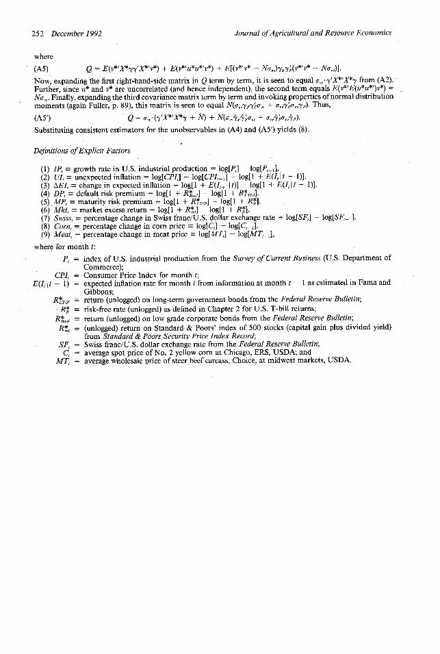
Definitions of Explicit Factors

(1) IP, = growth rate in U.S. industrial production = log[Pt] - log[P,_,].(2) UI, unexpected inflation - log[CPI,] - log[CPI,_] - log[l + E(I, t - 1)].(3) AEI, change in expected inflation = log[l + E(I,, It)] - log[l + E(I,t - 1)].(4) DP, = default risk premium = log[l + R*aa] - log[l + R*G,].(5) MP, = maturity risk premium - log[l + R,,] - log[l + Rt].(6) Mkt, = market excess return - log[l + R,] - log[l + Rft].(7) Swiss, percentage change in Swiss franc/U.S. dollar exchange rate = log[SF,] - log[SFt_].(8) Corn, - percentage change in corn price - log[Ct - log[C,_1].(9) Meat, = percentage change in meat price = log[MT,] - log[MT,_i],

where for month t:

P, = index of U.S. industrial production from the Survey of Current Business (U.S. Department ofCommerce);

CPI, = Consumer Price Index for month t;E(It It - 1) = expected inflation rate for month t from information at month t - 1 as estimated in Fama and

Gibbons;R*T, - return (unlogged) on long-term government bonds from the Federal Reserve Bulletin;

Rf*= risk-free rate (unlogged) as defined in Chapter 2 for U.S. T-bill returns;RBaat a return (unlogged) on low grade corporate bonds from the Federal Reserve Bulletin;R*t (unlogged) return on Standard & Poors' index of 500 stocks (capital gain plus divided yield)

from Standard & Poors Security Price Index Record;SFt - Swiss franc/U.S. dollar exchange rate from the Federal Reserve Bulletin;

C, = average spot price of No. 2 yellow corn at Chicago, ERS, USDA; andMTt = average wholesale price of steer beef carcass, Choice, at midwest markets, USDA.

252 December 1992

risk and return in agriculture: evidence from an explicit...

Documents