Risk analysis via heterogeneous models of SCADA interconnecting Power Grids and Telco Networks

A. Bobbio1, E. Ciancamerla2, S. Di Blasi2, A. Iacomini4, F. Mari3, I. Melatti3, M. Minichino2, A. Scarlatti4 , E.Tronci3 , R.Terruggia1, E. Zendri4

1Università del Piemonte Orientale, Alessamdria,Italy{bobbio,terruggia}@mfn.unipmn.it2 ENEA C.R. Casaccia, Rome, Italy

{ester.ciancamerla,saverio.diblasi,michele.minichino}@enea.it3 Università di Roma “La Sapienza”, Rome, Italy

{Mari,Melatti,Tronci}@di.uniroma1.it4 ACEA, Rome, Italy

{Iacomini,Scarlatti,Zendri}@acea.it

Abstract

The automation of Power Grids by means of Supervisory Control and Data Acquisition (SCADA) systems has led to an improvement of Power Grid operations and functionalities but also to pervasive cyber interdependencies between Power Grids and Telecommunication Networks. Many power grid services are increasingly depending upon the adequate functionality of SCADA system which in turn strictly depends on the adequate functionality of its Communication infrastructure. We propose to tackle the SCADA risk analysis by means of different and heterogeneous modeling techniques and software tools. We demonstrate the applicability of our approach through a case study on an actual SCADA system for an electrical power distribution grid. The modeling techniques we discuss aim at providing a probabilistic dependability analysis, followed by a worst case analysis in presence of malicious attacks and a real-time performance evaluation.

1 IntroductionSCADA systems constitute the nervous systems of Electrical infrastructures. They rely on SCADA communication infrastructures, which in turn are more and more depending upon Telco networks. For such a reason SCADA systems also represent one of the major means of mutual propagation of disturbances and adverse events between Electrical infrastructures and Telco networks. Many Power Grid services (i.e. availability of supply of critical users/large urban areas,

grid reconfiguration after failures, telemetry) are increasingly depending upon the adequate functionality of SCADA system which in turn strictly depend on the adequate functionality of Telco network. On the other hand both SCADA system and Telco network need to be adequately fed by Power Grid. Nowadays, SCADA communication infrastructure is typically composed by a proprietary network and a public telecommunication network. Such a solution guarantees an adequate performance for the transmission bandwidth, but introduces a number of potential failure points that did not exist previously. Questions arise about security, making SCADA systems also vulnerable to cyber-warfare and cyber terrorism attacks. Public IP networks are, in fact, sensitive to random failures, but also are highly sensitive to security holes, because information is transferred on wired public trunks and even on wireless trunks that are more “open” channels than cables. As a consequence, networks may be subjected to various kinds of malfunctions, like logical misconfigurations, compromised redundancy, possible security breaches, loss of application data, and degraded services. Real-time and bandwidth requirements of SCADA communication infrastructure need to be considered. Care must be taken when utilizing the same communication channel for real-time communication and transfer of non-real-time data because large data could hinder the transmission of the critical real-time data. In the present paper, we discuss a sequential application of heterogeneous modeling techniques and software tools aimed at investigating different and complementary properties of SCADA systems. We demonstrate their applicability by modeling and

analyzing an actual SCADA system for an electrical power distribution grid. The heterogeneous modeling techniques account for: i) the need of a probabilistic reasoning for the analysis of the dependability and quality of service in the presence of faults on the interdependent Power and Telco networks; ii) the need of considering the existence of malicious attackers with a given destructive power while at the same time evaluating the transmission capacity of the network in the presence of the worst-case attack; iii) the need of accounting performances of Telco networks which affect the timeliness of power grid operation through SCADA system. The evaluation of the dependability and quality of service, in the presence of random failures of SCADA, is performed by means of a Weighted Network Reliability Analyzer (WNRA) [4]. Worst case analysis in presence of hacker attacks, given disruption costs for nodes and edges and a specific budget, are computed by using a Mixed Integer Linear Programming (MILP) based algorithm. It is shown that the two techniques are complementary, in the sense that the dependability analysis can give information also on how likely a worst case attack may be launched. Finally, we study the influence of the performances of SCADA Communication infrastructure, and mainly of its a public, IP based and wireless Telco network on the power grid operations. We carry out this study by resorting to the NS2 network simulator.

2. SCADA system interconnecting power grid and Telco network

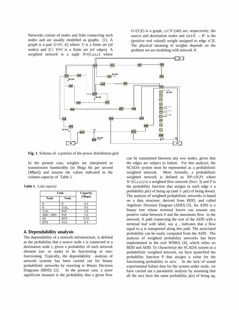
Figure 1 shows a portion of the Power Grid under consideration. It includes the High Voltage (HV) grid at 150 kV (Nodes Pi, large rectangles) and the backbone of the Medium Voltage (MV) grid at 20 kV (Nodes Mi, small rectangle). Nodes, named Ei, represent the substations of the national power transmission grid that interface and feed the power distribution grid. The physical link between any two nodes is an electrical trunk. Figure 2 reports the mapping of the SCADA system on the whole power distribution grid which include the Power Grid of Figure 1. Differently from Figure 1, the links among substations do not represent the electrical trunks, but the SCADA communication links. A Main SCADA Control Centre (MSC) directly controls and supervises the portion of the power grid of Figure 1. A Disaster Recovery SCADA centre (DRS), directly controls and supervises a complementary portion of the power distribution grid. There are two types of Remote Terminal Units (RTUs), which interface the SCADA with the power distribution grid: HV RTUs,

located at HV substations, and MV RTUs, located at MV substations. MSC (directly and through the DRS) controls and supervises the power grid, while DRS assumes the control and the supervision of all the grid, in case of MSC failure. MSC and DRS are connected, via firewalls, by two redundant, public, high speed Telco links. Information and data concerning the status of the power grid (i.e. power flows, voltages, frequencies, loads, breakers positions, power transformers status) are transmitted from the RTUs to the control centres, while commands (i.e. the remote control of switchgears for energizing/de energizing power transformers and distribution feeders under normal/disturbance/fault conditions) are transmitted from control centres to RTUs by means of communication channels. SCADA system can be decomposed in three interacting subnets, highlighted in Figure 2 by different icons and lines. The three networks transport digital information measured in Mega-bit per second (Mbps) units.

1. The Default Proprietary Network (DPN) serially connects the SCADA Control centres to HV RTUs. The DPN nodes (HV RTUs) are depicted as grey rectangles labeled Pi (i= 1, 44). DPN nodes can also communicate each other through the public PSTN (Public Switched Telephone Network) subnetwork since any DPN node is connected with a single link to one PSTN node.

2. The PSTN network represents the back up public Telco network which connects SCADA control centres and HV RTUs to MSC and to DRS. The PSTN nodes (numbered on the graph from 55 to 61 and from 63 to 66) are connected together (dotted lines) and cannot communicate each other through the DPN nodes. Two Virtual Private Networks (VPN) are established between the two SCADA Control Centres, via two HDSL (High data rate Digital Subscriber Line) connections, throughout two routers located in two PoP (Point of Presence), named PoP1(node 65) and PoP2 (node 66).

3. MV RTUs, differently from HV RTUs, are connected to SCADA centres by means of public Global System Mobile (GSM) connections (point/dashed lines). Particularly, MV_RTU are connected to their SCADA Control Centre throughout a Base Trans-receiver sub-System (BTS–node 62) and a Transit Exchange (Tex). MV_RTU nodes, labeled from M1 to M10, are terminal nodes that can be reached through the PSTN subnetwork only.

3. SCADA as a network

Networks consist of nodes and links connecting such nodes and are usually modelled as graphs [1]. A graph is a pair G=(V, E) where: V is a finite set (of nodes) and E⊆ V×V is a finite set (of edges). A weighted network is a tuple N=(G,s,t,c) where

G=(V,E) is a graph, s,t∈V (s≠t) are, respectively, the source and destination nodes and c(e):E → R+ is the (positive real valued) weight assigned to edge e∈E. The physical meaning of weights depends on the problem we are modeling with network N.

Fig. 1. Schema of a portion of the power distribution grid

In the present case, weights are interpreted as transmission bandwidths (in Mega bit per second [Mbps]) and assume the values indicated in the column capacity of Table 1.

Table 1. Link capacity

Link Capacity [Mbps]

Node Node

Pi Pj 0.5Pi TeXk 0.5TeXk PoP 1.0MSC, DRS PoP 2.0Mi BTS 0.35BTS TeX 0.5

4. Dependability analysis The dependability of a network infrastructure, is defined as the probability that a source node s is connected to a destination node t, given a probability of each network element (arc or node) to be functioning or non-functioning. Typically, the dependability analysis of network systems has been carried out for binary probabilistic networks by resorting to Binary Decision Diagrams (BDD) [2]. In the present case, a more significant measure is the probability that a given flow

can be transmitted between any two nodes, given that the edges are subject to failure. For this analysis, the SCADA system must be represented as a probabilistic weighted network. More formally, a probabilistic weighted network is defined as NP=(N,P) where N=(G,s,t,c) is a weighted flow network (Sect. 3) and P is the probability function that assigns to each edge e a probability p(e) of being up (and 1- p(e) of being down). The analysis of weighted probabilistic networks is based on a data structure, derived from BDD, and called Algebraic Decision Diagram (ADD) [3]. An ADD is a binary tree whose terminal leaves can assume any positive value between 0 and the maximum flow in the network. A path connecting the root of the ADD with a terminal leaf with label, say q , indicates that a flow equal to q is transported along this path. The associated probability can be easily computed from the ADD. The analysis of weighted probability networks has been implemented in the tool WNRA [4], which relies on BDD and ADD. To characterize the SCADA system as a probabilistic weighted network, we have quantified the probability function P that assigns a value for the functioning probability to arcs. In the lack of sound experimental failure data for the system under study, we have carried out a parametric analysis by assuming that all the arcs have the same probability p(e) of being up,

with p(e) =0.80, 0.90, 0.95, 0.99. In the analysis, we exploit the fact that the whole network is composed by different interacting sub-networks as described in Section 2, and that there are restrictions in the communication among nodes belonging to different sub networks.

4.1 PSTN networkSince the PSTN nodes communicate each other only through the public Telco network, we can analyze the PSTN subnet in isolation. The most crucial connection is between the main SCADA Control Centre (MSC) and the Disaster Recovery Centre (DRS).

Fig. 2. Schema of SCADA system and its mapping on the whole power distribution grid

The dependability of this connection is evaluated by assuming s=MSC, as a source node and t= DRS, as a terminal node. Table 2 reports the max-flow that can be transmitted from s to t and the associated probabilities.

Table 2: Max flows from s=MSC to t=DRS and probabilities

The data reported in Table 2 have the following meaning. The first column reports all the possible flow values that can be transmitted from s to t, given the capacity assigned to each link (in Table 1). The value 0 in the last row means that s and t are disconnected. The second column reports the probability that the network carries the corresponding flow. For what concerns the structural analysis of the network, the considered s-t connection has 16 minpaths: 2 are of length 2, and 14 are of length 4. Finally, the reliability is : R = 0.98009.

The ADD generated from the tool WNRA to compute the above figures has a size of 519 nodes.

4.2 Default Proprietary Network (DPN)The Default Proprietary Network (DPN) of SCADA is constituted by four non-interacting groups of RTU HV nodes which are serially connected and terminates in the MSC and DRS. To exemplify possible analysis and the obtained results, we have analyzed the connection between the far away node s=P22 and t=MSC. The flow analysis, obtained from tool WNRA (Table 3), is not very informative, since the connection s-t can carry only a capacity of 0.5 Mbps, due to the serial connection of the proprietary links.

Table 3: Max flow from s=P22 to t=MSC and probabilities

Max Flow [Mbps]

Probability

P=0.8 P=0.9 P=0.95 P=0.99

0.5 0.32768 0.59049 0.77378 0.95099

0 0.67232 0.40951 0.226219 0.04901

Max flow [Mbps]

ProbabilityP=0.8 P=0.9 P=0.95 P=0.99

4 0.4096 0.6561 0.81450 0.96059

2 0.51146 0.32399 0.1805 0.03920

1 0.00049 4.32e-06 2.449e-08 8.35e-14

0 0.07844 0.01990 0.00499 0.00012

The serial connection implies also that there is a single minpath whose length is 5. The reliability is R= 0.59049 and coincides with the first row of Table 3.

4.3 Interaction between the PSTN and DPN netsIn this last example we consider the interaction between the DPN subnet (comprising 12 HV-RTU nodes) and the PSTN network. The resulting network has 24 nodes and 88 edges. We assume the same source node s=P22 and the same sink node t=MSC considered in Section 4.2, where the DPN network was examined in isolation. The results are reported in Table 4.

Table 4: Max flows from s = P22 to t= MSC and probabilities

Max Flow

[Mbps]

Probability

P=0.8 P=0.9 P=0.95 P=0.99

1 0.58064 0.79188 0.89778 0.979900.5 0.3631 0.19604 0.09946 0.01999

0 0.0562 0.01207 0.00275 0.00010

The first column of Table 4 refers to the flow that can be transmitted between s and t and, in the second column, the corresponding probabilities. While the DPN network can carry a flow of 0.5 Mbps only (see also Table 3), the communication through the PSTN network can carry a flow of 1 Mbps. The total number of the mincuts is 57174 and the distribution of their order is reported in Figure 3.

Fig. 3: Connection between s=P22 and t=MSC - histogram of the length of mincuts

There is one shortest mincut of order 2, involving edges (P22-P19, P22-TeX 59), and two mincuts of order 3, involving edges (P12- MSC; TeX 59 - PoP1; TeX 59 - PoP2) and (P12 - MSC; MSC - PoP1; MSC - PoP2). The size of the BDD on which the Figure 3 has been obtained is of 54095 nodes, and the reliability is R = 0.98795. This last result should be compared with the

value R = 0.59049 obtained in Section 4.2 by considering the DPN links only. The difference between the two values shows the contribution in reliability increase that can be obtained by linking the proprietary subnetwork to the public PSTN network.

5. MGF under malicious attacksNetwork elements can be attacked in many ways. Typical examples are: software attacks (cyber-attacks), physical attacks, social engineering attacks. Our goal here is to evaluate the effect on the whole network infrastructure of successful attacks to network elements, independently on how such attacks are actually carried out. Malicious attacks are directed towards network elements with the goal of causing the maximum possible damage. However, destroying a network element has a destruction cost for the attacker who, in turn, does not have an infinite budget available. The destruction cost of a network element q models the degree of protection of q, whereas the attacker budget models the willingness of the attacker to carry out its destruction plans. Accordingly, identifying the worst case scenario comes down to the problem of computing the most severe and damaging attack that can be cast with the given attack budget. In the following we show how this problem can be formalized and effectively solved. Finally, we show experimental results obtained on the networked SCADA system described in Figure 2. A Maximum Guaranteed Flow (MGF) problem is a 6-tuple (N,B,Q,W,α,β) where N=(G,s,t,c) is a weighted network (see Section 3), B is a positive real number defining the destruction budget, Q is a subset of nodes V identifying indestructible nodes, W is a subset of E identifying indestructible edges. Functions α and β are functions associating a positive real number to each node of N and to each edge of E, respectively and model the cost incurred by an attacker to destroy a node or an edge in the network. The state of a network element (i.e. an edge or a node) is 1 if the element is working properly (up), 0 otherwise (i.e. has been destroyed by the attacker). Accordingly, an (N,B,Q,W,α,β) attack is a pair of Boolean functions (δ, ρ) associating a value {0,1} to each node (δ) and edge (ρ) of network N and satisfying the constraints that the total destruction cost does not exceed the budget B, that is:

∑v∈V α(v)δ(v) + ∑e∈E β(e)ρ(e) ≤ B.

We denote with (N, δ, ρ) the network obtained from N by removing all nodes v s.t. δ (v) = 1 and all edges e s.t. ρ (e) = 1. A solution to an MGF problem (N,B,Q,W,α,β) is an (N,B,Q,W,α,β) attack (δ, ρ) such that for all (N,B,Q,W,α,β) attacks (λ, µ), MaxFlow(N,δ,ρ) ≤

MaxFlow(N,λ,µ). If (δ, ρ) is a solution to the MGF problem (N,B,Q,W,α,β), we call MaxFlow(N,δ,ρ) the Maximum Guaranteed Flow (MGF) of (N,B,Q,W,α,β) (notation: MGF(N,B,Q,W,α,β)). Let N = (G,s,t,c) be a network on graph G. Consider the MGF problem (N,B,V,W,α,β) where only edges can be destroyed. This MGF problem has been independently studied in [5], [6] (as Network Inhibition Problem) and in [7] (as Network Interdiction Problem). Here we refer to it just as NIP. By suitably extending the approach in [7] we can show that any MGF problem (N,B,Q,W,α,β) can be formulated as a Mixed Integer Linear Programming (MILP) problem [8] P such that any solution to P defines a solution to the MGF problem (N,B,Q,W,α,β) and, conversely, any solution to the MGF problem (N,B,Q,W,α,β) is a solution to P. Furthermore, the optimal value of the objective function of P is MGF(N,B,Q,W,α,β). From [5], [7] we know that NIP is an NP-complete problem. From the above follows that also MGF is an NP-complete problem. Although in the worst case the MGF computation time can be exponential in the network size, resting on the effectiveness of MILP solvers (e.g. [9], [10]) our approach solves nontrivial MGF problems, as show by the experimental results in Sect. 5.1. We implemented our algorithm on top of the MILP solver GLPK [9].

5.1 Experimental results

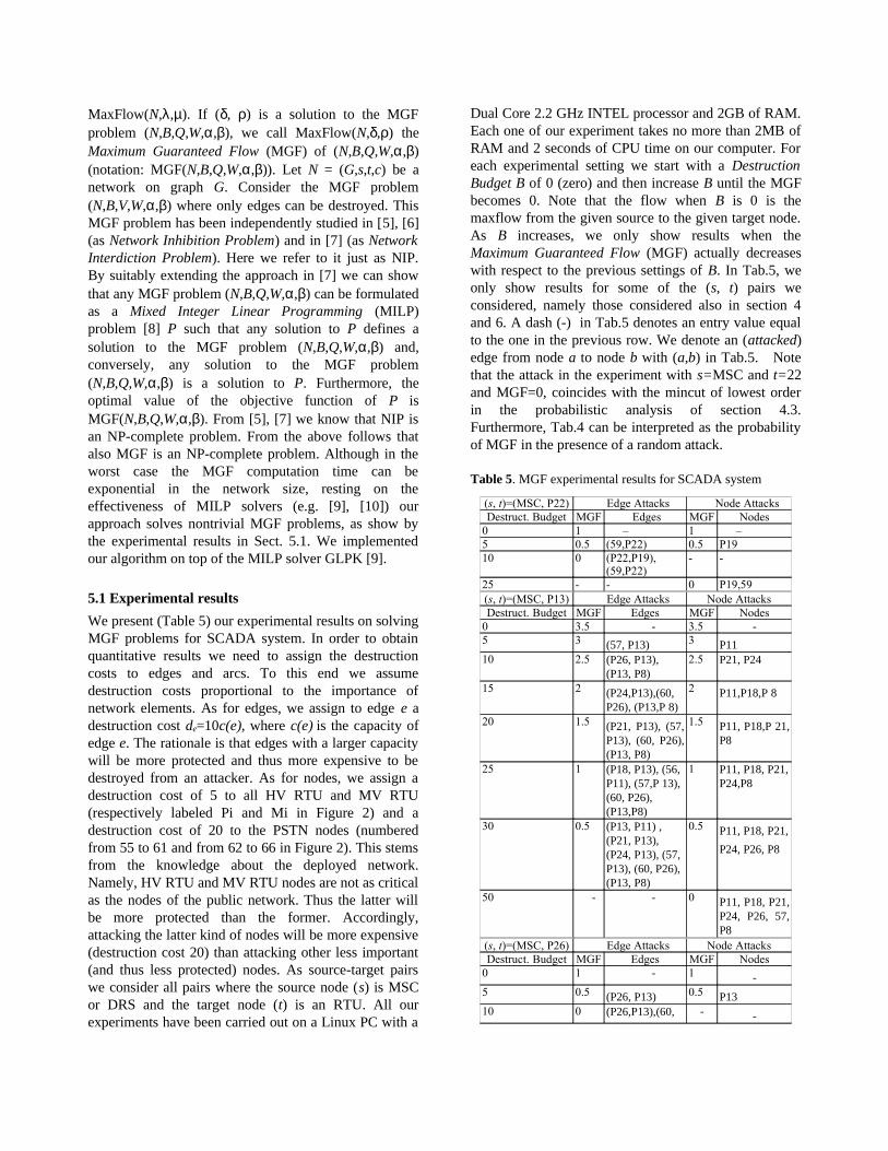
We present (Table 5) our experimental results on solving MGF problems for SCADA system. In order to obtain quantitative results we need to assign the destruction costs to edges and arcs. To this end we assume destruction costs proportional to the importance of network elements. As for edges, we assign to edge e a destruction cost de=10c(e), where c(e) is the capacity of edge e. The rationale is that edges with a larger capacity will be more protected and thus more expensive to be destroyed from an attacker. As for nodes, we assign a destruction cost of 5 to all HV RTU and MV RTU (respectively labeled Pi and Mi in Figure 2) and a destruction cost of 20 to the PSTN nodes (numbered from 55 to 61 and from 62 to 66 in Figure 2). This stems from the knowledge about the deployed network. Namely, HV RTU and MV RTU nodes are not as critical as the nodes of the public network. Thus the latter will be more protected than the former. Accordingly, attacking the latter kind of nodes will be more expensive (destruction cost 20) than attacking other less important (and thus less protected) nodes. As source-target pairs we consider all pairs where the source node (s) is MSC or DRS and the target node (t) is an RTU. All our experiments have been carried out on a Linux PC with a

Dual Core 2.2 GHz INTEL processor and 2GB of RAM. Each one of our experiment takes no more than 2MB of RAM and 2 seconds of CPU time on our computer. For each experimental setting we start with a Destruction Budget B of 0 (zero) and then increase B until the MGF becomes 0. Note that the flow when B is 0 is the maxflow from the given source to the given target node. As B increases, we only show results when the Maximum Guaranteed Flow (MGF) actually decreases with respect to the previous settings of B. In Tab.5, we only show results for some of the (s, t) pairs we considered, namely those considered also in section 4 and 6. A dash (-) in Tab.5 denotes an entry value equal to the one in the previous row. We denote an (attacked) edge from node a to node b with (a,b) in Tab.5. Note that the attack in the experiment with s=MSC and t=22 and MGF=0, coincides with the mincut of lowest order in the probabilistic analysis of section 4.3. Furthermore, Tab.4 can be interpreted as the probability of MGF in the presence of a random attack.

Table 5. MGF experimental results for SCADA system

(s, t)=(MSC, P22) Edge Attacks Node AttacksDestruct. Budget MGF Edges MGF Nodes

0 1 – 1 –5 0.5 (59,P22) 0.5 P1910 0 (P22,P19),

(59,P22)- -

25 - - 0 P19,59(s, t)=(MSC, P13) Edge Attacks Node AttacksDestruct. Budget MGF Edges MGF Nodes

0 3.5 - 3.5 -5 3 (57, P13) 3 P1110 2.5 (P26, P13),

(P13, P8)2.5 P21, P24

15 2 (P24,P13),(60, P26), (P13,P 8)

2 P11,P18,P 8

20 1.5 (P21, P13), (57, P13), (60, P26), (P13, P8)

1.5 P11, P18,P 21, P8

25 1 (P18, P13), (56, P11), (57,P 13), (60, P26), (P13,P8)

1 P11, P18, P21, P24,P8

30 0.5 (P13, P11) , (P21, P13), (P24, P13), (57, P13), (60, P26), (P13, P8)

0.5 P11, P18, P21,

P24, P26, P8

50 - - 0 P11, P18, P21, P24, P26, 57, P8

(s, t)=(MSC, P26) Edge Attacks Node AttacksDestruct. Budget MGF Edges MGF Nodes

0 1 - 1 -5 0.5 (P26, P13) 0.5 P1310 0 (P26,P13),(60, - -

P26)25 - - 0 P13, 60

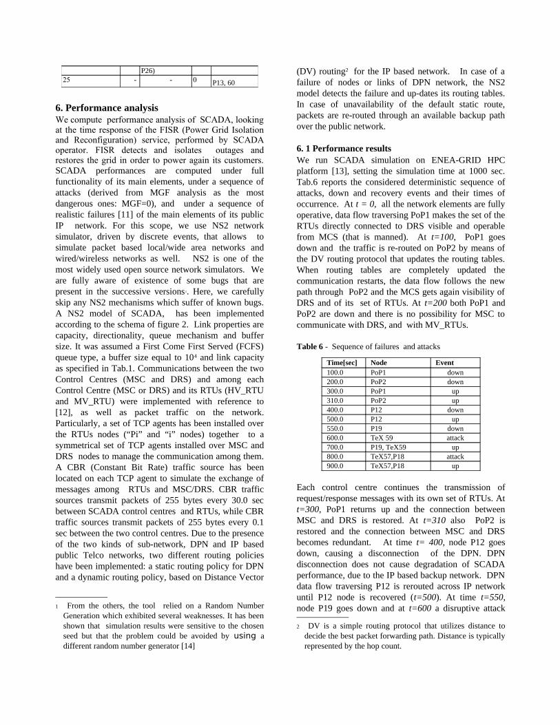
6. Performance analysis We compute performance analysis of SCADA, looking at the time response of the FISR (Power Grid Isolation and Reconfiguration) service, performed by SCADA operator. FISR detects and isolates outages and restores the grid in order to power again its customers. SCADA performances are computed under full functionality of its main elements, under a sequence of attacks (derived from MGF analysis as the most dangerous ones: MGF=0), and under a sequence of realistic failures [11] of the main elements of its public IP network. For this scope, we use NS2 network simulator, driven by discrete events, that allows to simulate packet based local/wide area networks and wired/wireless networks as well. NS2 is one of the most widely used open source network simulators. We are fully aware of existence of some bugs that are present in the successive versions1. Here, we carefully skip any NS2 mechanisms which suffer of known bugs. A NS2 model of SCADA, has been implemented according to the schema of figure 2. Link properties are capacity, directionality, queue mechanism and buffer size. It was assumed a First Come First Served (FCFS) queue type, a buffer size equal to 104 and link capacity as specified in Tab.1. Communications between the two Control Centres (MSC and DRS) and among each Control Centre (MSC or DRS) and its RTUs (HV_RTU and MV_RTU) were implemented with reference to [12], as well as packet traffic on the network. Particularly, a set of TCP agents has been installed over the RTUs nodes (“Pi” and “i” nodes) together to a symmetrical set of TCP agents installed over MSC and DRS nodes to manage the communication among them. A CBR (Constant Bit Rate) traffic source has been located on each TCP agent to simulate the exchange of messages among RTUs and MSC/DRS. CBR traffic sources transmit packets of 255 bytes every 30.0 sec between SCADA control centres and RTUs, while CBR traffic sources transmit packets of 255 bytes every 0.1 sec between the two control centres. Due to the presence of the two kinds of sub-network, DPN and IP based public Telco networks, two different routing policies have been implemented: a static routing policy for DPN and a dynamic routing policy, based on Distance Vector

1 From the others, the tool relied on a Random Number Generation which exhibited several weaknesses. It has been shown that simulation results were sensitive to the chosen seed but that the problem could be avoided by using a different random number generator [14]

(DV) routing2 for the IP based network. In case of a failure of nodes or links of DPN network, the NS2 model detects the failure and up-dates its routing tables. In case of unavailability of the default static route, packets are re-routed through an available backup path over the public network.

6. 1 Performance results We run SCADA simulation on ENEA-GRID HPC platform [13], setting the simulation time at 1000 sec. Tab.6 reports the considered deterministic sequence of attacks, down and recovery events and their times of occurrence. At t = 0, all the network elements are fully operative, data flow traversing PoP1 makes the set of the RTUs directly connected to DRS visible and operable from MCS (that is manned). At t=100, PoP1 goes down and the traffic is re-routed on PoP2 by means of the DV routing protocol that updates the routing tables. When routing tables are completely updated the communication restarts, the data flow follows the new path through PoP2 and the MCS gets again visibility of DRS and of its set of RTUs. At t=200 both PoP1 and PoP2 are down and there is no possibility for MSC to communicate with DRS, and with MV_RTUs.

Table 6 - Sequence of failures and attacks

Time[sec] Node Event100.0 PoP1 down200.0 PoP2 down300.0 PoP1 up310.0 PoP2 up400.0 P12 down500.0 P12 up550.0 P19 down600.0 TeX 59 attack700.0 P19, TeX59 up800.0 TeX57,P18 attack900.0 TeX57,P18 up

Each control centre continues the transmission of request/response messages with its own set of RTUs. At t=300, PoP1 returns up and the connection between MSC and DRS is restored. At t=310 also PoP2 is restored and the connection between MSC and DRS becomes redundant. At time t= 400, node P12 goes down, causing a disconnection of the DPN. DPN disconnection does not cause degradation of SCADA performance, due to the IP based backup network. DPN data flow traversing P12 is rerouted across IP network until P12 node is recovered (t=500). At time t=550, node P19 goes down and at t=600 a disruptive attack

2 DV is a simple routing protocol that utilizes distance to decide the best packet forwarding path. Distance is typically represented by the hop count.

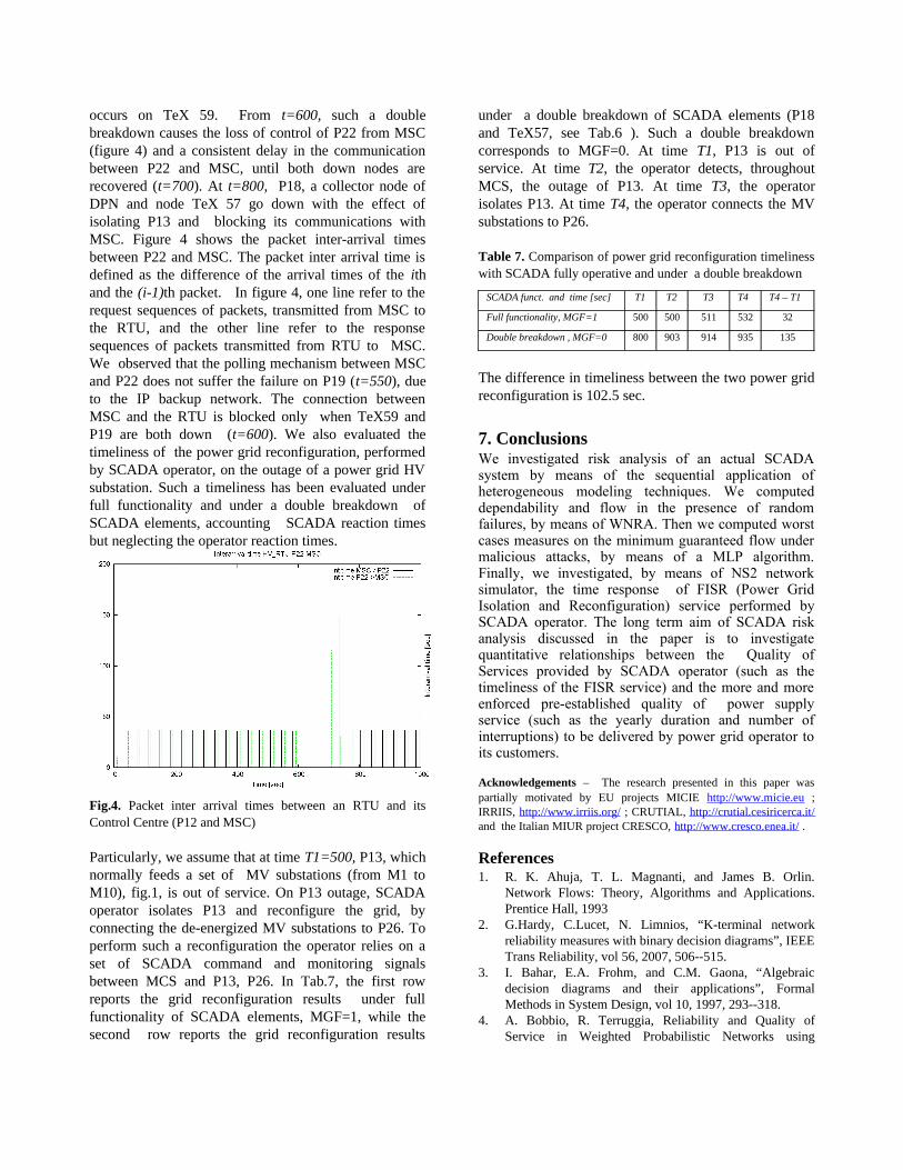
occurs on TeX 59. From t=600, such a double breakdown causes the loss of control of P22 from MSC (figure 4) and a consistent delay in the communication between P22 and MSC, until both down nodes are recovered (t=700). At t=800, P18, a collector node of DPN and node TeX 57 go down with the effect of isolating P13 and blocking its communications with MSC. Figure 4 shows the packet inter-arrival times between P22 and MSC. The packet inter arrival time is defined as the difference of the arrival times of the ith and the (i-1)th packet. In figure 4, one line refer to the request sequences of packets, transmitted from MSC to the RTU, and the other line refer to the response sequences of packets transmitted from RTU to MSC. We observed that the polling mechanism between MSC and P22 does not suffer the failure on P19 (t=550), due to the IP backup network. The connection between MSC and the RTU is blocked only when TeX59 and P19 are both down (t=600). We also evaluated the timeliness of the power grid reconfiguration, performed by SCADA operator, on the outage of a power grid HV substation. Such a timeliness has been evaluated under full functionality and under a double breakdown of SCADA elements, accounting SCADA reaction times but neglecting the operator reaction times.

Fig.4. Packet inter arrival times between an RTU and its Control Centre (P12 and MSC)

Particularly, we assume that at time T1=500, P13, which normally feeds a set of MV substations (from M1 to M10), fig.1, is out of service. On P13 outage, SCADA operator isolates P13 and reconfigure the grid, by connecting the de-energized MV substations to P26. To perform such a reconfiguration the operator relies on a set of SCADA command and monitoring signals between MCS and P13, P26. In Tab.7, the first row reports the grid reconfiguration results under full functionality of SCADA elements, MGF=1, while the second row reports the grid reconfiguration results

under a double breakdown of SCADA elements (P18 and TeX57, see Tab.6 ). Such a double breakdown corresponds to MGF=0. At time T1, P13 is out of service. At time T2, the operator detects, throughout MCS, the outage of P13. At time T3, the operator isolates P13. At time T4, the operator connects the MV substations to P26.

Table 7. Comparison of power grid reconfiguration timeliness with SCADA fully operative and under a double breakdown

SCADA funct. and time [sec] T1 T2 T3 T4 T4 – T1

Full functionality, MGF=1 500 500 511 532 32

Double breakdown , MGF=0 800 903 914 935 135

The difference in timeliness between the two power grid reconfiguration is 102.5 sec.

7. ConclusionsWe investigated risk analysis of an actual SCADA system by means of the sequential application of heterogeneous modeling techniques. We computed dependability and flow in the presence of random failures, by means of WNRA. Then we computed worst cases measures on the minimum guaranteed flow under malicious attacks, by means of a MLP algorithm. Finally, we investigated, by means of NS2 network simulator, the time response of FISR (Power Grid Isolation and Reconfiguration) service performed by SCADA operator. The long term aim of SCADA risk analysis discussed in the paper is to investigate quantitative relationships between the Quality of Services provided by SCADA operator (such as the timeliness of the FISR service) and the more and more enforced pre-established quality of power supply service (such as the yearly duration and number of interruptions) to be delivered by power grid operator to its customers.

Acknowledgements – The research presented in this paper was partially motivated by EU projects MICIE http://www.micie.eu ; IRRIIS, http://www.irriis.org/ ; CRUTIAL, http://crutial.cesiricerca.it/ and the Italian MIUR project CRESCO, http://www.cresco.enea.it/ .

References1. R. K. Ahuja, T. L. Magnanti, and James B. Orlin.

Network Flows: Theory, Algorithms and Applications. Prentice Hall, 1993

2. G.Hardy, C.Lucet, N. Limnios, “K-terminal network reliability measures with binary decision diagrams”, IEEE Trans Reliability, vol 56, 2007, 506--515.

3. I. Bahar, E.A. Frohm, and C.M. Gaona, “Algebraic decision diagrams and their applications”, Formal Methods in System Design, vol 10, 1997, 293--318.

4. A. Bobbio, R. Terruggia, Reliability and Quality of Service in Weighted Probabilistic Networks using

Algebraic Decision Diagrams, Proc IEEE-RAMS, pp 19-24, 2009

5. Cynthia A. Phillips.The network inhibition problem.In STOC ’93: Proc 25 annual ACM symposium on Theory of computing, p.776–785, New York, NY, USA, 1993.

6. Cynthia Phillips and Laura Painton Swiler.A graph-based system for network-vulnerability analysis. In NSPW ’98: Proceedings of the 1998 workshop on New security paradigms, pages 71–79, New York, NY, USA, 1998. ACM.

7. R.K. Wood. Deterministic network interdiction. Mathematical Computer Modelling, 17(2):1–18, 1993.

8. A. Schrijver, Theory of Linear and Integer Programming, John Wiley and Sons, 1998

9. http://www.gnu.org/software/glpk/10. http://www.ilog.com 11. G. Bonanni, E. Ciancamerla, M. Minichino, R.

Clemente, A. Iacomini, A. Scarlatti, E. Zendri, R. Terruggia - Exploiting stochastic indicators of interdependent infrastructures: the service availability of interconnected networks – Safety, Reliability and Risk Analysis: Theory, Methods and Applications, vol.3- 2009Taylor & Francis

12. IEC870-5-1 01/105 guidelines 13. http://cresco.enea.it 14. M. Umlauft, P. Reichl - Experiences with the ns-2

network simulator - explicitly setting seeds considered harmful- Wireless Telecommunications Symposium, 2007.