RISK ANALYSIS AND EXTREMES

Richard L. Smith

Department of Statistics and Operations Research

University of North Carolina

Chapel Hill, NC 27599-3260

rls@email.unc.edu

Opening Workshop

SAMSI program on Risk Analysis,

Extreme Events and Decision Theory

September 16, 2007

1

REFERENCES

Finkenstadt, B. and Rootzen, H. (editors) (2003), Extreme Val-

ues in Finance, Telecommunications and the Environment. Chap-

man and Hall/CRC Press, London.

(See http://www.stat.unc.edu/postscript/rs/semstatrls.pdf)

Coles, S.G. (2001), An Introduction to Statistical Modeling of

Extreme Values. Springer Verlag, New York.

Embrechts, P., Kluppelberg, C. and Mikosch, T. (1997), Mod-

elling Extremal Events for Insurance and Finance. Springer, New

York.

Leadbetter, M.R., Lindgren, G. and Rootzen, H. (1983), Ex-

tremes and Related Properties of Random Sequences and Series.

Springer Verlag, New York.

Resnick, S. (1987), Extreme Values, Point Processes and Reg-

ular Variation. Springer Verlag, New York.

2

OUTLINE OF TALK

I. Some Examples of Risk Analysis Involving Extreme Values

II. Univariate extreme value theory

• Probability Models

• Estimation

• Diagnostics

III. Insurance Extremes I

IV. Insurance Extremes II

V. Trends in Extreme Rainfall Events

3

I. SOME EXAMPLES OF RISKANALYSIS INVOLVING EXTREME

VALUES

• Insurance Claims by a Large Oil Company (Smith and Good-

man 2000)

• Returns on Stock Prices

• Hurricanes — are they becoming more frequent/stronger/more

costly and if so, is the change in any way connected with

global warming? (Tom Knutson’s talk on Tuesday)

• Are extreme rainfall events becoming more frequent? (and

does that have anything to do with global warming?)

4

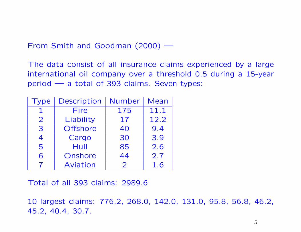
From Smith and Goodman (2000) —

The data consist of all insurance claims experienced by a largeinternational oil company over a threshold 0.5 during a 15-yearperiod — a total of 393 claims. Seven types:

Type Description Number Mean1 Fire 175 11.12 Liability 17 12.23 Offshore 40 9.44 Cargo 30 3.95 Hull 85 2.66 Onshore 44 2.77 Aviation 2 1.6

Total of all 393 claims: 2989.6

10 largest claims: 776.2, 268.0, 142.0, 131.0, 95.8, 56.8, 46.2,45.2, 40.4, 30.7.

5

Some plots of the insurance data.

6

Some problems:

1. What is the distribution of very large claims?

2. Is there any evidence of a change of the distribution over

time?

3. What is the influence of the different types of claim?

4. How should one characterize the risk to the company? More

precisely, what probability distribution can one put on the amount

of money that the company will have to pay out in settlement

of large insurance claims over a future time period of, say, three

years?

7

Stock Market Returns

The next page shows negative daily returns from closing prices

of 1982-2001 stock prices in three companies, Pfizer, GE and

Citibank. Typical questions here are

1. How to determine Value at Risk, i.e. the amount which might

be lost in a portfolio of assets over a specified time period with

a specified small probability,

2. Dependence among the extremes of different series, and ap-

plication to the portfolio management problem,

3. Modeling extremes in the presence of volatility.

8

Daily returns of Pfizer, GE and Citibank (thanks to Zhengjun

Zhang)

9

II. UNIVARIATE EXTREME VALUETHEORY

10

EXTREME VALUE DISTRIBUTIONS

X1, X2, ..., i.i.d., F (x) = Pr{Xi ≤ x}, Mn = max(X1, ..., Xn),

Pr{Mn ≤ x} = F (x)n.

For non-trivial results must renormalize: find an > 0, bn such that

Pr{Mn − bn

an≤ x

}= F (anx+ bn)

n → H(x).

The Three Types Theorem (Fisher-Tippett, Gnedenko) assertsthat if nondegenerate H exists, it must be one of three types:

H(x) = exp(−e−x), all x (Gumbel)

H(x) ={0 x < 0

exp(−x−α) x > 0(Frechet)

H(x) ={exp(−|x|α) x < 0

1 x > 0(Weibull)

In Frechet and Weibull, α > 0.

11

The three types may be combined into a single generalized ex-

treme value (GEV) distribution:

H(x) = exp

−(1 + ξ

x− µ

ψ

)−1/ξ

+

,(y+ = max(y,0))

where µ is a location parameter, ψ > 0 is a scale parameter

and ξ is a shape parameter. ξ → 0 corresponds to the Gumbel

distribution, ξ > 0 to the Frechet distribution with α = 1/ξ, ξ < 0

to the Weibull distribution with α = −1/ξ.

ξ > 0: “long-tailed” case, 1− F (x) ∝ x−1/ξ,

ξ = 0: “exponential tail”

ξ < 0: “short-tailed” case, finite endpoint at µ− ξ/ψ

12

EXCEEDANCES OVERTHRESHOLDS

Consider the distribution of X conditionally on exceeding some

high threshold u:

Fu(y) =F (u+ y)− F (u)

1− F (u).

As u→ ωF = sup{x : F (x) < 1}, often find a limit

Fu(y) ≈ G(y;σu, ξ)

where G is generalized Pareto distribution (GPD)

G(y;σ, ξ) = 1−(1 + ξ

y

σ

)−1/ξ

+.

Equivalence to three types theorem established by Pickands (1975).

13

The Generalized Pareto Distribution

G(y;σ, ξ) = 1−(1 + ξ

y

σ

)−1/ξ

+.

ξ > 0: long-tailed (equivalent to usual Pareto distribution), tail

like x−1/ξ,

ξ = 0: take limit as ξ → 0 to get

G(y;σ,0) = 1− exp(−y

σ

),

i.e. exponential distribution with mean σ,

ξ < 0: finite upper endpoint at −σ/ξ.

14

POISSON-GPD MODEL FOREXCEEDANCES

1. The number, N , of exceedances of the level u in any one

year has a Poisson distribution with mean λ,

2. Conditionally on N ≥ 1, the excess values Y1, ..., YN are IID

from the GPD.

15

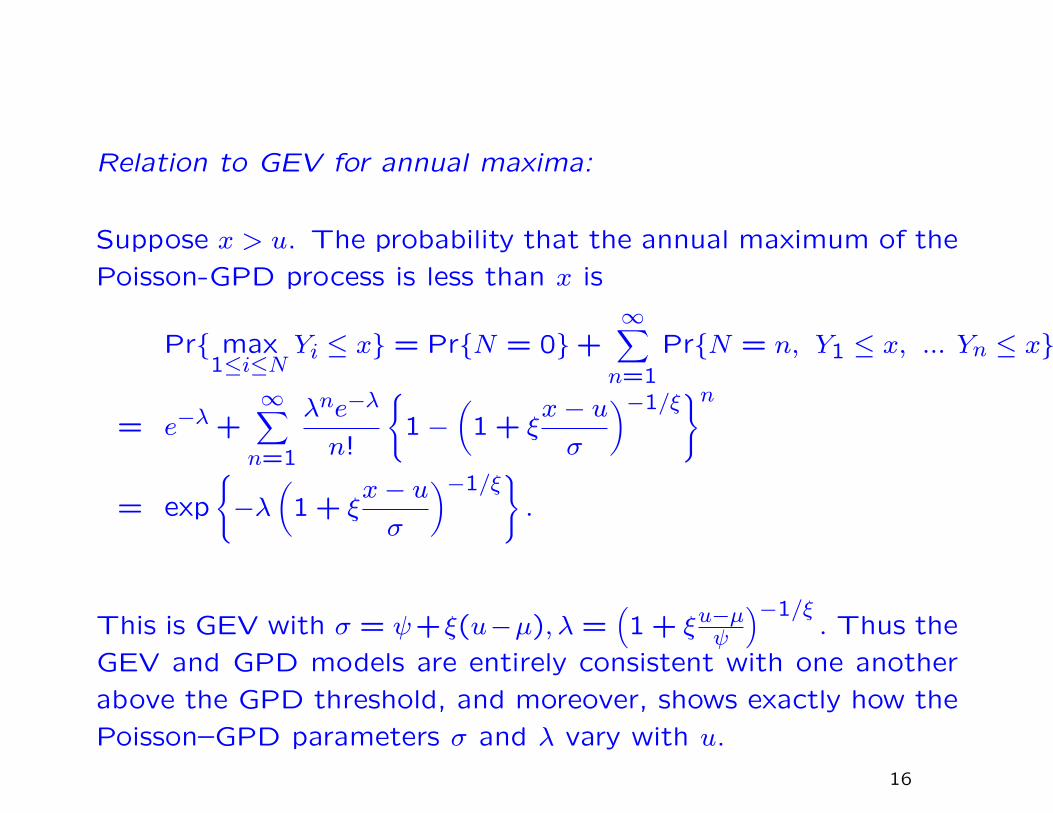
Relation to GEV for annual maxima:

Suppose x > u. The probability that the annual maximum of the

Poisson-GPD process is less than x is

Pr{ max1≤i≤N

Yi ≤ x} = Pr{N = 0}+∞∑n=1

Pr{N = n, Y1 ≤ x, ... Yn ≤ x}

= e−λ +∞∑n=1

λne−λ

n!

{1−

(1 + ξ

x− u

σ

)−1/ξ}n

= exp

{−λ

(1 + ξ

x− u

σ

)−1/ξ}.

This is GEV with σ = ψ+ξ(u−µ), λ =(1 + ξu−µψ

)−1/ξ. Thus the

GEV and GPD models are entirely consistent with one another

above the GPD threshold, and moreover, shows exactly how the

Poisson–GPD parameters σ and λ vary with u.

16

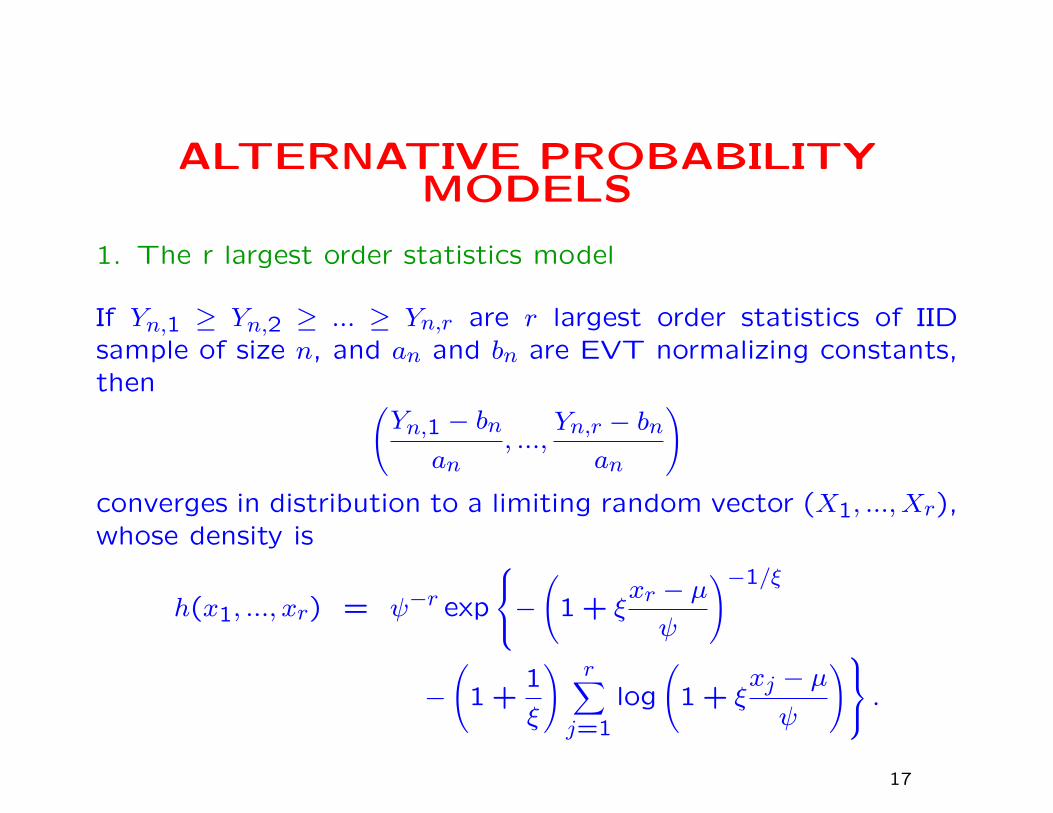
ALTERNATIVE PROBABILITYMODELS

1. The r largest order statistics model

If Yn,1 ≥ Yn,2 ≥ ... ≥ Yn,r are r largest order statistics of IIDsample of size n, and an and bn are EVT normalizing constants,then (

Yn,1 − bn

an, ...,

Yn,r − bn

an

)converges in distribution to a limiting random vector (X1, ..., Xr),whose density is

h(x1, ..., xr) = ψ−r exp

−(1 + ξ

xr − µ

ψ

)−1/ξ

−(1 +

1

ξ

) r∑j=1

log

(1 + ξ

xj − µ

ψ

) .17

2. Point process approach (Smith 1989)

Two-dimensional plot of exceedance times and exceedance levels

forms a nonhomogeneous Poisson process with

Λ(A) = (t2 − t1)Ψ(y;µ, ψ, ξ)

Ψ(y;µ, ψ, ξ) =

(1 + ξ

y − µ

ψ

)−1/ξ

(1 + ξ(y − µ)/ψ > 0).

18

Illustration of point process model.

19

An extension of this approach allows for nonstationary processes

in which the parameters µ, ψ and ξ are all allowed to be time-

dependent, denoted µt, ψt and ξt.

This is the basis of the extreme value regression approaches

introduced later

20

Plots of exceedances of River Nidd, (a) against day within year,

(b) against total days from January 1, 1934. Adapted from

Davison and Smith (1990).

21

ESTIMATION

GEV log likelihood:

`Y (µ, ψ, ξ) = −N logψ −(1

ξ+ 1

)∑i

log

(1 + ξ

Yi − µ

ψ

)

−∑i

(1 + ξ

Yi − µ

ψ

)−1/ξ

provided 1 + ξ(Yi − µ)/ψ > 0 for each i.

Poisson-GPD model:

`N,Y (λ, σ, ξ) = N logλ− λT −N logσ −(1 +

1

ξ

) N∑i=1

log(1 + ξ

Yiσ

)provided 1 + ξYi/σ > 0 for all i.

Usual asymptotics valid if ξ > −12 (Smith 1985)

22

Profile Likelihoods for Quantiles

Suppose we are interested in the N-year return level yN , i.e. the

(1− 1/N)-quantile of the annual maximum distribution. We can

construct a profile likelihood by reparameterizing the GEV so

that yN is one of the three parameters, and maximizing with

respect to the other two. Likelihood ratio asymptotics can then

be used to construct a confidence interval for yN .

Example from the Nidd data:

23

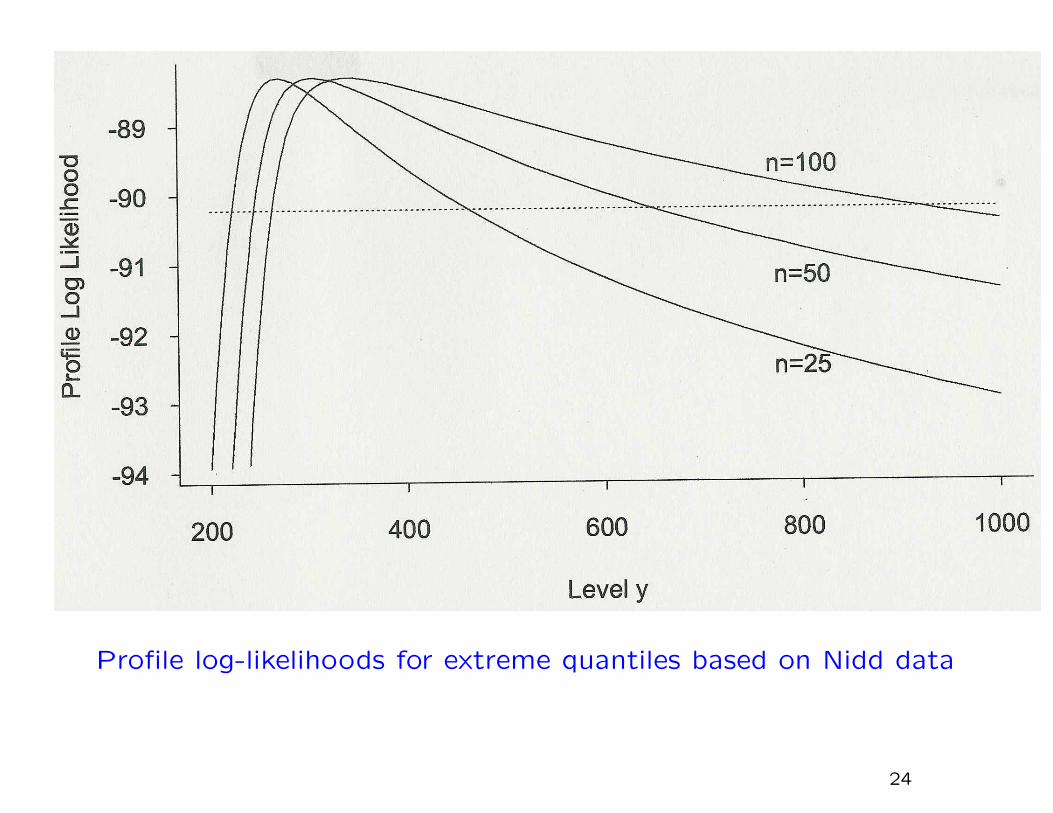
Profile log-likelihoods for extreme quantiles based on Nidd data

24

Bayesian approaches

An alternative approach to extreme value inference is Bayesian,

using vague priors for the GEV parameters and MCMC samples

for the computations. Bayesian methods are particularly useful

for predictive inference, e.g. if Z is some as yet unobserved ran-

dom variable whose distribution depends on µ, ψ and ξ, estimate

Pr{Z > z} by ∫Pr{Z > z;µ, ψ, ξ}π(µ, ψ, ξ|Y )dµdψdξ

where π(...|Y ) denotes the posterior density given past data Y

25

Plots of women’s 3000 meter records, and profile log-likelihood

for ultimate best value based on pre-1993 data.

26

Example. The left figure shows the five best running times by

different athletes in the women’s 3000 metre track event for

each year from 1972 to 1992. Also shown on the plot is Wang

Junxia’s world record from 1993. Many questions were raised

about possible illegal drug use.

We approach this by asking how implausible Wang’s performance

was, given all data up to 1992.

Robinson and Tawn (1995) used the r largest order statistics

method (with r = 5, translated to smallest order statistics) to

estimate an extreme value distribution, and hence computed a

profile likelihood for xult, the lower endpoint of the distribution,

based on data up to 1992 (right plot of previous figure)

27

Alternative Bayesian calculation:

(Smith 1997)

Compute the (Bayesian) predictive probability that the 1993 per-

formance is equal or better to Wang’s, given the data up to 1992,

and conditional on the event that there is a new world record.

The answer is approximately 0.0006.

28

DIAGNOSTICS

Gumbel plots

QQ plots of residuals

Mean excess plot

Z- and W-statistic plots

29

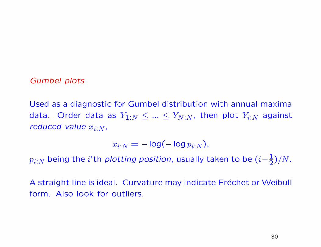
Gumbel plots

Used as a diagnostic for Gumbel distribution with annual maxima

data. Order data as Y1:N ≤ ... ≤ YN :N , then plot Yi:N against

reduced value xi:N ,

xi:N = − log(− log pi:N),

pi:N being the i’th plotting position, usually taken to be (i−12)/N .

A straight line is ideal. Curvature may indicate Frechet or Weibull

form. Also look for outliers.

30

Gumbel plots. (a) Annual maxima for River Nidd flow series. (b)

Annual maximum temperatures in Ivigtut, Iceland.

31

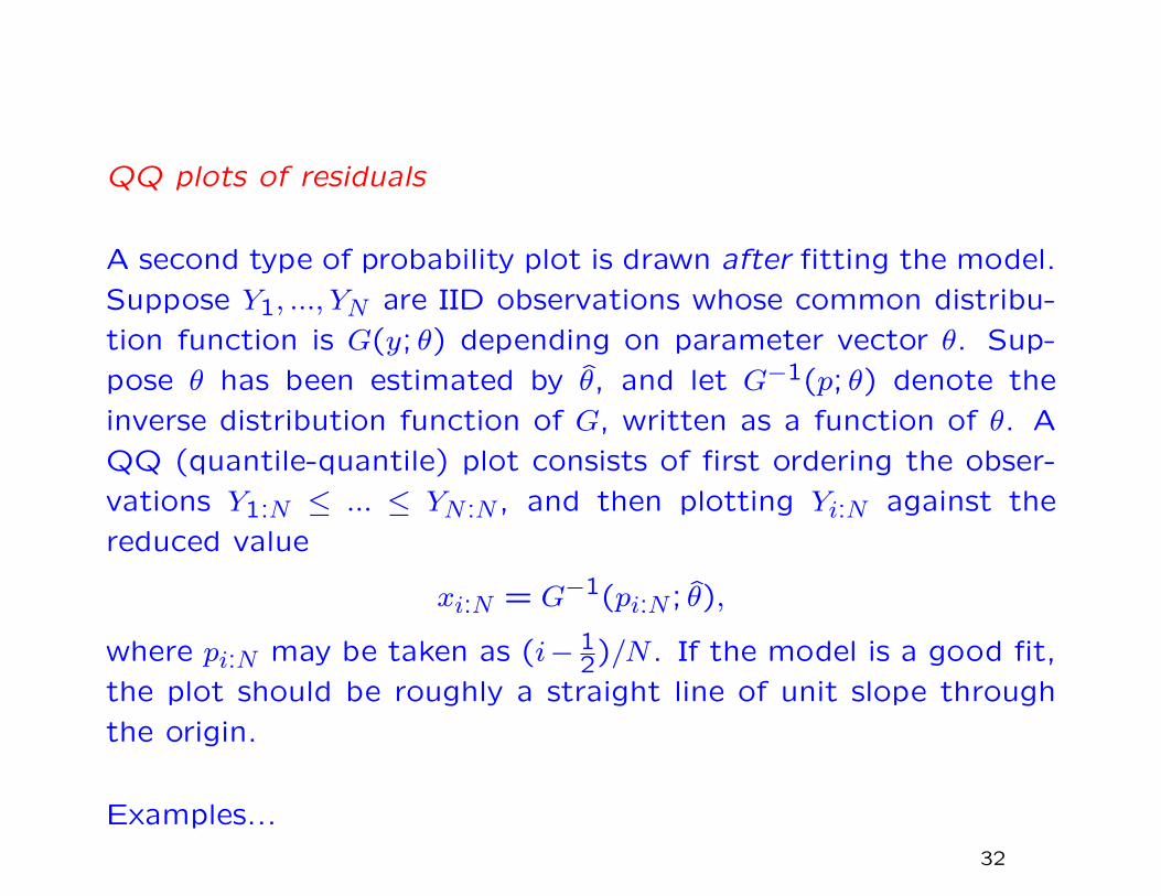
QQ plots of residuals

A second type of probability plot is drawn after fitting the model.

Suppose Y1, ..., YN are IID observations whose common distribu-

tion function is G(y; θ) depending on parameter vector θ. Sup-

pose θ has been estimated by θ, and let G−1(p; θ) denote the

inverse distribution function of G, written as a function of θ. A

QQ (quantile-quantile) plot consists of first ordering the obser-

vations Y1:N ≤ ... ≤ YN :N , and then plotting Yi:N against the

reduced value

xi:N = G−1(pi:N ; θ),

where pi:N may be taken as (i− 12)/N . If the model is a good fit,

the plot should be roughly a straight line of unit slope through

the origin.

Examples...

32

GEV model to Ivigtut data, (a) without adjustment, (b) exclud-

ing largest value from model fit but including it in the plot.

33

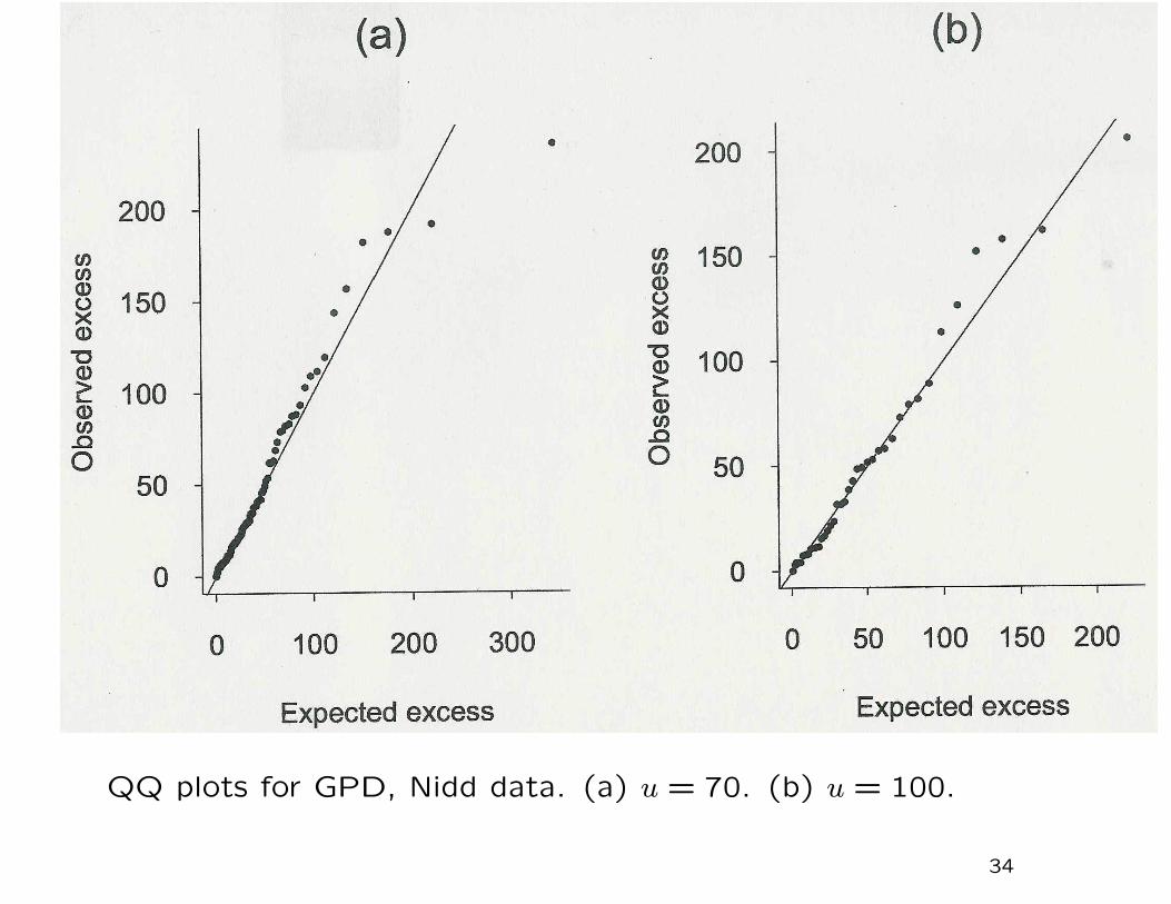
QQ plots for GPD, Nidd data. (a) u = 70. (b) u = 100.

34

Mean excess plot

Idea: for a sequence of values of w, plot the mean excess over

w against w itself. If the GPD is a good fit, the plot should be

approximately a straight line.

In practice, the actual plot is very jagged and therefore its “straight-

ness” is difficult to assess. However, a Monte Carlo technique,

assuming the GPD is valid throughout the range of the plot, can

be used to assess this.

Examples...

35

Mean excess over threshold plots for Nidd data, with Monte Carlo

confidence bands, relative to threshold 70 (a) and 100 (b).

36

Z- and W-statistic plots

Consider nonstationary model with µt, ψt, ξt dependent on t.

Z statistic based on intervals between exceedances Tk:

Zk =∫ TkTk−1

λu(s)ds,

λu(s) = {1 + ξs(u− µs)/ψs)}−1/ξs.

W statistic based on excess values: if Yk is excess over thresholdat time Tk,

Wk =1

ξTklog

{1 +

ξTkYk

ψTk + ξTk(u− µTk)

}.

Idea: if the model is exact, both Zk and Wk and i.i.d. exponentialwith mean 1. Can test this with various plots.

37

Diagnostic plots based on Z and W statistics for oil company

insurance data (u = 5)

38

III. INSURANCE EXTREMES I

We return to the oil company data set discussed in section I. Priorto any of the analysis, some examination was made of clusteringphenomena, but this only reduced the original 425 claims to 393“independent” claims (Smith & Goodman 2000)

GPD fits to various thresholds:

u Nu Mean σ ξExcess

0.5 393 7.11 1.02 1.012.5 132 17.89 3.47 0.915 73 28.9 6.26 0.8910 42 44.05 10.51 0.8415 31 53.60 5.68 1.4420 17 91.21 19.92 1.1025 13 113.7 74.46 0.9350 6 37.97 150.8 0.29

39

Point process approach:

u Nu µ logψ ξ0.5 393 26.5 3.30 1.00

(4.4) (0.24) (0.09)2.5 132 26.3 3.22 0.91

(5.2) (0.31) (0.16)5 73 26.8 3.25 0.89

(5.5) (0.31) (0.21)10 42 27.2 3.22 0.84

(5.7) (0.32) (0.25)15 31 22.3 2.79 1.44

(3.9) (0.46) (0.45)20 17 22.7 3.13 1.10

(5.7) (0.56) (0.53)25 13 20.5 3.39 0.93

(8.6) (0.66) (0.56)

Standard errors are in parentheses

40

Predictive Distributions of Future Losses

What is the probability distribution of future losses over a specific

time period, say 1 year?

Let Y be future total loss. Distribution function G(y;µ, ψ, ξ) —

in practice this must itself be simulated.

41

Traditional frequentist approach:

G(y) = G(y; µ, ψ, ξ)

where µ, ψ, ξ are MLEs.

Bayesian:

G(y) =∫G(y;µ, ψ, ξ)dπ(µ, ψ, ξ | X)

where π(· | X) denotes posterior density given data X.

42

Estimated posterior densities for the three parameters, and forthe predictive distribution function. Four independent MonteCarlo runs are shown for each plot.

43

Hierarchical models for claim type and year effects

Further features of the data:

1. When separate GPDs are fitted to each of the 6 main types,

there are clear differences among the parameters.

2. The rate of high-threshold crossings does not appear uniform,

but peaks around years 10–12.

44

A Hierarchical Model:

Level I. Parameters mµ, mψ, mξ, s2µ, s

2ψ, s

2ξ are generated from

a prior distribution.

Level II. Conditional on the parameters in Level I, parameters

µ1, ..., µJ (where J is the number of types) are independently

drawn from N(mµ, s2µ), the normal distribution with mean mµ,

variance s2µ. Similarly, logψ1, ..., logψJ are drawn independently

from N(mψ, s2ψ), ξ1, ..., ξJ are drawn independently from N(mξ, s

2ξ ).

Level III. Conditional on Level II, for each j ∈ {1, ..., J}, the point

process of exceedances of type j is generated from the Poisson

process with parameters µj, ψj, ξj.

45

This model may be further extended to include a year effect, as

follows. Suppose the extreme value parameters for type j in year

k are not µj, ψj, ξj but µj + δk, ψj, ξj. We fix δ1 = 0 to ensure

identifiability, and let {δk, k > 1} follow an AR(1) process:

δk = ρδk−1 + ηk, ηk ∼ N(0, s2η)

with a vague prior on (ρ, s2η).

We show boxplots for each of µj, logψj, ξj, j = 1, ...,6 and for

δk, k = 2,15.

46

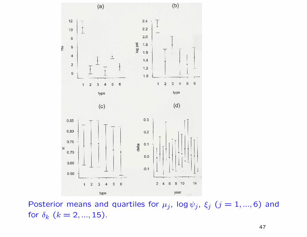
Posterior means and quartiles for µj, logψj, ξj (j = 1, ...,6) and

for δk (k = 2, ...,15).

47

Computations of posterior predictive distribution functions (plot-ted on a log-log scale) corresponding to the homogenous model(curve A) and three different versions of the hierarchical model.

48

IV. INSURANCE EXTREMES II

This example is based on a data set constructed by the U.K.insurance company Benfield-Greig, consisting of 57 historicalstorm events and losses calculated “as if” they occurred in 1998.Here, µt is modelled as a function of time t through various co-variates —

Seasonal effects (dominant annual cycle)

Polynomial terms in t

Nonparametric trends

Dependence on oscillation indices

Other models in which ψt and ξt depend on t were also tried butdo not produce significant differences from the constant case.

49

Plots of estimated storm losses against (a) time measured in

years, (b) day within the year.

50

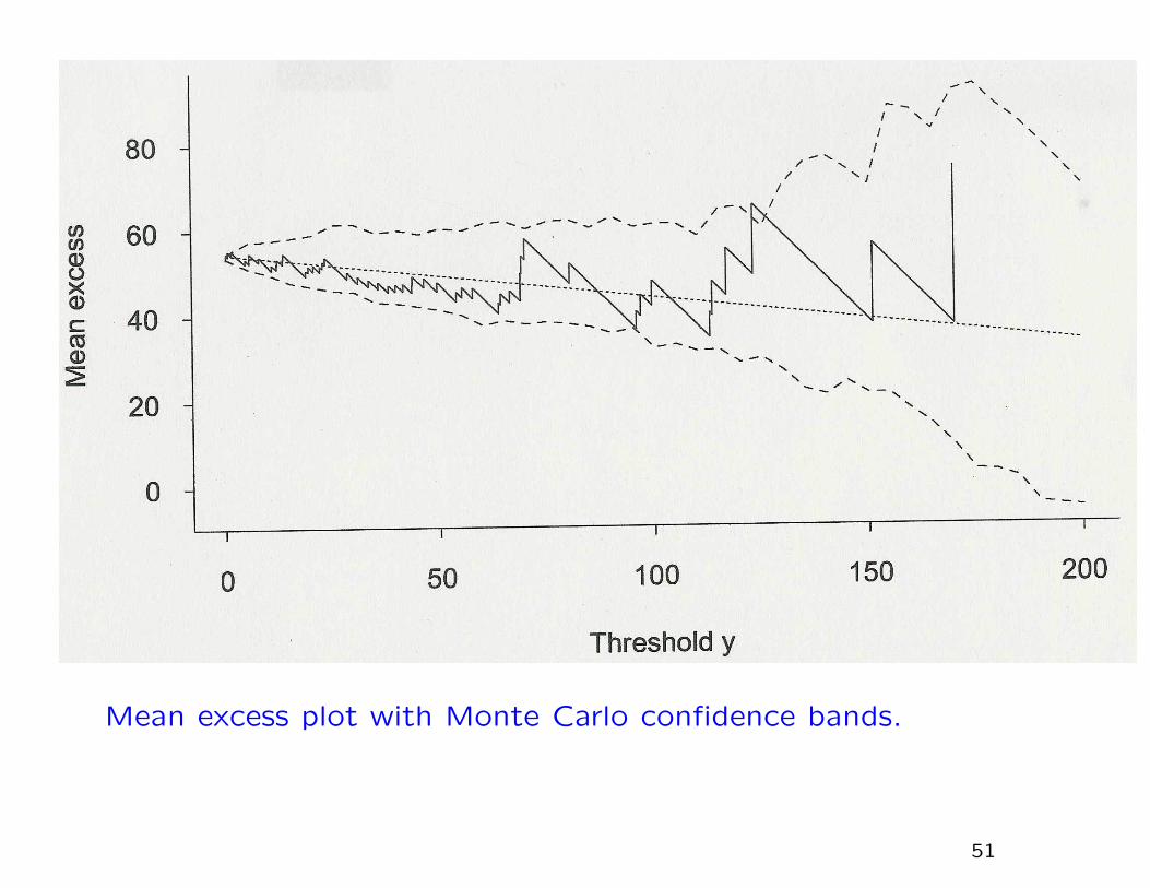
Mean excess plot with Monte Carlo confidence bands.

51

Comparison of models

Model Number of parameters NLLH AICSimple GPD 3 312.5 631.0

Seasonal 5 294.8 599.6Seasonal+cubic 8 289.3 594.6Seasonal+spline 10 289.6 599.2Seasonal+SOI 6 294.5 601.0Seasonal+NAO 6 289.0 590.0Sea+NAO+cub 9 284.4 586.8Sea+NAO+spl 11 284.6 591.2

(AIC = 2NLLH + 2p)

52

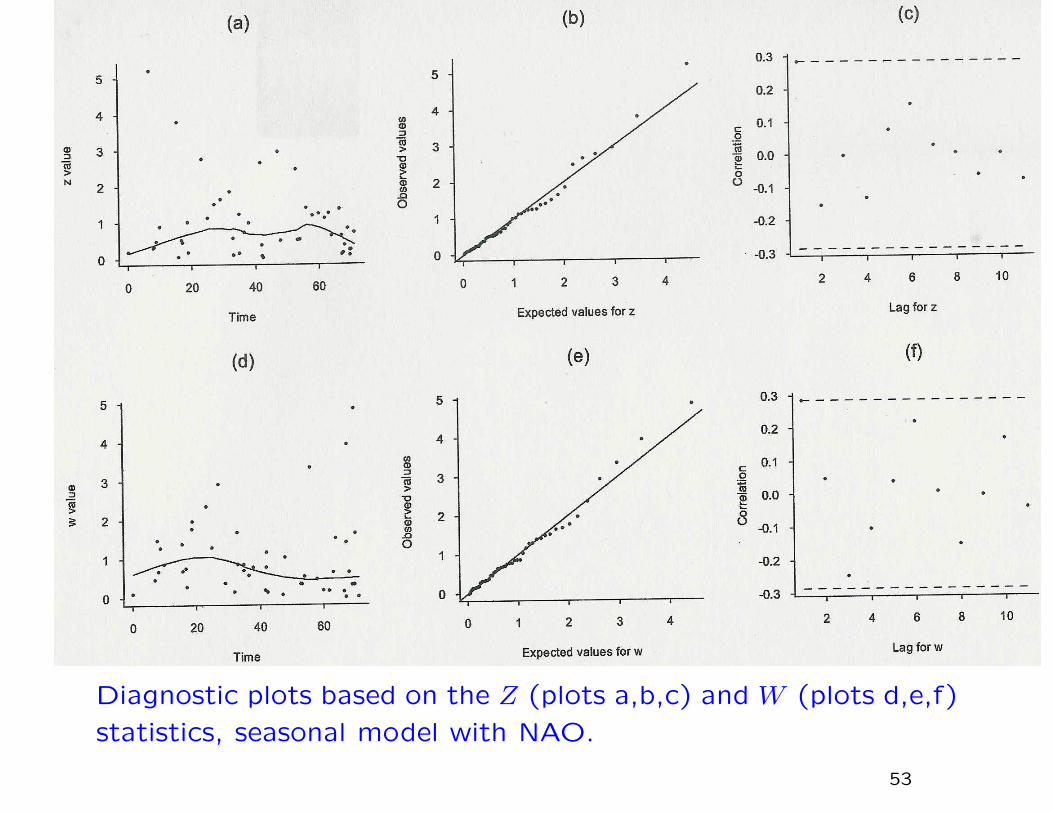
Diagnostic plots based on the Z (plots a,b,c) and W (plots d,e,f)

statistics, seasonal model with NAO.

53

(a) Estimates of 10-year (bottom), 100-year (middle) and 1000-year (top) return levels based on the fitted model for January,assuming long-term trend based on NAO. (b) 100-year returnlevel with confidence limits.

54

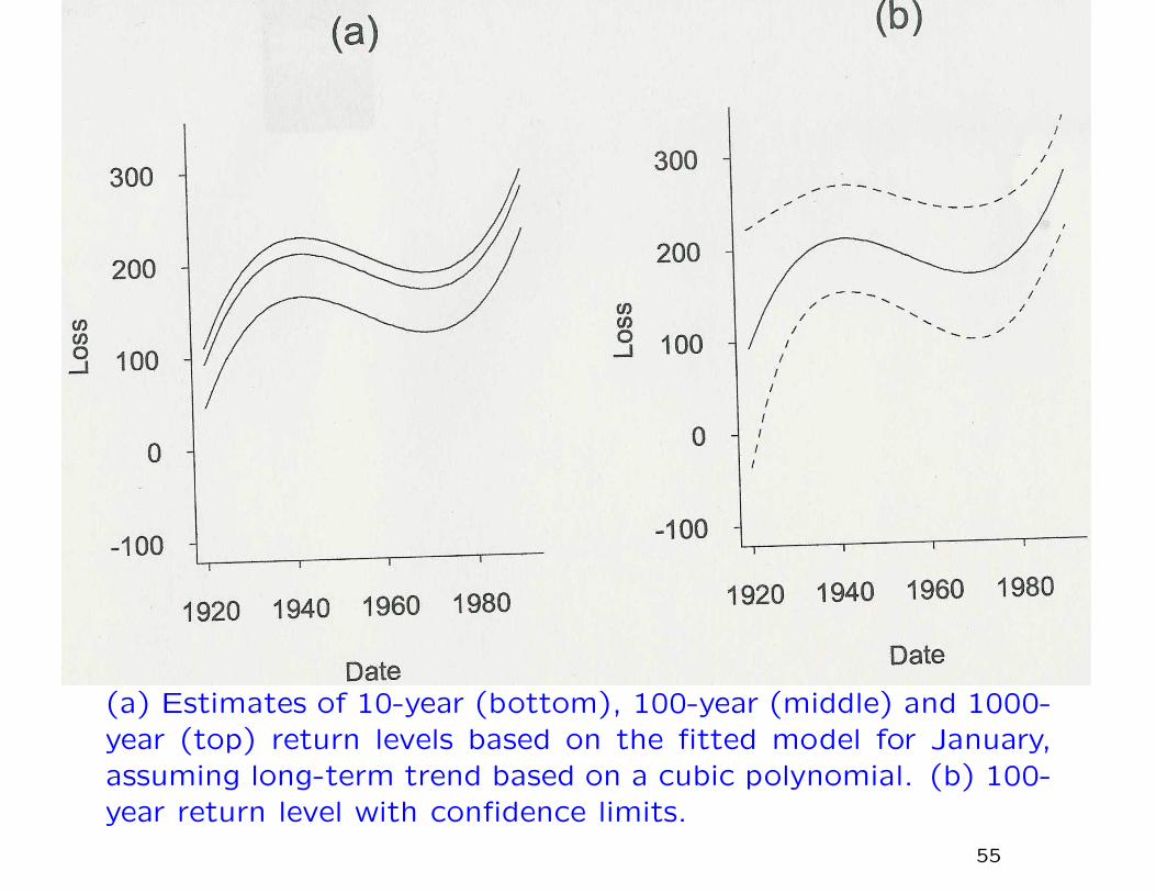
(a) Estimates of 10-year (bottom), 100-year (middle) and 1000-year (top) return levels based on the fitted model for January,assuming long-term trend based on a cubic polynomial. (b) 100-year return level with confidence limits.

55

(a) Estimates of 10-year (bottom), 100-year (middle) and 1000-year (top) return levels based on the fitted model for January,assuming long-term trend based on a cubic spline with 5 knots.(b) 100-year return level with confidence limits.

56

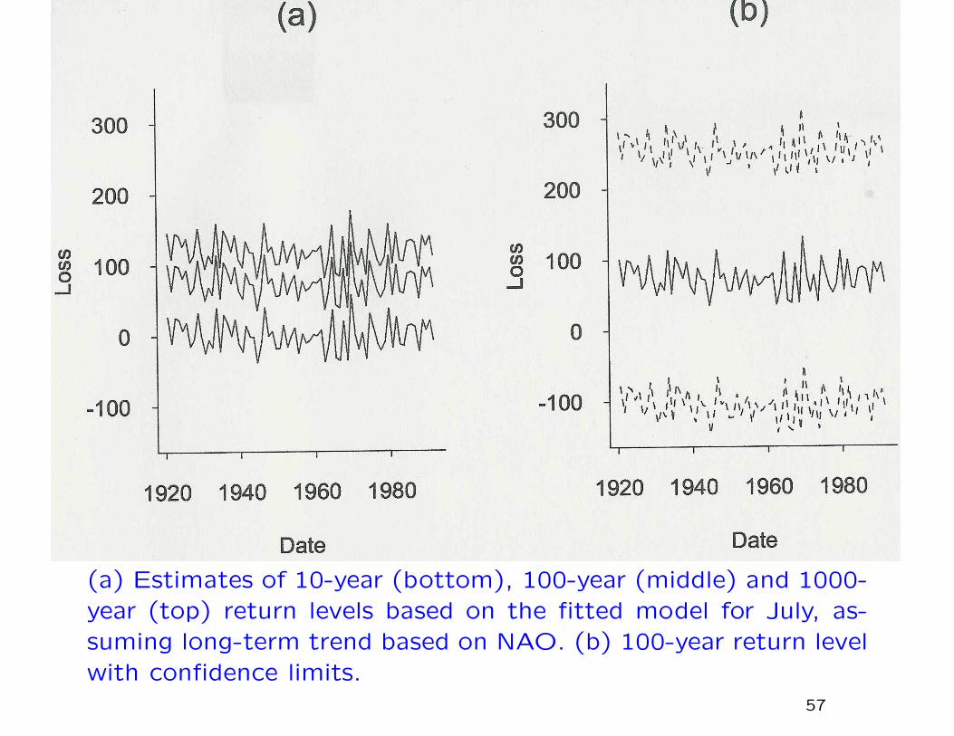
(a) Estimates of 10-year (bottom), 100-year (middle) and 1000-year (top) return levels based on the fitted model for July, as-suming long-term trend based on NAO. (b) 100-year return levelwith confidence limits.

57

How extreme was the 1990 Event?

Model Return Period (Years)Pareto 18.7

Exponential 487Gen. Pareto 333With seasons 348High NAO 187Low NAO 1106

Random NAO 432Current industry estimate? <50?

58

Note:

One reason I wanted to bring up this example is because a

dataset that is constructed along very similar lines, but for U.S.

hurricane damage, has recently been published in

R.A. Pielke Jr. et al. (2007), Normalized Hurricane Damages

in the United States: 1900-2005. Natural Hazards Review, (ac-

cepted).

(updating an earlier paper by Pielke and Landsea, 1998). They

claim, in essence, that there is no evidence of any trend in nor-

malized hurricane damage.

The data are available from Roger Pielke’s webpage and it would

be interesting to apply the same method as we have described

here!59

V. TREND IN PRECIPITATIONEXTREMES

(joint work with Amy Grady and Gabi Hegerl)

During the past decade, there has been extensive research byclimatologists documenting increases in the levels of extremeprecipitation, but in observational and model-generated data.

With a few exceptions (papers by Katz, Zwiers and co-authors)this literature have not made use of the extreme value distribu-tions and related constructs

There are however a few papers by statisticians that have ex-plored the possibility of using more advanced extreme valuemethods (e.g. Cooley, Naveau and Nychka, to appear JASA;Sang and Gelfand, submitted)

This discussion uses extreme value methodology to look fortrends

60

DATA SOURCES

• NCDC Rain Gauge Data (Groisman 2000)

– Daily precipitation from 5873 stations

– Select 1970–1999 as period of study

– 90% data coverage provision — 4939 stations meet that

• NCAR-CCSM climate model runs

– 20 × 41 grid cells of side 1.4o

– 1970–1999 and 2070–2099 (A2 scenario)

• PRISM data

– 1405 × 621 grid, side 4km

– Elevations

– Mean annual precipitation 1970–1997

61

EXTREME VALUES METHODOLOGY

Based on “point process” extreme values methodology (cf. Smith

1989, Coles 2001, Smith 2003)

62

Inhomogeneous case:

• Time-dependent threshold ut and parameters µt, ψt, ξt

• Exceedance y > ut at time t has probability

1

ψt

(1 + ξt

y − µt

ψt

)−1/ξt−1

+exp

−(1 + ξt

ut − µt

ψt

)−1/ξt

+

dydt• Estimation by maximum likelihood

63

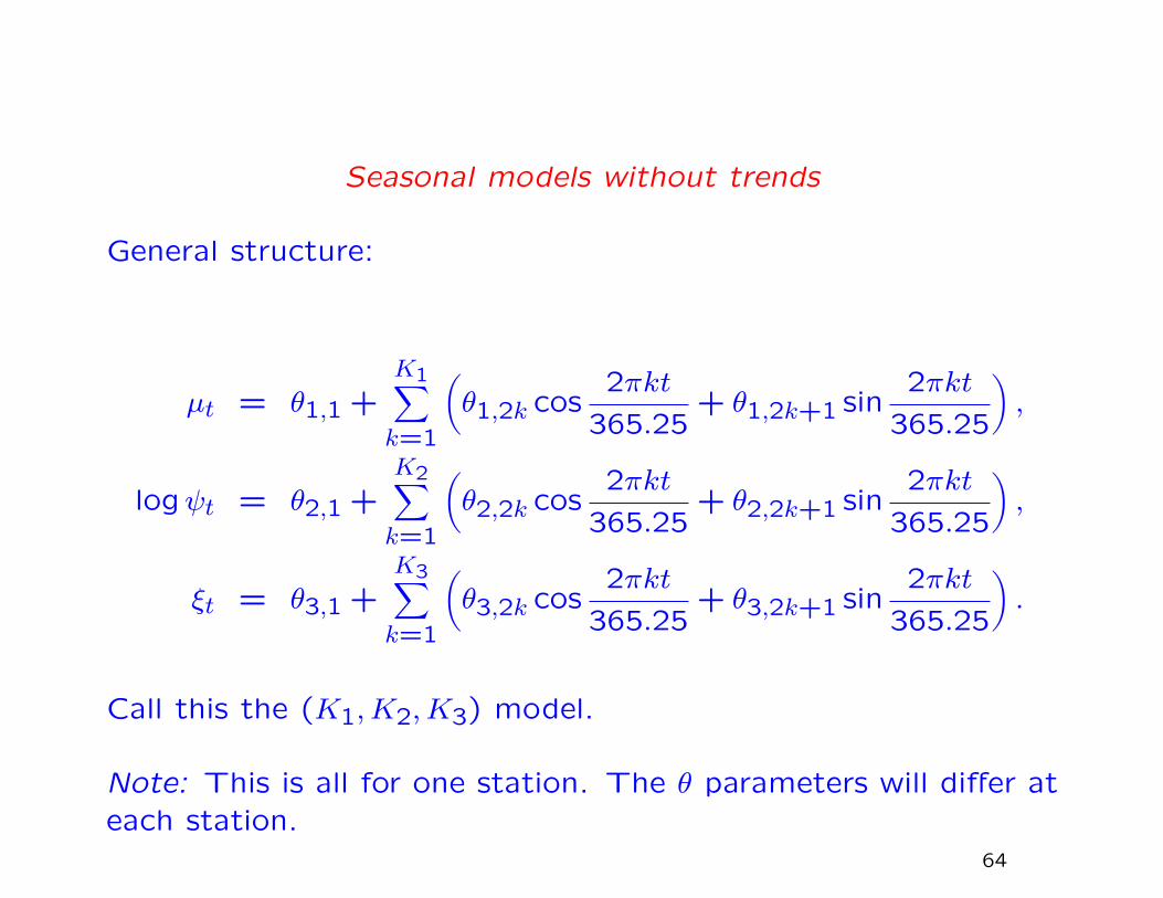
Seasonal models without trends

General structure:

µt = θ1,1 +K1∑k=1

(θ1,2k cos

2πkt

365.25+ θ1,2k+1 sin

2πkt

365.25

),

logψt = θ2,1 +K2∑k=1

(θ2,2k cos

2πkt

365.25+ θ2,2k+1 sin

2πkt

365.25

),

ξt = θ3,1 +K3∑k=1

(θ3,2k cos

2πkt

365.25+ θ3,2k+1 sin

2πkt

365.25

).

Call this the (K1,K2,K3) model.

Note: This is all for one station. The θ parameters will differ ateach station.

64

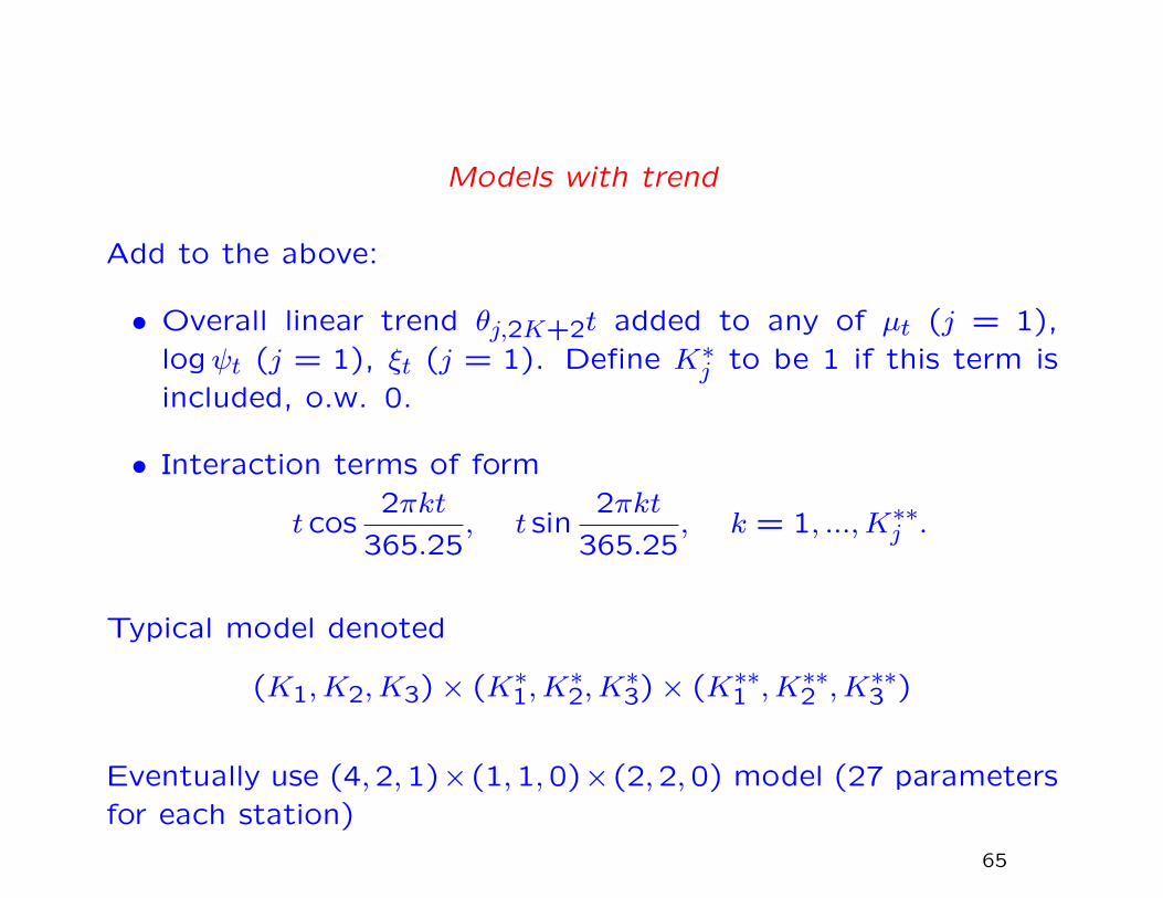
Models with trend

Add to the above:

• Overall linear trend θj,2K+2t added to any of µt (j = 1),logψt (j = 1), ξt (j = 1). Define K∗

j to be 1 if this term isincluded, o.w. 0.

• Interaction terms of form

t cos2πkt

365.25, t sin

2πkt

365.25, k = 1, ...,K∗∗

j .

Typical model denoted

(K1,K2,K3)× (K∗1,K

∗2,K

∗3)× (K∗∗

1 ,K∗∗2 ,K∗∗

3 )

Eventually use (4,2,1)×(1,1,0)×(2,2,0) model (27 parametersfor each station)

65

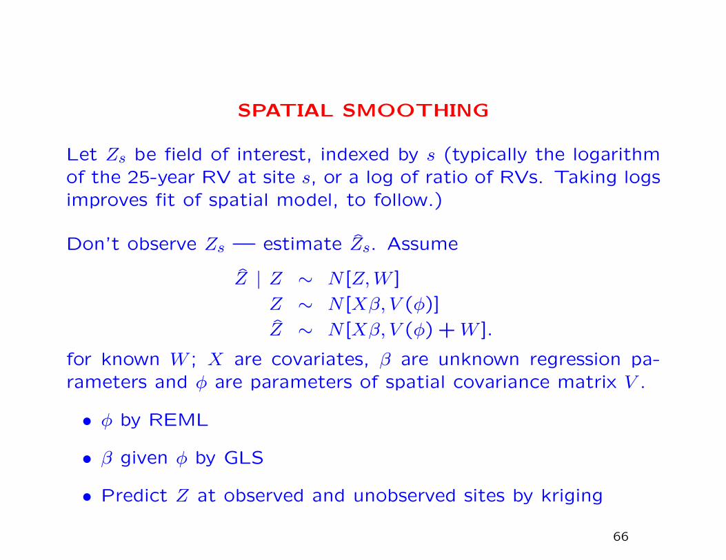
SPATIAL SMOOTHING

Let Zs be field of interest, indexed by s (typically the logarithmof the 25-year RV at site s, or a log of ratio of RVs. Taking logsimproves fit of spatial model, to follow.)

Don’t observe Zs — estimate Zs. Assume

Z | Z ∼ N [Z,W ]

Z ∼ N [Xβ, V (φ)]

Z ∼ N [Xβ, V (φ) +W ].

for known W ; X are covariates, β are unknown regression pa-rameters and φ are parameters of spatial covariance matrix V .

• φ by REML

• β given φ by GLS

• Predict Z at observed and unobserved sites by kriging

66

Spatial Heterogeneity

• Divide US into 19 overlapping regions, most 10o × 10o

– Kriging within each region

– Linear smoothing across region boundaries

– Same for MSPEs

– Also calculate regional averages, including MSPE

67

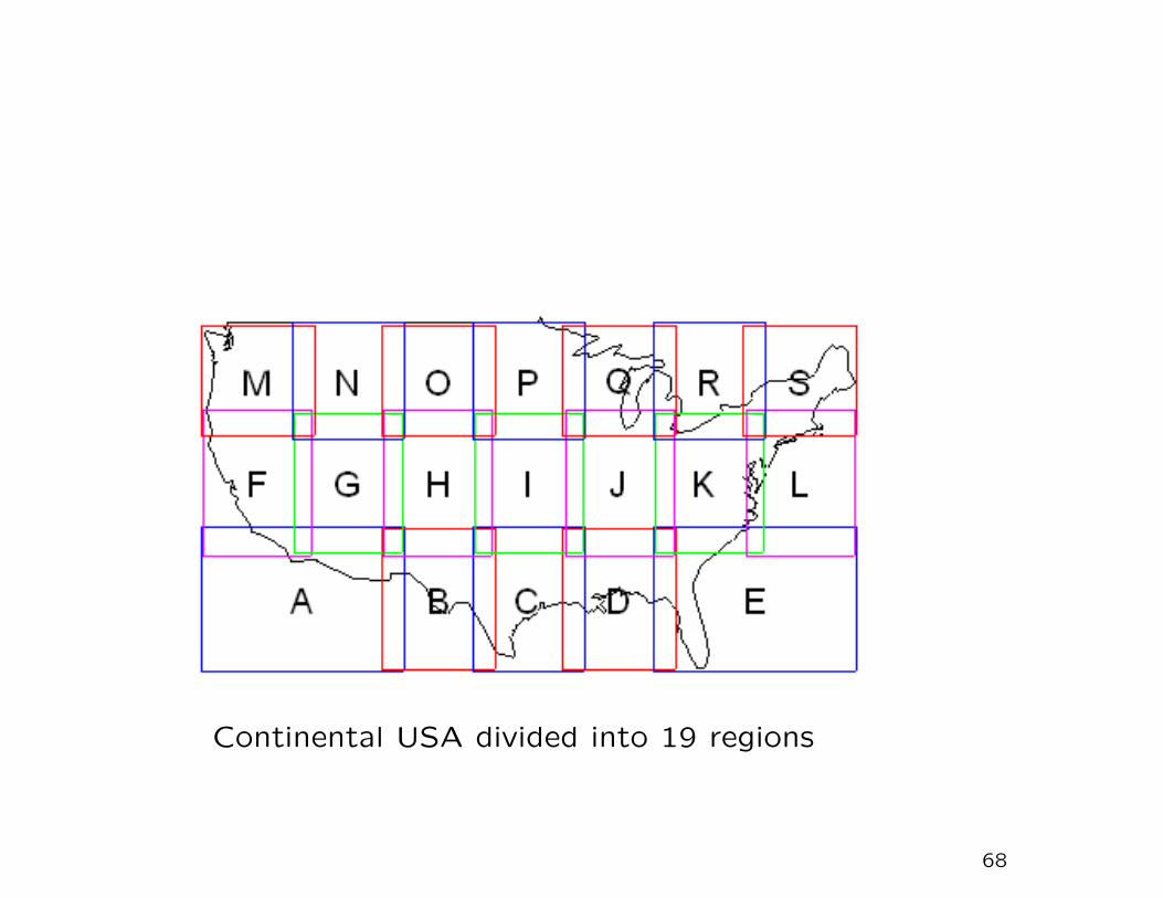
Continental USA divided into 19 regions

68

Trends across 19 regions (measured as change in log RV25) for 8 differ-ent seasonal models and one non-seasonal model with simple linear trends.Regional averaged trends by geometric weighted average approach.

69

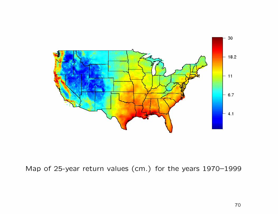
Map of 25-year return values (cm.) for the years 1970–1999

70

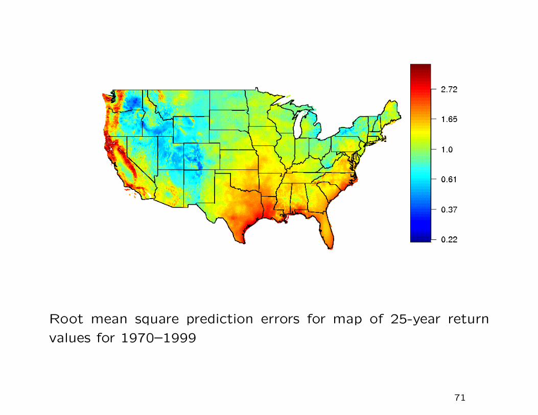
Root mean square prediction errors for map of 25-year return

values for 1970–1999

71

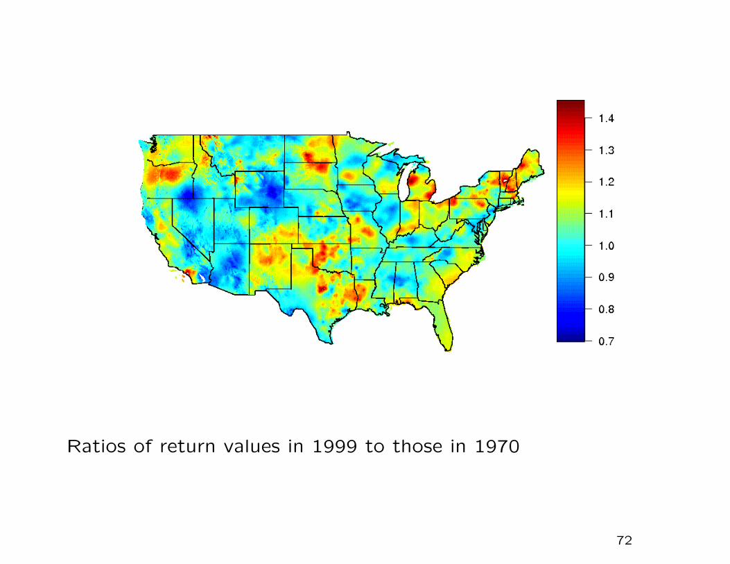
Ratios of return values in 1999 to those in 1970

72

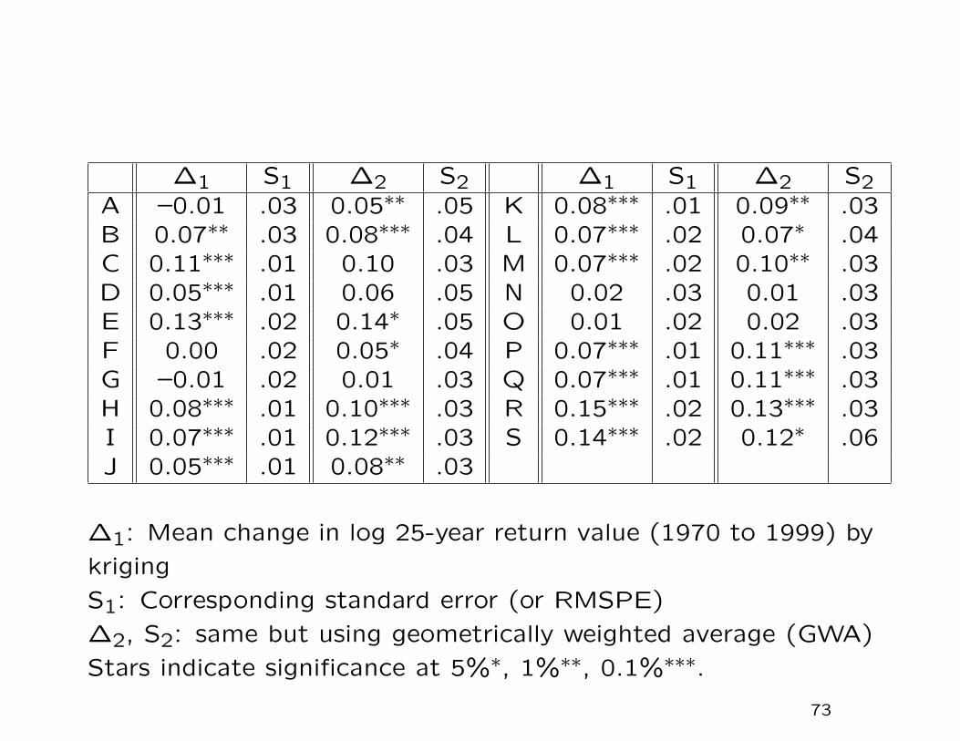
∆1 S1 ∆2 S2 ∆1 S1 ∆2 S2A –0.01 .03 0.05∗∗ .05 K 0.08∗∗∗ .01 0.09∗∗ .03B 0.07∗∗ .03 0.08∗∗∗ .04 L 0.07∗∗∗ .02 0.07∗ .04C 0.11∗∗∗ .01 0.10 .03 M 0.07∗∗∗ .02 0.10∗∗ .03D 0.05∗∗∗ .01 0.06 .05 N 0.02 .03 0.01 .03E 0.13∗∗∗ .02 0.14∗ .05 O 0.01 .02 0.02 .03F 0.00 .02 0.05∗ .04 P 0.07∗∗∗ .01 0.11∗∗∗ .03G –0.01 .02 0.01 .03 Q 0.07∗∗∗ .01 0.11∗∗∗ .03H 0.08∗∗∗ .01 0.10∗∗∗ .03 R 0.15∗∗∗ .02 0.13∗∗∗ .03I 0.07∗∗∗ .01 0.12∗∗∗ .03 S 0.14∗∗∗ .02 0.12∗ .06J 0.05∗∗∗ .01 0.08∗∗ .03

∆1: Mean change in log 25-year return value (1970 to 1999) by

kriging

S1: Corresponding standard error (or RMSPE)

∆2, S2: same but using geometrically weighted average (GWA)

Stars indicate significance at 5%∗, 1%∗∗, 0.1%∗∗∗.

73

Return value map for CCSM data (cm.): 1970–1999

74

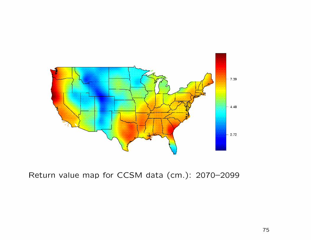
Return value map for CCSM data (cm.): 2070–2099

75

Estimated ratios of 25-year return values for 2070–2099 to those

of 1970–1999, based on CCSM data, A2 scenario

76

Extreme value model with trend: ratio of 25-year return value in

1999 to 25-year return value in 1970, based on CCSM data

77

CONCLUSIONS

1. Focus on N-year return values — strong historical tradition

for this measure of extremes (we took N = 25 here)

2. Seasonal variation of extreme value parameters is a critical

feature of this analysis

3. Overall significant increase over 1970–1999 except for parts

of western states — average increase across continental US

is 7%

4. Projections to 2070–2099 show further strong increases but

note caveat based on point 5

5. But... based on CCSM data there is a completely different

spatial pattern and no overall increase — still leavs some

doubt as to overall interpretation.

78

THANK YOU FOR YOURATTENTION!

79