rings notes

8/6/2019 Rings Notes

http://slidepdf.com/reader/full/rings-notes 1/40

Rings and Arithmetic—Notes for the Reader

The notes I am posting here are due to Dr Brian Stewart from last year with minor revisions.I intend to revise them further during Michaelmas term. These notes are a rough guide to

the contend of the course, you will probably find it helpful to read also from books. Aftereach lecture I have added some true/false questions that will help you check that you haveassimilated the basic notions. I advice you to attempt these questions before working on theproblem sheets.

Please tell me about any errors by sending an email to [email protected]

Panos Papazoglou



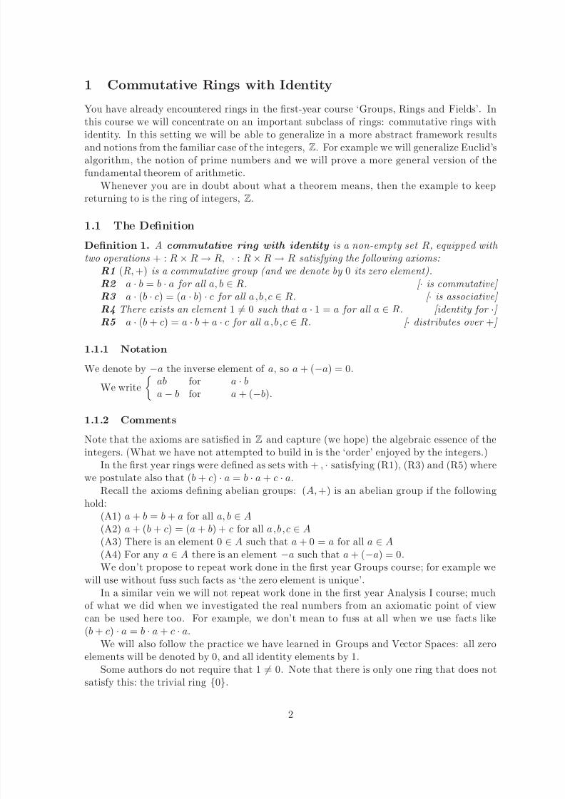
1 Commutative Rings with Identity

You have already encountered rings in the first-year course ‘Groups, Rings and Fields’. Inthis course we will concentrate on an important subclass of rings: commutative rings with

identity. In this setting we will be able to generalize in a more abstract framework resultsand notions from the familiar case of the integers, Z. For example we will generalize Euclid’salgorithm, the notion of prime numbers and we will prove a more general version of thefundamental theorem of arithmetic.

Whenever you are in doubt about what a theorem means, then the example to keepreturning to is the ring of integers, Z.

1.1 The Definition

Definition 1. A commutative ring with identity is a non-empty set R, equipped with two operations + : R × R → R, · : R × R → R satisfying the following axioms:

R1 (R, +) is a commutative group (and we denote by 0 its zero element).R2 a · b = b · a for all a, b ∈ R. [ · is commutative] R3 a · (b · c) = (a · b) · c for all a,b,c ∈ R. [ · is associative] R4 There exists an element 1 = 0 such that a · 1 = a for all a ∈ R. [identity for · ] R5 a · (b + c) = a · b + a · c for all a,b,c ∈ R. [ · distributes over + ]

1.1.1 Notation

We denote by −a the inverse element of a, so a + (−a) = 0.

We write

ab for a · ba − b for a + (−b).

1.1.2 Comments

Note that the axioms are satisfied in Z and capture (we hope) the algebraic essence of theintegers. (What we have not attempted to build in is the ‘order’ enjoyed by the integers.)

In the first year rings were defined as sets with + , · satisfying (R1), (R3) and (R5) wherewe postulate also that (b + c) · a = b · a + c · a.

Recall the axioms defining abelian groups: (A, +) is an abelian group if the followinghold:

(A1) a + b = b + a for all a, b ∈ A(A2) a + (b + c) = (a + b) + c for all a,b,c ∈ A(A3) There is an element 0 ∈ A such that a + 0 = a for all a ∈ A

(A4) For any a ∈ A there is an element −a such that a + (−a) = 0.We don’t propose to repeat work done in the first year Groups course; for example wewill use without fuss such facts as ‘the zero element is unique’.

In a similar vein we will not repeat work done in the first year Analysis I course; muchof what we did when we investigated the real numbers from an axiomatic point of viewcan be used here too. For example, we don’t mean to fuss at all when we use facts like(b + c) · a = b · a + c · a.

We will also follow the practice we have learned in Groups and Vector Spaces: all zeroelements will be denoted by 0, and all identity elements by 1.

Some authors do not require that 1 = 0. Note that there is only one ring that does notsatisfy this: the trivial ring {0}.

2



We state in the following lemma some familiar computational rules that hold also forrings.

Lemma 1.1.1. Let R be a commutative ring with identity. Then for any a, b ∈ R the following hold

1. a0 = 0a = 0.

2. −(−a) = a.

3. a(−b) = (−a)b = −(ab).

4. (−a)(−b) = ab.

5.(−1)a = −a

Proof. The proofs are quite straightforward. We give some hints below. To show 1 note that

a0 = a(0 + 0) = a0 + a0 ⇒ a0 = 0

Assertion 2 was proven last year in the groups course. For 3 we have

a(−b) + ab = a(b + (−b)) = a0 = 0

hence a(−b) is the additive inverse of ab, ie a(−b) = −(ab). We leave 4,5 as exercises.

1.1.3 An example

We will deal with examples later, but here is an example rather different in flavour from theintegers Z. For R take the set of diagonal n× n matrices with real entries; for the operationstake the usual matrix operations. Then we have a commutative ring with identity.

1.2 Two important classes

We begin with two definitions.

Definition 2. A non-zero element z of a commutative ring with identity R is called a zero-

divisor if there exists a non-zero element w ∈ R such that zw = 0.

For example, in the commutative ring with identity consisting of the 2 × 2 diagonal

matrices with real entries the element

1 00 0

and its friend

0 00 1

are both zero-divisors.

More generally, the zero-divisors are precisely the

a 00 d

with a = 0 or d = 0.

Definition 3. An element u of a commutative ring with identity R is called a unit if thereexists an element v ∈ R such that uv = 1. In this case we say that v is the inverse of u.We denote the set of units by R∗, which we call the (multiplicative) group of units of R.

We see easily that (R∗, ·) is indeed an abelian group. We remark that if u is a unit thenu is not a zero divisor. Indeed if u is a unit then there is some v such that uv = 1. If au = 0then (au)v = 0v ⇒ a(uv) = 0 ⇒ a = 0. So u is not a zero divisor.

For a trivial example, in any R the identity is a unit. For a more elaborate example takeagain for R the 2 × 2 diagonal matrices with real entries. Then the units are precisely the

a 00 d

with ad = 0.

3



1.2.1 Integral Domains

We can now define this important class of rings.

Definition 4. We say that a commutative ring with identity R is an integral domain if

there are no zero-divisors.

For example, Z is an integral domain; other examples appear below.

1.2.2 Fields

Even more specialized are the fields.

Definition 5. We say that the commutative ring with an identity is a field if every non-zeroelement is a unit.

Since units are not zero divisors fields are integral domains.

For example,R

is a field.Note that this definition of field (setting fields in a more general picture) is completelyconsistent with the definition used in the Linear Algebra course.

We note that

{fields} ⊂ {integral domains} ⊂ {commutative rings with identity}If R is an integral domain one can define the ‘field of fractions’ K of R. This is a

generalization of the construction of Q from Z. We outline this in the appendix.

1.3 Examples, Non-examples and Nearly Examples

1.3.1 The integersWe repeat: the integers, with the usual operations form a commutative ring with identity.

1.3.2 The integers mod n

The set of integers modn, Zn is a commutative ring with identity.

1.3.3 Polynomials over a field

Let K be any field. Then the set of polynomials K[X ], with the usual polynomial definitionsof addition and multiplication forms a commutative ring with identity.

Next toZ

these are our most important examples of commutative rings with identity.

1

1.3.4 Some fields

Here are examples of fields that we have met already: the rational field, Q, the real field R,the complex field C.

There are other, more exotic fields: many we will construct later as examples of theoremswe prove. For the moment you may like to check that Q[

√2] := {a + b

√2 | a, b ∈ Q} is a

field; and that C(X ) := {f (X)g(X) | f, g polynomials with complex coefficients, g = 0} is a field.

1Z is what number theorists study, the polynomial rings are what the geometers study; the similarity

between the structures goes very deep.

4



1.3.5 Not quite examples

The set of n×n matrices with entries from a field K is not a commutative ring with identity;it fails the ‘commutative’ requirement. But suitably adapted much of what we say and provecan be adapted to this situation. Various subsets, however, yield useful examples.

The set of even integers is not a commutative ring with identity; it fails the ‘identity’requirement. Again some of what we say can be suitably adapted to this sort of situation.

1.4 Subrings

Definition 6. Let R be a commutative ring with identity. A subset A ⊆ R is said to be a subring [more properly, a sub-(commutative ring with identity)] if it contains the identity and is a commutative ring with identity under the same operations.

For example, Z is a subring of Q.Just as for subgroups we have a

Proposition 1.4.1 (Test for Subringhood). Let R be a commutative ring with identity. Then A ⊆ R is a sub-(commutative ring with identity) if and only if

(i) 1 ∈ A;

(ii) if a, b ∈ A then (a − b) ∈ A;

(iii) if a, b ∈ A then ab ∈ A.

Proof. The proof is just as for groups or vector spaces; these criteria guarantee that theoperations restrict to operations on A and then the fact that the axioms which hold for allelements of R certainly hold in A.

As an application: the only sub-(commutative ring with identity) of Z is Z.

Note 1. Note that if by ‘ring’ we mean, as most authors do, a system satisfying our axioms(R1), (R3) and distributivity for ·, + , then there are many subrings of Z: for each d ∈ Z theset dZ := {dr | r ∈ Z} is a sub-ring, but has no identity. It is therefore sometimes important to adopt the tedious ‘sub-(commutative ring with identity)’ language.

1.5 Direct Products

This is an easy recipe to make new rings from old.

Proposition 1.5.1. Let R1 and R2 be commutative rings with identity. Then the set R1 × R2 := {(x1, x2) | xi ∈ Ri, i = 1, 2} is a commutative ring with identity under thecoordinatewise operations:

(i) the zero element is (0, 0);

(ii) −(a1, a2) := (−a1, −a2);

(iii) (a1, a2) + (b1, b2) := (a1 + b1, a2 + b2);

(iv) the identity element is (1, 1);

(v) (a1, a2)

·(b1, b2) := (a1

·b1, a2,

·b2).

5



Proof. Trivial.

We usually denote this ring by R1 ⊕ R2 (or sometimes just R1 × R2).For an example, take R⊕ R. This is a commutative ring with identity. Considered just

as an additive group it is isomorphic to C; but as rings they are very different, C has nozero-divisors, but every R1 ⊕ R2 has.

1.6 Polynomial Rings

This is another recipe to make new rings from old. Let R be a commutative ring withidentity. A polynomial over R in the indeterminate X is a formal expression of the form

a0 + a1X + ... + anX n

where a0, a1,...,an ∈ R. The elements a0, a1,...,an are called coefficients of the polynomial.If p(X ) = a0 + a1X + ... + anX n and an = 0 we say that the degree of p(X ) is n (if p(X )

is the zero polynomial then the degree is not defined). We add and multiply polynomials inthe familiar way; if

p(X ) =ni=0

aiX i, q(X ) =ki=0

biX i

then we define their sum by

p(X ) + q(X ) =

∞i=0

(ai + bi)X i

where by convention ai = 0 if i > n and bi = 0 if i > k. We define the product p(X )q(X ) to

be the polynomialr(X ) =

n+kt=0

ctX t

where

ct =t

i=0

aibt−i

It is easy to see that with this operations the set of polynomial with coefficients in Rbecomes a commutative ring with identity denoted by R[X ]. We give in an appendix to thissection a more formal definition of R[X ], which has the advantage that it gets rid of themysterious indeterminate X .

We can repeat the process, and manufacture for example R[X ][Y ], which we usuallyabbreviate to R[X, Y ]. The study of real plane curves is essentially the study of this ring.

Remark. One shouldn’t confuse polynomials in R[X ] with functions f : R → R. For ex-ample there are finitely many functions f : Z2 → Z2 but infinitely many distinct polynomialsin Z2[X ].

6



1.6.1 Power Series Rings

If R is a commutative ring with identity we can consider also infinite formal expressions of the form ∞

i=0

aiX i

, ai ∈ R

Such an expression is called a power series over R. Note that here convergence is irrelevant,these are just formal expressions. Addition and multiplication are defined again in theobvious way. The set of all power series over R is a commutative ring with identity, denotedby R[[X ]].

1.7 Important: Notation

All the rings in this course are commutative rings with identity. We will fromnow on usually just say ‘ring’. We will say ‘subring’ and mean ‘sub-(commutative

ring with identity)’ and later we will speak of ‘ring homomorphism’ and mean‘homomorphism of commutative rings with identity’ And so on.

7



1.8 Appendix

Integral domains and fields

Let R be an integral domain. We consider the set of pairs:

S = {(a, b) : a, b ∈ R, b = 0}

We want to see these pairs as ‘fractions’ in R. However we know from the example of Q thatdifferent fractions may represent the same number. So we define an equivalence relation:

(a, b) ∼ (c, d) if ad = bc

It is easy to see that ∼ is indeed reflexive, symmetric and transitive. We denote the equiva-lence class of (a, b) by a

band we consider the set

K = {a

b: (a, b) ∈ S }

We define now addition and multiplication on K .

a

b+

c

d=

ad + bc

bd

anda

b· c

d=

ac

bd

It is easy to check that these operations are well defined on equivalence classes. Oneverifies easily that K is a commutative ring with identity, for example we define

0 :=

0

1 , 1 :=

1

1

and we check that axioms R1-R5 hold. One sees further that K is a field as

a

b· b

a= 1

One can see R as a subring of K via the identification

a =a

1

Polynomials over rings

We give here a different definition of the ring of polynomials over a ring in order todemystify the ‘unknown’.

Proposition 1.8.1. Let R be a commutative ring with identity. Then the set of sequences

(ak)∞k=0 : ak ∈ R, only a finite number of the entries ak non-zero

is a commutative ring with identity under the operations:

(i) the zero element is (0, 0, . . . );

(ii) −(ak)∞k=0 := (−ak)∞k=0;

8



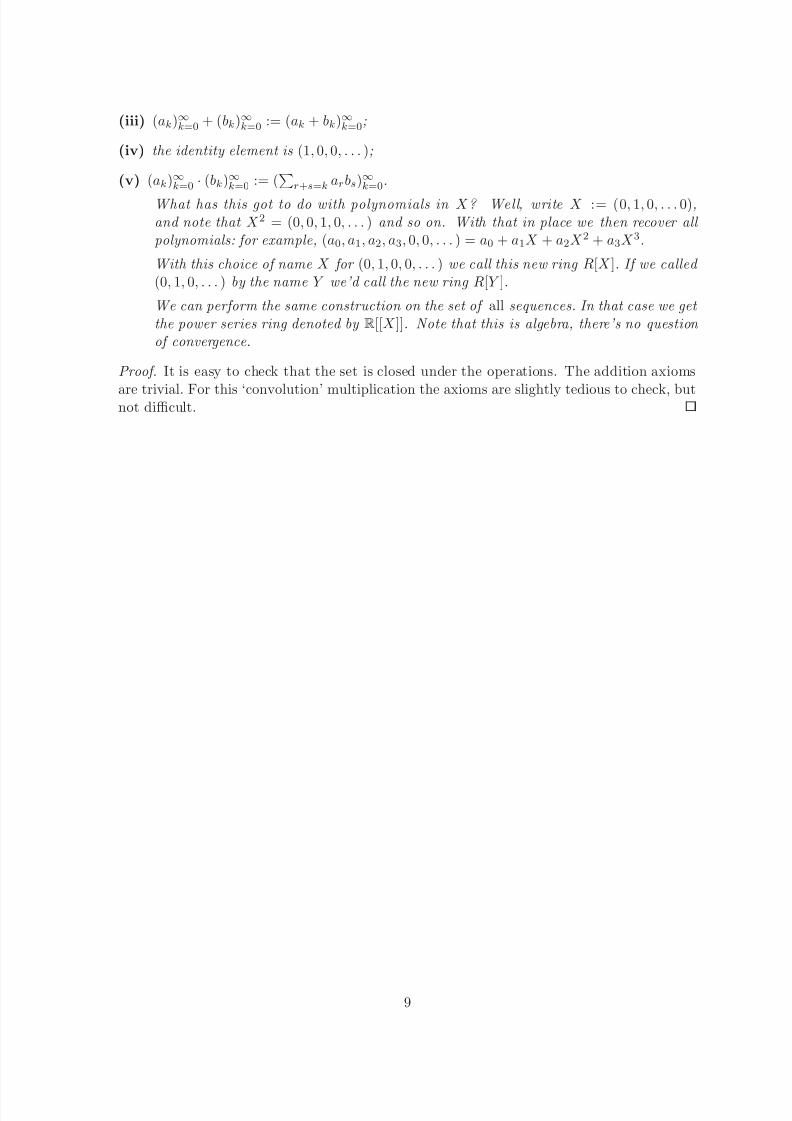
(iii) (ak)∞k=0 + (bk)∞k=0 := (ak + bk)∞k=0;

(iv) the identity element is (1, 0, 0, . . . );

(v) (ak)∞k=0·

(bk)∞k=0 := (r+s=k arbs)∞k=0.

What has this got to do with polynomials in X ? Well, write X := (0, 1, 0, . . . 0),and note that X 2 = (0, 0, 1, 0, . . . ) and so on. With that in place we then recover all polynomials: for example, (a0, a1, a2, a3, 0, 0, . . . ) = a0 + a1X + a2X 2 + a3X 3.

With this choice of name X for (0, 1, 0, 0, . . . ) we call this new ring R[X ]. If we called (0, 1, 0, . . . ) by the name Y we’d call the new ring R[Y ].

We can perform the same construction on the set of all sequences. In that case we get the power series ring denoted by R[[X ]]. Note that this is algebra, there’s no question of convergence.

Proof. It is easy to check that the set is closed under the operations. The addition axioms

are trivial. For this ‘convolution’ multiplication the axioms are slightly tedious to check, butnot difficult.

9



Which of the following are true?

1. If a,b,c are non zero elements of a ring R then ab = ac implies that b = c.

2. If a,b,c are non zero elements of an integral domain R then ab = ac implies that b = c.

3. If R is a finite integral domain and a ∈ R, a = 0 then for some n ≥ 1, an = 1.

4. If a, b are non zero elements of an integral domain R then the equation ax = b hasexactly one solution.

5. Any ring has finitely many units.

6. Every subring of a field is a field.

7. If R is an integral domain then R[X ] is also an integral domain.

8. Z[X ] has infinitely many subrings.

9. If p(X ), q(X ) ∈ Z6[X ] and deg p(X ) = 2, deg q(X ) = 3 then deg( p(X )q(X )) = 5.

10. If A, B are commutative rings with identity and A ⊂ B then A is a subring of B.

10



2 Ideals, Quotients, Homomorphisms

This section is a brief review of some of the key ideas of any algebraic system: the manufactureof ‘quotient structures’ and the analysis of the ‘homomorphisms’.

2.1 Ideals

We begin with two definitions.

Definition 7. We say that a subset I of a ring R is an ideal and write I ¡R if

(i) I is a subgroup under +;

(ii) for all a ∈ R and all i ∈ I we have ai ∈ I .

Examples. {0} and R are always ideals. If K is a field then the only ideals of K are {0}and K. If n ∈ Z then the set of all multiples of n, nZ is an ideal of Z. Generally if R is aring and a ∈ R then aR = {ax : x ∈ R} is an ideal of R. The ideal aR is sometimes denoted

by < a > or (a) and is known as the principal ideal generated by a.Proposition 2.1.1 (Test for ideals). Let R be a ring. Then I ⊆ R is an ideal of R if

(i) 0 ∈ I ;

(ii) if a, b ∈ I then (a − b) ∈ I ;

(iii) if a ∈ I , r ∈ R then ar ∈ I .

Proof. Easy.

Definition 8. Suppose that R is a ring and I ¡R. For each a ∈ R we call

a := a + I :=

{a + i

|i

∈I

}the coset of a.

The notation a is neat, but needs care if there are different ideals around as it doesn’tidentify I in the way that the ‘a + I ’ notation does.

2.2 Quotients

Suppose that R is a ring and that I ¡R, I = R. Then the set of cosets, which we denote byR or by R/I can be made into a ring. We recap briefly from the first year work.

2.2.1 Operations

(i) as zero element, the class 0;

(ii) −a := −a;

(iii) a + b := (a + b);

(iv) as identity element, the class 1;

(v) a · b := (a · b).

At once we have a doubt: are these good definitions? Let us deal only with the last one.Suppose that a = a′ and b = b′; can we be sure that a · b = a′ · b′? Of course we can, but ittakes a moment to check.

11



2.2.2 Axioms

Now that we have the operations we need to see whether the axioms are satisfied. Again letus do only one, (R5) say. We need to prove that for all a,b,c ∈ R the following holds:

a · (b + c) = a · b + a · c.

Well

LHS = a · (b + c) assumption

= a · ((b + c) definition of + on R

= (a · (b + c) definition of · on R

= (a · b + a · c) Axiom (R5) in R

= (a · b + a · c) definition of + on R

= (a

·b + a

·c) definition of

·on R (twice)

= RHS assumption

and we are done.

2.3 Applications

2.3.1 Modular Arithmetic

Clearly dZ := {dn | n ∈ Z} is an ideal. We can therefore carry out the construction, andmanufacture the quotient ring; in this case the coset notation Z = Z/dZ helps us keep trackof the modulus d. We call this the ring of integers modulo d and we denote it by Zd.

We can use these rings to illustrate other things we have done: for example, when is Z/dZan integral domain? Let 0 = a ∈ Z/dZ, and suppose that for some 0 = b ∈ Z/dZ we havethat ab = 0. Then ab is divisible by d. If d = d1d2 is composite this is always possible, justtake a := d1 and b := d2. So for an integral domain d must be prime (or 0). In both thesecases (for detailed proof see later, but most of us think it is obvious) we do get an integraldomain.

Perhaps more interestingly, what are the units of Z/dZ? Here we are seeking those u forwhich we can find a v such that uv − 1 is divisible by d. That is, given d and u we ask whenwe can find v and m such that vu + md = 1. If this is possible then the only common factorsof u and d are

±1; conversely if the only common factors are

±1 then by Euclid’s algorithm

we can find v and m. That is,

(Z/dZ)∗ = {u | (u, d) = 1}.

We denote the order of this group by φ(d); for example φ(12) = 4, since there are four units,±1 and ±5.

2.3.2 The Complex Numbers

Suppose we start with the real numbers. We can construct the polynomial ring R[X ]. In thisring the multiples of (X 2 + 1) form an ideal, which we write as X 2 + 1—trivial calculation.So we can form the quotient ring R[X ]/X 2 + 1.

12



What is it? It is, once again, the complex numbers C. Write i := X = X + X 2 + 1,then every element can be expressed as a + bi (use the Division Algorithm to see that everypolynomial can be written as a + bX + g(X )(X 2 + 1)). We have that

i2

=

X 2

= X 2

= X 2

+ 1 − 1 = X 2

+ 1 − 1 = 0 − 1 = −1.

We’ve now provided a theoretical underpinning for ideas like ‘adjoin a new number whosesquare is −1’.

2.3.3 The square root of 2

For a moment suppose we are Ancient Greeks. With much hard work we have constructed(in our own way) the rational field Q. Then we start drawing right-angled triangles and tryto find the length of the hypotenuse of the isoceles right-angled triangle of side 1. To ourhorror we find we need a number whose square is 2, and of course we have good proofs thatno such rational number exists. Our construction above would save the day: just look at the

ring Q[X ] and consider the ideal X 2 − 2 consisting of the multiples of X 2 − 2. The cosetα := X + X 2 − 2 in the quotient Q[X ]/X 2 − 2 is the number we are looking for.

(There is much more to be said here: see later in the course.)

2.4 More about ideals

Suppose that R is a ring, and that I, J ¡R. The following are easy to check.

Proposition 2.4.1. The set I ∩ J is an ideal of R, and whenever K ¡ R with K ⊆ I and K ⊆ J we have that K ⊆ I ∩ J .

Proposition 2.4.2. The set I + J := {i + j | i ∈ I, j ∈ J } is an ideal of R, and whenever K ¡R with I ⊆ K and J ⊆ K we have that I + J ⊆ K .

Proposition 2.4.3. The set I · J := {r ir · jr | ir ∈ I, jr ∈ J } is an ideal of R, and I · J ⊆ I ∩ J .

Definition 9. An ideal I of a ring R is said to be maximal if I = R and I ⊆ J ¡R impliesthat I = J or J = R.

Theorem 2.4.4. Let R be a ring and I ¡R. Then R/I is a field if and only if I is maximal.

Proof. Suppose that I is maximal, and that x ∈ I . Then J := I + < x >= I . Clearly J ¡R,so J = R. As 1 ∈ R we can write 1 = i + a · x for some i ∈ I and a ∈ R. Then 1 = i + ax,or ax = 1, and we have found an inverse for x.

Suppose that R/I is a field, and that I ⊆ J ¡ R with I = J . We can therefore choosex ∈ J \ I . Then x = 0, and so has an inverse a. That is, ax − 1 = 0, so that ax − 1 ∈ I . Asax ∈ J and I ⊆ J we get that 1 ∈ J . For any t ∈ R then, we get t = t · 1 ∈ J : hence R = J .

Since R/I has at least two elements I = R.

Definition 10. An ideal I of a ring R is said to be prime if I = R and xy ∈ I implies that either x ∈ I or y ∈ I .

13



Theorem 2.4.5. Let R be a ring and I ¡R. Then R/I is an integral domain if and only if I is prime.

Proof. Suppose that I is prime, and that x y = 0. Then xy = 0, so xy ∈ I . It follows thateither x = 0 or y = 0. So R/I is an integral domain.

Suppose that R/I is an integral domain. Then R/I has at least two elements so I = R.Suppose now that xy ∈ I . Then xy = 0 so x y = 0. As R/I is an integral domain x = 0 ory = 0. So either x ∈ I or y ∈ I . Hence I is prime.

Corollary 2.4.6. Let R be a ring and I ¡R. If I is maximal then I is prime.

Proof. If I is maximal then R/I is a field. So R/I is an integral domain, hence I is prime.

2.5 Constructing new fields

One can use theorem 2.4.4 to construct examples of fields.Let K be a field. Recall that a polynomial of positive degree p(X ) ∈ K[X ] is called

irreducible if there are no polynomials of positive degree f (X ), g(X ) ∈ K[X ] such that p(X ) = f (X )g(X ).

In the first year course you defined the highest common factor of two polynomials f, gand you saw that there exist polynomials m, n such that

hcf (f, g) = mf + ng

The proofs were done only in the case of R[X ] but the same proofs apply for any field K.

Proposition 2.5.1. Let K be a field, p(X ) ∈ K[X ] and I =< p(X ) >. Then I is maximal if and only if p(X ) is irreducible. It follows that the quotient ring K[X ]/I is a field if and only if p(X ) is irreducible.

Proof. Assume that I is a maximal ideal. Let

p(X ) = a(X )b(X )

be a factorisation of p(X ). Clearly I ⊆< a(X ) >. Since I is maximal either < a(X ) >= I or < a(X ) >= R.

If < a(X ) >= I then a(X ) = p(X )q(X ) for some q(X ) ∈ K[X ] so

p(X ) = p(X )q(X )b(X )

and q(X )b(X ) = 1. It follows that deg b(X ) = 0.

If < a(X ) >= R then 1 = a(X )q(X ) for some q(X ) ∈ K[X ], so deg a(X ) = 0. Weconclude that either deg a(X ) = 0 or deg b(X ) = 0. So p(X ) is irreducible.

Assume now that p(X ) is irreducible. Let’s say that I ⊆ J where J is an ideal of R,J = I . Let f (X ) ∈ J \ I . Since p(X ) is irreducible hcf (f (X ), p(X )) = 1. So there area(X ), b(X ) ∈ K[X ] such that

a(X ) p(X ) + b(X )f (X ) = 1

Since p(X ), f (X ) ∈ J we have that 1 ∈ J . So J = R and I is maximal.Finally we remark that by theorem 2.4.4, K[X ]/I is a field if and only if I is maximal.

So K[X ]/I is a field if and only if p(X ) is irreducible.

14



Remark 2.5.2. A polynomial of degree 2 or 3 in K[X ] ( K a field) is irreducible if and only if it has no roots in K.

Example 2.5.3. The quotient ring

Z3[X ]/ < X 2 + 1 >

is a field.

Proof. Indeed using the previous proposition it suffices to show that X 2 + 1 is irreducible.However X 2 + 1 has no roots in Z3 since 02 + 1 = 1, 12 + 1 = 2, 22 + 1 = 2 in Z3.

2.6 Homomorphisms

When we study algebraic objects the appropriate maps to consider are the maps that pre-serve the structure of these objects. So for K-vector spaces the appropriate maps are lineartransformations, for groups it is the group homomorphisms and so on. So we make thefollowing definition.

Definition 11. Let R and S be commutative rings with identity 2. We will say that a mapf : R → S is a homomorphism if, for all x, y ∈ R,

(i)f (1) = 1; (ii)f (x + y) = f (x) + f (y); (iii)f (x · y) = f (x) · f (y).

For an example, take R := R[x] and S := C and let for any a ∈ C, σa be the ‘evaluation’map, σa :

N 0 ckxk →N

0 ckak. This is a homomorphism.For another example, take R := Z and for any d ∈ Z let S := Z/dZ. Then the map

: R → S defined by : n → n (which maps each n to its equivalence class modulo d) is a

homomorphism. Our construction of the quotient Z/dZ achieved precisely this.For a non-example, consider the map p : Z ⊕ Z → Z ⊕ Z given by p(n1, n2) = (n1, 0).This satisfies the conditions (ii) and (iii), for being a homomorphism: but fails to map theidentity to the identity.

We also make the following definition.

Definition 12. Let f : R → S be a homomorphism of rings. We say that f is an isomor-

phism if f is 1–1 and onto. In this case we write R ∼= S .

2.6.1 The Kernel

Definition 13. Let f : R

→S be a homomorphism of rings. We say that f −1(0) :=

{z | f (z) = 0} is the kernel of the homomorphism. Sometimes we denote it by ker f .

Suppose that we have a homomorphism f : R → S of rings. Which elements get mappedto the same place? Well, it is clear that ‘mapping to the same place’ is an equivalence relationon R. f (x) = f (a) if and only if f (x − a) = f (x) − f (a) = 0, and so using x = a + (x − a)we have

{x | f (x) = f (a)} = a + {z | f (z) = 0} = a + ker f.

Note that we have at once a good test for f to be one-to-one: this is equivalent toker f = {0}.

2It matters here, so we emphasise the with identity .

15



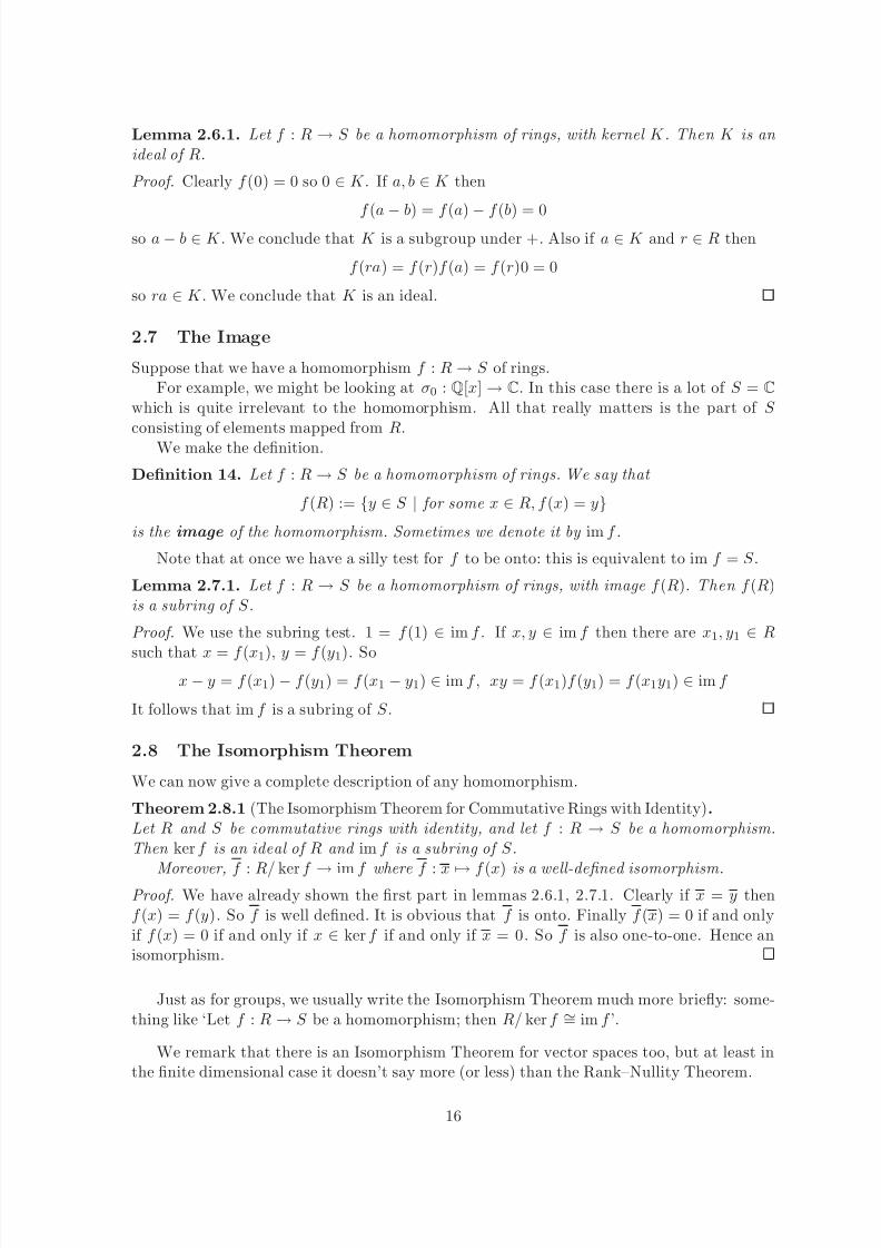
Lemma 2.6.1. Let f : R → S be a homomorphism of rings, with kernel K . Then K is an ideal of R.

Proof. Clearly f (0) = 0 so 0 ∈ K . If a, b ∈ K then

f (a − b) = f (a) − f (b) = 0so a − b ∈ K . We conclude that K is a subgroup under +. Also if a ∈ K and r ∈ R then

f (ra) = f (r)f (a) = f (r)0 = 0

so ra ∈ K . We conclude that K is an ideal.

2.7 The Image

Suppose that we have a homomorphism f : R → S of rings.For example, we might be looking at σ0 : Q[x] → C. In this case there is a lot of S = C

which is quite irrelevant to the homomorphism. All that really matters is the part of S consisting of elements mapped from R.

We make the definition.

Definition 14. Let f : R → S be a homomorphism of rings. We say that

f (R) := {y ∈ S | for some x ∈ R, f (x) = y}is the image of the homomorphism. Sometimes we denote it by im f .

Note that at once we have a silly test for f to be onto: this is equivalent to im f = S .

Lemma 2.7.1. Let f : R → S be a homomorphism of rings, with image f (R). Then f (R)is a subring of S .

Proof. We use the subring test. 1 = f (1) ∈ im f . If x, y ∈ im f then there are x1, y1 ∈ R

such that x = f (x1), y = f (y1). Sox − y = f (x1) − f (y1) = f (x1 − y1) ∈ im f , xy = f (x1)f (y1) = f (x1y1) ∈ im f

It follows that im f is a subring of S .

2.8 The Isomorphism Theorem

We can now give a complete description of any homomorphism.

Theorem 2.8.1 (The Isomorphism Theorem for Commutative Rings with Identity).Let R and S be commutative rings with identity, and let f : R → S be a homomorphism.Then ker f is an ideal of R and im f is a subring of S .

Moreover, f : R/ ker f → im f where f : x → f (x) is a well-defined isomorphism.Proof. We have already shown the first part in lemmas 2.6.1, 2.7.1. Clearly if x = y thenf (x) = f (y). So f is well defined. It is obvious that f is onto. Finally f (x) = 0 if and onlyif f (x) = 0 if and only if x ∈ ker f if and only if x = 0. So f is also one-to-one. Hence anisomorphism.

Just as for groups, we usually write the Isomorphism Theorem much more briefly: some-thing like ‘Let f : R → S be a homomorphism; then R/ ker f ∼= im f ’.

We remark that there is an Isomorphism Theorem for vector spaces too, but at least inthe finite dimensional case it doesn’t say more (or less) than the Rank–Nullity Theorem.

16



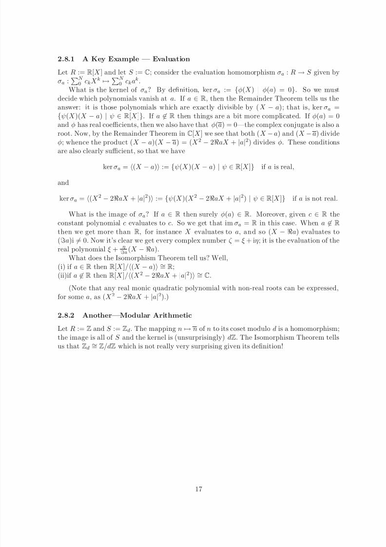
2.8.1 A Key Example — Evaluation

Let R := R[X ] and let S := C; consider the evaluation homomorphism σa : R → S given byσa :

N 0 ckX k →N

0 ckak.What is the kernel of σa? By definition, ker σa :=

{φ(X )

|φ(a) = 0

}. So we must

decide which polynomials vanish at a. If a ∈ R, then the Remainder Theorem tells us theanswer: it is those polynomials which are exactly divisible by (X − a); that is, ker σa ={ψ(X )(X − a) | ψ ∈ R[X ]}. If a ∈ R then things are a bit more complicated. If φ(a) = 0and φ has real coefficients, then we also have that φ(a) = 0—the complex conjugate is also aroot. Now, by the Remainder Theorem in C[X ] we see that both (X − a) and (X − a) divideφ; whence the product (X − a)(X − a) = (X 2 − 2ℜaX + |a|2) divides φ. These conditionsare also clearly sufficient, so that we have

ker σa = (X − a) := {ψ(X )(X − a) | ψ ∈ R[X ]} if a is real,

and

ker σa = (X 2 − 2ℜaX + |a|2) := {ψ(X )(X 2 − 2ℜaX + |a|2) | ψ ∈ R[X ]} if a is not real.

What is the image of σa? If a ∈ R then surely φ(a) ∈ R. Moreover, given c ∈ R theconstant polynomial c evaluates to c. So we get that im σa = R in this case. When a ∈ R

then we get more than R, for instance X evaluates to a, and so (X − ℜa) evaluates to(ℑa)i = 0. Now it’s clear we get every complex number ζ = ξ + iη; it is the evaluation of thereal polynomial ξ + η

ℑa(X − ℜa).What does the Isomorphism Theorem tell us? Well,

(i) if a ∈ R then R[X ]/(X − a) ∼= R;(ii)if a ∈ R then R[X ]/(X 2 − 2ℜaX + |a|2) ∼= C.

(Note that any real monic quadratic polynomial with non-real roots can be expressed,for some a, as (X 2 − 2ℜaX + |a|2).)

2.8.2 Another—Modular Arithmetic

Let R := Z and S := Zd. The mapping n → n of n to its coset modulo d is a homomorphism;the image is all of S and the kernel is (unsurprisingly) dZ. The Isomorphism Theorem tellsus that Zd ∼= Z/dZ which is not really very surprising given its definition!

17




1. If I, J are ideals then I ∪ J is an ideal.

2. If F, K are fields and φ : F → K is an onto homomorphism then φ is an isomorphism.

3. If R is an integral domain and I is an ideal of R then R/I is an integral domain.

4. There is a ring homomorphism f : Zn → Z.

5. There is a ring homomorphism f : Z → Zn.

6. There is a ring homomorphism f : Q → Z.

7. There is a ring homomorphism f : Q → Z p ,where p is a prime.

8. The rings Z[i] and Z[X ] are isomorphic.

9. C and R are isomorphic.

10. If an ideal I ⊂ R contains a unit of the ring R then I = R.

11. If p ∈ Z is a prime number and xy ∈ ( p) then either x ∈ ( p) or y ∈ ( p).

12. Q is an ideal of R.

13. If R is a ring and a1,...,an ∈ R then the set {a1r1 + ... + anrn : r1,...,rn ∈ R} is anideal of R.

14. < X > is a prime ideal of Z[X ].

15. Every prime ideal of Z[X ] is a maximal ideal.

16. If f : R → S is an isomorphism of the rings R, S then I ⊂ R is an ideal of R if andonly if f (I ) is an ideal of S .

17. If I ⊂ R is an ideal and f : R → S is a ring homomorphism then f (I ) is an ideal of S .

18. If I ⊂ S is an ideal of S and f : R → S is a ring homomorphism then f −1(I ) is anideal of R.

19. a + I ∈ R/I is a unit of R/I if and only if < a > +I = R.

18



3 The Chinese Remainder Theorem

3.1 Introduction

In the first year course we learned about the Division Algorithm and Euclid’s Algorithm for

both the ring of integers Z and polynomial rings over fields, K. We are going to slightlyextend these results, proving one of the most versatile theorems of algebra, the ChineseRemainder Theorem.

3.2 Abstract version

Although one of the most important things about the CRT is its efficiency and practical use,we start quite abstractly. This deals with rather dull technicalities once and for all, so thatwhen we come to concrete versions we can concentrate on what is interesting.

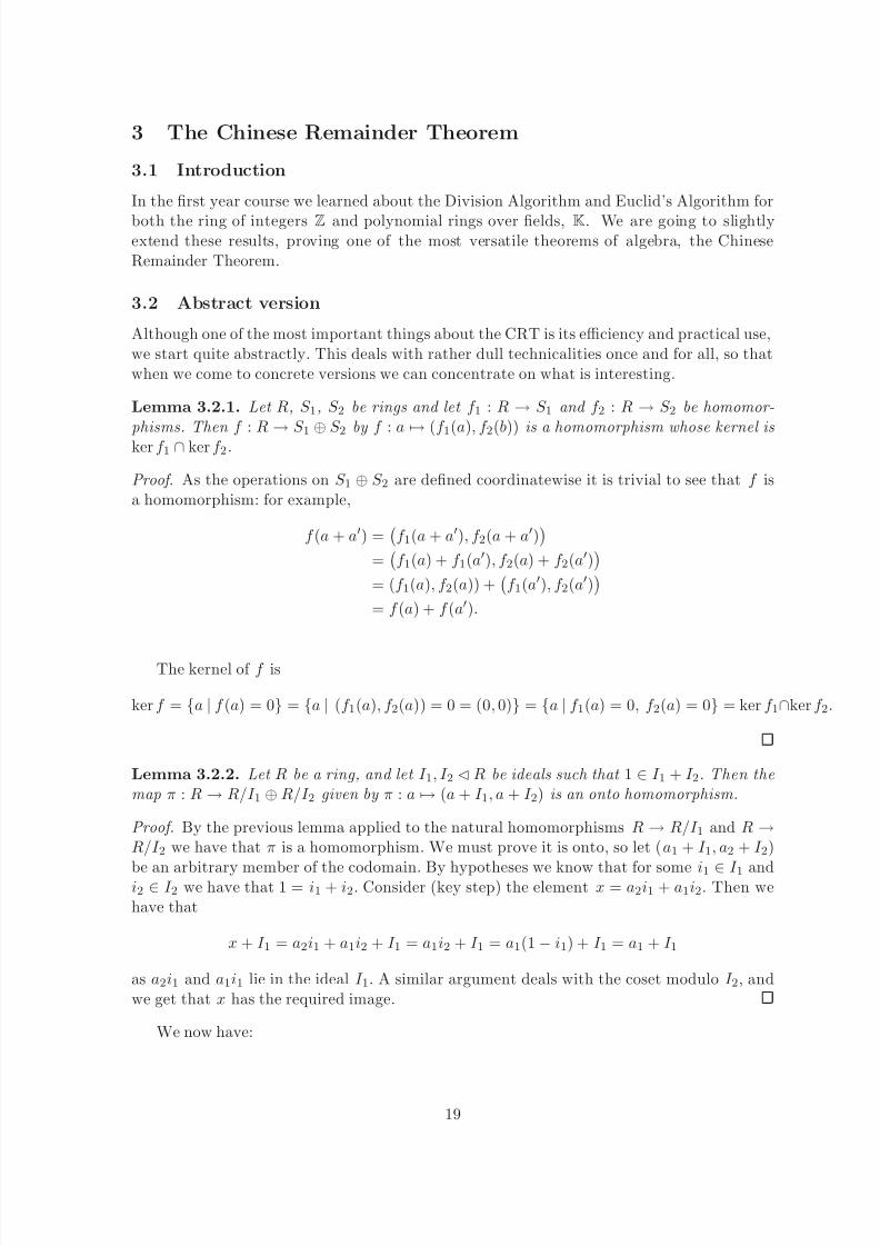
Lemma 3.2.1. Let R, S 1, S 2 be rings and let f 1 : R → S 1 and f 2 : R → S 2 be homomor-phisms. Then f : R

→S 1 ⊕

S 2

by f : a→

(f 1

(a), f 2

(b)) is a homomorphism whose kernel isker f 1 ∩ ker f 2.

Proof. As the operations on S 1 ⊕ S 2 are defined coordinatewise it is trivial to see that f isa homomorphism: for example,

f (a + a′) =

f 1(a + a′), f 2(a + a′)

=

f 1(a) + f 1(a′), f 2(a) + f 2(a′)

= (f 1(a), f 2(a)) +

f 1(a′), f 2(a′)

= f (a) + f (a′).

The kernel of f is

ker f = {a | f (a) = 0} = {a | (f 1(a), f 2(a)) = 0 = (0, 0)} = {a | f 1(a) = 0, f 2(a) = 0} = ker f 1∩ker f 2.

Lemma 3.2.2. Let R be a ring, and let I 1, I 2 ¡R be ideals such that 1 ∈ I 1 + I 2. Then themap π : R → R/I 1 ⊕ R/I 2 given by π : a → (a + I 1, a + I 2) is an onto homomorphism.

Proof. By the previous lemma applied to the natural homomorphisms R → R/I 1 and R →R/I 2 we have that π is a homomorphism. We must prove it is onto, so let (a1 + I 1, a2 + I 2)

be an arbitrary member of the codomain. By hypotheses we know that for some i1 ∈ I 1 andi2 ∈ I 2 we have that 1 = i1 + i2. Consider (key step) the element x = a2i1 + a1i2. Then wehave that

x + I 1 = a2i1 + a1i2 + I 1 = a1i2 + I 1 = a1(1 − i1) + I 1 = a1 + I 1

as a2i1 and a1i1 lie in the ideal I 1. A similar argument deals with the coset modulo I 2, andwe get that x has the required image.

We now have:

19



Theorem 3.2.3 (Abstract CRT). Let R be a ring, and let I 1, I 2 ¡ R be ideals such that I 1 + I 2 = R. Then

R/(I 1 ∩ I 2) ∼= R/I 1 ⊕ R/I 2

where the isomorphism is the natural x + (I 1∩

I 2)

→(x + I 1, x + I 2).

Proof. We consider the map π : R → R/I 1 ⊕ R/I 2 given by a → (a + I 1, a + I 2). By the firstlemma this is a homomorphism with kernel I 1 ∩ I 2. As R = I 1 + I 2 we have that 1 ∈ I 1 + I 2so we can use the second lemma to get that π is onto. Now apply the Isomorphism Theoremto π and get the result.

3.3 The CRT for Z

Originally the Chinese Remainder Theorem was the proposition that one could, if a, b arecoprime integers, and r, s are any integers, find a solution to the simultaneous congruences

x≡

r (mod a), x≡

s (mod b).

That is only part of what we are now able to prove.

Theorem 3.3.1 (CRT for integers). Let a, b ∈ Z have highest common factor 1. Then

Z/abZ ∼= Z/aZ⊕ Z/bZ,

the isomorphism being the natural x + abZ → (x + aZ, x + bZ).

Proof. By Euclid’s Algorithm we can find R, S such that 1 = Ra + Sb, so that Z = aZ+ bZ.Also, we have that lcm(a, b) = ab/ hcf(a, b) = ab, so that aZ ∩ bZ = abZ. The theorem nowfollows from the abstract version.

3.4 Applications

3.4.1 Simultaneous congruences

The result about simultaneous congruences, that if a, b are coprime integers, and r, s are anyintegers, then we can find a solution to the simultaneous congruences

x ≡ r (mod a), x ≡ s (mod b).

is an easy corollary of our CRT. For consider the pair of cosets (r + aZ, s + bZ); by the CRTthere exists a unique coset x + abZ such that (x + aZ, x + bZ) = (r + aZ, s + bZ).

Although fine in theory, this is not yet of practical use. How do we find the solutionx? We have answered this implicitly. When we proved the ontoness of the map π the keyconsideration was that we could express 1 = i1 + i2 with i1 ∈ I 1 and i2 ∈ I 2; then we got xas si1 + ri2.

So in practice, we use the (extended) Euclid Algorithm—a very efficient process—tocalculate the integers R and S such that 1 = aR + bS ; and the solution we then seek is, asper the proof of our abstract theorem, x = aRs + bSr.

3.4.2 Euler’s φ function

See problems sheet for an application.

20



3.4.3 Speeding up Arithmetic

Suppose again that a, b ∈ Z have highest common factor 1. By the CRT we have that

Z/abZ ∼= Z/aZ

⊕Z/bZ.

We can then carry out arithmetic calculations in Z/abZ in the following way:

Step 1 For each input x := x + abZ calculate x := x + aZ and x := x + bZ.

Step 2 Carry out the required calculations on the x in Za to get the answer y; and on thex in Zb to get y.

Step 3 Using the inverse of the isomorphism, calculate the value of y which maps to thepair (x, x).

Can this possibly be a good idea? The answer is a resounding Yes! Essentially we have

some setup costs we must pay once and for all: the calculation of integers R and S such thatRa + Sb = 1 which allow us to compute the inverse isomorphism. This is not very expensive:Euclid’s algorithm is very fast, requiring O(log a) steps. The reductions of step 1 are notexpensive, although an extra overhead. But the savings come in step 2: although we haveto carry out the calculations twice we do so in much smaller systems. If we make a carefulanalysis we’ll see that this really works.

3.5 The CRT for K[X ]

If we look at our proof of the CRT for Z we will see that all we needed to use about the ringZ and the elements a, b with hcf(a, b) = 1 were these facts, both consequences of Euclid’sAlgorithm:

(i) 1 = Ra + Sb for some R, S ;

(ii) aZ ∩ bZ = abZ.

We have the Division Algorithm, highest common factors, and Euclid’s Algorithm in thering K[X ], where K is any field; we saw this in the first-year course. Therefore we have, withno more work to be done:

Theorem 3.5.1 (CRT for K[X ] ). Let K be a field and let f (X ), g(X ) ∈ K[X ] have highest common factor 1. Then

K[X ]/f (X )g(X )K[X ] ∼= K[X ]/f (X )K[X ] ⊕K[X ]/g(X )K[X ],

the isomorphism being the natural t + f (X )g(X )K[X ] → (t + f (X )K[X ], t + f (X )K[X ]).

3.6 An application

There would be no point in this, of course, if there were not important applications.

21



3.6.1 Interpolation

Suppose we have k + 1 distinct members ai of a field K; and k + 1 arbitrary members bi of K.

We can apply the CRT first to the polynomials (X

−a1) and i>1(X

−ai), and then

inductively and get

K[X ]/

(X − ai)K[X ] ∼=

K[X ]/(X − ai)K[X ].

Let us look for a moment at K[X ]/(X − a)K[X ]. What does a coset b + (X − a)K[X ]represent? It is, as the Remainder Theorem tells us, the set of all polynomials which takethe value b at the point a.

So what the CRT tells us in part is this: there is a unique coset of polynomials

t(X ) +

(X − ai)K[X ]

consisting of those polynomials which take the values bi at the points ai. By the DivisionAlgorithm we can then find in the coset a unique t(X ) of degree at most k with this property.Once again, note that the CRT is actually constructive: Euclid’s Algorithm lets us

compute the inverse of the isomorphism efficiently, and find t(X ) from the data (ai, bi),i = 1, . . . , k + 1.

22



4 Divisibility in integral domains

We have until this moment used Z and K[X ] both as rich sources of examples, and alsoas prototypes: we have tried to develop ring theory in a way that captures the essential

properties of these structures. In this section we will try to generalize the divisibility andfactorization properties of these rings in a more general settings. For example we would liketo generalize the Fundamental Theorem of Arithmetic and the Euclidean Algorithm fromthe case of Z to more general rings. We begin with introducing the appropriate terminologyin the abstract setting of integral domains.

4.1 Divisibility

Definition 15. Let R be a ring, and let a, b ∈ R. We say that b divides a (and writeb|a) if for some c ∈ R we have that a = bc. We will also call b a divisor of a in thesecircumstances.

So for example the units are the divisors of 1, and everything divides 0.

Definition 16. Let R be a ring, and let a ∈ R. An element a′ of R is called an associate

of a if for some unit u ∈ R we have that a′ = ua.

We remark that this is an equivalence relation.For example the associates of n ∈ Z are ±n. Note that unique factorization in Z is not

really unique, for example −6 = 2·(−3) = (−2)·3. Of course this non uniqueness up to a signis quite harmless. In the unique factorization theorem that we will prove later uniquenesswill ‘fail’ up to units rather than signs, which is still not bad. As we want to think of 2 and

−2 as the ‘same factor’ of −6 associate elements are the ‘same’ as far as divisibility goes forgeneral rings.

Remark 4.1.1. If R is an integral domain and a, b ∈ R are such that a|b and b|a then a, bare associates.

Indeed if both a, b are 0 they are clearly associates. Otherwise let’s say that b = 0. Sincea|b and b|a we have b = au and a = bv for some u, v ∈ R. Substituting a in the first equalitywe get

b = (bv)u ⇒ b − b(vu) = 0 ⇒ b(1 − vu) = 0 ⇒ 1 − vu = 0

So u, v are units and a, b associates.

Definition 17. Let R be a ring, and let a ∈ R, a = 0. We say that a is irreducible in R

if a /

∈R∗ and

a = xy =⇒ x is a unit, or y is a unit.

Definition 18. Let R be a ring, and let a ∈ R \ {0} but a ∈ R∗ . We say that a is prime

in R if a|xy =⇒ a|x or a|y.

Essentially, irreducible elements can’t be factorised further; prime elements are thosewhich only divide products of which they already divide one factor.

In general we have this:

Proposition 4.1.2 (Prime ⇒ Irreducible). Let R be an integral domain, and let 0 = x ∈ Rbe prime. Then x is irreducible.

23



Proof. Suppose that x = yz. Then x = x1 so that x|x = yz. By the definition of ‘prime’we will get x|y or x|z; suppose the former, that y = xt say. Then x = yz = xtz, and sox(1−tz) = 0. As x = 0 we get tz = 1, and z is a unit. Hence x is by definition irreducible.

Definition 19. Let R be a ring, and let a, b∈

R. We say that d is a highest common

factor of a, b if

(i) d|a and d|b;

(ii) e|a and e|b implies that e|d.

So for example in Z a highest common factor of 9 and 6 is (−3); another is 3. Note thatin general there is no guarantee that highest common factors exist.

Proposition 4.1.3. Let R be an integral domain and let a, b ∈ R \{0}. Suppose that d1 and d2 are highest common factors of a, b. Then d1 and d2 are associates.

Proof. It is clear that neither d1 nor d2 is zero, as a and b are multiples of each.By condition (i) applied to d1 we see that d1|a and d1|b. So apply condition (ii) to d2using e = d1 to get that d1|d2. Similarly we get d2|d1. So by remark 4.1.1 we have that d1, d2are associates.

Proposition 4.1.4. Let R be an integral domain and let a, b ∈ R \ {0}. Suppose that d1is a highest common factor of a, b and that d2 is an associate of d1. Then d2 is a highest common factor too.

Proof. Suppose that d2 = d1u for some u such that uv = 1.For condition (i) note that a = d1x1 and b = d1y1, so that a = d2(vx1) and b = d2(vy1).For condition (ii) suppose that e|a and e|b. Then we have that e|d1, or d1 = ez. Then

d2 = d1u = ezu and we are done.

In some rings there is a sensible way to choose a particular highest common factor—in Z

we usually choose the non-negative associate, in K[X ] the monic associate—and call it thehighest common factor. But often we can work quite comfortably with the uncertainty of ‘up to a unit multiple’.

4.2 Euclidean Rings

In order to generalize the theorems of Arithmetic to rings we have to restrict to a specialclass of rings: Euclidean rings.

4.3 Definition

What we must do is express abstractly what is going on in the Division Algorithm. We‘divide’ a by b = 0 and get a ‘quotient’ q, leaving a remainder r which is ‘smaller’ in someway (size, degree, . . . ) than the divisor b.

Definition 20. We say that R is a Euclidean Ring with Euclidean function d if

(a) R is an integral domain;

(b) the function d : R \ {0} → N \ {0} satisfies:

24



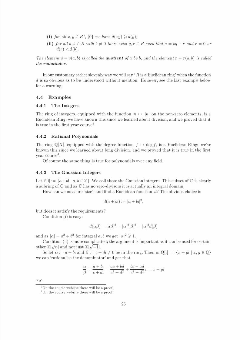
(i) for all x, y ∈ R \ {0} we have d(xy) d(y);

(ii) for all a, b ∈ R with b = 0 there exist q, r ∈ R such that a = bq + r and r = 0 or d(r) < d(b).

The element q = q(a, b) is called the quotient of a by b, and the element r = r(a, b) is called the remainder .

In our customary rather slovenly way we will say ‘R is a Euclidean ring’ when the functiond is so obvious as to be understood without mention. However, see the last example belowfor a warning.

4.4 Examples

4.4.1 The Integers

The ring of integers, equipped with the function n

→ |n

|on the non-zero elements, is a

Euclidean Ring: we have known this since we learned about division, and we proved that itis true in the first year course3.

4.4.2 Rational Polynomials

The ring Q[X ], equipped with the degree function f → deg f , is a Euclidean Ring: we’veknown this since we learned about long division, and we proved that it is true in the firstyear course4.

Of course the same thing is true for polynomials over any field.

4.4.3 The Gaussian Integers

Let Z[i] := {a + bi | a, b ∈ Z}. We call these the Gaussian integers. This subset of C is clearlya subring of C and as C has no zero-divisors it is actually an integral domain.

How can we measure ‘size’, and find a Euclidean function d? The obvious choice is

d(a + bi) := |a + bi|2,

but does it satisfy the requirements?Condition (i) is easy:

d(αβ ) = |αβ |2 = |α|2|β |2 = |α|2d(β )

and as |α| = a

2

+ b

2

for integral a, b we get |α|2

1.Condition (ii) is more complicated; the argument is important as it can be used for certainother Z[

√n] and not just Z[

√−1].So let α := a + bi and β := c + di = 0 be in the ring. Then in Q[i] := {x + yi | x, y ∈ Q}

we can ‘rationalise the denominator’ and get that

α

β =

a + bi

c + di=

ac + bd

c2 + d2+

bc − ad

c2 + d2i =: x + yi

say.

3On the course website there will be a proof.4On the course website there will be a proof.

25



This is the exact quotient in Q[i], but what is the best we can do in Z[i]? The nearestwe can get is the number κ := m + ni, where m is the integer nearest x, and n the integernearest y; note that |x − m| 1

2 and |y − n| 12 .

Nowα

β = x + yi = m + ni + (x − m) + (y − n)i

and multiplying by β we get

α = (m + ni)β + ((x − m) + (y − n)i) β.

Put as quotient q(α, β ) := m + ni ∈ Z[i]. As remainder we then would have

r(α, β ) := ((x − m) + (y − n)i) β = α − q(α, β ) ∈ Z[i].

We now compute

d(((x − m) + (y − n)i) β ) = | ((x − m) + (y − n)i) β |2

= | ((x − m) + (y − n)i) |2

|β |2

= ((x − m)2 + (y − n)2) |β |2 1

2 |β |2< d(β )

and see that condition (ii) is satisfied.

4.4.4 Fields

Let K be a field, and define d : K \ {0} → N \ {0} by d(x) = 1. It is then trivial to see thatwe have a (very dull) Euclidean Ring where all the remainders are 0.

4.4.5 The Integers, but not as we know them

The ring of integers, equipped with the function

d(n) = the number of digits when |n| is expressed in base 2,

is a Euclidean Ring.For condition (i), note that

2M + lower powers of 2 · 2N + lower powers of 2

=

2M +N + lower powers of 2

and so d(xy) = d(x) + d(y) d(y).

For condition (ii), all is clear if a = 0, or indeed if d(a) < d(b); just take q = 0 andr = a. So argue by induction on d(a). Suppose that a = ξ

2M + lower powers of 2

, and

b = η

2N + lower powers of 2

with ξ = ±1 and η = ±1. We are assuming M N , soconsider a =

a − 2M −N ξηb

+ 2M −N ξηb. The number

a − 2M −N ξηb

requires fewer than

M = d(a) binary digits, so we can find q and r such thata − 2M −N ξηb

= bq + r

and r = 0 or d(r) < d(b).Taking q = q + 2M −N ξη (=q ± 2M −N ) gives what we need.

This example shows that we need to take care when we say ‘R is a Euclidean Ring’.

26



4.5 Units and Associates

If we are interested in factorisations the first thing we need to deal with are the factorisationsof the identity: we must find the units of the ring. So let R equipped with d be a Euclideanring.

Lemma 4.5.1. For all a ∈ R, d(a) d(1).

Proof. Condition (i) applied to a = a · 1 gives this at once.

Lemma 4.5.2. For all units u ∈ R∗, d(u) d(1).

Proof. Condition (i) applied to 1 = v · u gives this at once.

Lemma 4.5.3. For all x ∈ R such that d(x) = d(1), we have that x is a unit.

Proof. Use condition (ii) to get q and r such that

1 = xq + r with r = 0, or d(r) < d(x).

If r = 0 then we have by hypothesis d(r) < d(x) = d(1); this contradicts Lemma 1. So weget exact division, 1 = xq and x is a unit.

To summarise:

Proposition 4.5.4 (Units of a Euclidean ring). Let R equipped with d be a Euclidean ring;then the group of units is given by

R∗ = {x ∈ R | d(x) = d(1)} .

In fact we may arrange things so that we have d(1) = 1. For suppose that d(1) = k + 1for k ∈ N. We’ve just seen that for all a ∈ R we have that d(a) d(1), so the functiond : R \ {0} → N \ {0} by d : a → d(a) − k is well-defined. It is clear that it also satisfiescondition (i) and condition (ii) with the same quotient and remainder.

The following is also useful about a Euclidean ring R:

Lemma 4.5.5. Let u ∈ R∗ and a ∈ R. Then d(ua) = d(a).

Proof. Let v ∈ a be such that vu = 1. We then have by condition (i) that d(a) = d(vua) d(ua) d(a); equalities rule, and d(a) = d(ua).

27



The following subsections, establishing that the integers and polynomial rings over fieldsare Euclidean are included purely for completeness; they were covered in the first year course.

Revision: integers

Let d : Z \ {0} → N \ {0} be given by d(n) = |n|.For condition (i) we can use the properties of and |n| we developed in Analysis I and

see that d(xy) = |xy| = |x||y| = |x|d(y) d(y).For condition (ii) note that

a = bq + r ⇐⇒ (−a) = b(−q) + (−r)

and |r| = | − r|; so it is enough to deal with the case a 0.We can argue by (strong) induction on a; the result is true for a = 0 if we take q = 0 and

r = 0. Indeed the result is true for a < |b|, just take q = 0 and r = a. For a |b| note thata = (a − |b|) + |b|, so we can use the inductive hypothesis to get (a − |b|) = bq + r with r = 0or |r| < |b|. Taking q = q ± 1 as case may be completes the proof.

Revision: polynomials

Let d : K[X ] \ {0} → N \ {0} be given by d(f ) = deg(f ), the degree of f .For condition (i) note that if f =

mk=0 akX k and g =

nk=0 bkX k, with am = 0 and

bn = 0 then f ·g =m+n

k=0 ckX k where cm+n = ambn. Hence deg f · g = deg f +deg g deg g.For condition (ii), again it is clearly true if f = 0; just take q = r = 0. Otherwise note

that if the top coefficient of f is α = 0 and the top coefficient of g is β = 0, then

f = gq + r ⇐⇒ 1α

f =1β

g

β α

q

+1α

r

;

clearly deg1α

f

= deg f , deg1β

g

= deg g and deg1α

r

= deg r. Hence we may assume

that f, g are monic, that is have top coefficients 1.Now we may argue by induction on deg f ; if deg f = 0 or more generally deg f < deg g we

put q = 0 and r = f and are done. Otherwise, note that f (X ) =

f (X ) − X deg f −deg gg(x)

+X deg f −deg gg(x), and that deg

f (X ) − X deg f −deg gg(x)

< deg f . By the inductive hypoth-

esis we can then find q and r such that

f (X )

−X deg f −deg gg(X ) = g(X )q(X ) + r(X )

with deg r < deg g or r = 0. Now put q(X ) = q(X ) + X deg f −deg g and we are done.

28




1. If K is a field then any non zero element of K divides any other non zero element of K.

2. If a, b are associates then a|b and b|a.

3. If a is irreducible and a, b are associates then b is also irreducible.

4. If a is prime and a, b are associates then b is also prime.

5. a|b if and only if (a) ⊇ (b).

6. The ideal < X > + < Y > of R[X, Y ] is principal.

7. R[X, Y ] is a Euclidean domain.

8. If R is Euclidean ring with Euclidean function d then d(a) > d(1) for all a = 0, a ∈ R.

29



5 Factorisation in Euclidean Rings

5.1 Ideals are ‘principal’

We recall a trivial fact and a definition:

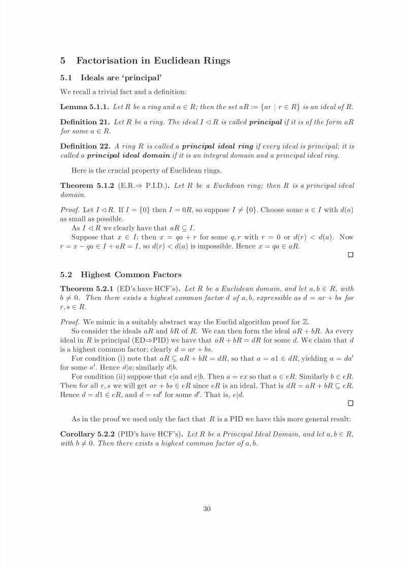
Lemma 5.1.1. Let R be a ring and a ∈ R; then the set aR := {ar | r ∈ R} is an ideal of R.

Definition 21. Let R be a ring. The ideal I ¡R is called principal if it is of the form aR for some a ∈ R.

Definition 22. A ring R is called a principal ideal ring if every ideal is principal; it iscalled a principal ideal domain if it is an integral domain and a principal ideal ring.

Here is the crucial property of Euclidean rings.

Theorem 5.1.2 (E.R.⇒ P.I.D.). Let R be a Euclidean ring; then R is a principal ideal domain.

Proof. Let I ¡R. If I = {0} then I = 0R, so suppose I = {0}. Choose some a ∈ I with d(a)as small as possible.

As I ¡R we clearly have that aR ⊆ I .Suppose that x ∈ I ; then x = qa + r for some q, r with r = 0 or d(r) < d(a). Now

r = x − qa ∈ I + aR = I , so d(r) < d(a) is impossible. Hence x = qa ∈ aR.

5.2 Highest Common Factors

Theorem 5.2.1 (ED’s have HCF’s). Let R be a Euclidean domain, and let a, b ∈ R, with

b = 0. Then there exists a highest common factor d of a, b, expressible as d = ar + bs for r, s ∈ R.

Proof. We mimic in a suitably abstract way the Euclid algorithm proof for Z.So consider the ideals aR and bR of R. We can then form the ideal aR + bR. As every

ideal in R is principal (ED⇒PID) we have that aR + bR = dR for some d. We claim that dis a highest common factor; clearly d = ar + bs.

For condition (i) note that aR ⊆ aR + bR = dR, so that a = a1 ∈ dR, yielding a = da′

for some a′. Hence d|a; similarly d|b.For condition (ii) suppose that e|a and e|b. Then a = ex so that a ∈ eR. Similarly b ∈ eR.

Then for all r, s we will get ar + bs ∈ eR since eR is an ideal. That is dR = aR + bR ⊆ eR.Hence d = d1

∈eR, and d = ed

′for some d

′. That is, e

|d.

As in the proof we used only the fact that R is a PID we have this more general result:

Corollary 5.2.2 (PID’s have HCF’s). Let R be a Principal Ideal Domain, and let a, b ∈ R,with b = 0. Then there exists a highest common factor of a, b.

30



5.3 Factorisation

Proposition 5.3.1 (Irreducible ⇒ Prime in a PID). Let R be a Principal Ideal Domain,and let x ∈ R be irreducible. Then x is prime.

We first prove an important lemma.

Lemma 5.3.2 (Euler’s Lemma). Suppose that h|ab and h, a have 1 as highest common factor. Then h|bProof. We have that 1 = hr + as, and that ab = hk for some r,s,k. Then

b = b(hr + as) = bhr + bas = bhr + hks = (br + ks)h

and we are done.

Now we prove the proposition.

Proof. Now suppose that x is irreducible and that x|ab. Suppose that x |a. Let d be ahighest common factor of x and a. Then d|x by definition, and so x = de for some e. As x isirreducible we have that d or e is a unit. Suppose that e is a unit, with ef = 1. Then d = xf ,and so xf |a; then at once x|a, a contradiction. So we have that d is a unit, an associate of 1. hence 1 is also a highest common factor, and then we are done by the lemma.

The following is an abstract version of the concrete fact that in Z we cannot go onfactorising a number into smaller and smaller pieces.

Proposition 5.3.3 (PID ⇒ ‘ascending ideal chains’ terminate). Let R be a Principal Ideal Domain, and I k ¡ R, and I k ⊆ I k+1 for k = 0, 1, . . . . Then for some N , I k = I N for all

k N .

Proof. Consider the subset I :=k I k; we prove that it is an ideal. Clearly 0 ∈ I 0 ⊆ I .

Suppose that x, y ∈ I and a ∈ R; then x ∈ I r and y ∈ I s for some r, s 0. Hence withn := max(r, s) we have that x, y ∈ I n ¡R. Then −x, x + y, r · x ∈ I n ⊆ I and we are done.

Now R is a PID, so we have that I = aRfor some a ∈ R. Then a = a1 ∈ aR = I =k I k,

so that a ∈ I N for some N , and indeed a ∈ I k ¡ R for all k N . Now we have thataR ⊆ I k ⊆ I = aR and are done.

5.4 Unique Factorisation

This is an area where our intuition developed in Z and K[X ] notoriously leads us astray inmore general domains.

Definition 23. We will say that the integral domain R is a Unique Factorisation Do-

main (UFD), or that it has unique factorisation , if

(i) every element 0 = a ∈ R is either a unit or can be written a = f 1f 2 . . . f M as a product of (a finite number of) irreducible elements f 1, f 2, . . . , f M ∈ R;

(ii) if f 1f 2 . . . f M = g1g2 . . . gN for irreducibles f 1, f 2, . . . , f M and g1, g2, . . . , gN then M = N ,and for each k = 1, . . . , M there exists a unit uk such that after relabelling the gk wehave gk = ukf k.

31



As a trivial example, every field is a UFD. From our experience we know that Z is aUFD.

Theorem 5.4.1 (PID ⇒ UFD). Let R be a Principal Ideal Domain. Then R is a UniqueFactorisation Domain.

Proof. There are two different things to be proved: the existence of factorisation into irre-ducibles and the uniqueness.

For the existence, consider 0 = x ∈ R, and suppose that we cannot express x in therequired form. Clearly x can’t be a unit, so x = yz where neither y nor z is a unit. If bothy and z are expressible as products of irreducibles so is x; so one of these, without loss ycan’t be so expressed. Now put I 0 := xR and I 1 := yR. As x = yz we have that I 0 ⊆ I 1.Moreover, if I 1 = I 0 we would have that y = y1 ∈ yR = xR, so that y = xa for some a.Then x = yz = xaz, and as x = 0 we have 1 = az and z is a unit—which it is not. Sowe have found unequal ideals I 0 ⊂ I 1. But we can repeat this process, starting now with y,and so construct eventually a properly ascending chain of ideals—which we have seen to be

impossible.As for uniqueness, we prove something slightly stronger. We prove that if uf 1f 2 . . . f M =

vg1g2 . . . gN for irreducibles f 1, f 2, . . . , f M and g1, g2, . . . , gN and units u, v then M = N andafter relabelling f k and gk are associates. We do this by induction on M + N , the resultbeing vacuously true when M + N = 0.

As f 1 is irreducible it is prime, and so f 1 divides some gk; relabel so that f 1|g1 and g1 =f 1u1 say. But g1 is irreducible, and so u1 is a unit. We therefore have that uu1f 1f 2 . . . f M =vu1g1g2 . . . gN = vf 1g2 . . . gM , and so (as R is an integral domain) (uu1)f 2 . . . f M = vg2 . . . gM .We can now apply the inductive hypothesis and get M − 1 = N − 1 and after relabelling theremaining f k and gk are associates.

Remark 5.4.2. We have shown the inclusions

{Euclidean rings} ⊂ {Principal ideal domains} ⊂ {Unique factorisation domains}

All these are proper inclusions. We will see in the exercises that Z[X ] is a UFD but not a

PID. It can be shown that Z[1+√−192 ] is a PID but it is not a Euclidean ring.

32




1. Z[X ] is a UFD.

2. Let f (X ), g(X ) ∈ Q(X ). Then there is some h(x) ∈ Q(X ) such that< f (X ) > + < g(X ) >=< h(X ) >.

3. Let f (X ), g(X ) ∈ Q(X ). Then there is some h(x) ∈ Z(X ) such that

< f (X ) > + < g(X ) >=< h(X ) >.

4. Let a be a prime element in a PID. Then the ideal < a > is maximal.

5. If F is a field and f : F[X ] → C is a homomorphism then kerf is a maximal ideal of F[X ].

33



6 The Euclidean Algorithm

In this section we revisit the Euclidean Algorithm we learned in the first year, and discusshow far it applies in general Euclidean Domains. We will see that the main part of the

algorithm is still in place.

6.1 Algorithms

Sometimes we don’t want simple assertions about the existence of a mathematical object, notmatter how carefully they’ve been proved: we want a way to find it in practice. In the firstyear courses we met several ‘algorithms’ which allowed us to find or construct things: explicitprocesses which can be carried out in a finite number of steps, and which are guaranteed todeliver the object we seek.

For example—but there are many others if you look closely—we have: the GaussianElimination process provides algorithms for finding all solutions of a set of linear equations(and hence inverting matrices where possible); the Division Algorithm for integers, and

for polynomials with rational coefficients, allows us to calculate a particular q, r such thata = bq + r; and the Extended Euclidean Algorithm lets us calculate hcf(x, y) and express itas Xx + Y y.

Some interesting things, though, are beyond our reach: there’s no effective way to calcu-late the decimal expansion of a/b where a, b ∈ R are given by their decimal expansions.

6.2 The Division Algorithm for K[X ]

Given f, g ∈ K[X ] with g = 0 we can find algorithmically q, r ∈ K[X ] such that f = gq + rwhere r = 0 or deg r < deg g: provided we can somehow carry out the arithmeticoperations in K. There is no way to do this in general, so in this subsection we assume

that we have an Oracle which will on demand deliver to us 0, −x, x + y, 1, xy, and (if y = 0)x/y.

Provided with this Oracle all we need to do is mimic the steps of the Division Algorithmwe learned for Q[X ].

It is clear what to do if deg f < deg g; just take q = 0 and r = f .Otherwise suppose that f = aX M +lower degree terms and g = bX N +lower degree terms;

here a, b are nonzero and M N 0. Consider f (X ) − (a/b)X N −M g(X ); the oracle helpsus with the coefficients of this polynomial. This is a polynomial of degree less than deg f weuse recursion, and find q, r such that

f (X ) − (a/b)X N −M g(X ) = g(X )q(X ) + r(X ) where r(X ) = 0 or deg r < deg g.

Now put r(X ) := r(X ) and q(X ) := g(X ) + (a/b)X N −M g(X ), where again the Oracle helpsus with the latter calculation.

It is easy to prove by induction that this process works.

6.3 Euclid’s Algorithm in Euclidean Domains

Let R equipped with d : R \ {0} → N \ {0} be a Euclidean Domain.Note that for a, b ∈ R this merely asserts the existence of a q, r such that a = bq + r

with r = 0 or d(r) < d(b. We’ve seen above that sometimes there are algorithms to calculatethese, although we may need an Oracle or Giant Look-up Table to help. Sometimes there

34



may not be. So throughout this subsection assume that there is an Oracle which will deliveron demand a suitable q and r.

In that case, the Extended Euclidean Algorithm we learned in the first-year course willcalculate hcf(x, y) and express it as Xx + Y y.

Proposition 6.3.1 (Extended Euclidean Algorithm). Let R equipped with d be a Euclidean Domain, and suppose that for any x, y = 0 we are given a definite q(x, y) and r(x, y) such that x = yq(x, y) + r(x, y) where r(x, y) = 0 or d(r(x, y)) < d(y).

For every pair of elements a, b ∈ R, not both 0, proceed as follows:

1. (a) let a0 := a, m0 := 1, and n0 := 0;

(b) let a1 := b, m1 := 0, and n1 := 1;

(c) let i := 1;

2. while ai = 0 repeat the following steps:

(a) let qi+1 := q(ai−1, ai);(b) i. let ai+1 := ai−1 − qi+1ai;

ii. let mi+1 := mi−1 − qi+1mi;

iii. let ni+1 := ni−1 − qi+1ni;

(c) increase i to i + 1;

3. (a) let d = ai−1;

(b) let m = mi−1;

(c) let n = ni−1.

Then the following are true:

1. the process stops after a finite number of steps;

2. every divisor of both a and b also divides d;

3. d divides both a and b;

4. d = ma + nb.

Proof. The proof is identical to the one for integers.

6.4 Chinese Remainder Theorem

A final remark is in order. The Extended Euclidean Algorithm is exactly what we need tocalculate the inverse of the isomorphism R/xyR ∼= R/xR ⊕ R/yR of the Chinese RemainderTheorem.

35



7 Factorisation in Q[X ]

In this section we deal with some very concrete matters concerning the factorisation of poly-nomials with rational coefficients. Any such polynomial is a rational multiple of a polynomial

with integer coefficients, and so we may concentrate on the integral associate. For such poly-nomials we have various techniques to help us, in particular we can work ‘modulo p’ forvarious primes; or we can use other arithmetic tricks. We describe some of these, and weprove the important theorem which reconciles factorisation of polynomials over Q and overZ.

7.1 Factorisation in Z[X ] and Z p[X ]

We begin with a general lemma.

Lemma 7.1.1. Let R and S be rings, and let f : R → S be a homomorphism, f : a → a.Then π : R[X ] → S [X ] given by π :

N k=0 akX k →

N k=0 akX k is a homomorphism with

image f (R)[X ] and kernel (ker f )[X ].

Proof. In view of how we add and multiply polynomials all we need to check is that

ak + b + k = ak + bk and

r+s=n

arbs =

r+s=n

arbs.

The remarks on kernel and image are clear.

We can use what we have learned about rings and homomorphisms to give a usefulpractical test for irreducibility5 in the ring Z[X ].

Proposition 7.1.2 (Eisenstein’s criterion). Let f (X ) = N

k=0ck

X k be a polynomial in Z[X ],and let p ∈ Z be a prime. Suppose that p|ck for all k = 0, 1, . . . , N − 1, p |cN and p2 |c0.Then f (X ) has no factor of smaller degree in Z[X ].

Proof. Suppose that we had that f (X ) = g(X )h(X ), with g(X ) =N 1

k=0 akX k and h(X ) =N 2k=0 bkX k and N 1, N 2 > 1. Extending the natural homomorphism Z → Z p to the poly-

nomial rings we would then have that π(g(X )π(h(X )) = π(f (X )) = cN X N = 0, so thatπ(g(X )) = aX N 1 and h(X ) = bX N 2 by the unique factorisation in the Euclidean domainZ p[X ]. Hence we have that a0 = b0 = 0; that is p|a0 and p|b0, yielding p2|a0b0 = c0 contraryto hypothesis.

There are many examples of this. For instance, (X 2+125)2(X 3+25)4+5 has only factorsof degree 16 in Z[X ] and so, being monic, is irreducible.

More famous are the cyclotomic polynomials or prime order. Let Φ p(X ) := Xp−1X−1 ; then

Φ p has no factor of degree k with 1 < k < ( p − 1). We can’t use Eisenstein directly; butinstead we apply the result to Φ p(X + 1); the details are an exercise.

5Well, almost irreducibility: see later.

36



7.2 Factorization in Z[X ] and Q[X ]

Although we often work with polynomials with integral coefficients, we are really interestedin whether these factorise in the ring Q[X ]. It is clear that in a trivial way a polynomialmay be a product of two irreducibles in Z[X ] but of only one irreducible in Q[X ]—take for

example f (X ) = 2X . We can easily check that in the large ring Q[X ] this is irreducible; butin the small ring it is the product of two irreducibles 2 and X . What we want to see is thatessentially nothing more complicated than this is possible.

Theorem 7.2.1. Let 0 = h ∈ Z[X ]. Suppose that h = f · g with f, g ∈ Q[X ]. Then thereexist f , g ∈ Z[X ] with deg f = deg f and deg g = deg g, such that h = f · g.

Proof. Write f =M

k=0 akX k, g =N

k=0 bkX k and let ck :=

r+s=k arbs be the coefficientsof h.

We may multiply f by the least common multiple of the denominators of its coefficients,and then divide the resulting polynomial by the highest common factor of its (integral!)

coefficients. In that way we get f = α˜

f , where α ∈Q

and˜

f is a polynomial of the samedegree as f , and has integral coefficients whose highest common factor is 1. We can findcorresponding β ∈ Q and g ∈ Z[X ] with g = β g.

We can find corresponding γ ∈ Z—there are no denominators to clear so γ is integral—and h ∈ Z[X ] with h = γ h.

Then we have, after re-arranging the rationals,

n · h(X ) = m · f (X ) · g(X ), for some m, n ∈ Z.

(The X ’s are inserted into the polynomials for clarity.)How are m and n related? Well n is the highest common factor of the coefficients of the

polynomial on the left hand side. But the highest common factor of the coefficients of the

polynomial on the right hand side is m times the highest common factor of the coefficientsof f (X ) · g(X ). In a moment we will prove that the latter highest common factor is 1. Som = n and we have that

h(X ) = f (X ) · g(X ),

which we multiply by γ ∈ Z to get

h(X ) = γ · h(X ) = γ · f (X ) · g(X ).

Define f := γ · f and g := g and we are done.

The missing lemma is so important it deserves a separate subsection.

7.3 Gauss’s Lemma

We begin with some pieces of notation.

Definition 24. Let 0 = f ∈ Z[X ]. Then by the content of f , denoted by c(f ), we mean the highest common factor of the coefficients of f . If the content of f is 1 then we say f isprimitive.

Proposition 7.3.1 (Gauss’s Lemma). Let f, g ∈ Z[X ] and suppose that c(f ) = c(g) = 1.Then c(f · g) = 1.

37



Proof. If false let the prime p divide all the coefficients of the product. Extend the naturalhomomorphism Z → Z p to a homomorphism π of the polynomial rings in the standard way.Then

0 = π(f · g) = π(f ) · π(g)

and so, since Z p[X ] is an integral domain, either π(f ) = 0 or π(g) = 0. But that implies pdivides every coefficient of f or every coefficient of g, a contradiction.

Corollary 7.3.2. Let f, g ∈ Z[X ]; then c(f · g) = c(f )c(g).

Proof. Trivial.

7.4 Z[X ] is a UFD

We can use Gauss’s Lemma and the techniques of the previous sections to prove that in thering Z[X ] every polynomial factorises uniquely into a product of primes in Z times a product

of primitive polynomials each irreducible in Q[X ].

7.5 An algorithm for factorisation in Q[X ]

How can we factorise a polynomial f ∈ Q[X ]? As we’ve seen we may assume that f ∈ Z[X ]and carry out our factorisations over Z.

Here are a couple of trivial starting points:

Lemma 7.5.1. Suppose that n ∈ Z. If f (n) = 0 then X − n|f .

Proof. Remainder Theorem and Gauss’s Lemma.

Lemma 7.5.2. Suppose that g|f in Z[X ]; and that n ∈ Z. Then g(n)|f (n).

Proof. Trivial.

With these in mind we search for factors of f in Z[X ] of degree d = 1, 2, . . . , deg f − 1.Of course whenever we find a factor we divide it out and then look recursively at two factorswe have found.

The following lemma controls the possible values of a factor of degree d may take.

Lemma 7.5.3. Let a0, a1, a2, . . . , ad ∈ Z be distinct integers, and suppose that f (ak) = 0 for each k. Then there are only finitely many (d + 1)-tuples (b0, b1, . . . , bd) such that bk|f (ak) for each k.

Proof. This is essentially the fact that Z is a UFD.

The following lemma allows us to reconstruct a polynomial of degree d from its values at(d + 1) places.

Lemma 7.5.4. Let a0, a1, a2, . . . , ad ∈ Z be distinct integers, and let b0, b1, . . . , bd ∈ Q. Thereis exactly one polynomial g ∈ Q[X ] of degree at most d such that g(ak) = bk for all k.

38



Proof. This is just the Chinese Remainder Theorem. To be absolutely specific we could, asLagrange did, take

g(X ) =d

k=0

bk j=k

X − a jak

−a j

.

By the previous two lemmas we can now construct a finite list of all those polynomials gof degree d in Q[X ] which can possibly be divisors of f .

be more precise if m = deg f for any d ≤ m − 1 we calculate, f (0), f (1),...,f (d + m).Since f has at most m roots, at least d + 1, among those are = 0. Let’s say that for

{a0, a1,...,ad} ⊂ {0, 1,...,d + m} we have f (ai) = 0. Using lemmas 7.5.3, 7.5.4 we produce afinite list of polynomials of degree d which are possible divisors of f . If g is such a polynomialwe check whether in fact g ∈ Z[X ], and then, by long division, whether g|f . If g|f for someg then we write f = gh and we repeat the procedure for g, h. This gives us an algorithm todecompose any polynomial f

∈Q[X ] as a product of irreducibles. Of course if no g from our

finite list divides f we conclude that f is irreducible.

7.6 Factorization in R[X ] and C[X ]

According to the Fundamental Theorem of Algebra any f ∈ C[X ] has a root in C. Inparticular a polynomial f ∈ C[X ] is irreducible if and only if deg f = 1.

Let f ∈ R[X ] be a polynomial with deg f > 2. If f has areal root clearly it is notirreducible. If a non-real a ∈ C is a root of f then a is also a root. So (X − a)(X − a) dividesf . But (X − a)(X − a) = X 2 − 2ℜaX + |a|2 ∈ R[X ]. So again f is not irreducible. Hencethe irreducible polynomials in R[X ] are the polynomials of degree 1 and the polynomials of

degree 2 with no real roots.

39




1. If the polynomial f (x) ∈ Z[X ] is irreducible in Z[X ] then f (X ) is also irreducible inZ3[X ].

2. If the polynomial f (x) ∈ Z7[X ] is irreducible in Z7[X ] then f (X ) is also irreducible inZ[X ].

3. If K is a field, a polynomial of degree 3, f (X ) ∈ K[X ] is irreducible if and only if it hasno roots in K.

4. There is a monic polynomial f (X ) ∈ Z[X ] such that f ( 20082009) = 0.

rings notes

Documents