HAL Id: hal-01570533https://hal.archives-ouvertes.fr/hal-01570533

Submitted on 31 Jul 2017

HAL is a multi-disciplinary open accessarchive for the deposit and dissemination of sci-entific research documents, whether they are pub-lished or not. The documents may come fromteaching and research institutions in France orabroad, or from public or private research centers.

L’archive ouverte pluridisciplinaire HAL, estdestinée au dépôt et à la diffusion de documentsscientifiques de niveau recherche, publiés ou non,émanant des établissements d’enseignement et derecherche français ou étrangers, des laboratoirespublics ou privés.

Distributed under a Creative Commons Attribution| 4.0 International License

Rigid-Body Dynamics with Friction and ImpactDavid E. Stewart

To cite this version:David E. Stewart. Rigid-Body Dynamics with Friction and Impact. SIAM Review, Society for Indus-trial and Applied Mathematics, 2000, 42 (1), pp.3-39. �10.1137/S0036144599360110�. �hal-01570533�

Rigid-Body Dynamics with Friction and Impact

David E. Stewart

Abstract. Rigid-body dynamics with unilateral contact is a good approximation for a wide range ofeveryday phenomena, from the operation of car brakes to walking to rock slides. It is alsoof vital importance for simulating robots, virtual reality, and realistic animation. However,correctly modeling rigid-body dynamics with friction is difficult due to a number of dis-continuities in the behavior of rigid bodies and the discontinuities inherent in the Coulombfriction law. This is particularly crucial for handling situations with large coefficients offriction, which can result in paradoxical results known at least since Painleve [C. R. Acad.Sci. Paris, 121 (1895), pp. 112–115]. This single example has been a counterexample andcause of controversy ever since, and only recently have there been rigorous mathematicalresults that show the existence of solutions to his example.

The new mathematical developments in rigid-body dynamics have come from severalsources: “sweeping processes” and the measure differential inclusions of Moreau in the1970s and 1980s, the variational inequality approaches of Duvaut and J.-L. Lions in the1970s, and the use of complementarity problems to formulate frictional contact problemsby Lotstedt in the early 1980s. However, it wasn’t until much more recently that thesetools were finally able to produce rigorous results about rigid-body dynamics with Coulombfriction and impulses.

Key words. rigid-body dynamics, Coulomb friction, contact mechanics, measure-differential inclu-sions, complementarity problems

1. Rigid Bodies and Friction. Rigid bodies are bodies that cannot deform. Theycan translate and rotate, but they cannot change their shape. From the outset thismust be understood as an approximation to reality, since no bodies are perfectlyrigid. However, for a vast number of applications in robotics, manufacturing, bio-mechanics (such as studying how people walk), and granular materials, this is anexcellent approximation. It is also convenient, since it does not require solving large,complex systems of partial differential equations, which is generally difficult to doboth analytically and computationally. To see the difference, consider the problemof a bouncing ball. The rigid-body model will assume that the ball does not deformwhile in flight and that contacts with the ground are instantaneous, at least while theball is not rolling. On the other hand, a full elastic model will model not only thecontacts and the resulting deformation of the entire ball while in contact, but alsothe elastic oscillations of the ball while it is in flight. Apart from the computationalcomplexity of all this, the analysis of even linearly elastic bodies in contact with a

rigid surface subject to Coulomb friction using a Signorini contact condition is notcompletely developed even now [22, 23, 56, 30, 57, 62, 65]. Even if all this can bedone, most of the details of the motion for the fully elastic body are not significanton the time- or length-scales of interest in many of the applications described above.For more information about applications of rigid-body dynamics, see, for example,[20, 21, 92] regarding granular flow and [11, 108] regarding virtual reality and computeranimation.

There are some disadvantages with a rigid-body model of mechanical systems.The main one is that the velocities must be discontinuous. Consider again a bouncingball. While the ball is in flight, there are no contact forces acting on it. But whenthe ball hits the ground, the negative vertical velocity must become a nonnegativevertical velocity instantaneously. The forces must be impulsive; they are no longerordinary functions of time but rather distributions or measures. While there has beenconsiderable work on differential equations with impulsive right-hand sides, these areusually concerned with situations where the impulsive part is known a priori and isnot part of the unknown solution. (The work of Bainov et al., for example, has thischaracter [8, 7, 71]. In these works Bainov et al. can allow for some dependence ofthe time of the discontinuity on the solution, but the way the solution changes at thediscontinuity is assumed to be known, and problems like bouncing balls, where theball comes to rest in finite time after infinitely many bounces, are beyond the scopeof their approach.)

The rigid body model with Coulomb friction has been subject to a great dealof controversy, mostly due to a simple model problem of Painleve which appearsnot to have solutions. The list of papers on this problem is quite extensive andincludes [11, 12, 27, 28, 36, 49, 68, 76, 77, 78, 84, 82, 88, 89, 91, 109, 131, 128]. Themodern resolution of Painleve’s problem involves impulsive forces and still generatescontroversy in some circles.

In this article, an approach is described that combines impulsive forces (measures)with convex analysis. It develops a line of work begun by Schatzman [117] andJ. J. Moreau [87, 88, 90, 91] and continued by Monteiro Marques, who produced thefirst rigorous results in this area [83, 84]. Related work has been done by Brogliato,which is directed at the control of mechanical systems with friction and impact, andis based on the approach of Moreau and Monteiro Marques; Brogliato’s book [14]gives an accessible account of many of these ideas. The intellectual heritage used inthis work is extensive: convex analysis, measure theory, complementarity problems,weak* compactness, and convergence are all used in the theory, along with energydissipation principles and other more traditional tools of applied mathematics.

A number of aspects of rigid-body dynamics nonetheless remain controversial andunresolved. These include the proper formulation of impact laws and how to correctlyhandle multiple simultaneous contacts. These are discussed below in sections 1.2and 4.4. Neither of these issues affects the internal consistency of rigid-body models;rather, they deal with how accurately they correspond to experimentally observedbehavior.

The structure of this article is as follows. This introduction continues with sub-sections dealing with Coulomb friction and discontinuous ODEs (section 1.1); impactmodels (section 1.2); the famous problem of Painleve (section 1.3); complementarityproblems, which are useful tools for formulating problems with discontinuities (section1.4); and measure differential inclusions (section 1.5). Section 2 discusses how to for-mulate rigid-body dynamics, first as a continuous problem (section 2.1) and then as a

θN

mg

Fv

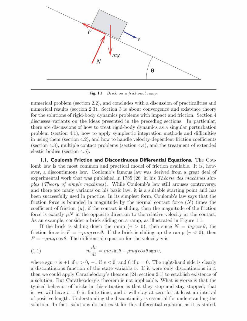
Fig. 1.1 Brick on a frictional ramp.

numerical problem (section 2.2), and concludes with a discussion of practicalities andnumerical results (section 2.3). Section 3 is about convergence and existence theoryfor the solutions of rigid-body dynamics problems with impact and friction. Section 4discusses variants on the ideas presented in the preceding sections. In particular,there are discussions of how to treat rigid-body dynamics as a singular perturbationproblem (section 4.1), how to apply symplectic integration methods and difficultiesin using them (section 4.2), and how to handle velocity-dependent friction coefficients(section 4.3), multiple contact problems (section 4.4), and the treatment of extendedelastic bodies (section 4.5).

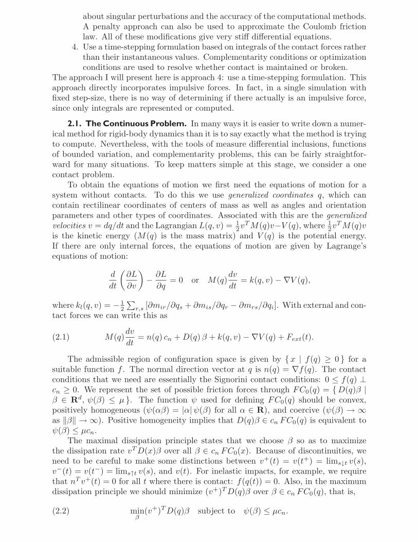
1.1. Coulomb Friction and Discontinuous Differential Equations. The Cou-lomb law is the most common and practical model of friction available. It is, how-ever, a discontinuous law. Coulomb’s famous law was derived from a great deal ofexperimental work that was published in 1785 [26] in his Theorie des machines sim-ples (Theory of simple machines). While Coulomb’s law still arouses controversy,and there are many variants on his basic law, it is a suitable starting point and hasbeen successfully used in practice. In its simplest form, Coulomb’s law says that thefriction force is bounded in magnitude by the normal contact force (N) times thecoefficient of friction (μ); if the contact is sliding, then the magnitude of the frictionforce is exactly μN in the opposite direction to the relative velocity at the contact.As an example, consider a brick sliding on a ramp, as illustrated in Figure 1.1.

If the brick is sliding down the ramp (v > 0), then since N = mg cos θ, thefriction force is F = +μmg cos θ. If the brick is sliding up the ramp (v < 0), thenF = −μmg cos θ. The differential equation for the velocity v is

mdv

dt= mg sin θ − μmg cos θ sgn v,(1.1)

where sgn v is +1 if v > 0, −1 if v < 0, and 0 if v = 0. The right-hand side is clearlya discontinuous function of the state variable v. If it were only discontinuous in t,then we could apply Caratheodory’s theorem [24, section 2.1] to establish existence ofa solution. But Caratheodory’s theorem is not applicable. What is worse is that thetypical behavior of bricks in this situation is that they stop and stay stopped; thatis, we will have v = 0 in finite time, and v will stay at zero for at least an intervalof positive length. Understanding the discontinuity is essential for understanding thesolution. In fact, solutions do not exist for this differential equation as it is stated,

since if v = 0 and dv/dt = 0, then we get 0 = mg sin θ − μmg sgn 0, which can onlybe true if sin θ = 0. To solve a discontinuous differential equation like this, we needto extend the concept of differential equations to differential inclusions [38, 39, 40],which were first considered by A. F. Filippov around 1960. A differential inclusionhas the form

dx

dt∈ F (t, x),

where F is a set-valued function. There are some properties that F should have. Itsgraph { (x, y) | y ∈ F (t, x) } should be a closed set. The values F (t, x) should allbe closed, bounded, convex sets. And F (t, x) should satisfy a condition to prevent“blow-up” in finite time, such as xT z ≤ C(1 + ‖x‖2) for all z ∈ F (t, x). Numericalmethods for discontinuous ODEs need to use this differential inclusion formulationif high accuracy is desired. If this is not done, then the methods typically havefirst order convergence due to rapid “chattering” of the numerical trajectories aroundthe discontinuities for simple discontinuous ODEs. The first published results onnumerical methods for discontinuous ODEs and differential inclusions were those byTaubert [137] in 1976. Further work on numerical methods for differential inclusionsand discontinuous ODEs includes [31, 35, 60, 61, 74, 95, 96, 126, 127, 136, 137, 138].Of these, only [60, 61, 126, 127] give methods with order higher than one.

Excellent overviews of numerical methods for differential inclusions can be foundin Dontchev and Lempio [31] or Lempio and Veliov [75].

Since the rigidity of objects is only an approximation, it is reasonable to considerapproximating the Coulomb law for the friction force by a continuous or smooth law.The discontinuity in the Coulomb friction law has an important physical consequence:a block on an inclined ramp will not move down the ramp as long as the appliedtangential forces do not exceed μN . If the Coulomb law were replaced by a smoothlaw, then the block would creep down the ramp at a velocity probably proportionalto the tangential force divided by μN . Experimentally, very little if any creep isobserved in typical situations with dry friction, which demands a friction force functionthat is discontinuous or very close to being discontinuous. On the other hand, usinga continuous approximation for numerical purposes leads to a stiff ODE. Applyingimplicit time-stepping procedures then results in solutions that are very close to thesolution obtained by applying the implicit method to the corresponding differentialinclusion. In summary, the physics points to real discontinuities, and there is littleadvantage numerically in smoothing the discontinuity. The discontinuity is here tostay.

So far we have considered only one-dimensional friction laws where the set ofpossible friction forces is one-dimensional. For ordinary three-dimensional objects incontact, the plane of relative motion is two-dimensional, and so the set of possiblefriction forces is two-dimensional. In this case, to allow for complications such asanisotropic friction, we need a better approach. A better basis for formulating phys-ically correct friction models is the maximum dissipation principle. This says thatgiven the normal contact force cn, the friction force cf is the one that maximizes therate of energy dissipation −cT

f vrel, where vrel is the relative velocity at the contact,out of all possible friction forces allowed by the given normal contact force cn. Tobe more formal, there is a set FC0 which is the set of possible friction forces cf forcn = 1. The set FC0 is assumed to be closed, convex, and balanced (FC0 = −FC0).So the maximum dissipation principle says that

cf maximizes − cTf vrel over cf ∈ cn FC0.(1.2)

In the case of two-dimensional isotropic friction acting on a particle, FC0 is a diskof radius μ (the coefficient of friction) in the plane of contact. If n is the normaldirection to the contact surface, then the total contact force is n cn + cf . The set ofpossible contact forces is the friction cone, which is given by

FC = { n cn + cf | cn ≥ 0 and cf ∈ cn FC0 }.(1.3)

Of course, as the contact point changes, so does the plane of the possible frictionforces. So we must allow FC0 and FC to depend on the configuration of the system:FC0 = FC0(q) and FC = FC(q). Some pathologies should be prevented, suchas having the normal direction n lying in the vector subspace generated by FC0.Note that FC0 and FC are again set-valued functions. However, they are generallycontinuous ones on the boundary of the admissible region. In the interior of theadmissible region, the normal and frictional contact forces must both be zero, so inthat case, FC(q) = {0}.

1.2. Impact Models. The behavior of impacting bodies is a topic in rigid-bodydynamics that does not arise in formulating other problems in mechanics. It wouldnormally be considered to be the result of the model, rather than an ingredient inbuilding the model. However, for rigid-body dynamics, an impact is regarded as anatomic (i.e., indivisible) event and must be modeled as such. The use of measuredifferential inclusions below does not save us from having to decide. And it is a factof nature that some materials behave more elastically than others on impact. Someseem to be inelastic with little or no “bounce,” and some are very elastic and seemto lose very little energy in an impact. As a general rule, modelers use a coefficientof restitution, usually denoted here by ε between zero and one to describe the impactbehavior of a pair of bodies or materials. For ε = 0 we have purely inelastic impacts,and for ε = 1 the impacts are purely elastic.

There are two generally pervasive approaches to modeling impact behavior. One(the Newtonian approach) relates pre- and postimpact velocities’ normal components(typically nT v(t+) = −ε nT v(t−)) [94]; the other (the Poisson approach) divides theimpact into compression and decompression phases and relates the impulse in thedecompression phase to the impulse in the compression phase: Ndecompr = −ε Ncompr

[110, 114]. The value of the contact impulse for the compression phase of the contactshould be determined by the impulse needed for inelastic impact. Each approach hasbeen found to produce an increase in the total mechanical energy in certain situations!For difficulties with the Newtonian approach in its naive form (even with only onecontact in two dimensions), see Stronge’s article [135] and the references therein andalso Keller’s short article [63].

Whichever approach is used, the case of inelastic impacts is an important referencecase that both approaches must handle: ε = 0. For one contact, this means thatnT v(t+) = 0 for any time t when there is contact. For a fuller discussion of howthe Newton and Poisson approaches can be used and modeled, the reader is againreferred to the excellent book of Brogliato [14]. Another discussion of the Newtonand Poisson formulations is given in Chatterjee and Ruina [18], who also discussalternative collision laws. Note that both the Newton and Poisson impact laws haveserious defects, which are discussed in [18, 135], for example.

One of the abiding difficulties in this area is the lack of understanding of thephysical mechanisms behind impact processes. It has long been believed that threemechanisms are responsible for energy dissipation in impact: (1) localized plasticdeformation; (2) viscous damping in the material; and (3) energy transfer to elastic

vibrations. Until recently it has not been clear which is the most important. Asa result, models have lagged in terms of their physical accuracy and sophistication.Recent work has thrown fresh light onto this issue.

Recent experimental and simulation work, particularly by Stoianovici and Hur-muzlu [133], has highlighted the importance of elastic vibrations, although localizedplastic deformation appears to play a role. Viscous damping seems to play very littledirect role in the impact behavior. This is mostly because the time-scale of the impact(typically between 10 μs and 10 ms for metal objects of sizes between 1 cm and 1 m)is too short for significant viscous damping, except for very high frequency modes.

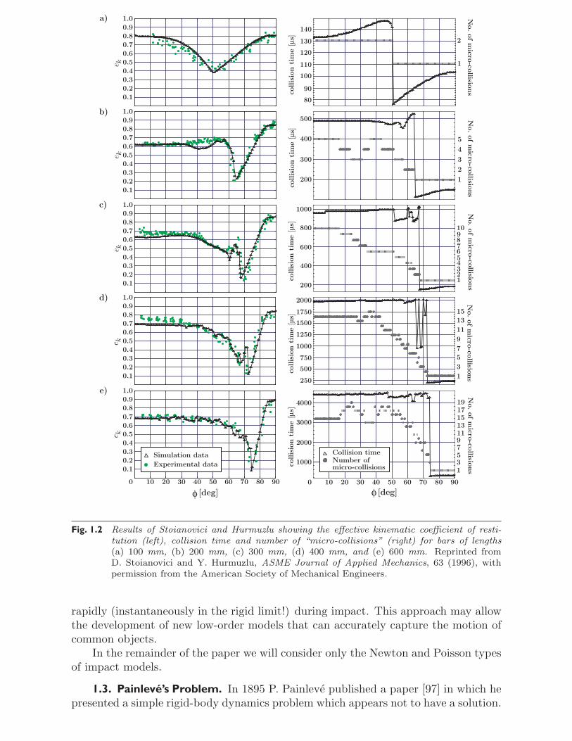
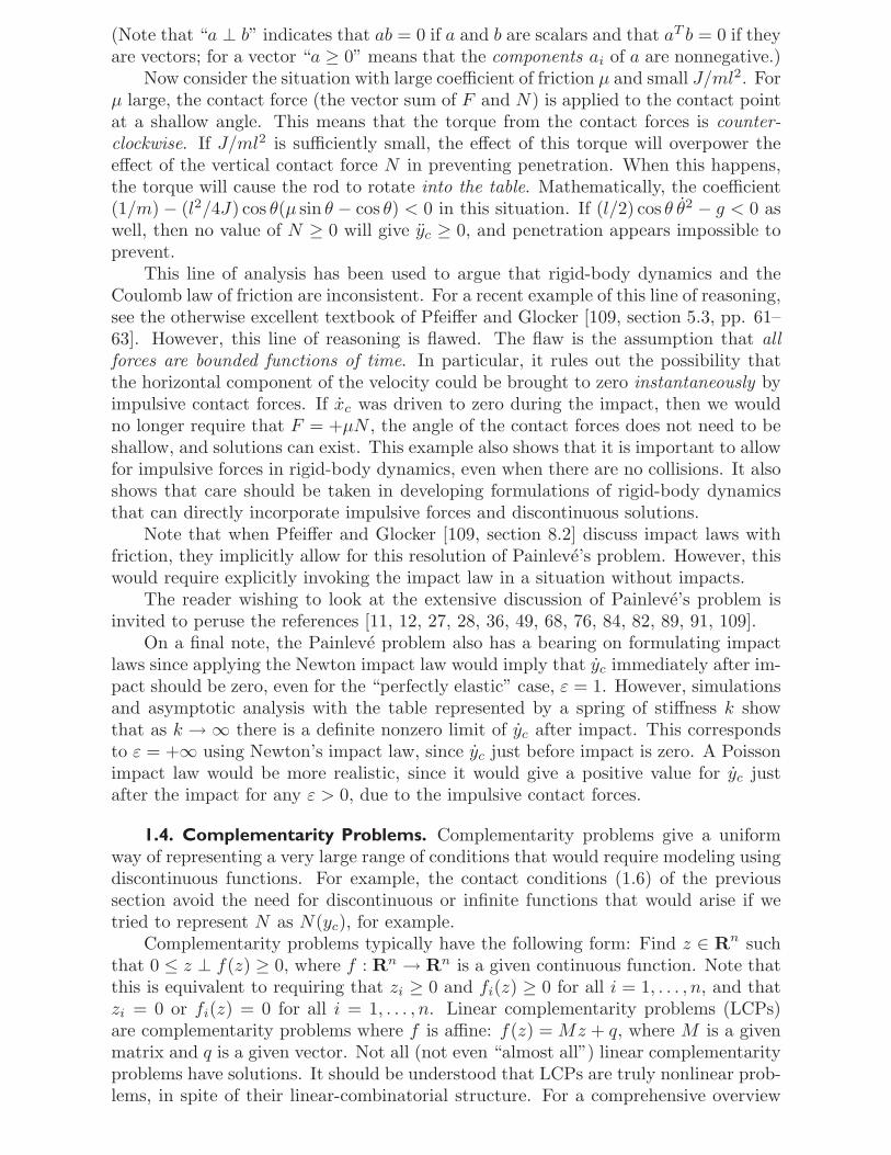
What Stoianovici and Hurmuzlu did was to drop steel bars onto a hard, massiveblock, record the impacts using high-speed video recorders, and identify contacts bymeasuring the current flowing from the bars to the block underneath. One of themain results of their experimental investigation was the way the kinematic coefficientof restitution ε = −(nT v+)/(nT v−) depended on the angle of the bar relative to theupper surface of the block (φ). Figure 1.2 is taken from Stoianovici and Hurmuzlu [133]with the kind permission of the authors and the ASME Journal of Applied Mechanics.As can be seen in Figure 1.2, if the bar is dropped vertically (φ = 90◦), then ε rangesbetween 0.8 and 0.9. As the angle is decreased, ε decreases until ε is between 0.1and 0.2, at an angle that appears to approach 90◦ as the bar becomes more slender.As φ is further reduced, ε increases in a sometimes erratic way until it reaches a valueof around 0.6 for φ = 0◦. The results of Stoianovici and Hurmuzlu [133] also includesimulation results, which show excellent agreement with the experimental results.The simulation results do not include plastic deformation, but viscous damping isincluded at the contact point. The viscous damping parameter was calibrated to fitthe experimental results.

If we assume that plastic deformation and viscous damping are insignificant dur-ing impact, then an effective coefficient of restitution can be computed for a givenbody using only linear elasticity and taking the material stiffness (i.e., Young’s modu-lus) to infinity to recover a rigid limit. This gives a coefficient of restitution ε = ε(q).However, to make ε(q) well defined, we need to assume that prior to contact thereare no excited modes of elastic vibration. If the body undergoes a rapid series ofimpacts, or if other damping mechanisms are too slow, then later impacts will haveexcited modes of vibration, which will invalidate the assumptions. Significant energycould be transferred from the elastic modes back into rigid-body modes. While com-mon experience suggests that these effects are probably not large, they may still beimportant for accurate simulations. Appropriate modeling of vibrational effects in arigid-body framework has not yet been attempted. An open question here is, “In therigid limit, do the phases (rather than just the amplitudes) of elastic vibrations playa significant role in the impact behavior of the body?” If the answer is “yes,” thenpractical prediction will be extremely difficult, because the elastic vibrations havefrequencies that are typically in the acoustic range of 100 Hz to 1 kHz, and futureimpact times will have to be computed to within a fraction of the period of thesevibrations (i.e., probably within 100 μs) in order to accurately simulate the behavior.In robotics, where speeds often range up to 1 ms−1, computing impact times to thisaccuracy would require knowledge of distances to within 0.1 mm, which is a veryhigh accuracy requirement. If only the amplitudes of the elastic vibrations are impor-tant, then a plausible approach to modeling is to consider the motion of the body asconsisting of rigid motions plus small high-frequency elastic vibrations. The elasticvibrations would generally decay while the body is in free flight but could change

collis

ion

tim

e[μ

s]

No.ofm

icro-co

llisions

80

90

100

110

120

130

140

1

2

0.10.20.30.40.50.60.70.80.91.0

collis

ion

tim

e[μ

s]

200

300

400

500

1

2

3

4

5

0.10.20.30.40.50.60.70.80.91.0

collis

ion

tim

e[μ

s]

No.ofm

icro-co

llisions200

400

600

800

1000

2

4

6

8

10

1

3

5

7

9

0.10.20.30.40.50.60.70.80.91.0

collis

ion

tim

e[μ

s]

No.ofm

icro-co

llisions

250

500

750

1000

1250

1500

1750

2000

1

3

57

9

11

13

15

0

0.10.20.30.40.50.60.70.80.91.0

collis

ion

tim

e[μ

s]

No.ofm

icro-co

llisions

1000

2000

3000

4000

135791113151719

10 20 30 40 50 60 70 80 90 10 20 30 40 50 60 70 80 90

0.10.20.30.40.50.60.70.80.91.0a)

b)

c)

d)

e)

Number ofmicro-collisions

Collision timeSimulation data

Experimental data

0

[deg]φ

e ke k

e ke k

e k

[deg]φ

No.ofm

icro-co

llisions

Fig. 1.2 Results of Stoianovici and Hurmuzlu showing the effective kinematic coefficient of resti-tution (left), collision time and number of “micro-collisions” (right) for bars of lengths(a) 100 mm, (b) 200 mm, (c) 300 mm, (d) 400 mm, and (e) 600 mm. Reprinted fromD. Stoianovici and Y. Hurmuzlu, ASME Journal of Applied Mechanics, 63 (1996), withpermission from the American Society of Mechanical Engineers.

rapidly (instantaneously in the rigid limit!) during impact. This approach may allowthe development of new low-order models that can accurately capture the motion ofcommon objects.

In the remainder of the paper we will consider only the Newton and Poisson typesof impact models.

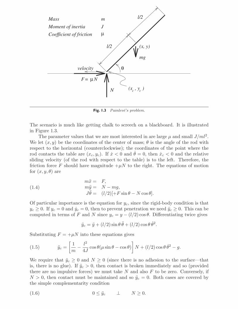
1.3. Painleve’s Problem. In 1895 P. Painleve published a paper [97] in which hepresented a simple rigid-body dynamics problem which appears not to have a solution.

mg

N

F

Mass

Moment of inertia

Coefficient of friction

m

Jμ

l/2

l/2

= μ N

θ

(x, y)

(x , y )c c

velocity

Fig. 1.3 Painleve’s problem.

The scenario is much like getting chalk to screech on a blackboard. It is illustratedin Figure 1.3.

The parameter values that we are most interested in are large μ and small J/ml2.We let (x, y) be the coordinates of the center of mass; θ is the angle of the rod withrespect to the horizontal (counterclockwise); the coordinates of the point where therod contacts the table are (xc, yc). If x < 0 and θ = 0, then xc < 0 and the relativesliding velocity (of the rod with respect to the table) is to the left. Therefore, thefriction force F should have magnitude +μN to the right. The equations of motionfor (x, y, θ) are

mx = F,my = N − mg,

Jθ = (l/2)[+F sin θ − N cos θ].(1.4)

Of particular importance is the equation for yc, since the rigid-body condition is thatyc ≥ 0. If yc = 0 and yc = 0, then to prevent penetration we need yc ≥ 0. This can becomputed in terms of F and N since yc = y − (l/2) cos θ. Differentiating twice gives

yc = y + (l/2) sin θ θ + (l/2) cos θ θ2.

Substituting F = +μN into these equations gives

yc =[

1m

− l2

4Jcos θ(μ sin θ − cos θ)

]N + (l/2) cos θ θ2 − g.(1.5)

We require that yc ≥ 0 and N ≥ 0 (since there is no adhesion to the surface—thatis, there is no glue). If yc > 0, then contact is broken immediately and so (providedthere are no impulsive forces) we must take N and also F to be zero. Conversely, ifN > 0, then contact must be maintained and so yc = 0. Both cases are covered bythe simple complementarity condition

0 ≤ yc ⊥ N ≥ 0.(1.6)

(Note that “a ⊥ b” indicates that ab = 0 if a and b are scalars and that aT b = 0 if theyare vectors; for a vector “a ≥ 0” means that the components ai of a are nonnegative.)

Now consider the situation with large coefficient of friction μ and small J/ml2. Forμ large, the contact force (the vector sum of F and N) is applied to the contact pointat a shallow angle. This means that the torque from the contact forces is counter-clockwise. If J/ml2 is sufficiently small, the effect of this torque will overpower theeffect of the vertical contact force N in preventing penetration. When this happens,the torque will cause the rod to rotate into the table. Mathematically, the coefficient(1/m) − (l2/4J) cos θ(μ sin θ − cos θ) < 0 in this situation. If (l/2) cos θ θ2 − g < 0 aswell, then no value of N ≥ 0 will give yc ≥ 0, and penetration appears impossible toprevent.

This line of analysis has been used to argue that rigid-body dynamics and theCoulomb law of friction are inconsistent. For a recent example of this line of reasoning,see the otherwise excellent textbook of Pfeiffer and Glocker [109, section 5.3, pp. 61–63]. However, this line of reasoning is flawed. The flaw is the assumption that allforces are bounded functions of time. In particular, it rules out the possibility thatthe horizontal component of the velocity could be brought to zero instantaneously byimpulsive contact forces. If xc was driven to zero during the impact, then we wouldno longer require that F = +μN , the angle of the contact forces does not need to beshallow, and solutions can exist. This example also shows that it is important to allowfor impulsive forces in rigid-body dynamics, even when there are no collisions. It alsoshows that care should be taken in developing formulations of rigid-body dynamicsthat can directly incorporate impulsive forces and discontinuous solutions.

Note that when Pfeiffer and Glocker [109, section 8.2] discuss impact laws withfriction, they implicitly allow for this resolution of Painleve’s problem. However, thiswould require explicitly invoking the impact law in a situation without impacts.

The reader wishing to look at the extensive discussion of Painleve’s problem isinvited to peruse the references [11, 12, 27, 28, 36, 49, 68, 76, 84, 82, 89, 91, 109].

On a final note, the Painleve problem also has a bearing on formulating impactlaws since applying the Newton impact law would imply that yc immediately after im-pact should be zero, even for the “perfectly elastic” case, ε = 1. However, simulationsand asymptotic analysis with the table represented by a spring of stiffness k showthat as k → ∞ there is a definite nonzero limit of yc after impact. This correspondsto ε = +∞ using Newton’s impact law, since yc just before impact is zero. A Poissonimpact law would be more realistic, since it would give a positive value for yc justafter the impact for any ε > 0, due to the impulsive contact forces.

1.4. Complementarity Problems. Complementarity problems give a uniformway of representing a very large range of conditions that would require modeling usingdiscontinuous functions. For example, the contact conditions (1.6) of the previoussection avoid the need for discontinuous or infinite functions that would arise if wetried to represent N as N(yc), for example.

Complementarity problems typically have the following form: Find z ∈ Rn suchthat 0 ≤ z ⊥ f(z) ≥ 0, where f : Rn → Rn is a given continuous function. Note thatthis is equivalent to requiring that zi ≥ 0 and fi(z) ≥ 0 for all i = 1, . . . , n, and thatzi = 0 or fi(z) = 0 for all i = 1, . . . , n. Linear complementarity problems (LCPs)are complementarity problems where f is affine: f(z) = Mz + q, where M is a givenmatrix and q is a given vector. Not all (not even “almost all”) linear complementarityproblems have solutions. It should be understood that LCPs are truly nonlinear prob-lems, in spite of their linear-combinatorial structure. For a comprehensive overview

of LCPs, see Cottle, Pang, and Stone [25]. A more recent overview of applications oflinear and nonlinear complementarity problems is the article by Ferris and Pang [37].

Complementarity problems arise in many contexts; one of the most important ofthese is constrained optimization. If we consider an optimization problem

minx

f(x) subject to gi(x) ≥ 0, i = 1, . . . , m,(1.7)

then provided a suitable constraint qualification [41] holds, there are Lagrange mul-tipliers λi such that

∇f(x) − ∑mi=1 λi∇gi(x) = 0,

λi, gi(x) ≥ 0,λigi(x) = 0

(1.8)

hold at the minimizing x. These are the Kuhn–Tucker (or Karush–Kuhn–Tucker)conditions for optimality [41, 43]. Note that the last two lines of (1.8) are actuallycomplementarity conditions: 0 ≤ λ ⊥ g(x) ≥ 0.

The existence of solutions and algorithms to compute them is known for a wideclass of LCPs. The best-known algorithms for LCPs are pivoting methods, whichare closely related to the simplex method for linear programming. The best knownof these is Lemke’s method [25, section 4.4]. The most useful result for our purposeshows that Lemke’s method computes a solution to the LCP 0 ≤ z ⊥ Mz + q ≥ 0,where M is a copositive matrix (defined below) and qT y ≥ 0 whenever y solves thehomogeneous LCP 0 ≤ y ⊥ My ≥ 0 [25, Thms. 3.8.6 and 4.4.12]. A matrix Mis copositive if y ≥ 0 implies that yT My ≥ 0. The application of complementarityproblems to general unilateral contact problems seems to have begun with the workof Lotstedt [76, 77, 78, 79]. In this work, Lotstedt was able to show the existenceof solutions of certain LCPs provided the coefficient of friction was sufficiently small.Since then, there has been much work applying complementarity problems to contactproblems [4, 5, 66, 67, 103, 102, 131, 139, 101], and the question of the existence ofsolutions to the complementarity problems has attracted a great deal of attention.

Complementarity problems can be extended to a more general setting which caninclude infinite-dimensional problems [55, 99]: if X is a Banach space and K is a closedconvex cone in X, then the dual cone is K∗ = { y ∈ X∗ | 〈y, x〉 ≥ 0 for all x ∈ K }.For a function f : X → X∗ the complementarity problem CP (f) is the problemof finding z ∈ K such that f(z) ∈ K∗and 〈f(z), z〉 = 0. One way in which wewill use this idea is to take X to be the set of continuous functions on [0, T ] sothat X∗ is the set of finite-valued Borel measures on [0, T ]. The cone K ⊂ C[0, T ]is the cone of nonnegative continuous functions, so K∗ is the cone of finite-valuednonnegative Borel measures. We understand complementarity between a measure μand a function φ on [0, T ] to mean that μ(E) ≥ 0 for all Borel E, φ(t) ≥ 0 for all t,and 〈μ, φ〉 =

∫φ(t) μ(dt) = 0. This we denote by the shorthand 0 ≤ μ ⊥ φ ≥ 0.

1.5. Measure Differential Inclusions. General rigid-body dynamics requires anew approach which can combine impulsive forces with differential inclusions. Aframework for this approach can be built using measure differential inclusions [87,90, 91]. For Moreau, this work developed out of a study of sweeping processes [16,69, 70, 85, 86]: in a sweeping process, there is a set-valued function C(t) which isconvex for all t and a “particle” at x(t) which is “swept” along by the C(t) so thatx(t) ∈ C(t) for all t. If x(t) is in the interior of C(t), then x′(t) will be zero, andif x(t) is on the boundary of C(t), then x′(t) will be in the normal cone of C(t) at

x(t). If C(t) is allowed to be discontinuous as a set-valued function, then x(t) mayalso have to “jump”: x(t+) − x(t−) must then belong to the normal cone of C(t) atx(t+). Measure differential inclusions (although not always called that) can be foundin other contexts in the work of Schatzman [117, 118, 119], for example.

In a measure differential inclusion,

dv

dt∈ F (t, x),

dx

dt= g(t, x, v),(1.9)

F (t, x) does not need to be bounded, and v(.) is only required to have boundedvariation. The other properties assumed about F for differential inclusions shouldhold: F (t, x) should be a closed convex set, and the graph of F should be closed. Thedifficulty is in interpreting “dv/dt ∈ F (t, x)” when v(.) is not absolutely continuousor is discontinuous. Then “dv/dt” is not an integrable function, or perhaps not evena function at all, but a distribution or measure. We do, however, suppose that v hasbounded variation on a finite interval [0, T ]. That is, the supremum of

N−1∑i=0

‖v(ti+1) − v(ti)‖

over all N and choice of 0 ≤ t0 ≤ t1 ≤ · · · ≤ tN ≤ T is finite. This supremum isdenoted

∨T0 v and is called the variation of v on [0, T ]. Then we can use Riemann–

Stieltjes integrals to define∫

φ(t) dv(t) for continuous functions φ; see, for example,[134, pp. 281–284] or [72, Chap. X]. By the Riesz representation theorem, the lin-ear functional φ −→ ∫

φ(t) dv(t) is a continuous linear functional and is thereforeequivalent to integration against a measure:

∫φ(t) dv(t) =

∫φ(t) μ(dt), where μ is a

Borel measure [72, Thm. 2.7, Chap. IX, pp. 264–265]. We write μ = Dv to denotethe distributional derivative of v(.). The expression “dv/dt” can be thought of as aRadon–Nikodym derivative of Dv with respect to the ordinary Lebesgue measure Dt.However, this will work only if Dv is an absolutely continuous measure with respectto Dt, which amounts to requiring that v(.) is an absolutely continuous function. Ifv(.) is not an absolutely continuous function we need to extend the notion of theRadon–Nikodym derivative.

Fortunately it is possible to split measures into absolutely continuous and singularparts: the Lebesgue decomposition of Dv is Dv = μs +a Dt, where a(.) is a Lebesgueintegrable function and μs is a Borel measure that is singular with respect to theLebesgue measure [64, pp. 111–113]. The singular part μs contains all the forcesand impulses “at infinity”; this singular part is supported on a set that has Lebesguemeasure zero. So we should require that a(t) ∈ F (t, x(t)) for Lebesgue almost all t.For μs we want to look at the part of F (t, x) “at infinity.” For closed convex F (t, x)we can use the asymptotic or regression cone [53]. This asymptotic cone of a closedconvex set K is the set of directions in K “at infinity”:

K∞ ={

x | x = limk→∞

tk xk, xk ∈ K

}.(1.10)

While we can’t take the Radon–Nikodym derivative of μs with respect to the Lebesguemeasure, we can “normalize” μs by using its variation |μs| which is a nonnegativeBorel measure: any finite-valued Borel measure μ has variation |μ|, which is anotherfinite-valued measure defined by

|μ|(E) = sup{Ei}

∑i

‖μ(Ei)‖,

where {Ei} ranges over all countable Borel partitions of a Borel set E. Then clearly‖μ(E)‖ ≤ |μ|(E) for all Borel sets E, and μ is an absolutely continuous measure withrespect to |μ|. So we define “dv/dt ∈ F (t, x)” to mean that

a(t) ∈ F (t, x(t)), Dt a.e.,(1.11)dμs

d|μs| (t) ∈ F (t, x(t))∞, |μs| a.e.(1.12)

An alternative definition that is useful for handling problems of convergence is thefollowing: for each continuous function φ ≥ 0, not everywhere zero,∫

φ(t) dv(t)∫φ(t) dt

∈ co⋃

τ :φ(τ) �=0

F (τ, x(τ)).(1.13)

The definition based on (1.11), (1.12) I call the strong definition, and the definitionbased on (1.13) I call the weak definition. Under conditions (C1)–(C3) below, the twodefinitions are equivalent [130].

• (C1) The graph of F is closed, and F (t, x) is a closed convex set for all (t, x).• (C2) The asymptotic cone F (t, x)∞ is always pointed. (A pointed cone K is

a cone where K ∩ (−K) = {0}.)• (C3) min{ ‖z‖ | z ∈ F (t, x) } is a bounded function of (t, x).

The strong definition is useful for proving properties about the solutions, while theweak definition is useful for obtaining existence results. Consider, for example, asequence of functions {vh}h>0 generated by some numerical procedure. If it canbe proved that

∨vh ≤ M for some constant M and vh(0) = v0 for all h > 0,

then by the Helly selection theorem [93], there is a pointwise convergent subsequencevhk(.) which converges to a function v(.) with

∨v ≤ M . In this subsequence, the

measures Dvhk ⇀ Dv weak*. If vh satisfies a measure differential inclusion dvh/dt ∈Fh(t, x(t)), and 0 < h′ < h implies that Fh′(t, x) ⊂ Fh(t, x), then using the weakformulation it is easy to show that dv/dt ∈ Fh(t, x(t)) for all h > 0, and consequentlydv/dt ∈ ⋂

h>0 Fh(t, x(t)).While measure differential inclusions cannot satisfactorily treat all aspects of

rigid-body dynamics, they give structure to a large part of it. The additional condi-tions can be specified in terms of complementarity conditions, usually between mea-sures and functions.

2. Formulation and Simulation. The paradoxes uncovered by Painleve showthe need for care in formulating the equations of rigid-body dynamics with contacts.When it comes to formulating numerical methods for simulating rigid-body systems,we must be even more careful. Current methods for handling rigid-body dynamicsfall into several categories:

1. For each possible configuration of contacts, solve for the forces that could begenerated and feed the result into an ODE or differential algebraic equation(DAE) solver. This method is vulnerable to Painleve’s problem as well asbeing very cumbersome.

2. Formulate the problem as in case 1 but use a complementarity problem todecide at each step which contacts are active. (This is basically the approachof Pfeiffer and Glocker [109].) This is still vulnerable to Painleve’s problem.

3. Use a penalty formulation of the no-interpenetration condition. This corre-sponds to approximating the rigid bodies by very stiff bodies. This avoids thetheoretical existence questions and avoids impulses but raises new questions

about singular perturbations and the accuracy of the computational methods.A penalty approach can also be used to approximate the Coulomb frictionlaw. All of these modifications give very stiff differential equations.

4. Use a time-stepping formulation based on integrals of the contact forces ratherthan their instantaneous values. Complementarity conditions or optimizationconditions are used to resolve whether contact is maintained or broken.

The approach I will present here is approach 4: use a time-stepping formulation. Thisapproach directly incorporates impulsive forces. In fact, in a single simulation withfixed step-size, there is no way of determining if there actually is an impulsive force,since only integrals are represented or computed.

2.1. The Continuous Problem. In many ways it is easier to write down a numer-ical method for rigid-body dynamics than it is to say exactly what the method is tryingto compute. Nevertheless, with the tools of measure differential inclusions, functionsof bounded variation, and complementarity problems, this can be fairly straightfor-ward for many situations. To keep matters simple at this stage, we consider a onecontact problem.

To obtain the equations of motion we first need the equations of motion for asystem without contacts. To do this we use generalized coordinates q, which cancontain rectilinear coordinates of centers of mass as well as angles and orientationparameters and other types of coordinates. Associated with this are the generalizedvelocities v = dq/dt and the Lagrangian L(q, v) = 1

2vT M(q)v−V (q), where 12vT M(q)v

is the kinetic energy (M(q) is the mass matrix) and V (q) is the potential energy.If there are only internal forces, the equations of motion are given by Lagrange’sequations of motion:

d

dt

(∂L

∂v

)− ∂L

∂q= 0 or M(q)

dv

dt= k(q, v) − ∇V (q),

where kl(q, v) = − 12

∑r,s [∂mir/∂qs + ∂mis/∂qr − ∂mrs/∂qi]. With external and con-

tact forces we can write this as

M(q)dv

dt= n(q) cn + D(q) β + k(q, v) − ∇V (q) + Fext(t).(2.1)

The admissible region of configuration space is given by { x | f(q) ≥ 0 } for asuitable function f . The normal direction vector at q is n(q) = ∇f(q). The contactconditions that we need are essentially the Signorini contact conditions: 0 ≤ f(q) ⊥cn ≥ 0. We represent the set of possible friction forces through FC0(q) = { D(q)β |β ∈ Rd, ψ(β) ≤ μ }. The function ψ used for defining FC0(q) should be convex,positively homogeneous (ψ(αβ) = |α|ψ(β) for all α ∈ R), and coercive (ψ(β) → ∞as ‖β‖ → ∞). Positive homogeneity implies that D(q)β ∈ cn FC0(q) is equivalent toψ(β) ≤ μcn.

The maximal dissipation principle states that we choose β so as to maximizethe dissipation rate vT D(x)β over all β ∈ cn FC0(x). Because of discontinuities, weneed to be careful to make some distinctions between v+(t) = v(t+) = lims↓t v(s),v−(t) = v(t−) = lims↑t v(s), and v(t). For inelastic impacts, for example, we requirethat nT v+(t) = 0 for all t where there is contact: f(q(t)) = 0. Also, in the maximumdissipation principle we should minimize (v+)T D(q)β over β ∈ cn FC0(q), that is,

minβ

(v+)T D(q)β subject to ψ(β) ≤ μcn.(2.2)

This is a convex program (with linear objective function), although it is nonsmooth.If cn > 0, then using a Slater condition, there exists a Lagrange multiplier λ ≥ 0such that ∂βh(β, λ) = 0 where h(β, λ) = vT D(q)β − λ(μcn − ψ(β)) and ∂f(z) is thegeneralized gradient of f at z [19, Thms. 6.1.1 and 6.3.1]. Furthermore, 0 ≤ λ ⊥μcn − ψ(β) ≥ 0. That is,

0 ∈ μ D(q)T v+ + λ ∂ψ(β),0 ≤ λ ⊥ μcn − ψ(β) ≥ 0.

(2.3)

If cn = 0, then β = 0 by the condition μcn − ψ(β) ≥ 0; since ∂ψ(0) contains aneighborhood of the origin, there is a value of λ ≥ 0 such that 0 ∈ D(q)T v++λ ∂ψ(0),no matter what v+ and D(q) are.

For a simple particle, we can take ψ(β) = ‖β‖2=√

βT β. Then as long as thecolumns of D(q) span the friction plane, we have a representation of the isotropicCoulomb law of friction.

2.1.1. Formulations and Function Spaces. The Signorini contact condition that0 ≤ f(q(t)) ⊥ cn ≥ 0 involves complementarity between a continuous functiont → f(q(t)) and a measure cn, so the complementarity condition can be representedby

∫f(q(t)) cn(dt) = 0 as well as the usual inequality conditions: f(q(t)) ≥ 0 for

all t and cn(E) ≥ 0 for all Borel sets E ⊂ [0, T ]. The integrated maximum dissi-pation principle minβ

∫(v+)T D(q)β subject to ψ(β) ≤ μcn can be formulated where

β is a measure. The main difficulty is that ψ(β) must be interpreted as a measure.Convex functions of measures were studied as measures in [29]. Since ψ(.) is a pos-itively homogeneous function, ψ(β) = ψ(dβ/d|β|) |β|, and the condition ψ(β) ≤ μcn

is equivalent to ψ(dβ/d|β|) |β| ≤ μcn or even ψ(dβ/dcn) ≤ μ a.e. Note that thederivatives dβ/d|β| and dβ/dcn are all Radon–Nikodym derivatives. The function λis a bounded Borel function; we can bound ‖λ‖∞ by maxt μ‖D(q(t))T v+(t)‖∞/Cψ,

where Cψ = min{ ‖z‖∞ | z ∈ ∂ψ(β), β �= 0 }.

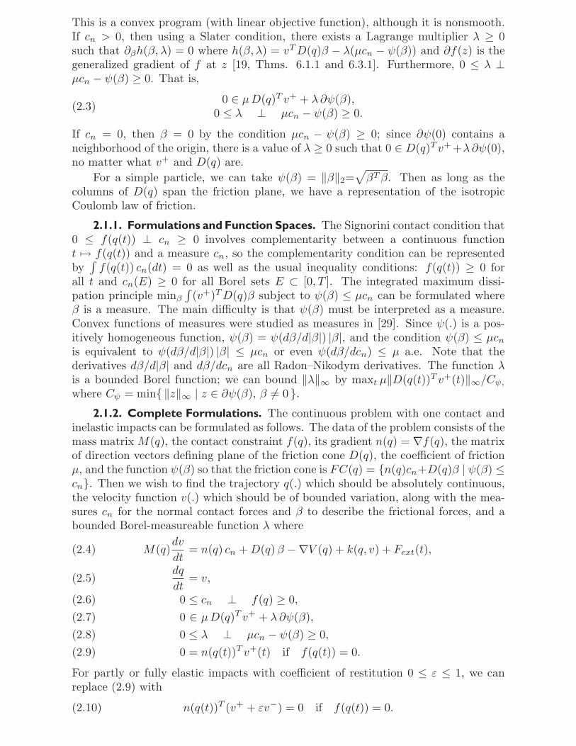
2.1.2. Complete Formulations. The continuous problem with one contact andinelastic impacts can be formulated as follows. The data of the problem consists of themass matrix M(q), the contact constraint f(q), its gradient n(q) = ∇f(q), the matrixof direction vectors defining plane of the friction cone D(q), the coefficient of frictionμ, and the function ψ(β) so that the friction cone is FC(q) = {n(q)cn+D(q)β | ψ(β) ≤cn}. Then we wish to find the trajectory q(.) which should be absolutely continuous,the velocity function v(.) which should be of bounded variation, along with the mea-sures cn for the normal contact forces and β to describe the frictional forces, and abounded Borel-measureable function λ where

M(q)dv

dt= n(q) cn + D(q) β − ∇V (q) + k(q, v) + Fext(t),(2.4)

dq

dt= v,(2.5)

0 ≤ cn ⊥ f(q) ≥ 0,(2.6)0 ∈ μ D(q)T v+ + λ ∂ψ(β),(2.7)0 ≤ λ ⊥ μcn − ψ(β) ≥ 0,(2.8)0 = n(q(t))T v+(t) if f(q(t)) = 0.(2.9)

For partly or fully elastic impacts with coefficient of restitution 0 ≤ ε ≤ 1, we canreplace (2.9) with

n(q(t))T (v+ + εv−) = 0 if f(q(t)) = 0.(2.10)

friction law‘‘regularized’’

N

v

F

μ

Fig. 2.1 Regularized Coulomb law to avoid discontinuity.

Related models and theory for partly elastic impacts, at least for the frictionless case,can be found in the work of Mabrouk [80, 81]. Note that this is a Newton-style modelof partly elastic impact. Interestingly, this formulation of the Newton approach alwaysdissipates energy, unlike the formulation of the Newton approach discussed by Strongein [135]. A Poisson approach for partly elastic impacts is developed in Anitescu andPotra [5]. A new Poisson-type formulation of impact recently developed by Pangand Tzitzouris [104] is based on complementarity problems and is guaranteed to bedissipative.

It has been argued that complementarity conditions between the normal contactforce and the normal velocity of the form of (2.6) are not always valid [17]. Thephenomena discussed in Chatterjee [17] are associated with multiple simultaneouscontacts and are discussed in section 4.4 of this article.

2.2. Numerical Methods. Numerical methods for rigid-body dynamics withoutfriction or impact have been studied extensively in the engineering and also mathe-matics literature. See, for example, [34, 143, 124, 122, 52, 2, 123, 111, 33, 107, 46,42, 142, 13], in reverse chronological order. One of the reasons for this is the need tosimulate mechanical systems, especially the complex mechanical systems that arise inmanufacturing processes and robotics. Even simple grasping problems involve prob-lems of contact, impact, and friction. So far, most of the numerical methods arebased on ODEs or DAEs or both. To avoid the difficulties with the discontinuity inCoulomb’s law, for instance, a regularized version is used, as shown in Figure 2.1. Inthis paper, a different strategy is recommended.

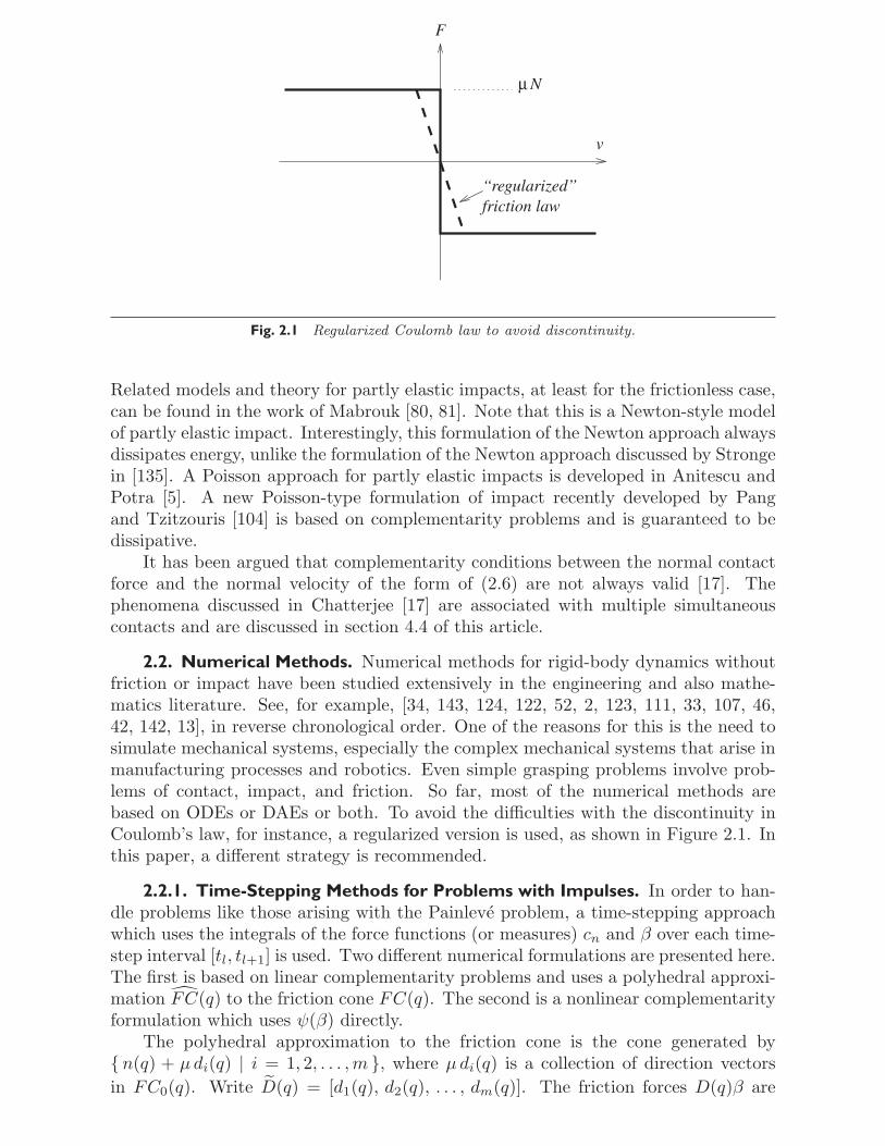
2.2.1. Time-Stepping Methods for Problems with Impulses. In order to han-dle problems like those arising with the Painleve problem, a time-stepping approachwhich uses the integrals of the force functions (or measures) cn and β over each time-step interval [tl, tl+1] is used. Two different numerical formulations are presented here.The first is based on linear complementarity problems and uses a polyhedral approxi-mation FC(q) to the friction cone FC(q). The second is a nonlinear complementarityformulation which uses ψ(β) directly.

The polyhedral approximation to the friction cone is the cone generated by{ n(q) + μ di(q) | i = 1, 2, . . . , m }, where μ di(q) is a collection of direction vectorsin FC0(q). Write D(q) = [d1(q), d2(q), . . . , dm(q)]. The friction forces D(q)β are

d3

c t

polyhedral approximationto friction cone

friction cone

n

d

d

dd

d1

2 4

5

d6

7d8

Fig. 2.2 Polyhedral approximation to the friction cone.

approximated by D(q)β, where βi ≥ 0 and∑

i βi ≤ μ cn. The relationship betweenFC(q) and FC(q) is illustrated in Figure 2.2. It is assumed that for each i there is aj, where di(q) = −dj(q). This is related to the assumption that FC0(q) is a balancedset: FC0(q) = −FC0(q).

The discretization of (2.4)–(2.9) is the problem of finding ql+1 and vl+1 (and theforce integrals cl+1

n , βl+1 and Lagrange multiplier λl+1) given ql and vl for a time-stepof size h > 0 that satisfy the following conditions:

M(ql+1)(vl+1 − vl) = n(ql)cl+1n + D(ql)βl+1(2.11)

+h[−∇V (ql) + k(ql, vl) + Fext(tl)],ql+1 − ql = h vl+1,(2.12)0 ≤ cl+1

n ⊥ n(ql)T (vl+1 + εvl) ≥ 0,(2.13)

0 ≤ βl+1 ⊥ λl+1 e + D(ql)T vl+1 ≥ 0,(2.14)

0 ≤ λl+1 ⊥ μ cl+1n − eT βl+1 ≥ 0,(2.15)

where f(ql + h vl) < 0; if f(ql + h vl) ≥ 0, then we set cl+1n = 0 and βl+1 = 0 and

solve the first two equations. Note that e is a vector of ones of the appropriate size.This discretization is a partly implicit Euler method. Therefore it can give only

O(h) accuracy at best. However, unlike conventional discretizations, it can handleimpulsive forces, in particular Painleve’s problem. Note that the complementaritycondition 0 ≤ f(q) ⊥ cn ≥ 0 does not appear explicitly in (2.11)–(2.15); (2.13) isessentially the differentiated form of this condition. Using the differentiated constraintonly can result in the true constraint “drifting” into the inadmissible region, which isan effect that has been noticed in relation to DAE formulations of rigid-body dynamicswith bilateral (i.e., equality) constraints [15]. It is tempting to replace (2.13) with

0 ≤ f(ql+1) ⊥ cl+1n ≥ 0. This does not work: the resulting discretization behaves

as if it had a “random” coefficient of restitution when impacts occur. (The effectivecoefficient of restitution depends on the time within the time-step [tl, tl+1] that contactoccurs.) Since (2.13) uses differentiated constraints, it may be occasionally advisableto project ql+1 back to the feasible region. This can be done without disturbing thetime-stepping, since the time-stepping method is a one-step method.

If we ignore the dependence of M on q and substitute for vl+1 and ql+1 in termsof cl+1

n , βl+1, and λl+1, then (2.11)–(2.15) with ε = 0 can be reduced to a pure LCPwhich has the form (superscripts suppressed)

0 ≤⎡⎣ nT M−1n nT M−1D 0

DT M−1n DT M−1D eμ −eT

⎤⎦

⎡⎣ cn

βλ

⎤⎦ +

⎡⎣ nT b1

DT b20

⎤⎦ ⊥

⎡⎣ cn

βλ

⎤⎦ ≥ 0.(2.16)

The 3 × 3 block matrix in this LCP is a copositive matrix; a solution to this LCPexists and can be constructed by Lemke’s algorithm [25, Cor. 4.4.12].

To avoid approximations of the friction cone, we can use the integrated maxi-mal dissipation principle: βl+1 maximizes −(vl+1)T D(ql)βl+1 over all βl+1 satisfyingψ(βl+1) ≤ μcl+1

n . The Kuhn–Tucker conditions for this problem replace (2.14), (2.15)above, giving

0 ∈ D(ql)T vl+1 + λl+1∂ψ(βl+1),(2.17)0 ≤ λl+1 ⊥ μ cl+1

n − ψ(βl+1) ≥ 0.(2.18)

Of course, (2.11) should be replaced by

M(ql+1)(vl+1 − vl) = n(ql)cl+1n + D(ql)βl+1(2.19)

+h[−∇V (ql) + k(ql, vl) + Fext(tl)].

Solving these systems requires more sophisticated methods since we have to solve foran inclusion 0 ∈ D(ql)T vl+1 + λl+1∂ψ(βl+1) as well as for nonlinear complementarityconditions 0 ≤ λl+1 ⊥ μcl+1

n − ψ(βl+1) ≥ 0.The existence of solutions to the one-time-step conditions above can be shown

under mild conditions via the results in [129] for the formulation using β and extendedvia [101] to the formulation(s) in β, using the nonlinear condition μcn − ψ(β) ≥ 0.

2.3. Practicalities. If we use the discretization (2.11)–(2.15), we can use Lemke’salgorithm in an iteration: given an estimate ql+1,k of ql+1, we can obtain an estimateql+1,k+1 by solving (2.11)–(2.15) with ql+1 replaced by ql+1,k. This iteration willusually converge (and converge quickly), giving a solution of the mixed nonlinearcomplementarity problem (2.11)–(2.15) [132].

Replacing (2.14)–(2.15) with (2.17)–(2.18), using the nonlinear condition μcn ≥ψ(β) instead of the conditions μcn ≥ eT β and β ≥ 0, leads to highly nonlinearcomplementarity problems. Since ψ is nonsmooth, it may be desirable to replace itwith smooth functions. For example, for isotropic friction, where ψ(β) = ‖β‖2, wecan replace the condition μcn ≥ ψ(β) with (μcn)2 ≥ ‖β‖2

2 = βT β. The difficulty inusing this condition is that if cn = 0, the constraint qualification fails, and Lagrangemultipliers may not exist for the maximal dissipation principle in this form. However,it can be restored by using a version of the Fritz John conditions (see [43, section 2.2,pp. 190–203], for example): replace (2.17) with

0 = cl+1n D(ql)T vl+1 + 2λl+1βl+1.

Not

e ch

ange

of d

irec

tion

of t

rave

lw

ith

each

bou

nce

due

to th

e ba

ll’s

spi

n.

thre

e in

itia

lly

ball

stat

iona

ry b

alls

thro

wn

(a) Plan view

Not

e ‘‘

jum

p’’ d

ue to

spi

n of

firs

t bal

l an

d

thro

wn

ball

thre

e in

itia

lly

stat

iona

ry b

alls

fric

tion

al im

puls

es.

(b) Elevation view

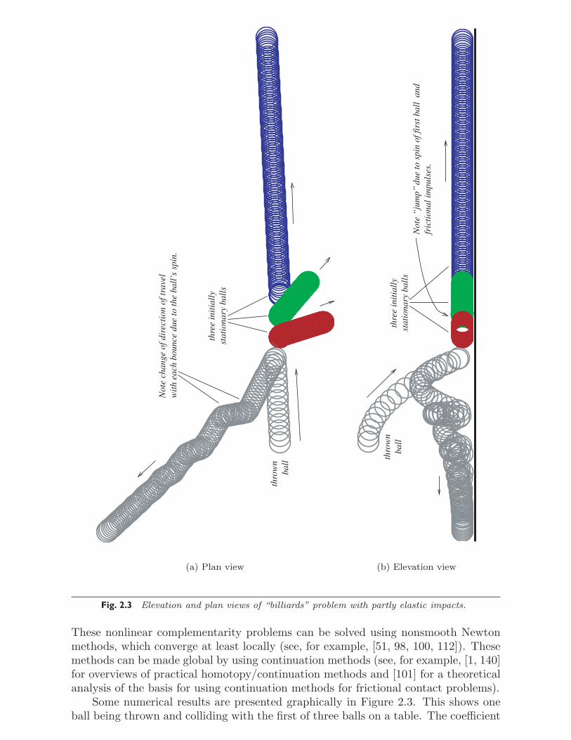
Fig. 2.3 Elevation and plan views of “billiards” problem with partly elastic impacts.

These nonlinear complementarity problems can be solved using nonsmooth Newtonmethods, which converge at least locally (see, for example, [51, 98, 100, 112]). Thesemethods can be made global by using continuation methods (see, for example, [1, 140]for overviews of practical homotopy/continuation methods and [101] for a theoreticalanalysis of the basis for using continuation methods for frictional contact problems).

Some numerical results are presented graphically in Figure 2.3. This shows oneball being thrown and colliding with the first of three balls on a table. The coefficient

0.0000.0200.0400.0600.0800.1000.1200.1400.160

0.1800.200

0.2100.220

0.2300.240

0.2500.260

0.2700.280

0.2900.300

0.3100.320

0.3300.340

0.3500.360

0.370

0.3800.3900.4000.410

0.4200.430

0.4400.450

0.4600.470

0.4800.490

0.5000.510

0.5200.530

0.5400.550

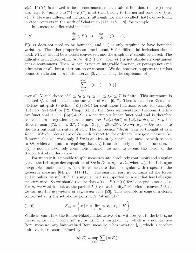
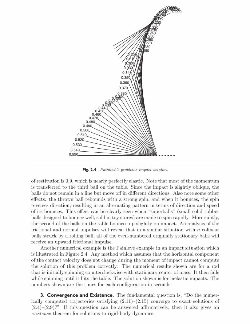
Fig. 2.4 Painleve’s problem: impact version.

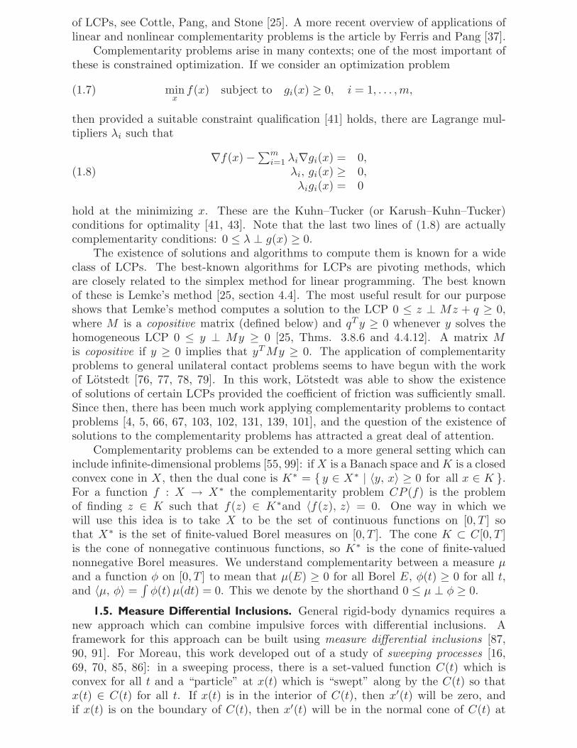
of restitution is 0.9, which is nearly perfectly elastic. Note that most of the momentumis transferred to the third ball on the table. Since the impact is slightly oblique, theballs do not remain in a line but move off in different directions. Also note some othereffects: the thrown ball rebounds with a strong spin, and when it bounces, the spinreverses direction, resulting in an alternating pattern in terms of direction and speedof its bounces. This effect can be clearly seen when “superballs” (small solid rubberballs designed to bounce well, sold in toy stores) are made to spin rapidly. More subtly,the second of the balls on the table bounces up slightly on impact. An analysis of thefrictional and normal impulses will reveal that in a similar situation with n colinearballs struck by a rolling ball, all of the even-numbered originally stationary balls willreceive an upward frictional impulse.

Another numerical example is the Painleve example in an impact situation whichis illustrated in Figure 2.4. Any method which assumes that the horizontal componentof the contact velocity does not change during the moment of impact cannot computethe solution of this problem correctly. The numerical results shown are for a rodthat is initially spinning counterclockwise with stationary center of mass. It then fallswhile spinning until it hits the table. The solution shown is for inelastic impacts. Thenumbers shown are the times for each configuration in seconds.

3. Convergence and Existence. The fundamental question is, “Do the numer-ically computed trajectories satisfying (2.11)–(2.15) converge to exact solutions of(2.4)–(2.9)?” If this question can be answered affirmatively, then it also gives anexistence theorem for solutions to rigid-body dynamics.

Certain situations are harder than others to deal with; we have already seenhow Painleve’s famous problem causes difficulties for analysis. The difficulties thatarise with Painleve’s problem can be related to the fact that M(q)−1FC(q) pointsoutside the set of admissible velocities. This can be avoided if we assume Erd-mann’s condition that for any q ∈ ∂C and z ∈ FC(q), n(q)T M(q)−1z ≥ 0 [36].Note that Erdmann’s condition holds automatically for frictionless problems, becausez ∈ FC(q) = cone(n(q)) implies that z = αn(q) (α ≥ 0) and n(q)T M(q)−1z =α n(q)T M(q)−1n(q) ≥ 0 since M(q) is positive definite. Also, Erdmann’s conditionimplies that there cannot be any impulses without collisions; that is, n(q(t))T v(t−) ≥ 0implies that v(t+) = v(t−) under Erdmann’s condition.

The question of convergence is answered affirmatively in [129] for one inelasticcontact (ε = 0) in the case of one-dimensional friction (that is, FC0(q) is a one-dimensional set), or if Erdmann’s condition holds [36]. This result includes Painleve’sproblem. It also extends the fundamental results of Monteiro Marques [84] for inelasticfrictional dynamics of a particle.

In this section we will review how to prove convergence (and thus existence) ofsolutions to rigid-body dynamics problems. This is based on the results in [129],which should be consulted for more details. A more complete summary of the proofis in [128].

3.1. The Easy Part. The main part of the theorem can be handled by standardtechniques once a few basic facts are established. The first is the existence of solutionsto the mixed complementarity conditions (2.11)–(2.15) at each time-step. This is donein [129] by a combination of an approximation argument and the Brouwer fixed-pointtheorem. The numerical solutions are approximately dissipative. This is based onthe result that for constant M , n, D, and linear V (q), the numerical solutions areexactly dissipative, which is proved using (vl+1)T M(vl+1 − vl) = 1

2 (vl+1)T Mvl+1 −12 (vl)T Mvl + 1

2 (vl+1 − vl)T M(vl+1 − vl) and substituting for M(vl+1 − vl) in termsof cl+1

n and βl+1. Using a generalization of the discrete Gronwall lemma to nonlinearODEs, the energy of the computed trajectory is shown to be bounded on some suffi-ciently small interval [t0, t1], t1 > t0. This means that the computed velocities vh(.)are bounded on [t0, t1]. Since dq/dt = v, the numerically computed functions qh(.) areuniformly Lipschitz and thus equicontinuous. By the Arzela–Ascoli theorem, there isa uniformly convergent subsequence. We restrict attention to the subsequence.

Assuming that the friction cones FC(q) are pointed and that q → FC(q) has aclosed graph, it can be concluded from the uniform boundedness of vh(.) that thevariations

∨vh are also uniformly bounded. By the Helly selection theorem, there is

a convergent subsequence where vh(.) → v(.) pointwise, and the differential measuresdvh ⇀ dv weak*. By the weak* closedness results in [130], the limit v(.) satisfies themeasure differential inclusion in the continuous formulation.

3.2. The Hard Part. The hard part involves nonstandard arguments and com-plementarity conditions between functions that converge pointwise and measures thatconverge weak*.

First, the limits q(.) and v(.) can be proved to be exactly dissipative in the sensethat the total energy of the solution 1

2v(t)T M(q(t))v(t) + V (q(t)) is a nonincreasingfunction of t. This could not be proved before, because the argument used at thisstage needs a uniform bound on

∨T0 vh. From the exact dissipativity result, we can go

on to show that the solution grows at most exponentially on any interval where thelimit exists. By “bootstrapping” this argument with the local boundedness result, itcan be shown that limits q(.) and v(.) exist on [0,∞).

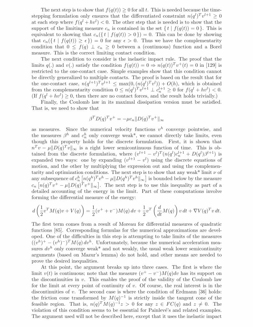
The next step is to show that f(q(t)) ≥ 0 for all t. This is needed because the time-stepping formulation only ensures that the differentiated constraint n(ql)T vl+1 ≥ 0at each step where f(ql + hvl) < 0. The other step that is needed is to show that thesupport of the limiting measure cn is contained in the set { t | f(q(t)) = 0 }. This isequivalent to showing that cn({ t | f(q(t)) > 0 }) = 0. This can be done by showingthat cn({ t | f(q(t)) ≥ ε }) = 0 for any ε > 0. Thus we have the complementaritycondition that 0 ≤ f(q) ⊥ cn ≥ 0 between a (continuous) function and a Borelmeasure. This is the correct limiting contact condition.

The next condition to consider is the inelastic impact rule. The proof that thelimits q(.) and v(.) satisfy the condition f(q(t)) = 0 ⇒ n(q(t))T v+(t) = 0 in [129] isrestricted to the one-contact case. Simple examples show that this condition cannotbe directly generalized to multiple contacts. The proof is based on the result that forthe one-contact case, n(ql+1)T vl+1 ≤ max(0, (n(ql)T vl)) + O(h), which is obtainedfrom the complementarity condition 0 ≤ n(ql)T vl+1 ⊥ cl+1

n ≥ 0 for f(ql + hvl) < 0.(If f(ql + hvl) ≥ 0, then there are no contact forces, and the result holds trivially.)

Finally, the Coulomb law in its maximal dissipation version must be satisfied.That is, we need to show that

βT D(q)T v+ = −μcn‖D(q)T v+‖∞

as measures. Since the numerical velocity functions vh converge pointwise, andthe measures βh and ch

n only converge weak*, we cannot directly take limits, eventhough this property holds for the discrete formulation. First, it is shown thatnT v − μ‖D(q)T v‖∞ is a right lower semicontinuous function of time. This is ob-tained from the discrete formulation, where (vl+1 − vl)T (n(ql)cl+1

n + D(ql)βl+1) isexpanded two ways: one by expanding (vl+1 − vl) using the discrete equations ofmotion, and the other by multiplying the expression out and using the complemen-tarity and optimization conditions. The next step is to show that any weak* limit ν ofany subsequence of ch

n

[n(qh)T vh − μ‖D(qh)T vh‖∞

]is bounded below by the measure

cn

[n(q)T v+ − μ‖D(q)T v+‖∞

]. The next step is to use this inequality as part of a

detailed accounting of the energy in the limit. Part of these computations involveforming the differential measure of the energy:

d

(12vT M(q)v + V (q)

)=

12(v+ + v−)M(q) dv +

12vT

(d

dtM(q)

)v dt + ∇V (q)T v dt.

The first term comes from a result of Moreau for differential measures of quadraticfunctions [85]. Corresponding formulas for the numerical approximations are devel-oped. One of the difficulties in this step is attempting to take limits of the measures((vh)+ − (vh)−)T M(q) dvh. Unfortunately, because the numerical acceleration mea-sures dvh only converge weak* and not weakly, the usual weak lower semicontinuityarguments (based on Mazur’s lemma) do not hold, and other means are needed toprove the desired inequalities.

At this point, the argument breaks up into three cases. The first is where thelimit v(t) is continuous; note that the measure (v+ − v−)M(q)dv has its support onthe discontinuities in v. This enables the proof of the validity of the Coulomb lawfor the limit at every point of continuity of v. Of course, the real interest is in thediscontinuities of v. The second case is where the condition of Erdmann [36] holds:the friction cone transformed by M(q)−1 is strictly inside the tangent cone of thefeasible region. That is, n(q)T M(q)−1z > 0 for any z ∈ FC(q) and z �= 0. Theviolation of this condition seems to be essential for Painleve’s and related examples.The argument used will not be described here, except that it uses the inelastic impact

result. The final case includes the Painleve case: it is the case where the frictionplane is one-dimensional (dim spanD(q) = 1). A general argument shows that theonly way the Coulomb law can fail for the limit is if the numerical friction impulseshave oscillations that are not O(h) in magnitude within a small time interval. In theone-dimensional case, the only way the numerical friction impulses can oscillate inthis way is if the sign of (D(q)T v)1 oscillates while cl+1

n is “large”; this is shown to beimpossible.

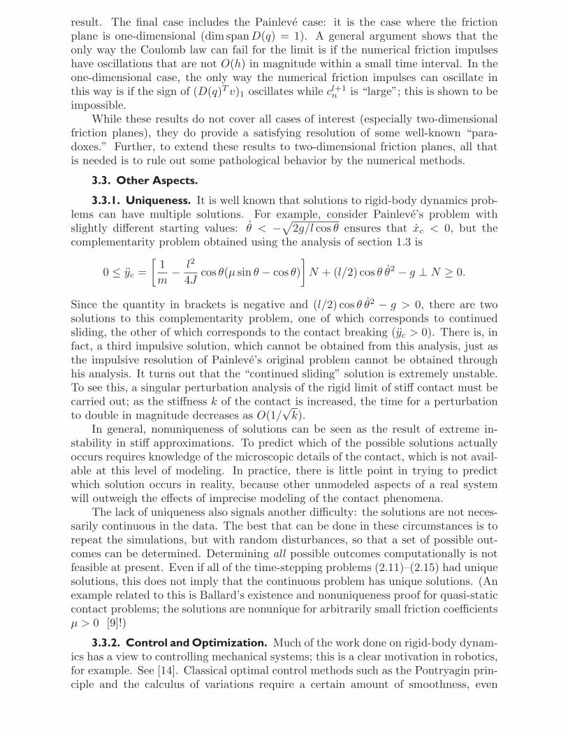
While these results do not cover all cases of interest (especially two-dimensionalfriction planes), they do provide a satisfying resolution of some well-known “para-doxes.” Further, to extend these results to two-dimensional friction planes, all thatis needed is to rule out some pathological behavior by the numerical methods.

3.3. Other Aspects.

3.3.1. Uniqueness. It is well known that solutions to rigid-body dynamics prob-lems can have multiple solutions. For example, consider Painleve’s problem withslightly different starting values: θ < −√

2g/l cos θ ensures that xc < 0, but thecomplementarity problem obtained using the analysis of section 1.3 is

0 ≤ yc =[

1m

− l2

4Jcos θ(μ sin θ − cos θ)

]N + (l/2) cos θ θ2 − g ⊥ N ≥ 0.

Since the quantity in brackets is negative and (l/2) cos θ θ2 − g > 0, there are twosolutions to this complementarity problem, one of which corresponds to continuedsliding, the other of which corresponds to the contact breaking (yc > 0). There is, infact, a third impulsive solution, which cannot be obtained from this analysis, just asthe impulsive resolution of Painleve’s original problem cannot be obtained throughhis analysis. It turns out that the “continued sliding” solution is extremely unstable.To see this, a singular perturbation analysis of the rigid limit of stiff contact must becarried out; as the stiffness k of the contact is increased, the time for a perturbationto double in magnitude decreases as O(1/

√k).

In general, nonuniqueness of solutions can be seen as the result of extreme in-stability in stiff approximations. To predict which of the possible solutions actuallyoccurs requires knowledge of the microscopic details of the contact, which is not avail-able at this level of modeling. In practice, there is little point in trying to predictwhich solution occurs in reality, because other unmodeled aspects of a real systemwill outweigh the effects of imprecise modeling of the contact phenomena.

The lack of uniqueness also signals another difficulty: the solutions are not neces-sarily continuous in the data. The best that can be done in these circumstances is torepeat the simulations, but with random disturbances, so that a set of possible out-comes can be determined. Determining all possible outcomes computationally is notfeasible at present. Even if all of the time-stepping problems (2.11)–(2.15) had uniquesolutions, this does not imply that the continuous problem has unique solutions. (Anexample related to this is Ballard’s existence and nonuniqueness proof for quasi-staticcontact problems; the solutions are nonunique for arbitrarily small friction coefficientsμ > 0 [9]!)

3.3.2. Control and Optimization. Much of the work done on rigid-body dynam-ics has a view to controlling mechanical systems; this is a clear motivation in robotics,for example. See [14]. Classical optimal control methods such as the Pontryagin prin-ciple and the calculus of variations require a certain amount of smoothness, even

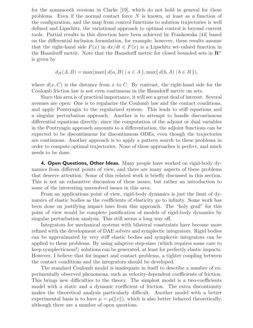
for the nonsmooth versions in Clarke [19], which do not hold in general for theseproblems. Even if the normal contact force N is known, at least as a function ofthe configuration, and the map from control functions to solution trajectories is welldefined and Lipschitz, the variational approach to optimal control is beyond currenttools. Partial results in this direction have been achieved by Frankowska [44] basedon the differential inclusion formulation, for example; however, these results assumethat the right-hand side F (x) in dx/dt ∈ F (x) is a Lipschitz set-valued function inthe Hausdorff metric. Note that the Hausdorff metric for closed bounded sets in Rn

is given by

dH(A, B) = max(max{ d(a, B) | a ∈ A },max{ d(b, A) | b ∈ B }),

where d(x, C) is the distance from x to C. By contrast, the right-hand side for theCoulomb friction law is not even continuous in the Hausdorff metric on sets.

Since this area is of practical importance, it will see a great deal of interest. Severalavenues are open: One is to regularize the Coulomb law and the contact conditions,and apply Pontryagin to the regularized system. This leads to stiff equations anda singular perturbation approach. Another is to attempt to handle discontinuousdifferential equations directly; since the computation of the adjoint or dual variablesin the Pontryagin approach amounts to a differentiation, the adjoint functions can beexpected to be discontinuous for discontinuous ODEs, even though the trajectoriesare continuous. Another approach is to apply a pattern search to these problems inorder to compute optimal trajectories. None of these approaches is perfect, and muchneeds to be done.

4. Open Questions, Other Ideas. Many people have worked on rigid-body dy-namics from different points of view, and there are many aspects of these problemsthat deserve attention. Some of this related work is briefly discussed in this section.This is not an exhaustive discussion of these issues, but rather an introduction tosome of the interesting unresolved issues in this area.

From an applications point of view, rigid-body dynamics is just the limit of dy-namics of elastic bodies as the coefficients of elasticity go to infinity. Some work hasbeen done on justifying impact laws from this approach. The “holy grail” for thispoint of view would be complete justification of models of rigid-body dynamics bysingular perturbation analysis. This still seems a long way off.

Integrators for mechanical systems with bilateral constraints have become morerefined with the development of DAE solvers and symplectic integrators. Rigid bodiescan be approximated by very stiff elastic bodies and symplectic integrators can beapplied to these problems. By using adaptive step-sizes (which requires some care tokeep symplecticness!) solutions can be generated, at least for perfectly elastic impacts.However, I believe that for impact and contact problems, a tighter coupling betweenthe contact conditions and the integrators should be developed.

The standard Coulomb model is inadequate in itself to describe a number of ex-perimentally observed phenomena, such as velocity-dependent coefficients of friction.This brings new difficulties to the theory. The simplest model is a two-coefficientsmodel with a static and a dynamic coefficient of friction. The extra discontinuitymakes the theoretical analysis particularly difficult. Another model with a betterexperimental basis is to have μ = μ(‖v‖), which is also better behaved theoretically,although there are a number of open questions.

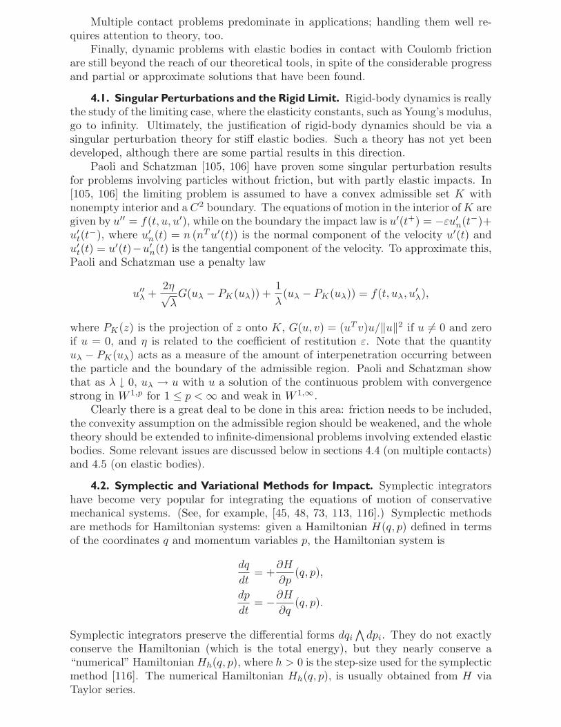
Multiple contact problems predominate in applications; handling them well re-quires attention to theory, too.

Finally, dynamic problems with elastic bodies in contact with Coulomb frictionare still beyond the reach of our theoretical tools, in spite of the considerable progressand partial or approximate solutions that have been found.

4.1. Singular Perturbations and the Rigid Limit. Rigid-body dynamics is reallythe study of the limiting case, where the elasticity constants, such as Young’s modulus,go to infinity. Ultimately, the justification of rigid-body dynamics should be via asingular perturbation theory for stiff elastic bodies. Such a theory has not yet beendeveloped, although there are some partial results in this direction.

Paoli and Schatzman [105, 106] have proven some singular perturbation resultsfor problems involving particles without friction, but with partly elastic impacts. In[105, 106] the limiting problem is assumed to have a convex admissible set K withnonempty interior and a C2 boundary. The equations of motion in the interior of K aregiven by u′′ = f(t, u, u′), while on the boundary the impact law is u′(t+) = −εu′

n(t−)+u′

t(t−), where u′

n(t) = n (nT u′(t)) is the normal component of the velocity u′(t) andu′

t(t) = u′(t)−u′n(t) is the tangential component of the velocity. To approximate this,

Paoli and Schatzman use a penalty law

u′′λ +

2η√λ

G(uλ − PK(uλ)) +1λ

(uλ − PK(uλ)) = f(t, uλ, u′λ),

where PK(z) is the projection of z onto K, G(u, v) = (uT v)u/‖u‖2 if u �= 0 and zeroif u = 0, and η is related to the coefficient of restitution ε. Note that the quantityuλ − PK(uλ) acts as a measure of the amount of interpenetration occurring betweenthe particle and the boundary of the admissible region. Paoli and Schatzman showthat as λ ↓ 0, uλ → u with u a solution of the continuous problem with convergencestrong in W 1,p for 1 ≤ p < ∞ and weak in W 1,∞.

Clearly there is a great deal to be done in this area: friction needs to be included,the convexity assumption on the admissible region should be weakened, and the wholetheory should be extended to infinite-dimensional problems involving extended elasticbodies. Some relevant issues are discussed below in sections 4.4 (on multiple contacts)and 4.5 (on elastic bodies).

4.2. Symplectic and Variational Methods for Impact. Symplectic integratorshave become very popular for integrating the equations of motion of conservativemechanical systems. (See, for example, [45, 48, 73, 113, 116].) Symplectic methodsare methods for Hamiltonian systems: given a Hamiltonian H(q, p) defined in termsof the coordinates q and momentum variables p, the Hamiltonian system is

dq

dt= +

∂H

∂p(q, p),

dp

dt= −∂H

∂q(q, p).

Symplectic integrators preserve the differential forms dqi

∧dpi. They do not exactly

conserve the Hamiltonian (which is the total energy), but they nearly conserve a“numerical” Hamiltonian Hh(q, p), where h > 0 is the step-size used for the symplecticmethod [116]. The numerical Hamiltonian Hh(q, p), is usually obtained from H viaTaylor series.

Adaptive versions of these methods can deal with certain kinds of singularities,such as those arising from terms of the form f(q)−α for large α which models “soft”contacts, and bilaterally constrained mechanical systems. Because of the possibilityof unbounded right-hand sides, implicit methods are necessary. Take, for example,the simplest implicit (nonpartitioned) symplectic method, the implicit midpoint rulefor dx/dt = f(t, x):

xn+1 = xn + h f((tn + tn+1)/2, (xn + xn+1)/2).

Consider the case of a single particle in one dimension with only contact forces andgravitation, and a simple inequality constraint: q(t) ≥ 0. The Hamiltonian of thesystem is H(q, p) = 1

2mp2 + ψ(q) + gq, where ψ(q) = 0 for q ≥ 0 and ψ(q) = +∞ forq < 0. This gives the differential equations and inclusions

dq

dt=

1m

p,

dp

dt∈ −∂ψ(q) − g.

Note that ∂ψ(q) = {0} if q > 0, ∂ψ(q) = R+ if q = 0, and ∂ψ(q) = ∅ if q < 0.Applying the implicit midpoint rule to this system gives the numerical scheme

qn+1 = qn +h

2m(pn + pn+1),

pn+1 ∈ pn − h

2∂ψ((qn+1 + qn)/2) − hg.

Writing Nn+1 for the element we choose from −(h/2)∂ψ((qn+qn+1)/2) (that is, Nn+1is the normal contact impulse), we get the mixed complementarity problem

pn+1 = pn + Nn+1 − hg,

qn+1 = qn +h

2m(pn + pn+1),

0 ≤ Nn+1 ⊥ (qn + qn+1)/2 ≥ 0.

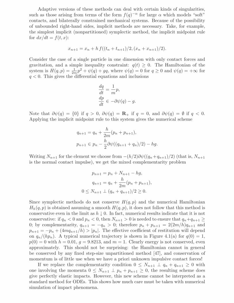
Since symplectic methods do not conserve H(q, p) and the numerical HamiltonianHh(q, p) is obtained assuming a smooth H(q, p), it does not follow that this method isconservative even in the limit as h ↓ 0. In fact, numerical results indicate that it is notconservative: if qn < 0 and pn < 0, then Nn+1 > 0 is needed to ensure that qn+qn+1 ≥0; by complementarity, qn+1 = −qn > 0; therefore pn + pn+1 = 2(2m/h)qn+1 andpn+1 = −pn + (4mqn+1/h) > |pn|. The effective coefficient of restitution will dependon qn/(hpn). A typical numerical trajectory is shown in Figure 4.1(a) for q(0) = 1,p(0) = 0 with h = 0.01, g = 9.8213, and m = 1. Clearly energy is not conserved, evenapproximately. This should not be surprising: the Hamiltonian cannot in generalbe conserved by any fixed step-size unpartitioned method [47], and conservation ofmomentum is of little use when we have a priori unknown impulsive contact forces!

If we replace the complementarity condition 0 ≤ Nn+1 ⊥ qn + qn+1 ≥ 0 withone involving the momenta 0 ≤ Nn+1 ⊥ pn + pn+1 ≥ 0, the resulting scheme doesgive perfectly elastic impacts. However, this new scheme cannot be interpreted as astandard method for ODEs. This shows how much care must be taken with numericalsimulation of impact phenomena.

0 1 2 3 4 5 6 7 8 9 105

0

5

10

15

20

25

30

t

q(t)

Numerical solution for midpoint rule with contact (h = 0.01)

(a) Midpoint rule

0 0.2 0.4 0.6 0.8 1 1.2 1.4 1.6 1.8 20

0.2

0.4

0.6

0.8

1

1.2

1.4

t

q(t)

Bouncing ball simulation using Newmark–type algorithm

β = 0, γ = 1

h = 103

(b) Newmark scheme

Fig. 4.1 Numerical trajectories using the midpoint rule and a Newmark scheme.

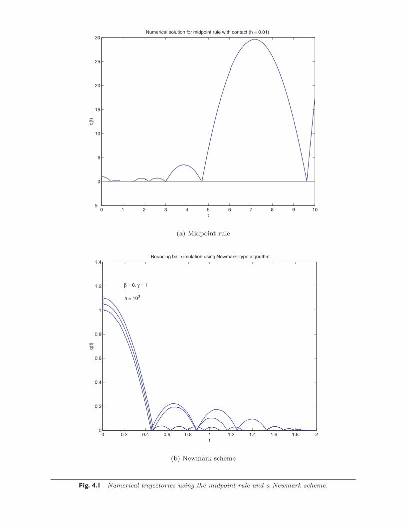
Other schemes, such as the Newmark schemes, can also be applied to contactproblems [59]. However, these schemes also suffer from indeterminism in the effectivecoefficient of restitution. In Figure 4.1(b), results are shown for a Newmark scheme[59] with β = 0, γ = 1, and step-size h = 10−3 for the same bouncing ball problem withseveral initial conditions to illustrate the nondeterminism. Even variational methodsbased on discrete Lagrangian principles [141] do not seem to behave correctly.

4.3. Static vs. Dynamic Friction. It is an experimentally observed phenomenonthat the coefficient of friction often depends on the sliding velocity as well as the natureof the materials in contact. This has a number of practical implications. For example,if you need to brake suddenly while driving, the common advice is to “pump” thebrakes. (This advice does not apply to vehicles equipped with ABS, which “pumps”automatically.) This is because when the car begins to slide the coefficient of frictionappears to decrease, and the car does not decelerate as quickly. (Many people perceivethis effect as the car actually accelerating; in fact it is still decelerating, but not asquickly.)

The standard Coulomb model of dry friction does not take this velocity depen-dence into account. There are several ways of incorporating velocity dependence intothe Coulomb model. The simplest is to have two coefficients of friction: the staticcoefficient μstatic and the dynamic coefficient μdynamic. From the differential inclusionpoint of view, it is clear that μdynamic ≤ μstatic, for if μdynamic > μstatic, there couldnot be any motion until the friction limit μdynamicN is overcome. Thus there is nosense having μdynamic > μstatic. This discontinuous model of friction leads to a num-ber of theoretical difficulties. For example, consider the “brick on a ramp” problemwith this model of friction. Treating the problem naively, the equations of motionbecome

mdv

dt∈ mg sin θ − mg cos θ Sgn v

{μdynamic if v �= 0,μstatic if v = 0,

and the right-hand side contains the right-hand side for the original friction model(1.1) with μ = μdynamic. This means that if we interpret this simply as a differ-ential inclusion, the brick can begin sliding whenever μdynamicmg cos θ < mg sin θ <μstaticmg cos θ. Clearly this is missing something crucial about the two-friction model:there is a hysteresis effect. Once v = 0, the coefficient of friction is “stuck” at μstatic

until such time as the external force is sufficient to overcome the static friction forcelimit μstaticN .

This model is vulnerable to some strong criticisms, such as those of Ruina [115,section 9.3.1], who discusses the model from a continuum point of view.

Even when the hysteresis effect is understood and is used to remove most of thenonuniqueness associated with this model, it is still quite possible to get multiplesolutions when the velocity function v(t) “grazes” v = 0; that is, v′(t) < 0 for t < t∗,v(t∗) = 0, v′(t∗) = 0, but v′′(t∗) > 0. Then the friction coefficient may jump fromμdynamic to μstatic and “grab” the solution, forcing it to stay at zero for an interval.Or perhaps the coefficient of friction might stay at μdynamic and allow the velocityto move away from zero again. How to treat this nonuniqueness is an unresolvedtheoretical issue with this model.

Another model which has a stronger experimental basis is to write μ = μ(‖v‖2),where μ′(s) < 0 and lims→∞ μ(s) = μ∞ > 0. An example of this model is shown inFigure 4.2(c). The behavior of systems with this friction model is very similar to thecommon understanding of the two-friction-coefficients model. If v �= 0, the fact that

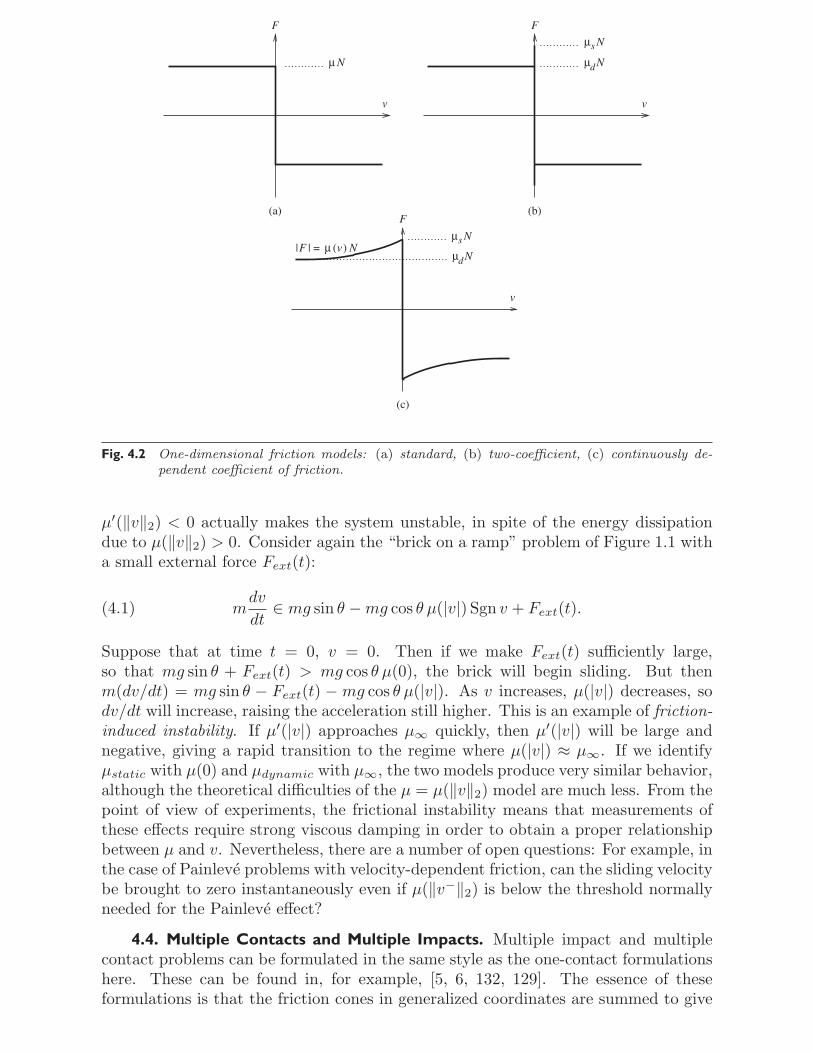
μ Ns

μ Ns

μ Nd

| | = μ (v N)F

(c)

v

F

v

F

v

F

μ N

μ Nd

(b)(a)

Fig. 4.2 One-dimensional friction models: (a) standard, (b) two-coefficient, (c) continuously de-pendent coefficient of friction.

μ′(‖v‖2) < 0 actually makes the system unstable, in spite of the energy dissipationdue to μ(‖v‖2) > 0. Consider again the “brick on a ramp” problem of Figure 1.1 witha small external force Fext(t):

mdv

dt∈ mg sin θ − mg cos θ μ(|v|) Sgn v + Fext(t).(4.1)

Suppose that at time t = 0, v = 0. Then if we make Fext(t) sufficiently large,so that mg sin θ + Fext(t) > mg cos θ μ(0), the brick will begin sliding. But thenm(dv/dt) = mg sin θ − Fext(t) − mg cos θ μ(|v|). As v increases, μ(|v|) decreases, sodv/dt will increase, raising the acceleration still higher. This is an example of friction-induced instability. If μ′(|v|) approaches μ∞ quickly, then μ′(|v|) will be large andnegative, giving a rapid transition to the regime where μ(|v|) ≈ μ∞. If we identifyμstatic with μ(0) and μdynamic with μ∞, the two models produce very similar behavior,although the theoretical difficulties of the μ = μ(‖v‖2) model are much less. From thepoint of view of experiments, the frictional instability means that measurements ofthese effects require strong viscous damping in order to obtain a proper relationshipbetween μ and v. Nevertheless, there are a number of open questions: For example, inthe case of Painleve problems with velocity-dependent friction, can the sliding velocitybe brought to zero instantaneously even if μ(‖v−‖2) is below the threshold normallyneeded for the Painleve effect?

4.4. Multiple Contacts and Multiple Impacts. Multiple impact and multiplecontact problems can be formulated in the same style as the one-contact formulationshere. These can be found in, for example, [5, 6, 132, 129]. The essence of theseformulations is that the friction cones in generalized coordinates are summed to give

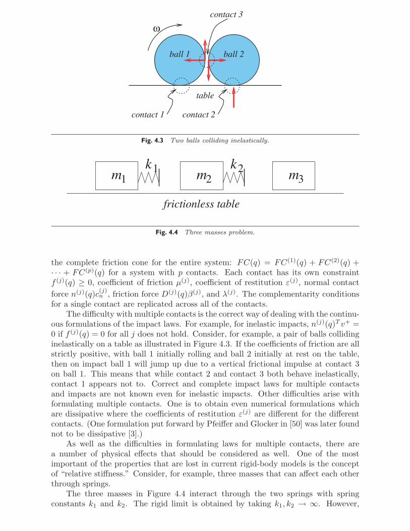
ball 1 ball 2

ω

table

contact 1 contact 2

contact 3

Fig. 4.3 Two balls colliding inelastically.

m1k1

frictionless table

m2k2 m3

Fig. 4.4 Three masses problem.

the complete friction cone for the entire system: FC(q) = FC(1)(q) + FC(2)(q) +· · · + FC(p)(q) for a system with p contacts. Each contact has its own constraintf (j)(q) ≥ 0, coefficient of friction μ(j), coefficient of restitution ε(j), normal contactforce n(j)(q)c(j)

n , friction force D(j)(q)β(j), and λ(j). The complementarity conditionsfor a single contact are replicated across all of the contacts.

The difficulty with multiple contacts is the correct way of dealing with the continu-ous formulations of the impact laws. For example, for inelastic impacts, n(j)(q)T v+ =0 if f (j)(q) = 0 for all j does not hold. Consider, for example, a pair of balls collidinginelastically on a table as illustrated in Figure 4.3. If the coefficients of friction are allstrictly positive, with ball 1 initially rolling and ball 2 initially at rest on the table,then on impact ball 1 will jump up due to a vertical frictional impulse at contact 3on ball 1. This means that while contact 2 and contact 3 both behave inelastically,contact 1 appears not to. Correct and complete impact laws for multiple contactsand impacts are not known even for inelastic impacts. Other difficulties arise withformulating multiple contacts. One is to obtain even numerical formulations whichare dissipative where the coefficients of restitution ε(j) are different for the differentcontacts. (One formulation put forward by Pfeiffer and Glocker in [50] was later foundnot to be dissipative [3].)

As well as the difficulties in formulating laws for multiple contacts, there area number of physical effects that should be considered as well. One of the mostimportant of the properties that are lost in current rigid-body models is the conceptof “relative stiffness.” Consider, for example, three masses that can affect each otherthrough springs.

The three masses in Figure 4.4 interact through the two springs with springconstants k1 and k2. The rigid limit is obtained by taking k1, k2 → ∞. However,

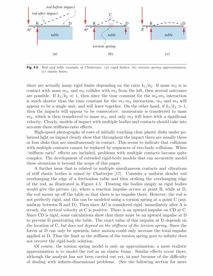
(b) (c)

rod before impact

rod after impact

table

B D

tableA

B D

tableA

B D

torsion spring

C

(a)

A

Fig. 4.5 Rod and table example of Chatterjee: (a) rigid bodies; (b) torsion spring approximation;(c) elastic beam.

there are actually many rigid limits depending on the ratio k1/k2. If mass m2 is incontact with mass m3, and m1 collides with m2 from the left, then several outcomesare possible. If k1/k2 � 1, then since the time constant for the m2-m3 interactionis much shorter than the time constant for the m1-m2 interaction, m2 and m3 willappear to be a single unit, and will leave together. On the other hand, if k1/k2 � 1,then the impacts will appear to be consecutive: momentum is transferred to massm2, which is then transferred to mass m3, and only m3 will leave with a significantvelocity. Clearly, models of impact with multiple bodies and contacts should take intoaccount these stiffness-ratio effects.

High-speed photographs of rows of initially touching clear plastic disks under po-larized light on impact clearly show that throughout the impact there are usually threeor four disks that are simultaneously in contact. This seems to indicate that collisionswith multiple contacts cannot be replaced by sequences of two-body collisions. When“stiffness ratio” effects are included, problems with multiple contacts become quitecomplex. The development of extended rigid-body models that can accurately modelthese situations is beyond the scope of this paper.

A further issue that is related to multiple simultaneous contacts and vibrationsof stiff elastic bodies is raised by Chatterjee [17]. Consider a uniform slender rodoverhanging the edge of a frictionless table and then striking the overhanging edgeof the rod, as illustrated in Figure 4.5. Treating the bodies simply as rigid bodieswould give the picture (a), where a reaction impulse occurs at point B, while at D,the rod moves up off the table so that there is no impulse there. However, the rod isnot perfectly rigid, and this can be modeled using a torsion spring at a point C (say,midway between B and D). Then since AC is considered rigid, immediately after A isstruck, the vertical velocity at C is positive. There is an upward impulse on CD at C.Since CD is rigid, some calculations show that there must be an upward impulse at Dto prevent D penetrating the table. The exact value of this impulse at D depends onthe location of C, but does not depend on the stiffness of the torsion spring. Since theforces at D can only be upwards, later motion could only increase the total impulseapplied at D. Thus the limit as the stiffness of the torsion spring goes to infinity doesnot recover the rigid-body solution.

Of course, the torsion spring model is only an approximation; a more realisticapproximation is to model the rod as an elastic beam. Similar effects occur there,although the analysis has not been carried out yet, in part because of the difficultyof dealing with infinite-dimensional problems. (See the following section for more

on these issues.) Simple experiments with a rod (like a knitting needle) and carbonpaper verify that this effect is real. Thus we have both nT

Dv+D > 0 and ND > 0 in the

limit as kspring → ∞, contradicting the usual assumption about complementarity:0 ≤ nT

Dv+D ⊥ ND ≥ 0. Nevertheless, it should be noted that the usual complemen-

tarity conditions hold for all times and spring stiffnesses in (b) and (c). In addition,complementarity between the vertical displacement and the normal contact force re-mains fundamental, as noted in [17].

Can the rigid-body solution (a) be obtained as some sort of limit of (b) or (c)? Theanswer is yes, and again is related to stiffness ratios: if ktable/kspring goes to zero asboth stiffnesses go to infinity, the rigid body solution (a) is recovered. The reason thatthis is not seen experimentally in [17] is that it is much easier to build a stiff table thanit is to find a stiff yet slender rod. Again we come to a question of how to deal withstiffness ratios and elastic vibrations. The problem is that as the material stiffnessgoes to infinity, the amplitudes of the elastic vibrations go to zero, but the amplitudesof the surface velocities do not. This means that complementarity conditions for rigidmotions may not be correct even though complementarity conditions for the truesurface velocities may be. This issue is more fundamental than the issue of whichimpact law to use, since all current impact laws must handle the inelastic case ε = 0at least as a model of the compression phase of the contact. In short, there area number of issues regarding multiple contact and multiple body impacts that needresolution, but new low-order models may be able to incorporate the effects of multiplecontacts and elastic vibrations.

4.5. Elastica in Impact. The problems in handling the infinite-dimensional prob-lems associated with elastic (and elastoviscous, elastoplastic) materials in frictionalcontact are substantial. Currently, the best results are either for quasi-static prob-lems where the forces are assumed to always be in equilibrium, or for special dynamicproblems with “small” coefficients of friction. Good starting points for understandingthese problems are the book by Kikuchi and Oden [65] and the book by Duvaut andLions [32]. However, the early formulations in terms of variational inequalities had toassume frictionless contact, that the normal contact force is given (Tresca friction), orsome other simplifying assumption. The feedback between the friction force and thenormal contact force was usually ignored in order to obtain a well-posed variationalinequality. If the feedback is used to construct a fixed-point problem, then results canbe obtained for coefficients of friction “small enough” by means of a contraction map-ping argument. For large coefficients of friction, this approach fails. An alternativethat uses a Leray–Schauder argument would be more attractive in this case, althoughthere are a number of technical difficulties with compactness, even for quasi-staticproblems. Often a mollifier is used to modify the friction law to satisfy the compact-ness requirements, but this also makes the friction law nonlocal, which does not seemphysically appropriate. The following references survey the state of the art in thisarea [22, 23, 30, 56, 57, 58, 62, 65].

Work on fully dynamic infinite-dimensional contact problems includes that ofP. Shi [125], Bamberger and Schatzman [10], Schatzman [120], and Schatzman andBercovier [121]. The work of P. Shi mainly concerns a one-dimensional wave equationwith contact only at one end; the work of Schatzman et al. is mainly about the waveequation with a rigid obstacle, where contact can be made over the whole spatialdomain. The problems in this area are characterized by a high level of technicaldifficulty. A full discussion of the issues in this area is beyond the scope of thisarticle.

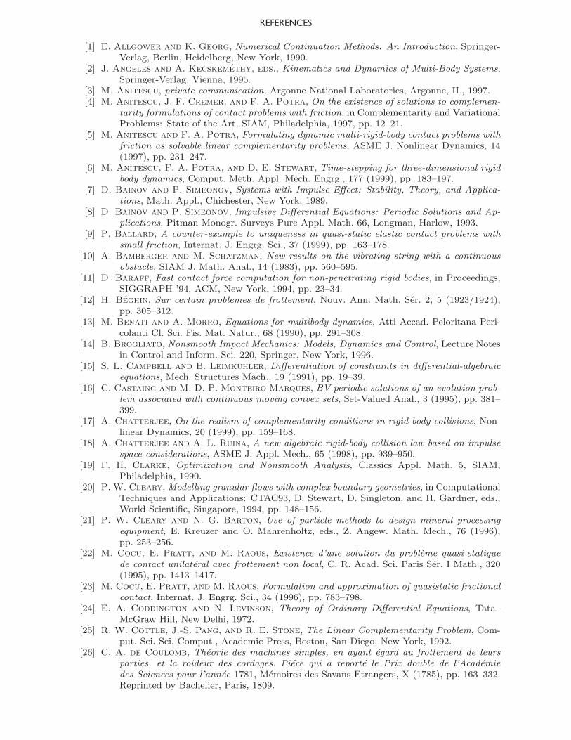
REFERENCES

[1] E. Allgower and K. Georg, Numerical Continuation Methods: An Introduction, Springer-Verlag, Berlin, Heidelberg, New York, 1990.

[2] J. Angeles and A. Kecskemethy, eds., Kinematics and Dynamics of Multi-Body Systems,Springer-Verlag, Vienna, 1995.

[3] M. Anitescu, private communication, Argonne National Laboratories, Argonne, IL, 1997.[4] M. Anitescu, J. F. Cremer, and F. A. Potra, On the existence of solutions to complemen-

tarity formulations of contact problems with friction, in Complementarity and VariationalProblems: State of the Art, SIAM, Philadelphia, 1997, pp. 12–21.

[5] M. Anitescu and F. A. Potra, Formulating dynamic multi-rigid-body contact problems withfriction as solvable linear complementarity problems, ASME J. Nonlinear Dynamics, 14(1997), pp. 231–247.

[6] M. Anitescu, F. A. Potra, and D. E. Stewart, Time-stepping for three-dimensional rigidbody dynamics, Comput. Meth. Appl. Mech. Engrg., 177 (1999), pp. 183–197.

[7] D. Bainov and P. Simeonov, Systems with Impulse Effect: Stability, Theory, and Applica-tions, Math. Appl., Chichester, New York, 1989.

[8] D. Bainov and P. Simeonov, Impulsive Differential Equations: Periodic Solutions and Ap-plications, Pitman Monogr. Surveys Pure Appl. Math. 66, Longman, Harlow, 1993.

[9] P. Ballard, A counter-example to uniqueness in quasi-static elastic contact problems withsmall friction, Internat. J. Engrg. Sci., 37 (1999), pp. 163–178.

[10] A. Bamberger and M. Schatzman, New results on the vibrating string with a continuousobstacle, SIAM J. Math. Anal., 14 (1983), pp. 560–595.

[11] D. Baraff, Fast contact force computation for non-penetrating rigid bodies, in Proceedings,SIGGRAPH ’94, ACM, New York, 1994, pp. 23–34.

[12] H. Beghin, Sur certain problemes de frottement, Nouv. Ann. Math. Ser. 2, 5 (1923/1924),pp. 305–312.

[13] M. Benati and A. Morro, Equations for multibody dynamics, Atti Accad. Peloritana Peri-colanti Cl. Sci. Fis. Mat. Natur., 68 (1990), pp. 291–308.

[14] B. Brogliato, Nonsmooth Impact Mechanics: Models, Dynamics and Control, Lecture Notesin Control and Inform. Sci. 220, Springer, New York, 1996.

[15] S. L. Campbell and B. Leimkuhler, Differentiation of constraints in differential-algebraicequations, Mech. Structures Mach., 19 (1991), pp. 19–39.

[16] C. Castaing and M. D. P. Monteiro Marques, BV periodic solutions of an evolution prob-lem associated with continuous moving convex sets, Set-Valued Anal., 3 (1995), pp. 381–399.

[17] A. Chatterjee, On the realism of complementarity conditions in rigid-body collisions, Non-linear Dynamics, 20 (1999), pp. 159–168.

[18] A. Chatterjee and A. L. Ruina, A new algebraic rigid-body collision law based on impulsespace considerations, ASME J. Appl. Mech., 65 (1998), pp. 939–950.

[19] F. H. Clarke, Optimization and Nonsmooth Analysis, Classics Appl. Math. 5, SIAM,Philadelphia, 1990.

[20] P. W. Cleary, Modelling granular flows with complex boundary geometries, in ComputationalTechniques and Applications: CTAC93, D. Stewart, D. Singleton, and H. Gardner, eds.,World Scientific, Singapore, 1994, pp. 148–156.

[21] P. W. Cleary and N. G. Barton, Use of particle methods to design mineral processingequipment, E. Kreuzer and O. Mahrenholtz, eds., Z. Angew. Math. Mech., 76 (1996),pp. 253–256.

[22] M. Cocu, E. Pratt, and M. Raous, Existence d’une solution du probleme quasi-statiquede contact unilateral avec frottement non local, C. R. Acad. Sci. Paris Ser. I Math., 320(1995), pp. 1413–1417.

[23] M. Cocu, E. Pratt, and M. Raous, Formulation and approximation of quasistatic frictionalcontact, Internat. J. Engrg. Sci., 34 (1996), pp. 783–798.

[24] E. A. Coddington and N. Levinson, Theory of Ordinary Differential Equations, Tata–McGraw Hill, New Delhi, 1972.

[25] R. W. Cottle, J.-S. Pang, and R. E. Stone, The Linear Complementarity Problem, Com-put. Sci. Sci. Comput., Academic Press, Boston, San Diego, New York, 1992.

[26] C. A. de Coulomb, Theorie des machines simples, en ayant egard au frottement de leursparties, et la roideur des cordages. Piece qui a reporte le Prix double de l’Academiedes Sciences pour l’annee 1781, Memoires des Savans Etrangers, X (1785), pp. 163–332.Reprinted by Bachelier, Paris, 1809.

[27] E. Delassus, Considerations sur le frottement de glissement, Nouv. Ann. Math. Ser. 4, 20(1920), pp. 485–496.

[28] E. Delassus, Sur les lois du frottement de glissement, Bull. Soc. Math. France, 51 (1923),pp. 22–33.

[29] F. Demengel and R. Temam, Convex functions of a measure and applications, Indiana Univ.Math. J., 33 (1984), pp. 673–709.

[30] L. Demkowicz and J. T. Oden, On some existence and uniqueness results in contact prob-lems with nonlocal friction, Nonlinear Anal., 6 (1982), pp. 1075–1093.

[31] A. Dontchev and F. Lempio, Difference methods for differential inclusions: A survey, SIAMRev., 34 (1992), pp. 263–294.

[32] G. Duvaut and J.-L. Lions, Inequalities in Mechanics and Physics, Grundlehren Math. Wiss.219, Springer-Verlag, Berlin, Heidelberg, New York, 1976.

[33] E. Eich, C. Fuhrer, and J. Yen, On the error control for multistep methods applied toODEs with invariants and DAEs in multibody dynamics, Mech. Structures Mach., 23(1995), pp. 159–179.

[34] E. Eich-Soellner and C. Fuhrer, Numerical Methods in Multibody Dynamics, B. G. Teub-ner, Stuttgart, 1998.

[35] C. M. Elliott, On the convergence of a one-step method for the numerical solution ofordinary differential inclusions, IMA J. Numer. Anal., 5 (1985), pp. 3–21.

[36] M. Erdmann, On a representation of friction in configuration space, Internat. J. RoboticsResearch, 13 (1994), pp. 240–271.

[37] M. C. Ferris and J.-S. Pang, Engineering and economic applications of complementarityproblems, SIAM Rev., 39 (1997), pp. 669–713.

[38] A. F. Filippov, Differential equations with discontinuous right-hand side, Amer. Math. Soc.Trans., 42 (1964), pp. 199–231; original published in Mat. Sb., 5 (1960), pp. 99–127 (inRussian).

[39] A. F. Filippov, Classical solutions of differential equations with multivalued right-hand side,SIAM J. Control Optim., 5 (1967), pp. 609–621.

[40] A. F. Filippov, Differential Equations with Discontinuous Right-Hand Side, Kluwer Aca-demic, Norwell, MA, 1988.

[41] R. Fletcher, Practical Methods of Optimization, 2nd ed., John Wiley, Chichester, New York,1987.

[42] C. G. Franchi, A general formulation in rigid multibody dynamics, Internat. J. Numer. Meth.Engrg., 38 (1995), pp. 1985–2016.

[43] J. Franklin, Methods of Mathematical Economics, Springer-Verlag, New York, Heidelberg,Berlin, 1980.

[44] H. Frankowska, The maximum principle for an optimal solution to a differential inclusionwith end points constraints, SIAM J. Control Optim., 25 (1987), pp. 145–157.

[45] C. Fuhrer and B. Leimkuhler, Numerical methods for differential-algebraic equations de-scribing constrained mechanical motion, in Computational Ordinary Differential Equa-tions (London, 1989), Oxford University Press, New York, 1992, pp. 275–284.

[46] J. Garcıa de Jalon and E. Bayo, Kinematic and dynamic simulation of multibody systems,Springer-Verlag, New York, 1994.

[47] Z. Ge and J. E. Marsden, Lie-Poisson Hamilton-Jacobi theory and Lie-Poisson integrators,Phys. Lett. A, 133 (1988), pp. 134–139.

[48] C. W. Gear, B. Leimkuhler, and G. K. Gupta, Automatic integration of Euler–Lagrangeequations with constraints, J. Comput. Appl. Math., 12/13 (1985) pp. 77–90.

[49] F. Genot and B. Brogliato, New results on Painleve paradoxes, European J. Mech.A Solids, 18 (1999), pp. 653–677. Also available as INRIA Research Report 3366 viaftp://ftp.inria.fr/INRIA/tech-reports/RR/RR-3366.ps.gz.

[50] C. Glocker and F. Pfeiffer, Multiple impacts with friction in rigid multibody systems,ASME J. Nonlinear Dynamics, 7 (1995), pp. 471–497.

[51] S.-P. Han, J.-S. Pang, and N. Rangaraj, Globally convergent Newton methods for non-smooth equations, Math. Oper. Res., 17 (1992), pp. 586–607.

[52] E. J. Haug, D. Negrut, and M. Iancu, A state-space-based implicit integration algorithmfor differential-algebraic equations of multibody dynamics, Mech. Structures Mach., 25(1997), pp. 311–334.

[53] J.-B. Hiriart-Urruty and C. Lemarechal, Convex Analysis and Minimization AlgorithmsI and II, Grundlehren Math. Wiss., Springer–Verlag, Berlin, Heidelberg, New York, 1993.

[54] R. Horst and P. Pardalos, eds., Handbook of Global Optimization, Nonconvex Optim.Appl., Kluwer Academic Publishers, Dordrecht, the Netherlands, 1995.

[55] G. Isac, Complementarity problems, Lecture Notes in Math. 1528, Springer-Verlag, Berlin,1992.

[56] J. Jarusek, Contact problems with bounded friction: Coercive case, Czechoslovak Math. J.,33 (1983), pp. 237–261.

[57] J. Jarusek and C. Eck, Dynamic contact problems with friction in linear viscoelasticity, C.R. Acad. Sci. Paris Ser. I Math., 322 (1996), pp. 497–502.

[58] J. Jarusek and C. Eck, Dynamic contact problems with small Coulomb friction for viscoelas-tic bodies. Existence of solutions, Math. Models Methods Appl. Sci., 9 (1999), pp. 11–34.

[59] C. Kane and M. Ortiz, Finite element analysis of non-smooth contact, Comput. Meth. Appl.Mech. Engrg., 180 (1999), pp. 1–26.

[60] A. E. Kastner-Maresch, Implicit Runge–Kutta methods for differential inclusions, Numer.Funct. Anal. Optim., 11 (1990), pp. 937–958.

[61] A. E. Kastner-Maresch, The implicit midpoint rule applied to discontinuous differentialequations, Computing, 49 (1992), pp. 45–62.

[62] Y. Kato, Signorini’s problem with friction in linear elasticity, Japan J. Appl. Math., 4 (1987),pp. 237–268.

[63] J. B. Keller, Impact with friction, ASME J. Appl. Mech., 53 (1986), pp. 1–4.[64] J. L. Kelley and T. P. Srinivasan, Measure and Integral, Volume 1, Grad. Texts in Math.

116, Springer-Verlag, New York, 1988.[65] N. Kikuchi and J. T. Oden, Contact Problems in Elasticity: A Study of Variational In-

equalities and Finite Element Methods, SIAM Stud. Appl. Math. 8, SIAM, Philadelphia,1988.

[66] A. Klarbring, Mathematical programming in contact problems, in Computational Methodsin Contact Mechanics, M. H. Aliabadi and C. A. Brebbia, eds., Internat. Ser. Comput.Engrg., Computational Mechanics Publications, London, 1993, pp. 233–263.

[67] A. Klarbring, Steady sliding and linear complementarity, in Complementarity and Varia-tional Problems, M. C. Ferris and J.-S. Pang, eds., SIAM, Philadelphia, 1997, pp. 132–147.

[68] F. Klein, Zu Painleves Kritik der Coulombschen Reibungsgesetze, Zeit. Math. Physik, 58(1909), pp. 186–191.

[69] M. Kunze and M. D. P. Monteiro Marques, Yosida-Moreau regularization of sweepingprocesses with unbounded variation, J. Differential Equations, 130 (1996), pp. 292–306.

[70] M. Kunze and M. D. P. Monteiro Marques, Existence of solutions for degenerate sweepingprocesses, J. Convex Anal., 4 (1997), pp. 165–176.

[71] V. Lakshmikantham, D. Bainov, and P. Simeonov, Theory of Impulsive Differential Equa-tions, World Scientific, Singapore, 1989.

[72] S. Lang, Real and Functional Analysis, 2nd ed., Grad. Texts in Math. 142, Springer-Verlag,Berlin, Heidelberg, New York, 1993.

[73] B. Leimkuhler and S. Reich, Symplectic integration of constrained Hamiltonian systems,Math. Comp., 63 (1994), pp. 589–605.

[74] F. Lempio, Modified Euler methods for differential inclusions, in Set-Valued Analysis andDifferential Inclusions, A. B. Kurzhansky and V. M. Veliov, eds., Birkhauser, Boston,Basel, Berlin, 1993.

[75] F. Lempio and V. Veliov, Discrete approximations of differential inclusions, Bayreuth.Math. Schr., 54 (1998), pp. 149–232.

[76] P. Lotstedt, Coulomb friction in two-dimensional rigid-body systems, Z. Angew. Math.Mech., 61 (1981), pp. 605–615.

[77] P. Lotstedt, Mechanical systems of rigid bodies subject to unilateral constraints, SIAM J.Appl. Math., 42 (1982), pp. 281–296.

[78] P. Lotstedt, Time-dependent contact problems in rigid-body mechanics, Math. Prog. Study,17 (1982), pp. 103–110.

[79] P. Lotstedt, Numerical simulation of time-dependent contact and friction problems in rigidbody mechanics, SIAM J. Sci. Statist. Comput., 5 (1984), pp. 370–393.

[80] M. Mabrouk, Liaisons unilaterales et chocs elastiques quelconques: Un resultat d’existence,C. R. Acad. Sci. Paris Ser. I Math., 326 (1998), pp. 1353–1357.

[81] M. Mabrouk, A unified variational model for the dynamics of perfect unilateral constraints,European J. Mech. A Solids, 17 (1998), pp. 819–842.

[82] M. T. Mason and Y. Wang, On the inconsistency of rigid-body frictional planar mechanics,in Proceedings, IEEE International Conference on Robotics Automation, IEEE, Piscat-away, NJ, 1988, pp. 524–528.

[83] M. D. P. Monteiro Marques, Chocs inelastiques standards: un resultat d’existence, Sem.Anal. Convexe, 15 (1985), pp. 1–32.

[84] M. D. P. Monteiro Marques, Differential Inclusions in Nonsmooth Mechanical Problems:Shocks and Dry Friction, Prog. Nonlinear Differential Equations Appl. 9, Birkhauser-Verlag, Basel, Boston, Berlin, 1993.

[85] J.-J. Moreau, Sur les mesures differentielles de fonctions vectorielles et certain problemesd’evolution, C. R. Acad. Sci. Paris Ser. A, 282 (1976), pp. 837–840.

[86] J.-J. Moreau, Evolution problem associated with a moving convex set in a Hilbert space, J.Differential Equations, 26 (1977), pp. 347–374.

[87] J.-J. Moreau, Application of convex analysis to some problems of dry friction, in Trendsin Applications of Pure Mathematics to Mechanics, Vol. II (Second Sympos., Kozubnik,1977), Monogr. Stud. Math. 5 , Pitman, Boston, 1979, pp. 263–280.

[88] J.-J. Moreau, Standard inelastic shocks and the dynamics of unilateral constraints, in Uni-lateral Problems in Structural Mechanics, G. del Piero and F. Maceri, eds., C.I.S.M.Courses and Lectures 288, Springer-Verlag, Vienna, New York, 1985, pp. 173–221.

[89] J.-J. Moreau, Une formulation du contact a frottement sec; application au calcul numerique,C. R. Acad. Sci. Paris Ser. II, 302 (1986), pp. 799–801.

[90] J.-J. Moreau, Bounded variation in time, in Topics in Nonsmooth Mechanics, Birkhauser,Basel, Boston, 1988, pp. 1–74.

[91] J.-J. Moreau, Unilateral contact and dry friction in finite freedom dynamics, in NonsmoothMechanics and Applications, J.-J. Moreau and P. D. Panagiotopoulos, eds., InternationalCentre for Mechanical Sciences, Courses and Lectures 302, Springer-Verlag, Vienna, NewYork, 1988, pp. 1–82.

[92] J.-J. Moreau, Numerical experiments in granular dynamics: Vibration-induced size segrega-tion, in Contact Mechanics, M. Raous, M. Jean, and J.-J. Moreau, eds., Plenum Press,Proceedings of the 2nd Contact Mechanics International Symposium, 1994, Carry-Le-Rouet, France, New York, 1995, pp. 347–158.

[93] I. P. Natanson, Theory of Functions of a Real Variable, rev. ed., Frederick Ungar, New York,1961; original translated from the Russian by L. F. Boron and annotated by E. Hewitt.

[94] I. Newton, Philosophiae Naturalis Principia Mathematica, Reg. Soc. Phreases, London, 1686.[95] H.-D. Niepage, Inverse stability and convergence of difference approximations for boundary

value problems for differential inclusions, Numer. Funct. Anal. Optim., 9 (1987), pp. 761–778.

[96] H.-D. Niepage and W. Wendt, On the discrete convergence of multistep methods for differ-ential inclusions, Numer. Funct. Anal. Optim., 9 (1987), pp. 591–617.

[97] P. Painleve, Sur le lois du frottement de glissemment, C. R. Acad. Sci. Paris, 121 (1895),pp. 112–115. Articles under the same title appeared in C. R. Acad. Sci. Paris, 141 (1905),pp. 401–405 and 546–552.

[98] J.-S. Pang, A B-differentiable equation-based, globally and locally quadratically convergentalgorithm for nonlinear programs, complementarity and variational inequality problems,Math. Programming, 51 (1991), pp. 101–131.

[99] J.-S. Pang, Complementarity problems, in Handbook of Global Optimization, Noncovex Op-tim. Appl. 2, Kluwer Academic Publishers, Dordrecht, the Netherlands, 1995, pp. 271–338, in [54].

[100] J.-S. Pang and L. Q. Qi, Nonsmooth equations: Motivation and algorithms, SIAM J. Optim.,3 (1993), pp. 443–465.

[101] J.-S. Pang and D. E. Stewart, A unified approach to frictional contact problems, Internat.J. Engrg. Sci., 37 (1999), pp. 1747–1768.

[102] J.-S. Pang and J. C. Trinkle, Complementarity formulations and existence of solutions ofdynamic multi-rigid-body contact problems with Coulomb friction, Math. Programming,73 (1996), pp. 199–226.

[103] J.-S. Pang, J. C. Trinkle, and G. Lo, A complementarity approach to a quasistatic multi-rigid–body contact problem, Comput. Optim. Appl., 5 (1996), pp. 139–154.

[104] J.-S. Pang and J. A. Tzitzouris, private communication, manuscript in preparation.[105] L. Paoli and M. Schatzman, Mouvement a un nombre fini de degres de liberte avec con-

traintes unilaterales: Cas avec perte d’energie, Math. Model. Numer. Anal., 27 (1993),pp. 673–717.

[106] L. Paoli and M. Schatzman, Vibrations avec contraintes unilaterales et perte d’energie auximpacts, en dimension finie, C. R. Acad. Sci. Paris Ser. I, 317 (1993), pp. 97–101.

[107] M. F. O. S. Pereira and J. A. C. Ambrosio, eds., Computational dynamics in multibodysystems, Papers from the NATO Advanced Study Institute on Computer Aided Analysisof Rigid and Flexible Mechanical Systems, Portugal, 1994, Kluwer Academic Publishers,Dordrecht, the Netherlands, 1995.

[108] J. B. Perry, P. Henning, J. Cremer, and G. Vanecek, Jr., Contact analysis in a virtualenvironment, in Proceedings of the First Workshop on Simulation and Interaction inVirtual Environments (SIVE 95), University of Iowa, Iowa City, IA, 1995.

[109] F. Pfeiffer and C. Glocker, Multibody Dynamics with Unilateral Contacts, Wiley Ser.Nonlinear Sci., John Wiley, New York, 1996.

[110] S. D. Poisson, Traite de Mecanique, 2nd ed., Bachelier, Paris, 1833.[111] F. A. Potra, Runge-Kutta integrators for multibody dynamics, Mech. Structures Mach., 23

(1995), pp. 181–197.[112] L. Q. Qi and J. Sun, A nonsmooth version of Newton’s method, Math. Programming, 58

(1993), pp. 353–367.[113] S. Reich, Symplectic integrators for systems of rigid bodies, in Integration Algorithms and

Classical Mechanics, AMS, Providence, RI, 1996, pp. 181–191.[114] E. J. Routh, Dynamics of a System of Rigid Bodies, MacMillan, London, 1860.[115] A. L. Ruina, Constitutive relations for frictional slip, in Mechanics of Geomaterials: Rocks,

Concrete, Soils, Z. P. Bazant, ed., John Wiley, Chichester, New York, Brisbane, Toronto,Singapore, 1985, pp. 169–188.

[116] J. M. Sanz-Serna, Symplectic integrators for Hamiltonian problems: An overview, in ActaNumerica 1992, A. Iserles, ed., Cambridge University Press, Cambridge, UK, 1992,pp. 273–279.

[117] M. Schatzman, Sue une classe de problemes hyperboliques non lineaires, C. R. Acad. Sci.Paris Ser. A-B, 277 (1973), pp. A671–A674.

[118] M. Schatzman, Le systeme differentiel (d2u/dt2) + ∂ϕ(u) � f avec conditions initiales, C.R. Acad. Sci. Paris Ser. A-B, 284 (1977), pp. A603–A606.

[119] M. Schatzman, A class of nonlinear differential equations of second order in time, NonlinearAnal., 2 (1978), pp. 355–373.

[120] M. Schatzman, A hyperbolic problem of second order with unilateral constraints: The vibrat-ing string with a concave obstacle, J. Math. Anal. Appl., 73 (1980), pp. 138–191.

[121] M. Schatzman and M. Bercovier, Numerical approximation of a wave equation with uni-lateral constraints, Math. Comp., 53 (1989), pp. 55–79.

[122] W. Schiehlen, Multibody system dynamics: Roots and perspectives, Multibody Syst. Dyn.,1, Portugal, (1997), pp. 149–188.

[123] M. F. O. Seabra Pereira and J. A. C. Ambrosio, eds., Computational methods for rigidand flexible mechanical systems, Papers from the NATO Advanced Study Institute onComputer Aided Analysis of Rigid and Flexible Mechanical Systems, Troia, Portugal,1993, Nonlinear Dynam. 9, Kluwer Academic Publishers, Dordrecht, the Netherlands,1996.

[124] A. A. Shabana, Flexible multibody dynamics: Review of past and recent developments, Multi-body Syst. Dyn., 1 (1997), pp. 189–222.

[125] P. Shi, The restitution coefficient of a linear elastic rod, Math. Comput. Modelling, 28 (1998),pp. 427–435.

[126] D. E. Stewart, A high accuracy method for solving ODEs with discontinuous right-handside, Numer. Math., 58 (1990), pp. 299–328.

[127] D. E. Stewart, Numerical methods for friction problems with multiple contacts, J. Austral.Math. Soc. Ser. B, 37 (1996), pp. 288–308.

[128] D. E. Stewart, Existence of solutions to rigid body dynamics and the paradoxes of Painleve,C. R. Acad. Sci. Paris Ser. I Math., 325 (1997), pp. 689–693.

[129] D. E. Stewart, Convergence of a time-stepping scheme for rigid body dynamics and resolu-tion of Painleve’s problems, Arch. Rational Mech. Anal., 145 (1998), pp. 215–260.

[130] D. E. Stewart, Reformulations of measure differential inclusions and their closedgraph property, J. Differential Equations, submitted; also available online fromhttp:/www.math.uiowa.edu/faculty/comp-math-1998.htm.

[131] D. E. Stewart and J. C. Trinkle, An implicit time-stepping scheme for rigid body dynamicswith inelastic collisions and Coulomb friction, Internat. J. Numer. Methods Engrg., 39(1996), pp. 2673–2691.

[132] D. E. Stewart and J. C. Trinkle, An implicit time-stepping scheme for rigid body dynamicswith inelastic collisions and Coulomb friction, Internat. J. Numer. Methods Engrg., 39(1996), pp. 2673–2691.

[133] D. Stoianovici and Y. Hurmuzlu, A critical study of the applicability of rigid-body collisiontheory, ASME J. Appl. Mech., 63 (1996), pp. 307–316.

[134] K. R. Stromberg, An Introduction to Classical Real Analysis, Wadsworth, Belmont, CA,1981.

[135] W. J. Stronge, Rigid body collisions with friction, Proc. Roy. Soc. London Ser. A, 431 (1990),pp. 168–181.

[136] K. Taubert, Differenzverfahren fur gewohnliche Anfangswertaufgaben mit unstetiger rechteSeite, in Numerische Behandlung Nichtlineare Integrodifferential- und Differentialgle-ichungen, R. Ansorge and W. Tornig, eds., Lecture Notes in Mathematics 395, Springer-Verlag, Berlin, New York, 1974, pp. 137–148.

[137] K. Taubert, Differenzverfahren fur Schwingungen mit trockener und zaher Reibung und furRegelungsysteme, Numer. Math., 26 (1976), pp. 379–395.

[138] K. Taubert, Converging multistep methods for initial value problems involving multivaluedmaps, Computing, 27 (1981), pp. 123–136.

[139] J. C. Trinkle, J.-S. Pang, S. Sudarsky, and G. Lo, On dynamic multi-rigid-body contactproblems with Coulomb friction, Z. Angew. Math. Mech., 77 (1997), pp. 267–279.

[140] L. T. Watson, S. C. Billups, and A. P. Morgan, Algorithm 652: HOMPACK: A suiteof codes for globally convergent homotopy algorithms, ACM Trans. Math. Software, 13(1987), pp. 281–310.

[141] J. M. Wendlandt and J. E. Marsden, Mechanical integrators derived from a discrete vari-ational principle, Phys. D, 106 (1997), pp. 223–246.

[142] J. Yen, Constrained equations of motion in multibody dynamics as ODEs on manifolds, SIAMJ. Numer. Anal., 30 (1993), pp. 553–568.

[143] J. Yen and L. R. Petzold, An efficient Newton-type iteration for the numerical solutionof highly oscillatory constrained multibody dynamic systems, SIAM J. Sci. Comput., 19(1998), pp. 1513–1534.