rights / license: research collection in copyright - non … · · 2017-07-18mewith the set-up...
TRANSCRIPT
Research Collection
Doctoral Thesis
Performance and driveability optimization of turbochargedengine systems
Author(s): Frei, Simon A.
Publication Date: 2004
Permanent Link: https://doi.org/10.3929/ethz-a-004832975
Rights / License: In Copyright - Non-Commercial Use Permitted
This page was generated automatically upon download from the ETH Zurich Research Collection. For moreinformation please consult the Terms of use.
ETH Library
Diss. ETH No. 15510
Performance and Driveability
Optimization of Turbocharged
Engine Systems
A dissertation submitted to the
SWISS FEDERAL INSTITUTE OF TECHNOLOGY
ZURICH
for the degree of
Doctor of Technical Sciences
presented by
Simon Andreas Frei
Dipl. Masch.-Ing. ETH
born 28 July 1973
citizen of Leuggern, AG
accepted on the recommendation of
Prof. Dr. L. Guzzella, examiner
Prof. Dr. G. Rizzoni, co-examiner
Dr. C. Nizzola, co-examiner
2004

11
contact: [email protected]
ETeX2£
page size: DIN A4
documentclass: extbook
standard character size: 14 pt
Simon Frei
2004

"I believe in feedback"
Âström (2000)
Dedicated to my parents

iv

V
Preface
This thesis is based on my research performed at the Measurement
and Control Laboratory of the Swiss Federal Institute of Technology
(ETH) in Zurich between 1999 and 2004. It was carried out with the
support of DaimlerChrysler AG, Germany.
I wish to thank my advisor, Professor Dr. Lino Guzzella, for the
initiation of the project and for providing support throughout the
course of this work.
Furthermore I would like to thank Professor Dr. Giorgio Rizzoni for
accepting to be my co-examiner and for being my host during my visit
at the Center of Automotive Research at The Ohio State University.A special thank you goes to Dr. Corrado Nizzola of DaimlerChrys¬
ler AG for his constant support and for accepting to be my second
co-examiner.
I immensely appreciated the fellowship and the support of the en¬
tire staff of the Measurement and Control Laboratory. In this context
I would like to especially thank Dr. Chris Onder for his constant inter¬
est and the many fruitful discussions, and Peter Spring for the goodbasis he provided me with the set-up of the test bench.
I would also like to thank all the people of DaimlerChrysler AG
who supported me during this work.
Finally, my thanks go to my parents whose support and encour¬
agement during all the years made this dissertation possible in the
first place.

vi
Contents
Abstract xi
Zusammenfassung xiii
Nomenclature xv
1 Introduction 1
1.1 Spark-ignited engines 2
1.1.1 Basic principles 2
1.1.2 Efficiency 3
1.2 Downsizing and supercharging 4
1.2.1 Discussion of the concept 4
1.2.2 Mechanical supercharging 5
1.2.3 The pressure-wave supercharger 5
1.2.4 Turbocharging 6
1.2.5 Conclusion 7
1.3 Contributions 8
1.4 Structure of the thesis 9
2 Engine modeling 11
2.1 System description 12
2.2 Causality diagram 13
2.2.1 System decomposition and flow directions...
13
2.3 The subsystems 13
2.3.1 Receiver 13
2.3.2 Incompressible flow restriction 17
2.3.3 Compressible flow restriction 18
2.3.4 Throttle plate area 20
2.3.5 Radial compressor 21
vn

vm CONTENTS
2.3.6 Intercooler 23
2.3.7 Mass flow through the engine 23
2.3.8 Fuel mass flow 25
2.3.9 Torque generation 26
2.3.10 Torque loss due to delayed spark timing ....29
2.3.11 Engine out temperature 30
2.3.12 Temperature at turbine inlet 31
2.3.13 Turbine 33
2.3.14 Wastegate 35
2.3.15 Adiabatic mixer 36
2.3.16 Turbocharger inertia 37
2.4 Calibration of the model 38
2.4.1 Mass flow through the engine 38
2.4.2 Torque generation 40
2.4.3 Temperature before turbine 41
2.4.4 Mass flow through the catalytic converter...
42
2.5 Map fitting 42
2.5.1 Motivation for the map fitting 42
2.5.2 Compressor mass flow 44
2.5.3 Compressor efficiency 46
2.5.4 Turbine mass flow 47
2.5.5 Turbine efficiency 47
2.6 Static calibration of the model 48
2.6.1 Results 49
2.7 Dynamic calibration of the model 52
3 Longitudinal dynamics of a vehicle 55
3.1 Quantification of agility 56
3.1.1 Literature search on agility 57
3.1.2 Specifications for the new agility criterion...
58
3.2 Solutions for better agility 62
3.2.1 System analysis 62
3.2.2 Solutions with auxiliary devices 63
3.2.3 Solutions without auxiliary devices 66
4 Optimization 69
4.1 Model extension 69
4.1.1 Modeling of the clutch 70

IX
4.1.2 Modeling of the engine dynamics 71
4.2 The optimal control problem 73
4.2.1 Formulation of the optimal control problem . .73
4.2.2 Means to solve the optimal control problem . .75
4.2.3 Solving the optimal control problem 76
4.2.4 Solutions of the optimal control problem ....78
5 Experimental verification 85
5.1 Implementation on the test bench 85
5.1.1 Choice from the set of optimal solutions....
85
5.1.2 Results 87
5.2 Implementation of the clutch strategy 96
5.2.1 Clutch specifications 96
5.2.2 Emissions 97
5.2.3 Implementation without a priori knowledge ...98
5.2.4 Consumer acceptance 99
5.2.5 Discussion of possible implementations 101
6 Conclusion 103
A Technical data of the vehicle 105
B Implementation on the test bench 107
B.l System description 107
B.2 System analysis and modeling 107
B.3 Controller design 112
B.3.1 Feedforward controller 112
B.3.2 Feedback controller 112

X
XI
Abstract
The demand for individual mobility still increases inexorably, increas¬
ing the use of vehicles with combustion engines. Gasoline engines can
reach excellent emission values, but they suffer from a lower efficiencythan compression ignited engines.
A good way to increase the overall efficiency of an engine-vehicle
system is to improve its part-load efficiency. This can be achieved
by a turbocharger using the enthalpy in the exhaust gas to drive a
compressor, which in turn raises the pressure in the intake manifold.
This allows to reduce the engine displacement, which causes lower
friction and pumping losses.
The application of a turbocharger implicates two problems, namelythe low boost pressure at low engine speeds and the delayed torque
development, the latter being due to the additional inertia broughtinto the system by the rotor of the turbocharger. Whereas the former
issue can be reduced by a sophisticated design, the latter is still critical.
Many solutions to overcome this problem are presented in literature,but they all entail the need for additional hardware.
The new approach presented in this thesis only needs an automated
starting clutch. By opening the clutch partially during the acceleration
phase, the engine can speed up and thus increase the exhaust mass
flow to the turbine. As the turbine experiences a higher enthalpyflow it produces more torque and thus accelerates faster. The faster
increase in speed leads to a faster increase in intake manifold pressure,
yielding a faster torque build-up of the engine.
Opening the clutch creates a new degree of freedom which in turn
poses the problem of an optimal use of this new input into the system.Therefore a new quality function is defined which considers the driver's
wish for a fast as well as a comfortable acceleration.
Furthermore, a mean value model is developed, allowing dynamicsimulations of the torque development of turbocharged spark-ignited
engines. The quality function and the model are then used to find an
optimal torque development of the engine.The results from the clutch-opening strategy have been tested and
verified on a test bench. When starting at a representative load pointof the new European driving cycle (NEDC), the time to reach 90%
of the full-load torque can be reduced by more than 1.8 s. This is a

Xll
reduction in time of 60%.
This new strategy has the potential to increase the acceptance of
the fuel-efficient turbocharged engines considerably and thus reduce
the need for fossil fuels in individual mobility.

xm
Zusammenfassung
Die Nachfrage nach individuellen Verkehrsmitteln steigt nach wie vor
und mit ihr der Bedarf an Fahrzeugen mit Verbrennungsmotoren.Benzinmotoren verfügen über ein ausgezeichnetes Emissionsverhalten,aber unterliegen den Dieselmotoren bezüglich Wirkungsgraden.
Eine gute Möglichkeit, den Gesamtwirkungsgrad von Verbren¬
nungsmotor-Fahrzeugsystemen zu verbessern, besteht darin, den Teil¬
lastwirkungsgrad des Verbrennungsmotors anzuheben. Dies kann
durch einen Turbolader erreicht werden, welcher die Enthalpie im Ab¬
gasstrom nutzt, um einen Verdichter anzutreiben, welcher zu einer
Druckerhöhung im Einlasstrakt führt. Dadurch kann der Hubraum
des Motors verringert werden, welches zu geringeren Reibungsverlu¬sten führt.
Die Anwendung eines Turboladers bringt zwei Probleme mit sich.
Zum einen wird bei zu tiefen Drehzahlen ein zu geringer Ladedruck
erreicht, zum anderen verzögert sich der Drehmomentaufbau durch
die zusätzliche Massenträgheit, die mit dem Läufer des Turboladers in
das System eingebracht wird. Während der erste Punkt durch eine ge¬
schickte Auslegung des Turboladers überwunden werden kann, bleibt
der letztere kritisch. In der Literatur sind diverse Lösungen vorgeschla¬
gen worden, um dieses Problem zu bewältigen. Sie bedingen aber alle
zusätzliche Bauteile und Komponenten.In dieser Arbeit wird ein neue Lösung präsentiert, welche ein¬
zig eine automatisierte Anfahrkupplung benötigt. Durch teilweises
Offnen der Kupplung während der Beschleunigungsphase kann der
Motor hochdrehen und somit den Massenstrom durch die Turbine
erhöhen. Da die Turbine mit einem grösseren Enthalpiestrom versorgt
wird, kann diese mehr Drehmoment erzeugen und somit schneller be¬
schleunigen. Der schnellere Drehzahlaufbau führt zu einem schnelleren
Druckanstieg im Saugrohr und somit zu einer schnelleren Entwicklungdes Motordrehmoments.
Durch das Offnen der Kupplung entsteht ein neuer Freiheitsgrad,welcher die Frage nach dessen optimaler Nutzung aufwirft. Zur Beant¬
wortung dieser Frage wird ein Gütekriterium definiert, welches sowohl
den Wunsch des Fahrers nach einer schnellen, als auch nach einer
gleichmässigen Beschleunigung berücksichtigt.Weiter wird ein Mittelwertmodell des Motors entwickelt, welches

XIV
die dynamische Simulation der Drehmomententwicklung erlaubt. Das
Gütekriterium und das Modell werden anschliessend verwendet, um
den optimalen Drehmomentverlauf der Kupplung zu bestimmen.
Die Ergebnisse dieser so genannten Kupplungsstrategie wurden auf
einem dynamischen Motorenprüfstand getestet und bestätigt. Wird
ein typischer Lastpunkt aus dem neuen europäischen Fahrzyklus als
Startpunkt gewählt, so kann die benötigte Zeit um 90% des Voll¬
lastmomentes zu erreichen um mehr als 1.8 s reduziert werden. Dies
entspricht einer Reduktion der Zeit von 60 %.
Diese neue Strategie hat das Potenzial, die Akzeptanz von ver¬
brauchsgünstigen turboaufgeladenen Motoren markant zu verbessern
und damit den Verbrauch von fossilen Brennstoffen im Individualver-
kehr nachhaltig zu senken.

XV
Nomenclature
Abbreviations, Acronyms, Names
BMEP brake mean effective pressure
CI compression ignition
CVT continuously variable transmission
DOHC double overhead camshaft
DSC downsizing and superchargingFTP-75 American combined drive cycleFMEP friction mean effective pressure
IC internal combustion
mps mean piston speed
MSC mechanical superchargerNA naturally aspiratedNEDC new European driving cycleODE ordinary differential equation
PWSC pressure-wave supercharger
rpm revolutions per minute
SI spark ignition
TC turbochargerVTG variable turbine geometry
VVA variable valve actuation
VVT variable valve timing
XVI
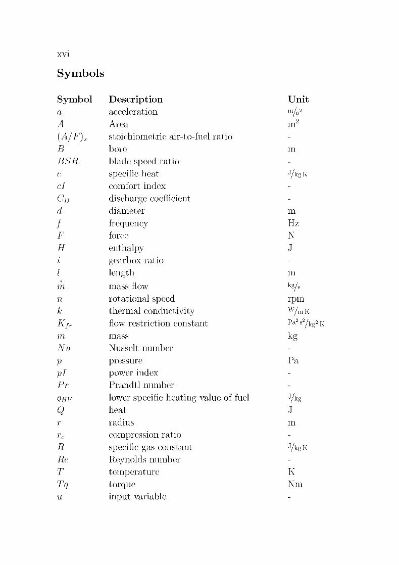
Symbols
Symbol Description Unit
a acceleration m/s2A Area 2
nr
(A/F), stoichiometric air-to-fuel ratio -
B bore m
BSR blade speed ratio -
c specific heat J/kgKci comfort index -
cD discharge coefficient -
d diameter m
f frequency Hz
F force N
H enthalpy J
i gearbox ratio -
I length m
*
m mass flow kg/sn rotational speed rpm
k thermal conductivity w/mK
Kfr flow restriction constant Pa2 sykg2 K
m mass kgNu Nusselt number -
V pressure Pa
pi power index -
Pr Prandtl number -
Qhv lower specific heating value of fuel J/kg
Q heat J
r radius m
rc compression ratio -
R specific gas constant J/kgKRe Reynolds number -
T temperature K
Tq torque Nm
u input variable -

XVII
U
Uc
V
Vd
v
w
x
y
a
7
A
r]
K
(1
n
nw
o
C
p
Î
inner energy
circumferential speed of the compressor
volume
displaced volume
velocitywork
state variable
output variable
throttle angle
weight in agility index
difference
efficiencyratio of specific heats
air-to-fuel ratio
dynamic viscosity
pressure ratio
layout boosting ratio
head parameter of the compressor
normalized mass flow rate
mass moment of inertia
ignition angle
densityload factor auxiliary devices
rotational speed
m
m"
m2
mA
rad
kg/
kg m2
o
kg/m3
rad
Subscripts
Subscript Description
a
air
af
aux
ax
b
c
ambient
air
air filter
auxiliaryaxle
before
compressor, compression
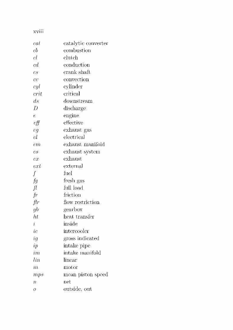
XV111
cat catalytic converter
cb combustion
cl clutch
cd conduction
CS crank shaft
cv convection
cyl cylindercrit critical
ds downstream
D discharge
e engine
eff effective
eg exhaust gas
el electrical
em exhaust manifold
es exhaust system
ex exhaust
ext external
f fuel
fg fresh gas
fl full load
fr friction
flr flow restriction
gb gearboxht heat transfer
i inside
ic intercooler
ig gross indicated
ip intake pipe
im intake manifold
lin linear
m motor
mps mean piston speed
n net
0 outside, out

XIX
p pumping
pr,gl piston rings under gas load
qS quasi-static
r restriction
R receiver
rad radiation
s stoichiometric
sh shaft
t turbine
tb test bench
tc turbochargerth throttle
tot total
us upstream
vap vaporization
veh vehicle
vol volumetric
vvt variable valve timing
wg wastegate
wh wheel
Notational Conventions
Pressure ratios
The pressure ratio over a component, acting as a flow restriction or
pump, is a frequently used quantity. The pressure ratio is alwaysdefined as the pressure after the component (downstream) divided bythe pressure before the component (upstream).
-prPds
Pus
For instance, any device increasing the pressure has a pressure ratio II
above unity, such as the compressor. Any device lowering the pressure
has a pressure ratio II below unity, such as the intercooler or the
throttle.PRC
^ -, TT Pmin - ±^-
> i Uth =^ < 1
Lc th
PRaf PRi

XX
Derivatives
Time derivatives are represented by the respective fractions (Eq. (1)).The flow, which is a quantity transported through a certain area (A)per time unit (dt), is represented by an asterisk (Eq. (2)).
dx
~dt* K A :
x=^-
dt
Subscripts
Subscripts denote components, or refer to states in the control volumes
after the corresponding component.
(i)
(2)
Chapter 1
Introduction
For more than one hundred years internal combustion engines have
been used for automotive applications. Whereas in the first years
power density and reliability where the main development goals, the
set of requirements has become considerably wider. Through the dra¬
matic increase in individual traffic, emissions of the vehicles have be¬
come a serious problem. In the early 1960's emission standards for
automobiles were introduced first in California, then nationwide in
the United States of America [Heywood (1988)]. Emission standards
in Europe and Japan followed. These measures have decreased the
emissions by automobiles considerably. Since the late 1970's catalyticconverters have been used in spark-ignited (SI) engines, which allow a
drastic decrease of NOx, HC and CO emission levels. Despite recent
improvements of the emissions by compression ignited (CI) engines
[Johnson (2003)], they still do not reach the level of SI engines.As neither a replacement of the combustion engine in automotive
applications nor a reduced demand of individual means of transporta¬
tion can be expected anytime soon, further improvements in the ef¬
ficiency of combustion engines continue to be a major goal of the
ongoing research. Soltic (2000) presented a comprehensive compari¬son of different measures to reduce fuel consumption. The SI enginecombined with a catalytic converter is able to reach current and future
regulations on emissions, but it is less efficient than a CI engine. In
this thesis only spark-ignited (SI) engines will be investigated. The
efficiency deficit of SI engines is mainly due to the load control of the
engine, as the air mass flow is throttled in order to control the power
output.
1
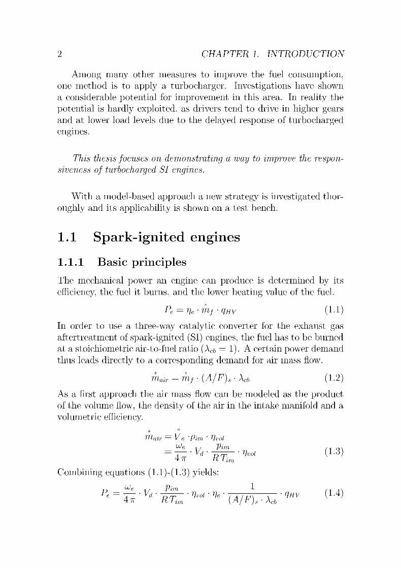
2 CHAPTER 1. INTRODUCTION
Among many other measures to improve the fuel consumption,one method is to apply a turbocharger. Investigations have shown
a considerable potential for improvement in this area. In reality the
potential is hardly exploited, as drivers tend to drive in higher gears
and at lower load levels due to the delayed response of turbocharged
engines.
This thesis focuses on demonstrating a way to improve the respon¬
siveness of turbocharged SI engines.
With a model-based approach a new strategy is investigated thor¬
oughly and its applicability is shown on a test bench.
1.1 Spark-ignited engines
1.1.1 Basic principles
The mechanical power an engine can produce is determined by its
efficiency, the fuel it burns, and the lower heating value of the fuel.
Pe = r)e-rhf quv (1.1)
In order to use a three-way catalytic converter for the exhaust gas
aftertreatment of spark-ignited (SI) engines, the fuel has to be burned
at a stoichiometric air-to-fuel ratio (Ac& = 1). A certain power demand
thus leads directly to a corresponding demand for air mass flow.
rriatr = rrif (A/F)s Xcb (1.2)
As a first approach the air mass flow can be modeled as the productof the volume flow, the density of the air in the intake manifold and a
volumetric efficiency.
**
"lair V e 'Pirn '
ijvol
^eJr
Vim /-. 0n=
T~'
Vd'
~^F~' ^ (L3)
4 7T Ri-vm
Combining equations (1.1)-(1.3) yields:
d^e
T/Vim -L
/., ,\
P' = T,-V"-Rf^- "»' ' * '
(A/F), Xd>qHV (L4)

1.1. SPARK-IGNITED ENGINES 3
This equation reveals the dominant parameters of the power produc¬tion.
The rotational speed (ue) is limited by dynamical forces result¬
ing from the moving pistons and valves. For small enginesthis limit is usually not reached due to the bad consumer ac¬
ceptance, resulting from the high-frequency noise [Soltic and
Guzzella (2001)].
The displaced volume (V^) directly influences the dimensions of
the engine, which again is coupled to the friction losses.
Pressure in the intake manifold {jpim) For naturally aspirated
(NA) engines this pressure is limited by the ambient pressure.
The concept of using intake manifold pressures higher than am¬
bient is called supercharging.
1.1.2 Efficiency
Engines in automotive applications are operated in part-load very of¬
ten1. A good part-load efficiency is thus very important.The load in SI engines is controlled by throttling the air mass flow
to the engine, which influences the pressure in the intake manifold.
This method is simple and entails excellent dynamic behavior, but
induces pumping losses. Especially for low loads the efficiency of the
engine becomes very poor.
This characteristic is quite evident in Table 1.1, which lists the
different losses at 15% and at 85% load of an SI engine running at
2000 rpm. At 15% of full load the gas exchange consumes 12.2% of
the invested energy, whereas close to full load the pumping losses are
roughly 2%.
A high potential for improving the fuel consumption comes from
either reducing part-load operation or increasing the efficiency while
operating at low load by reducing pumping losses. Whereas the former
requires a transmission unit with many transmission ratios, e. g., a
CVT, there are several solutions to tackle the latter problem.
1According to Soltic (2000) an engine of 40 kW is operated on average at roughly 10% of its
rated power during the New European Driving Cycle (NEDC)

4 CHAPTER 1. INTRODUCTION
Table 1.1: Energy distribution in an SI engine operating at 2000 rpm
under different load conditions [Langen et al. (1993)].
Load 15% 85%
Exhaust gases 48.6% 48.5%
Incomplete combustion 2.6% 2.1%
Heat flux through the cylinder wall 9.0% 10.7%
Gas exchange 12.2% 2.1%
Friction 10.3% 6.7%
Work 17.3% 29.9%
Sum 100.0% 100.0%
Equation (1.4) shows that the product of Vd, Vim and ue charac¬
terizes the power output of the engine. All three parameters can be
chosen within certain limits. As the displaced volume directly corre¬
lates to the friction losses, it has to be reduced for better efficiency.This demands higher pressures in the intake manifold or higher ro¬
tational speeds of the engine. As higher rotational speeds are not
accepted by the consumer, the only practicable way is to increase the
pressure before the engine. This approach is known as downsizing and
supercharging (DSC).
1.2 Downsizing and supercharging
1.2.1 Discussion of the concept
As mentioned above downsizing and supercharging can influence the
part-load efficiency positively. A smaller displaced volume reduces the
dimensions of the engine which results in lower friction losses. As an
additional benefit, the operating temperature is reached faster due to
the smaller thermal mass of the engine block.
Three types of superchargers can be distinguished: mechanical
superchargers (MSC), pressure-wave superchargers (PWSC) and tur-
bochargers (TC). They all have some advantages and disadvantageswhich will be discussed below. In general, it can be said that they

1.2. DOWNSIZING AND SUPERCHARGING 5
all increase the system complexity and that they demand a lower in¬
ner compression ratio of the engine in order to avoid the problem of
knocking2.
1.2.2 Mechanical supercharging
For mechanical supercharging blowers, compressors or pumps can be
used. They all are driven from the crank shaft.
The use of a mechanical supercharger involves the following ad¬
vantages and disadvantages:
+ good dynamic response to load demand
+ high boost pressure at low engine speed
+ no heat sink in the exhaust tract, thus faster light-off of the
catalytic converter
- torque to drive compressor is taken from crank shaft
- the compressor must be switched off in part-load operation for
realizing efficiency gains, which results in comfort problems when
the compressor is engaged again
- the drive belt and the considerable volume of the charger con¬
strain the packaging
- noise from pressure fluctuations at the compressor outlet
- dimensions of the compressor scale linearly with dimensions of
the engine displacement, thus the MSC is not suitable for engineswith Vd > 31
1.2.3 The pressure-wave supercharger
The core of the machine is the so-called cell wheel, a set of open-endedchannels arranged on a rotor between two casings. During a rotation,
2Knocking is a form of abnormal combustion where the charge is ignited spontaneously at
exothermic centers in the fresh-gas It appears randomly, can cause damage and strongly dependson the fuel used

6 CHAPTER 1. INTRODUCTION
each cell is first passing the exhaust manifold, where the entering gas
triggers a shock wave which runs through the cell and compresses the
fresh air. This compressed air then leaves the cell in the direction of
the intake manifold.
The use of a pressure-wave supercharger entails the following ad¬
vantages and disadvantages:
+ high boost pressure at low engine speed
+ very good part-load efficiency
+ good transient behavior
+ external EGR possible without any further devices
- complex control algorithms
- need for additional actuators and sensors
- mixture of fresh gas and exhaust gas possible
1.2.4 Turbocharging
For turbocharging, a turbine in the exhaust path is used to drive a ra¬
dial compressor, which pumps air into the intake manifold. Figure 2.1
shows a system overview.
The use of a turbocharger results in the following advantages and
disadvantages:
+ improved part-load efficiency, as exhaust enthalpy is used to
drive the compressor
+ easily applicable
+ easily controllable (one additional actuator, but no additional
sensor is necessary)
+ cost-efficient and robust production techniques available
o no connection to the crankshaft, but a placing close to the ex¬
haust openings of the engine block is advantageous
1.2. DOWNSIZING AND SUPERCHARGING 7
- increased back pressure decreases full-load efficiency
- low boost pressure for low engine speeds
- delayed boost pressure rise in transient operating condition
- delayed light-off of the catalytic converter due to the heat ex¬
traction from the exhaust gas through the turbine
1.2.5 Conclusion
Langen et al. (1993) compared the gain in fuel consumption of different
DSC concepts and found that a turbocharged engine has the highest
potential for a reduced consumption. In real traffic, the potential is
often not exploited by the driver, as the engine produces less torqueat low speeds and in addition has a delayed torque development. This
so-called turbo lag is due to the need to speed up the turbochargerbefore it can pressurize the intake air. The driver tends to operate
the engine at higher engine speed and thus lower load, which in turn
reduces the benefit from the downsizing supercharging concept. In
Figure 1.1 the fuel consumption of a turbocharged and a mechanically
supercharged engine are compared against the fuel consumption of a
naturally aspirated engine. The left column of each pair represents the
consumption resulting from an American driving cycle (FTP-75). The
right column of each pair depicts the average improvements realized
by a group of drivers. Both columns are scaled independently to 100 %
for the naturally aspirated engine.The big discrepancy between the gain technically realizable by
turbocharging and the gain realized by the consumer demand for a
strategy to overcome the turbo lag. In the automotive industry two
approaches are known.
Reduction of the boost level By designing the engine for low
boost levels, the turbo lag becomes less dominant. On the other
hand lower boost levels also lessen the gain from supercharging.
Improvement of the dynamic response Many approaches are
known to increase the responsiveness of a turbocharged engine
by modifications in the hardware. They are briefly discussed in
Section 3.2.

CHAPTER 1. INTRODUCTION
100%
40%
20% -L-
3%
IFTP-75
Consumer
Group
NA TC MSC
Figure 1.1: Comparison of the gains in fuel economy [Langen et al.
(1993)]
In this work a new approach is presented. This new approach allows to
increase the dynamic performance as well as the comfort by actuatingthe starting clutch.
1.3 Contributions
A new approach to increase the acceptance of turbocharged engines is
developed and investigated thoroughly.In order to investigate the responsiveness problem of turbocharged
engines a mean value model is developed. Most of the components are
modeled with known approaches. One crucial part of the model of
a TC engine is the compressor. Due to the quantitative load control
applied in SI engines, the air mass flow can become very small in part-
load operation. The map of the compressor usually used to represent
its behavior lacks data in this important region of the map, as deterio¬
rating effects render measurements too inaccurate. Here, the approachof Jensen et al. (1991) is extended to the region of low mass flows and
low pressure ratios. This allows an extrapolation of the compressor
map and thus the simulation of this important region.

1.4. STRUCTURE OF THE THESIS 9
Many approaches are known that attempt to quantify the subjec¬tive impression a driver has of a vehicle. Although the problem of the
turbo lag has been discussed for a long time, no index to quantify its
impact on the initial phase of the acceleration has been presented in
the literature. A new, simple, and comprehensive agility index is thus
developed, rating the wish for a fast torque development as well as the
expectation of a predictable and comfortable response to the variation
in accelerator pedal position.A new strategy to overcome the turbo lag is then presented, using
a partially slipping clutch. The control problem arising from this
strategy was solved and verified on an engine test bench.
1.4 Structure of the thesis
Chapter 2 covers the modeling of a turbocharged SI engine. This
model is then used as a basis for the investigation of agility and the
possible approaches to its improvement.In Chapter 3 the reasons for the turbo lag are discussed in detail. A
new index for the quantification of agility is presented. Finally, several
ways to improve the agility are discussed and two new strategies are
shown. Since the strategy with a partially opened clutch offered the
best potential, this strategy is investigated thoroughly in Chapter 4
with a model-based approach. In Chapter 5 the results are verified on
an engine test bench, and finally the applicability of the strategy is
discussed.

10 CHAPTER 1. INTRODUCTION

Chapter 2
Engine modeling
In order to perform a model-based investigation and optimization of
the dynamic behavior of a turbocharged SI engine, a suitable model
is necessary. There are several methods available to model a dynamic
system:
PT1 model Static maps are extended with one or several PT1 ele¬
ments in order to depict the dynamic behavior of the system.
Calculation time for a step response = o(10ms)l
O-dimensional models Receivers are modeled with lumped param¬
eters for temperature and pressure.
Calculation time for a step response = o(100s)l
1-dimensional models The state variables of the fluid vary alongthe path of the fluid.
Calculation time for a step response = o(l h)l
The O-dimensional approach is also called mean value approach, as
all the state variables in the different receivers represent mean values
of the state variables. It is very suitable for the task formulated,as it provides a sufficient degree of detailing as well as acceptablecalculation times.
After a system overview, the causality diagram for the tur¬
bocharged engine will be presented in this chapter, followed by all
the necessary submodels. The fitting of the maps used to depict the
1on a Pentium III, 700 MHz computer with Matlab
11

12 CHAPTER 2. ENGINE MODELING
compressor and the turbine will be discussed in more detail. Finally,the static and the dynamic identification of the parameters will be
presented.
2.1 System description
Figure 2.1 shows a sketch of the engine under consideration. After the
air filter the fresh air is compressed with a radial compressor. The
intercooler then reduces its temperature before it passes the throttle
and enters the engine. The enthalpy in the exhaust gas drives the
turbine, mounted on the same shaft as the compressor. The wastegateis used to bypass the turbine in case of an excess supply of enthalpy.
receiver after
air filter (Raf)
intercooler (ic)
intake
throttle (th) manifold (im)
exhaust system (es)
catalyticconverter (cat)
p\ wastegate (wg)
exhaust
manifold (em)
crank shaft (cs)
Figure 2.1: Sketch of the turbocharged engine.

2.2. CAUSALITY DIAGRAM 13
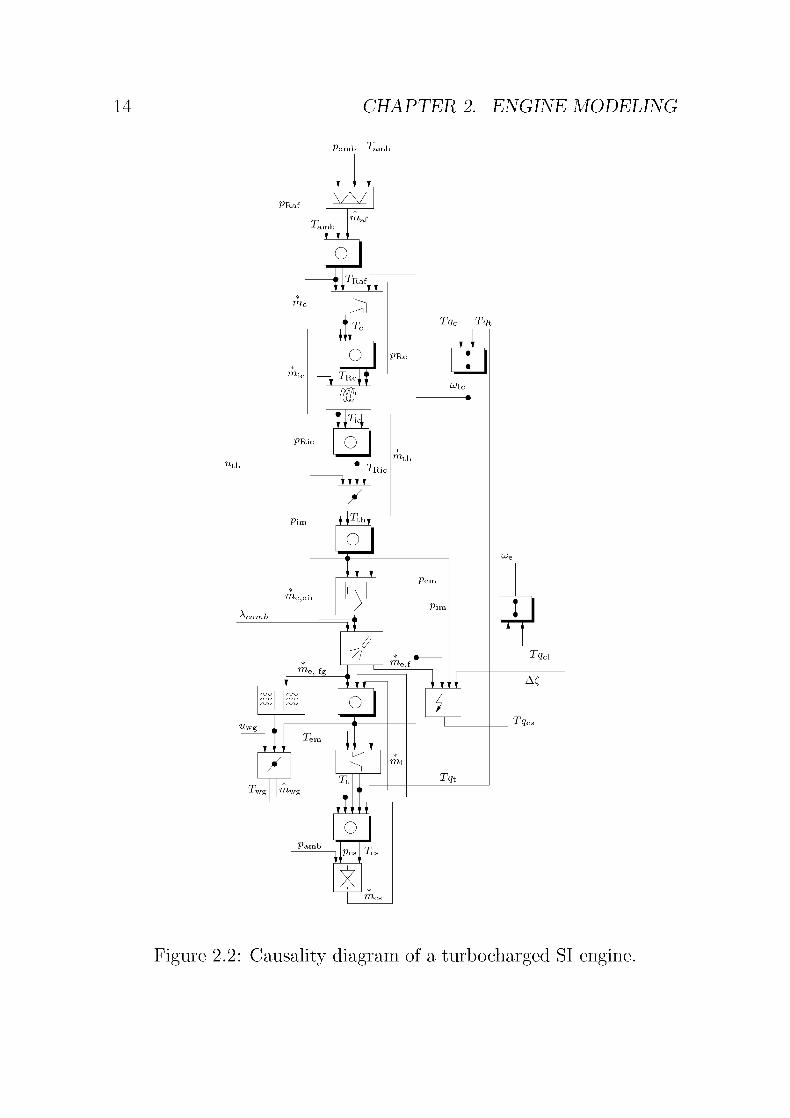
2.2 Causality diagram
The causality diagrams for the turbocharged engine are shown in Fig¬ure 2.2. Note that the structure follows the principle of restrictions in
series with control volumes. The outputs of the control volumes are
pressure and temperature, whereas the outputs for the restrictions are
mass flow and temperature of the flowing fluid.
2.2.1 System decomposition and flow directions
The model is built up using control volumes in series with restrictions
and pumps. Whereas for the control volume there is only one typeof model, for the restrictions there are two main components, namely
compressible and incompressible fluids.
2.3 The subsystems
As shown in Figure 2.2 the total model of the TC SI engine consists
of several subsystems, which are described in this section. Each
description is divided into the following categories:
Inputs
Outputs
Parameters
Equations
Assumptions
Remarks
2.3.1 Receiver
There are several receivers in the system that are modeled the same
way. These are:
• Receiver after air filter
CHAPTER 2. ENGINE MODELING
«th
Pamb ^amb
PRaf
T"laf
o
n
Tc
PRi<
o PRc
T9c Tqt
LD
mo
Wtc
Tr1c
O
IE
"ith
£.^
//i
me, fg Se,f
1/"W"g
o
_/ w
III Tem JLt
an?o
Pern
Pu
nil
Tqt
PambPes I Te
T?cl
AC
Tqc
2.2: Causality diagram of a turbocharged SI engine.

2.3. THE SUBSYSTEMS 15
• Receiver after compressor
• Receiver after intercooler
• Intake manifold
• Receiver after turbine
The exhaust manifold is modeled in a special way since heat trans¬
fer through the walls is relevant there.
Each receiver is modeled as a dynamic element with two states
taking into account mass and energy balances.
Inputs
*
fflm kg/s Mass flow in
VTLout kg/s Mass flow out
T-*- us
K Temperature upstream
^Om J/s Heat flow into the system
Outputs
VR
Tr
Pa
K
Pressure in the receiver
Temperature in the receiver
Parameters
Vr9
m Volume of receiver
R J/kgK Gas constant
K - Ratio of specific heats
Equations The model for the receiver is based on mass and energy
conservation laws. The mass balance yields the following time deriva¬
tive for the mass in the receiver:
dm,R(t) * *
T~. fffm ffvout (2.1)

16 CHAPTER 2. ENGINE MODELING
The receiver temperature is derived from the energy balance. The
internal energy in the receiver is:
UR = mRcvTR (2.2)
The complete time derivative of the inner energy is equal to the sum
of the energy flows crossing the system border:
dUR dmR dTR
dt dt dt
^ i^ ^
= Hm ~ Hout + Qm (2-3)
**
The enthalpy flow is H= mcpT. This yields the following expressionfor the time derivative of the temperature
dTR 1 ( *^
*„
dmR * \
—rr= m cPTus
- mout cpTR —— cv TR+ Qm (2.4)a t mR cv\ dt J
which can be rewritten as follows
dTR 1 / * * d mR Q
dt mR
[K,mmTus- KrhvutTds jt^Tr^ — ) (2-5)V at cv J
using the substitution: k = cp/cv.Finally, based on the ideal gas law the pressure is determined from
the mass and temperature
mRRTRVR =^^
(2.6)
Assumptions
• the fluid is a perfect gas
• constant temperature in the whole receiver
• immediate and complete mixture of the incoming gas
• no gas dynamics

2.3. THE SUBSYSTEMS 17
2.3.2 Incompressible flow restriction
Flow restrictions are found in several places along the air flow pathof the engine. The engine components that can be modeled using a
standard equation for the pressure loss in an incompressible fluid are:
• air filter
• intercooler
• lumped model of catalytic converter and exhaust system.
Further details and a validation of how well the model structure fits
the components of an engine may be found in Eriksson et al. (2001).
Inputs
Vus Pa Pressure upstream
Vds Pa Pressure downstream
T-*- us
K Temperature upstream
Outputs
*
m
T
kg/sK
Mass flow through restriction
Temperature of the flowing fluid
Parameters
Kfr
Vim
Paz sz
kg2K
Pa
Flow restriction resistance
Linearization limit
Equations The pressure drop for an incompressible flow over a com¬
ponent where there is wall friction, a change in area, or a change in
flow direction can be described by the following equation:
Ap/r = Vus ~ Vds = Kfr— (2.7)Vus
18 CHAPTER 2. ENGINE MODELING
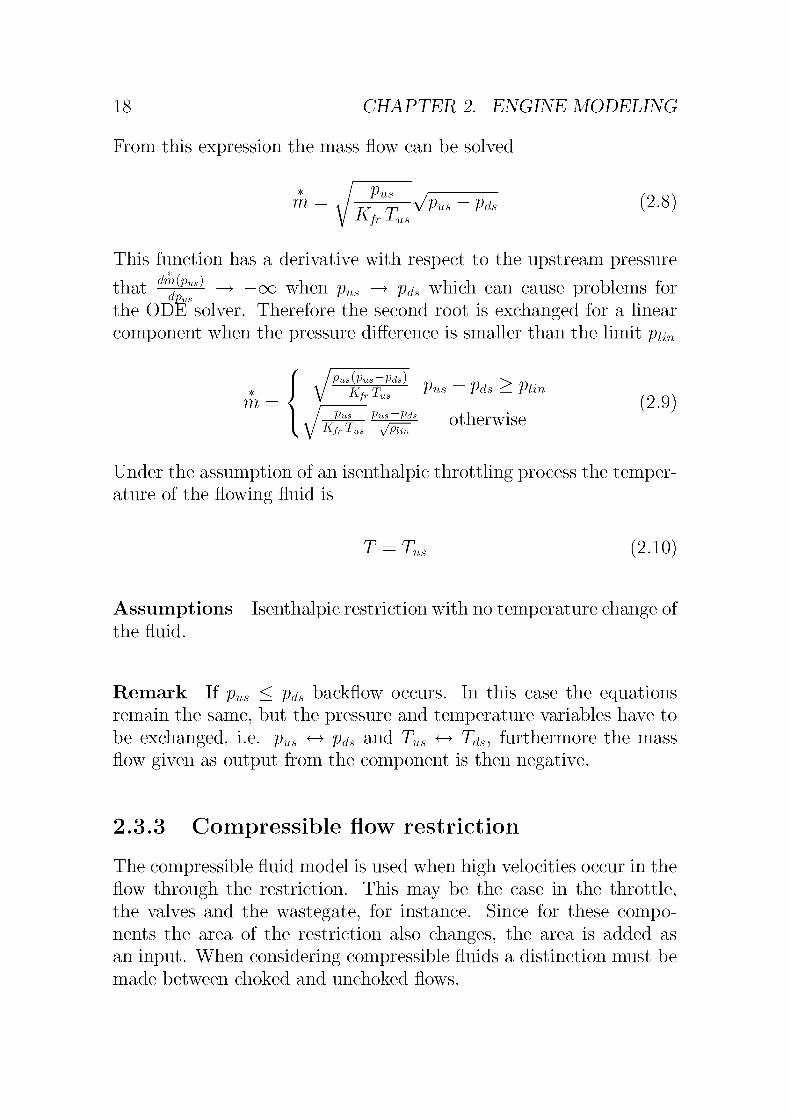
From this expression the mass flow can be solved
Vi
m= Jus
VVus-Vds (2.8)V KfrJ-us
This function has a derivative with respect to the upstream pressure
that m}-Pus> —>. — (X) when pus —> pd.s which can cause problems forMPus
the ODE solver. Therefore the second root is exchanged for a linear
component when the pressure difference is smaller than the limit p\m
Pus \Pus Pds
± I A/ Kr T Vus Vds—
Phn
m={ y KfrTus_ (2.9)KPusT PusPés otherwise-"-/r -*- us -yPlin
Under the assumption of an isenthalpic throttling process the temper¬ature of the flowing fluid is
T = TUS (2.10)
Assumptions Isenthalpic restriction with no temperature change of
the fluid.
Remark If pus < pds backflow occurs. In this case the equationsremain the same, but the pressure and temperature variables have to
be exchanged, i.e. pus ^ pds and Tus ^ T^s, furthermore the mass
flow given as output from the component is then negative.
2.3.3 Compressible flow restriction
The compressible fluid model is used when high velocities occur in the
flow through the restriction. This may be the case in the throttle,the valves and the wastegate, for instance. Since for these compo¬
nents the area of the restriction also changes, the area is added as
an input. When considering compressible fluids a distinction must be
made between choked and unchoked flows.

2.3. THE SUBSYSTEMS 19
Inputs
Aeff2
nr Effective area
Vus Pa Pressure upstream
Vds Pa Pressure downstream
T-1- US
K Temperature upstream
Tds K Temperature downstream
Outputs
*
m
T
kg/sK
Mass flow through restriction
Temperature of the flow
Parameters
R J/kgK
Ratio of specific heats
Ideal gas constant
Equations For a derivation of the throttle equations see for example
Appendix C in Heywood (1988). The mass flow through the restriction
is
Cd Ar pus*
m
yRTu^(n) 2.11
Ea± < 1. The product of the discharge coefficient Cd andPus
where II
the real flow area are lumped together to an effective area:
Aefj = Cd A7 ;2.i2)
The function ^/(II) separates the cases of when the flow is choked, i.e.
sonic conditions are reached in the flow restriction, and when it is not
choked
«GÄr)Ä> n<iw
(2.13)^2k
K-l
-K+l
i >n >ncritn« -n
The critical pressure ratio that determines when choking occurs is
( 2ncrit
K+ 12.14)

20 CHAPTER 2. ENGINE MODELING
As the throttle is assumed to be isenthalpic, the temperature after the
throttle is the same as before the restriction.
T = T [2.15)
Assumptions Isenthalpic throttling process, i. e., no temperature
change over the restriction.
2.3.4 Throttle plate area
The throttle plate is used to control the pressure in the intake mani¬
fold. It is modeled as a compressible flow restriction, using the block
described in the previous section. The only addition here is a function
for the effective area.
Inputs
Uth — Throttle signal
Outputs
As2
nr Effective area
Parameters
Cü,th — Discharge coefficient
dth m Diameter of throttle pipe
th,max rad Max. throttle opening angle
a0 rad Throttle angle when closed
Equations The throttle control input uth is within the range [0,1]and the throttle angle is determined as follows:
a = Uth {pLth,max ~ «o) + «0 ;2.i6)
A simple function for the area of the throttle is given below. Figure 2.3
shows a sketch of how the angles used in the equation are defined
Ath(a)ndth
1cos a
cos ( «o;2.i7)

2.3. THE SUBSYSTEMS 21
Finally the effective area is
A// = Ahipi) CD,th ;2.i8)
Figure 2.3: Sketch showing the angles used to model the throttle area.
Assumptions The assumptions for the compressible restriction de¬
scribed in Sec. 2.3.2 are valid as well.
2.3.5 Radial compressor
The compressor is mounted on a shaft together with the turbine. Both
devices work radially.
Inputs
^tc rad/s TC speed
VRaf Pa Pressure after air filter
VRc Pa Pressure after compressor
TRaf K Temperature after air filter
Outputs
Tqc Nm Compressor torque*
mc kg/s Compressor mass flow
T-L
CK Compressor temperature

22 CHAPTER 2. ENGINE MODELING
Parameters
Cp J/kgK Specific heat*
mc kg/s Mass flow map = /(IIC, L)tc)Parameters from map fitting
Vc— Efficiency map = /(IIC, mtc)
Parameters from map fitting
Equations
Pr
*
TflrCnc Cp^air-L Raf
n;K-l
1 ;2.i9)
The characteristics of a compressor are measured on a turbochargertest bench and stored in a compressor map. In order to make the
measurements independent of the measuring conditions, the rotational
speed (üütc,tb) and the mass flow (mCjtb) are corrected with reference
Values (Vrefj Tref).
T
&tc — Utc±bref
T
mc = mctb
'T
Vraeas \\ -*- ref
J2.20)
:2.21)
*
m. f(£ütc, nc) map or fitted function J2.22)
The mass flow through the compressor is calculated from the corrected
mass flow:
*
mf
* VRafmc
T
ref
Vref V Tr,afJ2.23)
f]c = f(mc, IIC) map or fitted function J2.24)
Tqc =^Vtc
iffc Cp,air -L be
Ve^te
n;K-l
[2.25)

2.3. THE SUBSYSTEMS 23
Tr = Tr
be 1 +n;
re-l
VeJ2.26)
2.3.6 Intercooler
The intercooler cools down the air heated by the compressor and
slightly restricts the air flow. The pressure drop over the intercooler
is modeled using the model flow restriction for incompressible fluids
(see Section 2.3.2). In the test bench setup, the original intercooler is
replaced with a water-air heat exchanger. Its output temperature is
controlled such that it cannot exceed a certain level. A model of the
heat exchanger is thus not necessary.
2.3.7 Mass flow through the engine
The mass flow through the engine is modeled using the volumetric
efficiency r\vo\ and the states of the fresh gas aspirated. The temper¬ature of the fresh gas is decreased by the vaporization energy of the
fuel and increased while it flows through the hot intake pipes.
Inputs
UJe rad/g Engine speed
Vim Pa Intake manifold pressure
Vera Pa Exhaust manifold pressure
T-*- im
K Intake manifold temperature
Outputs
*
iife,air kg/s Air mass flow into the engine
Parameters
vd m Displaced volume
R J/kgK Gas constant
rc — Compression ratio
K — Ratio of specific heat
24 CHAPTER 2. ENGINE MODELING
^ifvap
Cl, c2
J/kg Specific vaporization enthalpyParameters describing heat transfer in
intake pipe
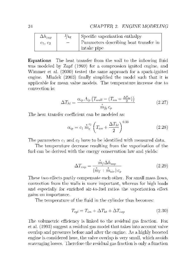
Equations The heat transfer from the wall to the inflowing fluid
was modeled by Zapf (1969) for a compression ignited engine, and
Wimmer et al. (2000) tested the same approach for a spark-ignited
engine. Mladek (2003) finally simplified the model such that it is
applicable for mean value models. The temperature increase due to
convection is:
AT;ht(%ip -ft-ip yJ-wall \-L vm T 2 ')
mfgCp
The heat transfer coefficient can be modeled as:
C2
aip c\ me Tvm +
AT;0.33
ht
J2.27)
J2.28)
The parameters c\ and c^ have to be identified with measured data.
The temperature decrease resulting from the vaporization of the
fuel can be derived with the energy conservation law and yields:
ATrrifAh.
'vap
vap (2.29)(rhf + mmr) cp
These two effects partly compensate each other. For small mass flows,convection from the walls is more important, whereas for high loads
and especially for enriched air-to-fuel ratios the vaporization effect
gains on importance.The temperature of the fluid in the cylinder thus becomes:
T,cyl Tm + ATht + AT- vap ;2.30)
The volumetric efficiency is linked to the residual gas fraction. Fox
et al. (1993) suggest a residual gas model that takes into account valve
overlap and pressures before and after the engine. As a highly boosted
engine is considered here, the valve overlap is very small, which avoids
scavenging losses. Therefore the residual gas fraction is only a function

2.3. THE SUBSYSTEMS 25
of the intake and exhaust manifold states as well as of the clearance
volume. Assuming isentropic expansion or compression of the residual
gas, the volumetric efficiency is a function of the compression ratio (rc)and the pressures before and after the engine.
1/kPern,
rivoi,p = ^r (2-31)
The volumetric efficiency is the product of a speed-dependent, a
pressure-dependent and a valve-timing-dependent efficiency.The speed-dependent efficiency f]vo\^ is a curve representing the
speed-dependent effects.
r]voi = r]voi,Uu) r]Voi,p(Vimi Vem) • r)voi,vvt{ue, bmep) (2.32)
The mass flow equation finally becomes:
*/ rp \
_
Vd Ue pvm , .
iife,air\Uei Vimi -Lirai Vera) ijvol , r> m yZ.ooj
4:71 H 1 cyl
Assumptions
• Isentropic expansion of the residual gases from pem to pvm.
• Backflow and scavenging are neglected as valve overlap is as¬
sumed to be very small.
• The volumetric efficiency is modeled without the effects depend¬
ing on gas dynamics (e. g., ram effect) and engine speed.
2.3.8 Fuel mass flow
The fuel mass flow is calculated from the air mass flow into the engine,
considering Ac& as the air-to-fuel ratio in the combustion chamber.
Inputs
*
fffair
AC6
kg/s Air mass flow
Air-to-fuel ratio
26
Outputs
Parameters
CHAPTER 2. ENGINE MODELING
fg*
mf
kg/s
kg/s
Mass flow fresh gas
Fuel mass flow
(A F) s— Stoichiometric air-to-fuel ratio
Equations
mf
*
mr,
(A/F)a Xcb
mfg = Tfff +mc
J2.34)
[2.35)
Assumptions It is assumed that the wall wetting dynamics are fully
compensated by the engine control unit and can therefore be neglected.
2.3.9 Torque generation
The torque produced by the engine is modeled as the sum of the three
addends gross indicated work, pumping work, and friction work. In
the torque model, the sum of the air and the fuel flows yields the total
mass flow through the engine into the exhaust manifold.
Inputs
rhe,f kg/s Fuel mass flow*
iife,air kg/s Air mass flow
Vim Pa Intake manifold pressure
Vera Pa Exhaust manifold pressure
UJe rad/g Engine speed

2.3. THE SUBSYSTEMS 27
Outputs
Tqcs Nm Torque at crankshaft*
me kg/s Total engine mass flow
Tqi9 Nm Gross indicated torque
Tqfr Nm Friction torque
TqP Nm Pumping torque
Parameters
vd9
m Engine displacementB m Bore
qnv J/kg Lower heating value for the fuel
(A/F)s — Stoichiometric air-to-fuel ratio
Vig— Indicated gross efficiency
nw — Boost layout
Çaux— Factor for auxiliary devices
Cmpsl,2— Parameter for FMEP
cbmep — Parameter for FMEP
CTqli CTq2— Parameters for estimation of brake
mean effective pressure
Equations The model of the engine torque production is based on
three components: the gross indicated work per cycle, pumping work
from the difference in intake and exhaust manifold pressures, and fric¬
tion work consumed by the engine components as well as the auxiliarydevices.
TqcWn Wt„ -Wn-W-,
ig frJ2.36)
47T 47T
The pumping is modeled using the intake and exhaust manifold pres¬
sures.
Wp = Vd (Vem ~ Vim) J2.37)
The indicated work is modeled as
W,w mf qHv -^{XXAd^e J2.38)
In the current implementation the gross indicated efficiency is onlyassumed to be a function of the air-to-fuel ratio

28 CHAPTER 2. ENGINE MODELING
fjtg(\, C, Vd, oje) = i]ig min(l, A) (2.39)
The spark timing will be considered in a separate subsystem (Sec¬tion 2.3.10) and its influence will be implemented as an additional
factor in the torque model (r]Tq,() •
The friction is modeled as
Wfr = Vd FMEP (2.40)
where friction mean effective pressure (FMEP) is based on the ETH
model [Inhelder (1996); Stöckli (1989)], a summary of which is givenin Soltic (2000). The model is derived from data published in papers
about engine friction. Its algebraic expression reads as follows:
FMEP = Çaux [{cmpsi + cmps2 nips1'8) • IIW • 105 + ...
/75\0'5• •• + cbmep BMEP] •
(—J (2.41)
where t;aux is the load from the auxiliary devices, 11^ is the boost layout
stemming from the effect that supercharging has on the dimensions of
the bearings, mps is the mean piston speed and B is the bore. One
disadvantage of this model is that it requires the brake mean effective
pressure (BMEP) to be known before FMEP can be calculated. How¬
ever, there are two solutions: one is to phrase the equations such that
BMEP can be solved from the model, the other is to approximateBMEP using for instance an affine function in the intake manifold
pressure.
BMEP = -cTqi + cTq2• Vim (2.42)
Assumptions The time-varying transport delays from fuel injectionto torque development are neglected.
Remarks There are currently no mean value engine models for in¬
dicated work and friction that can capture the influence of increased
exhaust back pressure.

2.3. THE SUBSYSTEMS 29
2.3.10 Torque loss due to delayed spark timing
By delaying the spark timing the torque resulting from the combustion
of the fuel in the combustion chamber decreases and the temperature
of the exhaust gas increases due to a reduced efficiency.
Inputs
AC
Tqcb
0
Nm
Deviation from optimal spark timing
Torque from combustion
Outputs
Tqcb,cATe
Nm
K
Corrected torque from combustion
Temperature rise
Parameters
VTq,C - Torque efficiency due to ignition timing
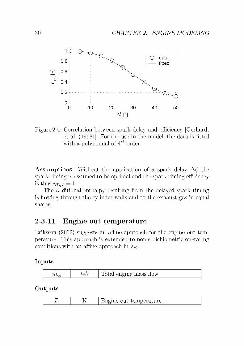
Equations By analyzing more than 1000 SI engines Gerhardt et al.
(1998) found a heuristic relation between the angle by which the spark
timing was delayed from its optimal position and the resulting ef¬
ficiency of the combustion. This relation can be depicted with the
curve presented in Figure 2.4.
The torque from the combustion is reduced due to the efficiencyreduction resulting from the spark timing delay.
Tqcb,c = Tqcb r)Tq,ç [2 A3)
By reducing the torque the temperature of the exhaust gas is increased
by
Tqcb-ue • (1 -r]Tq,c)AT
^ ' iffeg
'
^p,eg
[2 A4)
30 CHAPTER 2. ENGINE MODELING
O data
— fitted
0 10 20 30 40 50
AÇ[°]
Figure 2.4: Correlation between spark delay and efficiency [Gerhardtet al. (1998)]. For the use in the model, the data is fitted
with a polynomial of 4th order.
Assumptions Without the application of a spark delay AC the
spark timing is assumed to be optimal and the spark timing efficiencyis thus T)Tq,Ç = 1.
The additional enthalpy resulting from the delayed spark timingis flowing through the cylinder walls and to the exhaust gas in equalshares.
2.3.11 Engine out temperature
Eriksson (2002) suggests an affine approach for the engine out tem¬
perature. This approach is extended to non-stoichiometric operatingconditions with an affine approach in Xcb.
Inputs
meg kg/s Total engine mass flow
Outputs
T-L
eK Engine out temperature
0.8
cr
0.6
0.4
0.2
n

2.3. THE SUBSYSTEMS 31
Parameters
Teo K Temperature at 0 mass flow
Crp *
1 e,raKs/kg Temperature rise with mass flow
cTe,Xcb K Temperature rise with Xcb
Equations Measured data show that the linear model is sufficient
to capture the temperature variations in the exhaust manifold,
ATTe = Te0 + meg
- (1 - min(Xcb, 1)) •
cTe,xcb (2.45)iff
eg,max
Te,m
where Te o is the asymptote of the engine output temperature at zero
mass flow, AT is the temperature rise over the whole engine flow
region, and meg^max is the maximum flow through the engine.
2.3.12 Temperature at turbine inlet
The temperature at turbine inlet is very important, as it influences
directly the enthalpy flowing through the turbine. Heat transfer from
the exhaust gases to the surroundings decreases the temperature of the
gases flowing through the pipes. The temperature reduction is mod¬
eled as a function of air mass flow and of the internal heat transfer co¬
efficient, which is determined by a user selected correlation. Eriksson
(2002) provides a detailed derivation and a description of the model.
Inputs
*
life,eg kg/s Exhaust mass flow
T-L
eK Temperature engine out
T-La
K Ambient temperature
Outputs
T-1 era
K Temperature before turbine

32 CHAPTER 2. ENGINE MODELING
Parameters
d m Pipe diameter
I m Pipe lengthR J/kgK Gas constant
K — Ratio of specific heat
ß kg/ms Dynamic viscosity
k w/mK Heat transfer coefficient
ifpipe s
- Number of parallel exhaust pipes
Equations First the flow through each pipe is determined by divid¬
ing the total flow by the number of exhaust pipes
*
m
*
mf
pipen.
J2.46)pipes
The temperature drop through a pipe is modeled using a total heat
transfer coefficient from inside of the pipe to the environment. The
total heat transfer coefficient from the interior through the pipe wall
to the environment is:
1
ktot
A, I I 1— 1 1^io "Jcv,i f^cd "Jcv,ext * "Jcd,e T i^rad
[2A7)
In the implemented model this equation is simplified by using the fact
that ai/a0 « 1 and that the conduction through the walls is very highso that l/kcd « 0. In the engine model only the sum of the external
heat transfer coefficients (convection to ambient (kCVjext), conduction
to engine block (kcd,e), and radiation to environment (krad)), is given,i.e. they are lumped together as kext = kCVjext + kcdfi + krad. The total
heat transfer coefficient is then given by
1
ktot k
1 1— +
k[2 AS)
ext
The output temperature of the gas from the exhaust pipe is determined
by solving a simple partial differential equation for the temperature
drop of a fluid in the pipe. The result is the following equation:
ïiûi_
T-L p: Ta + (T, T
-L a.
k d I
g mpipe cP,eg J2.49)

2.3. THE SUBSYSTEMS 33
Assumptions The derivation of the equation is based on flow
through a straight pipe with a constant temperature of the surround¬
ings. In this equation the heat transfer by radiation is approximated
by an equivalent linear heat transfer coefficient.
2.3.13 Turbine
The turbine takes energy from the exhaust gases and generates power
to drive the compressor. The turbine acts as a flow restriction and
also reduces the temperature of the fluid. The mass flow through the
turbine is modeled as the flow through a special kind of an orifice.
Inputs
Ute rad/g Turbocharger speed
Vera Pa Pressure exhaust manifold
Ves Pa Pressure exhaust systemT-1 em
K Temperature exhaust manifold
Outputs
Tqt Nm Turbine torque
Tt K Temperature turbine out
*
mt kg/s Mass flow turbine
Parameters
ct
h
cP,eg
kg'VK/s.Pa
J/kgK
Fitting constant for turbine mass flow
Fitting constant for turbine mass flow
Specific heat constant
Equations
Ilt = — <1 (2-50)Vera
Pt = mt- cPjeg ATt (2.51)
34 CHAPTER 2. ENGINE MODELING
The efficiency is defined as
Vt
1--S-T-1- e,m,
[2.52)i-(nt)—
which leads to the following temperature difference over the turbine
AT = T,. 1 :u.K-l
The power of the turbine is defined as
±t lift '
Cp,eg' -L
e:1-OL
Vt
re-1
[2.53)
Vt [2.54)
and its torque can be calculated by dividing the power Pt by the
rotational speed of the turbocharger ujtc
Tqt^t *
Cp^eg* -L era
Utc
1 :n,K-l
^ [2.55)
The mass flow through the turbine is modeled as:
<5>t=ct\l-ll* Vem -r
mt = ,<P
v^
t
[2.56)
[2.57)em
The efficiency can be modeled as a parabolic function of the blade-
speed ratio (BSR) (Figure 2.5). For details see Guzzella and Onder
(2004).The blade-speed ratio is the quotient of the turbine tip speed and
the speed which exhaust gas reaches when it is expanded isentropicallyat the given pressure ratio Ut.
BSRnutc
£ Cp Iem \ 1 11^
(«-!)/«
[2.58)
m = m. '-{{BSR-0.6'
0.6[2.59)

2.3. THE SUBSYSTEMS 35
lit,max
0 Ï.2 BSR
Figure 2.5: Model of the turbine efficiency, using a parabolic function
in the blade-speed ratio (BSR).
2.3.14 Wastegate
The wastegate (WG) is used to control the turbocharger speed and
the pressure in the receiver after compressor. The wastegate flow is
modeled as a flow restriction for a compressible fluid (Section 2.3.3).The only component described here is the area function.
Inputs
U"wg— Wastegate control signal
Outputs
Awg,eff2
m Effective wastegate area
Parameters
i'wg,raax m Maximum wastegate lift
Q"wg m Diameter of wastegate plate
Cj),wg — Discharge coefficient

36
Equations
CHAPTER 2. ENGINE MODELING
Iwg,eff = mmu% I,
dwg
"wg ,jwg,maxi ,
^-wg,eff = ^D,wg ' ^wg,eff ' TT •
Uwg
J2.60)
;2.6i)
Assumptions Isenthalpic flow restriction, i.e. the temperature of
the fluid does not change while flowing through the throttle.
2.3.15 Adiabatic mixer
In the exhaust system after the wastegate and turbine there is a mixingof the gases. This mixing is modeled as an adiabatic process.
Inputs
Ti K Temperature of flow 1*
m\ kg/s Mass flow 1
T2 K Temperature of flow 2
*
m2 kg/s Mass flow 2
Outputs
T-1 mix
mtot
K
kg/s
Temperature of the mixed flow
Mass flow out
Parameters
cP,i
Cp,2
J/kgK
J/kgK
Specific heat of flow 1
Specific heat of flow 2
Equations The energy equation states that
(mi cPjl + m2 cp^)Tm%x = mx cPjl Tx + m2 cPj2 T2
which leads to the following temperature for the mixture
mi Cp^Ti + m2 cPj2T2
J2.62)
T
mi cPji + m2 cPj2
J2.63)
2.3. THE SUBSYSTEMS 37
The mass flow out is just the sum of the mass flows
mtot = mi+m2 J2.64)
Assumptions
• Adiabatic mixing, no heat transfer.
• The mixing takes place at constant pressure.
2.3.16 Turbocharger inertia
The turbocharger speed is modeled using an element with a mass
moment of inertia. The friction in the turbocharger is usually taken
into consideration when calculating the efficiency of the turbine from
measurements. However, the addition of a friction term to the rotat¬
ing system has been reported to solve some problems occurring when
simulating the system.
Inputs
Tqc
Tqt
Nm
Nm
Compressor torque
Turbine torque
Outputs
Utc rad/s TC speed
Parameters
Cfr
kgm2
Nm-s/rad
Inertia of the turbochargerFriction coefficient
Equations The differential equation for the rotational speed ujtc is
dutc 1
dt G(Tqt - Tqc - cfr utc [2.65)
tc

38 CHAPTER 2. ENGINE MODELING
2.4 Calibration of the model
After having defined the whole structure of the model, its parameters
have to be identified. First the parameters of single subsystems are
identified. The main purpose of the final model will be to predict the
torque. Therefore the parts lying between throttle signal and engine
torque are of special importance and will be discussed in detail.
After this step, the whole model is calibrated for steady-state con¬
ditions. Finally the model will be calibrated under dynamic condi¬
tions.
2.4.1 Calibration of the mass flow through the
engine
The mass flow through the engine is a function of many parameters,
as described in Section 2.3.7. Finally the parameters presented in
Table 2.1 were identified with a least square algorithm.
Table 2.1: Parameters identified for the mass flow through the engine
Parameter Symbol Value in
literature
Value
speed-dependent efficiency llvol,LU see Figure 2.6
Parameter 1 in Eq. (2.28) C\ 475 375
Parameter 2 in Eq. (2.28) c2 0.68 0.35
The result of the calibration is depicted in Figure 2.7.
Discussion of the parameters
The parameters found indicate that a heat exchange coefficient is less
dependent on the air mass flow than expected but the heat exchangevalue itself remains within reasonable boundaries.
The influence of the variable valve timing (i]voijVVt) was found to be
small and is only relevant in a small region of the engine map, namelyat high loads and low rotational speeds.

2.4. CALIBRATION OF THE MODEL 39
1
0.8
,0.6
p-S0.4
0.2
0
literature
fitted
0 1000 2000 3000 4000 5000 6000
ne [rpm]
Figure 2.6: Speed-dependent factor (rivoi^) of the volumetric efficiencyfrom Guzzella (1998) and identified values
x10
CO
Q.
2
1.5
1
0.5
0
m*.
[kq/s]
e.airL a J
0.01
0.005
0 1000 2000 3000
ne [rpm]
4000 5000
Figure 2.7: Calibration result of the air mass flow through the engine
The temperature of the intake pipes is assumed to be slightly
higher than the temperature of the cooling water, as the intake valve
is exposed to the combustion.

40 CHAPTER 2. ENGINE MODELING
2.4.2 Calibration of the torque generation
The torque development is modeled as a function of the energy indi¬
cated by the fuel, the effect of the pressure difference over the engineand the losses from friction and auxiliary devices. Aside from the in¬
dicated gross efficiency r\ig three parameters of the friction term are to
be identified (Eq. (2.41)). The results of the identification are listed
in Table 2.2.
Table 2.2: Comparison of the parameters identified and found in
[Guzzella (1998) and Soltic (2000)] for the torque of the
engine
Parameter Symbol Value in
literature
Value
indicated gross efficiency
engine speed-dependent parameter 1
engine speed-dependent parameter 2
load dependent parameter
Vig
Cmpsl
Cmps2
cbmep
0.37
0.464
0.0072
0.0215
0.337
0.36
0.00084
0.0253
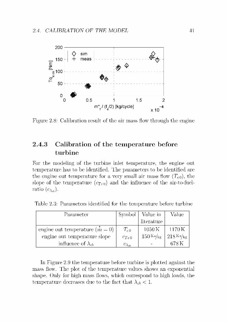
In Figure 2.8 the fuel mass per engine cycle is plotted versus its cor¬
responding torque. Note the affine correlation between the output and
the given input as described first by Willans [Urlaub (1994); Guzzella
(1998)]. The same approach is also used in a modified form for the
estimation of the brake mean effective pressure while calculating the
friction in Eq. (2.42).
Discussion of the parameters
The low value of cmps2 indicates a very low influence of the mean piston
speed on the friction, whereas the load dependence is slightly higherthan indicated in literature.
2.4. CALIBRATION OF THE MODEL 41
200
„
150
0 sim
+ meas
E-z.
«100ü
-
#**
50
0
0 0.5 1 1.5
m* / (f/2) [kg/cycle]x10
2
-4
Figure 2.8: Calibration result of the air mass flow through the engine
2.4.3 Calibration of the temperature before
turbine
For the modeling of the turbine inlet temperature, the engine out
temperature has to be identified. The parameters to be identified are
the engine out temperature for a very small air mass flow (Teo), the
slope of the temperature (c^eo) and the influence of the air-to-fuel-
ratio (cXcb).
Table 2.3: Parameters identified for the temperature before turbine
Parameter Symbol Value in
literature
Value
engine out temperature (m = 0)
engine out temperature slope
influence of Xcb
TeQ
CTeO
CAc6
1050 K
150Ks/kg
1170K
218Ks/kg678 K
In Figure 2.9 the temperature before turbine is plotted against the
mass flow. The plot of the temperature values shows an exponential
shape. Only for high mass flows, which correspond to high loads, the
temperature decreases due to the fact that Xcb < 1.

42 CHAPTER 2. ENGINE MODELING
1400
1200
g 1000
I-0 800
600 $
â$# «?
400
o 0.02
$
0+
sim
meas
0.04
m*eg [kg/s]
0.06 C0.08
Figure 2.9: Calibration result of the temperature in the exhaust man¬
ifold, i. e., at turbine inlet
2.4.4 Calibration of the mass flow through the
catalytic converter
Figure 2.10 shows the good results, which can be achieved by modelingthe catalytic converter as an incompressible flow restriction.
Table 2.4: Parameter identified for the mass flow through the catalyticconverter
Parameter Symbol Value in
literature
Value
throttling parameter Kcat - 2- 108
2.5 Map fitting
2.5.1 Motivation for the map fitting
The mass flow through the compressor is a function of the pressure
ratio and the rotational speed of the turbocharger. Due to the difficult

2.5. MAP FITTING 43
$ $
2000 4000
*
6000
Pn ~ Pu
[pal"Res "amb
L J
*0
0 sim
+ meas
8000 10000
Figure 2.10: Calibration result of the air mass flow through the cat¬
alytic converter
flow conditions in the compressor (which is working close to the unsta¬
ble region, deceleration of the fluid), fully physically based models are
still not available for mean value models [Nasser and Playfoot (1999)].Instead of physical laws, maps can be used which represent the behav¬
ior of the compressor. This allows the simulation of the compressor
mass flow in a mean value model (see Eq. (2.21) in Sec. 2.3.5). The
efficiency is depicted in a similar way (Eq. (2.24)).The disadvantages of depicting the mass flow on the basis of maps
are as follows:
• The mass flow function around the surge line is very steep. When
simulating the compressor in this region, the calculated mass
flow becomes unsteady because of the interpolation in this steep
region.
• The finite number of sampling points induces unsteady first
derivatives. This is unfavorable for a numerical optimization.
• The map is the result of measurements on a test bench. The
region with very small mass flow is usually not available, as con-
vective heat transfer negatively affects the measurement of the
efficiency and manufacturers usually do not take measurements

44 CHAPTER 2. ENGINE MODELING
in this particular region. For simulations in this region the data
thus have to be extrapolated.
One way to overcome the drawbacks of a map is to represent the
mass flow and the efficiency of the compressor with functions. The
procedure of finding these functions is called map fitting.
2.5.2 Compressor mass flow
Literature review
In order for the mass flow of the compressor to fit into the mean-value
model, it has to be expressed as a function of the pressure ratio and
the rotational speed.
mc = f(Tic Cute) (2.66)
Müller et al. (1998) suggest a physically based compressor map,
but they still need many parameters to tune the map. Isermann et al.
(2000) use a locally linear neural net to represent the compressor map.
Moraal and Kolmanovsky (1999) compare four different ways of fittinga function into a compressor map. They include an approach of Jensen
et al. (1991), which uses two dimensionless variables, which are: the
head parameter
*c = H- '- (2.67)2 c
and the normalized compressor flow rate
m d$c= °r
withUc=
^ÙJtc (2.68)^ -TTT7-
WithUc=
—
Pa\dlUc 2
The normalized compressor flow rate <ï>c is then approximated as fol¬
lows:
^ = hi ^ ~,h»
k* = ki + ^ Ma (2.69)K'2 + ^c

2.5. MAP FITTING 45
where Ma is the Mach number at the ring orifice of the compressor.
From the fitted compressor flow rate the mass flow can then be calcu¬
lated:
7ffc = /($c, Lute)= /($c(nc,ü>te,fe.),ü>fc) (2.70)
Results
The fitting of the function shown is done by a least-square method
(Gauss-Newton). This approach provides poor agreement, as the
speed lines intersect at an acute angle with the iso-pressure lines.
Much better results can be achieved when using the inverted ap¬
proach:
Uc = f(mC7Cütc) (2.71)
With this approach the speed lines intersect the mass flow lines almost
perpendicularly in the region of interest, which yields good fittingresults. The variables \I/ and <ï> are defined as above, and the fittingfunction becomes:
*' = *££The result of this fitting method is shown in Figure 2.11. The
suggested function is able to capture the shape of the speed lines,
especially at low load and speed that are of interest here. For pressure
ratios IIC < 2 the agreement is good. This is also the important region,as the boost pressure ratio will not be above 1.9.
A least-square algorithm is used to fit the function. The calculation
of the real mass flow (mc) is done according to Eq. (2.23).
Technical aspects of the map fitting
In order to obtain better fitting results in the region of interest (lowrotational speed) the error function was weighted with an affine, speed-
dependent function. This allows to weight the results in the important
region./ ~ \ 1
^tc Ldtc,max/n ,_0\
c{utc) = 1 z:
(2.73)^tc'raax

46 CHAPTER 2. ENGINE MODELING
n [1000rpm]
2.5
„2
1.5
200
AfP^gQ^Q^^
0 0.02 0.04 0.06 0.08
m*c [kg/s]
0.1
Figure 2.11: Comparison of the measured and fitted compressor speedlines
2.5.3 Compressor efficiency
Guzzella (1998a) suggests a method using ellipsoids to depict the com¬
pressor efficiency.
Tlcyffci *-*-c) ilc,max a tyn X
X
tyr
*
m.
*
m,c'raaxi *-*-c
nc,max\
q\q2
q2q3
J2.74)
[2.75)
This method was adapted by scaling the y axis for the fitting:
nc - 1 + y/Uc-l J2.76)
The parameters mC;TOaa;, UCjmax, rimax, qi...3 are fitted using a least-
square algorithm. The results from the fitting can be seen in Fig¬ure 2.12.

2.5. MAP FITTING 47
2.5
„2
1.5
icM
0 0.02 0.04 0.06 0.08
m*c [kg/s]
0.1
Figure 2.12: Comparison of the measured and fitted efficiency of the
compressor.
2.5.4 Turbine mass flow
For the fitting of the turbine mass flow the function from equation
(2.56) is used. The parameters C, K are determined using a least-
square fitting. The results of the curve fitting are shown in Figure 2.13.
2.5.5 Turbine efficiency
The efficiency of the turbine is modeled using the blade-speed ratio,
(Figure 2.5). The parameters mjmax and BSR^max from Eq. (2.59) is
determined using a least square fitting algorithm. The result is shown
in Figure 2.14. For low exhaust mass flows the heat conduction in the
housing of the turbine becomes dominant such that the fluid is heated
after the turbine wheel, leading to too high measured values of the
temperature after turbine. According to Equation (2.52) this leads to
efficiency values that are too high. These values are omitted for the
fitting of the parabola.

48 CHAPTER 2. ENGINE MODELING
Figure 2.13: Fitting of the mass flow through the turbine
1 -
*
• \
0.8
— 0.6 __————'^^— «
•
0.4 -
0.2 -
0 i i
• meas
— fitted
0.6 0.8 1
BSRt [-]
1.2
Figure 2.14: Fitting of the turbine efficiency
2.6 Static calibration of the model
For the static calibration of the engine model, all the subsystems are
joined together in accordance with the causality diagram shown in
Figure 2.2. The engine system has three inputs (angle of the throt¬
tle plate, position of the wastegate, and rotational speed). The only
2.6. STATIC CALIBRATION OF THE MODEL 49
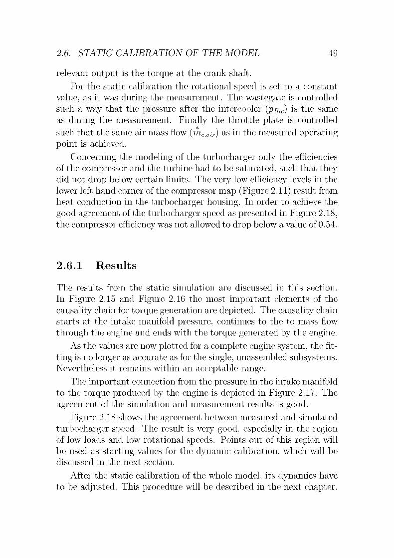
relevant output is the torque at the crank shaft.
For the static calibration the rotational speed is set to a constant
value, as it was during the measurement. The wastegate is controlled
such a way that the pressure after the intercooler (vric) is the same
as during the measurement. Finally the throttle plate is controlled
such that the same air mass flow (me^ir) as in the measured operating
point is achieved.
Concerning the modeling of the turbocharger only the efficiencies
of the compressor and the turbine had to be saturated, such that theydid not drop below certain limits. The very low efficiency levels in the
lower left hand corner of the compressor map (Figure 2.11) result from
heat conduction in the turbocharger housing. In order to achieve the
good agreement of the turbocharger speed as presented in Figure 2.18,the compressor efficiency was not allowed to drop below a value of 0.54.
2.6.1 Results
The results from the static simulation are discussed in this section.
In Figure 2.15 and Figure 2.16 the most important elements of the
causality chain for torque generation are depicted. The causality chain
starts at the intake manifold pressure, continues to the to mass flow
through the engine and ends with the torque generated by the engine.
As the values are now plotted for a complete engine system, the fit¬
ting is no longer as accurate as for the single, unassembled subsystems.Nevertheless it remains within an acceptable range.
The important connection from the pressure in the intake manifold
to the torque produced by the engine is depicted in Figure 2.17. The
agreement of the simulation and measurement results is good.
Figure 2.18 shows the agreement between measured and simulated
turbocharger speed. The result is very good, especially in the regionof low loads and low rotational speeds. Points out of this region will
be used as starting values for the dynamic calibration, which will be
discussed in the next section.
After the static calibration of the whole model, its dynamics have
to be adjusted. This procedure will be described in the next chapter.

50 CHAPTER 2. ENGINE MODELING
x10m*
.
[kg/s]e.air
L a J
2000 4000 5000
ne [rpm]
Figure 2.15: Comparison of the resulting air mass flow plotted versus
the engine speed and the pressure in the intake manifold
«T 0.05
0
Tqe [Nm]
1000 2000 3000 4000 5000
ne [rpm]
Figure 2.16: Comparison of the torque resulting form the mass flow
through the engine
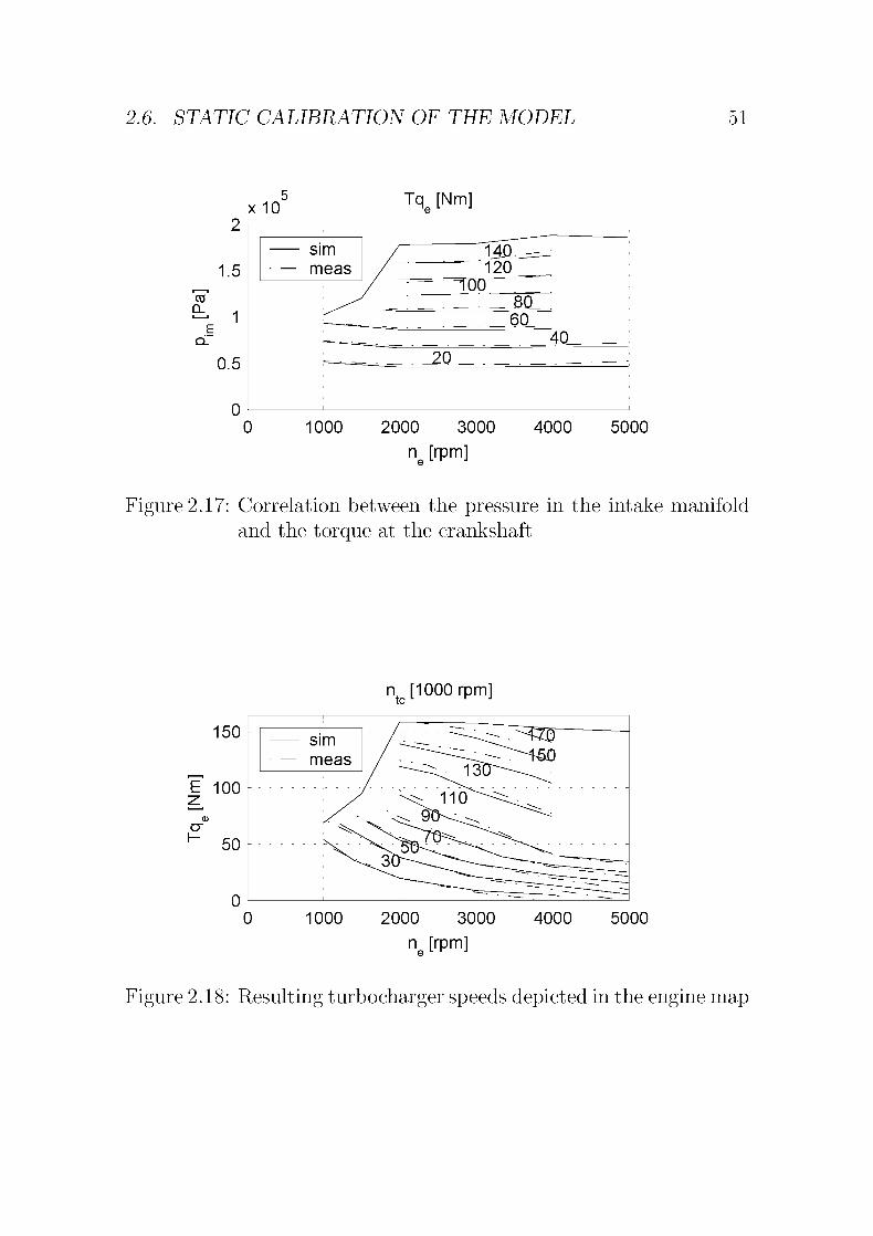
2.6. STATIC CALIBRATION OF THE MODEL 51
x10 Tqe [Nm]
2
1.5
of*=- 1
E
d
0.5
0
0 1000 2000 3000 4000 5000
ne [rpm]
Figure 2.17: Correlation between the pressure in the intake manifold
and the torque at the crankshaft
150
E 100
50
ntc[1000 rpm]
1000 2000 3000 4000 5000
ne [rpm]
Figure 2.18: Resulting turbocharger speeds depicted in the engine map

52 CHAPTER 2. ENGINE MODELING
2.7 Dynamic calibration of the model
In order to get a good agreement of the dynamic traces of the different
output signals, the dynamic elements, namely receiver volumes and
the inertia of the turbine, have to be adjusted.In the results shown below all the values of the volumes and the
inertia were be set to their physical values. The only adjustments had
to be made in the wastegate control.
Figure 2.19 shows a typical result from a comparison between mea¬
sured and simulated data. The initial condition is set to 2000 rpm and
20 Nm. The throttle signal is shown in the upper left-hand field. The
agreement between the pressure after the compressor (vrc) and the
pressure after the throttle plate Vim is good. In the lower right-handcorner the pressures before (pem) and after (pes) the turbine are de¬
picted.

2.7. DYNAMIC CALIBRATION OF THE MODEL 53
x 10
1.5
x:
Z3*"
0.5
°5
5
x10
meas
sim
10 15
TO
D.
1.5
0.5
0 55
x10
10 15
5 10 15
t[s]
1.5
TO
D.
a.
0.5
x 10
150
100
50
10 15
10 15
Figure 2.19: Comparison of the pressures, the turbocharger speed, and
the resulting torque at the crank shaft. Conditions: ne =
2000 rpm, initial load 20 Nm

54 CHAPTER 2. ENGINE MODELING

Chapter 3
Longitudinal dynamicsof a vehicle
As mentioned in the introductory chapter, a turbocharger can be ap¬
plied to achieve the necessary boost pressures for a desired torque at
the crank shaft.
The concept of turbocharging provides the advantage of better fuel
efficiency, but entails some new challenges as well. The turbocharger is
a representative of the group of turbo-machines and works best around
its setpoint. A combustion engine works volumetrically and can thus
cope with any mass flow.
As the turbocharger-engine system is laid out for medium to high
power demands, the boost pressure for low air mass flows is poor, i. e.,
at low engine speeds the engine only develops a low torque.
This problem is not very serious in modern SI engines. If the
combination of the turbine, the compressor, and the engine is well
chosen, the boost level is not too high and a wastegate is applied.
A more serious problem arises from the low-pass characteristic,which is brought into the system by the inertia of the turbocharger.In order to build up boost pressure, the turbocharger has to speed up
after a tip-in by the driver. This leads to an erratic torque develop¬ment. First the boost pressure reaches ambient pressure very fast, but
then the turbocharger has to speed up before the desired torque can
be reached. Figure 3.1 shows this unsteady torque development.
55

56 CHAPTER 3. LONGITUDINAL DYNAMICS OF A VEHICLE
150
100
x10
1.5
cc
± 1
0.5
/
/
E
350
300
250
200
T3
^o 150
HT3
100
50
0
measured
desired
\
/y'V"v,W..n ^ .m
2 4
5x10
1.5
Jz, 1
0.5
/
/
2 4 6 8
t[s]
2 4 6 8
t[s]
Figure 3.1: Torque development after a tip-in at 3 s and its derivative
with the typical peak right after the tip-in
3.1 Quantification of agility
In order to allow an optimization of agility, a quality function and a
test case are necessary. The test case has to depict a critical situation
3.1. QUANTIFICATION OF AGILITY 57
for a turbocharged engine, as well as having to provide a good basis
for future investigations by granting high reproducibility. The qualityfunction has to depict the crucial initial phase of the acceleration. Not
only does it have to depict the power development, but it also has to
rate the comfort a driver experiences while accelerating.
3.1.1 Literature search on agility
For the description of good dynamic behavior there are several expres¬
sions used in literature, such as: good transient behavior, elasticity,reaction time, no turbo lag, agility, good load response, or sprint¬
ing capability. In this thesis the longitudinal behavior will be called
"agility".A number of publications present criteria for the quantification of
the agility of a car.
Singer (1985), Hiereth (1986), and Uthoff and Yakimow (1987)suggest tests in which full load accelerations are made in a certain
range of speeds. In all these tests the mass of the vehicle as well as
the rated power of the engine are very important, since most of the
time the engine is operated close to its peak power. Lundstrom and
Gall (1986) suggest accelerations in a high gear without gear shiftingand measure the time to reach a predefined boost pressure. That
test can be seen as a base for the new test case and quality function
suggested in this thesis. As the tests are executed in cars rather than
on test benches, the engine speeds are not constant, which influences
the results.
Baker et al. (1989) proposes a test where an engine is mounted on
a test bench and the throttle is opened according to a linear function.
The quality function is represented by the time to increase the brake
mean effective pressure by 0.35 bar. Comfort is not considered.
Only Lezhnev et al. (2002) take power as well as comfort into
consideration with a weighted sum. One addend is the time delay
experienced in torque build-up, whereas the other addend measures
the overshoot of the torque.
Besides these specific tests, there are several generally applied tests
may be found in literature:
• £o-iookm/h time to reach 100km/h

58 CHAPTER 3. LONGITUDINAL DYNAMICS OF A VEHICLE
• ^0-200 km/h for sports cars
• t\ km time needed for the first km
The elasticity tests emphasize the full-load torque:
• ^60-iookm/h m the second-highest gear
• ^80-120 km/h in the highest gear
Neither of the tests presented so far fulfills all the requirements to
measure power as well as comfort of an acceleration. Most of these
approaches have the drawback that they grant too much weight to the
shape of the full load line and the peak power, whereas they do not
sufficiently consider the dynamic torque development in the first few
seconds.
In List and Schoeggel (1998) a commercial product is presentedwhich can quantify the agility of a vehicle. Fuzzy logic and generic
algorithms are used to find a correlation between vehicle behavior
and subjective impressions by the test drivers. Since a model-based
approach is used in this thesis that procedure is not suitable.
In SAE (1998) a standard is published for quantifying driveability.This procedure is only applicable for existing vehicles and providesa general value of the driveability of the vehicle tested. Thus this
standard is not applicable for the quantification of agility.Since all the presented procedures have certain drawbacks, a new
agility criterion is required.
3.1.2 Specifications for the new agility criterion
The new agility criterion has to reflect the important time period at
the beginning of an acceleration phase, especially when starting at low
load.
The test case
Hand in hand with the need for a new agility criterion comes the need
for a new test case. Especially high load demands at low rotational
speeds are crucial for good driveability. Such a case occurs for instance
when coasting in a high gear and then tipping in the driving pedal.

3.1. QUANTIFICATION OF AGILITY 59
With this information the test case summed up in Table 3.1 can be
defined.
Table 3.1: The test case
vehicle mid-size car
initial condition cruising at 60 km/hin 4th gear
action tip-in to full load
Assumptions
A driver feels the force between his body and the seat. Linked via his
mass (mfdnver) this force is proportional to the acceleration he experi¬ences.
"driver/Q 1 \
(^driver V /
'f"driver
In order to simplify the problem of quantifying the quality of the
acceleration, the following assumptions are made:
Stiff vehicle For the vehicle under consideration we assume a stiff
drive-train. This assumption is justified, as a good torque developmentat the clutch results in a good acceleration of the vehicle.
No slip Slip between road and tire is assumed to be sufficientlysmall that it can be neglected. This assumption is justified, as all the
tests will be run in 4th gear (Table 3.1).
Consequences If we assume a stiff drive-train and no slip between
wheel and street, the acceleration of the vehicle and the torque appliedto the gear box (Tqci) are proportional.
"driver ^ ("vehicle ^ -^ Qcl V /
Therefore we only consider the torque applied to the gear box Tqc\ for
further investigations.

60 CHAPTER 3. LONGITUDINAL DYNAMICS OF A VEHICLE
Analysis of the driver's demands
This allows us to analyze the behavior a driver likes when tipping in.
The driver wants two reactions when pressing the driver pedal
(tip-in):
• as much torque as possible as fast as possible
• a smooth and predictable torque development
The first point can be seen as a power issue whereas the second demand
is a comfort issue.
Both expectations can be fulfilled if the torque develops linearlywith time.
Based on this desired behavior a new cost functional can be de¬
rived. As outlined above, it is helpful to judge agility in terms of power
and comfort.
In the following paragraphs five indices are described. Figure 3.2
displays the torque development of a turbocharged engine and its cor¬
responding indices.
150
100
Ez
75cr
H
50
0
2468 2468
t [s] t [s]
Figure 3.2: Application of the different agility indices to the torque
and its corresponding derivative
90%Tq_
.-
•
e.max^
17-
Ez
cr
Ho
300
250
200
p150
100
50
n £_'NVV-''.UW ^ /

3.1. QUANTIFICATION OF AGILITY 61
Power Index 1
The first power index (vh) is the inverted slope of the line connectingthe point before tip-in with the point where 90 % of the full load torque
is reached.
t_
( U-^ J- (Jcs,raax\(jJ=const ~ J- Ccs,tipin \(°i°i)
V ^0.9 — Uipm j
The lower this power index is the better.
Power Index 2
The second power index (vh) is the integral of the power consumed
by the clutch on the gear box side in the first 3 s after a tip-in. This
index is especially helpful to compare different strategies on the same
set-up.
Vh = J Tqdugb)tndt (3.4)
The higher it is the better.
Power Index 3
Power index 3 (pi3) measures the time between tip-in and the pointwhere 90 % of the full load are reached. This index does not allow to
compare different operating points or even different engines, but pro¬
vides a good access to the improvement realized by a certain strategy.
Comfort Index 1
The driver expects a predictable increase of the torque. Any deviation
from this optimal trace is penalized with the first comfort index. It
is calculated as the area between the real torque trace and a fictitious
linear trace (cl\ in Figure 3.2).
['t<3 9
dl = / \Tqd,real —Tqci,ideai\dt (3.5)

62 CHAPTER 3. LONGITUDINAL DYNAMICS OF A VEHICLE
Comfort Index 2
The second comfort index (cl2) is the highest slope of the real torquetrace divided by the average slope, which is equal to a multiplicationwith the first power index.
^^16 Tgo g-TqUlnn \ dt I
^0 9 ^tipin
The smaller the comfort indices are, the better.
A summary of all the indices can be found in Table 3.2.
Table 3.2: Summary of the different agility indices
acronym description better if
ph inverted slope of the optimal Tq ramp \
Vh Jt0°+3S Pgb,mdtph At90%Tqfc-h J \Tqcijreai — Tqd,ideai\ dt
cl2 max(dT(ici/dt) • ph
While the first power index and the first comfort index will be used
for the optimization, the other indices give a better understanding of
the performance improvements. The indices used for the optimizationare set up such that the smaller they are, the better.
3.2 Solutions for better agility
3.2.1 System analysis
The causality diagram in Figure 2.2 on page 14 not only shows the
dependencies among the various subsystems, but also the inputs to
the engine system. They are listed in Table 3.3.
The ambient conditions (Ta, pa) cannot be controlled and are there¬
fore classified as disturbances.

3.2. SOLUTIONS FOR BETTER AGILITY 63
Table 3.3: Disturbances and inputs of a state-of-the-art turbocharged
engine
Disturbance Variable Input Variable
Ambient temperature Ta Throttle signal uth
Ambient pressure pa Wastegate opening uwg
Spark advance A(Clutch signal uc\
Air-to-fuel ratio Xcb
Although all inputs are potentially useful for increasing the agilityof a vehicle, not all of them can be used.
The air-to-fuel ratio cannot be chosen arbitrarily, because a cat¬
alytic converter is used for the exhaust gas after treatment, which
requires a stoichiometric combustion, i. e., Xcb = 1.
The wastegate in state-of-the-art turbocharged engines is alwaysclosed in order to achieve the highest possible pressure before the
turbine and thus the highest possible turbocharger speed. The higherthe turbocharger speed is, the smaller is the turbo lag, as the torque
build-up time is highly sensitive to the turbocharger inertia. The
wastegate is only opened to keep the boost pressure below a certain
limit, i. e., for boost pressure control. Eriksson et al. (2002) show in
detail why the wastegate has to be closed for the best possible agility.
After all these constraints only two inputs remain, namely the
spark advance and the torque from the clutch. Whereas the sparkadvance can be controlled without any additional hardware, an auto¬
mated starting clutch has to be applied in order to make the torquetransmitted by the clutch controllable.
3.2.2 Solutions with auxiliary devices
As turbocharged engines have suffered from the turbo lag ever since
their invention, many devices have been developed to overcome this
drawback.
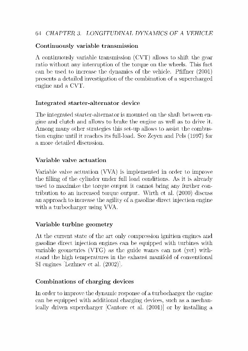
64 CHAPTER 3. LONGITUDINAL DYNAMICS OF A VEHICLE
Continuously variable transmission
A continuously variable transmission (CVT) allows to shift the gear
ratio without any interruption of the torque on the wheels. This fact
can be used to increase the dynamics of the vehicle. Pfiffner (2001)presents a detailed investigation of the combination of a supercharged
engine and a CVT.
Integrated starter-alternator device
The integrated starter-alternator is mounted on the shaft between en¬
gine and clutch and allows to brake the engine as well as to drive it.
Among many other strategies this set-up allows to assist the combus¬
tion engine until it reaches its full-load. See Zeyen and Pels (1997) for
a more detailed discussion.
Variable valve actuation
Variable valve actuation (VVA) is implemented in order to improvethe filling of the cylinder under full load conditions. As it is alreadyused to maximize the torque output it cannot bring any further con¬
tribution to an increased torque output. Wirth et al. (2000) discuss
an approach to increase the agility of a gasoline direct injection enginewith a turbocharger using VVA.
Variable turbine geometry
At the current state of the art only compression ignition engines and
gasoline direct injection engines can be equipped with turbines with
variable geometries (VTG) as the guide wanes can not (yet) with¬
stand the high temperatures in the exhaust manifold of conventional
SI engines [Lezhnev et al. (2002)].
Combinations of charging devices
In order to improve the dynamic response of a turbocharger the enginecan be equipped with additional charging devices, such as a mechan¬
ically driven supercharger [Cantore et al. (2001)] or by installing a
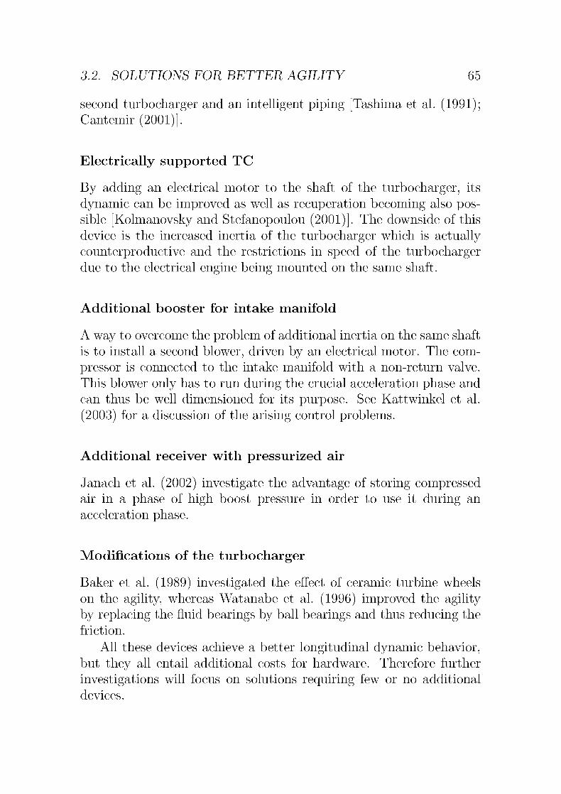
3.2. SOLUTIONS FOR BETTER AGILITY 65
second turbocharger and an intelligent piping [Tashima et al. (1991);Cantemir (2001)].
Electrically supported TC
By adding an electrical motor to the shaft of the turbocharger, its
dynamic can be improved as well as recuperation becoming also pos¬
sible [Kolmanovsky and Stefanopoulou (2001)]. The downside of this
device is the increased inertia of the turbocharger which is actually
counterproductive and the restrictions in speed of the turbochargerdue to the electrical engine being mounted on the same shaft.
Additional booster for intake manifold
A way to overcome the problem of additional inertia on the same shaft
is to install a second blower, driven by an electrical motor. The com¬
pressor is connected to the intake manifold with a non-return valve.
This blower only has to run during the crucial acceleration phase and
can thus be well dimensioned for its purpose. See Kattwinkel et al.
(2003) for a discussion of the arising control problems.
Additional receiver with pressurized air
Janach et al. (2002) investigate the advantage of storing compressedair in a phase of high boost pressure in order to use it during an
acceleration phase.
Modifications of the turbocharger
Baker et al. (1989) investigated the effect of ceramic turbine wheels
on the agility, whereas Watanabe et al. (1996) improved the agility
by replacing the fluid bearings by ball bearings and thus reducing the
friction.
All these devices achieve a better longitudinal dynamic behavior,but they all entail additional costs for hardware. Therefore further
investigations will focus on solutions requiring few or no additional
devices.
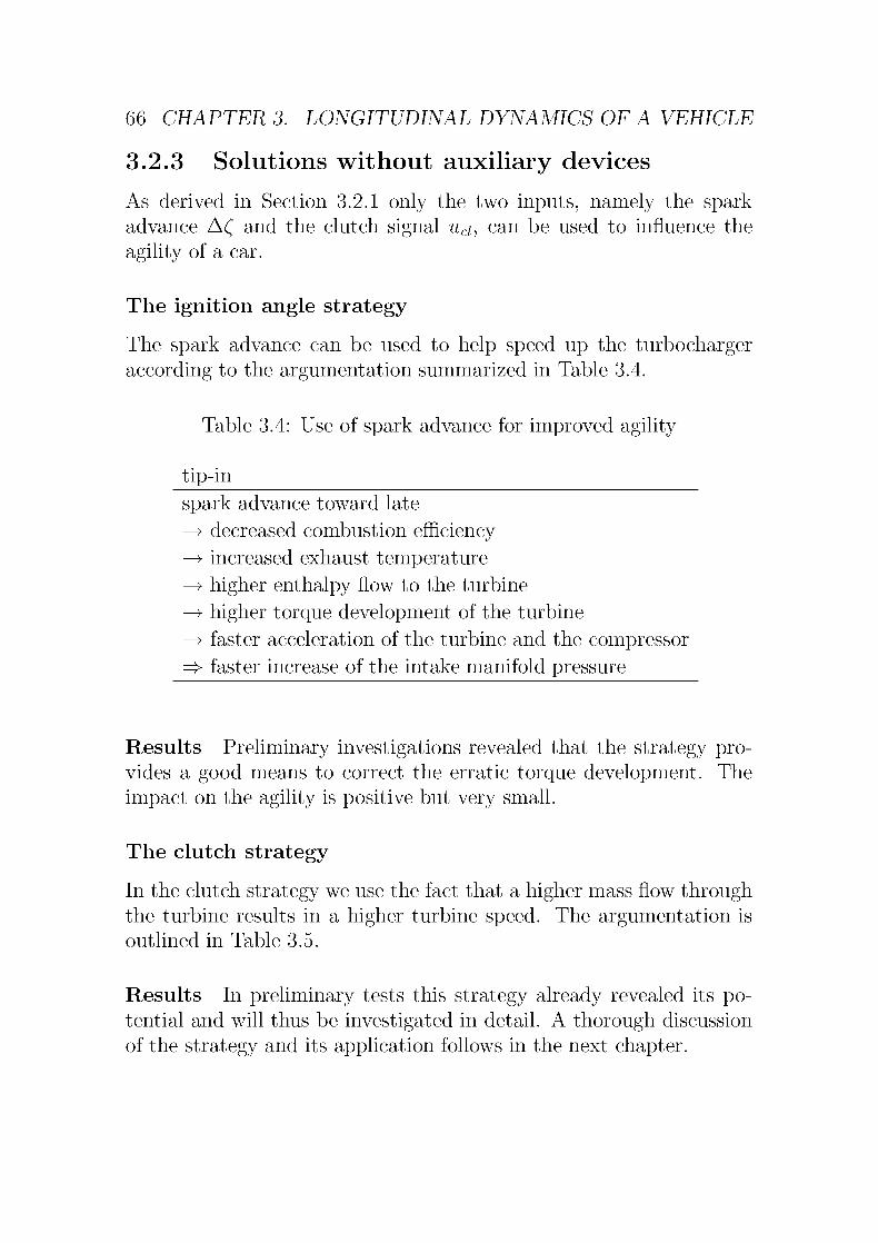
66 CHAPTER 3. LONGITUDINAL DYNAMICS OF A VEHICLE
3.2.3 Solutions without auxiliary devices
As derived in Section 3.2.1 only the two inputs, namely the sparkadvance A( and the clutch signal Ud, can be used to influence the
agility of a car.
The ignition angle strategy
The spark advance can be used to help speed up the turbocharger
according to the argumentation summarized in Table 3.4.
Table 3.4: Use of spark advance for improved agility
tip-in
spark advance toward late
—> decreased combustion efficiency—> increased exhaust temperature
—> higher enthalpy flow to the turbine
—> higher torque development of the turbine
—> faster acceleration of the turbine and the compressor
=> faster increase of the intake manifold pressure
Results Preliminary investigations revealed that the strategy pro¬
vides a good means to correct the erratic torque development. The
impact on the agility is positive but very small.
The clutch strategy
In the clutch strategy we use the fact that a higher mass flow throughthe turbine results in a higher turbine speed. The argumentation is
outlined in Table 3.5.
Results In preliminary tests this strategy already revealed its po¬
tential and will thus be investigated in detail. A thorough discussion
of the strategy and its application follows in the next chapter.

3.2. SOLUTIONS FOR BETTER AGILITY 67
Table 3.5: Use of the clutch for an improved agility of a vehicle
tip-in
controlled clutch opening
—> increased engine speed—> higher mass flow through the engine
—> increased pressure in the exhaust manifold
—> higher mass flow through the turbine
—> higher torque development of the turbine
—> faster acceleration of the turbine and the compressor
=> faster increase of the intake manifold pressure

68 CHAPTER 3. LONGITUDINAL DYNAMICS OF A VEHICLE

Chapter 4
Optimization
4.1 Model extension
Figure 4.1 shows a sketch of a complete vehicle with engine, clutch,
gearbox, axle, tires and chassis. By applying the simplifications from
Section 3.1.2 the structure can be simplified to a combination of the
engine, the clutch and a well-defined input (see Figure 4.2). The inputwill be derived in the next section.
oooo
Figure 4.1: Sketch of the whole vehicle under consideration
According to these assumptions the engine model derived in Chap¬ter 2 needs only a little extension, namely the clutch model.
69
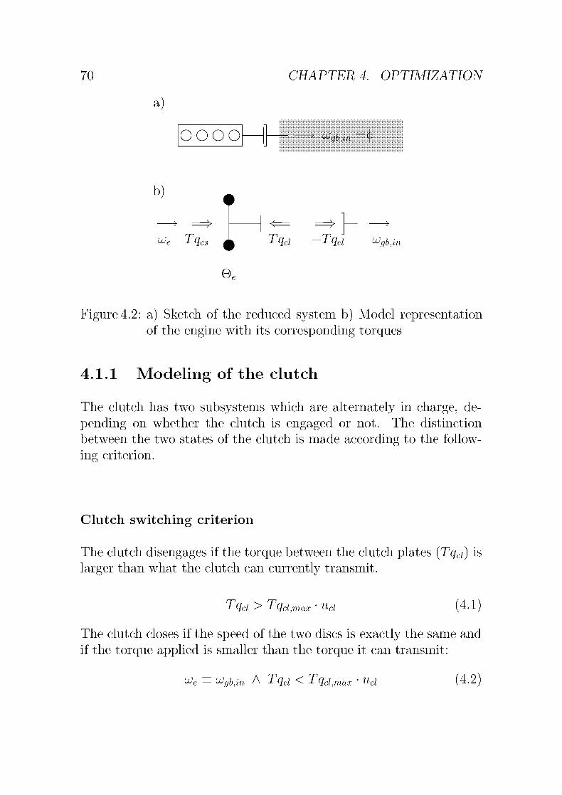
CHAPTER 4. OPTIMIZATION
oooo &Jgb,m Ç
b)
-> =>
Lüe Tqc Tqd —Tqd ugb,i
a
Figure 4.2: a) Sketch of the reduced system b) Model representationof the engine with its corresponding torques
4.1.1 Modeling of the clutch
The clutch has two subsystems which are alternately in charge, de¬
pending on whether the clutch is engaged or not. The distinction
between the two states of the clutch is made according to the follow¬
ing criterion.
Clutch switching criterion
The clutch disengages if the torque between the clutch plates (Tqd) is
larger than what the clutch can currently transmit.
Tqd > Tqd,r Ud (4.1)
The clutch closes if the speed of the two discs is exactly the same and
if the torque applied is smaller than the torque it can transmit:
UJe Ugb,m A Tqd < Tqd,r Ud (4.2;

4.1. MODEL EXTENSION 71
Modeling the open clutch
Inputs
Ud — Normalized clutch actuation signal
UJe rad/g Rotational speed of the engine
^gb,m rad/s Rotational speed of the gearbox in
shaft
Outputs
Tqd Nm Torque transmitted by the clutch
Parameters
Tqdoo
Tqdo
Nm
Nm
Maximal torque for gliding clutch discs
Maximal torque for adhering clutch
discs
Equations
Tqd,max(A.Lü)
Alu — uje — LUgbjîn
sign(Au) (Tqdoo ~ (Tqdo ~ Tqd
Tqd(Au) = ud Tqd,max(Auj)
|AuOO I
(4.3)
(4.4)
(4.5)
Modeling the closed clutch
In case of a closed clutch, its influence on the drive train disappearsand the inertias of the engine and the rest of the vehicle can be lumped
together.
EquationsGtot
e„ + a
Gveh,tot
e i ^veh,tot
wh "•" ^ ^whj[mveh rl,h + 4 G i2 -i2gb ax
(4.6)
(4.7)
4.1.2 Modeling of the engine dynamics
All pistons and rods, the crank shaft with all the auxiliary devices,and half the clutch are represented through one inertia.

72 CHAPTER 4. OPTIMIZATION
Tqdo
Tqdoo
-Tq{cloo
ALU
-Tqdo
Figure 4.3: Torque delivered by the clutch, depending on the difference
in angular speed
Inputs
Tqcs
Tqd
Nm
Nm
Torque at the crank shaft
Torque at the clutch
Outputs
UJe rad/g Rotational speed of the engine
Parameters
Ge kgm2 Mass moment of inertia
Equations The differential equation for the rotational speed ue is
düüP 1
dt G— (Tqcs - Tqcl I (4.!
Assumptions The friction in the engine and the torque resultingfrom the auxiliary devices are already included in the calculation of
the torque at the crankshaft (see Sec. 2.3.9 for details).

4.2. THE OPTIMAL CONTROL PROBLEM 73
4.2 The optimal control problem
The strategy outlined in Table 3.5 rises the question of how to open
and close the clutch in a way to maximize the agility. With the new
degree of freedom from the clutch opening, an optimal control problemhas thus to be solved.
Figure 4.4 shows all the inputs necessary in order to phrase an
optimal control problem.
quality function test case
(Chapter 3) (Chapter 3)
plant \ /
(Chapter 2) \ / constraints
C optimization problem ")
1optimal solution
Figure 4.4: Overview over the necessary inputs for solving an optimalcontrol problem
4.2.1 Formulation of the optimal control problem
The Plant
The plant is represented by the validated mean value model derived
in Chapter 2 extended by the clutch model derived in Section 4.1.
The inputs to the plant are the load pedal position (uth), the clutch
activation signal (ud), the rotational speed of the gearbox input shaft
(ugb,in), and the wastegate control signal (uwg). As the wastegate is
used to keep the turbocharger at the highest possible speed and for
controlling full-load torque, it is governed by a separate controller and
is thus not available for the optimization.

74 CHAPTER 4. OPTIMIZATION
The quality function and the test case
The quality function and the test case are derived in Chapter 3. The
test case allows the model of the vehicle and of the drive train to be
simplified considerably. In fact they only contribute to the definition
of the boundary conditions of the optimization problem (Fig. 4.2a) ).The quality function is a weighted sum of the power index (pi)
and the comfort index (cl). These two indices represent partially
conflicting goals. Equation (4.9) defines the quality function value J.
The solution of the optimization problem will thus be a Pareto front
with the parameter 7 e [0..1].
J = 1-ph + (l-7)-c/i (4.9)
The constraints
As derived in Section 3.1.2, the speed of the shaft into the gearbox
(ugb,m) can be assumed to be constant.
The speed can be calculated from the torque equivalence when the
vehicle is cruising at the proposed speed of 60 km/h:
-L qgb,m \" drag T "roll T "grade) ^gb'
*ax' '
'wh U ^4.1UJVgb
The three dragging forces can be expressed very simply. The air re¬
sistance is a function of the square of the speed:
"drag ~^' Pair '
--drag' &w '
^veh V /
The rolling resistance is a function of the mass of the vehicle and its
rolling coefficient.
Froii = Ufnc mveh g (4-12)
The force from climbing is zero, as the experiment takes place on a
horizontal street.
Fgr-ade = 0 (4-13)
The rotational speed of the shaft into the gearbox can be calculated
from the vehicle speed:
UVehf a -\ a\
Ugb,m = ~. : (4.14)''gb
'
*ax'
'wh

4.2. THE OPTIMAL CONTROL PROBLEM 75
Solving equations 4.10 and 4.14 with the parameters specified in
Appendix A yields Tqgbjin = 21.95 Nm and ngbjm = 1940 rpm. As
the optimization to follow is not used for the comparison with other
vehicles, but for the comparison with other load points in the engine
map, the following starting point will be used: Tqgbjin = 20.0 Nm and
ngb}Zn = 2000 rpm.
With these equations at hand all boundary conditions are defined.
4.2.2 Means to solve the optimal control problem
Although there is a lot of research going on in the field of optimal
control, there is no generally applicable solution for all optimal control
problems.Several ways exist to find a solution for an optimal control problem.
Figure 4.5 shows a condensed decision tree with some applicable tools
(in capitals).
optimal control problem
indirect methods
-BOUNDSOL
- OPTSOL
direct shooting direct colocation
- MATLAB SIMULINK - DIRCOL
-TOMP
Figure 4.5: Decision tree for optimal control tools
The indirect methods rely on the underlying optimization theory,i. e., they depend on adjoint variables, the Hamilton function, or the
maximum principle (e. g., by Pontryagin). This makes the calculation
often very difficult or even impossible.
direct methods

76 CHAPTER 4. OPTIMIZATION
The direct methods can be divided in direct shooting methods and
direct collocation methods. The former have been known since the
1960's. They use a discretization of the input signals and fulfill the
differential equations of motion via numeric integration. The direct
collocation methods discretize the state variables as well and use col¬
location to satisfy the differential equations.As the order of the system changes when the clutch opens or closes,
the adjoint variables cannot be expressed explicitly. This renders the
indirect methods inapplicable.As all the models are directly at hand in Matlab code, this pro¬
gramming and simulation environment is used for the optimizationtask.
4.2.3 Solving the optimal control problem
The idea of parameterizing the input is fairly standard in the optimalcontrol literature, see e. g., Bryson (1998).
Many ways of parameterization of the input signal (Tqd) were
tested, such as sampling the input signal with fixed and variable sam¬
pling times, superposition of orthogonal polynomials (e. g., Cheby-cheff [Bronstein and Semenjajew (1977)]), but the best results were
obtained by using an educated guess and parameterizing the input sig¬nal by concatenating linear input elements as depicted in Figure 4.6.
The points marked with 'o' were finally used. As the points marked
with 'x' only increased calculation time and did not improve the result
considerably, they were not used for the final optimization.Of the n parameters, n — 1 parameters were chosen by the opti¬
mization algorithm, whereas the n-th parameter was used to attain a
smooth clutch engagement.
Implementation in Matlab For the programming in Matlab
a shell concept was used, as depicted in Figure 4.7. An m-function
generates an input signal in accordance with the n — 1 parameters
obtained from the optimization algorithm. The n-th parameter is
then determined by applying a Regula-Falsi1 algorithm in order to
1The Regula-Falsi method is a robust algorithm to determine the zeros of a function [Bronsteinand Semenjajew (1977)]

4.2. THE OPTIMAL CONTROL PROBLEM 77
TqeJi
ttzpzn ^ S
Figure 4.6: Parameterization of the clutch torque.
ensure a smooth clutch engagement. When all the parameters are
determined, the quality function can be calculated and returned to
the optimization algorithm.
initial parameters parametrization technique
ammeterssignal
generation
u(t)^ l>L + y(t). qualityfunction
input signal output signal
1 optimal parameters
Simulink model
m-function
optimization routine
1 final value of the quality function
Figure 4.7: Shell concept for the implementation of the optimization
strategy in Matlab
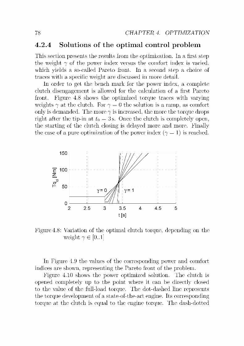
78 CHAPTER 4. OPTIMIZATION
4.2.4 Solutions of the optimal control problem
This section presents the results from the optimization. In a first stepthe weight 7 of the power index versus the comfort index is varied,which yields a so-called Pareto front. In a second step a choice of
traces with a specific weight are discussed in more detail.
In order to get the bench mark for the power index, a completeclutch disengagement is allowed for the calculation of a first Pareto
front. Figure 4.8 shows the optimized torque traces with varying
weights 7 at the clutch. For 7 = 0 the solution is a ramp, as comfort
only is demanded. The more 7 is increased, the more the torque drops
right after the tip-in at to = 3 s. Once the clutch is completely open,
the starting of the clutch closing is delayed more and more. Finallythe case of a pure optimization of the power index (7 = 1) is reached.
150
"e 100
15
I- 50
0
2 2.5 3 3.5 4 4.5 5
t[s]
Figure 4.8: Variation of the optimal clutch torque, depending on the
weight 7 G [0..1]
In Figure 4.9 the values of the corresponding power and comfort
indices are shown, representing the Pareto front of the problem.
Figure 4.10 shows the power optimized solution. The clutch is
opened completely up to the point where it can be directly closed
to the value of the full-load torque. The dot-dashed line representsthe torque development of a state-of-the-art engine. Its corresponding
torque at the clutch is equal to the engine torque. The dash-dotted

4.2. THE OPTIMAL CONTROL PROBLEM 79
1
0.8
Jl 0.6
^0.4
0.2
0
0 0.2 0.4 0.6 0.8 1
Pl1 H
Figure 4.9: Calculated Pareto front resulting from the optimizationwith a torque drop.
line represents the torque development of the engine with the applied
strategy and the solid line depicts the torque applied to the gear box.
The time to reach 90 % of the full-load torque can be improved bymore than 2.4 s. Unfortunately, this improvement cannot be realized,as no driver would accept such a torque drop after hitting the load
pedal.
Figure 4.11 shows the optimized torque traces without a torque
drop. Again, the torque trace for the comfort-optimized strategy (7 =
0), is represented by a ramp. With an increasing weight of the power
index, the clutch engagement has to be delayed more and more.
The Pareto front depicted in Figure 4.12 is very similar to the case
with torque drop.Parameterizations with a finer segmentation were tested as well.
The resulting torque trace had the same shapes.
Figure 4.13 depicts the power-optimized case without a torque
drop. The torque rise is delayed as long as possible and then the
torque is directly raised to its final value.
The time to reach 90 % of the full-load torque is slightly worse,
whereas the comfort is improved, but this behavior is still not accept¬
able for an acceleration.
The result from weighting power index and comfort index equally

80 CHAPTER 4. OPTIMIZATION
150
100 -
Ez
cr
50 -
/2.47s
y
/
Tq
Tq
Tq
cl.ref
cs, opt
cl.opt
400
5
t[s]
Figure 4.10: Power-optimized solution with torque drop, 7=1
(7 = 0.5) is depicted in Figure 4.14. The torque increase is only
delayed 100 ms. Thereafter it stays close to the comfort-optimal ramp.
The time to reach 90 % of the full-load torque is considerably longerthan in the power-optimized cases, but it is still more than with 1.8 s
better than the state-of-the-art strategy.The rise in engine speed is now less than 80rad/s.
Summary of the optimization results
Table 4.1 summarizes the results from the optimization of the three
important cases discussed above.
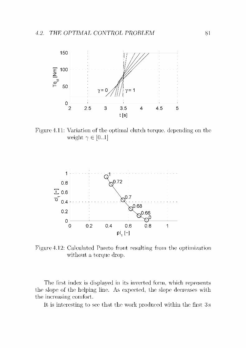
4.2. THE OPTIMAL CONTROL PROBLEM 81
150
"E 100
50
y=0
n I i i i i i i
2 2.5 3 3.5 4 4.5 5
t[s]
Figure 4.11: Variation of the optimal clutch torque, depending on the
weight 7 G [0..1]
Figure 4.12: Calculated Pareto front resulting from the optimizationwithout a torque drop.
The first index is displayed in its inverted form, which represents
the slope of the helping line. As expected, the slope decreases with
the increasing comfort.
It is interesting to see that the work produced within the first 3 s

CHAPTER 4. OPTIMIZATION
150 F
„100 -
50
A-
/2.37s
/
Tq
Tq
Tq
cl.ref
cs, opt
cl.opt
5
t[s]
gure 4.13: Power-optimized solution without torque drop, 7=1
Table 4.1: Summary of the optimization results
Tq-
drop
7
H
(Pli)"1[Nm/S]
pl2
kJ
pl3
N
di
[s-Nm]
Fig.No
ref 36.9 71.0 2.9 80 -
yes
no
no
l
l
0.5
292.1
233.3
114.3
82.6
82.3
83.3
0.4
0.5
1.0
29
26
2
4.10
4.13
4.14

4.2. THE OPTIMAL CONTROL PROBLEM 83
Ez
cr
150
//
1 1
/ /•'
____
—
—
100
/ 1.85s ,-
'
-
50 ~~
^cl.ref-
Tq'cs.opt
Tq^cl.opt
n
300
250 -
TO
200 -
150
5
t[s]
Figure 4.14: Agility-optimized solution without torque drop, 7 = 0.5
after tip-in is only little influenced by the chosen strategy, but in all
cases tested it is considerably higher than in the state-of-the-art case.
The strategy thus not only increases the comfort of the driver
considerably, but also the power output in the initial phase of the
acceleration.

84 CHAPTER 4. OPTIMIZATION

Chapter 5
Experimentalverification
5.1 Implementation on the test bench
The results in Chapter 4 gained with a mean value model of the enginehave to be verified on a real engine. Therefore a turbocharged enginewas installed on a dynamic test bench. The detailed specifications of
the engine can be found in Appendix A.
The setup of the test bench is sketched in Figure 5.1. The engineis mounted on a frame and connected to an asynchronous motor with
a cardan shaft. The motor can be used to brake as well as to propelthe engine. The bandwidth of its torque output extends to 100 rad/s.The power electronics for the motor are controlled with a real-time
PC based system.The gearbox is bypassed and a direct feed-through is implemented
instead. The motor is thus used to emulate the whole vehicle including
gearbox and clutch. In Figure 5.2 the engine is depicted with the
turbocharger.A detailed discussion of the control strategy used to emulate the
clutch can be found in Appendix B.
5.1.1 Choice from the set of optimal solutions
In Section 4.2.4 a set of optimal solutions was presented. They all have
different ratios of power and comfort. By applying further conditions
85

CHAPTER 5. EXPERIMENTAL VERIFICATION
TC SI enginewith gearbox
asynchronous power PC with
motor electronics real time
I system
-o cH
data link
Figure 5.1: Setup of the test bench for the implementation of the clutch
strategy
11 four-cylinder SI engine coupling to electric motor with torque shaft
turbocharger gearbox in direct gear
Figure 5.2: Engine on the test bench equipped with a turbocharger

5.1. IMPLEMENTATION ON THE TEST BENCH 87
the most suitable solution from this set can be chosen. Because of
comfort considerations the torque is not allowed to drop. As a rule
of thumb, 100 ms after tip-in the driver wants to feel the acceleration
and from the set fulfilling these conditions the one with the highest
power index is chosen. These constraints are summarized in Table 5.1.
Table 5.1: Additional constraints for the choice of an optimal solution.
> no torque drop
> delay from tip in to torque increase not more than 100 ms
> highest possible power index
This set of applications leads to a weight 7 = 0.5. Its corresponding
torque trace can be seen in Figure 4.14.
5.1.2 Results
Results from the chosen starting point
The torque signal found to be optimal in the previous section was
applied on the engine on a test bench. Figure 5.3 shows the results.
The dashed lines represent the optimized strategy, whereas the solid
lines represent the state-of-the-art strategy. The torque signals are
filtered for better readability. In the optimized case the torque at
the clutch develops linearly, as desired. The emulated clutch openingresults in an increased engine speed, culminating about 80 rad/s above
the initial value. In the upper right-hand corner the turbocharger
speed is shown. Due to the clutch strategy the turbocharger can speed
up considerably faster. The graph in the lower right-hand corner shows
a comparison of different indices.
Note that the very promising results from the simulation in the
previous chapter are now verified experimentally. The time to reach
90 % of the full-load torque can be reduced from 3 s to 1.2 s. This very
nice result is achieved by only optimizing the control of the system.The hardware remains unchanged.
The power and the comfort index are normalized to be one for
the state-of-the-art case. As expected the power index as well as the
comfort index can be improved considerably.

CHAPTER 5. EXPERIMENTAL VERIFICATION
x 10
400
350
300
^2502 200
150
100
50
0
/ \
v
4 6
t[s]
0
2 4 6
t[s]
3
2.5
2
1.5
1
0.5
t_90 pl_1 cl_1
Figure 5.3: Measurement of the agility improvement of a downsized
and supercharged engine, starting at 2000 rpm and 20 Nm
It is also interesting to note that this very good results are neither
achieved by optimizing the engine nor by optimizing the gearbox to¬
gether with the clutch. The good results are achieved by optimizingthe engine-clutch-gearbox system.

5.1. IMPLEMENTATION ON THE TEST BENCH 89
Varying starting points
In the Figures 5.4 - 5.8 the results from varying starting points are
presented. In Figure 5.9 each square represents a different starting
point. The darker a square is the more the time to reach 90 % of the
full-load can be improved.When starting at 2000 rpm the biggest improvement can be at¬
tained. For lower engine speeds the full-load torque becomes smaller
due to a lower boost pressure achievable. The less the turbochargercan contribute to the torque development, the smaller is its influence
on the dynamic torque development. This directly decreases the im¬
pact of the clutch strategy as well.
For engine speeds above 2000 rpm the impact decreases as well, but
for another reason. With higher engine speeds the mass flow increases,which leads to higher initial speeds of the turbine and compressor,
resulting in a faster response of the turbocharger. At 3000 rpm and a
load of 10 Nm the gain becomes very small, as shown in Figure 5.8.
With higher loads the air mass flow through the engine increases
as well. With higher air mass flows the initial turbocharger speedincreases and the turbo lag is thus less critical.
Although the region with a strong improvement is not very large, it
is a very important region. For the assessment of this fact a frequency
analysis of the new European driving cycle (NEDC) is used, as this
cycle is to represent an average driving habit. In Figure 5.10 the
frequency distribution of the operating points for a complete NEDC
is plotted for a VW GOL. The operating frequency is the operatingtime in the corresponding operation area divided by the total cycleduration. The engine's idling duration is taken into account but not
plotted.The points frequently used and thus of high importance lie exactly
in the region of where the clutch strategy can provide a considerable
benefit.

90 CHAPTER 5. EXPERIMENTAL VERIFICATION
Tq =20Nm, n = 1500rpm Tq =20Nm, n = 1750rpm
150 150
400 400
300
2 200
300
ST
2 200
100 100
0 0
2 4 6
t[s]
2 4 6
t[s]
2.5
1.5
0.5
2.5
2
1.5
0.5
t_90 pl_1 cl_1 t_90 pl_1 cl_1
Figure 5.4: Measurement of the agility improvement, initial load
20 Nm, initial speed 1500 rpm, 1750 rpm, respectively

5.1. IMPLEMENTATION ON THE TEST BENCH 91
Tq =40Nm, n = 1750rpm Tq = 10Nm, n = 2000rpm
150 150
F 100
400 400
300
ST
2 200
100
300
ST
2, 200
3
100
/ \
J_ A.
0
2 4 6
t[s]
2.5
0 L
2
3p
2.5
2
1.5
4 6
t[s]
0.5
t_90 pl_1 cl_1
II In Lt_90 pl_1 cl_1
Figure 5.5: Measurement of the agility improvement. Measurements
start with 1750 rpm and 2000 rpm. When starting at
2000 rpm the highest improvements can be achieved.

CHAPTER 5. EXPERIMENTAL VERIFICATION
Tq = 20Nm, n = 2000rpm Tq = 40Nm, n = 2000rpm
150 150
F 100
50
400 400
300
ST
2 200
100
/ \
_^,
300
ST
2, 200
3
100
/ \
4 6
t[s]
4 6
t[s]3 3
2.5 2.5
2 2
1.5 1.5
1 1
0.5 1 1 0.5 1 10
1 L0
1 nt_.90 PL_1 cl_1 t_.90 PL_1 cl_1
gure5.6: Measurement of the agility improvement. Starting points:20 Nm/2000 rpm and 40 Nm/2000 rpm
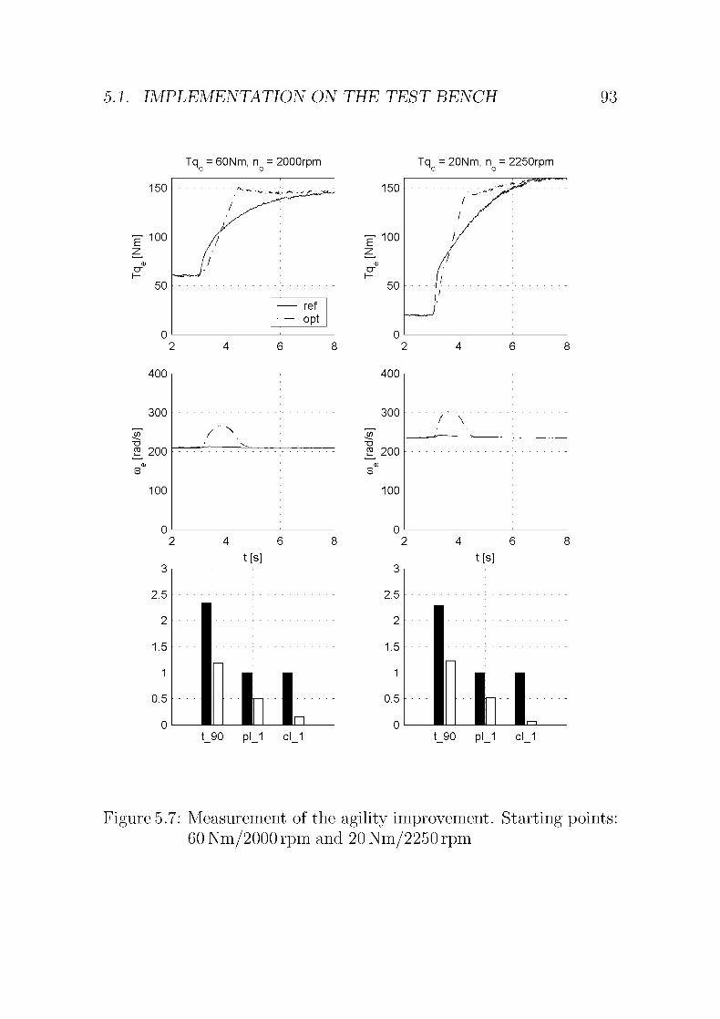
5.1. IMPLEMENTATION ON THE TEST BENCH 93
Tq = 60Nm, n = 2000rpm Tq = 20Nm, n = 2250rpm
ref
opt
150
F 100
50
400 400
300
ST
2 200
100
\
300
ST
]| 200
3
100
/ \
0
2 4 6
t[s]
t_90 pl_1 cl_1 t_90 pl_1 cl_1
Figure 5.7: Measurement of the agility improvement. Starting points:60 Nm/2000 rpm and 20 Nm/2250 rpm

94 CHAPTER 5. EXPERIMENTAL VERIFICATION
Tq = 40Nm, n = 2250rpm Tq = 10Nm, n = 3000rpm
150
100
400
300
ST
]| 200
0)
100
/ \
150
100
400
f\
300
2, 200
0)
100
0
2 4 6
t[s]
0
2 4 6
t[s]
2.5 2.5
1.5
:l l\ I Int_90 pl_1 cl_1 t_90 pl_1 cl_1
Figure 5.8: Measurement of the agility improvement. Starting points:40 Nm/2250 rpm and 10Nm/3000rpm. For the last start¬
ing point the improvement is very small due to good per¬
formance of the state-of-the-art solution.

5.1. IMPLEMENTATION ON THE TEST BENCH 95
150
E 100
CT
K50
0
0
12 16
1115 18 11
280
300
320 -^"g/kWh
0 29
1 9"
2000 4000 6000
ne [rpm]
w
o
Figure 5.9: Gain in £90 (time to reach 90% of the full-load torque) in
the engine map, fuel consumption specified in g/kWh
150
"e 100
<D
I- 50
0
1000 2000 3000 4000 5000 6000
ne [rpm]
Figure 5.10: Frequency plot of the different load and speed points in
the NEDC, applied to the vehicle under consideration.
Idling point is not displayed (24 %) for better resolution.
The fuel consumption is specified in g/kWh
96 CHAPTER 5. EXPERIMENTAL VERIFICATION
5.2 Remarks on the implementation of
the clutch strategy in a car
5.2.1 Clutch specifications
So far the clutch strategy for an improved agility was tested with a
dynamic model and on a test bench. As it was not possible within
the constraints of the project to implement the strategy in a car, some
theoretical reflections are presented.As the name of the strategy already says, the clutch is the central
element of the strategy. It thus has to fulfill certain specifications:
Automated The clutch has to be automated in order for the torquein the clutch becoming an input into the system.
Design Because of the more frequent use of the clutch, it has to be
designed in a virtually wear-free way. According to Steinhagen
(1980) a wet clutch can fulfill this requirement.
Bandwidth Schreiber et al. (2003) present an automated clutch
which can realize a torque ramp of 320 Nm in 50 ms. A clutch
with these specifications allows the implementation of the clutch
strategy.
Torque adaption The responsiveness can be further improved by
continuously keeping the clutch torque just slightly above the
engine torque, so that the clutch actuator only has to travel
very little until the clutch opens [Fischer and Salecker (1997)].
When the clutch is operated in slipping mode, the question arises
whether it can absorb the heat produced during the acceleration phase.The heat flux to be absorbed is equal to the difference between the
inflowing and the outflowing power.
7,rin
r out
dt
= LüeTqd-LügbTqd (5.1)

5.2. IMPLEMENTATION OF THE CLUTCH STRATEGY 97
The energy to be absorbed during one strategy application is thus
the integral over time from the opening of the clutch (to) to the pointwhen the clutch engages again (ti).
Qd = ue- Tqd -
LOgb Tqd dt (5.2)Jto
The simulation of the proposed strategy yields the heat to be absorbed
by the clutch plates as Qd = 0.22 J/mm2.This value is well below the acceptable limits given by Winkelmann
and Hartmuth (1985):
Table 5.2: Acceptable heat to be absorbed in a clutch [Winkelmannand Hartmuth (1985)]
Action maximal heat density
Shifting in a car
Shifting in a light-weight truck
1 •J/mm21.2 J/mm2
For a clutch the start of the vehicle is the critical case. As the
clutch strategy is shorter and requires less differential speed between
the clutch plates, the energy to be absorbed becomes smaller and thus
less critical.
5.2.2 Emissions
The application of the clutch strategy increases the engine dynamics
considerably. The correct control of the air-to-fuel ratio and the spark
timing could therefore be problematic.
The steepest torque increase happens in the state-of-the-art as well
as in the optimized case between tip-in and the moment when the full-
load torque of the underlying naturally aspirated engine is reached.
The control of the emissions is thus not a more difficult task than in
a state-of-the-art set up.
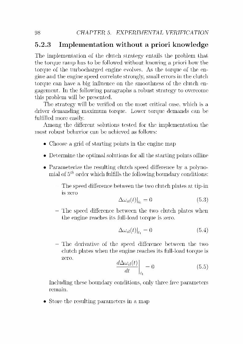
98 CHAPTER 5. EXPERIMENTAL VERIFICATION
5.2.3 Implementation without a priori knowledge
The implementation of the clutch strategy entails the problem that
the torque ramp has to be followed without knowing a priori how the
torque of the turbocharged engine evolves. As the torque of the en¬
gine and the engine speed correlate strongly, small errors in the clutch
torque can have a big influence on the smoothness of the clutch en¬
gagement. In the following paragraphs a robust strategy to overcome
this problem will be presented.The strategy will be verified on the most critical case, which is a
driver demanding maximum torque. Lower torque demands can be
fulfilled more easily.
Among the different solutions tested for the implementation the
most robust behavior can be achieved as follows:
• Choose a grid of starting points in the engine map
Determine the optimal solutions for all the starting points offline•
• Parameterize the resulting clutch speed difference by a polyno¬mial of hth order which fulfills the following boundary conditions:
— The speed difference between the two clutch plates at tip-inis zero
Aud(t)\to = 0 (5.3)
— The speed difference between the two clutch plates when
the engine reaches its full-load torque is zero.
Aud(t)\ti = 0 (5.4)
— The derivative of the speed difference between the two
clutch plates when the engine reaches its full-load torque is
zero.
dAujd(t)dt
= 0 (5.5)
Including these boundary conditions, only three free parameters
remain.
• Store the resulting parameters in a map

5.2. IMPLEMENTATION OF THE CLUTCH STRATEGY 99
• Store the parameters describing the optimal clutch torque trace
for the same grid points
• Use gain scheduling to determine the parameters for any given
starting point
In Figure 5.11 the optimal solution with a correct parameterizationof the clutch speed as well as the result of a parameterization error
of ±10% is depicted. Even in case of wrong parameterization, the
torque rises in a constant manner before it reaches its maximum level.
If the speed signal is chosen too high, a slight jerk cannot be
avoided, as the additional energy stored in the engine's inertia has
to be brought back into the system somehow. A speed trace that is
parameterized too low is less problematic as the engine just does not
reach its full-load torque as fast as intended.
5.2.4 Consumer acceptance
After the discussion of all the technical aspects of the clutch strat¬
egy, the consumer acceptance has to be discussed as well. A driver
mainly perceives the application of the clutch strategy through an al¬
tered torque development and a changed sound during the acceleration
phase.
As no experiments with a car were possible, only theoretical con¬
siderations can be used. In Table 5.3 the expected effects are summa¬
rized.
The higher acceleration capability as well as the improved com¬
fort will increase the acceptance of vehicles with turbocharged enginessince the number of gearshifts necessary can be reduced.
The effect of the sound is the most difficult part to be rated. As
Figure 5.3 shows a short rise of the engine speed, culminating at 80 rad/sabove the value without the strategy. This raise is most probablyaudible. As this rapid change in engine speed occurs unexpectedly, it
could be rated negative. On the other hand, since it yields a better
acceleration, it might be accepted as a sign for the ongoing boosting.

100 CHAPTER 5. EXPERIMENTAL VERIFICATION
200
Figure 5.11: Results of disturbed and optimal implementations ob¬
tained by simulation. The solid line represents the nom¬
inal case with correct parameterization, the dashed line
a too low parameterization of the engine speed and the
dash-dotted line a too high parameterization. The bot¬
tom graph shows the engine speeds and the top graph
depicts the corresponding torque development. Even for
such high parameterization errors as ±10% a constant
torque rise and an acceptable clutch engagement can be
achieved.

5.2. IMPLEMENTATION OF THE CLUTCH STRATEGY 101
Table 5.3: Rating of the consumer acceptance of the clutch strategy
Consequencefrom the
clutch
strategy
improved
torque
build-up
improvedcomfort
change in
engine sound
Expected
Rating± ± o(-)
Effect
use of higher
gears —>
improved fuel
efficiencyx
Better
acceptance of
cars with TC
engines
-
5.2.5 Discussion of possible implementations
Frequency of use
The strategy can be used for different purposes. It can either be used
for any acceleration in which the uneven torque development could
bother the driver or it could be applied only in the case of kick-down,
providing the driver with a faster torque development. If the strategyis used only for kick-down, a dry clutch could be considered as well.
Torque converter
When a torque converter is installed, the suggested strategy is inher¬
ently implemented. If a soft torque converter is applied, the enginecan speed up, but the driver experiences a delayed response. A stiff
torque converter, however, causes the responsiveness to increases, but
it prevents any fast engine speed-up, which would have been a desir¬
able effect.
One way to overcome this problem would be to use a torque con¬
verter with either variable guide vanes or a controllable bypass clutch.
This would allow the application of the clutch strategy and to profit
See Section 1 2 for a detailed discussion
102 CHAPTER 5. EXPERIMENTAL VERIFICATION
from the faster torque increase, if the dynamics of the actuator can
fulfill the conditions listed in Section 5.2.1.
Diesel engines
The clutch strategy has been developed and tested for spark ignited
engines. As compression ignited engines suffer from the turbo lag as
well, the same strategy can be applied as well. Since their variation
in air mass flow is far smaller, namely a factor of 6.5 instead of the 35
typical for SI engines, the turbocharger speed would remain on higherlevels and the gain from the clutch strategy would thus be smaller.
Heavy duty application
Heavy trucks are typically equipped with automated clutches, which
doubles the clutch lifetime compared to clutches in manually shifted
gearboxes. As wear is one of the main arguments for the automati¬
zation of the clutch, any strategy increasing the wear of the clutch is
not suitable.

Chapter 6
Conclusion
Turbocharging combustion engines provides a considerable potentialfor lower fuel consumption. However, due to delayed torque develop¬ment the driver tends to use lower gears, resulting in higher engine
speeds and lower loads. With this behavior most of the fuel saving
potential cannot be realized. This fact calls for a strategy eliminatingthe turbo lag or at least reducing it considerably.
For the investigation of the turbo lag, an agility criterion is sug¬
gested and used for the improvement of the dynamic torque devel¬
opment of the engine. The quality function weights the desire for a
fast torque increase as well as the need for a predictable and smooth
torque development.As turbocharged engines have suffered from the turbo lag ever
since their invention, many devices were developed to reduce the lag.In this work two strategies are investigated that do not require any
additional devices. The use of a modified spark timing improves the
comfort of the acceleration considerably, but the work output of the
engine is decreased. By applying the so-called clutch strategy, the
clutch is partially opened during the acceleration phase, allowing the
engine to speed up and thus increase the air mass flow. This in turn
increases the enthalpy flow to the turbine, forcing a faster speed-upof the turbine and the compressor. By closing the clutch again in a
suitable manner the kinetic energy from the inertia of the engine flows
back into the gear box, allowing the full load torque to be reached
even faster.
This strategy provides an accelerated torque development as well
as an increased comfort for the driver. This will not only increase
103

104 CHAPTER 6. CONCLUSION
the acceptance of turbocharged SI engines but also favor a more
consumption-optimized driving pattern.
The clutch strategy was developed based on models and verified on
an engine dynamometer. The experiments confirm the improvement
expected from the simulation. Accordingly, a patent has been filed
[DaimlerChrysler (2003)] that includes the main points of the clutch
strategy.In a next step the results will have to be verified with a vehicle
equipped with an automated clutch. This will allow to test the appli¬
cability of the strategy in different driving conditions and allow to gainresults on the influence of the clutch strategy on the driving pattern.
The only relevant premise is the use of an automated wet clutch or
a torque converter with a variable characteristic. Automated clutches
are already available in production type cars and the constructive
effort will thus be very small to realize this new technology.
By following a system oriented approach, combining the potentialof the turbocharged engine with an automated clutch, a considerable
improvement of the whole system has been achieved.
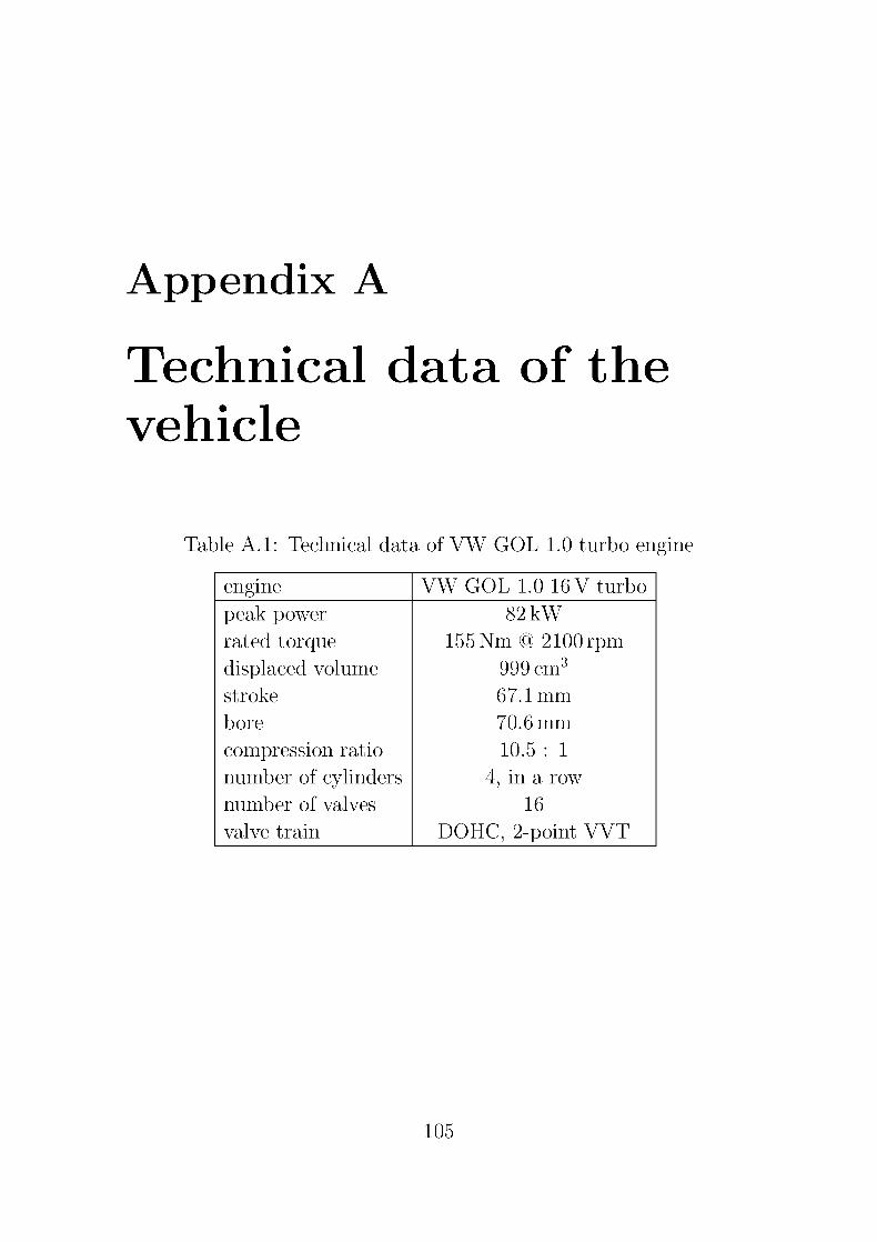
Appendix A
Technical data of the
vehicle
Table A.l: Technical data of VW GOL 1.0 turbo engine
engine VWGOL 1.0 16 V turbo
peak power 82 kW
rated torque 155 Nm@ 2100 rpm
displaced volume 999 cm3
stroke 67.1mm
bore 70.6 mm
compression ratio 10.5 : 1
number of cylinders 4, in a row
number of valves 16
valve train DOHC, 2-point VVT
105
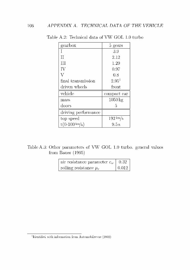
106 APPENDIX A. TECHNICAL DATA OF THE VEHICLE
Table A.2: Technical data of VW GOL 1.0 turbo
gearbox 5 gears
I
II
III
IV
V
final transmission
driven wheels
3.9
2.12
1.29
0.97
0.8
2.951
front
vehicle compact car
mass
doors
1050 kg5
driving performance
top speed
t (0-100 km/h)
192 km/h9.5s
Table A.3: Other parameters of VW GOL 1.0 turbo, general values
from Bauer (1995)
air resistance parameter c%
rolling resistance ur
0.32
0.012
1 Identified with information from Automobilrevue (2002)

Appendix B
Implementation on the
test bench
The strategy suggested in Chapter 3 was tested on a test bench. For
the emulation of the clutch, a dynamic test bench was used. This
test bench will be described in the following section. Thereafter an
analysis of the system will be presented and a controller consisting of
a feedforward and a feedback path will be designed and tested.
B.l System description
A cardan shaft is used to connect the engine and the asynchronousmotor. The shaft is equipped with a torque measurement sensor, al¬
lowing to determine the torque produced by the engine. The installed
gearbox is bypassed and the clutch is only used while starting the
engine. The clutch is emulated with the electrical motor. A generaloverview of the test bench is provided in Figure 5.1.
B.2 System analysis and modeling
By opening the clutch in a real vehicle, all the inertias of the drive
train and the vehicle are decoupled.In order to allow the emulation of a disengaged clutch the inertia
of the electrical motor has to be compensated. The system thus has
to be identified in a first step.
107

108 APPENDIX B. IMPLEMENTATION ON THE TEST BENCH
The system to be emulated is shown schematically in Figure B.l,
a) representing the setup of the test bench, b) showing the system to
be emulated, and c) depicting the corresponding physical model of the
test bench.
a TC SI enginewith gearbox
asynchronousmotor
testbench setup
b)system to be
emulated
n n
nn
physical model
Tqcs Lüe Tq.sh Tq
-> <p
sh ujmTqtel
a Or
Figure B.l: The system to be emulated is compared with the setup
on the test bench and the physical model used for the
identification of the test bench.
Under the assumption of a stiff connection between the engine and
the electrical motor, the speeds of the engine and the motor are the
same.
Lüe= Lüm = Lütb (B.l)

B.2. SYSTEM ANALYSIS AND MODELING 109
The differential equations for the rotational speed of the two inertias
can be written using d'Alembert's law.
^ = ^(Tte-Tto) (B.2)
due 1
dt O—(Tqcs-Tqsh) (B.3)
e
Using equations (B.1-B.3) yields the differential equation for the ro¬
tational speed of the test bench.
^T- =
r,
l
r,(TVcs ~ Tqel) (B.4)
The analysis of Eq. (B.4) reveals an integrating behavior between the
electrical torque and the rotational speed of the test bench. In or¬
der to identify the transfer function, a frequency analyzer was used.
Figure B.2 shows the measured and identified Bode plots. The shapeof the transfer function can be depicted by a low-pass element much
better than by an integrator. This effect comes from the speed de¬
pendence of the torque of the engine Tqcs(u)e). For low excitation fre¬
quencies the engine speed changes considerably and the torque from
the engine does not remain constant, although the throttle position is
kept constant.
The PT1 element depicting the transfer function best is:
PTqel2^ = 9totS\ 0 6withetot = 0M (B.5)
At high frequencies the agreement of the magnitude is good, whereas
the phase decreases faster than identified. This can be explained with
delays and the resulting phase drop.For the identification of the transfer function from the electrical
torque (Tqei) to the torque in the shaft (Tqcs) the rotational speedsare set equal (B.l). By combining (B.2) and (B.3) the correlation
between the torques becomes
1
{Tqsh - Tqel) = )-(Tqcs - Tqsh) (B.6)m. C
e

110 APPENDIX B. IMPLEMENTATION ON THE TEST BENCH
20
QU
p.
O)
CD
-20
-40
-60
meas
id
10
co [rad/s]
Figure B.2: Bode plot depicting the transfer function from Tqd —> lvt
With some simple algebraic transformations the torque in the cardan
shaft Tqsh can be expressed as:
Tqsh1
0P + Or-(eeTqd + emTqe (B.7)
The torque at the shaft is related to the electrical torque in the motor
with the algebraic factor ee/(ee+em) < 1.

B.2. SYSTEM ANALYSIS AND MODELING 111
10
co [rad/s]
Figure B.3: Bode plot depicting the transfer function from
TqeJ - Tqsh
The expected result is only partially visible in the Bode plot. At
very low frequencies, the torque from the crank shaft (Tqcs) is not
constant. At frequencies higher than 100rad/s the magnitude rolls off
and a delay can be identified in the phase plot. The replacing trans¬
fer function is a linear combination of a zero and a pole, a second-
order low-pass element and a delay approximated with a Padé element

112 APPENDIX B. IMPLEMENTATION ON THE TEST BENCH
(Eq. (B.8)). Figure B.3 shows how good the agreement is.
PTqel2Tqsh = Pzp PPT2 Pdelay (B.*9r
-s + 0.2p, =e£+eI2—: /BQx
ps+ 0.2
v ;
with—^-— = 0.3 (B.10)G 4- G
P^2 = -2—T^—-^ (B.ll)
with C = 1 and lui = 110 rad/s
Pdelay = pade(T = 10 ms) (B.12)
Solving Equation (B.5) and Equation (B.10) for GTO and Ge yieldsthe following values for the inertias: GTO = 0.25 kg m2 and Ge =
O.llkgm2.
B.3 Controller design
B.3.1 Feedforward controller
For the best possible feedforward control, the identified transfer func¬
tion is partially inverted. For a good roll-off behavior, a second-order
low-pass element is connected in series with the inverted controller.
B.3.2 Feedback controller
Whereas the feedforward part of the controller is mainly used for a
highly dynamic response, the feedback part cannot be tuned as fast
and is used to eliminate stationary errors. It is designed as a PI
controller.
The final result is displayed in Figure B.4. The magnitude of the
closed-loop system is close to the desired 0 dB-line up to a frequencyOf 60 rad/s.

B.3. CONTROLLER DESIGN 113
20
inT3
CD
-20
-40
-60 L
io~
P
P with ff
P with ff & fb
010 10 10 10
Figure B.4: Bode magnitude plot of the transfer function
Tqci,ref —> Tqc\.

114 APPENDIX B. IMPLEMENTATION ON THE TEST BENCH
Bibliography
Âstrom, K. J. (2000). The PID Controller: Design and Implemen¬tation Aspects. In 2ème Journée de l'automatique à VEPFL, Lau¬
sanne, Switzerland.
Automobilrevue, Katalog der ~ (2002). GOL Turbo 1.0 16V. EspaceMedia Groupe, Bern.
Baker, C. S., Kobayashi, R. J., and Baker, D. E. (1989). Garret Ex¬
perience in Ceramic Turbocharger Turbine Wheels. SAE Technical
Paper, 890426.
Bauer, H. (1995). Kraftfahrtechnisches Taschenbuch. Robert Bosch
GmbH, Düsseldorf, 22nd edition.
Bronstein, I. N. and Semenjajew, K. A. (1977). Taschenbuch der
Mathematik. Verlag Harri Deutsch, 17th edition.
Bryson, A. E. (1998). Dynamic Optimization. Addison-Wesley Long¬
man, Massachusetts, 1st edition.
Cantemir, C.-G. (2001). Twin Turbo Strategy Operation. SAE Tech¬
nical Paper, 2001-01-0666.
Cantore, G., Mattarelli, E., and Fontanesi, S. (2001). A New Conceptof Supercharging Applied to High-Speed DI Diesel Engines. SAE
Technical Paper, 2001-01-2485.
DaimlerChrysler AG (2003). Akte P803489/DE/1, Schutzrechtmeld¬
ung 10330951.9, Deutsches Patent- und Markenamt, Berlin.
Eriksson, L. (2002). Mean Value Models for Exhaust Temperatures.SAE Technical Paper, 2002-01-0374.
115

116 BIBLIOGRAPHY
Eriksson, L., Frei, S., Onder, C, and Guzzella, L. (2002). Control and
Optimization of Turbocharged Spark Ignited Engines. In Proceed¬
ings of the 15th World Congress of the International Federation ofAutomatic Control, Barcelona / Spain.
Eriksson, L., Nielsen, L., Brugard, J., Bergström, J., Pettersson, F.,and Andersson, P. (2001). Modeling and Simulation of a Tur¬
bocharged SI Engine. In 3rd IFAC Workshop, "Advances in Au¬
tomotive Control", 2001, pages 379 - 387, Karlsruhe.
Fischer, R. and Salecker, M. (1997). Strategien zur Kupplungsans¬
teuerung. In VDI Tagung Fulda: Kupplungen in Antriebssystemen
'97, volume VDI Berichte 1323, pages 269 - 290, Fulda, Germany.VDI-Gesellschaft Entwicklung Konstruktion Vertrieb.
Fox, J. W., Cheng, W. K., and Heywood, J. B. (1993). A Model for
Predicting Residual Gas Fraction in Spark-Ignition Engines. SAE
Technical Paper, 931025.
Gerhardt, J., Hönninger, H., and Bischoff, H. (1998). A New Approachto Functional and Software Structure for Engine Management Sys¬tems - BOSCH ME7. SAE Technical Paper, 980801:p. 197-207.
Guzzella, L. (1998) Motorsysteme. Vorlesungsskript. ETH Zurich, Me¬
chanical Engineering Department, Measurement and Control Lab.
Guzzella, L. (1998a). Optimization and Control of Supercharged Si-
Engines. In IEEE, editor, Advances in Vehicle Control and Safety
'98, Amiens, France.
Guzzella, L. and Onder, Ch. (2004). Introduction to Modeling and
Control of Internal Combustion Engine Systems. Springer Verlag
Berlin, Germany
Heywood, J. B. (1988). Internal Combustion Engine Fundamentals.
Automotive Technology Series. McGraw-Hill international editions.
Hiereth, H. (1986). Testing Methods for the Transient Behaviour of
Charged Vehicle Engines. SAE Technical Paper, 860451.

BIBLIOGRAPHY 117
Inhelder, J. (1996). Verbrauchs- und Schadstoffoptimiertes Ottomotor-
Aufladekonzept. Diss. ETH 11948.
Isermann, R., Jost, 0., and Schwarte, A. (2000). Modellgestützte Re¬
glerentwicklung für einen Abgasturbolader mit variabler Turbinen¬
geometrie an einem DI-Dieselmotor. MTZ, 61(3): 184-192.
Janach, W., Heini, K., and Hüsler, I. (2002). "p-Booster"und
AGR/Lambda-Kombisteuerung für aufgeladene Ottomotoren.
MTZ, 63:502 - 508.
Jensen, J.-P., Kristensen, A. F., Sorenson, S. C, Houbak, N., and Hen¬
dricks, E. (1991). Mean Value Modeling of a Small TurbochargedDiesel Engine. SAE Technical Paper, 910070.
Johnson, T. V. (2003). Diesel Emission Control in Review - The Last
12 Months. SAE Technical Paper, 2003-01-0039.
Kattwinkel, T., Weiss, R., and Boeschlin, J.-P. (2003). Mechatronic
Solution for Electronic Turbocharger. SAE Technical Paper, 2003-
01-0712.
Kolmanovsky, I. V. and Stefanopoulou, A. (2001). Control Techniquesfor Assessing Feasibility and Defining Subsystem Level Require¬ments: An Automotive Case Study. IEEE Transactions on Control
Systems Technology, Vol. 9(No. 3):524-534.
Langen, P., Theissen, M., and Zielinski, R. (1993). Aufladung als
Konzept der Verbrauchsreduzierung. MTZ, 54:522 - 533.
Lezhnev, L., Kolmanovsky, I. V., and Buckland, J. (2002). Boosted
Gasoline Direct Injection Engines: Comparison of Throttle and
VGT Controllers for Homogeneous Charge Operation. SAE Tech¬
nical Paper, 2002-01-0709.
List, H. and Schoeggel, P. (1998). Objective Evaluation of Vehicle
Driveability. SAE Technical Paper, 980204.
Lundstrom, R. R. and Gall, J. M. (1986). A Comparison of Tran¬
sient Vehicle Performance Using a Fixed Geometry, Wastegated

118 BIBLIOGRAPHY
Turbocharger and a Variable Geometry Turbocharger. SAE Tech¬
nical Paper, 860104.
Mladek, M. (2003). Cylinder Pressure for Control Purposes of Spark
Ignition Engines. Diss. ETH 14616, ETH Zurich.
Müller, M., Hendricks, E., and Sorenson, S. C. (1998). Mean Value
Modelling of Turbocharged Spark Ignition Engines. SAE Technical
Paper, 980784.
Moraal, P. and Kolmanovsky, I. V. (1999). Turbocharger Modellingfor Automotive Control Applications. SAE Technical Paper, 1999-
01-0908.
Nasser, S. H. and Playfoot, B. B. (1999). A Turbocharger Selection
Computer Model. SAE Special Publication SP-1^51, SI engine mod¬
eling, 1999-01-0559:233-252.
Pfiffner, R. (2001). Optimal Operation of CVT-Based Powertrains.
Diss. ETH 14136, ETH Zurich.
SAE Cold Start and Driveability Procedure. SAE Standard, J1635.
Schreiber, W., Rudolph, F., and Becker, V. (2003). Das neue Dop¬
pelkupplungsgetriebe von Volkswagen. ATZ Automobiltechnische
Zeitschrift, 105:1022-1039.
Singer, D. A. (1985). Comparison of a Supercharger vs. a Turbochargerin a Small Displacement Gasoline Engine Application. SAE Tech¬
nical Paper, 850244.
Soltic, P. (2000). Part-Load Optimized SI Engine Systems. Diss. ETH
13942, ETH Zurich.
Soltic, P. and Guzzella, L. (2001). Verbrauchsvergleich verschiedener
Verbrennungsmotorkonzepte für Leichtfahrzeuge. MTZ Motortech¬
nische Zeitschrift, 62:590-596.
Stöckli, M. (1989). Reibleistung von 4-Takt Verbrennungsmotoren. In¬
ternal technical report, Laboratory of Internal Combustion Engines,Swiss Federal Institute of Technology, Zurich (LVV/ETH-Zurich).

119
Steinhagen, H. G. (1980). The Plate Clutch. SAE Technical Paper,800978.
Tashima, S., Tadokoro, T., Okimoto, H., and Niwa, Y. (1991). Devel¬
opment of Sequential Twin Turbo System for Rotary Engine. SAE
Technical Paper, 910624.
Urlaub, A. (1994). Verbrennungsmotoren. Springer Verlag, Berlin.
Uthoff, L. H. and Yakimow, J. W. (1987). Supercharger versus Tur¬
bocharger in Vehicle Applications. SAE Technical Paper, 870704.
Watanabe, T., Koike, T., Furukawa, H., Ikeya, N., and Sakakida, M.
(1996). Development of Turbocharger for Improving Passenger Car
Acceleration. SAE Technical Paper, 960018.
Wimmer, A., Pivec, R., and Sams, T. (2000). Heat Transfer to the
Combustion Chamber and Port Walls on IC Engines - Measure¬
ments and Prediction. SAE Technical Paper, 2000-01-0568.
Winkelmann, S. and Hartmuth, H. (1985). Schaltbare Reibkupplungen.
Springer Verlag, Berlin.
Wirth, M., Mayerhofer, U., Piock, W. F., and Fraidl, G. K. (2000).Turbocharging the DI Gasoline Engine. SAE Technical Paper, 2000-
01-0251.
Zapf, H. (1969). Beitrag zur Untersuchung des Wärmeübergangswährend des Ladungswechsels im Viertakt-Dieselmotor. MTZ, 110
(30):461-465.
Zeyen, K.-P. and Pels, T. (1997). ISAD - A Computer-Controlled,
Integrated Starter-Alternator-Damper System: a New Approach to
Energy Engineering. SAE Technical Paper, 972660.

120

Curriculum Vitae
Personal Data
Name: Simon Andreas Frei
Date of birth: July 28, 1973
Parents: Siegfried Frei and Bertha Frei-Alder
Education
1980-1986 Primary school in Warth-Weiningen TG, Switzerland
1986-1988 Secondary school in Hüttwilen TG, Switzerland
1988-1993 Gymnasium in Frauenfeld TG, Switzerland
1993 Matura certificate, type C
1993-1994 Military service
1994-1999 Studies in mechanical engineering, Swiss Federal
Institute of Technology (ETH) Zurich, Switzerland
Major in system dynamics
1999 Diploma as Dipl. Masch.-Ing. ETH
1999-2004 Doctoral student and research assistant at the Mea¬
surement and Control Laboratory, Swiss Federal
Institute of Technology (ETH) Zurich, Switzerland
Professional Experience
2000 Feasibility study of a new measurement concept for
Hilti AG, Liechtenstein
121