rights / license: research collection in copyright - non ...8376/eth-8376-02.pdf · perimental...
TRANSCRIPT

Research Collection
Doctoral Thesis
Temperature dependence of activity coefficients in organicaerosols
Author(s): Ganbavale, Gouri
Publication Date: 2014
Permanent Link: https://doi.org/10.3929/ethz-a-010109026
Rights / License: In Copyright - Non-Commercial Use Permitted
This page was generated automatically upon download from the ETH Zurich Research Collection. For moreinformation please consult the Terms of use.
ETH Library

Diss. ETH No. 21374
Temperature Dependence ofActivity Coefficients in Organic
Aerosols
A dissertation submitted to
ETH ZURICH
for the degree of
Doctor of Sciences
presented by
GOURI GANBAVALE
M.Sc in Space Sciences, University of Pune
born 14. September 1983
citizen of India
accepted on the recommendation of
Prof. Dr. Thomas Peter, examiner
Dr. Claudia Marcolli, co-examiner
Dr. David Topping, co-examiner
2014


To loving memories of my parents..


Contents
Abstract ix
Zusammenfassung xiii
1 Introduction 1
1.1 Motivation . . . . . . . . . . . . . . . . . . . . . . . . . . . . . 1
1.2 Vertical structure of Earth’s atmosphere . . . . . . . . . . . . . 6
1.2.1 Composition of the Earth’s atmosphere . . . . . . . . . 8
1.3 Aerosols . . . . . . . . . . . . . . . . . . . . . . . . . . . . . . . 9
1.3.1 Sources . . . . . . . . . . . . . . . . . . . . . . . . . . . 9
1.3.2 Sinks . . . . . . . . . . . . . . . . . . . . . . . . . . . . . 10
1.3.3 Size distribution . . . . . . . . . . . . . . . . . . . . . . 13
1.3.4 Chemical composition . . . . . . . . . . . . . . . . . . . 15
1.4 Radiative Forcing . . . . . . . . . . . . . . . . . . . . . . . . . . 16
1.5 Aerosol thermodynamics . . . . . . . . . . . . . . . . . . . . . . 19
2 Chemical Thermodynamics and Molecular Interactions 25
2.1 Thermodynamics of multicomponent systems . . . . . . . . . . 25
2.1.1 Homogeneous Open and Closed System . . . . . . . . . 26
2.1.2 Thermodynamic Equilibrium . . . . . . . . . . . . . . . 30
2.1.3 Chemical Potential of Ideal Gas . . . . . . . . . . . . . . 32
2.1.4 Ideal Solutions . . . . . . . . . . . . . . . . . . . . . . . 33
2.1.5 Non-ideal Solutions . . . . . . . . . . . . . . . . . . . . . 35
v

vi
2.1.6 Gibbs excess energy . . . . . . . . . . . . . . . . . . . . 38
2.2 Solubility . . . . . . . . . . . . . . . . . . . . . . . . . . . . . . 40
2.2.1 Solid-liquid equilibria . . . . . . . . . . . . . . . . . . . 42
2.3 Intermolecular Interactions . . . . . . . . . . . . . . . . . . . . 47
2.3.1 Ion-dipole forces . . . . . . . . . . . . . . . . . . . . . . 49
2.3.2 Dipole-Dipole forces . . . . . . . . . . . . . . . . . . . . 50
2.3.3 Dipole-induced dipole interactions . . . . . . . . . . . . 50
2.3.4 Dispersion forces . . . . . . . . . . . . . . . . . . . . . . 51
2.3.5 Hydrogen bonds . . . . . . . . . . . . . . . . . . . . . . 53
3 Improved AIOMFAC temperature dependence 57
3.1 Introduction . . . . . . . . . . . . . . . . . . . . . . . . . . . . . 60
3.2 AIOMFAC model . . . . . . . . . . . . . . . . . . . . . . . . . . 63
3.2.1 Group-contribution method . . . . . . . . . . . . . . . . 65
3.2.2 Short-range contribution . . . . . . . . . . . . . . . . . . 65
3.3 Experimental data . . . . . . . . . . . . . . . . . . . . . . . . . 71
3.3.1 Solid-liquid equilibrium . . . . . . . . . . . . . . . . . . 71
3.3.2 Water activity measurements . . . . . . . . . . . . . . . 74
3.3.3 Liquid-liquid equilibria data . . . . . . . . . . . . . . . . 74
3.3.4 Vapour-liquid equilibria . . . . . . . . . . . . . . . . . . 75
3.4 Objective function and model parameter estimation . . . . . . 77
3.4.1 Dataset weighting and temperature range . . . . . . . . 78
3.5 Results and Discussion . . . . . . . . . . . . . . . . . . . . . . . 81
3.5.1 Aqueous organic mixtures . . . . . . . . . . . . . . . . . 82
3.5.2 Binary organic mixtures . . . . . . . . . . . . . . . . . . 86
3.5.3 Scope and limitations of the new parameterisation . . . 88
3.6 Conclusions . . . . . . . . . . . . . . . . . . . . . . . . . . . . . 96
3.7 . . . . . . . . . . . . . . . . . . . . . . . . . . . . . . . . . . . . 126
3.7.1 Appendix . . . . . . . . . . . . . . . . . . . . . . . . . . 126
vii
4 Experimental temperature dependence of water activity 133
4.1 Introduction . . . . . . . . . . . . . . . . . . . . . . . . . . . . . 135
4.2 Measurement Techniques . . . . . . . . . . . . . . . . . . . . . 139
4.2.1 Differential Scanning Calorimetry (DSC) . . . . . . . . 139
4.2.2 Water activity measurements . . . . . . . . . . . . . . . 141
4.2.3 Electrodynamic Balance (EDB) measurements . . . . . 142
4.2.4 Total pressure measurements . . . . . . . . . . . . . . . 143
4.3 Results . . . . . . . . . . . . . . . . . . . . . . . . . . . . . . . . 146
4.3.1 1,4-Butanediol . . . . . . . . . . . . . . . . . . . . . . . 146
4.3.2 Methoxyacetic acid . . . . . . . . . . . . . . . . . . . . . 147
4.3.3 2-(2-Ethoxyethoxy)ethanol . . . . . . . . . . . . . . . . 148
4.3.4 M5 (multicomponent dicarboxylic acid) mixture . . . . 149
4.4 Discussion . . . . . . . . . . . . . . . . . . . . . . . . . . . . . . 155
4.4.1 Measurement techniques: scope and limitations . . . . . 155
4.4.2 Hydrogen bonding in aqueous solutions . . . . . . . . . 157
4.4.3 Atmospheric Implications . . . . . . . . . . . . . . . . . 159
4.5 Conclusions . . . . . . . . . . . . . . . . . . . . . . . . . . . . . 162
5 Conclusions 177
List of Figures 179
List of Tables 190
Bibliography 197
Acknowledgements 233
Curriculum Vitae 235


Abstract
Submicrometer-sized aerosol particles are typically mixtures of organic and in-
organic substances originating from natural and anthropogenic sources. While
the prevalent inorganic aerosol constituents are relatively small in number, the
organic fraction is highly complex, containing hundreds of compounds with
a large fraction still unidentified. The organic aerosol fraction is expected to
be present in liquid or amorphous state since a large number of organic com-
pounds depresses the temperature at which crystalline solid formation takes
place. The properties of tropospheric aerosols in terms of their hygroscopic-
ity, phase transitions and light scattering are of great interest in view of their
cloud forming and climatic characteristics.
Semi-volatile organic and inorganic aerosol species partition between the gas
and aerosol particle phases to maintain thermodynamic equilibrium. The
gas-particle partitioning of semi-volatile organic species, water content and
the phase state of the particles can be calculated when the vapour pressures
and the activities of the involved species are known. To study the hygro-
scopicity and phase equilibria of mixed aerosol particles we use the Aerosol
Inorganic-Organic Mixtures Functional groups Activity Coefficients (AIOM-
FAC) developed by Zuend et al. (2008, 2011). AIOMFAC is a group contribu-
tion model used for computing the activity coefficients of inorganic, organic,
and organic-inorganic interactions in aqueous solutions over a wide composi-
tion range. Activity coefficients of aqueous organic solutions may exhibit a
considerable temperature dependence that has to be explicitly parameterised
in thermodynamic models in order to achieve accurate predictions at tem-
peratures other than room temperature. However, most water activity data
of aqueous organic solutions has been acquired at room or elevated temper-
atures. If temperature dependence of the activity coefficients is neglected,
errors on the order of 10-15% in aw at the homogenous freezing temperature
ix
x Abstract
may be expected which in turn may induce large uncertainties in estimating
the direct and the indirect effects of aerosols.
This thesis develops a new improved parameterisation of the temperature
dependence of activity coefficients at low temperatures. With the aim to
describe a wide variety of organic mixtures and aqueous organic solutions
of atmospheric importance we focused on organic compounds containing the
functionalities typically found in tropospheric aerosols such as alcohol/polyol,
carboxylic acids, ketones, ethers, esters, aromatic rings and aldehydes. Reli-
able parameterisation of the temperature dependence and estimation of group
interaction parameters requires a comprehensive and broad distribution of ex-
perimental database covering a wide variety of mixtures with compounds con-
sisting of the targeted functional groups. Different thermodynamic data types
such as vapour-liquid equilibria (VLE), liquid-liquid equilibria (LLE), solid-
liquid equilibria (SLE), and water activity (aw) measurements are needed to
cover a wide temperature range. To assess the performance of AIOMFAC and
to establish parameters for a new improved AIOMFAC version an extensive
literature search was therefore essential.
Since there were apparent gaps in the database compiled from the literature,
especially in the low temperature range, for which data was missing or of
insufficient quality, own measurements were performed for selected aqueous
organic systems. For performing aw measurements over a wide composition
range while focusing on low temperature, we used different measurement tech-
niques such as differential scanning calorimetry (DSC) and electrodynamic
balance (EDB) measurements to obtain aw data at low temperatures. The
direct aw measurements around room temperature were obtained by a dew-
point water activity meter. To complement these measurement techniques we
developed a setup to measure total gas phase pressure over solutions at low
temperatures for mixtures with low vapour pressures of organics. Measure-
ments were conducted over the concentration range of 10-90 wt% and temper-
ature range of 190 K to 313 K using these different measurement techniques.
The measured aw data obtained through different measurement techniques
are consistent with each other and show diverse temperature dependence at
low temperatures. The aqueous organic systems with 1,4-butanediol and 2-
methoxyacetic acid as the organic component showed a moderate decrease in

xi
aw with decreasing temperature. The aqueous M5 system (a multicomponent
system containing five different dicarboxylic acids) containing five different
dicarboxylic acids as the organic component showed almost no temperature
dependence of aw for T > 285 K and a strong increase of aw at lower tem-
peratures for high solution concentrations (> 75 wt%). For aqueous solutions
of 2-(2-ethoxyethoxy)ethanol a decrease in aw with decreasing temperature
was observed for temperatures from 290 K to 265 K. The temperature de-
pendence was reversed at higher concentrations of 2-(2-ethoxyethoxy)ethanol
(>70 wt%) and lower temperatures (T < 265 K) showing a strong increase
of aw with decreasing temperature. Water activity data obtained from own
measurements are used in the temperature dependence parametrisation of
AIOMFAC model.
The AIOMFAC model with the implementation of the new improved tem-
perature dependence parameterisation, shows an overall good agreement with
most of the experimental datasets and enables the calculation of activity coef-
ficients of a wide variety different aqueous/water-free organic solutions. Due
to lack of data for a wider temperature and concentration range or due to
inaccuracy in the datasets, some mixtures may show deviations. Such inter-
actions might be readjusted in future provided new reliable measurements are
available. AIOMFAC can be used for studying the temperature dependence in
wide variety organic mixtures, compute phase separations, and ice nucleation
studies. Since the present thesis only concentrates on aqueous organic mix-
tures, one of the further tasks is to develop the AIOMFAC model to study the
temperature dependence at low temperatures also in case of aqueous inorganic
solutions and organic-inorganic solutions.


Zusammenfassung
Mikrometergrosse Aerosol Teilchen bestehen typischerweise aus Mischungen
von organischen und anorganischen Substanzen, die aus naturlichen und an-
thropogenen Quellen stammen. Wahrend die Anzahl der verschiedenen anor-
ganischen Aerosolbestandteile relativ klein ist, bleibt der organische Anteil
sehr komplex mit mehreren hundert verschiedenen Substanzen und einem
noch nicht identifizierten Anteil. Es wird davon ausgegangen, dass der or-
ganische Anteil in flussiger oder amorpher Form vorliegt, da eine grosse An-
zahl der organischen Substanzen die Kristallisationstemperatur herabsenkt.
Die Eigenschaften der tropospharischen Aerosole betreffend Hygroskopizitat,
Phasenumwandlungen und Lichtstreuung sind von grossem Interesse im Hin-
blick auf die Wolkenbildung und klimatischen Auswirkungen.
Semi-volatile organische und anorganische Substanzen der Aerosolteilchen
teilen sich auf die Gasphase und die Partikelphase auf, um ein thermody-
namisches Gleichgewicht herzustellen. Die Gas-Partikel Aufteilung von semi-
volatilen organischen Substanzen, der Wassergehalt und der Phasenzustand
der Partikel kann berechnet werden, wenn der Dampfdruck und die Ak-
tivitaten der involvierten Substanzen bekannt sind. Um die Hygroskopizitat
und die Phasenumwandlungen von gemischten Aerosol Partikeln zu unter-
suchen, wird in dieser Arbeit das Aerosol Inorganic-Organic Mixtures Func-
tional groups Activity Coefficients (AIOMFAC) Modell verwendet, welches
von (Zuend et al., 2008, 2011) entwickelt wurde. AIOMFAC ist ein Modell,
welches auf Beitragen der funktionalen Gruppen der Molekule basiert und
verwendet wird um die Aktivitatskoeffizienten von anorganischen, organis-
chen und organisch-anorganischen Wechselwirkungen in wassrigen Losugen
uber einen grossen Konzentrationsbereich zu berechnen.
Aktivitatskoeffizienten in wassrigen organischen Losungen konnen starke
Temperaturabhangigkeiten aufweisen, welche explizit in thermodynamischen
xiii
xiv Zusammenfassung
Modellen parametrisiert sein mussen damit auch bei Nicht-Raumtemperatur
exakte Berechnungen moglich sind. Jedoch fanden aber die meisten
Wasseraktivitatsmessungen bei Raumtemperatur statt. Wenn die Tem-
peraturabhangigkeit der Aktivitatskoeffizienten vernachlassigt wird, konnen
sich Fehler in aw in der Grossenordnung von 10-15% bei der homogenen
Gefriertemperatur erwartet werden, was wiederum grosse Unsicherheiten bei
der Einschatzung der direkten und indirekten Aerosoleffekte auf das Klima
zur Folge hat.
In dieser Arbeit haben wir eine verbesserte Parameterisierung der Tem-
peraturabhangigkeit der Aktivitatskoeffizienten bei niedrigen Temperaturen
entwickelt, mit dem Ziel, die grosse Vielfalt von organischen Mischungen
und wassrigen Losungen, welche von Interesse fur die Atmosphare sind,
zu beschreiben. Deshalb liegt der Fokus hier auf organischen Substanzen
welche funktionale Gruppen besitzen, die typischerweise in tropospharischen
Aerosolen gefunden werden, wie Alkohole/Polyole, Carbonsauren, Ketone,
Ethern, Estern, Aromatische Ringe und Aldehyde. Die verlassliche Param-
eterisierung der Temperaturabhangigkeit und die Abschatzung der Wechsel-
wirkungsparameter der verschiedenen funktionalen Gruppen setzt eine um-
fassende und breite Abdeckung der experimentellen Datensatze voraus, welche
die grosse Vielfalt der Mischungen mit den gewunschten funktionalen Grup-
pen beinhalten. Um die Korrektheit von AIOMFAC zu beurteilen und neue
Parameter fur eine verbesserte Version von AIOMFAC einzufuhren, war de-
shalb eine detaillierte Literaturrecherche notwendig.
Um Lucken in der Datenbank, speziell bei tiefen Temperaturen wo Daten
nicht verfugbar oder von schlechter Qualitat sind, zu uberbrucken, wurden im
Rahmen dieser Arbeit eigene Messungen fur ausgewahlte wassrige organische
Systeme durchgefuhrt. Um die Wasseraktivitat uber einen grossen Konzen-
trationsbereich bei niedrigen Temperaturen zu messen, wurden verschiedene
Techniken wie die Differential-Scanning-Kalorimetrie (DSC) oder die elektro-
dynamische Teilchenfalle (EDB) angewandt. Bei Temperaturen im Bereich
der Raumtemperatur wurde die Wasseraktivitat mit einem Taupunktspiegel
gemessen. Erganzend zu diesen Techniken wurde ein Versuchsaufbau entwick-
elt, bei dem der Gesamtdruck uber einer Losung bestehend aus einer wassrigen
Mischung mit organischen Substanzen mit niedrigem Dampfdruck gemessen
xv
wird. Die Messungen wurden uber einen Konzentrationsbereich von 10-90
wt% und einen Temperaturbereich von 190 K bis 313 K mit den genannten
Techniken durchgefuhrt. Die mit den verschiedenen Techniken gemessenen
aw Werte sind miteinander konsistent und zeigen Temperaturabhangigkeiten
bei tiefen Temperaturen auf. Die wassrigen organischen Systeme mit 1,4-
butandiol und Methoxyessigsaure (2-methoxyacetic acid) als organische Kom-
ponente zeigten eine moderate Abnahme in aw mit abnehmender Temper-
atur. Die wassrigen M5 Systeme, welche funf verschiedene Dicarboxylsauren
beinhalten, wiesen eine sehr geringe Temperaturabhangigkeit fur aw fur T >
285 K und eine starke Zunahme von aw fur hochkonzentrierte (> 75 wt%)
Losungen auf. Bei wassrigen Losungen mit Diethylenglycolmonoethylether
[2-(2-ethoxyethoxy)ethanol] konnte eine Abnahme von aw mit abnehmender
Temperatur von 290 K bis 265 K beobachtet werden, wahrend bei hoheren
Konzentrationen (> 70 wt%) und niedrigeren Temperaturen (T < 265 K) eine
Zunahme in aw mit abnahmender Temperatur gemessen wurde.
Das AIOMFAC Modell mit der neu implementierten Parametrisierung der
Temperaturabhangigkeit zeigt im Allgemeinen eine gute Ubereinstimmung
mit den meisten Datensatzen und ermoglich die Berechnung von Ak-
tivitatskoeffizienten uber eine Vielfalt von verschiedenen wassrigen und
wasserfreien organischen Losungen. Aufgrund von fehlenden Daten uber einen
grosseren Temperatur- und Konzentrationsbereich oder aufgrund von Unge-
nauigkeiten in den Datensatzen konnen bei einigen Mischungen Abweichun-
gen auftreten. Diese fehlenden Wechselwirkungen konnen in einem weiteren
Schritt zu Entwicklung von AIOMFAC angepasst werden, sofern neue und
verlassliche Datensatze erhaltlich sind. AIOMFAC kann fur die Untersuchung
der Temperaturabhangigkeit einer grossen Menge von organischen Mischun-
gen, fur die Berechnung von Phasenseparationen und fur Eisnukleationsstu-
dien angewendet werden. Die vorliegende Arbeit fokussiert auf wassrigen
organischen Losungen, wahrend die Weiterentwicklung von AIOMFAC zur
Anwendbarkeit fur die Temperaturabhangigkeit von wassrigen inorganischen
und organisch-inorganischen Losungen bei tiefen Temperaturen in nachfolgen-
den Arbeiten behandelt werden konnen.

Chapter 1
Introduction
1.1 Motivation
Atmospheric aerosols are a complex mixture of organic and inorganic com-
ponents which significantly influence the Earth’s climate. Knowledge about
the composition and physical state of aerosols is essential since they play sig-
nificant roles in atmospheric processes such as heterogeneous and multiphase
chemistry in the troposphere and stratosphere, cloud formation, scattering
and absorption of visible light and infrared radiation. Changes in aerosol
loading and properties affect the Earth’s climate by altering the radiative
balance by means of direct and indirect mechanisms. The direct mechanism
involves the absorption and scattering of solar radiation by aerosol particles
which modifies the radiative balance of the atmosphere. The Earth’s mean
temperature and climate is controlled by the incoming short wave radiation
and the outgoing long wave emission of infrared radiation from the top edge
of the atmosphere. The indirect mechanism refer to the role of aerosols as
cloud condensation nuclei (CCN) or ice nuclei (IN) for cloud formation and
their influence on cloud properties i.e. cloud droplet size and number density.
Alteration of the CCN and IN concentration affects the drop size distribution,
cloud size, formation and coverage over temporal and spatial scale (Jacobson
et al., 2000; Kanakidou et al., 2005).
For accurate and reliable predictions of climate effects and implications, ad-
equate knowledge about atmospheric processes such as the linkage between
aerosol particles and cloud properties is required. Since atmospheric aerosols
1

2 Chapter 1. Introduction
act as nuclei onto which cloud droplet formation takes place, the radiative
effects of clouds can only be assessed provided that the relationship between
the physicochemical properties of atmospheric aerosols and their ability to
act as CCN is established. Organic and inorganic species present in aged
tropospheric aerosols show molecular interactions affecting the water uptake
and release (hygroscopicity), and may lead to liquid-liquid phase separation,
alteration in the efflorescence and deliquescence relative humidity of inor-
ganic species and gas-particle partitioning of semivolatile compounds (Choi
and Chan, 2002; Marcolli et al., 2004; Pankow, 2003; Marcolli and Krieger,
2006; Martin et al., 2008; Zuend et al., 2008, 2010; Ciobanu et al., 2009; Song
et al., 2012).
The prevalent inorganic aerosol constituents are relatively small in number
and are relatively well characterized in comparison to the organic fraction
which is highly complex and contains hundreds of compounds with a large
fraction still unidentified (Rogge et al., 1993; Jacobson et al., 2000; Hallquist
et al., 2009; Fuzzi et al., 2006; Goldstein and Galbally, 2007). The organic
aerosol fraction is expected to be present in the liquid state and to retain
water even at low relative humidity since the large fraction of organic species
depresses the temperature at which solids form (Marcolli et al., 2004). The
inorganic salts dominate the water uptake at high relative humidity (Ansari
and Pandis, 1999; Colberg et al., 2003). Experimental studies show that inter-
actions between the inorganic ions and organic species in aerosol particles may
induce a liquid-liquid phase separation during humidity cycles (Marcolli and
Krieger, 2006; Zuend et al., 2010; Song et al., 2012; Ciobanu et al., 2009). Ac-
curate description of the physical state of aerosol phases is important for the
estimation of the gas-particle partitioning of water and semivolatile substances
(Zuend et al., 2010; Zuend and Seinfeld, 2012). Phase equilibrium calculations
based on activity coefficient models allow to determine whether the aerosol
phase is a liquid, solid or mixture of solid and liquid phases. Partitioning of
semi-volatile species between gas and condensed phases, water content and
the physical state of the particles can be calculated when the vapour pressure
and activities of the involved species are known. To study the hygroscopicity
and phase equilibria of mixed aerosol particles we use the Aerosol Inorganic-
Organic Mixtures Functional groups Activity Coefficients (AIOMFAC) group

1.1. Motivation 3
contribution model developed by (Zuend et al., 2008, 2011). AIOMFAC is
based on the group contribution model LIFAC by (Yan et al., 1999) and in-
cludes the semi-empirical group contribution model UNIFAC (Fredenslund
et al., 1975; Hansen et al., 1991) for the description of organic mixtures and
aqueous organic solutions. The group contribution concept has the advantage
of being able to represent thousands of organic compounds using a limited
number of functional groups. The AIOMFAC model is able to calculate activ-
ity coefficients covering inorganic, organic and organic-inorganic interactions
in aqueous solutions over a wide composition range. The original UNIFAC
(Fredenslund et al., 1975) was developed for VLE (vapour-liquid equilibria)
calculations within a limited temperature range from 275 K to 400 K which
may result in poor predictions of real phase behaviour for mixtures at tem-
peratures lower than 290 K (Lohmann et al., 2001). To overcome this defi-
ciency, a modified UNIFAC model (UNIFAC Dortmund) has been developed
(Gmehling et al., 1998, 2002; Jakob et al., 2006) which includes temperature
dependent parameters. However, they are not optimized for the low temper-
atures present in the atmosphere. Moreover, water activity predictions for
atmospherically relevant organic solutions show poor performance when the
organic fraction consists of molecules typically carrying several strongly polar
functional groups (Saxena and Hildemann, 1997).
For atmospheric applications accurate physicochemical description of mix-
tures of organic and inorganic compounds at atmospherically relevant low
temperature is required. A number of studies have shown that at tropospheric
low temperature/or lower water content complex organic aerosols may form
highly viscous liquids (Marcolli et al., 2004) and may undergo glass transi-
tion to an amorphous state (Zobrist et al., 2008, 2011; Virtanen et al., 2010;
Cappa and Wilson, 2011; Vaden et al., 2011; Poschl, 2011; Koop et al., 2011).
Glasses are disordered materials that lack the periodicity of crystals but be-
have mechanically like solids (Debenedetti and Stillinger, 2001). This may
impede gas-particle mass transfer, water uptake, aerosol growth and evap-
oration behaviour, multiphase chemistry and may affect the ice nucleation
efficiency of aerosol particles (Zobrist et al., 2008; Koop et al., 2011; Knopf
and Rigg, 2011; Baustian et al., 2012).
In the upper troposphere heterogeneous ice nucleation and subsequent cirrus
4 Chapter 1. Introduction
cloud formation take place on aerosols which grow into ice crystals by dis-
sipating supersaturated water vapour (Knopf and Rigg, 2011; Poschl, 2011).
Homogeneous ice nucleation in supercooled aqueous solutions is independent
of the nature of the solute but depends on water activity (aw) (Koop et al.,
2000). The aw of a solution is defined as the ratio of the solution’s water
vapour pressure to the vapour pressure of pure water at the same tempera-
ture and pressure conditions (Koop et al., 2000; Koop, 2004; Knopf and Rigg,
2011). If aqueous aerosol particles are in equilibrium with the surrounding
gas phase, water activity and ambient relative humidity over a liquid solu-
tion correspond. Thus knowing the aw of solutions at low temperature is
a crucial parameter for the prediction of homogeneous ice nucleation. The
uncertainty in predicted homogeneous ice nucleation temperatures is stated
as ± 0.025 for higher temperatures and ± 0.05 for lower values (Koop et al.,
2000; Koop, 2004; Knopf and Rigg, 2011). These uncertainties may result
into significantly lower or higher values of homogeneous nucleation rate coef-
ficients (Jhom) (Knopf and Rigg, 2011). A change of aw by 0.025 may result
in a change of Jhom by 6 orders of magnitude which may significantly affect
predictions of the onset of ice crystal formation in cloud microphysical models.
For e.g. a difference of 3 orders of magnitude in Jhom could delay or acceler-
ate homogeneous ice nucleation by about an hour in a simulation (Knopf and
Rigg, 2011).
In most cases, aw measurements for the metastable range are not directly
available, although aw could be predicted using thermodynamic models such
as Pitzer ion-interaction models for aqueous electrolyte solutions (Pitzer, 1991;
Clegg et al., 1998; Zuend et al., 2008, 2011). For the mixtures of organics and
water UNIQUAC model (Abrams and Prausnitz, 1975) or its group contribu-
tion version UNIFAC (Fredenslund et al., 1975; Hansen et al., 1991) are used.
However, due to the experimental data scarcity at low temperature only a
limited number of models are available to predict aw at freezing point. In
absence of low temperature, (Koop et al., 2000) suggests that aw at the freez-
ing point is obtained from the corresponding aw determined at the melting
point of the solution with the assumption that aw does not change signifi-
cantly within this temperature range. This approach is valid for a variety of
aqueous inorganic solutions but may lead to significant errors in predictions

1.1. Motivation 5
of the homogeneous freezing temperatures for aqueous organic solutions. For
example, organic solutions composed of ethylene glycol and levoglucosan un-
dergo significant changes in aw with temperature (Zobrist et al., 2008; Knopf
and Lopez, 2009). Activity coefficients of organic compounds in solutions
may exhibit a considerable temperature dependence that has to be explicitly
parameterised by models in order to achieve accurate predictions at tempera-
tures other than room temperature. Neglecting the temperature dependence
of activity coefficients may lead to errors on the order of 10-15 % for water
activity estimations at the homogeneous freezing temperature (Zobrist et al.,
2008) thus indicating the need for an improved temperature dependence pa-
rameterisation. However, the modified UNIFAC model within AIOMFAC
shares the simple temperature dependence formulation as the standard UNI-
FAC (Zuend et al., 2008, 2011).
Considering the mentioned gaps in knowledge on several aspects related to
aerosol thermodynamics, this PhD thesis aims to improve the temperature
dependence parameterisation at low temperatures of AIOMFAC for aqueous
organic mixtures containing the functionalities typically found in tropospheric
aerosol components such as alcohol/polyol, carboxylic acids, ketones, ethers,
esters, aromatic rings and aldehydes. Reliable estimation of group interac-
tion parameters and correctly parametrising the temperature dependence re-
quires a comprehensive and broad distribution of experimental data covering a
wide variety of mixtures with compounds consisting of the targeted functional
groups. Different thermodynamic data types such as vapour-liquid equilibria
(VLE), liquid-liquid equilibria (LLE), solid-liquid equilibria (SLE), and water
activity (aw) measurements are needed to cover a wide temperature range.
To assess the performance of AIOMFAC and to establish parameters for a
new improved AIOMFAC version an extensive literature search is therefore
essential.
Since there were gaps in the database compiled from the literature, especially
in the low temperature range, for which data were missing or of insufficient
quality, own measurements were performed for selected aqueous organic sys-
tems. For performing water activity measurements over a wide composition
range while focusing on low temperature, we use different measurement tech-
niques such as differential scanning calorimetry (DSC) and electrodynamic
6 Chapter 1. Introduction
balance (EDB) measurements to obtain aw data at low temperatures while
direct aw measurements around room temperature were obtained by Aqualab
dewpoint water activity meter (model 3TE,Decagon devices, USA). To com-
plement these measurement techniques we developed a setup to measure total
gas phase pressure of solutions at low temperatures for mixtures with low or-
ganic vapour pressures.
This thesis is structured into five main chapters. The remaining part of the
current chapter gives an introduction to the general context and a brief charac-
terization of atmospheric aerosols. Chapter 2 introduces the thermodynamic
background and a brief description of intermolecular interactions. Chapter 3
describes the model framework, parameterisation and database implemented
and model results. Chapter 4 discusses the measurement techniques used to
perform water activity measurements at low temperature over wide concen-
tration range and also provides new data for selected aqueous organic systems.
Chapter 5 finally summaries the conclusions and outlook of this PhD thesis.
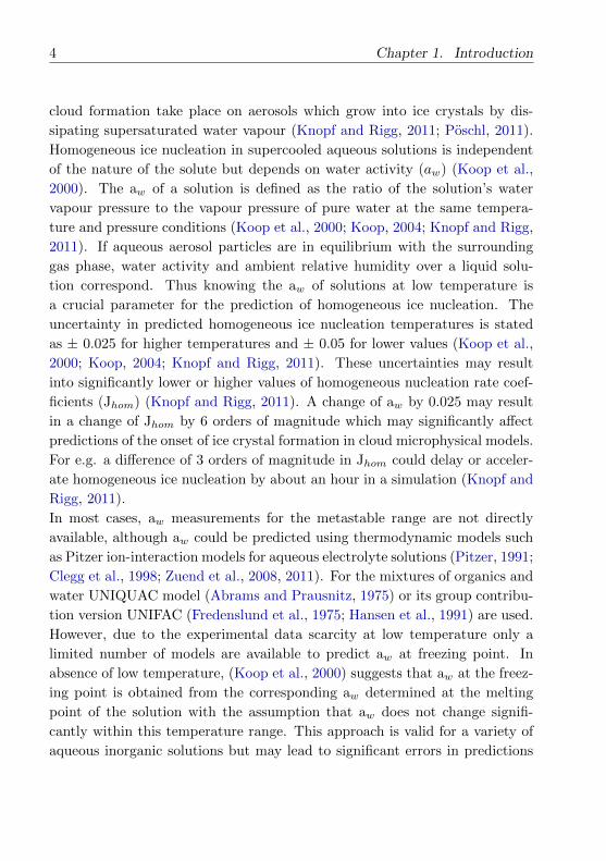
1.2 Vertical structure of Earth’s atmosphere
The atmosphere is a thin layer of gases that envelopes the Earth’s surface,
retained by the gravitational force. Figure 1.1 shows the temperature and
pressure of the atmosphere as a function of altitude. As the altitude increases
the air pressure decreases exponentially since there are fewer numbers of gas
molecules and atoms exerting pressure.
The Earth’s atmosphere is made up of several different layers, and in broad
terms each layer differs in chemical composition and vertical temperature pro-
file. The troposphere is the lowest layer of the Earth’s atmosphere. Up to
85 % of the atmospheric mass is contained in the troposphere where most
of the daily weather phenomena (e.g. clouds, precipitation, wind, etc.) and
most of Earth/atmosphere interactions occur (e.g. hydrological cycle). In the
troposphere the temperature decreases with about 6.5 K km−1 as altitude in-
creases due to adiabatic expansion and reaches a minimum at the tropopause.
The reason for this progressive decrease is the increasing distance from the
sun-warmed Earth (Seinfeld and Pandis, 1998). Depending on the season and

1.2. Vertical structure of Earth’s atmosphere 7
Figure 1.1: Vertical temperature structure of the atmosphere extending from the
surface of the Earth to approximately 110-km altitude as given in the U.S. Standard
Atmosphere, 1976. Source: Brasseur et al. (1999).
latitude the height of the tropopause reaches values up to 18 km in the trop-
ics and up to approximately 8 km in the polar regions. The lowest region of
the troposphere consists of the planetary boundary layer where most of the
primary trace gases and particle emissions enter the atmosphere. The tropo-
sphere is also the layer which contains most of the aerosols. The stratosphere
extends from the tropopause to the stratopause (∼ 45 to 55 km altitude),
here temperature increases with altitude which is due to the photolysis of
ozone into molecular and atomic oxygen, which recombine again to regener-
ate ozone. The ambient temperature increases when the rapid molecular and
atomic products of these reactions thermalise via collisions. Tropics where
the solar irradiance is the highest are the main source region of stratospheric
ozone. The air masses are transported from there to higher latitudes by
the Brewer-Dobson circulation. In the mesosphere, which extends from the
8 Chapter 1. Introduction
stratopause to the mesopause (∼ 80 to 90 km altitude) temperature decreases
with altitude. The thermosphere is located above the mesopause, and is char-
acterized by an increase in the temperature with height due to the absorption
of short wavelength radiation by N2 and O2 (Seinfeld and Pandis, 1998). The
ionosphere is a region of the upper mesosphere and lower thermosphere where
ions are produced by photoionization. The exosphere is the outermost region
of the atmosphere where gas molecules with sufficient energy can escape from
the Earth’s gravitational attraction.
1.2.1 Composition of the Earth’s atmosphere
It is believed that when the Earth was formed, He and H2 were the domi-
nant gases, but were mostly lost to space. The chemical composition of the
Earth’s atmosphere has undergone several changes during its evolution pro-
cess which lead to the cooling of the surface, formation of the Earth’s inner
core and generation of the magnetic field, condensation of water vapour and
other gases, ozone layer formation, photosynthesis by plants. The present at-
mosphere mainly consists of nitrogen (N2), oxygen (O2), water vapour (H2O),
argon (Ar) and carbon dioxide (CO2). Water vapour concentration is highly
variable, reaching concentrations as high as 3 % near the surface (Seinfeld
and Pandis, 1998) and is averaged over the full atmosphere of about 0.25
%. Almost all water vapour and condensed liquid water is confined to the
lower atmosphere and their abundance is controlled by evaporation and pre-
cipitation processes. The remaining gases which comprise less than 1 % of
the atmosphere are so-called trace gases; they include gases such as Ar, O3,
NO2, N2O, CO, CH4 and CO2. These trace gases play an important role in
the Earth’s radiative balance, acting as greenhouse gases and as reactants in
oxidation processes and in ozone chemistry, and also participate in the produc-
tion of condensable material for the formation of secondary aerosol particles.
Depending on chemical reactivity, meteorological conditions and atmospheric
life time, trace gases can exhibit an enormous range of spatial and temporal
variability. Inert gases such as the chlorofluorocarbon (CFC) which rise up to
the stratosphere and higher regions get converted into reactive species, formed
by the breakdown of their molecular bonds by the intense solar radiation at
1.3. Aerosols 9
high altitudes. The stratospheric ozone sometimes also referred as “good
ozone” plays a beneficial role by absorbing most of the harmful ultraviolet
radiation and thus protecting life on Earth.
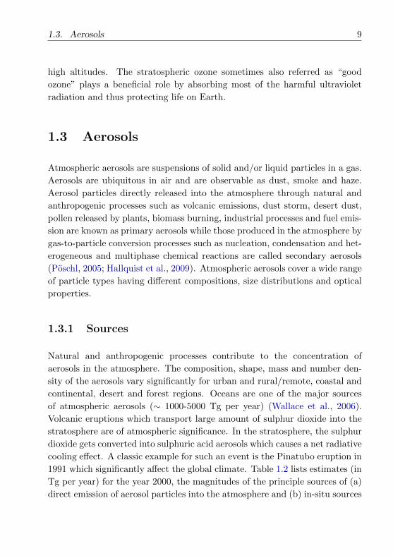
1.3 Aerosols
Atmospheric aerosols are suspensions of solid and/or liquid particles in a gas.
Aerosols are ubiquitous in air and are observable as dust, smoke and haze.
Aerosol particles directly released into the atmosphere through natural and
anthropogenic processes such as volcanic emissions, dust storm, desert dust,
pollen released by plants, biomass burning, industrial processes and fuel emis-
sion are known as primary aerosols while those produced in the atmosphere by
gas-to-particle conversion processes such as nucleation, condensation and het-
erogeneous and multiphase chemical reactions are called secondary aerosols
(Poschl, 2005; Hallquist et al., 2009). Atmospheric aerosols cover a wide range
of particle types having different compositions, size distributions and optical
properties.
1.3.1 Sources
Natural and anthropogenic processes contribute to the concentration of
aerosols in the atmosphere. The composition, shape, mass and number den-
sity of the aerosols vary significantly for urban and rural/remote, coastal and
continental, desert and forest regions. Oceans are one of the major sources
of atmospheric aerosols (∼ 1000-5000 Tg per year) (Wallace et al., 2006).
Volcanic eruptions which transport large amount of sulphur dioxide into the
stratosphere are of atmospheric significance. In the stratosphere, the sulphur
dioxide gets converted into sulphuric acid aerosols which causes a net radiative
cooling effect. A classic example for such an event is the Pinatubo eruption in
1991 which significantly affect the global climate. Table 1.2 lists estimates (in
Tg per year) for the year 2000, the magnitudes of the principle sources of (a)
direct emission of aerosol particles into the atmosphere and (b) in-situ sources

10 Chapter 1. Introduction
of secondary aerosol formation in both hemispheres. Aerosol formation in the
atmosphere through gas-to-particle conversion takes place by condensation of
semivolatile and low volatile species onto existing particles, thereby increasing
the mass (but not the number) of particles. On the other hand, new parti-
cle formation by nucleation and condensation of gaseous precursors, increases
the particle numbers substantially. The major families of chemical species
involved in gas-to-particle conversion are: sulphates, nitrates, organic com-
pounds (Wallace et al., 2006; Seinfeld and Pandis, 1998).
Figure 1.3 shows the seasonal and geographical changes of anthropogenic and
natural aerosol loading, illustrating the global fields of aerosol optical depth
(AOD), separated into fine mode (red) and coarse mode (green) components
observed by MODIS/Terra instrument(550nm) on 13th April and 22nd Au-
gust 2001. The fine mode AOD mainly consists of pollution and biomass
burning aerosols while the coarse mode consists of dust and sea salt aerosols.
Transport of dust and pollution from Asia to North America and the cross-
Atlantic transport of dust from Africa to central America can be seen on the
13th April 2001. On the 22nd August, large smoke plumes from South Amer-
ica to the southern Atlantic and from southern Africa to the Indian Ocean
are evident. The implications of such large-scale transport on the air qual-
ity of the receptor region depends on the perturbation of the surface aerosol
concentration (Chin et al., 2007).
1.3.2 Sinks
Aerosols undergo various physical and chemical interactions and transforma-
tion (atmospheric ageing) which modifies the particle size, structure and their
composition. Coagulation is one of the processes by which small particles are
converted into larger particles. Since the mobility of a particle rapidly de-
creases as its particle size increases, coagulation is essentially confined to par-
ticles less ∼ 0.2 µm in diameter (Wallace et al., 2006). Although coagulation
does not remove particles from the atmosphere, it modifies the size spectra of
aerosols and shifts small particles into size ranges where they can be removed
from the atmosphere by other mechanisms such as wet and dry deposition.
In the troposphere, precipitation and dry deposition on surfaces are the most

1.3. Aerosols 11
Figure 1.2: Estimates (in Tg per year) for the year 2000 of (a) direct particle
emissions into the atmosphere and (b) in-situ production. aSizes refer to diame-
ters. [Adapted from Intergovernmental Panel on Climate Change, 2001, Cambridge
University Press, pp.297 and 301, 2001.] Source: Wallace et al. (2006)

12 Chapter 1. Introduction
Figure 1.3: shows composites of MODIS/Terra, Aerosol optical Depth (AOD) by
the MODIS/Terra (550 nm) for the April 13 (top row) and August 22 (bottom row),
2001. Red colour indicates fine mode aerosols and green colour coarse mode aerosols.
On April 13, 2001, heavy dust and pollution is transported from Asia to the Pacific
and dust is transported from Africa to Atlantic. On August 22 large smoke plumes
from South America and South Africa are evident. Adapted from Chin et al. (2007);
(original figure from Yoram Kaufman and Reto Stockli).
1.3. Aerosols 13
effective sink mechanisms of aerosols. Depending on the aerosol properties
and the atmospheric conditions, the residence time of aerosol particles in the
troposphere range from hours to weeks (Seinfeld and Pandis, 1998; Poschl,
2005).
1.3.3 Size distribution
Particle size of atmospheric aerosols varies from a few tens of nanometers
(nm) to several hundreds of micrometers (µm). Depending on particle di-
ameter they are classified as fine mode (≤2.5 µm) and coarse mode (≥ 2.5
µm). The fine mode particles are subdivided into nuclei (Aitken) mode and
the accumulation mode (Seinfeld and Pandis, 1998). There is an additional
particle size mode, known as the ultra fine mode for particles below 0.01 µm
and originates from nucleation events of low volatility vapour (Whitby and
Cantrell, 1976). The fine and coarse mode aerosol particles differ in chemi-
cal composition, optical properties, origin, transport mechanism, and removal
mechanisms from the atmosphere and also differ significantly in their ability
to enter different levels of the respiratory tract of humans. Hence classifica-
tion of aerosols between fine and coarse mode particles is essential for studying
physicochemical properties, atmospheric implications and health effects.
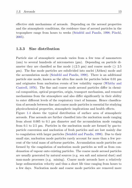
Figure 1.4 shows the typical distribution of surface area of atmospheric
aerosols. Fine aerosols are further classified into the nucleation mode ranging
from about 0.005 to 0.1 µm diameter and the accumulation mode ranging
from 0.1 to 2.5 µm. Particles in the nucleation mode are formed by gas-to-
particle conversion and nucleation of fresh particles and are lost mainly due
to coagulation with larger particles (Seinfeld and Pandis, 1998). Due to their
small size, nucleation mode particles rarely account for more than a few per-
cent of the total mass of airborne particles. Accumulation mode particles are
formed by the coagulation of nucleation mode particles as well as from con-
densation of vapour onto existing particles. The coarse mode aerosol particles
are usually generated by natural sources (e.g. sea salt and mineral dust) and
man-made processes (e.g. mining). Coarse mode aerosols have a relatively
large sedimentation velocity and thus a short life time ranging from hours to
a few days. Nucleation mode and coarse mode particles are removed more
14 Chapter 1. Introduction
Figure 1.4: Schematic representation of distribution of particle surface area of
atmospheric aerosols. Principle modes, formation and conversion processes, and
removal mechanisms are indicated. Source: Whitby and Cantrell (1976).

1.3. Aerosols 15
efficiently from the atmosphere in comparison to accumulation mode parti-
cles, and hence, the accumulation mode particles tend to have a considerably
longer residence times than those in either the nuclei or coarse mode.
1.3.4 Chemical composition
Aerosol particles depending on their natural or anthropogenic origin have
varying chemical compositions. The overall composition and the physical
structure of aerosol particles undergo changes due to physicochemical in-
teractions between different components over a period of time, also known
as (chemical) aging process. Regional and seasonal variations also cause a
change in the typical aerosol composition due to the influence of the differ-
ent biogenic and anthropogenic sources, transport and removal mechanisms
in the atmosphere. A significant fraction of the tropospheric aerosol con-
stituents are anthropogenic in origin (e.g. biomass burning, fuel combustion,
industrial processes, sulphates and nitrates). Tropospheric aerosols consists
of highly water soluble inorganic salts, inorganic acids, insoluble mineral dust
and carbonaceous material which includes organic compounds ranging from
very soluble to insoluble in water, plus elemental carbon. Numerous indi-
vidual organic compounds present in the ambient aerosol samples have been
identified such as n-alkanes, dicarboxylic acids, polycyclic aromatic hydrocar-
bons (PAH) and some nitrogen-containing compounds (Rogge et al., 1993;
Pio et al., 2001; Tsapakis et al., 2002). Experimental studies also suggest
the presence of additional compounds such as organic sulphates (Saxena and
Hildemann, 1996; Blando et al., 1998; Fuzzi et al., 2001).
Primary organic aerosols (POA) are emitted directly into the atmosphere
while secondary organic aerosols (SOA) are formed as a result of transforma-
tion and condensation of organic precursors, i.e., gas-to-particle conversion
(Farina et al., 2010; Jathar et al., 2011; Lin et al., 2012). Biomass burning
and fossil fuel combustion are considered to be responsible for most POA mass
that is emitted into the atmosphere (Liousse et al., 1996; Seinfeld and Pan-
dis, 1998; Hallquist et al., 2009). The process leading to SOA formation is a
sequential process: gas emissions → gas phase chemistry ↔ gas-particle par-
titioning/nucleation↔ aerosol chemistry/cloud processing (Kanakidou et al.,
16 Chapter 1. Introduction
2005). In case of semivolatile organic species, gas-particle partitioning de-
scribes the equilibrium fractions in the gas phase and particle phases (one or
several liquid, semi-solid, or solid phases) at ambient conditions.
Organic aerosols form a significant fraction of the fine atmospheric aerosol
mass and are extensively studied by using climate models to determine their
global impact (Zhang et al., 2007; Robinson et al., 2007; Hallquist et al.,
2009; Pye and Seinfeld, 2010; Lin et al., 2012). Distinction between the im-
plications and properties of POA and SOA are under debate, recent studies
show that the volatility of emitted particles can change due to evaporation
and gas-phase oxidation of primary emissions which could subsequently pro-
vide an additional source of SOA (Robinson et al., 2007; Lin et al., 2012).
Despite the significance of organic aerosols in the environment, data sets to
constrain models are limited. However based on the available data it appears
that models tend to underestimate SOA concentrations in the boundary layer
(Johnson et al., 2006; Volkamer et al., 2006; Kleinman et al., 2008; Simpson
et al., 2007; Jimenez et al., 2009). Recently, instruments such as Aerosol
Mass Spectrometer (AMS), Particle-Into-Liquid Sampler (PILS) and tech-
niques such as radiocarbon isotope analysis provide insight into the sources,
composition and reactivity of organic aerosol typically unavailable from mass
measurements (Jathar et al., 2011; Zhang et al., 2005). The AMS results sug-
gest that organic aerosols are dominated by SOA from the oxidation products
of gas-phase organic precursors (Robinson et al., 2007; Zhang et al., 2007;
Jathar et al., 2011). This indicates the significant difficulties in simulating
organic aerosols in global models. Although a lot is being done towards un-
derstanding the SOA formation, targeted chamber and field experiments are
needed to allow evaluation and provide confidence in chemical mechanisms
used in regional and global models that treat both gas phase chemistry and
SOA formation.
1.4 Radiative Forcing
Radiative forcing is referred to as a measure of how the energy balance of the
Earth-atmosphere system is influenced when the factors that affect the cli-
1.4. Radiative Forcing 17
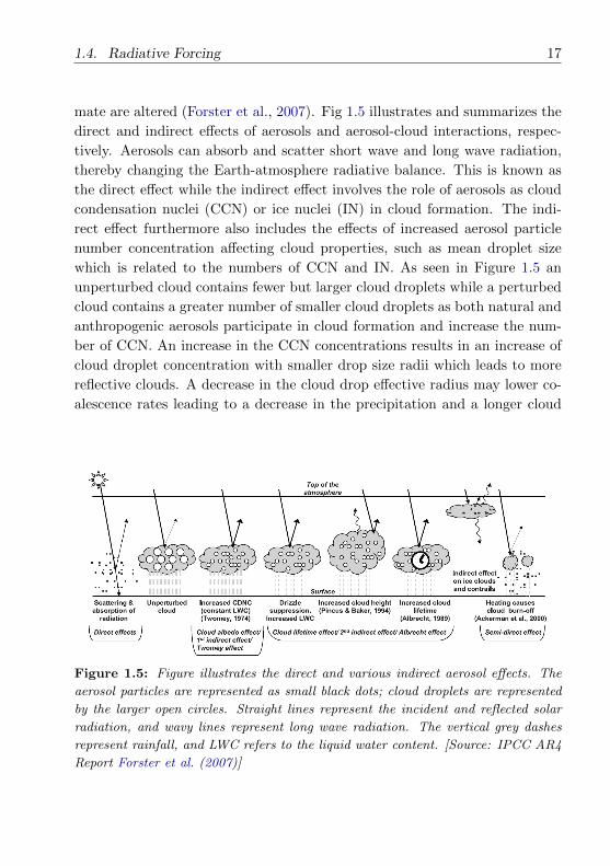
mate are altered (Forster et al., 2007). Fig 1.5 illustrates and summarizes the
direct and indirect effects of aerosols and aerosol-cloud interactions, respec-
tively. Aerosols can absorb and scatter short wave and long wave radiation,
thereby changing the Earth-atmosphere radiative balance. This is known as
the direct effect while the indirect effect involves the role of aerosols as cloud
condensation nuclei (CCN) or ice nuclei (IN) in cloud formation. The indi-
rect effect furthermore also includes the effects of increased aerosol particle
number concentration affecting cloud properties, such as mean droplet size
which is related to the numbers of CCN and IN. As seen in Figure 1.5 an
unperturbed cloud contains fewer but larger cloud droplets while a perturbed
cloud contains a greater number of smaller cloud droplets as both natural and
anthropogenic aerosols participate in cloud formation and increase the num-
ber of CCN. An increase in the CCN concentrations results in an increase of
cloud droplet concentration with smaller drop size radii which leads to more
reflective clouds. A decrease in the cloud drop effective radius may lower co-
alescence rates leading to a decrease in the precipitation and a longer cloud
Figure 1.5: Figure illustrates the direct and various indirect aerosol effects. The
aerosol particles are represented as small black dots; cloud droplets are represented
by the larger open circles. Straight lines represent the incident and reflected solar
radiation, and wavy lines represent long wave radiation. The vertical grey dashes
represent rainfall, and LWC refers to the liquid water content. [Source: IPCC AR4
Report Forster et al. (2007)]

18 Chapter 1. Introduction
life time and greater spatial extent, and is referred to as second indirect effect
(Albrecht, 1989) or the cloud lifetime effect. Hansen et al. (1997) identified a
so called semi-indirect effect: Aerosol solar absorption (e.g. by black carbon)
may reduce cloud cover and liquid water content by heating the cloud and
environment in which the cloud forms. These effects can alter the heat budget
and the hydrological cycle, including precipitation patterns, on a variety of
length and time scales (Ramanathan et al., 2001; Zhang et al., 2006).
Overall the current aerosol radiative forcing relative to preindustrial times is
estimated to be around -1 to -2 Wm−2 as opposed to a greenhouse gas forcing
of about +2.4 Wm−2 (Poschl, 2005). The values reflect the total forcing rel-
ative to the start of the industrial era (∼ 1750). Anthropogenic contributions
to aerosols (sulphate, organic carbon, nitrate and dust) together produce a
cooling effect, with a total direct radiative forcing of -0.5 (-0.9 to 0.1) Wm−2
and an indirect cloud albedo forcing of -0.7(-1.8 to -0.3) Wm−2 (Forster et al.,
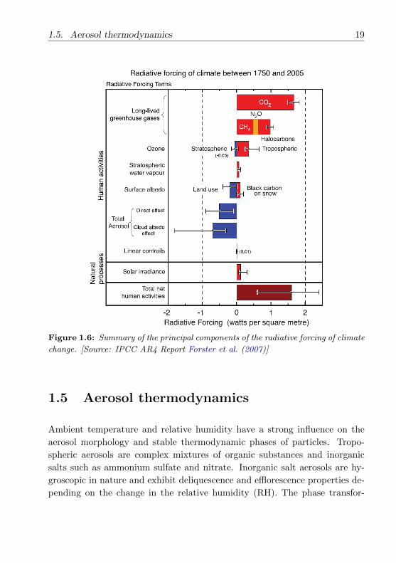
2007). Fig 1.6 shows the radiative forcing contributions of some of the cli-
mate agents influenced by human activities. The increase of greenhouse gases
especially CO2 concentrations are responsible for the largest positive forcing
over this period. There is a net increase in the tropospheric ozone leading
to warming (positive forcing), while stratospheric ozone decreases have con-
tributed to cooling in the stratosphere (and warming in the troposphere). In
case of aerosols, some cause a positive forcing (black carbon) while others
cause a negative forcing (organic carbon, mineral dust). Best estimates indi-
cate that the indirect effects of aerosols on climate overall constitute a negative
radiative forcing contribution. Compared to the well-established effects from
greenhouse gases with longer atmospheric life time, there are still considerable
gaps in the understanding concerning the absorption and scattering and cloud
interactions of aerosol particles.
1.5. Aerosol thermodynamics 19
Figure 1.6: Summary of the principal components of the radiative forcing of climate
change. [Source: IPCC AR4 Report Forster et al. (2007)]
1.5 Aerosol thermodynamics
Ambient temperature and relative humidity have a strong influence on the
aerosol morphology and stable thermodynamic phases of particles. Tropo-
spheric aerosols are complex mixtures of organic substances and inorganic
salts such as ammonium sulfate and nitrate. Inorganic salt aerosols are hy-
groscopic in nature and exhibit deliquescence and efflorescence properties de-
pending on the change in the relative humidity (RH). The phase transfor-
20 Chapter 1. Introduction
mation from a solid particle to a saline droplet usually occurs spontaneously
when the RH in the surrounding air reaches a level, known as deliquescence
humidity, that is specific to the chemical composition of the aerosol particle
(Tang and Munkelwitz, 1994; Zardini, 2007). The reverse process that is re-
lease of water to the air to form solid crystal below the RH threshold value is
known efflorescence relative humidity.
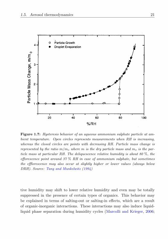
Figure 1.7 illustrates a pure ammonium sulphate (NH4)2SO4 aerosol parti-
cle showing a distinict hystersis behaviour during hygroscopic cycles. With
the initial increase in the RH the particle retains its solid state (no particle
growth). At about 80 % RH the particle undergoes deliquescence (abruptly
changes to liquid state) and retains its liquid state and takes up water (par-
ticle growth) up to RH 92 % (and above). In the reverse part of the cycle
for decreasing RH, the particle shrinks in size but stays in liquid state even
below 80 % RH (metastable, supersaturated) and at around 37 % RH the
particle undergoes efflorescence (abruptly changes back into a solid). Thus,
the ambient relative humidity, supersaturation of liquid droplet and the par-
ticle history determines whether the particle is in a stable, metastable, solid
or liquid state (Zardini, 2007).
This hysteresis behavior of aerosol particles significantly influence the direct
aerosol effect (Krieger et al., 2012). Studies show that inorganic sulphate
aerosol hysteresis results in an uncertainty of 20 % of the aerosol optical
thickness, and 34 % of the radiative effect in sulphate direct climate forcing
(Wang et al., 2008) while the organic compounds influence the hygroscopic-
ity and direct effect potentially causing less cooling by the aerosols (Randles
et al., 2004).
Deliquescence behavior of particles composed of inorganic salts and water sol-
uble organic species such as ammonium sulphate (AS) and sodium chloride
(NaCl) mixed with dicarboxylic acids, polyol or levoglucosan have been inves-
tigated by a variety of experimental techniques (Choi and Chan, 2002; Brooks
et al., 2002; Marcolli and Krieger, 2006; Zardini et al., 2008; Song et al., 2012;
Krieger et al., 2012). These studies suggest that in such mixed systems, the
deliquescence relative humidity (DRH) of the inorganic component may re-
main almost constant or decrease with respect to organic depending on the
mixing ratio and the nature of the organic species. The efflorescence rela-
1.5. Aerosol thermodynamics 21
Figure 1.7: Hysteresis behavior of an aqueous ammonium sulphate particle at am-
bient temperature. Open circles represents measurements when RH is increasing,
whereas the closed circles are points with decreasing RH. Particle mass change is
represented by the ratio m/mo where m is the dry particle mass and mo is the par-
ticle mass at particular RH. The deliquescence relative humidity is about 80 %, the
efforescence point around 37 % RH in case of ammonium sulphate, but sometimes
the efflorescence may also occur at slightly higher or lower values (always below
DRH). Source: Tang and Munkelwitz (1994)
tive humidity may shift to lower relative humidity and even may be totally
suppressed in the presence of certain types of organics. This behavior may
be explained in terms of salting-out or salting-in effects, which are a result
of organic-inorganic interactions. These interactions may also induce liquid-
liquid phase separation during humidity cycles (Marcolli and Krieger, 2006;
22 Chapter 1. Introduction
Song et al., 2012). Considering the typical organic-inorganic compositions
of tropospheric aerosols, liquid-liquid phase separation should indeed occur
frequently when particles in the atmosphere are exposed to varying relative
humidity. Experimental studies and model predictions suggest that at moder-
ate to high RH, a liquid-liquid phase separation into an organic-rich aqueous
phase and an electrolyte-rich aqueous phase can be expected (Erdakos and
Pankow, 2004; Marcolli and Krieger, 2006; Ciobanu et al., 2009; Smith et al.,
2011; Zuend et al., 2010; Krieger et al., 2012; Song et al., 2012; Reid et al.,
2011; Bertram et al., 2011; Zuend and Seinfeld, 2012).
Water and semivolatile species are distributed between the gas and aerosol
phases are governed by gas-particle thermodynamic equilibrium (Pankow,
2003; Donahue et al., 2006; Zuend et al., 2010; Zuend and Seinfeld, 2012).
The gas-particle partitioning is determined by the activity of the semivolatile
species in the aerosol phase and their pure component subcooled liquid vapour
pressures. Reliable phase state description of an aerosol is essential for the es-
timation of the gas-particle partitioning of water and semivolatile substances
(Zuend et al., 2008, 2010). In addition, the phases present in the aerosol par-
ticles define the reaction medium for heterogeneous and multiphase chemistry
occurring in aerosol particles (Kalberer et al., 2004; Knopf et al., 2005; Anttila
et al., 2006, 2007).
Thermodynamic equilibrium calculations based on activity coefficient models
allow to determine whether the aerosol phase is a liquid, solid or a mixture of
solid and liquid phases. A thermodynamic model can be used for predicting
the activity coefficients of all components in a mixture, thereby predicting
mixing effects including changes of deliquescence relative humidities (Zuend
et al., 2008, 2011). Significant efforts have been made towards developing ac-
tivity coefficient models of mixed organic-inorganic-water systems (Ming and
Russell, 2002; Raatikainen and Laaksonen, 2005; Topping et al., 2005; Tong
et al., 2008; Zuend et al., 2008, 2011; Zuend and Seinfeld, 2012). These models
are generally composed of three different parts, an inorganic term, an organic
term, and an organic-inorganic mixing term. Organic aerosols contain a high
degree of organic functional groups. For complex organic/non-electrolytes
systems the UNIFAC model (Fredenslund et al., 1975) is widely used because
of its simplicity to describe complex, multicomponent systems. UNIFAC uses

1.5. Aerosol thermodynamics 23
a group-contribution approach which has the advantage of reducing the pa-
rameterisation of huge quantity of organic substances to the description of a
restricted number of functional groups contained in that huge variety of com-
pounds. The UNIFAC group-contribution model has also been extended to
include inorganic components by including an extended Debye-Huckel term
and determining semi-empirical UNIFAC parameters for ions (Yan et al., 1999;
Chang and Pankow, 2006; Zuend et al., 2008, 2011).
To reduce the uncertainties related to the aerosol forcing, a better physical
representation of the aerosols, their mixing states and properties in thermo-
dynamic models is required. Also, the detailed monitoring of liquid-liquid
phase separation and crystallization in micrometer-sized droplets allows for
improving the fundamental understanding of these processes.
An important uncertainty in climate models is associated with the under-
standing of upper tropospheric ice cloud formation (Swanson, 2009; Knopf
and Rigg, 2011). Ice particles in the atmosphere form by homogeneous and
heterogeneous nucleation. Homogeneous ice nucleation describes the forma-
tion of ice from a supercooled (or metastable) aqueous particle (at the tem-
peratures below the melting point) in absence of pre-existing substrate. The
heterogeneous ice nucleation process represents nucleation of ice from the pre-
existing substrate (Knopf and Rigg, 2011) at warmer temperatures than the
homogeneous nucleation. Aerosol particles which act as a ice nuclei (IN) can
affect the radiative energy budget by altering the radiative properties and
formation processes of cirrus clouds (Baker and Peter, 2008; Forster et al.,
2007). Cirrus clouds cover about 30 % of Earth’s surface (Wylie et al., 2005)
and have a significant effect on the global radiative budget, resulting in a net
climate warming contribution.
Homogeneous ice freezing and ice melting temperatures of aqueous solutions
depend on the aw and solute concentration, irrespective of the nature of the
solute (Koop et al., 2000; Koop, 2004). The large variation in freezing and
melting temperature of aqueous solution reflects the non-ideal behaviour of
the solutions at moderate to high concentration. Water activity (aw) for
the metastable range is not directly available, in such a case thermodynamic
models such as Pitzer ion-interaction models which mainly account for inor-
ganic/electrolyte solutions (Pitzer, 1991) and the modified UNIFAC (Dort-
24 Chapter 1. Introduction
mund) (Gmehling et al., 1998, 2002; Jakob et al., 2006) which are widely used
for aqueous organic solutions can be applied to predict aw for the metastable
temperature regime. Laboratory studies show that aqueous solutions at low
temperatures may exhibit significant changes in aw with temperature (Zo-
brist et al., 2003, 2008; Zuberi, 2003; Clegg et al., 1998). Such studies on the
temperature dependence of aqueous solutions are useful for the understand-
ing of organic-water mixing effects on homogeneous ice nucleation. Model
predictions require validation by experimental data, however, due to scarcity
of experimental data at supercooled temperatures for aqueous inorganic and
organic solutions it is hard to obtain reliable predictions of water activity
at freezing temperatures. This therefore motivates additional measurements
in the temperature range below room temperature down to the low tempera-
tures representing upper tropospheric conditions. To obtain better predictions
and constrain the homogeneous freezing and ice nucleation rates of particles
with organics requires corresponding homogeneous ice nucleation experiments.
Furthermore, the role of organics on aw of solutions at the freezing point has
to be estimated for a aw based description of ice nucleation in atmospheric
applications (Knopf and Rigg, 2011). Thus, a combined modeling and ex-
perimental approach is carried out in this thesis with the goal to deepen the
understanding of gas-to-particle conversion, phase transitions in aerosols and
ice nucleation studies.
Chapter 2
Chemical Thermodynamics and
Molecular Interactions
2.1 Thermodynamics of multicomponent sys-
tems
The theory of classical thermodynamics (“thermodynamics” refers to thermo
- heat and dynamics - force) describes processes that involve change in tem-
perature, transformation of energy, and the relationship between heat, work
and energy. It is used to describe macroscopic variables of a defined portion
of matter, such as pressure, temperature, entropy, internal energy and also
the physics that deals with the relationship and conversion between heat and
other forms of energy.
The atmosphere is composed of several chemical components which exist in the
gas phase and in the form of liquid or solid aerosol particles. Thermodynamic
properties of aerosols are used to describe the partitioning of semivolatile
species between the gas and condensed phase. Since water acts as a solvent
for many of the constituents in the aerosol phase (Seinfeld and Pandis, 1998),
the focus in this chapter is on aqueous systems. A thermodynamic system
is a specified portion of space/matter on which the study of energy transfer
or conservation is made. All the space around the system is called the sur-
rounding. A system is separated from its surrounding by a real or virtual
boundary and the exchange of mass, energy or heat between the system and
25
26 Chapter 2. Chemical Thermodynamics and Molecular Interactions
the surrounding takes place across the boundary. A homogeneous system is
one in which the chemical composition and the physical properties are uni-
form all over the system in a macroscopic sense, e.g., the densities measured
in points A and B have the same values. A so-called “open system” is defined
as a system that may exchange both mass and energy with its surrounding,
while a “closed system” is one that allows only exchange of energy through
the system boundary.
The thermodynamics of mixtures of chemical species introduced in this chap-
ter is part of the scope of chemical thermodynamics. Therefore, the focus of
Section 2.1 is on the properties and theoretical relations of a thermodynamic
system subject to a change in the chemical composition.
2.1.1 Homogeneous Open and Closed System
Consider an air parcel as a homogeneous system of volume V at temperature
T containing a number of k independent chemical components. The number
of moles of component i is represented by ni. The internal energy U arises
due to the potential and kinetic energy of the atoms and molecules of the
system. If there is an infinitesimal change in the state of the air parcel (e.g.
if the parcel slightly rises in the atmosphere) but there is no exchange of
mass with the surrounding (closed system), then, according to the first law of
thermodynamics the change in the internal energy of such a closed system is
given by (Prausnitz et al., 1986; Seinfeld and Pandis, 1998)
dU = dQ+ dW (2.1)
where dQ is the heat absorbed (= TdS) and dW is the amount of work
that is done by the system (= −pdV ). Eq. (2.1) is valid only for a single
component in a closed system not generally for a mixture where interactions
among components may happen, such as chemical reactions etc.
dU = TdS − pdV (2.2)

2.1. Thermodynamics of multicomponent systems 27
with pressure p and entropy S. Detailed derivations of this equation can
be found in most textbooks on classical thermodynamics. Since the sys-
tem is assumed to be closed according to Eq. (2.2), if the number of moles
(n1, n2, n3, ...nk) of all the components in the system are constant (conserved
mass, no reactions), the change in the internal energy is a function of S and
V .
If mass exchange is allowed (open system), the number of moles ni of the
individual components i may change and the internal energy as a function of
S, V , and the number of moles of the individual components ni is given as
U = f(S, V, n1, n2, n3, ..nk) (2.3)
dU =
(∂U
∂S
)V,ni
dS +
(∂U
∂V
)S,ni
dV +
k∑i=1
(∂U
∂ni
)S,V,nj 6=i
dni (2.4)
For a closed, non-reactive system dni = 0, and comparing Eq. (2.2) with
Eq. (2.4), which both are valid for a closed system, we obtain
T =
(∂U
∂S
)V,ni
,−p =
(∂U
∂V
)S,ni
(2.5)
Eq. (2.4) can be written as
dU = TdS − pdV +
k∑i=1
(∂U
∂ni
)S,V,nj 6=i
dni (2.6)
Thus, Eq. (2.6) represents the change in the internal energy of an open system.
The partial derivative of the internal energy with respect to a variation in the
number of moles of substance i, while keeping all other variables constant, is
defined as chemical potential µi:
µi =
(∂U
∂ni
)S,V,nj 6=i
(2.7)

28 Chapter 2. Chemical Thermodynamics and Molecular Interactions
The chemical potential contributes to the internal energy of a system and is
of fundamental importance in thermodynamic systems, analogous to pressure
and temperature. A temperature difference between two bodies determines
the tendency of heat transfer as a system progresses in time; likewise, a chem-
ical potential difference can be viewed as the cause for chemical reaction or
for mass transfer from one phase to another. Other extensive thermodynamic
potentials for closed systems can be obtained by using different pairs of the
variables p, V , T and S as independent variables in Eq. (2.2). Three other
pairs retaining the property of fundamental equation can be defined with the
use of partial Legendre transformations (Prausnitz et al., 1986). For example
the Helmholtz energy, A, by interchanging T and S in Eq. (2.2),
A = U − TS (2.8)
dA = −SdT − pdV . (2.9)
In Eq. (2.9) T and V are the pair of independent variables. If T and p are
used as the independent variables, the fundamental thermodynamic relation
is:
G = U − TS − (−pV ) = H − TS, (2.10)
dG = −SdT + V dp, (2.11)
where G is called the Gibbs energy or (Gibbs free energy) and H is the en-
thalpy of a closed system. Similarly, using the definitions of other fundamen-
tal functions (A,H,G) in combination with Eq. (2.6), the four fundamental
equations for an open system are
dU = TdS − pdV +∑i
µidni (2.12)
2.1. Thermodynamics of multicomponent systems 29
dH = TdS + V dp+∑i
µidni (2.13)
dA = −SdT − pdV +∑i
µidni (2.14)
dG = −SdT + V dp+∑i
µidni (2.15)
where the sum is over all (k) system components. From the definition of the
chemical potential by Eq. (2.7) and the four fundamental equations Eq. (2.12
to 2.15), the chemical potential can be written as:
µi =
(∂G
∂ni
)T,p,nj 6=i
(2.16)
which is also the partial molar Gibbs energy. For practical atmospheric ap-
plications, S and V cannot be used as independent variables since a criterion
for thermodynamic equilibrium in terms of measurable quantities is required.
In such a case the Gibbs energy is the preferred function, since T and p are
measurable independent state variables of G.
At temperature T , the Gibbs free energy (G) is a function of enthalpy (H) and
entropy (S) as shown in Eq. (2.10) while, the change in the Gibbs free energy
is described by the fundamental equation Eq. (2.15). For a closed system at
constant pressure, the change in the Gibbs free energy with temperature is
given by:(∂G
∂T
)p,ni
= −S. (2.17)
Using Eq. (2.10), the Gibbs-Helmholtz relation can be derived(∂
∂T
(G
T
))p,ni
= − HT 2
(2.18)

30 Chapter 2. Chemical Thermodynamics and Molecular Interactions
At constant pressure, the corresponding change in the enthalpy and entropy
is given by the isobaric heat capacity (Cp):(∂H
∂T
)p
= Cp (2.19)
(∂S
∂T
)p
=CpT
(2.20)
The following sections discuss in more detail the properties obtained from the
Gibbs energy function.
2.1.2 Thermodynamic Equilibrium
A heterogeneous closed system is made up of different phases, considered as
homogeneous, open systems, within an overall closed system (Zuend, 2007).
Thermodynamic equilibrium can be described as the “state” a system tends
to reach when given sufficient time (Zuend, 2007). From Eq. (2.15) for a
system at constant pressure (dp = 0) and temperature (dT = 0) we obtain
dG =∑i
µidni. (2.21)
At constant composition (dni = 0), it follows that dG = 0, i.e., the Gibbs
energy is constant. According to the second law of thermodynamics, the
entropy of a system increases in case of an irreversible process and remains
constant for reversible processes. When the entropy reaches a maximum value
(dS ≥ 0), the system has reached to an equilibrium. At thermodynamic
equilibrium, dG = 0, and given a constant T and p,∑i=1
µidni = 0. (2.22)
Equation. (2.22) is the thermodynamic condition for chemical equilibrium.
For a system with two phases (α, β) in equilibrium at constant p and T , a
2.1. Thermodynamics of multicomponent systems 31
change in the composition of species i from phase α to β can be presented by
nαi − dni = nβi + dni (2.23)
applying Eq. (2.22) for this two-phase system:
µαi = µβi . (2.24)
Equation. (2.22) represents the basic formulation for phase equilibrium at
constant p and T conditions. Thermodynamic equilibrium with respect to
different processes can be expressed by excluding the special effects such as
interfacial forces, electric, magnetic and gravitational fields (Zuend, 2007). In
case of a multicomponent system with the component number denoted by i
and the number of phases denoted by variable j:
Tαi = T βi = . . . = T ji : thermal equilibrium
pαi = pβi = . . . = pji : mechanical equilibrium (2.25)
µαi = µβi = . . . = µji : chemical equilibrium
where i = 1,2,...,k goes over all system components. For a heterogeneous
closed system in an equilibrium state, each phase state is characterized by its
temperature, pressure and chemical potential of each individual component
present. Since there are k components, a total of k + 2 variables are used
to characterize the phase. However, not all are independent variables. The
Gibbs-Duhem equation shows how these variables are related. The fundamen-
tal equation in terms of U Eq. (2.12) can be used to characterize a particular
phase state. Integrating Eq. (2.12) from a state of zero mass to finite mass
(ni = 0 to i) at constant p, T , gives
U = TS − pV +∑i
µini (2.26)
In the above equation U is a function of T , p, composition and the size
of the system. Also since U is a state function, the results shown in the
32 Chapter 2. Chemical Thermodynamics and Molecular Interactions
above equation are independent of the path of integration. Differentiation of
Eq. (2.26) gives a general expression for dU
dU = TdS + SdT − pdV − V dp+∑i
µidni +∑i
nidµi (2.27)
comparing Eq. (2.27) with Eq. (2.12) we obtain
−SdT + V dp−∑i
nidµi = 0 (2.28)
This is known as the Gibbs-Duhem relation, which shows that when T and p
of a system change there is a corresponding change in the chemical potential
of the various component species of the system. Thus for a system with
k component species, there will be k + 1 independent variables (degrees of
freedom) of the k + 2 variables per phase.
2.1.3 Chemical Potential of Ideal Gas
For a pure substance i the chemical potential is related to temperature and
pressure by the differential equation Eq. (2.28):
dµi = − SnidT +
V
nidp. (2.29)
Using molar entropy si = S/ni and molar volume vi = V/ni in Eq. (2.29)
yields:
dµi = −sidT + vidp. (2.30)
Integrating and solving for µi for a certain temperature and pressure, we have
µi(T, p) = µi(T′, p′)−
T∫T ′
sidT +
p∫p′
vidp (2.31)

2.1. Thermodynamics of multicomponent systems 33
where superscript (T′, p′) refers to a reference state pressure and temperature.
According to the ideal gas equation (vi = RT/p) for a pure, ideal gas at
constant temperature T :
µi(T, p) = µi(T, p′) +RT ln
(p
p′
)(2.32)
where R is the universal gas constant. According to Eq. (2.32) at constant
temperature, the change in chemical potential of an ideal gas is a logarithmic
function of pressure.
Similarly, the approach for a pure, ideal gas, could be applied to define the
chemical potential of species i in an ideal gas mixture with total pressure p,
and is given by:
µi(T, p) = µi (T ) +RT ln
(p
p
)+RT ln yi (2.33)
where µi (T ) is the standard chemical potential of i under standard pressure
(p = 105 Pa). The mole fraction in the gas phase mixture is:
yi =ni∑k
nk(2.34)
where the sum goes over all species in the mixture. Introducing the partial
pressure of species pi = pyi in Eq. (2.33):
µi(T, p) = µi (T ) +RT ln
(pip
)(2.35)
is the chemical potential of species in the ideal gas mixture.
2.1.4 Ideal Solutions
A solution is defined as an ideal solution if the chemical potential of every
component is a linear function of the logarithm of its aqueous mole fraction
xi. The chemical potential for an ideal solution is given by:

34 Chapter 2. Chemical Thermodynamics and Molecular Interactions
µi(T, p) = µ∗i (T, p) +RT lnxi (2.36)
where µ∗i (T, p) is the standard chemical potential of pure species i (xi = 1)
at the same temperature and pressure as the solution under discussion. µ∗i is
a function of both Tand p but does not depend on the chemical composition
of the solution. In contrast to the ideal gas where there are no intermolecular
interactions, in case of liquids the molecular interactions can be substantial
and generally cannot be ignored. Any pure liquid is by definition an ideal
solution i.e., the interactions between the molecules of different species are
equal to the interactions between those of the same species hence practically
there is nothing like a ideal liquid. For example, a mixture of H2O and D2O,
where H stands for protons and D for deuterium, is a nearly perfect ideal
mixture (Zuend, 2007). A multicomponent solution, is ideal only if Eq. (2.36)
is satisfied by every component of the solution (which is typically not the
case).
To describe the distribution of a species between the different phases of a
system let us assume an ideal solution containing species j in thermodynamic
equilibrium with its gas phase:
µ(G)j = µ
(L)j (2.37)
using Eq. (2.33) and Eq. (2.36):
µj (T ) +RT ln
(pjp
)= µ∗
j (T, p) +RT lnxj (2.38)
For pure species j (i.e., an ideal solution; xj = 1), the pressure over the liquid
is the saturation vapour pressure psatj
µ∗j (T, p
satj ) = µ
j (T ) +RT ln
(psatj
p
)(2.39)
using Eq. (2.39) in Eq. (2.38)
ln
(pjp
)=µj (T ) +RT ln
(psatj
p
)− µ
j (T )
RT+ lnxj (2.40)
2.1. Thermodynamics of multicomponent systems 35
ln
(pjp
)= ln
(psatj
pxj
)(2.41)
pj = psatj xj (2.42)
is known as the Raoult’s law (for ideal solutions) which states that the vapour
pressure pj of species j over a solution is equal to the product of the pure
component vapour pressure psatj and its mole fraction xj in the solution. For
pure j, the reference state saturation vapour pressure psatj is often written as
pj (not to be confused with the standard total pressure p0).
2.1.5 Non-ideal Solutions
As shown in Fig 2.1(a,b) consider a solution with components A and B. In case
the solution is ideal, then the partial pressures of A and B will vary linearly
with the liquid-phase mole fraction of A, xA. The equilibrium pressure over
the solution is pA when xA = 1 and xB = 0 and according to Eq. (2.42) the
vapour pressure of A in equilibrium with the solution is:
pA = pAxA (2.43)
While in case of a solution highly dilute in B, when xA → 1,
pB = kBxB (2.44)
where kB is known as Henry’s constant and is calculated from the slope of
the pB curve as xA → 1. Henry’s law is valid for dilute solution of B (low
concentration of B). In the non-ideal case (the general case), the relation
between pA, pB , and xA is non-linear except at the concentration limits, when
xA → 0 or 1. Non-ideal solutions approach ideality when the concentrations
of all components but one approaches zero. Interactions between molecules

36 Chapter 2. Chemical Thermodynamics and Molecular Interactions
+
+
Figure 2.1: Vapour pressure over a non-ideal liquid mixture of components A and B
at vapour-liquid equilibrium (VLE).(a) Positive deviations from ideality, (b) negative
deviations from ideality. pA and pB are vapour pressures and pA and p
B are the
saturation vapour pressures of the pure components A and B in gas phase. Ptot
represents the total pressure and is the sum of partial pressure pA and pB.
of substances A and B may cause positive or negative deviation from ideality
and lead to non-ideal mixtures. Practically, almost all solutions are non-ideal.
Ideal solutions were generalized by using the fugacity function f , (Lewis, 1907;
Lewis and Randall, 1961). For an isothermal change of any component in any
system, whether solid, liquid, or gas, pure or mixed, ideal or not (Prausnitz
et al., 1986)
µi − µi = RT ln
fifoi
(2.45)
Note, while either µoi and foi is arbitrary, both may not be chosen indepen-
dently, i.e., if one is chosen arbitrarily, the other one is fixed (Prausnitz et al.,
1986; Zuend, 2007). Fugacity is equal to the pressure for pure, ideal gas,
while for a component i in ideal gas mixture, it is equal to its partial pressure
2.1. Thermodynamics of multicomponent systems 37
yip (Prausnitz et al., 1986). Since all systems, pure or mixed, at very low
pressures approach ideal gas behavior, the definition of fugacity is completed
by the limit
fiyip→ 1 (2.46)
as p → 0, where yi is the mole fraction of component i. Lewis called the
ratio fifoi
“the activity” designated by the symbol a (Prausnitz et al., 1986).
The activity of a substance gives an indication of how ‘active’ a substance is
relative to its standard state and provides a measure of the difference between
the actual chemical potential of the substance and that at its standard state.
Introducing the activity ai of a substance i, in Eq. (2.36)
µi(T, p) = µ∗i (T, p) +RT ln ai (2.47)
Comparing this equation with Eq. (2.36), deviation from the ideality can be
expressed as
γi =aixi
(2.48)
where the activity coefficient (γi) is defined on mole fraction basis. γi is
a factor used in thermodynamics to account for deviations from the ideal
behavior in a mixture of chemical substances. The chemical potential of a
non-ideal solution can be represented by introducing the activity coefficient
γi of a substance i, in Eq. (2.36)
µi(T, p) = µ∗i (T, p) +RT lnxi +RT ln γi (2.49)
where the chemical potential from ideal contributions µidi , are described by
the first two terms on the right hand side and the last term is the correction
or excess contribution µexi to the chemical potential.
Fig 2.1 shows component vapour pressures over a solution. The ideal curves
for the mixture components A and B are calculated from Raoult’s law. Non-
ideal mixtures show a positive or negative deviation which reflects the effect
of molecular interactions between the solution components A and B. In an
38 Chapter 2. Chemical Thermodynamics and Molecular Interactions
ideal solution γi = 1, the cohesive and the adhesive forces of the mixture
components balance each other. Figure 2.1(a) shows positive deviations (γ >
1) indicating that adhesive forces between like molecules are weaker than the
cohesive forces. The dissimilarities of polarity or internal pressure will lead
both components to escape solution more easily than expected from Raoult’s
law. Figure 2.1 (b) shows negative deviation (γ < 1) indicating that the
adhesive forces between different components are stronger than the average
cohesive forces between the components, as a consequence each component is
retained in the liquid phase by attractive forces which are stronger than in the
pure liquid so that its vapour pressure is lower than expected from Raoult’s
law. It is often the case that one component has an γ > 1 while the other
component has γ < 1 in parts of the composition range.
The Raoult’s law may be adapted to non-ideal solutions by accounting for the
interactions between the molecules of different components of the mixture.
For a more general case, assuming ideal behaviour in the gas phase, but
considering the real behaviour in the liquid mixture, the modified Raoult’s
law is:
pi = pi xiγi (2.50)
Hence, in general, activity coefficients (γ) are used to represent non-ideal mix-
ing and act as a correction for interactions of mixture components in different
phases. The fundamental Gibbs energy can be calculated if a mixture’s molar
composition, activity coefficients and standard chemical potential are known.
Hence, thermodynamic models and measurements of phase equilibria aim at
estimating activity coefficients.
2.1.6 Gibbs excess energy
The Gibbs energy of a system takes into account the non-ideal contribution
caused by intermolecular interactions, and can be separated from the ideal
contributions. Therefore, the Gibbs energy is considered as the sum of “ideal”
and the so called “excess” contribution (non-ideal contribution)(Zuend et al.,
2.1. Thermodynamics of multicomponent systems 39
2008). To obtain activity coefficients, an expression which gives excess Gibbs
energy (Gex) as a function of composition, temperature and pressure is re-
quired. For a system, at constant pressure and temperature the Gibbs energy:
G =∑i
µini. (2.51)
µidi and µexi from Eq. (2.49) in Eq. (2.51), can be used to define ideal Gibbs
energy Gid and excess Gibbs energy Gex contributions on mole fraction scale:
Gid =∑i
niµ∗,(x)i +
∑i
niRT lnxi (2.52)
Gex =∑i
niRT ln γ(x)i (2.53)
Applying the definition of chemical potential from Eq. (2.16), for a substance
A, the ideal chemical potential is:
(∂Gid
∂nA
)T,p,ni6=A
= µ∗,(x)A +
∂
∂nA
[∑i
niRT lnxi
](2.54)
(∂Gid
∂nA
)T,p,ni6=A
= µid,(x)A = µ
∗,(x)A +RT lnxA (2.55)
The correspondiong partial derivative of Gex is:
(∂Gex
∂nA
)T,p,ni6=A
= RT ln γ(x)A +RT
∑i
(ni∂ ln γ
(x)i
∂nA
)(2.56)
According to Gibbs-Duhem relation the partial derivative on the right side is
equal to zero. Thus the excess chemical potential is:
40 Chapter 2. Chemical Thermodynamics and Molecular Interactions
(∂Gex
∂nA
)T,p,ni6=A
= µex,(x)A = RT ln γ
(x)A (2.57)
The corresponding equations for the activity coefficients for substance A can
be derived from excess Gibbs equation:
ln γ(x)A =
[∂Gex/(RT )
∂nA
]p,T,ni6=A
(2.58)
For liquids at standard atmospheric pressure, the effect of pressure is neg-
ligible. The effect of temperature is not negligible and the temperature de-
pendence of the activity coefficients is described quantitatively by the Gibbs-
Helmholtz equation (Gmehling, 1995; Gmehling et al., 1998).(∂ ln γA∂(1/T )
)p,xA
=hexAR
(2.59)
The above expression provides a direct relationship between the temperature
dependence of the activity coefficients and molar excess enthalpy (hexA ). The
hexA measured at different temperatures are important for the revision and
extension of thermodynamic group contribution models.
2.2 Solubility
The dissolution process of solid (solute) in a solvent which is typically a liquid
or mixture of liquids takes place first by the fusion of the solid followed by
the mixing with the solvent. For example, when a (somewhat soluble) solid
(solute) is brought in contact with a liquid (solvent), the solid will start to
dissolve, to some extent, into the liquid. At a certain point, as we continue to
add more of the solid to the liquid, the solid will no longer dissolve into the
liquid on the macroscopic level. Thus the solution formed is then said to be
saturated (with respect to the solid) and the concentration of the saturated
solution is known as the solubility of the specific compound in the solvent
used. In equilibrium state, the concentration of the solution depends on the

2.2. Solubility 41
activity of the solid phase and the properties of the solution and temperature.
While a supersaturated solution may reach equilibrium by nucleation of the
solid in the solution (Nordstrom, 2008).
Solubility not only depends on the activity coefficients of the solute in solu-
tion (which is function of the intermolecular interactions between solute and
solvent), but also on the fugacity of the standard state to which that activity
coefficient refers and on the fugacity of the pure solid (Prausnitz et al., 1986).
Assuming that there is no appreciable solubility of the liquid solvent in the
solid phase (S), fugacity for a solute component i in equilibrium with its liquid
phase (L) is:
fLi = fSi (2.60)
using the activity coefficients and standard state fugacity, the expression for
fugacity can be given by (Diedrichs and Gmehling, 2010):
xLi γLi f
0,Li = xSi γ
Si f
0,Si (2.61)
where xi composition in mole fraction while γi is the activity coefficient for
component i in the solid and liquid phases. f0i is the standard state fugacity
to which γi refers. The value of f0i should belong to the same temperature as
that of the solution. Therefore, the solubility of a solute in the liquid phase
can be calculated by:
xLi =xSi γ
Si f
0,Si
γLi f0,Li
(2.62)
The SLE data is usually composed of systems where the pure solid crystallizes,
both the activity coefficients and the mole fraction of the component i in the
solid phase will be equal to unity (xSi , γSi = 1):
xLi =f0,Si
γLi f0,Li
(2.63)
Thus, Eq. (2.63) indicates that solubility not only depends on the activity
coefficients but also on the ratio of fugacities of i.

42 Chapter 2. Chemical Thermodynamics and Molecular Interactions
Solubilities of chemical substances can differ significantly because of differ-
ences in their melting points and heats of fusion (Jakob et al., 1995). Sol-
ubility also shows temperature dependence. The temperature influences the
intermolecular interactions between the solute and the solvent components
which are responsible for the solubility of solutes in a solution. But the main
effect is the increasing importance of entropy with the rise in temperature
since the entropy of the liquid solution is larger than the entropy of the crys-
talline solid phase.
2.2.1 Solid-liquid equilibria
Solid-liquid equilibria (SLE) can be more complex than those involving vapour
and liquids, since it is possible that a liquid phase can be accompanied by dif-
ferent coexisting solid phases which may be mixed crystals or crystals of pure
compounds whose formation is governed by thermodynamics and chemical be-
haviour of the components in the solution. The solid-liquid equilibrium shows
the dependence of solubility on temperature at constant pressure, where the
liquid phase is in equilibrium with a solid phase. Experimental solid-liquid
phase equilibria are therefore a source to derive activity coefficients typically
in a temperature range lower than room temperature. In a system at SLE,
and if the data for its pure components (solute and solvent) is known, it is
possible to calculate the activity coefficients in the liquid phase.
Let us consider chemical species i in solid-liquid equilibrium. At temperature
T and pressure p, the chemical potential of species i in the pure (single sub-
stance) solid phase (S) in equilibrium with the liquid phase (L) is given by:
µSi (T, p) = µLi (T, p) (2.64)
Analogous to Eq. (2.47) or Eq. (2.66) for liquid solutions, the chemical po-
tential of the species i in solid phase (µSi ) is given as:
µSi (T, p) = µ0,S,(x)i (T, p). (2.65)
2.2. Solubility 43
where µ0,S,(x)i is the standard state chemical potential of species i based on
mole fraction scale. The chemical potential of species i is equal to its standard
state chemical potential µ0,S,(x)i because the solid species i is in its standard
state defined as the pure crystalline component at system temperature (T )
and pressure (p).
The chemical potential of species i in liquid phase (µLi ) is given by:
µLi (T, p) = µ0,L,(x)i (T, p) +RT ln(γ
(x)i xi) (2.66)
where µ0,L,(x)i is the liquid phase standard state chemical potential and γ
(x)i
is the activity coefficient for i based on mole fraction scale. The liquid phase
mole fraction of species i is given by xi. Using Eq. (2.48) in Eq. (2.66) we get
µLi (T, p) = µ0,L,(x)i (T, p) +RT ln a
(x)i (2.67)
where a(x)i is the activity of species i based on mole fraction scale. Comparing
equations Eq. (2.64) and Eq. (2.67):
µ0,S,(x)i (T, p) = µ
0,L,(x)i (T, p) +RT ln a
(x)i (2.68)
The change in the molar Gibbs energy change of fusion (or melting) (∆Gf )
for pure component i at temperature T and pressure p is:
∆gf (T, p) = µL,(x)i (T, p)− µS,(x)
i (T, p) (2.69)
Using Eq. (2.68) and Eq. (2.69) the activity of species i in the solid phase is
given by:
ln a(x),SLE(T, p) =µ
0,S,(x)i (T, p)− µ0,L,(x)
i (T, p)
RT= −∆gf (T, p)
RT. (2.70)
From Eq. (2.10), for species i, the change in the Gibbs free energy of fusion at
temperature T is related to the corresponding change in enthalpy and entropy
and is given by:

44 Chapter 2. Chemical Thermodynamics and Molecular Interactions
∆Gf = ∆Hf − T∆Sf . (2.71)
Using Eq. (2.71) in Eq. (2.70)
ln a(x)i = −∆hf
RT+
∆sf
R(2.72)
where for species i, ∆sf (T ) and ∆hf (T ) represents the molar entropy and
enthalpy of fusion, respectively. The enthalpy of fusion at temperature T
equals:
∆Hf (T ) = HL(T )−HS(T ) (2.73)
where HL is the enthalpy of formation of i in the liquid state (L) while HS is
the enthalpy of formation of i in solid state (S) at temperature T and (total)
pressure p.
At constant pressure, integrating Eq. (2.19) from Tt,i to temperature T , where
Tt,i represents the triple point temperature of i :
∆Hf (T ) = ∆Hf (Tt,i) +
T∫Tt,i
CLp dT −T∫
Tt,i
CSp dT (2.74)
where CLp and CSp denote the temperature-dependent heat capacity at con-
stant pressure of i in the liquid and the solid state respectively.
∆Hf (T ) = ∆Hf (Tt,i) +
T∫Tt,i
∆CpdT (2.75)
where ∆Cp is the heat capacity difference at constant pressure between the
liquid and solid state and is given by:
∆Cp = CLp − CSp . (2.76)
2.2. Solubility 45
The entropy of fusion ∆Sf (T ) at constant pressure is obtained by integrating
Eq. (2.20) from temperature Tt,i to T , where Tt,i is the triple point tempera-
ture of species i and given by:
∆Sf (T ) = ∆Sf (Tt,i) +
T∫Tt,i
∆CpT
dT (2.77)
At (Tt,i), the activity (ai) for the component i in the solution at SLE is equal
to unity and the Gibbs free energy of fusion ∆Gf at the Tt,i is equal to zero
and hence Eq. (2.72) can be written as:
∆Sf (Tt,i) =∆Hf (Tt,i)
Tt,i(2.78)
using Eq. (2.71), Eq. (2.75), Eq. (2.77) and Eq. (2.78), the change in Gibbs
free energy is:
∆Gf (T ) = ∆Hft,i
(1− T
Tt,i
)+
T∫Tt,i
∆CpdT − TT∫
Tt,i
∆CpT
dT (2.79)
assuming that ∆Cp is constant over the temperature range T - Tt,i and using
Eq. (2.79) in Eq. (2.70), ai at constant pressure can be given as (Prausnitz
et al., 1986; Nordstrom, 2008):
ln a(x),SLEi = −
∆Hft,i
RT
(1− T
Tt,i
)+
∆CpR
(1− T
Tt,i
)+
∆CpR
lnT
Tt,i(2.80)
Eq. (2.80) can be made more practical by making some simplifications. Gen-
erally at atmospheric pressure levels, for most pure chemical species the triple
point (Tt,i) differs only very little from the melting point Tm,i often available
in the literature. Similarly, the difference in the molar enthalpy of fusion at

46 Chapter 2. Chemical Thermodynamics and Molecular Interactions
Tt,i and Tm,i are negligible. The Eq. (2.80) for species i at Tm is given by
(Jakob et al., 1995; Lohmann et al., 2001):
ln a(x),SLEi = −∆hm,i
RT
(1− T
Tm,i
)(2.81)
where ∆hm,i is the molar enthalpy of melting. Eq. (2.81) is a simplified ver-
sion, it in addition assumes that the ∆Cp terms of Eq. (2.80) approximately
cancel each other out and are generally small compared to changes in molar
enthalpy changes. Eq. (2.81) can be used to perform calculations to which
most of the non-electrolytes belong. A solid-solid phase transition between
different crystalline morphologies (structures) may occur below the melting
point of the pure solid and has to be taken in account when the temperature
under consideration lies below the transition temperature i.e., (T ≤ Ttr,i),
where Ttr,i is the solid-solid phase transition temperature. A solid-solid tran-
sition can be represented as:
ln a(x),SLEi = −∆hm,i
RT
(1− T
Tm,i
)− ∆htr,i
RT
(1− T
Ttr,i
)(2.82)
where ∆htr,i is the molar enthalpy of solid-solid phase transition, Ttr is the
transition temperature, T is the given absolute temperature, R is the univer-
sal gas constant. Since activity coefficients are concentration and temperature
dependent, Eq. (2.81) and Eq. (2.82) need to be solved iteratively for a given
system and target temperature level at SLE conditions. For ideal systems,
Eq. (2.81) suggests that solubility of the solute increases with the increase in
temperature until the melting point is reached. By accurate determination of
the solute activity in the liquid phase it is possible to differentiate the influence
of the solute-solvent interactions on the solubility of pure solid compounds in
different solvents. In thermodynamics modeling, the temperature dependence
of (γi) is quantitatively described by the molar excess enthalpy (hex) as shown
in Eq. (2.59). The excess enthalpy data at higher temperatures are required
as supporting data for higher temperatures while at lower temperatures the
SLE data which accounts information of ∆hm, i and ∆htr, i are useful for fit-
ting the temperature-dependent group interaction in thermodynamic models.
The excess heat capacities (Cexp ) provide quantitative information about the

2.3. Intermolecular Interactions 47
temperature dependence of the excess enthalpies. Thus Eq. (2.82) provides
a simple relation among the solubility (xi), system temperature (T ) and ac-
tivity coefficients (γi) if the melting temperature (Tm, i), enthalpy of fusion
(∆hm, i), enthalpy of transition (∆htr, i),and transition temperature (Ttr, i)
of component i are known.
2.3 Intermolecular Interactions
The basic structural unit of any substance/matter is formed by atoms and
molecules which are bound to each other by attractive forces. These forces are
classified into intramolecular forces and intermolecular forces. An intramolec-
ular force is any force that holds together the atoms making up a molecule
by covalent (polar/non-polar) and ionic bonding. The type and strength of
the bonds influence molecular shape, and the chemical behavior of substances.
On the other hand, non-covalent intermolecular forces exist between molecules
and are largely responsible for the physical state of a substance at a given tem-
perature and pressure. The thermodynamic properties of mixtures depend on
the intermolecular interactions between the different molecules/atoms/ions in
a mixture. However, in case of mixtures it is more complicated since consid-
eration has to be given not only to interactions between molecules belonging
to the same component, but also to interaction between dissimilar molecules
(Prausnitz et al., 1986).
The physical state of matter depends on the intermolecular forces and the ki-
netic energy of the atoms/molecules/ions of the mixture components. Solids
and liquids differ from gases due to the existence of stronger attractive forces
between closely confined of atoms/molecules/ions of lower kinetic energy. In
case of the gaseous state, molecules experience very week attractive forces
and have a relatively high kinetic energy. Intermolecular interactions are elec-
trostatic in nature; even the strongest intermolecular interactions are much
weaker than covalent or ionic bonds (≤ 15% as strong) (Brown et al., 2009).
However, they are strong enough to control the thermophysical properties
such as boiling and melting points, vapour pressure and viscosity of a sub-
stance. Fig 2.2 shows a comparison of a covalent bond (an intramolecular

48 Chapter 2. Chemical Thermodynamics and Molecular Interactions
Figure 2.2: Intramolecular and intermolecular forces in HCl molecules. The in-
tramolecular interactions within a HCl molecule is represented by a solid line while
intermolecular interactions between the two HCl molecules are represented by the
dash/dotted line.
force) and an intermolecular attraction. Since the intermolecular attractions
are weaker than the covalent bonds, they are usually represented by dash/dot
symbols. In case of the HCl molecule the energy required to break the cova-
lent bond to dissociate HCl into H+ and Cl− ions is 431 kJ/mol while at the
normal boiling point (-85C) of HCl only 16 kJ/mol is required to overcome
the intermolecular attraction between HCl molecules in the liquid state and
and its transition into the vapour state. Thus, when a molecular substance
such as HCl changes its physical state from solid to liquid to gas, the molecules
themselves remain intact (Brown et al., 2009).
Many properties of liquids, including their boiling points, reflect the strength
of the intermolecular forces, for example under normal atmospheric pressure (1
atm = 101325 Pa) HCl with weak intermolecular forces has a boiling point of
-85C. Liquid state molecules have to overcome the attractive forces to escape
to the vapour state. The boiling point of liquids increases for substances with
higher intermolecular forces. Similarly the melting point of solids is higher
for substances with higher intermolecular forces. Depending on the molecular
structure, functional groups and polarity, neutral molecules may take part in
four types of intermolecular interactions namely, dipole-dipole interactions,
dipole-induced dipole forces, London dispersion forces and hydrogen bonds.
The first three forms of attractions are collectively called as the van der Waals
forces. In addition, there is also a fifth type, ion-dipole interaction and these
are important in solutions containing ions.
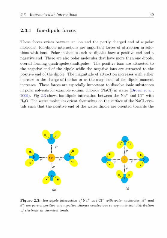
2.3. Intermolecular Interactions 49
2.3.1 Ion-dipole forces
These forces exists between an ion and the partly charged end of a polar
molecule. Ion-dipole interactions are important forces of attraction in solu-
tions with ions. Polar molecules such as dipoles have a positive end and a
negative end. There are also polar molecules that have more than one dipole,
overall forming quadrupoles/multipoles. The positive ions are attracted to
the negative end of the dipole while the negative ions are attracted to the
positive end of the dipole. The magnitude of attraction increases with either
increase in the charge of the ion or as the magnitude of the dipole moment
increases. These forces are especially important to dissolve ionic substances
in polar solvents for example sodium chloride (NaCl) in water (Brown et al.,
2009). Fig 2.3 shows ion-dipole interaction between the Na+ and Cl− with
H2O. The water molecules orient themselves on the surface of the NaCl crys-
tals such that the positive end of the water dipole are oriented towards the
Figure 2.3: Ion-dipole interaction of Na+ and Cl− with water molecules. δ+ and
δ− are partial positive and negative charges created due to asymmetrical distribution
of electrons in chemical bonds.
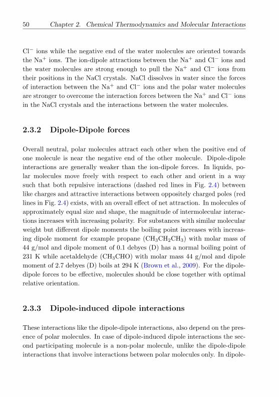
50 Chapter 2. Chemical Thermodynamics and Molecular Interactions
Cl− ions while the negative end of the water molecules are oriented towards
the Na+ ions. The ion-dipole attractions between the Na+ and Cl− ions and
the water molecules are strong enough to pull the Na+ and Cl− ions from
their positions in the NaCl crystals. NaCl dissolves in water since the forces
of interaction between the Na+ and Cl− ions and the polar water molecules
are stronger to overcome the interaction forces between the Na+ and Cl− ions
in the NaCl crystals and the interactions between the water molecules.
2.3.2 Dipole-Dipole forces
Overall neutral, polar molecules attract each other when the positive end of
one molecule is near the negative end of the other molecule. Dipole-dipole
interactions are generally weaker than the ion-dipole forces. In liquids, po-
lar molecules move freely with respect to each other and orient in a way
such that both repulsive interactions (dashed red lines in Fig. 2.4) between
like charges and attractive interactions between oppositely charged poles (red
lines in Fig. 2.4) exists, with an overall effect of net attraction. In molecules of
approximately equal size and shape, the magnitude of intermolecular interac-
tions increases with increasing polarity. For substances with similar molecular
weight but different dipole moments the boiling point increases with increas-
ing dipole moment for example propane (CH3CH2CH3) with molar mass of
44 g/mol and dipole moment of 0.1 debyes (D) has a normal boiling point of
231 K while acetaldehyde (CH3CHO) with molar mass 44 g/mol and dipole
moment of 2.7 debyes (D) boils at 294 K (Brown et al., 2009). For the dipole-
dipole forces to be effective, molecules should be close together with optimal
relative orientation.
2.3.3 Dipole-induced dipole interactions
These interactions like the dipole-dipole interactions, also depend on the pres-
ence of polar molecules. In case of dipole-induced dipole interactions the sec-
ond participating molecule is a non-polar molecule, unlike the dipole-dipole
interactions that involve interactions between polar molecules only. In dipole-

2.3. Intermolecular Interactions 51
Figure 2.4: Dipole-Dipole interactions. Solid red lines: strong interaction forces
between any two opposite charges, dashed red lines: strong repulsive interaction
forces between the like charges.
induced dipole interaction, the partial charges of the polar molecules causes
polarization, or distortion of the electron orbitals of the other molecule (i.e.,
the nonpolar molecule). As a result of this distortion, the second molecule
acquires partial negative and positive charges and thus becomes slightly polar.
The partial charges formed act just like the permanently polar molecules and
interact favorably with their counterparts in the polar molecule that origi-
nally induced them. For example, interaction between a polar HCl molecule
and Ar molecule. The Ar molecule experiences a dipole as its electrons are
attracted to H and or repelled by the Cl. The dipole-induced dipole interac-
tions are weaker than the dipole-dipole interactions but are stronger than the
dispersion forces.
2.3.4 Dispersion forces
Dipole-dipole interactions do not exist between non-polar atoms and molecules
due to the absence of a dipole moment. However, there are attractive forces

52 Chapter 2. Chemical Thermodynamics and Molecular Interactions
caused by momentary dipoles (temporary dipoles) created by the uneven dis-
tribution of electrons within the molecule/atom at any instant. This tem-
porary dipole in one molecule/atom induces an opposite temporary dipole
in the neighbouring molecule/atom and vice versa. These temporary partial
positive and negative charges that develop between molecules/atoms lead to
attractive interactions also known as dispersion forces. For example as seen
in Fig 2.5 the charge distribution in an He atom on average is spherical as
represented by the spherical electron orbitals. In Fig 2.5a electrons in the 1s
orbital of helium repel each other and therefore, tend to stay away from each
other (He atom 1), it does happen that they occasionally wind up on the same
side of the atom (He atom 2). At this instant, then, the He atom is polar,
with an excess of electrons on the left side and a shortage on the right side.
Figure 2.5b shows that the two dipoles arrange their position with the elec-
tric fields which leads to dipole formation. The strength of dispersion forces
depends on the ease with which the distribution of electrons in a molecule
is distorted also known as polarizability. Dispersion forces operate between
all molecules and atoms, whether they are polar or non-polar. Molecular size
and mass are highly correlated, thus overall effect of dispersion forces tends
to be stronger for substances with higher molecular weight.
When comparing the relative strength of intermolecular forces of polar
Figure 2.5: Dispersion forces. (a) Spherically symmetric charge distribution in
He atom 1. (b) The uneven electron distribution produces a momentary dipoles and
allows temporary electrostatic attraction between atoms.
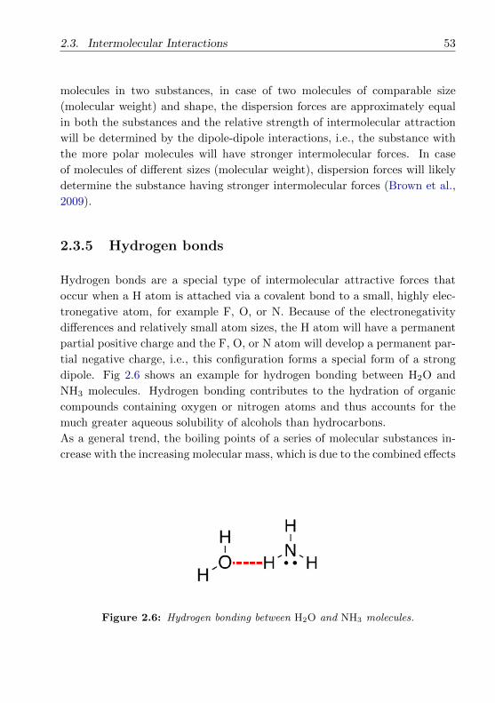
2.3. Intermolecular Interactions 53
molecules in two substances, in case of two molecules of comparable size
(molecular weight) and shape, the dispersion forces are approximately equal
in both the substances and the relative strength of intermolecular attraction
will be determined by the dipole-dipole interactions, i.e., the substance with
the more polar molecules will have stronger intermolecular forces. In case
of molecules of different sizes (molecular weight), dispersion forces will likely
determine the substance having stronger intermolecular forces (Brown et al.,
2009).
2.3.5 Hydrogen bonds
Hydrogen bonds are a special type of intermolecular attractive forces that
occur when a H atom is attached via a covalent bond to a small, highly elec-
tronegative atom, for example F, O, or N. Because of the electronegativity
differences and relatively small atom sizes, the H atom will have a permanent
partial positive charge and the F, O, or N atom will develop a permanent par-
tial negative charge, i.e., this configuration forms a special form of a strong
dipole. Fig 2.6 shows an example for hydrogen bonding between H2O and
NH3 molecules. Hydrogen bonding contributes to the hydration of organic
compounds containing oxygen or nitrogen atoms and thus accounts for the
much greater aqueous solubility of alcohols than hydrocarbons.
As a general trend, the boiling points of a series of molecular substances in-
crease with the increasing molecular mass, which is due to the combined effects
Figure 2.6: Hydrogen bonding between H2O and NH3 molecules.

54 Chapter 2. Chemical Thermodynamics and Molecular Interactions
of stronger dispersion forces among the atoms of larger molecules. However
H2O is a notable exception whose boiling point (100C) at 101.325 kPa (at-
mospheric pressure) is higher than expected from dispersion forces and typical
dipole-dipole force strength alone, when considering the relatively lower molar
mass (18.0153 g/mol) of H2O. Fig 2.7 shows the hydrogen bonding between
H2O molecules. The bent geometry of the water molecule and the highly
polar nature of the O-H bonds form a molecule with a strong dipole moment.
The two O-H bonds in a H2O molecule allow it to form strong hydrogen
bonds with other water molecules, resulting in a relatively high boiling point.
Hydrogen bonds are generally stronger than other dipole-dipole or dispersion
forces, and play a significant role in chemical processes, including those of
biological and atmospheric importance. Thus both the physical and chemical
properties play an important role in determining properties of solutions. The
purpose of applying thermodynamic methods to phase-equilibrium calcula-
tions is to classify, interpret, correlate, and predict properties of solutions.
The extent to which this purpose can be fulfilled relies on the degree of un-
derstanding of intermolecular forces, which are responsible for the molecular
behaviour on the microscopic scale, defining macroscopic thermodynamic be-
havior. Classical and statistical thermodynamics can define useful functions
Figure 2.7: Hydrogen bonding between water molecules. The red dash-lines are the
hydrogen bonds between the water molecules.
2.3. Intermolecular Interactions 55
and derive relationships between them, but the specific parameters describing
molecular interaction effects on the macroscopic scale cannot be defined by
thermodynamic theory alone. Determination of these values, requires exper-
iments which may help to derive the microscopic physicochemical properties
of a mixture.


Chapter 3
Improved AIOMFAC model
parameterisation of the
temperature dependence of
activity coefficients for
organic-water mixtures
G. Ganbavale 1, A. Zuend 1,2,3, C. Marcolli 1, T. Peter 1
1 Institute for Atmospheric and Climate Science, ETH Zurich, Zurich,
Switzerland2 Department of Chemical Engineering, California Institute of Technology,
Pasadena, California, USA3 Department of Atmospheric and Oceanic Sciences, McGill University, Mon-
treal, Quebec, Canada
This chapter is a reproduction of a corresponding article, which is in prepa-
ration to be submitted to the journal “Atmospheric Chemistry and Physics”.
The layout of the article as well as the section, figure, and table numberings
57

58 Chapter 3. Improved AIOMFAC temperature dependence
have been adapted to match with the thesis structuring. Cited literature is
referenced in the bibliography of the thesis.
59
This study presents a new, improved parameterisation of the temperature de-
pendence of activity coefficients in the AIOMFAC (Aerosol Inorganic-Organic
Mixtures Functional groups Activity Coefficients) model applicable for aque-
ous as well as water-free organic solutions. For electrolyte-free organic and
organic-water mixtures the AIOMFAC model uses a group-contribution ap-
proach based on UNIFAC (UNIversal quasi-chemical Functional-group Ac-
tivity Coefficients). This group-contribution approach explicitly accounts for
interactions among organic functional groups and between organic functional
groups and water. The previous AIOMFAC version uses a simple param-
eterisation of the temperature dependence of activity coefficients, aimed to
be applicable in the temperature range from ∼ 275 to ∼ 400 K. With the
goal to improve the description of a wide variety of organic compounds found
in atmospheric aerosols, we extend the AIOMFAC parameterisation for the
functional groups carboxyl, hydroxyl, ketone, aldehyde, ether, ester, alkyl,
aromatic carbon-alcohol, and aromatic hydrocarbon to atmospherically rele-
vant low temperatures with the introduction of a new temperature dependence
parameterisation. The improved temperature dependence parameterisation is
derived from macroscopic (classical) thermodynamic theory by describing ef-
fects from changes in molar enthalpy and heat capacity of a multicomponent
system. Thermodynamic equilibrium data of aqueous organic and water-free
organic mixtures from the literature are carefully assessed and complemented
with new measurements to establish a comprehensive database, covering a
wide temperature range (∼ 190 to ∼ 440 K) for many of the functional
group combinations considered. Different experimental data types and their
processing for the estimation of AIOMFAC model parameters are discussed.
The new AIOMFAC parameterisation for the temperature dependence of ac-
tivity coefficients from low to high temperatures shows an overall improvement
of 25 % in comparison to the previous model version. The new parameterisa-
tion of AIOMFAC agrees well with a large number of experimental datasets
and enables the calculation of activity coefficients of a wide variety of different
aqueous/water-free organic solutions down to the low temperatures present
in the upper troposphere.
60 Chapter 3. Improved AIOMFAC temperature dependence
3.1 Introduction
Atmospheric aerosols are complex mixtures of inorganic and organic compo-
nents. A large variety of organic compounds account for a significant fraction
of the tropospheric aerosol composition. Airborne and ground-based measure-
ments suggest that the aerosols in the free troposphere are composed of 30%
and up to about 80% of carbonaceous material mostly in the form of organics
(Murphy et al., 2006; Jacobson et al., 2000; Hallquist et al., 2009). Aerosol
loading, size distribution, composition, morphology and physical states of par-
ticles affect the Earth’s radiative budget through the direct effects of aerosols
on climate and the indirect effects, in which aerosols act as cloud condensa-
tion (CCN) or ice nuclei (IN), affecting cloud particle number concentrations,
precipitation, cloud albedo, and life time. Organic aerosols are expected to
stay in a liquid, viscous semi-solid, or amorphous solid state, since the very
large number of organic compounds depresses the temperature at which or-
ganic crystal formation takes place (Marcolli et al., 2004; Virtanen et al., 2010;
Koop et al., 2011).
Non-ideal interactions between different organic and inorganic species in the
particle phase influence water uptake and release (hygroscopicity), may in-
duce liquid-liquid phase separation (LLPS) (e.g., Marcolli and Krieger, 2006;
Zuend et al., 2010; Song et al., 2012), influence gas-particle partitioning of
semivolatile compounds (e.g., Zuend et al., 2010; Zuend and Seinfeld, 2012),
and alter efflorescence and deliquescence relative humidities (e.g., Krieger
et al., 2012). Thermodynamic phase equilibrium calculations allow to de-
termine whether the aerosol phase is a liquid (or viscous amorphous phase),
a crystalline solid, or a mixture of solid and liquid phases and to what degree
semivolatile species partition to the condensed phases (Zuend et al., 2010;
Zuend and Seinfeld, 2012). Phase equilibria calculations can be carried out
by using composition dependent activity coefficients which account for the
non-ideality of the liquid/amorphous phase (Gmehling, 1995; Raatikainen and
Laaksonen, 2005; Zuend et al., 2010). The mole fraction based activity co-
efficient, γ(x)s and activity a
(x)s of a compound s are related by a
(x)s = γ
(x)s xs,
where xs is the mole fraction of s in the liquid mixture.
Thermodynamic models for mixtures of organics and water in condensed

3.1. Introduction 61
phases are usually based on the UNIQUAC (UNIversal QUAsi Chemical)
model (Abrams and Prausnitz, 1975) or its group contribution version UNI-
FAC (UNIquac Functional group Activity Coefficients) (Fredenslund et al.,
1975). The original UNIFAC model was developed for vapour-liquid equilib-
ria (VLE) calculations within a temperature range from ∼ 275 to ∼ 400 K.
Using the UNIFAC model outside of its intended temperature range may re-
sult in poor predictions of real phase behaviour (Lohmann et al., 2001). For
very dilute mixtures, UNIFAC thermodynamic model calculations for compo-
nent activity coefficients at infinite dilution are sometimes not in agreement
with the experimental data. This can be understood since most VLE mea-
surements were performed for liquid mole fractions between 0.02 to 0.98 and,
hence, do not provide specific information for the highly dilute regions. Inac-
curate results were obtained for other types of thermodynamic data, e.g., mo-
lar enthalpies of mixing (hE) or solid-liquid equilibrium (SLE) data, following
the Gibbs-Helmholtz relation, this leads to inaccurate description of activity
coefficients as a function of temperature (Gmehling, 2003, 2009; Lohmann
et al., 2001). With the original UNIFAC model, due to data insufficiency,
inaccurate predictions were often obtained for asymmetric systems (systems
containing molecules of different sizes and shapes) (Lohmann et al., 2001;
Gmehling, 2003). Since then, the original UNIFAC model has been improved
and in addition, modified UNIFAC versions such as modified UNIFAC (Dort-
mund) and modified UNIFAC (Lyngby) have been developed (Hansen et al.,
1991; Gmehling et al., 1998, 2002; Jakob et al., 2006; Larsen et al., 1987),
which amended some of the original weaknesses. For mixtures containing mul-
tifunctional components, both UNIFAC and modified UNIFAC (Dortmund)
sometimes show poor results since the functional group interaction parameters
were mainly determined based on experimental data of mixtures of simple,
monofunctional components (Weidlich and Gmehling, 1987; Gmehling et al.,
2012).
One of the important differences between the UNIFAC model by Hansen et al.
(1991), which we call here “standard UNIFAC”, and the modified UNIFAC
(Dortmund), is the use of a more elaborate parameterisation for the tempera-
ture dependence of activity coefficients in the modified UNIFAC model. How-
ever, the modified UNIFAC models sometimes do not provide reliable predic-
62 Chapter 3. Improved AIOMFAC temperature dependence
tions of activity coefficients at low temperatures relevant in the troposphere.
Calculations of water activity (aw) of atmospherically relevant aqueous or-
ganic solutions have shown that the performance of standard UNIFAC may
be poor when the organic fraction consists of multifunctional molecules typi-
cally carrying several strong polar functional groups with enhanced hydrogen-
bonding potential (Saxena and Hildemann, 1997; Peng et al., 2001). Marcolli
and Peter (2005) have therefore proposed improved sets of interaction pa-
rameters for standard UNIFAC for alcohols and polyols. Peng et al. (2001)
reparameterised the interaction of the water (group) with the carboxyl group
and the hydroxyl group based on measured water activities of aqueous systems
containing dicarboxylic acids and substituted dicarboxylic and tricarboxylic
acids.
For atmospheric applications, an accurate description of aqueous organic mix-
tures at atmospherically relevant temperatures is required. At low tempera-
tures aw is a crucial parameter for homogeneous ice nucleation (Koop et al.,
2000). Extrapolations of aw of different aqueous organic solutions measured
in the temperature range from the ice melting curve to 313 K suggest that
if the temperature dependence of the activity coefficients is neglected, errors
on the order of 10 to 15 % result for aw at the homogeneous freezing tem-
perature (Zobrist et al., 2008). The uncertainty in predicted homogeneous
ice nucleation temperatures is stated as ± 0.025 aw at melting points and ±0.05 aw at ice freezing temperatures (Koop et al., 2000; Koop, 2004). A small
uncertainty in aw of about 0.025 can change the corresponding homogeneous
nucleation rate coefficients by 6 orders of magnitude (or the onset temperature
of homogeneous freezing by up to 8 K) and may significantly affect predictions
of the onset of ice crystal formation in cloud microphysical models (Knopf and
Rigg, 2011). This shows the need for an improved UNIFAC (and AIOMFAC)
parameterisation at low temperatures.
The AIOMFAC model (Aerosol Inorganic-Organic Mixtures Functional
groups Activity Coefficients) by Zuend et al. (2008, 2011) is a thermody-
namic group-contribution model specifically developed to meet the require-
ments of typical tropospheric aerosol compositions. The model enables calcu-
lations of activity coefficients covering inorganic (water, electrolytes), organic,
and organic-inorganic interactions in multicomponent solutions over a wide

3.2. AIOMFAC model 63
concentration range and includes the standard UNIFAC for the description
of organic and organic-water systems. AIOMFAC is based on the group-
contribution model LIFAC by Yan et al. (1999) and, therefore, includes the
standard UNIFAC model, yet also includes the modified parameter sets from
Peng et al. (2001) and those from Marcolli and Peter (2005). In its short-
range interaction part, the AIOMFAC model shares the simple temperature
dependence expressions of the original UNIFAC model and involves only one
main group interaction term involving two adjustable parameters, am,n and
an,m per binary interaction. Throughout this article, we will refer to this
(original) AIOMFAC model as “AIOMFAC-P1”. The aim of this study is to
improve the performance of AIOMFAC at low temperatures for multicompo-
nent organic + water systems. We will refer to the new AIOMFAC version,
with an improved temperature dependence parameterisation with two addi-
tional main group interaction terms, as AIOMFAC-P3, indicating a 3-term
parameterisation in the short-range (mod. UNIFAC) part. The focus is on
organic functional groups that have been identified in tropospheric aerosols,
namely hydroxyl, carboxyl, ketone, ether, ester, aldehyde, alkyl, and aromatic
functionalities.
3.2 AIOMFAC model
The thermodynamic group-contribution model AIOMFAC allows thermody-
namically consistent calculations of activity coefficients at temperatures close
to 298 K and covers multicomponent solutions containing water, inorganic
ions, and organic compounds. For electrolyte-free systems of organic com-
pounds and water, the applicable temperature range is ∼ 275 to ∼ 400 K, as
for the original UNIFAC model. As mentioned above, the concept of AIOM-
FAC is based on the LIFAC model (Yan et al., 1999), which merges a Pitzer-
like approach with a slightly modified version of the original UNIFAC model
to calculate activity coefficients.
The non-ideality of a thermodynamic system is characterized by the excess

64 Chapter 3. Improved AIOMFAC temperature dependence
Gibbs energy Gex (p, T, nj), which in AIOMFAC is expressed as the sum of a
long range (LR), middle range (MR) and short range (SR) contribution:
Gex (p, T, nj) = GexLR + Gex
MR + GexSR. (3.1)
Here, p is the total pressure, T the absolute temperature, and nj (j = 1, . . . , k)
the molar amounts of the k components in a system. Mole fraction based ac-
tivity coefficients γ(x)j with nj moles in a mixture are derived from expressions
for the different parts of Gex using the relation
ln γ(x)j =
[∂Gex/(RT )
∂nj
]p,T,nj′ 6=j
(3.2)
where R is the universal gas constant. Activity coefficients are calculated
from the three model parts:
ln γ(x)j = ln γ
(x),LRj + ln γ
(x),MRj + ln γ
(x),SRj . (3.3)
Electrolyte solutions which may range from dilute to highly supersaturated
concentrations are, aside from their SR contribution, considered in the Pitzer-
like part, which combines LR and MR interactions. The LR interactions are
described by an extended Debye-Huckel term and represents contributions by
Coulomb electrostatic forces between permanently charged ions, moderated
by the presence of the dielectric solvent medium. The MR part represents the
effects of interactions involving ions and permanent or induced dipoles and
contains most of the adjustable parameters to describe concentrated aqueous
electrolyte solutions and organic-inorganic mixtures. The original AIOMFAC
model by Zuend et al. (2008) has been extended and re-parameterised to
include organic-inorganic interactions of most of the functional groups typi-
cally present in atmospheric organic compounds (carboxyl, hydroxyl, ketone,
aldehyde, ether, ester, alkyl, aromatic carbon-alcohol, and aromatic hydrocar-
bon) (Zuend et al., 2011). In addition, Zuend and Seinfeld (2012) introduced
the functional groups hydroperoxide, peroxyacid, and peroxide, including es-
timated interaction parameters with the inorganic ions of the model. For
further details of the thermodynamic description of the LR and MR interac-
tions within the Pitzer-like part of AIOMFAC we refer to Zuend et al. (2008,
3.2. AIOMFAC model 65
2011). The interactions among non-charged species (organic molecules and
water) are calculated in the SR part of AIOMFAC.
3.2.1 Group-contribution method
A group contribution concept similar to UNIFAC has been adopted for the
AIOMFAC model. According to the group contribution concept, it is assumed
that the system is composed of combinations of functional groups instead of
whole molecules. The advantage of applying the group contribution method
is that a very large number of organic compounds can be defined using the
various combinations of a limited number of functional groups. In accordance
to the UNIFAC model, the functional groups are further classified into the
so called main groups and subgroups for their application in different model
parts (Fredenslund et al., 1975; Marcolli and Peter, 2005; Zuend et al., 2008,
2011). The main groups cover subgroups of the same functionality that only
differ by the number of hydrogen atoms. The subgroup classification of a
variety of organic compounds can be found in Table 3.1.
3.2.2 Short-range contribution
As in the UNIFAC model, in the SR part of AIOMFAC, activity coefficients
of a mixture component j are in general expressed as the sum of contributions
of a combinatorial part (denoted by superscript C), which accounts for the
size and shape of the molecule, and the residual part (denoted by superscript
R), which reflects the residual contribution from intermolecular (inter-group)
interactions (Fredenslund et al., 1975; Marcolli and Peter, 2005; Zuend et al.,
2008).
ln γSR,(x)j = ln γC
j + ln γRj (3.4)
The expression for the combinatorial part of UNIFAC is (Fredenslund et al.,
1975; Zuend et al., 2008):

66 Chapter 3. Improved AIOMFAC temperature dependence
ln γCj = ln
Φjxj
+z
2qj ln
Θj
Φj+ lj −
Φjxj
∑j′
xj′ lj′ (3.5)
where
Φj =rjxj∑
j′rj′xj′
; Θj =qjxj∑
j′qj′xj′
(3.6)
and
rj =∑t
ν(j)t Rt; qj =
∑t
ν(j)t Qt; (3.7)
lj =z
2(rj − qj)− (rj − 1). (3.8)
In these equations, xj is the mole fraction of component j and ν(j)t denotes
the number of subgroups of type t present in a formula unit of component j.
The relative van der Waals subgroup volume and surface area are given by
Rt and Qt respectively. The lattice coordinate number z is typically assumed
to be a constant set to z = 10 (Fredenslund et al., 1975). Relative subgroup
volume and surface area parameters published by Hansen et al. (1991) are used
for the neutral species. Enthalpic interaction contributions are considered in
the residual part of UNIFAC. The residual part of the activity coefficient of
component j is given by (γRj ):
ln γRj =
∑t
ν(j)t
[ln Γt − ln Γ
(j)t
], (3.9)
where Γt is the group residual activity coefficient in the mixture, while Γ(j)t
represents the one in a reference liquid containing only compound j. ν(j)t

3.2. AIOMFAC model 67
is the number of subgroups of type t in molecule j. The residual activity
coefficient of subgroup t is:
ln Γt = Qt
1− ln
(∑m
ΘmΨm,t
)−∑m
ΘmΨt,m∑n
ΘnΨn,m
, (3.10)
where
Θm =QmXm∑nQnXn
. (3.11)
In these expressions Θm is the relative surface area fraction of subgroupm, Xm
is the mole fraction of m in the mixture. The standard UNIFAC temperature-
dependent interaction between the subgroups m and n is given by Fredenslund
et al. (1975):
ln Ψn,m = −[Un,m − Un,n
RT
](3.12)
where Un,m is a measure of change in the molar Gibbs free energy due to
interaction between subgroups m and n. Eq. 3.12 is typically represented in
the more compact form of Eq. 3.13.
ln Ψn,m = −[an,mT
](3.13)
Due to the formulation of Eq. 3.12, with equivalent differences for the inter-
actions between subgroups m and n (with the difference Um,n − Um,m), the
main group interaction parameters an,m are unsymmetrical i.e., an,m 6= am,n.
Note that all interaction parameters are only resolved on the main group level,
i.e., all subgroups of a certain main group interacting with a subgroup of a
different main group will have the same interaction parameter. Hence, we
refer to the set of an,m as main group interaction parameters. In standard
UNIFAC, the an,m interaction parameters of organic solutions were estimated
using a large database of experimental vapour-liquid equilibrium (VLE) and
liquid-liquid equilibrium (LLE) datasets. This approach leads to satisfying

68 Chapter 3. Improved AIOMFAC temperature dependence
predictions for vapour-liquid equilibria, but reliable simultaneous description
of VLE, LLE, solid-liquid equilibria (SLE), and molar enthalpies of mixing
(hE) can often not be obtained (Lohmann et al., 2001). In order to overcome
these deficiencies of the standard UNIFAC, modified UNIFAC (Dortmund)
uses three main group interaction parameters in the residual part to improve
predictions of activity coefficients over a wider range of temperatures and dif-
ferent types of phase equilibria (Gmehling et al., 1993; Lohmann et al., 2001;
Jakob et al., 2006):
ln Ψn,m = −[an,m + bn,mT + cn,mT
2
T
]. (3.14)
In modified UNIFAC (Dortmund) the relative van der Waals volume (Rt)
and surface (Qt) coefficients for the structural groups are not calculated from
molecular parameters as in the standard UNIFAC approach; rather, they are
fit together with the interaction parameters (an,m, bn,m, cn,m) to experimen-
tal data.
The AIOMFAC model is aimed for a wide range of applications, including the
calculation of solid-liquid equilibria and other thermodynamic phase equilib-
ria. The temperature dependence of these equilibria is related to the molecular
interaction of the components in the liquid phase. Hence, the temperature
dependence of chemical reaction equilibria and phase equilibra are described
by the same thermodynamic functions and we can express them with param-
eterisations for the temperature dependence of reaction equilibria. According
to Clarke and Glew (1966), if the equilibrium constant Kp of a chemical re-
action or exchange process is a function of temperature, the changes in the
standard thermodynamic functions, i.e., change in molar Gibbs free energy
∆G, change in molar enthalpy ∆H and change in molar heat capacity ∆Cp
are directly related to Kp (by definition) and are well-behaved functions of
T . The relationship for the equilibrium constant Kp and temperature T ,
when excluding higher order derivatives of molar heat capacity change with
temperature, are given by (Clarke and Glew, 1966):
R lnKp = −∆G
T
T+∆H
T
[1
T− 1
T
]+∆C
pT
[TT− 1 + ln
T
T
], (3.15)

3.2. AIOMFAC model 69
where T is a reference temperature at which the changes in ∆G, ∆H and
∆Cp are determined or known. In order to better describe activity coeffi-
cients at low (and high) temperatures while preserving compatibility with the
already estimated values of the interaction parameters an,m at room temper-
ature, we introduce a similar but slightly modified expression for Ψn,m. We
define the temperature dependent interaction potential in AIOMFAC as
ln Ψn,m = −an,mT
+ bn,m
(1
T− 1
T
)+ cn,m
[(TT− 1
)+ ln
T
T
](3.16)
with the reference temperature T = 298.15 K. The first term is similar as in
standard UNIFAC, but slightly different from the equivalent term in Eq. 3.15,
due to the use of actual temperature T instead of reference temperature T for
consistency with standard UNIFAC/AIOMFAC. This term in Eq. 3.16 there-
fore includes both changes in ∆GT
as well as a part of the changes related
to ∆HT
(note: this is obvious when considering a hypothetical, very high
reference temperature for the second term on the right hand side of Eq. 3.16).
The second term includes the change in enthalpy and in addition acts as a
linear correction term for parameters an,m at temperatures different from the
reference temperature. The third term accounts for the contribution related
to the heat capacity change of a main group interaction, whose importance
increases for temperatures far away from the reference temperature.
We use a database of experimental thermodynamic equilibrium data for or-
ganic and organic-water systems (see (Sect. 3.3) and (Sect. 3.4)), covering
a wide temperature and concentration range, to determine simultanously the
AIOMFAC group interaction parameters bn,m and cn,m for pertaining organic
funcational groups. To preserve compatibility with the AIOMFAC model ver-
sion of (Zuend et al., 2011), and its fitted organic-inorganic interaction pa-
rameters at room temperature, all group-interaction parameters am,n are kept
the same, which implies that the performance of AIOMFAC at 298.15 K will
not be altered by the improved three-parameter temperature-dependence pa-
rameterisation. With a goal to describe a wide variety of organic compunds
at relevent atmospheric temperatures, we focus on the aqueous systems of
oxidized organics at lower temperatures. The temperature dependence for-
mulation given by Eq. (3.16) will at this point only be parametrised for interac-
70 Chapter 3. Improved AIOMFAC temperature dependence
tions between the UNIFAC main groups alkyl (CHn), specific variants of alkyl
groups in alcohols, such as (CH[alc]n ), (CH
[alc−tail]n ), and (CH
[OH]n ), hydroxyl
(OH), carboxyl (COOH), water (H2O), ketone (CHnCO), aldehyde (CHO),
ether (CHnO), ester (CCOO), alkenyl (C=C), aromatic carbon (ACHn), and
aromatic carbon alcohol (ACOH) (a phenol group). For all other group inter-
actions not considered, bn,m and cn,m are set to zero so that Eq. (3.16) reduces
to Eq. (3.13). The rules for the use of specific alkyl groups, are described be-
low. With this approach, an improved description of activities for organic
systems at low temperatures can be achieved, while maintaining compatibil-
ity with standard UNIFAC, hence, preserving the applicability of AIOMFAC
to a wider range of functional groups.
The UNIFAC functional groups in AIOMFAC include some modifications
with respect to standard UNIFAC to better describe the specific proper-
ties of organic aerosol constituents, which typically are molecules composed
of several (polar) functional groups. Therefore a more detailed descrip-
tion of alcohol/polyol group interaction parameters published by Marcolli
and Peter (2005) was implemented, where the relative positions of the OH
functional group as well as those of neighboring alkyl groups are taken
into account (Zuend et al., 2011). According to this approach, water-alkyl
and water-hydroxyl group interaction parameters for alcohols/polyols are
treated specifically, while keeping the alkyl-hydroxyl interaction parameter
unchanged in order to maintain the performance of AIOMFAC in case of wa-
ter free alkane/alcohol systems compatible with standard UNIFAC. Except
for CH[OH]n groups directly bonded to an OH group, standard UNIFAC CHn
groups are used for alkyl groups in multifunctional molecules that contain
hydroxyl groups combined with different other functional groups. Another
difference with respect to standard UNIFAC is that we use the parameters of
Peng et al. (2001) for the interaction of the COOH group with the OH group
and the H2O group. The use of these modified UNIFAC group interaction
parameters leads to improvements for certain aqueous systems of alcohols, di-
carboxylic and hydroxycarboxylic acids, while being compatible with the use
of standard UNIFAC parameters for other group interactions, as described in
more detail in Zuend et al. (2011).

3.3. Experimental data 71
3.3 Experimental data
Reliable estimation of group interaction parameters and temperature depen-
dence relies on a comprehensive database covering a wide variety of com-
pounds consisting of the targeted functional groups, with consideration of a
large temperature range. In order to establish such a database, an extensive
literature search was carried out. The DETHERM databank (Gesellschaft fur
Chemische Technik und Biotechnologie e.V., www.dechema.de), which offers
the world’s largest collection of thermodynamic mixture data was used to
check the completeness of the literature search and to directly purchase data
for which the original publication was not easily accessible.
Figure. 3.1 provides an overview of the database implemented in this study.
The matrix lists the number of datasets at temperatures substantially dif-
ferent from 298 K available for each main group pair interaction. The green
bars indicate the maximum number of overall datasets including all datatypes
available for each main group interaction pair. For each interaction pair, the
highest temperature (red shaded boxes) and lowest temperature (blue shaded
boxes), for which datapoints are available is indicated. The database overall
consists of 677 datasets covering different data types, for monofunctional and
multifunctional organic molecules in aqueous and water-free mixtures of bi-
nary and ternary systems. Table 3.1 lists the datasets and the data types used
for determining the main group interaction parameters (bn,m and cn,m) in the
SR part of the AIOMFAC model. The table lists the mixture components,
main groups, chemical formula (subgroups), data type, number of data points,
temperature range, assigned initial weighting used in the model parameter fit,
and the data source. Tables reporting new water activity measurements are
provided in the Appendix. Different data types and their processing for use
with the model parameterisation are described in the following.
3.3.1 Solid-liquid equilibrium
Most low temperature data available for the model parameterisation are bi-
nary SLE data with water and an organic component. SLE data can be

72 Chapter 3. Improved AIOMFAC temperature dependence
1 2 3 7 8 9 10 11 13 65 66 67 68 69
groupno main groups (CHn) (C=C) (ACHn) (H2O) (ACOH) (CHnCO) CHO (CCOO) CHnO (COOH) (CHn[alc]) (CHn[alc-tail]) (CHn[OH]) (OH) [aldehyde] [ether]
1 (CHn) 2 (C=C) set count: 26 T_low [K]: 191 T_high [K]: 2883 (ACHn) set count: 26 T_low [K]: 197 140 T_high [K]: 393 1707 (H2O) set count: 239 27 21 200 T_low [K]: 187 191 214 230 T_high [K]: 447 338 455 2608 (ACOH) set count: 7 23 17 290 T_low [K]: 298 214 214 320 T_high [K]: 383 455 455 3509 (CHnCO) set count: 91 10 46 2 380 T_low [K]: 154 225 198 323 410 T_high [K]: 423 348 406 333 44010 (CHO [aldehyde]) set count: 28 2 8 2 470 T_low [K]: 143 353 278 296 500 T_high [K]: 393 393 367 32911 (CCOO) set count: 69 3 45 2 6 2 lowest T[K] : 143 T_low [K]: 163 298 208 298 263 313 highest T[K] : 484 T_high [K]: 439 353 439 348 348 32313 (CHnO[ether]) set count: 105 9 81 6 2 2 7 T_low [K]: 148 197 187 214 322 288 208 T_high [K]: 423 383 423 383 330 304 40265 (COOH) set count: 140 27 12 111 7 24 3 10 21 T_low [K]: 173 191 214 191 214 173 295 243 194 T_high [K]: 447 338 387 447 348 391 386 366 36066 (CHn[alc]) set count: 12 2 96 1 4 3 5 T_low [K]: 288 185 196 313 288 319 288 T_high [K]: 399 313 442 313 333 399 32367 (CHn[alc-tail]) set count: 63 13 52 3 16 10 8 15 15 15 T_low [K]: 143 160 200 243 154 143 163 148 241 215 T_high [K]: 423 350 384 348 423 353 351 400 389 36768 (CHn[OH]) set count: 157 26 22 245 9 20 10 15 84 46 100 116 T_low [K]: 143 191 160 187 214 154 143 163 148 191 185 143 T_high [K]: 423 288 383 484 383 423 353 402 423 389 442 42369 (OH) set count: 159 26 22 247 9 20 10 15 84 48 100 116 323
T_low [K]: 143 191 160 187 214 154 143 163 148 191 185 143 143 T_high [K]: 423 288 383 484 383 423 353 402 423 389 442 423 484
Tem
pera
ture
scal
e (K
)
Figure 3.1: Database distribution for the water ↔ organic and organic ↔ organic
interaction parameters. The table lists the total number of datasets (set count)
available for each main group interaction at temperatures substantially different from
the chosen reference temperature (T = 298.15 K). The total number of datasets
available for each main group interaction pair are visualized by the green coloured
bars. The percentile-wise colouring is used to visualize the lowest temperature (Tlow,
blue colour) and the highest temperature (Thigh, red colour) (units of K) of the data
points available for each main group interaction pair.
obtained by measuring the melting point depression of solutes as a function
of solution composition. Consequently, at maximum two data points for each
temperature level can be acquired for binary systems, corresponding to the
points on the melting curves of the two components. However, most datasets
collected provide only data for one component forming a solid in equilibrium
with the remaining liquid solution. In many of these cases, hexagonal water
ice is the solid phase. Since the temperature dependence of water activity
(aw) of aqueous solutions in equilibrium with ice is well known, an accurate
determination of the activity coefficients (γ(x)w = aw
xw) of water as a function

3.3. Experimental data 73
of solution composition and temperature using SLE data is possible. At SLE,
the activity of water in a solution with organic mole fraction xorg at ther-
modynamic equilibrium with ice, aSLEw (T, p), is given by (Koop et al., 2000):
aSLEw (T, p) = exp
[µSw(T, p)− µ,L
w (T, p)
RT
], (3.17)
where µSw(T ) and µ,Lw (T ) are the pressure and temperature dependent chem-
ical potentials of ice (superscript S) and pure liquid water( superscript , L),
respectively. At ambient pressures, neglecting the pressure dependence of the
liquids and solids is well justified.
µSw(T )− µ,Lw (T ) = 210368 + 131.438 T
−3.32373× 10⁶ T−1 − 41729.1 ln(T ). (3.18)
The parameterisation in Eq. (3.18) represents the thermodynamically con-
sistent function valid at low (ambient) pressure in the temperature range
150 < T < 273 K (Koop et al., 2000).
The activity of dissolved organic component in equilibrium with its pure crys-
talline solid can be calculated using the following relationship (Prausnitz et al.,
1986; Domanska et al., 2009):
lnxiγSLEi = −∆hm,i
RT
(1− T
Tm,i
)− ∆htr,i
RT
(1− T
Ttr,i
)+
∆cp,m,iR
[(1− T
Tm,i
)+ ln
T
Tm,i
].(3.19)
where ∆hm,i is the molar enthalpy of fusion (melting, subscript m), ∆htr,i is
the molar enthalpy of a certain solid-solid phase transition, ∆cp,m,i is the mo-
lar heat capacity change upon fusion at constant pressure, Ttr is the solid-solid
phase transition temperature and Tm,i the melting temperature of pure com-
ponent i. The second term is only of significance when there is a solid-solid
phase transition (change of polymorphic form) between T and Tm,i. Equa-
tion 3.19 uses the simplification that the melting temperature and the triple
point temperature of an organic compound are relatively close at atmospheric

74 Chapter 3. Improved AIOMFAC temperature dependence
pressure. For obtaining activity coefficients from experimental data at given
temperatures and mole fractions (xorg, T ), Eq. 3.19 can be solved for the
SLE organic activity and/or activity coefficients. Pure component physico-
chemical properties such as ∆hm,i and ∆cp,m,i are obtained from tabulated
experimental data (Dean, 1999) and (Domalski and Hearing, 1996).
3.3.2 Water activity measurements
Water activity measurements were conducted for aqueous organic solutions
with an Aqualab dew point water activity meter (Model 3TE, Decagon De-
vices, USA), which enables water activity measurements within the tempera-
ture range from 289− 313 K for several concentrations at each different tem-
perature levels. Water activity data for measured binary aqueous organic bulk
solutions are tabulated in the Appendix. Additional measurements of aque-
ous multifunctional organic solutions are provided in Ganbavale et al.(2014).
Measured water activities were then used directly for the AIOMFAC-P3 pa-
rameter determination.
3.3.3 Liquid-liquid equilibria data
The equilibrium state between coexisting liquid phases is known as liquid-
liquid equilibrium (LLE). Liquid-liquid equilibria are useful as a source of data
for systems containing relatively hydrophobic organic compounds and water,
with a miscibility gap that depends on temperature and mixture composition.
In general, multicomponent systems may form more than two phases. For
salt-free aqueous organic systems with two coexisting liquid phases, usually
one phase is an aqueous (water-rich) phase while the other is an organic-rich
phase. Most available experimental LLE data has been measured relatively
close to room temperature and is useful for a better description of the phase
behaviour. However, for the purpose of our new parameterisation of AIOM-
FAC with regard to low temperatures far from room temperature, the LLE
data tend to be less useful than, e.g., SLE data. We use the tie-line data
from LLE measurements, which represents the composition of the two liquid

3.3. Experimental data 75
phases in equilibrium at a certain temperature. Initial mixture composition of
experimental tie-lines are used as input for computation of LLE phase sepa-
ration in order to compare the AIOMFAC model with the experimental data.
A direct calculation and comparison of activities in coexisting phases is pos-
sible at experimental LLE compositions. This data type can be implemented
in the model fit by minimizing the relative differences between the activities
of the components in the two liquid phases. We use the method introduced
by Zuend et al. (2011) for the comparison of calculated relative activity de-
viations between the activities of components j present in the two phases.
An initial mixture composition with mole fraction xinitj of component j on a
unstable/metastable point on a tie-line is generated by:
xinitj =
1
2
(xαj + xβj
)(3.20)
where xαj and xβj are the experimental compositions of the two liquid phases
α and β at equilibrium. This allows a direct comparison of the measured and
calculated phase compositions. According to the reference state definitions of
AIOMFAC, different independent components should have the same activities
in coexisting phases. i.e. a(x),αj = a
(x),βj .
Forward computations of LLE were also performed using the method of
(Zuend and Seinfeld, 2013), particularly for the graphical comparison of mea-
sured and predicted tie-line LLE data. For more details about the LLE com-
putations with AIOMFAC we refer to Zuend et al. (2010) and Zuend and
Seinfeld (2013); the specific method used for fitting LLE data based on rela-
tive activity deviations is described in more detail in Zuend et al. (2011).
3.3.4 Vapour-liquid equilibria
VLE data represent the temperature and pressure conditions where a liquid
(mixture) and its vapour(s) (gas phase) are in equilibrium with each other.
The VLE data is usually obtained by performing measurements either at
isobaric or isothermal conditions. VLE data considered in the model include
binary water + organic systems and binary data for water-free organic (1) +
76 Chapter 3. Improved AIOMFAC temperature dependence
organic (2) systems. Since isobaric measurements are usually conducted at 1
atm (= 101.325 kPa) pressure by measuring the boiling point temperature,
they typically provide data at relatively high temperatures. In order to be
used in the model parameterisation, the composition of the liquid in terms
of mole fraction xj of each component j, the composition of the gas phase in
terms of mole fraction yj and the total pressure p of the gas phase have to
be stated or need to be derived from the data source. VLE data provide the
composition dependence of activity coefficients. Assuming that the gas phase
can be treated as an ideal gas mixture, activity coefficients of the components
in the solution can be calculated by modified Raoult’s law:
γ(x)j =
pjp0jxj
, pj = yjp (3.21)
where pj is the partial pressure of component j, and poj (T ) is the pure liq-
uid component saturation vapour pressure calculated at the measurement
temperatures using the Antoine equation with coefficients from the Landolt-
Bornstein database (Dykyj et al., 2000), from Yaws et al. (2005) or, in some
cases, the p0j (T ) are directly available from the reference of the experimental
VLE data. Except for monocarboxylic acids such as formic, acetic, and pro-
pionic acid, which exhibit significant gas phase association (dimers, trimers),
assuming an ideal gas mixture for the total pressure and temperature ranges
of the data is acceptable. Other exceptions include certain diols and triols,
e.g., glycerol, which show moderate non-ideality in the gas phase, requiring
fugacity corrections. For mono-alcohols, fugacity corrections of the gas phase
did not lead to substantial changes in activity coefficients, due to the form of
(Eq. 3.21) (where the ratio of partial pressure and saturation vapour pressure,
both similarly affected by association effects, cancel most of the non-ideality),
and were typically ignored. To account for the gas phase dimerisation of car-
boxylic acids we obtain the monomer partial pressures using the dimerisation
equilibrium coefficients from Tsonopoulos and Prausnitz (1970). The proce-
dure for calculating experimental activity coefficients using this dimerization
correction is described in more detail in Zuend et al. (2011).
3.4. Objective function and model parameter estimation 77
3.4 Objective function and model parameter
estimation
Organic-organic and organic-water main group interactions are parametrised
in the SR part of AIOMFAC. The model parameter determination procedure
involves simultaneous fitting of the various group interaction parameters to
available thermodynamic phase equilibria data (see the database overview in
Fig. 3.1). In order to ensure intercomparability of different thermodynamic
quantities and with due consideration of the various aspects of the uncertainty
in measurements and the group-contribution concept of the model, we use the
following general objective function (Fobj), subject to minimization (Zuend
et al., 2011):
Fobj =∑d
∑u
wd,u
Qcalcd,u −Qref
d,u∣∣∣Qrefd,u
∣∣∣ + Qtold,u
2
. (3.22)
Here, wd,u is the weighting value of a data point and the sums cover all data
points u in all datasets d considered. Qrefd,u is a reference quantity, directly
determined from experiments (e.g., measured water activity value at a cer-
tain T and xw) or derived from measurements by means of thermodynamic
relations, e.g., SLE water activity on the ice melting curve at a specific tem-
perature. Qcalcd,u represents the corresponding quantity calculated with the
model at the given conditions. Qtold,u is a tolerance quantity (> 0) which rep-
resents the measurement uncertainty or model sensitivity and has the same
units as Qrefd,u. During the iterative fitting of the model parameters, we use the
AIOMFAC model (with the current parameter set at that iteration step) to
calculate the model activity sensitivity with respect to an assumed represen-
tative uncertainty in absolute mixture composition, a mole fraction tolerance
set to: xtol = 0.01. We refer to Zuend et al. (2011) (their Section 3.3) for
a detailed description of how the model sensitivity is calculated. We use the
AIOMFAC model to calculate the effect of a tiny change in composition on
the activity coefficients of the different mixture components by means of a
total molar derivative. Technically, this is done by scaling and summation of

78 Chapter 3. Improved AIOMFAC temperature dependence
the partial derivatives of the activity coefficients at a given solution compo-
sition by means of finite differences in molar composition (Eq. 10 of Zuend
et al. (2011).
3.4.1 Dataset weighting and temperature range
Both experimental uncertainties and model deficiencies need to be considered
while determining the main group interaction parameters. The measured
experimental quantities have some level of random and systematic errors,
which may also depend on mixture composition, rendering some data points
more reliable than others. This is considered during the parameter estimation
procedure by giving appropriate weighting to the datasets and by data point-
specific tolerance quantities computed in parallel from the model sensitivities
as the model fit progresses. With the aim of reducing a disproportionate
influence of datasets with a large number of data points, as well as preventing
an immoderate high weighting of datasets with a small number of data points,
Zuend et al. (2011) propose a simplified procedure of assigning individual
weighting to datasets on the basis of data type and number of data points Ndin a dataset:
wd,u =
winitd if Nd ≤ η,
winitd × η
Ndif Nd > η,
(3.23)
where winitd is an initial weighting of dataset d on the basis of its temperature
range, data type, and, in certain cases, additional expert judgement of its reli-
ability. η is a characteristic number of data points per dataset. The weighting
of individual data points that are part of large datasets can be reduced by
multiplication with η/Nd. In this work, we keep η = 10 as in Zuend et al.
(2011). Initial weightings assigned to datasets for the model fit are given in
Table 3.1.
With the goal of fitting the AIOMFAC model parameters for a better descrip-
tion of activities at (low/high) temperatures far from room temperature, a set
of rules was applied to assign initial weightings based on data type and the
temperature range covered. Low temperature aw data were assigned an ini-

3.4. Objective function and model parameter estimation 79
tial weighting winitd =5.0 while the SLE organic activity (SLE(org)) datasets
(i.e., SLE data where an organic compound forms the solid in equilibrium
with the liquid solution) are given an initial weighting of winitd =0.2 because
of the lower reliability of deriving solute activities using Eq. 3.19 compared
to calculating water activities with Eq. 3.17. Relying on the water activity
parameterisation of homogeneous freezing temperatures in aqueous solutions
(Koop et al., 2000), freezing point depressions were also used as data source
for parameter fitting. The aw from DSC measurements at homogeneous freez-
ing temperatures (Thom) are assigned winitd =1.0 (considering some uncertain-
ties associated with the Thom determination from DSC measurements). The
weighting of all types of datasets close to room temperature (289 - 307 K)
are set to zero to keep AIOMFAC unchanged around room temperature and
guarantee consistency with functional groups which were not included in the
new three-parameter temperature-dependence parameterisation. The LLE
and VLE datasets are assigned an initial weighting of winitd =1.0. However,
datasets showing large scatter or inconsistencies with other comparable data
(direct comparison of measurements or comparable via the thermodynamic
relations underpinning AIOMFAC) were given lower or even zero weightings.
To obtain parameters representing the best simultaneous description of all
phase equilibria, thermodynamically inconsistent data have been excluded
from the parameter fitting process (but only after test runs and a careful data
quality review).
For determining the set of main group interaction parameters, i.e., the set
of bm,n and cm,n values, where m,n represent all combinations of different
main groups, we use a set of selective criteria by considering the temperature
range of available experimental data. These criteria are separately applied to
each group interaction pair as follows: the bm,n values are determined only
if: ∆Tlow (= |Tlow − T|) or ∆Thigh = (|Thigh − T|) > 40 K and ∆T =
(|Tlow − Thigh|) > 40 K, where T = 298.15 K is the reference temperature.
Similarly, the cm,n parameters for the main groups are determined only if
∆Tlow > 80 K or ∆Thigh > 80 K and if ∆T > 80 K. In addition, we set limits
on the expected values of the fitted parameters. The three terms on the right
hand side of Eq. 3.16 contain parameters of different thermodynamical mean-
ing (see Eq. 3.15) and different magnitude. The terms containing am,n and
80 Chapter 3. Improved AIOMFAC temperature dependence
bm,n are associated with changes of molar enthalpy over a certain tempera-
ture difference, while cm,n is related to changes in the molar heat capacity at
constant pressure (hence, accounting for the change of the change of enthalpy
with temperature). These thermodynamic quantities tend to be of different
magnitude (molar heat capacity changes are roughly two to three orders of
magnitude smaller in value). Hence, the expected values and set limits on the
parameters bm,n and cm,n are quite different for these reasons. Symmetric pa-
rameter bounds for permissible values of bm,n are set to max [am,n, 200], while
the numerical limits on cm,n are set to ±max [4× 10⁻³ × |max [am,n, 200]|].With the implementation of these parameter bounds and based on the re-
duced set of experimental data fulfilling the selection criteria, 150 new inter-
action short-range parameters were determined simultaneously for 14 func-
tional main groups. Due to the high dimensionality, and nonlinear coupling
of the fit parameters, the minimization problem is a challenging task for any
global optimization method. For the parameter optimization, it is sufficient
to find a ‘good’ local minimum, rather than the global minimum. As a part
of data quality control and to avoid that a few datasets dominate the pa-
rameter optimization due to potential numerical issues or other reasons, such
as inconsistent datasets and outliers, a large number of trial parameter opti-
mization runs were carried out. To solve the parameter optimization problem,
we use the formulation by Zuend et al. (2011) which uses a combination of
algorithums to solve the parameter optimization problem. First, the Best-of-
Random Differential Evolution (BoRDE) algorithm Lin et al. (2011) is used
to explore the parameter space and to locate a minimum of Fobj subject to the
polarity series constraints. Second, the global trust region method BOBYQA
of Powell (2009) is applied to further refine the solution. Finally, the Downhill-
Simplex algorithm by Nelder and Mead (1965) is used to fully converge to the
minimum. More details are given in (Zuend et al., 2011).
During trial runs, the contributions of the individual datasets to the objective
function value (Eq. 3.22) were used to identify potential inconsistencies among
datasets, errors in data calculations and conversion or the implementation in
the model. This allowed us to establish a high level of data quality, correct
mistakes (e.g. typing errors) and compare thermodynamic data from different
types of experiments and references for general consistency. Table 3.2 provides
3.5. Results and Discussion 81
the final values of the determined organic main group interaction parameters.
For comparison and completeness, the values of am,n parameters, which were
preserved in the new UNIFAC parametrisation are listed as well. All main
group interaction parameters bm,n and cm,n, for which the database does not
satisfy our criteria concerning temperature range and data availability are set
to zero.
3.5 Results and Discussion
The new temperature dependence parameterisation is applied to aqueous
organic and water-free organic solutions covering a wide concentration and
temperature range. In this section, we compare and discuss the model per-
formance of the new AIOMFAC-P3 version, with AIOMFAC-P1 (original
AIOMFAC version) for a selection of aqueous organic mixtures and water-
free organic mixtures. The new AIOMFAC-P3 parameterisation for the tem-
perature dependence of activity coefficients shows an overall improvement of
25 % in terms of Fobj in comparison to AIOMFAC-P1. As stated earlier,
AIOMFAC-P1 uses the temperature-dependence expression of standard UNI-
FAC and represents the AIOMFAC performance using only am,n interaction
paramters. The AIOMFAC-P3 model version uses all the three parameters
i.e., am,n, bm,n and cm,n, where applicable, with our new expression for the
temperature dependence of group interactions.
It should be noted that the models were not just fitted to these datasets; rather
the figures show a few examples, and the AIOMFAC-P3 model is, of course,
based on the simultaneous optimisationt of all fit parameters to the complete
database. For each individual system, a specific fit of either AIOMFAC-P1 or
-P3 could better represent those datasets shown, but that is not the goal of a
versatile group-contribution model.
82 Chapter 3. Improved AIOMFAC temperature dependence
3.5.1 Aqueous organic mixtures
Figure. 3.2 shows the comparison of aqueous 1,2-ethanediol solutions using
the AIOMFAC-P1 and AIOMFAC-P3 models. Panels (a, b, c) represent the
AIOMFAC-P1 performance while panels (d-f) represent the corresponding
AIOMFAC-P3 results. The low-temperature SLE data (panels a and d) are
relatively well represented by both AIOMFAC-P1 and AIOMFAC-P3. The
high-temperature VLE data are much better represented by AIOMFAC-P3 in
comparison to AIOMFAC-P1. Panels (c) and (f) show predicted water activ-
ities covering the full concentration space from pure water to pure organic for
12 different temperature levels between 150 K and 480 K. Over all concen-
trations, aqueous 1,2-ethanediol indicates a small temperature dependence.
In comparison to the AIOMFAC-P1, the resulting temperature dependence
from low to high xorg is relatively small in the AIOMFAC-P3 case.
Figure. 3.3 compares the model performance of AIOMFAC-P1 and
AIOMFAC-P3 for SLE and VLE experimental data of aqueous acetic acid
systems. The SLE data is well represented by both AIOMFAC-P1 and
AIOMFAC-P3 (Figure. 3.3 a, d). At higher temperatures, covered by VLE
data, the AIOMFAC-P3 prediction is clearly in better agreement with the
experimental data than the AIOMFAC-P1 calculation. However, both model
parameterisations tend to underestimate the activity coefficients of water and
acetic acid, particularly at high and low mole fractions of water. Overall
for this system, the extended description of the temperature dependence of
activity coefficients in AIOMFAC-P3 allows a relatively good representation
of observations at low and high temperatures, while AIOMFAC-P1 shows
quite large deviations at higher temperatures. The temperature dependence
predictions for the temperature range 150 - 480 K are given in panel (c, f).
AIOMFAC-P1 predicts less pronounced temperature dependence at higher
temperatures, 360 - 480 K, while AIOMFAC-P3 predicts an overall wider
temperature dependence of water activity over the whole temperature range.
This steeper slope of changes in water activity with temperature seems to be
necessary to reproduce both VLE and SLE data for this system and other
systems containing compounds with common functional groups.
Figure. 3.4 shows measured SLE data for the malonic acid + water system
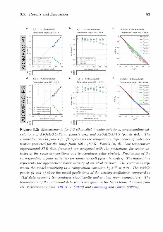
3.5. Results and Discussion 83
3F3 3F2 3F4 3F6 3F8 1F3
mole fraction xXH2OP
3F3
3F2
3F4
3F6
3F8
1F3
activity
aXxP
H2O X1P A 1I2MEthanediol X2P
Temperature range: 225 MM 267 K
EXP: 1I2MethanediolAwater γw
EXP: 1I2MethanediolAwater γorg
AIOMFAC γw
AIOMFAC γorg
H2O X1P A 1I2MEthanediol X2P
153 483KTemperature range: MM
3F3 3F2 3F4 3F6 3F8 1F3
xorgX2P
3F3
3F2
3F4
3F6
3F8
1F3
activity
aw
AIOMFACMP1
3F3 3F2 3F4 3F6 3F8 1F3
mole fraction xXH2OP
3F3
3F2
3F4
3F6
3F8
1F3
activity
aXxP
EXP: 1I2MethanediolAwater
AIOMFAC water activity aw
AIOMFAC organic activity aorg
ideal aw
AIOMFACMP3
H2O X1P A 1I2MEthanediol X2P
Temperature range: 225 MM 267 K
3F3 3F2 3F4 3F6 3F8 1F3
mole fraction xXH2OP
3F3
3F2
3F4
3F6
3F8
1F3
activitycoeffFγXxP
EXP: 1I2MethanediolAwater γw
EXP: 1I2MethanediolAwater γorg
AIOMFAC γw
AIOMFAC γorg
H2O X1P A 1I2MEthanediol X2P
153 483KTemperature range: MM
223
243
263
TXKP
223
243
263
TXKP
363383433423443
TXKP
363383433423443
TXKP
a b c
d e f
Figure 3.2: Measurements for 1,2-ethanediol + water solutions, corresponding cal-
culations of AIOMFAC-P1 in (panels a-c) and AIOMFAC-P3 (panels d-f). The
coloured curves in panels (c, f) represents the temperature dependence of water ac-
tivities predicted for the range from 150 - 480 K. Panels (a, d): Low temperature
experimental SLE data (crosses) are compared with the predictions for water ac-
tivity at the same compositions and temperatures (blue circles). Predictions of the
corresponding organic activities are shown as well (green triangles). The dashed line
represents the hypothetical water activity of an ideal mixture. The error bars rep-
resent the model sensitivity to a composition variation by xtol = 0.01. The middle
panels (b and e) show the model predictions of the activity coefficients compared to
VLE data covering temperatures significantly higher than room temperature. The
temperature of the individual data points are given in the boxes below the main pan-
els. Experimental data: Ott et al. (1972) and Gmehling and Onken (2003a).

84 Chapter 3. Improved AIOMFAC temperature dependenceAIOMFACuP1
AIOMFACuP3
a b c
d e f
K9K K92 K94 K96 K98 19K
mole fraction x_H2Od
K9K
K92
K94
K96
K98
19K
activity
a_xd
K9K K92 K94 K96 K98 19K
mole fraction x_H2Od
K9K
K95
19K
195
29K
295
activitycoeff9γ_xd
K9K K92 K94 K96 K98 19K
xorg_2d
K9K
K92
K94
K96
K98
19K
activity
aw
EXP: Acetic_acidTwater
AIOMFAC water activity aw
AIOMFAC organic activity aorg
ideal aw
EXP: acetic_acidTwater γw
EXP: acetic_acidTwater γorg
AIOMFAC γw
AIOMFAC γorg
K9K K92 K94 K96 K98 19K
mole fraction x_H2Od
K9K
K92
K94
K96
K98
19K
activity
a_xd
K9K K92 K94 K96 K98 19K
mole fraction x_H2Od
K9K
K95
19K
195
29K
295
activitycoeff9γ_xd
K9K K92 K94 K96 K98 19K
xorg_2d
K9K
K92
K94
K96
K98
19K
activity
aw
H2O _1d T Acetic_acid _2d
Temperature range: 249 uu 272 K
H2O _1d T Acetic_acid _2d
Temperature range: 249 uu 272 K
H2O _1d T Acetic_acid _2d
Temperature range: 373 uu 386 K
H2O _1d T Acetic_acid _2d
Temperature range: 373 uu 386 K
H2O _1d T Acetic_acid _2d
15K 48KKTemperature range: uu
H2O _1d T Acetic_acid _2d
15K 48KKTemperature range: uu
37K
38K
39K
T_Kd
37K
38K
39K
T_Kd
EXP: acetic_acidTwater γw
EXP: acetic_acidTwater γorg
AIOMFAC γw
AIOMFAC γorg
EXP: Acetic_acidTwater
AIOMFAC water activity aw
AIOMFAC organic activity aorg
ideal aw
Figure 3.3: Measurements for acetic acid + water solutions, corresponding calcu-
lations of AIOMFAC-P1 in and AIOMFAC-P3. The coloured curves in panels (c,
f) represents the temperature dependence of water activities predicted for the range
from 150 - 480 K. Panels (a, d): Low temperature experimental SLE data (crosses)
are compared with the predictions for water activity at the same compositions and
temperatures (blue circles). Predictions of the corresponding organic activities are
shown as well (green triangles). The dashed line represents the hypothetical water
activity of an ideal mixture. The error bars represent the model sensitivity to a
composition variation by xtol = 0.01. The middle panels (b and e) show the model
predictions of the activity coefficients compared to VLE data covering temperatures
significantly higher than room temperature. The temperature of the individual data
points are given in the boxes below the main panels. Experimental data: Faucon
(1910) and Narayana et al. (1985).

3.5. Results and Discussion 85
and its comparison with the predictions from AIOMFAC-P1 and AIOMFAC-
P3. In the panels a and c water is the component in equilibrium with ice
(hence the data describes the ice melting curve at different T and mixture
composition), while panels b and e show analogous data for the malonic acid
melting curve. The temperature ranges are slightly different, with the highest
temperature in the plots referring to the melting temperature of the pure com-
ponent or the SLE at the highest concentration of the organic, respectively.
The predicted aw shows slight deviations from the experimental data towards
lower water activities for both AIOMFAC-P1 and AIOMFAC-P3 (panels a, d).
The predicted aorg (in a range closer to and above room temperature) is well
represented in both AIOMFAC-P1 and AIOMFAC-P3 (b, e). No VLE data
is available for aqueous malonic acid at higher temperatures and hence could
not be compared. AIOMFAC-P3 predicts a larger temperature dependence
in comparison to AIOMFAC-P1 which shows a relatively small temperature
dependence of water activity at higher temperatures (panels c, f).
Figure. 3.5 shows an example of a binary system consisting of water and
2-butanone with a miscibility gap present over a large temperature and com-
position range. Both model parameterisations show deviations from the SLE
data (panels a, d). However, the AIOMFAC-P3 parameterisation clearly re-
duces the deviations from the experimental data in comparison to AIOMFAC-
P1, the latter showing deviations up to > 0.3 in aw at low water contents.
On the other hand, at the higher temperatures covered by VLE data, both
AIOMFAC-P1 (Fig. 3.5 b) and AIOMFAC-P3 (Fig. 3.5 e) are in good agree-
ment with the experimental data. A miscibility gap is also predicted by both
AIOMFAC parameterisations, although the width and temperature range of
the predicted phase separations do differ between the model results. Accord-
ing to the AIOMFAC-P3 prediction, a phase separation would occur in the
temperature range 150 to ≈ 390 K in the composition space bounded by one
of the local maxima of aw a horizontal line intersecting with the aw curve at
another xorg value. A miscibility gap is also found in the experiments and
is the reason why in panels (a, b, d, e) there are no data points in the mole
fraction range 0.35 < x(H2O) < 0.85.
Figure. 3.6 shows the model-measurement comparison for aqueous 2-
butoxyethanol. AIOMFAC-P1 and AIOMFAC-P3 show similar performance.

86 Chapter 3. Improved AIOMFAC temperature dependence
Both models are not in good agreement with the experimental data. Contrary
to the experimental data, both AIOMFAC-P1 and AIOMFAC-P3 predict aw> 1, implying a liquid-liquid phase separation over a wide range of tempera-
tures, explaining the reason for deviations in predicted water activity shown
in Fig. 3.6 (a, d) (see also local maxima in aw curves of panels c, d). Note that
the model predictions in these figures do not include phase separation compu-
tations on purpose, since the experimental data are for a homogenous single
phase and so are the model calculations here. Also, at higher temperatures
the activity coefficients of both water and 2-butoxyethanol show deviation
from experimental data (panels b, e). AIOMFAC-P3 (panel f) shows a larger
temperature dependence over the entire temperature range in comparison to
AIOMFAC-P1 (panel c).
3.5.2 Binary organic mixtures
Figure. 3.7 shows the water-free mixture of cyclohexanol + adipic acid. The
AIOMFAC-P3 prediction is in better agreement with the experimental data
than AIOMFAC-P1, which shows a positive deviation at lower mole fractions
of component 1 (cyclohexanol). In this binary system, the AIOMFAC-P3
parameterisation leads to a relatively large temperature dependence of the
activity of cyclohexanol, aorg(1), (panel d). In addition, with that parame-
terisation a phase separation occurs at lower xorg(2) values for temperatures
below ∼ 180 K. However, no phase separation is expected at higher temper-
atures, more relevant in the troposphere. AIOMFAC-P1 on the other hand
shows a much smaller temperature dependence and does not predict a phase
separation.
Measurements for water-free binary organic mixtures of ethanol + acetone
are shown in Fig. 3.8. The AIOMFAC-P3 predictions of the activities of ace-
tone are in a very good agreement with the experimental SLE derived data
(panel d), while AIOMFAC-P1 shows larger deviations from the experimental
data at these low temperatures (panel a). At high temperatures, the VLE
data for both AIOMFAC-P1 and AIOMFAC-P3 show similar results (Panel
b, d), with slightly larger deviations of γ(x)org2 (activity coefficient of acetone)
in AIOMFAC-P1. At temperatures higher than 300 K both AIOMFAC-P1

3.5. Results and Discussion 87
and AIOMFAC-P3 show a much smaller temperature dependence than for
the range below room temperature.
Figure. 3.9 shows a similar example, for ethanol + 3-heptanone mixtures. The
prediction from AIOMFAC-P3 is in relatively good agreement with the ex-
perimental SLE data, showing less deviations in 3-heptanone activities than
the results from the AIOMFAC-P1 calculations. Achieving better agreement
with the new (AIOMFAC-P3) parameterisation requires a larger temperature
dependence of the organic activities, particularly towards lower temperatures.
Figure. 3.10 shows the binary ethanol + diethyl ether system, where experi-
mental data are available for a temperature range of more than 200 K: from
149 K up to 378 K. Of course, additional data from other systems of our
database are also affecting the main group interaction parameters that are
necessary to describe this system with AIOMFAC-P3. Both models describe
the diethyl ether activity derived from SLE at low temperatures quite well
(panels a and d). AIOMFAC-P3 shows slight overprediction of the diethyl
ether activity, while AIOMFAC-P1 tends to underpredict the experimental
data. In contrast, at higher temperatures (∼ 350 to 380 K) covered by exper-
imental VLE data (panels b and e), the predicted γ(x)org2 both by AIOMFAC-
P1 and AIOMFAC-P3 are not in good agreement with the VLE experimental
data. The main reason for the observed deviations is due to inaccurately
predicted activity coefficients at infinite dilution (i.e., when one of the com-
pounds is present only as a tiny mole fraction in the solution) of the two
organic compounds at these temperatures. At infinite dilution conditions the
activity coefficients are dominated by subgroup properties in the UNIFAC
/ AIOMFAC model, so that the activity coefficient values are largely unaf-
fected by the new main group interaction parameterisation of AIOMFAC-P3
in comparison to AIOMFAC-P1. As is visible from Fig. 3.10 (c,f), particularly
at x(diethyl ether) > 0.4, the temperature dependence of ethanol activities
predicted by AIOMFAC-P3 is larger than the original one in AIOMFAC-P1.
The example of this system shows that it is not always possible to achieve
good model predictions for the full temperature range with the new treatment
of temperature dependence in AIOMFAC. For further improvements, other
model parts, such as the lattice constant (z), which is not really a constant,

88 Chapter 3. Improved AIOMFAC temperature dependence
would need to be considered for the introduction of additional, physically
meaningful temperature dependent parameterisations.
3.5.3 Scope and limitations of the new parameterisation
The thermodynamic model AIOMFAC has been developed based on modified
versions of UNIFAC and LIFAC (Yan et al., 1999), with the aim to establish
a versatile activity coefficient model for atmospheric applications. The new
parameterisation of the model aims at improving AIOMFAC predictions par-
ticularly at lower temperatures of atmospheric relevance. Deviations between
the experimental data and model predictions from the new AIOMFAC-P3 ver-
sion are associated with either the inaccuracy of the measurements, the lack of
data to better cover and parameterise the model for a wide composition and
temperature range, or limitations of the AIOMFAC expressions and the un-
derlying group contribution method. Own measurements were performed for
selected aqueous organic systems at low temperature and temperature around
room temperature, which were used together with experimental data from the
literature database for parameterising the model over a wider temperature
range. The complexity of organics in terms of their physical and chemical
properties such as size, shape and combinations of groups in multifunctional
molecules are important factors that influence the quality of AIOMFAC pre-
dictions.
Most of the SLE data at low temperature are limited to simple organic
molecules, which thus make up the majority of the model parameterisation
database. Due to this, the accuracy of AIOMFAC predictions is expected to
decrease with increasing complexity of multifunctional organic compounds.
However, the new AIOMFAC parameterisation provides a tool to predict ac-
tivity coefficients with better overall accuracy than the previous version and
offers the versatility of a group-contribution method for the prediction of ac-
tivity coefficients in complex mixtures containing many tens to thousands of
individual components.

3.5. Results and Discussion 89
AIOMFACXP1
AIOMFACXP3
a b c
d e f
0w0 0w2 0w4 0w6 0w8 1w0
mole fraction xgH2O:
0w0
0w2
0w4
0w6
0w8
1w0
activity
agx:
H2O g1: K Malonic_acid g2:
Temperature range: 262 XX 273 K
EXP: malonic_acidKwater
AIOMFAC water activity aw
AIOMFAC organic activity aorg
ideal aw
H2O g1: K Malonic_acid g2:
Temperature range: 262 XX 273 K
H2O g1: K Malonic_acid g2:
Temperature range: 278 XX 338 K
0w0 0w2 0w4 0w6 0w8 1w0
mole fraction xgH2O:
0w0
0w2
0w4
0w6
0w8
1w0
activity
agx:
EXP: malonic_acidKwater
AIOMFAC water activity aw
AIOMFAC organic activity aorg
ideal aw
0w0 0w2 0w4 0w6 0w8 1w0
mole fraction xgH2O:
0w0
0w2
0w4
0w6
0w8
1w0
activity
agx:
EXP: Malonic_acidKwater
AIOMFAC water activity aw
AIOMFAC organic activity aorg
ideal aw
H2O g1: K Malonic_acid g2:
Temperature range: 278 XX 338 K
0w0 0w2 0w4 0w6 0w8 1w0
mole fraction xgH2O:
0w0
0w2
0w4
0w6
0w8
1w0
activity
agx:
EXP: Malonic_acidKwater
AIOMFAC water activity aw
AIOMFAC organic activity aorg
ideal aw
0w0 0w2 0w4 0w6 0w8 1w0
xorgg2:
0w0
0w2
0w4
0w6
0w8
1w0
activity
aw
0w0 0w2 0w4 0w6 0w8 1w0
xorgg2:
0w0
0w2
0w4
0w6
0w8
1w0
activity
aw
H2O g1: K Malonic_acid g2:
150 480KTemperature range: XX
H2O g1: K Malonic_acid g2:
150 480KTemperature range: XX
250260270280
TgK:
250260270280
TgK:
280300320340
TgK:
280300320340
TgK:
Figure 3.4: Measurements for malonic acid + water solutions, corresponding cal-
culations of AIOMFAC-P1 in (panels a-c) and AIOMFAC-P3 (panels d-f). Panels
(c, f) show the temperature dependence of water activities predicted for the range
from 150 - 480 K. Panels(a, d): Low temperature experimental SLE data (crosses)
are compared with the predictions for water activity at the same compositions and
temperatures (blue circles). Predictions of the corresponding organic activities are
shown as well (green triangles) while panels b and e show analogous data for the
malonic acid melting curve. The error bars represent the model sensitivity to a com-
position variation by xtol =0.01. The dashed line represents the hypothetical water
activity of an ideal mixture. The temperature of the individual data points are given
in the boxes below the main panels. Experimental data: Braban et al. (2003) and
Apelblat and Manzurola (1987).

90 Chapter 3. Improved AIOMFAC temperature dependenceAIOMFACXP5
AIOMFACXP3
a b c
d e f
dbd db2 db4 db6 db8 5bd
mole fraction x:H2O9
dbd
db2
db4
db6
db8
5bd
activity
a:x9
H2O :59 K 2XButanone :29
Temperature range: 598 XX 273 K
EXP: 2XbutanoneKwater
AIOMFAC water activity aw
AIOMFAC organic activity aorg
ideal aw
H2O :59 K 2XButanone :29
Temperature range: 353 XX 326 K
dbd db2 db4 db6 db8 5bd
mole fraction x:H2O9
d
5
5d
55
2d
activitycoeffbγ:x9
EXP: waterK2Xbutanone γw
EXP: waterK2Xbutanone γorg
AIOMFAC γw
AIOMFAC γorg
dbd db2 db4 db6 db8 5bd
xorg:29
dbd
db2
db4
db6
db8
5bd
activity
aw
dbd db2 db4 db6 db8 5bd
xorg:29
dbd
db2
db4
db6
db8
5bd
activity
aw
55d 48dK
H2O :59 K 2XButanone :29
Temperature range: XX
55d 48dK
H2O :59 K 2XButanone :29
Temperature range: XX
H2O :59 K 2XButanone :29
Temperature range: 353 XX 326 K
dbd db2 db4 db6 db8 5bd
mole fraction x:H2O9
d
5
5d
55
2d
activitycoeffbγ:x9
EXP: waterK2Xbutanone γw
EXP: waterK2Xbutanone γorg
AIOMFAC γw
AIOMFAC γorg
H2O :59 K 2XButanone :29
Temperature range: 598 XX 273 K
2dd22d24d26d28d
T:K9
2dd22d24d26d28d
T:K9
dbd db2 db4 db6 db8 5bd
mole fraction x:H2O9
dbd
db2
db4
db6
db8
5bd
activity
a:x9
EXP: 2XbutanoneKwater
AIOMFAC water activity aw
AIOMFAC organic activity aorg
ideal aw
35d
32d
33d
T:K9
35d
32d
33d
T:K9
Figure 3.5: Measurements for 2-butanone + water solutions, corresponding calcu-
lations of AIOMFAC-P1 in (panels a-c) and AIOMFAC-P3 (panels d-f). Panels
(c, f) show the temperature dependence of water activities predicted for the range
from 150 - 480 K. Panels (a, d): Low temperature experimental SLE data (crosses)
are compared with the predictions for water activity at the same compositions and
temperatures (blue circles). Predictions of the corresponding organic activities are
shown as well (green triangles). The error bars represent the model sensitivity to
a composition variation by xtol =0.01. The dashed line represents the hypothetical
water activity of an ideal mixture. The middle panels (b and e) show the model
predictions of the activity coefficients compared to VLE data covering temperatures
significantly higher than room temperature. The temperature of the individual data
points are given in the boxes below the main panels. Experimental data: Lohmann
et al. (1997) and Gmehling et al. (1981).

3.5. Results and Discussion 91
AIOMFACEPd
AIOMFACEP3
a b c
d e f
wXw wX9 wX4 wX6 wX8 dXw
mole fraction xgH9O:
wXw
wX9
wX4
wX6
wX8
dXw
activity
agx:
H9O gd: 7 9EButoxyethanol g9:
Temperature range: 959 EE 973 K
H9O gd: 7 9EButoxyethanol g9:
Temperature range: 959 EE 973 K
EXP: 9Ebutoxyethanol7water
AIOMFAC water activity aw
AIOMFAC organic activity aorg
ideal aw
wXw wX9 wX4 wX6 wX8 dXw
mole fraction xgH9O:
wXw
wX9
wX4
wX6
wX8
dXw
activity
agx:
EXP: 9Ebutoxyethanol7water
AIOMFAC water activity aw
AIOMFAC organic activity aorg
ideal aw
H9O gd: 7 9EButoxyethanol g9:
Temperature: 383 K
H9O gd: 7 9EButoxyethanol g9:
Temperature: 383 K
wXw wX9 wX4 wX6 wX8 dXw
mole fraction xgH9O:
wXw
wX5
dXw
dX5
9Xw
9X5
3Xw
activitycoeffXγgx:
EXP: 9Ebutoxyethanol7water γw
EXP: 9Ebutoxyethanol7water γorg
AIOMFAC γw
AIOMFAC γorg
wXw wX9 wX4 wX6 wX8 dXw
mole fraction xgH9O:
wXw
wX5
dXw
dX5
9Xw
9X5
3Xw
activitycoeffXγgx:
EXP: 9Ebutoxyethanol7water γw
EXP: 9Ebutoxyethanol7water γorg
AIOMFAC γw
AIOMFAC γorg
H9O gd: 7 9EButoxyethanol g9:
d5w 48wKTemperature range: EE
wXw wX9 wX4 wX6 wX8 dXw
xorgg9:
wXw
wX9
wX4
wX6
wX8
dXw
activity
aw
wXw wX9 wX4 wX6 wX8 dXw
xorgg9:
wXw
wX9
wX4
wX6
wX8
dXw
activity
aw
H9O gd: 7 9EButoxyethanol g9:
d5w 48wKTemperature range: EE
94w95w96w97w98w
TgK:
94w95w96w97w98w
TgK:
38w
39w
TgK:
38w
39wTgK:
Figure 3.6: Measurements for 2-butoxyethanol + water solutions, corresponding
calculations of AIOMFAC-P1 in (panels a-c) and AIOMFAC-P3 (panels d-f). Pan-
els (c, f) show the temperature dependence of water activities predicted for the range
from 150 - 480 K. Panels (a, d): Low temperature experimental SLE data (crosses)
are compared with the predictions for water activity at the same compositions and
temperatures (blue circles). Predictions of the corresponding organic activities are
shown as well (green triangles). The error bars represent the model sensitivity to
a composition variation by xtol =0.01. The dashed line represents the hypothetical
water activity of an ideal mixture. The middle panels (b and e) show the model
predictions of the activity coefficients compared to VLE data covering temperatures
significantly higher than room temperature. The temperature of the individual data
points are given in the boxes below the main panels. Experimental data: Koga et al.
(1994) and Schneider and Wilhelm (1959).

92 Chapter 3. Improved AIOMFAC temperature dependence
AIOMFAC5P7
AIOMFAC5P3
a b
d
=K= =K2 =K4 =K6 =K8 7K=
mole fraction x+7h
=K=
=K2
=K4
=K6
=K8
7K=
activity
a+xh
org
EXP: Adipic_aciducyclohexanol
AIOMFAC organic activity aorg7AIOMFAC organic activity aorg2ideal aorg
Cyclohexanol +7h u Adipic_acid +2h
Temperature range: 299 55 352 K
=K= =K2 =K4 =K6 =K8 7K=
xorg+2h
=K=
=K2
=K4
=K6
=K8
7K=
activity
aorg+7h
=K= =K2 =K4 =K6 =K8 7K=
mole fraction x+7h
=K=
=K2
=K4
=K6
=K8
7K=
activity
a+xh
org
Cyclohexanol +7h u Adipic_acid +2h
Temperature range: 299 55 352 K
Cyclohexanol +7h u Adipic_acid +2h
75= 48=Temperature range: 55 K
Cyclohexanol +7h u Adipic_acid +2h
75= 48=Temperature range: 55 K
=K= =K2 =K4 =K6 =K8 7K=
xorg+2h
=K=
=K2
=K4
=K6
=K8
7K=
activity
aorg+7h
EXP: Adipic_aciducyclohexanol
AIOMFAC organic activity aorg7AIOMFAC organic activity aorg2ideal aorg
aorg+7h9 T = 75= K
aorg+7h9 T = 78= K
aorg+7h9 T = 27= K
aorg+7h9 T = 24= K
aorg+7h9 T = 27= K
aorg+7h9 T = 3== K
aorg+7h9 T = 33= K
aorg+7h9 T = 36= K
aorg+7h9 T = 39= K
aorg+7h9 T = 42= K
aorg+7h9 T = 45= K
aorg+7h9 T = 48= K
aorg+7h9 T = 75= K
aorg+7h9 T = 78= K
aorg+7h9 T = 27= K
aorg+7h9 T = 24= K
aorg+7h9 T = 27= K
aorg+7h9 T = 3== K
aorg+7h9 T = 33= K
aorg+7h9 T = 36= K
aorg+7h9 T = 39= K
aorg+7h9 T = 42= K
aorg+7h9 T = 45= K
aorg+7h9 T = 48= K
c
3==32=34=36=
T+Kh
3==32=34=36=
T+Kh
Figure 3.7: Measurements for cyclohexanol + adipic acid solutions, corresponding
calculations of AIOMFAC-P1 in panels (a, b) and AIOMFAC-P3 (c, d). Panels
(b, d) represent the temperature dependence predictions from AIOMFAC-P1 and
AIOMFAC-P3 for temperature range of 150 - 480 K. Panel (a, c): SLE of adipic
acid shown vs. mole fraction of cyclohexanol (component 1). The error bars rep-
resent the model sensitivity to a composition variation by xtol = 0.01. The dashed
line is the ideal solution curve for component 1. The temperature of the individual
data points are given in the boxes below the main panels. Experimental data: Lihua
et al. (2007).
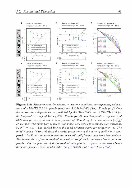
3.5. Results and Discussion 93
AIOMFAC5P1
AIOMFAC5P3
a b c
d e f
9,9 9,2 9,4 9,6 9,8 1,9
mole fraction x:17
9,9
9,2
9,4
9,6
9,8
1,9
activity
a:x7
org
Ethanol :17 X Acetone :27
Temperature range: 164 55 173 K
EXP: ethanolXacetone
AIOMFAC organic activity aorg1
AIOMFAC organic activity aorg2
ideal aorg
Ethanol :17 X Acetone :27
Temperature range: 339 55 359 K
9,9 9,2 9,4 9,6 9,8 1,9
mole fraction x:17
9,9
9,5
1,9
1,5
2,9
activitycoeff,γ(x7
EXP: ethanolXacetone γorg1:x7
EXP: ethanolXacetone γorg2:x7
AIOMFAC γorg1:x7
AIOMFAC γorg2:x7
Ethanol :17 X Acetone :27
159 489KTemperature range: 55
9,9 9,2 9,4 9,6 9,8 1,9
xorg:27
9,9
9,2
9,4
9,6
9,8
1,9
activity
aorg:17
aorg:17d T = 159 K
aorg:17d T = 189 K
aorg:17d T = 219 K
aorg:17d T = 249 K
aorg:17d T = 279 K
aorg:17d T = 399 K
aorg:17d T = 339 K
aorg:17d T = 369 K
aorg:17d T = 399 K
aorg:17d T = 429 K
aorg:17d T = 459 K
aorg:17d T = 489 K
9,9 9,2 9,4 9,6 9,8 1,9
mole fraction x:17
9,9
9,2
9,4
9,6
9,8
1,9
1,2
1,4
1,6
1,8
activitycoeff,γ:x7
Ethanol :17 X Acetone :27
Temperature range: 339 55 359 K
EXP: ethanolXacetone γorg1:x7
EXP: ethanolXacetone γorg2:x7
AIOMFAC γorg1:x7
AIOMFAC γorg2:x7
Ethanol :17 X Acetone :27
Temperature range: 164 55 173 K
EXP: ethanolXacetone
AIOMFAC organic activity aorg1
AIOMFAC organic activity aorg2
ideal aorg
169
179
189
T:K7
169
179
189
T:K7
Figure 3.8: Measurements for ethanol + acetone solutions, corresponding calcula-
tions of AIOMFAC-P1 in panels (a-c) and AIOMFAC-P3 (d-e). Panels (c, f) show
the temperature dependence as predicted by AIOMFAC-P1 and AIOMFAC-P3 for
the temperature range of 150 - 480 K. Panels (a, d): Low temperature experimental
SLE data (crosses), shown as mole fraction of ethanol, x(1), versus activity (a(x)org2)
of acetone. The error bars represent the model sensitivity to a composition variation
by xtol = 0.01. The dashed line is the ideal solution curve for component 1. The
middle panels (b and e) show the model predictions of the activity coefficients com-
pared to VLE data covering temperatures significantly higher than room temperature.
The temperature of the individual data points are given in the boxes below the main
panels. The temperature of the individual data points are given in the boxes below
the main panels. Experimental data: Sapgir (1929) and Amer et al. (1956).
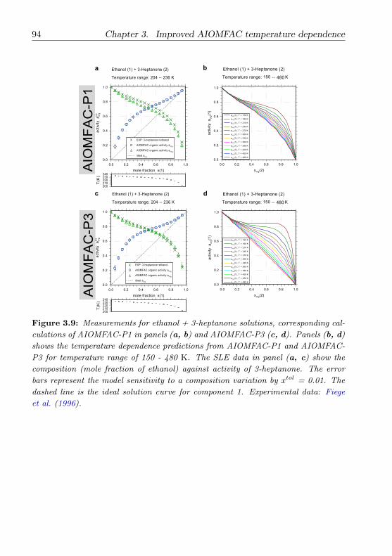
94 Chapter 3. Improved AIOMFAC temperature dependence
AIOMFACxPd
AIOMFACxP3
a b
d
aorg:d.i T = d5X K
aorg:d.i T = d8X K
aorg:d.i T = 2dX K
aorg:d.i T = 24X K
aorg:d.i T = 27X K
aorg:d.i T = 3XX K
aorg:d.i T = 33X K
aorg:d.i T = 36X K
aorg:d.i T = 39X K
aorg:d.i T = 42X K
aorg:d.i T = 45X K
aorg:d.i T = 48X K
c
Ethanol :d. c 3xHeptanone :2.
Temperature range: 2X4 xx 236 K
XvX Xv2 Xv4 Xv6 Xv8 dvX
mole fraction x:d.
XvX
Xv2
Xv4
Xv6
Xv8
dvX
activity
a:x.
org
EXP: 3xheptanonecethanol
AIOMFAC organic activity aorgdAIOMFAC organic activity aorg2ideal aorg
Ethanol :d. c 3xHeptanone :2.
d5X 48XTemperature range: xx K
XvX Xv2 Xv4 Xv6 Xv8 dvX
xorg:2.
XvX
Xv2
Xv4
Xv6
Xv8
dvX
activity
aorg:d.
XvX Xv2 Xv4 Xv6 Xv8 dvX
mole fraction x:d.
XvX
Xv2
Xv4
Xv6
Xv8
dvX
activity
a:x.
org
EXP: 3xheptanonecethanol
AIOMFAC organic activity aorgdAIOMFAC organic activity aorg2ideal aorg
Ethanol :d. c 3xHeptanone :2.
Temperature range: 2X4 xx 236 K
XvX Xv2 Xv4 Xv6 Xv8 dvX
xorg:2.
XvX
Xv2
Xv4
Xv6
Xv8
dvXactivity
aorg:d.
Ethanol :d. c 3xHeptanone :2.
d5X 48XTemperature range: xx K
aorg:d.i T = d5X K
aorg:d.i T = d8X K
aorg:d.i T = 2dX K
aorg:d.i T = 24X K
aorg:d.i T = 27X K
aorg:d.i T = 3XX K
aorg:d.i T = 33X K
aorg:d.i T = 36X K
aorg:d.i T = 39X K
aorg:d.i T = 42X K
aorg:d.i T = 45X K
aorg:d.i T = 48X K
2XX2dX22X23X24X
T:K.
2XX2dX22X23X24X
T:K.
Figure 3.9: Measurements for ethanol + 3-heptanone solutions, corresponding cal-
culations of AIOMFAC-P1 in panels (a, b) and AIOMFAC-P3 (c, d). Panels (b, d)
shows the temperature dependence predictions from AIOMFAC-P1 and AIOMFAC-
P3 for temperature range of 150 - 480 K. The SLE data in panel (a, c) show the
composition (mole fraction of ethanol) against activity of 3-heptanone. The error
bars represent the model sensitivity to a composition variation by xtol = 0.01. The
dashed line is the ideal solution curve for component 1. Experimental data: Fiege
et al. (1996).

3.5. Results and Discussion 95
AIOMFACxPX
AIOMFACxP3
a b c
d e f
aorgmXp. T = X5f K
aorgmXp. T = X8f K
aorgmXp. T = dXf K
aorgmXp. T = d4f K
aorgmXp. T = d7f K
aorgmXp. T = 3ff K
aorgmXp. T = 33f K
aorgmXp. T = 36f K
aorgmXp. T = 39f K
aorgmXp. T = 4df K
aorgmXp. T = 45f K
aorgmXp. T = 48f K
Ethanol mXp : Diethyl_ether mdp
X5f 48fKTemperature range: xx
fcf fcd fc4 fc6 fc8 Xcf
xorgmdp
fcf
fcd
fc4
fc6
fc8
Xcf
activity
aorgmXp
Ethanol mXp : Diethyl_ether mdp
X5f 48fKTemperature range: xx
fcf fcd fc4 fc6 fc8 Xcf
xorgmdp
fcf
fcd
fc4
fc6
fc8
Xcf
activity
aorgmXp
aorgmXp. T = X5f K
aorgmXp. T = X8f K
aorgmXp. T = dXf K
aorgmXp. T = d4f K
aorgmXp. T = d7f K
aorgmXp. T = 3ff K
aorgmXp. T = 33f K
aorgmXp. T = 36f K
aorgmXp. T = 39f K
aorgmXp. T = 4df K
aorgmXp. T = 45f K
aorgmXp. T = 48f K
Ethanol mXp : Diethyl_ether mdp
Temperature range: 34d xx 378 K
Ethanol mXp : Diethyl_ether mdp
Temperature range: 34d xx 378 K
fcf fcd fc4 fc6 fc8 Xcf
mole fraction xmXp
f
X
d
3
4
5
6
7
8
9
activitycoeffcγmxp
EXP: diethyl_ether:ethanol γorgXmxp
EXP: diethyl_ether:ethanol γorgdmxp
AIOMFAC γorgXmxp
AIOMFAC γorgdmxp
fcf fcd fc4 fc6 fc8 Xcf
mole fraction xmXp
f
X
d
3
4
5
6
7
8
9
activitycoeffcγmxp
EXP: diethyl_ether:ethanol γorgXmxp
EXP: diethyl_ether:ethanol γorgdmxp
AIOMFAC γorgXmxp
AIOMFAC γorgdmxp
fcf fcd fc4 fc6 fc8 Xcf
mole fraction xmXp
fcf
fcd
fc4
fc6
fc8
Xcf
activity
amxp
org
EXP: diethyl_ether:ethanol
AIOMFAC organic activity aorgXAIOMFAC organic activity aorgdideal aorg
fcf fcd fc4 fc6 fc8 Xcf
mole fraction xmXp
fcf
fcd
fc4
fc6
fc8
Xcf
activity
amxp
org
EXP: diethyl_ether:ethanol
AIOMFAC organic activity aorgXAIOMFAC organic activity aorgdideal aorg
X4f
X5f
X6f
TmKp
Ethanol mXp : Diethyl_ether mdp
Temperature range: X49 xx X56 K
Ethanol mXp : Diethyl_ether mdp
Temperature range: X49 xx X56 K
X4f
X5f
X6f
TmKp
34f35f36f37f38f
TmKp
34f35f36f37f38f
TmKp
Figure 3.10: Measurements for ethanol + diethyl ether solutions, corresponding
calculations of AIOMFAC-P1 and AIOMFAC-P3. Panels (c, f) show the tem-
perature dependence of the ethanol activity, as predicted by AIOMFAC-P1 and
AIOMFAC-P3 for the temperature range 150 - 480 K. Panel (a,d): Experimen-
tal SLE data (crosses) compared with model predictions (triangles) for the activity
of diethyl ether in the very low temperature range 149 to 156 K. The dashed line
is the ideal solution curve for component 1. The middle panels (b and e) show the
model predictions of the activity coefficients compared to VLE data covering temper-
atures significantly higher than room temperature. The temperature of the individual
data points are given in the boxes below the main panels. Experimental data:Lalande
(1934) and Moeller et al. (1951).
96 Chapter 3. Improved AIOMFAC temperature dependence
3.6 Conclusions
An improved temperature dependence parameterisation of aqueous organic
and binary organic water-free mixtures is presented for the thermodynamic
group contribution model AIOMFAC. A comprehensive database of experi-
mental thermodynamic equilibria data is established by collecting and care-
fully validating different data types covering a wide temperature and concen-
tration range. In addition, new measurements that have been performed for
selected aqueous organic systems, at room temperature and below, were also
included in the database. The database is used to determine new AIOM-
FAC group interaction parameters for organic main groups of atmospheric
relevance: carboxyl, hydroxyl, ketone, aldehyde, ether, ester, alkyl, aromatic
carbon-alcohol, and aromatic hydrocarbons. The parameter fitting proce-
dure involved the simultaneous determination of 150 interaction parameters
for the 14 main groups. Thus, the new temperature dependence parame-
terisation allows to calculate activity coefficients and their temperature de-
pendence for a wide variety of organic and water-free mixtures. In general,
the new AIOMFAC parameterisation achieves good agreement with a large
number of experimental datasets. In the case of some organic systems, lack
of experimental data to constrain the activity coefficients is a major limi-
tation. Further improvements of the AIOMFAC model description of these
systems and by that, the interactions of the functional groups involved, will
require additional measurements over a wide temperature and concentration
range.The improved AIOMFAC model can be used to better account for the
temperature dependence of activity coefficients relevant in predictions related
to atmospheric ice nucleation and gas-particle partitioning in multicomponent
systems.
Acknowledgements
This work was supported by the Swiss National Foundation, project 200020-
125151 and by the CCES projects IMBALANCE and OPTIWARES funded
by the ETH Domain.
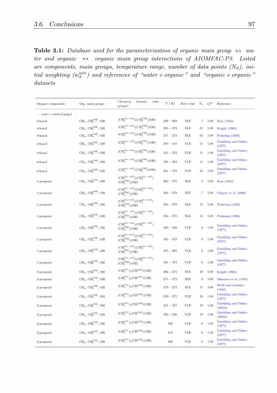
3.6. Conclusions 97
Table 3.1: Database used for the parameterisation of organic main group ↔ wa-
ter and organic ↔ organic main group interactions of AIOMFAC-P3. Listed
are components, main groups, temperature range, number of data points (Nd), ini-
tial weighting (winitd ) and references of “water + organic ” and “organic + organic ”
datasets
Organic compounds Org. main groupsChemical formula (sub-
groups)T ( K) Data type Nd winit
d Reference
— water + alcohol/polyol —
ethanol CHn, CH[OH]n , OH (CH
[alc−tail]3 )(CH
[OH]2 )(OH) 220− 269 SLE 7 5.00 Ross (1954)
ethanol CHn, CH[OH]n , OH (CH
[alc−tail]3 )(CH
[OH]2 )(OH) 265− 273 SLE 31 5.00 Knight (1962)
ethanol CHn, CH[OH]n , OH (CH
[alc−tail]3 )(CH
[OH]2 )(OH) 211− 273 SLE 62 1.00 Pickering (1893)
ethanol CHn, CH[OH]n , OH (CH
[alc−tail]3 )(CH
[OH]2 )(OH) 307− 318 VLE 11 1.00
Gmehling and Onken
(1977)
ethanol CHn, CH[OH]n , OH (CH
[alc−tail]3 )(CH
[OH]2 )(OH) 341− 353 VLE 11 1.00
Gmehling and Onken
(1977)
ethanol CHn, CH[OH]n , OH (CH
[alc−tail]3 )(CH
[OH]2 )(OH) 350− 363 VLE 11 1.00
Gmehling and Onken
(1977)
ethanol CHn, CH[OH]n , OH (CH
[alc−tail]3 )(CH
[OH]2 )(OH) 351− 372 VLE 34 1.00
Gmehling and Onken
(1977)
1-propanol CHn, CH[OH]n , OH
(CH[alc−tail]3 )(CH
[alc−tail]2 )
(CH[OH]2 )(OH) 263− 270 SLE 3 5.00 Ross (1954)
1-propanol CHn, CH[OH]n , OH
(CH[alc−tail]3 )(CH
[alc−tail]2 )
(CH[OH]2 )(OH) 264− 270 SLE 7 5.00 Chapoy et al. (2008)
1-propanol CHn, CH[OH]n , OH
(CH[alc−tail]3 )(CH
[alc−tail]2 )
(CH[OH]2 )(OH) 264− 270 SLE 12 5.00 Pickering (1893)
1-propanol CHn, CH[OH]n , OH
(CH[alc−tail]3 )(CH
[alc−tail]2 )
(CH[OH]2 )(OH) 264− 270 SLE 14 5.00 Pickering (1893)
1-propanol CHn, CH[OH]n , OH
(CH[alc−tail]3 )(CH
[alc−tail]2 )
(CH[OH]2 )(OH) 330− 339 VLE 8 1.00
Gmehling and Onken
(1977)
1-propanol CHn, CH[OH]n , OH
(CH[alc−tail]3 )(CH
[alc−tail]2 )
(CH[OH]2 )(OH) 345− 355 VLE 8 1.00
Gmehling and Onken
(1977)
1-propanol CHn, CH[OH]n , OH
(CH[alc−tail]3 )(CH
[alc−tail]2 )
(CH[OH]2 )(OH) 355− 365 VLE 8 1.00
Gmehling and Onken
(1977)
1-propanol CHn, CH[OH]n , OH
(CH[alc−tail]3 )(CH
[alc−tail]2 )
(CH[OH]2 )(OH) 361− 372 VLE 8 1.00
Gmehling and Onken
(1977)
2-propanol CHn, CH[OH]n , OH (CH
[alc]3 )2(CH[OH])(OH) 266− 273 SLE 29 5.00 Knight (1962)
2-propanol CHn, CH[OH]n , OH (CH
[alc]3 )2(CH[OH])(OH) 271− 273 SLE 9 5.00 Okamoto et al. (1978)
2-propanol CHn, CH[OH]n , OH (CH
[alc]3 )2(CH[OH])(OH) 272− 273 SLE 17 5.00
Webb and Lindsley
(1934)
2-propanol CHn, CH[OH]n , OH (CH
[alc]3 )2(CH[OH])(OH) 353− 372 VLE 24 1.00
Gmehling and Onken
(1977)
2-propanol CHn, CH[OH]n , OH (CH
[alc]3 )2(CH[OH])(OH) 341− 357 VLE 19 1.00
Gmehling and Onken
(2003a)
2-propanol CHn, CH[OH]n , OH (CH
[alc]3 )2(CH[OH])(OH) 325− 340 VLE 19 1.00
Gmehling and Onken
(2003a)
2-propanol CHn, CH[OH]n , OH (CH
[alc]3 )2(CH[OH])(OH) 328 VLE 8 1.00
Gmehling and Onken
(1977)
2-propanol CHn, CH[OH]n , OH (CH
[alc]3 )2(CH[OH])(OH) 318 VLE 8 1.00
Gmehling and Onken
(1977)
2-propanol CHn, CH[OH]n , OH (CH
[alc]3 )2(CH[OH])(OH) 308 VLE 8 1.00
Gmehling and Onken
(1977)

98 Chapter 3. Improved AIOMFAC temperature dependence
Table 3.1: Continued.
Organic compounds Org. main groupsChemical formula (sub-
groups)T (K) Data type Nd winit
d Reference
1-butanol CHn, CH[OH]n , OH
(CH[alc−tail]3 )(CH
[alc−tail]2 )2
(CH[OH]2 )(OH) 271− 273 SLE 22 5.00 Knight (1962)
1-butanol CHn, CH[OH]n , OH
(CH[alc−tail]3 )(CH
[alc−tail]2 )2
(CH[OH]2 )(OH) 200− 273 SLE 10 5.00 Lohmann et al. (1997)
1-butanol CHn, CH[OH]n , OH
(CH[alc−tail]3 )(CH
[alc−tail]2 )2
(CH[OH]2 )(OH) 366− 384 VLE 12 1.00
Gmehling and Onken
(1977)
1-butanol CHn, CH[OH]n , OH
(CH[alc−tail]3 )(CH
[alc−tail]2 )2
(CH[OH]2 )(OH) 365− 382 VLE 8 1.00
Gmehling and Onken
(2003a)
1-butanol CHn, CH[OH]n , OH
(CH[alc−tail]3 )(CH
[alc−tail]2 )2
(CH[OH]2 )(OH) 323 VLE 4 1.00 Gmehling et al. (1988)
1-butanol CHn, CH[OH]n , OH
(CH[alc−tail]3 )(CH
[alc−tail]2 )2
(CH[OH]2 )(OH) 343 VLE 4 1.00 Gmehling et al. (1988)
1-butanol CHn, CH[OH]n , OH
(CH[alc−tail]3 )(CH
[alc−tail]2 )2
(CH[OH]2 )(OH) 363 VLE 4 1.00 Gmehling et al. (1988)
2-butanol CHn, CH[OH]n , OH
(CH[alc]3 )(CH
[alc−tail]3 )
(CH[alc−tail]2 )(CH[OH])(OH) 215− 259 SLE 10 5.00 Lohmann et al. (1997)
2-butanol CHn, CH[OH]n , OH
(CH[alc]3 )(CH
[alc−tail]3 )
(CH[alc−tail]2 )(CH[OH])(OH) 240− 273 SLE 2 5.00 Lohmann et al. (1997)
2-butanol CHn, CH[OH]n , OH
(CH[alc]3 )(CH
[alc−tail]3 )
(CH[alc−tail]2 )(CH[OH])(OH) 268− 273 SLE 28 2.00 Knight (1962)
2-butanol CHn, CH[OH]n , OH
(CH[alc]3 )(CH
[alc−tail]3 )
(CH[alc−tail]2 )(CH[OH])(OH) 330− 335 VLE 11 1.00
Gmehling and Onken
(2003a)
2-butanol CHn, CH[OH]n , OH
(CH[alc]3 )(CH
[alc−tail]3 )
(CH[alc−tail]2 )(CH[OH])(OH) 345− 351 VLE 11 1.00
Gmehling and Onken
(2003a)
2-butanol CHn, CH[OH]n , OH
(CH[alc]3 )(CH
[alc−tail]3 )
(CH[alc−tail]2 )(CH[OH])(OH) 355− 360 VLE 11 1.00
Gmehling and Onken
(2003a)
2-butanol CHn, CH[OH]n , OH
(CH[alc]3 )(CH
[alc−tail]3 )
(CH[alc−tail]2 )(CH[OH])(OH) 360− 367 VLE 20 1.00
Gmehling and Onken
(2003a)
2-butanol CHn, CH[OH]n , OH
(CH[alc]3 )(CH
[alc−tail]3 )
(CH[alc−tail]2 )(CH[OH])(OH) 361− 367 VLE 11 1.00
Gmehling and Onken
(2003a)
isobutanol CHn, CH[OH]n , OH
(CH[alc−tail]3 )2(CH[alc−tail])
(CH[OH]2 )(OH) 225− 273 SLE 10 5.00 Lohmann et al. (1997)
tert-butanol CHn, CH[OH]n , OH (CH
[alc]3 )3(C[OH])(OH) 266− 273 SLE 34 5.00 Knight (1962)
tert-butanol CHn, CH[OH]n , OH (CH
[alc]3 )3(C[OH])(OH) 353− 364 VLE 15 1.00 Gmehling et al. (1981)
tert-butanol CHn, CH[OH]n , OH (CH
[alc]3 )3(C[OH])(OH) 331− 339 VLE 15 1.00
Gmehling and Onken
(1977)
tert-butanol CHn, CH[OH]n , OH (CH
[alc]3 )3(C[OH])(OH) 308− 317 VLE 17 1.00
Gmehling and Onken
(1977)
tert-butanol CHn, CH[OH]n , OH (CH
[alc]3 )3(C[OH])(OH) 353 VLE 9 1.00
Gmehling and Onken
(2003a)
tert-butanol CHn, CH[OH]n , OH (CH
[alc]3 )3(C[OH])(OH) 343 VLE 9 1.00
Gmehling and Onken
(2003a)
tert-butanol CHn, CH[OH]n , OH (CH
[alc]3 )3(C[OH])(OH) 303 VLE 16 1.00
Gmehling and Onken
(2003a)
glycerol CH[OH]n , OH (CH
[OH]2 )2(CH[OH])(OH)3 189− 231 SLE 10 1.00 Kanno et al. (2004)

3.6. Conclusions 99
Table 3.1: Continued.
Organic compounds Org. main groupsChemical formula (sub-
groups)T (K) Data type Nd winit
d Reference
glycerol CH[OH]n , OH (CH
[OH]2 )2(CH[OH])(OH)3 225− 271 SLE 7 5.00 Ross (1954)
glycerol CH[OH]n , OH (CH
[OH]2 )2(CH[OH])(OH)3 232− 271 SLE 10 5.00 Olsen et al. (1930)
glycerol CH[OH]n , OH (CH
[OH]2 )2(CH[OH])(OH)3 258− 272 SLE 5 5.00 Lerici et al. (2006)
glycerol CH[OH]n , OH (CH
[OH]2 )2(CH[OH])(OH)3 255− 291 SLE(org) d 11 0.20
Pushin and Glagoleva
(1922)
glycerol CH[OH]n , OH (CH
[OH]2 )2(CH[OH])(OH)3 289 aw(bulk) 15 0.0 this work
glycerol CH[OH]n , OH (CH
[OH]2 )2(CH[OH])(OH)3 298 aw(bulk) 15 0.0 this work
glycerol CH[OH]n , OH (CH
[OH]2 )2(CH[OH])(OH)3 313 aw(bulk) 15 1.0 this work
glycerol CH[OH]n , OH (CH
[OH]2 )2(CH[OH])(OH)3 347− 421 VLE 8 0.001 Soujanya et al. (2010)
glycerol CH[OH]n , OH (CH
[OH]2 )2(CH[OH])(OH)3 353− 447 VLE 9 0.001 Soujanya et al. (2010)
glycerol CH[OH]n , OH (CH
[OH]2 )2(CH[OH])(OH)3 358− 454 VLE 10 0.001 Soujanya et al. (2010)
glycerol CH[OH]n , OH (CH
[OH]2 )2(CH[OH])(OH)3 364− 484 VLE 9 0.001 Soujanya et al. (2010)
glycerol CH[OH]n , OH (CH
[OH]2 )2(CH[OH])(OH)3 373− 410 VLE 7 0.001 Soujanya et al. (2010)
1,2-ethanediol CH[OH]n , OH (CH
[OH]2 )2(OH)2 220− 270 SLE 6 5.00 Dykyj et al. (1956)
1,2-ethanediol CH[OH]n , OH (CH
[OH]2 )2(OH)2 271− 273 SLE 10 5.00 Okamoto et al. (1978)
1,2-ethanediol CH[OH]n , OH (CH
[OH]2 )2(OH)2 225− 267 SLE 7 5.00 Ott et al. (1972)
1,2-ethanediol CH[OH]n , OH (CH
[OH]2 )2(OH)2 224− 273 SLE 7 2.00 Ott et al. (1972)
1,2-ethanediol CH[OH]n , OH (CH
[OH]2 )2(OH)2 223− 270 SLE 6 5.00 Clendenning (1946)
1,2-ethanediol CH[OH]n , OH (CH
[OH]2 )2(OH)2 230− 260 SLE(org) d 11 0.20 Ott et al. (1972)
1,2-ethanediol CH[OH]n , OH (CH
[OH]2 )2(OH)2 298.15 aw(bulk) 14 0.0 Marcolli and Peter (2005)
1,2-ethanediol CH[OH]n , OH (CH
[OH]2 )2(OH)2 323 VLE 19 1.00 Gmehling et al. (1988)
1,2-ethanediol CH[OH]n , OH (CH
[OH]2 )2(OH)2 333 VLE 20 1.00 Gmehling et al. (1988)
1,2-ethanediol CH[OH]n , OH (CH
[OH]2 )2(OH)2 338 VLE 10 1.00 Gmehling et al. (1988)
1,2-ethanediol CH[OH]n , OH (CH
[OH]2 )2(OH)2 343 VLE 15 0.20
Gmehling and Onken
(2003a)
1,2-ethanediol CH[OH]n , OH (CH
[OH]2 )2(OH)2 363 VLE 12 1.00 Gmehling et al. (1988)
1,2-ethanediol CH[OH]n , OH (CH
[OH]2 )2(OH)2 359− 437 VLE 9 1.00
Gmehling and Onken
(2003a)
1,2 propanediol CHn, CH[OH]n , OH
(CH[alc]3 )(CH
[OH]2 )(CH[OH])
(OH)2207− 270 SLE 7 5.00 Ross (1954)
1,2 propanediol CHn, CH[OH]n , OH
(CH[alc]3 )(CH
[OH]2 )(CH[OH])
(OH)2216− 271 SLE 12 5.00 Boese et al. (1953)
1,2 propanediol CHn, CH[OH]n , OH
(CH[alc]3 )(CH
[OH]2 )(CH[OH])
(OH)2298 aw(bulk) 13 0.0 Marcolli and Peter (2005)
1,2 propanediol CHn, CH[OH]n , OH
(CH[alc]3 )(CH
[OH]2 )(CH[OH])
(OH)2288 VLE 5 1.00 Gmehling et al. (1988)
1,2 propanediol CHn, CH[OH]n , OH
(CH[alc]3 )(CH
[OH]2 )(CH[OH])
(OH)2298 VLE 5 0.0 Gmehling et al. (1988)
1,2 propanediol CHn, CH[OH]n , OH
(CH[alc]3 )(CH
[OH]2 )(CH[OH])
(OH)2303 VLE 5 1.00 Gmehling et al. (1988)

100 Chapter 3. Improved AIOMFAC temperature dependence
Table 3.1: Continued.
Organic compounds Org. main groupsChemical formula (sub-
groups)T (K) Data type Nd winit
d Reference
1,2 propanediol CHn, CH[OH]n , OH
(CH[alc]3 )(CH
[OH]2 )(CH[OH])
(OH)2308 VLE 5 1.00 Gmehling et al. (1988)
1,2 propanediol CHn, CH[OH]n , OH
(CH[alc]3 )(CH
[OH]2 )(CH[OH])
(OH)2318 VLE 5 1.00 Gmehling et al. (1988)
1,2 propanediol CHn, CH[OH]n , OH
(CH[alc]3 )(CH
[OH]2 )(CH[OH])
(OH)2323 VLE 5 1.00 Gmehling et al. (1988)
1,2 propanediol CHn, CH[OH]n , OH
(CH[alc]3 )(CH
[OH]2 )(CH[OH])
(OH)2353 VLE 8 1.00
Gmehling and Onken
(2003a)
1,2 propanediol CHn, CH[OH]n , OH
(CH[alc]3 )(CH
[OH]2 )(CH[OH])
(OH)2373 VLE 6 0.10
Gmehling and Onken
(2003a)
1,2 propanediol CHn, CH[OH]n , OH
(CH[alc]3 )(CH
[OH]2 )(CH[OH])
(OH)2383 VLE 11 1.00
Gmehling and Onken
(2003a)
1,2 propanediol CHn, CH[OH]n , OH
(CH[alc]3 )(CH
[OH]2 )(CH[OH])
(OH)2395 VLE 9 1.00
Gmehling and Onken
(2003a)
1,3 propanediol CHn, CH[OH]n , OH (CH
[alc]2 )(CH
[OH]2 )2(OH)2 200− 231 SLE 4 1.00 Ganbavale et al
1,3 propanediol CHn, CH[OH]n , OH (CH
[alc]2 )(CH
[OH]2 )2(OH)2 256− 270 SLE 5 5.00 Ganbavale et al
1,3 propanediol CHn, CH[OH]n , OH (CH
[alc]2 )(CH
[OH]2 )2(OH)2 249− 270 SLE 5 5.00 Ross (1954)
1,3 propanediol CHn, CH[OH]n , OH (CH
[alc]2 )(CH
[OH]2 )2(OH)2 298 aw(bulk) 13 0.00 Marcolli and Peter (2005)
1,3 propanediol CHn, CH[OH]n , OH (CH
[alc]2 )(CH
[OH]2 )2(OH)2 343− 442 VLE 19 0.1 Sanz et al. (2001)
1,3 propanediol CHn, CH[OH]n , OH (CH
[alc]2 )(CH
[OH]2 )2(OH)2 341− 428 VLE 12 1.00 Mun and Lee (1999)
1,3 propanediol CHn, CH[OH]n , OH (CH
[alc]2 )(CH
[OH]2 )2(OH)2 353− 441 VLE 18 0.20 Mun and Lee (1999)
1,4-butanediol CHn, CH[OH]n , OH (CH
[alc]2 )2(CH
[OH]2 )2(OH)2 196− 230 SLE 4 1.00 Zobrist et al. (2008)
1,4-butanediol CHn, CH[OH]n , OH (CH
[alc]2 )2(CH
[OH]2 )2(OH)2 258− 270 SLE 4 5.00 Zobrist et al. (2008)
1,4-butanediol CHn, CH[OH]n , OH (CH
[alc]2 )2(CH
[OH]2 )2(OH)2 258 SLE 2 1.00 Ganbavale et al a
1,4-butanediol CHn, CH[OH]n , OH (CH
[alc]2 )2(CH
[OH]2 )2(OH)2 260 SLE 6 1.00 Ganbavale et al a
1,4-butanediol CHn, CH[OH]n , OH (CH
[alc]2 )2(CH
[OH]2 )2(OH)2 263 SLE 6 1.00 Ganbavale et al a
1,4-butanediol CHn, CH[OH]n , OH (CH
[alc]2 )2(CH
[OH]2 )2(OH)2 265 SLE 7 1.00 Ganbavale et al a
1,4-butanediol CHn, CH[OH]n , OH (CH
[alc]2 )2(CH
[OH]2 )2(OH)2 268 SLE 7 1.00 Ganbavale et al a
1,4-butanediol CHn, CH[OH]n , OH (CH
[alc]2 )2(CH
[OH]2 )2(OH)2 270 SLE 8 1.00 Ganbavale et al a
1,4-butanediol CHn, CH[OH]n , OH (CH
[alc]2 )2(CH
[OH]2 )2(OH)2 273 SLE 6 1.00 Ganbavale et al a
1,4-butanediol CHn, CH[OH]n , OH (CH
[alc]2 )2(CH
[OH]2 )2(OH)2 275 SLE 8 1.00 Ganbavale et al a
1,4-butanediol CHn, CH[OH]n , OH (CH
[alc]2 )2(CH
[OH]2 )2(OH)2 278 SLE 11 1.00 Ganbavale et al a
1,4-butanediol CHn, CH[OH]n , OH (CH
[alc]2 )2(CH
[OH]2 )2(OH)2 280 SLE 11 1.00 Ganbavale et al a
1,4-butanediol CHn, CH[OH]n , OH (CH
[alc]2 )2(CH
[OH]2 )2(OH)2 283 SLE 11 1.00 Ganbavale et al a
1,4-butanediol CHn, CH[OH]n , OH (CH
[alc]2 )2(CH
[OH]2 )2(OH)2 285 SLE 11 1.00 Ganbavale et al a
1,4-butanediol CHn, CH[OH]n , OH (CH
[alc]2 )2(CH
[OH]2 )2(OH)2 288 SLE 11 0.00 Ganbavale et al a
1,4-butanediol CHn, CH[OH]n , OH (CH
[alc]2 )2(CH
[OH]2 )2(OH)2 290 SLE 11 0.00 Ganbavale et al a
1,4-butanediol CHn, CH[OH]n , OH (CH
[alc]2 )2(CH
[OH]2 )2(OH)2 298 aw(bulk) 16 0.00 Marcolli and Peter (2005)
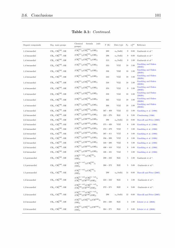
3.6. Conclusions 101
Table 3.1: Continued.
Organic compounds Org. main groupsChemical formula (sub-
groups)T (K) Data type Nd winit
d Reference
1,4-butanediol CHn, CH[OH]n , OH (CH
[alc]2 )2(CH
[OH]2 )2(OH)2 289 aw(bulk) 9 0.00 Ganbavale et al a
1,4-butanediol CHn, CH[OH]n , OH (CH
[alc]2 )2(CH
[OH]2 )2(OH)2 298 aw(bulk) 9 0.00 Ganbavale et al a
1,4-butanediol CHn, CH[OH]n , OH (CH
[alc]2 )2(CH
[OH]2 )2(OH)2 313 aw(bulk) 9 1.00 Ganbavale et al a
1,4-butanediol CHn, CH[OH]n , OH (CH
[alc]2 )2(CH
[OH]2 )2(OH)2 333 VLE 10 1.00
Gmehling and Onken
(2003b)
1,4-butanediol CHn, CH[OH]n , OH (CH
[alc]2 )2(CH
[OH]2 )2(OH)2 338 VLE 10 1.00
Gmehling and Onken
(2003b)
1,4-butanediol CHn, CH[OH]n , OH (CH
[alc]2 )2(CH
[OH]2 )2(OH)2 343 VLE 10 1.00
Gmehling and Onken
(2003b)
1,4-butanediol CHn, CH[OH]n , OH (CH
[alc]2 )2(CH
[OH]2 )2(OH)2 348 VLE 10 1.00
Gmehling and Onken
(2003b)
1,4-butanediol CHn, CH[OH]n , OH (CH
[alc]2 )2(CH
[OH]2 )2(OH)2 353 VLE 9 1.00
Gmehling and Onken
(2003b)
1,4-butanediol CHn, CH[OH]n , OH (CH
[alc]2 )2(CH
[OH]2 )2(OH)2 358 VLE 10 1.00
Gmehling and Onken
(2003b)
1,4-butanediol CHn, CH[OH]n , OH (CH
[alc]2 )2(CH
[OH]2 )2(OH)2 363 VLE 10 1.00
Gmehling and Onken
(2003b)
1,4-butanediol CHn, CH[OH]n , OH (CH
[alc]2 )2(CH
[OH]2 )2(OH)2 368 VLE 10 1.00
Gmehling and Onken
(2003b)
1,4-butanediol CHn, CH[OH]n , OH (CH
[alc]2 )2(CH
[OH]2 )2(OH)2 367− 409 VLE 13 1.00 Gmehling et al. (1988)
2,3-butanediol CHn, CH[OH]n , OH (CH
[alc]3 )2(CH[OH])2(OH)2 232− 270 SLE 6 5.00 Clendenning (1946)
2,3-butanediol CHn, CH[OH]n , OH (CH
[alc]3 )2(CH[OH])2(OH)2 298 aw(bulk) 13 0.00 Marcolli and Peter (2005)
2,3-butanediol CHn, CH[OH]n , OH (CH
[alc]3 )2(CH[OH])2(OH)2 375− 420 VLE 8 1.00 Gmehling et al. (1988)
2,3-butanediol CHn, CH[OH]n , OH (CH
[alc]3 )2(CH[OH])2(OH)2 373− 379 VLE 7 1.00 Gmehling et al. (1988)
2,3-butanediol CHn, CH[OH]n , OH (CH
[alc]3 )2(CH[OH])2(OH)2 367− 411 VLE 8 1.00 Gmehling et al. (1988)
2,3-butanediol CHn, CH[OH]n , OH (CH
[alc]3 )2(CH[OH])2(OH)2 356− 399 VLE 8 1.00 Gmehling et al. (1988)
2,3-butanediol CHn, CH[OH]n , OH (CH
[alc]3 )2(CH[OH])2(OH)2 340− 380 VLE 8 1.00 Gmehling et al. (1988)
2,3-butanediol CHn, CH[OH]n , OH (CH
[alc]3 )2(CH[OH])2(OH)2 408− 410 VLE 8 1.00 Gmehling et al. (1988)
2,3-butanediol CHn, CH[OH]n , OH (CH
[alc]3 )2(CH[OH])2(OH)2 426− 431 VLE 7 1.00 Gmehling et al. (1988)
1,5-pentanediol CHn, CH[OH]n , OH
(CH[alc−tail]2 )3(CH
[OH]2 )2
(OH)2200− 232 SLE 5 1.00 Ganbavale et al a.
1,5-pentanediol CHn, CH[OH]n , OH
(CH[alc−tail]2 )3(CH
[OH]2 )2
(OH)2260− 272 SLE 5 5.00 Ganbavale et al a.
1,5-pentanediol CHn, CH[OH]n , OH
(CH[alc−tail]2 )3(CH
[OH]2 )2
(OH)2298 aw(bulk) 14 0.00 Marcolli and Peter (2005)
1,2-hexanediol CHn, CH[OH]n , OH
(CH[alc−tail]3 )(CH
[alc−tail]2 )3
(CH[OH]2 )(CH[OH])(OH)2
223− 232 SLE 4 1.00 Ganbavale et al a.
1,2-hexanediol CHn, CH[OH]n , OH
(CH[alc−tail]3 )(CH
[alc−tail]2 )3
(CH[OH]2 )(CH[OH])(OH)2
272− 271 SLE 4 5.00 Ganbavale et al a.
1,2-hexanediol CHn, CH[OH]n , OH
(CH[alc−tail]3 )(CH
[alc−tail]2 )3
(CH[OH]2 )(CH[OH])(OH)2
298 aw(bulk) 12 0.00 Marcolli and Peter (2005)
2,5-hexanediol CHn, CH[OH]n , OH
(CH[alc]3 )2(CH
[alc]2 )2(CH[OH])2
(OH)2204− 230 SLE 3 1.00 Zobrist et al. (2008)
2,5-hexanediol CHn, CH[OH]n , OH
(CH[alc]3 )2(CH
[alc]2 )2(CH[OH])2
(OH)2264− 271 SLE 3 5.00 Zobrist et al. (2008)
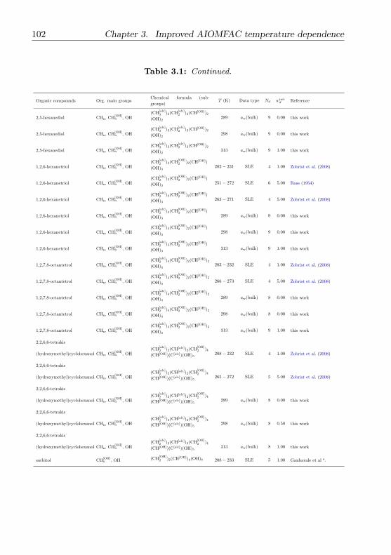
102 Chapter 3. Improved AIOMFAC temperature dependence
Table 3.1: Continued.
Organic compounds Org. main groupsChemical formula (sub-
groups)T (K) Data type Nd winit
d Reference
2,5-hexanediol CHn, CH[OH]n , OH
(CH[alc]3 )2(CH
[alc]2 )2(CH[OH])2
(OH)2289 aw(bulk) 9 0.00 this work
2,5-hexanediol CHn, CH[OH]n , OH
(CH[alc]3 )2(CH
[alc]2 )2(CH[OH])2
(OH)2298 aw(bulk) 9 0.00 this work
2,5-hexanediol CHn, CH[OH]n , OH
(CH[alc]3 )2(CH
[alc]2 )2(CH[OH])2
(OH)2313 aw(bulk) 9 1.00 this work
1,2,6-hexanetriol CHn, CH[OH]n , OH
(CH[alc]2 )3(CH
[OH]2 )2(CH[OH])
(OH)3202− 231 SLE 4 1.00 Zobrist et al. (2008)
1,2,6-hexanetriol CHn, CH[OH]n , OH
(CH[alc]2 )3(CH
[OH]2 )2(CH[OH])
(OH)3251− 272 SLE 6 5.00 Ross (1954)
1,2,6-hexanetriol CHn, CH[OH]n , OH
(CH[alc]2 )3(CH
[OH]2 )2(CH[OH])
(OH)3263− 271 SLE 4 5.00 Zobrist et al. (2008)
1,2,6-hexanetriol CHn, CH[OH]n , OH
(CH[alc]2 )3(CH
[OH]2 )2(CH[OH])
(OH)3289 aw(bulk) 9 0.00 this work
1,2,6-hexanetriol CHn, CH[OH]n , OH
(CH[alc]2 )3(CH
[OH]2 )2(CH[OH])
(OH)3298 aw(bulk) 9 0.00 this work
1,2,6-hexanetriol CHn, CH[OH]n , OH
(CH[alc]2 )3(CH
[OH]2 )2(CH[OH])
(OH)3313 aw(bulk) 9 1.00 this work
1,2,7,8-octantetrol CHn, CH[OH]n , OH
(CH[alc]2 )4(CH
[OH]2 )2(CH[OH])2
(OH)4203− 232 SLE 4 1.00 Zobrist et al. (2008)
1,2,7,8-octantetrol CHn, CH[OH]n , OH
(CH[alc]2 )4(CH
[OH]2 )2(CH[OH])2
(OH)4266− 273 SLE 4 5.00 Zobrist et al. (2008)
1,2,7,8-octantetrol CHn, CH[OH]n , OH
(CH[alc]2 )4(CH
[OH]2 )2(CH[OH])2
(OH)4289 aw(bulk) 8 0.00 this work
1,2,7,8-octantetrol CHn, CH[OH]n , OH
(CH[alc]2 )4(CH
[OH]2 )2(CH[OH])2
(OH)4298 aw(bulk) 8 0.00 this work
1,2,7,8-octantetrol CHn, CH[OH]n , OH
(CH[alc]2 )4(CH
[OH]2 )2(CH[OH])2
(OH)4313 aw(bulk) 9 1.00 this work
2,2,6,6-tetrakis
(hydroxymethyl)cyclohexanol CHn, CH[OH]n , OH
(CH[alc]2 )2(CH[alc])2(CH
[OH]2 )4
(CH[OH])(C[alc])(OH)5208− 232 SLE 4 1.00 Zobrist et al. (2008)
2,2,6,6-tetrakis
(hydroxymethyl)cyclohexanol CHn, CH[OH]n , OH
(CH[alc]2 )2(CH[alc])2(CH
[OH]2 )4
(CH[OH])(C[alc])(OH)5265− 272 SLE 5 5.00 Zobrist et al. (2008)
2,2,6,6-tetrakis
(hydroxymethyl)cyclohexanol CHn, CH[OH]n , OH
(CH[alc]2 )2(CH[alc])2(CH
[OH]2 )4
(CH[OH])(C[alc])(OH)5289 aw(bulk) 8 0.00 this work
2,2,6,6-tetrakis
(hydroxymethyl)cyclohexanol CHn, CH[OH]n , OH
(CH[alc]2 )2(CH[alc])2(CH
[OH]2 )4
(CH[OH])(C[alc])(OH)5298 aw(bulk) 8 0.50 this work
2,2,6,6-tetrakis
(hydroxymethyl)cyclohexanol CHn, CH[OH]n , OH
(CH[alc]2 )2(CH[alc])2(CH
[OH]2 )4
(CH[OH])(C[alc])(OH)5313 aw(bulk) 8 1.00 this work
sorbitol CH[OH]n , OH (CH
[OH]2 )2(CH[OH])4(OH)6 208− 233 SLE 5 1.00 Ganbavale et al a.
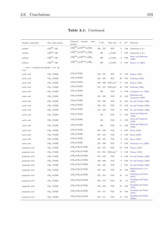
3.6. Conclusions 103
Table 3.1: Continued.
Organic compounds Org. main groupsChemical formula (sub-
groups)T (K) Data type Nd winit
d Reference
sorbitol CH[OH]n , OH (CH
[OH]2 )2(CH[OH])4(OH)6 256− 272 SLE 6 5.00 Ganbavale et al a.
sorbitol CH[OH]n , OH (CH
[OH]2 )2(CH[OH])4(OH)6 298 aw(bulk) 7 0.00 Ganbavale et al a.
sorbitol CH[OH]n , OH (CH
[OH]2 )2(CH[OH])4(OH)6 298 aw(bulk) 8 0.00
Bower and Robinson
(1963)
sorbitol CH[OH]n , OH (CH
[OH]2 )2(CH[OH])4(OH)6 298 aw(bulk) 8 0.00 Peng et al. (2001)
— water + carboxylic/dicarboxylic acid sys-
tems —
acetic acid CHn, COOH (CH3)(COOH) 249− 272 SLE 12 5.00 Faucon (1910)
acetic acid CHn, COOH (CH3)(COOH) 250− 289 SLE 26 5.00 Pickering (1893)
acetic acid CHn, COOH (CH3)(COOH) 249− 290 SLE(org) d 11 0.20 Faucon (1910)
acetic acid CHn, COOH (CH3)(COOH) 251− 273 SLE(org) d 20 0.20 Pickering (1893)
acetic acid CHn, COOH (CH3)(COOH) 298 VLE 8 0.00 Campbell et al. (1963)
acetic acid CHn, COOH (CH3)(COOH) 374− 389 VLE 10 0.20Sebastiani and
Lacquaniti (1967)
acetic acid CHn, COOH (CH3)(COOH) 373− 390 VLE 16 0.20 Ito and Yoshida (1963)
acetic acid CHn, COOH (CH3)(COOH) 340− 351 VLE 15 0.20 Ito and Yoshida (1963)
acetic acid CHn, COOH (CH3)(COOH) 318− 326 VLE 14 0.20 Ito and Yoshida (1963)
acetic acid CHn, COOH (CH3)(COOH) 343 VLE 11 0.20Arich and Tagliavini
(1958)
acetic acid CHn, COOH (CH3)(COOH) 353 VLE 11 0.20Arich and Tagliavini
(1958)
acetic acid CHn, COOH (CH3)(COOH) 363 VLE 11 0.20Arich and Tagliavini
(1958)
acetic acid CHn, COOH (CH3)(COOH) 322− 329 VLE 8 0.20 Keyes (1933)
acetic acid CHn, COOH (CH3)(COOH) 337− 342 VLE 8 0.20 Keyes (1933)
acetic acid CHn, COOH (CH3)(COOH) 350− 355 VLE 8 0.20 Keyes (1933)
acetic acid CHn, COOH (CH3)(COOH) 373− 386 VLE 9 0.20 Narayana et al. (1985)
propanoic acid CHn, COOH (CH3)(CH2)(COOH) 245− 273 SLE 19 5.00 Faucon (1910)
propanoic acid CHn, COOH (CH3)(CH2)(COOH) 244− 254 SLE(org) d 8 0.20 Faucon (1910)
propanoic acid CHn, COOH (CH3)(CH2)(COOH) 373− 405 VLE 8 0.20 Ito and Yoshida (1963)
propanoic acid CHn, COOH (CH3)(CH2)(COOH) 340− 368 VLE 9 0.20 Ito and Yoshida (1963)
propanoic acid CHn, COOH (CH3)(CH2)(COOH) 318− 345 VLE 7 0.01 Ito and Yoshida (1963)
propanoic acid CHn, COOH (CH3)(CH2)(COOH) 372− 401 VLE 18 0.20Dakshinamurty et al.
(1961)
propanoic acid CHn, COOH (CH3)(CH2)(COOH) 325− 354 VLE 24 0.2Gmehling and Onken
(1977)
propanoic acid CHn, COOH (CH3)(CH2)(COOH) 339− 373 VLE 25 0.2Gmehling and Onken
(1977)
propanoic acid CHn, COOH (CH3)(CH2)(COOH) 356− 392 VLE 23 0.20Gmehling and Onken
(1977)
propanoic acid CHn, COOH (CH3)(CH2)(COOH) 373− 411 VLE 24 0.20Gmehling and Onken
(1977)
propanoic acid CHn, COOH (CH3)(CH2)(COOH) 373− 411 VLE 12 0.01Gmehling and Onken
(2003a)
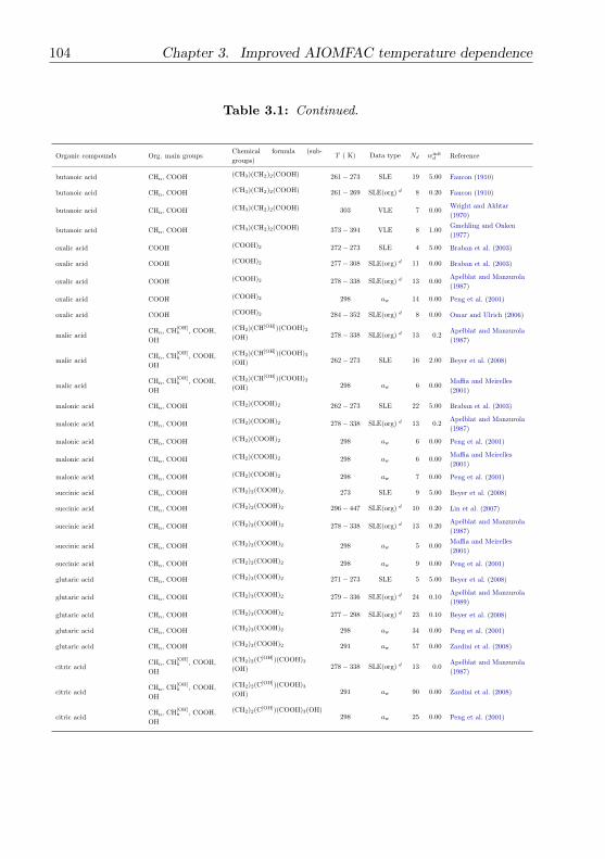
104 Chapter 3. Improved AIOMFAC temperature dependence
Table 3.1: Continued.
Organic compounds Org. main groupsChemical formula (sub-
groups)T ( K) Data type Nd winit
d Reference
butanoic acid CHn, COOH (CH3)(CH2)2(COOH) 261− 273 SLE 19 5.00 Faucon (1910)
butanoic acid CHn, COOH (CH3)(CH2)2(COOH) 261− 269 SLE(org) d 8 0.20 Faucon (1910)
butanoic acid CHn, COOH (CH3)(CH2)2(COOH) 303 VLE 7 0.00Wright and Akhtar
(1970)
butanoic acid CHn, COOH (CH3)(CH2)2(COOH) 373− 394 VLE 8 1.00Gmehling and Onken
(1977)
oxalic acid COOH (COOH)2 272− 273 SLE 4 5.00 Braban et al. (2003)
oxalic acid COOH (COOH)2 277− 308 SLE(org) d 11 0.00 Braban et al. (2003)
oxalic acid COOH (COOH)2 278− 338 SLE(org) d 13 0.00Apelblat and Manzurola
(1987)
oxalic acid COOH (COOH)2 298 aw 14 0.00 Peng et al. (2001)
oxalic acid COOH (COOH)2 284− 352 SLE(org) d 8 0.00 Omar and Ulrich (2006)
malic acidCHn, CH
[OH]n , COOH,
OH
(CH2)(CH[OH])(COOH)2
(OH) 278− 338 SLE(org) d 13 0.2Apelblat and Manzurola
(1987)
malic acidCHn, CH
[OH]n , COOH,
OH
(CH2)(CH[OH])(COOH)2
(OH) 262− 273 SLE 16 2.00 Beyer et al. (2008)
malic acidCHn, CH
[OH]n , COOH,
OH
(CH2)(CH[OH])(COOH)2
(OH) 298 aw 6 0.00Maffia and Meirelles
(2001)
malonic acid CHn, COOH (CH2)(COOH)2 262− 273 SLE 22 5.00 Braban et al. (2003)
malonic acid CHn, COOH (CH2)(COOH)2 278− 338 SLE(org) d 13 0.2Apelblat and Manzurola
(1987)
malonic acid CHn, COOH (CH2)(COOH)2 298 aw 6 0.00 Peng et al. (2001)
malonic acid CHn, COOH (CH2)(COOH)2 298 aw 6 0.00Maffia and Meirelles
(2001)
malonic acid CHn, COOH (CH2)(COOH)2 298 aw 7 0.00 Peng et al. (2001)
succinic acid CHn, COOH (CH2)2(COOH)2 273 SLE 9 5.00 Beyer et al. (2008)
succinic acid CHn, COOH (CH2)2(COOH)2 296− 447 SLE(org) d 10 0.20 Lin et al. (2007)
succinic acid CHn, COOH (CH2)2(COOH)2 278− 338 SLE(org) d 13 0.20Apelblat and Manzurola
(1987)
succinic acid CHn, COOH (CH2)2(COOH)2 298 aw 5 0.00Maffia and Meirelles
(2001)
succinic acid CHn, COOH (CH2)2(COOH)2 298 aw 9 0.00 Peng et al. (2001)
glutaric acid CHn, COOH (CH2)3(COOH)2 271− 273 SLE 5 5.00 Beyer et al. (2008)
glutaric acid CHn, COOH (CH2)3(COOH)2 279− 336 SLE(org) d 24 0.10Apelblat and Manzurola
(1989)
glutaric acid CHn, COOH (CH2)3(COOH)2 277− 298 SLE(org) d 23 0.10 Beyer et al. (2008)
glutaric acid CHn, COOH (CH2)3(COOH)2 298 aw 34 0.00 Peng et al. (2001)
glutaric acid CHn, COOH (CH2)3(COOH)2 291 aw 57 0.00 Zardini et al. (2008)
citric acidCHn, CH
[OH]n , COOH,
OH
(CH2)2(C[OH])(COOH)3
(OH) 278− 338 SLE(org) d 13 0.0Apelblat and Manzurola
(1987)
citric acidCHn, CH
[OH]n , COOH,
OH
(CH2)2(C[OH])(COOH)3
(OH) 291 aw 90 0.00 Zardini et al. (2008)
citric acidCHn, CH
[OH]n , COOH,
OH
(CH2)2(C[OH])(COOH)3(OH)298 aw 25 0.00 Peng et al. (2001)

3.6. Conclusions 105
Table 3.1: Continued.
Organic compounds Org. main groupsChemical formula (sub-
groups)T (K) Data type Nd winit
d Reference
adipic acid CHn, COOH (CH2)4(COOH)2 278− 338 SLE(org) d 13 0.20Apelblat and Manzurola
(1987)
pimelic acid CHn, COOH (CH2)5(COOH)2 279− 342 SLE(org) d 21 0.20Apelblat and Manzurola
(1989)
M5 b CHn, CH[OH]n , COOH,
OH, C=C
c191− 230 SLE 6 1.00 Zobrist et al. (2008)
M5 b CHn, CH[OH]n , COOH,
OH, C=C
c255− 271 SLE 6 5.00 Zobrist et al. (2008)
M5 b CHn, CH[OH]n , COOH,
OH, C=C
c233 SLE 3 0.20 Ganbavale et al a
M5 b CHn, CH[OH]n , COOH,
OH, C=C
c236 SLE 2 0.20 Ganbavale et al a
M5 b CHn, CH[OH]n , COOH,
OH, C=C
c244 SLE 6 0.50 Ganbavale et al a
M5 b CHn, CH[OH]n , COOH,
OH, C=C
c250 SLE 6 1.00 Ganbavale et al a
M5 b CHn, CH[OH]n , COOH,
OH, C=C
c253 SLE 3 0.50 Ganbavale et al a
M5 b CHn, CH[OH]n , COOH,
OH, C=C
c253 SLE 5 1.00 Ganbavale et al a
M5 b CHn, CH[OH]n , COOH,
OH, C=C
c255 SLE 3 0.50 Ganbavale et al a
M5 b CHn, CH[OH]n , COOH,
OH, C=C
c258 SLE 3 0.50 Ganbavale et al a
M5 b CHn, CH[OH]n , COOH,
OH, C=C
c260 SLE 4 1.00 Ganbavale et al a
M5 b CHn, CH[OH]n , COOH,
OH, C=C
c263 SLE 2 1.00 Ganbavale et al a
M5 b CHn, CH[OH]n , COOH,
OH, C=C
c263 SLE 5 1.00 Ganbavale et al a
M5 b CHn, CH[OH]n , COOH,
OH, C=C
c265 SLE 5 1.00 Ganbavale et al a
M5 b CHn, CH[OH]n , COOH,
OH, C=C
c268 SLE 6 1.00 Ganbavale et al a
M5 b CHn, CH[OH]n , COOH,
OH, C=C
c268 SLE 8 1.00 Ganbavale et al a
M5 b CHn, CH[OH]n , COOH,
OH, C=C
c270 SLE 6 1.00 Ganbavale et al a
M5 b CHn, CH[OH]n , COOH,
OH, C=C
c273 SLE 6 1.00 Ganbavale et al a
M5 b CHn, CH[OH]n , COOH,
OH, C=C
c273 SLE 10 1.00 Ganbavale et al a
M5 b CHn, CH[OH]n , COOH,
OH, C=C
c275 SLE 6 1.00 Ganbavale et al a
M5 b CHn, CH[OH]n , COOH,
OH, C=C
c278 SLE 6 1.00 Ganbavale et al a
M5 b CHn, CH[OH]n , COOH,
OH, C=C
c279 SLE 9 1.00 Ganbavale et al a
M5 b CHn, CH[OH]n , COOH,
OH, C=C
c280 SLE 6 1.00 Ganbavale et al a
M5 b CHn, CH[OH]n , COOH,
OH, C=C
c283 SLE 6 1.00 Ganbavale et al a
M5 b CHn, CH[OH]n , COOH,
OH, C=C
c285 SLE 6 1.00 Ganbavale et al a
M5 b CHn, CH[OH]n , COOH,
OH, C=C
c288 SLE 6 1.00 Ganbavale et al a

106 Chapter 3. Improved AIOMFAC temperature dependence
Table 3.1: Continued.
Organic compounds Org. main groupsChemical formula (sub-
groups)T (K) Data type Nd winit
d Reference
— water + ketone systems —
M5 b CHn, CH[OH]n , COOH,
OH, C=C
c289 SLE 10 0.00 Ganbavale et al a
M5 b CHn, CH[OH]n , COOH,
OH, C=C
c289 SLE 10 0.00 Ganbavale et al a
M5 b CHn, CH[OH]n , COOH,
OH, C=C
c290 SLE 6 0.00 Ganbavale et al a
M5 b CHn, CH[OH]n , COOH,
OH, C=C
c298 SLE 10 0.00 Ganbavale et al a
M5 b CHn, CH[OH]n , COOH,
OH, C=C
c313 SLE 10 0.00 Ganbavale et al a
acetone CHn, CHnCO (CH3)(CH3CO) 221− 273 SLE 17 5.00 Jakob (1994)
acetone CHn, CHnCO (CH3)(CH3CO) 298 VLE 13 0.00 Gmehling et al. (1988)
acetone CHn, CHnCO (CH3)(CH3CO) 308 VLE 13 1.00 Gmehling et al. (1988)
acetone CHn, CHnCO (CH3)(CH3CO) 318 VLE 13 1.00 Gmehling et al. (1988)
acetone CHn, CHnCO (CH3)(CH3CO) 323 VLE 13 1.00 Gmehling et al. (1988)
acetone CHn, CHnCO (CH3)(CH3CO) 328 VLE 13 1.00 Gmehling et al. (1988)
acetone CHn, CHnCO (CH3)(CH3CO) 373 VLE 20 1.00Griswold and Wong
(1952)
acetone CHn, CHnCO (CH3)(CH3CO) 295− 321 VLE 10 1.00Othmer and Benenati
(1945)
acetone CHn, CHnCO (CH3)(CH3CO) 309− 340 VLE 12 1.00Othmer and Benenati
(1945)
acetone CHn, CHnCO (CH3)(CH3CO) 318− 345 VLE 13 1.00Othmer and Benenati
(1945)
acetone CHn, CHnCO (CH3)(CH3CO) 331− 363 VLE 10 1.00Othmer and Benenati
(1945)
acetone CHn, CHnCO (CH3)(CH3CO) 330− 361 VLE 13 1.00 Othmer et al. (1952)
acetone CHn, CHnCO (CH3)(CH3CO) 371− 396 VLE 12 1.00 Othmer et al. (1952)
2-butanone CHn, CHnCO (CH3)(CH2)(CH3CO) 198− 273 SLE 19 5.00 Lohmann et al. (1997)
2-butanone CHn, CHnCO (CH3)(CH2)(CH3CO) 293 VLE 5 0.00 Gmehling et al. (1988)
2-butanone CHn, CHnCO (CH3)(CH2)(CH3CO) 308 VLE 4 1.00 Gmehling et al. (1988)
2-butanone CHn, CHnCO (CH3)(CH2)(CH3CO) 323 VLE 4 1.00 Gmehling et al. (1988)
2-butanone CHn, CHnCO (CH3)(CH2)(CH3CO) 323 VLE 15 1.00 Gaube et al. (1996)
2-butanone CHn, CHnCO (CH3)(CH2)(CH3CO) 333 VLE 20 1.00 Zou and Prausnitz (1987)
2-butanone CHn, CHnCO (CH3)(CH2)(CH3CO) 343 VLE 22 1.00 Zou and Prausnitz (1987)
2-butanone CHn, CHnCO (CH3)(CH2)(CH3CO) 313− 326 VLE 8 1.00 Gmehling et al. (1981)
2-butanone CHn, CHnCO (CH3)(CH2)(CH3CO) 330− 338 VLE 8 1.00 Gmehling et al. (1981)
2-butanone CHn, CHnCO (CH3)(CH2)(CH3CO) 340− 348 VLE 8 1.00 Gmehling et al. (1981)
2-butanone CHn, CHnCO (CH3)(CH2)(CH3CO) 347− 363 VLE 8 1.00 Gmehling et al. (1981)
2-butanone CHn, CHnCO (CH3)(CH2)(CH3CO) 385− 406 VLE 19 1.00 Othmer et al. (1952)
2-pentanone CHn, CHnCO (CH3)(CH2)2(CH3CO) 273− 363 solubil. 20 1.00 Stephenson (1992)
3-pentanone CHn, CHnCO (CH3)2(CH2)(CH2CO) 273− 353 solubil. 18 1.00 Stephenson (1992)

3.6. Conclusions 107
Table 3.1: Continued.
Organic compounds Org. main groupsChemical formula (sub-
groups)T (K) Data type Nd winit
d Reference
3-pentanone CHn, CHnCO (CH3)2(CH2)(CH2CO) 323 VLE 12 1.00Gmehling and Onken
(2003b)
3-pentanone CHn, CHnCO (CH3)2(CH2)(CH2CO) 338 VLE 12 0.50Gmehling and Onken
(2003b)
3-pentanone CHn, CHnCO (CH3)2(CH2)(CH2CO) 353 VLE 12 0.50Gmehling and Onken
(2003b)
3-pentanone CHn, CHnCO (CH3)2(CH2)(CH2CO) 368 VLE 12 0.50Gmehling and Onken
(2003b)
3-pentanone CHn, CHnCO (CH3)2(CH2)(CH2CO) 383 VLE 12 1.00Gmehling and Onken
(2003b)
— water + ether systems —
diethyl ether CHn, CHnO (CH3)2(CH2)(CH2O) 269− 272 SLE(org) d 7 5.00 Lalande (1934)
diethyl ether CHn, CHnO (CH3)2(CH2)(CH2O) 269− 303 solubli. 14 0.20 Hill (1923)
diethyl ether CHn, CHnO (CH3)2(CH2)(CH2O) 307− 367 VLE. 10 0.05 Borisova et al. (1983)
2-methoxyethanolCHn, CH
[OH]n , CHnO,
OH(CH2)(CH
[OH]2 )(CH3O)(OH) 343 VLE 16 0.50
Chiavone-Filho et al.
(1993)
2-methoxyethanolCHn, CH
[OH]n , CHnO,
OH(CH2)(CH
[OH]2 )(CH3O)(OH) 363 VLE 16 0.50
Chiavone-Filho et al.
(1993)
2-methoxyethanolCHn, CH
[OH]n , CHnO,
OH
(CH2)(CH[OH]2 ) (CH3O)(OH)
373− 394 VLE 12 0.50Gmehling and Onken
(2003a)
2-ethoxyethanolCHn, CH
[OH]n , CHnO,
OH
(CH3)(CH2)(CH[OH]2 )(CH2O)
(OH) 343 VLE 20 0.50Chiavone-Filho et al.
(1993)
2-ethoxyethanolCHn, CH
[OH]n , CHnO,
OH
(CH3)(CH2)(CH[OH]2 )(CH2O)
(OH) 363 VLE 18 0.50Chiavone-Filho et al.
(1993)
2-ethoxyethanolCHn, CH
[OH]n , CHnO,
OH
(CH3)(CH2)(CH[OH]2 )(CH2O)
(OH) 373− 407 VLE 34 0.50Hirata and Hoshino
(1982)
2-ethoxyethanolCHn, CH
[OH]n , CHnO,
OH
(CH3)(CH2)(CH[OH]2 )(CH2O)
(OH) 372− 406 VLE 17 0.50Gmehling and Onken
(2003b)
2-butoxyethanolCHn, CH
[OH]n , CHnO,
OH
(CH3)(CH2)3(CH[OH]2 )(CH2O)
(OH) 252− 273 SLE 23 0.50 Koga et al. (1994)
2-butoxyethanolCHn, CH
[OH]n , CHnO,
OH
(CH3)(CH2)3(CH[OH]2 )(CH2O)
(OH) 261− 273 SLE 23 5.00 Koga et al. (1994)
2-butoxyethanolCHn, CH
[OH]n , CHnO,
OH
(CH3)(CH2)3(CH[OH]2 )(CH2O)
(OH) 298 VLE 8 0.00Scatchard and Wilson
(1964)
2-butoxyethanolCHn, CH
[OH]n , CHnO,
OH
(CH3)(CH2)3(CH[OH]2 )(CH2O)
(OH)318 VLE 8 0.05
Scatchard and Wilson
(1964)
2-butoxyethanolCHn, CH
[OH]n , CHnO,
OH
(CH3)(CH2)3(CH[OH]2 )(CH2O)
(OH) 338 VLE 7 0.05Scatchard and Wilson
(1964)
2-butoxyethanolCHn, CH
[OH]n , CHnO,
OH
(CH3)(CH2)3(CH[OH]2 )(CH2O)
(OH) 358 VLE 7 0.50Scatchard and Wilson
(1964)
2-butoxyethanolCHn, CH
[OH]n , CHnO,
OH
(CH3)(CH2)3(CH[OH]2 )(CH2O)
(OH) 358 VLE 19 0.50Chiavone-Filho et al.
(1993)
2-butoxyethanolCHn, CH
[OH]n , CHnO,
OH
(CH3)(CH2)3(CH[OH]2 )(CH2O)
(OH) 363 VLE 22 0.50Escobedo-Alvarado and
Sandler (1999)
2-butoxyethanolCHn, CH
[OH]n , CHnO,
OH
(CH3)(CH2)3(CH[OH]2 )(CH2O)
(OH) 368 VLE 19 0.50Chiavone-Filho et al.
(1993)
2-butoxyethanolCHn, CH
[OH]n , CHnO,
OH
(CH3)(CH2)3(CH[OH]2 )(CH2O)
(OH) 371 VLE 20 0.50Escobedo-Alvarado and
Sandler (1999)
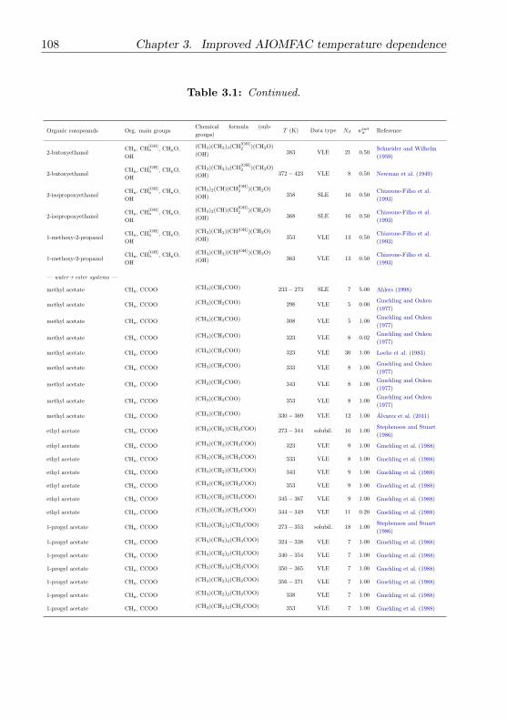
108 Chapter 3. Improved AIOMFAC temperature dependence
Table 3.1: Continued.
Organic compounds Org. main groupsChemical formula (sub-
groups)T (K) Data type Nd winit
d Reference
2-butoxyethanolCHn, CH
[OH]n , CHnO,
OH
(CH3)(CH2)3(CH[OH]2 )(CH2O)
(OH) 383 VLE 21 0.50Schneider and Wilhelm
(1959)
2-butoxyethanolCHn, CH
[OH]n , CHnO,
OH
(CH3)(CH2)3(CH[OH]2 )(CH2O)
(OH) 372− 423 VLE 8 0.50 Newman et al. (1949)
2-isopropoxyethanolCHn, CH
[OH]n , CHnO,
OH
(CH3)2(CH)(CH[OH]2 )(CH2O)
(OH) 358 SLE 16 0.50Chiavone-Filho et al.
(1993)
2-isopropoxyethanolCHn, CH
[OH]n , CHnO,
OH
(CH3)2(CH)(CH[OH]2 )(CH2O)
(OH) 368 SLE 16 0.50Chiavone-Filho et al.
(1993)
1-methoxy-2-propanolCHn, CH
[OH]n , CHnO,
OH
(CH3)(CH2)(CH[OH])(CH3O)
(OH) 353 VLE 13 0.50Chiavone-Filho et al.
(1993)
1-methoxy-2-propanolCHn, CH
[OH]n , CHnO,
OH
(CH3)(CH2)(CH[OH])(CH3O)
(OH) 363 VLE 13 0.50Chiavone-Filho et al.
(1993)
— water + ester systems —
methyl acetate CHn, CCOO (CH3)(CH3COO) 233− 273 SLE 7 5.00 Ahlers (1998)
methyl acetate CHn, CCOO (CH3)(CH3COO) 298 VLE 5 0.00Gmehling and Onken
(1977)
methyl acetate CHn, CCOO (CH3)(CH3COO) 308 VLE 5 1.00Gmehling and Onken
(1977)
methyl acetate CHn, CCOO (CH3)(CH3COO) 323 VLE 8 0.02Gmehling and Onken
(1977)
methyl acetate CHn, CCOO (CH3)(CH3COO) 323 VLE 30 1.00 Loehe et al. (1983)
methyl acetate CHn, CCOO (CH3)(CH3COO) 333 VLE 8 1.00Gmehling and Onken
(1977)
methyl acetate CHn, CCOO (CH3)(CH3COO) 343 VLE 8 1.00Gmehling and Onken
(1977)
methyl acetate CHn, CCOO (CH3)(CH3COO) 353 VLE 8 1.00Gmehling and Onken
(1977)
methyl acetate CHn, CCOO (CH3)(CH3COO) 330− 369 VLE 12 1.00 Alvarez et al. (2011)
ethyl acetate CHn, CCOO (CH3)(CH2)(CH3COO) 273− 344 solubil. 16 1.00Stephenson and Stuart
(1986)
ethyl acetate CHn, CCOO (CH3)(CH2)(CH3COO) 323 VLE 9 1.00 Gmehling et al. (1988)
ethyl acetate CHn, CCOO (CH3)(CH2)(CH3COO) 333 VLE 8 1.00 Gmehling et al. (1988)
ethyl acetate CHn, CCOO (CH3)(CH2)(CH3COO) 343 VLE 9 1.00 Gmehling et al. (1988)
ethyl acetate CHn, CCOO (CH3)(CH2)(CH3COO) 353 VLE 9 1.00 Gmehling et al. (1988)
ethyl acetate CHn, CCOO (CH3)(CH2)(CH3COO) 345− 367 VLE 9 1.00 Gmehling et al. (1988)
ethyl acetate CHn, CCOO (CH3)(CH2)(CH3COO) 344− 349 VLE 11 0.20 Gmehling et al. (1988)
1-propyl acetate CHn, CCOO (CH3)(CH2)2(CH3COO) 273− 353 solubil. 18 1.00Stephenson and Stuart
(1986)
1-propyl acetate CHn, CCOO (CH3)(CH2)2(CH3COO) 324− 338 VLE 7 1.00 Gmehling et al. (1988)
1-propyl acetate CHn, CCOO (CH3)(CH2)2(CH3COO) 340− 354 VLE 7 1.00 Gmehling et al. (1988)
1-propyl acetate CHn, CCOO (CH3)(CH2)2(CH3COO) 350− 365 VLE 7 1.00 Gmehling et al. (1988)
1-propyl acetate CHn, CCOO (CH3)(CH2)2(CH3COO) 356− 371 VLE 7 1.00 Gmehling et al. (1988)
1-propyl acetate CHn, CCOO (CH3)(CH2)2(CH3COO) 338 VLE 7 1.00 Gmehling et al. (1988)
1-propyl acetate CHn, CCOO (CH3)(CH2)2(CH3COO) 353 VLE 7 1.00 Gmehling et al. (1988)
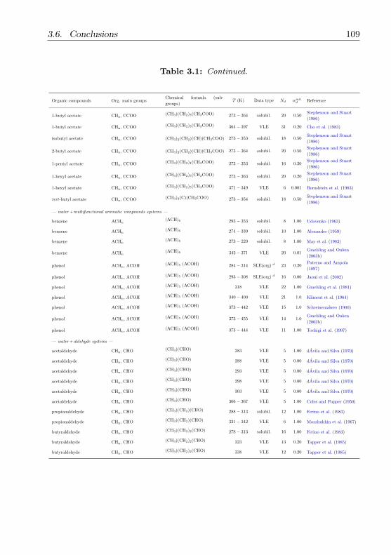
3.6. Conclusions 109
Table 3.1: Continued.
Organic compounds Org. main groupsChemical formula (sub-
groups)T (K) Data type Nd winit
d Reference
1-butyl acetate CHn, CCOO (CH3)(CH2)3(CH3COO) 273− 364 solubil. 20 0.50Stephenson and Stuart
(1986)
1-butyl acetate CHn, CCOO (CH3)(CH2)3(CH3COO) 364− 397 VLE 31 0.20 Cho et al. (1983)
isobutyl acetate CHn, CCOO (CH3)2(CH2)(CH)(CH3COO) 273− 353 solubil. 18 0.50Stephenson and Stuart
(1986)
2-butyl acetate CHn, CCOO (CH3)2(CH2)(CH)(CH3COO) 273− 364 solubil. 20 0.50Stephenson and Stuart
(1986)
1-pentyl acetate CHn, CCOO (CH3)(CH2)4(CH3COO) 273− 353 solubil. 16 0.20Stephenson and Stuart
(1986)
1-hexyl acetate CHn, CCOO (CH3)(CH2)5(CH3COO) 273− 363 solubil. 20 0.20Stephenson and Stuart
(1986)
1-hexyl acetate CHn, CCOO (CH3)(CH2)5(CH3COO) 371− 349 VLE 6 0.001 Bomshtein et al. (1983)
tert-butyl acetate CHn, CCOO (CH3)3(C)(CH3COO) 273− 354 solubil. 18 0.50Stephenson and Stuart
(1986)
— water + multifunctional aromatic compounds systems —
benzene ACHn(ACH)6 293− 353 solubil. 8 1.00 Udovenko (1963)
benzene ACHn(ACH)6 274− 339 solubil. 10 1.00 Alexander (1959)
benzene ACHn(ACH)6 273− 229 solubil. 8 1.00 May et al. (1983)
benzene ACHn(ACH)6 342− 371 VLE 20 0.01
Gmehling and Onken
(2003b)
phenol ACHn, ACOH (ACH)5 (ACOH) 284− 314 SLE(org) d 23 0.20Paterno and Ampola
(1897)
phenol ACHn, ACOH (ACH)5 (ACOH) 293− 308 SLE(org) d 16 0.00 Jaoui et al. (2002)
phenol ACHn, ACOH (ACH)5 (ACOH) 318 VLE 22 1.00 Gmehling et al. (1981)
phenol ACHn, ACOH (ACH)5 (ACOH) 340− 400 VLE 21 1.0 Kliment et al. (1964)
phenol ACHn, ACOH (ACH)5 (ACOH) 373− 442 VLE 15 1.0 Schreinemakers (1900)
phenol ACHn, ACOH (ACH)5 (ACOH) 373− 455 VLE 14 1.0Gmehling and Onken
(2003b)
phenol ACHn, ACOH (ACH)5 (ACOH) 373− 444 VLE 11 1.00 Tochigi et al. (1997)
— water + aldehyde systems —
acetaldehyde CHn, CHO (CH3)(CHO) 283 VLE 5 1.00 dAvila and Silva (1970)
acetaldehyde CHn, CHO (CH3)(CHO) 288 VLE 5 0.00 dAvila and Silva (1970)
acetaldehyde CHn, CHO (CH3)(CHO) 293 VLE 5 0.00 dAvila and Silva (1970)
acetaldehyde CHn, CHO (CH3)(CHO) 298 VLE 5 0.00 dAvila and Silva (1970)
acetaldehyde CHn, CHO (CH3)(CHO) 303 VLE 5 0.00 dAvila and Silva (1970)
acetaldehyde CHn, CHO (CH3)(CHO) 306− 367 VLE 5 1.00 Coles and Popper (1950)
propionaldehyde CHn, CHO (CH3)(CH2)(CHO) 288− 313 solubil. 12 1.00 Ferino et al. (1983)
propionaldehyde CHn, CHO (CH3)(CH2)(CHO) 321− 342 VLE 6 1.00 Mozzhukhin et al. (1967)
butyraldehyde CHn, CHO (CH3)(CH2)2(CHO) 278− 313 solubil. 16 1.00 Ferino et al. (1983)
butyraldehyde CHn, CHO (CH3)(CH2)2(CHO) 323 VLE 13 0.20 Tapper et al. (1985)
butyraldehyde CHn, CHO (CH3)(CH2)2(CHO) 338 VLE 12 0.20 Tapper et al. (1985)

110 Chapter 3. Improved AIOMFAC temperature dependence
Table 3.1: Continued.
Organic compounds Org. main groupsChemical formula (sub-
groups)T (K) Data type Nd winit
d Reference
— water + multifunctional systems —
glucoseCH
[OH]n , OH,
CHO[ether]
(CH[OH]2 )(CH[OH])4
(CHO[ether])(OH)5217− 233 SLE 9 1.00
Miyata and Kanno
(2005)
glucoseCH
[OH]n , OH,
CHO[ether]
(CH[OH]2 )(CH[OH])4
(CHO[ether])(OH)5204− 231 SLE 5 1.00 Zobrist et al. (2008)
glucoseCH
[OH]n , OH,
CHO[ether]
(CH[OH]2 )(CH[OH])4
(CHO[ether])(OH)5243− 273 SLE 8 5.00 Young (1957)
glucoseCH
[OH]n , OH,
CHO[ether]
(CH[OH]2 )(CH[OH])4
(CHO[ether])(OH)5260− 273 SLE 5 5.00 Zobrist et al. (2008)
glucoseCH
[OH]n , OH,
CHO[ether]
(CH[OH]2 )(CH[OH])4
(CHO[ether])(OH)5298 aw(bulk) 20 0.00 Ruegg and Blanc (1981)
glucoseCH
[OH]n , OH,
CHO[ether]
(CH[OH]2 )(CH[OH])4
(CHO[ether])(OH)5298 aw(bulk) 26 0.00
Bonner and Breazeale
(1965)
glucoseCH
[OH]n , OH,
CHO[ether]
(CH[OH]2 )(CH[OH])4
(CHO[ether])(OH)5298 aw(bulk) 8 0.00 Peng et al. (2001)
sucroseCH
[OH]n , OH,
CHO[ether]
(C)(CH[OH]2 )3(CH[OH])5
(CHO[ether])3(OH)8211− 235 SLE 16 1.00 Kanno et al. (2007)
sucroseCH
[OH]n , OH,
CHO[ether]
(C)(CH[OH]2 )3(CH[OH])5
(CHO[ether])3(OH)8217− 232 SLE 6 1.00 Ganbavale et al a
sucroseCH
[OH]n , OH,
CHO[ether]
(C)(CH[OH]2 )3(CH[OH])5
(CHO[ether])3(OH)8237− 273 SLE 10 5.00 Ablett et al. (1992)
sucroseCH
[OH]n , OH,
CHO[ether]
(C)(CH[OH]2 )3(CH[OH])5
(CHO[ether])3(OH)8247− 273 SLE 9 5.00
Williams and Carnahan
(1990)
sucroseCH
[OH]n , OH,
CHO[ether]
(C)(CH[OH]2 )3(CH[OH])5
(CHO[ether])3(OH)8259− 271 SLE 9 5.00 Blond et al. (1997)
sucroseCH
[OH]n , OH,
CHO[ether]
(C)(CH[OH]2 )3(CH[OH])5
(CHO[ether])3(OH)8261− 272 SLE 8 5.00 Zobrist et al. (2008)
sucroseCH
[OH]n , OH,
CHO[ether]
(C)(CH[OH]2 )3(CH[OH])5
(CHO[ether])3(OH)8262− 273 SLE 16 5.00 Kanno et al. (2007)
sucroseCH
[OH]n , OH,
CHO[ether]
(C)(CH[OH]2 )3(CH[OH])5
(CHO[ether])3(OH)8264− 272 SLE 5 5.00 Sei and Gonda (2006)
sucroseCH
[OH]n , OH,
CHO[ether]
(C)(CH[OH]2 )3(CH[OH])5
(CHO[ether])3(OH)8269− 273 SLE 6 5.00 Lerici et al. (2006)
sucroseCH
[OH]n , OH,
CHO[ether]
(C)(CH[OH]2 )3(CH[OH])5
(CHO[ether])3(OH)8289 aw(bulk) 8 0.00 this work
sucroseCH
[OH]n , OH,
CHO[ether]
(C)(CH[OH]2 )3(CH[OH])5
(CHO[ether])3(OH)8298 aw(bulk) 8 0.00 this work
sucroseCH
[OH]n , OH,
CHO[ether]
(C)(CH[OH]2 )3(CH[OH])5
(CHO[ether])3(OH)8313 aw(bulk) 8 1.00 this work
raffinoseCHn, CH
[OH]n ,
OH,CHO[ether]
(C)(CH)(CH[OH]2 )3(CH[OH])8
(CH2O)(CHO[ether])4(OH)11 214− 233 SLE 4 1.00 Zobrist et al. (2008)
raffinoseCHn, CH
[OH]n ,
OH,CHO[ether]
(C)(CH)(CH[OH]2 )3(CH[OH])8
(CH2O)(CHO[ether])4(OH)11 266− 273 SLE 4 5.00 Zobrist et al. (2008)
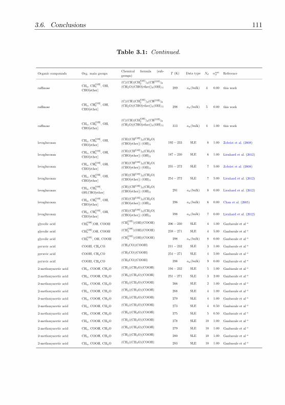
3.6. Conclusions 111
Table 3.1: Continued.
Organic compounds Org. main groupsChemical formula (sub-
groups)T (K) Data type Nd winit
d Reference
raffinoseCHn, CH
[OH]n , OH,
CHO[ether]
(C)(CH)(CH[OH]2 )3(CH[OH])8
(CH2O)(CHO[ether])4(OH)11 289 aw(bulk) 4 0.00 this work
raffinoseCHn, CH
[OH]n , OH,
CHO[ether]
(C)(CH)(CH[OH]2 )3(CH[OH])8
(CH2O)(CHO[ether])4(OH)11 298 aw(bulk) 5 0.00 this work
raffinoseCHn, CH
[OH]n , OH,
CHO[ether]
(C)(CH)(CH[OH]2 )3(CH[OH])8
(CH2O)(CHO[ether])4(OH)11 313 aw(bulk) 4 1.00 this work
levoglucosanCHn, CH
[OH]n , OH,
CHO[ether]
(CH)(CH[OH])3(CH2O)
(CHO[ether]) (OH)3192− 233 SLE 8 1.00 Zobrist et al. (2008)
levoglucosanCHn, CH
[OH]n , OH,
CHO[ether]
(CH)(CH[OH])3(CH2O)
(CHO[ether]) (OH)3187− 230 SLE 6 1.00 Lienhard et al. (2012)
levoglucosanCHn, CH
[OH]n , OH,
CHO[ether]
(CH)(CH[OH])3(CH2O)
(CHO[ether]) (OH)3255− 272 SLE 7 5.00 Zobrist et al. (2008)
levoglucosanCHn, CH
[OH]n , OH,
CHO[ether]
(CH)(CH[OH])3(CH2O)
(CHO[ether]) (OH)3254− 272 SLE 7 5.00 Lienhard et al. (2012)
levoglucosanCHn, CH
[OH]n ,
OH,CHO[ether]
(CH)(CH[OH])3(CH2O)
(CHO[ether]) (OH)3291 aw(bulk) 8 0.00 Lienhard et al. (2012)
levoglucosanCHn, CH
[OH]n , OH,
CHO[ether]
(CH)(CH[OH])3(CH2O)
(CHO[ether]) (OH)3296 aw(bulk) 6 0.00 Chan et al. (2005)
levoglucosanCHn, CH
[OH]n , OH,
CHO[ether]
(CH)(CH[OH])3(CH2O)
(CHO[ether]) (OH)3298 aw(bulk) 7 0.00 Lienhard et al. (2012)
glycolic acid CH[OH]n ,OH, COOH (CH
[OH]2 )(OH)(COOH) 206− 230 SLE 4 1.00 Ganbavale et al a
glycolic acid CH[OH]n ,OH, COOH (CH
[OH]2 )(OH)(COOH) 259− 271 SLE 4 5.00 Ganbavale et al a
glycolic acid CH[OH]n , OH, COOH (CH
[OH]2 )(OH)(COOH) 298 aw(bulk) 8 0.00 Ganbavale et al a
pyruvic acid COOH, CHnCO (CH3CO)(COOH) 211− 232 SLE 3 1.00 Ganbavale et al a
pyruvic acid COOH, CHnCO (CH3CO)(COOH) 254− 271 SLE 4 5.00 Ganbavale et al a
pyruvic acid COOH, CHnCO (CH3CO)(COOH) 298 aw(bulk) 9 0.00 Ganbavale et al a
2-methoxyacetic acid CHn, COOH, CHnO (CH2)(CH3O)(COOH) 194− 232 SLE 5 1.00 Ganbavale et al a
2-methoxyacetic acid CHn, COOH, CHnO (CH2)(CH3O)(COOH) 251− 271 SLE 3 2.00 Ganbavale et al a
2-methoxyacetic acid CHn, COOH, CHnO (CH2)(CH3O)(COOH) 266 SLE 2 1.00 Ganbavale et al a
2-methoxyacetic acid CHn, COOH, CHnO (CH2)(CH3O)(COOH) 268 SLE 4 1.00 Ganbavale et al a
2-methoxyacetic acid CHn, COOH, CHnO (CH2)(CH3O)(COOH) 270 SLE 4 1.00 Ganbavale et al a
2-methoxyacetic acid CHn, COOH, CHnO (CH2)(CH3O)(COOH) 273 SLE 4 0.50 Ganbavale et al a
2-methoxyacetic acid CHn, COOH, CHnO (CH2)(CH3O)(COOH) 275 SLE 5 0.50 Ganbavale et al a
2-methoxyacetic acid CHn, COOH, CHnO (CH2)(CH3O)(COOH) 278 SLE 10 1.00 Ganbavale et al a
2-methoxyacetic acid CHn, COOH, CHnO (CH2)(CH3O)(COOH) 279 SLE 10 1.00 Ganbavale et al a
2-methoxyacetic acid CHn, COOH, CHnO (CH2)(CH3O)(COOH) 280 SLE 10 1.00 Ganbavale et al a
2-methoxyacetic acid CHn, COOH, CHnO (CH2)(CH3O)(COOH) 283 SLE 10 1.00 Ganbavale et al a

112 Chapter 3. Improved AIOMFAC temperature dependence
Table 3.1: Continued.
Organic compounds Org. main groupsChemical formula (sub-
groups)T (K) Data type Nd winit
d Reference
2-methoxyacetic acid CHn, COOH, CHnO (CH2)(CH3O)(COOH) 285 SLE 10 1.00 Ganbavale et al a
2-methoxyacetic acid CHn, COOH, CHnO (CH2)(CH3O)(COOH) 288 SLE 10 1.00 Ganbavale et al a
2-methoxyacetic acid CHn, COOH, CHnO (CH2)(CH3O)(COOH) 289 SLE 10 0.00 Ganbavale et al a
2-methoxyacetic acid CHn, COOH, CHnO (CH2)(CH3O)(COOH) 290 SLE 10 0.00 Ganbavale et al a
2-methoxyacetic acid CHn, COOH, CHnO (CH2)(CH3O)(COOH) 298 aw(bulk) 9 0.00 Ganbavale et al a
2-ethoxyethyl acetate CHn, CHnO, CCOO(CH3)(CH2)(CH2O)2
(CH3COO) 208− 233 SLE 3 1.00 Ganbavale et al a
2-ethoxyethyl acetate CHn, CHnO, CCOO(CH3)(CH2)(CH2O)2
(CH3COO) 271− 272 SLE 3 2.00 Ganbavale et al a
2-ethoxyethyl acetate CHn, CHnO, CCOO(CH3)(CH2)(CH2O)2
(CH3COO) 276− 368 solubli. 12 1.00Carvoli and Delogu
(1986)
resorcinol ACHn, ACOH (ACH)4(ACOH)2 223− 232 SLE 4 1.00 Ganbavale et al a
resorcinol ACHn, ACOH (ACH)4(ACOH)2 267− 272 SLE 4 2.00 Ganbavale et al a
resorcinol ACHn, ACOH (ACH)4(ACOH)2 298 aw(bulk) 7 0.00 Ganbavale et al a
2-hydroxybenzoic acid ACHn, ACOH, COOH (ACH)4(AC)(ACOH)(COOH) 298− 348 SLE(org) d 11 0.20Shalmashi and Eliassi
(2008)
2-hydroxybenzoic acid ACHn, ACOH, COOH (ACH)4(AC)(ACOH)(COOH) 283− 339 SLE(org) d 13 0.20Apelblat and Manzurola
(1989)
2-(2-ethoxyethoxy)ethanol CHn, CHnO, OH (CH3)(CH2)2(CH2O)2 (OH) 211− 233 SLE 3 0.10 Ganbavale et al a
2-(2-ethoxyethoxy)ethanol CHn, CHnO, OH (CH3)(CH2)2(CH2O)2 (OH) 260− 272 SLE 4 0.10 Ganbavale et al a
2-(2-ethoxyethoxy)ethanol CHn, CHnO, OH (CH3)(CH2)2(CH2O)2 (OH) 265 SLE 5 0.10 Ganbavale et al a
2-(2-ethoxyethoxy)ethanol CHn, CHnO, OH (CH3)(CH2)2(CH2O)2 (OH) 268 SLE 5 0.10 Ganbavale et al a
2-(2-ethoxyethoxy)ethanol CHn, CHnO, OH (CH3)(CH2)2(CH2O)2 (OH) 270 SLE 5 0.10 Ganbavale et al a
2-(2-ethoxyethoxy)ethanol CHn, CHnO, OH (CH3)(CH2)2(CH2O)2 (OH) 273 SLE 5 0.10 Ganbavale et al a
2-(2-ethoxyethoxy)ethanol CHn, CHnO, OH (CH3)(CH2)2(CH2O)2 (OH) 275 SLE 6 0.10 Ganbavale et al a
2-(2-ethoxyethoxy)ethanol CHn, CHnO, OH (CH3)(CH2)2(CH2O)2 (OH) 278 SLE 9 0.10 Ganbavale et al a
2-(2-ethoxyethoxy)ethanol CHn, CHnO, OH (CH3)(CH2)2(CH2O)2 (OH) 279 SLE 12 0.10 Ganbavale et al a
2-(2-ethoxyethoxy)ethanol CHn, CHnO, OH (CH3)(CH2)2(CH2O)2 (OH) 280 SLE 9 0.10 Ganbavale et al a
2-(2-ethoxyethoxy)ethanol CHn, CHnO, OH (CH3)(CH2)2(CH2O)2 (OH) 283 SLE 9 0.10 Ganbavale et al a
2-(2-ethoxyethoxy)ethanol CHn, CHnO, OH (CH3)(CH2)2(CH2O)2 (OH) 285 SLE 9 0.10 Ganbavale et al a
2-(2-ethoxyethoxy)ethanol CHn, CHnO, OH (CH3)(CH2)2(CH2O)2 (OH) 288 SLE 9 0.10 Ganbavale et al a
2-(2-ethoxyethoxy)ethanol CHn, CHnO, OH (CH3)(CH2)2(CH2O)2 (OH) 289 SLE 12 0.00 Ganbavale et al a
2-(2-ethoxyethoxy)ethanol CHn, CHnO, OH (CH3)(CH2)2(CH2O)2 (OH) 290 SLE 9 0.00 Ganbavale et al a
2-(2-ethoxyethoxy)ethanol CHn, CHnO, OH (CH3)(CH2)2(CH2O)2 (OH) 298 SLE 12 0.00 Ganbavale et al a
vanillylmandelic acidACHn, CH
[OH]n , COOH,
CHnO, OH
(ACH)3(AC)2(ACOH)(CH3O)
(CH[OH])(OH)(COOH) 214− 232 SLE 4 1.00 Zobrist et al. (2008)
vanillylmandelic acidACHn, CH
[OH]n , COOH,
CHnO, OH
(ACH)3(AC)2(ACOH)(CH3O)
(CH[OH])(OH)(COOH) 267− 272 SLE 4 5.00 Zobrist et al. (2008)
vanillylmandelic acidACHn, CH
[OH]n , COOH,
CHnO, OH
(ACH)3(AC)2(ACOH)(CH3O)
(CH[OH])(OH)(COOH) 289 aw(bulk) 6 0.00 this work

3.6. Conclusions 113
Table 3.1: Continued.
Organic compounds Org. main groupsChemical formula (sub-
groups)T (K) Data type Nd winit
d Reference
vanillylmandelic acidACHn, CH
[OH]n , COOH,
CHnO, OH
(ACH)3(AC)2(ACOH)(CH3O)
(CH[OH])(OH)(COOH) 298 aw(bulk) 6 0.00 this work
vanillylmandelic acidACHn, CH
[OH]n , COOH,
CHnO, OH
(ACH)3(AC)2(ACOH)(CH3O)
(CH[OH])(OH)(COOH) 313 aw(bulk) 6 1.00 this work
— water + alcohol+ alcohol systems —
1-butanol, 1-propanolCHn, CH
[OH]n ,
OH,COOH
(CH[alc−tail]3 )(CH
[alc−tail]2 )2
(CH[OH]2 )(OH),
(CH[alc−tail]3 )(CH
[alc−tail]2 )
(CH[OH]2 )(OH)
298 LLE 20 0.00Gomis-Yagues et al.
(1998)
1-butanol, 1-propanolCHn, CH
[OH]n , OH,
COOH
(CH[alc−tail]3 )(CH
[alc−tail]2 )2
(CH[OH]2 )(OH),
(CH[alc−tail]3 )(CH
[alc−tail]2 )
(CH[OH]2 )(OH)
323 LLE 10 1.00Gomis-Yagues et al.
(1998)
1-butanol, 1-propanolCHn, CH
[OH]n , OH,
COOH
(CH[alc−tail]3 )(CH
[alc−tail]2 )2
(CH[OH]2 )(OH),
(CH[alc−tail]3 )(CH
[alc−tail]2 )
(CH[OH]2 )(OH)
358 LLE 6 1.00Gomis-Yagues et al.
(1998)
1-butanol, 1-propanolCHn, CH
[OH]n , OH,
COOH
(CH[alc−tail]3 )(CH
[alc−tail]2 )2
(CH[OH]2 )(OH),
(CH[alc−tail]3 )(CH
[alc−tail]2 )
(CH[OH]2 )(OH)
368 LLE 8 1.00Gomis-Yagues et al.
(1998)
1-pentanol, ethanolCHn, CH
[OH]n , OH,
COOH
(CH[alc−tail]3 )(CH
[alc−tail]2 )3
(CH[OH]2 )(OH),
(CH[alc−tail]3 )(CH
[OH]2 )(OH)
298 LLE 12 0.00Fernandez-Torres et al.
(1999)
1-pentanol, ethanolCHn, CH
[OH]n , OH,
COOH
(CH[alc−tail]3 )(CH
[alc−tail]2 )3
(CH[OH]2 )(OH),
(CH[alc−tail]3 )(CH
[OH]2 )(OH)
323 LLE 12 1.00Fernandez-Torres et al.
(1999)
1-pentanol, ethanolCHn, CH
[OH]n , OH,
COOH
(CH[alc−tail]3 )(CH
[alc−tail]2 )3
(CH[OH]2 )(OH),
(CH[alc−tail]3 )(CH
[OH]2 )(OH)
358 LLE 8 1.00Fernandez-Torres et al.
(1999)
1-pentanol, ethanolCHn, CH
[OH]n , OH,
COOH
(CH[alc−tail]3 )(CH
[alc−tail]2 )3
(CH[OH]2 )(OH),
(CH[alc−tail]3 )(CH
[OH]2 )(OH)
368 LLE 12 1.00Fernandez-Torres et al.
(1999)
— water + alcohol+ acid systems —
1-butanol, acetic acidCHn, CH
[OH]n , OH,
COOH
(CH[alc−tail]3 )(CH
[alc−tail]2 )2
(CH[OH]2 )(OH),
(CH3)(COOH)298 LLE 10 0.00 Ruiz Bevia et al. (1984)
1-butanol, acetic acidCHn, CH
[OH]n , OH,
COOH
(CH[alc−tail]3 )(CH
[alc−tail]2 )2
(CH[OH]2 )(OH),
(CH3)(COOH)303 LLE 12 0.00
Esquıvel and
Bernardo-Gil (1990)
1-butanol, acetic acidCHn, CH
[OH]n , OH,
COOH
(CH[alc−tail]3 )(CH
[alc−tail]2 )2
(CH[OH]2 )(OH),
(CH3)(COOH)323 LLE 14 1.00
Esquıvel and
Bernardo-Gil (1990)
2-butanol, acetic acidCHn, CH
[OH]n , OH,
COOH
(CH[alc]3 )(CH
[alc−tail]3 )
(CH[alc−tail]2 )(CH[OH])(OH),
(CH3)(COOH)303 LLE 10 0.00
Esquıvel and
Bernardo-Gil (1990)
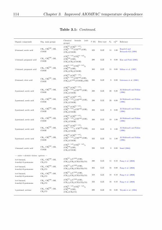
114 Chapter 3. Improved AIOMFAC temperature dependence
Table 3.1: Continued.
Organic compounds Org. main groupsChemical formula (sub-
groups)T (K) Data type Nd winit
d Reference
2-butanol, acetic acidCHn, CH
[OH]n , OH,
COOH
(CH[alc]3 )(CH
[alc−tail]3 )
(CH[alc−tail]2 )(CH[OH])(OH),
(CH3)(COOH)323 LLE 14 1.00
Esquıvel and
Bernardo-Gil (1990)
1-butanol, propanoic acidCHn, CH
[OH]n , OH,
COOH
(CH[alc−tail]3 )(CH
[alc−tail]2 )2
(CH[OH]2 )(OH),
(CH3)(CH2)(COOH)298 LLE 8 0.00 Kim and Park (2005)
1-butanol, propanoic acidCHn, CH
[OH]n , OH,
COOH
(CH[alc−tail]3 )(CH
[alc−tail]2 )2
(CH[OH]2 )(OH),
(CH3)(CH2)(COOH)303 LLE 14 0.00 Solimo et al. (1997)
2-butanol, citric acidCHn, CH
[OH]n , OH,
COOH
(CH[alc]3 )(CH
[alc−tail]3 )
(CH[alc−tail]2 )(CH[OH])(OH),
(CH2)2(C[OH])(COOH)3(OH) 298 LLE 8 0.00 Lintomen et al. (2001)
2-pentanol, acetic acidCHn, CH
[OH]n , OH,
COOH
(CH[alc]3 )(CH
[alc−tail]3 )
(CH[alc−tail]2 )2(CH[OH])(OH),
(CH3)(COOH)288 LLE 20 0.20
Al-Muhtaseb and Fahim
(1996)
2-pentanol, acetic acidCHn, CH
[OH]n , OH,
COOH
(CH[alc]3 )(CH
[alc−tail]3 )
(CH[alc−tail]2 )2(CH[OH])(OH),
(CH3)(COOH)298 LLE 20 0.00
Al-Muhtaseb and Fahim
(1996)
2-pentanol, acetic acidCHn, CH
[OH]n , OH,
COOH
(CH[alc]3 )(CH
[alc−tail]3 )
(CH[alc−tail]2 )2(CH[OH])(OH),
(CH3)(COOH)303 LLE 8 0.00
Al-Muhtaseb and Fahim
(1996)
2-pentanol, acetic acidCHn, CH
[OH]n , OH,
COOH
(CH[alc]3 )(CH
[alc−tail]3 )
(CH[alc−tail]2 )2(CH[OH])(OH),
(CH3)(COOH)308 LLE 10 1.00
Al-Muhtaseb and Fahim
(1996)
2-pentanol, acetic acidCHn, CH
[OH]n , OH,
COOH
(CH[alc]3 )(CH
[alc−tail]3 )
(CH[alc−tail]2 )2 (CH[OH])(OH),
(CH3)(COOH)318 LLE 8 1.00
Al-Muhtaseb and Fahim
(1996)
2-pentanol, acetic acidCHn, CH
[OH]n , OH,
COOH
(CH[alc]3 )(CH
[alc−tail]3 )
(CH[alc−tail]2 )2(CH[OH])(OH),
(CH3)(COOH)323 LLE 14 1.00
Al-Muhtaseb and Fahim
(1996)
1-hexanol, acetic acidCHn, CH
[OH]n , OH,
COOH
(CH[alc−tail]3 )(CH
[alc−tail]2 )4
(CH[OH]2 )(OH),
(CH3)(COOH)293 LLE 8 0.00 Senol (2004)
— water + alcohol+ ketone systems —
tert-butanol,
4-methyl-2-pentanone
CHn, CH[OH]n , OH,
CHnCO
(CH[alc]3 )3(C[OH])(OH),
(CH3)2(CH2)(CH)(CH3CO) 288 LLE 14 0.10 Fang et al. (2008)
tert-butanol,
4-methyl-2-pentanone
CHn, CH[OH]n , OH,
CHnCO
(CH[alc]3 )3(C[OH])(OH),
(CH3)2(CH2)(CH)(CH3CO) 304 LLE 16 0.00 Fang et al. (2008)
tert-butanol,
4-methyl-2-pentanone
CHn, CH[OH]n , OH,
CHnCO
(CH[alc]3 )3(C[OH])(OH),
(CH3)2(CH2)(CH)(CH3CO) 318 LLE 18 0.10 Fang et al. (2008)
tert-butanol,
4-methyl-2-pentanone
CHn, CH[OH]n , OH,
CHnCO
(CH[alc]3 )3(C[OH])(OH),
(CH3)2(CH2)(CH)(CH3CO) 333 LLE 16 0.10 Fang et al. (2008)
1-pentanol, acetoneCHn, CH
[OH]n , OH,
CHnCO
(CH[alc−tail]3 )(CH
[alc−tail]2 )3
(CH[OH]2 )(OH),
(CH3)(CH3CO)298 LLE 16 0.00 Tiryaki et al. (1994)

3.6. Conclusions 115
Table 3.1: Continued.
Organic compounds Org. main groupsChemical formula (sub-
groups)T (K) Data type Nd winit
d Reference
1-pentanol, acetoneCHn, CH
[OH]n , OH,
CHnCO
(CH[alc−tail]3 )(CH
[alc−tail]2 )3
(CH[OH]2 )(OH),
(CH3)(CH3CO)303 LLE 16 0.00 Tiryaki et al. (1994)
1-pentanol, acetoneCHn, CH
[OH]n , OH,
CHnCO
(CH[alc−tail]3 )(CH
[alc−tail]2 )3
(CH[OH]2 )(OH),
(CH3)(CH3CO)308 LLE 16 0.00 Tiryaki et al. (1994)
2-octanol, acetoneCHn, CH
[OH]n , OH,
CHnCO
(CH[alc−tail]3 )(CH
[alc]3 )
(CH[alc−tail]2 )5(CH[OH])(OH),
(CH3)(CH3CO)298 LLE 18 0.00 Tiryaki et al. (1994)
2-octanol, acetoneCHn, CH
[OH]n , OH,
CHnCO
(CH[alc−tail]3 )(CH
[alc]3 )
(CH[alc−tail]2 )5(CH[OH])(OH),
(CH3)(CH3CO)303 LLE 18 0.00 Tiryaki et al. (1994)
2-octanol, acetoneCHn, CH
[OH]n , OH,
CHnCO
(CH[alc−tail]3 )(CH
[alc]3 )
(CH[alc−tail]2 )5(CH[OH])(OH),
(CH3)(CH3CO)308 LLE 16 1.00 Tiryaki et al. (1994)
— water + alcohol+ ether systems —
ethanol,
2-ethoxy-2-methyl-propane
CHn, CH[OH]n , OH,
CHnO
(CH[alc−tail]3 )(CH
[OH]2 )(OH),
(CH3)4(C)(CH2O) 288 LLE 14 0.20 Fandary et al. (1999)
ethanol,
2-ethoxy-2-methyl-propane
CHn, CH[OH]n , OH,
CHnO
(CH[alc−tail]3 )(CH
[OH]2 )(OH),
(CH3)4(C)(CH2O) 298 LLE 14 0.00 Fandary et al. (1999)
ethanol,
2-ethoxy-2-methyl-propane
CHn, CH[OH]n , OH,
CHnO
(CH[alc−tail]3 )(CH
[OH]2 )(OH),
(CH3)4(C)(CH2O) 303 LLE 14 0.00 Fandary et al. (1999)
ethanol,
2-ethoxy-2-methyl-propane
CHn, CH[OH]n , OH,
CHnO
(CH[alc−tail]3 )(CH
[OH]2 )(OH),
(CH3)4(C)(CH2O) 308 LLE 14 0.00 Fandary et al. (1999)
— water + alcohol+ ester systems —
ethanol, ethyl acetateCHn, CH
[OH]n , OH,
CCOO
(CH[alc−tail]3 )(CH
[OH]2 ) (OH),
(CH3) (CH2)(CH3COO) 313 LLE 10 1.00 Mertl (1972)
ethanol, ethyl acetateCHn,CH
[OH]n , OH,
CCOO
(CH[alc−tail]3 )(CH
[OH]2 )(OH),
(CH3)(CH2) (CH3COO) 328 LLE 10 1.00 Mertl (1972)
ethanol, ethyl acetateCHn,CH
[OH]n , OH,
CCOO
(CH[alc−tail]3 )(CH
[OH]2 )(OH),
(CH3)(CH2) (CH3COO) 343 LLE 10 1.00 Mertl (1972)
— water + alcohol+ aromatic systems —
1-butanol, phenolCHn,CH
[OH]n , OH,
ACHn, ACOH
(CH[alc−tail]3 )(CH
[alc−tail]2 )2
(CH[OH]2 )(OH), (ACH)5
(ACOH)298 LLE 12 0.00
De Oliveira and Aznar
(2010)
2-butanol, phenolCHn,CH
[OH]n , OH,
ACHn, ACOH
(CH[alc]3 )(CH
[alc−tail]3 )
(CH[alc−tail]2 )(CH[OH])(OH),
(ACH)5(ACOH)298 LLE 12 0.00
De Oliveira and Aznar
(2010)
2-butanol, phenolCHn, CH
[OH]n , OH,
ACHn, ACOH
(CH[alc]3 )(CH
[alc−tail]3 )
(CH[alc−tail]2 )(CH[OH])(OH),
(ACH)5(ACOH)313 LLE 12 1.00
De Oliveira and Aznar
(2010)
— water + alcohol+ aldehyde systems —
ethanol, butyraldehyde CHn, CH[OH]n , OH, CHO
(CH[alc−tail]3 )(CH
[OH]2 )(OH),
(CH3) (CH2)2(CHO) 298 LLE 10 0.00 Letcher et al. (1996)

116 Chapter 3. Improved AIOMFAC temperature dependence
Table 3.1: Continued.
Organic compounds Org. main groupsChemical formula (sub-
groups)T (K) Data type Nd winit
d Reference
2-propanol, butyraldehyde CHn, CH[OH]n , OH, CHO
(CH[alc]3 )2(CH[OH]) (OH),
(CH3)(CH2)2(CHO) 298 LLE 10 0.00 Letcher et al. (1996)
2-butanol, butyraldehyde CHn, CH[OH]n , OH, CHO
(CH[alc]3 )(CH
[alc−tail]3 )
(CH[alc−tail]2 )(CH[OH])(OH),
(CH3)(CH2)2 (CHO)298 LLE 10 0.00 Letcher et al. (1996)
— water + acid+ ketone systems —
acetic acid, 2-butanone CHn, COOH, CHnCO(CH3)(COOH),
(CH3)(CH2)(CH3CO) 298 LLE 8 0.00 Correa et al. (1987)
acetic acid, 2-butanone CHn, COOH, CHnCO(CH3)(COOH),
(CH3)(CH2)(CH3CO) 308 LLE 8 1.00 Correa et al. (1987)
acetic acid, 2-butanone CHn, COOH, CHnCO(CH3)(COOH),
(CH3)(CH2)(CH3CO) 318 LLE 8 1.00 Correa et al. (1987)
propanoic acid, 2-butanone CHn, COOH, CHnCO(CH3)(CH2)(COOH),
(CH3)(CH2)(CH3CO) 298 LLE 8 0.00 Arce et al. (1995)
propanoic acid, 2-butanone CHn, COOH, CHnCO(CH3)(CH2)(COOH),
(CH3)(CH2)(CH3CO) 308 LLE 12 1.00 Arce et al. (1995)
propanoic acid, 2-butanone CHn, COOH, CHnCO(CH3)(CH2)(COOH),
(CH3)(CH2)(CH3CO) 318 LLE 10 1.00 Arce et al. (1995)
propanoic acid,
2-pentanoneCHn, COOH, CHnCO
(CH3)(CH2)(COOH),
(CH3)(CH2)2(CH3CO) 298 LLE 12 0.00 Arce et al. (1995)
propanoic acid,
2-pentanoneCHn, COOH, CHnCO
(CH3)(CH2)(COOH),
(CH3)(CH2)2(CH3CO) 308 LLE 12 1.00 Arce et al. (1995)
propanoic acid,
2-pentanoneCHn, COOH, CHnCO
(CH3)(CH2)(COOH),
(CH3)(CH2)2(CH3CO) 318 LLE 12 1.00 Arce et al. (1995)
propanoic acid,
2-pentanoneCHn, COOH, CHnCO
(CH3)(CH2)(COOH),
(CH3)(CH2)2(CH3CO) 328 LLE 16 1.00 Arce et al. (1995)
— water + acid+ ether systems —
acetic acid, 2-methoxy-2-
methylpropane CHn, COOH, CHnO(CH3)(COOH),
(CH3)3(C)(CH3O) 293 LLE 18 0.00 Miao et al. (2007)
acetic acid, 2-methoxy-2-
methylpropane CHn, COOH, CHnO(CH3)(COOH),
(CH3)3(C)(CH3O) 298 LLE 18 0.00 Miao et al. (2007)
acetic acid, 2-methoxy-2-
methylpropane CHn, COOH, CHnO(CH3)(COOH),
(CH3)3(C)(CH3O) 303 LLE 18 0.00 Miao et al. (2007)
acetic acid, 2-methoxy-2-
methylpropane CHn, COOH, CHnO(CH3)(COOH),
(CH3)3(C)(CH3O) 308 LLE 18 0.10 Miao et al. (2007)
— water + acid+ ester systems —
acetic acid, ethyl acetate CHn, COOH, CCOO(CH3)(COOH),
(CH3)(CH2)(CH3COO) 283 LLE 12 1.00 Colombo et al. (1999)
acetic acid, ethyl acetate CHn, COOH, CCOO(CH3)(COOH),
(CH3)(CH2)(CH3COO) 298 LLE 12 0.00 Colombo et al. (1999)
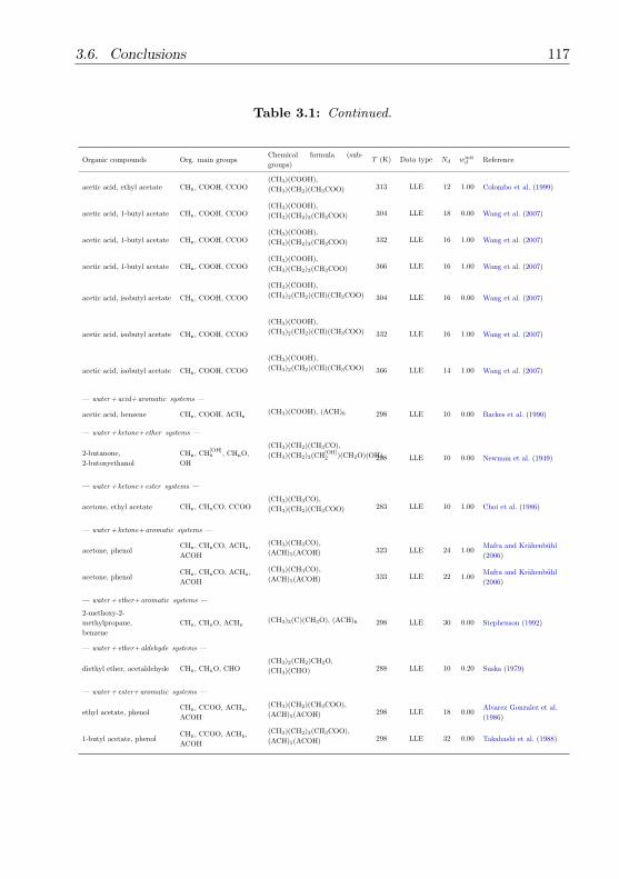
3.6. Conclusions 117
Table 3.1: Continued.
Organic compounds Org. main groupsChemical formula (sub-
groups)T (K) Data type Nd winit
d Reference
acetic acid, ethyl acetate CHn, COOH, CCOO(CH3)(COOH),
(CH3)(CH2)(CH3COO) 313 LLE 12 1.00 Colombo et al. (1999)
acetic acid, 1-butyl acetate CHn, COOH, CCOO(CH3)(COOH),
(CH3)(CH2)3(CH3COO) 304 LLE 18 0.00 Wang et al. (2007)
acetic acid, 1-butyl acetate CHn, COOH, CCOO(CH3)(COOH),
(CH3)(CH2)3(CH3COO) 332 LLE 16 1.00 Wang et al. (2007)
acetic acid, 1-butyl acetate CHn, COOH, CCOO(CH3)(COOH),
(CH3)(CH2)3(CH3COO) 366 LLE 16 1.00 Wang et al. (2007)
acetic acid, isobutyl acetate CHn, COOH, CCOO
(CH3)(COOH),
(CH3)2(CH2)(CH)(CH3COO) 304 LLE 16 0.00 Wang et al. (2007)
acetic acid, isobutyl acetate CHn, COOH, CCOO
(CH3)(COOH),
(CH3)2(CH2)(CH)(CH3COO) 332 LLE 16 1.00 Wang et al. (2007)
acetic acid, isobutyl acetate CHn, COOH, CCOO
(CH3)(COOH),
(CH3)2(CH2)(CH)(CH3COO) 366 LLE 14 1.00 Wang et al. (2007)
— water + acid+ aromatic systems —
acetic acid, benzene CHn, COOH, ACHn(CH3)(COOH), (ACH)6 298 LLE 10 0.00 Backes et al. (1990)
— water + ketone+ ether systems —
2-butanone,
2-butoxyethanol
CHn, CH[OH]n , CHnO,
OH
(CH3)(CH2)(CH3CO),
(CH3)(CH2)3(CH[OH]2 )(CH2O)(OH)298 LLE 10 0.00 Newman et al. (1949)
— water + ketone+ ester systems —
acetone, ethyl acetate CHn, CHnCO, CCOO(CH3)(CH3CO),
(CH3)(CH2)(CH3COO) 283 LLE 10 1.00 Choi et al. (1986)
— water + ketone+ aromatic systems —
acetone, phenolCHn, CHnCO, ACHn,
ACOH
(CH3)(CH3CO),
(ACH)5(ACOH) 323 LLE 24 1.00Mafra and Krahenbuhl
(2006)
acetone, phenolCHn, CHnCO, ACHn,
ACOH
(CH3)(CH3CO),
(ACH)5(ACOH) 333 LLE 22 1.00Mafra and Krahenbuhl
(2006)
— water + ether+ aromatic systems —
2-methoxy-2-
methylpropane,
benzene
CHn, CHnO, ACHn(CH3)3(C)(CH3O), (ACH)6 298 LLE 30 0.00 Stephenson (1992)
— water + ether+ aldehyde systems —
diethyl ether, acetaldehyde CHn, CHnO, CHO(CH3)2(CH2)CH2O,
(CH3)(CHO) 288 LLE 10 0.20 Suska (1979)
— water + ester+ aromatic systems —
ethyl acetate, phenolCHn, CCOO, ACHn,
ACOH
(CH3)(CH2)(CH3COO),
(ACH)5(ACOH) 298 LLE 18 0.00Alvarez Gonzalez et al.
(1986)
1-butyl acetate, phenolCHn, CCOO, ACHn,
ACOH
(CH3)(CH2)3(CH3COO),
(ACH)5(ACOH) 298 LLE 32 0.00 Takahashi et al. (1988)
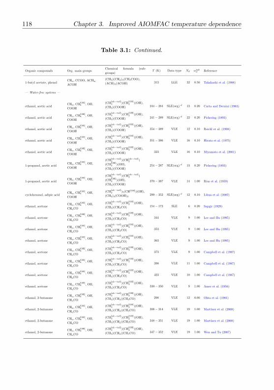
118 Chapter 3. Improved AIOMFAC temperature dependence
Table 3.1: Continued.
Organic compounds Org. main groupsChemical formula (sub-
groups)T (K) Data type Nd winit
d Reference
1-butyl acetate, phenolCHn, CCOO, ACHn,
ACOH
(CH3)(CH2)3(CH3COO),
(ACH)5(ACOH) 313 LLE 32 0.50 Takahashi et al. (1988)
— Water-free systems —
ethanol, acetic acidCHn, CH
[OH]n , OH,
COOH
(CH[alc−tail]3 )(CH
[OH]2 )(OH),
(CH3)(COOH) 244− 284 SLE(org) d 13 0.20 Carta and Dernini (1983)
ethanol, acetic acidCHn, CH
[OH]n , OH,
COOH
(CH[alc−tail]3 )(CH
[OH]2 )(OH),
(CH3)(COOH) 241− 289 SLE(org) d 22 0.20 Pickering (1893)
ethanol, acetic acidCHn, CH
[OH]n , OH,
COOH
(CH[alc−tail]3 )(CH
[OH]2 )(OH),
(CH3)(COOH) 354− 389 VLE 12 0.10 Reichl et al. (1998)
ethanol, acetic acidCHn, CH
[OH]n , OH,
COOH
(CH[alc−tail]3 )(CH
[OH]2 )(OH),
(CH3)(COOH) 351− 386 VLE 16 0.10 Hirata et al. (1975)
ethanol, acetic acidCHn, CH
[OH]n , OH,
COOH
(CH[alc−tail]3 )(CH
[OH]2 )(OH),
(CH3)(COOH) 323 VLE 16 0.10 Miyamoto et al. (2001)
1-propanol, acetic acidCHn, CH
[OH]n , OH,
COOH
(CH[alc−tail]3 )(CH
[alc−tail]2 )
(CH[OH]2 )(OH),
(CH3)(COOH)254− 287 SLE(org) d 13 0.20 Pickering (1893)
1-propanol, acetic acidCHn, CH
[OH]n , OH,
COOH
(CH[alc−tail]3 )(CH
[alc−tail]2 )
(CH[OH]2 )(OH),
(CH3)(COOH)370− 387 VLE 14 1.00 Rius et al. (1959)
cyclohexanol, adipic acidCHn, CH
[OH]n , OH,
COOH
(CH[alc−tail]2 )5(CH[OH])(OH),
(CH2)4(COOH)2299− 352 SLE(org) d 12 0.10 Lihua et al. (2007)
ethanol, acetoneCHn, CH
[OH]n , OH,
CHnCO
(CH[alc−tail]3 )(CH
[OH]2 )(OH),
(CH3)(CH3CO) 154− 173 SLE 6 0.20 Sapgir (1929)
ethanol, acetoneCHn, CH
[OH]n , OH,
CHnCO
(CH[alc−tail]3 )(CH
[OH]2 )(OH),
(CH3)(CH3CO) 344 VLE 9 1.00 Lee and Hu (1995)
ethanol, acetoneCHn, CH
[OH]n , OH,
CHnCO
(CH[alc−tail]3 )(CH
[OH]2 )(OH),
(CH3)(CH3CO) 353 VLE 9 1.00 Lee and Hu (1995)
ethanol, acetoneCHn, CH
[OH]n , OH,
CHnCO
(CH[alc−tail]3 )(CH
[OH]2 )(OH),
(CH3)(CH3CO) 363 VLE 9 1.00 Lee and Hu (1995)
ethanol, acetoneCHn, CH
[OH]n , OH,
CHnCO
(CH[alc−tail]3 )(CH
[OH]2 )(OH),
(CH3)(CH3CO) 373 VLE 9 1.00 Campbell et al. (1987)
ethanol, acetoneCHn, CH
[OH]n , OH,
CHnCO
(CH[alc−tail]3 )(CH
[OH]2 )(OH),
(CH3)(CH3CO) 398 VLE 11 1.00 Campbell et al. (1987)
ethanol, acetoneCHn, CH
[OH]n , OH,
CHnCO
(CH[alc−tail]3 )(CH
[OH]2 )(OH),
(CH3)(CH3CO) 423 VLE 10 1.00 Campbell et al. (1987)
ethanol, acetoneCHn, CH
[OH]n , OH,
CHnCO
(CH[alc−tail]3 )(CH
[OH]2 )(OH),
(CH3)(CH3CO) 330− 350 VLE 9 1.00 Amer et al. (1956)
ethanol, 2-butanoneCHn, CH
[OH]n , OH,
CHnCO
(CH[alc−tail]3 )(CH
[OH]2 )(OH),
(CH3)(CH2)(CH3CO) 298 VLE 12 0.00 Ohta et al. (1981)
ethanol, 2-butanoneCHn, CH
[OH]n , OH,
CHnCO
(CH[alc−tail]3 )(CH
[OH]2 )(OH),
(CH3)(CH2)(CH3CO) 308− 314 VLE 19 1.00 Martınez et al. (2008)
ethanol, 2-butanoneCHn, CH
[OH]n , OH,
CHnCO
(CH[alc−tail]3 )(CH
[OH]2 )(OH),
(CH3)(CH2)(CH3CO) 348− 351 VLE 19 1.00 Martınez et al. (2008)
ethanol, 2-butanoneCHn, CH
[OH]n , OH,
CHnCO
(CH[alc−tail]3 )(CH
[OH]2 )(OH),
(CH3)(CH2)(CH3CO) 347− 352 VLE 19 1.00 Wen and Tu (2007)
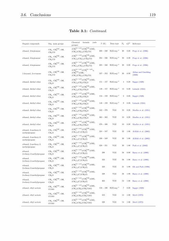
3.6. Conclusions 119
Table 3.1: Continued.
Organic compounds Org. main groupsChemical formula (sub-
groups)T (K) Data type Nd winit
d Reference
ethanol, 2-heptanoneCHn, CH
[OH]n , OH,
CHnCO
(CH[alc−tail]3 )(CH
[OH]2 )(OH),
(CH3)(CH2)4(CH3CO) 208− 238 SLE(org) d 20 0.20 Fiege et al. (1996)
ethanol, 3-heptanoneCHn, CH
[OH]n , OH,
CHnCO
(CH[alc−tail]3 )(CH
[OH]2 )(OH),
(CH3)2(CH2)3(CH2CO) 204− 236 SLE(org) d 20 0.20 Fiege et al. (1996)
ethanol, 4-heptanoneCHn, CH
[OH]n , OH,
CHnCO
(CH[alc−tail]3 )(CH
[OH]2 )(OH),
(CH3)2(CH2)3(CH3CO) 205− 240 SLE(org) d 20 0.20 Fiege et al. (1996)
1-hexanol, 2-octanoneCHn, CH
[OH]n , OH,
CHnCO
(CH[alc−tail]3 )(CH
[alc−tail]2 )4
(CH[OH]2 )(OH),
(CH3)(CH2)5(CH3CO)227− 253 SLE(org) d 20 0.20
Abbas and Gmehling
(2008)
ethanol, diethyl etherCHn, CH
[OH]n , OH,
CHnO
(CH[alc−tail]3 )(CH
[OH]2 )(OH),
(CH3)2(CH2)CH2O 151− 157 SLE(org) d 4 0.20 Sapgir (1929)
ethanol, diethyl etherCHn, CH
[OH]n , OH,
CHnO
(CH[alc−tail]3 )(CH
[OH]2 )(OH),
(CH3)2(CH2)CH2O 149− 157 SLE(org) d 13 0.20 Lalande (1934)
ethanol, diethyl etherCHn, CH
[OH]n , OH,
CHnO
(CH[alc−tail]3 )(CH
[OH]2 )(OH),
(CH3)2(CH2)CH2O 154− 159 SLE(org) d 2 0.20 Sapgir (1929)
ethanol, diethyl etherCHn, CH
[OH]n , OH,
CHnO
(CH[alc−tail]3 )(CH
[OH]2 )(OH),
(CH3)2(CH2)CH2O 148− 159 SLE(org) d 9 0.20 Lalande (1934)
ethanol, diethyl etherCHn, CH
[OH]n , OH,
CHnO
(CH[alc−tail]3 )(CH
[OH]2 )(OH),
(CH3)2(CH2)CH2O 342− 378 VLE 10 0.20 Moeller et al. (1951)
ethanol, diethyl etherCHn, CH
[OH]n , OH,
CHnO
(CH[alc−tail]3 )(CH
[OH]2 )(OH),
(CH3)2(CH2)CH2O 363− 382 VLE 10 0.20 Moeller et al. (1951)
ethanol, diethyl etherCHn, CH
[OH]n , OH,
CHnO
(CH[alc−tail]3 )(CH
[OH]2 )(OH),
(CH3)2(CH2)CH2O 378− 400 VLE 10 0.20 Moeller et al. (1951)
ethanol, 2-methoxy-2-
methylpropane
CHn, CH[OH]n , OH,
CHnO
(CH[alc−tail]3 )(CH
[OH]2 )(OH),
(CH3)3(C)(CH3O) 324− 347 VLE 22 1.00 Al-Rub et al. (2002)
ethanol, 2-methoxy-2-
methylpropane
CHn, CH[OH]n , OH,
CHnO
(CH[alc−tail]3 )(CH
[OH]2 )(OH),
(CH3)3(C)(CH3O) 326− 349 VLE 30 1.00 Al-Rub et al. (2002)
ethanol, 2-methoxy-2-
methylpropane
CHn, CH[OH]n , OH,
CHnO
(CH[alc−tail]3 )(CH
[OH]2 )(OH),
(CH3)3(C)(CH3O) 328− 351 VLE 30 1.00 Park et al. (2002)
ethanol,
2-ethoxy-2-methylpropane
CHn, CH[OH]n , OH,
CHnO
(CH[alc−tail]3 )(CH
[OH]2 )(OH),
(CH3)4(C)(CH2O) 298 VLE 56 0.00 Rarey et al. (1999)
ethanol,
2-ethoxy-2-methylpropane
CHn, CH[OH]n , OH,
CHnO
(CH[alc−tail]3 )(CH
[OH]2 )(OH),
(CH3)4(C)(CH2O) 323 VLE 56 1.00 Rarey et al. (1999)
ethanol,
2-ethoxy-2-methylpropane
CHn, CH[OH]n , OH,
CHnO
(CH[alc−tail]3 )(CH
[OH]2 )(OH),
(CH3)4(C)(CH2O) 333 VLE 21 1.00 Oh and Park (1998)
ethanol,
2-ethoxy-2-methylpropane
CHn, CH[OH]n , OH,
CHnO
(CH[alc−tail]3 )(CH
[OH]2 )(OH),
(CH3)4(C)(CH2O) 338 VLE 56 1.00 Rarey et al. (1999)
ethanol,
2-ethoxy-2-methylpropane
CHn, CH[OH]n , OH,
CHnO
(CH[alc−tail]3 )(CH
[OH]2 )(OH),
(CH3)4(C)(CH2O) 363 VLE 52 1.00 Rarey et al. (1999)
ethanol, ethyl acetateCHn, CH
[OH]n , OH,
CCOO
(CH[alc−tail]3 )(CH
[OH]2 )(OH),
(CH3)(CH2)(CH3COO) 158− 190 SLE(org) d 7 0.20 Sapgir (1929)
ethanol, ethyl acetateCHn, CH
[OH]n , OH,
CCOO
(CH[alc−tail]3 )(CH
[OH]2 )(OH),
(CH3)(CH2)(CH3COO) 313 VLE 14 1.00 Mertl (1972)
ethanol, ethyl acetateCHn, CH
[OH]n , OH,
CCOO
(CH[alc−tail]3 )(CH
[OH]2 )(OH),
(CH3)(CH2)(CH3COO) 328 VLE 14 1.00 Mertl (1972)

120 Chapter 3. Improved AIOMFAC temperature dependence
Table 3.1: Continued.
Organic compounds Org. main groupsChemical formula (sub-
groups)T (K) Data type Nd winit
d Reference
ethanol, ethyl acetateCHn, CH
[OH]n , OH,
CCOO
(CH[alc−tail]3 )(CH
[OH]2 )(OH),
(CH3)(CH2)(CH3COO) 343 VLE 15 1.00 Mertl (1972)
ethanol, ethyl acetateCHn, CH
[OH]n , OH,
CCOO
(CH[alc−tail]3 )(CH
[OH]2 )(OH),
(CH3)(CH2)(CH3COO) 345− 351 VLE 24 1.00 Calvar et al. (2005)
2-propanol, 1-butyl acetateCHn, CH
[OH]n , OH,
CCOO
(CH[alc]3 )2(CH[OH])(OH),
(CH3)(CH2)3(CH3COO) 355− 399 VLE 27 0.20 Gonzalez (1996)
tert-Butanol, tert-butyl
acetateCHn, OH, CCOO
(CH[alc]3 )3(C[OH])(OH),
(CH3)3(C)(CH3COO) 356− 369 VLE 21 1.00 Monton et al. (2005)
tert-Butanol, tert-butyl
acetateCHn, OH, CCOO
(CH[alc]3 )3(C[OH])(OH),
(CH3)3(C)(CH3COO) 319− 324 VLE 20 1.00 Monton et al. (2005)
ethanol, benzeneCHn, CH
[OH]n , OH,
ACHn
(CH[alc−tail]3 )(CH
[OH]2 )(OH),
(ACH)6160− 279 SLE(org) d 22 0.20 Viala (1914)
ethanol, benzeneCHn, CH
[OH]n , OH,
ACHn
(CH[alc−tail]3 )(CH
[OH]2 )(OH),
(ACH)6207− 279 SLE(org) d 10 0.20 Tarasenkov (1930)
ethanol, benzeneCHn, CH
[OH]n , OH,
ACHn
(CH[alc−tail]3 )(CH
[OH]2 )(OH),
(ACH)6202− 277 SLE(org) d 44 0.20 Pickering (1893)
ethanol, benzeneCHn, CH
[OH]n , OH,
ACHn
(CH[alc−tail]3 )(CH
[OH]2 )(OH),
(ACH)6328 VLE 17 1.00 Fu et al. (1995)
ethanol, benzeneCHn, CH
[OH]n , OH,
ACHn
(CH[alc−tail]3 )(CH
[OH]2 )(OH),
(ACH)6333 VLE 17 1.00 Fu et al. (1995)
ethanol, benzeneCHn, CH
[OH]n , OH,
ACHn
(CH[alc−tail]3 )(CH
[OH]2 )(OH),
(ACH)6341− 350 VLE 17 1.00 Cabezas et al. (1985)
2-propanol, benzeneCHn, CH
[OH]n , OH,
ACHn
(CH[alc]3 )2(CH[OH])(OH),
(ACH)6185− 279 SLE(org) d 23 0.20 Perrakis (1925)
1-butanol, benzeneCHn, CH
[OH]n , OH,
ACHn
(CH[alc−tail]3 )(CH
[alc−tail]2 )2
(CH[OH]2 )(OH), (ACH)6
192− 279 SLE(org) d 19 0.20 Perrakis (1925)
cyclohexanol, benzeneCHn, CH
[OH]n , OH,
ACHn
(CH[alc−tail]2 )5(CH[OH])(OH),
(ACH)6241− 265 SLE(org) d 11 0.20 Lohmann et al. (1997)
cyclohexanol, benzeneCHn, CH
[OH]n , OH,
ACHn
(CH[alc−tail]2 )5(CH[OH])(OH),
(ACH)6243− 279 SLE(org) d 17 0.20 Lohmann et al. (1997)
cyclohexanol, benzeneCHn, CH
[OH]n , OH,
ACHn
(CH[alc−tail]2 )5(CH[OH])(OH),
(ACH)6245− 289 SLE(org) d 9 0.20 Lohmann et al. (1997)
ethanol, 2-hydroxybenzoic
acid
CHn, CH[OH]n , OH,
ACHn, ACOH, COOH
(CH[alc−tail]3 )(CH
[OH]2 )(OH),
(ACH)4(AC)(ACOH)(COOH) 298− 348 SLE(org) d 11 0.10Shalmashi and Eliassi
(2008)
ethanol, phenolCHn, CH
[OH]n , OH,
ACHn, ACOH
(CH[alc−tail]3 )(CH
[OH]2 )(OH),
(ACH)5(ACOH) 243− 313 SLE(org) d 9 0.20 Perrakis (1925)
ethanol, acetaldehyde CHn, CH[OH]n , OH, CHO
(CH[alc−tail]3 )(CH
[OH]2 )(OH),
(CH3)(CHO) 146− 158 SLE(org) d 3 0.20 de Leeuw (1911)
ethanol, acetaldehyde CHn, OH, CHO(CH
[alc−tail]3 )(CH
[OH]2 )(OH),
(CH3)(CHO) 283 VLE 5 0.01 dAvila and Silva (1970)
ethanol, acetaldehyde CHn, CH[OH]n , OH, CHO
(CH[alc−tail]3 )(CH
[OH]2 )(OH),
(CH3)(CHO) 288 VLE 5 0.01 dAvila and Silva (1970)
ethanol, acetaldehyde CHn, CH[OH]n , OH, CHO
(CH[alc−tail]3 )(CH
[OH]2 )(OH),
(CH3)(CHO) 293 VLE 5 0.00 dAvila and Silva (1970)
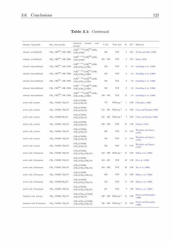
3.6. Conclusions 121
Table 3.1: Continued.
Organic compounds Org. main groupsChemical formula (sub-
groups)T (K) Data type Nd winit
d Reference
ethanol, acetaldehyde CHn, CH[OH]n , OH, CHO
(CH[alc−tail]3 )(CH
[OH]2 )(OH),
(CH3)(CHO) 303 VLE 5 0.01 dAvila and Silva (1970)
ethanol, acetaldehyde CHn, CH[OH]n , OH, CHO
(CH[alc−tail]3 )(CH
[OH]2 )(OH),
(CH3)(CHO) 302− 350 VLE 5 0.01 Suska (1979)
ethanol, butyraldehyde CHn, CH[OH]n , OH, CHO
(CH[alc−tail]3 )(CH
[OH]2 )(OH),
(CH3)(CH2)2(CHO) 323 VLE 9 1.0 Gmehling et al. (1988)
ethanol, butyraldehyde CHn, CH[OH]n , OH, CHO
(CH[alc−tail]3 )(CH
[OH]2 )(OH),
(CH3)(CH2)2(CHO) 333 VLE 9 1.0 Gmehling et al. (1988)
ethanol, butyraldehyde CHn, CH[OH]n , OH, CHO
(CH[alc−tail]3 )(CH
[OH]2 )(OH),
(CH3)(CH2)2(CHO) 343 VLE 9 1.0 Gmehling et al. (1988)
ethanol, butyraldehyde CHn, CH[OH]n , OH, CHO
(CH[alc−tail]3 )(CH
[OH]2 )(OH),
(CH3)(CH2)2(CHO) 353 VLE 9 1.0 Gmehling et al. (1988)
ethanol, butyraldehyde CHn, CH[OH]n , OH, CHO
(CH[alc−tail]3 )(CH
[OH]2 )(OH),
(CH3)(CH2)2(CHO) 346− 350 VLE 15 1.0 Gmehling et al. (1988)
acetic acid, acetone CHn, COOH, CHnCO(CH3)(COOH),
(CH3)(CH3CO) 173 SLE(org) d 1 0.20 Chesnokov (1969)
acetic acid, acetone CHn, COOH, CHnCO(CH3)(COOH),
(CH3)(CH3CO) 244− 284 SLE(org) d 8 0.20 Carta and Dernini (1983)
acetic acid, acetone CHn, COOH,CHnCO(CH3)(COOH),
(CH3)(CH3CO) 245− 283 SLE(org) d 5 0.20 Carta and Dernini (1983)
acetic acid, acetone CHn, COOH, CHnCO(CH3)(COOH),
(CH3)(CH3CO) 332− 383 VLE 10 1.00 Othmer (1943)
acetic acid, acetone CHn, COOH, CHnCO(CH3)(COOH),
(CH3)(CH3CO) 308 VLE 12 0.10Waradzin and Surovy
(1975)
acetic acid, acetone CHn, COOH, CHnCO(CH3)(COOH),
(CH3)(CH3CO) 318 VLE 11 0.10Waradzin and Surovy
(1975)
acetic acid, acetone CHn, COOH, CHnCO(CH3)(COOH),
(CH3)(CH3CO) 328 VLE 11 0.10Waradzin and Surovy
(1975)
acetic acid, 2-butanone CHn, COOH, CHnCO(CH3)(COOH),
(CH3)(CH2)(CH3CO) 242− 290 SLE(org) d 12 0.20 Dallos et al. (1986)
acetic acid, 2-butanone CHn, COOH, CHnCO(CH3)(COOH),
(CH3)(CH2)(CH3CO) 353− 391 VLE 40 1.00 Fu et al. (1986)
acetic acid, 2-butanone CHn, COOH, CHnCO(CH3)(COOH),
(CH3)(CH2)(CH3CO) 353− 388 VLE 22 0.00 Xie et al. (2009)
acetic acid, 2-butanone CHn, COOH, CHnCO(CH3)(COOH),
(CH3)(CH2)(CH3CO) 303 VLE 12 0.00 Dallos et al. (1986)
acetic acid, 2-butanone CHn, COOH,CHnCO(CH3)(COOH),
(CH3)(CH2)(CH3CO) 323 VLE 14 1.00 Dallos et al. (1986)
acetic acid, 2-butanone CHn, COOH, CHnCO(CH3)(COOH),
(CH3)(CH2)(CH3CO) 351 VLE 9 1.00 Dallos et al. (1986)
butanoic acid, acetone CHn, COOH, CHnCO(CH3)(CH2)2(COOH),
(CH3)(CH3CO) 240− 268 SLE(org) d 12 0.20Proust and Fernandez
(1986)
butanoic acid, 2-butanone CHn, COOH, CHnCO(CH3)(CH2)2(COOH),
(CH3)(CH2)(CH3CO) 240− 268 SLE(org) d 12 0.20Proust and Fernandez
(1986)

122 Chapter 3. Improved AIOMFAC temperature dependence
Table 3.1: Continued.
Organic compounds Org. main groupsChemical formula (sub-
groups)T (K) Data type Nd winit
d Reference
butanoic acid, 2-butanone CHn, COOH, CHnCO(CH3)(CH2)2(COOH),
(CH3)(CH2)(CH3CO) 343 VLE 9 1.00Rasmussen and
Fredenslund (1977)
butanoic acid, 2-butanone CHn, COOH, CHnCO(CH3)(CH2)2(COOH),
(CH3)(CH2)(CH3CO) 353 VLE 10 1.00Rasmussen and
Fredenslund (1977)
acetic acid, diethyl ether CHn, COOH, CHnO(CH3)(COOH),
(CH3)2(CH2)CH2O 207− 289 SLE(org) d 40 0.20 Pickering (1893)
acetic acid, diethyl ether CHn, COOH, CHnO(CH3)(COOH),
(CH3)2(CH2)CH2O 293− 343 VLE 7 1.00Meehan and Murphy
(1965)
acetic acid, diethyl ether CHn, COOH, CHnO(CH3)(COOH),
(CH3)2(CH2)CH2O 299− 351 VLE 7 1.00Meehan and Murphy
(1965)
acetic acid, diethyl ether CHn, COOH, CHnO(CH3)(COOH),
(CH3)2(CH2)CH2O 304− 360 VLE 7 1.00Meehan and Murphy
(1965)
acetic acid, ethyl acetate CHn, COOH, CCOO(CH3)(COOH),
(CH3)(CH2)(CH3COO) 323 VLE 9 1.00 Miyamoto et al. (2001)
hexadecanoic acid
(palmitic acid), ethyl
acetate
CHn, COOH, CCOO(CH3)(CH2)14(COOH),
(CH3)(CH2)(CH3COO) 243− 273 SLE(org) d 4 0.20 Kolb (1959)
octadecanoic acid (stearic
acid), ethyl acetateCHn, COOH, CCOO
(CH3)(CH2)16(COOH),
(CH3)(CH2)(CH3COO) 253− 283 SLE(org) d 4 0.20 Kolb (1959)
acetic acid, benzene CHn, COOH, ACHn(CH3)(COOH), (ACH)6 264− 289 SLE(org) d 20 0.20 Roloff (1895)
acetic acid, benzene CHn, COOH, ACHn(CH3)(COOH), (ACH)6 274− 289 SLE(org) d 8 0.20 Roloff (1895)
acetic acid, benzene CHn, COOH, ACHn(CH3)(COOH), (ACH)6 313 VLE 9 0.20 Miyamoto et al. (2000)
acetic acid, benzene CHn, COOH, ACHn(CH3)(COOH), (ACH)6 353− 387 VLE 15 1.00 Haughton (1967)
acetic acid, benzene CHn, COOH, ACHn(CH3)(COOH), (ACH)6 296− 322 VLE 12 1.00 Carta et al. (1979)
acetic acid, acetaldehyde CHn, COOH, CHO(CH3)(COOH), (CH3)(CHO)
295− 386 VLE 33 1.00Shanghai-Inst. and
Zhejiang (1978)
acetic acid, butyraldehyde CHn, COOH, CHO(CH3)(COOH),
(CH3)(CH2)2(CHO) 323 VLE 9 1.00 Miyamoto et al. (2001)
propanoic acid,
butyraldehydeCHn, COOH, CHO
(CH3)(CH2)(COOH),
(CH3)(CH2)2(CHO) 323 VLE 9 1.00 Miyamoto et al. (2001)
acetone, 2-methoxy-2-
methylpropaneCHn,CHnCO, CHnO
(CH3)(CH3CO),
(CH3)3(C)(CH3O) 322− 326 VLE 19 1.00 Mejıa et al. (2008)
2-butanone,
2-ethoxyethanol
CHn, CH[OH]n , CHnCO,
CHnO, OH
(CH3)(CH2)(CH3CO),
(CH3)(CH2)(CH[OH]2 )(CH2O)(OH) 330 VLE 9 1.00
Naumann and Wagner
(1986)
acetone, ethyl acetate CHn, CHnCO, CCOO(CH3)(CH3CO),
(CH3)(CH2)(CH3COO) 330− 348 VLE 16 1.00Subrahmanyam and
Murty (1964)
acetone, ethyl acetate CHn, CHnCO, CCOO(CH3)(CH3CO),
(CH3)(CH2)(CH3COO) 328− 348 VLE 16 1.00 Gilburd et al. (1979)
acetone, ethyl acetate CHn, CHnCO, CCOO(CH3)(CH3CO),
(CH3)(CH2)(CH3COO) 313− 330 VLE 12 1.00 Gilburd et al. (1981)
acetone, octadecanoic acid
methyl ester (methyl
stearate)
CHn, CHnCO, CCOO(CH3)(CH3CO),
(CH3)(CH2)16(CH3COO) 265− 311 SLE(org) d 6 0.10 Bailey et al. (1970)

3.6. Conclusions 123
Table 3.1: Continued.
Organic compounds Org. main groupsChemical formula (sub-
groups)T (K) Data type Nd winit
d Reference
acetone, octadecanoic acid
ethyl ester (ethyl stearate)CHn, CHnCO, CCOO
(CH3)(CH3CO),
(CH3)2(CH2)16(CH3COO) 263− 303 SLE(org) d 5 0.20 Bailey et al. (1970)
acetone, benzene CHn, CHnCO, ACHn(CH3)(CH3CO), (ACH)6 318 VLE 11 1.00 Brown and Smith (1957)
acetone, benzene CHn, CHnCO, ACHn(CH3)(CH3CO), (ACH)6 330− 348 VLE 21 1.00 Kurihara et al. (1998)
2-heptanone, benzene CHn, CHnCO, ACHn
(CH3)(CH2)4(CH3CO),
(ACH)6228− 279 SLE(org) d 13 0.20 Fiege et al. (1996)
2-heptanone, benzene CHn, CHnCO, ACHn
(CH3)(CH2)4(CH3CO),
(ACH)6228− 238 SLE(org) d 8 0.20 Fiege et al. (1996)
3-heptanone, benzene CHn, CHnCO, ACHn
(CH3)2(CH2)3(CH2CO),
(ACH)6228− 279 SLE(org) d 13 0.20 Fiege et al. (1996)
3-heptanone, benzene CHn, CHnCO, ACHn
(CH3)2(CH2)3(CH2CO),
(ACH)6225− 236 SLE(org) d 8 0.20 Fiege et al. (1996)
4-heptanone, benzene CHn, CHnCO, ACHn
(CH3)2(CH2)3(CH2CO),
(ACH)6227− 241 SLE(org) d 9 0.20 Fiege et al. (1996)
4-heptanone, benzene CHn, CHnCO, ACHn
(CH3)2(CH2)3(CH2CO),
(ACH)6238− 279 SLE(org) d 11 0.20 Fiege et al. (1996)
acetone, acetaldehyde CHn, CHnCO, CHO(CH3)(CH3CO), (CH3)
(CHO) 296− 326 VLE 8 0.20 Tikhonova et al. (1970)
acetone, propionaldehyde CHn, CHnCO, CHO(CH3)(CH3CO),
(CH3)(CH2)(CHO) 322− 329 VLE 13 1.00 Danciu (1970)
2-methoxyethanol, methyl
acetate
CHn, CH[OH]n , OH,
CHnO, CCOO
(CH2)(CH[OH]2 )(CH3O)(OH),
(CH3) (CH3COO) 298 VLE 9 0.00 Martin et al. (1994)
2-methoxyethanol, ethyl
acetate
CHn, CH[OH]n , OH,
CHnO, CCOO
(CH2)(CH[OH]2 )(CH3O)(OH),
(CH3)(CH2)(CH3COO) 343 VLE 13 0.20 Chandak et al. (1977)
2-methoxyethanol, ethyl
acetate
CHn, CH[OH]n , OH,
CHnO, CCOO
(CH2)(CH[OH]2 )(CH3O)(OH),
(CH3)(CH2)(CH3COO) 353 VLE 12 0.20 Chandak et al. (1977)
2-methoxyethanol, ethyl
acetate
CHn, CH[OH]n , OH,
CHnO, CCOO
(CH2)(CH[OH]2 )(CH3O)(OH),
(CH3)(CH2)(CH3COO) 351− 395 VLE 14 0.20 Chandak et al. (1977)
2-ethoxyethanol, methyl
acetate
CHn, CH[OH]n , OH,
CHnO, CCOO
(CH3)(CH2)(CH[OH]2 )(CH2O)
(OH), (CH3)(CH3COO) 298 VLE 9 0.00 Martin et al. (1994)
2-ethoxyethanol, ethyl
acetate
CHn, CH[OH]n , OH,
CHnO, CCOO
(CH3)
(CH2)(CH[OH]2 )(CH2O)(OH),
(CH3)(CH2)(CH3COO)351− 402 VLE 17 0.20
Thorat and Nageshwar
(1988)
diethyl ether, benzene CHn, CHnO, ACHn(CH3)2(CH2)CH2O, (ACH)6 197− 278 SLE(org) d 37 0.20 Pickering (1893)
2-butoxyethanol, benzeneCHn, CHnO, CH
[OH]n ,
OH, ACHn
(CH3)(CH2)3(CH[OH]2 )(CH2O)
(OH), (ACH)6217− 279 SLE(org) d 18 0.20 Negadi et al. (2006)
1-methoxy-2-propanol,
benzene
CHn, CH[OH]n , OH,
CHnO, ACHn
(CH3)(CH2)(CH[OH])(CH3O)
(OH), (ACH)6220− 279 SLE(org) d 18 0.20 Negadi et al. (2006)
2-ethoxyethanol, phenolCHn, CH
[OH]n , OH,
CHnO, ACHn
(CH3)(CH2)(CH[OH]2 )(CH2O)
(OH), (ACH)5(ACOH) 363 VLE 17 0.10 Chylinski et al. (2001)
2-ethoxyethanol, phenolCHn, CH
[OH]n , OH,
CHnO, ACHn
(CH3)(CH2)(CH[OH]2 )(CH2O)
(OH), (ACH)5(ACOH) 373 VLE 17 0.10 Chylinski et al. (2001)
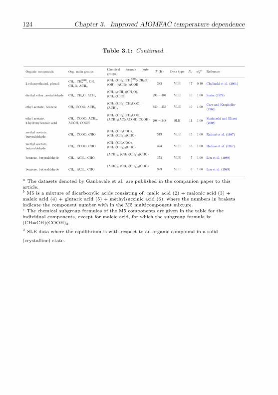
124 Chapter 3. Improved AIOMFAC temperature dependence
Table 3.1: Continued.
Organic compounds Org. main groupsChemical formula (sub-
groups)T (K) Data type Nd winit
d Reference
2-ethoxyethanol, phenolCHn, CH
[OH]n , OH,
CHnO, ACHn
(CH3)(CH2)(CH[OH]2 )(CH2O)
(OH), (ACH)5(ACOH) 383 VLE 17 0.10 Chylinski et al. (2001)
diethyl ether, acetaldehyde CHn, CHnO, ACHn
(CH3)2(CH2)(CH2O),
(CH3)(CHO) 293− 304 VLE 10 1.00 Suska (1979)
ethyl acetate, benzene CHn,CCOO, ACHn
(CH3)(CH2)(CH3COO),
(ACH)6350− 353 VLE 19 1.00
Carr and Kropholler
(1962)
ethyl acetate,
2-hydroxybenzoic acid
CHn, CCOO, ACHn,
ACOH, COOH
(CH3)(CH2)(CH3COO),
(ACH)4(AC)(ACOH)(COOH) 298− 348 SLE 11 1.00Shalmashi and Eliassi
(2008)
methyl acetate,
butyraldehydeCHn, CCOO, CHO
(CH3)(CH3COO),
(CH3)(CH2)2(CHO) 313 VLE 15 1.00 Radnai et al. (1987)
methyl acetate,
butyraldehydeCHn, CCOO, CHO
(CH3)(CH3COO),
(CH3)(CH2)2(CHO) 323 VLE 15 1.00 Radnai et al. (1987)
benzene, butyraldehyde CHn, ACHn, CHO(ACH)6, (CH3)(CH2)2(CHO)
353 VLE 5 1.00 Leu et al. (1989)
benzene, butyraldehyde CHn, ACHn, CHO(ACH)6, (CH3)(CH2)2(CHO)
393 VLE 6 1.00 Leu et al. (1989)
a The datasets denoted by Ganbavale et al. are published in the companion paper to this
article.b M5 is a mixture of dicarboxylic acids consisting of: malic acid (2) + malonic acid (3) +
maleic acid (4) + glutaric acid (5) + methylsuccinic acid (6), where the numbers in brakets
indicate the component number with in the M5 multicomponent mixture.c The chemical subgroup formulas of the M5 components are given in the table for the
individual components, except for maleic acid, for which the subgroup formula is:
(CH=CH)(COOH)2.
d SLE data where the equilibrium is with respect to an organic compound in a solid
(crystalline) state.

3.6. Conclusions 125
Table 3.2: Matrix of AIOMFAC short-range group interaction parameters. Pa-
rameter values for a(i, j) (units of K) are from the literature a, b(i, j) (units of K),
c(i, j) (dimensionless) are determined in this study.
group no. j → 1 2 3 7 8 9 10 11 13 65 66 67 68 69
i ↓ main groups CHn C=C ACHn H2O ACOH CHnCO CHO[aldehyde] CCOO CHnO[ether] COOH CH[alc]n CH
[alc−tail]n CH
[OH]n OH
1 CHn a(i, j): 0.0 8.6020 ×101 6.1130 ×101 1.3180 ×10³ 1.3330 ×10³ 4.7640 ×10² 6.7700 ×10² 2.3210 ×10² 2.5150 ×10² 6.6350 ×10² 0.0 c 0.0 c 0.0 c 9.8650 ×10²
b(i, j): 0.0 0.0 c 2.0000 ×10² 8.7765 ×10² 1.3330 ×10³ -4.7640 ×10² 2.0000 ×10² 2.3210 ×10² 1.5817 ×10² 6.6350 ×10² 0.0 c 0.0 c 0.0 c 9.8650 ×10²
c(i, j): 0.0 0.0 c 4.0000 ×10⁻¹ 2.6360 ×100 2.6660 ×100 9.5280 ×10⁻¹ 4.0000 ×10⁻¹ 4.6420 ×10⁻¹ 1.8636 ×10⁻¹ 1.3270 ×100 0.0 c 0.0 c 0.0 c 1.9730 ×100
2 C=C a(i, j): -3.5360 ×101 0.0 3.8810 ×101 2.7060 ×10² 5.2610 ×10² 1.8260 ×10² 4.4880 ×10² 3.7850 ×101 2.1450 ×10² 3.1890 ×10² -3.5360 ×101 -3.5360 ×101 -3.5360 ×101 5.2410 ×10²
b(i, j): 0.0 c 0.0 0.0 c 0.0 c 0.0 c 0.0 c 0.0 c 0.0 c 0.0 c 0.0 c 0.0 c 0.0 c 0.0 c 0.0 c
c(i, j): 0.0 c 0.0 0.0 c 0.0 c 0.0 c 0.0 c 0.0 c 0.0 c 0.0 c 0.0 c 0.0 c 0.0 c 0.0 c 0.0 c
3 ACHn a(i, j): -1.1120 ×101 3.4460 ×100 0.0 9.0380 ×10² 1.3290 ×10³ 2.5770 ×101 3.4730 ×10² 5.9940 ×100 3.2140 ×101 5.3740 ×10² -1.1120 ×101 -1.1120 ×101 -1.1120 ×101 6.3610 ×10²
b(i, j): 5.3819 ×101 0.0 c 0.0 9.0380 ×10² -1.3290 ×10³ -4.7477 ×101 -3.4730 ×10² 0.0 c -4.3180 ×100 -5.3740 ×10² 5.3819 ×101 5.3819 ×101 5.3819 ×101 -6.3610 ×10²
c(i, j): 4.0000 ×10⁻¹ 0.0 c 0.0 1.8076 ×100 -2.4726 ×100 0.0 c 0.0 c 0.0 c 4.0000 ×10⁻¹ -1.3577 ×10⁻¹ 4.0000 ×10⁻¹ 4.0000 ×10⁻¹ 4.0000 ×10⁻¹ 1.2722 ×100
7 H2O a(i, j): 3.0000 ×10² 4.9610 ×10² 3.6230 ×10² 0.0 3.2450 ×10² -1.9540 ×10² -1.1600 ×10² 7.2870 ×101 5.4050 ×10² -6.9290 ×101 1.6230 ×10² 3.6210 ×10² -8.9710 ×101 -1.5300 ×10²
b(i, j): 1.2542 ×101 0.0 c -3.6230 ×10² 0.0 5.4808 ×101 8.2298 ×101 -5.9018 ×100 4.4441 ×100 1.7880 ×10² -8.6552 ×101 -2.0000 ×10² -2.3073 ×10² -2.0000 ×10² 1.6393 ×10²
c(i, j): -6.0000 ×10⁻¹ 0.0 c 7.2460 ×10⁻¹ 0.0 6.0210 ×10⁻¹ -4.0000 ×10⁻¹ 0.0 c -4.0000 ×10⁻¹ 5.5486 ×10⁻¹ -4.0000 ×10⁻¹ 3.6193 ×10⁻¹ -7.2420 ×10⁻¹ -4.0000 ×10⁻¹ -4.0000 ×10⁻¹
8 ACOH a(i, j): 2.7580 ×10² 2.1750 ×10² 2.5340 ×101 -6.0180 ×10² 0.0 -3.5610 ×10² -2.7110 ×10² -4.4940 ×10² -1.6290 ×10² 4.0890 ×10² 2.7580 ×10² 2.7580 ×10² 2.7580 ×10² -4.5160 ×10²
b(i, j): 2.7580 ×10² 0.0 c 1.6367 ×10² 6.1488 ×101 0.0 3.5610 ×10² 0.0 c 3.9985 ×10² 0.0 c 4.0890 ×10² 2.7580 ×10² 2.7580 ×10² 2.7580 ×10² 4.5160 ×10²
c(i, j): 3.2281 ×10⁻¹ 0.0 c -4.0000 ×10⁻¹ 1.2036 ×100 0.0 0.0 c 0.0 c 0.0 c 0.0 c 8.8840 ×10⁻² 3.2281 ×10⁻¹ 3.2281 ×10⁻¹ 3.2281 ×10⁻¹ 9.0320 ×10⁻¹
9 CHnCO a(i, j): 2.6760 ×101 4.2920 ×101 1.4010 ×10² 4.7250 ×10² -1.3310 ×10² 0.0 -3.7360 ×101 -2.1370 ×10² -1.0360 ×10² 6.6940 ×10² 2.6760 ×101 2.6760 ×101 2.6760 ×101 1.6450 ×10²
b(i, j): 4.5409 ×101 0.0 c -1.8682 ×10² 1.0675 ×10² 2.0000 ×10² 0.0 0.0 c 2.1370 ×10² 0.0 c -5.7894 ×10² 4.5409 ×101 4.5409 ×101 4.5409 ×101 2.0000 ×10²
c(i, j): -4.0000 ×10⁻¹ 0.0 c 0.0 c -9.4500 ×10⁻¹ 0.0 c 0.0 0.0 c 0.0 c 0.0 c 1.9383 ×10⁻¹ -4.0000 ×10⁻¹ -4.0000 ×10⁻¹ -4.0000 ×10⁻¹ 4.0000 ×10⁻¹
10 CHO[aldehyde] a(i, j): 5.0570 ×10² 5.6300 ×101 2.3390 ×101 4.8080 ×10² -1.5560 ×10² 1.2800 ×10² 0.0 -1.1030 ×10² 3.0410 ×10² 4.9750 ×10² 5.0570 ×10² 5.0570 ×10² 5.0570 ×10² 5.2900 ×10²
b(i, j): 5.0570 ×10² 0.0 c -2.0000 ×10² 4.8080 ×10² 0.0 c 0.0 c 0.0 0.0 c 0.0 c 4.9750 ×10² 5.0570 ×10² 5.0570 ×10² 5.0570 ×10² -5.2900 ×10²
c(i, j): 1.0114 ×100 0.0 c 0.0 c 0.0 c 0.0 c 0.0 c 0.0 0.0 c 0.0 c 9.9500 ×10⁻¹ 1.0114 ×100 1.0114 ×100 1.0114 ×100 -1.0580 ×100
11 CCOO a(i, j): 1.1480 ×10² 1.3210 ×10² 8.5840 ×101 2.0080 ×10² -3.6720 ×101 3.7220 ×10² 1.8510 ×10² 0.0 -2.3570 ×10² 6.6020 ×10² 1.1480 ×10² 1.1480 ×10² 1.1480 ×10² 2.4540 ×10²
b(i, j): 2.0000 ×10² 0.0 c 0.0 c 1.3043 ×10² 5.5875 ×101 -2.2930 ×101 0.0 c 0.0 2.2988 ×100 -3.5339 ×101 2.0000 ×10² 2.0000 ×10² 2.0000 ×10² 2.4540 ×10²
c(i, j): 4.0000 ×10⁻¹ 0.0 c 0.0 c -4.0160 ×10⁻¹ 0.0 c 0.0 c 0.0 c 0.0 5.9724 ×10⁻² 0.0 c 4.0000 ×10⁻¹ 4.0000 ×10⁻¹ 4.0000 ×10⁻¹ 4.9080 ×10⁻¹
13 CHnO[ether] a(i, j): 8.3360 ×101 2.6510 ×101 5.2130 ×101 -3.1470 ×10² -1.7850 ×10² 1.9110 ×10² -7.8380 ×100 4.6130 ×10² 0.0 6.6460 ×10² 8.3360 ×101 8.3360 ×101 8.3360 ×101 2.3770 ×10²
b(i, j): 2.0000 ×10² 0.0 c -2.0000 ×10² -3.1470 ×10² 0.0 c 0.0 c 0.0 c -4.6130 ×10² 0.0 -6.6460 ×10² 2.0000 ×10² 2.0000 ×10² 2.0000 ×10² 2.3770 ×10²
c(i, j): -1.0905 ×10⁻¹ 0.0 c -6.1186 ×10⁻² -6.2940 ×10⁻¹ 0.0 c 0.0 c 0.0 c -1.5826 ×10⁻¹ 0.0 7.3512 ×10⁻¹ -1.0905 ×10⁻¹ -1.0905 ×10⁻¹ -1.0905 ×10⁻¹ 4.7540 ×10⁻¹
65 COOH a(i, j): 3.1530 ×10² 1.2640 ×10³ 6.2320 ×101 -1.4588 ×10² -1.1000 ×101 -2.9780 ×10² -1.6550 ×10² -2.5630 ×10² -3.3850 ×10² 0.0 3.1530 ×10² 3.1530 ×10² 3.1530 ×10² -1.0303 ×10²
b(i, j): 3.1530 ×10² 0.0 c -1.9014 ×101 3.8158 ×101 2.0000 ×10² -1.1715 ×10² -2.0000 ×10² 2.5630 ×10² 1.1390 ×101 0.0 3.1530 ×10² 3.1530 ×10² 3.1530 ×10² 2.0000 ×10²
c(i, j): 6.3060 ×10⁻¹ 0.0 c 3.5606 ×10⁻¹ -4.0000 ×10⁻¹ -3.4849 ×10⁻² -5.9560 ×10⁻¹ 4.0000 ×10⁻¹ 0.0 c 6.7700 ×10⁻¹ 0.0 6.3060 ×10⁻¹ 6.3060 ×10⁻¹ 6.3060 ×10⁻¹ 4.0000 ×10⁻¹
66 CH[alc]n a(i, j): 0.0 c 8.6020 ×101 6.1130 ×101 1.8900 ×10³ 1.3330 ×10³ 4.7640 ×10² 6.7700 ×10² 2.3210 ×10² 2.5150 ×10² 6.6350 ×10² 0.0 0.0 c 0.0 c 9.8650 ×10²
b(i, j): 0.0 c 0.0 c 2.0000 ×10² 1.8282 ×10³ 1.3330 ×10³ -4.7640 ×10² 2.0000 ×10² 2.3210 ×10² 1.5817 ×10² 6.6350 ×10² 0.0 0.0 c 0.0 c 9.8650 ×10²
c(i, j): 0.0 c 0.0 c 4.0000 ×10⁻¹ 3.7800 ×100 2.6660 ×100 9.5280 ×10⁻¹ 4.0000 ×10⁻¹ 4.6420 ×10⁻¹ 1.8636 ×10⁻¹ 1.3270 ×100 0.0 0.0 c 0.0 c 1.9730 ×100
67 CH[alc−tail]n a(i, j): 0.0 c 8.6020 ×101 6.1130 ×101 1.3250 ×10³ 1.3330 ×10³ 4.7640 ×10² 6.7700 ×10² 2.3210 ×10² 2.5150 ×10² 6.6350 ×10² 0.0 c 0.0 0.0 c 9.8650 ×10²
b(i, j): 0.0 c 0.0 c 2.0000 ×10² 6.7344 ×10² 1.3330 ×10³ -4.7640 ×10² 2.0000 ×10² 2.3210 ×10² 1.5817 ×10² 6.6350 ×10² 0.0 c 0.0 0.0 c 9.8650 ×10²
c(i, j): 0.0 c 0.0 c 4.0000 ×10⁻¹ -2.6500 ×100 2.6660 ×100 9.5280 ×10⁻¹ 4.0000 ×10⁻¹ 4.6420 ×10⁻¹ 1.8636 ×10⁻¹ 1.3270 ×100 0.0 c 0.0 0.0 c 1.9730 ×100
68 CH[OH]n a(i, j): 0.0 c 8.6020 ×101 6.1130 ×101 2.3140 ×10³ 1.3330 ×10³ 4.7640 ×10² 6.7700 ×10² 2.3210 ×10² 2.5150 ×10² 6.6350 ×10² 0.0 c 0.0 c 0.0 9.8650 ×10²
b(i, j): 0.0 c 0.0 c 2.0000 ×10² -8.0335 ×10² 1.3330 ×10³ -4.7640 ×10² 2.0000 ×10² 2.3210 ×10² 1.5817 ×10² 6.6350 ×10² 0.0 c 0.0 c 0.0 9.8650 ×10²
c(i, j): 0.0 c 0.0 c 4.0000 ×10⁻¹ -8.3200 ×10⁻¹ 2.6660 ×100 9.5280 ×10⁻¹ 4.0000 ×10⁻¹ 4.6420 ×10⁻¹ 1.8636 ×10⁻¹ 1.3270 ×100 0.0 c 0.0 c 0.0 1.9730 ×100
69 OH a(i, j): 1.5640 ×10² 4.5700 ×10² 8.9600 ×101 2.7640 ×10² -2.5970 ×10² 8.4000 ×101 -2.0360 ×10² 1.0110 ×10² 2.8060 ×101 2.2439 ×10² 1.5640 ×10² 1.5640 ×10² 1.5640 ×10² 0.0
b(i, j): 2.0000 ×10² 0.0 c 9.7617 ×101 2.7640 ×10² 2.5970 ×10² 2.0000 ×10² -2.0360 ×10² -6.4775 ×101 -2.6146 ×101 2.2439 ×10² 2.0000 ×10² 2.0000 ×10² 2.0000 ×10² 0.0
c(i, j): -4.0000 ×10⁻¹ 0.0 c 4.0000 ×10⁻¹ -5.5280 ×10⁻¹ 2.7684 ×10⁻¹ 4.0000 ×10⁻¹ -4.0720 ×10⁻¹ 4.0000 ×10⁻¹ -3.1087 ×10⁻¹ 4.4878 ×10⁻¹ -4.0000 ×10⁻¹ -4.0000 ×10⁻¹ -4.0000 ×10⁻¹ 0.0
a The values of ai,j for OH and COOH interactions with H2O are taken from Marcolli and
Peter (2005) and Peng et al. (2001), respectively. For all other functional groups the ai,j values
from the revised parameter set of Hansen et al. (1991) are used.
c Main group interactions bi,j and ci,j are set to zero since appropriate data to determine
these interactions are missing.
126 Chapter 3. Improved AIOMFAC temperature dependence
3.7
3.7.1 Appendix
The bulk water activities, aw, were measured for aqueous organic solu-
tions using an AquaLab water activity meter (Model 3TE, Decagon devices,
USA). The instrument applies the chilled mirror technique to determine the
dewpoint temperature of air equilibrated with the aqueous solution being
measured. The internal temperature control allows to perform measure-
ments under stable temperature from 289 - 313 K. The standard sample
block with a specified error of ±0.003 in aw was used for most measure-
ments. For aqueous mixtures with more volatile polyols (2,5-hexanediol, 1,2,6-
hexanetriol and glycerol), the volatile sample block, available as an accessory
to the instrument, was used to perform measurements. The manufacturer-
specified error for the volatile sample block is ±0.015 in aw. Potential In-
strument offsets were frequently diagnosed and corrected and the perfor-
mance of the sample block was controlled and readjusted with reference
samples of known water activity. All measurements were performed at sev-
eral temperatures in the range 289 K to 313 K. The substances were pur-
chased from Sigma-Aldrich in the best available purity. The following com-
pounds were investigated: glycerol (Sigma, >99%), 2,5-hexanediol (Fluka,
>97%), 1,2,6-hexanetriol (Fluka, >95%), 1,2,7,8-octanetetrol (Fluka, >97%),
2,2,6,6-tetrakis(hydroxymethyl)cyclohexanol (Aldrich, 97%), DL-4-hydroxy-
3-methoxy mandelic acid (Sigma, >95%), raffinose (Sigma, >98%). The sub-
stances were used without further purification. The water/polyol mixtures
were prepared by mass percent with MilliQ deionized water using an ana-
lytical balance. Each solution was measured at least three times at each
temperature.
3.7. 127
Table 3.3: Bulk water activity (aw) measurementsa of water (1) + glycerol (2) solu-
tions at three different temperatures at atmospheric pressure. Solution compositions
are given in mole fraction (x2) of the organic (component 2).
x2 aw(T = 289.15 K) aw(T = 298.15 K) aw(T = 313.15 K)
0.01769 0.976 0.980 0.980
0.03477 0.964 0.964 0.970
0.05128 0.956 0.953 0.955
0.06721 0.937 0.935 0.940
0.08263 0.916 0.920 0.920
0.09754 0.896 0.895 0.910
0.11199 0.872 0.875 0.883
0.12595 0.854 0.862 0.864
0.13950 0.838 0.841 0.856
0.15263 0.823 0.826 0.833
0.16960 0.802 0.802 0.815
0.22685 0.728 0.732 0.739
0.31338 0.622 0.628 0.628
0.43896 0.492 0.491 0.497
0.63774 0.297 0.298 0.299
a The accuracy of the water activity measurements is specified as ± 0.003 (absolute range) in
aw and ≤ 0.1 K in temperature.

128 Chapter 3. Improved AIOMFAC temperature dependence
Table 3.4: Bulk water activity (aw) measurements a of water (1) + 2,5-hexanediol
(2) solutions at three different temperatures at atmospheric pressure. Solution com-
positions are given in mole fraction (x2) of the organic (component 2).
x2 aw(T = 289.15 K) aw(T = 298.15 K) aw(T = 313.15 K)
0.0167 0.971 0.978 0.975
0.0365 0.974 0.978 0.973
0.0616 0.943 0.955 0.972
0.0934 0.917 0.937 0.953
0.1325 0.897 0.912 0.933
0.1790 0.882 0.894 0.912
0.2734 0.825 0.849 0.860
0.3607 0.781 0.790 0.804
0.5630 0.605 0.620 0.618
aThe accuracy of the water activity measurements is specified as ± 0.003 (absolute range) in
aw and ≤ 0.1 K in temperature.
3.7. 129
Table 3.5: Bulk water activity (aw) measurements a of water (1) + 1,2,6-
hexanetriol (2) solutions at three different temperatures at atmospheric pressure.
Solution compositions are given in mole fraction (x2) of the organic (component 2).
x2 aw(T = 289.15 K) aw(T = 298.15 K) aw(T = 313.15 K)
0.014 0.975 0.988 0.985
0.032 0.957 0.974 0.973
0.055 0.944 0.962 0.966
0.080 0.919 0.934 0.943
0.114 0.890 0.895 0.909
0.171 0.834 0.847 0.853
0.216 0.784 0.802 0.802
0.340 0.664 0.673 0.681
0.539 0.456 0.458 0.465
aThe accuracy of the water activity measurements is specified as ± 0.003 (absolute range) in
aw and ≤ 0.1 K in temperature.

130 Chapter 3. Improved AIOMFAC temperature dependence
Table 3.6: Bulk water activity (aw) measurements a of water (1) + 1,2,7,8-
octantetrol (2) solutions at three different temperatures at atmospheric pressure.
Solution compositions are given in mole fraction (x2) of the organic (component 2).
x2 aw(T = 289.15 K) aw(T = 298.15 K) aw(T = 313.15 K)
0.0109 0.987 0.988 0.993
0.0245 0.976 0.977 0.981
0.0407 0.963 0.965 0.969
0.0650 0.944 0.946 0.953
0.0878 0.927 0.924 0.933
0.1329 0.877 0.887 0.901
0.1890 0.803 0.817 0.837
0.2911 0.605 0.643 0.667
aThe accuracy of the water activity measurements is specified as ± 0.003 (absolute range) in
aw and ≤ 0.1 K in temperature.
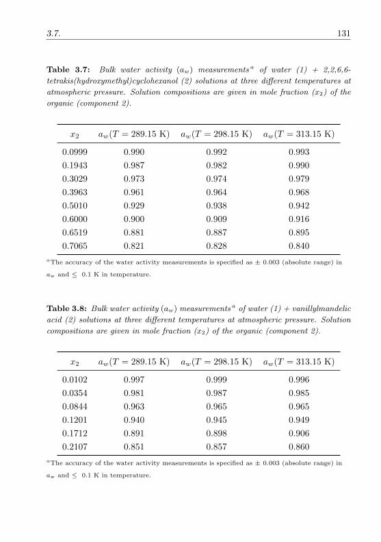
3.7. 131
Table 3.7: Bulk water activity (aw) measurements a of water (1) + 2,2,6,6-
tetrakis(hydroxymethyl)cyclohexanol (2) solutions at three different temperatures at
atmospheric pressure. Solution compositions are given in mole fraction (x2) of the
organic (component 2).
x2 aw(T = 289.15 K) aw(T = 298.15 K) aw(T = 313.15 K)
0.0999 0.990 0.992 0.993
0.1943 0.987 0.982 0.990
0.3029 0.973 0.974 0.979
0.3963 0.961 0.964 0.968
0.5010 0.929 0.938 0.942
0.6000 0.900 0.909 0.916
0.6519 0.881 0.887 0.895
0.7065 0.821 0.828 0.840
aThe accuracy of the water activity measurements is specified as ± 0.003 (absolute range) in
aw and ≤ 0.1 K in temperature.
Table 3.8: Bulk water activity (aw) measurements a of water (1) + vanillylmandelic
acid (2) solutions at three different temperatures at atmospheric pressure. Solution
compositions are given in mole fraction (x2) of the organic (component 2).
x2 aw(T = 289.15 K) aw(T = 298.15 K) aw(T = 313.15 K)
0.0102 0.997 0.999 0.996
0.0354 0.981 0.987 0.985
0.0844 0.963 0.965 0.965
0.1201 0.940 0.945 0.949
0.1712 0.891 0.898 0.906
0.2107 0.851 0.857 0.860
aThe accuracy of the water activity measurements is specified as ± 0.003 (absolute range) in
aw and ≤ 0.1 K in temperature.

132 Chapter 3. Improved AIOMFAC temperature dependence
Table 3.9: Bulk water activity (aw) measurements a of water (1) + raffinose (2)
solutions at three different temperatures at atmospheric pressure. Solution composi-
tions are given in mole fraction (x2) of the organic (component 2).
x2 aw(T = 289.15 K) aw(T = 298.15 K) aw(T = 313.15 K)
0.0089 0.993 0.993 0.992
0.0232 0.967 0.969 0.973
0.0364 0.938 0.944 0.948
0.0507 0.910 0.913 0.917
0.0781 0.835
aThe accuracy of the water activity measurements is specified as ± 0.003 (absolute range) in
aw and ≤ 0.1 K in temperature.
Table 3.10: Bulk water activity (aw) measurements a of water (1) + sucrose (2)
solutions at three different temperatures at atmospheric pressure. Solution composi-
tions are given in mole fraction (x2) of the organic (component 2).
x2 aw(T = 289.15 K) aw(T = 298.15 K) aw(T = 313.15 K)
0.0104 0.992 0.992 0.998
0.0162 0.981 0.988 0.992
0.0230 0.977 0.977 0.985
0.0306 0.965 0.971 0.977
0.0394 0.952 0.955 0.963
0.0487 0.938 0.939 0.946
0.0606 0.906 0.914 0.922
0.0732 0.883 0.888 0.893
aThe accuracy of the water activity measurements is specified as ± 0.003 (absolute range) in
aw and ≤ 0.1 K in temperature.
Chapter 4
Experimental determination of
the temperature dependence of
water activities for some
atmospherically relevant
aqueous organic solutions
G. Ganbavale 1, C. Marcolli 1, U. K. Krieger 1, A. Zuend 1,2,3, G. Stratmann 4,
T. Peter 1
1 Institute for Atmospheric and Climate Science, ETH Zurich, Zurich,
Switzerland2 Department of Chemical Engineering, California Institute of Technology,
Pasadena, California, USA3 Department of Atmospheric and Oceanic Sciences, McGill University, Mon-
treal, Quebec, Canada4 Department of Atmospheric Physics, DLR Oberpfaffenhofen, Germany
This chapter is a reproduction of a corresponding article, which is in prepa-
ration to be submitted to the journal “Atmospheric Chemistry and Physics”.
133
134 Chapter 4. Experimental temperature dependence of water activity
The layout of the article as well as the section, figure, and table numberings
have been adapted to match with the thesis structuring. Cited literature is
referenced in the bibliography of the thesis.

4.1. Introduction 135
This work presents experimental data of the temperature dependence of water
activity in aqueous organic solutions relevant for tropospheric conditions (200
- 273 K). Water activity (aw) at low temperatures is a crucial parameter for
predicting homogeneous ice nucleation. We investigated temperature depen-
dent water activities, ice freezing and melting temperatures of solutions, and
vapour pressures of a selection of atmospherically relevant aqueous organic
systems. To measure aw over a wide composition range and with a focus
on low temperatures, we use various aw measurement techniques and instru-
ments: a dew point water activity meter, an electrodynamic balance (EDB),
differential scanning calorimetry (DSC) and a setup to measure the total gas
phase pressure at equilibrium over aqueous solutions. Water activity mea-
surements were performed for aqueous multicomponent and multifunctional
organic mixtures containing the functional groups typically found in the at-
mospheric organic aerosol, such as hydroxyl, carboxyl, ketone, ether, ester,
and aromatic groups. The aqueous organic systems studied at several fixed
compositions over a considerable temperature range show differing tempera-
ture dependence. Aqueous organic systems of 1,4-butanediol and methoxy-
acetic acid show a moderate decrease in aw with decreasing temperature. The
aqueous M5 system (a multicomponent system containing five different dicar-
boxylic acids) and aqueous 2-(2-ethoxyethoxy)ethanol solutions both show a
strong increase of water activity with decreasing temperature at high solute
concentrations for T < 270 K and 260 K, respectively. These measurements
show that temperature dependence of aw can be reversed at low temperatures
and that linear extrapolations of high temperature data may lead to erroneous
predictions. To avoid this, experimentally determined aw at low temperature
are needed to improve thermodynamic models towards lower temperatures
and for improved predictions of the ice nucleation ability of organic-water
systems.
4.1 Introduction
Organic compounds account for a large fraction of airborne particulate mat-
ter. They constitute around 50 % of the total mass of the fine aerosol fraction

136 Chapter 4. Experimental temperature dependence of water activity
in the continental mid-latitudes (Saxena and Hildemann, 1996; Novakov et al.,
1997; Murphy et al., 2006; Jimenez et al., 2009) while in the tropics they may
contribute up to 90 % (Yamasoe et al., 2000; Roberts et al., 2002). In the up-
per troposphere a high fraction of organic aerosols are internally mixed with
sulphate aerosols (Murphy et al., 2006, 2007). The organic aerosol fraction is
expected to remain in a liquid or amorphous (viscous) state since the large
number of organic compounds depresses the temperature at which crystal-
lization takes place (Marcolli et al., 2004). Studies show that the presence of
an organic aerosol fraction may inhibit ice nucleation and growth (DeMott
et al., 2003; Cziczo et al., 2004; Peter et al., 2006; Knopf and Lopez, 2009).
The organic aerosol fraction contributes to aerosol effects in the atmosphere
through interactions with water vapour, radiation, precipitation, and trace
gases (Fuzzi et al., 2006). In turn, these interactions influence the physical and
chemical properties of aerosol particles such as physical state, hygroscopicity,
size, and shape (e.g., Ming and Russell, 2002; Kanakidou et al., 2005; Zobrist
et al., 2008; Ciobanu et al., 2009; Mikhailov et al., 2009; Reid et al., 2011;
Song et al., 2012). The aerosol scattering intensity depends on growth and
evaporation of the particles due to uptake and release of water vapour driven
by changes in ambient relative humidity (RH) (Carrico et al., 2003; Baynard
et al., 2006; Zieger et al., 2013). For an accurate description of this process,
the hygroscopicity of the typical aerosol compositions have to be known. The
hygroscopicities of most organic mixtures depend on temperature. Water ac-
tivity aw is equal to RH, provided that the aqueous aerosol particles are in
equilibrium with the surrounding gas phase and are sufficiently large so that
the Kelvin effect is negligible. However, aw data of aqueous organic com-
pounds at low temperatures are scarce. Therefore, most estimates of the RH
dependence of the direct aerosol effect rely on data at or close to room tem-
perature. A lot of uncertainty is involved in trying to understand the upper
tropospheric ice nucleation process for use of better process paramterisations
in climate models (Knopf and Lopez, 2009; Swanson, 2009). The uncertainty
in predicted homogeneous ice nucleation temperatures is stated as ±0.025 of
aw at homogeneous melting temperatures and ±0.05 of aw at homogeneous
freezing temperatures (Koop et al., 2000; Koop, 2004; Knopf and Rigg, 2011).
These uncertainties may result in significantly lower or higher values of homo-

4.1. Introduction 137
geneous ice nucleation rate coefficients (Jhom), which may significantly affect
predictions of the onset of ice crystal formation in cloud microphysical models
(Knopf and Rigg, 2011). However, at low tropospheric temperatures, hygro-
scopicity may be different and water uptake and release may be retarded due
to slow diffusion of water into highly viscous amorphous phases (glasses). (Zo-
brist et al., 2008, 2011; Bones et al., 2012).
Cloud formation and homogeneous ice nucleation in the upper troposphere
occur on aqueous aerosol particles that grow into ice crystals by uptake of
supersaturated water vapour. Unless solution droplets become glassy, homo-
geneous ice nucleation in supercooled aqueous solutions does not depend on
the specific nature of the solute; rather knowing the thermodynamic proper-
ties of the solution in terms of water activity (aw) is sufficient, which implicitly
accounts for specific properties of the solutes Koop et al. (2000) and Koop and
Zobrist (2009). Thus, aw of solutions is a crucial parameter for homogeneous
ice nucleation.
For a correct description of the ice nucleation process, deviations from ideal
mixing have to be taken into account. This is achieved by using activity co-
efficients to describe solution non-ideality. For water, with a thermodynamic
activity (aw) defined on a mole fraction basis, its mole fraction-based activity
coefficient is defined as γw = aw/xw, where xw is the water mole fraction
of the solution. Activity coefficients may exhibit considerable temperature
dependence, which has to be parametrised explicitly in thermodynamic mod-
els in order to give accurate predictions for the level of non-ideality over a
large range of temperatures. However, for aqueous organic solutions, ther-
modynamic models based on the UNIQUAC (UNIversal QUAsi Chemical)
model (Abrams and Prausnitz, 1975) or its group contribution version UNI-
FAC (UNIquac Functional group Activity Coefficients) (Fredenslund et al.,
1975) do not provide reliable predictions of activity coefficients, when they
are used outside of the temperature range for which the they have been pa-
rameterised, i.e., at T < 290 K or T > 400 K. Improvement of these models
for atmospheric conditions is strongly limited by the availability of reliable
activity data for T < 290 K (Saxena and Hildemann, 1997; Lohmann et al.,
2001; Marcolli and Peter, 2005). An approach of performing aw measurements
by combining different measurement techniques (e.g., EDB, DSC, total pres-
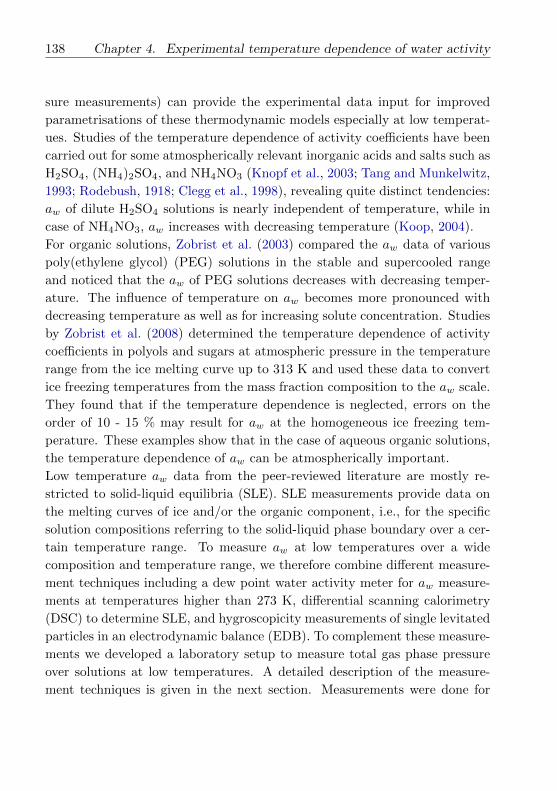
138 Chapter 4. Experimental temperature dependence of water activity
sure measurements) can provide the experimental data input for improved
parametrisations of these thermodynamic models especially at low temperat-
ues. Studies of the temperature dependence of activity coefficients have been
carried out for some atmospherically relevant inorganic acids and salts such as
H2SO4, (NH4)2SO4, and NH4NO3 (Knopf et al., 2003; Tang and Munkelwitz,
1993; Rodebush, 1918; Clegg et al., 1998), revealing quite distinct tendencies:
aw of dilute H2SO4 solutions is nearly independent of temperature, while in
case of NH4NO3, aw increases with decreasing temperature (Koop, 2004).
For organic solutions, Zobrist et al. (2003) compared the aw data of various
poly(ethylene glycol) (PEG) solutions in the stable and supercooled range
and noticed that the aw of PEG solutions decreases with decreasing temper-
ature. The influence of temperature on aw becomes more pronounced with
decreasing temperature as well as for increasing solute concentration. Studies
by Zobrist et al. (2008) determined the temperature dependence of activity
coefficients in polyols and sugars at atmospheric pressure in the temperature
range from the ice melting curve up to 313 K and used these data to convert
ice freezing temperatures from the mass fraction composition to the aw scale.
They found that if the temperature dependence is neglected, errors on the
order of 10 - 15 % may result for aw at the homogeneous ice freezing tem-
perature. These examples show that in the case of aqueous organic solutions,
the temperature dependence of aw can be atmospherically important.
Low temperature aw data from the peer-reviewed literature are mostly re-
stricted to solid-liquid equilibria (SLE). SLE measurements provide data on
the melting curves of ice and/or the organic component, i.e., for the specific
solution compositions referring to the solid-liquid phase boundary over a cer-
tain temperature range. To measure aw at low temperatures over a wide
composition and temperature range, we therefore combine different measure-
ment techniques including a dew point water activity meter for aw measure-
ments at temperatures higher than 273 K, differential scanning calorimetry
(DSC) to determine SLE, and hygroscopicity measurements of single levitated
particles in an electrodynamic balance (EDB). To complement these measure-
ments we developed a laboratory setup to measure total gas phase pressure
over solutions at low temperatures. A detailed description of the measure-
ment techniques is given in the next section. Measurements were done for

4.2. Measurement Techniques 139
binary aqueous organic mixtures covering functional groups and multifunc-
tional organic compounds which are abundantly available in the atmosphere.
The organic functional groups considered include hydroxyl (OH), carboxyl
(COOH), ketone (CHnCO), ester (CCOO), ether (CHnO) and aromatic car-
bon (ACHn, and aromatic carbon-alcohol) (“phenol group”, ACOH), where
“n” denotes the multiplicity of an atom in the compound. These new mea-
surements for atmospherically relevant functional groups provide useful data
for the improvement of thermodynamic models, and for ice nucleation studies.
4.2 Measurement Techniques
To perform measurements over a wide concentration and temperature range
for atmospherically relevant organic compounds we use different measurement
techniques, each of which covers a certain temperature range.
4.2.1 Differential Scanning Calorimetry (DSC)
Solid-liquid equilibria data were obtained by measuring the melting tempera-
tures (Tm) and homogeneous freezing temperatures (Thom) of aqueous organic
solutions for emulsified samples with a DSC instrument (Q10 from TA Instru-
ments) following the procedure described in Zobrist et al. (2008). Water-in-oil
emulsions with droplet diameters in the range of 0.5 µm to 5 µm were pre-
pared by adding four parts by volume of a 5 wt% lanolin/mineral oil solution
(Fluka/Aldrich) to one part by volume of an aqueous solution and stirring with
a rotor-stator homogenizer (Polytron PT 1300D with a PT-DA 1307/2EC dis-
persing aggregate) for 40 seconds at 7000 RPM. Samples (8 to 10 mg) were
pipetted into the DSC pans, which were immediately sealed to prevent any
evaporation. All aqueous solutions were made with distilled and deionized
water (resistivity >18.2 MΩ cm , total organic impurities < 5 ppb). Each
experiment comprised three subsequent cooling cycles starting from 293 K.
The first and the last cycle were run with a cooling rate of 10 K min−1 (used
as control for the emulsion stability) and the second cycle with a cooling rate
140 Chapter 4. Experimental temperature dependence of water activity
of 1 K min−1 (used for the melting and freezing point evaluation). Ice melting
temperatures were evaluated at the melting peak maxima of the heating cycle
run at a rate of 1 K min−1. A detailed calibration of the DSC resulted in a
maximum uncertainty for ice melting temperatures of ± 0.8 K (Zobrist et al.,
2008).
Aqueous solutions of the following organic compounds were investigated: 1,3-
propanediol (Aldrich, 98%), 1,5-pentanediol (Fluka, ≥ 97%), 1,2-hexanediol
(Aldrich, 97 %), glycolic acid (Aldrich, 99%), pyruvic acid (Aldrich, 99%),
methoxyacetic acid (Aldrich, 99%), 2-ethoxyethyl acetate (Aldrich, 99%), D-
sorbitol (Aldrich, ≥ 98%), sucrose (sigma, ≥99%), resorcinol (Aldrich, 99%),
2-(2-ethoxyethoxy)ethanol (Aldrich, ≥ 99%), and M5, a multicomponent di-
carboxylic acid mixture composed of DL-malic acid (Aldrich, 99%), maleic
acid (Aldrich, 99%), malonic acid (Aldrich, 99%), glutaric acid (Aldrich,
99%), and methylsuccinnic acid (Aldrich, 99%). Table 4.1 lists the com-
pounds used together with a selection of their physical properties. The ice
melting (Tm(xorg)) and homogeneous freezing (Thom(xorg)) temperatures ob-
tained by DSC measurements for the aqueous organic mixtures at different
liquid solution compositions given as mole fraction of the organic component,
xorg, are provided in Table 4.2. We use the parameterisation by Koop et al.
(2000) to calculate aw at the melting temperature of ice (Tm) for known so-
lution composition. The vapour pressures for solid phase (superscript S) of
pure hexagonal ice, p,Sice (= p,Sw ), and water in equilibrium with the liquid
(superscript L) solution, pLw on the melting curve (SLE) are the same:
pLw(T = Tm(xorg)) = p,Sice (T = Tm(xorg)), (4.1)
where vapour-liquid, vapour-solid, and solid-liquid equilibria (SLE) exist. At
SLE, the water activity of the aqueous organic solution, aSLEw (T, p), in equi-
librium with ice can therefore be expressed by:
aSLEw (T = Tm(xorg)) =
p,Sice (T = Tm)
p,Lw (T = Tm), (4.2)
4.2. Measurement Techniques 141
where p,Lw (T = Tm) is the vapour pressure of pure liquid (supercooled) water
at Tm. The activity of water in a solution at thermodynamic equilibrium with
ice is related to chemical potentials via (Koop et al., 2000):
aSLEw (T, p) = exp
[µSw(T, p)− µ,L
w (T, p)]
RT
, (4.3)
where R is the ideal gas constant and p is the total mechanical pressure. The
µSw(T, p) and µ,L
w (T, p) are the pressure and temperature dependent chemi-
cal potentials of water in pure ice and pure liquid water. At the relatively
low atmospheric pressures, neglecting the pressure dependence of liquids and
solids is well justified. Koop et al. (2000) provide a temperature dependent
parameterisation for the difference in standard state chemical potentials of
pure water and ice (and hence water activity at SLE), valid at low (ambient)
pressure in the temperature range 150 K < T < 273 K:
µSw(T )− µ,L
w (T ) = 210368 + 131.438 T
−3.32373× 10⁶T−1 − 41729.1 ln(T ). (4.4)
4.2.2 Water activity measurements
Water activity measurements were performed using an AquaLab water ac-
tivity meter (Model 3B, Decagon Devices, USA). The instrument employs
the chilled mirror method to determine the dew point temperature of the
gas phase in equilibrium with the sample. Infrared thermometry in addition
indicates the sample temperature. This instrument allows aw measurements
in the temperature range from 288 to 313 K for bulk samples. For most
measurements the volatile sample block available as an accessory with the
instrument was used since several of the organic compounds used have rather
low, but potentially significant vapour pressures at the probed temperatures.
Experimental errors for the volatile sample block are specified as ± 0.015 awby the manufacturer. The sample block was frequently calibrated and cor-
rected for drifts and offsets using saturated salt solutions and distilled water
samples covering the relevant aw range. For solutions of low-volatility organic
142 Chapter 4. Experimental temperature dependence of water activity
compounds and water, the standard sample block was used with a speci-
fied accuracy of ± 0.003 aw. Table 4.3 provides bulk solution aw data for
sorbitol, resorcinol, glycolic acid, pyruvic acid, and sucrose at 298.15 K. For
some selected systems additional bulk aw measurements at 279 K were carried
out by turning off the temperature control within the AquaLab instrument
and performing the measurements in a cold room at a constant temperature
of 279 K (with an uncertainty in room temperature, ± 0.5 K). Water ac-
tivity measurements were performed for aqueous solutions of 1,4-butanediol,
M5, methoxyacetic acid, and 2-(2-ethoxyethoxy) ethanol, for the temperature
range 279 K - 313 K.
4.2.3 Electrodynamic Balance (EDB) measurements
The basic experimental setup has been described previously (Krieger et al.,
2000; Zobrist et al., 2011). An electrically charged particle (typically 2-20 µm
in radius) is levitated in an electrodynamic balance. The balance is hosted
within a three wall glass chamber with a cooling agent flowing between the
inner walls and an insulation vacuum between the outer walls. A constant
flow of a N2/H2O mixture with a controlled H2O partial pressure is pumped
continuously through the chamber at a constant total pressure, adjustable
between 20 and 100 kPa. A charged, liquid particle is injected in the trap
using a single particle generator (Hewlett-Packard 51633A ink jet cartridge)
and is levitated in the balance, while keeping the temperature constant and
increasing or decreasing the relative humidity (RH) within the chamber con-
tinuously. This is achieved by changing the N2/H2O ratio in the gas phase,
using automatic mass flow controllers. The humidity sensor placed close to
the particle registers the RH with an accuracy of ±1.5 % RH (U.P.S.I. France,
Model G-TUS.13) between 10 and 90 % RH. The sensor was calibrated di-
rectly in the trap using the deliquescence relative humidity of different salts at
different temperatures in the range of interest. The concentration of the par-
ticle can be calculated from the DC voltage compensating the gravitational
force when the dry particle mass is known (measured at RH < 10 %). An
alternative, independent measure of concentration is based on Mie-resonance
spectroscopy. We use a ball lens type point source LED as a “white light”
4.2. Measurement Techniques 143
source to focus the light on the levitated particle and a pierced mirror to
collect Mie resonance spectra in a backscattering geometry. Radius informa-
tion is retrieved from the Mie-resonance spectra as described by Zobrist et al.
(2011). To convert radius to mass and concentration, we assume ideal mixing
to calculate the density of aqueous solutions. For the M5 mixture we use
a molar volume of 86.62 cm3/mol for the M5 mixture and a molarity based
linear parametrisation to calculate the refractive index, nD, at 589 nm for
aqueous M5 solution (nD = 1.3334 + 0.01297× molarity). Since the optically
retrieved concentration data are less noisy and more stable with respect to
drifts over longer measurement periods, we use those for the water activity
versus concentration data presented in Table 4.9.
4.2.4 Total pressure measurements
We use total gas phase pressure measurements of binary aqueous organic so-
lutions to determine aw at low temperatures over a wide concentration range.
The organic components of the binary systems were selected such that their
vapour pressure contribution to the total pressure is irrelevant, i.e., substan-
tially lower than the vapour pressure of water in the considered temperature
range. Given this prerequisite, measured total pressures can be evaluated as
being the vapour pressures of water in vapour-liquid equilibrium with the bi-
nary solutions at measured temperatures and known compositions. Since we
attribute measured total pressures entirely to water vapour, we are restricted
to binary mixtures with low organic vapour pressures that lie within or below
the measurement uncertainty of the total pressure over the whole investigated
composition range. The experimental setup used for the total pressure mea-
surements is shown in Figure 4.1. The setup consists of a round bottom flask
(500 ml) in which an aqueous organic mixture of a particular composition is
filled. For the total pressure measurements, the flask is immersed in a ther-
mostated ethanol bath (initially set to 223 K) whose temperature is slowly
ramped up to 290 K. The flask can be evacuated to ∼ 10−6 Pa using a vac-
uum pump and cooled in liquid N2 for the purpose of degassing residual air
naturally present in the samples. Glass beads (∼ 50 g, ∼ 3 mm diameter)
are added to the flask to prevent undesirable foaming of the solution during

144 Chapter 4. Experimental temperature dependence of water activity
Glass beads
VacuumPump
Aqueous solution
ethanol bath
Figure 4.1: Setup for total gas phase pressure measurements of aqueous organic
solutions at room temperature and below.
degassing cycles, which may occur when a frozen solution thaws relatively
quickly at room temperature after cooling to liquid nitrogen temperature.
Foaming may often lead to splashing of solution droplets up to the neck of
the flask, where the droplets remain without contact to the rest of the sample.
If such droplets were present above the level of the ethanol bath into which
the flask is submerged to maintain a temperature-controlled environment (Ju-

4.2. Measurement Techniques 145
labo, FP50 thermostat), they would be at a different temperature than the
bulk solution and present a cause of systematic errors. The pressure increase
during the temperature ramp is registered by two pressure heads operating in
the pressure ranges P1 (Pfeiffer Vacuum, CMR-262, range: 1 to 1× 10⁴ Pa)
and P2 (Pfeiffer Vacuum, PKR-251, range: 1× 10⁻² to 110 Pa).
A typical experiment involves the following operational procedure: A binary
aqueous solution mixture (volume of 3 to 5 ml) is added to the flask. To
remove the residual gases (e.g., N2, O2, Ar, and CO2) from the solution,
a thorough degassing procedure is carried out for which the flask is placed
in a liquid N2 bath (at T ≈ 77 K) and the valve to the vacuum pump is
opened to remove the gas phase above the solution until a low pressure of ∼10−6 Pa is reached. Thereafter, the valve is closed again and the solution is
slowly brought back to room temperature. These warming and cooling cycles
are carried out about 2 - 3 times so that all the residual gases are removed.
These degassing cycles are assumed to lead only to a very small loss of water
via the gas phase, so that the mixture composition remains practically unaf-
fected. Before the actual measurement starts, the sample flask is once more
cooled in liquid N2 and then transferred to the ethanol bath, which is held at
223 K, and further evacuated until a constant pressure is reached to allow the
removal of any remaining dissolved gases from the solution and ensuring that
the total pressure measured by the pressure sensors corresponds, within un-
certainty, to the one of water vapour alone. The valves to the pressure heads
are then opened and the total gas phase pressure measurement is carried out
in the temperature range from 228 to 290 K by increasing the temperature
of the ethanol bath at a constant rate of 10.6 K/h, over a time period of 350
minutes. The measured constant leak rate of the instrument, which we mea-
sured for the same time interval as the actual experiment, is subtracted from
the total pressure data and from the resulting values, water vapour pressure
data for the particular system compositions and temperatures are obtained.
For the investigated systems, aw values are derived by dividing the measured
water vapour pressure by the calculated liquid-state vapour pressure of pure
water (liquid-state saturation vapour pressure) at the prescribed temperature
of the ethanol bath using the parametrisation by Murphy and Koop (2006).
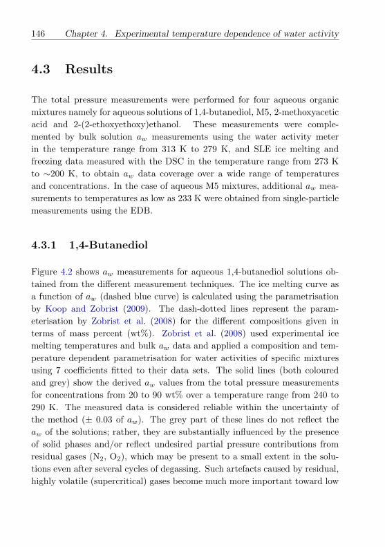
146 Chapter 4. Experimental temperature dependence of water activity
4.3 Results
The total pressure measurements were performed for four aqueous organic
mixtures namely for aqueous solutions of 1,4-butanediol, M5, 2-methoxyacetic
acid and 2-(2-ethoxyethoxy)ethanol. These measurements were comple-
mented by bulk solution aw measurements using the water activity meter
in the temperature range from 313 K to 279 K, and SLE ice melting and
freezing data measured with the DSC in the temperature range from 273 K
to ∼200 K, to obtain aw data coverage over a wide range of temperatures
and concentrations. In the case of aqueous M5 mixtures, additional aw mea-
surements to temperatures as low as 233 K were obtained from single-particle
measurements using the EDB.
4.3.1 1,4-Butanediol
Figure 4.2 shows aw measurements for aqueous 1,4-butanediol solutions ob-
tained from the different measurement techniques. The ice melting curve as
a function of aw (dashed blue curve) is calculated using the parametrisation
by Koop and Zobrist (2009). The dash-dotted lines represent the param-
eterisation by Zobrist et al. (2008) for the different compositions given in
terms of mass percent (wt%). Zobrist et al. (2008) used experimental ice
melting temperatures and bulk aw data and applied a composition and tem-
perature dependent parametrisation for water activities of specific mixtures
using 7 coefficients fitted to their data sets. The solid lines (both coloured
and grey) show the derived aw values from the total pressure measurements
for concentrations from 20 to 90 wt% over a temperature range from 240 to
290 K. The measured data is considered reliable within the uncertainty of
the method (± 0.03 of aw). The grey part of these lines do not reflect the
aw of the solutions; rather, they are substantially influenced by the presence
of solid phases and/or reflect undesired partial pressure contributions from
residual gases (N2, O2), which may be present to a small extent in the solu-
tions even after several cycles of degassing. Such artefacts caused by residual,
highly volatile (supercritical) gases become much more important toward low

4.3. Results 147
temperatures relative to the much lower partial pressure signal from water,
essentially enlarging the uncertainties of the derived water activities beyond
a practical limit for a meaningful data evaluation. The grey portions of the
curves merge within uncertainty on the SLE phase boundary of the aqueous
solution and ice for aw > 0.76 and analogously on the 1,4-butanediol SLE line
for aw < 0.70. Eutectic melting is observed at ∼ 243 to 245 K as a horizontal
peak to low aw because the sample temperature remains constant during the
melting process while the prescribed temperature in the surrounding ethanol
bath, which is used to derive the aw data shown in Figure 4.2, keeps increas-
ing. The area of the phase diagram below the melting curve of one of the
components, i.e., the green and blue shaded areas, is not accessible for awmeasurements by bulk techniques, because the presence of solid phases alters
the initial (known) composition of the remaining liquid solution. The dips
visible on the curves around T ≈ 275 K of the total pressure measurements
of the 20 wt% and 40 wt% mixtures, are artefacts, which are probably due to
the melting of tiny droplets that may have splashed to the neck of the flask
while degassing the solution prior to the actual measurements.
All measurements taken together provide a consistent picture of the temper-
ature dependence of aw of aqueous 1,4-butanediol, namely a more or less
constant decrease of aw with decreasing temperature, which is well described
by the parameterisation of Zobrist et al. (2008) (for bulk solutions at least
until the intersection with the melting curves). Table 4.4 provides aw data
obtained from the Aqualab water activity meter. Table 4.12 lists the aw data
derived from the total pressure measurements.
4.3.2 Methoxyacetic acid
Figure 4.3 shows aw measurements of aqueous methoxyacetic acid covering
the concentration range from 10 wt% to 90 wt% and temperatures from 240 to
298 K using different experimental techniques. Water activity of the aqueous
solution in equilibrium with ice, i.e., SLE for concentrations from 10 to 60
wt% covering a temperature range of 251 to 272 K are obtained using DSC
measurements (pentagons). The grey solid lines at lower concentrations rep-
resent the aw data derived from total pressure measurements which merge on

148 Chapter 4. Experimental temperature dependence of water activity
the ice melting curve (aw> 0.8), while the grey solid lines at higher concen-
trations (aw < 0.7) follow the melting curve of methoxyacetic acid. Eutectic
melting is observed at T ≈ 253 K. The colour shaded region below the
ice-melting and the methoxyacetic acid melting curves are not accessible for
total pressure measurements, because the presence of solid phases influences
the solution concentration (above the eutectic melting line), due to which the
measured aw will not correspond to the initial composition of the solution
being measured. The broad horizontal peaks to high aw on the 50, 60, and
70 wt% lines of the total pressure measurements indicate an increased total
pressure whose origin is unclear, but points to artefacts (perhaps due to the
melting of small solution droplets, splashed to the neck of the glass flask, that
are of lower organic concentrations).
The measured aw using the water activity meter and the aw data derived
from total pressure measurements indicate a small temperature dependence
and are consistent within 2 to 5 % at higher concentration wt% of methoxy-
acetic acid. A reason for this deviation might be that full equilibration of the
solution was not reached after the melting of solid methoxyacetic acid over
the timescale of the experiment. In the more dilute composition range with
respect to the organic component, deviations < 2 % aw are found, indicating
the principle validity of the total pressure data in the temperature range con-
sidered reliable. Measurements and the parametrisation for the temperature
dependence of water activity by (Zobrist et al., 2008) (dashed-dotted lines in
Figure 4.3) indicate a small aw decrease with the decrease in the temperature.
The bulk aw data from the water activity meter measurements is provided in
Table 4.5. The calculated aw data obtained from the total pressure experi-
ments for various solution compositions are given in Table 4.13.
4.3.3 2-(2-Ethoxyethoxy)ethanol
Water activity measurements for aqueous solutions of 2-(2-ethoxyethoxy)
ethanol (also known as carbitol) in the concentration range from 10 to 90
wt% of organic in the temperature range from 230 to 298 K are presented
in Fig 4.4. DSC measurements were performed for a concentration range
of 10 to 40 wt% covering the temperature range from 248 to 272 K. Bulk
4.3. Results 149
aw measurements using the water activity meter in the temperature range
from 279 to 298 K are listed in Table 4.6 and shown as coloured circles in
Fig 4.4. Eutectic melting was not observed since the melting point of pure
2-(2-ethoxyethoxy)ethanol (Tm = 197 K) is lower than the considered temper-
ature range. The aw data measured using the water activity meter and DSC
data are in good agreeement with the parametrised temperature dependence
by Zobrist et al. (2008), the latter is displayed by the coloured dash-dotted
lines. Both the aw measurements and the parametrisation indicate a decrease
in aw with decrease in temperature. The aw derived from the total pressure
measurements are in good agreement with the aw data obtained from the
water activity meter and the parametrisation for T > 265 K and for mass
fractions of the organic component, worg, of 60 wt% ≤ worg ≤ 90 wt%. At
lower temperatures, aw strongly increases with decreasing temperature for
worg ≥ 80%. At T = 225 K, all the solid lines converge. Such a temperature
dependence of water activity is expected for solutions that exhibit a phase
transition (as seen when the curves bend and follow the melting curves in the
previous systems, where two solid phases exist at lower T). Another possibility
for such a convergence would be that a phase transition in terms of a liquid-
liquid phase separation occurs at low temperatures. It should be noted that
the measurement artefacts would not be expected to lead to a convergence of
the curves onto the ice melting curve at a common temperature. Complemen-
tary measurements using the EDB could not be performed for this system due
to the comparably high vapour pressure of 2-(2-ethoxyethoxy)ethanol at room
temperature, which leads to fast evaporation during injection of the particle
into the EDB. At lower worg (10 to 50 wt%) the solid coloured lines show
good agreement with the parametrisation by Zobrist et al. (2008). The water
activity data derived from the total “equilibrium” pressure measurements for
various concentrations are provided in Table 4.14.
4.3.4 M5 (multicomponent dicarboxylic acid) mixture
Figure 4.5 shows aw measurements for aqueous solutions of M5 over a concen-
tration range from 10 to 84 wt% M5, i.e., up to the solution saturation limit
at 298 K, in the temperature range from 225 to 313 K. Bulk aw measurements

150 Chapter 4. Experimental temperature dependence of water activity
performed in the temperature range from 279 to 313 K are represented by the
coloured circles and are listed in Table 4.7 and Table 4.8. Humidity cycles
of single levitated particles in the EDB were performed in the temperature
range from 233 to 289 K and are represented by filled coloured diamonds.
M5 mixture compositions and aw data for the aqueous solutions are listed
in Table 4.9, Table 4.10, and Table 4.11. The total pressure measurements
are represented by solid and dashed lines (dashed for M5 mass fractions from
75 to 84 wt%) in Figure 4.5. For mass fractions wM5 > 50 wt% both EDB
measurements and total pressure measurements show an increase in aw with
decreasing temperature, with a stronger effect at higher concentrations. No
simple (pseudo-binary) eutectic melting was observed because in case of the
total pressure measurements individual components of the M5 mixture did
crystallise at different temperatures and mass fractions of M5. We assume
that the total pressure data for wM5 > 70 wt% (shown by dashed coloured
lines in Figure 4.5) are influenced by the crystallization of certain compo-
nents of the M5 mixture. These data are not considered to reflect the water
activity of the initial mixtures and are therefore not tabulated. The same
might be true for the bulk aw data points at 279 K and concentrations of 80
and 84 wt%, which might explain their high water activity. Table 4.15 pro-
vides the composition of the M5 + water mixtures used for the total pressure
measurements; corresponding water activities are listed in Table 4.16. The
parametrisation of Zobrist et al. (2008) is shown by the dash-dotted lines.
Thus it should be noted, both M5 and 2-(2-ethoxyethoxy)ethanol solutions
show a similar effect of increase in aw with decrease in temperature at higher
concentrations.

4.3. Results 151
0.4 0.5 0.6 0.7 0.8 0.9 1.0230
240
250
260
270
280
290
300
310
32010rwt,60rwt,
20rwt,30rwt,
40rwt,50rwt,62rwt,
65rwt,70rwt,75rwt,80rwt,85rwt,90rwt,
Te
mp
era
ture
rbK
d
waterractivity, aw
organicrbSdr+r solutionrbLd
icerbSdr+r1,4-butanediolrbSd
icerbSdr+rsolutionrbLd
Figure 4.2: Measured water activities of aqueous 1,4-butanediol solutions versus
temperature. The different colours indicate the solution compositions in wt% of
the organic component. The solid lines show data derived from the total pressure
measurements. The coloured portion of the solid lines represents the temperature
range for which the measurements are considered reliable within the uncertainty of
the method (±0.03 of aw). Water activities derived from DSC measurements on the
ice melting curve are represented by pentagons. Bulk aw measurements using the
water activity meter are represented by solid circles. The dash-dotted lines show the
composition and temperature dependent aw parametrisation by Zobrist et al. (2008).
The blue dashed line is the ice melting curve (Koop and Zobrist, 2009). In the colour
shaded regions one or both components are supersaturated with respect to the solid
phase and therefore, above the eutectic temperature (245 K), at equilibrium one solid
phase coexists with the remaining solution.

152 Chapter 4. Experimental temperature dependence of water activity
0.3 0.4 0.5 0.6 0.7 0.8 0.9 1.0230
240
250
260
270
280
290
300
310
32010+wtd
20+wtd30+wtd40+wtd
50+wtd60+wtd70+wtd80+wtd85+wtd90+wtd
Te
mp
era
ture
+sK
l
water+activity,+aw
organic+sSl+++ solution+sLl
ice+sSl+++2-methoxyacetic+acid+sSl
Figure 4.3: Measured water activities of aqueous 2-methoxyacetic acid solutions
versus temperature. The different colours indicate the solution compositions in wt%
of the organic component. The solid lines show data derived from the total pressure
measurements. The coloured portion of the solid lines represents the temperature
range for which the measurements are considered reliable within the uncertainty of
the method (±0.03 of aw). Water activities derived from DSC measurements on the
ice melting curve are represented by pentagons. Bulk aw measurements using the
water activity meter are represented by solid circles. The dash-dotted lines show the
composition and temperature dependent aw parametrisation by Zobrist et al. (2008).
The blue dashed line is the ice melting curve (Koop and Zobrist, 2009). In the colour
shaded regions one or both components are supersaturated with respect to the solid
phase and therefore, above the eutectic temperature ( 253 K), at equilibrium one
solid phase coexists with the remaining solution.
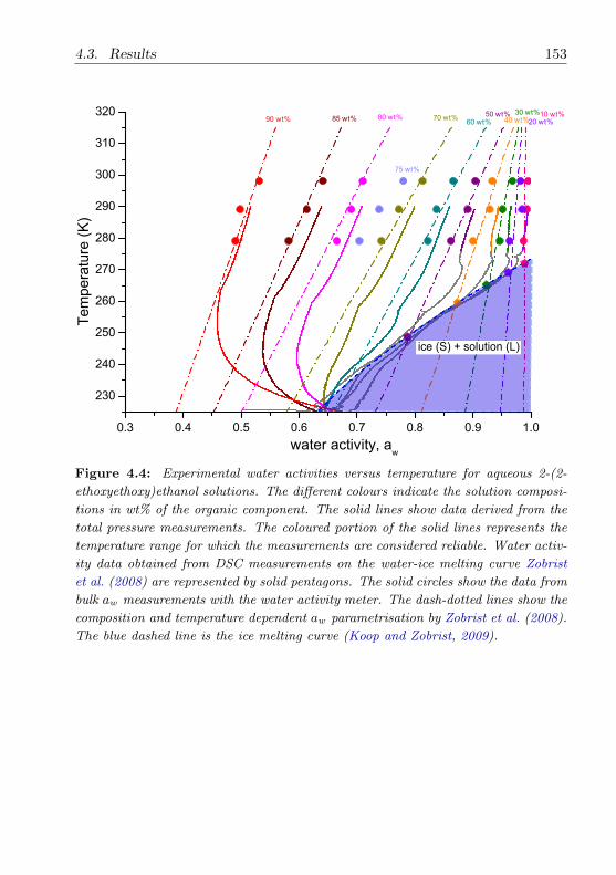
4.3. Results 153
0.3 0.4 0.5 0.6 0.7 0.8 0.9 1.0
230
240
250
260
270
280
290
300
310
320
75+wtL
10+wtL20+wtL
30+wtL40+wtL
50+wtL60+wtL
70+wtL80+wtL85+wtL90+wtL
Te
mp
era
ture
+(K
)
water+activity, aw
ice+(S)+++solution+(L)
Figure 4.4: Experimental water activities versus temperature for aqueous 2-(2-
ethoxyethoxy)ethanol solutions. The different colours indicate the solution composi-
tions in wt% of the organic component. The solid lines show data derived from the
total pressure measurements. The coloured portion of the solid lines represents the
temperature range for which the measurements are considered reliable. Water activ-
ity data obtained from DSC measurements on the water-ice melting curve Zobrist
et al. (2008) are represented by solid pentagons. The solid circles show the data from
bulk aw measurements with the water activity meter. The dash-dotted lines show the
composition and temperature dependent aw parametrisation by Zobrist et al. (2008).
The blue dashed line is the ice melting curve (Koop and Zobrist, 2009).
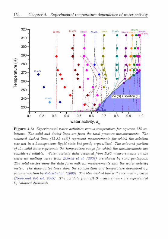
154 Chapter 4. Experimental temperature dependence of water activity
0.1 0.2 0.3 0.4 0.5 0.6 0.7 0.8 0.9 1.0
230
240
250
260
270
280
290
300
310
32020rwt,
10rwt,
30rwt,40rwt,50rwt,60rwt,70rwt,75rwt,80rwt,84rwt,90rwt,
97rwt,
Te
mp
era
ture
r(K
)
waterractivity,raw
95rwt,
icer(S)r+rsolutionr(L)
Figure 4.5: Experimental water activities versus temperature for aqueous M5 so-
lutions. The solid and dotted lines are from the total pressure measurements. The
coloured dashed lines (75-84 wt%) represent measurements for which the solution
was not in a homogeneous liquid state but partly crystallized. The coloured portion
of the solid lines represents the temperature range for which the measurements are
considered reliable. Water activity data obtained from DSC measurements on the
water-ice melting curve from Zobrist et al. (2008) are shown by solid pentagons.
The solid circles show the data form bulk aw measurements with the water activity
meter. The dash-dotted lines show the composition and temperature dependent aw
parametrisation by Zobrist et al. (2008). The blue dashed line is the ice melting curve
(Koop and Zobrist, 2009). The aw data from EDB measurements are represented
by coloured diamonds.

4.4. Discussion 155
4.4 Discussion
4.4.1 Measurement techniques: scope and limitations
Water activity as a function of solute concentration can be measured either for
bulk solutions or by single particle measurement techniques. To measure aw of
bulk solutions, commercial dew point water activity meters are probably the
best choice because they have high accuracy and cover a wide concentration
range, thus, providing aw data from saturated to dilute solutions. However,
their accuracy decreases for water activities close to 1. Therefore they are
less suited for very dilute solutions. Moreover, the commercially available
water activity meters typically provide data for temperatures > 273 K and
experiments are time consuming when point-to-point measurements have to
be performed over a wide temperature range.
The DSC technique provides accurate measurements of solid-liquid equilib-
rium curves. DSC measurements are performed at fixed composition and can
provide Tm, Thom and glass transition temperatures (Tg) of aqueous solutions.
From the melting point depression of ice in aqueous solutions, accurate val-
ues of aw on the SLE phase boundary of the aqueous solution and ice can
be obtained, because the vapour pressures of ice and water at atmospheric
temperatures are well known (see Sect. 4.2.1). When oil-in-water emulsions
instead of bulk samples are measured, homogeneous freezing temperatures
Thom can also be obtained. This is especially useful because homogeneous ice
nucleation temperatures of aqueous solutions can be parametrised in terms
of water activity following Koop et al. (2000). The drawback of the DSC
technique is that only aw on the ice melting curve, thus, over a limited range
of compositison, are obtained.
The electrodynamic balance and optical tweezers in addition offer a possibil-
ity to measure the water activity via the mass or size change of hygroscopic,
micrometre-sized particles. In both techniques, the particles are levitated
without contact to any surface sites. Hence the supersatured concentration
range can be investigated when the particles are exposed to humidity cycles.
In the absence of liquid/gas phase diffusion limitations and given the rela-
tively large diameters of solution droplets (Kelvin effect can be ignored), RH
156 Chapter 4. Experimental temperature dependence of water activity
of the gas phase corresponds with aw of the condensed phase. Thus the water
content of the levitated particle in terms of a mass or molar fraction can be
calculated from the mass data when the dry particle mass is known. The
more accurate radius data obtained from the Mie scattering pattern can be
used to derive mass or mole fractions of solute but need refractive index data
and density data. The available temperature range depends on the cooling
and heating possibilities of the specific setup. Since the particles are airborne
without contact to any surface sites, aw of highly supersaturated solutions
can be obtained, covering thus a concentration range that is not accessible by
bulk methods.
Gas phase pressure measurements over aqueous solutions can provide water
activities when the measured total pressure can be totally ascribed to water
vapour. Since this technique needs bulk volumes, aw data can be obtained
from dilute upto saturated solutions. When the sample is kept in an ex-
ternally regulated thermostat, temperature profiles can be run that provide
water activity data of solutions at fixed concentration covering a wide tem-
perature range. Apart from deriving aw from the measured data, the total
pressure measurements can also provide information about eutectic melting
points and solid-liquid equilibria. However, accurate measurements of water
activities rely on efficient removal of the residual gases from the solution to
make sure that the measured total pressure corresponds to the water vapour
pressure over the solution. A lot of care needs to be taken during the re-
moval of residual gases since there is always the danger of overpumping which
may change the concentration of the solution (removal of significant amounts
of water vapour). The total pressure measurements are also prone to arte-
facts. The freezing/thawing process can lead to composition heterogeneity
in the sample. Some solutions show a strong foaming during melting lead-
ing to tiny droplets settling on the walls of the solution flask. These drops
can influence the gas phase pressure when they are at a higher temperature
than the bulk solution or when they are at a different composition due to
heterogeneity during freezing and thawing process. To cover a large concen-
tration and temperature range, substances with a low melting point and a
high water solubility are required. These conditions strongly reduce the num-
ber of compounds for which total pressure measurements may provide a large

4.4. Discussion 157
extension to composition/temperature ranges that are not covered by other
methods. These drawbacks together with the rather difficult handling of the
instrumental setup render total pressure measurements to be less attractive
than the alternative techniques such as DSC and EDB measurements. A
good temperature and concentration coverage can be achieved when aw bulk
measurements are combined with EDB experiments.
4.4.2 Hydrogen bonding in aqueous solutions
Hydrogen bonds are electrostatic dipole-dipole interactions that occur be-
tween covalently bound hydrogen atoms and the free electron pair of a highly
electronegative atom, such as nitrogen (N), oxygen (O) or fluorine (F). They
have some features of covalent bonding since they are directional and lead
to interatomic distances shorter than the sum of van der Waals radii of the
involved atoms. Hydrogen bonds have a strong influence on the activity of the
constituents in a solution. In aqueous solutions of alcohols and acids, solute-
solute, solute-water, and water-water hydrogen bonds can form. In general,
solute-water hydrogen bonds decrease aw while association of solute molecules
among each other leads to an increase in water activity. The strength and
average number of hydrogen bonds per molecule depends on concentration
and temperature. A strong increase of aw with decreasing temperature can
be rationalized in terms of association of solute molecules among each other.
Therefore, the analysis of the hydrogen bonds present in aqueous solutions
can help to understand the temperature dependence of water activity.
The carboxyl group of organic acids can build hydrogen bonds with water
or other dicarboxylic acids. The hydrogen atoms of the carboxyl group form
hydrogen bonds with the free electron pair of the oxygen atoms of a carboxyl
group of another acid molecule. Similarly, for dicarboxylic acids when the
hydrogen bonds connect to another dicarboxylic acid molecule this leads to
an association of dicarboxylic acids and formation of a dimer, which reduces
the effective number of dissolved species and leads to a relative increase in
water activity. Hydrogen bonds between water and dicarboxylic acids lead to
a decrease of water activtiy.
Aqueous solutions of poly(ethylene glycol) (PEG) have attracted much atten-

158 Chapter 4. Experimental temperature dependence of water activity
tion because of their extraordinary mixing behavior with water and their im-
portance in pharmaceutical and biomedical appliances Dormidontova (2002).
2-(2-ethoxyethoxy)ethanol shares with PEG the −CH2−CH2−O− repetition
unit as the main structural feature. Different from PEG with two termi-
nal hydroxyl groups, 2-(2-ethoxyethoxy)ethanol carries one terminal methyl
and one terminal hydroxyl group, which makes it less hydrophilic. The
−CH2−CH2−O− repetition unit lends 2-(2-ethoxyethoxy)ethanol and PEG a
higher solubility than typical for ethers. This behavior can be rationalized by
the increased structuring of water around PEG molecules. This structuring
is a consequence of hydrogen bonding and the ability of the PEG structure
to fill out the natural cavities in the hydrogen bonded network of water. The
increased structuring of the water is reflected in the large negative excess en-
tropy of the solution, while its large positive excess heat capacity is due to the
temperature sensitivity of the structure (Kjellander and Florin, 1981). This
interplay of entropic and enthalpy contributions to the Gibbs energy leads to a
closed loop miscibility gap at elevated temperature for aqueous PEG solutions
with PEG molecular weights of 2200 g mol−1 and higher (e.g.(Dormidontova,
2004; Kjellander and Florin, 1981; Zobrist et al., 2003)).
PEG with molecular weight below 2000 do not show liquid-liquid phase sep-
aration close to room temperature. However liquid-liquid equilibria are ob-
served for aqueous triethylene glycol solutions (Salabat, 2010) and smaller
poly(ethylene glycols) when a salt is added (e.g.(Marcolli and Krieger, 2006;
Ciobanu et al., 2009)). Liquid-liquid phase separation below room temper-
ature is not easily accessible because of the competition with crystallization
of either the PEG, the ice phase or both phases depending on solution com-
position and temperature. Ciobanu et al. (2009) have investigated in detail
liquid-liquid phase separation of aqueous PEG-400 solutions when ammonium
sulfate is added as a salting-out agent. This phase separation seems to persist
or even grow with decreasing temperature. At the onset of liquid-liquid phase
separation water activity lines of different concentration converge at a high awvalue. Therefore strong increase of aw with decreasing temperature in aque-
ous M5 and 2-(2-ethoxyethoxy) ethanol solutions can be rationalized in terms
of approaching a low temperature miscibility gap that is not experimentally

4.4. Discussion 159
accessible because it falls in the concentration/temperature range where ice
forms.
4.4.3 Atmospheric Implications
In the upper troposphere, one of several pathways for cirrus cloud formation is
by means of homogeneous ice nucleation on/in liquid aqueous aerosol particles,
which subsequently grow into supermicron-sized ice crystals by condensing
water vapour. Water-activity-based ice nucleation theory can be employed to
predict homogeneous ice nucleation temperatures and corresponding ice nucle-
ation rate coefficients for aqueous solution droplets without explicit knowledge
of the nature of the solute (Koop et al., 2000; Koop and Zobrist, 2009). While
for known mixture compositions the ice melting temperature and the corre-
sponding equilibrium water activity can be measured and/or parametrised
precisely (Koop et al., 2000; Koop, 2004; Knopf and Rigg, 2011), the same
level of information is not accessible experimentally in the case of supercooled
aqueous solution droplets, which exhibit homogeneous freezing of ice at a
temperature lower than the corresponding melting point, denoted as Thom.
As is well understood in the case of the ice melting process, with the melting
temperature being a function of aqueous solution composition (melting point
depression), similar behavior is observed in droplet freezing experiments for
the composition and temperature dependence of the homogeneous freezing
process. However, the water activity at the freezing temperature is typically
not accessible in experiments and/or subject to relatively large uncertainty.
Koop et al. (2000) suggest that aw at the homogeneous freezing tempera-
ture Thom(xorg) can be obtained from the corresponding aw determined at
the melting temperature Tm(xorg) of the solution at the same composition
with the assumption that aw does not change significantly over the tempera-
ture difference from Tm(xorg) to Thom(xorg). This approach has been tested
and shown to be a good approximation for a variety of inorganic solutions
(Koop et al., 2000; Koop, 2004), but may lead to significant errors in predic-
tions of the homogeneous freezing temperatures for aqueous organic solutions.
Figure 4.6 shows aw at melting and freezing conditions for aqueous organic
solutions investigated in this work. The Thom(xorg) and Tm(xorg) tempera-
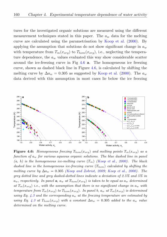
160 Chapter 4. Experimental temperature dependence of water activity
tures for the investigated organic solutions are measured using the different
measurement techniques stated in this paper. The aw data for the melting
curve are calculated using the parametrisation by Koop et al. (2000). By
applying the assumption that solutions do not show significant change in awwith temperature from Tm(xorg) to Thom(xorg), i.e., neglecting the tempera-
ture dependence, the aw values evaluated this way show considerable scatter
around the ice-freezing curve in Fig 4.6 a. The homogeneous ice freezing
curve, shown as dashed black line in Figure 4.6, is calculated by shifting the
melting curve by ∆aw = 0.305 as suggested by Koop et al. (2000). The awdata derived with this assumption in most cases lie below the ice freezing
180
190
200
210
220
230
240
250
260
270
280
290
1.0 0.9 0.8 0.7 0.6 0.5 0.4
Water,activity,,aw
Te
mp
era
ture
,sK
b
a b
180
190
200
210
220
230
240
250
260
270
280
290
1.0 0.9 0.8 0.7 0.6 0.5 0.4
Water,activity,,aw
Te
mp
era
ture
,sK
b
1,3-propanediol1,5-propanediol1,2-hexanediolresorcinolsucroseglycolic,acidpyruvic,acidmethoxyacetic,acidsorbitol2-s2-ethoxyethoxyb,ethanol2-ethoxyethyl,acetateM51,4-butanediola
wsT
homsx
orgbb
awsT
msx
orgbb
awsT
homsx
orgbb ± 0.025
awsT
homsx
orgbb ± 0.05
Figure 4.6: Homogeneous freezing Thom(xorg) and melting points Tm(xorg) as a
function of aw for various aqueous organic solutions. The blue dashed line in panel
(a, b) is the homogeneous ice-melting curve (Tm) (Koop et al., 2000). The black
dashed line is the homogeneous ice-freezing curve (Thom) calculated by shifting the
melting curve by ∆aw = 0.305 (Koop and Zobrist, 2009; Koop et al., 2000). The
grey dotted line and grey dashed-dotted lines indicate a deviation of 2.5% and 5% in
aw, respectively. In panel a, aw at Thom(xorg) is taken to be equal as aw determined
at Tm(xorg) i.e., with the assumption that there is no significant change in aw with
temperature from Tm(xorg) to Thom(xorg). In panel b, aw at Tm(xorg) is determined
using Eq. 4.3 and the corresponding aw at the freezing temperature are estimated by
using Eq. 4.3 at Thom(xorg) with a constant ∆aw = 0.305 added to the aw value
determined on the melting curve.
4.4. Discussion 161
curve. This result could be interpreted as freezing occurring at lower tem-
peratures than predicted by the water-activity-based ice nucleation theory
for the known mixture compositions Fig 4.6 a. However, since the water-
activity-based freezing curve parametrisation is actually very successful in
describing the freezing behavior of many inorganic solutions, for which the
experimental or predicted temperature dependence in water activity is small,
it is more likely the case that assuming constant water activity from Tm(xorg)
to Thom(xorg) is the reason for the apparent discrepancy. Figure 4.6 b shows
the same experimental homogeneous freezing data, but in contrast to Fig 4.6a,
the corresponding water activities at the freezing temperature are estimated
by using Eq. 4.3 at Thom(xorg) with a constant ∆aw = 0.305 added to the
aw value determined on the melting curve for the same mixture. With this
method of aw data evaluation, the experimental data show much less scatter
and outline in good approximation a single “experimental” freezing curve.
This freezing curve described by the ensemble of aqueous organic solution
data is in relatively good agreement with the estimated homogeneous freezing
curve according to Koop et al. (2000). A slight, yet systematic deviation of
the experimental data towards higher freezing temperatures / lower water ac-
tivities is found, especially for the freezing temperatures below 220 K. These
deviations may result in significantly lower values of homogeneous nucleation
rate coefficients (Jhom) (Knopf and Rigg, 2011). A change of aw by 0.025 may
result in a change of Jhom by 6 orders of magnitude, which may significantly
affect predictions of the onset of ice crystal formation in cloud microphysical
models. A difference of 3 orders of magnitude in Jhom could delay or accel-
erate homogeneous ice nucleation by about an hour in a simulation shown by
Knopf and Rigg (2011).
The strong increase of aw with decreasing temperature of aqueous M5 and
2-(2-ethoxyethoxy)ethanol solutions at low temperatures and high solute con-
centrations has consequences for the hygroscopic growth of these systems at
low temperatures. First, the water uptake assuming thermodynamic equilib-
rium between the gas and the condensed phase will be much smaller. Second,
the low water content at these low temperatures will promote high viscosi-
ties or even glass formation leading in addition to kinetic limitations of water
uptake.

162 Chapter 4. Experimental temperature dependence of water activity
4.5 Conclusions
Water activity measurements for selected atmospherically relevant aqueous
organic systems were carried out using different experimental techniques with
the aim of covering a broad concentration and temperature range. Hygro-
scopicity measurements of single levitated aerosol particles with an electrody-
namic balance cover RH between 10 and 90 % RH and temperature from 200
to 300 K. DSC measurements provide the melting and freezing point data
at various solution concentrations and can be used to derive composition and
temperature dependent water activities. To complement these measurements,
total pressure measurements were performed for aqueous organic mixtures.
The measured aw data obtained from the different experiments are consistent
with each other and reveal that organic solutes exhibit differing water activ-
ity temperature dependence; both substantially increasing and decreasing awvalues with decreasing temperatures below 298 K are observed.
More accurate aw data at low temperatures are needed in the context of appli-
cations of homogeneous ice nucleation theory at upper tropospheric tempera-
tures. The experiments presented in this study provide new equilibrium data
sets useful for the development and improvement of thermodynamic activ-
ity coefficient models, such as UNIFAC (UNIquac Functional group Activity
Coefficients) and AIOMFAC (Aerosol Inorganic-Organic Mixtures Functional
groups Activity Coefficients). In turn, improved thermodynamic models can
be used for more accurate predictions of the temperature dependence of activ-
ity coefficients of water and other solution constituents, as well as equilibrium
compositions of multiphase systems for mixtures and environmental condi-
tions, for which experimental data is unavailable.
Acknowledgements
This work was supported by the Swiss National Foundation, project 200020-
125151 and by the CCES projects IMBALANCE and OPTIWARES funded
by the ETH Domain.

4.5. Conclusions 163
Table 4.1: Selected physical properties of organic components used for the experi-
ments: molar mass (M), melting point (Tm), boiling point (Tb) at standard pressure
(101.325 kPa), functional groups, and structure.
Organic compounds Chemical formula M (g mol-1) Tm( K) Tb(K) Functional groups Structure
1,3-propanediol C3H8O2 76.094 246.15 487.55 CHn,OH HO OH
1,4-butanediol C4H10O2 90.121 292.15 501.15 CHn,OH HO
OH
1,5-pentanediol C5H12O2 104.148 257.15 512.15 CHn,OH HO OH
1,2-hexanediol C6H14O2 118.174 318.15 496.65 CHn,OH OH
OH
sorbitol C6H14O2 182.172 372.15 568.15 CHn,OHOH
OH
OH
OH
OH
HO
resorcinol C6H6O2 110.111 383.15 549.2 CHn,OH
HO OH
sucrose C12H22O11 342.116 459.15 decomposes CHn,OH,CHnOHO
OH
OH
O
HO
O
OH
OH
HO
HO
O
glycolic acid C2H4O3 76.051 353.15 385 CHn,OH,COOH HO
O
OH
pyruvic acid C3H4O3 88.062 284.65 438.37 CHnCO,COOH
O
O
OH
2-methoxyacetic acid C3H6O3 90.077 281.15 477.5 CHn,CHnO,COOH
O
OH
O
2-ethoxyethyl acetate C6H12O3 132.158 212.15 428.71 CHn,CHnO,CCOO
O
O
O
2-(2-ethoxyethoxy)ethanol
(carbitol)C6H14O3 134.174 193.15 475.49 CHn,CHnO,OH
O
OHO
malic acid C4H6O5 134.087 405.15 509.13 CHn,OH,COOH
OH
O
OH
O
HO
malonic acid C3H4O4 104.061 409.15 339.99 CHn,COOH
O
OH
O
HO
maleic acid C4H4O4 116.011 403.15 256 CHn,COOHO
OH
OHO
glutaric acid C5H8O4 132.042 369.65 575.96 CHn,COOH
O
OH
O
HO
methylsuccinic acid C5H8O4 132.042 383− 388 decomposes CHn,COOH
O
OH
O
HO
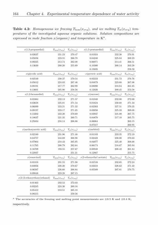
164 Chapter 4. Experimental temperature dependence of water activity
Table 4.2: Homogeneous ice freezing Thom(xorg), and ice melting Tm(xorg) tem-
peratures of the investigated aqueous organic solutions. Solution compositions are
expressed in mole fraction x(organic) and temperature in Ka.
x(1,3-propanediol) Thom(xorg) Tm(xorg) x(1,5-pentanediol) Thom(xorg) Tm(xorg)
0.02637 231.23 270.47 0.01924 232.38 270.91
0.05656 223.55 266.78 0.04240 225.04 269.23
0.09225 212.74 262.08 0.06971 214.41 266.51
0.13630 200.20 255.69 0.10300 200.14 263.28
0.15035 259.59
x(glycolic acid) Thom(xorg) Tm(xorg) x(pyruvic acid) Thom(xorg) Tm(xorg)
0.02549 230.37 270.54 0.02223 231.72 276.76
0.05612 224.03 267.46 0.04879 223.68 267.06
0.09191 217.77 262.99 0.08090 210.84 261.65
0.13601 205.90 258.56 0.12026 209.45 253.58
x(1,2-hexanediol) Thom(xorg) Tm(xorg) x(sucrose) Thom(xorg) Tm(xorg)
0.01664 232.13 271.57 0.01040 232.00 272.00
0.03658 225.01 271.54 0.01624 230.68 271.34
0.06099 223.21 271.32 0.02303 227.51 270.35
0.09197 223.17 271.05 0.03056 225.33 269.08
0.13202 222.20 270.69 0.03937 221.09 267.75
0.18637 221.35 269.71 0.04870 217.10 265.75
0.25834 216.14 268.86 0.06064 263.15
0.07317 260.95
x(methoxyacetic acid) Thom(xorg) Tm(xorg) x(sorbitol) Thom(xorg) Tm(xorg)
0.02180 231.96 271.48 0.01103 233.35 272.19
0.04757 244.69 268.98 0.02422 230.00 270.63
0.07904 218.43 265.95 0.04077 225.40 268.68
0.11765 208.79 262.64 0.06174 218.67 265.94
0.16709 193.55 257.67 0.08948 208.42 261.84
0.22937 251.31 0.12867 255.75
x(resorcinol) Thom(xorg) Tm(xorg) x(2-ethoxyethyl acetate) Thom(xorg) Tm(xorg)
0.01818 231.55 271.98 0.01516 232.65 272.24
0.03956 228.20 270.67 0.03318 228.62 271.22
0.06567 226.60 268.84 0.05509 207.81 270.75
0.09848 223.28 267.15
x(2-(2-ethoxyethoxy)ethanol) Thom(xorg) Tm(xorg)
0.01463 232.52 272.03
0.03245 224.30 269.16
0.05412 210.51 265.18
0.08215 259.56
a The accuracies of the freezing and melting point measurements are ±0.5 K and ±0.4 K,
respectively.

4.5. Conclusions 165
Table 4.3: Bulk water activity (aw) measurements a at 298.15 K of different aqueous
organic solutions. Solution compositions are expressed in mole fraction x(organic).
x(sorbitol) aw x(resorcinol) aw x(glycolic acid) aw x(pyruvic acid) aw x(sucrose) aw
0.0110 0.981 0.01818 0.985 0.02564 0.962 0.02267 0.966 0.01040 0.992
0.0242 0.956 0.03956 0.950 0.05588 0.934 0.04868 0.925 0.01624 0.988
0.0408 0.934 0.06567 0.938 0.09209 0.887 0.08068 0.883 0.02303 0.977
0.0617 0.898 0.09848 0.893 0.13644 0.838 0.12020 0.836 0.03056 0.971
0.0895 0.834 0.13992 0.877 0.19154 0.767 0.16986 0.778 0.03937 0.955
0.1287 0.752 0.19312 0.843 0.25957 0.665 0.23467 0.704 0.04870 0.939
0.1872 0.621 0.27629 0.836 0.35447 0.570 0.32089 0.596 0.06064 0.914
0.48560 0.451 0.45005 0.434 0.07317 0.888
0.61773 0.193 0.16527 0.692
a The accuracy of the water activity measurements is specified as ± 0.015 (absolute range) in
aw and ≤ 0.1 K in temperature.
Table 4.4: Bulk water activity (aw) measurements a of water (1) + 1,4-butanediol
(2) solutions at three different temperatures. Solution compositions are given in mole
fraction (x2) of the organic component (2).
x2 aw(T = 289.15 K) aw(T = 298.15 K) aw(T = 313.15 K)
0.02192 0.978 0.985 0.982
0.04731 0.940 0.959 0.965
0.08020 0.918 0.935 0.958
0.11570 0.888 0.899 0.914
0.16604 0.844 0.860 0.871
0.23358 0.787 0.808 0.816
0.31787 0.717 0.733 0.745
0.44309 0.611 0.626 0.631
0.61890 0.424 0.445 0.450
a The accuracy of the water activity measurements is specified as ± 0.015 (absolute range) in
aw and ≤ 0.1 K in temperature.
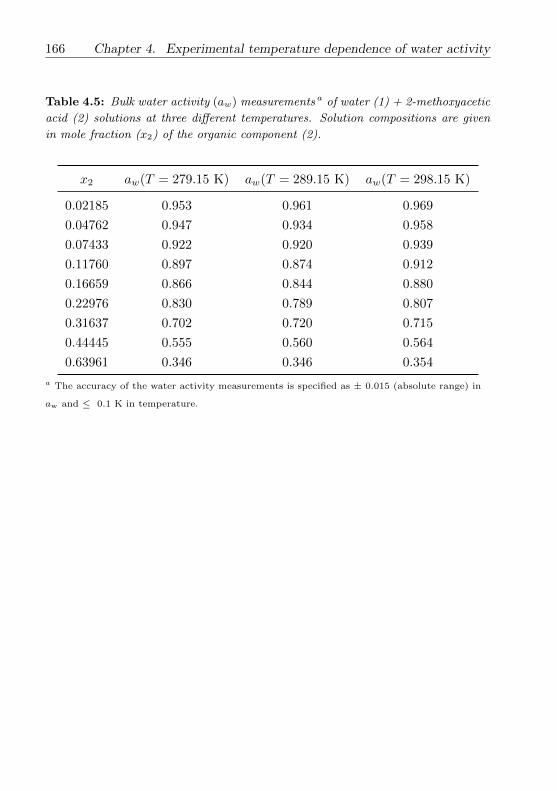
166 Chapter 4. Experimental temperature dependence of water activity
Table 4.5: Bulk water activity (aw) measurements a of water (1) + 2-methoxyacetic
acid (2) solutions at three different temperatures. Solution compositions are given
in mole fraction (x2) of the organic component (2).
x2 aw(T = 279.15 K) aw(T = 289.15 K) aw(T = 298.15 K)
0.02185 0.953 0.961 0.969
0.04762 0.947 0.934 0.958
0.07433 0.922 0.920 0.939
0.11760 0.897 0.874 0.912
0.16659 0.866 0.844 0.880
0.22976 0.830 0.789 0.807
0.31637 0.702 0.720 0.715
0.44445 0.555 0.560 0.564
0.63961 0.346 0.346 0.354
a The accuracy of the water activity measurements is specified as ± 0.015 (absolute range) in
aw and ≤ 0.1 K in temperature.
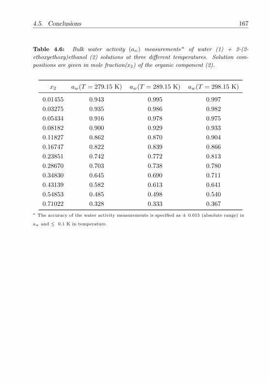
4.5. Conclusions 167
Table 4.6: Bulk water activity (aw) measurements a of water (1) + 2-(2-
ethoxyethoxy)ethanol (2) solutions at three different temperatures. Solution com-
positions are given in mole fraction(x2) of the organic component (2).
x2 aw(T = 279.15 K) aw(T = 289.15 K) aw(T = 298.15 K)
0.01455 0.943 0.995 0.997
0.03275 0.935 0.986 0.982
0.05434 0.916 0.978 0.975
0.08182 0.900 0.929 0.933
0.11827 0.862 0.870 0.904
0.16747 0.822 0.839 0.866
0.23851 0.742 0.772 0.813
0.28670 0.703 0.738 0.780
0.34830 0.645 0.690 0.711
0.43139 0.582 0.613 0.641
0.54853 0.485 0.498 0.540
0.71022 0.328 0.333 0.367
a The accuracy of the water activity measurements is specified as ± 0.015 (absolute range) in
aw and ≤ 0.1 K in temperature.
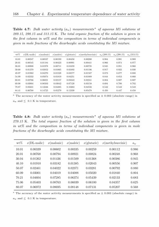
168 Chapter 4. Experimental temperature dependence of water activity
Table 4.7: Bulk water activity (aw) measurements a of aqueous M5 solutions at
289.15, 298.15 and 313.15 K. The total organic fraction of the solution is given in
the first column in wt% and the composition in terms of individual components is
given in mole fractions of the dicarboxylic acids constituting the M5 mixture.
wt% x(DL-malic) x(malonic) x(maleic) x(glutaric) x(methylsuccinic) aw(289.15) aw(298.15) aw(313.15)
10.01 0.00247 0.00537 0.00193 0.00450 0.00200 0.984 0.991 0.989
20.01 0.00545 0.01184 0.00423 0.00991 0.00441 0.966 0.974 0.977
30.01 0.00908 0.01978 0.00711 0.01659 0.00735 0.945 0.951 0.960
39.68 0.01370 0.02852 0.01065 0.02492 0.01106 0.917 0.922 0.930
49.97 0.01962 0.04270 0.01528 0.03577 0.01587 0.873 0.877 0.880
54.99 0.02332 0.05074 0.01819 0.04251 0.01889 0.844 0.853 0.860
60.01 0.02766 0.06021 0.02157 0.05043 0.02241 0.804 0.807 0.807
69.98 0.03904 0.08503 0.03042 0.07120 0.03158 0.694 0.700 0.702
79.87 0.05631 0.12246 0.04385 0.10263 0.04556 0.542 0.543 0.543
84.41 0.06768 0.14725 0.05279 0.12339 0.05478 0.450 0.447 0.458
a The accuracy of the water activity measurements is specified as ± 0.003 (absolute range) in
aw and ≤ 0.1 K in temperature.
Table 4.8: Bulk water activity (aw) measurements a of aqueous M5 solutions at
279.15 K. The total organic fraction of the solution is given in the first column
in wt% and the composition in terms of individual components is given in mole
fractions of the dicarboxylic acids constituting the M5 mixture.
wt% x(DL-malic) x(malonic) x(maleic) x(glutaric) x(methylsuccinic) aw
10.01 0.00339 0.00602 0.00335 0.00259 0.00112 0.986
20.01 0.00768 0.00794 0.00921 0.00824 0.00248 0.968
30.04 0.01262 0.01436 0.01509 0.01368 0.00386 0.945
40.10 0.01910 0.03182 0.01385 0.02043 0.00556 0.907
50.07 0.02461 0.04022 0.02371 0.03281 0.00792 0.880
60.09 0.03001 0.04019 0.04088 0.05020 0.01840 0.804
70.21 0.04604 0.07285 0.06374 0.05439 0.02133 0.683
75.06 0.05403 0.08763 0.06039 0.06100 0.04357 0.625
80.07 0.06972 0.08695 0.08148 0.07131 0.05207 0.568
a The accuracy of the water activity measurements is specified as ± 0.003 (absolute range) in
aw and ≤ 0.1 K in temperature.

4.5. Conclusions 169
Table 4.9: EDB measurements: The total organic fraction of the solution is given
in the first column in wt% and the composition in terms of individual components
is given in mole fractions of the dicarboxylic acids constituting the M5 mixture.
wt% x(DL-malic) x(malonic) x(maleic) x(glutaric) x(methylsuccinic)
10.01 0.00247 0.00537 0.00193 0.00450 0.00200
20.01 0.00545 0.01184 0.00423 0.00991 0.00441
30.01 0.00908 0.01978 0.00711 0.01659 0.00735
39.68 0.01370 0.02852 0.01065 0.02492 0.01106
49.97 0.01962 0.04270 0.01528 0.03577 0.01587
54.99 0.02332 0.05074 0.01819 0.04251 0.01889
60.01 0.02766 0.06021 0.02157 0.05043 0.02241
69.98 0.03904 0.08503 0.03042 0.07120 0.03158
79.87 0.05631 0.12246 0.04385 0.10263 0.04556
84.41 0.06768 0.14725 0.05279 0.12339 0.05478

170 Chapter 4. Experimental temperature dependence of water activity
Table 4.10: Water activity (aw) measurements a of aqueous M5 solutions from
EDB hygroscopic growth curves evaluated at the indicated weight fractions Mention
that the corresponding M5 solution compositions in terms of organic components are
given in Table 4.9.
wt% aw(289 K) aw(273 K) aw(263 K) aw(244 K) aw(233 K)
10.01 0.987
20.01 0.969
30.01 0.947
39.68 0.915
49.97 0.874 0.867
54.99 0.839 0.839 0.841
60.01 0.805 0.802 0.805
69.98 0.694 0.699 0.714
79.87 0.540 0.562 0.572 0.648 0.667
84.41 0.448 0.470 0.490 0.569 0.626
90.00 0.318 0.329 0.362 0.429 0.544
a The accuracy of the water activity measurements is specified as ± 0.015 (absolute range) in
aw and ≤ 0.1 K in temperature.

4.5. Conclusions 171
Table 4.11: Water activity (aw) measurements a of aqueous M5 solutions from
EDB hygroscopic growth curves evaluated at the indicated weight fractions.
wt% aw(268 K) aw(253 K) aw(236 K)
60.00 0.791
65.00 0.767
70.00 0.725
73.00 0.700
75.00 0.676
80.00 0.602 0.611
85.00 0.504 0.507
90.00 0.364 0.385
95.60 0.172 0.216 0.347
97.20 0.264
a The accuracy of the water activity measurements is specified as ± 0.015 (absolute range) in
aw and ≤ 0.1 K in temperature.

172 Chapter 4. Experimental temperature dependence of water activity
Table 4.12: Measured water activities of water (1) + 1,4-butanediol (2) mixtures
derived from total pressure measurements, listed for a selection of temperatures in
the range 270 K < T < 291 K. Solution compositions are given in mole fractions
of the organic (x2).
x2 aw(270.15 K) x2 aw(273.15 K) x2 aw(275.15 K)
0.24441 0.762 0.24441 0.766 0.23200 0.812
0.26933 0.751 0.26933 0.754 0.24441 0.768
0.31705 0.688 0.31705 0.694 0.26933 0.755
0.37368 0.654 0.37368 0.658 0.31705 0.697
0.44332 0.604 0.44332 0.606 0.37368 0.660
0.52556 0.502 0.44332 0.607
0.52556 0.504
x2 aw(278.15 K) x2 aw(280.15 K) x2 aw(283.15 K)
0.24441 0.772 0.04797 0.971 0.04797 0.971
0.26933 0.757 0.11823 0.900 0.11823 0.901
0.31705 0.702 0.16701 0.868 0.16701 0.868
0.37368 0.663 0.23200 0.813 0.23200 0.813
0.44332 0.608 0.24441 0.775 0.24441 0.776
0.52556 0.507 0.26933 0.759 0.26933 0.761
0.64080 0.396 0.31705 0.706 0.31705 0.710
0.37368 0.665 0.37368 0.667
0.44332 0.608 0.44332 0.610
0.52556 0.508 0.52556 0.510
0.64080 0.399 0.64080 0.402
x2 aw(285.15 K) x2 aw(288.15 K) x2 aw(290.15 K)
0.04797 0.969 0.04797 0.967 0.04797 0.969
0.11823 0.901 0.11823 0.901 0.11823 0.906
0.16701 0.869 0.16701 0.868 0.16701 0.873
0.23200 0.814 0.23200 0.815 0.23200 0.818
0.24441 0.778 0.24441 0.780 0.24441 0.786
0.26933 0.763 0.26933 0.766 0.26933 0.770
0.31705 0.712 0.31705 0.716 0.31705 0.724
0.37368 0.667 0.37368 0.669 0.37368 0.673
0.44332 0.611 0.44332 0.611 0.44332 0.615
0.52556 0.512 0.52556 0.513 0.52556 0.517
0.64080 0.403 0.64080 0.404 0.64080 0.406
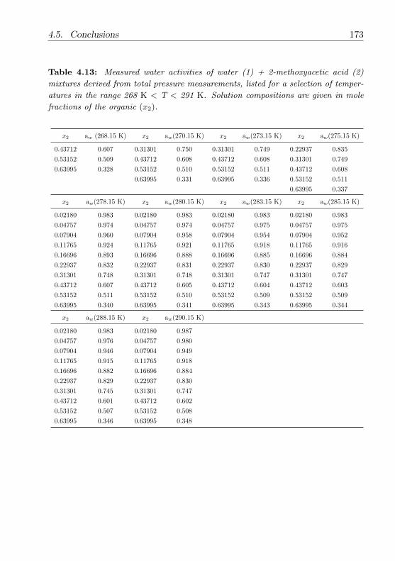
4.5. Conclusions 173
Table 4.13: Measured water activities of water (1) + 2-methoxyacetic acid (2)
mixtures derived from total pressure measurements, listed for a selection of temper-
atures in the range 268 K < T < 291 K. Solution compositions are given in mole
fractions of the organic (x2).
x2 aw (268.15 K) x2 aw(270.15 K) x2 aw(273.15 K) x2 aw(275.15 K)
0.43712 0.607 0.31301 0.750 0.31301 0.749 0.22937 0.835
0.53152 0.509 0.43712 0.608 0.43712 0.608 0.31301 0.749
0.63995 0.328 0.53152 0.510 0.53152 0.511 0.43712 0.608
0.63995 0.331 0.63995 0.336 0.53152 0.511
0.63995 0.337
x2 aw(278.15 K) x2 aw(280.15 K) x2 aw(283.15 K) x2 aw(285.15 K)
0.02180 0.983 0.02180 0.983 0.02180 0.983 0.02180 0.983
0.04757 0.974 0.04757 0.974 0.04757 0.975 0.04757 0.975
0.07904 0.960 0.07904 0.958 0.07904 0.954 0.07904 0.952
0.11765 0.924 0.11765 0.921 0.11765 0.918 0.11765 0.916
0.16696 0.893 0.16696 0.888 0.16696 0.885 0.16696 0.884
0.22937 0.832 0.22937 0.831 0.22937 0.830 0.22937 0.829
0.31301 0.748 0.31301 0.748 0.31301 0.747 0.31301 0.747
0.43712 0.607 0.43712 0.605 0.43712 0.604 0.43712 0.603
0.53152 0.511 0.53152 0.510 0.53152 0.509 0.53152 0.509
0.63995 0.340 0.63995 0.341 0.63995 0.343 0.63995 0.344
x2 aw(288.15 K) x2 aw(290.15 K)
0.02180 0.983 0.02180 0.987
0.04757 0.976 0.04757 0.980
0.07904 0.946 0.07904 0.949
0.11765 0.915 0.11765 0.918
0.16696 0.882 0.16696 0.884
0.22937 0.829 0.22937 0.830
0.31301 0.745 0.31301 0.747
0.43712 0.601 0.43712 0.602
0.53152 0.507 0.53152 0.508
0.63995 0.346 0.63995 0.348

174 Chapter 4. Experimental temperature dependence of water activity
Table 4.14: Measured water activities of water (1) + 2-(2-ethoxyethoxy)ethanol (2)
mixtures derived from total pressure measurements, listed for a selection of temper-
atures in the range 265 K < T < 291 K. Solution compositions are given in mole
fractions of the organic (x2).
x2 aw (265.15 K) x2 aw(268.15 K) x2 aw(270.15 K) x2 aw(273.15 K)
0.54409 0.469 0.54409 0.477 0.54409 0.481 0.54409 0.488
0.42719 0.573 0.42719 0.583 0.42719 0.589 0.42719 0.598
0.34418 0.644 0.34418 0.654 0.34418 0.660 0.34418 0.669
0.23774 0.732 0.23774 0.742 0.23774 0.748 0.23774 0.756
0.16753 0.801 0.16753 0.811 0.16753 0.817 0.16753 0.824
x2 aw (275.15 K) x2 aw(278.15 K) x2 aw(280.15 K) x2 aw(283.15 K)
0.54409 0.492 0.54409 0.497 0.54409 0.501 0.54409 0.506
0.42719 0.603 0.42719 0.610 0.42719 0.616 0.42719 0.622
0.34418 0.674 0.34418 0.681 0.34418 0.685 0.34418 0.692
0.23774 0.762 0.23774 0.769 0.23774 0.774 0.23774 0.782
0.16753 0.828 0.16753 0.835 0.16753 0.839 0.16753 0.845
0.11810 0.878 0.11810 0.883 0.11810 0.886 0.11810 0.891
0.08217 0.932 0.08217 0.932 0.08217 0.935
0.05412 0.961 0.05412 0.961 0.05412 0.961
0.03245 0.988 0.03245 0.989 0.03245 0.990
x2 aw(285.15 K) x2 aw(288.15 K) x2 aw(290.15 K)
0.54409 0.509 0.54409 0.514 0.54409 0.518
0.42719 0.627 0.42719 0.634 0.42719 0.643
0.34418 0.696 0.34418 0.704 0.34418 0.711
0.23774 0.787 0.23774 0.795 0.23774 0.815
0.16753 0.849 0.16753 0.855 0.16753 0.864
0.11810 0.895 0.11810 0.900 0.11810 0.907
0.08217 0.938 0.08217 0.941 0.08217 0.946
0.05412 0.962 0.05412 0.964 0.05412 0.967
0.03245 0.992 0.03245 0.994 0.03245 0.998

4.5. Conclusions 175
Table 4.15: Mixture compositions at different overall organic mass fractions (wt%)
of the aqueous M5 system used for total pressure measurements. Component mole
fractions (x) of the dicarboxylic acids constituting the M5 mixture are given, with
water accounting for the remaining fraction.
wt% x(DL-malic acid) x(malonic acid) x(maleic acid) x(glutaric acid) x(methylsuccinic acid)
20 0.00545 0.01183 0.00428 0.00992 0.00441
40 0.01353 0.02815 0.01064 0.02453 0.01085
50 0.01959 0.04236 0.01526 0.03581 0.01672
60 0.02746 0.06049 0.02135 0.04971 0.02241
70 0.03833 0.08327 0.02997 0.06984 0.03090
75 0.04547 0.09924 0.03549 0.08310 0.03700
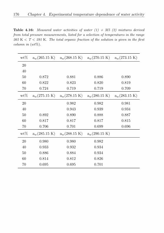
176 Chapter 4. Experimental temperature dependence of water activity
Table 4.16: Measured water activities of water (1) + M5 (2) mixtures derived
from total pressure measurements, listed for a selection of temperatures in the range
265 K < T < 291 K. The total organic fraction of the solution is given in the first
column in (wt%).
wt% aw(265.15 K) aw(268.15 K) aw(270.15 K) aw(273.15 K)
20
40
50 0.872 0.881 0.886 0.890
60 0.822 0.823 0.820 0.819
70 0.724 0.719 0.719 0.709
wt% aw(275.15 K) aw(278.15 K) aw(280.15 K) aw(283.15 K)
20 0.982 0.982 0.981
40 0.943 0.939 0.934
50 0.892 0.890 0.888 0.887
60 0.817 0.817 0.817 0.815
70 0.706 0.701 0.699 0.696
wt% aw(285.15 K) aw(288.15 K) aw(290.15 K)
20 0.980 0.980 0.982
40 0.933 0.932 0.934
50 0.886 0.884 0.934
60 0.814 0.812 0.826
70 0.695 0.695 0.701

Chapter 5
Conclusions
In this thesis we investigated the temperature dependence of activity coeffi-
cients in aqueous organic and water-free organic mixtures at tropospheric low
temperatures. For this we use a thermodynamic model, AIOMFAC which is a
group contribution model developed by (Zuend et al., 2008, 2011) to compute
the activity coefficients of mixed organic, inorganic and organic-inorganic mix-
tures. AIOMFAC is based on the group contribution model LIFAC by Yan
et al. (1999) and includes the semi-empirical group contribution model UNI-
FAC (Fredenslund et al., 1975; Hansen et al., 1991) for the description of
organic mixtures and aqueous organic solutions. The UNIFAC within the
AIOMFAC uses a simple temperature dependence parameterisation around
∼ 275 to ∼ 400 K. To study the temperature dependence of activity coeffi-
cients at atmospheric low temperatures we develop a new improved temper-
ature dependence parametrization to include the organic functional groups
such as carboxyl, hydroxyl, ketone, aldehyde, ether, ester, alkyl, aromatic
carbon-alcohol, and aromatic hydrocarbon. For reliable estimation of group
interaction parameters, database covering organic functional groups covering
a wide composition and temperature range using different thermodynamic
data types such as vapour-liquid equilibria (VLE), liquid-liquid equilibria
(LLE), solid-liquid equilibria (SLE), and water activity (aw) measurements
was collected. Considering the apparent gaps in the database especially in
the low temperature range, for which literature data were missing or of in-
sufficient quality, we performed aw measurements for aqueous organic mix-
tures which included the selected monofunctional and multifunctional, this
177

178 Chapter 5. Conclusions
additional data is included in the AIOMFAC database. Measurement tech-
niques such dewpoint water activity meter covering the temperature range
from 289 K - 313 K, ice melting curves obtained from differential scanning
calorimetry (DSC) measurements yielding SLE data, and the hygroscopicity
measurements of single levitated aerosol particles with an electrodynamic bal-
ance covering dry conditions up to ice saturation from 200 K to 300 K were
used to obtain aw data at low temperatures. To complement these measure-
ment techniques we developed a setup to measure total gas phase pressure
at equilibrium over the solutions at low temperatures. The aw data obtained
from the different experiments are consistent with each other and reveal that
different organic solutes can lead to distinct aw temperature dependence; both
substantially increasing and decreasing aw values with decreasing temperature
are observed. In general, the new temperature dependence parameterisation
is in good agreement with most of the experimental datasets. The AIOM-
FAC model can be used for more accurate predictions of the temperature
dependence of activity coefficients of water and other solution constituents,
ice nucleation studies, phase transitions, and gas-particle partitioning. With
a combined approach of performing experimental and model predictions have
facilitated in better understanding the temperature dependence of organic
mixtures at low temperatures. The new parameterisation is implemented to
selected number of organic functional groups and can be further extended to
include new additional organic functional groups. The AIOMFAC model with
the new temperature dependence is parameterised for only aqueous/water-free
organic mixtures. For a wider atmospheric application of AIOMFAC model to
atmospheric conditions, implementing the temperature dependence parame-
terisation for aqueous/water-free inorganic and inorganic-organic mixtures is
essential. However, the database for low temperature measurements is in-
sufficient or of poor quality. A similar approach of combining experimental
studies with model calculations will be beneficial. The improved thermody-
namic models can be used for more accurate predictions of the temperature
dependence of activity coefficients of water and other solution constituents,
as well as equilibrium compositions of multiphase systems for mixtures and
environmental conditions, for which experimental data of insufficient quality.

List of Figures
1.1 Vertical temperature structure of the atmosphere extending
from the surface of the Earth to approximately 110-km alti-
tude as given in the U.S. Standard Atmosphere, 1976. Source:
Brasseur et al. (1999). . . . . . . . . . . . . . . . . . . . . . . . 7
1.2 Estimates (in Tg per year) for the year 2000 of (a) direct par-
ticle emissions into the atmosphere and (b) in-situ production.aSizes refer to diameters. [Adapted from Intergovernmental
Panel on Climate Change, 2001, Cambridge University Press,
pp.297 and 301, 2001.] Source: Wallace et al. (2006) . . . . . . 11
1.3 shows composites of MODIS/Terra, Aerosol optical Depth
(AOD) by the MODIS/Terra (550 nm) for the April 13 (top
row) and August 22 (bottom row), 2001. Red colour indicates
fine mode aerosols and green colour coarse mode aerosols. On
April 13, 2001, heavy dust and pollution is transported from
Asia to the Pacific and dust is transported from Africa to At-
lantic. On August 22 large smoke plumes from South America
and South Africa are evident. Adapted from Chin et al. (2007);
(original figure from Yoram Kaufman and Reto Stockli). . . . . 12
1.4 Schematic representation of distribution of particle surface
area of atmospheric aerosols. Principle modes, formation and
conversion processes, and removal mechanisms are indicated.
Source: Whitby and Cantrell (1976). . . . . . . . . . . . . . . . 14
179

180 List of Figures
1.5 Figure illustrates the direct and various indirect aerosol effects.
The aerosol particles are represented as small black dots; cloud
droplets are represented by the larger open circles. Straight
lines represent the incident and reflected solar radiation, and
wavy lines represent long wave radiation. The vertical grey
dashes represent rainfall, and LWC refers to the liquid water
content. [Source: IPCC AR4 Report Forster et al. (2007)] . . . 17
1.6 Summary of the principal components of the radiative forcing
of climate change. [Source: IPCC AR4 Report Forster et al.
(2007)] . . . . . . . . . . . . . . . . . . . . . . . . . . . . . . . . 19
1.7 Hysteresis behavior of an aqueous ammonium sulphate particle
at ambient temperature. Open circles represents measurements
when RH is increasing, whereas the closed circles are points
with decreasing RH. Particle mass change is represented by
the ratio m/mo where m is the dry particle mass and mo is
the particle mass at particular RH. The deliquescence relative
humidity is about 80 %, the efforescence point around 37 % RH
in case of ammonium sulphate, but sometimes the efflorescence
may also occur at slightly higher or lower values (always below
DRH). Source: Tang and Munkelwitz (1994) . . . . . . . . . . . 21
2.1 Vapour pressure over a non-ideal liquid mixture of components
A and B at vapour-liquid equilibrium (VLE).(a) Positive devi-
ations from ideality, (b) negative deviations from ideality. pAand pB are vapour pressures and p
A and pB are the satura-
tion vapour pressures of the pure components A and B in gas
phase. Ptot represents the total pressure and is the sum of
partial pressure pA and pB . . . . . . . . . . . . . . . . . . . . . 36
2.2 Intramolecular and intermolecular forces in HCl molecules.
The intramolecular interactions within a HCl molecule is repre-
sented by a solid line while intermolecular interactions between
the two HCl molecules are represented by the dash/dotted line. 48
List of Figures 181
2.3 Ion-dipole interaction of Na+ and Cl− with water molecules.
δ+ and δ− are partial positive and negative charges created due
to asymmetrical distribution of electrons in chemical bonds. . . 49
2.4 Dipole-Dipole interactions. Solid red lines: strong interac-
tion forces between any two opposite charges, dashed red lines:
strong repulsive interaction forces between the like charges. . . 51
2.5 Dispersion forces. (a) Spherically symmetric charge distribu-
tion in He atom 1. (b) The uneven electron distribution pro-
duces a momentary dipoles and allows temporary electrostatic
attraction between atoms. . . . . . . . . . . . . . . . . . . . . . 52
2.6 Hydrogen bonding between H2O and NH3 molecules. . . . . . . 53
2.7 Hydrogen bonding between water molecules. The red dash-
lines are the hydrogen bonds between the water molecules. . . . 54
3.1 Database distribution for the water ↔ organic and organic ↔organic interaction parameters. The table lists the total num-
ber of datasets (set count) available for each main group inter-
action at temperatures substantially different from the chosen
reference temperature (T = 298.15 K). The total number of
datasets available for each main group interaction pair are visu-
alized by the green coloured bars. The percentile-wise colouring
is used to visualize the lowest temperature (Tlow, blue colour)
and the highest temperature (Thigh, red colour) (units of K) of
the data points available for each main group interaction pair. . 72

182 List of Figures
3.2 Measurements for 1,2-ethanediol + water solutions, corre-
sponding calculations of AIOMFAC-P1 in (panels a-c) and
AIOMFAC-P3 (panels d-f). The coloured curves in panels (c,
f) represents the temperature dependence of water activities
predicted for the range from 150 - 480 K. Panels (a, d): Low
temperature experimental SLE data (crosses) are compared
with the predictions for water activity at the same composi-
tions and temperatures (blue circles). Predictions of the corre-
sponding organic activities are shown as well (green triangles).
The dashed line represents the hypothetical water activity of
an ideal mixture. The error bars represent the model sensi-
tivity to a composition variation by xtol = 0.01. The middle
panels (b and e) show the model predictions of the activity co-
efficients compared to VLE data covering temperatures signifi-
cantly higher than room temperature. The temperature of the
individual data points are given in the boxes below the main
panels. Experimental data: Ott et al. (1972) and Gmehling
and Onken (2003a). . . . . . . . . . . . . . . . . . . . . . . . . 83
List of Figures 183
3.3 Measurements for acetic acid + water solutions, correspond-
ing calculations of AIOMFAC-P1 in and AIOMFAC-P3. The
coloured curves in panels (c, f) represents the temperature de-
pendence of water activities predicted for the range from 150
- 480 K. Panels (a, d): Low temperature experimental SLE
data (crosses) are compared with the predictions for water ac-
tivity at the same compositions and temperatures (blue circles).
Predictions of the corresponding organic activities are shown
as well (green triangles). The dashed line represents the hy-
pothetical water activity of an ideal mixture. The error bars
represent the model sensitivity to a composition variation by
xtol = 0.01. The middle panels (b and e) show the model
predictions of the activity coefficients compared to VLE data
covering temperatures significantly higher than room tempera-
ture. The temperature of the individual data points are given
in the boxes below the main panels. Experimental data: Fau-
con (1910) and Narayana et al. (1985). . . . . . . . . . . . . . . 84
3.4 Measurements for malonic acid + water solutions, corre-
sponding calculations of AIOMFAC-P1 in (panels a-c) and
AIOMFAC-P3 (panels d-f). Panels (c, f) show the temper-
ature dependence of water activities predicted for the range
from 150 - 480 K. Panels(a, d): Low temperature experimen-
tal SLE data (crosses) are compared with the predictions for
water activity at the same compositions and temperatures (blue
circles). Predictions of the corresponding organic activities are
shown as well (green triangles) while panels b and e show anal-
ogous data for the malonic acid melting curve. The error bars
represent the model sensitivity to a composition variation by
xtol =0.01. The dashed line represents the hypothetical water
activity of an ideal mixture. The temperature of the individ-
ual data points are given in the boxes below the main panels.
Experimental data: Braban et al. (2003) and Apelblat and
Manzurola (1987). . . . . . . . . . . . . . . . . . . . . . . . . . 89

184 List of Figures
3.5 Measurements for 2-butanone + water solutions, corresponding
calculations of AIOMFAC-P1 in (panels a-c) and AIOMFAC-
P3 (panels d-f). Panels (c, f) show the temperature depen-
dence of water activities predicted for the range from 150 -
480 K. Panels (a, d): Low temperature experimental SLE
data (crosses) are compared with the predictions for water ac-
tivity at the same compositions and temperatures (blue circles).
Predictions of the corresponding organic activities are shown as
well (green triangles). The error bars represent the model sensi-
tivity to a composition variation by xtol =0.01. The dashed line
represents the hypothetical water activity of an ideal mixture.
The middle panels (b and e) show the model predictions of the
activity coefficients compared to VLE data covering tempera-
tures significantly higher than room temperature. The temper-
ature of the individual data points are given in the boxes below
the main panels. Experimental data: Lohmann et al. (1997)
and Gmehling et al. (1981). . . . . . . . . . . . . . . . . . . . . 90
3.6 Measurements for 2-butoxyethanol + water solutions, corre-
sponding calculations of AIOMFAC-P1 in (panels a-c) and
AIOMFAC-P3 (panels d-f). Panels (c, f) show the temper-
ature dependence of water activities predicted for the range
from 150 - 480 K. Panels (a, d): Low temperature experimen-
tal SLE data (crosses) are compared with the predictions for
water activity at the same compositions and temperatures (blue
circles). Predictions of the corresponding organic activities are
shown as well (green triangles). The error bars represent the
model sensitivity to a composition variation by xtol =0.01. The
dashed line represents the hypothetical water activity of an
ideal mixture. The middle panels (b and e) show the model
predictions of the activity coefficients compared to VLE data
covering temperatures significantly higher than room tempera-
ture. The temperature of the individual data points are given
in the boxes below the main panels. Experimental data: Koga
et al. (1994) and Schneider and Wilhelm (1959). . . . . . . . . 91
List of Figures 185
3.7 Measurements for cyclohexanol + adipic acid solutions, cor-
responding calculations of AIOMFAC-P1 in panels (a, b) and
AIOMFAC-P3 (c, d). Panels (b, d) represent the temperature
dependence predictions from AIOMFAC-P1 and AIOMFAC-P3
for temperature range of 150 - 480 K. Panel (a, c): SLE of
adipic acid shown vs. mole fraction of cyclohexanol (compo-
nent 1). The error bars represent the model sensitivity to a
composition variation by xtol = 0.01. The dashed line is the
ideal solution curve for component 1. The temperature of the
individual data points are given in the boxes below the main
panels. Experimental data: Lihua et al. (2007). . . . . . . . . . 92
3.8 Measurements for ethanol + acetone solutions, corresponding
calculations of AIOMFAC-P1 in panels (a-c) and AIOMFAC-
P3 (d-e). Panels (c, f) show the temperature dependence as
predicted by AIOMFAC-P1 and AIOMFAC-P3 for the tem-
perature range of 150 - 480 K. Panels (a, d): Low tempera-
ture experimental SLE data (crosses), shown as mole fraction
of ethanol, x(1), versus activity (a(x)org2) of acetone. The error
bars represent the model sensitivity to a composition variation
by xtol = 0.01. The dashed line is the ideal solution curve for
component 1. The middle panels (b and e) show the model
predictions of the activity coefficients compared to VLE data
covering temperatures significantly higher than room tempera-
ture. The temperature of the individual data points are given
in the boxes below the main panels. The temperature of the
individual data points are given in the boxes below the main
panels. Experimental data: Sapgir (1929) and Amer et al. (1956). 93

186 List of Figures
3.9 Measurements for ethanol + 3-heptanone solutions, corre-
sponding calculations of AIOMFAC-P1 in panels (a, b) and
AIOMFAC-P3 (c, d). Panels (b, d) shows the temperature
dependence predictions from AIOMFAC-P1 and AIOMFAC-
P3 for temperature range of 150 - 480 K. The SLE data in
panel (a, c) show the composition (mole fraction of ethanol)
against activity of 3-heptanone. The error bars represent the
model sensitivity to a composition variation by xtol = 0.01.
The dashed line is the ideal solution curve for component 1.
Experimental data: Fiege et al. (1996). . . . . . . . . . . . . . . 94
3.10 Measurements for ethanol + diethyl ether solutions, corre-
sponding calculations of AIOMFAC-P1 and AIOMFAC-P3.
Panels (c, f) show the temperature dependence of the ethanol
activity, as predicted by AIOMFAC-P1 and AIOMFAC-P3 for
the temperature range 150 - 480 K. Panel (a,d): Experimental
SLE data (crosses) compared with model predictions (triangles)
for the activity of diethyl ether in the very low temperature
range 149 to 156 K. The dashed line is the ideal solution curve
for component 1. The middle panels (b and e) show the model
predictions of the activity coefficients compared to VLE data
covering temperatures significantly higher than room tempera-
ture. The temperature of the individual data points are given in
the boxes below the main panels. Experimental data:Lalande
(1934) and Moeller et al. (1951). . . . . . . . . . . . . . . . . . 95
4.1 Setup for total gas phase pressure measurements of aqueous
organic solutions at room temperature and below. . . . . . . . 144

List of Figures 187
4.2 Measured water activities of aqueous 1,4-butanediol solutions
versus temperature. The different colours indicate the solu-
tion compositions in wt% of the organic component. The solid
lines show data derived from the total pressure measurements.
The coloured portion of the solid lines represents the tempera-
ture range for which the measurements are considered reliable
within the uncertainty of the method (±0.03 of aw). Water
activities derived from DSC measurements on the ice melting
curve are represented by pentagons. Bulk aw measurements
using the water activity meter are represented by solid circles.
The dash-dotted lines show the composition and temperature
dependent aw parametrisation by Zobrist et al. (2008). The
blue dashed line is the ice melting curve (Koop and Zobrist,
2009). In the colour shaded regions one or both components
are supersaturated with respect to the solid phase and there-
fore, above the eutectic temperature (245 K), at equilibrium
one solid phase coexists with the remaining solution. . . . . . . 151
4.3 Measured water activities of aqueous 2-methoxyacetic acid so-
lutions versus temperature. The different colours indicate the
solution compositions in wt% of the organic component. The
solid lines show data derived from the total pressure measure-
ments. The coloured portion of the solid lines represents the
temperature range for which the measurements are considered
reliable within the uncertainty of the method (±0.03 of aw).
Water activities derived from DSC measurements on the ice
melting curve are represented by pentagons. Bulk aw mea-
surements using the water activity meter are represented by
solid circles. The dash-dotted lines show the composition and
temperature dependent aw parametrisation by Zobrist et al.
(2008). The blue dashed line is the ice melting curve (Koop
and Zobrist, 2009). In the colour shaded regions one or both
components are supersaturated with respect to the solid phase
and therefore, above the eutectic temperature ( 253 K), at equi-
librium one solid phase coexists with the remaining solution. . 152

188 List of Figures
4.4 Experimental water activities versus temperature for aqueous
2-(2-ethoxyethoxy)ethanol solutions. The different colours in-
dicate the solution compositions in wt% of the organic compo-
nent. The solid lines show data derived from the total pressure
measurements. The coloured portion of the solid lines repre-
sents the temperature range for which the measurements are
considered reliable. Water activity data obtained from DSC
measurements on the water-ice melting curve Zobrist et al.
(2008) are represented by solid pentagons. The solid circles
show the data from bulk aw measurements with the water ac-
tivity meter. The dash-dotted lines show the composition and
temperature dependent aw parametrisation by Zobrist et al.
(2008). The blue dashed line is the ice melting curve (Koop
and Zobrist, 2009). . . . . . . . . . . . . . . . . . . . . . . . . . 153
4.5 Experimental water activities versus temperature for aqueous
M5 solutions. The solid and dotted lines are from the to-
tal pressure measurements. The coloured dashed lines (75-
84 wt%) represent measurements for which the solution was
not in a homogeneous liquid state but partly crystallized. The
coloured portion of the solid lines represents the temperature
range for which the measurements are considered reliable. Wa-
ter activity data obtained from DSC measurements on the
water-ice melting curve from Zobrist et al. (2008) are shown
by solid pentagons. The solid circles show the data form bulk
aw measurements with the water activity meter. The dash-
dotted lines show the composition and temperature dependent
aw parametrisation by Zobrist et al. (2008). The blue dashed
line is the ice melting curve (Koop and Zobrist, 2009). The
aw data from EDB measurements are represented by coloured
diamonds. . . . . . . . . . . . . . . . . . . . . . . . . . . . . . . 154

List of Figures 189
4.6 Homogeneous freezing Thom(xorg) and melting points Tm(xorg)
as a function of aw for various aqueous organic solutions. The
blue dashed line in panel (a, b) is the homogeneous ice-melting
curve (Tm) (Koop et al., 2000). The black dashed line is the
homogeneous ice-freezing curve (Thom) calculated by shifting
the melting curve by ∆aw = 0.305 (Koop and Zobrist, 2009;
Koop et al., 2000). The grey dotted line and grey dashed-dotted
lines indicate a deviation of 2.5% and 5% in aw, respectively. In
panel a, aw at Thom(xorg) is taken to be equal as aw determined
at Tm(xorg) i.e., with the assumption that there is no significant
change in aw with temperature from Tm(xorg) to Thom(xorg).
In panel b, aw at Tm(xorg) is determined using Eq. 4.3 and the
corresponding aw at the freezing temperature are estimated
by using Eq. 4.3 at Thom(xorg) with a constant ∆aw = 0.305
added to the aw value determined on the melting curve. . . . . 160


List of Tables
3.1 Database used for the parameterisation of organic main group
↔ water and organic ↔ organic main group interactions of
AIOMFAC-P3. Listed are components, main groups, tempera-
ture range, number of data points (Nd), initial weighting (winitd )
and references of “water + organic ” and “organic + organic ”
datasets . . . . . . . . . . . . . . . . . . . . . . . . . . . . . . . 97
3.1 Continued. . . . . . . . . . . . . . . . . . . . . . . . . . . . . . 98
3.1 Continued. . . . . . . . . . . . . . . . . . . . . . . . . . . . . . 99
3.1 Continued. . . . . . . . . . . . . . . . . . . . . . . . . . . . . . 100
3.1 Continued. . . . . . . . . . . . . . . . . . . . . . . . . . . . . . 101
3.1 Continued. . . . . . . . . . . . . . . . . . . . . . . . . . . . . . 102
3.1 Continued. . . . . . . . . . . . . . . . . . . . . . . . . . . . . . 103
3.1 Continued. . . . . . . . . . . . . . . . . . . . . . . . . . . . . . 104
3.1 Continued. . . . . . . . . . . . . . . . . . . . . . . . . . . . . . 105
3.1 Continued. . . . . . . . . . . . . . . . . . . . . . . . . . . . . . 106
3.1 Continued. . . . . . . . . . . . . . . . . . . . . . . . . . . . . . 107
3.1 Continued. . . . . . . . . . . . . . . . . . . . . . . . . . . . . . 108
3.1 Continued. . . . . . . . . . . . . . . . . . . . . . . . . . . . . . 109
3.1 Continued. . . . . . . . . . . . . . . . . . . . . . . . . . . . . . 110
191

192 List of Tables
3.1 Continued. . . . . . . . . . . . . . . . . . . . . . . . . . . . . . 111
3.1 Continued. . . . . . . . . . . . . . . . . . . . . . . . . . . . . . 112
3.1 Continued. . . . . . . . . . . . . . . . . . . . . . . . . . . . . . 113
3.1 Continued. . . . . . . . . . . . . . . . . . . . . . . . . . . . . . 114
3.1 Continued. . . . . . . . . . . . . . . . . . . . . . . . . . . . . . 115
3.1 Continued. . . . . . . . . . . . . . . . . . . . . . . . . . . . . . 116
3.1 Continued. . . . . . . . . . . . . . . . . . . . . . . . . . . . . . 117
3.1 Continued. . . . . . . . . . . . . . . . . . . . . . . . . . . . . . 118
3.1 Continued. . . . . . . . . . . . . . . . . . . . . . . . . . . . . . 119
3.1 Continued. . . . . . . . . . . . . . . . . . . . . . . . . . . . . . 120
3.1 Continued. . . . . . . . . . . . . . . . . . . . . . . . . . . . . . 121
3.1 Continued. . . . . . . . . . . . . . . . . . . . . . . . . . . . . . 122
3.1 Continued. . . . . . . . . . . . . . . . . . . . . . . . . . . . . . 123
3.1 Continued. . . . . . . . . . . . . . . . . . . . . . . . . . . . . . 124
3.2 Matrix of AIOMFAC short-range group interaction parameters.
Parameter values for a(i, j) (units of K) are from the literaturea, b(i, j) (units of K), c(i, j) (dimensionless) are determined in
this study. . . . . . . . . . . . . . . . . . . . . . . . . . . . . . 125
3.3 Bulk water activity (aw) measurementsa of water (1) + glycerol
(2) solutions at three different temperatures at atmospheric
pressure. Solution compositions are given in mole fraction (x2)
of the organic (component 2). . . . . . . . . . . . . . . . . . . 127

List of Tables 193
3.4 Bulk water activity (aw) measurements a of water (1) + 2,5-
hexanediol (2) solutions at three different temperatures at at-
mospheric pressure. Solution compositions are given in mole
fraction (x2) of the organic (component 2). . . . . . . . . . . . 128
3.5 Bulk water activity (aw) measurements a of water (1) + 1,2,6-
hexanetriol (2) solutions at three different temperatures at at-
mospheric pressure. Solution compositions are given in mole
fraction (x2) of the organic (component 2). . . . . . . . . . . . 129
3.6 Bulk water activity (aw) measurements a of water (1) + 1,2,7,8-
octantetrol (2) solutions at three different temperatures at at-
mospheric pressure. Solution compositions are given in mole
fraction (x2) of the organic (component 2). . . . . . . . . . . . 130
3.7 Bulk water activity (aw) measurements a of water (1) + 2,2,6,6-
tetrakis(hydroxymethyl)cyclohexanol (2) solutions at three dif-
ferent temperatures at atmospheric pressure. Solution compo-
sitions are given in mole fraction (x2) of the organic (component
2). . . . . . . . . . . . . . . . . . . . . . . . . . . . . . . . . . . 131
3.8 Bulk water activity (aw) measurements a of water (1) + vanil-
lylmandelic acid (2) solutions at three different temperatures
at atmospheric pressure. Solution compositions are given in
mole fraction (x2) of the organic (component 2). . . . . . . . . 131
3.9 Bulk water activity (aw) measurements a of water (1) + raf-
finose (2) solutions at three different temperatures at atmo-
spheric pressure. Solution compositions are given in mole frac-
tion (x2) of the organic (component 2). . . . . . . . . . . . . . 132
3.10 Bulk water activity (aw) measurements a of water (1) + sucrose
(2) solutions at three different temperatures at atmospheric
pressure. Solution compositions are given in mole fraction (x2)
of the organic (component 2). . . . . . . . . . . . . . . . . . . 132

194 List of Tables
4.1 Selected physical properties of organic components used for
the experiments: molar mass (M), melting point (Tm), boil-
ing point (Tb) at standard pressure (101.325 kPa), functional
groups, and structure. . . . . . . . . . . . . . . . . . . . . . . . 163
4.2 Homogeneous ice freezing Thom(xorg), and ice melting Tm(xorg)
temperatures of the investigated aqueous organic solutions. So-
lution compositions are expressed in mole fraction x(organic)
and temperature in Ka. . . . . . . . . . . . . . . . . . . . . . . 164
4.3 Bulk water activity (aw) measurements a at 298.15 K of dif-
ferent aqueous organic solutions. Solution compositions are
expressed in mole fraction x(organic). . . . . . . . . . . . . . . 165
4.4 Bulk water activity (aw) measurements a of water (1) + 1,4-
butanediol (2) solutions at three different temperatures. Solu-
tion compositions are given in mole fraction (x2) of the organic
component (2). . . . . . . . . . . . . . . . . . . . . . . . . . . 165
4.5 Bulk water activity (aw) measurements a of water (1) + 2-
methoxyacetic acid (2) solutions at three different tempera-
tures. Solution compositions are given in mole fraction (x2) of
the organic component (2). . . . . . . . . . . . . . . . . . . . . 166
4.6 Bulk water activity (aw) measurements a of water (1) + 2-(2-
ethoxyethoxy)ethanol (2) solutions at three different tempera-
tures. Solution compositions are given in mole fraction(x2) of
the organic component (2). . . . . . . . . . . . . . . . . . . . . 167
4.7 Bulk water activity (aw) measurements a of aqueous M5 solu-
tions at 289.15, 298.15 and 313.15 K. The total organic fraction
of the solution is given in the first column in wt% and the com-
position in terms of individual components is given in mole
fractions of the dicarboxylic acids constituting the M5 mixture. 168
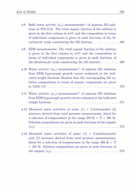
List of Tables 195
4.8 Bulk water activity (aw) measurements a of aqueous M5 solu-
tions at 279.15 K. The total organic fraction of the solution is
given in the first column in wt% and the composition in terms
of individual components is given in mole fractions of the di-
carboxylic acids constituting the M5 mixture. . . . . . . . . . . 168
4.9 EDB measurements: The total organic fraction of the solution
is given in the first column in wt% and the composition in
terms of individual components is given in mole fractions of
the dicarboxylic acids constituting the M5 mixture. . . . . . . . 169
4.10 Water activity (aw) measurements a of aqueous M5 solutions
from EDB hygroscopic growth curves evaluated at the indi-
cated weight fractions Mention that the corresponding M5 so-
lution compositions in terms of organic components are given
in Table 4.9. . . . . . . . . . . . . . . . . . . . . . . . . . . . . 170
4.11 Water activity (aw) measurements a of aqueous M5 solutions
from EDB hygroscopic growth curves evaluated at the indicated
weight fractions. . . . . . . . . . . . . . . . . . . . . . . . . . . 171
4.12 Measured water activities of water (1) + 1,4-butanediol (2)
mixtures derived from total pressure measurements, listed for
a selection of temperatures in the range 270 K < T < 291 K.
Solution compositions are given in mole fractions of the organic
(x2). . . . . . . . . . . . . . . . . . . . . . . . . . . . . . . . . 172
4.13 Measured water activities of water (1) + 2-methoxyacetic
acid (2) mixtures derived from total pressure measurements,
listed for a selection of temperatures in the range 268 K < T
< 291 K. Solution compositions are given in mole fractions of
the organic (x2). . . . . . . . . . . . . . . . . . . . . . . . . . . 173

196 List of Tables
4.14 Measured water activities of water (1) + 2-(2-ethoxyethoxy)ethanol (2)
mixtures derived from total pressure measurements, listed for
a selection of temperatures in the range 265 K < T < 291 K.
Solution compositions are given in mole fractions of the organic
(x2). . . . . . . . . . . . . . . . . . . . . . . . . . . . . . . . . 174
4.15 Mixture compositions at different overall organic mass fractions
(wt%) of the aqueous M5 system used for total pressure mea-
surements. Component mole fractions (x) of the dicarboxylic
acids constituting the M5 mixture are given, with water ac-
counting for the remaining fraction. . . . . . . . . . . . . . . . 175
4.16 Measured water activities of water (1) + M5 (2) mixtures de-
rived from total pressure measurements, listed for a selection
of temperatures in the range 265 K < T < 291 K. The total
organic fraction of the solution is given in the first column in
(wt%). . . . . . . . . . . . . . . . . . . . . . . . . . . . . . . . 176
Bibliography
Abbas, R. and Gmehling, J.: Vapour–liquid equilibria, azeotropic data, excess
enthalpies, activity coefficients at infinite dilution and solid–liquid equilib-
ria for binary alcohol–ketone systems, Fluid Phase Equilib., 267, 119–126,
2008.
Ablett, S., Izzard, M., and Lillford, P.: Differential scanning calorimetric
study of frozen sucrose and glycerol solutions, J. Chem. Soc., Faraday
Trans., 88, 789–794, doi:10.1039/FT9928800789, 1992.
Abrams, D. S. and Prausnitz, J. M.: Statistical thermodynamics of liquid mix-
tures: a new expression for the excess Gibbs energy of partly or completely
miscible systems, AIChE Journal, 21, 116–128, 1975.
Ahlers, J.: Measurement, modeling and evaluation of solid-liquid phase equi-
libria, 1998.
Al-Muhtaseb, S. and Fahim, M.: Phase equilibria of the ternary system wa-
ter/acetic acid/2-pentanol, Fluid Phase Equilib., 123, 189–203, 1996.
Al-Rub, F., Abdel-Jabbar, N., Darwish, N., and Ghanem, H.: Vapor–liquid
equilibrium data for the 2-methoxy-2-methylpropane (MTBE)–ethanol,
MTBE–ethanol–calcium chloride, and MTBE–ethanol–copper chloride,
Sep. Sci. Technol., 37, 1911–1926, doi:10.1081/SS-120003051, 2002.
Albrecht, B.: Aerosols, cloud microphysics, and fractional cloudiness., Science
(New York, NY), 245, 1227, 1989.
Alexander, D.: The solubility of benzene in water, J. Phys. Chem, 63, 1021–
1022, doi:10.1021/j150576a608, 1959.
197
198 Bibliography
Alvarez, V., Mattedi, S., Iglesias, M., Gonzalez-Olmos, R., and Resa, J.:
Phase equilibria of binary mixtures containing methyl acetate, water,
methanol or ethanol at 101.3 kPa, Phys. Chem. Liq., 49, 52–71, 2011.
Alvarez Gonzalez, J., Macedo, E., Soares, M., and Medina, A.: Liquid-liquid
equilibria for ternary systems of water-phenol and solvents: data and rep-
resentation with models, Fluid phase equilib., 26, 289–302, 1986.
Amer, H., Paxton, R., and Winkle, M.: Methanol-Ethanol-Acetone, Ind. Eng.
Chem., 48, 142–146, doi:10.1021/ie50553a041, 1956.
Ansari, A. S. and Pandis, S.: Prediction of multicomponent inorganic atmo-
spheric aerosol behavior, Atmospheric Environment, 33, 745–757, 1999.
Anttila, T., Kiendler-Scharr, A., Tillmann, R., and Mentel, T.: On the reac-
tive uptake of gaseous compounds by organic-coated aqueous aerosols: The-
oretical analysis and application to the heterogeneous hydrolysis of N2O5,
J. Phys. Chem. A, 110, 10 435–10 443, doi:10.1021/jp062403c, 2006.
Anttila, T., Kiendler-Scharr, A., Mentel, T., and Tillmann, R.: Size depen-
dent partitioning of organic material: evidence for the formation of or-
ganic coatings on aqueous aerosols, J. Atmos. Chem., 57, 215–237, doi:
10.1007/s10874-007-9067-9, 2007.
Apelblat, A. and Manzurola, E.: Solubility of oxalic, malonic, succinic, adipic,
maleic, malic, citric, and tartaric acids in water from 278.15 to 338.15 K,
J. Chem. Thermodyn., 19, 317–320, 1987.
Apelblat, A. and Manzurola, E.: Solubility of ascorbic, 2-furancarboxylic,
glutaric, pimelic, salicylic, and o-phthalic acids in water from 279.15 to
342.15 K, and apparent molar volumes of ascorbic, glutaric, and pimelic
acids in water at 298.15 K, J. Chem. Thermodyn., 21, 1005–1008, 1989.
Arce, A., Blanco, A., Souza, P., and Vidal, I.: Liquid-liquid equilibria of the
ternary mixtures water+ propanoic acid+ methyl ethyl ketone and water+
propanoic acid+ methyl propyl ketone, J. Chem. Eng. Data, 40, 225–229,
doi:10.1021/je00017a047, 1995.

Bibliography 199
Arich, G. and Tagliavini, G.: Isotherme di equilibrio liquido-vapore nel sis-
tema acqua-acido acetico., La Ricerca scientifica, 28, 2493–2500, 1958.
Backes, H., Jing Jun, M., et al.: Interfacial tensions in binary and ternary
liquid-liquid systems, Chem. Eng. Sci., 45, 275–286, 1990.
Bailey, A., Harris, J., and Skau, E.: Solubilities of some normal saturated
and unsaturated long-chain fatty acid methyl esters in acetone, n-Hexane,
Toluene, and 1, 2-Dichloroethane, J. Chem. Eng. Data, 15, 583–585, doi:
10.1021/je60047a027, 1970.
Baker, M. and Peter, T.: Small-scale cloud processes and climate, Nature,
451, 299–300, doi:10.1038/nature06594, 2008.
Baustian, K., Wise, M., Jensen, E., Schill, G., Freedman, M., and Tolbert,
M.: State transformations and ice nucleation in glassy or (semi-) solid amor-
phous organic aerosol, Atmos. Chem. Phys. Discuss, 12, 27 333–27 366, doi:
10.5194/acpd-12-27333-2012, 2012.
Baynard, T., Garland, R., Ravishankara, A., Tolbert, M., and Lovejoy, E.:
Key factors influencing the relative humidity dependence of aerosol light
scattering, Geophys. Res. Lett., 33, L06 813, doi:10.1029/2005GL024898,
2006.
Bertram, A., Martin, S., Hanna, S., Smith, M., Bodsworth, A., Chen, Q.,
Kuwata, M., Liu, A., You, Y., and Zorn, S.: Predicting the relative hu-
midities of liquid-liquid phase separation, efflorescence, and deliquescence
of mixed particles of ammonium sulfate, organic material, and water using
the organic-to-sulfate mass ratio of the particle and the oxygen-to-carbon
elemental ratio of the organic component, Atmos. Chem. Phys, 11, 10 995–
11 006, doi:10.5194/acp-11-10995-2011, 2011.
Beyer, K., Friesen, K., Bothe, J., and Palet, B.: Phase Diagrams and Water
Activities of Aqueous Dicarboxylic Acid Systems of Atmospheric Impor-
tance, J. Phys. Chem. A, 112, 11 704–11 713, doi:10.1021/jp805985t, 2008.
Blando, J., Porcja, R., Li, T., Bowman, D., Lioy, P., and Turpin, B.: Sec-
ondary formation and the Smoky Mountain organic aerosol: An examina-

200 Bibliography
tion of aerosol polarity and functional group composition during SEAVS,
Environ. Sci. Technol, 32, 604–613, doi:10.1021/es970405s, 1998.
Blond, G., Simatos, D., Catte, M., Dussap, C., and Gros, J.: Modeling of
the water-sucrose state diagram below 0 C, Carbohydrate research, 298,
139–145, 1997.
Boese, A. B., Fink, C., Goodman, H., Hillenbrand, E., Holden, R., Jones, W.,
Livrngood, S., Rector, P.R.and Schultze, H., Smyth, H., Tamplin, W., and
Toussaint, W.: Glycols. Chapters 1 - 16, vol. 114, 1953.
Bomshtein, A.L.and Trofimov, A., Kudakina, E., and Serafimov, L.: Vapor-
liquid phase equilibrium in binary systems formed by water, carboxylic
acids C2 - C4 and esters, Deposited Doc. Oniitekhim, pp. 1–12, 1983.
Bones, D., Reid, J., Lienhard, D., and Krieger, U.: Comparing the mechanism
of water condensation and evaporation in glassy aerosol, Proc. Natl. Acad.
Sci. U.S.A., 109, 11 613–11 618, 2012.
Bonner, O. and Breazeale, W.: Osmotic and Activity Coefficients of Some
Nonelectrolytes., Journal of Chemical and Engineering Data, 10, 325–327,
doi:10.1021/je60027a007, 1965.
Borisova, I., Erlykina, M., Vatskova, V., Sokolov, N., and Mikhailov, V.:
Vapor-liquid equilibrium in the diethyl ether - water system at atmospheric
pressure, Deposited Doc. Oniitekhim, pp. 1–9, 1983.
Bower, V. and Robinson, R.: Isopiestic Vapor Pressure Measurements Of The
Ternary System: Sorbitol-Sodium Chloride-Water At 25 J. Phys. Chem, 67,
1540–1541, doi:10.1021/j100801a033, 1963.
Braban, C., Carroll, M., Sarah, A., and Abbatt, J.: Phase transitions of
malonic and oxalic acid aerosols, J. Phys. Chem. A, 107, 6594–6602, doi:
10.1021/jp034483f, 2003.
Brasseur, G., Orlando, J., and Tyndall, G.: Atmospheric chemistry and global
change, Oxford University Press New York, 1999.
Bibliography 201
Brooks, S., Wise, M., Cushing, M., and Tolbert, M.: Deliquescence behavior
of organic/ammonium sulfate aerosol, Geophys. Res. Lett., 29, 1917, doi:
10.1029/2002GL014733, 2002.
Brown, I. and Smith, F.: Liquid-Vapor equilibria VIII.The systems ace-
tone+benzene and Acetone+carbon tetrachloride at 45C, Aust. J. Chem.,
10, 423–428, 1957.
Brown, T., LeMay, H., Bursten, B., Murpy, C., and Woodward, P.: Chem-
istry: The central science, Pearson Education, 2009.
Cabezas, J., Arranz, J., and Berrueta, J.: Binary Vapor-liquid equilibrium of
benzene-alcohol systems., Rev.Roum.Chim, 30, 903–908, 1985.
Calvar, N., Dominguez, A., and Tojo, J.: Vapor–liquid equilibria for the
quaternary reactive system ethyl acetate+ ethanol+ water+ acetic acid and
some of the constituent binary systems at 101.3 kPa, Fluid phase equilib.,
235, 215–222, 2005.
Campbell, A., Kartzmark, E., and Gieskes, J.: Vapor-liquid equilibria, den-
sities, and refractivities in the system acetic acid-chloroform-water at 25,
Can. J. Chem., 41, 407–429, 1963.
Campbell, S., Wilsak, R., and Thodos, G.: Vapor-liquid equilibrium mea-
surements for the ethanol-acetone system at 372.7, 397.7, and 422.6 K, J.
Chem. Eng. Data, 32, 357–362, doi:10.1021/je00049a021, 1987.
Cappa, C. D. and Wilson, K. R.: Evolution of organic aerosol mass
spectra upon heating: implications for OA phase and partitioning
behavior, Atmospheric Chemistry and Physics, 11, 1895–1911, doi:
10.5194/acp-11-1895-2011, URL http://www.atmos-chem-phys.net/11/
1895/2011/, 2011.
Carr, A. and Kropholler, H.: Vapor Liquid Equilibria at Atmospheric Pres-
sure. Binary Systems of Ethyl Acetate-Benzene, Ethyl Acetate-Toluene,
and Ethyl Acetate-p-Xylene, J. Chem. Eng. Data, 7, 26–28, doi:10.1021/
je60012a007, 1962.

202 Bibliography
Carrico, C., Kus, P., Rood, M., Quinn, P., and Bates, T.: Mixtures of pol-
lution, dust, sea salt, and volcanic aerosol during ACE-Asia: Radiative
properties as a function of relative humidity, J. Geophys. Res., 108, 8650,
doi:10.1029/2003JD003405, 2003.
Carta, R. and Dernini, S.: Solubility of solid acetic acid in liquid organic
solvents, J. Chem. Eng. Data, 28, 328–330, doi:10.1021/je00033a013, 1983.
Carta, R., Dernini, S., and De Santis, R.: Activity coefficients from solid-
liquid and vapor-liquid equilibriums of some associated solutions, J. Chem.
Eng. Data, 24, 100–103, doi:10.1021/je60081a025, 1979.
Carvoli, G. and Delogu, P.: Phase equilibria of the quaternary system acetic
acid-ethylene glycol monoethyl ether acetate-ethylene glycol monoethyl
ether-water, Fluid phase equilibria, 25, 91–105, 1986.
Chan, M., Choi, M., Ng, N., and Chan, C.: Hygroscopicity of water-soluble
organic compounds in atmospheric aerosols: Amino acids and biomass
burning derived organic species, Environ. Sci. Technol., 39, 1555–1562, doi:
10.1021/es049584l, 2005.
Chandak, B., Nageshwar, G., and Mene, P.: Excess enthalpy, volume, and
Gibbs free energy and viscosity of ethyl acetate-methyl cellosolve mixtures,
J. Chem. Eng. Data, 22, 137–141, doi:10.1021/je60073a022, 1977.
Chang, E. and Pankow, J.: Prediction of activity coefficients in liquid aerosol
particles containing organic compounds, dissolved inorganic salts, and water
– Part 2: Consideration of phase separation effects by an X-UNIFAC model,
Atmospheric Environment, 40, 6422–6436, 2006.
Chapoy, A., Anderson, R., Haghighi, H., Edwards, T., and Tohidi, B.: Can
n-Propanol Form Hydrate?, Ind.Eng.Chem.Res., 47, 1689–1694, 2008.
Chesnokov, V.: Uber die Stabilitat der Komplexe von Dimethylsulfoxyd
mit Essigsaure in Anwesenheit von Carbamid, Acetamid und Aceton,
Zh.Obshch.Khim., 39, 1437–1442, 1969.

Bibliography 203
Chiavone-Filho, O., Proust, P., and Rasmussen, P.: Vapor-liquid equilibria
for glycol ether+ water systems, J. Chem. Eng. Data, 38, 128–131, doi:
10.1021/je00009a031, 1993.
Chin, M., Diehl, T., Ginoux, P., and Malm, W.: Intercontinental transport
of pollution and dust aerosols: implications for regional air quality, Atmo-
spheric Chemistry and Physics, 7, 5501–5517, doi:10.5194/acp-7-5501-2007,
2007.
Cho, T., Ochi, K., and Kojima, K.: Measurement of vapor-liquid equilibrium
for systems with limited miscibility, Fluid Phase Equilib., 11, 137–152, 1983.
Choi, J., Park, D., and Rhim, J.: Prediction of ternary Liquid-liquid equilibria
using the NRTL and the UNIQUAC Models, Korean J. Chem. Eng., 3, 141–
151, 1986.
Choi, M. and Chan, C.: The effects of organic species on the hygroscopic
behaviors of inorganic aerosols, Environ. Sci. Technol., 36, 2422–2428, doi:
10.1021/es0113293, 2002.
Chylinski, K., Fras, Z., and Malanowski, S.: Vapor-Liquid Equilibrium in
Phenol+ 2-Ethoxyethanol at 363.15 to 383.15 K, J. Chem. Eng. Data, 46,
29–33, doi:10.1021/je0001072, 2001.
Ciobanu, V., Marcolli, C., Krieger, U., Weers, U., and Peter, T.: Liquid-
Liquid Phase Separation in Mixed Organic/Inorganic Aerosol Particles, J.
Phys. Chem. A., 113, 10 966–10 978, doi:10.1021/jp905054d, 2009.
Clarke, E. C. W. and Glew, D. N.: Evaluation of thermodynamic functions
from equilibrium constants, Trans. Faraday Soc., 62, 539–547, 1966.
Clegg, S. L., Brimblecombe, P., and Wexler, A. S.: Thermodynamic model
of the system H+–NH+4 –SO2−
4 –NO−3 –H2O at tropospheric temperatures, J.
Phys. Chem. A, 102, 2137–2154, 1998.
Clendenning, K.: Production and properties of 2,3-butanediol. XI. Evaluation
of levo-2,3-butanediol as a non-volatile antifreeze compound, Can. J. Res.
Sect., 24, 249–271, 1946.
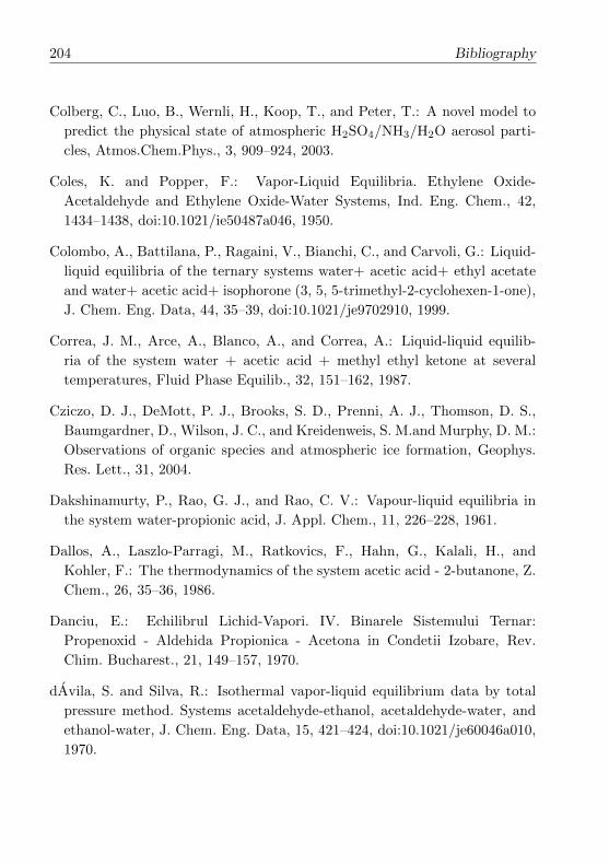
204 Bibliography
Colberg, C., Luo, B., Wernli, H., Koop, T., and Peter, T.: A novel model to
predict the physical state of atmospheric H2SO4/NH3/H2O aerosol parti-
cles, Atmos.Chem.Phys., 3, 909–924, 2003.
Coles, K. and Popper, F.: Vapor-Liquid Equilibria. Ethylene Oxide-
Acetaldehyde and Ethylene Oxide-Water Systems, Ind. Eng. Chem., 42,
1434–1438, doi:10.1021/ie50487a046, 1950.
Colombo, A., Battilana, P., Ragaini, V., Bianchi, C., and Carvoli, G.: Liquid-
liquid equilibria of the ternary systems water+ acetic acid+ ethyl acetate
and water+ acetic acid+ isophorone (3, 5, 5-trimethyl-2-cyclohexen-1-one),
J. Chem. Eng. Data, 44, 35–39, doi:10.1021/je9702910, 1999.
Correa, J. M., Arce, A., Blanco, A., and Correa, A.: Liquid-liquid equilib-
ria of the system water + acetic acid + methyl ethyl ketone at several
temperatures, Fluid Phase Equilib., 32, 151–162, 1987.
Cziczo, D. J., DeMott, P. J., Brooks, S. D., Prenni, A. J., Thomson, D. S.,
Baumgardner, D., Wilson, J. C., and Kreidenweis, S. M.and Murphy, D. M.:
Observations of organic species and atmospheric ice formation, Geophys.
Res. Lett., 31, 2004.
Dakshinamurty, P., Rao, G. J., and Rao, C. V.: Vapour-liquid equilibria in
the system water-propionic acid, J. Appl. Chem., 11, 226–228, 1961.
Dallos, A., Laszlo-Parragi, M., Ratkovics, F., Hahn, G., Kalali, H., and
Kohler, F.: The thermodynamics of the system acetic acid - 2-butanone, Z.
Chem., 26, 35–36, 1986.
Danciu, E.: Echilibrul Lichid-Vapori. IV. Binarele Sistemului Ternar:
Propenoxid - Aldehida Propionica - Acetona in Condetii Izobare, Rev.
Chim. Bucharest., 21, 149–157, 1970.
dAvila, S. and Silva, R.: Isothermal vapor-liquid equilibrium data by total
pressure method. Systems acetaldehyde-ethanol, acetaldehyde-water, and
ethanol-water, J. Chem. Eng. Data, 15, 421–424, doi:10.1021/je60046a010,
1970.

Bibliography 205
de Leeuw, H.: About the System Acetaldehyde - Ethanol, Z. Phys. Chem.
Stoechiom. Verwandtschaftsl, 77, 284–314, 1911.
De Oliveira, L. and Aznar, M.: (Liquid+ liquid) equilibrium of water+ phe-
nol+ (1-butanol, or 2-butanol, or tert-butanol) systems, J. Chem. Ther-
modyn., 42, 1379–1385, 2010.
Dean, J. A. e. a.: Langes Handbook of Chemistry, McGraw-Hill, 15 edn.,
1999.
Debenedetti, P. and Stillinger, F.: Supercooled liquids and the glass transi-
tion, Nature, 410, 259–267, 2001.
DeMott, P. J., Cziczo, D. J., Prenni, A. J., Murphy, D. M., Kreidenweis,
S. M., Thomson, D. S., Borys, R., and Rogers, D. C.: Measurements of the
concentration and composition of nuclei for cirrus formation, PNAS, 100,
14 655–14 660, 2003.
Diedrichs, A. and Gmehling, J.: Solubility calculation of active pharmaceu-
tical ingredients in alkanes, alcohols, water and their mixtures using vari-
ous activity coefficient models, Ind. Eng. Chem. Res, 50, 1757–1769, doi:
10.1021/ie101373k, 2010.
Domalski, E. S. and Hearing, E. D.: Heat capacities and entropies of organic
compounds in the condensed phase. Volume III, Journal of Physical and
Chemical Reference Data, 25, 1, 1996.
Domanska, U., Morawski, P., and Piekarska, M.: Solid-Liquid Phase Equilib-
ria of 1-Decanol and 1-Dodecanol with Fragrance Raw Materials Based on
Cyclohexane, J. Chem. Eng. Data, 54, 1271–1276, 2009.
Donahue, N., Robinson, A., Stanier, C., and Pandis, S.: Coupled partitioning,
dilution, and chemical aging of semivolatile organics, Environ. Sci. Technol.,
40, 2635–2643, doi:10.1021/es052297c, 2006.
Dormidontova, E. E.: Role of competitive PEO-water and water-water hy-
drogen bonding in aqueous solution PEO behavior, Macromolecules, 35,
987–1001, 2002.

206 Bibliography
Dormidontova, E. E.: Influence of end groups on phase behavior and proper-
ties of PEO in aqueous solutions, Macromolecules, 37, 7747–7761, 2004.
Dykyj, J., V., K., and Seprakova, M.: Physical Properties of Ethylene Glycol
and its Derivatives. I. Solidification Points of Solutions of Ethylene Glycols,
Chem.Zvesti, 10, 193–203, 1956.
Dykyj, J., Svoboda, J., Wilhoit, R. C., Frenkel, M., and Hall, K. R.: Or-
ganic Compounds, C1 to C57. Part 1., in: Landolt-Bornstein - Group
IV Physical Chemistry Numerical Data and Functional Relationships in
Science and Technology, edited by Hall, K. R., vol. 20B: Vapor Pres-
sure and Antoine Constants for Oxygen Containing Organic Compounds,
pp. 14–110, SpringerMaterials - The Landolt-Bornstein Database, doi:
10.1007/10688583 3, URL http://www.springermaterials.com, 2000.
Erdakos, G. and Pankow, J.: Gas/particle partitioning of neutral and ionizing
compounds to single-and multi-phase aerosol particles. 2. Phase separation
in liquid particulate matter containing both polar and low-polarity organic
compounds, Atmospheric Environment, 38, 1005–1013, 2004.
Escobedo-Alvarado, G. and Sandler, S.: Vapor-liquid equilibrium of two aque-
ous systems that exhibit liquid-liquid phase separation, J. Chem. Eng. Data,
44, 319–322, doi:10.1021/je980228q, 1999.
Esquıvel, M. and Bernardo-Gil, M.: Liquid-liquid equilibria for the systems
water-alcohols-acetic acid, Fluid Phase Equilib., 57, 307–316, 1990.
Fandary, M., Aljimaz, A., Al-Kandary, J., and Fahim, M.: Liquid-liquid equi-
libria for the system water+ ethanol+ ethyl tert-butyl ether, J. Chem. Eng.
Data, 44, 1129–1131, doi:10.1021/je980253w, 1999.
Fang, W., Liu, G., Wang, L., Zhang, X., Mi, Z., Zhang, S., and Yin, Y.:
Liquid–Liquid Equilibria for the Ternary System Water+ Methyl Isobutyl
Ketone+ tert-Butyl Alcohol at Several Temperatures, J. Chem. Eng. Data,
53, 466–470, doi:10.1021/je700554u, 2008.
Farina, S., Adams, P., and Pandis, S.: Modeling global secondary organic
aerosol formation and processing with the volatility basis set: Implica-
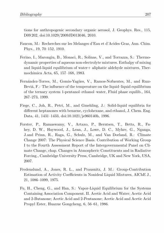
Bibliography 207
tions for anthropogenic secondary organic aerosol, J. Geophys. Res., 115,
D09 202, doi:10.1029/2009JD013046, 2010.
Faucon, M.: Recherches sur les Melanges d’Eau et d’Acides Gras, Ann. Chim.
Phys., 19, 70–152, 1910.
Ferino, I., Marongiu, B., Monaci, R., Solinas, V., and Torrazza, S.: Thermo-
dynamic properties of aqueous non-electrolyte mixtures. Enthalpy of mixing
and liquid-liquid equilibrium of water+ aliphatic aldehyde mixtures, Ther-
mochimica Acta, 65, 157–168, 1983.
Fernandez-Torres, M., Gomis-Yagues, V., Ramos-Nofuentes, M., and Ruız-
Bevia, F.: The influence of the temperature on the liquid–liquid equilibrium
of the ternary system 1-pentanol–ethanol–water, Fluid phase equilib., 164,
267–273, 1999.
Fiege, C., Joh, R., Petri, M., and Gmehling, J.: Solid-liquid equilibria for
different heptanones with benzene, cyclohexane, and ethanol, J. Chem. Eng.
Data, 41, 1431–1433, doi:10.1021/je960140h, 1996.
Forster, P., Ramaswamy, V., Artaxo, P., Berntsen, T., Betts, R., Fa-
hey, D. W., Haywood, J., Lean, J., Lowe, D. C., Myhre, G., Nganga,
J.and Prinn, R., Raga, G., Schulz, M., and Van Dorland, R.: Climate
Change 2007: The Physical Science Basis. Contribution of Working Group
I to the Fourth Assessment Report of the Intergovernmental Panel on Cli-
mate Change, chap. Changes in Atmospheric Constituents and in Radiative
Forcing., Cambridge University Press, Cambridge, UK and New York, USA,
2007.
Fredenslund, A., Jones, R. L., and Prausnitz, J. M.: Group-Contribution
Estimation of Activity Coefficients in Nonideal Liquid Mixtures, AIChE J.,
21, 1086–1099, 1975.
Fu, H., Cheng, G., and Han, S.: Vapor-Liquid Equilibrium for the Systems
Containing Association Component. II. Acetic Acid and Water; Acetic Acid
and 2-Butanone; Acetic Acid and 2-Pentanone; Acetic Acid and Acetic Acid
Propyl Ester, Huaxue Gongcheng, 6, 56–61, 1986.
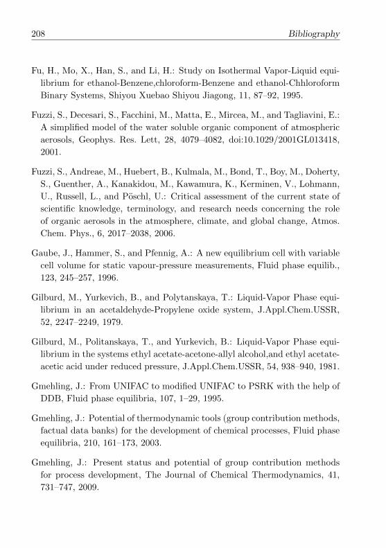
208 Bibliography
Fu, H., Mo, X., Han, S., and Li, H.: Study on Isothermal Vapor-Liquid equi-
librium for ethanol-Benzene,chloroform-Benzene and ethanol-Chhloroform
Binary Systems, Shiyou Xuebao Shiyou Jiagong, 11, 87–92, 1995.
Fuzzi, S., Decesari, S., Facchini, M., Matta, E., Mircea, M., and Tagliavini, E.:
A simplified model of the water soluble organic component of atmospheric
aerosols, Geophys. Res. Lett, 28, 4079–4082, doi:10.1029/2001GL013418,
2001.
Fuzzi, S., Andreae, M., Huebert, B., Kulmala, M., Bond, T., Boy, M., Doherty,
S., Guenther, A., Kanakidou, M., Kawamura, K., Kerminen, V., Lohmann,
U., Russell, L., and Poschl, U.: Critical assessment of the current state of
scientific knowledge, terminology, and research needs concerning the role
of organic aerosols in the atmosphere, climate, and global change, Atmos.
Chem. Phys., 6, 2017–2038, 2006.
Gaube, J., Hammer, S., and Pfennig, A.: A new equilibrium cell with variable
cell volume for static vapour-pressure measurements, Fluid phase equilib.,
123, 245–257, 1996.
Gilburd, M., Yurkevich, B., and Polytanskaya, T.: Liquid-Vapor Phase equi-
librium in an acetaldehyde-Propylene oxide system, J.Appl.Chem.USSR,
52, 2247–2249, 1979.
Gilburd, M., Politanskaya, T., and Yurkevich, B.: Liquid-Vapor Phase equi-
librium in the systems ethyl acetate-acetone-allyl alcohol,and ethyl acetate-
acetic acid under reduced pressure, J.Appl.Chem.USSR, 54, 938–940, 1981.
Gmehling, J.: From UNIFAC to modified UNIFAC to PSRK with the help of
DDB, Fluid phase equilibria, 107, 1–29, 1995.
Gmehling, J.: Potential of thermodynamic tools (group contribution methods,
factual data banks) for the development of chemical processes, Fluid phase
equilibria, 210, 161–173, 2003.
Gmehling, J.: Present status and potential of group contribution methods
for process development, The Journal of Chemical Thermodynamics, 41,
731–747, 2009.

Bibliography 209
Gmehling, J. and Onken, U.: Vapor-Liquid Equilibrium Data Collec-
tion: Volume I, Part 1-Aqueous-Organic Systems, Chemistry Data Series,
DECHEMA, 1977.
Gmehling, J. and Onken, U.: Vapor-Liquid Equilibrium Data Collection: Vol-
ume I, Part 1c(in conjunction with part 1d)-Aqueous Systems (Supplement
3), Chemistry Data Series, DECHEMA, 2003a.
Gmehling, J. and Onken, U.: Vapor-Liquid Equilibrium Data Collection: Vol-
ume I, Part 1d(in conjunction with part 1c)-Aqueous Systems (Supplement
4), Chemistry Data Series, DECHEMA, 2003b.
Gmehling, J., Onken, U., and Arlt, W.: Vapor-Liquid Equilibrium Data
Collection: Volume I, Part 1a-Aqueous-Organic Systems(Supplement 1),
Chemistry Data Series, DECHEMA, 1981.
Gmehling, J., Onken, U., and Rarey-Nies, J. R.: Vapor-Liquid Equilibrium
Data Collection: Volume I, Part 1b-Aqueous Systems (Supplement 2),
Chemistry Data Series, DECHEMA, 1988.
Gmehling, J., Li, J., and Schiller, M.: A modified UNIFAC model. 2. Present
parameter matrix and results for different thermodynamic properties, Ind.
Eng. Chem. Res., 32, 178–193, doi:10.1021/ie00013a024, 1993.
Gmehling, J., Lohmann, J., Jakob, A., Li, J., and Joh, R.: A modified UNI-
FAC (Dortmund) model. 3. Revision and extension, Ind. Eng. Chem. Res.,
37, 4876–4882, doi:10.1021/ie980347z, 1998.
Gmehling, J., Wittig, R., Lohmann, J., and Joh, R.: A modified UNIFAC
(Dortmund) model. 4. Revision and extension, Ind. Eng. Chem. Res., 41,
1678–1688, doi:10.1021/ie0108043, 2002.
Gmehling, J., Kolbe, B., Kleiber, M., and Rarey, J.: Chemical Thermody-
namics for Process Simulation, Wiley-VCH:Weinheim, 2012.
Goldstein, A. H. and Galbally, I. E.: Known and unexplored organic con-
stituents in the earth’s atmosphere, Environ. Sci.Technol., 41, 1514–1521,
doi:10.1021/es072476p, 2007.
210 Bibliography
Gomis-Yagues, V., Ruız-Bevia, F., Ramos-Nofuentes, M., and Fernandez-
Torres, M.: The influence of the temperature on the liquid–liquid equilib-
rium of the ternary system 1-butanol–1-propanol–water, Fluid phase equi-
lib., 149, 139–145, 1998.
Gonzalez, E.: Vapor-liquid equilibria at 101.32 kPa mixtures of butyl esters
and propan-2-ol., J. Chem. Eng. Jpn., 29, 294–299, 1996.
Griswold, J. and Wong, S.: Phase-equilibria of the actone-methanol-water
system from 100- into the critical region, Chem.eng.symp.ser., 48, 18–34,
1952.
Hallquist, M., Wenger, J., Baltensperger, U., Rudich, Y., Simpson, D., Claeys,
M., Dommen, J., Donahue, N., George, C., Goldstein, A., Hamilton, J. F.,
Herrmann, H., Hoffmann, T., Iinuma, Y., Jang, M., Jenkin, M. E., Jimenez,
J. L., Kiendler-Scharr, A., Maenhaut, W., McFiggans, G., Mentel, T. F.,
Monod, A., Prevot, A. S. H., Seinfeld, J. H., Surratt, J. D., Szmigielski, R.,
and Wildt, J.: The formation, properties and impact of secondary organic
aerosol: current and emerging issues, Atmos. Chem. Phys., 9, 5155–5236,
2009.
Hansen, H. K., Rasmussen, P., Fredenslund, A., Schiller, M., and Gmehling,
J.: Vapor–liquid-equilibria by UNIFAC group contribution. 5. Revision and
extension, Ind. Eng. Chem. Res., 30, 2352–2355, 1991.
Hansen, J., Sato, M., and Ruedy, R.: Radiative forcing and climate response,
J. Geophys. Res., 102, 6831–6864, 1997.
Haughton, C.: V-I equilbria of benzene and acetic acid, Br.Chem.Eng., 12,
1102–1103, 1967.
Hill, A.: The mutual solubility of liquids. I. The mutual solubility of ethyl
ether and water. II. The solubility of water in benzene, J. Am. Chem. Soc.,
45, 1143–1155, doi:10.1021/ja01658a007, 1923.
Hirata, M. and Hoshino, D.: A Study on Vapor-Liquid Equilibria Based on
the Theory of Solution of Groups Model, Asahi Garasu Kogyo Gijutsu
Shoreikai Kenkyu Hokoku, 41, 115–122, 1982.

Bibliography 211
Hirata, M., Ohe, S., and Nagahama, K.: Computer aided data book of vapor-
liquid equilibria, Elsevier Science & Technology, 1975.
Ito, T. and Yoshida, F.: Vapor-Liquid Equilibria of Water-Lower Fatty Acid
Systems: Water-Formic Acid, Water Acetic Acid and Water-Propionic
Acid., J. Chem. Eng. Data, 8, 315–320, 1963.
Jacobson, M., Hansson, H., Noone, K., and Charlson, R.: Organic atmo-
spheric aerosols: Review and state of the science, Rev.Geophys., 38, 267–
294, doi:10.1029/1998RG000045, 2000.
Jakob, A.: unpublished data, Universitaet Oldenburg, 1994.
Jakob, A., Joh, R., Rose, C., and Gmehling, J.: Solid-liquid equilibria in
binary mixtures of organic compounds, Fluid Phase Equilib., 113, 117–126,
1995.
Jakob, A., Grensemann, H., Lohmann, J., and Gmehling, J.: Further devel-
opment of modified UNIFAC (Dortmund): Revision and extension 5, Ind.
Eng. Chem. Res., 45, 7924–7933, doi:10.1021/ie060355c, 2006.
Jaoui, M., Achard, C., and Rogalski, M.: Solubility as a function of tem-
perature of selected chlorophenols and nitrophenols in aqueous solutions
containing electrolytes or surfactants, J. Chem. Eng. Data, 47, 297–303,
doi:10.1021/je0102309, 2002.
Jathar, S., Farina, S., Robinson, A., and Adams, P.: The influence of semi-
volatile and reactive primary emissions on the abundance and properties
of global organic aerosol, Atmospheric Chemistry and Physics Discussions,
11, 5493–5540, doi:10.5194/acp-11-7727-2011, 2011.
Jimenez, J. L., Canagaratna, M.R.and Donahue, N. M., Prevot, A. S. H.,
Zhang, Q., Kroll, J. H., DeCarlo, P. F., Allan, J. D., Coe, H., Ng,
N. L., Aiken, A. C., Docherty, K., Ulbrich, I., Grieshop, A., Robinson,
A. L.and Duplissy, J., Smith, J. D., Wilson, K., Lanz, V. A. Hueglin, C.,
Sun, Y., Tian, J., Laaksonen, A., Raatikainen, T., Rautiainen, J., Vaatto-
vaara, P., Ehn, M., Kulmala, M., Tomlinson, J. M., Collins, D., Cubison,
M., Dunlea, E., Huffman, J., Onasch, T., Alfarra, M., Williams, P., Bower,

212 Bibliography
K., Kondo, Y., Schneider, J., Drewnick, F., Borrmann, S., Weimer, S.,
Demerjian, K., Salcedo, D., Cottrell, L., Griffin, R., Takami, A., Miyoshi,
T., Hatakeyama, S., Shimono, A., Sun, J. Y., Zhang, Y. M., Dzepina, K.,
Kimmel, J. R., Sueper, D., Jayne, J. T., Herndon, S. C., Trimborn, A. M.,
Williams, L. R., Wood, E., Middlebrook, A. M., Kolb, C., Baltensperger,
U., and Worsnop, D. R.: Evolution of organic aerosols in the atmosphere,
Science, 326, 1525–1529, doi:10.1126/science.1180353, 2009.
Johnson, D., Utembe, S., and Jenkin, M.: Simulating the detailed chemical
composition of secondary organic aerosol formed on a regional scale during
the TORCH 2003 campaign in the southern UK, Atmos. Chem. Phys., 6,
419–431, 2006.
Kalberer, M., Paulsen, D., Sax, M., Steinbacher, M., Dommen, J., Prevot,
A., Fisseha, R., Weingartner, E., Frankevich, V., Zenobi, R., and Bal-
tensperger, U.: Identification of polymers as major components of at-
mospheric organic aerosols, Science, 303, 1659–1662, doi:10.1126/science.
1092185, 2004.
Kanakidou, M., Seinfeld, J. H., Pandis, S. N., Barnes, I., Dentener, F. J.,
Facchini, M. C., Van Dingenen, R., Ervens, B., Nenes, A., Nielsen, C. J.,
Swietlicki, E., Putaud, J. P., Balkanski, Y., Fuzzi, S., Horth, J., Moort-
gat, G. K., Winterhalter, R., Myhre, C. E. L., Tsigaridis, K., Vignati,
E., Stephanou, E. G., and Wilson, J.: Organic aerosol and global climate
modelling: a review, Atmos. Chem. Phys., 5, 1053–1123, 2005.
Kanno, H., Miyata, K., Tomizawa, K., and Tanaka, H.: Additivity rule holds
in supercooling of aqueous solutions, J. Phys. Chem. A, 108, 6079–6082,
doi:10.1021/jp048676u, 2004.
Kanno, H., Soga, M., and Kajiwara, K.: Linear relation between
TH(homogeneous ice nucleation temperature) and Tm(melting tempera-
ture) for aqueous solutions of sucrose, trehalose, and maltose, Chem. Phys.
Lett., 443, 280–283, 2007.
Keyes, D.: Liquid-Vapor Composition Curves of Acetic Acid and Wa-
ter at Subatmospheric Pressures, Ind. Eng. Chem., 25, 569–569, doi:
10.1021/ie50281a026, 1933.

Bibliography 213
Kim, J. and Park, D.: Liquid-liquid equilibrium for the ternary systems of
solvents+ water+ propionic acid at 25 and atmospheric pressure, Korean
J. Chem. Eng., 22, 256–263, 2005.
Kjellander, R. and Florin, E.: Water structure and changes in thermal sta-
bility of the system poly (ethylene oxide)–water, J. Chem. Soc., Faraday
Trans. 1, 77, 2053–2077, 1981.
Kleinman, L. I., Springston, S. R., Daum, P. H., Lee, Y.-N., Nunnerma-
cker, L. J., Senum, G. I., Wang, J., Weinstein-Lloyd, J., Alexander,
M. L., Hubbe, J., Ortega, J., Canagaratna, M. R., and Jayne, J.: The
time evolution of aerosol composition over the Mexico City plateau, At-
mos. Chem. Phys, 8, 1559–1575, doi:10.5194/acp-8-1559-2008, URL http:
//www.atmos-chem-phys.net/8/1559/2008/, 2008.
Kliment, V., Fried, V., and Pick, J.: Gleichgewicht Flussigkeit-dampf
XXXIII.Systeme Butylacetat-Phenol und wasser-Phenol, Collect. Czech.
Chem. Commun., 29, 2008–2015, 1964.
Knight, W.: Thermodynamics of Aqueous Solutions of Alcohols and P-
dioxane, Princeton University, URL http://books.google.ch/books?id=
D3icPQAACAAJ, 1962.
Knopf, D. and Rigg, Y.: Homogeneous ice nucleation from aqueous inor-
ganic/organic particles representative of biomass burning: Water activity,
freezing temperatures, nucleation rates, J. Phys. Chem. A, 115, 762–773,
doi:10.1021/jp109171g, 2011.
Knopf, D., Luo, B., Krieger, U., and Koop, T.: Thermodynamic dissociation
constant of the bisulfate ion from Raman and ion interaction modeling
studies of aqueous sulfuric acid at low temperatures, J. Phys. Chem. A.,
107, 4322–4332, doi:10.1021/jp027775+, 2003.
Knopf, D., Anthony, L., and Bertram, A.: Reactive uptake of O3 by multi-
component and multiphase mixtures containing oleic acid, J. Phys. Chem.
A,, 109, 5579–5589, doi:10.1021/jp0512513, 2005.

214 Bibliography
Knopf, D. A. and Lopez, M. D.: Homogeneous ice freezing temperatures and
ice nucleation rates of aqueous ammonium sulfate and aqueous levoglucosan
particles for relevant atmospheric conditions, Phys. Chem. Chem. Phys., 11,
8056–8068, 2009.
Koga, Y., Tanaka, T., Atake, T., Westh, P., and Hvidt, A.: Mixing Schemes
and Liquid-Solid Phase Diagram in the Water-Rich Region of Aqueous 2-
Butoxyethanol., Bull. Chem. Soc. Jpn., 67, 2393–2397, 1994.
Kolb, D.: Solubilities of fatty acids in selected organic solvents at low tem-
peratures, Diss. Abstr., 20, 82–86, 1959.
Koop, T.: Homogeneous ice nucleation in water and aqueous solutions, Z.
Phys. Chem., 218, 1231–1258, doi:10.1524/zpch.218.11.1231.50812, 2004.
Koop, T. and Zobrist, B.: Parameterizations for ice nucleation in biological
and atmospheric systems, Phys. Chem. Chem. Phys., 11, 10 839–10 850,
2009.
Koop, T., Luo, B., Tsias, A., and Peter, T.: Water activity as the determinant
for homogeneous ice nucleation in aqueous solutions, Nature, 406, 611–614,
doi:10.1038/35020537, 2000.
Koop, T., Bookhold, J., Shiraiwa, M., and Poschl, U.: Glass transition and
phase state of organic compounds: dependency on molecular properties and
implications for secondary organic aerosols in the atmosphere, Phys. Chem.
Chem. Phys., 13, 19 238–19 255, doi:10.1039/C1CP22617G, 2011.
Krieger, U., Colberg, C., Weers, U., Koop, T., and Peter, T.: Supercool-
ing of single H2SO4/H2O aerosols to 158 K: No evidence for the oc-
currence of the octrahydrate, Geophys. Res. Lett, 27, 2097–2100, doi:
10.1029/2000GL011613, 2000.
Krieger, U. K., Marcolli, C., and Reid, J. P.: Exploring the complexity of
aerosol particle properties and processes using single particle techniques,
Chem. Soc. Rev., 41, 6631 – 6662, 2012.
Bibliography 215
Kurihara, K., Hori, H., and Kojima, K.: Vapor-liquid equilibrium data for
acetone + methanol + benzene, chloroform + methanol + benzene, and
constituent binary systems at 101.3 kPa, J. Chem. Eng. Data, 43, 264–268,
doi:10.1021/je970231u, 1998.
Lalande, A.: Equilibres entre Phases Condensees dans le systeme eau-alcool-
ether, J. Chim. Phys. Phys. Chim. Biol., 31, 583–609, 1934.
Larsen, B., Rasmussen, P., and Fredenslund, A.: A modified UNIFAC group-
contribution model for prediction of phase equilibria and heats of mixing,
Ind. Eng. Chem. Res., 26, 2274–2286, doi:10.1021/ie00071a018, 1987.
Lee, M. and Hu, C.: Isothermal vapor-liquid equilibria for mixtures of ethanol,
acetone, and diisopropyl ether, Fluid phase equilib., 109, 83–98, 1995.
Lerici, C., Piva, M., and ROSA, M.: Water activity and freezing point de-
pression of aqueous solutions and liquid foods, J. Food Sci., 48, 1667–1669,
2006.
Letcher, T., Redhi, G., Radloff, S., and Domanska, U.: Liquid-Liquid Equi-
libria for Mixtures of Butanal+ an Alkanol+ Water at 298.15 K, J. Chem.
Eng. Data, 41, 707–712, 1996.
Leu, A., Chen, C., and Robinson, D.: Vapor-Liquid Equilibrium in Selected
Binary Systems, AIChE Symp. Ser., 85, 11–16, 1989.
Lewis, G.: Outlines of a new system of thermodynamic chemistry, in: Pro-
ceedings of the American Academy of Arts and Sciences, pp. 259–293, JS-
TOR, 1907.
Lewis, G. and Randall, M.: Thermodynamics, Mc-Graw-Hill, New York, ed,
2, 236, 1961.
Lienhard, D., Bones, D., Zuend, A., Krieger, U., Reid, J., and Peter, T.:
Measurements of Thermodynamic and Optical Properties of Selected Aque-
ous Organic and Organic-Inorganic Mixtures of Atmospheric Relevance, J.
Phys. Chem. A, doi:10.1021/jp3055872, 2012.

216 Bibliography
Lihua, F., Peisheng, M., and Zhengle, X.: Measurement and correlation for
solubility of adipic acid in several solvents, Chin. J. Chem. Eng., 15, 110–
114, 2007.
Lin, C., Qing, A., and Feng, Q.: A new differential mutation base generator
for differential evolution, J. Glob. Optim, 49, 69–90, 2011.
Lin, G., Penner, J., Sillman, S., Taraborrelli, D., and Lelieveld, J.:
Global modeling of SOA formation from dicarbonyls, epoxides, organic
nitrates and peroxides, Atmos. Chem. Phys, 12, 4743–4774, doi:10.5194/
acp-12-4743-2012, 2012.
Lin, H., Tien, H., Hone, Y., and Lee, M.: Solubility of selected dibasic
carboxylic acids in water, in ionic liquid of [Bmim][BF4], and in aqueous
[Bmim][BF4] solutions, Fluid Phase Equilib., 253, 130–136, 2007.
Lintomen, L., Pinto, R., Batista, E., Meirelles, A., and Maciel, M.: Liquid-
liquid equilibrium of the water+ citric acid+ short chain alcohol+ tr-
icaprylin system at 298.15 K, J. Chem. Eng. Data, 46, 546–550, doi:
10.1021/je000226h, 2001.
Liousse, C., Penner, J., Chuang, C., Walton, J., Eddleman, H., and Cachier,
H.: A global three-dimensional model study of carbonaceous aerosols, J.
Geophys. Res., 101, 19 411–19, 1996.
Loehe, J. R., Van Ness, H. C., and Abbott, M. M.: Vapor/liquid/liquid equi-
librium. Total-pressure data and GE for water/methyl acetate at 50, J.
Chem. Eng. Data, 28, 405–407, doi:10.1021/je00034a017, 1983.
Lohmann, J., Joh, R., and Gmehling, J.: Solid-liquid equilibria of viscous
binary mixtures with alcohols, J. Chem. Eng. Data, 42, 1170–1175, doi:
10.1021/je9700683, 1997.
Lohmann, J., Joh, R., and Gmehling, J.: From UNIFAC to modified UNIFAC
(Dortmund), Ind. Eng. Chem. Res., 40, 957–964, doi:10.1021/ie0005710,
2001.

Bibliography 217
Maffia, M. and Meirelles, A.: Water activity and pH in aqueous polycarboxylic
acid systems, J. Chem. Eng. Data, 46, 582–587, doi:10.1021/je0002890,
2001.
Mafra, M. and Krahenbuhl, M.: Liquid-Liquid Equilibrium of (Water+ Ace-
tone) with Cumene or α-Methylstyrene or Phenol at Temperatures of
(323.15 and 333.15) K, J. Chem. Eng. Data, 51, 753–756, 2006.
Marcolli, C. and Krieger, U. K.: Phase changes during hygroscopic cycles of
mixed organic/inorganic model systems of tropospheric aerosols, J. Phys.
Chem. A, 110, 1881–1893, doi:10.1021/jp0556759, 2006.
Marcolli, C. and Peter, T.: Water activity in polyol/water systems: new
UNIFAC parameterization, Atmos. Chem. Phys., 5, 1545–1555, 2005.
Marcolli, C., Luo, B. P., Peter, T., and Wienhold, F. G.: Internal mixing
of the organic aerosol by gas phase diffusion of semivolatile organic com-
pounds, Atmos. Chem. Phys., 4, 2593–2599, doi:10.5194/acp-4-2593-2004,
URL http://www.atmos-chem-phys.net/4/2593/2004/, 2004.
Martin, M., Cocero, M., and Mato, R.: Vapor-Liquid Equilibrium Data at
298.15 K for Binary Systems Containing Methyl Acetate or Methanol with
2-Methoxyethanol or 2-Ethoxyethanol, J. Chem. Eng. Data, 39, 535–537,
doi:10.1021/je00015a030, 1994.
Martin, S., Rosenoern, T., Chen, Q., and Collins, D.: Phase changes of am-
bient particles in the Southern Great Plains of Oklahoma, Geophys. Res.
Lett., 35, L22 801, doi:10.1029/2008GL035650, 2008.
Martınez, N., Lladosa, E., Burguet, M., and Monton, J.: Isobaric vapour–
liquid equilibria for binary systems of 2-butanone with ethanol, 1-propanol,
and 2-propanol at 20 and 101.3 kPa, Fluid Phase Equilib., 270, 62–68, 2008.
May, W., Wasik, S., Miller, M., Tewari, Y., Brown-Thomas, J., and Gold-
berg, R.: Solution thermodynamics of some slightly soluble hydrocarbons
in water, J. Chem. Eng. Data, 28, 197–200, doi:10.1021/je00032a021, 1983.
Meehan, G. and Murphy, N.: A new correlation for binary systems with an
associating component, Chemical Engineering Science, 20, 757–769, 1965.

218 Bibliography
Mejıa, A., Segura, H., Cartes, M., Cifuentes, L., and Flores, M.: Phase equi-
libria and interfacial tensions in the systems methyl tert-butyl ether+ ace-
tone+ cyclohexane, methyl tert-butyl ether+ acetone and methyl tert-butyl
ether+ cyclohexane, Fluid Phase Equilib., 273, 68–77, 2008.
Mertl, I.: Liquid-Vapor Equilibrium.IL.Phase Equilibria in the ternary system
ethyl acetate-ethanol-water, Collect. Czech. Chem. Commun., 37, 366–374,
1972.
Miao, X., Zhang, H., Wang, T., and He, M.: Liquid-liquid equilibria of the
ternary system water+ acetic acid+ methyl tert-butyl ether, J. Chem. Eng.
Data, 52, 789–793, doi:10.1021/je060409p, 2007.
Mikhailov, E., Vlasenko, S., Martin, S., Koop, T., and Poschl, U.: Amorphous
and crystalline aerosol particles interacting with water vapor: conceptual
framework and experimental evidence for restructuring, phase transitions
and kinetic limitations, Atmos. Chem. Phys, 9, 9491–9522, 2009.
Ming, Y. and Russell, L.: Thermodynamic equilibrium of organic-electrolyte
mixtures in aerosol particles, AIChE journal, 48, 1331–1348, doi:10.1002/
aic.690480619, 2002.
Miyamoto, S., Nakamura, S., Iwai, Y., and Arai, Y.: Measurement of isother-
mal vapor-liquid equilibria for hydrocarbon+ monocarboxylic acid binary
systems by a flow-type apparatus, J. Chem. Eng. Data, 45, 857–861, doi:
10.1021/je000015c, 2000.
Miyamoto, S., Nakamura, S., Iwai, Y., and Arai, Y.: Measurement of isother-
mal vapor-liquid equilibria for binary and ternary systems containing mono-
carboxylic acid, J. Chem. Eng. Data, 46, 1225–1230, doi:10.1021/je0003849,
2001.
Miyata, K. and Kanno, H.: Supercooling behavior of aqueous solutions of
alcohols and saccharides, Journal of molecular liquids, 119, 189–193, 2005.
Moeller, W., Englund, S., Tsui, T. K., and Othmer, D.: Compositions of
Vapors from Boiling Solutions - Equilibria under Pressure of Systems:
Ethyl Ether-Ethyl Alcohol and Ethyl Ether-Water-Ethyl Alcohol, Ind. Eng.
Chem., 43, 711–717, doi:10.1021/ie50495a039, 1951.
Bibliography 219
Monton, J., Munoz, R., Burguet, M., and Torre, J.: Isobaric vapor–liquid
equilibria for the binary systems isobutyl alcohol+ isobutyl acetate and
tert-butyl alcohol+ tert-butyl acetate at 20 and 101.3 kPa, Fluid phase
equilib., 227, 19–25, 2005.
Mozzhukhin, A., Mitropolskaya, V., Serafimov, L., and Torubarov, A.:
Liquid-Vapor Phase Equilibrium in Binary Mixtures of Some Oxygen-
Containing Products at 760 mm Hg, Zh. Fiz. Khim., 41, 116–119, 1967.
Mun, S. and Lee, H.: Vapor-liquid equilibria of the water+ 1, 3-propanediol
and water+ 1, 3-propanediol+ lithium bromide systems, J. Chem. Eng.
Data, 44, 1231–1234, 1999.
Murphy, D. and Koop, T.: Review of the vapour pressures of ice and su-
percooled water for atmospheric applications, Q.J.R.Meteorol. Soc., 131,
1539–1565, doi:10.1256/qj.04.94, 2006.
Murphy, D., Cziczo, D., Froyd, K., Hudson, P., Matthew, B., Middlebrook,
A., Peltier, R., Sullivan, A., Thomson, D., and Weber, R.: Single-particle
mass spectrometry of tropospheric aerosol particles, J. Geophys. Res., 111,
D23S32, doi:10.1029/2006JD007340, 2006.
Murphy, D., Cziczo, D., Hudson, P., and Thomson, D.: Carbonaceous mate-
rial in aerosol particles in the lower stratosphere and tropopause region, J.
Geophys. Res., 112, D04 203, doi:10.1029/2006JD007297, 2007.
Narayana, A., Naik, S., and Rath, P.: Salt effect in isobaric vapor-liquid
equilibria of acetic acid-water system, J. Chem. Eng. Data, 30, 483–485,
doi:10.1021/je00042a035, 1985.
Naumann, D. and Wagner, H.: Vapour-liquid equilibria of several mixtures
containing 2-butanone, 2-butenal, ethoxyethanol, and toluene at 330.15 K,
J. Chem. Thermodyn., 18, 81–87, 1986.
Negadi, L., Wilken, M., and Gmehling, J.: Solid-liquid equilibria for binary
organic systems containing 1-methoxy-2-propanol and 2-butoxy ethanol, J.
Chem. Eng. Data, 51, 1873–1876, 2006.

220 Bibliography
Nelder, J. A. and Mead, R.: A simplex method for function minimization,
Comput. J, 7, 308–313, 1965.
Newman, M., Hayworth, C., and Treybal, R.: Dehydration of Aqueous Methyl
Ethyl Ketone-Equilibrium Data for Extractive Distillation and Solvent Ex-
traction, J. Chem. Eng. Data, 41, 2039–2043, doi:10.1021/je00009a031,
1949.
Nordstrom, F.: Solid-liquid Phase Equilibria and Crystallization of Disubsti-
tuted Benzene Derivatives, Ph.D. thesis, KTH, 2008.
Novakov, T., Hegg, D., and Hobbs, P.: Airborne measurements of carbona-
ceous aerosols on the East Coast of the United States, J. Geophys. Res.,
102, 30 023–30, doi:10.1029/97JD02793, 1997.
Oh, J. and Park, S.: Isothermal vapor-liquid equilibria at 333.15 K and excess
molar volumes at 298.15 K of ethyl tert-butyl ether (ETBE)+ alcoh-1-
ol (C1-C4) mixtures, J. Chem. Eng. Data, 43, 1009–1013, doi:10.1021/
je980089c, 1998.
Ohta, T., Koyabu, J., and Nagata, I.: Vapor-liquid equilibria for the ternary
Ethanol–2-butanone–benzene system at 298.15 K, Fluid Phase Equilib., 7,
65–73, 1981.
Okamoto, B., Wood, R., and Thompson, P.: Freezing points of aqueous alco-
hols. Free energy of interaction of the CHOH, CH2, CONH and C=C func-
tional groups in dilute aqueous solutions, J. Chem. Soc., Faraday Trans. 1,
74, 1990–2007, 1978.
Olsen, J., Brunjes, A., and Olsen, J.: Freezing and Flow Points for Glycerol,
Prestone, Denatured Alcohol, and Methanol, Ind. Eng. Chem., 22, 1315–
1317, 1930.
Omar, W. and Ulrich, J.: Solid liquid equilibrium, metastable zone, and
nucleation parameters of the oxalic acid-water system, Crystal growth &
design, 6, 1927–1930, doi:10.1021/cg060112n, 2006.
Othmer, D.: Composition of vapors from boiling binary solutions, nd. Eng.
Chem, 35, 614–620, doi:10.1021/ie50401a018, 1943.

Bibliography 221
Othmer, D., Chudgar, M., and Levy, S.: Binary and ternary systems of ace-
tone, methyl ethyl ketone, and water, Ind. Eng. Chem., 44, 1872–1881,
doi:10.1021/ie50512a042, 1952.
Othmer, D. F. and Benenati, R.: Composition of Vapors from Boiling Binary
Solutions., Ind. Eng. Chem, 37, 299–303, doi:10.1021/ie50423a024, 1945.
Ott, J., Goates, J., and Lamb, J.: Solid-liquid phase equilibria in water+
ethylene glycol, J. Chem. Thermodyn., 4, 123–126, 1972.
Pankow, J.: Gas/particle partitioning of neutral and ionizing compounds to
single and multi-phase aerosol particles. 1. Unified modeling framework,
Atmospheric Environment, 37, 3323–3333, 2003.
Park, S., Han, K., and Gmehling, J.: Vapor–liquid equilibria and excess prop-
erties for methyl¡ i¿ tert¡/i¿-butyl ether (MTBE) containing binary systems,
Fluid phase equilib., 200, 399–409, 2002.
Paterno, E. and Ampola, G.: SUl Massimo abassamento nella temperatura
di congelamento dei miscugli, Gazz.Chim.Ital, 27, 481–536, 1897.
Peng, C., Chan, M. N., and Chan, C. K.: The hygroscopic properties of dicar-
boxylic and multifunctional acids: Measurements and UNIFAC predictions,
Environ. Sci. Technol., 35, 4495–4501, doi:10.1021/es0107531, 2001.
Perrakis, N.: The physical properties of liquid double mixtures in the neigh-
borhood of the critical state of miscibility, J. Chim. Phys., 22, 280–305,
1925.
Peter, T., Marcolli, C., Spichtinger, P., Corti, T., Baker, M. B., and Koop,
T.: When dry air is too humid, Science, 314, 1399–1402, 2006.
Pickering, S.: LXXI. A study of the properties of some strong solutions, J.
Chem.Soc., 63, 998–1027, 1893.
Pio, C., Alves, C., and Duarte, A.: Identification, abundance and origin of
atmospheric organic particulate matter in a Portuguese rural area, Atmo-
spheric Environment, 35, 1365–1375, 2001.
Pitzer, K.: Activity coefficients in electrolyte solutions, CRC press, 1991.

222 Bibliography
Poschl, U.: Atmospheric aerosols: Composition, transformation, climate and
health effects, Angew. Chem. Int. Ed., 44, 7520–7540, doi:10.1002/anie.
200501122, 2005.
Poschl, U.: Gas–particle interactions of tropospheric aerosols: Kinetic and
thermodynamic perspectives of multiphase chemical reactions, amorphous
organic substances, and the activation of cloud condensation nuclei, Atmo-
spheric Research, 101, 562–573, 2011.
Powell, M.: The BOBYQA algorithm for bound constrained optimization
without derivatives, Cambridge NA Report NA2009/06, University of Cam-
bridge, Cambridge, 2009.
Prausnitz, J., Lichtenthaler, R., and de Azevedo, E.: Molecular thermody-
namics of fluid-phase equilibria, Prentice-Hall Inc., Englewood Cliffs, New
Jersey, USA. 2nd edn, 1986.
Proust, P. and Fernandez, J.: Experimental solid-liquid equilibria of binary
mixtures of organic compounds, Fluid Phase Equilib., 29, 265–272, 1986.
Pushin, N. and Glagoleva, A.: CCCXXXVII. The equilibrium in systems
composed of water and alcohols: methyl alcohol, pinacone, glycerol, and
erythritol, J. Chem. Soc., 121, 2813–2822, 1922.
Pye, H. and Seinfeld, J.: A global perspective on aerosol from low-volatility
organic compounds, Atmos. Chem. Phys., 10, 4377–4401, doi:10.5194/
acp-10-4377-2010, 2010.
Raatikainen, T. and Laaksonen, A.: Application of several activity coefficient
models to water-organic-electrolyte aerosols of atmospheric interest, Atmos.
Chem. Phys., 5, 2475–2495, 2005.
Radnai, G., Rasmussen, P., and Fredenslund, A.: :Vapor-Liquid Equilib-
rium data for binary mixtures contianing aldehydes and esters and for
the mixture 1,1,2 Tricholoro-1,2,2 Trifluoroethane plus n-hexane, AIChE
Symp.Ser., 83, 70–79, 1987.

Bibliography 223
Ramanathan, V., Crutzen, P., and Kiehl, J.T.and Rosenfeld, D.: Aerosols,
climate, and the hydrological cycle, science, 294, 2119–2124, doi:10.1126/
science.1064034, 2001.
Randles, C., Russell, L., and Ramaswamy, V.: Hygroscopic and optical prop-
erties of organic sea salt aerosol and consequences for climate forcing, Geo-
phys. Res. Lett., 31, L16 108, doi:10.1029/2004GL020628, 2004.
Rarey, J., Horstmann, S., and Gmehling, J.: Vapor-liquid equilibria and vapor
pressure data for the systems ethyl tert-butyl ether+ ethanol and ethyl
tert-butyl ether+ water, J. Chem. Eng. Data, 44, 532–538, doi:10.1021/
je980229i, 1999.
Rasmussen, P.and Kierkegaard, L. and Fredenslund, A.: Vapor-Liquid Equi-
libria in Ketone - Organic Acid Mixtures, Chemical Engineering with Per
Soltoft, Copenhagen, pp. 129–139, 1977.
Reichl, A., Daiminger, U., Schmidt, A., Davies, M., Hoffmann, U.,
Brinkmeier, C., Reder, C., and Marquardt, W.: A non-recycle flow still
for the experimental determination of vapor–liquid equilibria in reactive
systems, Fluid phase equilib., 153, 113–134, 1998.
Reid, J., Dennis-Smither, B., Miles, R., Hanford, K., Homer, C., et al.:
The morphology of aerosol particles consisting of hydrophobic and hy-
drophilic phases: hydrocarbons, alcohols and fatty acids as the hydropho-
bic component, Phys. Chem. Chem. Phys., 13, 15 559–15 572, doi:10.1039/
c1cp21510h, 2011.
Rius, A., Otero, J., and Macarron, A.: Equilibres liquide-vapeur de melanges
binaires donnant une reaction chimique: systemes methanol-acide acetique
; ethanol-acide acetique ; n-propanol-acide acetique ; n-butanol-acide
acetique, Chem. Eng. Sci., 10, 105 – 111, doi:10.1016/0009-2509(59)
80029-4, 1959.
Roberts, G., Artaxo, P., Zhou, J., Swietlicki, E., and Andreae, M.: Sensitivity
of CCN spectra on chemical and physical properties of aerosol: A case
study from the Amazon Basin, J. Geophys. Res., 107, 8070, doi:10.1029/
2001JD000583, 2002.

224 Bibliography
Robinson, A., Donahue, N., Shrivastava, M., Weitkamp, E., Sage, A.,
Grieshop, A., Lane, T., Pierce, J., and Pandis, S.: Rethinking organic
aerosols: Semivolatile emissions and photochemical aging, Science, 315,
1259–1262, doi:10.1126/science.1133061, 2007.
Rodebush, W.: The freezing points of concentrated solutions and the free
energy of solutions of salts., J. Am. Chem. Soc., 40, 1204–1213, doi:10.
1021/ja02241a008, 1918.
Rogge, W., Mazurek, M., Hildemann, L., Cass, G., and Simoneit, B.: Quan-
tification of urban organic aerosols at a molecular level: identification, abun-
dance and seasonal variation, Atmos. Environ. Part A, 27, 1309–1330, 1993.
Roloff, M.: Beitrage zur Kenntnis der Kryohydrate, Z.Phys.Chem.Leipzig.,
17, 325–356, 1895.
Ross, H.: Cryoscopic Studies-Concentrated Solutions of Hydroxy Compounds,
Ind. Eng. Chem, 46, 601–610, doi:10.1021/ie50531a054, 1954.
Ruegg, M. and Blanc, B.: The water activity of honey and related sugar
solutions, Lebensm.-Wiss.u.-Technol., 14, 1–6, 1981.
Ruiz Bevia, F., Prats Rico, D., Gomis Yagues, V., and Varo Galvan, P.:
Quaternary liquid-liquid equilibrium: water-acetic acid-1-butanol-n-butyl
acetate at 25, Fluid Phase Equilibria, 18, 171–183, 1984.
Salabat, A.: Liquid–liquid equilibrium in the ternary systems triethylene gly-
col+ salts+ water at different temperatures: Experimental determination
and correlation, Fluid Phase Equilibria, 288, 63–66, 2010.
Sanz, M., Blanco, B., Beltran, S., Cabezas, J., and Coca, J.: Vapor liquid
equilibria of binary and ternary systems with water, 1, 3-propanediol, and
glycerol, J. Chem. Eng. Data, 46, 635–639, 2001.
Sapgir, S.: Studies on the theory of concentrated solutions. VII. Application
of thermal analysis to binary mixtures consisting of organic substances with
very low melting points, Bull.Soc.Chim.Belg, 38, 392–408, 1929.

Bibliography 225
Saxena, P. and Hildemann, L.: Water-soluble organics in atmospheric parti-
cles: A critical review of the literature and application of thermodynamics
to identify candidate compounds, J. Atmos. Chem., 24, 57–109, 1996.
Saxena, P. and Hildemann, L. M.: Water absorption by organics: Survey of
laboratory evidence and evaluation of UNIFAC for estimating water activ-
ity, Environ. Sci. Technol., 31, 3318–3324, 1997.
Scatchard, G. and Wilson, G.: Vapor-liquid equilibrium. XIII. the system
water-butyl glycol from 5 to 85 J. Am. Chem. Soc., 86, 133–137, doi:10.
1021/ja01056a004, 1964.
Schneider, G. and Wilhelm, G.: Vapor-Liquid Equilibrium of the System
Water - 2-Butoxyethanol, Z. Phys. Chem. NF, 20, 219–232, 1959.
Schreinemakers, F.: Dampfdrucke binarer und ternarer Gemische,
Z.Phys.Chem., 35, 459–479, 1900.
Sebastiani, E. and Lacquaniti, L.: Acetic acid-water system thermodynamical
correlation of vapor-liquid equilibrium data, Chem. Eng. Sci., 22, 1155–
1162, 1967.
Sei, T. and Gonda, T.: Melting point of ice in aqueous saccharide solutions,
Journal of crystal growth, 293, 110–112, 2006.
Seinfeld, J. H. and Pandis, S. N.: Atmospheric Chemistry and Physics: From
Air Pollution to Climate Change, J. Wiley and Sons, New York, USA,,
1998.
Senol, A.: Phase equilibria for ternary liquid systems of (water+ carboxylic
acid or alcohol+ 1-hexanol) at T = 293.15 K: modelling considerations, J.
Chem. Thermodyn., 36, 1007–1014, 2004.
Shalmashi, A. and Eliassi, A.: Solubility of salicylic acid in water, ethanol,
carbon tetrachloride, ethyl acetate, and xylene, J. Chem. Eng. Data, 53,
199–200, 2008.
Shanghai-Inst. and Zhejiang, U.: Measurement of Vapor-Liquid Equilib-
rium for the Systems in the Industrial Preparation of Acetic Acid (I),
Huaxue.Gongcheng, 1, 75–85, 1978.

226 Bibliography
Simpson, D., Yttri, K., Klimont, Z., Kupiainen, K., Caseiro, A., Gelencser,
A., Pio, C., Puxbaum, H., and Legrand, M.: Modeling carbonaceous aerosol
over Europe: Analysis of the CARBOSOL and EMEP EC/OC campaigns,
J. Geophys. Res., 112, D23S14, doi:10.1029/2006JD008158, 2007.
Smith, M., Kuwata, M., and Martin, S.: Secondary Organic Material Pro-
duced by the Dark Ozonolysis of α-Pinene Minimally Affects the Deliques-
cence and Efflorescence of Ammonium Sulfate, Aerosol Sci. Technol., 45,
244–261, doi:10.1080/02786826.2010.532178, 2011.
Solimo, H., Bonatti, C., Zurita, J., and Gramajo de Doz, M.: Liquid-liquid
equilibria for the system water+ propionic acid + 1-butanol at 303.2 K.
Effect of addition of sodium chloride, Fluid Phase Equilib., 137, 163–172,
1997.
Song, M., Marcolli, C., Krieger, U., Zuend, A., and Peter, T.: Liquid-
liquid phase separation and morphology of internally mixed dicarboxylic
acids/ammonium sulfate/water particles, Atmos. Chem. Phys., 12, 2691–
2712, doi:10.5194/acp-12-2691-2012, 2012.
Soujanya, J., Satyavathi, B., and Vittal Prasad, T.: Experimental (vapour+
liquid) equilibrium data of (methanol+ water),(water+ glycerol) and
(methanol+ glycerol) systems at atmospheric and sub-atmospheric pres-
sures, J. Chem. Thermodyn., 42, 621–624, 2010.
Stephenson, R.: Mutual solubilities: water-ketones, water-ethers, and water-
gasoline-alcohols, J. Chem. Eng. Data, 37, 80–95, doi:10.1021/je00005a024,
1992.
Stephenson, R. and Stuart, J.: Mutual binary solubilities: water-alcohols
and water-esters, J. Chem. Eng. Data, 31, 56–70, doi:10.1021/je00043a019,
1986.
Subrahmanyam, V. and Murty, P.: Vapour–liquid equilibria: Systems:(1)
Acetone-ethyl acetate;(2) acetone–n–propyl acetate, J. Appl. Chem., 14,
500–502, doi:10.1002/jctb.5010141106, 1964.
Suska, J.: Phase-Equilibria in binary-systems containing acetaldehyde, Col-
lect. Czech. Chem. Commun., 44, 1852–1856, 1979.

Bibliography 227
Swanson, B.: How Well Does Water Activity Determine Homogeneous Ice
Nucleation Temperature in Aqueous Sulfuric Acid and Ammonium Sul-
fate Droplets?, J. Atmos. Sci., 66, 741–754, doi:http://dx.doi.org/10.1175/
2008JAS2542.1, 2009.
Takahashi, S., Otake, K., Takahashi, T., and Iguchi, A.: Liquid-liquid equilib-
ria of phenol-water-solvent systems, Kagaku Kogaku Ronbunshu, 14, 531–
535, 1988.
Tang, I. and Munkelwitz, H.: Composition and temperature dependence of
the deliquescence properties of hygroscopic aerosols, Atmos. Environ. Part
A, 27, 467–473, 1993.
Tang, I. and Munkelwitz, H.: Water activities, densities, and refractive indices
of aqueous sulfates and sodium nitrate droplets of atmospheric importance,
J. Geophys. Res., 99, 18 801–18 808, 1994.
Tapper, M., Engelhardt, C., Schecter, B.A.;Fried, V., and Zudkevitch, D.:
Vapor-Liquid Equilibrium and Liquid-Liquid Equilibrium of The n-Butanal
- Water System, AIChE Symp. Ser., 81, 136–141, 1985.
Tarasenkov, D.: Freezing Temperature of Mixtures of Benzene with Toluene,
Alcohol and Gasoline, Zh. Prikl.Khim., 3, 153–155, 1930.
Thorat, R. and Nageshwar, G.: Excess Thermodynamic Properties and Iso-
baric Vapor-Liquid Equilibrium Data for the Binary System: Ethyl Acetate
- 2-Ethoxy Ethanol, J. Inst. Eng. India Chem. Eng. Div., 68, 59–63, 1988.
Tikhonova, N., Timofeev, V., Serafimov, L., and Kupriyanova, Z.: Vapor-
Liquid Equilibrium in the Ternary System Acetaldehyde - Acetone - Vinyl
Acetate at Atmospheric Pressure, Izv. Vyssh. Uchebn. Zaved. Khim. Khim.
Tekhnol, 13, 349–351, 1970.
Tiryaki, A., Guruz, G., and Orbey, H.: Liquid-liquid equilibria of ternary
systems of water+ acetone and C5 and C8alcohols at 298, 303 and 308 K,
Fluid phase equilib., 94, 267–280, 1994.

228 Bibliography
Tochigi, K., Goto, T., Kurita, S., and Kojima, K.: Activity coefficients for
water plus phenol system, J. Chem. Eng. Jpn, 30, 1116–1119, doi:10.1252/
jcej.30.1116, 1997.
Tong, C., Clegg, S., and Seinfeld, J.: Comparison of activity coefficient models
for atmospheric aerosols containing mixtures of electrolytes, organics, and
water, Atmospheric Environment, 42, 5459–5482, 2008.
Topping, D., McFiggans, G., and Coe, H.: A curved multi-component aerosol
hygroscopicity model framework: Part 2 Including organic compounds, At-
mos. Chem. Phys., 5, 1223–1242, 2005.
Tsapakis, M., Lagoudaki, E., Stephanou, E., Kavouras, I., Koutrakis, P.,
Oyola, P., and von Baer, D.: The composition and sources of PM2.5 organic
aerosol in two urban areas of Chile, Atmospheric Environment, 36, 3851–
3863, 2002.
Tsonopoulos, C. and Prausnitz, J. M.: Fugacity Coefficients in Vapor-Phase
Mixtures of Water and Carboxylic Acids, Chem. Eng. J., 1, 273–278, doi:
10.1016/0300-9467(70)85014-6, 1970.
Udovenko, V.V.and Aleksandrova, L.: Vapor Pressure in Three-Component
Systems. IV. Formic Acid - Benzene - Water System, Russ. J. Phys. Chem,
37, 25–27, 1963.
Vaden, T., Imre, D., Beranek, J., Shrivastava, M., and Zelenyuk, A.: Evap-
oration kinetics and phase of laboratory and ambient secondary organic
aerosol, Proceedings of the National Academy of Sciences, 108, 2190–2195,
doi:10.1073/pnas.1013391108, 2011.
Viala, M.: Etude thermique et cryoscopique des melanges de benzene et
dalcool ethylique, Bull. Soc. Chim.Fr., 15, 5–11, 1914.
Virtanen, A., Joutsensaari, J., Koop, T., Kannosto, J., Yli-Pirila, P., Lesk-
inen, J., Makela, J., Holopainen, J., Poschl, U., Kulmala, M., et al.: An
amorphous solid state of biogenic secondary organic aerosol particles, Na-
ture, 467, 824–827, doi:10.1038/nature09455, 2010.

Bibliography 229
Volkamer, R., Jimenez, J., San Martini, F., Dzepina, K., Zhang, Q., Salcedo,
D., Molina, L., Worsnop, D., and Molina, M.: Secondary organic aerosol for-
mation from anthropogenic air pollution: Rapid and higher than expected,
Geophys. Res. Lett., 33, L17 811, doi:10.1029/2006GL026899, 2006.
Wallace, J., Wallace, J., and Hobbs, P.: Atmospheric science: an introductory
survey, Academic press, 2006.
Wang, J., Jacob, J., and Martin, S.: Sensitivity of sulfate direct climate
forcing to the hysteresis of particle phase transitions, J. Geophys. Res.,
113, D11 207, 2008.
Wang, L., Cheng, Y., Xiao, X., and Li, X.: Liquid-liquid equilibria for the
ternary systems acetic acid+ water+ butyl acetate and acetic acid+ water+
2-methyl propyl acetate at 304.15 K, 332.15 K, and 366.15 K, J. Chem. Eng.
Data, 52, 1255–1257, doi:10.1021/je6005746, 2007.
Waradzin, W. and Surovy, J.: Equilibrium Data of the Liquid-Vapor Systems
Containing Acetone, Vinyl acetate, Crotonaldehyde, and Acetic acid. I.
Experimental Data for Isothermal Binary Systems Processed by Means of
the Wilson Equation, Chem. Zvesti, 29, 783–794, 1975.
Webb, T. and Lindsley, C.: The cryoscopic study of certain aliphatic alcohols,
J. Am. Chem. Soc., 56, 874–878, 1934.
Weidlich, U. and Gmehling, J.: A modified UNIFAC model. 1. Prediction
of VLE, hE, and. gamma.. infin., Ind. Eng. Chem. Res., 26, 1372–1381,
doi:10.1021/ie00067a018, 1987.
Wen, C. and Tu, C.: Vapor–liquid equilibria for binary and ternary mixtures
of ethanol, 2-butanone, and 2, 2, 4-trimethylpentane at 101.3 kPa, Fluid
phase equilib., 258, 131–139, 2007.
Whitby, K. T. and Cantrell, B.: Atmospheric aerosols – Characteristics and
measurement, 1976.
Williams, R. and Carnahan, D.: Fracture faces and other interfaces as ice
nucleation sites, Cryobiology, 27, 479–482, 1990.
230 Bibliography
Wright, E. and Akhtar, B.: Soluble surface films of short-chain monocar-
boxylic acids on organic and aqueous substrates, J. Chem. Soc. B, pp.
151–157, doi:10.1039/J29700000151, 1970.
Wylie, D., Jackson, D., Menzel, W., and Bates, J.: Trends in global cloud
cover in two decades of HIRS observations, Journal of climate, 18, 3021–
3031, doi:http://dx.doi.org/10.1175/JCLI3461.1, 2005.
Xie, Q., Wan, H., Han, M., and Guan, G.: Investigation on isobaric vapor–
liquid equilibrium for acetic acid+ water+ methyl ethyl ketone+ isopropyl
acetate, Fluid Phase Equilib., 280, 120–128, 2009.
Yamasoe, M., Artaxo, P., Miguel, A., and Allen, A.: Chemical composition
of aerosol particles from direct emissions of vegetation fires in the Amazon
Basin: water-soluble species and trace elements, Atmos. Environ., 34, 1641–
1653, 2000.
Yan, W. D., Topphoff, M., Rose, C., and Gmehling, J.: Prediction of vapor–
liquid equilibria in mixed-solvent electrolyte systems using the group con-
tribution concept, Fluid Phase Equilib., 162, 97–113, 1999.
Yaws, C. L., Narasimhan, P. K., and Gabbula, C.: Yaws’ Handbook of An-
toine coefficients for vapor pressure [electronic resource], Knovel, 2005.
Young, F.: D-glucose-water phase diagram, J. Phys. Chem., 61, 616–619,
doi:10.1021/j150551a023, 1957.
Zardini, A. A.: The effects of organic compounds on the hygroscopic prop-
erties of inorganic aerosols, Phd thesis, ETH Zurich, Zurich, Switzerland,
2007.
Zardini, A. A., Sjogren, S., Marcolli, C., Krieger, U. K., Gysel, M., Wein-
gartner, E., Baltensperger, U., and Peter, T.: A combined particle
trap/HTDMA hygroscopicity study of mixed inorganic/organic aerosol par-
ticles, Atmos. Chem. Phys., 8, 5589–5601, doi:10.5194/acp-8-5589-2008,
URL http://www.atmos-chem-phys.net/8/5589/2008/, 2008.

Bibliography 231
Zhang, Q., Worsnop, D., Canagaratna, M., and Jimenez, J.: Hydrocarbon-
like and oxygenated organic aerosols in Pittsburgh: insights into sources
and processes of organic aerosols, Atmos. Chem..Phys., 5, 3289–3311, 2005.
Zhang, Q., Jimenez, J., Canagaratna, M., Allan, J., Coe, H., Ulbrich, I.,
Alfarra, M., Takami, A., Middlebrook, A., Sun, Y., Dzepina, K., Dun-
lea, E., Docherty, K., DeCarlo, P., Salcedo, D., Onasch, T., Jayne,
J.T.and Miyoshi, T., Shimono, A., Hatakeyama, S., Takegawa, N., Kondo,
Y., Schneider, J., Drewnick, F., Borrmann, S., Weimer, S.and Demerjian,
K., Williams, P., Bower, K., Bahreini, R., Cottrell, L., Griffin, R., Rauti-
ainen, J., Sun, J., Zhang, Y., and Worsnop, D.: Ubiquity and dominance
of oxygenated species in organic aerosols in anthropogenically-influenced
Northern Hemisphere midlatitudes, Geophys. Res. Lett., 34, L13 801, doi:
10.1029/2007GL029979, 2007.
Zhang, X., Zwiers, F., and Stott, P.: Multimodel multisignal climate change
detection at regional scale, J. Clim., 19, 4294–4307, 2006.
Zieger, P., Fierz-Schmidhauser, R., Weingartner, E., and Baltensperger, U.:
Effects of relative humidity on aerosol light scattering: results from different
European sites, Atmos. Chem. Phys, 13, 10 609–10 631, 2013.
Zobrist, B., Weers, U., and Koop, T.: Ice nucleation in aqueous solutions
of poly [ethylene glycol] with different molar mass, J. Chem. Phys., 118,
10 254, doi:/10.1063/1.1571818, 2003.
Zobrist, B., Marcolli, C., Pedernera, D. A., and Koop, T.: Do atmo-
spheric aerosols form glasses?, Atmos. Chem. Phys., 8, 5221–5244, doi:10.
5194/acp-8-5221-2008, URL http://www.atmos-chem-phys.net/8/5221/
2008/, 2008.
Zobrist, B., Soonsin, V., Luo, B., Krieger, U., Marcolli, C., Peter, T., and
Koop, T.: Ultra-slow water diffusion in aqueous sucrose glasses, Phys.
Chem. Chem. Phys., 13, 3514–3526, doi:10.1039/c0cp01273d, 2011.
Zou, M. and Prausnitz, J.: Vapor-liquid and liquid-liquid equilibria in binary
aqueous systems, J. Chem. Eng. Data, 32, 34–37, doi:10.1021/je00047a009,
1987.

232 Bibliography
Zuberi, B.: Microphysics of atmospheric aerosols: phase transitions and cloud
formation mechanisms, Ph.D. thesis, Massachusetts Institute of Technology,
2003.
Zuend, A.: Modelling the Thermodynamics of Mixed Organic-Inorganic
Aerosols to Predict Water Activities and Phase Separations., Phd the-
sis, ETH Zurich, Zurich, Switzerland, doi:10.3929/ethz-a-005582922, URL
http://e-collection.ethbib.ethz.ch/view/eth:30457, 2007.
Zuend, A. and Seinfeld, J. H.: Modeling the gas-particle partitioning of sec-
ondary organic aerosol: the importance of liquid-liquid phase separation,
Atmos. Chem. Phys., 12, 3857–3882, doi:10.5194/acp-12-3857-2012, URL
http://www.atmos-chem-phys.net/12/3857/2012/, 2012.
Zuend, A. and Seinfeld, J. H.: A practical method for the calculation of liquid-
liquid equilibria in multicomponent organic-water-electrolyte systems using
physicochemical constraints, Fluid Phase Equilibria, 337, 201–213, 2013.
Zuend, A., Marcolli, C., Luo, B. P., and Peter, T.: A thermodynamic model
of mixed organic-inorganic aerosols to predict activity coefficients, Atmos.
Chem. Phys., 8, 4559–4593, doi:10.5194/acp-8-4559-2008, URL http://
www.atmos-chem-phys.net/8/4559/2008/, 2008.
Zuend, A., Marcolli, C., Peter, T., and Seinfeld, J. H.: Computation
of liquid-liquid equilibria and phase stabilities: implications for RH-
dependent gas/particle partitioning of organic-inorganic aerosols, Atmos.
Chem. Phys., 10, 7795–7820, doi:10.5194/acp-10-7795-2010, URL http:
//www.atmos-chem-phys.net/10/7795/2010/, 2010.
Zuend, A., Marcolli, C., Booth, A. M., Lienhard, D. M., Soonsin, V.,
Krieger, U. K., Topping, D. O., McFiggans, G., Peter, T., and Seinfeld,
J. H.: New and extended parameterization of the thermodynamic model
AIOMFAC: calculation of activity coefficients for organic-inorganic mix-
tures containing carboxyl, hydroxyl, carbonyl, ether, ester, alkenyl, alkyl,
and aromatic functional groups, Atmos. Chem. Phys., 11, 9155–9206, doi:
10.5194/acp-11-9155-2011, URL http://www.atmos-chem-phys.net/11/
9155/2011/, 2011.

AcknowledgementsThe successful completion of this thesis has been facilitated by the co-
operation and support of many colleagues and friends. I express my sincere
gratitude towards
- Thomas Peter for offering me this opportunity to perform the work presented
here, for the excellent support and for asking challenging scientific questions
which helped me improve this work. I also thank you for being a rescue sup-
port in the couple of adventures that I did during the group retreats.
- Claudia Marcolli for being my primary supervisor, for guiding me through
this thesis, for the scientific discussions, for the understanding and excellent
support.
- David Topping for agreeing to co-examine my Ph.D thesis, and coming to
Zurich for my Ph.D defence.
- Andreas Zuend for guiding me through the model work, for the good dis-
cussions and suggestions, for all the prompt help you provide, and all the fun
in Pasadena. I have learned a lot from you.
- Many thanks to Ulrich Krieger for introducing me to the experimental mea-
surements with EDB and total pressure measurements, for helpful discussions
and suggestions related to the experimental work.
- Uwe Weers and Sandro Tiegermann for repair and maintenance of the ex-
perimental apparatus.
- Best thanks to Eve Choffat and Petra Forney for supporting in the admin-
istrative formalities.
- the entire Institute for Atmospheric and Climate Science (IACETH) and
the Atmospheric Chemistry for a great working atmosphere. Special thanks
to my officemates, Julien Anet and Daniel Lienhard for being my german to
english translators, for all the fun time, and for the birthday cakes and cook-
ies.
- Teachers, supervisors and friends from India, special thanks to Dr. P.Pradeep
Kummar from University of Pune, for motivating me towards my thesis. My
friends Prasad Arlulkar, Roschelle Martis, Vidya Varma, Dhanraj Warjurkar,
Praveen Pandey and Pranjali Potdar for all the scientific and non-scientific
discussions, and for all the time that we spend together.
233

- My friends in Zurich, many thanks to Bhavana Rachuri, Mahesh Rachuri,
Neelam Nirantar, Ajinkya Gaikaiwari, Awanti Gaikaiwari, Arghya Sen,
Sharmila Subramaniam, Sarita Jain, Ashwinkumar Iyer, Ipsita Maharana,
Ambili Nair, Sonali Patil, Vidya Dongre, Fredrick Moses, Ramananda Siri-
gireddy and Arti Kulkarni for your friendship, for sharing my worries, weekend
parties, road trips around Europe, swimming and badminton games, and for
all the care and understanding. Special thanks to Trupti Dubley, Shalaka
Patki and Dr. P.N.Kulkarni for your friendship and motivation all through
these years.
- My family, special thanks to my sisters and my brother for being my strong
support system, and keeping me balanced all these years.
234

Curriculum VitaeGouri Ganbavale
Date of Birth: 14.09.1983
Place of Birth: Kolhapur, India
Citizen: India
EducationNov 2009 - July 2013 PhD student at the Swiss Fedral Institute of
Technology Zurich (ETH Zurich), Institute of
Atmospheric and Climate Science (IACETH),
Atmospheric Chemistry group. Thesis title:
Temperature Dependence of Activity Coeffi-
cients in Organic Aerosols.
July 2004 - July 2008 Student at the Atmospheric and Space Sci-
ences,University of Pune, India.
June 2001 - March 2004 Bachlors of Science, Shivaji University, Kolha-
pur, India.
June 1999 - Feb 2001 Higher Secondary School, Swami Vivekanand
College, Kolhapur, India.
March 1999 Secondary School, Holy Cross Convent high
School, Kolhapur, India.
Work Experience:
- M.Sc. Project Work: Internal Structure of Moon and Moonquakes
- Variability of aerosol optical depth and its relation to drop size effective
radius over pune and surroundings.
- Luminescence dating of rock samples.
- Geomagnetic and paleomagnetic studies of the rock samples.
- Experimental and model studies of temperature dependence of activity co-
efficients in organic mixtures.

International Conferences and Workshops:
- Goldschmidt Conference, 2013, Florence, Italy
- European Aerosol Conference (EAC), 2012, Granada, Spain.
- European Geosciences Union (EGU) General Assembly, 2011, Vienna, Aus-
tria.
- International Conference for Advanced Oxidation Processes, 2010, Kot-
tayam, India.