richard thomas newman - connecting repositories · single proton transfer on 55mn richard thomas...
TRANSCRIPT

Single Proton Transfer on 55Mn
Richard Thomas Newman
A thesis submitted in ~· fulfihnent of the requirements
for the degree of Doctor of Philosophy
in the Department of Physics
University of Cape Town
September 1996
.... ,,,,.., ...... ,,, ·. ~-......... ·. ~·· .

The copyright of this thesis vests in the author. No quotation from it or information derived from it is to be published without full acknowledgement of the source. The thesis is to be used for private study or non-commercial research purposes only.
Published by the University of Cape Town (UCT) in terms of the non-exclusive license granted to UCT by the author.

9/ ) 112-1
f 6OCT1997
Single Proton Transfer on 55Mn
Richard Thomas Newman
National Accelerator Centre, P. 0. Box 72, Faure, 7131, South Africa
e-mail: [email protected]
Abstract
Differential cross sections for the 55 Mn(d,3 He)54 Cr and 55 Mn(d,d)55 Mn(g.s.) reac
tions at Ed = 45.6 MeV were measured in the 6°-48° angular region (laboratory
frame) using a k = 600 MeV magnetic spectrometer with a resolution of,..., 40 keV
(full-width at half maximum). Spectroscopic factors associated with the observed
transitions to twenty-four 54 Cr final states up to 6.107 MeV exdtation were deter
mined from local, zero-range distorted-wave Born approximation (DWBA) analyses
of the measured angular distributions, allowing for e = 0, 1, 2 and 3 transfers.
An optical-model analysis of the (d,d) data has been performed in order to yield
optimum values of the potential parameters required for calculating the distorted
wave-functions associated with the entrance channel.
Spin-dependent non-energy weighted sum-rule (NEWSR) analyses of the Ofz 2
proton transfer data were made using existing complementary stripping data ob
tained from a study of the 55 Mn(a,t) 56 Fe reaction. The NEWSR analyses, together
with comparisons with the predictions of Oflp shell-model calculations exploiting
a new effective interaction for A = 41-66 nuclei, have resulted in the assignment
of spins 5+, 5+ and 5+ to the 54 Cr levels located at 3.222, 3.786 and 4.042 MeV
excitation respectively. For the remaining orbitals of the Oflp shell, the findings
are consistent with a small lpQ., and negligible Ofr,. and lp1 proton occupancy in 2 2 2
55Mn. A substantial fraction of the Osld proton pickup strength was located above
4.128 Me V excitation energy, allowing further spin and parity assignments to be
made, in particular that of 3- to the 4.245 MeV state of 54 Cr. The NEWSR fits,
though acceptable, are inferior to those preyiously obtained, indicating some defi
ciencies in the Ofz proton transfer data used. Nevertheless, good overall agreement 2 .
with the results of the shell-model calculations was found, underlining the reliability
of these calculations.

;

• Mr. Zain Karriem0 for his assistance with the calculations reported on
in appendix A;
• D. S. for making his energy-loss program STACK available to me;
• Dr. Friedrich NeumeyerE and Mr. Steffen Strauch{ for supplying me
with their peak-fitting program FIT2.l;
• R. S., C. S, Mr. Adriaan Miiller.B and Mr. Bruno Eisinger.B for provid
ing me with some of the figures shown below;
• Drs. John Pilcher.B and Kobus Lawrie,e for their assistance with many
aspects of the data handling;
• Drs. Bruce Simpson.B, R. S., K. L. and D. S. for sharing their insight
concerning many aspects of the data analysis;
• my thesis proof-readers: B. S., R. S., Dr. Siegie Fortsch.B, D. S., J.P.
and Dr. Lowry Conradie,e;
• The University of Cape Town (UCT) Research Committee, the UCT
Mellon Foundation and the Foundation. for Research Development for
their financial support and
• last but not least, those closest to me: my mother (to whom I dedi
cate this thesis), my father, Des, Gilli, Pierre, Raquel, Simon, Nina,
Candice, Eunice, Howard, Garth and Crystal for their loving support
throughout the duration of this project.
Richard Newman, Faure, September 1996

Acknowledgements
I wish to express my sincere gratitude to the following1 for making the
realization of this thesis possible:
• my co-supervisors, Prof. Sandy Perez°' and Dr. Roger Fearick°', for
their patient guidance and support throughout the duration of the
project;
• the director of the National Accelerator Centre (Faure, South Africa)
and members of its program advisory panel for their allocation of
beam-time to this project;
• Dr. Adriaan Botha.6 and his skilled team for delivering a reliable
deuteron beam onto target;
• Dr. RiCky Smit.6, Dr. Deon Steyn.6, Mr. Charles Stevens.6 and Mr. Charles
Wikner.6 for their design and construction of spectrometer hardware,
especially items required for the experiments discussed below;
• those who assisted with the manufacture of the target and its thickness
measurement: Mr. Dieter Geduld°', Mr. Chris Theron8 , Dr. Cecil
Churms8, Dr. Terence Marais8 and Dr. Raven Naidoo1fi;
• those who assisted during the many weekends of data acquisition:
R. F., R. S., Mr. Victor Tshivhase°''.6, Mr. Trevor Volkwyn°', Prof. Kr
ish Bharuth-Ram7 and Prof. David Aschman°';
• Dr. Werner Richter¢ for performing the shell-model calculations;
• Mr. Garrett de Villiers.6 for performing the ion-optical simulations;
• R. S. and D. S. for performing the drift-chamber simulations;
1n: University of Cape Town, (3: National Accelerator Centre, 1: University of Durban
Westville, ¢: University of Stellenbosch, 0: Van de Graaff group (National Accelerator
Centre}, 1/J: Ministry of Trade and Industry,€: Technische Hochschule, Darmstadt (Federal
Republic of Germany), o: University of the Western Cape.

Contents
Chapter 1 Introduction
1.1 Measurement of occupancies .
1.2 Aims and scope of this study
1.3 Thesis overview ...... .
Chapter 2 The Experiments
2.1 Overview . . .
2.2 Deuteron beam
2.3 K = 600 spectrometer
2.3.l Focal-plane detectors .
2.3.2 Angle modes
2.3.3 Collimators
2.4 Targets . . .
2.5 Trigger logic .
2.6 Particle identification .
2.6.1 (d,3He)-Mode
2.6.2 (d,d)-Mode
2. 7 Electronics . . . .
2.7.1 Paddle signals.
2.7.2 VDC signals
2.7.3 Beam-current integration
2. 7.4 Deadtime measurement
2.8 Data handling . . . . . .
2.9 Experimental procedure
1
2
8
11
13
13
14
18
18
26
27
27
33
35
35
39
39
40
43
44
44
46
49
11 CONTENTS.
Chapter 3 Analysis of Pickup Data 55
55
59
63
66
68
68
70
71
71
3.1 Data replay ...... .
3.2 Momentum calibration .
3.3 Identifying observed final states .
3 .4 Cross sections . .
3.4.l Jacobian .
3.4.2 Yields ..
3.4.3 Incident flux
3.4.4 Solid angle
3.4.5 Target nuclear density
3.4.6 K = 600 transmission 72
3.4. 7 Livetime . . . . . 72
3.4.8 Paddle efficiency 72
3.4.9 VDC efficiency 74
3.4.10 Results 74
3.5 DWBA analyses 75
3.5.1 Optical-model parameters 76
3.5.2 Extraction of spectroscopic factors 80
3.5.3 Results . . . . . . . . . . . . . . . 82
Chapter 4 Shell-model calculations and sum-rule analyses 91
4.1 Shell-model calculations 91
4.1.l Results . . 92
4.2 Sum-rule analyses
4.2.1 Formalism.
4.2.2 Ofz transfer spin-distributions 2
4.2.3 Results . . . . . . . . . . . . .
4.2.4 Estimate of absolute normalizations
Chapter 5, Conclusion
5.1 Summary ..... .
5.2 Possible further studies
Appendix A VDC Spatial Resolution
92
92
99
106
113
115
115
116
119

CONTENTS iii
Appendix B VDC Wire Hit-analysis 123
Appendix C Calculation of Focal-plane Co-ordinates 129
Appendix D Spectrometer Transmission
Appendix E Cross-section Tables
Appendix F Analysis of {d,d}-Mode Data
F.l Generation of angular distribution
F.2 Analysis of angular distribution ..
Appendix G Treatment of Uncertainties
References
133
139
143
143
156
159
161

List of Figures
1.1 Results of a NEWSR analysis of complementary spin-distributions
associated with Ofz proton transfer on 51 V. . . . . . . . . . . 7 2
2.1 Floor-plan of the NAC cyclotron facility. . . . . . . . . . . . 15
· 2.2 Drawing of the k = 600 magnetic spectrometer at the NAC. 17
2.3 Positioning of spectrometer focal-plane detectors. . . . . . . 20
2.4 Magnified view of the focal-plane detector array arrangement. 21
· 2.5 Schematic cross-sectional view of the VDC used. . . . . . . . 23
2.6 Positioning of the VDC w.r.t. the k = 600 spectrometer's
central-momentum trajectory. . . . . . . . . . . . . . . . . . . 25
2. 7 Schematic top-view of a charged particle's trajectory across
the VDC and a plastic scintillator. . . . . . . . . . . . . . . . 26
2.8 Beam-stop configuration used in the spectrometer's small-
angle mode (12 ° ~ () ~18 °). . . . . . . . . . . . . . . . . . . 28
2.9 Beam-stop configuration used in the spectrometer's small-
angle mode (6 ° ~ () ~12 °) ............ : . . . . . . . 29
2.10 Drawing of brass collimator used to define the spectrometer
acceptance. . . . . . . . . . . . . . .
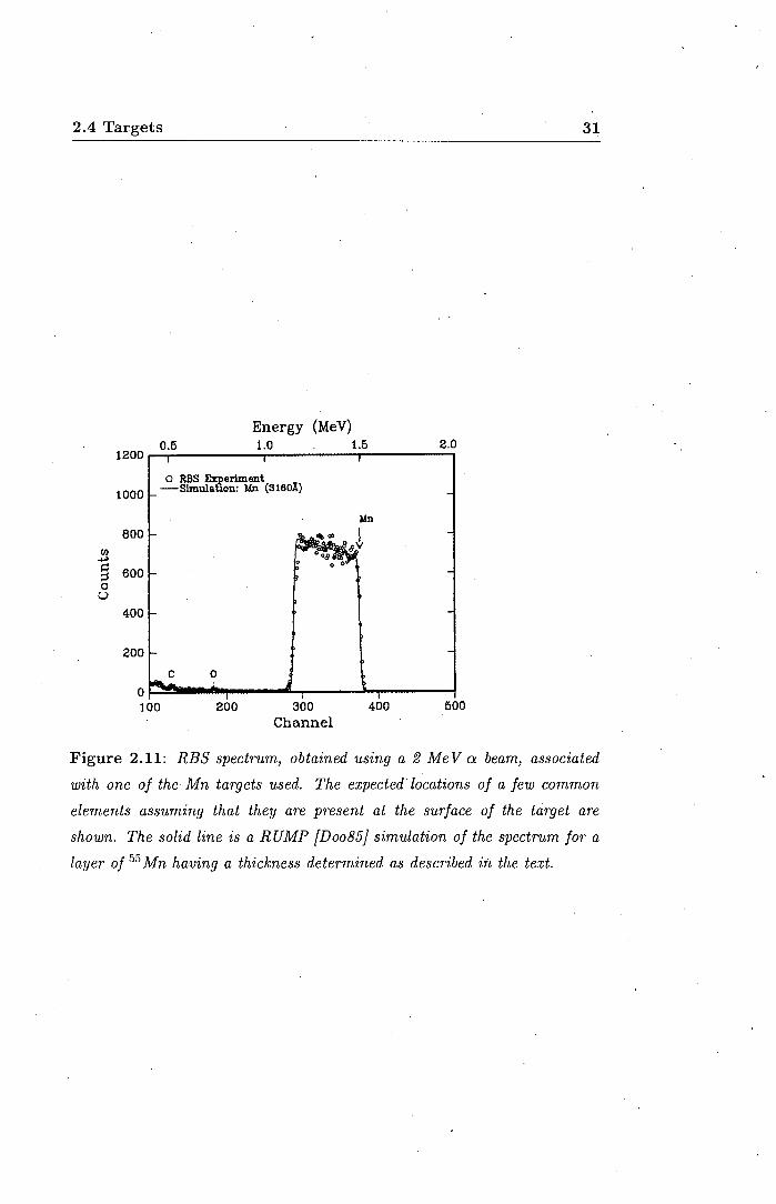
2.11 Typical example of a RBS spectrum.
30
31
2.12 Simulated trajectories through the NAC k = 600 spectrometer. 37
2.13 Predicted absolute time-of-flight spectrum for the (d,3 He)-
mode. . . . . . . . . . . . . . . . . . . . . . . . . . . . . . . . 38
2.14 Schematic representation of the electronics used to process
the paddle and VDC signals. . . . . . . . . . . . . . . . . . . 42
2 .15 Schematic representation of the electronics used to measure
the effective deadtime and the integrated beam current. . . . 45

LIST OF FIGURES v
2.16 Schematic representation of the EVAL algorithm used to pro-
cess VDC and paddle data. . . . . . . . . . . . . . . . . . . . 48
2.17 Typical time-of-flight spectra associated with rigidity-selected
reaction products that traverse the spectrometer focal-plane
detector array. . . . . . . . . . . . . . . . . . . . . . . . . . . 50
2.18 Typical example of a "white" VDC average drift-time spec-
trum and corresponding lookup table. . . . . . . . . . . . . . 51
2.19 Effect of adjusting the spectrometer K- and H-coils on the
time-of-flight versus focal-plane position spectrum. 53
3.1 Helion time-of-flight spectra. 57
3.2 Typical VDC average drift-time spectrum acquired in the
(d,3He)-mode. . . . . . . . . . . . . . . . . . . . . . . . . . . . 58
3.3 Typical examples of spectra with respective software gate
settings used to improve the signal-to-noise ratio in focal
plane position spectra. . . . . . . . . . . . . . . . . . . . . . . 60
3.4 Typical example of a focal-plane position spectrum showing 54Cr final states used to obtain a momentum calibration via
a quadratic least-squares fit. . . . . . . . . . . . . . . . . . . . 61
3.5 Example of a focal-plane position spectrum showing observed 54 Cr final states. . . . . . . . . . . . . . . . . . . . . . . . . . 64
3.6 Plot of the 54Cr excitation region screened by the 15 N(g.s.)
peak versus spectrometer angle. . . . . . . . . 66
3. 7 Typical fit to a set of unresolved final states. 69
3.8 Relative differential cross section for the 55Mn(d,3He) 54 Cr(l)
(Ed = 46 MeV, e = 18°) reaction versus centroid of the 54Cr(l) state along the focal plane. . . . . . . . . . . . . . . . 73
3.9 Measured c.m. angular distributions for 'the 55Mn(d,3He) 54 Cr(E*
= 3.220 MeV) reaction at an average incident energy of 45.6
MeV ................................. 79
3.10 Measured c.m. angular distributions for the 55 Mn(d,3He) 54 Cr
reaction for final-state excitation energies, E*, ranging be
tween 0.0 and 2.622 MeV, at an average incident energy of
45.6 MeV. . . . . . . . . . . . . . . . . . . . . . . . . . . . . . 83

VI LIST OF FIGURES.
3.11 The same as in figure 3.10 but for 54 Cr final-state excitation
energies ranging between 3.076 and 3.429 MeV. . . . . 84
3.12 The same as in figure 3.10 but for 54Cr final-state excitation
energies ranging between 3.656 and 4.042 MeV. . . . . 85
3.13 The same as in figure 3.10 but for 54 Cr final-state excitation
energies ranging between 4.128 and 4.620 MeV. . . . 86
3.14 The same as in figure 3.10 but for 54 Cr final-state excitation
energies ranging between 4.868 and 5.311 MeV. . . . . 87
3.15 The same as in figure 3.10 but for 54 Cr final-state excitation
energies ranging between 5.574 and 6.107 MeV. . . 88
4.1 Comparison of results from a recent Oflp shell-model calcula
tion with the experimental Oh proton stripping spectroscopic 2
strength. . . . . . . . . . . . . . . . . . . . . . . . . . . . 103
4.2 Comparison of results from a recent Oflp shell-model calcu
lation with the experimental Oh proton pickup spectroscopic 2
strength. . . . . . . . . . . . . . . . . . . . . . . . . 104
4.3 Plot ofrelative spectroscopic factor error parameter, er, versus
pickup renormalization constant, n-. . . . . . . . . . 107
4.4 Plot of goodness-of-fit indicator, x2, versus normalization n. 108
4.5 Plots illustrating the sensitivity of the NEWSR to the spin
distribution. . . . . . . . . . . . . . . . . . . . 110
4.6 Gaussian fits to the 54Cr final state observed at 3. 788 Me V
excitation. . . . . . . . . . . . . . . . . . . . . . 112
A. l Schematic representation of a charged particle's trajectory
intersecting the VDC resulting in a six-wire event. . . 120
A.2 Gaussian fit to a distribution of differences in trajectory slope. 121
B.l Schematic top-view of a charged particle's trajectory inter-
secting the VDC. . . . . . . . . . . . . . . . . . . . . 124
B.2 Simulated trajectories through the NAC k = 600 spectrome-
ter shown in the vicinity of the focal plane. . . . . 125
B.3 Simulated lines of equipotential for the VDC used in this study, 126

LIST OF FIGURES vii
C.1 Plots of VDC drift time and drift distance versus wire number.130
D.1 Schematic two-dimensional representation of a particle mov-
ing from target to spectrometer focal plane. . ......... 134
D.2 Drawing of the variable-slot collimator used to check spec
trometer transmission. . . . . . . . . . . . . . . . . . . . . . . 135
F.l Typical time-of-flight spectrum for the spectrometer operated
in (d,d)-mode . ........................... 144
F.2 Typical focal-plane position spectrum generated from (d,d)-
mode data. . ........................... 145
F.3 Typical software gate setting on a density plot of time-of-flight
versus focal-plane position. . .................. 146
F.4 Focal-plane position spectra for the spectrometer operated in
the (d,d) small-angle mode .................... 147
F :5 Relative differential cross section for the 55Mn( d,d) 55 Mn(g.s.)
(Ed= 46 MeV, () = 18°) reaction versus spectrometer central-
trajectory energy tune ....................... 149
F.6 Measured overlap differential cross sections associated with
the 55 Mn(d,d) 55 Mn(g.s.) (Ed= 46MeV,()=12°,18°) reaction
plotted versus spectrometer angle. . .............. 150
, F. 7 Measured c.m. angular distribution for the 55Mn(d,d) 55 Mn(g.s.)
reaction at an average incident energy of 45.6 MeV. . .... 153
List of Tables
1.1 Absolute and corresponding relative spectroscopic factors for
Ofz proton removal from 51 V. . 5 2
1.2 Remaining odd-even f p-shell nuclei with incomplete Oh trans-2
fer data. 9
1.3 Summary of available proton stripping data on 55 Mn. 10
1.4 Summary of available proton pickup data on 55 Mn. . 10
2.1 Technical specifications for the medium-momentum disper-
sion mode of the NAC k = 600 magnetic spectrometer. . 19
2.2 Manganese layer thicknesses associated with the two targets
used. . . . . . 32
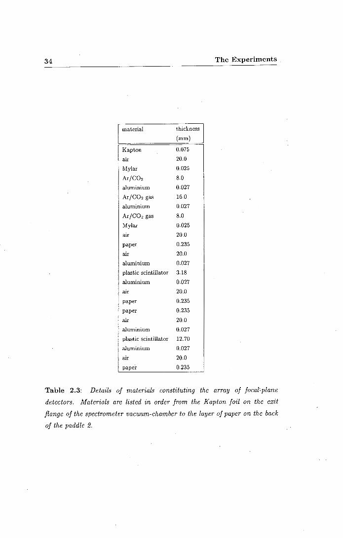
2.3 Details of materials constituting the array of focal-plane de-
tectors.
2.4 Trigger logic used in conjunction with the (d,3He)- and (d,d)
modes. . . .
2.5 Kinetic energies of other particles having the same energy
34
35
constant as that of a 39 Me V helion. 36
2.6 Kinetic energies of particles having the same energy constant
as that of a 44 Me V deuteron. . 39
2. 7 Listing of electronic modules used. 41
3.1 Uncertainties associated with quantities used to calculate the
c.m. differential cross sections for the 55 Mn(d,3He) 54 Cr (Ed
= 45.6·MeV) reaction. 74
3.2 Trost et al. parameterization of a 3He optical-model potential
at 41 MeV. 77

LIST OF TABLES ix
3.3 Parameterization by Barr and DelVecchio of a 3He optical
model potential at 39.7 MeV. . . . . . . . . . . . . . . . . . . 77
3.4 Potential parameters used in the DWBA analyses of angular
distributions for the 55 Mn(d,3He) 54 Cr reaction at an average
incident energy of 45.6 MeV. . . . . . . . . . . . . . . . . . . 80
3.5 Allowed final-state spins and parities for single proton pickup
on 55 Mn from Of Ip and Odls shells. . . . . . . . . . . . . . . 81
3.6 Spectroscopic information from the 55Mn(d,3He)54 Cr reaction
at an average incident energy of 45.6 MeV.
4.1 Calculated stripping strengths associated with transitions to
positive parity states reached in 56Fe via proton stripping on
90
55 Mn. . . . . .. . . . . . . . . . . . . . . . . . . . . . . . . . . 93
4.2 Calculated pickup strengths associated with transitions to
positive parity states reached in 54Cr via proton pickup on 55Mn. . . . . . . . . . . . . . . . . . . . . . . . . . . . . . . . 94
4.3 Spectroscopic information on P = 3 transfer stripping strength
from the 55 Mn(a,t) 56 Fe reaction as reported by Matoba. 100
4.4 Spectroscopic factors for Ofz proton transfer on 55 Mn. . 101 2
4.5 Results of dipole sum-rule analyses of Ofz proton transfer 2
data on 55 Mn ............................ 114
A.1 FWHM associated with distributions. used to determine the
VDC intrinsic cell accuracy. . . . . . . 122
B.l Results of the VDC wire hit-analysis .. 127
D.l Relative differential cross section measured using the variable-
slot collimator. ..... · ..................... 136
F.l Uncertainties associated with quantities used to calculate the
c.m. differential cross sections for the 55 Mn(d,d) 55Mn(g.s.)
(Ed = 45.6 MeV) reaction ..................... 152
F.2 Measured c.m. angular distribution for the 55 Mn(d,d) 55 Mn(g.s.)
reaction at an average incident energy of 45.6 MeV. . .... 155

x · LIST OF TABLES
F.3 Bojowald et al. parameterization of a global optical-model
potential for deuterons. 1.57
Chapter 1
Introduction
One of the most successful models of the intrinsically many-body nature of
the atomic nucleus is the tractable and intuitively appealing single particle1
shell model developed by Goeppert-Mayer, Jensen, Haxel and Suss in 1949
(for example, [Man85, Sic91, Gra92, Hey94, Wal95]). In this model the
nucleus is described as an assembly of independent nucleons, each of which
moves in a well-defined orbit subject to a mean field associated with the
remaining nucleons. Despite its many successes, including the accounting for
the nuclear magic numbers and the prediction of the ground-state properties
of nuclei near closed shells, the validity of the shell model remains a subject
of ongoing research (for example,[den88a, Per88, Wag90, Gra94]). This is a
consequence of experimental findings that the number of nucleons occupying
single particle orbits may be considerably smaller than naive shell-model
predictions. Since the mean field approximation (MFA) is the leading contri
bution in an expansion of multi-particle correlations [Udi93], this quenching
of the single particle occupancy is considered by·some (for example, [Wag90,
Gra94]) to be indicative of a fundamental shortcoming in the shell model.
In particular, the above evidence supports the contention that the residual
interaction between nucleons is significant [Gra92]. The validity of this
contention depends crucially on whether single particle occupancies can
be accurately extracted from experimental measurements. The manner in
which these occupancies are measured is addressed next.
1 Also referred to as the independent-particle shell model.

2 Introduction
' 1.1 Measurement of occupancies
In order to obtain the occupancy of the single particle state a in a given
nucleus, single-nucleon transfer spectroscopic factors, Sa, need to be deter
mined for that nucleus. For reactions in which a single nucleon is removed
(for example via pickup or quasifree-knockout reactions) from an initial state
i of a nucleus of mass A resulting in a final state f of a nucleus of mass A-1,
Sa is given by
s-; = I (A - 1, flaalA, i) 12 (1.1)
where aa is the annihilation operator [Wag90]. For the analogous reaction in
which a nucleon is added to a nucleus (for example via a stripping reaction),
the corresponding Sa reads
S't_ =I (A+ 1,flcalA,i) 12 (1.2)
where Ca is the creation operator.
The particle (hole) occupancy of a state a can then be determined by
summing up to infinite excitation the spectroscopic factors Sa determined
from experiments in which a single nucleon is removed (added) from (to) a
nucleus [Gra94]. In a variant of the above, derived by French and MacFar
lane (for example [Cle73, Wag90, Cle91, Gra94]), the sum of particle and
hole occupancies associated with a state characterized by a total angular
momentum j, should amount to (2j + 1). This sum rule, also referred to as
the total sum rule, will be further discussed below.
Two approaches (other than the application of spin-dependent spectro
scopic sum rules) are currently considered the most reliable in determining
absolute spectroscopic factors and occupancies associated with single par
ticle states. The first of these involves the use of the quasifree-knockout
( e,e' p) reaction. Since the, electromagnetic interaction is well understood
this approach should enable absolute spectroscopic factors to be determined
with good accuracy. There are, however, ambiguities stemming from the
manner in which the (e,e'p) reaction mechanism is modelled which result
in uncertainties in the extracted spectroscopic information. In this regard
the treatment of the Coulomb distortion of the electron has been shown
to be important [Udi93]. Analyses based on a nonrelativistic treatmerit of

1.1 Measurement of occupancies 3
this distortion using the eikonal approximation have resulted in severely
quenched occupancies [Udi93, Udi95]. So for example, one study has shown
that for target nuclei with A ~ 12 the observed spectroscopic strength for
valence orbits is only 50% of the shell-model limit [Wag90]. Subsequently
a full partial-wave analysis of electron waves in the Coulomb potential of
the target has led to an increase from rv 0.50 to rv 0. 70 of the spectroscopic
factor associated with the much-studied reaction in which a proton is re
moved from the 3s1 orbital in 208 Pb [Udi95]. Further questions surrounding 2
the use of nonrelativistic and relativistic optical model potentials (for ex-
ample, [Hod74, Eis88, Sat90, Bur95]) for the outgoing proton waves have
recently been raised and are being investigated [Udi95).
The second manner in which occupancies are believed to be reliably
determined is via the CERES (Qombined Evaluation of Relative spectro
scopic factors and Electron Scattering) formalism [Wag90, Sic91, Gra92,
Gra94]. This approach involves the use of the ratio of truncated sums2 of
relative spectroscopic factors (extracted via single-nucleon transfer reactions
on neighbouring target nuclei) and charge-density differences of isotones
obtained via elastic electron scattering. In a recent study [Udi93) an occu
pation probability of 0. 78 ± 0.12 has been found for the 3s 1 orbital in 208 Pb 2
using this approach. The extraction of occupancies from CERES analyses
is however also not free of ambiguities, as for example in the assumption of
equal quenching of transfer strength in different nuclei.
The use of spectroscopic factors obtained directly from transfer reactions
involving hadrons in the entrance and exit channels is largely ineffective as a
means of determining occupancies because of uncertainties associated with
the absolute normalization of these spectroscopic factors [Moa79, Nan89,
Cle91). These uncertainties stem primarily from the manner in which the
reaction mechanism is modelled. For single-nucleon transfer reactions the
experimentally measured differential cross section for the transition to a
particular final state is proportional to the product of the spectroscopic
factor and the corresponding differential cross section calculated within
2 Normally over a~ 5 MeV excitation region since the level densities become too high
above this region to determine spectroscopic factors associated with transitions to discrete
states.

4 Introduction.
the framework of the distorted-wave Born approximation (DWBA) (for
example, [Aus60, Aus64, Roy67, Jac77, Sat83, Eis88, Bur95]). In particular,
for the case of pickup and stripping reactions respectively:
where
a(e)expt = L c;sjg(a(e)DWBA)j£ jf
a(e)expt = ~ i~]c?SJg(a(e)owsA)j£
(1.3)
(1.4)
• j and f, denote total and orbital angular-momentum transfer, respec
tively;
• J' and lt denote the final-state and target ground-state spin, respec
tively;
• [ x J = ( 2x + 1);
• a(e)expt and a(e)owBA denote the measured and calculated DWBA
differential cross sections, respectively;
• SP and ss denote pickup and stripping spectroscopic factors, respec
tively; and
• Gp and Cs denote the corresponding isospin Clebsch-Gordan coeffi
cients.
In practice, spectroscopic factors are determined by normalizing a portion
(normally including the peak) of the DWBA angular distribution to the
corresponding experimental data. One of the main sources of uncertainty
associated with the extracted spectroscopic factors is the strong depen
dence of the calculated cross section on the potential parameters used to
generate the distorted wave-functions for the entrance and exit channels,
and the bound-state wave function, 1/Ja(r), which describes the transferred
nucleon [Moa79, Gra92]. The dependence of the calculated DWBA dif
ferential cross section on the bound-state radius has been shown to be
particularly pronounced [Wag90, Cle91, Sic91 ]. So for example, a 1 % change
in the radius parameter of the potential used to calculate 1/Ja(r) translates

1.1 Measurement of occupancies
E* J1f (d,3He)a
(MeV)
0 o+ 0.73 (0.78)
1.55 2+ 0.39 (0.42)
2.67 4+ 0.64 (0.68)
3.22 6+ 1.05 (1.12)
Total: 2.81 (3.00)
a from Ref. [Hin67].
b from Ref. [Kra88].
c from Ref. [den88b].
5
(d,3 He)b (e,e'p)c
0.41 (0.73) 0.37 (0.83)
0.22 (0.39) 0.15 (0.33)
0.41 (0.73) 0.33 (0.74)
0.65 (1.15) 0.49 (1.10)
1.69 (3.00) 1.34 (3.00)
Table 1.1: Absolute and, in parentheses, the corresponding relative
spectroscopic factors for Oh proton removal from 51 V. (Adapted from 2
Ref. [Wag90}.)
into about a 103 change in absolute spectroscopic factor [Moa79, Sic91].
As a result absolute spectroscopic factors are inherently strongly model
dependent. Furthermore summing these spectroscopic factors to calculate
occupancies is problematic since only a finite excitation energy region can
be sampled, and the spectroscopic strength of an orbit of interest may not
have been exhausted. Typically only strength associated with transitions to
states at excitation energies, E*, up to about 5 Me V in the residual nucleus
can be reliably extracted. Any higher-lying strength due to, for example,
short-range correlations and the coupling of single particle strength to giant
resonance excitations, is therefore ignored in calculating occupancies in this
way [Sic91].
In contrast to their absolute counterparts, relative values of spectroscopic
factors from independent experiments generally agree to within,...., 103 [Cle77,
Cle91]. This is due to the fact that many experimental and theoretical
sources of error largely cancel, as is illustrated in table 1.1 where the ab
solute and the corresponding relative spectroscopic factors associated with
the Oh proton removal on 51 V are compared. This consistency of rela-2
tive spectroscopic factors has led to the development of a formalism based
on the standard (asymmetric) form of the non-energy weighted sum rules

6 Introduction
(NEWSR) [Cle91], whereby complementary sets of spectroscopic strength
spin-distributions (spectroscopic factors and corresponding final-state spins)
can be critically examined. The NEWSR formalism has been used, inter alia,
to assess the consistency of the input data (i.e. the spin distributions),
determine absolute DWBA normalizations [Cha77, Cle77, Moa77], make
spin assignments to final states [Cle73]; and provide insight, albeit indirectly,
into the unobservable single particle strength located beyond the excitation
region probed experimentally [New95].
An important component of the formalism, which is detailed in chapter 4,
involves introducing the renormalization constants n- and n+ to take into
account errors in the absolute normalizations of pickup and stripping spec
troscopic factors, respectively, as derived from DWBA analyses of transfer
data. The goodness-of-fit to the NEWSR is assessed by plotting an error
parameter CT, which is indicative of the average uncertainty a.Ssociated with
relative spectroscopic factors, as a function of n+ or n-. For cases where
the NEWSR fit the input data well the curve of a versus renormalization
constant displays a distinct minimum. The smaller the minimum value
CT min of CT, the more significant any fit to the sum rules is and the more
reliable the complementary sets of transfer spin-distributions are. If a value
of Clmin ~ 10% is obtained the transfer spin-distributions are considered to
satisfy the sum rules. In this event the absolute DWBA normalizations can
be determined from the values of n+ and n- corresponding to Clmin· These
spectroscopic factors can then be used, inter alia, to determine expectation
values associated with one-body operators acting on the target ground-state
by using further sum rules. One such extensively used sum rule is the dipole
sum rule [Cle91] which allows the target ground-state spin to be calculated
from the estimated absolute spectroscopic factors.
NEWSR analyses have mostly been performed on Ofz transfer data 2
acquired in the lower part of the fp shell [Cle77, Cle91]. This is because
the large energy gap between the Oh and Oh_ orbitals allows a confident ' 2 2
assignment of Oh to any e = 3 transition to a low excitation energy final 2 '
state in this mass region. A further reason for focussing on 0 fl transfer 2
is the fact that the number of independent linear relations constituting the
NEWSR is equal to the smaller of [Jt] and [j] [Cle91]. Thus the larger

1.1 Measurement of occupancies 7
I All tran1f•r data includ•d
0·3 n 2·77 M•V stripping stat• omill•d
n
0·2
0·1
n·
Figure 1.1: Results of a NEWSR analysis of complementary sets of spin
distributions associated with Of 1 proton transfer on 51 V. The relative error ' 2 parameter, <J, is plotted as a function of pickup renormalization constant,
n-. The effect of omitting all the strength {20% of the total strength}
associated with the 2. 77 Me V stripping state is shown. (Reproduced from
Ref. { Cle91}.)

8 . Introduction
Jt, the greater the number3 of linear relations representing the NEWSR,
and the greater the overdeterminancy of any quantity to be determined
through the sum rules (e.g. the renormalization constants n+ and n-). So
for example, using 0 h transfer data for 51 V (Jt = ~) in a NEW SR analysis 2
involves eight independent linear relations in sixteen partial spectroscopic
sums. It is this overdeterminancy which makes the NEWSR formalism such
a powerful diagnostic tool. The sensitivity of the NEWSR to the distribution
of transfer strength is shown in figure 1.1, where the effect of omitting some
of the strength is illustrated.
Analyses of Oh transfer data on 41 Ca, 43 Ca, 45Sc, 49 Ti and 51 V that 2
have been made thus far have resulted in successful fits to the NEWSR
in all cases [Cle77, Cle91], with values of amin varying between 3% and
9% [Cle91]. Renormalization constants obtained from these NEWSR analy
ses, together with subsequent dipole sum-rule analyses, are consistent with
orbit occupancies being close to those expected from the shell model. This is
in contrast to results from (e,e'p) work and CERES analyses which indicate
a quenching of occupancy, as discussed above, of "' 303.
1.2 Aims and scope of this study
The primary motivation for conducting this study [New96] was the desire to
complement the existing NEWSR analyses of Of 1 transfer data on odd-even 2
f p-shell nuclei, in order to attempt obtaining further corroboration for the
trends delineated above.
Odd-even nuclei with 40 < A < 60 for which complete sets of Oh 2
transfer data were unavailable before the completion of this study are listed
in table 1.2. From this table it can be seen that 47Ti and 55 Mn were
the only remaining targets in the lower part of the f p shell with Jt 2: ~
for which NEWSR analyses4 had not been performed [Cle91]. The latter
target was focussed on in this study mainly because a set of stripping
3 Even-even targets, with Jt = 0, yield only the total sum rule, from which the
renormalization constants n - and n + cannot be determined. 4 A sum-rule analysis on these two targets will therefore involve six independent
linear relations.

1.2 Aims and scope of this study 9
nucleus isotopic abundance (%) ground-state spin N
47Ti 7.4 5 6 2 53Cr 2.36 3 4 2 55Mn 100 5 6 2 57Fe 2.2 1 2 2
Table 1.2: Remaining odd-even f p-shell nuclei with incomplete Ofz transfer 2
data. N represents the number of independent linear relations constituting
the NEWSR.
spectroscopic factors for single proton transfer on 55Mn is available in the
literature [Mat68]. The fact :that 54Cr final states, which are reached via
proton pickup on 55 Mn, are mostly well-separated and have known spins,
along with the fact that 55 Mn occurs with a 100% natural isotopic abundance
while 47Ti occurs with an abundance of only 7.4%, were additional reasons
for choosing 55 Mn as the target nucleus in this study.
Two earlier studies of proton stripping on 55Mn exist. A summary of the
pertinent results are given in table 1.3. The first study was performed using
the (3He,d) reaction [Hin67]. The transitions to only three 56 Fe final states
were studied and no spectroscopic factors were reported. A more extensive
study by Matoba [Mat68] used the (a,t) reaction to study transitions to
twelve 56 Fe final states. Two previous studies of proton pickup on 55 Mn
also exist. The main results from these studies are summarized in table 1.4.
In the first, Colli et al. [Col59, Col61] reported transitions to five final
states observed via the (n,d) reaction. However they only extracted the
spectroscopic factor for the transition to the 54Cr ground state. The second
study, by Yntema et al. [Ynt61] who employed the (d,3He) reaction, yielded
no spectroscopic factors.
A reliable set of spectroscopic factors for Ofz proton pickup on 55 Mn 2
was therefore required. In the present study these were obtained through
DWBA analyses of new measurements of the differential cross section for the 55 Mn(d,3He) 54 Cr reaction at a nominal beam energy of 45 MeV. This beam
energy was chosen to exploit available parameterizations of the mass depen
dence of optical potentials for 3He at 39.7 MeV [Bar77] and 41 MeV [Tro80],

10 Introduction .
reaction E* I!. transfer L0c2s [Jt] Ref.
(MeV)
(3He,d) 0.85 1,3 [Hin67]
2.09 1,3
2.66 1
(a,t) 0.00 3 0.01 [Mat68]
0.85 3 1.45
2.09 3 0.36
2.66 3 0.14
2.97 3 0.08
3.15 3
3.40 3 0.90
3.78 3 0.25
4.08 1
4.42 1
4.73 1
5.20 1
Table 1.3: Summary of available proton stripping data on 55 Mn as compiled
in Refs. [Jun87, Jun92}.
reaction E* I!. transfer s Ref.
(MeV)
(n,d) 0.00 3 0.59 [Col59, Col61]
0.90
1.80
,.,,, 3.0
,.,,, 4.0
(d, 3He) 0.00 [Ynt61]
0.84
1.90
Table 1.4: Summary of available proton pickup data on 55 Mn as compiled
in Refs. {Gon87, Jun93}.

1.3 Thesis overview 11
from which distorted wave-functions for the exit channel could be deter
mined.
The form of the optical potential used to generate the distorted waves
for the entrance channel was identical to the one used to obtain a global
parameterization of deuteron optical-model parameters [Boj88]. In order
to obtain optimum parameters for this potential, the angular distribution
for the 55 Mn(d,d) 55 Mn(g.s.) reaction was measured in conjunction with the
pickup data, and subsequently analysed with a standard optical-model code.
Another aim of this study was to further investigate the use [New95] of
a symmetric form of the diagonal NEWSR together with an improved error
analysis formalism. A further advantage of using the symmetric rather than
the standard form of the NEWSR is that the total sum rule is obtained
separately for one of the linear relations constituting the former sum rules,
and is thus decoupled from the remaining linear relations. After estimating
the fraction, /, of transfer strength located above the excitation region
considered (typically in the 0-5 Me V region), absolute spectroscopic factors
can be determined. Furthermore, the symmetric form is suggestive of a
possible spin distribution associated with the transfer strength located above
the excitation region studied [New95].
Recently, shell-model calculations have been performed for A = 41-66
nuclei, using a new two-body effective interaction and a model space which
allows for the excitation of a Oh. particle to the lp1, Oh and lp1 sub-2 2 2 2
shells [van94]. Theoretical energy levels and static electromagnetic moments
have been shown to be in good agreement with their experimental counter
parts [van94]. In order to further assess the quality of these calculations,
the derived wave functions were used to calculate spectroscopic factors for
comparison with those determined through single proton transfer on 55 Mn.
This assessment constituted the third and final aim of this study.
1.3 Thesis overview
To conclude the introduction, the structure of the remainder of this disser
tation is outlined.

12 Introduction.
The experimental methods used to acquire the proton pickup and deuteron
elastic scattering data on 55 Mn are discussed in chapter 2. The extraction
of pickup angular distributions from these data and subsequent calculation
of spectroscopic factors via DWBA analyses are described in chapter 3;
while the analysis of the deuteron elastic scattering data is discussed in
appendix F. In chapter 4 the results of the shell-model calculations are
first presented. This is followed by a description of how the stripping and
pickup spin-distributions for Ofz proton transfer on 55 Mn were established. 2
Non-energy weighted sum-rule analyses of these spin distributions are then
described. A concluding summary, along with suggestions for possible com
plementary studies, are presented in the final chapter.

Chapter 2
The Experiments
In this chapter the experimental techniques which were used to measure the
data required to perform non-energy weighted sum-rule (NEWSR) analyses
of data for Ofz proton transfer on 55Mn are detailed. As discussed in 2
section 1.2, Matoba's 55Mn(a,t) 56 Fe study [Mat68] yielded a set of strip-
ping spectroscopic factors, leaving the complementary set of pickup data
to be measured. In this study these data were extracted from measured
differential cross sections associated with the 55Mn(d,3He)54 Cr reaction at
a nominal beam energy of 45 MeV. As a by-product of the above, the 55Mn(d,d) 55 Mn(g.s.) reaction was studied at the same beam energy. These
data were then used (see appendix F) to obtain optimized optical-potential
parameters for the entrance channel of the 55 Mn(d,3He)54Cr reaction in the
distorted-wave Born approximation (DWBA) analyses.
2 .1 Overview
The differential cross sections for the 55Mn(d,3He) 54 Cr and 55 Mn(d,d)55 Mn(g.s.)
reactions were measured using a k = 600 magnetic spectrometer1 at the
National Accelerator Centre (NAC), the national multi-disciplinary research
1The energy constant, k, is defined ask= ~'where q and mare in units of proton q
charge and mass respectively; and E is the the kinetic energy of the particle in MeV
units [Weg87].

14 The Experiments.
facility at Faure2 in the Republic of South Africa. The measurements were
made intermittently between December 1991 and September 1994.
The light (charged) reaction products were detected in the spectrome
ter's focal-plane detector array [Fu185] consisting of a vertical drift cham
ber3 (VDC) (Ber77] followed by two plastic scintillator paddle detectors.
Signals from the paddles were used to generate the event trigger, while
the momenta of the ejectiles were determined from the position where they
intersected the wire-plane of the VDC. Particle identification of the rigidity
selected reaction products was effected by studying their times-of-flight
through the spectrometer.
2. 2 Deuteron beam
At the NAC, particle beams are initially accelerated using one of two solid
pole injector cyclotrons [Bot84, Pil89a]. The first injector, solid-pole cy
clotron 1 (SPCl), is used to accelerate light-ion beams, while the sec
ond, SPC2, is used to accelerate mainly heavy ions, polarized protons and
deuterons. Beams extracted from the injectors are then further accelerated
in a separated-sector cyclotron (SSC) until the beam particles attain the
required kinetic energy. A floor-plan of the NAC facility showing, inter alia,
the locations of these cyclotrons is shown in figure 2.1.
·For this experiment deuterium gas molecules were ionized in a Penning
Ion Gauge ion-source located at the centre of SPCl (k = 8). A hot filament
inside the ion-source thermally ejects electrons from a lanthanum hexa
boride (LaB6 ) pellet (cathode) into a plasma-filled anode column [Con94].
Deuterons were extracted from the plasma by m<"._ans of negatively charged
puller electrodes and accelerated in SPCl. At a radius of about 0.48 m
the deuterons have been accelerated to an energy of 4 Me V and were then
extracted from SPCl for injection into the NAC's main cyclotron, the k =
200 SSC. To accelerate deuterons to about 45 MeV a radio frequency of
,.._, 9.9 MHz is used for the acceleration voltage. Although a maximum pulse
2 Located approximately 30 km from Cape Town. 3The term was coined to refer to drift chambers in which the direction of electron drift
is perpendicular to the wire-plane.

2.2 Deuteron beam 15
Figure 2.1: Floor-plan of the NAG cyclotron facility.

16 The Experiments
selection of one in three is available for a deuteron beam of 45 Me V, no pulse
selection was used since the associated beam-burst interval of about 100 ns
proved convenient for identifying particles by means of the time-of-flight
technique (see section 2.6).
After extraction from the SSC the deuteron beam was steered along
the X, P1 , P2 and S beam-lines (see figures 2.1 and 2.2), and delivered
achromatically onto the target. The beam energy was calculated from the
currents supplied to two 90° bending magnets located along the extraction
beam-line. An uncertainty of ,._.., 0.25 MeV [Bot95] is associated with this
measurement. The average energy of the beam delivered for this study was
45.6 MeV. In order to optimize resolution on target the widths of energy
defining slits located along the X and P1 beam-lines respectively, were kept
fixed at 1.00 mm. As a result the energy spread in the beam was about 10
ke V since this spread, JE, is calculated using the relation
(2.1)
where E is the beam energy and R1 the first-order resolving power4 .
At the start of an experimental session the beam alignment on target
was checked by reducing the current to about 3 nA and using closed circuit
television to monitor the beam spot on an aluminium oxide viewer. This
viewer had a 3 mm diameter hole located at its centre. When perfectly
aligned, the beam passed through the central hole in the viewer with no
afterglow. Beam halo was reduced by tuning the beam in order to minimize
the paddle count rate (see section 2.7.1) when using an empty target frame.
In this manner it was possible to reduce the halo rate down to ~ 4% of the
count rate obtained with the target in place. Beam intensities on target
varied between 1 nA and 29 nA. The accumulated charge associated with
4 The first-order resolving power, R 1 , expresses the capability of a spectrometer to
separate particles of different momenta and is defined as the ratio of the horizontal
momentum dispersion to image size, i.e.
RI6 R1 =RX
11 o
where Xo is the slit-width, R11 relates the final beam-width to the initial beam-width and
RI6 describes the broadening of the beam caused by the dispersion of the system. While
performing the experiments the first-order resolving power was typically 8000.

2.2 Deuteron beam 17
K600 SPECTROMETER
0 lm
FOCAL PLANES
AC:
HE:
OU:
FP:
aperture carousel
hexapole
quadrupole
field probe
Figure 2.2: Drawing of the k = 600 magnetic spectrometer at the NAG.
The locations of the focal planes associated with the low-, high- and medium
momentum dispersion modes respectively, are shown.
1.Sm/s turbo pump station
vacuum valve
BEAM STOP
TARGET
S-UNE

18 The Experiments
pickup data-sets varied between 96 11C and 506 11C, while that for elastic
scattering varied between 0.02 11C and 48 11C.
2.3 K = 600 spectrometer
The k = 600 magnetic spectrometer at the NAC is based on the design of
the K600 spectrometer at the Indiana University Cyclotron Facility (IUCF)
[Ber86, Ber88, Ber89, Bac90]. This spectrometer comprises5 , inter alia, a
quadrupole, two dipole magnets, and K and H trim-coils (see figure 2.2).
The K-coil which is located inside the second dipole (D2) is used to adjust
(x/8) for first-order point-to-point focussing from the object-slit to the focal
plane while the H-coil, located inside the first dipole (D1), is used to correct
for (x/82) aberrations [Ber79, Off87] (see also section 2.9).
The spectrometer can be operated in a low-, high- or medium-momentum
dispersion mode, with the last mentioned being the one used in this study.
The focal-planes associated with each of these modes are also shown in
figure 2.2. A summary of the NAC k = 600 spectrometer's technical speci
fications for its medium dispersion mode is given in table 2.1.
Targets (see section 2.4) were mounted inside a 301 mm diameter scatter
ing chamber which was positioned in relation to the incident deuteron beam
as shown in figure 2.3. After exiting the scattering chamber, the ejectiles pass
through a collimator which defines the spectrometer's angular acceptance
(detailed in section 2.3.3). Those particles which are charged follow a cur':ed
path through the spectrometer causing particles with different momenta,
but with sufficient rigidity, to be focussed at different points along the
spectrometer focal plane (see figure 2.12).
2.3.1 Focal-plane detectors
Reaction products which moved through the spectrometer were detected by
means of a vertical drift chamber (VDC) followed by two plastic scintilla
tion paddle detectors. These detectors were positioned along the medium-
5The hexapole magnet was not used.

2.3 K = 600 spectrometer
feature
maximum momentum per charge, p/Q
maximum proton energy
maximum particle rigidity
maximum dipole fields (D1 and D2)
dipole field ratio
nominal bend radius
nominal bend angle
maximum solid angle, b..Bb..¢
maximum horizonal acceptance, b..B
maximum vertical acceptance, b..¢
momentum range, Pmax/Pmin
resolving power, P /SP (0.6 mm object slit)
momentum dispersion
energy dispersion (200 MeV protons)
horizontal magnification at Pmax
vertical magnification at Pmax
central-ray angle w.r.t. focal plane
horizontal VDC acceptance
vertical VDC acceptance
value
1080 MeV /c
493 MeV
3.60 Tm
1.64 (T)
1
2.1 m
115°
6.0 msr
± 44 mrad
± 44 mrad
1.0.97
28000
8.4 cm/%
42 kev/mm
-0.52
7.4
35.75°
78 cm
10 cm
19
Table 2.1: Technical specifications for the medium-momentum. dispersion
mode of the NAG k = 600 magn~tic spectrometer.

20
K600 SPECTROMETER
OIL -FLOW' INDICATOR
DIPOLE 1
FLOW' CONTROL VAL VE
PRESSURE GAUGE
OXYSORB
HYDROSORB
u 10% CO, /90% ARGON
The Experiments .
Figure 2.3: Positioning of the spectrometer focal-plane detectors. A
schematic representation of the VDC gas-handling system is also shown.

2.3 K 600 spectrometer 21
PLASTIC SCINTILLA~OR ~" PHQT..,.,UL TIPLIER TUBE
PERSPEX LIGHT CUIDE
SUPPORT RAIL
0 500 mm
Figure 2.4: Magnified view of the focal-plane detector array arrangement.

22 The Experiments .
momentum dispersion focal plane of the spectrometer on steel support rails
(see figures 2.3 and 2.4).
Vertical Drift Chamber
The VDC6 used in this work was designed and built by NAC personnel.
It comprises, inter alia, two high voltage (HV) anode planes, an earthed
signal-wire cathode plane situated midway between the cathodes and a gas
which fills the VDC volume. Two 25 µm thick Mylar windows are used
to seal off the gas-filled VDC interior from the environment, while two
27 µm thick aluminium foils separated by 16.0 mm are used as cathode
high voltage planes (see figure 2.5). The earthed signal wire-plane situated
midway between these foils comprises 198 signal wires, each 25 µm thick, and
spaced 4.0 mm apart. In order to improve the field shaping and facilitate
the application of lower high voltages on the cathode planes, these wires
are interspersed with 199 guard wires, each of thickness 50 µm and also
positioned 4.00 mm apart.· All wires used were made from gold-plated
tungsten. Negative high voltages of 3.50 kV and 550 V are applied to the
cathode planes and guard wires respectively. A 90%Ar/10%C02 gas mixture
at atmospheric pressure is used as a VDC fill gas. The gas is supplied to the
VDC by means of the gas-handling system shown schematically in figure 2.3.
Under the above operating conditions the position accuracy, <Jx, achieved
with the VDC was 81 µm (see appendix A).
The VDC is positioned flush up against a 75 µm thick Kapton window
on the exit-flange of the spectrometer vacuum chamber. It was arranged in
a way such that its wire-plane coincides with the spectrometer's focal plane
which is at an angle fh.p. = 35.75° with respect to the central-momentum tra
jectory through the spectrometer (see figure 2.6). This angle was determined
via three-dimensional ion-optical simulations using the computer program
TRACK [Geo91] which utilizes calculated three-dimensional median-plane
field maps7 associated with the spectrometer magnets [NAC94]. A schematic
6 For a detailed overview of the principles of drift chambers, the reader is referred to
(Sau77] and references therein. 7These maps were generated from the measured two-dimensional median-plane field
maps using the computer program NACCON developed at the NAC.

2.3 K 600 spectrometer 23
Figure 2.5: Schematic cross-sectional view of the VDC used.

24 The Experiments
representation of a charged particle traversing a VDC is shown in figure 2.7.
The particle ionizes gas molecules along its path through the VDC. Because
of the applied potential difference, electrons generated by the ionization drift
at nearly constant velocity8 to within less than 1 mm of the signal wires,
whereupon avalanching [Cha84] occurs.· As a result, pulses are induced on
the signal wire. By measuring the time it takes for these electrons to drift
from the point of primary ionization to the point where avalanching occurs,
and by making use of a mapping from drift time to drift distance, it is
possible to reconstruct the particle's in-plane trajectory through the VDC
(see section 2.8, appendix A and appendix C). The position where the
particle's trajectory crosses the focal plane can therefore be determined and
hence the particle's momentum calculated.
Paddles
Pulses from the plastic scintillation detectors mounted behind the VDC were
used to generate an event trigger and a start signal for the measurement of
the time-of-flight of particles through the spectrometer. In the following,
the paddle scintillation detector which was located behind the VDC relative
to particles moving through the spectrometer will be labelled paddle 1; and
the following one will be labelled paddle 2 (see figure 2.4). Both paddles
were constructed using plastic scintillator (Bicron BC408) with a rectangular
cross section of 122.0 cm x 10.2 cm. The scintillator thicknesses for paddles
1 and 2 are 3.18 mm and 12. 70 mm respectively. Silgel (NE586) was used to
link two fishtail perspex lightguides to each end of the scintillators. The same
compound was used to couple photomultiplier tubes (Hamamatsu R329) to
each lightguide. Hamamatsu E934 bases are used on all photomultiplier
tubes, each being magnetically shielded with a mu-metal shield. The as
sembled paddles are mounted inside black paper-covered rectangular frames
in order to make them light-tight and positioned directly behind the VDC.
Both paddles were operated at a negative high voltage of,...., 1500 V.
8The inverse drift velocity for the VDC used is ~ 18 ns/mm.

2.3 K = 600 spectrometer 25
c
medium dispersion focal plane 0 \ M B
-~·~sJ_ ~-----
geometrical central ray
Figure 2.6: Schematic representation of the positioning. of the VDC w.r.t.
the k = 600 spectrometer's central-momentum trajectory. The distances
between points A and B; B and C; and, M and B are 535.54 mm, 498.82
mm and 18.36 mm respectively. Point M is located midway between points
A and C.
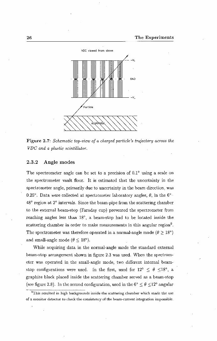
26 The Experiments
voe viewed from above
Particle
Figure 2. 7: Schematic top-view of a charged particle's trajectory across the
VDC and a plastic scintillator.
2.3.2 Angle modes
The spectrometer angle can be set to a precision of 0.1° using a scale on
the spectrometer vault floor. It is estimated that the uncertainty in the
spectrometer angle, primarily due to uncertainty in the beam direction, was
0.25°. Data were collected at spectrometer laboratory angles, e, in the 6°-
480 region at 2° intervals. Since the beam-pipe from the scattering chamber
to the external beam-stop (Faraday cup) prevented the spectrometer from
reaching angles less than 18°, a beam-stop had to be located inside the
scattering chamber in order to make measurements in this angular region9 .
The spectrometer was therefore operated in a normal-angle mode (B 2: 18°)
and small-angle mode (B ~ 18°).
While acquiring data in the normal-angle mode the standard external
beam-stop arrangement shown in figure 2.3 was used. When the spectrom
eter was operated in the small-angle mode, two different internal beam
stop configurations were used. In the first, used for 12° ~ e ~18°, a
graphite block placed inside the scattering chamber served as a beam-stop
(see figure 2.8). In the second configuration, used in the 6° ~ e ~12° angular
9This resulted in high backgrounds inside the scattering chamber which made the use
of a monitor detector to check the consistency of the beam-current integration impossible.

2.4 Targets 27
region, the beam-pipe extending from the scattering chamber to the external
beam-stop was removed, thereby allowing the spectrometer to reach further
forward angles. In this case the beam was stopped on a graphite block
placed inside an evacuated chamber located behind the scattering chamber
as shown in figure 2.9.
2.3.3 Collimators
The spectrometer acceptance was defined by brass collimators having the
shape shown in figure 2.10. Two collimators were used10 ; one for e 2:: 12° •
and the other for e :::; 12°. The former collimator, which was located inside
the collimator carousel shown in figure 2.8, had the dimensions shown in
figure 2.10. These dimensions were chosen so as to maximize the solid
angle, minimize the kinematic spread due to the in-plane angular acceptance
but yet yield 100% transmission through the spectrometer (see appendix D
for a study of the spectrometer's transmission). The second collimator,
which was located further down-stream (see figure 2.9) had its dimensions
scaled in order to give the same solid angle as that associated with the first.
The distances from the target centre to the back of the two collimators
were 735.5 mm and 545.0 mm respectively. The arrangements resulted in
horizontal angular acceptances of 1.09° and 1.07° respectively; while the
vertical angular acceptances were 4.28° in both cases. The solid angle
subtended by both collimators was 1.34 msr.
2.4 Targets
Since manganese is not self-supporting it is usually deposited onto a backing
when making targets (for example, [Mat68, Pee74, Cam81]). A backing
made of Mylar was used in this work because of its robustness. Two 55 Mn
targets were manufactured at the Van de Graaff facility at the NAC for use
in this experiment. These targets were made under vacuum by evaporating
99.99% pure11 Mn onto a 1.5 µm thick Mylar backing.
10See figure F.6 of appendix F for the results of a consistency check regarding the use
of these two collimators. 11 The natural isotopic abundance of 55 Mn is 100%.

28 The Experiments .
DIPOLE
OVADRVPOlE
COLLlf.IATOR CAROUSEL
0 500 mm
Figure 2.8: Beam-stop configuration used in the spectrometer's small-angle
mode for 12 ° s e s18 °.

2.4 Targets . 29
DIPOLE
0 500 mm
d
Figure 2.9: Beam-stop configuration used in the spectrometer's small-angle
mode for 6 ° :S () :S12 °.

30
···©· I
14.0
The Experiments .
.o .q-
Figure 2.10: Drawing of brass collimator used to define the spectrometer
acceptance. The dimensions shown are for the collimator used for() 2: 12 °.
All dimensions shown are in mm.
2.4 Targets
00 ...,
1000
800
§ 600 0 u
400
200
Energy (MeV) 0.5 1.0 1.5
0 RBS Experiment -Simulat1on: Mn (31601)
c 0
2.0
ot=:!!!!lllll ... ..,. __ .... ~.....,.-~~.....i....,-~~--f 100 200 300
Channel 400 500
31
Figure 2.11: RBS spectrum, obtained using a 2 Me Va beam, associated
with one of the Mn targets used. The expected locations of a few common
elements assuming that they are present at the surface of the target are
shown. The solid line is a RUMP [Doo85} simulation of the spectrum for a
layer of 55 Mn having a thickness determined as described in the text.

32 The Experiments
. target no. experimental session Mn layer thickness
(A) (µg/cm 2)
1 December 1991 - December 1993 2132 159
2 January 1993 - September 1994 3160 235
Table 2.2: Manganese layer thicknesses associated with the two targets
used. The maximum uncertainty associated with the quoted thicknesses is
10% (see text for details}.
A rough estimate of the thickness of the Mn layer deposited onto the
Mylar was obtained using a quartz crystal film-thickness and deposition rate
meter (Inficon XTM). A more accurate measurement of the Mn layer thick
ness was made using Rutherford backscattering spectrometry (RBS) [Chu78].
A 2 MeV a beam and a standard experimental arrangement [Cha93, Mar93]
were used to perform RBS on the two targets at the Van de Graaff facility.
A backscattering angle of 170° was used. The RBS spectra collected were
analysed off-line using the Rutherford backscattering Utilities and Manipu
lation Program (RUMP) [Doo85], a standard software package for analysing
RBS spectra. RUMP was used to determine12 thicknesses of Mn layers from
the the full-width at half maximum (FWHM) of the 55 Mn peaks observed in
the RBS spectra. The limiting factor on the accuracies of thicknesses deter
mined in this manner, is the 5-10% accuracy associated with the stopping
power tables used by RUMP. The RBS spectrum associated with one of the
manufactured targets is shown in figure 2.11. A RUMP simulation of the
expected spectrum assuming that the target comprises only a Mn layer of
thickness determined in the manner described above, is also shown in this
figure. The thicknesses so obtained are given in table 2.2.
Targets were mounted in the scattering chamber on a target ladder which
was linked to a remote target-positioner. The target angle was always set
to half the spectrometer angle in order to fix the target transformation
factor 13 [Hen74] to a value of 1.0 as is common practice. On the ladder
12 In particular the width-thick function, which is based on the mean-energy
approximation for the stopping power, was used. 13Th" f . . b cos(0-4>) h ,I. . h I 1s actor 1s given y t11 = cos4> , w ere 'I' is t e target ang e.

2.5 Trigger logic 33
was a 55 Mn target, an aluminium oxide viewer-target used for beam-spot
alignment, an empty target frame for beam-halo reduction and a 1.5 µm
thick Mylar target used for background checks. Care was taken to mount
the Mn target with the Mylar backing facing the beam in order to minimize
the deterioration in the spectrometer resolution.
2. 5 Trigger logic
Since both pickup and elastic scattering data were required, the spectrome
ter had to be operated in two modes. These will be referred to below as the
(d,3He)- and (d,d)-modes respectively. Calculations of the energy lost by the
helions and deuterons in the materials constituting the focal-plane detectors
(given in table 2.3) were performed in order to decide on the trigger logic
required for the (d,3He)- and (d,d)-modes respectively.
For an assumed deuteron beam energy of 45 MeV, the lowest energy
helions of interest (i.e. those associated with an excitation energy of 6
MeV in 54 Cr at a spectrometer angle of 48°) are stopped 0.2 mm inside14
the scintillator of paddle 1. Each of these helions deposit 9.2 Me V in this
scintillator. The corresponding highest energy helions of interest (i.e. those
associated with the transition to the 54Cr(g.s.) at () = 6°) are stopped 0.8
mm inside15 paddle l's scintillator where they each deposit 27.1 MeV. Since
no thinner scintillator was available, the paddle 1 signal, P1, was used in
anti-coincidence with the paddle 2 signal (P2 ) to generate an event trigger
while operating in the (d,3He)-mode. In order to minimize the data buffered
to tape for off-line analysis in this mode, a VDC "or"-box was used. This
module, which was designed and built at the NAC, generates a logic signal,
Ov, whenever one or more VDC signal wires register a hit. A (d,3He)-mode
event trigger was therefore generated only when P1, P2 and Ov signals were
in coincidence. It was found that by including the Ov signal -in the trigger
14 The angle of the helion trajectory w.r.t. the focal plane was assumed to be 32.8°,
i.e. the minimum value expected from ion-optical simulation of trajectories through the
spectrometer (see appendix B). 15 The angle of the helion trajectory w.r.t. the focal plane was assumed to be 40.1°,
i.e. the maximum value expected from ion-optical simulations of trajectories through the
spectrometer (see appendix B).
34 The Experiments
material thickness
(mm)
Kap ton O.Q75
air 20.0
Mylar 0.025
Ar/C02 8.0
aluminium 0.027
Ar/C02 gas 16.0
aluminium 0.027
Ar/C02 gas 8.0
Mylar 0.025
air 20.0
paper 0.235
air 20.0
aluminium 0.027
plastic scintillator 3.18
aluminium 0.027
air 20.0
paper 0.235
paper 0.235
air 20.0
aluminium 0.027
plastic scintillator 12.70
aluminium 0.027
air 20.0
paper 0.235
Table 2.3: Details of materials constituting the array of focal~plane
detectors. Materials are listed in order from the Kapton foil on the exit
flange of the spectrometer vacuum-chamber to the layer of paper on the back
of the paddle 2.

2.6 Particle identification 35
\ spectrometer mode trigger logic I (d,d) P1 · P2
(d,3He) P1 · P2 · Ov
Table 2.4: Trigger logic used when acquiring proton pickup and deuteron
elastic scattering data. P1 and P2 are the signals associated with paddle 1
and paddle 2 respectively while Ov is the signal associated with the VDC
"or" -box used.
logic, a 40% improvement in the signal-to-noise ratio was obtained without
giving rise to a statistically significant variation in helion yield.
Using the same assumed beam energy and trajectory geometry as above,
the lowest and highest energy deuterons of interest are found to have ranges
of 2.0 mm and 3. 7 mm respectively inside the scintillator of paddle 2. These
deuterons deposit energies of 17.1 Me V and 25.0 Me V respectively in the
scintillator. For the (d,d)-mode, therefore, an event trigger was generated
whenever a P1 signal was coincident with a P2 signal. The coincidence
requirement resulted in relatively good signal-to-noise ratios which obviated
the need for the "or"-box. The trigger logic used in conjunction with the
two spectrometer modes is summarized in table 2.4.
2.6 Particle identification
2.6.1 (d,3He)-Mode
The helions of interest are expected to have a kinetic energy of about 39
MeV16 . Table 2.5 shows the other particles with the same energy constant
(k) as these helions. Energy-loss calculations show, that of the latter, only
29 MeV protons, 15 MeV deuterons and 10 MeV tritons should reach the
scintillator of paddle l. Four time-of-flight (TOF) peaks were therefore
expected when operating the spectrometer in the (d,3He)-mode.
The minimum and maximum flight-paths from target to focal plane
associated with the spectrometer's effective momentum-acceptance and in
plane angular acceptance were obtained by means of ion-optical simulations
16For an assumed beam energy of 45 MeV and a spectrometer angle of 18°.

36 The Experiments
particle kinetic energy
(MeV)
p
d
t
29
15
10
29
Table 2.5: Kinetic energies of other particles having the same energy
constant, k, as that of a 39 Me V helion.
(see appendix B). The simulated trajectories are shown in figure 2.12. The
788 cm and 887 cm flight-paths17 found to be associated with the extreme
trajectories were used to calculate the corresponding extreme times-of-flight
for the helions, protons, deuterons and tritons respectively from the target to
the focal plane. The results of these calculations (see figure 2.13) show that
the helion peak is well separated from the others on an absolute time scale. A
typical (relative18 ) TOF spectrum acquired in the (d,3He)-mode is shown in
figure 2.17(a). By assuming a location of the helion TOF peak, the location
of the proton, deuteron and triton peaks can be predicted using knowledge of
the beam-burst interval ("' 100 ns for this study) and the results summarized
in figure 2.13. Excellent correspondence was found between prediction and
experiment as is shown in figure 2.l 7(a). The helion, proton, deuteron and
triton peaks are clearly seen. The additional structure observed in this
spectrum is thought to be associated with the beam-stop. Since the helion
peak could be identified and did not overlap with any other peaks, it was not
necessary to understand this additional structure in detail. The helions of
interest in the (d,3He)-mode could therefore be selected by setting a software
gate on the TOF spectrum.
17 The dependence of flight-paths on the vertical dimension was estimated from figure D .1
(see' appendix D) to be negligible. 18Timing start- and stop-signals were derived from the paddle- and the cyclotron RF-
signals respectively as detailed in section 2.7.

2.6 Particle identification 37
E PATHLENGTHS u
400 !cm]
Divergence pmin Pcentral P max
-9.5 mrad 788.0 0.0 mrad 841. 6
•9.5 mrad 886.8
TARGET
200
!cm]
-400 -200 0 200 400
Figure 2.12: Simulated trajectories through the NAG k = 600 spectrometer.
The pathlengths from target to focal plane associated with the minimum
' maximum- and central-momentum trajectories through the spectrometer
are shown. The simulations were made using the computer program
TRACK (Geo91}.
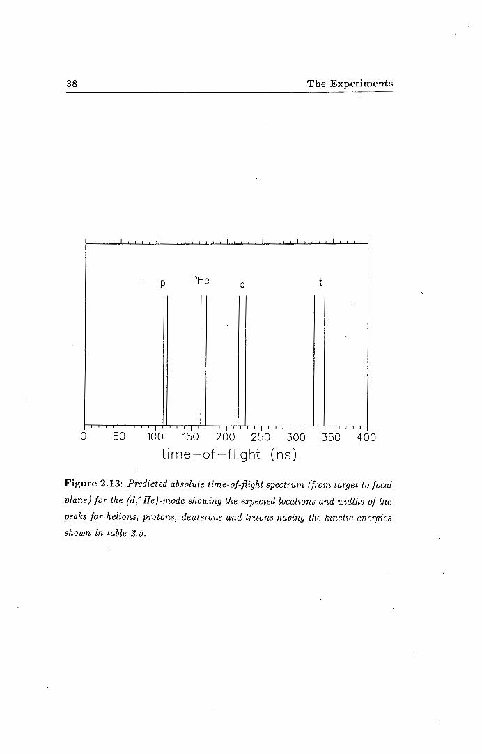
38 The Experiments.
I I I I I I I
p 3He d t
I I I I I I I
0 50 100 150 200 250 300 350 400
time-of-flight (ns)
Figure 2.13: Predicted absolute time-of-flight spectrum (from target to focal
plane) for the (d, 3 He)-mode showing the expected locations and widths of the
peaks for helions, protons, deuterons and tritons having the kinetic energies
shown in table 2. 5.

2. 7 Electronics 39
particle kinetic energy
(MeV)
p 88
t 29 3He 117
a 88
Table 2.6: Kinetic energies of particles having the same energy constant,
k, as that of a 44 Me V deuteron.
2.6.2 ( d,d)-Mode
For an assumed beam energy of 45 Me V the elastically scattered deuterons of
interest have a kinetic energy of about 44 MeV. The other particles with the
same energy constant as a 44 MeV deuteron are listed in table 2.6. Protons, 3He and a particles which have the same k value as a 44 MeV deuteron
are kinematically not allowed assuming they are produced by deuterons
interacting with 55 Mn or the constituent nuclei of Mylar. By considering
only rigidity and kinematics it is possible for tritons with an energy of
about 29 MeV to reach the focal plane along with the deuterons of interest.
Energy-loss calculations show however that 29 MeV tritons will stop in the
scintillator19 of paddle 1. These tritons are therefore not expected to appear
in the TOF spectrum since they would not satisfy the P1 · P2 trigger logic
used in the (d,d)-mode. A typical TOF spectrum acquired in (d,d)-mode,
shown in figure 2.17 (b), shows only the expected deuteron peak.
2. 7 Electronics
Signals from the VDC and paddles were processed in the spectrometer vault
(see figure 2.1), while the electronics used to measure the effective data
acquisition dead time, measure the integrated current and monitor the paddle
rate for the beam-halo measurement were located in the NAC dataroom,
where the data acquisition computer was located. In the main, commercially
available electronic modules adhering to the Nuclear Instrument Module
19The tritons have a range of 2.6 mm in this scintillator where they deposit 24.9 MeV.

40 The Experiments
(NIM) and Computer Automated Measurement and Control (CAMAC)
standards were used in the electronic set-up (see table 2.7).
2.7.1 Paddle signals
A block diagram of the electronics used to process signals associated with
the paddles is shown in figure 2.14. The output pulse from each of the four
photomultiplier tubes associated with the two paddles was fed into a linear
fan-in/fan-out channel. One of the outputs associated with this channel,
delayed by 100 ns, served as an input to an analogue-to-digital converter
(ADC) which was located in one of the CAMAC crates in the spectrometer
vault, while a second output served as the input to a constant fraction
discriminator ( CFD).
In order to get an accurate time-pickoff the two CFD outputs associated
with each paddle were fed into a mean timer, and the output from there
served as input to a discriminator. The width of the discriminator output
pulse associated with paddle 1 was made narrow (""' 5 ns) while the corre
sponding pulse width for the paddle 2 pulse was set to 20 ns in order to pick
the timing off the thinner paddle 1. In the ( d,d)-mode the latter two pulses
served as input to a four-fold logic unit (4FLU) where a paddle coincidence
(Pi · P2) pulse was generated as the event trigger20 .
In the (d,3He)-mode the Pi and P2 paddle pulses along with the output
pulse from the VDC "or" -box, Ov, were instead sent to this 4FL U, enabling
the (Pi · P2 · Ov) logic pulse to be generated as the event trigger in this
mode. One of the outputs from this 4FLU was fed to a discriminator from
which an event trigger for the CAMAC event trigger module (ETM) 2i, an
ADC gate (for the paddle pulse heights) and the experimental common stop
signal for time-to-digital converters (TDC) (which digitized the VDC drift
times) were derived. A further output channel from the 4FLU served as
the start signal for a TDC which measured the time-of-flight of rigidity-' selected particles through the spectrometer. The stop signal for this TDC
was generated by another 4FLU channel which was operated in two-fold
20The generation of an event trigger was vetoed by the VDC-associated electronics
(detailed in section 2.7.2) in the manner shown in figure 2.14. 21 Not shown in figure 2.14.

2. 7 Electronics
module
analogue-to-digital converter (ADC)
CAMAC crate controller (CC)
CAMAC current integrator interface
CAMAC differential branch extender
CAMAC event trigger module (ETM)
CAMAC scaler
constant fraction discriminator (CFD)
current integrator
discriminator
four-fold logic unit (4fLU)
gate-and-delay generator (GDG)
LED counter
level adapter (LA)
log/Jin ratemeter
logic fan-in/fan~out (FIFO)
mean· timer
paddle high voltage (HV) supply unit
time-to-digital converter (TDC)
timer
timing single channel analyser (TSCA)
VDC high voltage supply unit
VDC preamplifier/discriminator (A/D)
VDC time digitizer module (TDM)
VDC dedicated crate controller (DCC)
VDC DATABUS interface module (DIM)
VDC threshold supply module
model
LeCroy 2249A
Hytec 1180 (crate CCA2)
EDA14-5 (NAC)
Hytex 6501A
EDAlO (NAC)
Kinetic Systems 3615 Hex Counter
Ortec 934
41
Brookhaven Instruments Corporation lOOOc
Phillips 711 or LeCroy 821
LeCroy 365AL
Ortec 416A
Ortec 875
LeCroy 688 AL
Ortec 449-2
LeCroy 429A
LeCroy 624
Ortec 456
LeCroy 2228A
Ortec 719
Ortec 551
F.U.G. HCN 35-12500
LeCroy 2735
LeCroy 4291B
LeCroy 4298
LeCroy 4299
EDA47 (NAC)
Table 2. 7: Electronic modules used to process signals associated with the
paddles, VDC, beam current integration, deadtime measurement and the
CAMAC system.

42
lliieOnl ~
T log/fin
ralemeler
The Experiments
I high vollO(je I
r podd~ 2
'------1 discriminotor
cyclotron RF
Figure 2.14: Schematic representation of the electronics used to process
the paddle and VDC signals.

2. 7 Electronics 43
coincidence mode. The first input to this 4FLU was a discriminated P1 · P2
or P 1 · P 2 · Ov pulse, depending on the spectrometer mode used. The second
input was generated by attenuating and discriminating the cyclotron RF
signal. In effect, a TDC (TOF) stop was only produced when an RF signal
was coincident with an event trigger.
The monitoring of the paddle rates, required for checking the beam halo
on target, was achi~ved by feeding the paddle coincidence (d,d)-mode or
anti-coincidence (d,3 He)-mode signal from the spectrometer vault to the
dataroom where it served as input into a level adapter, the output of which
was fed into a ratemeter.
2.7.2 VDC signals
The VDC signals were processed by means of a dedicated CAMAC data
acquisition system (LeCroy 4290) which is used to handle data associated
with multiwire drift chambers. The system comprised 16-channel VDC
mounted preamplifier/discriminator (A/D) cards, 32-channel drift chamber
time digitizer modules (TDM), a dedicated CAMAC crate controller (CC)
and DATABUS interface/buffer module (DIM). A schematic diagram of the
VDC electronics are also shown schematically in figure 2.14.
Each signal22 from the A/D card served as an input to a channel on
a TDM, each occupying a single slot in the CAMAC crate. A total of
seven of these modules were used in order to process the pulses from the
VDC's 198 signal wires. In the crate used to house the TDMs there was
a dedicated crate controller (DCC), which amongst other operations, pre
processed TDM outputs, rejecting unwanted zero or full-scale values during
data acquisition. The TDMs were operated in common stop mode which
was selected by a side-panel switch on the DCC. In this mode the timing
cycle was started on receipt of a wire signal and stopped on receipt of an
experiment common trigger which was obtained by delaying by 500 ns the
output pulse from the 4FLU, which generated the event trigger as described
above. Valid data from the DCC were transferred by means of a fast bi-
22 Thresholds in 0.0-0. 7 V region could be set on A/D cards by means of a threshold
supply module (see table 2.7) which was designed and built by the NAC electronics staff.
The threshold was 0.25 V during data acquisition.
44 The Experiments .
directional DATABUS to the memory (4K x 16 bit) of the DIM located in
a slot of an adjacent CAMAC crate which housed a standard CC.
2. 7. 3 Beam-current integration
The electronics used to process pulses associated with the beam-current
integrator system are shown schematically in figure 2.15. The current from
the beam-stop was patched through to the dataroom where it was fed into
the current integrator (CI). A thousand pulses per second are generated if
this current equals the full-scale current setting on the CI. The digital output
from the CI served as input into a timing single channel analyser, the output
of which was in turn fed into a discriminator. One output from the latter
formed the input to a CAMAC scaler module, while a second was sent to
an identical scaler module which was inhibited by the busy signal from the
CAMAC crates.in the spectrometer vault. The latter scaler, in conjunction
with the CI full-scale range setting, was used to calculate the integrated
current_ corrected for. the data acquisition dead time. The full-scale range
setting from the CI was fed into a CI CAMAC interface module, which was
designed and built by N AC personnel.
2. 7.4 Dead time measurement
The deadtime of the data acquisition system was measured by using a pulser
and two scalers. The electronics used are shown schematically in figure 2.15.
The signal from an adjustable frequency pulser, which was constructed using
a timer, served as the input to a discriminator. One of its outputs served as
the uninhibited input to a CAMAC scaler module while a second output was
fed into an identical CAMAC scaler which was inhibited by the busy signal
associated with the focal-plane electronics. The number of inhibited and
uninhibited pulses recorded by the two scalers were then used to determine
the effective deadtime.

2. 7 Electronics
logic
fan-in/fan-out
veto
4-fold logic unit
discriminator
inhibited CAMAC scaler
uninhibited CAMAC scaler
45
spectrometer busy I - -
Faraday 1
cup
--r current integrator
full-scale range setting
I L
discriminator
veto .
current integrator .
CAMAC interface
l CA MAC
timing single channel
analyser
discriminator
4-fald logic unit"
inhibited uninhibited
CAMAC scaler CAMAC scaler
Figure 2.15: Schematic representation of the electronics used to measure
the effective deadtime and measure the integrated beam current.

46 The Experiments.
2.8 Data handling
The CAMAC system configuration comprised four crates, two of which
were located in the dataroom, while a further two were in the spectrometer
vault, linked to each other by means of a differential branch extender. The
CAMAC branch highway, which linked the CAMAC crates, was interfaced to
a VAX-11/750 (Digital Equipment Corporation) dedicated data acquisition
computer by means of a BiRa microprogrammed branch driver (MBD).
The MBD is a 16 bit micro-computer which controls the flow of data
and commands between the VAX and the CAMAC branch highway. It has
a 430 ns instruction execution time and is capable of transferring data from
the branch highway to the memory of the VAX via one of eight channels,
each of which acts as a direct memory access device (Kin81, Pil89b, Pil92].
In this experiment two MBD channels were used. The first channel was
used to transfer data relating to the VDC and paddles, while the second
was used to transfer scaler data. On receipt of a CAMAC look-at-me
(LAM) signal associated with one of the channels, a user-specified list of
CN AF commands23 was executed. These commands were downloaded to
the MBD from the VAX in the form of a single re-entrant data acquisition
program (DAP) which was custom-written for the CAMAC configuration
used. The transfer of data associated with the MBD scaler channel was also
controlled via CNAF commands in the DAP program. A software trigger,
which was automatically generated by the VAX every ten seconds, initiated
this transfer of data.
The data acquisition and analysis package, XSYS (Gou81, Gou83, Pil88,
Pil92], which is a modular, structured system written to support the CA
MAC branch highway and the MBD-11 branch driver, was used to process
the acquired data. XSYS enables single or multi-parameter data to be
acquired and mar.iipulated according to the user's specifications and finally
sorted into spectrum arrays. It consists of stand-alone FORTRAN subrou
tines which communicate with each other by means of two global sections of
memory called XSCOM and XDATA. The former global section is the key
23 Crate-slotNumber-subAddress- F\mction.

2.8 Data handling 47
XSYS data structure which contains control information, while the latter
holds spectrum definitions and stores spectral data.
The data from the two MBD channels used were associated with a set
of three data buffers in VAX memory. Buffers are filled by the code running
in the MBD. As each buffer was filled the XSYS sorting process, XSORT,
running on the VAX was signalled. While XSORT processed the data in
a buffer, the MBD code started filling another buffer. As soon as XSORT
had finished sorting all the events in a buffer, it in turn signalled the MBD
code that the buffer was available again for receiving new event data. An
algorithm programmed in the event analysis language (EVAL) is used by
XSORT in the sorting of data into spectra, amongst other tasks [Hol81]. If
writing to storage medium was enabled, the XSORT subprocess wrote the
raw event buffers to a digital audio tape mounted on a tape drive which was
accessed from the N AC local area network via an Infoserver 150 (Digital
Equipment Corporation).
A schematic flow diagram showing how XSORT processed the data
associated with a non-scaler event is shown in figure 2.16. The DIM word
count was first checked to see whether at least one VDC signal wire registered
a hit24 . If this was the case the spectrometer time-of-flight (TOF) spectrum
was incremented. For every event that fell within the software gate set
around the peak of interest in this TOF spectrum, the four paddle pulse
height spectra associated with the left and right photomultiplier tubes of
paddles 1 and 2 were also incremented. A FORTRAN subroutine was
then called from within the EVAL program to process data in the event
buffer relating to the DIM. This subroutine determined which VDC wires
registered hits and whether the number of wires that fired constituted an
acceptable hit pattern (see appendix C). A second TOF spectrum was
then incremented using data associated with the first TOF spectrum which
corresponded to valid VDC events. Typical TOF spectra for the two reaction
modes are shown in figures 2.17(a) and 2.17(b). For every valid VDC
hit-pattern event, the subroutine discussed above passed drift times and
associated wire numbers back to the EVAL program. These drift times
24 This check was not necessary when analysing (d,3He)-mode data because of the "or"
box .used.

48
No ddoVDCrrefre?
Yes
,,._ __ No _ __.( eveit fijs within gate?
l Yes
lb ( erertlalsrilingate?
l spectrometer mode ?
)
eren\ fdl; rihin .,rte?
Yes
COITleCI drift tine to drift listim ~o
kd~toble
trajectory ooje fall
lillin lll<J~ !,de ?
col mw to slulf voe rires
I iillSiliiiiiAinelo -+ alclirtef~
co-mfrdes
iraer!M ._ focal-jlklle co-ordioole
spectra
itrm .......,__,__~, Pll vs. FP pos11ion
Pll vs. FP posttion
event fols ritlin
Pt vs.~P 00 ·~n? Yes
Yes
The Experiments
No
No
No
No
erenl fall ritijn
Ph.gal~ on . ion ?
Figure 2.16: Schematic representation of the event analysis language
·(EVAL) algorithm used by XSYS's sorting subprocess, XSORT, to process
VDC and paddle data. PnL(R) denote the pulse height associated with
left( right) photomultiplier of the n 'th plastic scintillator paddle.

2.9 Experimental procedure 49
were then converted to drift distances by using the integral-time-spectrum
method [Bre74, Ber77, Hen87] which makes use of a lookup table.
The calculated drift distances and associated wire numbers were then
passed to a second FORTRAN subroutine which calculated the focal-plane
position and angle co-ordinates. These co-ordinates were determined by
doing a linear least-squares fit to three data points which had as one co
ordinate the drift distance perpendicular to the VDC signal wire-plane,
while the second was the distance along this plane (see appendix C). The
calculated focal-plane co-ordinates were then used to increment the focal
plane position and angle spectra. In view of a poorer signal-to-noise ratio
associated with the (d,3He)-mode further software gates were implemented
in order to improve this ratio. These software cuts are described in more
detail in section 3.1.
2.9 Experimental procedure
At the start of each data acquisition session, the XSYS process was first
initiated on the VAX. This entailed, inter alia, the execution of a command
procedure which defined the XSYS spectra and allocated associated memory; I
followed by the loading of the EVAL and DAP programs. A lookup table,
which was used to calculate focal plane co-ordinates as discussed above, was
then read into memory. The lookup table was generated from the average
VDC drift-time spectrum associated with inelastically scattered protons
from the 12 C(p,p')(E* ,....., 30 MeV) reaction at an incident energy of 66 MeV.
This "white" spectrum25 is shown in figure 2.18(a) while the corresponding
lookup table generated from it is shown in figure 2.18(b).
In order to measure accurate relative drift times with the VDC it is nec
essary that all TDC channels associated with the TDM respond identically
to a fixed time interval. In order to align26 TDC values the DCC's Autotrim
feature was used27 . This feature makes use of a crystal-controlled time mark
25 So termed because all VDC wires fire. 26 This was necessary if the CAMAC crates in the spectrometer vault were off-line before
the start of a data acquisition session. 27 A threshold of+ 0.7 V was used on all A/D cards during this procedure.

50 The Experiments
(a) p
d
(j) c c
.o _c
10° u ""- 0 30 60 90 120
(/) 105 -+-' c
(b) ~ 0 u
d 103
10°-+-r-r-r-,.-,-,c'-r-T-r'r-r--l'-~r'r'-t-r'T--M-~c"r-T--r-r..,..,._~...,...,.-,...,-,--rl-o 30 60 90 120
time-of-flight (ns)
Figure 2.17: Typical time-of-flight spectra associated with rigidity-selected
reaction products that reach the spectrometer focal-plane detector array and
result in a satisfactory VDC hit pattern. {a} Spectrum acquired in {d, 3 He)
mode The predicted locations of the proton, deuteron and tritori peaks are
shown, along with the expected width of the helion peak. {b} Spectrum
acquired in {d,d}-mode with the expected width of the deuteron peak shown.

2.9 Experimental procedure
1200
1000
Q) c 800 c 0 r. 0
-........ 600 (/) +' c ::J 0 400 0
200
0
,...... 1.2 •(/) c
·;:; 0
1.0 0.. (/)
Q) \....
·30 0.8 I 0 c 0.6 O'
~ Q) 0.4 0 c 0 +' (/)
0.2 'a +' .,__ ·c 0.0 -0
250 300 350 400
drift time (channel)
450
51
(a)
(b)
500
Figure 2.18: (a) Typical "white" VDC average drift-time spectrum
associated with inelastically scattered protons from the 12 C(p,p' )(E' ,...., 30
Me VJ reaction at an incident energy of 66 Me Vand spectrometer angle of
18°. One drift-time channel is equivalent to ,...., 0. 9 ns. (b) The lookup table,
which provides a mapping of drift time to drift distance, generated from the
data shown in (a).

52 The Experiments
generator to generate alternating zero- and full-scale TDC values which are
used to trim the pedestals and gains of all the TDC channels to the same
values. This procedure was implemented in a manner which calibrated' out
all variations in times due to variations in the VDC-mounted A/D cards and
differences in the lengths of cables connecting these cards with the TDMs.
Preparations were then made to acquire (d,d)-mode data. This in
volved changing the event trigger logic to P1 · P2 and setting the quadrupole
and dipole magnetic fields such that deuteron trajectories associated with
the 55Mn(d,d) 55Mn(g.s.) reaction corresponded closely with the central
momentum trajectory through the spectrometer. The magnetic fields were
set remotely from a PC in the dataroom which was connected to the NAC
local area network. The required spectrometer magnet currents were cal
culated by means of a FORTRAN program which utilizes measured two
dimensional median plane field maps of the spectrometer's magnets to cal
culate the quadrupole and dipole currents necessary to cause a particle of
a specific energy to travel along the central-momentum trajectory through
the spectrometer. The paddle and VDC high voltages, and target angle
were then set remotely from the dataroom. Once the beam was delivered
to the spectrometer vault, the beam spot on target was optimized with the
aid of the viewer-target and the halo reduced by monitoring the paddle
rate (see section 2.2). The spectrometer resolution was then optimized by
adjusting the spectrometer's K- and H-coil currents to cancel out the effect
of kinematics [NAC92]. This was done with the aid of a two-dimensional
correlation spectrum in which the deuterons' time-of-flight (TOF) through
the spectrometer was plotted as a function of their position along the focal
plane. With the resolution of the spectrometer optimized, it is expected
that the focal-plane position of a peak should show no dependence on the
associated TOF. In this case straight-line loci parallel to the TOF axis were
expected. The effect of coil current adjustments on the TOF versus position
spectrum is shown in figure 2.19. K- and H-coil currents were optimized
by studying the expected locus of elastically scattered deuterons off 55Mn.
Deuteron scattering data were were then acquired using these coil currents.
The duration of runs was typically twenty minutes.
The trigger logic was then changed to P1 · P2 · Ov and spectrometer fields
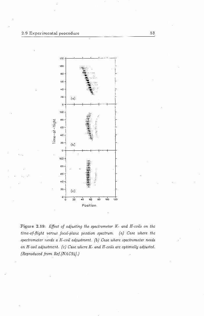
2. 9 Experimental procedure
~
.c 01 -I -0 I
Q)
E f-
100
60
60
~o
20 (a)
0
100
60
60
40
20 (b)
0
100
80
60
20 (c)
1,;~~.'~/'
iL! ·~QI['·- . '~;'
,!I.I; :'Ill· ,.,.;,:,.-.-. ':'1¥·· ,,,..,,.,." .... ",·1-.;:·:·
·""ti ."".'·
'·iijif"
o-<-~~~~~~~~~~--+
0 20 40 60 80 100 120
Position
53
Figure 2.19: Effect of adjusting the spectrometer K- and H-coils on the
time-of-flight versus focal-plane position spectrum. (a} Case where the
spectrometer needs a K-coil adjustment. (b) Case where spectrometer needs
an H-coil adjustment. (c} Case where K- and H-coils are optimally adjusted.
(Reproduced from Ref.[NAC94J.)

54 The Experiments.
set to detect helions associated with the (d,3 He)-mode. Fields were set so
that hclions associated with a 54 Cr excitation energy of"' 3 MeV followed
.the central-momentum trajectory through the spectrometer. The total 54 Cr
excitation energy range available with one setting of the spectrometer's
magnetic fields in the (d,3He)-mode was therefore "' 6 MeV, which was
sufficient for the purpose of this study. Since the (d,3 He)-mode event rate
was much lower than the (d,d)-mode event rate it was not feaSible to optimize
the K- and H-coil currents in the manner described above. Instead the coil
currents were kept the same as for the (d,d)-mode. The duration of runs
was typically five hours.
After acquiring the (d,3He)-mode data-set the scattering chamber was
vented to allow the spectrometer angle to be changed. The spectrometer
and target angles were then changed while the quadrupole and dipole fields
were being set to acquire the next set of (d,d)-mode data. In this manner
the spectrometer modes were cycled.

Chapter 3
Analysis of Pickup Data
Data reduction and analysis of data acquired while operating the spectrome
ter in the (d,3He)-mode is described in this chapter. The generation of focal
plane position spectra associated with the helions from the 55Mn(d,3He) 54 Cr
reaction at an average1 incident energy of 45.6 Me V is described first.
Thereafter the momentum calibration of the spectrometer's focal plane, the
identification of 54Cr final states and the calculation of the corresponding
pickup differential cross sections are discussed. In concluding the chapter,
the extraction of pickup spectroscopic factors from the measured angular.
distributions by means of a distorted-wave Born approximation (DWBA)
formalism is described.
3.1 Data replay
Focal-plane position spectra for helion events acquired in the (d,3He)-mode
were generated through off-line replay of event-by-event data using XSYS,
the same software package used during data acquisition. The data sorting
algorithm used in the EVAL program was almost identical to the one used
during data acquisition (section 2.8).
Two of the modifications introduced into the sorting algorithm related
to the subroutine which calculates the focal plane co-ordinates. A VDC wire
hit-analysis discussed in appendix B showed that for a valid event, the num-
1 Mean beam energy delivered as discussed in section 2.2.

56 Analysis of Pickup Data
ber of signal wires which are expected to register hits should range between 5
and 8. On the basis of a study made of the VDC intrinsic efficiency using the
deuteron elastic scattering data (see appendix F), this condition was relaxed
during final replay so that a VDC event was considered valid only if between
3 and 10 wires registered hits. During data acquisition the focal-plane co
ordinates were determined from least-squares fits to only three data points
relating to measured VDC data. In order to improve the resolution in the
focal-plane position spectra, fits were made to between three and seven data
points during off-line analysis. A more detailed description of the algorithm
used to calculate focal-plane co-ordinates can be found in appendix C.
Helion events were selected by means of a software gate set on the
helion peak appearing in the raw time-of-flight (TOF) spectrum (see also
section 2.6.1). An example of such a gate setting is shown in figure 3.l(a).
VDC data corresponding to the selected times-of-flight were then used by a
sorting subroutin,e, which was called from the main EVAL program, to cal
culate the focal-plane position spectra. One of the criteria used in selecting
valid VDC data was whether their drift times fell within an acceptable range.
This range was defined by a software gate set on an average VDC drift-time
spectrum as shown in figure 3.2. During data acquisition a rough setting
of this gate was used. By iteratively applying different gate settings and
recording the corresponding helion yield in the focal-plane position spectrum
during data replay, the width of this gate was optimized.
In order to improve the signal-to-noise ratio in the (d,3He)-mode focal
plane position spectra, additional spectra were introduced on which software
cuts were implemented. The first of these involved the focal-plane angle
spectrum. Since the VDC was positioned at an angle of 35.75° w.r.t. the
central-momentum trajectory through the spectrometer (see figure 2.6),
valid events through the spectrometer should yield an event distribution
in the focal-plane angle spectrum with its centroid corresponding to this
angle. In order to exclude events which fall outside this distribution, a
gate was also set on the focal-plane angle spectrum. A typical setting of
such a gate is shown in figure 3.3(a). Software gates were also set on the
two-dimensional correlation spectrum in which the pulse heights associated

3.1 Data replay 57
1500
1250 (a) Q) c 1000 c 0
£ u 750 ............ en _..., c :::i 0
500 u
250
0 35 40 45 50 55
1500
1250
Q)
(b) c 1000 c 0
£ u 750 ............ en _..., c :::i 0
500 u
250
0 35 40 45 50 55
time-of-flight (ns)
Figure 3.1: Helion time-of-flight spectra. (a) Raw spectrum with software
gate used. (b) Spectrum corresponding to one above associated with valid
VDC data.

58
Q) c c 0
_c u
""-(f) +-' c ::J 0 u
Analysis of Pickup Data.
4000
3000
2000
1000
o-k~~::::::'.~~~~~~~
100 180 260 340 420 500
average drift time (channel)
Figure 3.2: Typical VDC average drift-time spectrum. ·One drift-time
channel is equivalent to ,...., 0. 9 ns. A software gate set to encompass an
optimal drift-time range is also shown.

3.2 Momentum calibration 59
with the left2 and right photomultiplier tubes of paddle 1 respectively were
plotted as a function of focal-plane position. An example of such a spectrum
along with the corresponding applied software gate is shown in figure 3.3(b).
Finally gates were also set on the two-dimensional spectra in which the pulse
heights associated with the photomultiplier tubes of paddle 1 were plotted as
a function of TOF through the spectrometer. Figure 3.3(c) shows a typical
example of a gate set on one of these spectra.
3.2 Momentum calibration
The momentum calibration of the focal plane was obtained using a sim
ilar approach to that used by Niwano et al. [Niw82]. In this approach
the peak centroids of prominent (more than 100 counts) 54 Cr final states
were determined followed by a calculation of the helion momenta associated
with transitions to these states. A least-squares fit to the centroids and
momenta associated with each of these states was then performed to obtain
a momentum calibration.
Peak centroids of prominent 54 Cr final states were determined by least
squares fitting Gaussian lineshapes to these states as were seen in the focal
plane position spectra. The peak fitting was done using the computer
program FIT2.l [Neu94]. Because of the improvement in the signal-to
noise ratio achieved as a result of the additional software cuts discussed
above, the background in the spectra was assumed to be negligible during
this procedure. MINUIT [Jam75, Jam89], the non-linear least-squares min
imization program selectable from FIT2.l, was used in order to calculate
uncertainties in parameters by taking into account parameter correlations.
No constraints were placed on fit parameters during the fitting procedure.
Examples of typical fits obtained are shown in figure 3.4(a).
The momenta of the helions associated with transitions to these promi
nent states were calculated using a nonrelativistic kinematics formalism
[Mar68, Lu84] which required as input the deuteron beam energy, spectrom
eter angle, the Q-value associated with the 55 Mn(d,3He) 54 Cr(g.s.) reaction
and the excitation energies of known 54 Cr final states as most recently
2 From the perspective of a rigidity-selected particle approaching the focal plane.

60
(a)
(b)
(c)
(j) c c 0
...c 0
""' (/) .._, c ::J 0 0
+-' .r:. -21 Q)
.r:. I
Q) en
""5 a.
~ "'Cl "'Cl 0 a.
+-' .r:. oi
·a; .r:. I Q) en
""5 a.
10'
10J
10° 10
50
0
89
50
73
Analysis of Pickup Data
20 30 40 50 60
focal-plane angle (deg)
20 40 60 80 100 127
focal-plane position
·i! l!llllill!i ........
80 90 100 110 120 127
time-of-flight
Figure 3.3: Typical examples of spectra with respective software gate
settings used to improve the signal-to-noise ratio in focal-plane position
spectra {a) A focal-plane angle spectrum. {b) Density plot of pulse height
associated with the left photomultiplier of paddle 1 is ploUed versus focal
plane position. {c} Density plot of pulse height associated with the left
photomultiplier of paddle 1 versus time-of-flight .through the spectrometer.

3.2 Momentum calibration
100
~ 80 c: 0
J:: < 60 en +' c: 6 40 u
20
(a) 3.160 MeV
> > Q) Q)
:::;: :::;:
Ll) N Ll) N co N 3.074 MeV n ,,)'- /
1.824 MeV 0.835 MeV
0-t:Jl!!lL..."-" ........... ~UU.l......__.~ ........... \llL-L--~ ......... "l--'~~~---...-............. '-"'-........... ----+-
600 800 1000 1200 1400 1600
focal-plane position (channel)
4.85 -+----~----~---~---~-----r-
--;:;- 480 '-... > Q)
L
E 475 ::::i • +' c: Q)
E 0 470 E
(b)
465-+-------...----~~---..,-----.------+-
600 800 1000 1200 1400 1600
focal-plane position (channel)
61
Figure 3.4: (a) Typical example of a focal-plane position spectrum showing
the location of 54 Cr final states used to obtain a momentum calibration of
the focal plane. Gaussian lineshapes fitted to the identified states in order
to determine their centroids are shown. The data shown were acquired at a
spectrometer angle of 3fI'. (b) Quadratic least-squares fit to data associated
with the selected states shown in (a).

62 Analysis of Pickup Data.
reported [J un93]. Pairs of momentum and centroid co-ordinates were then
least-squares fitted to obtain the momentum calibration. F-test analyses of
reduced chi-squared (x~) values obtained for fits made using polynomials,
varying in order between one and three, showed that a polynomial of order
two was the optimal function to use in describing the relationship between
focal-plane position and momentum. All final fits were therefore performed
using a quadratic function. The co-variance matrix associated with each fit
was used later in calculating the uncertainty in the excitation energies of
states identified (section 3.3).
The 15N(g.s.) peak reached through the 160(d,3He) 15 N reaction was
. clearly seen in almost all the focal-plane position spectra. The first and
second excited states in 54 Cr were also prominent at all spectrometer an
gles. A rough momentum calibration using only the 54 Cr(l), 54 Cr(2) states
and the 15N(g.s.) was therefore first determined for each data-set. These
calibrations were then used to ascertain whether any other prominent states
corresponded, to within a 40 ke V uncertainty3 , with any of the 54 Cr adopted
levels. Additional states in 54 Cr identified in this way were then used
along with the first two excited states in 54 Cr to obtain a final momentum
calibration. Typically six prominent 54 Cr final states ranging in excitation
energy up to "' 4 MeV were used to obtain final momentum calibrations. ·
An example of a focal-plane position spectrum revealing the states used to
obtain a final momentum calibration is shown in figure 3.4(a), while the
quadratic fit to the centroids and momenta associated with these states is
shown in figure 3.4(b).
In the nonrelativistic approximation the relationship between momen
tum resolving power, b.f, particle energy E and energy resolution, 6..E, is
given by 6..E 26..P E ----p-· (3.1)
The energy resolution associated with each focal-plane position spectrum
analysed was calculated with equation 3.1, using the momentum calibration
obtained from this spectrum and the FWHM of the peak associated with
the transition to the 54 Cr(l) state seen in the spectrum. The resolution was
3This value was chosen since the average spectrometer resolution was ""' 40 keV.

3.3 Identifying observed final states 63
found to vary between 32 and 60 keV, yielding an average energy resolution
of "' 40 ke V (FWHM).
3.3 Identifying observed final states
In order to identify less prominent and unresolved states, all peaks in the
focal-plane position spectra were fitted with Gaussian lineshapes so as to
determine their centroids. The peak-fitting was again performed using the
program FIT2.l together with the assumption that the background in the
spectra was negligible. Fits, in which all parameters were allowed to vary,
were first made to prominent well-resolved peaks in each spectrum in order to
determine an average peak FWHM for that spectrum. Gaussian functions
with .. widths fixed to these average FWHM were then again fitted to less
prominent,and unresolved states in all spectra. The excitation energies of all
states seen in a particular focal-plane position spectrum were then calculated
with standard formulae [Mar68, Lu84], using the peak centroids associated
with these states as determined from the peak fitting and a corresponding
momentum calibration. If a particular 54 Cr final state, k, excited through
the 55 Mn(d,3He) 54 Cr(k) reaction was observed at the same excitation energy
(to within statistical uncertainties) at a minimum of six spectrometer angles,
the differential cross sections associated with the transition to this state
and the corresponding spectrometer angles, were considered to constitute
a pickup angular distribution. Since the counting statistics associated with 54 Cr final states observed in spectra for angles(} ~ 30° were rather poor, only
data acquired in the 6°-30° angular region were used to extract spectroscopic
factors. The mean excitation energies4 of the twenty-four 54 Cr states which
were found to satisfy the criterion stated above from these data are tabulated
in table 3.6, while an example of a focal-plane position spectrum showing
the location of identified 54Cr final states is shown in figure 3.5.
4 Note that the values above 3.926 Me\! excitation differ by a few keV from those
quoted in Ref. (New96]. This is due to an error in the momentum calibration which was
discovered and subsequently corrected after the paper was in press.

64
(])
c c 0
_c
Analysis of Pickup Data
1000 __ _._______. _ __.__~-~--'--~---r-55Mn( d,
3He )
54Cr Ed 46 MeV e 14°
750 > Q.J
~ >
Q.J
~
~ 500 ll) t') co ci
(/) +-' c :J 0 u
x20
250 '(/}'
: ci>:
0-+--"'-"-.,,......~.-.;..l-IZ'-.l.L..ll.llJ~ ............ ...l.l.....ll .......... ~....J...\-~__,,J_~...6-'l.14-~--+-
o 500 1000 1500 2000
position along focal plane (channel)
Figure 3.5: Example of a focal-plane position spectrum associated with the 55 Mn{d, 3 He)54 Cr reaction showing the location of some of the 54 Cr final
states observed. The data shown were obtained at a spectrometer angle of
14°. The 15 N(g.s.) peak is due to {d, 3 He) reactions on the oxygen nuclei
present in the Mylar target-backing used.

3.3 Identifying observed final states 65
The total uncertainty, b.E*, in the mean excitation energy of each of
these states was calculated using the relation:
(3.2)
where
• 6.EA. is the type A (statistical) uncertainty5 associated with the state's
excitation energy and
• 6.EB is the type B (non-statistical) uncertainty associated with this
state's excitation energy, evaluated by non-statistical means.
The former uncertainty was assumed to be equal to the standard deviation
associated with the mean excitation energy for a particular state, while the
latter uncertainty was found by averaging in quadrature over the type B
un_certainties (at the ±la level) associated with each excitation energy. The
last mentioned uncertainties were calculated using the relation:
(3.3)
where
• 6.E~ is the energy uncertainty stemming from the uncertainty in the
centroid position for each state as determined from the peak-fitting
procedure,
• 6.E:n_ is the energy uncertainty stemming from the uncertainty in the
parameters obtained from the co-variance matrix associated with each
momentum calibration and
• f = 0.46 is the numerical factor used to make estimates of standard de
viations from a trapezoidal probability distribution (see appendix G).
The total uncertainty in excitation energy of the twenty-four states observed
varied between 1 and 11 ke V. These uncertainties are also tabulated in
table 3.6. Only two states, observed at excitation energies of 5.574 MeV
5See appendi~ G for an overview of treatment of experimental uncertainties adopted
in this study.

66 Analysis of Pickup Data .
30
10
0-+-.-~~~~~~~~--,-r~~~~~~r-r-.~--,-r+
4.00 4.25 4.50 4.75 5.00 5.25 5.50 5.75 6.00
excitation energy (MeV)
Figure 3.6: Plot of the 54 Cr excitation region screened by the 15 N(g.s.) peak
versus spectrometer angle. The 15 N(g.s.) is reached through 16 O(d, 3 He)1 5 N
reactions in the Mylar backing of the target.
and 5.776 MeV respectively, did not correspond with the adopted levels for 54 Cr [Gon87, Jun93] to within the calculated uncertainties.
Impurity states in focal-plane position spectra arising from (d,3He) re
actions on impurities in the target were identifiable since their lo_cation in
relation to 54Cr excitation energy displayed a systematic shift as a function
of spectrometer angle. The most significant impurity state seen was the 15 N(g.s.) reached by deuteron interactions on oxygen in the Mylar backing.
Because the Mylar was relatively thick there was concern that the 15N(g.s.)
state would completely screen part of the 0-6 MeV excitation region under
study. The excitation region corresponding to the 54 Cr residual nucleus
which was found to be screened by this state as a function of spectrometer
angle is shown in figure 3.6. It is seen from this figure that no excitation
region was completely screened for all .spectrometer angles.
3.4 Cross sections
The absolute centre-of-mass ( c.m.) differential cross section associated with
the transition to the kth final state, reached via the 55 Mn(d,3 H~) 54 Cr(k) reaction, at a spectrometer angle e and corresponding c.m. angle Bc.m., was

3.4 Cross sections 67
calculated using the formula
(3.4)
where
• J is the Jacobian used to transform differential cross sections from the
laboratory to the c.m. system,
• Yk is the number of helions, associated with the reaction, which are
detected at the spectrometer's focal plane per unit time interval,
• cos~ is the factor used to correct the target thickness since the target
angle was always set to half the spectrometer's angle6 ,
• Nd is the number of deuterons incident on the target per unit time
interval,
• ~n is the solid angle subtended by the entrance collimator to the
spectrometer,
• nt is the number of 55 Mn nuclei per unit volume in the target,
• Tk6oo is the transmission efficiency through the k = 600 spectrometer
for the helions of interest,
• L is the effective fractional livetime of the data acquisition system,
• Ep is the efficiency of the plastic scintillator at detecting the helions of
interest and
• Ev is the VDC efficiency at detecting the helions of interest.
The determination of the quantities delineated above are discussed in more
detail below.
6 See section 2.4.

68 Analysis of Pickup Data.
3.4.1 Jacobian
.Jacobians were calculated using standard nonrelativistic kinematics [Mar68,
Lu84]. The energy spread in the beam and the uncertainty in scattering
angle because of the finite in-plane angular acceptance cause uncertainties
in the .Jacobian. Assuming a JO keV spread in the beam energy and a
0.5° uncertainty in 0, the uncertainty in the .Jacobian typically amounted to
0.013.
3.4.2 Yields
Helion yields were determined from the focal-plane position spectra which
were generated in the manner described in section 3.1. These yields were
determined by means of two approaches, both of which assumed the back
ground in the spectra to be negligible. In the case of free-standing, resolved
states (for example the 54Cr states at 0.835 MeV and 1.824 MeV shown in
figure 3.4 and the 5.574 MeV and 5.776 MeV states shown in figure 3.7) Yk
was determined by summing the counts in the peak of interest. The yield
associated with such peaks was considered to be distributed over j channels,
each of which contained s(j) counts, so that
Yk = 2:s(j). j
(3.5)
It was assumed that s(j) followed the usual Poisson counting statistics so
that the type A (statistical) uncertainty in Yk was given by y'Yk.
In the case of unresolved states the yield associated with each of the
states was determined by a combination of the summing procedure described
above and the Gaussian peak-fitting procedure described in section 3.3.
Gaussian lineshapes having FWHM values fixed to an average value, de
termined from' fits to resolved states in a particular spectrum; were first
fitted to these states. A typical fit to a set of unresolved states is shown in
figure 3.7. Consider the case in which n Gaussians were fitted to a region of
the spectrum spanning m channels. Let the area7 under the nth Gaussian
and the total number of counts in the region of the focal-plane position
7The yield associated with a particular Gaussian lineshape parameterized by height A
and standard deviation a is given by Vf; A a.

3.4 Cross sections 69
350 55Mn( d,
3He )
54Cr
300 Ed 46 MeV isN(g.s.)
e = 26° /
Q) 250 c c 0 200 > Q)
_L 2 u
"'- ~ (f) 150 ...j-.J lf)
> > c \ Q) (])
::J 2 2 0 > > <D O'.)
u 100 (]) Q) <D 2 2 I")
~ (j,
'<!" '<!" '<!" r--
l I 50 ~
0 200 300 400 500 focal-plane position (channel)
Figure 3. 7: A typical fit to a set of unresolved final states in order to
determine helion yields. The widths of the Gaussians lineshapes used to
fit 54 Cr final states were fixed to an average value determined from fits to
resolved 54 Cr states observed in the same spectrum. The yield associated
with the 5.574 Me V and 5. 776 Me V states were determined via a summing
procedure (see text for details). The 15 N(g.s.) is reached via {d, 3 He)
reactions on oxygen present in the Mylar target-backing used.

70 Analysis of Pickup Data .
spectrum considered be denoted by An and Ytot respectively. The yield
associated with the kth state, Yk, was then determined using the relation:
where
yk = Ak Ytot LnAn
Ytot = L .s(m). m
(3.6)
By using the above relation, mismatch between the assumed Gaussian line
shape and the actual peak shape is taken into account when determining
yields. The type A uncertainty associated with the Yk was taken to be equal
to the uncertainty associated with Ak· This uncertainty was obtained from
the program FIT2. l.
To assess whether helion yield was lost as a result of the additional
software cuts used to improve the signal-to-noise ratio (section 3.1), the
yield associated with the transition to the 54Cr(l) final state was studied
as a function of various cuts. In the worst case the helion yield was found
to be reduced by,....., 43 so that the uncertainty (la) associated with yields
stemming from the setting of software gates mentioned above was estimated
to be ~ 2% using a trapezoidal probability distribution (see appendix G).
The average uncertainties associated with the pickup differential cross sec
tions due to counting statistics ranged between 24% (for the transition to
the 54Cr ground state) and 3% (for the transition to the state observed at
3. 788 MeV excitation).
3.4.3 Incident flux
Nd, the number of deuterons incident on the target for the same time interval
in which Yk helions were detected was determined from the relation:
N _ (Nci) (F S) d - 1000 e (3.7)
where Nci is the number of digital pulses generated by the current integrator
in response to the current from the beam-stop, F S is the current integra
tor full-scale setting set during data acquisition and e is the fundamental
unit of electric charge. The current integrator's (see table 2. 7) technical
specifications state that current can be read to an accuracy of 0.02%. In

3.4 Cross sections 71
order to accommodate any contribution to the uncertainty from calibration
adjustments, a maximum type B (non-statistical) uncertainty of 13 was
assumed. This was again assumed to be drawn from a trapezoidal proba
bility distribution in order to extract an estimated standard deviation. The
uncertainty in the accumulated charge was thus taken to be 0.53.
3.4.4 Solid angle
Since the distance between the target and the entrance collimator of the
spectrometer was much larger than the dimensions of this collimator, the
solid angle, .6.0, subtended by this collimator at the target was calculated
by dividing the area of the collimator aperture by the target-to-collimator
distance [Kno89] (see figures 2.2, 2.8, 2.9 and 2.10). The solid angle was
therefore calculated using the relationship:
· .6.0 = 7rr2 + (l - 2r)2r £2 (3.8)
where 2r is the width of the collimator, l is the length of the collimator
slit and L is the distance from the centre of the target to the back of the
collimator. For both collirnators used in the normal- and the small-angle
mode, .this solid angle amounted to 1.34 rnsr. The total uncertainty in
.6.D, calculated by propagating the experimentally measured uncertainties
associated with the target-collimator distance and collimator dimensions in
the normal manner, amounted to 0.3%; while the uncertainty in .6.0 due to
beam-spot size was found to be negligible.
3.4.5 Target nuclear density
The number of 55 Mn nuclei per unit volume, nt, was calculated using the
relationship
(3.9)
where t is the thickness of the 55 Mn layer, p is the bulk density of 55 Mn, NA
is Avogadro's constant and M is the atomic mass of 55Mn. The uncertainty
in the nt sterns from the uncertainty associated with thicknesses determined
using the computer program RUMP (see section 2.4). The latter uncertainty
is estimated to vary between 53 and 10%. A 103 type B uncertainty was

72 Analysis of Pickup Data .
assumed. Using a trapezoidal probability distribution, the uncertainty in nt
at the one standard deviation level amounted to 5%.
3.4.6 K = 600 transmission
In appendix D a study of the transmission through the spectrometer as
a function of size of its entrance collimator is described. In this study,
conducted by means of a variable-slot collimator, it was found that 100%
transmission was still achieved when using a collimator slot which has a
width (or height) of less than or equal to 55.0 mm. In view of the collimator
geometry used in this study (see section 2.3.3), Tk600 was therefore taken to
be 100% in the evaluation of all differential cross sections.
3.4. 7 Livetime
The effective fractional livetime of the data acquisition system was measured
using the busy signal associated with the focal-plane electronics as described
in section 2. 7.4. The busy signal was generated whenever the VDC TD Cs
were busy digitizing, data was being transferred from the dedicated crate
controller to the databus interface module or when there was a paddle signal.
The livetimes associated with the data-sets analysed were typically 96% and
was never less than 89%. The corresponding deadtimes were accounted for
in hardware by inhibiting pulses from the current integrator whenever a
busy signal was present.
3.4.8 Paddle efficiency
The efficiency of the paddle at detecting the helions of interest, Ep, can be
written as the product [Kno89]
(3.10)
where Ep9
and EP; are the paddle geometric and intrinsic efficiencies, respec
tively, for detecting these helions.
The paddle geometric efficiency was checked at () = 18° by sweeping
the helions associated with the transition to the 54Cr(l) peak across the
focal plane by adjusting the magnetic field of dipole 2. A plot of relative

3.4 Cross sections
,---... 2 go-+-~~~~'~~~-----'--'~~~-'--'~~---''~~~--J
c ::J
..0 80 -L 0 '-'
-
70 - -
~ 60- ~.:~.~:~}~.:~J~:~:~.~~-~:~:i~:.~:~:~:~.~,:~:~ -(/) (/)
0 \...
u
0 ...., c (j) \... (j) -~ -0
50 -
40-
30-
20 ' 100 420
55Mn( d, 3He )54Cr( 1)
E = d
46 MeV
e 18° -
' ' ' 740 1060 1380 1700
peak centroid (channel)
73
Figure 3.8: Relative differential cross section for 55 Mn(d,3 He)54 Cr(1) (Ed
= 46 MeV,e = 18°) reaction versus centroid of the 54 Cr(1) state along the
focal plane. The dashed line represents the mean value while the dotted lines
are located ± fo from the mean.
differential cross section8 associated with the 55Mn(d,3He) 54Cr(l) (Ed = 46
MeV, e = 18°) reaction as a function of the centroid of the 54Cr(l) peak
along the focal plane is presented in figure 3.8. Since the cross sections
were found to be consistent to within statistical uncertainties, the paddle
geometric efficiency was taken to be 100%. It is rare for primary charged
particles not to produce some sort of ionization or excitation interaction in
the active detecting material [Kno89]. In view of this and the fact that the
thresholds on the constant fraction discriminators which were used to process
the paddle signals were set to a minimum, the paddle intrinsic efficiency at
detecting helions was assumed to be 100% as well. This was checked by
studying the ratio of the photomultiplier-tube count rates as is normally
done.
8 Calculated by dividing the yield associated with the peak in the focal-plane position
spectrum, by the product of the integrated current and the VDC efficiency.

74 Analysis of Pickup Data.
quantity I symbol I % uncertainty I yield y 3-24 (type A)
:S 2 (type B)
solid angle t..n < 1
incident deuteron flux Nd < 1
target nuclear density nt 5
Jacobian J '"'-' 0.01
Table 3.1: Breakdown of uncertainties associated with quantities appearing
in equation 3.4 which were used to calculate the c.m. differential cross
sections for th~ 55 Mn(d, 3 He)54 Cr (Ed= 45.6 Me VJ reaction.
3.4.9 VDC efficiency
The VD C's efficiency, Ev, is an indication of how efficient (relative to that of
the plastic paddles) it is at detecting charged particles at the focal plane. As
in the case of the paddles, the VDC efficiency is the product of a geometric
and intrinsic efficiency:
(3.11)
It was established by means of a horizontal drift chamber (HDC) (located
behind the VDC) which measures focal-plane position in the vertical direc
tion, that the rigidity-selected particles are well-focussed9. In view of the
above and the consistency shown in figure 3.8, the VDC geometric efficiency,
Ev9, was taken to be 100%. The intrinsic VDC efficiency was obtained from
an analysis of (d,d)-mode data as discussed in section F.l of appendix F.
An average efficiency of 99% was obtained.
3.4.10 Results
A breakdown of the uncertainties associated with the pickup differential
cross sections is given in table 3.1. The combined uncertainty (la) associated
with the target thickness, current integration, solid angle and setting of
software gates was estimated to be '""' 6%. The measured c.m~ angular
9 The FWHM of a peak is typically 2.0 cm.

3.5 DWBA analyses 75
distributions, associated with the transition to the twenty-four 54Cr final
states observed, and which were used in the DWBA analyses, are plotted
in figures 3.9-3.15 and are tabulated in appendix E. Only the uncertainties
contributing to random scatter, obtained by combining in quadrature the
uncertainty due to counting statistics and the estimated uncertainty (la)
in target thickness, are shown in these figures. The latter component was
included since two targets were used to measure the angular distributions.
3.5 DWBA analyses
Pickup spectroscopic factors, C2 Sijl (with C denoting the Clebsch-Gordan
coefficient), are associated with the transfer of a proton, having orbital
and total angular momentum f and j respectively, leading to the ith final
state of 54Cr in the 55Mn(d,3He) 54Cr(i) reaction. These were determined by
normalizing a distorted-wave Born approximation (DWBA) angular distri
bution to the measured angular distribution. The normalization was done
by minimizing x2' defined by:
x2 = L (aexpt(Bc.m.)i - C2Sijl aca1c(Bc.mJijl)
2 (3.12)
Oc.m. .6.aexpt ( Bc.m.)i
where aexpt(Bc.m.)i is the experimentally measured c.m. differential cross
section associated with the transition to the ith final state, .6.aexpt(Bc.m.)i is
the uncertainty (obtained by combining in quadrature the uncertainty due
to counting statistics and estimated uncertainty (la) in target thickness)
associated with this cross section and aca1c(Bc.m.)ijl is the corresponding
DWBA differential cross section.
DWBA differential cross sections were calculated with the computer code
DWUC'K4 [Kun93] using a local, zero-range formalism. Non-local and finite
range corrections were not applied since in the first instance the interest is
in relative spectroscopic factors which have been shown to be insensitive to
the inclusion or omission of these corrections [Cle77, Cle91]. In the case
of the (d,3He) reaction, DWBA differential cross sections are related to the
correspl)nding DWUCK4 cross sections via the relation
No aca1c(Bc.m.) = 2j + l aowUCK4(0c.m.), (3.13)

76 Analysis of Pickup Data
where j is the total angular momentum transfer and N 0 is the Bassel nor
malization factor, equal to 2.95 in the case of the (d,3He) reaction [Bru77,
Kun93].
3.5.1 Optical-model parameters
Part of the input needed to calculate anwuCK4 ( Bc.m.) is a specification of the
potentials needed to generate the distorted wave-functions for the entrance
and exit channels, and to calculate the bound-state wave functions.
An optical potential having a form identical to the one used by Bojowald
et al. [Boj88] to obtain a global potential for deuteron scattering up to
100 MeV, was used to obtain the distorted wave-functions for the d + 55Mn
channel. This potential, which comprised Coulomb, central, imaginary
volume, imaginary surface and real spin-orbit terms [Mar70], had the form·
U(r) = Vc(r)-Vfv(r,flu,av)-i[Wvodw(r,Rw,aw) (3.14)
d ] ( 1i )2
1 d - 4awWsurf-d fw(r, Rw, aw) + Vz.s -- (£ · s)--d f1.s(r, R1.s, a1.s)· r m1rc r r
·The nuclear potential formfactors in the expression above had a Saxon
Woods form given by:
(3.15)
1 with radius Rk = rkA3 and diffuseness ak. The Coulomb potential had the
standard form:
v; ( ) _ ZpZte2 [3-( If- )2
] R c r - 2Rc 'r < c (3.16)
_ ZpZte2 > R
- T ,r C
where Zp is the charge of the projectile, Zt is the charge of the target
and Re is the Coulomb radius. The values of the parameters used in
conjunction with the potential form above are given in table 3.4. These
parameters were obtained from an analysis of the angular distribution for
the 55 Mn(d,d) 55Mn(g.s.) (Ed = 45.6 MeV, 6° ~ e ~ 48°) reaction. This
analysis which is detailed in appendix F, was performed using the computer
code SNOOPY8 [Sch82] which utilizes a chi-square minimization procedure
to obtain best-fit optical potential parameters.

3.5 DWBA analyses 77
I parameter j parameterization/value j
v 104.1 + 0.2A
Wsurf 21(1 - e-0.09A)
rv 1.15
rw 1.25
av 0.80
aw 0.80
Table 3.2: Trost et al. (TroBO} parameterization of a 3 He optical-model
potential at 41 Me V having the same form as that in equation 3.14 but with
Wvol and Vz.s set to zero {see text for details). A denotes the target nucleus
mass. All potential depths are in Me V, and all geometrical parameters are
infm.
I parameter j par~meterizatio~/val~ V 179.87 - 0.1526A
Wvol 19.81 - 0.0137 A
rv 1.14
rw 1.60
re 1.40
av 0.71
aw 0.875
Table 3.3: Parameterization by Barr and Del Vecchio (Bar77} of a 3 He
optical-model potential at 39. 7 Me V having the same form as that in
equation 3.14 but with Wsur f and Vl.s set to zero {see text for details). A
denotes the target nucleus mass. All potential depths are in Me V, and all
geometrical parameters are in fm.
78 Analysis of Pickup Data
As discussed in the introductory chapter, the bound-state potential pa
rameters, especially the radius parameter, strongly affect the magnitude
of spectroscopic factors. In this study, a 1 % change in the bound-state
potential radius was found to cause a 7% change in absolute spectroscopic
factors but negligible change in relative spectroscopic factors. A standard
bound-state potential comprising a Coulomb, central and Thomas spin-orbit
term with >. = 25 was used. Standard values av = al.s = 0.650 fm were
used. The potential well-depth was automatically adjusted by DWUCK4
to reproduce the experimental proton separation energies [Wap71]. The
bound-state potential radii (Rv = R1.s) were adjusted in order to obtain
an fp shell proton occupancy of,.._, 5 in 55Mn. The bound-state potential ·
parameters used are also shown in table 3.4.
Since helion beams are not available at NAC an optical potential and
the corresponding distorted wave-functions for the exit channel could not
be determined from an analysis of measured helion elastic scattering data.
Instead 3He optical potentials found in the literature were used. 'frost et
al. [Tuo80] studied the mass dependence of the helion optical potential for
light to medium mass nuclei at a beam energy of 41 MeV. They employed
a "physical" potential characterized by a volume integral of the real part
JR(58 Ni) = 330 MeV fm3 . This potential has the same form as that given
by equation 3.14, but with Wvol and Vi.s set to zero. The parameterization
associated with this potential is given in table 3.2. The other study of 3He optical potentials was by Barr and DelVecchio [Bar77] who studied 3He elastic scattering data at 39.7 MeV on targets ranging from 12C to 197 Au. The optical potentials they studied had a form similar to the one in
equation 3.14, but with Wsurf and Vi.s set to zero. The parameterization10
associated with this potential is given in table 3.3.
Since the 5+ 54Cr final state observed at 3.220 MeV excitation can only
be reached via Oh transfer, the angular distribution associated with this 2
state was used to assess the relative merits of the potential parameterizations
of 'frost et al. and that of Barr and DelVecchio. DWBA angular distribu
tions associated with the transition were obtained using these parameteriza-
10The parameterization of Barr and De!Vecchio labelled "Fit G" was used.

3.5 DWBA analyses 79
103
E* = 3.220 MeV
Of 7/2 transfer
~ I I
\...._
102
(/)
..0 ! . - ..... :j_ ! /·! ! '
'--..../ '- ... , E \ ()
c '"O
""'- -----·-·-· Trost et al. b '"O
Barr et al.
10° 0 10 20 30 40
e (deg) c.m.
Figure 3.9: Measured c.m. angular distributions for the 55 Mn{d, 3 He) 54 Cr{E* = 3.220 Me V) reaction at an average incident
energy of 45. 6 Me V. The curves result from DWBA calculations made using
the descriptions of Trost et al. {Tro80j and Barr and DelVecchio {Bar77]
for the exit channel potential, respectively. The potential parameters used
to calculate the entrance channel and bound-state wave functions are listed
in table 3.4.

80 Analysis of Pickup Data .
reaction channel
parameter d + 55Mn 3He. + 54Cr
v 82.14 171.63
rv 1.18 1.14
av 0.786 0.71
Wvol 0.079 19.07
4Wsurf 53.00
rw 1.27 1.60
aw 0.837 0.875
Vi.s 4.73
r1.s 0.922
a1.s 0.605
re 1.30 1.40
a Well-depth was adjusted by the program
DWUCK4 [Kun93] to reproduce the experimental
proton separation energies.
p
a
1.21
0.650
),:::25
1.21
0.650
1.30
Table 3.4: Potential parameters used in the DWBA analyses of angular
distributions for the 55 Mn(d, 3 He)54 Cr reaction at an average incident energy
of 45. 6 Me V. All potential depths are in Me V, and all geometrical parameters
are in fm.
tions along with the entrance channel and bound-state potential parameters
shown in table 3.4. The resulting fits to the experimental data are shown
in figure 3.9. The parameterization of Barr and DelVecchio was found to
be. the most suitable, as it resulted in a better fit to experimental points
at forward angles which are more important for determining spectroscopic
factors. The corresponding parameter values used are shown in table 3.4.
3.5.2 Extraction of spectroscopic factors
For 55Mn it was assumed that proton pickup from the Ofz, Oh., lpl, lp1, 2 2 2 2
OdQ., Odl and ls1 subshells was in principle observable in this study. Since 2 2 2
55 Mn has a known ground-state spin and parity of ~ - , it is possible to
establish the range of 54 Cr final-state spins, J', and parities, n', for proton
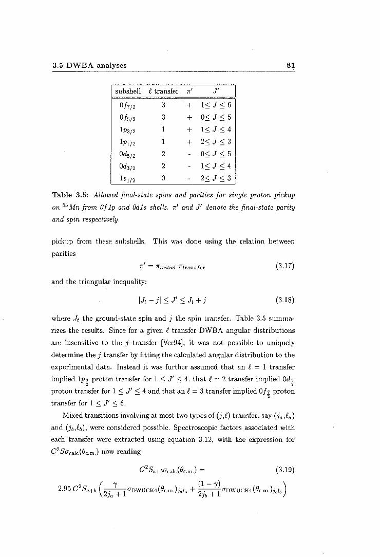
3.5 DWBA analyses 81
j subshell € transfer 7f1 I'
Of1;2 3 + lS Is 6
Of5;2 3 + OS JS 5
lp3;2 1 + 1::;; I s 4
lP1/2 1 + 2S Is 3
Od5;2 2 - OS IS 5
Od3;2 2 - 1SI:s;4
ls1;2 0 - 2S Is 3
Table 3.5: Allowed final-state spins and parities for single proton pickup
on 55 Mn from Of lp and Odis shells. 1f1 and I' denote the final-state parity
and spin respectively.
pickup from these subshells. This was done using the relation between
parities I
7f = 1finitial 1ftransfer (3.17)
and the triangular inequality:
I It - j I ::;; I' ::;; It + j (3.18)
where It the ground-state spin and j the spin transfer. Table 3.5 summa
rizes the results. Since for a given f transfer DWBA angular distributions
are insensitive to the j transfer [Ver94], it was not possible to uniquely
determine the j transfer by fitting the calculated angular distribution to the
experimental data. Instead it was further assumed that an f = 1 transfer
implied lp;! proton transfer for 1 :::; I' :::; 4, that f = 2 transfer implied Odi! 2 2
proton transfer for 1 :::; I' :::; 4 and that an€= 3 transfer implied Oh proton 2
transfer for 1 :::; I' :::; 6.
Mixed transitions involving at most two types of (j,f) transfer, say (ja,fa)
and (jb,fb), were considered possible. Spectroscopic factors associated with
each transfer were extracted using equation 3.12, with the expression for
C 2Sacalc(ec.m.) now reading
(3.19)
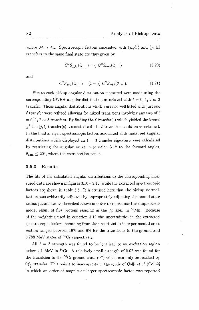
82 Analysis of Pickup Data
where o::; / :::; 1. Spectroscopic factors associated with Ua ,1'.a) and (jbl-b)
transfers to the same final state are thus given by
(3.20)
and
(3.21)
Fits to each pickup angular distribution measured were made using the
corresponding DWBA angular distribution associated with P. = 0, 1, 2 or 3
transfer. Those angular distributions which were not well fitted with just one
P. transfer were refitted allowing for mixed transitions involving any two of P.
= O,' 1, 2 or 3 transfers. By finding the P. transfer(s) which yielded the lowest
x2 the (j, l) transfer(s) associated with that transition could be ascertained.
In the final analysis spectroscopic factors associated with measured angular
distributions which displayed an P. = 3 transfer signature were calculated
by restricting the angular range in equation 3.12 to the forward angles,
ec.m. :::; 20°, where the cross section peaks.
3.5.3 Results
The fits of the calculated angular distributions to the corresponding mea
sured data are shown in figures 3.10 - 3.15, while the extracted spectroscopic
factors are shown in table 3.6. It is stressed here that the pickup normal
ization was arbitrarily adjusted by appropriately adjusting the bound-state
radius parameter as described above in order to reproduce the simple shell
model result of five protons residing in the f p shell in 55Mn. Because
of the weighting used in equation 3.12 the uncertainties in the extracted
spectroscopic factors stemming from the uncertainties in experimental cross
section ranged between 16% and 6% for the transitions to the ground and
3.788 MeV states of 54 Cr respectively.
All P. = 3 strength was found to be localized to an excitation region
below 4.1 MeV in 54 Cr. A relatively small strength of 0.02 was found for
the transition to the 54 Cr ground state (o+) which can only be reached by
Oh. transfer. This points to inaccuracies in the study of Colli et al. [Col59] 2
in which an order of magnitude larger spectroscopic factor was reported
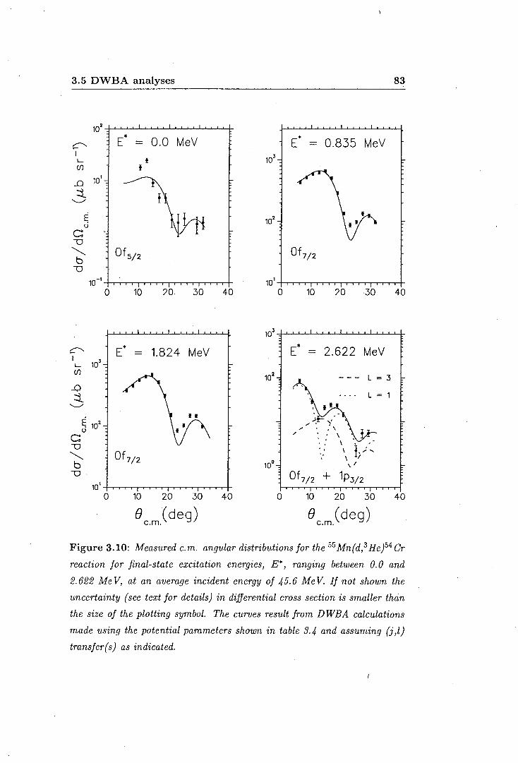
3.5 DWBA analyses 83
102
~ E* - 0.0 MeV E* 0.835 MeV
I 103 L t (/) t
..0 101
~ .....___,,,
~ I
102 0
c --0
""- Of s/2 Of 7/2 b
--0
10-1 101
0 10 20 30 40 0 10 20 -30 40
103
~ E* 1.824 MeV E* - 2.622 MeV I
103 L (/)
102
-0 ~ .....___,,,
~ 102 u
c --0 '' t ,;', '.
""- Of 7/2 '•
b 100 --0 Of 7/2 + 1p3/2
101
0 10 20 30 40 0 10 20 30 40
e (deg) c.m.
e (deg) c.m.
Figure 3.10: Measured c.m. angular distributions for the 55 Mn(d, 3 He)54 Cr
reaction for final-state excitation energies, E*, ranging between 0. 0 and
2. 622 Me V, at an average incident energy of 4 5. 6 Me V. If not shown the
uncertainty (see text for details) in differential cross section is smaller than
the size of the plotting symbol. The curves result from D WBA calculations
made using the potential parameters shown in table 3.4 and assuming (j ,l)
transfer(s) as indicated.

84
103
c:::' I !.._
(/)
_o 102
::t. '--/
~ u
c \J
""' b \J
c:::' I
100
0
E* - 3.076 MeV ---L=3
- - - - - L = 1
'•
Of 7/2 + 1p3/2
10 20 30 40
E* - 3.220 MeV
Of 7/2
100 ~-r-.--r-.-~~~-.-.-~~-..-.-+-0 10 20 30 40
8 (deg) c.m.
103
102
10°
Analysis of Pickup Data.
0
( - 3.159 MeV ---L=3
/ - - - - -L = 1 /
.. .. ..
Of 7/2 + 1p3/2
10 20 30
3.429 MeV
---L=3
· · - - - L = 1
40
10 _, ~~~~-.-.-~-..-.--..-.--..-.--..-.-+-
0 10 20 30 40
8 (deg) c.m.
Figure 3 .11: The same as in figure 3.10 but for 54 Cr final-state excitation
energies ranging between 3.076 and 3.429 Me V.

3.5 DWBA analyses 85
103
~ E* 3.656 MeV E* 3.788 MeV I 10
3 I._
([)
...0 102
~ ~
E < 102 u
c -0
Of 7/2 Of 7/2 ""' b -0
100 101
0 10 20 30 40 0 10 20 30 40
I I I I I I I 1-1 I I I I I I I I I I
• 1a2 E = 4.042 MeV
Of 7/2
0 10 20 30 40
8 (deg) c.m. .
Figure 3.12: The same as in figure 3.10 but for 54 Cr final-state excitation
energies ranging between 3. 656 and 4. 042 Me V.

86 Analysis of Pickup Data.
10• 10•
~ E* E* 4.237 MeV
I 4.128 MeV L ---L=O (/)
L = 0 - - - - - L = 2 ..D
102 :j__ L = 2 ....__,,
102
~ 0
c '' --0 I
"'- . ~ •'1
b 1s112 + Od3;2 1s1;2 + Od3;2 --0
10-1 10° 0 10 20 30 40 0 10 20 30 40
103 103
~ E* 4.552 MeV E* 4.620 MeV I - -L (/) ---L=O ---L=O
..D - - - - - L = 2 :j__
I I I ....__,,
101 101 I I I I I
E I I I
0
c \/
--0
"'-b 1s1i2 1sv2 + Od3;2 --0
10-1 10-1
0 10 20 30 40 0 10 20 30 40
8 (deg) c.m.
8 (deg) c.m.
Figure 3.13: The same as in figure 3.10 but for 54 Cr final-state excitation
energies ranging between 4.128 and 4.620 Me V.

3.5 DWBA analyses
~
I L (f)
...0 ::i_
'-.../
E u
c: -0 "-.. b -0
~ I L (f)
104
102
10-1
. ...o. ::i_ 102
·"''-.../
0
E*
1p3/2
10
4.868 MeV
----L=1
· · · · · · L = 2
~
\ I --
+ Od3;2
20 30
5.194 MeV
---L=O
· · · · · L = 2
40
10-1 -+-r...,...,....,...,...,.......,.....-,--,--,--,--.-.--.-.--.-.-+-0 10 20 30 40
8 (deg) c.m.
87
104
E* = 4.936 MeV
L = O
L = 2 102
I I
I I I
I I I \I
I I I \I I
I
1s112 + Od3;2 10-1
0 10 20 30 40
5.311 MeV
10 0 -+~-r-r-.--r-r-r-r-r-r-r-r-r--.-r--r-r-T-.-+-0 10 20 30 40
8 (deg) c.m.
Figure 3.14: The same as in figure 3.10 but for 54 Cr final-state excitation
energies ranging between 4.868 and 5.311 Me V.

88 Analysis of Pickup Data .
104 104
~ E* 5.574 MeV E* 5.776 MeV I L (f) ---·L = 0 L = 0
_o 1(/ - - - - - · L = 2 102 L = 2
::i_ ~ -....__., \ \
E I
u c: -0 "'-.. b
1sv2 + Od3;2 1s112 + Od3;2 -0 10-1 10-1
0 10 20 30 40 0 10 20 30 40
104 103
~ E* 5.979 MeV E* 6.107 MeV I L (f)
102
L = 0 _o \
::i_ 102 -· I, L = 2
\ . . ' ....__., \ I ~ .. ;- -. \ \ I \ '
~ .• I -. \ I I ' \
\ I I' ,,. .... u I I
.. \ I I .. I c: •\ \ \I I I
-0 " I I
"'-.. y I I I
b 1sv2 + Od3;2 100 1s1;2 I I I
-0 \I I
10-1 + Od3 2 0 10 20 30 40 0 10 20 30 40
() (deg) c.m.
() (deg) c.m.
Figure 3.15: The same as in figure 3.10 but for 54 Cr final-state excitation
energies ranging between 5. 574 and 6.107 Me V.

3.5 DWBA analyses 89
for the transition to this state reached via the 55 Mn(n,d) 54 Cr reaction (see
table 1.4). The other o+ adopted levels at 2.830 and 4.013 MeV were not
seen. These observations support the expectation that the Oh proton orbital 2
is essentially unoccupied in 55Mn. This is further supported by results from
shell-model calculations which are discussed in section 4.1. Any remaining
e = 3 strength was therefore assumed to be associated with Ofz transfer. 2
Pickup from the lsOd shell was also observed, leading to final states
beginning with the known 3- state at an excitation energy of 4.127 MeV.
For all such states the best fits to the angular distributions were obtained
using a mixture of e = O (j = ~) and e = 2 (assumed j = ~) pickup. However,
wherever the e = 0 spectroscopic factor was less than 0.05 the improvement
over pure R = 2 was marginal, and it was felt prudent not to assign J' = (2,3)- to these states on the basis of such small R = 0 contributions. An
assignment of J' = (1-4)- is therefore made to these states in table 3.6.
However, for the adopted levels at 4.245, 5.321 and 5.981 MeV the R = 0
contribution to the pickup cross section is much more secure, allowing the
assignment J' = (2,3)- to be made to these states, and hence J' = 3- to
the 4.245 MeV state using prior information. Also, the spin assignment of
J' = (0,1,2) to the adopted level at 5.189 MeV can be tightened to (1,2)-.
The observed adopted level at 4.865 MeV has a spin assignment of
(1-' ,4+). An optimal fit to the corresponding angular distribution was
obtained by allowing for R transfers of 1 and 2, and it is likely that the
state observed is a doublet. No new information about the spin assignment
for this level was therefore obtained.
As mentioned in section 3.3, two new levels were observed at excitation
energies of 5.574 and 5.776 MeV. Their associated angular distributions were
fitted well by allowing for R = 0, 2 transfer, and again assignments of J' = (1-4)- were made to these states.
All new spin assignments made on the basis of the DWBA analyses
as discussed above, are shown in the last column of table 3.6. The spin
assignments of 6+, 5+ and 6+ made to states at observed excitation energies
of 3.220, 3.788 and 4.042 MeV, respectively will be discussed in chapter 4
together with the results of shell-model calculations and NEWSR analyses
of Oh pickup and stripping transfer strength. 2

90 Analysis of Pickup Data .
- From Ref. [Jun93] -. - This work
c2s I
New J"
E* llE* /rr E' llE* f=O £=1 £=2 £=3 assignment
(MeV) (keV) (MeV) (keV)
0.0 o+ 0.0 0 0.02
0.835 9 2+ 0.835 1 0.85
1.824 .::;1 4+ 1.824 2 0.99
2.620 9 2+ 2.622 4 0.01 0.02
3.074 9 2+ 3.076 3 0.05 0.09
3.160 9 4+ 3.159 1 0.09 0.84
3.222 9 (6)+ 3.220 5 0.27 5+
3.437 9 2+ 3.429 8 0.01 0.05
3.655 9 4+ 3.656 4 0.34
3.786 9 (4,5)+ 3.788 3 1.06 5+
3.928 9 2+ 3.926 4 0.05 0.22
4.042 9 (7)+ 4.042 4 0.13 5+
4.127 9 3-:- 4:128 5 0.04 0.07
4.245 5 2+,3- 4.237 4 0.61 0.35 3-
4.561 11 4.552 6 0.02 0.11 (1-4)-
4.618 6 4.620 6 0.02 0.11 (1-4)-
4.865 4 (1- ,4+) 4.868 7 0.03 0.67
4.936 6 4.936 8 0.05 0.87 (1-4)-
5.189 9 (0,1,2) 5.194 11 0.04 0.47 (1,2)-
5.321 10 5.311 8 0.96 (2-3)-
5.574 10 O.Q2 0.33 (1-4)-
5.776 9 0.05 0.34 (1-4)-
5.981 10 5.979 8 0.12 0.59 (2,3)-
6.113 10 6.107 9 0.0~ 0.22 (1-4)-
Table 3.6: Spectroscopic information from the 55 Mn{d, 3 He)54 Cr reaction
at an average incident energy of 45. 6 Me V. New spin assignments shown
have been made as discussed in the text. See footnote on p. 63.

Chapter 4
Shell-model calculations and
sum-rule analyses
In this chapter, results from shell-model calculations based on a new effec
tive interaction for A = 41-66 nuclei [van94] are first compared with the
experimentally measured proton pickup (this work) and stripping ([Mat68])
data on 55 Mn, in particular those data for f p-shell transfer. The formalisms
based on the non-energy weighted sum rules (NEWSR) are reviewed next,
followed by a discussion of the Ofz transfer spin-distributions for proton 2
transfer on 55 Mn. Analyses, based on the standard and symmetric forms of
the NEWSR, of these spin distributions are then presented.
4.1 Shell-model calculations
The shell-model calculations assume an inert 4°Ca core and a model space
consisting of
configurations, with n + m the number of valence nucleons outside the 4°Ca
core for a given nucleus, n the maximum number of nucleons allowed in the
Oh orbit by the Pauli principle, and m is the minimum number of valence 2
nucleons outside this orbit. For 54 Cr, 55 Mn and 56Fe, all the valence protons
can be accommodated in the Oh orbit, and of the ten valence neutrons in 2

92 Shell-model calculations and sum-rule analyses
each case, a maximum of eight can be accommodated in the Ofz orbit. Thus 2
m = 2 for this study.
Spectroscopic factors associated with transitions from the 55 Mn ground
state to 54Cr and 56Fe final states were obtained by calculating the overlaps
of the 55 Mn wave-function with the wave-functions obtained after operating
on the 54Cr wave-functions with the creation operator and on the 56 Fe
wave-functions with the annihilation operator, respectively. The Oxford- ·
Buenos Aires shell-model (OXBASH) code [Val91] was used to perform these
calculations with matrix elements of the effective interaction [Hey94] fixed
by the requirement of a best fit between experiment and theory for a large
set of energy levels in A= 41-66 nuclei [van94].
4.1.1 Results
Calculated spectroscopic factors associated with transitions to 56 Fe and 54Cr final states reached via single proton transfer on 55 Mn are shown in
tables 4.1 and 4.2 respectively. No significant Ofz stripping strength is - 2
predicted to lie above 3.737 MeV. This is in good agreement with Matoba's
results (see table 4.3) which show the last fragment of Ofz strength to be 2 .
located at 3.78 MeV. The shell-model results also show negligible Oh and 2
lp l pickup strength, thus supporting the assumption used in the DWBA 2
analyses (section 3.5) that e = 3 and e = 1 transfers imply Ofz and lp;i_ 2 2
transfers respectively.
4.2 Sum-rule analyses
4.2.1 Formalism
The sum-rule formalisms, based on the standard and symmetric forms of
the NEWSR, which are used to evaluate the consistency of single-nucleon
transfer data [Cle91, New95] are discussed next.

4.2 Sum-rule analyses 93
J' k E* -fftc2s-J,.
(MeV) Oh 2
Ip~ 2
Ofr,. 2
lp1 2
€=3 €=1 €=3 €=1
21 0.888 1.400 0.003 0.002
41 2.107 0.215
22 2.567 0.237 0.003 0.001
23 3.148 0.033 0.007 0.002 0.002
42 3.162 0.071 0.011
11 3.197 0.175 0.004
31 3.316 0.016 0.002
61 3.458 0.714
24 3.527 0.004 0.091 0.007 0.025
32 3.585 0.041 0.004
25 3.675 0.154 0.007 0.042
62 3.737 0.310
33 4.044 0.001 0.173 0.006 0.062
43 4.176 0.030
34 4.421 0.004 0.006 0.004 0.016
44 4.480 0.026 0.005
35 4.608 0.007 0.450 0.036 0;099
63 4.614 0.076
25 4.663 0.017 0.002 0.005 0.016
45 4.668 0.003 0.021
36 4.814 0.002 0.090 0.011 0.007
b 4.903 0.037 0.158 0.001
51 4.969 0.018
l3 5.042 0.006 0.034
46 5.042 0.008 0.242 0.078
52 5.061 0.016
37 5.100 0.002 0.027 0.001
}4 5.400 0.034 0.003
Table 4.1: Calculated stripping strengths associated with transitions to
positive parity states in 56 Fe via proton stripping on 55 Mn. Jt and J'
denote target ground-state spin and final-state spins respectively; while E*
denotes excitation energy in the final nucleus. Results were obtained from
a shell-model calculation using a new effective interaction for A = 41-66
nuclei {van94J. Shown are only those final states for which the spectroscopic
strength associated with any f transfer is 2: 0. 02.
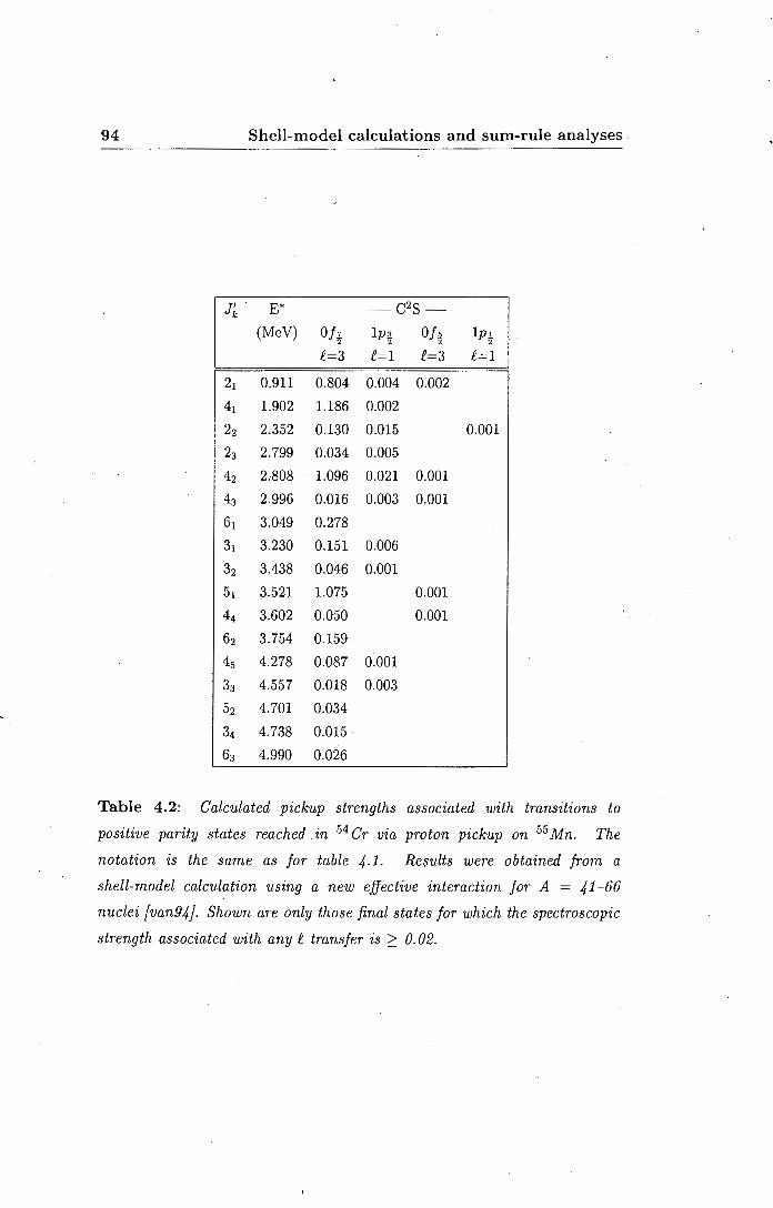
94 Shell-model calculations and sum-rule analyses
J~ E* -c2s-(MeV) Ofz
2 lp;i_
2 Ofr,.
2 lp1
2
£=3 £=1 £=3 £=1
21 0.911 0.804 0.004 0.002
41 1.902 1.186 0.002
22 2.352 0.130 0.015 0.001
23 2.799 0.034 0.005
42 2.808 1.096 0.021 0.001
43 2.996 0.016 0.003 0.001
61 3.049 0.278
31 3.230 0.151 0.006
32 3.438 0.046 0.001
51 3.521 1.075 0.001
44 3.602 0.050 0.001
62 3.754 0.159
45 4.278 0.087 0.001
33 4.557 0.018 0.003
52 4.701 0.034
34 4.738 0.015
63 4.990 0.026
Table 4.2: Calculated pickup strengths associated with transitions to
positive parity states reached in 54 Cr via proton pickup on 55 Mn. The
notation is the same as for table 4 .1. Results were obtained from a
shell-model calculation using a new effective interaction for A = 41-66
nuclei (van94J. Shown are only those final states for which the spectroscopic
strength associated with any e transfer is ;:::: 0. 02.

4.2 Sum-rule analyses 95
Standard form
The starting point for this discussion is the standard form of the exact,
model~independent NEWSR represented by
(4.1)
where
• - and + denotes pickup and stripping respectively;
• j and lt are the total angular-momentum transfer and target ground
state spin, respectively;
• [x] = 2x + l;
• la and Jn are the spins of final states reached by pickup and stripping,
respectively;
• { Jn j lt la j lt
via [Ros5 7]:
} is the 6j symbol, related to the Racah coefficient, W,
W(JnjjJa; Jtlt) = (--l)Jn+J+J+Jo { Jn ~ lt } ; la J lt
• and S1 denotes the partial spectroscopic sum1 which is determined by
summing all spectroscopic factors associated with transitions to the
same final-state spin, J.
Equation 4.1 is then modified by the introduction of two renormalization
constants, n+ and n-, to take into account possible errors in the absolute
normalization of stripping and pickup spectroscopic factors respectively, as
determined by DWBA analyses of the transfer data. This modified form of
the standard NEWSR reads
n+ s+ ( ") + (-1) 2It+1[Jn]" { Jn j lt } n-s- ( ") = [Jn.]. (4.2) Jn J ~ J · J Jo J [J j
J0
a J t t
1 So for example the partial surp. S{ is obtained by summing all stripping spectroscopic
factors associated with transitions to J = 1 final states.

96 Shell-model calculations and sum-rule analyses
The renormalization constants, n+ and n-, are related by the total sum
rule:
which is obtained from equation 4.2 by summing over Jn. Equation 4.2
represents a set of N = min{[Jt],[j]} linear relations involving 2N partial
sums s-;o. and st. In applications of the sum rules, the uncertainty, 6.S, in a spectroscopic
factor S is assumed proportional to S itself [Cle73, Cle91], with proportion
ality constant (J, the relative error parameter, so that
t::,.S =(JS. (4.4)
A measure of the goodness-of-fit to the sum rule corresponding to spin Jn
is given by Q1n with expectation value zero, where
Q1 =n+s+ (j)+(-1)21t+1[Jn]"{ Jn j It }n-s- (j)-[Jn]_ (4.5) n Jn L J . J la [J] la a J t t
Equation 4.4 and the standard error propagation formula (for example, [Miil84])
results in an uncertainty b,.QJn in Q1n given by:
The above expressions lead to a condition for an acceptable overall fit to the
N linear.relations constituting the standard NEWSR, in which no sum rule
is overemphasized at the expense of another [Cle91 ]. Setting Q}n = b,.Q}n,
dividing by [Jn], and summing over Jn yields
As a next step n+ is written in terms of n- using the total sum rule of
equation 4.3, and (J2 emerges as a function of the input spectroscopic factors
and of n - . The latter can then be varied to determine the minimum value of
(J = (Jmin· The smaller (Jmin is, the better the fit to the sum rules is. A value

4.2 Sum-rule analyses 97
of <Jmin = 0.00, for example, indicates that a perfect fit to the sum rules was
obtained for unique values of n- and n+. For an acceptable fit [Cle91]
0-min :S 0.10. (4.8)
If this criterion is satisfied it indicates that both stripping and pickup
spin-distributions are consistent with the sum rules, to within the assumed
uncertainties. The values of n!,in and n~in determined via equation 4. 7
can then be used to obtain estimates of absolute stripping and pickup
spectroscopic factors. On the other hand a failure to fit the NEWSR points
to inaccuracies in the stripping and/or pickup spin-distributions.
Symmetric form
An equivalent formalism to the one above based on a symmetric form of the
NEWSR was recently developed and has been successfully used to analyse
Ofz transfer data on 51 V and 59Co [New95]. The symmetric sum rules are 2
represented by
(4.9)
where J' now denotes final-state spin and J is constrained by
0::; J::; (N - 1). (4.10)
Equation 4.9 represents a set of N = min{[JtJ, [j]} linear relations in the
partial sums SJ, and Sj,. Unlike in the case of the standard NEWSR, the
total sum rule (equation 4.3) is recovered by using only one of the N linear
relations, namely the one for which J = 0. The remaining N - l relations are
thus decoupled from the total sum rule, thereby removing a bias which was
present in the standard NEWSR formalism, i.e. that the observed strength
necessarily exhausts the total sum rule.
The same steps which were used to establish the standard NEWSR
formalism were followed in establishing the symmetric NEWSR formalism.
The symmetric NEWSR of equation 4.9 are first modified by introducing
the renormalization constants n+ and n-, to read:

98 Shell-model calculations and sum-rule analyses.
By putting n = ~~ in equation 4.11 for cases where J > 0, the (N - 1)
linearly independent relations
2:)-l)lt+J+l' { J 1' J'
lt lt } { + 1 - } -
1 j nS 1' + ( -1) S 1' - O (4.12)
can then be used to assess the consistency of the experimentally obtained
partial sums with the NEWSR by again introducing a quantity Ql, which
is defined as:
Q1 = 2:)-l)lt+]+l' { J 1' J'
(4.13)
and which has zero expectation value. Once again, some scatter in the Q 1
values is expected because the spectroscopic partial sums, Sj, and Sji, are
themselves subject to some scatter about their true values. This scatter in
Ql, denoted by 6.Q1, can be calculated using equations 4.4, 4.13 and the
error propagation formula to give
(6.Q1)2 =I: {
1
1' J' (4.14)
To assess the accuracy of the transfer spin-distributions a goodness-of-fit
indicator, x2 , which is similar in form to the expression for the reduced
chi-square (equation 3.12 divided by the number of degrees of freedom), is
introduced. This goodness-of-fit indicator has the form
2 1 Q2 x = (N - 2) L (fl.ch )2 .
1>0
(4.15)
The fit can now be optimized by varying n, thus determining the minimum
value of x2 = X~in• and the corresponding value of n = nmin· With a
= 0.10, a value of X~in ~ 1 implies that, using n = nmin, the set of
(N - 1) linear relations of equation 4.12 are fitted to within 10% fractional
uncertainties in the partial sums Sj, and Sji. Any such fit, obtained using
only the seen strength below '""' 5 Me V excitation energy, implies that any
unseen strength also satisfies equation 4.12, since the total strength must

4.2 Sum-rule analyses 99
certainly do so. It then follows [New95] that once nmin has been obtained,
the total sum rule, together with an estimate of the fraction, /, of unobserved
strength total strength, can then be used to determine n+ and n- as is done
below in section 4.2.4. Further, it should be noted that, given the structure
of equation 4.12, a likely spin distribution for any unseen strength is one
with SJ' ex [J'] [New95]. Importantly, such unseen strength then makes no
contribution to the dipole sum rule of equations 4.17 (see section 4.2.4),
4.2.2 Oh transfer spin-distributions 2
For the remainder of this chapter the Oh transfer strength is focussed 2
on. The establishment of stripping and pickup spin-distributions which are
required for the sum-rule analyses is discussed first.
Stripping
For the stripping strength a summary of the £ = 3 spectroscopic information
from Matoba's study [Mat68] which was previously given in table 1.3 is
presented in table 4.3, together with the most recent adopted levels (E* < 4.0 MeV) [Jun87, Jun92]. Except for the transition to the 56 Fe ground
state (o+), it was assumed that the £ = 3 strength seen by Matoba is
associated with Oh proton transfer. The negligible Oh strength below 2 2
4.0 MeV excitation predicted by the shell model (see table 4.1), supports
this assumption.
The 56 Fe excited states at excitation energies of 0.85, 2.09 and 2.66 MeV
as reported by Matoba correspond unambiguously with the adopted levels
at 0.847, 2.085 and 2.658 MeV respectively. These three states have spins
of 2+, 4 + and 2+ respectively.
The mapping of the next three states reported by Matoba to the presently
adopted 56Fe levels is ambiguous because of a relatively large uncertainty of
40 ke V associated with the excitation energies of these states. Matoba found
an £ = 3 stripping strength of 0.08 to be associated with the state-complex
at (2.97 + 3.15) MeV. By considering only excitation energies, this strength
could be associated with transitions to adopted levels at energies of 2.942
(J' = o+), 2.960 (J' = 2+), 3.070 (J' = (3-)), 3.120 (J' = (1 +)) or 3.123

100 Shell-model calculations and sum-rule analyses
- from Refs. [Jun87, Jun92] - - from Ref. [Mat68] -
E* ~E* J'1T E* ~E*
(MeV) (keV) (MeV) (keV)
0.0 o+. 0
0.847 < 1 2+ 0.85
2.085 < 1 4+ 2.09
2.658 < 1 2+ 2.66
2.942 < 1 o+
2.960 < 1 2+
a2.97 40
3.070 30 (3-)
3.120 < 1 (1 +)
3.123 < 1 4+
a3.15 40
3.370 < 1 2+
3.388 < 1 5+
3.40 40
3.748 5 2+
3.756 < 1 6+
3.760 10 (2-6)
3.78 40
3.832 < 1 2+
a Member of the state-complex at (2.97 + 3.15) MeV
with combined e = 3 strength of 0.08.
£ ~c2s t
3 0.01
3 1.45
3 0.36
3 0.14
3 0.04
3 0.04
3 0.90
3 0.25
Table 4.3: Spectroscopic information on £ = 3 transfer stripping strength
from the 55 Mn{a,t)56 Fe reaction as reported by Matoba [Mat68}. The
possible 56 Fe adopted levels [Jun87, Jun92] which correspond with observed
states reached via £ = 3 transfer are shown. lt and J' denote target ground
and final-state spin respectively. Note that the state-complex at (2. 97 + 3.15) Me Vis not indicated in Refs. {Jun87, Jun92j (see table 1.3).

4.2 Sum-rule analyses
stripping pickup
J' E* (MeV) fff c2s J' E* (MeV) c2s t
2+ 0.847 1.45 2+ 0.835 0.85
4+ 2.085 0.36 4+ 1.824 0.99
2+ 2.658 0.14 2+ 2.622 0.02
2+ 2.960 ao.027 2+ 3.076 0.09
1+ 3.120 ao.027 4+ 3.159 0.84
4+ 3.123 ao.027 d6+ 3.220 0.27
b6+ 3.388 0.90 2+ 3.429 0.05
2+ 3.748 co.125 4+ 3.656 0.34
6+ 3.756 co.125 <l5+ 3.788 1.06
2+ 3.926 0.22
d6+ 4.042 0.13
a Strength of 0.08 distributed equally over final-state spins
of 1 +, 2+ and 4 + as discussed in text. b
c
d
Assignment made on basis of Matoba's suggestion [Mat68],
sum-rule analyses and shell-model calculations as discussed in text.
Strength of 0.25 distributed equally over final-state
spins 2+ and 6+ as discussed in text.
Spin assignments made as discussed in text.
101
Table 4.4: Spectroscopic factors for Ofz proton transfer on 55 Mn associated 2
with final states of spin J' at excitation energy E* in the final nucleus. The
partial sums Sj,, Sj,, used in the text are obtained by summing over final
states of the same spin J'. The excitation energies of final states reached
via stripping were obtained from Refs. [Jun87, Jun92} while those for pickup
final states were obtained from this study.
102 Shell-model calculations and sum-rule analyses .
(J' = 4+) MeV. 55 Mn has a ground-state spin r, and if it is assumed that
an e = 3 transfer implies a transfer of a proton to the Oh subshell, the only 2
possible transitions are to the 2.960, 3.120 and 3.123 MeV states. The small
. stripping strength of 0.08 was therefore shared equally amongst final-state
spins of 1 +, 2+ and 4 +.
The state seen by Matoba at 3.40 Me V could correspond to adopted
levels at excitation energies of 3.370 MeV (J' = 2+) or 3.388 MeV (J' = 6+), with the latter being the one suggested by Matoba [Mat68]. If it is
assumed that this is a 2+ state, a significant deterioration in the quality of
NEWSR fits results. Furthermore the shell-model results shown in table 4.1
indicate the presence of a strong transition to a 5+ 56 Fe final state at an
excitation energy of 3.458 Me V. It was. therefore assumed that this state
corresponds to the adopted level at 3.388 MeV. The spectroscopic strength
of 0.90 was therefore associated with a 5+ final state.
The state seen by Matoba at 3.78 MeV could correspond with adopted
levels at excitation energies of 3.748 (J' = 2+), 3.756 (J' = 6+) or 3.760 (J'
= (2-6)) MeV. In view of this and the uncertainties in parity assignments
to the 3. 760 Me V state, the strength of 0.25 associated with Matoba's state
at 3.78 MeV was shared equally between 2+ and 5+ final states.
Pickup
For the particle occupancy in 55 Mn of proton orbits other than .the Oh, ta-2
ble 3.6 shows that the summed lp strength observed in the 55Mn(d,3He) 54Cr
reaction is 0.24. Further, the weak excitation of the 54 Cr ground state (o+)
in this reaction strongly suggests a similarly small Oh occupancy. These 2
observations are in line with the shell-model findings that for 55 Mn the lp;i, 2
proton occupancy is 0.06, and that the lp1 and Oh proton occupancies are 2 2
negligible.
For the Ofz pickup strength, as shown in table 3.6, three 54 Cr final 2
states observed which are reached via e = 3 transfer have u~certain spin
assignments. An e = 3 pickup strength of 0.13 was found for the transition
to the 54Cr state observed at 4.042 MeV. This state corresponds with the
adopted level at 4.042 MeV which has an uncertain spin assignment of (7)+.

4.2 Sum-rule analyses
Shell Model Experiment
6
,.---.,. 5 >
Q) 5+ 2 '-/
>. 4 01 5+ 2+,s+ L 5• 5• Q) c ,. Q) 3 4•
2• c 2' 0
-+-' 2 4+ 4•
0 -+-'
0 x Q)
2• 2+
0
(a)
..c -+-' 01 c Q) L
-+-' (/)
01 c ()_ ()_
L ....... (/)
2
- Matobo
D Shell Model
0 ----.__..-'--+-'-"'l-'-~-""l--'--+-0 1 2 3 4 5 6 7
final-state spin
(b)
103
Figure 4.1: Comparison of results from a recent Of lp shell-model
calculation with the Ofz proton stripping spectroscopic strength shown in 2
table 4.4. In {a) spectroscopic strength is plotted versus 56 Fe excitation
energy while the summed spectroscopic strength is plotted versus 56 Fe final
state spin in {b). Only those final states for which spectroscopic strength is
> 0. 05 are shown.

104
Shell
6
,.----.._ 5 >
Q)
:2 .....__,,
>. 4 CJl L 5• Q) c Q) 3
4•
c 0
-+-' 2 4' 0 :';::'. () x Q)
2•
0
Shell-model calculations and sum-rule analyses
Model Experiment
4+_ .r: ~2·
5+ s• t--4'
-+-' CJl c Q)
3+ s• 4' s•-
L -+-' en Q_
2'- ::J .Y
4' ()
Q_
2'
(a)
3
2
0
I I I I I I
- This work
D Shell Model
- ~
- ~
n rn I I
0 1 2 3 4 5 6 7 final-state spin
(b)
Figure 4.2: Comparison of results from a recent Of lp shell-model
calculation with the Oh proton pickup spectroscopic strength shown in 2
table 4.4. In {a) spectroscopic strength is plotted versus 54 Cr excitation
energy while the summed spectroscopic strength is plotted versus 54 Cr final
state spin in {b). Only those final states for which spectroscopic strength is
> 0. 05 are shown.

4.2 Sum-rule analyses 105
However, the angular distribution for pickup to this state is unambiguously
fl. = 3, and this limits the spin of this state to 1 + ::; J' ::; 6+. It is therefore
unlikely that the 4.042 Me V state has a spin of 7+. Gamma decay selection
rules favour a large value of the spin. The shell-model results shown in
table 4.2 indicate a 6+ state at 3.754 MeV with a pickup strength of 0.16.
In view of the above a spin assignment of 6+ was made to the 4.042 MeV
state.
The next uncertain spin assignment was the one associated with the
state observed at an excitation energy of 3.788 MeV. This excitation energy
is consistent with that of the adopted level at 3.786 MeV which has a (4,5)+
spin assignment. There is also a 54Cr adopted level at 3.799 MeV,......, 13 keV
away from the 3.786 MeV state which could not be resolved experimentally.
However, this level is known to have a spin of 4+, so that the pickup strength
of 1.06 must be associated solely with final-state spins of 4+ or 5+. The
shell-model calculations predict a significant fragment of strength (1.08) to
be located in a 5+ state at an excitation of 3.521 MeV. Also, unless it is
assumed that the bulk of the experimentally observed strength is associated
with a 5+ final state, very poor fits to the NEWSR are obtained. A spin
assignment of 5 + was thus made to the adopted level state at 3. 786 Me V,
and the 4+ state at 3.799 MeV was assumed not to have been seen. The
possibility that the 3. 799 Me V state is excited but is not resolved will be
explored further below.
Finally, the adopted level observed at 3.220 Me V in this study has an
uncertain spin assignment of (6)+. This level, which has an associated
strength of 0.27, most likely corresponds to the shell-model level 6+ state at
· 3.049 MeV which has an associated strength of 0.278. Changing this spin
assignment would also result in a significant deterioration of the sum-rule
fits.
A summary of all the spin assignments made to 56 Fe and 54Cr final
states as discussed above, are tabulated in table 4.4, and are compared with
the corresponding results of the shell-model calculation in figures 4.1 and
4.2. Figures 4.l(a) and 4.2(a) compare the experimental and shell-model
distributions of the Oh proton spectroscopic strength as a function of final-2
state excitation energy and spin, while figures 4.l(b) and 4.2(b) compare

106 Shell-model calculations and sum-rule analyses .
the corresponding summed strengths as a function of final-state spin. The
overall agreement is good, particularly in the latter case.
4.2.3 Results
The results of the NEWSR analyses of the Ofz transfer spin-distributions 2
discussed above are shown graphically in figures 4.3 (standard form) and
4.4 (symmetric form).
There is a clear minimum in curve I of a versus the pickup renormaliza
tion constant, n-, (figure 4.3) obtained for the pickup spin-distribution given
in table 4.4. A minimum a of 123 was obtained while the corresponding
value of n- was 0.98. The sum rule fit criterion, a ::; 0.10, was therefore not
satisfied with this spin distribution. Distinct minima are also seen in fig
ure 4.4 in which the curves of x2 as a function of the ratio of renormalization
constants, n(=~~) are shown. Here again curve I corresponds to the pickup
spin-distribution given in table 4.4. The minimum value of x2 was found to
be 3.6 for n = 0.89. The minimum value of x2 exceeds the fit criterion by a
factor of,...., 4. Although the fits obtained are poorer than those obtained in
previous studies (Cle91, New95], they are still reasonable. This is illustrated
in figure 4.5 where the sensitivity of the NEWSR to an arbitrary change in
the stripping spin-distribution is shown.
It should be stressed here that the standard NEWSR analyses employ
a different fit criterion to the one used in the symmetric NEWSR analyses.
In the former, the criterion on the value of a 2 obtained from equation 4. 7
damps out the effect of an anomalously poorly fitted sum rule, whereas
in the symmetric sum-rule analyses the standard x2 test of equation 4.15
retains any such effect. Thus in the symmetric sum-rule analysis, it is the
sum rule with J = 3 in equation 4.12 which makes an anomalously large
contribution to the value of x2 as given by equation 4.15.
As pointed out earlier, a failure to satisfy the NEWSR is indicative of
inaccuracies in the spin distributions of transfer strength. These inaccuracies
can arise from one or more of the following:
• wrongly assigning spectroscopic strength because of the ambiguity
stemming from the fact that one I! transfer can be associated with

4.2 Sum-rule analyses 107
~
~ '--./ I b 20
10 . ' -----~---~---------
'II 0 -h-"T"T"T..,..-r,CT"T""r-r-r,....,...,..,...,.,."T"T"T..,..-r,_,....,-r-r-r,....,...,..,...,.,...,.......,-.,..+-
0. 8 0.9 1.0 1. 1 1.2
n Figure 4.3: Plot of relative spectroscopic factor error parameter, er, versus
renormalization constant, n-. Curve I was obtained using the data shown
in table 4.4 while curve II was obtained after relocating 17% of the pickup
strength associated with the 3. 786 Me V 5+ final state to the 3. 799 Me V 4+ final state (see text for details}.

108 Shell-model calculations and sum-rule analyses .
6 I
N
>< 4 II
2
0 ---+-.-TT"T"~,.-,-,--,-,-,-.,...~~~T"T"TTT"T"~..,..,..-Y,.-,-j-0. 6 0.8 1.0 1.2 1.4
n Figure 4.4: Plot of goodness-of-fit indicator, x2, versus normalization n.
Curve I was obtained using the data shown in table 4.4 while curve II was
obtained after relocating 17% of the pickup strength associated with the 3. 186
Me V 5+ final state to the 3. 799 Me V 4+ final state (see text for details).

4.2 Sum-rule analyses 109
more than one j transfer,
• the location of significant transfer spectroscopic strength at excitation
energies greater than'"'"' 5.0 MeV.
• scatter at more than the 103 level in pickup and/or stripping relative
spectroscopic factors, or
• one or more inaccurate spin assignments to final states reached by
pickup or stripping.
Although possible, it is unlikely that the £ = 3 stripping strength was
wrongly associated with Ofz rather than Oh transfer. The small strength 2 2
of 0.01 associated with the transition to the 56 Fe ground state (O+) and
the absence of excitation of the o+ state (E* = 2.941 MeV) supports this
assumption. As pointed out in the previous chapter, a similar argument
involving the 54 Cr ground state (o+) and the o+ states at 2.830 MeV and
4.013 Me V excitation, holds for the pickup case. It is therefore unlikely that
the first possible source of inaccuracy listed above is playing a role in this
work.
Although some spin assignments were made by comparing experimental
with shell-model spectroscopic information and NEWSR analyses, the ma
jority of spin assignments were made using the adopted levels for 54 Cr and 56 Fe. Although possible, it is unlikely that errors exist in spin assignments
to final states which have unique, unambiguous spin assignments according
to the adopted levels. This possibility will therefore not be further explored.
The sensitivity of the sum rules to the manner in which the 0.08 and 0.25
stripping strength was shared amongst 1 + ,2+ ,4+ and 6+ states, as described
above was investigated using the standard form of the NEWSR. This was
done using pickup spin-distribution given in table 4.4 and
• allocating all the 0.08 strength to either 1 + ,2+ or 4+ final states and
• allocating all the 0.25 strength to either 2+ or 6+ final states.
A study of all possible permutations of the above, has yielded minimum
values of CY varying between 113 and 143. The "equal sharing" of stripping
strength as described above is therefore not critical.

110 Shell-model calculations and sum-rule analyses
60
50 ,...-... ~ 40 '--"'
b 30
20 (a) m ------------------------
0.8
15
N
>< 10
5
0.4 0.6
1.0
n
0.8
n 1.0
1.2
(b)
1.2
1.4
1.4
Figure 4.5: Plots illustrating the sensitivity of the NEWSR to the spin
distribution. The curves shown were obtained after arbitrarily assigning all
the stripping strength associated with 4+ final states, amounting to ,....., 5% of
the total sum-rule strength, to :;+ final states. (a} Plot of relative error
parameter, O", versus pickup renormalization constant, n-. {b} Plot of
goodness-of-fit indicator, x2 , versus normalization n.

4.2 Sum-rule analyses 111
However, the fit to the sum rules turns out to be particularly sensitive
to a transfer of strength from the partial sum S5 to the partial sum Si. Of
course, other possibilities of reducing the original discrepancy exist, but a
virtue of applying the sum rules is to focus attention on likely candidates.
In the present case, the obvious focus is on s4 and s5 partial spectroscopic
sums. In this regard the possibility that the strong 5+ state seen at 3. 788
MeV excitation in 54 Cr could be masking some strength to the 3.799 MeV
( 4 +) state, was investigated. This was done by attempting to deconvolute
the yield which in the analysis above was assumed to be associated with the
3.786 MeV (4,5)+ adopted level. Pickup data for which the resolution was
the highest, namely 32 keV, were used. As a first step a Gaussian function
was fitted to the region of interest in 54 Cr spectrum, with its width and
centroid parameters fixed. The width was fixed to a mean width determined
from fits to resolved states in the vicinity of 3. 786 Me V excitation, while the
position was fixed to that expected for the 3.786 MeV adopted level using
the momentum calibration. The resulting fit with an associated reduced
x2 of 4.43 is shown in figure 4.6. Two Gaussian functions were then fitted
to the region of interest using the same width parameters. The positions
were fixed at 3.786 and 3.799 MeV. In this case a reduced x2 of 2.78 was
obtained. The fit obtained is a:lso shown in figure 4.6. Using these fits, it
was possible to establish the relative intensity of the state at 3.799 MeV
excitation w.r.t. the 3.786 MeV state. An intensity ratio of 20:100 was
obtained. Although the reduced x2 obtained is lower using two Gaussians,
the full-width at half maximum (FWHM) of the superposition is bigger than
the average FWHM for this run. It does however fall within three standard
deviations of the average FWHM. Since the FWHM obtained using two
Gaussians is consistent to within statistical uncertainty, with that obtained
using only one Gaussian, it is unlikely that the 3.799 MeV state is excited.
In view of this, the intensity ratio was taken to represent an upper limit.
No lower limit on the relative intensities could however be established.
The quoted intensity ratio was nevertheless used to relocate2 17% of the
pickup strength (1.06) initially assumed to be associated with the transition
2It has been argued above that the 3.786 MeV (4,5)+ is a 5+ state.

112 Shell-model calculations and sum-rule analyses .
500
x2/v = 4.43 (a)
400
3.788 MeVl/ (adopted level)
300 3.786 MeV
200 Q)
c c 100 0
..c u
0 "'-.. (fJ (b) +-' x2/v 2.78 c 400 ::J 0 3.788 MeV u
~ 300 (adopted level)
3.786 MeV 200
(adopted level) 3.799 MeV
100
o-l=~~~~=-~~~~...:::..=o~~~--=>-===~=1-
770 780 790 800 810
position along focal plane (channel)
Figure 4.6: (a) Gaussian fit to the 54 Cr final state observed at 3.188
Me V excitation. (b) A fit to the same peak using two Gaussian functions.
The solid curve represents a superposition of these Gaussians (see text for
discussion).
to 3.786 MeV adopted level, from 5+ to 4+ final states. Fits to both
the standard and symmetric sum rules improve when using the pickup
spin-distribution given in table 4.4 modified in this manner. The NEWSR
results are shown graphically in figures 4.3 and 4.4 as curves II. With
this distribution a minimum a of 8.0% for n- = 0.96 is obtained, thus
satisfying the fit criterion associated with the standard NEWSR formalism.
The corresponding symmetric sum rule results show a minimum x2 of 1.6
for n = 1.06, just failing to satisfy the symmetric NEWSR fit criterion.
The sur~ rule results therefore suggest that the 54 Cr level at 3.799 MeV
excitation will be observed if the total instrumental resolution is sufficiently
good ("-'15 keV) in order to resolve it from the level at 3.786 MeV. However

4.2 Sum~rule analyses 113
because of the absence of a lower limit on the ratio of intensities of the 3. 786
to 3. 799 Me V states, no conclusive statement can be made about whether
the 3. 799 Me V state is seen.
4.2.4 Estimate of absolute normalizations
With nmin determined from the symmetric· NEWSR analyses described
above, estimates of the absolute normalizations required for the stripping
and pickup data of table 4.4 can be extracted [New95], given an estimate
of the fraction, "/, of the total Oh proton strength that resides outside 2
the excitation energy region probed by the transfer experiments. These
. normalization factors, which will be denoted as ntbs and n;;:-bs respectively,
were estimated using a modified form of the total sum rule (equation 4.3):
n+ where nmin = ~
nabs
(4.16)
Analyses of ( e,e' p) data have suggested that "I could be as large as ,.....,
503 [Wag90]. More recent analyses of (e,e'p) data [Jin92] and theoretical
considerations [Mah91] point to "I being smaller at ,....., 303 and possibly still
smaller, while dipole sum rule fits to transfer data [Cle91] and studies of
. the decay of analogue states [van89] indicate "I to be ,....., 103. For this study
"I was taken as 0.2 ± 0.1 in order to straddle the various estimates. With
nmin = 0.89 from curve I of figure 4.4 and this value of "f, it was found
that the stripping and pickup data of table 4.4 should be multiplied by
n~bs = 0. 7 4 ± 0.09 and n;;:-bs = 0.83 ± 0.10 respectively. In order to assess
the accuracy of these normalizations, the diagonal contributions of the Ofz 2
proton orbit to various one-body observables was calculated, in particular
J{, the contribution to lt, the maximum z-projection of the spin of the 55Mn
ground state. This was done using the dipole sum rule [Cle91], which in
the case of pickup data, is given by
1 Jf = 2(.J, l) L {Jt(lt + 1) + j(j+ 1) - J'(J' + 1)} n-;:bss;,
t + J' (4.17)
where, once again, lt is the target ground-state spin (Jt = 2.5 in the case
of 55 Mn), J' is the final-state spin, j is the spin of the orbital involved in
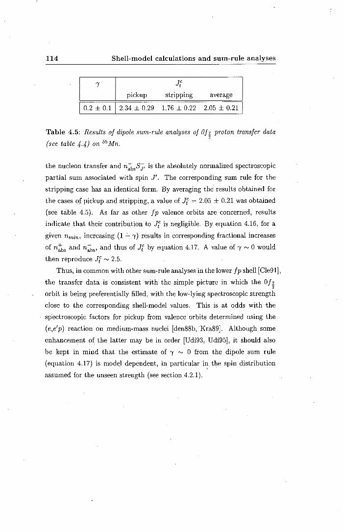
114 Shell-model calculations and sum-rule analyses.
I 7
pickup
J{
stripping average
I 0.2 ± 0.1 I 2.34 ± 0.29 1. 76 ± 0.22 2.05 ± 0.21
Table 4.5: Results of dipole sum-rule analyses of Oh proton transfer data 2
(see table 4.4) on 55 Mn.
the nucleon transfer and n-;_bsSj, is the absolutely normalized spectroscopic
partial sum associated with spin J'. The corresponding sum rule for the
stripping case has an identical form. By averaging the results obtained for
the cases of pickup and stripping, a value of J{ = 2.05 ± 0.21 was obtained
(see table 4.5). As far as other fp valence. orbits are concerned, results
indicate that their contribution to J{ is negligible. By equation 4.16, for a
given nmin, increasing (1 .:_ 'Y) results in corresponding fractional increases
of n~bs and n-;_bs' and thus of J{ by equation 4.17. A value of 'Y rv 0 would
then reproduce J? rv 2.5.
Thus, in common with other sum-rule analyses in the lower fp shell [Cle91],
the transfer data is consistent with the simple picture in which the Oh 2
orbit is being preferentially filled, with the low-lying spectroscopic strength
close to the corresponding shell-model values. This is at odds with the
spectroscopic factors for pickup from valence orbits determined using the
(e,e'p) reaction on medium-mass nuclei [den88b, Kra89]. Although some
enhancement of the latter may be in order [Udi93, Udi95], it should also
be kept in mind that the estimate of 'Y rv 0 from the dipole sum rule
(equation 4.17) is model dependent, in particular i1! the spin distribution
assumed for the unseen strength (see section 4.2.1).

/
Chapter 5
Conclusion
In conclusion, the main results obtained from this study of single proton
transfer on 55Mn are first summarized and discussed. Thereafter possible
complementary further studies are suggested.
5.1 Summary
Angular distributions for the 55Mn(d,3He)54Cr and 55Mn(d,d) 55 Mn(g.s.) re
actions were measured at an average incident energy of 45.6 MeV. Analyses
of the pickup angular distributions made using the distorted-wave Born
approximation (DWBA) formalism have yielded spectroscopic factors asso
ciated with the twenty-four 54 Cr states observed up to 6.107 MeV excitation.
An optical-model analysis of the deuteron elastic scattering data has been
performed to yield optimum values of the potential parameters used in ob
taining the distorted wave-functions for the entrance channel in the DWBA
calculations.
The Ofz pickup spin-distribution required for the non-energy weighted 2
sum-rule (NEWSR) analyses, was obtained using the f, = 3 strength ob-
served below 4.2 Me V excitation, in conjunction with the spins of adopted 54 Cr levels. Three of the adopted levels seen had uncertain spin assignments.
Sum-rule fits and comparisons with the shell-model results were used to
make spin assignments of 5+, 5+ and 5+ to these levels which are located
116 Conclusion
at excitation energies of 3.222 ((6)+), 3.786((4,5)+) and 4.042 ((7)+) MeV
respectively.
Stripping spectroscopic factors for Oh transfer were obtained from a 2
study by Matoba [Mat68] while corresponding 56 Fe final-state spins were
obtained from the adopted levels. Because of relatively large uncertainties
associated with the excitation energies of final states seen by Matoba, it was
not possible to uniquely assign the Oh stripping spin-distribution. However, 2
the relatively large strength (0.90) associated with a state seen at 3.40 MeV,
was shown to most likely associated with the excitation of the 6+ 56 Fe level
at 3.388 MeV.
The results of shell-model calculations using a new effective interaction
for A = 41-66 nuclei [van94] are in good agreement with the Oh transfer 2
spin-distributions used. NEWSR analyses, using both the standard and
symmetric forms of the spectroscopic sum rules, were made using these spin
distributions. Acceptable fits to the NEWSR were obtained, but the quality
of fits were poorer than for those obtained in previous studies [Cle91, New95].
5.2 Possible further studies
An examination of pickup spectra in the vicinity of the 54Cr adopted level
at 3. 786 Me V excitation has not excluded the possibility that the 4 + level
at 3. 799 Me V is excited but not resolved. If it is assumed that this state is
indeed present and that 17% of the spectroscopic ·strength associated with
the observed state at 3.788 MeV excitation is assigned to this 4+ state,
significant improvement in the quality of the NEWSR fits are observed.
Higher resolution ("" 15 ke V) measurements of proton pickup data on 55 Mn
will be instrumental in addressing this uncertainty.
An additional set of stripping spectroscopic factors for proton transfer
on 55 Mn will facilitate a further assessment of the assumptions made in
this study regarding the Oh stripping spin-distribution. In this regard high 2
resolution studies of the 55 Mn(a,t) 56 Fe and 55Mn(3He,d) 56 Fe reactions are
possibilities.
The use of a polarized beam would allow the assignment of unique total
angular momentum transfer, j, in contrast to the approach used in this

5.2 Possible further studies 117
study where it was assumed that an e = 3 signature was sufficient to assign
a j transfer of~- Although the observed weakness of transitions to o+ final
states is consistent with a small Oh. occupancy in 55 Mn, measurements with 2
a polarized beam would facilitate the direct determination of this occupancy.
It is however unlikely that a focal-plane polarimeter for the NAC k = 600
spectrometer will be available in the foreseeable future.
As discussed in the introductory chapter, the number of sum rules and
thus the efficiency in comparing the theoretical and observed spin distribu
tions of transfer strength, depends on the target ground-state spin ( Jt) and
j. 4 7 Ti is the sole remaining target in the lower f p shell with It 2:: ~ and
a study of single proton (and/or neutron) transfer on this nucleus will thus
represent the completion of a major program of experimental and theoretical
work which has been dedicated to studying Ofz nucleon transfer on j p-shell 2
nuclei. It would then be possible to draw global conclusions concerning the
Ofz occupancies for these nuclei. 2
Finally, there is scope for some improvement in the symmetric NEWSR
formalism, particularly in relation to the assumption that the error associ
ated with a relative spectroscopic factor is proportional to the latter. This
is at present being investigated.


Appendix A
VDC Spatial Resolution
The position accuracy, ax, obtainable with a single drift cell is the usual
figure-of-merit reported for a VDC [Ber77]. It is a factor which contributes
to the overall position resolution achievable with the spectrometer and also
determines the angle accuracy, ao, which can be achieved with the VDC.
A schematic representation of a charged particle trajectory traversing a
VDC, having a signal-wire spacings is shown in figure A.l. In the trajectory
shown, six primary ionizations in the gas-filled VDC were caused, each
associated with a separate drift cell. The drift time from the point of primary
ionization to the point where avalanching occurs in each cell is measured
experimentally. By using the time-to-position relationship provided by a
lookup table it is possible to determine the position along the drift cell
where the primary ionization occurred. It is therefore possible to reconstruct
trajectories of particles across the VDC wire-plane. Since the trajectories
of particles in the vicinity of the VDC are to a good approximation straight
lines, the slope of each trajectory should be constant. This property of the
trajectories was used to determine ax.
The slope of the trajectory shown in figure A.I can be calculated in a
number of ways. One way in which this c£n be done is to use the drift
distances associated with two adjacent wires, say wires a and b. In this case
the trajectory slope, S, is given by:
S _db - da a,b -
8 ' (A.I)

120 VDC Spatial Resolution
a b c • . . •
e f
signal wire
Figure A.1: Schematic representation of a trajectory associated with a
charged particle intersecting the VDC resulting in a six-wire event.
where d denotes drift distance. The slope could also be determined using
the drift distances associated with for example wires e and J. Since the
slope should be constant, the difference between the two slopes, denoted by
D, given by
D = Sa,b - Se,j (A.2)
should ideally be zero. However because of statistical fluctuations a distri
bution centered around zero is obtained when one calculates the difference
in slope for a number of events. Let us denote the standard deviation of
this distribution by CJd· By applying the general law of error propagation to
equation A.2, with covariances assumed to be zero, one obtains:
(A.3)
If each 6. appearing in equation A.3 is replaced by its mathematical expec
tation, namely a standard deviation, and it is assumed that
(A.4)
CJd is then related to the intrinsic cell accuracy, CJc, by [Ber77]
(A.5)
The relationship between intrinsic cell accuracy and the cell position accu
racy is given by [Ber77] CJc
(J - -x - Jii,' (A.6)

121
300
6 wire events
(wires 162, 163, .. etc.)
(s,.2 - 55.6)
c 200 ·-.D
"'-(/) ...,__, c :J 0 u 100
o_},.p~~~~~~~~~~~~
-100 -50 0 50 100 bin ( 10µm/bin)
Figure A.2: Typical result obtained after fitting a Gaussian lineshape to a
distribution of differences in slope D.

122 VDC Spatial Resolution
distribution no. FWHM type B uncertainty
(1m1) (%)
1 239.5 1.3
2 220.2 1.3
3 239.0 1.3
Table A.I: FWHM(= 2.35ad) associated with the three distributions of D,
obtained by fitting Gaussians lineshapes to the distributions as described in
the text. The type B (non-statistical) uncertainty quoted was obtained using
the MINOS subroutine in MINUIT [Jam75, Jam89}.
where n is the number of points used to determine the trajectory.
· For this analysis 6000 events associated with the 55Mn(d,d) 55 Mn(g.s.)
reaction at a beam energy of 46 MeV and() = 16° were used. These data
were acquired with the VDC operated in the manner detailed in section 2.3.l.
Each event selected was a six-wire event. Three distributions of D were
obtained. Th~ first was obtained using S1,2 and Ss,6, the second using S2,3
and S4,5 and third using S 1,2 and S4,5· Each distribution was fitted with a
Gaussian lineshape in order to determine its associated standard deviation,
crd. A typical fit to one of the distributions is shown in figure A.2. The results
obtained from the fitting procedure are summarized in table A.l. Taking
the average of these results one obtains, via equation A.5, a mean intrinsic
cell accuracy (ac) of 198.2 ± 9.4 ± 2.6 µm, where the uncertainties are of
types A (statistical) and B (non-statistical) respectively. From equation A.6
it is seen that the position accuracy is dependent on the number of drift
cells, n, used to reconstruct the trajectory. In this work n varied between 3
and 10 (see appendices B and C). An average cell position accuracy (crx)
achievable with the VDC was calculated by assuming that six drift cells
were used to calculate the focal plane position. By using this assumption
the mean position accuracy was found to be ,..__, 80.9 µ.m.

Appendix '.B
VDC Wire Hit-analysis
In order to select valid VDC events it was necessary to know how many
VDC signal wires are expected to register hits when a charged particle of
interest traverses the focal plane. The expected number of wires firing is a
function of:
• the geometry of the entrance collimator to the spectrometer,
• the angle of a particle's trajectory w.r.t. the spectrometer focal plane,
• the VDC geometry and
• the VDC operating high voltages used.
A schematic representation of the VDC geometry used is shown in fig··
ure B. l. In this figure Br.p. denotes the angle which the charged particle
trajectory makes w.r.t. the VDC, s denotes the VDC signal wire spacing,
l denotes half the separation between the aluminium high voltage (HV)
planes and w denotes the effective signal-wire cell width. For the VDC used
in this work (detailed in section 2.3.1), .s and l were 4.0 mm and 8.0 mm
respectively .
. The angles which particle trajectories made w.r.t. the focal plane were
determined by means of ion-optical simulations of trajectories from the tar
get to the focal plane using computer program TRACK [Geo91]. A central
momentum trajectory corresponding to a 42 MeV deuteron was chosen.
The deuterons with extreme momenta which are expected to impinge on

124 VDC Wire Hit-analysis
high voltage plone
/ signal wire
e
I f.p.
t "' C'l
'()-W~' i I
s
charged particle
Figure B.l: Schematic top-view of a charged particle's trajectory
intersecting the VDC which has its wire plane positioned along the k = 600
spectrometer focal plane. The notation is described in the text.
the VDC when the field settings are such that the central trajectory makes
an angle of 35.75° w.r.t. the focal plane, were also ray-traced through the
spectrometer. These extreme momenta were determined using the relations
and
6+ = Pmax - Pcentral
Pcentral
6_ = Pmin - Pcentral.
Peen tr al
(B.1)
(B.2)
where P denotes momentum and max and min denote the maximum- and
minimum-momentum trajectories through the spectrometer. 15+ and 15-
were empirically determined from TRACK calculations to be 3.8% and
5.0% respectively for the N AC spectrometer. Allowance was made for an
angular divergence of ±9.5 mrad at the target thereby taking into account
the geometry of the collimator used and its distance from the target (see
section 2.3.3). For each extreme momentum two additional trajectories were
thus simulated. The simulated trajectories from the target to the focal plane
are shown in figure B.2. The angle, Br.p., which each of these trajectories

X lcrril JOO
280
260
140
220 240
/ ii
1:/ ;ii.
/ti' //i
/// /1/
260
/
:l 1?· ;/I
1.%' //I
/
I I
/ /1/ ///
;// //!
/// ///
/// .t> 1i/ b ~ /// ~'lj ~ /// ~
v, /// v, o..· /// C\" . 1// ,
280
125
Z !cml
JOO 320
Figure B.2: Simulated trajectories through the NAG k = 600 spectrometer
shown in the vicinity of the focal plane. The simulations were made using
the computer program TRACK [Geo91j.
made w.r.t. the VDC were then determined from TRACK. The minimum
and maximum values of er.p. were found to be 32.8° and 40. l 0 respectively.
If the axis parallel to the VDC is denoted as the x-axis, the projection, xp,
of a given trajectory onto the VDC is given by:
21 (B.3)
xµ = tan(er.p.) ·
For the VDC and collimator geometry used the minimum and maximum
values of Xp projections are therefore 19.0 mm and 24.9 "rnm respectively.
These extreme projections in conjunction with the VDC signal-wire spacing
( s) and the effective signal-wire cell width ( w) were then used to determine

126 VDC Wire Hit-analysis
the minimum and maximum number of VDC wires expected to register a
hit.
The effective signal-wire cell widths were calculated with the drift-chamber
computer simulation program GARFIELD [Vee93] which allowed the shape
of electric field lines inside the VDC to be predicted. For this study the VDC
was operated with negative high voltages of 3.50 kV and 550 V applied to
the at31minium HV planes and the guard wires respectively. The lines of
equipotential for a VDC having a geometry identical to that used in this
study, and operated at voltages as described above, are shown in figure B.3.
From this figure the effective signal-wire cell width was estimated to be 2.28
mm.
-3
*10 :=================~~=============,
180:--' ------------------"
-1.io:t:-=====--=========--------.; t========---========-~~--~~ ·160't======-----:====---------! -ISO;,_----------------_;
~ g ~ 8..::: . Cl.·
x-axis (cm) -
Figure B.3: Simulated lines of equipotential for a VDC having the same
geometry as the one used for this study with negative high voltages of
3. 50 kV and 550 V applied to the aluminium HV planes and guard wires
respectively. A signal wire is shown flanked by two guard wires. The dashed
lines demarcate the effective signal-wire cell width. The simulation was made
using the computer program GARFIELD [Vee93}.

127
Xp
19.0 mm 24.9 mm
6 7
Table B.1: Results of the VDC wire hit-analysis. nmin and nmax represent
the minimum and maximum number of wires, respectively, expected to
register hits. The projections of 19.0 mm and 24.9 mm are associated with
trajectories which make angles of 40.1° and 32.8° respectively w.r.t. the focal
plane as discussed in the text.
By utilizing the calculated trajectory projections, xµ, and effective signal
wire cell width, it was then possible to determine the minimum and max
imum number of signal wires which were expected to register hits. The
hit analysis results are given in table B.l. It was found that the expected
number of VDC wires registering hits ranged between 5 and 8.

..

Appendix C
Calculation of Focal-plane
Co-ordinates
The procedure used to calculate the focal-plane position and angle co
ordinates for each VDC event using knowledge of which wires registered
hits as well as drift times associated with these wires, is discussed below.
A VDC event was considered valid if:
• there was at least one minimum drift time amongst all the drift times
associated with the event,
• the number of VDC signal wires which registered hits varied between
3 and 10 (see appendices B and F) and
• not more than one drift time fell outside a valid drift-time range which
was specified by setting a software gate (as detailed in section 3.1) on
the average drift-time spectrum1 .
Drift times associated with valid events were then scrutinized to ascertain
whether drift times were monotonically decreasing and increasing to the
left and right of the wire associated with the minimum drift time. A
plot of drift time versus wire number for an event satisfying this criterion
forms a "V"-like pattern (see figure C.l(a)). The corresponding plot of
drift distance versus wire number is shown in figure C.l(b). The absolute
1 Invalid drift times were not used to calculate the focal plane co-ordinates.

130
440 ,...-..
(])
c 413 c 0
_c () 387
'-"'
(])
E 360 +-'
+-' 333 '+-I,_
-0 307
3: 0 I,_
280 160
Calculation of Focal-plane Co-ordinates .
1.00 I I I I
(a) (])
(b) () c 0 0.63-+-' (f)
-0
+-' '+-I,_
-0 0.27-
3: 0 I,_
-0.10 I I I I
162 164 166 168 170 160 162 164 166 168
wire number wire number
1.0 -4---'-----'-----'----'----+-
(c) (]) () c 0.3 0
+-' (f)
-0
+-' :-= -0.4 I,_
-0
-1.1-+--~-~-~-~---+-
160 162 164 166 168 170
wire number
-
170
Figure C.1: (a) Plot of raw drift time versus wire number for a VDC event
in which drift times monotonically decrease/increase to left/right of the wire
registering the minimum drift time. One drift-time channel is equivalent to
,...., 0.9 ns. {b) Plot of of raw drift distance (in units of signal-wire spacing)
versus wire number corresponding to (a) above. {c) Plot of drift distance
versus wire number {corresponding to (a) and {b) above) after + and -
signs have been assigned to drift times {see text for details). The resulting
linear least-squares fit through these data are shown.

131
values of drift times were then converted to drift distances via a lookup table
generated using the integral-time-spectrum method [Ber77] as mentioned in
section 2.8. After the wire with a minimum drift time was found, + and -
signs were assigned to the drift distances based on geometric considerations
in conjunction with the assumption tpat the electron drift velocity was
constant. So, for example, the corresponding plot of raw drift distance
versus wire number shown in figure C.l(b) is modified to a straight-line
pattern as shown in figure C.l(c). Drift distances and corresponding wire
numbers forming the points constituting straight-line patterns were then
least-squares fitted with a linear function [Bev69]. An example of such
a fit is shown in figure C.l(c). The intercept of the fitted line with the
zero horizontal axis (dashed curve) yielded the intersection of trajectories
with the VDC signal-wire plane and hence the focal-plane position. The
trajectory angles relative to the focal plane, Br.p_, were calculated from the
slopes obtained from the fitting procedure.
During data replay the linear correlation coefficients associated with
least-squares fits were studied in order to optimize the resolution. The linear
correlation coefficient for a fit to the point associated with the minimum
drift_ time and the points associated with wires on either side of this wire
was first calculated. If this linear correlation was found to be worse than for
the corresponding coefficient found by fitting all the points other than the
point associated with the minimum drift time, the fo~al-plane co-ordinates
were calculated from a fit to all points besides this point.

Appendix D
Spectrometer Transmission
I
One of the concerns related to the horizontal transmission through the spec-
trometer was the possibility that, for a collimator having a specific width,
particles which are supposed to move through the spectrometer hit instead
the spacers (shown in figure 2.2) separating the yokes of the spectrometers's
magnets, thereby resulting in a loss of yield at the focal plane. A schematic
two-dimensional representation of the trajectory associated with a particle
moving from the target through the spectrometer magnets to the focal plane
is shown in figure D.l. With respect to the vertical transmission, concern
surrounded the possibility that, for a collimator having a specific height,
particles which are supposed to move through the spectrometer hit the top
or the bottom of the dipole magnets and/or the H-coil, also resulting in a
yield loss at the focal plane.
The horizontal and vertical transmission through the spectrometer was
studied using a 51.0 mm thick brass collimator which comprised seven slots,
each of which could be independently blanked or opened. The location
and dimensions of these slots on the collimator are shown schematically in
figure D.2. In order to check the horizontal transmission the collimator was
positioned inside the collimator carousel with its slots orientated horizontally
(i.e. as shown in figure D.2) and the spectrometer tuned for H(p,p) (Ep =
66 MeV, () = 20°) elastic reaction using a CH2 target. Relative differential
cross sections associated with this reaction were then measured with first
the extreme left slot and then the extreme right slot open. The centre of

'j
b ,.,,
" 2
0
134 Spectrometer Transmission
K600 VsRTICAL FOCUSSING-
(VE~.TICAL ~CCE"'"fU.NCE;)
2 3 4 5 6 7
•c (m)
Figure D.1: Schematic two-dimensional representation of the trajectory
associated with a particle moving from the target to the k = 600 spectrometer
focal plane. {Reproduced from Ref. (Sch86}.}
T~

f------- ~102.0 --------j
t. 0
20.5
27.5
135
Figure D.2: Drawing of the 51.0 mm thick variable-slot collimator used to
study the spectrometer transmission. All dimensions shown are in mm.

136 Spectrometer Transmission
each of these slots was 27.5 mm from the centre of the collimator. The col
limator was then rotated through 90° resulting in the slots being orientated
vertically. Measurements of the same cross section were then made with
first the extreme top slot and then the extreme bottom slot open in order to
check the vertical transmission (all other experimental parameters remained
unchanged).
collimator orientation open slot differential cross section
(arb. units)
horizontal extreme right 327.6 ± 3.2
extreme left 323.8 ± 3.4
vertical extreme top 328.3 ± 3.3
extreme bottom 331.0 ± 3.3
Table D.1: Results for the measurement of the relative differential cross
sections associated with the H{p,p) (Ep = 66 Me v,e = 2fI') elastic reaction
using extreme slots and different orientations of the variable-slot collimator
{see figure D.2). Only type A (statistical) uncertainties associated with yields
are quoted.
The results of these measurements are shown in table D.l. All four
relative differential cross sections are consistent to within the quoted sta
tistical uncertainties. Given this, and in particular the fact that the two
cross sections measured using extreme left and right slots respectively were
consistent, no loss of yield due to particles of interest hitting the spacers
or the edges of the magnets was indicated. The horizontal transmission
for a collimator having a width of ~ 55.0 mm should therefore be 100%.
Furthermore since the two cross sections measured using the extreme top
and bottom slots respectively were consistent, no loss of transmission in the
vertical direction due to particles of interest hitting the dipole magnets or
the H-coil when using a collimator of height ~ 55.0 mm was indicated.
In view of the above analyses and the collimator geometry used (see
section 2.3.3) during data acquisition, the spectrometer transmission was
assumed to be 100% in the evaluation of the proton pickup and deuteron

137
elastic. differential cross sections as detailed in sections 3 .4 and F .1 respec
tively.


Appendix E
Cross-section Tables
Measured c.m. differential cross sections associated with the 55 Mn(d,3He) 54 Cr
(Ed = 45.6 Me V) reaction which were used in the DWBA analyses (detailed
in section 3.5) are tabulated below. The uncertainties quoted were obtained
by combining in quadrature the uncertainties contributing to random scatter
a.Ssociated with the helion yields and the target thickness (see section 3.4).
E* denotes the excitation energy1 in the final-state nucleus.
1 See footnote on p. 63.

140 Cross-section Tables .
Bc.m. ~~ (Bc.m ) (µb sr- 1)
(degrees) E* = 0.0 MeV E* = 0.835 MeV E* = 1.824 MeV I E* ~ 2.622 MeV
6.3 439 ± 26 377 ± 23 85.2 ± 7.4
8.4 522 ± 29 450 ± 25 56.7 ± 4.7
10.5 18.0 ± 2.0 591 ± 31 560 ± 30 28.5 ± 2.6
12.6 24.7 ± 2.6 626 ± 33 636 ± 34 11.6 ± 1.6
14.7 9.0 ± 1.4 665 ± 35 686 ± 36 20.9 ± 2.3.
16.8 4.63 ± 0.94 506 ± 27 517 ± 28 24.3 ± 2.4
18.9 4.61 ± 0.99 290 ± 16 310 ± 17 23.0 ± 2.4
21.0 1.65 ± 0.50 135.0 ± 8.1 151.6 ± 9.0 14.7 ± 1.7
23.0 1.50 ± 0.67 87.l ± 6.7 84.3 ± 6.6
. 25.l 1.77 ± 0.50 97.8 ± 6.1 101.9 ± 6.3 2.17 ± 0.55
27.2 134.9 ± 9.1 147.6 ± 9.7 5.5 ± 1.2
29.3 1.41 ± 0.45 124.4 ± 7.5 145.9 ± 8.6 5.50 ± 0.92
31.4 1.48 ± 0.43 97.6 ± 6.0 96.9 ± 6.0
Bc.m. ~~ (Bc.m ) (µb sr- 1)
(degrees) E* = 3.076 MeV E* = 3.159 MeV E* = 3.220 MeV j E* = 3.429 MeV
6.3 292 ± 19 712 ± 40 58.83 ± 7.5 47.4 ± 5.1
8.4 212 ± 13 610 ± 33 87.5 ± 7.8 41.8 ± 3.8
10.5 104.9 ± 7.0 484 ± 26 106.6 ± 9.0 29.2 ± 2.7
12.6 54.4 ± 4.5 413 ± 23 132.2 ± 9.0 28.7 ± 2.8
14.7 65.8 ± 5.2 471 ± 26 157 ± 10 26.1 ± 2.7
16.8 83.3 ± 5.9 445 ± 24 121 ± 7.9 27.7 ± 2.6
18.9 82.9 ± 6.1 314 ± 18 67.4 ± 6.4 17.6 ± 2.1
21.0 46.6 ± 3.7 157.5 ± 9.5 39.6 ± 3.4 10.2 ± 1.3
23.0 21.2 ± 2.7 99.7 ± 9.6 41.9 ± 5.8
25.1 11.0 ± 1.5 77.3 ± 5.4 34.2 ± 3.1 4.07 ± 0.77
27.2 14.4 ± 2.5 114.3 ± 8.9 43.4 ± 4.9
29.3 26.6 ± 2.5 120.3 ± 7.6 41.4 ± 3.4 7.0 ± 1.1
31.4 22.9 ± 2.2 103.9 ± 6.6 27.6 ± 2.7 8.6 ± 1.1

141
Bc.m. ~~(Be m) (p.b sr- 1)
(degrees) E• = 3.656 MeV E• = 3.788 MeV E' = 3.926 MeV E• = 4.042 MeV
6.3 77.7 ± 7.0 269 ± 17 305 ± 19
8.4 100.2 ± 7.1 336 ± 20 256 ± 15 26.5 ± 3.1
10.5 126.5 ± 7.9 369 ± 20 151.8 ± 9.2 38.9 ± 3.3
12.6 161.2 ± 9.9 429 ± 23 99.l ± 6.7 53.6 ± 4.3
14.7 172 ± 10 473 ± 26 113.7 ± 7.5 59.4 ± 4.6
16.8 129.2 ± 8.0 418 ± 23 124.7 ± 7.8 53.8 ± 4.1
18.9 75.0 ± 5.4 258 ± 15 116.7 ± 7.6 31.5 ± 3.2
21.0 34.7 ± 2.9 122.7 ± 7.5 58.9 ± 4.2 10.5 ± 1.4
23.0 17.9 ± 2.5 72.2 ± 5.9 26.9 ± 3.1
25.1 19.9 ± 1.9 82.2 ± 5.3 19.7 ± 1.9 11.9 ± 1.4
27.2 30.8 ± 3.3 106.7 ± 7.6 35.4 ± 3.6 15.7 ± 3 .. 7
29.3 31.4 ± 2.6 109.8 ± 6.8 41.5 ± 3.2 16.4 ± 1.7
31.4 25.4 ± 2.2 75.6 ± 4.9 29.4 ± 2.4 9.4 ± 1.2
Bc.m. ~~(Bc.m.) (µb sr- 1)
(degrees) E* = 4.128 MeV \ E* = 4.237 MeV \ E* = 4.552 MeV \ E* = 4.620 MeV
6.3 43.3 ± 4.5 55.2 ± 7.7 61.9 ± 8.1
8.4 46.6 ± 5.4 46.5 ± 5.4
10.5 47.2 ± 3.7 444 ± 25 51.4 ± 4.3 57.7 ± 4.6
12.6 66.l ± 5.0 900 ± 47 60.7 ± 4.8 71.9 ± 5.4
14.7 67.0 ± 5.0 935 ± 49 46.1 ± 3.9 33.3 ± 3.1
16.8 48.6 ± 3.8 680 ± 36 33.3 ± 3.3
18.9 15.6 ± 2.2 219 ± 13
21.0 46.6 ± 3.5 14.8 ± 1.7 5.53 ± 0.95
23.0 122.9 ± 8.6
25.1 18.2 ± 1.8 234 ± 13 9.3 ± 2.6 13.2 ± 3.0
27.2 18.6 ± 4.2 261 ± 16 14.0 ± 5.2 15.3 ± 5.0
29.3 11.3 ± 1.4 164 ± 9.5 8.6 ± 1.2 18.0 ± 1.8
31.4 6.77 ± 0.97 75.8 ± 4.9 7.5 ± 2.1 8.6 ± 2.3

142 Cross-section Tables ·
Bc.m. ~~ (Bc.m.) (µb sr- 1)
(degrees) E• = 4.868 MeV I E• = 4.936 MeV I E• = 5.194 MeV W = 5.311 MeV
6.3 314 ± 21 299 ± 20 254 ± 17 1180 ± 64
8.4 269 ± 17 338 ± 20 179 ± 13 245 ± 15
10.5 289 ± 17 371 ± 21 202 ± 12 540 ± 29
12.6 247 ± 14 345 ± 21 184 ± 11 957 ± 50
14.7 207 ± 13 220 ± 14 148.1 ± 9.5 1137 ± 59
16.8 97.1 ± 6.8 140.8 ± 9.1 54.4 ± 5.3 742 ± 39
18.9 51.2 ± 5.0 60.6 ± 5.5 34.3 ± 6.1 248 ± 15
21.0 45.6 ± 4.2 42.4 ± 3.8 46.4 ± 3.4 29.6 ± 4.2
23.0 31.1 ± 4.0 125 ± 11
25.l 53.l ± 4.2 46.4 ± 3.4 282 ± 16
27.2 47.6 ± 5.1 69.6 ± 6.3 311 ± 18
29.3 37.8 ± 3.3 44.0 ± 3.7 25.4 ± 2.4
31.4 17.2 ± 1.8 15.8 ± 1.7 13.9 ± 1.5 105.2 ± 6.4
Bc.m. ~~ (Bc.m) (µb sr- 1)
(degrees) E• = 5.574 MeV E• = 5.776 MeV W = 5.979 MeV J E• = 6.107 MeV
6.3 96 ± 10 131 ± 12 286 ± 19
8.4 116.7 ± 7.9 129.0 ± 9.7 178 ± 12 57.8 ± 5.6
10.5 120.5 ± 7.6 163 ± 10 226 ± 14 78.8 ± 5.9
12.6 147.6 ± 9.2 108.2 ± 7.2 249 ± 15
14.7 68.6 ± 5.1 133.6 ± 8.5 241 ± 16 61.8 ± 5.1
16.8 53.5 ± 4.3 68.7 ± 4.9 146 ± 10 43.2 ± 3.5
18.9 31.1 ± 4.7 78.4 ± 6.9
21.0 18.3 ± 2.8 31.1 ± 3.8
23.0 30.3 ± 3.4 41.0 ± 8.3 54.0 ± 9.4
25.1 27.9 ± 2.4 39.6 ± 3.0 62.5 ± 4.8 16.0 ± 1.7
27.2 26.9 ± 3.0 41.6 ± 4.0 75.4 ± 7.2 17.8 ± 3.1
29.3 20.7 ± 3.3 25.l ± 2.3 43.4 ± 4.4 13.3 ± 1.5
31.4 11.8 ± 1.4 11.6 ± 1.3 24.l ± 2.1

Appendix F
Analysis of ( d,d)-Mode Data
The generation of the 55Mn(d,d) 55 Mn(g.s.) angular distribution (Ed = 45.6
Me V, 6° ::; B ::; 48°) and the subsequent extraction of optimized values of
optical model parameters for the entrance channel of the 55Mn(d,3He) 54 Cr
reaction in the DWBA calculations (see section 3.5), is discussed below.
F.1 Generation of angular distribution
Focal-plane position spectra associated with deuteron events were generated
from off-line analyses of event-by-event data acquired while operating the
spectrometer in (d,d)-mode (see section 2.5). In the discussion below only
those software gates specific to the analysis of (d,d)-mode data will be
discussed 1.
Deuteron events were selected by setting a software gate on the deuteron
peak appearing in the spectrometer time-of-flight (TOF) spectrum. A typi
cal gate setting on this spectrum is shown in figure F .1. VDC data (the
numbers of wires registering hits and associated drift times) associated
with each event which fell in the TOF gate were then checked to ascertain
whether, amongst others, drift times fell within an acceptable range and
whether these data constituted a satisfactory hit pattern (see appendices B
and C). The drift times and wire numbers for valid VDC events were then
used to calculate the position where the deuteron trajectories intersected the
1The reader is referred to section 3.1 for a more general discussion on software gates.

144
(J)
c c 0
_c
600
~ 400 UJ
-<--' c :J 0 u 200
55Mn( d,d) 55Mn
Ed = 46 MeV
e = 8°
Analysis of (d,d)-Mode Data .
O-;--.-.,-,--,.-....-,-_,.-.,_....r-'-T-r-r---.-=-,-..,.--,-,-----,--,---t-
80 85 90 95 100
time-of-flight (ns)
Figu:e F .1: Typical time-of-flight spectrum associated with rigidity-selected
reaction products that reach the k = 600 focal-plane detector array with the
spectrometer operated in (d,d}-mode. The timing start-signal was derived
fr~m the paddle plastic scintillation detectors while the stop-signal was
generated from the cyclotron RF signal. The peak shown is associated with
deuterons as discussed in chapter 2. A typical software gate set on this peak
during data reduction, is shown.

F .1 Generation of angular distribution
2000
~ 1500 c 0
_c u
? 1000 c ::J 0 u
500
Ed 46 MeV
12C(g.s.)
Mn(1)
'60(g.s.) \
e 18'
°'Mn(g.s.)
O+---.~-t=-~-.-"'--,..c.._-"r-~,-----i"'~-+---'-'r--r·~-.----t-
1300 1350 1400 1450 1500 1550 1600
position along focal plane (channel)
145
Figure F.2: Typical focal-plane position spectrum generated from (d,d}
mode data.. The 16 O(g.s.) and 12 C(g.s.) peaks are due to the elastic
scattering of deuterons on the oxygen and carbon nuclei present in the 1. 5
µm thick Mylar target backing used. The data. shown were acquired at a
spectrometer angle of 1 ff.
focal plane as described in appendix C. A typical example of a focal-plane
position spectrum generated is shown in figure F.2.
Because of the target-backing2 used, peaks associated with the 160(d,d) 16 0
and 12 C(d,d) 12 C reactions were also seen in the focal-plane position spectrum
as shown in figure F.2. Due to kinematics the separation between these
peaks and the 55 Mn(g.s.) peak decreased as (), the spectrometer angle,
was reduced. This caused the 55Mn(g.s.) peak to be partially obscured
by the 160(g.s.) peak for 6° < (} < 12°. It was however possible to
deconvolute these peaks by setting a gate on a two-dimensional spectrum in
which the time-of-flight through the spectrometer was plotted versus focal
plane position3. Since the spectrometer K- and H-coil field settings were
optimized for detecting deuterons associated with the (d,d) reaction on 55 Mn
and not on 160 and 12C, the loci for events arising from 55 Mn(d,d) 55 Mn
reactions appearing in this spectrum were straight while the loci associated
2 i.e. Mylar. 3 This is the same spectrum used to optimize the K- and H-coil fields in order to obtain
optimum spectrometer resolution (see section 2.9).

146 Analysis of (d,d)-Mode Data
"' (j)
+'
[
J E:i A
_o L
0
.100
J ci :::·::: .::::;:::·I
\,J 80
+' _[
CJl ······· .... ······-····· 60
'+-
I .........
'+- 40
0 I Q)
E 20
+'
20 40 GO 80 '100
focal-plane position (orb. units)
Figure F.3: Typical software gate setting on a density plot of time
of-fiight versus focal-plane position which was used to deconvolute the 55 Mn(d,d}55 Mn(g.s.) peak {locus A) from the 16 O(d,d}16 O(g.s.) and 12 C(d,d}12 C(g.s.) peaks {locus B) in the small-angle mode. The data shown
were acquired at a spectrometer angle of lf1.
with the scattering off 16 0 and 12 C were slanted (see also figure 2.19). A gate
could therefore be set around the 55 Mn(g.s.) locus, as shown in figure F.3,
in order to select the events of interest. Only events falling inside this
gate were then used to generate a second focal-plane position spectrum
from which yields associated with the 55 Mn(d,d)55 Mn(g.s.) reaction could
be determined. Typical focal-plane position spectra in the vicinity of the 55 Mn(d,d)55 Mn(g.s.) peak before and after the introduction of this gate are
shown in figure F.4.
The absolute centre-of-mass (c,m.} differential cross section associated
with the 55 Mn(d,d) 55 Mn(g.s.) reaction, at a c.m. angle Bc.m., was calculated

F.1 Generation of angular distribution
<lJ c c 0
..c u
1400 -+---~----+-(a)
55Mn(g.s.)
1050 ~
"-- 700
'so(g.s.) + •2c(g.s.)
Ul .._, c ::J 0 u
~
350
0 -+---<--,-.-~-+-1500 1550 1600
focal-plane position (channel)
<lJ c c 0
..c u
1400 -t----~1 ---+-
(b) 55
Mn( g.s.)
1050 - \ -
"-- 700 -Ul .._, c ::J 0 u
350 -
0 -+----r-'-,--''--+-1500 1550 1600
focal-plane position (channel)
147
Figure F .4: Focal-plane position spectra before {a) and after {b) the
introduction of a software gate on the spectrum shown in figure F.3 for the
spectrometer operated in the {d,d} small-angle mode.
using the formula
da ( ) _ J Y cos* ec m - --- ---=----dn . . Nd L\D, nt Tk600 L Ep EV
(F.1)
which has an identical form to equation 3.4. Therefore only those factors
specific to the (d,d)-mode appearing in equation F.1 will be discussed below.
L, the effective livetime of the data acquisition system while acquiring ( d,d)
mode data was 2: 90% (typically 96%). The yield associated with the
transition to the 55 Mn ground-state, Y, was determined from the focal
plane position spectrum. Since counts in the 55 Mn(g.s.) peak could always
be well separated from the counts in the 55 Mn(l), 16 0(g.s.) and 12C(g.s.)
peaks, and in view of negligible background in the spectra (as shown in
figure F.2 for example), yields were determined by summing the counts in
the 55 Mn(g.s.) peak like that done with resolved helion peaks (section 3.4.2).
It was assumed that the usual Poisson counting statistics applied so that
the uncertainty in Y was simply VY. Consistency checks have shown that
the contribution to the uncertainties in yields stemming from the setting of
software gates were less than 1 %.
The efficiency of the paddles at detecting the deuterons of interest, Ep,

148 Analysis of (d,d)-Mode Data
can be written as the product
(F.2)
where Ep9
and Epi ate the paddle geometric and intrinsic efficiencies [Kno89]
respectively for detecting the deuterons of interest. In the (d,d)-mode, the
spectrometer magnetic fields were set so that the deuterons associated with
the transition to the 55Mn(g.s.) were always located near the centre of the
focal plane. The deuterons of interest therefore always traversed the.VDC
close to its centre. The paddles located behind the VDC could therefore
always be reached by these deuterons (i.e. there was no obstruction or
absence of scintillator material) and Ep9
was therefore assumed to be 1003.
This assumption was checked at e = 18° by sweeping the 55Mn(g.s.) peak
across the focal plane by adjusting the central-trajectory energy tune. A plot
of relative differential cross section associated with the 55Mn( d,d)55 Mn(g.s.)
(Ed = 46 MeV, e = 18°) reaction as a function of the central-trajectory
energy tune is shown in figure F.5, displaying the consistency of, inter alia,
Ep9 across the focal plane. It is rare for primary charged particles not to
produce some sort of ionization or excitation interaction in the active detect
ing material [Kno89]. In view of this, the fact that the deuterons deposited
relatively large energies4 and the fact that the thresholds on the constant
fraction discriminators used to process the paddle signals (section 2.7.1)
were set to a minimum, Epi was assumed to be 1003 as well.
The VDC's efficiency, EV, is an indication of its efficiency (relative to
that of the plastic paddles) at detecting charged particles that pass through
the spectrometer onto the focal plane where they intersect the VDC and the
paddles. As in the case of the paddles, the VDC efficiency can be written
as the product of a geometric and intrinsic efficiency:
(F.3)
Since the 55 Mn(g.s.) peak was always located at the centre of the focal
plane, there were no factors which could cause a geometric inefficiency in
horizontal direction (parallel to the length of the VDC). In tests with a
4See section 2.5.

F .1 Generation of angular distribution
,.--.. (/)
60 -+J
i::: ::i
_o 58 !.... 0
..._, 56 i::: 0
-+J 54 u Q) (/)
(/) 52 (/)
0 !.... 50 u
0 -+J 48 i::: Q) !.... Q) 46 4-
4-
""()
42
55Mn( d,d) 55Mn( g.s.)
E = 46 MeV d
e = 18°
44 46 48 50 central-trajectory tune (MeV)
149
52
Figure F.5: Relative differential cross section for the 55 Mn{d,d)55 Mn(g.s.)
{Ed = 46 Me V, (} = lff') reaction plotted as a function of spectrometer
central-trajectory energy tune. The 55 Mn(g.s.) peak was moved by changing
only the magnetic field of dipole 2. The dashed line represents the mean
value while the dotted lines are located ± la from the mean.

150 Analysis of (d,d)-Mode Data
~ 35+------'----'---'--~---+ c ~
..c:i ~
.!;., c ~ u
"' Ul 30 Ul Ul
!:' u
0 -;; c
"' Q;
B A
~ 25+------.----,----,..----;"0 11.0 11.5 . 12.0 12.5 13.0
8 (deg)
~
~ 5.5 +--------'----'-----~---;~
c 0
-;; u Q)
(/) 4.5 Ul II)
!:' u
0 -;; c ~
c D
~ 15 3.5 +------,----,----,..----;-nn D5 IBn IB5 mn
8 (deg)
Figure F.6: Measured overlap differential cross sections for 55 Mn(d,d) 55 Mn(g.s.) (Ed = 46 MeV, (} = lff,18") reaction plotted
versus spectrometer angle. One point at each angle is offset by 0.5° for
purposes of clarity. The uncertainties shown were obtained by combining
in quadrature the statistical uncertainties associated deuteron yields and
the uncertainty ( 1cr) associated with the target thickness. (a) Point A
was measured using a graphite beam-stop located in the scattering chamber
while point B was measured using a graphite beam-stop located in the steel
chamber used to house the collimator in the spectrometer small-angle mode
(see figures 2.8 and 2.9) (b) Point C was measured using the normal
external beam-stop while point D was measured using a graphite beam-stop
located inside the scattering chamber.

F.1 Generation of angular distribution 151
horizontal drift chamber (located behind the VDC) which measured position
in the vertical direction it was observed that the rigidity-selected particles
were well-focussed5 in the vertical direction. In view of the above and the
consistency shown in figure F.5, the VDC geometric efficiency, Ev9
, was taken
to be 100%.
The VDC intrinsic detection efficiency, Ev;, was defined as follows:
Nr.p. (F 4) EV;= N .
g
where Nr.p. is the total number of counts recorded in the focal-plane position
spectrum after setting two gates. The first of these were set on the spectrom
eter time-of-flight spectrum while the second was set on the two-dimensional
spectrum in which the summed pulse height for paddle 1 was plotted versus
the summed pulse height for paddle 2. The former was set to encompass
only a thin central slice of the full time-of-flight peak, while the latter was
set to encompass only a central portion of the locus relating to elastic events
in order to minimize the possibility of including background events in the
determination of Ev;. Ng in equation F.4 represents the number of counts
located inside the two-dimensional gate associated with a particular gate
set on the TOF spectrum. In view of the criteria characterizing valid VDC
events (detailed in appendix C), NJ.p. and Ng are related via:
Ng= Nr.p. + N~max + N~min + N~ln; (F.5)
where:
• max (min) is the maximum (minimum) number of VDC wires ex
pected to register hits,
• ni is the number of invalid drift times associated with a particular
event,
• N>max (N~min) is the number of events for which 2: max (~ min)
wires registered hits,
• N~1n; is the number of events in which 2: ni ( = 1, for this study) drift
time is outside a valid drift-time range. 5 See section 3.4.9.

152 Analysis of (d,d)-Mode Data
quantity I symbol I % uncertainty I yield y :::; 4 (type A)
:::; 1 (type B)
solid angle t.n < 1
incident deuteron flux Nd < 1
target nuclear density nt 5
Jacobian J '""0.01
Table F.1: Breakdown of uncertainties associated with quantities appearing
in equation F.1, which was used to calculate c. m. differential cross sections
for the 55 Mn{d,d)55 Mn(g.s.) (Ed = 45.6 Me V) reaction.
According to the VDC wire hit-analysis (appendix B) max= 8 and min= 5.
However checks with various values of max and min have shown that Ev; is
optimum if max = 10 and min = 3. These values were therefore used during
the final data replay. Each data set used to generate the deuteron elastic
angular distribution was analysed in the manner described above in order
to obtain a value of E,v; required for calculating the differential cross section
at that angle.· An average VDC intrinsic efficiency of 99% was obtained.
As mentioned in section 2.3.2, three methods were used to measure the
integrated current for 6° :::; () :::; 48°. In order to assess the relative accuracy
of these charge collection techniques, overlap differential cross sections were
measured at laboratory angles of 12° and 18°. The first differential cross
section at 12° was measured using a graphite beam-stop located inside
the scattering chamber (see figure 2.8), while the second was measured
using a beam-stop located inside the special chamber designed to house
the collimator in the spectrometer small-angle mode (see figure 2.9). These
cross sections which ar~ plotted in figure F.6(a) (offset by 0.5° for purposes
of clarity) were found to be consistent. The first cross section at 18° was
measured using the external beam-stop while the second was measured using
a graphite internal beam-stop. These cross sections were also found to be
consistent (see figure F.6(b) where the two points were also offset by 0.5°).
There was therefore no need to introduce any corrections due to the charge-

F .1 Generation of angular distribution
105
~ I I,_
(fJ
..0
E .....__,, 102 E 0
c -0
"-b
-0
10-1
4
• •
16 28
Bojowald et al.
SNOOPY8 best fit
" ..
40
e (deg) c.m.
153
52
Figure F. 7: Measured c. m. angular distribution for the 55 Mn{d,dj55 Mn(g.s.} reaction at an average incident energy of 45.6
Me V. The uncertainty (see text) in differential cross section is smaller than
the size of the plotting symbol. The solid curve is a prediction based on
the global parameterization by Bojowald et al. [Boj88}, while the broken
line results from a calculation based on a potential having the same form
as that of Bojowald et al., but with parameters optimized using the code
SNOOPYB [Sch82}.

154 Analysis of (d,d)-Mode Data
collection technique.
The uncertainties associated with the (d,d) cross sections due to counting
statistics were ::::; 43 while the combined uncertainty (lcr) associated with
the target thickness, current integration and solid angle was estimated to
be '"" 5% (see table F.1 for a breakdown). The experimentally measured 55 Mn(d,d) 55 Mn(g.s.} c.m. angular distribution is plotted in figure F.7,
while the respective values of the differential cross sections and c.m. · angles
are tabulated in table F.2. In view of the fact that the measured angu
lar distribution was least-squares fitted in order to extract optical-model
parameters and since data were acquired on two targets, the uncertainties
(lcr) associated with the yield and target thickness (combined in quadra
ture) were utilized in calculating the weights used in the fitting procedure
(see equation F.6). Only these uncertainties are shown in figure F.7 and
tabulated in table F.2.
The solid curve shown in figure F.7 is a calculated6 angular distribution
obtained using the global parameterization of deuteron optical potentials
obtained by Bojowald et al. as given in table F.3. They used a potential
comprising Coulomb, real volume, imaginary v.olume, imaginary surface and
real spin orbit terms. The form of the potential is given by equation 3.14.
In figure F. 7 it is seen that the Bojowald et al. parameterization generally
gives a good fit to the measured data. In order to check the absolute
normalization, a portion of the measured angular distribution, consisting
of the measured differential cross sections at c.m. angles of 22.8°, 24.9°
and 26.9°, were normalized to t.he corresponding calculated points using a
x2 minimization procedure. A normalization factor of 1.06 was obtained.
Therefore, in view of the magnitude of the total experimental uncertainty
associated with the measured differential cross sections, no normalization
factor was introduced.
A closer inspection of figure F. 7 shows that the theoretical angular
distribution is consistently higher than the measured data for Bc.m. :S 14°.
In view of this these data were re-analysed. Analysing only a subset of the
data at each angle resulted in the same deviation, thereby ruling out the
6The DWBA computer code DWUCK4 [Kun93] was used.

F.1 Generation of angular distribution 155
ec.m. da (e ) dD. c.m.
(degrees) (mb sr- 1)
6.2 18864 ± 987
8.3 9320 ± 478
10.4 4479 ± 226
12.4 1335.3 ± 68.2
14.5 330.1 ± 17.3
16.6 93.05 ± 4.77
18.6 208.5 ± 10.5
20.7 300.9 ± 15.1
22.8 275.0 ± 14.4
24.9 142.34 ± 7.15
26.9 47.26 ± 2.51
29.0 8.874± 0.473
31.1 3.457 ± 0.210
33.l 6.834 ± 0.414
35.2 12.423 ± 0.667
39.3 6.296 ± 0.355
43.4 2.630 ± 0.140
45.5 4.461 ± 0.245
49.6 6.508 ± 0.337
Table F.2: Measured c.m. differential cross sections associated with
the 55 Mn{d,d)55 Mn(g.s.) reaction at an average incident energy of 45. 6
· Me V. The uncertainties quoted were obtained by combining in quadrature
the statistical uncertainties associated with the deuteron yields and the
uncertainty {la) associated with the target thickness.
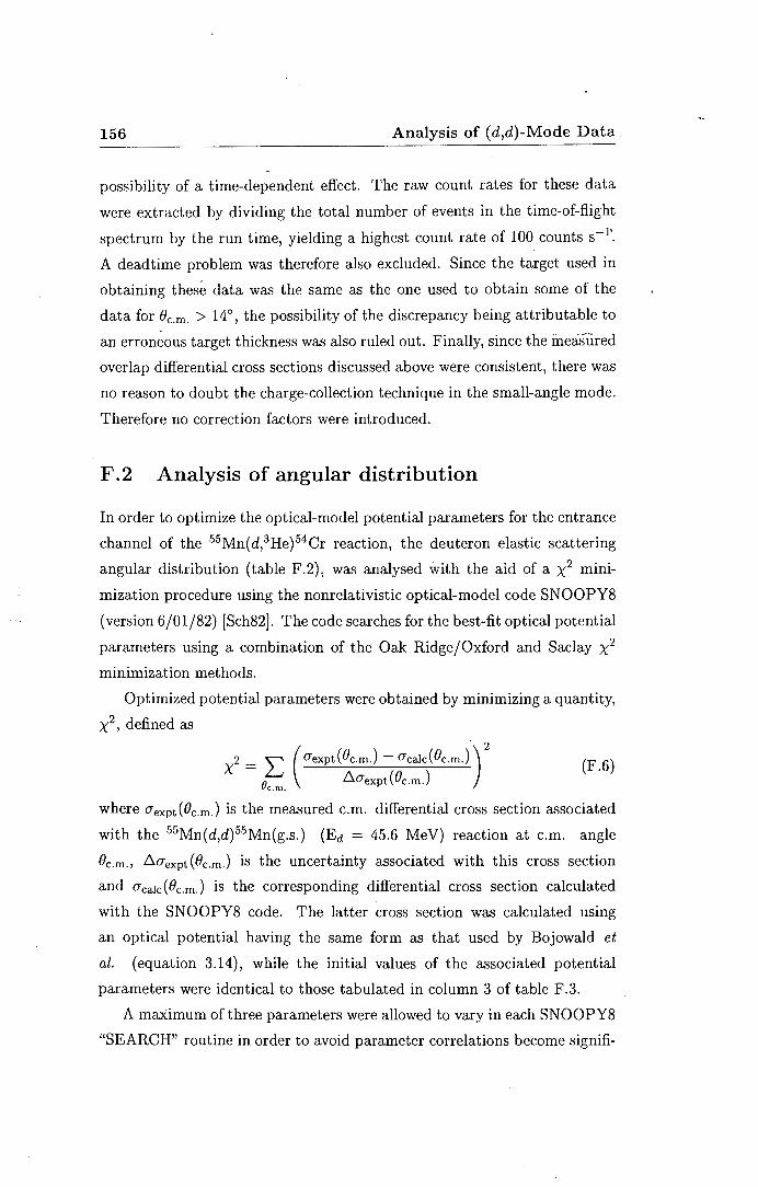
156 Analysis of (d,d)-Mode Data.
possibility of a time-dependent effect. The raw count rates for these data
were extracted by dividing the total number of events in the time-of-flight
spectrum by the run time, yielding a highest count rate of 100 counts s- 1'.
A deadtime problem was therefore also excluded. Since the target used in
obtaining these data was the same as the one used to obtain some of the
data for Bc.m. > 14°, the possibility of the discrepancy being attributable to
an erron~ous target thickness was also ruled out. Finally, since the measured
overlap differential cross sections discussed above were consistent, there was
no reason to doubt the charge-collection technique in the small-angle mode.
Therefore no correction factors were introduced.
F .2 Analysis of angular distribution
In order to optimize the optical-model potential parameters for the entrance
channel of the 55 Mn(d,3He) 54Cr reaction, the deuteron elastic scattering
angular distribution (table F.2), was analysed with the aid of a x2 mini
mization procedure using the nonrelativistic optical-model code SNOOPY8
(version 6/01/82) [Sch82]. The code searches for the best-fit optical potential
parameters using a combination of the Oak Ridge/Oxford and Saclay x2
minimization methods.
Optimized potential parameters were obtained by minimizing a quantity,
x2' defined as
x2 = L (aexpt(Bc.m.) - aca1c(Bc.m.))2
(} b.aexpt(Bc.m.) c.m.
(F.6)
where a ex pt ( Bc.m.) is the measured c.m. differential cross section associated
with the 55Mn(d,d) 55 Mn(g.s.) (Ed = 45.6 MeV) reaction at c.m. angle
Bc.m., b.aexpt(Bc.m.) is the uncertainty associated with this cross section
and aca1c(Bc.m.) is the corresponding differential cross section calculated
with the SNOOPY8 code. The latter cross section was calculated using
an optical potential having the same form as that used by Bojowald et
al. (equation 3.14), while the initial values of the associated potential
parameters were identical to those tabulated in column 3 of table F.3.
A maximum of three parameters were allowed to vary in each SNOOPY8
"SEARCH" routine in order to avoid parameter correlations become signifi-

F .2 Analysis of angular distribution 157
potential Bojowald et al. specialization to SNOOPY 8
parameter parameterization this work best fit
v 1 81.32 + l.43ZA-3 - 0.24Ed 79.80 82.14
rv 1.18 1.18 1.18 1
av 0.636 + 0.035A3 0.769 0.786
Wvol O (Ed ~ 45.0)
0.132(Ed - 45.0) (Ed 2: 45.0) 0.079 0.079
Wsurf 1
7.80 + l.04A 3 - 0. 712Wvol 11.70 13.25
rw 1.27 1.27 1.27
aw 0.850 0.850 0.837
Vi.s 6.00 6.00 4.73
rz.s b.925 . 0.925 0.922
az.s 0.925 0.925 0.605
re 1.30 1.30 1.30
Table F .3: Parameterization of a global optical-model potential for
deuterons having a forrri as given by equation 3.14 taken from the study of
Bojowald et al. [Boj88}. A and Z denote the target-nucleus mass and charge
respectively. The parameter values tabulated in column 3 were calculated
with this parameterization, for the 55 Mn(d,d)55 Mn(g.s.) (Ed = 45. 6 Me V)
reaction, and were used as starting values in the search for best-fit parameters
(column 4) performed with the code SNOOPY8 [Sch82} (see text for details).
All potential depths are in Me V, and all geometrical parameters are in fm.

158 Analysis of (d,d)-Mode Data
cant when four to six parameters are allowed to vary simultaneously [Sch82).
The minimization prncedure, which is similar to the one adopted by Barnard
et al. [Bar68), entailed first varying the well-depths V, Vl.s and Wsur J to find
a first minimum x2 , X~in· These well-depths were fixed at the best-fit values
after which the radius parameters rri r1.s and rw were allowed to vary7 to
find a new X~in- With the potential depth and radius parameters fixed
at the best-fit values, the diffuseness parameters av, aw and a1.s were then
allowed to vary to find a final X~in . The best-fit parameters8 obtained
from the minimization procedure are tabulated in table F.3 (column 4)
while the angular distribution generated using these parameters is shown·
superimposed on the measured angular distribution in figure F.7.
7The imaginary volume well depth Wvol and the Coulomb radius re were not varied.
8The dependence of the best-fit parameters on the sequence in which parameters were
varied was also investigated. A maximum variation of 0.23 was found in any best-fit
parameter obtained using a different sequence.

Appendix G
Treatment of Uncertainties
The treatment of uncertainties suggested in Refs. [Miil79, Miil84] was adopted
in this study. The main feature of the adopted approach is the distinction
between
• type A uncertainties which can be evaluated via statistical means and
• type B uncertainties which have to be evaluated via other means.
In order to make estimates of standard deviations associated with type
B uncertainties a trapezoidal probability distribution was used. For this
distribution [IS092]:
f1+7i () =ay(5 =af (G.l)
where
• a is the half-width of the distribution,
• 0 ::; {3 ::; 1 ( {3 = 1 gives a rectangular distribution and {3= 0 gives a
triangular distribution) and
• () is the estimated standard deviation.
For this study {3 was assumed to be 0.50 so that f = 0.46.


References
' (Aus60] N. Austern, in Proceedings of the International Conference on
Nuclear Structure, Kingston, Canada, 1960, D. A. Bromley and
E. W. Vogt (eds.), (North-Holland, Amsterdam, 1960), pp. 323-
335.
(Aus64] N. Austern, R. M. Drisko, E. C. Halbert, and G. R. Satchler, Phys.
Rev. 113, B3 (1964).
(Bac90] A. Bacher, G. P. Berg, D. Bilodeau, C. Foster, J. Lisantti,
T. Rinckel, P. Schwandt, E. J. Stephenson, Y. Wang, and
S. Wells, Scientific and Technical Report, May 1989 - April
1990, (Indiana University Cyclotron Facility , Bloomington,
1990), pp. 178-179.
(Bar68] R. W. Barnard and G. D. Jones, Nucl. Phys. A106, 497 (1968).
(Bar77] S. M. Barr and R. M. DelVecchio, Phys. Rev. C 15, 114 (1977).
[Ber77] W. Bertozzi, M. V. Hynes, C. P. Sargent, C. Creswell, P. C. Dunn,
A. Hirsch, M. Leitch, B. Norum, F. N. Rad, and T. Sasanuma,
Nucl. Instrum. Methods 141, 457 (1977).
(Ber79] W. Bertozzi, M. V. Hynes, C. P. Sargent, W. Turchinetz, and
C. Williamson, Nucl. Instrum. Methods 162, 211 (1979).
(Ber86) G. P. A. Berg, L. C. Bland, B. M. Cox, D. DuPlantis, ·
D. W. Miller, K. Murphy, P. Schwandt, K. A. Solberg,
E. J. Stephenson, B. Flanders, and H. Seifert, Scientific and

162 REFERENCES
Technical Report, (Indiana University Cyclotron Facility, Bloom
ington, 1986), pp. 152-162.
[Ber88] G. P. A. Berg, L. C. Bland, D. DuPlantis, C. C. Fos
ter, D. W. Miller, P. Schwandt, R. Sawafta, K. Solberg, and
E. Stephenson, Scientific and Technical Report, January 1987
- April 1988, (Indiana University Cyclotron Facility, Blooming
ton, 1988), pp. 233-237.
[Ber89] G. P. A. Berg, L. Bland, C. C. Foster, J. Lisantti, T. Rinckel,
R. Sawafta, P. Schwandt, K. Solberg, and E. J. Stephenson,
Scientific and Technical Report, May 1988 - April 1989, (Indiana
University Cyclotron Facility, Bloomington, 1989), pp. 200-204.
[Bev69] P. R. Bevington, Data Reduction and Error Analysjs for the
Physical Sciences, (McGraw-Hill, New York, 1969), p. 105.
[Boj88] J. Bojowald, H. Machner, H. Nann, W. Oelert, M. Rogge, and
P. Turek, Phys. Rev. C 38, 1153 (1988).
[Bot84] A. H. Botha and H. N. Jungwirth, m Proceedings of
the Tenth International Conference on Cyclotrons and their
Applications, Michigan, 1984, F. Marti (ed.) (IEEE, New
York, 1984), p. 263.
[Bot95] A.H. Botha, private communication, National Accelerator Centre,
(1995).
[Bre74] A. Breskin, G. Charpak, B. Gabioud, F. Sauli, N. Traut
ner, W. Duinker, and G. Schultz, Nucl. Instrum. Meth
ods 119, 9 (1974).
[Bru77] P. J. Brussaard and P. W. M. Glaudemans, Shell-Model Applica
tions in Nuclear Spectroscopy, (North-Holland, Amsterdam, 1977),
pp. 144-175.
[Bur95] W. E. Burcham and M. Jobes, Nuclear and Particle Physics,
(Longman, Essex, 1995), pp. 184-204.

REFERENCES 163
(Cam81] J. A. Cameron, E. Habib, A. A. Pilt, R. Schubank, and V. Janzen,
Nucl. Phys. A365, 113 (1981).
[Cha77] N. S. Chant, N. S. Hall, C. F. Clement, S. M. Perez, and
J. N. Cr~ig, Phys. Rev. C 15, 53 (1977).
(Cha84] G. Charpak and F. Sauli, Ann. Rev. Nucl. Part. Sci. 34, 285 (1984).
[Cha93] C. H. C. Challens, M.Sc. thesis, University of the Western Cape,
unpublished (1993).
[Chu78] W. K. Chu, J. W. May~r, and M. A. Nicolet, Backscattering
Spectrometry, (Academic Press, New York, 1978).
[Cle73] C. F. Clement and S. M. Perez, Nucl. Phys. A213, 510 (1973).
[Cle77] C. F. Clement and S. M. Perez, Nucl. Phys. A284, 469 (1977).
[Cle91] C. F. Clement and S. M. Perez, Rep. Prog. Phys. 54, 127 (1991).
[Col59] L. Colli, F. Cvelber, S. Micheletti, and M. Pignanelli, Nuovo
Cimento 14, 1120 (1959).
[Col61] L. Colli, I. Iori, S. Micheletti, and M. Pignanelli, Nuovo Cimento
20, 94 (1961).
[Con94] J. L. Conradie, Ph.D. thesis, University of Stellenbosch,
unpublished (1994).
[den88a] J. W. A. den Herder, H. P. Blok, E. Jans, L. Lapikas, and
P. K. A. de Witt Huberts, Phys. Lett. 60, 1343 (1988).
[den88b] J. W. A. den Herder, H. P. Blok, E. Jans, P. H. M. Keizer,
L. Lapikas, E. N. M. Quint, G. van der Steenhoven, and P. K. A. de
Witt Huberts, Nucl. Phys. A490, 507 (1988).
[Doo85] L. R. Doolittle, Nucl. Instrum. Methods B9, 344 (1985).
[Eis88] J. M. Eisenberg and W. Greiner, Excitation Mechanisms of the
Nucleus, (North-Holland, Amsterdam, 1988), pp. 412-422.

164 REFERENCES
[Fu185] H. W. Fulbright, in Treatise on Heavy-Ion Science: Vol. 1 -
Instrumentation and Techniques, D. A. Bromley (ed.), (Plenum
Press, New York, 1985), pp. 179-224.
[Geo91] D. George and V. Vrankovic, ion-optical computer simulation
program TRACK (version 4.8), unpublished (1991).
[Gon87] Wang Gongqing, Zhu Jiabi, and Zhang Jingen, Nucl. Data
Sheets 50, 255 (1987).
[Gou81] C.R. Gould, L. G. Holzsweig, S. E. King, Y. C. Lau, R. V. Poore,
N. R. Roberson, and S. A. Wender, IEEE Trans. Nucl. Sci. NS-
28, 3708 (1981).
[Gou83] C.R. Gould and N. R. Robertson, IEEE Trans. Nucl. Sci. NS-30
5, 3758 (1983).
[Gra92] P. Grabmayr, Prog. Part. Nucl. Phys. 29, 251 (1992).
[Gra94] P. Grabmayr, A. Mondry, G. J. Wagner, P. Woldt, G. P. A. Berg,
J. Lisantti, D. W. Miller, H. Nann, and E. J. Stephenson, Phys.
Rev. C 49, 2971 (1994).
[Hen74] D. L. Hendrie, in Nuclear Spectroscopy and Reactions: Part A,
J. Cerny (ed.), (Academic Press, New York, 1974), pp. 365-412.
[Hen87] R. S. Henderson, 0. Hausser, K. Hicks, C. Gunther, W .. Faszer,
R. Sawafta, ·and N. Poppe, Nucl. Instrum.
Methods A524, 61 (1987).
[Hey94] K. L. G. Heyde, The Nuclear Shell Model, 2nd edition, (Springer
Verlag, Berlin, 1994), pp. 58-148.
[Hin67] P. F. Hinrichsen and B. Rosner, Bull. Amer. Phys.
Soc. 12, 696 (1967).
[Hod74] P. E. Hodgson, Nature Vol. 249, No. 5456, 412 (1974).
[Hol81] L. G. Holzsweig and R. V. Poore, IEEE Trans. Nucl. Sci. NS-
28, 3815 (1981).

REFERENCES 165
[IS092] Guide to the Expression of Uncertainty in Measurement, document
no. ISO /TAG 4/WG 3, '1st edition, (International Organization
for Standardization, Geneva, 1992), pp. 12:-16.
[Jac77] D. F. Jackson and R. C. Barrett, Nuclear Sizes and Structure,
(Clarendon Press, Oxford, 1977), pp. 332-351.
[Jam75] F. James and M. Roos, Comput. Phys. Commun. 10, 343 (1975).
[Jam89] F. James and M. Roos, document no. D506, (CERN, Geneva,
1989).
. [Jin92] Yanhe Jin, D. S. Onley, and L. E. Wright, Phys. Rev. C 45,
131 (1992).
[Jun87] Huo Junde, Hu Dailing, Zhou Chunmei, Han Xiaoling, Hu Baohua,
and Wu Yaodong, Nucl. Data Sheets 51, 1 (1987).
[Jun92] Huo Junde, Nucl. Data Sheets 67, 523 (1992).
[Jun93] Huo Junde, Sun Huibin, Zhao Weizhong, and Zhou Qing, Nucl.
Data Sheets 68, 887 (1_993).
[Kin81] S. E. King, Y. C. Lau, and C. R. Gould, IEEE Trans. Nucl. Sci.
NS-28 5, 3822 (1981).
[Kno89] G. F. Knoll, Radiation Detection and Measurement, (John Wiley
and Sons, New York, 1989), pp. 117-120.
[Kra88] G. J. Kramer, H. P. Blok, J. F. A. van Hienen, S. Brandenburg,
M. N. Harakeh, S. Y. van der Werf, P. W. M. Glaudemans, and
A. A. Wolters, Nucl. Phys. A477, 55 (1988).
[Kra89] G. J. Kramer, H. P. Blok, J. F. J. van den Brand, H. J. Bulten, l
R. Ent, E. Jans, J. B. J. M. Lanen, L. Lapikas, H. Nann,
E. N. M. Quint, G. van der Steenhoven, P. K. A. de Witt Huberts,
and G. J. Wagner, Phys. Lett. B227, 199 (·1989).
[Kun93) P. D. Kunz and E. Rost, in Computational Nuclear Physics 2 -
Nuclear Reactions, K. Langanke, J. A. Maruhn, and S. E. Koonin
(eds.), (Springer-Verlag, New York, 1993), p. 88-107.

166 REFERENCES.
[Lu84] Xi-Ting Lu, Nucl. Instrum. Methods 225, 283 (1984).
[Mah91] C. Mahaux and R. Sartor, Adv. in Nucl. Phys. 20, 1 (1991).
[Man85] H. J. Mang, in Proceedings of the Winter College on
Fundamental Nuclear Physics, Vol.1, International Centre for
Theoretical Physics, Trieste, Italy, 7 Feb - 30 Mar 1984,
K. Dietrich, M. Di Toro, and H. J. Mang (eds.), (World
Scientific, Singapore, 1985), pp. 15-55.
[Mar68] J. B. Marion and F. C. Young, Nuclear Reaction Analysis, (North
Holland, Amsterdam, 1968).
[Mar70] P. Marmier and E. Sheldon, Physics of Nuclei and Particles,
Vol. II, (Academic Press, London, 1970), pp. 1087-1169.
[Mar93] T. K. Marais, Ph.D. thesis, University of the Western Cape,
unpublished (1993).
[Mat68] M. Matoba, Nucl. Phys. All8, 207 (1968).
[Moa77] A. Moalem, Nucl. Phys. A289, 45 (1977).
[Moa79] A. Moalem and Z. Vardi, Nucl. Phys. A332, 195 (1979).
[Mul79] J. W. Muller, Nucl. Instrum. Methods 163, 241 (1979).
[Mul84] J. W. Muller, Precision Measurement and Fundamental Constants
II, B. N. Taylor and W. D. Phillips (eds.), Natl. Bur. Stand.
(U.S.A.), Spec. Publ. No. 617 (1984).
[NAC92] NAC annual report NAC/ AR/92-01, (National Accelerator
Centre, Faure, 1992), pp. 27-28.
[NAC94] NAC annual report, NAC/ AR/94-01, (National Accelerator
Centre, Faure, 1994), pp. 28-29.
[Nan89] H. Nann, in Direct Nuclear Reactions - Proceedings of the
International Seminar, 1989, (Indian Academy of Sciences, Ban
galore, 1989), pp. 317-319.

REFERENCES 167
[Neu94] F. Neumeyer and S. Strauch, peak-fitting computer program
FIT2.1, Technische Hochschule Darmstadt, unpublished (1994).
[New95] R. T. Newman and S. M. Perez, Phys. Rev. C 51, 1414 (1995).
[New96] R. T. Newman, R. W. Fearick, S. M. Perez, D. G. Aschman,
K. Bharuth-Ram, F. D. Smit, V. M. Tshivhase, and T. S. Volkwyn,
Phys. Rev. C, (1996) (in press).
(Niw82] M. Niwano, T. Ishimatsu, R. Asano T. Suehiro, and M. Tanaka,
Nucl. Phys. A377, 148 (1982).
[Off8!] E. A. J. M. Offerman, C. W. De Jager, and H. De Vries,
Nucl. Instrum. Methods A262, 298 (1987).
[Pee74] R. J. Peel, D.R. Dixon, M. W. Hill, G. L. Jensen, N. F. Mangelson,
N. Nath, and V. C. Rogers, Nucl. Phys. A235, 205 (1974).
[Per88] S. M. Perez, Phys. Rev. Lett. 60 13, 1342 (1988).
[Pil88] J. V. Pilcher, NAC internal report, (National Accelerator Centre,
Faure, 1988).
[Pil89a] J. V. Pilcher, A. A. Cowley, D. M. Whittal, and J. J. Lawrie, Phys.
Rev. C 40, 1937 (1989).
[Pil89b) J. V. Pilcher, Ph.D. thesis, University of Cape Town,
unpubHshed (1989).
(Pil92] J. V. Pilcher, NAC internal report, (National Accelerator Centre,
Faure, 1992).
[Ros57] M. E. Rose, Elementary Theory of Angular Momentum, (John
Wiley and Sons, New York, 1957).
[Roy67] R. R. Roy and B. P. Nigam, Nuclear Physics - Theory and
Experiment, (John Wiley and Sons, New York, 1967), pp. 393-
431.
[Sat83] G. R. Satchler, Direct Nuclear Reactions, (Oxford University
Press, New York, 1983), pp. 90-96.

168 REFERENCES.
[Sat90] G. R. Satchler, Introduction to Nuclear Reactions, 2nd edition,
(MacMillan, London, 1990), pp. 153-277.
[Sau77] F. Sauli, Principles of Operation of Multiwire Proportional and
Drift chambers, document no. 77-09, (CERN, Geneva, 1977).
[Sch82] P. Schwandt, SNOOPY8 - Optical Potential Code for Elastic
Scattering Analysis, report no. 82-3, (Indiana University
Cyclotron Facility, Bloomington, 1982).
[Sch86] P. Schwandt, notes on the Indiana University Cyclotron Facility
K600 spectrometer, unpublished (1986).
[Sic91] I. Sick and P. de Witt Huberts, Comments Nucl. Part. Phys. 20,
177 (1991)
[Tro80] H. -J. Trost, A. Schwarz, U. Feindt, F. H. Heimlich, S. Heinzel,
J. Hintze, F. Korber, R. Lekebusch, P. Lezoch, G. Mock, W. Paul,
E. Roick, M. Wolff, J. Worzeck, and U. Strohbusch, Nucl.
Phys. A337, 377 (1980).
[Udi93] J. M. Udias, P. Sarriguren, E. Moya de Guerra, E. Garrido, and
J. A. Caballero, Phys. Rev. C 48, 2731 (1993).
[Udi95J J. M. Udias, P. Sarriguren, E. Moya de Guerra, E. Garrido, and
J. A. Caballero, Phys. Rev. C 51, 3246 (1995).
[Val91] M: Vallieres and H. Wua, Computational Nuclear Physics I -
Nuclear Structure, K. Langanke, J. A. Maruhn, and S. E. Koonin
(eds.), (Springer-Verlag, New York, 1991), pp. 1-23.
[van89] S. Y. van der Werf, M. N. Harakeh, and E. N. M. Quint, Phys.
Lett. B 216, 15 (1989).
[van94] M. G. van der Merwe, W. A. Richter, and B. A. Brown, Nucl.
Phys. A579, 173 (1994).
[Vee93] R. Veenhof, drift-chamber simulation computer program
GARFIELD (version 4.29), CERN program library entry
W5050, (CERN, Geneva, 1993).

REFERENCES 169
[Ver94] J. Vernotte, G. Berrier-Ronsin, S. Fortier, E. Hourani, J. Kalifa,
A. Khendriche, J.M. Maison, L. H. Rosier, and G. Rotbard, Phys.
Rev. C 49, 1559 (1994).
[Wag90] G. J. Wagner, Prog. Part. Nucl. Phys. 24, 17 (1990).
(Wa195] J. D. Walecka, Theoretical Nuclear and Subnuclear Physics,
(Oxford Unversity Press, New York, 1995), p. 42.
[Wap71] A. H. Wapstra and N. B. Grove, Nucl. Data Tables 9 4-
5, 303 (1971) .
• [Weg87] H. E. Wegner, D. J. Clark, H. Wiedemann, H. A. Grunder,
K. Batchelor, H. E. Jackson Jr., K. Strauch, M. Q. Barton, and
U. Schumacher, in Nuclear and Particle Phyiscs Source Book,
S. P. Parker (ed.), (McGraw-Hill, New York, 1987), pp. 398-453.
[Ynt61] J. L. Yntema, T. H. Braid, B. Zeidman, and H. W. Broek, in
Proceedings of the Rutherford Jubilee International Conference,
Manchester, 1961, J. B. Birks (ed.), (Academic Press, New
York, 1961), p. 521.

J