richard larsen morris marx - testallbank.com

INSTRUCTOR’S SOLUTIONS MANUAL

AN INTRODUCTION TO MATHEMATICAL STATISTICS

AND ITS APPLICATIONS SIXTH EDITION

Richard Larsen Vanderbilt University

Morris Marx University of West Florida

Introduction to Mathematical Statistics and Its Applications 6th Edition Larsen Solutions ManualFull Download: https://alibabadownload.com/product/introduction-to-mathematical-statistics-and-its-applications-6th-edition-larsen-solutions-manual/

This sample only, Download all chapters at: AlibabaDownload.com

https://alibabadownload.com/product/introduction-to-mathematical-statistics-and-its-applications-6th-edition-larsen-solutions-manual/

The author and publisher of this book have used their best efforts in preparing this book. These efforts include the development, research, and testing of the theories and programs to determine their effectiveness. The author and publisher make no warranty of any kind, expressed or implied, with regard to these programs or the documentation contained in this book. The author and publisher shall not be liable in any event for incidental or consequential damages in connection with, or arising out of, the furnishing, performance, or use of these programs. Reproduced by Pearson from electronic files supplied by the author. Copyright © 2018, 2012, 2006 Pearson Education, Inc. Publishing as Pearson, 330 Hudson Street, NY NY 10013 All rights reserved. No part of this publication may be reproduced, stored in a retrieval system, or transmitted, in any form or by any means, electronic, mechanical, photocopying, recording, or otherwise, without the prior written permission of the publisher. Printed in the United States of America.

ISBN-13: 978-0-13-411427-9 ISBN-10: 0-13-411427-2

Copyright © 2018 Pearson Education, Inc. iii

Contents

Chapter 2: Probability ..............................................................................................................1

2.2 Samples Spaces and the Algebra of Sets ............................................................................. 1 2.3 The Probability Function ..................................................................................................... 6 2.4 Conditional Probability ....................................................................................................... 7 2.5 Independence ..................................................................................................................... 13 2.6 Combinatorics ................................................................................................................... 17 2.7 Combinatorial Probability ................................................................................................. 24

Chapter 3: Random Variables ................................................................................................27 3.2 Binomial and Hypergeometric Probabilities ..................................................................... 27 3.3 Discrete Random Variables ............................................................................................... 36 3.4 Continuous Random Variables .......................................................................................... 41 3.5 Expected Values ................................................................................................................ 44 3.6 The Variance ..................................................................................................................... 52 3.7 Joint Densities ................................................................................................................... 57 3.8 Transforming and Combining Random Variables............................................................. 69 3.9 Further Properties of the Mean and Variance .................................................................... 73 3.10 Order Statistics .................................................................................................................. 79 3.11 Conditional Densities ........................................................................................................ 82 3.12 Moment-Generating Functions .......................................................................................... 88

Chapter 4: Special Distributions ............................................................................................93 4.2 The Poisson Distribution ................................................................................................... 93 4.3 The Normal Distribution ................................................................................................... 98 4.4 The Geometric Distribution ............................................................................................. 105 4.5 The Negative Binomial Distribution ............................................................................... 107 4.6 The Gamma Distribution ................................................................................................. 109

Chapter 5: Estimation ...........................................................................................................111 5.2 Estimating Parameters: The Method of Maximum Likelihood

and Method of Moments ................................................................................................. 111 5.3 Interval Estimation .......................................................................................................... 118 5.4 Properties of Estimators .................................................................................................. 123 5.5 Minimum-Variance Estimators: The Cramér-Rao Lower Bound ................................... 128 5.6 Sufficient Estimators ....................................................................................................... 130 5.7 Consistency ..................................................................................................................... 133 5.8 Bayesian Estimation ........................................................................................................ 135

Copyright © 2018 Pearson Education, Inc. iv

Chapter 6: Hypothesis Testing .............................................................................................137 6.2 The Decision Rule ........................................................................................................... 137 6.3 Testing Binomial Data................................................................................................................................................................ 138 6.4 Type I and Type II Errors ................................................................................................ 139 6.5 A Notion of Optimality: The Generalized Likelihood Ratio ........................................... 144

Chapter 7: Inferences Based on the Normal Distribution ....................................................147 7.3 Deriving the Distribution of

/YS n

.................................................................................... 147 7.4 Drawing Inferences About ......................................................................................... 150 7.5 Drawing Inferences About 2 ........................................................................................ 156

Chapter 8: Types of Data: A Brief Overview ......................................................................161 8.2 Classifying Data .............................................................................................................. 161

Chapter 9: Two-Sample Inference .......................................................................................163 9.2 Testing 0 : X YH ....................................................................................................... 163 9.3 Testing 2 2

0 : X YH —The F Test ................................................................................. 166 9.4 Binomial Data: Testing 0 : X YH p p ............................................................................. 168 9.5 Confidence Intervals for the Two-Sample Problem ........................................................ 170

Chapter 10: Goodness-of-Fit Tests ......................................................................................173 10.2 The Multinomial Distribution ......................................................................................... 173 10.3 Goodness-of-Fit Tests: All Parameters Known ............................................................... 175 10.4 Goodness-of-Fit Tests: Parameters Unknown ................................................................. 178 10.5 Contingency Tables ......................................................................................................... 185

Chapter 11: Regression ........................................................................................................189 11.2 The Method of Least Squares .......................................................................................... 189 11.3 The Linear Model ............................................................................................................ 199 11.4 Covariance and Correlation ............................................................................................. 204 11.5 The Bivariate Normal Distribution .................................................................................. 208

Chapter 12: The Analysis of Variance .................................................................................211 12.2 The F test ......................................................................................................................... 211 12.3 Multiple Comparisons: Tukey’s Method ......................................................................... 214

Copyright © 2018 Pearson Education, Inc. v

12.4 Testing Subhypotheses with Constrasts .......................................................................... 216 12.5 Data Transformations ...................................................................................................... 218 Appendix 12.A.2 The Distribution of /( 1)

/( )SSTR kSSE n k

When 1H Is True ............................................ 218

Chapter 13: Randomized Block Designs .............................................................................221 13.2 The F Test for a Randomized Block Design ................................................................... 221 13.3 The Paired t Test.............................................................................................................. 224

Chapter 14: Nonparametric Statistics...................................................................................229 14.2 The Sign Test .................................................................................................................. 229 14.3 Wilcoxon Tests ................................................................................................................ 232 14.4 The Kruskal-Wallis Test ................................................................................................. 236 14.5 The Friedman Test ........................................................................................................... 239 14.6 Testing for Randomness .................................................................................................. 241

Copyright © 2018 Pearson Education, Inc. 1

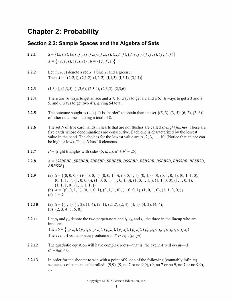
Chapter 2: Probability Section 2.2: Sample Spaces and the Algebra of Sets 2.2.1 S = ( , , ), ( , , ), ( , , ), ( , , ), ( , , ), ( , , ), ( , , ), ( , , )s s s s s f s f s f s s s f f f s f f f s f f f A = ( , , ), ( , , )s f s f s s ; B = ( , , )f f f 2.2.2 Let (x, y, z) denote a red x, a blue y, and a green z.

Then A = (2,2,1), (2,1,2), (1,2,2), (1,1,3), (1,3,1), (3,1,1) 2.2.3 (1,3,4), (1,3,5), (1,3,6), (2,3,4), (2,3,5), (2,3,6) 2.2.4 There are 16 ways to get an ace and a 7, 16 ways to get a 2 and a 6, 16 ways to get a 3 and a

5, and 6 ways to get two 4’s, giving 54 total. 2.2.5 The outcome sought is (4, 4). It is “harder” to obtain than the set {(5, 3), (3, 5), (6, 2), (2, 6)}

of other outcomes making a total of 8. 2.2.6 The set N of five card hands in hearts that are not flushes are called straight flushes. These are

five cards whose denominations are consecutive. Each one is characterized by the lowest value in the hand. The choices for the lowest value are A, 2, 3, …, 10. (Notice that an ace can be high or low). Thus, N has 10 elements.

2.2.7 P = {right triangles with sides (5, a, b): a2 + b2 = 25} 2.2.8 A = {SSBBBB, SBSBBB, SBBSBB, SBBBSB, BSSBBB, BSBSBB, BSBBSB, BBSSBB, BBSBSB,

BBBSSB} 2.2.9 (a) S = {(0, 0, 0, 0) (0, 0, 0, 1), (0, 0, 1, 0), (0, 0, 1, 1), (0, 1, 0, 0), (0, 1, 0, 1), (0, 1, 1, 0), (0, 1, 1, 1), (1, 0, 0, 0), (1, 0, 0, 1), (1, 0, 1, 0), (1, 0, 1, 1, ), (1, 1, 0, 0), (1, 1, 0, 1), (1, 1, 1, 0), (1, 1, 1, 1, )} (b) A = {(0, 0, 1, 1), (0, 1, 0, 1), (0, 1, 1, 0), (1, 0, 0, 1), (1, 0, 1, 0), (1, 1, 0, 0, )} (c) 1 + k 2.2.10 (a) S = {(1, 1), (1, 2), (1, 4), (2, 1), (2, 2), (2, 4), (4, 1), (4, 2), (4, 4)} (b) {2, 3, 4, 5, 6, 8} 2.2.11 Let p1 and p2 denote the two perpetrators and i1, i2, and i3, the three in the lineup who are

innocent. Then S = 1 1 1 2 1 3 2 1 2 2 2 3 1 2 1 2 1 3 2 3( , ), ( , ), ( , ), ( , ), ( , ), ( , ), ( , ), ( , ), ( , ), ( , )p i p i p i p i p i p i p p i i i i i i . The event A contains every outcome in S except (p1, p2). 2.2.12 The quadratic equation will have complex roots—that is, the event A will occur—if

b2 4ac < 0. 2.2.13 In order for the shooter to win with a point of 9, one of the following (countably infinite)

sequences of sums must be rolled: (9,9), (9, no 7 or no 9,9), (9, no 7 or no 9, no 7 or no 9,9), …

2 Chapter 2: Probability

Copyright © 2018 Pearson Education, Inc.

2.2.14 Let (x, y) denote the strategy of putting x white chips and y red chips in the first urn (which results in 10 x white chips and 10 y red chips being in the second urn). Then S = ( , ) : 0,1,...,10, 0,1,...,10, and 1 19x y x y x y . Intuitively, the optimal strategies are (1, 0) and (9, 10).

2.2.15 Let Ak be the set of chips put in the urn at 1/2k minute until midnight. For example, A1 = {11, 12, 13, 14, 15, 16, 17, 18, 19, 20}. Then the set of chips in the urn at midnight is

1( { 1})k

k

A k

.

2.2.16 move arrow on first figure raise B by 1

2.2.17 If x2 + 2x 8, then (x + 4)(x 2) 0 and A = {x: 4 x 2}. Similarly, if x2 + x 6, then

(x + 3)(x 2) 0 and B = {x: 3 x 2). Therefore, A B = {x: 3 x 2} and A B = {x: 4 x 2}.

2.2.18 A B C = {x: x = 2, 3, 4} 2.2.19 The system fails if either the first pair fails or the second pair fails (or both pairs fail). For

either pair to fail, though, both of its components must fail. Therefore, A = (A11 A21) (A12 A22).

2.2.20 (a) (b) (c) empty set (d) 2.2.21 40 2.2.22 (a) {E1, E2} (b) {S1, S2, T1, T2} (c) {A, I} 2.2.23 (a) If s is a member of A (B C) then s belongs to A or to B C. If it is a member of A or

of B C, then it belongs to A B and to A C. Thus, it is a member of (A B) (A C).

Conversely, choose s in (A B) (A C). If it belongs to A, then it belongs to A (B C). If it does not belong to A, then it must be a member of B C. In that case it also is a member of A (B C).

Section 2.2: Sample Spaces and the Algebra of Sets 3


(b) If s is a member of A (B C) then s belongs to A and to B C. If it is a member of B, then it belongs to A B and, hence, (A B) (A C). Similarly, if it belongs to C, it is a member of (A B) (A C). Conversely, choose s in (A B) (A C). Then it belongs to A. If it is a member of A B then it belongs to A (B C). Similarly, if it belongs to A C, then it must be a member of A (B C).

2.2.24 Let B = A1 A2 … Ak. Then 1 2 ...C C C

kA A A = (A1 A2 … Ak)C = BC. Then the expression is simply B BC = S.

2.2.25 (a) Let s be a member of A (B C). Then s belongs to either A or B C (or both). If s

belongs to A, it necessarily belongs to (A B) C. If s belongs to B C, it belongs to B or C or both, so it must belong to (A B) C. Now, suppose s belongs to (A B) C. Then it belongs to either A B or C or both. If it belongs to C, it must belong to A (B C). If it belongs to A B, it must belong to either A or B or both, so it must belong to A (B C).

(b) Suppose s belongs to A (B C), so it is a member of A and also B C. Then it is amember of A and of B and C. That makes it a member of (A B) C. Conversely, if s is a member of (A B) C, a similar argument shows it belongs to A (B C).

2.2.26 (a) AC BC CC (b) A B C (c) A BC CC (d) (A BC CC) (AC B CC) (AC BC C) (e) (A B CC) (A BC C) (AC B C) 2.2.27 A is a subset of B. 2.2.28 (a) {0} {x: 5 x 10} (b) {x: 3 x < 5} (c) {x: 0 < x 7} (d) {x: 0 < x < 3} (e) {x: 3 x 10} (f) {x: 7 < x 10} 2.2.29 (a) B and C (b) B is a subset of A. 2.2.30 (a) A1 A2 A3 (b) A1 A2 A3 The second protocol would be better if speed of approval matters. For very important issues,

the first protocol is superior. 2.2.31 Let A and B denote the students who saw the movie the first time and the second time,

respectively. Then N(A) = 850, N(B) = 690, and [( ) ]CN A B = 4700 (implying that N(A B) = 1300). Therefore, N(A B) = number who saw movie twice = 850 + 690 1300 = 240.



2.2.32 (a) (b) 2.2.33 (a) (b) 2.2.34 (a) A (B C) (A B) C (b) A (B C) (A B) C 2.2.35 A and B are subsets of A B.

Section 2.2: Sample Spaces and the Algebra of Sets 5


2.2.36 (a) ( )C CA B = AC B (b) ( )C CB A B A B (c) ( )C CA A B A B 2.2.37 Let A be the set of those with MCAT scores 27 and B be the set of those with GPAs 3.5.

We are given that N(A) = 1000, N(B) = 400, and N(A B) = 300. Then ( )C CN A B = [( ) ]CN A B = 1200 N(A B) = 1200 [(N(A) + N(B) N(A B)] = 1200 [(1000 + 400 300] = 100. The requested proportion is 100/1200.

2.2.38 N(A B C) = N(A) + N(B) + N(C) N(A B) N(A C) N(B C) + N(A B C) 2.2.39 Let A be the set of those saying “yes” to the first question and B be the set of those saying

“yes” to the second question. We are given that N(A) = 600, N(B) = 400, and N(AC B) = 300. Then N(A B) = N(B) ( )CN A B = 400 300 = 100. ( )CN A B = N(A) N(A B) = 600 100 = 500.

2.2.40 [( ) ]CN A B = 120 N(A B) = 120 [N( CA B) + N(A CB ) + N(A B)]

= 120 [50 + 15 + 2] = 53



Section 2.3: The Probability Function 2.3.1 Let L and V denote the sets of programs with offensive language and too much violence,

respectively. Then P(L) = 0.42, P(V) = 0.27, and P(L V) = 0.10. Therefore, P(program complies) = P((L V)C) = 1 [P(L) + P(V) P(L V)] = 0.41.

2.3.2 P(A or B but not both) = P(A B) P(A B) = P(A) + P(B) P (A B) P(A B)

= 0.4 + 0.5 0.1 0.1 = 0.7 2.3.3 (a) 1 P(A B) (b) P(B) P(A B) 2.3.4 P(A B) = P(A) + P(B) P(A B) = 0.3; P(A) P(A B) = 0.1. Therefore, P(B) = 0.2.

2.3.5 No. P(A1 A2 A3) = P(at least one “6” appears) = 1 P(no 6’s appear) = 35 11

6 2

.

The Ai’s are not mutually exclusive, so P(A1 A2 A3) P(A1) + P(A2) + P(A3). 2.3.6 P(A or B but not both) = 0.5 – 0.2 = 0.3 2.3.7 By inspection, B = (B A1) (B A2) … (B An). 2.3.8 (a) (b) (b)

Section 2.4: Conditional Probability 7


2.3.9 P(odd man out) = 1 P(no odd man out) = 1 P(HHH or TTT) = 1 2 38 4

2.3.10 A = {2, 4, 6, …, 24}; B = {3, 6, 9, …, 24); A B = {6, 12, 18, 24}.

Therefore, P(A B) = P(A) + P(B) P(A B) = 12 8 4 1624 24 24 24

.

2.3.11 Let A: State wins Saturday and B: State wins next Saturday. Then P(A) = 0.10, P(B) = 0.30,

and P(lose both) = 0.65 = 1 P(A B), which implies that P(A B) = 0.35. Therefore, P(A B) = 0.10 + 0.30 0.35 = 0.05, so P(State wins exactly once) = P(A B) P(A B) = 0.35 0.05 = 0.30.

2.3.12 Since A1 and A2 are mutually exclusive and cover the entire sample space, p1 + p2 = 1.

But 3p1 p2 = 12

, so p2 = 58

.

2.3.13 Let F: female is hired and T: minority is hired. Then P(F) = 0.60, P(T) = 0.30, and

P(FC TC) = 0.25 = 1 P(F T). Since P(F T) = 0.75, P(F T) = 0.60 + 0.30 0.75 = 0.15.

2.3.14 The smallest value of P[(A B C)C] occurs when P(A B C) is as large as possible.

This, in turn, occurs when A, B, and C are mutually disjoint. The largest value for P(A B C) is P(A) + P(B) + P(C) = 0.2 + 0.1 + 0.3 = 0.6. Thus, the smallest value for P[(A B C)C] is 0.4.

2.3.15 (a) XC Y = {(H, T, T, H), (T, H, H, T)}, so P(XC Y) = 2/16 (b) X YC = {(H, T, T, T), (T, T, T, H), (T, H, H, H), (H, H, H, T)} so P(X YC) = 4/16 2.3.16 A = {(1, 5), (2, 4), (3, 3), (4, 2), (5, 1)} A BC = {(1, 5), (3, 3), (5, 1)}, so P(A BC) = 3/36 = 1/12. 2.3.17 A B, (A B) (A C), A, A B, S 2.3.18 Let A be the event of getting arrested for the first scam; B, for the second. We are given

P(A) = 1/10, P(B) = 1/30, and P(A B) = 0.0025. Her chances of not getting arrested are P[(A B)C] = 1 P(A B) = 1 [P(A) + P(B) P(A B)] = 1 [1/10 + 1/30 0.0025] = 0.869

Section 2.4: Conditional Probability

2.4.1 P(sum = 10|sum exceeds 8) = (sum 10 and sum exceeds 8)(sum exceeds 8)

PP

= (sum 10) 3 36 3(sum 9,10,11, or 12) 4 36 3 36 2 36 1 36 10

P /P / / / /

.



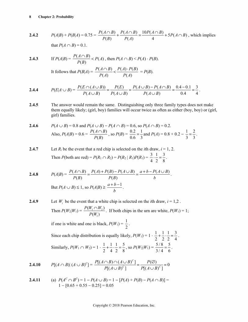
2.4.2 P(A|B) + P(B|A) = 0.75 = ( ) ( ) 10 ( ) 5 ( )( ) ( ) 4

P A B P A B P A B P A BP B P A , which implies

that P(A B) = 0.1.

2.4.3 If P(A|B) = ( ) ( )( )

P A B P AP B , then P(A B) < P(A) P(B).

It follows that P(B|A) = ( ) ( ) ( )( ) ( )

P A B P A P BP A P A = P(B).

2.4.4 P(E|A B) = ( ( )) ( ) ( ) ( ) 0.4 0.1 3( ) ( ) ( ) 0.4 4

P E A B P E P A B P A BP A B P A B P A B

.

2.4.5 The answer would remain the same. Distinguishing only three family types does not make

them equally likely; (girl, boy) families will occur twice as often as either (boy, boy) or (girl, girl) families.

2.4.6 P(A B) = 0.8 and P(A B) P(A B) = 0.6, so P(A B) = 0.2.

Also, P(A|B) = 0.6 = ( )( )

P A BP B , so P(B) = 0.2 1

0.6 3 and P(A) = 0.8 + 0.2 1 2

3 3 .

2.4.7 Let Ri be the event that a red chip is selected on the ith draw, i = 1, 2.

Then P(both are red) = P(R1 R2) = P(R2 | R1)P(R1) = 3 1 34 2 8 .

2.4.8 P(A|B) = ( ) ( ) ( ) ( ) ( )( ) ( )

P A B P A P B P A B a b P A BP B P B b .

But P(A B) 1, so P(A|B) 1a bb

.

2.4.9 Let iW be the event that a white chip is selected on the ith draw, i = 1,2 .

Then P(W2|W1) = 1 2

1

( )( )

P W WP W . If both chips in the urn are white, P(W1) = 1;

if one is white and one is black, P(W1) = 12

.

Since each chip distribution is equally likely, P(W1) = 1 1 1 1 32 2 2 4 .

Similarly, P(W1 W2) = 1 1 1 1 52 4 2 8 , so P(W2|W1) = 5 / 8 5

3 / 4 6 .

2.4.10 P[(A B)| (A B)C] = [( ) ( ) ] ( ) 0[( ) ] [( ) ]

C

C C

P A B A B PP A B P A B

2.4.11 (a) P(AC BC) = 1 P(A B) = 1 [P(A) + P(B) P(A B)] =

1 [0.65 + 0.55 0.25] = 0.05

Section 2.4: Conditional Probability 9


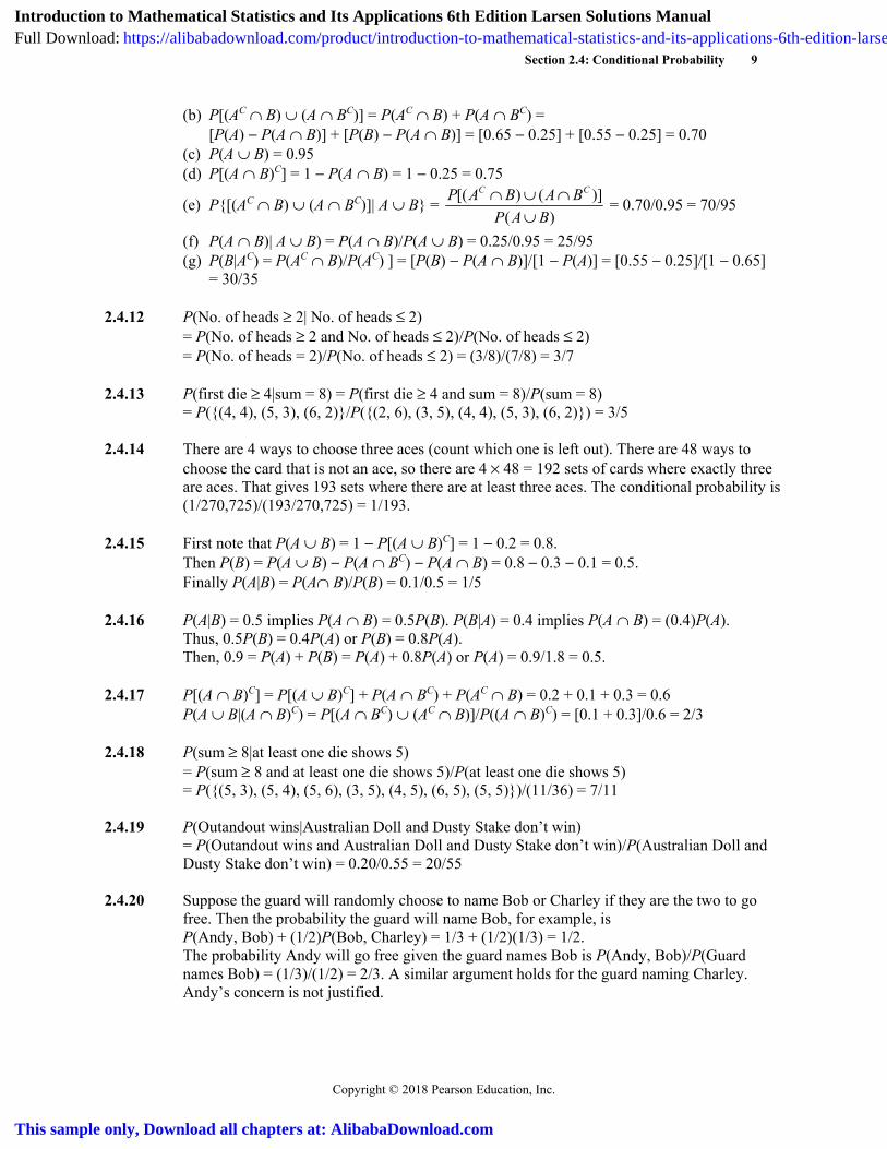
(b) P[(AC B) (A BC)] = P(AC B) + P(A BC) = [P(A) P(A B)] + [P(B) P(A B)] = [0.65 0.25] + [0.55 0.25] = 0.70

(c) P(A B) = 0.95 (d) P[(A B)C] = 1 P(A B) = 1 0.25 = 0.75

(e) P{[(AC B) (A BC)]| A B} = [( ) ( )]( )

C CP A B A BP A B

= 0.70/0.95 = 70/95

(f) P(A B)| A B) = P(A B)/P(A B) = 0.25/0.95 = 25/95 (g) P(B|AC) = P(AC B)/P(AC) ] = [P(B) P(A B)]/[1 P(A)] = [0.55 0.25]/[1 0.65]

= 30/35 2.4.12 P(No. of heads 2| No. of heads 2)

= P(No. of heads 2 and No. of heads 2)/P(No. of heads 2) = P(No. of heads = 2)/P(No. of heads 2) = (3/8)/(7/8) = 3/7

2.4.13 P(first die 4|sum = 8) = P(first die 4 and sum = 8)/P(sum = 8)

= P({(4, 4), (5, 3), (6, 2)}/P({(2, 6), (3, 5), (4, 4), (5, 3), (6, 2)}) = 3/5 2.4.14 There are 4 ways to choose three aces (count which one is left out). There are 48 ways to

choose the card that is not an ace, so there are 4 48 = 192 sets of cards where exactly three are aces. That gives 193 sets where there are at least three aces. The conditional probability is (1/270,725)/(193/270,725) = 1/193.

2.4.15 First note that P(A B) = 1 P[(A B)C] = 1 0.2 = 0.8.

Then P(B) = P(A B) P(A BC) P(A B) = 0.8 0.3 0.1 = 0.5. Finally P(A|B) = P(A B)/P(B) = 0.1/0.5 = 1/5

2.4.16 P(A|B) = 0.5 implies P(A B) = 0.5P(B). P(B|A) = 0.4 implies P(A B) = (0.4)P(A).

Thus, 0.5P(B) = 0.4P(A) or P(B) = 0.8P(A). Then, 0.9 = P(A) + P(B) = P(A) + 0.8P(A) or P(A) = 0.9/1.8 = 0.5. 2.4.17 P[(A B)C] = P[(A B)C] + P(A BC) + P(AC B) = 0.2 + 0.1 + 0.3 = 0.6 P(A B|(A B)C) = P[(A BC) (AC B)]/P((A B)C) = [0.1 + 0.3]/0.6 = 2/3 2.4.18 P(sum 8|at least one die shows 5) = P(sum 8 and at least one die shows 5)/P(at least one die shows 5) = P({(5, 3), (5, 4), (5, 6), (3, 5), (4, 5), (6, 5), (5, 5)})/(11/36) = 7/11 2.4.19 P(Outandout wins|Australian Doll and Dusty Stake don’t win) = P(Outandout wins and Australian Doll and Dusty Stake don’t win)/P(Australian Doll and

Dusty Stake don’t win) = 0.20/0.55 = 20/55 2.4.20 Suppose the guard will randomly choose to name Bob or Charley if they are the two to go

free. Then the probability the guard will name Bob, for example, is P(Andy, Bob) + (1/2)P(Bob, Charley) = 1/3 + (1/2)(1/3) = 1/2. The probability Andy will go free given the guard names Bob is P(Andy, Bob)/P(Guard

names Bob) = (1/3)/(1/2) = 2/3. A similar argument holds for the guard naming Charley. Andy’s concern is not justified.

Introduction to Mathematical Statistics and Its Applications 6th Edition Larsen Solutions ManualFull Download: https://alibabadownload.com/product/introduction-to-mathematical-statistics-and-its-applications-6th-edition-larsen-solutions-manual/

This sample only, Download all chapters at: AlibabaDownload.com

https://alibabadownload.com/product/introduction-to-mathematical-statistics-and-its-applications-6th-edition-larsen-solutions-manual/

richard larsen morris marx - testallbank.com

Documents