richard froese and brian wetton - yale university
TRANSCRIPT

Notes for Math 152: Linear Systems Spring, 2013
Richard Froese and Brian Wetton © 2010 Richard Froese and Brian Wetton. Permission is granted to make and distribute copies of this document provided the copyright notice and this permission notice are preserved on all copies.

Contents
1 Introduction 51.1 Course Goals . . . . . . . . . . . . . . . . . . . . . . . . . . . . . 51.2 About the Subject . . . . . . . . . . . . . . . . . . . . . . . . . . 6
1.2.1 Connection to Geometry . . . . . . . . . . . . . . . . . . . 61.2.2 Linear Systems . . . . . . . . . . . . . . . . . . . . . . . . 61.2.3 Eigen-analysis . . . . . . . . . . . . . . . . . . . . . . . . . 7
1.3 About These Notes . . . . . . . . . . . . . . . . . . . . . . . . . . 81.4 About The Computer Labs . . . . . . . . . . . . . . . . . . . . . 9
2 Vectors and Geometry 102.1 Chapter Introduction . . . . . . . . . . . . . . . . . . . . . . . . . 102.2 Vectors . . . . . . . . . . . . . . . . . . . . . . . . . . . . . . . . 10
2.2.1 Multiplication by a number and vector addition . . . . . . 112.2.2 Co-ordinates . . . . . . . . . . . . . . . . . . . . . . . . . 122.2.3 Properties of vector addition and scalar multiplication . . 162.2.4 MATLAB: basic scalar and vector operations . . . . . . . 172.2.5 Problems . . . . . . . . . . . . . . . . . . . . . . . . . . . 18
2.3 Geometrical Aspects of Vectors . . . . . . . . . . . . . . . . . . . 192.3.1 Length of a vector . . . . . . . . . . . . . . . . . . . . . . 192.3.2 The dot product . . . . . . . . . . . . . . . . . . . . . . . 192.3.3 Projections . . . . . . . . . . . . . . . . . . . . . . . . . . 222.3.4 MATLAB: norm and dot commands . . . . . . . . . . . . 232.3.5 Problems . . . . . . . . . . . . . . . . . . . . . . . . . . . 23
2.4 Determinants and the Cross Product . . . . . . . . . . . . . . . . 252.4.1 The determinant in two and three dimensions . . . . . . . 252.4.2 The cross product . . . . . . . . . . . . . . . . . . . . . . 272.4.3 The triple product and the determinant in three dimensions 302.4.4 MATLAB: assigning matrices and det and cross commands 312.4.5 MATLAB: generating scripts with the MATLAB editor . 312.4.6 MATLAB: floating point representation of real numbers . 322.4.7 Problems . . . . . . . . . . . . . . . . . . . . . . . . . . . 33
2.5 Lines and Planes . . . . . . . . . . . . . . . . . . . . . . . . . . . 342.5.1 Describing linear sets . . . . . . . . . . . . . . . . . . . . 342.5.2 Lines in two dimensions: Parametric form . . . . . . . . . 34
1

CONTENTS CONTENTS
2.5.3 Lines in two dimensions: Equation form . . . . . . . . . . 352.5.4 Lines in three dimensions: Parametric form . . . . . . . . 352.5.5 Lines in three dimensions: Equation form . . . . . . . . . 362.5.6 Planes in three dimensions: Parametric form . . . . . . . 372.5.7 Planes in three dimensions: Equation form . . . . . . . . 372.5.8 Problems . . . . . . . . . . . . . . . . . . . . . . . . . . . 37
2.6 Introduction to Linear Systems . . . . . . . . . . . . . . . . . . . 402.6.1 Description of points and the geometry of solutions to
systems of equations . . . . . . . . . . . . . . . . . . . . . 402.6.2 Describing the whole plane in two dimensions and all of
space in three dimensions . . . . . . . . . . . . . . . . . . 422.6.3 Linear dependence and independence . . . . . . . . . . . . 432.6.4 Problems . . . . . . . . . . . . . . . . . . . . . . . . . . . 44
2.7 Additional Topics . . . . . . . . . . . . . . . . . . . . . . . . . . . 452.7.1 Application: rotational motion . . . . . . . . . . . . . . . 452.7.2 Application: 3-D graphics . . . . . . . . . . . . . . . . . . 46
2.8 Solutions to Chapter Problems . . . . . . . . . . . . . . . . . . . 49
3 Solving Linear Systems 633.1 Linear Systems . . . . . . . . . . . . . . . . . . . . . . . . . . . . 63
3.1.1 General Form of Linear Systems . . . . . . . . . . . . . . 633.1.2 Solving Linear Systems by Substitution . . . . . . . . . . 633.1.3 Elementary row (equation) operations . . . . . . . . . . . 643.1.4 Augmented Matrices . . . . . . . . . . . . . . . . . . . . . 653.1.5 Problems . . . . . . . . . . . . . . . . . . . . . . . . . . . 66
3.2 Gaussian Elimination . . . . . . . . . . . . . . . . . . . . . . . . . 673.2.1 Using MATLAB for row reductions . . . . . . . . . . . . . 733.2.2 Problems . . . . . . . . . . . . . . . . . . . . . . . . . . . 74
3.3 Homogeneous Equations . . . . . . . . . . . . . . . . . . . . . . . 763.3.1 Properties of solutions of homogeneous systems. . . . . . 773.3.2 Connection of solutions to homogeneous and inhomoge-
neous systems. . . . . . . . . . . . . . . . . . . . . . . . . 773.3.3 Problems . . . . . . . . . . . . . . . . . . . . . . . . . . . 79
3.4 Geometric Applications . . . . . . . . . . . . . . . . . . . . . . . 803.4.1 Problems . . . . . . . . . . . . . . . . . . . . . . . . . . . 81
3.5 Resistor Networks . . . . . . . . . . . . . . . . . . . . . . . . . . 823.5.1 Elements of Basic Circuits . . . . . . . . . . . . . . . . . . 823.5.2 Two Simple Examples Made Complicated . . . . . . . . . 843.5.3 Loop Currents . . . . . . . . . . . . . . . . . . . . . . . . 863.5.4 Alternate Presentation of Resistor Networks . . . . . . . . 903.5.5 Problems . . . . . . . . . . . . . . . . . . . . . . . . . . . 93
3.6 Additional Topics . . . . . . . . . . . . . . . . . . . . . . . . . . . 963.6.1 Quadratic Functions . . . . . . . . . . . . . . . . . . . . . 963.6.2 Least squares fit . . . . . . . . . . . . . . . . . . . . . . . 983.6.3 Equilibrium configuration of hanging weights and springs 993.6.4 Problems . . . . . . . . . . . . . . . . . . . . . . . . . . . 101
2

CONTENTS CONTENTS
3.7 Solutions to Chapter Problems . . . . . . . . . . . . . . . . . . . 102
4 Matrices and Determinants 1174.1 Matrix operations . . . . . . . . . . . . . . . . . . . . . . . . . . 117
4.1.1 MATLAB . . . . . . . . . . . . . . . . . . . . . . . . . . . 1204.1.2 Problems . . . . . . . . . . . . . . . . . . . . . . . . . . . 120
4.2 Linear Transformations and Matrices . . . . . . . . . . . . . . . . 1214.2.1 Linear Transformations . . . . . . . . . . . . . . . . . . . 1214.2.2 Rotations in two dimensions . . . . . . . . . . . . . . . . . 1224.2.3 Projections in two dimensions . . . . . . . . . . . . . . . . 1234.2.4 Reflections in two dimensions . . . . . . . . . . . . . . . . 1244.2.5 Every linear transformation is multiplication by a matrix 1254.2.6 Composition of linear transformations and matrix product 1274.2.7 Problems . . . . . . . . . . . . . . . . . . . . . . . . . . . 127
4.3 Application: random walks . . . . . . . . . . . . . . . . . . . . . 1294.3.1 Problems . . . . . . . . . . . . . . . . . . . . . . . . . . . 134
4.4 The Transpose . . . . . . . . . . . . . . . . . . . . . . . . . . . . 1364.4.1 MATLAB . . . . . . . . . . . . . . . . . . . . . . . . . . . 1384.4.2 Problems . . . . . . . . . . . . . . . . . . . . . . . . . . . 138
4.5 Matrix Inverses . . . . . . . . . . . . . . . . . . . . . . . . . . . . 1384.5.1 Computing the inverse . . . . . . . . . . . . . . . . . . . . 1414.5.2 Inverses of Products . . . . . . . . . . . . . . . . . . . . . 1444.5.3 MATLAB . . . . . . . . . . . . . . . . . . . . . . . . . . . 1454.5.4 Problems . . . . . . . . . . . . . . . . . . . . . . . . . . . 145
4.6 Return to Resistor Networks . . . . . . . . . . . . . . . . . . . . 1464.7 Determinants . . . . . . . . . . . . . . . . . . . . . . . . . . . . . 150
4.7.1 Definition of Determinants . . . . . . . . . . . . . . . . . 1504.7.2 Determinants of Triangular matrices . . . . . . . . . . . . 1514.7.3 Summary of determinant calculation rules . . . . . . . . . 1524.7.4 Calculation of determinant using row operations . . . . . 1534.7.5 More expansion formulae . . . . . . . . . . . . . . . . . . 1534.7.6 MATLAB . . . . . . . . . . . . . . . . . . . . . . . . . . . 1554.7.7 Problems . . . . . . . . . . . . . . . . . . . . . . . . . . . 155
4.8 Additional Topics . . . . . . . . . . . . . . . . . . . . . . . . . . . 1574.8.1 Application: General Least Squares . . . . . . . . . . . . 1574.8.2 Least squares solutions . . . . . . . . . . . . . . . . . . . . 1584.8.3 Problems . . . . . . . . . . . . . . . . . . . . . . . . . . . 1594.8.4 Elementary matrices . . . . . . . . . . . . . . . . . . . . . 1594.8.5 Problems . . . . . . . . . . . . . . . . . . . . . . . . . . . 1624.8.6 Exchanging two rows changes the sign of the determinant 1634.8.7 The determinant is linear in each row separately . . . . . 1644.8.8 Adding a multiple of one row to another doesn’t change
the determinant . . . . . . . . . . . . . . . . . . . . . . . 1654.8.9 The determinant of QA . . . . . . . . . . . . . . . . . . . 1664.8.10 The determinant of A is zero exactly when A is not invertible1674.8.11 The product formula: det(AB) = det(A) det(B) . . . . . . 167
3

CONTENTS CONTENTS
4.8.12 The determinant of the transpose . . . . . . . . . . . . . . 1684.8.13 An impractical formula for the inverse . . . . . . . . . . . 1694.8.14 Cramer’s rule, an impractical way to solve systems . . . . 1704.8.15 Problems . . . . . . . . . . . . . . . . . . . . . . . . . . . 170
4.9 Solutions to Chapter Problems . . . . . . . . . . . . . . . . . . . 170
5 Complex numbers 1935.1 Complex arithmetic . . . . . . . . . . . . . . . . . . . . . . . . . 1935.2 Complex exponential . . . . . . . . . . . . . . . . . . . . . . . . . 1945.3 Polar representation of a complex number . . . . . . . . . . . . . 1965.4 MATLAB . . . . . . . . . . . . . . . . . . . . . . . . . . . . . . . 1965.5 Problems . . . . . . . . . . . . . . . . . . . . . . . . . . . . . . . 1975.6 Solutions to Chapter Problems . . . . . . . . . . . . . . . . . . . 197
6 Eigen-analysis 2006.1 Eigenvalues and eigenvectors . . . . . . . . . . . . . . . . . . . . 200
6.1.1 Computing the eigenvalues and eigenvectors . . . . . . . . 2016.1.2 Complex eigenvalues and eigenvectors . . . . . . . . . . . 2076.1.3 MATLAB . . . . . . . . . . . . . . . . . . . . . . . . . . . 2096.1.4 Problems . . . . . . . . . . . . . . . . . . . . . . . . . . . 210
6.2 Eigenanalysis simplifies matrix powers . . . . . . . . . . . . . . . 2116.2.1 Problems . . . . . . . . . . . . . . . . . . . . . . . . . . . 215
6.3 Systems of linear differential equations . . . . . . . . . . . . . . . 2156.3.1 Problems . . . . . . . . . . . . . . . . . . . . . . . . . . . 221
6.4 LCR circuits . . . . . . . . . . . . . . . . . . . . . . . . . . . . . 2226.4.1 Capacitors and inductors . . . . . . . . . . . . . . . . . . 2226.4.2 Differential equations for LCR circuits . . . . . . . . . . . 2236.4.3 Alternate description of LCR circuits . . . . . . . . . . . . 2256.4.4 Problems . . . . . . . . . . . . . . . . . . . . . . . . . . . 227
6.5 Additional Topics . . . . . . . . . . . . . . . . . . . . . . . . . . . 2276.5.1 Diagonalization . . . . . . . . . . . . . . . . . . . . . . . . 2276.5.2 Computing high powers of a matrix . . . . . . . . . . . . 2296.5.3 Another formula for the determinant . . . . . . . . . . . . 2306.5.4 The matrix exponential and differential equations . . . . . 2306.5.5 Converting higher order equations into first order systems 2316.5.6 Springs and weights . . . . . . . . . . . . . . . . . . . . . 2336.5.7 Problems . . . . . . . . . . . . . . . . . . . . . . . . . . . 238
6.6 Solutions to Chapter Problems . . . . . . . . . . . . . . . . . . . 239
4

Chapter 1
Introduction
Linear Algebra is a branch of Mathematics. Many applied problems from Sci-ence, Engineering and Finance can be written in terms of Linear Algebra ques-tions. This is also true of Calculus, which is why these two fields are stressedin undergraduate Mathematics education at UBC and other universities. Byputting a class of commonly occurring problems into a unified, abstract frame-work, the problems can be studied in detail and well understood. This under-standing can then be taken back to problems in many different fields. It isespecially important to realize that very large problems (with potentially mil-lions of unknowns) can be understood in the same framework as the modelproblems we do by hand in these courses. This course has computer labs thatinvolve the mathematical software, MATLAB, that will allow you to solve largerproblems using numerical computations.
Unlike Calculus, Linear Algebra does not require a lot of background knowl-edge. Basic operations in Linear Algebra are just arithmetic. However, thereis a powerful connection between these simple arithmetic operations and geo-metric quantities. Simple ideas in this course start to become abstract whencombined together. Linear Algebra is a subject you can study with very limitedmatematical background, but you are advised to keep up with course lectures,readings, assignments and computer labs so you won’t be left behind at thetransition from concrete ideas to abstract ones.
1.1 Course Goals
The goal of the course is to enable students to
1. recognize linear algebra questions (for which there are straight-forwardanalytic and numerical solution techniques) as parts of applied problems
2. make the connection between geometric properties and analytic quantities(determinants, dot and cross products, eigenvalues, etc.)
5

Chapter 1. Introduction 1.2. About the Subject
Figure 1.1: Force vector and coordinate systems.
3. recognize that linear systems of equations can have unique, infinite or nosolutions and know how to determine all solutions or that none exist
4. recognize matrix multiplication as a linear transformation and that suchtransformations (to the same dimensional space) can be simplified usingeigen-analysis
5. use complex numbers, which arise naturally in the eigen-analysis of ma-trices
1.2 About the Subject
The subject of the course is Linear Algebra, focussing on three main topics:vectors and matrices and connections to geometry, linear systems, and eigen-analysis of matrices. Several applications are considered including resistor net-works and random walks.
1.2.1 Connection to Geometry
The first topic considered in the course is vectors, which are quantities with bothmagnitude and direction. A typical quantity represented as a vector is a forceF on an object as shown in Figure 1.1. The force F in that figure acts in thex− y plane as shown. The vector force F can be represented by its components(Fx, Fy). Some interesting questions you will be able to answer after completingthis course are: what directions are perpendicular to this force?; what are thecoordinates of the force in the rotated coordinate system x′ − y′?; what are thecoordinates of the force if its direction is rotated? These last two questions arerelated.
1.2.2 Linear Systems
Consider the following simple example. You probably saw something like thisin high school.
6

Chapter 1. Introduction 1.2. About the Subject
Example 1.1 Bob and Sue together have 12 dollars. Sue has 2 dollars morethan Bob. How much money do each have? You can probably guess the solutionby trial and error, but let us proceed a bit more formally. Let x be the amount ofmoney Sue has and y the amount Bob has. The two statements in the examplecan be written mathematically as
x+ y = 12
x− y = 2.
The equations above are a linear system for the unknowns x and y. A techniquethat can be used to solve the system (that is, determine the values of x andy that simultaneously solve both equations above) is substitution. The secondequation can be written as
x = y + 2
This can be substituted into the first equation above, eliminating y from theproblem
(y + 2) + y = 12 or 2y + 2 = 12 so 2y = 10 so y = 5
The value of y = 5 determines x = 7 from either of the original relationships.Thus it is determined that Bob has 5 dollars and Sue has 7.
Often (but not always) a linear system of n equations for n unknowns hasa unique solution. The example above was for the case n = 2. However, thesubstitution technique used above becomes impractical when n is larger than 3.In this course you will learn the Gaussian Elimination technique to solve linearsystems. This systematic method can find all solutions when there are any andalso determine if the system has no solutions. This method can be implementedin numerical software and used to solve very large systems.
1.2.3 Eigen-analysis
The final subject of the course is eigen-analysis of matrices and its applications.A simple, motivational example comes from the study of discrete dynamicalsystems. Consider a sequence of values
x0, x1, · · ·xn · · ·
where the index n is a time level. Suppose that xn is determined by the previousvalue xn−1 in the same way for every n, that is
xn = f(xn−1) for every n ≥ 1 (1.1)
for a given function f . This could describe the population number xn of aspecies at year n. The simple model assumes that the population the next yearonly depends on the population this year through the function f . If the initialvalue x0 were given, then the values x1, x2 · · ·xn · · · could be determined using(1.1) repeatedly. A linear problem arises when we take the specific example
7

Chapter 1. Introduction 1.3. About These Notes
f(x) = ax where a is a given constant. In this case, it is easy to compute theentries of the sequence:
x1 = f(x0) = ax0
x2 = f(x1) = f(ax0) = a2x0
......
xn = f(xn−1)) = anx0
For this example, we can determine how the sequence behaves very well becausewe have an expression for xn above that is easy to understand. There are severalcases:
1. If x0 = 0 then xn = 0 for all n.
2. if |a| < 1 then limn→∞ xn = 0.
3. if a = 1 then xn = x0 for all n.
4. if a = −1 then the values alternate in sign: xn has the value x0 is n iseven, −x0 if n is odd.
5. if |a| > 1 and x0 6= 0 then the values of the sequence grow in absolutevalue as n→∞.
Linear discrete dynamical systems for vectors are also of interest. In thesecases, multiplication by the number a in the example above is replaced bymultiplication by a matrix A. Eigen-analysis of the matrix A allows one tounderstand how the system behaves as n → ∞ in a similar way to the simpleexample above.
1.3 About These Notes
The first version of these notes was written by Richard Froese for Math 152taught in the Spring of 2004. There are many text books on elementary linearalgebra material, but none have the material in the order we want for Math152 for Applied Science students. These notes stress geometric concepts intwo and three dimensional space. They also treat applications and numericalapproximation using MATLAB in more detail than most texts. For this reason,the authors have felt it was worthwhile to maintain and improve these notes forMath 152. Additionally, we believe it is a social benefit for students to haveaccess to this material without having to purchase an expensive, commercialtext.
An update to the notes was made by Richard Froese for the course in 2007,including solutions to the exercises. The version written for the 2009 coursehad some updates by Brian Wetton: this introductory chapter, some additionalcomments on MATLAB commands, a reworked section on linear systems arising
8

Chapter 1. Introduction 1.4. About The Computer Labs
from electrical networks, and additional problems and solutions. In addition, thenotes were converted to standard LATEXformat to make them easier to maintain.
Substantial revisions for the notes for 2010 were done by Ignacio Rozada,who was supported by a UBC Skylight grant over the Summer of 2009 to add theproblems and solutions used in weekly assignments the previous year. He alsoadded additional MATLAB material. Brian Wetton also added additional notesto Chapter 4 on the use of matrix multiplication and inverses in the derivationof solutions to the “fundamental problem” of resistor networks.
These notes for 2012 had minor revisions done by Ozgur Yilmaz. Furtherrevisions are planned. There will be additional MATLAB material added to thenotes and additional problems and solutions. We have considered having thenotes printed and available at cost at the UBC bookstore but are not yet sureof the demand from students.
1.4 About The Computer Labs
The course includes six one-hour computer labs. These are given to small groupsof students every other week starting in the second week of the term. Locationsand times for the lab sections can be found following a link from the course webpage. The labs are being updated slightly for the 2012 course and will be postedduring the term as they are finalized. The labs are designed to be done duringthe lab hour, and must be handed in at the end of the lab period. It is a goodidea to read through the lab notes before going to the lab so you are ready tobegin in the lab. After your first lab, you will be able to go to the lab rooms inopen hours to improve your MATLAB skills and to prepare for upcoming labsif you find you are not able to complete the labs in the lab hour. Computerlab material including your knowledge of MATLAB commands will be testedon midterms and the final exam.
There are two main goals for the labs. The first is to gain familiarity withthe computational tool, MATLAB, that is commonly used in later courses andEngineering careers. The second is to be able to solve larger, more interestingapplied problems that would otherwise be inaccessible using analytic methods.Seeing the algorithms of MATLAB in action may also help you understand theunderlying mathematical concepts you see in the lectures.
9

Chapter 2
Vectors and Geometry
2.1 Chapter Introduction
This chapter contains an introduction to vectors, which correspond to points intwo, three and higher dimensional spaces. In this chapter, you will become famil-iar with basic vector operations such as addition, scalar multiplication, length,the dot product, and the cross product (for three dimensional vectors). Vectorrepresentation of lines in 2D and 3D and planes in 3D is presented. Criteria forwhen such objects intersect at unique points is given in terms of determinants.This geometric presentation motivates our study of these kind of problems inhigher dimensional settings in later chapters. Throughout this chapter, MAT-LAB commands are introduced that perform the operations described in thetext. For 2D and 3D problems, using MATLAB is only a convenience. Forhigher dimensions, doing the computations by hand (even with a calculator) isimpractical, and a computational framework like MATLAB is essential to beable to solve linear problems.
2.2 Vectors
Vectors are used to describe quantities that have both a magnitude and a di-rection. You are probably familiar with vector quantities in two and threedimensions, such as forces and velocities.
Later in this course we will see that vectors can also describe the configura-tion of a mechanical system of weights and springs, or the collections of voltagesand currents in an electrical circuit. These more abstract vector quantities arenot so easily visualized since they take values in higher dimensional spaces.
We begin this course by discussing the geometry of vectors in two and threedimensions. In two and three dimensions, vectors can be visualized as arrows.Before we can draw a vector, we have to decide where to place the tail of thevector. If we are drawing forces, we usually put the tail of the vector at the
10

Chapter 2. Vectors and Geometry 2.2. Vectors
Figure 2.1: Forces acting on a pendulum (left) and position and velocity of aparticle (right)
Figure 2.2: Scalar multiplication.
place where the force is applied. For example, in Figure 2.1 (left) the forcesacting on a pendulum bob are gravity and the restraining force along the shaft.
If we are drawing the velocity of a particle at a given time, we would placethe tail of the velocity vector v(t) at the position of the particle at that timeas shown in Figure 2.1 (right). Once we have chosen a starting point for thetails of our vectors (i.e., an origin for space), every point in space correspondsto exactly one vector, namely the vector whose tail is at the origin and whosehead is at the given point. For example, in Figure 2.1 (right) we have chosen anarbitrary point as the origin (marked with a circle) and identified the positionof the particle with the vector r(t).
2.2.1 Multiplication by a number and vector addition
There are two basic operations defined for vectors. One is multiplication of avector by a number (also called scalar multiplication). The other is addition oftwo vectors.
A vector a can be multiplied by a number (or scalar) s to produce a newvector sa. If s is positive then sa points in the same direction as a and haslength s times the length of a. This is shown in Figure 2.2. If s is negative thensa points in the direction opposite to a and has length |s| times the length of a.
11

Chapter 2. Vectors and Geometry 2.2. Vectors
Figure 2.3: Vector Addition.
To add two vectors a and b and we draw the parallelogram that has a andb as two of its sides as shown in Figure 2.3. The vector a + b has its tail atthe origin and its head at the vertex of the parallelogram opposite the origin.Alternatively we can imagine sliding (or translating) one of the vectors, withoutchanging its direction, so that its tail sits on the head of the other vector. (Inthe diagram we translated the vector a.) The sum a + b is then the vectorwhose tail is at the origin and whose head coincides with the vector we moved.
Example 2.1 Describe and sketch the following set of points sa : s ∈ R(that is, the set of all scalar multiples of a) where a is a non-zero vector in R2.The set is a straight line going through the origin with direction a as shown inFigure 2.4.
2.2.2 Co-ordinates
In order to do calculations with vectors, we have to introduce co-ordinate axes.Once we have chosen in what directions the co-ordinate axes will lie, we canspecify a vector by giving its components in the co-ordinate directions.
In the Figure 2.5 we see two choices of x and y axes. For the first choice ofaxes, the vector a has co-ordinates [5, 3] and for the second choice of axes theco-ordinates are [
√34, 0]. In a given problem, it makes sense to choose the axes
so that at least some of the vectors have a simple representation. For example,in analyzing the forces acting on a pendulum, we would either choose the y axiseither to be vertical, or to lie along the shaft of the pendulum.
We can choose to write the co-ordinates of a vector in a row, as above, or ina column, like [
53
]Later on, we will almost always write vectors as columns. But in this chapter wewill write vectors as rows. Writing vectors as rows saves space on the page butwe will learn later how to write vectors in row form even when we want them tobe column vectors for other reasons. Note: When writing vector coordinates
12

Chapter 2. Vectors and Geometry 2.2. Vectors
~a
Figure 2.4: Figure for Example 2.1.
by hand or in this text, either square or round brackets can be used. However,when using MATLAB, vectors must be created with square brackets (roundbrackets are used for other purposes).
A convenient way to choose the co-ordinate axes is to specify unit vectors(that is, vectors of length one) that lie along each of the axes. These vectorsare called standard basis vectors and are denoted i and j (in two dimensions)and i, j and k (in three dimensions). These vectors are shown in Figure 2.6(Sometimes they are also denoted e1 and e2 (in two dimensions) and e1, e2 ande3 (in three dimensions).)
The unit vectors have co-ordinates
i = e1 = [1, 0]
j = e2 = [0, 1]
in two dimensions, and
i = e1 = [1, 0, 0]
j = e2 = [0, 1, 0]
k = e3 = [0, 0, 1]
in three dimensions.Often, we make no distinction between a vector and its co-ordinate repre-
sentation. In other words, we regard the co-ordinate axes as being fixed onceand for all. Then a vector in two dimensions is simply a list of two numbers (the
13

Chapter 2. Vectors and Geometry 2.2. Vectors
Figure 2.5: Two choices of co-ordinate axes.
Figure 2.6: Unit vectors in 2D (left) and 3D (right).
14

Chapter 2. Vectors and Geometry 2.2. Vectors
Figure 2.7: Adding vector co-ordinates.
components) [a1, a2], and a vector in three dimensions is a list of three numbers[a1, a2, a3]. Vectors in higher dimensions are now easy to define. A vector in ndimensions is a list of n numbers [a1, a2, . . . , an].
When a vector is multiplied by a number, each component is scaled by thesame amount. Thus if a = [a1, a2], then
sa = s[a1, a2]
= [sa1, sa2]
Similarly, when two vectors are added, their co-ordinates are added component-wise. So if a = [a1, a2] and b = [b1, b2], then
a + b = [a1, a2] + [b1, b2]
= [a1 + b1, a2 + b2]
This is shown in Figure 2.7.The analogous formulae hold in three (and higher dimensions). If a =
[a1, a2, . . . , an] and b = [b1, b2, . . . , bn], then
sa = s[a1, a2, . . . , an]
= [sa1, sa2, . . . , san]
a + b = [a1, a2, . . . , an] + [b1, b2, . . . , bn]
= [a1 + b1, a2 + b2, . . . , an + bn]
Example 2.2 Sketch axes x1-x2. Add the vectors (1,1) and (2,-1) to yoursketch. Draw these vectors with base point at the origin. Now add the vector(1,-2) to your sketch, starting at the base point (1,1). That is, draw the vectorwith components 1 to the right and 2 down starting at (1,1). Note: your sketchshould show graphically that (1,1)+(1,-2)=(2,-1). See Figure 2.8.
15

Chapter 2. Vectors and Geometry 2.2. Vectors
Figure 2.8: Figure for example 2.2
2.2.3 Properties of vector addition and scalar multiplica-tion
Let 0 denote the zero vector. This is the vector all of whose components arezero. The following properties are intuitive and easy to verify.
1. a + b = b + a
2. a + (b + c) = (a + b) + c
3. a + 0 = a
4. a + (−a) = 0
5. s(a + b) = (sa + sb)
6. (s+ t)a = sa + ta
7. (st)a = s(ta)
8. 1a = a
They follow from similar properties which hold for numbers. For example,for numbers a1 and b1 we know that a1 + b1 = b1 + a1. Thus
a + b = [a1, a2] + [b1, b2]
= [a1 + b1, a2 + b2] = [b1 + a1, b2 + a2]
= [b1, b2] + [a1, a2] = b + a,
so property 1 holds. Convince yourself that the rest of these properties aretrue. (What is the vector −a?). It might seem like a waste of time fussing overobvious properties such as these. However, we will see when we come to thecross product and matrix product, that sometimes such “obvious” propertiesturn out to be false!
16

Chapter 2. Vectors and Geometry 2.2. Vectors
2.2.4 MATLAB: basic scalar and vector operations
On the course web page there is a link to the Math 152 computer lab page,where information on the location of computer labs can be found, as well ashow to start up the MATLAB program on the computers in these labs. Inthe command window at the prompt >>, you can type MATLAB commandsdirectly. Some basic commands are given below
assignment: Scalar and vector variables can be assigned using the “=” oper-ator. For example
a = 2
followed by <enter> assigns the scalar value of 2 to the variable a. Theresult of the command is printed out although this can be suppressed byusing a colon at the end of the command:
a = 2;
Here a is still assigned the value of 2 but no output is generated. Vectorvariables are assigned with the following notation:
b = [1 2];
Note that b = [1, 2] has the same meaning in MATLAB, i.e., numbersseparated by a comma or a space imply row vectors. For column vectors,the entries have to be separated by semicolons:
b1 = [2; 3];
Note also that there are no special distinctions between the names of scalarand vector variables.
addition: Both scalar and vector addition can be done with the “+” operator.Keeping the values of scalar a and vector b above, we enter the commands
a2 = 5;
b2 = [2 9];
a+a2
c = b+b2;
The first two lines above assign a new scalar and vector. The third lineprints out the answer 7 (2+5). The last line assigns the resulting vector[3 11] ([1 2] + [2 9]) to the new vector c but prints nothing.
scalar multiplication Scalar multiplication (of vectors and other scalars) isimplemented using the “*” command. Using the variables defined above,
17

Chapter 2. Vectors and Geometry 2.2. Vectors
a*a2
a*b
would result in 10 (2 times 5) and [2 4] (2 times [1 2]). The “*” commandalso implements matrix-vector and matrix-matrix multiplication discussedlater in the course. Vector-vector multiplication (dot products and crossproducts) are implemented using different commands as discussed in thenext section.
other commands: There are many useful functions built in to MATLAB suchas sqrt (square root), cos (cosine, taking an argument in radians), acos(inverse cosine, giving an result in radians) and many more. They arecalled as follows
sqrt(2)
which will return√
2 to 4 decimal places. Type help followed by a com-mand name gives you a description of that command. Try typing help
atan2 since atan2 is a pretty useful function. These MATLAB functionscan take vector arguments, they act on each entry of the vector. Forexample
sqrt([1 4])
will produce the vector [1 2].
2.2.5 Problems
Problem 2.1 Sketch axes x1-x2. Add the vectors (2,2) and (1,-1) to yoursketch. Draw these vectors with base point at the origin. Now add the vector(1,-1) to your sketch, starting at the base point (2,2). That is, draw the vectorwith components 1 to the right and 1 down starting at (2,2). Note: your sketchshould show graphically that (2,2)+(1,-1)=(3,1).
Problem 2.2 Let a, b and c be fixed non-zero vectors. Describe and sketch thefollowing sets of points in two and three dimensions:
(i) sa : s ∈ R (i.e., the set of all scalar multiples of a)
(ii) sa : s > 0 (i.e., the set of all positive scalar multiples of a)
(iii) b + sa : s ∈ R
(iv) sa + tb : s, t ∈ R
(v) c + sa + tb : s, t ∈ R
Problem 2.3 Describe the vectors a− b and b− a.
Problem 2.4 Find an expression for the midpoint between a and b. Find anexpression for a point one third of the way between a and b.
Problem 2.5 Find an expression for the line segment joining a and b.
18

Chapter 2. Vectors and Geometry 2.3. Geometrical Aspects of Vectors
Figure 2.9: Pythagorean Formula.
2.3 Geometrical Aspects of Vectors
2.3.1 Length of a vector
It follows from the Pythagorean formula that the length ‖a‖ of a = [a1, a2]satisfies ‖a‖2 = a2
1 + a22. This is shown in Figure 2.9.
Thus
‖a‖ =√a2
1 + a22.
Similarly, for a vector a = [a1, a2, a3] in three dimensions,
‖a‖ =√a2
1 + a22 + a2
3.
The distance between two vectors a and b is the length of the difference b− a.
2.3.2 The dot product
The dot product of two vectors is defined in both two and three dimensions(actually in any dimension). The result is a number. Two main uses of the dotproduct are testing for orthogonality and computing projections.
The dot product of a = [a1, a2] and b = [b1, b2] is given by
a · b = a1b1 + a2b2.
Similarly, the dot product of a = [a1, a2, a3] and b = [b1, b2, b3] is given by
a · b = a1b1 + a2b2 + a3b3.
The properties of the dot product are as follows:
0. If a and b are vectors, then a · b is a number.
1. a · a = ‖a‖2.
19

Chapter 2. Vectors and Geometry 2.3. Geometrical Aspects of Vectors
Figure 2.10: The vectors a, b and a− b (left) Lengths of Segments (right).
2. a · b = b · a.
3. a · (b + c) = a · b + a · c.
4. s(a · b) = (sa) · b.
5. 0 · a = 0.
6. a · b = ‖a‖‖b‖ cos(θ), where θ is angle between a and b.
7. a·b = 0 ⇐⇒ a = 0 or b = 0 or a and b are orthogonal (i.e,. perpendicular).
Properties 0 to 5 are easy consequences of the definitions. For example, to verifyproperty 5 we write
0 · a = [0, 0, 0] · [a1, a2, a3] = 0a1 + 0a2 + 0a3 = 0.
Property 6 is the most important property and is often taken as the definitionof the angle θ between vectors a and b. Notice that our definition is given interms of the components of the vectors, which depend on how we chose theco-ordinate axes. It is not at all clear that if we change the co-ordinate axis,and hence the co-ordinates of the vectors, that we will get the same answer forthe dot product. However, property 6 says that the dot product only dependson the lengths of the vectors and the angle between them. These quantitiesare independent of how co-ordinate axes are chosen, and hence so is the dotproduct.
To show that property 6 holds we compute ‖a − b‖2 in two different ways.First of all, using properties 1 to 5, we have
‖a− b‖2 = (a− b) · (a− b)
= a · a− a · b− b · a + b · b= ‖a‖2 + ‖b‖2 − 2a · b (2.1)
(Which properties were used in each step?) Next we compute ‖a−b‖ as depictedin Figure 2.10 (left).
20

Chapter 2. Vectors and Geometry 2.3. Geometrical Aspects of Vectors
We mark the lengths of each of the line segments in Figure 2.10 (right).Using Pythagoras’ theorem for the right angled triangle on the right of thisdiagram, we see that
‖a− b‖2 = (‖a‖ − ‖b‖ cos(θ))2 + ‖b‖2 sin2(θ).
Thus, using cos2(θ) + sin2(θ) = 1,
‖a− b‖2 = ‖a‖2 + ‖b‖2 cos2(θ)− 2‖a‖‖b‖ cos(θ) + ‖b‖2 sin2(θ)
= ‖a‖2 + ‖b‖2 − 2‖a‖‖b‖ cos(θ) (2.2)
Actually, this is just the cosine law applied to the triangle in Figure 2.10 and youmay have been able to write (2.2) directly. Now we equate the two expressions(2.1, 2.2) for ‖a− b‖2. This gives
‖a‖2 + ‖b‖2 − 2a · b = ‖a‖2 + ‖b‖2 − 2‖a‖‖b‖ cos(θ)
Subtracting ‖a‖2 + ‖b‖2 from both sides and dividing by −2 now yields
a · b = ‖a‖‖b‖ cos(θ).
This proves property 6.Property 7 now follows directly from 6. If a · b = 0 then ‖a‖‖b‖ cos(θ) = 0
so either ‖a‖ = 0, in which case a = 0, or ‖b‖ = 0, in which case b = 0, orcos(θ) = 0, which implies that θ = π/2 (since θ lies between 0 and π). Thisimplies a and b are orthogonal.
Property 6 can be used to compute the angle between two vectors as shownin the example below.
Example 2.3 What is the angle between the vectors whose tails lie at the centreof a cube and whose heads lie on adjacent vertices? To compute this take acube of side length 2 and centre it at the origin, so that the vertices lie at thepoints [±1,±1,±1]. Then we must find the angle between a = [1, 1, 1] andb = [−1, 1, 1]. Since
a · b = −1 + 1 + 1 = 1 = ‖a‖‖b‖ cos(θ) =√
3√
3 cos(θ)
we obtainθ = arccos(1/3) ∼ 1.231 (∼ 70.5)
Here is an example to review the basic operations on vectors we know so far.
Example 2.4 Consider the vectors a = (2, 3) and b = (1,−3) in R2. Computethe following:
(a) a + b
(b) 3a
(c) 2a + 4b
21

Chapter 2. Vectors and Geometry 2.3. Geometrical Aspects of Vectors
a
b
proj ab
Figure 2.11: Projection.
(d) a · b
(e) ‖b‖
Solutions:
(a) a + b = (2, 3) + (1,−3) = (3, 0)
(b) 3a = 3(2, 3) = (6, 9)
(c) 2a + 4b = 2(2, 3) + 4(−1, 3) = (4, 6) + (4,−12) = (8,−6)
(d) a · b = (2, 3) · (1,−3) = 2− 9 = −7.
(e) ‖b‖ =√
12 + (−3)2 =√
10.
2.3.3 Projections
Suppose a and b are two vectors. The projection of a in the direction of b,denoted projba, is the vector in the direction of b whose length is determinedby drawing a line perpendicular to b that goes through a. In other words, thelength of projba is the component of a in the direction of b. This is shown inFigure 2.11
To compute projba, we first note that it is a multiple of b. Thus projba = sbfor some number s. To compute s, we use the fact that the vector projba − a(along the dotted line in the diagram) is orthogonal to b. Thus (projba−a)·b =0, or (sb− a) · b = 0, or s = a · b/b · b = a · b/‖b‖2. Thus
projba =a · b‖b‖2
b.
If b is a unit vector (i.e., ‖b‖ = 1) this expression is even simpler. In this case
projba = (a · b) b.
Projections are useful for computing the components of a vector in variousdirections. An easy example is given be the co-ordinates of a vector. These are
22

Chapter 2. Vectors and Geometry 2.3. Geometrical Aspects of Vectors
simply the components of a vector in the direction of the standard basis vectors.So in two dimensions
a1 = a · i = [a1, a2] · [1, 0]
a2 = a · j = [a1, a2] · [0, 1]
2.3.4 MATLAB: norm and dot commands
MATLAB has built-in functions that implement most of the mathematical op-erations introduced this course. For example, the commands
norm(a) returns the length (norm) of the vector a.
dot(a,b) returns the dot product of the vectors a and b (if the vectors do nothave the same length, an error results as you would expect).
Using these commands and scalar multiplication of vectors, a projection of aonto the direction b can be implemented:
(dot(a,b)/norm(b)^2))*b
where / denotes division (of scalar quantities in this case) and ^ p gives thep’th power of a quantity.
2.3.5 Problems
Problem 2.6 Consider the vectors a = (1, 2) and b = (1,−2) in R2 (the setof vectors with 2 components). Compute the following:
1. a + b
2. 2a
3. a− b
4. a · b
5. ‖b‖
Problem 2.7 A circle in the x1-x2 plane has centre at (2,5). A given pointon its circumference is (3,3). Write an equation that describes all the points(x1, x2) on the circle.
Problem 2.8 Find the equation of a sphere centred at a = [a1, a2, a3] withradius r. (Hint: the sphere is the set of points x = [x1, x2, x3] whose distancefrom a is r
Problem 2.9 Find the equation of a sphere if one of its diameters has end-points [2, 1, 4] and [4, 3, 10]
23

Chapter 2. Vectors and Geometry 2.3. Geometrical Aspects of Vectors
Problem 2.10 Compute the dot product of the vectors a and b and find theangle between them.
(i) a = [1, 2], b = [−2, 3]
(ii) a = [−1, 2], b = [1, 1]
(iii) a = [1, 1], b = [2, 2]
(iv) a = [1, 2, 1], b = [−1, 1, 1]
(v) a = [−1, 2, 3], b = [3, 0, 1]
Problem 2.11 Let a = (1, 1, 1) and b = (3, 1,−2). Compute the following:
1. The angle between a and b.
2. projab (the projection of b in the direction of a).
Problem 2.12 Let a = (1, 4, 0) and b = (2,−1, 5). Compute the following:
(a) The angle between a and b.
(b) projab (the projection of b in the direction of a).
Problem 2.13 For which value of s is the vector [1, 2, s] orthogonal to [−1, 1, 1]?
Problem 2.14 Does the triangle with vertices [1, 2, 3], [4, 0, 5] and [3, 4, 6] havea right angle?
Problem 2.15 Determine the values of c1 and c2 such that the vector [c1 1 c2]is a scalar multiple of [2 -2 3].
Problem 2.16 An air-plane with an approach speed of 70 knots is on approachto runway 26 (i.e., pointing in the direction of 260 degrees). This is shownin Figure 2.12 (left). If the wind is from 330 degrees at 10 knots, what head-ing should the pilot maintain to stay lined up with the runway? What is thegroundspeed of the air-plane?
Problem 2.17 Suppose the angle of the pendulum shaft makes an angle of θwith the vertical direction as shown in Figure 2.12 (right). The force of gravityhas magnitude (length) equal to mg and points downwards. The force along theshaft of the pendulum acts to keep the shaft rigid, i.e., the component of thetotal force along the shaft is zero. Write down the co-ordinates of the two forcesand the total force using two different sets of co-ordinate axes — one horizontaland vertical, and one parallel to and orthogonal to the shaft of the pendulum.
Problem 2.18 (Matlab) In Matlab code, if one defines a vector a = [a1, a2, · · · , an],with the ai’s being any numbers, the output of typing a(j) would be aj.
Suppose that you have a two element vector. How would you write a line ofMatlab code to compute the norm of the vector, without using the norm or dot
commands?
24

Chapter 2. Vectors and Geometry 2.4. Determinants and the Cross Product
Figure 2.12: Runway diagram for problem 2.16 (left) and the pendulum ofproblem 2.17 (right)
2.4 Determinants and the Cross Product
2.4.1 The determinant in two and three dimensions
The determinant is a number that is associated with a square matrix, that is, asquare array of numbers.
In two dimensions it is defined by
det
[a1 a2
b1 b2
]= a1b2 − a2b1.
The definition in three dimensions is
det
a1 a2 a3
b1 b2 b3c1 c2 c3
= a1 det
[b2 b3c2 c3
]− a2 det
[b1 b3c1 c3
]+ a3 det
[b1 b2c1 c2
]= a1b2c3 − a1b3c2 + a2b3c1 − a2b1c3 + a3b1c2 − a3b2c1
We want to determine the relationship between the determinant and thevectors a = [a1, a2] and b = [b1, b2] (in two dimensions) and a = [a1, a2, a3],b = [b1, b2, b3] and c = [c1, c2, c3] (in three dimensions). We will do the twodimensional case now, but postpone the three dimensional case until after wehave discussed the cross product.
So let a = [a1, a2] and b = [b1, b2] be two vectors in the plane. Define
a⊥ = [−a2, a1].
Notice that a⊥ has the same length as a, and is perpendicular to a, since
a⊥ · a = −a2a1 + a1a2 = 0.
There are exactly two vectors with these properties. The vector a⊥ is the onethat is obtained from a by a counterclockwise rotation of π/2 (i.e., 90). To seethis, notice that if a lies in the first quadrant (that is, a1 > 0 and a2 > 0) then
25

Chapter 2. Vectors and Geometry 2.4. Determinants and the Cross Product
Figure 2.13: The vector a⊥.
a⊥ lies in the second quadrant, and so on. Later in the course we will studyrotations and this will be a special case. Notice now that the determinant canbe written as a dot product.
a⊥ · b = −a2b1 + a1b2 = det
[a1 a2
b1 b2
]We want to use the geometric formula for the dot product of a⊥ and b. Let θbe the angle between a and b and π/2 − θ be the angle between a⊥ and b, asshown in Figure 2.13.
Using the geometric meaning of the dot product, we obtain
det
[a1 a2
b1 b2
]= a⊥ · b
= ‖a⊥‖‖b‖ cos(π/2− θ)= ‖a‖‖b‖ sin(θ)
We need to be a bit careful here. When we were discussing the dot product,we always assumed that the angle between two vectors was in the range 0 toπ. In fact, the geometric formula for the dot product is not sensitive to how wemeasure the angle. Suppose that instead of θ in the range 0 to π we use θ1 = −θ(measuring the angle “backwards”) or θ2 = 2π − θ (measuring the angle goingthe long way around the circle). Since cos(θ) = cos(−θ) = cos(2π − θ) we have
c · d = ‖c‖‖d‖ cos(θ) = ‖c‖‖d‖ cos(θ1) = ‖c‖‖d‖ cos(θ2).
In other words, the geometric formula for the dot product still is true.In the diagram above, we want to let the angle θ between a and b range
between −π and π. In this case the angle π/2−θ between a⊥ and b is sometimesnot in the range between 0 or 2π. But if this happens, then it is still the anglebetween a⊥ and b, just “backwards” or “the long way around.” Thus thegeometric formula above still is correct.
26

Chapter 2. Vectors and Geometry 2.4. Determinants and the Cross Product
Values of θ between 0 and π correspond to the situation where the directionof b is obtained from the direction of a by a counterclockwise rotation of lessthan π. This is the case in the diagram. On the other hand, θ between −π and0 corresponds to the case where a clockwise rotation of less than π is needed toget from the direction of a to the direction of b.
The quantity sin(θ) can be positive or negative, depending on the orienta-tions of a and b, but in any case the positive quantity ‖b‖| sin(θ)| is the heightof the parallelogram spanned by a and b if we take a to be the base. In thiscase, the length of the base is ‖a‖. Recall that the area of a parallelogram isthe length of the base times the height. Thus∣∣∣∣det
[a1 a2
b1 b2
]∣∣∣∣ = Area of parallelogram spanned by a and b
The determinant is positive if sin(θ) is positive, that is, if θ is positive. This isthe case if the direction of b is obtained by a counterclockwise rotation of halfa circle or less from the direction of a. Otherwise the determinant is negative.
Notice that the determinant whose rows are the components of two non-zerovectors a and b is zero exactly when the vectors a and b are pointing in thesame direction, or in the opposite direction, that is, if one is obtained from theother by scalar multiplication. The sign of the determinant gives informationabout their relative orientation.
2.4.2 The cross product
Unlike the dot product, the cross product is only defined for vectors in threedimensions. And unlike the dot product, the cross product of two vectors isanother vector, not a number. If a = [a1, a2, a3] and b = [b1, b2, b3], then a× bis a vector given by
a× b = [a2b3 − a3b2, a3b1 − a1b3, a1b2 − a2b1].
An easy way to remember this is to write down a 3× 3 matrix whose first rowcontains the unit basis vectors and whose second and third rows contain thecomponents of a and b. Then the cross product is obtained by following theusual rules for computing a 3× 3 determinant.
det
i j ka1 a2 a3
b1 b2 b3
= i det
[a2 a3
b2 b3
]− j det
[a1 a3
b1 b3
]+ k det
[a1 a2
b1 b2
]= [a2b3 − a3b2, a3b1 − a1b3, a1b2 − a2b1]
The geometric meaning of the cross product is given the following three prop-erties:
1. a× b is orthogonal to a and to b
27

Chapter 2. Vectors and Geometry 2.4. Determinants and the Cross Product
Figure 2.14: The parallelogram spanned by a and b.
2. ‖a × b‖ = ‖a‖‖b‖ sin(θ), where θ is the angle between a and b. In thisformula, θ lies between 0 and π, so that sin(θ) is positive. This is the sameas saying that the length of a×b is the area of the parallelogram spannedby a and b.
3. The vectors a, b and a× b obey the right hand rule.
This geometric description of the cross product shows that the definition of thecross product is independent of how we choose our co-ordinate axes. To verify1, we compute the dot products a · (a× b) and b · (a× b) and verify that theyare zero. (This is one of the problems below.)
To verify 2 we must show that the length of a × b is the area of the paral-lelogram spanned by a and b, since the quantity ‖a‖‖b‖ sin(θ) is precisely thisarea.
Since both the length and the area are positive quantities , it is enough tocompare their squares. We have
‖a× b‖2 = (a2b3 − a3b2)2 + (a3b1 − a1b3)2 + (a1b2 − a2b1)2 (2.3)
On the other hand, the area A of the parallelogram spanned by a and b islength ‖a‖ times the height. This height is the length of the vector b−projab =b − (a · b)a/‖a‖2 as shown in Figure 2.14. Using these facts, we arrive at thefollowing formula for the square of the area of the parallelogram.
A2 = ‖a‖2‖b− (a · b)a/‖a‖2‖2
= ‖a‖2(‖b‖2 + (a · b)2‖a‖2/‖a‖4 − 2(a · b)2/‖a‖2
)= ‖a‖2‖b‖2 − (a · b)2
= (a21 + a2
2 + a23)(b21 + b22 + b23)− (a1b1 + a2b2 + a3b3)2 (2.4)
Expanding the expressions in (2.3) and (2.4) reveals that they are equal.
28

Chapter 2. Vectors and Geometry 2.4. Determinants and the Cross Product
Notice that there are exactly two vectors satisfying properties 1 and 2, thatis, perpendicular to the plane spanned by a and b and of a given length. Thecross product of a and b is the one that satisfies the right hand rule. We saythat vectors a, b and c (the order is important) satisfy the right hand rule ifyou can point the index finger of your right hand in the direction of a and themiddle finger in the direction of b and the thumb in the direction of c. Try toconvince yourself that if a, b and c (in that order) satisfy the right hand rule,then so do b, c, a and c, a, b.
Here are some properties of the cross product that are useful in doing com-putations. The first two are maybe not what you expect.
1. a× b = −b× a
2. a× (b× c) = (c · a)b− (b · a)c.
3. s(a× b) = (sa)× b = a× (sb).
4. a× (b + c) = a× b + a× c.
5. a · (b× c) = (a× b) · c.
Example 2.5 Let a = (1, 3,−2) and b = (−1, 2, 3). Compute the following:
(a) The area of the parallelogram whose sides are a and b.
(b) The angle between a and b.
Solution:
(a) The area of the parallelogram is equal to the length of a× b:
a× b =
∣∣∣∣∣∣i j k1 3 −2−1 2 3
∣∣∣∣∣∣ = i(9 + 4) + j(2− 3) + k(2 + 3) = (13,−1, 5)
so the area is
‖a× b‖ =√
132 + (−1)2 + 52 =√
195 ≈ 13.96
(b) Note that the formula ‖a × b‖ = ‖a‖‖b‖ sin θ cannot be used for thisquestion since it cannot distinguish between θ and π− θ (think about thispoint). Instead, use the cos, dot product formula which should always beused for the calculation of angles between vectors unless you really knowwhat you are doing:
cos θ =a · b‖a‖‖b‖
=(1, 3,−2) · (−1, 2, 3)
‖(1, 3,−2)‖‖(−1, 2, 3)‖=
−1 + 6− 6√1 + 9 + 4
√1 + 4 + 9
=−1
14
so
θ = cos−1
(−1
14
)≈ 1.64 radians or ≈ 94.10
29

Chapter 2. Vectors and Geometry 2.4. Determinants and the Cross Product
Figure 2.15: The Triple Product.
2.4.3 The triple product and the determinant in three di-mensions
The cross product is defined so that the dot product of a with b × c is adeterminant:
a · (b× c) = det
a1 a2 a3
b1 b2 b3c1 c2 c3
This determinant is called the triple product of a, b and c.
Using this fact we can show that the absolute value of the triple product isthe volume of the parallelepiped spanned by a, b and c.
A diagram of the parallepiped is shown in Figure 2.15. The absolute valueof the triple product is
|a · (b× c)| = ‖a‖ cos(θ)‖b× c‖.
Here θ is the angle between a and b× c. The quantity ‖a‖ cos(θ) is the heightof parallelepiped and ‖b × c‖ is the area of the base. The product of these isthe volume of the parallepiped, as claimed. Thus∣∣∣∣∣∣det
a1 a2 a3
b1 b2 b3c1 c2 c3
∣∣∣∣∣∣ = Volume of the parallelepiped spanned by a, b and c
The sign of the triple product is positive if θ is between zero and π/2 andnegative if θ lies between π/2 and π. This is the case if a is on the same side ofthe plane spanned by b and c as b× c. This holds if the vectors b, c and a (inthat order) satisfy the right hand rule. Equivalently a, b and c (in that order)satisfy the right hand rule.
Mathematically, it is more satisfactory to define the right hand rule usingthe determinant. That is, we say that vectors a, b and c satisfy the right handrule if the determinant a · (b× c) is positive.
30

Chapter 2. Vectors and Geometry 2.4. Determinants and the Cross Product
2.4.4 MATLAB: assigning matrices and det and cross com-mands
cross The command cross(a,b) computes the cross product a× b. An errorresults if a or b are not vectors of length 3. As an example, the command
cross([1 0 0],[0 1 0])
gives the vector result [0 0 1].
matrices: The syntax to generate a matrix is shown below using a 2×2 example
a = [1 2; 3 4]
This command assigns a matrix to a that has the vector [1 2] in its first rowand [3 4] in its second. Entries of a matrix can be accessed individually,for example a(1,2) is the entry in the first row, second column.
zeros: Many applications can lead to large matrices with many rows and columns.Even though MATLAB can do matrix computations, it can be tedious toenter these large matrices by hand. In some cases the matrices have mostlyzeros as entries (these matrices are called sparse). In these cases it is moreefficient to generate a matrix of all zeros and then modify the entries thatare not zero. For example
a = zeros(2,2);
a(1,1) = 1;
generates a 2 × 2 matrix with entries that are all zero except the upperleft entry which is 1. Note that zeros(n,m) generates a matrix with nrows and m columns with all zero entries. So zeros(1,m) is a row vectorof length m and zeros(n,1) is a column vector of length m with all zeroentries.
rand: rand (n,m) generates a matrix with n rows and m columns with entriesthat are random numbers uniformly distributed in the interval [0,1].
det: The command det(a) returns the determinant of the matrix a. An erroroccurs if a is not a square (same number of rows and columns) matrix.Determinants of larger matrices (than 2 × 2 and 3 × 3 discussed in thissection) are discussed in Chapter 4.
2.4.5 MATLAB: generating scripts with the MATLABeditor
Often times using the command window in MATLAB to solve a problem can betedious, because if the need arises to redo the problem, or change a parameter,one has to rewrite it all. The editor comes in handy for such cases. The editor
31

Chapter 2. Vectors and Geometry 2.4. Determinants and the Cross Product
is a text window (accesed from the command window: File → New → Blank
M-file) where one can write commands in the same syntax as the editor, andwhen one runs it, the results appear in the command window exactly as if onehad written them there one after the other.
For example, the code to generate three random orthogonal vectors wouldlook something like this:
a1 = rand(3,1)
b = rand(3,1);
a2 = cross(a1,b)
a3 = cross(a1,a2)
dot(a1,a2)
dot(a1,a3)
dot(a2,a3)
Note that the last three lines are there to check that the three vectors aremutually orthogonal. Once the code was written, save it from the editor window:File → Save as, making sure that the name of the file has a “.m” extension(and the file name should contain no spaces). There are several different waysof running the script, the fastest one is to hit the F5 key. Alternatively, from theeditor window it can be run from Debug → Run, or directly from the commandwindow by typing the name of the script into the MATLAB command line.
2.4.6 MATLAB: floating point representation of real num-bers
MATLAB can represent integers exactly (up to limited but large size). Using a“floating point representation”, MATLAB can represent most real numbers onlyapproximately (but quite accurately - to 16 digits or so). In certain cases, theerrors made in floating point approximation of numbers can be amplified andlead to noticeable errors in computed results. This will not happen typically inthe examples and computer labs for Math 152, but the reader should be awareof the possibility.
Example 2.6 Consider the vectors
a = [1 1 1]
b = [√
2√
2 0]
and c = a + b. If a 3 × 3 matrix A is made with rows a, b and c then thedeterminant of A is zero (by construction, the vectors lie on the same plane).If this computation is done in MATLAB,
a = [1 1 1];
b = [sqrt(2) sqrt(2) 0 ];
c = a + b;
A = [a; b; c];
det(A)
32

Chapter 2. Vectors and Geometry 2.4. Determinants and the Cross Product
the result is 3.1402e-16 not zero due to floating point approximation of inter-mediate computations. You can type eps in MATLAB to see the maximumrelative error made by floating point approximation. On the computer used todo the computation above, eps had a value of 2.2204e-16, so it is believable thatthe calculation error in the determinant was made by the combination of a fewfloating point approximations.
Try to determine how many decimal digits of accuracy the floating pointrepresentation in your calculator uses (typically, the accuracy is greater thanwhat is displayed).
2.4.7 Problems
Problem 2.19 Compute [1, 2, 3]× [4, 5, 6]
Problem 2.20 Use the definition to find the determinant of the matrix 1 1 11 2 31 0 −1
.Do the computation by hand showing your work, but you can check your resultusing MATLAB. From your result, decide if the vectors [1 1 1], [1 2 3] and [10 -1] lie in the same plane (justify your answer, very briefly).
Problem 2.21 Verify that a · (a× b) = 0 and b · (a× b) = 0.
Problem 2.22 Simplify each of the following expressions:
(a) ((1, 4,−1) · (2, 1, 3))((2, 1, 4)× (1, 4, 9))
(b) (7, 1, 0) · ((2, 0,−1)× (1, 4, 3))
(c) (a× b)× (b× a)
Problem 2.23 Explain why ‖a‖‖b‖ sin(θ) is the area of the parallelogram spannedby a and b. Here θ is the angle between the two vectors.
Problem 2.24 Find examples to show that in general a × b 6= b × a anda× (b× c) 6= (a× b)× c.
Problem 2.25 (Matlab) The Matlab command a=rand(1,n) generates an n×1vector with random entries. Write a script that generates three random vectorsand write what you obtain from a×b−b×a, and from a× (b×c)− (a×b)×c.Does that constitute a proof?
Problem 2.26 Show that a× (b× c) = (a · c)b− (a · b)c.
Problem 2.27 (Matlab) Write a script that generates three random vectors andchecks that the result from problem 2.26 holds: a× (b× c) = (a · c)b− (a ·b)c.
33

Chapter 2. Vectors and Geometry 2.5. Lines and Planes
Problem 2.28 Derive an expression for (a × b) · (c × d) that involves dotproducts but not cross products.
Problem 2.29 (a) Draw a sketch containing the vectors a, b and a×(a×b).Assume that a and b lie in the plane of the paper and have an acute anglebetween them.
(b) Find a formula for a × (a × b) which involves only ‖a‖, b and projab.Hint: use a property of the dot product.
Problem 2.30 What is the analog of the cross product in two dimensions?How about four dimensions?
2.5 Lines and Planes
2.5.1 Describing linear sets
The following sections we will consider points, lines, planes and space in twoand three dimensions. Each of these sets have two complementary (or dual)descriptions. One is is called the parametric form and the other the equationform. Roughly speaking, the parametric form specifies the set using vectors thatare parallel to the set, while the equation form uses vectors that are orthogonalto the set. Using the parametric description, it is easy to write down explicitlyall the elements of the set, but difficult to check whether a given point lies inthe set. Using the equation description its the other way around: if someonegives you a point, it is easy to check whether it lies in the set, but it is difficultto write down explicitly even a single member of the set.
One way of thinking about solving a system of linear equations is simplygoing from one description to the other. This will (hopefully) become clearlater on.
These sections will always follow the same pattern. We will consider theparametric and equation descriptions, first in the special case when the setpasses through the origin. Then we consider the general case. Recall that whenwe say “the point x” this means “the point at the head of the vector x whose tailis at the origin.” In these sections we have used the notation [x1, x2] insteadof [x, y] and [x1, x2, x3] instead of [x, y, z] for typical points in two and threedimensions.
2.5.2 Lines in two dimensions: Parametric form
First we consider lines passing through the origin. Let a = [a1, a2] be vector inthe direction of the line. Then all the points x on the line are of the form
x = sa
for some number s. The number s is called a parameter. Every value of scorresponds to exactly one point (namely sa) on the line.
34

Chapter 2. Vectors and Geometry 2.5. Lines and Planes
ab
Line through the origin Line through q
b a
q
x
x-q
Figure 2.16: A line in two dimensions.
Now we consider the general case. Let q be a point on the line and a lie inthe direction of the line. Then the points on the line can be thought of as thepoints on the line through the origin in the direction of a shifted or translatedby q. Then a point x lies on the line through q in the direction of a exactlywhen
x = q + sa
for some value of s.
2.5.3 Lines in two dimensions: Equation form
First we consider lines passing through the origin shown in Figure 2.16 (left).Let b = [b1, b2] be orthogonal to the direction of line. The point x is on the lineexactly when x · b = 0. This can be written
x1b1 + x2b2 = 0.
Now we consider the general case shown in Figure 2.16 (right). Let q be apoint on the line and b = [b1, b2] be orthogonal to the direction of line. A pointx lies on the line through q in the direction of a exactly when x− q lies on theline through the origin in the direction of a. Thus (x− q) · b = 0. This can bewritten
(x1 − q1)b1 + (x2 − q2)b2 = 0
orx1b1 + x2b2 = c,
where c = q · b.
2.5.4 Lines in three dimensions: Parametric form
The parametric form of a line in three (or higher) dimensions looks just thesame as in two dimensions. The points x on the line are obtained by startingat some point q on the line and then adding all multiples of a vector a pointingin the direction of the line. So
x = q + sa
35

Chapter 2. Vectors and Geometry 2.5. Lines and Planes
Figure 2.17: A line in three dimensions.
The only difference is that now q and a are vectors in three dimensions.
2.5.5 Lines in three dimensions: Equation form
We begin with lines through the origin. A line through the origin can be de-scribed as all vectors orthogonal to a plane. Choose two vectors b1 and b2 lyingin the plane that are not collinear (or zero). Then a vector is orthogonal tothe plane if and only if it is orthogonal to both b1 and b2. Therefore the lineconsists of all points x such that x ·b1 = 0 and x ·b2 = 0. If b1 = [b1,1, b1,2, b1,3]and b2 = [b2,1, b2,2, b2,3] then these equations can be written
b1,1x1 + b1,2x2 + b1,3x3 = 0b2,1x1 + b2,2x2 + b2,3x3 = 0
Notice that there are many possible choices for the vectors b1 and b2. Themethod of Gaussian elimination, studied later in this course, is a method ofreplacing the vectors b1 and b2 with equivalent vectors in such a way that theequations become easier to solve.
Now consider a line passing through the point q and orthogonal to thedirections b1 and b2 as shown in Figure 2.17. A point x lies on this lineprecisely when x−q lies on the line through the origin that is orthogonal to b1
and b2. Thus (x− q) · b1 = 0 and (x− q) · b2 = 0. This can be written
b1,1(x1 − q1) + b1,2(x2 − q2) + b1,3(x3 − q3) = 0b2,1(x1 − q1) + b2,2(x2 − q2) + b2,3(x3 − q3) = 0,
orb1,1x1 + b1,2x2 + b1,3x3 = c1b2,1x1 + b2,2x2 + b2,3x3 = c2
where c1 = q · b1 and c2 = q · b2
36

Chapter 2. Vectors and Geometry 2.5. Lines and Planes
2.5.6 Planes in three dimensions: Parametric form
We begin with planes through the origin. Since a plane is a two dimensionalobject, we will need two parameters to describe points on the plane. Let a1 anda2 be non-collinear vectors in the direction of the plane. Then every point onthe plane can be reached by adding some multiple of a1 to some other multipleof a2. In other words, points x on the plane are all points of the form
x = sa1 + ta2
for some values of s and t.If the plane passes through some point q in the directions of a1 and a2, then
we simply shift all the points on the parallel plane through the origin by q. Sox lies on the plane if
x = q + sa1 + ta2
for some values of s and t.
2.5.7 Planes in three dimensions: Equation form
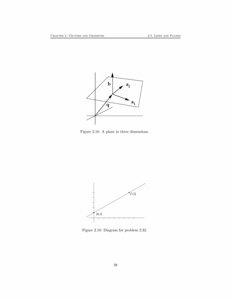
A plane through the origin can be described as all vectors orthogonal to a givenvector b as shown in Figure 2.18. (In this situation, if b has unit length it iscalled the normal vector to the plane and is often denoted n.) Therefore x lieson the plane whenever x · b = 0, or
b1x1 + b2x2 + b3x3 = 0.
If a plane with normal vector b is translated so that it passes through the pointq, then x lies on the plane whenever x − q lies on the parallel plane throughthe origin. Thus x lies on the plane whenever (x− q) · b = 0. Equivalently
b1(x1 − q1) + b2(x2 − q2) + b3(x3 − q3) = 0,
orb1x1 + b2x2 + b3x3 = c,
where c = q · b.
2.5.8 Problems
Problem 2.31 A line orthogonal to b can be described as the set of all pointsx whose projections onto b all have the same value. Using the formula forprojections, show that this leads to the equation description of the line.
Problem 2.32 Find both the parametric form and equation form for the linein Figure 2.19. Write down five points on the line (notice that the parametricform is more useful for this). Check whether the point [ 1012
3 , 106921 ] is on the line
(notice that the equation form is more useful for this.)
37
Chapter 2. Vectors and Geometry 2.5. Lines and Planes
Figure 2.18: A plane in three dimensions.
[0,1]
[7,5]
Figure 2.19: Diagram for problem 2.32.
38

Chapter 2. Vectors and Geometry 2.5. Lines and Planes
Problem 2.33 Find the equation form for the line [1, 1] + s[−1, 2].
Problem 2.34 Find the parametric form for the line x1 − 3x2 = 5
Problem 2.35 Use a projection to find the distance from the point [−2, 3] tothe line 3x1 − 4x2 = −4
Problem 2.36 Consider the plane x− y + 2z = 7.
1. What is the normal direction to the plane?
2. Find the coordinates of any point (your choice) on the plane.
Problem 2.37 Let a, b and c be the vertices of a triangle. By definition, themedian of a triangle is a straight line that passes through a vertex of the triangleand through the midpoint of the opposite side.
(i) Find the parametric form of the equation for each median.
(ii) Do all the medians meet at a common point? If so, which point?
Problem 2.38 Find a pair of equations which define the line
(2, 0,−4) + s(0, 1, 3) : s ∈ R
Problem 2.39 Find the intersection point between the line
(2,−1, 6) + s(1,−1, 0) : s ∈ R
and the planet(0, 1,−3) + u(−1, 2, 0) : t, u ∈ R
Hint: first find an equation for the plane.
Problem 2.40 Find the intersection point of the line with parametric formbelow
(1, 2, 3) + t(1, 0,−1)
and the planex+ 2y − z = 5.
.
Problem 2.41 Find the equation of the plane containing the points [1, 0, 1],[1, 1, 0] and [0, 1, 1].
Problem 2.42 Find the equation of the sphere which has the two planes x1 +x2 + x3 = 3 and x1 + x2 + x3 = 9 as tangent planes if the centre of the sphereis on the planes 2x1 − x2 = 0, 3x1 − x3 = 0.
Problem 2.43 The planes x+ y+ z = 2 and x− y+ 2z = 7 intersect in a line.Find a parametric representation of this line.
39

Chapter 2. Vectors and Geometry 2.6. Introduction to Linear Systems
Problem 2.44 Find the equation of the plane that passes through the point[−2, 0, 1] and through the line of intersection of 2x1 + 3x2 − x3 = 0, x2 − 4x2 +2x3 = −5.
Problem 2.45 What’s wrong with the question “Find the equation for the planecontaining [1, 2, 3], [2, 3, 4] and [3, 4, 5].”?
Problem 2.46 Find the distance from the point p to the plane b · x = c.
Problem 2.47 Find the equation for the line through [2,−1,−1] and parallel toeach of the two planes x1 + x2 = 0 and x1− x2 + 2x3 = 0. Express the equationfo the line in both parametric and equation form.
Problem 2.48 (Matlab) Plotting figures in Matlab is quite simple. Simply typeplot(1,2) in the command window and observe what you get. Copy the follow-ing script (call it basicplot.m for example), and run it:
x = -2:0.1:2
m = 2
x_0 = 1
y_0 = 1
y = y_0 + m*(x-x_0)
plot(x,y,’.’)
Type help plot in the command window to learn about different options forthe plot command. Without closing the figure window, type hold on in thecommand window, and re-run the script after changing the slope to m = -1/2
(the hold on command allows you to overlap plots). Notice that the two linesshould be perpendicular, but because of the scaling they appear not to be. Typein the command axis equal to fix that. How would you modify the script toplot a circle of radius 3?
2.6 Introduction to Linear Systems
2.6.1 Description of points and the geometry of solutionsto systems of equations
So far we have considered the parametric and equation descriptions of lines andplanes in two and three dimensions. We can also try to describe points in thesame way. This will help you get a geometric picture of what it means to solvea system of equations.
The “parametric” description of a point doesn’t have any parameters! Itsimply is the name of the point x = q. In two dimensions the equation form fordescribing a point will look like
b1,1x1 + b1,2x2 = c1b2,1x1 + b2,2x2 = c2
40

Chapter 2. Vectors and Geometry 2.6. Introduction to Linear Systems
Figure 2.20: Intersection of lines in 2D that are not collinear is a point.
where the vectors b1 = [b1,1, b1,2] and b2 = [b2,1, b2,2] are not collinear. Eachone of this equations describes a line. The point x = [x1, x2] will satisfy bothequations if it lies on both lines, i.e., on the intersection. Since the vectors b1
and b2 are not co-linear, the lines are not parallel, so the intersection is a singlepoint. This situation is shown in Figure 2.20.
In three dimensions the equation form for describing a point will look like
b1,1x1 + b1,2x2 + b1,3x3 = c1b2,1x1 + b2,2x2 + b2,3x3 = c2b3,1x1 + b3,2x2 + b3,3x3 = c3
where b1, b2 and b3 don’t all lie on the same plane. This can be interpreted asthe intersection of three planes in a single point.
Notice that going from the equation description of a point to the parametricdescription just means finding the solution of the system of equations. If, in twodimensions, the vectors b1 and b2 are not collinear, or in three dimensions, b1,b2 and b3 don’t all lie on the same plane, then the system of equations has aunique solution.
Now suppose that you are handed an arbitrary system of equations
b1,1x1 + b1,2x2 + b1,3x3 = c1b2,1x1 + b2,2x2 + b2,3x3 = c2b3,1x1 + b3,2x2 + b3,3x3 = c3
What does the set of solutions x = [x1, x2, x3] look like? As we just have seen,if b1, b2 and b3 don’t all lie on the same plane, there is a unique solution givenas the intersection of three planes. Recall that the determinant can be usedto test whether the vectors b1, b2 and b3 lie on the same plane. So a uniquesolution exists to the equation precisely when
det
b1,1 b1,2 b1,3b2,1 b2,2 b2,3b3,1 b3,2 b3,3
6= 0
What happens when the determinant is zero and three vectors b1, b2 and b3 dolie on the same plane? Then it could be that the three planes intersect in a line.
41

Chapter 2. Vectors and Geometry 2.6. Introduction to Linear Systems
Figure 2.21: Planes intersecting.
In this case every point on that line is a solution of the system of equations,and the solution set has a parametric description of the form x = q + sa. Itcould also be that all three planes are the same, in which case the solution setis the plane. In this case the solution set has a parametric description of theform x = q + s1a1 + s2a2 Another possibility is that two of the planes could beparallel with no intersection. In this case there are no solutions at all! Some ofthese possibilities are illustrated in Figure 2.21.
2.6.2 Describing the whole plane in two dimensions andall of space in three dimensions
If the set we are trying to describe is the whole plane in two dimensions or allof space in three dimensions, then we don’t need any equations, since there areno restrictions on the points. However it does make sense to think about theparametric form.
Lets start with two dimensions. Consider Figure 2.22. If we pick any twovectors a1 and a2 that don’t lie on the same line, then any vector x = [x1, x2]in the plane can be written as s1a1 + s2a2. Notice that every choice of s1
and s2 corresponds to exactly one vector x. In this situation we could use theparameters s1 and s2 as co-ordinates instead of x1 and x2. In fact if a1 anda2 are unit vectors orthogonal to each other, this just amounts to changing theco-ordinate axes to lie along a1 and a2. (The new co-ordinates [s1, s2] are thenjust what we were calling [x′1, x
′2] before.) (In fact, even if the vectors a1 and
a2 are not unit vectors orthogonal to each other, we can still think of them oflying along new co-ordinate axes. However, now the axes have been stretchedand sheared instead of just rotated, and need not lie at right angles any more.)
The situation in three dimensions is similar. Now we must pick three vectorsa1, a2 and a3 that don’t lie on the same plane. Then every vector x has a uniquerepresentation x = s1a1 + s2a2 + s3a3. Again, we could use s1, s2 and s3 asco-ordinates in place of x1, x2 and x3. Again, if a1, a2 and 3a3 are orthogonalwith unit length, then this amounts to choosing new (orthogonal) co-ordinateaxes.
42

Chapter 2. Vectors and Geometry 2.6. Introduction to Linear Systems
Figure 2.22: A basis in 2D
2.6.3 Linear dependence and independence
The condition in two dimensions that two vectors are not co-linear, and thecondition in three dimensions that three vectors do not lie on the same planehas now come up several times — in ensuring that a system of equations has aunique solutions and in ensuring that every vector can be written in a uniqueway in parametric form using those vectors. This condition can be tested bycomputing a determinant.
We will now give this condition a name and define the analogous conditionin any number of dimensions.
First, some terminology. If a1,a2, . . .an are a collection of vectors then avector of the form
s1a1 + s2a2 + · · · snan
for some choice of numbers s1, . . . sn is called a linear combination of a1,a2, . . .an.Now, the definition. A collection of vectors a1,a2, . . .an is called linearly
dependent if some linear combination of them equals zero, i.e.,
s1a1 + s2a2 + · · · snan = 0
for s1, . . . sn not all zero. A collection of vectors is said to be linearly independentif it is not linearly dependent. In other words, the vectors a1,a2, . . .an arelinearly independent if the only way a linear combination of them s1a1 + s2a2 +· · · snan can equal zero is for s1 = s2 = · · · = sn = 0.
What does linear dependence mean in three dimensions? Suppose that a1,a2 and a3 are linearly dependent. Then there are some numbers s1, s2 and s3,not all zero, such that
s1a1 + s2a2 + s3a3 = 0.
Suppose that s1 is one of the non-zero numbers. Then we can divide by −s1
and find that−a1 + s′2a2 + s′3a3 = 0
for s′2 = −s2/s1 and s′3 = −s3/s1. Thus
a1 = s′2a2 + s′3a3,
43

Chapter 2. Vectors and Geometry 2.6. Introduction to Linear Systems
or a1 is a linear combination of a2 and a3. But this implies that a1 lies onthe plane spanned by a2 and a3, i.e., the vectors all lie on the same plane. Ifs1 happens to be zero we can repeat the same argument with one of the si’swhich is not zero. Thus linear dependence implies that all three vectors lie onthe same plane. Conversely, if all three vectors lie on the same plane, then wecan write one vector as a linear combination of the other two, a1 = s′2a2 + s′3a3
which implies −a1 + s′2a2 + s′3a3 = 0 which says that the vectors are linearlydependent.
So in three dimensions, linear dependence means the vectors lie on the sameplane. Similarly, in two dimensions, linear dependence means the vectors areco-linear.
One final piece of terminology. A collection of n linearly independent vectorsa1,a2, . . .an in n dimensional space is called a basis. If a1,a2, . . .an is a basis,then every vector x can be written in a unique way as a linear combination
x = s1a1 + s2a2 + · · · snan
2.6.4 Problems
Problem 2.49 Is the collection of vectors a1 = [1, 1], a2 = [1, 0] a basis for twodimensional space? If so, express the vector x = [0, 1] as a linear combinationof a1 and a2
Problem 2.50 Let a = [2, 2, 2] and b = [3, 4, 1]. Find all vectors c such thatthe list of vectors a,b, c is not a basis of R3.
Problem 2.51 Show that the collection of vectors a = [1, 1, 1], b = [1, 1, 0] andc = [1, 0, 0] is a basis of R3. Express [1, 2, 3] as a linear combination of thevectors a, b and c.
Problem 2.52 Let the vectors a = [1, 0, 4], b = [2,−1, 0]and c = [8,−3, 8]. Dothese vectors form a basis of R3?
Problem 2.53 Is it possible for four vectors to be linearly independent in threedimensional space?
Problem 2.54 Show that the collection of vectors a = [2, 1, 3], b = [1, 0, 2] andc = [3, 0, 0] is a basis of R3. Express [12, 2, 4] as a linear combination of thevectors a,b and c.
Problem 2.55 Suppose that a1,a2, . . .an is a basis. Show that if some vectorx has representation x = s1a1 + s2a2 + · · · snan and x = t1a1 + t2a2 + · · · tnan,then s1 = t1, s2 = t2,. . .,sn = tn. (Hint: subtract the two expressions for x anduse the fact that the basis vectors are linearly independent.)
Problem 2.56 (Matlab) Start by convincing yourself that the vectors (1, 3),and (5, 2) are linearly independent. This can easily be shown by writing a scriptthat plots the vectors:
44

Chapter 2. Vectors and Geometry 2.7. Additional Topics
v
θ
0
ra
Ω
Figure 2.23: Rotational Motion.
plot([1,0],[3,0])
hold on
plot([5,0],[2,0])
We can extend this script by also plotting a linear combination of the two vectors:
alfa=1;
beta=1;
clf()
plot([alfa*1,0],[alfa*3,0])
hold on
plot([beta*5,0],[beta*2,0])
plot([alfa*1+beta*5,alfa*1],[alfa*3+beta*2,alfa*3],’--’)
Play around with the script and find parameters alfa and beta so that thevector (1, 1) can be written as a linear combination of (1, 3) and (5, 2).
2.7 Additional Topics
These topics are not covered in Math 152 this year.
2.7.1 Application: rotational motion
Consider a rigid body rotating about an axis given by the unit vector a at arate of Ω radians per second. Let r be the position vector of a point on thebody as shown in Figure 2.23.
What is the velocity of the point? The point travels on a circle with radius‖r‖ sin(θ), where θ is the angle that r makes with the axis. Therefore, in onesecond, the point travels a distance of Ω‖r‖ sin(θ). Thus
(i) the magnitude of the velocity is ‖v‖ = Ω‖r‖ sin(θ).
45

Chapter 2. Vectors and Geometry 2.7. Additional Topics
(ii) Now notice that v is orthogonal to the plane spanned by a and r.
(iii) Finally notice that Ωa, r and v obey the right hand rule.
The facts (i), (ii) and (iii) imply that v is exactly the cross product of Ωaand r. It is customary to let Ω denote the vector Ωa. Then
v = Ω× r.
Problem 2.57 A body rotates at an angular velocity of 10 rad/sec about theaxis through the points [1, 1,−1] and [2,−3, 1]. Find the velocity of the point[1, 2, 3] on the body.
Problem 2.58 The line L passing through the origin and the point [1,1,1]passes through the midpoint of a thin metal rod of length 2 that is orientedin the direction [1,0,0]. The rod begins rotating about L at 3 revolutions perminute. What is the fastest speed (length of velocity vector) of any point on therod?
Problem 2.59 Imagine a plate that lies in the xy–plane and is rotating aboutthe z–axis. Let P be a point that is painted on this plane. Denote by r thedistance from P to the origin, by θ(t) the angle at time t between the line fromthe origin to P and the x–axis and by [x(t), y(t)] the co-ordinates of P at thetime t. Find x(t) and y(t) in terms of θ(t). Compute the velocity of P in twoways: 1. by differentiating [x(t), y(t)] and 2. by computing Ω× r.
2.7.2 Application: 3-D graphics
How can we represent a three dimensional object on piece of paper or computerscreen? Imagine the object in space and, a certain distance away, a point prepresenting the eye of the observer. Between the observer and the object is aplane called the view plane. The position of the origin of this plane is describedby a point q, and its orientation is given by three orthogonal unit vectors oflength 1, denoted e1, e2 and e3. (These are not the same as the standard basisvectors i, j and k in this problem.) This situation is shown in Figure 2.24. Asusual, only the heads of the vectors (points) p, x, y and q are shown on thediagram. (The origin, where the tails of these vectors lie, is not depicted at all.)We will assume that the view plane is a distance one from the observer in thedirection e3. Thus, e3 can be thought of as the direction that the observer islooking. Think of light rays leaving the object at point x and travelling to theobserver’s eye at p. At some point y this line intersects the view plane. All thevectors y on the view plane that correspond to some vector x on our object willfurnish the two dimensional representation of the object.
How do we determine the point y? The parametric form of points on theplane is q + s1e1 + s2e2. So we must have that y = q + s1e1 + s2e2 for somevalues of s1 and s2. We also know that the vector x−p is in the same direction
46
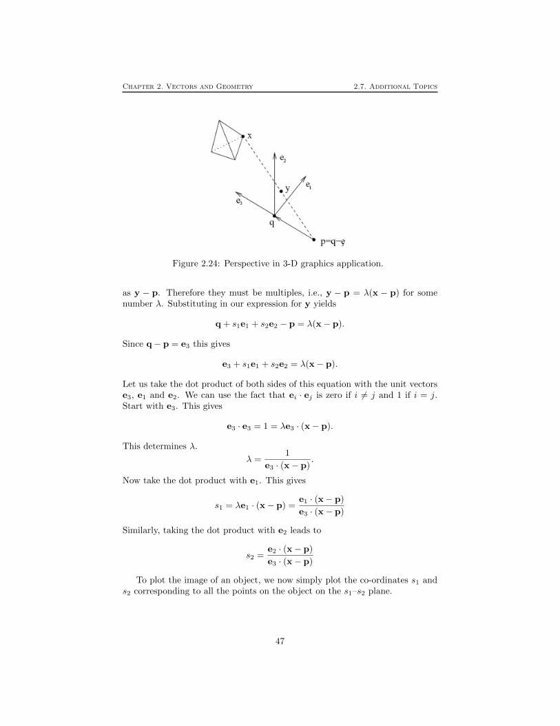
Chapter 2. Vectors and Geometry 2.7. Additional Topics
Figure 2.24: Perspective in 3-D graphics application.
as y − p. Therefore they must be multiples, i.e., y − p = λ(x − p) for somenumber λ. Substituting in our expression for y yields
q + s1e1 + s2e2 − p = λ(x− p).
Since q− p = e3 this gives
e3 + s1e1 + s2e2 = λ(x− p).
Let us take the dot product of both sides of this equation with the unit vectorse3, e1 and e2. We can use the fact that ei · ej is zero if i 6= j and 1 if i = j.Start with e3. This gives
e3 · e3 = 1 = λe3 · (x− p).
This determines λ.
λ =1
e3 · (x− p).
Now take the dot product with e1. This gives
s1 = λe1 · (x− p) =e1 · (x− p)
e3 · (x− p)
Similarly, taking the dot product with e2 leads to
s2 =e2 · (x− p)
e3 · (x− p)
To plot the image of an object, we now simply plot the co-ordinates s1 ands2 corresponding to all the points on the object on the s1–s2 plane.
47

Chapter 2. Vectors and Geometry 2.8. Solutions to Chapter Problems
Example 2.7 Take p = [11, 0, 0], q = [10, 0, 0], e1 = [0, 1, 0], e2 = [0, 0, 1]and e3 = [−1, 0, 0]. What is the image of the point x = [1, 1, 1]? We computex− p = [−10, 1, 1] so that
e1 · (x− p) = 1
e2 · (x− p) = 1
e3 · (x− p) = 10
So s1 = s2 = 1/10.
Example 2.8 Continue the previous example and compute the image of a linesegment between [1, 1, 1] and [2, 0, 1]. These are all points of the form x =[1, 1, 1] + t([2, 0, 1]− [1, 1, 1]) = [1 + t, 1− t, 1] as t varies between 0 and 1. Thistime we have x− p = [1 + t− 11, 1− t, 1] so that
e1 · (x− p) = 1− te2 · (x− p) = 1
e3 · (x− p) = 10− t
Thus s1 = (1−t)/(10−t) and s2 = 1/(10−t). Even though it is not immediatelyobvious, the points [s1, s2], as t varies, all lie on a line segment. In fact
s1 + 9s2 = (1− t)/(10− t) + 9/(10− t) = (10− t)/(10− t) = 1.
This shows that the points [s1, s2] lie on a line perpendicular to [1, 9].
In fact, it is possible to show that any line segment in space maps to a linesegment on the s1–s2 plane. Thus, to plot the image of an object consistingof straight line segments (such as the tetrahedron in the picture) it is onlynecessary to plot the vertices and then join them by straight lines.
Problem 2.60 What are the s1 and s2 co=ordinates of the point x = [1, 2, 3],if p, q are as above, e1 = [0, 1/
√2, 1/√
2] and e2 = [0,−1/√
2, 1/√
2].
Problem 2.61 Plot the image on the s1–s2 plane of the tetrahedron whosevertices are located at [0, 0, 0], [0, 1, 0], [0, 1/2,
√3/2] and [
√3/6,√
6/3, 1/2] (Usethe same values as before: p = [−10, 0, 0], q = [10, 0, 0], e1 = [0, 1, 0], e2 =[0, 0, 1] and e3 = [−1, 0, 0].)
Problem 2.62 Suppose that that points x lie on the line x = x0 + tv. Showthat corresponding planar points [s1, s2] also lie on a line. (Hint: show thatthere are numbers a, b, c that do not depend on t, so that as1 + bs2 = c forevery t.)
Problem 2.63 Consider a different drawing procedure where the point x mapsto the point on the view plane given by the intersection of the plane with the linethrough x parallel to e3. Find a formula for the s1 and s2 co-ordinates of x.
48

Chapter 2. Vectors and Geometry 2.8. Solutions to Chapter Problems
−2 −1 0 1 2 3 4 5−2
−1
0
1
2
3
4
(1,−1)
(3,1)
(2,2)
(1,−1)
Figure 2.25: Solution to problem 2.1
2.8 Solutions to Chapter Problems
Solution 2.1 See Figure 2.25.
Solution 2.2
(i) A straight line passing through the origin in the direction of a.
(ii) A ray (half line) passing through the origin in the direction of a.
(iii) A straight line parallel to a passing through b.
(iv) If a and b do not lie on the same line: a plane passing through the originparallel to a and b (in two dimensions, this is the whole plane). If a andb lie on the same line: a straight line passing through the origin in thedirection of a (and b).
(v) If a and b both lie on the same line: a line passing through c parallel to a(and b). If a and b do not lie on the same line: a plane passing throughc parallel to a and b (in two dimensions, this is the whole plane).
Solution 2.3 a− b is the vector that when added to b gives a. So if we drawit with its tail at b then its head is at a. Similarly b− a when drawn with itstail at a has its head at b.
Solution 2.4 To find the midpoint we add half of the vector with its tail at aand head at b to a. So the midpoint is a+(1/2)(b−a) = (1/2)(a+b). Similarly,the point one third of the way from a to b is a+(1/3)(b−a) = (2/3)a+(1/3)b.
49

Chapter 2. Vectors and Geometry 2.8. Solutions to Chapter Problems
Solution 2.5 The line segment is given by the vectors a + t(b− a) as t variesbetween 0 and 1.
Solution 2.6 a = (1, 2); b = (1,−2)
(a) a + b = (2, 0)
(b) 2a = (2, 4)
(c) a− b = (0, 4)
(d) a · b = 1− 4 = −3.
(e) ‖b‖ =√
1 + 4 =√
5.
Solution 2.7 The radius of the circle is
‖(2, 5)− (3, 3)‖ = ‖(−1, 2)‖ =√
1 + 4 =√
5.
Thus using the standard equation for a circle
(x− 2)2 + (y − 5)2 = (√
5)2 = 5.
Solution 2.8 The equation is ‖x− a‖ = r, or√(x1 − a1)2 + (x2 − a2)2 + (x3 − a3)2 = r
or(x1 − a1)2 + (x2 − a2)2 + (x3 − a3)2 = r2
Solution 2.9 The midpoint of the sphere is the midpoint of [2, 1, 4] and [4, 3, 10],i.e., (1/2)([2, 1, 4] + [4, 3, 10]) = [3, 2, 7]. The radius is half the distance between[2, 1, 4] and [4, 3, 10], i.e.,
(1/2)√
(2− 4)2 + (1− 3)2 + (4− 10)2 =√
11. Thus the equation is
(x1 − 3)2 + (x2 − 2)2 + (x3 − 7)2 = 11.
Solution 2.10
(a) a · b = −2 + 6 = 4, θ = arccos(4/(√
5√
13)) = 1.05 . . .
(b) a · b = 1, θ = 1.249 . . .
(c) a · b = 4, θ = 0
(d) a · b = 2, θ = 1.079 . . . . . .
(e) a · b = 0, θ = π/2 . . .
50

Chapter 2. Vectors and Geometry 2.8. Solutions to Chapter Problems
Solution 2.11 Consider the dot product to determine angles between vectors,not the dot product (which only applies to 3D and cannot distinguish anglesθ in the range (0, π/2) from those in (π/2, π), as discussed in the solution toproblem 2.10 in the online notes).
(a) a = (1, 1, 1), b = (3, 1,−2)a · b = 3 + 1− 2 = 2||a|| =
√3, ||b|| =
√32 + 12 + (−2)2 =
√14.
cos θ = 2√3√
14, θ = cos−1 2√
3√
14' 1.26 radians, or ' 72.0o
(b) Using a · b and ||a|| above,projab = 2
3 (1, 1, 1) =(
23 ,
23 ,
23
). Remember, projab should be in the di-
rection of a.
Solution 2.12
a = (1, 4, 0) ‖a‖ =√
17
b = (2,−1, 5) ‖b‖ =√
4 + 1 + 25 =√
30
(a) cos θ = b·a‖a‖‖b‖ = 2−4√
17√
30= −2√
510so
θ = cos−1
(−2√510
)≈ 1.66 in radians or ≈ 95
(b) projab = b·a‖a‖2 a = −2
17 (1, 4, 0) = (−2/17,−8/17, 0).
Solution 2.13 The dot product is zero if −1 + 2 + s = 0, i.e., if s = −1.
Solution 2.14 Let a = [1, 2, 3], b = [4, 0, 5] and c = [3, 4, 6]. The sides of thetriangle are in the directions of a − b = [−3, 2,−2], a − c = [−2,−2,−3], andb−c = [1,−4,−1]. To see if there are any right angles we compute (a−b) ·(a−c) = [−3, 2,−2] · [−2,−2,−3] = 8, (a−b) ·(b−c) = [−3, 2,−2] · [1,−4,−1] = −9and (a − c) · (b − c) = [−2,−2,−3] · [1,−4,−1] = 9. Since none of these arezero, there are no right angles.
Solution 2.15 If [c1, 1, c2] = s[2,−2, 3], with s a scalar multiple, then s = − 12
(from the values in the second component), hence:c1 = −1, c2 = −3/2.
Solution 2.16 The problem becomes much simpler if we choose the y axisto run along the runway and the x axis to run perpendicular to the runway.Replace the wind and plane velocities by vectors w and p as on the diagram inFigure 2.26.
The wind vector has components [−10 cos(20),−10 sin(20)] while the planevelocity has components [70 sin(θ), 70 cos(θ)]. We want the x component to bezero hence we need 10 cos(20) = 70 sin(θ). This gives θ = 7.7, i.e, the get theheading of the plane we have to add 7.7 to the runway direction. Thus the
51

Chapter 2. Vectors and Geometry 2.8. Solutions to Chapter Problems
Figure 2.26: Coordinate system for Solution 2.16.
plane’s heading is 267.7. The groundspeed is the magnitude of the velocity, inthis case simply the y component given by 70 cos(7.7)−10 sin(20) = 66 knots.
Solution 2.17 If we use the co-ordinate system where the x axis is horizontaland the y axis is vertical, then the force of gravity is Fg = [0,−mg] The unitvector in the direction along the shaft is p = [− sin(θ), cos(θ)]. The force Fsexerted by the shaft is in the direction of the shaft, hence a multiple of p.So Fs = tp for some number t. To find t we use that the component of thetotal force in the direction of the shaft must be zero. Thus projpFg + Fs = 0,i.e. p · Fg + t = 0, i.e., t = mg cos(θ). Thus the total force is Fg + Fs =[0,−mg] +mg cos(θ)[− sin(θ), cos(θ)] = mg[− cos(θ) sin(θ),−1 + cos2(θ)]. Notethat this is orthogonal to p, as it must be.
If we use co-ordinates where the y axis runs along the shaft of the pendulum,and the x axis perpendicular to it, then Fg = [−mg sin(θ),−mg cos(θ)] whileFs = [0, t] for some value of t. In this case it is simply the y component thatmust be zero, so t = mg cos(θ) and Fg + Fs = [−mg sin(θ), 0]
Solution 2.18
sqrt(a(1)^2+a(2)^2)
Solution 2.19 [1, 2, 3]× [4, 5, 6] = [−3, 6,−3]
Solution 2.20
det
1 1 11 2 31 0 −1
= 1(−2− 0)− 1(−1− 3) + 1(0− 2)
= −2 + 4− 2 = 0
Since the determinant is zero, the volume of the parallelepiped generated by therow vectors is zero. This implies that the vectors lie on the same plane.
52

Chapter 2. Vectors and Geometry 2.8. Solutions to Chapter Problems
Solution 2.21 a · (a×b) = [a1, a2, a3] · [a2b3− a3b2, a3b1− a1b3, a1b2− a2b1] =a1a2b3 − a1a3b2 + a2a3b1 − a2a1b3 + a3a1b2 − a3a2b1 = 0. Now b · (a × b) =−b · (b× a) = 0 by the previous calculation.
Solution 2.22
(a) ((1, 4,−1) · (2, 1, 3))((2, 1, 4)× (1, 4, 9))
= (2 + 4− 3)
∣∣∣∣∣∣i j k2 1 41 4 9
∣∣∣∣∣∣= 3(i(9− 16) + j(4− 18) + k(8− 1)
= 3(−7,−14, 7) = (−21,−42, 21)
(b) (7, 1, 0) · ((2, 0,−1)× (1, 4, 3))
= (7, 1, 0) ·
∣∣∣∣∣∣i j k2 0 −11 4 3
∣∣∣∣∣∣= (7, 1, 0) · (i(0 + 4) + j(−1− 6) + k(8− 0)
= (7, 1, 0) · (4,−7, 8) = 28− 7 + 0 = 21
(c) (a× b)× (b× a)
= (a× b)× (−a× b) = −(a× b)× (a× b) = 0
because c× c = 0 for any vector c.
Solution 2.23 Here we are assuming that θ lies in [0, π] so that sin(θ) is positive.The quantity ‖a‖ is the length of the base of the parallelogram while ‖b‖ sin(θ)is the height. The area of a parallelogram is the product of these.
Solution 2.24 Since a × b = −b × a it is never true that a × b = −b × a,unless a× b = 0. For the other example, just try i, j and k. We have i× j = kso i× (i× j) = i× k = −j On the other hand (i× i)× j = 0× j = 0
Solution 2.25
a=rand(3,1);
b=rand(3,1);
c=rand(3,1);
cross(a,b) - cross(b,a)
cross(a,cross(b,c)) - cross(cross(a,b),c)
This actually constitutes a proof, since we found a counter example. We don’thave to show that it’s always the case, we only had to show that in general thetwo assertions are not true.
53

Chapter 2. Vectors and Geometry 2.8. Solutions to Chapter Problems
Solution 2.26 This a just a long calculation. One way to break it up is toconsider a = i, j and k separately. Suppose we can prove it for these specialcases. Then write a general a as a1i + a2j + a3k. Then a × (b × c) = a1i ×(b × c) + a2j × (b × c) + a3k × (b × c) Assuming for the moment we knowthat the special cases hold, then this equals a1((i · c)b − (i · b)c) + a2((j ·c)b − (j · b)c) + a3((k · c)b − (k · b)c) = (a · c)b − (a · b)c Now we stillhave to prove the special cases. For example if a = i we have i × (b × c) =
det
i j k1 0 0
b2c3 − b3c2 b3c1 − b1c3 b1c2 − b2c1
= −(b1c2−b2c1)j+(b3c1−b1c3)k =
[0,−b1c2 + b2c1, b3c1− b1c3] On the other hand(i · c)b− (i ·b)c = c1[b1, b2, b3]−b1[c1, c2, c3] = [0, c1b2 − b1c2, c1b3 − b1c3]. The other two are similar.
Solution 2.27
a=rand(3,1);
b=rand(3,1);
c=rand(3,1);
cross(a,cross(b,c)) - (dot(a,c)*b - dot(a,b)*c)
Solution 2.28 (a×b)·(c×d) = ((a×b)×c)·d (by property 5) = −(c×(a×b))·d(by property 1) = −((c · b)a + (c · a)b) · d = −(c · b)(a · d) + (c · a)(b · d)
Solution 2.29
(a) Let v = a× (a×b). Since a×b is orthogonal to the paper, v must lie inthe plane of the paper. v is also orthogonal to a. Checking orientationswith the right hand rule, there are only two sketches (up to rotation andresizing the vectors) shown in Figure 2.27.
(b) a× (a× b) = (b · a)a− (a · a)b by property 2 in the notes.
= ‖a‖2(
b · a‖a‖2
a− b
)= ‖a‖2(projab− b).
Solution 2.30 Actually there is no one right answer to this problem. But intwo dimensions the analog of the cross product could be an operation on a single
vector say ×(a) with the property that ×(a) · b = det
[a1 a2
b1 b2
]This implies
that ×(a) = [a2,−a1]. Note that ×(a) is orthogonal to a. The answer in 4dimensions is a little more obscure. In this case the cross product could be anoperation on three vectors that produces a vector that is orthogonal to all ofthem. One way of producing such a vector would be to do the formal calculationof a 4 × 4 determinant, where the first row contains the four unit vectors e1,e2, e3 and e4, while the other three rows contain the entries of a,b and c. Doyou see why? (There is another possible, perhaps better answer, involving adifferent type of product called the wedge product.)
54

Chapter 2. Vectors and Geometry 2.8. Solutions to Chapter Problems
Figure 2.27: Vector sketch for the solution to 2.29.
Solution 2.31 Let q be a point on the line. Then the projection of x in thedirection of b is x·b
‖b‖2 . The set of all points whose projection in the direction of
b are the same as the projection of the point q in the direction of b is thereforethe set of points x such that x·b
‖b‖2 = q·b‖b‖2 . Multiplying both sides by by ‖b‖2
gives x · b = q · b.
Solution 2.32 The line is in the direction of a = [7, 5] − [0, 1] = [7, 4] andis therefore perpendicular to b = [4,−7]. q = [0, 1] is a point on the line.So the parametric form for the line is [0, 1] + s[7, 4] and the equation formis 4x1 − 7x2 = −7. So five points on the line are (picking s = −2, 1, 0, 1, 2)[−14,−7], [−7,−3], [0, 1], [7, 5], [14, 9]. To check whether [1012/3, 1069/21] lieson the line, plug it into the equation: 4 · 1012/3− 7 · 1069/21 6= −7 so the pointdoes not lie on the line.
Solution 2.33 We can take q = [1, 1] and b = [2, 1] so the equation is 2x1+x2 =3.
Solution 2.34 We have to find a point on the line. Try for one of the form[t, 0]. This is on the line if t − 3 · 0 = 5. So [5, 0] is on the line. The vectororthogonal to the line is [1,−3] so a vector parallel is [3, 1]. Thus the parametricform is [5, 0] + s[3, 1].
Solution 2.35 Pick a point q on the line and let b be orthogonal to the line.Then the distance from a point x to the line is the length of the projection ofx − q onto b as shown in Figure 2.28. In this case we can take b = [3,−4],q = [0, 1] and x = [−2, 3]. The projection is ((x − q) · b/‖b‖2)b This equals([−2, 2] · [3,−4]/25)[3,−4] = (−14/25)[3, 4] The length of this vector is 14/5.
Solution 2.36
(a) the normal direction to the plane is (1,−1, 2)
(b) the point (7, 0, 0) is on the plane (look for a solution with y = z = 0 thatis the intersection of the plane with the line of the x-axis).
Solution 2.37 The midpoint between b and c is (b + c)/2. So the vector froma to this midpoint is (b+c)/2−a and thus the parametric form for the median
55
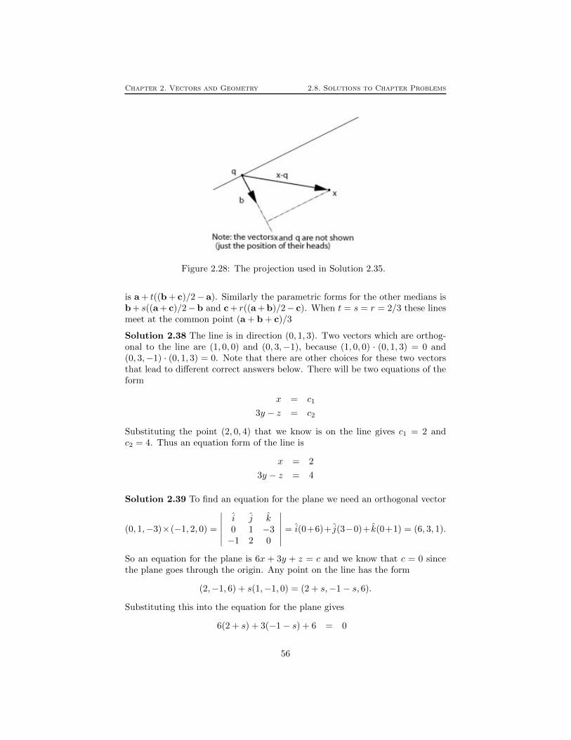
Chapter 2. Vectors and Geometry 2.8. Solutions to Chapter Problems
Figure 2.28: The projection used in Solution 2.35.
is a + t((b + c)/2− a). Similarly the parametric forms for the other medians isb + s((a + c)/2−b and c + r((a + b)/2− c). When t = s = r = 2/3 these linesmeet at the common point (a + b + c)/3
Solution 2.38 The line is in direction (0, 1, 3). Two vectors which are orthog-onal to the line are (1, 0, 0) and (0, 3,−1), because (1, 0, 0) · (0, 1, 3) = 0 and(0, 3,−1) · (0, 1, 3) = 0. Note that there are other choices for these two vectorsthat lead to different correct answers below. There will be two equations of theform
x = c1
3y − z = c2
Substituting the point (2, 0, 4) that we know is on the line gives c1 = 2 andc2 = 4. Thus an equation form of the line is
x = 2
3y − z = 4
Solution 2.39 To find an equation for the plane we need an orthogonal vector
(0, 1,−3)×(−1, 2, 0) =
∣∣∣∣∣∣i j k0 1 −3−1 2 0
∣∣∣∣∣∣ = i(0+6)+ j(3−0)+ k(0+1) = (6, 3, 1).
So an equation for the plane is 6x + 3y + z = c and we know that c = 0 sincethe plane goes through the origin. Any point on the line has the form
(2,−1, 6) + s(1,−1, 0) = (2 + s,−1− s, 6).
Substituting this into the equation for the plane gives
6(2 + s) + 3(−1− s) + 6 = 0
56

Chapter 2. Vectors and Geometry 2.8. Solutions to Chapter Problems
3s+ 15 = 0
s = −5
So the intersection point is
(2,−1, 6)− 5(1,−1, 0) = (2,−1, 6) + (−5, 5, 0) = (−3, 4, 6).
Note: it can be checked that t = −2 and u = 3 in the parametric form of theplane gives this point as well.
Solution 2.40 Points on the line satisfy
x = 1 + t
y = 2
z = 3− t.
To be on the plane, x+2y−z = 5, or (1+t)+2(2)−(3−t) = 5, or 2t+2 = 5,or t = 3/2.
Thus the intersection occurs at (1, 2, 3) + ( 32 )(1, 0,−1) = (5
2 , 2,32 ).
Solution 2.41 Two vectors in the direction of the plane are [1, 1, 0]− [1, 0, 1] =[0, 1,−1] and [0, 1, 1] − [1, 0, 1] = [−1, 1, 0] To find a normal vector take thecross product [0, 1,−1] × [−1, 1, 0] = [1, 1, 1]. So the equation of the plane isx1 + x2 + x3 = 2.
Solution 2.42 The centre of the sphere lies in the plane halfway between theplanes x1 +x2 +x3 = 3 and x1 +x2 +x3 = 9. This is the plane x1 +x2 +x3 = 6.So the centre satisfies the three equations
x1 +x2 +x3 = 62x1 −3x2 = 03x1 −x3 = 0
We will develop efficient techniques for solving such systems of equations. Fornow, we can just use brute force: The second equation says x2 = 2x1 and thethird x3 = 3x1. Substituting this into the first equation yieldsx1 = 1, so x2 = 2and x3 = 3. Therefore the centre of the sphere is [1, 2, 3]. To compute theradius, we must find the distance between the planes x1 + x2 + x3 = 3 andx1 + x2 + x3 = 6 If we divide the equations by ‖[1, 1, 1]‖ =
√3, the first can be
interpreted as vectors whose projection onto the direction ‖[1, 1, 1]‖ has length3/√
3 =√
3, the second can be interpreted as vectors whose projection onto thedirection ‖[1, 1, 1]‖ has length 6/
√3 = 2
√3. The radius is
√3 so the equation
is (x1 − 1)2 + (x2 − 2)2 + (x3 − 3)2 = 3.
Solution 2.43x+ y + z = 2 normal (1, 1, 1) = ~b1x− y + 2z = 7 normal (1,−1, 2) = ~b2
The line direction can be found as
~a = ~b1 × ~b2 =
i j k1 1 11 −1 2
= (3,−1,−2).
57

Chapter 2. Vectors and Geometry 2.8. Solutions to Chapter Problems
We also need a point on the line. We can look for a point which has z = 0(the point that is the intersection of the line and the x-y plane). We get thetwo by two system
x+ y = 2, x− y = 7
Solving the system yields that x = 92 , and y = − 5
2 .So(
92 ,−
52 , 0)
+ s(3,−1,−2) is a parametric form of the line with parameters.
Solution 2.44 Set x2 = 0 and solve 2x1 − x3 = 0 and x1 + 2x3 = −5 givingx1 = −1 andx2 = −2. This implies [−1, 0,−2] is in the plane we are looking for.Set x3 = 0 and solve 2x1 + 3x2 = 0x1− 4x2 = −5 giving x1 = −15/11 and x2 =10/11] Hence [−15/11, 10/11, 0] also lies on the plane. We now have three pointson the plane. Two vectors in the direction of the plane are therefore [−2, 0, 1]−[−1, 0,−2] = [−1, 0, 3] and[−15/11, 10/11, 0] − [−1, 0,−2] = [−4/11, 10/11, 2].Thus a normal vector is [−1, 0, 3]× [−4/11, 10/11, 2] = [−30/11, 10/11,−10/11]This is parallel to [−3, 1,−1]. Hence the equation is −3x1 + x2 − x3 = 5.
Solution 2.45 The three points are all on the same line. To see this, noticethat the vectors [2, 3, 4] − [1, 2, 3] = [1, 1, 1] and [3, 4, 5] − [1, 2, 3] = [2, 2, 2] areparallel.
Solution 2.46 The distance of p to the plane b · x = c is the length of theprojection of p − q onto b, where q is any point on the plane. A point on theplane is [c/b1, 0, 0] (unless b1 = 0 in which case we choose either [0, c/b2, 0] or[0, 0, c/b3]) The length of the projection is (p− q) · b/‖b‖ = (b · p− c)/‖b‖.
Solution 2.47 If the line is parallel to both planes, then it is orthogonal to bothnormal vectors. Therefore [1, 1, 0]× [1,−1, 2] = [2,−2,−2] is in the direction ofthe line. Therefore the parametric form of the line is [2,−1,−1] + s[2,−2,−2]The two equations are x1 + x2 = [1, 1, 0] · [2,−1,−1] = 1 and x1 − x2 + 2 =[1,−1, 2] · [2,−1,−1] = 1.
Solution 2.48
x=-3:0.1:3
y = sqrt(9-x.^2)
plot(x,y,’.’)
hold on
plot(x,-y,’.’)
axis equal
Solution 2.49 Yes [1, 1] and [1, 0] do form a basis, since they don’t lie on thesame line. (By the way, there is some potential for confusion here. When Isay here that [1, 1] and [1, 0] don’t lie on the same line, I’m thinking of them asposition vectors, drawn with their tails at the origin. It probably would be moreclear to say that the vectors are not parallel.) Every vector in the plane can bewritten as a linear combination of these two. In particular [0, 1] = [1, 1]− [1, 0]
58

Chapter 2. Vectors and Geometry 2.8. Solutions to Chapter Problems
Solution 2.50 Note that a and b are linearly independent (they are not multi-ples of one another). So a, b and c will be linearly independent and so a basisfor R3 unless c is a linear combination of a and b, that is it can be written as
c = ra + sb
for some r and s.
Solution 2.51 The collection is a basis if the vectors are linearly independent.We consider ra + sb + tc = 0 which leads to
r + s+ t = 0
r + s = 0
r = 0
Starting from the last equation and working up, we see that r = 0, s = 0, andt = 0 which shows that the vectors are linearly independent and therefore forma basis. The linear independence could also have been shown by considering thedeterminant ∣∣∣∣∣∣
1 1 11 1 01 0 0
∣∣∣∣∣∣ = 1 6= 0
Since the determinant is not zero the vectors do not lie on the same plane andso are linearly independent. To write [1, 2, 3] as a linear combination
[1, 2, 3] = r[1, 1, 1] + s[1, 1, 0] + t[1, 0, 0]
match components working backwards to get successively r = 3, s = −1 andt = −1.
Solution 2.52 The vectors a, b, and c are vectors in 3-D. Thus they form abasis if and only if they are linearly independent.
The three vectors are linearly independent if and only if the matrix A withrows given by the three vectors satisfies
det(A) 6= 0.
Here
A =
1 0 42 −1 08 −3 8
Solution 2.53 No, it is not possible for four vectors to be linearly independent
in three dimensional space. To see this, first notice that if four vectors are lin-early independent any subset of three vectors must also be linearly independent(If three vectors would lie on the same plane, we could find a non-trivial linearcombination of those three equal to zero. Then by adding 0 times the left overvector, we would get a non-trivial linear combination of all four vectors equal
59

Chapter 2. Vectors and Geometry 2.8. Solutions to Chapter Problems
to zero, contradicting their independence.) But this means that those threevectors form a basis for three dimensional space. So the fourth vector mustbe expressible as a linear combination of the first three. This means the fourvectors are not independent.
Solution 2.54 It is enough to check that det(A) 6= 0. We have that
A =
2 1 31 0 23 0 0
, det(A) = 6 6= 0,
so they form a basis. We want to find s1, s2, and s3 such that 1224
= s1
213
+ s2
102
+ s3
300
.
We have the following system of equations:
12 = 2s1 + s2 + 3s3
2 = s1
4 = 3s1 + 2s2
Hence s1 = 2, s2 = −1, s3 = 3.
Solution 2.55 If x = s1a1 + s2a2 + · · · snan and x = t1a1 + t2a2 + · · · tnan,then 0 = x− x = (s1 − t1)a1 + (s2 − t2)a2 + · · · (sn − tn)an. Since the vectorsa1,a2, . . .an are linearly independent, the only way this can happen is s1− t1 =0, . . . , sn − tn = 0, or s1 = t1, . . . , sn = tn.
Solution 2.56 The values alpha = 0.23, beta = 0.15 provide a good ap-proximation to the linear combination.
Solution 2.57 The axis is parallel to [2,−3, 1]− [1, 1,−1] = [1,−4, 2]. The unitvector in this directions is 1/
√21[1,−4, 2] (Actually there is an ambiguity in the
problem: the unit vector could also point in the opposite direction. This wouldchange the sign of the answer.) So Ω = (10/
√21)[1,−4, 2]. The vector r has
its tail co-inciding with the tail of Ω and its head at [1, 2, 3]. So r = [1, 2, 3] −[1, 1,−1] = [0, 1, 4] and the velocity is v = Ω× [0, 1, 4] = (10/
√21)[−18,−4, 1]
Solution 2.58 Some preliminary discussion:
(i) it does not matter where the centre of the rod is along L, we can take itto be at the origin for convenience.
(ii) the fastest speed is at the rod tip, and this does not change in time, so
(iii) it is OK to evaluate the speed at the initial position.
Ω = 3 · 2π = 6π radians/min.a = 1√
3(1, 1, 1) unit vector in the direction of the axis of rotation.
60

Chapter 2. Vectors and Geometry 2.8. Solutions to Chapter Problems
Figure 2.29: Mapped tetrahedron of Solution 2.61.
~v = Ωa× ~r = 6π√3(1, 1, 1)× (1, 0, 0), with ~r the initial position of the tip.
Now evaluate the cross product: i j k1 1 11 0 0
= (0, 1,−1),
so ~v = 6π√3(0, 1,−1), and hence the speed is ||v|| = 2π
√6m/min
Solution 2.59 We have [x(t), y(t), 0] = r[cos(θ(t)), sin(θ(t)), 0] so the velocityis
[x(t), y(t), 0] = r[− sin(θ(t))θ(t), cos(θ(t))θ(t), 0]
= rθ(t)[− sin(θ(t)), cos(θ(t)), 0]
On the other hand Ω = [0, 0, θ(t)] so that Ω× r[cos(θ(t)), sin(θ(t)), 0] gives thesame answer.
Solution 2.60 We have q−p = [20, 0, 0], x−p = [11, 3, 2]. Thus e1 · (q−p) =e2 · (q− p) = 0, e3 · (q− p) = −20, e1 · (x− p) = 5
√2/2, e2 · (q− p) =
√2/2,
e3 · (x− p) = −11. So s1 = 50√
2/11 and s1 = 10√
2/11.
Solution 2.61 The image of the vertices are [0, 0], [2, 0], [1,√
3] and some morehorrible expression which is approximately [1.587 . . . , 0.9719 . . .]. So the imageon the screen looks something like what is shown in Figure 2.29. Notice thatthe first three points—[0, 0], [2, 0] and [1,
√3]— are simply double the x2 and x3
co-ordinates of the original points in space. Can you explain this geometrically?(I know these are supposed to be answers, not questions, but still . . .) (By theway, I actually intended the last point in the question to be [
√6/3, 1/2,
√3/6].
Can you say why?)
Solution 2.62 We can write
[s1, s2] =1
e3 · (x0 − p) + te3 · v[e1 · (x0 − p) + te1 · v, e2 · (x0 − p) + te2 · v]
61

Chapter 2. Vectors and Geometry 2.8. Solutions to Chapter Problems
This means that as1 + bs2 = c can be rewritten
a(e1 · (x0−p) + te1 ·v) + b(e2 · (x0−p) + te2 ·v)− c(e3 · (x0−p) + te3 ·v) = 0
This holds for every t if both these equations hold:
a(e1 · (x0 − p)) +b(e2 · (x0 − p)) −c(e3 · (x0 − p)) = 0ae1 · v +be2 · v −ce3 · v = 0
This is a system of two equations in three unknowns, a, b, and c. Such a systemalways has a non trivial solution (as we will see in the following chapter.)
Solution 2.63 In this case we want y − x to point in the same direction ase3 so y − x = λe3. On the other hand y lies on the plane of the screen, soy = q + s1e1 + s2e2. Therefore
q− x + s1e1 + s2e2 = λe3.
Now to find s1 and s2 take dot products with e1 and e2. This yields s1 =−e1 · (q− x) and s2 = −e2 · (q− x).
62

Chapter 3
Solving Linear Systems
3.1 Linear Systems
3.1.1 General Form of Linear Systems
So far, we have seen systems of linear equations as the equations that describepoints, lines and planes. However, linear systems of equations show up in manyother ways in engineering problems. We will solve linear systems to find thebehaviour of an electrical circuit. Other examples would be the calculation ofequilibrium temperature distributions or electric fields. Such examples ofteninvolve the discretization of a continuous function. In other words, a continuousfunction like the temperature distribution in a body (which has a value foreach of the infinitely many points in the body) will be replaced by a list oftemperatures at a large but finite number n of closely spaced points. This givesrise to a system of linear equations in n unknowns, where n can be in the tensof thousands, or higher. Therefore, we want to develop a technique to solvesystems of linear equations in n unknowns when n is large.
The most general form of a linear system of equations is
a1,1x1 + a1,2x2 + · · · + a1,nxn = c1a2,1x1 + a2,2x2 + · · · + a2,nxn = c2
......
......
am,1x1 + am,2x2 + · · · + am,nxn = cm
Here the numbers ai,j and cj are known, and the goal is to find all values ofx1, . . . , xn that satisfy all the equations.
3.1.2 Solving Linear Systems by Substitution
Let us start with an example, which we will solve using the method of substitu-tion.
63

Chapter 3. Solving Linear Systems 3.1. Linear Systems
Example 3.1 Consider the system of equations
x1 + x2 + x3 = 6x1 − x2 + x3 = 02x1 + x2 − 8x3 = −11
One could try to proceed as follows. Solve the first equations for, say, x3. Thisgives
x3 = 6− x1 − x2.
Now substitute this value for x3 into the second and third equations. This gives
x1 − x2 + (6− x1 − x2) = 02x1 + x2 − 8(6− x1 − x2) = −11
or
−2x2 = −6
10x1 + 9x2 = 37
Now solve the first of these equations for x2 and substitute into the last equation.This gives x2 = 3 and x1 = 1. Finally we can go back and calculate x3 =6− 1− 3 = 2.
Although this procedure works fine for n = 2 or even n = 3, it rapidly be-comes unwieldy for larger values of n. We will now introduce a technique calledGaussian elimination that works well for large n and can be easily implementedon a computer.
We have already observed that there may be many systems of equationswith the same solution. When there are only two unknowns, this amounts tosaying that different pairs of lines may intersect in the same point. Gaussianelimination is based on the following idea. We introduce three elementary rowoperations. These operations change the system of the equations into anothersystem with exactly the same the set of solutions. We then apply these elemen-tary row operations in a systematic way to change the system of equations intoa system that is easily solved.
3.1.3 Elementary row (equation) operations
The first elementary row operation is
1. Multiplication of a row (equation) by a non-zero number
For example, if we multiply the first equation in the system of Example 3.1above by 3, we end up with
3x1 + 3x2 + 3x3 = 18x1 − x2 + x3 = 02x1 + x2 − 8x3 = −11
64
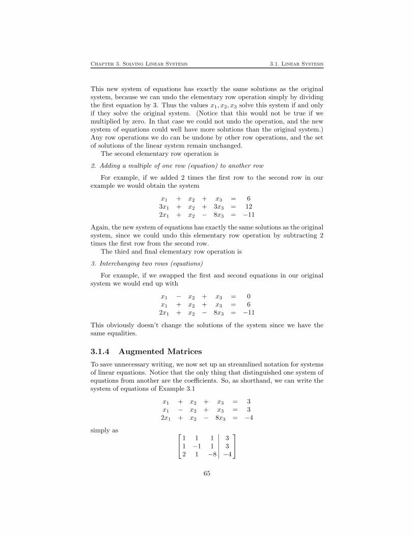
Chapter 3. Solving Linear Systems 3.1. Linear Systems
This new system of equations has exactly the same solutions as the originalsystem, because we can undo the elementary row operation simply by dividingthe first equation by 3. Thus the values x1, x2, x3 solve this system if and onlyif they solve the original system. (Notice that this would not be true if wemultiplied by zero. In that case we could not undo the operation, and the newsystem of equations could well have more solutions than the original system.)Any row operations we do can be undone by other row operations, and the setof solutions of the linear system remain unchanged.
The second elementary row operation is
2. Adding a multiple of one row (equation) to another row
For example, if we added 2 times the first row to the second row in ourexample we would obtain the system
x1 + x2 + x3 = 63x1 + x2 + 3x3 = 122x1 + x2 − 8x3 = −11
Again, the new system of equations has exactly the same solutions as the originalsystem, since we could undo this elementary row operation by subtracting 2times the first row from the second row.
The third and final elementary row operation is
3. Interchanging two rows (equations)
For example, if we swapped the first and second equations in our originalsystem we would end up with
x1 − x2 + x3 = 0x1 + x2 + x3 = 62x1 + x2 − 8x3 = −11
This obviously doesn’t change the solutions of the system since we have thesame equalities.
3.1.4 Augmented Matrices
To save unnecessary writing, we now set up an streamlined notation for systemsof linear equations. Notice that the only thing that distinguished one system ofequations from another are the coefficients. So, as shorthand, we can write thesystem of equations of Example 3.1
x1 + x2 + x3 = 3x1 − x2 + x3 = 32x1 + x2 − 8x3 = −4
simply as 1 1 11 −1 12 1 −8
∣∣∣∣∣∣33−4
65

Chapter 3. Solving Linear Systems 3.1. Linear Systems
This is called an augmented matrix. “Augmented” refers to the column tothe right of the line that contains the information about the right side of eachequation.
3.1.5 Problems
Problem 3.1 Express the system
x1 − 2x2 + 3x3 = 64x1 − 5x2 − 6x3 = 78x1 + 9x2 + 10x3 = 11
as an augmented matrix.
Problem 3.2 Start with the system
x1 + x2 + x3 = 6x1 − x2 + x3 = 02x1 + x2 − 8x3 = −11
and perform the following sequence of row operations:
1. Subtract the first row from the second row
2. Subtract twice the first row from the third row
3. Multiply the second row by −1/2
4. Add the second row to the third row
5. Multiply the third row by −1/10
Solve the resulting system of equations by starting with the third equation,then the second and then the first.
Problem 3.3 (Matlab) Let’s try to solve problem 3.2 using Matlab.
1. Start by generating an extended matrix to represent the system of equations:
A=[1, 1, 1, 6; 1, -1, 1, 0; 2, 1, -8, -11]
2. Subtract the first row from the second row:
A(2,:)=A(2,:)-A(1,:)
3. Subtract twice the first row from the third row:
A(3,:)=A(3,:)-2*A(1,:)
4. Multiply the second row by −1/2:
66

Chapter 3. Solving Linear Systems 3.2. Gaussian Elimination
A(2,:)=-A(2,:)/2
5. etc.
What other commands are necessary to arrive at the solution? Does it coincidewith the paper and pen solution?
Problem 3.4 Start with the system
x1 − x2 + x3 = 10x1 − x2 − x3 = 6
6x1 + 3x2 + x3 = 0
Perform the following sequence of row operations1. Subtract the second row from the first row2. Add the first row to the second row3. Subtract the first row from the third row4. Multiply the second row by 35. Add the second row to the third rowShow that the resulting system of equations can be easily solved and find thesolution of the above system of equations.
Problem 3.5 Without using the calculator or computer, find the solution tothe system
2x1 + x2 = 53x1 + 5x2 = −10
You can leave the solutions as fractions.
3.2 Gaussian Elimination
Recall that we want to use a sequence of elementary row operations to turn anarbitrary system of equations into an easily solved system of equations (withexactly the same solutions). What equations are easily solved? Well, the easiestpossible equations to solve are ones of the form below, written as an augmentedmatrix: 1 0 0
0 1 00 0 1
∣∣∣∣∣∣33−4
If we translate from the shorthand back to the equations they represent, the firstrow says x1 = 3, the second row says x2 = 3 and the third row says x3 = −4.In other words, we can just read off the values of x1, x2 and x3 in the rightmostcolumn. The equations are already solved, and there is nothing left to do!
Slightly more work, but still easy to do, are upper triangular systems. Theseare systems where all the entries below the diagonal are equal to zero, as in 1 1 1
0 −1 10 0 −4
∣∣∣∣∣∣33−8
67

Chapter 3. Solving Linear Systems 3.2. Gaussian Elimination
The reason these are easy to solve is that the equation represented by the jthrow only involves the variables xj , xj+1, . . . , xn. So if we start with the lastequation (in the example −4x3 = −8), we can solve it immediately for xn (inthe example x3 = 2). Now we move up one equation. This equation onlyinvolves xn−1 and xn, and we already know xn. So we can solve it for xn−1 (inthe example −x2 + x3 = 3 so −x2 + 2 = 3 so x2 = −1). We can continue inthis way until all the xn’s have been found. (In the example there is one moreequation x1 + x2 + x3 = 3 or x1 − 1 + 2 = 3 or x1 = 2.)
In practise (i.e., in a typical computer program) the procedure that is ac-tually used is to apply a sequence of row operations to turn the system ofequations into an upper triangular system. Then the equations are solved oneby one, starting at the bottom and working up. This is the most efficient wayto solve a system of equations. However, its sometimes convenient to apply rowoperations to bring the equation into the “completely solved” form. Then, youcan just read off the solution from the last column.
Let us now do a bunch of examples to illustrate this procedure. I’ll cookthem up so that everything that possibly can go wrong, does go wrong. (I’ll alsocook them up so that the numbers come out looking nice. This will definitely notbe the case in an example coming up in a real application!). Here is a shorthandfor indicating which elementary row operation was done. The notation 3(1, :)means the first row was multiplied by the non-zero number 3. The notation(2, :) = (2, :)− 4(5, :) means that 4 times the fifth row was subtracted from thesecond row. Finally, (2, :) ↔ (3, :) means that the second and third row wereinterchanged.
Example 3.2 Let us start with1 2 −2 −71 2 −1 −50 3 0 −3−1 4 1 1
∣∣∣∣∣∣∣∣−29−18−614
We are trying to put this matrix in upper triangular form. So we start by tryingto produce zero entries in the first column under the top entry. We can do thisby adding multiples of the first row to the other rows. So, the first move is tosubtract the first row from the second row. The result is
1 2 −2 −70 0 1 20 3 0 −3−1 4 1 1
∣∣∣∣∣∣∣∣−2911−614
(2, :) = (2, :)− (1, :)
The third row already has a zero in the first column, so there is nothing to dohere. To put a zero in the fourth row we add the first row to the last row.
1 2 −2 −70 0 1 20 3 0 −30 6 −1 −6
∣∣∣∣∣∣∣∣−2911−6−15
(4, :) = (4, :) + (1, :)
68

Chapter 3. Solving Linear Systems 3.2. Gaussian Elimination
Now we shift our attention to the second column. We want to produce zerosbelow the diagonal. If we attempt to do this by adding multiples of the first rowto other rows, we will destroy the zeros that we have already produced. So wetry to use the second row. This is where we run into the first glitch. Since theentry in the second column of the second row is zero, adding a multiple of thisrow to the others won’t have any effect on the numbers in the second columnthat we are trying to change. To remedy this we simply swap the second andthird rows.
1 2 −2 −70 3 0 −30 0 1 20 6 −1 −6
∣∣∣∣∣∣∣∣−29−611−15
(2, :)↔ (3, :)
Now we can complete the job on the second column by subtracting 2 times thesecond row from the last row.
1 2 −2 −70 3 0 −30 0 1 20 0 −1 0
∣∣∣∣∣∣∣∣−29−611−3
(4, :) = (4, :)− 2(2, :)
Now we shift our attention to the third column. To produce a zero in the entrybelow the diagonal we must add the third row to the last row.
1 2 −2 −70 3 0 −30 0 1 20 0 0 2
∣∣∣∣∣∣∣∣−29−6118
(4, :) = (4, :) + (3, :)
The matrix is now in upper triangular form. Let us find the solution. This lastrow is shorthand for the equation 2x4 = 8. So x4 = 2. The third row now givesx3 + 2(4) = 11, so x3 = 3. The second row gives 3x2 − 3(4) = −6 so x2 = 2.Finally the first row gives x1 + 2(2)− 2(3)− 7(4) = −29 so x1 = 1.
Example 3.3 There is really no need to do anything more in Example 3.2, butlet us continue with elementary row operations to put the equations into the“completely solved” form, just to see how this goes. First we divide the secondrow by 3.
1 2 −2 −70 1 0 −10 0 1 20 0 0 2
∣∣∣∣∣∣∣∣−29−2118
(2, :) = (1/3)(2, :)
Now we subtract twice the second row from the first row.1 0 −2 −50 1 0 −10 0 1 20 0 0 2
∣∣∣∣∣∣∣∣−25−2118
(1, :) = (1, :)− 2(2, :)
69

Chapter 3. Solving Linear Systems 3.2. Gaussian Elimination
Now add twice the third row to the first row. Then divide the last row by 2.1 0 0 −10 1 0 −10 0 1 20 0 0 1
∣∣∣∣∣∣∣∣−3−2114
(1, :) = (1, :) + 2(3, :)
(4, :) = (1/2)(4, :)
Finally, we add various multiples of the last row to the previous rows.1 0 0 00 1 0 00 0 1 00 0 0 1
∣∣∣∣∣∣∣∣1234
(1, :) = (1, :) + (4, :)(2, :) = (2, :) + (4, :)(3, :) = (3, :)− 2(4, :)
We now can read the solution off from the last column.
In the previous example there was a unique solution to the system of equa-tions. We already know, from the geometrical meaning of the equations, thatsometimes there will be lots of solutions depending on a parameter. This isexpected to happen when there are fewer equations than unknowns (e.g., theintersections of two planes in three dimensional space is usually a line) but willalso occur in certain degenerate cases when the number of equations is equalto or more than the number of unknowns (e.g., three, or even four, planes mayintersect in a line too). What happens in the procedure of row reductions whenthere are parameters in the solution? Let us look at another example.
Example 3.4 Consider the system1 3 2 −21 3 4 −2−2 −6 −4 5−1 −3 2 1
∣∣∣∣∣∣∣∣−1356
Perform Gaussian Elimination on this system. We begin, as before, by tryingto produce zeros in the first column under the diagonal entry. This procedureyields
1 3 2 −20 0 2 00 0 0 10 0 4 −1
∣∣∣∣∣∣∣∣−1435
(2, :) = (2, :)− (1, :)(3, :) = (3, :) + 2(1, :)(4, :) = (4, :) + (1, :)
As in the previous example, there is now a zero sitting in the diagonal spot inthe second column. Last time, we swapped rows at this point to put a non-zeroentry in this place. But now, all the other entries below this one are zero too!So there is nothing we can swap in to save the situation. (Clearly, swapping thefirst row down is not a good idea, since that would destroy the zero in the firstcolumn.) So we just have to admit defeat, and shift our attention one column
70

Chapter 3. Solving Linear Systems 3.2. Gaussian Elimination
to the right. We subtract twice the second row from the fourth row.1 3 2 −20 0 2 00 0 0 10 0 0 −1
∣∣∣∣∣∣∣∣−143−3
(4, :) = (4, :)− 2(2, :)
Now we complete the job by adding the third row to the last row.1 3 2 −20 0 2 00 0 0 10 0 0 0
∣∣∣∣∣∣∣∣−1430
(4, :) = (4, :) + (3, :)
What are the solutions? The third equation says x4 = 3 and the second equationsays x3 = 2. There is nothing new here. However the first equation introducesnot just one, but two new variables x1 and x2. It reads x1 + 3x2 + 2(2)−2(3) =−1, or, x1 + 3x2 = 1 Clearly, there are infinitely many values of x1 and x2 thatsatisfy this equation. In fact, if we fix x2 to be any arbitrary value x2 = s, andthen set x1 = 1− 3s, x1 and x2 will be solutions. So for any choice of s
x1 = 1− 3s, x2 = s, x3 = 2, x4 = 3
is a solution. There are infinitely many solutions depending on a parameter s.We could also write this as
x1
x2
x3
x4
=
1023
+ s
−3100
and recognize the solutions as a line in four dimensional space passing through[1, 0, 2, 3] in the direction [−3, 1, 0, 0].
There is one situation left to consider, namely when there are no solutionsat all. Geometrically, this happens, for example, when we are trying to find theintersection of two parallel planes. Let us look at an example.
Example 3.5 Perform Gaussian Elimination on the following system1 31 4−1 −32 6
∣∣∣∣∣∣∣∣1204
We begin in the usual way.
1 30 10 00 0
∣∣∣∣∣∣∣∣1112
(2, :) = (2, :)− (1, :)(3, :) = (3, :) + (1, :)(4, :) = (4, :)− 2(1, :)
71

Chapter 3. Solving Linear Systems 3.2. Gaussian Elimination
** *
* * * * ** * *
* * * * * * *
* * * * *
* * * *
* *
*
* * *
Figure 3.1: After Gaussian Elimination the augmented matrix will be in rowechelon form (left). With further work, the augmented matrix can be put inreduced row echelon form (right).
There is nothing left to do in the second column, so we shift our attention tothe third column and subtract twice the third row from the fourth row.
1 30 10 00 0
∣∣∣∣∣∣∣∣1110
(4, :) = (4, :)− 2(3, :)
Now we are done. If we write down the equation corresponding to the thirdrow, we get 0x1 + 0x2 = 1, or 0 = 1. Clearly there is no choice of x1 or x2 thatmakes this true. So this is a system of equations with no solutions.
Let us summarize what we have done in this section. Every system of equa-tions can be brought into upper triangular form using a sequence of elementaryrow transformations. The resulting upper triangular matrix will look somethinglike what is shown in Figure 3.1 (left). In this diagram, all the entries below thestaircase line are zero. The boxes represent non-zero entries. The stars representarbitrary entries, that may or may not be zero. Each circled star correspondsto a parameter that must be introduced.
If we want to put this example in completely reduced form, we use elementaryrow operations to zero out the entries lying above the boxes too. Then wemultiply each row by a number so that the corner entries (in the boxes) become1. The completely reduced form for the example above would look like thediagram in Figure 3.1 (right). The official name of this form is the reduced rowechelon form.
If the bottom of the matrix has a row that is all zeroes, except for theaugmented entry, then the system of equations has no solutions. This is becausethe bottom row stands for an equation of the form 0 = with 6= 0. A typicalexample is shown in Figure 3.2 (left).
If all the steps on the staircase in the non-augmented part of the matrix havesize one, then there are no parameters to introduce, and the solution is unique.Notice that in this case there are the same number of equations as variables. Atypical example is shown in Figure 3.2 (right).
72

Chapter 3. Solving Linear Systems 3.2. Gaussian Elimination
** *
* * * * ** * *
* * * * * * *
* * * * *
* * * *
* *
*
* * *
Figure 3.2: Augmented matrices after Gaussian Elimination with no solutions(left) and with a single solution (right).
Finally, we introduce some terminology. The rank of a matrix is the numberof non-zero rows in the matrix obtained after reducing it to the upper triangularform described above. In other words the rank is the number of boxes in thediagrams above. We can now rephrase the different possibilities in terms ofrank. If the rank of the augmented matrix is greater than the rank of theunaugmented matrix (i.e., the matrix without the last column) then there areno solutions. If the rank of the matrix is equal to the number of unknowns thenthe solution is unique. If the rank r of the matrix is equal to the rank of theunaugmented matrix, but less than the number n of unknowns, then there aren− r parameters in the solution.
3.2.1 Using MATLAB for row reductions
MATLAB has a built in command called rref that reduces a matrix to reducedrow echelon form. Let us try it on the example in the previous section. Firstwe define the initial matrix A. Remember that the last column of this matrix isthe augmented part.
A = [1 2 -2 -7 -29; 1 2 -1 -5 -18; 0 3 0 -3 -6; -1 4 1 1 14]
To find the reduced row echelon form, simply type
>> rref(A)
ans =
1 0 0 0 1
0 1 0 0 2
0 0 1 0 3
0 0 0 1 4
Notice that this MATLAB command did the work of Examples 3.2 and 3.3. Thesolution to the system can be read off the result of the rref command above.
It is important to realize that floating point rounding errors as discussedin Section 2.4.6 can lead to errors in solutions to linear systems computed byMATLAB and other computational tools. At worst, these errors will lead to
73

Chapter 3. Solving Linear Systems 3.2. Gaussian Elimination
MATLAB finding “solutions” to problems that do not have exact solutions. Inthese cases, solutions will often have very large values and often MATLAB willgive a warning about the problem being “ill-conditioned”.
3.2.2 Problems
Problem 3.6 Show that the lower triangular system of equations representedby 1 0 0
1 −1 02 1 −8
∣∣∣∣∣∣33−4
is also easily solved, by easily solving it! It’s just a matter of convention whetherwe aim for upper triangular or lower triangular systems in the elimination pro-cedure.
Problem 3.7 The following equations have already been put in upper triangularform. In each case there are infinitely many solutions, depending on one ormore parameters. Write down the general expression for the solution in termsof parameters.
1 2 1 20 0 1 10 0 0 10 0 0 0
∣∣∣∣∣∣∣∣1420
1 2 1 20 0 1 10 0 0 00 0 0 0
∣∣∣∣∣∣∣∣1400
[
1 2 1 20 0 1 1
∣∣∣∣ 14]
Problem 3.8 Consider the system of equations represented by the augmentedmatrix
1 2 2 2 11 3 −1 3 −11 0 1 1 50 3 −2 2 −6
Show that this set of equations has infinitely many solutions and find a generalparametric representation of the solutions.
Problem 3.9 Consider the system of equations represented by the augmentedmatrix
1 2 2 −7 203 6 −3 −5 −150 6 0 −6 −102 −8 −2 −2 30
74

Chapter 3. Solving Linear Systems 3.2. Gaussian Elimination
Put this matrix in upper triangular form and find the solution of the linearsystem of equations. You can leave your answers in fractions but show theoperations you perform in full detail.
Problem 3.10 Solve the following system of equations.
x1 − 2x2 + 3x3 = 22x1 − 3x2 + 2x3 = 23x1 + 2x2 − 4x3 = 9
Problem 3.11 Solve the following system of equations.
2x1 + x2 − 1x3 = 6x1 − 2x2 − 2x3 = 1−x1 + 12x2 + 8x3 = 7
Problem 3.12 Solve the following system of equations.
x1 + 2x2 + 4x3 = 1x1 + x2 + 3x3 = 22x1 + 5x2 + 9x3 = 1
Problem 3.13 Solve the following system of equations.
x1 + 2x2 + 4x3 = 1x1 + x2 + 3x3 = 22x1 + 5x2 + 9x3 = 3
Problem 3.14 Solve the following system of equations.
3x1 + x2 − x3 + 2x4 = 72x1 − 2x2 + 5x3 − 7x4 = 1−4x1 − 4x2 + 7x3 − 11x4 = −13
Problem 3.15 For what values of a, b, c, d, α and β does the system of equa-tions
ax1 + bx2 = αcx1 + dx2 = β
have a unique solution?
Problem 3.16 Consider the system of equations represented by the augmentedmatrix 1 2 0 7
4 8 6 10−4 −8 10 81
How many solutions does this linear system of equations have?
Problem 3.17 (Matlab) Consider the following system of equations
x1 + 2x2 + 4x3 = 74x1 + x2 + 3x3 = 20 + 5x2 + 9x3 = a
Write a script in Matlab that generates the augmented matrix and solves thesystem with the rref command for various values of a. Specifically, how doesthe solution of x1 vary when you range a from 1 to 10 (equally spaced)?
75

Chapter 3. Solving Linear Systems 3.3. Homogeneous Equations
3.3 Homogeneous Equations
If the coefficients on the right sides of a system of equations are all zero, thesystem is said to be homogeneous. In other words, a homogeneous system is asystem of equations of the form
b1,1x1 + b1,2x2 + · · · + b1,nxn = 0b2,1x1 + b2,2x2 + · · · + b2,nxn = 0
......
......
bm,1x1 + bm,2x2 + · · · + bm,nxn = 0
Given a system of equations, the associated homogeneous system is the homo-geneous system of equations you get by setting all the right sides to zero.
Geometrically, homogeneous systems describe points, lines and planes thatpass through the origin. In fact x = 0, i.e., x1 = 0, x2 = 0, . . . , xn = 0 is alwaysa solution to a homogeneous system of equations.
When are there other (nonzero) solutions to the above homogeneous sys-tem? We have n unknowns and m equations. When we perform the Gaussianreduction, the right-hand sides of the equations will stay zero so the augmentedmatrix will generally have the form
1 ∗ ∗ ∗ · · · · · · · · · ∗0 1 ∗ ∗ · · · · · · · · · ∗0 0 0 1 ∗ · · · · · · ∗· · · · · · · · · · · · · · · · · · · · · · · ·0 0 0 · · · 0 1 ∗ ∗0 0 0 · · · · · · · · · 1 ∗0 0 0 · · · 0 0 0 1· · · · · · · · · · · · · · · · · · · · · · · ·0 0 0 · · · 0 0 0 0
∣∣∣∣∣∣∣∣∣∣∣∣∣∣∣∣∣
000· · ·000· · ·0
.
The last several lines may be identically zero. In the last section we saw thatthere are solutions depending on parameters if the number of variables is greaterthan the rank of the matrix. Thus, if n (the number of unknowns) is bigger thanthe number of non-zero lines in the above row-reduced matrix, then there existsa non-zero solution. Otherwise only a trivial solution x1 = 0, x2 = 0, . . . , xn = 0is present. We illustrate the idea with some examples below.
Example 3.6 Consider a homogeneous system
3x1 + 6x2 + x3 = 06x1 + 2x2 + 2x3 = 0x1 + x2 + 3x3 = 0
The augmented matrix can be reduced by row operations to the form (check!) 1 0 00 1 00 0 1
∣∣∣∣∣∣000
,76

Chapter 3. Solving Linear Systems 3.3. Homogeneous Equations
which implies x1 = x2 = x3 = 0. And, in agreement with our above statement,the number of variables (3) is not more than the number of non-zero rows (also3).
Example 3.7 Consider another homogeneous system:
−x1 + 2x2 + 4x3 = 02x1 − 4x2 − 8x3 = 0x1 − x2 + 3x3 = 0
.
Its augmented matrix is−1 2 42 −4 −81 −1 3
∣∣∣∣∣∣000
→−1 2 4
0 0 00 1 7
∣∣∣∣∣∣000
→ 1 0 10
0 1 70 0 0
∣∣∣∣∣∣000
,and the number of nonzero rows is 2, which is less than the number of unknowns,3. Hence by the above statement there must be a nonzero solution. We findx1 = −10x3, x2 = −7x3, with no requirement on x3. Hence x3 is any numbert, and we obtain infinitely many nonzero solutions
x1 = −10t, x2 = −7t, x3 = t, t ∈ (−∞,∞),
one for each value of t.
In a similar manner, if for some homogeneous system with 4 variables theaugmented matrix has only 2 nonzero rows, then the general solution has 4-2=2free (undefined) variables on which the other two depend.
3.3.1 Properties of solutions of homogeneous systems.
1. A homogeneous system has either one zero-solution (x1 = ... = xn = 0)or infinitely-many solutions that depend on parameters.
2. If (x1, ..., xn) and (y1, ..., yn) are solutions to a given homogeneous system,(x1 + y1, ..., xn + yn) is also a solution. (Solutions are additive.)
3. If (x1, ..., xn) is a solution to a given homogeneous system, (ax1, ..., axn)is also a solution, for any number a. (Solutions are scalable.)
The first statement follows from our previous discussion; the other two areeasy to verify, using the initial homogeneous system.
3.3.2 Connection of solutions to homogeneous and inho-mogeneous systems.
The importance of homogeneous equations comes from the following fact. If x =[x1, x2, . . . , xn] and y = [y1, y2, . . . , yn] are two solutions to a (not necessarily
77

Chapter 3. Solving Linear Systems 3.3. Homogeneous Equations
homogeneous) system of equations,
b1,1x1 + b1,2x2 + · · · + b1,nxn = c1b2,1x1 + b2,2x2 + · · · + b2,nxn = c2
......
......
bm,1x1 + bm,2x2 + · · · + bm,nxn = cm
then the difference x− y = [x1 − y1, x2 − y2, . . . , xn − yn] solves the associatedhomogeneous system. This is a simple calculation
b1,1(x1 − y1) + b1,2(x2 − y2) + · · · + b1,n(xn − yn) = (c1 − c1) = 0b2,1(x1 − y1) + b2,2(x2 − y2) + · · · + b2,n(xn − yn) = (c2 − c2) = 0
......
......
bm,1(x1 − y1) + bm,2(x2 − y2) + · · · + bm,n(xn − yn) = (cm − cm) = 0
To see the implications of this let us suppose that x = q is any particularsolution to a (non-homogeneous) system of equations. Then if y is any othersolution y − x = z is a solution of the corresponding homogenous system. Soy = q + z. In other words any solution can be written as q+ some solution ofthe corresponding homogenous system. Going the other way, if z is any solutionof the corresponding homogenous system, then q + z solves the original system.This can be seen by plugging q + z into the equation. So the structure of theset of solutions is
x = q + ( solution to homogeneous system)
As you run through all solutions to the homogenous system on the right, xruns through all solutions of the original system. Notice that it doesn’t matterwhich q you choose as the starting point. This is completely analogous to theparametric form for a line, where the base point can be any point on the line.
If we have applied the process of Gaussian elimination to the original system,and concluded that the general solution has parameters, we will end up with ageneral solution of the form
q + s1a1 + · · ·+ snan.
Notice that q is a particular solution (corresponding to all parameters equalto zero) and s1a1 + · · · + snan is the general solution to the correspondinghomogeneous system.
These considerations have practical importance if you have to solve a bunchof systems, all with the same coefficients on the left side, but with different coef-ficients on the right. In this situation, you could first find the general solution tothe corresponding homogeneous system of equations. Then to find the generalsolution to one of the systems, you would only need to find a single particularsolution, and then add the general solution to the homogeneous system to ob-tain all solutions. The only trouble with this is that it might not really be anyeasier to find a single particular solution than it is to find all solutions.
78

Chapter 3. Solving Linear Systems 3.3. Homogeneous Equations
Example 3.8 Find the general solution of the system of equations 1 1 0 0−1 −1 1 23 3 −1 −2
∣∣∣∣∣∣111
In the form x = q + s1a1 + s2a2. Verify that a1 and a2 solve the correspondinghomogeneous equation. The matrix 1 1 0 0
−1 −1 1 23 3 −1 −2
∣∣∣∣∣∣111
reduces to 1 1 0 0
0 0 1 20 0 0 0
∣∣∣∣∣∣120
so the solutions are x1 = 1 − s1, x2 = s1, x3 = 2 − 2s2, x4 = s2. This can bewritten
x =
1020
+ s1
−1100
+ s2
00−21
It’s easy to check that a1 = [−1, 1, 0, 0] and a2 = [0, 0,−2, 1] solve the corre-sponding homogeneous system.
3.3.3 Problems
Problem 3.18 Find the general solution of the system of equations 1 0 1 0 10−1 1 1 1 40 1 2 1 14
In the form x = q + s1a1 + s2a2, where a1 and a2 solve the correspondinghomogeneous system of equations.
Problem 3.19 Consider the system of equations 1 1 0 0−1 −1 1 23 3 −1 −2
∣∣∣∣∣∣4−19
Verify that [4, 0, 3, 0] is a solution and write down the general solution.
Problem 3.20 Consider the system of equations given by the augmented matrix 1 −3 4 61 9 −10 100 6 −7 2
Put this matrix in reduced row echelon form and comment on the number ofsolutions of this system of equations.
79

Chapter 3. Solving Linear Systems 3.4. Geometric Applications
3.4 Geometric Applications
Now we will apply Gaussian elimination to some of the geometry problems westudied in the first part of this course.
Let us start with the question of linear independence. Recall that a collectionof vectors x1,x2, . . . ,xn is called linearly dependent if we can find some non-zerocoefficients c1, c2, . . . , cn such that
c1x1 + c2x2 + · · ·+ cnxn = 0
This is actually a homogeneous system of linear equations for the numbersc1, . . . , cn. If c1 = c2 = · · · = cn = 0 is the only solution, then the vectors arelinearly independent. Otherwise, they are linearly dependent. To decide, wemust set up the matrix for the system of equations and perform a row reductionto decide if there is a unique solution or not. In setting up the equations, it isconvenient to treat the xi’s as column vectors.
Example 3.9 Decide if
x1 =
120
x2 =
111
x3 =
121
are linearly independent. The equation c1x1 + c2x2 + c3x3 = 0 can be written
c1 +c2 +c3 = 02c1 +c2 +2c3 = 00c1 +c2 +c3 = 0
The matrix for this system of equations is 1 1 12 1 20 1 1
Since this is a homogeneous system, we don’t have to write the augmented partof the matrix. Performing a row reduction yields 1 1 1
0 1 00 0 1
Since the number of non-zero rows is the same as the number of variables (three)there are no non-zero solutions. Therefore the vectors are linearly independent.
The row reduction in Example 3.9 also shows that any vector y in R3 canbe written as a linear combination of x1, x2 and x3. Writing y as a linearcombination of x1, x2 and x3 means finding coefficients c1, c2 and c3 such that
80

Chapter 3. Solving Linear Systems 3.4. Geometric Applications
c1x1 +c2x2 +c3x3 = y. This is a (non-homogeneous) system of linear equationswith augmented matrix 1 1 1
2 1 20 1 1
∣∣∣∣∣∣y1
y2
y3
Using the same Gaussian elimination steps as above, this matrix reduces to 1 1 1
0 1 00 0 1
∣∣∣∣∣∣∗∗∗
where the ∗’s are some numbers. This system has a (unique) solution.
Example 3.10 Here is another geometric example. Do the planes whose equa-tions are given by x1 + x2 + x3 = 1, 2x1 + x2 + 2x1 = 1 and x2 = 1 intersect ina single point? To answer this, we note that the intersection of the three planesis given by the set of points that satisfy all three equations. In other words theysatisfy the system of equations whose augmented matrix is 1 1 1
2 1 20 1 0
∣∣∣∣∣∣111
A row reduction yields 1 1 1
0 −1 00 0 0
∣∣∣∣∣∣1−10
Thus solutions are given by 0
10
+ s
10−1
This is the parametric equation of a line. Thus the three planes intersect in aline, not a point.
3.4.1 Problems
Problem 3.21 Are the following vectors linearly dependent or independent?
x1 =
1202
x2 =
11−11
x3 =
1010
Can every vector in R4 be written as a linear combination of these vectors?How about the vector the
y1 =
24−34
?
81

Chapter 3. Solving Linear Systems 3.5. Resistor Networks
Problem 3.22 Consider the following vectors a1, a2 and a3 such that:
a1 =
[12
]a2 =
[31
]a3 =
[−34
]Are they linearly independent? Can the vector y =
[−15
5
]be written as a
linear combination of a1 and a2?
Problem 3.23 Consider the following 4 dimensional vectors a1, a2, and a3
such that
a1 =
1100
a2 =
004−3
a3 =
100−50
Are these linearly independent? Can the vector y below be written as linearcombination of the above three vectors?
Problem 3.24 (Matlab) Consider the following 3 vectors a1, a2, and a3:
a1 =
123
a2 =
−12−1
a3 =
41−1
The Matlab command
plot3([a,0], [b,0], [c,0])
draws a line between (0, 0, 0) and a point with coordinates (a, b, c). Write ascript that draws the three vectors (use the command hold on to be able tooverlap them). Are the vectors linearly independent?
3.5 Resistor Networks
3.5.1 Elements of Basic Circuits
Electrical current, often denoted with the variable I, is a measure of charge flowwith MKS units of Amperes or Amps (Coulombs per second, where a Coulomb isa measure of electrical charge). The voltage V is an electrical potential measuredin Volts (Joules per Coulomb). Thus IV has the units of power (J/s or Watts).
A resistor is a simple electrical component that obeys Ohm’s law, that thecurrent through it is proportional to the voltage drop across it. The constant ofproportionality is called the resistance R in Ohms (abbreviated Ω, V/A). Thecurrent I through a resistor across which there is a voltage drop V satisfies
V = IR.
The current goes from high to low potential through the resistor.The resistor networks considered in these notes are circuits with three types
of components:
82

Chapter 3. Solving Linear Systems 3.5. Resistor Networks
Figure 3.3: Elements in resistor networks.
1. Resistors
2. Voltage sources
3. Current sources
The notation we will use for these elements in circuit schematics is shown inFigure 3.3. Later (in Chapter 5) we will see that such a network represents anetwork with additional elements (inductors and capacitors) at a given instantin time. At a given time, an inductor acts as a current source and a capacitoracts as a voltage source. The current through the capacitor at that instantdetermines the rate of change of voltage across it, and the voltage across theinductor determines the rate of change of current through it.
In the network, the resistances of all resistors will be given. The voltageacross all voltage sources and the currents through all current sources will begiven. There are two basic questions to answer about a resistor network withthese components.
basic problem: Find the currents through each resistor and each power sourceand also the voltage drops across each current source. This problem is alinear system of equations and so serves as an example of the mathematicaltechniques learnt in this chapter.
fundamental problem: An important sub-problem is to find the currentsthrough every power source and the voltage drops across each currentsource. These quantities can be written in terms of the given voltages andcurrent sources directly (eliminating the terms involving resistor currents).Later, solving this problem will tell us how to write a differential equationfor the currents through inductors and the voltages across capacitors.
There are two fundamental laws governing the behaviour of circuits that canbe used to set up equations that can be solved to answer the questions above.They are Kirchhoff’s laws:
1. The sum of voltage drops around any closed loops in the network must bezero.
83

Chapter 3. Solving Linear Systems 3.5. Resistor Networks
2. The sum of currents entering a node must be zero.
3.5.2 Two Simple Examples Made Complicated
Consider the simple network with one current source and one resistor shown inFigure 3.4 (left). Clearly, the current through the resistor must be I and thevoltage drop across the resistor must be IR using Ohms Law (use the signs inthe diagram for the direction of the drop).
Example 3.11 Consider the same example, introducing two nodes into the net-work as shown in Figure 3.4 (right). We now have three unknowns, V1, V2 andI2. Find a linear system for these unknowns and then solve the system. Wehave made this simple example more complicated but we will learn somethingas we work through it. Note that by specifying voltages at nodes (which willdetermine voltage drops across components) we will always satisfy Kirchhoff’sfirst law. Let us write down every other law that applies to this diagram:
I − I2 = 0, Kirchhoff’s second law at node 2
I2 − I = 0, Kirchhoff’s second law at node 1
V2 − V1 = I2R, Ohm’s Law over the resistor
If you didn’t look too closely, you might be happy thinking these are threeequations for the three unknowns I2, V1 and V2. However, rewriting gives
I2 = I
I2 = I
V2 − V1 − I2R = 0
In augmented matrix form we can write the system and do Gaussian Elimina-tion: 1 0 0
1 0 0−R −1 1
∣∣∣∣∣∣II0
∼ 1 0 0
0 −1 10 0 0
∣∣∣∣∣∣I−RI
0
In the augmented matrix above, the unknowns are ordered I2, V1 and then V2.The solutions are I2 = I (expected), V2 = s and V1 = s − RI where s is aparameter that can take any value. This seems much more complicated thatthe intuitive solution at the beginning of this section. However, the conclusionsare the same: the current through the resistor is I and the voltage drop acrossthe resistor is
V2 − V1 = s− (s−RI) = RI.
The arbitrary constant in the voltage occurs here because no reference voltagehas been specified (no point in the circuit has been grounded).
84

Chapter 3. Solving Linear Systems 3.5. Resistor Networks
Figure 3.4: The simple resistor network considered in Example 3.11.
Example 3.12 Consider the circuit in Figure 3.5. Learning from the last ex-ample, we have set a reference voltage at the lower left corner of the circuit,and then voltage at the upper left corner is known. The current I1 is the branchcurrent from the V2 node to the V1 node. Form a linear system matching cur-rents and voltages across resistors to Ohms Law, and matching branch currentsat the two nodes. Solve the linear system. There are 5 unknowns V1, V2, I1, I2and I3 in the circuit as shown in the figure (the augmented matrices below willbe written with the unknowns in this order). Ohm’s law on the four resistorsgives the following linear equations (in order of small to large resistance)
12− V1 = I1
V1 − V2 = 2I2
V1 − V2 = 3I3
V2 = 4I1
and matching the currents at the two nodes gives
I1 = I2 + I3
I2 + I3 = I1
This gives six equations in five unknowns! (maybe you already see why thishappened to us). Writing the six equations above in an augmented matrix gives
−1 0 −1 0 01 −1 0 −2 01 −1 0 0 −30 1 −4 0 00 0 1 −1 −10 0 −1 1 1
∣∣∣∣∣∣∣∣∣∣∣∣
−1200000
∼
1 0 0 0 00 1 0 0 00 0 1 0 00 0 0 1 00 0 0 0 10 0 0 0 0
∣∣∣∣∣∣∣∣∣∣∣∣
2184/2171680/217420/217252/217168/217
0
On the left above is the result of Gaussian elimination to reduced row echelonform. The solutions for V1, V2, I1, I2 and I3 can be read off the last columnof the augmented matrix after reduction (V1 = 2184/217 etc.). Notice that the“extra” equation became the bottom row (all zeros) in the reduced form, which
85

Chapter 3. Solving Linear Systems 3.5. Resistor Networks
Figure 3.5: The resistor network considered in Example 3.12.
indicates that there was redundant information given in the linear system. Ifyou go back to the expressions for conservation of current at the two nodesabove, it is easy to see that these two equations carry the same information.
As the two previous examples show, one has to be a bit careful picking theunknowns and equations in a circuit to get a unique solution without introduc-ing redundant equations. There are several ways to do this and when solvingsmall circuits by hand the linear system can be made much simpler to solve ifyou pick the “right” technique. In the next section we will describe the “loopcurrent” technique which always leads to a solvable linear system with no extra(redundant) equations.
3.5.3 Loop Currents
We want to be able to see any resistor network and write down equations thatwill solve it uniquely, with no redundant equations like in the previous exampleand no non-uniqueness (like that coming from the lack of a reference potential).This can always be done using the following variables: loop currents, that iscurrents in every elementary loop of the network, and voltage drops across anycurrent sources. This technique is described in more detail below.
Consider a circuit that can be drawn on a piece of paper with no branchesoverlapping (a so-called planar network). The branches in the circuit divide thediagram into smaller areas. The set of branches around each of these small areasis called an elementary loop. By assigning a loop current to each elementaryclosed loop of the circuit, the second of Kirchhoff’s Circuit Laws is satisfiedautomatically because in a closed loop the current entering any one point isequal to the current travelling away from that point. Consider Figure 3.7 (left).
86

Chapter 3. Solving Linear Systems 3.5. Resistor Networks
There are three elementary loops and loop currents i1, i2 and i3 associated witheach of them. Loop currents sum when they overlap in a branch. For example,the current downwards through the 3 Ω resistor in Figure 3.7 is i2 − i3. Becareful of signs as you sum loop currents. In the example above, i2 is downwardsthrough the 3 Ω resistor but i3 is upwards, hence it appears with a negative signin our expression.
In a circuit, it is convenient to take loop currents and voltage drops acrosscurrent sources as the unknowns. The first step in solving any electric networkis to identify the number of elementary loops in the network. If there are mindependent loops present, then variables i1, i2, . . . , im must be introduced torepresent the loop currents of each. If there are n current sources, then thevariables v1, v2, . . . vn must be introduced to represent the voltage drop acrosseach source. Together there are n+m unknowns.
We can apply Kirchhoff’s voltage law to each of the m loops and obtain mlinear equations for the unknowns. The current through each current sourcemust match the loop currents through it. This gives n more linear equationsfor a total of n+m linear equations for the n+m unknowns.
Example 3.13 Solve the resistor network in Figure 3.6. Note that this is thesame circuit as Example 3.12 but here the loop current method will be used.The unknowns are the loop currents i1 and i2 (there are no current sources).Remember that the loop currents add in shared components. For example, thecurrent downwards in the 2Ω resistor is i1 − i2. Using loop currents Kirch-hoff’s second law is always satisfied. The equations needed to solve for the loopcurrents are obtained by summing voltage drops around each elementary loop:
i1 + 2(i1 − i2) + 4i1 − 12 = 0, voltage drops going around loop 1
3i2 + 2(i2 − i1) = 0, voltage drops going around loop 2.
Collecting terms:
7i1 − 2i2 = 12
−2i1 + 5i2 = 0
which can be solved to give i2 = 24/31 and i1 = 420/217. With these valuesof i1 and i2 the current through each resistor and the power source can bedetermined, solving the problem.
There are easier ways to solve this particular small problem (the easiest isprobably to use combinations of the series and parallel resistor laws). However,the loop current rule works for networks of arbitrarily large size and leads tosystems of equations with a relatively small number of unknowns. On testsand exams, it is expected that students will be able to apply the idea of loopcurrents.
Example 3.14 Solve the network shown in Figure 3.7 There are three inde-pendent loop currents which are labelled i1, i2 and i3. There is a single current
87

Chapter 3. Solving Linear Systems 3.5. Resistor Networks
Figure 3.6: The resistor network for Example 3.13
source of 4A with voltage drop v across it (minus to plus in the direction of thecurrent). There are also two 10V voltage sources. Remember that the currentin an electrical branch shared by two loop currents is equal to the (signed) sumof the two loops currents, i.e. the current moving to the left through the 5Ωresistor of Figure 3.7 is i1− i3 and thus the voltage drop is 5(i1− i3). Be carefulalso of the sign of voltage drops. Moving around loop 1 in the circuit in Fig-ure 3.7 clockwise, when the current source is crossed, there a voltage increaseof v, so this would be a voltage drop of −v in the expression for Kirchhoff’ssecond law for this loop written below. We sum the voltage drops around loop1 beginning at the current source and moving clockwise (the same direction asi1) to obtain
−v + 2i1 + 5(i1 − i3) + 2(i1 − i2) = 0
which can be simplified to
9i1 − 2i2 − 5i3 − v = 0
The equations for the voltage drops around loops 2 and 3 are derived similarly
−2i1 + 5i2 − 3i3 = −10−5i1 − 3i2 + 8i3 = 10
The final linear equation comes from matching the loop currents to the currentsource:
i1 = 4
The four linear equations above can be solved for the four unknowns i1, i2, i3, v.The solution can be found using MATLAB (the details are in the computer lab#4 guide):
i1 = 4Ai2 ≈ 2.3871Ai3 ≈ 4.6452Av = 8V
Now that the loop currents are determined, the branch currents can be writtendown. For example the current over the 5Ω resistor to the right is i3 − i1 =0.6452A. The right hand panel of Figure 3.7 displays all six branch currents.
88

Chapter 3. Solving Linear Systems 3.5. Resistor Networks
Figure 3.7: The left panel displays the schematic circuit from Example 3.14with two 10V voltage sources, four resistors and a current source of 4A. Theloop currents i1, i2 i3 represent the current in each of the independent closedloops. The right panel is the solution to the electric network on the left panelwith branch currents shown.
Example 3.15 Solve the resistor network in Figure 3.8. In this case, solve boththe basic problem when V = 9 and I = 1, and then the fundamental problemfor arbitrary V and I. The unknowns for the problem are i1, i2, i3 and E. Oneequation in the system of unknowns comes from the fact that the loop currentvariables must match the current source:
i3 = −I.
Note that this equation is so simple we will no longer consider i3 as a variablebut replace i3 by the known value −I in the equations below. Voltage dropsacross the three loops give:
i1 + 2(i1 − i2) + 5i1 − V = 0
3(i2 − i3) + 2(i2 − i1) = 0
5i3 + E + 3(i3 − i2) = 0
Since I and V and i3 (by the discussion above) are known quantities, we movethem to the right hand side of the linear equations for i1, i2 and E which arewritten below
8i1 − 2i2 = V
−2i1 + 5i2 = −3I (3.1)
−3i2 + E = 8I.
89

Chapter 3. Solving Linear Systems 3.5. Resistor Networks
Figure 3.8: The resistor network for Example 3.15
With V = 9 and I = 1 this is solved using Gaussian Elimination to give thesolution E = 7 1
2 , i2 = −1/6 and i1 = 13/12. Note that the negative value for i2means that this loop current physically goes in the opposite direction to that inthe Figure. For the fundamental problem, we consider (3.1) for arbitrary valuesof V and I. We write the system as an augmented matrix and do GaussianElimination with symbolic terms in the right hand sides: 8 −2 0
−2 5 00 −3 1
∣∣∣∣∣∣V−3I8I
∼ 1 −1/4 0
0 1 00 0 1
∣∣∣∣∣∣V/8
−2/3I + V/186I + V/6
so E = 6I+V/6 (the voltage across the current source in terms of the given volt-age and currents of sources) and (after some algebra) i1 = 10
72V −16I (the current
through the power source). An alternate approach to solving the fundamentalproblem is given in next section.
3.5.4 Alternate Presentation of Resistor Networks
Linear systems from resistor networks was presented in a previous version ofthe notes in a different way. That previous presentation is reproduced herebeginning in the next paragraph. This alternate explanation may be helpful tosome students.
Consider the circuit shown in Figure 3.9. We won’t be able to solve thiscircuit until we a studied differential equations in the last part of this course.However we can make some progress using what we know already.
There are three types of components: resistors, inductors (coils) and ca-pacitors. Associated with each component is the current I flowing through thatcomponent, and the voltage drop V across that component. If there are n differ-ent components in a circuit, then there are 2n variables (currents and voltages)to determine. In the circuit above there are 8.
Of course, these variables are not all independent. They satisfy two typesof linear relations: algebraic and differential. We won’t touch the differentialrelations for now, but we can consider the algebraic relations.
90

Chapter 3. Solving Linear Systems 3.5. Resistor Networks
L
R1
R2C
I V1 1
I V3 3
I V2 2I V44
Figure 3.9: A resistor network.
The first algebraic relation relates the current and voltage drop across aresistor. If R is the resistance and I and V are the current and voltage droprespectively, then V = IR. In our example, this gives two equations
V1 = I1R1
V2 = I2R2
The other two algebraic relations are Kirchhoff’s laws. The first of thesestates that the total voltage drop across any loop in the circuit is zero. For thetwo loops in the example circuit, this gives the equations
V4 − V2 = 0
V1 + V3 + V2 = 0
Notice we have to take the direction of the arrows into account. The secondKirchhoff law states that current cannot accumulate at a node. At each node,the current flowing in must equal the current flowing out. In the example circuitthere are three nodes, giving the equations.
I4 + I2 − I1 = 0
I1 − I3 = 0
I3 − I2 − I4 = 0
We now want to pick a few of the variables, and solve for all the rest in termsof these. In a small circuit like the example, this can be done “by hand.” Forexample, its pretty obvious that I1 = I3 and V2 = V4 so one could eliminate twovariables right off the bat. However, it is also useful to have a systematic wayof doing it, that will work for any circuit (but probably will require a computerfor anything but the simplest circuit).
As a rule of thumb, you can pick the voltages across the capacitor and thecurrents across the inductors as basic variables and solve for the rest in termsof these. In other words, we want I3 and V4 to be parameters when we solve
91

Chapter 3. Solving Linear Systems 3.5. Resistor Networks
the system of equations. To accomplish this we will choose the order of thevariables with I3 and V4 at the end of the list. With this in mind we choose theorder I1, I2, I4, V1, V2, V3, I3, V4. Then the equations become
R1I1 −V1 = 0R2I2 −V2 = 0
−V2 +V4 = 0V1 +V2 +V3 = 0
−I1 +I2 +I4 = 0I1 −I3 = 0
−I2 −I4 +I3 = 0
The matrix for this system is (since it is a homogeneous system of equations,we don’t have to bother writing the augmented part)
R1 0 0 −1 0 0 0 00 R2 0 0 −1 0 0 00 0 0 0 −1 0 0 10 0 0 1 1 1 0 0−1 1 1 0 0 0 0 01 0 0 0 0 0 −1 00 −1 −1 0 0 0 1 0
Here is the reduced form of this matrix.
1 0 0 0 0 0 −1 00 1 0 0 0 0 0 − 1
R2
0 0 1 0 0 0 −1 1R2
0 0 0 1 0 0 −R1 00 0 0 0 1 0 0 −10 0 0 0 0 1 R1 10 0 0 0 0 0 0 0
Thus
I1 = I3
I2 =1
R2V4
I4 = I3 −1
R2V4
V1 = R1I3
V2 = V4
V3 = −R1I3 − V4
So we have succeeded in expressing all the variables in terms of I3 and V4. Wetherefore need only determine these to solve the circuit completely.
92
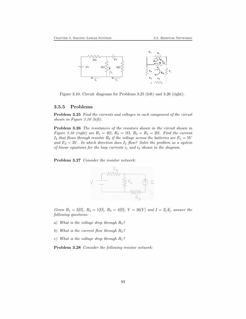
Chapter 3. Solving Linear Systems 3.5. Resistor Networks
Figure 3.10: Circuit diagrams for Problems 3.25 (left) and 3.26 (right).
3.5.5 Problems
Problem 3.25 Find the currents and voltages in each component of the circuitshown in Figure 3.10 (left).
Problem 3.26 The resistances of the resistors shown in the circuit shown inFigure 3.10 (right) are R1 = 4Ω, R2 = 1Ω, R3 = R4 = 2Ω. Find the currentI2 that flows through resistor R2 if the voltage across the batteries are E1 = 5Vand E2 = 3V . In which direction does I2 flow? Solve the problem as a systemof linear equations for the loop currents i1 and i2 shown in the diagram.
Problem 3.27 Consider the resistor network:
Given R1 = 3[Ω], R2 = 1[Ω], R3 = 4[Ω], V = 26[V ] and I = 2[A], answer thefollowing questions:
a) What is the voltage drop through R3?
b) What is the current flow through R2?
c) What is the voltage drop through R1?
Problem 3.28 Consider the following resistor network:
93

Chapter 3. Solving Linear Systems 3.5. Resistor Networks
Suppose that R1 = 4[Ω], R2 = 1[Ω], R3 = 2[Ω] and that the current flow throughR3 is 1.5[A]. Solve the resistor network and answer the following questions:
a) What is the voltage drop across R3?
b) What is the current flow through R2?
c) What is the voltage drop through V ?
Problem 3.29 Consider the following resistor network:
Suppose that R1 = 4[Ω], R2 = 2[Ω], R3 = 10[Ω] and that V = 60[V ]. Solve theresistor network and answer the following questions:
a) What is the voltage drop through R2?
b) What is the current flow through R1?
c) What is the current flow through R3?
Problem 3.30 Find the loop currents i1, i2, i3 in the following network:
where R1 = 1[Ω], R2 = 3[Ω], R3 = 5[Ω], R4 = 2[Ω], E1 = 10[V ] andE2 = 4[V ].
94

Chapter 3. Solving Linear Systems 3.5. Resistor Networks
Problem 3.31 Consider the following network:
where R1 = 1[Ω], R2 = 2[Ω], R3 = [Ω], R4 = [Ω], V = 25[V ] and I = 3[A].
a) Set up and solve the linear system for the loop currents i1, i2, i3 and thevoltage E across the current source.
b) What is the voltage drop through R2?
c) What is the current flow through V ?
d) What is the voltage drop through I?
Problem 3.32 Consider the resistor network:
with R1 = 2[Ω], R2 = 5[Ω], R3 = 3[Ω], V = 10[V ], I2 = 3[A]. Suppose thatthe voltage drop through I2 is E2 = 5[V ].
a) What is the current flow through R2?
b) What is the voltage drop through I1?
c) What is the current flow through I1?
Problem 3.33 If a circuit contains only resistors, then we can solve it com-pletely using the ideas of this section. Write down the linear equations satisfiedby the currents in the circuit shown in Figure 3.11. In this diagram, the compo-nent on the far left is a voltage source (battery). The voltage across the voltagesource is always E.
95

Chapter 3. Solving Linear Systems 3.6. Additional Topics
RR1 R3 2n-1
R2 R4 R2nE
Figure 3.11: The circuit from Problem 3.33.
Figure 3.12: The minimization of a quadratic function in one variable.
3.6 Additional Topics
3.6.1 Quadratic Functions
Let begin by recalling how we would find the minimum of a quadratic functionin one variable, namely a parabola given by f(x) = ax2 + bx + c as shown inFigure 3.12. We simply find the value of x for which the derivative is zero, thatis, we solve f ′(x) = 0. Notice that since f is quadratic, this is a linear equation
2ax+ b = 0
which is easily solved for x = −b/2a (provided a 6= 0). So the minimum valueis f(−b/2a) = −b2/(4a) + c.
Of course, if a is negative, then the parabola points downwards, and we havefound the maximum value, not the minimum value.
A quadratic function of two variables x1 and x2 is a function of the form
f(x1, x2) = ax21 + 2bx1x2 + cx2
2 + dx1 + ex2 + f.
(The 2 in front of b is just for convenience.) For what values of x1 and x2 isf(x1, x2) the smallest? Just like with the parabola in one variable, there maybe no such values. It could be that f has a maximum instead, or that f haswhat is called a saddle point. However if f does have a minimum, the procedure
96

Chapter 3. Solving Linear Systems 3.6. Additional Topics
described below is guaranteed to find it. (If f has a maximum or saddle point,the procedure will find these points instead.)
The idea behind finding the minimum is simple. Suppose that x1 and x2 arethe values for which f(x1, x2) is smallest. Then the function g(s) = f(x1 +s, x2)must have a minimum at s = 0. So g′(0) = 0. But
g′(s) =d
dsf(x1 + s, x2)
=d
dsa(x1 + s)2 + 2b(x1 + s)x2 + cx2
2 + d(x1 + s) + ex2 + f
= 2a(x1 + s) + 2bx2 + d
so that the condition is
g′(0) = 2ax1 + 2bx2 + d = 0.
Notice that this expression can be obtained by holding x2 fixed and differenti-ating with respect to x1. It is called the partial derivative of f with respect tox1 and is denoted ∂f
∂x1.
The same argument can be applied to h(s) = f(x1, x2 + s) (or ∂f∂x2
.) Thisyields
h′(0) =∂f(x1, x2)
∂x2= 2bx1 + 2cx2 + e = 0.
Therefore we conclude that the pair of values x1 and x2 at which f achievesits minimum satisfy the system of linear equations
2ax1 +2bx2 = −d2bx1 +2cx2 = −e
This is a 2 by 2 system with augmented matrix[2a 2b2b 2c
∣∣∣∣−d−e]
This is easily generalized to n variables. In this case the quadratic functionis given by
f(x1, x2, . . . , xn) =
n∑i=1
n∑j=1
ai,jxixj +
n∑i=1
bixi + c
To see this is the same, let us expand out the first term when n = 2. Then
n∑i=1
n∑j=1
ai,jxixj = a1,1x1x1 + a1,2x1x2 + a2,1x2x1 + a2,2x2x2
= a1,1x21 + (a1,2 + a2,1)x1x2 + a2,2x
22
So this is just the same as before with a1,1 = a, a1,2 + a2,1 = 2b and a2,2 = c.Notice that we might as well assume that ai,j = aj,i, since replacing both ai,jand aj,i with (a1,2 + a2,1)/2 doesn’t change f .
97

Chapter 3. Solving Linear Systems 3.6. Additional Topics
i iy -ax -b
(x ,y )
(x ,y )
1 1
n n
y
ax +b
i
i
xi
(x ,y )i i
Figure 3.13: Fitting a line through data.
If this function f has a minimum we can find it by generalizing the procedureabove. In other words we try to find values of x1, . . . , xn for which ∂f/∂x1 =∂f/∂x2 = · · · = ∂f/∂xn = 0. This leads to a system of n linear equations whoseassociated augmented matrix is
2a1,1 2a1,2 . . . 2a1,n
2a2,1 2a2,2 . . . 2a2,n
......
...2an,1 2an,2 . . . 2an,n
∣∣∣∣∣∣∣∣−b1−b2
...−bn
3.6.2 Least squares fit
As a first application let us consider the problem of finding the “best” straightline going through a collection of data points (x1, y1), (x2, y2), . . . , (xn, yn). (Care-ful! the xi’s are not the unknowns in this problem, but rather the known fixeddata points, together with the yi’s.) Consider Figure 3.13. Which straight linefits best? There is no one answer. One can measure how good the fit of astraight line is in various ways. However the following way of measuring the fitresults in a problem that is easy to solve.
Each line is given by an equation y = ax+b. So the variables in this problemare a and b. We want to find the values of a and b that give the best fittingline. The vertical distance between the point (xi, yi) and the line is given by|yi − axi − b|. We will take as a measure of the fit, the square of this quantity,added up over all the data points. So
f(a, b) =∑i
(yi − axi − b)2
=∑i
(y2i + x2
i a2 + b2 − 2xiyia− 2yib+ 2xiab
)=
(∑i
x2i
)a2 + 2
(∑i
xi
)ab+ nb2 − 2
(∑i
xiyi
)a− 2
(∑i
yi
)b+
(∑i
y2i
)
Here we used that (∑i 1) = n, the number of points. Therefore the linear
98

Chapter 3. Solving Linear Systems 3.6. Additional Topics
equations we must solve for a and b are[2(∑
i x2i
)2 (∑i xi)
2 (∑i xi) 2n
∣∣∣∣ 2 (∑i xiyi)
2 (∑i yi)
]We could solve these equations numerically in each particular case, but since itsjust a 2 by 2 system we can also write down the answer explicitly. In fact, thesolution to [
A BC D
∣∣∣∣EF]
is [ DE−BFAD−BCAF−CEAD−BC
],
provided AD − BC 6= 0, as you may check directly, or derive using a sequenceof row transformations. So in this case
a =n(∑xiyi)− (
∑xi)(
∑yi)
n(∑x2i )− (
∑xi)2
b =(∑x2i )(∑yi)− (
∑xi)(
∑xiyi)
n(∑x2i )− (
∑xi)2
Example 3.16 Suppose we want to find the best straight line through the points(1, 1), (2, 2), (2, 3), (3, 3) and (3, 4). Calculate∑
1 = n = 5∑xi = 1 + 2 + 2 + 3 + 3 = 11∑yi = 1 + 2 + 3 + 3 + 4 = 13∑x2i = 1 + 4 + 4 + 9 + 9 = 27∑y2i = 1 + 4 + 9 + 9 + 16 = 39∑
xiyi = 1 + 4 + 6 + 9 + 12 = 32
soa = (5 · 32− 11 · 13)/(5 · 27− 112) = 17/14 = 1.214 . . .
andb = (27 · 13− 11 · 32)/(5 · 27− 112) = −1/14 = −0.0714 . . .
The result is shown in Figure 3.14.
3.6.3 Equilibrium configuration of hanging weights andsprings
Consider the problem of n vertically hanging weight connected by springs. Whatis the equilibrium configuration? We can solve this problem by calculating thetotal potential energy of the system. The equilibrium configuration minimizesthe total potential energy. A diagram of the setup is shown in Figure 3.15. Ourgoal is to compute the numbers x1, . . ., xn. In the diagram n = 3.
99

Chapter 3. Solving Linear Systems 3.6. Additional Topics
Figure 3.14: The solution in Example 3.16.
x1
x2
x3
k l
k l
k l
1 1
2 2
3 3
m1
m2
m3
,
,
,
Figure 3.15: Equilibrium configuration of springs.
There are two sources of potential energy. One is the potential energy storedin the spring. This is equal to ks2/2, where k is the spring constant thatmeasures the stiffness of the spring, and s is the amount that the spring hasbeen stretched from its natural length. In our problem, suppose that the springconstant of the ith spring is ki and its natural length is li. Then the potentialenergy stored in the ith spring is ki(xi − xi−1 − li)2/2. To make this formulawork out correctly for the first spring we set x0 = 0.
The other source of potential energy is gravity. The gravitational potentialenergy of the ith weight is −migxi. The reason for the minus sign is that weare measuring distances downward.
Thus the total potential energy in the system for n weights is the function
f(x1, x2, . . . , xn) =
n∑i=1
ki2
(xi − xi−1 − li)2 −migxi.
When n = 3 this becomes
f(x1, x2, x3) =k1
2(x1−l1)2+
k2
2(x2−x1−l2)2+
k3
2(x3−x2−l3)2−m1gx1−m2gx2−m3gx3
This is a quadratic function, so we know how to find the minimum. The equa-tions are obtained by taking partial derivatives: To get the first equation we
100

Chapter 3. Solving Linear Systems 3.6. Additional Topics
hold x2 and x3 fixed and differentiate with respect to x1 and so on. Thus theequations are
k1(x1 − l1)− k2(x2 − x1 − l2)−m1g = 0
k2(x2 − x1 − l2)− k3(x3 − x2 − l3)−m2g = 0
k3(x3 − x2 − l3)−m3g = 0
The augmented matrix for this system is k1 + k2 −k2 0−k2 k2 + k3 −k3
0 −k3 k3
∣∣∣∣∣∣m1g + k1l1 − k2l2m2g + k2l2 − k3l3
m3g + k3l3
Example 3.17 Suppose that the spring constants are k1 = 1, k2 = 2 and k3 =1. The masses are all equal to 1, g = 10 and the natural length of the springs is1 for all springs (in appropriate units). Find the equilibrium configuration. Wemust solve 3 −2 0
−2 3 −10 −1 1
∣∣∣∣∣∣91111
Gaussian elimination gives 3 −2 0
0 −1 10 0 2
∣∣∣∣∣∣911106
which can be solved to give x1 = 31, x2 = 42, x3 = 53.
3.6.4 Problems
Problem 3.34 Find the “best” straight line going through the points (1, 1),(2, 1), (2, 3), (3, 4), (3, 5) and (4, 4).
Problem 3.35 Consider the problem of finding the parabola y = ax2 + bx + cthat best fits the n data points (x1, y1) . . . (xn, yn). Derive the system of threelinear equations which determine a, b and c. (You need not solve solve them!)
Problem 3.36 Write down the augmented matrix for a system of n weightsand springs.
Problem 3.37 Write down the system of equations you would have to solve ifthere are 5 identical springs with ki = 1 and li = 1 and five weights with m1 = 1,m2 = 2, m3 = 3, m4 = 4, and m5 = 5.
101

Chapter 3. Solving Linear Systems 3.7. Solutions to Chapter Problems
3.7 Solutions to Chapter Problems
Solution 3.1 The augmented matrix is
A =
1 −2 3 64 −5 −6 78 9 10 11
Solution 3.2 Here is the sequence of systems of equations you would get:
x1 + x2 + x3 = 6x1 − x2 + x3 = 02x1 + x2 − 8x3 = −11
x1 + x2 + x3 = 6− 2x2 = −6
2x1 + x2 − 8x3 = −11
x1 + x2 + x3 = 6− 2x2 = −6− x2 − 10x3 = −23
x1 + x2 + x3 = 6x2 = 3
− x2 − 10x3 = −23
x1 + x2 + x3 = 6x2 = 3
− 10x3 = −20
So x3 = 2, x2 = 3 and x1 = 1.
Solution 3.3
A = [1, 1, 1, 6; 1, -1, 1, 0; 2, 1, -8, -11]
A(2,:) = A(2,:) - A(1,:)
A(3,:) = A(3,:) - 2*A(1,:)
A(2,:) = -A(2,:)/2
A(3,:) = A(3,:) + A(2,:)
A(3,:) = -A(3,:)/10
We get the same solution as in the pen-and-paper version in problem 3.2.
Solution 3.4 Perform the sequence of operations to finally end up with thesystem
2x3 = 4
3x1 − 3x2 + 3x3 = 30
9x1 + 2x3 = 26.
Hence, x1 = 22/9, x2 = −50/9, and x3 = 2.
102

Chapter 3. Solving Linear Systems 3.7. Solutions to Chapter Problems
Solution 3.5 We want to solve the system
2x1 + x2 = 5
3x1 + 5x2 = −10.
We shall use the method of substitution.From the first equation, we solve for x2:
x2 = 5− 2x1
We then substitute it into the second equation:
3x1 + 5(5− 2x1) = −10
. We now have a decoupled equation, and the solution is x1 = 5, x2 = −5.
Solution 3.6 The first equation reads x1 = 3. The second reads x1−x2 = 3, or3−x2 = 3, or x2 = 0. The third reads 2x1 +x2−8x3 = −4, or 6+0−8x3 = −4or x3 = 5/4.
Solution 3.7 The last equation gives x4 = 2 and the second last one x3 = 2.Then we have to introduce a parameter x2−s and the we find that x1 = −5−2s
Thus x =
−5022
+ s
−2100
In the second system, we have to introduce a
parameter right off the bat. So x4 = s1 and x3 = 4−s1. Moving up one row, wehave to introduce another parameter x2 = s2 and then x1 = 1−2s2− (4− s1)−
2s1 = −3− s1 − 2s2 so x =
−3040
+ s1
−10−11
+ s2
−2100
The third system is
just the same. The extra rows of zeros have no effect.
Solution 3.8 Perform the following sequence of row operations:
i) (2, :) = (2, :)− (1, :)
ii) (3, :) = (3, :)− (1, :)
iii) (3, :) = (3, :) + 2(2, :)
iv) (4, :) = (4, :)− 3(2, :)
v) (4, :) = (4, :) + (3, :),
in order to get the reduced row echelon form (RREF)1 2 2 2 10 1 −3 1 −20 0 −7 1 00 0 0 0 0
.103

Chapter 3. Solving Linear Systems 3.7. Solutions to Chapter Problems
Thus, we have that the rank of the augmented matrix, which is the same asthe rank of the unaugmented matrix is r = 3, while the number of unknownsis n = 4. Therefore, the system has infinitely many solutions, that can berepresented as the general solution
x = q + sa,
where s is any real number, q = (q1, q2, q3, q4) is any particular solution ofthe original system, and a = (a1, a2, a3, a4) is any non-zero solution of thecorresponding homogeneous system.
From the row echelon form we can see that q has to satisfy −7q3 + q4 = 0.Let q4 = 7, then q3 = 1. For the other two q values we have
q2 = −2 + 3q3 − q4 = −6
q1 = 1− 2q2 − 2q3 − 2q4 = −3.
Hence, we have that q = (−3,−6, 1, 7).Now, to find a, the homogenous row echelon form is
1 2 2 2 00 1 −3 1 00 0 −7 1 00 0 0 0 0
.Thus, a has to satisfy −7a3 + a4 = 0. Take a4 = 7, then a3 = 1.
From the second row we have that a2 = 3a3 − a4 = −4, and from the firstrow we get that a1 = −2a2 − 2a3 − 2a4 = −8. So a = (−8,−4, 1, 7), and ageneral form of the solution is
x =
−3−617
+ s
−8−417
Solution 3.9 Perform the following sequence of row operations
i) (2, :) = (2, :)− 3(1, :)
ii) (4, :) = (4, :)− 2(1, :)
iii) (4, :) = (4, :) + 2(3, :)
iv) (3, :)↔ (2, :)
v) (4, :)↔ (3, :)
vi) (4, :) = (4, :)− 32 (3, :),
104

Chapter 3. Solving Linear Systems 3.7. Solutions to Chapter Problems
to transform the augmented matrix into the reduced row echelon form1 2 2 −7 200 6 0 −6 −100 0 −6 0 −300 0 0 16 −30
.We can now solve the system starting from the bottom:
x4 = −30
16= −15
8
x3 =−30
−6= 5
x2 =−10 + 6x4
6= −85
24
x1 = 20− 2x2 − 2x3 + 7x4 =95
24
Solution 3.10 The matrix 1 −2 32 −3 23 2 −4
∣∣∣∣∣∣229
reduces to 1 −3 3
0 1 40 0 19
∣∣∣∣∣∣2−219
which has as solution x1 = 3, x2 = 2, x3 = 1.
Solution 3.11 The matrix 2 1 −11 −2 −2−1 12 8
∣∣∣∣∣∣617
reduces to 2 1 −1
0 −5/2 −3/20 0 0
∣∣∣∣∣∣6−20
which has as solution x1 = 13/5 + 4s/5, x2 = 4/5− 3s/5, x3 = s.
Solution 3.12 The matrix 1 2 41 1 32 5 9
∣∣∣∣∣∣121
reduces to 1 2 4
0 −1 −10 0 0
∣∣∣∣∣∣110
105

Chapter 3. Solving Linear Systems 3.7. Solutions to Chapter Problems
Thus , setting x3 = s, we obtain x2 = −1− s and x1 = 3− 2s.
Solution 3.13 The matrix 1 2 41 1 32 5 9
∣∣∣∣∣∣123
reduces to 1 2 4
0 −1 −10 0 0
∣∣∣∣∣∣112
which has no solutions.
Solution 3.14 The matrix 3 1 −1 22 −2 5 −7−4 −4 7 −11
∣∣∣∣∣∣71−13
reduces to 3 1 −1 2
0 −8/3 17/3 −25/30 0 0 0
∣∣∣∣∣∣7
−11/30
which has as solution x1 = 15/8− 3s1/8 + 3s2/8, x2 = 11/8 + 17s1/8− 25s2/8,x3 = s1, x4 = s2.
Solution 3.15 Probably the easiest way to do this problem is to think geomet-rically. This system of equations describes the intersection of two lines. Thelines will intersect in a single point if they are not parallel. This will happenexactly when the two vectors [a, b] and [c, d] are not parallel. Recall that thiscan be tested using the determinant. So the equations have a unique solution
exactly when det
[a bc d
]= ad− bc 6= 0.
Solution 3.16 Perform the following sequence of row operations:
i) (2, :) = (2, :)− 4(1, :)
ii) (3, :) = (3, :) + 4(1, :)
iii) (3, :) = (3, :) + 53 (3, :)
to get the reduced row echelon matrix 1 2 0 70 0 6 −180 0 0 139
.The last equation says 0 = 139, which cannot happen, therefore this linearsystem has zero solutions.
Solution 3.17 The script is the following:
106
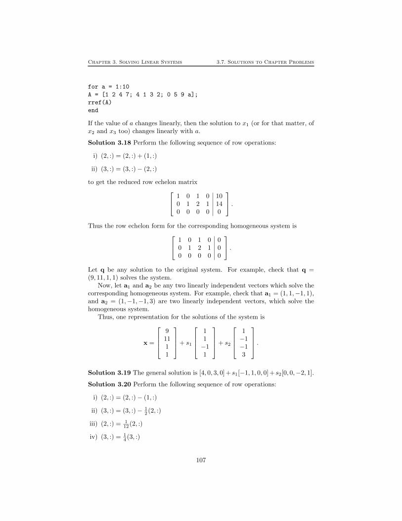
Chapter 3. Solving Linear Systems 3.7. Solutions to Chapter Problems
for a = 1:10
A = [1 2 4 7; 4 1 3 2; 0 5 9 a];
rref(A)
end
If the value of a changes linearly, then the solution to x1 (or for that matter, ofx2 and x3 too) changes linearly with a.
Solution 3.18 Perform the following sequence of row operations:
i) (2, :) = (2, :) + (1, :)
ii) (3, :) = (3, :)− (2, :)
to get the reduced row echelon matrix 1 0 1 0 100 1 2 1 140 0 0 0 0
.Thus the row echelon form for the corresponding homogeneous system is 1 0 1 0 0
0 1 2 1 00 0 0 0 0
.Let q be any solution to the original system. For example, check that q =(9, 11, 1, 1) solves the system.
Now, let a1 and a2 be any two linearly independent vectors which solve thecorresponding homogeneous system. For example, check that a1 = (1, 1,−1, 1),and a2 = (1,−1,−1, 3) are two linearly independent vectors, which solve thehomogeneous system.
Thus, one representation for the solutions of the system is
x =
91111
+ s1
11−11
+ s2
1−1−13
.Solution 3.19 The general solution is [4, 0, 3, 0] + s1[−1, 1, 0, 0] + s2[0, 0,−2, 1].
Solution 3.20 Perform the following sequence of row operations:
i) (2, :) = (2, :)− (1, :)
ii) (3, :) = (3, :)− 12 (2, :)
iii) (2, :) = 112 (2, :)
iv) (3, :) = 14 (3, :)
107

Chapter 3. Solving Linear Systems 3.7. Solutions to Chapter Problems
v) (2, :) = (2, :) + 13 (3, :)
vi) (1, :) = (1, :)− 6(3, :)
vii) (1, :) = (1, :) + 3(2, :)
to get the reduced row echelon matrix 1 0 12 0
0 1 − 76 0
0 0 0 1
.Here the rank of the augmented matrix (ra = 2) is less than the rank of theunaugmented matrix ()ru = 3), therefore the linear system has zero solutions.
Solution 3.21 To decide whether the vectors are linearly independent we mustdecide whether the homogeneous system of equations represented by the matrix
1 1 12 1 00 −1 12 1 0
has a non zero solution. Row reduction yields
1 1 10 −1 −20 0 30 0 0
.
This shows that the zero solution is unique and therefore the vectors are indepen-dent. It can’t happen that three vectors span a four dimensional space. To testwhether y1 is a linear combination of the xi’s we try to solve the equation with
augmented matrix
1 1 12 1 00 −1 12 1 0
∣∣∣∣∣∣∣24−34
. Row reduction gives
1 1 10 −1 −20 0 30 0 0
∣∣∣∣∣∣∣20−30
.
This system does have a solution, therefore the vector y1 is a linear combinationof the xi’s.
Solution 3.22 Three vectors in the plane cannot be linearly independent.There are two ways to see that y is a linear combination of a1 and a2:
• a1 and a2 are linearly independent because
det
[1 23 1
]= −5
Therefore a1, a2 form a basis of R2, and every vector is a linear combi-nation of a1 and a2.
• Solve the systemx1a1 + x2a2 = y
i.e.
x1
[12
]+ x2
[31
]=
[−15
5
].
108

Chapter 3. Solving Linear Systems 3.7. Solutions to Chapter Problems
This system yields the augmented matrix[1 3 −152 1 5
]→ (2, :) = (2, :)− 2(1, :)→
[1 3 −150 −5 35
]→ (2, :) = −1
5(2, :)→
[1 3 −150 1 −7
],
which gives x2 = 7, and x1 = 6.
Solution 3.23 The vectors a1, a2, and a3 are linearly independent if the onlysolution to the system
x1a1 + x2a2 + x3a3 = 0
is x1 = x2 = x3 = 0 So,1 0 10 01 0 0 00 4 −5 00 −3 0 0
→ (2, :) = (2, :)− (1, :)(4, :) = − 1
3 (4, :)→
1 0 10 00 0 −10 00 4 −5 00 1 0 0
→ (2, :) = − 110 (2, :)
(3, :)↔ (4, :)→
1 0 10 00 0 1 00 1 0 00 4 −5 0
→ (2, :)↔ (3, :)(4, :) = (4, :)− 4(3, :) + 5(2, :)
→
1 0 10 00 1 0 00 0 1 00 0 0 0
The system has a unique solution x1 = x2 = x3 = 0, hence the three vectorsare linearly independent.
To find if y can be written as a linear combination of the three vectors, welook for a solution of the system
1 0 10 111 0 0 10 4 −5 −10 −3 0 10
→ (2, :) = (2, :)− (1, :)(3, :) = (3, :) + (4, :)
→
1 0 10 110 0 −10 −100 1 −5 90 −3 0 10
→(2, :) = − 1
10 (2, :)(4, :) = (4, :) + 3(3, :)
→
1 0 10 110 0 1 10 1 −5 90 0 −15 37
The second row of the reduced row echelon matrix implies that x3 = 1, whilethe third row yields that x3 = − 37
15 . This contradiction means that the systemhas no solution, and y is therefore not a linear combination of a1, a2, and a3.
Solution 3.24
109

Chapter 3. Solving Linear Systems 3.7. Solutions to Chapter Problems
plot3([1,0],[2,0],[3,0])
hold on
plot3([-1,0],[2,0],[1,0])
plot3([4,0],[1,0],[-1,0])
In the figure window, if you go to Tools → Rotate 3D, you will see right awaythat the three vectors do not share the same plane, therefore they must belinearly independent.
Solution 3.25 We apply Kirchhoff’s junction rule
I1 + I2 − I3 = 0
and Kirchhoff’s loop rules, moving around first the left loop and then the rightloop in a clockwise direction:
−2I1 + 5I2 + 6 = 0
−5− 6I3 − 5I2 = 0
Writing these three equations in an augmented matrix with the unknowns or-dered I1, I2 and I3 gives 1 1 −1
−2 5 00 −5 −6
∣∣∣∣∣∣0−65
which is solved to give I1 = 41/52, I2 = −23/26 and I3 = −5/52 with unitsof Amperes. The voltage drops are I1R1 = 41/26, I2R2 = 115/26 and I3R3 =15/26 across the three resistors, with drops in the direction of positive currents.Note that this problem is more easily solved using two loop currents (try it andmake sure you get the same solution).
Solution 3.26 We write voltage drops around the two loops in the direction ofthe loop currents:
4i1 + (i1 − i2) + 5 = 0 or 5i1 − i2 = −5
(i2 − i1) + 6i2 − 3 = 0 or − i1 − i2 = −5
which is solved to give i2 = 5/17 and i1 = −16/17. Thus, I2 = i2 − i1 = 21/17.Since it is positive, this current flows to the right.
Solution 3.27 We use loop currents to solve the network depicted in figure3.27.
Kirchhoff’s second law gives that i2 = −I, and the first law applied to theclosed loop on the left gives
R1i1 +R2(i1 − i2) = V.
As R1 = 3[Ω], R2 = 1[Ω], R3 = 4[Ω], V = 26[V ], and I = 2[A], we get
i2 = −2[A] (3.2)
3i1 + i1 + 2 = 26 (3.3)
110

Chapter 3. Solving Linear Systems 3.7. Solutions to Chapter Problems
Figure 3.16: Problem 3.27.
Figure 3.17: Problem 3.28.
Hence i1 = 6[A], and from the sign we get that i2 flows in the opposite directionas initially supposed.
a) Voltage drop = R3i2 = −8[V ]. The - sign indicates that the potential ishigher at the left of R3 than on the right.
b) The flow through R2 is i1 − i2 = 8[A].
c) Voltage drop = R1i1 = 18[V ].
Solution 3.28 Again, we use loop currents to solve the problem depicted infigure 3.28.
R1i1 +R2(i1 − i2) = V
R3i2 +R2(i2 − i1) = 0,
with R1 = 4[Ω], R2 = 1[Ω], R3 = 2[Ω].The flow through R3 is i2, which is 1.5[A]. The system becomes
4i1 + (i1 − 1.5) = V3 + (1.5− i1) = 0
5i1 − V = 32
i1 = 92
Therefore V = 21[V ], and i1 = 4.5[A]
111

Chapter 3. Solving Linear Systems 3.7. Solutions to Chapter Problems
Figure 3.18: Problem 3.29.
a) Voltage drop = R3i2 = 3[V ].
b) Current flow = i1 − i2 = 3[A].
c) Voltage drop = V = 21[V ]
Solution 3.29 As before:R1(i1 − i2) = V
R2i2 +R3i2 +R1(i2 − i1) = 0,
with R1 = 4[Ω], R2 = 2[Ω], R3 = 10[Ω], V = 60[V ].Hence, the system becomes
4(i1 − i2) = 152i2 + 10i2 + 4(i2 − i1) = 0
,
i1 − i2 = 154i2 − i1 = 0
.
Solving the system we get i1 = 20[A], i2 = 5[A].
a) Voltage drop = R2i2 = 10[V ].
b) Current flow through R1 = i1 − i2 = 15[A].
c) Current flow through R3 = i2 = 5[A].
Solution 3.30 Using Kirchhoff’s laws we get the following equations: R1i1 +R2(i1 − i2) = E1
R3i2 +R2(i2 − i1) = −E2
R4i3 = E2
,
112

Chapter 3. Solving Linear Systems 3.7. Solutions to Chapter Problems
Plugging in the values of R1, R2, R3, R4, E1, and E2, we get i1 + 3(i1 − i2) = 105i2 + 3(i2 − i1) = −4
2i3 = 4,
We have that i3 = 2. To find i1 and i2 we solve the augmented system[4 −3 10−3 8 −4
]→ (1, :) = (1, :) + (2, :) →[
1 5 6−3 8 −4
]→ (2, :) = (2, :) + 3(1, :) →
[1 5 60 23 14
].
So i1 = 6823 [A], i2 = 14
23 [A], i3 = 2[A].
Solution 3.31 From Kirchhoff’s first law:
I + i3 = i2
From Kirchhoff’s second law:
R1i1 +R2(i1 − i2) = V
E +R2(i2 − i1) = 0
R4i3 +R3i3 = E
Substituting in the actual values, we geti1 + (i1 − i2) = 25
i2 − i3 = 3E + 2(i2 − i1) = 0
2i3 = E
The system, with respect to i1, i2, i3, and E, yields the following augmentedmatrix:
2 −1 0 0 250 1 −1 0 3−2 2 0 1 00 0 2 −1 0
→ (3, :) = (3, :) + (1, :) →
2 −1 0 0 250 1 −1 0 30 1 0 1 00 0 2 −1 0
→ (3, :) = (3, :)− (2, :) →
2 −1 0 0 250 1 −1 0 30 0 1 1 −30 0 2 −1 0
→ (4, :) = (4, :)− 2(3, :) →
2 −1 0 0 250 1 −1 0 30 0 1 1 −30 0 0 −3 6
113

Chapter 3. Solving Linear Systems 3.7. Solutions to Chapter Problems
Figure 3.19: Problem 3.32.
a) Then i1 = 272 [A], i2 = 2[A], i3 = −1[A], E = −2[V ].
b) Voltage drop: R2(i1 − i2) = 23[V ].
c) Current flow through V : i1 = 272 [A].
d) Voltage drop through I: E = −2[V ].
Solution 3.32 From Kirchhoff’s second law:
I1 = i1
I2 = −i2
From Kirchhoff’s first law:
R1i1 +R2(i1 − i2) = E1
V +R3i2 + E2 +R2(i2 − i1) = 0,
which becomes i1 = I1i2 = −3
7i1 − 5i2 = E1
10 + 8i2 − 5i1 + 5 = 0
We seek i1 and E1: 7i1 − E1 = −15−5i1 = 9
.
Therefore we have that i1 = − 95 [A], E1 = 12
5 [V ].
a) Current flow through R2: i1 − i2 = 65 [A].
114

Chapter 3. Solving Linear Systems 3.7. Solutions to Chapter Problems
b) Voltage drop through I1 = E1 = 125 [V ].
c) Current flow through I1 = i1 = − 95 [A].
Solution 3.33 Note that this solution follows the alternate description of resis-tor networks in the notes. Using the identities Vi = IiRi, the voltage equationsfor the loops can be written
I1R1 + I2R2 + E = 0
I3R3 + I4R4 − I2R2 = 0
...
I2n−1R2n−1 + I2nR2n − I2n−2R2n−2 = 0
The current equations for the nodes are
I1 − I3 − I2 = 0
I3 − I5 − I4 = 0
...
I2n−1 − I2n = 0
Solution 3.34 We have n = 6,∑xi = 15,
∑x2i = 43,
∑yi = 18,
∑xiyi = 52,
so a = 14/11 ∼ 1.27 . . . and b = −2/11 ∼ −0.18 . . ..
Solution 3.35 We would want to minimize the quadratic function
f(a, b, c) =∑
(ax2i + bxi + c− yi)2
=∑(
a2x4i + b2x2
i + c2 + y2i + 2abx3
i + 2acx2i − 2ax2
i yi + 2bcxi − 2bxiyi − 2cyi)
=(∑
x4i
)a2 +
(∑x2i
)b2 + nc2 + 2
(∑x3i
)ab+ 2
(∑x2i
)ac+ 2
(∑xi
)bc
−2(∑
x2i yi
)a− 2
(∑xiyi
)b− 2
(∑yi
)c+
(∑y2i
)The corresponding system of equations is
(∑x4i
) (∑x3i
) (∑x2i
)(∑x3i
) (∑x2i
)(∑xi)(∑
x2i
)(∑xi) n
∣∣∣∣∣∣(∑
x2i yi)
(∑xiyi)
(∑yi)
(I’ve divided each equation by two.)
115

Chapter 3. Solving Linear Systems 3.7. Solutions to Chapter Problems
Solution 3.36 The matrix is
k1 + k2 −k2 0 0 . . . 0 0 0−k2 k2 + k3 −k3 0 . . . 0 0 0
0 −k3 k3 + k4 −k4 . . . 0 0 00 0 −k4 k4 + k5 . . . 0 0 00 0 0 −k5 . . . 0 0 0...
......
......
......
0 0 0 0 . . . −kn−1 kn−1 + kn −kn0 0 0 0 . . . 0 −kn kn
∣∣∣∣∣∣∣∣∣∣∣∣∣∣∣∣
m1g + k1l1 − k2l2m2g + k2l2 − k3l3m3g + k3l3 − k4l4m4g + k4l4 − k5l5m5g + k5l5 − k6l6
...mn−1g + kn−1ln−1 − knln
mg + knln
Solution 3.37 The system of equations would be
2 −1 0 0 0−1 2 −1 0 00 −1 2 −1 00 0 −1 2 −10 0 0 −1 1
∣∣∣∣∣∣∣∣∣g
2g3g4g
5g + 1
116

Chapter 4
Matrices and Determinants
4.1 Matrix operations
A matrix is a rectangular array of numbers. Here is an example of an m × nmatrix.
A =
a1,1 a1,2 · · · a1,n
a2,1 a2,2 · · · a2,n
......
...am,1 am,2 · · · am,n
This is sometimes abbreviated A = [ai,j ]. An m × 1 matrix is called a columnvector and a 1×n matrix is called a row vector. (The convention is that m×nmeans m rows and n columns).
Addition and scalar multiplication are defined for matrices exactly as forvectors. If s is a number
s
a1,1 a1,2 · · · a1,n
a2,1 a2,2 · · · a2,n
......
...am,1 am,2 · · · am,n
=
sa1,1 sa1,2 · · · sa1,n
sa2,1 sa2,2 · · · sa2,n
......
...sam,1 sam,2 · · · sam,n
,anda1,1 a1,2 · · · a1,n
a2,1 a2,2 · · · a2,n
......
...am,1 am,2 · · · am,n
+
b1,1 b1,2 · · · b1,nb2,1 b2,2 · · · b2,n
......
...bm,1 bm,2 · · · bm,n
=
a1,1 + b1,1 a1,2 + b1,2 · · · a1,n + b1,na2,1 + b2,1 a2,2 + b2,2 · · · a2,n + b2,n
......
...am,1 + bm,1 am,2 + bm,2 · · · am,n + bm,n
The product of an m× n matrix A = [ai,j ] with a n× p matrix B = [bi,j ] is
a m× p matrix C = [ci.j ] whose entries are defined by
ci,j =
n∑k=1
ai,kbk,j .
117

Chapter 4. Matrices and Determinants 4.1. Matrix operations
B1
B2
B3
2A
A3
A4
A1 A1 A1
B1
B1
A1
2A 2A 2A
A3 A3 A3
A4 A4 A4
B1
B1
B2
B2
B2
B2
B3
B3
B3
A1
B3
=
Figure 4.1: Schematic of matrix multiplication as the inner product of rows andcolumns of the product matrices.
An easy way to remember this is to chop the matrix A into m row vectors oflength n and to chop B into p column vectors also of length n, as in the followingdiagram. The i, jth entry of the product is then the dot product Ai · Bj . Thisis shown schematically in Figure 4.1.
It is important to notice that the matrix product AB only makes sense if thethe number of columns of A equals the number of rows of B. So A2 = AA onlymakes sense for a square matrix.
Here is an example 1 0 1 21 1 1 40 0 1 1
1 23 45 67 8
=
1× 1 + 0× 3 + 1× 5 + 2× 7 1× 2 + 0× 4 + 1× 6 + 2× 81× 1 + 1× 3 + 1× 5 + 4× 7 1× 2 + 1× 4 + 1× 6 + 4× 80× 1 + 0× 3 + 1× 5 + 1× 7 0× 2 + 0× 4 + 1× 6 + 1× 8
=
20 2437 4412 14
Notice that if A is an m× n matrix, and
x =
x1
x2
x3...xn
and
b =
b1b2b3...bm
Then the equation
Ax = b
is a short way of writing the system of linear equations corresponding to theaugmented matrix [A|b].
118

Chapter 4. Matrices and Determinants 4.1. Matrix operations
We will see shortly why matrix multiplication is defined the way it is. Fornow, you should be aware of some important properties that don’t hold formatrix multiplication, even though they are true for multiplication of numbers.First of all, in general, AB is not equal to BA, even when both products aredefined and have the same size. For example, if
A =
[0 10 0
]and
B =
[1 00 0
]then
AB =
[0 00 0
]but
BA =
[0 10 0
].
This example also shows that two non-zero matrices can be multiplied togetherto give the zero matrix.
Here is a list of properties that do hold for matrix multiplication.
1. A+B = B +A
2. A+ (B + C) = (A+B) + C
3. s(A+B) = sA+ sB
4. (s+ t)A = sA+ tA
5. (st)A = s(tA)
6. 1A = A
7. A+ 0 = A (here 0 is the matrix with all entries zero)
8. A−A = A+ (−1)A = 0
9. A(B + C) = AB +AC
10. (A+B)C = AC +BC
11. A(BC) = (AB)C
12. s(AB) = (sA)B = A(sB)
119

Chapter 4. Matrices and Determinants 4.1. Matrix operations
4.1.1 MATLAB
Multiplication of matrices can be done using the * operator just as for multi-plication of scalars. An error results if the matrices are not of compatible size.Powers of matrices can be found using the ^ command like for scalars. TheMATLAB command
A^4
produces the same result as
A*A*A*A
where A is a previously defined, square matrix. Using these commands mightbe helpful in working out the details of Problem 4.4 below, although you shouldwork out the first few matrix powers by hand for practise. Taking high powersof a matrix will also be helpful in understanding the long time behaviour ofrandom walks described in Section 4.3.
4.1.2 Problems
Problem 4.1 Define
A =
[1 2 31 2 1
]B =
−1 2−3 1−2 1
C = [ 2 −2 0 ]D =
2−11
2
Compute all products of two of these (i.e., AB, AC, etc.) that are defined.
Problem 4.2 Consider the following matrices:
A =
3 0−1 21 1
; B =
[0 10 0
]; C =
[1 4 23 1 5
].
Compute all the possible products between them.
Problem 4.3 Compute A2 = AA and A3 = AAA for
A =
0 a b0 0 c0 0 0
and
A =
1 0 a0 1 00 0 1
Problem 4.4 Let
A =
[1 10 1
]
120

Chapter 4. Matrices and Determinants 4.2. Linear Transformations and Matrices
(a) Find A2, A3 and A4.
(b) Find Ak for all positive integers k.
(c) Find etA (part of the problem is to invent a reasonable definition!)
(d) Find a square root of A (i.e., a matrix B with B2 = A).
(e) Find all square roots of A.
Problem 4.5 Compute Ak for k = 2, 3, 4 when
A =
0 1 0 00 0 1 00 0 0 10 0 0 0
4.2 Linear Transformations and Matrices
4.2.1 Linear Transformations
Recall that a function f is a rule that takes an input value x and producesan output value y = f(x). Functions are sometimes called transformations ormaps (since they transform, or map, the input value to the output value). Incalculus, you have mostly dealt with functions whose input values and outputvalues are real numbers. However, it is also useful to consider functions whoseinput values and output values are vectors.
We have already encountered this idea when we discussed quadratic func-tions. A quadratic function such as f(x1, x2, x3) = x2
1 + x22 + x2
3 can be con-sidered as a transformation (or map) whose input is the vector x = [x1, x2, x3]and whose output is the number y = x2
1 + x22 + x2
3. In this case we could writef(x1, x2, x3) as f(x).
An example of a transformation whose inputs and outputs are both vectorsin two dimensions is rotation by some angle, say 45. If x is the input vector,then the output vector R(x) is the vector you get by rotating x by 45 in thecounter-clockwise direction as shown in Figure 4.2 (left).
A transformation T is called linear if for any two input vectors x and y andany two numbers s and t,
T (sx + ty) = sT (x) + tT (y) (4.1)
This condition is saying that when we scalar multiply and add two vectors, itdoesn’t matter whether we (i) do scalar multiplication and addition first andthen apply a linear transformation, or (ii) do a linear transformation first andthen do scalar multiplication and addition. In both cases we get the same an-swer. The linearity condition (4.1) is equivalent to the following two conditions:
(i) For any two vectors x and y,
T (x + y) = T (x) + T (y).
121

Chapter 4. Matrices and Determinants 4.2. Linear Transformations and Matrices
x
y=R( )x
Rotation by 45 degrees Rotation by 45 degrees
y x+y
xR( )
R( )R( + )=R( )+R( )
xx x
y
y y
Figure 4.2: Rotation of a vector in 2D (left), graphical evidence that property(i) of linear transformations holds for rotation in 2D (right).
(ii) For any vector x and any scalar s,
T (sx) = sT (x)
Notice that the quadratic function f above is not a linear transformation,since
f(2x) = (2x1)2 + (2x2)2 + (2x3)2 = 4(x21 + x2
2 + x23) = 4f(x).
So f(2x) is not equal to 2f(x) as would need to be true if f were linear.However, rotation by 45 is a linear transformation. The picture in Figure 4.2
(right) demonstrates that condition (i) holds.The most important example of a linear transformation is multiplication
by a matrix. If we regard vectors as column vectors, then multiplying an ndimensional vector x with an m × n matrix A results in an m dimensionalvector y = Ax. The linearity property (4.1) is a consequence of properties 9and 12 of matrix multiplication listed in Section 4.1. We will see that in factevery linear transformation is of this form.
4.2.2 Rotations in two dimensions
Let us obtain a formula for the transformation that rotates a vector in twodimensions counterclockwise by θ degrees. Let x be an arbitrary vector. Denoteby Rotθx the vector obtained by rotating x counterclockwise by θ degrees. If theangle between x and the x axis is φ, then the components of x can be writtenx = [x1, x2] with x1 = ‖x‖ cos(φ) and x2 = ‖x‖ sin(φ). This is shown graphicallyin Figure 4.2.2 (right). To obtain the vector that has been rotated by θ degrees,we simply need to add θ to φ in this representation. Thus y = Rotθx = [y1, y2],where y1 = ‖x‖ cos(φ+ θ) and y2 = ‖x‖ sin(φ+ θ).
To simplify this we can use the addition formulae for sin and cos. Recallthat
cos(a+ b) = cos(a) cos(b)− sin(a) sin(b)
sin(a+ b) = cos(a) sin(b) + sin(a) cos(b)
122

Chapter 4. Matrices and Determinants 4.2. Linear Transformations and Matrices
a
b
proj ab
φθ
x = || || cos( )1 x φ
x
y = || || cos( )x1 θφ+
y= Rotθx
Figure 4.3: Graphical representation of a projection (left). Details of compo-nents in a rotation by an angle θ.
Thus
y1 = ‖x‖ cos(φ+ θ)
= ‖x‖(cos(φ) cos(θ)− sin(φ) sin(θ))
= cos(θ)x1 − sin(θ)x2
and so
y2 = ‖x‖ sin(φ+ θ)
= ‖x‖(sin(φ) cos(θ) + cos(φ) sin(θ))
= sin(θ)x1 + cos(θ)x2
Notice now that this can be written as a matrix product:[y1
y2
]=
[cos(θ) − sin(θ)sin(θ) cos(θ)
] [x1
x2
]The matrix [
cos(θ) − sin(θ)sin(θ) cos(θ)
],
also denoted Rotθ, is called a rotation matrix. What this formula is saying isthat the linear transformation of rotation by θ degrees in the same as the lineartransformation of multiplication by the matrix. In other words, if we want toknow the co-ordinates of the vector obtained by rotating x by θ degrees, wesimply calculate Rotθx.
4.2.3 Projections in two dimensions
Now we consider the transformation which projects a vector x in the directionof another vector a as shown in Figure 4.2.2 (left). We already have a formulafor this transformation. In the special case that a has unit length, the formulais
Projax = (x · a)a.
123

Chapter 4. Matrices and Determinants 4.2. Linear Transformations and Matrices
It follows from the properties of the dot product that
Proja(sx + ty) = ((sx + ty) · a)a
= ((sx · a + ty · a)a
= s((x · a)a) + t((y · a)a)
= sProjax + tProjay
Thus Proja is a linear transformation. Let us now see that Proja is also givenby multiplication by a matrix. If a = [a1, a2], then
Projax =
[(x1a1 + x2a2)a1
(x1a1 + x2a2)a2
]=
[a2
1x1 + a1a2x2
a2a1x1 + a22x2
]=
[a2
1 a1a2
a2a1 a22
] [x1
x2
]If a is the unit vector making an angle of θ with the x axis, then a1 = cos(θ)and a2 = sin(θ). Using half angle formulae, we have
a21 = cos2(θ) =
1 + cos(2θ)
2
a22 = sin2(θ) =
1− cos(2θ)
2
a1a2 = cos(θ) sin(θ) =sin(2θ)
2
Thus the matrix which when multiplied by x produces the projection of x ontothe line making an angle of θ with the x axis is given by
Projθ =1
2
[1 + cos(2θ) sin(2θ)
sin(2θ) 1− cos(2θ)
]4.2.4 Reflections in two dimensions
A third example of a geometric linear transformation is reflection across a line.The following figure illustrates reflection across a line making an angle θ withthe x axis. Let Refθx denote the reflected vector as shown in Figure 4.4.
We can obtain the matrix for reflection from the following observation. Thevector with tail at x and head at Projθx is Projθx − x. If we add twice thisvector to x, we arrive at Refθx. Therefore
Refθx = x + 2(Projθx− x)
= 2Projθx− x
Now if I =
[1 00 1
], then Ix = x for any vector x, since[
1 00 1
] [x1
x2
]=
[1x1 + 0x2
0x1 + 1x2
]=
[x1
x2
]
124

Chapter 4. Matrices and Determinants 4.2. Linear Transformations and Matrices
θ
Proj ( )θ x
Ref ( )θ x
x
Figure 4.4: Graphical representation of a reflection.
I is called the identity matrix.Now we can write
Refθx = 2Projθx− Ix = (2Projθ − I)x.
This means that the matrix for reflections is 2Projθ − I. Explicitly
Refθ =
[1 + cos(2θ) sin(2θ)
sin(2θ) 1− cos(2θ)
]−[
1 00 1
]=
[cos(2θ) sin(2θ)sin(2θ) − cos(2θ)
]4.2.5 Every linear transformation is multiplication by a
matrix
We have just seen three examples of linear transformations whose action on avector is given by multiplication by a matrix. Now we will see that for any lineartransformation T (x) there is a matrix T such that T (x) is the matrix productTx.
To illustrate this suppose that T is a linear transformation that takes threedimensional vectors as input.
Let e1, e2 and e3 be the standard basis vectors in three dimensions, that is
e1 =
100
e2 =
010
e3 =
001
Then any vector can be written
x =
x1
x2
x3
= x1
100
+ x2
010
+ x3
001
= x1e1 + x2e2 + x3e3
Now, using the linearity property of the linear transformation T , we obtain
T (x) = T (x1e1 + x2e2 + x3e3) = x1T (e1) + x2T (e2) + x3T (e3)
125

Chapter 4. Matrices and Determinants 4.2. Linear Transformations and Matrices
T( )e2
θ
e
e1
2
T( )
=[cos( ),sin( )]
e1=[-sin( ),cos( )]
θ θ
θθ
Figure 4.5: Derivation of the matrix representing 2D rotation by rotating coor-dinate directions.
Now take the three vectors T (e1), T (e2) and T (e3) and put them in the columnsof a matrix which we’ll also call T . Then
Tx =
[T (e1)
∣∣∣∣∣T (e2)
∣∣∣∣∣T (e3)
]x1
x2
x3
= T (e1)x1 + T (e2)x2 + T (e3)x3 = T (x)
In other words, the action of the transformation T on a vector x is the same as
multiplying x by the matrix T =
[T (e1)
∣∣∣∣∣T (e2)
∣∣∣∣∣T (e3)
]The same idea works in any dimension. To find the matrix of a linear
transformation T (x) we take the standard basis vectors e1, e2, . . . , en (whereek has zeros everywhere except for a 1 in the kth spot) and calculate the ac-tion of the linear transformation on each one. We then take the transformedvectors T (e1), T (e2), . . . , T(en) and put them into the columns of a matrix
T =
[T (e1)
∣∣∣∣∣T (e2)
∣∣∣∣∣ · · ·∣∣∣∣∣T (en)
]. This matrix T then reproduces the action of
the linear transformation, that is, T (x) = Tx.To see how this works in practise, let’s recalculate the matrix for rotations
in two dimensions. Under a rotation angle of θ, the vector e1 =
[10
]gets
transformed to T (e1) =
[cos(θ)sin(θ)
]while the vector e2 =
[01
]gets transformed
to T (e2) =
[− sin(θ)cos(θ)
]. This is shown graphically in Figure 4.5.
According to our prescription, we must now put these two vectors into thecolumns of a matrix. This gives the matrix
T =
[cos(θ) − sin(θ)sin(θ) cos(θ)
]which is exactly the same as Rotθ.
126

Chapter 4. Matrices and Determinants 4.2. Linear Transformations and Matrices
4.2.6 Composition of linear transformations and matrixproduct
Suppose we apply one linear transformation T and then follow it by anotherlinear transformation S. For example, think of first rotating a vector and thenreflecting it across a line. Then S(T (x)) is again a linear transformation, since
S(T (sx + ty)) = S(sT (x) + tT (y)) = sS(T (x)) + tS(T (y)).
What is the matrix for the composition S(T (x))? We know that there arematrices S and T that reproduce the action of S(x) and T (x). So T (x) isthe matrix product Tx and S(Tx)) is the matrix product S(Tx) (here theparenthesis just indicate in which order we are doing the matrix product) Butmatrix multiplication is associative. So S(Tx) = (ST )x. In other words thematrix for the composition of S(x) and T (x) is simply the matrix product ofthe corresponding matrices S and T .
For example, to compute the matrix for the transformation of rotation by45 followed by reflection about the line making an angle of 30 with the x axiswe simply compute the product
Ref30Rot45 =
[cos(60) sin(60)sin(60) − cos(60)
] [cos(45) − sin(45)sin(45) cos(45)
]=
[12
√3
2√3
2 − 12
][ √2
2 −√
22√
22
√2
2
]
=
[ √2+√
64
−√
2+√
64√
6−√
24
−√
6−√
24
]
4.2.7 Problems
Problem 4.6 Let a be a fixed nonzero vector. Show that the transformationT (x) = x + a is not a linear transformation.
Problem 4.7 Let a be a fixed vector. Show that the transformation T (x) = a·xis a linear transformation (whose output values are numbers).
Problem 4.8 Find the matrices which project on the lines
(a) x1 = x2
(b) 3x1 + 4x2 = 0
Problem 4.9 Find the matrices that reflect about the lines
(a) x1 = x2
(b) 3x1 + 4x2 = 0
127

Chapter 4. Matrices and Determinants 4.2. Linear Transformations and Matrices
Problem 4.10 Find the matrices which rotate about the origin in two dimen-sions by
(a) π/4
(b) π/2
(c) π
Problem 4.11 Find the matrix which first reflects about the line making anangle of φ with the x axis, and then reflects about the line making an angle of θwith the x axis. Give another geometric interpretation of this matrix.
Problem 4.12 Let f : R2 → R2 be the linear transformation that reflects pointsacross the line x = 2y.
1. What is the image of (1, 10), that is, the vector
f
([110
])?
2. Write down the matrix of f .
Problem 4.13 Let g : R2 → R2 be the linear transformation that first reflectspoints across the line x = −y and then rotates points π/2 radians. Write downthe matrix of f .
Problem 4.14 Find the matrix that rotates about the z axis by and angle of θin three dimensions.
Problem 4.15 Let T : R4 → R3 be the map defined by
T (x1, x2, x3, x4) = (x1 + 4x2 + 5x3, 3x1 − 2x2 + x3 − x4,−x1 − x3 + x4)
Show that T is a linear transformation.
Problem 4.16 Let T : R2 → R3 given by T (x) = Ax, where
A =
1 20 11 1
.Determine whether each given vector is in the range of T . Recall that the rangeof T is every vector that can “come out” or T , that is every vector in R3 thatcan be written as T (x) for some x in R2. Note that answering these questionsis the same as determining if a linear system has a solution.
1.
142
.128

Chapter 4. Matrices and Determinants 4.3. Application: random walks
2.
111
.Problem 4.17 Suppose T : R3 → R2 is a linear transformation such that
T
100
=
[11
], T
1−10
=
[20
], T
001
=
[−15
].
1. Find T
123
.
2. Write down the matrix of T .
Problem 4.18 Let g : R3 → R2 and h : R2 → R4 be linear transformationsgiven by
g
x1
x2
x3
=
[x1 − x3 + x2
x3 − 2x2
], h
([x1
x2
])=
x1
−x1
x2
−x2
.The questions below concern h g, the composition of h and g defined by
h g(x) = h(g(x))
for x ∈ R3. Note that this composition is defined because the output of g andthe input of h have the same dimension, two.
1. Find h g
10−5
.
2. Find the matrices of g and h.
3. Find the matrix of h g.
4.3 Application: random walks
Consider a system with three states, labelled 1, 2 and 3 in Figure 4.6.To make the problem more vivid, one can imagine these as being actual
locations. A random walker starts off at some location, say location 1 at time 0.Then at a sequence of times, 1, 2, . . . , n . . ., the walker either stays where he is,or moves to one of the other locations. The next location is chosen randomly,but according to the transition probabilities pi,j . These are numbers between0 and 1 that measure how likely it is that, starting from location j, the walker
129

Chapter 4. Matrices and Determinants 4.3. Application: random walks
2
3
1
p12
21p
p23p
32p13p
31
p
p11
22
p33
Figure 4.6: Graphical description of a random walk with three states.
will move to location i. If pi,j = 0, then there is no chance that the walker willmove from j to i, and if pi,j = 1, then the walker will move for sure from j to i.
Since the walker must either move from j to another site or stay put, thesum of these probabilities must equal one:
p1,j + p2,j + p3,j =
3∑i=1
pi,j = 1
At each time n there is a vector
xn =
xn,1xn,2xn,3
that gives the probabilities that the walker is in location 1, 2 or 3 at time n. Letus compute the vector xn+1, given xn. To start, we must compute xn+1,1, theprobability that the walker is at location 1 at time n+ 1. There are three waysthe walker can end up at location 1. The walker might have been at location1 at time n and have stayed there. The probability of this is p1,1xn,1. Or hemight have been at location 2 and have moved to 1. The probability of this isp1,2xn,2. Finally, he might have been at location 3 and have moved to 1. Theprobability of this is p1,3xn,3. Thus the total probability that the walker is atlocation 1 at time n+ 1 is the sum
xn+1,1 = p1,1xn,1 + p1,2xn,2 + p1,3xn,3
Similarly, for all i
xn+1,i = pi,1xn,1 + pi,2xn,2 + pi,3xn,3
But this is exactly the formula for matrix multiplication. So
xn+1 = Pxn
where P is the matrix with entries [pij ].
130
Chapter 4. Matrices and Determinants 4.3. Application: random walks
Now suppose the initial probabilities are given by some vector x0. For ex-ample, if the walker starts off at location 1, then
x0 =
100
Then after one time step, we have
x1 = Px0
Then,x2 = Px1 = P 2x0
and so on, so after n time steps
xn = Pnx0
Notice that the sum xn,1 + xn,2 + xn,3 =∑3i=1 xn,i should equal one, since
the total probability of being in one of the three locations must add up to one.If the initial vector has this property, then it is preserved for all later times.
To see this, suppose that∑3j=1 xj = 1 Then, since
∑3i=1 pij = 1
3∑i=1
(Px)i =
3∑i=1
3∑j=1
pijxj
=
3∑j=1
(3∑i=1
pij
)xj
=
3∑j=1
xj = 1
In other words, the vector for the next time step also has components summingto one. Of course, one can generalize this to a system with an arbitrary numberof states or locations. Later in the course we will see how to use eigenvaluesand eigenvectors to efficiently compute the limit as n tends to infinity of thisexpression.
A specific but somewhat nerdy example is given below.
Example 4.1 Ydnew the sorcerer and his apprentice, Xavier, have a magicalduel as part of a circus act. They take turns casting spells, which don’t alwayswork, but when they do the opponent is knocked out. Xavier always goes firstin the duel but his spells only work 1/3 of the time. Ydnew’s spells work 1/2 ofthe time. When they practise, they find that each wins half the time. However,in performances, the duel is limited to three attempts by Xavier. After that, ifthere has been no knock-out, Ydnew is declared the winner.
(a) Describe the duel as a random walk.
131

Chapter 4. Matrices and Determinants 4.3. Application: random walks
(b) Write the matrix for the random walk.
(c) Use the matrix to analyze the probability that Ydnew will win the duel whenXavier’s attempts are limited and also when they are unlimited.
There are four possible states:
(1) No winner yet, Xavier’s turn
(2) No winner yet, Ydnew’s turn
(3) Xavier has won.
(4) Ydnew has won.
These are shown with transition probabilities in Figure 4.7. The transitionmatrix with the node ordering we have chosen is
P =
0 1/2 0 0
2/3 0 0 01/3 0 1 00 1/2 0 1
The duel begins in state (1), that is Xavier’s turn, no winner yet:
x(0) =
1000
The circus duel ends after 3 attempts by Xavier, that is after 5 transitions inthe state diagram (five rounds XYXYX). Using MATLAB we compute
x(5) = P 5x(0) ≈
0
0.07410.48150.4444
.This means that Ydnew will win with probability 0.5185, the sum of the secondand fourth components in x(5) (he can win by a knock-out or if Xavier hasnot defeated him after his third attempt). To investigate what happens in theunlimited turn version of the duel they use when they practise, you can compute
x(n) = Pnx(0)
for n increasingly large. This gives strong numerical evidence that
limn→∞
x(n) =
00
1/21/2
.132

Chapter 4. Matrices and Determinants 4.3. Application: random walks
Figure 4.7: Diagram of the sorcerers’ duel described in Example 4.1.
That is, in the unlimited duel they each win half the time, as they observed.This unlimited case can be analyzed rigorously. The techniques used are notpart of the course, but it is done below for completeness. Xavier has a chanceto win on any odd turn. On turn 1 he can win if his spell works (1/3 chance).On turn 3 Xavier can win if his spell missed on turn 1, Ydnew missed on turn 2but Xavier succeeds on turn 3 ( 2
312
13 = 1
9 chance). On turn 5 he can win if therewere failures in turns 1-4 but success on turn 5, with a chance of 2
312
23
12
13 = 1
27 .Notice the pattern that each successive chance to win goes down by a factorof 3. The total chance of success is the sum of the chances to win at everyopportunity:
1
3+
1
9+
1
27+ · · · = 1
3(1 +
1
3+
1
9+ · · ·) =
1
3
∞∑i=0
(1
3
)i=
1
3
1
1− 1/3=
1
2
as predicted from the MATLAB numerical results. To get the second last termabove, the expression for the sum of a geometric series was used.
Example 4.2 Investigate a modified sorcerer’s duel to the one described in Ex-ample 4.1 in which both sorcerers are given a shield which can protect them fromone successful spell cast on them. Here, there are 10 possible states
(1) No winner yet, Xavier’s turn, both have shields still.
(2) No winner yet, Xavier’s turn, Xavier has lost his shield, but Ydnew stillhas his.
(3) No winner yet, Xavier’s turn, Xavier still has his shield, but Ydnew haslost his.
(4) No winner yet, Xavier’s turn, both have lost their shields.
(5-8) Same as (1)-(4) above, but Ydnew’s turn.
(9) Xavier has won.
133

Chapter 4. Matrices and Determinants 4.3. Application: random walks
(10) Ydnew has won.
Using the ordering of states above, the transition matrix is
P =
0 0 0 0 1/2 0 0 0 0 00 0 0 0 1/2 1/2 0 0 0 00 0 0 0 0 0 1/2 1/2 0 00 0 0 0 0 0 1/2 0 0 0
2/3 0 0 0 0 0 0 0 0 00 2/3 0 0 0 0 0 0 0 0
1/3 0 2/3 0 0 0 0 0 0 00 1/3 0 2/3 0 0 0 0 0 00 0 1/3 1/3 0 0 0 0 1 00 0 0 0 0 1/2 0 1/2 0 1
This matrix can be entered in MATLAB (remember the techniques for enter-ing sparse matrices, that is matrices with mostly zero entries, learnt in yourcomputer lab #2). Starting with x(0) = e1 we can compute
x(5) = P 5x(0)
numerically in MATLAB. Adding components 5-8 (Ydnew wins by default)and component 10 (Ydnew wins by knock-out) gives approximately 0.7778, thechance that Ydnew will win the circus duel. The unlimited duel can be investi-gated numerically, giving
limn→∞
Pnx(0) ≈
00000000
0.37500.6250
So in an unlimited match, Ydnew will win about 62.5% of the time.
4.3.1 Problems
Problem 4.19 Consider a random walk with 3 states, where the probability ofstaying in the same location is zero. Suppose
• the probability of moving from location 1 to location 2 is 1/2
• the probability of moving from location 2 to location 1 is 1/3
• the probability of moving from location 3 to location 1 is 1/4
134

Chapter 4. Matrices and Determinants 4.3. Application: random walks
Write down the matrix P . What is the probability that a walker starting inlocation 1 is in location 2 after two time steps?
Problem 4.20 Consider a random walk with 3 states, where the probability ofstaying in the same location is zero. Suppose
• the probability of moving from location 1 to location 2 is 1/3, that is p2,1 =13 .
• the probability of moving from location 2 to location 1 is 2/5, that is p1,2 =25 .
• the probability of moving from location 3 to location 1 is 1/4, that is p1,3 =14 .
1. Write down the matrix P.
2. What is the probability that a walker starting in location 1 is in location 2after three time steps?
3. What is the probability that a walker starting in location 3 is in location 1after two time steps?
Problem 4.21 Consider a random walk with 4 states, where all the probabilitiespi,j are equal to 1/4.
1. Compute P and Pn, for every positive integer n.
2. Compute the probability location vectors xn (xn = Pnx0) in each of thefollowing cases:
x0 =
1000
, or x0 =
0001
.Problem 4.22 Suppose that the matrix P given below is the matrix of a randomwalk:
P =
13
14
25
0 12
15
23
14
25
.1. What is the probability that a walker starting in location 2 is in location 1
after one time step?
2. What is the probability that a walker starting in location 2 is in location 1after two time steps?
3. If x0 =
1/31/32/3
what is the probability that the walker is in location 3
after two time steps?
135

Chapter 4. Matrices and Determinants 4.4. The Transpose
Figure 4.8: Diagram of the random walk in Problem 4.24.
Problem 4.23 Consider a random walk with 3 states, where all the probabilitiespi,j are all equal to 1/3. What is P , Pn? Compute the probabilities Pnx0 when
x0 =
100
(em i.e the walker starts in location 1), x0 =
010
(em i.e. the walker
starts in location 2), and x0 =
001
(em i.e. the walker starts in location 3)
Problem 4.24 Consider a random walk with three states with transition prob-abilities shown in Figure 4.8.
1. Suppose the system starts in state 3. What is the probability that it is instate 2 after 2 steps?
2. Given that
P k →
0.25 0.25 0.250.375 0.375 0.3750.375 0.375 0.375
as k tends to infinity, what are the probabilities of the system being in eachstate after the system has been running for a long time. Show that theseprobabilities do not depend on the initial state.
4.4 The Transpose
If A is an m×n matrix, then its transpose AT is the matrix obtained by flippingA about its diagonal. So the columns of AT are the rows of A (in the same order)and vice versa. For example, if
A =
[1 2 34 5 6
]
136

Chapter 4. Matrices and Determinants 4.4. The Transpose
then
AT =
1 42 53 6
Another way of saying this is that the i, jth entry of AT is the same as the j, ithentry of A, that is,
aTi,j = aj,i.
There are two important formulae to remember for the transpose of a matrix.The first gives a relation between the transpose and the dot product. If A is anm× n matrix, then for every x ∈ Rn and y ∈ Rm we have
y · (Ax) = (ATy) · x (4.2)
The proof of this formula is a simple calculation.
y · (Ax) =
m∑i=1
yi
n∑j=1
ai,jxj
=
m∑i=1
n∑j=1
yiai,jxj
=
n∑j=1
m∑i=1
aTj,iyixj
=
n∑j=1
(m∑i=1
aTj,iyi
)xj
= (ATy) · x
In fact, the formula (4.2) could be used to define the transpose. Given A, thereis exactly one matrix AT for which (4.2) is true for every x and y, and thismatrix is the transpose.
The second important formula relates the transpose of a product of matricesto the transposes of each one. For two matrices A and B such that AB is definedthe formula reads
(AB)T = BTAT (4.3)
Notice that the order of the factors is reversed on the right side. To see why(4.3) is true, notice that on the one hand
y · (ABx) = ((AB)Ty) · x
while on the other hand
y · (ABx) = y · (A(Bx)) = (ATy) · (Bx) = (BTATy) · x
Thus ((AB)Ty) · x = (BTATy) · x for every x and y. This can only be true if(4.3) holds.
137
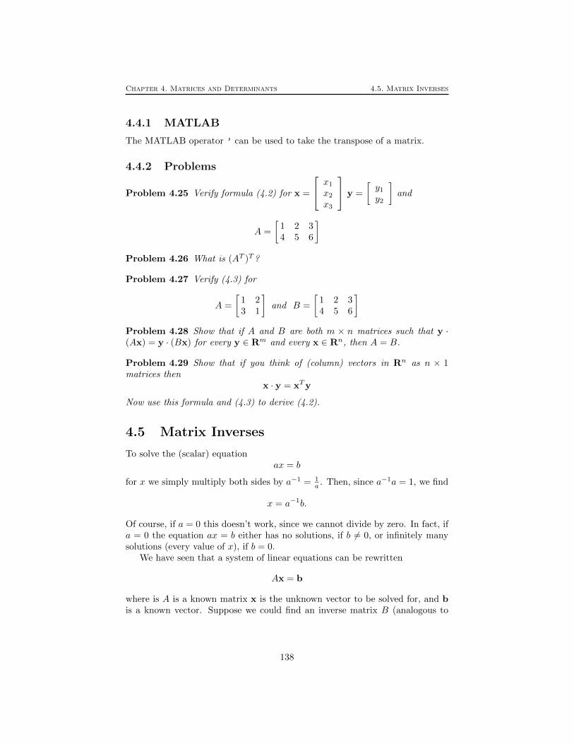
Chapter 4. Matrices and Determinants 4.5. Matrix Inverses
4.4.1 MATLAB
The MATLAB operator ’ can be used to take the transpose of a matrix.
4.4.2 Problems
Problem 4.25 Verify formula (4.2) for x =
x1
x2
x3
y =
[y1
y2
]and
A =
[1 2 34 5 6
]Problem 4.26 What is (AT )T ?
Problem 4.27 Verify (4.3) for
A =
[1 23 1
]and B =
[1 2 34 5 6
]Problem 4.28 Show that if A and B are both m × n matrices such that y ·(Ax) = y · (Bx) for every y ∈ Rm and every x ∈ Rn, then A = B.
Problem 4.29 Show that if you think of (column) vectors in Rn as n × 1matrices then
x · y = xTy
Now use this formula and (4.3) to derive (4.2).
4.5 Matrix Inverses
To solve the (scalar) equationax = b
for x we simply multiply both sides by a−1 = 1a . Then, since a−1a = 1, we find
x = a−1b.
Of course, if a = 0 this doesn’t work, since we cannot divide by zero. In fact, ifa = 0 the equation ax = b either has no solutions, if b 6= 0, or infinitely manysolutions (every value of x), if b = 0.
We have seen that a system of linear equations can be rewritten
Ax = b
where is A is a known matrix x is the unknown vector to be solved for, and bis a known vector. Suppose we could find an inverse matrix B (analogous to
138

Chapter 4. Matrices and Determinants 4.5. Matrix Inverses
a−1) with the property that BA = I (recall that I denotes the identity matrix).Then we could matrix multiply both sides of the equation by B yielding
BAx = Bb
But BAx = Ix = x, so x = Bb. Thus there is a unique solution and we have aformula for it.
Just as in the numerical case, where a could be zero, we can’t expect tofind an inverse matrix in all cases. After all, we know that there are linearsystems of equations with no solutions and with infinitely many solutions. Inthese situations there can be no inverse matrix.
When considering matrix inverses, we will always assume that we are dealingwith square (i.e., n× n) matrices.
Definition 4.1 If A is an n× n matrix, then B is called the inverse of A, anddenoted B = A−1, if
BA = I
where I is the n×n identity matrix (with each diagonal entry equal to 1 and allother entries 0).
Here is an example. Suppose
A =
[2 15 3
]then the inverse matrix is
B = A−1 =
[3 −1−5 2
]since [
2 15 3
] [3 −1−5 2
]=
[6− 5 3− 3
10− 10 −5 + 6
]=
[1 00 1
]This means that to solve the linear equation
2x1 +x2 = 25x1 +3x2 = 4
we write it as a matrix equation[2 15 3
] [x1
x2
]=
[24
]and then multiply both sides by the inverse to obtain[
x1
x2
]=
[3 −1−5 2
] [24
]=
[2−2
]
139

Chapter 4. Matrices and Determinants 4.5. Matrix Inverses
Figure 4.9: Diagram of the reduced form of an invertible matrix.
Here is an example of a matrix that doesn’t have an inverse. Let
A =
[1 00 0
].
To see that A doesn’t have an inverse, notice that the homogeneous equations
Ax = 0 has a non-zero solution x =
[01
]. If A had an inverse B, then we could
multiply both sides of the equation Ax = 0 by B to obtain x = B0 = 0. Butthis is false. Therefore there cannot be an inverse for A.
Clearly, having an inverse is somehow connected to whether or not thereare any non-zero solutions of the homogeneous equation Ax = 0. Recall thatAx = 0 has only the zero solution precisely when Ax = b has a unique solutionfor any b.
Let A be an n× n matrix. The following conditions are equivalent:
(1) A is invertible.
(2) The equation Ax = b always has a unique solution.
(3) The equation Ax = 0 has as the only solution x = 0.
(4) The rank of A is n.
(5) The reduced form of A is as shown in Figure 4.9.
We already know that the conditions (2), (3), (4) and (5) are all equivalent.We also just have seen that if A is invertible with inverse B, then the solutionof Ax = b is x = Bb so it exists and since we have a formula for it, it is unique.
So we just have to show that if Ax = b always has a unique solution, thenA has an inverse. Consider the transformation that takes a vector b to theunique solution x of Ax = b, em i.e., Tb = x. It is easy to check that thisis a linear transformation, since if Tb1 = x1, i.e., Ax1 = b1 and Tb2 = x2,i.e., Ax2 = b2, then A(t1x1 + t2x2) = t1Ax1 + t2Ax2 = t1b1 + t2b2, so thatT (t1b1+t2b2) = t1x1+t2x2 = t1Tb1+t2Tb1 Since T is a linear transformation,
140

Chapter 4. Matrices and Determinants 4.5. Matrix Inverses
it is given by some matrix B, and since T (Ax) = x, we must have BAx = xwhich implies that BA is the identity matrix.
Going back to our first example, notice that not only is BA = I, but AB = Itoo, since [
3 −1−5 2
] [2 15 3
]=
[6− 5 −2 + 2
15− 15 −5 + 6
]=
[1 00 1
]For a general choice of A and B, BA need not be equal to AB. But if B is theinverse of A, then it is always true that AB = BA = I.
To see this, suppose that A is invertible with BA = I but we don’t know yetwhether AB = I. So what we need to show is that for every vector x, ABx = x.First notice that if A is invertible, then any vector x can be written in the formAy for some y, since this is just the same as saying that the equation Ay = xhas a solution y. Thus ABx = ABAy = AIy = Ay = x.
4.5.1 Computing the inverse
How can we compute the inverse of an n × n matrix A? Suppose that A isinvertible and B is the inverse. Then AB = I. We can rewrite this equation asfollows. Think of the columns of B as being column vectors so that
B =
[b1
∣∣∣∣∣b2
∣∣∣∣∣ · · ·∣∣∣∣∣bn]
Then the rules of matrix multiplication imply that
AB =
[Ab1
∣∣∣∣∣Ab2
∣∣∣∣∣ · · ·∣∣∣∣∣Abn
]
Now the identity matrix can also be written as a matrix of column vectors. Inthis case the kth column is simply the matrix with zeros everywhere except fora 1 in the kth place, in other words the vector ek. Thus
I =
[e1
∣∣∣∣∣e2
∣∣∣∣∣ · · ·∣∣∣∣∣en]
So if AB = I then the n equations
Ab1 = e1
Ab2 = e2
...
Abn = en
hold. If we solve each of these equations for b1, b2, . . ., bn, then we have foundthe inverse B.
141

Chapter 4. Matrices and Determinants 4.5. Matrix Inverses
Here is a simple example. Suppose we want to find the inverse for
A =
[2 15 3
].
According to our discussion, we must solve Ab1 = e1 and Ab2 = e2. Theaugmented matrix for Ab1 = e1 is[
2 15 3
∣∣∣∣ 10]
We now perform a sequence of row operations. First divide the first row by 2.This gives [
1 1/25 3
∣∣∣∣ 1/20
].
Now subtract 5 times the first row from the second row. This gives[1 1/20 1/2
∣∣∣∣ 1/2−5/2
].
Now subtract the second row from the first row. This gives[1 00 1/2
∣∣∣∣ 3−5/2
].
Finally, multiply the second row by 2. This gives[1 00 1
∣∣∣∣ 3−5
].
Therefore b1 =
[3−5
]The augmented matrix for Ab2 = e2 is
[2 15 3
∣∣∣∣ 01]
We now perform a sequence of row operations. First divide the first row by 2.This gives [
1 1/25 3
∣∣∣∣ 01].
Now subtract 5 times the first row from the second row. This gives[1 1/20 1/2
∣∣∣∣ 01].
Now subtract the second row from the first row. This gives[1 00 1/2
∣∣∣∣−11
].
142

Chapter 4. Matrices and Determinants 4.5. Matrix Inverses
Finally, multiply the second row by 2. This gives[1 00 1
∣∣∣∣−12
].
Therefore b2 =
[−12
]. So
B =[b1
∣∣∣b2
]=
[3 −1−5 2
]Notice that we performed exactly the same sequence of row operations in findingb1 and b2. This is because the row operations only depend on the left side ofthe augmented matrix, in other words, the matrix A. If we used this procedureto find the inverse of an n× n matrix, we would end up doing exactly the samerow operations n times. Clearly this is a big waste of effort! We can save a lotof work by solving all the equations at the same time. To do this we make asuper-augmented matrix with both right sides.[
2 15 3
∣∣∣∣ 1 00 1
]Now we only have to go through the sequence of row operations once, keepingtrack of both right sides simultaneously. Going through the same sequence, weobtain [
1 1/25 3
∣∣∣∣ 1/2 00 1
].[
1 1/20 1/2
∣∣∣∣ 1/2 0−5/2 1
].[
1 00 1/2
∣∣∣∣ 3 −1−5/2 1
].[
1 00 1
∣∣∣∣ 3 −1−5 2
].
Notice that the vectors b1 and b2 are automatically arranged as columns onthe right side, so the matrix on the right is the inverse B.
The same procedure works for any size of square matrix. To find the inverseof A form the super-augmented matrix [A|I]. Then do a sequence of row oper-ations to reduce A to the identity. If the resulting matrix is [I|B] then B is theinverse matrix.
What happens if A doesn’t have an inverse? In this case it will be impossibleto reduce A to the identity matrix, since the rank of A is less than n. So theprocedure will fail, as it must.
As another example, let us now compute the inverse of an arbitrary invertible2× 2 matrix
A =
[a bc d
].
143

Chapter 4. Matrices and Determinants 4.5. Matrix Inverses
We will see that A is invertible precisely when its determinant ∆ = ad − bc isnon-zero. So let’s assume this is the case, and do the computation. To startwith, let’s assume that ac 6= 0. Then neither a or c are zero. Here is thesequence of row transformations.[
a bc d
∣∣∣∣ 1 00 1
][ac bcac ad
∣∣∣∣ c 00 a
]c(1)a(2)
Notice that multiplication by a and by c would not be legal row transformationsif either a or c were zero.[
ac bc0 ad− bc
∣∣∣∣ c 0−c a
](2)− (1)[
1 b/a0 1
∣∣∣∣ 1/a 0−c/∆ a/∆
](1/ac)(1)(1/∆)(2)[
1 00 1
∣∣∣∣ d/∆ −b/∆−c/∆ a/∆
](1)− (b/a)(2)
(1/∆)(2)
Thus the inverse matrix is
A−1 =1
ad− bc
[d −b−c a
].
This was derived under the additional assumption that ac 6= 0. However onecan check directly that the same formula works, so long as ∆ = ad− bc 6= 0.
4.5.2 Inverses of Products
If both A and B are invertible, then so is AB. The inverse of AB is given byB−1A−1. To check this, simply compute
ABB−1A−1 = AIA−1 = AA−1 = I.
If one of A or B is not invertible then AB is not invertible. To see this recallthat a matrix C is not invertible exactly whenever there is a non-zero solutionx to Cx = 0. If B is not invertible, then there is a non-zero vector x withBx = 0. Then ABx = A0 = 0 so AB is not invertible too. If B is invertible,but A is not, then there is a non-zero x with Ax = 0. Let y = B−1x. SinceB−1 is invertible, y cannot be zero. We have ABy = ABB−1x = Ax = 0 soAB is not invertible.
144

Chapter 4. Matrices and Determinants 4.5. Matrix Inverses
4.5.3 MATLAB
If A is an invertible n × n matrix then the MATLAB command inv(A) willreturn its inverse. A system of linear equations corresponding to Ax = b whereA is an invertible n×n matrix and b is a column vector with n components canbe solved with the command
x = A\b
Note that if A is not square or A is square but not invertible the correspondingsystem cannot be solved in this way. In this case, use the MATLAB commandrref on the augmented matrix of the system as described in Chapter 3.
4.5.4 Problems
Problem 4.30 Which of the following matrices are invertible?
(a)
[1 23 4
]
(b)
1 2 30 3 40 1 1
(c)
1 2 30 3 40 1 2
Problem 4.31 Find the inverse for[
1 23 5
]Problem 4.32 Determine which of these matrices are invertible, and find theinverse for the invertible ones.
(a)
2 3 −11 2 3−1 −1 4
(b)
1 −1 1−1 2 −12 −1 1
(c)
1 1 11 2 31 4 9
(d)
2 1 43 2 50 −1 1
145

Chapter 4. Matrices and Determinants 4.6. Return to Resistor Networks
(e)
1 0 a0 1 00 0 1
(f)
1 a b0 1 c0 0 1
Problem 4.33 The following matrices are invertible. Find their inverses.
A =
1 1 10 2 35 5 1
, B =
1 2 −3 1−1 3 −3 −22 0 1 53 1 −2 5
.Problem 4.34 Consider the system x+ 5z = 6
x− 2y + 3z = 142x+ y − 3z = −2
1. Write the above system in the matrix-form, in other words find a matrix
A such that Ax =
614−2
.
2. Find the inverse of A, if possible.
3. How many solutions the system have? Write them all down.
4.6 Return to Resistor Networks
Let us revisit the resistor networks we considered in section 3.5. These networksconsist of resistors and voltage and current sources. The fundamental problemwas introduced, which was to write the current through the voltage sources andthe voltage across current sources in terms of arbitrary values of the sources.
Recall example 3.15 which considered the circuit shown again in figure 4.10.The sources are V and I. The fundamental problem is to determine E and J(the current through the voltage source) in terms of V and I. The solutionfound in section 3.5.3 was
E = 6I + V/6 (4.4)
J = −1
6I +
10
72V
This solution can be given in matrix-vector form as[EJ
]=
[6 1
6− 1
61072
] [IV
](4.5)
146

Chapter 4. Matrices and Determinants 4.6. Return to Resistor Networks
Figure 4.10: The circuit considered in Example 3.15.
where we will call the 2 × 2 matrix in the equation above F . It can be shownthat for any circuit with n sources, the solution of the fundamental problem canbe written as multiplication by an n × n matrix. We will show below how Fcan be constructed in a systematic way. Look back to section 3.5.3 to see howwe arrived at (4.4). There were three parts to the process:
1. We wrote the linear system for the loop currents and the voltage dropacross the current source. The equations for the system had the sourcesI and V in the right hand sides.
2. We solved the system symbolically in terms of the right hand side involvingV and I.
3. We identified the elements of the solution that solved the fundamentalproblem.
We will now describe these three steps by matrix multiplication and do themultiplication as an alternate way to determine the matrix F in (4.5). Recallthat the unknowns for the circuit are the three loop currents and E, the voltageacross the current source. Define the intermediate unknown column vector
x = (i1, i2, i3, E)T .
Proceeding as in example 3.15 we find equations for x by considering the volt-age drops around each elementary loop (the first three equations) around eachelementary loop (the first three equations) and matching the current throughthe current source (the last equation below):
8i1 −2i2 = V−2i1 +5i2 −3i3 = 0
−3i2 +8i3 +E = 0i3 = −I
(4.6)
Here, we did not eliminate i3 from the equations as was done in section 3.5.3.The system (4.6) can be written
F2x = F1
[IV
](4.7)
147
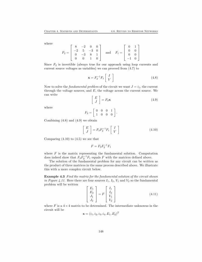
Chapter 4. Matrices and Determinants 4.6. Return to Resistor Networks
where
F2 =
8 −2 0 0−2 5 −3 00 −3 8 10 0 1 0
and F1 =
0 10 00 0−1 0
Since F2 is invertible (always true for our approach using loop currents andcurrent source voltages as variables) we can proceed from (4.7) to
x = F−12 F1
[IV
](4.8)
Now to solve the fundamental problem of the circuit we want J = i1, the currentthrough the voltage sources, and E, the voltage across the current source. Wecan write [
EJ
]= F3x (4.9)
where
F3 =
[0 0 0 11 0 0 0
].
Combining (4.8) and (4.9) we obtain[EJ
]= F3F
−12 F1
[IV
](4.10)
Comparing (4.10) to (4.5) we see that
F = F3F−12 F1
where F is the matrix representing the fundamental solution. Computationdoes indeed show that F3F
−12 F1 equals F with the matrices defined above.
The solution of the fundamental problem for any circuit can be written asthe product of three matrices in the same process described above. We illustratethis with a more complex circuit below.
Example 4.3 Find the matrix for the fundamental solution of the circuit shownin Figure 4.11. Here there are four sources I1, I2, V1 and V2 so the fundamentalproblem will be written
E1
E2
J1
J2
= F
I1I2V1
V2
(4.11)
where F is a 4× 4 matrix to be determined. The intermediate unknowns in thecircuit will be
x = (i1, i2, i3, i4, E1, E2)T
148

Chapter 4. Matrices and Determinants 4.6. Return to Resistor Networks
Figure 4.11: The circuit considered in Example 4.3. All resistors are 1Ω.
as shown in the figure. Equations for these unknowns are found using the loopcurrent method:
3i1 −i2 −i4 −E2 = 0−i1 +3i2 −i3 +E1 = 0
−i2 +3i3 −i4 = V1 − V2
−i1 −i3 +3i4 +E2 = V1
i2 = −I1−i1 +i4 = −I2
(4.12)
where the first four equations above come from matching voltage drops aroundthe four elementary loops and the last two equations come from matching theloop currents to the current sources. Note that (4.12) can be written
F2x = F1
I1I2V1
V2
(4.13)
where
F2 =
3 −1 0 −1 0 −1−1 3 −1 0 1 00 −1 3 −1 0 0−1 0 −1 3 0 10 1 0 0 0 0−1 0 0 1 0 0
and F1 =
0 0 0 00 0 0 00 0 1 −10 0 1 0−1 0 0 00 −1 0 0
149

Chapter 4. Matrices and Determinants 4.7. Determinants
Now J2 = i4 − i3 and J1 = i3 so we can writeE1
E2
J1
J2
= F3x (4.14)
where
F3 =
0 0 0 0 1 00 0 0 0 0 10 0 1 0 0 00 0 −1 1 0 0
.As above we can combine (4.13) and (4.14) to obtain
E1
E2
J1
J2
= F3F−12 F1
I1I2V1
V2
.Comparing the equation above to the desired form (4.11) we see that the fun-damental matrix F can be computed as
F = F3F−12 F1.
A MATLAB computation with the matrices defined above gives
F ≈
2.1818 0.2727 0.8182 −0.45450.2727 1.9091 0.7273 −0.1818−0.4545 −0.1818 0.4545 −0.36360.0909 −0.3636 −0.0909 0.2727
This technique can be used to find the fundamental solution of circuits even
if they are very large. You can imagine that the process of setting up thematrices F1, F2 and F3, computing an approximation of F−1
2 and multiplyingthe matrices together can all be automated and done computationally.
In Chapter 5, fundamental matrices for circuits will be used to investigate thetransient behaviour of circuits with capacitors and inductors as well as resistors.
4.7 Determinants
4.7.1 Definition of Determinants
We have already encountered determinants for 2 × 2 and 3 × 3 matrices. For2× 2 matrices
det
[a1,1 a1,2
a2,1 a2,2
]= a1,1a2,2 − a1,2a2,1.
150

Chapter 4. Matrices and Determinants 4.7. Determinants
For 3 × 3 matrices we can define the determinant by expanding along the toprow:
det
a1,1 a1,2 a1,3
a2,1 a2,2 a2,3
a3,1 a3,2 a3,3
= a1,1 det
[a2,2 a2,3
a3,2 a3,3
]−a1,2 det
[a2,1 a2,3
a3,1 a3,3
]+a1,3 det
[a2,1 a2,2
a3,1 a3,2
]If we multiply out the 2 × 2 determinants in this definition we arrive at theexpression
det
a1,1 a1,2 a1,3
a2,1 a2,2 a2,3
a3,1 a3,2 a3,3
= a1,1a2,2a3,3−a1,1a2,3a3,2+a1,2a2,3a3,1−a1,2a2,1a3,3+a1,3a2,1a3,2−a1,3a2,2a3,1
We now make a similar definition for an n×n matrix. Let A be an n×n matrix.Define Mi,j to be the (n− 1)× (n− 1) matrix obtained by crossing out the ithrow and the jth column. So, for example, if
A =
1 2 3 45 6 7 89 0 1 23 4 5 6
then
M1,2 =
× × × ×5 × 7 89 × 1 23 × 5 6
=
5 7 89 1 23 5 6
We now define the determinant of an n× n matrix A to be
det(A) = a1,1 det(M1,1)−a1,2 det(M1,2)+· · ·±a1,n det(M1,n) =
n∑j=1
(−1)j+1a1,j det(M1,j).
Of course, this formula still contains determinants on the right hand side. How-ever, they are determinants of (n − 1) × (n − 1) matrices. If we apply thisdefinition to those determinants we get a more complicated formula involving(n − 2) × (n − 2) matrices, and so on, until we arrive at an extremely longexpression (with n! terms) involving only numbers.
Calculating an expression with n! is completely impossible, even with thefastest computers, when n gets reasonable large. For example 100! ≈ 10158. Yet,your computer at home can compute the determinant of a 100× 100 matrix inless than a second. The secret, of course, is to compute the determinant in adifferent way. We start by computing the determinant of triangular matrices.
4.7.2 Determinants of Triangular matrices
Recall that triangular matrices are matrices whose entries above or below thediagonal are all zero. For 2× 2 matrices
det
[a1,1 a1,2
0 a2,2
]= a1,1a2,2 − a1,20 = a1,1a2,2
151

Chapter 4. Matrices and Determinants 4.7. Determinants
and
det
[a1,1 0a2,1 a2,2
]= a1,1a2,2 − 0a2,1 = a1,1a2,2
so the determinant is the product of the diagonal elements. For 3× 3 matrices
det
a1,1 0 0a2,1 a2,2 0a3,1 a3,2 a3,3
= a1,1 det
[a2,2 0a3,2 a3,3
]− 0 + 0
= a1,1a2,2a3,3
A similar expansion shows that the determinant of an n × n lower triangularmatrix is the product of the diagonal elements. For upper triangular matriceswe have
det
a1,1 a1,2 a1,3
0 a2,2 a2,3
0 0 a3,3
= a1,1 det
[a2,2 a2,3
0 a3,3
]−a1,2 det
[0 a2,3
0 a3,3
]+a1,3 det
[0 a2,2
0 0
]
Since we already know that the determinant of a 2 × 2 triangular matrix isthe product of the diagonals, we can see easily that the last two terms in thisexpression are zero. Thus we get
det
a1,1 a1,2 a1,3
0 a2,2 a2,3
0 0 a3,3
= a1,1 det
[a2,2 a2,3
0 a3,3
]= a1,1a2,2a3,3
Once we know that the determinant of a 3 × 3 upper triangular matrix is theproduct of the diagonal elements, we can do a similar calculation to the oneabove to conclude that determinant of a 4 × 4 upper triangular matrix is theproduct of the diagonal elements, and so on.
Thus, the determinant of any (upper or lower) triangular n×n matrix is theproduct of the diagonal elements.
We know that an arbitrary n×nmatrix can be reduced to an upper (or lower)triangular matrix by a sequence of row operations. This is the key to computingthe determinant efficiently. We need to determine how the determinant of amatrix changes when we do an elementary row operation on it.
4.7.3 Summary of determinant calculation rules
We summarize the results on determinant calculation shown in more detail inthe additional topics sections 4.8.6 to 4.8.12 below. The first three rules belowshow how a determinant changes when row operations are applied to it. Thiscan be used to simplify determinant calculation as shown in the next section.In the statements below, A is a square matrix.
1. If B is obtained from A by multiplying one row of A by the constant cthen det(B) = cdet(A).
152
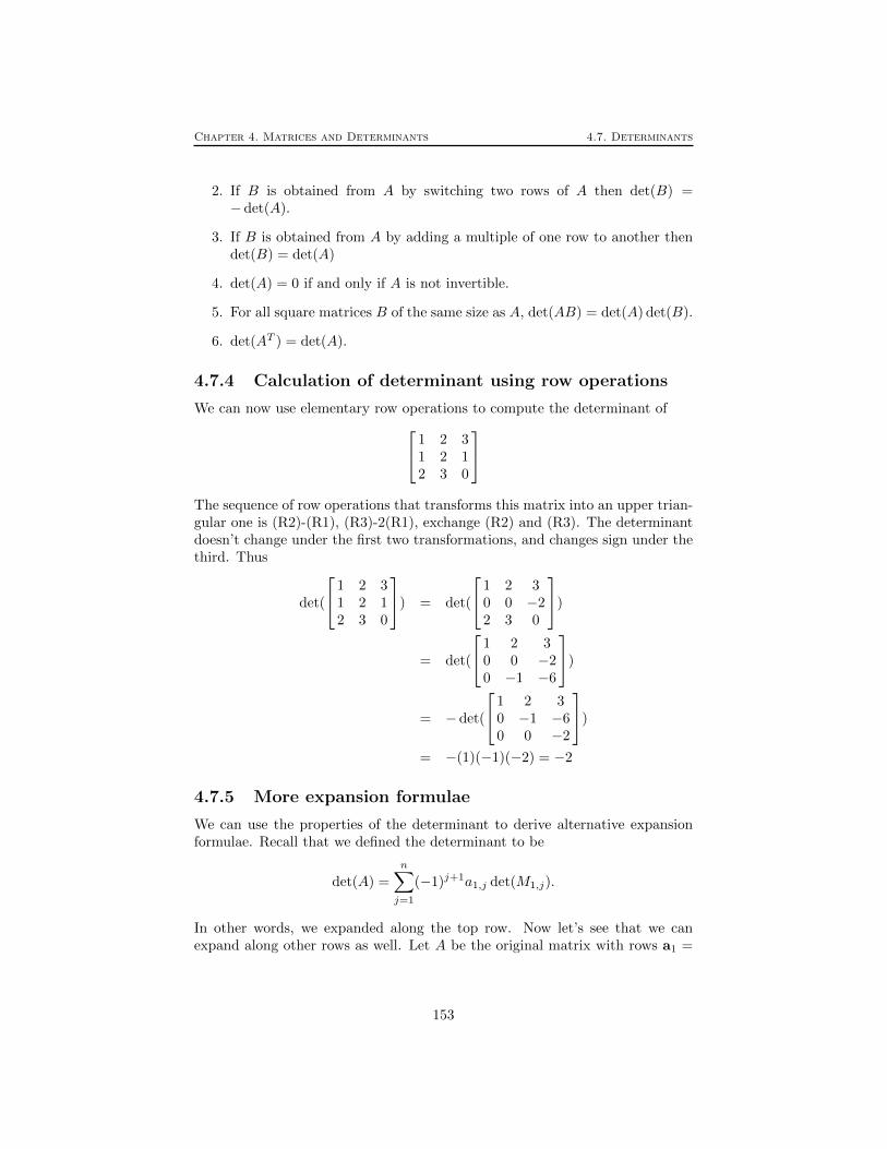
Chapter 4. Matrices and Determinants 4.7. Determinants
2. If B is obtained from A by switching two rows of A then det(B) =−det(A).
3. If B is obtained from A by adding a multiple of one row to another thendet(B) = det(A)
4. det(A) = 0 if and only if A is not invertible.
5. For all square matrices B of the same size as A, det(AB) = det(A) det(B).
6. det(AT ) = det(A).
4.7.4 Calculation of determinant using row operations
We can now use elementary row operations to compute the determinant of 1 2 31 2 12 3 0
The sequence of row operations that transforms this matrix into an upper trian-gular one is (R2)-(R1), (R3)-2(R1), exchange (R2) and (R3). The determinantdoesn’t change under the first two transformations, and changes sign under thethird. Thus
det(
1 2 31 2 12 3 0
) = det(
1 2 30 0 −22 3 0
)
= det(
1 2 30 0 −20 −1 −6
)
= −det(
1 2 30 −1 −60 0 −2
)
= −(1)(−1)(−2) = −2
4.7.5 More expansion formulae
We can use the properties of the determinant to derive alternative expansionformulae. Recall that we defined the determinant to be
det(A) =
n∑j=1
(−1)j+1a1,j det(M1,j).
In other words, we expanded along the top row. Now let’s see that we canexpand along other rows as well. Let A be the original matrix with rows a1 =
153
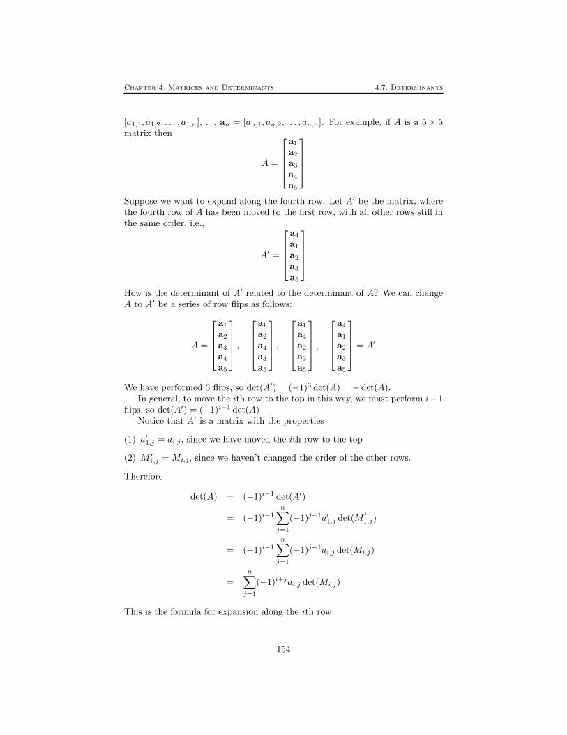
Chapter 4. Matrices and Determinants 4.7. Determinants
[a1,1, a1,2, . . . , a1,n], . . . an = [an,1, an,2, . . . , an,n]. For example, if A is a 5 × 5matrix then
A =
a1
a2
a3
a4
a5
Suppose we want to expand along the fourth row. Let A′ be the matrix, wherethe fourth row of A has been moved to the first row, with all other rows still inthe same order, i.e.,
A′ =
a4
a1
a2
a3
a5
How is the determinant of A′ related to the determinant of A? We can changeA to A′ be a series of row flips as follows:
A =
a1
a2
a3
a4
a5
,
a1
a2
a4
a3
a5
,
a1
a4
a2
a3
a5
,
a4
a1
a2
a3
a5
= A′
We have performed 3 flips, so det(A′) = (−1)3 det(A) = − det(A).In general, to move the ith row to the top in this way, we must perform i−1
flips, so det(A′) = (−1)i−1 det(A)Notice that A′ is a matrix with the properties
(1) a′1,j = ai,j , since we have moved the ith row to the top
(2) M ′1,j = Mi,j , since we haven’t changed the order of the other rows.
Therefore
det(A) = (−1)i−1 det(A′)
= (−1)i−1n∑j=1
(−1)j+1a′1,j det(M ′1,j)
= (−1)i−1n∑j=1
(−1)j+1ai,j det(Mi,j)
=
n∑j=1
(−1)i+jai,j det(Mi,j)
This is the formula for expansion along the ith row.
154

Chapter 4. Matrices and Determinants 4.7. Determinants
As an example let’s compute the determinant of a 3×3 matrix by expandingalong the second row.
det
1 2 31 3 11 2 1
= −det
[2 32 1
]+ 3 det
[1 31 1
]− det
[1 21 2
]= −2 + 6 + 3− 9− 2 + 2 = −2
The formula for expanding along the ith row is handy if the matrix happens tohave a row with many zeros.
Using the fact that det(A) = det(AT ) we can also write down expansionformulae along columns, since the columns of A are the rows of AT . We end upwith the formula
det(A) =
n∑i=1
(−1)i+jai,j det(Mi,j)
As an example let’s compute the determinant of a 3×3 matrix by expandingalong the second column.
det
1 2 31 3 11 2 1
= −2 det
[1 11 1
]+ 3 det
[1 31 1
]− 2 det
[1 31 1
]= −2 + 2 + 3− 9− 2 + 6 = −2
The formula for expanding along the jth column is handy if the matrix happensto have a column with many zeros.
4.7.6 MATLAB
The MATLAB command det(A) can be used to determine the determinant ofa square matrix as introduced in Chapter 3.
4.7.7 Problems
Problem 4.35 Find the determinant of1 1 1 11 2 4 81 3 9 271 4 16 64
Problem 4.36 Find the determinant of
1 −1 1 −11 2 4 81 −2 4 −81 1 1 1
155

Chapter 4. Matrices and Determinants 4.7. Determinants
Problem 4.37 Consider the matrix
A =
2 0 2 40 0 3 22 2 4 43 0 6 2
.1. Find the determinant of A by expanding on the first row.
2. Find the determinant of A by expanding on the row or column of yourchoice. This expansion should be simpler than the one used in part (a).
Problem 4.38 Compute
det
1 0 11 2 33 0 1
by expanding along the second row, and by expanding along the third column.
Problem 4.39 Find the determinant of A given above by using row operationsto put A into echelon form.
Problem 4.40 We know that the determinant of the n× n matrixa1
a2
. . .
an
is a1a2 · · · an if the blank entries represent 0. What is the equivalent formulafor the determinant of the n× n matrix
an
. . .
a2
a1
?
Justify your answer.
Problem 4.41 Find all values of λ for which the matrix 2− λ 1 0−1 −λ 11 3 1− λ
is not invertible.
Problem 4.42 Determine whether each of the following statements is true orfalse. If true, explain briefly why it is true without showing specific examples.If false, explain briefly why it is false or give a simple counterexample, and givea correct statement by making small changes to the underlined text.
156

Chapter 4. Matrices and Determinants 4.8. Additional Topics
1. The determinant of a square matrix is the product of the entries on itsmain diagonal.
2. For every matrix A, we have det(AAT ) = det(ATA)
3. If A and B are both invertible n×n matrices, then det(B−1AB) = det(BAB−1) = det(A).
4. If an n × n matrix A is multiplied by a scalar c, the determinant of theresulting matrix is c · det(A).
5. If the column vectors of an n×n matrix are linearly independent, then therow vectors of the same matrix are also linearly independent.
4.8 Additional Topics
4.8.1 Application: General Least Squares
Let us restate our results from Chapter 3 on minimization of quadratic functionsusing matrix notation. A quadratic function of
x =
x1
...xn
in Rn can be written in matrix form as
f(x) = x ·Ax + b · x + c
where A is an n×n matrix and b ∈ Rn and c is a number. The vector containingthe partial derivatives can be computed to be ∂f/∂x1
...∂f/∂xn
= (A+AT )x + b
Recall that we made the assumption that aij = aji when we considered thisproblem before. This property can be stated in compact form as A = AT . Ifthis is true then (A+AT ) = 2A so ∂f/∂x1
...∂f/∂xn
= 2Ax + b
To find the minimum value of f (if it exists) we need to find the value of x forwhich the vector above is zero. In other words, x solves the equation
2Ax = −b.
This is the same equation that we derived before.
157

Chapter 4. Matrices and Determinants 4.8. Additional Topics
4.8.2 Least squares solutions
Let’s take another look the situation where a system of linear equations, whichwe now can write
Bx = c,
has no solution. Typically this will be the case if there are more equations thanvariables, that is, B is an matrix with more rows than columns. In this casethere is no value of x that makes the left side equal the right side. However, wemay try to find the value of x for which the right side Bx is closest to the leftside c.
One way to go about this is to try to minimize distance between the left andright sides. It is more convenient to minimize the square of the distance. Thisquantity can be written
‖Bx− c‖2 = (Bx− c) · (Bx− c)
= (Bx) · (Bx)− (Bx) · c− c · (Bx) + c · c= x · (BTBx)− 2(BT c) · x + c · c
This is a quadratic function, written in matrix form. We want to use the formulaof the previous section with A = BTB and b = BT c. Before we can do so, wemust verify that A = BTB satisfies AT = A. This is true because
(ATA)T = AT (AT )T = ATA
Thus the formula of the previous section implies that the minimum occurs atthe value of x that solves the linear equation
BTBx = BT c
Here we have cancelled a factor of 2 on each side.Now let’s derive the same result in another way. Think of all the values ofBx,
as x ranges through all possible values in Rn as forming a (high dimensional)plane in Rm. Our goal is to find the value of x so that the corresponding valueof Bx on the plane is closest to c. Using the analogy to the geometric picture inthree dimensions, we see that the minimum will occur when Bx−c is orthogonalto the plane. This means that the dot product of Bx − c with every vector inthe plane, that is, every vector of the form By, should be zero. Thus we have
(By) · (Bx− c) = 0
for every y ∈ Rn. This is the same as
y · (BT (Bx− c)) = y · (BTBx−BT c) = 0
for every y ∈ Rn. This can happen only if
BTBx = BT c
which is the same result we obtained before.
158

Chapter 4. Matrices and Determinants 4.8. Additional Topics
4.8.3 Problems
Problem 4.43 Find the least squares solution to
x1 +x2 = 1x1 = 1x1 +x2 = 0
Compare Bx and b.
Problem 4.44 Refer back to the least squares fit example, where we tried tofind the best straight line going through a collection of points (xi, yi). Anotherway of formulating this problem is this. The line y = ax+ b passes through thepoint (xi, yi) if
axi + b = yi (4.15)
So, saying that the straight line passes through all n points is the same as sayingthat a and b solve the system of n linear equations given by (4.15) for i =1, . . . , n. Of course, unless the points all actually lie on the same line, thissystem of equations has no solutions. Show that the least squares solution tothis problem is the same as we obtained before. (You may simplify the problemby assuming there are only three points (x1, y1), (x2, y2) and (x3, y3).)
4.8.4 Elementary matrices
Recall that there are three row operation that are used in Gaussian elimination:(1) multiplication of a row by a non-zero number, (2) add a multiple of one rowto another row and (3) exchanging two rows.
It turns out that each elementary row operation can be implemented by leftmultiplication by a matrix. In other words, for each elementary row operationthere is a matrix Q such that QA is what you get by doing that row operationto the matrix A.
Here is an example. Suppose
A =
1 0 2 12 0 0 11 2 3 4
and suppose that the row operation is multiplying the first row by 2. Then thematrix you get by doing that row operation to the matrix A is
A′ =
2 0 4 22 0 0 11 2 3 4
In this case the matrix Q turns out to be
Q =
2 0 00 1 00 0 1
159

Chapter 4. Matrices and Determinants 4.8. Additional Topics
Since 2 0 00 1 00 0 1
1 0 2 12 0 0 11 2 3 4
=
2 0 4 22 0 0 11 2 3 4
i.e., QA = A′.
Now suppose that the elementary row operation is subtracting twice the firstrow from the second row. Then the matrix you get by doing that row operationto the matrix A is
A′ =
1 0 2 10 0 −4 −11 2 3 4
In this case the matrix Q turns out to be
Q =
1 0 0−2 1 00 0 1
Since 1 0 0
−2 1 00 0 1
1 0 2 12 0 0 11 2 3 4
=
1 0 2 10 0 −4 −11 2 3 4
i.e., again, QA = A′.
Finally, suppose that the elementary row operation is exchanging the secondand the third rows. Then the matrix you get by doing that row operation tothe matrix A is
A′ =
1 0 2 11 2 3 42 0 0 1
In this case the matrix Q turns out to be
Q =
1 0 00 0 10 1 0
Since 1 0 0
0 0 10 1 0
1 0 2 12 0 0 11 2 3 4
=
1 0 2 11 2 3 42 0 0 1
i.e., again, QA = A′.
How can we find the matrices Q (called elementary matrices)? Here is theprocedure. Start with the identity matrix I and do the row transformation to it.The resulting matrix Q is the matrix that implements that row transformationby multiplication from the left. Notice that this is true in the examples above.
160

Chapter 4. Matrices and Determinants 4.8. Additional Topics
In the first example, the row transformation was multiplying the first row by 2.If you multiply the first row of
I =
1 0 00 1 00 0 1
by two you get
Q =
2 0 00 1 00 0 1
.In the second example, the row transformation was subtracting twice the firstrow from the second row. If you subtract twice the second row from the firstrow of I by two you get
Q =
1 0 0−2 1 00 0 1
.In the third example, the row transformation was exchanging the second andthird rows. If you exchange the second and third rows of I, you get 1 0 0
0 0 10 1 0
.Elementary matrices are useful in theoretical studies of the Gaussian elimi-
nation process. We will use them briefly when studying determinants.Suppose A is a matrix, and R is its reduced form. Then we can obtain R from
A via a sequence of elementary row operations. Suppose that the correspondingelementary matrices are Q1, Q2, . . ., Qk. Then, starting with A, the matrix afterthe first elementary row operation is Q1A, then after the second elementary rowoperation is Q2Q1A, and so on, until we have
QkQk−1 · · ·Q2Q1A = R.
Now let us apply the inverse matrices, starting with Q−1k . This gives
Q−1k QkQk−1 · · ·Q2Q1A = Qk−1 · · ·Q2Q1A = Q−1
k R.
Continuing in this way we see that
A = Q−11 Q−1
2 · · ·Q−1k R
In the special case that A is an n × n invertible matrix, A can be reducedto the identity matrix. In other words, we can take R = I. In this case A canbe written as a product of elementary matrices.
A = Q−11 Q−1
2 · · ·Q−1k I = Q−1
1 Q−12 · · ·Q
−1k
161

Chapter 4. Matrices and Determinants 4.8. Additional Topics
Notice that in this case
A−1 = QkQk−1 · · ·Q2Q1.
As an example, let us write the matrix
A =
[2 15 3
]as a product of elementary matrices. The sequence of row transformations thatreduce A to the identity are:
1) (1/2)(R1)
2) (R2)-5(R1)
3) (R1)-(R2)
4) 2(R2)
The corresponding elementary matrices and their inverses are
Q1 =
[1/2 00 1
]Q−1
1 =
[2 00 1
]Q2 =
[1 0−5 1
]Q−1
2 =
[1 05 1
]Q3 =
[1 −10 1
]Q−1
3 =
[1 10 1
]Q4 =
[1 00 2
]Q−1
4 =
[1 00 1/2
]Therefore
A = Q−11 Q−1
2 Q−13 Q−1
4
or [2 15 3
]=
[2 00 1
] [1 05 1
] [1 10 1
] [1 00 1/2
]4.8.5 Problems
Problem 4.45 Each elementary matrix is invertible, and the inverse is alsoan elementary matrix. Find the inverses of the three examples of elementarymatrices above. Notice that the inverse elementary matrix is the matrix for therow transformation that undoes the original row transformation.
Problem 4.46 Write the matrix 2 3 −11 2 3−1 −1 1
as a product of elementary matrices.
162

Chapter 4. Matrices and Determinants 4.8. Additional Topics
4.8.6 Exchanging two rows changes the sign of the deter-minant
We start with the elementary row operation of exchanging two rows. For 2× 2determinants,
det
[a bc d
]= ad− bc,
while
det
[c da b
]= cb− da = −(ad− bc),
so exchanging two rows changes the sign of the determinant.We can do a similar calculation for 3 × 3 matrices. Its a a bit messier, but
still manageable. Again, we find that exchanging two rows changes the sign ofthe determinant.
How about the n × n case? We will assume that we have already provedthe result for the (n− 1)× (n− 1) case, and show how we can use this to showthe result for an n × n matrix. Thus knowing the result for 2 × 2 matrices,implies it for 3 × 3, which in turn implies it for 4 × 4 matrices, and so on. Weconsider three cases, depending on which rows we are exchanging. Suppose Ais the original matrix and A′ is the matrix with two rows exchanged.
(1) Exchanging two rows other than the first row: In this case we cross out thefirst row and any column from A′ we obtain M ′1,j which is the same as thematrix M1,j (corresponding to A) except with two of its rows exchanged.Since the size of M1,j is n− 1 we know that det(M ′1,j) = −det(M1,j) so
det(A′) =
n∑j=1
(−1)j+1a1,j det(M ′1,j)
= −n∑j=1
(−1)j+1a1,j det(M1,j)
= −det(A)
(2) Exchanging the first and second row. Do see that this changes the signof the determinant we have to expand the expansion. The following is abit sketchy. I’ll probably skip it in class, but give the argument here forcompleteness. If we expand M1,j we get
det(M1,j) =
j−1∑k=1
(−1)k+1a2,k det(M1,2,j,k) +
n∑k=j+1
(−1)ka2,k det(M1,2,j,k)
where M1,2,j,k is the matrix obtained from A by deleting the first and secondrows, and the jth and kth columns. Inserting this into the expansion for Agives
det(A) =
n∑j=1
j−1∑k=1
(−1)j+ka1,ja2,k det(M1,2,j,k)−n∑j=1
n∑k=j+1
(−1)j+ka1,ja2,k det(M1,2,j,k)
163

Chapter 4. Matrices and Determinants 4.8. Additional Topics
The sum splits into two parts. Flipping the first two rows ofA just exchangesthe two sums. In other words S −R becomes R− S which is −(S −R). Soexchanging the first two rows also changes the sign of the determinant.
(3) Exchanging the first row with the kth row. We can effect this exchange byfirst exchanging the kth and the second row, then exchanging the first andthe second row, then exchanging the kth and the second row again. Eachflip changes the determinant by a minus sign, and since there are three flips,the overall change is by a minus sign.
Thus we can say that for any n × n matrix, exchanging two rows changesthe sign of the determinant.
One immediate consequence of this fact is that a matrix with two rowsthe same has determinant zero. This is because if exchange the two rows thedeterminant changes by a minus sign, but the matrix doesn’t change. Thusdet(A) = −det(A) which is only possible if det(A) = 0.
4.8.7 The determinant is linear in each row separately
To say that the determinant is linear in the jth row means that if we write amatrix as a matrix of row vectors,
A =
a1
a2...
aj...
an
then
det(
a1
a2...
sb + tc...
an
) = sdet(
a1
a2...b...
an
) + tdet(
a1
a2...c...
an
)
It is easy to from the expansion formula that the determinant is linear inthe first row. For a 3× 3 example we have
det(
sb1 + tc1 sb2 + tc2 sb3 + tc3a2,1 a2,2 a2, 3a3,1 a3,2 a3, 3
)
= (sb1 + tc1) det(M1,1)− (sb2 + tc2) det(M1,2) + (sb3 + tc3) det(M1.3)
= s(b1 det(M1,1)− b2 det(M1,2) + b3 det(M1.3))
164
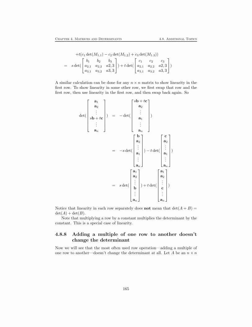
Chapter 4. Matrices and Determinants 4.8. Additional Topics
+t(c1 det(M1,1)− c2 det(M1,2) + c3 det(M1.3))
= sdet(
b1 b2 b3a2,1 a2,2 a2, 3a3,1 a3,2 a3, 3
) + tdet(
c1 c2 c3a2,1 a2,2 a2, 3a3,1 a3,2 a3, 3
)
A similar calculation can be done for any n× n matrix to show linearity in thefirst row. To show linearity in some other row, we first swap that row and thefirst row, then use linearity in the first row, and then swap back again. So
det(
a1
a2...
sb + tc...
an
) = −det(
sb + tca2...
a1...
an
)
= −sdet(
ba2...
a1...
an
)− tdet(
ca2...
a1...
an
)
= sdet(
a1
a2...b...
an
) + tdet(
a1
a2...c...
an
)
Notice that linearity in each row separately does not mean that det(A+B) =det(A) + det(B).
Note that multiplying a row by a constant multiplies the determinant by theconstant. This is a special case of linearity.
4.8.8 Adding a multiple of one row to another doesn’tchange the determinant
Now we will see that the most often used row operation—adding a multiple ofone row to another—doesn’t change the determinant at all. Let A be an n× n
165

Chapter 4. Matrices and Determinants 4.8. Additional Topics
matrix. Write A as a matrix of rows.
A =
a1...ai...
aj...
an
Adding s times the ith row to the jth row yields
A′ =
a1...ai...
aj + sai...
an
So
det(A′) = det(
a1...ai...
aj + sai...
an
) = det(
a1...ai...
aj...
an
) + sdet(
a1...ai...ai...
an
) = det(A) + 0
Here we used linearity in a row and the fact that the determinant of a matrixwith two rows the same is zero.
4.8.9 The determinant of QA
To begin, we compute the determinants of the elementary matrices. Recall thatif A′ is the matrix obtained from A by an elementary row operation, then
(1) det(A′) = −det(A) if the row operation is swapping two rows
(2) det(A′) = sdet(A) if the row operation is multiplying a row by s
(3) det(A′) = det(A) if the row operation is adding a multiple of one row toanother
166

Chapter 4. Matrices and Determinants 4.8. Additional Topics
Recall that the elementary matrices are obtained from the identity matrix I byan elementary row operation. So we can take A = I and A′ = Q in the formulaeabove to obtain
(1) det(Q) = −det(I) = −1 if the row operation is swapping two rows
(2) det(Q) = sdet(I) = s if the row operation is multiplying a row by s
(3) det(Q) = det(I) = 1 if the row operation is adding a multiple of one row toanother
Going back to the first set of formulae, we have that in each case A′ = QA. Ineach case the factor in front of det(A) is exactly det(Q) So we see that in eachcase
det(QA) = det(Q) det(A).
This formula can be generalized. If Q1, Q2, . . ., Qk are elementary matrices thendet(Q1Q2Q3 · · ·QkA) = det(Q1) det(Q2Q3 · · ·QkA) = det(Q1) det(Q2) det(Q3 · · ·QkA)and so on, so we arrive at the formula
det(Q1Q2Q3 · · ·QkA) = det(Q1) det(Q2) · · · det(Qk) det(A).
4.8.10 The determinant of A is zero exactly when A is notinvertible
Recall that if R denotes the reduced form of A, obtained by performing thesequence of row reductions corresponding to Q1, Q2, . . ., Qk, then
A = Q−11 Q−1
2 · · ·Q−1k R
Each Q−1i is an elementary matrix, therefore
det(A) = det(Q−11 ) det(Q−1
2 ) · · · det(Q−1k ) det(R)
If A is not invertible, then R has a row of zeros along the bottom. Thus R is anupper triangular matrix with at least one zero on the diagonal. The determinantof R is the product of the diagonal elements so det(R) = 0. Thus det(A) = 0too.
If A is invertible, then we can reduce A to to identity matrix. In otherwords, we can take R = I. Then det(R) = 1. Each det(Q−1
i ) is non-zero too,so det(A) 6= 0.
4.8.11 The product formula: det(AB) = det(A) det(B)
If eitherA orB is non-invertible, thenAB is non-invertible too. Thus det(AB) =0 and one of det(A) or det(B) is zero, so det(A) det(B) = 0 too. Thus det(AB) =det(A) det(B).
If both A and B are invertible, then
A = Q−11 Q−1
2 · · ·Q−1k
167

Chapter 4. Matrices and Determinants 4.8. Additional Topics
sodet(A) = det(Q−1
1 ) det(Q−12 ) · · · det(Q−1
k )
andB = Q−1
1 Q−12 · · · Q
−1j
sodet(B) = det(Q−1
1 ) det(Q−12 ) · · · det(Q−1
j )
ThereforeAB = Q−1
1 Q−12 · · ·Q
−1k Q−1
1 Q−12 · · · Q
−1j
so
det(AB) = det(Q−11 ) det(Q−1
2 ) · · · det(Q−1k ) det(Q−1
1 ) det(Q−12 ) · · · det(Q−1
j ) = det(A) det(B)
4.8.12 The determinant of the transpose
Recall that the transpose AT of a matrix A is the matrix you get when you flipA about its diagonal. If A is an n × n matrix, so is AT and we can ask whatthe relationship between the determinants of these two matrices is. It turns outthat they are the same.
det(AT ) = det(A).
If A is an upper or lower triangular matrix, this follows from the fact that thedeterminant of a triangular matrix is the product of the diagonal entries. If Ais an arbitrary n× n matrix then the formula follows from two facts.
(1) The transpose of a product of two matrices is given by (AB)T = BTAT .This implies that (A1A2 · · ·An)T = ATn · · ·AT2 AT1 .
(2) For an elementary matrix Q we have det(QT ) = det(Q).
If you accept these two facts, then we may write
A = Q−11 Q−1
2 · · ·Q−1k R
where R is upper triangular. Thus
AT = RT (Q−1k )T · · · (Q−1
2 )T (Q−11 )T
so
det(AT ) = det(RT ) det((Q−1k )T ) · · · det((Q−1
1 )T )
= det(R) det(Q−1k ) · · · det(Q−1
1 )
= det(Q−11 ) · · · det(Q−1
k ) det(R)
= det(A)
168
Chapter 4. Matrices and Determinants 4.8. Additional Topics
4.8.13 An impractical formula for the inverse
We can use the expansion formulae of the previous section to obtain a formulafor the inverse of a matrix A. This formula is really only practical for 3×3 matri-ces, since for larger matrices, the work involved in computing the determinantsappearing is prohibitive.
We begin with the expansion formula
det(A) =
n∑j=1
(−1)i+jai,j det(Mi,j)
If A is invertible, then det(A) 6= 0 so we can divide by it to obtain
1 =
n∑j=1
ai,j(−1)i+j det(Mi,j)
det(A)
Now suppose we take the matrix A and replace the ith row by the kth row forsome k 6= i. The resulting matrix A′ has two rows the same, so its determinantis zero. Its expansion is the same as that for A, except that ai,j is replaced byak,j . Thus, if k 6= i
0 =
n∑j=1
(−1)i+jak,j det(Mi,j)
Dividing by det(A) yields
0 =
n∑j=1
ak,j(−1)i+j det(Mi,j)
det(A)
Now let B be the matrix with entries
bi,j =(−1)i+j det(Mj,i)
det(A)
This turns out to be the inverse A−1.It gets a bit confusing with all the indices, but let’s think about what we
need to show. The k, ith entry of the product AB is given by
(AB)k,i =
n∑j=1
ak,jbj,i
=
n∑j=1
ak,j(−1)i+j det(Mi,j)
det(A)
According to the formulae above, this sum is equal to 1 if k = i and equal to 0 ifk 6= i. In other words, AB is the identity matrix I. This shows that B = A−1.Remember that
169

Chapter 4. Matrices and Determinants 4.9. Solutions to Chapter Problems
4.8.14 Cramer’s rule, an impractical way to solve systems
Given an impractical way to compute the inverse, we can derive an impracticalformula for the solution of a system of n equations in n unknowns, i.e., a matrixequation
Ax = b
The solution x is equal to A−1b. So if x =
x1
x2...xn
and b =
b1b2...bn
, then using
the formula of the previous section for the inverse, we get
xi =
n∑j=1
A−1i,j bj =
n∑j=1
(−1)i+j det(Mj,i)
det(A)bj
but this is exactly (1/det(A)) times the formula for expanding the determinantmatrix obtained from A by replacing the ith column with b. Thus
xi =det(matrix obtained from A by replacing the ith column with b)
det(A)
4.8.15 Problems
Problem 4.47 Find the inverse of
1 0 11 2 33 0 1
using the “impractical” for-
mula.
Problem 4.48 Solve the equation 1 0 11 2 33 0 1
x1
x2
x3
=
101
using Cramer’s rule.
4.9 Solutions to Chapter Problems
Solution 4.1
AB =
[−13 7−9 5
]
BA =
1 2 −1−2 −4 −8−1 −2 −5
AD =
[−14−18
]
170

Chapter 4. Matrices and Determinants 4.9. Solutions to Chapter Problems
CB = [ 4 2 ]
CD = [ 26 ]
DC =
4 −4 0−22 22 0
4 −4 0
AC, CA, DA, BC, BD and DB are not defined.
Solution 4.2
A =
3 0−1 21 1
; B =
[0 10 0
]; C =
[1 4 23 1 5
];
The matrix A is 3x2, the matrix B is 2x2, and the matrix C is 2x3. For a productof two matrices to be possible, the number of columns in the left matrix has tobe equal to the number of rows in the right matrix. Hence there are 5 possibleproducts:
1. A ·B =
0 30 −10 1
2. A · C =
3 12 65 −2 84 5 7
3. B ·B =
[0 00 0
]4. B · C =
[3 1 50 0 0
]5. C ·A =
[1 1013 7
]Solution 4.3 If
A =
0 a b0 0 c0 0 0
then
A2 =
0 0 ac0 0 00 0 0
A3 =
0 0 00 0 00 0 0
If
A =
1 0 a0 1 00 0 1
171

Chapter 4. Matrices and Determinants 4.9. Solutions to Chapter Problems
then
A2 =
1 0 2a0 1 00 0 1
A3 =
1 0 3a0 1 00 0 1
Solution 4.4
a,b) Ak =
[1 k0 1
]c) Use the power series formula
ex = 1 + x+x2
2+x3
3!+ · · ·
and substitute in the matrix tA for each occurrence of x. Substitute theidentity matrix for 1. This gives
etA =
[1 00 1
]+ t
[1 10 1
]+t2
2
[1 20 1
]+ . . .
=
[1 + t+ t2
2 + t3
3! + · · · t+ 2 t2
2 + 3 t3
3! + · · ·0 1 + t+ t2
2 + t3
3! + · · ·
]=
[1 + t+ t2
2 + t3
3! + · · · t+ t2 + t3
2! + · · ·0 1 + t+ t2
2 + t3
3! + · · ·
]=
[et tet
0 et
]
d,e) We are looking for all matrices that satisfy B2 = A. Let B =
[a bc d
].
Then B2 =
[a2 + bc ab+ bdca+ dc bc+ d2
]so we need to satisfy the equations
a2 + bc = 1
ab+ bd = 1
ca+ dc = 0
bc+ d2 = 1
The third equation says c(a + d) = 0 so either c = 0 or a + d = 0. Buta+ d = 0 would contradict the second equations, so we must have c = 0.So
a2 = 1
b(a+ d) = 1
d2 = 1
172

Chapter 4. Matrices and Determinants 4.9. Solutions to Chapter Problems
So a = ±1 and d = ±1. If a = 1 then to satisfy the second equation wemust have d = 1 and b = 1/2. If If a = −1 then to satisfy the secondequation we must have d = −1 and b = −1/2. Thus the two square roots
are
[1 1/20 1
]and
[−1 −1/20 −1
]. In general, a matrix may have more
than two square roots.
Solution 4.5
A =
0 1 0 00 0 1 00 0 0 10 0 0 0
A2 =
0 0 1 00 0 0 10 0 0 00 0 0 0
A3 =
0 0 0 10 0 0 00 0 0 00 0 0 0
A4 = A5 = · · · = 0
Solution 4.6 T (x + y) = x + y + a whereas T (x) + T (y) = x + a + y + a =x + y + 2a. Since these are not equal, T is not linear.
Solution 4.7 It follows from the properties of the dot product that a·(sx+ty) =sa · x + ta · y.
Solution 4.8 One way to do these problems is to determine the angle θ thatthe lines make with the x axis, and then substitute into the formula. So, forpart (a), we have θ = π/4 (45). Thus the projection matrix is
1
2
[1 + cos(2θ) sin(2θ)
sin(2θ) 1− cos(2θ)
]=
1
2
[1 + cos(π/2) sin(π/2)
sin(π/2) 1− cos(π/2)
]=
1
2
[1 11 1
]Another way to do this problem is to go back to the derivation of the projectionmatrix, and redo the formula for the matrix for projection in the direction of awhen a is not necessarily a unit vector. This gives
1
a21 + a2
2
[a2
1 a1a2
a2a1 a22
].
For part (a) the vector a = [1, 1] so this formula gives the same answer. Forpart (b) the vector a = [4,−3] so the projection matrix is
1
25
[16 −12−12 9
].
173

Chapter 4. Matrices and Determinants 4.9. Solutions to Chapter Problems
Solution 4.9 Since we have already computed the corresponding projectionmatrices, we can use the formula 2P − I to get the reflection matrices. Thisgives
(a) [0 11 0
](b) [
7/25 −24/25−24/25 −7/25
]
Solution 4.10 Here we can just substitute into the formula for the rotationmatrix. This gives
(a) [1/√
2 −1/√
21/√
2 1/√
2
](b) [
0 −11 0
](c) [
−1 00 −1
]
Solution 4.11 We need to compute the matrix product[cos(2θ) sin(2θ)sin(2θ) − cos(2θ)
] [cos(2φ) sin(2φ)sin(2φ) − cos(2φ)
]This equals[
cos(2θ) cos(2φ) + sin(2θ) sin(2φ) cos(2θ) sin(2φ)− sin(2θ) cos(2φ)sin(2θ) cos(2φ)− cos(2θ) sin(2φ) sin(2θ) sin(2φ) + cos(2θ) cos(2φ)
]Using the addition formulae for cos and sin this can be rewritten[
cos(2θ − 2φ) − sin(2θ − 2φ)sin(2θ − 2φ) cos(2θ − 2φ)
]This is the matrix for rotation by 2θ − 2φ.
174

Chapter 4. Matrices and Determinants 4.9. Solutions to Chapter Problems
Figure 4.12: Problem 4.12.
Solution 4.12 We first find the angle θ between the line x = 2y and the x-axis.
Note that (using Pythagoras) cos θ = 2√5, sin θ = 1√
5.
Now,
f
([110
])=
[cos(2θ) sin(2θ)sin(2θ) − cos(2θ)
] [110
]So, we need to calculate cos(2θ) and sin(2θ).
We have cos(2θ) = cos2 θ − sin2 θ = 45 −
15 = 3
5 , and sin(2θ) = 2 sin θ cos θ =2 2√
51√5
= 45 .
So,
f
([110
])=
[35
45
45 − 3
5
] [110
]=
1
5
[3 44 −3
] [110
]=
1
5
[43−26
].
Therefore, the matrix of f is
1
5
[3 44 −3
].
Solution 4.13 Notice that g is in fact the composition of Refθ and Rπ/2, thatis:
g = Rπ/2 Refθwhere θ is the angle between the line x = −y and the x-axis (so, θ = π/2+π/4 =3π/4).
The matrix of g is given by the product of the matrices Rπ/2 and Ref3π/4.Note that
[g] = [Rπ/2][Ref3π/4]
175

Chapter 4. Matrices and Determinants 4.9. Solutions to Chapter Problems
=
[cosπ/2 − sinπ/2sinπ/2 cosπ/2
] [cos 6π/4 sin 6π/4sin 6π/4 − cos 6π/4
]=
[0 −11 0
] [0 −1−1 0
]=
[1 00 −1
]
Solution 4.14 Under this rotation, the vector e1 = [1, 0, 0] gets transformedto [cos(θ), sin(θ), 0], e2 = [0, 1, 0] gets transformed to [− sin(θ), cos(θ), 0], ande3 = [0, 0, 1] is transformed to itself (em i.e. it doesn’t change). Putting this inthe columns of a matrix yields cos(θ) − sin(θ) 0
sin(θ) cos(θ) 00 0 1
Solution 4.15 Let
x = (x1, x2, x3, x4)
y = (y1, y2, y3, y4)
1.
T (x + y) = T (x1 + y1, x2 + y2, x3 + y3, x4 + y4)
= ((x1 + y1) + 4(x2 + y2) + 5(x3 + y3), 3(x1 + y1)− 2(x2 + y2) + ...
(x3 + y3)− (x4 + y4),−(x1 + y1)− (x3 + y3) + (x4 + y4))
= (x1 + 4x2 + 5x3 + y1 + 4y2 + 5y3, 3x1 − 2x2 + x3 − x4 + ...
3y1 − 2y2 + y3 − y4,−x1 − x3 + x4 − y1 − y3 + y4)
= (x1 + 4x2 + 5x3, 3x1 − 2x2 + x3 − x4,−x1 − x3 + x4) + ...
(y1 + 4y2 + 5y3, 3y1 − 2y2 + y3 − y4,−y1 − y3 + y4)
= T (x) + T (y).
This holds for any x,y ∈ R4
2.
T (cx) = T (cx1, cx2, cx3, cx4)
= (cx1 + 4cx2 + 5cx3, 3cx1 − 2cx2 + cx3 − cx4,−cx1 − cx3 + cx4)
= (c(x1 + 4x2 + 5x3), c(3x1 − 2x2 + x3 − x4), c(−x1 − x3 + x4))
= c(x1 + 4x2 + 5x3, 3x1 − 2x2 + x3 − x4,−x1 − x3 + x4)
= cT (x).
This holds for any x ∈ R4, and any c ∈ R. It is clear then that T is linear.
Solution 4.16 First recall the definition: a vector y = (y1, y2, y3) is said to bein the range of T if there exists a vector x = (x1, x2) such that T (x) = y.
176

Chapter 4. Matrices and Determinants 4.9. Solutions to Chapter Problems
a) We should be looking for x = (x1, x2), if any, such that T (x) = (1, 4, 2). But 142
= T
([x1
x2
])= A
[x1
x2
]=
1 20 11 1
[ x1
x2
]=
x1 + 2x2
x2
x1 + x2
.We get the following system of equations: x1 + 2x2 = 1
x2 = 4x1 + x2 = 2
⇒x1 + 8 = 1x1 + 4 = 2
⇒x1 = −7x1 = −2
So, the system does not have any solutions.
In other words, there is no x = (x1, x2) that satisfy the system above. Sothere is no x such that T (x) = (1, 4, 2). Hence, (1, 4, 2) is not in the rangeof T .
b) We are looking for x = (x1, x2), if any, such that T (x) = (1, 1, 1). So 111
= T
([x1
x2
])= A
[x1
x2
]=
1 20 11 1
[ x1
x2
]=
x1 + 2x2
x2
x1 + x2
.We get the following system of equations: x1 + 2x2 = 1
x2 = 1x1 + x2 = 1
⇒x1 + 2 = 1x1 + 1 = 2
⇒x1 = −1x1 = 0
So, as in the previous case, the system does not have any solutions; in otherwords, (1, 1, 1) is not in the range of T .
Solution 4.17
a) Note that 123
= 3
100
− 2
1−10
+ 3
001
.So,
T
123
= 3T
100
− 2T
1−10
+ 3T
001
= 3
[11
]− 2
[20
]+ 3
[−15
]=
[−418
]
177

Chapter 4. Matrices and Determinants 4.9. Solutions to Chapter Problems
b) In order to write the matrix of T , we need to find T (0, 1, 0). Note that 010
=
100
− 1−10
.So,
T
010
= T
100
− T 1
−10
=
[11
]−[
20
]=
[−11
].
Now, the matrix of T is given by
T =
T 1
00
T
010
T
001
=
[1 −1 −11 1 5
]
Solution 4.18
a)
(h g)
10−5
= h
g 1
0−5
= h
([1 + 5 + 0−5− 2× 0
])(4.16)
= h
[6−5
]=
6−6−55
. (4.17)
b) We first find the matrix of g. To do so, we need to know g(1, 0, 0), g(0, 1, 0),and g(0, 0, 1).
We have that
g
100
=
[10
], g
010
=
[1−2
], g
001
=
[−11
], .
So, the matrix of g is
g =
[1 1 −10 −2 1
].
Now we find the matrix of h. As with g, we need to find h(1, 0), and h(0, 1).We have that
h
[10
]=
1−100
, h
[01
]=
001−1
.178

Chapter 4. Matrices and Determinants 4.9. Solutions to Chapter Problems
So, the matrix of h is
h =
1 0−1 00 10 −1
.c) The matrix of h g is given by
hg = [h]4×2[g]2×3 =
1 0−1 00 10 −1
[ 1 1 −10 −2 1
]=
1 1 −1−1 −1 10 −2 10 2 −1
4×3
We can confirm them that h g : R3 → R4. So, the matrix of h g will have4 rows and 3 columns, as expected.
Solution 4.19 We can determine the transition matrix, since we know eachpi,i = 0, and the sum over each column is one. We are given that p2,1 = 1/2.Then, since p1,1 + p2,1 + p3,1 = 1, we have 0 + 1/2 + p3,1 = 1, so p3,1 = 1/2.Similarly p1,2 = 1/3, p3,2 = 2/3, and p1,3 = 1/4, p2,3 = 3/4. Thus
P =
0 1/3 1/41/2 0 3/41/2 2/3 0
If we start out with the probability vector x0 =
100
(i.e., the walker is in
location 1) then after two time steps the probability vector is P 2x0, i.e.,
x2 =
7/24 1/6 1/43/8 2/3 1/81/3 1/6 5/8
100
=
7/243/81/3
So the probability that the walker is in position 2 after two time steps is 3/8.
Solution 4.20
a) Since Pi,i = 0, and the sum of entries in each column is 1, the matrix P is
P =
0 2/5 1/41/3 0 3/42/3 3/5 0
.b) The random walker starts at location 1. So x0 = (1, 0, 0)T . The positions
after three time steps will be
x1 = Px0 =
01/32/3
, x2 = Px1 =
3/101/21/5
, x3 = Px2 =
1/41/41/2
,179
Chapter 4. Matrices and Determinants 4.9. Solutions to Chapter Problems
So, x3,2, that is, the probability that the random walker is in location 2 after3 steps, will be 1
4 = 0.25.
c)
x0 =
001
, x1 = Px0 =
1/43/40
, x2 = Px1 =1
60
18537
,So, x2,1, the probability that the random walker is in location 1 after 2 steps,will be 18
60 = 0.333...
Solution 4.21
a)
P
1/4 1/4 1/4 1/41/4 1/4 1/4 1/41/4 1/4 1/4 1/41/4 1/4 1/4 1/4
=1
4
1 1 1 11 1 1 11 1 1 11 1 1 1
(4.18)
P 2 =1
4
1
4
4 4 4 44 4 4 44 4 4 44 4 4 4
=1
4 · 4· 4
1 1 1 11 1 1 11 1 1 11 1 1 1
. (4.19)
So, P 2 = P , thus P 3 = P · P 2 = P · P = P . Hence, Pn = P for every n ≥ 1
b) Let
x0 =
1000
.Then
x1 =1
4
1111
.Hence, xn = Pnx0. But Pn = P , for every n ≥ 1. So,
xn = Pnx0 = Px0 = x1 =1
4
1111
.Now, let
x0 =
0001
, x1 = Px0 =1
4
1111
.180

Chapter 4. Matrices and Determinants 4.9. Solutions to Chapter Problems
Again
xn = Pnx0 = Px0 =1
4
1111
.Solution 4.22
P =
1/3 1/4 2/50 1/2 1/5
2/3 1/4 2/5
a) We are given
x0 =
010
.Then
x1 = Px0 =
1/41/21/4
.So, x1,1 = 1
4 is the probability that the random walker is location 1 after onetime step.
b) Again
x0 =
010
.Then
x1 = Px0 =
1/41/21/4
, x2 = Px1 =
3712031047120
⇒ x2,1 =37
120.
c)
x0 =
1/31/31/3
.We have
x1 = Px0 =
5918073079180
, x2 = Px1 =
185354004622524435400
Therefore, x2,3 = 2443
5400
181

Chapter 4. Matrices and Determinants 4.9. Solutions to Chapter Problems
Solution 4.23 In this situation the transition matrix is
P =1
3
1 1 11 1 11 1 1
so P = P 2 = p3 = · · ·Pn. In this case, if we start out with any probabilityvector x0 = [x1 x2 x3cr ] with x1 + x2 + x3 = 1, then
Px0 =
1/31/31/3
= Pnx0
for each n.
Solution 4.24
(a) The transition matrix is
P =
1/2 0 1/31/4 1/2 1/31/4 1/2 1/3
The system starts in state 3 so x(0) = e3. After one step, the probabilityvector is
x(1) = Px(0) =
1/2 0 1/31/4 1/2 1/31/4 1/2 1/3
001
=
1/31/31/3
That is, there is a equal probability of being in any state. After anotherstep,
x(2) = Px(1) =
1/2 0 1/31/4 1/2 1/31/4 1/2 1/3
1/31/31/3
=
5/1813/3613/36
So the probability that the system is in state 2 is 13/36.
(b) Suppose that the initial probabilities are given by the vector
x(0) =
x1
x2
x3
.Then after k steps, the probabilities will be x(k) = P kx(0). After manysteps (using the limiting behaviour of P k stated in the question):
x(k) ≈
0.25 0.25 0.250.375 0.375 0.3750.375 0.375 0.375
x1
x2
x3
182

Chapter 4. Matrices and Determinants 4.9. Solutions to Chapter Problems
=
0.25x1 + 0.25x2 + 0.25x3
0.375x1 + 0.375x2 + 0.375x3
0.375x1 + 0.375x2 + 0.375x3
= (x1 + x2 + x3)
0.250.3750.375
=
0.250.3750.375
where the last line follows because the initial probabilities must sum to one.Note that the state tends to this probability distribution no matter whatthe initial state is (or initial probabilities are). This is known as the steadystate probability vector of this random walk.
Solution 4.25
Ax =
[x1 + 2x2 + 3x3
4x1 + 5x2 + 6x3
]so y ·Ax = y1x1 + 2y1x2 + 3y1x3 + 4y2x1 + 5y2x2 + 6y2x3. On the other hand
ATy =
y1 + 4y2
2y1 + 5y2
3y1 + 6y2
so (ATy) ·x = y1x1 + 4y2x1 + 2y1x2 + 5y2x2 + 3y1x3 + 6y2x3. These expressionsare equal.
Solution 4.26 (AT )T = A.
Solution 4.27 AB =
[9 12 157 11 15
]so (AB)T =
9 712 1115 15
. On the other
hand BTAT =
1 42 53 6
[ 1 32 1
]=
9 712 1115 15
.
Solution 4.28 If y = ei and x = ej (vectors that are all zeros except in onespot) then y · (Ax) = ei · (Aej) is the matrix entry aij . So we can concludethat all the matrix entries of A are the same as those for B. This means thematrices must be the same.
Solution 4.29 x · (Ay) = xTAy = (ATx)Ty = (ATx) · y
Solution 4.30 To determine whether these matrices invertible we reduce themusing Gaussian elimination. This gives
(a)
[1 20 −2
]
183

Chapter 4. Matrices and Determinants 4.9. Solutions to Chapter Problems
(b)
1 2 30 3 40 0 −1/3
(c)
1 2 30 3 40 0 2/3
Since these all have rank equal to their size, they are all invertible.
Solution 4.31 The inverse is [−5 23 −1
]
Solution 4.32
(a) This matrix reduces to
2 3 −10 1/2 7/20 0 0
and so is not invertible
(b) The inverse is
−1 0 11 1 03 1 −1
(c)
3 −5/2 1/2−3 4 −11 −3/2 1/2
(d)
−7 5 33 −2 −23 −2 −1
(e)
1 0 −a0 1 00 0 1
(f)
1 −a ac− b0 1 −c0 0 1
Solution 4.33 In order to find the inverse of A, we form the augmented matrix[A|I]. Then we apply elementary row operations to A, to reduce A to its rref-form. If A is invertible, then using this method [A|I] transfers to [I|B], whereB is the inverse of A.
Now, let
A =
1 1 10 2 35 5 1
184

Chapter 4. Matrices and Determinants 4.9. Solutions to Chapter Problems
and form the augmented matrix: 1 1 1 1 0 00 2 3 0 1 05 5 1 0 0 1
The reduced row echelon form of the augmented matrix is 1 0 0 13/8 −1/2 −1/8
0 1 0 −15/8 1/2 3/80 0 1 5/4 0 −1/4
Therefore, the inverse of A is
A−1 =
13/8 −1/2 −1/8−15/8 1/2 3/8
5/4 0 −1/4
.Let
B =
1 2 −3 1−1 3 −3 −22 0 1 53 1 −2 5
Applying the same method, we observe that B is not invertible because
rref(B) =
1 0 0 20 1 0 10 0 1 10 0 0 0
.Note that rank of B = 3, which is the number of non-zero rows in rref(B).
Solution 4.34
a) Let
A =
1 0 51 −2 32 1 −3
be the coefficient matrix. Then
Ax =
614−2
b)
A−1 =
3/28 5/28 5/149/28 −13/28 1/145/28 −1/28 −1/14
=1
28
3 5 109 −13 25 −1 −2
185

Chapter 4. Matrices and Determinants 4.9. Solutions to Chapter Problems
c) In order to solve the system Ax = b, we multiply both sides by A−1:
A−1Ax = A−1b = A−1
614−2
=1
7
17−33
5
⇒ Ix = x =
17−33
5
.So, the system has the unique solution
x =
17−33
5
Solution 4.35 We reduce the matrix as follows:
1 1 1 11 2 4 81 3 9 271 4 16 64
1 1 1 10 1 3 70 2 8 260 3 15 63
(R2)− (R1)(R3)− (R1)(R4)− (R1)
1 1 1 10 1 3 70 0 2 120 0 6 42
(R3)− 2(R2)(R4)− 3(R2)
1 1 1 10 1 3 70 0 2 120 0 0 6
(R4)− 3(R3)
None of these operations affect the determinant. So the determinant of theoriginal matrix is the same as the determinant of the reduced diagonal matrix.This determinant is the product of the diagonal elements which equals 12.
Solution 4.36 We reduce the matrix as follows:1 −1 1 −11 2 4 81 −2 4 −81 1 1 1
1 −1 1 −10 3 3 90 −1 3 −70 2 0 2
(R2)− (R1)(R3)− (R1)(R4)− (R1)
186

Chapter 4. Matrices and Determinants 4.9. Solutions to Chapter Problems
1 −1 1 −10 1 1 30 −1 3 −70 2 0 2
(1/3)(R2)
1 −1 1 −10 1 1 30 0 4 −40 0 −2 −4
(R3) + (R2)(R4)− 2(R2)
1 −1 1 −10 1 1 30 0 1 −10 0 −2 −4
(1/4)(R3)
1 −1 1 −10 1 1 30 0 1 −10 0 0 −6
(R4) + 2(R3)
The two operations that changed the determinant were multiplying the thesecond row by 1/3 and multiplying the third row by 1/4. Thus the determinantof the diagonal matrix is (1/3)(1/4)× the determinant of the original matrix.Hence the determinant of the original matrix is 3× 4× (−6) = −72.
Solution 4.37
a)
detA = det
2 0 2 40 0 3 22 2 4 43 0 6 2
= 2 det
0 3 22 4 40 6 2
− 0 + 2 det
0 0 22 2 43 0 2
− 4 det
0 0 32 2 43 0 6
= 2
(0− 3 det
[2 40 2
]+ 2 det
[2 40 6
])+ 2(2) det
[2 23 0
]− · · ·
4(3) det
[2 23 0
]= 2(0− 3(4− 0) + 2((2− 0)) + 4(0− 6)− 12(0− 6)
= 2(12)− 24 + 72 = 72.
b)
detA = det
2 0 2 40 0 3 22 2 4 43 0 6 2
187

Chapter 4. Matrices and Determinants 4.9. Solutions to Chapter Problems
= −0 + 0− 2 det
2 2 40 3 23 6 2
+ 0
= −2
(−0 + 3 det
[2 43 2
]− 2 det
[2 23 6
])= −2(3(4− 12)− 2(12− 6))
= −2(−24− 12) = 72
Solution 4.38
det
1 0 11 2 33 0 1
= −1 det
[0 10 1
]+ 2 det
[1 13 1
]− 3 det
[1 03 0
]= −1× 0 + 2× (1− 3)− 3× 0 = −4
det
1 0 11 2 33 0 1
= 1 det
[1 23 0
]− 3 det
[1 03 0
]+ 1 det
[1 01 2
]= 1× (0− 6)− 3× 0 + 1× (2− 0) = −4
Solution 4.39
D = det
2 0 2 40 0 3 22 2 4 43 0 6 2
→ (1, :) =1
2(1, :)
1
2D = det
1 0 1 20 0 3 22 2 4 43 0 6 2
→ (3, :) = (3, :)− 2(1, :)(4, :) = (4, :)− 3(1, :)
1
2D = det
1 0 1 20 0 3 20 2 2 00 0 3 −4
→ (4, :) = (4, :)− (2, :)
1
2D = det
1 0 1 20 0 3 20 2 2 00 0 0 −6
→ (2, :)↔ (3, :)
−1
2D = det
1 0 1 20 2 2 00 0 3 20 0 0 −6
Therefore, − 1
2D = (1)(2)(3)(−6) = −36 → D = 72.
188

Chapter 4. Matrices and Determinants 4.9. Solutions to Chapter Problems
Solution 4.40 If n is even, then n2 row interchanges are required to reduce the
matrix to a diagonal matrix. Therefore, the determinant is (−1)n/2a1a2 · · · an.If n is odd, then n−1
2 row interchanges are required to reduce the matrix toa diagonal matrix (note that the centre row stays). Therefore, the determinant
is (−1)n−12 a1a2 · · · an.
In other words:
det
an
. ..
a2
a1
= (−1)k det
a1
a2
. . .
an
= (−1)ka1a2 · · · an,
where
k =
n2 n evenn−1
2 n odd
Alternatively, we can expand the determinant on the first row:
det
an
. ..
a2
a1
= (−1)1+nan det
an−1
. ..
a2
a1
= (−1)1+nan(−1)1+(n−1)an−1 det
an−2
. ..
a2
a1
= · · ·= (−1)1+nan(−1)1+(n−1)an−1 · · · (−1)1+1a1
= (−1)(1+n)+n+···+2a1a2 · · · an= (−1)
(n+1)(n+2)2 −1a1a2 · · · an
Solution 4.41 A matrix is not invertible if and only if its determinant is equalto zero. Therefore, all we need to do is find the determinant of the matrix, anddetermine the values of λ that make the determinant zero.
det
2− λ 1 0−1 −λ 11 3 1− λ
= (2− λ) det
[−λ 13 1− λ
]− det
[−1 11 1− λ
]+ 0
= (2− λ)(−λ(1− λ)− 3)− (−(1− λ)− 1)
= (2− λ)(λ2 − λ− 3
)− (λ− 2)
= (2− λ)(λ2 − λ− 2)
= (2− λ)(λ− 2)(λ+ 1) = 0
⇒ λ = 2,−1
189

Chapter 4. Matrices and Determinants 4.9. Solutions to Chapter Problems
Solution 4.42
a) False Counterexample:
det
[1 11 1
]= 0 6= 1
The correct statement should be:
The determinant of a triangular (or diagonal) matrix is the product ofthe entries of its main diagonal.
b) False Counterexample:
A = [1 2] ∈ R1×2.
Then
det(AAT ) = det
([1 2]
[12
])= det([5]) = 5
det(ATA) = det
([12
][1 2]
)= det
[1 22 4
]= 0
Therefore, det(AAT ) 6= (ATA).
The correct statement should be:
For every square matrix A, we have det(AAT ) = (ATA).
c) True Since
det(B−1AB) = det(B−1) det(A) det(B) =det(A) det(B)
det(B)= det(A)
det(BAB−1) = det(B) det(A) det(B−1) =det(B) det(A)
det(B)= det(A).
d) False Counterexample: Let
A =
[1 00 1
]Then
det(A) = 1
det(2A) = det
[2 00 2
]= 4
⇒ det(A) 6= 2 det(A).
190

Chapter 4. Matrices and Determinants 4.9. Solutions to Chapter Problems
The correct statement should be:
If an n × n matrix A is multiplied by a scalar c, the determinant of theresulting matrix is det(cA) = cn · det(A).
e) True Since suppose the column vectors of A ∈ Rn×n are linearly inde-pendent, then Ax = 0 has a unique solution x = ~0. The row vectors of AT
will also be linearly independent, hence ATx = 0 also has a unique solutionx = ~0. Furthermore, since the columns are linearly independent,
det(A) 6= 0 ⇒ det(AT ) = det(A) 6= 0.
Solution 4.43 B =
1 11 01 1
and b =
110
so BTB =
[3 22 2
]and BTb =[
21
]The equation BTBx = BTb has solution x =
[1−1/2
]. For this vector
x we have Bx =
1/21
1/2
Solution 4.44 We obtain B =
x1 1x2 1x3 1
and b =
y1
y2
y3
so that BTB =[∑x2i
∑xi∑
xi n
](where n = 3 in this example) and BTb =
[∑xiyi∑yi
]. Thus
we end up with the same equations as before.
Solution 4.45 The inverse operation to multiplying the first row by two ismultiplying the first row by 1/2. Therefore the inverse elementary matrix to 2 0 0
0 1 00 0 1
is
1/2 0 00 1 00 0 1
.
The inverse operation to subtracting twice the first row from the secondrow is adding twice the first row to the second row. Therefore the inverse
elementary matrix to
1 0 0−2 1 00 0 1
is
1 0 02 1 00 0 1
.
The inverse operation to exchanging the last two rows is exchanging them
again. Therefore the inverse elementary matrix to
1 0 00 0 10 1 0
is the same
matrix
1 0 00 0 10 1 0
.
191

Chapter 4. Matrices and Determinants 4.9. Solutions to Chapter Problems
In each case one can check directly that the inverse matrices when multipliedby the original matrices give the identity matrix.
Solution 4.46 We can reduce A to the identity with the following rowoperations: (R2)− (1/2)(R1), (R3) + (1/2)(R1), (R3)− (R2), (R1)− 6(R2),(R2)− (5/4)(R3), (R1) + 7(R3), (1/2)(R1), 2(R2), (1/2)(R3). So[
1 0 00 1 00 0 1/2
] [1 0 00 2 00 0 1
] [1/2 0 00 1 00 0 1
] [1 0 70 1 00 0 1
] [1 0 00 1 −5/40 0 1
] [1 −6 00 1 00 0 1
] [1 0 00 1 00 −1 1
] [1 0 00 1 0
1/2 0 1
] [1 0 0
−1/2 1 00 0 1
]A = I
so
A =[
1 0 01/2 1 00 0 1
] [1 0 00 1 0
−1/2 0 1
] [1 0 00 1 00 1 1
] [1 6 00 1 00 0 1
] [1 0 00 1 5/40 0 1
] [1 0 −70 1 00 0 1
] [2 0 00 1 00 0 1
] [1 0 00 1/22 00 0 1
] [1 0 00 1 00 0 2
]Solution 4.47 The determinant is −4 by problem 4.38, and
M1,1 =
[2 30 1
]M1,2 =
[1 33 1
]M1,3 =
[1 23 0
]M2,1 =
[0 10 1
]M2,2 =
[1 13 1
]M2,3 =
[1 03 0
]M3,1 =
[0 12 3
]M3,2 =
[1 11 3
]M3,3 =
[1 01 2
]Thus the inverse is
1
−4
2 −0 −2−(−8) −2 −2−6 −0 2
=
− 12 0 1
2−2 1
212
32 0 − 1
2
Solution 4.48 According to Cramer’s rule
x1 =1
−4det
1 0 10 2 31 0 1
= 0
x2 =1
−4det
1 1 11 0 33 1 1
= −3
2
x3 =1
−4det
1 0 11 2 03 0 1
= 1
192
Chapter 5
Complex numbers
5.1 Complex arithmetic
Complex numbers can be thought of as points on the xy plane. The point(x, y), thought of as a complex number, is written x + iy (or x + jy if you arean electrical engineer). The i stands for an “imaginary” quantity such thati2 = −1. If z = x + iy then x is called the real part of z and y is called theimaginary part of z.
Complex numbers are added just as if they were vectors in two dimensions.If z = x+ iy and w = s+ it, then
z + w = (x+ iy) + (s+ it) = (x+ s) + i(y + t)
To multiply two complex numbers, just remember that i2 = −1. So ifz = x+ iy and w = s+ it, then
zw = (x+ iy)(s+ it) = xs+ i2ytr + iys+ ixt = (xs− yt) + i(xt+ ys)
The modulus of a complex number, denoted |z| is simply the length of thecorresponding vector in two dimensions. If z = x+ iy
|z| = |x+ iy| =√x2 + y2
An important property is|zw| = |z||w|
just like for real numbers.The complex conjugate of a complex number z, denoted z, is the reflection
of z across the x axis (also called the real axis). Thus x+ iy = x − iy. Thuscomplex conjugate is obtained by changing all the i’s to −i’s. We have
zw = zw
andzz = |z|2
193

Chapter 5. Complex numbers 5.2. Complex exponential
This last equality is useful for simplifying fractions of complex numbers byturning the denominator into a real number, since
z
w=
zw
|w|2
For example, to simplify (1 + i)/(1− i) we can write
1 + i
1− i=
(1 + i)2
(1− i)(1 + i)=
1− 1 + 2i
2= i
A complex number z is real (i.e. the y part in x+iy is zero) whenever z = z. Wealso have the following formulas for the real and imaginary part. If z = x+ iythen x = (z + z)/2 and y = (z − z)/(2i)
Complex numbers are indispensable in many practical calculations. We willdiscuss complex exponentials when we talk about differential equations. Thereason why we are interested in them now is the following fact:
Theorem 5.1 If we use complex numbers, every polynomial can be completelyfactored. In other words, given a polynomial λn + an−1λ
n−1 + · · · + a1λ + a0,there exist (possibly complex) numbers r1, r2, . . . , rn such that
λn + an−1λn−1 + · · ·+ a1λ+ a0 = (λ− r1)(λ− r2) · · · (λ− rn)
The numbers r1 are the values of λ for which the polynomial is zero.
So for example the polynomial λ2 +1 has no real roots, since there is no realnumber λ for which it is zero. However there are two complex roots, ±i and
λ2 + 1 = (λ+ i)(λ− i)
Of course, actually finding the roots of a high degree polynomial is difficult.Here are some points to keep in mind.
You can always find the roots of a quadratic polynomial using the quadraticformula. In other words, the roots of aλ2 + bλ+ c are
−b±√b2 − 4ac
2a
If the quantity inside the square root is negative, then the roots are complex.So, for example the roots of λ2 + λ+ 1 are
−1±√
12 − 4
2=−1±
√−3
2=−1±
√−1√
3
2=−1
2± i√
3
2.
5.2 Complex exponential
We begin by considering the differential equation
y′(t) = y(t)
194

Chapter 5. Complex numbers 5.2. Complex exponential
In other words we are looking for a function whose derivative is equal to thefunction. The exponential is such a function, so y(t) = et is a solution to thisdifferential equation. So is y(t) = Cet, where C is a constant.
Now consider the equation
y′(t) = ay(t)
where a is a real number. Then, using the chain rule, we see that y(t) = Ceat isa solution for any choice of constant C. Notice that the constant C is y(0), thevalue of the solution at time zero. If we insist that the solution at time t = 0take on a particular value
y(0) = y0
Then this forces the constant C to be y0
Now consider the equation
y′(t) = iy(t)
A solution to this equation is given by
y(t) = cos(t) + i sin(t)
To check this, just differentiate.
y′(t) = − sin(t) + i cos(t)
= i(cos(t) + i sin(t))
= iy(t)
So it is natural to define the exponential, eit, of a purely imaginary number itto be
eit = cos(t) + i sin(t)
The complex exponential satisfies the familiar rule ei(s+t) = eiseit since by theaddition formulas for sine and cosine
ei(s+t) = cos(s+ t) + i sin(s+ t)
= cos(s) cos(t)− sin(s) sin(t) + i(sin(s) cos(t) + cos(s) sin(t))
= (cos(s) + i sin(s))(cos(t) + i sin(t))
= eiseit
Now it easy to check that solutions to
y′(t) = iby(t)
are given by y(t) = Ceibt, where C is an arbitrary constant. Since we are dealingwith complex numbers, we allow C to be complex too.
The exponential of a number that has both a real and imaginary part isdefined in the natural way.
ea+ib = eaeib = ea(cos(b) + i sin(b))
195

Chapter 5. Complex numbers 5.3. Polar representation of a complex number
eiθ
eiθ
θ
r
r
Figure 5.1: Polar representation of a complex number.
and it is easy to check that the solution to the differential equation
y′(t) = λy(t) = (a+ ib)y(t)
is given by y(t) = Ceλt = Ce(a+ib)t. As before, if we insist that the solution attime t = 0 take on a particular value
y(0) = y0,
then this forces the constant C to be y0.
5.3 Polar representation of a complex number
Notice that the number eiθ = cos(θ) + i sin(θ) lies on the unit circle on thecomplex plane, at the point making an angle of θ (radians) with the x axis. Ifwe multiply eiθ by a real number r, then we obtain the complex number whosepolar co-ordinates are r and θ. This is shown in Figure 5.1.
Notice that r is exactly the length (sometimes called the modulus) of thecomplex number reiθ. The angle θ is called the argument. This representa-tion of complex numbers makes the definition of complex multiplication moretransparent. We have
r1eiθ1r2e
iθ2 = r1r2ei(θ1+θ2)
In other words, when we multiply two complex numbers, the moduli getmultiplied and the arguments get added.
5.4 MATLAB
Complex numbers are handled naturally by MATLAB. Specifying a complexnumber is done with the syntax z = 1+3i. The commands real(z) and imag(z)
return the real and imaginary parts of a complex number z. The commandsabs(z) and conj(z) return the length and conjugate of z. Typing sqrt(-1)
returns
196

Chapter 5. Complex numbers 5.5. Problems
ans =
0 + 1.0000i
5.5 Problems
Problem 5.1 Show that |zw| = |z||w| for complex numbers z and w.
Problem 5.2 Show that zw = zw for complex numbers z and w.
Problem 5.3 Show that zz = |z|2 for every complex numbers z.
Problem 5.4 Simplify the following expressions to the form x+ iy.
1. i(2− 3i)(−2 + i)
2.5
(1− i)(2− i)(3− i)
3. (−1 + i)50
Problem 5.5 Prove that
1.
∣∣∣∣z1
z2
∣∣∣∣ =|z1||z2|
;
2. (zn) = (z)n for all n ∈ N;
3.1
z= z if |z| = 1;
4. z is either real or pure imaginary if (z)2 = z2.
Problem 5.6 There are three values of z which gives z3 = −i. Find all threevalues in the form x+ iy.
5.6 Solutions to Chapter Problems
Solution 5.1 If z = x + iy and w = s + it then zw = xs − yt + i(xt + ys) so|zw|2 = (xs− yt)2 + (xt+ ys)2 = x2s2 + y2t2 − 2xyst+ x2t2 + y2s2 + 2xyst =(x2 + y2)(s2 + t2) = |z|2|w|2.
Solution 5.2 If z = x + iy and w = s + it then zw = xs − yt + i(xt + ys)so zw = xs − yt − i(xt + ys). On the other hand zw = (x − iy)(s − it) =xs− yt− i(xt+ ys).
Solution 5.3 If z = x+ iy then zz = (x+ iy)(x− iy) = x2 + y2 = |z|2.
Solution 5.4
197

Chapter 5. Complex numbers 5.6. Solutions to Chapter Problems
a)
i(2− 3i)(−2 + i) = (3 + 2i)(−2 + i)
= −6− 4i+ 3i+ 2i2
= −8− i
b)
5
(1− i)(2− i)(3− i)=
5(1 + i)(2 + i)(3 + i)
(1− i)(2− i)(3− i)(1 + i)(2 + i)(3 + i)
=5(1 + 3i)(3 + i)
2 · 5 · 10
=5(10i)
100= i/2
c)
(−1 + i)50 =(√
2ei3π4
)50
= 225ei75π2
= 225ei(3π2 +36π)
= 225(−i) = −225i
Solution 5.5
a) Let z1 = |z1|eiθ1 , z2 = |z1|eiθ2 ,∣∣∣∣z1
z2
∣∣∣∣ =
∣∣∣∣ |z1|eiθ1|z2|eiθ2
∣∣∣∣ =
∣∣∣∣ |z1||z2|
ei(θ1−θ2)
∣∣∣∣ =|z1||z2|
Alternatively,∣∣∣∣z1
z2
∣∣∣∣2 =
(z1
z2
)(z1
z2
)=
(z1
z2
)(z1
z2
)=z1z1
z2z2=|z1|2
|z2|2
Since∣∣∣ z1z2 ∣∣∣ > 0, |z1| > 0, |z2| > 0, we have that∣∣∣∣z1
z2
∣∣∣∣ =|z1||z2|
b) Let z = reiθ. Then
zn = rneinθ = rne−inθ =(re−iθ
)n= (z)n
198

Chapter 5. Complex numbers 5.6. Solutions to Chapter Problems
c) If |z| = 1, then z = eiθ. So
1
z=
1
eiθ= e−iθ = z
d) Let z = x+ iy. Then
(z)2 = (x− iy)2 = x2 − y2 − 2ixy
z2 = (x+ iy)2 = x2 − y2 + 2ixy.
If (z)2 = z2, then x2 − y2 − 2ixy = x2 − y2 + 2ixy, therefore the conditionis that −2ixy = 2ixy, that is, xy = 0.
Hence, (z)2 = z2 only when z is either real or pure imaginary.
Solution 5.6 If z3 = −i, then
z = (−i)1/3 =(ei
3π2 +2kπ
)1/3
k = 0 ⇒(ei
3π2
)1/3
= eiπ2 = i
k = 1 ⇒(ei
7π2
)1/3
= ei7π6 = cos
7π
6+ i sin
7π
6= −√
3
2− 1
2i
k = 2 ⇒(ei
11π2
)1/3
= ei11π6 = cos
11π
6+ i sin
11π
6=
√3
2− 1
2i
199
Chapter 6
Eigen-analysis
6.1 Eigenvalues and eigenvectors
Definition 6.1 Let A be an n × n matrix. A number λ and a vector x arecalled an eigenvalue eigenvector pair if
(1) x 6= 0
(2) Ax = λx
In other words, the action of A on the vector x is to stretch or shrink it byan amount λ without changing its direction. We say λ is an eigenvalue of A ifthere exists a vector x so that λ and x are an eigenvalue eigenvector pair. Noticethat we do not allow x = 0. If we did, any number λ would be an eigenvalue.However we do allow λ = 0. Saying that 0 is an eigenvalue of A means thatthere is a non-zero solution x (the eigenvector) of Ax = 0x = 0. So we see that0 is an eigenvalue of A precisely when A is not invertible.
Let’s look at some examples. Consider first the matrix of reflection abouta line making an angle of θ with the x axis shown in Figure 6.1. Let x beany vector that lies along the line. Then the reflection doesn’t affect x. Thismeans that Rx = x. In other words, x is an eigenvector with eigenvalue 1. Onthe other hand, suppose that y is a vector at right angles to the line. Thenthe reflection flips y into minus itself. So Ry = −y. In other words, y is aneigenvector with eigenvalue −1. If we take any other vector and reflect it, wedon’t end up with a vector that lies on the same line as the original vector.Thus there are no further eigenvectors or eigenvalues.
An important point to notice is that the eigenvector is not uniquely deter-mined. The vector x could be any vector along the line, and y could be anyvector orthogonal to the line. In fact, if we go back to the original definition ofeigenvalue and eigenvector we can see that if λ and x are an eigenvalue eigen-vector pair, then so are λ and sx for any non-zero number s, since sx 6= 0 andAsx = sAx = sλx = λsx. So the important thing about an eigenvector is its
200

Chapter 6. Eigen-analysis 6.1. Eigenvalues and eigenvectors
θx
y
= Rx
Ry = - y
Figure 6.1: Eigenvalues and eigenvectors of a 2D reflection.
direction, not its length. However, there is no such ambiguity in the definitionof the eigenvalue. The reflection matrix has exactly two eigenvalues: 1 and −1.
In some sense, the reflection matrix R illustrates the most satisfactory sit-uation. R is a 2 × 2 matrix with two distinct eigenvalues. The correspondingeigenvectors x and y are linearly independent (in fact they are orthogonal) andform a basis for two dimensional space. It will be important in applications todetermine whether or not there exists a basis of eigenvectors of a given matrix.In this example, x and y are a basis of eigenvectors of R.
As our next example, consider the identity matrix I. Since the identitymatrix doesn’t change a vector, we have Ix = x for any vector x. Thus anyvector x is an eigenvector of I with eigenvalue 1. This example shows that agiven eigenvalue may have many eigenvectors associated with it. However, inthis example, there still exists a basis of eigenvectors: any basis at all is a basisof eigenvectors of I.
Next we will consider the rotation matrix . . . and run into trouble. SupposeR is the matrix of rotation by π/4 (i.e. 45). Then Rx is never in the samedirection as x, since R changes the direction of x by π/4. So R has no eigenvaluesand no eigenvectors. This unfortunate state of affairs will cause us to make aconsiderable detour into the theory of complex numbers. It turns out that if wework with complex numbers rather than real numbers, then the rotation matrixhas eigenvalues too.
6.1.1 Computing the eigenvalues and eigenvectors
We now consider the problem of finding all eigenvalue eigenvector pairs for agiven n × n matrix A. To start, suppose someone tells you that a particularvalue λ is an eigenvalue of A. How can you find the corresponding eigenvectorx? This amounts to solving the equation Ax = λx for x. This can be rewritten
(A− λI)x = 0,
where I denotes the identity matrix. In other words x is a non-zero solution toa homogeneous equation. It can be found by Gaussian elimination.
201

Chapter 6. Eigen-analysis 6.1. Eigenvalues and eigenvectors
For example, suppose you know that 4 is an eigenvalue of 3 −6 −71 8 5−1 −2 1
.To find the corresponding eigenvector, we must solve 3 −6 −7
1 8 5−1 −2 1
− 4
1 0 00 1 00 0 1
x1
x2
x3
=
000
.This can be written −1 −6 −7
1 4 5−1 −2 −3
x1
x2
x3
=
000
.To solve this we reduce the matrix. This yields−1 −6 −7
0 −2 −20 0 0
The fact that the rank of this matrix is less than 3 confirms that 4 is indeedan eigenvalue. If the rank of the matrix were 3 then the only solution to theequation would be 0 which is not a valid eigenvector.
Taking x3 = s as a parameter, we find that x2 = −s and x1 = −s. Thus
x = s
−1−11
is an eigenvector (for any non-zero choice of s). In particular, we could takes = 1. Then
x =
−1−11
.When doing calculations by hand, it makes sense to take the scalar multiple sin the eigenvector calculation so that it simplifies the form of the eigenvector(clears common denominators in the components, for example). Eigenvectorscomputed in MATLAB are normalized (scaled so that they have length 1).
Now that we have a method for finding the eigenvectors once we know theeigenvalues, the natural question is: Is there a way to determine the eigenvalueswithout knowing the eigenvectors? This is where determinants come in. Thenumber λ is an eigenvector if there is some non-zero solution x to the equation(A− λI)x = 0. In other words, λ is an eigenvalue if the matrix (A− λI) is notinvertible. This happens precisely when det(A− λI) = 0.
202
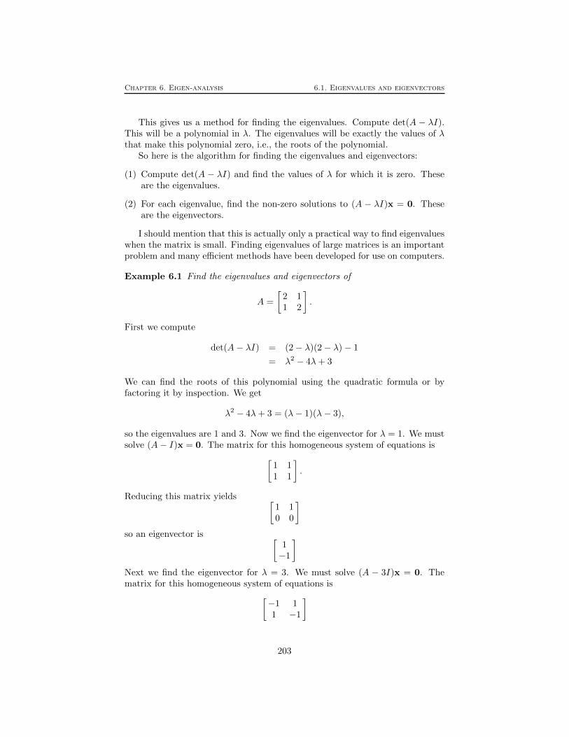
Chapter 6. Eigen-analysis 6.1. Eigenvalues and eigenvectors
This gives us a method for finding the eigenvalues. Compute det(A − λI).This will be a polynomial in λ. The eigenvalues will be exactly the values of λthat make this polynomial zero, i.e., the roots of the polynomial.
So here is the algorithm for finding the eigenvalues and eigenvectors:
(1) Compute det(A − λI) and find the values of λ for which it is zero. Theseare the eigenvalues.
(2) For each eigenvalue, find the non-zero solutions to (A − λI)x = 0. Theseare the eigenvectors.
I should mention that this is actually only a practical way to find eigenvalueswhen the matrix is small. Finding eigenvalues of large matrices is an importantproblem and many efficient methods have been developed for use on computers.
Example 6.1 Find the eigenvalues and eigenvectors of
A =
[2 11 2
].
First we compute
det(A− λI) = (2− λ)(2− λ)− 1
= λ2 − 4λ+ 3
We can find the roots of this polynomial using the quadratic formula or byfactoring it by inspection. We get
λ2 − 4λ+ 3 = (λ− 1)(λ− 3),
so the eigenvalues are 1 and 3. Now we find the eigenvector for λ = 1. We mustsolve (A− I)x = 0. The matrix for this homogeneous system of equations is[
1 11 1
].
Reducing this matrix yields [1 10 0
]so an eigenvector is [
1−1
]Next we find the eigenvector for λ = 3. We must solve (A − 3I)x = 0. Thematrix for this homogeneous system of equations is[
−1 11 −1
]
203

Chapter 6. Eigen-analysis 6.1. Eigenvalues and eigenvectors
Reducing this matrix yields [−1 10 0
]so an eigenvector is [
11
].
Example 6.2 Let us find the eigenvalues and eigenvectors of
A =
3 −6 −71 8 5−1 −2 1
.First we compute
det(A− λI) = det
3− λ −6 −71 8− λ 5−1 −2 1− λ
= (3− λ)((8− λ)(1− λ) + 10) + 6((1− λ) + 10)− 7(−2 + (8− λ))
= −λ3 + 12λ2 − 44λ+ 48
It is not always easy to find the zeros of a polynomial of degree 3. However, ifwe already know one solution, we can find the other two. Sometimes, one canfind one solution by guessing. In this case we already know that 4 is a solution(since this is the same matrix that appeared in the example in the last section).We can check this:
−64 + 12× 16− 44× 4− 48 = 0
This means that λ3 +12λ2−44λ+48 can be factored as −λ3 +12λ2−44λ+48 =(λ− 4)q(λ), where q(λ) is a second degree polynomial. To find q(λ) we can uselong division of polynomials.
−λ2 +8λ −12
λ− 4)−λ3 +12λ2 −44λ +48
−λ3 +4λ2
8λ2 −44λ8λ2 −32λ
−12λ +48−12λ +48
This yields q(λ) = −λ2 + 8λ − 12 This can be factored using the quadraticformula (or by inspection) as q(λ) = −(λ− 2)(λ− 6) So we conclude
−λ3 + 12λ2 − 44λ+ 48 = −(λ− 4)(λ− 2)(λ− 6)
204

Chapter 6. Eigen-analysis 6.1. Eigenvalues and eigenvectors
and the eigenvalues are 2, 4 and 6. Now we find the eigenvector for λ = 2. Wemust solve (A−2I)x = 0. The matrix for this homogeneous system of equationsis 1 −6 −7
1 6 5−1 −2 −1
Reducing this matrix yields 1 −6 −7
0 −8 −80 0 0
so an eigenvector is 1
−11
Next we find the eigenvector for λ = 4. We must solve (A − 4I)x = 0. Thematrix for this homogeneous system of equations is−1 −6 −7
1 4 5−1 −2 −3
Reducing this matrix yields −1 −6 −7
0 −2 −20 0 0
so an eigenvector is −1
−11
Finally we find the eigenvector for λ = 6. We must solve (A − 6I)x = 0. Thematrix for this homogeneous system of equations is−3 −6 −7
1 2 5−1 −2 −5
Reducing this matrix yields −3 −6 −7
0 0 80 0 0
so an eigenvector is −2
10
205
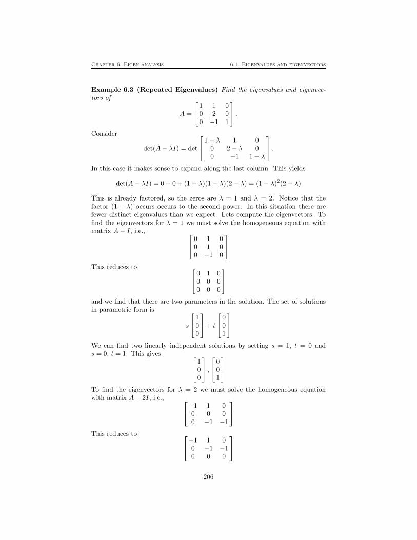
Chapter 6. Eigen-analysis 6.1. Eigenvalues and eigenvectors
Example 6.3 (Repeated Eigenvalues) Find the eigenvalues and eigenvec-tors of
A =
1 1 00 2 00 −1 1
.Consider
det(A− λI) = det
1− λ 1 00 2− λ 00 −1 1− λ
.In this case it makes sense to expand along the last column. This yields
det(A− λI) = 0− 0 + (1− λ)(1− λ)(2− λ) = (1− λ)2(2− λ)
This is already factored, so the zeros are λ = 1 and λ = 2. Notice that thefactor (1 − λ) occurs occurs to the second power. In this situation there arefewer distinct eigenvalues than we expect. Lets compute the eigenvectors. Tofind the eigenvectors for λ = 1 we must solve the homogeneous equation withmatrix A− I, i.e., 0 1 0
0 1 00 −1 0
This reduces to 0 1 0
0 0 00 0 0
and we find that there are two parameters in the solution. The set of solutionsin parametric form is
s
100
+ t
001
We can find two linearly independent solutions by setting s = 1, t = 0 ands = 0, t = 1. This gives 1
00
, 0
01
To find the eigenvectors for λ = 2 we must solve the homogeneous equationwith matrix A− 2I, i.e., −1 1 0
0 0 00 −1 −1
This reduces to −1 1 0
0 −1 −10 0 0
206

Chapter 6. Eigen-analysis 6.1. Eigenvalues and eigenvectors
and we find that the set of solutions in parametric form is
s
11−1
Setting s = 1 gives the eigenvector 1
1−1
In this 3 × 3 example, even though there are only two distinct eigenvalues, 1and 2, there are still three independent eigenvectors (i.e., a basis), because theeigenvalue 1 has two independent eigenvectors associated to it.
Example 6.4 (Repeated Eigenvalues with “Missing” Eigenvectors) Findthe eigenvalues and eigenvectors of
A =
[2 10 2
].
Heredet(A− λI) = (λ− 2)2
so there is only one eigenvalues λ = 2. To find the eigenvectors, we must solvethe homogeneous system with matrix[
0 10 0
].
The solutions are
s
[10
]so there is only one eigenvector direction. So here is a matrix that does nothave a basis of eigenvectors. Matrices like this, that have too few eigenvectors,will not be studied further in this course, but they do occur in applications.
6.1.2 Complex eigenvalues and eigenvectors
Since eigenvalues are found as roots of polynomials, we now see that they can becomplex. A discussion of complex eigenvalues and eigenvectors is given below.
Example 6.5 Lets consider the matrix of rotation by π/2. This is the matrix
A =
[0 1−1 0
].
We compute
det(A− λI) = det
[−λ 1−1 −λ
]= λ2 + 1
207

Chapter 6. Eigen-analysis 6.1. Eigenvalues and eigenvectors
The roots are ±i so the eigenvalues are i and −i. Now we compute the eigenvec-tor corresponding to the eigenvalue i. We must solve the homogeneous equationwith matrix [
−i 1−1 −i
]Notice that we will have to do complex arithmetic to achieve this, since thematrix now has complex entries. To reduce this matrix we have to add i timesthe first row to the second row. This gives[
−i 1−1 +−i2 −i+ i
]=
[−i 10 0
]So if we let the x2 = s, then −ix1 + s = 0, or x1 = −is. So the solution is
s
[−i1
]and we may choose s = 1. Lets check that this is really an eigenvector:[
0 1−1 0
] [−i1
]=
[1i
]= i
[−i1
].
To find the other eigenvector we can use a trick. Suppose that the originalmatrix A has only real entries. This will always be the case in our examples.Suppose that A has a complex eigenvalue eigenvector pair λ and x. ThenAx = λx. Taking the complex conjugate of this equation, we obtain Ax = λx.(Here conjugating a matrix or a vector just means conjugating each entry).Now, since A has real entries, A = A. Hence Ax = λx. In other words λ is aneigenvalue with eigenvector x. In the present example, we already know thati = −i is an eigenvalue. But now we don’t have to compute the eigenvector thatgoes along with it. It is simply the conjugate of the one we already computed.So the eigenvector corresponding to −i is[
i1
]The eigenvalues of A are the zeros or roots of the polynomial det(A − λI).
If we use complex numbers then det(A− λI) can be completely factored, i.e.,
det(A− λI) = ±(λ− λ1)(λ− λ2) · · · (λ− λn)
Finding the roots may be difficult. However for 2× 2 matrices we may use thequadratic formula.
If all the roots are distinct (i.e., λi 6= λj for i 6= j) then the correspondingeigenvectors x1,x2, . . . ,xn are linearly independent (I didn’t show you why thisis true, so I’m just asking you to believe it!) and therefore form a basis.
If there are repeated roots, then there are fewer than n distinct eigenvalues.In this situation, it might happen that there are not enough eigenvectors to
208

Chapter 6. Eigen-analysis 6.1. Eigenvalues and eigenvectors
form a basis . However it also might happen that more than one eigenvectorassociated to a given eigenvalue, so that in the end there are enough eigenvectorsto form a basis. Compare Examples 6.3 and 6.4 from earlier, where we saw thateither situation can occur. Unfortunately, the only way we have to find out isto try to compute them all.
6.1.3 MATLAB
When applied to a square matrix A, eig(A) will return the eigenvalues and theeigenvectors of A. To use this command enter the following in MATLAB:
>> [P,D] = eig(A)
What will be returned is a matrix P with the normalized (unit length) eigen-vectors of A in its columns, and a matrix D with the eigenvalues of A alongit’s diagonal. The eigenvalue corresponding to the ith column of P is foundin the (i, i) position of D. Using the eig command above will return complexeigenvalues and eigenvectors when present.
Example 6.6 Consider A
A =
1 4 56 3 92 7 8
(6.1)
We can enter A into MATLAB and find its eigenvectors and eigenvalues withthe following commands:
>> A=[1 4 5; 6 3 9; 2 7 8];
>> [P,D] = eig(A)
P =
-0.3919 -0.5895 0.2238
-0.6401 -0.5446 -0.8511
-0.6609 0.5966 0.4750
D =
15.9657 0 0
0 -0.3653 0
0 0 -3.6004
These results tell us that A has eigenvectors v1, v2, v3 and correspondingeigenvalues λ1, λ2, λ3 as follows:
v1, v2, v3 ≈
−0.3919−0.6401−0.6609
,
−0.5895−0.54460.5966
,
0.2238−0.85110.4750
209

Chapter 6. Eigen-analysis 6.1. Eigenvalues and eigenvectors
λ1, λ2, λ3 ≈ 15.9657,−0.3653,−3.6004
6.1.4 Problems
Problem 6.1 Show that
[11
]and
[1−1
]are eigenvectors for the matrix
[1 11 1
].
What are the corresponding eigenvalues?
Problem 6.2 Suppose P is a projection matrix. What are the eigenvalues andeigenvectors of P?
Problem 6.3 Find the eigenvalues and eigenvectors for
a)
[0 33 0
]b)
[−2 −84 10
]c)
[29 −10105 −36
]d)
[−9 −147 12
]Problem 6.4 Find the eigenvalues and the corresponding eigenvectors of thematrix [
2 32 1
].
Problem 6.5 Find the eigenvalues and eigenvectors for
a)
0 −1 11 0 22 0 2
b)
1 1 11 0 −21 −1 1
c)
7 −9 −150 4 03 −9 −11
d)
31 −100 7018 −59 4212 −40 29
Problem 6.6 Let P be a 2× 2 transitional probability matrix in the form[
p11 1− p22
1− p11 p22
].
Prove that one of the eigenvalues of P must be 1, and another one must be inthe interval [−1, 1]. (Hint: Let c = p11 + p22.)
Problem 6.7 Find the eigenvalues and the corresponding eigenvectors of thefollowing matrix.
A =
0 1 −15 0 10 1 −1
Problem 6.8 Find the eigenvalues and the corresponding eigenvectors of thefollowing matrix.
A =
2 0 10 2 11 0 2
210

Chapter 6. Eigen-analysis 6.2. Eigenanalysis simplifies matrix powers
Problem 6.9 Is there a rank two matrix M, such that vectors −→v µ1 = [1, 2, 3]T
and −→v µ2 = [3, 2, 1]T are eigenvectors of M, both corresponding to the sameeigenvalue µ1 = µ2 = −1? If your answer is yes then find such a matrix, andif your answer is no, then justify your answer.
Problem 6.10 Find the eigenvalues and the corresponding eigenvectors of thematrix [
2 3−2 −1
].
Problem 6.11 Given a 2× 2 matrix
A =
[a ii b
]a, Find values for a and b that A2 = A.b, Find values for a and b that A3 = A and A4 6= A.c, Find values for a and b that A8 6= A and A9 = A.
Problem 6.12 Like in the previous question, given a 2× 2 matrix
A =
[a ii b
]a, Find values for a and b that the two eigenvalues of A are µ1 = 2 + i and
µ2 = 2− i.b, Find the eigenvectors of A in the previous question. (where the two eigen-
values are 2± i)
6.2 Eigenanalysis simplifies matrix powers
In the previous section we learnt how to find eigenvalues and eigenvectors of amatrix, including the case when they are complex. There are two main usesof this eigenanalysis: efficiently computing powers of a matrix (studied in thissection) and in the solution of differential equations considered in Section 6.3below.
Recall that in the random walk application in Section 4.3 we were interestedin high powers of a matrix, specifically
limn→∞
Pnx(0)
where P is the matrix of transition probabilities and x(0) is the column vectorof initial probabilities. We will explore the use of eigenanalysis to simplify ourunderstanding of these kind of problems in two examples below.
211

Chapter 6. Eigen-analysis 6.2. Eigenanalysis simplifies matrix powers
Example 6.7 We consider again the sorcerers’ duel in Example 4.1. We willconsider what happens if the duel is allowed to continue without limit until thereis a winner. Rather than compute
limn→∞
Pnx(0)
numerically in MATLAB as was done in Section 4.3 we will use an eigenanalysisof P to understand this limit. The transition matrix for this problem is
P =
0 1/2 0 0
2/3 0 0 01/3 0 1 00 1/2 0 1
with initial state x(0) = (1, 0, 0, 0)T . The eigenanalysis of P is summarizedbelow:
λ1 = 1 k1 = (0, 0, 1, 0)T
λ2 = 1 k2 = (0, 0, 0, 1)T
λ3 =1√3
k3 = (1−√
3,2√3
(1−√
3),1√3, 1)T
λ4 = − 1√3
k4 = (1 +√
3,− 2√3
(1 +√
3),− 1√3, 1)T
Note that λ = 1 is a repeated eigenvalue but there there is still a basis ofeigenvectors (the set of eigenvectors associated with λ = 1 is two-dimensional).We can write
x(0) = c1k1 + c2k2 + c3k3 + c4k4 (6.2)
for some coefficients c1, c2, c3 and c4 uniquely determined. Equation (6.2) canbe written in matrix-vector form
Tc = x(0) (6.3)
where c = (c1, c2, c3, c4)T and T is the 4×4 matrix with eigenvectors k1, k2, k3
and k4 in its columns. Solving (6.3) (I used MATLAB) gives c1 = 1/2, c2 = 1/2,c3 ≈ −0.6830 and c4 ≈ 0.1830. With these values of c (6.2) is a representationof x(0) as a linear combination of eigenvectors of P . This makes working outlater states x(n) easy, as shown below.
x(1) = Px(0) = P (c1k1 + c2k2 + c3k3 + c4k4)
= c1λ1k1 + c2λ2k2 + c3λ3k3 + c4λ4k4
= c1k1 + c2k2 +1√3c3k3 −
1√3c4k4
where in the middle line we have remembered that the ki vectors are eigenvec-tors, so Pki = λki for i = 1, 2, 3, 4. Similarly
x(2) = Px(1) = P 2x(0) = c1k1 + c2k2 +1
3c3k3 +
1
3c4k4
212

Chapter 6. Eigen-analysis 6.2. Eigenanalysis simplifies matrix powers
and
x(n) = Pnx(0) = c1k1 + c2k2 +
(1√3
)nc3k3 +
(− 1√
3
)nc4k4 (6.4)
This formula (6.4) is a simple formula for the state at any time n that doesnot involve much computational work. In addition, it is easy to see from thisformula that
limn→∞
x(n) = (0, 0, 1/2, 1/2)T
as found numerically in Example 4.1
Example 6.8 The weather in Vancouver is either good, average or bad on anygiven day. If the weather is good on any day, there is a 60% chance the weatherwill be good, 30% chance average, and 10% bad on the next day. If the weatheris average, then on the next day there is a 40% chance of good, 30% of averageand 30% of bad weather. If the weather is bad then on the next day there isa 40% chance of good, 50% of average and 10% of bad. If the weather is goodtoday, what will the weather be like a long time from now? We number thestates
1) good
2) average
3) bad
The corresponding transition matrix is
P =1
10
6 4 43 3 51 3 1
The initial state is x(0) = [1, 0, 0]T . The eigenanalysis of P is summarized below:
λ1 = 1, k1 = [1/2, 1/3, 1/6]T
λ2 = 0.2, k2 = [−2, 1, 1]T
λ3 = −0.2, k1 = [0,−1, 1]T
As above, we put the eigenvectors into the columns of a matrix T and solve
Tc = (1, 0, 0)T
for c = (1,−1/4, 1/12). The right hand side (1, 0, 0)T of the system abovecorresponds to the initial state x(0) of good weather. As before, this gives usthe representation of the initial state as a linear combination of the eigenvectors:
x(0) = k1 −1
4k2 +
1
12k3.
213

Chapter 6. Eigen-analysis 6.2. Eigenanalysis simplifies matrix powers
Again, we see that multiplying by P in this representation leads to an easyformula since ki are eigenvectors:
x(n) = Pnx(0) = k1 −1
4(0.2)nk2 +
1
12(−0.2n)k3
Note that after a long time (n→∞) the second and third terms above tend tozero, so
limn→∞
x(n) = k1 = (1/2, 1/3, 1/6)
so after a long time after the first nice day, the weather will have a 1/2 chanceof being good, 1/3 average and 1/6 bad.
Let us consider the example above a bit more closely. Intuitively, the weatherafter a long time should not depend on what it was like the day you started. Infact, we can show that
limn→∞
x(n) = k1 (6.5)
for any starting probability x(0) (for which the entries must be non-negative andsum to one).
To show this, we have to show that writing
x(0) = c1k1 + c2k2 + c3k3 (6.6)
always gives c1 = 1 no matter what x(0) is. Note that the entries of k2 andk3 sum to zero and the entries of k1 and x(0) sum to one. So by summing theentries of (6.6) we see that c1 = 1 which shows that (6.5) is true for any startingprobability x(0) as our intuition predicted. The probability k1 that all initialstates tend to is called an equilibrium probability. In some cases described in thetheorem below you can guarantee the existence of an equilibrium probability.
Theorem 6.1 If P is a transition matrix (non-negative entries with all columnssumming to one) that in addition has all positive entries then P has an eigen-value 1 with a single eigenvector k1 that can chosen to be a probability vector.All other eigenvalues λ satisfy |λ| < 1 with eigenvectors with components thatsum to zero. Thus,
limn→∞
x(n) = k1
for any x(0). That is, k1 is an equilibrium probability.
Note that the Example 6.8 the transition matrix satisfied the conditionsof the theorem and had a equilibrium probability. The transition matrix ofExample 6.7 did not satisfy the conditions of the theorem and does not have anequilibrium probability (depending on the initial state, you can tend to differentfractions of times that each sorcerer wins the duel).
We can summarize the process used to analyze these examples: writinga vector x (the initial probability in our examples) as a linear combinationof eigenvectors of a matrix A (the transition matrix for our examples) theneasily writing Anx as a linear combination of eigenvectors. This process canbe summarized in matrix-vector notation as Diagonalization discussed in moredetail in Section 6.5.1.
214

Chapter 6. Eigen-analysis 6.3. Systems of linear differential equations
6.2.1 Problems
Problem 6.13 Find the eigenvalues and corresponding eigenvectors of the stochas-tic matrix P below. Use the eigenvectors and eigenvalues to describe
limn→∞
Pnx(0),
where x(0) = [1, 0, 0]T , and
P =
0 14
12
12
12
12
12
14 0
Problem 6.14 What is the necessary condition on a and b, for P having anequilibrium probability? Find the equilibrium probability vector (if it exists) fora = b = 1/4.
P =
14
13
12
12
13 b
14
13 a
6.3 Systems of linear differential equations
Consider the system of differential equations
y′1(t) = a1,1y1(t) +a1,2y2(t)y′2(t) = a2,1y1(t) +a2,2y2(t)
(6.7)
This system of equations describes a situation where we have two quantities y1
and y2, where the rate of change of each one of the quantities depends on thevalues of both. We can rewrite this as a matrix equation. Let y(t) be the vector
y(t) =
[y1(t)y2(t)
],
and define the derivative of a vector to be the vector of derivatives, i.e.,
y′(t) =
[y′1(t)y′2(t)
].
Define A to be the matrix
A =
[a1,1 a1,2
a2,1 a2,2
].
Then the system of equations (6.7) can be rewritten
y′(t) = Ay.
A general system of linear equations has this form, except y(t) is an n-dimensional vector and A is an n×n matrix. How can we find solutions to such
215

Chapter 6. Eigen-analysis 6.3. Systems of linear differential equations
a system of equations? Taking a hint from the scalar case, we can try to findsolutions of the form
y(t) = eλtx
where x is a fixed vector (not depending on t). With this definition
y′(t) = λeλtx
so that y′ = Ay whenever
λeλtx = Aeλtx = eλtAx
Dividing by eλt, this condition becomes
λx = Ax.
In other words, y(t) = eλtx is a solution exactly whenever λ and x are aneigenvalue eigenvector pair for A. So we can find as many solutions as we haveeigenvalue eigenvector pairs.
To proceed we first notice that if y1(t) and y2(t) are two solutions to theequation y′ = Ay, then a linear combination c1y1(t)+c2y2(t) is also a solution,since
d
dt
(c1y1(t) + c2y2(t)
)= c1y
′1(t) + c2y
′2(t)
= c1Ay1(t) + c2Ay2(t)
= A(c1y1(t) + c2y2(t)
)Notice that we are assuming that the constants c1 and c2 do not depend on t.Similarly, if y1(t), y2(t), . . ., yn(t) are n solutions then c1y1(t) + c2y2(t) + · · ·+cnyn(t) is a solution for any choice of constants c1, c2, . . . , cn.
Now suppose that A is an n× n matrix. Suppose that λ1, λ2, . . . , λk are itseigenvalues with eigenvectors x1,x2, . . . ,xk. Then we have that for any choiceof constants c1, c2, . . . , ck,
y(t) = c1eλ1tx1 + c2e
λ2tx2 + · · ·+ ckeλktxk (6.8)
is a solution. Have we found all solutions? In other words, could there be asolution of the equation that is not this form, or is every solution of the form(6.8) for some choice of c1, c2, . . . , ck?
There is a theorem in differential equations that says that given an initialcondition x0 there is one and only one solution of y′ = Ay satisfying y(0) = y0.So our theoretical question above is equivalent to the following quite practicalquestion. Given an initial vector y0, does there exist a solution y(t) of the form(6.8) whose value at zero is the given initial condition, i.e., y(0) = y0?
This will be true if, given any vector x0, one can find c1, c2, . . . , ck so that
y(0) = c1x1 + c2x2 + · · ·+ ckxk = x0
216

Chapter 6. Eigen-analysis 6.3. Systems of linear differential equations
This is exactly the condition that the eigenvectors form a basis. It turns outthat in the “bad” cases where there are not enough eigenvectors of A to form abasis, there are solutions that don’t have the form (6.8).
Now suppose that there are n eigenvectors that do form a basis. How canwe actually find the numbers c1, c2, . . . , cn such that
c1x1 + c2x2 + · · ·+ ckxn = x0?
Just notice that this is a system linear equations
[x1
∣∣∣∣∣x2
∣∣∣∣∣ · · ·∣∣∣∣∣xn]
c1c2...cn
= x0
so you know what to do.
Example 6.9 Find the general solution to the system of equations
y′1(t) = 2y1(t) +y2(t)y′2(t) = y1(t) +2y2(t)
This is equivalent to the matrix equation
y′(t) =
[2 11 2
]y(t)
The matrix
[2 11 2
]has eigenvector and eigenvalues λ1 = 1, x1 =
[1−1
]and
λ2 = 3, x2 =
[11
]. The eigenvectors x1 and x2 form a basis, so the general
solution is
y(t) = c1eλ1tx1 + c2e
λ2tx2 = c1et
[1−1
]+ c2e
3t
[11
]Example 6.10 Continue Example 6.9 above and find the solution satisfyingthe initial condition
y(0) =
[21
]We have to find constants c1 and c2 so that
c1
[1−1
]+ c2
[11
]=
[21
]This is the same as solving [
1 1−1 1
] [c1c2
]=
[21
]The solution is [
c1c2
]=
[1/23/2
]
217

Chapter 6. Eigen-analysis 6.3. Systems of linear differential equations
Example 6.11 Now let’s do an example where the eigenvalues are complex.Consider the equation
y′(t) =
[0 1−1 0
]y(t).
Find the general solution of this differential equation. The matrix
[0 1−1 0
]has
eigenvector and eigenvalues λ1 = i, x1 =
[−i1
]and complex conjugate λ2 = −i,
x2 =
[i1
]. The eigenvectors x1 and x2 form a basis, so the general solution is
y(t) = c1eλ1tx1 + c2e
λ2tx2 = c1eit
[−i1
]+ c2e
−it[i1
]In most applications, the solutions that we are interested in are real. The
solution above looks decidedly complex! Remember, however, that the constantsc1 and c2 can be complex too. Perhaps for special choices of c1 and c2 thesolution will turn out to be real. This is in fact always true when the originalmatrix is real. In this case the complex eigenvalues and eigenvectors occur inconjugate pairs. So if
y1(t) = eλtx
is a solution, then so isy1(t) = eλtx
So if we choose c1 = a/2 and c2 = a/2 for a real number a, then
c1eλtx + c2e
λtx = a/2(eλtx + eλtx)
= a<(eλtx)
(here < stands for the real part. We used that for a complex number z, z+ z =2<z). Similarly, if we choose c1 = a/2i and c2 = −a/2i, then
c1eλtx + c2e
λtx = a/2i(eλtx− eλtx)
= a=(eλtx)
where =() denotes the imaginary part of the argument. The upshot is that thereal and imaginary parts of a solution are also solutions. Its sometimes easier tojust start with one the complex solutions and find its real and imaginary parts.This gives us two real solutions to work with. Notice that it doesn’t matterwhich one of the complex solutions we pick. Because they are conjugate, theirreal parts are the same, and their imaginary parts differ by only a minus sign.
Example 6.12 Continuing Example 6.11 In the example we have
y1(t) = eit[−i1
]
218

Chapter 6. Eigen-analysis 6.3. Systems of linear differential equations
=
[−ieiteit
]=
[−i(cos(t) + i sin(t))
cos(t) + i sin(t)
]=
[−i cos(t) + sin(t)cos(t) + i sin(t)
]=
[sin(t)cos(t)
]+ i
[− cos(t)+ sin(t)
]The real part and imaginary part are[
sin(t)cos(t)
]and [
− cos(t)sin(t)
]One can check directly that these are solutions to the original equation. Thegeneral solution can also be written
a1
[sin(t)cos(t)
]+ a2
[− cos(t)sin(t)
]The advantage of this way of writing the solution is that if we choose a1 and a2
to be real the solution is real too.
Example 6.13 Continuing Example 6.12 Now suppose we want to satisfyan initial condition. Let’s find the solution y(t) of the equation that satisfies
y(0) =
[2−2
].
There are two ways to proceed. we could use the complex form of the generalsolution. Then we must find c1 and c2 such that
c1
[−i1
]+ c2
[i1
]=
[2−2
]This amounts to solving [
−i i1 1
] [c1c2
]=
[2−2
]The solution is [
c1c2
]=
[−i i1 1
]−1 [2−2
]=
1
−2i
[1 −i−1 −i
] [2−2
]=
[i+ 1/2i− 1/2
]
219

Chapter 6. Eigen-analysis 6.3. Systems of linear differential equations
So c1 = i + 1/2 and c2 = i − 1/2. If we plug these into the expression for thegeneral solution we get the right answer. However, there is still a fair amountof complex arithmetic needed to show explicitly that the solution is real. It’seasier to start with the real solutions. In this approach we must find a1 and a2
so that
a1
[sin(0)cos(0)
]+ a2
[− cos(0)sin(0)
]= a1
[01
]+ a2
[−10
]=
[2−2
]Thus a1 = a2 = −2 so the solution is
−2
[sin(t)cos(t)
]+−2
[− cos(t)sin(t)
]=
[−2 sin(t) + 2 cos(t)−2 cos(t)− 2 sin(t)
]Example 6.14 Now let’s do an example where the eigenvalues are complex,and have both a real and imaginary part. Let’s solve
y′(t) =
[−1 1−1 −1
]y(t)
with initial condition
y(0) =
[11
]The first step is to find the eigenvalues and eigenvectors. I’ll omit the compu-
tations. The result is λ1 = −1 + i with eigenvector x1 =
[1i
]and the complex
conjugates λ2 = −1− i with eigenvector x2 =
[1−i
]. Thus a solution is
y1(t) = e(−1+i)t
[1i
]To find real solutions we calculate the real and imaginary parts of this.
y1(t) =
[e(−1+i)t
ie(−1+i)t
]=
[e−teit
ie−teit
]=
[e−t(cos(t) + i sin(t))ie−t(cos(t) + i sin(t))
]=
[e−t cos(t)−e−t sin(t)
]+ i
[e−t sin(t)e−t cos(t)
]So the general solution can be written
a1
[e−t cos(t)−e−t sin(t)
]+ a2
[e−t sin(t)e−t cos(t)
]
220

Chapter 6. Eigen-analysis 6.3. Systems of linear differential equations
To satisfy the initial condition, we need
a1
[10
]+ a2
[01
]=
[11
]so that a1 = 1 and a2 = 1. Thus the solution is
y(t) = e−t[
cos(t) + sin(t)− sin(t) + cos(t)
]6.3.1 Problems
Problem 6.15 Find the general solution to y′ = Ay when A =
[−2 −84 10
].
(Hint: This matrix appeared in the problems of last chapter). Find the solution
satisfying the initial condition y(0) =
[11
].
Problem 6.16 Find the general solution to y′ = Ay when A =
[1 −22 1
].
Find both the complex form and the real form. Find the solution satisfying the
initial condition y(0) =
[11
].
Problem 6.17 Find the general solution to y′ = Ay when A =
6 0 135 1 13−2 0 −4
.
Find both the complex form and the real form. Find the solution satisfying the
initial condition y(0) =
111
.
Problem 6.18 Find the general solution of the following system of differentialequations:
y′(t) =
[1 15 1
]y(t)
Problem 6.19 Find the solution of the following system of differential equa-tions, that satisfy the initial condition y(0) = [0, 1]T .
y′(t) =
[3 −11 −1
]y(t)
Problem 6.20 Find the real form of the solution of the following system ofdifferential equations, that satisfy the initial condition y(0) = [2,−1]T .
y′(t) =
[−3 −17 1
]y(t)
Problem 6.21 Is it true that every 3 × 3 matrix with real entries always hasat least one real eigenvalue? Why?
221

Chapter 6. Eigen-analysis 6.4. LCR circuits
Figure 6.2: Diagrams of capacitors and inductors.
6.4 LCR circuits
6.4.1 Capacitors and inductors
We introduce new elements into our study of electrical circuits: capacitors andinductors. At an instant in time t, a capacitor acts as a voltage source withvoltage V (t). At a given instant in time an inductor acts as a current sourcewith current I(t). These circuit elements are shown in Figure 6.2.
The voltage across the capacitor changes proportional to the current i (withdirection as in Figure 6.2) through it
dV
dt= − i
C(6.9)
where the constant of proportionality C is the capacitance of the capacitor withMKS units of Farads. Note that a capacitor with large capacitance can providemore current for the same drop in voltage.
The current through an inductor changes proportional to the voltage v acrossit (with direction as in Figure 6.2)
dI
dt= − v
L(6.10)
where the constant of proportionality L is the inductance with MKS units ofHenrys.
We consider here at a high level how the behaviour in time of circuits withmany capacitors, inductors and resistors. At a given instant in time, capacitorscan be treated as a voltage sources and inductors as current sources. To de-termine how these sources change in time, the current through the capacitors(6.9) and the voltage across the inductors (6.10) is needed. However, deter-mining these from the sources is the fundamental circuit problem considered inSection 3.5.3 and Section 4.6. Thus, a system of differential equations can bederived for circuit networks with capacitors and inductors by solving the fun-damental problem for the circuit and scaling the result by the capacitance andinductance of the elements. Some specific examples are given below.
222

Chapter 6. Eigen-analysis 6.4. LCR circuits
Figure 6.3: A simple LRC circuit.
6.4.2 Differential equations for LCR circuits
Example 6.15 The simplest example of an LRC circuit is the simple seriescircuit shown in Figure 6.3. We will derive a system of differential equationsfor V (t) and I(t) in the circuit and determine what combination of values forthe components L, R, and C lead to oscillations. The equation is simple enoughthat the solution to the fundamental problem can just be written down. Thecurrent through the capacitor is I and the voltage v across the inductor isIR− V . Using the relationships (6.9, 6.10) we write
dV
dt= −I/C
dI
dt= −(IR− V )/L = V/L− IR/L
or in matrix vector formx′ = Ax
where x = (V, I)T and
A =
[0 −1/C
1/L −R/L
]The eigenvalues λ of A satisfy
det(A− λI) = λ2 +R
Lλ+
1
LC= 0
with solutions
λ =1
2L
(−R±
√R2 − 4L/C
).
Considering this expression carefully you can see that if the λ values are realthey are negative. If they are complex, the real part is −R/(2L). Thus solutionsalways decay exponentially. This is to be expected in a circuit with no externalpower. For the circuit to have oscillations, the eigenvalues must be complex, so
R2 − 4L/C < 0
223

Chapter 6. Eigen-analysis 6.4. LCR circuits
Figure 6.4: Circuit diagram for Example 6.16.
which is commonly rewritten as
R
2
√C
L< 1.
Example 6.16 Consider the circuit shown in Figure 6.4. The capacitor hascapacitance C = 1 Farad and the inductor inductance L = 1 Henry. Thecapacitor is charged up to 12V and then the switch is closed (so E(0) = 12 andI(0) = 0).
(a) Derive a system of differential equations for I(t) and E(t).
(b) We expect that E(t) and I(t)→ 0 as t→∞ (no external power). Will therebe oscillations in E and I in time?
Remember that if i(t) is the current upward through the capacitor then
dE
dt= − i
C= −i (6.11)
since C = 1. If e(t) is the voltage across the inductor as shown then
dI
dt= − e
L= −e (6.12)
since L = 1. It is still necessary to work out i(t) and e(t) in terms of E(t) andI(t). This is the fundamental problem for the circuit. We solved this problemin Example 3.13 in Section 3.6 and considered it from a different perspective inthe additional notes to Chapter 4. We found that
i =5
36E − 1
6I
e =1
6E + 6I
224

Chapter 6. Eigen-analysis 6.4. LCR circuits
L
R1
R2C
I V1 1
I V3 3
I V2 2I V44
Figure 6.5: Circuit diagram.
Inserting these into (6.11) and (6.12) gives the desired system for E and I:
dE
dt= − 5
36E +
1
6I
dI
dt= −1
6E − 6I
or in vector form x′ = Ax where
x =
[EI
]and A =
[−5/36 1/6−1/6 −6
]An eigenanalysis of A gives λ1 ≈ −0.1436 and λ2 ≈ −5.9953. Since these arenot complex, the circuit does not exhibit oscillations.
6.4.3 Alternate description of LCR circuits
LCR circuits were presented differently in a previous version of the notes. Thatapproach is reproduced below starting in the next paragraph. It follows thediscussion in Section 3.5.4.
We now return to the circuit that we discussed previously, shown in Fig-ure 6.5. Recall that we chose as basic variables I3 and V4 and solved for all theother variables in terms of these. The result was
I1 = I3
I2 =1
R2V4
I4 = I3 −1
R2V4
V1 = R1I3
V2 = V4
V3 = −R1I3 − V4
Now we can complete the job and determine I3 and V4. We have to take intoaccount now that the currents and voltages are functions of time. The relations
225

Chapter 6. Eigen-analysis 6.4. LCR circuits
between currents and voltages across capacitors and inductors involves the timederivatives.
If I and V are the current flowing through and the voltage across a capacitorwith capacitance C, then
dV
dt=
1
CI
If I and V are the current flowing through and the voltage across an inductorwith inductance L, then
dI
dt=
1
LV
Notice that we have chosen as basic the variables that get differentiated.Using these relations for I3 and V4 yields
dI3dt
=1
LV3
dV4
dt=
1
CI4
Now we re-express everything in terms of I3 and V4 using the equations wederived previously.
dI3dt
=1
L(−R1I3 − V4) =
−R1
LI3 −
1
LV4
dV4
dt=
1
C(I3 −
1
R2V4) =
1
CI3 −
1
R2CV4
This can be written as [I3V4
]′=
[ −R1
L − 1L
1C − 1
R2C
] [I3V4
]Lets try to determine for what values of R1, L, C and R2 the circuit exhibitsoscillations. Recall that the solution will involve sines and cosines whenever thematrix has complex eigenvalues.
The polynomial det(A− λI) = λ2 + bλ+ c, where
b =R1
L+
1
R2C
and
c =R1
R2LC+
1
LC.
The eigenvalues are the roots of this polynomial, given by (−b ±√b2 − 4c)/2.
These will be complex if b2 < 4c, i.e., if(R1
L+
1
R2C
)2
< 4
(R1
R2LC+
1
LC
)Notice that this can be achieved by decreasing R1 and increasing R2
226

Chapter 6. Eigen-analysis 6.5. Additional Topics
L
R
CV I
Figure 6.6: Circuit diagram for Problem 6.23.
6.4.4 Problems
Problem 6.22 In the circuit in Figure 6.5, suppose that R1 = R2 = 1 ohm,C = 1 farad and L = 1 henry. If the initial current across the inductor isI3(0) = 1 ampere and initial voltage across the capacitor is V4(0) = 1 volt, findI3(t) and V4(t) for all later times. What is V1(t)?
Problem 6.23 Consider the circuit with diagram in Figure 6.6 Write down thesystem of equations satisfied by I and V . For what values of L, C and R doesthe circuit exhibit oscillations? Suppose that R = 1 ohm, C = 1 farad and L = 1henry. If the initial current across the inductor is I(0) = 1 ampere and initialvoltage across the capacitor is V (0) = 1 volt, find I(t) and V (t) for all latertimes.
6.5 Additional Topics
6.5.1 Diagonalization
Diagonal matrices (that is, matrices that have zero entries except on the diago-nal) are extremely easy to work with. For a start, the eigenvalues of a diagonalmatrix are exactly the diagonal entries. If
D =
λ1 0 · · · 00 λ2 · · · 0...
......
0 0 · · · λn
then det(D − λI) = (λ1 − λ)(λ2 − λ) · · · (λn − λ) which is zero precisely whenλ equals one of λ1, λ2, . . ., λn. The corresponding eigenvectors are just thestandard basis vectors e1, e2, . . ., en.
227

Chapter 6. Eigen-analysis 6.5. Additional Topics
It is also easy to compute powers of a diagonal matrix. We simply obtain
Dk =
λk1 0 · · · 00 λk2 · · · 0...
......
0 0 · · · λkn
This formula makes it easy to compute the matrix exponential of D. Recallthat the matrix etD is defined to be the matrix power series
etD = I + tD +t2
2D2 +
t3
3!D3 + · · ·
Using the formula above we find that
etD =
1 0 · · · 00 1 · · · 0...
......
0 0 · · · 1
+
tλ1 0 · · · 00 tλ2 · · · 0...
......
0 0 · · · tλn
+
t2λ2
1
2 0 · · · 0
0t2λ2
2
2 · · · 0...
......
0 0 · · · t2λ2n
2
+ · · ·
=
1 + tλ1 +
t2λ21
2 + · · · 0 · · · 0
0 1 + tλ2 +t2λ2
2
2 · · · 0...
......
0 0 · · · 1 + tλn +t2λ2
n
2 + · · ·
=
etλ1 0 · · · 0
0 etλ2 · · · 0...
......
0 0 etλn
Things are not quite so simple for an arbitrary n × n matrix A. However, ifA has a basis of eigenvectors then it turns out that there exists an invertiblematrix B such that AB = DB, where D is the diagonal matrix whose diagonalelements are the eigenvalues of A. Multiplying by B−1 from either the left orright gives
A = BDB−1, D = B−1AB
In fact, B is simply the matrix whose columns are the eigenvectors of A. In other
words, if x1, x2, . . ., xn are the eigenvectors for A then B =[x1
∣∣∣x2
∣∣∣ · · · ∣∣∣xn].To see this notice that
AB = A[x1
∣∣∣x2
∣∣∣ · · · ∣∣∣xn]=
[Ax1
∣∣∣Ax2
∣∣∣ · · · ∣∣∣Axn
]=
[λ1x1
∣∣∣λ2x2
∣∣∣ · · · ∣∣∣λnxn
]
228

Chapter 6. Eigen-analysis 6.5. Additional Topics
=[x1
∣∣∣x2
∣∣∣ · · · ∣∣∣xn]λ1 0 · · · 00 λ2 · · · 0...
......
0 0 · · · λn
= BD
The assumption that A has a basis of eigenvectors implies that the matrix B isinvertible.
Using the representation A = BDB−1 it is easy to calculate powers of A.We have
A2 = BDB−1BDB−1 = BDIDB−1 = BD2B−1
and similarlyAk = BDkB−1
Therefore we can now also sum the power series for the exponential and obtain
etA = BetDB−1
6.5.2 Computing high powers of a matrix
Recall that when we were discussing the random walk problem, we ended upwith the problem of computing the limit for large n of Pnx0 where P is thematrix of transition probabilities.
We can now solve this problem using diagonalization. Lets do an example.Suppose that
P =
[12
14
23
34
]We wish to compute Pn for large n.
We begin by diagonalizing P . This involves finding the eigenvalues andeigenvectors. I won’t give the details of this computation. The results are
λ1 = 1, x1 =
[1
8/3
]and λ2 = 1/12, x1 =
[−11
]. So
P =
[1 −183 1
] [1 00 1
12
] [1 −183 1
]−1
and
Pn =
[1 −183 1
] [1n 00
(112
)n ] [ 1 −183 1
]−1
But 1n = 1 for all n and(
112
)n → 0 as n→∞, since 112 < 1. So
limn→∞
Pn =
[1 −183 1
] [1 00 0
] [1 −183 1
]−1
=
[1 −183 1
] [1 00 0
] [311
311−8
11311
]=
[311
311
811
811
]
229

Chapter 6. Eigen-analysis 6.5. Additional Topics
6.5.3 Another formula for the determinant
If A has a basis of eigenvectors, then we can get another formula for the deter-minant. Using the multiplicative property of the determinant, we have
det(A) = det(BDB−1) = det(B) det(D) det(B)−1 = det(D).
But det(D) is just the product of the diagonal elements, i.e., the eigenvalues.Thus the determinant of A is the product of its eigenvalues:
det(A) = λ1λ2 · · ·λn.
Actually, this is true even if A doesn’t have a basis of eigenvectors and isn’tdiagonalizable.
6.5.4 The matrix exponential and differential equations
The matrix exponential etA can be used to solve the differential equation
y′(t) = Ay(t)
with initial conditiony(0) = x0
To see this notice that etA satisfies the differential equation ddte
tA = AetA. Thisfollows from the power series representation
etA = I + tA+t2
2A2 +
t3
3!A3 + · · ·
since
d
dtetA = A+
2t
2A2 +
3t2
3!A3 + · · ·
= A+ tA2 +t2
2!A3 + · · ·
= A(I + tA+t2
2A2 + · · ·)
= AetA
Alsoe0A = I
These two facts imply that y(t) = etAx0 is the solution to our differentialequation and initial condition, since y′(t) = d
dtetAx0 = AetAx0 = Ay(t) and
y(0) = e0Ax0 = Ix0 = x0.The matrix exponential is a nice theoretical construction. However, to actu-
ally compute the matrix exponential using diagonalization involves just the sameingredients—computing the eigenvalues and vectors—as our original solution.In fact it is more work.
230

Chapter 6. Eigen-analysis 6.5. Additional Topics
However, there is one situation where the matrix exponential gives us some-thing new. This is the situation where A does not have a basis of eigenvectors.The power series definition of the matrix exponential still makes sense, and can
compute it in certain special cases. Consider the matrix A =
[1 10 1
]. This
matrix does not have a basis of eigenvectors. So it cannot be diagonalized.
However, in a homework problem, you showed that etA =
[et tet
0 et
]. Thus the
solution to
y′(t) =
[1 10 1
]y(t)
with initial condition
y(0) =
[21
]is
y(t) = etA[
21
]=
[et tet
0 et
] [21
]=
[2et + tet
et
]Notice that this solution involves a power of t in addition to exponentials.
6.5.5 Converting higher order equations into first ordersystems
So far we have only considered first order differential equations. In other words,the equations have only involved first derivatives y′(t) and not higher derivativeslike y′′(t). However higher order equations, especially second order equations,occur often in practical problems. In this section we will show that a higherorder linear differential equation can be converted into an equivalent first ordersystem.
Suppose we want to solve the equation
y′′(t) + ay′(t) + by(t) = 0
with initial conditions
y(0) = y0
y′(0) = y′0
Define the new functions z1(t) and z2(t) by
z1(t) = y(t)
z2(t) = y′(t)
Thenz′1(t) = y′(t) = z2(t)z′2(t) = y′′(t) = −ay′(t)− by(t) = −az2(t)− bz1(t)
231
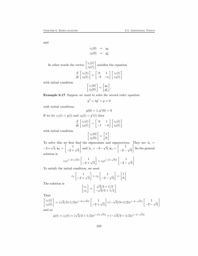
Chapter 6. Eigen-analysis 6.5. Additional Topics
and
z1(0) = y0
z2(0) = y′0
In other words the vector
[z1(t)z2(t)
]satisfies the equation
d
dt
[z1(t)z2(t)
]=
[0 1−b −a
] [z1(t)z2(t)
]with initial condition [
z1(0)z2(0)
]=
[y0
y′0
].
Example 6.17 Suppose we want to solve the second order equation
y′′ + 4y′ + y = 0
with initial conditionsy(0) = 1, y′(0) = 0
If we let z1(t) = y(t) and z2(t) = y′(t) then
d
dt
[z1(t)z2(t)
]=
[0 1−1 −4
] [z1(t)z2(t)
]with initial condition [
z1(0)z2(0)
]=
[10
].
To solve this we first find the eigenvalues and eigenvectors. They are λ1 =
−2+√
3, x1 =
[1
−2 +√
3
]and λ1 = −2−
√3, x1 =
[1
−2−√
3
]So the general
solution is
c1e(−2+
√3)t
[1
−2 +√
3
]+ c2e
(−2−√
3)t
[1
−2−√
3
]To satisfy the initial condition, we need
c1
[1
−2 +√
3
]+ c2
[1
−2−√
3
]=
[10
]The solution is [
c1c2
]=
[ √3/3 + 1/2
−√
3/3 + 1/2
]Thus[z1(t)z2(t)
]= (√
3/3+1/2)e(−2+√
3)t
[1
−2 +√
3
]+(−√
3/3+1/2)e(−2−√
3)t
[1
−2−√
3
]and so
y(t) = z1(t) = (√
3/3 + 1/2)e(−2+√
3)t + (−√
3/3 + 1/2)e(−2−√
3)t
232

Chapter 6. Eigen-analysis 6.5. Additional Topics
klm
,x(t)
Figure 6.7: A simple mass-spring system.
Actually, to solve the equation
y′′(t) + ay′(t) + by(t) = 0
it is not really necessary to turn it into a first order system. We can simply tryto find solutions of the form y(t) = eλt. If we plug this into the equation we get(λ2 + aλ+ b)eλt which is zero if λ is a root of λ2 + aλ+ b. This polynomial hastwo roots, which yields two solutions.
Still, the procedure of turning a higher order equation into a first order sys-tem is important. This is because on a computer it is much easier to solve a firstorder system than a high order equation. If the coefficients a and b are functionsof t, then exact solutions (like exponentials) usually can’t be found. However,one can still turn the equation into a first order system y′(t) = A(t)y(t) wherethe matrix now depends on t and solve this on a computer.
6.5.6 Springs and weights
To begin, lets consider the situation where we have a single weight hanging ona spring shown in Figure 6.7. We want to determine how the weight moves intime. To do this we calculate the forces acting on the weight and use Newton’slaw of motion F = ma.
One force acting on the weight are the force of gravity. This acts in thepositive x direction (i.e., downward) and has magnitude mg. The other forceis due to the spring. It’s magnitude is k(x − l) in the negative x direction.The acceleration is the second derivative x′′(t). Thus the total force is F =mg − k(x(t)− l) and ma = mx′′(t) Newton’s law reads
mx′′(t) = mg − k(x− l) = −kx+mg + lk
This is not quite in the form we can handle, due to the term mg + lk onthe right. What we must do is first find the equilibrium solution. In a previouslecture we found the equilibrium position by minimizing the potential energy.There is another, equivalent, way. That is to find the value of x for which thetotal force is zero. In other words
−kxeq +mg + lk = 0
233

Chapter 6. Eigen-analysis 6.5. Additional Topics
orxeq = (mg + lk)/k
Notice that the total force can be written
−kx+mg + lk = −k(x− xeq)
Now let y(t) = x(t)−xeq be the displacement from the equilibrium point. Noticethat y′(t) = x′(t) and y′′(t) = x′′(t), since xeq is a constant. So the equation fory(t) is
my′′(t) = −ky(t)
or
y′′(t) +k
my(t) = 0
We could turn this into a first order system. However, it is easier to trysolutions of the form eλt. Substituting this into the equation yields
(λ2 + k/m)eλt = 0
so we require that λ2 +k/m = 0, or λ = ±i√k/m. Thus, solutions are ei
√k/mt
and e−i√k/mt. To obtain real solutions, we can take the real and imaginary
parts. This gives as solutions sin(√k/mt) and cos(
√k/mt) , and the general
solution isc1 sin(
√k/mt) + c2 cos(
√k/mt)
We can make the equation a little more interesting by adding friction. Africtional force is proportional to the velocity and acts in the direction oppositeto the motion. Thus the equation with friction reads
y′′(t) + βy′(t) +k
my(t) = 0
This can be solved by turning it into a first order system, or directly, using trialsolution of the form eλt as above.
Now we turn the problem with several weights and springs shown in Fig-ure 6.8. In this problem matrices play an essential role.
We begin by computing the forces acting on each weight. Let us start withthe first weight. Gravity is pulling down, and the springs above and below arepushing or pulling with a force proportional to their extensions. Thus the totalforce on the first weight is m1g − k1(x1 − l1) + k2(x2 − x1 − l2). To get thesigns right on the spring forces, think of what happens when one of the xi’s getslarge. For example, when x1 gets large, the first spring stretches and pulls up,so the sign of the force should be negative for large x1. So Newton’s equationfor the first weight is
m1x′′1(t) = m1g−k1(x1−l1)+k2(x2−x1−l2) = −(k1+k2)x1+k2x2+m1g+k1l1−k2l2
or
x′′1(t) = −k1 + k2
m1x1 +
k2
m1x2 + g +
k1l1 − k2l2m1
234

Chapter 6. Eigen-analysis 6.5. Additional Topics
x1
x2
x3
k l
k l
k l
1 1
2 2
3 3
m1
m2
m3
,
,
,
Figure 6.8: A more complicated mass-spring system.
Similarly the equations for the second and third weights are
x′′2(t) =k2
m2x1 −
k2 + k3
m2x2 +
k3
m2x3 + g +
k2l2 − k3l3m2
x′′3(t) =k3
m3x2 −
k3
m3x3 + g +
k3l3m3
Thus can be written as a second order matrix equation
x′′(t) = Kx(t) + b
where
x(t) =
x1(t)x2(t)x3(t)
,K =
−k1+k2m1
k2m1
0k2m2
−k2+k3m2
k3m2
0 k3m3
− k3m3
and
b =
g + k1l1−k2l2m1
g + k2l2−k3l3m2
g + k3l3m3
.With this notation, the equilibrium solution is the value of x that makes all theforces zero. That is,
Kxeq + b = 0
or,xeq = −K−1b
As in the case of one weight the force side of the equation can now be writtenas
Kx + b = K(x +K−1b) = K(x− xeq)
235

Chapter 6. Eigen-analysis 6.5. Additional Topics
so if we definey(t) = x(t)− xeq,
the equation for y(t) isy′′(t) = Ky(t)
To solve this second order 3× 3 system, we could turn it in to a first order6× 6 system. However, just as in the case of a single higher order equation wecan proceed directly. We try trial solutions of the form eκty. Substituting thisinto the equation, we see that the equation is satisfied if
κ2y = Ky
in other words, κ2 is an eigenvalue of K with eigenvector y, or κ is one of thetwo square roots of and eigenvalue.
So, if K has eigenvalues λ1, λ2 and λ3 with eigenvectors y1, y2 and y3,then six solutions of the equation are given by e
√λ1ty1, e−
√λ1ty1, e
√λ2ty2,
e−√λ2ty2, e
√λ3ty3 and e−
√λ3ty3. If some of the λi’s are negative, then these
solutions are complex exponentials, and we may take their real and imaginaryparts to get real solutions. The general solution is a linear combination of these,and the coefficients in the linear combination may be chosen to satisfy an initialcondition.
To make this clear we will do an example. Suppose that all the masses mi,lengths li and spring constants ki are equal to 1. Then
K =
−2 1 01 −2 10 1 −1
Suppose that the initial position of the weights is x1 = 30, x2 = 60 and x3 = 70,and that the initial velocities are x′1 = 1 and x′2 = x′3 = 0. We will determine thepositions of the weights for all subsequent times. The numbers in this problemdon’t turn out particularly nicely, so I’ll just give them to 3 significant figures.
The first step is to find the eigenvalues and eigenvectors of K. They aregiven by
λ1 = −0.198 λ2 = −1.55 λ3 = −3.25
x1 =
0.4450.8021.00
x2 =
−1.25−0.555
1.00
x3 =
1.80−2.251.00
Let µ1 =
√0.198 = 0.445, µ2 =
√1.55 = 1.25 and µ3 =
√3.25 = 1.80 Then if
y(t) = x(t)− xeq, then general solution for y(t) is
y(t) = (c1eiµ1t + d1e
−iµ1t)x1 + (c2eiµ2t + d2e
−iµ2t)x2 + (c3eiµ3t + d3e
−iµ3t)x3
where c1, d1, c2, d2, c3, d3 are arbitrary constants. Taking real and imaginaryparts, we can also write the general solution as
y(t) = (a1 cos(µ1t)+b1 sin(µ1t))x1+(a2 cos(µ2t)+b2 sin(µ2t))x2+(a3 cos(µ3t)+b3 sin(µ3t))x3
236

Chapter 6. Eigen-analysis 6.5. Additional Topics
where a1, b1, a2, b2, a3, b3 are arbitrary constants. Notice that we can find thegeneral solution for y(t) = x(t)− xeq without knowing xeq. However, since theinitial conditions were given in terms of x and not y, we now have to find xeq
to be able to convert initial conditions for x to initial conditions for y. If wework in units where g = 10 then
b =
101011
and
xeq = −K−1b =
315263
so
y(0) = x(0)− xeq =
306070
− 31
5263
=
−187
Also
y′(0) = x′(0) =
100
So to satisfy the first initial condition, since cos(0) = 1 and sin(0) = 0, we needthat
y(0) = a1x1 + a2x2 + a3x3 =
−187
.Explicitly, we need to solve
[x1|x2|x3]
a1
a2
a3
=
−187
,or 0.445 −1.25 1.80
0.802 −0.555 −2.251.00 1.00 1.00
a1
a2
a3
=
−187
This is not a pretty sight, but I can punch the numbers into my computer andfind that a1
a2
a3
=
7.041.33−1.37
To satisfy the second initial condition, we differentiate the expression for thegeneral solution of y(t) and set t = 0. This gives
µ1b1x1 + µ2b2x2 + µ3b3x3 =
100
237

Chapter 6. Eigen-analysis 6.5. Additional Topics
Solving this numerically givesµ1b1µ2b2µ3b3
=
0.242−0.4350.194
Finally, we divide by the µ′is to give b1b2
b3
=
0.543−0.348
1.80
Now we have completely determined all the constants, so the solution is com-plete.
6.5.7 Problems
Problem 6.24 Consider the second order equation
y′′ − 5y′ + 6y = 0
with initial conditions y(0) = 1, y′(0) = 0. Solve this by turning it into a 2× 2system. Then solve it directly by using trial solutions eλt.
Problem 6.25 Consider the second order equation
y′′ + y′ + y = 0
with initial conditions y(0) = 1, y′(0) = 0. Solve this by turning it into a 2× 2system. Then solve it directly by using trial solutions eλt.
Problem 6.26 How can you turn a third order equation
y′′′ + ay′′ + by′ + cy = 0
into an equivalent 3× 3 system of equations?
Problem 6.27 Suppose K is a 3× 3 matrix with eigenvalues and eigenvectorsgiven by
λ1 = −1 λ2 = −4 λ3 = −9
x1 =
101
x2 =
10−1
x3 =
010
Find the solution of
y′′(t) = Ky(t)
satisfying
y(0) =
121
238

Chapter 6. Eigen-analysis 6.6. Solutions to Chapter Problems
y′(0) =
011
Problem 6.28 Consider a system of two hanging weights and springs. Supposethat all the masses, spring constants and spring lengths are equal to one, andthat g = 10. Find the positions x1(t) and x2(t) for all times if x1(0) = 20,x2(0) = 30, x′1(0) = 1, x′2(0) = 1.
6.6 Solutions to Chapter Problems
Solution 6.1 We compute
[1 11 1
] [11
]=
[22
]= 2
[11
], so
[11
]is an eigen-
vector with eigenvalue 2. Also
[1 11 1
] [1−1
]=
[00
]= 0
[1−1
], so
[1−1
]is an
eigenvector with eigenvalue 0.
Solution 6.2 If P projects onto some line, then a vector x lying on that linedoesn’t get changed by P so Px = x and x is an eigenvector with eigenvalue 1.On the other hand, if x is perpendicular to the line, then Px = 0 = 0x so x isan eigenvector with eigenvalue 0.
Solution 6.3
a) det(A − λI) = λ2 − 9 = (λ − 3)(λ + 3) so the eigenvalues are λ1 = 3 andλ2 = −3. To find the eigenvector for λ1 = 3 we must solve the homogeneous
equation with matrix
[−3 33 −3
]. The matrix reduces to
[−3 30 0
]and the
eigenvector is x1 =
[11
]. To find the eigenvector for λ2 = −3 we must
solve the homogeneous equation with matrix
[3 33 3
]. The matrix reduces
to
[3 30 0
]and the eigenvector is x2 =
[1−1
].
b) det(A−λI) = λ2−8λ+12 = (λ−2)(λ−6) so the eigenvalues are λ1 = 3 andλ2 = −3. To find the eigenvector for λ1 = 2 we must solve the homogeneous
equation with matrix
[−4 −84 8
]. The matrix reduces to
[−4 −80 0
]and the
eigenvector is x1 =
[2−1
]. To find the eigenvector for λ2 = 6 we must solve
the homogeneous equation with matrix
[−8 −84 4
]. The matrix reduces to[
−8 −80 0
]and the eigenvector is x2 =
[1−1
].
c) det(A− λI) = λ2 + 7λ+ 6 = (λ+ 6)(λ+ 1) so the eigenvalues are λ1 = −6and λ2 = −1. To find the eigenvector for λ1 = −6 we must solve the
239

Chapter 6. Eigen-analysis 6.6. Solutions to Chapter Problems
homogeneous equation with matrix
[35 −10105 −30
]. The matrix reduces to[
35 −100 0
]and the eigenvector is x1 =
[27
]. To find the eigenvector for
λ2 = −1 we must solve the homogeneous equation with matrix
[30 −10105 −35
].
The matrix reduces to
[30 −100 0
]and the eigenvector is x2 =
[13
].
d) det(A−λI) = λ2−3λ−10 = (λ+2)(λ−5) so the eigenvalues are λ1 = −2 andλ2 = 5. To find the eigenvector for λ1 = −2 we must solve the homogeneous
equation with matrix
[−7 −147 14
]. The matrix reduces to
[−7 −140 0
]and
the eigenvector is x1 =
[2−1
]. To find the eigenvector for λ2 = 5 we must
solve the homogeneous equation with matrix
[−14 −14
7 7
]. The matrix
reduces to
[−14 −14
0 0
]and the eigenvector is x2 =
[1−1
].
Solution 6.4
det
[2− λ 3
2 1− λ
]= (2− λ)(1− λ)− 6 = 2− 3λ+ λ2 − 6
= λ2 − 3λ− 4 = (λ− 4)(λ− 5) = 0
⇒ λ = −1, 4.
The eigenvector for λ = −1:[3 32 2
] [k1
k2
]= ~0 ⇒ 3k1 + 3k2 = 0
2k1 + 2k2 = 0⇒ k1 = −k2
If we set k2 = 1 for convenience, we have that the first eigenpair is
λ1 = −1, ~v1 =
[−11
].
Now, the eigenvector for λ = 4:[−2 32 −3
] [k1
k2
]= ~0 ⇒ −2k1 + 3k2 = 0
2k1 − 3k2 = 0⇒ k1 =
3
2k2
If we set k2 = 1 for convenience, we have that the second eigenpair is
λ2 = 4, ~v2 =
[3/21
].
Solution 6.5
240

Chapter 6. Eigen-analysis 6.6. Solutions to Chapter Problems
a) det(A−λI) = −λ3 + 2λ2 +λ− 2 = −(λ− 1)(λ− 2)(λ+ 1) so the eigenvaluesare λ1 = 1 and λ2 = 2 and λ3 = −1. To find the eigenvector for λ1 = 1
we must solve the homogeneous equation with matrix
−1 −1 11 −1 22 0 1
. The
matrix reduces to
−1 −1 10 −2 30 0 0
and the eigenvector is x1 =
1−32
. To
find the eigenvector for λ2 = 2 we must solve the homogeneous equation
with matrix
−2 −1 11 −2 22 0 0
. The matrix reduces to
−2 −1 10 −1 10 0 0
and the
eigenvector is x2 =
011
. To find the eigenvector for λ3 = −1 we must solve
the homogeneous equation with matrix
1 −1 11 1 22 0 3
. The matrix reduces
to
1 −1 10 2 10 0 0
and the eigenvector is x3 =
31−2
.
b) det(A − λI) = −λ3 + 2λ2 + 3λ − 6 = −(λ − 2)(λ −√
3)(λ +√
3) so theeigenvalues are λ1 = 2 and λ2 =
√3 and λ3 = −
√3.. To find the eigen-
vector for λ1 = 2 we must solve the homogeneous equation with matrix−1 1 11 −2 −21 −1 −1
. The matrix reduces to
0 −1 −10 0 0−1 1 1
and the eigen-
vector is x1 =
0−11
. To find the eigenvector for λ2 =√
3 we must solve
the homogeneous equation with matrix
1−√
3 1 11 −
√3 −2
1 −1 1−√
3
. The
matrix reduces to
1−√
3 1 10 2−
√3 −3 + 2
√3
0 0 0
and the eigenvector is
x2 =
−1−√
31
. To find the eigenvector for λ3 = −√
3 we must solve the ho-
mogeneous equation with matrix
1 +√
3 1 11 +
√3 −2
1 −1 1 +√
3
. The matrix re-
241

Chapter 6. Eigen-analysis 6.6. Solutions to Chapter Problems
duces to
1 +√
3 1 10 2 +
√3 2
√3 + 1
0 0 0
and the eigenvector is x3 =
−1√3
1
.
c) det(A − λI) = −λ3 + 48λ − 128 = −(λ + 8)(λ − 4)2 so the eigenvaluesare λ1 = −8 and λ2 = 4. To find the eigenvector for λ1 = −8 we must
solve the homogeneous equation with matrix
15 −9 −150 12 03 −9 −3
. The matrix
reduces to
15 −9 −150 12 00 0 0
and the eigenvector is x1 =
101
. To find
the eigenvector(s) for λ2 = 4 we must solve the homogeneous equation with
matrix
3 −9 −150 4 03 −9 −15
. The matrix reduces to
3 −9 −150 0 00 0 0
. Thus
there are two eigenvectors corresponding to this eigenvalues, for example
x2 =
310
and x3 =
501
.
d) det(A − λI) = −λ3 + λ2 + λ − 1 = −(λ + 1)(λ − 1)2 so the eigenvaluesare λ1 = −1 and λ2 = 1. To find the eigenvector for λ1 = −1 we must
solve the homogeneous equation with matrix
32 −100 7018 −58 4212 −40 30
. The matrix
reduces to
32 −100 700 −14 210 0 0
and the eigenvector is x1 =
532
. To find the
eigenvector for λ2 = 1 we must solve the homogeneous equation with matrix 30 −100 7018 −60 4212 −40 28
. The matrix reduces to
30 −100 700 0 00 0 0
Thus there are
two eigenvectors corresponding to this eigenvalues, for example x2 =
70−3
and x3 =
0710
.
Solution 6.6
det
[p11 − λ 1− p22
1− p11 p22 − λ
]= (p11 − λ)(p22 − λ)− (1− p11)(1− p22)
= p11p22 − (p11 + p22)λ+ λ2 − (1− (p11 + p22) + p11p22)
= λ2 − (p11 + p22)λ+ (p11 + p22)− 1 = 0
242
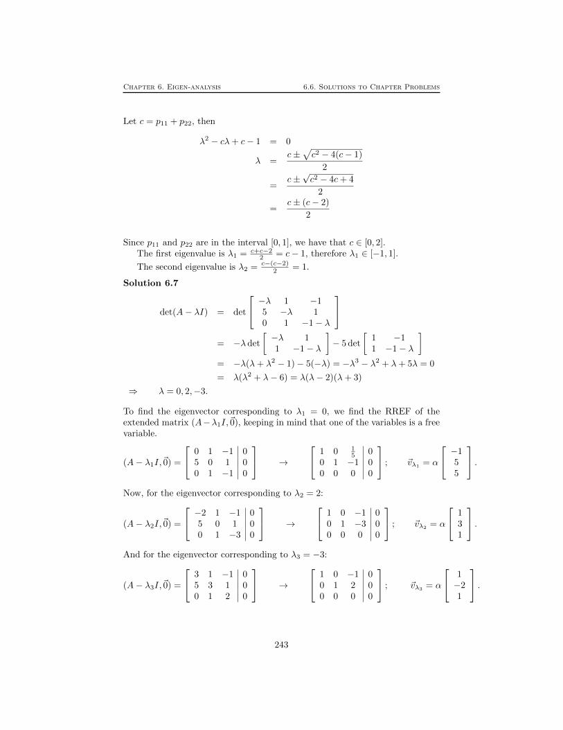
Chapter 6. Eigen-analysis 6.6. Solutions to Chapter Problems
Let c = p11 + p22, then
λ2 − cλ+ c− 1 = 0
λ =c±
√c2 − 4(c− 1)
2
=c±√c2 − 4c+ 4
2
=c± (c− 2)
2
Since p11 and p22 are in the interval [0, 1], we have that c ∈ [0, 2].The first eigenvalue is λ1 = c+c−2
2 = c− 1, therefore λ1 ∈ [−1, 1].
The second eigenvalue is λ2 = c−(c−2)2 = 1.
Solution 6.7
det(A− λI) = det
−λ 1 −15 −λ 10 1 −1− λ
= −λ det
[−λ 11 −1− λ
]− 5 det
[1 −11 −1− λ
]= −λ(λ+ λ2 − 1)− 5(−λ) = −λ3 − λ2 + λ+ 5λ = 0
= λ(λ2 + λ− 6) = λ(λ− 2)(λ+ 3)
⇒ λ = 0, 2,−3.
To find the eigenvector corresponding to λ1 = 0, we find the RREF of theextended matrix (A−λ1I,~0), keeping in mind that one of the variables is a freevariable.
(A− λ1I,~0) =
0 1 −1 05 0 1 00 1 −1 0
→
1 0 15 0
0 1 −1 00 0 0 0
; ~vλ1 = α
−155
.Now, for the eigenvector corresponding to λ2 = 2:
(A− λ2I,~0) =
−2 1 −1 05 0 1 00 1 −3 0
→
1 0 −1 00 1 −3 00 0 0 0
; ~vλ2= α
131
.And for the eigenvector corresponding to λ3 = −3:
(A− λ3I,~0) =
3 1 −1 05 3 1 00 1 2 0
→
1 0 −1 00 1 2 00 0 0 0
; ~vλ3= α
1−21
.
243

Chapter 6. Eigen-analysis 6.6. Solutions to Chapter Problems
Solution 6.8
det(A− λI) = det
2− λ 0 10 2− λ 11 0 2− λ
= (2− λ) det
[2− λ 1
0 2− λ
]+ det
[0 1
2− λ 1
]= (2− λ)3 − (2− λ) = (2− λ)
((2− λ)2 − 1
)= 0
= (2− λ)(λ2 − 4λ+ 3) = (λ− 2)(λ− 1)(λ− 3)
⇒ λ = 1, 2, 3.
To find the eigenvector corresponding to λ1 = 1, we again find the RREF of theextended matrix (A−λ1I,~0), keeping in mind that one of the variables is a freevariable.
(A− λ1I,~0) =
1 0 1 00 1 1 01 0 1 0
→
1 0 1 00 1 1 00 0 0 0
; ~vλ1= α
11−1
.Now, for the eigenvector corresponding to λ2 = 2:
(A− λ2I,~0) =
0 0 1 00 0 1 01 0 0 0
→
1 0 0 00 0 1 00 0 0 0
; ~vλ2= α
010
.And for the eigenvector corresponding to λ3 = 3:
(A− λ3I,~0) =
−1 0 1 00 −1 1 01 0 −1 0
→
1 0 −1 00 1 −1 00 0 0 0
; ~vλ3 = α
111
.Solution 6.9 The answer is yes. The two eigenvectors and eigenvalues definesix equations. There are nine unknowns -the entries of M- however, there isan extra condition; the rank of M is two. There are several solutions, here wepresent one.
Let’s try
M =
a11 0 a13
a21 0 a23
a31 0 a33
.We have here six unknowns and six equations, so there is a chance to find asolution. If the two non-zero column vectors are independent, then we are done,it has rank 2. a11 0 a13
a21 0 a23
a31 0 a33
123
=
−1−2−3
, and
a11 0 a13
a21 0 a23
a31 0 a33
321
=
−3−2−1
244

Chapter 6. Eigen-analysis 6.6. Solutions to Chapter Problems
a11 + 3a13 = −1, and 3a11 + a13 = −3
From this we have a13 = 0, and a11 = −1.
a21 + 3a23 = −2, and 3a21 + a23 = −2
From this we have that a21 = a23 = − 12 .
a131 + 3a33 = −3, and 3a31 + a33 = −1
This is similar to the first pair: a33 = −1, and a31 = 0.The resulting M matrix is
M =
−1 0 0− 1
2 0 − 12
0 0 −1
.M has rank 2, and −1 0 0− 1
2 0 − 12
0 0 −1
123
=
−1−2−3
, and
−1 0 0− 1
2 0 − 12
0 0 −1
321
=
−3−2−1
Solution 6.10
det
[2− λ 3−2 −1− λ
]= (2− λ)(−1− λ) + 6 = −2− 2λ+ λ+ λ2 + 6
= λ2 − λ+ 4 =
(λ− 1
2+ i
√15
2
)(λ− 1
2− i√
15
2
)= 0
⇒ λ =1
2± i√
15
2
Solution 6.11
a) Find values for a and b such that A2 = A[a ii b
] [a ii b
]=
[a ii b
]⇒ a2 − 1 = a ai+ bi = i
ai+ bi = i −1 + b2 = b
Hence, a2 − a− 1 = 0, and a+ b = 1. Upon solving the system we get
a =1±√
5
2, b =
1∓√
5
2
b) If A3 = A, then we can try
A−1A3 = A−1A ⇒ A2 = I
245

Chapter 6. Eigen-analysis 6.6. Solutions to Chapter Problems
[a ii b
] [a ii b
]=
[1 00 1
]⇒ a2 − 1 = 1 ai+ bi = 0
ai+ bi = 0 −1 + b2 = 1
Hence, a2 = 2, and a = −b. We get
a = ±√
2, b = ∓√
2[ √2 i
i −√
2
]2
= I ⇒ A3 = A; A4 = I 6= A
c) From the previous solution, we want A8 = I 6= A. If A4 = I, then A4 ·A4 =A8 = I, hence A9 = A.
Solution 6.12
a)
A =
[a ii b
]The two eigenvalues are 2 + i and 2− i. The characteristic polynomial is
(a− λ)(b− λ) + 1 = 0
λ2 − (a+ b)λ+ ab+ 1 = 0
λ1,2 =a+ b±
√(a+ b)2 − 4ab− 4
2
λ1,2 =a+ b
2±
√(a+ b
2
)2
− 1
λ1,2 should be 2 ± i. This is only possible if(a+b
2
)= 0, hence a = b, and
a+ b = 4. Therefore, a = b = 2, and the matrix is
A =
[2 ii 2
]b) Now, to find the eigenvectors, we now that the eigenvalues are λ1,2 = 2 +
i, 2− i For the first eigenvector we have
(A− λ1I)~v1 =
[−i ii −i
] [x1
x2
]= ~0
Hence x1 = x2, and v1 = α(1, 1)T .
For the second eigenvector we have
(A− λ2I)~v2 =
[i ii i
] [x1
x2
]= ~0
Hence x1 = −x2, and v2 = α(1,−1)T .
246

Chapter 6. Eigen-analysis 6.6. Solutions to Chapter Problems
Solution 6.13
P =
0 14
12
12
12
12
12
14 0
The characteristic polynomial is λ3 − 1
2λ2 − 1
2λ. From this, the eigenvalues arefound to be λ1,2,3 = 0, 1,− 1
2 .To find the eigenvector associated with λ1, we find the reduced row-echelon
form of the matrix (P − λ1I): 0 14
12 0
12
12
12 0
12
14 0 0
→
1 1 1 00 1 2 02 1 0 0
→
1 0 −1 00 1 2 00 −1 −2 0
→
1 0 −1 00 1 2 00 0 0 0
→ ~v1 =
1−21
To find the eigenvector associated with λ2, we find the RREF of the matrix
(P − λ2I): −1 14
12 0
12 − 1
212 0
12
14 −1 0
→
1 − 14 − 1
2 00 − 3
432 0
0 34 − 3
2 0
→
1 0 −1 00 1 −2 00 −1 −2 0
→ ~v2 =
1−21
Finally, to find the eigenvector associated with λ3, we find the RREF of the
matrix (P − λ3I): 12
14
12 0
12 1 1
2 012
14
12 0
→
1 12 1 0
0 34 0 0
0 0 0 0
→
1 0 1 00 1 0 00 −1 −2 0
→ ~v3 =
−101
We can express x(0) as a linear combination of the eigenvectors:
x(0) =1
4
1−21
+1
4
121
− 1
2
−101
=
100
.From the notes, we know that for n > 0 x(n) = Pnx(0), therefore the zeroeigenvalue and the −1/2 disappear for large n, and we have that
limn→∞
x(n) =
141214
247

Chapter 6. Eigen-analysis 6.6. Solutions to Chapter Problems
Solution 6.14
P =
14
13
12
12
13 b
14
13 a
We know that a ≥ 0, b ≥ 0, and that a + b = 1/2. If a > 0, and b > 0,by theorem 6.1 we know that the existence of an equilibrium probability isguaranteed. There are two cases left to be analyzed:
i) a = 0 and b = 1/2
ii) a = 1/2 and b = 0
In both cases one value of the matrix is zero, so we can’t apply theorem 6.1directly. On the other hand, P 2 for both cases is
i)
P 2 =
1748
1336
724
512
49
512
1148
736
724
ii)
P 2 =
1748
1336
38
724
518
14
1748
1336
38
with all positive entries in both cases, so there is always an equilibrium proba-bility.
Now, for the case a = b = 1/4 we have to find the aforementioned equilib-rium probability vector. From theorem 6.1, the vector will be the eigenvectorcorresponding to the eigenvalue λ = 1, with all its entries summing to one. Wefind the eigenvalue by finding the reduced row-echelon form of the extendedmatrix (P − λI,~0):
P =
− 34
13
12 0
12 − 2
314 0
14
13 − 3
4 0
→
4 0 −5 00 16 −21 00 0 0 0
→ ~v = α
202116
Since the entries of ~v have to sum to one, we get that the equilibrium probabilityvector is
1
57
202116
248

Chapter 6. Eigen-analysis 6.6. Solutions to Chapter Problems
Solution 6.15 The eigenvalues and vectors are λ1 = 2 x1 =
[−21
]and λ2 = 6
x2 =
[−11
]. Thus the general solution is
c1e2t
[−21
]+ c2e
6t
[−11
]To satisfy the initial condition we need
c1
[−21
]+ c2
[−11
]=
[11
]or [
−2 −11 1
] [c1c2
]=
[11
]which has solution [
c1c2
]=
[−23
]so the solution is
−2e2t
[−21
]+ 3e6t
[−11
]
Solution 6.16 The eigenvalues and vectors are λ1 = 1 + 2i x1 =
[i1
]and
λ2 = 1− 2i x2 =
[−i1
]. Thus the general solution in complex form is is
c1e(1+2i)t
[i1
]+ c2e
(1−2i)t
[−i1
]To find two real solution we take the real and imaginary parts of
e(1+2i)t
[i1
]=
[ie(1+2i)t
e(1+2i)t
]= et
[i(cos(2t) + i sin(2t))
cos(2t) + i sin(2t)
]= et
[− sin(2t) + i cos(2t)cos(2t) + i sin(2t)
]Thus the general solution in real form is
a1et
[− sin(2t)cos(2t)
]+ a2e
t
[cos(2t)sin(2t)
]To satisfy the initial condition we need
a1
[01
]+ a2
[10
]=
[11
]
249
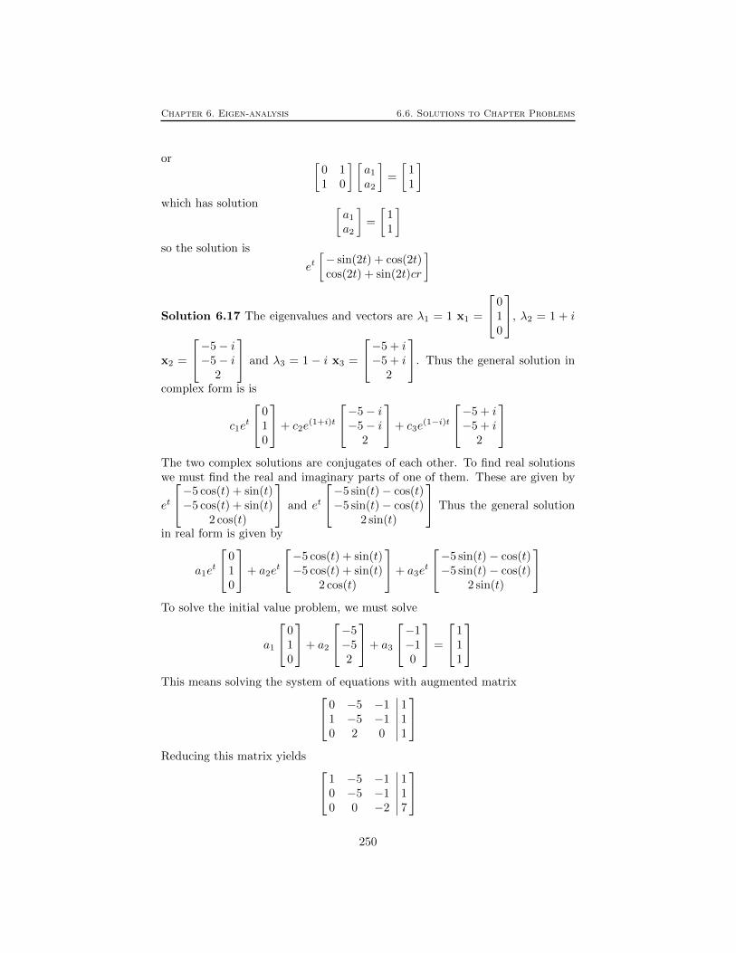
Chapter 6. Eigen-analysis 6.6. Solutions to Chapter Problems
or [0 11 0
] [a1
a2
]=
[11
]which has solution [
a1
a2
]=
[11
]so the solution is
et[− sin(2t) + cos(2t)cos(2t) + sin(2t)cr
]
Solution 6.17 The eigenvalues and vectors are λ1 = 1 x1 =
010
, λ2 = 1 + i
x2 =
−5− i−5− i
2
and λ3 = 1 − i x3 =
−5 + i−5 + i
2
. Thus the general solution in
complex form is is
c1et
010
+ c2e(1+i)t
−5− i−5− i
2
+ c3e(1−i)t
−5 + i−5 + i
2
The two complex solutions are conjugates of each other. To find real solutionswe must find the real and imaginary parts of one of them. These are given by
et
−5 cos(t) + sin(t)−5 cos(t) + sin(t)
2 cos(t)
and et
−5 sin(t)− cos(t)−5 sin(t)− cos(t)
2 sin(t)
Thus the general solution
in real form is given by
a1et
010
+ a2et
−5 cos(t) + sin(t)−5 cos(t) + sin(t)
2 cos(t)
+ a3et
−5 sin(t)− cos(t)−5 sin(t)− cos(t)
2 sin(t)
To solve the initial value problem, we must solve
a1
010
+ a2
−5−52
+ a3
−1−10
=
111
This means solving the system of equations with augmented matrix 0 −5 −1
1 −5 −10 2 0
∣∣∣∣∣∣111
Reducing this matrix yields 1 −5 −1
0 −5 −10 0 −2
∣∣∣∣∣∣117
250

Chapter 6. Eigen-analysis 6.6. Solutions to Chapter Problems
Which yields the solution a1 = 0, a2 = 1/2 and a3 = −7/2. So the final answeris
1
2et
−5 cos(t) + sin(t)−5 cos(t) + sin(t)
2 cos(t)
− 7
2et
−5 sin(t)− cos(t)−5 sin(t)− cos(t)
2 sin(t)
= et
cos(t) + 18 sin(t)cos(t) + 18 sin(t)cos(t)− 7 sin(t)
Solution 6.18
y′(t) =
[1 15 1
]y(t)
The characteristic polynomial is (1− λ)2 − 5 = 0, hence λ1,2 = 1±√
5We need to find the eigenvectors:[−√
5 1
5 −√
5
]→ ~v1 =
[1√5
];
[ √5 1
5√
5
]→ ~v2 =
[1
−√
5
]The general solution is given by
y(t) = c1eλ1t~v1 + c2e
λ2t~v2
= c1e(1+√
5)t
[1√5
]+ c2e
(1−√
5)t
[1
−√
5
]Or, equivalently
y1(t) = c1e(1+√
5)t + c2e(1−√
5)t
y2(t) = c1√
5e(1+√
5)t − c2√
5e(1−√
5)t
Solution 6.19
y′(t) =
[3 −11 −1
]y(t)
The characteristic polynomial is λ2 − 2λ− 2 = 0, hence λ1,2 = 1±√
3We need to find the eigenvectors:[
2−√
3 −1
1 −2−√
3
]→ ~v1 =
[2 +√
31
][
2 +√
3 −1
1 −2 +√
3
]→ ~v2 =
[2−√
31
]The general solution is given by
y(t) = c1e(1+√
3)t
[2 +√
31
]+ c2e
(1−√
3)t
[2−√
31
]The initial condition states that y(0) = [0, 1]T . Hence
c1(2 +√
3) + c2(2−√
3) = 0
c1 + c2 = 1
c1 =1
2− 1√
3, c2 =
1
2+
1√3
251

Chapter 6. Eigen-analysis 6.6. Solutions to Chapter Problems
Or, equivalently
y1(t) = − 1
2√
3e(1+
√3)t +
1
2√
3e(1−
√3)t
y2(t) =
(1
2− 1√
3
)e(1+
√3)t −
(1
2+
1√3
)e(1−
√3)t
Solution 6.20
y′(t) =
[3 −17 1
]y(t)
The characteristic polynomial is λ2 + 2λ+ 4 = 0, hence λ1,2 = −1± i√
3Finding the eigenvectors:[
−2− i√
3 −1 0
7 2− i√
3
]→ ~v1 =
[−2 + i
√3
7
]The function below is a solution. We will separate the real and imaginary partsto get two independent solutions:
e(−1+i√
3)t
[−2 + i
√3
7
]=
1
etei√
3t
[−2 + i
√3
7
]=
1
et
[−2 + i
√3
7
](cos(
√3t) + i sin(
√3t))
=1
et
[−2 cos(
√3t)−
√3 sin(
√3t)
7 cos(√
3t)
]+ · · ·
i
et
[ √3 cos(
√3t)− 2 sin(
√3t)
7 sin(√
3t)
]The general solution is
y(t) =c1et
[−2 cos(
√3t)−
√3 sin(
√3t)
7 cos(√
3t)
]+c2et
[ √3 cos(
√3t)− 2 sin(
√3t)
7 sin(√
3t)
]The initial condition states that y(0) = [2,−1]T . Hence
−2c1 +√
3c2 = 2
7c1 = −1
c1 = −1
7, c2 =
12
7√
3
Solution 6.21 If A is a 3 × 3 matrix with real entries, then det(A − λI) isa polynomial of the form −λ3 + aλ2 + bλ + c. If you plot the graph of thispolynomial, it tends to infinity for large positive λ and to negative infinity forlarge negative λ. Thus there must be a place where the polynomial crossesthe real axis, that is, a real zero. This means that there is always at least one
252

Chapter 6. Eigen-analysis 6.6. Solutions to Chapter Problems
real eigenvalue. The other two eigenvalues can be either both real, or complexconjugates (as in the previous problem).
Solution 6.22 We have to solve the equation
x′(t) =
[−1 −11 −1
]x(t)
with
x(0) =
[11
]The eigenvalues and eigenvectors of the matrix are λ1 = −1 + i, x1 =
[1−i
],
λ2 = −1− i, x2 =
[1i
]Real solutions are the real and imaginary parts of
e(−1+i)t
[1−i
],
which are
e−t[
cos(t)sin(t)
]and
e−t[
sin(t)− cos(t)
]Thus the general solution is
x(t) = a1e−t[
cos(t)sin(t)
]+ a2e
−t[
sin(t)− cos(t)
].
To satisfy the initial conditions, we need
a1
[10
]+ a2
[0−1
]=
[11
]so a1 = 1, a2 = −1 and the solution is
e−t[
cos(t)− sin(t)sin(t) + cos(t)
]Solution 6.23 The current is the same through each component. The voltageacross the resistor is IR, so if VL is the voltage across the inductor, then VL +V + IR = 0 so VL = −V − IR. The equations are therefore
I ′ = 1LVL = −RL I −
1LV
V ′ = 1C I
or [IV
]′=
[−RL − 1
L1C 0
] [IV
]
253
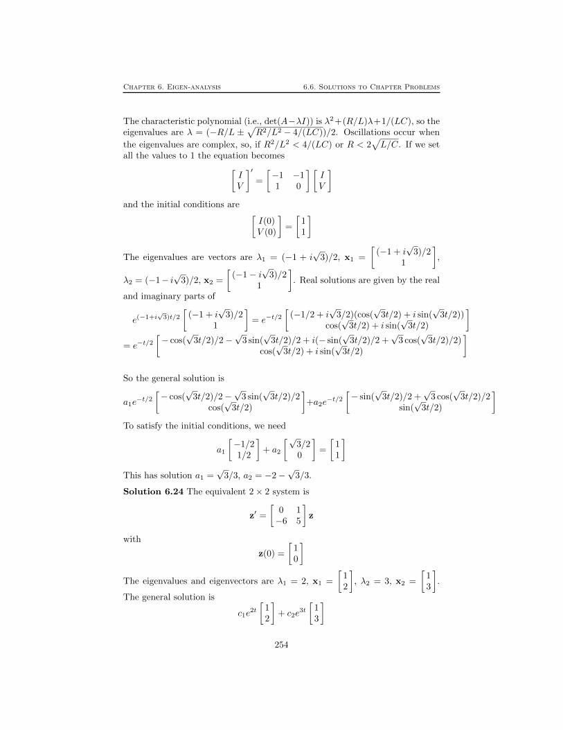
Chapter 6. Eigen-analysis 6.6. Solutions to Chapter Problems
The characteristic polynomial (i.e., det(A−λI)) is λ2 +(R/L)λ+1/(LC), so theeigenvalues are λ = (−R/L ±
√R2/L2 − 4/(LC))/2. Oscillations occur when
the eigenvalues are complex, so, if R2/L2 < 4/(LC) or R < 2√L/C. If we set
all the values to 1 the equation becomes[IV
]′=
[−1 −11 0
] [IV
]and the initial conditions are [
I(0)V (0)
]=
[11
]
The eigenvalues are vectors are λ1 = (−1 + i√
3)/2, x1 =
[(−1 + i
√3)/2
1
],
λ2 = (−1− i√
3)/2, x2 =
[(−1− i
√3)/2
1
]. Real solutions are given by the real
and imaginary parts of
e(−1+i√
3)t/2
[(−1 + i
√3)/2
1
]= e−t/2
[(−1/2 + i
√3/2)(cos(
√3t/2) + i sin(
√3t/2))
cos(√
3t/2) + i sin(√
3t/2)
]= e−t/2
[− cos(
√3t/2)/2−
√3 sin(
√3t/2)/2 + i(− sin(
√3t/2)/2 +
√3 cos(
√3t/2)/2)
cos(√
3t/2) + i sin(√
3t/2)
]
So the general solution is
a1e−t/2
[− cos(
√3t/2)/2−
√3 sin(
√3t/2)/2
cos(√
3t/2)
]+a2e
−t/2[− sin(
√3t/2)/2 +
√3 cos(
√3t/2)/2
sin(√
3t/2)
]To satisfy the initial conditions, we need
a1
[−1/21/2
]+ a2
[√3/20
]=
[11
]This has solution a1 =
√3/3, a2 = −2−
√3/3.
Solution 6.24 The equivalent 2× 2 system is
z′ =
[0 1−6 5
]z
with
z(0) =
[10
]The eigenvalues and eigenvectors are λ1 = 2, x1 =
[12
], λ2 = 3, x2 =
[13
].
The general solution is
c1e2t
[12
]+ c2e
3t
[13
]
254

Chapter 6. Eigen-analysis 6.6. Solutions to Chapter Problems
The initial conditions are satisfied if
c1
[12
]+ c2
[13
]=
[10
]which has solution c1 = 3, c2 = −2. So y(t) = z1(t) = 3e2t − 2e3t. To solve thisdirectly, plug in eλt. This solves the equation if λ2 − 5λ+ 6 = 0, or λ = 2 or 3.So the general solution is y(t) = c1e
2t + c2e3t. Satisfying the initial conditions
y(0) = 1 and y′(0) = 0 leads to c1 = 3 and c2 = −2 as above.
Solution 6.25 The equivalent 2× 2 system is
z′ =
[0 1−1 −1
]z
with
z(0) =
[10
]The eigenvalues and eigenvectors are λ1 = −1/2+i
√3/2, x1 =
[1
−1/2 + i√
3/2
],
λ2 = −1/2 − i√
3/2, x2 =
[1
−1/2− i√
3/2
]Real solutions are the real and
imaginary parts of
e(−1/2+i√
3/2)t
[1
−1/2 + i√
3/2
]which leads to the general solution
a1e−t/2
[cos
−(1/2) cos−(√
3/2) sin
]+ a2e
−t/2[
sin(√
3/2) cos−(1/2) sin
](the sines and cosines are evaluated at
√3t/2). Initial conditions require
a1
[1
−(1/2)
]+ a2
[0
(√
3/2)
]=
[10
]which has solution a1 = 1 and a2 =
√3/3. Thus the solution is y(t) = z1(t) =
e−t/2(cos(√
3t/2) + (√
3/3) sin(√
3t/2)) If we try to solve directly by substi-tuting eλt, we get λ = −1/2 ± i
√3/2. The real and imaginary parts of eλt
are e−t/2(cos(√
3t/2) and e−t/2 sin(√
3t/2)), so we obtain the general solutiony(t) = a1e
−t/2(cos(√
3t/2) + a2e−t/2 sin(
√3t/2)). Choosing a1 and a2 to solve
the initial condition yields the same answer as above.
Solution 6.26 Set z1(t) = y(t), z2(t) = y′(t) and z3(t) = y′′(t). Then z =
z1
z2
z3
solves the equation
z′ =
0 1 00 0 1−c −b −a
z
255

Chapter 6. Eigen-analysis 6.6. Solutions to Chapter Problems
Solution 6.27 The general solution is
(a1 cos(t)+b1 sin(t))
101
+(a2 cos(2t)+b2 sin(2t))
10−1
+(a3 cos(3t)+b3 sin(3t))
010
To satisfy the initial conditions, we need
a1
101
+ a2
10−1
+ a3
010
=
121
which has solution a1 = 1, a2 = 0 and a3 = 2, and
b1
101
+ 2b2
10−1
+ 3b3
010
=
011
which has solution b1 = 1/2, 2b2 = −1/2 and 3b3 = 1, so that b1 = 1/2,b2 = −1/4 and b3 = 1/3
Solution 6.28 Going through the analysis with two springs and weights, weend up with
K =
[−2 11 −1
]and
b =
[1011
]Then
xeq = K−1b =
[2131
]so if we define y = x− xeq, we obtain initial conditions
y(0) =
[11
]and
y′(0) =
[11
]The eigenvalues of K are λ1 = (−3 +
√5)/2 and λ2 = (−3 −
√5)/2 with
eigenvectors x1 =
[(−1 +
√5)/2
1
]and x2 =
[(−1−
√5)/2
1
]. If we set µ1 =
√−λ1 and µ2 =
√−λ2, then the general solution is
y(t) = (a1 cos(µ1t) + b1 sin(µ1t))x1 + (a2 cos(µ2t) + b2 sin(µ2t))x1
The initial condition are satisfied if
a1x1 + a2x2 =
[11
]
256
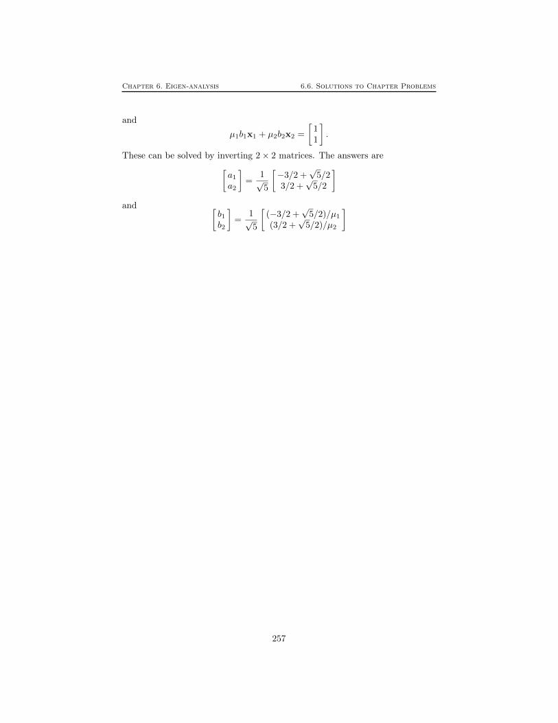
Chapter 6. Eigen-analysis 6.6. Solutions to Chapter Problems
and
µ1b1x1 + µ2b2x2 =
[11
].
These can be solved by inverting 2× 2 matrices. The answers are[a1
a2
]=
1√5
[−3/2 +
√5/2
3/2 +√
5/2
]and [
b1b2
]=
1√5
[(−3/2 +
√5/2)/µ1
(3/2 +√
5/2)/µ2
]
257