IFN Working Paper No. 965, 2013 Rich Man’s War, Poor Man’s Fight? Socioeconomic Representativeness in the Modern Military Andrea Asoni and Tino Sanandaji

Research Institute of Industrial Economics P.O. Box 55665

SE-102 15 Stockholm, Sweden info@ifn.se www.ifn.se

Rich Man’s War, Poor Man’s Fight? 

Socioeconomic representativeness in the modern military  

Andrea Asonii, Tino Sanandajiii 

Historically, the American armed forces were disproportionally drawn from lower

socioeconomic backgrounds. A transition toward a smaller and more selective military has

changed this tendency. Since the armed forces do not gather data on recruits’ family income,

previous studies relied on geographic data to proxy for economic background. We improve on

previous literature using individual-level data from the National Longitudinal Survey of Youth

1997 and study population representativeness in the years 1997–2011.

We find that recruits score higher than the civilian population on cognitive skill tests, and come

from households with above average median parental income and wealth. Moreover, both the

lowest and highest parental income categories are under-represented. Higher skill test scores

increase enlistment rates from lower- and middle-income families while decreasing them for

high income families. The over-representation of minorities in the military has declined in recent

decades. Non-Hispanic White casualties are now over-represented in Iraq and Afghanistan.

Keywords: military service; occupational choice; human capital.

JEL Codes: H41; J18; J24;

 

 

1. Introduction

It is often considered a societal goal that the burden of serving in the armed forces does not

disproportionally fall on a few social groups (for example, Cooper 1977, CBO 2007, Wright

2012). The Democratic Leadership Council (1988) argued the United States “cannot ask the poor

and under-privileged alone to defend us while our more fortunate sons and daughters take a free

ride, forging ahead with their education and careers.” The Department of Defense (1997) points

out that: “Imbalances in socioeconomic representation in the military have often been a

controversial social and political issue. In debate over the establishment of the volunteer force,

opponents argued that it would lead to a military composed of those from poor and minority

backgrounds, forced to turn to the military as an employer of last resort.”

Concerns about population representativeness and shared sacrifice were already

important during the American Revolution and the Civil War. Discussing compulsory service,

Benjamin Franklin is quoted as having written “The question will then amount to this; whether it

be just in a community, that the richer part should compel the poor to fight for them and their

properties” (Warner and Asch 2001). A popular saying since the Civil War has been the phrase

“It is a rich man’s war and a poor man’s fight.” (Moore 1924).

Concerns were raised again during the Vietnam War, when young men from higher

socioeconomic background had better opportunities of evading the draft (Rostker 2006, Rohlfs

2012). Studies of Vietnam era veterans found that recruits of high socioeconomic background

 

 

were under-represented by half compared to their representation in the overall population

(Boulanger 1981).

In association with the creation of the volunteer army, the problem has shifted from

disparities in the opportunity to evade service to disparities in incentives to join. The idea is that

the under-privileged, lacking outside options, are pushed or lured into the armed forces. One of

the main arguments against replacing the draft with a volunteer military was that relying on

economic incentives to enlist personnel would lead to over-representation of the poor among

casualties. According to Laurence (2004), opponents of a volunteer military argued that

“economic incentives used as the key to ending conscription were tantamount to luring the poor

to their deaths.” Besides fairness, there are other concerns with a military recruited primarily

among the poor. For example, Janowitz (1975) argued that by recruiting predominantly among

lower socioeconomic groups, a volunteer military would lead to divisions between the military

and the rest of society.

Recruits from lower socioeconomic background continue to have stronger incentives to

join the military for employment or to finance education. The move toward a smaller and more

technologically advanced military has however made military recruitment more selective and

created a tendency in the opposite direction. Individuals without high-school degrees, with

criminal records, a poor health record, and those scoring low in skill tests are significantly less

likely to be allowed in the military. This has created a powerful force against recruiting from

lower socioeconomic background. It is no longer clear that the armed forces come from

disadvantaged backgrounds.

 

 

The assumption that the armed forces disproportionally recruit from the poor and ethnic

minorities is still widely used in political science and sociological research (e.g Vasquez 2005,

Gelpi et al. 2009, Horowitz et al. 2011, Kriner and Shen 2013). Moreover, a widespread public

impression remains that the poor and ethnic minorities disproportionally bear the burden of

defending the United States (for example, Rangel 2004, Tyson 2005, DLC 1988, Kristof 2012).

Representative Charles Rangel has referred to the war in Iraq as a “death tax […] on the poor”

(Rangel 2004). In order to ensure “shared sacrifice” in war congressman Rangel has called for

the reinstatement of the draft. A New York Times column recently described joining the military

as “a traditional escape route for poor, rural Americans” (Kristof 2012).

It has proven difficult to settle this issue since the United States armed forces do not track

parental income of recruits. This is in part due to the experience of the military that “recruit-aged

youth are not accurate at estimating their parents’ income” (DoD 2000). CBO (2007) points out

that “The socioeconomic backgrounds of service members have been less well documented than

other characteristics because data on the household income of recruits before they joined the

military are sparse.” Studies which attempt to estimate representativeness have instead relied on

proxies such as the median income in the recruit zip code or parental education (Kane 2005,

Kriner and Shen 2010, DoD 2011). However geography-based studies are inherently limited in

determining individual-level behavior, and have reached conflicting conclusions. In this paper,

we rely on individual-level data from the National Longitudinal Survey of Youth 1997

(NLSY97) to estimate population representativeness. The NLSY97 collects detailed data and

follows a large, representative sample of young Americans. Between 1997 and 2011, a

 

 

significant share of the sample joined the military, which allows us to compare recruits with the

rest of the population.

After reviewing previous studies, we describe results derived from the Department of

Defense data and compare when possible with the NLSY97 data. Our fourth section illustrates

the NSLY97 data and our empirical approach. The results from the NLSY97 data are presented

in section five, while the sixth section discusses related evidence from other sources. Finally,

section seven illustrates the hazards of the geographic data and section eight concludes.

2. Previous Studies and Common Perceptions

Since 1989, the US military has administered “The Survey of Recruit Socioeconomic

Backgrounds” at recruit training centers to ascertain recruits’ background, including information

on “parents’ education, employment status, occupation, and home ownership.” However

household income of the youth, arguably the most straightforward proxy for social position, is

not included in the data. The reason is that the military believes that “While income is a widely

used measure of socioeconomic status, research provides evidence that recruit-aged youth are not

accurate at estimating their parents' income. Therefore, home ownership is included as a proxy

for income” (DoD 1998). In 1995, a survey conducted by the military found that recruits scored

lower than the general population in terms of socioeconomic index (DoD 1997).

The NLSY79 was used to study the socioeconomic background of recruits, finding that

those who served in the military in 1979 were from lower than average socioeconomic

background (Fredland and Little 1982). This was a few years after the abolition of the draft in

 

 

1973. Earlier studies that followed the end of the draft confirmed that recruits were

disproportionally drawn from lower socioeconomic backgrounds (for example, Cooper 1977 and

Fernandez 1989). Teachman et al. (1993) similarly found that white male recruits tend to come

from more disadvantaged backgrounds.

Lacking individual-level data has forced researchers to rely on the geographic origin of

recruits as a proxy for socioeconomic background. However this approach is not always reliable.

The department of defense writes on the topic (DoD 2000) “While this type of data is useful for

demographic trend analysis and advertising and marketing research, it is not reliable for

comparing socioeconomic representation in the military to that of the general population. For

example, applicants and recruits may not come from the background indicated by the zip code

for their current address (i.e., these individuals may move away from home to go to college or to

work).” Kane (2005) used the median household income of the census bureau zip codes of

recruits as a proxy for the income of the recruits. He concluded that the burden of service was

not as unbalanced as previously believed, and that middle and higher middle income groups

where in fact disproportionally represented among the recruits.

Kriner and Shen (2010) study enlistment during 1999-2006 using geographic data and

come to the opposite conclusion. They find that enlistment was significantly higher in zip-codes

with below average median income. Kriner and Shen (2010) also rely on geographic data to

study casualty rather than service. They find that lower income communities were over-

represented as casualties in wars since the Korean War, including the war in Iraq. The conflicting

results of geographic-level data for a similar time period emphasizes the need to use individual-

level data to estimate representativeness. Simon and Warner (2007) also follow a geographic

 

 

approach and find that individuals from lower-income zip codes were more likely to enlist. Lien

(2012) also relies on geographic data and finds that recruits disproportionally come from zip-

codes with lower than average median income. The literature which relies on zip-code average

income levels as proxies for the income of recruits has thus not provided a definitive answer.

One explanation is that some studies control for background variables. Elder et al. (2010)

for example finds that males with college educated parents are less likely to enlist in the military

directly after high-school once controlling for test scores. Controlling for background variables

can be misleading if we are interested in actual socioeconomic representativeness.

Despite the existence of conflicting results in the literature, the notion that recruits and

casualties are disproportionally poor and non-white has however remained a stylized fact in

much of political science and sociology. This assumption is used in theoretical models, and when

interpreting other results.

According to a fairly influential theory, the lack of socioeconomic representativeness in

the armed forces diminishes the pacifying effect of democracy (Vasquez 2005, Horowitz et al.

2011). Immanuel Kant famously argued that citizens of democratic societies are more cautious of

war because the citizens themselves risk becoming casualties. In other words, the costs of

wartime casualties are internalized to a greater extent in democracies.

In the same vein, Vasquez (2005) argues that the pacifying effect of democracy is

weakened in societies with volunteer armies where elites are under-represented. In particular,

 

 

casualties suffered by conscript armies recruited from broad segments of society are more likely

to affect elites than casualties suffered by volunteer forces recruited from lower income groups.

Vasquez (2005) does not discuss the socioeconomic representation of the military in detail and

accepts the premise that volunteer forces disproportionally come from underprivileged

backgrounds: “volunteer militaries are often composed largely of self-selected, economically

motivated volunteers who come from social groups that lack economic or career opportunities in

civilian life.”

Gelpi et al. (2009) estimates how many wartime casualties the American public is willing

to accept as a price for various security goals. The authors speculate that one cause for lower

casualty tolerance among African Americans is the worry that their community is asked to

shoulder a disproportionate burden of American casualties, assuming that African Americans are

still over-represented in war casualties.

A study by Kriner and Shen (2013) points out that casualty aversion among the American

public is not merely a function of numbers, but also depends on how sacrifice is shared across

society. The empirically uncertain notion that casualties tend to be poor was used as a fact told to

respondents in surveys. In an experiment, the authors show that casualty aversion increases if

respondents are told that in wars in Korea, Vietnam and Iraq, “America’s poor communities have

suffered significantly higher casualty rates than America’s rich communities.” The notion that

disadvantaged groups are over-represented as casualties rests on geographic-level data. The

study concludes that “Americans are less willing to accept casualties in future military endeavors

when informed that the costs of war fall disproportionately on the shoulders of a disadvantaged

few.” Many conclusions in Kriner and Shen (2013) are based on the premise that casualties in

 

 

the Iraq war disproportionally came from the bottom of the socioeconomic spectrum. This is,

however, not established empirically using individual-level data.

The military is one of the largest employers in the United States. Close to one in ten

American males serve in the military. The socioeconomic background of military recruits is

therefore potentially important for broad economic outcomes. Kentor et al. (2012) argue that a

reduced emphasis on manpower in the armed forces in favor of equipment can indirectly increase

inequality: “We hypothesize that this new, increasingly capital-intensive military is no longer a

pathway of upward mobility or employer of last resort for many uneducated, unskilled, or

unemployed people, with significant consequences for those individuals and society as a whole.”

3. Population representativeness in the

Department of Defense Data

We rely on the NLSY97 to study recruitment among a representative sample, in part because this

enables us to study variables such as income which are otherwise hard to gather. For many other

variables the Department of Defense provides data on the universe of recruits. This includes the

state of residence of recruits, and the race and ethnicity of military fatalities. This data is hard to

accurately estimate using the NLSY97. We also report the race and ethnicity of recruits from the

Department of Defense data. Since this can also be estimated using the NLSY97, it is interesting

to compare the DoD universe of recruits data with the NLSY97 data as a measure of external

validity for using the latter to study the background of recruits.

 

 

Minorities were historically over-represented in the American military, but this has

changed recently. African Americans’ share of recruits has fallen since the 1990s: in 2011 the

group accounted for 15 percent of the civilian population aged 18–24, and 16 percent of recruits.

Hispanics constituted 19 percent of the civilian population and 17 percent of recruits (DoD

2011). We find similar results in our data.

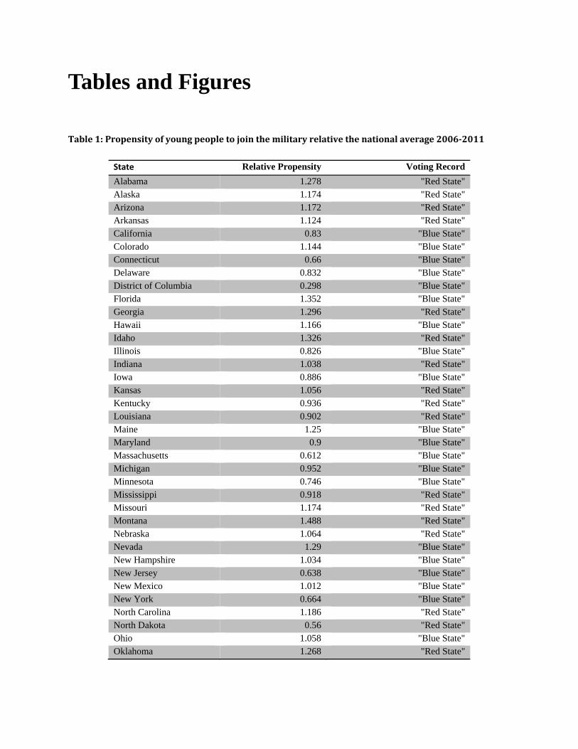
Recruits also differ in terms of geographic patterns. The propensity to join the military

can be estimated through the recruit-to-population ratio, based on the 18–24 year old population

in each state. We average the recruit-to-population ratio for the years 2006 through 2011, with

results in Table 1. This figure is calculated using the annual Department of Defense Population

Representation in the Military Services report, supplemented by figures provided by Watkins and

Sherk (2008). The sample is divided in states carried by Mitt Romney in the 2012 elections

(“Red States”) and those carried by Barack Obama (“Blue States”). Overall, young residents of

“Red States” were 36 percent more likely to join the military than young residents of “Blue

States.” The correlation between the recruit-to-population ratio and Mitt Romney’s share of the

vote is 0.48.

4. The National Longitudinal Survey of Youth

Our main source of data is the National Longitudinal Survey of Youth 1997 cohort (NLSY97).

The NLSY97 is a nationally-representative social science survey maintained by the U.S. Bureau

of Labor Statistics. The survey contains a rich set of data about the participants, including labor

market history, skill test scores, socioeconomic background, and military service. The sample is

 

 

comprised of 8,984 youths born between 1980 and 1984 who were initially interviewed in 1997

and in every year since.

The individual is determined to have joined the military if he or she reports to having

served at least one year in the regular military or the reserve. Those who serve in the National

Guard but no other service are excluded from the analysis.

The United States military screens its recruits based on a number of criteria. Potential

recruits who have poor health, are obese, or have a criminal record are less likely to be admitted.

The military also tends to require a high-school degree. Recruitment is made to a large extent

based on the Armed Forces Qualification Test (AFQT), a composite score which estimates

knowledge and skills. The AFQT is derived from the ten part test Armed Forces Vocational

Aptitude Test Battery (ASVAB). Only a small fraction of those who score among the lowest 30

percent in the AFQT are allowed to join the military. In fact, the AFQT is rewarded a high

weight in recruitment of soldiers. The United States armed forces state that: “AFQT scores are

the primary measure of recruit potential.” (DoD 2006). A version of the AFQT was administered

to the NLSY97 sample, which gives us an estimate of their skill level.

Socioeconomic status is estimated through family income and family wealth in 1997,

when nearly the entire sample still lived with their parents. We also calculate education as the

number of years of education completed by 2010. In 2008 the NLSY includes a question asking

the respondents “All things considered, how satisfied are you with your life as a whole these

days? Please give me an answer from 1 to 10”. This variable is used to estimate self-reported life

satisfaction.

 

 

5. Demographic Characteristics of Recruits

This section reports the results of our analysis of military recruits. Each sub-section focuses on a

few demographic characteristics. In the end, we present a comprehensive regression analysis that

includes several of these variables and additional ones. All analyses use population weights

designed to correspond to the demographic distribution of the general population.

5.1GenderandMortality

Table 2 lists the characteristics of those who joined the military and those who did not; the latter

we refer to as civilians.

Between 1997 and 2011, 465 individuals from the sample joined the military,

representing 5.3 percent of the reference population using sample weights. Of these, 442 joined

the regular military and 32 individuals joined the National Guard. Among men, 8.5 percent

joined the military, compared to 2.0 percent of women.

We look at mortality rates among those who served and civilians. We do not find

evidence of people who joined the military being more likely to die: only 0.37 percent of men

who served are reported dead in 2010 while this number is approximately 1.63 percent for

civilians. Among women, none of those who served are reported dead in 2010 while 1 percent

are reported dead among civilians. Needless to say, military and civilian death rates are not

comparable due to population heterogeneity, such as the requirement for recruits to be healthy.

Armed Forces Health Surveillance Center (2012) looks at the deaths of active duty personnel in

 

 

the armed forces in the period 1990–2011. They also find that the death rate is significantly

lower in the military than for similarly aged members of the civilian population. While this may

appear surprising, it is worth noting that even during the wars in Iraq and Afghanistan, no more

than one third of deaths among active duty personnel were caused by combat. In fact the single

biggest cause of death is transportation accidents.

5.2ParentalIncomeandWealth

Table 2 shows that median family income was $68,000 for men and $71,000 for women who

joined the military. These figures are higher than the median family income of civilians which

was around $61,000.iii The average family income of those who joined was around 4 percent

higher than that of civilians. Table 3 shows the probability of joining the military by quintile of

parental income. The income group most likely to join is the 4th quintile. Figure 1 shows the

distribution of income and the likelihood of joining.iv The figure shows that the probability of

joining follows a reversed U-shape, with both the poorest and the richest youngsters being less

likely to join while middle-income individuals are more likely to do so. The figure shows that the

probability of joining the military peaks above the median and average income in the sample.

Again in Table 2, it is shown that the median household wealth of males who served is

also higher than civilians. In contrast to median, average parental wealth is lower among male

military recruits than civilians. This is due to high inequality in the distribution of wealth.

Because much of wealth is owned by the very rich and because the children of the rich are less

likely to join, the average wealth of recruits is lower than civilians. Table 3 shows the probability

of joining the military by quintile of parental wealth. The income groups most likely to join are

 

 

the 3rd and 4th quintile. Figure 2 shows the likelihood of joining against the distribution of

parental wealth. Once more we observe a reversed U-shaped curve, with the richest and poorest

under-represented.

These results are similar to those provided by the zip-code based analysis of Kane (2005);

recruits in recent years have disproportionally come from somewhat higher than average income

groups, and both the richest and the poorest are under-represented. We thus observe a reversal of

patterns with respect to studies of the NLSY79. For the year 1979, Fredland and Little (1982)

found that those who served were disproportionally from lower socioeconomic background.

5.3TheEffectofParentalIncomebySkillandRace

A natural question that arises from the analyses presented so far is whether the effect of income

differs across races and ethnicities, tested skill levels, or education. In order to investigate the

effect of the interaction between parental income and skills on the probability of joining the

military, we employ a standard regression analysis technique. We use a Logit model to estimate

the effect of the different variables illustrated above and some additional ones on the probability

of joining the military in the years 1998–2010. Marginal effects derived from the regression are

reported in Table 4. We employed various specifications that included an increasing number of

independent variables in order to test the robustness of our findings.

The dependent variable is a dummy indicator, equal to one if the individual has joined the

military in any of the years under scrutiny and equal to zero otherwise. The regression analysis

confirms the findings illustrated earlier. Both income and skills have a positive effect on the

probability of joining the military. The negative coefficients on the square of income and the

 

 

square of skills indicate that as they increase, the positive effects of income and intelligence

decrease. These findings confirm the reverse U-shape we illustrated earlier for income and

suggest a similar shape for the effect of skills. Note that the coefficient on the square of income

is not always statistically different from zero.

The positive and statistically significant coefficients on the African-American and

Hispanic dummies indicate that minorities are more likely to join the military, but only after

controlling for skills. Without controlling for skill test results as measured by the AFQT, we are

left with the impression that, on average, minorities are not more likely to join the military. Other

coefficients have the expected signs: being male, healthy, from the South, and not obese are all

positively associated with the probability of joining the military.v Being born in the US and

coming from a rural area do not seem to have a statistically significant effect on the probability

of joining the military.

5.3.1ParentalIncomeandSkills

Columns (5) to (7) in Table 4 show that the coefficient on the interaction between

parental income and the AFQT score is negative and statistically significant. The negative sign

indicates that the positive effect of skills (income) on the probability of joining the military

decreases with income (skills). In other words, skills increase the likelihood of joining the

military more for individual from a low income family than for high income earners.

In fact, the effect of skills changes sign from positive to negative for high levels of

income, as shown in Figure 3. For yearly family incomes higher than $130,000, the effect of the

AFQT score becomes negative, and grows more negative as income increases. Thus higher skills

 

 

significantly increase enlistment rates of individuals from low income homes, while at the same

time reducing rates for individuals from high income families. We speculate that a reason for this

phenomenon is that high income, individuals with high skill test scores have greater access to

higher education. Low income high skill individuals by comparison may join the military in

order to finance their studies. This group may moreover view the military as a substitute carrier

to the civilian sector which values skills without entry barriers in the form of costly higher

education.

5.3.2ParentalIncomeandParentalEducation

In column (7) of Table 4 we add both parental education and the interaction between parental

education and parental income to the regression. Note that while parental education does not

have a statistically significant effect by itself, the coefficient on the interaction between parental

income and parental education is negative and statistically significant. Similar to what we have

discussed above for skills, the arguably positive effect of income on the probability of joining the

military decreases with parental education.

We also looked at the interaction between parental income, race, and ethnicity, being

from the South, and a rural dummy, but found no statistically significant result. These

regressions are not reported in the table.

5.4Education

There is no statistically significant difference between civilians and recruits in terms of parental

education. There is however a statistically significant difference among recruits and civilian

 

 

youths themselves. By 2010, when the sample was aged 25 to 31, military recruits have on

average 0.25 more years of education than the civilian sample. One explanation is that

educational subsidies are an important form of payment for military service. No claim about

causality can be made, as those who join the military differ in many ways from civilians.

5.5LifeSatisfaction

Interestingly, those who joined the military tend to have higher than average self-reported life

satisfaction. The average difference is 0.13 standard deviations, which is statistically significant.

By contrast, Fredland and Little (1982) found that in the 1979 NLSY, those who served had

lower job satisfaction than those with civilian jobs, indicating a change of recruit attitudes during

the last few decades.

5.6Interestinjoiningthemilitary

Participants in the NLSY who took the ASVAB skill test were asked “How likely are you to join

the military in the future?” Perhaps not surprisingly this question strongly predicts the

probability of joining the military. 12 percent of those who answered “likely” or “very likely”

joined, compared to merely 3 percent of those who answered “unlikely” or “very unlikely”.

Respondents who are interested in joining the military tend to come from homes with lower than

average income compared to the general population. On average recruits who were interested in

joining the military but did not enlist scored poorly on the ASVAB. This indicates that screening

for skills may be an explanation for the under-representation of low income recruits.

 

 

6. Combat fatalities in Iraq and Afghanistan

by race and state

Perceptions of representativeness of the military are based not only on those who join but

also on military casualties. In fact, only a sub-segment of those who serve in the military serve in

combat. The socioeconomic background of combat fatalities therefore might differ from that of

recruits as a whole. The NLSY97 does not have data on combat casualties, hence we have turned

to other sources.

In the past, African Americans were severely over-represented as combat casualties,

which many viewed as a reflection of racial injustice (Kriner and Shen 2010). During the

Vietnam War, for example, African Americans were, on a per capita basis, 27 percent more

likely to die in service than Whites (including Hispanic Whites). African Americans constituted

10 percent of the military-aged population but accounted for 12 percent of fatalities (CBO 2007).

This over-representation was highest at the beginning of the war, where almost one fifth of those

killed were black, and was reduced somewhat in later periods partially due to active political

action to achieve more balance (CBO 2007).

This pattern of racial bias observed in the Vietnam War reversed sharply in the wars in

Iraq and Afghanistan. The congressional research service reports fatalities in the wars in Iraq and

Afghanistan between 2002 and 2014 (Fischer 2014). In contrast to past wars, African Americans

were under-estimated in fatalities compared to their population share while Whites were over-

 

 

represented. African Americans account for 9.7 percent of fatalities and 14.0 percent of the

population in ages 20-44. Whites, including Hispanic Whites, account for 87 percent of fatalities

compared to their population share of 79.4 percent among the military aged. Asians and

Hispanics are also under-represented as fatalities, implying that the representation ratio for non-

Hispanic Whites was even higher.

The over-representation of African Americans as fatalities in Vietnam and Korea was smaller in

relative terms than the over-representation of Whites in Iraq and Afghanistan. It should however

be kept in mind that the wars in Vietnam and Korea caused an order of magnitude more fatalities

than the recent wars in Iraq and Afghanistan. In absolute terms therefore, the over-representation

of African Americans as casualties in Vietnam and Korea remains larger than the over-

representation of Whites in Iraq and Afghanistan.

Fatalities and total recruits differ in part because Whites are more likely to serve in

combat units. Differences in the motivation for joining may account for some of these patterns.

African Americans are more likely to join the military as a career, while Whites are more likely

to join for non-pecuniary reasons. In one survey, 47 percent of African Americans listed material

reasons and 20 percent the desire to serve the country as primary reason to join. By contrast,

among non-Hispanic Whites 20 percent listed material motivation compared to 38 percent who

listed the desire to serve (Peachey 2006).

The historic pattern of over-representation of African American combat casualties has

reversed in recent conflicts. Surveys of casualty tolerance find that African Americans are more

averse to war casualties relative to achieving foreign policy goals Gelpi et al. (2009). It is

 

 

possible that lower African American casualty tolerance in part reflects the lingering perception

that the historical inequity remains.

7. The hazard of geographic data

The reason our results differ from previous studies and one contributing factor to the

conflicting conclusions reached by the previous literature is the nature of the data used. We

relied on individual-level data, while many previous studies have used the average characteristics

of the zip code of origin of the individual as proxy.

The most important issue with geographic data is the non-linear relationship between

military recruitment and income levels shown above. This can also be seen in some geographic-

level data. The National Priorities Project (2011) reports the average income level of recruits’ zip

codes in 2005-2010 by deciles. The pattern is shown in Table 5. The relationship between the

average income level of the recruits’ neighborhood and probability of joining the military is a

“reversed U” shape. The poorest and richest zip codes are both under-represented, while zip

codes with average levels of income are over-represented. This pattern is similar to the

individual-level data found in this study. If one were to incorrectly assume that the relationship

between income and recruitment is linear, the geographic data produces a weakly negative

correlation between income and the probability of joining the military.

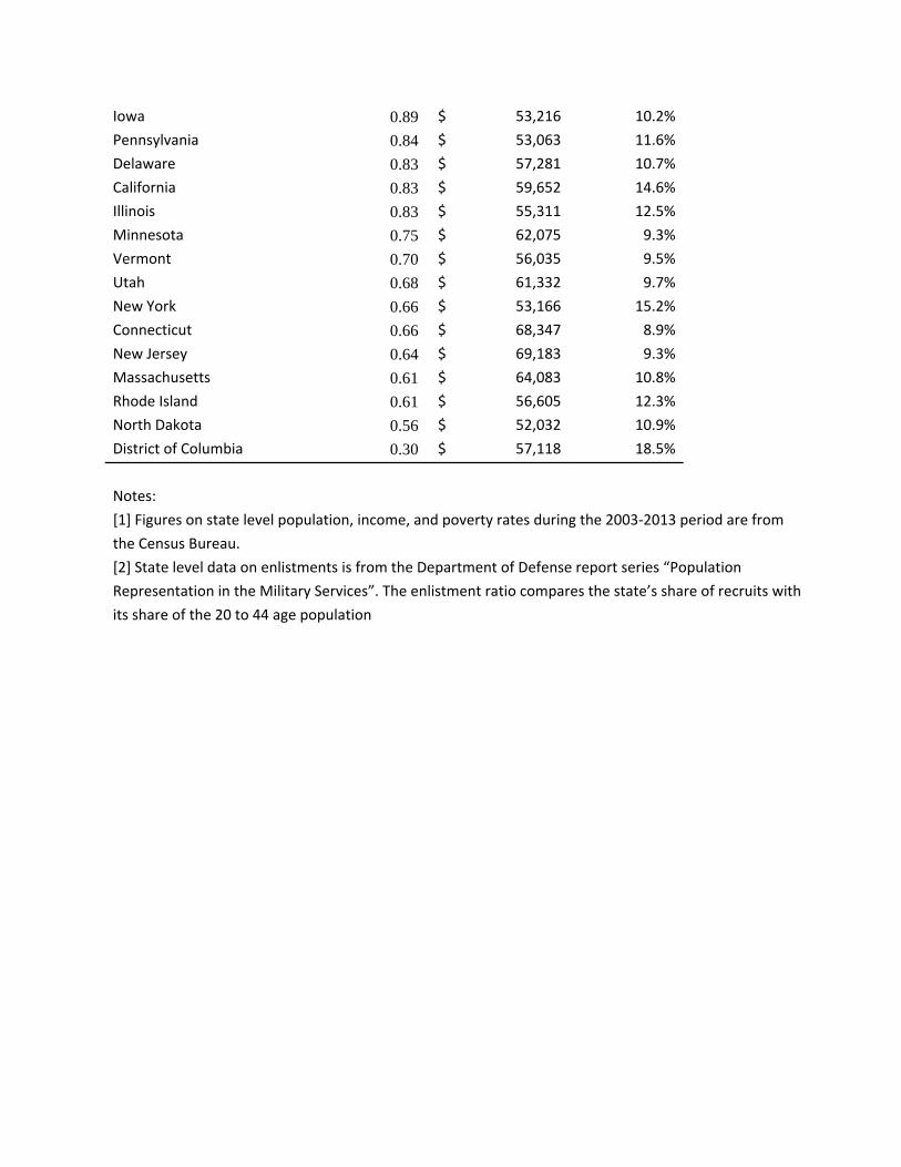
For example, let us consider State-level enlistment rates and income. Table 6 shows

enlistment and fatality ratios for each U.S. State, as well as their median income and poverty

rate. The enlistment rate correlates negatively with median (and mean, not shown) family

 

 

income. However, we know from the individual-level analysis that the family income of recruits

is slightly above the national average, and the relationship between income and enlistment

probability is positive. Furthermore, note that the same State-level data shows that enlistment is

negatively correlated with the poverty rate, a finding somewhat inconsistent with the suggested

negative correlation between income and enlistment ratio.

This complex and non-linear relationship between income and likelihood of joining the

military may in part explain why studies which rely on geographic-level data and do not adjust

for distributional complexity come to conflicting conclusions about socioeconomic

representativeness.

8. Summary and Discussion

DoD (1997) points out that “Many of the assertions about the class composition of the

military have been based on impressions and anecdotes rather than on empirical data.” The

widespread belief among the American public and law-makers that the poor bear a

disproportionate burden in fighting America’s wars is probably derived from the fact that recruits

were historically more likely to come from lower income households. Previous attempts to study

the socioeconomic representativeness of the military have led to conflicting results, in part

because of the imperfect nature of using geographic data to answer individual-level questions.

Our individual-level analysis based on the recent NLSY97 dataset does not suffer from

the bias and problems of previous studies based on geographic-level data; our findings suggest

that, in recent years, the military has been recruiting principally from the middle-class rather than

 

 

the poor (or the rich). We show that recent recruits tend to have higher than average

socioeconomic background: they disproportionally come from the middle of the family income,

family wealth, and tested skill distributions, with both tails under-represented. We also show that

higher scores in cognitive skill tests increase the probability of joining the military for lower- and

middle-class individuals, but decrease the enlistment likelihood of young men and women

coming from the right tail of the income distribution. We also discussed related evidence that on

a per capita basis non-Hispanic White casualties have been over-represented in the Iraq and

Afghanistan wars.

We can only speculate about the causes of this historic shift toward higher socioeconomic

background of recruits. One explanation is that a smaller and more technologically-advanced

military has become more selective in admitting recruits since the late 1970s. It appears that

military recruits have in recent years been positively selected in terms of background variables,

including skills measured by the AFQT/ASVAB tests. Warner and Asch (2001) document that

the average AFQT score increased from the 53rd percentile in 1978 to the 59th percentile in 1998.

This has a number of implications not only for policy- and law-makers, but also for

researchers and social scientists who want to understand how modern countries, and in particular

the United States, fight wars.

First, if bearing the burden of military service and war fatalities is viewed as a “tax”, the

tax is paid disproportionally by the middle class, with both the poor and the rich under-

represented.

 

 

Second, there is a more direct relationship than previously assumed between the middle

class who votes and participates in civil life, and the fighting men and women that protect the

interests and further the goals of the State abroad. Rather than an entity separated from the rest of

society, men and women who serve are likely to embody the values and culture of the median

voters. This changes not only the nature of the military itself, but also the costs and benefits

calculations of democracies electing to go to war.

Third, it explains the concern of the American population for both those who have served

and those who are serving in the Armed Forces. The American public and government have been

increasing their focus not only on war casualties but also on the fate of the veterans who return to

civilian life. For example, many charities and government policies have been created or

overhauled to facilitate the return to civilian life of those who have served.

Fourth, it changes the role of the military as employer of last resort and vehicle for

upward mobility. On one hand, as the military becomes more selective in terms of personnel

enlisted, we expect it to spend more per soldier, both to incentivize people with higher outside

options to join its rank, and to protect more effectively the life of each soldier, as they are more

expensive. On the other hand, as the military loses its role of employer of last resort, the State

will have to spend more resources on programs helping those with lower levels of human capital

to participate effectively in civil life.

We believe more research is needed to fully address these and other questions outside the

scope of this article. We have provided a novel set of findings that we hope will help other

 

 

researchers expand the literature and provide guidance to the public and politicians in these very

sensitive matters.

 

 

References

Armed Forces Health Surveillance Center, 2012. Deaths while on active duty in the U.S. Armed

Forces, 1990-2011. MSMR 19(5), 2-5.

Baskir, L., Strauss, W., 1978. Chance and Circumstance: The Draft, the War, and the Vietnam

Generation. Alfred A. Knopf, New York.

Boulanger, G., 1981. Who Goes to War? in A. Egendorf, C. Kadushin, R.S. Laufer, G. Rothbart,

and L. Sloan (Eds.), Legacies of Vietnam: Comparative Adjustment of Veterans and Their Peers,

Vol. 4. Long-term Stress Reactions: Some Causes, Consequences, and Naturally Occurring

Support Systems Washington, DC: U.S. Government Printing Office, pp. 494-515.

Congressional Budget Office, 2007. The All Volunteer military: Issues and Performance. Pub.

No. 2960

Cooper, R. 1977. Military Manpower and the All Volunteer Force. RAND Corporation Report,

223-250.

Daymont, T., Andrisani, P., 1986. The Economic Returns to Military Service. Technical Report,

Center for Labor and Human Resource Studies, Temple University.

Democratic Leadership Council, 1988. Citizenship and National Service: A Blueprint for Civic

Enterprise. Washington, DC:

 

 

Department of Defense 1997. Population Representation in the Military Services, Fiscal Year

1996. Office of the Assistant Secretary of Defense, Washington, DC.

Department of Defense 2000. Population Representation in the Military Services, Fiscal Year

1999. Office of the Assistant Secretary of Defense, Washington, DC.

Department of Defense 2006., Population Representation in the Military Services, Fiscal Year

2005. Office of the Assistant Secretary of Defense, Washington, DC.

Department of Defense 2012. Population Representation in the Military Services, Fiscal Year

2011. Office of the Assistant Secretary of Defense, Washington, DC.

Elder, G. H., L. Wang, N. J. Spence, D. E. Adkins, and T. H. Brown. 2010. Pathways to the All‐

Volunteer Military. Social Science Quarterly 91 (2): 455-475.

Fernandez, R.L., 1989. Social Representation in the U.S. Military. Congressional Budget Office,

Washington, DC.

Fischer, H., Klarman, K., Oboroceanu, M., 2007. American War and Military Operations

Casualties: Lists and Statistics. CRS report for Congress, Washington DC.

Fischer, H., 2014. A Guide to U.S. Military Casualty Statistics: Operation New Dawn, Operation

Iraqi Freedom, and Operation Enduring Freedom. CRS report for Congress, Washington DC.

Fredland, J.E., Little, R.D., 1982. Socioeconomic Characteristics of the All Volunteer Force:

Evidence from the National Longitudinal Survey, 1979. U.S. Naval Academy, Annapolis, MD.

 

 

Gelpi, C., P. Feaver, and J. Reifler. 2009. Paying the human costs of war: American public

opinion and casualties in military conflicts. Princeton University Press, Princeton, NJ.

Janowitz, M., 1975. The All Volunteer Military as a Socio-Political Problem. Social Problems,

432-449.

Horowitz, M. C., E. M. Simpson, and A. C. Stam. 2011. Domestic Institutions and Wartime

Casualties. International Studies Quarterly 55 (4): 909-936.

Kane, T., 2005. Who Bears the Burden? Demographic Characteristics of U.S. Military Recruits

Before and After 9/11. Heritage Foundation Center for Data Analysis Report No. 05–08

Kane, T., 2006. Who Are the Recruits? The Demographic Characteristics of U.S. Military

Enlistment, 2003-2005. Heritage Center for Data Analysis Report No. 06-09

Kentor, J., A. K. Jorgenson, and E. Kick. 2012. The “new” military and income inequality: A

cross national analysis. Social Science Research 41 (3): 514-526.

Kriner, D. L., and F. X. Shen. 2014. Responding to War on Capitol Hill: Battlefield Casualties,

Congressional Response, and Public Support for the War in Iraq. American Journal of Political

Science 58 (1): 157-174.

Kriner, D. L., and F. X. Shen. 2013. Reassessing American Casualty Sensitivity The Mediating

Influence of Inequality. Journal of Conflict Resolution: 0022002713492638.

Kriner, D. L., and F. X. Shen. 2010. The Casualty Gap: The Causes and Consequences of

American Wartime Inequalities. Oxford University Press, Oxford, UK.

 

 

Kristof, N., 2012. Profiting From a Child’s Illiteracy. New York times (December 7)

Laurence, J., 2004. The All-Volunteer Force: A Historical Perspective. Office of Under

Secretary of Defense, Washington DC.

Lien, D. S. 2012. An Investigation of FY10 and FY11 Enlisted Accessions’ Socioeconomic

Characteristics. DRM-2012-U-001362-1REV.

Moore, A., 1924. Conscription and Conflict in the Confederacy. Hillary House, New York.

Mehay, S., 1996. The Post-Military Earnings of Female Veterans. Industrial Relations, 35(2),

197-217.

National Priorities Project. 2011. “Military Recruitment 2010“

Peachey, T., 2006. Military Recruitment, Communities of Color and Immigrants. Mennonite

Central Committee.

Rangel, C., 2004. Representative Rangel Remarks at the National Press Club speech,

Washington, DC (April 15).

Rohlfs, C., 2012. The Economic Cost of Conscription and an Upper Bound on the Value of a

Statistical Life: Hedonic Estimates from Two Margins of Response to the Vietnam Draft. Journal

of Benefit-Cost Analysis 3(3), Article 4.

Rose, E., 2007. Siblings and Soldiers: Family Background and Military Service in the All-

Volunteer Era. Mimeo, University of Washington.

 

 

Rostker, B. 2006. I Want You! The Evolution of the All-Volunteer Force (Santa Monica, Calif.:

RAND Corporation

Teachman, J. D. 2007. Military Service and Educational Attainment in the All-Volunteer Era.

Sociology of Education 80, 359-374.

Teachman, J. D., V.R.A. Call, and M. W. Segal. 1993. The selectivity of military enlistment.

Journal of Political and Military Sociology 21 (2): 287-309.

Tyson, A., 2005. Youths in Rural U.S. Are Drawn to Military. The Washington Post, November

4.

Vasquez, J. P. 2005. Shouldering the Soldiering Democracy, Conscription, and Military

Casualties. Journal of Conflict Resolution 49 (6): 849-873.

Warner, J., Asch, B., 2001. The Record and Prospects of the All-Volunteer Military in the United

States. Journal of Economic Perspectives 15(2), 169-192

Wright, J., 2012. Those Who Have Borne the Battle: A History of America's Wars and Those

Who Fought Them. Public Affairs, New York.

 

 

Tables and Figures

Table1:Propensityofyoungpeopletojointhemilitaryrelativethenationalaverage2006‐2011

State  Relative Propensity Voting Record

Alabama 1.278 "Red State" Alaska 1.174 "Red State" Arizona 1.172 "Red State" Arkansas 1.124 "Red State" California 0.83 "Blue State" Colorado 1.144 "Blue State" Connecticut 0.66 "Blue State" Delaware 0.832 "Blue State" District of Columbia 0.298 "Blue State" Florida 1.352 "Blue State" Georgia 1.296 "Red State" Hawaii 1.166 "Blue State" Idaho 1.326 "Red State" Illinois 0.826 "Blue State" Indiana 1.038 "Red State" Iowa 0.886 "Blue State" Kansas 1.056 "Red State" Kentucky 0.936 "Red State" Louisiana 0.902 "Red State" Maine 1.25 "Blue State" Maryland 0.9 "Blue State" Massachusetts 0.612 "Blue State" Michigan 0.952 "Blue State" Minnesota 0.746 "Blue State" Mississippi 0.918 "Red State" Missouri 1.174 "Red State" Montana 1.488 "Red State" Nebraska 1.064 "Red State" Nevada 1.29 "Blue State" New Hampshire 1.034 "Blue State" New Jersey 0.638 "Blue State" New Mexico 1.012 "Blue State" New York 0.664 "Blue State" North Carolina 1.186 "Red State" North Dakota 0.56 "Red State" Ohio 1.058 "Blue State" Oklahoma 1.268 "Red State"

 

 

Oregon 1.27 "Blue State" Pennsylvania 0.84 "Blue State" Rhode Island 0.61 "Blue State" South Carolina 1.284 "Red State" South Dakota 0.922 "Red State" Tennessee 1.146 "Red State" Texas 1.27 "Red State" Utah 0.678 "Red State" Vermont 0.696 "Blue State" Virginia 1.222 "Blue State" Washington 1.134 "Blue State" West Virginia 1.082 "Red State" Wisconsin 0.952 "Blue State" Wyoming 1.186 "Red State"

 

 

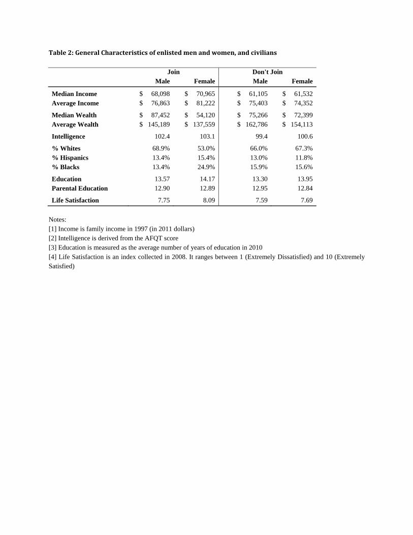
Table2:GeneralCharacteristicsofenlistedmenandwomen,andcivilians

Join Don't Join Male Female Male Female

Median Income $ 68,098 $ 70,965 $ 61,105 $ 61,532 Average Income $ 76,863 $ 81,222 $ 75,403 $ 74,352

Median Wealth $ 87,452 $ 54,120 $ 75,266 $ 72,399 Average Wealth $ 145,189 $ 137,559 $ 162,786 $ 154,113

Intelligence 102.4 103.1 99.4 100.6

% Whites 68.9% 53.0% 66.0% 67.3% % Hispanics 13.4% 15.4% 13.0% 11.8% % Blacks 13.4% 24.9% 15.9% 15.6%

Education 13.57 14.17 13.30 13.95 Parental Education 12.90 12.89 12.95 12.84

Life Satisfaction 7.75 8.09 7.59 7.69 Notes: [1] Income is family income in 1997 (in 2011 dollars) [2] Intelligence is derived from the AFQT score [3] Education is measured as the average number of years of education in 2010 [4] Life Satisfaction is an index collected in 2008. It ranges between 1 (Extremely Dissatisfied) and 10 (Extremely Satisfied)

 

 

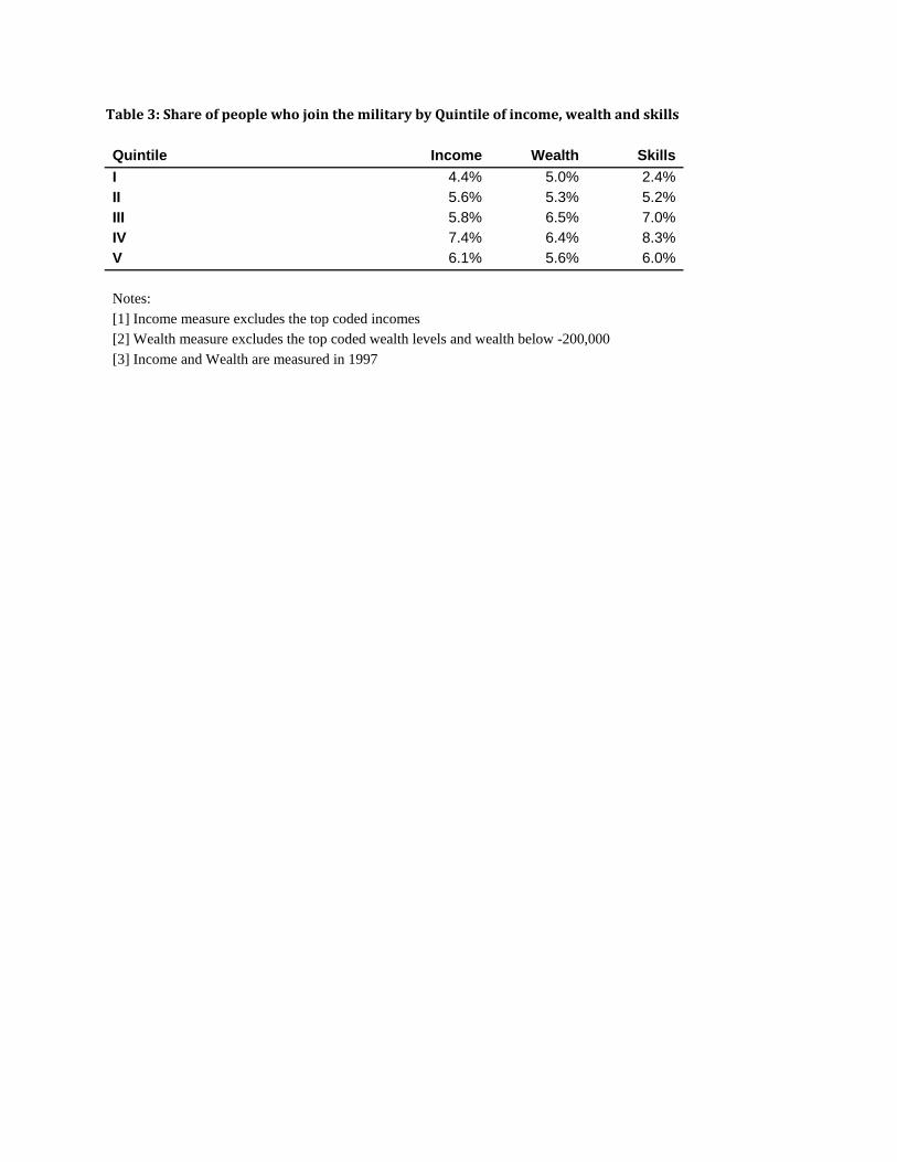
Table3:ShareofpeoplewhojointhemilitarybyQuintileofincome,wealthandskills

Quintile Income Wealth Skills I 4.4% 5.0% 2.4% II 5.6% 5.3% 5.2% III 5.8% 6.5% 7.0% IV 7.4% 6.4% 8.3% V 6.1% 5.6% 6.0%

Notes: [1] Income measure excludes the top coded incomes [2] Wealth measure excludes the top coded wealth levels and wealth below -200,000 [3] Income and Wealth are measured in 1997

 

 

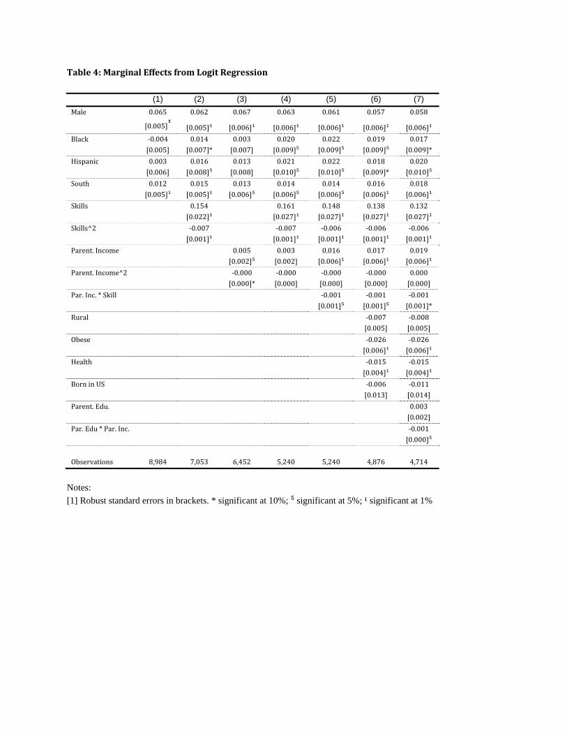
Table4:MarginalEffectsfromLogitRegression

(1) (2) (3) (4) (5) (6) (7) Male 0.065 0.062 0.067 0.063 0.061 0.057 0.058

[0.005]¹ [0.005]¹ [0.006]¹ [0.006]¹ [0.006]¹ [0.006]¹ [0.006]¹

Black ‐0.004 0.014 0.003 0.020 0.022 0.019 0.017

[0.005] [0.007]* [0.007] [0.009]⁵ [0.009]⁵ [0.009]⁵ [0.009]*

Hispanic 0.003 0.016 0.013 0.021 0.022 0.018 0.020

[0.006] [0.008]⁵ [0.008] [0.010]⁵ [0.010]⁵ [0.009]* [0.010]⁵

South 0.012 0.015 0.013 0.014 0.014 0.016 0.018

[0.005]¹ [0.005]¹ [0.006]⁵ [0.006]⁵ [0.006]⁵ [0.006]¹ [0.006]¹

Skills 0.154 0.161 0.148 0.138 0.132

[0.022]¹ [0.027]¹ [0.027]¹ [0.027]¹ [0.027]¹

Skills^2 ‐0.007 ‐0.007 ‐0.006 ‐0.006 ‐0.006

[0.001]¹ [0.001]¹ [0.001]¹ [0.001]¹ [0.001]¹

Parent.Income 0.005 0.003 0.016 0.017 0.019

[0.002]⁵ [0.002] [0.006]¹ [0.006]¹ [0.006]¹

Parent.Income^2 ‐0.000 ‐0.000 ‐0.000 ‐0.000 0.000

[0.000]* [0.000] [0.000] [0.000] [0.000]

Par.Inc.*Skill ‐0.001 ‐0.001 ‐0.001

[0.001]⁵ [0.001]⁵ [0.001]*

Rural ‐0.007 ‐0.008

[0.005] [0.005]

Obese ‐0.026 ‐0.026

[0.006]¹ [0.006]¹

Health ‐0.015 ‐0.015

[0.004]¹ [0.004]¹

BorninUS ‐0.006 ‐0.011

[0.013] [0.014]

Parent.Edu. 0.003

[0.002]

Par.Edu*Par.Inc. ‐0.001

[0.000]⁵

Observations 8,984 7,053 6,452 5,240 5,240 4,876 4,714

Notes: [1] Robust standard errors in brackets. * significant at 10%; ⁵ significant at 5%; ¹ significant at 1%

 

 

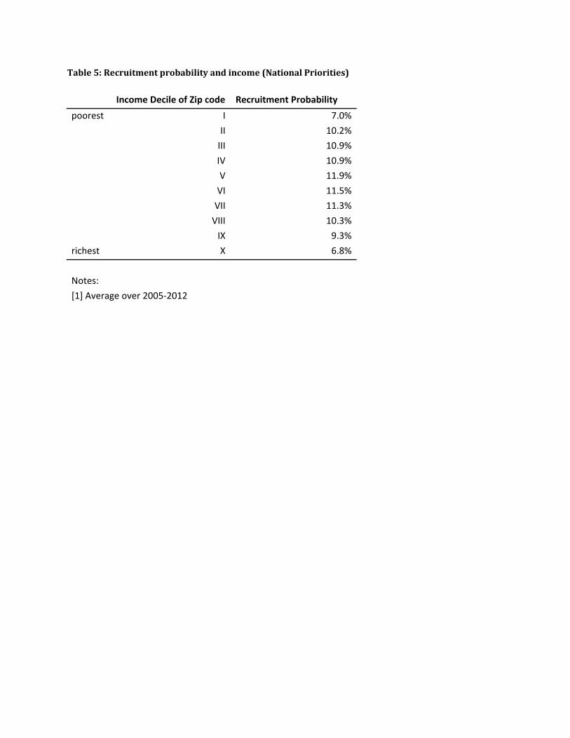
Table5:Recruitmentprobabilityandincome(NationalPriorities)

   Income Decile of Zip code  Recruitment Probability 

poorest  I  7.0%

II  10.2%

III  10.9%

IV  10.9%

V  11.9%

VI  11.5%

VII  11.3%

VIII  10.3%

IX  9.3%

richest  X  6.8%

Notes: 

[1] Average over 2005‐2012 

 

 

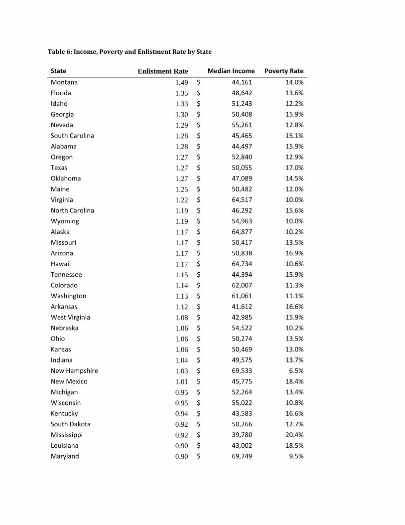
Table6:Income,PovertyandEnlistmentRatebyState

State  Enlistment Rate  Median Income  Poverty Rate 

Montana  1.49  $                   44,161   14.0% 

Florida  1.35  $                   48,642   13.6% 

Idaho  1.33  $                   51,243   12.2% 

Georgia  1.30  $                   50,408   15.9% 

Nevada  1.29  $                   55,261   12.8% 

South Carolina  1.28  $                   45,465   15.1% 

Alabama  1.28  $                   44,497   15.9% 

Oregon  1.27  $                   52,840   12.9% 

Texas  1.27  $                   50,055   17.0% 

Oklahoma  1.27  $                   47,089   14.5% 

Maine  1.25  $                   50,482   12.0% 

Virginia  1.22  $                   64,517   10.0% 

North Carolina  1.19  $                   46,292   15.6% 

Wyoming  1.19  $                   54,963   10.0% 

Alaska  1.17  $                   64,877   10.2% 

Missouri  1.17  $                   50,417   13.5% 

Arizona  1.17  $                   50,838   16.9% 

Hawaii  1.17  $                   64,734   10.6% 

Tennessee  1.15  $                   44,394   15.9% 

Colorado  1.14  $                   62,007   11.3% 

Washington  1.13  $                   61,061   11.1% 

Arkansas  1.12  $                   41,612   16.6% 

West Virginia  1.08  $                   42,985   15.9% 

Nebraska  1.06  $                   54,522   10.2% 

Ohio  1.06  $                   50,274   13.5% 

Kansas  1.06  $                   50,469   13.0% 

Indiana  1.04  $                   49,575   13.7% 

New Hampshire  1.03  $                   69,533   6.5% 

New Mexico  1.01  $                   45,775   18.4% 

Michigan  0.95  $                   52,264   13.4% 

Wisconsin  0.95  $                   55,022   10.8% 

Kentucky  0.94  $                   43,583   16.6% 

South Dakota  0.92  $                   50,266   12.7% 

Mississippi  0.92  $                   39,780   20.4% 

Louisiana  0.90  $                   43,002   18.5% 

Maryland  0.90  $                   69,749   9.5% 

 

 

Iowa  0.89  $                   53,216   10.2% 

Pennsylvania  0.84  $                   53,063   11.6% 

Delaware  0.83  $                   57,281   10.7% 

California  0.83  $                   59,652   14.6% 

Illinois  0.83  $                   55,311   12.5% 

Minnesota  0.75  $                   62,075   9.3% 

Vermont  0.70  $                   56,035   9.5% 

Utah  0.68  $                   61,332   9.7% 

New York  0.66  $                   53,166   15.2% 

Connecticut  0.66  $                   68,347   8.9% 

New Jersey  0.64  $                   69,183   9.3% 

Massachusetts  0.61  $                   64,083   10.8% 

Rhode Island  0.61  $                   56,605   12.3% 

North Dakota  0.56  $                   52,032   10.9% 

District of Columbia  0.30  $                   57,118   18.5% 

Notes: 

[1] Figures on state level population, income, and poverty rates during the 2003‐2013 period are from 

the Census Bureau. 

[2] State level data on enlistments is from the Department of Defense report series “Population 

Representation in the Military Services”. The enlistment ratio compares the state’s share of recruits with 

its share of the 20 to 44 age population 

 

 

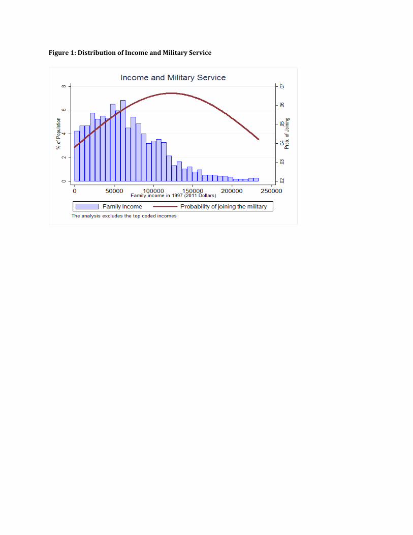
Figure1:DistributionofIncomeandMilitaryService

 

 

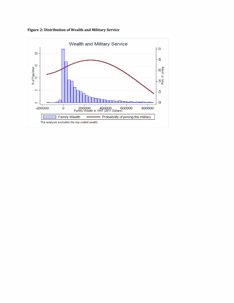
Figure2:DistributionofWealthandMilitaryService

 

 

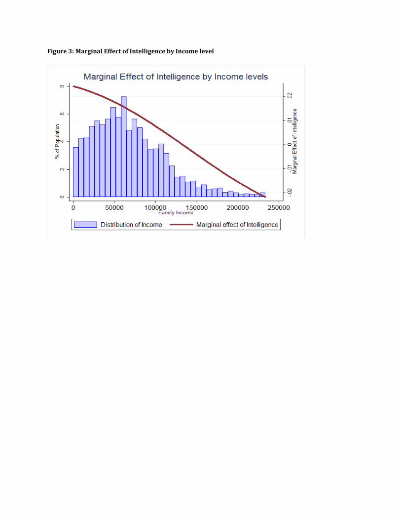
Figure3:MarginalEffectofIntelligencebyIncomelevel

 

 

Endnotes

                                                            

i Charles River Associates, Washington DC and IFN – Research Institute for Industrial Economics. Stockholm, Sweden. The views presented here are my own and do not necessarily reflect those of CRA or any CRA employee. Corresponding author: asoni@uchicago.edu 

ii IFN – Research Institute for Industrial Economics. Stockholm, Sweden.  

iii Family income refers to income in 1996, reported in 2011 dollars.

iv The probability of joining is estimated through a logistic regression that includes only income and income squared together with a constant as regressors. The dependent variable is a dummy indicator that is equal to one if the individual joined the military anytime between 1997 and 2010. A more complete regression is discussed later.

v We also tested a specification with a more complete geographic characterization. We found that only the “South” dummy is statistically significant. Department of Defense data shows an over-representation for the south of 20% compared to the national average 2006–2011.