For comments, suggestions or further inquiries please contact:

Philippine Institute for Development StudiesSurian sa mga Pag-aaral Pangkaunlaran ng Pilipinas

The PIDS Discussion Paper Seriesconstitutes studies that are preliminary andsubject to further revisions. They are be-ing circulated in a limited number of cop-ies only for purposes of soliciting com-ments and suggestions for further refine-ments. The studies under the Series areunedited and unreviewed.

The views and opinions expressedare those of the author(s) and do not neces-sarily reflect those of the Institute.

Not for quotation without permissionfrom the author(s) and the Institute.

The Research Information Staff, Philippine Institute for Development Studies5th Floor, NEDA sa Makati Building, 106 Amorsolo Street, Legaspi Village, Makati City, PhilippinesTel Nos: (63-2) 8942584 and 8935705; Fax No: (63-2) 8939589; E-mail: publications@pids.gov.ph

Or visit our website at http://www.pids.gov.ph

October 2012

Rice Prices and the

National Food Authority

DISCUSSION PAPER SERIES NO. 2012-27

Ponciano S. Intal, Jr., Leah Francine Cuand Jo Anne Illescas

1

RICE PRICES AND THE NATIONAL FOOD AUTHORITY1 Ponciano Intal, Jr., Leah Francine Cu and Jo Anne Illescas Abstract: This study examines the performance of the NFA with respect to its function of price stability, its implications for public finances, and recommends policy reforms where warranted. It finds that NFA has been unsuccessful in stabilizing producer prices, but relatively successful in stabilizing retail prices, largely through exercise of its import monopoly. However it does so at high cost, partly due to operational inefficiency, but largely owing to its fundamental policy mandate. The study recommends relinquishing this mandate, and leaving a greater role for the private sector in stabilizing rice prices, with NFA function and price policy limited to maintaining strategic reserves a variable import levy. Key words: food security, price stabilization, financial sustainability, National Food Authority Introduction The National Food Authority (NFA) is one of the most important policy instrumentalities

of the Philippine government with respect to agricultural price policy and food security.

Despite its name, the government-owned and controlled corporation deals primarily with

rice, the country’s foremost food grain which accounts for the largest share of the food

basket of the average (but especially of the poor) Filipino consumer. At the same time,

rice is a major agricultural commodity accounting for a significant share of farmers in the

country. Many of the rice farmers are also poor.

NFA is tasked to stabilize the price of rice consistent with farm prices that are

remunerative to the country’s rice farmers and retail prices reasonable enough for the

country’s consumers. Also, it is mandated to respond immediately (within 48 hours) to

ensure supply of rice during emergencies and calamities and stabilize rice prices within

two weeks in the calamity-stricken areas to levels prior to the calamity or emergency

(Coffrey International Development, 2007, p.27).

1 This study is conducted as part of a project on Monitoring and Evaluation of Agricultural Policy – Capacity Development Project of the Philippine Institute for Development Studies, funded by the World Bank and Food and Agriculture Organization.

2

Clearly, the mission of NFA is daunting and almost a recipe for failure. To a large extent,

this is because NFA is tasked to address potentially conflicting objectives for consumers

and rice farmers. At the same time, the organization has to be agile to be responsive in

times of calamities, spread out geographically to meet rice supply and demand pressures

all over the country (in the light of a relatively inadequate infrastructure and logistic

system in the country), and efficient enough to be competitive with the private sector in

the provision of rice marketing services.

Not surprisingly, NFA’s performance over the years has been extremely mixed. The basic

issue is whether the society’s investment in NFA has been worth it given the resources

put into the corporation. If not, what can be done to address the fundamental concerns

being pursued by NFA, which are rice price stability and food security.

The paper examines the performance of NFA during the past decade or so, examines why

and presents policy recommendations accordingly.

Price Stabilization and Food Security: Some Analytics

Virtually all countries have intervened in the market pricing of food grains to promote

price stability. The most common method of intervening is the use of buffer stock

usually in tandem with trade policies (see Islam and Thomas, 1996 , pp1-2). The

Philippines is no exception to this. In developing countries, the management of the

buffer stock is usually handled by a government instrumentality. In the Philippines, it is

the National Food Authority that has the mandate to manage the country’s buffer stock of

rice, the country’s key food grain.

There is some political logic to price stabilization of basic food commodities like rice.

Rice accounts for the largest share of the food basket of poor and near poor Filipinos.

And food costs constitute the largest portion of the Filipinos’ overall budget. Finally, a

3

significant share of Filipinos hovers near the poverty line. Thus, large hikes in the price

of rice can push a large number of Filipinos into poverty unless the price hike happens

together with a corresponding increase in their household incomes (which is likely

unlikely especially for poor urban consuming households). Similarly, rice farmers are the

most numerous farmers in the country, and a large proportion of them is poor or near

poor. Thus, significant price falls of palay, especially during the peak harvest season,

have significant adverse impact on the incomes and poverty status of the rice farmers,

especially because most of them do not have the wherewithal to hold off the sale of their

harvest due to credit and storage constraints. Both the poor and near poor rice consumers

and the rice farmers are major voting constituencies in the country.

The importance of rice price stabilization is even more highlighted in a paper (2002) by

the DAI Food Policy Advisory Team in Indonesia, probably mainly authored by Peter

Timmer, for Indonesia’s BAPPENAS. The paper emphasizes that food price stability,

especially rice price stability, is a critical element of what is the East Asian approach to

food security. Specifically, the approach that can be termed ―growth mediated food

security‖ consists of rapid economic growth that benefits the poor combined with food

price stability. This is food security at the macro level wherein ―policymakers have an

opportunity to create the aggregate conditions in which households at the "micro" level can

gain access to food on a reliable basis through self-motivated interactions with local markets

and home resources‖ (p.23). Rapid economic growth is the long run solution to food security

through the Lorenz curve, because at the resulting much higher per capita income, the share

of food expenditures to total family expenditures declines dramatically and therefore

significant price swings of rice prices would only have minor adverse welfare effects. In the

short run however, it is the relative price stability of food, especially rice, which gives the

sense of food security to households. Food and rice price stability can have macroeconomic

benefit through possibly less overall inflation rate and less variable overall inflation rate,

which would likely lead to improved investment climate and higher rate of investments

thereby engendering a more robust economic growth rate.

For countries with relatively large population like the Philippines or Indonesia, food

(rice) security has a large element of the drive for self-sufficiency because of the relative

4

thinness of the world rice market as compared to the world wheat or corn markets. Global

rice trade volumes are only about a fifth of global trade in wheat; and the ratio of

internationally traded rice is only about 5 percent of world production as compared to

about 20 percent for wheat (and 15 percent for corn). This relatively thin market has

meant that historically world rice prices have tended to be more unstable that world

wheat prices. As a result, rice importing countries have tended to insulate their domestic

markets from the volatility of world rice prices. (See DAI, 2002, pp.31-33.)

Three nuances of price stabilization. There are three nuances of price stabilization that

are of interest. The first is the most politically cogent, which is that when there is an

emergency or calamity, the supply of rice is restored and the price of rice stabilized the

soonest possible. Where the transportation and warehousing infrastructure is not well

developed, a calamity or emergency leads to private hoarding and possible sharp hikes in

the price of rice, which will aggravate further the emergency condition. Thus,

government intervention to restore rice supplies and temper price hikes during the

emergency is needed. This is done primarily through a strategic rice reserve for such

eventualities and stored at various locations in the country for quick response. In

addition, the government tends to become more vigilant with respect to its regulations

against hoarding of basic commodities during emergencies in affected areas.

Note also that government intervention through the provision and activation of an

emergency rice reserve addresses both the first nuance of price stabilization, and

probably more importantly, that of food security during emergencies.

The second nuance of price stabilization is to temper the seasonal variation of the price

of rice within a year. Given that rice is consumed continuously and regularly the whole

year round while domestic production is seasonal, there is inevitably some seasonal

variation in the price of rice such that it is lower during the harvest season and higher

during the lean season. The market allows for the seasonal price variation in order to pay

for the storage and handling services of traders so that there is some domestic supply

even during the lean season. Tempering this seasonal variation in the price of rice means

5

that the price of rice, especially palay, is higher than the market price would be without

government intervention during the harvest season (which rice farmers with marketable

surplus would like) while the retail price is lower than the market price without

government intervention during the lean months (which the rice consumers would like).

That there is seasonal variation in the price of rice both at the farm gate and at the retail

level over the course of a year does not necessarily call for possible government policy

intervention as such. This is because the seasonality of rice price is a known reality and is

therefore incorporated in the pricing information that shapes expectations and decisions

of rice farmers (especially) and even possibly of rice consumers (hopefully). What gives

policy salience with respect to the second nuance of price stabilization is that the volume

of rice production is uncertain due to weather and pest factors among others. This means

that farm prices can spike up or register large droops during harvest season due to such

production uncertainties, thereby immediately affecting the incomes and welfare of rice

farmers accordingly. Such production shocks can also affect the consumer market and the

consumer price down the road if there is no appropriate inventory management response

either in terms of inventory drawdown (or increase) and/or imports (or exports) of rice.

To effect the second nuance of price stabilization, the government tempers the seasonal

variation of the price of rice primarily through the purchase of palay during harvests and

the sale of rice especially during the lean months. In case there is an overall shortage of

rice for the whole year, the government would need to import rice to augment domestic

purchases primarily for the lean season. This is essentially what the National Food

Authority does in its price stabilization mission.

It needs to be emphasized though that what NFA does is also what the private sector does

in rice trading. The private sector purchases rice during harvests, sells to consumers all

year round, and if allowed by the government and is profitable, imports rice to meet

domestic supply shortfalls. In either the NFA or the private sector, resources are

expended for the cost of domestic purchases, storing, transporting, processing, importing

or exporting, and selling. The challenge is to ensure that the marketing margin is

6

reasonable enough in order for the traders to have reasonable profit but at the same it is

not too high at the expense of consumers. The marketing margin must be enough to pay

for the cost of all marketing related costs plus reasonable profits (on the average in the

course of several months or years) in order to make the provision of marketing services

sustainable. In short, the trading, storing, transporting and processing stage needs to be

as efficient as possible in order to minimize the marketing margin

If the government intervenes in the marketing stage through a government corporation

such as the National Food Authority, the challenge is to minimize the subsidy cost (if

any) of government intervention in the rice marketing stage consistent with the price

stabilization and food security concerns of the country. Heavy subsidization by the

government in the marketing stage can have distortionary effects on the rice marketing

system. The most long lasting adverse effect is that unclear and haphazard interventions

by the government entity lead to business uncertainty which discourages the private

sector to invest adequately in facilities, systems, and relationships needed for greater

efficiencies in the rice marketing system. There are some economies of scale in the

marketing system. The better integrated the system is and the more adequate facilities

are, the lower the cost per unit of rice marketed would be, which can potentially benefit

either the consumers (through lower retail prices) or the farmers (through higher farm

gate prices) or both.

It needs to be pointed out that the economic basis for government intervention in the

marketing system is far less apparent in the second nuance of price stabilization than in

the first nuance. In terms of efficiency considerations, the possible basis for government

intervention is that there are significant inefficiencies in the private rice marketing system

either because of possible lack of competition or because the private sector does not have

the wherewithal to invest in the appropriate facilities and systems for efficient rice

marketing (which presumably the government intervention would address). There is an

implicit assumption therefore that the government instrumentality involved in rice

marketing (e.g., National Food Authority) would be more efficient and have better

facilities than the private sector. If in fact the government instrumentality is ex ante

7

expected to be less efficient than the private sector and therefore needs to be subsidized,

then the basis for government intervention (for this second nuance of price stabilization)

is purely for non-economic or political reasons.

The third nuance of price stabilization is that the domestic price of rice is more stable

than the world price of rice; that is, government intervention is such that domestic rice

price for consumers is more stable than the world price of rice. In a completely open rice

economy, the domestic price of rice would largely follow the gyrations in the world price

of rice adjusted for changes in the exchange rate (as well as possible changes in the tariff

rate on rice, which tends to be constant or are changed very infrequently or change very

little over time, and international shipping costs for rice). Domestic supply and demand

gaps are addressed through export and import of rice. Government intervention in the

third nuance of price stabilization rests on the assumption that the gyrations in the world

price of rice are too large for political comfort in the domestic arena; thus, the need for

government intervention in order to shield the domestic economy somewhat from the

presumably volatile world price of rice.

Assuming that there is some basis for de-linking the domestic rice price from the world

rice price movements, the government has two alternative approaches for doing so. The

first approach is for the government to still rely on the private sector to import and

export rice but where the tariff on rice is adjusted to counteract the movements in the

world price of rice. In this case, domestic price stabilization is undertaken through a

variable tariff system such that the import tariff on rice is decreased when the world price

of rice is high and is correspondingly increased when the world price of rice is low. In

this intervention strategy, the government can rely fully on the private sector in rice

trading with respect to imports and exports. The government does not have to expend

resources to support a government instrumentality like the National Food Authority to

undertake domestic price stabilization relative to world prices. Indeed, the government

can potentially even earn from this approach through the tariff revenues from levies on

imported rice.

8

The second approach is to have a government entity like the National Food Authority

managing buffer rice stock and having the sole (or dominant) authority to import and

export rice. In this case, de-linking domestic price from the world price of rice is

determined solely on the pricing decisions of the government entity in the domestic

market(s). The second option entails a lot more resources from the government as

compared to the first option. The choice of the second option stems from a specific price

stabilization strategy, which is the reliance on a government buffer stock policy managed

by a government instrumentality like the National Food Authority. A corollary of the

buffer stock strategy is that the government would rely on importing and exporting by the

government instrumentality instead of on the use of variable tariff rates on private

importation or exportation of rice. Implicit in this government preference for the second

option is the assumption that the private sector has less leverage vis-à-vis foreign

exporter-suppliers (or foreign importer-buyers as the case may be) or that it has less

resources—financial or otherwise--than the government to undertake import and export

of rice. Both presumptions do not seem to be compelling because international rice

trading is primarily commercial involving substantially the private sector in the export

countries (e.g., Thailand) and because the private sector has in fact greater financial

wherewithal than the perennially financially strapped Philippine government. The more

likely reason for the Philippine government not relying on the first approach to domestic

price stabilization via the private sector trading cum variable tariff is that the second

approach is the logical extension to the international trading arena of the buffer stock-

cum-price stabilization strategy relying on a government instrumentality in the domestic

economy.

Requirements for effective public buffer stock management. In their review of the

experiences of developing Asian countries in price stabilization through buffer stock

management in tandem with the use of trade policies, Islam and Thomas (1996) state the

following as the conditions for a successful and effective program, quoting verbatim

(p.2):

9

1. The buffer stock agency must have an assured, flexible access to adequate

financial resources since its requirements cannot be predicted.

2. The buffer stock agency must be in control of the timing of its purchases and

sales. Inappropriate timing would detract from its ability to influence market

prices.

3. Public stocks must be properly managed. Cost-effective purchases and sales

must be made and stocks must be rolled over frequently to avoid spoilage in

storage.

4. Timely and efficient management is also essential to avoid counter-

speculation, when traders, lacking confidence in the public agency, refrain

from buying in times of surplus and buy rather than sell in times of shortage.

5. If publicly held reduce or substitute for private storage, the success of the

public effort is compromised. Policies should encourage private trade;

otherwise the cost of public stock will be higher.

In summary, there is some compelling basis for the government to intervene in rice

distribution in times of calamities and emergencies. The intervention is primarily through

the maintenance of an emergency reserve. The economic basis for the government to

intervene in rice marketing in order to temper the seasonal variation in rice prices rests

ultimately on the presumption that the private sector is less efficient and effective in

providing the needed marketing services from the farm to the consumer than the

government agency. Similarly, the economic basis for the government to intervene

through the public management of a buffer stock plus the control of imports and exports

of rice rests on the presumption that this is a more expeditious and effective way of

stabilizing domestic rice prices relative to world rice prices rather than the reliance on the

private sector to undertake the appropriate importing and exporting of rice together with

the imposition of flexible and variable tariffs (and negative tariffs or subsidies where

appropriate). However, as the lessons of the developing countries in managing buffer

stock cum trade policies for price stabilization of food grains indicate, the conditions in

order to have an effective and efficient public agency managing the buffer stock are

extremely stringent indeed.

10

Rice Prices

Domestic and international prices and price stabilization. Table 1 presents the

average annual deflated prices of rice for the whole Philippines at the farm, wholesale

and retail levels during the 1990-2008 period.. The data are deflated using the consumer

price index for the Philippines with 1994 as the base year. Table 1 shows that the period

1990-2008 is characterized by two notable price spikes; i.e., 1995-1996 and 2008 with

the highest being during the 1995-1996 period. Nonetheless, excluding the two price

spikes, the real price of rice has largely been relatively stable without any pronounced

secular trend.

As will be discussed later in the paper, the price spike in 1995-1996 was largely domestic

in origin while the price spike in 2008 was global (but where nonetheless the Philippines

played a significant role as the world’s largest rice importer during the year). Excepting

the two price spikes, the relative stability of the real price of rice is consistent with the

price stabilization concern of the Philippine government. However, as will be discussed

later, the price spikes are to some extent endogenous to the decisions and operations of

the government’s rice intervention strategy through the National Food Authority.

Table 2 compares the international price of rice and the Philippine wholesale rice price.

The international price is represented by the f.o.b. Bangkok price of Thai rice, 35 %

brokens. This is likely of a lower quality than the average Philippine rice by the 1990s,

although this is what may be relevant for the provision of rice reserve for emergencies as

well as the rice for the poor. (The lower the percentage of rice brokens is, the higher the

quality. Cristina David uses an average of the price of Thai rice 15% brokens and Thai

rice 35% brokens in her computations of the nominal rate of protection. However, this is

11

essentially a synthetic price, not a real market price.) Nonetheless, the prices of the Thai

rice of different percentage of rice brokens tend to move together. Because the

Philippines imports much of its rice from Vietnam, the Vietnam export price at 25%

brokens is more direct comparator international price for the Philippine domestic rice

price. However, the series starts in 1998 only and is intermittent (i.e., there were some

months when there were no published export quotes). Thus, for longer period analysis,

the Bangkok price at 35% is used in the paper (there is no series for 25% brokens for

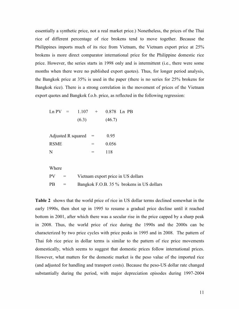
Bangkok rice). There is a strong correlation in the movement of prices of the Vietnam

export quotes and Bangkok f.o.b. price, as reflected in the following regression:

Ln PV = 1.107 + 0.878 Ln PB

(6.3) (46.7)

Adjusted R squared = 0.95

RSME = 0.056

N = 118

Where

PV = Vietnam export price in US dollars

PB = Bangkok F.O.B. 35 % brokens in US dollars

Table 2 shows that the world price of rice in US dollar terms declined somewhat in the

early 1990s, then shot up in 1995 to resume a gradual price decline until it reached

bottom in 2001, after which there was a secular rise in the price capped by a sharp peak

in 2008. Thus, the world price of rice during the 1990s and the 2000s can be

characterized by two price cycles with price peaks in 1995 and in 2008. The pattern of

Thai fob rice price in dollar terms is similar to the pattern of rice price movements

domestically, which seems to suggest that domestic prices follow international prices.

However, what matters for the domestic market is the peso value of the imported rice

(and adjusted for handling and transport costs). Because the peso-US dollar rate changed

substantially during the period, with major depreciation episodes during 1997-2004

12

before a significant peso appreciation in 2007, the pattern of the international price of rice

in peso is heavily muted by the exchange rate changes. What comes out is a pronounced

secular rise in the price of international price in peso terms during the period, highlighted

by the sharp rise in 2008.

Figure 1 puts in starker relief the significant difference in the movement of the

international price of rice in peso terms and of the domestic price of rice. Specifically, the

domestic price of rice (in terms of the wholesale price and even of the farm price) was

very much higher than the international price in peso terms (and adjusted for transport

and handling costs) during the 1990s, especially in the early 1990s when the implicit

nominal rate of protection of domestic rice was much more than 100 percent. The

nominal rate of protection remained high in the latter 1990s, measuring more than 50

percent, but declined dramatically by 2004 to about 10 percent or less as the foreign price

of rice started substantial rise while domestic prices continued to decline secularly since

1996 albeit very slowly. Indeed, as the rise in the international price of rice gathered

further steam while domestic prices remained relatively stable until 2007, the nominal

rate of protection turned zero or negative during 2005-2008. Figure 1 also shows the

Vietnam rice export price beginning 1998. The discussion above remains the same for the

Vietnam price as the international referent price. (Appendix Figures A.1 and A.2 show

the yearly comparison between the Philippine wholesale price and Thailand export price

(35 % brokens) and Vietnam export prices (25% brokens) respectively in peso terms and

adjusted for transport and handling on a monthly basis.)

Table 2 and Figure 1 are all at current prices; i.e., not deflated. They bring out most

forcefully the implicit major objective of the government’s rice price policy, which is

apparently one of rice price stability at current prices. The government has largely

succeeded in its objective during the period despite significant gyrations in the exchange

rate and in the world price in dollar terms. The exceptions include 1995-1996, which had

political impact in the sense that the sitting administration’s senatorial team did not fare

well during the elections in part because of the sharp rise in the price of rice. The price

peak in the domestic market in the mid-1990s is primarily determined by domestic

13

factors. Indeed, David ( 1997 ) attributes the 1995-1996 price peak as primarily a result

of policy failure. The other exception is the recent ―global rice crisis‖ of 2008, which

some analysts view was partly caused by the overreaction of both the major exporting

(e.g., India, Vietnam, Thailand) and importing (read: Philippines) countries to a

tightening global rice situation as reflected by the secular rise in the world price of rice

since 2003.

Below are regressions of the Philippine wholesale price of rice on the Bangkok export

price (35 % brokens) for 1990-1998 and selected sub-periods, where PP is the

Philippine wholesale price of rice and PT is the Bangkok f.o.b. price in peso terms and

where the numbers in parentheses are the t-values:

1990-2008

ln PP = 10.796 - 0.111 ln PT

(60.4) (-5.7)

Adjusted R squared = 0.13 ; F = 32.4

RMSE = 0.102; N = 218

1990 - 1996

ln PP = 6.545 + 0.370 ln PT

(11.5) (5.8)

Adjusted R squared = 0.28; F = 33.1

RMSE = 0.103; N = 84

1997 - 2008

Ln PP = 11.325 - 0.168 ln PT

(52.9) (-7.4)

Adjusted R squared = 0.29; F = 54.7

RMSE = 0.074; N = 134

14

1990 – 1994

ln PP = 11.567 - 0.204 ln PT

(17.3) (-2.7)

Adjusted R squared = 0.10; F = 7.3

RMSE = 0.07; N = 60

1994 – 1996

ln PP = 3.81 + 0.676 ln PT

(3.9) (8.2)

Adjusted R squared = 0.65; F = 66.7

RMSE = 0.07; N = 36

1997 - 2000

ln PP = 9.801 + 0.005 ln PT

(19.801) (0.1)

Adjusted R squared = -0.02; F = 0.01

RMSE = 0.058; N = 48

2001 – 2004

ln PP = 10.546 - 0.091 ln PT

(61.2) (-4.9)

Adjusted R squared = 0.33; F = 24.4

RMSE = 0.02; N = 48

The regression results above indicate that Philippine wholesale rice prices moved

somewhat against the Bangkok export price for the whole 1990-2008 period, primarily

during the 1997 – 2008 sub-period and most especially during the years since 2001. As

will be shown later in the paper, the years since 1997 can be characterized by the greater

effort of the National Food Authority towards rice price stabilization as reflected in the

15

rise of its rice stock and in the expenses for rice operations during the period. This

appears to show the political importance given by the government to rice price stability

after the results of the senatorial elections in the mid1990s; in short, rice is a political

commodity in the country.

Table 2 and Figure 1 also show that the very high nominal rate of protection of the early

1990s eventually turned into a negative rate of protection by the mid 2000s. This

remarkable shift in the nominal rate of protection has tremendous impact on the National

Food Authority’s operations and budget. The very high rate of protection could provide

NFA some buffer on its finances (i.e., NFA could import rice cheaply and sell it at a

much higher price domestically) in much of the 1990s. However, the pursuit of rice price

stability domestically in the face of soaring international price in peso terms, which

resulted in the sharp drop in the nominal rate of protection and the eventual turn to

negative rate of protection, could only be done through heavy government subsidies of

NFA operations.

Similarly, Table 1 and Figure 1 suggest that the implicit policy bias of the Philippine

government during the 1990-2008 period has been an overriding focus on rice consumers

through rice price stability especially since the latter 1990s. The support to rice farmers

through some reasonable rate of protection was largely a secondary corollary to the

pursuit of rice price stability in the context of the changing international market

conditions for rice.

National and regional rice prices, marketing margins and price volatility.

Figures 2 to 4 show the pattern of average annual farm, wholesale and retail prices of

rice from 1990 to 2008 by region. The figures suggest the following:

1. Rice prices tend to move reasonably closely among the regions.

16

2. Farm gate prices seem to be more volatile than retail prices, and possibly

even than wholesale prices.

The last observation that farm gate prices tend to be more volatile than retail or even

wholesale prices is corroborated by Table 3a which shows the standard deviation of

(deflated) farm gate, wholesale and retail rice prices for the whole country annually

during 1990-2008 and by Table 3b which presents the standard deviation estimates at the

regional level during the period. (Appendix Tables A.1.a-A.1.c present the standard

deviation estimates per year.) The tables show that the standard deviation measure for

farm gate prices is higher than those of wholesale prices and retail prices except most

notably in 1995 when retail prices zoomed up. The table also suggests that wholesale rice

prices tend to be more volatile than retail prices.

This pattern on relative price volatility among farm, wholesale and retail prices is

probably not surprising because the storage function of the private sector is meant partly

to help stabilize prices at the wholesale and retail levels. At the same time, the stability in

the price of rice at the retail level is precisely the key objective of government

intervention in rice marketing through buffer stock management. Thus, the greater

stability in the price of rice at the retail level could be caused by the normal storage

function of traders as well as by government interventions in rice marketing. The

challenge is to determine whether indeed the government intervention was the dominant

factor for the greater stability of the price of rice at the retail level.

Figures 5-7 show the monthly pattern of (deflated) farm gate, wholesale and retail prices

of rice for the period 1990-2008. The tables show that prices are clustered within a

narrow band, except for a few years most notably 1995, 1996 and 2008. As the tables

indicate, rice prices shot up in the latter 1995 and early 1996 before gradually declining

by the latter 1996; similarly, there was a sharp rise in the price of rice during the second

and third quarters of 2008 before declining afterwards. Those three years of markedly

different pattern of the movement of the price of rice are related to the sharp price

increases that were noted earlier during 1995-1996 and the year 2008. Excepting the three

17

outlier years, the clustered prices suggest that there is some seasonality in the prices of

rice, more pronounced for farm prices (with lower prices in the last quarter of the year)

and less so for retail prices (although rice prices tend to rise somewhat during the third

quarter of the year).

The clustering of prices in Figures 5-7 is also evident among regions. For the most part,

there is strong correlation between regional wholesale prices and Manila wholesale price

during much of the period. Nonetheless, the correlation is not hard and fast; indeed, there

are significant annual variations as well as differences in the extent of price correlation

among the regions vis-à-vis Manila (see Tables 4). Two-thirds of all the regions have

correlation coefficients with Manila wholesale rice price of at least 0.90 and the rest in

the 80 percent. The lower correlation coefficients are largely in Mindanao. The same

apparent weaker linkage between Mindanao wholesale prices and Manila prices is echoed

in the results of regressions of regional wholesale prices on wholesale price of Metro

Manila and on the previous month’s regional wholesale price (see Table 5 and Appendix

Table A.2). The tables show that the long run coefficient is close to one (1) in most

regions of Luzon and Visayas (and interestingly, ARMM) but the long run coefficients

for most Mindanao regions hover in the 70s percent. It is possible that the long distance

between Manila and Mindanao is a factor such that shortages and surpluses among

Mindanao regions are mainly handled within the island and perhaps from Western

Visayas, and not from Luzon. This likely allows for some de-linking of Mindanao prices

from Manila prices.

From Tables 4a and 4b there also seems to be indication also that the correlation

improves especially during periods of high price increases. This is probably not at all

surprising because the shortage of domestic supply at the national level ultimately

reverberates into the whole rice marketing system across the country.

Figure 8 presents the ratio of wholesale price of rice in the various regions of the country

to the wholesale price of rice in Metro Manila. Figure 8 brings out interesting insights.

The first one is that a number of the regions have lower wholesale prices than in Metro

18

Manila while a few others have higher wholesale prices than Metro Manila. The regions

which have largely higher wholesale prices than Metro Manila (e.g., ARMM,

CALABARZON, Eastern Visayas, Central Visayas) tend to have mainly rice deficit

provinces. Similarly, those regions which have lower wholesale prices than Metro Manila

tend to have more provinces that are either self-sufficient or are surplus provinces in rice.

The result is probably not surprising among rice deficit regions in the sense that Metro

Manila is the main domestic market and therefore the transport and storage facilities are

geared more for the main market called Metro Manila. Note however that a number of the

rice deficit regions are poor regions, which means that the comparatively higher price of

rice in the poor but rice deficit regions will have more adverse effect on the relatively

poor regions.

The second interesting insight is that the ratios of regional wholesale rice prices to Metro

Manila’s wholesale rice price jump up and down during the period. This suggests that

there does not seem to be a strong correlation between the regional wholesale price and

the Manila wholesale price of rice in the short run. This result is well corroborated by

both the elasticities from regression results in Table 5 and the correlation coefficients in

Tables 4a and 4b. Table 5 shows the results of the natural logarithm of the deflated

regional price as a function of the natural logarithm of the deflated Manila wholesale

price and the one period-lagged logarithm of the deflated regional wholesale price. The

results show that there is not that strong relationship between the Manila wholesale price

and the regional price in the short run (i.e., within a month) but that there is strong

relationship in the long run. Appendix Table A.2 presents the regression results more

starkly. The annual correlation coefficients vary substantially, with a few cases of even

negative correlation between regional wholesale prices and the Manila wholesale price.

Over the 1990-2008 period, however, the correlation coefficients between the regional

wholesale prices and the Manila wholesale price are very high, in many cases in the 90

percent range. There is some regional variation. The regions with the strongest price

correlation with Manila are Regions 3 (Central Luzon), 4 (Southern Luzon) and 5 (Bicol),

which are essentially the neighboring regions of Manila, as well as Region 7 (Central

Visayas), which is another key rice deficit area. The regions with the weakest price

19

correlation with Manila during the 1990-2008 period are the Mindanao regions, except

for ARMM which is somewhat surprising given the high transport and logistics cost of

moving goods between ARMM and Metro Manila.

A comparison of the volatility of rice prices during the 1990-2008 period with those of

the 1974-1986 and 1957-1963 periods indicates that seasonal variation during the 1990s

and 2000s was less than during the 1970s and the 1980s, which in turn was also less than

during the 1957-1963 period (see Table 6). Umali (1990, p. 194) attributes the lower

seasonal price variation in the 1970s and 1980s as compared to the late 1950s and early

1960s to (a) the shift of rice production from rain-fed to irrigated water systems, (b)

government rice distribution since NFA was‖… relatively successful in defending the

rice ceiling price during the period 1974 to 1986‖ (p.194), and (c) improvements in

internal transport. The greater price stability of rice in the 1990s and 2000s is likely

similarly caused by (a) more even rice production, (b) improvements in internal transport,

and (c) government rice distribution. especially since the late 1990s as the National Food

Authority expanded its rice buffer stock.

Prices, Marketing Efficiency and Policy

The ratios of farm price to wholesale price, wholesale price to retail price and farm price

to retail price during 1990-2008 by region are presented in Figures 9-11 respectively.

The figures indicate that the wholesale to retail price ratio was relatively stable over the

period while the ratio of farm price to wholesale price declined somewhat from the mid-

1990s until the early 2000s before inching up again, although to a level that was still

lower than in the early 1990s. The result begs for some explanation. One is that

macroeconomic variables play a big role. Specifically, storing and transporting rice

entails costs including financial costs. Higher interest rates lead to higher inventory costs,

and, other things being equal, to higher marketing margin. Nominal interest rate largely

declined secularly during the period while the real interest rates was more volatile with

no clear pattern in the early 1990s but largely secularly declined since the late 1990s

20

except for a sharp rise in 2007 (see Figures 12a and 12b.). Figures 12a and 12b

juxtapose the annual average ratio of farm price to wholesale price with the nominal and

real interest rates during 1990-2008. The result is mixed: The ratio of farm price to

wholesale price and the nominal interest rate declined secularly during the 1990s but the

two diverged in the 2000 with the nominal interest rate declining further overall while the

ratio of farm price to wholesale price inched up. The pattern in the 2000s is more

consistent with the ex ante expectation of an inverse relationship between the two.

However, that the two were positively correlated in the 1990s suggest that there are other

factors, perhaps more important, that influence the ratio of farm price to wholesale price.

The ratio of farm price to the wholesale price and the ratio of farm price to the retail price

are the indirect measures of marketing margin. The lower the ratios are, the higher is the

marketing margins are. Although low ratios may indicate market inefficiency, there are

likely other factors that can lead to the low ratios. In this regard, it would be useful to

compare the Philippine ratios for rice with those of other countries (see Table 7). It is

apparent from the table that government intervention plays a significant part in the

determination of farm price, with an impact on the ratio of farm price to wholesale price.

This is exemplified by India where is the ratio is equal to 1 or even slightly higher,

suggesting that farm price and/or wholesale price is heavily subsidized so much so that

the ex post ratio does not capture the cost of marketing. Similarly, the ratios for Thailand

during 1996 and 2000 are suggestive of heavy government intervention, probably a high

farm support price that masked the true cost of marketing. Clearly, in these cases,

macroeconomic factors such as interest rates will have no bearing on the ex post ratio of

farm price to the wholesale price. Table 7 seems to indicate that Philippine marketing

margins are lower than for Bangladesh and possibly Indonesia but higher than Thailand.

In both Bangladesh and Indonesia, the marketing margin appears to be increasing while

the margin in the Philippines has declined as a proportion of the wholesale price in recent

years.

In view of the above discussion, it is not feasible to use the ratio of the farm price to

wholesale (and correspondingly, the ratio of farm price to the retail price) to examine the

21

relative efficiency of the rice marketing system as well as the impact of government

intervention on rice marketing and rice prices. To examine the above, the paper uses two

regression models that have been used to determine the efficiency of the rice price system

and the impact of government policies on rice prices. The two regression models are the

so-called Ravallion-type models used by Umali ( 1990 ) and the regression models

utilized by Yao,Shively and Masters ( 2005 ). The use of the two models is deliberate in

that comparisons could be made with the authors’ results and therefore provide a longer

run and hopefully more robust evaluation of the rice marketing system and government

policies.

Ravallion Regressions. Ravallion regressions can be used to test market integration

between marketing levels, and thereby provide indication of the efficiency of the market

system.; Umali (1990) may be the first to use Ravallion regressions to examine the

Philippine rice marketing system. This paper follows Umali in part to compare her results

for the 1970s and 1980s with the findings of the paper which focuses on the 1990s and

the early 2000s, thereby providing insights into the evolution and effectiveness of the

Philippine government interventions in the rice industry over the past few decades.

Geographically separated markets are integrated when prices in the said markets

―…move together in response to stimuli from changing demand and supply and other

economic conditions.‖ (Farruk as quoted by Umali (1990, p.143). The faster and more

accurate prices in the said markets react to such stimuli, the more integrated they are.

(Ibid.) Informational, infrastructural and logistic, and policy barriers will reduce the

degree of integration of markets. As a result, markets become less efficient as

mechanisms for the allocation of scarce resources. At the extreme where markets are not

interlinked at all, gluts or deficits in one market could not be readily be addressed by the

appropriate movement of goods and services to and from other markets. The end result is

lower social welfare to the whole economy. Market integration can be horizontal within

the same marketing chain (say the wholesale markets of a given commodity like rice in

various regions of the country) or vertical between marketing or processing levels

situated in various locations of the country (e.g., farm, wholesale, retail). The degree of

market integration can differ in the short run from the medium or long term, with the

22

expectation that markets tend to be more interlinked and integrated in the medium/long

term as against in the short term.

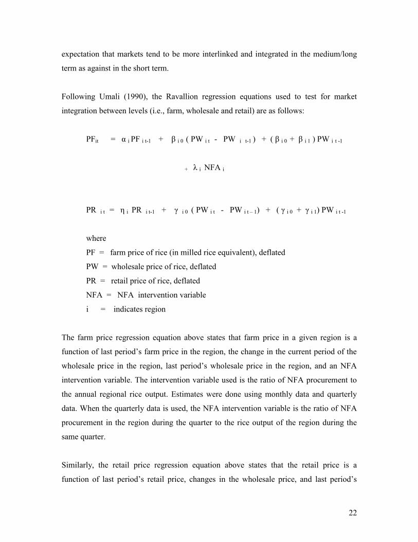
Following Umali (1990), the Ravallion regression equations used to test for market

integration between levels (i.e., farm, wholesale and retail) are as follows:

PFit = α i PF i t-1 + β i 0 ( PW i t - PW i t-1 ) + ( β i 0 + β i 1 ) PW i t -1

+ λ i NFA i

PR i t = η i PR i t-1 + γ i 0 ( PW i t - PW i t – 1) + ( γ i 0 + γ i 1) PW i t -1

where

PF = farm price of rice (in milled rice equivalent), deflated

PW = wholesale price of rice, deflated

PR = retail price of rice, deflated

NFA = NFA intervention variable

i = indicates region

The farm price regression equation above states that farm price in a given region is a

function of last period’s farm price in the region, the change in the current period of the

wholesale price in the region, last period’s wholesale price in the region, and an NFA

intervention variable. The intervention variable used is the ratio of NFA procurement to

the annual regional rice output. Estimates were done using monthly data and quarterly

data. When the quarterly data is used, the NFA intervention variable is the ratio of NFA

procurement in the region during the quarter to the rice output of the region during the

same quarter.

Similarly, the retail price regression equation above states that the retail price is a

function of last period’s retail price, changes in the wholesale price, and last period’s

23

wholesale price. As an initial hypothesis, no NFA intervention variable is included in the

equation on the presumption that NFA intervenes through the wholesale market, which is

already captured in the wholesale price of rice. In the actual estimation, the retail price

regression was estimated without and, for the national level estimates, with NFA

intervention variable (i.e., ratio of NFA distribution to total rice consumption). The

rationale for the inclusion of an NFA intervention variable is that the agency also has

retail segment, albeit very small, that seems to be popular with the sitting Philippine

president (their names tend to be emblazoned in this retail component of NFA). There are

no quarterly or monthly regional rice consumption that the authors are aware of; hence, it

is not possible to test the ―with NFA‖ regressions.

The Ravallion regression equations for farm prices were estimated for the whole year and

by season (i.e., main harvest season, dry season, and off season) given the pronounced

seasonality of rice production and of farm prices. This suggests that the implicit

assumption of constant marketing margins in the Ravallion model may not be met in

using monthly data that do not consider the seasonality of rice production.

The Ravallion regression estimates can be used to determine whether or not there is

market integration in the short run as well as to estimate the degree of market integration

(see Umali, 1990, for an extended discussion). Short run full market integration between

farm and wholesale markets, as strictly construed, means that the changes in the

wholesale price during the current month are fully reflected in the farm price; that is:

β i 0 = 1 ; β i 1 = 0 ; α i = 0

Similarly, for the retail market and the wholesale market, short run full market integration

requires:

γ i 0 = 1 ; γ i 1 = 0; η i = 0

24

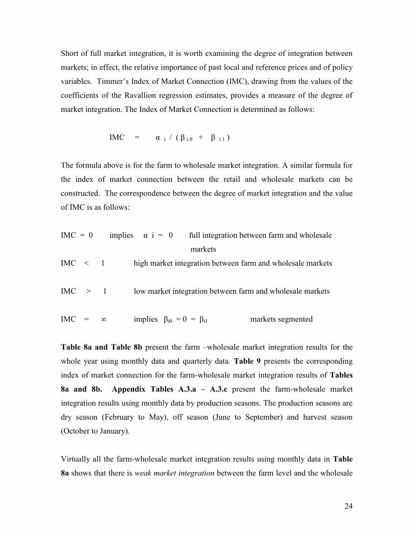
Short of full market integration, it is worth examining the degree of integration between

markets; in effect, the relative importance of past local and reference prices and of policy

variables. Timmer’s Index of Market Connection (IMC), drawing from the values of the

coefficients of the Ravallion regression estimates, provides a measure of the degree of

market integration. The Index of Market Connection is determined as follows:

IMC = α i / ( β i 0 + β i 1 )

The formula above is for the farm to wholesale market integration. A similar formula for

the index of market connection between the retail and wholesale markets can be

constructed. The correspondence between the degree of market integration and the value

of IMC is as follows:

IMC = 0 implies α i = 0 full integration between farm and wholesale

markets

IMC < 1 high market integration between farm and wholesale markets

IMC > 1 low market integration between farm and wholesale markets

IMC = ∞ implies βi0 = 0 = βi1 markets segmented

Table 8a and Table 8b present the farm –wholesale market integration results for the

whole year using monthly data and quarterly data. Table 9 presents the corresponding

index of market connection for the farm-wholesale market integration results of Tables

8a and 8b. Appendix Tables A.3.a – A.3.c present the farm-wholesale market

integration results using monthly data by production seasons. The production seasons are

dry season (February to May), off season (June to September) and harvest season

(October to January).

Virtually all the farm-wholesale market integration results using monthly data in Table

8a shows that there is weak market integration between the farm level and the wholesale

25

level in much of the country. In short, it is the past local farm prices that primarily

determine the current farm prices. However, when quarterly data is used, the results in

Table 8b show a completely different picture. Specifically, the quarterly results

show that there is strong market integration in virtually all the regions except ARMM

and marginally Eastern Visayas. The contrast between the monthly results and the

quarterly results is best shown by the index of market concentration in Table 9: while

the regression results using monthly data show IMC values of more than 1, and in a few

cases at very high levels of more than 3, the regression results using quarterly data show

IMC values very much lower than 1 with the exception of ARMM and marginally,

Eastern Visayas ( and the whole Philippines). In short, what the Ravallion regression

results suggest is that price adjustments at the farm level vis-à-vis the wholesale level

takes more than one month, but largely within one quarter, to complete.

Umali’s (1990) Ravallion regressions used monthly data. Like the results in Appendix

Tables A.3.a-A.3.c, Umali’s results show weak farm-wholesale market integration in

virtually all of the country. Umali did not have quarterly results; hence no comparison

could be made with the paper’s results. Nonetheless, it is likely that the conclusion of

farm price adjustment taking longer than one month but largely finishing within a quarter

was also prevailing during the 1970s and the 1980s. This is just a reflection of the still

inadequate infrastructural facilities in the country. Indeed, as the country’s rice granaries

are moving further away from Manila to such regions as Cagayan Valley and the

Cotabato basin, the demands of the rice marketing system on the country’s infrastructure

has become greater while at the same time that the quality of infrastructure in the more

far flung areas of the country leaves much to be desired.

The Ravallion regressions involving the retail price of rice by region are shown in Tables

10a and 10b and Appendix A.4.a – A.4.c. Like in the case of farm prices using monthly

data, the regression results show weak long run market integration between the wholesale

markets and the retail markets in the various regions of the country. The results seem to

suggest that it takes more than a month for prices to adjust fully to stimuli coming from

the wholesale market.

26

Regression results and effectiveness of NFA intervention. The weak market

integration between various market levels may not always be due to structural factors

such as the quality of infrastructural facilities in the regions and between regions. It can

also be due to government intervention in the rice marketing system. Indeed, a key point

of market intervention of the government is to temper the price movements in the market

to be more consistent with the price stability and food security objectives of the

government.

The big question is whether indeed such weak market integration implied by the

Ravallion regression results do arise because of government intervention. In the farm-

wholesale market integration regressions, a government intervention variable is included.

The intervention variable for the farm-wholesale regressions is either the ratio of NFA

procurement in the region during the month to the annual output of rice of the given

region (for the regressions with monthly data) or the ratio of NFA procurement in the

region during the quarter to the region’s rice output during the same quarter (for the

regressions with quarterly data). The analytic framework for Ravallion regressions at the

retail level is that no government intervention variable needs to be included because

much of NFA intervention in the rice market is done primarily at the wholesale level,

which presumably means that the actual wholesale price of rice already incorporates the

effect of NFA intervention.

The Ravallion regression results at the farm level regionally or nationally as well over the

whole period or by season shown in Tables 8a and 8b and Appendix Tables A.3.a –

A.3.c indicate that for the most part NFA intervention did not significantly influence

farm prices especially. Where the NFA intervention variable is statistically significant,

the sign of the coefficients was of the wrong, or more precisely, opposite of the

presumptive impact of such NFA intervention on farm prices. What the Ravallion

regression estimates at the farm level indicates is that NFA domestic rice procurement

was largely ineffective in influencing the farm level prices regionally and nationally.

27

This finding is largely consistent with the finding of Umali (1990) that ―…NFA paddy

procurement continued to exhibit minimal influence on farm prices. Region 3 during the

wet and off-season and Region 1 and 8 during the dry season displayed NFP coefficients

that were statistically significantly different from 0 and negative. This may be due to the

fact that although NFA made large purchases of paddy in these regions, the amount

purchased was not sufficient to prevent farm prices from falling. Government

intervention at the farm level was only effective in Region 6 during the dry season.

Region 6 in the dry season showed a statistically significant and positive coefficient for

NFP of 0.636‖ (p. 166).

Similar to the explanation of Umali, the negative relationship between NFA procurement

and farm prices is indicative of the failure of the NFA intervention from preventing farm

prices to fall.

The Umali dissertation is primarily on the (structure and) price performance of the

Philippine rice marketing system, and only secondarily on the performance of Philippine

rice price policy and NFA interventions. The Yao, Shively and Masters (2005) paper is

specifically about the question of how successful the Philippine government is in its

intervention in the country’s rice market. As in the case of the Umali dissertation, the

analysis relies on the estimation of price formation regressions that include government

intervention variables. This paper also estimated the Yao, Shively and Masters (YSM)

regressions with a slightly different time frame in order to further examine the impact of

NFA interventions on the Philippine rice markets.

The YSM regression equation at the regional level is as follows (see Yao, Shively and

Masters, 2005, p.5):

∆ P it = α i Ti + β it NFA i + Σ ijt DM ijt + Σ θ iht DY iht

where

28

∆ P = change in the monthly price of rice (farm or retail)

T = unit step time trend

NFA = NFA intervention variable, either the change in the NFA stock or change

in the NFA purchase or change in sales price

DM = dummy for months

DY = dummy for year

i = region; j = month; h = year

The YSM regression at the national level modifies the intervention variable and includes

additional policy instruments (see Yao, Shively and Masters, 2005, p.5):

∆ Pit = α T + β NFA t + Σ j DM j t + Σ h DY h t

+ γ I t + η ∆Rt + θ (I x ∆ R)t

where

NFA = changes in aggregate stock or target price of NFA

I = binary number where 1 is for years with rice importation, 0 otherwise

∆ R = change in international price of rice (Bangkok f.o.b.)

I x ∆R = interaction term

The regression results of Yao, Shively and Masters show that, at the national level,

government intervention through changes in NFA stock and in the support price have

statistically significant effect on the farm price at the national level, the first negatively

and the other positively. The positive relationship between changes in the support price

and the farm price is expected. The authors consider the negative relationship between

the changes in NFA stock and the change in the farm price as reasonable in that NFA

does much of its purchasing during the ―peak harvest months‖ of September and October

when the farm price is low. Nonetheless, a stricter interpretation of the regression result is

29

that an increase in the NFA rice stock (presumably through higher procurement) will

reduce the farm price, which is contrary to expectations.

An alternative interpretation of the negative relationship in Yao, Shively and Masters is

that the increase in the NFA stock of rice leads to lower farm price because the increase

in stock was largely from imports, which suggests that there is poor timing in the arrival

of imports such that the imports occur during the harvest season. This alternative

interpretation appears to be more consistent with some view that, due to delays in the

release of funds to NFA, actual importation is delayed to the point that part of the rice

imports arrive during the harvest season thereby dampening the price of rice at the farm

level.

The international variables in the Yao, Shively and Masters regressions are not

statistically significant. The authors attribute this to the very small percentage that

imports play in the domestic rice market. While feasible, this interpretation is not

compelling because in an open economy, prices are determined at the margin which will

be the import price. The more robust explanation for the statistical insignificance of the

international trade variables is that the level of protection of the domestic rice is large,

which in effect insulates the domestic rice market from the variations in the international

rice market.

Thus, the most robust finding of the national level analysis of Yao, Shively and Masters

is the positive impact of the government support price or purchase price of rice on the

market farm price. However, as the authors point out, the impact on the farm price is very

small, almost negligible. Moreover, the increase in the support price also increases the

retail price. Thus, overall, the net welfare of the increase in support price is negligible

indeed.

In their regional analysis, Yao, Shively and Masters indicate that NFA stock draw downs

of rice was effective in lowering the retail rice prices in Regions 1, 4., 5, 9, and 12; that

producer support price program benefited Regions 4,6, 10, 12 and 13; and that NFA rice

30

stock increases (implying rice procurement) benefited Region 4. Thus the results of the

regional analysis suggest that the impact of NFA intervention is mixed among the

regions, with different regions benefiting from the various intervention measures, except

for Region 4 which seems to be the most benefited of all. This varied impact on the

regions may explain the muted impact of the NFA interventions at the national level.

This paper estimated the YSM regressions for both the farm price and the retail price,

nationally and by region. In the regressions in the paper, however, the NFA intervention

variable used is the level of NFA procurement or distribution in addition to the change in

NFA stocks. This is because procurement or distribution is the more direct measure of

NFA intervention, rather than the change in stock which can be due to imports also.

Tables 11 and Appendix Tables A.5.a-A.5.d present the results. The national level

results show that NFA distribution helped temper retail prices but that NFA procurement

did not influence farm prices. The regional regressions show that only a few regions

benefited from the interventions. Thus, on the rice procurement side, it is essentially

Region 4 that benefited from it (using quarterly data) in terms of a resulting increase in

the farm price while NFA procurement in Regions 6 and 13 did not prevent the fall in the

farm price of rice (using quarterly data). On the retail and rice distribution side, only

Regions 1 and 4 benefited from the NFA distribution through lower retail prices. The

regression results suggest that NFA interventions (in terms of procurement or

distribution) did not have statistically significant effect on the farm or retail prices of the

other regions. The national level analysis also suggests that international prices did not

have statistically significant impact on local prices, which is consistent with the

historically high protection rate for rice and the apparently overriding price stabilization

objective of the Philippine government, as was discussed earlier in the paper.

Like the results of the Yao, Shively and Masters paper, the results of the regressions

indicate that the impact of NFA interventions is muted at the national level and that only

a few regions benefited perceptively (in terms of statistically significant impact on local

prices) from the NFA interventions. In contrast to the Yao, Shively and Masters paper,

the results of the regressions in the paper suggest that, at the national level, it is in the

31

retail and consumer side that NFA interventions have had an effect rather than at the

procurement and production side. This is probably more consistent with the revealed bias

of the Philippine government towards domestic (nominal) rice price stability in the face

of volatility in the international rice prices to the point that the ex post high nominal rate

of protection in the early 1990s was totally eroded by the mid 2000s.

In summary, the regression results in Umali (1990), Yao, Shively and Masters (2005) and

this paper point out that NFA interventions have not been overwhelmingly successful. At

best, the impact was small; it was also mixed across regions. Indeed, for many regions,

NFA interventions did not have statistically significant impact on their farm or retail

prices.

A further look at rice prices and NFA interventions. It may be useful to look at the

issue of the impact of NFA interventions on rice prices beyond regression results. One

approach is to juxtapose the ratio of the farm price in a region to the national average

farm price with the ratio of NFA procurement of rice to the region’s rice output. This

juxtaposition is shown in the series of regional graphs in Figure 13. The presumption

here is that the farm price of a region would be higher than the national average farm

price if NFA procures more of the region’s output (i.e., NFA rice procurement in the

region as a ratio of the region’s rice output is high).A corollary to the previous statement

is that the ratio of the region’s farm price to the national average farm price increases as

the ratio of NFA rice procurement in the region to the total regional rice output increases.

The series of graphs in Figure 13 use annual data to make the patterns crisper and

clearer. (Graphs involving monthly data were also prepared.) As the graphs suggest, there

appears no correlation between the ratio of farm price to the national average farm price

and the ratio of NFA procurement to the region’s rice output. In a number of cases, the

relationship even appears perverse; that is, the farm price ratio declines as the NFA

procurement ratio rises or that the farm price ratio increases as the NFA procurement

ratio declines. Examples of such perverse relationship are Eastern Visayas and Western

32

Visayas during 1998-2002 as well as Southern Tagalog and the Zamboanga Peninsula

during 1999-2002. There are also examples where variations in the NFA procurement

ratio have no bearing on the ratio of the regional farm price to the national average farm

price; e.g., ARMM. In short, the series of graphs in Figure 13 suggest that NFA

procurement has been largely ineffective in influencing the regional farm price relative to

the national average price.

What can explain for the failure of NFA procurement to impact on the farm price? A

likely reason is the value of the percentage on the right hand of the graphs. As the graphs

show, the ratio of NFA procurement to the regional output is very small, almost

negligible in some cases. The highest ratio is at Region 4 with more than 10 percent in

some years, followed by Regions 5, 3, 12 and ARMM at more than 5 percent in some

years. In some cases, the procurement ratio is a miniscule less than 1 percent (Eastern and

Central Visayas). Thus, the NFA is a very small and (given the volatility in the

procurement ratio) inconsistent player in the rice purchasing business. Even if a

substantial portion of the regional output is effectively not traded and is for the own

consumption of the farmers themselves, the numbers nonetheless point out to an NFA

that buys so small a share of regional (tradable) output to be able to effectively determine

local prices instead of the local rice traders. Given the numbers, it is more the local

traders that determine local prices at the farm level.

Figure 14 is a series of graphs that relate the ratio of regional retail and wholesale prices

to the average national retail or wholesale prices with the regional distribution bias of

NFA distribution of rice. The NFA distribution bias is measured by the share of a region

to the total NFA distribution of rice as a ratio of the region’s share if all regions have

equal share of NFA distribution. Regions with NFA distribution bias measure much

greater than 1 are the regions that are given priority by NFA in its distribution strategy of

rice. Not surprisingly, Manila has a particularly high measure of NFA distribution bias.

The other regions where NFA appears to give particular emphasis in its rice distribution

are Southern Luzon (Calabarzon and Mimaropa), Central Luzon (at times), Bicol (at

times) and Central Visayas (at times). Suplus regions like Cagayan Valley and

33

Socksargen are expectedly given less emphasis by NFA. Interestingly, much of

Mindanao is given less priority by NFA in its distribution of rice. The reasons can be

because Mindanao is relatively self-sufficient (although some provinces have low self-

sufficiency ratios) and in part due to the relatively lower population density of the

Mindanao regions as compared to the more industrialized National Urban Beltway area

(Central Luzon, Metro Manila and Calabarzon).

In the series of graphs in Figure 14, it is apparent that in some regions there is some

negative relationship between the NFA distribution bias and the ratio of the regional

retail or wholesale price to the national average price, at least in some years during the

period. Specifically, the regional price ratio tends to be lower when the NFA distribution

bias increases. This is apparent for Regions 1, 4B, 5, 6, 7 and 8. The case of Metro

Manila appears to be more reactive behavior for NFA in the sense that when the Manila

retail or wholesale price rises significantly relative to the national average, NFA becomes

more focused on Metro Manila by raising its distribution bias towards Metro Manila.

This apparent reactive behavior is consistent with the bias by the government for rice

price stability, especially in such a politically important region like Manila. The results in

Figure 14 seem to corroborate the apparent greater focus of NFA towards the rice

consumer during the latter 1990s and the 2000s, as was discussed earlier in the paper.

Summary and an apparent puzzle. In summary, the regression results of Umali

(1990), Yao, Shively, and Masters (2005) and this paper indicate that NFA interventions

in the rice market, primarily through the domestic purchase of (rough) rice and

distribution of milled rice sourced domestically and abroad has not been a resounding

success in affecting the price of rice at the farm level and at the retail level. Indeed, the

findings are that the impact had been very small if at all. The graphical juxtapositions

also suggest that NFA procurement relative to the regional rice output has been largely

ineffective in influencing the price of rice at the farm level.

However, this apparent small, even negligible, impact of NFA intervention in the rice

market (as drawn from the regression results) flies in the face of the apparent success of

34

the Philippines in maintaining a relatively stable price of rice domestically as compared

to the more volatile international price during the 1990s and the 2000s, at least up until

recently. The apparent success of the country in maintaining a relatively more stable rice

price has been done primarily through NFA. Similarly, the graphical juxtaposition of the

relative regional retail prices with NFA distribution bias suggests that NFA regional

distribution bias affects the relative regional retail price in some regions of the country,

and that to some extent, there appears to be some bias for relative price parity (in the

sense that sharp rises in the relative regional prices are addressed through the

corresponding increase in the regional bias in NFA’s rice distribution). This is consistent

with the apparent overriding bias of NFA and the government for rice price stability and

parity all over the country.

Thus, the big question and a puzzle arises: how can NFA which seems to have been

largely ineffective in its rice purchase and distribution functions be largely effective in

ensuring relatively greater rice price stability (in nominal terms) in the domestic market

than the international market during the 1990s and the 2000s?

The answer is likely because of NFAs use of its dominant power to import rice.

Specifically, it appears that the volume of NFA rice imports had been largely consistent

with the natural growth of demand based on population growth and income growth taking

into consideration the domestic output. In effect, the implicit bias is to import, in the face

of the projected demand and domestic output, just enough to maintain domestic prices. In

effect, NFAs import decisions determine the overall rice price in the country. At the same

time, because the share of imports to total output is small and its domestic purchase

increasingly miniscule, NFA has not had significant impact on local rice prices as against

the private rice traders.

However, if the above analysis of the apparent NFA puzzle is correct, that is , that it is

primarily the international trade ―monopoly‖ of NFA that mattered in affecting overall

relative rice price stability in the country, then the current NFA is potentially

redundant! This is because the same result can be gotten through the use of flexible

35

or variable tariff but relying on the private sector traders to do the importing or

exporting. This approach does not cost much; in fact, the approach could earn income for

the government as long as the government is willing to follow the long term trend of the

world rice price as the basis for the long term price in the domestic market, with

appropriate adjustment for tariffs and exchange rate changes. In view of the nearly zero

nominal rate of protection in recent years and given the pressures for tariff reduction of

commodities in regional trade agreements, the country will have little choice but to

follow the long term trend of the world price of rice for its domestic price unless the

government is willing to provide substantial subsidy to rice farmers and rice consumers.

It is likely that this approach of relying on the private sector for international trading and

on the use of a variable tariff to temper the domestic effect of changes in the world rice

price could generate significant cost savings for the government than the current

approach under NFA.

The Cost of NFA: Too Much for So Little?

The National Food Authority is a substantial component of the national budget for the

agriculture sector as well as of the whole government corporate sector. For example, for

the period 1998-2005, the direct subsidy to NFA (and excluding contingent liabilities

from NFA’s borrowings) averaged about Php 4.5 billion per year. This is equivalent to

37.4 percent of the average annual expenditures of the Department of Agriculture under

the Office of the Secretary (where virtually all the major production programs of the

Department including those of the regions are lodged). The average annual subsidy to

NFA during the period is also equivalent to 186 per cent of the average annual

expenditures of ALL the attached agencies of the Department of Agriculture. The

national fiscal transfers to the NFA during the 1998-2005 dwarfed the total fiscal

transfers of ALL of the other government corporations under the Department of

Agriculture, including the National Irrigation Administration, Philippine Coconut

Authority, National Crop Insurance Corporation, and the Philippine Rice Research

Institute. In short, the National Food Authority has loomed large in the overall budget for

36

the agricultural sector in the country. This large role of NFA in the agricultural budget

was even heightened during the past three years when the government subsidy of the

NFA increased much further as the government attempted to temper domestic rice prices

in the face of sharply rising world rice prices during 2007-2008.

Table 12 shows the profit and loss statement of NFA; Table 13 shows NFA’s balance

sheet and Table 14 presents the sources and uses of funds of NFA. The three tables are

all interrelated. As the profit and loss statement shows, NFA has been largely losing in its

operations, thereby requiring subsidies from the national government to survive. The

balance sheet data in Table 13 shows an essentially bankrupt corporation, with a negative

net worth. As such, the only way that NFA could borrow funds if such borrowings are

guaranteed by the national government. It is probably not surprising that the borrowings

of NFA are virtually domestic credits as it is more difficult and costly for a bankrupt

corporation to borrow internationally.

The large fiscal cost of NFA stems from both policy imperatives and operational

inefficiency. The policy imperatives are intimately linked to the price stabilization

objectives of the government. Specifically, one key policy mandate is to ―buy high and

sell low‖. The mandate of ―buy high‖ is obviously geared for domestic purchases of rice

although NFA has relied a lot on imports to beef up its rice stock. Up until the early

1990s when the nominal rate of protection of rice was high, the reliance on imports could

be a mechanism for NFA to generate internal funds by ―buying low‖ from a foreign

country and ―sell high‖ in the domestic market. However, as the nominal rate of

protection dropped sharply with the sharp rise in the world price of rice in the 2006-2008

precisely, maintaining the domestic price of rice necessitated large fiscal subsidies by the

national government. Thus, not surprisingly, the deficits of NFA in recent years were

huge. During the 2000-2005 period, NFA’s deficit accounted for 31 percent in 2002 and

43 percent in 2005 of the total deficit of all the (monitored) government corporations

(World Bank, 2007, Table 10, p. 14).

37

The other major reason for the fiscal cost of NFA is operational inefficiency. The Coffrey

International Development Report ―Review of the National Food Authority’s Operational

Efficiency and Effectiveness‖ (March 2007) lays out many of the important operational

issues that virtually assure that NFA operations are substantially higher than the

competing private sector. Drawing from the Report, the following are note worthy:

1. NFA’s stock turnover is only 4 times a year as compared to about 21 times a year

for the private sector. This means, other things being equal, higher inventory

financing and storage costs and higher rate of deterioration of stock which adds

up to higher overall inventory unit costs compared to the private sector.

2. Poor financial management information system, lack of integrated logistics-

related information system and out of date/inadequate computer facilities have led

to ineffective monitoring of stocks and operations, serious backlogs in

reconciliations of financial and inventory statements, inadequate use of financial

statements pro-actively for management decisions, and to overall loose controls,

both financial and physical. The result is wastage and lower operational

efficiency.

3. Overstaffing and government bureaucratic rules prevent a more flexible

deployment of staff consistent with the ebb and flow of rice trading in various

parts of the country. The result is higher administrative costs than necessary.

4. Policy constraints (e.g., forward contracts not feasible) and bureaucratic processes

(e..g, emphasis on IAC recommendations on volume of imports) leads to tight

importing window for NFA and generally higher rice contract prices than the

world price, even adjusted for freight cost.

5. The corporation has a weak equity base. As a result, it relies a lot on borrowings

to finance a significant part of its operations. This means a growing interest cost

as a drag to its overall financial performance.

The Report brings out other operational and organizational issues facing NFA; e.g.,

NFA’s management structure and corporate governance leave much to be desired.

38

The upshot of the discussion above is that given the policy constraints (e.g. pricing,

import procurement), organizational and governance inadequacies, and operational

weaknesses, it is not surprising that the National Food Authority is a major money losing

government corporation.

It must be noted that the experience of the National Food Authority is not unusual among

public instrumentalities tasked to undertake price stabilization functions of basic

commodities in developing countries. Even one of the more successful NFA-type

institutions in the developing world, BULOG (Badan Ulrusan Logistic Nasional or

National Food Logistics Agency) of Indonesia, had to rely at some point on substantial

implicit subsidies from the government through subsidized interest rates on its

outstanding credits with Bank of Indonesia (Indonesia’s Central Bank) then later the

Bank Rakyat Indonesia as well as relatively higher price paid for BULOG’s rice

delivered to the government’s military and civil servants. The BULOG experience also

shows that it is not easy to manage transitory surpluses and deficits in the face of

weather-related production shocks as well as global price shocks. (See DAI, 2002.) And

in the early 2000s, the agency was rocked with a series of financial scandals called

Bulogate I, Bulogate II and Bulogate III, in part linked to Bulog’s finances being partly

used for election purposes (Guerin, 2003).

Are NFA’s losses and the government subsidies worth it? Given the results of the

previous sections that indicate that NFA’s domestic rice purchasing and distribution

interventions have not been effective in influencing farm prices and only mildly effective

in influencing consumer prices at best, it can be concluded that the cost of NFA has been

too much for so little benefit.

If NFA as it is now is expensive and ineffective, what is the way forward?

The Way Forward and Policy Implications

39

There are essentially two alternative options to undertake price stabilization for basic

commodities; to wit:

1. Rely primarily on a government instrumentality like an NFA but managed better

as well as given more operational leeway than the current NFA; and

2. Rely more on the private sector to undertake the rice trading and use variable

tariffs or explicit subsidies to influence private sector behavior consistent with the

government’s price stabilization objectives

For the first option, given that NFA is virtually bankrupt, the current approach to

government intervention relying on NFA as it is currently operated does not appear to be

viable and sustainable simply because the agency cannot continue to finance operational

losses from continued borrowing with an ever increasing interest and debt payment

(Coffrey International Development Report , 2007). Thus, if the government were to

continue to pursue Option 1 as its primary means of stabilizing rice prices, then NFA has

to be recapitalized at the same time that substantial policy and bureaucratic changes in

the national government and operational improvements at NFA have to be made. These

changes and improvements are spelled out in the Coffrey International Development

Report (2007).

The experiences and lessons from BULOG are also relevant for the revitalized NFA in

this regard. Specifically, BULOG explicitly compared the cost of price stabilization with

the benefits from price stabilization, as a significant factor determining their operational

strategy. An important by - product of this mindset is the pursuit of ― self-sufficiency on

trend‖ instead of every year as a means of reducing cost to BULOG. This means that

international trade is used to minimize storage costs for BULOG. BULOG also ensured

that the marketing margins were wide enough to make it profitable for the private sector.

This suggests that the government views the private sector as central to the rice marketing

system, such that price distortions have to be minimized as much as possible. (See DAI,

2002.)

40

With respect to Option 2, given that NFA is virtually bankrupt, it is also unrealistic to

expect that NFA can be operated as if it were a private corporation unless there is a

massive infusion of equity into a new and revitalized NFA. However, it is not at all clear

and compelling that indeed a massive equity infusion into NFA is enough to make it

competitive with the private sector in the rice trading business, unless it is allowed to

operate as a private corporation altogether. If NFA were to operate as a private firm

however, it can be argued why not just rely on the private sector in the first place to do

the rice trading but with clear regulatory regime and price stabilization intervention

approaches? Unless, of course, there are indications that there is a possibility of collusion

among private sector traders, in which case the government’s agency provides

competitive pressure to the private sector.

As discussed earlier in the paper, there are three nuances of price stabilization; i.e, a

more stable domestic price relative to the world price, lower seasonal price variability,

and prevention of sharp price spikes and fast resumption of supply chain after a calamity

strikes an area. Of the three, the prevention of sharp price spikes and fast resumption of

the supply chain during a calamity or disaster is the most compelling reason for

government intervention in the rice market. More stable domestic prices relative to the

global crises remain an important political imperative for the Philippines. The least

compelling reason for government intervention in the rice marketing industry is to reduce

seasonal price variability, in part because there is yet no compelling evidence of either a

rice trading monopoly or a rice trading monopsony in the country.

A cursory look at rice trading in Asia indicates that rice trading is left to the private sector

in capitalist countries that are net exporters (e.g., Thailand) or in high income countries

where the share of rice in total family expenses is miniscule (e.g., Singapore, Japan,

Korea, Hong Kong). (Countries like rice exporting Vietnam or Myanmar are best viewed

as transitional economies in this regard, as government corporations play a significant

role in the rice trading sector as well as in many sectors of the economy.) Indonesia and

the Philippines are the two major developing East Asian countries that are net rice

importers (although Indonesia has been a marginal exporter at times in recent years) and

41

which have a large population of rice consumers and rice farmers. So far, the high

political salience of rice has meant that the governments had to have a government entity

(i.e., either NFA or BULOG) that has to be engaged in rice trading, both as a seller and as

a buyer. A key reason behind this is the deep concern about the thinness of the global

rice market and the volatility of world rice prices, which can bring unwanted rise in the

volatility of domestic rice prices and the possible attendant spill - over effects on wages

and other sectors of the economy as well as on the political stability of the country.

It may be noted that historically the Philippines and Indonesia have been the two biggest

rice importers in the world, so much so that their buying behavior affects world rice

prices. (The latest example was the buying spree of the Philippines –the world’s largest

importer at present--in early 2008 that led to some extent to the skyrocketing of world

rice prices at that time.) It must also be noted though that neither NFA nor BULOG have

been very successful in this regard: in either case, there were instances when the agency

got caught flatfooted with unexpected shocks in the international rice market as well as in

the domestic market.

In view of the deep concern about the global rice market and the overriding emphasis on

price stability domestically, a key issue is how can a purely private rice trading system

ensure domestic price stability as well as reliability of supply for a primarily rice

importing country like the Philippines? In principle, domestic price stabilization vis a vis

global price variability can be done in a straightforward manner through a variable tariff

system, wherein the tariff is reduced when the world price increases beyond a target price

and the tariff is increased if the world price of rice decreases to a level below a target

price. What is needed here is that the process of tariff rate changes for rice imports has to

be less bureaucratic than it is now (with public hearings, etc.) and that it can be done

anytime when it is needed , unlike today that the tariff changes need to be done through

Congress unless the legislature is in recess, in which case the President can issue the tariff

change executive order. This will clearly require a law that exempts the changes in the

tariff rates of rice from the current strictures on rate setting; in effect, Congress cedes its

inherent power to set the tariffs on rice imports.

42

The private sector can likely provide supply reliability if there is much greater policy

certainty of its involvement in the international rice trade. Indeed, the private sector needs

to be allowed to import (or export as the case may be) as is warranted in order to address

domestic supply and demand mismatches as well as to manage rice inventory and thereby

reduce cost. Unlike NFA that cannot undertake long term contracts with exporters, the

private sector can, which would likely lead to greater certainty in supply of rice. The

greater policy certainty allowing the private sector to trade internationally in rice could

encourage private investments in logistic facilities as well as business relationships

domestically and internationally. In this respect, international rice trading need not be

much different from the importation (and domestic trade) of, say, wheat flour and yellow

corn which are currently all handled by the private sector in the country.

The country’s emergency rice reserves can be handled by (an appropriately scaled down)

NFA or even by the private sector for the government. The emergency rice reserves can

be expected to be primarily for the poor and near poor who would be particularly hard hit

by price hikes in case of calamities. Thus, the rice stock can likely be of lower quality

(i.e., higher brokens) which fetches lower price internationally. Although the private

sector can manage the storage function for the government for the emergency reserves, it

is likely that a scaled down NFA would have greater political salience because it still

signals the government can have control over the strategic reserves especially in cases of

emergency or calamity. Moreover, national and local agencies and officials are involved

in the distribution of rice reserves during emergencies, hence it may be more expeditious

to have the reserves under the control of a government instrumentality like a scaled down

NFA.

Because rice stocks deteriorate over time unless there is high turnover, the scaled down

NFA may need to have also a very limited market presence in the low quality market in

the more depressed areas of the country to allow it to have a turnover of its rice stocks.

In summary, what seems to be the most sensible course of action is to trim down NFA’s

focus towards primarily the management of the strategic reserves, monitoring of the

43

global rice market that will help the government decide on the appropriate tariff on rice

imports, and monitoring or regulating the private sector to prevent collusion and

monopoly at the local level.

The trimmed down NFA has one significant impact, which is the reduction in the budget

spent by the government on NFA subsidies. The amount that is released can be used more

productively for more productivity enhancing agricultural functions like agricultural

research and development, irrigation investments and improvement of facilities to

monitor implementation of standards by the private sector. Studies have shown that the

returns from agricultural research and development are particularly high, yet the

Philippines lags behind competitor countries like Thailand and Malaysia and China in

terms of the overall investment in agricultural research and development. Moreover,

much of the R & D funding has been in rice, which is not quite surprising given the high

political salience of rice in the country. Nonetheless, the country has large potentials in

other agricultural crops and even fisheries, e.g., tropical fruits, mariculture. However,

research and extension funding has been low and inadequate and the quality of support R

& D institutions leaves much to be desired especially because other countries in the

region have been investing a lot more than the Philippines for so long.

In short, playing catch up with the rest of the countries in the region would require

substantial amount to build the human and physical capacity to undertake research,

development and extension effectively. In the light of the tight budgetary constraint

facing the Philippines, it is the realignment of funds from the hitherto large subsidies of

the National Food Authority that will provide the significant leeway for the needed

substantial increase in investments in agricultural R & D as well as other productivity

enhancing investments in the sector (including farmer education, demonstration farms,

and farm to market roads).

The above mentioned way forward of a trimmed down NFA to handle emergency

reserves, much greater reliance on the private sector in tandem with a variable tariff

system to handle overall domestic rice price stabilization, and the reallocation of much of

44

the subsidies to NFA toward productivity enhancing investments like agricultural

research, development and extension would likely result to a more sustainable macro-

level self-sufficiency in the country. This is because the proposed way forward addresses

the two critical elements of macro level self-sufficiency; i.e., relative price stability of the

major food grain and the higher earning potentials of farmers who are among the poorest

in the country.

45

. REFERENCES

Coffrey International Development (2007). Philippines: PEGR Reform Agenda R003-

A-01. Review of the National Food Authority’s Operational Efficiency and

Effectiveness. Final Report, March 2007.

DAI Food Policy Advisory Team (2002). Food Security in an Era of Decentralization:

Historical Lessons and Policy Implications for Indonesia. Working Paper No.

7. Indonesian Food Policy Program, February. Accessed.

http://pdf.usaid.gov/pdf_docs/PNADE883.pdf

David, C. (1997). Food Policy: Its Role in Price Stability and Food Security.

Discussion Paper Series 97-11. Philippine Institute for Development Studies,

May.

Guerin, B. (2003) ― Indonesia’s Bulog Rises Again‖. Asia Times Online, August 23.

Http://www.atimes.com/atimes/Southeast_Asia/EH23Ae04.html

Islam, N. and S. Thomas (1996). Food Price Stabilization in Developing Countries:

Issues and Experiences in Asia. Food Policy Review No. 3. Washington D.C.,

International Food Policy Research Institute,

Umali, D. (1990). The Structure and Price Performance of the Philippine Rice

Marketing System. Ph.D. dissertation. Stanford University.

World Bank (2007). Philippines: Agriculture Public Expenditure Review. Technical

working paper of the Rural development, natural resources and environment

sector unit of the East Asia and Pacific Region of the World Bank, June.

46

Yao, R., Shively, G. and Masters, W. (2005). “How successful are government

interventions in food markets: insights from the Philippine rice market”. Staff

Paper 05-06. Lafayette: Department of Agricultural Economics, Purdue

University, May.

47

Table 1: Rice Prices in the Philippines, (in constant 1994 prices) Year Farm Gate

Price Wholesale

Price Retail Price

1990 16.24 19.53 21.02 1991 13.69 16.94 18.60 1992 12.74 16.29 17.87 1993 13.38 17.36 19.08 1994 13.23 17.68 19.37 1995 15.22 20.55 22.30 1996 15.89 22.10 24.14 1997 14.66 20.31 22.32 1998 14.06 19.16 20.96 1999 12.59 18.15 19.92 2000 12.95 17.77 19.45 2001 11.77 16.49 18.19 2002 12.34 16.55 18.16 2003 11.95 16.08 17.75 2004 12.06 15.85 17.45 2005 12.36 16.12 17.63 2006 11.67 15.51 17.08 2007 12.17 15.93 17.43 2008 14.08 19.23 21.10

Table 2. Rice: International Price and Philippine Wholesale Price

(a) (b) (a*b*1.2)

Year Bangkok fob 35% in USD

PHP/USD Exchange

Rate

Bangkok 35%in PHP - Adjusted for Transport and Handling

Costs

Philippine wholesale

Price

1990 201.98 28.00 5883.14 19,555.00 1991 223.80 26.67 7381.12 16,973.00 1992 217.20 25.32 6652.96 16,274.00 1993 192.12 27.79 6258.66 17,340.00 1994 219.06 24.15 6932.42 17,664.00 1995 290.63 26.21 8975.91 20,441.00 1996 275.63 26.29 8670.41 22,099.00 1997 246.65 37.17 8644.81 20,320.00 1998 250.22 39.07 12292.84 19,190.00 1999 210.17 40.62 9845.95 18,154.00 2000 167.02 49.90 8812.44 17,777.00 2001 149.01 51.79 9122.93 16,492.00 2002 170.73 53.52 10572.07 16,554.00 2003 178.13 55.45 11586.22 16,085.00 2004 223.17 56.18 15010.28 15,856.00 2005 262.08 53.61 17323.34 16,120.00 2006 272.25 49.47 16765.77 15,507.00 2007 300.25 41.74 16583.12 15,933.00

Sep-2008 635.00 48.09 35579.46 19,193.00

48

Table 3a: Standard Deviation of Philippine Deflated Rice Prices, by Year Year Farmgate Wholesale Retail Average 1990 0.76 0.55 0.36 0.56 1991 1.04 0.85 0.72 0.87 1992 0.76 0.78 0.78 0.77 1993 0.66 0.92 0.93 0.84 1994 0.56 0.57 0.48 0.54 1995 1.54 2.81 3.28 2.54 1996 1.94 1.16 0.90 1.33 1997 0.84 0.48 0.41 0.58 1998 1.07 0.35 0.33 0.58 1999 0.87 0.43 0.35 0.55 2000 0.87 0.43 0.35 0.55 2001 0.49 0.25 0.21 0.32 2002 0.75 0.46 0.51 0.57 2003 0.64 0.37 0.28 0.43 2004 0.80 0.45 0.35 0.54 2005 0.92 0.57 0.43 0.64 2006 0.70 0.25 0.15 0.36 2007 0.58 0.34 0.34 0.42 2008 2.15 2.13 2.25 2.17

Table 3b: Standard Deviation of Deflated Rice Prices for the Whole Period, 1990-2008, by

Region Region Farm Gate

Price Wholesale

Price Retail Price

Philippines 1.70 2.06 2.20 NCR NA 2.29 2.42 CAR 2.17 2.25 2.30

1 2.19 2.29 2.33 2 2.02 2.11 2.24 3 2.01 2.28 2.43

4-A 2.09 2.84 3.04 4-B 2.14 2.32 2.47

5 1.86 2.25 2.66 6 2.01 2.16 2.21 7 1.67 2.38 2.83 8 1.71 2.15 2.19 9 1.65 1.94 2.03

10 1.51 1.98 2.04 11 1.56 1.92 2.02 12 1.91 2.10 1.93 13 1.50 1.70 1.78

ARMM 1.75 2.38 2.31

49

Table 4: Correlation Coefficients of Regional Wholesale Price with Manila Wholesale Price Region Whole Period 1995 2000 2004 2008 CAR 0.72 0.96 0.62 -0.78 0.92

1 0.92 0.96 0.83 0.27 0.95 2 0.95 0.96 0.56 0.22 0.96 3 0.92 0.95 0.92 0.80 0.95

4-A 0.95 0.86 0.79 0.78 0.98 4-B 0.97 0.94 0.85 0.45 0.93

5 0.93 0.94 0.14 0.29 0.96 6 0.95 0.89 0.53 0.69 0.97 7 0.99 0.97 0.87 0.11 0.96 8 0.75 0.95 0.92 0.22 0.96 9 0.90 0.95 0.83 0.07 0.75

10 0.95 0.96 0.83 0.35 0.78 11 0.90 0.96 0.74 0.28 0.96 12 0.83 0.93 0.74 0.49 0.92 13 0.91 0.86 0.72 0.31 0.94

ARMM 0.88 0.93 0.79 0.38 0.92

Note: The years 1995, 2000, 2004 and 2008 are indicative of the estimates, which were done on a yearly basis.

50

Table 5: Short Run and Long Run Elasticity of Regional Wholesale Prices with Manila Wholesale Price

Region Short Run

Long Run

CAR 0.26 0.99 1 0.27 1.1 2 0.31 0.96 3 0.41 1.04

4-A 0.29 1.22 4-B 0.35 1.02

5 0.36 1.01 6 0.21 0.86 7 0.34 0.99 8 0.33 0.94 9 0.16 0.78 10 0.30 0.81 11 0.20 0.74 12 0.17 0.77 13 0.21 0.72

ARMM 0.25 1.07

51

Table 6: Standard Deviation of Paddy Rice Price, in Selected Regions Region

Farm Gate Wholesale Retail 1957-1963 1974-1986 1990-2008 1974-1986 1990-2008 1952-1963 1974-1986 1990-2008

1 5.21 3.36 2.19 4.29 2.29 4.57 3.46 2.33 3 6.47 4.10 2.01 3.26 2.28 1.43 2.43

4-A 5.78 3.29 2.09 7.69 2.84 4.31 4.34 3.04 4-B 2.14 2.32 2.47

6 7.50 7.04 2.01 5.28 2.16 3.78 3.26 2.21 8 4.48 2.99 1.71 3.12 2.15 2.16 2.20 2.19

10 2.09 1.51 2.31 1.98 2.31 2.04 11 3.12 4.18a 1.56 2.10a 1.92 2.69 1.07a 2.02 12 5.53 3.43 1.91 4.04 2.10 2.89 2.78 1.93

a ____ 1978-86 Source: Umali, (1990), Table 5.1 p.195 Notes: The Mindanao regions are somewhat different from the earlier periods with the addition of CARAGA. CARAGA’s standard deviations are even lower than those of the other Mindanao regions.

52

Table 7: Ratio of farm price to wholesale price (in milled rice terms), selected countries

Bangladesh India Indonesia Philippines Thailand 1985 0.73 0.71 0.71 0.80 0.76 1986 0.75 0.74 0.57 0.75 1.06 1987 0.72 0.81 0.56 0.84 1.15 1988 0.72 0.77 0.73 0.78 0.94 1989 0.74 0.67 0.75 0.94 0.77 1990 0.76 0.71 0.77 0.84 0.85 1991 0.76 1.03 0.81 0.77 0.83 1992 0.88 1.02 0.73 0.76 0.80 1993 0.76 0.99 0.70 0.76 1.08 1994 0.67 0.95 0.71 0.71 0.99 1995 0.75 1.06 0.69 0.75 0.98 1996 0.66 1.05 0.70 0.72 1.11 1997 0.54 0.79 0.72 0.72 0.84 1998 0.57 0.77 0.56 0.72 0.60 1999 0.62 0.96 0.66 0.69 0.98 2000 0.59 1.00 0.68 0.73 0.99 2001 0.57 0.95 0.68 0.71 0.97 2002 0.62 - 0.63 0.75 0.95 2003 0.54 - 0.58 0.74 1.01 2004 0.75 - 0.73 0.74 0.93

53

Table 8a: Ravallion Regressions: Monthly Farm Price (Robust) (1) (2) (3) (4) (5) (6) (7) (8) fphil^ freg1 freg2 freg3 freg4a freg4b freg5^ freg6 Farm price, previous pd. 0.780*** 0.539*** 0.709*** 0.659*** 0.636*** 0.495*** 0.554*** 0.656***

(0.0753) (0.0896) (0.0607) (0.0688) (0.0915) (0.0920) (0.0702) (0.117) Wholesale price, previous pd. 0.0637 0.211* 0.113 0.0845 0.150 0.262*** 0.216*** 0.117

(0.0746) (0.0954) (0.0664) (0.0708) (0.0816) (0.0584) (0.0619) (0.122) Change in wholesale price 0.607*** 1.003*** 0.663*** 0.736*** 0.291 0.950*** 0.887*** 0.853***

(0.170) (0.171) (0.105) (0.172) (0.209) (0.102) (0.145) (0.179) Ratio of Procurement and Prod’n -7.065 -50.28* -26.91 -16.88 -18.23* -15.48* -17.14 -31.82

(15.75) (20.69) (19.74) (17.36) (7.285) (6.999) (15.43) (35.76) dum9596 0.386 0.950** 0.564 0.799* 0.360 0.745** 0.432 0.648** (0.210) (0.296) (0.290) (0.318) (0.356) (0.279) (0.259) (0.219) dum9799 0.136 0.238 0.263 0.265 0.0752 0.269 0.0984 0.289 (0.158) (0.244) (0.213) (0.245) (0.257) (0.245) (0.185) (0.154) _cons 1.682** 2.818* 1.933* 3.116** 2.020* 1.823* 1.485 2.382*** (0.590) (1.172) (0.842) (1.058) (0.860) (0.780) (0.756) (0.706) N 156 156 156 156 156 156 156 156 adj. R2 0.859 0.840 0.903 Durbin's alternative test for autocorrelation chi2 1.682 2.957 3.601 Prob > chi2 0.1946 0.0855 0.0578

(9) (10) (11) (12) (13) (14) (15) (16) freg7 freg8^ freg9 freg10 freg11 freg12^ freg13 farmm Farm price, previous pd. 0.624*** 0.403* 0.526*** 0.617*** 0.503*** 0.620*** 0.503*** 0.534***

(0.0829) (0.161) (0.0800) (0.0808) (0.135) (0.0875) (0.103) (0.0764) Wholesale price, previous pd. 0.0415 0.338** 0.265** 0.173* 0.302* 0.193* 0.284* 0.253***

(0.0550) (0.108) (0.0979) (0.0767) (0.132) (0.0926) (0.110) (0.0725) Change in wholesale price 0.370*** 0.570*** 0.874*** 0.685*** 0.707*** 0.817*** 0.894*** 0.179

(0.0997) (0.147) (0.177) (0.142) (0.0990) (0.0786) (0.155) (0.132) Ratio of Procurement and Prod’n -478.4 -184.9 -111.9** -45.77 7.801 -17.32 -1859.1*** -18.48

(294.3) (101.0) (37.45) (33.46) (13.27) (9.506) (444.8) (9.378) dum9596 0.424 0.145 -0.0716 0.149 0.332 0.592** 0.363 -0.637 (0.333) (0.314) (0.340) (0.214) (0.244) (0.202) (0.296) (0.358) dum9799 0.0751 0.181 -0.0867 -0.115 0.152 0.376** -0.123 -0.330

(0.224) (0.285) (0.255) (0.192) (0.163) (0.140) (0.203) (0.263)

_cons 4.221*** 1.190 1.385 1.747* 0.870 1.814** 1.232 1.448 (1.071) (1.039) (1.160) (0.844) (0.784) (0.568) (0.982) (0.863) N 156 156 156 156 156 156 156 156 adj. R2 0.595 0.755 0.808 0.832 0.806 0.606 Durbin's alternative test for autocorrelation chi2 0.202 0.338 0.008 0.017 1.817 0.290 Prob > chi2 0.6534 0.5612 0.9281 0.8948 0.1777 0.5905 Standard errors in parentheses * p < 0.05, ** p < 0.01, *** p < 0.001 ^Newey-West HAC Standard Errors

54

Table 8a: Ravallion Regressions: Quarterly Farm Price (Robust) (1) (2) (3) (4) (5) (6) (7) (8) fqphil fqreg1 fqreg2 fqreg3 fqreg4a fqreg4b fqreg5 fqreg6 Farm price, previous pd. 0.0682 0.170 0.102 0.266* 0.130 0.105 -0.103 0.0381

(0.0993) (0.108) (0.116) (0.114) (0.0990) (0.146) (0.148) (0.161) Wholesale price, previous pd. 0.608*** 0.668*** 0.696*** 0.457*** 0.457*** 0.668*** 0.735*** 0.713***

(0.0736) (0.116) (0.111) (0.107) (0.0806) (0.118) (0.0977) (0.121) Change in wholesale price 0.730*** 1.159*** 0.947*** 0.789*** 0.570*** 0.775*** 0.811*** 0.946***

(0.154) (0.151) (0.149) (0.130) (0.0615) (0.0537) (0.0981) (0.139) Ratio of Procurement and Prod’n -10.33 -2.041 -12.62 -11.27 -7.908*** -6.391** -2.738 -13.74**

(5.721) (2.801) (7.648) (7.873) (2.051) (1.964) (2.453) (4.982) _cons 1.554 0.288 0.522 2.146 3.261** -0.0406 0.379 0.690 (0.926) (1.313) (1.196) (1.352) (0.978) (0.703) (0.691) (1.044) N 52 52 52 52 52 52 52 52 adj. R2 0.860 0.827 0.816 0.755 0.848 0.903 0.847 0.883 Durbin's alternative test for autocorrelation chi2 0.043 0.009 0.203 2.733 0.538 0.048 0.170 0.447 Prob > chi2 0.8357 0.9241 0.6526 0.0983 0.4632 0.8266 0.6799 0.5039

(9) (10) (11) (12) (13) (14) (15) (16) fqreg7 fqreg8 fqreg9 fqreg10 fqreg11 fqreg12 fqreg13 fqarmm Farm price, previous pd. 0.188 0.405* 0.0859 0.294* -0.0556 0.0341 0.185 0.365**

(0.128) (0.161) (0.127) (0.122) (0.223) (0.117) (0.160) (0.120) Wholesale price, previous pd. 0.208** 0.374** 0.514*** 0.377*** 0.812*** 0.850*** 0.566*** 0.247***

(0.0683) (0.110) (0.0855) (0.0838) (0.173) (0.108) (0.128) (0.0652) Change in wholesale price 0.333* 0.398*** 0.744*** 0.714*** 0.752*** 0.792*** 1.038*** 0.314*

(0.131) (0.0735) (0.124) (0.0943) (0.106) (0.0789) (0.0836) (0.140) Ratio of Procurement and Prod’n -117.3 -20.17 -22.98** -8.299 0.333 -5.554*** -373.4*** -1.665

(83.10) (11.49) (7.446) (5.993) (1.691) (1.434) (45.62) (1.565) _cons 7.097*** 0.578 2.611 2.116 -0.970 -0.962 0.335 3.524** (1.366) (0.972) (1.345) (1.170) (0.743) (0.543) (1.180) (1.147) N 52 51 52 52 52 52 51 52 adj. R2 0.341 0.800 0.669 0.727 0.804 0.931 0.783 0.554 Durbin's alternative test for autocorrelation chi2 0.213 3.811 0.462 0.015 0.007 0.913 3.814 0.145 Prob > chi2 0.6447 0.0501 0.4968 0.9014 0.9336 0.3392 0.0508 0.7038 Standard errors in parentheses * p < 0.05, ** p < 0.01, *** p < 0.001

55

Table 9: Index of Market Concentration (IMC) of Farm Gate to Wholesale Market, by Region

Region Monthly Quarterly

Philippines 6.00 1.12 n.s 1 2.00 0.25 n.s 2 3.53 0.15 n.s 3 4.06 0.58 **

4-A 3.58 0.28 n.s 4-B 1.49 0.16 n.s 5 2.03 0.14 n.s 6 2.87 0.04 n.s 7 9.60 0.92 n.s 8 1.11 1.08 * 9 2.18 0.17 n.s 10 3.92 0.77 ** 11 1.45 0.07 n.s 12 1.84 0.04 n.s 13 1.87 0.31 n.s

ARMM 3.39 4.00 *** Notes:

* p < 0.01, ** p < 0.05, *** p < 0.10

56

Table 10a: Ravallion Regressions: Monthly Retail Prices (Robust) (1) (2) (3) (4) (5) (6) (7) (8) (9) rphil rmm^ rcar rreg1^ rreg2 rreg3 rreg4a rreg4b rreg5^ Retail price, previous pd. 0.596*** 0.673*** 0.683*** 0.758*** 0.616*** 0.667*** 0.831*** 0.670*** 0.731***

(0.0866) (0.111) (0.0620) (0.0463) (0.0605) (0.0649) (0.0430) (0.0443) (0.0585) Wholesale price, previous pd. 0.437*** 0.324** 0.310*** 0.225*** 0.411*** 0.335*** 0.179*** 0.344*** 0.321***

(0.0889) (0.104) (0.0609) (0.0440) (0.0643) (0.0621) (0.0467) (0.0454) (0.0621) Change in wholesale price 0.890*** 0.577*** 0.815*** 0.953*** 0.899*** 0.976*** 0.873*** 0.783*** 0.957***

(0.0721) (0.130) (0.0733) (0.0668) (0.0770) (0.0297) (0.0605) (0.0442) (0.144) dum9596 0.0327 0.275 0.157 0.161 -0.00214 0.182 0.0140 0.128 0.0969 (0.0565) (0.212) (0.161) (0.0932) (0.0883) (0.117) (0.0754) (0.0842) (0.149) dum9799 -0.0160 0.0470 -0.0360 0.129* -0.0528 0.103* 0.0507 0.0794 -0.0576

(0.0350) (0.126) (0.0627) (0.0510) (0.0535) (0.0515) (0.0695) (0.0591) (0.0797)

_cons 0.0980 0.698 0.548 0.617** 0.134 0.477 0.0903 0.267 -0.349 (0.183) (0.567) (0.332) (0.217) (0.223) (0.247) (0.154) (0.219) (0.487) N 227 227 227 227 227 227 227 227 227 adj. R2 0.995 0.978 0.982 0.993 0.991 0.990 Durbin's alternative test for autocorrelation chi2 0.243 1.940 1.699 3.369 1.173 0.484 Prob > chi2 0.6223 0.1637 0.1924 0.0664 0.2788 0.4865 (10) (11) (12) (13) (14) (15) (16) (17) (18) rreg6 rreg7^ rreg8 rreg9 rreg10 rreg11 rreg12 rreg13 rarmm Retail price, previous pd. 0.845*** 0.832*** 0.617*** 0.673*** 0.654*** 0.612*** 0.538*** 0.754*** 0.648***

(0.0467) (0.0388) (0.0832) (0.0689) (0.0567) (0.0451) (0.0662) (0.0468) (0.0636) Wholesale price, previous pd. 0.186*** 0.226*** 0.353*** 0.336*** 0.373*** 0.435*** 0.461*** 0.294*** 0.360***

(0.0477) (0.0449) (0.0745) (0.0700) (0.0559) (0.0416) (0.0416) (0.0510) (0.0653) Change in wholesale price 0.947*** 0.702*** 0.929*** 0.805*** 0.779*** 0.880*** 0.731*** 0.866*** 0.831***

(0.0956) (0.0760) (0.103) (0.0465) (0.0584) (0.0728) (0.0826) (0.0832) (0.0550) dum9596 -0.0612 -0.203 0.268* 0.132 -0.00817 -0.0351 -0.169 -0.155 -0.0489 (0.153) (0.132) (0.113) (0.0953) (0.114) (0.123) (0.140) (0.102) (0.108) dum9799 0.00885 -0.216** 0.0554 -0.0200 -0.0888 -0.0237 -0.0904 -0.0919 -0.248**

(0.0968) (0.0718) (0.0609) (0.0541) (0.0686) (0.0707) (0.0795) (0.0585) (0.0776)

_cons -0.124 -0.631* 1.071** 0.259 0.0935 -0.217 0.820 -0.426 0.405 (0.521) (0.300) (0.391) (0.274) (0.345) (0.437) (0.654) (0.404) (0.261) N 227 227 227 227 227 227 227 227 227 adj. R2 0.971 0.976 0.984 0.976 0.978 0.975 0.979 0.986 Durbin's alternative test for autocorrelation chi2 0.024 0.644 1.860 1.452 0.565 1.157 3.072 0.844 Prob > chi2 0.8767 0.4224 0.1727 0.2282 0.4521 0.2820 0.0796 0.3584 Standard errors in parentheses * p < 0.05, ** p < 0.01, *** p < 0.001 ^Newey-West HAC Standard Errors

57

Table 10b: Ravallion Regressions: Quarterly Retail Prices (Robust) (1) (2) (3) (4) (5) (6) (7) (8) (9) rqphil^ rqmm^ rqcar^ rqreg1^ rqreg2^ rqreg3^ rqreg4a^ rqreg4b^ rqreg5^ rqphilp 0.751*** 0.788*** 0.864*** 0.678** 0.715*** 0.878*** 0.646** 0.697*** 0.692** (0.154) (0.216) (0.148) (0.204) (0.156) (0.0989) (0.199) (0.160) (0.207) wqphilp 0.262 0.223 0.150 0.328 0.289 0.128 0.359 0.309 0.320 (0.154) (0.221) (0.146) (0.203) (0.157) (0.100) (0.201) (0.163) (0.208) wqphilch 0.975*** 0.992*** 0.992*** 0.992*** 0.965*** 1.001*** 0.945*** 0.954*** 0.973*** (0.0260) (0.0116) (0.0121) (0.0118) (0.0303) (0.00675) (0.0605) (0.0424) (0.0240) _cons -0.226 -0.175 -0.232 -0.0896 -0.0549 -0.101 -0.0614 -0.0775 -0.192 (0.179) (0.201) (0.144) (0.0886) (0.133) (0.0676) (0.123) (0.175) (0.147) N 75 75 75 75 75 75 75 75 75 adj. R2

(10) (11) (12) (13) (14) (15) (16) (17) (18) rqreg6^ rqreg7^ rqreg8^ rqreg9^ rqreg10^ rqreg11^ rqreg12^ rqreg13^ rqarmm^ rqreg5p 0.534* 0.845*** 0.649*** 0.673*** 0.561** 0.479 0.450 0.777*** 0.720*** (0.209) (0.0912) (0.111) (0.183) (0.212) (0.279) (0.255) (0.125) (0.185) wqreg5p 0.496* 0.185 0.357** 0.336 0.461* 0.538 0.581* 0.239 0.290 (0.205) (0.0993) (0.114) (0.183) (0.203) (0.272) (0.256) (0.126) (0.186) wqreg5ch 0.974*** 0.979*** 0.972*** 1.000*** 0.904*** 0.962*** 0.935*** 0.985*** 0.987*** (0.0435) (0.0385) (0.0202) (0.00428) (0.0720) (0.0370) (0.0637) (0.0156) (0.0210) _cons -0.466 -0.555 -0.0865 -0.136 -0.339 -0.254 -0.462 -0.272 -0.156 (0.413) (0.418) (0.143) (0.151) (0.475) (0.322) (0.373) (0.232) (0.122) N 75 75 75 75 75 75 75 75 75 adj. R2 Standard errors in parentheses * p < 0.05, ** p < 0.01, *** p < 0.001 ^Newey-West HAC Standard Errors

58

Table 11: YSM Regressions: Farm and Retail, Philippines (1) (2) rphilch^ fphilch^ time 0.00109 0.000639 (0.000674) (0.00107) distphil -0.00000184* (0.000000876) procphil 0.00000132 (0.00000191) bkkch -0.0000261 0.0000250 (0.0000948) (0.0000818) dumjan -0.818** (0.305) dumfeb -0.711* 0.0552 (0.342) (0.146) dummar -0.692* -0.149 (0.341) (0.154) dumapr -0.696* -0.0502 (0.339) (0.144) dummay -0.631 -0.118 (0.323) (0.141) dumjun -0.602* -0.0524 (0.286) (0.140) dumjul -0.303 -0.190 (0.268) (0.156) dumaug -0.489** (0.183) dumsep -0.588* -1.267*** (0.236) (0.177) dumoct -1.143*** -0.788*** (0.310) (0.190) dumnov -1.158** -0.407* (0.346) (0.166) dumdec -0.859** -0.0409 (0.326) (0.149) dum91 -0.274** -0.120 (0.0907) (0.150)

Continued on next page.

59

Table 11: Shively Farm and Retail Philippine Level - Continued (1) (2) rphilch^ fphilch^ dum92 0.0389 0.139 (0.0927) (0.138) dum93 0.155 0.168 (0.115) (0.157) dum94 -0.0706 0.132 (0.116) (0.123) dum95 0.251 0.410 (0.472) (0.216) dum96 -0.0570 -0.110 (0.202) (0.219) dum97 -0.109 0.115 (0.117) (0.144) dum98 -0.00628 -0.00264 (0.0776) (0.161) dum99 -0.0381 -0.0378 (0.106) (0.156) dum00 -0.0405 0.0368 (0.0842) (0.167) dum01 -0.121 0.0202 (0.107) (0.161) dum02 0.00259 0.0719 (0.0809) (0.160) dum03 -0.0794 -0.0104 (0.0897) (0.155) dum04 -0.0480 0.0653 (0.0935) (0.165) dum05 0.0840 0.0533 (0.0954) (0.220) _cons 0.715* 0.128 (0.327) (0.163) N 203 203 adj. R2 0.210 0.417 Durbin-Watson statistic 1.924528 1.969824 Standard errors in parentheses * p < 0.05, ** p < 0.01, *** p < 0.001 ^Prais-Winsten AR(1) regression

60

Figure 1: Domestic and Foreign Rice Prices (Landed Cost), in Pesos, 1990-2008

61

Figure 2: Average Deflated Farm Gate Prices, by Region, 1990-2008

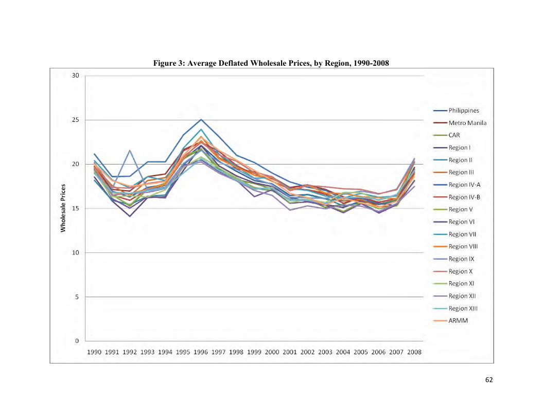
62

Figure 3: Average Deflated Wholesale Prices, by Region, 1990-2008

63

Figure 4: Average Deflated Retail Prices, by Region, 1990-2008

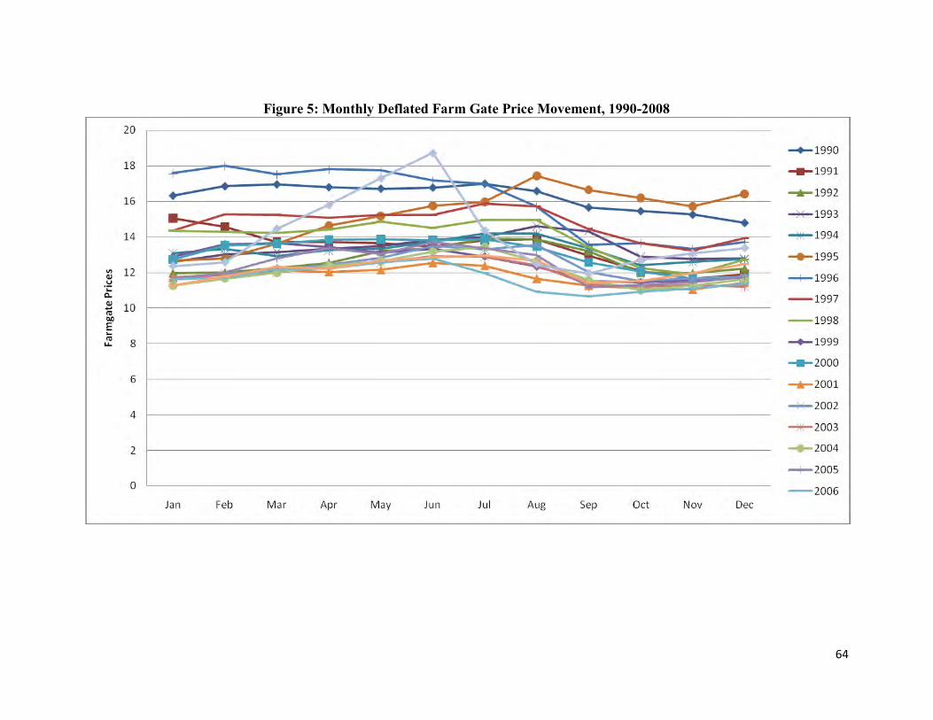
64

Figure 5: Monthly Deflated Farm Gate Price Movement, 1990-2008

65

Figure 6: Monthly Deflated Wholesale Price Movement, 1990-2008

66

Figure 7: Monthly Deflated Retail Price Movement, 1990-2008

67

Figure 8: Regional Wholesale Prices as a Ratio of Manila Wholesale Prices, 1990-2008

68

Figure 9: Farm Gate Prices to Wholesale Prices Ratio (Deflated Prices), by Region, 1990-2008

69

Figure 10: Wholesale Prices to Retail Prices Ratio (Deflated Prices), by Region, 1990-2008

70

Figure 11: Farm Gate Prices to Retail Prices (Deflated Prices), by Region, 1990-2008

71

Figure 13: Regional Farm Price Ratio and NFA Procurement Ratio

Continued on next page.

72

Figure 13: Regional Farm Price Ratio and NFA Procurement Ratio – Continued

73

Figure 13: Regional Farm Price Ratio and NFA Procurement Ratio – Continued

74

Figure 13: Regional Farm Price Ratio and NFA Procurement Ratio – Continued

75

Figure 14: Regional Retail Price Ratio and NFA Distribution Bias

Continued on next page.

76

Figure 14: Regional Retail Price Ratio and NFA Distribution Bias - Continued

Continued on next page.

77

Figure 14: Regional Retail Price Ratio and NFA Distribution Bias - Continued

Continued on next page.

78

Figure 14: Regional Retail Price Ratio and NFA Distribution Bias - Continued

79

Table A.1a: Standard Deviation of Rice Farm Gate Prices (Deflated), by Region Region 1990 1991 1992 1993 1994 1995 1996 1997 1998 1999 2000 2001 2002 2003 2004 2005 2006 2007 2008

Philippines 0.76 1.04 0.76 0.66 0.56 1.54 1.94 0.84 1.07 0.87 0.87 0.49 0.75 0.64 0.80 0.92 0.70 0.58 2.15 NCR N/A N/A N/A N/A N/A N/A N/A N/A N/A N/A N/A N/A N/A N/A N/A N/A N/A N/A N/A CAR 0.83 0.85 1.57 1.39 0.76 1.97 2.42 1.35 0.82 1.54 1.17 0.79 0.66 0.78 0.93 1.09 0.99 0.73 2.58

1 0.58 1.60 1.05 0.99 1.07 2.79 3.10 1.07 1.02 1.16 1.04 0.94 0.94 1.00 1.15 1.11 0.85 0.69 1.78 2 1.45 0.87 1.03 0.94 0.73 2.15 2.71 1.15 1.25 1.42 1.43 0.74 1.24 0.90 1.15 1.16 0.63 0.83 2.71 3 0.50 1.06 0.36 1.01 1.03 2.41 3.06 0.94 0.92 1.17 0.91 0.55 0.91 1.00 1.11 1.01 0.98 1.05 2.65

4-A 0.78 1.41 0.68 0.95 0.87 2.24 2.80 0.77 0.94 0.88 1.00 0.92 0.61 0.24 0.62 0.57 0.71 0.48 2.51 4-B 0.99 0.95 0.78 0.97 0.82 2.98 1.59 1.21 1.61 0.71 0.75 0.49 0.55 1.09 0.78 1.14 0.68 0.85 2.03 5 1.15 1.18 0.99 0.92 0.45 1.78 1.89 0.82 1.01 1.00 0.97 0.68 0.45 0.97 1.35 0.94 0.69 0.43 1.92 6 1.62 1.63 1.32 1.18 0.95 1.63 1.92 1.31 1.65 0.59 1.05 0.62 1.03 1.17 0.73 1.43 1.11 1.02 1.58 7 1.02 2.20 1.17 0.72 0.51 1.22 1.19 1.13 1.11 0.94 1.67 0.85 0.81 0.86 1.58 1.45 0.95 0.85 2.19 8 0.77 1.06 1.29 1.34 0.59 2.14 1.69 0.80 1.34 0.63 1.04 0.37 0.18 0.23 0.71 0.82 0.30 0.79 1.64 9 1.61 1.43 1.55 0.86 0.83 1.16 2.24 0.71 1.67 0.81 0.98 0.58 0.92 0.50 1.36 1.33 0.99 0.99 2.02 10 1.37 1.07 0.96 0.63 0.75 1.30 1.68 0.68 1.13 0.76 0.69 0.91 0.89 0.58 1.56 0.78 0.83 0.67 2.02 11 0.71 0.87 0.95 0.77 0.83 1.52 1.47 0.59 1.06 0.56 0.99 0.66 0.94 0.46 1.56 1.12 0.71 0.56 2.03 12 1.10 1.45 1.48 0.74 0.88 1.44 1.50 0.72 1.21 0.83 1.22 0.56 1.11 0.99 1.40 1.19 1.01 1.09 1.94 13 0.48 0.75 0.61 0.34 0.70 1.50 1.64 0.81 1.01 0.71 0.94 0.55 1.37 0.58 1.67 1.16 0.50 0.51 1.78

ARMM 0.61 0.98 0.65 0.50 0.89 1.19 1.17 1.27 1.59 0.72 0.57 0.56 1.08 0.95 1.17 0.87 1.34 0.62 2.92 Philippines 0.76 1.04 0.76 0.66 0.56 1.54 1.94 0.84 1.07 0.87 0.87 0.49 0.75 0.64 0.80 0.92 0.70 0.58 2.15

80

Table A.1b: Standard Deviation of Rice Wholesale Prices (Deflated), by Region Region 1990 1991 1992 1993 1994 1995 1996 1997 1998 1999 2000 2001 2002 2003 2004 2005 2006 2007 2008

Philippines 0.55 0.85 0.78 0.92 0.57 2.81 1.16 0.48 0.35 0.43 0.43 0.25 0.46 0.37 0.45 0.57 0.25 0.34 2.13 NCR 0.82 0.55 0.84 1.44 1.46 3.44 2.01 0.54 0.46 0.25 0.29 0.16 0.52 0.25 0.50 0.29 0.17 0.81 2.27 CAR 1.27 0.52 0.29 1.61 0.50 3.84 0.80 0.80 0.24 0.54 0.44 0.26 0.74 0.21 1.00 0.29 0.16 0.68 2.08

1 0.72 0.90 0.42 1.60 0.68 3.52 1.20 0.91 0.34 0.39 0.43 0.43 0.39 0.20 0.12 0.54 0.44 0.69 2.42 2 0.65 0.50 0.50 0.90 0.63 3.13 1.24 0.65 0.28 0.62 0.60 0.19 0.72 0.55 0.61 0.44 0.13 1.41 1.73 3 0.35 0.61 0.38 1.56 0.34 3.49 0.76 0.35 0.28 0.33 0.35 0.20 0.43 0.28 0.38 0.53 0.12 0.31 2.04

4-A 0.27 0.88 0.66 0.55 0.21 4.03 1.00 0.48 0.81 0.40 0.32 0.27 0.29 0.31 0.49 0.41 0.12 0.60 1.90 4-B 0.33 1.01 0.47 1.12 0.34 3.99 0.75 0.46 0.27 0.26 0.28 0.36 0.29 0.48 0.41 0.97 0.26 0.54 2.00 5 0.61 1.14 1.00 1.52 0.54 3.28 1.73 0.43 0.38 0.71 0.41 0.29 0.35 0.35 0.23 0.60 0.23 0.50 2.09 6 1.51 1.18 1.01 1.55 0.51 2.63 1.58 1.29 1.02 0.48 0.93 0.49 0.79 0.68 0.44 1.28 0.81 0.82 1.95 7 0.54 1.16 1.14 1.06 1.27 3.21 1.48 0.56 0.49 0.69 0.66 0.36 0.45 0.28 0.44 0.65 0.27 0.40 2.43 8 0.89 0.84 1.55 1.01 0.77 3.12 1.37 0.36 0.42 0.42 0.42 0.34 0.39 0.31 0.44 0.28 0.18 0.31 2.27 9 1.01 0.91 0.85 0.58 0.95 1.85 1.15 0.49 0.70 0.38 0.50 0.13 0.26 0.38 0.68 0.74 0.31 0.21 2.73 10 0.96 1.42 1.29 0.72 1.06 2.32 1.21 0.49 0.61 0.71 0.64 0.35 0.90 0.47 0.58 0.58 0.36 0.38 2.64 11 0.69 0.97 1.25 0.53 0.78 2.26 1.25 0.85 1.04 0.73 0.85 0.46 1.29 0.88 1.21 1.10 0.57 0.48 2.96 12 0.85 1.30 1.69 0.43 0.94 1.76 1.28 0.82 0.75 0.60 0.57 0.63 1.33 1.11 1.45 1.45 1.06 0.90 2.84 13 0.58 1.16 1.19 0.51 1.08 1.55 0.91 0.76 0.50 0.31 0.44 0.29 0.80 0.48 0.78 0.53 0.19 0.24 2.85

ARMM 0.43 1.22 1.24 0.82 1.02 2.54 1.22 0.38 0.37 0.26 0.55 0.30 0.23 0.39 0.55 0.22 0.39 0.56 2.20

81

Table A.1c: Standard Deviation of Rice Retail Prices (Deflated), by Region 1990 1991 1992 1993 1994 1995 1996 1997 1998 1999 2000 2001 2002 2003 2004 2005 2006 2007 2008

Philippines 0.36 0.72 0.78 0.93 0.48 3.28 0.90 0.41 0.33 0.35 0.35 0.21 0.51 0.28 0.35 0.43 0.15 0.34 2.25 NCR 0.49 0.55 0.56 1.08 0.54 3.52 0.34 0.39 0.59 0.18 0.41 0.22 0.30 0.20 0.45 0.25 0.16 0.58 2.23 CAR 0.76 0.64 0.39 1.43 0.57 3.74 1.03 0.50 0.22 0.34 0.37 0.25 0.63 0.10 0.56 0.37 0.18 0.83 2.12

1 0.67 0.67 0.35 1.61 0.68 3.94 1.13 0.62 0.19 0.39 0.37 0.48 0.39 0.25 0.32 0.29 0.30 0.37 2.43 2 0.61 0.65 0.33 1.24 0.58 3.61 1.10 0.56 0.32 0.40 0.48 0.16 0.94 0.36 0.33 0.30 0.18 1.26 1.91 3 0.27 0.56 0.39 1.59 0.35 3.64 0.79 0.30 0.27 0.26 0.36 0.22 0.48 0.35 0.30 0.29 0.18 0.40 2.17

4-A 0.45 0.53 1.20 0.46 0.27 4.28 0.65 0.37 0.72 0.36 0.48 0.38 0.40 0.32 0.53 0.33 0.11 0.73 1.87 4-B 0.32 0.56 0.42 1.17 0.29 4.15 0.57 0.26 0.42 0.23 0.28 0.26 0.26 0.28 0.26 0.81 0.13 0.38 1.98 5 0.36 1.07 1.16 1.55 0.43 5.03 1.68 0.28 0.64 0.48 0.29 0.25 0.24 0.34 0.25 0.61 0.21 0.36 1.85 6 1.80 0.99 0.77 1.34 0.43 3.46 0.98 0.94 0.58 0.32 0.78 0.33 0.73 0.68 0.57 1.10 0.55 0.60 1.92 7 0.54 1.63 0.60 0.84 1.11 3.24 1.53 0.42 0.24 0.47 0.60 0.28 0.42 0.14 0.29 0.57 0.09 0.39 2.39 8 0.78 0.50 1.51 0.67 0.78 3.39 1.45 0.49 0.40 0.47 0.38 0.34 0.57 0.33 0.37 0.24 0.19 0.22 2.34 9 0.70 0.84 1.06 0.42 1.18 1.89 0.97 0.36 0.58 0.39 0.54 0.24 0.34 0.29 0.62 0.60 0.23 0.25 2.63 10 0.57 1.20 1.05 0.73 1.03 2.60 0.76 0.24 0.57 0.49 0.58 0.20 0.75 0.36 0.49 0.30 0.19 0.17 2.91 11 0.59 1.02 1.48 0.74 0.72 2.49 0.83 0.59 0.78 0.41 0.50 0.34 1.51 0.75 1.13 0.71 0.33 0.29 3.30 12 0.54 0.81 1.33 0.62 0.68 2.00 0.92 0.60 0.70 0.57 0.67 0.25 0.96 0.71 1.03 1.13 0.56 0.61 3.17 13 0.45 1.02 1.45 0.45 0.82 1.70 0.76 0.63 0.44 0.35 0.36 0.27 1.01 0.45 0.71 0.28 0.15 0.16 3.08

ARMM 0.39 1.07 1.18 0.57 0.79 2.70 1.16 0.26 0.28 0.36 0.24 0.31 0.25 0.30 0.59 0.18 0.33 0.43 2.62

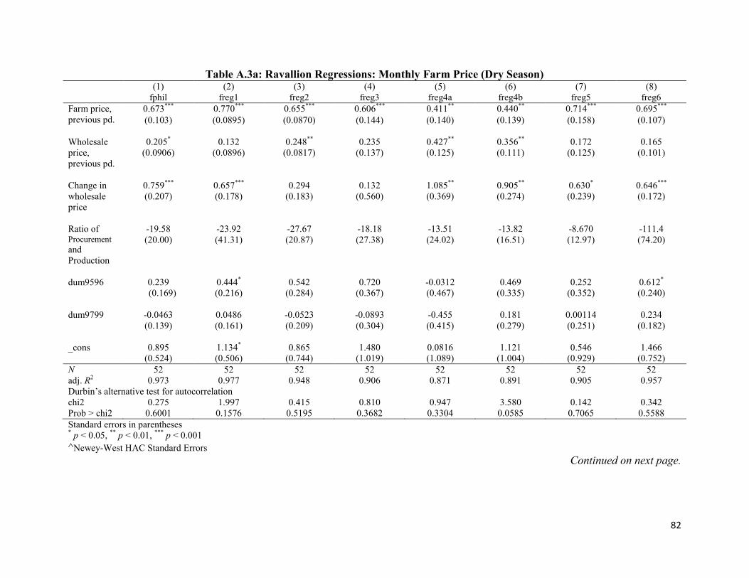
82

Table A.3a: Ravallion Regressions: Monthly Farm Price (Dry Season) (1) (2) (3) (4) (5) (6) (7) (8) fphil freg1 freg2 freg3 freg4a freg4b freg5 freg6 Farm price, previous pd.

0.673*** 0.770*** 0.655*** 0.606*** 0.411** 0.440** 0.714*** 0.695*** (0.103) (0.0895) (0.0870) (0.144) (0.140) (0.139) (0.158) (0.107)

Wholesale price, previous pd.

0.205* 0.132 0.248** 0.235 0.427** 0.356** 0.172 0.165 (0.0906) (0.0896) (0.0817) (0.137) (0.125) (0.111) (0.125) (0.101)

Change in wholesale price

0.759*** 0.657*** 0.294 0.132 1.085** 0.905** 0.630* 0.646*** (0.207) (0.178) (0.183) (0.560) (0.369) (0.274) (0.239) (0.172)

Ratio of Procurement and Production

-19.58 -23.92 -27.67 -18.18 -13.51 -13.82 -8.670 -111.4 (20.00) (41.31) (20.87) (27.38) (24.02) (16.51) (12.97) (74.20)

dum9596 0.239 0.444* 0.542 0.720 -0.0312 0.469 0.252 0.612* (0.169) (0.216) (0.284) (0.367) (0.467) (0.335) (0.352) (0.240) dum9799 -0.0463 0.0486 -0.0523 -0.0893 -0.455 0.181 0.00114 0.234

(0.139) (0.161) (0.209) (0.304) (0.415) (0.279) (0.251) (0.182)

_cons 0.895 1.134* 0.865 1.480 0.0816 1.121 0.546 1.466 (0.524) (0.506) (0.744) (1.019) (1.089) (1.004) (0.929) (0.752) N 52 52 52 52 52 52 52 52 adj. R2 0.973 0.977 0.948 0.906 0.871 0.891 0.905 0.957 Durbin’s alternative test for autocorrelation chi2 0.275 1.997 0.415 0.810 0.947 3.580 0.142 0.342 Prob > chi2 0.6001 0.1576 0.5195 0.3682 0.3304 0.0585 0.7065 0.5588 Standard errors in parentheses * p < 0.05, ** p < 0.01, *** p < 0.001 ^Newey-West HAC Standard Errors

Continued on next page.

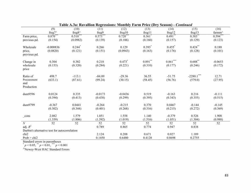
83

Table A.3a: Ravallion Regressions: Monthly Farm Price (Dry Season) - Continued (9) (10) (11) (12) (13) (14) (15) (16) freg7^ freg8^ freg9 freg10 freg11 freg12 freg13 farmm^ Farm price, previous pd.

0.870*** 0.510*** 0.573*** 0.720*** 0.361* 0.491** 0.383** 0.594*** (0.154) (0.0982) (0.139) (0.106) (0.160) (0.157) (0.129) (0.123)

Wholesale price, previous pd.

-0.000836 0.244* 0.266 0.129 0.393* 0.455* 0.424** 0.188 (0.0820) (0.121) (0.151) (0.0943) (0.163) (0.176) (0.128) (0.101)

Change in wholesale price

0.304 0.382 0.218 0.473* 0.891** 0.861*** 0.688** -0.0653 (0.153) (0.320) (0.284) (0.221) (0.310) (0.177) (0.246) (0.172)

Ratio of Procurement and Production

498.7 -113.1 -84.89 -29.36 36.55 -51.75 -2280.1*** 12.71 (633.1) (87.61) (99.24) (30.15) (58.45) (56.76) (579.0) (27.95)

dum9596 0.0124 0.335 -0.0173 -0.0436 0.519 -0.163 0.216 -0.111 (0.394) (0.413) (0.438) (0.299) (0.395) (0.343) (0.355) (0.515) dum9799 -0.367 0.0441 -0.264 -0.215 0.370 0.0467 -0.144 -0.145

(0.302) (0.344) (0.401) (0.268) (0.316) (0.215) (0.272) (0.369)

_cons 2.082 1.579 1.051 1.558 1.140 -0.379 0.526 1.908 (1.359) (1.806) (1.592) (1.019) (1.516) (1.051) (1.304) (0.988) N 52 52 52 52 52 52 52 52 adj. R2 0.789 0.865 0.774 0.947 0.838 Durbin's alternative test for autocorrelation chi2 2.124 0.208 0.671 0.027 1.189 Prob > chi2 0.1450 0.6480 0.4128 0.8698 0.2755 Standard errors in parentheses * p < 0.05, ** p < 0.01, *** p < 0.001 ^Newey-West HAC Standard Errors

84

Table A.3b: Ravallion Regressions: Monthly Farm Price (Harvest Season) (1) (2) (3) (4) (5) (6) (7) (8) fphil freg1 freg2 freg3 freg4a freg4b freg5 freg6 fphilp 0.700*** 0.123 0.275* 0.657*** 0.514** 0.270 0.319* 0.391*** (0.149) (0.182) (0.126) (0.132) (0.163) (0.137) (0.128) (0.106) wphilp 0.184 0.379 0.406** 0.0182 0.182 0.443*** 0.438*** 0.559*** (0.114) (0.200) (0.135) (0.128) (0.113) (0.111) (0.105) (0.0931) wphilch 0.620*** 0.844* 0.609** 0.257 -0.226 0.494** 1.242*** 1.025*** (0.152) (0.324) (0.221) (0.316) (0.240) (0.150) (0.265) (0.160) procphil -34.51 -60.05 -149.1** -27.61 -12.96 -9.438 -59.83** -73.65* (23.49) (33.08) (44.08) (30.46) (11.55) (7.855) (21.88) (31.10) dum9596 0.200 1.620* 0.711 1.435* 0.0296 0.400 0.342 -0.381 (0.294) (0.703) (0.461) (0.621) (0.592) (0.345) (0.353) (0.283) dum9799 -0.0994 0.662 0.311 0.546 0.120 -0.126 -0.0370 -0.404* (0.209) (0.474) (0.296) (0.431) (0.384) (0.244) (0.230) (0.174) _cons 0.739 4.972* 2.362 3.951* 2.633* 1.099 0.345 -1.156 (0.843) (1.922) (1.222) (1.566) (1.177) (0.842) (0.884) (0.781) N 52 52 52 52 52 52 52 52 adj. R2 0.932 0.703 0.867 0.772 0.811 0.931 0.914 0.944 Durbin's alternative test for autocorrelation chi2 0.912 0.000 0.250 1.728 0.545 0.144 0.763 0.050 Prob > chi2 0.3395 0.9877 0.6169 0.1887 0.4602 0.7039 0.3823 0.8224 Standard errors in parentheses * p < 0.05, ** p < 0.01, *** p < 0.001 ^Newey-West HAC Standard Errors

Continued on next page.

85

Table A.3b: Ravallion Regressions: Monthly Farm Price (Harvest Season) - Continued (9) (10) (11) (12) (13) (14) (15) (16) freg7 freg8 freg9 freg10 freg11 freg12^ freg13 farmm freg7p 0.247* 0.194 0.491*** 0.516*** 0.458*** 0.650*** 0.584*** 0.358* (0.110) (0.130) (0.120) (0.117) (0.127) (0.116) (0.108) (0.137) wreg7p 0.0894 0.492*** 0.389** 0.386*** 0.441*** 0.241* 0.212 0.465** (0.0737) (0.115) (0.129) (0.0909) (0.112) (0.0994) (0.116) (0.148) wreg7ch 0.447* 0.214 0.973*** 0.813*** 0.811*** 0.743*** 0.618*** 0.712 (0.179) (0.175) (0.217) (0.124) (0.104) (0.143) (0.151) (0.395) procreg7 -1128.8** -1095.3 -89.10 -25.32 20.21 -18.94 -454.7 -8.068 (353.9) (749.8) (57.25) (40.69) (15.31) (10.04) (769.8) (25.31) dum9596 1.114* 0.0345 -0.307 -0.292 -0.170 0.526* 0.632 -1.204 (0.513) (0.457) (0.524) (0.349) (0.292) (0.228) (0.347) (0.812) dum9799 0.522 0.209 -0.246 -0.683** -0.0548 0.306* 0.0221 -0.667 (0.294) (0.294) (0.394) (0.246) (0.181) (0.144) (0.237) (0.619) _cons 7.823*** 0.874 -0.404 -0.865 -0.916 0.749 1.104 -0.223 (1.629) (1.343) (1.910) (1.330) (0.902) (0.578) (1.238) (2.206) N 52 52 52 52 52 52 52 52 adj. R2 0.606 0.837 0.750 0.850 0.922 0.878 0.511 Durbin's alternative test for autocorrelation chi2 0.626 0.001 0.005 0.177 0.346 0.032 3.413 Prob > chi2 0.4290 0.9757 0.9437 0.6742 0.5562 0.8572 0.0647 Standard errors in parentheses * p < 0.05, ** p < 0.01, *** p < 0.001 ^Newey-West HAC Standard Errors

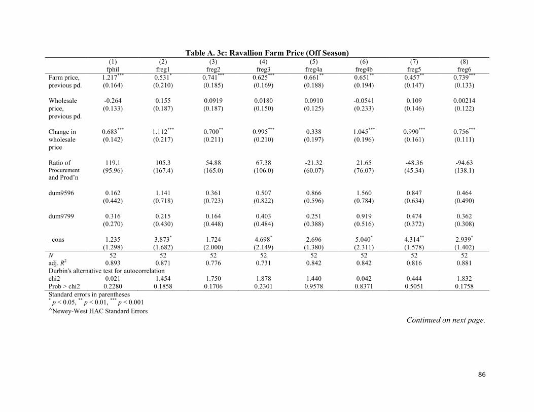
86

Table A. 3c: Ravallion Farm Price (Off Season) (1) (2) (3) (4) (5) (6) (7) (8) fphil freg1 freg2 freg3 freg4a freg4b freg5 freg6 Farm price, previous pd.

1.217*** 0.531* 0.741*** 0.625*** 0.661** 0.651** 0.457** 0.739*** (0.164) (0.210) (0.185) (0.169) (0.188) (0.194) (0.147) (0.133)

Wholesale price, previous pd.

-0.264 0.155 0.0919 0.0180 0.0910 -0.0541 0.109 0.00214 (0.133) (0.187) (0.187) (0.150) (0.125) (0.233) (0.146) (0.122)

Change in wholesale price

0.683*** 1.112*** 0.700** 0.995*** 0.338 1.045*** 0.990*** 0.756*** (0.142) (0.217) (0.211) (0.210) (0.197) (0.196) (0.161) (0.111)

Ratio of Procurement and Prod’n

119.1 105.3 54.88 67.38 -21.32 21.65 -48.36 -94.63 (95.96) (167.4) (165.0) (106.0) (60.07) (76.07) (45.34) (138.1)

dum9596 0.162 1.141 0.361 0.507 0.866 1.560 0.847 0.464 (0.442) (0.718) (0.723) (0.822) (0.596) (0.784) (0.634) (0.490) dum9799 0.316 0.215 0.164 0.403 0.251 0.919 0.474 0.362 (0.270) (0.430) (0.448) (0.484) (0.388) (0.516) (0.372) (0.308) _cons 1.235 3.873* 1.724 4.698* 2.696 5.040* 4.314** 2.939* (1.298) (1.682) (2.000) (2.149) (1.380) (2.311) (1.578) (1.402) N 52 52 52 52 52 52 52 52 adj. R2 0.893 0.871 0.776 0.731 0.842 0.842 0.816 0.881 Durbin's alternative test for autocorrelation chi2 0.021 1.454 1.750 1.878 1.440 0.042 0.444 1.832 Prob > chi2 0.2280 0.1858 0.1706 0.2301 0.9578 0.8371 0.5051 0.1758 Standard errors in parentheses * p < 0.05, ** p < 0.01, *** p < 0.001 ^Newey-West HAC Standard Errors

Continued on next page.

87

Table A. 3c: Ravallion Farm Price (Off Season) - Continued (9) (10) (11) (12) (13) (14) (15) (16) freg7 freg8^ freg9 freg10^ freg11^ freg12 freg13 farmm Farm price, previous pd.

0.730*** 0.433 0.475** 0.594** 0.503* 0.810*** 0.276 0.583*** (0.134) (0.227) (0.169) (0.208) (0.192) (0.157) (0.162) (0.145)

Wholesale price, previous pd.

-0.0595 0.311 0.112 0.0933 0.309 -0.0302 0.336 0.242 (0.132) (0.167) (0.199) (0.171) (0.206) (0.174) (0.191) (0.141)

Change in wholesale price

0.341 0.865*** 0.984*** 0.718** 0.657*** 0.774*** 1.073*** -0.0890 (0.207) (0.185) (0.255) (0.207) (0.140) (0.107) (0.234) (0.328)

Ratio of Procurement and Prod’n

-379.5 -2396.3 -170.2 -177.2 -69.90 -37.72 -5174.8 -17.21 (925.7) (1812.0) (102.3) (153.4) (53.41) (46.07) (5489.5) (75.01)

dum9596 0.978 -0.285 0.375 0.429 0.242 0.510 0.629 -0.930 (0.948) (0.630) (0.778) (0.587) (0.513) (0.438) (0.548) (0.939) dum9799 0.247 0.437 0.223 0.299 0.0353 0.261 -0.325 -0.581 (0.541) (0.632) (0.544) (0.412) (0.271) (0.270) (0.399) (0.638) _cons 4.332 1.407 4.701 3.338 0.707 2.834 3.314 1.151 (2.664) (1.914) (2.766) (2.291) (1.774) (1.510) (2.240) (2.319) N 52 52 52 52 52 52 52 52 adj. R2 0.508 0.617 0.912 0.682 0.446 Durbin's alternative test for autocorrelation chi2 0.348 1.221 1.769 1.463 0.021 Prob > chi2 0.5554 0.2692 0.1835 0.2265 0.8844 Standard errors in parentheses * p < 0.05, ** p < 0.01, *** p < 0.001 ^Newey-West HAC Standard Errors

88

Table A.4a: Ravallion Regressions: Monthly Retail Price (Dry Season) (1) (2) (3) (4) (5) (6) (7) (8) (9) rphil rmm rcar rreg1 rreg2 rreg3^ rreg4a rreg4b rreg5 Retail price, previous pd. 0.693*** 0.804*** 0.853*** 0.869*** 0.636*** 0.591*** 0.872*** 0.665*** 0.821***

(0.0729) (0.0526) (0.0845) (0.0738) (0.0864) (0.146) (0.0573) (0.0821) (0.0462) Wholesale price, previous pd. 0.318*** 0.182*** 0.196* 0.128 0.375*** 0.425** 0.131* 0.366*** 0.182***

(0.0729) (0.0471) (0.0791) (0.0725) (0.0929) (0.144) (0.0608) (0.0830) (0.0501) Change in wholesale price 0.914*** 0.437*** 0.701*** 0.963*** 0.813*** 1.071*** 0.738*** 0.882*** 0.749***

(0.0304) (0.0552) (0.0803) (0.0548) (0.0702) (0.0378) (0.0558) (0.0479) (0.0466) dum9596 -0.0252 0.0526 -0.210 -0.00793 0.0895 0.214 -0.0332 -0.00155 0.0340 (0.0493) (0.166) (0.160) (0.101) (0.152) (0.206) (0.114) (0.103) (0.0944) dum9799 0.0541 0.128 -0.225 0.0249 0.0200 0.126 0.0432 0.112 0.0722

(0.0428) (0.141) (0.114) (0.0881) (0.120) (0.0954) (0.0958) (0.0997) (0.0716)

_cons 0.282 0.661 -0.531 0.225 0.342 0.333 0.146 -0.0280 0.274 (0.182) (0.512) (0.450) (0.296) (0.386) (0.446) (0.262) (0.316) (0.227) N 76 76 76 76 76 76 76 76 76 adj. R2 0.998 0.978 0.977 0.989 0.980 0.993 0.991 0.994 Durbin’s alternative test for autocorrelation chi2 0.111 0.853 0.403 2.418 0.023 0.187 2.292 0.167 Prob > chi2 0.7385 0.3556 0.5253 0.1199 0.8799 0.6655 0.1300 0.6827 Standard errors in parentheses * p < 0.05, ** p < 0.01, *** p < 0.001 ^Newey-West HAC Standard Errors

Continued on next page.

89

Table A.4a: Ravallion Regressions: Monthly Retail Price (Dry Season) - Continued (10) (11) (12) (13) (14) (15) (16) (17) (18) rreg6 rreg7 rreg8 rreg9^ rreg10 rreg11 rreg12 rreg13 rarmm Retail price, previous pd. 0.891*** 0.803*** 0.704*** 0.632*** 0.651*** 0.470*** 0.414*** 0.759*** 0.562***

(0.0543) (0.0446) (0.0776) (0.0772) (0.0893) (0.0810) (0.0837) (0.0674) (0.0983) Wholesale price, previous pd. 0.0925 0.277*** 0.234** 0.371*** 0.368*** 0.516*** 0.574*** 0.269*** 0.419***

(0.0504) (0.0596) (0.0715) (0.0767) (0.0833) (0.0784) (0.0777) (0.0665) (0.0942) Change in wholesale price 0.795*** 0.671*** 0.580*** 0.876*** 0.767*** 0.763*** 0.662*** 0.799*** 0.865***

(0.0524) (0.0790) (0.0709) (0.0678) (0.0606) (0.0490) (0.0483) (0.0497) (0.0582) dum9596 0.154 -0.281 0.195 0.143 -0.0441 0.137 -0.326** -0.0671 0.165 (0.109) (0.196) (0.154) (0.0915) (0.136) (0.0996) (0.109) (0.0858) (0.146) dum9799 0.0348 -0.384* 0.201 -0.0100 0.0360 0.221* 0.0168 -0.0252 -0.131

(0.0956) (0.160) (0.118) (0.0681) (0.117) (0.0861) (0.0823) (0.0695) (0.120)

_cons 0.489 -0.919 1.488** 0.381 0.226 0.921* 1.226** -0.112 0.946* (0.368) (0.493) (0.478) (0.312) (0.521) (0.350) (0.398) (0.326) (0.441) N 76 76 76 76 76 76 76 76 76 adj. R2 0.985 0.977 0.978 0.979 0.987 0.984 0.987 0.983 Durbin’s alternative test for autocorrelation chi2 0.006 0.974 0.010 0.016 0.284 0.557 0.071 0.044 Prob > chi2 0.9406 0.3238 0.9221 0.8984 0.5940 .4554 0.7895 0.8339 Standard errors in parentheses * p < 0.05, ** p < 0.01, *** p < 0.001 ^Newey-West HAC Standard Errors

90

Table A.4b: Ravallion Regressions: Monthly Retail Price (Harvest Season) (1) (2) (3) (4) (5) (6) (7) (9) (8) rphil^ rmm rcar rreg1 rreg2 rreg3 rreg4a rreg5 rreg4b^ Retail price, previous pd. 0.636*** 0.564*** 0.681*** 0.638*** 0.749*** 0.683*** 0.767*** 0.716*** 0.653***

(0.102) (0.0900) (0.0794) (0.0726) (0.0883) (0.0812) (0.0550) (0.0482) (0.0686) Wholesale price, previous pd. 0.354** 0.452*** 0.265*** 0.281*** 0.244* 0.292*** 0.234*** 0.284*** 0.337***

(0.106) (0.0967) (0.0762) (0.0788) (0.101) (0.0827) (0.0601) (0.0588) (0.0711) Change in wholesale price 0.614*** 0.580*** 0.563*** 0.724*** 0.707*** 0.779*** 0.754*** 0.642*** 0.628***

(0.0517) (0.148) (0.0633) (0.0681) (0.0746) (0.0645) (0.0611) (0.0842) (0.129) dum9596 0.133 0.628 0.0326 0.410** -0.0227 0.282* -0.0402 0.106 0.101 (0.113) (0.418) (0.161) (0.153) (0.155) (0.123) (0.149) (0.144) (0.213) dum9799 0.0348 -0.120 0.0816 0.395*** -0.0192 0.129 0.0578 0.0759 0.0597

(0.0476) (0.290) (0.101) (0.108) (0.101) (0.0880) (0.1000) (0.0836) (0.128)

_cons 0.721** 0.685 1.279** 1.737*** 0.442 0.874** 0.335 0.721 (0.244) (1.107) (0.431) (0.380) (0.410) (0.313) (0.286) 0.482 (0.573) N 75 75 75 75 75 75 75 (0.304) 75 adj. R2 0.913 0.981 0.984 0.983 0.993 0.994 75 Durbin's alternative test for autocorrelation chi2 0.112 0.088 2.962 0.047 0.004 0.342 1.909 Prob > chi2 0.7382 0.7663 0.0852 0.8289 0.9523 0.5585 0.1670 Standard errors in parentheses * p < 0.05, ** p < 0.01, *** p < 0.001 ^Newey-West HAC Standard Errors

Continued on next page.

91

Table A.4b: Ravallion Regressions: Monthly Retail Price (Harvest Season) - Continued

(9) (10) (11) (12) (13) (14) (15) (16) (17) (18) rreg5 rreg6 rreg7 rreg8 rreg9^ rreg10 rreg11 rreg12^ rreg13 rarmm Retail price, previous pd. 0.716*** 0.910*** 0.954*** 0.682*** 0.669*** 0.767*** 0.503*** 0.498*** 0.776*** 0.921***

(0.0482) (0.0463) (0.0512) (0.0918) (0.0794) (0.0635) (0.0790) (0.108) (0.0429) (0.0492)

Wholesale price, previous pd. 0.284*** 0.0547 0.0321 0.317*** 0.344*** 0.195* 0.476*** 0.444*** 0.191*** 0.0935* (0.0588) (0.0529) (0.0754) (0.0916) (0.0844) (0.0750) (0.0854) (0.0903) (0.0492) (0.0432)

Change in wholesale price 0.642*** 0.737*** 0.322** 0.796*** 0.641*** 0.577*** 0.719*** 0.578*** 0.566*** 0.586***

(0.0842) (0.0555) (0.0985) (0.0673) (0.0774) (0.0519) (0.0539) (0.0806) (0.0560) (0.0763) dum9596 0.106 -0.142 -0.0281 0.0874 -0.00716 0.0642 0.335* 0.0375 0.0524 -0.171 (0.144) (0.139) (0.258) (0.171) (0.103) (0.146) (0.154) (0.133) (0.115) (0.215) dum9799 0.0759 0.0585 0.0197 -0.0280 -0.0337 0.0221 0.191 -0.0405 0.0427 -0.0957 (0.0836) (0.0977) (0.161) (0.114) (0.0801) (0.107) (0.0996) (0.0980) (0.0779) (0.0823) _cons 0.482 0.707 0.174 0.463 0.194 0.994* 1.079* 1.802** 0.835* -0.00719 (0.304) (0.384) (0.633) (0.502) (0.347) (0.486) (0.471) (0.621) (0.402) (0.425) N 75 75 75 75 75 75 75 75 75 75 adj. R2 0.993 0.984 0.976 0.980 0.980 0.979 0.981 Durbin's alternative test for autocorrelation chi2 1.909 0.003 0.773 1.365 1.824 0.887 1.227 Prob > chi2 0.1670 0.9563 0.3792 0.2427 0.1769 0.3462 0.2680 Standard errors in parentheses * p < 0.05, ** p < 0.01, *** p < 0.001 ^Newey-West HAC Standard Errors

92

Table A.4c: Ravallion Regressions: Monthly Retail Price (Off Season) (1) (2) (3) (4) (5) (6) (7) (8) (9) rphil rmm rcar rreg1 rreg2^ rreg3 rreg4a rreg4b rreg5 Retail price, previous pd. 0.635*** 0.544*** 0.547*** 0.922*** 0.546*** 0.733*** 0.896*** 0.674*** 0.900***

(0.120) (0.0946) (0.0801) (0.0734) (0.121) (0.0890) (0.0693) (0.0758) (0.125) Wholesale price, previous pd. 0.422** 0.451*** 0.434*** 0.0934 0.500*** 0.266** 0.131 0.333*** 0.203

(0.126) (0.0905) (0.0838) (0.0685) (0.131) (0.0933) (0.0729) (0.0790) (0.135) Change in wholesale price 1.000*** 0.768*** 0.878*** 1.086*** 0.999*** 1.007*** 0.939*** 0.786*** 1.054***

(0.0327) (0.0710) (0.0459) (0.0501) (0.0786) (0.0342) (0.0610) (0.0304) (0.0666) dum9596 0.00278 0.152 0.616*** 0.0638 0.00712 0.0513 0.0531 0.330** 0.108 (0.0924) (0.273) (0.172) (0.141) (0.161) (0.115) (0.186) (0.112) (0.265) dum9799 -0.0609 0.125 0.0130 -0.0293 -0.0684 0.103 0.00480 0.128 -0.287 (0.0638) (0.200) (0.114) (0.0996) (0.0704) (0.0807) (0.136) (0.0851) (0.169) -1.514* _cons -0.394 0.863 0.893* -0.139 -0.0789 0.418 -0.292 0.337 (0.606) (0.257) (0.704) (0.381) (0.361) (0.382) (0.275) (0.399) (0.278) 76 N 76 76 76 76 76 76 76 76 0.972 adj. R2 0.995 0.960 0.983 0.989 0.994 0.987 0.994 0.458 Durbin's alternative test for autocorrelation chi2 0.997 2.308 0.730 1.403 3.551 0.063 0.019 0.4985 Prob > chi2 0.3180 .1287 0.3929 0.2363 0.0595 0.8025 0.8894 Standard errors in parentheses * p < 0.05, ** p < 0.01, *** p < 0.001 ^Newey-West HAC Standard Errors

Continued on next page.

93

Table A.4c: Ravallion Regressions: Monthly Retail Price (Off Season) - Continued (10) (11) (12) (13) (14) (15) (16) (17) (18) rreg6 rreg7^ rreg8 rreg9 rreg10 rreg11 rreg12 rreg13 rarmm Retail price, previous pd. 0.925*** 0.791*** 0.428*** 0.686*** 0.561*** 0.661*** 0.462*** 0.651*** 0.725***

(0.105) (0.0698) (0.0943) (0.112) (0.105) (0.0961) (0.103) (0.126) (0.0894) Wholesale price, previous pd. 0.137 0.261** 0.525*** 0.319** 0.486*** 0.447*** 0.597*** 0.448** 0.281**

(0.103) (0.0763) (0.0943) (0.113) (0.111) (0.103) (0.110) (0.139) (0.0933) Change in wholesale price 1.064*** 0.826*** 1.151*** 0.866*** 0.893*** 0.998*** 0.788*** 0.953*** 0.920***

(0.0608) (0.101) (0.0488) (0.0552) (0.0587) (0.0367) (0.0418) (0.0389) (0.0614) dum9596 0.121 -0.190 0.412* 0.301* 0.0552 -0.310* -0.306 -0.268 -0.0902 (0.248) (0.277) (0.169) (0.147) (0.185) (0.151) (0.193) (0.135) (0.157) dum9799 -0.0152 -0.147 0.128 -0.00608 -0.155 -0.298** -0.243 -0.241* -0.162

(0.176) (0.102) (0.110) (0.104) (0.133) (0.112) (0.133) (0.102) (0.129)

_cons -0.776 -0.397 1.546*** 0.307 -0.181 -1.311** -0.115 -1.145** 0.320 (0.696) (0.493) (0.424) (0.406) (0.538) (0.433) (0.555) (0.395) (0.378) N 76 76 76 76 76 76 76 76 76 adj. R2 0.957 0.983 0.981 0.971 0.977 0.961 0.977 0.987 Durbin's alternative test for autocorrelation chi2 2.282 0.005 0.121 2.680 0.300 0.099 0.189 1.445 Prob > chi2 0.1309 0.9458 0.7277 0.1016 0.5839 0.7531 0.6638 0.2293 Standard errors in parentheses * p < 0.05, ** p < 0.01, *** p < 0.001 ^Newey-West HAC Standard Errors

94

Table A.5a: YSM Regressions: Monthly Farm, with Level of Procurement (1) (2) (3) (4) (5) (6) (7) (8) freg1ch freg2ch freg3ch freg4ach freg4bch freg5ch freg6ch freg7ch time -0.000708 0.000982 -0.000559 0.000270 0.000338 -0.000214 0.000688 -0.00214 (0.00156) (0.00171) (0.00185) (0.00169) (0.00196) (0.00177) (0.00171) (0.00230) Procurement 0.00000342 0.0000133 -0.0000141 0.0000191 0.00000931 -0.0000344 0.00000902 -0.00403**

(0.0000273) (0.0000232) (0.0000156) (0.0000160) (0.0000186) (0.0000388) (0.0000252) (0.00132) dumjan 0.702** 0.615* 0 0.842** 0.233 0 0.462 0.491 (0.264) (0.267) (.) (0.323) (0.374) (.) (0.272) (0.358) dumfeb 0.290 0.774** -0.0582 0.946** 0.820* 0.516 0.753** -0.227 (0.278) (0.269) (0.288) (0.338) (0.392) (0.277) (0.271) (0.361) dummar 0.203 0.501 -0.371 0.352 0.136 -0.150 0.786** -0.198 (0.278) (0.266) (0.288) (0.335) (0.388) (0.280) (0.266) (0.360) dumapr 0.206 0.534* -0.264 0.0859 0.571 0.227 0.841** 0.289 (0.277) (0.257) (0.288) (0.316) (0.366) (0.297) (0.271) (0.359) dummay 0.154 0.381 -0.112 0.873** 0.596 0.357 0.671* 0.145 (0.276) (0.256) (0.289) (0.313) (0.363) (0.283) (0.272) (0.361) dumjun 0.105 0.482 0.0785 0.685* 0.543 0.190 0.285 -0.383 (0.280) (0.264) (0.287) (0.335) (0.388) (0.277) (0.274) (0.357) dumjul 0.163 0.384 -0.340 0.733* 0.688 0.478 0.389 -0.746* (0.284) (0.270) (0.287) (0.346) (0.401) (0.277) (0.275) (0.365) dumaug 0.454 0.0920 -0.155 0.487 0.318 0.0906 -0.307 -0.0700 (0.284) (0.270) (0.288) (0.350) (0.406) (0.277) (0.274) (0.366) dumsep -1.107*** -0.701** -1.492*** -0.0120 -0.899* -0.981*** -1.316*** -1.101** (0.284) (0.269) (0.288) (0.350) (0.405) (0.277) (0.265) (0.366) dumoct -1.813*** -0.912*** -1.449*** -0.406 -0.489 -0.816** 0 -0.978** (0.261) (0.257) (0.288) (0.305) (0.353) (0.282) (.) (0.359) dumnov 0 0 0.0321 0 0 0.282 0.722** -0.189 (.) (.) (0.299) (.) (.) (0.285) (0.256) (0.349) dumdec 0.144 0.459 -0.00594 0.567* 0.431 0.826** 0.698** 0 (0.240) (0.256) (0.297) (0.272) (0.316) (0.279) (0.261) (.) dum90 0 0 0 0 0 0 0 0 (.) (.) (.) (.) (.) (.) (.) (.) dum91 -0.601* -0.0458 -0.238 -0.335 -0.193 -0.140 -0.151 0.132 (0.284) (0.303) (0.334) (0.315) (0.365) (0.321) (0.303) (0.425) dum92 0.0924 0.160 0.138 0.0851 0.0360 0.0437 0.158 -0.0377 (0.275) (0.294) (0.324) (0.305) (0.353) (0.313) (0.295) (0.401) dum93 0.0513 0.389 0.173 0.152 0.214 0.0610 0.192 -0.169 (0.270) (0.291) (0.322) (0.297) (0.344) (0.307) (0.297) (0.398) dum94 -0.232 0.0466 -0.130 -0.0478 0.0325 0.0515 0.171 -0.217 (0.264) (0.286) (0.315) (0.291) (0.338) (0.302) (0.293) (0.389) dum95 0.333 0.639* 0.451 0.463 0.395 0.266 0.397 0.0546 (0.261) (0.283) (0.308) (0.289) (0.334) (0.296) (0.286) (0.382) dum96 -0.322 -0.189 -0.331 -0.290 -0.0276 -0.0488 -0.117 -0.171 (0.253) (0.272) (0.301) (0.281) (0.326) (0.289) (0.280) (0.372) dum97 -0.0467 0.163 0.0992 0.0873 0.0400 -0.0285 0.108 -0.132 (0.251) (0.271) (0.299) (0.277) (0.322) (0.287) (0.276) (0.369)

Continued on next page.

95

(1) (2) (3) (4) (5) (6) (7) (8) freg1ch freg2ch freg3ch freg4ach freg4bch freg5ch freg6ch freg7ch dum98 -0.0509 0.0945 -0.0267 -0.0628 -0.110 -0.0470 -0.00537 -0.156 (0.252) (0.271) (0.297) (0.277) (0.321) (0.285) (0.273) (0.367) dum99 -0.128 -0.0483 -0.0000479 -0.0950 -0.0986 0.124 0.0183 0.168 (0.251) (0.273) (0.299) (0.280) (0.324) (0.309) (0.266) (0.363) dum00 -0.0348 0.0368 0.177 -0.0374 0.0776 0.164 0.0471 -0.00358 (0.261) (0.274) (0.307) (0.282) (0.327) (0.301) (0.267) (0.364) dum01 -0.128 0.0438 0.0624 -0.0946 0.00806 0.103 0.0000435 0.153 (0.257) (0.275) (0.300) (0.288) (0.333) (0.300) (0.271) (0.369) dum02 0.0467 0.112 0.121 -0.0767 -0.0909 0.127 0.0922 0.127 (0.258) (0.275) (0.304) (0.293) (0.340) (0.298) (0.275) (0.375) dum03 -0.0561 0.00518 0.0261 -0.0712 0.00114 0.0472 -0.0183 0.0622 (0.272) (0.281) (0.310) (0.296) (0.343) (0.300) (0.282) (0.383) dum04 0.0207 0.0852 0.188 -0.104 -0.0220 0.161 0.0615 0.105 (0.270) (0.288) (0.318) (0.304) (0.352) (0.308) (0.287) (0.392) dum05 0.111 0.0854 0.0962 -0.0134 0.0706 0.110 0.0201 0.145 (0.277) (0.296) (0.326) (0.307) (0.356) (0.314) (0.295) (0.402) dum06 0 0 0 0 0 0 0 0 (.) (.) (.) (.) (.) (.) (.) (.) _cons 0.144 -0.458 0.358 -0.535 -0.361 -0.113 -0.502 0.557 (0.331) (0.331) (0.337) (0.377) (0.437) (0.319) (0.349) (0.450) N 203 203 203 203 203 203 203 203 adj. R2 0.465 0.267 0.234 0.144 0.147 0.222 0.349 0.093 Durbin-Watson d-statistic

2.040138 2.290893 2.377124 2.32144 2.439047 2.555805 2.71869 2.456515

Standard errors in parentheses * p < 0.05, ** p < 0.01, *** p < 0.001

Continued on next page.

96

Table A.5a: YSM Regressions: Monthly Farm, with Level of Procurement - Continued (9) (10) (11) (12) (13) (14) (15) freg8ch freg9ch freg10ch freg11ch freg12ch freg13ch farmmch time 0.000148 0.00152 0.000351 0.00116 0.000763 0.00116 0.00106 (0.00245) (0.00196) (0.00159) (0.00184) (0.00151) (0.00171) (0.00217) Procurement -0.000230 0.0000544 -0.000129 0.0000313 0.00000645 -0.00886** 0.0000214

(0.000367) (0.000145) (0.0000873) (0.0000675) (0.0000226) (0.00333) (0.000103) dumjan 0 0.438 0.0621 0 0.649** 0 0.286 (.) (0.306) (0.244) (.) (0.238) (.) (0.360) dumfeb 0.0523 0.256 0.271 0.0432 0.543* 0.0867 0.0242 (0.372) (0.306) (0.247) (0.274) (0.239) (0.274) (0.361) dummar 0.225 0.0371 -0.0184 0.228 0.690** -0.358 0.603 (0.372) (0.301) (0.243) (0.274) (0.237) (0.274) (0.355) dumapr 0.0669 0.285 0.328 -0.288 0.906*** 0.0148 0.367 (0.392) (0.300) (0.234) (0.275) (0.238) (0.278) (0.362) dummay 0.361 0.0828 0.0345 -0.214 0.609* 0.00883 0.265 (0.382) (0.307) (0.233) (0.274) (0.239) (0.274) (0.363) dumjun 0.534 0.275 -0.134 -0.285 0.470 -0.167 0.212 (0.372) (0.311) (0.234) (0.274) (0.238) (0.274) (0.365) dumjul 0.0771 0.0406 0.0718 0.125 0.673** 0.312 0.431 (0.371) (0.312) (0.244) (0.274) (0.240) (0.274) (0.365) dumaug 0.587 -0.594 -0.0280 -0.277 0.100 -0.360 -0.157 (0.372) (0.308) (0.246) (0.274) (0.238) (0.274) (0.361) dumsep -0.203 -1.128*** -1.103*** -0.933*** -1.313*** -0.871** -0.606 (0.372) (0.303) (0.245) (0.274) (0.234) (0.274) (0.358) dumoct -0.398 -0.975** -0.948*** -0.828** 0 -0.730** 0.102 (0.372) (0.291) (0.234) (0.284) (.) (0.274) (0.342) dumnov -0.209 0 0 -0.670* 0.542* -0.645* 0 (0.376) (.) (.) (0.287) (0.223) (0.277) (.) dumdec 0.169 -0.104 0.138 -0.103 0.776*** -0.276 -0.121 (0.373) (0.291) (0.234) (0.278) (0.226) (0.274) (0.345) dum90 0 0 0 0 0 0 0 (.) (.) (.) (.) (.) (.) (.) dum91 -0.101 -0.0492 0.152 -0.0555 -0.192 -0.186 -0.108 (0.443) (0.350) (0.275) (0.318) (0.270) (0.318) (0.406) dum92 0.237 0.159 0.220 0.0979 0.192 0.0737 0.176 (0.420) (0.332) (0.267) (0.311) (0.262) (0.309) (0.394) dum93 -0.0302 0.285 0.0931 0.145 0.189 0.0973 0.00229 (0.412) (0.331) (0.267) (0.308) (0.258) (0.301) (0.383) dum94 0.115 0.233 0.259 0.145 0.139 0.00605 0.146 (0.410) (0.330) (0.266) (0.309) (0.255) (0.294) (0.372) dum95 0.223 0.273 0.225 0.406 0.383 0.292 0.269 (0.405) (0.322) (0.261) (0.302) (0.249) (0.288) (0.365) dum96 -0.242 -0.0136 -0.0620 -0.0599 -0.122 -0.236 -0.0241 (0.395) (0.312) (0.253) (0.290) (0.242) (0.284) (0.359) dum97 0.00605 0.285 0.0712 0.152 0.104 0.00320 0.0491 (0.390) (0.310) (0.250) (0.290) (0.240) (0.281) (0.356)

Continued on next page.

97

Table A.5a: YSM Regressions: Monthly Farm, with Level of Procurement - Continued (9) (10) (11) (12) (13) (14) (15) freg8ch freg9ch freg10ch freg11ch freg12ch freg13ch farmmch dum98 0.0879 -0.131 -0.0295 -0.0951 -0.108 -0.0966 -0.196 (0.387) (0.303) (0.247) (0.286) (0.235) (0.280) (0.354) dum99 -0.0658 0.0747 0.0638 0.0766 0.0101 -0.110 0.165 (0.382) (0.307) (0.242) (0.281) (0.232) (0.280) (0.366) dum00 -0.108 0.0450 0.249 -0.0615 -0.130 -0.0398 0.00623 (0.384) (0.304) (0.251) (0.283) (0.243) (0.282) (0.393) dum01 -0.0372 -0.0489 0.151 -0.0442 -0.0282 -0.0996 -0.152 (0.388) (0.307) (0.252) (0.287) (0.236) (0.285) (0.363) dum02 0.0875 0.0866 0.110 0.0474 0.0699 -0.0530 0.0373 (0.394) (0.312) (0.251) (0.290) (0.240) (0.290) (0.367) dum03 -0.0246 0.0353 0.143 0.00506 -0.00585 -0.0911 -0.0181 (0.401) (0.318) (0.255) (0.296) (0.245) (0.296) (0.374) dum04 -0.00465 -0.0597 -0.00772 0.0218 0.0394 0.250 -0.0181 (0.411) (0.326) (0.261) (0.303) (0.251) (0.330) (0.383) dum05 -0.0119 -0.0739 0.0642 -0.0965 -0.0746 -0.0466 -0.0929 (0.422) (0.335) (0.268) (0.311) (0.258) (0.318) (0.394) dum06 0 0 0 0 0 0 0 (.) (.) (.) (.) (.) (.) (.) _cons -0.124 -0.144 0.0198 0.0673 -0.520 0.155 -0.271 (0.444) (0.391) (0.316) (0.335) (0.307) (0.314) (0.401) N 203 203 203 203 203 203 203 adj. R2 -0.054 0.172 0.226 0.072 0.402 0.107 -0.031 Durbin-Watson d-statistic

2.801014 2.50492 2.530034 2.516219 2.316282 2.495205 2.544482

Standard errors in parentheses * p < 0.05, ** p < 0.01, *** p < 0.001

98

Table A.5b: YSM Regressions: Quarterly Farm, with Level of Procurement (1) (2) (3) (4) (5) (6) (7) (8) fqreg1ch fqreg2ch fqreg3ch fqreg4ach fqreg4bch fqreg5ch fqreg6ch fqreg7ch time -0.00187 0.00585 -0.000224 -0.00241 0.00385 0.00439 -0.00913 -0.0139 (0.0136) (0.0131) (0.0131) (0.0135) (0.00994) (0.0117) (0.0113) (0.0147) Procurement 0.0000272 -0.00000904 0.00000823 0.0000182 0.0000404* -0.0000146 -0.0000501* -0.00181 (0.0000305) (0.0000230) (0.0000138) (0.0000204) (0.0000151) (0.0000344) (0.0000212) (0.00109) dumq1 0.785* 2.706*** 2.454*** 0.296 -0.217 0.374 -0.117 1.718*** (0.390) (0.384) (0.405) (0.408) (0.301) (0.348) (0.297) (0.403) dumq2 0.339 2.730*** 2.011*** -0.412 0.0541 0 0 1.847*** (0.375) (0.342) (0.373) (0.424) (0.313) (.) (.) (0.405) dumq3 0 1.715*** 1.761*** 0 0 -0.0865 -1.995*** 0.450 (.) (0.403) (0.410) (.) (.) (0.356) (0.288) (0.428) dumq4 -2.863*** 0 0 -2.099** -3.038*** -1.538*** -1.933*** 0 (0.535) (.) (.) (0.710) (0.523) (0.321) (0.344) (.) dum90 0 0 0 0 0 0 0 0 (.) (.) (.) (.) (.) (.) (.) (.) dum91 -1.453 0.0149 -1.028 -1.242 -0.854 -0.167 -0.999 -0.399 (0.812) (0.732) (0.769) (0.838) (0.617) (0.689) (0.635) (0.859) dum92 0.00575 0.429 0.196 0.194 0.207 0.444 0.196 -0.226 (0.779) (0.711) (0.748) (0.805) (0.593) (0.670) (0.618) (0.821) dum93 0.367 0.916 0.603 0.407 0.706 0.656 -0.0920 -0.370 (0.770) (0.715) (0.747) (0.783) (0.577) (0.662) (0.637) (0.823) dum94 -0.547 0.253 -0.291 -0.162 0.348 0.309 -0.220 -0.400 (0.746) (0.703) (0.728) (0.767) (0.566) (0.650) (0.629) (0.803) dum95 1.026 1.421* 1.216 1.051 1.851** 1.222 0.463 0.391 (0.738) (0.693) (0.708) (0.765) (0.564) (0.633) (0.608) (0.785) dum96 -0.802 -0.469 -0.833 -0.611 -0.213 -0.283 -0.804 -0.437 (0.704) (0.650) (0.685) (0.731) (0.539) (0.611) (0.588) (0.752)

Continued on next page.

99

Table A.5b: YSM Regressions: Quarterly Farm, with Level of Procurement - Continued (1) (2) (3) (4) (5) (6) (7) (8) fqreg1ch fqreg2ch fqreg3ch fqreg4ach fqreg4bch fqreg5ch fqreg6ch fqreg7ch dum97 -0.0458 0.403 0.396 0.284 0.251 0.297 -0.317 -0.263 (0.694) (0.646) (0.676) (0.715) (0.527) (0.603) (0.574) (0.740) dum98 -0.0754 0.180 -0.128 -0.125 -0.143 0.0466 -0.459 -0.159 (0.698) (0.645) (0.668) (0.712) (0.525) (0.595) (0.560) (0.733) dum99 -0.387 -0.0789 -0.302 -0.320 -0.364 0.0861 0.0559 0.0839 (0.686) (0.638) (0.664) (0.724) (0.533) (0.664) (0.529) (0.706) dum00 -0.319 0.402 0.0192 0.0445 -0.0118 0.699 0.167 -0.00326 (0.723) (0.641) (0.684) (0.728) (0.537) (0.633) (0.529) (0.707) dum01 -0.517 0.200 -0.0607 -0.201 -0.376 0.0833 0.0115 0.369 (0.700) (0.639) (0.659) (0.749) (0.552) (0.626) (0.532) (0.713) dum02 0.0901 0.442 0.250 0.0156 -0.405 0.488 0.208 0.377 (0.699) (0.634) (0.668) (0.763) (0.562) (0.614) (0.539) (0.724) dum03 -0.388 -0.0322 -0.000712 -0.172 -0.346 0.0734 0.242 0.229 (0.745) (0.645) (0.679) (0.761) (0.561) (0.610) (0.551) (0.737) dum04 0.0102 0.114 0.264 -0.121 -0.310 0.402 0.242 0.303 (0.728) (0.660) (0.695) (0.783) (0.577) (0.627) (0.561) (0.753) dum05 0.204 0.306 0.193 0.232 0.360 0.236 0.106 0.378 (0.745) (0.678) (0.713) (0.772) (0.569) (0.638) (0.577) (0.772) dum06 0 0 0 0 0 0 0 0 (.) (.) (.) (.) (.) (.) (.) (.) _cons 0.477 -2.266** -1.705* 0.367 0.0680 -0.152 1.492* -0.449 (0.685) (0.772) (0.759) (0.696) (0.513) (0.646) (0.593) (0.850) N 67 67 67 67 67 67 67 67 adj. R2 0.582 0.547 0.400 0.225 0.556 0.337 0.611 0.273 Durbin-Watson d-statistic 2.633364 2.423854 2.636594 2.826111 2.440906 2.828205 2.708325 2.728024 Standard errors in parentheses * p < 0.05, ** p < 0.01, *** p < 0.001

Continued on next page.

100

Table A.5b: YSM Regressions: Quarterly Farm, with Level of Procurement - Continued (9) (10) (11) (12) (13) (14) (15) fqreg8ch fqreg9ch fqreg10ch fqreg11ch fqreg12ch fqreg13ch fqarmmch time 0.000311 0.00439 0.000815 0.0116 -0.000596 0.00471 0.00498 (0.0122) (0.0135) (0.0111) (0.0125) (0.0108) (0.0105) (0.0122) Procurement -0.000279 -0.000144 -0.000150 0.0000624 -0.0000135 -0.00997** 0.0000307 (0.000239) (0.000120) (0.0000756) (0.0000534) (0.0000196) (0.00308) (0.0000731) dumq1 -0.588 2.299*** 1.744*** 1.964*** -0.183 -0.315 -0.669 (0.346) (0.388) (0.308) (0.362) (0.283) (0.312) (0.358) dumq2 0 2.213*** 2.008*** 1.782*** 0 0 0 (.) (0.401) (0.277) (0.358) (.) (.) (.) dumq3 0.183 1.114** 1.047** 1.529*** -1.284*** -0.183 -0.676 (0.357) (0.407) (0.314) (0.373) (0.277) (0.306) (0.350) dumq4 -1.052** 0 0 0 -2.152*** -1.704*** -1.409** (0.323) (.) (.) (.) (0.334) (0.300) (0.409) dum90 0 0 0 0 0 0 0 (.) (.) (.) (.) (.) (.) (.) dum91 -0.0432 0.245 0.265 -0.257 -0.942 -0.793 -0.577 (0.695) (0.760) (0.597) (0.693) (0.629) (0.645) (0.764) dum92 0.546 0.277 0.580 0.630 0.408 0.207 0.159 (0.665) (0.727) (0.586) (0.681) (0.608) (0.624) (0.738) dum93 -0.0343 0.738 0.330 0.350 0.340 -0.00277 -0.0844 (0.655) (0.738) (0.595) (0.677) (0.600) (0.605) (0.715) dum94 0.259 0.205 0.368 0.580 0.159 -0.0808 0.350 (0.659) (0.738) (0.598) (0.681) (0.594) (0.588) (0.688) dum95 0.826 0.737 0.808 1.376* 0.874 0.791 0.455 (0.649) (0.716) (0.582) (0.660) (0.575) (0.574) (0.671) dum96 -0.566 -0.393 -0.376 -0.111 -0.368 -0.752 0.00973 (0.626) (0.681) (0.556) (0.626) (0.551) (0.563) (0.658)

Continued on next page.

101

Table A.5b: YSM Regressions: Quarterly Farm, with Level of Procurement - Continued (9) (10) (11) (12) (13) (14) (15) fqreg8ch fqreg9ch fqreg10ch fqreg11ch fqreg12ch fqreg13ch fqarmmch dum97 -0.00920 0.446 0.180 0.507 0.115 -0.0189 0.634 (0.613) (0.674) (0.547) (0.624) (0.542) (0.554) (0.648) dum98 0.334 -0.520 -0.227 -0.0977 -0.460 -0.434 -0.837 (0.603) (0.649) (0.535) (0.609) (0.525) (0.549) (0.642) dum99 -0.407 0.603 0.329 0.181 0.104 -0.261 0.118 (0.582) (0.647) (0.507) (0.585) (0.507) (0.547) (0.669) dum00 0.109 0.254 0.817 0.0223 -0.0148 -0.0505 0.0137 (0.583) (0.637) (0.527) (0.588) (0.533) (0.548) (0.732) dum01 -0.0625 -0.0289 0.389 -0.231 -0.0917 -0.302 -0.245 (0.585) (0.642) (0.526) (0.593) (0.511) (0.552) (0.653) dum02 0.224 0.170 0.321 0.193 0.276 -0.0467 -0.0860 (0.590) (0.651) (0.521) (0.598) (0.520) (0.559) (0.654) dum03 0.0194 0.396 0.544 0.156 -0.0137 -0.206 0.135 (0.599) (0.662) (0.527) (0.610) (0.528) (0.570) (0.665) dum04 0.0671 -0.429 -0.0757 0.0589 0.157 1.003 0.169 (0.612) (0.678) (0.540) (0.624) (0.541) (0.688) (0.681) dum05 0.119 -0.0395 0.114 -0.157 0.00137 0.246 -0.450 (0.629) (0.695) (0.553) (0.640) (0.554) (0.625) (0.699) dum06 0 0 0 0 0 0 0 (.) (.) (.) (.) (.) (.) (.) _cons 0.292 -1.633 -1.325 -2.069** 0.874 0.492 0.424 (0.713) (0.824) (0.661) (0.761) (0.560) (0.532) (0.626) N 67 67 67 67 67 67 67 adj. R2 0.146 0.469 0.496 0.291 0.557 0.416 0.039 Durbin-Watson d-statistic 2.65257 2.52659 2.692067 2.805163 2.58955 2.629436 2.56271 Standard errors in parentheses * p < 0.05, ** p < 0.01, *** p < 0.001

102

Table A.5c: YSM Regressions: Monthly Retail , with Level of Distribution (1) (2) (3) (4) (5) (6) (7) (8) rmmch rreg1ch^ rreg2ch rreg3ch^ rreg4ach^ rreg4bch^ rreg5ch^ rreg6ch time -0.000203 0.000578 0.00111 0.00111 0.0000124 0.000761 0.00136 0.000517 (0.00156) (0.000943) (0.000887) (0.00106) (0.000904) (0.000972) (0.00123) (0.00309) Distribution 0.00000158 -0.0000292 -0.0000391 -0.0000208 -0.00000584 -0.0000196* -0.0000296 0.0000250 (0.00000460) (0.0000155) (0.0000390) (0.0000139) (0.00000830) (0.00000865) (0.0000263) (0.0000292) dumjan 0 -0.677 0 -1.053* -0.784* -1.125** -0.977 0 (.) (0.425) (.) (0.469) (0.383) (0.390) (0.564) (.) dumfeb -0.0412 -0.648 0.108 -0.767 -0.603 -0.712 -0.892 0.0803 (0.171) (0.418) (0.131) (0.470) (0.374) (0.386) (0.578) (0.133) dummar 0.0382 -0.539 0.166 -0.738 -0.517 -0.885* -0.984 0.0483 (0.173) (0.409) (0.136) (0.460) (0.366) (0.376) (0.555) (0.112) dumapr 0.0362 -0.354 0.303* -0.799 -0.588 -0.851* -1.114 0.306** (0.175) (0.405) (0.128) (0.467) (0.365) (0.376) (0.591) (0.110) dummay 0.0633 -0.528 0.144 -0.880 -0.546 -0.658 -0.787 0.489** (0.181) (0.380) (0.141) (0.452) (0.351) (0.363) (0.562) (0.158) dumjun -0.133 -0.548 0.158 -0.651 -0.489 -0.539 -0.869 0.0566 (0.176) (0.354) (0.126) (0.400) (0.326) (0.335) (0.533) (0.159) dumjul 0.219 -0.384 0.613*** -0.521 -0.343 -0.403 -0.528 0.185 (0.225) (0.323) (0.182) (0.353) (0.304) (0.310) (0.473) (0.222) dumaug 0.531 0 0.771 0 0 0 0 0.699 (0.396) (.) (0.447) (.) (.) (.) (.) (0.436) dumsep 0.195 -0.276 0.424* -0.351 -0.126 -0.519* -0.514 -0.946** (0.205) (0.271) (0.198) (0.303) (0.232) (0.261) (0.364) (0.331) dumoct 0.179 -0.994* -0.281 -0.965* -0.566 -0.689* -1.249* -0.917*** (0.231) (0.390) (0.159) (0.426) (0.323) (0.334) (0.542) (0.200) dumnov -0.442 -1.301** -0.304 -1.313** -0.896* -1.211** -1.147* -0.271* (0.462) (0.435) (0.196) (0.489) (0.403) (0.392) (0.548) (0.131) dumdec -0.0185 -1.029* 0.0144 -0.928* -0.825* -0.957* -0.912 0.0783 (0.175) (0.428) (0.148) (0.460) (0.393) (0.414) (0.524) (0.119) dum90 0 0 0 0 0 0 0 0 (.) (.) (.) (.) (.) (.) (.) (.) dum91 0.0316 -0.194 -0.0294 -0.245 -0.270 -0.231 -0.243 -0.0577 (0.195) (0.135) (0.174) (0.160) (0.186) (0.187) (0.197) (0.541) dum92 0.102 0.108 0.239 -0.0157 0.116 -0.0612 0.102 0.139 (0.203) (0.125) (0.185) (0.184) (0.184) (0.171) (0.193) (0.526) dum93 0.217 0.344* 0.307 0.256 0.142 0.216 0.235 0.273 (0.171) (0.149) (0.201) (0.220) (0.187) (0.165) (0.206) (0.535) dum94 0.0664 -0.186 0.0151 -0.216 -0.128 -0.114 -0.0741 0.261 (0.210) (0.130) (0.160) (0.151) (0.227) (0.190) (0.179) (0.444) dum95 0.322 0.506 0.530 0.302 0.332 0.281 0.454 0.569 (0.881) (0.516) (0.472) (0.485) (0.570) (0.538) (0.778) (0.719) dum96 0.0960 0.0552 0.0418 -0.0177 0.00693 0.0178 -0.277 0.0488 (0.189) (0.204) (0.227) (0.215) (0.225) (0.242) (0.215) (0.386)

Continued on next page.

103

Table A.5c: YSM Regressions: Monthly Retail, with Level of Distribution - Continued (1) (2) (3) (4) (5) (6) (7) (8) rmmch rreg1ch^ rreg2ch rreg3ch^ rreg4ach^ rreg4bch^ rreg5ch^ rreg6ch dum97 -0.0396 -0.0129 -0.0473 -0.190 -0.0638 -0.128 -0.0383 0.0976 (0.159) (0.158) (0.125) (0.133) (0.186) (0.130) (0.166) (0.346) dum98 -0.119 0.0803 0.0748 0.146 -0.197 -0.0686 0.102 0.0334 (0.115) (0.117) (0.123) (0.173) (0.232) (0.116) (0.242) (0.323) dum99 -0.00251 0.0692 0.0101 0.0110 -0.0575 0.00318 0.201 0.0228 (0.136) (0.105) (0.104) (0.122) (0.119) (0.111) (0.279) (0.298) dum00 -0.0344 0.0513 0.134 -0.141 -0.0270 0.0368 0.102 0.0781 (0.138) (0.102) (0.104) (0.0963) (0.145) (0.120) (0.139) (0.245) dum01 0.0197 -0.0876 0.0396 -0.144 0.00428 0.0688 -0.0883 0.0481 (0.189) (0.130) (0.128) (0.139) (0.171) (0.117) (0.121) (0.222) dum02 0.206 0.229* 0.171 -0.0440 0.0478 -0.00989 0.0410 0.000137 (0.200) (0.113) (0.112) (0.172) (0.117) (0.105) (0.127) (0.222) dum03 0.00811 0.122 -0.0215 -0.124 -0.0975 -0.0494 -0.121 0.0306 (0.163) (0.0929) (0.103) (0.141) (0.110) (0.140) (0.138) (0.163) dum04 -0.0319 0.142 -0.00736 -0.0673 -0.0992 0.00121 -0.0410 -0.0349 (0.216) (0.107) (0.0905) (0.123) (0.113) (0.157) (0.136) (0.186) dum05 0 0.187 0.0763 0.0487 0.0296 0.107 0.105 0.191 (.) (0.102) (0.0853) (0.107) (0.126) (0.172) (0.137) (0.168) dum06 -0.0207 0 0 0 0 0 0 0 (0.133) (.) (.) (.) (.) (.) (.) (.) _cons -0.133 0.591 -0.308 0.806 0.559 0.787 0.836 -0.223 (0.233) (0.422) (0.165) (0.456) (0.382) (0.399) (0.567) (0.580) N 203 203 203 203 203 203 203 203 adj. R2 -0.034 0.145 0.155 0.127 0.047 0.109 0.078 0.232 2.438547 1.909910 1.850123 1.971661 1.896760 1.939942 1.806706 2.499565

Standard errors in parentheses * p < 0.05, ** p < 0.01, *** p < 0.001 ^Prais-Winsten AR(1) regression

Continued on next page.

104

Table A.5c: YSM Regressions: Monthly Retail, with Level of Distribution - Continued (9) (10) (11) (12) (13) (14) (15) (16) rreg7ch rreg8ch rreg9ch^ rreg10ch^ rreg11ch rreg12ch^ rreg13ch^ rarmmch time 0.000194 0.00222 0.000987 0.000619 0.000386 0.000516 0.00132 0.0000767 (0.00121) (0.00116) (0.000829) (0.000988) (0.00109) (0.000849) (0.00155) (0.000861) distreg7 -0.0000307 -0.0000925 -0.00000363 -0.0000384 -0.00000689 0.0000146 -0.0000616 -0.0000353 (0.0000185) (0.0000477) (0.0000145) (0.0000235) (0.0000201) (0.0000224) (0.0000697) (0.0000242) dumjan 0 0.623** -0.243 -0.681* 0 0 0 -0.256 (.) (0.227) (0.168) (0.269) (.) (.) (.) (0.175) dumfeb 0.252 0.577*** -0.285* -0.633* 0.00959 0.303** 0.136 -0.258 (0.153) (0.141) (0.144) (0.271) (0.123) (0.112) (0.139) (0.173) dummar 0.180 0.410** -0.389** -0.668* -0.00441 0.291* -0.0200 -0.289* (0.189) (0.137) (0.142) (0.257) (0.146) (0.125) (0.182) (0.145) dumapr 0.273 0 -0.221 -0.639* 0.0263 0.223 -0.133 -0.253 (0.197) (.) (0.140) (0.251) (0.148) (0.140) (0.157) (0.180) dummay 0.512** 0.356*** -0.159 -0.467 0.0823 0.457*** 0.0195 0.0765 (0.158) (0.0907) (0.134) (0.246) (0.142) (0.136) (0.148) (0.206) dumjun 0.359 0.556*** -0.271* -0.554* 0.0510 0.197 -0.0547 -0.257 (0.187) (0.115) (0.116) (0.245) (0.147) (0.133) (0.148) (0.139) dumjul 0.690** 0.983*** 0 -0.203 0.608** 0.500* 0.303 0 (0.251) (0.180) (.) (0.227) (0.224) (0.202) (0.188) (.) dumaug 0.783* 1.503** 0.0402 0 0.581 0.426* 0.578* 0.122 (0.391) (0.551) (0.164) (.) (0.328) (0.181) (0.287) (0.189) dumsep 0.616** 0.783** -0.593*** -0.639** -0.331 -0.411* 0.168 -0.191 (0.206) (0.270) (0.152) (0.236) (0.176) (0.159) (0.235) (0.152) dumoct -0.187 0.325 -0.915*** -1.433*** -1.097*** -0.585*** -0.595** -0.422* (0.209) (0.236) (0.161) (0.300) (0.176) (0.149) (0.193) (0.198) dumnov 0.0922 -0.00458 -0.597*** -1.030*** -0.494*** -0.265 -0.436* -0.585*** (0.171) (0.184) (0.161) (0.274) (0.121) (0.143) (0.172) (0.166) dumdec 0.271 0.358* -0.512** -0.691** -0.0530 0.127 -0.0381 -0.575** (0.139) (0.170) (0.155) (0.261) (0.155) (0.115) (0.136) (0.174) dum90 0 0 0 0 0 0 0 0 (.) (.) (.) (.) (.) (.) (.) (.) dum91 -0.670* -0.199 -0.0480 -0.360 -0.231 -0.195 0 -0.352 (0.320) (0.229) (0.197) (0.238) (0.178) (0.188) (.) (0.187) dum92 -0.169 0.00172 0.160 0.134 0.110 0.159 0 0.101 (0.255) (0.269) (0.214) (0.182) (0.201) (0.182) (.) (0.175) dum93 -0.0877 0.189 0.164 -0.0510 0.0810 0.149 0 -0.0278 (0.233) (0.198) (0.174) (0.180) (0.241) (0.172) (.) (0.126) dum94 -0.114 -0.157 0.201 0.0194 0.159 0.160 0 0.0287 (0.271) (0.251) (0.233) (0.188) (0.168) (0.170) (.) (0.180) dum95 0.262 0.138 0.283 0.183 0.315 0.299 0.192 0.319 (0.423) (0.461) (0.277) (0.352) (0.265) (0.197) (0.246) (0.309) dum96 -0.407 -0.00545 0.0814 -0.0370 -0.115 -0.101 -0.0822 -0.132 (0.297) (0.302) (0.237) (0.215) (0.140) (0.159) (0.210) (0.189)

Continued on next page.

105

Table A.5c: YSM Regressions: Monthly Retail, with Level of Distribution - Continued (9) (10) (11) (12) (13) (14) (15) (16) rreg7ch rreg8ch rreg9ch^ rreg10ch^ rreg11ch rreg12ch^ rreg13ch^ rarmmch dum97 -0.270 -0.0108 -0.0146 -0.0775 -0.0409 0.0451 -0.0700 0.0225 (0.159) (0.180) (0.115) (0.131) (0.148) (0.189) (0.215) (0.137) dum98 -0.0371 0.169 -0.0291 0.00218 -0.0616 -0.146 -0.136 -0.0712 (0.134) (0.175) (0.121) (0.145) (0.132) (0.171) (0.164) (0.131) dum99 -0.137 -0.113 0.00469 0.0464 -0.00333 0.00360 0 -0.0764 (0.130) (0.173) (0.148) (0.156) (0.141) (0.125) (.) (0.122) dum00 -0.0893 0.127 -0.0417 -0.0496 -0.0379 -0.0682 0 0.0450 (0.164) (0.113) (0.132) (0.135) (0.123) (0.127) (.) (0.122) dum01 -0.0601 -0.188 -0.0341 -0.0467 -0.0660 -0.0282 -0.178 -0.145 (0.115) (0.163) (0.106) (0.132) (0.146) (0.117) (0.207) (0.117) dum02 -0.0902 -0.0216 0.0407 0.0609 0.00923 0.0358 -0.0796 0.0125 (0.138) (0.173) (0.0988) (0.118) (0.305) (0.170) (0.225) (0.105) dum03 -0.0541 -0.0325 -0.0533 -0.000488 -0.0181 -0.0394 -0.0345 -0.00368 (0.104) (0.0989) (0.107) (0.162) (0.168) (0.134) (0.144) (0.119) dum04 -0.0870 -0.0123 0.0293 -0.103 0.0939 0.0260 0.154 -0.0371 (0.0988) (0.122) (0.107) (0.132) (0.181) (0.188) (0.137) (0.199) dum05 0.219 0.0773 0.0151 0.0212 0.0419 -0.0499 0.0289 0.0339 (0.163) (0.125) (0.111) (0.147) (0.160) (0.179) (0.121) (0.122) dum06 0 0 0 0 0 0 0 0 (.) (.) (.) (.) (.) (.) (.) (.) _cons -0.120 -0.396* 0.194 0.698* 0.0117 -0.226 -0.0844 0.280 (0.237) (0.185) (0.227) (0.297) (0.161) (0.150) (0.206) (0.170) N 203 203 203 203 203 203 131 203 adj. R2 0.093 0.160 0.227 0.252 0.362 0.353 0.219 0.128 2.12804 1.994307 1.949283 1.951732 1.90845 1.980009 1.914901 2.102311

Standard errors in parentheses * p < 0.05, ** p < 0.01, *** p < 0.001 ^Prais-Winsten AR(1) regression

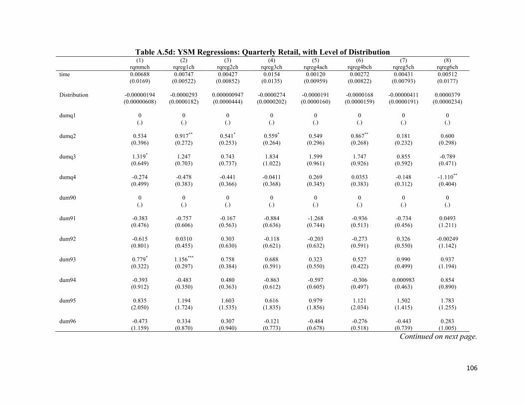
106

Table A.5d: YSM Regressions: Quarterly Retail, with Level of Distribution (1) (2) (3) (4) (5) (6) (7) (8) rqmmch rqreg1ch rqreg2ch rqreg3ch rqreg4ach rqreg4bch rqreg5ch rqreg6ch time 0.00688 0.00747 0.00427 0.0154 0.00120 0.00272 0.00431 0.00512 (0.0169) (0.00522) (0.00852) (0.0135) (0.00959) (0.00822) (0.00793) (0.0177) Distribution -0.00000194 -0.0000293 0.000000947 -0.0000274 -0.0000191 -0.0000168 -0.00000411 0.0000379 (0.00000608) (0.0000182) (0.0000444) (0.0000202) (0.0000160) (0.0000159) (0.0000191) (0.0000234) dumq1 0 0 0 0 0 0 0 0 (.) (.) (.) (.) (.) (.) (.) (.) dumq2 0.534 0.917** 0.541* 0.559* 0.549 0.867** 0.181 0.600 (0.396) (0.272) (0.253) (0.264) (0.296) (0.268) (0.232) (0.298) dumq3 1.319* 1.247 0.743 1.834 1.599 1.747 0.855 -0.789 (0.649) (0.703) (0.737) (1.022) (0.961) (0.926) (0.592) (0.471) dumq4 -0.274 -0.478 -0.441 -0.0411 0.269 0.0353 -0.148 -1.110** (0.499) (0.383) (0.366) (0.368) (0.345) (0.383) (0.312) (0.404) dum90 0 0 0 0 0 0 0 0 (.) (.) (.) (.) (.) (.) (.) (.) dum91 -0.383 -0.757 -0.167 -0.884 -1.268 -0.936 -0.734 0.0493 (0.476) (0.606) (0.563) (0.636) (0.744) (0.513) (0.456) (1.211) dum92 -0.615 0.0310 0.303 -0.118 -0.203 -0.273 0.326 -0.00249 (0.801) (0.455) (0.630) (0.621) (0.632) (0.591) (0.550) (1.142) dum93 0.779* 1.156*** 0.758 0.688 0.323 0.527 0.990 0.937 (0.322) (0.297) (0.384) (0.591) (0.550) (0.422) (0.499) (1.194) dum94 -0.393 -0.483 0.480 -0.863 -0.597 -0.306 0.000983 0.854 (0.912) (0.350) (0.363) (0.612) (0.605) (0.497) (0.463) (0.890) dum95 0.835 1.194 1.603 0.616 0.979 1.121 1.502 1.783 (2.050) (1.724) (1.535) (1.835) (1.856) (2.034) (1.415) (1.255) dum96 -0.473 0.334 0.307 -0.121 -0.484 -0.276 -0.443 0.283 (1.159) (0.870) (0.940) (0.773) (0.678) (0.518) (0.739) (1.005)

Continued on next page.

107

Table A.5d: YSM Regressions: Quarterly Retail, with Level of Distribution – Continued (1) (2) (3) (4) (5) (6) (7) (8) rqmmch rqreg1ch rqreg2ch rqreg3ch rqreg4ach rqreg4bch rqreg5ch rqreg6ch dum97 0.0570 -0.249 0.0165 -0.502 -0.519 -0.105 0.0613 0.422 (0.577) (0.369) (0.230) (0.448) (0.396) (0.332) (0.206) (0.725) dum98 -0.342 0.0726 0.268 0.663 -0.104 -0.0358 0.107 0.0851 (0.455) (0.226) (0.372) (0.736) (0.602) (0.457) (0.482) (0.721) dum99 -0.235 0.183 -0.0198 0.0346 -0.0922 0.0642 -0.0294 0.0596 (0.532) (0.355) (0.330) (0.456) (0.325) (0.347) (0.634) (0.636) dum00 -0.303 0.104 0.348 -0.394 0.0491 0.266 0.299 0.499 (0.474) (0.245) (0.369) (0.316) (0.306) (0.418) (0.323) (0.608) dum01 -0.438 -0.241 0.236 -0.588 0.0654 0.105 -0.0736 0.186 (0.687) (0.521) (0.310) (0.496) (0.342) (0.346) (0.233) (0.560) dum02 -0.00541 0.476 0.509 -0.146 0.0509 0.208 0.236 0.0523 (0.467) (0.361) (0.374) (0.300) (0.249) (0.268) (0.228) (0.559) dum03 -0.380 0.283 0.0458 -0.495 -0.0231 -0.0256 -0.0421 0.205 (0.630) (0.204) (0.288) (0.466) (0.343) (0.465) (0.289) (0.498) dum04 -0.539 0.469 0.113 -0.520 -0.0815 0.0747 0.0289 -0.0626 (0.873) (0.255) (0.355) (0.316) (0.270) (0.495) (0.317) (0.642) dum05 0 0.449* 0.502 0.0333 0.299 0.490 0.423 0.329 (.) (0.177) (0.416) (0.341) (0.425) (0.522) (0.455) (0.732) dum06 -0.222 0 0 0 0 0 0 0 (0.454) (.) (.) (.) (.) (.) (.) (.)

_cons -0.435 -0.478 -0.773 -0.371 -0.150 -0.441 -0.538 -0.595 (0.451) (0.357) (0.397) (0.570) (0.588) (0.450) (0.323) (1.071) N 67 67 67 67 67 67 67 67 adj. R2 -0.031 0.127 0.049 0.035 -0.015 0.036 0.094 0.193 Durbin-Watson d-statistic

2.819562 2.963387 3.063074 2.931814 2.946246 2.958975 2.737092 2.527938

Standard errors in parentheses * p < 0.05, ** p < 0.01, *** p < 0.001

Continued on next page.

108

Table A.5d: YSM Regressions: Quarterly Retail, with Level of Distribution – Continued (9) (10) (11) (12) (13) (14) (15) (16) rqreg7ch rqreg8ch rqreg9ch rqreg10ch rqreg11ch rqreg12ch rqreg13ch rqarmmch time 0.00628 0.0114 0.00271 -0.00444 0.000613 0.00753 0.0163 -0.000923 (0.0127) (0.0110) (0.0190) (0.00660) (0.0100) (0.00849) (0.0135) (0.0100) Distribution -0.0000386 -0.0000224 0.0000491 0.00000860 0.00000208 0.0000490 -0.0000693 -0.0000351 (0.0000199) (0.0000354) (0.0000536) (0.0000284) (0.0000248) (0.0000356) (0.0000757) (0.0000368) dumq1 0 -0.0659 0 0 1.273*** 0.811* 0.623* 0.327 (.) (0.280) (.) (.) (0.348) (0.346) (0.279) (0.363) dumq2 0.914* 0 -0.0683 0.440 1.584*** 1.446*** 0.592* 0.881* (0.446) (.) (0.475) (0.287) (0.389) (0.340) (0.225) (0.362) dumq3 1.386 1.171 0.785 0.366 1.307* 0.189 1.235*** 1.095** (0.711) (0.652) (1.095) (0.463) (0.618) (0.467) (0.330) (0.398) dumq4 0.170 -0.432 -1.922 -0.693 0 0 0 0 (0.466) (0.377) (1.386) (0.346) (.) (.) (.) (.) dum90 0 0 0 0 0 0 0 0 (.) (.) (.) (.) (.) (.) (.) (.) dum91 -1.823* -0.337 0.203 -0.853 -0.679 0.0664 -0.527 -1.171 (0.809) (0.699) (1.412) (0.724) (0.872) (0.721) (0.626) (0.619) dum92 -0.897 0.295 0.445 -0.273 -0.0658 0.440 0.416 -0.186 (1.300) (1.046) (8.384) (0.839) (0.807) (1.009) (0.624) (0.839) dum93 -0.220 0.614 0.844 0.222 0.301 0.647 0.0979 -0.135 (0.682) (0.572) (1.043) (0.443) (0.405) (0.440) (0.460) (0.479) dum94 -0.247 0.242 1.076 0.111 0.321 0.954 0.307 -0.0484 (0.725) (0.609) (1.088) (0.678) (0.447) (0.667) (0.528) (0.645) dum95 0.489 1.187 1.674 0.968 1.052 1.434 0.505 0.839 (1.673) (1.609) (1.140) (0.955) (0.913) (0.875) (0.587) (1.044) dum96 -0.545 0.218 0.641 -0.0269 -0.184 0.190 -0.110 -0.158 (0.971) (0.850) (1.369) (0.840) (0.580) (0.633) (0.703) (0.906)

Continued on next page.

109

Table A.5d: YSM Regressions: Quarterly Retail, with Level of Distribution – Continued (9) (10) (11) (12) (13) (14) (15) (16) rqreg7ch rqreg8ch rqreg9ch rqreg10ch rqreg11ch rqreg12ch rqreg13ch rqarmmch dum97 -0.614 0.0358 0.290 -0.0784 0.0146 0.363 -0.335 0.0134 (0.450) (0.460) (0.854) (0.235) (0.385) (0.454) (0.506) (0.361) dum98 -0.0675 0.253 -0.341 -0.320 -0.309 -0.489 -0.400 -0.245 (0.411) (0.468) (0.883) (0.364) (0.340) (0.430) (0.445) (0.443) dum99 -0.142 -0.102 -0.0488 -0.272 -0.156 0.0380 -0.446 -0.233 (0.685) (0.484) (0.900) (0.547) (0.395) (0.339) (0.494) (0.370) dum00 -0.0254 0.182 0.0379 -0.0989 0.0961 0.0284 -0.317 -0.0840 (0.654) (0.457) (0.796) (0.392) (0.517) (0.402) (0.555) (0.567) dum01 -0.279 -0.141 0.0853 -0.160 -0.200 0.0908 -0.643 -0.367 (0.379) (0.548) (0.907) (0.376) (0.488) (0.562) (0.621) (0.369) dum02 0.00971 0.111 0.125 0.317 0.206 0.248 -0.502 -0.00681 (0.293) (0.376) (0.776) (0.379) (0.521) (0.486) (0.690) (0.321) dum03 -0.243 -0.0125 0.284 0.00907 0.00245 0.290 -0.0393 -0.0750 (0.361) (0.366) (0.958) (0.293) (0.676) (0.630) (0.265) (0.371) dum04 -0.0866 0.0224 0.0276 0.0127 0.278 0.244 0.132 0.0412 (0.275) (0.466) (0.794) (0.268) (0.625) (0.740) (0.472) (0.367) dum05 0.865 0.0582 -0.00300 0.218 -0.0357 0.109 0.130 -0.0421 (0.478) (0.445) (0.954) (0.393) (0.524) (0.805) (0.346) (0.342) dum06 0 0 0 0 0 0 0 0 (.) (.) (.) (.) (.) (.) (.) (.) _cons -0.166 -0.506 -0.663 -0.0284 -1.198*** -1.521*** -0.978** -0.369 (0.752) (0.566) (1.374) (0.354) (0.232) (0.368) (0.358) (0.562) N 67 67 67 67 67 67 67 67 adj. R2 -0.057 0.022 -0.273 0.054 0.200 0.174 0.107 0.059 Durbin-Watson d-statistic

2.657281 2.96879 2.969141 2.815614 2.671165 2.66576 2.578591 2.65297

Standard errors in parentheses * p < 0.05, ** p < 0.01, *** p < 0.001

110

Table A2: Regressions of Regional WP on Manila WP and Previous Regional WP

(1) (2) (3) (4) (5) (6) (7) (8) lncar lnreg1 lnreg2 lnreg3 lnreg4a lnreg4b lnreg5 lnreg6 Natural Log Wholesale NCR 0.263*** 0.268*** 0.315*** 0.412*** 0.293*** 0.346*** 0.361*** 0.213***

(0.0325) (0.0283) (0.0360) (0.0255) (0.0277) (0.0319) (0.0366) (0.0462) Natural Log, Wholesale Previous Pd. 0.735*** 0.756*** 0.672*** 0.602*** 0.760*** 0.660*** 0.643*** 0.753***

(0.0320) (0.0265) (0.0367) (0.0252) (0.0232) (0.0314) (0.0353) (0.0448) _cons -0.00763 -0.0860 0.0149 -0.0461 -0.145*** -0.0256 -0.0360 0.0760 (0.0534) (0.0455) (0.0473) (0.0331) (0.0368) (0.0443) (0.0443) (0.0702) N 227 227 227 227 227 227 227 227 adj. R2 0.930 0.952 0.941 0.972 0.975 0.951 0.951 0.878

Standard errors in parentheses * p < 0.05, ** p < 0.01, *** p < 0.001

(9) (10) (11) (12) (13) (14) (15) (16) lnreg7 lnreg8 lnreg9 lnreg10 lnreg11 lnreg12 lnreg13 lnarmm Natural Log Wholesale NCR 0.336*** 0.331*** 0.547*** 0.297*** 0.198*** 0.167*** 0.208*** 0.248***

(0.0355) (0.0306) (0.0747) (0.0350) (0.0371) (0.0450) (0.0288) (0.0300) Natural Log, Wholesale Previous Pd. 0.663*** 0.648*** 0.231*** 0.635*** 0.730*** 0.782*** 0.711*** 0.768***

(0.0350) (0.0327) (0.0641) (0.0408) (0.0422) (0.0439) (0.0369) (0.0281) _cons 0.00582 0.0588 0.636*** 0.203*** 0.194* 0.127 0.219*** -0.0484 (0.0492) (0.0482) (0.184) (0.0583) (0.0762) (0.0778) (0.0655) (0.0439) N 227 227 227 227 227 227 227 227 adj. R2 0.940 0.939 0.398 0.909 0.843 0.852 0.880 0.955 Standard errors in parentheses * p < 0.05, ** p < 0.01, *** p < 0.001

111

Table A.3a: Ravallion Regressions: Monthly Farm Price (Dry Season) (1) (2) (3) (4) (5) (6) (7) (8) fphil freg1 freg2 freg3 freg4a freg4b freg5 freg6 Farm price, previous pd.

0.673*** 0.770*** 0.655*** 0.606*** 0.411** 0.440** 0.714*** 0.695*** (0.103) (0.0895) (0.0870) (0.144) (0.140) (0.139) (0.158) (0.107)

Wholesale price, previous pd.

0.205* 0.132 0.248** 0.235 0.427** 0.356** 0.172 0.165 (0.0906) (0.0896) (0.0817) (0.137) (0.125) (0.111) (0.125) (0.101)

Change in wholesale price

0.759*** 0.657*** 0.294 0.132 1.085** 0.905** 0.630* 0.646*** (0.207) (0.178) (0.183) (0.560) (0.369) (0.274) (0.239) (0.172)

Ratio of Procurement and Production

-19.58 -23.92 -27.67 -18.18 -13.51 -13.82 -8.670 -111.4 (20.00) (41.31) (20.87) (27.38) (24.02) (16.51) (12.97) (74.20)

dum9596 0.239 0.444* 0.542 0.720 -0.0312 0.469 0.252 0.612* (0.169) (0.216) (0.284) (0.367) (0.467) (0.335) (0.352) (0.240) dum9799 -0.0463 0.0486 -0.0523 -0.0893 -0.455 0.181 0.00114 0.234

(0.139) (0.161) (0.209) (0.304) (0.415) (0.279) (0.251) (0.182)

_cons 0.895 1.134* 0.865 1.480 0.0816 1.121 0.546 1.466 (0.524) (0.506) (0.744) (1.019) (1.089) (1.004) (0.929) (0.752) N 52 52 52 52 52 52 52 52 adj. R2 0.973 0.977 0.948 0.906 0.871 0.891 0.905 0.957 Durbin’s alternative test for autocorrelation chi2 0.275 1.997 0.415 0.810 0.947 3.580 0.142 0.342 Prob > chi2 0.6001 0.1576 0.5195 0.3682 0.3304 0.0585 0.7065 0.5588 Standard errors in parentheses * p < 0.05, ** p < 0.01, *** p < 0.001 ^Newey-West HAC Standard Errors

Continued on next page.

112

Table A.3a: Ravallion Regressions: Monthly Farm Price (Dry Season) - Continued (9) (10) (11) (12) (13) (14) (15) (16) freg7^ freg8^ freg9 freg10 freg11 freg12 freg13 farmm^ Farm price, previous pd.

0.870*** 0.510*** 0.573*** 0.720*** 0.361* 0.491** 0.383** 0.594*** (0.154) (0.0982) (0.139) (0.106) (0.160) (0.157) (0.129) (0.123)

Wholesale price, previous pd.

-0.000836 0.244* 0.266 0.129 0.393* 0.455* 0.424** 0.188 (0.0820) (0.121) (0.151) (0.0943) (0.163) (0.176) (0.128) (0.101)

Change in wholesale price

0.304 0.382 0.218 0.473* 0.891** 0.861*** 0.688** -0.0653 (0.153) (0.320) (0.284) (0.221) (0.310) (0.177) (0.246) (0.172)

Ratio of Procurement and Production

498.7 -113.1 -84.89 -29.36 36.55 -51.75 -2280.1*** 12.71 (633.1) (87.61) (99.24) (30.15) (58.45) (56.76) (579.0) (27.95)

dum9596 0.0124 0.335 -0.0173 -0.0436 0.519 -0.163 0.216 -0.111 (0.394) (0.413) (0.438) (0.299) (0.395) (0.343) (0.355) (0.515) dum9799 -0.367 0.0441 -0.264 -0.215 0.370 0.0467 -0.144 -0.145

(0.302) (0.344) (0.401) (0.268) (0.316) (0.215) (0.272) (0.369)

_cons 2.082 1.579 1.051 1.558 1.140 -0.379 0.526 1.908 (1.359) (1.806) (1.592) (1.019) (1.516) (1.051) (1.304) (0.988) N 52 52 52 52 52 52 52 52 adj. R2 0.789 0.865 0.774 0.947 0.838 Durbin's alternative test for autocorrelation chi2 2.124 0.208 0.671 0.027 1.189 Prob > chi2 0.1450 0.6480 0.4128 0.8698 0.2755 Standard errors in parentheses * p < 0.05, ** p < 0.01, *** p < 0.001 ^Newey-West HAC Standard Errors

113

Table A.3b: Ravallion Regressions: Monthly Farm Price (Harvest Season) (1) (2) (3) (4) (5) (6) (7) (8) fphil freg1 freg2 freg3 freg4a freg4b freg5 freg6 fphilp 0.700*** 0.123 0.275* 0.657*** 0.514** 0.270 0.319* 0.391*** (0.149) (0.182) (0.126) (0.132) (0.163) (0.137) (0.128) (0.106) wphilp 0.184 0.379 0.406** 0.0182 0.182 0.443*** 0.438*** 0.559*** (0.114) (0.200) (0.135) (0.128) (0.113) (0.111) (0.105) (0.0931) wphilch 0.620*** 0.844* 0.609** 0.257 -0.226 0.494** 1.242*** 1.025*** (0.152) (0.324) (0.221) (0.316) (0.240) (0.150) (0.265) (0.160) procphil -34.51 -60.05 -149.1** -27.61 -12.96 -9.438 -59.83** -73.65* (23.49) (33.08) (44.08) (30.46) (11.55) (7.855) (21.88) (31.10) dum9596 0.200 1.620* 0.711 1.435* 0.0296 0.400 0.342 -0.381 (0.294) (0.703) (0.461) (0.621) (0.592) (0.345) (0.353) (0.283) dum9799 -0.0994 0.662 0.311 0.546 0.120 -0.126 -0.0370 -0.404* (0.209) (0.474) (0.296) (0.431) (0.384) (0.244) (0.230) (0.174) _cons 0.739 4.972* 2.362 3.951* 2.633* 1.099 0.345 -1.156 (0.843) (1.922) (1.222) (1.566) (1.177) (0.842) (0.884) (0.781) N 52 52 52 52 52 52 52 52 adj. R2 0.932 0.703 0.867 0.772 0.811 0.931 0.914 0.944 Durbin's alternative test for autocorrelation chi2 0.912 0.000 0.250 1.728 0.545 0.144 0.763 0.050 Prob > chi2 0.3395 0.9877 0.6169 0.1887 0.4602 0.7039 0.3823 0.8224 Standard errors in parentheses * p < 0.05, ** p < 0.01, *** p < 0.001 ^Newey-West HAC Standard Errors

Continued on next page.

114

Table A.3b: Ravallion Regressions: Monthly Farm Price (Harvest Season) - Continued (9) (10) (11) (12) (13) (14) (15) (16) freg7 freg8 freg9 freg10 freg11 freg12^ freg13 farmm freg7p 0.247* 0.194 0.491*** 0.516*** 0.458*** 0.650*** 0.584*** 0.358* (0.110) (0.130) (0.120) (0.117) (0.127) (0.116) (0.108) (0.137) wreg7p 0.0894 0.492*** 0.389** 0.386*** 0.441*** 0.241* 0.212 0.465** (0.0737) (0.115) (0.129) (0.0909) (0.112) (0.0994) (0.116) (0.148) wreg7ch 0.447* 0.214 0.973*** 0.813*** 0.811*** 0.743*** 0.618*** 0.712 (0.179) (0.175) (0.217) (0.124) (0.104) (0.143) (0.151) (0.395) procreg7 -1128.8** -1095.3 -89.10 -25.32 20.21 -18.94 -454.7 -8.068 (353.9) (749.8) (57.25) (40.69) (15.31) (10.04) (769.8) (25.31) dum9596 1.114* 0.0345 -0.307 -0.292 -0.170 0.526* 0.632 -1.204 (0.513) (0.457) (0.524) (0.349) (0.292) (0.228) (0.347) (0.812) dum9799 0.522 0.209 -0.246 -0.683** -0.0548 0.306* 0.0221 -0.667 (0.294) (0.294) (0.394) (0.246) (0.181) (0.144) (0.237) (0.619) _cons 7.823*** 0.874 -0.404 -0.865 -0.916 0.749 1.104 -0.223 (1.629) (1.343) (1.910) (1.330) (0.902) (0.578) (1.238) (2.206) N 52 52 52 52 52 52 52 52 adj. R2 0.606 0.837 0.750 0.850 0.922 0.878 0.511 Durbin's alternative test for autocorrelation chi2 0.626 0.001 0.005 0.177 0.346 0.032 3.413 Prob > chi2 0.4290 0.9757 0.9437 0.6742 0.5562 0.8572 0.0647 Standard errors in parentheses * p < 0.05, ** p < 0.01, *** p < 0.001 ^Newey-West HAC Standard Errors

115

Table A. 3c: Ravallion Farm Price (Off Season) (1) (2) (3) (4) (5) (6) (7) (8) fphil freg1 freg2 freg3 freg4a freg4b freg5 freg6 Farm price, previous pd.

1.217*** 0.531* 0.741*** 0.625*** 0.661** 0.651** 0.457** 0.739*** (0.164) (0.210) (0.185) (0.169) (0.188) (0.194) (0.147) (0.133)

Wholesale price, previous pd.

-0.264 0.155 0.0919 0.0180 0.0910 -0.0541 0.109 0.00214 (0.133) (0.187) (0.187) (0.150) (0.125) (0.233) (0.146) (0.122)

Change in wholesale price

0.683*** 1.112*** 0.700** 0.995*** 0.338 1.045*** 0.990*** 0.756*** (0.142) (0.217) (0.211) (0.210) (0.197) (0.196) (0.161) (0.111)

Ratio of Procurement and Prod’n

119.1 105.3 54.88 67.38 -21.32 21.65 -48.36 -94.63 (95.96) (167.4) (165.0) (106.0) (60.07) (76.07) (45.34) (138.1)

dum9596 0.162 1.141 0.361 0.507 0.866 1.560 0.847 0.464 (0.442) (0.718) (0.723) (0.822) (0.596) (0.784) (0.634) (0.490) dum9799 0.316 0.215 0.164 0.403 0.251 0.919 0.474 0.362 (0.270) (0.430) (0.448) (0.484) (0.388) (0.516) (0.372) (0.308) _cons 1.235 3.873* 1.724 4.698* 2.696 5.040* 4.314** 2.939* (1.298) (1.682) (2.000) (2.149) (1.380) (2.311) (1.578) (1.402) N 52 52 52 52 52 52 52 52 adj. R2 0.893 0.871 0.776 0.731 0.842 0.842 0.816 0.881 Durbin's alternative test for autocorrelation chi2 0.021 1.454 1.750 1.878 1.440 0.042 0.444 1.832 Prob > chi2 0.2280 0.1858 0.1706 0.2301 0.9578 0.8371 0.5051 0.1758 Standard errors in parentheses * p < 0.05, ** p < 0.01, *** p < 0.001 ^Newey-West HAC Standard Errors

Continued on next page.

116

Table A. 3c: Ravallion Farm Price (Off Season) - Continued (9) (10) (11) (12) (13) (14) (15) (16) freg7 freg8^ freg9 freg10^ freg11^ freg12 freg13 farmm Farm price, previous pd.

0.730*** 0.433 0.475** 0.594** 0.503* 0.810*** 0.276 0.583*** (0.134) (0.227) (0.169) (0.208) (0.192) (0.157) (0.162) (0.145)

Wholesale price, previous pd.

-0.0595 0.311 0.112 0.0933 0.309 -0.0302 0.336 0.242 (0.132) (0.167) (0.199) (0.171) (0.206) (0.174) (0.191) (0.141)

Change in wholesale price

0.341 0.865*** 0.984*** 0.718** 0.657*** 0.774*** 1.073*** -0.0890 (0.207) (0.185) (0.255) (0.207) (0.140) (0.107) (0.234) (0.328)

Ratio of Procurement and Prod’n

-379.5 -2396.3 -170.2 -177.2 -69.90 -37.72 -5174.8 -17.21 (925.7) (1812.0) (102.3) (153.4) (53.41) (46.07) (5489.5) (75.01)

dum9596 0.978 -0.285 0.375 0.429 0.242 0.510 0.629 -0.930 (0.948) (0.630) (0.778) (0.587) (0.513) (0.438) (0.548) (0.939) dum9799 0.247 0.437 0.223 0.299 0.0353 0.261 -0.325 -0.581 (0.541) (0.632) (0.544) (0.412) (0.271) (0.270) (0.399) (0.638) _cons 4.332 1.407 4.701 3.338 0.707 2.834 3.314 1.151 (2.664) (1.914) (2.766) (2.291) (1.774) (1.510) (2.240) (2.319) N 52 52 52 52 52 52 52 52 adj. R2 0.508 0.617 0.912 0.682 0.446 Durbin's alternative test for autocorrelation chi2 0.348 1.221 1.769 1.463 0.021 Prob > chi2 0.5554 0.2692 0.1835 0.2265 0.8844 Standard errors in parentheses * p < 0.05, ** p < 0.01, *** p < 0.001 ^Newey-West HAC Standard Errors

117

Table A.4a: Ravallion Regressions: Monthly Retail Price (Dry Season) (1) (2) (3) (4) (5) (6) (7) (8) (9) rphil rmm rcar rreg1 rreg2 rreg3^ rreg4a rreg4b rreg5 Retail price, previous pd. 0.693*** 0.804*** 0.853*** 0.869*** 0.636*** 0.591*** 0.872*** 0.665*** 0.821***

(0.0729) (0.0526) (0.0845) (0.0738) (0.0864) (0.146) (0.0573) (0.0821) (0.0462) Wholesale price, previous pd. 0.318*** 0.182*** 0.196* 0.128 0.375*** 0.425** 0.131* 0.366*** 0.182***

(0.0729) (0.0471) (0.0791) (0.0725) (0.0929) (0.144) (0.0608) (0.0830) (0.0501) Change in wholesale price 0.914*** 0.437*** 0.701*** 0.963*** 0.813*** 1.071*** 0.738*** 0.882*** 0.749***

(0.0304) (0.0552) (0.0803) (0.0548) (0.0702) (0.0378) (0.0558) (0.0479) (0.0466) dum9596 -0.0252 0.0526 -0.210 -0.00793 0.0895 0.214 -0.0332 -0.00155 0.0340 (0.0493) (0.166) (0.160) (0.101) (0.152) (0.206) (0.114) (0.103) (0.0944) dum9799 0.0541 0.128 -0.225 0.0249 0.0200 0.126 0.0432 0.112 0.0722

(0.0428) (0.141) (0.114) (0.0881) (0.120) (0.0954) (0.0958) (0.0997) (0.0716)

_cons 0.282 0.661 -0.531 0.225 0.342 0.333 0.146 -0.0280 0.274 (0.182) (0.512) (0.450) (0.296) (0.386) (0.446) (0.262) (0.316) (0.227) N 76 76 76 76 76 76 76 76 76 adj. R2 0.998 0.978 0.977 0.989 0.980 0.993 0.991 0.994 Durbin’s alternative test for autocorrelation chi2 0.111 0.853 0.403 2.418 0.023 0.187 2.292 0.167 Prob > chi2 0.7385 0.3556 0.5253 0.1199 0.8799 0.6655 0.1300 0.6827 Standard errors in parentheses * p < 0.05, ** p < 0.01, *** p < 0.001 ^Newey-West HAC Standard Errors

Continued on next page.

118

Table A.4a: Ravallion Regressions: Monthly Retail Price (Dry Season) - Continued (10) (11) (12) (13) (14) (15) (16) (17) (18) rreg6 rreg7 rreg8 rreg9^ rreg10 rreg11 rreg12 rreg13 rarmm Retail price, previous pd. 0.891*** 0.803*** 0.704*** 0.632*** 0.651*** 0.470*** 0.414*** 0.759*** 0.562***

(0.0543) (0.0446) (0.0776) (0.0772) (0.0893) (0.0810) (0.0837) (0.0674) (0.0983) Wholesale price, previous pd. 0.0925 0.277*** 0.234** 0.371*** 0.368*** 0.516*** 0.574*** 0.269*** 0.419***

(0.0504) (0.0596) (0.0715) (0.0767) (0.0833) (0.0784) (0.0777) (0.0665) (0.0942) Change in wholesale price 0.795*** 0.671*** 0.580*** 0.876*** 0.767*** 0.763*** 0.662*** 0.799*** 0.865***

(0.0524) (0.0790) (0.0709) (0.0678) (0.0606) (0.0490) (0.0483) (0.0497) (0.0582) dum9596 0.154 -0.281 0.195 0.143 -0.0441 0.137 -0.326** -0.0671 0.165 (0.109) (0.196) (0.154) (0.0915) (0.136) (0.0996) (0.109) (0.0858) (0.146) dum9799 0.0348 -0.384* 0.201 -0.0100 0.0360 0.221* 0.0168 -0.0252 -0.131

(0.0956) (0.160) (0.118) (0.0681) (0.117) (0.0861) (0.0823) (0.0695) (0.120)

_cons 0.489 -0.919 1.488** 0.381 0.226 0.921* 1.226** -0.112 0.946* (0.368) (0.493) (0.478) (0.312) (0.521) (0.350) (0.398) (0.326) (0.441) N 76 76 76 76 76 76 76 76 76 adj. R2 0.985 0.977 0.978 0.979 0.987 0.984 0.987 0.983 Durbin’s alternative test for autocorrelation chi2 0.006 0.974 0.010 0.016 0.284 0.557 0.071 0.044 Prob > chi2 0.9406 0.3238 0.9221 0.8984 0.5940 .4554 0.7895 0.8339 Standard errors in parentheses * p < 0.05, ** p < 0.01, *** p < 0.001 ^Newey-West HAC Standard Errors

119

Table A.4b: Ravallion Regressions: Monthly Retail Price (Harvest Season) (1) (2) (3) (4) (5) (6) (7) (9) (8) rphil^ rmm rcar rreg1 rreg2 rreg3 rreg4a rreg5 rreg4b^ Retail price, previous pd. 0.636*** 0.564*** 0.681*** 0.638*** 0.749*** 0.683*** 0.767*** 0.716*** 0.653***

(0.102) (0.0900) (0.0794) (0.0726) (0.0883) (0.0812) (0.0550) (0.0482) (0.0686) Wholesale price, previous pd. 0.354** 0.452*** 0.265*** 0.281*** 0.244* 0.292*** 0.234*** 0.284*** 0.337***

(0.106) (0.0967) (0.0762) (0.0788) (0.101) (0.0827) (0.0601) (0.0588) (0.0711) Change in wholesale price 0.614*** 0.580*** 0.563*** 0.724*** 0.707*** 0.779*** 0.754*** 0.642*** 0.628***

(0.0517) (0.148) (0.0633) (0.0681) (0.0746) (0.0645) (0.0611) (0.0842) (0.129) dum9596 0.133 0.628 0.0326 0.410** -0.0227 0.282* -0.0402 0.106 0.101 (0.113) (0.418) (0.161) (0.153) (0.155) (0.123) (0.149) (0.144) (0.213) dum9799 0.0348 -0.120 0.0816 0.395*** -0.0192 0.129 0.0578 0.0759 0.0597

(0.0476) (0.290) (0.101) (0.108) (0.101) (0.0880) (0.1000) (0.0836) (0.128)

_cons 0.721** 0.685 1.279** 1.737*** 0.442 0.874** 0.335 0.721 (0.244) (1.107) (0.431) (0.380) (0.410) (0.313) (0.286) 0.482 (0.573) N 75 75 75 75 75 75 75 (0.304) 75 adj. R2 0.913 0.981 0.984 0.983 0.993 0.994 75 Durbin's alternative test for autocorrelation chi2 0.112 0.088 2.962 0.047 0.004 0.342 1.909 Prob > chi2 0.7382 0.7663 0.0852 0.8289 0.9523 0.5585 0.1670 Standard errors in parentheses * p < 0.05, ** p < 0.01, *** p < 0.001 ^Newey-West HAC Standard Errors

Continued on next page.

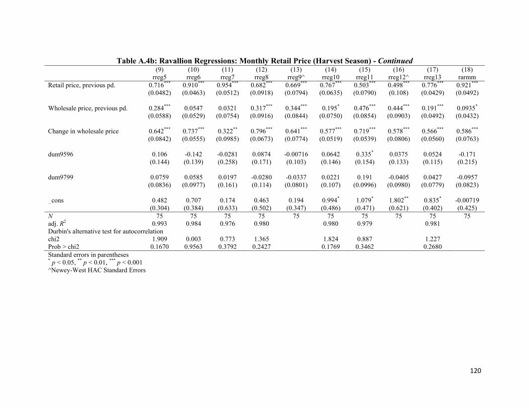
120

Table A.4b: Ravallion Regressions: Monthly Retail Price (Harvest Season) - Continued

(9) (10) (11) (12) (13) (14) (15) (16) (17) (18) rreg5 rreg6 rreg7 rreg8 rreg9^ rreg10 rreg11 rreg12^ rreg13 rarmm Retail price, previous pd. 0.716*** 0.910*** 0.954*** 0.682*** 0.669*** 0.767*** 0.503*** 0.498*** 0.776*** 0.921***

(0.0482) (0.0463) (0.0512) (0.0918) (0.0794) (0.0635) (0.0790) (0.108) (0.0429) (0.0492)

Wholesale price, previous pd. 0.284*** 0.0547 0.0321 0.317*** 0.344*** 0.195* 0.476*** 0.444*** 0.191*** 0.0935* (0.0588) (0.0529) (0.0754) (0.0916) (0.0844) (0.0750) (0.0854) (0.0903) (0.0492) (0.0432)

Change in wholesale price 0.642*** 0.737*** 0.322** 0.796*** 0.641*** 0.577*** 0.719*** 0.578*** 0.566*** 0.586***

(0.0842) (0.0555) (0.0985) (0.0673) (0.0774) (0.0519) (0.0539) (0.0806) (0.0560) (0.0763) dum9596 0.106 -0.142 -0.0281 0.0874 -0.00716 0.0642 0.335* 0.0375 0.0524 -0.171 (0.144) (0.139) (0.258) (0.171) (0.103) (0.146) (0.154) (0.133) (0.115) (0.215) dum9799 0.0759 0.0585 0.0197 -0.0280 -0.0337 0.0221 0.191 -0.0405 0.0427 -0.0957 (0.0836) (0.0977) (0.161) (0.114) (0.0801) (0.107) (0.0996) (0.0980) (0.0779) (0.0823) _cons 0.482 0.707 0.174 0.463 0.194 0.994* 1.079* 1.802** 0.835* -0.00719 (0.304) (0.384) (0.633) (0.502) (0.347) (0.486) (0.471) (0.621) (0.402) (0.425) N 75 75 75 75 75 75 75 75 75 75 adj. R2 0.993 0.984 0.976 0.980 0.980 0.979 0.981 Durbin's alternative test for autocorrelation chi2 1.909 0.003 0.773 1.365 1.824 0.887 1.227 Prob > chi2 0.1670 0.9563 0.3792 0.2427 0.1769 0.3462 0.2680 Standard errors in parentheses * p < 0.05, ** p < 0.01, *** p < 0.001 ^Newey-West HAC Standard Errors

121

Table A.4c: Ravallion Regressions: Monthly Retail Price (Off Season) (1) (2) (3) (4) (5) (6) (7) (8) (9) rphil rmm rcar rreg1 rreg2^ rreg3 rreg4a rreg4b rreg5 Retail price, previous pd. 0.635*** 0.544*** 0.547*** 0.922*** 0.546*** 0.733*** 0.896*** 0.674*** 0.900***

(0.120) (0.0946) (0.0801) (0.0734) (0.121) (0.0890) (0.0693) (0.0758) (0.125) Wholesale price, previous pd. 0.422** 0.451*** 0.434*** 0.0934 0.500*** 0.266** 0.131 0.333*** 0.203

(0.126) (0.0905) (0.0838) (0.0685) (0.131) (0.0933) (0.0729) (0.0790) (0.135) Change in wholesale price 1.000*** 0.768*** 0.878*** 1.086*** 0.999*** 1.007*** 0.939*** 0.786*** 1.054***

(0.0327) (0.0710) (0.0459) (0.0501) (0.0786) (0.0342) (0.0610) (0.0304) (0.0666) dum9596 0.00278 0.152 0.616*** 0.0638 0.00712 0.0513 0.0531 0.330** 0.108 (0.0924) (0.273) (0.172) (0.141) (0.161) (0.115) (0.186) (0.112) (0.265) dum9799 -0.0609 0.125 0.0130 -0.0293 -0.0684 0.103 0.00480 0.128 -0.287 (0.0638) (0.200) (0.114) (0.0996) (0.0704) (0.0807) (0.136) (0.0851) (0.169) -1.514* _cons -0.394 0.863 0.893* -0.139 -0.0789 0.418 -0.292 0.337 (0.606) (0.257) (0.704) (0.381) (0.361) (0.382) (0.275) (0.399) (0.278) 76 N 76 76 76 76 76 76 76 76 0.972 adj. R2 0.995 0.960 0.983 0.989 0.994 0.987 0.994 0.458 Durbin's alternative test for autocorrelation chi2 0.997 2.308 0.730 1.403 3.551 0.063 0.019 0.4985 Prob > chi2 0.3180 .1287 0.3929 0.2363 0.0595 0.8025 0.8894 Standard errors in parentheses * p < 0.05, ** p < 0.01, *** p < 0.001 ^Newey-West HAC Standard Errors

Continued on next page.

122

Table A.4c: Ravallion Regressions: Monthly Retail Price (Off Season) - Continued (10) (11) (12) (13) (14) (15) (16) (17) (18) rreg6 rreg7^ rreg8 rreg9 rreg10 rreg11 rreg12 rreg13 rarmm Retail price, previous pd. 0.925*** 0.791*** 0.428*** 0.686*** 0.561*** 0.661*** 0.462*** 0.651*** 0.725***

(0.105) (0.0698) (0.0943) (0.112) (0.105) (0.0961) (0.103) (0.126) (0.0894) Wholesale price, previous pd. 0.137 0.261** 0.525*** 0.319** 0.486*** 0.447*** 0.597*** 0.448** 0.281**

(0.103) (0.0763) (0.0943) (0.113) (0.111) (0.103) (0.110) (0.139) (0.0933) Change in wholesale price 1.064*** 0.826*** 1.151*** 0.866*** 0.893*** 0.998*** 0.788*** 0.953*** 0.920***

(0.0608) (0.101) (0.0488) (0.0552) (0.0587) (0.0367) (0.0418) (0.0389) (0.0614) dum9596 0.121 -0.190 0.412* 0.301* 0.0552 -0.310* -0.306 -0.268 -0.0902 (0.248) (0.277) (0.169) (0.147) (0.185) (0.151) (0.193) (0.135) (0.157) dum9799 -0.0152 -0.147 0.128 -0.00608 -0.155 -0.298** -0.243 -0.241* -0.162

(0.176) (0.102) (0.110) (0.104) (0.133) (0.112) (0.133) (0.102) (0.129)

_cons -0.776 -0.397 1.546*** 0.307 -0.181 -1.311** -0.115 -1.145** 0.320 (0.696) (0.493) (0.424) (0.406) (0.538) (0.433) (0.555) (0.395) (0.378) N 76 76 76 76 76 76 76 76 76 adj. R2 0.957 0.983 0.981 0.971 0.977 0.961 0.977 0.987 Durbin's alternative test for autocorrelation chi2 2.282 0.005 0.121 2.680 0.300 0.099 0.189 1.445 Prob > chi2 0.1309 0.9458 0.7277 0.1016 0.5839 0.7531 0.6638 0.2293 Standard errors in parentheses * p < 0.05, ** p < 0.01, *** p < 0.001 ^Newey-West HAC Standard Errors

123

Table A.5a: YSM Regressions: Monthly Farm, with Level of Procurement (1) (2) (3) (4) (5) (6) (7) (8) freg1ch freg2ch freg3ch freg4ach freg4bch freg5ch freg6ch freg7ch time -0.000708 0.000982 -0.000559 0.000270 0.000338 -0.000214 0.000688 -0.00214 (0.00156) (0.00171) (0.00185) (0.00169) (0.00196) (0.00177) (0.00171) (0.00230) Procurement 0.00000342 0.0000133 -0.0000141 0.0000191 0.00000931 -0.0000344 0.00000902 -0.00403**

(0.0000273) (0.0000232) (0.0000156) (0.0000160) (0.0000186) (0.0000388) (0.0000252) (0.00132) dumjan 0.702** 0.615* 0 0.842** 0.233 0 0.462 0.491 (0.264) (0.267) (.) (0.323) (0.374) (.) (0.272) (0.358) dumfeb 0.290 0.774** -0.0582 0.946** 0.820* 0.516 0.753** -0.227 (0.278) (0.269) (0.288) (0.338) (0.392) (0.277) (0.271) (0.361) dummar 0.203 0.501 -0.371 0.352 0.136 -0.150 0.786** -0.198 (0.278) (0.266) (0.288) (0.335) (0.388) (0.280) (0.266) (0.360) dumapr 0.206 0.534* -0.264 0.0859 0.571 0.227 0.841** 0.289 (0.277) (0.257) (0.288) (0.316) (0.366) (0.297) (0.271) (0.359) dummay 0.154 0.381 -0.112 0.873** 0.596 0.357 0.671* 0.145 (0.276) (0.256) (0.289) (0.313) (0.363) (0.283) (0.272) (0.361) dumjun 0.105 0.482 0.0785 0.685* 0.543 0.190 0.285 -0.383 (0.280) (0.264) (0.287) (0.335) (0.388) (0.277) (0.274) (0.357) dumjul 0.163 0.384 -0.340 0.733* 0.688 0.478 0.389 -0.746* (0.284) (0.270) (0.287) (0.346) (0.401) (0.277) (0.275) (0.365) dumaug 0.454 0.0920 -0.155 0.487 0.318 0.0906 -0.307 -0.0700 (0.284) (0.270) (0.288) (0.350) (0.406) (0.277) (0.274) (0.366) dumsep -1.107*** -0.701** -1.492*** -0.0120 -0.899* -0.981*** -1.316*** -1.101** (0.284) (0.269) (0.288) (0.350) (0.405) (0.277) (0.265) (0.366) dumoct -1.813*** -0.912*** -1.449*** -0.406 -0.489 -0.816** 0 -0.978** (0.261) (0.257) (0.288) (0.305) (0.353) (0.282) (.) (0.359) dumnov 0 0 0.0321 0 0 0.282 0.722** -0.189 (.) (.) (0.299) (.) (.) (0.285) (0.256) (0.349) dumdec 0.144 0.459 -0.00594 0.567* 0.431 0.826** 0.698** 0 (0.240) (0.256) (0.297) (0.272) (0.316) (0.279) (0.261) (.) dum90 0 0 0 0 0 0 0 0 (.) (.) (.) (.) (.) (.) (.) (.) dum91 -0.601* -0.0458 -0.238 -0.335 -0.193 -0.140 -0.151 0.132 (0.284) (0.303) (0.334) (0.315) (0.365) (0.321) (0.303) (0.425) dum92 0.0924 0.160 0.138 0.0851 0.0360 0.0437 0.158 -0.0377 (0.275) (0.294) (0.324) (0.305) (0.353) (0.313) (0.295) (0.401) dum93 0.0513 0.389 0.173 0.152 0.214 0.0610 0.192 -0.169 (0.270) (0.291) (0.322) (0.297) (0.344) (0.307) (0.297) (0.398) dum94 -0.232 0.0466 -0.130 -0.0478 0.0325 0.0515 0.171 -0.217 (0.264) (0.286) (0.315) (0.291) (0.338) (0.302) (0.293) (0.389) dum95 0.333 0.639* 0.451 0.463 0.395 0.266 0.397 0.0546 (0.261) (0.283) (0.308) (0.289) (0.334) (0.296) (0.286) (0.382) dum96 -0.322 -0.189 -0.331 -0.290 -0.0276 -0.0488 -0.117 -0.171 (0.253) (0.272) (0.301) (0.281) (0.326) (0.289) (0.280) (0.372) dum97 -0.0467 0.163 0.0992 0.0873 0.0400 -0.0285 0.108 -0.132 (0.251) (0.271) (0.299) (0.277) (0.322) (0.287) (0.276) (0.369)

Continued on next page.

124

(1) (2) (3) (4) (5) (6) (7) (8) freg1ch freg2ch freg3ch freg4ach freg4bch freg5ch freg6ch freg7ch dum98 -0.0509 0.0945 -0.0267 -0.0628 -0.110 -0.0470 -0.00537 -0.156 (0.252) (0.271) (0.297) (0.277) (0.321) (0.285) (0.273) (0.367) dum99 -0.128 -0.0483 -0.0000479 -0.0950 -0.0986 0.124 0.0183 0.168 (0.251) (0.273) (0.299) (0.280) (0.324) (0.309) (0.266) (0.363) dum00 -0.0348 0.0368 0.177 -0.0374 0.0776 0.164 0.0471 -0.00358 (0.261) (0.274) (0.307) (0.282) (0.327) (0.301) (0.267) (0.364) dum01 -0.128 0.0438 0.0624 -0.0946 0.00806 0.103 0.0000435 0.153 (0.257) (0.275) (0.300) (0.288) (0.333) (0.300) (0.271) (0.369) dum02 0.0467 0.112 0.121 -0.0767 -0.0909 0.127 0.0922 0.127 (0.258) (0.275) (0.304) (0.293) (0.340) (0.298) (0.275) (0.375) dum03 -0.0561 0.00518 0.0261 -0.0712 0.00114 0.0472 -0.0183 0.0622 (0.272) (0.281) (0.310) (0.296) (0.343) (0.300) (0.282) (0.383) dum04 0.0207 0.0852 0.188 -0.104 -0.0220 0.161 0.0615 0.105 (0.270) (0.288) (0.318) (0.304) (0.352) (0.308) (0.287) (0.392) dum05 0.111 0.0854 0.0962 -0.0134 0.0706 0.110 0.0201 0.145 (0.277) (0.296) (0.326) (0.307) (0.356) (0.314) (0.295) (0.402) dum06 0 0 0 0 0 0 0 0 (.) (.) (.) (.) (.) (.) (.) (.) _cons 0.144 -0.458 0.358 -0.535 -0.361 -0.113 -0.502 0.557 (0.331) (0.331) (0.337) (0.377) (0.437) (0.319) (0.349) (0.450) N 203 203 203 203 203 203 203 203 adj. R2 0.465 0.267 0.234 0.144 0.147 0.222 0.349 0.093 Durbin-Watson d-statistic

2.040138 2.290893 2.377124 2.32144 2.439047 2.555805 2.71869 2.456515

Standard errors in parentheses * p < 0.05, ** p < 0.01, *** p < 0.001

Continued on next page.

125

Table A.5a: YSM Regressions: Monthly Farm, with Level of Procurement - Continued (9) (10) (11) (12) (13) (14) (15) freg8ch freg9ch freg10ch freg11ch freg12ch freg13ch farmmch time 0.000148 0.00152 0.000351 0.00116 0.000763 0.00116 0.00106 (0.00245) (0.00196) (0.00159) (0.00184) (0.00151) (0.00171) (0.00217) Procurement -0.000230 0.0000544 -0.000129 0.0000313 0.00000645 -0.00886** 0.0000214

(0.000367) (0.000145) (0.0000873) (0.0000675) (0.0000226) (0.00333) (0.000103) dumjan 0 0.438 0.0621 0 0.649** 0 0.286 (.) (0.306) (0.244) (.) (0.238) (.) (0.360) dumfeb 0.0523 0.256 0.271 0.0432 0.543* 0.0867 0.0242 (0.372) (0.306) (0.247) (0.274) (0.239) (0.274) (0.361) dummar 0.225 0.0371 -0.0184 0.228 0.690** -0.358 0.603 (0.372) (0.301) (0.243) (0.274) (0.237) (0.274) (0.355) dumapr 0.0669 0.285 0.328 -0.288 0.906*** 0.0148 0.367 (0.392) (0.300) (0.234) (0.275) (0.238) (0.278) (0.362) dummay 0.361 0.0828 0.0345 -0.214 0.609* 0.00883 0.265 (0.382) (0.307) (0.233) (0.274) (0.239) (0.274) (0.363) dumjun 0.534 0.275 -0.134 -0.285 0.470 -0.167 0.212 (0.372) (0.311) (0.234) (0.274) (0.238) (0.274) (0.365) dumjul 0.0771 0.0406 0.0718 0.125 0.673** 0.312 0.431 (0.371) (0.312) (0.244) (0.274) (0.240) (0.274) (0.365) dumaug 0.587 -0.594 -0.0280 -0.277 0.100 -0.360 -0.157 (0.372) (0.308) (0.246) (0.274) (0.238) (0.274) (0.361) dumsep -0.203 -1.128*** -1.103*** -0.933*** -1.313*** -0.871** -0.606 (0.372) (0.303) (0.245) (0.274) (0.234) (0.274) (0.358) dumoct -0.398 -0.975** -0.948*** -0.828** 0 -0.730** 0.102 (0.372) (0.291) (0.234) (0.284) (.) (0.274) (0.342) dumnov -0.209 0 0 -0.670* 0.542* -0.645* 0 (0.376) (.) (.) (0.287) (0.223) (0.277) (.) dumdec 0.169 -0.104 0.138 -0.103 0.776*** -0.276 -0.121 (0.373) (0.291) (0.234) (0.278) (0.226) (0.274) (0.345) dum90 0 0 0 0 0 0 0 (.) (.) (.) (.) (.) (.) (.) dum91 -0.101 -0.0492 0.152 -0.0555 -0.192 -0.186 -0.108 (0.443) (0.350) (0.275) (0.318) (0.270) (0.318) (0.406) dum92 0.237 0.159 0.220 0.0979 0.192 0.0737 0.176 (0.420) (0.332) (0.267) (0.311) (0.262) (0.309) (0.394) dum93 -0.0302 0.285 0.0931 0.145 0.189 0.0973 0.00229 (0.412) (0.331) (0.267) (0.308) (0.258) (0.301) (0.383) dum94 0.115 0.233 0.259 0.145 0.139 0.00605 0.146 (0.410) (0.330) (0.266) (0.309) (0.255) (0.294) (0.372) dum95 0.223 0.273 0.225 0.406 0.383 0.292 0.269 (0.405) (0.322) (0.261) (0.302) (0.249) (0.288) (0.365) dum96 -0.242 -0.0136 -0.0620 -0.0599 -0.122 -0.236 -0.0241 (0.395) (0.312) (0.253) (0.290) (0.242) (0.284) (0.359) dum97 0.00605 0.285 0.0712 0.152 0.104 0.00320 0.0491 (0.390) (0.310) (0.250) (0.290) (0.240) (0.281) (0.356)

Continued on next page.

126

Table A.5a: YSM Regressions: Monthly Farm, with Level of Procurement - Continued (9) (10) (11) (12) (13) (14) (15) freg8ch freg9ch freg10ch freg11ch freg12ch freg13ch farmmch dum98 0.0879 -0.131 -0.0295 -0.0951 -0.108 -0.0966 -0.196 (0.387) (0.303) (0.247) (0.286) (0.235) (0.280) (0.354) dum99 -0.0658 0.0747 0.0638 0.0766 0.0101 -0.110 0.165 (0.382) (0.307) (0.242) (0.281) (0.232) (0.280) (0.366) dum00 -0.108 0.0450 0.249 -0.0615 -0.130 -0.0398 0.00623 (0.384) (0.304) (0.251) (0.283) (0.243) (0.282) (0.393) dum01 -0.0372 -0.0489 0.151 -0.0442 -0.0282 -0.0996 -0.152 (0.388) (0.307) (0.252) (0.287) (0.236) (0.285) (0.363) dum02 0.0875 0.0866 0.110 0.0474 0.0699 -0.0530 0.0373 (0.394) (0.312) (0.251) (0.290) (0.240) (0.290) (0.367) dum03 -0.0246 0.0353 0.143 0.00506 -0.00585 -0.0911 -0.0181 (0.401) (0.318) (0.255) (0.296) (0.245) (0.296) (0.374) dum04 -0.00465 -0.0597 -0.00772 0.0218 0.0394 0.250 -0.0181 (0.411) (0.326) (0.261) (0.303) (0.251) (0.330) (0.383) dum05 -0.0119 -0.0739 0.0642 -0.0965 -0.0746 -0.0466 -0.0929 (0.422) (0.335) (0.268) (0.311) (0.258) (0.318) (0.394) dum06 0 0 0 0 0 0 0 (.) (.) (.) (.) (.) (.) (.) _cons -0.124 -0.144 0.0198 0.0673 -0.520 0.155 -0.271 (0.444) (0.391) (0.316) (0.335) (0.307) (0.314) (0.401) N 203 203 203 203 203 203 203 adj. R2 -0.054 0.172 0.226 0.072 0.402 0.107 -0.031 Durbin-Watson d-statistic

2.801014 2.50492 2.530034 2.516219 2.316282 2.495205 2.544482

Standard errors in parentheses * p < 0.05, ** p < 0.01, *** p < 0.001

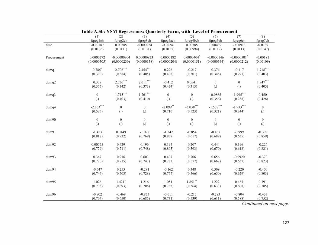
127

Table A.5b: YSM Regressions: Quarterly Farm, with Level of Procurement (1) (2) (3) (4) (5) (6) (7) (8) fqreg1ch fqreg2ch fqreg3ch fqreg4ach fqreg4bch fqreg5ch fqreg6ch fqreg7ch time -0.00187 0.00585 -0.000224 -0.00241 0.00385 0.00439 -0.00913 -0.0139 (0.0136) (0.0131) (0.0131) (0.0135) (0.00994) (0.0117) (0.0113) (0.0147) Procurement 0.0000272 -0.00000904 0.00000823 0.0000182 0.0000404* -0.0000146 -0.0000501* -0.00181 (0.0000305) (0.0000230) (0.0000138) (0.0000204) (0.0000151) (0.0000344) (0.0000212) (0.00109) dumq1 0.785* 2.706*** 2.454*** 0.296 -0.217 0.374 -0.117 1.718*** (0.390) (0.384) (0.405) (0.408) (0.301) (0.348) (0.297) (0.403) dumq2 0.339 2.730*** 2.011*** -0.412 0.0541 0 0 1.847*** (0.375) (0.342) (0.373) (0.424) (0.313) (.) (.) (0.405) dumq3 0 1.715*** 1.761*** 0 0 -0.0865 -1.995*** 0.450 (.) (0.403) (0.410) (.) (.) (0.356) (0.288) (0.428) dumq4 -2.863*** 0 0 -2.099** -3.038*** -1.538*** -1.933*** 0 (0.535) (.) (.) (0.710) (0.523) (0.321) (0.344) (.) dum90 0 0 0 0 0 0 0 0 (.) (.) (.) (.) (.) (.) (.) (.) dum91 -1.453 0.0149 -1.028 -1.242 -0.854 -0.167 -0.999 -0.399 (0.812) (0.732) (0.769) (0.838) (0.617) (0.689) (0.635) (0.859) dum92 0.00575 0.429 0.196 0.194 0.207 0.444 0.196 -0.226 (0.779) (0.711) (0.748) (0.805) (0.593) (0.670) (0.618) (0.821) dum93 0.367 0.916 0.603 0.407 0.706 0.656 -0.0920 -0.370 (0.770) (0.715) (0.747) (0.783) (0.577) (0.662) (0.637) (0.823) dum94 -0.547 0.253 -0.291 -0.162 0.348 0.309 -0.220 -0.400 (0.746) (0.703) (0.728) (0.767) (0.566) (0.650) (0.629) (0.803) dum95 1.026 1.421* 1.216 1.051 1.851** 1.222 0.463 0.391 (0.738) (0.693) (0.708) (0.765) (0.564) (0.633) (0.608) (0.785) dum96 -0.802 -0.469 -0.833 -0.611 -0.213 -0.283 -0.804 -0.437 (0.704) (0.650) (0.685) (0.731) (0.539) (0.611) (0.588) (0.752)

Continued on next page.

128

Table A.5b: YSM Regressions: Quarterly Farm, with Level of Procurement - Continued (1) (2) (3) (4) (5) (6) (7) (8) fqreg1ch fqreg2ch fqreg3ch fqreg4ach fqreg4bch fqreg5ch fqreg6ch fqreg7ch dum97 -0.0458 0.403 0.396 0.284 0.251 0.297 -0.317 -0.263 (0.694) (0.646) (0.676) (0.715) (0.527) (0.603) (0.574) (0.740) dum98 -0.0754 0.180 -0.128 -0.125 -0.143 0.0466 -0.459 -0.159 (0.698) (0.645) (0.668) (0.712) (0.525) (0.595) (0.560) (0.733) dum99 -0.387 -0.0789 -0.302 -0.320 -0.364 0.0861 0.0559 0.0839 (0.686) (0.638) (0.664) (0.724) (0.533) (0.664) (0.529) (0.706) dum00 -0.319 0.402 0.0192 0.0445 -0.0118 0.699 0.167 -0.00326 (0.723) (0.641) (0.684) (0.728) (0.537) (0.633) (0.529) (0.707) dum01 -0.517 0.200 -0.0607 -0.201 -0.376 0.0833 0.0115 0.369 (0.700) (0.639) (0.659) (0.749) (0.552) (0.626) (0.532) (0.713) dum02 0.0901 0.442 0.250 0.0156 -0.405 0.488 0.208 0.377 (0.699) (0.634) (0.668) (0.763) (0.562) (0.614) (0.539) (0.724) dum03 -0.388 -0.0322 -0.000712 -0.172 -0.346 0.0734 0.242 0.229 (0.745) (0.645) (0.679) (0.761) (0.561) (0.610) (0.551) (0.737) dum04 0.0102 0.114 0.264 -0.121 -0.310 0.402 0.242 0.303 (0.728) (0.660) (0.695) (0.783) (0.577) (0.627) (0.561) (0.753) dum05 0.204 0.306 0.193 0.232 0.360 0.236 0.106 0.378 (0.745) (0.678) (0.713) (0.772) (0.569) (0.638) (0.577) (0.772) dum06 0 0 0 0 0 0 0 0 (.) (.) (.) (.) (.) (.) (.) (.) _cons 0.477 -2.266** -1.705* 0.367 0.0680 -0.152 1.492* -0.449 (0.685) (0.772) (0.759) (0.696) (0.513) (0.646) (0.593) (0.850) N 67 67 67 67 67 67 67 67 adj. R2 0.582 0.547 0.400 0.225 0.556 0.337 0.611 0.273 Durbin-Watson d-statistic 2.633364 2.423854 2.636594 2.826111 2.440906 2.828205 2.708325 2.728024 Standard errors in parentheses * p < 0.05, ** p < 0.01, *** p < 0.001

Continued on next page.

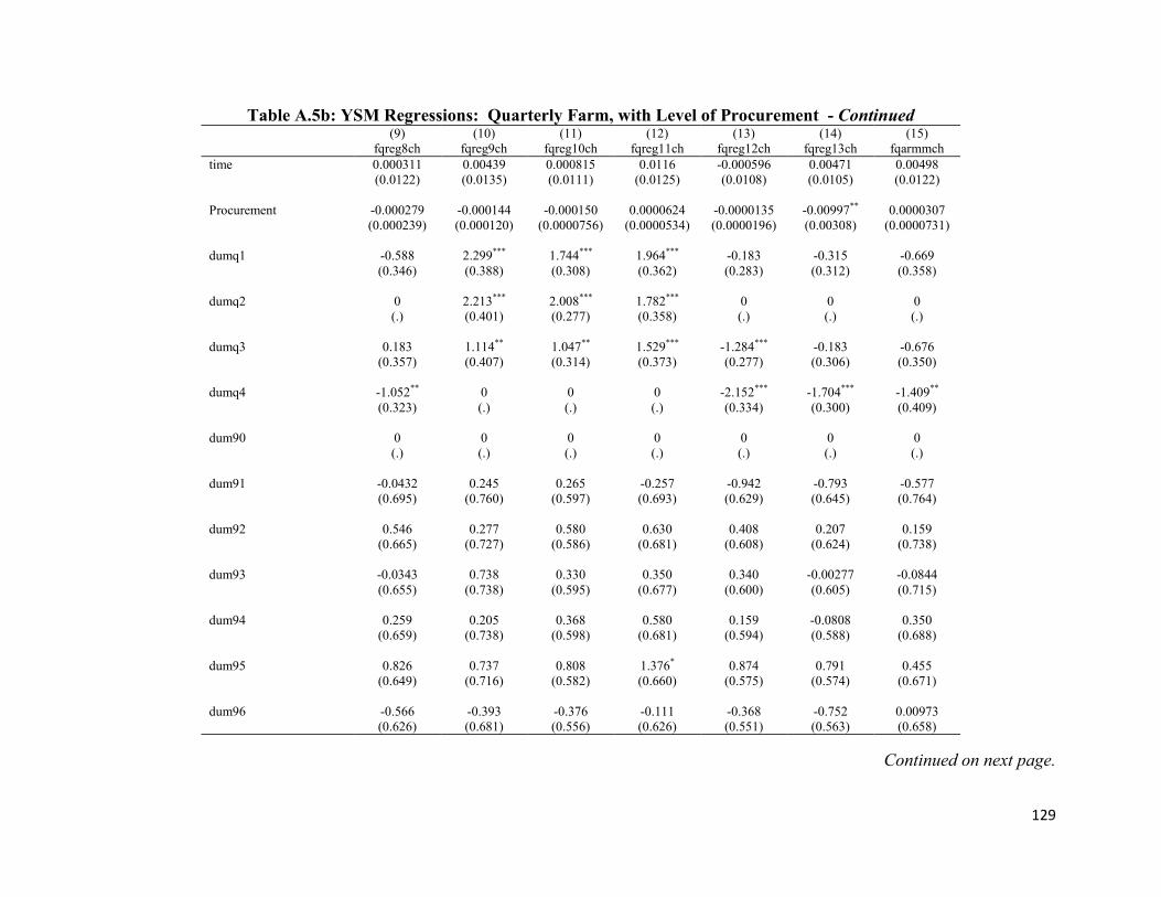
129

Table A.5b: YSM Regressions: Quarterly Farm, with Level of Procurement - Continued (9) (10) (11) (12) (13) (14) (15) fqreg8ch fqreg9ch fqreg10ch fqreg11ch fqreg12ch fqreg13ch fqarmmch time 0.000311 0.00439 0.000815 0.0116 -0.000596 0.00471 0.00498 (0.0122) (0.0135) (0.0111) (0.0125) (0.0108) (0.0105) (0.0122) Procurement -0.000279 -0.000144 -0.000150 0.0000624 -0.0000135 -0.00997** 0.0000307 (0.000239) (0.000120) (0.0000756) (0.0000534) (0.0000196) (0.00308) (0.0000731) dumq1 -0.588 2.299*** 1.744*** 1.964*** -0.183 -0.315 -0.669 (0.346) (0.388) (0.308) (0.362) (0.283) (0.312) (0.358) dumq2 0 2.213*** 2.008*** 1.782*** 0 0 0 (.) (0.401) (0.277) (0.358) (.) (.) (.) dumq3 0.183 1.114** 1.047** 1.529*** -1.284*** -0.183 -0.676 (0.357) (0.407) (0.314) (0.373) (0.277) (0.306) (0.350) dumq4 -1.052** 0 0 0 -2.152*** -1.704*** -1.409** (0.323) (.) (.) (.) (0.334) (0.300) (0.409) dum90 0 0 0 0 0 0 0 (.) (.) (.) (.) (.) (.) (.) dum91 -0.0432 0.245 0.265 -0.257 -0.942 -0.793 -0.577 (0.695) (0.760) (0.597) (0.693) (0.629) (0.645) (0.764) dum92 0.546 0.277 0.580 0.630 0.408 0.207 0.159 (0.665) (0.727) (0.586) (0.681) (0.608) (0.624) (0.738) dum93 -0.0343 0.738 0.330 0.350 0.340 -0.00277 -0.0844 (0.655) (0.738) (0.595) (0.677) (0.600) (0.605) (0.715) dum94 0.259 0.205 0.368 0.580 0.159 -0.0808 0.350 (0.659) (0.738) (0.598) (0.681) (0.594) (0.588) (0.688) dum95 0.826 0.737 0.808 1.376* 0.874 0.791 0.455 (0.649) (0.716) (0.582) (0.660) (0.575) (0.574) (0.671) dum96 -0.566 -0.393 -0.376 -0.111 -0.368 -0.752 0.00973 (0.626) (0.681) (0.556) (0.626) (0.551) (0.563) (0.658)

Continued on next page.

130

Table A.5b: YSM Regressions: Quarterly Farm, with Level of Procurement - Continued (9) (10) (11) (12) (13) (14) (15) fqreg8ch fqreg9ch fqreg10ch fqreg11ch fqreg12ch fqreg13ch fqarmmch dum97 -0.00920 0.446 0.180 0.507 0.115 -0.0189 0.634 (0.613) (0.674) (0.547) (0.624) (0.542) (0.554) (0.648) dum98 0.334 -0.520 -0.227 -0.0977 -0.460 -0.434 -0.837 (0.603) (0.649) (0.535) (0.609) (0.525) (0.549) (0.642) dum99 -0.407 0.603 0.329 0.181 0.104 -0.261 0.118 (0.582) (0.647) (0.507) (0.585) (0.507) (0.547) (0.669) dum00 0.109 0.254 0.817 0.0223 -0.0148 -0.0505 0.0137 (0.583) (0.637) (0.527) (0.588) (0.533) (0.548) (0.732) dum01 -0.0625 -0.0289 0.389 -0.231 -0.0917 -0.302 -0.245 (0.585) (0.642) (0.526) (0.593) (0.511) (0.552) (0.653) dum02 0.224 0.170 0.321 0.193 0.276 -0.0467 -0.0860 (0.590) (0.651) (0.521) (0.598) (0.520) (0.559) (0.654) dum03 0.0194 0.396 0.544 0.156 -0.0137 -0.206 0.135 (0.599) (0.662) (0.527) (0.610) (0.528) (0.570) (0.665) dum04 0.0671 -0.429 -0.0757 0.0589 0.157 1.003 0.169 (0.612) (0.678) (0.540) (0.624) (0.541) (0.688) (0.681) dum05 0.119 -0.0395 0.114 -0.157 0.00137 0.246 -0.450 (0.629) (0.695) (0.553) (0.640) (0.554) (0.625) (0.699) dum06 0 0 0 0 0 0 0 (.) (.) (.) (.) (.) (.) (.) _cons 0.292 -1.633 -1.325 -2.069** 0.874 0.492 0.424 (0.713) (0.824) (0.661) (0.761) (0.560) (0.532) (0.626) N 67 67 67 67 67 67 67 adj. R2 0.146 0.469 0.496 0.291 0.557 0.416 0.039 Durbin-Watson d-statistic 2.65257 2.52659 2.692067 2.805163 2.58955 2.629436 2.56271 Standard errors in parentheses * p < 0.05, ** p < 0.01, *** p < 0.001

131

Table A.5c: YSM Regressions: Monthly Retail , with Level of Distribution (1) (2) (3) (4) (5) (6) (7) (8) rmmch rreg1ch^ rreg2ch rreg3ch^ rreg4ach^ rreg4bch^ rreg5ch^ rreg6ch time -0.000203 0.000578 0.00111 0.00111 0.0000124 0.000761 0.00136 0.000517 (0.00156) (0.000943) (0.000887) (0.00106) (0.000904) (0.000972) (0.00123) (0.00309) Distribution 0.00000158 -0.0000292 -0.0000391 -0.0000208 -0.00000584 -0.0000196* -0.0000296 0.0000250 (0.00000460) (0.0000155) (0.0000390) (0.0000139) (0.00000830) (0.00000865) (0.0000263) (0.0000292) dumjan 0 -0.677 0 -1.053* -0.784* -1.125** -0.977 0 (.) (0.425) (.) (0.469) (0.383) (0.390) (0.564) (.) dumfeb -0.0412 -0.648 0.108 -0.767 -0.603 -0.712 -0.892 0.0803 (0.171) (0.418) (0.131) (0.470) (0.374) (0.386) (0.578) (0.133) dummar 0.0382 -0.539 0.166 -0.738 -0.517 -0.885* -0.984 0.0483 (0.173) (0.409) (0.136) (0.460) (0.366) (0.376) (0.555) (0.112) dumapr 0.0362 -0.354 0.303* -0.799 -0.588 -0.851* -1.114 0.306** (0.175) (0.405) (0.128) (0.467) (0.365) (0.376) (0.591) (0.110) dummay 0.0633 -0.528 0.144 -0.880 -0.546 -0.658 -0.787 0.489** (0.181) (0.380) (0.141) (0.452) (0.351) (0.363) (0.562) (0.158) dumjun -0.133 -0.548 0.158 -0.651 -0.489 -0.539 -0.869 0.0566 (0.176) (0.354) (0.126) (0.400) (0.326) (0.335) (0.533) (0.159) dumjul 0.219 -0.384 0.613*** -0.521 -0.343 -0.403 -0.528 0.185 (0.225) (0.323) (0.182) (0.353) (0.304) (0.310) (0.473) (0.222) dumaug 0.531 0 0.771 0 0 0 0 0.699 (0.396) (.) (0.447) (.) (.) (.) (.) (0.436) dumsep 0.195 -0.276 0.424* -0.351 -0.126 -0.519* -0.514 -0.946** (0.205) (0.271) (0.198) (0.303) (0.232) (0.261) (0.364) (0.331) dumoct 0.179 -0.994* -0.281 -0.965* -0.566 -0.689* -1.249* -0.917*** (0.231) (0.390) (0.159) (0.426) (0.323) (0.334) (0.542) (0.200) dumnov -0.442 -1.301** -0.304 -1.313** -0.896* -1.211** -1.147* -0.271* (0.462) (0.435) (0.196) (0.489) (0.403) (0.392) (0.548) (0.131) dumdec -0.0185 -1.029* 0.0144 -0.928* -0.825* -0.957* -0.912 0.0783 (0.175) (0.428) (0.148) (0.460) (0.393) (0.414) (0.524) (0.119) dum90 0 0 0 0 0 0 0 0 (.) (.) (.) (.) (.) (.) (.) (.) dum91 0.0316 -0.194 -0.0294 -0.245 -0.270 -0.231 -0.243 -0.0577 (0.195) (0.135) (0.174) (0.160) (0.186) (0.187) (0.197) (0.541) dum92 0.102 0.108 0.239 -0.0157 0.116 -0.0612 0.102 0.139 (0.203) (0.125) (0.185) (0.184) (0.184) (0.171) (0.193) (0.526) dum93 0.217 0.344* 0.307 0.256 0.142 0.216 0.235 0.273 (0.171) (0.149) (0.201) (0.220) (0.187) (0.165) (0.206) (0.535) dum94 0.0664 -0.186 0.0151 -0.216 -0.128 -0.114 -0.0741 0.261 (0.210) (0.130) (0.160) (0.151) (0.227) (0.190) (0.179) (0.444) dum95 0.322 0.506 0.530 0.302 0.332 0.281 0.454 0.569 (0.881) (0.516) (0.472) (0.485) (0.570) (0.538) (0.778) (0.719) dum96 0.0960 0.0552 0.0418 -0.0177 0.00693 0.0178 -0.277 0.0488 (0.189) (0.204) (0.227) (0.215) (0.225) (0.242) (0.215) (0.386)

Continued on next page.

132

Table A.5c: YSM Regressions: Monthly Retail, with Level of Distribution - Continued (1) (2) (3) (4) (5) (6) (7) (8) rmmch rreg1ch^ rreg2ch rreg3ch^ rreg4ach^ rreg4bch^ rreg5ch^ rreg6ch dum97 -0.0396 -0.0129 -0.0473 -0.190 -0.0638 -0.128 -0.0383 0.0976 (0.159) (0.158) (0.125) (0.133) (0.186) (0.130) (0.166) (0.346) dum98 -0.119 0.0803 0.0748 0.146 -0.197 -0.0686 0.102 0.0334 (0.115) (0.117) (0.123) (0.173) (0.232) (0.116) (0.242) (0.323) dum99 -0.00251 0.0692 0.0101 0.0110 -0.0575 0.00318 0.201 0.0228 (0.136) (0.105) (0.104) (0.122) (0.119) (0.111) (0.279) (0.298) dum00 -0.0344 0.0513 0.134 -0.141 -0.0270 0.0368 0.102 0.0781 (0.138) (0.102) (0.104) (0.0963) (0.145) (0.120) (0.139) (0.245) dum01 0.0197 -0.0876 0.0396 -0.144 0.00428 0.0688 -0.0883 0.0481 (0.189) (0.130) (0.128) (0.139) (0.171) (0.117) (0.121) (0.222) dum02 0.206 0.229* 0.171 -0.0440 0.0478 -0.00989 0.0410 0.000137 (0.200) (0.113) (0.112) (0.172) (0.117) (0.105) (0.127) (0.222) dum03 0.00811 0.122 -0.0215 -0.124 -0.0975 -0.0494 -0.121 0.0306 (0.163) (0.0929) (0.103) (0.141) (0.110) (0.140) (0.138) (0.163) dum04 -0.0319 0.142 -0.00736 -0.0673 -0.0992 0.00121 -0.0410 -0.0349 (0.216) (0.107) (0.0905) (0.123) (0.113) (0.157) (0.136) (0.186) dum05 0 0.187 0.0763 0.0487 0.0296 0.107 0.105 0.191 (.) (0.102) (0.0853) (0.107) (0.126) (0.172) (0.137) (0.168) dum06 -0.0207 0 0 0 0 0 0 0 (0.133) (.) (.) (.) (.) (.) (.) (.) _cons -0.133 0.591 -0.308 0.806 0.559 0.787 0.836 -0.223 (0.233) (0.422) (0.165) (0.456) (0.382) (0.399) (0.567) (0.580) N 203 203 203 203 203 203 203 203 adj. R2 -0.034 0.145 0.155 0.127 0.047 0.109 0.078 0.232 2.438547 1.909910 1.850123 1.971661 1.896760 1.939942 1.806706 2.499565

Standard errors in parentheses * p < 0.05, ** p < 0.01, *** p < 0.001 ^Prais-Winsten AR(1) regression

Continued on next page.

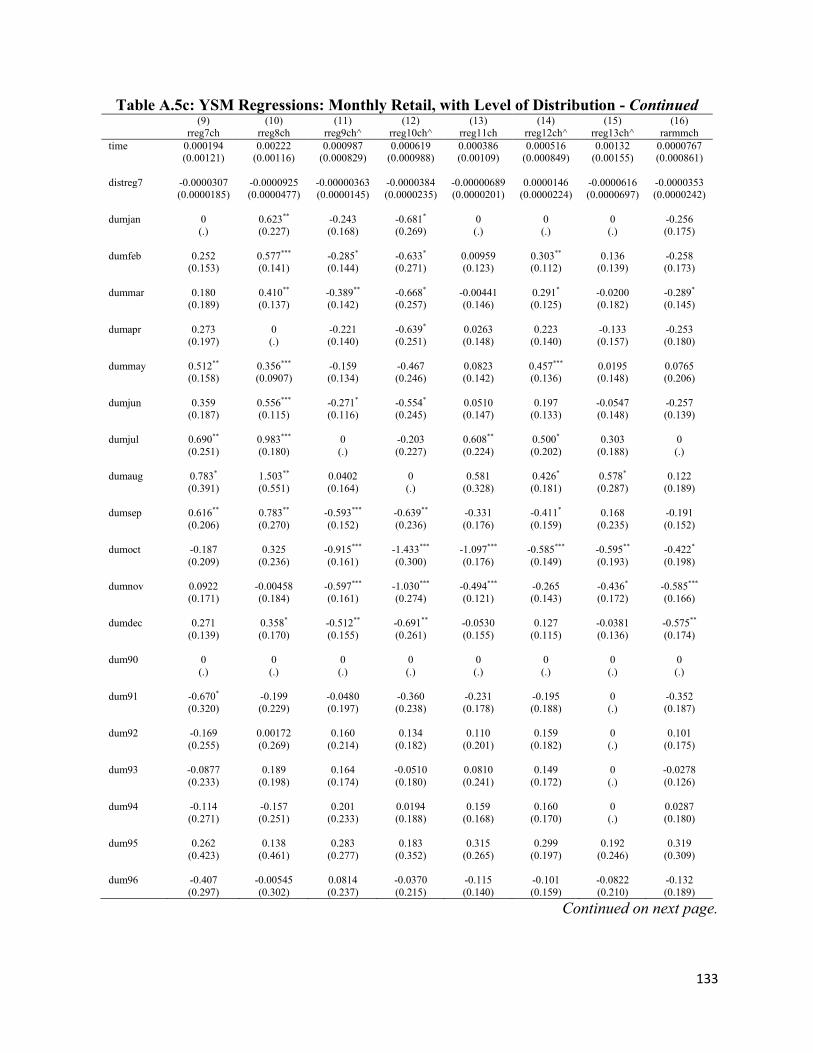
133

Table A.5c: YSM Regressions: Monthly Retail, with Level of Distribution - Continued (9) (10) (11) (12) (13) (14) (15) (16) rreg7ch rreg8ch rreg9ch^ rreg10ch^ rreg11ch rreg12ch^ rreg13ch^ rarmmch time 0.000194 0.00222 0.000987 0.000619 0.000386 0.000516 0.00132 0.0000767 (0.00121) (0.00116) (0.000829) (0.000988) (0.00109) (0.000849) (0.00155) (0.000861) distreg7 -0.0000307 -0.0000925 -0.00000363 -0.0000384 -0.00000689 0.0000146 -0.0000616 -0.0000353 (0.0000185) (0.0000477) (0.0000145) (0.0000235) (0.0000201) (0.0000224) (0.0000697) (0.0000242) dumjan 0 0.623** -0.243 -0.681* 0 0 0 -0.256 (.) (0.227) (0.168) (0.269) (.) (.) (.) (0.175) dumfeb 0.252 0.577*** -0.285* -0.633* 0.00959 0.303** 0.136 -0.258 (0.153) (0.141) (0.144) (0.271) (0.123) (0.112) (0.139) (0.173) dummar 0.180 0.410** -0.389** -0.668* -0.00441 0.291* -0.0200 -0.289* (0.189) (0.137) (0.142) (0.257) (0.146) (0.125) (0.182) (0.145) dumapr 0.273 0 -0.221 -0.639* 0.0263 0.223 -0.133 -0.253 (0.197) (.) (0.140) (0.251) (0.148) (0.140) (0.157) (0.180) dummay 0.512** 0.356*** -0.159 -0.467 0.0823 0.457*** 0.0195 0.0765 (0.158) (0.0907) (0.134) (0.246) (0.142) (0.136) (0.148) (0.206) dumjun 0.359 0.556*** -0.271* -0.554* 0.0510 0.197 -0.0547 -0.257 (0.187) (0.115) (0.116) (0.245) (0.147) (0.133) (0.148) (0.139) dumjul 0.690** 0.983*** 0 -0.203 0.608** 0.500* 0.303 0 (0.251) (0.180) (.) (0.227) (0.224) (0.202) (0.188) (.) dumaug 0.783* 1.503** 0.0402 0 0.581 0.426* 0.578* 0.122 (0.391) (0.551) (0.164) (.) (0.328) (0.181) (0.287) (0.189) dumsep 0.616** 0.783** -0.593*** -0.639** -0.331 -0.411* 0.168 -0.191 (0.206) (0.270) (0.152) (0.236) (0.176) (0.159) (0.235) (0.152) dumoct -0.187 0.325 -0.915*** -1.433*** -1.097*** -0.585*** -0.595** -0.422* (0.209) (0.236) (0.161) (0.300) (0.176) (0.149) (0.193) (0.198) dumnov 0.0922 -0.00458 -0.597*** -1.030*** -0.494*** -0.265 -0.436* -0.585*** (0.171) (0.184) (0.161) (0.274) (0.121) (0.143) (0.172) (0.166) dumdec 0.271 0.358* -0.512** -0.691** -0.0530 0.127 -0.0381 -0.575** (0.139) (0.170) (0.155) (0.261) (0.155) (0.115) (0.136) (0.174) dum90 0 0 0 0 0 0 0 0 (.) (.) (.) (.) (.) (.) (.) (.) dum91 -0.670* -0.199 -0.0480 -0.360 -0.231 -0.195 0 -0.352 (0.320) (0.229) (0.197) (0.238) (0.178) (0.188) (.) (0.187) dum92 -0.169 0.00172 0.160 0.134 0.110 0.159 0 0.101 (0.255) (0.269) (0.214) (0.182) (0.201) (0.182) (.) (0.175) dum93 -0.0877 0.189 0.164 -0.0510 0.0810 0.149 0 -0.0278 (0.233) (0.198) (0.174) (0.180) (0.241) (0.172) (.) (0.126) dum94 -0.114 -0.157 0.201 0.0194 0.159 0.160 0 0.0287 (0.271) (0.251) (0.233) (0.188) (0.168) (0.170) (.) (0.180) dum95 0.262 0.138 0.283 0.183 0.315 0.299 0.192 0.319 (0.423) (0.461) (0.277) (0.352) (0.265) (0.197) (0.246) (0.309) dum96 -0.407 -0.00545 0.0814 -0.0370 -0.115 -0.101 -0.0822 -0.132 (0.297) (0.302) (0.237) (0.215) (0.140) (0.159) (0.210) (0.189)

Continued on next page.

134

Table A.5c: YSM Regressions: Monthly Retail, with Level of Distribution - Continued (9) (10) (11) (12) (13) (14) (15) (16) rreg7ch rreg8ch rreg9ch^ rreg10ch^ rreg11ch rreg12ch^ rreg13ch^ rarmmch dum97 -0.270 -0.0108 -0.0146 -0.0775 -0.0409 0.0451 -0.0700 0.0225 (0.159) (0.180) (0.115) (0.131) (0.148) (0.189) (0.215) (0.137) dum98 -0.0371 0.169 -0.0291 0.00218 -0.0616 -0.146 -0.136 -0.0712 (0.134) (0.175) (0.121) (0.145) (0.132) (0.171) (0.164) (0.131) dum99 -0.137 -0.113 0.00469 0.0464 -0.00333 0.00360 0 -0.0764 (0.130) (0.173) (0.148) (0.156) (0.141) (0.125) (.) (0.122) dum00 -0.0893 0.127 -0.0417 -0.0496 -0.0379 -0.0682 0 0.0450 (0.164) (0.113) (0.132) (0.135) (0.123) (0.127) (.) (0.122) dum01 -0.0601 -0.188 -0.0341 -0.0467 -0.0660 -0.0282 -0.178 -0.145 (0.115) (0.163) (0.106) (0.132) (0.146) (0.117) (0.207) (0.117) dum02 -0.0902 -0.0216 0.0407 0.0609 0.00923 0.0358 -0.0796 0.0125 (0.138) (0.173) (0.0988) (0.118) (0.305) (0.170) (0.225) (0.105) dum03 -0.0541 -0.0325 -0.0533 -0.000488 -0.0181 -0.0394 -0.0345 -0.00368 (0.104) (0.0989) (0.107) (0.162) (0.168) (0.134) (0.144) (0.119) dum04 -0.0870 -0.0123 0.0293 -0.103 0.0939 0.0260 0.154 -0.0371 (0.0988) (0.122) (0.107) (0.132) (0.181) (0.188) (0.137) (0.199) dum05 0.219 0.0773 0.0151 0.0212 0.0419 -0.0499 0.0289 0.0339 (0.163) (0.125) (0.111) (0.147) (0.160) (0.179) (0.121) (0.122) dum06 0 0 0 0 0 0 0 0 (.) (.) (.) (.) (.) (.) (.) (.) _cons -0.120 -0.396* 0.194 0.698* 0.0117 -0.226 -0.0844 0.280 (0.237) (0.185) (0.227) (0.297) (0.161) (0.150) (0.206) (0.170) N 203 203 203 203 203 203 131 203 adj. R2 0.093 0.160 0.227 0.252 0.362 0.353 0.219 0.128 2.12804 1.994307 1.949283 1.951732 1.90845 1.980009 1.914901 2.102311

Standard errors in parentheses * p < 0.05, ** p < 0.01, *** p < 0.001 ^Prais-Winsten AR(1) regression

135

Table A.5d: YSM Regressions: Quarterly Retail, with Level of Distribution (1) (2) (3) (4) (5) (6) (7) (8) rqmmch rqreg1ch rqreg2ch rqreg3ch rqreg4ach rqreg4bch rqreg5ch rqreg6ch time 0.00688 0.00747 0.00427 0.0154 0.00120 0.00272 0.00431 0.00512 (0.0169) (0.00522) (0.00852) (0.0135) (0.00959) (0.00822) (0.00793) (0.0177) Distribution -0.00000194 -0.0000293 0.000000947 -0.0000274 -0.0000191 -0.0000168 -0.00000411 0.0000379 (0.00000608) (0.0000182) (0.0000444) (0.0000202) (0.0000160) (0.0000159) (0.0000191) (0.0000234) dumq1 0 0 0 0 0 0 0 0 (.) (.) (.) (.) (.) (.) (.) (.) dumq2 0.534 0.917** 0.541* 0.559* 0.549 0.867** 0.181 0.600 (0.396) (0.272) (0.253) (0.264) (0.296) (0.268) (0.232) (0.298) dumq3 1.319* 1.247 0.743 1.834 1.599 1.747 0.855 -0.789 (0.649) (0.703) (0.737) (1.022) (0.961) (0.926) (0.592) (0.471) dumq4 -0.274 -0.478 -0.441 -0.0411 0.269 0.0353 -0.148 -1.110** (0.499) (0.383) (0.366) (0.368) (0.345) (0.383) (0.312) (0.404) dum90 0 0 0 0 0 0 0 0 (.) (.) (.) (.) (.) (.) (.) (.) dum91 -0.383 -0.757 -0.167 -0.884 -1.268 -0.936 -0.734 0.0493 (0.476) (0.606) (0.563) (0.636) (0.744) (0.513) (0.456) (1.211) dum92 -0.615 0.0310 0.303 -0.118 -0.203 -0.273 0.326 -0.00249 (0.801) (0.455) (0.630) (0.621) (0.632) (0.591) (0.550) (1.142) dum93 0.779* 1.156*** 0.758 0.688 0.323 0.527 0.990 0.937 (0.322) (0.297) (0.384) (0.591) (0.550) (0.422) (0.499) (1.194) dum94 -0.393 -0.483 0.480 -0.863 -0.597 -0.306 0.000983 0.854 (0.912) (0.350) (0.363) (0.612) (0.605) (0.497) (0.463) (0.890) dum95 0.835 1.194 1.603 0.616 0.979 1.121 1.502 1.783 (2.050) (1.724) (1.535) (1.835) (1.856) (2.034) (1.415) (1.255) dum96 -0.473 0.334 0.307 -0.121 -0.484 -0.276 -0.443 0.283 (1.159) (0.870) (0.940) (0.773) (0.678) (0.518) (0.739) (1.005)

Continued on next page.

136

Table A.5d: YSM Regressions: Quarterly Retail, with Level of Distribution – Continued (1) (2) (3) (4) (5) (6) (7) (8) rqmmch rqreg1ch rqreg2ch rqreg3ch rqreg4ach rqreg4bch rqreg5ch rqreg6ch dum97 0.0570 -0.249 0.0165 -0.502 -0.519 -0.105 0.0613 0.422 (0.577) (0.369) (0.230) (0.448) (0.396) (0.332) (0.206) (0.725) dum98 -0.342 0.0726 0.268 0.663 -0.104 -0.0358 0.107 0.0851 (0.455) (0.226) (0.372) (0.736) (0.602) (0.457) (0.482) (0.721) dum99 -0.235 0.183 -0.0198 0.0346 -0.0922 0.0642 -0.0294 0.0596 (0.532) (0.355) (0.330) (0.456) (0.325) (0.347) (0.634) (0.636) dum00 -0.303 0.104 0.348 -0.394 0.0491 0.266 0.299 0.499 (0.474) (0.245) (0.369) (0.316) (0.306) (0.418) (0.323) (0.608) dum01 -0.438 -0.241 0.236 -0.588 0.0654 0.105 -0.0736 0.186 (0.687) (0.521) (0.310) (0.496) (0.342) (0.346) (0.233) (0.560) dum02 -0.00541 0.476 0.509 -0.146 0.0509 0.208 0.236 0.0523 (0.467) (0.361) (0.374) (0.300) (0.249) (0.268) (0.228) (0.559) dum03 -0.380 0.283 0.0458 -0.495 -0.0231 -0.0256 -0.0421 0.205 (0.630) (0.204) (0.288) (0.466) (0.343) (0.465) (0.289) (0.498) dum04 -0.539 0.469 0.113 -0.520 -0.0815 0.0747 0.0289 -0.0626 (0.873) (0.255) (0.355) (0.316) (0.270) (0.495) (0.317) (0.642) dum05 0 0.449* 0.502 0.0333 0.299 0.490 0.423 0.329 (.) (0.177) (0.416) (0.341) (0.425) (0.522) (0.455) (0.732) dum06 -0.222 0 0 0 0 0 0 0 (0.454) (.) (.) (.) (.) (.) (.) (.)

_cons -0.435 -0.478 -0.773 -0.371 -0.150 -0.441 -0.538 -0.595 (0.451) (0.357) (0.397) (0.570) (0.588) (0.450) (0.323) (1.071) N 67 67 67 67 67 67 67 67 adj. R2 -0.031 0.127 0.049 0.035 -0.015 0.036 0.094 0.193 Durbin-Watson d-statistic

2.819562 2.963387 3.063074 2.931814 2.946246 2.958975 2.737092 2.527938

Standard errors in parentheses * p < 0.05, ** p < 0.01, *** p < 0.001

Continued on next page.

137

Table A.5d: YSM Regressions: Quarterly Retail, with Level of Distribution – Continued (9) (10) (11) (12) (13) (14) (15) (16) rqreg7ch rqreg8ch rqreg9ch rqreg10ch rqreg11ch rqreg12ch rqreg13ch rqarmmch time 0.00628 0.0114 0.00271 -0.00444 0.000613 0.00753 0.0163 -0.000923 (0.0127) (0.0110) (0.0190) (0.00660) (0.0100) (0.00849) (0.0135) (0.0100) Distribution -0.0000386 -0.0000224 0.0000491 0.00000860 0.00000208 0.0000490 -0.0000693 -0.0000351 (0.0000199) (0.0000354) (0.0000536) (0.0000284) (0.0000248) (0.0000356) (0.0000757) (0.0000368) dumq1 0 -0.0659 0 0 1.273*** 0.811* 0.623* 0.327 (.) (0.280) (.) (.) (0.348) (0.346) (0.279) (0.363) dumq2 0.914* 0 -0.0683 0.440 1.584*** 1.446*** 0.592* 0.881* (0.446) (.) (0.475) (0.287) (0.389) (0.340) (0.225) (0.362) dumq3 1.386 1.171 0.785 0.366 1.307* 0.189 1.235*** 1.095** (0.711) (0.652) (1.095) (0.463) (0.618) (0.467) (0.330) (0.398) dumq4 0.170 -0.432 -1.922 -0.693 0 0 0 0 (0.466) (0.377) (1.386) (0.346) (.) (.) (.) (.) dum90 0 0 0 0 0 0 0 0 (.) (.) (.) (.) (.) (.) (.) (.) dum91 -1.823* -0.337 0.203 -0.853 -0.679 0.0664 -0.527 -1.171 (0.809) (0.699) (1.412) (0.724) (0.872) (0.721) (0.626) (0.619) dum92 -0.897 0.295 0.445 -0.273 -0.0658 0.440 0.416 -0.186 (1.300) (1.046) (8.384) (0.839) (0.807) (1.009) (0.624) (0.839) dum93 -0.220 0.614 0.844 0.222 0.301 0.647 0.0979 -0.135 (0.682) (0.572) (1.043) (0.443) (0.405) (0.440) (0.460) (0.479) dum94 -0.247 0.242 1.076 0.111 0.321 0.954 0.307 -0.0484 (0.725) (0.609) (1.088) (0.678) (0.447) (0.667) (0.528) (0.645) dum95 0.489 1.187 1.674 0.968 1.052 1.434 0.505 0.839 (1.673) (1.609) (1.140) (0.955) (0.913) (0.875) (0.587) (1.044) dum96 -0.545 0.218 0.641 -0.0269 -0.184 0.190 -0.110 -0.158 (0.971) (0.850) (1.369) (0.840) (0.580) (0.633) (0.703) (0.906)

Continued on next page.

138

Table A.5d: YSM Regressions: Quarterly Retail, with Level of Distribution – Continued (9) (10) (11) (12) (13) (14) (15) (16) rqreg7ch rqreg8ch rqreg9ch rqreg10ch rqreg11ch rqreg12ch rqreg13ch rqarmmch dum97 -0.614 0.0358 0.290 -0.0784 0.0146 0.363 -0.335 0.0134 (0.450) (0.460) (0.854) (0.235) (0.385) (0.454) (0.506) (0.361) dum98 -0.0675 0.253 -0.341 -0.320 -0.309 -0.489 -0.400 -0.245 (0.411) (0.468) (0.883) (0.364) (0.340) (0.430) (0.445) (0.443) dum99 -0.142 -0.102 -0.0488 -0.272 -0.156 0.0380 -0.446 -0.233 (0.685) (0.484) (0.900) (0.547) (0.395) (0.339) (0.494) (0.370) dum00 -0.0254 0.182 0.0379 -0.0989 0.0961 0.0284 -0.317 -0.0840 (0.654) (0.457) (0.796) (0.392) (0.517) (0.402) (0.555) (0.567) dum01 -0.279 -0.141 0.0853 -0.160 -0.200 0.0908 -0.643 -0.367 (0.379) (0.548) (0.907) (0.376) (0.488) (0.562) (0.621) (0.369) dum02 0.00971 0.111 0.125 0.317 0.206 0.248 -0.502 -0.00681 (0.293) (0.376) (0.776) (0.379) (0.521) (0.486) (0.690) (0.321) dum03 -0.243 -0.0125 0.284 0.00907 0.00245 0.290 -0.0393 -0.0750 (0.361) (0.366) (0.958) (0.293) (0.676) (0.630) (0.265) (0.371) dum04 -0.0866 0.0224 0.0276 0.0127 0.278 0.244 0.132 0.0412 (0.275) (0.466) (0.794) (0.268) (0.625) (0.740) (0.472) (0.367) dum05 0.865 0.0582 -0.00300 0.218 -0.0357 0.109 0.130 -0.0421 (0.478) (0.445) (0.954) (0.393) (0.524) (0.805) (0.346) (0.342) dum06 0 0 0 0 0 0 0 0 (.) (.) (.) (.) (.) (.) (.) (.) _cons -0.166 -0.506 -0.663 -0.0284 -1.198*** -1.521*** -0.978** -0.369 (0.752) (0.566) (1.374) (0.354) (0.232) (0.368) (0.358) (0.562) N 67 67 67 67 67 67 67 67 adj. R2 -0.057 0.022 -0.273 0.054 0.200 0.174 0.107 0.059 Durbin-Watson d-statistic

2.657281 2.96879 2.969141 2.815614 2.671165 2.66576 2.578591 2.65297

Standard errors in parentheses * p < 0.05, ** p < 0.01, *** p < 0.001

139

Figure A..1: Thailand Export Prices and Philippine Wholesale Prices

Continued on next page.

140

Figure A.1 : Thailand Export Prices and Philippine Wholesale Prices – Continued

Continued on next page.

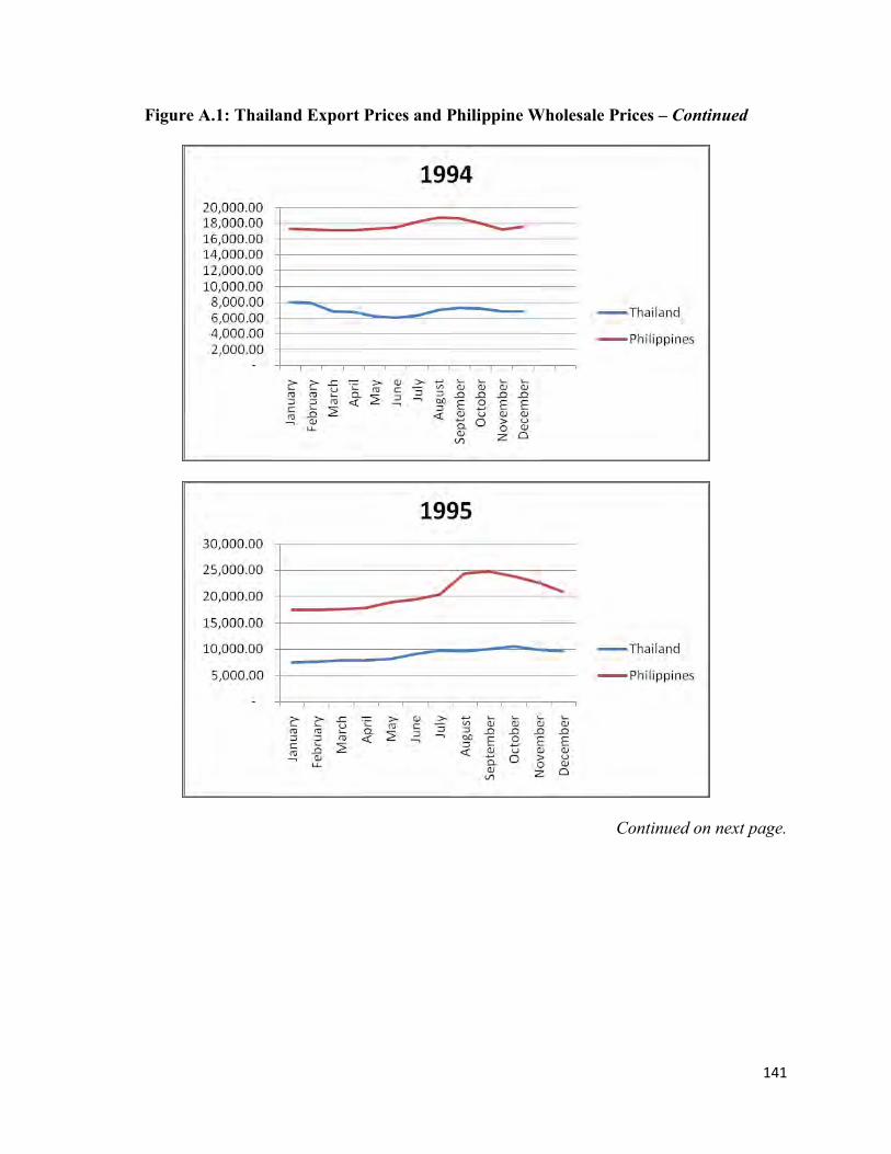
141

Figure A.1: Thailand Export Prices and Philippine Wholesale Prices – Continued

Continued on next page.

142

Figure A.1: Thailand Export Prices and Philippine Wholesale Prices – Continued

Continued on next page.

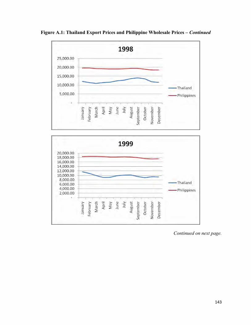
143

Figure A.1: Thailand Export Prices and Philippine Wholesale Prices – Continued

Continued on next page.

144

Figure A.1: Thailand Export Prices and Philippine Wholesale Prices – Continued

Continued on next page.

145

Figure A.1: Thailand Export Prices and Philippine Wholesale Prices – Continued

Continued on next page.

146

Figure A.1: Thailand Export Prices and Philippine Wholesale Prices – Continued

Continued on next page.

147

Figure A.1: Thailand Export Prices and Philippine Wholesale Prices – Continued

’

Continued on next page.

148

Figure A.1: Thailand Export Prices and Philippine Wholesale Prices – Continued

149

Figure A.2: Vietnam Export Prices and Philippine Wholesale Prices

Continued on next page.

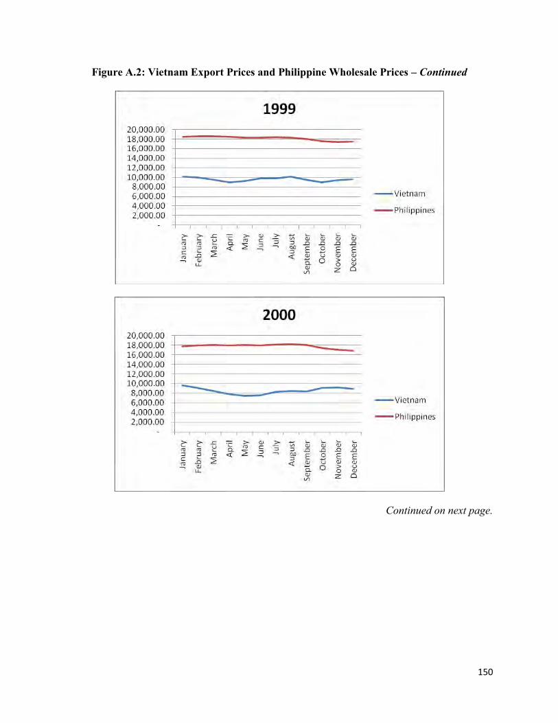
150

Figure A.2: Vietnam Export Prices and Philippine Wholesale Prices – Continued

Continued on next page.

151

Figure A.2: Vietnam Export Prices and Philippine Wholesale Prices – Continued

Continued on next page.

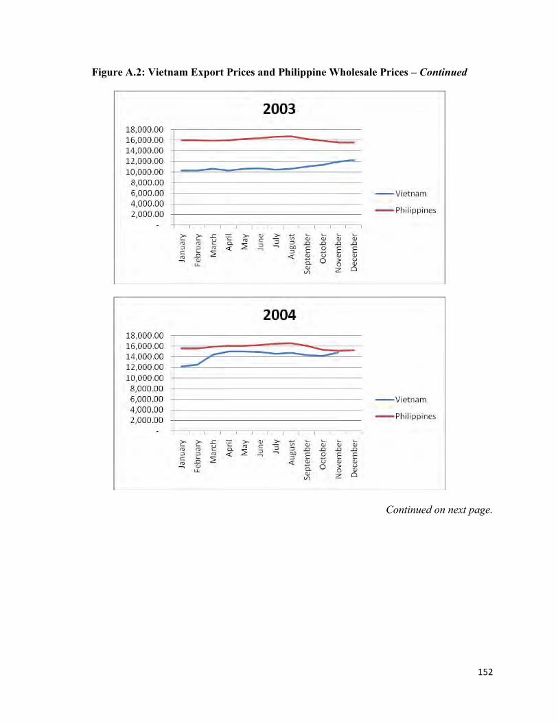
152

Figure A.2: Vietnam Export Prices and Philippine Wholesale Prices – Continued

Continued on next page.

153

Figure A.2: Vietnam Export Prices and Philippine Wholesale Prices – Continued

Continued on next page.

154

Figure A.2: Vietnam Export Prices and Philippine Wholesale Prices – Continued