ricardo roberto comunicações de tempo-real em switched ...sistemas embutidos, sistemas...
TRANSCRIPT
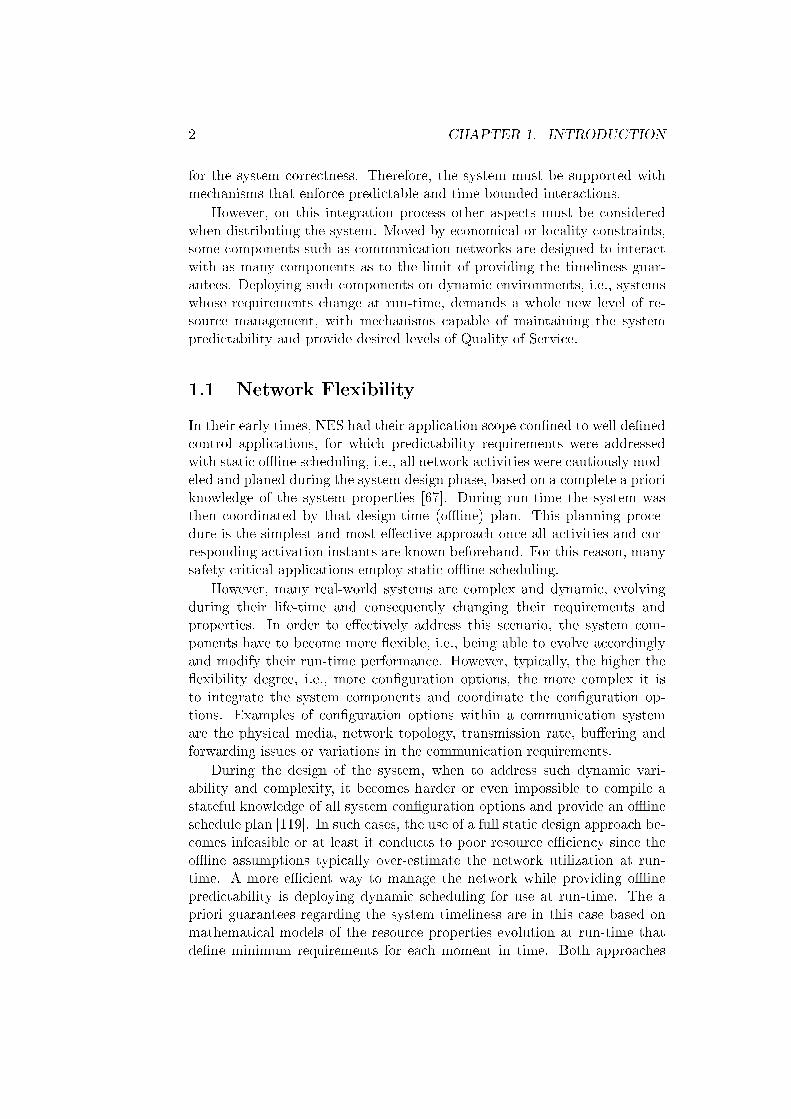
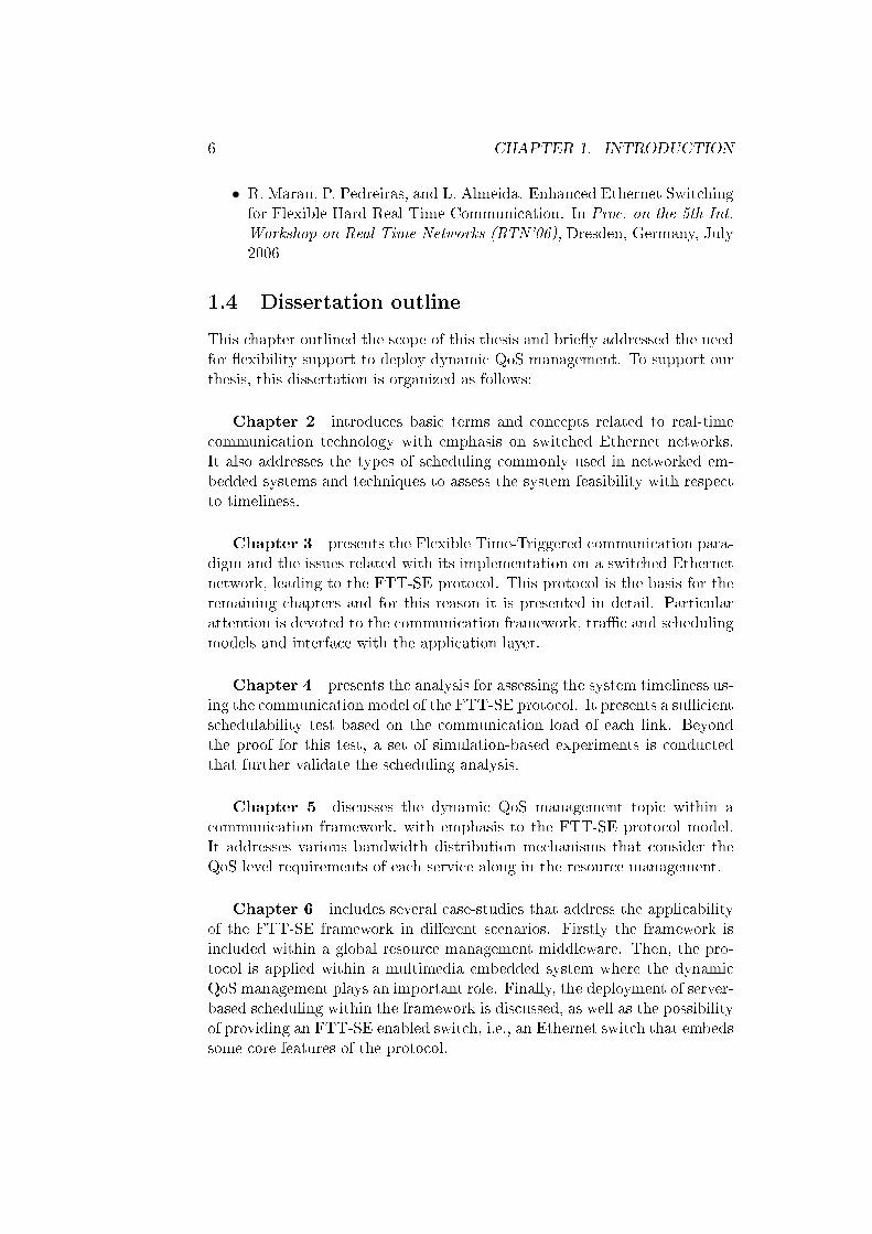
Master NIC
FT
T-SE
SRDB
EC registerReadyqueue
SchedulerDispatcher
Built-inSlave
signaling TM
NRDBs updateNRDB Memory pool
TMDispatcherC
ore
Man
agem
ent Connection DB
QoS DB
Queuing
Connectivity
QoS/Admissioncontrol
Inte
rfac
e
Slave NIC
Streammanagement
Applicationthreads
n
Streamcommunication
m nodes
Streammanagement
Universidade de Aveiro Departamento de Electrónica, Telecomunicações e2009 Informática
Ricardo RobertoDuarte Marau
Comunicações de tempo-real em switched Ethernetsuportando gestão dinâmica de QdS
Real-time communications over switched Ethernetsupporting dynamic QoS management

Universidade de Aveiro Departamento de Electrónica, Telecomunicações e2009 Informática
Ricardo RobertoDuarte Marau
Comunicações de tempo-real em switched Ethernetsuportando gestão dinâmica de QdS
Real-time communications over switched Ethernetsupporting dynamic QoS management


Universidade de Aveiro Departamento de Electrónica, Telecomunicações e2009 Informática
Ricardo RobertoDuarte Marau
Comunicações de tempo-real em switched Ethernetsuportando gestão dinâmica de QdS
Real-time communications over switched Ethernetsupporting dynamic QoS management
Dissertação apresentada à Universidade de Aveiro para cumprimento dosrequisitos necessários à obtenção do grau de Doutor em EngenhariaInformática, realizada sob a orientação científica do Prof. Doutor Luís MiguelPinho de Almeida, Professor Associado da Faculdade de Engenharia daUniversidade do Porto e co-orientação do Prof. Doutor Paulo Bacelar ReisPedreiras, Professor Auxiliar do Departamento de Electrónica,Telecomunicações e Informática da Universidade de Aveiro.
Este trabalho foi apoiado por:
Ministério da Ciência e do Ensino Superior, por meio da Fundação para aCiência e a Tecnologia, que me concedeu uma bolsa de Doutoramento noâmbito do III Quadro Comunitário de Apoio, (SFRH /BD/25261/2005).
Universidade de Aveiro, que me concedeu uma bolsa de Doutoramento deJaneiro a Dezembro de 2005 e proporcionou as condições logisticas, técnicase humanas para a prossecução dos trabalhos realizados no âmbito desta tese.
Instituto de Engenharia Electrónica e Telemática de Aveiro, que apoioufinanceiramente a minha participação em conferências internacionais paraapresentação de resultados parciais obtidos no âmbito desta tese.
Projectos europeus ARTIST2 (IST-2004-004527) e ArtistDesign(ICT-NoE-214373), no âmbito dos quais se realizou parte dos trabalhos destatese.


Dedicatória
aos meus paise à minha irmã.


o júri / the jury
presidente / president Doutor Amadeu Mortágua Velho da Maia SoaresProfessor Catedrático da Universidade de Aveiro(por delegação da Reitora da Universidade de Aveiro)
vogais / examiners committee Doutor Raj RajkumarFull Professor da Carnegie Mellon University, Estados Unidos da América
Doutora Maria de la Soledad Garcia VallsAssociate Professor da Universidad Carlos III de Madrid
Doutor Luís Miguel Pinho de AlmeidaProfessor Associado da Faculdade de Engenharia da Universidade do Porto(Orientador)
Doutor José Alberto Gouveia FonsecaProfessor Associado da Universidade de Aveiro
Doutor Paulo Bacelar Reis PedreirasProfessor Auxiliar da Universidade de Aveiro(Co-Orientador)


Agradecimentos /Acknowledgements
A jornada que culminou, entre outras coisas, nesta dissertação começouhá cinco anos em Aveiro. Durante este período percorri uma viagem deenriquecimento pessoal que me permitiu adquirir competências a vários níveisbem como conhecer e interagir com pessoas maravilhosas que me ajudarame apoiaram em várias etapas da viagem. Como em qualquer viagem, houvemomentos bons e momentos menos bons, penosos e mesmo desmotivantes.Mas quando eis chegado o momento de parar, respirar, olhar para trás e fazero balanço, apenas me ocorre: valeu a pena. A todas as pessoas que directa oudirectamente se envolveram nesta viagem, expresso o meu profundo e sinceroagradecimento. Contudo, dada a sua relevância, gostaria de agradecer emparticular:
I would like to thank:
a Luís de Almeida, por me ter proposto e convencido a iniciar a viagem;pela orientação exemplar a nível técnico, ciêntifico e pedagógico; pela enormegenerosidade e paciência que sempre demonstrou ao longo destes cinco anos;pelas acesas discussões técnicas que se alongavam pela noite e que, muitasvezes, se misturavam com umas cervejas no Ramona.
a Paulo Pedreiras, por ter acompanhado os meus trabalhos durante estes anoscomo orientador, com uma competência técnico-científica irrepreensível; portê-lo feito de uma forma bastante próxima, atenta e humana.
a ambos pelo empenho e dedicação profissional, bom como pelas condiçõese meios oferecidos para desenvolver o meu trabalho; pelos bons momentosde amizade, convívio e entre-ajuda, o meu sincero e sentido agradecimento.Obrigado pela inspiração! Gostaria ainda de manifestar o meu apreço à Nani eà Cristina, à Sofia, Joana, Pedro e Francisco, pela simpatia e compreensão.
to Michael González Harbour, to Daniel Sangorrín and to Julio L. Med-ina, from the University of Cantabria, for the support and collaboration in partof my work. Also, for having received me in Santander in a visit that althoughshort, happened in an early stage and was very helpful to clarify much of thepurpose of my work. "¡Gracias!"
to Javier Silvestre, from the Polytechnic University of Valencia (Alcoy), forits valuable collaboration and skills in Multimedia and QoS, letting the devel-opment of a case-study application that wraps much of my work, making itmeaningful. For having invited me to Alcoy and provided all the means andsupport during my stay. "Gracias también a su familia, Mónica, Jaime y Conchaque me recibieron con mucha alegría y cariño. Moltes gràcies!"


to Raj Rajkumar Karthik and to Lakshmanan from the Carnegie Mellon Uni-versity, for their valuable scientific contribution to the work in this dissertationand also for having made possible and pleasant my visit to Pittsburgh. I haveto remark and be thankful for the outstanding commitment and support to myresearch topics during my stay. This collaboration was determinant to thetheoretical formulation in Chapters 4 and 5. Thanks a lot!
to Thomas Nolte, Professor at Mälardalen University, Sweeden, for itsvaluable collaboration in the Servers and Hierarchical composition topics thatenriched and amplified the applicability scope of this work. Thanks!
a Nuno Figueiredo, que prontamente aceitou o repto de, no âmbito dasua tese de Mestrado, integrar o protocolo apresentado nesta dissertaçãona plataforma de controlo por ele desenvolvida, permitindo desta forma umaavaliação real de algumas propriedades do protocolo. De destacar o espíritopro-activo e empreendedor que imprimiu no trabalho, permitindo o desenvolvi-mento de agradáveis discussões técnicas e linhas de trabalho futuro. Obrigado!
a Isidro Calvo, a Manuel Barranco, a Iria Ayres, a Pablo Basanta, quepassaram longos períodos em Aveiro e com eles trouxeram alegria e boa--disposição ao laboratório. Obrigado pela vossa amizade, companheirismo eclaro... por me haber enseñado algo de español. "Gracias chicos!"
a Valter Silva, a Frederico Santos, a Rui Santos, a Margarida Urbano, aAlexandre Vieira colegas de laboratório e amigos com quem tive o prazer dedesenvolver agradáveis discussões técnicas durante estes anos, bem como,discussões menos técnicas que proporcionavam agradáveis gargalhadas emomentos de descontracção. Obrigado!
a José Luís Azevedo, a José Alberto Fonseca, a Pedro Fonseca, professoresdurante a minha Licenciatura que tiveram um papel relevante na definiçãodas minhas áreas de interesse em comunicações e sistemas embutidos e naconsequente vontade em prosseguir os meus estudos nesse âmbito. Obrigado!
a Ana Margarida, a Alexandre Santos, a Pedro Leite, a Ana Ferreira, aTiago Silveira, grande amigos, que sem dúvida ajudaram a vincar o início destaviagem. Obrigado malta, jamais esquecerei!
a Rodolfo Andrade, a Nuno Letão, a Alexandra Moura, pelas muitas palavrasde apoio e pelas quartas-feiras loucas.
ao grupo de Salsa, que durante estes anos ajudou a descontrair e des-comprimir nos momentos de maior tensão. Em particular agradeço à Luísa eao Hugo Leite pela amizade, pelo apoio e pelas muitas salsas animadas comboa música. E sem esquecer o que a Salsa me deu, agradeço à Jeanette quesoube marcar a sua presença amiga e cúmplice. Obrigado!
Finalmente, agradeço às pessoas mais importantes na minha vida: osmeus pais e irmã. A base de tudo o que sou e de todo este trabalho, foram vósque a construíram.
Ricardo Marau


Palavras-chave Tempo-real, Comunicações de tempo-real, Comunicações industriais,Sistemas embutidos, Sistemas distribuídos, Escalonamento de tempo-real,Gestão de Qualidade de Serviço, Ethernet.
Resumo Durante a última década temos assistido a um crescente aumento na utilizaçãode sistemas embutidos para suporte ao controlo de processos, de sistemasrobóticos, de sistemas de transportes e veículos e até de sistemas domóticose eletrodomésticos. Muitas destas aplicações são críticas em termos desegurança de pessoas e bens e requerem um alto nível de determinismo comrespeito aos instantes de execução das respectivas tarefas. Além disso, a im-plantação destes sistemas pode estar sujeita a limitações estruturais, exigindoou beneficiando de uma configuração distribuída, com vários subsistemascomputacionais espacialmente separados. Estes subsistemas, apesar deespacialmente separados, são cooperativos e dependem de uma infraestruturade comunicação para atingir os objectivos da aplicação e, por consequência,também as transacções efectuadas nesta infraestrutura estão sujeitas àsrestrições temporais definidas pela aplicação.
As aplicações que executam nestes sistemas distribuídos, chamadosnetworked embedded systems (NES), podem ser altamente complexas eheterogéneas, envolvendo diferentes tipos de interacções com diferentesrequisitos e propriedades. Um exemplo desta heterogeneidade é o modelo deactivação da comunicação entre os subsistemas que pode ser desencadeadaperiodicamente de acordo com uma base de tempo global (time-triggered),como sejam os fluxos de sistemas de controlo distribuído, ou ainda serdesencadeada como consequência de eventos assíncronos da aplicação(event-triggered). Independentemente das características do tráfego ou doseu modelo de activação, é de extrema importância que a plataforma decomunicações disponibilize as garantias de cumprimento dos requisitos daaplicação ao mesmo tempo que proporciona uma integração simples dosvários tipos de tráfego.


Uma outra propriedade que está a emergir e a ganhar importância no seiodos NES é a flexibilidade. Esta propiedade é realçada pela necessidade dereduzir os custos de instalação, manutenção e operação dos sistemas. Nestesentido, o sistema é dotado da capacidade para adaptar o serviço fornecido àaplicação aos respectivos requisitos instantâneos, acompanhando a evoluçãodo sistema e proporcionando uma melhor e mais racional utilização dosrecursos disponíveis.
No entanto, maior flexibilidade operacional é igualmente sinónimo demaior complexidade derivada da necessidade de efectuar a alocação dinâmicados recursos, acabando também por consumir recursos adicionais no sistema.A possibilidade de modificar dinâmicamente as caracteristicas do sistematambém acarreta uma maior complexidade na fase de desenho e especifi-cação. O aumento do número de graus de liberdade suportados faz aumentaro espaço de estados do sistema, dificultando a uma pre-análise. No sentido deconter o aumento de complexidade são necessários modelos que representema dinâmica do sistema e proporcionem uma gestão optimizada e justa dosrecursos com base em parâmetros de qualidade de serviço (QdS).
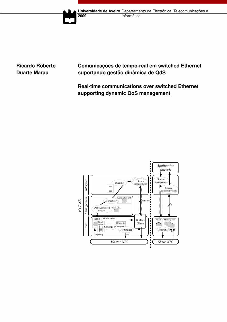
É nossa tese que as propriedades de flexibilidade, pontualidade e gestãodinâmica de QdS podem ser integradas numa rede switched Ethernet (SE),tirando partido do baixo custo, alta largura de banda e fácil implantação. Nestadissertação é proposto um protocolo, Flexible Time-Triggered communicationover Switched Ethernet (FTT-SE), que suporta as propriedades desejadas eque ultrapassa as limitações das redes SE para aplicações de tempo-real taiscomo a utilização de filas FIFO, a existência de poucos níveis de prioridadee a pouca capacidade de gestão individualizada dos fluxos. O protocolobaseia-se no paradigma FTT, que genericamente define a arquitectura de umapilha protocolar sobre o acesso ao meio de uma rede partilhada, impondodesta forma determinismo temporal, juntamente com a capacidade parareconfiguração e adaptação dinâmica da rede. São ainda apresentados váriosmodelos de distribuição da largura de banda da rede de acordo com o nível deQdS especificado por cada serviço utilizador da rede.Esta dissertação expõe a motivação para a criação do protocolo FTT-SE,apresenta uma descrição do mesmo, bem como a análise de algumas dassuas propiedades mais relevantes. São ainda apresentados e comparadosmodelos de distribuição da QdS. Finalmente, são apresentados dois casos deaplicações que sustentam a validade da tese acima mencionada.


Keywords Real-time, Real-time communications, Industrial communications,Embedded systems, Networked embedded systems, Distributed systems,Real-time scheduling, Quality of Service management, Ethernet.
Abstract During the last decade we have witnessed a massive deployment of embeddedsystems on a wide applications range, from industrial automation to processcontrol, avionics, cars or even robotics. Many of these applications have aninherently high level of criticality, having to perform tasks within tight temporalconstraints. Additionally, the configuration of such systems is often distributed,with several computing nodes that rely on a communication infrastructure tocooperate and achieve the application global goals. Therefore, the communica-tions are also subject to the same temporal constraints set by the applicationrequirements.
Many applications relying on such networked embedded systems (NES)are complex and heterogeneous, comprehending different activities with differ-ent requirements and properties. For example, the communication betweensubsystems may follow a strict temporal synchronization with respect to aglobal time-base (time-triggered), like in a distributed feedback control loop,or it may be issued asynchronously upon the occurrence of events (event-triggered). Regardless of the traffic characteristics and its activation model, itis of paramount importance having a communication framework that providesseamless integration of heterogeneous traffic sources while guaranteeing theapplication requirements.


Another property that has been emerging as important for NES design andoperation is flexibility. The need to reduce installation and operational costs,while facilitating maintenance is promoting a more rational use of the availableresources at run-time, exploring the ability to tune service parameters as thesystem evolves.
However, such operational flexibility comes with the cost of increasing thecomplexity of the system to handle the dynamic resource management, whichon the other hand demands the allocation of additional system resources.Moreover, the capacity to dynamically modify the system properties alsocauses a higher complexity when designing and specifying the system, sincethe operational state-space increases with the degrees of flexibility of thesystem.
Therefore, in order to bound this complexity appropriate operational mod-els are needed to handle the system dynamics and carry on an efficient andfair resource management strategy based on quality of service (QoS) metrics.
This thesis states that the properties of flexibility and timeliness as neededfor dynamic QoS management can be provided to switched Ethernet basedsystems. Switched Ethernet, although initially designed for general purposeInternet access and file transfers, is becoming widely used in NES-based appli-cations. However, COTS switched Ethernet is insufficient regarding the needsfor real-time predictability and for supporting the aforementioned properties duethe use of FIFO queues too few priority levels and for stream-level managementcapabilities. In this dissertation we propose a protocol to overcome thoselimitations, namely the Flexible Time-Triggered communication over SwitchedEthernet (FTT-SE). The protocol is based on the FTT paradigm that genericallydefines a protocol architecture suitable to enforce real-time determinism on acommunication network supporting the desired flexibility properties.
This dissertation addresses the motivation for FTT-SE, describing theprotocol as well as its schedulability analysis. It additionally covers the resourcedistribution topic, where several distribution models are proposed to managethe resource capacity among the competing services and while consideringthe QoS level requirements of each service. A couple of application cases areshown that support the aforementioned thesis.

Contents
Abstract xv
Contents xxi
1 Introduction 11.1 Network Flexibility . . . . . . . . . . . . . . . . . . . . . . . . 21.2 E�cient resource management . . . . . . . . . . . . . . . . . . 31.3 Proposition and contributions . . . . . . . . . . . . . . . . . . 41.4 Dissertation outline . . . . . . . . . . . . . . . . . . . . . . . . 6
2 Background 92.1 Real-time systems . . . . . . . . . . . . . . . . . . . . . . . . 9
2.1.1 Real-time scheduling . . . . . . . . . . . . . . . . . . . 102.1.2 Examples of scheduling policies . . . . . . . . . . . . . 132.1.3 Schedulability analysis . . . . . . . . . . . . . . . . . . 152.1.4 Handling asynchronous events . . . . . . . . . . . . . . 192.1.5 Hierarchical schedulers . . . . . . . . . . . . . . . . . . 20
2.2 Real-time communications . . . . . . . . . . . . . . . . . . . . 202.2.1 Event- and Time-triggered communication . . . . . . . 212.2.2 Message scheduling . . . . . . . . . . . . . . . . . . . . 232.2.3 Co-operation models . . . . . . . . . . . . . . . . . . . 26
2.3 Real-Time and Switched Ethernet . . . . . . . . . . . . . . . 272.3.1 Switched Ethernet . . . . . . . . . . . . . . . . . . . . 272.3.2 Real-Time protocols over SE . . . . . . . . . . . . . . 342.3.3 Schedulability analysis . . . . . . . . . . . . . . . . . . 41
2.4 Conclusion . . . . . . . . . . . . . . . . . . . . . . . . . . . . . 45
3 The FTT-SE protocol 473.1 Introduction . . . . . . . . . . . . . . . . . . . . . . . . . . . . 473.2 FTT-SE: An enhancement of FTT-Ethernet . . . . . . . . . . 48
3.2.1 FTT-SE for micro-segmented networks . . . . . . . . . 493.2.2 Handling aperiodic transmissions in FTT-SE . . . . . 51
3.3 The scheduling model . . . . . . . . . . . . . . . . . . . . . . 553.3.1 The periodic tra�c scheduling model . . . . . . . . . . 55
xix
xx CONTENTS
3.3.2 Building EC-schedules . . . . . . . . . . . . . . . . . . 56
3.3.3 The aperiodic tra�c scheduling model . . . . . . . . . 59
3.3.4 Bounding the aperiodic service latency . . . . . . . . . 59
3.4 Implementation details . . . . . . . . . . . . . . . . . . . . . . 62
3.4.1 Middleware abstraction . . . . . . . . . . . . . . . . . 62
3.4.2 Data addressing modes . . . . . . . . . . . . . . . . . . 71
3.5 Simulation and experimental assessment . . . . . . . . . . . . 73
3.5.1 Periodic tra�c simulation results . . . . . . . . . . . . 73
3.5.2 Experimental results . . . . . . . . . . . . . . . . . . . 75
3.6 Conclusion . . . . . . . . . . . . . . . . . . . . . . . . . . . . . 78
4 Tra�c schedulability analysis 81
4.1 Introduction . . . . . . . . . . . . . . . . . . . . . . . . . . . . 81
4.2 Interference in the switch architecture . . . . . . . . . . . . . 82
4.3 Interference within the FTT-SE periodic model . . . . . . . . 84
4.3.1 Window con�nement . . . . . . . . . . . . . . . . . . . 84
4.3.2 Deferred release in the downlinks . . . . . . . . . . . . 85
4.3.3 Scheduling multiple links . . . . . . . . . . . . . . . . 86
4.4 Schedulability test - unicast . . . . . . . . . . . . . . . . . . . 86
4.4.1 One node sending to one destination, only . . . . . . . 87
4.4.2 One node sending to multiple destinations . . . . . . . 88
4.4.3 Schedulability utilization bounds with release jitter . . 89
4.4.4 Upper bounding the indirect load . . . . . . . . . . . . 93
4.5 Simulation results . . . . . . . . . . . . . . . . . . . . . . . . . 95
4.6 Multicast/Broadcast analysis . . . . . . . . . . . . . . . . . . 98
4.7 Conclusion . . . . . . . . . . . . . . . . . . . . . . . . . . . . . 99
5 Dynamic QoS management 101
5.1 Introduction . . . . . . . . . . . . . . . . . . . . . . . . . . . . 101
5.2 The QoS management problem . . . . . . . . . . . . . . . . . 102
5.2.1 The resource capacity . . . . . . . . . . . . . . . . . . 104
5.2.2 The application model . . . . . . . . . . . . . . . . . . 105
5.3 Bandwidth distribution . . . . . . . . . . . . . . . . . . . . . 107
5.3.1 Fixed importance distribution . . . . . . . . . . . . . . 108
5.3.2 Weighted distribution . . . . . . . . . . . . . . . . . . 108
5.3.3 Need for iteration . . . . . . . . . . . . . . . . . . . . . 110
5.3.4 Application mapping models . . . . . . . . . . . . . . 121
5.4 Operational parameters mapping . . . . . . . . . . . . . . . . 127
5.4.1 Complete application model . . . . . . . . . . . . . . . 128
5.4.2 Bandwidth reclaiming . . . . . . . . . . . . . . . . . . 129
5.5 QoS management on FTT-SE . . . . . . . . . . . . . . . . . . 131
5.6 Conclusion . . . . . . . . . . . . . . . . . . . . . . . . . . . . . 135
CONTENTS xxi
6 FTT-SE case studies 1376.1 Integration in the FRESCOR framework . . . . . . . . . . . . 137
6.1.1 FRESCOR background . . . . . . . . . . . . . . . . . 1386.1.2 FRESCOR application example . . . . . . . . . . . . . 1426.1.3 FTT-SE under FRESCOR . . . . . . . . . . . . . . . . 1436.1.4 Internals of the contracting procedure . . . . . . . . . 1466.1.5 (Re-)negotiation procedure time . . . . . . . . . . . . 1486.1.6 Summary . . . . . . . . . . . . . . . . . . . . . . . . . 150
6.2 Industrial multimedia application . . . . . . . . . . . . . . . . 1516.2.1 Related work . . . . . . . . . . . . . . . . . . . . . . . 1526.2.2 System Architecture . . . . . . . . . . . . . . . . . . . 1556.2.3 QoS Management . . . . . . . . . . . . . . . . . . . . . 1586.2.4 Experimental results . . . . . . . . . . . . . . . . . . . 1656.2.5 Summary . . . . . . . . . . . . . . . . . . . . . . . . . 170
6.3 Server-SE . . . . . . . . . . . . . . . . . . . . . . . . . . . . . 1726.3.1 Server-based scheduling . . . . . . . . . . . . . . . . . 1736.3.2 The Server-SE protocol . . . . . . . . . . . . . . . . . 1746.3.3 Experimental results . . . . . . . . . . . . . . . . . . . 1786.3.4 Summary . . . . . . . . . . . . . . . . . . . . . . . . . 181
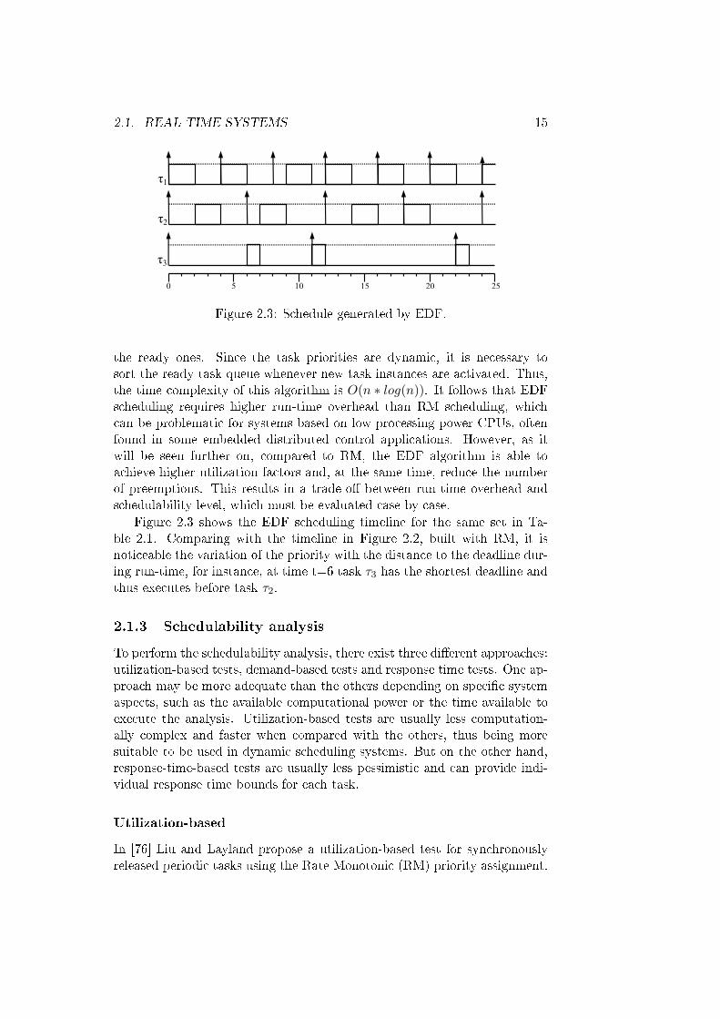
6.4 FTT-SE enabled switch . . . . . . . . . . . . . . . . . . . . . 1836.4.1 Switch Architecture . . . . . . . . . . . . . . . . . . . 1836.4.2 Experimental results . . . . . . . . . . . . . . . . . . . 1866.4.3 Summary . . . . . . . . . . . . . . . . . . . . . . . . . 187
6.5 Conclusion . . . . . . . . . . . . . . . . . . . . . . . . . . . . . 189
7 Conclusions 1917.1 Thesis, contributions and validations . . . . . . . . . . . . . . 1917.2 On-going and Future research . . . . . . . . . . . . . . . . . . 193

List of Figures
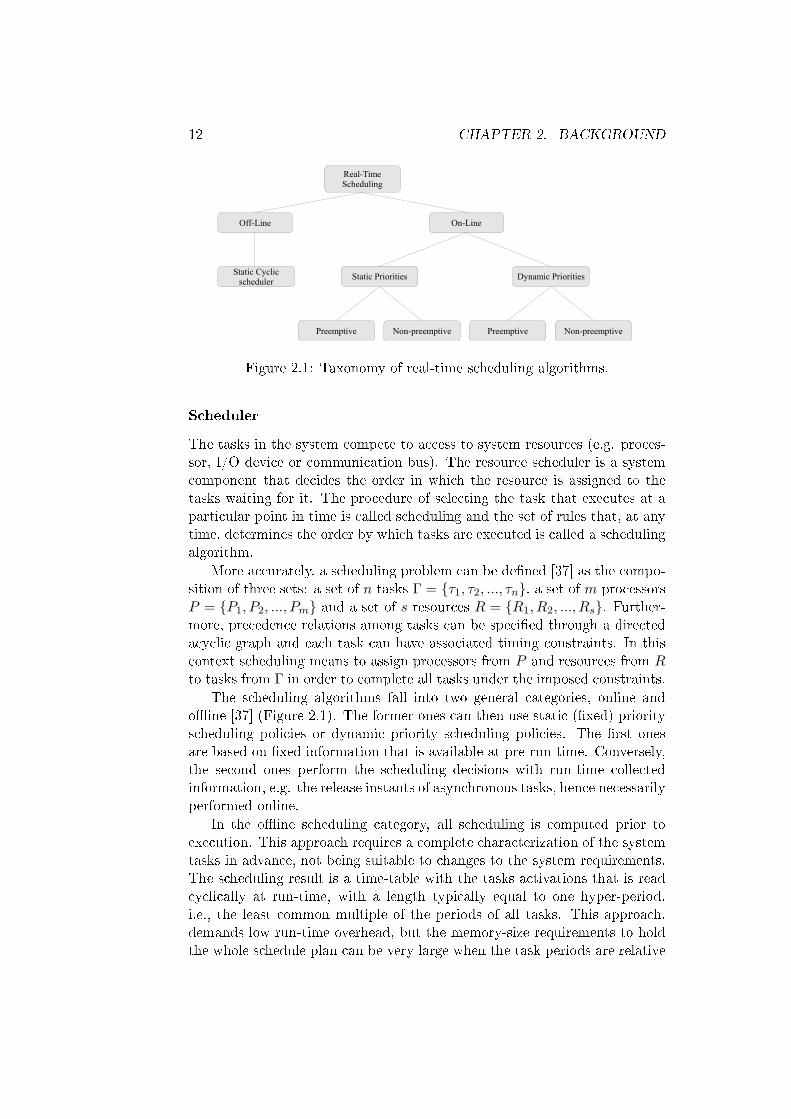
2.1 Taxonomy of real-time scheduling algorithms. . . . . . . . . . 12
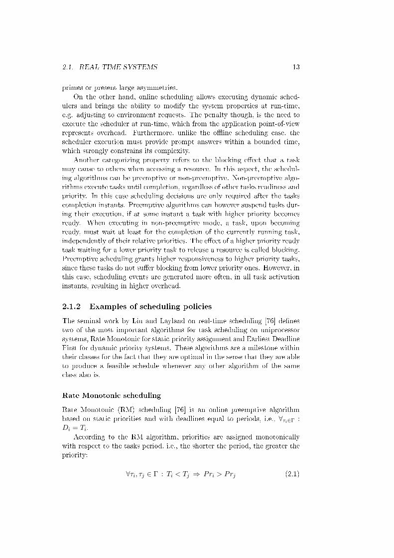
2.2 Schedule generated by RM. . . . . . . . . . . . . . . . . . . . 14
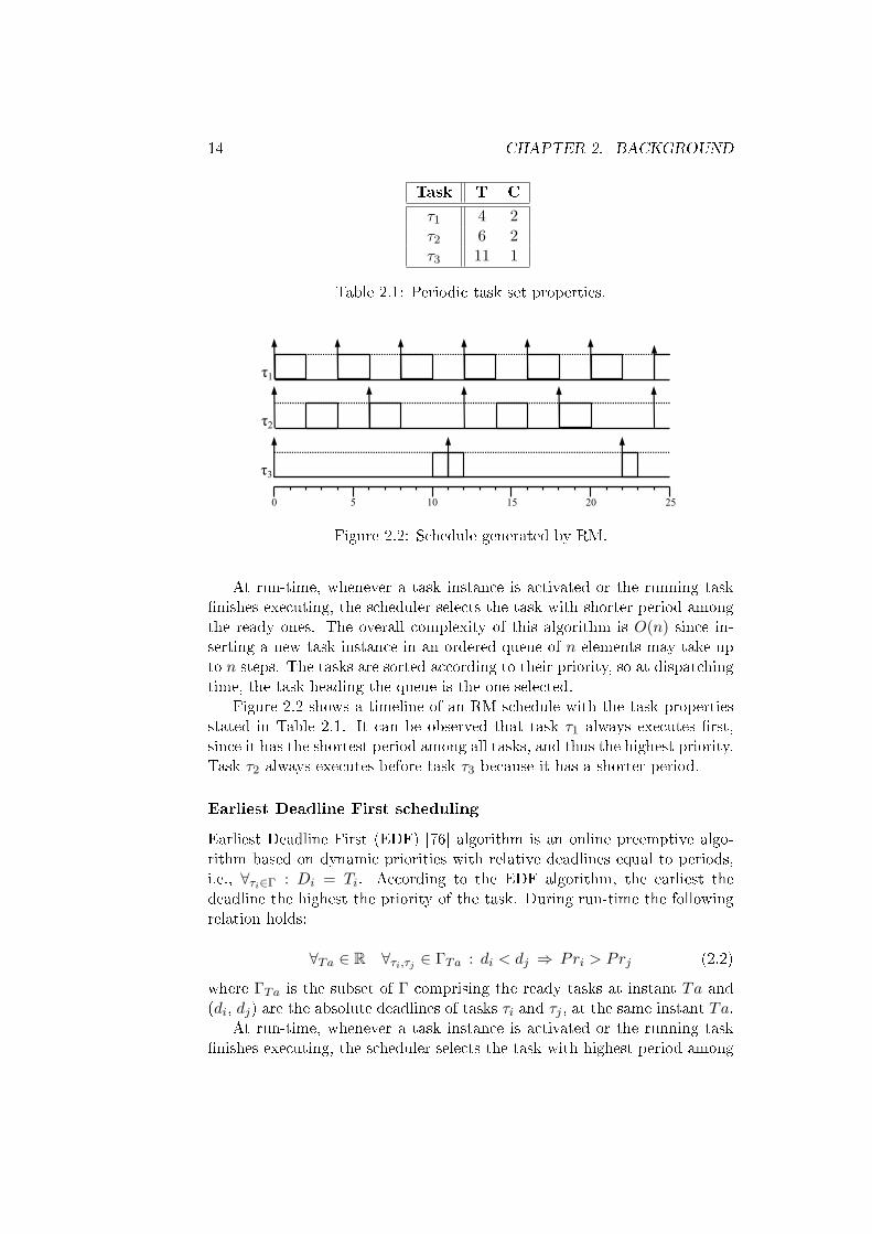
2.3 Schedule generated by EDF. . . . . . . . . . . . . . . . . . . . 15
2.4 The ISO/OSI reference model. . . . . . . . . . . . . . . . . . 24
2.5 Switch micro-segmentation. . . . . . . . . . . . . . . . . . . . 28
2.6 Ethernet II frame. . . . . . . . . . . . . . . . . . . . . . . . . 28
2.7 Ethernet IEEE 802.3ac frame. . . . . . . . . . . . . . . . . . . 29
2.8 Typical switch internal architecture. . . . . . . . . . . . . . . 30
2.9 IEEE 802 MAC address (MAC-48). . . . . . . . . . . . . . . . 32
2.10 IGMP basic architecture. . . . . . . . . . . . . . . . . . . . . 33
2.11 The EC structure in the original FTT-Ethernet. . . . . . . . . 35
2.12 ETHERNET Powerlink cycle structure. . . . . . . . . . . . . 36
2.13 Arbitrary release in k's busy-interval. . . . . . . . . . . . . . . 44
3.1 The EC structure in the original FTT-Ethernet. . . . . . . . . 48
3.2 FTT-SE system architecture. . . . . . . . . . . . . . . . . . . 50
3.3 Polling token. . . . . . . . . . . . . . . . . . . . . . . . . . . . 52
3.4 FTT-SE signaling proposal. . . . . . . . . . . . . . . . . . . . 54
3.5 The scheduling model with FTT-SE. . . . . . . . . . . . . . . 56
3.6 Constraining the synchronous tra�c to the synchronous window. 57
3.7 Causality constraint in the downlinks. . . . . . . . . . . . . . 58
3.8 Response time to Asynchronous messages with FTT-SE (casewith Lschi = 0). . . . . . . . . . . . . . . . . . . . . . . . . . 61
3.9 FTT-SE internal layering. . . . . . . . . . . . . . . . . . . . . 63
3.10 FTT-SE internal details. . . . . . . . . . . . . . . . . . . . . . 64
3.11 Schedulable sets versus the aggregated submitted load withEDF (bottom) and RM (top). . . . . . . . . . . . . . . . . . . 74
3.12 The experimental platform. . . . . . . . . . . . . . . . . . . . 75
3.13 The infrastructure jitter. . . . . . . . . . . . . . . . . . . . . . 77
3.14 Histogram of inter-arrival times for message 7. . . . . . . . . . 78
3.15 Histogram of inter-arrival times for message 1. . . . . . . . . . 79
4.1 Tra�c aggregation on switched Ethernet. . . . . . . . . . . . 82
xxiii
xxiv LIST OF FIGURES
4.2 Inserted Idle Time on switch output queues (the numbers de-note the destinations). . . . . . . . . . . . . . . . . . . . . . . 83
4.3 Impact of inserted idle time. . . . . . . . . . . . . . . . . . . . 85
4.4 Worst-case situation with release jitter and the virtually addedtask in RM. . . . . . . . . . . . . . . . . . . . . . . . . . . . . 90
4.5 Worst-case situation with release jitter and the virtually addedtask in EDF. . . . . . . . . . . . . . . . . . . . . . . . . . . . 91
4.6 Interfering task. . . . . . . . . . . . . . . . . . . . . . . . . . . 93
4.7 Schedulability vs. Utilization(1→1). . . . . . . . . . . . . . . . 97
4.8 Schedulability vs. Utilization using maximum virtual load perset (1→ 2, 3). . . . . . . . . . . . . . . . . . . . . . . . . . . . 98
5.1 Remaining bandwidth. . . . . . . . . . . . . . . . . . . . . . . 107
5.2 Computational complexity, excluding services sort. . . . . . . 119
5.3 Discrete bandwidth to linear range mapping. . . . . . . . . . 129
6.1 FRESCOR resources. . . . . . . . . . . . . . . . . . . . . . . . 140
6.2 Network application model. . . . . . . . . . . . . . . . . . . . 141
6.3 FRESCOR example. . . . . . . . . . . . . . . . . . . . . . . . 142
6.4 FRESCOR example pseudocode. . . . . . . . . . . . . . . . . 144
6.5 Architecture overview. . . . . . . . . . . . . . . . . . . . . . . 145
6.6 FRESCOR interface for network contracts. . . . . . . . . . . . 146
6.7 Negotiation steps. . . . . . . . . . . . . . . . . . . . . . . . . . 147
6.8 Master contract negotiation procedure. . . . . . . . . . . . . . 148
6.9 Generic encoding process. . . . . . . . . . . . . . . . . . . . . 152
6.10 System architecture. . . . . . . . . . . . . . . . . . . . . . . . 156
6.11 QoS management model. . . . . . . . . . . . . . . . . . . . . . 157
6.12 qi adaptation. . . . . . . . . . . . . . . . . . . . . . . . . . . . 159
6.13 Error in frame size caused by ∆qe = 1 for di�erent values of q. 160
6.14 Frame size evolution in time (q = 55). . . . . . . . . . . . . . 165
6.15 Contribution of each stream to QoS'. . . . . . . . . . . . . . . 169
6.16 Bandwidth evolution of stream M1. . . . . . . . . . . . . . . . 170
6.17 Internals of the Server-SE Master. . . . . . . . . . . . . . . . 175
6.18 Server-SE Server Hierarchy. . . . . . . . . . . . . . . . . . . . 176
6.19 Top histogram: inter-arrival times of the AM3 requests; Lowerhistogram: inter-arrival times of AM3 messages. . . . . . . . . 179
6.20 Platform connections diagram. . . . . . . . . . . . . . . . . . 180
6.21 Mean Square Error of the ball with FTT-SE. . . . . . . . . . 182
6.22 Mean Square Error of the ball with Raw Ethernet. . . . . . . 182
6.23 FTT-enabled switch functional architecture. . . . . . . . . . . 184
6.24 Histogram of the di�erences between consecutive NRT mes-sages (uplink). . . . . . . . . . . . . . . . . . . . . . . . . . . 186
6.25 Histogram of the di�erences between the beginning of the ECand NRT messages (downlink). . . . . . . . . . . . . . . . . . 187

List of Tables
2.1 Periodic task set properties. . . . . . . . . . . . . . . . . . . . 14
3.1 AM Response times with uniform arrival (case with Lschi +Lpoll = 0). . . . . . . . . . . . . . . . . . . . . . . . . . . . . 62
3.2 Message set used in the FTT-SE experiments. . . . . . . . . . 76
6.1 Contract Parameters. . . . . . . . . . . . . . . . . . . . . . . . 1406.2 Stream properties for dynamic experiments. . . . . . . . . . . 1666.3 Results with dynamic scenarios. . . . . . . . . . . . . . . . . . 1676.4 Results with static scenarios. . . . . . . . . . . . . . . . . . . 1686.5 QoS' results. . . . . . . . . . . . . . . . . . . . . . . . . . . . . 1696.6 Load characterization - Controller downlink. . . . . . . . . . . 181
xxv

Chapter 1
Introduction
System - A group of interacting, interrelated, or interdependentelements forming a complex whole.
The American Heritage Dictionary of the English Language,Fourth Edition.
For the last decades we have witnessed the generalization of the automationconcept as the mean to provide comfort assistance, economic bene�ts andeven mission-critical aid, in a wide range of application domains. The grow-ing deployment of embedded systems has been supporting such evolutionaryprocess, pushing the development of large-scale embedded systems that in-teract with the environment as within a system. On the quest to realizea completely integrated system, connectivity became the key on promotingsuch interaction between electronic devices and the environment.
Large-scale networked embedded systems (NES) can be found in areassuch as transportation, industrial, medical or communications. The deploy-ment of NES on these domains is constrained by the natural applicationgoal that many times poses stringent timeliness requirements, as well as bynon-technical aspects such as deployment cost and time-to-market that can-not be neglected. Additionally, these systems are attaining complexity levelsthat make them hard to be assessed with a single holistic view. To cope withsuch complexity, there are methodologies that promote seamless integrationbetween the several individual elements, such as component-based develop-ment that o�ers dependable modular composability and the cyber-physicalsystems concept that abstracts data fusion and services ubiquity.
On the process of integrating those subsystems towards the applicationgoal, it is of utmost importance de�ning how they interact and the con-sequences of such interaction. The timeliness requirements on these inter-actions are frequently critical when there are activities to be done withinstrict temporal bounds, which if not met, may result on severe consequences
1
2 CHAPTER 1. INTRODUCTION
for the system correctness. Therefore, the system must be supported withmechanisms that enforce predictable and time-bounded interactions.
However, on this integration process other aspects must be consideredwhen distributing the system. Moved by economical or locality constraints,some components such as communication networks are designed to interactwith as many components as to the limit of providing the timeliness guar-antees. Deploying such components on dynamic environments, i.e., systemswhose requirements change at run-time, demands a whole new level of re-source management, with mechanisms capable of maintaining the systempredictability and provide desired levels of Quality of Service.
1.1 Network Flexibility
In their early times, NES had their application scope con�ned to well de�nedcontrol applications, for which predictability requirements were addressedwith static o�ine scheduling, i.e., all network activities were cautiously mod-eled and planed during the system design phase, based on a complete a prioriknowledge of the system properties [67]. During run-time the system wasthen coordinated by that design-time (o�ine) plan. This planning proce-dure is the simplest and most e�ective approach once all activities and cor-responding activation instants are known beforehand. For this reason, manysafety-critical applications employ static o�ine scheduling.
However, many real-world systems are complex and dynamic, evolvingduring their life-time and consequently changing their requirements andproperties. In order to e�ectively address this scenario, the system com-ponents have to become more �exible, i.e., being able to evolve accordinglyand modify their run-time performance. However, typically, the higher the�exibility degree, i.e., more con�guration options, the more complex it isto integrate the system components and coordinate the con�guration op-tions. Examples of con�guration options within a communication systemare the physical media, network topology, transmission rate, bu�ering andforwarding issues or variations in the communication requirements.
During the design of the system, when to address such dynamic vari-ability and complexity, it becomes harder or even impossible to compile astateful knowledge of all system con�guration options and provide an o�ineschedule plan [119]. In such cases, the use of a full static design approach be-comes infeasible or at least it conducts to poor resource e�ciency since theo�ine assumptions typically over-estimate the network utilization at run-time. A more e�cient way to manage the network while providing o�inepredictability is deploying dynamic scheduling for use at run-time. The apriori guarantees regarding the system timeliness are in this case based onmathematical models of the resource properties evolution at run-time thatde�ne minimum requirements for each moment in time. Both approaches
1.2. EFFICIENT RESOURCE MANAGEMENT 3
require the same amount of information of the system evolution. However,with the dynamic approach, based on a more accurate resource requirementsestimation, it is possible to integrate the system with less over-provisioning,thus providing better feasibility results.
NESs rely on a communication network as the central component tointer-connect the distributed nodes. Adding operational �exibility to thesystem is not constrained to the network, it must be coordinated comprisingall related components. As an example, any data exchange is closely relatedto tasks that ultimately have to be scheduled in the sending and receivingnodes.
As referred above, the main motivation to improve the operational �ex-ibility of a communication network is to enable its use within a dynamicoperational scenario. A similar motivation is argued by Prasad [103] et al.and Lu et al. [80], stating that the use of static schedule plans, thus withoutoperational �exibility, leads to ine�cient resource usage and to non-gracefulservice degradation, i.e., the services are either fully functional or inactive,there is no solution in between. And they complement saying that it is moree�cient to leave some operational decisions in terms of resource usage torun-time.
Therefore, �exibility as a means to recon�gure and/or adjust the systemon-the-�y is an important property to provide e�cient resource management,naturally extending to the network, the fundamental resource in a NES.
1.2 E�cient resource management
E�cient resource management of evolving systems requires the ability to re-act to changes. In the scope of this thesis we will distinguish two di�erentaspects related to the �exibility properties of a resource, namely recon�g-uration, which means adding and removing components and subsystems,and adaptability, which denotes the ability to adjust (semi-)autonomouslythe amount of resources provided to each application subsystem, accordingto the instantaneous requirements. This adaptability property becomes spe-cially relevant when integrating application subsystems from di�erent scopesthat share common resources.
Such �exibility properties leverage the resource usage and performance,while providing the necessary Quality of Service (QoS) levels to each appli-cation subsystem. In one hand, it can be used in a system with variablenumber of users, either human or not, to minimize the QoS levels of eachin order to minimize the total resource usage and accommodate a highernumber of users [71, 91]. In the other hand, it can be used to maximizethe resource utilization, delivering the best possible QoS level to the services[60, 104]. Additionally, systems that can self-recon�gure dynamically areable to cope with hazardous events by evolving to operational con�guration
4 CHAPTER 1. INTRODUCTION
states that maintain the system integrity and dependability in general (e.g.military systems or telecommunication systems) [51, 92, 112].
This introduces the need for dynamic QoS management within a resourceframework. However, to achieve it, a proper infrastructure is required thatprovides a resource with recon�guration and adaptation properties, and inthe other hand application-oriented models are also required in order toprovide seamless integration with the system changes.
1.3 Proposition and contributions
The thesis supported by this dissertation argues that using a resource thatprovides recon�gurability and adaptability properties allows supporting e�-cient QoS management in a dynamic environment.
The Flexible Time-Triggered (FTT) paradigm has been proposed in thepast to provide real-time communications in dynamic environments, havingbeen deployed over communication protocols such as CAN and shared Eth-ernet. In this thesis it is proposed implementing the FTT on a switchedEthernet communication framework, leading to the Flexible Time-Triggeredover Switched Ethernet (FTT-SE) protocol. We show that FTT-SE canbring substantial improvements and contributions in terms of recon�gura-bility and adaptability with respect to COTS switched Ethernet systems,namely:
• Support for parallel multi-path tra�c forwarding in the switch (unicastand broadcast models), while maintaining the protocol requirementsfor predictability, with any scheduling policy.
• Handling the asynchronous tra�c with a novel message signaling mech-anism that improves its scheduling �exibility, particularly supportingopen server-based scheduling approaches, and allows a seamless inte-gration between asynchronous and synchronous tra�c.
• System analysis including the schedulability analysis of the periodictra�c, based on a utilization bound that accounts for the impact ofrelease jitter.
Finally, this work also presents a systematic methodology on the de-ployment of dynamic QoS management mechanisms over a communicationresource such as the FTT-SE. Several bandwidth distribution approachesare proposed to handle speci�c QoS level requirements. This methodology isgeneral and includes other existing QoS management techniques as particularcases.
Some of these contributions have been published in conference proceed-ings and journals and are listed below:
1.3. PROPOSITION AND CONTRIBUTIONS 5
• Ricardo Marau, Luís Almeida, Paulo Pedreiras, and Thomas Nolte.Towards Server-based Switched Ethernet for Real-Time Communica-tions. In Proc. of the WiP session of the 20th Euromicro Conferenceon Real-Time Systems(ECRTS'08), 2 July 2008
• Ricardo Marau, Luís Almeida, Paulo Pedreiras, M. González Harbour,Daniel Sangorrín, and Julio M. Medina. Integration of a �exible net-work in a resource contracting framework. In Proc. of the WiP ses-sion of the 13th Real-Time and Embedded Technology and ApplicationsSymposium (RTAS'07). IEEE, 3 April 2007
• Javier Silvestre, Luís Almeida, Ricardo Marau, and Paulo Pedreiras.Dynamic QoS management for multimedia real-time transmission inindustrial environments. In Proc. of the 12th IEEE Int. Conference onEmerging Technologies and Factory Automation (ETFA'07), Septem-ber 2007
• Ricardo Marau, Luís Almeida, and Paulo Pedreiras. Enhancing real-time communication over COTS Ethernet switches. In Proc. of 6thInt. Workshop on Factory Communication Systems (WFCS'06), pages295�302, Torino, Italy, 27 June 2006. IEEE
• Javier Silvestre, Luís Almeida, Ricardo Marau, and Paulo Pedreiras.MJPEG Real-Time transmission in industrial environment using aCBR channel. In Proc. of 16th Int. Conf. on Computer and Informa-tion Society Engineering (CISE'06), Venice, Italy, 24 November 2006.(also published on Enformatika Trans. on Engineering, Computing andTechnology, Vol 16, Nov. 2006 ISSN 1305-5313)
• Ricardo Marau, N. Figueiredo, R. Santos, P. Pedreiras, L. Almeida, andThomas Nolte. Server-based Real-Time Communications on SwitchedEthernet. In Workshop on Compositional Theory and Technology forReal-Time Embedded Systems (CRTS-RTSS'08), 2008
• Ricardo Marau, Luís Almeida, Paulo Pedreiras, M. González Harbour,Daniel Sangorrín, and Julio M. Medina. Integration of a �exible timetriggered network in the FRESCOR resource contracting framework.In Proc of the 12th IEEE Conference on Emerging Technologies andFactory Automation (ETFA'07), Patras, Greece, 25 September 2007.IEEE
• R. Marau, P. Pedreiras, and L. Almeida. Signaling asynchronous tra�cover a Master-Slave Switched Ethernet protocol. In Proc. on the 6thInt. Workshop on Real Time Networks (RTN'07), Pisa, Italy, 2 July2007
6 CHAPTER 1. INTRODUCTION
• R. Marau, P. Pedreiras, and L. Almeida. Enhanced Ethernet Switchingfor Flexible Hard Real-Time Communication. In Proc. on the 5th Int.Workshop on Real Time Networks (RTN'06), Dresden, Germany, July2006
1.4 Dissertation outline
This chapter outlined the scope of this thesis and brie�y addressed the needfor �exibility support to deploy dynamic QoS management. To support ourthesis, this dissertation is organized as follows:
Chapter 2 introduces basic terms and concepts related to real-timecommunication technology with emphasis on switched Ethernet networks.It also addresses the types of scheduling commonly used in networked em-bedded systems and techniques to assess the system feasibility with respectto timeliness.
Chapter 3 presents the Flexible Time-Triggered communication para-digm and the issues related with its implementation on a switched Ethernetnetwork, leading to the FTT-SE protocol. This protocol is the basis for theremaining chapters and for this reason it is presented in detail. Particularattention is devoted to the communication framework, tra�c and schedulingmodels and interface with the application layer.
Chapter 4 presents the analysis for assessing the system timeliness us-ing the communication model of the FTT-SE protocol. It presents a su�cientschedulability test based on the communication load of each link. Beyondthe proof for this test, a set of simulation-based experiments is conductedthat further validate the scheduling analysis.
Chapter 5 discusses the dynamic QoS management topic within acommunication framework, with emphasis to the FTT-SE protocol model.It addresses various bandwidth distribution mechanisms that consider theQoS level requirements of each service along in the resource management.
Chapter 6 includes several case-studies that address the applicabilityof the FTT-SE framework in di�erent scenarios. Firstly the framework isincluded within a global resource management middleware. Then, the pro-tocol is applied within a multimedia embedded system where the dynamicQoS management plays an important role. Finally, the deployment of server-based scheduling within the framework is discussed, as well as the possibilityof providing an FTT-SE enabled switch, i.e., an Ethernet switch that embedssome core features of the protocol.

1.4. DISSERTATION OUTLINE 7
Chapter 7 sets the conclusion of this dissertation, discussing the con-tributions, validating the thesis and suggesting some lines for future research.

8 CHAPTER 1. INTRODUCTION
Chapter 2
Background
This chapter introduces basic terms and concepts related to real-time schedul-ing and communication used throughout this dissertation.
2.1 Real-time systems
Computer based embedded systems are already supporting a wide range ofapplications that we use in our everyday life, ranging from home appliancesand o�ce equipment to communication in transportation systems, roboticsand process/manufacturing industries. These applications use sensing andactuating devices, forming a computer-based control architecture to interactwith the environment. A control algorithm is implemented to collect sensingdata and produce correct logical output through the actuator. However,many of such applications include time as an integral part of that algorithmand thus the outputs have to be produced within speci�c time windows.
These systems are called real-time systems in which the correctness ofthe system behavior depends not only on the value of the computation butalso on the time at which the results are produced [120]. Typically, a timebound called deadline is de�ned, representing the instant up to which theresults must be produced. Due to its inherent importance, a considerableresearch e�ort has been devoted to this issue, and thus over the last decades,several techniques have been developed to determine whether a computationcompletes within that deadline, in a worst-case scenario.
Depending on the particular system, the violation of deadlines may con-duct to results that ultimately lead to bad or catastrophic scenarios. As anexample, consider the airbag system of a car. The purpose of the airbag isto, in a collision scenario, absorb the shock of one's head inside the car. Thetiming at which the bag in�ates is critical, if it goes o� too early, too muchgas leaves the bag before the head impact. Conversely, if it goes o� too late,the airbag becomes useless. Therefore, all the procedure starting from thecollision sensing until in�ating the bag is critical and the intermediate steps
9
10 CHAPTER 2. BACKGROUND
for processing and communication have to be time bounded.
In [68] deadlines are classi�ed as hard, �rm or soft. If the result is some-how valid even after the deadline passes, the deadline is classi�ed as soft,otherwise it is �rm. Whenever failing to meet a �rm deadline leads to acatastrophe, the deadline is called hard. Similarly, a computer system isconsidered a hard real-time system if it is constrained by at least one harddeadline, otherwise, it is considered as soft real-time system.
The execution of a real-time system can be con�ned to a single computingunit (CPU) or comprehend several CPUs. These CPUs can either be togetherand coupled with shared memory (multiprocessor system), or decoupled withdistributed memory (distributed system).
Distributed embedded systems (DES) represent a subset of embeddedapplications where the sensing, computing and actuating nodes are dis-persed, motivated by either spatial or processing constraints, and connectedby means of a network. This distributed approach to realize embedded appli-cations has received a lot of attention from the research and industrial com-munities due to its advantages over a centralized system, mainly in terms ofcomposability, maintainability, installation, cost reduction, fault-tolerance,among others.
2.1.1 Real-time scheduling
One of the top requirements for a real-time system is timing predictability,i.e., the ability to predict and enforce certain temporal properties of thesystem. Thus, a number of real-time models have been developed to capturethe temporal behavior of the system.
A typical real-time system can be modeled as a set of tasks that interactand cooperate with each other and the environment, towards a common andglobal goal. Tasks thus represent activities handled by the computationalsystem.
Task
A task is the computational unit in the system that implements a part ofthe application logic. One important characteristic is its triggering model.Depending on the activation source, tasks can either be time-triggered orevent-triggered, depending whether they are activated at prede�ned timeinstants or by the occurrence of an event, i.e., a signi�cant change in thesystem state. Time-triggered tasks are usually periodic with a �xed inter-arrival time. Conversely, event-triggered tasks are usually aperiodic or spo-radic. Aperiodic tasks have no speci�c arrival pattern, i.e., can be triggeredat any time. Sporadic tasks, although having no strict periodic pattern, theiractivation pattern is regulated by a known minimum inter-arrival.
2.1. REAL-TIME SYSTEMS 11
Choosing the task model to implement a speci�c part of the system de-pends on the characteristics and requirements for each subsystem. The time-triggered model is more oriented to tasks regularly executed synchronouslywith others in the system, such as a periodic sampling in control systems. Tohandle asynchronous events such as alarms or interrupts, aperiodic or spo-radic tasks provide better performance results. However, the performance ofan aperiodic task cannot be guaranteed due to the lack of determinism onthe release pattern. Such tasks can only be considered when the system isconstructed in a way to con�ne their interference on the real-time functions.The sporadic tra�c is one option to include asynchronous tasks with real-time properties in the system task set. The minimum inter-arrival patternresults either naturally from the triggering event or from some timing en-forcement mechanism. In the worst-case they can be considered as periodictra�c with period equal to their minimum inter-arrival time.
A set of periodic tasks Γ can be formally de�ned as:
Γ = {τi(Ci, Ti, Phi, Di, P ri), i = 1, ..., n}
where:
• Ci is the worst-case computation time required by task τi, also referredas Worst-Case Execution Time (WCET);
• Ti is the period of task τi;
• Phi is the initial phase of task τi;
• Di is the relative deadline of task τi;
• Pri is the priority or value of task τi.
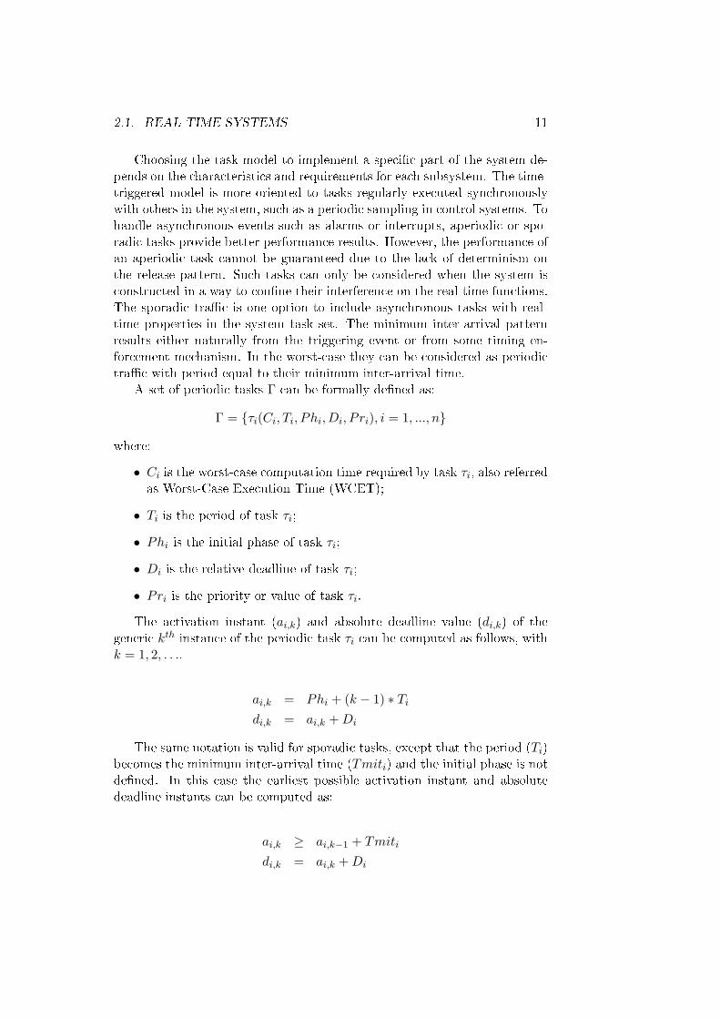
The activation instant (ai,k) and absolute deadline value (di,k) of thegeneric kth instance of the periodic task τi can be computed as follows, withk = 1, 2, . . ..
ai,k = Phi + (k − 1) ∗ Tidi,k = ai,k +Di
The same notation is valid for sporadic tasks, except that the period (Ti)becomes the minimum inter-arrival time (Tmiti) and the initial phase is notde�ned. In this case the earliest possible activation instant and absolutedeadline instants can be computed as:
ai,k ≥ ai,k−1 + Tmiti
di,k = ai,k +Di
12 CHAPTER 2. BACKGROUND
Real-TimeScheduling
Off-Line
Static Cyclicscheduler
On-Line
Static Priorities Dynamic Priorities
Preemptive Non-preemptive Preemptive Non-preemptive
Figure 2.1: Taxonomy of real-time scheduling algorithms.
Scheduler
The tasks in the system compete to access to system resources (e.g. proces-sor, I/O device or communication bus). The resource scheduler is a systemcomponent that decides the order in which the resource is assigned to thetasks waiting for it. The procedure of selecting the task that executes at aparticular point in time is called scheduling and the set of rules that, at anytime, determines the order by which tasks are executed is called a schedulingalgorithm.
More accurately, a scheduling problem can be de�ned [37] as the compo-sition of three sets: a set of n tasks Γ = {τ1, τ2, ..., τn}, a set of m processorsP = {P1, P2, ..., Pm} and a set of s resources R = {R1, R2, ..., Rs}. Further-more, precedence relations among tasks can be speci�ed through a directedacyclic graph and each task can have associated timing constraints. In thiscontext scheduling means to assign processors from P and resources from Rto tasks from Γ in order to complete all tasks under the imposed constraints.
The scheduling algorithms fall into two general categories, online ando�ine [37] (Figure 2.1). The former ones can then use static (�xed) priorityscheduling policies or dynamic priority scheduling policies. The �rst onesare based on �xed information that is available at pre-run-time. Conversely,the second ones perform the scheduling decisions with run-time collectedinformation, e.g. the release instants of asynchronous tasks, hence necessarilyperformed online.
In the o�ine scheduling category, all scheduling is computed prior toexecution. This approach requires a complete characterization of the systemtasks in advance, not being suitable to changes to the system requirements.The scheduling result is a time-table with the tasks activations that is readcyclically at run-time, with a length typically equal to one hyper-period,i.e., the least common multiple of the periods of all tasks. This approach,demands low run-time overhead, but the memory-size requirements to holdthe whole schedule plan can be very large when the task periods are relative
2.1. REAL-TIME SYSTEMS 13
primes or present large asymmetries.
On the other hand, online scheduling allows executing dynamic sched-ulers and brings the ability to modify the system properties at run-time,e.g. adjusting to environment requests. The penalty though, is the need toexecute the scheduler at run-time, which from the application point-of-viewrepresents overhead. Furthermore, unlike the o�ine scheduling case, thescheduler execution must provide prompt answers within a bounded time,which strongly constrains its complexity.
Another categorizing property refers to the blocking e�ect that a taskmay cause to others when accessing a resource. In this aspect, the schedul-ing algorithms can be preemptive or non-preemptive. Non-preemptive algo-rithms execute tasks until completion, regardless of other tasks readiness andpriority. In this case scheduling decisions are only required after the taskscompletion instants. Preemptive algorithms can however suspend tasks dur-ing their execution, if at some instant a task with higher priority becomesready. When executing in non-preemptive mode, a task, upon becomingready, must wait at least for the completion of the currently running task,independently of their relative priorities. The e�ect of a higher priority readytask waiting for a lower priority task to release a resource is called blocking.Preemptive scheduling grants higher responsiveness to higher priority tasks,since these tasks do not su�er blocking from lower priority ones. However, inthis case, scheduling events are generated more often, in all task activationinstants, resulting in higher overhead.
2.1.2 Examples of scheduling policies
The seminal work by Liu and Layland on real-time scheduling [76] de�nestwo of the most important algorithms for task scheduling on uniprocessorsystems, Rate Monotonic for static-priority assignment and Earliest DeadlineFirst for dynamic-priority systems. These algorithms are a milestone withintheir classes for the fact that they are optimal in the sense that they are ableto produce a feasible schedule whenever any other algorithm of the sameclass also is.
Rate Monotonic scheduling
Rate Monotonic (RM) scheduling [76] is an online preemptive algorithmbased on static priorities and with deadlines equal to periods, i.e., ∀τi∈Γ :Di = Ti.
According to the RM algorithm, priorities are assigned monotonicallywith respect to the tasks period, i.e., the shorter the period, the greater thepriority:
∀τi, τj ∈ Γ : Ti < Tj ⇒ Pri > Prj (2.1)
14 CHAPTER 2. BACKGROUND
Task T C
τ1 4 2τ2 6 2τ3 11 1
Table 2.1: Periodic task set properties.
0
τ3
τ1
τ2
5 10 15 20 25
Figure 2.2: Schedule generated by RM.
At run-time, whenever a task instance is activated or the running task�nishes executing, the scheduler selects the task with shorter period amongthe ready ones. The overall complexity of this algorithm is O(n) since in-serting a new task instance in an ordered queue of n elements may take upto n steps. The tasks are sorted according to their priority, so at dispatchingtime, the task heading the queue is the one selected.
Figure 2.2 shows a timeline of an RM schedule with the task propertiesstated in Table 2.1. It can be observed that task τ1 always executes �rst,since it has the shortest period among all tasks, and thus the highest priority.Task τ2 always executes before task τ3 because it has a shorter period.
Earliest Deadline First scheduling
Earliest Deadline First (EDF) [76] algorithm is an online preemptive algo-rithm based on dynamic priorities with relative deadlines equal to periods,i.e., ∀τi∈Γ : Di = Ti. According to the EDF algorithm, the earliest thedeadline the highest the priority of the task. During run-time the followingrelation holds:
∀Ta ∈ R ∀τi,τj ∈ ΓTa : di < dj ⇒ Pri > Prj (2.2)
where ΓTa is the subset of Γ comprising the ready tasks at instant Ta and(di, dj) are the absolute deadlines of tasks τi and τj , at the same instant Ta.
At run-time, whenever a task instance is activated or the running task�nishes executing, the scheduler selects the task with highest period among
2.1. REAL-TIME SYSTEMS 15
0
τ3
τ1
τ2
5 10 15 20 25
Figure 2.3: Schedule generated by EDF.
the ready ones. Since the task priorities are dynamic, it is necessary tosort the ready task queue whenever new task instances are activated. Thus,the time complexity of this algorithm is O(n ∗ log(n)). It follows that EDFscheduling requires higher run-time overhead than RM scheduling, whichcan be problematic for systems based on low processing power CPUs, oftenfound in some embedded distributed control applications. However, as itwill be seen further on, compared to RM, the EDF algorithm is able toachieve higher utilization factors and, at the same time, reduce the numberof preemptions. This results in a trade-o� between run-time overhead andschedulability level, which must be evaluated case by case.
Figure 2.3 shows the EDF scheduling timeline for the same set in Ta-ble 2.1. Comparing with the timeline in Figure 2.2, built with RM, it isnoticeable the variation of the priority with the distance to the deadline dur-ing run-time, for instance, at time t=6 task τ3 has the shortest deadline andthus executes before task τ2.
2.1.3 Schedulability analysis
To perform the schedulability analysis, there exist three di�erent approaches:utilization-based tests, demand-based tests and response time tests. One ap-proach may be more adequate than the others depending on speci�c systemaspects, such as the available computational power or the time available toexecute the analysis. Utilization-based tests are usually less computation-ally complex and faster when compared with the others, thus being moresuitable to be used in dynamic scheduling systems. But on the other hand,response-time-based tests are usually less pessimistic and can provide indi-vidual response time bounds for each task.
Utilization-based
In [76] Liu and Layland propose a utilization-based test for synchronouslyreleased periodic tasks using the Rate Monotonic (RM) priority assignment.
16 CHAPTER 2. BACKGROUND
The task model consists of independent periodic tasks with relative deadlinesequal to their periods. All tasks are released at the same time called criticalinstant. Moreover, it is assumed that once started, the task instances executeuntil completion or preemption and that the operating system overhead (e.g.time required for context switching and tick handling) is small and can beignored. However, when required, the operating system overhead can beaccounted for in the analysis.
The utilization factor U of a task set composed of n tasks is de�ned as:
U =n∑i=1
(CiTi
)According to [76] there is a least upper bound for the task set utilization
that guarantees the existence of a feasible schedule. The least upper bound,on the right side of Inequality 2.3, supports the following schedulability test.
n∑i=1
(CiTi
)< n× (2
1n − 1) (2.3)
The authors prove that if the test succeeds, the tasks will always meettheir deadlines. The lower bound given by this test tends to 69% as napproaches in�nity. However, this is a su�cient test, only, and thus thereare task sets that may not pass the test and yet meet all their deadlines.
Several other utilization-based analysis followed for RM scheduling. Forexample, Lehoczky et al. developed an exact analysis in [72] and an extensionto �t arbitrary deadlines [73]. However, these tests are much more complexcompared to Inequality 2.3. Within Inequality 2.3, a task set with nmessagestakes n steps, thus the computational complexity of this method is O(n).
In [111], Sha et al. further extended Inequality 2.3 to cover blocking-timedue to non-preemption. In this case high priority tasks can be blocked bylower priority tasks, during a time B. This blocking, also called priorityinversion, occurs at most once in each task instance activation if a suitableresource access protocol is used (e.g. Priority Ceiling Protocol). For theseassumptions, a set of n periodic tasks is schedulable by RM if:
∀i, 1 ≤ i ≤ n,i−1∑j=1
(CjTj
)+Ci +BiTi
≤ i× (21i − 1) (2.4)
whereBi is the time during which task τi is blocked by lower priority tasks(priority inversion). The task set is supposed to be ordered by decreasingpriorities, i.e., ∀i, j : i < j ⇒ Pri ≥ Prj .
The blocking factor Bi is de�ned as follows:{Bi = 0, P ri = minj=1..n {Prj}Bi = max
j∈lep(i){Cj} , P ri 6= minj=1..n {Prj} (2.5)

2.1. REAL-TIME SYSTEMS 17
where lep(i) is the set of tasks with priority less than or equal to task i.Liu and Layland [76] also present a utilization-based test for EDF, but
in this case they prove that the least upper bound is 1, i.e., full resourceutilization can be achieved.
Following the same model that led Inequality 2.3:
n∑i=1
(CiTi
)< 1 (2.6)
This is a necessary and su�cient condition (exact) that if veri�ed assuresa task set feasibility. In terms of complexity, for a task set with n tasks thistakes at most n steps, thus the complexity of this method is also O(n).
Demand-based
Demand-based schedulability analysis has been developed for EDF and itmeasures the amount of computation needed by the task set, within a timeinterval t ∈ [t1, t2). The processor demand h[t1,t2) is given by:
h[t1,t2) =∑
t1≤rk,dk≤t2
Ck (2.7)
where rk and dk are the release time and absolute deadline of all the kinstances of all tasks activated at or after t1 and with deadline at or earlierthan t2.
Assuming a synchronous release, i.e., ti = 0 and t2 = t, Equation 2.7 canbe expressed as h(t), given by:
h(t) =∑Di≤t
([1 +
⌊t−Di
Ti
⌋]× Ci
)(2.8)
where Di is the relative deadline of task i. Given this processor demand, atask set is feasible i�
∀t, h(t) ≤ t
This test needs to be checked at speci�c time instants, only, as proved in[37].
Response time
Response time tests evaluate the worst-case response time of all tasks inthe set and compare it with the respective deadlines. These tests have beenparticularly useful in �xed priority systems ([111] and [31, 32]). According toAudsley et al. in [32], the longest response time of a periodic task τi, denotedas Ri, is given by the sum of its computation time (Ci) with the amount ofinterference that it can su�er from higher priority tasks (Ii), calculated atthe critical instant.

18 CHAPTER 2. BACKGROUND
For �xed-priority scheduled systems, the critical instant occurs whenreleasing task i synchronously with all other higher priority tasks, typicallyconsidered time 0. The worst-case response time is then calculated as follows:
Ri = Ci + Ii (2.9)
The amount of interference due to higher priority tasks is:
Ii =∑
∀j∈hp(i)
⌈RiTj
⌉Cj (2.10)
where hp(i) is the set of tasks with higher priority than task i and deadlinesare shorter than or equal to periods.
Hence, combining Equations 2.9 and 2.10 results:
Ri = Ci +∑
∀j∈hp(i)
(⌈RiTj
⌉× Cj
)(2.11)
Equation 2.11 can be solved using the following iterative procedure,where the approximation to the (n+ 1)th value happens in n steps.
Rn+1i = Ci +
∑∀j∈hp(i)
(⌈RniTj
⌉× Cj
)(2.12)
The �rst approximation step can be initialized to R0i = Ci and the solution
is reached when Rn+1i = Rni , or the deadline is violated.
The analysis presented in [32] also includes the e�ect of non-preemptiondue to resource sharing. In this case Equation 2.9 can be used rede�ningthe interference to include the blocking factor due to lower priority tasks, asfollows:
Ii = Bi +∑
∀j∈hp(i)
⌈IiTj
⌉× Cj (2.13)
Note that the blocking factor Bi results from the non-preemption duelower priority tasks that may be executing and holding a shared resourcewhen task i is released. Bi is given by Equation 2.5.
Contrarily to what happens in �xed priority systems, the worst-case re-sponse time of a tasks scheduled with dynamic priorities is not necessarilyobtained considering the �rst instance released with the synchronous releasepattern. Instead, the task τi is found in a deadline-i busy period in which alltasks but τi are released synchronously and must be computed inside. Thisinterval ends when all tasks with relative deadline shorter than or equalto that of task i �nish their execution. The interval may contain severalinstances of task i, one of which has the worst-case response time [56]. Fur-thermore, Palencia and González Harbour have extended the response timeanalysis for EDF scheduled systems to include o�sets [59, 98, 97].
2.1. REAL-TIME SYSTEMS 19
2.1.4 Handling asynchronous events
Periodic tasks have known activation patterns controlled and synchronizedwith the scheduler framework. However, sporadic and aperiodic tasks thathandle asynchronous events are activated asynchronously with respect tothe scheduler. The challenge is scheduling jointly the synchronous and asyn-chronous tasks while preventing the asynchronous ones from jeopardizingthe ful�llment of the timeliness requirements of the periodic tra�c and stillproviding the best response times possible.
There are several approaches to handle both sporadic and aperiodic tasksthat provide bounded and predictable interference, based on �xed-priorityscheduling (namely RMS):
• Background scheduling. This is the simplest approach to handle theaperiodic activities. It con�nes the aperiodic tasks to be scheduled inbackground, i.e., when no periodic tasks are ready for execution. Theperiodic guarantees are preserved, however, there are no guarantees tothe aperiodic tasks, which execute in a best-e�ort manner.
• Polling Server (PS) [124]. This approach uses a regular periodic taskto run the aperiodic handling. At any activation instance of that task,the arrival of aperiodic events is checked which, if positive, triggersthe execution of the aperiodic task within the budget delimited bythe periodic polling task (server). The bandwidth is strictly reservedfor the aperiodic task, i.e., aperiodic tasks execute only during theserver execution. At the end of each serving instance the executingtasks are preempted and resumed in the following serving job. Theaperiodic execution is thus constrained by the timeliness guaranties ofthe periodic task.
• Deferrable Server (DS) [124]. This approach, also referred to aspreserving capacity PS, improves the average response time of the ape-riodic requests with respect to the PS. The DS preserves the capacity(budget) of the server periodic task until the end of its period, sothat aperiodic requests can be serviced at anytime, given that thereis enough budget. However, deferring the server execution causes acertain schedulability penalty in the periodic task set.
• Sporadic Server (SS) [117]. This approach is bandwidth conser-vative, as opposed to the DS. It di�ers from the DS in the way itreplenishes its capacity. Whereas the DS replenishes the server capac-ity periodically, the SS schedules the replenishment of the server whenthe budget is consumed. Hence, it preserves the reactivity of the DSwithout penalizing the schedulability of the periodic tra�c.
20 CHAPTER 2. BACKGROUND
• Slack Stealing [74]. This approach substantially improves the re-sponse time to the aperiodic events over the previous methods (SS orDS). Instead of reserving a bandwidth as of a periodic task, it createspassive tasks that collect the execution time for the aperiodic tasksby promptly stealing the time to the periodic tasks, without causingtheir deadlines to be missed. On the arrival of an aperiodic task theexecution of periodic tasks is delayed as far as to execute the request,while avoiding deadline misses.
These approaches are however constrained by a low schedulability boundinherent to the �xed-priority scheduling. Similar techniques exist to han-dle the aperiodic events with dynamic-priority scheduling. Such techniquesprovide a better resource utilization comparing with the �xed-priority ones.An example is the Total Bandwidth Server (TBS) and the Constant Band-width Server (CBS). A more exhaustive overview and analysis of �xed- anddynamic-priority servers can be found in [37].
2.1.5 Hierarchical schedulers
A hierarchy of schedulers generalizes the role of CPU schedulers by allowingthem to schedule threads as well as groups of threads scheduled with theirown scheduler. A general, heterogeneous scheduling hierarchy is one thatallows arbitrary (or nearly arbitrary) scheduling algorithms throughout thehierarchy.
This enables a better use of the system, in which in some cases one spe-ci�c scheduling policy better �ts a part of the system whereas other partsbene�t more from using other scheduling policies. This hierarchical sepa-ration facilitates the system composability at design phase, which can beparticularly useful to integrate legacy applications or subsystems.
Using server-based schedulers, the budget or share capacity provided bythe server can be scheduled at the same time as the rest of the system relyingon �xed- or dynamic-priority scheduling. In this way several servers can beintegrated as a hierarchical composition that provides timeliness con�nementdomains to the whole system.
2.2 Real-time communications
Originally, computer based applications were mainly centralized using unipro-cessor systems. The availability of low-cost micro-controllers serial intercon-nections enabled the development of "intelligent" nodes, i.e., nodes withprocessing and communication faculties, fostering the development of dis-tributed architectures.
In these distributed architectures, the processing units need to exchangeinformation, thus each one is attached or integrates a network interface unit
2.2. REAL-TIME COMMUNICATIONS 21
providing access to a suitable communication system. This type of systemis loosely coupled in the sense that all information exchange is performedexclusively via the communication system using messages.
A distributed real-time system is one distributed system that integratesactivities with strictly de�ned completion time bounds. These time-constrai-ned activities include both tasks execution within the processors and mes-sages exchange in the communication network that must be considered to-gether when de�ning the system timeliness properties.
An example of a distributed real-time system is the ABS breaking systemin a vehicle. The system prevents the wheels on a vehicle from locking whilebraking. There are several sensors in the wheels that sense the angularvelocity of each wheel. Then, the velocity of each wheel is compared todetect the moment a wheel is about to lock, which triggers a mechanismthat alleviates the braking pressure on the required wheel. The system iscomposed by a central computing unit and several sensors and actuatorsconnected by a communication network. The success of the system dependson the time interval that goes from the wheel lock detection to the brakeactuation. Moreover, the operating control loop relies on low jitter activities,hence the need for determinism and predictability.
Therefore, the temporal behavior of the whole distributed system de-pends not only on the timeliness of tasks executing on each processing de-vice but also on the capability to provide message delivery within speci�ctiming requirements [128, 96]. Communication systems able to support suchtemporal requirements are called real-time communication systems. The re-mainder of this section addresses some important issues concerning real-timecommunication.
2.2.1 Event- and Time-triggered communication
The event-triggered(ET) and time-triggered(TT) communication paradigmsrepresent two di�erent approaches to trigger the communications within dis-tributed systems. While in event-triggered communication, messages are sentby the application upon the occurrence of some asynchronous event, e.g. asensor changing value, according to the time-triggered paradigm, messagesare sent only at precisely prede�ned time instants.
The two models can be compared as follows:
• Predictability. In time-triggered systems the system information isnormally managed within a cycle to periodically update/poll the statusof the system variables. This approach exhibits greater determinismsince it is possible to compute in advance the instants at which thestreams and communications will take place. On the other hand, suchlevel of knowledge is not available for event-based systems since eventsmay occur at arbitrary and unforeseeable time instants. Thus, the

22 CHAPTER 2. BACKGROUND
temporal predictability of this class of systems is lower. Therefore,while TT systems allow a per job timing analysis, ET systems normallyrely on worst-case analysis.
• Resource utilization. In real-time system, resources have to be di-mensioned to address the worst possible scenario occurring during thesystem operation. For TT systems, the resources are issued with knownactivation patterns, so the amount of resources can be pre-allocatedand then used at run-time. Conversely, for ET systems, since theload activation pattern is not regular, the worst-case scenario has tobe considered in which all activations occur every Tmit (the minimuminter-arrival time). This may result in a resource utilization penaltyfor ET systems. On the other hand, in TT systems the committedresources are e�ectively used at run-time, whereas in ET systems theresources are used when actually needed, only. This may lead to arather large reduction in average resource utilization in ET systems.
• Temporal composition. This property assures that when di�erentsubsystems are integrated within the same system, the temporal be-havior of each part is una�ected. On event-triggered subsystems, thatintegration necessarily disturbs the individual temporal behavior ofeach part. Events from di�erent subsystems ultimately may happensimultaneously and interfere. The integration of time-triggered sys-tems allows avoiding this scenario by introducing temporal o�sets thatprevent simultaneous activations.
• Alarm shower. Alarm showers are normally rare and thus di�cultto predict. An alarm shower is typically triggered by a system failurethat triggers a large burst of asynchronous events in consequence ofthat failure. This scenario may lead to overload in ET systems, whilein TT systems the load is kept constant.
Given these features, it is normally considered that time-triggered ap-proaches are better suited to control systems [99], to cater the demands forperiodic messages with low latency and jitter, related to the periodic sam-pling and actuation. On the other hand, event-triggered approaches are moreadequate to promptly handle asynchronous messages with low latency. Inan overload period of asynchronous requests, systems can be designed to in-clude the so called graceful degradation, by allowing the failure of some lessimportant activities while striving to execute the tasks considered as moreimportant to the system. Another alternative is to switch to a TT approachto handle the asynchronous events overload. This allows maintaining thesystem load within a prede�ned bound.
Despite their di�erences, many applications include both periodic andasynchronous activities and thus bene�t from a joint support for both event
2.2. REAL-TIME COMMUNICATIONS 23
and time-triggered tra�c (e.g. automotive systems [77]) and thus, a com-bination of both paradigms in order to share their advantages is desirable.An important aspect is that temporal isolation of both types of tra�c mustbe enforced or, otherwise the asynchronous nature of event-triggered tra�cwould corrupt the properties of the time-triggered tra�c. This isolation isachieved by allocating bandwidth exclusively to each type of tra�c.
A typical implementation makes use of communication slots called el-ementary cycles, or micro-cycles (e.g. [105]), containing two consecutivephases dedicated to each type of tra�c. The communication timeline be-comes, then, an alternate sequence of time-triggered and event-triggeredphases. The maximum duration of each phase can be tailored to suit theneeds of a particular application. If each type of tra�c is forced to remainwithin the respective phase then temporal isolation is guaranteed. This con-cept is used, for example, in the WorldFIP [23], Foundation Fieldbus-H1 [23]and FlexRay [33] �eldbuses, as well as in FTT-CAN [28] and FTT-Ethernet[101].
2.2.2 Message scheduling
Distributed systems are normally built over a shared medium network throughwhich the nodes exchange data messages. Similarly to any shared resourcethat integrates a real-time system, its use is subject to time constraints thatmust be met. Therefore, as with tasks in microprocessors, the access to thecommunication network must also be properly scheduled. Referring to thereal-time properties presented in Section 2.1, other similarities can be foundbetween message scheduling in communication networks and task schedul-ing in microprocessors; messages can also be categorized according to thetimeliness requirements (soft, hard and best-e�ort) and the activation pat-tern (periodic, sporadic or aperiodic). This allows the use of some resultsobtained for processor scheduling (e.g. [127] and [47]). Additionally, alsothe real-time scheduling paradigms (o�ine, online with �xed or dynamicpriorities assignment) are present in real-time message scheduling [26].
However, there are additional challenges posed by the constraints inher-ent to a distributed architecture. One characteristic of a resource scheduleris that it needs to keep the resource status updated to accurately controlits usage. However, due to the distributed nature of the system, completeknowledge about the system state, including network and nodes, is hard togather or even unavailable, and thus scheduling decisions may have to betaken based on incomplete information [111]. This is particularly importantwhen the access to the network is distributed in which case it is necessary toassure the system status consistency when taking communication schedulingdecisions. The lack of complete information about the system state or thesubstantial overhead required to get such information consistently, leads toscheduling techniques that do not keep their optimality, comparing to the
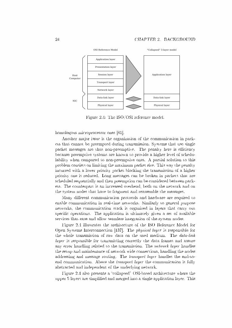
24 CHAPTER 2. BACKGROUND
Figure 2.4: The ISO/OSI reference model.
homologous microprocessor ones [81].
Another major issue is the organization of the communication in pack-ets that cannot be preempted during transmission. Systems that use singlepacket messages are thus non-preemptive. The penalty here is e�ciencybecause preemptive systems are known to provide a higher level of schedu-lability when compared to non-preemptive ones. A partial solution to thisproblem consists on limiting the maximum packet size. This way the penaltyincurred with a lower priority packet blocking the transmission of a higherpriority one is reduced. Long messages can be broken in packets that arescheduled sequentially and then preemption can be considered between pack-ets. The counterpart is an increased overhead, both on the network and onthe system nodes that have to fragment and reassemble the messages.
Many di�erent communication protocols and hardware are required toenable communication in real-time networks. Similarly to general purposenetworks, the communication stack is organized in layers that carry outspeci�c operations. The application is ultimately given a set of availableservices that ease and allow seamless integration of the system nodes.
Figure 2.4 illustrates the architecture of the ISO Reference Model forOpen Systems Interconnection [137]. The physical layer is responsible forthe whole transmission of raw data on the used medium. The data-linklayer is responsible for transmitting correctly the data frames and assureany error handling related to the transmission. The network layer handlesthe setup and maintenance of network wide connections, handling the nodesaddressing and message routing. The transport layer handles the end-to-end communication. Above the transport layer the communication is fullyabstracted and independent of the underlying network.
Figure 2.4 also presents a �collapsed� OSI-based architecture where theupper 5 layers are simpli�ed and merged into a single application layer. This
2.2. REAL-TIME COMMUNICATIONS 25
simpli�cation is frequently found when implementing real-time communica-tion infrastructures. The OSI Reference model was developed for genericcommunication systems and the reason for such simpli�cation is the needto provide a lightweight protocol stack for low-end devices with real-timerequirements. In fact the full OSI reference model becomes too expensive interms of both CPU power and memory, as well as network bandwidth forsuch resource-constrained devices.
When it comes to design a protocol stack with real-time performanceproperties, one of the strategies to improve that performance is providingdistinct handling paths (queues and computing priority) for real-time andnon-real-time tra�c (e.g. [114]).
The Medium Access Control (MAC) protocol within the data-link layerdetermines to a large extent the degree of timing predictability of the net-work technology. Common MAC protocols used in real-time communicationsnetworks can be classi�ed in random access protocols, �xed-assignment pro-tocols and demand-assignment protocols. Examples of random access pro-tocols are:
• CSMA/CD (Carrier Sense Multiple Access / Collision Detection),
• CSMA/CR (Carrier Sense Multiple Access / Collision Resolution),
• CSMA/CA (Carrier Sense Multiple Access / Collision Avoidance).
Examples of �xed-assignment protocols are:
• TDMA (Time Division Multiple Access),
• FTDMA (Flexible TDMA).
Examples of demand-assignment protocols are:
• distributed solutions relying on tokens,
• centralized solutions by the usage of masters.
A comprehensive study and classi�cation of access protocols used in real-time communication over multiple-access networks can be found in [81]. TheMAC protocols are described as consisting of two processes: access arbitra-tion and transmission control. The access arbitration process determineswhen the node is allowed to access the communication channel to send mes-sages, whereas the transmission control process determines for how long anode is able to use the medium to send messages. It also provides examplesof protocols relying either in access arbitration or transmission control.
26 CHAPTER 2. BACKGROUND
2.2.3 Co-operation models
As referred in the beginning of this section, in a distributed system multipleautonomous processing units cooperate towards a common objective. Thereare di�erent ways and models to realize such cooperation. These modelsde�ne who initiates a transaction as well as the number of partners involvedin the process.
Two well-known co-operation models are the producer-consumer andclient-server [133].
The producer-consumer model associates to each message stream aunique logical value that identi�es the respective exchanges over the net-work. Messages are generated and received based only on these logical han-dles, without any explicit reference to the source nor destination nodes ofthe messages. The producers do not need information regarding the nodesconsuming a speci�c message and vice versa.
The producer-consumer co-operation model inherently supports one-to-one and one-to-many communication, without incurring in spatial data con-sistency problems, since the same data message is used to update all the localimages in all the nodes in the network that need such data, the consumer.The only requirement for the underlying network is the support for atomicbroadcast or multicast.
On the other hand, this model does not solve the problem of tem-poral consistency that occurs when several producers interfere and causetransmission delays, ultimately leading to outdated values. The producer-distributor-consumer (PDC) model [126] provides the necessary synchro-nization between the producers, by adding a coordination layer to the producer-consumer model. A new network component is introduced to coordinate thetransmissions and minimize con�icts that lead to transmission delays. Thiscoordination is usually realized in one node, called master, that aggregatesthe temporal requirements of the network and enforces a suitable schedulethat grants the right to transmit to each producer.
Another approach is the client-server model. According to this modelthe nodes holding information to share are servers that serve the clients uponrequest. The client nodes issue requests to the servers holding the desireddata and then, on turn, reply with the demanded data. This communicationmodel is by nature one-to-one and may lead to both spatial and temporaldata inconsistency problems when used to support one-to-many or many-to-one communication. The server addresses the requests sequentially and whenissued to transmit, at the same time, to di�erent clients, it is inevitable thetemporal inconsistency resulting from the serialization process. Additionally,it might occur that in this process the value changes and so the clients receiveinconsistent results, i.e., spacial inconsistency. Another related issue refersto the asynchronous requests to the server. Inside the servers, the requeststake some time to be processed and replied. When multiple requests have to
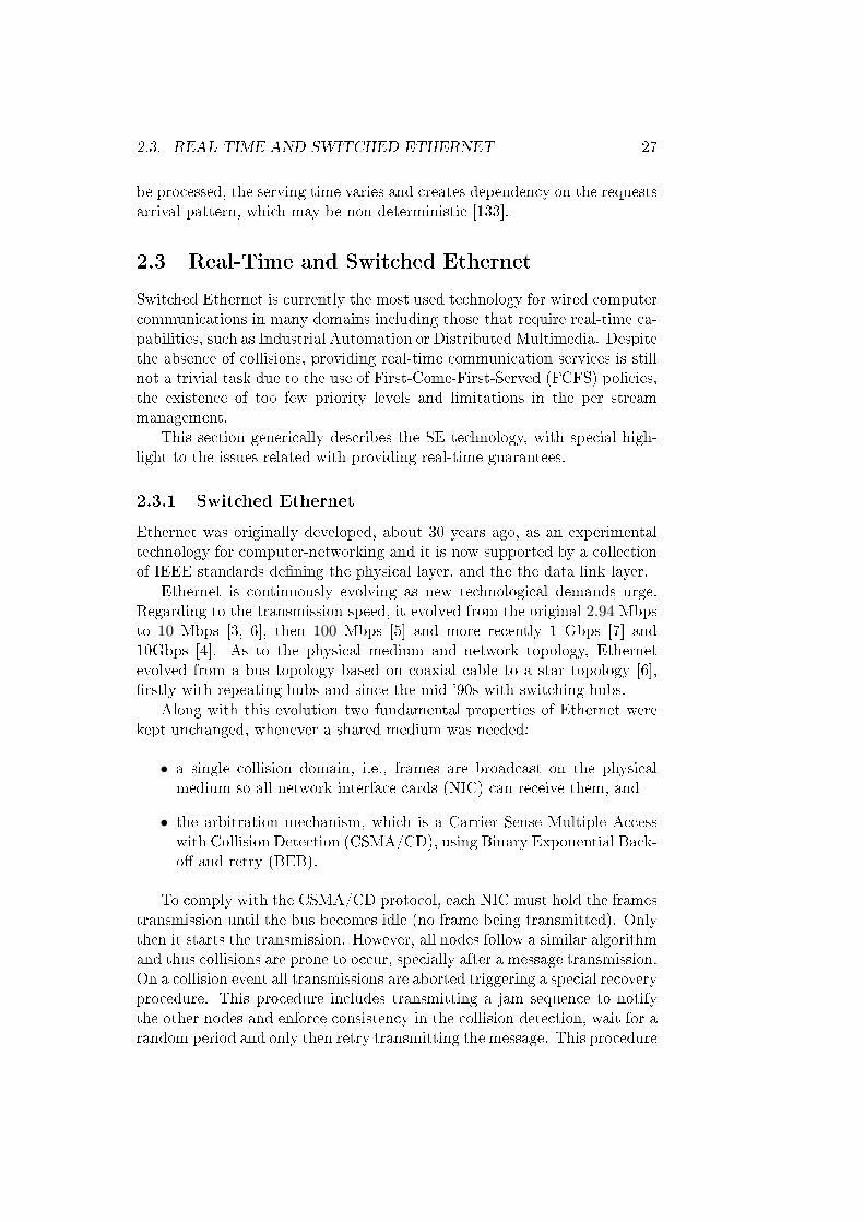
2.3. REAL-TIME AND SWITCHED ETHERNET 27
be processed, the serving time varies and creates dependency on the requestsarrival pattern, which may be non-deterministic [133].
2.3 Real-Time and Switched Ethernet
Switched Ethernet is currently the most used technology for wired computercommunications in many domains including those that require real-time ca-pabilities, such as Industrial Automation or Distributed Multimedia. Despitethe absence of collisions, providing real-time communication services is stillnot a trivial task due to the use of First-Come-First-Served (FCFS) policies,the existence of too few priority levels and limitations in the per streammanagement.
This section generically describes the SE technology, with special high-light to the issues related with providing real-time guarantees.
2.3.1 Switched Ethernet
Ethernet was originally developed, about 30 years ago, as an experimentaltechnology for computer-networking and it is now supported by a collectionof IEEE standards de�ning the physical layer, and the the data link layer.
Ethernet is continuously evolving as new technological demands urge.Regarding to the transmission speed, it evolved from the original 2.94 Mbpsto 10 Mbps [3, 6], then 100 Mbps [5] and more recently 1 Gbps [7] and10Gbps [4]. As to the physical medium and network topology, Ethernetevolved from a bus topology based on coaxial cable to a star topology [6],�rstly with repeating hubs and since the mid-'90s with switching hubs.
Along with this evolution two fundamental properties of Ethernet werekept unchanged, whenever a shared medium was needed:
• a single collision domain, i.e., frames are broadcast on the physicalmedium so all network interface cards (NIC) can receive them, and
• the arbitration mechanism, which is a Carrier Sense Multiple Accesswith Collision Detection (CSMA/CD), using Binary Exponential Back-o� and retry (BEB).
To comply with the CSMA/CD protocol, each NIC must hold the framestransmission until the bus becomes idle (no frame being transmitted). Onlythen it starts the transmission. However, all nodes follow a similar algorithmand thus collisions are prone to occur, specially after a message transmission.On a collision event all transmissions are aborted triggering a special recoveryprocedure. This procedure includes transmitting a jam sequence to notifythe other nodes and enforce consistency in the collision detection, wait for arandom period and only then retry transmitting the message. This procedure
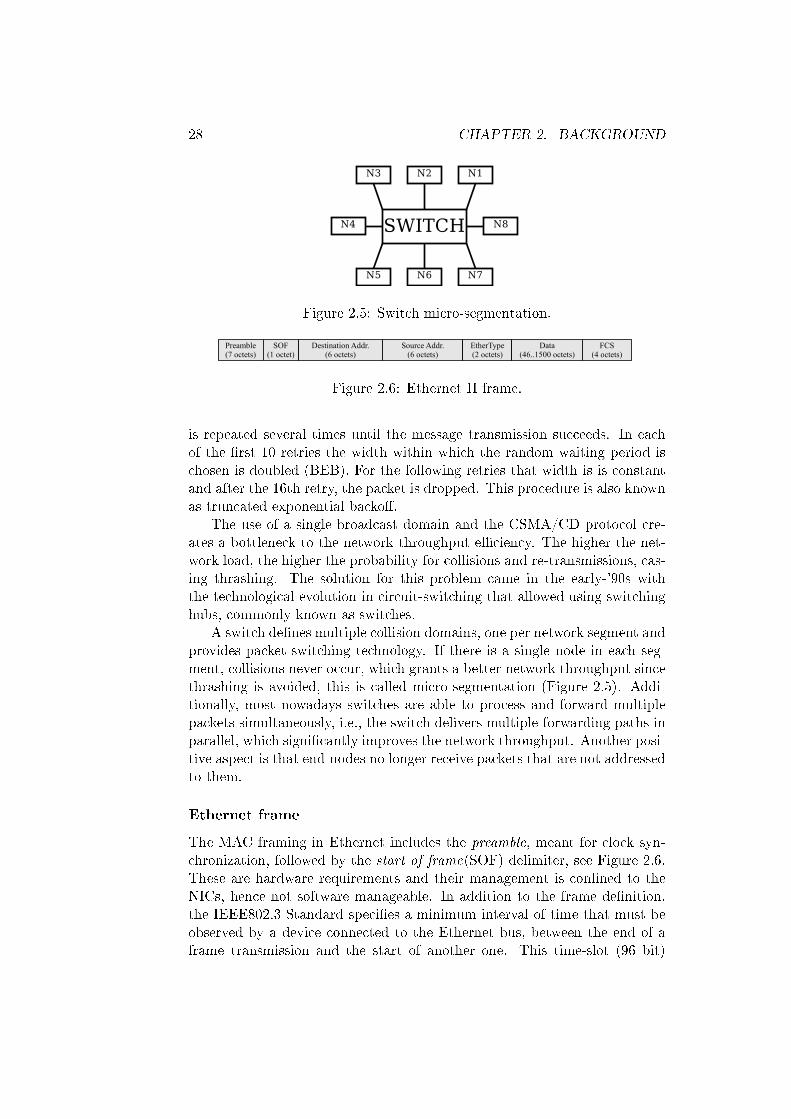
28 CHAPTER 2. BACKGROUND
Figure 2.5: Switch micro-segmentation.
Preamble(7 octets)
Destination Addr.(6 octets)
Source Addr.(6 octets)
EtherType(2 octets)
SOF(1 octet)
Data(46..1500 octets)
FCS(4 octets)
Figure 2.6: Ethernet II frame.
is repeated several times until the message transmission succeeds. In eachof the �rst 10 retries the width within which the random waiting period ischosen is doubled (BEB). For the following retries that width is is constantand after the 16th retry, the packet is dropped. This procedure is also knownas truncated exponential backo�.
The use of a single broadcast domain and the CSMA/CD protocol cre-ates a bottleneck to the network throughput e�ciency. The higher the net-work load, the higher the probability for collisions and re-transmissions, cas-ing thrashing. The solution for this problem came in the early-'90s withthe technological evolution in circuit-switching that allowed using switchinghubs, commonly known as switches.
A switch de�nes multiple collision domains, one per network segment andprovides packet-switching technology. If there is a single node in each seg-ment, collisions never occur, which grants a better network throughput sincethrashing is avoided, this is called micro-segmentation (Figure 2.5). Addi-tionally, most nowadays switches are able to process and forward multiplepackets simultaneously, i.e., the switch delivers multiple-forwarding paths inparallel, which signi�cantly improves the network throughput. Another posi-tive aspect is that end-nodes no longer receive packets that are not addressedto them.
Ethernet frame
The MAC framing in Ethernet includes the preamble, meant for clock syn-chronization, followed by the start of frame(SOF) delimiter, see Figure 2.6.These are hardware requirements and their management is con�ned to theNICs, hence not software manageable. In addition to the frame de�nition,the IEEE802.3 Standard speci�es a minimum interval of time that must beobserved by a device connected to the Ethernet bus, between the end of aframe transmission and the start of another one. This time-slot (96 bit)

2.3. REAL-TIME AND SWITCHED ETHERNET 29
Preamble(7 octets)
Destination Addr.(6 octets)
Source Addr.(6 octets)
802.1Q tag(2 octets)
SOF(1 octet)
Data(46..1500 octets)
FCS(4 octets)
Tag Control(2 octets)
EtherType/Length(2 octets)
PCP(3 bits)
CPI(1 bit)
VID(12 bits)
Figure 2.7: Ethernet IEEE 802.3ac frame.
between transmitted frames is referred to as the minimum inter-frame gap.
There are several types of Ethernet frames, from which Ethernet II (DIXv2.0)[3] frame (Figure 2.6) is the most widely used and the base for the otherstandard types and formats that although di�erent, can coexist on the samephysical medium.
The MAC header includes the packet destination and source addressesthat denote respectively the recipient(s) and the sender of the message andthe EtherType �eld (2 octets) that holds a sub-protocol identi�er. For exam-ple, an EtherType value of 0x0800 means that the packet contains an IPv4datagram, or a value of 0x0806 an ARP frame. The data itself is placed inthe Data �eld, which can contain between 0 and 1500 bytes. However, thereis a minimum frame size of 64 octets and so padding may be necessary for aminimum data of 46 octets. Finally, the Ethernet frame ends with a framecheck sequence (FCS), meant for error detection.
As the industry-developed Ethernet II passed the IEEE standardizationprocess, the EtherType �eld was modi�ed to hold the length �eld in the new802.3 standard [6], which additionally includes the IEEE 802.2 LLC header,in the �rst two bytes of the data segment. The two versions may howevercoexist considering that EtherType values are greater than 0x0600, whichis a value larger than the longest frame size. In practice, both formats arein wide use, with the original Ethernet framing being the most commonin Ethernet local area networks, since it is used by many deeply deployedprotocols and applications.
Another framing format is the Novell's "raw" 802.3 frame, that discardsthe LLC header. Although, not compliant with the IEEE 802.3 standardthat de�nes the LLC header at the start of header the Data �eld, this frameis meant to support IPX networks that use datagrams starting with "FF",which does not occur with the LLC header. Hence, physical compatibility isensured.
LANs are increasingly used by new service classes, some of them withrequirements quite di�erent from the traditional ones. For instance interac-tive voice and video are increasingly used. To address the original lack ofsupport for this class of services, a set of standards have been proposed toextend the framing formats, providing tra�c di�erentiation. Such enhance-ments include VLAN tagging (IEEE 802.1Q [20]) and a priority identi�er(IEEE 802.1p [12]) for quality of service (QoS) purposes. The IEEE 802.3ac[13] describes the extension to the basic frame as illustrated in Figure 2.7. In

30 CHAPTER 2. BACKGROUND
this extension, the before called EtherType is set with a �xed IEEE802.1Qtag type (0x8100) that identi�es the extended format. The new framingadds 4 octets preceding the Data �eld, namely the Tag Control and the newEtherType/Length. In the former, the three most signi�cant bits of the �rstoctet (PCP-Priority Code Point) indicate the frame priority level from 0(lowest) to 7 (highest), the following bit (CFI-Canonical Format Indicator)is used for compatibility issues with Token-ring networks, indicating if theMAC address is in the canonical format. The remaining 12-bit �eld (VID-VLAN Identi�er) specify the VLAN to which the frame belongs, a value of'0' indicates no VLAN.
Queuing model
Considering a switched Ethernet scenario with a micro-segmented topology,i.e., one NIC connection per switch port, and full-duplex links, the mediumwill always be free for transmission and thus the original medium accessprotocol (MAC) of Ethernet is not used. Any contention in output ports issorted out using queues inside the switch that allow serializing transmissions.
Switch
Inpu
t por
ts Packethandling
- Address lookup- Traffic classification
Receiving buffers Output Queues
Scheduler
Scheduler
Out
put p
orts
Figure 2.8: Typical switch internal architecture.
Typical commercial switches are based on IEEE 802.1D-2004 [19] that im-plements FIFO queues 1 at the output ports, as shown in Figure 2.8. Hence,a packet arriving at the queue is blocked for the time needed to transmit thetra�c already held in the queue. Additionally, switches supporting prioritiesimplement several queues on each output port, one per priority level. Thetra�c is dispatched starting from the queue with highest priority, with nopreemption at the packet level. The standard de�nes up to eight prioritylevels, however, most available switches implement just two or three.
Another characteristic of the implementation of the queues in commercialswitches is that they share a common memory pool [102], without any cap
1A First-In-First-Out queue implements an FCFS policy
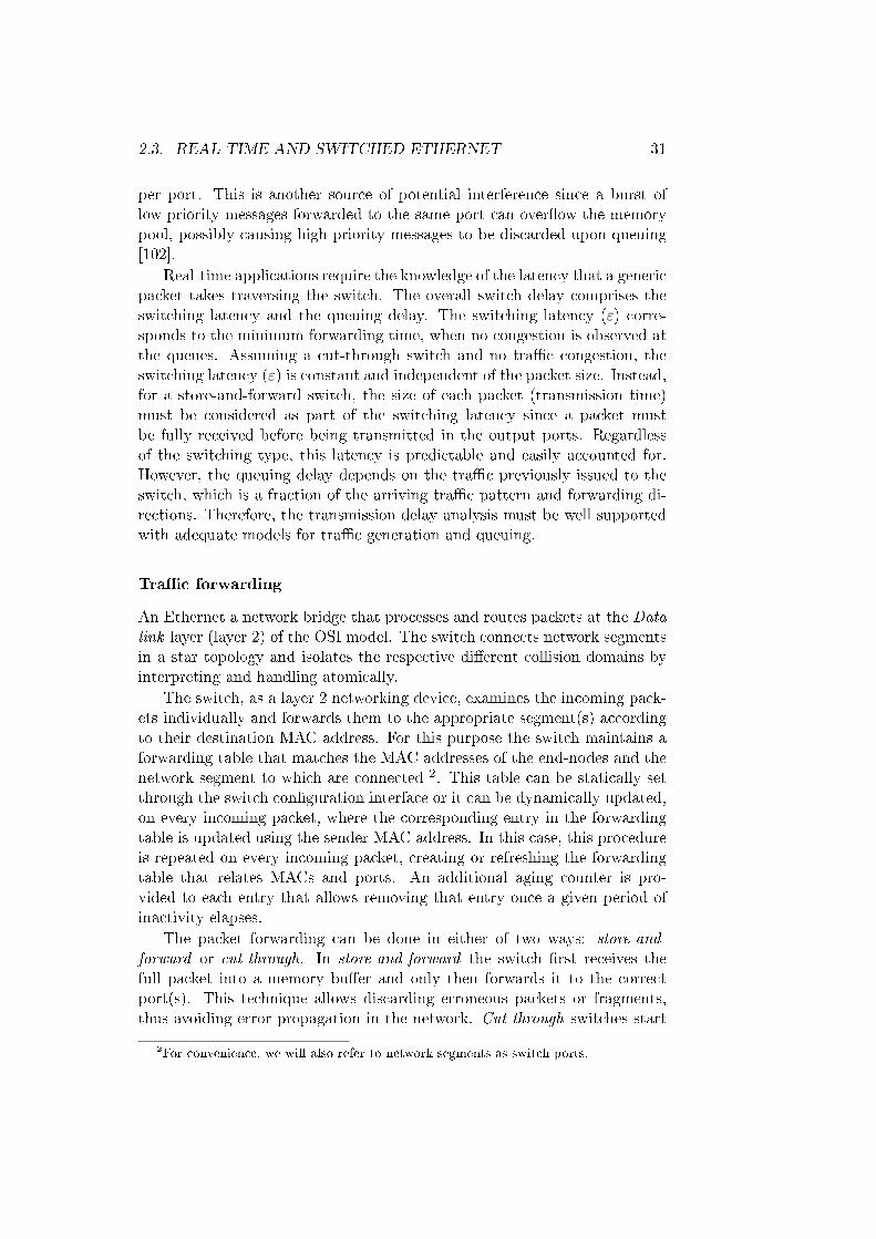
2.3. REAL-TIME AND SWITCHED ETHERNET 31
per port. This is another source of potential interference since a burst oflow-priority messages forwarded to the same port can over�ow the memorypool, possibly causing high-priority messages to be discarded upon queuing[102].
Real-time applications require the knowledge of the latency that a genericpacket takes traversing the switch. The overall switch delay comprises theswitching latency and the queuing delay. The switching latency (ε) corre-sponds to the minimum forwarding time, when no congestion is observed atthe queues. Assuming a cut-through switch and no tra�c congestion, theswitching latency (ε) is constant and independent of the packet size. Instead,for a store-and-forward switch, the size of each packet (transmission time)must be considered as part of the switching latency since a packet mustbe fully received before being transmitted in the output ports. Regardlessof the switching type, this latency is predictable and easily accounted for.However, the queuing delay depends on the tra�c previously issued to theswitch, which is a fraction of the arriving tra�c pattern and forwarding di-rections. Therefore, the transmission delay analysis must be well supportedwith adequate models for tra�c generation and queuing.
Tra�c forwarding
An Ethernet a network bridge that processes and routes packets at the Datalink layer (layer 2) of the OSI model. The switch connects network segmentsin a star topology and isolates the respective di�erent collision domains byinterpreting and handling atomically.
The switch, as a layer 2 networking device, examines the incoming pack-ets individually and forwards them to the appropriate segment(s) accordingto their destination MAC address. For this purpose the switch maintains aforwarding table that matches the MAC addresses of the end-nodes and thenetwork segment to which are connected 2. This table can be statically setthrough the switch con�guration interface or it can be dynamically updated,on every incoming packet, where the corresponding entry in the forwardingtable is updated using the sender MAC address. In this case, this procedureis repeated on every incoming packet, creating or refreshing the forwardingtable that relates MACs and ports. An additional aging counter is pro-vided to each entry that allows removing that entry once a given period ofinactivity elapses.
The packet forwarding can be done in either of two ways: store-and-forward or cut-through. In store-and-forward the switch �rst receives thefull packet into a memory bu�er and only then forwards it to the correctport(s). This technique allows discarding erroneous packets or fragments,thus avoiding error propagation in the network. Cut-through switches start
2For convenience, we will also refer to network segments as switch ports.
32 CHAPTER 2. BACKGROUND
Organizationally UniqueIdentifier (OUI)
Network Interface Controller(NIC) specific
3 octets 3 octets
Figure 2.9: IEEE 802 MAC address (MAC-48).
forwarding the packets as soon as the destination address is received and in-terpreted, resulting in lower switching latencies and more determinism sincethe latency becomes independent of the size of packet being forwarded.
When more than one message contends for the same output port, oneof them is promptly forward while the others are queued in memory. Thosemessages are arranged in a FIFO queue per output port.
There are three forwarding address types, unicast, multicast and broad-cast. In case of a broadcast transmission, the switch forwards the packetto all other active ports with an active link. On a unicast packet transmis-sion, the switch �rst examines the forwarding table for the correspondingMAC address and forwards the packet to the matching port. However, ifthere is no entry with that MAC address, the switch sends it to all ports,i.e., forwards it as with a broadcast address. This is normally referred toas �ooding. Concerning the forwarding of multicast tra�c, until recently, amulticast address was treated as a broadcast, being forwarded to all activeoutput ports. Currently, the so-called layer 3 (or 2+) switches follow theIGMP protocol [40] that enables a true multicast forwarding.
The unique assignment of a MAC address to each network interface card(NIC) allows addressing each device within a LAN. Each manufactured NICis assigned a MAC address that in Ethernet is 6-octets long (MAC-48), asillustrated in Figure 2.9. In order to regulate such assignment, the identi�eris partially managed by the IEEE that issues an Organizationally UniqueIdenti�er (OUI) to the network manufacturers, de�ning the three most sig-ni�cant octets of the MAC address, whereas the remaining three octets areassigned by the manufacturers.
This universal identi�er directly supports the unicast transmissions as itprovides an individual address within a network segment. Additionally, theIEEE de�nes special group or multicast addresses that allow the same packetbeing received by several stations. The least signi�cant bit of the �rst octetof a MAC address distinguishes individual addresses from group addresses.If set to '1' it refers to a group address, either multicast or broadcast. Apacket sent with a multicast destination address is received by all stationsin a LAN that have been con�gured to receive from that address, whereasa packet sent with a broadcast address (all-ones, "FF:FF:FF:FF:FF:FF") isreceived by all stations within the LAN. As for the multicast addresses, theInternet Assigned Number Authority (IANA) reserves an OUI that it usesfor mapping IP multicast addresses to MAC addresses. The result is a range
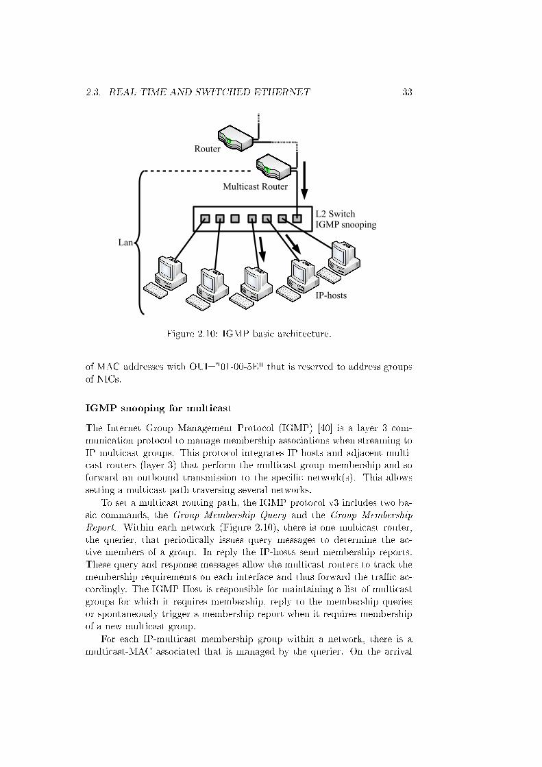
2.3. REAL-TIME AND SWITCHED ETHERNET 33
L2 SwitchIGMP snooping
Multicast Router
IP-hosts
Router
Lan
Figure 2.10: IGMP basic architecture.
of MAC addresses with OUI="01-00-5E" that is reserved to address groupsof NICs.
IGMP snooping for multicast
The Internet Group Management Protocol (IGMP) [40] is a layer 3 com-munication protocol to manage membership associations when streaming toIP multicast groups. This protocol integrates IP-hosts and adjacent multi-cast routers (layer 3) that perform the multicast group membership and soforward an outbound transmission to the speci�c network(s). This allowssetting a multicast path traversing several networks.
To set a multicast routing path, the IGMP protocol v3 includes two ba-sic commands, the Group Membership Query and the Group MembershipReport. Within each network (Figure 2.10), there is one multicast router,the querier, that periodically issues query messages to determine the ac-tive members of a group. In reply the IP-hosts send membership reports.These query and response messages allow the multicast routers to track themembership requirements on each interface and thus forward the tra�c ac-cordingly. The IGMP Host is responsible for maintaining a list of multicastgroups for which it requires membership, reply to the membership queriesor spontaneously trigger a membership report when it requires membershipof a new multicast group.
For each IP-multicast membership group within a network, there is amulticast-MAC associated that is managed by the querier. On the arrival
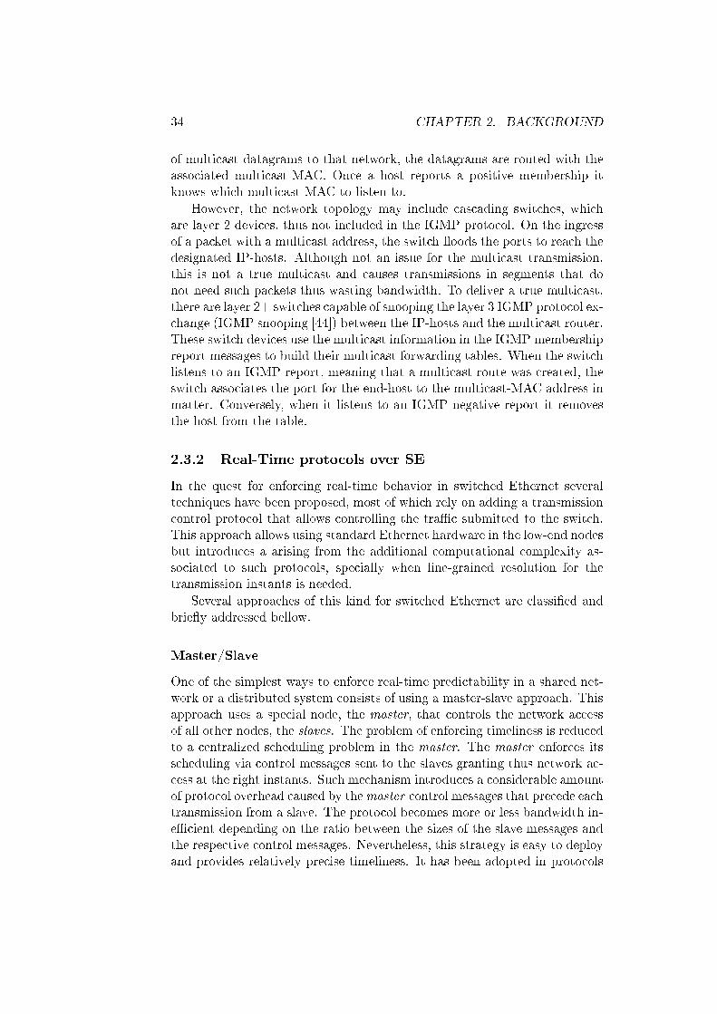
34 CHAPTER 2. BACKGROUND
of multicast datagrams to that network, the datagrams are routed with theassociated multicast-MAC. Once a host reports a positive membership itknows which multicast-MAC to listen to.
However, the network topology may include cascading switches, whichare layer 2 devices, thus not included in the IGMP protocol. On the ingressof a packet with a multicast address, the switch �oods the ports to reach thedesignated IP-hosts. Although not an issue for the multicast transmission,this is not a true multicast and causes transmissions in segments that donot need such packets thus wasting bandwidth. To deliver a true multicast,there are layer 2+ switches capable of snooping the layer 3 IGMP protocol ex-change (IGMP snooping [44]) between the IP-hosts and the multicast router.These switch devices use the multicast information in the IGMP membershipreport messages to build their multicast forwarding tables. When the switchlistens to an IGMP report, meaning that a multicast route was created, theswitch associates the port for the end-host to the multicast-MAC address inmatter. Conversely, when it listens to an IGMP negative report it removesthe host from the table.
2.3.2 Real-Time protocols over SE
In the quest for enforcing real-time behavior in switched Ethernet severaltechniques have been proposed, most of which rely on adding a transmissioncontrol protocol that allows controlling the tra�c submitted to the switch.This approach allows using standard Ethernet hardware in the low-end nodesbut introduces a arising from the additional computational complexity as-sociated to such protocols, specially when �ne-grained resolution for thetransmission instants is needed.
Several approaches of this kind for switched Ethernet are classi�ed andbrie�y addressed bellow.
Master/Slave
One of the simplest ways to enforce real-time predictability in a shared net-work or a distributed system consists of using a master-slave approach. Thisapproach uses a special node, the master, that controls the network accessof all other nodes, the slaves. The problem of enforcing timeliness is reducedto a centralized scheduling problem in the master. The master enforces itsscheduling via control messages sent to the slaves granting thus network ac-cess at the right instants. Such mechanism introduces a considerable amountof protocol overhead caused by themaster control messages that precede eachtransmission from a slave. The protocol becomes more or less bandwidth in-e�cient depending on the ratio between the sizes of the slave messages andthe respective control messages. Nevertheless, this strategy is easy to deployand provides relatively precise timeliness. It has been adopted in protocols
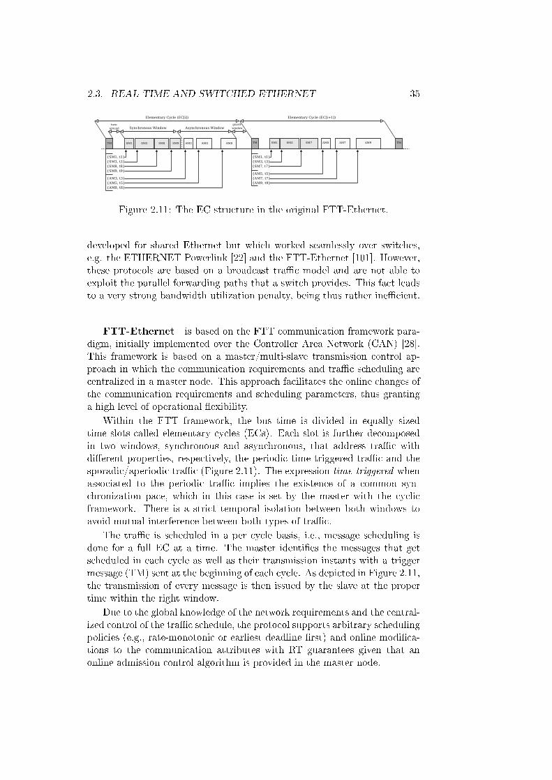
2.3. REAL-TIME AND SWITCHED ETHERNET 35
Figure 2.11: The EC structure in the original FTT-Ethernet.
developed for shared Ethernet but which worked seamlessly over switches,e.g. the ETHERNET Powerlink [22] and the FTT-Ethernet [101]. However,these protocols are based on a broadcast tra�c model and are not able toexploit the parallel forwarding paths that a switch provides. This fact leadsto a very strong bandwidth utilization penalty, being thus rather ine�cient.
FTT-Ethernet is based on the FTT communication framework para-digm, initially implemented over the Controller Area Network (CAN) [28].This framework is based on a master/multi-slave transmission control ap-proach in which the communication requirements and tra�c scheduling arecentralized in a master node. This approach facilitates the online changes ofthe communication requirements and scheduling parameters, thus grantinga high level of operational �exibility.
Within the FTT framework, the bus time is divided in equally sizedtime slots called elementary cycles (ECs). Each slot is further decomposedin two windows, synchronous and asynchronous, that address tra�c withdi�erent properties, respectively, the periodic time-triggered tra�c and thesporadic/aperiodic tra�c (Figure 2.11). The expression time-triggered whenassociated to the periodic tra�c implies the existence of a common syn-chronization pace, which in this case is set by the master with the cyclicframework. There is a strict temporal isolation between both windows toavoid mutual interference between both types of tra�c.
The tra�c is scheduled in a per cycle basis, i.e., message scheduling isdone for a full EC at a time. The master identi�es the messages that getscheduled in each cycle as well as their transmission instants with a triggermessage (TM) sent at the beginning of each cycle. As depicted in Figure 2.11,the transmission of every message is then issued by the slave at the propertime within the right window.
Due to the global knowledge of the network requirements and the central-ized control of the tra�c schedule, the protocol supports arbitrary schedulingpolicies (e.g., rate-monotonic or earliest deadline �rst) and online modi�ca-tions to the communication attributes with RT guarantees given that anonline admission control algorithm is provided in the master node.
36 CHAPTER 2. BACKGROUND
Figure 2.12: ETHERNET Powerlink cycle structure.
ETHERNET Powerlink (EPL) [22] is a master-slave protocol thatprovides deterministic real-time communication for standard Ethernet. Theprotocol was initially designed for shared Ethernet, providing a very highprecision, under 1µs. When deployed over a switch-based network, theprecision is reduced due to extra and variable latencies introduced by theswitches. The protocol also supports both periodic (isochronous) and aperi-odic (asynchronous) tra�c in two consecutive but isolated phases in a cyclicframework.
A master (Managing Node) controls the communications by assigningtime slots for the slaves to transmit. The slaves are passive bus stations,reacting to the master explicit requests.
The communication scheduling is conducted by the master that issuestime-critical data exchanges in isochronous phases within consecutive cy-cles. The overall cycle duration depends on the amount of isochronous datato exchange in the system. Figure 2.12 illustrates one such cycle. Eachcycle is divided in four distinct phases: start, isochronous, asynchronousand idle. In the Start Phase the master sends a synchronization message(SoC - start of cycle) that noti�es the nodes of a new starting cycle. In theIsochronous Phase the master triggers the periodic data transactions sendinga poll request (Preq) for each. The slaves reply with the Pres (poll response)that is broadcasted to all nodes in a producer-distributor-consumer model.Isochronous transmissions are repeatedly issued every cycles, however, thetransmission slots may be multiplexed in time, issuing a message every ncycles. In the Asynchronous Phase the master grants one node the right totransmit a message. It sends the SoA (Start of Asynchronous) message thataddresses that node, which then replies with the respective asynchronousmessage. After this phase, the master introduces some idle time before thefollowing cycle, to enforce a precise cycle start with low jitter.
The asynchronous transmission mechanism is very limited and cannot beused to handle time-critical communications. Unlike the isochronous tra�c,for which the master is exactly aware of the messages to be polled at eachtime, for the asynchronous tra�c, each slave has to notify the master. Thisis performed piggybacking a status signal onto the isochronous messages.Asynchronous-only nodes are also supported by the protocol, in which case
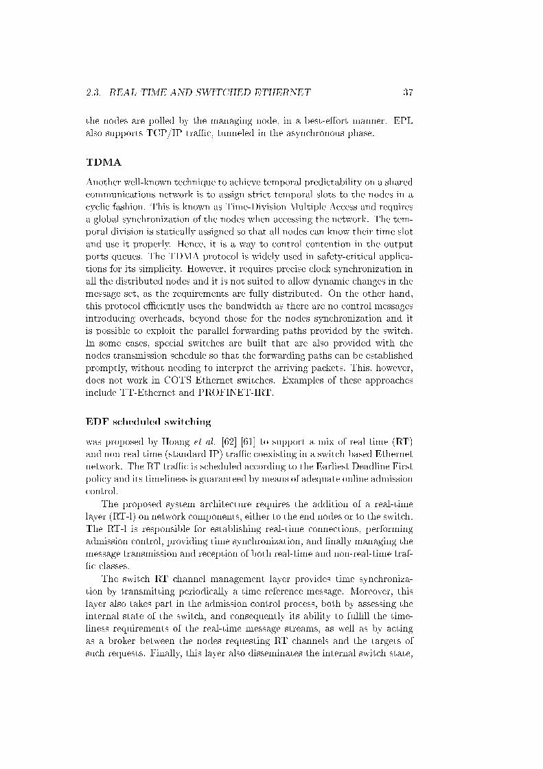
2.3. REAL-TIME AND SWITCHED ETHERNET 37
the nodes are polled by the managing node, in a best-e�ort manner. EPLalso supports TCP/IP tra�c, tunneled in the asynchronous phase.
TDMA
Another well-known technique to achieve temporal predictability on a sharedcommunications network is to assign strict temporal slots to the nodes in acyclic fashion. This is known as Time-Division Multiple Access and requiresa global synchronization of the nodes when accessing the network. The tem-poral division is statically assigned so that all nodes can know their time slotand use it properly. Hence, it is a way to control contention in the outputports queues. The TDMA protocol is widely used in safety-critical applica-tions for its simplicity. However, it requires precise clock synchronization inall the distributed nodes and it is not suited to allow dynamic changes in themessage set, as the requirements are fully distributed. On the other hand,this protocol e�ciently uses the bandwidth as there are no control messagesintroducing overheads, beyond those for the nodes synchronization and itis possible to exploit the parallel forwarding paths provided by the switch.In some cases, special switches are built that are also provided with thenodes transmission schedule so that the forwarding paths can be establishedpromptly, without needing to interpret the arriving packets. This, however,does not work in COTS Ethernet switches. Examples of these approachesinclude TT-Ethernet and PROFINET-IRT.
EDF scheduled switching
was proposed by Hoang et al. [62] [61] to support a mix of real-time (RT)and non-real-time (standard IP) tra�c coexisting in a switch-based Ethernetnetwork. The RT tra�c is scheduled according to the Earliest Deadline Firstpolicy and its timeliness is guaranteed by means of adequate online admissioncontrol.
The proposed system architecture requires the addition of a real-timelayer (RT-l) on network components, either to the end nodes or to the switch.The RT-l is responsible for establishing real-time connections, performingadmission control, providing time synchronization, and �nally managing themessage transmission and reception of both real-time and non-real-time traf-�c classes.
The switch RT channel management layer provides time synchroniza-tion by transmitting periodically a time reference message. Moreover, thislayer also takes part in the admission control process, both by assessing theinternal state of the switch, and consequently its ability to ful�ll the time-liness requirements of the real-time message streams, as well as by actingas a broker between the nodes requesting RT channels and the targets ofsuch requests. Finally, this layer also disseminates the internal switch state,
38 CHAPTER 2. BACKGROUND
namely in what concerns the queues status, to allow �ow-control of non-real-time tra�c on the end nodes.
Real-time communication is carried out within real-time channels, apoint-to-point logical connection with reserved bandwidth. Whenever a nodeneeds to send real-time data, it issues a request to the switch, indicating boththe source and destination addresses (both MAC and IP), and the period,transmission time and deadline of the message. Upon reception of such a re-quest, the switch performs the �rst part of the admission control mechanism,which consists in evaluating the feasibility of the communication between thesource node and the switch (uplink) and between the switch and the targetnode (downlink). If the switch �nds the request feasible, forwards the requestto the destination node. The target node analyzes the request and informsthe switch about its will on accepting or not the real-time connection. Theswitch, then, forwards this answer to the originator node. If the RT channelis accepted, it is assigned with a system wide channel ID that univocallyidenti�es the connection.
The real-time layer comprises two distinct queues, one for the real-timetra�c, and the other for the non-real-time tra�c. The former is a priorityqueue, where messages are kept sorted by distance to their deadlines. Thenon-real-time queue holds the messages in a FIFO queue. Therefore, real-time messages are transmitted according to their deadlines, while non-real-time messages are transmitted according to their arrival instant.
The feasibility analysis proposed [61] is derived from EDF task schedulinganalysis, but with adaptations to account for some system speci�cs, such asincluding the overheads due to control messages and the impact of non-preemptive message transmission.
In the scope of that work, deadlines are de�ned on an end-to-end basis.Since the tra�c is transmitted in two separate steps (uplink and downlink),the analysis must assure that the total delay induced by these steps togetherdoes not exceed the total end-to-end deadline. For a given real-time messagestream i, if diu is the deadline for the uplink and did the deadline for thedownlink, then the end-to-end deadline diee must be at least as large as thesum of the previous two: diu + did ≤ diee. In [62], the authors assume theend-to-end deadline equal to the period of the respective message stream,and a symmetric partitioning of that deadline between the uplink and thedownlink. An improvement is presented in [61], where the authors proposean asymmetric deadline partition scheme. Although more complex, thismethod allows a higher e�ciency in bandwidth utilization, because a largerfraction of the deadline can be assigned to more loaded links, thus increasingthe overall schedulability level.
2.3. REAL-TIME AND SWITCHED ETHERNET 39
EtheReal
[132] is another protocol that was proposed to achieve real-time behavioron switched Ethernet networks. In this approach, the protocol is supportedby services implemented on the switch, only, without any changes in theoperating system and network layers of end nodes. The switch services areaccessible to the end nodes by means of user-level libraries.
EtheReal has been designed to support both real-time and non-real-timetra�c via two distinct classes. The Real-Time Variable Bit Rate service class(RT-VBR) is meant to support real-time applications. These services use re-served bandwidth and try to minimize the packet delay and packet delayvariation (jitter). Applications must provide the desired tra�c characteris-tics during the connection set-up, namely average tra�c rate and maximumburst length. If these parameters are violated at run-time, the real-timeguarantees do not hold, and packets may be lost. The second service classis Best-E�ort (BE), and it was developed speci�cally to support existingnon-real-time applications like telnet, http, etc., without requiring any mod-i�cation. No guarantees are provided for this type of tra�c.
Real-time services in EtheReal are connection-oriented, which means thatapplications have to follow a connection setup protocol before being able tosend data to the real-time channels. The connection setup procedure isstarted by sending a reservation request to a user-level process called Real-Time Communication Daemon (RTCD), running on the same host. Thisdaemon is responsible for the set-up and tear down of all connections inwhich the host node is engaged in. The reservation request for RT connec-tions contains the respective Quality of Service (QoS) requirements, namelyaverage tra�c rate and maximum burst length.
Upon reception of a connection set-up request, the RTCD contacts theneighbor EtheReal switch that evaluates whether it has enough resourcesto meet the QoS requirements of the new RT connection without jeopar-dizing the existing ones, namely switch fabrics bandwidth, CPU bandwidthfor packet scheduling and data bu�ers for packet queuing. If it has suchresources and if the destination node is directly attached to the same switch,it positively acknowledges the request. If the destination node is in anothersegment, i.e., connected to another switch, the switch that received the re-quest forwards it to the next switch in the path. A successful connection isachieved if and only if all the switches in the path between the source and thetarget node have enough resources to accommodate the new RT connection.If one switch has not enough resources, it sends back a reject message, whichis propagated down to the requester node. This procedure serves to notifythe requester application about the result of the operation, as well as to letthe intermediate EtheReal switches to de-allocate the resources associatedwith that connection request.
The EtheReal architecture employs tra�c shaping and policing, within
40 CHAPTER 2. BACKGROUND
both hosts and switches. The tra�c shaping is performed to smooth theinter-packet arrival time, generating a constant rate �ow of tra�c. Tra�cpolicing is used to ensure that the declared QoS parameters are met duringrun-time. Those functions are also implemented on the switches to ensurethat an ill-behaved node, either due to malfunction or malicious software,does not harm the other connections on the network.
With respect to the packet scheduling inside the switch, the EtheRealarchitecture employs a cyclic round-robin scheduling algorithm. All real-time connections are served within a prede�ned cycle. A part of that cycle isalso reserved to best-e�ort tra�c, to avoid starvation and subsequent time-outs on the upper layer protocols.
Applications access the real-time services by means of a Real-Time DataTransmission/Reception library (RTTR), which provides services for connec-tion set-up and tear down and data transmission and reception, beyond otherinternal functions already referred to, such as tra�c shaping and policing.
Another interesting feature of this protocol is its scalability and highrecovery capability, when compared with standard switches. For example,the spanning tree protocol (IEEE 802.1D) is used in networks of standardswitches to allow redundant paths and automatic recon�guration upon alink/switch failure. However, such recon�guration may take several tensof seconds with the network down, typically around 30 seconds, which isintolerable for most real-time applications. On the other hand, the authorsclaim that EtheReal networks may recover nearly three orders of magnitudefaster, within 32ms [131].
Tra�c shaping
As opposed to transmission control, that strictly enforces the transmissiontimes for each message on the network, this technique follows an approachbased on limiting burst. Therefore, the probability of long priority inversionsin the queues is kept low.
This is a fully distributed approach technique. In each network station,an interface layer called tra�c smoother is placed just on top of the Ethernetdriver. This layer handles and controls the message transmission rate in eachnode to limit bursts. Real-Time tra�c is assumed to be well-behaved, i.e.,periodically triggered at some control process rate, thus without bursts andso handed to the Ethernet driver right away, bypassing the smoother.
Conversely, the non-real-time (NRT) tra�c can be bursty and has to gothrough the tra�c smoother that forces an average transmission rate and amaximum burst length. This way, at the network level, the interference onthe RT tra�c due to NRT tra�c is kept inside a bound [78].
One major drawback of this approach is that the smoothers are all dis-tributed and it is di�cult to adapt them online. In fact, adaptive techniquessuch as proposed in [70] and [41] only work in shared Ethernet. When using
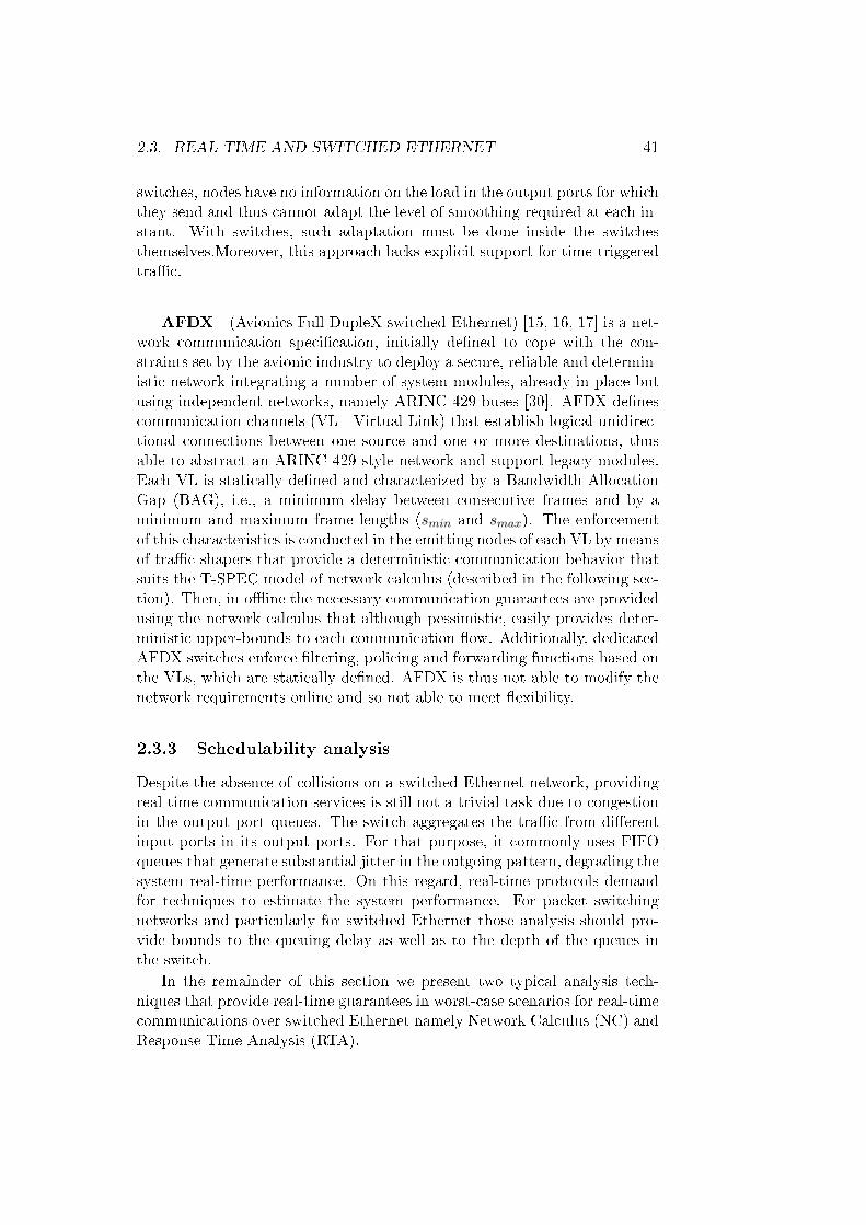
2.3. REAL-TIME AND SWITCHED ETHERNET 41
switches, nodes have no information on the load in the output ports for whichthey send and thus cannot adapt the level of smoothing required at each in-stant. With switches, such adaptation must be done inside the switchesthemselves.Moreover, this approach lacks explicit support for time-triggeredtra�c.
AFDX (Avionics Full DupleX switched Ethernet) [15, 16, 17] is a net-work communication speci�cation, initially de�ned to cope with the con-straints set by the avionic industry to deploy a secure, reliable and determin-istic network integrating a number of system modules, already in place butusing independent networks, namely ARINC 429 buses [30]. AFDX de�nescommunication channels (VL - Virtual Link) that establish logical unidirec-tional connections between one source and one or more destinations, thusable to abstract an ARINC 429 style network and support legacy modules.Each VL is statically de�ned and characterized by a Bandwidth AllocationGap (BAG), i.e., a minimum delay between consecutive frames and by aminimum and maximum frame lengths (smin and smax). The enforcementof this characteristics is conducted in the emitting nodes of each VL by meansof tra�c shapers that provide a deterministic communication behavior thatsuits the T-SPEC model of network calculus (described in the following sec-tion). Then, in o�ine the necessary communication guarantees are providedusing the network calculus that although pessimistic, easily provides deter-ministic upper-bounds to each communication �ow. Additionally, dedicatedAFDX switches enforce �ltering, policing and forwarding functions based onthe VLs, which are statically de�ned. AFDX is thus not able to modify thenetwork requirements online and so not able to meet �exibility.
2.3.3 Schedulability analysis
Despite the absence of collisions on a switched Ethernet network, providingreal-time communication services is still not a trivial task due to congestionin the output port queues. The switch aggregates the tra�c from di�erentinput ports in its output ports. For that purpose, it commonly uses FIFOqueues that generate substantial jitter in the outgoing pattern, degrading thesystem real-time performance. On this regard, real-time protocols demandfor techniques to estimate the system performance. For packet switchingnetworks and particularly for switched Ethernet those analysis should pro-vide bounds to the queuing delay as well as to the depth of the queues inthe switch.
In the remainder of this section we present two typical analysis tech-niques that provide real-time guarantees in worst-case scenarios for real-timecommunications over switched Ethernet namely Network Calculus (NC) andResponse Time Analysis (RTA).
42 CHAPTER 2. BACKGROUND
Network Calculus (NC)
Network Calculus, initially introduced by Cruz [45, 46] and later comple-mented by Boudec and Thiran [34], describes an algebra for analyzing perfor-mance in computer networks. It uses the Min-plus and Max-plus algebra toassess the impact of network communication constraints such as the limitedlinks capacity, tra�c congestion in the switch, interference from backgroundtra�c and tra�c shaping policies enforced in the nodes. The algebra relieson a tra�c characterization model that de�nes streams by their burstinesspeak (σ) and their long-term rate (ρ), called T-SPEC.
In the real-time community, some solutions based on the NC emerged totarget hard-real-time applications over SE. Loeser and Haertig [78, 79] use a�ne grained tra�c shaping in the nodes to guarantee that the injected tra�cconforms with the T-SPEC model parameters used within the NC, so thatall analysis follows naturally from that algebra. For a generic real-time jobi, modeled with aWi budget and an arrival period of Ti, the T-SPEC arrivalpattern is denoted by: σi = Wi,ρi = Wi/Ti. Once all tra�c is characterizedwith (σi, ρi) i=1...N, the queuing delay for a c bit/s server comes as follows[45]:
For �xed priorities:
Di max =
∑ij=1 σj +maxi+1≤j≤N (Wj)
c−∑i−1
j=1 ρj
For FCFS policy:
Di max =
∑Nj=1 σj +maxi+1≤j≤N (Wj)
c−∑N−1
j=1 ρj
Once the tra�c is fully characterized according to T-SPEC the timelinessanalysis of a stream traversing the network is straight-forward. However,this technique only applies when the application streams conform with theT-SPEC model and it is not trivial to deduce the T-SPEC for certain tra�cscenarios that are highly jittered.
Response time analysis (RTA)
Section 2.1.3 described several scheduling analysis techniques for computingtasks. The response time analysis provides relatively accurate results onwhether a task set is schedulable or not. Section 2.2.2 then presented waysto map a tra�c model in order to use the analysis developed in this context.For example, Koubâa and Song [115] conduct a response-time-based analysisfor the tra�c traversing an Ethernet switch. Their work is only focused onthe switch queues. The impact of the nodes queues is modeled as release jittera�ecting the arrival pattern of the packets to the switch queues. However,
2.3. REAL-TIME AND SWITCHED ETHERNET 43
nothing is said concerning how to determine this release jitter, nor how tohandle di�erent streams coming from the same node with a scheduling policydi�erent than the one in the switch. Therefore, it only addresses the impactof the FIFO queuing policy of the switch.
The queuing delay (Rti) that a�ects a job of stream i with respect toits periodic activation, is thus upper-bounded through the usual iterativeprocess for the case of a non-preemptive �xed priority queue:
In+1i = max
i≤j≤N(Cj) +
i−1∑j=1
(⌊Ini + JjTj
⌋+ 1)× Cj
Rti = Ci + Ii + Ji
where Ji stands for the release jitter that stream i might su�er when arrivingat the queue, which is the maximum deviation from its periodic activation,and Ii stands for the maximum interference. Notice that we also assumethat Rti should be no greater than Ti.
For an FIFO queue, the queuing delay is obtained in the following way,if the release is strictly periodic:
Ii =N∑
j=1,j 6=iCj
Rti = Ci + Ii
If the streams su�er release jitter the analysis is rather more complex as wewill see further on.
Xing Fan et al. conduct a wider covering analysis that includes both, thequeues at the sending nodes and the queues in the switch. Both queues areanalyzed independently and the overall end-to-end delay is considered addingup both stages. The �rst stage analysis (node queue) is easily achievedestimating the interference caused by the streams within the same node.As for the second stage, the analysis becomes more complex in which it isnecessary to consider all the streams that target an output link in the switch.In this case the analysis is performed over the load submitted to the switchqueue.
The cumulative workload Wk(t1, t2) of a set of real-time streams Γ ={τ1, τ2, . . . , τn} originating from source node k, is given by the sum of thetra�c volume of messages released by the real-time streams during the timeinterval [t1, t2),∀i, t1 ≤ t2:
Wk(t1, t2) =n∑i=1
max((⌊
t2 − t1Ti
⌋+ 1)× Ci, 0
)

44 CHAPTER 2. BACKGROUND
busy-interval
t'
end of the last idle periodr1 releases a message
ri releases a message
t'+Δri
end of busy-interval
Figure 2.13: Arbitrary release in k's busy-interval.
For the switch queue analysis, given any message release pattern, withoutloss of generality, assume that τi releases messages at t = t′ + ∆ri,∆ri ≥ 0,as illustrated in Figure 2.13. The commutative workload for the incominglink from node k during [t′, t) is derived as:
Wk(t′, t) =n∑i=1
(1 +
⌊t− (t′ + ∆ri)
Ti
⌋)× Ci
This estimates the busy-interval for node k and so the real-time guaran-tees can be assessed from it.
NC versus RTA
The major di�erence between the two system analysis techniques, networkcalculus and response time analysis, resides in the communication model onwhich each rely. The NC uses the T-SPEC model that de�nes a long-termaverage transmission rate and a maximum burst that better suits the event-based tra�c, whereas, the RTA evaluates the system feasibility by evaluatingthe interference that occurs on a periodic activation basis.
The T-SPEC model, despite its limitations, is very general and allowsmodeling large range of real tra�c scenarios. However, in some cases amore precise but more limited model can be used such as in control-orientedor multimedia applications in which a periodic activation model is natural.A relationship method to map the periodic model onto the NC model isproposed in [115]. Using the pseudo-periodic model (periodic with releasejitter), the authors conduct a work for �xed priorities scheduling inside theswitch in which two queuing delay analysis are compared, the NC algebraand the classical RTA. They conclude by saying that RTA analysis is less pes-simistic than the use of NC with the penalty of being more computationallydemanding.
2.4. CONCLUSION 45
2.4 Conclusion
Ethernet is the most popular technology for LANs today. Due to its lowcost, high throughput, high availability and easy deployment, among otherfeatures, Ethernet is wide spread in multiple application domains, even thosefor which it was not initially designed. An example is industry automation inwhich Ethernet is used in a variety of applications, including those that im-pose critical real-time constraints. The CSMA/CD arbitration protocol usedin shared Ethernet, which con�icts with the requirements for timing, was by-passed introducing switched Ethernet that additionally provides full-duplexcommunication and allows multiple parallel forwarding paths. Despite theabsence of collisions, it is still necessary to control the tra�c admission inthe switch queues. Several real-time protocols emerged for this purpose inorder to obtain the timeliness guarantees.
This chapter presented a brief overview of real-time systems modelingwith focus on real-time communications. It introduced some backgroundconcerning real-time operating models, scheduling and the necessary anal-ysis techniques that support timeliness guarantees. Speci�cally concerningthe real-time communications deployment over switched Ethernet, this chap-ter described a communication model suited to characterize the switch andcovered some paradigmatic techniques to control the tra�c admission toprevent over�ow in the switch queues, while supporting the designation ofworst-case delay bounds.

46 CHAPTER 2. BACKGROUND
Chapter 3
The FTT-SE protocol
This chapter presents the Flexible Time Triggered protocol over SwitchedEthernet (FTT-SE). It describes the overall system architecture, includingthe mechanisms that support it, and presents a formulation for the globaltra�c scheduling problem.
The chapter includes a section with some details of an hardware imple-mentation and the distributed middleware abstraction.
It, �nally, presents a set of simulations and experimental results con-ducted to illustrate and validate the advantages of using the FTT-SE.
3.1 Introduction
As mentioned in Section 1.1, there is a trend towards the development of�exible protocols as a mean to e�ciently address dynamic and evolving en-vironments. The protocol hereby proposed for switched Ethernet is based onthe Flexible Time-Triggered communication paradigm to enforce such oper-ational �exibility. At the switching level, it globally coordinates the tra�csubmitted at each instant, avoiding potential queue over�ow problems andbypassing the tra�c scheduling performed by the switch allowing thus, anydesired policy. The FTT-SE (FTT over Switched Ethernet), follows the sameparadigm that has already been used over shared Ethernet to overcome thenon-determinism of its MAC, namely the FTT-Ethernet protocol [101].
Therefore, it is proposed an adaptation of that protocol to micro-segmen-ted networks, i.e., based on switches and with only one station connected toeach port. As common to all FTT implementations [100], the main advan-tages of this protocol are the global tra�c coordination in a common timeline,the possibility for fast and atomic online updates to the set of streams, thecapability to support wide ranges of streams periods, the support of arbitrarytra�c scheduling policy and the capability of handling periodic, aperiodicand non-real-time tra�c with temporal isolation.
47
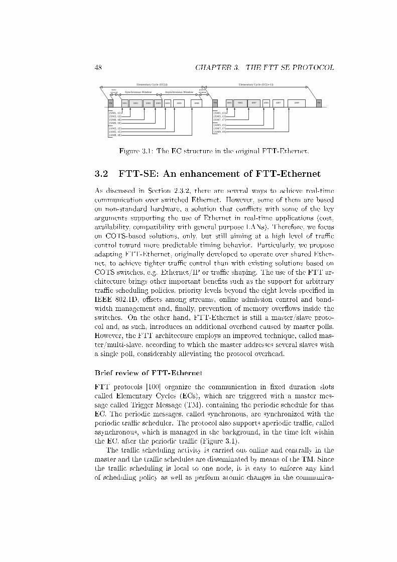
48 CHAPTER 3. THE FTT-SE PROTOCOL
Figure 3.1: The EC structure in the original FTT-Ethernet.
3.2 FTT-SE: An enhancement of FTT-Ethernet
As discussed in Section 2.3.2, there are several ways to achieve real-timecommunication over switched Ethernet. However, some of them are basedon non-standard hardware, a solution that con�icts with some of the keyarguments supporting the use of Ethernet in real-time applications (cost,availability, compatibility with general purpose LANs). Therefore, we focuson COTS-based solutions, only, but still aiming at a high level of tra�ccontrol toward more predictable timing behavior. Particularly, we proposeadapting FTT-Ethernet, originally developed to operate over shared Ether-net, to achieve tighter tra�c control than with existing solutions based onCOTS switches, e.g. Ethernet/IP or tra�c shaping. The use of the FTT ar-chitecture brings other important bene�ts such as the support for arbitrarytra�c scheduling policies, priority levels beyond the eight levels speci�ed inIEEE 802.1D, o�sets among streams, online admission control and band-width management and, �nally, prevention of memory over�ows inside theswitches. On the other hand, FTT-Ethernet is still a master/slave proto-col and, as such, introduces an additional overhead caused by master polls.However, the FTT architecture employs an improved technique, called mas-ter/multi-slave, according to which the master addresses several slaves witha single poll, considerably alleviating the protocol overhead.
Brief review of FTT-Ethernet
FTT protocols [100] organize the communication in �xed duration slotscalled Elementary Cycles (ECs), which are triggered with a master mes-sage called Trigger Message (TM), containing the periodic schedule for thatEC. The periodic messages, called synchronous, are synchronized with theperiodic tra�c scheduler. The protocol also supports aperiodic tra�c, calledasynchronous, which is managed in the background, in the time left withinthe EC, after the periodic tra�c (Figure 3.1).
The tra�c scheduling activity is carried out online and centrally in themaster and the tra�c schedules are disseminated by means of the TM. Sincethe tra�c scheduling is local to one node, it is easy to enforce any kindof scheduling policy as well as perform atomic changes in the communica-
3.2. FTT-SE: AN ENHANCEMENT OF FTT-ETHERNET 49
tion requirements. This last feature allows for online stream admission andremoval under guaranteed timeliness as well as online bandwidth manage-ment. Similarly to the freedom with respect to the tra�c scheduling policy,the speci�c bandwidth management scheme can also be any. These featuresare the kernel of the FTT paradigm and are the justi�cation for the �exibleattribute.
The EC schedules are built considering a broadcast transmission modelas common in shared segments. Moreover, in order to bypass the non-deterministic CSMA/CD arbitration of Ethernet, the EC schedules also con-tain an o�set from the start of the EC for the transmission of each messagethat grants a collision-free medium access. The slaves transmit the scheduledmessages with the speci�ed o�sets and for an e�cient use of the bandwidthsuch o�sets must be respected with a good precision.
3.2.1 FTT-SE for micro-segmented networks
FTT-Ethernet can be seamlessly deployed over shared or switched Ethernetnetworks but it uses a full broadcast communication model. Important e�-ciency gains may be achieved by tailoring the FTT-Ethernet protocol to takeadvantage of the distinctive features of micro-segmented topologies, namelythe absence of collisions and the existence of parallel transmission paths.
The inherent absence of collisions that results from the existence of pri-vate collision domains for each port leads to a noteworthy simpli�cation ofthe protocol implementation in the slave nodes, which no longer need to en-force a collision-free medium access. Messages are transmitted immediatelyafter decoding the TM, with the switch taking care of the serialization withineach EC. Consequently the contents of the TM itself is also simpli�ed, sincethe speci�cation of the transmission instants is no longer needed.
On the other hand it becomes possible to take full advantage of multipletransmission paths by abandoning the pure broadcast architecture of FTT-Ethernet as long as we provide the FTT Master with information aboutthe nature of the data exchanges, i.e., unicast, multicast and broadcast,and which end nodes are involved. With this information the master cancompute which messages follow disjoint paths, i.e., non-overlapping sourceand destination nodes, and thus build schedules that exploit this parallelism,increasing the aggregated throughput.
This new feature corresponds to move from the broadcast-based pro-ducer/consumer cooperation model in FTT-Ethernet to a multicast pub-lisher/subscriber scheme in FTT-SE. The master keeps a data structure withthe currently existing groups of publisher/subscribers, with the identi�cationof the respective streams and the associated physical addresses and ports.Speci�c calls issued by the publishers and subscribers allow creating groupsand binding nodes to groups. Two di�erent cases must be considered ac-cording to the type of switches uses. For non-multicast switches only unicast

50 CHAPTER 3. THE FTT-SE PROTOCOL
Ethernet switch
Trigger message
TM
FTT master
Figure 3.2: FTT-SE system architecture.
and broadcast streams can be considered. For true multicast switches thestandard Internet Group Multicast Protocol (IGMP, RFC 2236) is used tosetup up multicast groups. The binding process for subscribers uses IGMPmessages sent explicitly to the FTT Master, which are also snooped by theswitch, allowing both master and switch to build coherent forwarding tables.The master must be correctly con�gured to the type of switch being used.
Figure 3.2 shows the communication system architecture, with the FTTMaster attached to one switch port and scheduling the transmission of theremaining stations.
The previous FTT-Ethernet protocol manages two distinct tra�c classes,the periodic tra�c and the aperiodic tra�c. They have di�erent schedulingmodels, thus being managed separately. However, in both classes the trans-mission is issued only upon a dispatching order that polls the messages cycleby cycle. For the periodic tra�c, polling is natural since the master knowswhen to transmit as well as the bus status. However, the master does nothave such knowledge concerning the asynchronous tra�c, since it is triggeredby local events in the slave nodes. Thus, asynchronous messages are blindlypolled by the master, which may result or not on a message transmission,depending on whether there is a pending request.
In the case of FTT-SE, the management of both types of tra�c is sub-stantially simpli�ed and enhanced in several aspects.
Concerning the periodic tra�c, all slaves answer the master polls in theTMs transmitting as soon as possible the scheduled tra�c, i.e., after theturn-around time. The precise transmission instants inside the synchronouswindow are not known since they depend on the speed of the slaves answer-
3.2. FTT-SE: AN ENHANCEMENT OF FTT-ETHERNET 51
ing the poll. However, the scheduled periodic tra�c will be transmitted ina burst, or nearly, with practically no wasted intervals between consecutivemessages. This was not the case in FTT-Ethernet in which the speci�ca-tion of the transmission o�set could lead to such wasted intervals due tolimitations in timing resolution of the operative system in the slaves.
Concerning the aperiodic tra�c, its management is also substantiallyimproved with respect to FTT-Ethernet due to a new signaling mechanism.
3.2.2 Handling aperiodic transmissions in FTT-SE
The asynchronous management is a problem for a variety of protocols seekinglow communication jitter and latency in switched Ethernet. Unconstrainedaperiodic communication may generate bursts that �ll in the output queues,leading to long priority inversions in typical FIFO queues and possibly toqueues over�ow and consequent packet losses. One way to improve thissituation is constraining the transmission of aperiodic tra�c in the nodesusing tra�c shaping or smoothing. This way, transmission instants are notconstrained but the amount of tra�c generated within a given time window isbounded. Alternatively, a more robust and timely accurate but less e�cientmechanism, is the one used originally in FTT-Ethernet, based on polling.In this case, the transmission instants are adequately planned by the globalscheduler. However, this approach is not very e�cient given the possiblelong latency periods to serve the aperiodic requests, which result from theperiodic polling and also the bus bandwidth that is wasted by unsuccessfulpolling attempts.
The polling mechanism encompasses two di�erent phases. In the �rstone, called signaling phase, the master inquires the nodes about the exis-tence of asynchronous tra�c ready to be transmitted. In the second one,called transmission phase, the master polls the transmission of that tra�c inadequate instants in time. These two phases can either be separately imple-mented, where the transmission phase comes as consequence of the signalingphase in which case the transmission phase only occurs if the signaling phaseindicated the presence of pending aperiodic tra�c, or merged in a single pe-riodic poll that leads to unused bandwidth when no messages are pendingat the poll instant.
Note that, whether the two phases are jointly or separately implemented,in both there is an intrinsic compromise between responsiveness and over-head; a higher responsiveness requires polling at higher rates, but polling athigher rates potentially implies a higher bandwidth overhead.
To improve the aperiodic tra�c management, we propose exploring thefull duplex features of common Ethernet switches to implement a new sig-naling mechanism in master/slave switched Ethernet protocols that does notsu�er from the referred responsiveness versus overhead compromise and maydramatically improve the QoS given to the asynchronous tra�c.

52 CHAPTER 3. THE FTT-SE PROTOCOL
Figure 3.3: Polling token.
The out-of-band signaling mechanism
Switches with full-duplex capabilities provide the possibility of simultaneoustransmissions in opposite directions in each link without interference. Thisfeature is used to e�ciently deploy a signaling path between the slaves andthe master in a master/slave architecture that does not collide with thecommon polled transmissions.
Another property intrinsic to a master/slave architecture is the overheadthat comes in two forms, one due to the need to transmit the master poll andanother caused by the time spent by the slaves decoding and preparing thereply to the poll, which is normally called the turnaround time. This intervalof time, which mediates between the poll reception and the beginning of thereply transmission, depends on the slave implementation technology. Forstandard PC-based solutions and network interface cards (NICs) can reach200µs [83], even using RT kernels and stacks. Reducing this value to a fewtens of microseconds is possible with special hardware support, only.
Yet another common property of master/slave architectures is the strictslaves synchronization on the master tokens. This behavior is typicallyachieved reserving a window (guard window) for transmitting the token withno interfering tra�c nor software blocking activities in the nodes, thus avoid-ing jitter.
In a full-duplex switch, the master download link, i.e., the link that
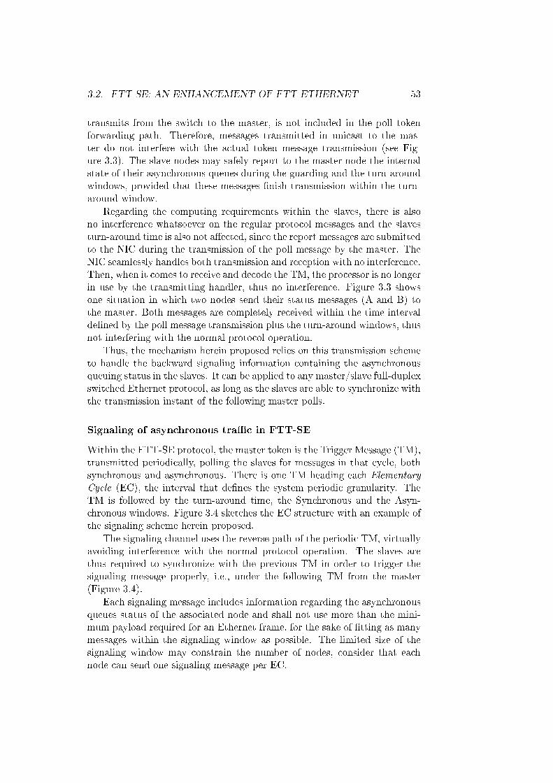
3.2. FTT-SE: AN ENHANCEMENT OF FTT-ETHERNET 53
transmits from the switch to the master, is not included in the poll tokenforwarding path. Therefore, messages transmitted in unicast to the mas-ter do not interfere with the actual token message transmission (see Fig-ure 3.3). The slave nodes may safely report to the master node the internalstate of their asynchronous queues during the guarding and the turn-aroundwindows, provided that these messages �nish transmission within the turn-around window.
Regarding the computing requirements within the slaves, there is alsono interference whatsoever on the regular protocol messages and the slavesturn-around time is also not a�ected, since the report messages are submittedto the NIC during the transmission of the poll message by the master. TheNIC seamlessly handles both transmission and reception with no interference.Then, when it comes to receive and decode the TM, the processor is no longerin use by the transmitting handler, thus no interference. Figure 3.3 showsone situation in which two nodes send their status messages (A and B) tothe master. Both messages are completely received within the time intervalde�ned by the poll message transmission plus the turn-around windows, thusnot interfering with the normal protocol operation.
Thus, the mechanism herein proposed relies on this transmission schemeto handle the backward signaling information containing the asynchronousqueuing status in the slaves. It can be applied to any master/slave full-duplexswitched Ethernet protocol, as long as the slaves are able to synchronize withthe transmission instant of the following master polls.
Signaling of asynchronous tra�c in FTT-SE
Within the FTT-SE protocol, the master token is the Trigger Message (TM),transmitted periodically, polling the slaves for messages in that cycle, bothsynchronous and asynchronous. There is one TM heading each ElementaryCycle (EC), the interval that de�nes the system periodic granularity. TheTM is followed by the turn-around time, the Synchronous and the Asyn-chronous windows. Figure 3.4 sketches the EC structure with an example ofthe signaling scheme herein proposed.
The signaling channel uses the reverse path of the periodic TM, virtuallyavoiding interference with the normal protocol operation. The slaves arethus required to synchronize with the previous TM in order to trigger thesignaling message properly, i.e., under the following TM from the master(Figure 3.4).
Each signaling message includes information regarding the asynchronousqueues status of the associated node and shall not use more than the mini-mum payload required for an Ethernet frame, for the sake of �tting as manymessages within the signaling window as possible. The limited size of thesignaling window may constrain the number of nodes, consider that eachnode can send one signaling message per EC.
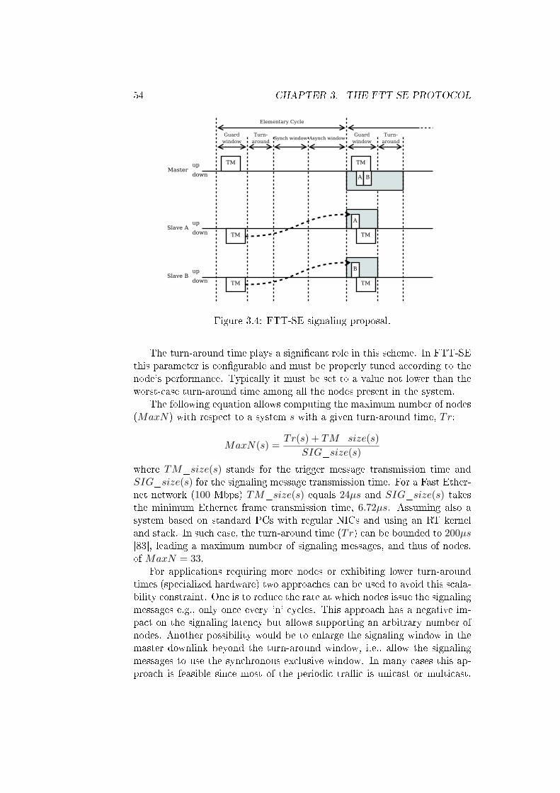
54 CHAPTER 3. THE FTT-SE PROTOCOL
Figure 3.4: FTT-SE signaling proposal.
The turn-around time plays a signi�cant role in this scheme. In FTT-SEthis parameter is con�gurable and must be properly tuned according to thenode's performance. Typically it must be set to a value not lower than theworst-case turn-around time among all the nodes present in the system.
The following equation allows computing the maximum number of nodes(MaxN) with respect to a system s with a given turn-around time, Tr:
MaxN(s) =Tr(s) + TM_size(s)
SIG_size(s)
where TM_size(s) stands for the trigger message transmission time andSIG_size(s) for the signaling message transmission time. For a Fast Ether-net network (100 Mbps) TM_size(s) equals 24µs and SIG_size(s) takesthe minimum Ethernet frame transmission time, 6.72µs. Assuming also asystem based on standard PCs with regular NICs and using an RT kerneland stack. In such case, the turn-around time (Tr) can be bounded to 200µs[83], leading a maximum number of signaling messages, and thus of nodes,of MaxN = 33.
For applications requiring more nodes or exhibiting lower turn-aroundtimes (specialized hardware) two approaches can be used to avoid this scala-bility constraint. One is to reduce the rate at which nodes issue the signalingmessages e.g., only once every 'n' cycles. This approach has a negative im-pact on the signaling latency but allows supporting an arbitrary number ofnodes. Another possibility would be to enlarge the signaling window in themaster downlink beyond the turn-around window, i.e., allow the signalingmessages to use the synchronous exclusive window. In many cases this ap-proach is feasible since most of the periodic tra�c is unicast or multicast,
3.3. THE SCHEDULING MODEL 55
thus not being forward to the master, leaving the downlink of the masternode partially unused. In this case, this extra tra�c in the master downlinkmust also be considered by the synchronous messages scheduler.
3.3 The scheduling model
The scheduler speci�es the order with which the messages are transmittedin the network, once activated. The master node handles such operationtaking into account the individual priorities of each message that may eitherbe static or dynamic as in EDF scheduling. We have seen that the schedulingplan is enforced by means of the TM that polls the messages in the slaves.
Such model supports strict priority scheduling but at a coarse time scale,only, with a resolution of ECs. Priority inversion may occur within the ECsince the master does not control the speci�c instants at which the messagesare transmitted by the slaves and queued in the native FCFS queues withinthe switch output ports.
3.3.1 The periodic tra�c scheduling model
The periodic scheduling model considers Ns periodic streams (SMi) thatare stored in a structure called Synchronous Requirements Table (SRT) asshown in 3.1.
SRT ={SMi : SMi = (Ci, Di, Ti, Oi, P ri, Si, {R1
i ..Rkii }), i = 1..Ns
}(3.1)
Each stream is characterized by the total transmission time of each in-stance Ci, the relative deadline Di, the stream period Ti, the o�set Oi. Priis an optional parameter that allows associating explicitly a priority to themessage. Both Di, Ti and Oi are expressed as integer numbers of ECs. Then,Si is the sender node and {R1
i ..Rkii } is the set of ki receivers for stream i.
The calculation of Ci deserves a special note because the protocol automat-ically fragments large messages in a sequence of packets that are scheduledsequentially and individually by the master. This is particularly useful totransmit regularly large amounts of data such as video frames.
The set of streams in the SRT is scheduled by the FTT Master accordingto any online policy, implementing a single queue of ready periodic messages.This queue is used to build the EC-schedule that will be encoded in the TMand broadcast through the switch. The periodic scheduling though con�nesthe tra�c to the synchronous window, with duration of LSW , within theEC.
The reception of the TM causes all nodes that are senders in that EC tofeed the scheduled streams to the switch through a set of M upload links luj .When these streams arrive at the switch they are conveyed, with latency ε, to

56 CHAPTER 3. THE FTT-SE PROTOCOL
TM
Sched
FP, EDF, RM, ...
streams m1 (...) m2 (...) ... mi (...)
Switch with M portsM nodesFTT-SE Master
l ju l j
d
Figure 3.5: The scheduling model with FTT-SE.
the respective output ports and queued for transmission in the M downloadlinks ldj (Figure 3.5). The transmission of each packet is non-preemptive,as usual, but the transmission of long messages, i.e., those with multiplepackets per instance, can be preempted between packets.
Scheduling over this model becomes a two-fold problem. In one hand,it is necessary to build the EC-schedules so that the transmission of theperiodic messages �ts within the synchronous window of that EC, while inthe other hand, it is important to to have schedulability bounds adequate tothe scheduling policy.
The former issue is covered in the remainder of this chapter, includingscheduling multiple links simultaneously, while the schedulability bounds areaddressed in the following chapter.
3.3.2 Building EC-schedules
One issue that needs to be addressed in order to carry out the tra�c schedul-ing online is how to build the EC-schedules considering the multiple queuesassociated to the M upload and download links.
The �rst aspect to note is that most of the current switches are full-duplex, which permits overlapping transmissions in the download and uploadlinks. Additionally, switches are many times capable of performing cut-through forwarding, from the uplinks to the downlinks with a small latencyshift, the switch latency ε.
The second aspect is the initial constraint that limits the communicationactivity to the synchronous window, whose maximum duration is LSW ,meaning that no link can be used more than LSW − ε (Figure 3.6). Theturnaround time tr is the time needed by the stations to decode the TM andstart their own synchronous transmissions.
A third aspect is that the transmissions in the downlinks are causal with
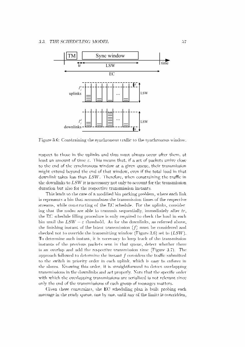
3.3. THE SCHEDULING MODEL 57
TM Sync window
tr LSW
EC
time
LSW
...LSW
l ju
uplinks
l jd
downlinks
...
Figure 3.6: Constraining the synchronous tra�c to the synchronous window.
respect to those in the uplinks and thus must always occur after them, atleast an amount of time ε. This means that, if a set of packets arrive closeto the end of the synchronous window at a given queue, their transmissionmight extend beyond the end of that window, even if the total load in thatdownlink takes less than LSW . Therefore, when constraining the tra�c inthe downlinks to LSW it is necessary not only to account for the transmissionduration but also for the respective transmission instants.
This leads to the case of a modi�ed bin packing problem, where each linkis represents a bin that accumulates the transmission times of the respectivestreams, while constructing of the EC-schedule. For the uplinks, consider-ing that the nodes are able to transmit sequentially, immediately after tr,the EC-schedule �lling procedure is only required to check the load in eachbin until the LSW − ε threshold. As for the downlinks, as referred above,the �nishing instant of the latest transmission (f) must be considered andchecked not to override the transmitting window (Figure 3.6) set to (LSW ).To determine such instant, it is necessary to keep track of the transmissioninstants of the previous packets sent in that queue, detect whether thereis an overlap and add the respective transmission time (Figure 3.7). Theapproach followed to determine the instant f considers the tra�c submittedto the switch in priority order in each uplink, which is easy to enforce inthe slaves. Knowing this order, it is straightforward to detect overlappingtransmissions in the downlinks and act properly. Note that the speci�c orderwith which the overlapping transmissions are serialized is not relevant sinceonly the end of the transmissions of each group of messages matters.
Given these constraints, the EC scheduling plan is built probing eachmessage in the ready queue, one by one, until any of the limits is overridden,
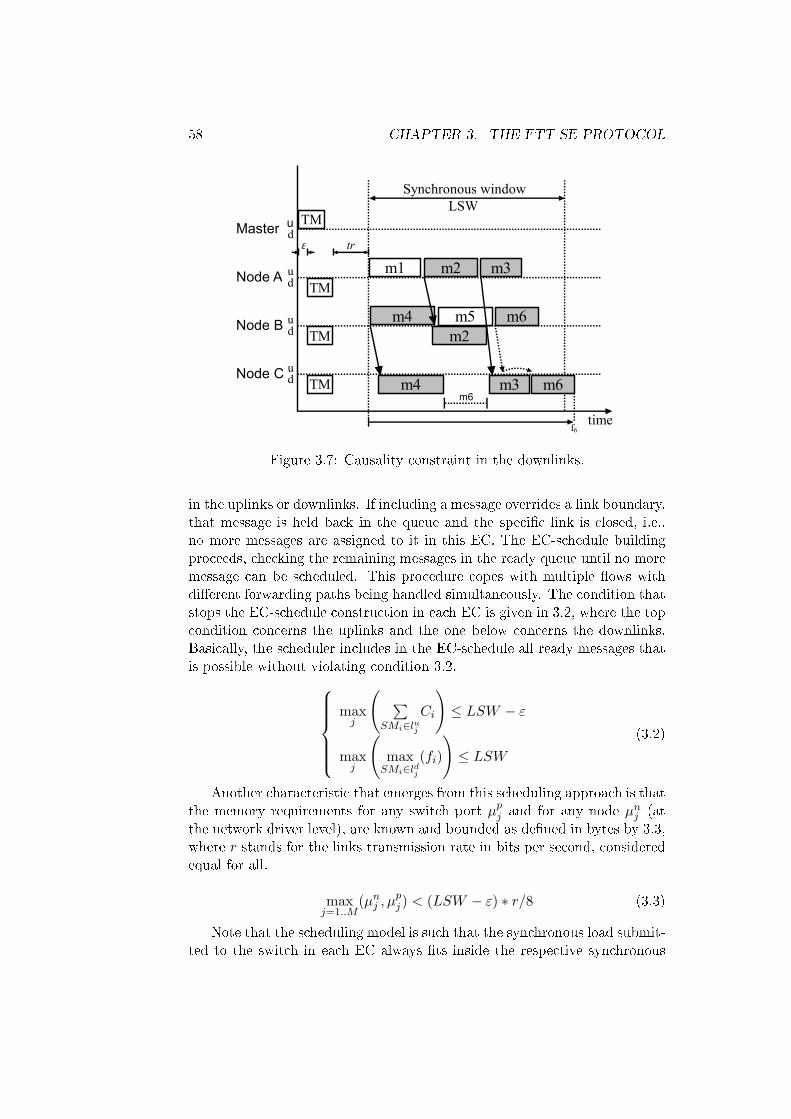
58 CHAPTER 3. THE FTT-SE PROTOCOL
TM
TM
TM
TM
m1
m4
m4
m2
m2m5
m3
m3
m6
m6
LSW
tr
time
Node C
ud
ud
ud
ud
Synchronous window
f6
m6
Node B
Node A
Master
Figure 3.7: Causality constraint in the downlinks.
in the uplinks or downlinks. If including a message overrides a link boundary,that message is held back in the queue and the speci�c link is closed, i.e.,no more messages are assigned to it in this EC. The EC-schedule buildingproceeds, checking the remaining messages in the ready queue until no moremessage can be scheduled. This procedure copes with multiple �ows withdi�erent forwarding paths being handled simultaneously. The condition thatstops the EC-schedule construction in each EC is given in 3.2, where the topcondition concerns the uplinks and the one below concerns the downlinks.Basically, the scheduler includes in the EC-schedule all ready messages thatis possible without violating condition 3.2.
maxj
( ∑SMi∈luj
Ci
)≤ LSW − ε
maxj
(maxSMi∈ldj
(fi)
)≤ LSW
(3.2)
Another characteristic that emerges from this scheduling approach is thatthe memory requirements for any switch port µpj and for any node µnj (atthe network driver level), are known and bounded as de�ned in bytes by 3.3,where r stands for the links transmission rate in bits per second, consideredequal for all.
maxj=1..M
(µnj , µpj ) < (LSW − ε) ∗ r/8 (3.3)
Note that the scheduling model is such that the synchronous load submit-ted to the switch in each EC always �ts inside the respective synchronous
3.3. THE SCHEDULING MODEL 59
window. Thus there will be no synchronous messages left in the switchqueues at the end of each EC.
3.3.3 The aperiodic tra�c scheduling model
The aperiodic scheduling model is similar to the periodic one with similarparameters having similar meaning. Equation 3.4 shows the model of anaperiodic stream (AMi), stored in a structure called Asynchronous Require-ments Table (ART ), holding Na streams. Opposed to the periodic model,there are no o�sets and instead of a period there is a minimum inter-arrivaltime Tmiti, also expressed as an integer number of ECs. Large aperiodicmessages are similarly fragmented and scheduled in a packet basis.
ART ={AMi : AMi = (Ci, Tmiti, P ri, Si, {R1
i ..Rkii }), i = 1..Na
}(3.4)
The set of streams in the ART is scheduled by the FTT Master accordingto any online policy, possibly using periodic servers, implementing a singlequeue, also similarly to the periodic tra�c. The di�erence to the periodicscheduling is that messages are no longer activated implicitly, as a functionof time, but upon an explicit application request. The master receives thoserequests through the signaling mechanism described in Section 3.2.2. Oncescheduled, the aperiodic messages are similarly polled via the TM in eachEC and then transmitted in the respective window.
Non-real-time (NRT) messages are handled as a special case of aperiodicmessages, being handled with the lowest priority and having the deadline setto in�nity, in order to avoid the generation of deadline violation exceptions.Thus NRT messages are transmitted in background with respect to the real-time messages, both periodic and aperiodic. One particular aspect to noteis that the sender and the receivers of these messages are not known aheadof time. However, the respective MAC addresses are sent to the master inthe associated signaling message, which allows it to carry out the respectivepoll, later on, when such tra�c is scheduled.
Note, again, that the aperiodic and NRT tra�c is scheduled in a givenEC only if it can be transmitted in that EC. This means that, by the end ofthe EC, there will be no tra�c queued in the switch. This is very important,being the feature that e�ectively allows bypassing the tra�c scheduling car-ried out by the switch in its internal queues, on a sparse time-base, with ECresolution.
3.3.4 Bounding the aperiodic service latency
The Tmit parameter sets the maximum transmission rate with which a givenAM may arrive at the switch and, in conjunction with the message length,bounds the message maximum bandwidth utilization (C/Tmit). However,
60 CHAPTER 3. THE FTT-SE PROTOCOL
the sporadic messages frequently have average activation rates signi�cantlylower than the maximum one. The aperiodic signaling scheme presentedin Section 3.2.2 yields for a better use of the bandwidth, which is only usedupon explicit requests, allowing other messages to reclaim the slack wasted bymessages activated at lower rates. However, RT tra�c is typically admittedconsidering the worst-case scenario and so the reclaimed extra bandwidthdoes not result in better schedulability levels for the RT asynchronous tra�c.The advantage of this signaling mechanism for the RT asynchronous tra�cis the reduction of the average response time, specially for the lower prioritytra�c that is promptly scheduled whenever there is slack. Furthermore, thereclaimed bandwidth may also be used by the background non-RT tra�c,improving its average throughput signi�cantly.
The response time of an asynchronous message (AM_Rt), de�ned asthe time lapse between the instant in which the application generates themessage, i.e., the message becomes ready at the sender interface, and theinstant in which its transmission �nishes, depends on the signaling latency(Lsig), on the scheduling latency (Lschi) and on the message size (3.5).Lsig is the time required for the aperiodic transmission request to arrive atthe master and be included in the scheduling structures and Lschi is thedelay induced by the tra�c scheduler until the message is actually includedin a TM (integer number of ECs) and Lpoll is the time for the respectiveproducer to answer to the poll in that TM (Lpoll < 1EC).
AM_Rt = Lsig + Lschi + Lpoll (3.5)
While the scheduling delay depends on the particular scheduling algo-rithm and current tra�c load, the signaling latency is independent of theparticular tra�c con�guration and can be bounded approximately between1 and 2 ECs (Figure 3.8b), corresponding to the situations in which the AMmessage is queued just before or after the transmission instant of the signal-ing message. Notice that 1 EC is always needed after the signaling messagearrives at the master so that it is inserted in the scheduling structures.
To compare the impact of the signaling mechanism in the AMs responsetime with respect to the common periodic polling mechanism, Figure 3.8sketches a timeline with the worst-case situation for the response time of anasynchronous message (AM_Rt) in the two cases. In (a) a periodic pollingmechanism is used in which the master periodically schedules the AM in ablind way, while (b) represents the proposed aperiodic signaling mechanism.In both scenarios the asynchronous message is registered with a minimuminter-transmission time of 3 ECs.
When activations are periodically triggered (a), the slave may ultimatelyhave an AM transmission request right after the last poll, leading to a re-sponse time (AM_Rt) as given by Equation 3.6, where δ is an in�nitesimal
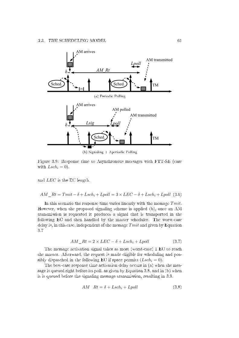
3.3. THE SCHEDULING MODEL 61
δ
Sched. TM
AM_Rt
AM arrives
AM transmitted
idle
Sched.
Lpoll
(a) Periodic Polling
δ
Sched. TM
LpollLsig
AM arrivesAM polled
AM transmitted
(b) Signaling + Aperiodic Polling
Figure 3.8: Response time to Asynchronous messages with FTT-SE (casewith Lschi = 0).
and LEC is the EC length.
AM_Rt = Tmit− δ+Lschi +Lpoll = 3×LEC − δ+Lschi +Lpoll (3.6)
In this scenario the response time varies linearly with the message Tmit.However, when the proposed signaling scheme is applied (b), once an AMtransmission is requested it produces a signal that is transported in thefollowing EC and then handled by the master scheduler. The worst-casedelay is, in this case, independent of the message Tmit and given by Equation3.7
AM_Rt = 2× LEC − δ + Lschi + Lpoll (3.7)
The message activation signal takes at most (worst-case) 1 EC to reachthe master. Afterward, the request is made eligible for scheduling and pos-sibly dispatched in the following EC if space permits (Lschi = 0).
The best-case response time activation delay occurs in (a) when the mes-sage is queued right before its poll, as given by Equation 3.8, and in (b) whenit is queued before the signaling message transmission, resulting in 3.9.
AM_Rt = δ + Lschi + Lpoll (3.8)

62 CHAPTER 3. THE FTT-SE PROTOCOL
scenario Worst Best Average
(a) Tmit 0 Tmit/2(b) 2× LEC 1× LEC 1.5× LEC
Table 3.1: AM Response times with uniform arrival (case with Lschi +Lpoll = 0).
AM_Rt = 1× LEC + δ (3.9)
If the asynchronous messages are randomly triggered by the applicationwith uniform distribution, the average response time will vary uniformlybetween the best and the worst-cases.
Table 3.1 outlines the response times for the two scenarios in the worst,best and average cases. The proposed signaling scheme (b) induces a betterasynchronous responsiveness for values of Tmit greater than 2 ECs. Thebene�t for messages registered with longer Tmit is obvious.
3.4 Implementation details
The FTT-SE protocol integrates a communication framework that providesa set of services possibly directly to the application. These services arepart of a speci�c middleware that addresses distribution and system startuprecon�guration.
3.4.1 Middleware abstraction
In a distributed system the middleware provides the means to abstract thecomplexity of bringing together several services running on di�erent nodes,towards an integrated computational platform.
The FTT-SE middleware provides the abstraction for synchronizationmechanisms as well as a logical abstraction that associates services and thenodes, guarantees a consistent resource allocation and provides network loadaccounting, which yields an admission control for new sessions, specially im-portant in dynamic and open environments. Basically the idea with thislayer is to bring forth a common application interface available at all nodes,handling the communication details and providing seamless design composi-tion.
Such abstraction layer is a valuable tool for an easier and more e�cientapplication development and deployment. Figure 3.9 depicts a layered viewof the protocol structure, including the management, interface and core lay-ers. The protocol lies over a full-duplex Switched Ethernet network. Inter-nally, the FTT-SE core layer represents the protocol basic communication
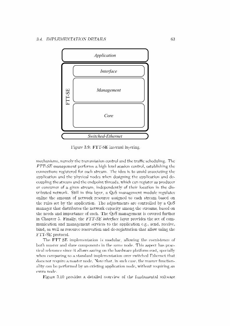
3.4. IMPLEMENTATION DETAILS 63
Switched-Ethernet
Application
Core
Management
InterfaceFTT-SE
Figure 3.9: FTT-SE internal layering.
mechanisms, namely the transmission control and the tra�c scheduling. TheFTT-SE management performs a high level session control, establishing theconnections registered for each stream. The idea is to avoid associating theapplication and the physical nodes when designing the application and de-coupling the stream and the endpoint threads, which can register as produceror consumer of a given stream, independently of their location in the dis-tributed network. Still in this layer, a QoS management module regulatesonline the amount of network resource assigned to each stream based onthe rules set by the application. The adjustments are controlled by a QoSmanager that distributes the network capacity among the streams, based onthe needs and importance of each. The QoS management is covered furtherin Chapter 5. Finally, the FTT-SE interface layer provides the set of com-munication and management services to the application e.g., send, receive,bind, as well as resource reservation and de-registration that allow using theFTT-SE protocol.
The FTT-SE implementation is modular, allowing the coexistence ofboth master and slave components in the same node. This aspect has prac-tical relevance since it allows saving on the hardware platform cost, speciallywhen comparing to a standard implementation over switched Ethernet thatdoes not require a master node. Note that, in such case, the master function-ality can be performed by an existing application node, without requiring anextra node.
Figure 3.10 provides a detailed overview of the fundamental software
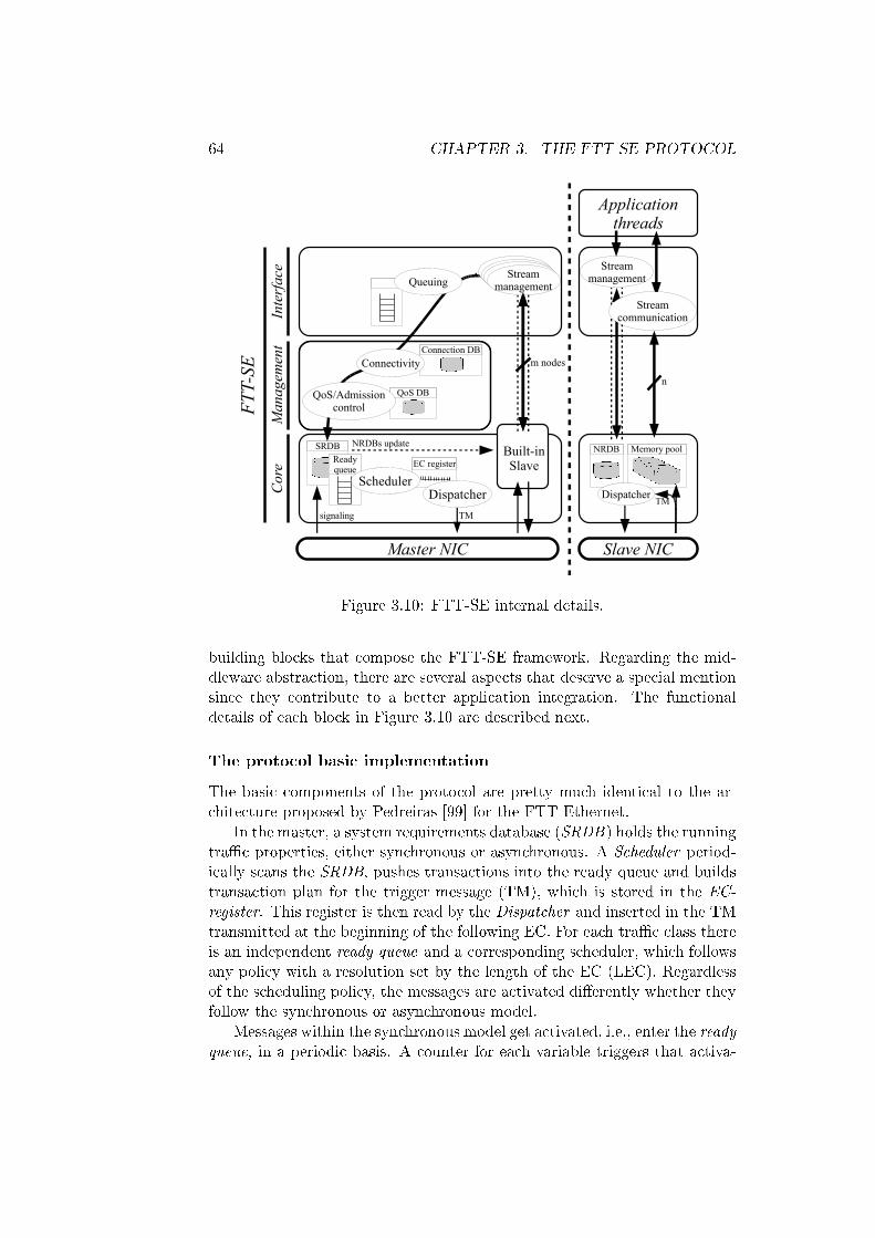
64 CHAPTER 3. THE FTT-SE PROTOCOL
Master NIC
FT
T-SE
SRDB
EC registerReadyqueue
SchedulerDispatcher
Built-inSlave
signaling TM
NRDBs updateNRDB Memory pool
TMDispatcherC
ore
Man
agem
ent Connection DB
QoS DB
Queuing
Connectivity
QoS/Admissioncontrol
Inte
rfac
e
Slave NIC
Streammanagement
Applicationthreads
n
Streamcommunication
m nodes
Streammanagement
Figure 3.10: FTT-SE internal details.
building blocks that compose the FTT-SE framework. Regarding the mid-dleware abstraction, there are several aspects that deserve a special mentionsince they contribute to a better application integration. The functionaldetails of each block in Figure 3.10 are described next.
The protocol basic implementation
The basic components of the protocol are pretty much identical to the ar-chitecture proposed by Pedreiras [99] for the FTT-Ethernet.
In the master, a system requirements database (SRDB) holds the runningtra�c properties, either synchronous or asynchronous. A Scheduler period-ically scans the SRDB, pushes transactions into the ready queue and buildstransaction plan for the trigger message (TM), which is stored in the EC-register. This register is then read by the Dispatcher and inserted in the TMtransmitted at the beginning of the following EC. For each tra�c class thereis an independent ready queue and a corresponding scheduler, which followsany policy with a resolution set by the length of the EC (LEC). Regardlessof the scheduling policy, the messages are activated di�erently whether theyfollow the synchronous or asynchronous model.
Messages within the synchronous model get activated, i.e., enter the readyqueue, in a periodic basis. A counter for each variable triggers that activa-
3.4. IMPLEMENTATION DETAILS 65
tion every Ti. As for the asynchronous messages, their activation is relatedto asynchronous triggering of messages in the node, which are interceptedand kept waiting for transmission order. As previously described in Sec-tion 3.2.2, at the end of the EC, a signaling message is sent to the masterwith an indication of the asynchronous messages queued in the node. Themaster then schedules those messages according to their tra�c class. Thismechanism allows enforcing minimum inter-transmission time speci�ed forreal-time asynchronous messages. Therefore, similarly to the synchronoustra�c, a counter tracks the last transmitting time of such message, andenforces a separation of at least Tmiti between consecutive transmissions.Referring to the asynchronous tra�c without real-time requirements that op-erates in the background in a best-e�ort basis, it is handled through a FIFOqueue, �lling the slack left unused by the other tra�c, without schedulabil-ity or over�ow-free guarantees. All the remaining procedures, mainly thepolling with the TM, are similar for all messaging models.
In the slaves, the TM is received, decoded and its contents comparedagainst the node requirements database (NRDB). For each message that ispolled by the TM, if the node is a producer of it, the dispatcher fetchesthe message from the memory pool and orders the its transmission. Con-versely, when a slave receives a data message, it checks whether the nodeis a consumer and, if not, stores the message contents in the memory pool.The memory pool operates di�erently whether the message being stored issynchronous or asynchronous. Synchronous messages have state semanticsand each message is associated to a bu�er holding the latest state update.Asynchronous messages have an event semantics and so are stored in a FIFOqueue, both in the sender and receiver. Therefore, the memory pool addi-tionally holds the dynamic information related to each stream, such as thequeuing status or the message freshness. Still in the memory pool compo-nent, application signals are associated to each bu�ering entity in order tosupport synchronization events to the application upon a transmission orreception of a message.
The NRDB component records the model properties of all streams re-lated to that node, i.e., all the static (long-term lasting) information. Suchinformation must be consistent with the information present in the masterSRDB. There is a clear bound between the streams set in the NRDB andthe items in the memory pool.
As proposed in Section 3.2.2 the slave nodes additionally produce a sig-naling message that reports the status of the queues of the streams for whichthe node is a producer. That message, a unicast message is sent to the mas-ter node at approximately the same instant as the master sends the TM.For this purpose, the dispatcher, which is the same component that decodesthe TM and issues the message productions, synchronizes with the everyreceived TM in order to program the instant of transmission of the nextsignaling message, slightly less than 1 EC later.

66 CHAPTER 3. THE FTT-SE PROTOCOL
Resource allocation consistency
The basic infrastructure described before has no mechanism supporting therequirements consistency between the master SRDB and the nodes NRDB.If no automatic mechanism is provided, the application necessarily has toensure that streams are registered consistently across the master and therelated slaves. This coordination requires an agreement between these el-ements in the distributed network specially when addressing the dynamicchanges that may occur in the network requirements. Note that the proper-ties of a given stream may vary at run-time, with data being generated, andthat not only the FTT-SE stack must be consistent but also the applicationthreads must be aware of the updates taking place and react accordingly.
To address this issue the FTT-SE framework is provided with mecha-nisms that transparently update the protocol internal databases (NRDB)that report to the application threads the updates on the streams to whichthey are bound. In a way, this is a synchronization mechanism between thedistributed threads in a recon�guration procedure.
The network management interface is con�ned to the FTT-SE core layerin the master node, as illustrated in Figure 3.10. All the con�guration com-mands that modify the network requirements are issued through the master.This facilitates consistency and alleviates the application in the slaves side,suppressing the need for additional synchronization (logic and time) betweenthe distributed nodes.
Every time the master SRDB is updated, all related NRDBs are noti�ed,using a broadcast channel established within the FTT-SE core and connect-ing the master and the slaves. The channel is created along with the FTT-SEcore layer, making use of the Built-in Slave component in the master thatrequests the creation of an asynchronous broadcast channel. This channelis unique and serves all slaves. It is con�gured in all nodes with a reserveddefault ID that is �xed and hard-coded. The master registers a producingendpoint whereas each slave registers a consuming one.
The SRDB interface mechanisms guarantee that the updates are simulta-neously committed in the master and all slaves, within the system resolution(one EC). Moreover, depending on the nature of the update, changes maynot be considered immediately, having to wait, for instance, for asynchronousmessages already queued. In such cases the two instances may co-exist inthe databases, to provide a soft transition to the application. For exam-ple, consider a thread producing messages considering a set of properties Afor the channel. Meanwhile, the stream requirements are modi�ed to ex-hibit properties B. The producing thread is immediately noti�ed for the newproperties and the receiving thread is informed right after the last receptionof the message already queued with properties A. Another mechanism pro-vided by the SRDB interface is group handling. It provides the ability toperform atomic changes of several modi�cation requests, i.e., the commands
3.4. IMPLEMENTATION DETAILS 67
are committed by the system all at once.
The Built-in Slave component in the master node is introduced to handlethe asynchronous communications of this node, as needed for the networkmanagement. In fact, this component provides a full asynchronous com-munication interface to the master, allowing the registration of synchronousor asynchronous endpoints. The interface to this component is alike in allnodes, except for the NRDB updates received in the slaves and the asyn-chronous signaling messages received in the master that bypass the need formessage exchange in the network.
activations that go directly to the master without a transporting mech-anism through the network.
With these mechanisms the slave nodes are automatic and accuratelysynchronized with each other and the master node that de�nes the networkrequirements, at the basic protocolar level.
Plug 'n Play
When addressing �exible and, particularly, open systems, the network startsexecuting without any pre-con�guration or knowledge about the systemtopology. The architecture must be prepared to support the online con-nection and disconnection of services and nodes in a random order. Thisdemands for mechanisms that detect and act on such events, without dis-rupting nor jeopardizing the ongoing communications.
When booting-up the system, each of the layers described in Figure 3.9starts in a bottom-up order, preparing the software components to operateproperly. Some of the local components are related and dependent and sothey follow a hierarchical boot procedure. Moreover, some components aredistributed and also related and dependent, more speci�cally, between themaster node and the slave nodes.
It is thus necessary to provide the mechanisms to �rstly detect changes tothe network topology and then discover the streams provided by each node.We shall now focus on the former, covering the latter afterwards, along withthe FTT-SE interface layer.
The boot-up procedure is conducted individually in each distributed nodeand globally in the distributed system, where the nodes (including the mas-ter) may be randomly included. It is however obvious that the network onlyoperates after the master connection and that this cannot be disconnected af-terwards. Each node enters the network with zero-con�guration, i.e., a plug'n play procedure has to be conducted. Hence, the slaves must suspend theirboot until a Master is detected and resume it afterwards simultaneously, asif they were connected at time zero.
When starting the slave's FTT-SE core layer the �rst procedure, aftersensing the master, is to become visible to the Master's FTT-SE core. Themaster aggregates the system con�guration and thus requires the knowledge
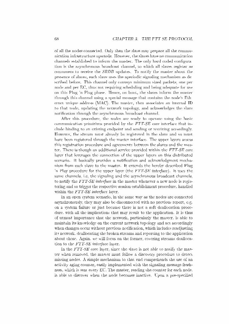
68 CHAPTER 3. THE FTT-SE PROTOCOL
of all the nodes connected. Only then the slave may prepare all the commu-nication infrastructure upwards. However, the slaves have no communicationchannels established to inform the master. The only hard-coded con�gura-tion is the asynchronous broadcast channel, to which all slaves register asconsumers to receive the SRDB updates. To notify the master about thepresence of slaves, each slave uses the aperiodic signaling mechanism as de-scribed before. This channel only conveys minimum sized packets, one pernode and per EC, thus not requiring scheduling and being adequate for useon this Plug 'n Plug phase. Hence, on boot, the slaves inform the masterthrough this channel using a special message that contains the node's Eth-ernet unique address (MAC). The master, then associates an internal IDto that node, updating the network topology, and acknowledges the slavenoti�cation through the asynchronous broadcast channel.
After this procedure, the nodes are ready to operate using the basiccommunication primitives provided by the FTT-SE core interface that in-clude binding to an existing endpoint and sending or receiving accordingly.However, the stream must already be registered in the slave and so musthave been registered through the master interface. The upper layers assessthis registration procedure and agreements between the slaves and the mas-ter. There is though an additional service provided within the FTT-SE corelayer that leverages the connection of the upper layers on this distributedscenario. It basically provides a noti�cation and acknowledgment mecha-nism from each slave to the master. It extends the hereby described Plug'n Play procedure for the upper layer (the FTT-SE interface). It uses thesame channels, i.e, the signaling and the asynchronous broadcast channels,to notify the FTT-SE interface in the master whenever a new node is regis-tering and so trigger the respective session establishment procedure, handledwithin the FTT-SE interface layer.
In an open system scenario, in the same way as the nodes are connectedasynchronously, they may also be disconnected with no previous report, e.g.on a system failure or just because there is not a soft deallocation proce-dure, with all the implications that may result to the application. It is thusof utmost importance that the network, particularly the master, is able tomaintain its knowledge on the current network topology and act accordinglywhen changes occur without previous noti�cation, which includes readjustingits network, deallocating the broken streams and reporting to the applicationabout those. Again, we will focus on the former, covering streams dealloca-tion to the FTT-SE interface layer.
In the FTT-SE core layer, since the slave is not able to notify the mas-ter when removed, the master must follow a discovery procedure to detectmissing nodes. A simple mechanism to that end comprehends the use of anactivity aging counter, easily implemented with the signaling message fresh-ness, which is sent every EC. The master, reading the counter for each node,is able to discover when the node becomes inactive. Upon a pre-speci�ed
3.4. IMPLEMENTATION DETAILS 69
sequence of inactivity events, the master removes the slave from the networktopology, letting the FTT-SE interface layer to be aware of the change andapply the necessary measures that exclude the node from all the runningservices.
Application interface and management
The purpose of a middleware layer is to provide to the application a com-munication interface that fully abstracts the protocol internals providing auniform and transparent access to the communication services throughoutthe distributed system.
The FTT-SE interface layer plays an important role to support suchdistribution and network abstraction. It provides the interface for the net-work management and the data communication transactions then estab-lished, where it entirely abstracts the network internal namespace for nodesand streams, creating a full separation with the application-de�ned names-pace. The abstraction mapping is achieved with a binding process thatassociates the namespaces and allows, for instance, application threads tobe node independent regarding execution.
Referring to the internal implementation of the communication prim-itives, the FTT-SE interface simply redirects the interchanged data andcontrol signals to/from the FTT-SE core layer. It should be noted, though,that these transactions are optimized to minimize the number of copies whengoing through the protocol stack. Depending on the Ethernet driver, it ispossible to accomplish the whole process with a single memory copy trans-action.
The management related requests are triggered by the slaves and gothrough the master, before reaching the FTT-SE management layer. Theinterface layer assures the abstraction of this communication with the mas-ter, serializing the requests in a queue and allowing the submission of severalrequests as a group. This serialization and group handling mechanism isnecessary if we consider the need for atomic changes and the fact that nodesmay compete asynchronously for the opportunity of modifying the networkrequirements. This mechanism demands a direct communication link be-tween the slaves and the master. Hence, whenever a node is attached, twoasynchronous message streams per node are automatically created. Theseform a bidirectional channel that is transparent to the application and al-lows carrying out the requests and acknowledgment with the Master FTT-SEinterface layer.
Synchronization properties
Regarding to the middleware and services made available to ease the appli-cation design, there are three synchronization aspects to highlight related to
70 CHAPTER 3. THE FTT-SE PROTOCOL
the streams communication. The �rst aspect refers to the synchronizationof the threads that handle the streams directly. There are three kinds ofthreads supporting a stream, the producing thread, one or more receivingthreads and one management thread, being the latter the one that negoti-ates and de�nes the stream requirements with the FTT-SE network. Thesethreads can execute on any node, all apart in di�erent nodes or even sharethe same node. The issue here is that all threads are attached to the samelogical entity, the stream, and so have to be set together and run as a whole,e.g. there is no point in issuing a transmission if there is no thread receivingand handling the data.
As part of the communication endpoints establishment procedure, eachapplication thread, either producer or consumer, registers itself in the mas-ter. However, a single endpoint registration is not enough to set a stream.The stream only becomes valid once associated to one producer and at leastone consumer. Therefore, each thread individually, after registering the end-point, must wait on a binding procedure until the stream is fully registered.In the slaves this binding procedure becomes possible when the stream prop-erties are visible in the NRDB.
This stream registration procedure takes place in the Master FTT-SEmanagement layer that collects each registered endpoint to build the streamconnectivity table, associating the stream application ID Si with the nodeIDs. When the stream becomes fully described it is issued to the network,which eventually unblocks all threads synchronously. This mechanism pro-vides a full synchronization of the application right from the stream startup.
The second synchronization feature refers to the noti�cation of commu-nication events on a channel already established and running. In the slaves,whenever a message, synchronous or asynchronous, is transmitted or re-ceived, a signal is raised that unblocks any blocked thread waiting for thatevent. This allows an easier and simpler interaction with the network, spe-cially in event-triggered communication scenarios.
Finally the third synchronization aspect refers to getting all threads up-dated regarding the stream requirements. When the management threadsets the base requirements, all threads have access to that information, asthey share the same design scope. Each thread then produces and receivesdata according to those requirements, for example a video frame with a givensize. However, when the requirements set by the application allow instanta-neous variations, as a result of a QoS manager, the application is not ableto directly control the properties of a stream on the network. The result ofthe QoS manager depends on the global requirements set for each stream aswell as the current network load. Furthermore, these variations may occurasynchronous, e.g. upon adding or removing another stream that ultimatelya�ects the network current load, forcing the network re-con�guration. Aftera re-con�guration all the involved threads must be properly noti�ed of thosechanges. Failing to do so, may lead to potentially catastrophic consequences,

3.4. IMPLEMENTATION DETAILS 71
since the application threads may inconsistently address the produced andconsumed data. Another implication of this kind of synchronization is thatthe application does not stop while updating the running properties of a givenstream. The architecture must be able to support those changes online andinteract with the application. This latter topic was brie�y introduced whendescribing the online synchronization between the SRDB and the NRDBswithin the slaves.
This online synchronization issue is handled using an tagging mechanismthat associates a unique tag to the requirements of a stream. Whenever thecharacteristics of the stream change, so does the tag. During the transitionphase from one state into the other, i.e., one tag to another, the two require-ment sets co-exist in the SRDB as well as in the corresponding NRDBs.This is necessary for a smooth transition, where from one side the pendingmessages (old-tagged) have to be scheduled and transmitted, and from theother, newly-tagged messages are being produced.
For the application, this tagging mechanism allows a friendly synchro-nization of each thread to the environment dynamics. Production of old-tagged data is denied from the moment the new tag is visible in the NRDB,guaranteeing that no old-tagged messages are bu�ered. The thread produc-ing that message must then poll the new tag requirements and rearrangethe data being produced. In the consuming side, threads get all messagesalong with the associated tag that informs how the message must be han-dled and so they are explicitly noti�ed of any changes on the current streamproperties.
Figure 3.10 shows some of the components that play a part supportingthese synchronization mechanisms. In the FTT-SE management layer, theConnections_db stores the connectivity of the streams. After a complete con-nectivity registration, the stream passes an admission control and the QoSmanagement that determines the �nal properties submitted to the network.In the slaves, the memory pool bu�ers the transactions data and holds thesignaling �ags that trigger the communication activity events. These eventspass through the FTT-SE interface layer where the stream ID is translatedand passed to the application layer. Still in the slave nodes, the NRDB holdsthe streams requirements currently registered in the network.
3.4.2 Data addressing modes
The centralized architecture of FTT-SE relies on the master to coordinatethe tra�c that crosses the switch. In this task, the scheduler handles theswitching queues independently, building timelines for each, while allowingparallel forwarding paths.
The Ethernet switch operates in the data link layer, routing Ethernetpackets according to the destination MAC address, see Section 2.3. Thepackets can be forward as unicast, multicast or even broadcast. A unicast
72 CHAPTER 3. THE FTT-SE PROTOCOL
packet is forward to a single output queue, corresponding to the packet des-tination MAC in the forwarding table. A broadcast packet uses a specialdestination address, reserved to replicate the packet into all the output portqueues, except for the one from where the packet arrives. Finally, the mul-ticast transmission also uses a special MAC address type to forward packetsto multiple destination ports. This address is taken out of a range reservedfor multicast transmissions, where each address designates a multicast class.The switch forwarding table registers the ports that refer to each multicastgroup. However, the building procedure of this forwarding table is morecomplex, as the receivers have to establish a registration to the multicastgroup. The IGMP protocol, detailed in Section 2.3, handles this registra-tion that is supported by switches with IGMP snooping capability. Oncethe forwarding addresses are properly set in the table, the multicast packetsthat match the indexed forwarding addresses are replicated to the respectiveoutput queues, similarly to the broadcast address.
In general, broadcast messaging better suits the producer-consumer com-munication model, which is not the model followed by the FTT-SE protocol.It can also be used as a trade-o� replacement for when multicast is not sup-ported and using multiple unicast messages becomes too expensive. Anotherapplication scenario for broadcast messaging is on network discovery services,where polls are required to �ood the network through all its branches.
The FTT-SE protocol, follows the publisher-subscriber model, which ismore e�ciently supported by the multicast transmission model. Multicastmessaging lies between the unicast and broadcast models that are the twoopposite addressing extremes. In fact, it generalizes both, since a multicastcan address either a single port (unicast) or all the other ports (broadcast),without additional penalty other than the layer 2 subscription required forthe receivers.
The two tra�c models within the FTT-SE architecture, synchronousand asynchronous, de�ne for each stream a sending node and one or morereceivers, as de�ned in Equations 3.1 and 3.4. Depending on the speci�cs ofeach variable it is possible to enforce a unicast, multicast or even broadcasttransmission. Thus, the multicast transmission, if supported by the switchdevice, is the preferable choice since it is more resource e�cient de�ning themessage stream.
Section 3.4.1 described the procedure necessary to register a messagingstream in the protocol. The registration procedure is centralized in the mas-ter node and then unfolded to all the nodes that take part in each transaction.During the process, the producer and consumers of each stream get to knowthe transition details, among which, the destination MAC address. Thataddress can either be a broadcast directive, a speci�c node MAC address ora multicast de�ned group. When de�ning a multicast, the master associatesthe stream to a multicast group, from the range of MAC addresses reservedby the IGMP protocol, which is then used in the stream destination �eld.
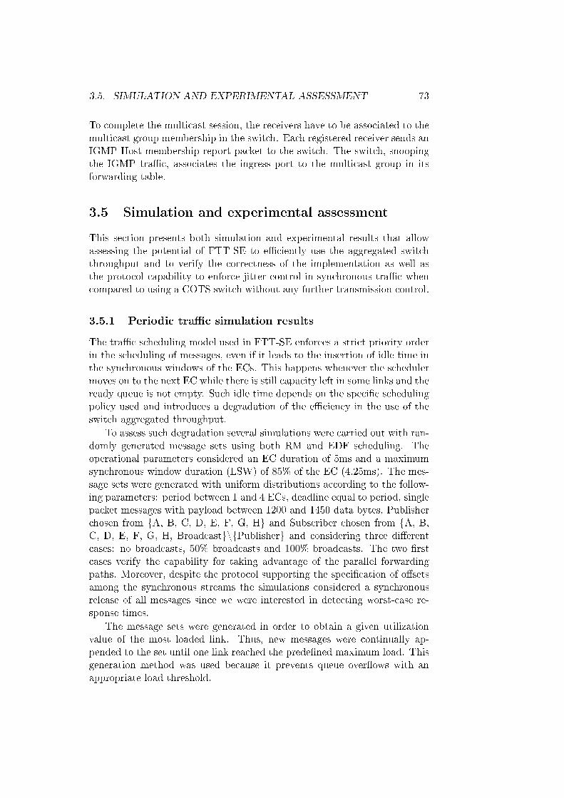
3.5. SIMULATION AND EXPERIMENTAL ASSESSMENT 73
To complete the multicast session, the receivers have to be associated to themulticast group membership in the switch. Each registered receiver sends anIGMP Host membership report packet to the switch. The switch, snoopingthe IGMP tra�c, associates the ingress port to the multicast group in itsforwarding table.
3.5 Simulation and experimental assessment
This section presents both simulation and experimental results that allowassessing the potential of FTT-SE to e�ciently use the aggregated switchthroughput and to verify the correctness of the implementation as well asthe protocol capability to enforce jitter control in synchronous tra�c whencompared to using a COTS switch without any further transmission control.
3.5.1 Periodic tra�c simulation results
The tra�c scheduling model used in FTT-SE enforces a strict priority orderin the scheduling of messages, even if it leads to the insertion of idle time inthe synchronous windows of the ECs. This happens whenever the schedulermoves on to the next EC while there is still capacity left in some links and theready queue is not empty. Such idle time depends on the speci�c schedulingpolicy used and introduces a degradation of the e�ciency in the use of theswitch aggregated throughput.
To assess such degradation several simulations were carried out with ran-domly generated message sets using both RM and EDF scheduling. Theoperational parameters considered an EC duration of 5ms and a maximumsynchronous window duration (LSW) of 85% of the EC (4.25ms). The mes-sage sets were generated with uniform distributions according to the follow-ing parameters: period between 1 and 4 ECs, deadline equal to period, singlepacket messages with payload between 1200 and 1450 data bytes, Publisherchosen from {A, B, C, D, E, F, G, H} and Subscriber chosen from {A, B,C, D, E, F, G, H, Broadcast}\{Publisher} and considering three di�erentcases: no broadcasts, 50% broadcasts and 100% broadcasts. The two �rstcases verify the capability for taking advantage of the parallel forwardingpaths. Moreover, despite the protocol supporting the speci�cation of o�setsamong the synchronous streams the simulations considered a synchronousrelease of all messages since we were interested in detecting worst-case re-sponse times.
The message sets were generated in order to obtain a given utilizationvalue of the most loaded link. Thus, new messages were continually ap-pended to the set until one link reached the prede�ned maximum load. Thisgeneration method was used because it prevents queue over�ows with anappropriate load threshold.
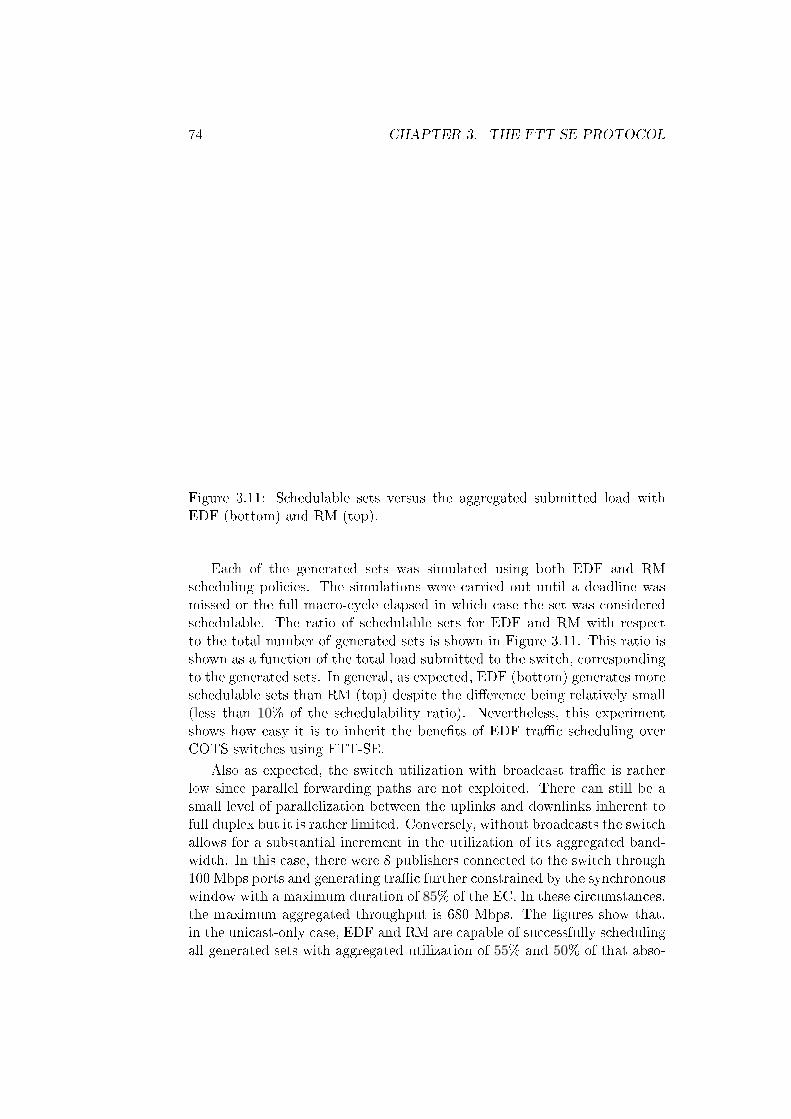
74 CHAPTER 3. THE FTT-SE PROTOCOL
Figure 3.11: Schedulable sets versus the aggregated submitted load withEDF (bottom) and RM (top).
Each of the generated sets was simulated using both EDF and RMscheduling policies. The simulations were carried out until a deadline wasmissed or the full macro-cycle elapsed in which case the set was consideredschedulable. The ratio of schedulable sets for EDF and RM with respectto the total number of generated sets is shown in Figure 3.11. This ratio isshown as a function of the total load submitted to the switch, correspondingto the generated sets. In general, as expected, EDF (bottom) generates moreschedulable sets than RM (top) despite the di�erence being relatively small(less than 10% of the schedulability ratio). Nevertheless, this experimentshows how easy it is to inherit the bene�ts of EDF tra�c scheduling overCOTS switches using FTT-SE.
Also as expected, the switch utilization with broadcast tra�c is ratherlow since parallel forwarding paths are not exploited. There can still be asmall level of parallelization between the uplinks and downlinks inherent tofull duplex but it is rather limited. Conversely, without broadcasts the switchallows for a substantial increment in the utilization of its aggregated band-width. In this case, there were 8 publishers connected to the switch through100 Mbps ports and generating tra�c further constrained by the synchronouswindow with a maximum duration of 85% of the EC. In these circumstances,the maximum aggregated throughput is 680 Mbps. The �gures show that,in the unicast-only case, EDF and RM are capable of successfully schedulingall generated sets with aggregated utilization of 55% and 50% of that abso-
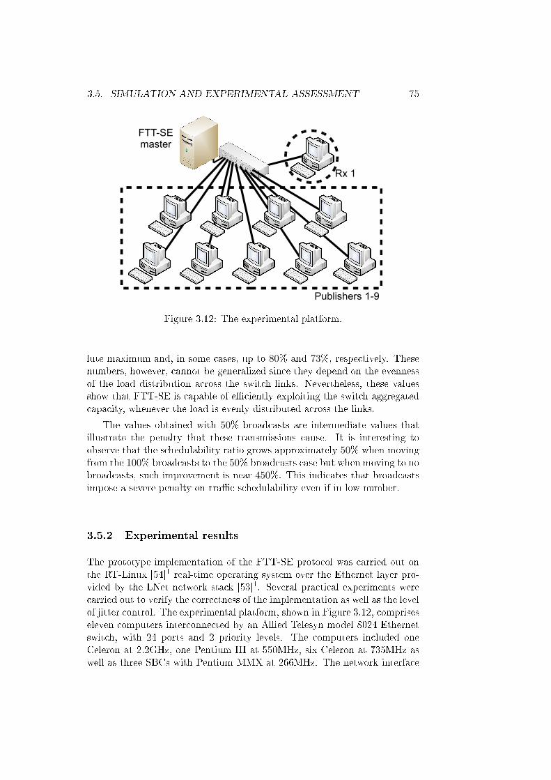
3.5. SIMULATION AND EXPERIMENTAL ASSESSMENT 75
Publishers 1-9
Rx 1
FTT-SEmaster
Figure 3.12: The experimental platform.
lute maximum and, in some cases, up to 80% and 73%, respectively. Thesenumbers, however, cannot be generalized since they depend on the evennessof the load distribution across the switch links. Nevertheless, these valuesshow that FTT-SE is capable of e�ciently exploiting the switch aggregatedcapacity, whenever the load is evenly distributed across the links.
The values obtained with 50% broadcasts are intermediate values thatillustrate the penalty that these transmissions cause. It is interesting toobserve that the schedulability ratio grows approximately 50% when movingfrom the 100% broadcasts to the 50% broadcasts case but when moving to nobroadcasts, such improvement is near 450%. This indicates that broadcastsimpose a severe penalty on tra�c schedulability even if in low number.
3.5.2 Experimental results
The prototype implementation of the FTT-SE protocol was carried out onthe RT-Linux [54]1 real-time operating system over the Ethernet layer pro-vided by the LNet network stack [53]1. Several practical experiments werecarried out to verify the correctness of the implementation as well as the levelof jitter control. The experimental platform, shown in Figure 3.12, compriseseleven computers interconnected by an Allied Telesyn model 8024 Ethernetswitch, with 24 ports and 2 priority levels. The computers included oneCeleron at 2.2GHz, one Pentium III at 550MHz, six Celeron at 735MHz aswell as three SBCs with Pentium MMX at 266MHz. The network interface
76 CHAPTER 3. THE FTT-SE PROTOCOL
ID C(bytes) T(=D)(ms) maxjw(µs) maxjwo (µs)2 1000 1 483 9967 1000 1 174 9848 1000 1 170 10033 3840 3 92 9321 3840 4 893 5594 3840 4 316 4465 3840 4 1000 5216 3840 4 137 5619 1480 8 4132 436
Table 3.2: Message set used in the FTT-SE experiments.
cards (NICs) were Intel 8255 and 3Com 3C905B.
One of the computers was dedicated to the FTT Master, nine computerswere data publishers, publishing one message each, and the last computerwas a subscriber of all those nine message streams. Only one subscriber isused in this experimental assessment to maximize the messages concurrencyin a single link, creating a worst-case latency, and probably jitter, situation.The message set is detailed in Table 3.2 and mixes messages with di�erentperiods as well as single-packet (messages 2 and 7 to 9) and multi-packet(messages 1 and 3 to 6). Remember that FTT-SE handles transparently thefragmentation and re-assembly of multi-packet messages, allowing preemp-tion between packets. The total load submitted by this set is approximately68,6 Mbps. Concerning the operational con�guration of FTT-SE, the ECduration was set to 1ms and the LSW to 85% of the EC, i.e., 0,85ms. Thetra�c scheduling was RM.
The same experiments were also carried out with the publishers sendinginformation at the same rate but without the transmission control mecha-nisms provided by FTT-SE. The inter-arrival instants of all messages at thesubscriber node were recorded for both of these con�gurations referred to aswith and without FTT.
Firstly, an experiment was carried out to assess the infrastructure jitter,i.e., the jitter due to the operating system, network device drivers and packetswitching. This is the base jitter of the system without any scheduling in-terference. This preliminary experiment consisted in the transmission of asingle periodic message, with 1500 data bytes, transmitted every EC (1ms)by one of the slower computers, during 560s. In this case there is no schedul-ing jitter and thus the jitter observed is only caused by the communicationinfrastructure. As depicted in Figure 3.13, the infrastructure jitter is lower
1RTLinux and LNET were by 2006 supported by FSMLabs Inc. They are currentlydistributed by Wind River Systems Inc.
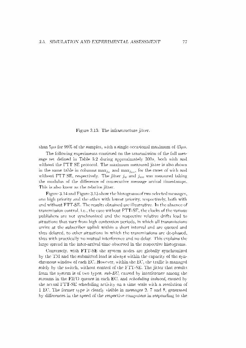
3.5. SIMULATION AND EXPERIMENTAL ASSESSMENT 77
Figure 3.13: The infrastructure jitter.
than 5µs for 99% of the samples, with a single occasional maximum of 43µs.
The following experiments consisted on the transmission of the full mes-sage set de�ned in Table 3.2 during approximately 300s, both with andwithout the FTT-SE protocol. The maximum measured jitter is also shownin the same table in columns maxjw and maxjwo , for the cases of with andwithout FTT-SE, respectively. The jitter jw and jwo was measured takingthe modulus of the di�erence of consecutive message arrival timestamps.This is also know as the relative jitter.
Figure 3.14 and Figure 3.15 show the histograms of two selected messages,one high priority and the other with lowest priority, respectively, both withand without FTT-SE. The results obtained are illustrative. In the absence oftransmission control, i.e., the case without FTT-SE, the clocks of the variouspublishers are not synchronized and the respective relative drifts lead tosituations that vary from high contention periods, in which all transmissionsarrive at the subscriber uplink within a short interval and are queued andthus delayed, to other situations in which the transmissions are de-phased,thus with practically no mutual interference and no delay. This explains thelarge spread in the inter-arrival time observed in the respective histograms.
Conversely, with FTT-SE the system nodes are globally synchronizedby the TM and the submitted load is always within the capacity of the syn-chronous window of each EC. However, within the EC, the tra�c is managedsolely by the switch, without control of the FTT-SE. The jitter that resultsfrom the system is of two types, sub-EC, caused by interference among thestreams in the FIFO queues in each EC, and scheduling induced, caused bythe actual FTT-SE scheduling activity on a time scale with a resolution of1 EC. The former type is clearly visible in messages 2, 7 and 8, generatedby di�erences in the speed of the respective computers in responding to the

78 CHAPTER 3. THE FTT-SE PROTOCOL
Figure 3.14: Histogram of inter-arrival times for message 7.
TM. In some cases, e.g., multi-packet message 3, the jitter value is especiallylow because it refers to the last packet, which is sent later in the EC, beingqueued after all others and thus in a relatively constant position in the FIFOqueue. The latter type of jitter, i.e., scheduling jitter, is visible in message9 which has the lowest priority, thus being sometimes scheduled several ECslater by RM scheduler.
Finally, the transmission control enforced by FTT-SE may also be bene-�cial under highly bursty loads. Without the transmission control the levelof contention at the receivers might be too high for many network devicedrivers, which simply crash. The transmission control of FTT-SE preventsthis abnormal situation by maintaining the submitted load under manage-able levels per EC, obviously at the expense of enlarging the processing timefor the same load. Nevertheless, this is su�cient to avoid such crashes andkeep the system running. This phenomenon has been observed several timesduring the practical experiments.
3.6 Conclusion
The advent of switched Ethernet has opened new perspectives for real-timecommunication over Ethernet. However, a few problems subsist related withqueue management policies, queue over�ows and limited priority support.Meanwhile, several techniques were proposed to overcome such di�cultiesbut they require speci�c hardware, are in�exible with respect to commu-nication parameters or do not enforce timeliness guarantees. This chapterproposed using the FTT paradigm to achieve �exible communication withhigh level of control to guarantee timeliness and provide adequate queues
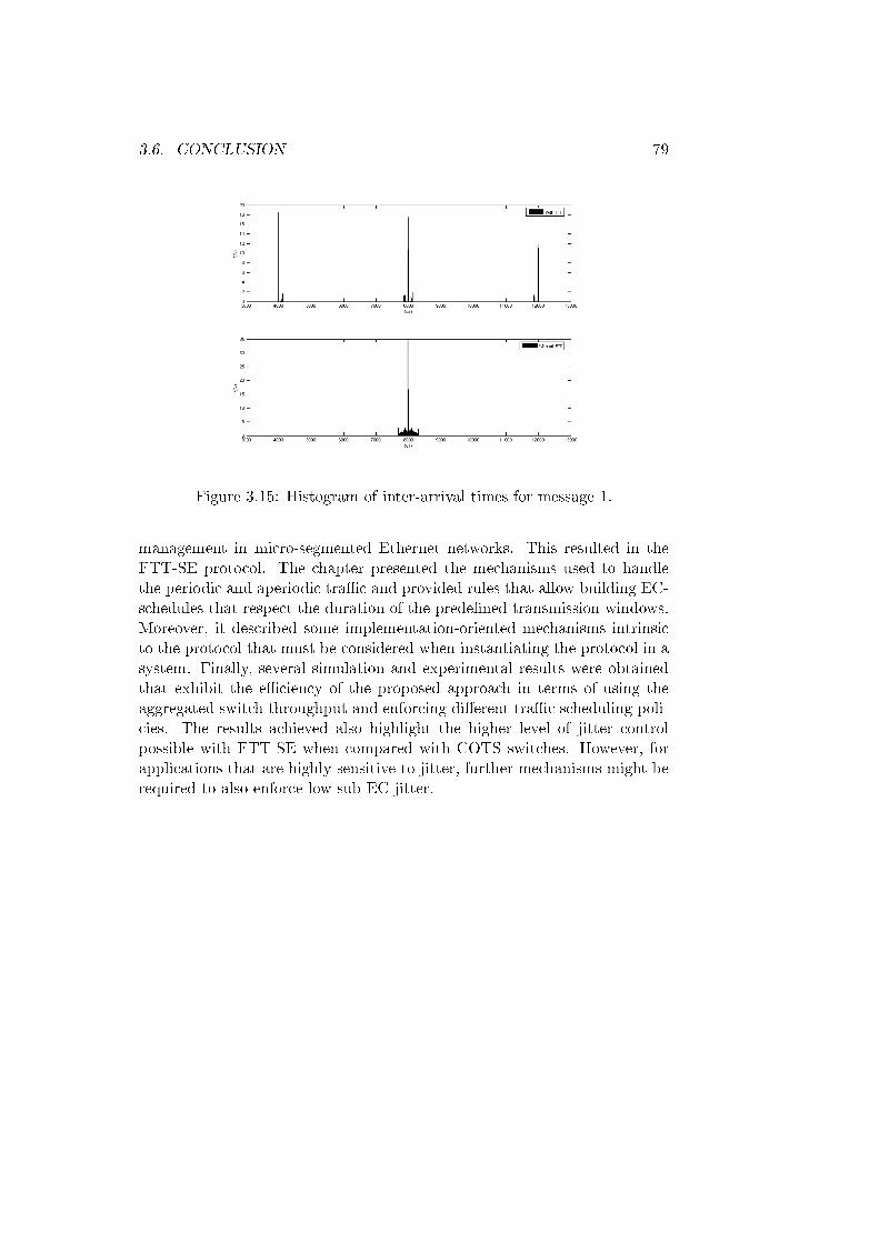
3.6. CONCLUSION 79
Figure 3.15: Histogram of inter-arrival times for message 1.
management in micro-segmented Ethernet networks. This resulted in theFTT-SE protocol. The chapter presented the mechanisms used to handlethe periodic and aperiodic tra�c and provided rules that allow building EC-schedules that respect the duration of the prede�ned transmission windows.Moreover, it described some implementation-oriented mechanisms intrinsicto the protocol that must be considered when instantiating the protocol in asystem. Finally, several simulation and experimental results were obtainedthat exhibit the e�ciency of the proposed approach in terms of using theaggregated switch throughput and enforcing di�erent tra�c scheduling poli-cies. The results achieved also highlight the higher level of jitter controlpossible with FTT-SE when compared with COTS switches. However, forapplications that are highly sensitive to jitter, further mechanisms might berequired to also enforce low sub-EC jitter.

80 CHAPTER 3. THE FTT-SE PROTOCOL
Chapter 4
Tra�c schedulability analysis
This chapter presents RM and EDF schedulability tests for the FTT-SE pro-tocol. As described in the previous chapter, the schedulability tests have tobe executed online. For this reason, the research has focused on utilization-based tests, which can be implemented with linear time complexity. Ad-ditionally, the nature of utilization-based tests facilitates their adoption indynamic Quality of Service (QoS) management mechanisms supporting abandwidth-based QoS distribution through the services.
4.1 Introduction
Despite the relatively large amount of work on network-induced delay causedby switches, particularly on Ethernet switches [78][49], low attention hasbeen devoted to utilization-based tests.
Utilization-based analysis are typically more pessimistic, compared toother analysis such as Network Calculus (NC) and Response Time Analysis(RTA), but on the other hand, they are faster, thus more appealing for use indynamic frameworks such as the FTT-SE. Moreover, utilization-based anal-ysis provide information on the amount of resource, bandwidth in this case,that can be used without compromising the system schedulability, which isof paramount importance to carry out bandwidth distribution among di�er-ent streams within a dynamic QoS management framework. This topic isextensively described in Chapter 5.
In Ethernet switches, the usual presence of FCFS policy queues compli-cates using utilization-based tests. The works that consider such tests arebuilt upon modi�ed switches that carry out di�erent scheduling policies suchas RM or EDF. Conversely, FTT-SE overrides the e�ect of those FCFS pol-icy queues and supports any scheduling policy on a COTS switch such asthose that are suited for utilization-based tests. Nevertheless, these policiesare implemented on a coarse scale (EC) and thus the use of utilization-basedschedulability tests in FTT-SE requires some adaptations to the tra�c model
81

82 CHAPTER 4. TRAFFIC SCHEDULABILITY ANALYSIS
Figure 4.1: Tra�c aggregation on switched Ethernet.
of such protocol.
4.2 Interference in the switch architecture
Multiple services competing for a common shared resource inevitably causeinterference on each other. Contention among services is managed serializingthe access to the resources under consideration. The most common approachto handle serialization is by using a ready queue, where all services wantingto use the resource are placed. The order in which the services are placed isde�ned by the scheduling policy.
On a switched Ethernet network, the nodes are connected by means ofparallel links with each link being an active shared resource. The �owsthat traverse the switch establish interdependencies that make the tra�cscheduling more complicated than just the scheduling of multiple indepen-dent resources.
Figure 4.1 sketches the interference path for a generic message mi, whenissued to a switched Ethernet network. The interference appears when aggre-gating tra�c from di�erent sources into bandwidth limited channels. Firstly,in the output queue of the sending node, mi competes for the access in theuplink that conveys all messages from node Srci to the switch. Once inthe switch, mi is forward to the destination link, Dsti, where it eventuallycompetes with messages from other source nodes.
Therefore, the transmission delay results from combining the delays onboth queues, from the moment the application issues the packet transmissionuntil it arrives at the destination node. Unless stated otherwise, in thefollowing analysis the propagation times and switching delays are neglected,as they are �xed and easily accounted within the packet size. Also thecomputational delay within the nodes, sender and receiver, is included withinthe propagation time.
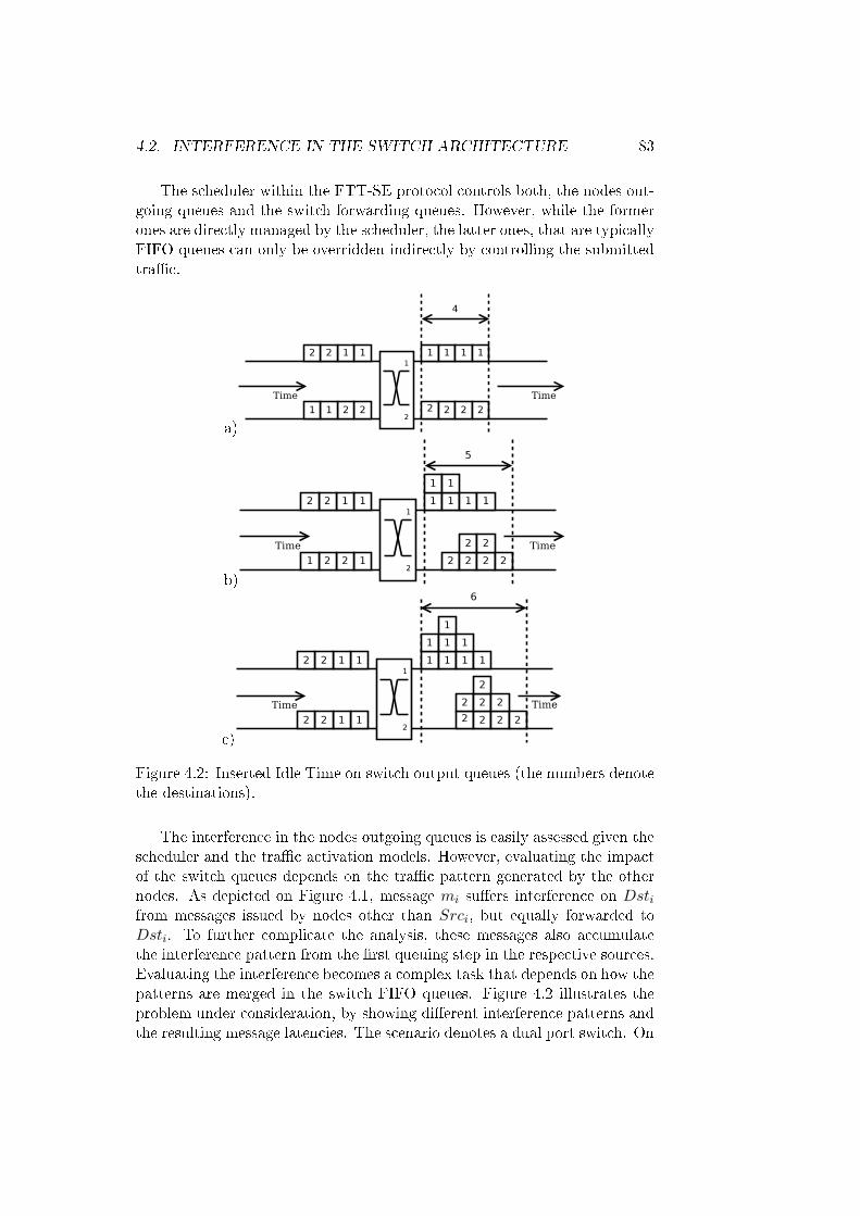
4.2. INTERFERENCE IN THE SWITCH ARCHITECTURE 83
The scheduler within the FTT-SE protocol controls both, the nodes out-going queues and the switch forwarding queues. However, while the formerones are directly managed by the scheduler, the latter ones, that are typicallyFIFO queues can only be overridden indirectly by controlling the submittedtra�c.
a)
b)
c)
Figure 4.2: Inserted Idle Time on switch output queues (the numbers denotethe destinations).
The interference in the nodes outgoing queues is easily assessed given thescheduler and the tra�c activation models. However, evaluating the impactof the switch queues depends on the tra�c pattern generated by the othernodes. As depicted on Figure 4.1, message mi su�ers interference on Dstifrom messages issued by nodes other than Srci, but equally forwarded toDsti. To further complicate the analysis, these messages also accumulatethe interference pattern from the �rst queuing step in the respective sources.Evaluating the interference becomes a complex task that depends on how thepatterns are merged in the switch FIFO queues. Figure 4.2 illustrates theproblem under consideration, by showing di�erent interference patterns andthe resulting message latencies. The scenario denotes a dual port switch. On
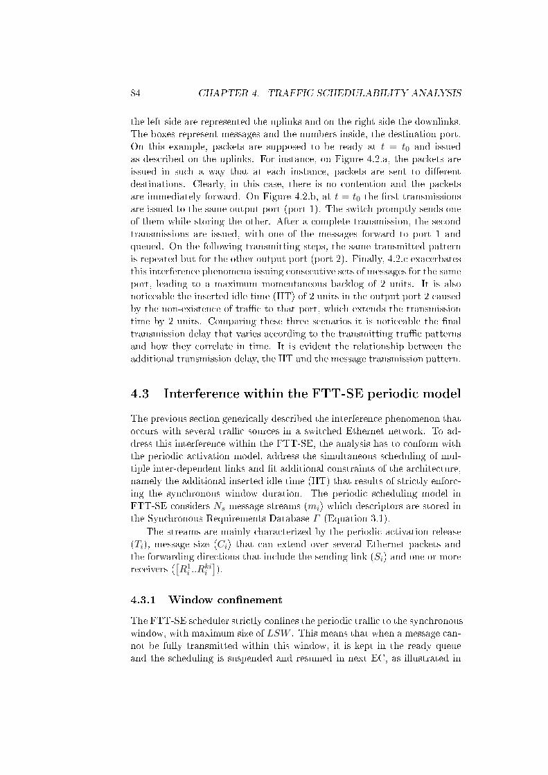
84 CHAPTER 4. TRAFFIC SCHEDULABILITY ANALYSIS
the left side are represented the uplinks and on the right side the downlinks.The boxes represent messages and the numbers inside, the destination port.On this example, packets are supposed to be ready at t = t0 and issuedas described on the uplinks. For instance, on Figure 4.2.a, the packets areissued in such a way that at each instance, packets are sent to di�erentdestinations. Clearly, in this case, there is no contention and the packetsare immediately forward. On Figure 4.2.b, at t = t0 the �rst transmissionsare issued to the same output port (port 1). The switch promptly sends oneof them while storing the other. After a complete transmission, the secondtransmissions are issued, with one of the messages forward to port 1 andqueued. On the following transmitting steps, the same transmitted patternis repeated but for the other output port (port 2). Finally, 4.2.c exacerbatesthis interference phenomena issuing consecutive sets of messages for the sameport, leading to a maximum momentaneous backlog of 2 units. It is alsonoticeable the inserted idle time (IIT) of 2 units in the output port 2 causedby the non-existence of tra�c to that port, which extends the transmissiontime by 2 units. Comparing these three scenarios it is noticeable the �naltransmission delay that varies according to the transmitting tra�c patternsand how they correlate in time. It is evident the relationship between theadditional transmission delay, the IIT and the message transmission pattern.
4.3 Interference within the FTT-SE periodic model
The previous section generically described the interference phenomenon thatoccurs with several tra�c sources in a switched Ethernet network. To ad-dress this interference within the FTT-SE, the analysis has to conform withthe periodic activation model, address the simultaneous scheduling of mul-tiple inter-dependent links and �t additional constraints of the architecture,namely the additional inserted idle time (IIT) that results of strictly enforc-ing the synchronous window duration. The periodic scheduling model inFTT-SE considers Ns message streams (mi) which descriptors are stored inthe Synchronous Requirements Database Γ (Equation 3.1).
The streams are mainly characterized by the periodic activation release(Ti), message size (Ci) that can extend over several Ethernet packets andthe forwarding directions that include the sending link (Si) and one or morereceivers (
[R1i ..R
kii
]).
4.3.1 Window con�nement
The FTT-SE scheduler strictly con�nes the periodic tra�c to the synchronouswindow, with maximum size of LSW . This means that when a message can-not be fully transmitted within this window, it is kept in the ready queueand the scheduling is suspended and resumed in next EC, as illustrated in
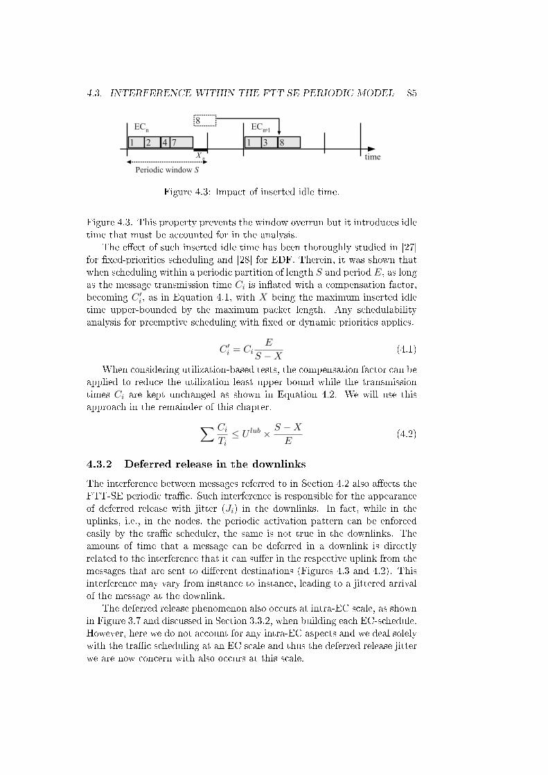
4.3. INTERFERENCE WITHIN THE FTT-SE PERIODIC MODEL 85
1
time
2 4 7X n
ECn
Periodic window S
1 3 8
8ECn+1
Figure 4.3: Impact of inserted idle time.
Figure 4.3. This property prevents the window overrun but it introduces idletime that must be accounted for in the analysis.
The e�ect of such inserted idle time has been thoroughly studied in [27]for �xed-priorities scheduling and [28] for EDF. Therein, it was shown thatwhen scheduling within a periodic partition of length S and period E, as longas the message transmission time Ci is in�ated with a compensation factor,becoming C ′i, as in Equation 4.1, with X being the maximum inserted idletime upper-bounded by the maximum packet length. Any schedulabilityanalysis for preemptive scheduling with �xed or dynamic priorities applies.
C ′i = CiE
S −X(4.1)
When considering utilization-based tests, the compensation factor can beapplied to reduce the utilization least upper bound while the transmissiontimes Ci are kept unchanged as shown in Equation 4.2. We will use thisapproach in the remainder of this chapter.∑ Ci
Ti≤ U lub × S −X
E(4.2)
4.3.2 Deferred release in the downlinks
The interference between messages referred to in Section 4.2 also a�ects theFTT-SE periodic tra�c. Such interference is responsible for the appearanceof deferred release with jitter (Ji) in the downlinks. In fact, while in theuplinks, i.e., in the nodes, the periodic activation pattern can be enforcedeasily by the tra�c scheduler, the same is not true in the downlinks. Theamount of time that a message can be deferred in a downlink is directlyrelated to the interference that it can su�er in the respective uplink from themessages that are sent to di�erent destinations (Figures 4.3 and 4.2). Thisinterference may vary from instance to instance, leading to a jittered arrivalof the message at the downlink.
The deferred release phenomenon also occurs at intra-EC scale, as shownin Figure 3.7 and discussed in Section 3.3.2, when building each EC-schedule.However, here we do not account for any intra-EC aspects and we deal solelywith the tra�c scheduling at an EC scale and thus the deferred release jitterwe are now concern with also occurs at this scale.
86 CHAPTER 4. TRAFFIC SCHEDULABILITY ANALYSIS
4.3.3 Scheduling multiple links
The scheduler operates over the message requirements data-base (SRDB)and builds a single global ready queue, serializing messages according to theirpriority, either static or dynamic. However, when dispatching the messagesin the global ready queue, the protocol attempts to �ll up the uplinks anddownlinks in each EC in order to exploit as much as possible the parallelforwarding paths available in the switch.
This scheduling methodology approximates the model to a link orientedscheduling. The global ready queue is parsed in several ready queues, oneper link, with the messages that traverse that link, and a scheduler thatoperates quasi-independently on each link with the restriction of schedulingmessages together (in the same EC) in the uplinks and the downlinks. Theintra-EC scheduling is handled according to the rules in Equation 3.2 thatenforce the window protection and the causality e�ect between the uplinkand the downlink.
Therefore, the tra�c on a speci�c downlink is in fact constrained by thetra�c explicitly submitted to that port and also the tra�c scheduled in theuplinks of each message, causing interference. In a multicast or broadcasttransmission scenario, messages are only scheduled if �tting the uplink andall downlinks in a given EC. In this case, it is enough to have one downlinkfull to prevent that message from being transmitted in that EC even if theother downlinks and uplink are lightly loaded. This represents a very stronginterference. In a unicast message scenario this type of interference does notapply, since only one uplink and one downlink are involved. The interferenceveri�ed in the uplink does not propagate to other downlinks.
In terms of schedulability analysis of a downlink, in the unicast scenario,only the interference from the uplinks is considered. However, in a multicastor broadcast messaging scenario, a multitude of interfering sources a�ectingthe downlink must be considered. The interference in the downlinks is notcon�ned to the tra�c in the uplinks but also to the tra�c in other down-links, which by themselves may su�er interference from other uplinks anddownlinks in a cascade procedure, pushing the complexity of the analysis toa higher magnitude.
Therefore, in this work we focus in the unicast scenario, only. At theend of this chapter a few considerations are done addressing the multi-cast/broadcast scenario.
4.4 Schedulability test - unicast
This section presents a schedulability test for the unicast only scenario.For all messages we consider the deadline equal to the activation period(∀i, Di = Ti) to prevent excessive e�ciency degradation of RM and EDFschedulability utilization tests, and the release o�sets equal to zero, i.e.,
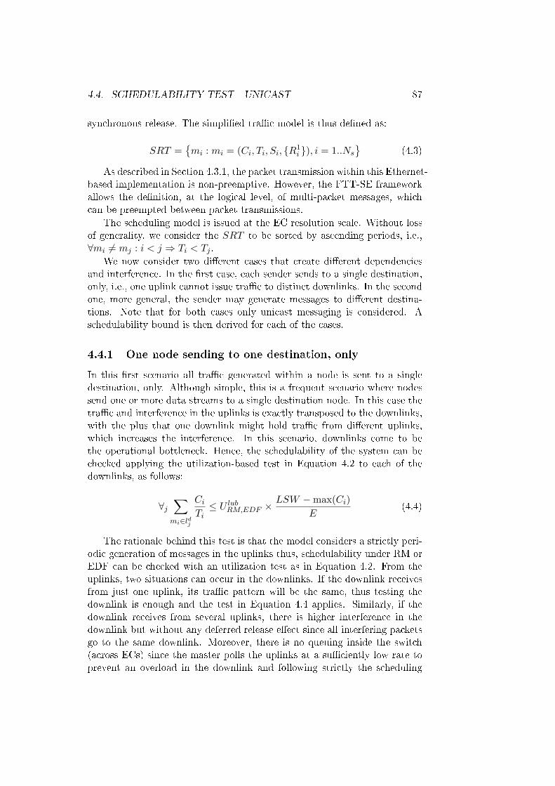
4.4. SCHEDULABILITY TEST - UNICAST 87
synchronous release. The simpli�ed tra�c model is thus de�ned as:
SRT ={mi : mi = (Ci, Ti, Si, {R1
i }), i = 1..Ns
}(4.3)
As described in Section 4.3.1, the packet transmission within this Ethernet-based implementation is non-preemptive. However, the FTT-SE frameworkallows the de�nition, at the logical level, of multi-packet messages, whichcan be preempted between packet transmissions.
The scheduling model is issued at the EC resolution scale. Without lossof generality, we consider the SRT to be sorted by ascending periods, i.e.,∀mi 6= mj : i < j ⇒ Ti < Tj .
We now consider two di�erent cases that create di�erent dependenciesand interference. In the �rst case, each sender sends to a single destination,only, i.e., one uplink cannot issue tra�c to distinct downlinks. In the secondone, more general, the sender may generate messages to di�erent destina-tions. Note that for both cases only unicast messaging is considered. Aschedulability bound is then derived for each of the cases.
4.4.1 One node sending to one destination, only
In this �rst scenario all tra�c generated within a node is sent to a singledestination, only. Although simple, this is a frequent scenario where nodessend one or more data streams to a single destination node. In this case thetra�c and interference in the uplinks is exactly transposed to the downlinks,with the plus that one downlink might hold tra�c from di�erent uplinks,which increases the interference. In this scenario, downlinks come to bethe operational bottleneck. Hence, the schedulability of the system can bechecked applying the utilization-based test in Equation 4.2 to each of thedownlinks, as follows:
∀j∑mi∈ldj
CiTi≤ U lubRM,EDF ×
LSW −max(Ci)E
(4.4)
The rationale behind this test is that the model considers a strictly peri-odic generation of messages in the uplinks thus, schedulability under RM orEDF can be checked with an utilization test as in Equation 4.2. From theuplinks, two situations can occur in the downlinks. If the downlink receivesfrom just one uplink, its tra�c pattern will be the same, thus testing thedownlink is enough and the test in Equation 4.4 applies. Similarly, if thedownlink receives from several uplinks, there is higher interference in thedownlink but without any deferred release e�ect since all interfering packetsgo to the same downlink. Moreover, there is no queuing inside the switch(across ECs) since the master polls the uplinks at a su�ciently low rate toprevent an overload in the downlink and following strictly the scheduling
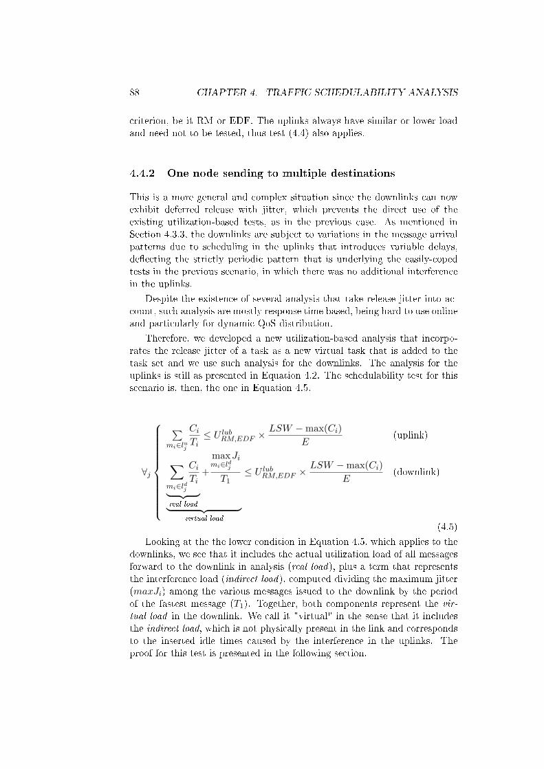
88 CHAPTER 4. TRAFFIC SCHEDULABILITY ANALYSIS
criterion, be it RM or EDF. The uplinks always have similar or lower loadand need not to be tested, thus test (4.4) also applies.
4.4.2 One node sending to multiple destinations
This is a more general and complex situation since the downlinks can nowexhibit deferred release with jitter, which prevents the direct use of theexisting utilization-based tests, as in the previous case. As mentioned inSection 4.3.3, the downlinks are subject to variations in the message arrivalpatterns due to scheduling in the uplinks that introduces variable delays,de�ecting the strictly periodic pattern that is underlying the easily-copedtests in the previous scenario, in which there was no additional interferencein the uplinks.
Despite the existence of several analysis that take release jitter into ac-count, such analysis are mostly response time based, being hard to use onlineand particularly for dynamic QoS distribution.
Therefore, we developed a new utilization-based analysis that incorpo-rates the release jitter of a task as a new virtual task that is added to thetask set and we use such analysis for the downlinks. The analysis for theuplinks is still as presented in Equation 4.2. The schedulability test for thisscenario is, then, the one in Equation 4.5.
∀j
∑mi∈luj
CiTi≤ U lubRM,EDF ×
LSW −max(Ci)E
(uplink)
∑mi∈ldj
CiTi︸ ︷︷ ︸
real load
+
maxmi∈ldj
Ji
T1
︸ ︷︷ ︸virtual load
≤ U lubRM,EDF ×LSW −max(Ci)
E(downlink)
(4.5)
Looking at the the lower condition in Equation 4.5, which applies to thedownlinks, we see that it includes the actual utilization load of all messagesforward to the downlink in analysis (real load), plus a term that representsthe interference load (indirect load), computed dividing the maximum jitter(maxJi) among the various messages issued to the downlink by the periodof the fastest message (T1). Together, both components represent the vir-tual load in the downlink. We call it "virtual" in the sense that it includesthe indirect load, which is not physically present in the link and correspondsto the inserted idle times caused by the interference in the uplinks. Theproof for this test is presented in the following section.

4.4. SCHEDULABILITY TEST - UNICAST 89
4.4.3 Schedulability utilization bounds with release jitter
In this section we present the new utilization bounds for RM and EDFscheduling for general periodic and preemptive task sets with release jitter.For the sake of generality, the theorems use the expressions such as task(symbol τ) referring to message and execution time referring to transmissiontime.
These bounds directly support the lower schedulability condition in Equa-tion 4.5, after applying the compensation factor due to the inserted idle timeinside the synchronous window ((LSW −max(Ci))/E).
Theorem 4.1. A preemptive task set Γ ≡ {τi (Ci, Ti, Ji) , i = 1..n} with Di =Ti is schedulable under RM if:
∀i=1..n
i∑j=1
CjTj
+maxj=1..i
Jj
Ti≤ U lubRM (i) (4.6)
Proof:
In this model, the worst-case situation occurs when all tasks su�er themaximum release delay and are activated all at the same time and fromthen on, all following activations su�er no release delay [31]. Consider thatt = 0 corresponds to the virtual periodic activation of some generic taskτi that is released Ji later, in a worst-case interference scenario, illustratedin Figure 4.4 (top). Under these circumstances, the response time of taskτi is upper bounded by the earliest instant t after t = Ji that satis�es thefollowing equation (Rwci):
Rwci= mint>Ji
: t =i−1∑j=1
⌈t− Ji + Jj
Tj
⌉Cj + Ci + Ji
Let us now advance the time scale so that t′ = 0 will coincide with theearliest virtual periodic arrival among all tasks with priority equal to orhigher than τi, i.e., t → t′ = t + maxj=1..i Jj − Ji. In this situation, theresponse time Rwc′i is now given by:
Rwc′i= mint′>maxj=1..i Jj
: t′=i−1∑j=1
t′−max
k=1..iJk+Jj
Tj
Cj + Ci + maxj=1..i
Jj
Since t′ −maxj=1..i Jj = t− Ji, we can conclude that Rwc′i ≥ Rwci.The sum can be upper bounded by replacing Jj with maxj=1..i Jj . Let
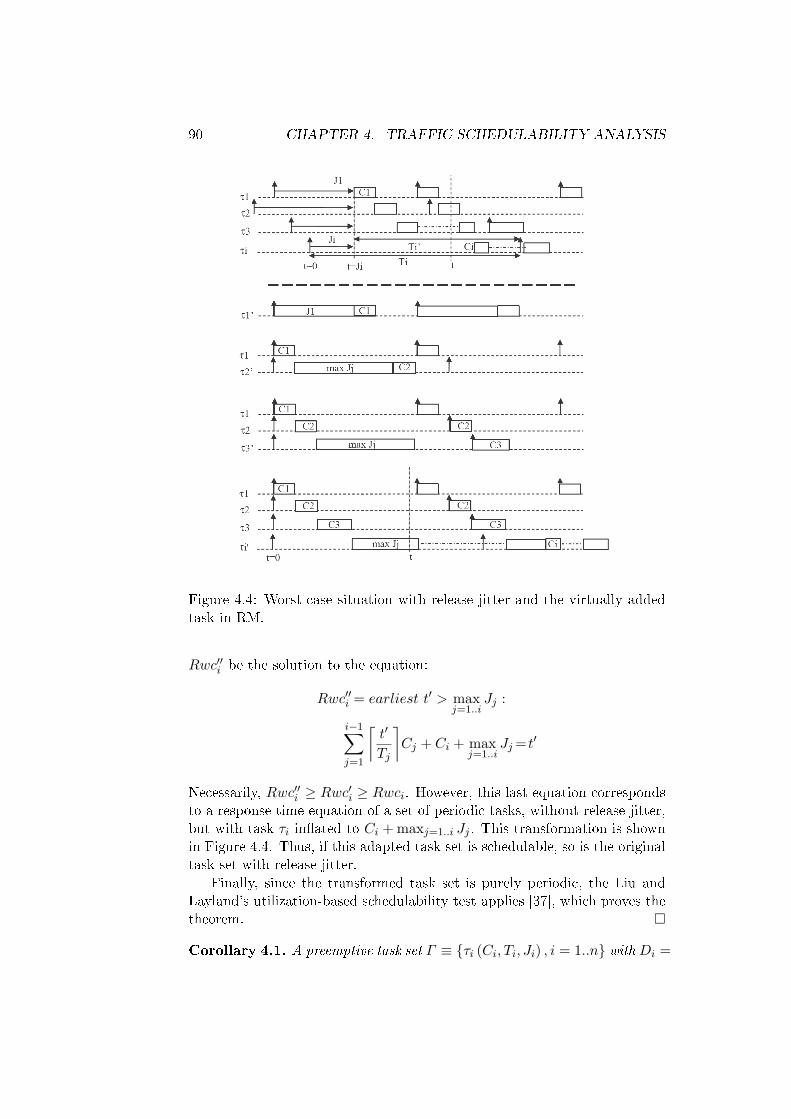
90 CHAPTER 4. TRAFFIC SCHEDULABILITY ANALYSIS
Figure 4.4: Worst-case situation with release jitter and the virtually addedtask in RM.
Rwc′′i be the solution to the equation:
Rwc′′i = earliest t′ > maxj=1..i
Jj :
i−1∑j=1
⌈t′
Tj
⌉Cj + Ci + max
j=1..iJj = t′
Necessarily, Rwc′′i ≥ Rwc′i ≥ Rwci. However, this last equation correspondsto a response time equation of a set of periodic tasks, without release jitter,but with task τi in�ated to Ci + maxj=1..i Jj . This transformation is shownin Figure 4.4. Thus, if this adapted task set is schedulable, so is the originaltask set with release jitter.
Finally, since the transformed task set is purely periodic, the Liu andLayland's utilization-based schedulability test applies [37], which proves thetheorem. �
Corollary 4.1. A preemptive task set Γ ≡ {τi (Ci, Ti, Ji) , i = 1..n} with Di =

4.4. SCHEDULABILITY TEST - UNICAST 91
Figure 4.5: Worst-case situation with release jitter and the virtually addedtask in EDF.
Ti is schedulable under RM if:
n∑i=1
CiTi
+maxi=1..n
Ji
T1≤ U lubRM (n) (4.7)
Proof: Just note that ∀i,maxj=1..i (Jj)/Ti ≤ maxj=1..n (Jj)/T1,
∀i, U lubRM (i) ≥ U lubRM (n)
�
Theorem 4.2. A preemptive task set Γ ≡ {τi (Ci, Ti, Ji) , i = 1..n} is schedu-lable under EDF if:
∀i=1..n
i∑j=1
CjTj
+maxj=1..i
Jj
Ti≤ U lubEDF = 1 (4.8)
Proof:With this model, the worst-case situation in terms of highest consecutive
processor demand also occurs in a similar manner as in the previous theorem[121]. The situation is also illustrated in Figure 4.5 (top), in which all tasks

92 CHAPTER 4. TRAFFIC SCHEDULABILITY ANALYSIS
are released as late as possible and all at the same instant. Let us de�nesuch instant as t = 0. Then, following a processor demand approach, thisset is schedulable if:
∀t, h(t) =∑
i:(Ti−Ji)≤t
⌊t+ JiTi
⌋Ci ≤ t
⇔ ∀t, h(t) + maxi=1..n
Ji ≤ t+ maxi=1..n
Ji
Now, let us carry out a scale shift making t′ = 0 coincide with theearliest virtual periodic arrival, i.e., t′ → t′ = t+ maxi=1..n Ji. The previousschedulability condition can be written as:
∀t′ , h(t′ − maxi=1..n
Ji) + maxi=1..n
Ji ≤ t′ ⇔
∑i:(Ti−Ji+ max
j=1..nJj)≤t′
t′−maxj=1..n
(Jj)+Ji
Ti
Ci + maxj=1..n
(Jj)≤ t′
Again, the sum is upper bounded by replacing Ji with maxj=1..n Jj . Thus,the following condition implies the previous one and still guarantees task setschedulability.
∀t′ ,∑i:T i≤t′
⌊t′
Ti
⌋Ci + max
j=1..n(Ji) ≤ t′
In order to obtain an utilization-based expression we divide both sides by t′
leading to:
∀t′ ,∑i:Ti≤t′
⌊t′
Ti
⌋Cit′
+maxj=1..n
(Ji)
t′≤ 1
Observe that,⌊t′
Ti
⌋≤ t′
Ti⇒⌊t′
Ti
⌋Cit′≤ C ′i
t′∗ t′
Ti=C ′iTi
(asC ′it′≥ 0)
Therefore, the term inside the sum is upper bounded by Ci/Ti. Thus,the following condition also implies the previous and still guarantees task setschedulability.
∀t′ ,∑i:T i≤t′
CiTi
+maxj=1..n
(Ji)
t′≤ 1
This condition needs to be evaluated at the instants in which t′ is an integermultiple of any of the tasks periods. This is particularly relevant for T1 ≤t′ ≤ Tn. Within this interval, each time t′ reaches the �rst period of anytask, say τi, the corresponding term Ci/Ti is included in the sum. At thesame time, the term maxj=1..n Jj/Ti becomes lower as i grows since the set

4.4. SCHEDULABILITY TEST - UNICAST 93
timeTi
Ci
Jj
Figure 4.6: Interfering task.
is sorted by ascending periods. For t′ > Tn, the left term in the conditiondecreases monotonically and the condition is trivially veri�ed if it was veri�edin the previous interval. �
Corollary 4.2. A preemptive task set Γ ≡ {τi (Ci, Ti, Ji) , i = 1..n} is schedu-lable under EDF if:
n∑i=1
CiTi
+maxi=1..n
Ji
T1≤ U lubEDF = 1 (4.9)
Proof: Again just note that
∀i, maxj=1..i
(Jj)/Ti ≤ maxj=1..n
(Jj)/T1
�
4.4.4 Upper bounding the indirect load
Inequalities 4.6 and 4.8, for RM and EDF respectively, are computed con-sidering the real load directly obtained from each task utilization load andthe indirect load that represents the interference. The latter term is not as-sessed using each task utilization load though. For this reason, the followingproposed test aims at upper bounding this indirect load in a way to becomeutilization-based.
The indirect load in Inequalities 4.6 and 4.8 is equivalent to the impactof an additional task with a load given by U indi (Equation 4.10).
U indi =maxj=1..i
Jj
Ti, ∀i = 1..n
= maxj=1..i
JjTi
(4.10)
For simplicity let U indi,j =JjTi
be the interference caused by the jth task
(τj) in τi. Figure 4.6 illustrates one such task for which the load is U indi,j .Coming back to the switch case, remember that the release jitter that
a�ects message mj in its downlink is a consequence of messages in the same

94 CHAPTER 4. TRAFFIC SCHEDULABILITY ANALYSIS
uplink that are transmitted to other downlinks. Call CRM and CEDF the setof such messages for RM and EDF scheduling, respectively. For each case,we can also express Jj as the sum of the transmission times of the interferingmessages leading to an indirect load that can be expressed as in Equation4.11 and 4.12 for RM and EDF, respectively.
U indRMi,j =
∑CRM
⌈JjTk
⌉Ck
Ti, where CRM ≡ ∀mk :
Sk=Sj
Rk 6=Rjk<j
(4.11)
U indEDFi,j =
∑CEDF
⌈JjTk
⌉Ck
Ti, where CEDF ≡ ∀mk :
{Sk=Sj
Rk 6=Rj(4.12)
Knowing that Jj < Ti − Ci < Ti an upper bound to the interfering loadis given by Equation 4.13, as follows 1:
U indi,j <
∑⌈TiTk
⌉Ck
Ti
<
∑(TiTk
+ 1)Ck
Ti=∑ Ck
Tk+∑ Ck
Ti⇔
U indi,j <∑
Uk +∑ Ck
Ti(4.13)
Thus, we obtain the schedulability test for RM and EDF given by In-equalities 4.14 and 4.15 that must be conducted to each message mi of agiven downlink.
RM:
∀i=1..n
i∑j=1
Uj + maxj=1..i
(∑CRM
Uk +∑CRM
CkTi
)≤ U lubRM (i) (4.14)
EDF:
∀i=1..n
i∑j=1
Uj + maxj=1..i
( ∑CEDF
Uk +∑
CEDF
CkTi
)≤ U lubEDF (i) (4.15)
This test, that requires the veri�cation of n conditions, can be simpli�edto one condition, only, upper bounding the terms in the sums leading to a
1For the sake of clarity we omit the indexes in the sums.
4.5. SIMULATION RESULTS 95
pair of tests, for RM and EDF, that contain one single condition, Equations4.16 and 4.17.
RM:
∑mi∈ldj
Uj + maxmi∈ldj
(∑CRM
Uk
)+
maxmi∈ldj
(∑CRM
Ck
)T1
≤ U lubRM (i) (4.16)
EDF:
∑mi∈ldj
Uj + maxmi∈ldj
( ∑CEDF
Uk
)+
maxmi∈ldj
( ∑CEDF
Ck
)T1
≤ U lubEDF (i) (4.17)
These tests only contain additive utilization terms that particularly wellsuited to our purpose of supporting dynamic QoS management. In orderto use these terms in FTT-SE we just need to include the idle time com-pensation factors in the right side of the inequalities, and replace the lowercondition in 4.5.
4.5 Simulation results
The previous analysis provides the conditions to assess the schedulability ofthe tra�c submitted to the switch. However, the conditions contain severalapproximations that introduce a non-negligible level of pessimism. In orderto validate the analysis and develop a notion of the pessimism embedded inthese schedulability tests we carried out simulations with randomly generatedtra�c. For each generated set, it is veri�ed whether the set passes theschedulability tests and if so, the message set is submitted to the schedulingsimulator that runs for the LCM of the message periods to determine theset schedulability (note that simulations consider a synchronous release).
The message sets are pseudo-randomly generated with a load aroundthe theoretical schedulability bound, in order to have schedulable and non-schedulable sets. The pseudo-random generation uses the following param-eters:
• 4 ports switch with 100 Mbps links• Packet length uniformly distributed within [100 1500] bytes• EC of 1ms• Periods uniformly distributed within [1, 5] ECs• Unicast messages, only• 1, 2 or 3 destinations per uplink (source)• Scheduling with EDF and RM
96 CHAPTER 4. TRAFFIC SCHEDULABILITY ANALYSIS
• Inserted idle time compensation factor of 88% (already including EClength, TM transmission, turnaround, and maximum packet length)• 200000 points per utilization point in the graphs in the part whereschedulability starts to reduce.
The theoretical tests in Equations 4.5 and the extension to the down-link test in Equations 4.16 and 4.17 compare the tra�c utilization with theEDF or RM utilization bounds. The simulation procedures di�er only inthe pseudo-random generator that for each case generates message/task setsaround the respective schedulability limits.
For the sake of clarity, note that the designation virtual load is de�nedin the downlinks to include real load plus the interference load given by
maxmi∈ldj
( ∑CRM,EDF
Uk
)+
maxmi∈ldj
( ∑CRM,EDF
Ck
)T1
,
in Equations 4.16 and 4.17. For simplicity, let us extend this designation tothe uplinks in which case virtual load coincides with the real load. The switchlinks, either uplinks or downlinks, can now be analyzed inter-changeably withthe same per link utilization limit U lub. The virtual load is the per link loadused to verify the schedulability in the uplinks and downlinks on each of theswitch ports (4 ports in this simulation scenario).
Each message set was generated computing random messages that weresequentially added to the set while keeping the virtual load on each linkunder a given value, lets say x Mbps. New messages were continuouslyadded until there were 1000 consecutive failed attempts,i.e., attempts thatcause an excess to the desired load. This guarantees that the virtual loadgenerated in any link is no more that x Mbps and yet very close to thatlimit on most of the links, mainly in the downlinks that tend to reach thelimit before, given the interference load. In fact, the real tra�c load on thedownlinks is much lower than the corresponding virtual load.
The generated sets were simulated with synchronous release during LCMof the periods and the percentage of schedulable sets was plotted as a functionof the maximum virtual load (x Mbps). The following plots were obtainedforcing the maximum allowed virtual load per link. They also show the Liuand Layland schedulability bounds for RM and EDF, after the inserted idletime compensation factor, which become 61% and 88%, respectively. Notethat the analysis only guarantees positive scheduling results when the vitualload in all links is below these thresholds. The points of virtual load largerthan the schedulability bounds with 100% schedulable sets is a measure ofthe pessimism that is implicit in the analysis.
Figure 4.7 shows the case of one destination per source, i.e., messagesfrom one uplink go all to the same downlink, for which schedulability test in
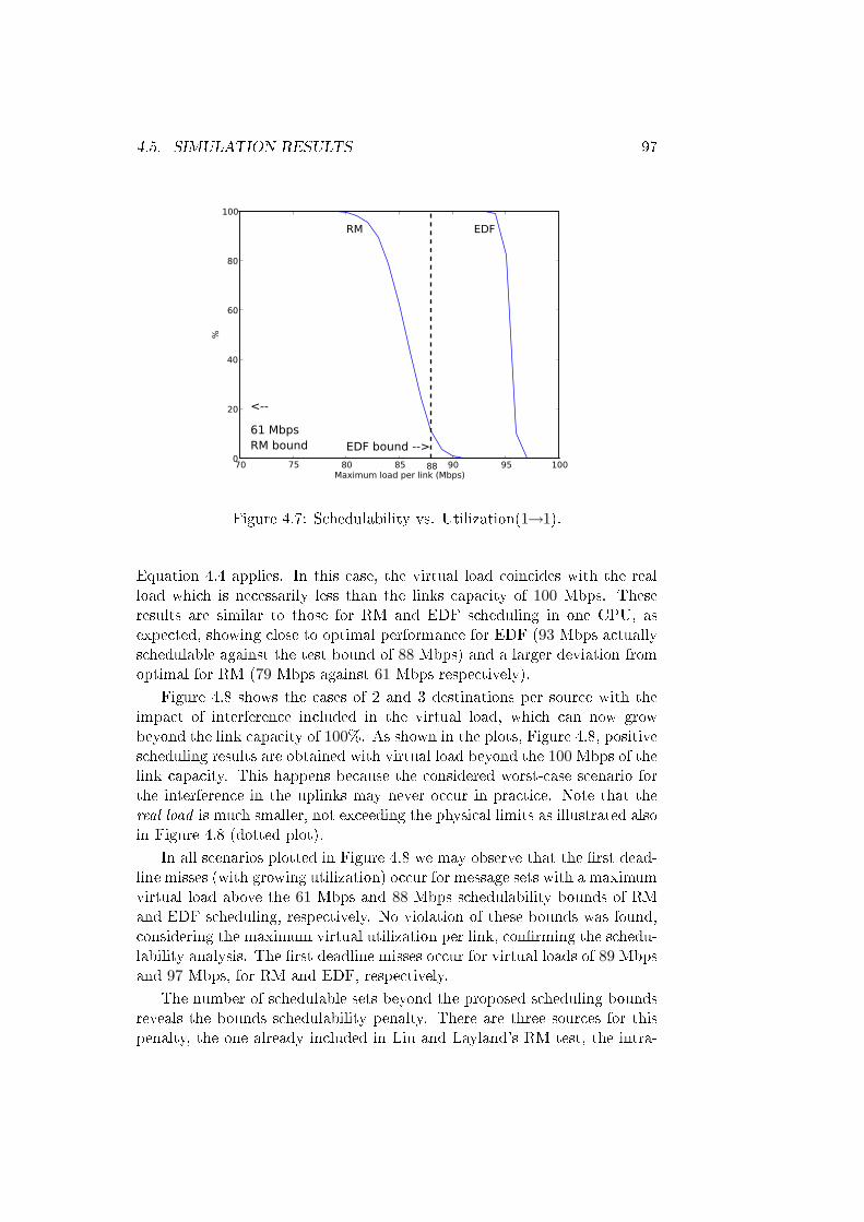
4.5. SIMULATION RESULTS 97
70 75 80 85 90 95 100Maximum load per link (Mbps)
0
20
40
60
80
100%
EDF bound -->
<--
61 MbpsRM bound
88
RM EDF
Figure 4.7: Schedulability vs. Utilization(1→1).
Equation 4.4 applies. In this case, the virtual load coincides with the realload which is necessarily less than the links capacity of 100 Mbps. Theseresults are similar to those for RM and EDF scheduling in one CPU, asexpected, showing close to optimal performance for EDF (93 Mbps actuallyschedulable against the test bound of 88 Mbps) and a larger deviation fromoptimal for RM (79 Mbps against 61 Mbps respectively).
Figure 4.8 shows the cases of 2 and 3 destinations per source with theimpact of interference included in the virtual load, which can now growbeyond the link capacity of 100%. As shown in the plots, Figure 4.8, positivescheduling results are obtained with virtual load beyond the 100 Mbps of thelink capacity. This happens because the considered worst-case scenario forthe interference in the uplinks may never occur in practice. Note that thereal load is much smaller, not exceeding the physical limits as illustrated alsoin Figure 4.8 (dotted plot).
In all scenarios plotted in Figure 4.8 we may observe that the �rst dead-line misses (with growing utilization) occur for message sets with a maximumvirtual load above the 61 Mbps and 88 Mbps schedulability bounds of RMand EDF scheduling, respectively. No violation of these bounds was found,considering the maximum virtual utilization per link, con�rming the schedu-lability analysis. The �rst deadline misses occur for virtual loads of 89 Mbpsand 97 Mbps, for RM and EDF, respectively.
The number of schedulable sets beyond the proposed scheduling boundsreveals the bounds schedulability penalty. There are three sources for thispenalty, the one already included in Liu and Layland's RM test, the intra-
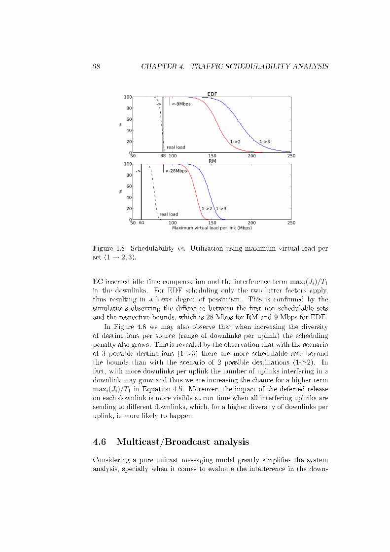
98 CHAPTER 4. TRAFFIC SCHEDULABILITY ANALYSIS
50 100 150 200 2500
20
40
60
80
100
%
88
1->2 1->3real load
-> <-9Mbps
EDF
50 100 150 200 250Maximum virtual load per link (Mbps)
0
20
40
60
80
100
%
61
1->2 1->3real load
-> <-28Mbps
RM
Figure 4.8: Schedulability vs. Utilization using maximum virtual load perset (1→ 2, 3).
EC inserted idle time compensation and the interference term maxi(Ji)/T1
in the downlinks. For EDF scheduling only the two latter factors apply,thus resulting in a lower degree of pessimism. This is con�rmed by thesimulations observing the di�erence between the �rst non-schedulable setsand the respective bounds, which is 28 Mbps for RM and 9 Mbps for EDF.
In Figure 4.8 we may also observe that when increasing the diversityof destinations per source (range of downlinks per uplink) the schedulingpenalty also grows. This is revealed by the observation that with the scenarioof 3 possible destinations (1->3) there are more schedulable sets beyondthe bounds than with the scenario of 2 possible destinations (1->2). Infact, with more downlinks per uplink the number of uplinks interfering in adownlink may grow and thus we are increasing the chance for a higher termmaxi(Ji)/T1 in Equation 4.5. Moreover, the impact of the deferred releaseon each downlink is more visible at run-time when all interfering uplinks aresending to di�erent downlinks, which, for a higher diversity of downlinks peruplink, is more likely to happen.
4.6 Multicast/Broadcast analysis
Considering a pure unicast messaging model greatly simpli�es the systemanalysis, specially when it comes to evaluate the interference in the down-
4.7. CONCLUSION 99
links. When considering a multicast or broadcast scenario, the tra�c inter-ference observed in the downlinks is due to other tra�c patterns triggered tothe respective uplinks, as well to tra�c issued to downlinks, other than theone in analysis. The reason is that all transmissions in all involved downlinksmust occur in the same EC.
Referring to the downlinks analysis test within the unicast model, whenit comes to include the interference as release jitter, it is considered themaximum possible jitter generated on each of the uplinks. In the multicastscenario however, evaluating the jitter is not as simple. In this case, the jit-ter must include the interference within the uplinks, which may additionallysu�er interference related to the scheduling on other downlinks and recur-rently other uplinks. This recurrent procedure may reach high complexitylevels that vary with the system scale and with the message dependenciesacross the resource components used (uplinks and downlinks).
The strong penalty that this kind of tra�c can have was already illus-trated in Section 3.5.1 in Figure 3.11. In the limit, if usinf only broadcastmessages, the throughput of the switch is reduced to that of a single link.The analysis for this situation is out of the scope of this thesis.
4.7 Conclusion
In order to support e�ciently dynamic QoS distribution, the FTT-SE frame-work needs a fast schedulability analysis tool that provides operational bounds,supporting quantitative information on the amount of free resources. Oftenassociated to the periodic activation model, utilization-based tests are onepossible choice to meet such requirements.
However, on switched Ethernet, the switch queues introduce distortionto the periodic model and so the well known utilization-based analysis doesnot directly apply. This chapter addressed this topic and proposed a newschedulability test based on the well known utilization bounds for EDF andRM preemptive scheduling. These tests have very low time complexity andcan be performed online in dynamic environments. Another property of thisanalysis is the ability to consider the links as di�erent resources. These prop-erties make this analysis an important building block to support dynamicQoS management. However, due to the large complexity of analyzing themulticast/broadcast transmissions, only the unicast transmission model wasanalyzed and validated with simulations. The former models are left forfuture work.
This theoretical work, for the schedulability test that includes consideringthe interference on a periodic message caused by release jitter is general andapplicable to the FTT-SE framework as well as to a set of periodic tasksscheduled preemptively with RM or EDF and su�ering release jitter. Theexact-case characterization of the proposed analysis and comparison with

100 CHAPTER 4. TRAFFIC SCHEDULABILITY ANALYSIS
other known ones, such as response time based tests, is also left for futurework.
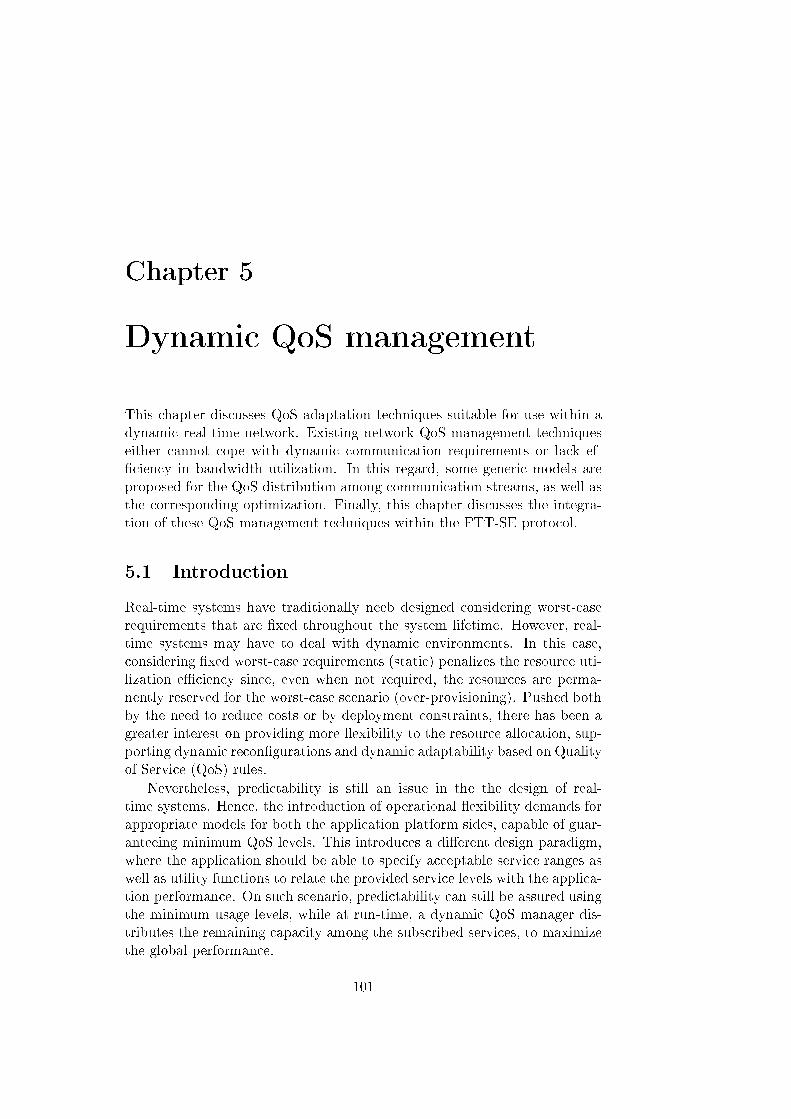
Chapter 5
Dynamic QoS management
This chapter discusses QoS adaptation techniques suitable for use within adynamic real-time network. Existing network QoS management techniqueseither cannot cope with dynamic communication requirements or lack ef-�ciency in bandwidth utilization. In this regard, some generic models areproposed for the QoS distribution among communication streams, as well asthe corresponding optimization. Finally, this chapter discusses the integra-tion of these QoS management techniques within the FTT-SE protocol.
5.1 Introduction
Real-time systems have traditionally neeb designed considering worst-caserequirements that are �xed throughout the system lifetime. However, real-time systems may have to deal with dynamic environments. In this case,considering �xed worst-case requirements (static) penalizes the resource uti-lization e�ciency since, even when not required, the resources are perma-nently reserved for the worst-case scenario (over-provisioning). Pushed bothby the need to reduce costs or by deployment constraints, there has been agreater interest on providing more �exibility to the resource allocation, sup-porting dynamic recon�gurations and dynamic adaptability based on Qualityof Service (QoS) rules.
Nevertheless, predictability is still an issue in the the design of real-time systems. Hence, the introduction of operational �exibility demands forappropriate models for both the application platform sides, capable of guar-anteeing minimum QoS levels. This introduces a di�erent design paradigm,where the application should be able to specify acceptable service ranges aswell as utility functions to relate the provided service levels with the applica-tion performance. On such scenario, predictability can still be assured usingthe minimum usage levels, while at run-time, a dynamic QoS manager dis-tributes the remaining capacity among the subscribed services, to maximizethe global performance.
101
102 CHAPTER 5. DYNAMIC QOS MANAGEMENT
The focus of this work is on studying such dynamic QoS managementschemes, given the requirements for operational �exibility. In this regard,several distribution models are presented and compared according to theircomputational complexity. While some of the results are generic, the workherein presented is mainly focused on the FTT-SE framework, addressed inthis thesis. Therefore, the QoS models and distribution schemes are pre-sented within this framework.
5.2 The QoS management problem
Consider a system composed of several subsystems that compete for theaccess to system resources, e.g., network links or nodes CPUs. For a broadrange of applications of this kind there is a direct relationship between theamount of resources allocated to the application services and their individualperformance. This is the case of many control systems in which, withincertain limits, higher sampling frequencies and thus higher CPU utilizationand network bandwidth in distributed architectures, provide a better controlquality (lower error, more stable control signals,...)[29].
A natural and simple solution for the resource capacity distribution wouldbe to give maximum service level to each of the service subsystems involved.However, if done without control, it would eventually end up with an overloador a worst-case situation. If the system becomes overloaded, ultimately, theservices get degraded in an uncontrolled manner, which is not acceptable inmost systems.
Another simple approach would be to give only the minimum possibleservice level to each subsystem. In this case, it is possible to have a situationwhere there are available resources that are not allocated to subsystems thatcould take advantage of them, thus the global application performance issub-optimal.
A third option can be followed by enforcing service degradation in acontrolled manner. Modeling the services with QoS ranges allows managingthe QoS degradation of each speci�c service with respect to its maximumrequirements in order to maximize the overall resource usage and assure thesystem correctness. Along with this model, it is essential the deployment ofproper management policies with speci�c strategies regarding the resourcecapacity distribution.
This section describes such resource capacity distribution strategy basedon Quality of Service management rules associated to the service model. Yet,one question raises:
What exactly do we mean by Quality of Service?
Quality of Service (QoS), in a broader sense, is a measure of the perfor-mance level provided by a generic server. The term is sometimes confused
5.2. THE QOS MANAGEMENT PROBLEM 103
with service quality, which more closely refers to the quality experienced bythe user [64]. QoS frequently denotes a more precise and objective measure,usually associated to a negotiation contract between a service vendor andthe respective client [50].
There are di�erent metrics to measure the QoS level, varying with the ap-plication class and purpose. For example, in generic processing it is commonhaving, for general purpose jobs, metrics that minimize the time by which ajob is delayed, or in control-oriented applications metrics that minimize thesampling execution jitter.
In the communication networks domain, a direct relationship is com-monly established between the service bandwidth and the QoS delivered.For example, in video streaming, within certain limits, higher bandwidthresults in higher user perceived quality or Quality of Experience [55].
The role of the QoS manager comprehends the coordination and manage-ment of all resource parameters that play actively in the QoS level. In thenetworking domain, it includes the management of the communications load,that must be kept within the network capacity, and the tra�c scheduling.
In real-time systems, the QoS guarantees come along with the abilityto meet the timeliness constraints set within the service description model.Those guarantees are the result of a schedulability analysis performed at theadmission phase. The role of a QoS manager on such a real-time network isthen focused on the bandwidth distribution and enforcing QoS di�erentiationbetween the services, while maximizing the global system performance [39].
For the networking and multimedia communities the QoS management isoften considered a service broker [93] that analyzes the resource status andaccepts or rejects a service request with a given QoS level. Several negotia-tion protocols are example of this, Di�Serv [94], IntServ [36] or RSVP [136].These approaches however, do �xed provisioning of network resources at ser-vice startup that remains constant for the service duration, thus resulting ina �xed QoS. If a QoS variability range is considered in the reservation con-tract, de�ning when the service is practicable, it becomes possible adjusting,at run-time, the QoS of currently active services in order to better accom-modate more service requests and maximize the throughput of the resource[65]. This is hereby designated as dynamic QoS management.
Notwithstanding, the following question raises:
When free network bandwidth is available, how to distribute itamong the current services?
And conversely:
When the network bandwidth is overloaded, how to manage theQoS degradation of current services, needed to eliminate the over-load?

104 CHAPTER 5. DYNAMIC QOS MANAGEMENT
These are two perspectives of the same problem: the QoS distributionamong a set of services that individually seek for the best QoS, within theresource capacity.
This work focuses on online QoS management schemes for dynamic net-worked environments. This imposes a constraint since the QoS algorithmsmust be su�ciently fast to enable fast adaptation.
5.2.1 The resource capacity
Resource capacity is one key property of a shared resource. It de�nes theresource sharing limits for providing services. Communication networks areresources which the capacity limit is given by the maximum data they cantransmit per time unit, i.e., the network bandwidth. However, the use ofspeci�c scheduling models poses additional constraints that may reduce suchcapacity.
A scheduler is an important piece in the resource management, being re-sponsible for temporally organizing the execution of services in the resource,given the services run-time constraints. It is thus an integral and determi-nant component for the system analyzability.
The schedulability test conducted within the system analysis phase ulti-mately determines whether a service is admitted or not, which thus meansthat this test is based on the de�nition of the resource capacity.Schedulabilitytests can be more or less accurate and complex.Usually, there is an interde-pendency between the test accuracy and the associated computational com-plexity. More accurate tests often imply higher computational overhead, e.g.tests that mimic the scheduler execution or perform a response time analysis.Pessimism is sometimes the price to pay for a faster analysis, meaning teststhat are just su�cient, thus potentially rejecting services QoS combinationsthat would be schedulable.
Dynamic real-time systems often require a bounded response time tothe system modi�cation requests. Hence, the amount of time spent in thisprocess must be as low as possible. In a QoS management procedure, thistime must allow quantifying the amount of available resource and �nding aresource distribution that leads to a global utilization as large as possibleand is schedulable.
Therefore the scheduling analysis must rely on a per service metric thatrepresents simultaneously the quality-level and the respective share of theresource capacity. This direct relationship between the quality-level and theshare of the resource capacity with an appropriate schedulability test, assuresthe system correct behavior.
Resources such as networks or processors commonly make use of sched-ulers with feasibility tests that de�ne bandwidth bounds as guarantees forthe system schedulability. Hence, as long as the resource utilization loadstays within those limits, the system schedulability is assured. In this case
5.2. THE QOS MANAGEMENT PROBLEM 105
the resource capacity may be de�ned as that schedulability utilization bound.Then, the bandwidth distribution mechanism becomes independent from theschedulability test that is implicitly enforced by using a resource capacityequal to that bound.
5.2.2 The application model
Dynamically changing the quality level of a service requires a tight coopera-tion with the application. For example, if in a video surveillance applicationthe bandwidth allocated to a given stream is suddenly reduced, the applica-tion has to adapt accordingly, e.g. by reducing the frame-rate or increasingthe compression factor.
Therefore, a re�exive model is needed according to which the resourceinforms the application of its current QoS level allowing the application toadjust to it.
Such model is compatible with a �exible use of the resource and it allowsthe application to operate with di�erent requirements and adapt online. Inthis regard, the application services are categorized in two classes, the inelas-tic services that only operate under �xed requirements and the elastic onesthat operate with di�erent con�gurations within a prede�ned requirementsrange [39].
For the elastic class of services, several service/task models have beenproposed toward the extension of the timing requirements beyond the usualhard and soft real-time, based on the assumption that services can have theirperformance degraded without jeopardizing the application. Generically, themodel speci�es the services with minimum requirements, i.e., least requiredQoS, which are granted once the service is admitted. The quality level maythen be improved depending on the resource availability given the otheradmitted services that compete for the shared resource.
Chapter 2 described several of these models in detail. Some of themare based on the enforcement of speci�c job skipping patterns to alleviatethe system load when in overload. For example a control system can skipcycles occasionally or a video transmission that can skip frames. However,these models cause a sudden drop in the instantaneous QoS provided to theapplication whenever a skip is done that might produce undesired e�ects.Moreover, there is not a univocal and direct relationship between the cho-sen skipping patterns and the QoS that is obtained [42]. Additionally, theschedulability analysis techniques become computationally heavier as theyrequire a careful analysis of the patterns and the impact of the interference.
Therefore, other techniques have been proposed to distribute the resourcecapacity based on the utilization load, mostly by changing the tasks periods.These schemes aim at providing a fair and correct bandwidth distribution ofthe resource. However, they are either speci�c to a QoS metric, or require acomplex and computationally heavy structure, a problem aggravated by the

106 CHAPTER 5. DYNAMIC QOS MANAGEMENT
fact that in some cases it is necessary to manage multiple resources, thusa multi-dimensional problem. Similarly to the elastic task model (ETM)proposed by Butazzo et. al. [38], we propose several QoS distribution modelsthat use the bandwidth as the di�erentiation metric. However, our proposalgoes beyond the speci�c ETM model that uses a single distribution model tomanage the tasks periods since we allow an integrated management of bothperiods and execution times.
Another important aspect to add relates to the de�nition of the operat-ing range. The proposed schemes de�ne a continuous bandwidth range, orperiod range in the ETM, wherein the application operates. However, someapplications pose additional constraints to the operating range, for exam-ple being only able to operate with discrete bandwidth values. Example ofthis are video cameras that sometimes operate under certain speci�c framesizes and frame rates. This topic is further detailed in Section 5.4, wherethe application service model is extended to include a discrete model thatde�nes multiple operating points. For now, consider the existence of a validcontinuous bandwidth range describing the minimum and the maximum (orpreferred) requirements.
Let St denote the set of services concurring for a resource R and URdenote the resource capacity.
St ≡ {Sti (Umini , Ulaxi , qosi) , i = 1..n}
Each service Sti de�nes a minimum bandwidth Umini , maximum band-width (Umini +Ulaxi) and importance, qosi. The system integrity is assuredas long as the minimums �t the resource capacity, de�ned within the schedu-lability analysis, i.e.,
∑ni=1 Umini ≤ UR. After distributing those minimums,
the remaining bandwidth Uspare is available to be distributed by the QoSmanager, being given by:
Uspare = UR −n∑i=1
Umini (5.1)
The resource is overloaded when the services maximum load exceeds theresource capacity, i.e.,
∑ni=1 Ulaxi > Uspare, leading to a lack of bandwidth
given by:
Uspare =n∑i=1
Ulaxi − Uspare (5.2)
Figure 5.1 depicts the distribution model for two concurrent services St1and St2. Ulax1 and Ulax2 represent the bandwidth �exible part of each serviceand Uspare the resource bandwidth that remains free for distribution.
The distribution problem is now reduced to distribute Uspare by the ser-vices given their Ulaxi operating ranges. In many applications, di�erent
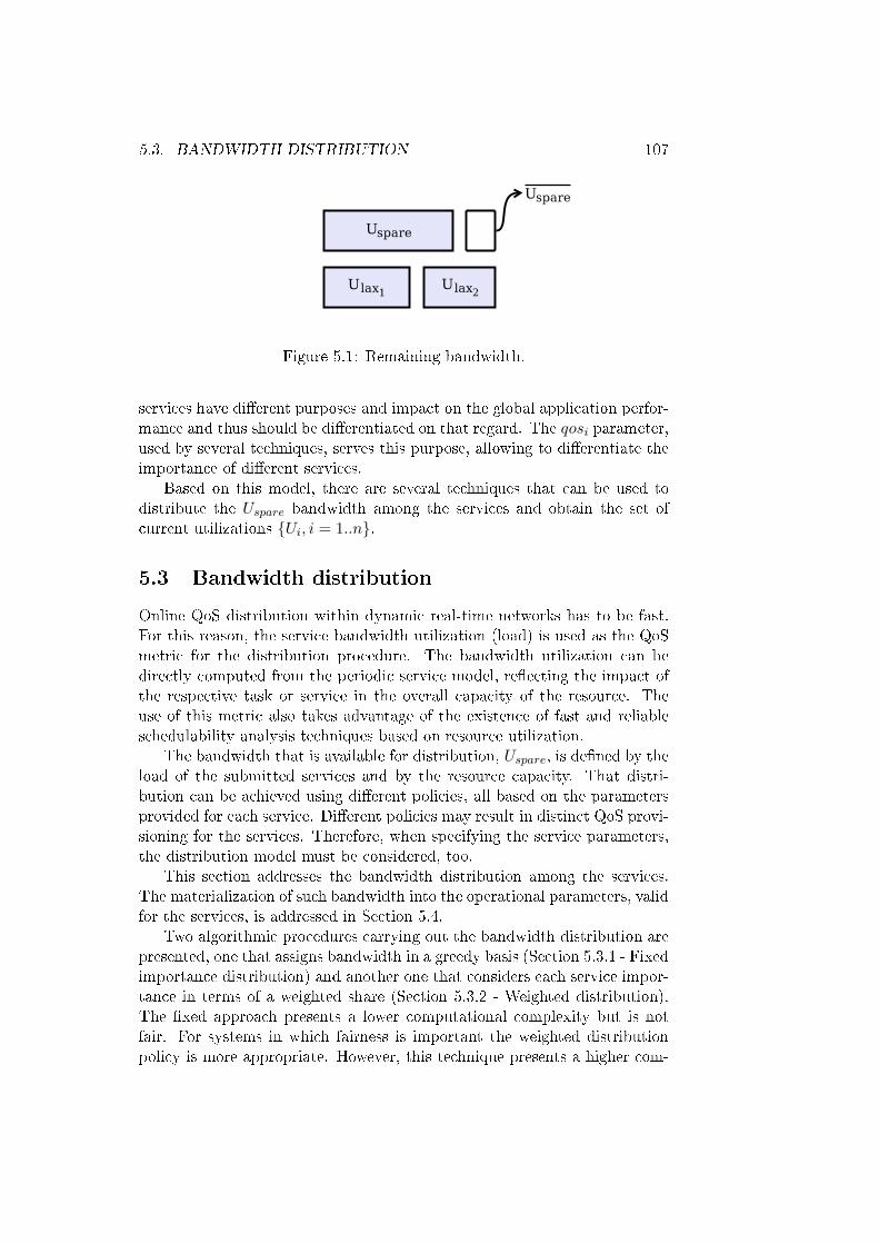
5.3. BANDWIDTH DISTRIBUTION 107
Figure 5.1: Remaining bandwidth.
services have di�erent purposes and impact on the global application perfor-mance and thus should be di�erentiated on that regard. The qosi parameter,used by several techniques, serves this purpose, allowing to di�erentiate theimportance of di�erent services.
Based on this model, there are several techniques that can be used todistribute the Uspare bandwidth among the services and obtain the set ofcurrent utilizations {Ui, i = 1..n}.
5.3 Bandwidth distribution
Online QoS distribution within dynamic real-time networks has to be fast.For this reason, the service bandwidth utilization (load) is used as the QoSmetric for the distribution procedure. The bandwidth utilization can bedirectly computed from the periodic service model, re�ecting the impact ofthe respective task or service in the overall capacity of the resource. Theuse of this metric also takes advantage of the existence of fast and reliableschedulability analysis techniques based on resource utilization.
The bandwidth that is available for distribution, Uspare, is de�ned by theload of the submitted services and by the resource capacity. That distri-bution can be achieved using di�erent policies, all based on the parametersprovided for each service. Di�erent policies may result in distinct QoS provi-sioning for the services. Therefore, when specifying the service parameters,the distribution model must be considered, too.
This section addresses the bandwidth distribution among the services.The materialization of such bandwidth into the operational parameters, validfor the services, is addressed in Section 5.4.
Two algorithmic procedures carrying out the bandwidth distribution arepresented, one that assigns bandwidth in a greedy basis (Section 5.3.1 - Fixedimportance distribution) and another one that considers each service impor-tance in terms of a weighted share (Section 5.3.2 - Weighted distribution).The �xed approach presents a lower computational complexity but is notfair. For systems in which fairness is important the weighted distributionpolicy is more appropriate. However, this technique presents a higher com-
108 CHAPTER 5. DYNAMIC QOS MANAGEMENT
putational complexity and may require an iterative procedure, discussed inSection 5.3.3, to converge to an optimal solution.
5.3.1 Fixed importance distribution
Perhaps the simplest and most direct policy to discriminate the services whenassigning free bandwidth is the one that, starting from the most important(highest qosi), sequentially concedes all the bandwidth that each one mayuse until exhausting the resource capacity. However, if the most importantservices drain all the spare bandwidth, the low rated services get no extrabandwidth share.
This model appears in resource management frameworks such as FRES-COR, see Section 6.1, where an importance parameter is included along withthe contract negotiation of each service. The FRESCOR framework furtherprovides a quality weight that di�erentiates services within the same impor-tance class, i.e., hierarchical composition of two distribution mechanisms.
5.3.2 Weighted distribution
The weighted distribution technique contrasts with the greedy technique byproviding a fair distribution based on weights. The weights are the applica-tion speci�cations and in�uence the bandwidth share obtained.
Each service weight wi is obtained through service application parame-ters, namely the qosi parameter and the bandwidth laxity parameter, Ulaxi .This section only covers the impact of using such weights. Section 5.3.4 ad-dresses the weights formulation based on the application parameters. Noticethough that we assume the weights to be normalized, i.e., given a set ofservices
∑i=1..nwi = 1.
After the distribution, a service i gets the bandwidth given by:
Uvi = Umini + Vi (5.3)
where Vi represents the share allocated to Sti from Uspare.Now, two bandwidth distribution mechanisms are presented:
• Direct Share, in which the services are given a direct weighted sharefrom Uspare (equation 5.4);
∀Sti : V ′i = w′i.Uspare (5.4)
• Indirect Share, where a weighted share of Uspare is taken from each ofthe Ulaxi (equation 5.5).
∀Sti ∈ St : V ′′i = Ulaxi − w′′i .Uspare (5.5)
= Ulaxi − w′′i .
n∑j=1
Ulaxj − Uspare
(5.6)
5.3. BANDWIDTH DISTRIBUTION 109
These are two bandwidth distribution schemes, with distinct mathemati-cal formulation, that fully distribute the resource capacity (Uspare), given theproper weights. However, each scheme perceives di�erently the weights andso produces distinct results. The wi weights have in fact opposite meaningsin the two schemes. While in Equation 5.4, w′i is proportional to the amountof resource that is granted to service i, in Equation 5.5, w′′i controls theamount of resource that is taken from the maximum resource requirements.Besides the semantic di�erence on the wi parameter, there is another, morefactual, di�erence between the direct and the indirect approaches. While inthe former one, the Ulaxi parameter has no in�uence on the resource distri-bution, besides constraining the maximum amount of the resource one canuse, in the latter approach, Ulaxi is a direct part of the equation, since it isthe baseline from which the bandwidth is taken, upon overload.
However, despite of the di�erences between both models it is still possi-ble to, from the application perspective, map the models one into the other.By putting both equations (5.4 and 5.5) together and assuming equal distri-bution results (V ′i = V ′′i ) leads to Equation (5.7) that maps w′′i into w′i.
w′i =UlaxiUspare
− w′′i .UspareUspare
(5.7)
Notwithstanding, from a design perspective, there are di�erences betweenthe models. The same variation on the weights results on di�erent distribu-tion, as can be easily shown by taking the respective derivatives (Equation5.8): ∣∣∣∣ δV ′iδw′i
∣∣∣∣ 6= ∣∣∣∣ δV ′′iδw′′i
∣∣∣∣ (5.8)
Therefore, despite the similarities, the two techniques are di�erent andare worth a separate analysis. Moreover, there are QoS distribution schemesin the literature, as mentioned further, that are based on both of theseschemes.
Both the direct and indirect approaches are formulated in terms of linearequations, which, at a �rst glance, makes these QoS distribution techniquesexhibit a low computational complexity (O(n)). However, the bandwidthspeci�cation is upper and lower bounded, and the distribution results ofequations 5.4 and 5.5 may fall o� those limits. Respectively, they may leadto situations where services receive an amount of bandwidth that exceeds orfalls bellow the minimum speci�ed requirements.
Optimality
As mentioned before, each service de�nes a range of allowed bandwidth val-ues. Assuming that the distribution procedure is optimal if the availablebandwidth is fully assigned, the direct application of equations 5.4 and 5.5
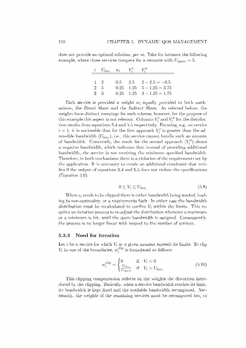
110 CHAPTER 5. DYNAMIC QOS MANAGEMENT
does not provide an optimal solution, per se. Take for instance the followingexample, where three services compete for a resource with Uspare = 5.
i Ulaxi wi V ′i V ′′i
1 2 0.5 2.5 2− 2.5 = −0.52 5 0.25 1.25 5− 1.25 = 3.753 3 0.25 1.25 3− 1.25 = 1.75
Each service is provided a weight wi equally provided to both mech-anisms, the Direct Share and the Indirect Share. As referred before, theweights have distinct meanings for each scheme, however, for the purpose ofthis example this aspect is not relevant. Columns V ′i and V
′′i list the distribu-
tion results from equations 5.4 and 5.5 respectively. Focusing, e.g. on servicei = 1, it is noticeable that for the �rst approach V ′i is greater than the ad-missible bandwidth (Ulaxi), i.e., this service cannot handle such an amountof bandwidth. Conversely, the result for the second approach (V ′′i ) showsa negative bandwidth, which indicates that instead of providing additionalbandwidth, the service is not receiving the minimum speci�ed bandwidth.Therefore, in both mechanisms there is a violation of the requirements set bythe application. It is necessary to create an additional constraint that veri-�es if the output of equations 5.4 and 5.5 does not violate the speci�cations(Equation 5.9).
0 ≤ Vi ≤ Ulaxi (5.9)
When vi needs to be clipped there is either bandwidth being wasted, lead-ing to non-optimality, or a requirements fault. In either case the bandwidthdistribution must be recalculated to con�ne Vi within the limits. This re-quires an iteration process to re-adjust the distribution whenever a maximumor a minimum is hit, until the spare bandwidth is assigned. Consequently,the process is no longer linear with respect to the number of services.
5.3.3 Need for iteration
Let i be a service for which Vi at a given moment exceeds its limits. To clipVi in one of the boundaries, wclipi is formulated as follows:
wclipi =
{0 if Vi < 0UlaxiUspare
if Vi > Ulaxi(5.10)
This clipping compensation re�ects on the weights the distortion intro-duced by the clipping. Basically, when a service bandwidth reaches its limit,its bandwidth is kept �xed and the available bandwidth recomputed. Nec-essarily, the weights of the remaining services must be recomputed too, to
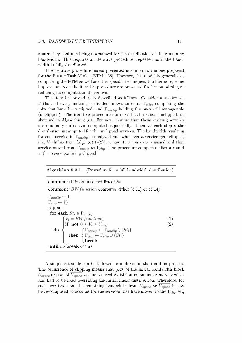
5.3. BANDWIDTH DISTRIBUTION 111
assure they continue being normalized for the distribution of the remainingbandwidth. This requires an iterative procedure, repeated until the band-width is fully distributed.
The iterative procedure herein presented is similar to the one proposedfor the Elastic Task Model (ETM) [38]. However, this model is generalized,comprising the ETM as well as other speci�c techniques. Furthermore, someimprovements on the iterative procedure are presented further on, aiming atreducing its computational overhead.
The iterative procedure is described as follows. Consider a service setΓ that, at every instant, is divided in two subsets: Γclip, comprising thejobs that have been clipped, and Γunclip holding the ones still manageable(unclipped). The iterative procedure starts with all services unclipped, assketched in Algorithm 5.3.1. For now, assume that those starting servicesare randomly sorted and computed sequentially. Then, at each step k thedistribution is computed for the unclipped services. The bandwidth resultingfor each service in Γunclip is analyzed and whenever a service gets clipped,i.e., Vi di�ers from (alg. 5.3.1-(2)), a new iteration step is issued and thatservice moved from Γunclip to Γclip. The procedure completes after a roundwith no services being clipped.
Algorithm 5.3.1: (Procedure for a full bandwidth distribution)
comment: Γ is an unsorted list of St
comment:BWfunction computes either (5.11) or (5.14)
Γunclip ← ΓΓclip ← {}repeatfor each Sti ∈ Γunclip
do
Vi = BWfunction() (1)if not 0 ≤ Vi ≤ Ulaxi (2)
then
Γunclip ← Γunclip \ {Sti}Γclip ← Γclip ∪ {Sti}break
until no break occurs
A simple rationale can be followed to understand the iteration process.The occurrence of clipping means that part of the initial bandwidth blockUspare or part of Uspare was not correctly distributed on one or more servicesand had to be �xed overriding the initial linear distribution. Therefore, foreach new iteration, the remaining bandwidth from Uspare or Uspare has tobe re-computed to account for the services that have moved to the Γclip set,
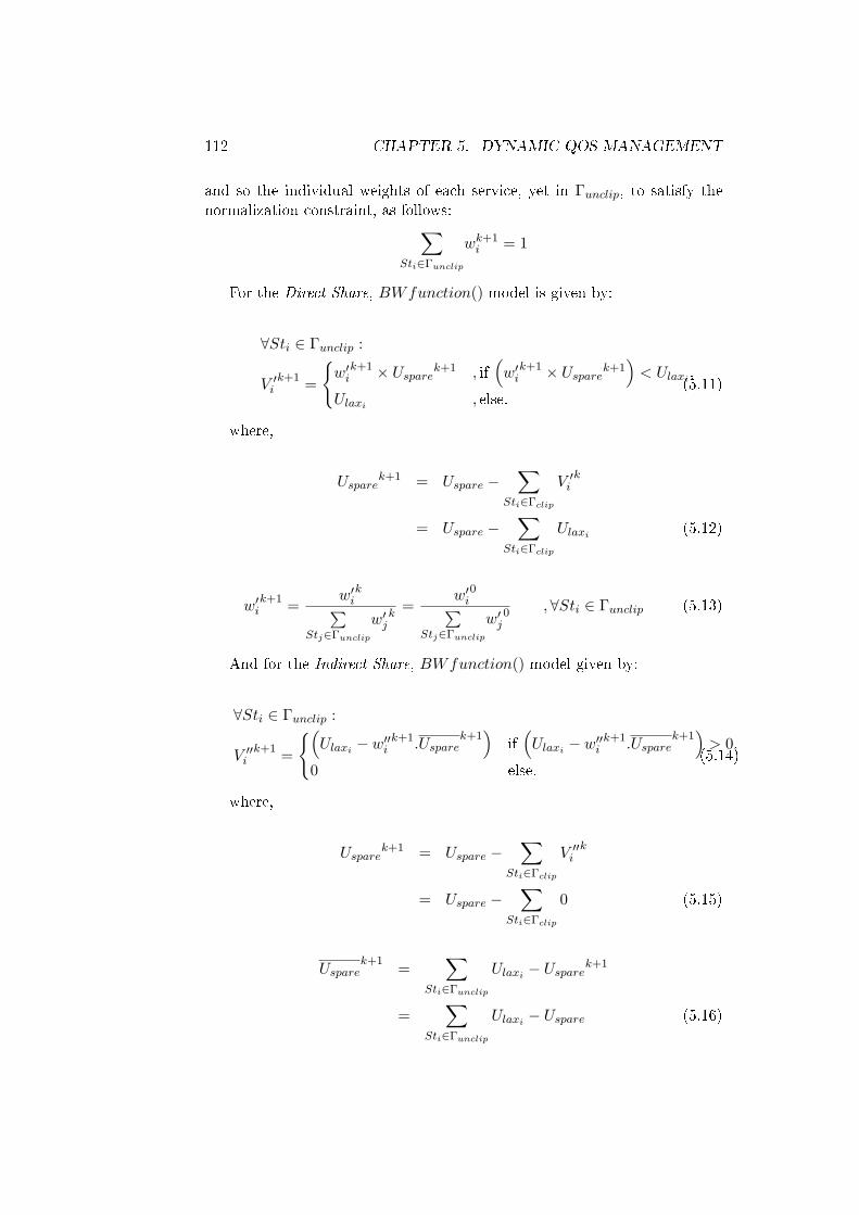
112 CHAPTER 5. DYNAMIC QOS MANAGEMENT
and so the individual weights of each service, yet in Γunclip, to satisfy thenormalization constraint, as follows:∑
Sti∈Γunclip
wk+1i = 1
For the Direct Share, BWfunction() model is given by:
∀Sti ∈ Γunclip :
V ′ik+1 =
{w′i
k+1 × Usparek+1 , if(w′i
k+1 × Usparek+1)< Ulaxi ,
Ulaxi , else.(5.11)
where,
Usparek+1 = Uspare −
∑Sti∈Γclip
V ′ik
= Uspare −∑
Sti∈Γclip
Ulaxi (5.12)
w′ik+1 =
w′ik∑
Stj∈Γunclip
w′jk
=w′i
0∑Stj∈Γunclip
w′j0 , ∀Sti ∈ Γunclip (5.13)
And for the Indirect Share, BWfunction() model given by:
∀Sti ∈ Γunclip :
V ′′ik+1 =
{(Ulaxi − w′′i
k+1.Usparek+1)
if(Ulaxi − w′′i
k+1.Usparek+1)> 0,
0 else.(5.14)
where,
Usparek+1 = Uspare −
∑Sti∈Γclip
V ′′ik
= Uspare −∑
Sti∈Γclip
0 (5.15)
Usparek+1 =
∑Sti∈Γunclip
Ulaxi − Usparek+1
=∑
Sti∈Γunclip
Ulaxi − Uspare (5.16)

5.3. BANDWIDTH DISTRIBUTION 113
w′′ik+1 =
w′′ik∑
Stj∈Γunclip
w′′jk
=w′′i
0∑Stj∈Γunclip
w′′j0 , ∀Sti ∈ Γunclip (5.17)
Equations 5.11 and 5.14 describe the bandwidth distribution for eachservice within an iteration step. Only unclipped services are computed. Theclipped services, remain constant through the rest of the procedure.
The unclipped weights are permanently modi�ed in each iteration, how-ever, as denoted by Equation 5.13 and 5.17, the weights can be assessedgiven the initial application weights and still re�ect the application speci�-cation. Thus, this process respects the relative importance of the servicesthroughout the iterative procedure.
Each wik+1 uniquely depends on the distribution status between Γclip
and Γunclip. Given k = m to be the last iteration, the weights in m are givenby:
wmi =wi∑
Stj∈Γunclip
wj,∀Sti ∈ Γunclip
These weights refer to the distribution of the bandwidth portion left forthe last iteration. Translating those �nal values into the scope of the initialUspare bandwidth, gives:
For the Direct Share model:
wfinali =
UlaxiUspare
, ∀Sti ∈ Γclip
wiPStj∈Γunclip
wj
(1−
∑Stj∈Γclip
wj
), ∀Sti ∈ Γunclip
(5.18)
And for the Indirect Share model:
wfinali =
0 ,∀Sti ∈ ΓclipwiP
Stj∈Γunclip
wj,∀Sti ∈ Γunclip (5.19)
Given this �nal distribution, the respective weights are still normalized:∑Sti∈Γunclip
wfinali +∑
Sti∈Γclip
wfinali = 1
Observing equations (5.18) and (5.19), the �nal weights regarding Uspare,do not depend on the procedure steps, but only on the result of the distri-bution between Γclip and Γunclip. This is important to understand that the

114 CHAPTER 5. DYNAMIC QOS MANAGEMENT
order by which the services are accounted for during the bandwidth distri-bution is irrelevant to the �nal result. However, it is still required to provethat the separation result between Γclip and Γunclip is unique given the initialparameters.
The following subsection shows such proof. Then, the bandwidth dis-tribution procedure is evaluated and ways to improve its performance arediscussed.
Existence of a unique solution
Theorem 5.1. There exists a unique solution to the bandwidth distributionproblem.
Proof. The solution generated by the bandwidth distribution procedure is ofthe format {Wclip,Wunclip}, where Wclip is the set of weights corresponding
to services (Sti ∈ Γclip) that have a �nal bandwidth share of (Uspare.wclipi ),
and Wunclip is the set of weights corresponding to services (Stj ∈ Γunclip)that have a �nal bandwidth share of (Uspare.w
unclipj ).
The sets are given by
Wclip = {wclipi : Sti ∈ Γclip} (5.20)
The remaining weights (1 −∑
Sti∈Γclipwclipi ) are shared proportionally
by the applications in Γunclip. The weights allocated to Γunclip are thereforegiven by:
Wunclip =
wj .
1−∑
Sti∈Γclip
wclipi∑Stp∈Γunclip
wp
: Stj ∈ Γunclip
(5.21)
As can be seen from the above expression, the weights in Γunclip areequally scaled by a factor of k, where k is given by,
k =
1−∑
Sti∈Γclip
wclipi∑Stp∈Γunclip
wp(5.22)
This value k is a �ngerprint of the solution to the bandwidth distri-bution problem. There is a one-to-one mapping between k and the sets{Wclip,Wunclip}. So far, it has been shown that given {Wclip,Wunclip} (Equa-tions 5.20 and 5.21), a �ngerprint k can be found (Equation 5.22). Now, itis shown the other way around, i.e., there cannot be two distribution resultswith the same k.

5.3. BANDWIDTH DISTRIBUTION 115
From the de�nitions of the sets {Wclip} and {Wunclip}, observe that
∀Sti ∈ Γclip : wi.k ≥ wclipi (5.23)
∀Stj ∈ Γunclip : wj .k < wclipj (5.24)
Also, ∑Sti∈Γclip
wclipi +∑
Stj∈Γunclip
wj .k = 1 (5.25)
We can observe a one-to-one mapping between the �ngerprint k and anysolution of the QoS maximization problem {Wclip,Wunclip}.
In order to prove the uniqueness of the solution, it is su�cient to provethe uniqueness of the �ngerprint.
Case 1: Assume that there exists a solution (k + δ), where δ > 0.Let the corresponding solution to the bandwidth distribution problem be{W ′clip,W ′unclip}.
In this case, the following relationships should also hold:
∀Sti ∈ Γ′clip : wi.(k + δ) ≥ wclipi (5.26)
∀Stj ∈ Γ′unclip : wj .(k + δ) < wclipj (5.27)
∑Sti∈Γ′clip
wclipi +∑
Stj∈Γ′unclip
wj .(k + δ) = 1 (5.28)
Observe that all services that satisfy Inequality 5.23 also satisfy the In-equality 5.26, hence
Γclip ⊂ Γ′clip (5.29)
Γclip = Γ′clip \ Sδ (5.30)
since Γclip is the complement of Γunclip,
Γunclip = Γ′unclip ∪ Sδ (5.31)
Γ′unclip ⊂ Γunclip (5.32)
Sδ ⊂ Γunclip (5.33)

116 CHAPTER 5. DYNAMIC QOS MANAGEMENT
Rewriting (5.25), gives∑Sti∈(Γ′clip−Sδ)
wclipi +∑
Stj∈(Γ′unclip+Sδ)
wj .k = 1 (5.34)
∑Sti∈Γ′clip
wclipi −∑
Stp∈Sδ
wclipp +∑
Stj∈Γ′unclip
wj .k +∑
Stq∈Sδ
wq.k = 1 (5.35)
Subtracting (5.28), gives
−∑
Stp∈Sδ
wclipp −∑
Stj∈Γ′unclip
wj .(δ) +∑
Stq∈Sδ
wq.k = 0 (5.36)
∑Stj∈Γ′unclip
wj .δ =∑
Stq∈Sδ
wq.k −∑
Stp∈Sδ
wclipp (5.37)
Using the fact that Sδ ⊂ Γunclip and Inequality 5.24,∑Stj∈Γ′unclip
wj .δ < 0 (5.38)
Which is not possible, since the weights wj are positive.
Case 2: Assume that there exists a solution (k−δ), where δ > 0. Let thecorresponding solution to the QoS maximization problem be {W ′′clip,W ′′unclip}.
In this case, the following relationships should hold good:
∀Sti ∈ Γ′′clip : wi.(k − δ) ≥ wclipi (5.39)
∀Stj ∈ Γ′′unclip : wj .(k − δ) < wclipj (5.40)
∑Sti∈Γ′′clip
wmaxi +∑
Stj∈Γ′′unclip
wj .(k − δ) = 1 (5.41)
Observe that all the applications that satisfy Inequality 5.39 also satisfythe Inequality 5.23, hence
Γ′′clip ⊂ Γclip (5.42)
Γ′′clip = Γclip −Rδ (5.43)
Rδ ⊂ Γclip (5.44)

5.3. BANDWIDTH DISTRIBUTION 117
since Γclip is the complement of Γunclip,
Γ′′unclip = Γunclip +Rδ (5.45)
Γunclip ⊂ Γ′′unclip (5.46)
Rewriting (5.25), gives∑Sti∈(Γ′′clip+Rδ)
wclipi +∑
Stj∈(Γ′′unclip−Rδ)
wj .k = 1 (5.47)
∑Sti∈Γ′′clip
wclipi +∑
Stp∈Rδ
wclipp +∑
Stj∈Γ′′unclip
wj .k −∑
Stq∈Rδ
wq.k = 1 (5.48)
Subtracting (5.41), gives∑Stp∈Rδ
wclipp +∑
Stj∈Γ′′unclip
wj .δ −∑
Stq∈Rδ
wq.k = 0 (5.49)
∑Stj∈Γ′′unclip
wj .δ =∑
Stp∈Rδ
wclipp −∑
Stq∈Rδ
wq.k (5.50)
Using the fact that Rδ ⊂ Γclip and Inequality 5.23,∑Stj∈Γ′′unclip
wj .δ < 0 (5.51)
Which is not possible, since the weights wj are positive.Hence, once proved that there exists a unique �ngerprint to the band-
width distribution problem, the solution to the problem is also unique sincethere is a one-to-one mapping between the �ngerprints and solutions to theQoS maximization problem.
Computational complexity of the iterative procedure
The QoS distribution mechanisms addressed in this work aim at online use,thus their computational complexity is a key factor.
The computational complexity is related to the number of times Vi iscomputed (alg. 5.3.1-(1)). In a scenario where the result appears with noneed for iterations, the number of times Vi is computed equals the numberof services, which is in fact the best-case scenario.
Every time a new iteration is triggered the remaining services in Γunclipare re-computed, requiring new Vi results. Therefore, given a generic set Stand the number of iterations, the worst scenario occurs when Vi is computed
118 CHAPTER 5. DYNAMIC QOS MANAGEMENT
in each iteration as many times as the number of services in the unclippedset.
From the algorithm (5.3.1), the number of iterations is given by thenumber of times condition (alg. 5.3.1-2) is not veri�ed, i.e., the number ofjobs that are clipped.
Let Γ1,Γ2 ⊆ St be two arbitrary subsets of St. As previously shown,the number of iterations (or breaks) that result when running the iterativealgorithm will be the same for both lists, even though the number of timesVi is computed varies. For each new iteration, Vi is re-calculated for theservices not yet clipped. Therefore, depending on the list arrangement, thecomputational time might vary. If the list is sorted in such a way that theservices that might be clipped head the list, the number of re-calculationsis minimized. Conversely, if the list is reversely sorted the number of re-calculations will be the highest, leading to the worst-case situation.
For a given list Γ, let TΓ be the number of times Vi is computed and nthe number of services in the list. If Γ is sorted as in the best-case scenario,the services that do not clip are computed in the last iteration. Thereforethere are no services for which Vi is computed more than once. The numberof times Vi is computed is then given by:
StBest-case : TΓ(sorted) = n (5.52)
To evaluate the impact of Γ being reverse-sorted, leading to a worst-case scenario, we have to estimate the total number of iterations that occur.We have seen that, no matter the sorting order, the number of iterations isunique for a given set St. Let ItSt represent that number. In the worst-casescenario, we have a situation where in the �rst iteration all services pass thecondition but the last one breaks, causing Vi to be computed n times. Then,in the second iteration, with one less element, it might be that the, nowlast element (previously last but one), breaks the condition. The number oftimes Vi is computed is now n− 1. Assuming this worst scenario for all thefollowing iterations, we have in fact a decreasing arithmetic progression thatstarts with the value n and ends with n − ItSt. The overall number of Vicomputations is then given by:
TΓ(rev−sorted) = (2.n− ItSt).ItSt + 1
2
Yet, in a real scenario, for a generic St there is no way of predicting ItStwithout computing through all services. Thus, a priori, we have to assumethe maximum number of iterations, ItSt = n− 1:
StWorst-case : TΓ(rev−sorted) =n+ 1
2.n (5.53)

5.3. BANDWIDTH DISTRIBUTION 119
Figure 5.2: Computational complexity, excluding services sort.
Figure 5.2 plots the complexity growth with the number of services, bothfor the best-case (Equation 5.52) and the worst-case (Equation 5.53). It isclear the advantage of having the list sorted before applying the algorithm.While the best-case is computed with an O(n) complexity, the worst-caserequires an O(n2).
The di�erence between the two cases is noticeable. However, there aretwo aspects that so far have not been considered, the sorting computationaloverhead and the conditional parameters that de�ne the sorting. For nowassume that there is a static parameter to guide the sorting. In other words,a parameter constrained to the scope of a single service speci�cation and notin�uenced by the number nor the parameters of other services.
Regarding the sorting computational time, if appropriate measures aretaken in the implementation, such as keeping the list always sorted fromthe beginning, the sorting procedure is reduced to a binary search withcomplexity O(log n). Hence, the full procedure can be classi�ed as havingan O(n log n) complexity, which is still better than the unsorted approach,with complexity O(n2).
Sorting the services - Overview
The sorting algorithm is still relying on the existence of a conditional expres-sion that enables an e�cient and fast sorting procedure, otherwise, it cannotbe neglected when addressing the iterative procedure complexity.
To �nd that sorting parameter, we must understand what triggers theconditions failure, and the subsequent new iteration.
120 CHAPTER 5. DYNAMIC QOS MANAGEMENT
Direct Share: From (5.4) and (5.9), the necessary condition for havingan iteration is given by:
Vi > Ulaxi ⇔
Uspare >Ulaxiwi
(5.54)
Indirect Share: From (5.5) and (5.9), the necessary condition for havingan iteration is given by:
Vi < 0 ⇔
Uspare >Ulaxiwi
, wi > 0 ⇔n∑j=1
Ulaxj − Uspare >Ulaxiwi
(5.55)
The QoS weights are provided by the application and are normalized.Each weight is obtained comparing certain parameters across all the services.For the sake of simplicity, assume for now, that wi, the QoS weight of Sti, isuniquely dependent from Sti parameters, i.e, its calculation does not dependon Stj parameters, for instance.
Based on that assumption, in both inequalities, (5.54) and (5.55), theleft member re�ects the global impact of all the services set, whereas theright member depends only on Sti service parameters. Generalizing theinequalities members, follows that:
∀Sti ∈ Γ Const (Γ) > V ar (Sti) (5.56)
where Const() function is determined by all the current services, and thus�xed regarding Sti, the service being compared, while the V ar() functiondepends on Sti only.
To de�ne the sorting condition, consider two services Stj , Stk ∈ Γ, sothat V ar(Stj) > V ar(Stk). Comparing Inequality 5.56) when applied toboth, j and k, we may say that if Stj meets Inequality 5.56, so does Stk,since Const(Γ) is the same for both. But the reverse is not valid. Therefore,Stk is more likely to cause an iteration than Stj . Generalizing to the Γ list,if the services are sorted in ascending order regarding the V ar(Sti) value,the services that most probably cause an iteration will be heading the list,hence being analyzed �rst in the iterative algorithm 5.3.1.
Therefore, by assuming wi independent from other services, it is possibleto have a parameter, V ar(Sti), that determines if a service is more likelyto break the condition, i.e., the sorting condition. However, the previousassumption may not be valid for the QoS mapping models, a subject that isinvestigated in the next section.
5.3. BANDWIDTH DISTRIBUTION 121
5.3.4 Application mapping models
Section 5.3.3 addressed two distribution models that use parameter wi (w′i
and w′′i ) to distribute the spare load among the services. This section ad-dresses how that parameter is obtained from the application model parame-ters, i.e., how the application indications are interpreted when to distributethe bandwidth.
The weights are assessed with a function δ of application parameters, asfollows:
wi = δ([qosj , Stj ∈ St], [Ulaxj , Stj ∈ St])
Function δ has the only constraint of providing weights such that∑wi =
1. Given this constraint, three mapping models are proposed to be appliedalong with the distribution models, either the Direct Share or the IndirectShare.
The combination of the application mapping models and the bandwidthdistribution techniques, results on some QoS management techniques similarto other techniques already formulated in the literature. In this case, they areplaced side by side and the axiomatic analogy is discussed. For each model itis also addressed the iterative optimization issue, discussed in Section 5.3.3.
Mapping model A
Weighted fair queuing (WFQ) [122] is a data packet scheduler that enforcesreduced latency in a per packet basis. It prioritizes services in order togive bandwidth guarantees based on an application given parameter. Theapproach hereby described, although in a di�erent context, is based on thesame principle. When a resource is shared by several services and we want todistinguish between the performance quality of these, the easiest approachis to make a direct mapping between the application requirements and theresource shares.
In this model the QoS level weights, {wi : Sti ∈ Γ}, are obtained nor-malizing the service application parameter, qosi as follows:
∀Sti ∈ Γ : wi =qosi∑
Stj∈Γ
qosj
The model is very simple and easy to understand from the applicationperspective: the higher is the qosi, the higher wi becomes. However, aswe have seen that w′i and w
′′i , the weights within the Direct Share and the
Indirect Share models respectively, have opposite meanings regarding thebandwidth distribution. Therefore, to equalize those meanings, we obtain:
For Direct Share:
∀Sti ∈ Γ : w′i =qosi∑
Stj∈Γ
qosj(5.57)
122 CHAPTER 5. DYNAMIC QOS MANAGEMENT
For Indirect Share:
∀Sti ∈ Γ : w′′i =(qos−1
i )∑Stj∈Γ
(qos−1j )
(5.58)
Hence, we have for both models the parameter qosi directly controllingthe bandwidth obtained.
Regarding the sorting optimization issue, Section 5.3.3 discussed the ex-istence of a sorting condition given by the Inequality 5.56. Such inequalityis characterized by having a member that is constant to all services beingcompared and another one that is unique to each service. However, it wasassumed that wi depends solely on Sti service parameters, which is not validfor this mapping model, as illustrated in Equations 5.57 and 5.58, since widepends on parameters from all the services. Yet, it is possible to obtainan inequality similar to Equation 5.56 with a member depending on Γ anda separate one depending on Sti parameters. The proof is applied for bothdistribution techniques using this model.
Const (Γ) >Ulaxiwi
,∀i ∈ Γ
Direct Share:
Const (Γ)∑Stj∈Γ
qosj>Ulaxiqosi
Const (Γ)′ > V ar (i)′ (5.59)
Indirect Share:
Const (Γ)∑Stj∈Γ
(qos−1j )
>Ulaxi
(qos−1i )
Const (Γ)′′ > V ar (i)′′ (5.60)
Both inequalities are similar to (5.56) where the leftmost members areconstant and the rightmost depend only on application given parameters, assought. This result validates the assumption that led the original condition
(5.56) and identi�es the sorting parameter, V ar(i)′ =Ulaxiqosi
for the Direct
Share and V ar(i)′′ = Ulaxi .qosi for the Indirect Share.The integration of this mapping model with the Direct Share or the In-
direct Share distribution mechanisms and the sorting optimization schemedescribed in Section 5.3.3, results in a QoS distribution procedure with com-plexity O(n log n).
The QoS distribution scheme that results from the Direct Share methodis perhaps the simplest and most intuitive to understand from the application
5.3. BANDWIDTH DISTRIBUTION 123
point of view, thus being used in resource management frameworks such asFRESCOR [52].
The integration with the Indirect Share method is not entirely novel,either. Buttazzo et al proposed a mechanism that addresses the problem ofoverload in task sets that tolerate service degradation, the elastic task model(ETM) [38]. The model is analogous to the physical model of springs beingcompressed. A generic task (spring) i with a nominal size Ui0 is compressedwith a QoS level (elastic coe�cient) ei. The task i is compressed along withall other tasks until a �nal distribution balance is found, with all tasks �ttingUd, the desired total task utilization. Similarly to the iterative procedurein Section 5.3.3, a task is given Uimin when the maximum compression isreached. Consider a task set Γ divided in two subsets: a set Γf with the�xed tasks, the ones that reached the minimum requirements, and a set Γvwith the tasks that are still adaptable. Ui denotes the bandwidth given totask i in each iteration, as follows:
∀Sti ∈ Γv Ui = Ui0 − (U0 − Ud + Uf )eiEv
(5.61)
where U0 is the nominal utilization load and
Uf =∑
Sti∈Γf
Uimin
Ev =∑
Sti∈Γv
ei
The ETM is thus analogous to the one that results integrating this map-ping model A along with the Indirect Share distribution technique, withoutloss of generalization. We can map one model into the other, comparingEquations (5.61) and (5.5) results:
Ui = V ′′i + UimineiEv
= w′′i
Ui0 = Ulaxi + Uimin
(U0 − Ud + Uf ) = Uspare
To complete this comparison, keep in mind that our model distributesthe spare bandwidth after having reserved the minimum requirements, whilethe ETM operates with the full bandwidth. This small di�erence introducesan o�set in the iterative procedure, which does not a�ect the result nor thealgorithm e�ciency.
There is however an e�ciency di�erence regarding the iterative procedurecomplexity that is reduced from O(n2) in the ETM to O(n log n) in ourapproach.
124 CHAPTER 5. DYNAMIC QOS MANAGEMENT
Mapping model B
For diverse application domains, e.g. multimedia, there is a direct relation-ship between the dynamic QoS range that a given service can accept andits importance to the global system performance. Consider, for instance,a video surveillance application, comprising diverse services with identicalquality expectations, except for one stream with higher quality level require-ments. This particular service is able to operate with higher bandwidthrequirements, higher QoS range (laxity) and should be getting more band-width than the others. It is thus reasonable to establish the relation betweenthe QoS range with which services are speci�ed and the di�erentiation levelof each one.
This is a simple approach to the service di�erentiation problem thatin this case further simpli�es the bandwidth distribution procedure. Themodel uses simple calculus to obtain the weighted parameters based on thebandwidth laxity of each service. While the previous model uses a parameterdirectly issued to handle QoS management (qosi), this mechanism instead,uses the slack value, Ulaxi , to obtain the distribution weights, as follows:
∀Sti ∈ Γ : wi =Ulaxi∑
Stj∈Γ
Ulaxj(5.62)
This model can be seen as a particular case of the previous model, pro-vided that qosi = Ulaxi . However, there are a few characteristics that makethis mechanism special.
The �rst particularity of this mechanism is that there is no di�erencebetween integrating this model with the Direct Share or the Indirect Sharemechanism. They become mathematically equal given Equation 5.62. Merg-ing equations (5.4) and (5.5) with the same wi, follows:
V ′i = V ′′i , wi = w′i = w′′i
wi.Uspare = Ulaxi − wi.
∑j=1
nUlaxj − Uspare
wi =
Ulaxi∑Stj∈Γ
Ulaxj
Comparing Direct Share and Indirect Share models for when the resultis the same, the only possible weights are the ones given by Equation 5.62,which makes both schemes equal.
Another characteristic that emerges from this model is that the band-width distribution procedure executes with no iterations, i.e., the inequal-ities in (5.9) are always met. This is because each wi denotes the ratio of
5.3. BANDWIDTH DISTRIBUTION 125
the service bandwidth laxity among all the services that must be shrunkto �t Uspare. The proof for this statement is easily followed showing thatconditions in (5.9) are always met.
For the Direct Share, or Indirect Share, we have to show that given theoverload condition, the following conditions are always true:
∀Sti ∈ Γ : 0 ≤ Vi ≤ Ulaxi (5.63)
where (Umini + Vi) is the bandwidth allocated to the service Sti, and(Umini + Ulaxi) is the maximum possible bandwidth allocated to it.
For the �rst condition, from (5.5) and (5.62) we have,
Ulaxi − wi.
∑Stj∈Γ
Ulaxj − Uspare
>= 0
Ulaxi −
Ulaxi∑Stj∈Γ
Ulaxj
.
∑Stj∈Γ
Ulaxj − Uspare
>= 0
Ulaxi .Uspare∑Stj∈Γ
Ulaxj>= 0
which is always met since both, Ulaxi and Uspare are always positives. Thisveri�es the �rst condition.
Similarly, for the second condition, from (5.4) and (5.62) we have,
wi.Uspare ≤ Ulaxi Ulaxi∑Stj∈Γ
Ulaxj
.Uspare ≤ Ulaxi
Uspare ≤∑Stj∈Γ
Ulaxj , ∀Sti ∈ Γ : Ulaxi > 0
which is the necessary overload condition. This makes the second conditionin (Equation 5.63) to be always valid, and proves that using the weightsproposed for this model, the distribution procedure goes with no iterations.
Thus, the use of this mapping model within the bandwidth distributionscheme introduces a substantial reduction on the computational complexity.Avoiding the iterations, it eliminates the need to sort the services sequen-tially, and so the complexity is reduced to O(n).
Mapping model C
The QoS distribution approach followed for the previous model assumes atight relationship between the importance given to one service and the re-quirements range in which that service operates.

126 CHAPTER 5. DYNAMIC QOS MANAGEMENT
However, some applications are strictly con�ned to operate under spe-ci�c requirements, which constrains the manageability of the requirementsspeci�cation towards a given di�erentiation level. As an example of thisconstraint, consider a video surveillance system similar to the one presentedfor the previous model, but where a given service is constrained to operateon a speci�c range of frame rates, hence not able to increase the bandwidthlaxity and so increase the resource share with respect to other services.
To address this class of applications, a model is proposed that uses a vir-tual operating bandwidth laxity for the QoS management, while the serviceoperates within the real laxity. Compared to the previous approach, thismodel provides extra �exibility to, at design time, adjust the importance ofservices with operational constraints. The virtual range is obtained apply-ing a scaling ratio to the e�ective operational range. The ratio, speci�ed byqosi, increases or decreases the base operational range (Ulaxi), i.e., qosi > 1or qosi < 1 respectively. The weighted parameters for this model are givenby:
∀Sti ∈ Γ : wi =(Ulaxi .qosi)∑
Stj∈Γ
(Ulaxj .qosj
)From a designing perspective, the presented model is easily mapped into
the �rst model (A), giving qos′i = (Ulaxi .qosi). The only di�erence for thismodel is the way the designer distributes the qosi importance. Addressingseparately the Direct Share and the Indirect Share models, follows:
For Direct Share:
∀Sti ∈ Γ : w′i =(Ulaxi .qosi)∑
Stj∈Γ
(Ulaxj .qosj
) (5.64)
For Indirect Share:
∀Sti ∈ Γ : w′′i =(Ulaxi .qosi)
−1∑Stj∈Γ
(Ulaxj .qosj
)−1 (5.65)
Similarly to model A, the optimal bandwidth distribution is not guaran-teed in a single iteration step. It is necessary to follow the iteration procedureas described in Section 5.3.3. For the mapping model A, the performanceimpact is minimized by having the service list sorted. The same is true withthis model.
The performance impact minimization results from the validation for thismapping model of the assumption that led to (5.56). So, taking (5.56) and(5.64) for the Direct Share, or (5.65) for the Indirect Share:
Const (Γ) >Ulaxiwi
, ∀Sti ∈ Γ
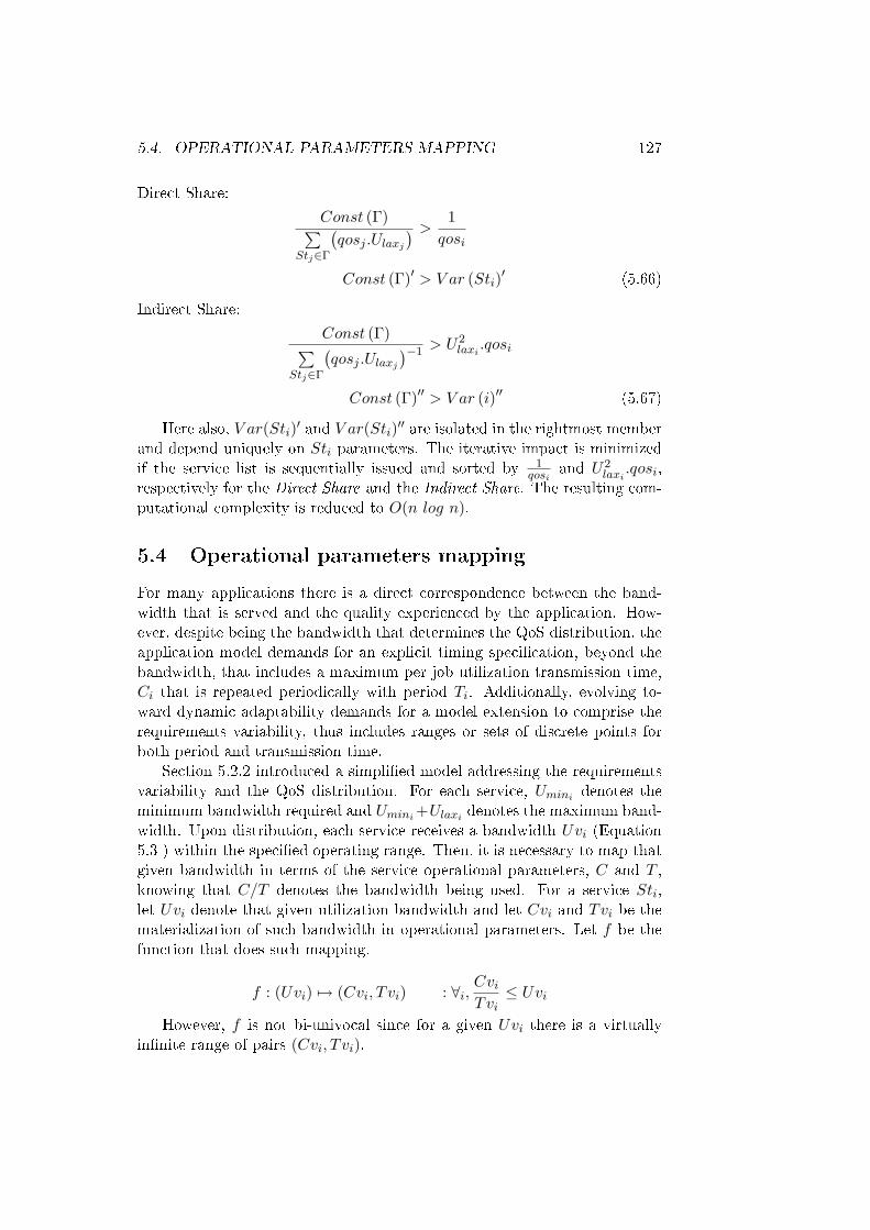
5.4. OPERATIONAL PARAMETERS MAPPING 127
Direct Share:
Const (Γ)∑Stj∈Γ
(qosj .Ulaxj
) > 1qosi
Const (Γ)′ > V ar (Sti)′ (5.66)
Indirect Share:
Const (Γ)∑Stj∈Γ
(qosj .Ulaxj
)−1 > U2laxi
.qosi
Const (Γ)′′ > V ar (i)′′ (5.67)
Here also, V ar(Sti)′ and V ar(Sti)′′ are isolated in the rightmost memberand depend uniquely on Sti parameters. The iterative impact is minimizedif the service list is sequentially issued and sorted by 1
qosiand U2
laxi.qosi,
respectively for the Direct Share and the Indirect Share. The resulting com-putational complexity is reduced to O(n log n).
5.4 Operational parameters mapping
For many applications there is a direct correspondence between the band-width that is served and the quality experienced by the application. How-ever, despite being the bandwidth that determines the QoS distribution, theapplication model demands for an explicit timing speci�cation, beyond thebandwidth, that includes a maximum per job utilization transmission time,Ci that is repeated periodically with period Ti. Additionally, evolving to-ward dynamic adaptability demands for a model extension to comprise therequirements variability, thus includes ranges or sets of discrete points forboth period and transmission time.
Section 5.2.2 introduced a simpli�ed model addressing the requirementsvariability and the QoS distribution. For each service, Umini denotes theminimum bandwidth required and Umini+Ulaxi denotes the maximum band-width. Upon distribution, each service receives a bandwidth Uvi (Equation5.3 ) within the speci�ed operating range. Then, it is necessary to map thatgiven bandwidth in terms of the service operational parameters, C and T ,knowing that C/T denotes the bandwidth being used. For a service Sti,let Uvi denote that given utilization bandwidth and let Cvi and Tvi be thematerialization of such bandwidth in operational parameters. Let f be thefunction that does such mapping.
f : (Uvi) 7→ (Cvi, T vi) : ∀i,CviTvi≤ Uvi
However, f is not bi-univocal since for a given Uvi there is a virtuallyin�nite range of pairs (Cvi, T vi).
128 CHAPTER 5. DYNAMIC QOS MANAGEMENT
However, this mapping function may be subject to additional constraintsderived from the application operational limitations. The application mayconstrain the function co-domain to speci�c value sets. An example is a videocamera streaming that de�nes speci�c discrete values for the frame size (Cv)as well as for the frame-rate (Tv). It is thus necessary for each service Sti,not only, to include such limitations within the application model, specifyinga space region of allowed (Cvi, T vi) pairs that correspond to a bandwidthspace BWi, but also, to enforce those limitations within the f function.
When the allowed operational space is discrete, further constraints areimposed as the bandwidth distribution scheme that decrease the e�ciency inassigning bandwidth, typically leading to waste. This situation is addressednext.
5.4.1 Complete application model
Section 5.2 presented a QoS-oriented service model Sti (Umini , Ulaxi , qosi),according to which each service gets a bandwidth Uvi within the rangeUmini ≤ Uvi ≤ Umini + Ulaxi
Let us now focus on the case in which the service operational space isrestricted to a set of discrete points.
Let Ci denote a discrete list of Cs available for Sti and Ti denote adiscrete list of T s. Zi denotes the list of pairs available for Sti, such that:
Zi ≡ {(Cj , Tm),∀Cj ∈ Ci, ∀Tm ∈ Ti}
The service model can thus be written as:
Sti (Zi, qosi)
For each service, it is speci�ed a list of admissible pairs and the QoSimportance parameter, qosi.
Opposed to the linear bandwidth range referred in the simpli�ed model,in this model, the available bandwidth is denoted with a discrete domainas the basis for the bandwidth distribution. For this reason, the bandwidthdistribution urges for a �ne-grained procedure that assigns the bandwidthbased on such domain.
In order to use the QoS distribution models described in Section 5.3,which are based on a continuous bandwidth adaptation range, we proposede�ning a continuous range that contains all the discrete points.
Thus, considering the set BW′i with all discrete bandwidth points allowedfor Sti, such that:
bw : zki ∈ Zi 7→ BW′i ≡ bw(zki ) =CkTk

5.4. OPERATIONAL PARAMETERS MAPPING 129
Figure 5.3: Discrete bandwidth to linear range mapping.
we de�ne the bandwidth range BWi = [Umini , Umaxi ], where:
Umini = minzki ∈Zi
bw(zki )
Umaxi = maxzki ∈Zi
bw(zki )
Figure 5.3 illustrates the BW′i space and the corresponding continuousrange BWi for a service Sti.
After applying the bandwidth distribution to BWi we obtain, for eachservice Sti, the bandwidth Uvi, which then needs to be mapped onto a pointUv′i < Uvi. This condition is necessary to maintain the schedulability of thebandwidth distribution.
This procedure is non-optimal in terms of bandwidth distribution andresource usage because the di�erence between the granted bandwidth andthe one actually used, Uvi − Uv′i, is wasted.
For systems where wasting bandwidth means a signi�cant degradationpenalty on the resource management, it is possible to reclaim that bandwidthand reassign it in one or more iterations. This topic is further addressed inSection 5.4.2.
However, we still need to address the assignment of a concrete (C, T ) pairwhenever there are several possible pairs for the same given Uv′i bandwidthvalue. In this case, given a bandwidth Uv′i, there must be a policy thatchooses the pair that best meets the application goals.
The option for any mapping rule is independent from the bandwidthdistribution scheme in place. In fact, it is even possible to allow that di�erentservices be managed by di�erent rules. For this purpose and since the choicefor these rules is mainly application oriented, an additional parameter isattached to the service description model, Pi, to denote this policy. The�nal service model used for the bandwidth distribution is thus:
Sti{Zi, qosi, Pi},∀k : Zki ∈ Zi
5.4.2 Bandwidth reclaiming
At this point we address the reclaiming of bandwidth left free because ofusing discrete operational points as refered in the previous section.
130 CHAPTER 5. DYNAMIC QOS MANAGEMENT
For a service Sti, with granted bandwidth Uvi and allowed discrete band-width Uv′i, we de�ne the wasted bandwidth Wi as follows:
Wi = Uvi − Uv′iThe basis of the bandwidth reclamation is to group all the individual
wastes of all services and redistribute it again.
Wsum =∑i=1..n
Wi
As mentioned in Section 5.3, there are two possible distribution schemes,the greedy scheme and the weighted one. For the greedy scheme, the sparebandwidth is allocated to each service in sequence, staring from the highestpriority to the lowest priority one. Each service either gets all the bandwidthit can use or the remainder. Going through all services the wasted bandwidthWsum will eventually be completely allocated to the services or a certainamount will remain that cannot be used by any service.
However, the situation is di�erent with the weighted scheme. I this case,repeating the bandwidth distribution over Wsum with the same di�erentia-tion weights (wi), will result in a distribution for each service equal to Wi,thus unusable. Therefore, a distortion to the weights must be done for thesake of e�ciency. We proposed two methods. One is to distribute Wsum tothe services sequentially based on their weight (wi), from the largest to thesmallest one, and grant them the bandwidth that they can , until all Wsum
is assigned. This procedure is identical to the greedy bandwidth distribu-tion scheme in which the weights (wi) are used as priorities. Therefore, theprocedure is performed in a single pass with reduced complexity (O(n)).
Despite simple, the above procedure violates the weighted bandwidthdistribution principal. The other method tries to improve the approximationof the reclaimed bandwidth distribution to the initial weights by sequentiallyremoving some services from the process and distribute the bandwidth bythe remaining ones. Each time a service j is removed from the process, itsbandwidth share (Wj) is made available to others that might be promotedto the discretized output bandwidth, Uv′i, reducing Wi.
When iterating this process, in order to improve the chances of assigningmore bandwidth to the services with larger weight, in each iteration we re-move from the service set the one with the lowest weight. Therefore, after themain bandwidth distribution and the related discretization mapping, whereall services are included, the distribution is re-issued with one less service,the one with lower weight coe�cient. The process is repeated iteratively,removing the services one by one, starting from the lower weighted service,until all the wasted bandwidth is fully distributed or all services have beenremoved. For each new iteration the remaining services adjust the distri-bution parameters in order to account with the already assigned bandwidth
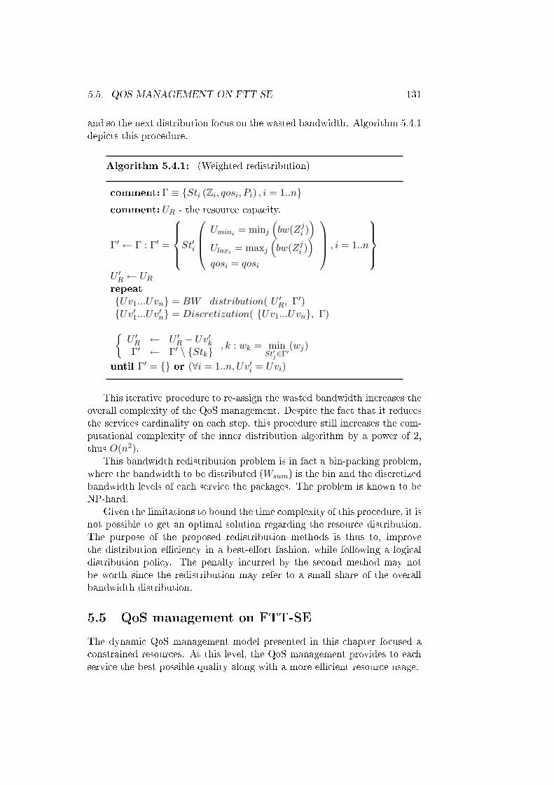
5.5. QOS MANAGEMENT ON FTT-SE 131
and so the next distribution focus on the wasted bandwidth. Algorithm 5.4.1depicts this procedure.
Algorithm 5.4.1: (Weighted redistribution)
comment: Γ ≡ {Sti (Zi, qosi, Pi) , i = 1..n}comment: UR - the resource capacity.
Γ′ ← Γ : Γ′ =
St′i
Umini = minj(bw(Zji )
)Ulaxi = maxj
(bw(Zji )
)qosi = qosi
, i = 1..n
U ′R ← URrepeat{Uv1...Uvn} = BW_distribution( U ′R, Γ′){Uv′1...Uv′n} = Discretization( {Uv1...Uvn}, Γ){U ′R ← U ′R − Uv′kΓ′ ← Γ′ \ {Stk}
, k : wk = minSt′j∈Γ′
(wj)
until Γ′ = {} or (∀i = 1..n, Uv′i = Uvi)
This iterative procedure to re-assign the wasted bandwidth increases theoverall complexity of the QoS management. Despite the fact that it reducesthe services cardinality on each step, this procedure still increases the com-putational complexity of the inner distribution algorithm by a power of 2,thus O(n2).
This bandwidth redistribution problem is in fact a bin-packing problem,where the bandwidth to be distributed (Wsum) is the bin and the discretizedbandwidth levels of each service the packages. The problem is known to beNP-hard.
Given the limitations to bound the time complexity of this procedure, it isnot possible to get an optimal solution regarding the resource distribution.The purpose of the proposed redistribution methods is thus to, improvethe distribution e�ciency in a best-e�ort fashion, while following a logicaldistribution policy. The penalty incurred by the second method may notbe worth since the redistribution may refer to a small share of the overallbandwidth distribution.
5.5 QoS management on FTT-SE
The dynamic QoS management model presented in this chapter focused aconstrained resources. At this level, the QoS management provides to eachservice the best possible quality along with a more e�cient resource usage.
132 CHAPTER 5. DYNAMIC QOS MANAGEMENT
However, there are limitations to the deployment of this model regardingthe type of resource since it must be able to support online recon�gurability,while enforcing the requirements setup for each given service. Additionally,when addressing a distributed resource, it demands for a consistent dis-tribution agreement in order to globally enforce the resource management.Finally, and perhaps the most demanding feature is, related to the sched-uler and the schedulability test that is part of the admission control. Theadmission test must be fast and execute in bounded time in order to besuited for dynamic environments. Moreover, in order to accomplish the QoSdistribution and maximize the resource usage, the schedulability test mustbe based on the individual load of each service and their sum, which mustbe compared with the resource capacity, i.e., there must exist a utilizationbound de�ning the schedulability region.
The FTT-SE protocol, described in Chapter 3, supports all these fea-tures. It is a hard real-time communication protocol deployed on top of aswitched Ethernet network, suited for dynamic environments and enforcingthe service requirements by means of a centralized tra�c control architecturethat consistently issues the services transmissions. Additionally, the proto-col supports any tra�c scheduling policies, namely EDF and RM, for whichthere are utilization-based schedulability tests.
However, given the multiple links of a switch the analysis has the partic-ularity of addressing the network as a multi-dimensional scheduling problem,where each uplink and downlink represents a resource with dependent rela-tionships. Nevertheless, the problem is reduced to several uni-dimensionalutilization-based analysis, in spite of being assessed globally for the completeswitch.
Similarly, the integration of the QoS distribution has to be conductedindividually on each link. In the following we discuss this integration withinthe FTT-SE protocol.
The QoS distribution is intimately related to the capacity provided toeach link by the schedulability bound. Although the links have similar initialcapacity, the utilization load is irregular with the di�erent forwarding pathsgenerated and the dependencies that thereby result.
Recalling the distribution base model described in Section 5.2.2, for asingle resource, after assigning the default bandwidth of each service, theUspare bandwidth is distributed among the services according to a distribu-tion policy. The same principle applies here to each individual link. Thedi�erence though, is that di�erent links have distinct loads and the sameservice may be seen in di�erent links, resulting on multiple bandwidth reser-vations for the same service. There may be a di�erent reservation value foreach resource where a service takes part.
The distribution model is generically de�ned as follows. Let M be thelist of m individual resources, uplinks and downlinks, and St the list of sservices following the QoS distribution model. Each Mj resource holds a list

5.5. QOS MANAGEMENT ON FTT-SE 133
of services from St, denoted by SMj , which may appear in di�erent resources,co-existing with di�erent other services. Therefore, assessing each resourceindividually results on di�erent reservation values for the same service.
However, despite the variety of reservation values per service, there mustexist a global agreement regarding the resources assigned to the service thatmust be unique since it is not possible to execute a service with di�erentcharacteristics across resources. Therefore, the bandwidth reserved for aservice is determined by the resource that provides the lowest reservationlevel, as follows:
Uvi = min∀Mj∈M
(Uv(i,j))
where Uv(i,j) denotes the bandwidth reserved within the resource j for servicei.
The consequence of such limitation is the bandwidth being left unused,leading to a more ine�cient distribution. For each resource, the wastedbandwidth is given by:
∀Mj ∈M, Wsumj =∑
Sti∈SMj
(Uv(i,j) − Uvi)
This bandwidth waste is inevitable when addressing the distributionof the resources independently. Though, when considering the distribu-tion method that assigns the bandwidth on a �xed importance basis (Sec-tion 5.3.1), it is possible to avoid this waste, comprising all the resourcestogether in the same distribution �ow. Starting from the most importantservice, the bandwidth is reserved with the exact amount, relating all theresources. This avoids inconsistency on reserving across several resourcesand leverages a more e�cient distribution.
However, the same reasoning cannot be followed when addressing theweighted distribution method. The resource distribution is resource indepen-dent and cannot be merged in a single procedure �ow. Yet, the bandwidthcan be reclaimed and redistributed among the services, following a simi-lar procedure as when mapping the bandwidth onto operational parameters(Section 5.4). In this case, after distributing and truncating the bandwidthby the minimums, the remaining bandwidth can be redistributed as depictedin the following algorithm.
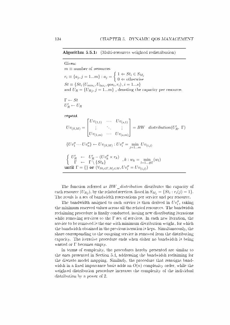
134 CHAPTER 5. DYNAMIC QOS MANAGEMENT
Algorithm 5.5.1: (Multi-resources weighted redistribution)
Given:m ≡ number of resources
ri ≡ {aj , j = 1...m} : aj ={
1⇐ Sti ∈ SMj
0⇐ otherwiseSt ≡ {Sti (Umini , Ulaxi , qosi, ri) , i = 1...s}and UR = {URj , j = 1...m} , denoting the capacity per resource.
Γ← StU ′R ← UR
repeat
Uv(S,M) =
Uv(1,1) · · · Uv(s,1)...
. . ....
Uv(1,m) · · · Uv(s,m)
= BW_distribution(U ′R, Γ)
{Uv′′1 · · ·Uv′′n} ← Uv(S,M) : Uv′′i = minj=1...m
Uv(i,j)
{U ′R ← U ′R − (Uv′′k × rk)
Γ ← Γ \ {Stk}, k : wk = min
l=1...#Γ(wl)
until Γ = {} or (∀Sti∈Γ,Mj∈M , Uv′′i = Uv(i,j))
The function referred as BW_distribution distributes the capacity ofeach resource (URj), by the related services, listed in SMj = {Sti : ri(j) = 1}.The result is a set of bandwidth reservations per service and per resource.
The bandwidth assigned to each service is then derived in Uv′′i , takingthe minimum reserved values across all the related resources. The bandwidthreclaiming procedure is �nally conducted, issuing new distributing iterationswhile removing services to the Γ set of services. In each new iteration, theservice to be removed is the one with minimum distribution weight, for whichthe bandwidth obtained in the previous iteration is kept. Simultaneously, theshare corresponding to the outgoing service is removed from the distributingcapacity. The iterative procedure ends when either no bandwidth is beingwasted or Γ becomes empty.
In terms of complexity, the procedures hereby presented are similar tothe ones presented in Section 5.4, addressing the bandwidth reclaiming forthe discrete model mapping. Similarly, the procedure that reassigns band-width in a �xed importance basis adds an O(n) complexity order, while theweighted distribution procedure increases the complexity of the individualdistribution by a power of 2.
5.6. CONCLUSION 135
5.6 Conclusion
The embedded systems in general and the network communications in partic-ular are following a trend that includes making a better use of the resources,by e�ciently adjusting online the requirements according to the applicationdynamics, while guaranteeing the system correct behavior regarding timeli-ness issues.
On this regard, applications have to be supported with models that de�nethe environment dynamics and how each individual application service orjob adapts facing those dynamic changes. However, the search for thesemodels is con�ned to the ability of delivering fast and reliable adjustmentsas demanded by the online properties of the system.
This chapter aims to categorize several of those models, oriented in adesign perspective of providing quality-levels that distinguish the preferredservices when the resource, or network, is overloaded. The models providethe means so the application may de�ne the quality of service requirementsfor each service contract as well as de�ning how that quality evolves beforeother competitor services.
This whole QoS management problem is decomposed in several concep-tual phases, 1) the application interpretation and mapping of the model intoactual quality-levels, 2) the bandwidth distribution of the resource capacitythat based on those quality-levels assigns bandwidth to the services, 3) themapping of the obtained bandwidth into the operational parameters usedby the application, and �nally, 4) the management of a resource in a multi-dimensional perspective as in the FTT-SE protocol.
The models are categorized according to their distribution fairness onregard to the application speci�cations and according to the computationalcomplexity overhead. Through the QoS management decomposition layersseveral approaches are conducted to minimize the impact on that complexityand optimize the bandwidth distribution, where one of the issues compre-hends the minimization of bad resources allocation, i.e., bandwidth waste.
Concerning the deployment of these models within the FTT-SE frame-work, the proposed models �t under the constraint that distribution has tobe carried on multi-dimensionally. To validate such integration Chapter 6carries an experiment with surveillance cameras where this QoS distribu-tion is actually implemented as the mean to deliver the best instantaneousthroughput of the network and considering the application de�ned expecta-tions concerning QoS.

136 CHAPTER 5. DYNAMIC QOS MANAGEMENT
Chapter 6
FTT-SE case studies
This chapter compiles a collection of case-studies developed on top of theFTT-SE architecture. Firstly, it addresses the integration of the protocolwithin a wider-scoped resource management framework, which includes re-serving for multiple resources with distinct class types (Section 6.1). In Sec-tion 6.2 the FTT-SE framework is used in a real application scenario where itsrecon�gurability and QoS management properties play an active role. Then,Section 6.3 shows how the protocol is able to support complex schedulingstructures such as aperiodic servers and hierarchical composition, in orderto ease the application design. Finally, Section 6.4 describes a preliminaryvalidation of a work-in-progress and future work related implementation thatincludes the master node within the switch.
6.1 Integration in the FRESCOR framework
Networked Embedded Systems (NES) were originally associated with indus-trial supervision and control applications, which employed simple sensors,actuators and controllers. However, a steep evolution in this applicationdomain is being experienced, pushed by the growing number of sensors andoverall complexity present at the plant level. As an example, the use of imag-ing sensors, both for supervision and control purposes, is spreading widely inclasses of applications such as mobile robotics, tra�c control and assemblylines inspection. Consequently, the sensors become inherently more complex,so as the �ows of information exchanged at the cell and plant levels, integrat-ing periodic and aperiodic �ows of short and large data, some of multimedianature, with considerable variability during run-time.
The new demands and increased complexity posed by these applicationspushed the development on new techniques and design methodologies. Twokey aspects in this regard are the complexity management and the resourcemanagement. Complexity management is being addressed by the adoptionof adequate middleware layers in NES (e.g. CORBA, Java RMI, DCOM,
137
138 CHAPTER 6. FTT-SE CASE STUDIES
etc)[134], which abstract away distribution, aiming at transparent interactionmechanisms between objects, components or applications. Regarding theresource management (e.g. CPU, memory, network, energy, etc) severalapproaches have been proposed recently, aiming at ful�lling the needs ofthose emerging applications in aspects like dynamic con�guration and QoSmanagement, support for new and more e�cient scheduling techniques, etc.
The FIRST Scheduling Framework (FSF) [25] provides a high-level ab-straction for real time resource schedulers while maintaining predictabilityand performance e�ciency. It provides a homogeneous interface so it canbe used in di�erent platform architectures. This framework was initiallydesigned to cope with the application needs for processor and network man-agement, although with some limitations in the latter. The Framework forReal-time Embedded Systems based on COntRats (FRESCOR) [66] aimsat extending the FSF framework for multi-resource reservation, comprisingvarious classes of resources commonly found in NES applications.
Regarding the communication subsystem, an early implementation hasbeen proposed to address negotiation over an Ethernet resource. This is theReal-Time Ethernet Protocol (RT-EP) [90]. The proposed Flexible TimeTriggered communication over Switched Ethernet (FTT-SE) (Chapter 3)provides �exible and deterministic real-time communication services com-bined with dynamic Quality of Service (QoS) management. This protocolhas been developed speci�cally to address the requirements presented by theemerging applications referred above, combining real-time requirements witha high degree of adaptability. It looks, thus, a natural network candidatefor inclusion in a contracting framework, to e�ciently exploit and enrich thehigh level of �exibility that it already o�ers.
This section the integration of the FTT-SE protocol in the scope of thecontract model framework and describes how this integration can be per-formed ful�lling issues like distribution consistency, reservation guaranteesand run-time �exibility. The work has been carried out in cooperation withMichael González Harbour, Daniel Sangorrín e a Julio L. Medina from theUniversity of Cantabria in Spain [86].
6.1.1 FRESCOR background
The FRESCOR framework is based on the notion of contracts between theapplication and the system resource manager. These contracts are created,managed and enforced by a Contract Layer, which assures that su�cient re-sources capacity is available. The framework is divided in modules that allowabstracting away the speci�cities of the resources typically found in NES. Ofparticular interest to this work are the Core module, which contains the basiccontract information that must exist in all contracted resources, the Sparecapacity module, which de�nes how the application may take advantage ofcurrently unused resource capacity, and the Distribution module that deals
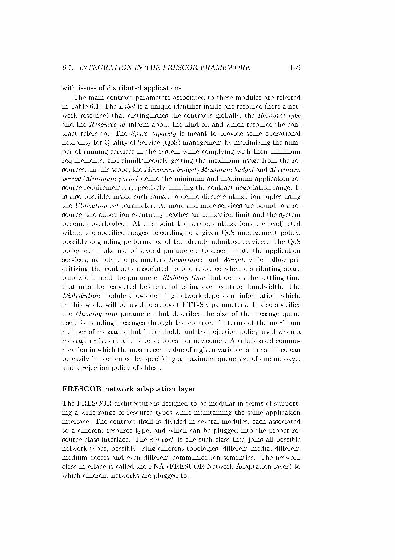
6.1. INTEGRATION IN THE FRESCOR FRAMEWORK 139
with issues of distributed applications.
The main contract parameters associated to these modules are referredin Table 6.1. The Label is a unique identi�er inside one resource (here a net-work resource) that distinguishes the contracts globally, the Resource typeand the Resource id inform about the kind of, and which resource the con-tract refers to. The Spare capacity is meant to provide some operational�exibility for Quality of Service (QoS) management by maximizing the num-ber of running services in the system while complying with their minimumrequirements, and simultaneously getting the maximum usage from the re-sources. In this scope, theMinimum budget/Maximum budget andMaximumperiod/Minimum period de�ne the minimum and maximum application re-source requirements, respectively, limiting the contract negotiation range. Itis also possible, inside such range, to de�ne discrete utilization tuples usingthe Utilization set parameter. As more and more services are bound to a re-source, the allocation eventually reaches an utilization limit and the systembecomes overloaded. At this point the services utilizations are readjustedwithin the speci�ed ranges, according to a given QoS management policy,possibly degrading performance of the already admitted services. The QoSpolicy can make use of several parameters to discriminate the applicationservices, namely the parameters Importance and Weight, which allow pri-oritizing the contracts associated to one resource when distributing sparebandwidth, and the parameter Stability time that de�nes the settling timethat must be respected before re-adjusting each contract bandwidth. TheDistribution module allows de�ning network dependent information, which,in this work, will be used to support FTT-SE parameters. It also speci�esthe Queuing info parameter that describes the size of the message queueused for sending messages through the contract, in terms of the maximumnumber of messages that it can hold, and the rejection policy used when amessage arrives at a full queue: oldest, or newcomer. A value-based commu-nication in which the most recent value of a given variable is transmitted canbe easily implemented by specifying a maximum queue size of one message,and a rejection policy of oldest.
FRESCOR network adaptation layer
The FRESCOR architecture is designed to be modular in terms of support-ing a wide range of resource types while maintaining the same applicationinterface. The contract itself is divided in several modules, each associatedto a di�erent resource type, and which can be plugged into the proper re-source class interface. The network is one such class that joins all possiblenetwork types, possibly using di�erent topologies, di�erent media, di�erentmedium access and even di�erent communication semantics. The networkclass interface is called the FNA (FRESCOR Network Adaptation layer) towhich di�erent networks are plugged to.
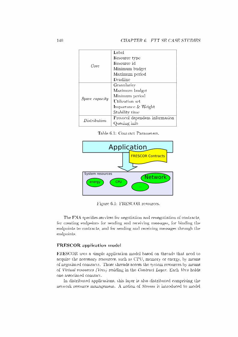
140 CHAPTER 6. FTT-SE CASE STUDIES
Core
LabelResource typeResource idMinimum budgetMaximum periodDeadline
Spare capacity
GranularityMaximum budgetMinimum periodUtilization setImportance & WeightStability time
DistributionProtocol dependent informationQueuing info
Table 6.1: Contract Parameters.
Figure 6.1: FRESCOR resources.
The FNA speci�es services for negotiation and renegotiation of contracts,for creating endpoints for sending and receiving messages, for binding theendpoints to contracts, and for sending and receiving messages through theendpoints.
FRESCOR application model
FRESCOR uses a simple application model based on threads that need toacquire the necessary resources, such as CPU, memory or energy, by meansof negotiated contracts. Those threads access the system resources by meansof Virtual resources (Vres) residing in the Contract Layer. Each Vres holdsone associated contract.
In distributed applications, this layer is also distributed comprising thenetwork resource management. A notion of Stream is introduced to model
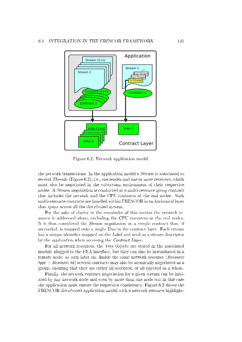
6.1. INTEGRATION IN THE FRESCOR FRAMEWORK 141
Figure 6.2: Network application model.
the network transactions. In the application model a Stream is associated toseveral Threads (Figure 6.2), i.e., one sender and one or more receivers, whichmust also be negotiated in the subsystem environment of their respectivenodes. A Stream negotiation is conducted as a multi-resource group contractthat includes the network and the CPU contracts at the end nodes. Suchmulti-resource contracts are handled within FRESCOR in an horizontal layerthat spans across all the distributed system.
For the sake of clarity in the remainder of this section the network re-source is addressed alone, excluding the CPU resources at the end nodes.It is thus considered the Stream negotiation as a simple contract that, ifsucceeded, is mapped onto a single Vres in the contract layer. Each streamhas a unique identi�er mapped on the Label and used as a stream descriptorby the application when accessing the Contract Layer.
For all network resources, the Vres objects are stored in the associatedmodule plugged to the FNA interface, but they can also be instantiated in aremote node, as seen later on. Inside the same network resource (Resourcetype + Resource id) several contracts may also be atomically negotiated as agroup, ensuring that they are either all accepted, or all rejected as a whole.
Finally, the network contract negotiation for a given stream can be initi-ated by any network node and even by more than one node but in this casethe application must ensure the respective consistency. Figure 6.2 shows theFRESCOR distributed application model with a network resource highlight-

142 CHAPTER 6. FTT-SE CASE STUDIES
Figure 6.3: FRESCOR example.
ing the network contracts in two possible situations: when a contract Virtualresource is created in a transmitter node (Stream 1), or in a contract groupsituation (Streams 2 .. (2+n)). Details on the FRESCOR interface servicesfor networked applications are better described in Section 6.1.3
6.1.2 FRESCOR application example
The following example illustrates the use of FRESCOR through a very simpledistributed system that integrates a welding system. The system captures anarray of points from a laser pro�ler representing the depth of the welding areaand then send it to another node where a controller activates an actuator,for moving the welding torch. The distributed system is supported by anFTT-SE network, which provides communication channels upon negotiation.
As shown in Figure 6.3, three contracts must be negotiated:
• Network contract: this is the contract needed to send the arrayof points to the controller. It speci�es a range of budgets so thatif the network has enough capacity it can send all the points, but ifthe network becomes overloaded, e.g. in consequence of new contractsbeing negotiated, a lower capacity would be granted by the system,
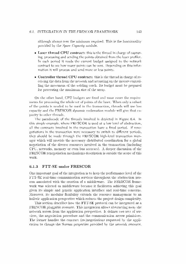
6.1. INTEGRATION IN THE FRESCOR FRAMEWORK 143
although always over the minimum required. This is the functionalityprovided by the Spare Capacity module.
• Laser thread CPU contract: this is the thread in charge of captur-ing, processing and sending the points obtained from the laser pro�ler.In each period it reads the current budget assigned to the networkcontract to see how many points can be sent. Depending on this infor-mation it will process and send more or less points.
• Controller thread CPU contract: this is the thread in charge of re-ceiving the data from the network and actuating on the motors control-ling the movement of the welding torch. Its budget must be preparedfor processing the maximum size of the array.
On the other hand, CPU budgets are �xed and must cover the require-ments for processing the whole set of points of the laser. When only a subsetof the points is needed to be used in the transaction, threads will use lesscapacity and the FRESCOR dynamic reclamation module will give that ca-pacity to other threads.
The pseudocode of the threads involved is depicted in Figure 6.4. Inthis simple example, where FRESCOR is used at a low level of abstraction,all the contracts involved in the transaction have a �xed period. If rene-gotiations in the transaction were necessary to switch to di�erent periods,they should be made through the FRESCOR high-level transaction man-ager which will provide the necessary distributed coordination for a globalnegotiation of the diverse resources involved in the transaction (includingCPU, networks, memory or even bus accesses). A deeper discussion of theFRESCOR renegotiation mechanisms description is outside the scope of thiswork.
6.1.3 FTT-SE under FRESCOR
One important goal of the integration is to keep the performance level of theFTT-SE real-time communication services throughout the abstraction pro-cess associated with the creation of a middleware. The FRESCOR frame-work was selected as middleware because it facilitates achieving this goalgiven its simple and generic application interface and real-time concerns.Moreover, its modular �exibility extends the resource management to anholistic application perspective which reduces the project design complexity.
This section describes how the FTT-SE protocol can be integrated as aFRESCOR pluggable resource. This integration allows abstracting away thenetwork access from the application perspective. It de�nes two sets of ser-vices, the negotiation procedure and the communication access primitives.The former handles the contract (re-)negotiations requested by the appli-cation to change the Stream properties provided by the network resource.
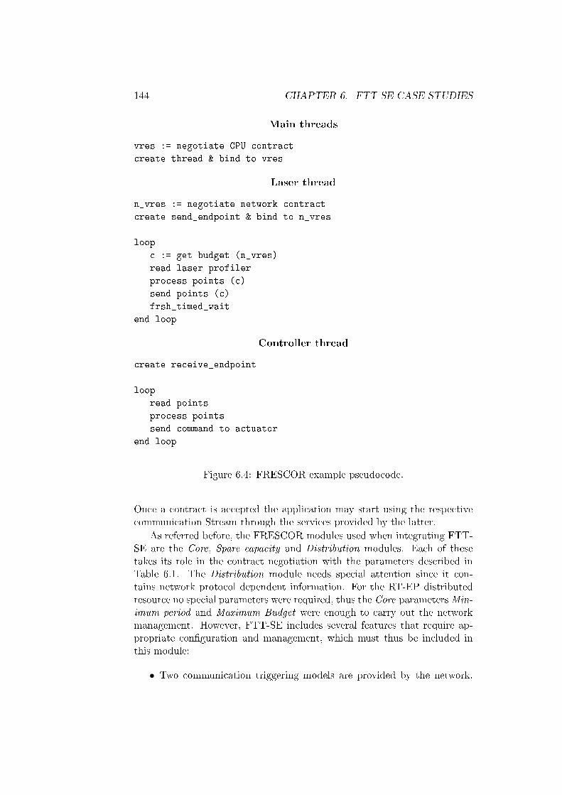
144 CHAPTER 6. FTT-SE CASE STUDIES
Main threads
vres := negotiate CPU contract
create thread & bind to vres
Laser thread
n_vres := negotiate network contract
create send_endpoint & bind to n_vres
loop
c := get budget (n_vres)
read laser profiler
process points (c)
send points (c)
frsh_timed_wait
end loop
Controller thread
create receive_endpoint
loop
read points
process points
send command to actuator
end loop
Figure 6.4: FRESCOR example pseudocode.
Once a contract is accepted the application may start using the respectivecommunication Stream through the services provided by the latter.
As referred before, the FRESCOR modules used when integrating FTT-SE are the Core, Spare capacity and Distribution modules. Each of thesetakes its role in the contract negotiation with the parameters described inTable 6.1. The Distribution module needs special attention since it con-tains network protocol dependent information. For the RT-EP distributedresource no special parameters were required, thus the Core parametersMin-imum period and Maximum Budget were enough to carry out the networkmanagement. However, FTT-SE includes several features that require ap-propriate con�guration and management, which must thus be included inthis module:
• Two communication triggering models are provided by the network,
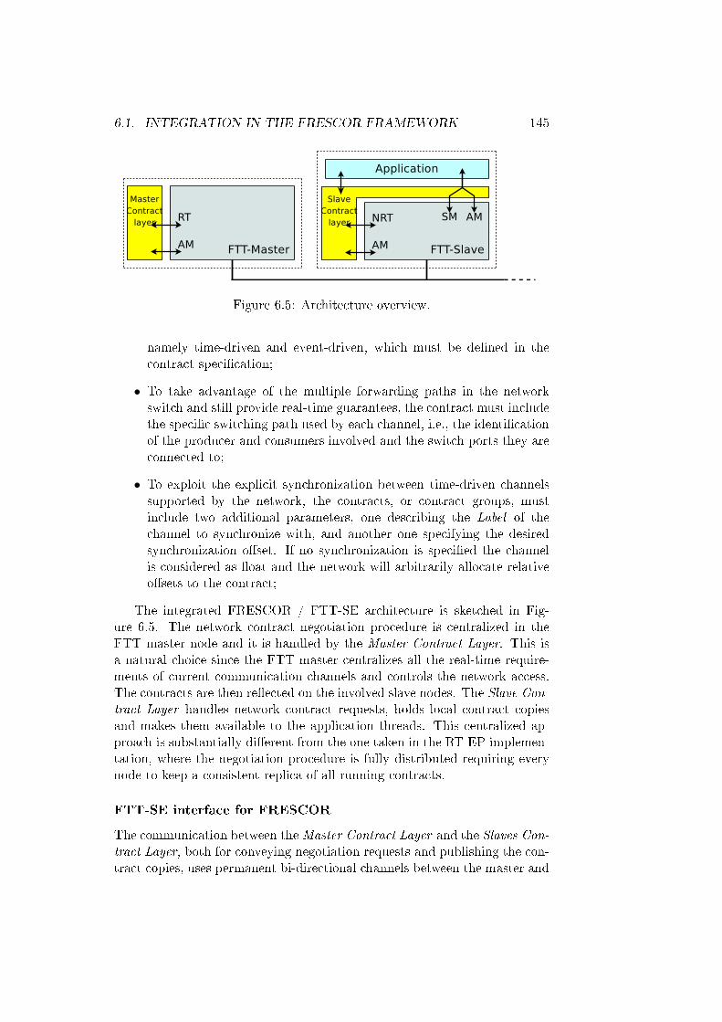
6.1. INTEGRATION IN THE FRESCOR FRAMEWORK 145
Figure 6.5: Architecture overview.
namely time-driven and event-driven, which must be de�ned in thecontract speci�cation;
• To take advantage of the multiple forwarding paths in the networkswitch and still provide real-time guarantees, the contract must includethe speci�c switching path used by each channel, i.e., the identi�cationof the producer and consumers involved and the switch ports they areconnected to;
• To exploit the explicit synchronization between time-driven channelssupported by the network, the contracts, or contract groups, mustinclude two additional parameters, one describing the Label of thechannel to synchronize with, and another one specifying the desiredsynchronization o�set. If no synchronization is speci�ed the channelis considered as �oat and the network will arbitrarily allocate relativeo�sets to the contract;
The integrated FRESCOR / FTT-SE architecture is sketched in Fig-ure 6.5. The network contract negotiation procedure is centralized in theFTT master node and it is handled by the Master Contract Layer. This isa natural choice since the FTT master centralizes all the real-time require-ments of current communication channels and controls the network access.The contracts are then re�ected on the involved slave nodes. The Slave Con-tract Layer handles network contract requests, holds local contract copiesand makes them available to the application threads. This centralized ap-proach is substantially di�erent from the one taken in the RT-EP implemen-tation, where the negotiation procedure is fully distributed requiring everynode to keep a consistent replica of all running contracts.
FTT-SE interface for FRESCOR
The communication between theMaster Contract Layer and the Slaves Con-tract Layer, both for conveying negotiation requests and publishing the con-tract copies, uses permanent bi-directional channels between the master and

146 CHAPTER 6. FTT-SE CASE STUDIES
Figure 6.6: FRESCOR interface for network contracts.
each slave node in the network, implemented with FTT-SE asynchronousmessages (AM).
The network contracts in the Master Contract Layer are re�ected inthe FTT Master, in the SRDB. This layer also provides interfaces to theapplication, to negotiate contracts and to access the communication services,both synchronous (SM) and asynchronous (AM).
Supporting the application interface
Figure 6.6 shows the FRESCOR common resource interface and the objectsinvolved in network contracts. The Negotiation service allows the systemto establish the required resource reservations and, in this case, involvescommunication with theMaster Contract Layer. Upon a negotiation success,the respective contract Virtual resource(s) is(are) created/updated in theMaster Contract Layer and the Virtual resource copies are created/updatedin the Slaves Contract Layer. The access to the contracted resource, a Streamin this case, is made through an endpoint, which is created and bound tothe Vres by the Create & Bind Endpoint services. Finally, the Send/Receiveservices allow the communication through the respective endpoint.
The network Virtual resources in the contract layer must be consistentwith the communication parameters within FTT-SE so that the protocolactually enforces the contracted communication parameters with its controlmechanisms. Therefore, a parameters daemon is used to keep such consis-tency. Whenever a server is created or updated dynamically, the daemoncommunicates such changes to the FTT-SE layer.
6.1.4 Internals of the contracting procedure
The setup of network contracts with FTT-SE, as referred before, requires aninteraction between the Slave Contract Layer of the involved nodes and theMaster Contract Layer. The process is triggered by the thread that manages
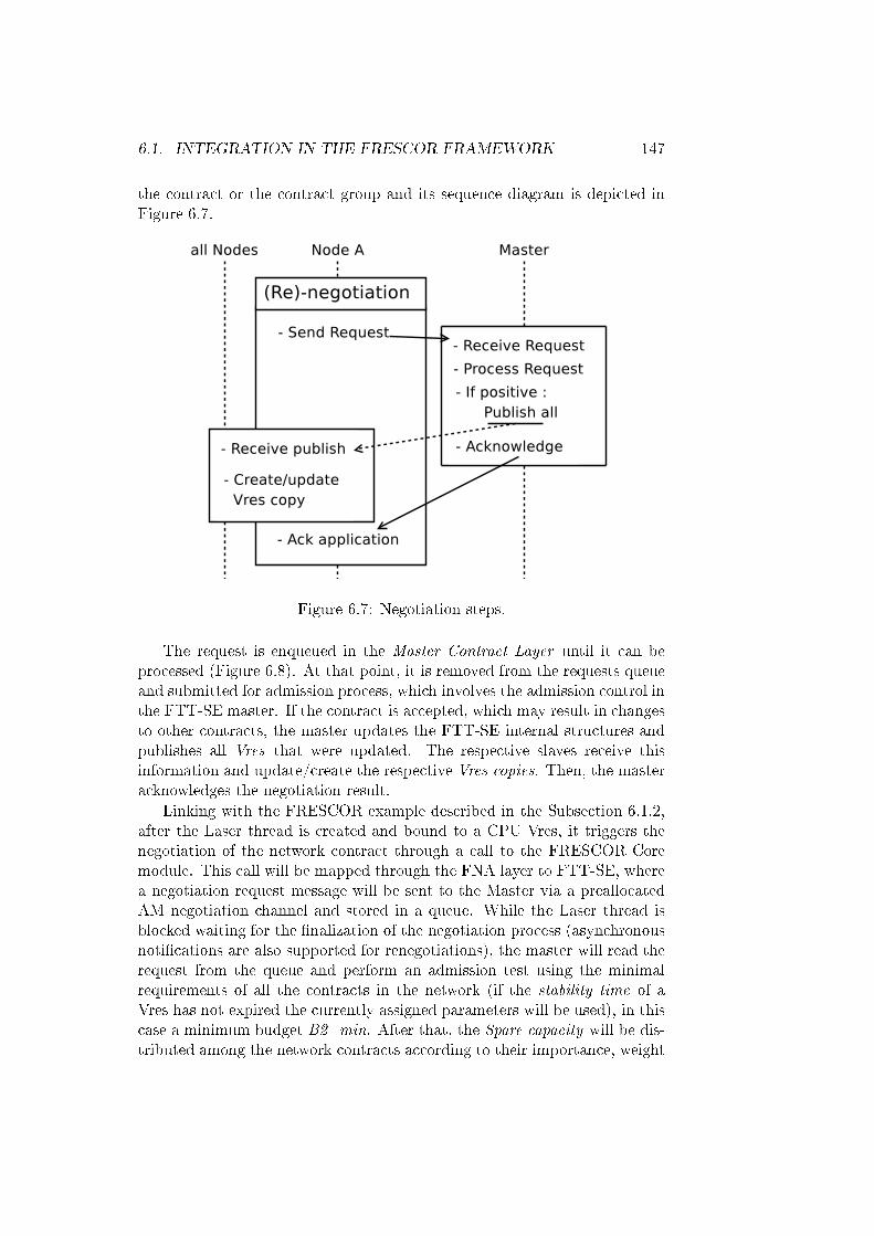
6.1. INTEGRATION IN THE FRESCOR FRAMEWORK 147
the contract or the contract group and its sequence diagram is depicted inFigure 6.7.
Figure 6.7: Negotiation steps.
The request is enqueued in the Master Contract Layer until it can beprocessed (Figure 6.8). At that point, it is removed from the requests queueand submitted for admission process, which involves the admission control inthe FTT-SE master. If the contract is accepted, which may result in changesto other contracts, the master updates the FTT-SE internal structures andpublishes all Vres that were updated. The respective slaves receive thisinformation and update/create the respective Vres copies. Then, the masteracknowledges the negotiation result.
Linking with the FRESCOR example described in the Subsection 6.1.2,after the Laser thread is created and bound to a CPU Vres, it triggers thenegotiation of the network contract through a call to the FRESCOR Coremodule. This call will be mapped through the FNA layer to FTT-SE, wherea negotiation request message will be sent to the Master via a preallocatedAM negotiation channel and stored in a queue. While the Laser thread isblocked waiting for the �nalization of the negotiation process (asynchronousnoti�cations are also supported for renegotiations), the master will read therequest from the queue and perform an admission test using the minimalrequirements of all the contracts in the network (if the stability time of aVres has not expired the currently assigned parameters will be used), in thiscase a minimum budget B2_min. After that, the Spare capacity will be dis-tributed among the network contracts according to their importance, weight
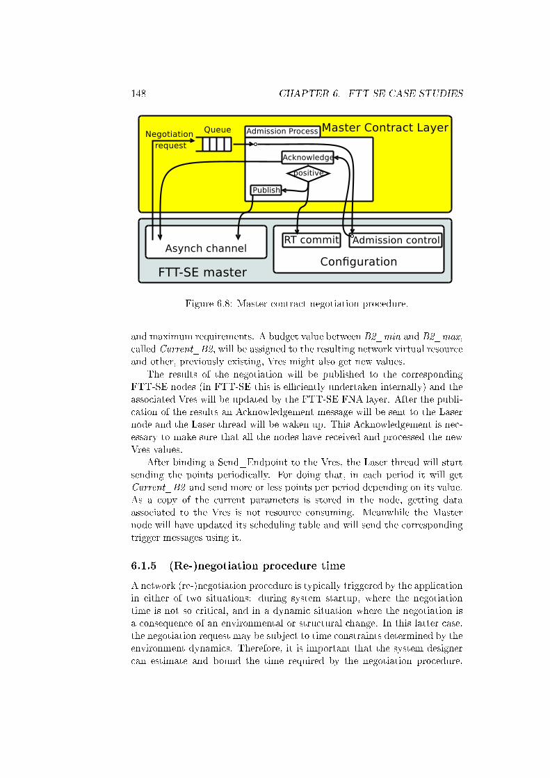
148 CHAPTER 6. FTT-SE CASE STUDIES
Figure 6.8: Master contract negotiation procedure.
and maximum requirements. A budget value between B2_min and B2_max,called Current_B2, will be assigned to the resulting network virtual resourceand other, previously existing, Vres might also get new values.
The results of the negotiation will be published to the correspondingFTT-SE nodes (in FTT-SE this is e�ciently undertaken internally) and theassociated Vres will be updated by the FTT-SE FNA layer. After the publi-cation of the results an Acknowledgement message will be sent to the Lasernode and the Laser thread will be waken up. This Acknowledgement is nec-essary to make sure that all the nodes have received and processed the newVres values.
After binding a Send_Endpoint to the Vres, the Laser thread will startsending the points periodically. For doing that, in each period it will getCurrent_B2 and send more or less points per period depending on its value.As a copy of the current parameters is stored in the node, getting dataassociated to the Vres is not resource consuming. Meanwhile the Masternode will have updated its scheduling table and will send the correspondingtrigger messages using it.
6.1.5 (Re-)negotiation procedure time
A network (re-)negotiation procedure is typically triggered by the applicationin either of two situations: during system startup, where the negotiationtime is not so critical, and in a dynamic situation where the negotiation isa consequence of an environmental or structural change. In this latter case,the negotiation request may be subject to time constraints determined by theenvironment dynamics. Therefore, it is important that the system designercan estimate and bound the time required by the negotiation procedure,
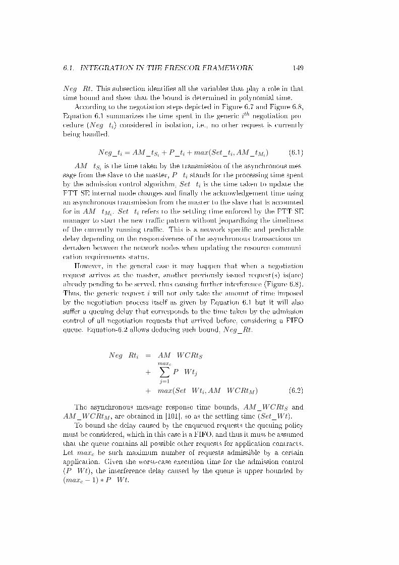
6.1. INTEGRATION IN THE FRESCOR FRAMEWORK 149
Neg_Rt. This subsection identi�es all the variables that play a role in thattime bound and show that the bound is determined in polynomial time.
According to the negotiation steps depicted in Figure 6.7 and Figure 6.8,Equation 6.1 summarizes the time spent in the generic ith negotiation pro-cedure (Neg_ti) considered in isolation, i.e., no other request is currentlybeing handled.
Neg_ti = AM_tSi + P_ti +max(Set_ti, AM_tMi) (6.1)
AM_tSi is the time taken by the transmission of the asynchronous mes-sage from the slave to the master, P_ti stands for the processing time spentby the admission control algorithm, Set_ti is the time taken to update theFTT-SE internal mode changes and �nally the acknowledgement time usingan asynchronous transmission from the master to the slave that is accountedfor in AM_tMi . Set_ti refers to the settling time enforced by the FTT-SEmanager to start the new tra�c pattern without jeopardizing the timelinessof the currently running tra�c. This is a network speci�c and predictabledelay depending on the responsiveness of the asynchronous transactions un-dertaken between the network nodes when updating the resource communi-cation requirements status.
However, in the general case it may happen that when a negotiationrequest arrives at the master, another previously issued request(s) is(are)already pending to be served, thus causing further interference (Figure 6.8).Thus, the generic request i will not only take the amount of time imposedby the negotiation process itself as given by Equation 6.1 but it will alsosu�er a queuing delay that corresponds to the time taken by the admissioncontrol of all negotiation requests that arrived before, considering a FIFOqueue. Equation-6.2 allows deducing such bound, Neg_Rt.
Neg_Rti = AM_WCRtS
+maxc∑j=1
P_Wtj
+ max(Set_Wti, AM_WCRtM ) (6.2)
The asynchronous message response time bounds, AM_WCRtS andAM_WCRtM , are obtained in [101], so as the settling time (Set_Wt).
To bound the delay caused by the enqueued requests the queuing policymust be considered, which in this case is a FIFO, and thus it must be assumedthat the queue contains all possible other requests for application contracts.Let maxc be such maximum number of requests admissible by a certainapplication. Given the worst-case execution time for the admission control(P_Wt), the interference delay caused by the queue is upper bounded by(maxc − 1) ∗ P_Wt.
150 CHAPTER 6. FTT-SE CASE STUDIES
Therefore, an upper bound for the negotiation time Neg_Rt+ can beobtained from Equation 6.3.
Neg_Rt+i = AM_WCRtS
+ (maxc − 1) ∗ P_Wt
+ max(Set_Wti, AM_WCRtM ) (6.3)
6.1.6 Summary
The FRESCOR framework has been proposed recently to cope with thegrowing application complexity and interoperability requirements in embed-ded systems. The approach followed by FRESCOR allows abstracting themanagement of the application resources, which are accessed through a com-mon interface based on contracts.
This section discussed the integration of the FTT-SE real-time commu-nication protocol within the FRESCOR contracting framework. This frame-work e�ciently exploits the FTT-SE natural ability for dynamically adaptingthe network resource usage while maintaining predictability. Another pos-itive aspect in this symbiosis is that the interface given by the frameworkto the application can be commonly applied together with other shared re-sources of the system.
Previously, only the RT-EP network protocol had been integrated withinthe FSF/FRESCOR framework. Such protocol works over a shared mediumwith a priority based event-triggered messaging paradigm. The integrationof FTT-SE brings in the features of a di�erent network paradigm and topol-ogy, namely time-triggered and event-triggered communication over switchedEthernet. The dynamism of FTT-SE positively impacts the e�ciency of thenetwork management in the FRESCOR framework. On the other hand, theabstraction provided by FRESCOR bene�ts the FTT-SE protocol in termsof its usability and applications development.
Finally, this section presented a worst-case analysis for the time takenby the negotiation process, provided a few network parameters, easily deter-mined, as well as a bound on the number of possible simultaneous negotiationrequests. Such bound guarantees the timeliness for the negotiation proce-dure, which is of utmost importance for adaptive critical systems operatingwithin dynamic scenarios.
6.2. INDUSTRIAL MULTIMEDIA APPLICATION 151
6.2 Industrial multimedia application
The use of Media Control Applications [57] (MCA) such as machine vision,automated inspection, object tracking and vehicle guidance [109, 75, 43, 69]in today's industry is increasing strongly. Such applications can be classi-�ed in two broad classes [57], Supervised Multimedia Control Subsystems andMultimedia Embedded Systems (MES). While the former class emphasizes thequality of the media processing, relieving the real-time constraints to a softreal-time level, the latter applications class (MES), in addition to the mediaprocessing concerns, establishes hard real-time requirements on their appli-cation goals. These applications are typically complex and heterogeneous,comprising several real-time activities in addition to the media processingones. Thus, the interference of the multimedia processing components mustbe limited and predictable.
Many MES applications rely on networked embedded systems (NES) thatdepend on real-time communication protocols to support the necessary real-time services. However, multimedia tra�c in general, and video streamingin particular, have speci�c characteristics that con�ict with the operationalmodel of conventional real-time protocols. In particular, video compressorsgenerate highly variable bit rate (VBR) transmission patterns that mismatchthe constant bit rate (CBR) channels typically provided by real-time pro-tocols, severely reducing the e�ciency of network utilization. Matching aVBR source to a CBR channel is not trivial and may lead either to a wasteof bandwidth or rejection of frames. This di�culty becomes particularlychallenging with the emergence of the MES applications described above,which typically impose reliability and timeliness requirements that cannotbe ful�lled with standard network protocols [125], due to lack of temporalisolation and consequent unbounded mutual interference between streams.
This section is based on a work conducted in cooperation Javier Silvestrefrom the Polytechnic University of Valencia in Spain [63, 113], which pro-poses taking advantage of the dynamic QoS management features of theFTT-SE protocol to carry out the referred adaptation with MJPEG videostreams. In particular, it proposes managing in an integrated way both thecompression parameters and the frame acquisition properties, which drivethe encoding of frames that must �t strictly inside the bandwidth allocatedto each stream. This approach aims at maximizing the QoS level provided byeach communication channel and by that means minimizing the compressionused at each instant.
The QoS adaptation is presented in two stages, regarding the variationdegrees of the acquisition properties. In a �rst stage only the frame acquisi-tion period is manageable to best re�ect the bandwidth provided. The framesize, although actually variable with the compression result, is considered to�t a �xed size container, property of the FTT-SE allocated channel. In asecond stage both parameters, period and frame container are manageable
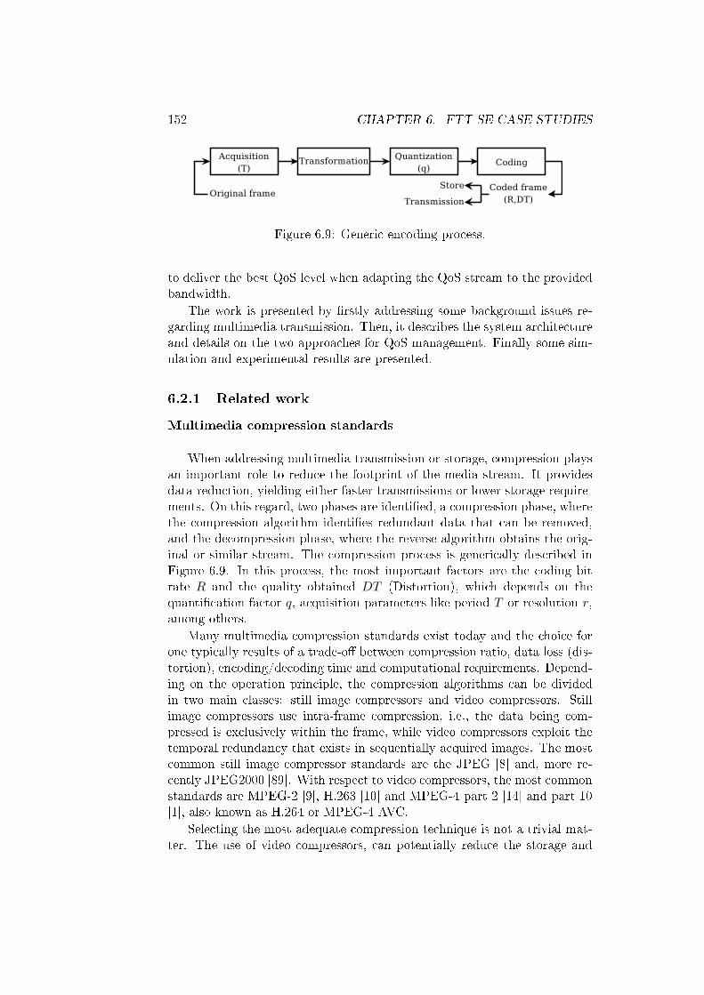
152 CHAPTER 6. FTT-SE CASE STUDIES
Figure 6.9: Generic encoding process.
to deliver the best QoS level when adapting the QoS stream to the providedbandwidth.
The work is presented by �rstly addressing some background issues re-garding multimedia transmission. Then, it describes the system architectureand details on the two approaches for QoS management. Finally some sim-ulation and experimental results are presented.
6.2.1 Related work
Multimedia compression standards
When addressing multimedia transmission or storage, compression playsan important role to reduce the footprint of the media stream. It providesdata reduction, yielding either faster transmissions or lower storage require-ments. On this regard, two phases are identi�ed, a compression phase, wherethe compression algorithm identi�es redundant data that can be removed,and the decompression phase, where the reverse algorithm obtains the orig-inal or similar stream. The compression process is generically described inFigure 6.9. In this process, the most important factors are the coding bitrate R and the quality obtained DT (Distortion), which depends on thequanti�cation factor q, acquisition parameters like period T or resolution r,among others.
Many multimedia compression standards exist today and the choice forone typically results of a trade-o� between compression ratio, data loss (dis-tortion), encoding/decoding time and computational requirements. Depend-ing on the operation principle, the compression algorithms can be dividedin two main classes: still image compressors and video compressors. Stillimage compressors use intra-frame compression, i.e., the data being com-pressed is exclusively within the frame, while video compressors exploit thetemporal redundancy that exists in sequentially acquired images. The mostcommon still image compressor standards are the JPEG [8] and, more re-cently JPEG2000 [89]. With respect to video compressors, the most commonstandards are MPEG-2 [9], H.263 [10] and MPEG-4 part 2 [14] and part 10[1], also known as H.264 or MPEG-4 AVC.
Selecting the most adequate compression technique is not a trivial mat-ter. The use of video compressors, can potentially reduce the storage and
6.2. INDUSTRIAL MULTIMEDIA APPLICATION 153
bandwidth with respect to, for instance, motion JPEG (MJPEG) by ra-tios as high as 10:1. However, taking the example of surveillance/recordingsystems, images are frequently captured at low rates and sometimes multi-plexed, which reduces or even eliminates the temporal redundancy and thusseriously compromises the e�ciency of these compression algorithms. Inaddition, video algorithms apply techniques that compensate variations inthe network load or processing throughput, adjusting the video image qual-ity, which may be adequate for monitoring applications, but not for MESor surveillance/recording applications [18], often found in industrial envi-ronments. Moreover, still image frames tend to be better accepted withinsystems that interpret frames individually as a sensor data quantum, e.g.a control system that periodically acquires a frame. The use of motionJPEG (MJPEG)is generally found only in digital cameras and monitoringsystems (e.g., Lumera, Cast, Axis [18], Mobotix [21]). Concerning the useof JPEG2000, it was expected by 2001 that this compressor would replaceJPEG in 2 or 3 years. Though, some drawbacks have made this transi-tion more di�cult, among others, the lack of backward compatibility andthe additional complexity in terms of memory footprint requirements andcomputing time that nearly triples for the compression and decompressionalgorithms. Also, the gains in terms of perceived quality are not relevant,being only noticeable with extreme compression levels and the licensing forthe JPEG2000 codec limits the adoption such technology.
Furthermore, still image transmission is more robust than video trans-mission. This conclusion can be drawn from the fact that in still image com-pression the frames are independent of each other, and thus losing one image(or parts of one image) has no consequence for the following images. In turn,video transmission uses di�erent frame types, namely I-frames (independentframes), P-frames (inter-frames coded depending on previous frames) andsometimes B-frames (on pass and future frames). Only I-frames are self-contained, thus the loss of a frame (or part of a frame) may have impacton several of the following frames, until the arrival of another I-frame. Thise�ect is further aggravated by a common practice that consists in enlargingthe distance between I-frames to reduce the bandwidth utilization. Anotheraspect that penalizes the use of video compression is related to the fact thatin industrial applications the images are frequently captured at low rates andsometimes are multiplexed. Any of these situations can reduce severely thetemporal redundancy and thus the level of compression that can be attained.
Whenever timeliness requirements come into play, the lower latency ofJPEG with regard to other video/still image compression techniques presentsa signi�cant advantage. The relevance of this aspect is growing in con-sequence of the use of increasingly higher resolution image sensors, whichhave evolved from the traditional CIF (Common Intermediate Format) andQCIF (Quarter CIF, 352x288 and 176x144 pixels), with a maximum size of4CIF 704x576 pixels, to VGA (Video Graphics Array, 640x480 pixels), XGA

154 CHAPTER 6. FTT-SE CASE STUDIES
(Extended Graphics Array) with a 1024x768 pixels, SXGA with 1280x1024pixels, WUXGA with 1920x1200 pixels, arriving to the WHUXGA format,with 7680x4800 pixels. Thus, the amount of data to process in each frameis growing exponentially, emphasizing the importance of the compressor la-tency.
Multimedia transmission
Multimedia transmission over the Internet has been the subject of intenseresearch in the recent years [35, 130]. Typical solutions are based on theTCP/IP protocol stack complemented by other protocols, e.g., RTP/RTCP(Real Time Protocol/Real Time Control Protocol [108]), RTSP (Real TimeStreaming Protocol [107]) or SIP (Session Initiation Protocol [58]), whichmeasure key network parameters, such as bandwidth usage, packet loss rateand round-trip delays to control the load submitted to the network.
The main drawback of these technologies concerning their use for in-dustrial communications is the latency introduced. For example, there arevideo algorithms [110] that use memory bu�ers between the producer andthe consumer to smooth out the bit rate variations. The estimation of the re-quired bandwidth and of the amount of bu�ers can be done o�ine, for storedvideo, or based on a number of images bu�ered before their transmission,for live (non interactive) video streams. The quality given by this smoothingmechanisms is however highly dependent on the application requirements.This latency problem is addressed by the low-delay Rate Control algorithms[106, 129], such as those used in TMN8 [11], which achieve a high level ofperformance for the applications for which they have been designed, mainlyvideophone and video-conference. However, these algorithms are based onthe use of only one I-frame and a following sequence of P-frames, an approachthat can be used in soft real-time applications like videophone and video-conference, but not in MES applications. For example, within an industrialcontrol process based on vision, the appearance of a new object in the scenewill either generate a tra�c peak, if the compression is kept unchanged, or astrong quality reduction if the compression is changed to keep the bandwidthutilization stable. Any of these situations is susceptible to introduce errorsinto the system, thus making the use of this class of protocols unsuited forMES applications.
From the above discussion it can be concluded that the solutions devel-oped for generic video transmission, despite e�cient and �exible, do not �llin the requirements of MES, towards an e�cient �t of a VBR source withina CBR channel. Taking a conservative approach, it is possible to reserve achannel with a capacity equal to the maximum bandwidth of the multimediasource. While taking this approach guarantees that no frames are lost, thefact is that the bandwidth generated by multimedia sources typically exhibit
6.2. INDUSTRIAL MULTIMEDIA APPLICATION 155
high variance, leading to a potentially signi�cant bandwidth waste. An al-ternative approach to overcome this ine�ciency problem would be reservinga channel with a capacity equal to the average bandwidth necessary. Despitemore e�cient, from the bandwidth point of view, this approach can lead toadditional delays or even frame losses, depending on the existence and size ofbu�ers at the source nodes, whenever the instantaneous bandwidth exceedsthe average value. At this point it should be stressed that many applicationscomprise the transmission of several multimedia streams, thus multiplyingthe impact of these sources of ine�ciency.
The di�culty in �tting VBR sources in CBR channels motivated the workpresented in this section that also illustrates the capabilities of the FTT-SEframework on supporting dynamic QoS management. The dynamic QoSmanagement features present in FTT-SE are used to dynamically adapt thebandwidth of the real-time communication channels. Such integration allowsadjusting the QoS of each stream given as inputs the relative importance of amedia stream, the currently allocated bandwidth and the compression levelof each multimedia source, as well as the global network utilization. The goalis to provide, at every instant, the best possible QoS to each stream. Theadmission control and scheduling faculties of the FTT-SE protocol allow car-rying out seamless online transitions without losing the real-time guarantees,thus being suitable for MES applications.
6.2.2 System Architecture
This case-study addresses a generic monitoring industrial application, wherep multimedia sources, also called producers, send a set M ≡ {Mi, i = 1..p}of video streams to c multimedia sinks, called consumers, via a local areanetwork executing the FTT-SE protocol (Figure 6.10). Besides the videostreams, the network may also support other tra�c sources, potentially withstringent real-time requirements, e.g. related with real-time control, as wellas non-real-time, e.g. con�guration or even general-purpose Internet ac-cess. This communication scenario is e�ectively supported by the FTT-SEprotocol, which provides dynamic QoS management while guaranteeing thereal-time performance. Moreover, the protocol enforces mutual isolation be-tween tra�c classes and thus Therefore, these additional tra�c classes arenot considered throughout this work.
Several producers may reside in one single node but, for the sake ofsimplicity, in the scope of this work a single producer per transmitting nodeis considered. Figure 6.11 illustrates how the application uses the protocol.The QoS manager within the FTT-SE master node, concentrates the requestsfrom the system nodes, holding the network requirements for the contractedstreams, including operational and QoS aspects. It receives channel changerequests from di�erent system nodes and assigns the bandwidth to each ofthe streams. Then, each node holds a QoS sublayer that addresses the QoS

156 CHAPTER 6. FTT-SE CASE STUDIES
FTT-SE
P1
www
P2 P3 P4
C
Figure 6.10: System architecture.
management requirements in terms of a video-speci�c application.
The QoS sublayer is included to handle the QoS contracts of each stream,while conserving their run-time properties. As depicted in Figure 6.11, thislayer acts in between the application and the FTT-SE protocol, adaptingthe instantaneous requirements of each video stream (VBR source) to theFTT-SE communication channels (CBR). This mapping is straightforwardwith PrFTTi = PrAPPi , TFTTi = TAPPi and C li = Bl
i. The upper bound ofthe transmission bu�er size range Cui is determined in each QoS negotiation,expressing the desired bu�er size from the QoS sublayer perspective at thatmoment.
At the application level, the QoS model considers each stream beingcharacterized by a normalized relative priority PrAPPi such that
∑∀i Pri =
1), a range of allowed quanti�cation factors that imply di�erent compressionlevels QAPP
i ≡[qli, q
ui
], a range of possible frame sizes after compression
BAPPi ≡[Bli, B
ui
]and a set of possible inter-frame intervals corresponding
to the ni allowed frame rates TAPPi ≡ {T ji , j = 1..ni}, as follows:
MAPPi = {Pri,Qi,Bi,Ti}APP (6.4)
As described back in Section 5.3, the FTT streams are characterized bya priority that re�ects the relative channel importance PrFTTi , a range of
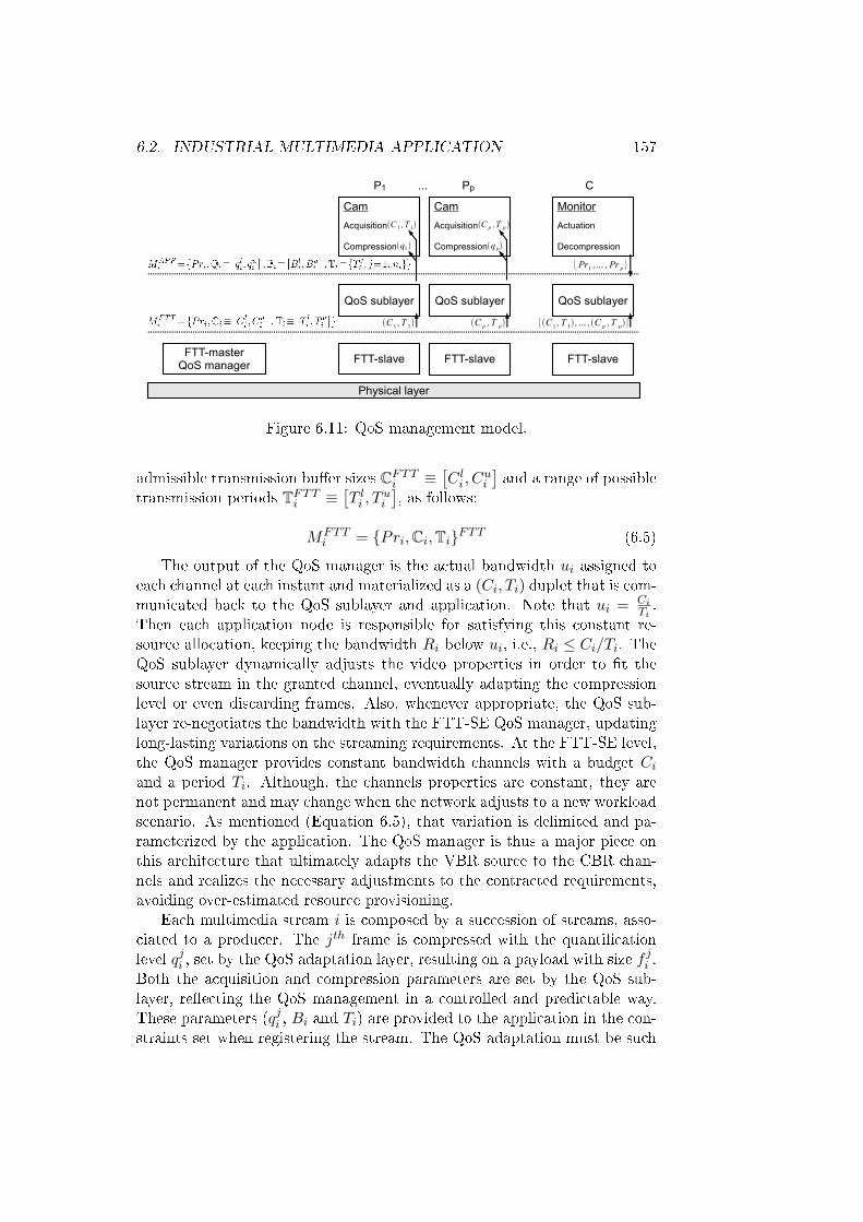
6.2. INDUSTRIAL MULTIMEDIA APPLICATION 157
Physical layer
FTT-masterQoS manager
FTT-slave FTT-slave FTT-slave
QoS sublayer QoS sublayer QoS sublayer
C1 ,T 1 C p , T p {C1 , T 1 , ... ,C p , T p}
Cam
Acquisition
Compression
C1 ,T 1
q1
Monitor
Decompression
Actuation
Cam
Acquisition
Compression
C p ,T p
q p
P1 Pp... C
{Pr1 ,... , Pr p }
Figure 6.11: QoS management model.
admissible transmission bu�er sizes CFTTi ≡
[C li , C
ui
]and a range of possible
transmission periods TFTTi ≡[T li , T
ui
], as follows:
MFTTi = {Pri,Ci,Ti}FTT (6.5)
The output of the QoS manager is the actual bandwidth ui assigned toeach channel at each instant and materialized as a (Ci, Ti) duplet that is com-municated back to the QoS sublayer and application. Note that ui = Ci
Ti.
Then each application node is responsible for satisfying this constant re-source allocation, keeping the bandwidth Ri below ui, i.e., Ri ≤ Ci/Ti. TheQoS sublayer dynamically adjusts the video properties in order to �t thesource stream in the granted channel, eventually adapting the compressionlevel or even discarding frames. Also, whenever appropriate, the QoS sub-layer re-negotiates the bandwidth with the FTT-SE QoS manager, updatinglong-lasting variations on the streaming requirements. At the FTT-SE level,the QoS manager provides constant bandwidth channels with a budget Ciand a period Ti. Although, the channels properties are constant, they arenot permanent and may change when the network adjusts to a new workloadscenario. As mentioned (Equation 6.5), that variation is delimited and pa-rameterized by the application. The QoS manager is thus a major piece onthis architecture that ultimately adapts the VBR source to the CBR chan-nels and realizes the necessary adjustments to the contracted requirements,avoiding over-estimated resource provisioning.
Each multimedia stream i is composed by a succession of streams, asso-ciated to a producer. The jth frame is compressed with the quanti�cationlevel qji , set by the QoS adaptation layer, resulting on a payload with size f
ji .
Both the acquisition and compression parameters are set by the QoS sub-layer, re�ecting the QoS management in a controlled and predictable way.These parameters (qji , Bi and Ti) are provided to the application in the con-straints set when registering the stream. The QoS adaptation must be such
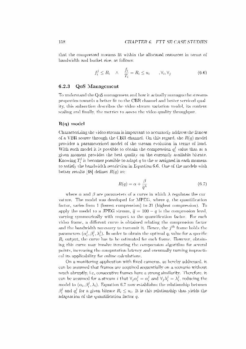
158 CHAPTER 6. FTT-SE CASE STUDIES
that the compressed streams �t within the allocated resources in terms ofbandwidth and bucket size, as follows:
f ji ≤ Bi ∧ fiTi
= Ri ≤ ui ,∀i, ∀j (6.6)
6.2.3 QoS Management
To understand the QoS management and how it actually manages the streamsproperties towards a better �t to the CBR channel and better serviced qual-ity, this subsection describes the video stream variation model, its contentscaling and �nally, the metrics to assess the video quality throughput.
R(q) model
Characterizing the video stream is important to accurately address the �tnessof a VBR source through the CBR channel. On this regard, the R(q) modelprovides a parameterized model of the stream evolution in terms of load.With such model it is possible to obtain the compression qji value that at agiven moment provides the best quality on the currently available bitrate.Knowing T ji it becomes possible to adapt q to the w assigned in each momentto satisfy the bandwidth restriction in Equation 6.6. One of the models withbetter results [48] de�nes R(q) as:
R(q) = α+β
qλ(6.7)
where α and β are parameters of a curve in which λ regulates the cur-vature. The model was developed for MPEG, where q, the quanti�cationfactor, varies from 1 (lowest compression) to 31 (highest compression). Toapply the model to a JPEG stream, q = 100 − q is the compression level,varying symmetrically with respect to the quanti�cation factor. For eachvideo frame, a di�erent curve is obtained relating the compression factorand the bandwidth necessary to transmit it. Hence, the jth frame holds theparameters (αji , β
ji , λ
ji ). In order to obtain the optimal qi value for a speci�c
Ri output, the curve has to be estimated for each frame. However, obtain-ing this curve may involve iterating the compression algorithm for severalpoints, increasing the computation latency and eventually turning impracti-cal its applicability for online calculations.
On a monitoring application with �xed cameras, as hereby addressed, itcan be assumed that frames are acquired sequentially on a scenario withoutmuch abruptly, i.e, consecutive frames have a strong similarity. Therefore, itcan be assumed for a stream i that ∀jαji = αji and ∀jλ
ji = λji , reducing the
model to (αi, βji , λi). Equation 6.7 now establishes the relationship between
βji and qji for a given bitrate Ri ≤ ui. It is this relationship that yields the
adaptation of the quanti�cation factor q.
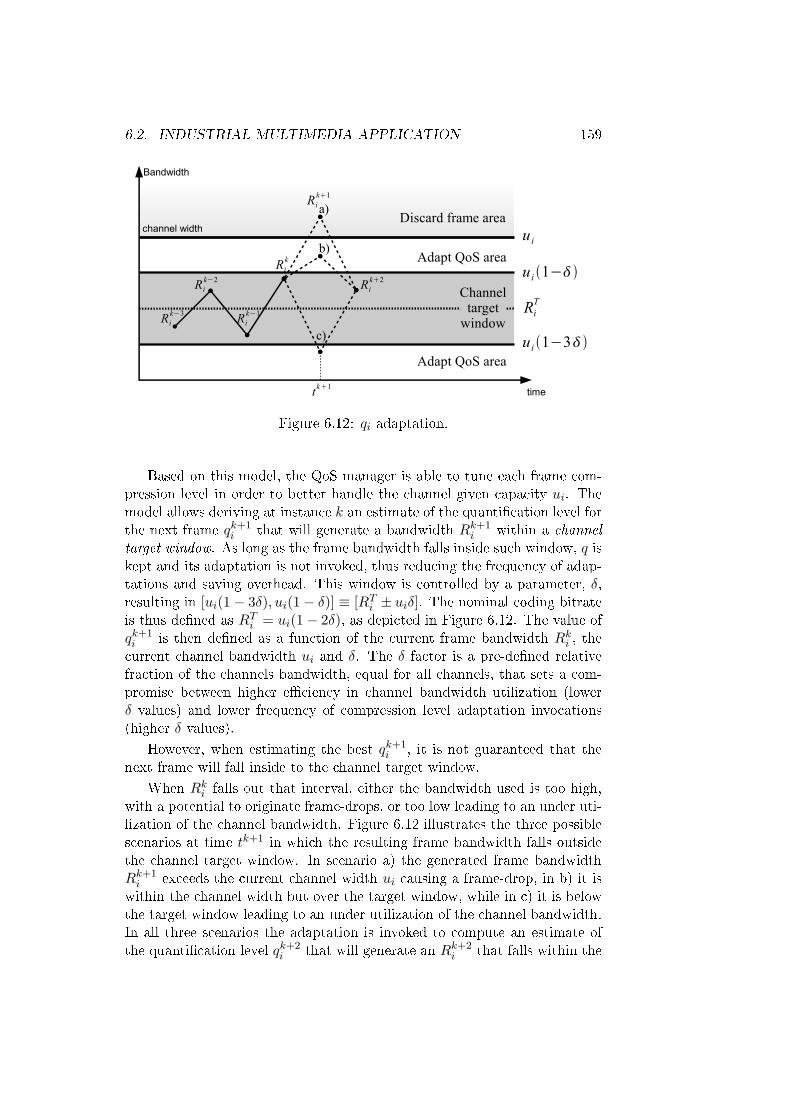
6.2. INDUSTRIAL MULTIMEDIA APPLICATION 159
a)
b)
c)
Rik1
Rik
Rik−1Ri
k−3
Rik−2
Adapt QoS area
Adapt QoS area
Discard frame areau i
u i 1−
u i 1−3
RiT
Rik2
timetk1
Channeltarget
window
channel width
Bandwidth
Figure 6.12: qi adaptation.
Based on this model, the QoS manager is able to tune each frame com-pression level in order to better handle the channel given capacity ui. Themodel allows deriving at instance k an estimate of the quanti�cation level forthe next frame qk+1
i that will generate a bandwidth Rk+1i within a channel
target window. As long as the frame bandwidth falls inside such window, q iskept and its adaptation is not invoked, thus reducing the frequency of adap-tations and saving overhead. This window is controlled by a parameter, δ,resulting in [ui(1− 3δ), ui(1− δ)] ≡ [RTi ± uiδ]. The nominal coding bitrateis thus de�ned as RTi = ui(1− 2δ), as depicted in Figure 6.12. The value ofqk+1i is then de�ned as a function of the current frame bandwidth Rki , thecurrent channel bandwidth ui and δ. The δ factor is a pre-de�ned relativefraction of the channels bandwidth, equal for all channels, that sets a com-promise between higher e�ciency in channel bandwidth utilization (lowerδ values) and lower frequency of compression level adaptation invocations(higher δ values).
However, when estimating the best qk+1i , it is not guaranteed that the
next frame will fall inside to the channel target window.
When Rki falls out that interval, either the bandwidth used is too high,with a potential to originate frame-drops, or too low leading to an under uti-lization of the channel bandwidth. Figure 6.12 illustrates the three possiblescenarios at time tk+1 in which the resulting frame bandwidth falls outsidethe channel target window. In scenario a) the generated frame bandwidthRk+1i exceeds the current channel width ui causing a frame-drop, in b) it is
within the channel width but over the target window, while in c) it is belowthe target window leading to an under utilization of the channel bandwidth.In all three scenarios the adaptation is invoked to compute an estimate ofthe quanti�cation level qk+2
i that will generate an Rk+2i that falls within the
160 CHAPTER 6. FTT-SE CASE STUDIES
Figure 6.13: Error in frame size caused by ∆qe = 1 for di�erent values of q.
channel target window.
To bring coding the bitrate back inside the operating window we tune thequanti�cation level for the following frame. In fact, this is the most e�ectiveway to control the output bitrate, hence varying the stream QoS.
When computing the following frame (k + 1), if the current frame (k) isinside the target window, the same quanti�cation factor is used, qk+1
i = qki .Otherwise, qk+1
i is adjusted based on the desired variation of R(q), i.e., basedon ∆Rk,k+1
i needed to bring the current frame bitrate to the nominal value.The calculation of the new qk+1
i factor is carried out using the followingsequence of operations. Firstly, we compute βk+1 as in Equation 6.8.
βk+1 = ∆Rk,k+1qλ + βk (6.8)
With this value we can compute qk+1i to be use in next frame, using the
R(q) model as in Equation 6.9.
qk+1i =
(RTi − αβk+1
)1/−λ
(6.9)
However, this estimation becomes more inaccurate as the quantizationvalue becomes higher. Let the di�erence between the estimated qk+1
i andthe actual qi that generates a perfect match with the frame nominal bitrateRTi be ∆qe. Figure 6.13 plots the deviation between the predicted and thee�ective frame sizes for a �xed ∆qe = 1, while increasing the compressionfactor. The higher the compression, the higher the deviation observed. Forexample, for q < 65 and ∆qe = 1 the error in frame size is below 1000 bytes,which represents about 200 kbps when using a frame period of T = 40ms.When q > 90 the error may reach 1 Mbps, in the same conditions.

6.2. INDUSTRIAL MULTIMEDIA APPLICATION 161
Therefore, it is advisable to keep the quanti�cation factor bounded, asdenoted in the application model with an upper and lower limits.
Content scaling
To attenuate the problem of adjusting the QoS near the compression bound-aries, we propose the extension of the R(q) model to include the managementof the stream properties such as the acquisition period (T ) and the trans-mission budget C. However, such properties require a more complex andcoordinated management beyond the simple compression adjustment. Thoseproperties are intimately related to the channel provided by the network. Iffor any reason the R(q) model is not able to obtain a q value within theallowable range, then the application must renegotiate its requirements withthe network, ultimately increasing or decreasing the demands for bandwidth.On the other hand, renegotiating the channel properties involves a time andresource usage penalty and thus cannot be issued on a frame-by-frame basis.Thus, the frequency by which QoS changes are requested should be limited.
Additionally, in many applications QoS changes have a negative impacton the perceived quality, and thus its occurrence should be as sparse aspossible.
Therefore, to reduce the number of QoS changes there is a hierarchyof procedures to be followed. Algorithm 6.2.1 summarizes the hierarchy ofprocedures involved in the QoS adaptation process.
Algorithm 6.2.1: q′i = qosAdaptation(Ri, qi)
comment: computes qi for next frame
q′i ← qiif Ri > ui(1− δ)
then
{q′i ← R−1(RTi )over_cnt← over_cnt+ 1
else over_cnt← 0if Ri < ui(3− δ)
then
{q′i ← R−1(RTi )under_cnt← under_cnt+ 1
else under_cnt← 0if q′i not in[qli, q
ui ]
then
q′i ← saturation(qli, q
ui )
if over_cnt > QCT or under_cnt > QCTthen qosRenegotiation()
return (q′i)
Firstly, the QoS adaptation layer autonomously adjusts the compres-sion factor, in a frame-by-frame basis, trying to keep the stream bandwidth
162 CHAPTER 6. FTT-SE CASE STUDIES
within the target window. Whenever changing the compression factor isnot enough to keep the stream bandwidth within the target window, i.e., qreaches the upper or lower limit while the stream bandwidth is above/belowthe target window, a renegotiation has to be issued. To prevent excessiverequests two event counters are implemented, namely the over_frames andunder_frames counters, which count the number of consecutive frames thatfall above and below the target window. A channel renegotiation is trig-gered as soon as any of these counters exceeds the Quality Change ThresholdQCT . This threshold is a system parameter that controls the frequency ofautonomous channel renegotiations. The higher this parameter is, the longerit will take for the system to trigger a channel renegotiation. Such procedurerelegates short term conditions to be handled locally by the QoS adaptationlayer, while long-lasting situations, resulting for example from infrastructuralchanges in the image or explicit QoS changes by the application, eventuallyleading to a global QoS renegotiation.
Negotiating
On the FTT-SE interface, the requirements for bandwidth are expressed bythe QoS requirements de�ned for each CBR channel, including the �exibil-ity pro�le of each. Those requirements are set as described in Equation 6.5,with the transmission periodicity values that are acceptable to be used bythe application (acquisition frame-rate) and the variation range for the trans-mission budget. Modifying those parameters ultimately leads to changes onthe bandwidth delivered to each of the contracted channels (ui).
When re-negotiating channels, the QoS sublayer starts by estimatingthe new desired transmission bu�er sizes Cui , to be reported to the FTT-SE QoS manager. These are determined in a way to ful�ll the maximumbandwidth requirement of each stream at each instant, i.e., using the R(q)model with the minimum quanti�cation levels, considering the current inter-frame interval Ti. Such values are then capped to the application speci�edupper bound on the frame size Bu
i . The following expression shows howthese values are computed.
Cui = min(Bui ,
R(qli)(1− 2δ)
× Ti)
(6.10)
Once the desired channel bandwidths are determined the QoS sublayerhands them over to the FTT QoS manager through the FTT QoS interface.The �rst operation of the QoS manager is to compute, for each channel,the desired bandwidth (udi = Cui /Ti) as well as the minimum bandwidth
(umini = C li/maxjTji ). The minimum bandwidth is always checked upon
addition of a new stream as part of an admission control that is embeddedin the QoS management. In fact, a stream can only be accepted if all theminimum channel bandwidths, including its own, can be granted.
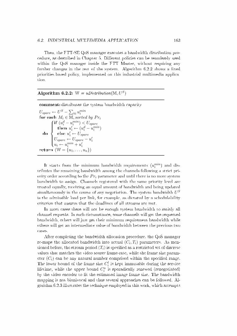
6.2. INDUSTRIAL MULTIMEDIA APPLICATION 163
Then, the FTT-SE QoS manager executes a bandwidth distribution pro-cedure, as described in Chapter 5. Di�erent policies can be seamlessly usedwithin the QoS manager inside the FTT Master, without requiring anyfurther changes in the rest of the system. Algorithm 6.2.2 shows a �xedpriorities-based policy, implemented on this industrial multimedia applica-tion.
Algorithm 6.2.2: W = uDistribution(M, US)
comment: distributes the system bandwidth capacity
Uspare ← US −∑∀i u
mini
for each Mi ∈M, sorted by Pri
do
if (udi − umini ) < Usparethen u′i ← (udi − umini )else u′i ← Uspare
Uspare ← Uspare − u′iui ← umini + u′i
return (W = {u1, . . . , un})
It starts from the minimum bandwidth requirements (umini ) and dis-tributes the remaining bandwidth among the channels following a strict pri-ority order according to the Pri parameter and until there is no more systembandwidth to assign. Channels registered with the same priority level aretreated equally, receiving an equal amount of bandwidth and being updatedsimultaneously in the course of any negotiation. The system bandwidth US
is the admissible load per link, for example, as dictated by a schedulabilitycriterion that assures that the deadlines of all streams are met.
In most cases there will not be enough system bandwidth to satisfy allchannel requests. In such circumstance, some channels will get the requestedbandwidth, others will just get their minimum requirement bandwidth whileothers will get an intermediate value of bandwidth between the previous twocases.
After completing the bandwidth allocation procedure, the QoS managerre-maps the allocated bandwidth into actual (Ci, Ti) parameters. As men-tioned before, the stream period (Ti) is speci�ed as a restricted set of discretevalues that matches the video source frame-rate, while the frame size param-eter (Ci) can be any natural number comprised within the speci�ed range.The lower bound of the frame size C li is kept immutable during the servicelifetime, while the upper bound Cui is sporadically renewed (renegotiated)by the video encoder to �t the estimated image frame size. The bandwidthmapping is not biunivocal and thus several approaches can be followed. Al-gorithm 6.2.3 illustrates the technique employed in this work, which attempts
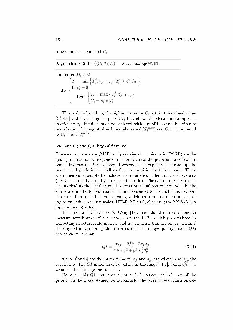
164 CHAPTER 6. FTT-SE CASE STUDIES
to maximize the value of Ci.
Algorithm 6.2.3: {(Ci, Ti)∀i} = uCTmapping(W,M)
for each Mi ∈M
do
Ti = min
{T ji ,∀j=1..ni : T ji ≥ Cui /ui
}if Ti = ∅
then
{Ti = max
{T ji ,∀j=1..ni
}Ci = ui × Ti
This is done by taking the highest value for Ci within the de�ned range[C li , C
ui ] and then using the period Ti that allows the closest under approx-
imation to ui. If this cannot be achieved with any of the available discreteperiods then the longest of such periods is used (Tmaxi ) and Ci is recomputedas Ci = ui × Tmaxi .
Measuring the Quality of Service
The mean-square-error (MSE) and peak-signal-to-noise ratio (PSNR) are thequality metrics most frequently used to evaluate the performance of codecsand video transmission systems. However, their capacity to match up theperceived degradation as well as the human vision factors is poor. Thereare numerous attempts to include characteristics of human visual systems(HVS) in objective quality assessment metrics. These attempts try to geta numerical method with a good correlation to subjective methods. In thesubjective methods, test sequences are presented to instructed non expertobservers, in a controlled environment, which perform an evaluation accord-ing to prede�ned quality scales (ITU-R BT.500), obtaining the MOS (MeanOpinion Score) value.
The method proposed by Z. Wang [135] uses the structural distortionmeasurement instead of the error, since the HVS is highly specialized inextracting structural information, and not in extracting the errors. Being fthe original image, and g the distorted one, the image quality index (QI)can be calculated as:
QI =σfgσfσg
2f g
f2 + g2
2σfσgσ2fσ
2g
(6.11)
where f and g are the intensity mean, σf and σg its variance and σfg thecovariance. The QI index assumes values in the range [-1,1], being QI = 1when the both images are identical.
However, this QI metric does not entirely re�ect the in�uence of thepriority on the QoS obtained nor accounts for the correct use of the available
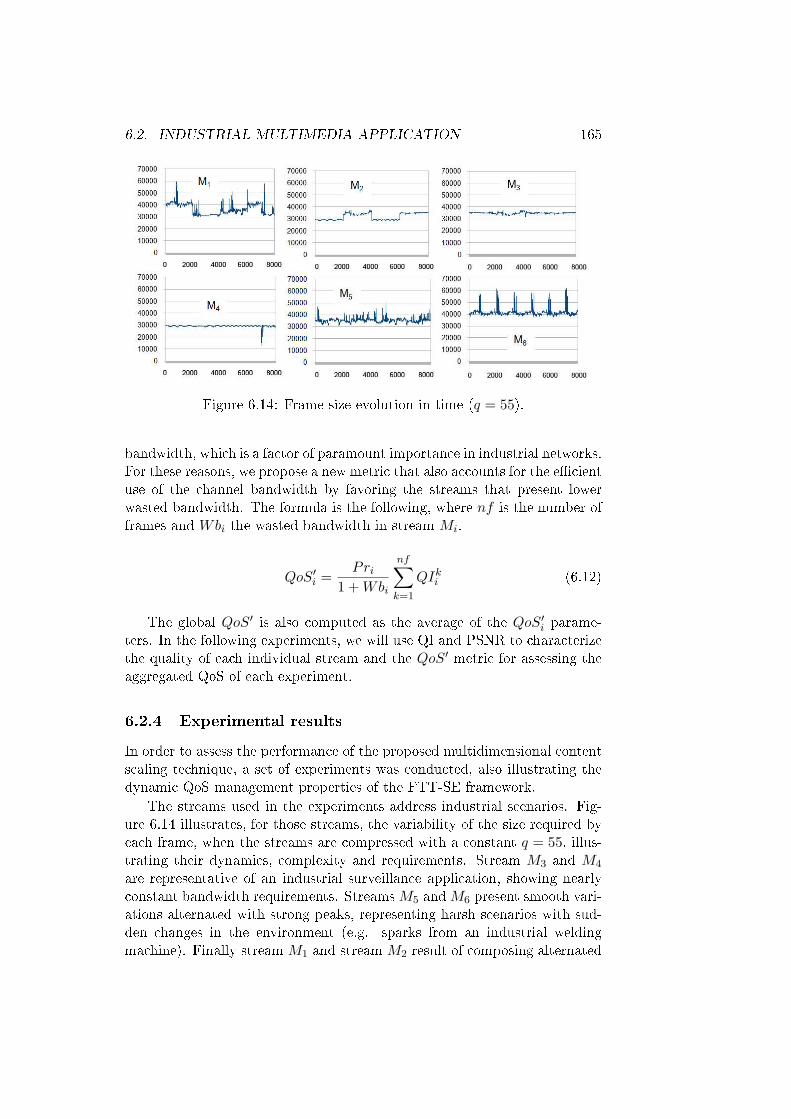
6.2. INDUSTRIAL MULTIMEDIA APPLICATION 165
Figure 6.14: Frame size evolution in time (q = 55).
bandwidth, which is a factor of paramount importance in industrial networks.For these reasons, we propose a new metric that also accounts for the e�cientuse of the channel bandwidth by favoring the streams that present lowerwasted bandwidth. The formula is the following, where nf is the number offrames and Wbi the wasted bandwidth in stream Mi.
QoS′i =Pri
1 +Wbi
nf∑k=1
QIki (6.12)
The global QoS′ is also computed as the average of the QoS′i parame-ters. In the following experiments, we will use QI and PSNR to characterizethe quality of each individual stream and the QoS′ metric for assessing theaggregated QoS of each experiment.
6.2.4 Experimental results
In order to assess the performance of the proposed multidimensional contentscaling technique, a set of experiments was conducted, also illustrating thedynamic QoS management properties of the FTT-SE framework.
The streams used in the experiments address industrial scenarios. Fig-ure 6.14 illustrates, for those streams, the variability of the size required byeach frame, when the streams are compressed with a constant q = 55, illus-trating their dynamics, complexity and requirements. Stream M3 and M4
are representative of an industrial surveillance application, showing nearlyconstant bandwidth requirements. StreamsM5 andM6 present smooth vari-ations alternated with strong peaks, representing harsh scenarios with sud-den changes in the environment (e.g. sparks from an industrial weldingmachine). Finally stream M1 and stream M2 result of composing alternated
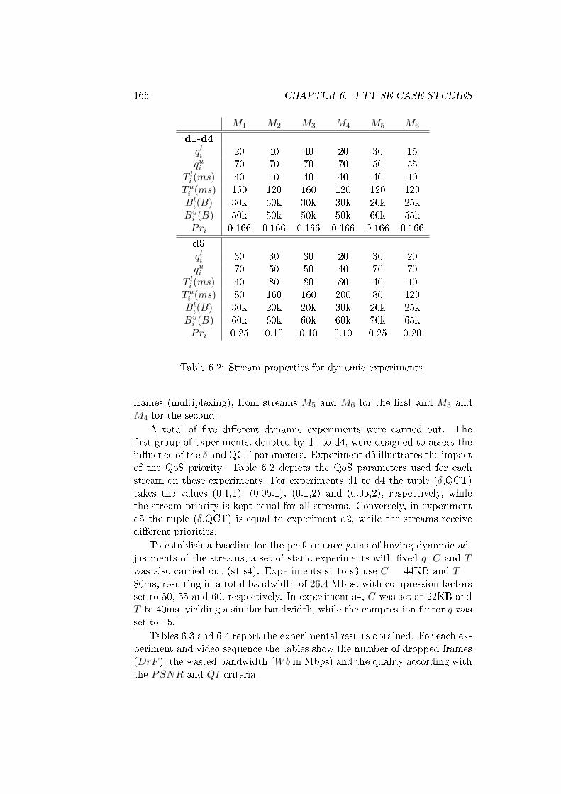
166 CHAPTER 6. FTT-SE CASE STUDIES
M1 M2 M3 M4 M5 M6
d1-d4qli 20 40 40 20 30 15qui 70 70 70 70 50 55
T li (ms) 40 40 40 40 40 40T ui (ms) 160 120 160 120 120 120Bli(B) 30k 30k 30k 30k 20k 25k
Bui (B) 50k 50k 50k 50k 60k 55kPri 0.166 0.166 0.166 0.166 0.166 0.166
d5qli 30 30 30 20 30 20qui 70 50 50 40 70 70
T li (ms) 40 80 80 80 40 40T ui (ms) 80 160 160 200 80 120Bli(B) 30k 20k 20k 30k 20k 25k
Bui (B) 60k 60k 60k 60k 70k 65kPri 0.25 0.10 0.10 0.10 0.25 0.20
Table 6.2: Stream properties for dynamic experiments.
frames (multiplexing), from streams M5 and M6 for the �rst and M3 andM4 for the second.
A total of �ve di�erent dynamic experiments were carried out. The�rst group of experiments, denoted by d1 to d4, were designed to assess thein�uence of the δ and QCT parameters. Experiment d5 illustrates the impactof the QoS priority. Table 6.2 depicts the QoS parameters used for eachstream on these experiments. For experiments d1 to d4 the tuple (δ,QCT)takes the values (0.1,1), (0.05,1), (0.1,2) and (0.05,2), respectively, whilethe stream priority is kept equal for all streams. Conversely, in experimentd5 the tuple (δ,QCT) is equal to experiment d2, while the streams receivedi�erent priorities.
To establish a baseline for the performance gains of having dynamic ad-justments of the streams, a set of static experiments with �xed q, C and Twas also carried out (s1-s4). Experiments s1 to s3 use C = 44KB and T =80ms, resulting in a total bandwidth of 26.4 Mbps, with compression factorsset to 50, 55 and 60, respectively. In experiment s4, C was set at 22KB andT to 40ms, yielding a similar bandwidth, while the compression factor q wasset to 15.
Tables 6.3 and 6.4 report the experimental results obtained. For each ex-periment and video sequence the tables show the number of dropped frames(DrF ), the wasted bandwidth (Wb in Mbps) and the quality according withthe PSNR and QI criteria.
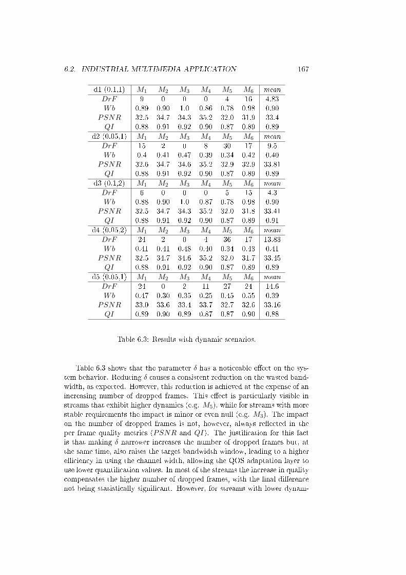
6.2. INDUSTRIAL MULTIMEDIA APPLICATION 167
d1 (0.1,1) M1 M2 M3 M4 M5 M6 mean
DrF 9 0 0 0 4 16 4.83Wb 0.89 0.90 1.0 0.86 0.78 0.98 0.90
PSNR 32.5 34.7 34.3 35.2 32.0 31.9 33.4QI 0.88 0.91 0.92 0.90 0.87 0.89 0.89
d2 (0.05,1) M1 M2 M3 M4 M5 M6 mean
DrF 15 2 0 8 30 17 9.5Wb 0.4 0.41 0.47 0.39 0.34 0.42 0.40
PSNR 32.6 34.7 34.6 35.2 32.9 32.9 33.81QI 0.88 0.91 0.92 0.90 0.87 0.89 0.89
d3 (0.1,2) M1 M2 M3 M4 M5 M6 mean
DrF 6 0 0 0 5 15 4.3Wb 0.88 0.90 1.0 0.87 0.78 0.98 0.90
PSNR 32.5 34.7 34.3 35.2 32.0 31.8 33.41QI 0.88 0.91 0.92 0.90 0.87 0.89 0.91
d4 (0.05,2) M1 M2 M3 M4 M5 M6 mean
DrF 24 2 0 4 36 17 13.83Wb 0.41 0.41 0.48 0.40 0.34 0.43 0.41
PSNR 32.5 34.7 34.6 35.2 32.0 31.7 33.45QI 0.88 0.91 0.92 0.90 0.87 0.89 0.89
d5 (0.05,1) M1 M2 M3 M4 M5 M6 mean
DrF 24 0 2 11 27 24 14.6Wb 0.47 0.30 0.35 0.25 0.45 0.55 0.39
PSNR 33.0 33.6 33.4 33.7 32.7 32.6 33.16QI 0.89 0.90 0.89 0.87 0.87 0.90 0.88
Table 6.3: Results with dynamic scenarios.
Table 6.3 shows that the parameter δ has a noticeable e�ect on the sys-tem behavior. Reducing δ causes a consistent reduction on the wasted band-width, as expected. However, this reduction is achieved at the expense of anincreasing number of dropped frames. This e�ect is particularly visible instreams that exhibit higher dynamics (e.g. M5), while for streams with morestable requirements the impact is minor or even null (e.g. M3). The impacton the number of dropped frames is not, however, always re�ected in theper frame quality metrics (PSNR and QI). The justi�cation for this factis that making δ narrower increases the number of dropped frames but, atthe same time, also raises the target bandwidth window, leading to a highere�ciency in using the channel width, allowing the QOS adaptation layer touse lower quanti�cation values. In most of the streams the increase in qualitycompensates the higher number of dropped frames, with the �nal di�erencenot being statistically signi�cant. However, for streams with lower dynam-
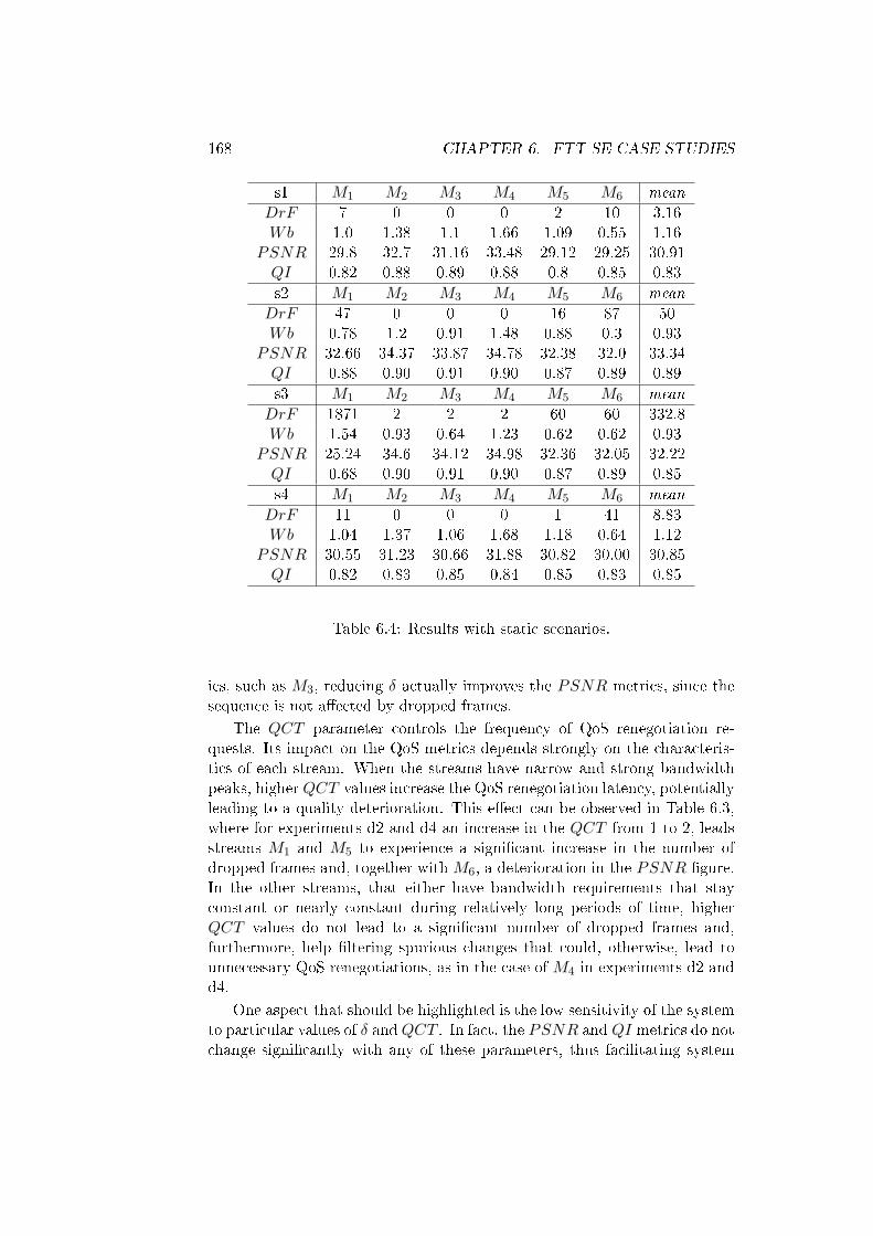
168 CHAPTER 6. FTT-SE CASE STUDIES
s1 M1 M2 M3 M4 M5 M6 mean
DrF 7 0 0 0 2 10 3.16Wb 1.0 1.38 1.1 1.66 1.09 0.55 1.16
PSNR 29.8 32.7 31.16 33.48 29.12 29.25 30.91QI 0.82 0.88 0.89 0.88 0.8 0.85 0.83
s2 M1 M2 M3 M4 M5 M6 mean
DrF 47 0 0 0 16 87 50Wb 0.78 1.2 0.91 1.48 0.88 0.3 0.93
PSNR 32.66 34.37 33.87 34.78 32.38 32.0 33.34QI 0.88 0.90 0.91 0.90 0.87 0.89 0.89
s3 M1 M2 M3 M4 M5 M6 mean
DrF 1871 2 2 2 60 60 332.8Wb 1.54 0.93 0.64 1.23 0.62 0.62 0.93
PSNR 25.24 34.6 34.12 34.98 32.36 32.05 32.22QI 0.68 0.90 0.91 0.90 0.87 0.89 0.85
s4 M1 M2 M3 M4 M5 M6 mean
DrF 11 0 0 0 1 41 8.83Wb 1.04 1.37 1.06 1.68 1.18 0.64 1.12
PSNR 30.55 31.23 30.66 31.88 30.82 30.00 30.85QI 0.82 0.83 0.85 0.84 0.85 0.83 0.85
Table 6.4: Results with static scenarios.
ics, such as M3, reducing δ actually improves the PSNR metrics, since thesequence is not a�ected by dropped frames.
The QCT parameter controls the frequency of QoS renegotiation re-quests. Its impact on the QoS metrics depends strongly on the characteris-tics of each stream. When the streams have narrow and strong bandwidthpeaks, higher QCT values increase the QoS renegotiation latency, potentiallyleading to a quality deterioration. This e�ect can be observed in Table 6.3,where for experiments d2 and d4 an increase in the QCT from 1 to 2, leadsstreams M1 and M5 to experience a signi�cant increase in the number ofdropped frames and, together with M6, a deterioration in the PSNR �gure.In the other streams, that either have bandwidth requirements that stayconstant or nearly constant during relatively long periods of time, higherQCT values do not lead to a signi�cant number of dropped frames and,furthermore, help �ltering spurious changes that could, otherwise, lead tounnecessary QoS renegotiations, as in the case of M4 in experiments d2 andd4.
One aspect that should be highlighted is the low sensitivity of the systemto particular values of δ and QCT . In fact, the PSNR and QI metrics do notchange signi�cantly with any of these parameters, thus facilitating system
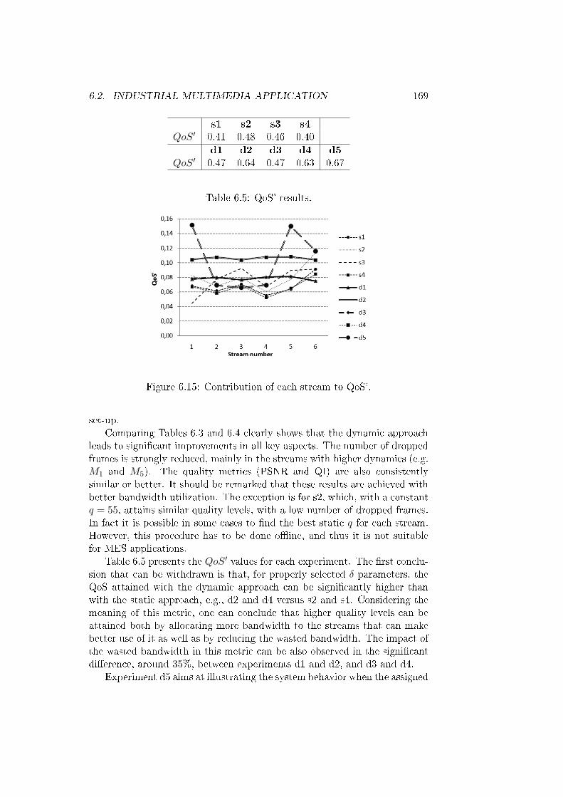
6.2. INDUSTRIAL MULTIMEDIA APPLICATION 169
s1 s2 s3 s4QoS′ 0.41 0.48 0.46 0.40
d1 d2 d3 d4 d5QoS′ 0.47 0.64 0.47 0.63 0.67
Table 6.5: QoS' results.
Figure 6.15: Contribution of each stream to QoS'.
set-up.Comparing Tables 6.3 and 6.4 clearly shows that the dynamic approach
leads to signi�cant improvements in all key aspects. The number of droppedframes is strongly reduced, mainly in the streams with higher dynamics (e.g.M1 and M5). The quality metrics (PSNR and QI) are also consistentlysimilar or better. It should be remarked that these results are achieved withbetter bandwidth utilization. The exception is for s2, which, with a constantq = 55, attains similar quality levels, with a low number of dropped frames.In fact it is possible in some cases to �nd the best static q for each stream.However, this procedure has to be done o�ine, and thus it is not suitablefor MES applications.
Table 6.5 presents the QoS′ values for each experiment. The �rst conclu-sion that can be withdrawn is that, for properly selected δ parameters, theQoS attained with the dynamic approach can be signi�cantly higher thanwith the static approach, e.g., d2 and d4 versus s2 and s4. Considering themeaning of this metric, one can conclude that higher quality levels can beattained both by allocating more bandwidth to the streams that can makebetter use of it as well as by reducing the wasted bandwidth. The impact ofthe wasted bandwidth in this metric can be also observed in the signi�cantdi�erence, around 35%, between experiments d1 and d2, and d3 and d4.
Experiment d5 aims at illustrating the system behavior when the assigned
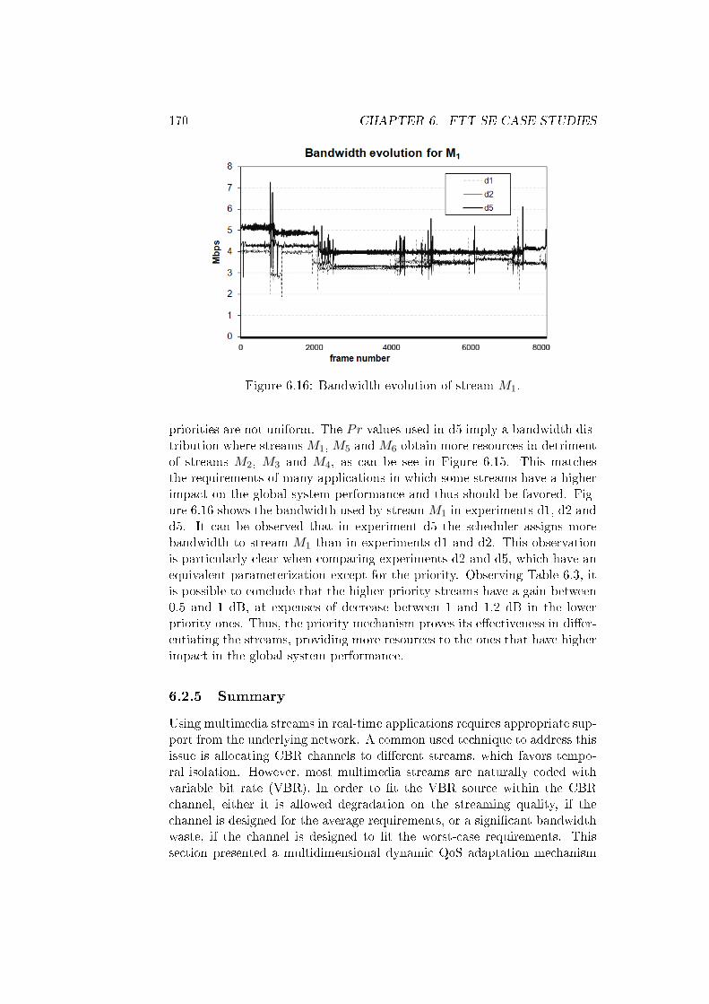
170 CHAPTER 6. FTT-SE CASE STUDIES
Figure 6.16: Bandwidth evolution of stream M1.
priorities are not uniform. The Pr values used in d5 imply a bandwidth dis-tribution where streamsM1, M5 andM6 obtain more resources in detrimentof streams M2, M3 and M4, as can be see in Figure 6.15. This matchesthe requirements of many applications in which some streams have a higherimpact on the global system performance and thus should be favored. Fig-ure 6.16 shows the bandwidth used by stream M1 in experiments d1, d2 andd5. It can be observed that in experiment d5 the scheduler assigns morebandwidth to stream M1 than in experiments d1 and d2. This observationis particularly clear when comparing experiments d2 and d5, which have anequivalent parameterization except for the priority. Observing Table 6.3, itis possible to conclude that the higher priority streams have a gain between0.5 and 1 dB, at expenses of decrease between 1 and 1.2 dB in the lowerpriority ones. Thus, the priority mechanism proves its e�ectiveness in di�er-entiating the streams, providing more resources to the ones that have higherimpact in the global system performance.
6.2.5 Summary
Using multimedia streams in real-time applications requires appropriate sup-port from the underlying network. A common used technique to address thisissue is allocating CBR channels to di�erent streams, which favors tempo-ral isolation. However, most multimedia streams are naturally coded withvariable bit rate (VBR). In order to �t the VBR source within the CBRchannel, either it is allowed degradation on the streaming quality, if thechannel is designed for the average requirements, or a signi�cant bandwidthwaste, if the channel is designed to �t the worst-case requirements. Thissection presented a multidimensional dynamic QoS adaptation mechanism
6.2. INDUSTRIAL MULTIMEDIA APPLICATION 171
that allows dynamically changing the channel bandwidth according to thee�ective stream needs and overall available bandwidth. The capacity of theCBR channels is dynamically adjusted, from time-to-time, re�ecting the in-stantaneous requirements of each stream.
This adaptation mechanism is extensively assessed, with its performancebeing compared against a corresponding situation with static CBR channels,using a set of stored video sequences from industrial environments. Theperformance level is assessed with a QoS metric that includes both the imagequality, the stream QoS priorities and the capacity of the system to reducethe wasted bandwidth. The results obtained show a consistent superiority ofthe dynamic approach over the static one, specially when streams of di�erentpriorities are in place. Moreover, the adaptation is carried out with reservedchannels, thus maintaining the temporal isolation feature among the streamsand other real-time tra�c, thus being suitable for integration in complexMES systems, integrating real-time sources of diverse natures, e.g. closed-loop control.
This industrial application scenario illustrates the bene�ts from using adynamically adaptable system, based on sing the framework proposed in thisthesis (FTT-SE) along with its dynamic QoS management capabilities. Itprovides an example of the integration of these features with the applicationand its dynamics.
172 CHAPTER 6. FTT-SE CASE STUDIES
6.3 Server-SE
In Chapter 2 we have seen the major bene�ts of an Ethernet switch-based ar-chitecture to support real-time communications. Several limitations remain,though, and thus, several protocols have been proposed to provide real-timeservices over such architectures, including FTT-SE, proposed in this thesis.However, in spite of the particular mechanisms employed, they share a com-mon di�culty in the e�cient handling of real-time messages with di�erentarrival patterns, such as periodic and aperiodic, by treating them in di�erentways. The approach proposed in this section is di�erent in the sense that itaims at providing a uniform model, through which messages are scheduledin an integrated way, with no distinction between periodic and aperiodic.
The core of this approach is the integration of the FTT-SE (Section 3)and the Server-CAN [95] protocols. The FTT-SE architecture facilitatesenforcing full control over streams of messages, due to the master/slave op-eration, no matter of their corresponding arrival patterns. Furthermore, thecentralization of the scheduling decisions on the master node also facilitatesthe implementation of arbitrary server policies as well as their hierarchicalcomposition. This property allows complex applications to be decomposedinto sub-applications, each one requiring a share of the bandwidth. Al-though common in CPU scheduling, this level of �exibility, permitting theimplementation of arbitrary server mechanisms as well as their hierarchicalcomposition, is new in the context of RTE networks. Summarizing, this ap-proach for SE systems (1) is free of queues over�ows, (2) supports advancedtra�c scheduling policies and (3) can enforce real-time guarantees even inthe presence of aperiodic communication and/or time-domain faults, e.g.,babbling idiots.
This section is based on work conducted in cooperation with ThomasNolte from Mälardalen University in Sweden [87] and Nuno Figueiredo [88],while he was pursuing his Master thesis. The following section providesan overview of server-based CPU scheduling as well as server-based traf-�c scheduling techniques. Then, Section 6.3.2 proposes using the FTT-SEprotocol to allow a local management of all servers, facilitating their on-line creation, deletion, adaptation and composition. It advocates that sucha centralized management of the servers provides the required support foropen distributed real-time systems as well as for dynamic QoS management.Moreover, the proposed approach also allows any CPU-oriented server-basedscheduling policy to be implemented for network scheduling, possibly withhierarchical composition, increasing the �exibility of the system.
Afterwards, we present a prototype implementation that validates theframework by means of a case study based on a control-based testbed.
6.3. SERVER-SE 173
6.3.1 Server-based scheduling
In the real-time scheduling literature many types of server-based schedulershave been presented for Fixed Priority Systems (FPS) and Dynamic PrioritySystems (DPS). These schedulers are characterized partly by the mechanismfor assigning deadlines, and partly by a set of parameters used to con�gurethe servers, e.g., bandwidth, period and capacity. The Polling Server (PS)[116] is one of the simplest FPS servers. A PS allocates a share of a resourceto the users of the server. This share is de�ned by the server period andcapacity. The Deferrable Server (DS) [123] improves the responsiveness of thePS by permitting deferring its execution whenever there are no user requests.In general the DS gives better response times than the PS at expenses of alower schedulability bound. By changing the way capacity is replenished fora server, the Sporadic Server (SS) [116] is a server-based scheduler for FPSsystems that allows high schedulability without compromising too much theresponsiveness.
Examples of Earliest Deadline First (EDF) based DPS servers include,e.g., the Dynamic Sporadic Server (DSS) [118]. A very simple (implemen-tation wise) server-based scheduler that provides faster response time com-pared with SS is the Total Bandwidth Server (TBS) [118]. TBS makes surethat the server never uses more bandwidth than allocated to it, yet provid-ing a fast response time to its users (under the assumption that the users donot consume more capacity than what they have speci�ed). When the usersdesired usage is unknown, the Constant Bandwidth Server (CBS) [24] can beused, guaranteeing that the server users will never use more than the servercapacity. This is particularly e�cient to enforce temporal isolation betweenthe server users and the remainder of the system.
In the network domain, probably for historical reasons, the names givento servers are di�erent. For example, a common server used in networkingis the leaky bucket. This is a speci�c kind of a general server category calledtra�c shapers, which purpose is to limit the amount of tra�c that a nodecan submit to the network within a given time window, bounding the nodeburstiness. These servers use a technique similar to those described in theprevious section, based on capacity that is eventually replenished. Many dif-ferent replenishment policies are also possible, being the periodic replenish-ment as with PS or DS, the most common. However, it is hard to categorizethese network servers similarly to the CPU servers referred in the previoussection because networks seldom use clear �xed or dynamic priority tra�cmanagement schemes. For example, there is a large variability of MediumAccess Control (MAC) protocols, some of them mixing di�erent schemessuch as round-robin scheduling with �xed priorities, �rst-come-�rst-served,�rst-come-�rst-served with multiple priority queues, etc.
This work advocates that, using an adequate protocol, such as one basedon the FTT paradigm [28, 84, 101], it is possible to control the tra�c in a way
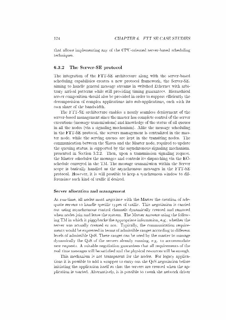
174 CHAPTER 6. FTT-SE CASE STUDIES
that allows implementing any of the CPU-oriented server-based schedulingtechniques.
6.3.2 The Server-SE protocol
The integration of the FTT-SE architecture along with the server-basedscheduling capabilities creates a new protocol framework, the Server-SE,aiming to handle general message streams in switched Ethernet with arbi-trary arrival patterns while still providing timing guarantees. Hierarchicalserver composition should also be provided in order to support e�ciently thedecomposition of complex applications into sub-applications, each with itsown share of the bandwidth.
The FTT-SE architecture enables a nearly seamless deployment of theserver-based management since the master has complete control of the serverexecutions (message transmissions) and knowledge of the status of all queuesin all the nodes (via a signaling mechanism). Alike the message schedulingin the FTT-SE protocol, the servers management is centralized in the mas-ter node, while the serving queues are kept in the transiting nodes. Thecommunication between the Slaves and the Master node, required to updatethe queuing status, is supported by the asynchronous signaling mechanism,presented in Section 3.2.2. Then, upon a transmission signaling request,the Master schedules the messages and controls its dispatching via the EC-schedule conveyed in the TM. The message transmission within the Serverscope is basically handled as the asynchronous messages in the FTT-SEprotocol. However, it is still possible to keep a synchronous window to dif-ferentiate such kind of tra�c if desired.
Server allocation and management
At run-time, all nodes must negotiate with the Master the creation of ade-quate servers to handle speci�c types of tra�c. This negotiation is carriedout using asynchronous control channels dynamically created and removedwhen nodes join and leave the system. The Master answers using the follow-ing TM in which it piggybacks the appropriate information, e.g., whether theserver was actually created or not. Typically, the communication require-ments would be expressed in terms of admissible ranges according to di�erentlevels of admissible QoS. These ranges can be used by the master to managedynamically the QoS of the servers already running, e.g. to accommodatenew requests. A suitable negotiation guarantees that all requirements of thereal-time messages will be satis�ed and the physical resources will be enough.
This mechanism is not transparent for the nodes. For legacy applica-tions it is possible to add a wrapper to carry out the QoS negotiation beforeinitiating the application itself so that the servers are created when the ap-plication is started. Alternatively, it is possible to tweak the network driver
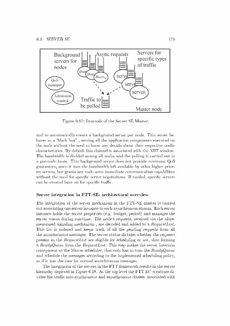
6.3. SERVER-SE 175
Figure 6.17: Internals of the Server-SE Master.
and to automatically create a background server per node. This server be-haves as a �black box� , serving all the application components executed onthe node without the need to know any details about their respective tra�ccharacteristics. By default this channel is associated with the NRT window.The bandwidth is divided among all nodes and the polling is carried out ina per-node basis. This background server does not provide minimum QoSguarantees, since it uses the bandwidth left available by other higher prior-ity servers, but grants any node some immediate communication capabilitieswithout the need for speci�c server negotiations. If needed, speci�c serverscan be created later on for speci�c tra�c.
Server integration in FTT-SE: architectural overview
The integration of the server mechanism in the FTT-SE master is carriedout associating one server instance to each asynchronous stream. Each serverinstance holds the server properties (e.g. budget, period) and manages theserver status during run-time. The node's requests, received via the afore-mentioned signaling mechanism , are decoded and added to a RequestList.This list is ordered and keeps track of all the pending requests from allthe asynchronous messages. The server status dictates whether the requestspresent in the RequestList are eligible for scheduling or not, thus forminga ReadyQueue from the RequestList. This step makes the server insertiontransparent to the Master scheduler, that only has to scan the ReadyQueueand schedule the messages according to the implemented scheduling policy,as if it was the case for normal asynchronous messages.
The integration of the servers in the FTT framework results in the serverhierarchy depicted in Figure 6.18. At the top level the FTT EC structure di-vides the tra�c into synchronous and asynchronous classes, associated with
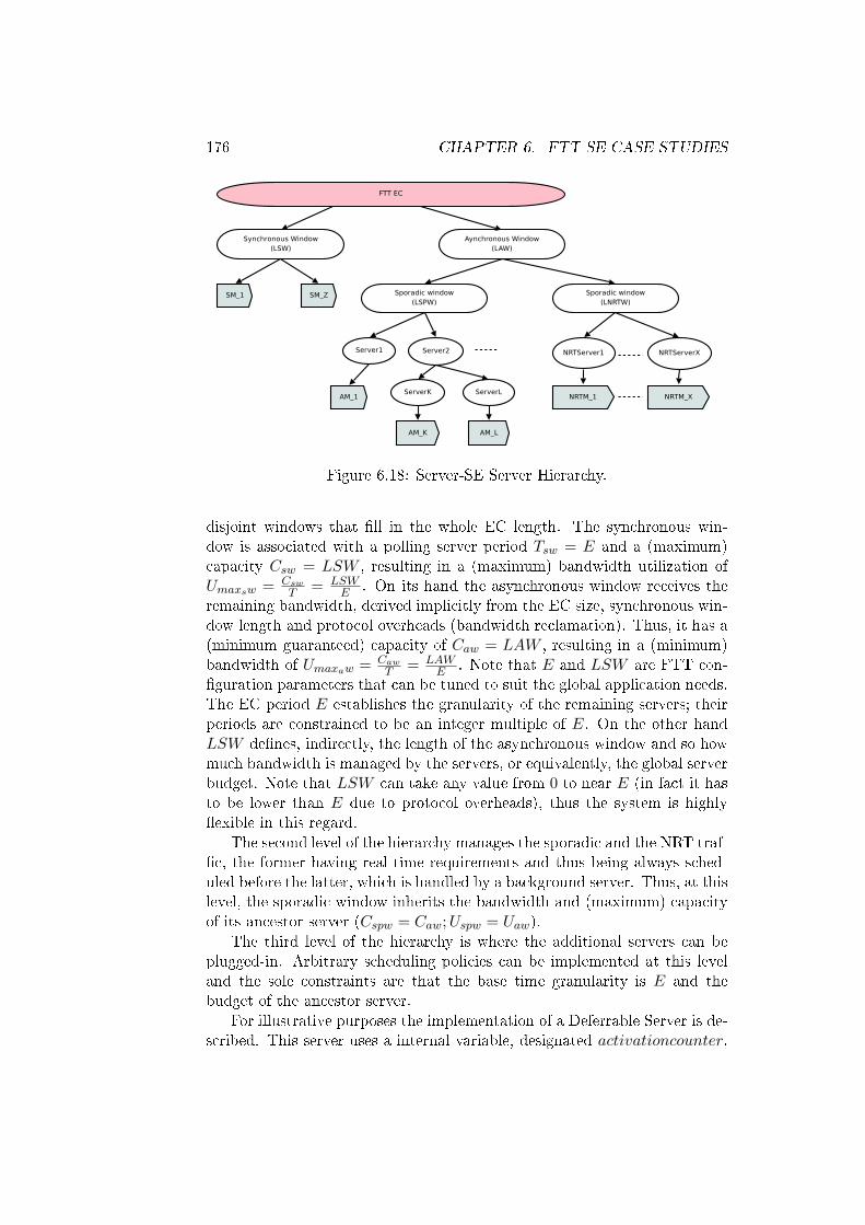
176 CHAPTER 6. FTT-SE CASE STUDIES
Figure 6.18: Server-SE Server Hierarchy.
disjoint windows that �ll in the whole EC length. The synchronous win-dow is associated with a polling server period Tsw = E and a (maximum)capacity Csw = LSW , resulting in a (maximum) bandwidth utilization ofUmaxsw = Csw
T = LSWE . On its hand the asynchronous window receives the
remaining bandwidth, derived implicitly from the EC size, synchronous win-dow length and protocol overheads (bandwidth reclamation). Thus, it has a(minimum guaranteed) capacity of Caw = LAW , resulting in a (minimum)bandwidth of Umaxaw = Caw
T = LAWE . Note that E and LSW are FTT con-
�guration parameters that can be tuned to suit the global application needs.The EC period E establishes the granularity of the remaining servers; theirperiods are constrained to be an integer multiple of E. On the other handLSW de�nes, indirectly, the length of the asynchronous window and so howmuch bandwidth is managed by the servers, or equivalently, the global serverbudget. Note that LSW can take any value from 0 to near E (in fact it hasto be lower than E due to protocol overheads), thus the system is highly�exible in this regard.
The second level of the hierarchy manages the sporadic and the NRT traf-�c, the former having real-time requirements and thus being always sched-uled before the latter, which is handled by a background server. Thus, at thislevel, the sporadic window inherits the bandwidth and (maximum) capacityof its ancestor server (Cspw = Caw;Uspw = Uaw).
The third level of the hierarchy is where the additional servers can beplugged-in. Arbitrary scheduling policies can be implemented at this leveland the sole constraints are that the base time granularity is E and thebudget of the ancestor server.
For illustrative purposes the implementation of a Deferrable Server is de-scribed. This server uses a internal variable, designated activationcounter,
6.3. SERVER-SE 177
that controls the replenishment period. This variable is set to zero uponcreation, meaning that the server is eligible for transmitting. Whenever amessage is sent, the variable is set to the replenishment period (mit) andis decremented every EC until its value reaches zero. This event meansthat the server is replenished and thus any pending messages present in theRequestList are moved to the ReadyQueue, becoming eligible for trans-mission. The process repeats itself. As can be seen, the integration of theserver-based mechanism produces minor implications in the FTT-SE archi-tecture. The changes were restricted to the message activation procedure,maintenance of the activationcounter and ReadyQueue management. Morecomplex servers can require additional structures, specially when compris-ing several messages in a single server scope, similarly to the case of servermechanisms for processor scheduling.
Limitations and alternative approaches
The Server-SE approach hereby proposed relies on the FTT-SE protocol and,consequently, also inherits most of the limitations and drawbacks of this pro-tocol. From a conceptual point-of-view the main issues that can be identi�edin the current approach are the requirement for a cooperative architectureand the explicit signaling mechanism. FTT-SE is a master/multi-slave proto-col and thus, as any other master/slave protocol, depends on the cooperationof all the nodes in the system. Malfunctioning or non-compliant nodes thatuse the transmission medium without respecting the mediation of the Mas-ter can jeopardize all the temporal guarantees. This aspect constrains one ofthe goals of Server-SE that is to e�ciently support open systems, in whichnodes can leave and join at will, while still providing timeliness guarantees.On the other hand, the explicit signaling mechanism induces an undesirablelatency. Nodes can only report their status in discrete time instants, namelythe beginning of the ECs. Thus the signaling latency is, at minimum, 1 to 2ECs, and can be bigger for systems with a relatively high number of nodes(> 30, see Section 3.3.4).
Both of these problems can be solved by an alternative FTT-SE im-plementation currently under development and addressed in Chapter 7 asfuture work. A preliminary implementation for proof of concept is describedin Section 6.4.The main idea is to integrate the FTT master within a customEthernet switch, con�ning, by itself, the non-FTT tra�c to con�gurable pre-de�ned windows, thus preventing negative e�ects from non-compliant nodes.Furthermore, the modi�ed switch carries out tra�c policing, i.e., messagesthat violate the agreed time domain parameters are trashed and, preserv-ing the correct behavior of real-time tra�c. Finally, the explicit signalingmechanism is no longer needed and the nodes are allowed to transmit asyn-chronous messages autonomously. Incoming messages are queued, classi�edand veri�ed by the switch. Thus, servers can be noti�ed internally on the
178 CHAPTER 6. FTT-SE CASE STUDIES
arrival of new messages, update their status and turn messages eligible fortransmission when appropriate. This is on-going work that is currently beingexplored.
6.3.3 Experimental results
This section presents experimental results obtained from a prototype imple-mentation of Server-SE. The �rst experiment is a basic test meant essentiallyto verify the correctness of the implementation of the server mechanisms.The second experiment involves a mixed environment composed by a dis-tributed control system, with timeliness requirements, and other sources oftra�c, eventually causing overloads. This experiment aims at assessing thesuitability of server-based mechanisms to handle time sensitive distributedsystems comprising di�erent tra�c sources with distinct activation and time-liness requirements.
Tra�c con�nement
For this experiment we created FTT-SE system comprising one Master nodeand two slave nodes. The EC duration is set to 1ms and the network operatesat 100 Mbps. The application submits three aperiodic streams to the networkstack with the following properties: AM1 and AM2 sent by Slave 1 with 2kBand Mean Time Between Activations (MTBA) of 6 and 10 ECs, respectively,and AM3 sent by Slave 2 with 1kB and MTBA 5 ECs. Three sporadicservers [37] were set, one for each message. Each server has a budget equalto one instance and a replenishment period equal to MTBA. The serverswere scheduled according to Rate Monotonic, considering the replenishmentperiods. LAW was constrained to be 240µseconds, which was su�cient toschedule the three servers. In this con�guration the servers can schedule nomore than 2 packets of the referred messages per EC.
The generation of the message transmission requests was carried outrandomly by an application program, which uniformly distributes the acti-vations along the EC time frame, respecting the messageMTBA. Figure 6.19shows the results for message AM3, with the time expressed in ECs. Thetop histogram shows the inter-arrival times of the requests (signaling mes-sages arrived at the Master). The lower histogram shows the inter-arrivaltimes of message AM3 as scheduled by the Master (and transmitted by therespective Slave). The measures were actually carried out within the Master(di�erence between consecutive requests arrivals and di�erence between con-secutive scheduled transmissions). It is clear that, despite the frequent burstsof consecutive requests, the transmissions respect the MTBA correspondingto the respective sporadic server replenishment period. The histograms ofthe other two messages show similar behavior and thus are not presented.
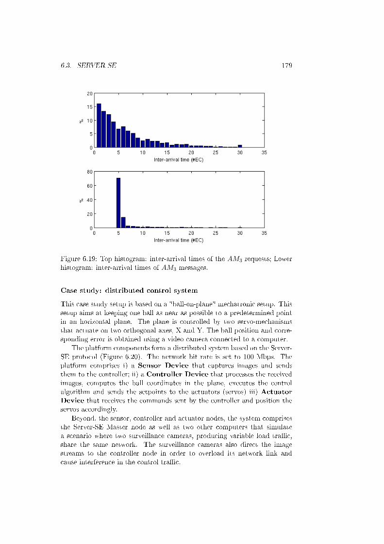
6.3. SERVER-SE 179
Figure 6.19: Top histogram: inter-arrival times of the AM3 requests; Lowerhistogram: inter-arrival times of AM3 messages.
Case study: distributed control system
This case study setup is based on a "ball-on-plane" mechatronic setup. Thissetup aims at keeping one ball as near as possible to a predetermined pointin an horizontal plane. The plane is controlled by two servo-mechanismsthat actuate on two orthogonal axes, X and Y. The ball position and corre-sponding error is obtained using a video camera connected to a computer.
The platform components form a distributed system based on the Server-SE protocol (Figure 6.20). The network bit rate is set to 100 Mbps. Theplatform comprises i) a Sensor Device that captures images and sendsthem to the controller; ii) a Controller Device that processes the receivedimages, computes the ball coordinates in the plane, executes the controlalgorithm and sends the setpoints to the actuators (servos) iii) ActuatorDevice that receives the commands sent by the controller and position theservos accordingly.
Beyond, the sensor, controller and actuator nodes, the system comprisesthe Server-SE Master node as well as two other computers that simulatea scenario where two surveillance cameras, producing variable load tra�c,share the same network. The surveillance cameras also direct the imagestreams to the controller node in order to overload its network link andcause interference in the control tra�c.
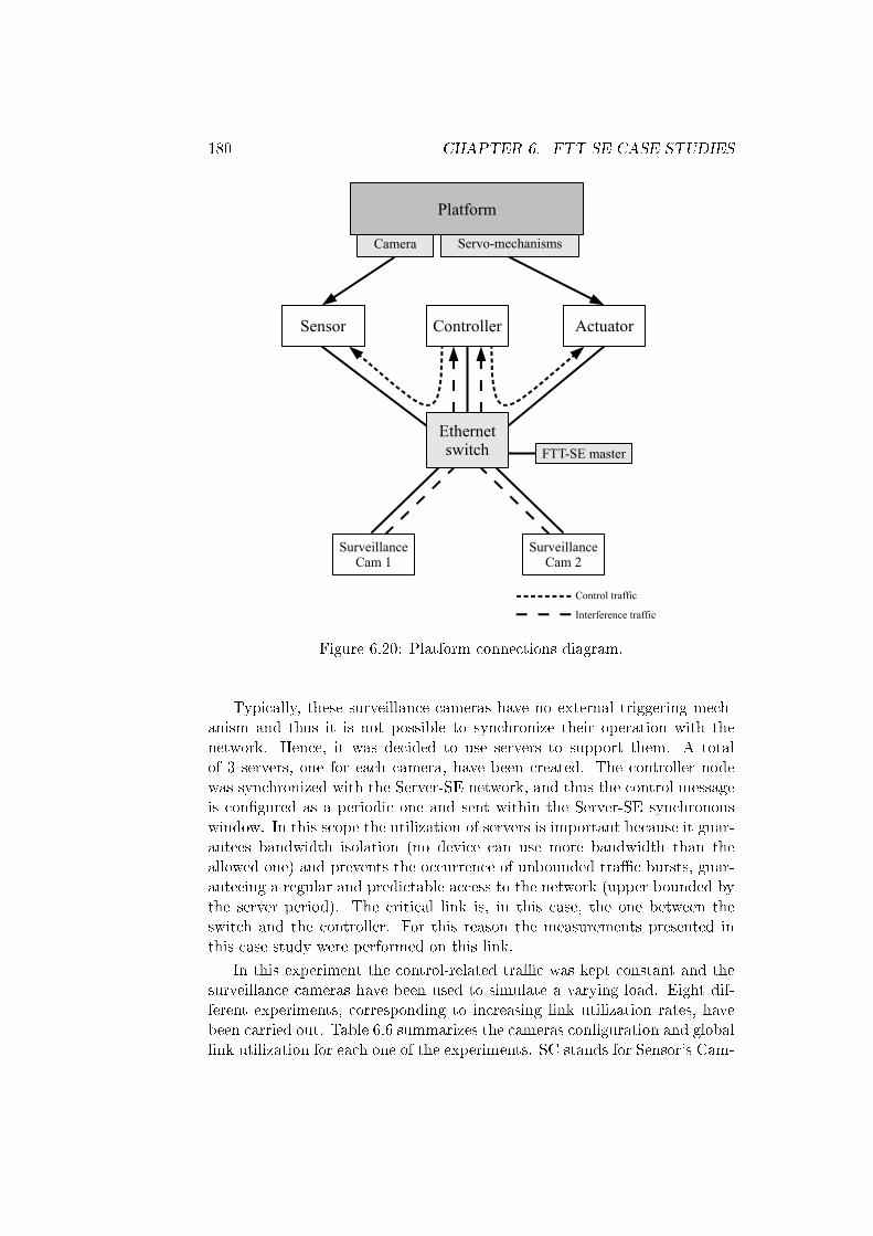
180 CHAPTER 6. FTT-SE CASE STUDIES
ControllerSensor Actuator
FTT-SE master
Servo-mechanismsCamera
Platform
SurveillanceCam 1
SurveillanceCam 2
Ethernetswitch
Control traffic
Interference traffic
Figure 6.20: Platform connections diagram.
Typically, these surveillance cameras have no external triggering mech-anism and thus it is not possible to synchronize their operation with thenetwork. Hence, it was decided to use servers to support them. A totalof 3 servers, one for each camera, have been created. The controller nodewas synchronized with the Server-SE network, and thus the control messageis con�gured as a periodic one and sent within the Server-SE synchronouswindow. In this scope the utilization of servers is important because it guar-antees bandwidth isolation (no device can use more bandwidth than theallowed one) and prevents the occurrence of unbounded tra�c bursts, guar-anteeing a regular and predictable access to the network (upper bounded bythe server period). The critical link is, in this case, the one between theswitch and the controller. For this reason the measurements presented inthis case study were performed on this link.
In this experiment the control-related tra�c was kept constant and thesurveillance cameras have been used to simulate a varying load. Eight dif-ferent experiments, corresponding to increasing link utilization rates, havebeen carried out. Table 6.6 summarizes the cameras con�guration and globallink utilization for each one of the experiments. SC stands for Sensor's Cam-
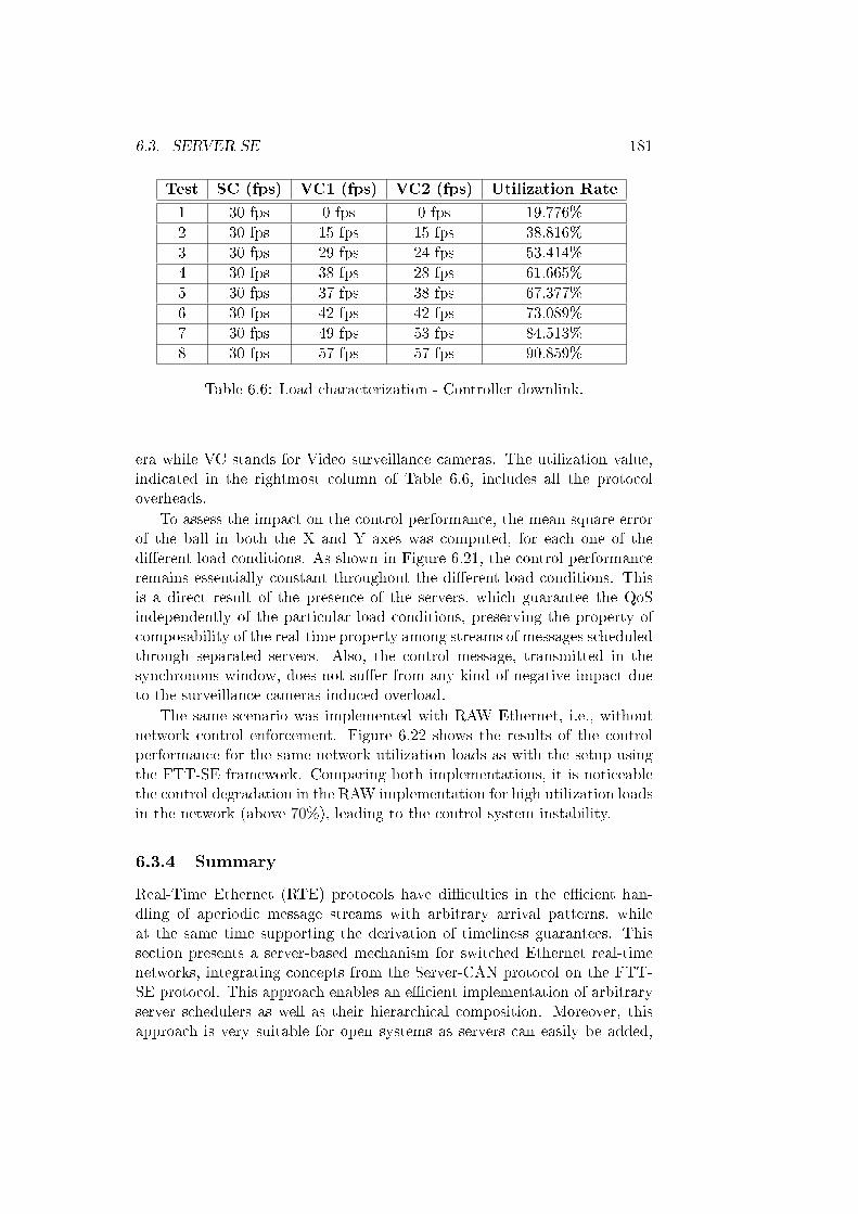
6.3. SERVER-SE 181
Test SC (fps) VC1 (fps) VC2 (fps) Utilization Rate
1 30 fps 0 fps 0 fps 19.776%
2 30 fps 15 fps 15 fps 38.816%
3 30 fps 29 fps 24 fps 53.414%
4 30 fps 38 fps 28 fps 61.665%
5 30 fps 37 fps 38 fps 67.377%
6 30 fps 42 fps 42 fps 73.089%
7 30 fps 49 fps 53 fps 84.513%
8 30 fps 57 fps 57 fps 90.859%
Table 6.6: Load characterization - Controller downlink.
era while VC stands for Video surveillance cameras. The utilization value,indicated in the rightmost column of Table 6.6, includes all the protocoloverheads.
To assess the impact on the control performance, the mean square errorof the ball in both the X and Y axes was computed, for each one of thedi�erent load conditions. As shown in Figure 6.21, the control performanceremains essentially constant throughout the di�erent load conditions. Thisis a direct result of the presence of the servers, which guarantee the QoSindependently of the particular load conditions, preserving the property ofcomposability of the real-time property among streams of messages scheduledthrough separated servers. Also, the control message, transmitted in thesynchronous window, does not su�er from any kind of negative impact dueto the surveillance cameras induced overload.
The same scenario was implemented with RAW Ethernet, i.e., withoutnetwork control enforcement. Figure 6.22 shows the results of the controlperformance for the same network utilization loads as with the setup usingthe FTT-SE framework. Comparing both implementations, it is noticeablethe control degradation in the RAW implementation for high utilization loadsin the network (above 70%), leading to the control system instability.
6.3.4 Summary
Real-Time Ethernet (RTE) protocols have di�culties in the e�cient han-dling of aperiodic message streams with arbitrary arrival patterns, whileat the same time supporting the derivation of timeliness guarantees. Thissection presents a server-based mechanism for switched Ethernet real-timenetworks, integrating concepts from the Server-CAN protocol on the FTT-SE protocol. This approach enables an e�cient implementation of arbitraryserver schedulers as well as their hierarchical composition. Moreover, thisapproach is very suitable for open systems as servers can easily be added,
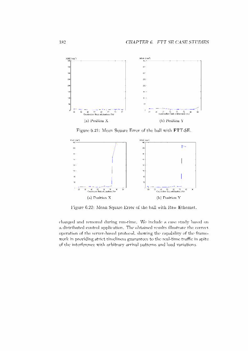
182 CHAPTER 6. FTT-SE CASE STUDIES
(a) Position X (b) Position Y
Figure 6.21: Mean Square Error of the ball with FTT-SE.
(a) Position X (b) Position Y
Figure 6.22: Mean Square Error of the ball with Raw Ethernet.
changed and removed during run-time. We include a case study based ona distributed control application. The obtained results illustrate the correctoperation of the server-based protocol, showing the capability of the frame-work in providing strict timeliness guarantees to the real-time tra�c in spiteof the interference with arbitrary arrival patterns and load variations.
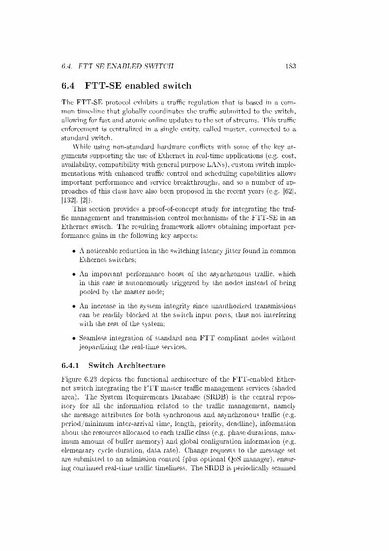
6.4. FTT-SE ENABLED SWITCH 183
6.4 FTT-SE enabled switch
The FTT-SE protocol exhibits a tra�c regulation that is based in a com-mon time-line that globally coordinates the tra�c submitted to the switch,allowing for fast and atomic online updates to the set of streams. This tra�cenforcement is centralized in a single entity, called master, connected to astandard switch.
While using non-standard hardware con�icts with some of the key ar-guments supporting the use of Ethernet in real-time applications (e.g. cost,availability, compatibility with general purpose LANs), custom switch imple-mentations with enhanced tra�c control and scheduling capabilities allowsimportant performance and service breakthroughs, and so a number of ap-proaches of this class have also been proposed in the recent years (e.g. [62],[132], [2]).
This section provides a proof-of-concept study for integrating the traf-�c management and transmission control mechanisms of the FTT-SE in anEthernet switch. The resulting framework allows obtaining important per-formance gains in the following key aspects:
• A noticeable reduction in the switching latency jitter found in commonEthernet switches;
• An important performance boost of the asynchronous tra�c, whichin this case is autonomously triggered by the nodes instead of beingpooled by the master node;
• An increase in the system integrity since unauthorized transmissionscan be readily blocked at the switch input ports, thus not interferingwith the rest of the system;
• Seamless integration of standard non FTT compliant nodes withoutjeopardizing the real-time services.
6.4.1 Switch Architecture
Figure 6.23 depicts the functional architecture of the FTT-enabled Ether-net switch integrating the FTT master tra�c management services (shadedarea). The System Requirements Database (SRDB) is the central repos-itory for all the information related to the tra�c management, namelythe message attributes for both synchronous and asynchronous tra�c (e.g.period/minimum inter-arrival time, length, priority, deadline), informationabout the resources allocated to each tra�c class (e.g. phase durations, max-imum amount of bu�er memory) and global con�guration information (e.g.elementary cycle duration, data rate). Change requests to the message setare submitted to an admission control (plus optional QoS manager), ensur-ing continued real-time tra�c timeliness. The SRDB is periodically scanned
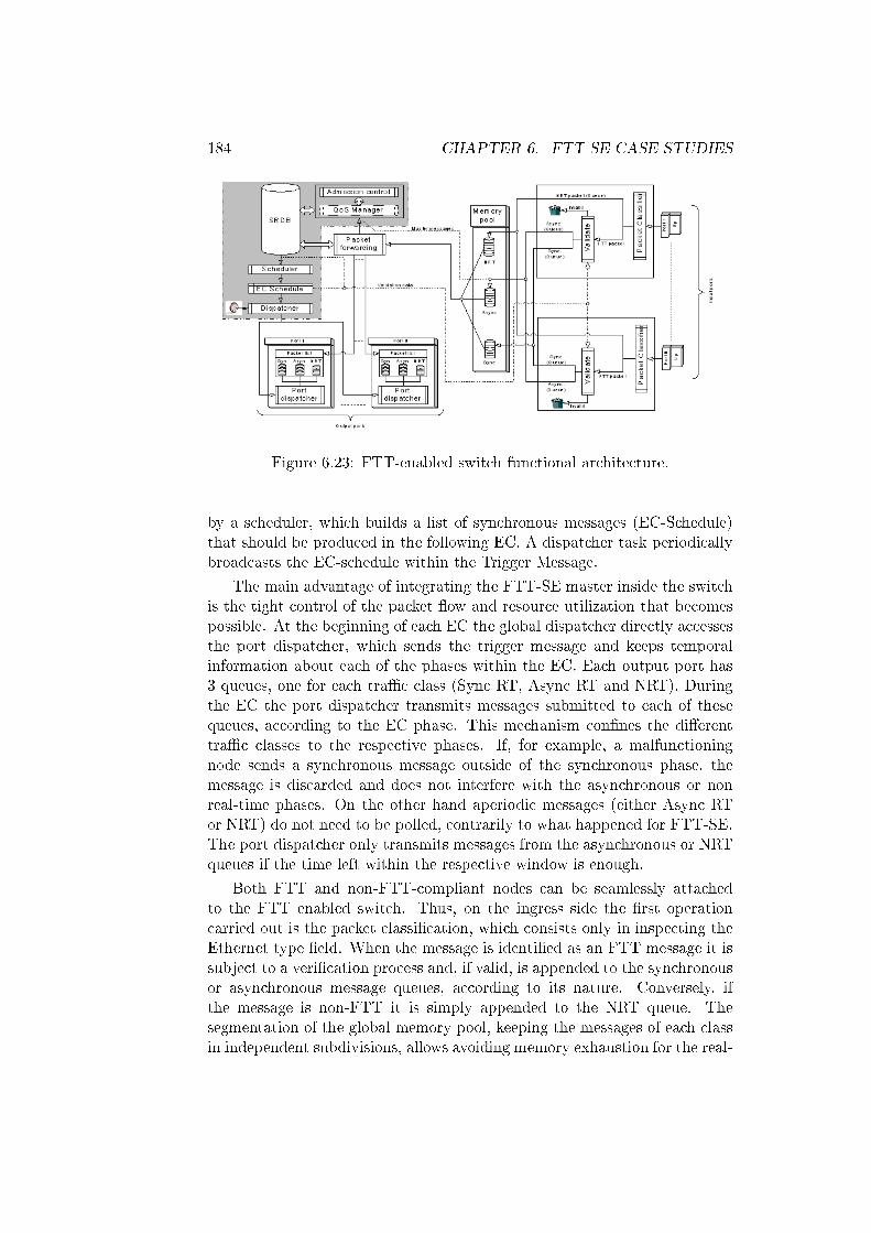
184 CHAPTER 6. FTT-SE CASE STUDIES
Figure 6.23: FTT-enabled switch functional architecture.
by a scheduler, which builds a list of synchronous messages (EC-Schedule)that should be produced in the following EC. A dispatcher task periodicallybroadcasts the EC-schedule within the Trigger Message.
The main advantage of integrating the FTT-SE master inside the switchis the tight control of the packet �ow and resource utilization that becomespossible. At the beginning of each EC the global dispatcher directly accessesthe port dispatcher, which sends the trigger message and keeps temporalinformation about each of the phases within the EC. Each output port has3 queues, one for each tra�c class (Sync RT, Async RT and NRT). Duringthe EC the port dispatcher transmits messages submitted to each of thesequeues, according to the EC phase. This mechanism con�nes the di�erenttra�c classes to the respective phases. If, for example, a malfunctioningnode sends a synchronous message outside of the synchronous phase, themessage is discarded and does not interfere with the asynchronous or nonreal-time phases. On the other hand aperiodic messages (either Async RTor NRT) do not need to be polled, contrarily to what happened for FTT-SE.The port dispatcher only transmits messages from the asynchronous or NRTqueues if the time left within the respective window is enough.
Both FTT and non-FTT-compliant nodes can be seamlessly attachedto the FTT enabled switch. Thus, on the ingress side the �rst operationcarried out is the packet classi�cation, which consists only in inspecting theEthernet type �eld. When the message is identi�ed as an FTT message it issubject to a veri�cation process and, if valid, is appended to the synchronousor asynchronous message queues, according to its nature. Conversely, ifthe message is non-FTT it is simply appended to the NRT queue. Thesegmentation of the global memory pool, keeping the messages of each classin independent subdivisions, allows avoiding memory exhaustion for the real-
6.4. FTT-SE ENABLED SWITCH 185
time messages, a situation that standard switches do not guarantee [102].Note, however, that the amount of memory needed for the real-time messagesis typically small given their temporal properties that are enforced at theswitch ingress. It is also known in advance since the RT tra�c is subject toan explicit registration. During the registration process the producers muststate the �ow properties, in particular the length and period for periodicmessages or minimum inter-arrival time for sporadic ones. With this data itis possible to compute and pre-allocate the amount of memory that RT tra�crequires and thus guarantee that the resources are enough for all admittedmessages.
The validation process of the RT classes gathers data both from the EC-schedule and from the SRDB. Regarding synchronous messages, the analysisof the EC-schedule allows detecting failures in the time domain, namely thetransmission of unscheduled messages or the late transmission of scheduledmessages resulting from malfunctioning nodes. An equivalent set of tests(e.g. minimum inter-arrival time, burstiness) is also performed for asyn-chronous messages with those that fail the validation process being trashed.The policing and enforcement of the tra�c attributes in the time domainguarantees the timeliness of the real-time tra�c even in the presence of mal-functioning nodes.
Whenever a message is placed in the global memory pool, a packet for-warding process is executed. Control messages, targeted to the master aresubmitted to the Admission control/QoS manager module and possibly resultin changes on the SRDB. Data messages should be forwarded to the targetnodes. The forwarding mechanism of FTT messages is based on a producer-consumer model, and does not depend on MAC addresses. Whenever anFTT message arrives the Packet Forwarding module inquires the SRDB todetermine the set of ports having consumers attached, and updates the out-put queue (synchronous or asynchronous, depending on the message nature)of each one of these ports. Non-FTT messages are forwarded according tothe normal procedures of standard Ethernet switches, based on the MACaddress. From the point of view of NRT tra�c, the FTT-enabled switchbehaves as a common switch but with restricted bandwidth arising from thecon�nement of this tra�c to the NRT phase in the EC.
The integration of the FTT-SE master in the switch is transparent to thenodes in what concerns the synchronous tra�c. There are, however, severalsimpli�cations for the aperiodic tra�c. Nodes that do not produce real-timemessages can use any standard Ethernet driver. The transmission control ofthis class in FTT-SE is no longer required here, being replaced by adequatecon�nement by the switch. Nodes that produce real-time messages requirethe FTT-SE network driver to be updated to include di�erent queues forthe three tra�c classes and avoid blocking of the synchronous tra�c in theuplinks.
186 CHAPTER 6. FTT-SE CASE STUDIES
Figure 6.24: Histogram of the di�erences between consecutive NRT messages(uplink).
6.4.2 Experimental results
A prototype implementation, based on the RT-Linux real-time operatingsystem with the Ethernet layer provided by the LNet network stack, wascarried out to validate the extended services provided by the FTT-enabledswitch. This prototype switch is based on a Pentium III PC at 550MHz withfour 3Com 3C905B PCI network interface cards.
The �rst experiment consists in the implementation of a policing servicefor the synchronous tra�c. The ID of incoming synchronous messages ismatched against the ECschedule and discarded if a positive match is notfound. This way only scheduled messages are disseminated, guaranteeingthat the synchronous window is not overrun. To verify the correct behaviorof the policing service we con�gured a setup with one synchronous messagewith period Ti=3ECs while the respective producer slave was tampered tosend that message every EC. We observed that the consumer node onlyreceived the scheduled messages, one every 3ECs, and the extra messageswere discarded. The second experiment consists in the veri�cation of theenforcement of the tra�c temporal isolation. The experimental setup iscon�gured with an EC of 40ms, with the last 3ms of the EC dedicated tothe NRT tra�c. The NRT test load consists in UDP packets carrying 1400data bytes, periodically sent every 5ms. The load is generated with Pack-Eth (http://packeth.sourceforge.net/) running on a plain Linux distribution(RedHat 9.0). Figure 6.24 depicts the histogram of the time di�erences be-tween consecutive NRT messages in the uplink.
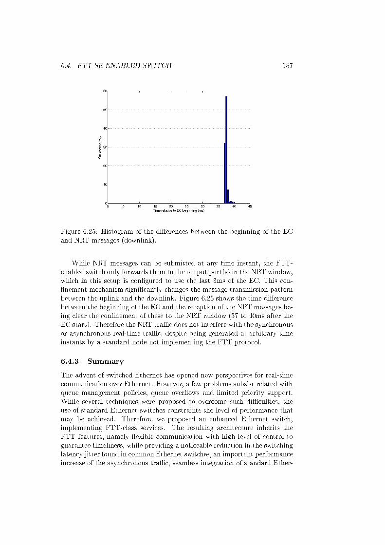
6.4. FTT-SE ENABLED SWITCH 187
Figure 6.25: Histogram of the di�erences between the beginning of the ECand NRT messages (downlink).
While NRT messages can be submitted at any time instant, the FTT-enabled switch only forwards them to the output port(s) in the NRT window,which in this setup is con�gured to use the last 3ms of the EC. This con-�nement mechanism signi�cantly changes the message transmission patternbetween the uplink and the downlink. Figure 6.25 shows the time di�erencebetween the beginning of the EC and the reception of the NRT messages be-ing clear the con�nement of these to the NRT window (37 to 40ms after theEC start). Therefore the NRT tra�c does not interfere with the synchronousor asynchronous real-time tra�c, despite being generated at arbitrary timeinstants by a standard node not implementing the FTT protocol.
6.4.3 Summary
The advent of switched Ethernet has opened new perspectives for real-timecommunication over Ethernet. However, a few problems subsist related withqueue management policies, queue over�ows and limited priority support.While several techniques were proposed to overcome such di�culties, theuse of standard Ethernet switches constraints the level of performance thatmay be achieved. Therefore, we proposed an enhanced Ethernet switch,implementing FTT-class services. The resulting architecture inherits theFTT features, namely �exible communication with high level of control toguarantee timeliness, while providing a noticeable reduction in the switchinglatency jitter found in common Ethernet switches, an important performanceincrease of the asynchronous tra�c, seamless integration of standard Ether-

188 CHAPTER 6. FTT-SE CASE STUDIES
net nodes and a substantial increase in the system integrity as unauthorizedtransmissions from the nodes can be readily blocked at the switch inputports. On-going work (Chapter 7) addresses the FPGA implementation ofthis switch.

6.5. CONCLUSION 189
6.5 Conclusion
The core contribution of this thesis is a new real-time communication pro-tocol for switched Ethernet, namely FTT-SE,that is capable of handlingthe dynamic communication requirements as needed for dynamic QoS man-agement or simply for open and dynamically recon�gurable systems. Thischapter compiled four case-studies that highlight such capability and providesome insight over the performance and usability of such protocol.
The �rst case-study addresses the integration of the FTT-SE protocol inan open-scoped resource handling framework (FRESCOR). FRESCOR pro-vides a uni�ed and common application interface for handling together themanagement of several resources, needed by a service. It handles a number ofresource types in classes. The integration with the FTT-SE protocol bringsin a new network communication class type with di�erent communicationparadigms, namely time and event-triggered, and switched Ethernet topol-ogy. Moreover, FTT-SE supports in a direct and e�cient way the integratedcontracts management of FRESCOR. This results on a smooth integrationof FTT-SE in the global application design scope.
The second case-study shows the use of FTT-SE QoS management inimproving the performance of a multimedia industrial system. The scenarioincludes the transmission of video streams over an FTT-SE network withspeci�c QoS requirements that may vary within a given quality range, de-pending on the network load. We propose a feedback mechanism based ontuning the parameters of MJPEG streams that directly a�ect the servicequality and the network load, such as, the compression factor, the periodictransmission rate and the frame transmission bu�er. Given that FTT-SEalready assures a QoS-aware resource management based on bandwidth dis-tribution, this case-study illustrates how a multimedia application can takeadvantage of the QoS-aware resource management to carry out dynamicQoS adaptation. The QoS management includes the adaption of variablebitrate (VBR) services, such as multimedia streams, in deterministic con-stant bitrate (CBR) channels, such as the ones provided within the FTT-SEframework. The results of this case-study endorse the use of dynamic QoSmanagement policies in resources that support �exible recon�guration.
The third case-study shows how FTT-SE can be used to support bothsynchronous and asynchronous tra�c in an integrated way using servers.The centralized scheduling architecture of FTT-SE enables a seamless de-ployment of a variety of servers, allowing the designer to choose the best onefor an application domain and even to compose several servers hierarchically,promoting a good component-oriented integration. In order to illustrate andvalidate the server-based tra�c scheduling approach, we used a distributedcontrol application. The results demonstrate the capability of the serversin providing strict timeliness guarantees to the real-time tra�c in spite ofinterfering tra�c with arbitrary arrival patterns and load variations.
190 CHAPTER 6. FTT-SE CASE STUDIES
Finally, the fourth case-study presented a proof-of-concept for pushingfurther the FTT-SE framework to a di�erent level, including some of theMaster functionalities inside the switch. As presented in this thesis, the FTT-SE protocol relies on an external Master node to enforce tra�c timeliness aswell as the cooperative behavior of every single node.
Hence, only FTT-SE-enabled nodes are allowed to connect to the switch.Otherwise, the communication timeliness would be compromised. Thus, wepropose enhancing the switch with special capabilities to directly enforce, atthe packets ingress, the results from the scheduler and enforce policing rulesthat prevent non-conforming nodes from communicating outside the de�nedwindows. This preliminary implementation used a PC with several networkinterfaces, acting as a modi�ed switch. Further exploration of this line ofwork is stated as future work, as described in the following chapter.
Chapter 7
Conclusions
7.1 Thesis, contributions and validations
The central proposition of this thesis, supported by this dissertation, claimsthat it is possible to develop a communication protocol over a switched Eth-ernet network able to support hard real-time communications combined withoperational �exibility, including the ability to recon�gure the network prop-erties online and adapt to variable requirements supporting an e�cient QoSmanagement in dynamic environments. On the quest for this achievementthe following network characteristics have been identi�ed as required:
• Support for time- and event-triggered tra�c with temporal isolation;
• Real-time support in dynamic systems, with online message scheduling;
• Support di�erent scheduling policies based on dynamic or static re-quirements, including aperiodic servers;
• Support for on-line recon�gurability and admission control;
• Support open systems with a contract-based resource management;
• Yield a seamless deployment for dynamic QoS management policies;
• Support for multiple parallel forwarding paths available at the Ethernetswitches.
Current state of the art protocols for switched Ethernet cannot ful�llall these characteristics, a situation that motivated the proposal for a newprotocol, the Flexible Time-Triggered over Switched Ethernet (FTT-SE),which is one of the core contributions of this work. This protocol is basedon the master/slave FTT paradigm that de�nes a conceptual framework tocombine �exibility and timeliness in communication networks. The followingcontributions have been made on this regard:
191

192 CHAPTER 7. CONCLUSIONS
• Support for parallel multi-path tra�c forwarding in the switch (unicastand broadcast models), while maintaining the protocol requirementsfor predictability and support any tra�c scheduling policy (Chapter 3);
• Handling the asynchronous tra�c with a novel message signaling mech-anism that improves its scheduling �exibility, particularly supportingopen server-based scheduling approaches, and allows a seamless inte-gration between asynchronous and synchronous tra�c (Chapter 3);
• System analysis including the schedulability analysis of the periodictra�c, based on a utilization bound that accounts for the impact ofrelease jitter (Chapter 4).
In addition, it has been proposed a systematic methodology for the de-ployment of dynamic QoS management mechanisms over communication re-sources such as the FTT-SE. Contributions on this research line include theproposal of several bandwidth distribution approaches to handle speci�c QoSlevel requirements. The methodology is general and includes other existingQoS management techniques as particular cases (Chapter 5).
The thesis and its related contributions were validated with:
• Simulation and practical experiments using synthetic workloads. TheFTT-SE framework has been implemented in COTS hardware andsome of its properties validated, including hard real-time enforcementand support for multiple parallel forwarding paths (Chapter 3). Simu-lations with di�erent workload scenarios have also been conducted tovalidate the hard real-time message scheduling as well as the proposedschedulability analysis, which is the basis for the online admission con-trol (Chapter 4);
• The integration in a global contract-based resource manager/middle-ware. In Section 6.1 the FTT-SE is proposed to integrate FRESCOR, aresource management framework, validating the architecture in termsof supporting contract-based negotiation.
• An industrial video surveillance application with dynamic QoS man-agement (Section 6.2), validates the protocol support for on-line recon-�gurability, adaptability and the seamless deployment of dynamic QoSmanagement policies;
• A distributed control platform with high interference workloads (Sec-tion 6.3), validates the protocol e�ciency on supporting temporal isola-tion and its correct behavior when implementing server-based schedul-ing. Asynchronous tra�c is used in the servers as well as during allthe contract negotiation procedure, which validates the proposed asyn-chronous message signaling mechanism.
7.2. ON-GOING AND FUTURE RESEARCH 193
7.2 On-going and Future research
The work conducted for this thesis unveiled some interesting research ideasthat worth future consideration.
Servers and hierarchical compositionThe FTT-SE framework relies on a centralized architecture to schedule
the network and enforce temporal determinism, providing a scheduling en-vironment similar to the one found for processor scheduling. This yieldsthe possibility of deploying, on a distributed network, any scheduling pol-icy as for processor scheduling and enables a �exible handling of any kindof messages, a property specially suited for systems with dynamic behaviorconcerning the communication requirements as well as open systems thataccept new components online, possibly legacy components developed withspeci�c communication models.
Moreover, while addressing open systems, such �exibility supports thedeployment of servers and services that might join, leave, or be modi�ed atrun-time, leveraging a composable design perspective.
From the design perspective, the use of servers to handle the commu-nication requirements allows the integration of di�erent and independentapplications. The servers de�ne operational boundaries from the resourceunderneath and provides to the application an abstracted interface. Thiscomponent-oriented integration ultimately leads to a full abstracted andcomposable design, where servers are composed hierarchically, allowing a�exible resource utilization.
The use of servers in the FTT-SE framework has been veri�ed in Chap-ter 6 with an implementation of a server handling the sporadic tra�c ofa control system. This case-study is a preliminary proof-of-concept for aserver-based scheduling approach. It unveils promising research results onthe integration of a communication framework in general, and the FTT-SEin particular, within a compositional design.
FTT-SE enabled switchThe design of the FTT-SE framework had in consideration its deploy-
ment over regular Ethernet compliant hardware, in order to guarantee a moregeneral hardware integration and maintain the hardware costs reduced. Theprotocol then relies on a protocol stack to intermediate every node transmis-sion and so enforce temporal determinism. Thus, it is not possible to includenon-FTT-SE compliant nodes. Such functional and deployment limitationsendorse the pursuit for a more robust and generally applicable solution forthe FTT-SE protocol. A possible approach is developing a customized switchthat enforces some of these properties. The main bene�ts that outcome froman FTT-SE enabled switch are the possibility to enforce tra�c policing rulesat the incoming ports and directly actuate at the output queues, classifying
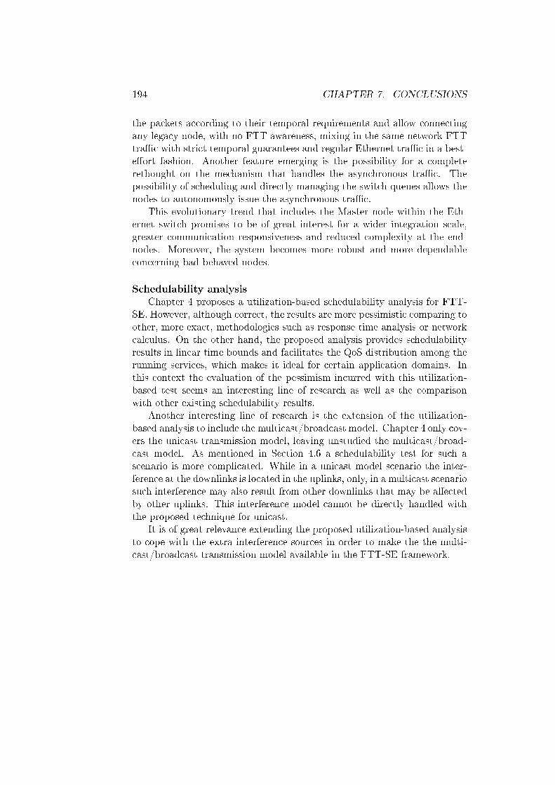
194 CHAPTER 7. CONCLUSIONS
the packets according to their temporal requirements and allow connectingany legacy node, with no FTT awareness, mixing in the same network FTTtra�c with strict temporal guarantees and regular Ethernet tra�c in a best-e�ort fashion. Another feature emerging is the possibility for a completerethought on the mechanism that handles the asynchronous tra�c. Thepossibility of scheduling and directly managing the switch queues allows thenodes to autonomously issue the asynchronous tra�c.
This evolutionary trend that includes the Master node within the Eth-ernet switch promises to be of great interest for a wider integration scale,greater communication responsiveness and reduced complexity at the end-nodes. Moreover, the system becomes more robust and more dependableconcerning bad behaved nodes.
Schedulability analysisChapter 4 proposes a utilization-based schedulability analysis for FTT-
SE. However, although correct, the results are more pessimistic comparing toother, more exact, methodologies such as response time analysis or networkcalculus. On the other hand, the proposed analysis provides schedulabilityresults in linear time bounds and facilitates the QoS distribution among therunning services, which makes it ideal for certain application domains. Inthis context the evaluation of the pessimism incurred with this utilization-based test seems an interesting line of research as well as the comparisonwith other existing schedulability results.
Another interesting line of research is the extension of the utilization-based analysis to include the multicast/broadcast model. Chapter 4 only cov-ers the unicast transmission model, leaving unstudied the multicast/broad-cast model. As mentioned in Section 4.6 a schedulability test for such ascenario is more complicated. While in a unicast model scenario the inter-ference at the downlinks is located in the uplinks, only, in a multicast scenariosuch interference may also result from other downlinks that may be a�ectedby other uplinks. This interference model cannot be directly handled withthe proposed technique for unicast.
It is of great relevance extending the proposed utilization-based analysisto cope with the extra interference sources in order to make the the multi-cast/broadcast transmission model available in the FTT-SE framework.
Bibliography
[1] Coding of audio-visual objects - Part 10: Advanced Video Coding(AVC) ISO/IEC 14496-10, ITU-T recommendation H.264 AVC forgeneric audio visual services.
[2] Real-time PROFINET IRT. http://www.profibus.com.
[3] DIX Ethernet V2.0 speci�cation. IEEE, 1982.
[4] IEEE 802.3ae-2002 - 10Gbps. IEEE, 1982.
[5] IEEE 802.3c 100BASE-T standard. IEEE, 1982.
[6] IEEE 802.3i 10BASE-T standard. IEEE, 1982.
[7] IEEE 802.3z 1000BASE-T standard. IEEE, 1982.
[8] ISO/IEC 10918-1:1994 - Information technology � Digital compressionand coding of continuous-tone still images: Requirements and guide-lines, February 1994.
[9] ISO/IEC 13818-2 Information technology � Generic coding of movingpictures and associated audio information, May 1994.
[10] Video Coding for Low Bit Rate Communications ITU-T recommenda-tion H.263, April 1995.
[11] Video codec test model: TMN8, June 1997.
[12] IEEE 802.1p. IEEE, 1998.
[13] IEEE 802.3ac-1998. IEEE, 1998.
[14] Coding of audio-visual objects - Part 2: Visual, ISO/IEC 14496-2(MPEG-4 Visual Version 1), April 1999.
[15] ARINC 664, Aircraft Data Network, Part 1: System Concepts andOverview, 2002.
[16] ARINC 664, Aircraft Data Network, Part 2: Ethernet Physical andData Link Link Layer Speci�cation, 2002.
195
196 BIBLIOGRAPHY
[17] ARINC 664, Aircraft Data Network, Part 7: Deterministic Networks,2003.
[18] Axis Communications WHITE PAPER: Digital video compression, Re-viewing the methodologies and standards to use for video transmissionand storage. http://www.vns.net/axis/documents/compression_
standards.pdf, June 2004.
[19] IEEE 802.1D-2004. IEEE, 2004.
[20] IEEE 802.1Q-2005. IEEE, 2005.
[21] Mobotix. What IP did next. Security Installer. www.mobotix.com/
ger_DE/file/33573/Security+Installer+bench+test+M22M.pdf,July 2006.
[22] Ethernet Powerlink protocol. http://www.ethernet-powerlink.org,2008.
[23] Foundation Fieldbus HSE. www.�eldbus.org, 2008.
[24] L. Abeni and G. Buttazzo. Integrating Multimedia Applications inHard Real-Time Systems. In Proc. of the 19th IEEE Int. Real-TimeSystems Symposium (RTSS'98), pages 4�13, Madrid, Spain, December1998. IEEE Computer Society.
[25] M. Aldea, G. Bernat, I. Broster, A. Burns, R. Dobrin, J.M. Drake,G. Fohler, P. Gai, M.G. Harbour, G. Guidi, J.J. Gutierrez, T. Lennvall,G. Lipari, J.M. Martinez, J.L. Medina, J.C. Palencia, and M. Tri-marchi. FSF: A Real-Time Scheduling Architecture Framework. InProceedings of the 12th IEEE Real Time on Embedded Technology andApplications Symposium (RTAS'06), pages 113�124, April 2006.
[26] Luís Almeida and J. A. Fonseca. The planning schedule: compromisingbetween operational �exibility and run-time overhead. In Proceedingsof the IFAC Int. Symposium on Infromation Control and Manufactur-ing (INCOM'98), June 1998.
[27] Luís Almeida and José Alberto Fonseca. Analysis of a Simple Modelfor Non-Preemptive Blocking-Free Scheduling. In Proc. of the 13thEUROMICRO Conference on Real-Time Systems (ECRTS'01), June2001.
[28] Luís Almeida, Paulo Pedreiras, and José A. Fonseca. The FTT-CANProtocol: Why and How. IEEE Transactions on Industrial Electronics,49(6):1189�1201, December 2002.
BIBLIOGRAPHY 197
[29] A. Antunes, P. Pedreiras, L. Almeida, and A. Mota. Dynamic Rateand Control Adaptation in Networked Control Systems. In IEEE Int.Conf. on Industrial Informatics, 2007, volume 2, pages 841�846, June2007.
[30] Aeronautical Radio Inc. ARINC 429. ARINC Speci�cation 429, 2001.
[31] N. Audsley, A. Burns, M. Richardson, K. Tindell, and A. J. Wellings.Applying New Scheduling Theory to Static Priority Pre-EmptiveScheduling. Software Engineering Journal, 8(5):284�292, September1993.
[32] N. C. Audsley, A. Burns, M. F. Richardson, and A. J. Wellings. Hardreal-time scheduling: the deadline-monotonic approach. In Proceed-ings of the 8th IEEE Workshop on Real-Time Operating Systems andSoftware, pages 133�137, May 1991.
[33] F. Bogenbergerand, B. Muller, and T. Fuher. Protocol overview. InProceedings of the 1st FlexRay Int. Workshop, April 2002.
[34] Jean-Yves Le Boudec and Patrick Thiran. Network calculus: a theoryof deterministic queuing systems for the internet. Springer-Verlag NewYork, Inc., New York, NY, USA, July 2001.
[35] Ch. Bouras and A. Gkamas. Multimedia transmission with adaptiveQoS based on real-time protocols. International Journal ofCommuni-cations Systems, Wiley InterScience, 16:225�248, 2003.
[36] R. Braden, D. Clark, and S. Shenker. Integrated Services in the InternetArchitecture: an Overview. RFC 1633, July 1994.
[37] Giorgio C. Buttazzo. Hard Real-Time Computing Systems: PredictableScheduling Algorithms and Applications. Kluwer Academic Publishers,Norwell, MA, USA, 1997.
[38] Giorgio C. Buttazzo, Giuseppe Lipari, and Luca Abeni. Elastic taskmodel for adaptive rate control. In IEEE Real-Time Systems Sympo-sium, pages 286�295, 1998.
[39] Giorgio C. Buttazzo, Giuseppe Lipari, Marco Caccamo, and LucaAbeni. Elastic Scheduling for Flexible Workload Management. IEEETrans. Comput., 51(3):289�302, 2002.
[40] B. Cain, S. Deering, I. Kouvelas, B. Fenner, and A. Thyagarajan.Internet Group Management Protocol, Version 3. http://www.ietf.
org/rfc/rfc3376, October 2002.
198 BIBLIOGRAPHY
[41] A. Carpenzano, R. Caponetto, L. Lo Bello, and O. Mirabella. Fuzzytra�c smoothing: an approach for real-time communication over Eth-ernet networks. In Proceedings of the 4th IEEE Int. Workshop onFactory Communication Systems (WFCS'02), pages 241�248, August2002.
[42] Thidapat Chantem, Xiaobo Sharon Hu, and M. D. Lemmon. General-ized Elastic Scheduling. In Proc. of the 27th IEEE Int. Real-Time Sys-tems Symposium (RTSS'06), pages 236�245, Washington, DC, USA,2006. IEEE Computer Society.
[43] C.-S. Cho, B.-M. Chung, and M.-J. Park. Development of Real-TimeVision-Based Fabric Inspection System. Industrial Electronics, IEEETransactions on, 52(4):1073�1079, Aug. 2005.
[44] M. Christensen, K. Kimball, and F. Solensky. Considerations for In-ternet Group Management Protocol (IGMP) and Multicast ListenerDiscovery (MLD) Snooping Switches. http://www.ietf.org/rfc/
rfc4541, May 2006.
[45] Rene L. Cruz. A calculus for network delay, Part I: Network elements inisolation. IEEE Transactions on Information Theory, 37(1):114�131,January 1991.
[46] Rene L. Cruz. A calculus for network delay, Part II: Network analysis.IEEE Transactions on Information Theory, 37(1):132�141, January1991.
[47] M. Di Natale. Scheduling the CAN bus with earliest deadline tech-niques. In Proceedings of the 21st IEEE Real-Time Systems Symposium(RTSS'00), pages 259�268, 2000.
[48] Wei Ding and Bede Liu. Rate control of MPEG video coding andrecording by rate-quantization modeling. Circuits and Systems forVideo Technology, IEEE Transactions on, 6(1):12�20, Feb 1996.
[49] Xing Fan, Magnus Jonsson, and Jan Jonsson. Guaranteed Real-TimeCommunication in Packet-Switched Networks with FCFS queuing.Technical report, School of Information Science, Computer and Elec-trical Engineering, Halmstad University, Sweden, April 2007.
[50] Paul Ferguson and Geo� Huston. Quality of service: delivering QoSon the Internet and in corporate networks. John Wiley & Sons, Inc.,New York, NY, USA, 1998.
[51] Sebastian Fischmeister and Klemens Winkler. Non-blocking Determin-istic Replacement of Functionality, Timing, and Data-Flow for Hard
BIBLIOGRAPHY 199
Real-Time Systems at Runtime. In Proceedings of the 17th Euromi-cro Conference on Real-Time Systems (ECRTS'05), pages 106�114,Washington, DC, USA, 2005. IEEE Computer Society.
[52] G. Fohler. FRSCOR - Initial application requirements collection.FRESCOR deliverable D-RA1, November 2006.
[53] Inc. FSMLabs. LNet Programming with RTCore, June 2006.
[54] FSMLabs Inc. Real-time Programming in RTCore (v2.2.3), 2006.
[55] E. Gallo, M. Siller, and J. Woods. An Ontology for the Quality ofExperience framework. In Int. Conf. on Systems, Man and Cybernetics(SMC'07), pages 1540�1544, October 2007.
[56] L. George, N. Riviere, and M. Spuri. Preemptive and non-preemptivereal-time uniprocessor scheduling. Technical Report RR-2966, INRIA,Le Chesnay Cedex, France, 1996.
[57] F. Gomez-Molinero. Real-Time Requirement of Media Control Appli-cations. In Proceedings of the 19th Euromicro Conference on Real-TimeSystems (ECRTS '07), pages 4�4, July 2007.
[58] M. Handley, H. Schulzrinne, E. Schooler, and J. Rosenberg. SIP: Ses-sion Initiation Protocol, RFC 2543, March 1999.
[59] M. González Harbour and J. C. Palencia. Response Time Analysisfor Tasks Scheduled under EDF within Fixed Priorities. In Proceed-ings of the 24th IEEE International Real-Time Systems Symposium(RTSS'03), page 200, Washington, DC, USA, 2003. IEEE ComputerSociety.
[60] H. Hassan, J. Simo, and A. Crespo. Enhancing the �exibility andthe quality of service of autonomous mobile robotic applications. InProceedings of the 14th Euromicro Conference on Real-Time Systems(ECRTS'02), pages 213�220, 2002.
[61] H. Hoang and Magnus Jonsson. Switched real-time Ethernet in in-dustrial applications � asymmetric deadline partitioning scheme. InProceedings of the 2st Int. Workshop on Real-time LANs in the Inter-net age (RTLIA'03), July 2003.
[62] Hoai Hoang, Magnus Jonsson, Ulrik Hagström, and Anders Kallerdahl.Switched real-time Ethernet and earliest deadline �rst scheduling -protocols and tra�c handling. In Proceedings of the 16th Int. Conf.on Parallel and Distributed Processing Symposium (IPDPS '02). IEEEComputer Society, 2002.
200 BIBLIOGRAPHY
[63] Javier Silvestre, Luís Almeida, Ricardo Marau, and Paulo Pedreiras.MJPEG Real-Time transmission in industrial environment using aCBR channel. In Proc. of 16th Int. Conf. on Computer and Informa-tion Society Engineering (CISE'06), Venice, Italy, 24 November 2006.(also published on Enformatika Trans. on Engineering, Computing andTechnology, Vol 16, Nov. 2006 ISSN 1305-5313).
[64] R. Johnston and G. Clark. Service operations management. PearsonEducation, 2001.
[65] Michael B. Jones. Adaptive Real-Time Resource Management Sup-porting Composition of Independently Authored Time-Critical Ser-vices. In In Proceedings of the Fourth Workshop on Workstation Op-erating Systems, pages 135�139, 1993.
[66] Frescor project home page. http://www.frescor.org.
[67] H. Kopetz. Speci�cation of the ttp/c protocol , version 0.5. Technicalreport, TTTech Computertechnik, July 1999.
[68] Hermann Kopetz. Real-Time Systems: Design Principles for Dis-tributed Embedded Applications. Kluwer Academic Publishers, Norwell,MA, USA, 1997.
[69] A. Kumar. Computer-Vision-Based Fabric Defect Detection: A Sur-vey. Industrial Electronics, IEEE Transactions on, 55(1):348�363, Jan.2008.
[70] Seok-Kyu Kweon and K.G. Shin. Achieving real-time communicationover Ethernet with adaptive tra�c smoothing. In Proceedings of the 6thIEEE Real-Time Technology and Applications Symposium (RTAS'00),pages 90�100, June 2000.
[71] Chang-Gun Lee, Chi-Sheng Shih, and Lui Sha. Online QoS optimiza-tion using service classes in surveillance radar systems. Real-TimeSystems, 28(1):5�37, 2004.
[72] J. Lehoczky, L. Sha, and Y. Ding. The rate monotonic schedulingalgorithm: exact characterization and average case behavior. In Pro-ceedings of the 10th IEE Real-Time Systems Symposium (RTSS'89),pages 166�171, Dec 1989.
[73] J.P. Lehoczky. Fixed priority scheduling of periodic task sets with ar-bitrary deadlines. In Proceedings of the 11th IEEE Real-Time SystemsSymposium (RTSS'90), pages 201�209, Dec 1990.
BIBLIOGRAPHY 201
[74] J.P. Lehoczky and S. Ramos-Thuel. An optimal algorithm for schedul-ing soft-aperiodic tasks in �xed-priority preemptive systems. In Pro-ceedings of the 13th IEEE Real-Time Systems Symposium (RTSS'92),pages 110�123, Dec 1992.
[75] Xiaoli Li, S.K. Tso, Xin-Ping Guan, and Qian Huang. Improving Au-tomatic Detection of Defects in Castings by Applying Wavelet Tech-nique. Industrial Electronics, IEEE Transactions on, 53(6):1927�1934,Dec. 2006.
[76] C. L. Liu and James W. Layland. Scheduling Algorithms for Multi-programming in a Hard-Real-Time Environment. Journal of the As-sociation for Computing Machinery, 20(1):46�61, 1973.
[77] H. Lonn and J. Axelsson. A comparison of �xed-priority and staticcyclic scheduling for distributed automotive control applications. InProceedings of the 11th Euromicro Conference on Real-Time Systems(ECRTS'99), pages 142�149, 1999.
[78] Jork Löser and Hermann Härtig. Low-Latency Hard Real-Time Com-munication over Switched Ethernet. In Proc. of the 16th EUROMICROConference on Real-Time Systems (ECRTS'04), pages 13�22. IEEEComputer Society, July 2004.
[79] Jork Löser and Hermann Härtig. Using Switched Ethernet for HardReal-Time Communication. In Proc of Int. Conference on ParallelComputing in Electrical Engineering (PARELEC'04), pages 349�353,September 2004.
[80] Chenyang Lu, John A. Stankovic, Sang H. Son, and Gang Tao. Feed-back control real-time scheduling: framework, modeling, and algo-rithms. Journal of Real-Time Systems, Special Issue on Control-Theoretical Approaches to Real-Time Computing, 23:85�126, 2002.
[81] Nicholas Malcolm, Wei Zhao, and A. Stankovic. Hard Real-Time Com-munication in Multiple-Access Networks. Real-Time Systems, 8:35�77,1995.
[82] R. Marau, P. Pedreiras, and L. Almeida. Enhanced Ethernet Switchingfor Flexible Hard Real-Time Communication. In Proc. on the 5th Int.Workshop on Real Time Networks (RTN'06), Dresden, Germany, July2006.
[83] R. Marau, P. Pedreiras, and L. Almeida. Signaling asynchronous tra�cover a Master-Slave Switched Ethernet protocol. In Proc. on the 6thInt. Workshop on Real Time Networks (RTN'07), Pisa, Italy, 2 July2007.

202 BIBLIOGRAPHY
[84] Ricardo Marau, Luís Almeida, and Paulo Pedreiras. Enhancing real-time communication over COTS Ethernet switches. In Proc. of 6thInt. Workshop on Factory Communication Systems (WFCS'06), pages295�302, Torino, Italy, 27 June 2006. IEEE.
[85] Ricardo Marau, Luís Almeida, Paulo Pedreiras, M. González Harbour,Daniel Sangorrín, and Julio M. Medina. Integration of a �exible net-work in a resource contracting framework. In Proc. of the WiP ses-sion of the 13th Real-Time and Embedded Technology and ApplicationsSymposium (RTAS'07). IEEE, 3 April 2007.
[86] Ricardo Marau, Luís Almeida, Paulo Pedreiras, M. González Harbour,Daniel Sangorrín, and Julio M. Medina. Integration of a �exible timetriggered network in the FRESCOR resource contracting framework.In Proc of the 12th IEEE Conference on Emerging Technologies andFactory Automation (ETFA'07), Patras, Greece, 25 September 2007.IEEE.
[87] Ricardo Marau, Luís Almeida, Paulo Pedreiras, and Thomas Nolte.Towards Server-based Switched Ethernet for Real-Time Communica-tions. In Proc. of the WiP session of the 20th Euromicro Conferenceon Real-Time Systems(ECRTS'08), 2 July 2008.
[88] Ricardo Marau, N. Figueiredo, R. Santos, P. Pedreiras, L. Almeida,and Thomas Nolte. Server-based Real-Time Communications onSwitched Ethernet. In Workshop on Compositional Theory and Tech-nology for Real-Time Embedded Systems (CRTS-RTSS'08), 2008.
[89] Michael W. Marcellin, Ali Bilgin, Michael J. Gormish, and Martin P.Boliek. An Overview of JPEG-2000. In DCC '00: Proceedings of theConference on Data Compression, page 523, Washington, DC, USA,2000. IEEE Computer Society.
[90] J. Martínez, M. González Harbour, and J. Gutiérrez. RT-EP: real-timeEthernet protocol for analyzable distributed applications on a mini-mum real-time POSIX kernel. In Proceedings of the 2st Int. Workshopon Real-time LANs in the Internet age (RTLIA'03), July 2003.
[91] R. Moghal and M. S. Mian. Adaptive QoS-based resource allocationin distributed multimedia systems. In Proceedings of Workshop onParallel and Distributed Real-Time Systems (WPDRTS), 2003.
[92] Jami Montgomery. A Model for Updating Real-Time Applications.Real-Time Systems, 27(2):169�189, 2004.
[93] Klara Nahrstedt and Jonathan M. Smith. The QoS Broker. IEEEMultimedia, 2:53�67, 1995.

BIBLIOGRAPHY 203
[94] K. Nichols, S. Blake, F. Baker, and D. Black. De�nition of the Di�er-entiated Services Field (DS Field) in the IPv4 and IPv6 Headers. RFC2474, December 1998.
[95] T. Nolte. Share-Driven Scheduling of Embedded Networks. PhD the-sis, Department of Computer and Science and Electronics, MälardalenUniversity, Sweden, May 2006.
[96] J. C. Palencia and M. González Harbour. Schedulability analysis fortasks with static and dynamic o�sets. In Proceedings of the 19th IEEEReal-Time Systems Symposium (RTSS'98), pages 26�37, 1998.
[97] J. C. Palencia and M. González Harbour. Response time analysis ofEDF distributed real-time systems. Journal of Embedded Computing(JEC), 1(2):225�237, November 2005.
[98] J.C. Palencia and M.G. Harbour. O�set-based response time analysisof distributed systems scheduled under EDF. In Proceedings of the 15thEuromicro Conference on Real-Time Systems (ECRTS'03), pages 3�12, July 2003.
[99] Paulo Pedreiras. Supporting Flexible Real-Time Communication onDistributed Systems. PhD thesis, University of Aveiro, Aveiro, Portu-gal, 2003.
[100] Paulo Pedreiras and Luís Almeida. Approaches to Enforce Real-TimeBehavior in Ethernet. CRC Press, 2005.
[101] Paulo Pedreiras, Paolo Gai, Luís Almeida, and Giorgio C. Buttazzo.FTT-Ethernet: a �exible real-time communication protocol that sup-ports dynamic QoS management on Ethernet-based systems. IEEETransactions on Industrial Informatics, 1(3):162�172, August 2005.ISSN: 1551-3203.
[102] Paulo Pedreiras, Ricardo Leite, and Luis Almeida. Characterizing theReal-Time Behavior of Prioritized Switched-Ethernet. In Proc. of the2nd Workshop on Real-Time LANs in the Internet Age (RTLIA'03satellite of ECRTS'03), July 2003.
[103] D. Prasad, A. Burns, and M. Atkins. The valid use of utility in adaptivereal-time systems. Real-Time Systems, 25(2-3):277�296, 2003.
[104] Ala' Qadi, S. Goddard, Jiangyang Huang, and S. Farritor. A perfor-mance and schedulability analysis of an autonomous mobile robot. InProceedings of the 17th Euromicro Conference on Real-Time Systems(ECRTS'05), pages 239�248, July 2005.

204 BIBLIOGRAPHY
[105] Prasad Raja and Guevara Noubir. Static and dynamic polling mecha-nisms for �eldbus networks. ACM Operating Systems Review, 27(3):34�45, 1993.
[106] J. Ribas-Corbera and Shawmin Lei. Rate control in DCT video codingfor low-delay communications. Circuits and Systems for Video Tech-nology, IEEE Transactions on, 9(1):172�185, Feb 1999.
[107] H. Schulzrinne, A. Rao, and R. Lanphier. Real Time Streaming Pro-tocol (RTSP), RFC 2326, April 1998.
[108] Henning Schulzrinne, Stephen L. Casner, Ron Frederick, and Van Ja-cobson. RTP: A Transport Protocol for Real-Time Applications, RFC1889, 1996.
[109] V.M. Sempere and J. Silvestre. Multimedia applications in industrialnetworks: integration of image processing in Pro�bus. IEEE Transac-tions on Industrial Electronics, 50(3):440�448, June 2003.
[110] S. Sen, J. L. Rexford, J. K. Dey, J. F. Kurose, and D. F. Towsley. On-line smoothing of variable-bit-rate streaming video. IEEE Transactionson Multimedia, 2(1):37�48, 2000.
[111] Lui Sha and Shirish S. Sathaye. A systematic approach to designingdistributed real-time systems. IEEE Computer, 26:68�78, 1993.
[112] C.P. Shelton and P. Koopman. Improving system dependability withfunctional alternatives. In Procedings of Int. Conf. on Dependable Sys-tems and Networks (DSN'04), pages 295�304, June 2004.
[113] Javier Silvestre, Luís Almeida, Ricardo Marau, and Paulo Pedreiras.Dynamic QoS management for multimedia real-time transmission inindustrial environments. In Proc. of the 12th IEEE Int. Conference onEmerging Technologies and Factory Automation (ETFA'07), Septem-ber 2007.
[114] T. Skeie, S. Johannessen, and O. Holmeide. The road to an end-to-enddeterministic Ethernet. In Proceedings of the 4th IEEE Int. Workshopon Factory Communication Systems (WFCS'02), pages 3�9, 2002.
[115] Yeqiong Song, Anis Koubaa, and Loria Inria Lorraine. Switched Eth-ernet for real-time industrial communication: Modelling and messageBu�ering delay evaluation. In Proc. of the 4th Int. Workshop onFactory Communication Systems (WFCS'02), pages 27�30. Springer-Verlag, August 2002.
[116] B. Sprunt, L. Sha, and J. P. Lehoczky. Aperiodic Task Scheduling forHard Real-Time Systems. Real-Time Systems, 1(1):27�60, June 1989.
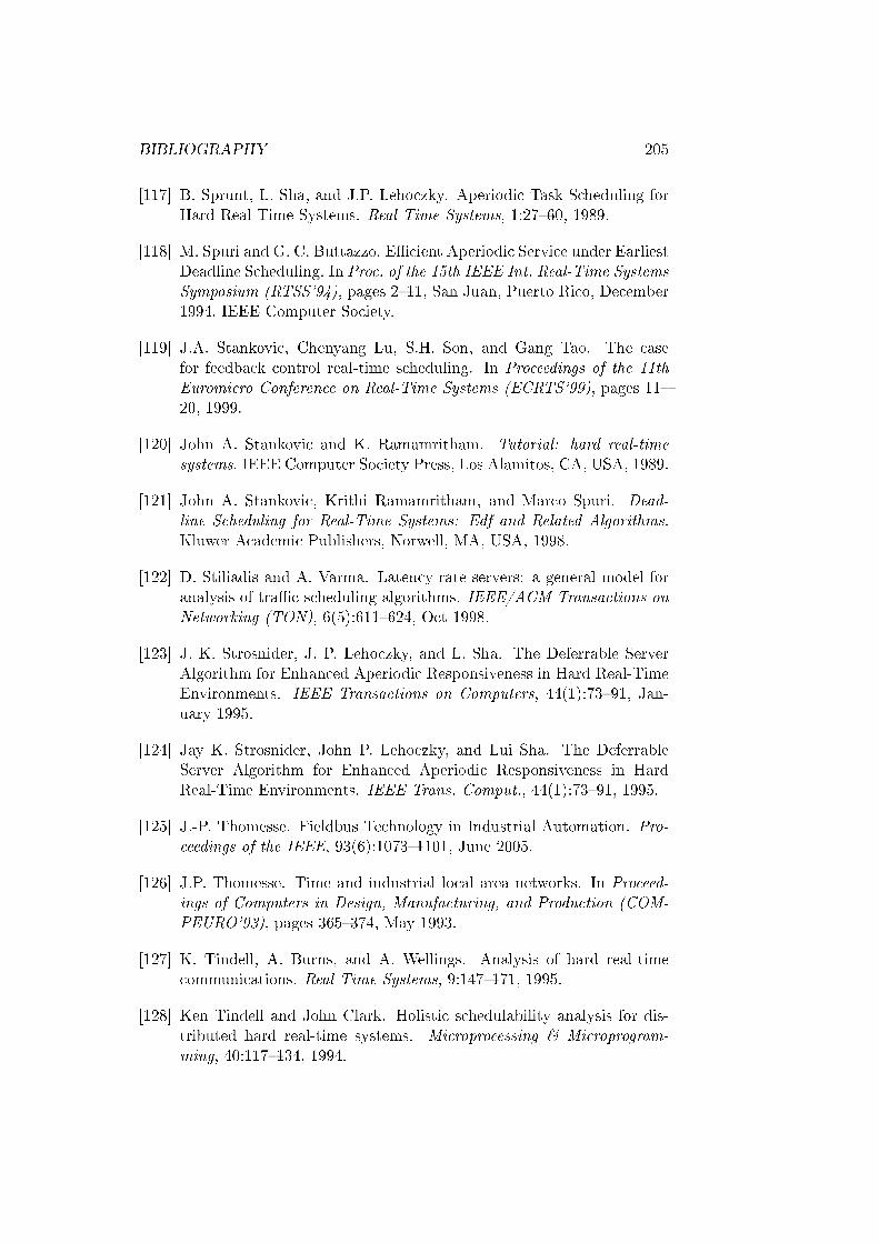
BIBLIOGRAPHY 205
[117] B. Sprunt, L. Sha, and J.P. Lehoczky. Aperiodic Task Scheduling forHard-Real-Time Systems. Real-Time Systems, 1:27�60, 1989.
[118] M. Spuri and G. C. Buttazzo. E�cient Aperiodic Service under EarliestDeadline Scheduling. In Proc. of the 15th IEEE Int. Real-Time SystemsSymposium (RTSS'94), pages 2�11, San Juan, Puerto Rico, December1994. IEEE Computer Society.
[119] J.A. Stankovic, Chenyang Lu, S.H. Son, and Gang Tao. The casefor feedback control real-time scheduling. In Proceedings of the 11thEuromicro Conference on Real-Time Systems (ECRTS'99), pages 11�20, 1999.
[120] John A. Stankovic and K. Ramamritham. Tutorial: hard real-timesystems. IEEE Computer Society Press, Los Alamitos, CA, USA, 1989.
[121] John A. Stankovic, Krithi Ramamritham, and Marco Spuri. Dead-line Scheduling for Real-Time Systems: Edf and Related Algorithms.Kluwer Academic Publishers, Norwell, MA, USA, 1998.
[122] D. Stiliadis and A. Varma. Latency-rate servers: a general model foranalysis of tra�c scheduling algorithms. IEEE/ACM Transactions onNetworking (TON), 6(5):611�624, Oct 1998.
[123] J. K. Strosnider, J. P. Lehoczky, and L. Sha. The Deferrable ServerAlgorithm for Enhanced Aperiodic Responsiveness in Hard Real-TimeEnvironments. IEEE Transactions on Computers, 44(1):73�91, Jan-uary 1995.
[124] Jay K. Strosnider, John P. Lehoczky, and Lui Sha. The DeferrableServer Algorithm for Enhanced Aperiodic Responsiveness in HardReal-Time Environments. IEEE Trans. Comput., 44(1):73�91, 1995.
[125] J.-P. Thomesse. Fieldbus Technology in Industrial Automation. Pro-ceedings of the IEEE, 93(6):1073�1101, June 2005.
[126] J.P. Thomesse. Time and industrial local area networks. In Proceed-ings of Computers in Design, Manufacturing, and Production (COM-PEURO'93), pages 365�374, May 1993.
[127] K. Tindell, A. Burns, and A. Wellings. Analysis of hard real-timecommunications. Real-Time Systems, 9:147�171, 1995.
[128] Ken Tindell and John Clark. Holistic schedulability analysis for dis-tributed hard real-time systems. Microprocessing & Microprogram-ming, 40:117�134, 1994.
206 BIBLIOGRAPHY
[129] Jyi-Chang Tsai. Rate control for low-delay video using a dynamic ratetable. Circuits and Systems for Video Technology, IEEE Transactionson, 15(1):133�137, Jan. 2005.
[130] Bobby Vandalore, Wu chi Feng, Raj Jain, and Sonia Fahmy. A surveyof application layer techniques for adaptive streaming of multimedia.Real-Time Imaging, 7(3):221�235, 2001.
[131] S. Varadarajan. Experiences with EtheReal: a fault-tolerant real-time Ethernet switch. In Proceedings of the 8th IEEE Int. Conferenceon Emerging Technologies and Factory Automation (ETFA'01), pages183�194 vol.1, October 2001.
[132] S. Varadarajan and T Chiueh. EtheReal: A host-transparent real-timefast Ethernet switch. In Proc of the 6th Int. conference on networkprotocols, pages 12�21, October 1998.
[133] P. Veríssimo and Luís Rodrigues. Distributed systems for system ar-chitects. Kluwer Academic Publishers, 2001.
[134] N. Wang, D. Schmidt, K. Parameswaran, and M. Kircher. Towards are�ective middleware framework for QoS-enabled CORBA componentmodel applications. IEEE Distributed Systems Online special issue onRe�ective Middleware (Vol. 2, No. 5), May 2001.
[135] Zhou Wang, A.C. Bovik, H.R. Sheikh, and E.P. Simoncelli. Imagequality assessment: from error visibility to structural similarity. IEEETransactions on Image Processing, 13(4):600�612, April 2004.
[136] L. Zhang, S. Berson, S. Herzog, and S. Jamin. Resource ReSerVationProtocol (RSVP). RFC 2205, September 1997.
[137] H. Zimmermann. OSI reference model: The ISO model of architecturefor open systems interconnection. IEEE Transactions on Communica-tions, 28(4):425�432, 1980.