Tampere University of Technology

Revisiting Gaussian Process Regression Modeling for Localization in Wireless SensorNetworks

CitationRichter, P., & Toledano-Ayala, M. (2015). Revisiting Gaussian Process Regression Modeling for Localization inWireless Sensor Networks. Sensors, 15(9), 22587-22615. https://doi.org/10.3390/s150922587

Year2015

VersionPublisher's PDF (version of record)

Link to publicationTUTCRIS Portal (http://www.tut.fi/tutcris)

Published inSensors

DOI10.3390/s150922587

LicenseCC BY

Take down policyIf you believe that this document breaches copyright, please contact cris.tau@tuni.fi, and we will remove accessto the work immediately and investigate your claim.

Download date:15.01.2020

Sensors 2015, 15, 22587-22615; doi:10.3390/s150922587OPEN ACCESS

sensorsISSN 1424-8220

www.mdpi.com/journal/sensors

Article

Revisiting Gaussian Process Regression Modeling forLocalization in Wireless Sensor NetworksPhilipp Richter * and Manuel Toledano-Ayala

Facultad de Ingeniería, Universidad Autónoma de Querétaro, Cerro de las Campanas s/n.,Col. Las Campanas, Santiago de Querétaro 76010, Mexico; E-Mail: toledano@uaq.mx

* Author to whom correspondence should be addressed; E-Mail: philipp.richter@uaq.mx;Tel.: +52-192-1200-6023; Fax: +52-192-1200-6006.

Academic Editor: Leonhard M. Reindl

Received: 14 June 2015 / Accepted: 25 August 2015 / Published: 8 September 2015

Abstract: Signal strength-based positioning in wireless sensor networks is a key technologyfor seamless, ubiquitous localization, especially in areas where Global Navigation SatelliteSystem (GNSS) signals propagate poorly. To enable wireless local area network (WLAN)location fingerprinting in larger areas while maintaining accuracy, methods to reduce theeffort of radio map creation must be consolidated and automatized. Gaussian processregression has been applied to overcome this issue, also with auspicious results, but the fit ofthe model was never thoroughly assessed. Instead, most studies trained a readily availablemodel, relying on the zero mean and squared exponential covariance function, withoutfurther scrutinization. This paper studies the Gaussian process regression model selectionfor WLAN fingerprinting in indoor and outdoor environments. We train several models forindoor/outdoor- and combined areas; we evaluate them quantitatively and compare them bymeans of adequate model measures, hence assessing the fit of these models directly. Toilluminate the quality of the model fit, the residuals of the proposed model are investigated,as well. Comparative experiments on the positioning performance verify and conclude themodel selection. In this way, we show that the standard model is not the most appropriate,discuss alternatives and present our best candidate.

Keywords: sensor modeling; WLAN received signal strength; Gaussian process regression;machine learning; location fingerprinting

Sensors 2015, 15 22588

1. Introduction

The knowledge of location is crucial for an uncountable number of applications driven by anever-increasing number of mobile users. The Global Navigation Satellite System (GNSS) covers mostof these applications very well; however, in dense urban areas and indoor environments, trackingof GNSS signals is unreliable due to signal attenuation and blocking, thus creating a demand foraiding and alternative positioning systems. Localization in wireless sensor networks presents such analternative, whereupon a wireless local area network (WLANs) and, in particular, WLAN-based locationfingerprinting, is one of the most promising methods, because it does not need a line-of-sight to thetransmitter and works with low-cost, standardized hardware. Moreover, WLAN signals penetrate wallsand, hence, in contrast to GNSS, enable seamless indoor/outdoor positioning.

WLAN fingerprinting constitutes the drawback of creating the reference database, consisting ofreceived signal strengths (RSS) at known positions: the radio map. The number of reference points(fingerprints) affects its accuracy, and establishing an elaborate prepared radio map is very laborious.The denser the fingerprints and larger the area of interest, the more expensive is this undertaking. (Thesmaller the distance between two signal strength measurements, the smaller the difference between theRSSs. It is worth noting that due to the quantization of RSS to one decibel, the RSSs in a small areaare certainly equal. This, in turn, leads to a saturation of the accuracy improvement when densifying thefingerprint further.)

A reduction of the labor of radio map creation is widely desired [1,2]. Interpolating or predicting thesignal strength allows one to reduce the number of fingerprints while retaining the positioning accuracy.Elnahrawy et al. [3] proposed Delaunay triangulation to interpolate between reference points, whereasChai et al. [4] interpolated linearly between neighboring likelihood functions, and Howard et al. [5] usedinterpolation filters. These interpolation schemes do not capture the random nature of RSS sufficiently,in particular if the fingerprints are sparse.

The authors of [6–9] used Gaussian process regression in the context of WLAN location fingerprintingto model RSSs. Gaussian process regression is able to predict the nonlinear, spatial relation ofsignal strength, resulting in a continuous spatial description of RSSs. Furthermore, the computervision community applies Gaussian process regression for localization tasks, especially in roboticapplications [10,11]. Instead of RSS, spatially-unique features are extracted from camera images andstored with their corresponding location to establish reference locations. During position estimation,this process is repeated, and the resulting features are matched with the previously-stored features inwhich the best match corresponds to the most likely location.

In [6–11], the “default” Gaussian process model, with zero mean and squared exponential kernel,was chosen. Gaussian process models that employ the zero mean function converge to zero in areaswithout training data; a property that is clearly not appropriate for RSSs. Hence, the authors of [6,8]approximated the RSS decay with a linear model and estimated in an additional step its parameters. Thisprocedure is either not realistic in areas where the access point positions are not known or would requirea survey of these positions. In addition, the choice of the squared exponential kernel in these studiesis unsound.

Sensors 2015, 15 22589

Only Bekkali et al. [12] investigated several Gaussian process models in order to find the mostappropriate model for WLAN location fingerprinting; however, their focus was solely on indoorenvironments, and the results were obtained under idealized conditions. They based their study onray-launching, a method that simulates wave propagation based on geometrical optics (reflection,diffraction, wave guiding effects, etc.). Though, ray-launching only considers spatial variations ofthe signal power, it does not simulate spatiotemporal variations, for example due to moving peopleand objects; the complex power patterns that occur in real-world environments are not fully captured.Furthermore, the discrete ray increment with which each ray is launched from the transmitter is known tobe disadvantageous, since not all wedges might be hit by a ray, and hence, it omits possible new sourcesof interferences. Besides, they assessed the models only in terms of the position accuracy and did notevaluate the quality of the model fit.

An alternative method to model WLAN power spatially was recently presented by Depatla et al. [13].They use WLAN power readings and approximations to Maxwell’s equations to obtain a highly accuratemodel of the electric field in a small area. This WLAN signal strength model is used to solve theinverse scattering problem and allows high-resolution imaging of, possible occluded, objects. Theirmodel of the electric field can potentially be used for localization and replace the Gaussian processregression approach; however, it is even more expensive regarding labor, and its practicality for WLANfingerprinting is doubtful.

In vision-based localization, the choice of appropriate features is a problem on its own, and thefeatures extracted from images are diverse among different studies. Hence, each feature may requirea different Gaussian process prior distribution, whose examination is not in the scope of this study.

Very accurate Gaussian process models are fundamental to achieve WLAN locationfingerprinting-based seamless indoor/outdoor positioning; even more if the objective is to fuseRSS with other sensor data. Therefore, building upon [12], these models need to be re-studied inrealistic conditions, with actual RSS measurements. This work revisits Gaussian process modelselection for the interpolation of radio maps. It presents detailed experimental results that challenge themodel choice made in former studies, analyzes different Gaussian process models with respect to indoorand outdoor environments and explores the most appropriate Gaussian process model. We hypothesizedwhether different Gaussian process regression models for indoor and outdoor environments could beobtained and if this improves the radio map accuracy compared to a common model. The fit of theGaussian process models is evaluated by the models’ test error and the Bayesian information criterion(both obtained via cross-validation) and supplemented with an analysis of the residuals. The validityof these findings is sought by comparing the models’ localization accuracy, assessed by Gaussianprocess-based maximum likelihood estimators.

2. Gaussian Process Regression Model for WLAN RSS Fingerprinting

Interpolating WLAN RSS, to improve radio maps, equates to predicting the spatial distribution ofsignal strength. Such a prediction demands a description that relates coordinates in space and thecorresponding sets of RSSs, received from WLAN access points. Gaussian process regression is a toolwidely used in geostatistics, where it is known as Bayesian kriging, but it also drew, especially in the last

Sensors 2015, 15 22590

decade, much attention in the machine learning community. Gaussian process regression, as a supervisedlearning task, permits predicting RSSs at arbitrary coordinates on the basis of acquired data.

A Gaussian process is a collection of random variables {f(x) | x ∈ X} that underlie the condition thatany finite subset of realizations of the process f = {f(xi)}ni=1 is jointly Gaussian distributed [14]. Sucha process is a generalization of a normal multivariate distribution into infinite dimension: it describes adistribution over functions. A Gaussian process is fully specified by its mean function µ(x) = E[f(x)]

and covariance function cov(f(x), f(x′)) = E[(f(x) − µ(x))(f(x′) − µ(x′))]. The set X is the indexset, a set of possible input values.

We use a Gaussian process to model the relationship between RSS, s, and points in two-dimensionalspace, p, some subset of R2; this spatial process is denoted by:

si = f(pi) + εi

The regression problem consists of interfering the non-linear function f(·) from noisy observationsthat emerged from an identical independent distribution and have the variance σ2

ε . When generating theradio map, one draws samples from this process, obtaining {pi, si}ni=1, the so-called training data. Fornotational convenience, we stack the training data together, yielding a 2 × n matrix of input values Pand a n-dimensional vector s, the target values.

From a Bayesian point of view, the interference of f(p) corresponds to estimating theposterior distribution:

p(f(p) | s, P ) =p(s | f(p), P )p(f(p))

p(s | P )(1)

The term p(s | f(p), P ), known as the likelihood function, denotes the probability of obtaining theRSS, s, given the function f(p), where p(f(p)) presents the prior distribution of the latent function, aGaussian process in itself.

To interpolate RSSs at arbitrary positions, Gaussian process regression exploits the covariance ofneighboring RSSs. This dependence is expressed by the process’ covariance function that specifiesthe similarity of two function values evaluated at their input values. Assumptions on the problem orprior knowledge about it can be encoded in the mean and covariance function of the prior distribution,thus giving the model characteristics, such as different signal or noise levels, periodicity or linearity.Gaussian process’ covariance functions are based on kernel functions; functions that peak when thedistance in input space is minimal and decrease with increased distance of the input points, expressingthe drop-off of dependence between RSSs farther from each other. The specific choice of a covariancefunction depends on the problem; the most common kernel, the squared exponential kernel, is given asan example:

cov(f(pi), f(pj)) = k(pi,pj) = exp(−12‖pi − pj‖2)

For all pairs of training targets, we denote the covariance matrix by K(P, P ). Knowing that RSSobservations are noisy, we encode that characteristic in the model and write the covariance function ofthe prior distribution as cov(s) = K(P, P )+σ2

ε I , with I being the identity matrix. Assuming a noise thatis identical independent normal distributed allows an analytic description of Gaussian process regression,as presented as follows.

Sensors 2015, 15 22591

The target values of the training data, s, are correlated between each other, as they are also correlatedwith any arbitrary target values. This fact is employed to predict RSSs, s∗ ≡ f(P ∗). We denote thematrix of the corresponding n∗ positions by P ∗ and refer to the sought target values and their index setas test data. We can describe the joint Gaussian distribution of target values, assuming a zero mean priordistribution, as: [

s

s∗

]∼ N

(0,

[K(P, P ) + σ2

ε I K(P, P ∗)

K(P ∗, P ) K(P ∗, P ∗)

])whereK(P, P ∗) is a n×n∗ matrix containing the covariances between all pairs of s and s∗. Conditioningthis distribution on the training RSS yields again a Gaussian process with mean Function (2) andcovariance Function (3):

s∗ | s, P, P ∗ ∼ N (s̄∗, cov(s∗))

s̄∗ = K(P ∗, P )[K(P, P ) + σ2ε I]−1s (2)

cov(s∗) = K(P ∗, P ∗)−K(P ∗, P )[K(P, P ) + σ2ε I]−1K(P, P ∗) (3)

This is the posterior distribution, also called predictive distribution. Note that Gaussian processregression also estimates the uncertainty of the predictions, given by the covariance function.

The principle structure of the model is determined by the mean and covariance functions, but to fitthe observations appropriately, the function’s optimal hyperparameters need to be found. This is usuallydone by maximizing the marginal likelihood function (This log-likelihood function is usually attributedthe term marginal, since it is obtained by integrating out the unobtained observations.), the probabilityof the data given the model, with respect to the hyperparameters. For Gaussian distributed noise, itslogarithmic form is given by:

log p(s | X,θ) = −12sT [K(P, P ) + σ2

ε I]−1s− 12

log|K(P, P ) + σ2ε I| − n

2log 2π (4)

where θ collects the model’s hyperparameters and T denotes the matrix transpose. This function isintrinsic to Gaussian process regression, and it balances between model complexity and data fit, henceavoiding overly complex models.

The Gaussian process regression framework can also account for non-Gaussian observations. Theapproach to that is to replace the noise term of the covariance function (σ2

ε I) by an appropriate covariancematrix of the non-Gaussian errors. (The covariance matrix of the observation noise must be full rank.) Ofcourse, the likelihood function becomes non-Gaussian, and approximations to the intractable integralsare required.

The above derivation uses the default mean function of zero, that is the Gaussian process convergesto zero in the absence of training data. However, nonzero mean functions are possible; they provide theGaussian process with a global structure, for instance a linear or polynomial behavior. A nonzero meanfunction µ(P ) can be integrated into the Gaussian process regression framework by scaling Equation (2)as follows:

s̄∗ = µ(P ∗) +K(P ∗, P )[K(P, P ) + σ2ε I]−1(s− µ(P ))

One transforms the observations, such that the zero mean assumption holds, meaning one basicallysubtracts the nonzero prior mean values from the observations. After inferring the posterior distribution,

Sensors 2015, 15 22592

the nonzero mean is added back to the predictive mean function. This works for mean functions withknown parameters. Notice that the mean function of the data is not necessarily the mean function ofthe process.

It is also possible to make the mean function variable, in which the principle idea is the same asdescribed above. A parametrization can be achieved by selecting a set of fix basis functions and inferringtheir parameters from the data. Rassmussen et al. [14] describe this procedure for normal distributednoise, in which case the inference of these parameters can be described analytically. This procedure hasthe advantage of including the uncertainty of the mean function’s parameters in the covariance function.The simplest mean function is a constant mean function, possessing a single hyperparameter.

For more details on inference with Gaussian processes, such as examples of covariance functions, werefer the reader to [14].

On the Gaussianity of WLAN RSS

In all cited studies where Gaussian process regression was applied to predict WLAN RSS, Gaussianmeasurement noise was assumed (as in the previous section). The assumption of normal distributed noisefacilitates regression with a Gaussian process greatly, because it allows one to describe the Bayesianinterference in closed form. Even though normal distributed noise is usually assumed for WLANRSS, this does not necessarily mean it is correct. Note that Gaussian processes regression can be usedwith different noise distributions, but it requires a different likelihood function that, in turn, entailscumbersome interference methods to compute the predictive distribution. In this section, we intend tojustify the Gaussian process model approach with the Gaussian likelihood function for WLAN RSS andto point out the conditions for which this assumption holds.

A general valid, analytic model describing the variability of RSSs in indoor environments has notbeen consolidated. The distance signal power relationship is determined by the log-distance path lossmodel, describing the average attenuation of signal power. Random variations due to the environment,known as large-scale shadowing, have been integrated into that model by adding a normal distributednoise term (when measured in logarithmic scale) [15]. Therefore, the most common model that describesthe randomness of RSS is a log-normal distribution, but this model is still not sufficiently accurate andreliable to describe RSSs. Normal distributions of RSSs have been observed under certain circumstances,but as a generally valid model, it has been refuted [16,17]. Nonetheless, several authors model RSSs witha normal distribution as a trade-off of complexity and feasibility [16,18–20].

To capture the complete RSS characteristic at a WLAN reference point, the RSS histogram shouldbe recorded [20,21]. Such a comprehensive approximation of a RSS distribution can only be obtained ifenough samples are observed [17,22], which requires a certain time period. Though, for most positioningapplications, this is a temporal constraint that is hardly practical. In opposition to capturing a completehistogram, a single RSS sample is clearly not robust enough. Thus, a common approach is to usean average value and the variance (hence, implying normality) to capture the RSS characteristic at areference point, even though this disregards potentially useful information.

Sensors 2015, 15 22593

An in-depth analysis of the statistical properties of RSSs in indoor environments can be found in [16].These properties also facilitate interpretations and conclusions about the distributions of the regressionmodel residuals. On this account, we extend study [16] slightly by an analysis of the distributionsof averaged RSSs. The corresponding results can be found in Section 5.1, preceding the Gaussianprocess modeling.

3. Location Estimation Based on Gaussian Process Regression Models

In the previous section, we explained how RSS can be modeled spatially. This sections treats theuse of these models for localization. For this study, we use a maximum likelihood estimator (MLE) toestimate a position, a standard method for parameter estimation. The sought parameter in our applicationis the most probable position given the measured RSSs. The maximum likelihood method considers theposition p as an unknown constant, whereas the RSS observations are random variables. The functionp(s | p) expresses the likelihood that the observed RSS, s, was measured at position p. As the likelihoodis rather a function of p, one often writes L(p). Maximizing this function with respect to p yields theML position estimate:

p̂ = arg maxpL(p) (5)

Let us extend this method to fingerprinting, which incorporates RSS from n = 1, . . . , N access points.As opposed to standard fingerprinting, which consists of recognizing a vector of RSS observations withinthe entries of the radio map, this probabilistic approach uses the interpolated radio map given by thepredicted mean, s̄∗n (and covariance function covn(s∗)), for the n-th access point. Continuing with theassumption of normal distributed RSS noise, Equations (2) and (3) provide the mean value and variancefor this distribution. If we assign the same RSS observation, sn, emitted by the n-th access point,repeatedly to each of the test positions p ∈ P ∗ and collect them in the vector s∗,n, we can computethe likelihood value of receiving sn at all test positions P ∗. We obtain a spatial, multivariate Gaussianlikelihood function:

p(s∗,n | sn, P n, P ∗) =1

(2π)|P ∗|/2 covn(s∗)1/2exp

(−1

2(s∗,n − s̄∗,n)T covn(s∗)−1(s∗,n − s̄∗,n)

)where P n are the training positions that correspond to the n-th access point and P ∗ are the test positionsof the Gaussian process regression.

Stressing the common assumption that RSSs from different access points are mutual independent, thejoint likelihood function becomes:

L(p) =L∏l=1

p(s∗,n | sn, P n, P ∗) (6)

Substituting the former equation into Equation (5) provides the most probable position.Since the test positions can be arbitrarily chosen on R2, the likelihood function is continuous. A

likelihood function, as given by Equation (6), can be easily integrated into the Bayesian filteringframework. The use of that framework is two-fold: facilitating sensor data fusion and integration ofa motion model.

Sensors 2015, 15 22594

The likelihood function can be combined with likelihood functions of other sensor readings, thusintegrating RSSs with other sensor data. The extra information of a further sensor may improve theposition accuracy, especially when fused with sensory data that constitutes complementary errors; forinstance, data of systems that deduce a position estimate of signal propagation delays, Global NavigationSatellite Systems, among others.

The Bayesian filter additionally facilitates the integration of a motion model. A carefully-chosenmotion model captures the kinematics of the moving object and is able to reduce the position error ofthe estimates by confining or excluding measurement outliers that are inconclusive with the predictionbased on the motion model.

4. Experimental Setup

For this work, two independent experiments were conducted: an experiment to verify thepracticability of modeling the uncertainty of RSS with Gaussian distributions; and an experiment tocreate RSS radio maps to be used as training data, to generate the Gaussian process models in orderto predict the RSSs and to investigate the model fit. Previous to this, the equipment and tools usedare specified.

To record WLAN RSS, a Unix-based laptop and an USB WLAN adapter were used. The wirelessnetwork adapter is equipped with an Atheros AR9271 chip set and a dipole antenna providing 4 dBi ofadditional gain. We used the API of the netlink protocol library (libnl, http://www.infradead.org/~tgr/libnl/) and the packet capture library (TCPDUMP & libpcap, http://www.tcpdump.org/) to read WLANpackages unprocessed, at the rate an access point sends packages (Only broadcast packages of accesspoints were captured, since they contain the needed information (RSS, MAC address), and this helps toavoid concerns with respect to privacy. WLAN broadcast packages are usually sent at a rate of 100 ms).We stored the data in SQLite (http://www.sqlite.org/) databases. The positions of the fingerprintswere retrieved from OpenStreetMap (https://www.openstreetmap.org) data, wherefore we integrated thepackage capture software into JMapViewer (http://wiki.openstreetmap.org/wiki/JMapViewer).

4.1. Static RSSs Measurement from a Single Access Point

For the analyses of the distributions of RSS, we collected RSSs in a static setting and applied differentpost-processing. We recorded a measurement series indoors, from a single access point with a fixedtransceiver and access point position. The RSSs were captured in three independent, but temporallyconsecutive measurement series, each containing about 900 (raw) RSS values. The RSSs of the firstmeasurement series were captured and stored unprocessed. In the second take, RSSs of one secondwere used to compute their arithmetic mean, which was then stored. The last set of measurements wastreated as the former one, but the time period to compute the RSS mean was increased to 5 s; a timeinterval still practicable when recording fingerprints for an RSS reference database. We will refer to thismeasurement series as the Single-AP (access point) data.

Sensors 2015, 15 22595

4.2. Gaussian Process RSS Radio Map Modeling

The experiments took place at the faculty of engineering of the Universidad Autónoma de Querétaro(UAQ). The test bed (http://osm.org/go/S9GSwH2Qb?layers=N&m=) includes two, relatively smallbuildings: both are about 8×45 m; one building has one story; the other has two stories; and thesurrounding area is about 80×50 m. These two buildings are divided mostly by soft partitions. Thecorridor and stairways of the two-story building are semi-open (covered by a roof) and located outsidethe building; this fact, the dimension of the buildings and the windows and doors being open most of thetime give these buildings outdoor properties, with respect to WLAN signal powers.

4.2.1. Radio Map

The RSS fingerprints were taken in three parts on three different days: one radio map, the Indoor data,contains the fingerprints of the two mentioned buildings, and two other radio maps, called Outdoor-1 andOutdoor-2, contain the fingerprints of the surrounding area. Figure 1 shows the test area. The Indoordata were recorded in the yellow shaded areas and the Outdoor-2 radio map in the blue-framed region,and the remaining fingerprints are collected in the Outdoor-1 dataset.

Figure 1. Test area and fingerprint positions (magenta dots) of one access point. Referencepoints within the yellow shaded area belong to the Indoor dataset; reference points lyingin the blue shaded area form the Outdoor-2 dataset; and all other fingerprints belong toOutdoor-1. c©OpenStreetMap contributors (www.openstreetmap.org).

Each fingerprint contains the mean RSS that was obtained by averaging over about two to five seconds.To account for the experimenter attenuating the signals from a certain orientation, the radio maps Indoorand Outdoor-1 contain up to four fingerprints at each reference position, one for each cardinal orientation.

Sensors 2015, 15 22596

The reference positions shown in Figure 1 belong to a relatively strong access point, whose signalscover the complete test area. Access points with many fingerprints in the radio map are usually near thetest area; hence, their signals are stronger and received more often all over the test area; whereas accesspoints with less fingerprints in the database are supposedly farther away from the test area; thereforetheir signals are weaker and are received on less occasions. The number of fingerprints from otheraccess points than shown in Figure 1 may be much smaller and possibly situated in a certain region ofthe test bed. In addition to the three radio maps, we created a fourth one by joining the three radio mapsinto one: the Test-bed dataset.

4.2.2. Model Fitting and Evaluation

To find the most appropriate Gaussian process prior to predicting an RSS radio map, a variety of meanand covariance functions were evaluated. The squared exponential (SE), the Matérn Matν=1/2[,3/2,5/2]

with three different parameters ν, the rational quadratic (RQ) and the independent noise kernel (IN)are the kernels we used to construct the different covariance functions. These basis kernels were useddirectly or they were used in combination with each other, for example as summand (sum of · and ·) ormultiplicand (prod of · and ·), to form a new kernel. Furthermore, additive kernels (add of ·) (composedof a sum of low-dimensional kernels) [23] were tested. Moreover, we also included three different meanfunctions in the evaluation: (1) the zero mean function (Zero); (2) the constant mean function (Const)and (3) the linear mean function (Lin).

The evaluation of the Gaussian process models is based on the test error and the Bayesian informationcriterion (BIC), both obtained as an average from a 10-fold cross-validation. As test error measuring theroot mean square (RMS) of the model residuals was chosen. The BIC is derived from the marginallog-likelihood (see Equation (4)) of the data and contains an additive term penalizing larger numbers ofmodel parameters. Albeit that the data do not meet all of the assumptions for applying the BIC, it yieldeda more reliable model measure than using just the marginal log-likelihood of the data; see also [24].

For each of the datasets, one model was trained for each access point; but to assure that the modelfitting was able to succeed, we excluded access points with less than 30 fingerprints from the radio maps(in cases with too few fingerprints, the optimization procedure failed).

As each radio map has a different number of access points, a different number of models were trainedfor each: the Indoor training dataset consists of 49 access points; the Outdoor-1 data has 91 access points;the Outdoor-2 radio map contains 35; and the Test-bed radio map holds 100 distinct access points. (Thetest area is partially equipped with virtual access points that have distinct MAC addresses. We treatedthese as distinct access points.)

To fit the Gaussian process models, the gpml package (gpml v3.5, http://www.gaussianprocess.org/gpml/code/matlab/doc/) and GNU Octave (http://www.gnu.org/software/octave/) were used. Thehyperparameters for Gaussian process models were found by minimizing the negative logarithmiclikelihood function of the training data with a gradient descent method, the limited-memoryBroyden–Fletcher–Goldfarb–Shanno (L-BFGS) algorithm. The number of function evaluations of theL-BFGS algorithm was set to 70, and the initial values of the hyperparameters were set to values foundby antecedent parameter optimization with a wide range of initial values.

Sensors 2015, 15 22597

4.3. Maximum Likelihood Position Estimation

The localization performance was evaluated with two trajectories along the outdoor area and corridorsof the buildings. We refer to these trajectories as Trajectory-1 and Trajectory-2. Both trajectories containindoor and outdoor sections.

A dataset of a trajectory consists of the RSSs measured at certain positions of the trajectory and thecoordinates of this position. To record a trajectory, we used the same software as for the radio maps. Thisallowed us to record the RSSs and the corresponding positions, which are used as the ground truth. Ateach position of the trajectories, the RSSs of all receivable access points were captured for about 2–3 s,and their mean was stored and used for further processing.

We used the method described in Section 3 to estimate the position at each point of a trajectory andcomputed the root mean square of the error of the trajectory as the accuracy measure.

5. Results

This section is divided into two parts, according to the two experimental setups in Section 4. The firstone presents study results preliminary to the Gaussian process modeling, examining the distributions ofRSS raw data and averages. The second part presents the results from the Gaussian process model fitting.

5.1. Single-Position Single Access Point RSSs Measurement

In the following, we present the results from the Single-AP data to corroborate the use of averagedRSSs to fit Gaussian process models with the objective of robustly predicting WLAN radio maps.

Figure 2 depicts the histograms of the RSSs, and Figure 2a shows the raw RSS samples.

−90 −85 −80 −75 −70 −65

0

50

100

150

RSS (dBm)

freq

uenc

y

RSSmean

median

(a)

−85 −80 −75 −70 −65

0

10

20

30

RSS (dBm)

freq

uenc

y

RSSmean

median

(b)

−76 −75 −74 −73 −72 −71 −70 −69

0

2

4

6

8

RSS (dBm)

freq

uenc

y

RSSmean

median

(c)

Figure 2. Received signal strength (RSS) histograms at a fixed location: (a) Histogram ofRSS; (b) histogram of RSS averaged over one second; (c) histogram of RSS averaged overfive seconds. The mean and median are marked by vertical lines.

The histogram is considerably left-skewed and multimodal, showing that these samples are clearly notGaussian distributed. The skewness is explained by the bounds of the RSS, which was already pointedout in [16].

Sensors 2015, 15 22598

The corresponding normal probability plot, presented in Figure 3a, shows a nonlinear trend, reflectsthe heavy tail seen in the histogram and confirms the non-Gaussianity of raw RSSs. Furthermore, theirdiscrete nature is visible.

−90 −85 −80 −75 −70 −65

0.00010.010.34.5255075

95.599.7

99.99

RSS (dBm)

%pr

obab

ility

RSS

(a)

−85 −80 −75 −70 −650.0001

0.01

0.3

4.5

255075

95.5

99.7

RSS (dBm)

%pr

obab

ility

RSS

(b)

−76 −74 −72 −701

4.510

25

50

75

9095.5

99

RSS (dBm)

%pr

obab

ility

RSS

(c)

Figure 3. Received signal strength normal probability plot at a fixed location: (a) Normprobability plot of RSS; (b) norm probability plot of RSS averaged over one second;(c) norm probability plot of RSS averaged over five seconds. The linear graph in the normalprobability figures connects the first and the third quartile of the data and is then extrapolatedtowards the ends.

The histogram of the RSS averaged over one second is depicted in Figure 2b, and the normalprobability plot of this data can be found in Figure 3b. In both graphs, one may observe that the averagedRSS values are less spread out, bringing the lower and upper bounds closer to the mean. Figure 3bshows that the mean RSSs are smeared around the formerly discrete values. The normal probability plotis reasonably linear around the central tendency measure, but outliers, especially on the left, but also onthe right, are present.

Similar observations apply for the third set of data, the RSSs averaged over five seconds. The trendfrom the raw RSS to the 1-s averages is further amplified for these data. The panels on the right-handside (Figures 2c and 3c) illustrate the corresponding histogram and the normal probability plot. Thehistogram is approximately symmetric; the bounds on both ends came closer to the central tendencymeasure; and the long tails are reduced. The normal probability plot in Figure 3c shows that almostall data points lie on the line indicating normality, hence suggesting a Gaussian model for the RSSsaveraged over 5 s. However, the tails are still slightly fat.

In addition, instead the mean and the variance being possibly more consistent and therefore morerobust, measures of central tendency and dispersion may be used; especially under non-Gaussianconditions. For instance, the median and the median absolute deviation (MAD) are known to be morerobust with respect to outliers from normal distributions. However, only a measure of central tendencyis of interest, and since, the difference between the mean and median is small compared to the standarddeviations of RSS (see Table 1 and [16]), we prefer the mean over the median because of its moreconvenient properties.

Sensors 2015, 15 22599

Table 1. Mean and median of static RSS measurements (these values correspond to the meanand median shown in Figure 2a–c).

Central Tendency Measure Raw RSS 1-s Averaged RSS 5-s Averaged RSS

mean −71.29 −71.69 −72.38median −71.00 −71.00 −72.63

5.2. Gaussian Process Model Determination

In order to find the most appropriate Gaussian process prior distribution, different mean andcovariance functions were used to train various models with the three radio maps and the dataset thatcombines these radio maps. We evaluated the models on the basis of the test error and the BIC, averagedover all access points. Additionally, some predicted mean and covariance functions and the residuals(Section 5.2.2) are examined for a few selected access points.

Three different mean functions have been used to fit the model: the zero mean function, the constantmean function and the linear mean function. These mean functions were combined with basis kernels(SE, Mat ν=1/2[,3/2,5/2], RQ). The independent noise kernel (IN), which we combined additively with thebasis kernels, resulted consequently in a poor model fit (larger residual and BIC), when compared tothe model without this kernel, and was therefore excluded from the results. Since the hyperparameteroptimization did sometimes not succeed when using an additive kernel with order higher than one, wealso withhold these data. Further kernel functions, such as periodic ones, were not examined, becausewe expect only local structures due to the log-distance path loss model and due to the lower and upperbounds of RSSs.

5.2.1. Test Error and Bayesian Information Criterion

The following tables show the test error and the BIC of the predictions obtained from Gaussianprocess regression with priors formed by the combinations of mean and covariance functions as shownin the tables. A better fitting model is indicated by the smallest test error and the lowest BIC.

The model measures for the Indoor training data can be found in Table 2.Consider the test error with respect to the mean functions. One can observe that the constant mean

function outperforms the zero mean and the linear mean function consistently; the zero mean functionyields always lower test errors than the linear mean function. The BIC shows contrasting results. Thelinear mean function presents most times a lower BIC than the constant mean function; anyhow, they arevery close. The BIC for the models with zero mean function is the largest at all times when compared tothe other mean functions.

With regard to the different kernel functions, the test error does not point to a candidate. The modelwith the additive SE kernel yielded the lowest test error; the SE and Matérnν=1/2 kernel show a similarresult. The SE kernel works better when combined with the zero mean function and the Matérn kernelbetter with the constant mean function. The BIC reveals more clearly the more appropriate models:the Matérnν=5/2 kernel fits the data best followed by the Matérnν=3/2 and then followed by the squaredexponential kernel. As expected, the more complex models (the last three) have larger BICs than the

Sensors 2015, 15 22600

models with fewer parameters. Note that the model derived with a zero mean and squared exponentialcovariance function is also a model with few parameters, but yielding a relatively high BIC.

Table 2. Test error and BIC of a Gaussian process regression for different Gaussian processmodels trained with Indoor data. Model measures are averages over several access pointsand 10-fold cross-validation. The lowest values are highlighted.

Mean Function/KernelTest Error/dBm BIC

Zero Const Lin Zero Const Lin

SE 9.856 9.714 9.864 703.093 682.127 682.051Matν=1/2 9.727 9.686 9.890 691.012 684.433 684.421Matν=3/2 9.829 9.715 9.916 693.923 682.010 681.903Matν=5/2 9.847 9.741 9.915 697.181 681.882 681.730RQ 9.796 9.727 9.900 691.367 684.291 684.075sum of SE and SE 9.860 9.709 9.922 707.760 686.931 687.104prodof SE and SE 9.900 9.723 9.854 707.089 686.870 686.856addof SE0=1 9.765 9.684 9.762 704.530 693.851 694.259

Table 3. Test error and BIC for different Gaussian process models trained with the outdoordata. The values are averages over several access points and 10-fold cross-validation. Thelowest test error and BIC are highlighted.

Mean Function/KernelTest Error/dBm BIC

Zero Const Lin Zero Const Lin

Out

door

-1

SE 8.982 9.025 9.085 1015.224 994.559 994.662Matν=1/2 9.075 9.041 9.090 999.759 993.034 992.891Matν=3/2 9.087 9.054 9.101 1004.740 991.610 991.580Matν=5/2 9.065 9.051 9.097 1009.041 992.243 992.330RQ 9.064 9.055 9.107 1002.027 995.405 995.051sum of SE and SE 8.984 9.034 9.068 1020.611 999.941 1000.402prod of SE and SE 9.008 9.026 9.082 1020.691 1000.822 1000.060add of SEo=1 8.971 8.964 9.017 1032.788 1021.243 1020.440

Out

door

-2

SE 7.315 7.348 7.401 372.575 356.170 357.956Matν=1/2 7.326 7.289 7.333 366.333 357.939 360.296Matν=3/2 7.338 7.322 7.382 368.586 356.720 358.833Matν=5/2 7.345 7.335 7.393 370.125 356.221 358.537RQ 7.354 7.361 7.418 367.016 357.939 359.611sum of SE and SE 7.317 7.337 7.401 376.122 359.774 361.995prod of SE and SE 7.296 7.339 7.386 376.388 359.774 362.188add of SEo=1 7.225 7.207 7.283 375.852 366.793 367.726

Sensors 2015, 15 22601

Based on the test error and BIC and contemplating both model measures, we consider a Gaussian priorwith constant mean function and Matérnν=5/2 covariance function as the best candidate for this dataset.

In Table 3, the test error and the BIC from the outdoor data sets can be observed.Give consideration to the mean functions first. For both outdoor datasets, mostly the constant mean

function provides the lowest test errors, but also models trained with the zero mean function yielded lowtest errors: in 38% of the models trained with the Outdoor-1 radio map and in 50% of the models fittedto the Outdoor-2 data. Regarding the BIC for the Outdoor-1 radio map, on average, the constant and thelinear mean function perform equally well, even though the linear mean function achieved the lowestBIC. For the Outdoor-2 data, the constant mean function provides throughout the lowest BIC. The zeromean function on the contrary produced models that attained always the largest BIC.

Choosing a kernel based solely on the smallest test error would result again in the additive SEkernel function, followed by the SE and the kernels derived as the sum or product of the SE kernel.However, taking the BIC into account shows that exactly these kernels fit the data worst, particularlywhen combined with the zero mean functions. For both outdoor radio maps, the lowest BICs resultedfrom models with the Matérn class or squared exponential functions.

We believe a model based on the constant mean function and the Matérn kernel with ν = 3/2 orν = 5/2 balances well between the obtained test errors and BICs for the outdoor data. Comparingthis to the outcomes from the Indoor data also implies that the Gaussian process models incorporatinga Gaussian prior distribution with constant mean and Matérn covariance function fit indoor and outdoorradio maps equally well.

The results from the data joining the three radio maps (see Table 4) confirm the alreadyobtained findings.

Table 4. Test error and BIC for different Gaussian process models trained with the Test-beddata. Model measures are averages over several access points and 10-fold cross-validation.The lowest values of each category are typeset in bold.

Mean Function/KernelTest Error / dBm BIC

Zero Const Lin Zero Const Lin

SE 9.277 9.286 9.403 1498.148 1458.365 1460.108Matν=1/2 9.351 9.318 9.422 1459.503 1451.745 1452.113Matν=3/2 9.346 9.308 9.435 1472.590 1452.499 1453.363Matν=5/2 9.347 9.305 9.433 1481.816 1454.384 1455.309RQ 9.334 9.325 9.428 1462.458 1455.182 1456.116sum of SE and SE 9.278 9.290 9.388 1504.146 1464.460 1466.045prod of SE and SE 9.274 9.287 9.400 1504.203 1464.387 1466.445add of SEo=1 9.059 9.051 9.141 1544.440 1531.548 1531.577

With respect to the test error, models using the constant mean function or zero mean functionoutperform models relying on the linear mean functions. The best test error was obtained with priorsbased on the additive SE kernel, but the corresponding BIC is also one of the largest. Furthermore, thetest error of the model trained with the zero mean and SE covariance function is quite low, but the BICs,

Sensors 2015, 15 22602

which were obtained with the zero mean function, are throughout the largest. Once again, the zero meanand linear mean function perform contrary to the low model measures; the zero mean function has thelow test errors, but large BICs and, vice versa, the linear mean function. On the contrary the constantmean function yielded consistently low model measures.

Consider the model measure for the different kernels: again, only the combination of constant meanfunction and Matérn kernels attained low test errors and low BICs. The SE kernel yielded again low testerrors, but relatively high BICs, as well, which is not expected for a kernel with few hyperparameters(having the same number of hyperparameters as, for instance, the Matérn kernel). This dataset alsoreconfirms that models with the additive kernel attain very low test errors.

The evaluation of the test error and BIC for the presented data already provides some insights, whichwe summarize:

• In all datasets, it can be seen that the lowest BIC was achieved when the constant mean functionwas combined with the Matérn kernels with the roughness parameter: ν = 5/2 for the indoor data,ν = 3/2 and ν = 5/2 for the two outdoor datasets and ν = 1/2 for the joined radio map. Thesame models yielded low test errors, as well.• Models employing the zero mean function produced the largest BICs no matter the dataset. As the

SE function only result in low test errors when the zero mean function was used, we sort out thesquared exponential kernel as an immediate choice.• For all datasets, the lowest test error was obtained by models with a constant mean function and an

additive SE kernel of order one; however, the BIC obtained by these models is much larger than,for instance, the BIC of the models with Matérn functions, indicating a poor fit.• The test error and BIC obtained from models trained with either indoor or outdoor data are not

distinguishable. In other words, for the available data, the choice of the Gaussian process priordistribution does not affect the final model notably.

For the Matérn class functions, we choose ν = 3/2 as a tradeoff between general applicability(roughness versus smoothness) and model fit (BIC and the test error are in all cases very close to thelowest model measures)

Up to this point, we only narrowed down the search for the most suitable prior distribution to acombination of the constant mean function with a kernel from the Matérn class or with the additivesquared exponential function; all of following results are obtained by Gaussian process models based ona prior with a constant mean function.

The two leftover prior candidates, constant mean function with either Matérnν=3/2 or additive SEo=1,are examined as follows. Figure 4 presents the predictive mean functions for the test bed dataset, themodel based on the Matérnν=3/2 function on the left and the model based on the additive SE kernel onthe right.

Figure 4a shows a spatial RSS distribution with a decaying function with a global maximum and localminima and maxima. The corresponding variance function (Figure 4c) is low where information fromtraining data is available and grows towards regions where no information about the underlying processis available. In contrast, the results in Figures 4b,d are not comprehensible. The predicted mean functionin Figure 4b shows an almost constant structure along the y-axis, around 590 m. The covariance function

Sensors 2015, 15 22603

in Figure 4d is flat over a large area and rises towards the edges of the test area. The flat region doesnot reflect the uncertainty that is expected considering the training points. Such a spatial distributionof signal strengths is nonphysical and unexplainable by the existing environment and/or the models ofwave propagation.

540560

580600

620

0

50−80

−60

x (m)y (m)

s̄∗(d

Bm

)

predicted RSS mean

−80

−70

−60

−50

(a)

540560

580600

620

0

50−80

−60

x (m)y (m)

s̄∗(d

Bm

)

predicted RSS mean

−90

−80

−70

−60

(b)

540 560 580 600 620−40

−20

0

20

40

x (m)

y(m

)

predicted RSS variancetraining RSS

−50

0

50

(c)

540 560 580 600 620−40

−20

0

20

40

x (m)

y(m

)

predicted RSS variancetraining RSS

−50

0

50

100

(d)

Figure 4. Predicted RSS mean and covariance functions of two Gaussian processes of oneaccess point. The two models were obtained by a Gaussian process regression model withprior distributions chosen according the lowest residuals and BIC: constant mean function incombination with Matérnν=3/2 and additive SE kernel. (a) Predicted RSS mean function ofa Gaussian process using a prior with Matérnν=3/2 kernel; (b) predicted RSS mean functionof a Gaussian process using a prior with additive SE kernel of order one; (c) predictedRSS mean function of a Gaussian process using a prior with Matérnν=3/2 kernel and thecorresponding training data; (d) predicted RSS mean function of a Gaussian process a priorwith additive SE kernel of order one and the corresponding training data. The two processeswhere trained with the same data. The magnitudes of the mean and covariance functionare indicated with the color bars. The panels depicting the covariance functions presentthe training data, as well. Large training data are colored purple–dark blue and low RSSlight blue–white.

Sensors 2015, 15 22604

The mean and covariance functions have shown that a Gaussian process regression with a prior basedon the additive SE kernel fails to fit the data and that the small test error is misleading. As a result, weestablish the Matérn kernel-based covariance function for the RSS Gaussian process model as the kernelof choice.

We also like to address a point made in [12]: that a model with a prior distribution based on the SEkernel fits RSSs better when the training data are scarcely distributed than a model with a prior using theMatérn kernel. Therefore, we looked also into the model fit obtained from undersampled training dataof a single access point from the Test-bed data; only every forth point of the radio map was used to trainthe model. We compare models using the constant mean plus squared exponential or Matérn covariancefunction trained with either the complete or undersampled fingerprints. The data in Table 5 confirm thestatement of [12], but only if the training data are very scarce.

Table 5. Test error and BIC obtained from eight Gaussian process model fits with constantmean function. For each of the two kernels, the model was fitted either using the completetraining data (full) or using only a subset of the training data (undersampled) for both accesspoints. The lowest BIC is typeset in bold.

Training Data/KernelBIC-APD BIC-APS

Full Undersampled Full Undersampled

SE 3559.841 939.622 1077.977 288.091Matν=3/2 3542.781 936.257 1073.987 288.178

The table presents the BICs of eight models, four of these are fitted with data from an access pointwith a dense fingerprint distribution (APD; see Figure 4c), and four models are trained with data from anaccess point with a scarce fingerprint distribution (APS, see Figure 5a). If the data from APD are usedto fit the models, the Matérn kernel based model fits the data better than the model with the SE kernel,even if only the forth part of the fingerprints is used. This changes when we use data from APS to trainthe models. When using the full set of fingerprints, the Matν=3/2 function-based model outperforms theSE kernel-based model, but if the number of fingerprints is further reduced, the model employing the SEkernel fits the data better.

The reason lies in the greater adaptability of the Matérn function. The Matérn function is moreflexible than the smoother squared exponential function; hence, it is able to model spatially very closeRSSs, which may vary a lot, better. However, at the same time, it might overfit the data in cases wherethe structure of the training data is actually smooth.

Nonetheless, the decision when the number of training data is low enough to use the squaredexponential function is difficult. Besides the radio map generation process, the principle factors affectingthe “visibility” of access points at a certain position are the distance to the access points, objects of theenvironment and the variance of RSSs. In reality, without additional provisions, the spatial densityof RSSs of an access point is hard to control and to predict. The general trend, however, is that thespatial density of fingerprints of an access point is lower in regions far from that access point. Sincethe Matérnν=3/2 function is the more flexible and wider applicable kernel and no indicator of fingerprintdensity is known, we do not suggest using the squared exponential function.

Sensors 2015, 15 22605

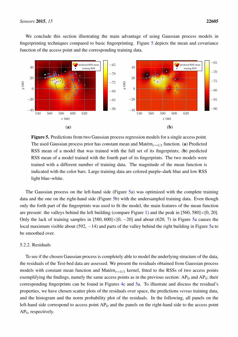
We conclude this section illustrating the main advantage of using Gaussian process models infingerprinting techniques compared to basic fingerprinting. Figure 5 depicts the mean and covariancefunction of the access point and the corresponding training data.

540 560 580 600 620−40

−20

0

20

40

x (m)

y(m

)

predicted RSS meantraining RSS

−90

−85

−80

−75

−70

−65

(a)

540 560 580 600 620−40

−20

0

20

40

x (m)y

(m)

predicted RSS meantraining RSS

−90

−85

−80

−75

−70

−65

(b)

Figure 5. Predictions from two Gaussian process regression models for a single access point.The used Gaussian process prior has constant mean and Matérnν=3/2 function. (a) PredictedRSS mean of a model that was trained with the full set of its fingerprints; (b) predictedRSS mean of a model trained with the fourth part of its fingerprints. The two models weretrained with a different number of training data. The magnitude of the mean function isindicated with the color bars. Large training data are colored purple–dark blue and low RSSlight blue–white.

The Gaussian process on the left-hand side (Figure 5a) was optimized with the complete trainingdata and the one on the right-hand side (Figure 5b) with the undersampled training data. Even thoughonly the forth part of the fingerprints was used to fit the model, the main features of the mean functionare present: the valleys behind the left building (compare Figure 1) and the peak in [560, 580]×[0, 20].Only the lack of training samples in [580, 600]×[0, −20] and about (620, 7) in Figure 5a causes thelocal maximum visible about (592, −14) and parts of the valley behind the right building in Figure 5a tobe smoothed over.

5.2.2. Residuals

To see if the chosen Gaussian process is completely able to model the underlying structure of the data,the residuals of the Test-bed data are assessed. We present the residuals obtained from Gaussian processmodels with constant mean function and Matérnν=3/2 kernel, fitted to the RSSs of two access pointsexemplifying the findings, namely the same access points as in the previous section: APD and APS; theircorresponding fingerprints can be found in Figures 4c and 5a. To illustrate and discuss the residual’sproperties, we have chosen scatter plots of the residuals over space, the predictions versus training data,and the histogram and the norm probability plot of the residuals. In the following, all panels on theleft-hand side correspond to access point APD and the panels on the right-hand side to the access pointAPS, respectively.

Sensors 2015, 15 22606

To examine the residuals dependent on the fingerprint positions, we refer the reader to Figure 6.

560 580 600 620 −20

020

40−10

0

10

x (m) y (m)

resi

dual

s(d

Bm

)

residuals

−10

0

10

(a)

560580

600620

0

20−10

0

10

x (m)y (m)

resi

dual

s(d

Bm

)

residuals

−10

−5

0

5

(b)

Figure 6. Residuals plotted against space for two different access points: (a) An accesspoint with many fingerprints; (b) an access point with few fingerprints. The magnitude ofthe residuals are indicated by the color bars.

The spatial dependency of the residuals for two-dimensional input data is difficult to assess in thesestatic figures. No perspective allows a proper view, and the evaluation of many different cross-sectionswould be required to assess the spatial dependency rigorously. Moreover, the unknown positions ofaccess points, possibly affecting the spatial distribution of the residuals, make this even harder. Besidesthe two examples, we visually examined the residuals of many access points from different datasets.This inspection did not reveal any spatial dependency or systematic pattern of the residuals.

Figure 7 depicts the predicted RSS versus the training data. For perfect predictions, all points wouldlie on the red line; here, the points are basically randomly distributed around that line, indicating anappropriate model fit. However, in both panels (Figure 7a,b), outliers within large training RSS regioncan be observed, meaning that the largest training samples could not be “reached” by the model’s meanfunction. This observation suggests that the chosen model underestimates the RSS observations at thesepeaks (these RSSs are the largest and probably measured very close to the access point). It is noteworthythat not all access points present these outliers. On the lower RSS bound, points concentrate a bit on theupper half in both figures, again suggesting an underestimation. This effect was only observed for a fewaccess points.

Recall Equation (1); Gaussian process regression expects a Gaussian process prior distribution. Giventhat a Gaussian distributions was chosen as the likelihood function, the residuals are expected to be aboutnormally distributed and centered around zero. The histograms of the residuals are shown in Figure 8.Most importantly, in both cases, the residuals are symmetrically distributed around zero, though theresiduals are not normally distributed. The left-hand side panel shows outliers at the upper and lowerbound of the residuals. The histogram obtained from data of APS (Figure 8b) presents multiple modes,and also, the tails are too large for a normal distribution; however, the small sample size might contributeto these observations.

For further details, the norm probability plot is examined; see Figure 9 (samples from a normaldistribution would ideally lie on the red line). The majority of the residuals in Figure 9a follow a normal

Sensors 2015, 15 22607

distribution. However, heavy tails can be observed, and also, the number of outliers is fairly small: about1.5% of the sample. The residuals in the second example are approximately Gaussian distributed, as canbe seen in Figure 9b. Their distribution also has slightly larger tails than normally-distributed sampleswould have. The few atypical residuals that exist are not that large, as in Figure 9a.

−80 −60 −40 −20

−80

−60

−40

−20

training RSS (dBm)

pred

icte

dR

SSm

ean

(dB

m) RSS

(a)

−80 −60 −40 −20

−80

−60

−40

−20

training RSS (dBm)

pred

icte

dR

SSm

ean

(dB

m) RSS

(b)

Figure 7. Predicted RSS versus training RSS for two access points: (a) An access point withmany fingerprints; (b) an access point with few fingerprints. The red line indicates under-and over-fitting of the training data.

−15 −10 −5 0 5 10 15

0

20

40

60

80

RSS residuals (dBm)

freq

uenc

y

(a)

−10 −5 0 5 10

0

5

10

15

RSS residuals (dBm)

freq

uenc

y

(b)

Figure 8. Histogram of residuals of two Gaussian process regression models, each for adifferent access point: (a) An access point with many fingerprints; (b) an access point withfew fingerprints.

Sensors 2015, 15 22608

−15 −10 −5 0 5 10 15

0.00010.010.34.5255075

95.599.7

99.99

RSS residuals (dBm)

%pr

obab

ility

RSS

(a)

−10 −5 0 5 10

0.01

0.3

4.5

255075

95.5

99.7

99.99

RSS residuals (dBm)

%pr

obab

ility

RSS

(b)

Figure 9. Norm probability plot of the model residuals from Gaussian process regressionmodels of two different access points: (a) An access point with many fingerprints; (b) anaccess point with few fingerprints.

5.3. Positioning Accuracy

The findings favoring the Gaussian process model based on the Matérn kernel were all concludedfrom the model measures. In the following, we present the results on the positioning accuracy obtainedfrom ML estimators in accordance with Equation (5).

Table 6 contrasts the positioning accuracy yielded by ML estimators derived from Gaussian processmodels using different covariance functions. All models have the constant mean function in common.The accuracy of the estimators is expressed in terms of the root mean square error and is presented fortwo trajectories.

The accuracies for both trajectories exhibit the same tendencies: the most accurate Gaussian processmodel is the one with the Matérn kernel and ν = 1/2; the same model that yielded the lowest BIC forthe Test-bed radio map; see the corresponding Table 4. The second best model is based on a rationalquadratic kernel function, followed by the Matérnν=3/2 function. Models using the squared exponentialor one of the more complex kernels yielded position errors about 40% larger than that of the best MLestimator. Focusing on the results achieved by the ML estimator with the Matérn kernel and the estimatorbased on the squared exponential kernel, one can observe an improvement in favor of our proposed modelof 1.3 m, in case of Trajectory-1, and 0.78 m for Trajectory-2.

These results on the positioning performance recommend the use of rough kernels over smoother ones.They further demonstrate that the differences seen in the model measure propagate via the likelihoodfunction to the localization error.

The superiority of the Matérn class functions over the squared exponential kernel with respect toWLAN RSS modeling and prediction is hereby confirmed again. However, our proposed Gaussianprocess model did not perform the best, but the Matérn kernel parametrized with ν = 1/2 did.

Sensors 2015, 15 22609

Table 6. Root mean square position error of different position estimators, using the jointradio map, for Trajectory-1 and Trajectory-2. The Gaussian process ML estimators werederived from the Test-bed radio map.

Gaussian Process ML EstimatorPosition Error (m)

Trajectory-1 Trajectory-2

SE 10.21 6.46Matν=1/2 5.90 3.97Matν=3/2 8.90 5.68Matν=5/2 8.98 5.92RQ 6.18 5.30sum of SE and SE 10.48 6.46prod of SE and SE 10.46 6.35add of SE 14.42 11.45

Figure 10 depicts x over y of Trajectory-1 (compare to Figure 1 to relate the trajectory within thetest area).

550 560 570 580 590 600 610

−20

0

20

40

x (m)

y(m

)

ground truthMLE with SE

MLE with Matν=1/2

Figure 10. Estimates of Trajectory-1 and the ground truth. The MLEs are based on aGaussian process model with a constant mean and (1) the squared exponential (SE) or (2) theMatérn class (Matν=1/2) kernel.

Apparent in this figure are large outliers at its beginning at (607, −9), which are shared by bothestimators. From there, the experimenter followed the outdoor corridor and entered the right building twotimes at [600, 0] × [595, 20] and [603, 27] × [610, 33]. The entering of the building was well estimated,but the section of the outdoor corridor in between presents again large errors. These errors are dueto the similarity of the fingerprints, common in outdoor areas. Nothing attenuates the RSSs betweenthe outdoor corridor (left of the indoor area) and the Outdoor-2 area; thus, neighboring fingerprintsconstitute similar RSSs, which pulls the estimates outward, into the Outdoor-2 area. The same effectcan be observed about [550, 25] × [565, 41], a small, empty lawn area. The larger errors in this area

Sensors 2015, 15 22610

are again due to similar neighboring fingerprints. Besides these three problematic sections, typical forlocation fingerprinting systems, the estimated trajectory follows the ground truth well.

6. Discussion

6.1. Normality of Averaged RSSs

According to the central limit theorem, the mean of a random variable with finite variance isasymptotically normally distributed. Furthermore, RSSs obey the central limit theorem, as shown inSection 5.1. The RSS averages converge to a normal distribution. Although the RSSs averaged over oneand five seconds may not follow a Gaussian distribution, they are more likely symmetric and less likelyheavy-tailed than the raw data. Moreover, Kaemarungsi et al. [16] argued that symmetric signal strengthdistributions can be approximated by the log-normal distribution.

On these grounds, we consider that the distribution of RSSs averages resembles a Gaussiandistribution sufficiently to justify a normally-distributed likelihood function for Gaussian processregression and to expect more robust predictions as compared to raw RSSs.

6.2. Structure Search in RSSs

The model training has to cope with a wide range of conditions: for instance, the number of trainingpoints and their spatial density, the contribution of access points to the fingerprints. Furthermore, thedynamics of RSSs is a challenge for the model fitting, especially RSSs of close by access points havinga large variance, particularly if the fingerprint density is high, as for example, for the radio maps thatcontain four fingerprints at almost the same position (recall the four orientations of RSS recording; seeSection 4.2.1).

The first part of the Gaussian process modeling is to find an adequate prior distribution, that is its meanand covariance function. The comparison of various combinations of mean functions and covariancefunctions could narrow down the search to the constant mean function and, regarding the covariancefunctions, to the Matérn and the additive squared exponential kernel.

We already touched the issue of using the zero mean function to model spatial RSS distributions inSection 1. Gaussian process priors with constant or linear mean function fits RSS data better, becausethey avoid either that the predictive distribution eventually converges to zero in the absence of trainingdata or an additional estimation step, as in [6,8]. Using the linear mean function is intuitive, because itapproximates the decay of RSS over distance and most likely fits the data well when the access pointposition is at an edge of the test area. On the other hand, if the access point is located in the center ofthe test area, a linear function only approximates one slope of the RSS reasonably well, but the othersrespectively poorly; whereas the constant mean function solely assumes that the process converges to aconstant value. For the majority of access points in this study, the mean function converged to RSS levelsabout −80 dBm in regions without training data. A further advantage of the constant mean function isthat it has one hyperparameter less than the linear mean function, making the model less complex andthe hyperparameter optimization faster. Thus, we recommend the constant mean function as the mostappropriate mean function to model WLAN RSS.

Sensors 2015, 15 22611

The outcome of covariance functions is not surprising given that both kernels are very flexible, ableto model smooth, but also rough changes in WLAN RSS. The properties of these two kernel functionsexplain this result:

To construct an additive kernel, a basis kernel is specified for each input dimension, and the additivekernel becomes a sum of all possible combinations of the input dimensions. The interaction betweenthe different input dimensions take place corresponding to the degree of additive structure defined bythe order of the additive kernel. This combinatory capability permits the resulting Gaussian processesto be more flexible than others. Nonetheless, as the hyperparameter optimization for additive kernels ofsecond order was faulty, we used only the first order additive kernel, possibly explaining the structurevisible in the right-hand side of Figure 4.

For certain parameters, the Matérn class functions become a product of an exponential and apolynomial function, giving the kernel its adaptability. Furthermore, the roughness parameter contributesto that adaptability: choosing ν = 1/2 makes the Matérn function very rough, and for ν → ∞, itconverges to the SE kernel, which is a very smooth one (it is infinitely differentiable).

The outcome of the positioning experiment favors rough kernels. If the radio map is very dense, theMatérn kernel with ν = 1/2 or even the rational quadratic kernel might be more appropriate. As weuse Gaussian processes with the objective of interpolating radio maps, dense radio maps are rather theexception. In light of the findings of the positioning experiments, we still recommend the Matérnν=3/2

kernel as the basis for a Gaussian prior covariance function.Given that the combination with the independent noise kernel, sums and products of kernels and the

additive kernel did not fit the data as well as less complex kernels, this suggests that spatial WLANRSS distributions do not constitute a very complex structure. A simple covariance function based onan exponential function, as the Matérnν=1/2 or SE the kernel, is able to capture the fundamental RSSpatterns. Recall the tables of Section 5.2.1 and focus on the kernels that yielded the lower BICs (SE,Mat, RQ), then it becomes evident that not choosing the zero mean function improves the model morethan the choice of the covariance functions.

This study did not disclose a Gaussian process model particularly for indoors or outdoors, refutingour hypothesis. However, the Gaussian processes that model RSSs indoors or outdoors might still haveconsiderably different structures due to the hyperparameters, which were optimized with respect to thedata; but an examination of the hyperparameters for six randomly chosen access points and all datasetsdid not support our hypothesis either; the hyperparameters lacked any pattern.

We identified several possible reasons why the RSS characteristics of the Gaussian process modelsdid not differ between the indoor and outdoor environments of our test area: (i) The spatial distributionof RSSs indoors and outdoors is indeed indistinguishable, due to the properties of the buildings, such assize (at least in one dimension), materials (e.g., soft partitions), structure and contained objects; (ii) Thediscrete fingerprints capture only a small fraction of the true signal power distribution (see Figure 1),and the information we look for is not contained in our datasets; (iii) The fingerprints may capturethe information, but the spatial distribution and resolution of fingerprints, which influences the modelfitting, outweigh the effect we were seeking; (iv) The tested Gaussian process models are insensitive tothe possibly existing differences in RSSs between indoor and outdoor environments, and they smoothout these differences.

Sensors 2015, 15 22612

A combination of these reasons may actually occur simultaneously.

6.3. Quality of Gaussian Process Model Fit

Even though several research groups used Gaussian processes to model and interpolate RSSs, thequality of the fit of these models was never demonstrated. Section 5.2.2 showed that the residuals areindeed random and do not posses a systematic trend.

The lack of structure in the residuals confirms that the Gaussian processes are appropriate tointerpolate WLAN RSS accurately.

For RSS distributions with very large dynamics, we found that the model underestimates the peakvalues. The decision to capture four fingerprints at virtually the same position, but in the four cardinaldirections, may contribute to this effect. It eventually generates very high RSS differences over verysmall distances and forces the Gaussian process mean function to be very rough. However, if the rest ofthe training data is rather smooth, the model is not rough enough to cover these RSS differences.

Furthermore, we found that the residuals are approximately normally distributed, but often possesheavy tails; as do the distributions of the RSS measurements. To mitigate this issue, one could, onthe one hand, extend the duration when the RSSs are recorded and averaged, such that they becomemore likely normally distributed. On the other hand, one could use a more robust Gaussian processlikelihood function, for example a Student’s t-distribution or the Laplace distribution. This may decreasethe residuals of the Gaussian process models, hence increasing their accuracy and potentially increasingthe positioning results, as well.

Besides the fat-tailed distributions, we noticed a few residual distributions that are skewed or havean unrecognizable shape. We found that these distributions belong to access points featuring low powerRSSs and that their shape is due to the small RSS sample size and the often discrete RSSs.

We give a last remark with respect to [12]. Based on the synthetic data and the positioning accuracy asa measure of model fit, the authors favored the squared exponential kernel over the Matérn and rationalquadratic kernel. Given their data, this is a reasonable choice. However, much more details than just thespatial density of the fingerprints affect the choice of the Gaussian process prior, and again, the effect ofthe Gaussian process prior’s mean function should not be underestimated.

7. Conclusions

Gaussian processes are indeed appropriate to model RSS for WLAN location fingerprinting.Relatively simple models are able to model the spatial structure of RSS entirely.

The very common use of the “default”, zero mean/squared exponential kernel, model in the fieldof WLAN fingerprinting is reasonable, but better model fits can be achieved with different mean andcovariance functions. The most suited and general Gaussian process regression model has a Gaussianprocess prior with constant mean function and Matérn class covariance function with ν = 3/2. Thesuperiority of the Matérn kernel over the squared exponential kernel was confirmed by the results of thepositioning accuracy, achieved by their ML estimators. Our proposed model is proficient for indoor andoutdoor environments. Different model fits for indoor and outdoor environments could not be discovered.

Sensors 2015, 15 22613

The robustness and versatility of Gaussian processes allow the use of a common model to approximatespatial RSS distributions, even with observations that violate the model’s assumptions; the use ofaveraged RSSs contributes to this versatility and should be preferred over RSS raw data. Such a generalmodel actually facilitates its further application, as particular models for certain areas are unnecessary.

In the first instance, these models help to reduce the effort of radio map creation, compared to classicalfingerprinting, while increasing the spatial resolution of RSS potentially improves the location accuracy.What is more, Gaussian process mean functions provide a basis for continuous likelihood functions thatcan be used for Bayesian location finding and data fusion, wherefore the predicted covariance functionis a measure of uncertainty.

A more profound assessment of the influence of different Gaussian process models on the positioningaccuracy is an open task.

Supplementary Material

The three radio maps (Indoor, Outdoor-1, Outdoor-2) are published with this article. They areprovided in SQLite 3.x database format as supplementary material, named File S1, indoor.db, File S2,outdoor-1.db, and File S3, outdoor-2.db.

The optimized hyperparameters of six access points, mentioned in the discussion in Section 6.2, arealso included as supplementary material and are contained in Table S, hypertable.pdf.

Acknowledgments

Philipp Richter acknowledges the funding of Consejo Nacional de Ciencia y Tecnología forhis PhD studies and for publishing this manuscript in open access. The authors also thankEduardo Castaño-Tostado for his valuable advice and Albano Peña-Torres for the data acquisition.

Author Contributions

Philipp Richter designed the study and analyzed and interpreted the data. He also drafted, revised andedited the manuscript. Manuel Toledano-Ayala revised and edited the manuscript.

Conflicts of Interest

The authors declare no conflict of interest.

References

1. Chen, L.; Li, B.; Zhao, K.; Rizos, C.; Zheng, Z. An Improved Algorithm to Generate a Wi-FiFingerprint Database for Indoor Positioning. Sensors 2013, 13, 11085–11096.

2. Du, Y.; Yang, D.; Xiu, C. A Novel Method for Constructing a WIFI Positioning System withEfficient Manpower. Sensors 2015, 15, 8358–8381.

Sensors 2015, 15 22614

3. Elnahrawy, E.; Li, X.; Martin, R.P. The limits of localization using signal strength: A comparativestudy. In Proceedings of the First Annual IEEE Communications Society Conference on Sensorand Ad Hoc Communications and Networks (IEEE SECON 2004), Santa Clara, CA, USA, 4–7October 2004; pp. 406–414.

4. Chai, X.; Yang, Q. Reducing the Calibration Effort for Probabilistic Indoor Location Estimation.IEEE Trans. Mob. Comput. 2007, 6, 649–662.

5. Howard, A.; Siddiqi, S.; Sukhatme, G.S. An Experimental Study of Localization UsingWireless Ethernet. In Proceedings of the International Conference on Field and Service Robotics,Yamanashi, Japan, 14–16 July 2003; pp. 145–153.

6. Ferris, B.; Hähnel, D.; Fox, D. Gaussian processes for signal strength-based location estimation.In Proceedings of Robotics: Science and Systems II, Philadelphia, PA, USA, 16–19 August 2006.

7. Duvallet, F.; Tews, A.D. WiFi position estimation in industrial environments using Gaussianprocesses. In Proceedings of the IEEE/RSJ International Conference on Intelligent Robots andSystems (IROS 2008), Nice, France, 22–26 September 2008; pp. 2216–2221.

8. Atia, M.M.; Noureldin, A.; Korenberg, M.J. Dynamic Online-Calibrated Radio Maps for IndoorPositioning in Wireless Local Area Networks. IEEE Trans. Mob. Comput. 2013, 12, 1774–1787.

9. Yoo, J.; Kim, H.J. Target Tracking and Classification from Labeled and Unlabeled Data in WirelessSensor Networks. Sensors 2014, 14, 23871–23884.

10. Brooks, A.; Makarenko, A.; Upcroft, B. Gaussian Process Models for Indoor and OutdoorSensor-Centric Robot Localization. IEEE Trans. Robot. 2008, 24, 1341–1351.

11. Do, H.N.; Jadaliha, M.; Choi, J.; Lim, C.Y. Feature selection for position estimation using anomnidirectional camera. Image Vis. Comput. 2015, 39, 1–9.

12. Bekkali, A.; Masuo, T.; Tominaga, T.; Nakamoto, N.; Ban, H. Gaussian processes forlearning-based indoor localization. In Proceedings of the IEEE International Conference on SignalProcessing, Communications and Computing (ICSPCC), Xi’an, China, 14–16 September 2011;pp. 1–6.

13. Depatla, S.; Buckland, L.; Mostofi, Y. X-ray Vision with Only WiFi Power Measurements UsingRytov Wave Models. IEEE Trans. Veh. Technol. 2015, 64, 1376–1387.

14. Rasmussen, C.E.; Williams, C.K.I. Gaussian Processes for Machine Learning; MIT Press:Cambridge, MA, USA, 2006.

15. Rappaport, T.S. Wireless Communications: Principles and Practice, 2 ed.; Prentice Hall PTR:Upper Saddle River, NJ, USA, 2001.

16. Kaemarungsi, K.; Krishnamurthy, P. Analysis of WLAN’s received signal strength indication forindoor location fingerprinting. Pervasive Mob. Comput. 2012, 8, 292–316.

17. Mirowski, P.; Steck, H.; Whiting, P.; Palaniappan, R.; MacDonald, M.; Ho, T.K. KL-divergencekernel regression for non-Gaussian fingerprint based localization. In Proceedings of theInternational Conference on Indoor Positioning and Indoor Navigation (IPIN), Guimarães,Portugal, 21–23 September 2011.

18. Chen, A.; Harko, C.; Lambert, D.; Whiting, P. An Algorithm for Fast, Model-free Tracking Indoors.SIGMOBILE Mob. Comput. Commun. Rev. 2007, 11, 48–58.

Sensors 2015, 15 22615

19. Youssef, M.; Agrawala, A.; Shankar, U. WLAN Location Determination via Clustering andProbability Distributions. In Proceedings of the First IEEE International Conference on PervasiveComputing and Communications, 2003 (PerCom 2003), Fort Worth, TX, USA, 26–26 March 2003.

20. Mirowski, P.; Whiting, P.; Steck, H.; Palaniappan, R.; MacDonald, M.; Hartmann, D.; Ho, T.K.Probability kernel regression for WiFi localisation. J. Locat. Based Serv. 2012, 6, 81–100.

21. Roos, T.; Myllymäki, P.; Tirri, H.; Misikangas, P.; Sievänen, J. A Probabilistic Approach to WLANUser Location Estimation. Int. J. Wirel. Inf. Netw. 2002, 9, 155–164.

22. Honkavirta, V.; Perälä, T.; Ali-Löytty, S.; Piché, R. A Comparative Survey of WLAN LocationFingerprinting Methods. In Proceedings of the 6th Workshop on Positioning, Navigation andCommunication 2009 (WPNC’09), Hannover, Germany, 19 March 2009; pp. 243–251.

23. Duvenaud, D.; Nickisch, H.; Rasmussen, C.E. Additive Gaussian Processes. Available online:http://papers.nips.cc/paper/4221-additive-gaussian-processes (accessed on 28 August 2015).

24. Lloyd, J.R.; Duvenaud, D.; Grosse, R.; Tenenbaum, J.B.; Ghahramani, Z. Automatic Constructionand Natural-Language Description of Nonparametric Regression Models. ArXiv E-Prints 2014,arXiv:1402.4304.

c© 2015 by the authors; licensee MDPI, Basel, Switzerland. This article is an open access articledistributed under the terms and conditions of the Creative Commons Attribution license(http://creativecommons.org/licenses/by/4.0/).