EI @ Haas WP 245R

Towards Understanding the Role of Price in Residential Electricity Choices: Evidence from a Natural

Experiment

Katrina Jessoe, David Rapson, and Jeremy B. Smith October 2013

Revised version published in Journal of Economic Behavior and Organization

107: 191 – 208, 2014

Energy Institute at Haas working papers are circulated for discussion and comment purposes. They have not been peer-reviewed or been subject to review by any editorial board. © 2013 by Katrina Jessoe, David Rapson, and Jeremy B. Smith. All rights reserved. Short sections of text, not to exceed two paragraphs, may be quoted without explicit permission provided that full credit is given to the source.

http://ei.haas.berkeley.edu

Are Residential Electricity Consumers Utility

Maximizers? Evidence from a Natural Experiment∗

Katrina Jessoe †

UC Davis, ARE

David Rapson ‡

UC Davis, Economics

Jeremy B. Smith§

Analysis Group

October 21, 2013

Abstract

We examine a choice setting in which residential electricity consumers may respond to

incentives other than contemporaneous prices. We test predictions from the standard

model of utility maximization using data from a natural field experiment that exposed

some households to a change in their electricity rates. Households reduce electricity

usage in response to a decrease in electricity prices, suggesting that factors aside from

price influence customer choice. An understanding of household behavior in energy

markets is essential for the effective implementation of climate change mitigation pol-

icy. Documenting this and similar results is a necessary step in achieving such an

understanding.

∗We would like to thank Michael Anderson, Marcus Asplund, Anette Boom, Jim Bushnell, Lucas Davis,Kelsey Jack, Kevin Lang, Alan Meier, Michael Manove, Marc Rysman, Johannes Schmieder, and the manyother participants in seminars at Boston University Economics, the UC Energy Institute, UC BerkeleyARE, UC San Diego Economics, Copenhagen Business School Economics, the University of New SouthWales Economics, and the JEBO conference at University of Tennessee for their comments. Bo Young Choiand Brock Smith provided excellent research assistance. Financial support for this project was providedby UCE3. Rapson thanks the Energy Institute at Haas for support under a research contract from theCalifornia Energy Commission. The views presented are those of the authors and do not reflect those ofAnalysis Group. Any errors are our own.†E-mail: kkjessoe@ucdavis.edu; Website: http://kkjessoe.ucdavis.edu/‡E-mail: dsrapson@ucdavis.edu; Website: http://www.econ.ucdavis.edu/faculty/dsrapson§111 Huntington Avenue, Tenth Floor, Boston, MA 02199. The author is an Associate at Analysis Group,

Inc. Research for this article was undertaken when he was a PhD student at Boston University.

1 Introduction

A major policy goal in coming decades is to reduce greenhouse gas emissions. Most economists,

including ourselves, favor market-based approaches due to their ability to achieve an emis-

sions target cost-effectively. The strength of such instruments relies partly on the assumption

that consumers will respond optimally to prices; but a growing body of evidence suggests

that within the energy choice setting, consumer behavior does not strictly adhere to the

predictions derived from standard models. Understanding when and under what conditions

households respond to prices as standard theory would predict is crucial to achieve climate

change mitigation objectives and efficiency in energy markets.

In this paper, we document an instance in which households did not respond to a retail

electricity price intervention as standard theory would predict. Our empirical setting offers

a unique opportunity to test whether consumers are static utility maximizers, and we find

conclusively that in this instance they were not. While we are left to speculate about the

exact reason for this deviation, our results suggest that there may be risk in adhering too

ideologically to price interventions in terms of missing policy goals or achieving them only

imperfectly or inefficiently. An assertion that price incentives always work can be disproven

by the counter-example we provide.

This result should not be entirely surprising. The theory of “bounded rationality” has

long predicted that it may be rational for consumers to be imperfectly informed or to not

deploy full cognitive effort in the face of information acquisition or cognition costs (Simon

(1955)), leading to outcomes that appear sub-optimal. People may also be motivated by

intrinsic forces in addition to extrinsic (financial) incentives. This concept has been long-

accepted by psychologists and sociologists, and has recently entered the economics domain

in Benabou and Tirole (2003). In the residential electricity choice setting non-monetary

incentives such as moral license or pressure to conform to social norms can dominate financial

2

incentives. Voluntary enrollees in a carbon offset and green electricity programs increase their

electricity consumption despite also facing higher prices (Harding and Rapson (2013) and

Jacobsen, Kotchen, and Vandenbergh (2012)), and customers informed of their neighbors’

electricity usage respond by using less themselves (Allcott (2011)). Altruism and green

identity also play important roles, with environmental concerns becoming a relevant aspect

of consumer decisions (as in Kotchen and Moore (2007)).

These results may help reconcile the variety of price elasticities of demand that have

been reported for residential electricity customers (Alberini, Gans, and Velez-Lopez (2011),

Fell, Li, and Paul (2012), Ito (forthcoming), Reiss and White (2005)). Consumers grapple

with the complexity of the electricity choice setting. Features such as multi-tiered pricing

structures (as explored by Reiss and White (2005)) or noisy signals about consumption

may limit customers’ ability to respond to prices. Consumers facing an increasing-block

electricity rate structure appear to respond more to average price than marginal price (Ito

(forthcoming)), and high frequency information about real-time consumption increases the

price elasticity of electricity demand (Jessoe and Rapson (forthcoming)). Interventions that

make prices (expenditure) more salient may meaningfully influence household electricity

usage. Residential consumers have been shown to conserve electricity immediately after

receiving their electricity bill (Gilbert and Graff-Zivin (2013)). Thus, price elasticity may be

affected by several very specific aspects of the respective setting that are usually impossible

to observe or control for in empirical analyses, potentially accounting for the heterogeneity

of estimates found in the literature. It is for this reason that findings like those of Faruqui

and Sergici (2010) – who provide a meta-analysis of a number of examples in which price

interventions do indeed appear to have led to desired reductions – can be misleading: while

they may indicate that prices often work, they cannot prove that prices always work; and

they can provide only limited guidance as to the circumstances under which prices might

work best.

3

We partnered with an electricity distribution company (EDC) in the northeast US to

evaluate a large-scale mandatory residential time-of-use (TOU) program that forced house-

holds to switch irrevocably from a flat rate tariff to a TOU tariff after breaching a monthly

usage threshold.1 The setting gives rise to a regression discontinuity framework in which we

compare outcomes of households just above the usage threshold to those of households falling

just below the cutoff. Due to customers’ inability to perfectly control monthly usage, in the

neighborhood of the usage threshold assignment to the TOU rate is as good as random. The

large-scale deployment of the program exhibits a high density around the threshold, creating

a large sample of treatment and control households on which to test our hypothesis.

In the first summer months of the program in 2008, TOU rates were low relative to

the flat rate alternative. Whereas the standard formulation of TOU prices is for the on-

peak rate to be substantially higher than the flat rate and the off-peak rate substantially

lower, in our setting TOU households faced on-peak rates in June to September of 2008

that were either lower than the relevant flat rate, or only slightly higher.2 Off-peak rates

were correspondingly even lower. The financial incentives for TOU households are clear:

total electricity use in those months – regardless of substitution patterns across on-peak and

off-peak hours – should increase.

We find the opposite. TOU customers reduced total electricity consumption, as measured

by our estimates of the treatment effect at the threshold. These results are inconsistent with

static utility maximization. It is clear that households are responding to incentives other

than contemporaneous prices. There are ways to rationalize their choices. We discuss these

1TOU electricity pricing divides electricity use into two blocks according to the time of day at whichelectricity is consumed, and applies a higher rate to the block corresponding to historically high-cost times.It is a small step towards aligning retail electricity prices with marginal production costs. It is also the mostcommon corrective measure used by electricity regulators to achieve such an alignment, due largely to thecrucial advantage of being easy for consumers to understand and, in principle, respond to.

2Customers may purchase the generation component of their electricity services from either our EDCpartner or an alternate supplier. This choice affects the relative on-peak and off-peak prices (the “TOUgradient”). In the discussion below we demonstrate why this does not affect our conclusions.

4

but do not perform formal tests, which our data cannot support. Nevertheless, the simple

documentation of this result is an important step towards understanding energy demand

behavior, and how future policy interventions might be improved.

The paper is organized as follows: in Section 2 we present a review of the standard

theoretical framework for demand in this setting; Section 3 describes the program design,

which forms the basis for our empirical setting; we explain how the setting can be viewed as

a natural experiment and provide a description of our data in Section 4; treatment effects

are reported in Section 5 and interpreted in Section 6; and Section 7 concludes.

2 Theoretical Framework

Several studies assessing early TOU experiments characterized consumer preferences using a

framework that has since become the standard for modeling short-run household electricity

demand by time of use. This framework, presented in detail in Aigner and Poirier (1979), was

first used by Hausman, Kinnucan, and McFadden (1979) and Caves and Christensen (1980)

to estimate the on-peak and off-peak price elasticities corresponding to TOU experiments

in Connecticut and Wisconsin, respectively. We will rely on this framework as a baseline to

define rational household responses to TOU pricing in a static optimization setting.

Following Hausman et al. (1979), we specify a household’s monthly utility function as

U = U(xon, xoff ,y), (1)

where xon and xoff are the household’s monthly on-peak and off-peak electricity usage,

respectively, and y is a vector of all other goods.3 We then make a weak separability

3An important assumption underlying this utility specification is that the stock of electricity-using appli-ances is fixed. Therefore, xon and xoff should be thought of as derived electricity demand based on demandfor household services that use these appliances and the times of day that the household prefers to consumesuch services.

5

assumption so that utility can be characterized as

U = W (f(xon, xoff ), y), (2)

where f(xon, xoff ) represents a homogeneous of degree one Hicksian aggregation of on-peak

and off-peak electricity consumption, and y is a Hicksian composite of all the goods in y.

Normalizing the price of y to unity permits y to be interpreted simply as expenditure on all

goods besides electricity.

The weak separability condition allows the household’s monthly maximization problem

to be decomposed into two levels. One level represents the household’s choice of how much

to spend on total electricity usage, where the remainder of its (fixed) income is spent on all

other goods. The other level describes the household’s choice of how to allocate electricity

consumption across on-peak and off-peak hours, which depends only on electricity rates.

The choice of total electricity usage, X ≡ xon + xoff , will depend on an aggregated price

of electricity p given by

p = ponson + poffsoff , (3)

where son and soff are the shares of on-peak and off-peak usage in total usage as determined

in the allocation level of the maximization problem.4 These shares sum to unity and depend

only on the parameters of f(). Therefore, the aggregated price of electricity is a weighted

average of the on-peak rate pon and the off-peak rate poff .

Thus, conditional on the optimal choices of xon and xoff from the allocation level of the

maximization problem, total electricity consumption can be viewed as being determined by

a straightforward utility-maximizing division of total income between good X, with price

4The aggregated price in our empirical setting will also include a small adjustment for a fixed monthlycharge and for the increasing-block structure of the non-TOU rate. This will be discussed in more detail inthe following section.

6

p, and expenditure on all other goods. Once properties of W () are pinned down, deriving

predictions concerning total electricity consumption is accomplished as in any two-good

setting characterized by these properties. For example, if W () is such that X is a normal

good, the model clearly predicts that a drop in p will lead unambiguously to an increase in

the quantity demanded of X.

We use this theoretical framework and its predictions on total electricity consumption

as a backdrop when discussing the structure of electricity rates faced by the households

in our dataset in the following section, and when discussing our empirical results in the

interpretation section below. Of course, the model is also capable of generating predictions

concerning load shifting, i.e. the substitution of electricity usage across on-peak and off-peak

times. However, we do not discuss these predictions, as our dataset, which we will introduce

in Section 4 below, does not provide us with the means to investigate them empirically.

3 Program Design

Beginning in 2006, an electric distribution company in northeastern United States imple-

mented a mandatory time-of-use (TOU) program for residential customers. Prior to the

introduction of this program, most residential customers were billed according to a seasonal

flat rate, with the price of electricity varying seasonally but remaining constant within a day.

Approximately 12% of customers chose to be placed instead on a seasonal TOU rate, with

the price of electricity varying seasonally and within a day. In the analysis that follows, we

exclude these voluntary adopters.

Under the policy, when a residential customer’s electricity usage in any 30-day billing

period exceeded a pre-determined threshold, the customer was automatically placed onto

TOU pricing. Beginning November 2006, a household was to be placed on TOU pricing by

January of 2008 if usage in any 30-day billing period exceeded 4000 kWh. This threshold

7

applied until December 31, 2007. The threshold was lowered to 3000 kWh in 2008 and to

2000 kWh in 2009. The present study focuses on households that crossed the 4000 kWh

threshold due to the unusual rate change that occurred at that time, to which we now turn.

The residential TOU rate plan charges a high per-kWh rate at on-peak times (noon

through 8pm on weekdays) and a low per-kWh rate at off-peak times (all other times and

days). Table 1 shows the TOU rates that were in effect over the period of our analysis, and

compares them to the corresponding non-TOU rates. In our study, the summer non-TOU

tariff had an increasing-block structure, with the first 500 kWh of usage in a billing month

charged at a base “headblock” per-kWh rate and the remaining usage in that billing month

charged at a higher “tailblock” per-kWh rate.

Given this increasing-block structure for the flat rate and the fact that all of the house-

holds in our analysis exceed 500 kWh in total electricity consumption in every month, the

non-TOU monthly budget constraint can be expressed as

pt(X − 500) + ph500 + g = E, (4)

where E is total electricity expenditure, pt is the tailblock rate, ph is the headblock rate, and

g is a fixed monthly charge. Noting once again that total electricity consumption is simply

the sum of on-peak and off-peak consumption, this can be re-written as

ptxon + ptxoff − (pt − ph)500 + g = E, (5)

which emphasizes the fact that the marginal rate faced by non-TOU customers in both

on-peak and off-peak hours is the tailblock rate. Meanwhile, the TOU monthly budget

constraint is given by

ponxon + poffxoff + g = E, (6)

8

where the fixed monthly charge g is the same as that for non-TOU customers in all months.

Within the theoretical framework presented in the previous section, total electricity ex-

penditure is defined as the product of the aggregated electricity price and total electricity

consumption, or E ≡ pX. Inserting this definition into equations (5) and (6) and dividing

by total consumption gives expressions for the aggregated non-TOU and TOU electricity

prices,

pN = pt + φN (7)

and

pT = ponson + poffsoff + φT , (8)

where the subscript s ∈ {N, T} refers to non-TOU and TOU respectively, and the φs are

small constants based on the fixed charge and the headblock adjustment.

We can now link the rates in Table 1 – and thus the change in the aggregated electricity

price experienced by a household that was switched from the flat rate to the TOU rate –

to predictions generated by the theoretical framework. Setting φT = φN as a convenient

approximation for now, it is clear that pT < pN if pt > pon > poff , which was the case with

the unbundled rates in Table 1 throughout the summer of 2008.5 Further, pT < pN as well

if pon > pt >off and son is sufficiently small. Therefore, as a first approximation, Table 1

indicates that households that were switched to TOU in 2008 experienced a decrease in the

aggregated price of electricity that they faced compared to households that remained on the

5The unbundled rates include delivery and distribution charges only. They reflect the on-peak/off-peakgradient faced by all customers that chose to pay the generation rates of alternate suppliers, though theabsolute level of the all-inclusive rates depends on the specific alternate supplier that a given household wasserved by, which we do not observe. The bundled rates are the all-inclusive rates that were faced by allcustomers that chose the EDC as their supplier, which includes about 45% of the EDC’s overall customerbase. All customers had the EDC in question as distributor, as there are no alternative distributors in theregion.

9

flat rate. As discussed in the previous section, the standard theoretical framework would

hence predict that households that were switched to TOU would increase their total elec-

tricity consumption. In the interpretation section below, we will demonstrate more formally

that these households did indeed face a lower electricity price, but that their response – a

decrease in total electricity consumption – cannot be reconciled with this or other predictions

of the standard model.6

4 Experimental Setting and Data

In this section we explain in detail how the TOU program we study gives rise to a regression

discontinuity design, and discuss some nuances of our empirical setting. We then describe

the billing data used to identify the effect of mandatory TOU pricing on total usage and

total bills.

The key feature of the regression discontinuity design in general is that assignment to the

treatment group is triggered by crossing some threshold. In our setting, this occurs when

monthly usage exceeds a pre-determined level. For estimated treatment effects to be valid,

it must be the case that within the neighborhood of this threshold, assignment to TOU is

effectively random. This will occur if some idiosyncratic factors push some individuals over

the threshold but not others, or as described by Lee and Lemieux (2010), households lack

precise control over the “forcing variable”. We define the forcing variable in our context,

according to the rules of the program design discussed above, to be maximum monthly

electricity usage between November 2006 and December 2007 net of the 4000 kWh threshold.

We will define and discuss this forcing variable more formally in the following section when

6The summer of 2008 is the only period in which households faced such a clear price reduction whenbeing switched to TOU. By 2009, the EDC had a more standard TOU pricing scheme, with the on-peakand off-peak rates straddling the non-TOU flat rate. The change in the aggregate price of electricity forhouseholds switched to TOU by virtue of crossing either the 3000 kWh or 2000 kWh threshold in morerecent years therefore cannot be determined as unequivocally as it can in the present case.

10

presenting our empirical specifications.

It seems reasonable to assume that households have only imprecise control over their exact

electricity usage in any billing period, since precise control would likely require sophisticated

equipment for monitoring and regulating usage. The validity of this assumption can be

assessed more formally by examining the distribution of the forcing variable. If there were

“bunching” in the density of this variable just below the crossing threshold, this might

indicate that households could manipulate usage to avoid crossing the TOU threshold. Figure

1 demonstrates that there is no such bunching in our setting, and thus provides supporting

evidence that crossing the threshold is random. We will therefore proceed to interpret

differences in outcomes between individuals on either side of the threshold as causal effects.

However, one feature of the program – the varying lag across households between crossing

a threshold and receiving the TOU treatment – complicates the regression discontinuity

design, and in turn affects how the magnitude of these causal effects can be interpreted. To

frame the issue, we divide the time period of our analysis into three sub-periods: the pre-

experiment period; the qualification period; and the treatment period. The pre-experiment

period is defined as the set of months preceding the introduction of the mandatory TOU rule.

The qualification period is defined as November 2006 through December 2007, the months

during which a household, should it exceed 4000 kWh, would eventually be assigned to TOU

pricing. No household was actually assigned to TOU pricing until February 2008.7 Thus, up

until this month there is no difference between crossers and non-crossers in the propensity to

be treated. However, not all qualifying households were switched at this point, and indeed,

some were not switched for several more months.8 Therefore, the propensity to be treated

7There were some households that had previously adopted TOU on a voluntary basis, but again, voluntaryadopters have been excluded from the analysis. This was done because such self-selection into treatmentwould invalidate the experimental design.

8The long delays between crossing and switching and the failure to switch some qualifying households al-together mainly occur because of technical and administrative difficulties associated with installing requisitemetering equipment. Households suffering from a serious illness or other life threatening situation necessi-tating the use of specialized electrical devices could apply for exemption from the program. We observe a

11

did not immediately jump to 100% in February 2008. The treatment period, the focus of

our analysis, comprises June - September 2008, months when most households that crossed

the threshold (“crossers”) should have been switched onto TOU. We choose these months

to be the treatment period because households on TOU faced an unambiguously lower per

kWh rate (net generation) than households on the non-TOU rate during this period.

Another nuance in our setting is that customers would also qualify to be switched to TOU

if they breached a lower (3000 kWh) threshold in any month in 2008. This implies that it

is possible for some households who never crossed the 4000 kWh threshold to nonetheless

be on TOU in the later months of 2008. The joint effect of these two features is that the

propensity to be treated increases over time for both groups, and thus that the difference in

this propensity across groups will be substantial for a limited window only. The fact that

“control” households may become treated in greater numbers in the later months of 2008 is

another reason that we terminate the treatment period after September 2008.

It follows that, unlike in a canonical “sharp” regression discontinuity setting, in our set-

ting crossing the TOU usage threshold is not a perfect determinant of being in the treatment

group in any given month. Instead, the empirical setting should be viewed as having been

generated by the Fuzzy Regression Discontinuity (FRD) design, where the “fuzziness” refers

to the imperfection of the crosser/non-crosser distinction as a predictor of TOU status in a

given experimental month. While the FRD design allows us to interpret differences in out-

comes between crossers and non-crossers as causal treatment effects, we must adjust their

magnitudes for the propensity for each group to be treated. These treatment effects can

be estimated consistently only for treatment months in which a sufficiently high proportion

of crossers is on TOU relative to the proportion of non-crossers on TOU (i.e. in which the

small number of crossers that were switched to TOU but eventually allowed to revert to a non-TOU, andinterpret this to be the result of the granting of a medical exemption. These households have been removedfrom the analysis. It is possible that some of the crossers that were never switched to TOU were granted amedical exemption pre-emptively, but we cannot observe this.

12

crosser/non-crosser distinction is a strong instrument for treatment status).

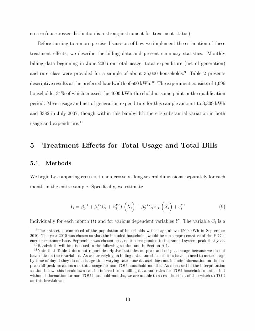
Before turning to a more precise discussion of how we implement the estimation of these

treatment effects, we describe the billing data and present summary statistics. Monthly

billing data beginning in June 2006 on total usage, total expenditure (net of generation)

and rate class were provided for a sample of about 35,000 households.9 Table 2 presents

descriptive results at the preferred bandwidth of 600 kWh.10 The experiment consists of 1,096

households, 34% of which crossed the 4000 kWh threshold at some point in the qualification

period. Mean usage and net-of-generation expenditure for this sample amount to 3,309 kWh

and $382 in July 2007, though within this bandwidth there is substantial variation in both

usage and expenditure.11

5 Treatment Effects for Total Usage and Total Bills

5.1 Methods

We begin by comparing crossers to non-crossers along several dimensions, separately for each

month in the entire sample. Specifically, we estimate

Yi = βY t0 + βY t

1 Ci + βY t2 f

(Xi

)+ βY t

3 Ci×f(Xi

)+ εY t

i (9)

individually for each month (t) and for various dependent variables Y . The variable Ci is a

9The dataset is comprised of the population of households with usage above 1500 kWh in September2010. The year 2010 was chosen so that the included households would be most representative of the EDC’scurrent customer base. September was chosen because it corresponded to the annual system peak that year.

10Bandwidth will be discussed in the following section and in Section A.1.11Note that Table 2 does not report descriptive statistics on peak and off-peak usage because we do not

have data on these variables. As we are relying on billing data, and since utilities have no need to meter usageby time of day if they do not charge time-varying rates, our dataset does not include information on the on-peak/off-peak breakdown of total usage for non-TOU household-months. As discussed in the interpretationsection below, this breakdown can be inferred from billing data and rates for TOU household-months; butwithout information for non-TOU household-months, we are unable to assess the effect of the switch to TOUon this breakdown.

13

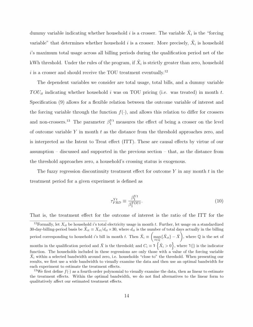
dummy variable indicating whether household i is a crosser. The variable Xi is the “forcing

variable” that determines whether household i is a crosser. More precisely, Xi is household

i’s maximum total usage across all billing periods during the qualification period net of the

kWh threshold. Under the rules of the program, if Xi is strictly greater than zero, household

i is a crosser and should receive the TOU treatment eventually.12

The dependent variables we consider are total usage, total bills, and a dummy variable

TOUit indicating whether household i was on TOU pricing (i.e. was treated) in month t.

Specification (9) allows for a flexible relation between the outcome variable of interest and

the forcing variable through the function f(·), and allows this relation to differ for crossers

and non-crossers.13 The parameter βY t1 measures the effect of being a crosser on the level

of outcome variable Y in month t as the distance from the threshold approaches zero, and

is interpreted as the Intent to Treat effect (ITT). These are causal effects by virtue of our

assumption – discussed and supported in the previous section – that, as the distance from

the threshold approaches zero, a household’s crossing status is exogenous.

The fuzzy regression discontinuity treatment effect for outcome Y in any month t in the

treatment period for a given experiment is defined as

τY tFRD ≡

βY t1

βTOUt1

. (10)

That is, the treatment effect for the outcome of interest is the ratio of the ITT for the

12Formally, let Xit be household i’s total electricity usage in month t. Further, let usage on a standardized30-day-billing-period basis be Xit ≡ Xit/dit×30, where dit is the number of total days actually in the billing

period corresponding to household i’s bill in month t. Then Xi ≡(

maxt∈Q{Xit} − X

), where Q is the set of

months in the qualification period and X is the threshold; and Ci ≡ 1

{Xi > 0

}, where 1{} is the indicator

function. The households included in these regressions are only those with a value of the forcing variableXi within a selected bandwidth around zero, i.e. households “close to” the threshold. When presenting ourresults, we first use a wide bandwidth to visually examine the data and then use an optimal bandwidth foreach experiment to estimate the treatment effects.

13We first define f(·) as a fourth-order polynomial to visually examine the data, then as linear to estimatethe treatment effects. Within the optimal bandwidth, we do not find alternatives to the linear form toqualitatively affect our estimated treatment effects.

14

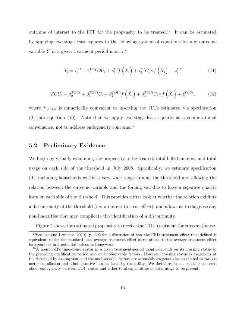
outcome of interest to the ITT for the propensity to be treated.14 It can be estimated

by applying two-stage least squares to the following system of equations for any outcome

variable Y in a given treatment-period month t:

Yi = τY t0 + τY t

1 TOUi + τY t2 f

(Xi

)+ τY t

3 Ci×f(Xi

)+ ωY t

i (11)

TOUi = βTOUt0 + βTOUt

1 Ci + βTOUt2 f

(Xi

)+ βTOUt

3 Ci×f(Xi

)+ εTOUt

i , (12)

where τ1,2SLS is numerically equivalent to inserting the ITTs estimated via specification

(9) into equation (10). Note that we apply two-stage least squares as a computational

convenience, not to address endogeneity concerns.15

5.2 Preliminary Evidence

We begin by visually examining the propensity to be treated, total billed amount, and total

usage on each side of the threshold in July 2008. Specifically, we estimate specification

(9), including households within a very wide range around the threshold and allowing the

relation between the outcome variable and the forcing variable to have a separate quartic

form on each side of the threshold. This provides a first look at whether the relation exhibits

a discontinuity at the threshold (i.e. an intent to treat effect), and allows us to diagnose any

non-linearities that may complicate the identification of a discontinuity.

Figure 2 shows the estimated propensity to receive the TOU treatment for crossers (house-

14See Lee and Lemieux (2010), p. 300 for a discussion of how the FRD treatment effect thus defined isequivalent, under the standard local average treatment effect assumptions, to the average treatment effectfor compliers in a potential outcomes framework.

15A household’s time-of-use status in a given treatment-period month depends on its crossing status inthe preceding qualification period and on unobservable factors. However, crossing status is exogenous atthe threshold by assumption, and the unobservable factors are ostensibly exogenous issues related to variousmeter installation and administrative hurdles faced by the utility. We therefore do not consider concernsabout endogeneity between TOU status and either total expenditure or total usage to be present.

15

holds that exceeded the 4000 kWh threshold) and non-crossers. Crossing the threshold is

clearly a strong predictor of having received the TOU treatment by July 2008, as illustrated

by the dramatic discontinuity at the threshold. However, it is not a perfect indicator, as

some non-crossers just to the left of the threshold – i.e. whose maximum 30-day usage during

the 4000kWh qualification period was very close but did not exceed the 4000kWh threshold

– have a small but positive propensity to be treated. Likewise, a few crossers still had not

received the TOU treatment by July 2008.

In Figures 3 and 4, we present the estimated total billed amount and usage, respectively,

on each side of the 4000 kWh threshold in July 2008. These graphs illustrate a discontinuity

both in expenditure and usage at the threshold, suggesting that a crosser had a substantially

lower electricity bill than a non-crosser at the threshold (by about $100). While the relation in

Figure 3 exhibits some non-linearity, particularly for very high levels of the forcing variable,

these figures provide fairly clear evidence that the difference in usage and expenditure is

indeed the result of a discontinuity.

5.3 Treatment Effects

Having provided visual evidence of the discontinuity, we now restrict specification (9) to be

linear in the forcing variable and in its interaction with crossing status, and include only

households within a narrower, optimally-chosen bandwidth of 600 kWh.16 We use this form

to identify ITTs for each dependent variable for several pre-qualification and qualification

months, as well as our treatment months of June - September 2008. To present the results

as compactly as possible, we graph time series of the set of estimated coefficients for each

16The method used to determine the optimal bandwidth is described in Section A.1. A larger bandwidthleads to more precise estimates of the discontinuity. However, it also means that households further awayfrom the threshold are being used to identify the discontinuity at the threshold, which can impart a bias;and this bias can be large if the relation is highly non-linear around the threshold. We choose an optimalbandwidth for a given experiment to apply uniformly for the estimation of all ITTs and treatment effects ineach month of the treatment period.

16

of the three dependent variables. For dependent variable Y , we graph βY t0 – the estimate of

outcome Y in month t for a non-crosser exactly at the threshold – and βY t0 + βY t

1 – the same

for a crosser exactly at the threshold – for every month, also indicating when the difference

between the two is statistically significant.

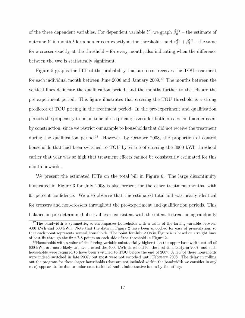
Figure 5 graphs the ITT of the probability that a crosser receives the TOU treatment

for each individual month between June 2006 and January 2009.17 The months between the

vertical lines delineate the qualification period, and the months further to the left are the

pre-experiment period. This figure illustrates that crossing the TOU threshold is a strong

predictor of TOU pricing in the treatment period. In the pre-experiment and qualification

periods the propensity to be on time-of-use pricing is zero for both crossers and non-crossers

by construction, since we restrict our sample to households that did not receive the treatment

during the qualification period.18 However, by October 2008, the proportion of control

households that had been switched to TOU by virtue of crossing the 3000 kWh threshold

earlier that year was so high that treatment effects cannot be consistently estimated for this

month onwards.

We present the estimated ITTs on the total bill in Figure 6. The large discontinuity

illustrated in Figure 3 for July 2008 is also present for the other treatment months, with

95 percent confidence. We also observe that the estimated total bill was nearly identical

for crossers and non-crossers throughout the pre-experiment and qualification periods. This

balance on pre-determined observables is consistent with the intent to treat being randomly

17The bandwidth is symmetric, so encompasses households with a value of the forcing variable between-600 kWh and 600 kWh. Note that the data in Figure 2 have been smoothed for ease of presentation, sothat each point represents several households. The point for July 2008 in Figure 5 is based on straight linesof best fit through the first 7-8 points on each side of the threshold in Figure 2.

18Households with a value of the forcing variable substantially higher than the upper bandwidth cut-off of600 kWh are more likely to have crossed the 4000 kWh threshold for the first time early in 2007, and suchhouseholds were required to have been switched to TOU before the end of 2007. A few of these householdswere indeed switched in late 2007, but most were not switched until February 2008. The delay in rollingout the program for these larger households (that are not included within the bandwidth we consider in anycase) appears to be due to unforeseen technical and administrative issues by the utility.

17

assigned at the threshold. It also suggests that the large ITTs observed in the summer

2008 are not spuriously caused by systematic difference in summer usage patterns between

crossers and non-crossers.

Figure 7 illustrates the estimated ITTs on total electricity usage over time. Total usage

was nearly identical between crossers and non-crossers throughout the pre-experiment and

qualification periods, providing evidence of another observable along which the two groups

are balanced. However, during the treatment periods, there is a significant difference in total

usage in June and July 2008, when crossers at the threshold exhibited lower usage than non-

crossers at the threshold. We also see some visual evidence of lower usage for TOU households

in August and September, though we cannot distinguish these from zero with confidence.

The absence of significant differences in total usage between crossers and non-crossers during

the pre-experiment and qualification periods indicates that the differences in June and July

2008 are not driven by pre-existing differences between the groups. It also indicates that

non-crossers were not purposely restraining their usage during the qualification period to

avoid crossing the threshold, which would violate the random assignment assumption.

Table 3 shows the treatment effects, adjusted for the propensity to be treated, on total

usage and total bills for each month in the treatment period. To give a better sense of

magnitudes, treatment effects are reported as a percentage of the level of the respective

variable for non-TOU households at the threshold.19 We find that the switch to TOU

pricing caused economically and statistically significant reductions in electricity expenditure

in all treatment months by at least 21% and as much as 30% in July. This is matched by

statistically significant declines in total electricity usage in June and July of 9-10%, and

noisy declines of 5 and 2 percent in August and September, respectively.

When interpreting the expenditure estimates, it seems natural that electricity expen-

19That is, each entry shows τY t1 /τY t

0 ×100 from a separate two-stage least squares application of equations(11)-(12). We discuss the bootstrap methods we employ to estimate the standard errors of these transformedcoefficient estimates in Section A.2

18

diture would decline or remain unchanged since customers on TOU faced lower peak and

off-peak rates compared to flat rate households. In contrast, basic intuition suggests that

demand for electricity should increase with a reduction in electricity prices; yet we find the

opposite to be true. We now investigate the revealed choice behavior more directly.

6 Interpretation

To assist us in digesting the empirical results, we turn to Figures 8 and 9, which provide a

simple visual way to evaluate the nature of consumer choice. These figures present graphs of

budget frontiers and revealed choices as implied by the empirical results described in Table

3. Each graph presents the consumption bundle chosen by TOU customers, as well as two

budget frontiers. These features of the choice setting are derived directly from prices and

estimates of behavior in treatment (TOU) and control (non-TOU) at the threshold. The

TOU consumption bundle is revealed arithmetically from the relationship between total

consumption (τ kWht0 + τ kWht

1 ) and the TOU tariff rates. Budget frontiers are determined by

the revealed consumption level at the threshold (from the application of the 2SLS estimation)

and relative prices.20

The first frontier is based on non-TOU rates and the level of expenditure of the non-

TOU household, and has a slope of -1 to reflect equality of peak and off-peak prices. This

frontier represents all combinations of on-peak and off-peak usage that sum to the estimated

non-TOU total usage at the threshold. Note that any point on the interior of this frontier

is unequivocally a drop in total consumption relative to the non-TOU bundle. The second,

analogous, frontier is based on TOU rates and the expenditure of the non-TOU household at

the threshold. Were expenditure for treated households to remain at the revealed non-TOU

20Algebraically, the budget frontiers are expressed by equations (5) and (6), with the values of actual ratesand revealed total expenditure inserted where appropriate. The imputation of the TOU consumption bundleis discussed in Section A.3. A technical issue involving an adjustment of calendar-month rates for billingcycles that is necessary for implementing this imputation is discussed in Section A.4.

19

level, their TOU bundle would reside on this second frontier. Each budget constraint is

presented for the months June to September 2008.

We present two different rate types – unbundled in Figure 8 and bundled in Figure 9

– to reflect differences in the TOU gradient between two customer types in our sample.

Unbundled rates are paid by customers who have elected to purchase electricity generation

from an “alternate supplier” (i.e. not from the regulated electricity distribution company).

During the period of analysis, all alternate supplier generation rates were time-invariant,21

implying that the entire TOU gradient was transmitted through the unbundled price for

these customers. On the other hand, bundled rates include generation charges that are paid

to the electricity distribution company. In our setting, these generation charges transmit an

additional peak/off-peak price gradient. As such, the choice setting is different for customers

who have elected to purchase generation from an alternate supplier than for those purchasing

exclusively from the regulated utility, so we present budget frontiers separately for each.

Recall that the TOU rates/non-TOU expenditure frontier represents the theoretical con-

sumption possibilities available to a household that is switched to TOU pricing and retains

the non-TOU level of electricity expenditure. This frontier describes the set of on-peak/off-

peak bundles from which a static utility maximizing household would choose if on-peak and

off-peak electricity were the only two goods consumed. The non-TOU bundle lies somewhere

on the interior line, and from these figures it is apparent that the chosen TOU bundle was

feasible under the non-TOU budget. Thus the original non-TOU bundle is revealed preferred

to the TOU bundle. Note that this is true irrespective of the presence of crossing of the

budget constraints (which we discuss below). In this simplified two-good setting, each graph

reveals an outcome in which treated consumer choices appear to violate the Weak Axiom of

Revealed Preference (WARP).

21A thorough search of alternate supplier rates by the authors in 2010 confirmed what our utility partnersasserted: time-varying generation rates were not offered by alternate suppliers until more recently.

20

A more realistic interpretation of the setting includes an outside consumption good in

addition to both electricity goods, as in the theoretical framework presented in the second

section. Here we will distinguish between instances in which the TOU frontier lies completely

above the non-TOU frontier and those in which the TOU and non-TOU budget constraints

cross. When we allow for the presence of an outside good, the possibility exists that an

electricity price change will induce substitution towards the outside good. In regions where

the TOU budget is on the exterior of the non-TOU budget constraint, the outside good has

become relatively more expensive in treatment. In these cases, a net reduction in electricity

consumption and increase in consumption of the outside alternative would imply that the

entire bundle of non-electricity household expenditures was a Giffen good. We consider this

to be an unsatisfactory explanation with which to reconcile the empirical findings.

In regions where the TOU budget is interior to the non-TOU budget (i.e. in the lower-

right region of graphs where the frontiers cross), the story becomes slightly more nuanced.

For households with non-TOU bundles in that region, the switch from flat rate to TOU

implies a decrease in the relative price of the outside good. In this case, a net decrease in

electricity consumption does not require the aggregate good to be a Giffen good. However,

the likelihood of a household’s chosen peak/off-peak bundle initiating on this region of the

non-TOU budget frontier is essentially zero. In months where we observe a cross in the

budget frontier, this crossing occurs at an extremely high peak/off-peak ratio. Appealing to

an external dataset on the peak-to-off-peak usage ratio for a random sample of customers, we

can examine the likelihood that the observed “crossing” ratio falls within the observed range

of ratios.22 With the exception of bundled rates for June, the crossing ratio is much higher

than any peak-to-off-peak ratio observed in the data. Even for a customer on a bundled rate

in June, the “crossing” ratio is in the 99th percentile of the observed distribution. We hence

22This load profile dataset comprises hourly usage data between January 2006 and October 2011 for arandom sample of households present for between 2 and 48 months. Figure 12 shows the peak-to-off-peakusage ratio by total usage from this dataset.

21

consider extreme preferences for on-peak electricity usage to be an unlikely explanation for

our results.

The abundance of evidence does not allow much scope for household choice behavior

to be consistent with static utility maximization. A two-good view leads immediately to

violations of WARP. When we allow for the consumption of an outside good, for static utility

maximization to hold, it must be that the composite bundle of non-electricity expenditures

is Giffen, or that the initial non-TOU bundle lay on a region of the budget frontier that is

inconsistent with observed data.

So where does this leave us? One might conjure several reasonable explanations to

rationalize the observed behavior. While we are not able and thus do not strive to test them

here, we consider this an important area of future research. We hope that a description of

some of these hypotheses will be helpful to readers.

One hypothesis allows for a dynamic consumer – one that is in a sense more sophisticated

than the static utility optimizer for which we test earlier. In our setting, the peak price did

eventually increase. A consumer correctly expecting this increase in future rates ought to

incorporate such expectations into the choice of durable goods investments.23 That is, if elec-

tricity is expected to become more expensive during peak hours of air conditioning demand,

a rational, forward-looking consumer will be willing to pay for a more energy-efficient air

conditioner today. Making such a choice would manifest in lower derived electricity demand

for electricity today, which is consistent with behavior in our setting.

Another potential hypothesis that could explain the observed outcome is that households

were not only responding to contemporaneous rates, but also engaging in what is becom-

ing known as “intermittent updating”. Under this hypothesis, consumers are attentive to

choices infrequently, and thus may exhibit behavior that resulted from optimization at some

previous time, but which does not correspond to utility maximization in each moment.24

23See Rapson (2013).24While we remain agnostic about mechanisms, support for the “intermittent updating” hypothesis resides

22

Intermittent updating may equivalently be thought of as a symptom of “rational inatten-

tion”, whereby consumers educate themselves about their energy consumption in response

to (new) incentives provided by the TOU rate structure.

Finally, there is a growing body of evidence on the importance of “behavioral” consid-

erations in this choice setting. Each treated household received a letter notifying them of

their new rate plan, and it is possible that receipt of the letter itself was responsible for the

observed treatment effect. There is some evidence from the literature that is consistent with

this explanation. For example, households that are informed that their usage is abnormally

high tend to engage in behavior that brings them closer to the norm (Allcott (2011)). Since

treated households in our setting have been told that they had “high” usage, this informa-

tion may have induced a response towards conforming to social norms, or perhaps towards

attempting to atone for or counteract this high usage.

7 Conclusion

This study exploits a natural experiment to document a setting in which households do

not respond to price incentives in the way that standard theory predicts. Despite growing

evidence that non-monetary and inter-temporal factors are important in a wide range of en-

vironments, there are few well-identified cases of this behavior in environmental economics.

Evaluating customer response to price incentives is a necessary step in understanding con-

sumer choice in this setting.

The randomized nature of assignment into TOU pricing that arises from the structure

and implementation of the program provides us with an empirical setting to evaluate con-

sumer behavior. Customers were automatically placed on the TOU rate after exceeding the

usage threshold, creating an appropriate setting in which to apply a regression discontinuity

in the fact that hundreds of households just below the threshold could have saved substantial amounts byvolunteering for TOU, but didn’t.

23

design. This differentiates our research design from most studies of time-varying electricity

pricing which rely on framed field experiments in which participants are aware of their par-

ticipation.25 Thus, our paper offers a novel estimate of how certain residential consumers

behave when exposed to TOU pricing.

The baseline model of consumer behavior employed in this paper is rooted in the tra-

ditional framework for modeling consumer electricity choice (Aigner and Poirier (1979),

Hausman, Kinnucan, and McFadden (1979) and Caves and Christensen (1980)). And while

this framework should serve as a starting point to frame consumer response to electricity

prices, we highlight that in some instances it may not describe customer behavior accurately.

In these cases, structural estimates based on the classic theoretical framework may lead to

misleading conclusions.

Admittedly, the households in our setting are very large, and not representative of the

“average” electricity user. On the other hand, the intensity of electricity use which they

exhibit makes them a particularly important target for energy conservation efforts. Questions

of external validity, though, are almost beside the point since what we observe in this setting

is potentially present in many other settings. An assertion that price incentives always work

can be disproven by the counter-example we have provided.

We must achieve a more thorough understanding of what drives behavior to inform

planners about how to effectively achieve climate change mitigation. If what we observe

here suggests that failure of the utility maximization assumption could arise more generally

in some settings, then market-based policies designed on the basis of this assumption may

fail to achieve the emissions target and/or fail to achieve a given reduction cost effectively.

On the other hand, if we knew the mechanism driving consumer behavior, this information

could be leveraged to effectively introduce price-based policies (for example, by coupling

25We refer here to the taxonomy of field experiments proposed by Harrison and List (2004). Wolak (2006)and Jessoe and Rapson (forthcoming) are examples of recent studies of the effect of time-varying pricingthat are based on framed field experiments.

24

prices with real-time feedback) or non-price interventions. Our findings suggest that there

may be a risk in adhering too ideologically to price interventions alone, in terms of missing

policy goals or achieving them only imperfectly or inefficiently.

References

Aigner, D., and D. Poirier (1979): “Electricity Demand and Consumption by Time-of-Use: A Survey,” Electric Power Research Institute Report, EA-1294.

Alberini, A., W. Gans, and D. Velez-Lopez (2011): “Residential Consumption ofGas and Electricity in the U.S.: The Role of Prices and Income,” Energy Economics, 33,870–881.

Allcott, H. (2011): “Social Norms and Energy Conservation,” Journal of Public Eco-nomics, 95, 820–842.

Benabou, R., and J. Tirole (2003): “Intrinsic and Extrinsic Motivation,” Review ofEconomic Studies, 70(3), 489–520.

Cameron, C., and P. Trivedi (2009): Microeconometrics Using Stata. Stata Press.

Caves, D. W., and L. R. Christensen (1980): “Econometric analysis of residentialtime-of-use electricity pricing experiments,” Journal of Econometrics, 14(3), 287–306.

Faruqui, A., and S. Sergici (2010): “Household Response to Dynamic Pricing of Elec-tricity: A Survey of the Experimental Evidence,” Journal of Regulatory Economics, 38,193–225.

Fell, H., S. Li, and A. Paul (2012): “A New Look at Residential Electricity DemandUsing Household Expenditure Data,” Working Paper.

Gilbert, B., and J. Graff-Zivin (2013): “Dynamic Salience with Intermittent Billing:Evidence from Smart Electricity Meters,” Working Paper.

Harding, M., and D. Rapson (2013): “Do Voluntary Carbon Offsets Induce EnergyRebound? A Conservationist’s Dilemma,” Working Paper.

Harrison, G., and J. List (2004): “Field Experiments,” Journal of Economic Literature,42(4), 1009–55.

Hausman, J., M. Kinnucan, and D. McFadden (1979): “A Two-Level ElectricityDemand Model: Evaluation of the Connecticut Time-of-Day Pricing Test,” Journal ofEconometrics, 10, 263–289.

25

Imbens, G., and K. Kalyanaraman (2012): “Optimal Bandwidth Choice for the Regres-sion Discontinuity Estimator,” Review of Economic Studies, 79, 933–59.

Ito, K. (forthcoming): “Do Consumers Respond to Marginal or Average Price? Evidencefrom Nonlinear Electricity Pricing,” American Economic Review.

Jacobsen, G., M. Kotchen, and M. Vandenbergh (2012): “The Behavioral Responseto Voluntary Provision of an Environmental Public Good: Evidence From ResidentialElectricity Demand,” European Economic Review, 56, 946–960.

Jessoe, K., and D. Rapson (forthcoming): “Knowledge is (Less) Power: ExperimentalEvidence from Residential Energy Use,” American Economic Review.

Kotchen, M., and M. Moore (2007): “Private Provision of Environmental Public Goods:Household Participation in Green-Electricity Programs,” Journal of Environmental Eco-nomics and Management, 53, 1–16.

Lee, D., and T. Lemieux (2010): “Regression Discontinuity Designs in Economics,” Jour-nal of Economic Literature, 48, 281–355.

Rapson, D. (2013): “Durable Goods and Long-Run Electricity Demand: Evidence fromAir Conditioner Purchase Behavior,” Working Paper.

Reiss, P., and M. White (2005): “Household Electricity Demand Revisited,” The Reviewof Economic Studies, 72, 853–883.

Simon, H. (1955): “A Behavioral Model of Rational Choice,” Quarterly Journal of Eco-nomics, 69(1), 99–118.

Wolak, F. (2006): “Residential Customer Response to Real-Time Pricing: The AnaheimCritical-Peak Pricing Experiment,” Working Paper.

26

Tables and Figures

Table 1: Electricity Rates, 2008, Cents per kWh

Non-TOU TOU

Headblock Tailblock On-Peak Off-Peak

unbundled

Jun. 7.9 11.8 11.4 7.6Jul. 8.6 12.6 12.0 8.1bundled

Jun. 20.1 24.1 26.2 18.9Jul. 20.6 24.6 26.5 19.2

Notes: Unbundled rates include distribution, transmission, and delivery charges plus fees only. Bundledrates also include the generation prices that were charged by the utility to those customers opting to keepthe utility as both distributor and supplier. About 55% of the customer base opted to pay generationprices charged by alternate suppliers; no alternate suppliers had TOU generation prices, so the unbundledrates represent the relative on-peak/off-peak all-inclusive rates faced by these customers, but not theabsolute level. The headblock is the first 500kWh of total usage in the billing month. The July ratesstayed in place through September.

Table 2: Summary Statistics, July of the Qualification Period

TotalUsage(kWh)

TotalBill ($)

Crossers(%) N

4000kWh Experiment (2007) 3,309 382 0.339 1,096[751] [91] [0.473]

Notes: Standard deviations are in square brackets. The households included for each experiment are thosewithin an optimally-chosen bandwidth around the threshold; see the text for details.

27

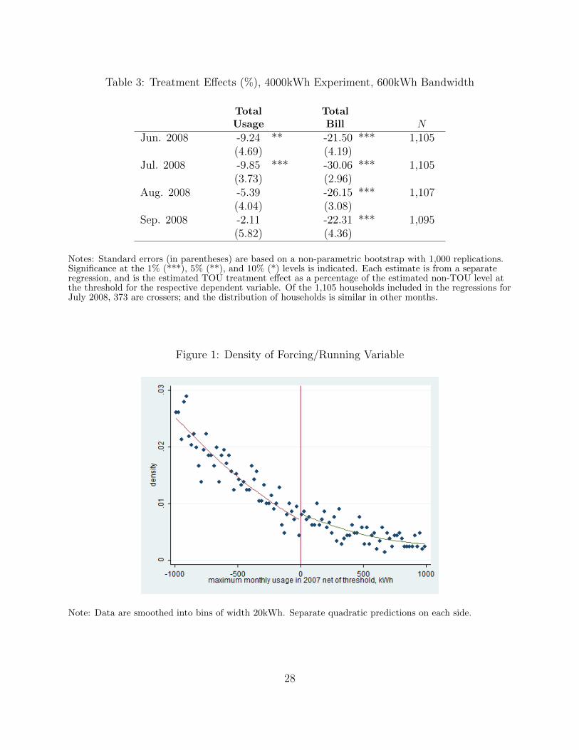
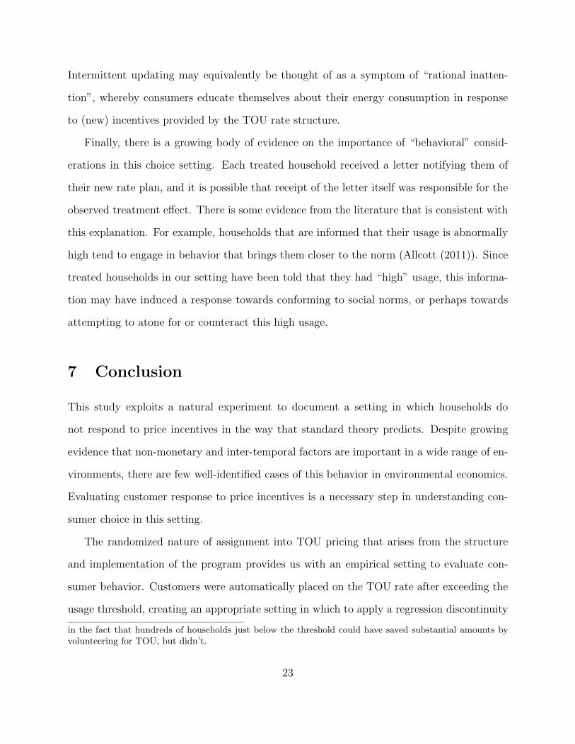
Table 3: Treatment Effects (%), 4000kWh Experiment, 600kWh Bandwidth

TotalUsage

TotalBill N

Jun. 2008 -9.24 ** -21.50 *** 1,105(4.69) (4.19)

Jul. 2008 -9.85 *** -30.06 *** 1,105(3.73) (2.96)

Aug. 2008 -5.39 -26.15 *** 1,107(4.04) (3.08)

Sep. 2008 -2.11 -22.31 *** 1,095(5.82) (4.36)

Notes: Standard errors (in parentheses) are based on a non-parametric bootstrap with 1,000 replications.Significance at the 1% (***), 5% (**), and 10% (*) levels is indicated. Each estimate is from a separateregression, and is the estimated TOU treatment effect as a percentage of the estimated non-TOU level atthe threshold for the respective dependent variable. Of the 1,105 households included in the regressions forJuly 2008, 373 are crossers; and the distribution of households is similar in other months.

Figure 1: Density of Forcing/Running Variable

Note: Data are smoothed into bins of width 20kWh. Separate quadratic predictions on each side.

28

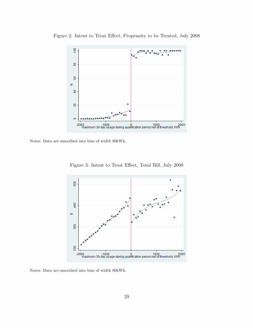
Figure 2: Intent to Treat Effect, Propensity to be Treated, July 2008

Notes: Data are smoothed into bins of width 80kWh.

Figure 3: Intent to Treat Effect, Total Bill, July 2008

Notes: Data are smoothed into bins of width 80kWh.

29

Figure 4: Intent to Treat Effect, Total Usage, July 2008

Notes: Data are smoothed into bins of width 80kWh.

Figure 5: Intent to Treat Effects, Propensity to be Treated, 4000kWh Experiment, 600kWhBandwidth

Notes: The qualification period is the set of months between the vertical lines.

30

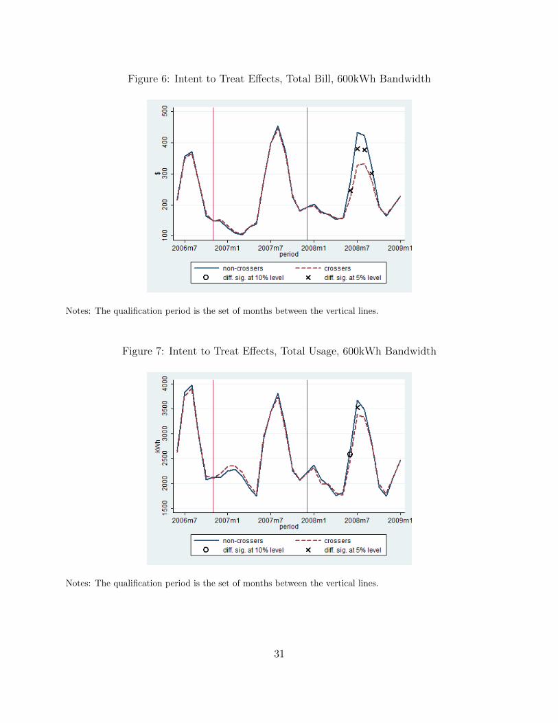
Figure 6: Intent to Treat Effects, Total Bill, 600kWh Bandwidth

Notes: The qualification period is the set of months between the vertical lines.

Figure 7: Intent to Treat Effects, Total Usage, 600kWh Bandwidth

Notes: The qualification period is the set of months between the vertical lines.

31

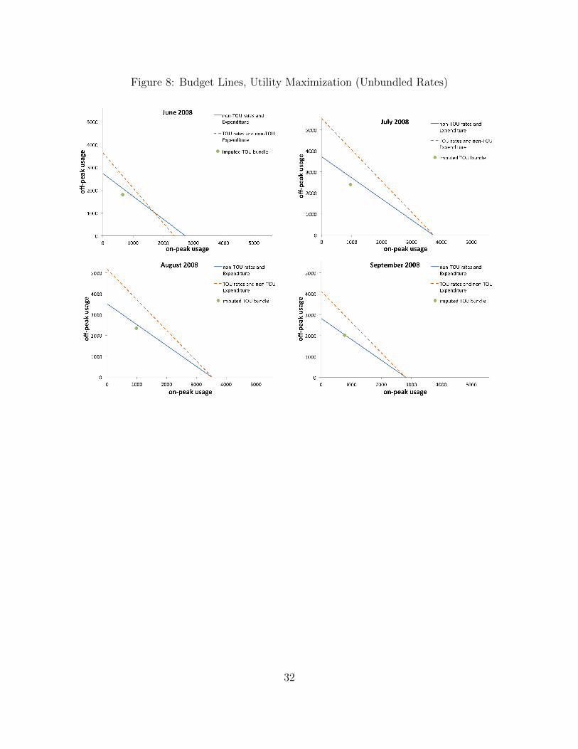
Figure 8: Budget Lines, Utility Maximization (Unbundled Rates)

32

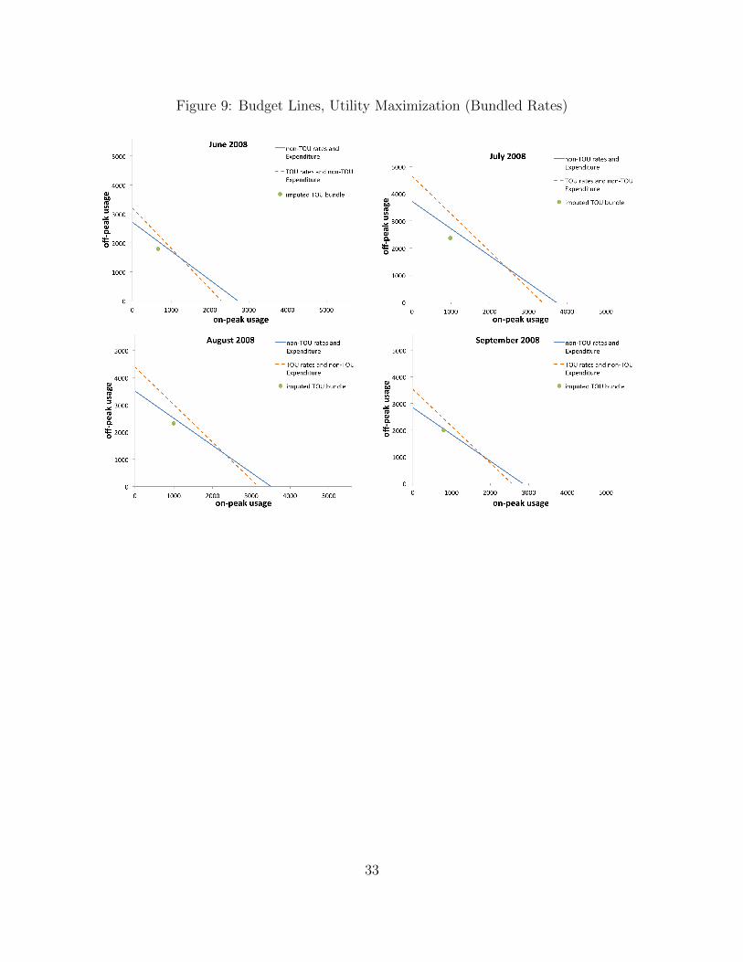
Figure 9: Budget Lines, Utility Maximization (Bundled Rates)

33

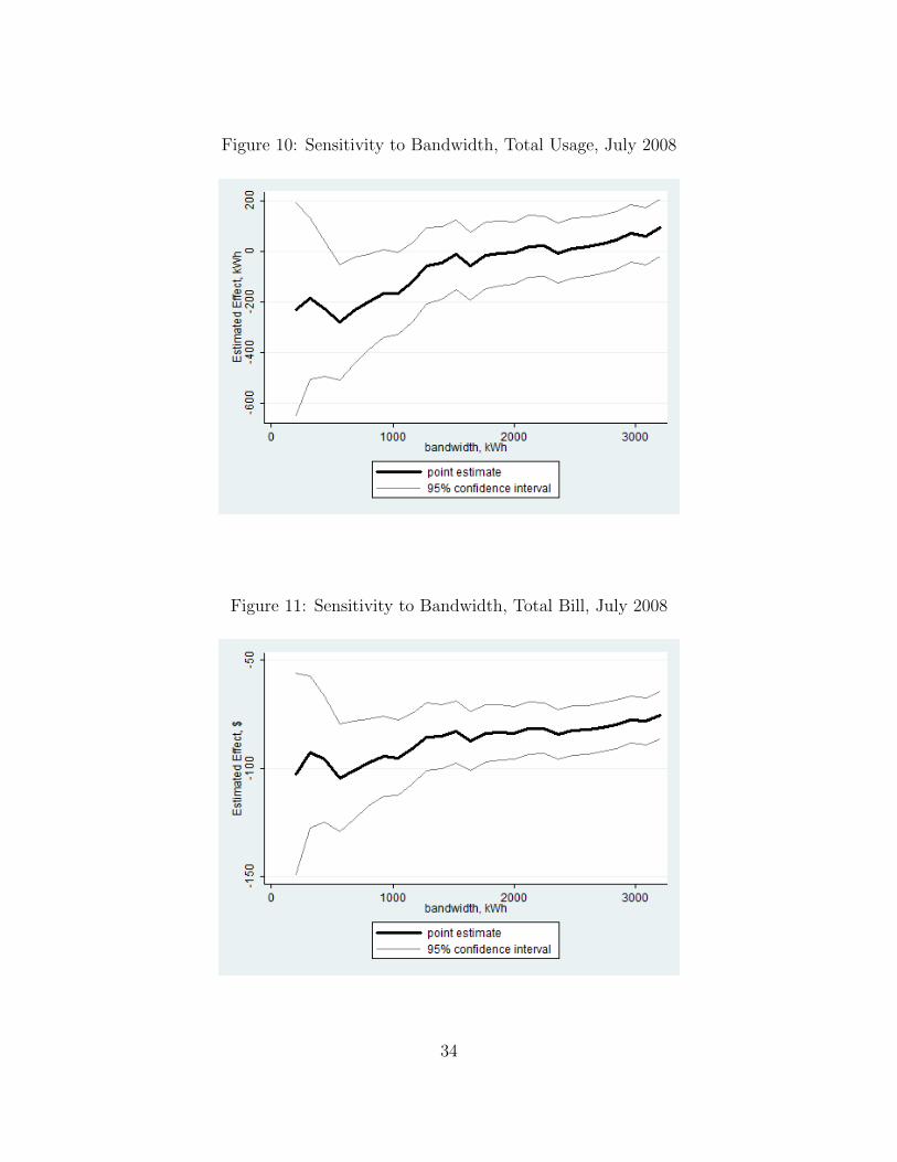
Figure 10: Sensitivity to Bandwidth, Total Usage, July 2008

Figure 11: Sensitivity to Bandwidth, Total Bill, July 2008

34

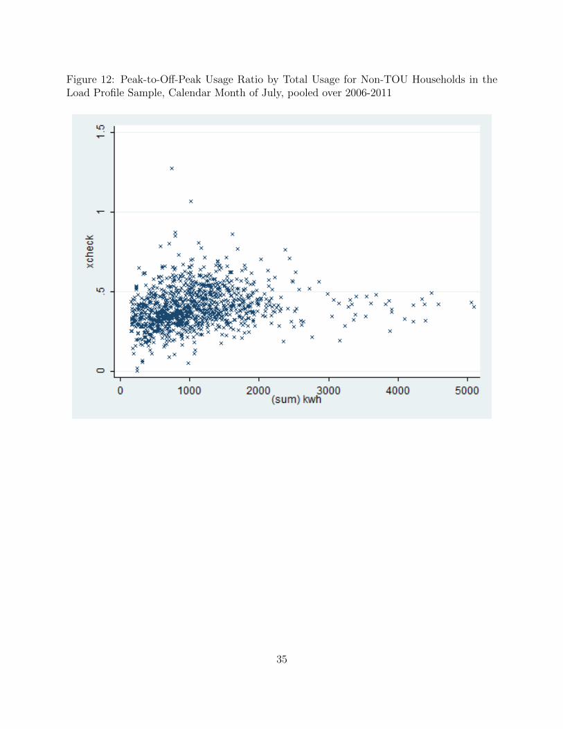
Figure 12: Peak-to-Off-Peak Usage Ratio by Total Usage for Non-TOU Households in theLoad Profile Sample, Calendar Month of July, pooled over 2006-2011

35

A Appendix

A.1 Bandwidth

The trade-off involved with increasing the bandwidth is as follows: on the positive side, the

precision of the estimate is improved; on the negative side, a bias is imparted on the estimate

of the effect at the threshold by including observations further away from the threshold. As

discussed by Lee and Lemieux (2010), when the relationship between the forcing variable

and the outcome variable is approximately linear on both sides of the threshold, the bias

concern becomes less prominent (and, therefore, the optimal bandwidth exercise less useful).

Lee and Lemieux (2010) suggest a plug-in rule-of-thumb bandwidth that we implement in

order to derive the optimal bandwidths used in the text and figures. Imbens and Kalyanara-

man (2012) provide a completely data-driven approach to selecting an optimal bandwidth,

which we have found to produce similar results. In either case, we wish to adopt a uniform

bandwidth for every month, dependent variable, and estimator (ITT or treatment effect).

To do so, we apply the two-stage rule-of-thumb procedure with a quartic form common to

each side of the threshold repeatedly for various treatment months and the ITT specification

with total usage and total expenditure as dependent variables. From the set of optimal

bandwidth estimates thus produced, we informally choose one in the lower range to apply

uniformly in the estimation of all ITTs and treatment effects.

Figures 10 and 11 show the ITT on total usage and the total bill in July 2008 for

the 4000kWh experiment, with 95% confidence bounds, for bandwidths ranging from 200

kWh to 3200 kWh. The graphs shows a rapid tightening of the confidence interval and

relative stability in the absolute magnitude of the point estimate up to a bandwidth of

about 1000kWh. For both usage and total bill, there is a steady decrease in the absolute

magnitude of the point estimate and moderate tightening of the confidence interval beyond

the 1000 kWh bandwidth. Correspondingly, as shown in Figures 3 and 4, beyond a value of

36

the forcing variable of about 1000 kWh to the right of the threshold, the relation with the

usage and bill outcome variables becomes quite non-linear, indicating, along with Figures 10

and 11, that bias is becoming a more prominent concern than precision.

A.2 Bootstrapped Standard Errors

We use nonparametric bootstrap methods to perform statistical inference on the treatment

effects for total usage and total bills, which are estimated in levels but reported as percent

changes. In this section, we describe the sampling method that we have used. In both

notation and procedure, what follows draws upon Cameron and Trivedi (2009).

Let wi denote the full time series of data for household i, wi = (Xi, Ei, TOUi, Ci, Xi)

(corresponding to the notation in equation 9, where Y referred generically to either total

usage (X), total expenditure (E), or the treatment indicator (TOU)). We draw a bootstrap

sample of size N by sampling w1, . . . , wN with replacement at the household level from

the subsample of the billing dataset corresponding to the optimal bandwidth restriction.

Denoting the bootstrap sample by w∗1, . . . , w∗N , we calculate an estimate, θ∗, of the vector

of parameters of interest, θ, and apply our desired transformation f(θ∗) to these parameter

estimates. We repeat this for a total of 1000 separate bootstrap samples. Given the 1000

bootstrap estimates, f(θ∗1), . . . , f(θ∗1000), we calculate the bootstrap estimate of the variance-

covariance matrix according to

VBoot(f(θ)) =1

999

1000∑b=1

(f(θ∗b )− f(θ∗)

)(f(θ∗b )− f(θ∗)

)′(13)

where f(θ∗) =∑1000

b=1 f(θ∗b )/1000.

37

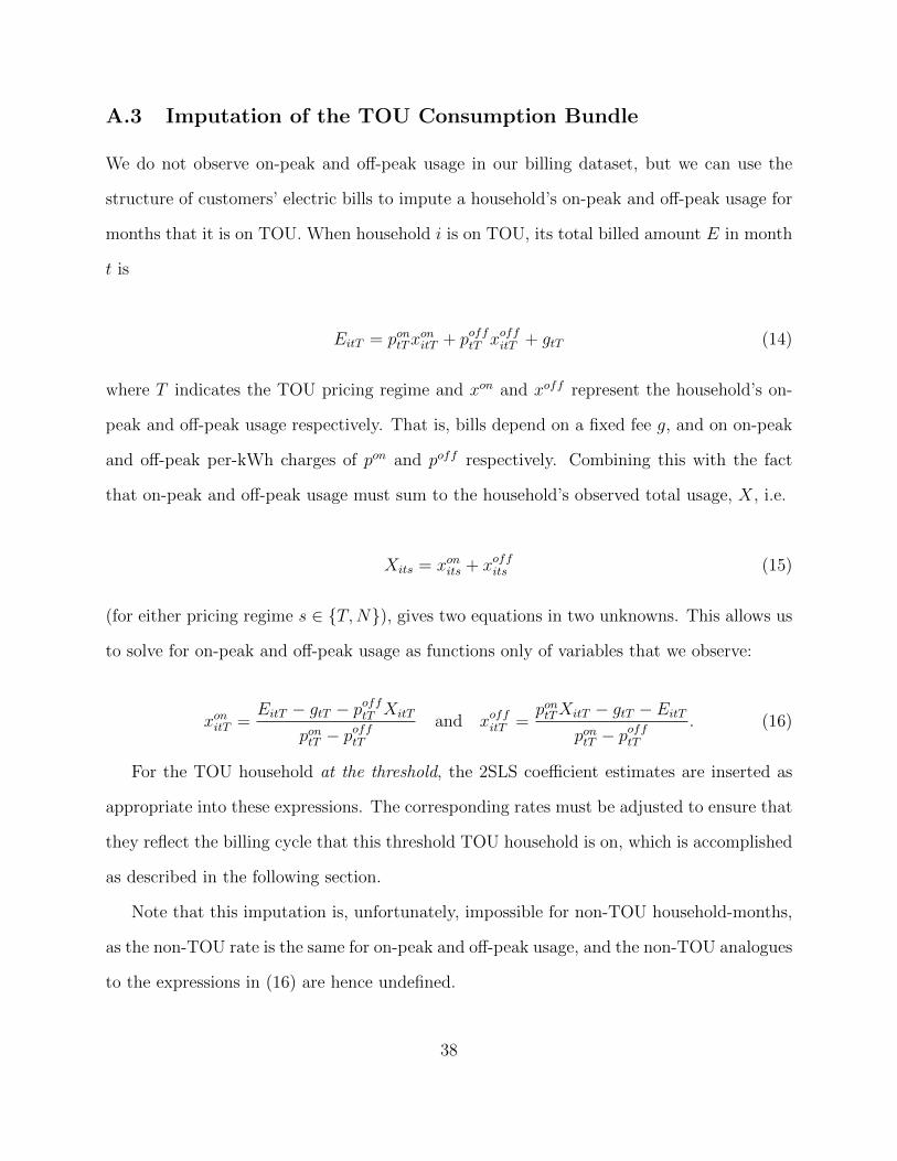
A.3 Imputation of the TOU Consumption Bundle

We do not observe on-peak and off-peak usage in our billing dataset, but we can use the

structure of customers’ electric bills to impute a household’s on-peak and off-peak usage for

months that it is on TOU. When household i is on TOU, its total billed amount E in month

t is

EitT = pontTxonitT + pofftT xoffitT + gtT (14)

where T indicates the TOU pricing regime and xon and xoff represent the household’s on-

peak and off-peak usage respectively. That is, bills depend on a fixed fee g, and on on-peak

and off-peak per-kWh charges of pon and poff respectively. Combining this with the fact

that on-peak and off-peak usage must sum to the household’s observed total usage, X, i.e.

Xits = xonits + xoffits (15)

(for either pricing regime s ∈ {T,N}), gives two equations in two unknowns. This allows us

to solve for on-peak and off-peak usage as functions only of variables that we observe:

xonitT =EitT − gtT − pofftT XitT

pontT − pofftT

and xoffitT =pontTXitT − gtT − EitT

pontT − pofftT

. (16)

For the TOU household at the threshold, the 2SLS coefficient estimates are inserted as

appropriate into these expressions. The corresponding rates must be adjusted to ensure that

they reflect the billing cycle that this threshold TOU household is on, which is accomplished

as described in the following section.

Note that this imputation is, unfortunately, impossible for non-TOU household-months,

as the non-TOU rate is the same for on-peak and off-peak usage, and the non-TOU analogues

to the expressions in (16) are hence undefined.

38

A.4 Billing Cycles

There were 17 distinct billing cycles for residential customers over the period covered by

our dataset. Each billing cycle corresponds to a given day of the month (which can change

by a couple of days in either direction depending on month and year, due to weekends and

holidays) on which the meter is read and the billing period for customers on that billing cycle

closes. For customers on billing cycle 1, the total usage and total bill data for “July 2008”,

for example, correspond to usage that mostly happened in the calendar month of June; on

the other hand, for customers on billing cycle 17, total usage and total bill data for “July

2008” correspond to usage that mostly happened in the calendar month of July. There is

thus heterogeneity in our billing data in what “July 2008” (and every other month) refers

to. This is relevant because we only have rate information on a calendar-month basis. So

the total bill in “July 2008” depends on a weighted average of the rates that were in place in

the calendar month of June and those that were in place in the calendar month of July, with

the appropriate weight depending on which billing cycle a household is on. We describe here

how we retrieve billing cycle weights by household-month, and how we apply the weights

thus retrieved to align variables observed on a calendar-month basis with variables observed

on a billing-month basis.

We reconstruct the total billed amount for all non-TOU household months based on the

observed rates, total usage, and the unknown weight; then solve for the weight that exactly

aligns the reconstructed total billed amount with the observed total billed amount for each

individual household-month. (We cannot do the same for TOU household-months because

we do not observe the on-peak/off-peak breakdown of total usage. We can also not perform

the calculation for months in which there was no rate change from the previous month.)

A few households chronically had weights outside the sensible 0-1 range in the months for

which weights could be calculated, and have been dropped completely from all analysis; a

few remaining households occasionally had a month with a nonsensical weight, in which case

39

it was just the single household-month observation that was dropped.

Finally, we calculate average billing cycle weights by billing cycle-month-year group over

all household-months we could calculate the initial weights for; fill in the missing month-

years (i.e. months across which there were no rate adjustments) with annual averages; then

apply the appropriate billing cycle-month-year average to every corresponding non-TOU and

TOU household-month. (We observe which billing cycle each household was on in September

2010, and know that households are supposed to always stay on the same billing cycle.)

We need to account for billing cycles in the imputation of on-peak and off-peak usage for

the TOU household at the threshold. We align billing-month estimates with calendar-month

rates by taking a weighted average of the latter across the relevant months. The weight we

use in the calculation must be the billing cycle weight for a TOU household at the threshold.

This is furnished by once more applying 2SLS estimation to equations (11)-(12), this time

with average billing cycle weights as the outcome variable of interest.

We estimate total expenditure based on bundled generation-inclusive rates in a similar

fashion. We first impute on-peak and off-peak usage levels for TOU household-months using

the method described in the previous section. We then align billing-month usage levels

with calendar-month bundled rates by individual household-month using average billing cycle

weights. Finally, we use the weighted rates and observed usage to estimate what the total

generation-inclusive billed amount would have been had the household had the utility as

supplier in addition to distributor. Expenditure levels at the threshold based on bundled

rates are then estimated via the usual application of 2SLS to equations (11)-(12), with these

constructed billed amounts as the dependent variable.

40