review quasinormal modes
DESCRIPTION
Review Quasinormal modes.Berti, Cardoso, StarinetsTRANSCRIPT

arX
iv:0
905.
2975
v2 [
gr-q
c] 2
9 Ju
l 200
9
TOPICAL REVIEW
Quasinormal modes of black holes and black branes
Emanuele Berti1,2, Vitor Cardoso1,3, Andrei O. Starinets4
1 Department of Physics and Astronomy, The University of Mississippi,University, MS 38677-1848, USA2 Theoretical Astrophysics 130-33, California Institute of Technology, Pasadena,CA 91125, USA3 Centro Multidisciplinar de Astrofısica - CENTRA, Departamento de Fısica,Instituto Superior Tecnico, Av. Rovisco Pais 1, 1049-001 Lisboa, Portugal4 Rudolf Peierls Centre for Theoretical Physics, Department of Physics,University of Oxford, 1 Keble Road, Oxford, OX1 3NP, United Kingdom
E-mail: [email protected], [email protected],
Abstract. Quasinormal modes are eigenmodes of dissipative systems. Pertur-bations of classical gravitational backgrounds involving black holes or branes nat-urally lead to quasinormal modes. The analysis and classification of the quasinor-mal spectra requires solving non-Hermitian eigenvalue problems for the associatedlinear differential equations. Within the recently developed gauge-gravity dual-ity, these modes serve as an important tool for determining the near-equilibriumproperties of strongly coupled quantum field theories, in particular their trans-port coefficients, such as viscosity, conductivity and diffusion constants. In as-trophysics, the detection of quasinormal modes in gravitational wave experimentswould allow precise measurements of the mass and spin of black holes as well asnew tests of general relativity. This review is meant as an introduction to thesubject, with a focus on the recent developments in the field.
PACS numbers: 04.70.-s, 04.30.Tv, 11.25.Tq, 11.10.Wx, 04.50.-h, 04.25.dg
Contents
1 Introduction 31.1 Milestones . . . . . . . . . . . . . . . . . . . . . . . . . . . . . . . . . 71.2 Notation and conventions . . . . . . . . . . . . . . . . . . . . . . . . . 10
2 A black hole perturbation theory primer 112.1 Perturbations of the Schwarzschild-anti-de Sitter geometry . . . . . . . 112.2 Higher-dimensional gravitational perturbations . . . . . . . . . . . . . 152.3 Weak fields in the Kerr background: the Teukolsky equation . . . . . . 15
3 Defining quasinormal modes 173.1 Quasinormal modes as an eigenvalue problem . . . . . . . . . . . . . . 173.2 Quasinormal modes as poles in the Green’s function . . . . . . . . . . 18

Quasinormal modes of black holes and black branes 2
4 Computing quasinormal modes 204.1 Exact solutions . . . . . . . . . . . . . . . . . . . . . . . . . . . . . . . 214.2 The WKB approximation . . . . . . . . . . . . . . . . . . . . . . . . . 254.3 Monodromy technique for highly-damped modes . . . . . . . . . . . . 274.4 Asymptotically anti-de Sitter black holes: a series solution . . . . . . . 284.5 Asymptotically anti-de Sitter black holes: the resonance method . . . 304.6 The continued fraction method . . . . . . . . . . . . . . . . . . . . . . 30
5 The spectrum of asymptotically flat black holes 315.1 Schwarzschild . . . . . . . . . . . . . . . . . . . . . . . . . . . . . . . . 315.2 Reissner-Nordstrom . . . . . . . . . . . . . . . . . . . . . . . . . . . . 355.3 Kerr . . . . . . . . . . . . . . . . . . . . . . . . . . . . . . . . . . . . . 385.4 Kerr-Newman . . . . . . . . . . . . . . . . . . . . . . . . . . . . . . . . 415.5 Higher dimensional Schwarzschild-Tangherlini black holes . . . . . . . 41
6 The spectrum of asymptotically anti-de Sitter black holes 436.1 Schwarzschild anti-de Sitter black holes . . . . . . . . . . . . . . . . . 436.2 Reissner-Nordstrom and Kerr anti-de Sitter black holes . . . . . . . . 486.3 Toroidal, cylindrical and plane-symmetric anti-de Sitter black holes . . 49
7 The spectrum of asymptotically de Sitter and other black holes 497.1 Asymptotically de Sitter black holes . . . . . . . . . . . . . . . . . . . 497.2 Black holes in higher-derivative gravity . . . . . . . . . . . . . . . . . . 507.3 Braneworlds . . . . . . . . . . . . . . . . . . . . . . . . . . . . . . . . . 517.4 Black holes interacting with matter . . . . . . . . . . . . . . . . . . . . 51
8 Quasinormal modes and the gauge-gravity duality 518.1 The duality . . . . . . . . . . . . . . . . . . . . . . . . . . . . . . . . . 518.2 Dual quasinormal frequencies as poles of the retarded correlators . . . 538.3 The hydrodynamic limit . . . . . . . . . . . . . . . . . . . . . . . . . . 558.4 Universality of the shear mode and other developments . . . . . . . . . 58
9 Quasinormal modes of astrophysical black holes 599.1 Physical parameters affecting ringdown detectability . . . . . . . . . . 609.2 Excitation of black hole ringdown in astrophysical settings . . . . . . . 629.3 Astrophysical black holes: mass and spin estimates . . . . . . . . . . . 689.4 Detection range for Earth-based and space-based detectors . . . . . . 759.5 Event rates . . . . . . . . . . . . . . . . . . . . . . . . . . . . . . . . . 779.6 Inferring black hole mass and spin from ringdown measurements . . . 799.7 Tests of the no-hair theorem . . . . . . . . . . . . . . . . . . . . . . . . 829.8 Matching inspiral and ringdown: problems and applications . . . . . . 84
10 Other recent developments 8510.1 Black hole area quantization: in search of a log . . . . . . . . . . . . . 8510.2 Thermodynamics and phase transitions in black hole systems . . . . . 8610.3 Non-linear quasinormal modes . . . . . . . . . . . . . . . . . . . . . . 8710.4 Quasinormal modes and analogue black holes . . . . . . . . . . . . . . 87
11 Outlook 89

Quasinormal modes of black holes and black branes 3
Appendix A 90
Appendix B 94
Appendix C 95
Appendix D 96
1. Introduction
“The mathematical perfectness of the black holes of Nature is [...] revealed at everylevel by some strangeness in the proportion in conformity of the parts to one anotherand to the whole.” S. Chandrasekhar, “The Mathematical Theory of Black Holes”
Characteristic modes of vibration are persistent in everything around us. Theymake up the familiar sound of various musical instruments but they are alsoan important research topic in such diverse areas as seismology, asteroseismology,molecular structure and spectroscopy, atmospheric science and civil engineering. Allof these disciplines are concerned with the structure and composition of the vibratingobject, and with how this information is encoded in its characteristic vibration modes:to use a famous phrase, the goal of studying characteristic modes is to “hear theshape of a drum” [1]. This is a review on the characteristic oscillations of blackholes (BHs) and black branes (BHs with plane-symmetric horizon), called quasinormalmodes (QNMs). We will survey the theory behind them, the information they carryabout the properties of these fascinating objects, and their connections with otherbranches of physics.
Unlike most idealized macroscopic physical systems, perturbed BH spacetimesare intrinsically dissipative due to the presence of an event horizon. This precludesa standard normal-mode analysis because the system is not time-symmetric and theassociated boundary value problem is non-Hermitian. In general, QNMs have complexfrequencies, the imaginary part being associated with the decay timescale of theperturbation. The corresponding eigenfunctions are usually not normalizable, and,in general, they do not form a complete set (see Refs. [2, 3] for more extensivediscussions). Almost any real-world physical system is dissipative, so one mightreasonably expect QNMs to be ubiquitous in physics. QNMs are indeed useful inthe treatment of many dissipative systems, e.g. in the context of atmospheric scienceand leaky resonant cavities.
Two excellent reviews on BH QNMs [4, 5] were written in 1999. However, muchhas happened in the last decade that is not covered by these reviews. The recentdevelopments have brought BH oscillations under the spotlight again. We refer, inparticular, to the role of QNMs in gravitational wave astronomy and their applicationsin the gauge-gravity duality. This work will focus on a critical review of the newdevelopments, providing our own perspective on the most important and active linesof research in the field.
After a general introduction to QNMs in the framework of BH perturbationtheory, we will describe methods to obtain QNMs numerically, as well as someimportant analytic solutions for special spacetimes. Then we will review the QNMspectrum of BHs in asymptotically flat spacetimes, asymptotically (anti-)de Sitter(henceforth AdS or dS) spacetimes and other spacetimes of interest. After this generaloverview we will discuss what we regard as the most active areas in QNM research.

Quasinormal modes of black holes and black branes 4
Schematically, we will group recent developments in QNM research into three mainbranches:(i) AdS/CFT and holography. In 1997-98, a powerful new technique known as theAdS/CFT correspondence or, more generally, the gauge-string duality was discoveredand rapidly developed [6]. The new method (often referred to as holographiccorrespondence) provides an effective description of a non-perturbative, stronglycoupled regime of certain gauge theories in terms of higher-dimensional classicalgravity. In particular, equilibrium and non-equilibrium properties of strongly coupledthermal gauge theories are related to the physics of higher-dimensional BHs andblack branes and their fluctuations. Quasinormal spectra of the dual gravitationalbackgrounds give the location (in momentum space) of the poles of the retardedcorrelators in the gauge theory, supplying important information about the theory’squasiparticle spectra and transport (kinetic) coefficients. Studies of QNMs in theholographic context became a standard tool in considering the near-equilibriumbehavior of gauge theory plasmas with a dual gravity description. Among otherthings, they revealed the existence of a universality of the particular gravitationalfrequency of generic black branes (related on the gauge theory side to the universalityof the viscosity-entropy ratio in the regime of infinitely strong coupling), as well asintriguing connections between the dynamics of BH horizons and hydrodynamics [7].The duality also offers a new perspective on notoriously difficult problems, such asthe BH information loss paradox, the nature of BH singularities and quantum gravity.Holographic approaches to these problems often involve QNMs. This active area ofresearch is reviewed in Section 8.(ii) QNMs of astrophysical black holes and gravitational wave astronomy.The beginning of LIGO’s first science run (S1) in 2002 and the achievement of designsensitivity in 2005 marked the beginning of an era in science where BHs and othercompact objects should play a prominent observational role. While electromagneticobservations are already providing us with strong evidence of the astrophysical realityof BHs [8], gravitational wave observations will incontrovertibly show if these compactobjects are indeed rotating (Kerr) BHs, as predicted by Einstein’s theory of gravity.BH QNMs can be used to infer their mass and angular momentum [9] and to testthe no-hair theorem of general relativity [10, 11]. Dedicated ringdown searches ininterferometric gravitational wave detector data are ongoing [12, 13]. The progress onthe experimental side was accompanied by a breakthrough in the numerical simulationof gravitational wave sources. Long-term stable numerical evolutions of BH binarieshave been achieved after 4 decades of efforts [14, 15, 16], confirming that ringdownplays an important role in the dynamics of the merged system. These developmentsare reviewed in Section 9.(iii) Other developments. In 1998, Hod suggested that highly-damped QNMscould bridge the gap between classical and quantum gravity [17]. The following yearswitnessed a rush to compute and understand this family of highly damped modes.The interest in this subject has by now faded substantially but, at the very least,Hod’s proposal has contributed to a deeper analytical and numerical understandingof QNM frequencies in many different spacetimes, and it has highlighted certaingeneral properties characterizing some classes of BH solutions. These ideas and otherrecent developments (including a proposed connection between QNMs and BH phasetransitions, the QNMs of analogue BHs, the stability of naked singularities and itsrelation with the so-called algebraically special modes) are reviewed in Section 10.
The present work is mostly intended to make the reader familiar with the new

Quasinormal modes of black holes and black branes 5
developments by summarizing the vast (and sometimes confusing) bibliography on thesubject. We tried to keep the review as self-contained as possible, while avoiding toduplicate (as far as possible to preserve logical consistency) material that is treatedmore extensively in other reviews on the topic, such as Refs. [4, 5, 2, 18]. A detailedunderstanding of BH QNMs and their applications requires some specialized technicalbackground. QNM research has recently expanded to encompass a very wide range oftopics: a partial list includes analogue gravity, alternative theories of gravity, higher-dimensional spacetimes, applications to numerical relativity simulations, explorationsof the gauge-gravity duality, the stability analysis of naked singularities and ringdownsearches in LIGO. Because of space limitations we cannot discuss all of this material indetail, and we refer the reader to other reviews. Topics that are treated in more detailelsewhere include: (1) a general overview of gravitational radiation [19, 20] and itsmultipolar decomposition [21]; (2) BH perturbation theory [22, 23, 24, 25, 26, 27]; (3)the issue of quantifying QNM excitation in different physical scenarios (see e.g. [28] foran introduction pre-dating the numerical relativity breakthroughs of 2005, and [29] fora more updated overview of the field); (4) tests of general relativity and of the no-hairtheorem that either do not make use of ringdown [30], or do not resort to gravitationalwave observations at all [31, 32, 33]; (5) BH solutions in higher dimensions [34]; (6)many aspects of the gauge-gravity duality [7, 35, 36, 37, 38]. The reviews listedabove provide more in-depth looks at different aspects of QNM research, but we triedto provide concise introductions to all of these topics while (hopefully) keeping thepresentation clear and accessible.
Chandrasekhar’s fascination with the mathematics of BHs was due to theirsimplicity. BHs in four-dimensional, asymptotically flat spacetime must belong to theKerr-Newman family, which is fully specified by only three parameters: mass, chargeand angular momentum (see e.g. Ref. [39], or Carter’s contribution to Ref. [40]).One expresses this by saying that BHs have no hair (or more precisely, that theyhave three hairs). A consequence of the no-hair theorem is that all perturbationsin the vicinities of a BH must decay to one and the same final state, i.e. that allhairs (except three) must be lost. Perturbative and numerical calculations show thatthe hair loss proceeds, dynamically, via quasinormal ringing. The gravitational wavesignal from a perturbed BH can in general be divided in three parts: (i) A promptresponse at early times, that depends strongly on the initial conditions and is thecounterpart to light-cone propagation; (ii) An exponentially decaying “ringdown”phase at intermediate times, where QNMs dominate the signal, which depends entirelyon the final BH’s parameters; (iii) A late-time tail, usually a power-law falloff of thefield [41]. Mathematically, each of these stages arises from different contributions tothe relevant Green’s function (see Section 3.2). QNM frequencies depend only on theBH’s parameters, while their amplitudes depend on the source exciting the oscillations.
Numerical and analytical analysis of processes involving BHs confirm theseexpectations. QNMs were observed for the first time in numerical simulations of thescattering of Gaussian wavepackets by Schwarzschild BHs in 1970, soon after the BHconcept itself was introduced and popularized by John Wheeler. Vishveshwara [42]noticed that the waveform at late times consists of a damped sinusoid, with ringingfrequency almost independent of the Gaussian’s parameters. Ringdown was observedagain in the linearized approximation to the problem of a test mass falling from infinityinto a Schwarzschild BH [43]. By now, decades of experience have shown that anyevent involving BH dynamics is likely to end in this same characteristic way: thegravitational wave amplitude will die off as a superposition of damped sinusoids.

Quasinormal modes of black holes and black branes 6
0 100 200 300
(t-r)/M-0.08
-0.06
-0.04
-0.02
0.00
0.02
0.04
0.06
0.08
Re(
Mrψ
22)
Quasi-circular BH merger
-30 -20 -10 0 10 20 30 40 50 60
(t-r)/M-0.20
-0.15
-0.10
-0.05
0.00
0.05
0.10
0.15
0.20
Mrψ
20
Ultrarelativistic head-on
-100 -80 -60 -40 -20 0 20 40 60 80 100
(t-r)/M-0.40
-0.20
0.00
0.20
0.40
(M/µ
)ψ2
Infalling particle
0 2 4 6 8 10
(t-r) (ms)-4×10
-5
-3×10⁻⁵
-2×10⁻⁵
-1×10⁻⁵
0
1×10⁻⁵
2×10⁻⁵
3×10⁻⁵
4×10⁻⁵
rψ22
/M
Neutron star merger
Figure 1. Four different physical processes leading to substantial quasinormalringing (see text for details). With the exception of the infalling-particle case(where M is the BH mass, µ the particle’s mass and ψ2 the Zerilli wavefunction),ψ22 is the l = m = 2 multipolar component of the Weyl scalar Ψ4, M denotesthe total mass of the system and r the extraction radius (see e.g. Ref. [44]).
Figure 1 shows four different processes involving BH dynamics. In all of them,quasinormal ringing is clearly visible. The upper-left panel (adapted from Ref. [44])is the signal from two equal-mass BHs initially on quasi-circular orbits, inspirallingtowards each other due to the energy loss induced by gravitational wave emission,merging and forming a single final BH [14]. The upper-right panel of Fig. 1 showsgravitational waveforms from numerical simulations of two equal-mass BHs, collidinghead-on with v/c = 0.94 in the center-of-mass frame: as the center-of-mass energygrows (i.e., as the speed of the colliding BHs tends to the speed of light) the waveformis more and more strongly ringdown-dominated [45]. The bottom-left panel showsthe gravitational waveform (or more precisely, the dominant, l = 2 multipole ofthe Zerilli function) produced by a test particle of mass µ falling from rest into aSchwarzschild BH [43]: the shape of the initial precursor depends on the details ofthe infall, but the subsequent burst of radiation and the final ringdown are universalfeatures. The bottom-right panel (reproduced from Ref. [46]) shows the waves emittedby two massive neutron stars (NSs) with a polytropic equation of state, inspirallingand eventually collapsing to form a single BH.
QNM frequencies for gravitational perturbations of Schwarzschild and Kerr BHs

Quasinormal modes of black holes and black branes 7
have been computed by many authors. Rather than listing numerical tables of well-known results, we have set up a web page providing tabulated values of the frequenciesand fitting coefficients for the QNMs that are most relevant in gravitational waveastronomy [47]. On this web page, we also provide Mathematica notebooks to computeQNMs of Kerr and asymptotically AdS BHs [47].
1.1. Milestones
QNM research has a fifty-year-long history. We find it helpful to provide the readerwith a “roadmap” in the form of a chronological list of papers that, in our opinion,have been instrumental to shape the evolution of the field. Our summary is necessarilybiased and incomplete, and we apologize in advance for the inevitable omissions. Amore complete set of references can be found in the rest of this review.• 1957 – Regge and Wheeler [48] analyze a special class of gravitational perturbationsof the Schwarzschild geometry. This effectively marks the birth of BH perturbationtheory a decade before the birth of the BH concept itself. The “one-way membrane”nature of the horizon is not yet fully understood, and the boundary conditions of theproblem are not under control.• 1961 – Newman and Penrose [49] develop a formalism to study gravitational radiationusing spin coefficients.• 1963 – Kerr [50] discovers the mathematical solution of Einstein’s field equationsdescribing rotating BHs. In the same year, Schmidt identifies the first quasar (“quasi-stellar radio source”). Quasars (compact objects with luminosity ∼ 1012 that of oursun, located at cosmological distance [51]) are now believed to be supermassive BHs(SMBHs), described by the Kerr solution.• 1964 – The UHURU orbiting X-ray observatory makes the first surveys of the X-raysky discovering over 300 X-ray “stars”, most of which turn out to be due to matteraccreting onto compact objects. One of these X-ray sources, Cygnus X-1, is soonaccepted as the first plausible stellar-mass BH candidate (see e.g. [52]).• 1967 – Wheeler [53, 54] coins the term “black hole” (see the April 2009 issue ofPhysics Today, and Ref. [55] for a fascinating, first-person historical account).• 1970 – Zerilli [56, 57] extends the Regge-Wheeler analysis to general perturbationsof a Schwarzschild BH. He shows that the perturbation equations can be reduced to apair of Schrodinger-like equations, and applies the formalism to study the gravitationalradiation emitted by infalling test particles.• 1970 – Vishveshwara [42] studies numerically the scattering of gravitational wavesby a Schwarzschild BH: at late times the waveform consists of damped sinusoids (nowcalled “ringdown waves”).• 1971 – Press [58] identifies ringdown waves as the free oscillation modes of the BH.• 1971 – Davis et al. [43] carry out the first quantitative calculation of gravitationalradiation emission within BH perturbation theory, considering a particle fallingradially into a Schwarzschild BH. Quasinormal ringing is excited when the particlecrosses the maximum of the potential barrier of the Zerilli equation, which is locatedat r ≃ 3M (i.e., close to the unstable circular orbit corresponding to the “light ring”).• 1972 – Goebel [59] points out that the characteristic modes of BHs are essentiallygravitational waves in spiral orbits close to the light ring.• 1973 – Teukolsky [60] decouples and separates the equations for perturbations inthe Kerr geometry using the Newman-Penrose formalism [49].• 1974 – Moncrief [61] introduces a gauge-invariant perturbation formalism.

Quasinormal modes of black holes and black branes 8
• 1975 – Chandrasekhar and Detweiler [62] compute numerically some weakly dampedcharacteristic frequencies. They prove that the Regge-Wheeler and Zerilli potentialshave the same spectra.• 1978 – Cunningham, Price and Moncrief [63, 64, 65] study radiation from relativisticstars collapsing to BHs using perturbative methods. QNM ringing is excited.• 1979 – Gerlach and Sengupta give a comprehensive and elegant mathematicalfoundation for gauge-invariant perturbation theory [66, 67].• 1983 – Chandrasekhar’s monograph [22] summarizes the state of the art in BHperturbation theory, elucidating connections between different formalisms.• 1983 – York [68] attempts to relate the QNM spectrum to Hawking radiation. Toour knowledge, this is the first attempt to connect the (purely classical) QNMs withquantum gravity.• 1983 – Mashhoon [69] suggests to use WKB techniques to compute QNMs. Ferrariand Mashhoon [70] analytically compute QNMs using their connection with boundstates of the inverted BH effective potentials.• 1985 – Stark and Piran [71] extract gravitational waves from a simulation of rotatingcollapse to a BH in numerical relativity. QNM excitation is observed, as confirmed bymore recent work [72].• 1985 – Confirming the validity of Goebel’s arguments [59], Mashhoon [73] regardsQNMs as waves orbiting around the unstable photon orbit and slowly leaking out, andestimates analytically some QNM frequencies in Kerr-Newman backgrounds.• 1985 – Schutz and Will [74] develop a WKB approach to compute BH QNMs.• 1985 – Leaver [75, 76, 77] provides the most accurate method to date to computeBH QNMs using continued fraction representations of the relevant wavefunctions, anddiscusses their excitation using Green’s function techniques.• 1986 – McClintock and Remillard [78] show that the X-ray nova A0620-00 containsa compact object of mass almost certainly larger than 3M⊙, paving the way for theidentification of many more stellar-mass BH candidates.• 1989 – Echeverria [9] estimates the accuracy with which one can estimate themass and angular momentum of a BH from QNM observations. The formalism islater improved by Finn [79] and substantially refined in Ref. [10], where ringdown-based tests of the no-hair theorem of general relativity are shown to be possible. AnAppendix of Ref. [10] provides QNM tables to be used in data analysis and in theinterpretation of numerical simulations; these data are now available online [47].• 1992 – Nollert and Schmidt [80] use Laplace transforms to compute QNMs. Fromanet al. [81] first introduce phase-integral techniques in the context of BH physics.• 1993 – Anninos et al. [82] first succeed in simulating the head-on collision of twoBHs, and observe QNM ringing of the final BH.• 1993 – Bachelot and Motet-Bachelot [83] show that a potential with compact supportdoes not cause power-law tails in the evolution of Cauchy data. Subsequently Chinget al. [84, 41] generalize this result to potentials falling off faster than exponentially.• 1996 – Gleiser et al. [85] extend the perturbative formalism to second order anduse it to estimate radiation from colliding BHs employing the so-called “close limit”approximation, quantifying the limits of validity of linear perturbation theory [86].• 1997 – Maldacena [6] formulates the AdS/CFT (Anti-de Sitter/Conformal FieldTheory) duality conjecture. Shortly afterward, the papers by Gubser, Klebanov,Polyakov [87] and Witten [88] establish a concrete quantitative recipe for the duality.The AdS/CFT era begins.

Quasinormal modes of black holes and black branes 9
• 1998 – The AdS/CFT correspondence is generalized to non-conformal theories in avariety of approaches (see [35] for a review). The terms “gauge-string duality”, “gauge-gravity duality” and “holography” appear, referring to these generalized settings.• 1998 – Flanagan and Hughes [89] show that, under reasonable assumptions anddepending on the mass range, the signal-to-noise ratio for ringdown waves is potentiallylarger than the signal-to-noise ratio for inspiral waves in both Earth-based detectors(such as LIGO) and planned space-based detectors (such as LISA).• 1998 – Hod [17] uses earlier numerical results by Nollert [90] to conjecture thatthe real part of highly-damped QNMs is equal to T ln 3 (T being the Hawkingtemperature), a conjecture later proven by Motl [91] using the continued fractionmethod. Hod also proposes a connection between QNMs and Bekenstein’s ideas onBH area quantization.• 1999 – Creighton [12] describes a search technique for ringdown waveforms in LIGO.• 1999 – Two reviews on QNMs appear: Quasinormal modes of stars and black holes,by Kokkotas and Schmidt [4] and Nollert’s Quasinormal modes: the characteristic“sound” of black holes and neutron stars [5].• 1999 – Horowitz and Hubeny [92] compute QNMs of BHs in AdS backgrounds ofvarious dimensions and relate them to relaxation times in the dual CFTs.• 2000 – Shibata and Uryu [93] perform the first general relativistic simulation of themerger of two neutron stars. More recent simulations confirm that ringdown is excitedwhen the merger leads to BH formation [46].• 2001 – Birmingham, Sachs and Solodukhin [94] point out that QNM frequencies ofthe (2 + 1)-dimensional Banados-Teitelboim-Zanelli (BTZ) BH [95] coincide with thepoles of the retarded correlation function in the dual (1 + 1)-dimensional CFT.• 2002 – Baker, Campanelli and Lousto [96] complete the “Lazarus” program to“resurrect” early, unstable numerical simulations of BH binaries and extend thembeyond merger using BH perturbation theory.• 2002 – Dreyer [97] proposes to resolve an ambiguity in Loop Quantum Gravity usingthe highly damped QNMs studied by Hod [17].• 2002 – Son and Starinets [98] formulate a recipe for computing real-time correlationfunctions in the gauge-gravity duality. They use the recipe to prove that, in thegauge-gravity duality, QNM spectra correspond to poles of the retarded correlationfunctions.• 2002 – QNMs of black branes are computed [99]. The lowest QNM frequencies ofblack branes in the appropriate conserved charges channels are naturally interpretedas hydrodynamic modes of the dual theory [100].• 2003 – Motl and Neitzke [101] use a monodromy technique (similar to the phaseintegral approaches of Ref. [81]) to compute analytically highly damped BH QNMs.• 2003 – In a series of papers [102, 103, 104], Kodama and Ishibashi extend the Regge-Wheeler-Zerilli formalism to higher dimensions.• 2003 – In one of the rare works on probing quantum aspects of gravity withgauge theory in the context of the gauge-gravity duality (usually, the correspondenceis used the other way around), Fidkowski et al. [105] study singularities of BHsby investigating the spacelike geodesics that join the boundaries of the Penrosediagram. The complexified geodesics’ properties yield the large-mass QNM frequenciespreviously found for these BHs. This work is further advanced in Ref. [106] andsubsequent publications.• 2004 – Following Motl and Neitzke [101], Natario and Schiappa analytically computeand classify asymptotic QNM frequencies for d-dimensional BHs [107].
Quasinormal modes of black holes and black branes 10
• 2005 – The LIGO detector reaches design sensitivity [108].• 2005 – Pretorius [14] achieves the first long-term stable numerical evolution of a BHbinary. Soon afterwards, other groups independently succeed in evolving merging BHbinaries using different techniques [15, 16]. The waveforms indicate that ringdowncontributes a substantial amount to the radiated energy.• 2005 – Kovtun and Starinets [109] extend the QNM technique in the gauge-gravityduality to vector and gravitational perturbations using gauge-invariant variables forblack brane fluctuations. A classification of the fluctuations corresponding to polesof the stress-energy tensor and current correlators in a dual theory in arbitrarydimension is given. These methods and their subsequent development and applicationin [110, 111, 112, 113] become a standard approach in computing transport propertiesof strongly coupled theories from dual gravity.• 2006–2008 – An analytic computation of the lowest QNM frequency in the shearmode gravitational channel of a generic black brane [114] reveals universality, related tothe universality of the shear viscosity to entropy density ratio in dual gauge theories.This and further developments [115, 116] also point to a significance of the QNMspectrum in the context of the BH membrane paradigm (for a recent review of themembrane paradigm approach, see [117]).• 2008–2009 – QNM spectra are computed in applications of the gauge-gravity dualityto condensed matter theory [37, 38].
1.2. Notation and conventions
Unless otherwise and explicitly stated, we use geometrized units where G = c = 1, sothat energy and time have units of length. We also adopt the (− + ++) conventionfor the metric. For reference, the following is a list of symbols that are used oftenthroughout the text.
d Total number of spacetime dimensions (we always consider one timelikeand d− 1 spatial dimensions).
L Curvature radius of (A)dS spacetime, related to the negativecosmological constant Λ in the Einstein equations (Gµν + Λgµν = 0)through L2 = ∓(d− 2)(d− 1)/(2Λ). The − sign is for AdS, + for dS.
M Mass of the BH spacetime.a Kerr rotation parameter: a = J/M ∈ [0,M ].r+ Radius of the BH’s event horizon in the chosen coordinates.ω Fourier transform variable. The time dependence of any field is ∼ e−iωt.
For stable spacetimes, Im(ω) < 0. Also useful is w ≡ ω/2πT .ωR, ωI Real and imaginary part of the QNM frequencies.s Spin of the field.l Integer angular number, related to the eigenvalue Alm = l(l+ d− 3)
of scalar spherical harmonics in d dimensions.n Overtone number, an integer labeling the QNMs by increasing |Im(ω)|.
We conventionally start counting from a “fundamental mode” with n = 0.

Quasinormal modes of black holes and black branes 11
2. A black hole perturbation theory primer
Within general relativity (and various extensions thereof involving higher-derivativegravity), QNMs naturally appear in the analysis of linear perturbations of fixedgravitational backgrounds. The perturbations obey linear second-order differentialequations, whose symmetry properties are dictated by the symmetries of thebackground. In most cases, these symmetries allow one to separate variables withan appropriate choice of coordinates reducing the system to a set of linear ordinarydifferential equations (ODEs) or a single ODE. The ODEs are supplemented byboundary conditions, usually imposed at the BH’s horizon and at spatial infinity.QNMs are the eigenmodes of this system of equations. The precise choice ofthe boundary conditions is physically motivated, but it is clear that the presenceof the horizon, acting for classical fields as a one-sided membrane, is of crucialimportance: it makes the boundary value problem non-hermitian and the associatedeigenvalues complex. The methods used to reduce the problem to a single ODEdepend on the metric under consideration; some of them are discussed and comparedin Chandrasekhar’s book [22]. Given the progress in the field in recent years andthe vast literature on the subject, we will not attempt to describe these techniques indetail. As a simple example illustrating the main extensions of the formalism describedin [22] we discuss field perturbations in d-dimensional, non-rotating geometries. Forthe interested reader, Sections 5, 6 and 7 provide references on other backgroundgeometries.
2.1. Perturbations of the Schwarzschild-anti-de Sitter geometry
Consider the Einstein-Hilbert gravitational action for a d−dimensional spacetime withcosmological constant Λ:
S =1
16πG
∫
ddx√−g (R− 2Λ) +
∫
ddx√−gLm , (1)
where Lm is the Lagrangian representing a generic contribution of the “matter fields”(scalar, Maxwell, p−form, Dirac and so on) coupled to gravity. The specific form ofLm depends on the particular theory. The Einstein equations read
Gµν + Λgµν = 8πGTµν , (2)
where Tµν is the stress-energy tensor associated with Lm. Eq. (2) should besupplemented by the equations of motion for the matter fields. Together with Eq. (2),they form a complicated system of non-linear partial differential equations describingthe evolution of all fields including the metric. A particular solution of this systemforms a set of background fields gBG
µν ,ΦBG, where Φ is a cumulative notation for all
matter fields present. By writing gµν = gBGµν + hµν , Φ = ΦBG + φ, and linearizing the
full system of equations with respect to the perturbations hµν and φ, we obtain a setof linear differential equations satisfied by the perturbations.
Maximally symmetric vacuum (TBGµν = 0) solutions to the field equations are
Minkowski, de Sitter (dS) and anti-de Sitter (AdS) spacetimes, depending on thevalue of the cosmological constant (zero, positive or negative, respectively). Genericsolutions of Eq. (2) are asymptotically flat, dS or AdS. We will be mostly interestedin asymptotically flat or AdS spacetimes. AdS spacetimes of various dimension ariseas a natural groundstate of supergravity theories and as the near-horizon geometry

Quasinormal modes of black holes and black branes 12
of extremal BHs and p-branes in string theory, and therefore they play an importantrole in the AdS/CFT correspondence [35, 118, 119, 120, 121].
BHs in asymptotically AdS spacetimes form a class of solutions interestingfrom a theoretical point of view and central for the gauge-gravity duality at finitetemperature. Their relation to dual field theories is discussed in Section 8. In additionto the simplest Schwarzschild-AdS (SAdS) BH, one finds BHs with toroidal, cylindricalor planar topology [122, 123, 124, 125, 126, 127] as well as the Kerr-Newman-AdS family [128]. The standard BH perturbation theory [22] is easily extended toasymptotically AdS spacetimes [102, 129, 130, 131]. For illustration we consider thenon-rotating, uncharged d-dimensional SAdS (or SAdSd) BH with line element
ds2 = −fdt2 + f−1dr2 + r2dΩ2d−2 , (3)
where f(r) = 1 + r2/L2 − rd−30 /rd−3, dΩ2
d−2 is the metric of the (d − 2)-sphere,and the AdS curvature radius squared L2 is related to the cosmological constant byL2 = −(d − 2)(d − 1)/2Λ. The parameter r0 is proportional to the mass M of thespacetime: M = (d − 2)Ad−2r
d−30 /16π, where Ad−2 = 2π(d−1)/2/Γ[(d− 1)/2]. The
well-known Schwarzschild geometry corresponds to L→ ∞.
Scalar field perturbations Let us focus, for a start, on scalar perturbations in vacuum.The action for a complex scalar field with a conformal coupling is given by Sm ≡∫
ddx√−gLm, where
Lm = − (∂µΦ)†∂µΦ − d− 2
4(d− 1)γ RΦ†Φ −m2Φ†Φ . (4)
For γ = 1, m = 0 the action is invariant under the conformal transformationsgµν → Ω2gµν ,Φ → Ω1−d/2Φ, and for γ = 0, m = 0 one recovers the usual minimallycoupled massless scalar. The equations of motion satisfied by the fields gµν and(massless) Φ are
∇µ∇µΦ =d− 2
4(d− 1)γRΦ , Gµν + Λ gµν = 8πGTµν , (5)
where Tµν is quadratic in Φ. Considering perturbations of the fields, gµν = gBGµν +hµν
and Φ = ΦBG + φ with ΦBG = 0, we observe that the linearized equations of motionfor hµν and φ decouple, and thus the metric fluctuations hµν can be consistently setto zero. The background metric satisfies GBG
µν + ΛgBGµν = 0. We choose gBG
µν to be theSAdSd metric (3). The scalar fluctuation satisfies the equation
1√−gBG
∂µ
(
√−gBG gµνBG∂νφ
)
=d(d− 2)γ
4L2φ . (6)
The time-independence and the spherical symmetry of the metric imply thedecomposition
φ(t, r, θ ) =∑
lm
e−iωt Ψs=0(r)
r(d−2)/2Ylm(θ) , (7)
where Ylm(θ) denotes the d−dimensional scalar spherical harmonics, satisfying∆Ωd−2
Ylm = −l(l + d − 3)Ylm, with ∆Ωd−2the Laplace-Beltrami operator, and the
“s = 0” label indicates the spin of the field. Here and in the rest of this paper,for notational simplicity, we usually omit the integral over frequency in the Fourier

Quasinormal modes of black holes and black branes 13
transform. Substituting the decomposition into Eq. (6) we get a radial wave equationfor Ψs=0(r):
f2 d2Ψs=0
dr2+ ff ′dΨs=0
dr+(
ω2 − Vs=0
)
Ψs=0 = 0 . (8)
We will see shortly that perturbations with other spins satisfy similar equations. Inthe particular case of s = 0, the radial potential Vs is given by
Vs=0 = f
[
l(l+ d− 3)
r2+d− 2
4
(
(d− 4)f
r2+
2f ′
r+dγ
L2
)]
. (9)
Finally, if we define a “tortoise” coordinate r∗ by the relation dr∗/dr = 1/f , Eq. (8)can be written in the form of a Schrodinger equation with the potential Vs
d2Ψs
dr2∗+(
ω2 − Vs
)
Ψs = 0 . (10)
Notice that the tortoise coordinate r∗ → −∞ at the horizon (i.e. as r → r+), but itsbehavior at infinity is strongly dependent on the cosmological constant: r∗ → +∞ forasymptotically-flat spacetimes, and r∗ → constant for the SAdSd geometry.
Electromagnetic, gravitational and half-integer spin perturbations Equations forlinearized Maxwell field perturbations in curved spacetimes can be obtained along thelines of the scalar field example above. To separate the angular dependence we nowneed vector spherical harmonics [5, 132, 133]. In d = 4, electromagnetic perturbationscan be completely characterized by the wave equation (10) with the potential
V d=4s=1 = f
[
l(l+ 1)
r2
]
. (11)
A comprehensive treatment of the four-dimensional case can be found in Ref. [132]for the Schwarzschild spacetime, and in Ref. [130] for the SAdS geometry. Higher-dimensional perturbations are discussed in Ref. [134].
The classification of gravitational perturbations hµν(x) on a fixed backgroundgBG
µν (x) is more complicated. We focus on the SAdS4 geometry. After a decompositionin tensorial spherical harmonics, the perturbations fall into two distinct classes: odd(Regge-Wheeler or vector-type) and even (Zerilli or scalar-type), with parities equalto (−1)l+1 and (−1)l, respectively [27, 21, 57, 135]. In the Regge-Wheeler gauge[4, 5, 27, 48, 136], the perturbations are written as hµν = e−iωthµν , where for oddparity
hµν =
0 0 0 h0(r)0 0 0 h1(r)0 0 0 0
h0(r) h1(r) 0 0
(
sin θ∂
∂θ
)
Yl0(θ) , (12)
whereas for even parity
hµν =
H0(r)f H1(r) 0 0H1(r) H2(r)/f 0 0
0 0 r2K(r) 00 0 0 r2K(r) sin2 θ
Yl0(θ) . (13)
The angular dependence of the perturbations is dictated by the structure of tensorialspherical harmonics [27, 21, 57, 135]. Inserting this decomposition into Einstein’s

Quasinormal modes of black holes and black branes 14
equations one gets ten coupled second-order differential equations that fully describethe perturbations: three equations for the odd radial variables, and seven for theeven variables. The odd perturbations can be combined in a single Regge-Wheeler orvector-type gravitational variable Ψ−
s=2, and the even perturbations can likewise becombined in a single Zerilli or scalar-type gravitational wavefunction Ψ+
s=2. The Regge-Wheeler and Zerilli functions (Ψ−
s=2 and Ψ+s=2, respectively) satisfy the Schrodinger-
like equation (10) with the potentials
V −s=2 = f(r)
[
l(l + 1)
r2− 6M
r3
]
(14)
and
V +s=2 =
2f(r)
r3
9M3 + 3λ2Mr2 + λ2 (1 + λ) r3 + 9M2(
λr + r3
L2
)
(3M + λr)2 . (15)
The parameters h0 and h1 of the vector-type perturbation are related to Ψ−s=2 by
Ψ−s=2 =
f(r)
rh1(r) , h0 =
i
ω
d
dr∗
(
rΨ−s=2
)
. (16)
For the scalar-type gravitational perturbation, the functions H1 and K can beexpressed through Ψ+
s=2 via
K =6M2 + λ (1 + λ) r2 + 3M
(
λr − r3
L2
)
r2 (3M + λr)Ψ+
s=2 +dΨ+
s=2
dr∗, (17)
H1 =iω(
3M2 + 3λMr − λr2 + 3M r3
L2
)
r (3M + λr) f(r)Ψ+
s=2 −iωr
f(r)
dΨ+s=2
dr∗, (18)
where λ ≡ (l − 1)(l + 2)/2, and H0 is then obtained from the algebraic relation[
(l − 1)(l + 2) +6M
r
]
H0 +
[
il(l+ 1)
ω r2(M + r3/L2) − 2iω r
]
H1
−[
(l − 1)(l + 2) + rf ′ − 4ω2r2 + r2f ′2
2f
]
K = 0 . (19)
A complete discussion of Regge-Wheeler or vector-type gravitational perturbationsof the four-dimensional Schwarzschild geometry can be found in the original papersby Regge and Wheeler [48] as well as in Ref. [137], where some typos in theoriginal work are corrected. For Zerilli or scalar-type gravitational perturbations, thefundamental reference is Zerilli’s work [56, 57]; typos are corrected in Appendix A ofRef. [138]. An elegant, gauge-invariant decomposition of gravitational perturbations ofthe Schwarzschild geometry is described by Moncrief [61] (see also [66, 67, 139, 140]).These papers are reviewed by Nollert [5] and Nagar and Rezzolla [27]. For analternative treatment, see Chandrasekhar’s book [22]. Chandrasekhar’s book andpapers [141, 142] use a different notation, exploring mathematical aspects of therelations between different gravitational perturbations (see Appendix A). Extensionsto the SAdS4 geometry can be found in Ref. [130], while the general d−dimensionalcase has been explored in a series of papers by Kodama and Ishibashi [102, 103, 104].
The case of Dirac fields seems to have been discussed first by Brill and Wheeler[143], with important extensions of the formalism by Page [144], Unruh [145] andChandrasekhar [22]. For the treatment of Rarita-Schwinger fields, see [146].
Quasinormal modes of black holes and black branes 15
To summarize this Section: in four-dimensional Schwarzschild or SAdSbackgrounds, scalar (m = 0, γ = 0, s = 0), electromagnetic (s = ±1) and Regge-Wheeler or vector-type gravitational (s = 2) perturbations, can be described by themaster equation (10) with the potential
Vs = f
[
l(l+ 1)
r2+ (1 − s2)
(
2M
r3+
4 − s2
2L2
)]
. (20)
The potentials for the scalar-type gravitational perturbations and half-integer spinperturbations have forms different from (20), see for instance Refs. [102, 147].However, the vector-type (Regge-Wheeler) and scalar-type (Zerilli) potentials have theremarkable property of being isospectral, i.e. they possess the same QNM spectrum.The origin of this isospectrality, first discovered by Chandrasekhar [22], is reviewed inAppendix A.
2.2. Higher-dimensional gravitational perturbations
The literature on gravitational perturbations can be quite confusing. Namingconventions were already unclear in 1970, so much so that Zerilli decided to listequivalent terminologies referring to odd and even tensor spherical harmonics (cf.Table II of Ref. [57]). The situation got even worse since then. Chandrasekhar’sbook, which is the most complete reference in the field, established a differentterminology: “odd” (Regge-Wheeler) perturbations were called “axial” and describedby a master variable Ψ−, while “even” (Zerilli) perturbations were renamed “polar”and described by a master variable Ψ+. In recent years, Kodama and Ishibashi[102, 103, 104] extended the gauge-invariant perturbation framework to higher-dimensional, non-rotating BHs. In higher dimensions three master variables arenecessary to completely describe the perturbations [102]. Two of them (the vector-type gravitational perturbations and the scalar-type gravitational perturbations) reduceto the Regge-Wheeler and Zerilli master variables in d = 4. Kodama and Ishibashirefer to the third type of perturbations, which have no four-dimensional analogue,as tensor-type gravitational perturbations. In this review we will usually adopt theKodama-Ishibashi terminology.
2.3. Weak fields in the Kerr background: the Teukolsky equation
In four-dimensional asymptotically flat spacetimes, the most general vacuum BHsolution of Einstein’s equations is the Kerr metric. In the standard Boyer-Linquistcoordinates, the metric depends on two parameters: the mass M and spin J = aM .The spacetime has a Cauchy horizon at r = r− = M−
√M2 − a2 and an event horizon
at r = r+ = M +√M2 − a2. The separation of variables for a minimally coupled
scalar field in the Kerr background was first reported by Brill et al. [148].Teukolsky [60, 149] showed that if one works directly in terms of curvature
invariants, the perturbation equations decouple and separate for all Petrov type-Dspacetimes. He derived a master perturbation equation governing fields of generalspin, including the most interesting gravitational perturbations (see [22, 150] forreviews). Teukolsky’s approach is based on the Newman-Penrose [49] formalism. Inthis formalism one introduces a tetrad of null vectors l ,n ,m ,m∗ at each point inspacetime, onto which all tensors are projected. The Newman-Penrose equations arerelations linking the tetrad vectors, the spin coefficients, the Weyl tensor, the Riccitensor and the scalar curvature [49]. The most relevant perturbation variables, which
Quasinormal modes of black holes and black branes 16
both vanish in the background spacetime, are the Weyl scalars Ψ0 and Ψ4, obtainedby contracting the Weyl tensor Cµνλσ [151] on the tetrad legs (roughly speaking, thesequantities describe ingoing and outgoing gravitational radiation):
Ψ0 = − C1313 = −Cµνλσ lµmν lλmσ , (21)
Ψ4 = − C2424 = −Cµνλσnµm∗νnλm∗σ . (22)
Two analogous quantities Φ0 and Φ2 describe electromagnetic perturbations:
Φ0 = Fµν lµmν , Φ2 = Fµνm
∗µnν . (23)
By Fourier-transforming a spin-s field ψ(t , r , θ , φ) and expanding it in spin-weightedspheroidal harmonics as follows:
ψ(t , r , θ , φ) =1
2π
∫
e−iωt∞∑
l=|s|
l∑
m=−l
eimφsSlm(θ)Rlm(r)dω , (24)
Teukolsky finds separated ODEs for sSlm and Rlm [60, 149]:[
∂
∂u(1 − u2)
∂
∂u
]
sSlm
+
[
a2ω2u2 − 2aωsu+ s+ sAlm − (m+ su)2
1 − u2
]
sSlm = 0 ,
∆∂2rRlm + (s+ 1)(2r − 2M)∂rRlm + V Rlm = 0 . (25)
Here u ≡ cos θ, ∆ = (r − r−)(r − r+) and
V = 2isωr− a2ω2 − sAlm +1
∆
[
(r2 + a2)2ω2 − 4Mamωr + a2m2
+ is(
am(2r − 2M) − 2Mω(r2 − a2))
]
. (26)
The solutions to the angular equation (25) are known in the literature as spin-weighted spheroidal harmonics: sSlm = sSlm(aω , θ , φ). For aω = 0 the spin-weighted spheroidal harmonics reduce to spin-weighted spherical harmonics sYlm(θ , φ)[152]. In this case the angular separation constants sAlm are known analytically:
sAlm(a = 0) = l(l+1)−s(s+1). The determination of the angular separation constantin more general cases is a non-trivial problem (see [153] and references therein).
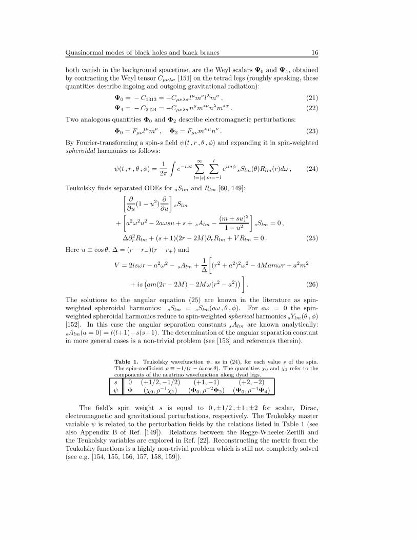
Table 1. Teukolsky wavefunction ψ, as in (24), for each value s of the spin.The spin-coefficient ρ ≡ −1/(r − ia cos θ). The quantities χ0 and χ1 refer to thecomponents of the neutrino wavefunction along dyad legs.
s 0 (+1/2,−1/2) (+1,−1) (+2,−2)ψ Φ (χ0, ρ
−1χ1) (Φ0, ρ−2Φ2) (Ψ0, ρ
−4Ψ4)
The field’s spin weight s is equal to 0 ,±1/2 ,±1 ,±2 for scalar, Dirac,electromagnetic and gravitational perturbations, respectively. The Teukolsky mastervariable ψ is related to the perturbation fields by the relations listed in Table 1 (seealso Appendix B of Ref. [149]). Relations between the Regge-Wheeler-Zerilli andthe Teukolsky variables are explored in Ref. [22]. Reconstructing the metric from theTeukolsky functions is a highly non-trivial problem which is still not completely solved(see e.g. [154, 155, 156, 157, 158, 159]).

Quasinormal modes of black holes and black branes 17
3. Defining quasinormal modes
3.1. Quasinormal modes as an eigenvalue problem
In a spherically symmetric background, the study of BH perturbations due tolinearized fields of spin s can be reduced to the study of the differential equation(10). Henceforth, to simplify the notation, we will usually drop the s-subscript inall quantities. To determine the free modes of oscillation of a BH, which correspondto “natural” solutions of this unforced ODE, we must impose physically appropriateboundary conditions at the horizon (r∗ → −∞) and at spatial infinity (r∗ → ∞).These boundary conditions are discussed below.
Boundary conditions at the horizon For most spacetimes of interest the potentialV → 0 as r∗ → −∞, and in this limit solutions to the wave equation (10) behaveas Ψ ∼ e−iω(t±r∗). Classically nothing should leave the horizon: only ingoing modes(corresponding to a plus sign) should be present, and therefore
Ψ ∼ e−iω(t+r∗) , r∗ → −∞ (r → r+) . (27)
This boundary condition at the horizon can also be seen to follow from regularityrequirements. For non-extremal spacetimes, the tortoise coordinate tends to
r∗ =
∫
f−1 dr ∼ [f ′(r+)]−1
log (r − r+) , r ∼ r+ , (28)
with f ′(r+) > 0. Near the horizon, outgoing modes behave as
e−iω(t−r∗) = e−iωve2iωr∗ ∼ e−iωv(r − r+)2iω/f ′(r+) , (29)
where v = t+ r∗. Now Eq. (29) shows that unless 2iω/f ′(r+) is a positive integer theoutgoing modes cannot be smooth, i.e. of class C∞, and they must be discarded. Anelegant discussion of the correct boundary conditions at the horizon of rotating BHscan be found in Appendix B of Ref. [160].
Boundary conditions at spatial infinity: asymptotically flat spacetimes For asymp-totically flat spacetimes, the metric at spatial infinity tends to the Minkowski metric.From Eq. (20) with L→ ∞ we see that the potential is zero at infinity. By requiring
Ψ ∼ e−iω(t−r∗), r → ∞ , (30)
we discard unphysical waves “entering the spacetime from infinity”.The main difference between QNM problems and other prototypical physical
problems involving small oscillations, such as the vibrating string, is that the systemis now dissipative: waves can escape either to infinity or into the BH. For this reasonan expansion in normal modes is not possible [4, 5, 77, 80]. There is a discrete infinityof QNMs, defined as eigenfunctions satisfying the above boundary conditions. Thecorresponding eigenfrequencies ωQNM have both a real and an imaginary part, thelatter giving the (inverse) damping time of the mode. One usually sorts the QNMfrequencies by the magnitude of their imaginary part, and labels them by an integer ncalled the overtone number. The fundamental mode n = 0 is the least damped mode,and being very long-lived it usually dominates the ringdown waveform.
A seemingly pathological behavior occurs when one imposes the boundaryconditions (27) and (30). When the mode amplitude decays in time, the characteristicfrequency ωQNM must have a negative imaginary component. Then, the amplitude
Quasinormal modes of black holes and black branes 18
near infinity (r∗ → +∞) must blow up. So it is in general impossible to representregular initial data on the spacetime as a sum of QNMs. QNMs should be thoughtof as quasistationary states which cannot have existed for all times: they decayexponentially with time, and are excited only at a particular instant in time (see[161] for an alternative viewpoint on “dynamic” QNM excitation). In more formalterms, QNMs do not form a complete set of wavefunctions [5].
Boundary conditions at spatial infinity: asymptotically anti-de Sitter spacetimesWhen the cosmological constant does not vanish, by inspection of Eq. (10) we seethat
Ψs=0 ∼ Ar−2 +Br , Ψs=1,2 ∼ A/r +B , r → ∞ . (31)
Regular scalar field perturbations should have B = 0, corresponding to Dirichletboundary conditions at infinity. The case for electromagnetic and gravitationalperturbations is less clear: there is no a priori compelling reason for a specific boundarycondition. A popular choice implements Dirichlet boundary conditions for the Regge-Wheeler and Zerilli variables [130], but other boundary conditions were investigated,e.g., in Ref. [162]. A discussion of preferred boundary conditions in the context of theAdS/CFT correspondence can be found in Refs. [163, 164, 165] (see also Section 8.2).
3.2. Quasinormal modes as poles in the Green’s function
The QNM contribution to the BH response to a generic perturbation can be identifiedformally by considering the Green’s function solution to an inhomogeneous waveequation [77, 80, 166, 161, 167]. Consider the Laplace transform of the field,LΨ(t, r) ≡ Ψ(ω , r) =
∫∞
t0Ψ(t, r)eiωtdt, which is well defined if ωI ≥ c (the usual
Laplace variable is s = −iω; we use ω for notational consistency with previousworks). The problem of computing the gravitational waveform produced when a BHis perturbed by some material source (such as a particle of mass m ≪ M falling intothe BH) can be reduced to a wave equation of the form (10) with a source term:
d2Ψ
dr2∗+(
ω2 − V)
Ψ = I(ω , r) . (32)
We can solve this equation by the standard Green’s function technique [168] (seeRefs. [77, 80, 166, 161, 167] for applications in this context), focusing for definitenesson asymptotically flat spacetimes. Take two independent solutions of the homogeneousequation: one has the correct behavior at the horizon,
limr→r+
Ψr+ ∼ e−iωr∗ , (33)
limr→∞
Ψr+ ∼ Ain(ω)e−iωr∗ +Aout(ω)eiωr∗ , (34)
and the second independent solution Ψ∞+ ∼ eiωr∗ for large r. The Wronskian of thesetwo wavefunctions is W = 2iωAin, and we can express the general solution as [77]
Ψ(ω , r) = Ψ∞+
∫ r∗
−∞
I(ω , r)Ψr+
2iωAindr′∗ + Ψr+
∫ ∞
r∗
I(ω , r)Ψ∞+
2iωAindr′∗ .(35)
The time-domain response is obtained by inversion of the Laplace transform:
Ψ(t, r) =1
2π
∫ ∞+ic
−∞+ic
Ψ(ω , r)e−iωtdω . (36)

Quasinormal modes of black holes and black branes 19
x x
xx
xx
xx
Im(ω)
Re(ω)
Figure 2. Integration contour for Eq. (36). The hatched area is the branch cutand crosses mark zeros of the Wronskian W (the QNM frequencies).
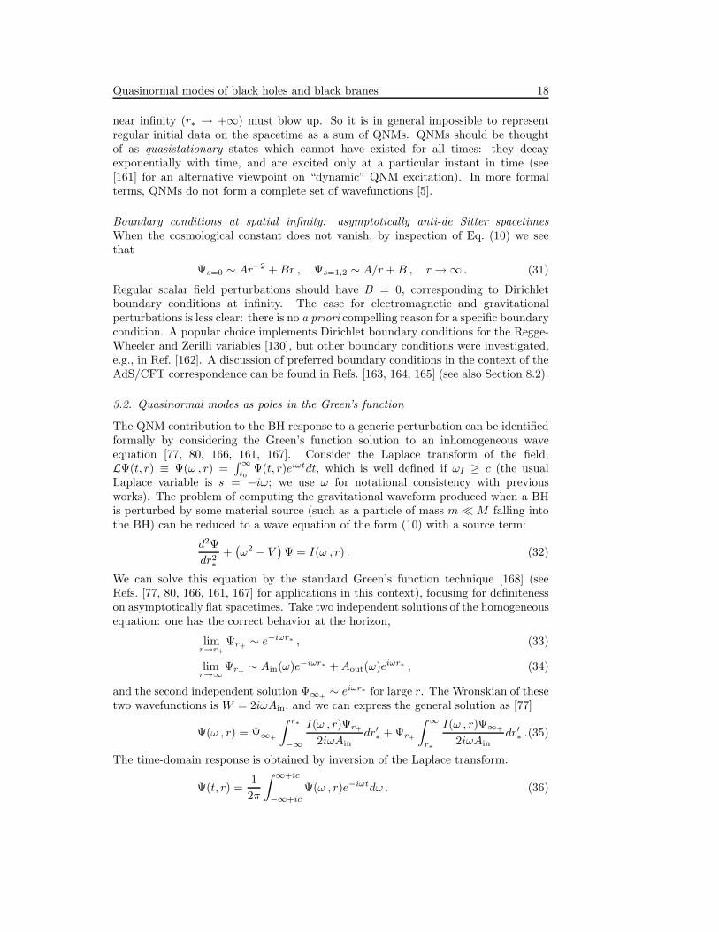
The frequency integral can be performed by the integration contour shown in Fig. 2.There are in general three different contributions to the integral. The integral alongthe large quarter-circles is the flat-space analogue of the prompt response, i.e. wavespropagating directly from the source to the observer at the speed of light. Dependingon the asymptotic structure of the potential, there is usually a branch point at ω = 0[41]. To prevent it from lying inside the integration contour, we place a branch cutalong the negative imaginary-ω axis and split the half circle at |ω| → ∞ into twoquarter circles [169, 170, 84]. The branch-cut contribution gives rise to late-timetails [171, 77, 84]: physically, these tails are due to backscattering off the backgroundcurvature [171], and therefore they depend on the asymptotics of the spacetime. Tailsare absent for certain backgrounds, such as the SAdS [92] or the Nariai spacetime [172].The third contribution comes from a sum-over-residues at the poles in the complexfrequency plane, which are the zeros of Ain. These poles correspond to perturbationssatisfying both in-going wave conditions at the horizon and out-going wave conditionsat infinity, so (by the very definition of QNMs) they represent the QNM contributionto the response. Although we used the asymptotic behavior of the solutions of thewave equation, this discussion can be trivially generalized to any spacetime.
Far from the source, the QNM contribution in asymptotically flat spacetimes canbe written as [166, 167]
Ψ(t, r) = −Re
[
∑
n
Cne−iωn(t−r∗)
]
, (37)
where the sum is over all poles in the complex plane. The Cn’s are called quasinormalexcitation coefficients and they quantify the QNM content of the waveform. Theyare related to initial-data independent quantities, called the quasinormal excitationfactors (QNEFs) and denoted by Bn, as follows:
Cn = Bn
∫ ∞
−∞
I(ω , r)Ψr+
Aoutdr′∗ , Bn =
Aout
2ω
(
dAin
dω
)−1∣
∣
∣
∣
∣
ω=ωn
. (38)
In general the QNM frequencies ωn, the Bn’s and the Cn’s depend on l, m and on thespin of the perturbing field s, but to simplify the notation we will omit this dependence

Quasinormal modes of black holes and black branes 20
whenever there is no risk of confusion.The QNEFs play an important role in BH perturbation theory: they depend only
on the background geometry, and (when supplemented by specific initial data) theyallow the determination of the QNM content of a signal, i.e. of the Cn’s. This has beenknown for over two decades, but relatively little effort has gone into understandinghow these modes are excited by physically relevant perturbations. The QNEFshave long been known for scalar, electromagnetic and gravitational perturbations ofSchwarzschild BHs [77, 173, 166, 161], and they have recently been computed forgeneral perturbations of Kerr BHs [167]. In [167] it was also shown that for largeovertone numbers (n → ∞) Bn ∝ n−1 for all perturbing fields in a large class ofnon-rotating spacetimes. The excitation factors Cn have mainly been computed forthe simple case where the initial data are Gaussian pulses of radiation [166, 167]. Theonly work we are aware of studying the excitation factors Cn for a point particle fallinginto a Schwarzschild BH is Leaver’s classic paper [77].
Besides the theoretical interest of quantifying QNM excitation by generic initialdata in the framework of perturbation theory, excitation factors and excitationcoefficients have useful applications in gravitational wave data analysis. First of all, aformal QNM expansion of the BH response can simplify the calculation of the self-forceacting on small bodies orbiting around BHs. It was shown recently, using as a modelproblem the Nariai spacetime, that a QNM expansion of the Green’s function can beused for a matched expansion of the “quasi-local” and “distant-past” contributionsto the self force [172]. The problem of quantifying QNM excitation is of paramountimportance to search for inspiralling compact binaries in gravitational wave detectordata. All attempts to match an effective-one-body description of inspiralling binariesto numerical relativity simulations found that the inclusion of several overtones in theringdown waveform is a crucial ingredient to improve agreement with the numerics[174, 175]. So far the matching of the inspiral and ringdown waveforms has beenperformed by ad hoc procedures. For example, the amplitudes and phases of the Cn’shave been fixed by requiring continuity of the waveform on a grid of points, or “comb”[176]. These matching procedures have their own phenomenological interest, but aself-consistent estimation of the excitation coefficients within perturbation theory isneeded to improve our physical understanding of the inspiral-ringdown transition.
Finally, we point out that recent investigations have addressed the issue of modeexcitation in the gauge/gravity duality [177, 178]. There it was found, for example,that the residue of the diffusion and shear mode decays at small wavelength, so thesemodes effectively cease to exist.
4. Computing quasinormal modes
To determine the QNMs and compute their frequencies we must solve the eigenvalueproblem represented by the wave equation (10), with boundary conditions specified byEq. (27) at the horizon and Eq. (30) at infinity. There is no universal prescription tocompute QNMs. In this section we discuss various methods to obtain such a solution,pointing out that different methods are better suited to different spacetimes.
For a start we consider the exceptional cases where an exact, analytical solutionto the wave equation can be found. In some spacetimes the potential appearing in thewave equation can be shown to reduce to the Poschl-Teller potential [179], for which anexact QNM calculation is possible [70]. These spacetimes and their QNM spectra arereviewed in Section 4.1. In the general case, QNM calculations require approximations

Quasinormal modes of black holes and black branes 21
or numerical methods ‡. Some of these (including WKB approximations, monodromymethods, series solutions in asymptotically AdS backgrounds and Leaver’s continuedfraction method) are reviewed in Sections 4.2-4.6.
4.1. Exact solutions
In general exact solutions to the wave equation are hard to find, and they must becomputed numerically. There are a few noteworthy exceptions, some of which wesummarize here.
We begin our review of exact solutions by sketching the analytical derivation ofthe QNMs of the Poschl-Teller potential. Many of the difficulties in computing QNMsin BH spacetimes arise from the slow decay of the potential as r → ∞, which isdue (mathematically) to the presence of a branch cut and gives rise (physically) tobackscattering of gravitational waves off the gravitational potential and to late-timetails. Ferrari and Mashhoon realized that these difficulties can be removed and exactsolutions can be found if one considers instead a potential that decays exponentiallyas r → ∞, while recovering the other essential features of the Schwarzschild potential.Such a potential is the Poschl-Teller potential [70]. After reviewing QNM solutionsfor the Poschl-Teller potential we briefly review the modes of pure AdS and dSspacetimes. Then we show that perturbations of the near-extreme Schwarzschild de-Sitter (SdS) and of the Nariai spacetime reduce to a wave equation with a Poschl-Tellerpotential, so they can be solved analytically. We also discuss two asymptoticallyAdS BH spacetimes which have improved our understanding of the role of QNMsin the AdS/CFT correspondence: the (2 + 1)-dimensional BTZ BH [184] and thed−dimensional topological (massless) BH [122, 123, 124, 125, 126, 127]. The BTZ BHis the first BH spacetime for which an exact, analytic expression for the QNMs hasbeen derived [95], and it offers interesting insights into the validity of the AdS/CFTcorrespondence [94, 185, 186].
The Poschl-Teller potential In this section we analytically compute the QNMs ofthe Poschl-Teller potential [179, 70], which will serve as a prototype for several BHspacetimes to be discussed below. Consider the equation
∂2Ψ
∂r2∗+
[
ω2 − V0
cosh2 α(r∗ − r∗)
]
Ψ = 0 . (39)
The quantity r∗ is the point r∗ at which the potential attains a maximum, i.e.dV/dr∗(r∗) = 0, and V0 is the value of the Poschl-Teller potential at that point:V0 = V (r∗). The quantity α is related to the second derivative of the potential atr∗ = r∗, α
2 ≡ −(2V0)−1d2V/dr2∗(r∗). The solutions of Eq. (39) that satisfy both
boundary conditions (27) and (30) are the QNMs [70]. To find these solutions we
define a new independent variable ξ =[
1 + e−2α(r∗−r∗)]−1
and rewrite Eq. (39) as
ξ2(1−ξ)2 ∂2Ψ
∂ξ2−ξ(1−ξ)(2ξ−1)
∂Ψ
∂ξ+
[
ω2
4α2− V0
α2ξ(1 − ξ)
]
Ψ = 0 .(40)
‡ Fiziev [180, 181] actually showed that the Regge-Wheeler and Teukolsky equations can besolved analytically in terms of confluent Heun’s functions. These solutions allow a high-accuracydetermination of the Schwarzschild quasinormal frequencies. The calculation of Heun’s functions isquite contrived, but it already proved useful to address interesting open problems in perturbationtheory [182, 183].

Quasinormal modes of black holes and black branes 22
Near spatial infinity 1 − ξ ∼ e−2α(r∗−r∗), and near the horizon ξ ∼ e2α(r∗−r∗). Ifwe define a =
[
α+√α2 − 4V0 − 2iω
]
/(2α) , b =[
α−√α2 − 4V0 − 2iω
]
/(2α) , c =
1− i ω/α and set Ψ = (ξ(1 − ξ))−iω/(2α)
y, we get a standard hypergeometric equationfor y [187]:
ξ(1−ξ)∂2ξy + [c− (a+ b+ 1)ξ]∂ξy − aby = 0 , (41)
and therefore
Ψ = Aξi ω/(2α)(1 − ξ)−iω/(2α)F (a− c+ 1, b− c+ 1, 2 − c, ξ)
+ B (ξ(1 − ξ))−iω/(2α)
F (a, b, c, ξ) . (42)
Recalling that F (a1, a2, a3, 0) = 1 and that ξi ω/(2α) ∼ eiωr∗ near the horizon, wesee that the first term represents, according to our conventions, an outgoing waveat the horizon, while the second term represents an ingoing wave. QNM boundaryconditions require A = 0. To investigate the behavior at infinity, one uses the z → 1−ztransformation law for the hypergeometric function [187]:
F (a, b, c, z) = (1−z)c−a−b Γ(c)Γ(a+ b− c)
Γ(a)Γ(b)F (c−a, c−b, c−a−b+1, 1−z)
+Γ(c)Γ(c− a− b)
Γ(c− a)Γ(c− b)F (a, b,−c+a+b+1, 1−z) . (43)
The boundary condition at infinity implies either 1/Γ(a) = 0 or 1/Γ(b) = 0, which aresatisfied whenever
ω = ±√
V0 − α2/4 − iα(2n+ 1)/2 , n = 0, 1, 2, .... (44)
where n is the overtone index.A popular approximation scheme to compute BH QNMs consists in replacing the
true potential in a given spacetime by the Poschl-Teller potential. This approximationworks well for the low-lying modes of the Schwarzschild geometry. It predictsMω = 0.1148 − 0.1148i, 0.3785 − 0.0905i for the fundamental l = s = 0, 2perturbations, respectively [70]. This can be compared to the numerical result[75, 10, 47] Mω = 0.1105 − 0.1049i, 0.3737 − 0.0890i. In the eikonal limit (l → ∞)the Poschl-Teller approximation yields the correct solution: it predicts the behavior3√
3Mω = ±(l + 1/2) − i(n + 1/2), in agreement with WKB-based calculations[58, 188, 189] (see also [190]).
The Poschl-Teller approximation provides a solution which is more and moreaccurate for near-extremal SdS BHs, since the event horizon and the cosmologicalhorizon coalesce in the extremal limit [162, 191, 192].
Normal modes of the anti-de Sitter spacetime A physically interesting analyticalsolution concerns the QNMs of pure AdS spacetime, which can be obtained by settingr0 = 0 in the metric (3). In this case, QNMs are really normal modes of the spacetime,and have been computed for scalar field perturbations by Burgess and Lutken [193].They satisfy
Lω = 2n+ d+ l − 1 , n = 0, 1, 2, ... s = 0 , (45)
where l is related to the eigenvalue of spherical harmonics in d dimensions byAlm = l(l+d−3) [153]. Normal modes of electromagnetic perturbations in d = 4 wereshown to be the same as normal modes for gravitational perturbations (see Appendixin Ref. [194]); for general d, they can be computed from the potentials for wave

Quasinormal modes of black holes and black branes 23
propagation derived by Kodama and Ishibashi [104]. Ref. [107] studies the normalmodes of gravitational perturbations. Tensor gravitational perturbations obey thesame equation as s = 0 fields, and therefore their normal modes are
Lω = 2n+ d+ l − 1 , n = 0, 1, 2, ... s = 2 tensor − type . (46)
Vector-type gravitational perturbations have normal modes with the followingcharacteristic frequencies
Lω = 2n+ d+ l − 2 , n = 0, 1, 2, ... s = 2 vector − type . (47)
Finally, scalar-type gravitational perturbations have a somewhat surprising behavior.For d = 4 they are given by Eq. (47). For d = 5 they have a continuous spectrum,and for d > 5 one finds [107]
Lω = 2n+ d+ l − 3 , n = 0, 1, 2, ... s = 2 scalar− type . (48)
Quasinormal modes of the de Sitter spacetime The dS spacetime is an extensivelystudied solution of the Einstein field equations, most of the early investigations beingmotivated by cosmological considerations. It satisfies Eq. (3) with r0 = 0 andf(r) = 1 − r2/L2. Natario and Schiappa found that no QNM solutions are allowedin even-dimensional dS space [107]. For scalar fields and tensor-type gravitationalperturbations in odd-dimensional dS backgrounds the QNM frequencies are purelyimaginary, and given by
Lω = −i (2n+ d+ l) , n = 0, 1, 2, ...tensor − type . (49)
For the other types of gravitational perturbations Ref. [107] finds
Lω = − i (2n+ d+ l + 1) , n = 0, 1, 2, ...vector− type , (50)
Lω = − i (2n+ d+ l + 2) , n = 0, 1, 2, ...scalar− type . (51)
Notice the striking similarity with the pure AdS results when one replaces L → iL.Fields of other spins were considered in Refs. [195, 192].
Nearly-extreme SdS and the Nariai spacetime The metric for d-dimensionalSchwarzschild de-Sitter (SdSd) BHs can be obtained from Eq. (3) by the replacementL → iL, i.e., f(r) = 1 − r2/L2 − rd−3
0 /rd−3. The corresponding spacetime has twohorizons: an event horizon at r = r+ and a cosmological horizon at r = rc. It wasobserved in Ref. [196] that for rc/r+ − 1 ≪ 1 perturbations of this spacetime satisfy awave equation with a Poschl-Teller potential. In particular, setting kb ≡ (rc−r+)/2r2c ,for near-extreme SdSd one findsM/rd−3
+ ∼ 1/(d−1) , r2+/L2 ∼ (d−3)/(d−1) [196, 197].
QNM frequencies for scalar field and tensor-like gravitational perturbations are thengiven by [196, 197]
ω
k=
√
l(l + d− 3) − 1
4− i
(
n+1
2
)
, tensor − type , (52)
where k = (d − 3)(rc − r+)/(2r2+) is the surface gravity of the BH. For gravitationalperturbations the result is
ω
k=
√
(l − 1)(l + d− 2) − 1
4− i
(
n+1
2
)
, vector − type , (53)
ω
k=
√
(l − 1)(l + d− 2) − d+15
4− i
(
n+1
2
)
, scalar − type .

Quasinormal modes of black holes and black branes 24
Through an appropriate limiting procedure [196, 198], the nearly-extreme SdSd
geometry can yield a spacetime with a different topology, the Nariai spacetime[196, 199, 200, 201], of the form
ds2 = −(
−r2/L2 + 1)
dt2 +(
−r2/L2 + 1)−1
dr2 + r2dΩ2d−2 . (54)
This manifold has topology dS2 × Sd−2 and two horizons (with the same surfacegravity). The QNM frequencies are the same as for nearly-extreme SdSd, if k isreplaced by the surface gravity of each horizon [198].
The BTZ black hole Ichinose and Satoh [202] were the first to realize that the waveequation in the (2 + 1)-dimensional, asymptotically AdS BTZ BH [184] can be solvedin terms of hypergeometric functions. An analytical solution for the QNMs of this BHwas first found in Ref. [95]. The non-rotating BTZ BH metric is given by [184]
ds2 =(
r2/L2 −M)
dt2 −(
r2/L2 −M)−1
dr2 − r2dφ2 , (55)
where M is the BH mass and r+ = M1/2L is the horizon radius. In 2 + 1 dimensionsgravity is “trivial”: the full curvature tensor is completely determined by the localmatter distribution and the cosmological constant. In particular, in vacuum thecurvature tensor Rµνλρ = Λ (gµλgνρ − gµρgνλ) and R = 6Λ. Curvature effectsproduced by matter do not propagate through the spacetime. There are no dynamicaldegrees of freedom, and no gravitational waves [203, 204]. Therefore, we will focuson scalar fields and assume an angular dependence of the form eimφ. Scalar QNMfrequencies are given by
ωL = ±m− 2i(n+ 1)r+/L , (56)
with m the azimuthal number, and n the overtone number [95]. This result has beengeneralized by Birmingham, Sachs and Solodukhin [94] to the rotating BTZ BH. Forgeneral massive scalar perturbations with mass parameter µ they find
ωL = ±m− i[2n+ (1 +√
µ2 + 1)] (r+ − r−)/L . (57)
The BTZ background has provided a first quantitative test of the AdS/CFTcorrespondence: the QNM frequencies (57) match the poles of the retarded correlationfunction of the corresponding perturbations in the dual CFT [94]. Recently the QNMsof BTZ BHs were shown to be Breit-Wigner-type resonances generated by surfacewaves supported by the boundary at infinity, which acts as a photon sphere [205].This interpretation is highly reminiscent of work in asymptotically flat spacetimes,interpreting QNMs as null particles slowly leaking out of circular null geodesics (seeRefs. [59, 73, 70, 206, 207, 208, 209] and Section 4.2 below).
An alternative to Einstein’s gravity in three dimensions is the so-called“topologically massive gravity”, obtained by adding a Chern-Simons term to the action[210, 211]. Topologically massive gravity allows for dynamics, i.e. gravitational waves.The QNMs of BTZ BHs in this theory have recently been computed, providing yetanother confirmation of the AdS/CFT correspondence [185, 186].
Massless topological black holes It is also possible to obtain exact solutions in arestricted set of higher-dimensional BH spacetimes. These asymptotically AdSsolutions are known as topological BHs. The horizon is an Einstein space of positive,zero, or negative curvature [122, 123, 124, 125, 126, 127]. In the negative-curvature

Quasinormal modes of black holes and black branes 25
case there is a massless BH playing a role quite similar to the BTZ BH in threedimensions. Consider the exterior region of the massless topological BH [212]
ds2 = −(
r2/L2 − 1)
dt2 +(
r2/L2 − 1)−1
dr2 + r2dσ2 .
This is a manifold of negative constant curvature with an event horizon at r = L.Here dσ2 stands for the line element of a (d− 2)-dimensional surface Σd−2 of negativeconstant curvature.
The wave equation for a massive scalar field with non-minimal coupling can besolved by the ansatz Φ = Ψ(r)e−iωtY , where Y is a harmonic function of finite
norm with eigenvalue −Q = − (d− 3)2/4 − ξ2. The parameter ξ is generically
restricted, assuming only discrete values if Σd−2 is a closed surface. If the effectivemass m2
eff= µ2 − γd(d − 2)/4L2 (with µ the mass of the field and γ the conformal
coupling factor) satisfies the boundm2effL2 ≥ −[(d−1)/2]2, one set of QNM frequencies
is given by [212]
ω L = ±ξ − i(
2n+ 1 +√
(d− 1)2/4 +m2effL
2)
, n = 0, 1, 2... . (58)
If the mass and the coupling constant γ satisfy the relations√
(d− 1)2/4 +m2effL2 =
d−12 − γ
2d−2
d−1−γ(d−2) and −(
d−12
)2< m2
effL2 < 1−
(
d−12
)2, there is another set of modes
for which the QNM frequencies are given by [212]
ω L = ±ξ − i(
2n+ 1 −√
(d− 1)2/4 +m2effL
2)
. (59)
This computation represents the first exact analytic determination of QNMs in fourand higher dimensions. The generalization to other fields (and in particular togravitational perturbations) can be found in Ref. [213].
4.2. The WKB approximation
Normal modes of vibration of an object usually have a simple interpretation in termsof waves traveling across or around the object. For example, the Earth’s free modes ofoscillation were highly excited and measured for the first time in the 1960 earthquakein Chile [214]. These (roughly) one-hour long periodic oscillations correspond to wavestraveling around the globe, and carry information about the Earth’s interior. Just likethe Earth’s free modes of oscillation, BH QNMs can be thought of as waves travelingaround the BH [58, 59, 70, 73, 206, 207, 208, 209]. More precisely, QNMs can beinterpreted as waves trapped at the unstable circular null geodesic (also known asthe light-ring) and slowly leaking out. The instability timescale of the geodesic is thedecay timescale of the QNM, and the oscillation frequency ω ∼ c/rLR, with c thespeed of light and rLR the light-ring radius [208].
This intuitive picture, first proposed by Goebel [59], is related to a more rigorousWKB approximation developed by Mashhoon [69] and by Schutz and Will [74] (seealso [58, 70, 73, 206, 207, 208, 209]). Their derivation and results closely parallel theBohr-Sommerfeld quantization rule from quantum mechanics. The procedure involvesrelating two WKB solutions across a “matching region” whose limits are the classicalturning points, where ω2 = V (r). The technique works best when the classical turningpoints are close, i.e. when ω2 ∼ Vmax, where Vmax is the peak of the potential. Underthese assumptions we can expand in a Taylor series around the extremum of thepotential r∗:
Q ≡ ω2 − V ∼ Q0 +Q′′0(r∗ − r∗)
2/2 , Q′′0 ≡ d2Q/dr2∗ . (60)

Quasinormal modes of black holes and black branes 26
In this region, the wave equation d2Ψdr2
∗
+QΨ = 0 can be approximated by
d2Ψ
dr2∗+
[
Q0 +1
2Q′′
0(r∗ − r∗)2
]
Ψ = 0 . (61)
This equation has an exact solution in terms of parabolic cylinder functions [187, 215]:
Ψ = ADν(z) +BD−ν−1(iz) , z ≡ (2Q′′0)
14 ei π
4 (r∗ − r∗) , (62)
with ν = −iQ0/√
2Q′′0 − 1/2. Using the asymptotic behavior of cylinder functions
[187, 215] and demanding only outgoing waves at spatial infinity we get, near thehorizon,
Ψ ∼ Ae−iπνzνe−z2
2 − i√
2πA [Γ(−ν)]−1 e5iπ/4z−ν−1ez2
2 . (63)
QNM boundary conditions imply that the outgoing term, proportional to ez2/2, shouldbe absent, so 1/Γ(−ν) = 0, or ν = n(= 0 , 1 , 2 , ...). As we anticipated, the leading-order WKB approximation yields a “Bohr-Sommerfeld quantization rule” defining theQNM frequencies:
Q0/√
2Q′′0 = i(n+ 1/2) , n = 0 , 1 , 2 , ... (64)
0 1 2 3 4 5 6n (overtone number)
10-7
10-6
10-5
10-4
10-3
10-2
10-1
100
101
% e
rror
l=2l=3l=4l=5l=6Real part
0 1 2 3 4 5 6n (overtone number)
10-6
10-5
10-4
10-3
10-2
10-1
100
101
% e
rror
l=2l=3l=4l=5l=6Imaginary part
Figure 3. Percentage errors for the real (left) and imaginary part (right) of theQNM frequencies as predicted from WKB calculations. Thick lines: third-orderWKB approximation; thin lines: sixth-order WKB approximation.
Higher-order corrections to Eq. (60) have been computed [58]. Iyer and Will[188, 189] carried out a third-order WKB expansion, and more recently Konoplya [216]pushed the expansion up to sixth order. There is no rigorous proof of convergence,but the results do improve for higher WKB orders. This is shown in Fig. 3, where wecompare numerical results for the QNMs of Schwarzschild BHs from Leaver’s continuedfraction method (to be discussed in Section 5.1 below) against third- and sixth-orderWKB predictions. The WKB approximation works best for low overtones, i.e. modeswith a small imaginary part, and in the eikonal limit of large l (which corresponds tolarge quality factors, or large ωR/ωI). The method assumes that the potential has asingle extremum, which is the case for most (but not all) BH potentials: see Ref. [103]for interesting counterexamples.
Ref. [217] introduces a new, WKB-inspired asymptotic expansion of QNMfrequencies and eigenfunctions in powers of the angular momentum parameter l+1/2.

Quasinormal modes of black holes and black branes 27
Their asymptotic expansion technique is easily iterated to high orders, and it seemsto provide very accurate results in spherically-symmetric spacetimes. The asymptoticexpansion also provides physical insight into the nature of QNMs, nicely connectingthe geometrical understanding of QNMs as perturbations of unstable null geodesicswith the singularity structure of the Green function.
4.3. Monodromy technique for highly-damped modes
A powerful variant of the WKB approximation, which is particularly useful in thehighly-damped limit ωI → ∞, is the so-called monodromy technique [101]. Thebasic idea is related to Stokes’ phenomenon in the theory of asymptotic expansions(see e.g. [218] for an excellent introduction to the topic). As shown by Anderssonand Howls [219], the monodromy technique is a simple variant of the phase-integralapproach, whose application to BH physics dates back to the work by Froman et al.[81].
Let us consider the wave equation (10) for the Schwarzschild geometry, butallowing r and r∗ to be complex variables. In the complex-r plane, solutions toEq. (10) may be multivalued around the singular points (r = 0 and r = 2M). Todeal with the singular points we introduce branch cuts emanating from r = 0 andr = 2M . The relation r∗(r) is also multi-valued: in the Schwarzschild geometryr∗(r) = r+2M log (r/2M − 1), and we choose the branch such that log(−1) = iπ. Wecan now define a variable z ≡ r∗/2M − iπ which tends to zero as r → 0. The Stokeslines are defined as the lines for which Re(r∗) = 0 [218], and they are shown in Fig. 4(near the singular point r = 0, the Stokes lines form an angle π/4). The idea now is
r z
10 0
A
B B
A
Figure 4. Left panel: contour for calculation of the QNM frequencies in thecomplex-r plane. The different regions are separated by the associated Stokeslines. Not shown in the plot are branch cuts from r = −∞ to the origin and fromr = 1 to point A. Right panel: integration contour in the complex-z plane, withz ≡ r∗/2M − iπ. For more details see Ref. [101].
to equate the monodromy as computed in two different ways. The first computationtakes the contour in Fig. 4, starting and ending at point A and following the Stokeslines, joined at infinity by the large semi-circles shown in Fig. 4. If we start from Awith a plane wave eiωz, we can extrapolate the behavior to near the singularity z = 0.This is because for large imaginary ω the term ω2 is much larger than the other terms

Quasinormal modes of black holes and black branes 28
in the potential. Near the origin (r = 0) the solutions to the wave equation can bewritten as
Ψ(z) = A+
√4πMωzJ s
2(2Mωz) +A−
√4πMωzJ− s
2(2Mωz) , (65)
where A± are constants and Js/2 is a Bessel function. From the asymptotics of Besselfunctions for large ωz one has
Ψ(z) ∼ ei2Mωz [A+e−iα++A−e
−iα− ]+e−i2Mωz[A+eiα++A−e
iα− ] , (66)
with α± = π(1 ± s)/4. The second term must vanish because of the boundaryconditions. Continuing along the contour, we make a 3/2π turn around r = 0. Interms of the z coordinate, this means a 3π rotation. Using the representation for theBessel functions
J±s/2(η) = η±s/2+∞∑
n=0
(−1)nη2n
22n±s/2Γ(±s/2 + n+ 1)n!, (67)
one can see that J±s/2(e3iπ2Mωz) = e±i3πs/2J±s/2(2Mωz). Therefore
Ψ ∼ ei2Mωz [A+e7iα+ +A−e
7iα− ]+e−i2Mωz [A+e5iα+ +A−e
5iα− ] .(68)
The e−i2Mωz term is exponentially small, since we are in the region where Re(z) ≫ 0and ωI ≪ 0. Using Eq. (66) we get for the coefficient of eiωz the monodromy
A+e7iα+ +A−e
7iα−
A+e−iα+ +A−e−iα−. (69)
Requiring that the second term in Eq. (66) vanishes, Eq. (69) yields − (1 + 2 cos(πs))for the monodromy. On the other hand, the only singularity inside the contour is atr = 1, giving a factor e−4i(2Mω) and leading to the condition
8πMω = ± log 3 − iπ(2n+ 1) (70)
for the highly damped QNM frequencies of Schwarzschild BHs with s = 0 , 2 (s = 1 ispredicted to have a vanishing real part). This formula is in agreement with numericalstudies by Nollert [220] for the Schwarzschild spacetime. The procedure has beengeneralized to several other backgrounds, including Reissner-Nordstrom (RN) [101],Kerr [221, 222], SAdS [223] and other BH spacetimes [107], always finding excellentagreement with numerical calculations [224, 225, 194].
The application of the monodromy method requires extreme care in identifyingthe appropriate Stokes lines and integration contours. Natario and Schiappa [107]point out some instances of inappropriate applications of the technique. A morerigorous mathematical treatment of these methods is highly desirable.
4.4. Asymptotically anti-de Sitter black holes: a series solution
With the exception of the monodromy technique, the methods discussed so farwork for asymptotically flat or (with some minor modifications) dS spacetimes.For asymptotically AdS spacetimes, the perturbation equations exhibit regularsingularities both at the horizon and at spatial infinity. Local solutions in the vicinityof the regular singular points are represented by convergent Frobenius series [226].In many cases, the radius of convergence of the series is equal to or larger than theinterval of interest. In this case, a simple numerical procedure (implemented e.g. byHorowitz and Hubeny in [92]) is possible. Consider, for example, a scalar field Ψ

Quasinormal modes of black holes and black branes 29
in the SAdS4 spacetime, satisfying the wave equation (10). Defining Φ for a genericwavefunction as Φ = eiωr∗Ψ, we find
f(r)d2Φ
dr2+ [f ′ − 2iω]
dΦ
dr− V
fΦ = 0 , (71)
where f ′ ≡ df/dr. To find the frequencies ω that satisfy the boundary conditions wefirst note that Eq. (71) has only regular singularities in the range of interest. To dealwith the point at infinity, we first change the independent variable r to x = 1/r andget
(x− x+)s(x)d2Φ
dx2+ t(x)
dΦ
dx+
u(x)
x− x+Φ = 0 , (72)
where x+ = 1/r+ ≡ h, s = −fx4/(x − x+), t = −[
2fx3 − f ′x2 − 2iωx2]
, u =V (x− x+)/f . Eq. (72) admits a local (near x = h) Frobenius solution of the form
Φ(x) = (x− h)α∞∑
n=0
an(x− h)n , (73)
where an(ω) is a function of the frequency. The radius of convergence of the series islimited by the distance to the next nearest singular point of the equation. The indexα is determined by imposing the boundary condition at the horizon. Writing
s(x) =
∞∑
i=0
si(x−h)i , t(x) =
∞∑
i=0
ti(x−h)i , u(x) =
∞∑
i=0
ui(x−h)i , (74)
and substituting Eqs. (73) and (74) in Eq. (71) we get an indicial equation for α:α(α − 1)s0 + αt0 + u0 = 0. We also have s0 = 2h2κ , t0 = 2h2(κ − iω) and u0 = 0,where the surface gravity is κ = f ′(r+)/2. Therefore, either α = 0 or α = iω/κ. Onecan check that the second option corresponds to outgoing waves at the horizon, so wechoose α = 0. Inserting the decomposition (73) with α = 0 in Eq. (71) and comparingpowers of (x− h) we get a recurrence relation for the an’s:
an = − 1
n(n− 1)s0 + nt0
n−1∑
i=0
[i(i− 1)sn−i + itn−i + un−i] ai . (75)
Since the differential equation is linear, a0 is just an arbitrary normalization constant.Using the boundary condition Φ = 0 at infinity (x = 0) we finally obtain a simplerelation determining the QNM frequencies:
∞∑
n=0
an(−h)n = 0 . (76)
In practice one computes the N -th partial sum of the series (76) and finds the roots ωof the resulting polynomial expression, checking for convergence by comparison with(say) the roots obtained from the N + 1-th partial sum. The method can be easilyimplemented: see e.g. the publicly available Mathematica notebook [47] that was usedin [130] to compute low-lying modes of the SAdS4 geometry. This notebook can beeasily modified to deal with other geometries.
Some mathematical aspects of the series solution method as applied to QNMs inasymptotically AdS backgrounds are discussed in Ref. [99].

Quasinormal modes of black holes and black branes 30
4.5. Asymptotically anti-de Sitter black holes: the resonance method
The series solution described in the previous subsection converges very slowly for smallSAdS BHs. Fortunately, in this regime there is a simple alternative: the resonancemethod [227]. This method requires a numerical integration of the wave equation,but unlike the original numerical procedure by Chandrasekhar and Detweiler [62], oneonly needs to search for roots on the real-ω line.
It is well known that quasi-bound states manifest themselves as poles in thescattering matrix, and as Breit-Wigner resonances in the scattering amplitude.Chandrasekhar and Ferrari made use of the form of the scattering cross section nearthese resonances in their study of gravitational wave scattering by ultra-compact stars[228, 229]. For quasi-bound, trapped modes of ultra-compact stars, the asymptoticwave amplitude at spatial infinity Ψ ∼ α cosωr + β sinωr has a Breit-Wigner-typebehavior close to the resonance:
α2 + β2 ≈ constant[
(ω − ωR)2 + ω2I
]
, (77)
where ω−1I is the lifetime of the quasi-bound state and ω2
R its characteristic “energy”.The example of ultra-compact stars shows that the search for weakly damped QNMscorresponding to quasi-bound states (ω = ωR − iωI with ωI ≪ ωR) is extremelysimplified. One locates the resonances by looking for minima of α2 + β2 on theω = ωR line, and the corresponding damping time ωI can then be obtained by a fit toa parabola around the minimum [228, 229].
It was shown in [227] that these ideas can be used very successfully in BHspacetimes, if one integrates in from spatial infinity to the BH horizon (i.e., theappropriately re-defined quantities α2 + β2 are taken close to the horizon). Theresonance method is extremely simple and accurate, especially for small SAdS BHs[227] (see also Section 6.1). It is presently unclear whether it can be appliedsuccessfully to study QNMs in other BH spacetimes.
4.6. The continued fraction method
Applications of the continued fractions to eigenvalue problems have an interestinghistory dating back to Jaffe’s 1933 paper on the spectrum of the hydrogen moleculeion, or perhaps to even earlier times (some details and relevant references can be foundin [99]).
The method was applied to gravitational problems by Leaver, leading to whatis possibly the most successful algorithm to date to compute QNM frequencies[75, 76, 77]. Leaver’s approach is based on the observation that the Teukolsky equationis a special case of a general class of spheroidal wave equations that appear in thecalculation of the electronic spectra of the hydrogen molecule ion [76]. These equationscan be solved through a three-term recurrence relation, and the boundary conditionslead to a continued fraction equation characterizing the QNMs. Originally devisedfor the Schwarzschild and Kerr geometries [220, 230, 231, 225], the method has alsobeen applied to RN BHs [232], Kerr-Newman BHs [233], higher-dimensional BHs[234, 235, 236, 237], SdS BHs [238, 239] and acoustic BHs [240] (see Section 10.4below), among others. We illustrate the main ideas by considering the Kerr case. Startwith the following series solution for the angular eigenfunctions defined in Eq. (25):
sSlm(u) = eaωu (1 + u)k− (1 − u)k+
∞∑
p=0
ap(1 + u)p , (78)
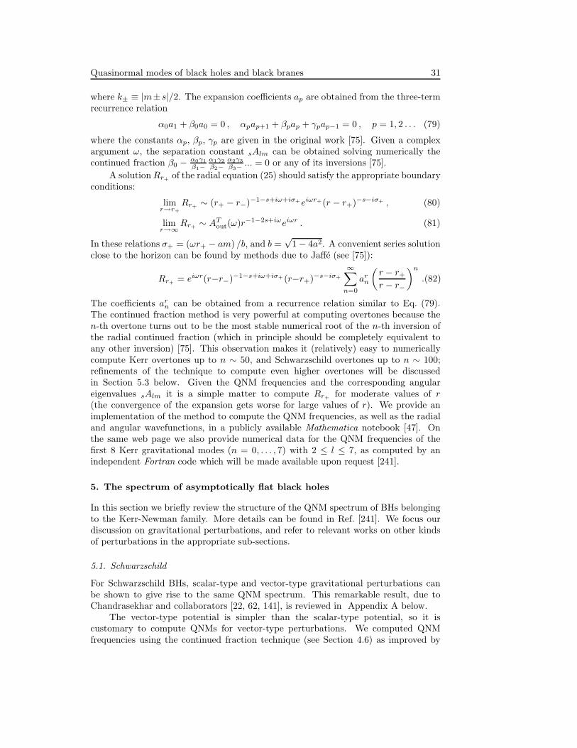
Quasinormal modes of black holes and black branes 31
where k± ≡ |m±s|/2. The expansion coefficients ap are obtained from the three-termrecurrence relation
α0a1 + β0a0 = 0 , αpap+1 + βpap + γpap−1 = 0 , p = 1, 2 . . . (79)
where the constants αp, βp, γp are given in the original work [75]. Given a complexargument ω, the separation constant sAlm can be obtained solving numerically thecontinued fraction β0 − α0γ1
β1−α1γ2
β2−α2γ3
β3−... = 0 or any of its inversions [75].
A solutionRr+ of the radial equation (25) should satisfy the appropriate boundaryconditions:
limr→r+
Rr+ ∼ (r+ − r−)−1−s+iω+iσ+eiωr+(r − r+)−s−iσ+ , (80)
limr→∞
Rr+ ∼ ATout(ω)r−1−2s+iωeiωr . (81)
In these relations σ+ = (ωr+ − am) /b, and b =√
1 − 4a2. A convenient series solutionclose to the horizon can be found by methods due to Jaffe (see [75]):
Rr+ = eiωr(r−r−)−1−s+iω+iσ+ (r−r+)−s−iσ+
∞∑
n=0
arn
(
r − r+r − r−
)n
.(82)
The coefficients arn can be obtained from a recurrence relation similar to Eq. (79).
The continued fraction method is very powerful at computing overtones because then-th overtone turns out to be the most stable numerical root of the n-th inversion ofthe radial continued fraction (which in principle should be completely equivalent toany other inversion) [75]. This observation makes it (relatively) easy to numericallycompute Kerr overtones up to n ∼ 50, and Schwarzschild overtones up to n ∼ 100;refinements of the technique to compute even higher overtones will be discussedin Section 5.3 below. Given the QNM frequencies and the corresponding angulareigenvalues sAlm it is a simple matter to compute Rr+ for moderate values of r(the convergence of the expansion gets worse for large values of r). We provide animplementation of the method to compute the QNM frequencies, as well as the radialand angular wavefunctions, in a publicly available Mathematica notebook [47]. Onthe same web page we also provide numerical data for the QNM frequencies of thefirst 8 Kerr gravitational modes (n = 0, . . . , 7) with 2 ≤ l ≤ 7, as computed by anindependent Fortran code which will be made available upon request [241].
5. The spectrum of asymptotically flat black holes
In this section we briefly review the structure of the QNM spectrum of BHs belongingto the Kerr-Newman family. More details can be found in Ref. [241]. We focus ourdiscussion on gravitational perturbations, and refer to relevant works on other kindsof perturbations in the appropriate sub-sections.
5.1. Schwarzschild
For Schwarzschild BHs, scalar-type and vector-type gravitational perturbations canbe shown to give rise to the same QNM spectrum. This remarkable result, due toChandrasekhar and collaborators [22, 62, 141], is reviewed in Appendix A below.
The vector-type potential is simpler than the scalar-type potential, so it iscustomary to compute QNMs for vector-type perturbations. We computed QNMfrequencies using the continued fraction technique (see Section 4.6) as improved by

Quasinormal modes of black holes and black branes 32
-1.0 -0.5 0.0 0.5 1.02MωR
0
10
20
30
40
50-2
Mω I
l=2
l=3
-0.8 -0.6 -0.4 -0.2 0.0 0.2 0.4 0.6 0.82MωR
0
10
20
30
40
50
-2M
ω I
s=2, l=2s=0, l=0s=1, l=1
Figure 5. Top: QNM frequencies for gravitational perturbations with l = 2(black circles) and l = 3 (red diamonds). In both cases we mark by an arrowthe algebraically special mode, given analytically by Eq. (83); a more extensivediscussion of this mode is given in Appendix A. Notice that as the imaginary partof the frequency tends to infinity the real part tends to a finite, l-independent limit.Bottom: comparison of the l = |s| QNM frequencies for scalar, electromagneticand gravitational perturbations.
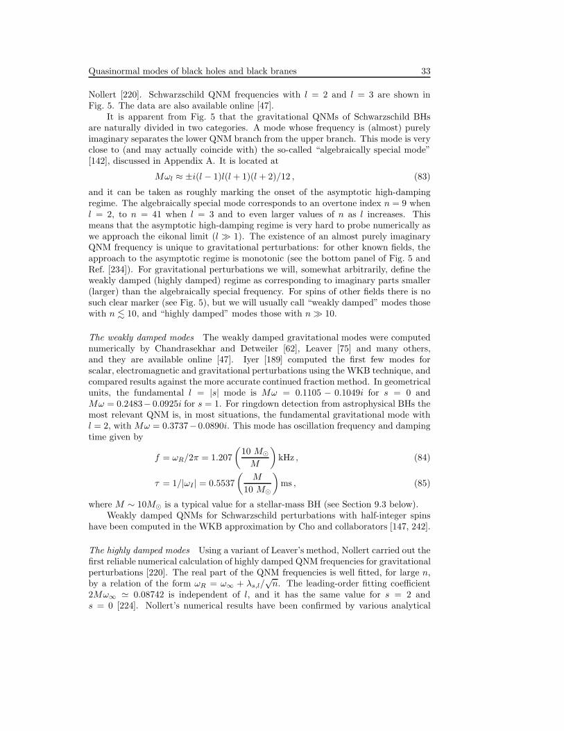
Quasinormal modes of black holes and black branes 33
Nollert [220]. Schwarzschild QNM frequencies with l = 2 and l = 3 are shown inFig. 5. The data are also available online [47].
It is apparent from Fig. 5 that the gravitational QNMs of Schwarzschild BHsare naturally divided in two categories. A mode whose frequency is (almost) purelyimaginary separates the lower QNM branch from the upper branch. This mode is veryclose to (and may actually coincide with) the so-called “algebraically special mode”[142], discussed in Appendix A. It is located at
Mωl ≈ ±i(l − 1)l(l+ 1)(l + 2)/12 , (83)
and it can be taken as roughly marking the onset of the asymptotic high-dampingregime. The algebraically special mode corresponds to an overtone index n = 9 whenl = 2, to n = 41 when l = 3 and to even larger values of n as l increases. Thismeans that the asymptotic high-damping regime is very hard to probe numerically aswe approach the eikonal limit (l ≫ 1). The existence of an almost purely imaginaryQNM frequency is unique to gravitational perturbations: for other known fields, theapproach to the asymptotic regime is monotonic (see the bottom panel of Fig. 5 andRef. [234]). For gravitational perturbations we will, somewhat arbitrarily, define theweakly damped (highly damped) regime as corresponding to imaginary parts smaller(larger) than the algebraically special frequency. For spins of other fields there is nosuch clear marker (see Fig. 5), but we will usually call “weakly damped” modes thosewith n . 10, and “highly damped” modes those with n≫ 10.
The weakly damped modes The weakly damped gravitational modes were computednumerically by Chandrasekhar and Detweiler [62], Leaver [75] and many others,and they are available online [47]. Iyer [189] computed the first few modes forscalar, electromagnetic and gravitational perturbations using the WKB technique, andcompared results against the more accurate continued fraction method. In geometricalunits, the fundamental l = |s| mode is Mω = 0.1105 − 0.1049i for s = 0 andMω = 0.2483− 0.0925i for s = 1. For ringdown detection from astrophysical BHs themost relevant QNM is, in most situations, the fundamental gravitational mode withl = 2, with Mω = 0.3737−0.0890i. This mode has oscillation frequency and dampingtime given by
f = ωR/2π = 1.207
(
10 M⊙
M
)
kHz , (84)
τ = 1/|ωI | = 0.5537
(
M
10 M⊙
)
ms , (85)
where M ∼ 10M⊙ is a typical value for a stellar-mass BH (see Section 9.3 below).Weakly damped QNMs for Schwarzschild perturbations with half-integer spins
have been computed in the WKB approximation by Cho and collaborators [147, 242].
The highly damped modes Using a variant of Leaver’s method, Nollert carried out thefirst reliable numerical calculation of highly damped QNM frequencies for gravitationalperturbations [220]. The real part of the QNM frequencies is well fitted, for large n,by a relation of the form ωR = ω∞ + λs,l/
√n. The leading-order fitting coefficient
2Mω∞ ≃ 0.08742 is independent of l, and it has the same value for s = 2 ands = 0 [224]. Nollert’s numerical results have been confirmed by various analytical

Quasinormal modes of black holes and black branes 34
calculations. Motl [91] used Leaver’s continued fraction conditions to show that in thelimit n→ ∞ the following asymptotic expansion holds:
ω ∼ T ln 3 − (2n+ 1)πiT + O(n−1/2) , (86)
where T = (8πM)−1 is the Hawking temperature. This conclusion was confirmed bycomplex-integration [101] and phase-integral techniques [219].
Corrections of order ∼ n−1/2 to Eq. (86) were first obtained by Neitzke [243]and Maassen van den Brink [244]. Ref. [245] developed a systematic perturbativeapproach to determine subdominant corrections as n → ∞, using a solution of theRegge-Wheeler equation in terms of Bessel functions. Ignoring contributions of orderO(1/n), the result for s = 0 and s = 2 can be written as
ω
T= −(2n+1)πi+ln3+
1 + i√
n+ 1/2
3l(l+ 1) − (s2 − 1)
18|s2 − 1|√
2π3/2Γ4
(
1
4
)
.(87)
The subdominant coefficients are in agreement with fits of numerical results [220, 224,234]. For electromagnetic perturbations, analytic and numerical results suggest thatthe real part ωR → 0 in the asymptotic limit [101, 234], which is also apparent fromFig. 5. The above calculation has been generalized to massless fermionic perturbations.By solving the Teukolsky equation in terms of confluent hypergeometric functions,Refs. [246, 247] confirmed the known results for integer spins, and found in additionthat the result for s = 1/2 and s = 5/2 can be written as:
ω
T= −(2n+1)πi+
2(1 + i)
(s2 + 23/4)√n
(
3l(l+ 1) + 1 − s2)
Γ2
(
1
4
)
.(88)
For s = 3/2 there is no correction at order O(n−1/2). Numerical studies on s = 1/2fields confirm that ωR → 0 and the spacing δωI → 2πT = 1/4M as n→ ∞ [248].
In summary, numerical and analytical results for Schwarzschild BHs are in perfectagreement. As |ωI | → ∞, ωR → T ln 3 for scalar and gravitational oscillationfrequencies, and ωR → 0 for perturbations of other spins. The spacing of the imaginaryparts for large n is always given by 2πT . By considering the scattering amplitude inthe Born approximation, Padmanabhan showed that this universality in the spacingarises from the exponential redshift of the wave modes close to the horizon [249].
The eikonal limit By their own nature, WKB methods become increasingly accuratefor large l, and they can be used to compute the QNM frequencies analytically whenl ≫ 1. Up to order O(l−2) the result is [58, 188, 189, 190]
Mω =1
3√
3
[(
l +1
2
)
− 1
3
(
5(n+ 12 )2
12+
115
144− 1 + s2
)(
1
l− 1
2l2
)]
− i(n+ 1
2 )
3√
3
[
1 +1
9
(
235(n+ 12 )2
432− 1415
1728+ 1 − s2
)
1
l2
]
. (89)
The convergence of the series gets worse with increasing n (cf. also Fig. 3). In theeikonal limit the asymptotic behavior of the potential is not important, so it shouldnot be surprising that a Poschl-Teller approximation of the Schwarzschild potential,discussed in Section 4.1, yields the correct result (to leading order) for large l. Theeikonal regime of Schwarzschild BHs is related to the properties of unstable circularnull geodesics [58, 59, 70, 73, 206, 207, 208, 209]: the leading order of Eq. 89 can bewritten as ω = Ωc l − i (n+ 1/2)λ, where Ωc is the orbital frequency and 1/λ is theinstability timescale of the unstable circular null geodesic. Such a connection can be
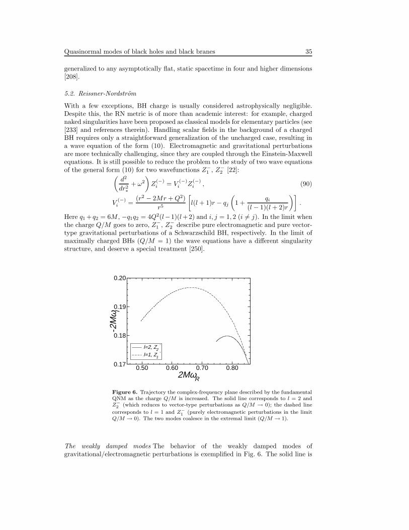
Quasinormal modes of black holes and black branes 35
generalized to any asymptotically flat, static spacetime in four and higher dimensions[208].
5.2. Reissner-Nordstrom
With a few exceptions, BH charge is usually considered astrophysically negligible.Despite this, the RN metric is of more than academic interest: for example, chargednaked singularities have been proposed as classical models for elementary particles (see[233] and references therein). Handling scalar fields in the background of a chargedBH requires only a straightforward generalization of the uncharged case, resulting ina wave equation of the form (10). Electromagnetic and gravitational perturbationsare more technically challenging, since they are coupled through the Einstein-Maxwellequations. It is still possible to reduce the problem to the study of two wave equationsof the general form (10) for two wavefunctions Z−
1 , Z−2 [22]:
(
d2
dr2∗+ ω2
)
Z(−)i = V
(−)i Z
(−)i , (90)
V(−)i =
(r2 − 2Mr +Q2)
r5
[
l(l + 1)r − qj
(
1 +qi
(l − 1)(l + 2)r
)]
.
Here q1 + q2 = 6M , −q1q2 = 4Q2(l−1)(l+2) and i, j = 1, 2 (i 6= j). In the limit whenthe charge Q/M goes to zero, Z−
1 , Z−2 describe pure electromagnetic and pure vector-
type gravitational perturbations of a Schwarzschild BH, respectively. In the limit ofmaximally charged BHs (Q/M = 1) the wave equations have a different singularitystructure, and deserve a special treatment [250].
0.50 0.60 0.70 0.802MωR
0.17
0.18
0.19
0.20
-2M
ω I
l=2, Z2-
l=1, Z1-
Figure 6. Trajectory the complex-frequency plane described by the fundamentalQNM as the charge Q/M is increased. The solid line corresponds to l = 2 andZ−
2(which reduces to vector-type perturbations as Q/M → 0); the dashed line
corresponds to l = 1 and Z−
1(purely electromagnetic perturbations in the limit
Q/M → 0). The two modes coalesce in the extremal limit (Q/M → 1).
The weakly damped modes The behavior of the weakly damped modes ofgravitational/electromagnetic perturbations is exemplified in Fig. 6. The solid line is

Quasinormal modes of black holes and black branes 36
the trajectory described in the complex–frequency plane by the fundamental QNMwith l = 2 corresponding to Z−
2 (perturbations that reduce to the vector-typegravitational Schwarzschild case as Q/M → 0). The dashed line is the trajectoryof the fundamental QNM with l = 1 corresponding to Z−
1 (which reduces to purelyelectromagnetic perturbations as Q/M → 0). The Schwarzschild limit correspondsto the bottom left of each curve, and the trajectories are described clockwise asQ increases. The real part of the frequency grows monotonically with Q, and theimaginary part shows an extremum. A striking feature is that modes of Z−
2 withangular index l coalesce with modes of Z−
1 with index (l − 1) in the extremal limit.We will elaborate on the significance of this result later in this section. In generalthere are two algebraically special frequencies for RN BHs [142], located at
ω1,2 = ± i
2
(l − 1)l(l+ 1)(l + 2)
3M ∓√
9M2 + 16Q2(l − 1)(l + 2). (91)
Using the numerical procedure described by Chandrasekhar and Detweiler [62], Guntercomputed the lowest-lying QNMs of electromagnetic/gravitational perturbations [251].Extensive comparisons of Gunter’s results against WKB predictions were done byKokkotas and Schutz [252]. The continued-fraction method can be generalized tocharged BHs with relatively minor modifications [232], and it was used to computenumerically the weakly and highly damped QNMs of gravitational/electromagneticperturbations [232, 253, 250, 254, 241, 224]. Weakly damped modes of massivecharged fields were computed by WKB techniques in Ref. [255]. Dirac QNMs inthe Kerr-Newman metric (which includes RN as a special case) have been computedby continued fractions in Ref. [256]. For generalizations to higher-dimensional chargedBHs, see [257] and references therein.
The highly damped modes Let us focus our attention on the high-damping regime forZ−
2 ; results for Z−1 are similar. For a more detailed discussion of highly-damped modes,
see [224, 241]. The modes’ behavior is better understood by looking separately at the
0.00 0.05 0.10 0.15Q/2M
0.00
0.05
0.10
2Mω R
n=5000Analytic
0.00 0.05 0.10 0.15Q/2M
2500.2
2500.3
-2M
ω I
n=5000Analytic
Figure 7. Numerical and analytical predictions for the real and imaginary partof the RN QNM frequencies as a function of charge for n = 5 × 10³.
real and imaginary parts of their frequencies as functions of charge. Numerical resultsare shown in Fig. 7. Frequencies and damping times oscillate as a function of charge

Quasinormal modes of black holes and black branes 37
whenever Q is larger than some Qcrit, and Qcrit/M decreases with overtone number.For moderate-to-large values of Q/M , numerical data are in excellent agreement withthe analytical prediction by Motl and Neitzke [101, 219, 107], valid for scalar andelectromagnetic-gravitational perturbations of a RN BH in the large-damping limit:
eω/T + 2 + 3e(Q4 ω)/(r4
+ T ) = 0 , T =√
M2 −Q2/[
2πr2+]
, (92)
where r+ = M +√
M2 −Q2 is the radius and T is the Hawking temperature of theouter horizon. The complex solutions of Eq. (92) exactly overlap with the oscillationsobserved in Fig. 7 for large enough values of Q/M . This agreement gives support tothe asymptotic formula (92), while confirming that the numerics are still accurate forlarge values of n and Q/M [243]. However, Eq. (92) presents us with some strikingpuzzles. The predicted asymptotic RN QNM frequencies do not reduce to the expectedSchwarzschild limit of Eq. (86): one finds instead ωR → T ln 5 as Q/M → 0 [101, 243].Eq. (92) should also be taken with care in the extremal limit (Q/M → 1): in thiscase the inner and outer horizons coalesce, the topology of the singularities in thedifferential equation changes, and the problem requires a separate analysis [107]. Suchan analysis shows that the asymptotic oscillation frequency for extremal RN BHs isnot given by the limit of Eq. (92) as Q/M → 1. Instead, the modes are purely damped(ωR → 0). An interesting classification of the solutions of Eq. (92) can be found inFig. 3 and Section 4.4 of [219]. Besides “spiralling” solutions, the equation also admitsperiodic solutions when
√
1 −Q2/M2 is a rational number, and even pure imaginarysolutions that may not be QNMs at all. A survey of highly-damped QNM spectra ofcharged BHs can be found in Ref. [107]. For a complete account of the asymptoticQNM spectrum of several perturbing fields in the RN metric, see Ref. [258].
The eikonal limit The eikonal regime (l ≫ 1) is well described by a WKB analysis.The lowest-order WKB approximation yields
ωR ∼ (l + 1/2)Ωc , ωI ∼ −1/2 Ωc
√
3M/r0 − 4Q2/r20 , (93)
where rc and Ωc are the radius and frequency of the unstable circular null geodesic,
rc =(
3M +√
9M2 − 8Q2)
/2 and Ωc =√
M/r30 −Q2/r40 [252, 254]. QNMs in this
regime can also be interpreted, from a geometrical-optics point of view, as wavestrapped at the unstable circular null geodesics [73, 208].
Extremal Reissner-Nordstrom A direct application of Leaver’s method fails in theextremal limit. In this limit the two horizons coalesce, and the radial wave equationhas irregular singular points at the horizon and at infinity. Onozawa et al. [250]managed to reduce the problem to a five-term recurrence relation. As anticipated fromFig. 6, the QNM spectrum for extremal RN BHs is characterized by an isospectralitybetween electromagnetic and gravitational perturbations: modes of Z−
2 with angularindex l coalesce with modes of Z−
1 with index (l − 1) in the extremal limit. This hasbeen shown to be a manifestation of supersymmetry [259, 260, 261].
The resulting QNM spectrum [241, 224, 250] looks qualitatively similar to theSchwarzschild spectrum of Fig. 5. The real part first decreases, approaching thepure-imaginary axis as the overtone index grows. A QNM seems to be located atω = (0,−3.0479), while Chandrasekhar’s formula (91) predicts a mode at ω = (0,−3).The numerical method used so far becomes unreliable for |ωI | & 10, and bettertechniques will be needed to verify analytical predictions [101, 107].
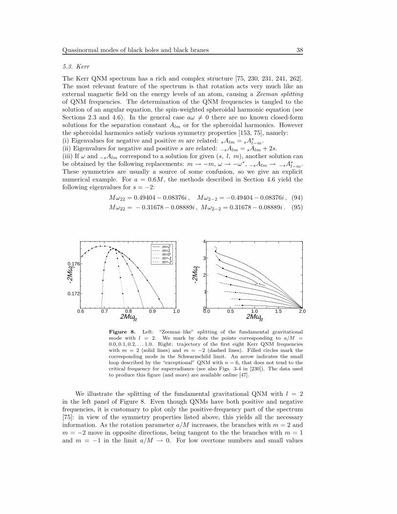
Quasinormal modes of black holes and black branes 38
5.3. Kerr
The Kerr QNM spectrum has a rich and complex structure [75, 230, 231, 241, 262].The most relevant feature of the spectrum is that rotation acts very much like anexternal magnetic field on the energy levels of an atom, causing a Zeeman splittingof QNM frequencies. The determination of the QNM frequencies is tangled to thesolution of an angular equation, the spin-weighted spheroidal harmonic equation (seeSections 2.3 and 4.6). In the general case aω 6= 0 there are no known closed-formsolutions for the separation constant Alm or for the spheroidal harmonics. Howeverthe spheroidal harmonics satisfy various symmetry properties [153, 75], namely:(i) Eigenvalues for negative and positive m are related: sAlm = sA
∗l−m.
(ii) Eigenvalues for negative and positive s are related: −sAlm = sAlm + 2s.(iii) If ω and −sAlm correspond to a solution for given (s, l, m), another solution canbe obtained by the following replacements: m → −m, ω → −ω∗, −sAlm → −sA
∗l−m.
These symmetries are usually a source of some confusion, so we give an explicitnumerical example. For a = 0.6M , the methods described in Section 4.6 yield thefollowing eigenvalues for s = −2:
Mω22 = 0.49404− 0.08376i , Mω2−2 = −0.49404− 0.08376i , (94)
Mω22 = − 0.31678− 0.08889i , Mω2−2 = 0.31678− 0.08889i . (95)
0.6 0.7 0.8 0.9 1.02MωR
0.172
0.176
-2M
ω I
m=2m=1m=0m=-1m=-2
0.0 0.5 1.0 1.5 2.02MωR
0
1
2
3
4
-2M
ω I
Figure 8. Left: “Zeeman–like” splitting of the fundamental gravitationalmode with l = 2. We mark by dots the points corresponding to a/M =0.0, 0.1, 0.2, . . . 1.0. Right: trajectory of the first eight Kerr QNM frequencieswith m = 2 (solid lines) and m = −2 (dashed lines). Filled circles mark thecorresponding mode in the Schwarzschild limit. An arrow indicates the smallloop described by the “exceptional” QNM with n = 6, that does not tend to thecritical frequency for superradiance (see also Figs. 3-4 in [230]). The data usedto produce this figure (and more) are available online [47].
We illustrate the splitting of the fundamental gravitational QNM with l = 2in the left panel of Figure 8. Even though QNMs have both positive and negativefrequencies, it is customary to plot only the positive-frequency part of the spectrum[75]: in view of the symmetry properties listed above, this yields all the necessaryinformation. As the rotation parameter a/M increases, the branches with m = 2 andm = −2 move in opposite directions, being tangent to the the branches with m = 1and m = −1 in the limit a/M → 0. For low overtone numbers and small values

Quasinormal modes of black holes and black branes 39
of a/M the rotation-induced splitting of the modes is roughly proportional to m, asphysical intuition would suggest.
The weakly damped modes of Kerr black holes In the right panel of Figure 8 we showthe first eight gravitational QNM frequencies with m = 2 (solid lines) and m = −2(dashed lines). A general feature is that almost all modes with m > 0 cluster at thecritical frequency for superradiance, 2Mω = m, as a/M → 1. This fact was firstobserved by Detweiler [262], and a thorough examination of the extremal limit can befound in Refs. [263, 264, 265]. The mode with n = 6 (marked by an arrow) shows apeculiar deviation from the general trend, illustrating the fact that some positive-mmodes do not tend to this critical frequency in the extremal limit.
0.0 0.2 0.4 0.6 0.8 1.0a/M
0.0
0.2
0.4
0.6
0.8
1.0
1.2
1.4
1.6
1.8
Mω lm
n
l=2
l=3
l=4
0.0 0.2 0.4 0.6 0.8 1.0a/M
0.0
2.0
4.0
6.0
8.0
Qlm
n
l=2
l=3
l=4
Figure 9. Frequencies and quality factors for the fundamental modes withl = 2, 3, 4 and different values of m. Solid lines refer to m = l, .., l (fromtop to bottom), the dotted line to m = 0, and dashed lines refer to m = −1, ..,−l(from top to bottom). Quality factors for the higher overtones are lower than theones we display here.
For gravitational wave detection we are mostly interested in the frequency andquality factor of the dominant modes, which determine whether the mode lies in thesensitive frequency band of a given detector and the number of observable cycles.Figure 9 shows these quantities for QNMs with l < 5. Improving on previous results[9, 266], Ref. [10] presented accurate fits for the first three overtones with l = 2, 3, 4and all values of m, matching the numerical results to within 5% or better over a rangeof a/M ∈ [0, 0.99] (see Tables VIII-X in Ref. [10] and the numerical data available
online [47]). For instance, defining b ≡ 1 − a/M , the frequency ωlm = ωR and qualityfactor Qlm ≡ ωR/(2ωI) of the fundamental l = m = 2 and l = 2 ,m = 0 modes are
Mω22 ≃ 1.5251− 1.1568 b0.1292 , Q22 ≃ 0.700 + 1.4187 b0.4990 , (96)
Mω20 ≃ 0.4437− 0.0739 b0.3350 , Q20 ≃ 4.000 − 1.9550 b0.1420 , (97)
The highly damped modes The intermediate- and large-damping regime of the QNMspectrum of Kerr BHs is even more puzzling than the RN spectrum. The maintechnical difficulty in pushing the calculation to higher damping is that Leaver’sapproach requires the simultaneous solution of the radial and angular continued
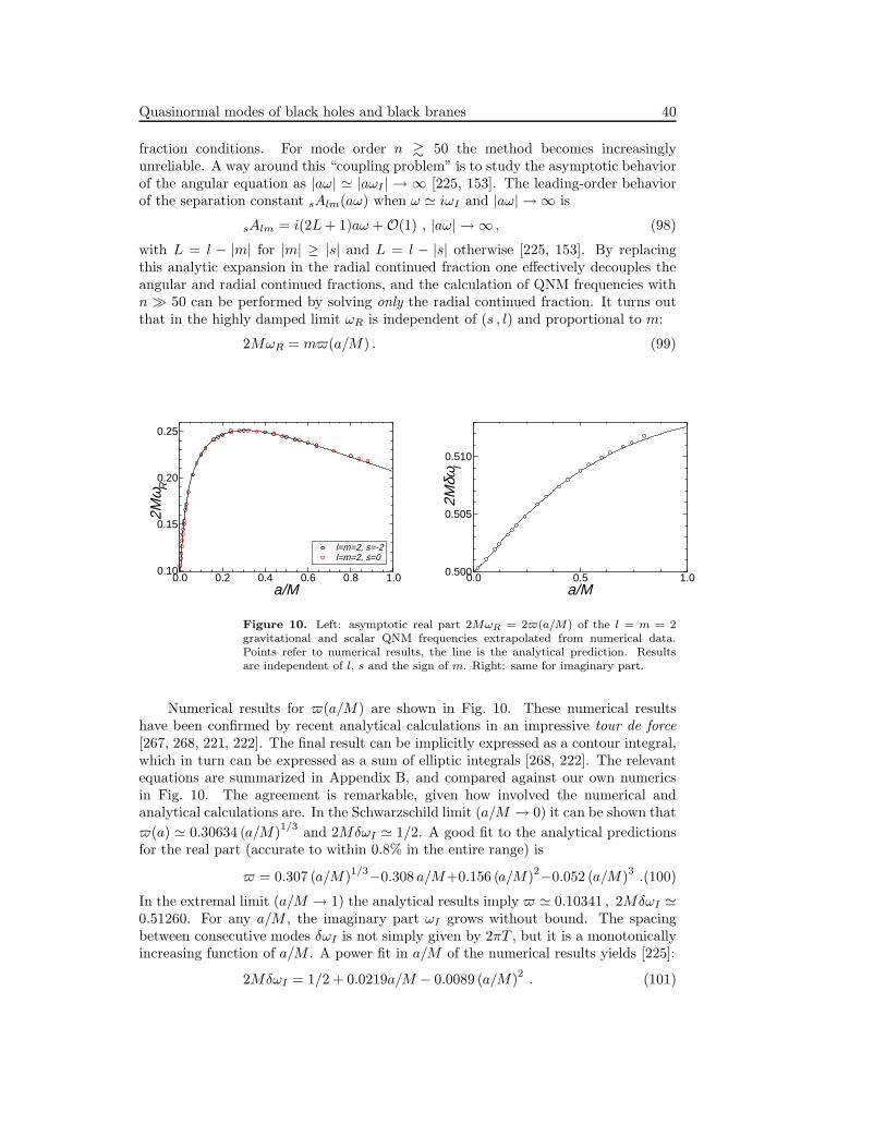
Quasinormal modes of black holes and black branes 40
fraction conditions. For mode order n & 50 the method becomes increasinglyunreliable. A way around this “coupling problem” is to study the asymptotic behaviorof the angular equation as |aω| ≃ |aωI | → ∞ [225, 153]. The leading-order behaviorof the separation constant sAlm(aω) when ω ≃ iωI and |aω| → ∞ is
sAlm = i(2L+ 1)aω + O(1) , |aω| → ∞ , (98)
with L = l − |m| for |m| ≥ |s| and L = l − |s| otherwise [225, 153]. By replacingthis analytic expansion in the radial continued fraction one effectively decouples theangular and radial continued fractions, and the calculation of QNM frequencies withn ≫ 50 can be performed by solving only the radial continued fraction. It turns outthat in the highly damped limit ωR is independent of (s , l) and proportional to m:
2MωR = m(a/M) . (99)
0.0 0.2 0.4 0.6 0.8 1.0a/M
0.10
0.15
0.20
0.25
2Mω R
l=m=2, s=-2l=m=2, s=0
0.0 0.5 1.0a/M
0.500
0.505
0.5102M
δωI
Figure 10. Left: asymptotic real part 2MωR = 2(a/M) of the l = m = 2gravitational and scalar QNM frequencies extrapolated from numerical data.Points refer to numerical results, the line is the analytical prediction. Resultsare independent of l, s and the sign of m. Right: same for imaginary part.
Numerical results for (a/M) are shown in Fig. 10. These numerical resultshave been confirmed by recent analytical calculations in an impressive tour de force[267, 268, 221, 222]. The final result can be implicitly expressed as a contour integral,which in turn can be expressed as a sum of elliptic integrals [268, 222]. The relevantequations are summarized in Appendix B, and compared against our own numericsin Fig. 10. The agreement is remarkable, given how involved the numerical andanalytical calculations are. In the Schwarzschild limit (a/M → 0) it can be shown that
(a) ≃ 0.30634 (a/M)1/3
and 2MδωI ≃ 1/2. A good fit to the analytical predictionsfor the real part (accurate to within 0.8% in the entire range) is
= 0.307 (a/M)1/3−0.308 a/M+0.156 (a/M)2−0.052 (a/M)3 .(100)
In the extremal limit (a/M → 1) the analytical results imply ≃ 0.10341 , 2MδωI ≃0.51260. For any a/M , the imaginary part ωI grows without bound. The spacingbetween consecutive modes δωI is not simply given by 2πT , but it is a monotonicallyincreasing function of a/M . A power fit in a/M of the numerical results yields [225]:
2MδωI = 1/2 + 0.0219a/M − 0.0089 (a/M)2. (101)
Quasinormal modes of black holes and black branes 41
The agreement between the analytical predictions for the mode spacing and the fit ofEq. (101) is better than 0.1% in the entire range of a/M . A generalization of theseasymptotic results to higher-dimensional rotating BHs can be found in Ref. [222].
The eikonal limit The eikonal limit of Kerr QNMs is not yet fully understood. Partialresults concern l = ±m modes, for which [73, 10, 208]
ω = ±mΩc − (n+ 1/2) |Ωc|√
3M/rc δ−1 , (l = |m| → ∞) , (102)
where rc , Ωc are counter-rotating or co-rotating radius and orbital frequencies at theunstable circular null geodesics, and 2δ = rc(rc −M)/(r2c − 2Mrc + a2). Again, thisresult can be expressed as ω ∼ lΩc − i(n + 1/2)/τ , with τ the typical instabilitytimescale of the unstable circular null geodesic [73, 10, 208]. To our knowledge, asimple geometrical optics interpretation is still lacking for modes with l 6= |m|.
5.4. Kerr-Newman
General BH solutions of the Einstein-Maxwell system are described by the Kerr-Newman metric. For this metric the Klein-Gordon equation and the Dirac equation arestill separable [269], so QNMs can be computed using the same general methods thatapply to Kerr BHs [256]. The scalar spectrum was analyzed by Berti and Kokkotas[233], who showed in particular that the eikonal limit can still be understood in termsof unstable circular null geodesics.
Unfortunately, studies of the interplay of electromagnetic and gravitational fieldsin the Kerr-Newman metric are plagued by a major technical difficulty: to date, allattempts to decouple the electromagnetic and gravitational perturbations have failed(see e.g. Section 111 of Ref. [22]). Approximations to gravitational/electromagneticperturbations of the Kerr-Newman geometry either keep the geometry fixed andperturb the electric field, or (more interestingly) keep the electric field fixed andperturb the geometry. This approach should be appropriate for values of the charge Qat most as large as the perturbations of the spacetime metric. QNMs for gravitationaland electromagnetic perturbations in this approximation scheme were computed inRefs. [270, 233], but a solution of the general problem is highly desirable, and it couldshed light on many open problems in BH physics.
5.5. Higher dimensional Schwarzschild-Tangherlini black holes
Here we briefly discuss the QNM spectrum of the higher-dimensional analogs of theSchwarzschild solution, known as Schwarzschild-Tangherlini BHs. Electromagneticperturbations of these BHs were considered by Crispino, Higuchi and Matsas [134].The elegant work by Kodama and Ishibashi [102, 103, 104] laid the foundations forthe analysis of higher-dimensional RN BHs.
Weakly damped modes The lowest lying QNMs of a d−dimensional Schwarzschild-Tangherlini BH were computed in a WKB approximation in Refs. [216, 271, 272, 204].Leaver’s method can be generalized to these higher-dimensional BHs [234, 235],although the number of terms in the recurrence relation rapidly grows with d.For instance, in d = 5 the recurrence relation for vector-gravitational and tensor-gravitational perturbations has four terms, while for scalar-type gravitational QNMfrequencies it has eight terms [235]. A naive application of Leaver’s method breaks
Quasinormal modes of black holes and black branes 42
down for d > 9. For large d more and more singularities, spaced uniformly on the circle|r| = rh (where rh is the horizon radius) approach the horizon at r = rh. A solutionsatisfying the outgoing wave boundary condition at the horizon must be continuedto some mid point, and only then can the continued fraction condition be applied[273]. Alternative calculations of weakly damped modes for scalar and gravitationalperturbations in d dimensions make use of time evolutions [274].
Highly-damped modes In the large-damping limit, the leading-order result of themonodromy calculation, Eq. (86), generalizes to the d-dimensional Schwarzschild-Tangherlini metric. This was first suggested in Ref. [101], and then it was explicitlyshown by Birmingham [275] (see also [276]). The perturbative technique of Ref. [245]has been extended to bosonic fields in higher-dimensional Schwarzschild-TangherliniBHs, with the result [234]
ω = T ln(1 + 2 cosπj) + (2n+ 1)πiT + kdω−(d−3)/(d−2)I . (103)
Here j = 0 for scalar fields and tensor-type gravitational perturbations, j = 2 forvector-type gravitational perturbations and j = 2/(d − 2) , 2 − 2/(d − 2) for vector-and scalar-type electromagnetic perturbations, respectively. The coefficient kd canbe determined analytically for given values of d and j [234]. For electromagneticperturbations in d = 5, Eq. (103) is singular: this either means that there are noasymptotic QNM frequencies at all (a possibility first suggested in [101]) or that theasymptotic frequency is zero. Numerical results support the latter possibility [234].
The result above illustrates a general feature of the high-damping regime, whichconcerns the damping itself. It was shown by several authors [277, 278, 249] that forspacetimes with a single horizon, for all values of l one has
ωI = −2πin/T , n→ ∞ , (104)
where T is the Hawking temperature. General results for the oscillation frequencieswere obtained in Ref. [279] for single-horizon spacetimes (see also [280] for BHs intwo-dimensional dilaton gravity). An elegant unification of these results dealing witha rather general class of wave equations is given in Ref. [281] (but see Ref. [282] forwords of caution on the generality of the results). A review on the highly dampedregime of QNMs for several spacetimes can be found in Ref. [107].
Eikonal limit For l ≫ 1, a WKB analysis of the Schwarzschild-Tangherliniperturbation equations yields [216, 208],
ω r+ = Ωc
(
l + d/2 − 3/2 − i(n+ 1/2)√d− 3
)
. (105)
where Ωc =√d− 3/
√d− 1 [2/(d− 1)]
1d−3 is the orbital angular velocity at the circular
null geodesic [208].
Infinite-dimensional limit (d→ ∞) To our knowledge, the interesting limit where thedimensionality d tends to infinity has not been studied in much detail in the literature.Using a WKB analysis for scalar fields or gravitational tensor modes we find
ω r+ = d/2 − iκ√
d/2 , d→ ∞ , (106)
with κ a factor of order unity depending on the perturbing field (κ = 1, 1/√
2 for scalarfields and vector gravitational perturbations, respectively). BHs in higher dimensions

Quasinormal modes of black holes and black branes 43
are much better resonators, with a quality factor Q ≡ ωR/[2ωI ] increasing as√d. As
far as we know, no numerical studies are available to confirm this analytical prediction.It is important to recall that black objects in higher dimensions may have other
topologies beside the spherical one. One family consists of the so-called black strings,whose gravitational perturbations were studied by Gregory and Laflamme [283, 284]and Kudoh [285]. Higher-dimensional “squashed” Kaluza-Klein BHs were consideredin [286], and perturbations of brane-localized BHs were studied, for instance, in[287, 288, 289]. Apart from specific noteworthy exceptions [290, 291, 292, 293],gravitational perturbations of higher-dimensional rotating solutions are yet to beunderstood. For a review on higher-dimensional BHs, see Ref. [34].
6. The spectrum of asymptotically anti-de Sitter black holes
6.1. Schwarzschild anti-de Sitter black holes
The metric (3) of an uncharged static BH in an (asymptotically) AdS spacetime hastwo parameters, r0 and L, related, respectively, to the mass of the BH and thecosmological constant. The horizon radius r+ is the largest root of the equationf(r) = 0. The Hawking temperature associated with the metric (3) is
T =[
d− 3 + (d− 1)ξ2]
/ (4πξL) , (107)
where ξ = r+/L. For d ≥ 4, this function has a characteristic minimum atξmin =
√
(d− 3)/(d− 1) with Tmin =√
(d− 1)(d− 3)/2πL (see Fig. 11).
0 1 2 3ξ=r+ /L
0.0
0.2
0.4
0.6
0.8
1.0
TL
TcL
ξc
Figure 11. The (dimensionless) Hawking temperature TL as a function of the(dimensionless) horizon radius r+/L for asymptotically AdS BHs (shown here ford = 5). The horizontal line is the critical temperature of the Hawking-Page phasetransition.
The specific heat of BHs with ξ < ξmin (ξ > ξmin) is negative (positive). ForT < Tmin, no BH solution exists, and the state with minimal free energy is “thermalAdS” (Euclidean AdS/Z). For T > Tmin, there are two solutions with the sametemperature, “small” and “large” BHs. Small BHs have negative specific heat andare thermodynamically unstable. Large BHs exist in equilibrium with the heat bath.

Quasinormal modes of black holes and black branes 44
Moreover, for ξ < 1, the minimum of the free energy still corresponds to thermal AdS,even for T > Tmin. Thus the stable ground state is given by large BHs with ξ > 1(and T > Tc = (d − 2)/2πL). The (first order) transition between thermal AdS anda large AdS BH is known as the Hawking-Page phase transition [294]. As shown byWitten [295], in the gauge-gravity duality this transition corresponds to a first orderdeconfinement transition in a dual thermal strongly coupled gauge theory on a sphereof radius L. These considerations can be extended to charged and rotating AdS BHs(see e.g. [296, 297] and references therein). The role of small AdS BHs in the gauge-gravity duality is not well understood (see, however, Ref. [298]). The limit of extralarge BHs with r+/L → ∞ in the appropriate scaling leads to black branes dual tostrongly coupled gauge theories in flat space (see Section 8).
BHs in AdS in the context of the gauge-string duality attract considerable interestbecause they serve as a good laboratory for studying the most acute problems of atheory of gravity: the information loss paradox, BH singularities and some aspectsof quantum gravity. Although we will not venture into this fascinating field in thisreview, in Section 8 we mention some of these topics which involve the use of QNMs.
Another peculiar feature of asymptotically AdS space is the “active role” playedby its boundary. In AdS, null geodesics reach the boundary in finite coordinate time.One thus often refers to an asymptotically AdS space as a box, having in mind thatAdS boundary conditions directly affect the bulk physics [299, 300, 301]. This shouldbe contrasted with the asymptotically flat case, where the only physically relevantchoice for the boundary conditions of the bulk fluctuations corresponds to outgoingwaves at spatial infinity. In the gauge-gravity duality, the choice of the AdS boundaryconditions is dictated by a holographic prescription [98, 302, 303, 304], see Section 8.
QNMs in asymptotically AdS backgrounds were first considered by Chan andMann for a conformally coupled scalar field [305] (see also Ref. [306]). Subsequentinterest was strongly motivated by the development of the AdS/CFT correspondence.An interesting albeit somewhat qualitative discussion of thermalization in AdS/CFTfirst mentioning QNMs appeared in Ref. [307] (see also the important work ofDanielsson, Keski-Vakkuri and Kruczenski [308, 309]). Horowitz and Hubeny [92]explicitly pointed out the fundamental link between QNMs of a large AdS BH, whichdescribe the background’s relaxation into a final state, and the dual field theory, wherethey describe the approach to thermal equilibrium. Ref. [92] computed the QNMs ofa minimally coupled massless scalar in intermediate or large AdS BHs for dimensionsd = 4, 5, 7. After this seminal work, a series of studies in four and higher dimensionsled to a deeper understanding of QNMs in asymptotically AdS backgrounds.
The following is a brief overview of the QNMs of the four and higher-dimensionalSAdS geometries. For more details we refer to the original works (see [92, 107, 130, 131,310, 194, 311, 312, 313, 223, 314, 315, 316, 317, 318, 319, 320, 271, 321, 322, 323, 324]and references therein). The results below focus mostly on the large BH regimer+/L ≫ 1 and on Dirichlet boundary conditions, which are more relevant forholography. Other boundary conditions were investigated in Refs. [162, 163, 164, 165].
The weakly damped modes of large black holes The fundamental QNM frequenciesfor scalar field perturbations were first computed by Horowitz and Hubeny [92]for intermediate and large BHs. In Refs. [130, 194] the analysis was extendedto electromagnetic and gravitational perturbations. These works considered onlyd = 4; the d = 5 case was analyzed in Ref. [316], and half-integer spins wereconsidered in Refs. [325, 326]. Approximate analytical solutions have been discussed

Quasinormal modes of black holes and black branes 45
in Refs. [312, 313, 314] with particular emphasis on the d = 5 geometry.
-10 -5 0 5 10L
2ωR /r+
0
5
10
15
20-L
2 ω I/r +
Scalar/Vector-type/Scalar-type
Electromagnetic
"Special" vector-type
Figure 12. QNM frequencies for scalar (s = 0), electromagnetic (s = 1) andgravitational (s = 2) perturbations of large SAdS BH, computed for r+/L = 100and l = s. In the large BH regime the frequencies scale with r+/L and arebasically independent of l for l ≪ r+/L. Furthermore, scalar-field, tensor-typeand vector-type gravitational perturbations are nearly isospectral, except for aspecial mode belonging to the vector-type family and marked by a red diamond.For further details see [194, 311].
The weakly-damped QNM spectrum of a large (r+/L = 100) SAdS BH ind = 4 is shown in Fig. 12. Usually the QNM frequencies scale with the horizonradius, ω ∝ r+/L
2 [92, 194], so the modes of any large BH can be obtainedby rescaling appropriately the numbers in the figure. The exception to this ruleis marked by a red diamond and will be discussed in more detail below. Thefrequencies of different perturbations are very similar: scalar perturbations and scalar-type gravitational perturbations have basically the same spectra, while vector-typegravitational perturbations are displaced by one overtone relative to these two [194].The QNM frequencies are practically independent of l for l ≪ r+/L; the large-l limit isdiscussed below. The QNM spectrum for electromagnetic perturbations has a peculiarstructure [130, 311, 194, 327, 328]: the real part of some modes asymptotes to zerowhen r+/L→ ∞, and for the dominant mode ωIL
2/r+ → −1.5.The fundamental QNM for vector-type gravitational perturbations is extremely
long-lived when compared to all other modes of other kinds of perturbations. Thismode has an interesting interpretation in the gauge/gravity duality, discussed inSection 8. The timescale of this long-lived mode is proportional to r+, and the modeitself is easily computed numerically by a straightforward application of the seriessolution [130, 194]. In a general d−dimensional SAdS geometry it is well described by
r+ ωvector−typen=0 = −i(l− 1)(l + d− 2)/(d− 1) , r+/L≫ 1 . (108)
This was first observed numerically in Refs. [130, 194] for d = 4, and in Ref. [316] ford = 5. The four-dimensional result was later confirmed analytically by Miranda andZanchin [315]. Eq. (108) for general d was derived by Siopsis [324], and we checked

Quasinormal modes of black holes and black branes 46
that it agrees with numerical results for d = 4 up to d = 8. In d = 4 and for r+/L≫ l,corrections to Eq. (108) can be found:
r+ ωvector−typen=0 = −i(l− 1)(l + 2)/3 − 0.0288 i l4L2/r2+ . (109)
We estimate the uncertainty in the l4 term to be about 5%. Analytical calculationsof these corrections have been done in the r+ → ∞ limit [109, 329, 330] and areconsistent with the numerical results above after proper identifications. In this limitthe geometry becomes that of a black brane and the angular wavefunctions Ylm arereplaced by ei~p~x. For large l, p one has the correspondence Lp = l [331]. In particular,it is found that in the large l/L limit,
ω r+ = − il2
3− iL2l4
9 − 9 log 3 +√
3 π
162r2+∼ − il
2
3− 0.0281L2l4
r2+, (110)
in quite good agreement with the numerical fits. For similar high-order analyticalcorrections in higher-dimensional AdS backgrounds, see Refs. [109, 329, 330].
If Dirichlet boundary conditions are imposed at infinity, the scalar-typegravitational sector does not have such a long-lived mode. It was suggested that thepreferred boundary conditions in the AdS/CFT framework are of Robin type, and inparticular that the perturbations should not deform the metric on the AdS boundary[316, 163]. Using Robin conditions, a long-lived mode for gravitational perturbationswas discovered in Refs. [316, 163, 324].
The weakly damped modes of small black holes The series solution method, whichworks so well for large BHs, converges very slowly for small BHs [318, 310, 194].Recent results make use of Breit-Wigner type resonances in the scattering cross-sectionto study the very small BH regime [227], described briefly in Section 4.5. Small andlarge BHs have a very different behavior from a QNM perspective. This is relatedto the qualitatively different behavior of the potential in the two regimes, which isshown in the left panel of Fig. 13 for s = 0: for small BHs (r+/L < 1) the potentialdevelops a well capable of sustaining trapped, long-lived modes, corresponding toquasi-stationary states in quantum mechanics [332, 331, 227]. In the right panel ofFig. 13 we plot the QNMs of scalar fields for different BH sizes and l = 0, 1. In thislimit (and under the assumption that MωR ≪ 1) it is possible to prove that [333]
ωR L ≃ l + 3 + 2n− kln r+/L , (111)
ωI L ≃ −γ0(l, n) (l + 3 + 2n) (r+/L)2l+2
/π . (112)
The constant γ0(l, n) (n = 0, 1, 2, . . .) and selected values of the constants kl0 canbe found in Ref. [227]. The analytic prediction is consistent with numerical results.Likewise, for gravitational perturbations with r+/L≪ 1 one finds
ωR L ≃ l + 2 + 2n− cln r+/L , (113)
ωI L ≃ −γ2(l, n) (l + 2 + 2n) (r+/L)2l+2
, (114)
where the constants cln and γ2(l, n) can be found in Refs. [334, 227]. In conclusion: forscalar field and gravitational perturbations of small SAdS BHs the damping timescaleωIL ∼ (r+/L)2l+2, and the oscillation frequencies approach the pure AdS value in thelimit r+/L→ 0 (see [310, 227] for more details). To our knowledge, generalizations ofthese results to charged, higher-dimensional and rotating AdS BHs are still lacking.

Quasinormal modes of black holes and black branes 47
10-5
10-4
10-3
10-2
10-1
100
101
102
103
104
105
106
r/L10
-110
010
110
210
310
410
510
610
710
810
910
1010
1110
1210
13
V s=0
r+ /L=10-4
r+ /L=10-3
r+ /L=10-2
r+ /L=10-1
r+ /L=1
r+ /L=102
r+ /L=104
l=0
1 10 100ωRL
10-9
10-8
10-7
10-6
10-5
10-4
10-3
10-2
10-1
100
101
102
103
-ωIL
l=0l=1
Figure 13. Left: Potential for scalar field propagation of l = 0 modes in aSAdS background, for different values of the BH size r+/L. A local maximum(and a potential well) only exist for small BHs. Right: Track described by thefundamental scalar field QNMs with l = 0 and l = 1 as we vary the BH size r+/L.Counterclockwise starting from the top-right of the figure we marked the pointscorresponding to different decades in r+/L (r+/L = 102, 101, 100, 10−1, . . .).Modes with different l coalesce in the large BH regime, as long as l ≪ r+/L.
The highly-damped modes The large-damping regime (n ≫ 1) can be studied usingthe monodromy method for both small and large AdS BHs [107, 223]. For n≫ 1 andr+/L≫ 1 (large BHs) the QNMs are given by
ωL2
r+= (d− 1) sin
(
π
d− 1
)
eiπ
d−1
[
n+d+ 1
4− i
log 2
2π
]
. (115)
Results for arbitrarily sized BHs can be found in Refs. [107, 223]. Eq. (115) describesscalar fields, gravitational tensor and gravitational vector-type perturbations. Ityields ωL2/r+ ≈ (1.299 + 2.250i)n + (0.573 + 0.419i) for d = 4 and ωL2/r+ ≈(2 + 2i)n+ 3.22064+ 2.77936 for d = 5, in good agreement with numerical results ford = 4 [194] and d = 5 [316]. For large SAdS BHs the asymptotic high-damping regimeis approached very quickly, so Eq. (115) describes fairly well even weakly-dampedmodes. There is some disagreement concerning the offset for scalar-type gravitationalperturbations [107].
An asymptotic analysis based on the monodromy method was recently used topredict the existence of a new family of modes [335]. So far, this new part of thespectrum has not been confirmed by numerical studies. In Ref. [336] the authorsdiscuss the interesting possibility of describing the highly damped QNM regime interms of geodesics of the SAdS spacetime.
The eikonal limit of large black holes In asymptotically AdS spacetimes the eikonallimit is especially interesting, since large-l modes can be very long-lived [92, 331].A WKB analysis [331] and numerical investigations [337] show that for scalar fieldperturbations, r+/L≫ 1 and l ≫ 1
ω L = l + Πn (r+/L)2d−2d+1 l−
d−3d+1 , (116)
Quasinormal modes of black holes and black branes 48
Πn ≡ 1
2
(√π(d− 1)
[
d+ 1
2+ 2n
]
Γ (3/2 + 1/(d− 1))
Γ (1/(d− 1))
)
2d−2d+1
e−i2π
d+1 .
So large-l modes are very long-lived, and they could play a prominent role in the BH’sresponse to generic perturbations. This is at variance with the asymptotically flatcase, where the damping timescale is roughly constant as l varies. Notice also that thescaling with the BH size differs from that of the weakly-damped and highly-dampedmodes. Other types of perturbations also display a similar qualitative behavior [337].
The eikonal limit of small black holes For scalar and electromagnetic perturbationsof small BHs the potential for wave propagation for l ≫ 1 develops a minimum,potentially supporting quasi-stationary states, i.e. long-lived modes (see Fig. 13).Define rb > rc to be the two real zeros (turning points) of ω2
R − p2f/r2 = 0. Then thereal part of a class of long-lived modes in four spacetime dimensions is given by theWKB condition
2
∫ ∞
rb
√
r2ω2R − p2f
rfdr = π
(
2n+ 1 +3
2
)
, (117)
where p = l + d/2 − 3/2. Their imaginary part is given by
ωI =γΓ
8ωR, log Γ = 2i
∫ rc
rb
√
r2ω2R − p2f
rfdr . (118)
The prefactor γ, not shown in Ref. [331], can be obtained by standard methods asshown in Ref. [227], where these results are also supported by numerical calculations.
6.2. Reissner-Nordstrom and Kerr anti-de Sitter black holes
The analysis of QNMs of large RNAdS BHs was performed in Ref. [338, 339] forweakly damped modes of a massless scalar field, and later extended to charged scalarfields [340]. Scalar field, electromagnetic and gravitational perturbations of RNAdSBHs were analyzed and compared in Ref. [311]. Half-integer spins were studied inRefs. [341, 342]. Gravitational perturbations of higher-dimensional charged solutionswere considered in [343], and the highly-damped regime was explored analytically byNatario and Schiappa [107].
Ref. [311] pointed out some interesting facts: (i) a near-isospectrality of differentclasses of perturbations holds for large BHs, but it breaks down as r+/L decreases,i.e. in the small BH limit; (ii) the imaginary part of the purely damped modes foundfor electromagnetic and vector-type gravitational perturbations tends to zero as thecharge Q tends to the extremal value Qext, possibly pointing to a marginal instabilityof extremal RNAdS BHs; (iii) for all kinds of perturbations, the real part of thefundamental QNM frequency, LωR, has a minimum for Q/Qext ≃ 0.366, followedby a maximum at LωR ≃ 0.474. A reanalysis of massless scalar field perturbationsfound that the imaginary part of scalar QNMs also tends to zero in the extremallimit [344]. However, comparing time-evolutions of the field with results from theHorowitz-Hubeny series solution, Wang et al. [344] found that the BH response turnsfrom a standard, oscillatory QNM-type decay below some critical value of the charge(Q < Qcrit ≃ 0.3895Qext) to a non-oscillatory behavior characterized by a purelyimaginary QNM frequency for Q > Qcrit. Furthermore, these authors suggested thatthe potential marginal instability proposed in Ref. [311] does not pose a threat forextremal RNAdS BHs, because (at least for scalar perturbations) the asymptotic field

Quasinormal modes of black holes and black branes 49
in the near-extremal limit is dominated by a power-law tail of the type first analyzedby Price [171]. The implications of these findings in the context of the AdS/CFTcorrespondence deserve further investigation.
There are few studies of QNMs of rotating BHs in AdS backgrounds. Theformalism to handle perturbations of these spacetimes was laid down by Chambersand Moss [345]. Giammatteo and Moss [346] considered axially symmetric QNMsof large Kerr-AdS BHs. These spacetimes behave as a BH in a box. Superradiantamplification of incident waves at the expense of the BH’s rotational energy canthen produce instabilities in the non-axisymmetric modes of small Kerr AdS BHs[347, 333, 334, 348, 349, 292, 350]: this is an interesting example of the “black holebomb” first investigated by Press and Teukolsky [351].
6.3. Toroidal, cylindrical and plane-symmetric anti-de Sitter black holes
The uniqueness theorems that apply for asymptotically flat BHs (see e.g. [39]) can beevaded when the cosmological constant is non-zero: solutions have been found withthe topology of a cylinder, of a plane or of a doughnut [122, 123, 124, 125, 126, 127].Defining f(r) = r2/L2 − 4M/r, these spacetimes are described by
ds2 = f dt2 − f−1dr2 − r2 dz2 − r2dφ2. (119)
The range of the coordinates z and φ dictates the topology of the BH spacetime. Fora BH with toroidal topology the coordinate z is compactified such that z/L rangesfrom 0 to 2π, and φ ranges from 0 to 2π as well. For the cylindrical BH, or blackstring, the coordinate z has range −∞ < z <∞, and 0 ≤ φ < 2π. For the planar BH,or black membrane, the coordinate φ is further decompactified (−∞ < Lφ <∞). Forthe torus, M is related to the system’s ADM mass; for the cylinder, to the mass perunit length of a constant-z line; and for the plane, to the mass per unit area of the(φ, z) plane [122, 123, 124, 125, 126, 127].
A formalism to handle electromagnetic and gravitational perturbations of thesespacetimes was developed and used to investigate numerically the QNMs of scalar,electromagnetic and gravitational perturbations in Ref. [131]. A thorough analysis byMiranda and Zanchin [315, 327] confirmed and extended the results of Ref. [131].
7. The spectrum of asymptotically de Sitter and other black holes
7.1. Asymptotically de Sitter black holes
BHs in a dS background have a rich structure. Consider an uncharged sphericallysymmetric BH, the SdSd solution,
ds2 = fdt2 − f−1dr2 − r2dΩ2d−2 , (120)
where f(r) = 1−r2/L2−rd−30 /rd−3, dΩ2
d−2 is the metric of the (d−2)−sphere, and r0is related to the mass M of the spacetime by M = (d−2)Ad−2r
d−30 /(16π). Depending
on the value of r0/L2, in general this solution has two horizons, the event and the
cosmological horizon. When the cosmological and event horizons coalesce one has aso-called extremal SdSd solution, which is related to a topologically different solution,known as the Nariai spacetime [199, 200, 201, 196].

Quasinormal modes of black holes and black branes 50
Weakly damped modes The first calculations of the fundamental gravitational modeswere done by Mellor and Moss [129] for Reissner-Nordstrom-de Sitter (RNdS) BHs,using numerical techniques. Brady et al. [352] complemented this study througha numerical time evolution of scalar fields in the SdS spacetime. Time evolutionswere also performed in Ref. [353], where the results were compared against WKBpredictions (see also Ref. [274]). Approximations to the correct, lowest order QNMswere considered in Refs. [162] (s = 2, SdS), [354] (s = 0, SdS), [355] (s = 1/2, RNdS)and [356] (s = 2, RNdS), where the true potential was approximated by a Poschl-Teller potential. Cardoso and Lemos [191] showed that the true potential reducesto the Poschl-Teller potential for near extremal SdS geometries, which explains whyprevious results based on the Poschl-Teller approximation gave accurate predictionsfor the QNMs. The results in [191] were later generalized to d-dimensional RNdS BHs[197]. Other analytical results used the WKB approximation for spins s = 0, 1, 2, 1/2in the vicinity of SdS BHs [357].
Highly-damped modes The highly-damped limit, where the imaginary part is muchlarger than the real part, was studied numerically by Yoshida and Futamase [238] fornear-extremal uncharged BHs (s = 1, 2) and in the general case in Ref. [358, 239]. Theresults were confirmed analytically in Refs. [223] (s = 0, 1, 2 SdS) and [107] (s = 0, 1, 2RNdS).
Eikonal limit In the large-l limit, WKB techniques [190, 357] yield
3√
3Mω =√
1 − 27M2/L2 [l + 1/2 − i(n+ 1/2)] . (121)
QNMs in the eikonal limit can be interpreted as perturbations of unstable circularnull geodesics [208]. For studies on charged and rotating BHs in dS backgrounds, see[359] and references therein.
7.2. Black holes in higher-derivative gravity
Among all possible theories of gravity with higher derivative terms, theories modifiedby the addition of a Gauss-Bonnet term RGB = RµνρσR
µνρσ − 4RµνRµν + R2, are
particularly attractive and have been considered by many authors [360]. There aresimple BH solutions in these theories [361, 362, 363, 364, 365, 366, 367, 368, 369,370], whose perturbations were studied in a series of works by Dotti and Gleiser[371, 372, 373], Moura and Schiappa [360] and Takahashi and Soda [374]. In fourdimensions the Gauss-Bonnet term is a total divergence, and yields upon integrationa topological invariant, being therefore equivalent to Einstein’s theory. Thereforethese theories are interesting in higher dimensions only. Non-trivial four-dimensionalscenarios can be accomplished by coupling the Gauss-Bonnet term to a dilaton[367]: the resulting theory also arises from the low-energy limit of certain stringtheories [360]. Perturbations of BH spacetimes in these scenarios were consideredin Refs. [367, 375, 365].
QNMs of BHs in these theories were first investigated by Iyer et al. [376], whoused a WKB approach to study scalar perturbations. QNMs of these spacetimes werealso studied through a WKB approach [377, 378, 379], and numerically [380, 377]for the low-lying modes. The highly-damped regime was analytically explored inRef. [282]. The eikonal limit was considered by Konoplya [380] and interpreted interms of circular null geodesics in Ref. [208].

Quasinormal modes of black holes and black branes 51
7.3. Braneworlds
Braneworld scenarios, where the standard model lives in a four-dimensional braneembedded in a higher dimensional spacetime, have been a popular research topicin the last decade. The extra dimensions can be compact [381, 382] or eveninfinite, flat [383] or curved [384, 385]. BH solutions in these theories are extremelydifficult to find (see for instance Ref. [386, 387] for a discussion), some solutions areknown perturbatively in some regimes. For instance, in the case of flat compactextra dimensions, Tangherlini BHs should be a good approximation to a static BHsolution as long as the horizon radius is much smaller than the size of the extradimension [386]. In these scenarios the standard model is localized on the brane andtherefore BH oscillations are non-trivial, especially for QNMs of standard-model fields[388, 389, 390, 391, 392, 393].
7.4. Black holes interacting with matter
Astrophysical BHs are not expected to be in complete isolation, so it is important tounderstand how QNMs change when BHs interact with the surrounding environment.Leung et al. [394, 395] investigated how the low-order QNMs of a BH are affected bya small amount of matter. For such a BH, in the static, spherically-symmetric case,Medved et al. [277, 278] proved that highly-damped QNMs depend only on the surfacegravity. Specific models for BHs interacting with matter were constructed by severalauthors. A popular cosmological scenario invokes the existence of dynamical vacuumenergy (“quintessence”, see e.g. [396, 397]) or phantom fields [398, 399] to explain theacceleration of the universe. The QNMs of BHs with quintessence or phantom fieldshave been investigated in Refs. [400, 401, 402, 403, 404, 405] and [406], respectively.
8. Quasinormal modes and the gauge-gravity duality
In this Section, we review a particular entry in the gauge-gravity duality dictionarydirectly related to QNMs. It turns out that quasinormal spectra of asymptoticallyAdSd+1 and more general backgrounds correspond to poles of the (retarded) thermalcorrelators of dual d-dimensional strongly interacting quantum gauge theories. Thelowest quasinormal frequencies of black branes have a direct interpretation asdispersion relations of hydrodynamic excitations in the dual theory. More informationon near-equilibrium properties of BHs and black branes and their holographicinterpretation can be found in the reviews [7, 117, 36, 37, 38].
8.1. The duality
The discovery [407] and subsequent studies of D-branes in string theory led tothe concept of gauge-string duality. In the original example of the duality,known as the AdS/CFT correspondence [6], the full type IIB string theory onthe background AdS5 × S5 (five-dimensional AdS space times a five-sphere) wasconjectured§ to be equivalent to the specific supersymmetric gauge theory, N = 4SU(Nc) supersymmetric Yang-Mills theory (SYM) in flat four-dimensional spacetime.The equivalence is understood as an equivalence of quantum partition functions. In
§ During the last decade, the AdS/CFT correspondence and, more generally, the gauge-string duality,survived numerous, often very non-trivial tests of validity. At the moment, there is very little doubt,if any, that the conjecture is valid.

Quasinormal modes of black holes and black branes 52
quantum field theory, there is very strong evidence supporting the claim that N = 4SYM is a conformal field theory (CFT), with the beta-function identically equal tozero and coupling constant gY M being independent of the energy scale. The twoparameters characterizing N = 4 SYM are the ’t Hooft coupling λ ≡ g2
Y MNc and thenumber of colors Nc. In the AdS/CFT correspondence, these parameters are mappedinto the string theory parameters L and gs:
g2Y M Nc ∼ gsNc ∼ L4/l4s , Nc ∼ L4/l4P , (122)
where L is the parameter of AdS5 and the radius of the five-sphere, gs is the stringcoupling and ls, lP are the string and Planck lengths, respectively. The full quantumstring theory on AdS5 × S5 is poorly understood. However, its low-energy limit, typeIIB supergravity, has been extensively studied since the 1980s. Restricting duality tothe supergravity limit of the full string theory restricts the values of the gauge theoryparameters to g2
Y M Nc ≫ 1, Nc ≫ 1. Thus the gauge theory at large values of couplingand large Nc is effectively described by classical gravity in the AdS background.
Following the original example of AdS/CFT correspondence, many more dualpairs have been discovered, including those involving non-supersymmetric and non-conformal theories. Gauge-string duality thus includes the original AdS/CFTcorrespondence and all its “non-conformal” and “non-AdS” generalizations, oftencommonly referred to as “AdS/CFT”. The gauge-string duality in the supergravityapproximation is known as the gauge-gravity duality. The duality provides aquantitative correspondence between classical gravity in ten (or five) dimensions anda gauge theory (in the limit g2
Y M Nc ≫ 1, Nc ≫ 1) in flat four-dimensional spacetime.Such a correspondence between higher-dimensional gravity and lower-dimensional non-gravitational theory is often referred to as “holography”. The gauge-gravity dualityserves as a quantitative example of the “holographic principle” proposed by ’t Hooftand Susskind [408, 409].
Since classical higher-dimensional gravity is holographically encoded into the dualgauge theory’s properties, one may wonder about the gauge theory interpretationof the QNM spectrum. The short answer, conjectured in [94], established in [98],and further generalized in [109] and many subsequent publications, is that theQNM spectrum of the fluctuation δφ of a higher-dimensional gravitational backgroundcoincides with the location of the poles of the retarded correlation function of the gaugetheory operator O dual to the fluctuation δφ. In the rest of this Section, we elaborateon this statement and provide some explicit examples.
The main ingredient of the gauge-gravity duality is the ten-dimensional(super)gravity background characterized by the values of the metric and othersupergravity fields such as the dilaton, the axion and various tensor fields. Thebackground fields must satisfy supergravity equations of motion. (In most cases, onlybosonic supergravity fields are considered, thus eliminating the need for the prefix“super”.) For example, the near-horizon limit of the black three-brane background,which is the basic ingredient of the AdS/CFT duality at finite temperature, consistsof the metric
ds210 =r2
L2
[
−fdt2 + dx2 + dy2 + dz2
]
+L2
r2f−1dr2 + L2dΩ2
5 , (123)
where f(r) = 1 − r40/r4, and the Ramond-Ramond five-form field,
F5 = −4r3
L4(1 + ∗) dt ∧ dx ∧ dy ∧ dz ∧ dr , (124)

Quasinormal modes of black holes and black branes 53
with all other fields vanishing. According to the gauge/gravity correspondence, thebackground (123)–(124) with non-extremality parameter r0 and Hawking temperatureT = r0/πL
2 is dual to N = 4 SU(Nc) SYM at finite temperature T in the limit ofNc → ∞, g2
Y MNc → ∞. The N = 4 SYM is defined in Minkowski space withcoordinates t, x, y, z. The fifth (radial) coordinate r of the dual metric (123) playsthe role of the energy scale in the gauge theory (with the boundary at r → ∞corresponding to the ultraviolet in the gauge theory), and the five-sphere describesinternal degrees of freedom associated with the R-symmetry group SU(4) specific totheories with N = 4 supersymmetries.
Quite often, the internal degrees of freedom are of less interest, and thebackground can be dimensionally reduced from ten to five dimensions. For the metric(123), the result of such a reduction is the five-dimensional Schwarzschild-AdS metricwith translationally invariant horizon
ds25 =r2
L2
[
−fdt2 + dx2 + dy2 + dz2
]
+L2
r2f−1dr2 , (125)
obeying Einstein’s equations Rµν = 2Λ/3 gµν in a five-dimensional space withcosmological constant‖ Λ = −6/L2. Thus the gauge-gravity duality often appearsas a correspondence involving the five-dimensional (super)gravity bulk and the four-dimensional boundary gauge theory. One should always remember, however, that allfive-dimensional fields and their fluctuations have ten-dimensional origin.
As a remark, we note that the metric (123) with translationally invariant horizoncan be obtained from the Schwarzschild-AdS BH metric
ds25 = −f dt2 +dr2
f+ r2dΩ2
3 , f = 1 +r2
L2− r40r2L2
(126)
by rescaling r → λ1/4r, r0 → λ1/4r0, t → λ−1/4t, and taking the limit λ → ∞ whilesimultaneously blowing up the sphere
L2 dΩ23 → λ−1/2
(
dx2 + dy2 + dz2)
. (127)
Similar rescalings for more general metrics can be found in [296, 410]. This differencebetween black hole and black brane metrics leads to the fact that black brane QNMspectra are functions ω = ω(q) of the continuous parameter q (rather than a discreteparameter l), where q is the momentum along the translationally invariant directions.
8.2. Dual quasinormal frequencies as poles of the retarded correlators
Quantitatively, the gauge-string (gauge-gravity) duality is the equivalence of thepartition functions
ZY M [J ] = 〈e−R
JOd4x〉Y M ≡ Zstring[J ] ≃ e−Sgrav[J] , (128)
where the semiclassical approximation on the right-hand side corresponds to passingfrom the gauge-string to the gauge-gravity duality in the appropriate limit (e.g. inthe limit Nc → ∞, g2
Y MNc → ∞ for N = 4 SYM). The equivalence (128) means thatthe classical gravity action effectively serves as a generating functional for correlationfunctions of gauge-invariant operators O in the dual gauge theory. On the gravityside, the role of J for a given operator O is played by the boundary value δφ0 of
‖ The cosmological constant in five dimensions arises as a result of the dimensional reduction of thefive-form (124) on S5.

Quasinormal modes of black holes and black branes 54
the background fluctuation δφ (for a moment, we are ignoring all indices the field δφmight have). For example, the boundary value of the background metric fluctuationhµν plays the role of J in computing the correlators of the energy-momentum tensorTµν in a four-dimensional gauge theory (see Table 2).
The recipe for applying the equivalence (128) is the following. To compute thecorrelators of a gauge-invariant operator O, one has to
• identify the dual fluctuation field δφ associated with O• solve the linearized bulk equations of motion satisfied by δφ with the boundary
condition¶ δφ→ δφ0 ≡ J
• using this solution, compute the on-shell supergravity action Sgrav[J ] as afunctional of δφ0 ≡ J
• compute the correlators in the usual field theory sense by taking functionalderivatives of exp (−Sgrav[J ]) with respect to J .
The recipe given above is sufficient for computing Euclidean correlation functionsfrom dual gravity. For Minkowski space correlators, there are subtleties resolved in[98, 302] (recent work on the Lorentzian AdS/CFT includes [411, 304]). Ref. [98]contains an exact prescription on how to compute the Minkowski space two-pointfunctions from fluctuations of a dual gravity background. As a byproduct, theprescription establishes a one-to-one correspondence between poles of the retardedquantum field theory correlators and QNM spectra of the dual background. Indeed,the dual gravity fluctuation field δφ(r, t, x, y, z) associated with the operator O, whoseretarded two-point functionGR we are interested in, satisfies an ordinary linear second-order differential equation with respect to the radial coordinate r. The fluctuation’sdependence on the “usual” four-dimensional space-time coordinates t, x, y, z in thebulk is typically trivial, allowing one to Fourier transform with respect to them:
δφ(r, t, x, y, z) =
∫
dωdq
(2π)4e−iωt+iqx δφ(r, ω,q) . (129)
Note that at finite temperature the Lorentz invariance is broken, thus the componentsω, q of the four-momentum are independent variables. For theories with unbrokenrotation invariance, the fluctuation will depend on the magnitude of the three-momentum q = |q|, and one can conveniently choose q along the direction z of thebrane, with the four-momentum being given by (ω, 0, 0, q). The ODE satisfied by thefluctuation δφ(r, ω, q) typically has singular points at the horizon r = r0 and at theboundary r → ∞. The solution δφ(r, ω, q) satisfying the incoming wave boundarycondition at the horizon can be written near the boundary as
δφ(r, ω, q) = A(ω, q) r−∆− (1 + · · ·) + B(ω, q) r−∆+ (1 + · · ·) , (130)
where ∆+, ∆− are the exponents of the ODE at r = ∞ (these exponents are relatedto the conformal dimension of the operator O), and ellipses denote higher powers of r.In most cases, fields can be redefined so that ∆+ > 0, ∆− = 0. Applying the gauge-gravity duality recipe for Minkowski correlators, for the retarded two-point functionof the operator O one finds
GR(ω, q) ∼ BA + contact terms . (131)
¶ The second boundary condition on the fluctuation δφ is either a regularity condition (e.g. for zero-temperature global AdS space) or the incoming (outgoing) wave boundary condition. For metrics withhorizons the incoming (outgoing) wave condition corresponds to computing the retarded (advanced)correlators in the boundary theory.

Quasinormal modes of black holes and black branes 55
Table 2. The correspondence between the boundary gauge theory operators andthe dual five-dimensional gravity bulk fields.
Gauge theory operator O Dual gravity fluctuationenergy-momentum tensor Tµν metric fluctuation hµν
conserved current Jµ Maxwell field Aµ
Tr F 2µν minimally coupled massless scalar ϕ
Zeros of the coefficient A correspond to the poles of GR(ω, q). On the other hand,from the general relativity point of view, the condition A = 0 (for ∆− = 0 this isjust the Dirichlet boundary condition) defines the QNM spectrum of the fluctuationδφ. Thus, all the information about the poles of the retarded correlators of a quantumfield theory with a gravity dual description is encoded in the QNM spectra of the dualgravity fluctuations. This statement is a useful entry in the gauge-gravity dualitydictionary, since the poles of thermal correlators carry important information abouttransport properties and excitation spectra of the theory. Consider, for illustration,the relatively simple case of a two-dimensional CFT at finite temperature dual to the(2 + 1)-dimensional BTZ BH background. The retarded two-point function of theoperator of conformal dimension ∆ = 2 at finite temperature is given by [98]
GR ∼ ω2 − q2
4π2
[
ψ
(
1 − iω − q
4πT
)
+ ψ
(
1 − iω + q
4πT
)]
, (132)
where ψ(z) = Γ′(z)/Γ(z); we put TL = TR and ignored the constant prefactor forsimplicity. The correlator (132) has infinitely many poles in the complex frequencyplane, located at
ωn = ±q − i 4πT (n+ 1) , n = 0, 1, 2, ... . (133)
These poles are precisely the BTZ quasinormal frequencies [305, 95, 412].The role of QNM spectra as frequencies defining relaxation times in the dual
thermal field theory was realized and discussed in early publications [307, 92, 309].Birmingham, Sachs and Solodukhin [94] were the first to note explicitly that the QNMspectrum of the BTZ BH coincides with the poles of the retarded correlators of thedual (1+1)-dimensional CFT. With the appearance of the Minkowski AdS/CFT recipefor the retarded correlators [98], the relationship between QNMs and the poles of thecorrelators has been established quantitatively first for the scalar [98], [99] and laterfor general fluctuations [100, 109]. In the case of non-scalar fluctuations, consideringgauge-invariant combinations of fluctuating fields is especially useful [109], althoughthis is not the only possible approach [413, 414].
A word of caution is necessary. As we have seen, asymptotically AdS spacetimesoffer a variety of choices for the boundary conditions at spatial infinity. Not all suchchoices produce QNM spectra which have a meaningful interpretation in the dualquantum field theory. In order to say that a computed QNM corresponds to a poleof a dual theory correlator, one has to analyse the bulk fluctuation along the linesleading to Eq. (131) to establish the precise form of the boundary condition.
8.3. The hydrodynamic limit
The most interesting results for QNM spectra with a dual field theory interpretationare obtained for five-dimensional gravitational backgrounds (note, however, the

Quasinormal modes of black holes and black branes 56
growing body of work on the AdS-Condensed Matter Theory correspondence [37, 38],where, for the purposes of studying (2 + 1)-dimensional condensed matter systems,one is interested in (3 + 1)-dimensional gravitational backgrounds). For example, thepoles of the retarded thermal two-point function
GRµν,λσ(ω, q) = −i
∫
d4x e−iq·x θ(t) 〈[Tµν(x), Tλσ(0)]〉T (134)
of the stress-energy tensor in four-dimensional N = 4 SU(Nc) SYM in the limitNc → ∞, g2
Y MNc → ∞ are given by the QNM frequencies of the gravitationalperturbation hµν of the metric (125). By symmetry, the perturbations are divided intothree groups [415, 109]. Indeed, since the dual gauge theory is spatially isotropic, weare free to choose the momentum of the perturbation along, say, the z direction, leavingthe O(2) rotational symmetry of the (x, y) plane intact. The perturbations hµν(r, t, z)are thus classified according to their transformation properties under O(2). Following[415, 109], we call them the scalar (hxy), shear (htx, hzx or hty, hzy) and sound (htt,htz, hzz, hxx +hyy) channels. (Here we partially fixed the gauge by requiring hµr=0.)The O(2) symmetry ensures that the equations of motion for perturbations of differentsymmetry channels decouple. Linear combinations of perturbations invariant under the(residual) gauge transformations hµν → hµν −∇µξν −∇νξµ form the gauge-invariantvariables
Z1 = qHtx + ωHzx , (135)
Z2 = q2fHtt + 2ωqHtz + ω2Hzz +[
q2 (2 − f) − ω2]
H , (136)
Z3 = Hxy (137)
in the shear, sound and scalar channels, respectively (here Htt = L2htt/r2f , Hij =
L2hij/r2 (i, j 6= t), H = L2(hxx + hyy)/2r2). From the equations of motion satisfied
by the fluctuations one obtains three independent second-order ODEs for the gauge-invariant variables Z1, Z2, Z3.
The QNM spectra in all three channels share a characteristic feature: an infinitesequence of (asymptotically) equidistant frequencies approximated (for q = 0) by asimple formula [99, 100, 107]
ωn = 2πTn (±1 − i) + ω0 , n→ ∞ . (138)
Each frequency has a non-trivial dependence on q [99, 100]. Spectra in the shearand sound channels are shown in Fig. (14). In addition to the sequence mentionedabove, they contain the so called hydrodynamic frequencies shown in Fig. 14 by hollowred dots. The hydrodynamic frequencies are remarkable, in that their existence anddependence on q are predicted by the hydrodynamics of the dual field theory. Forexample, low-frequency, small momenta fluctuations of the stress-energy tensor Tµν
of any d-dimensional theory are characterized by the dispersion relations (see e.g.[415, 110, 416])
ω = − iη
ǫ+ Pq2 +O
(
q4)
, (139)
ω = ± csq −i
ǫ+ P
[
ζ
2+
(
1 − 1
d
)
η
]
q2 +O(
q3)
, (140)
where ǫ, P , η, ζ are, respectively, energy density, pressure, shear and bulk viscosities,and cs is the speed of sound. For conformal theories, some of the higher order termsare also known (see e.g. [416]). In quantum field theory, the dispersion relations(139), (140) appear as poles of the retarded correlation functions of the stress-energy

Quasinormal modes of black holes and black branes 57
tensor. Therefore, according to the holographic dictionary discussed in Section 8.2,Eqs. (139), (140) are precisely the lowest quasinormal frequencies in the spectrum ofgravitational perturbations. For N = 4 SYM in d = 4 with zero chemical potentialwe have ζ = 0, cs = 1/
√3, ǫ+ P = sT , where s is the (volume) entropy density, and
the dispersion relations (139), (140) become
ω = − iη
sTq2 +O
(
q4)
, (141)
ω = ± q√3− iη
sTq2 +O
(
q3)
. (142)
On the other hand, the lowest QNMs of the fluctuations Z1, Z2 of the dual blackbrane background (125) can be computed analytically [415, 413]:
ω = − i1
4πTq2 +O
(
q4)
, (143)
ω = ± q√3− i
4πTq2 +O
(
q3)
. (144)
Comparing Eqs. (141) and (143), (142) and (144), one finds that 1) the real part ofthe mode (144) is correctly predicted by hydrodynamics (yet another piece of evidencein favor of the AdS/CFT conjecture) and 2) assuming the validity of AdS/CFT, theratio η/s is equal to 1/4π in N = 4 SYM theory (in the limit of infinite coupling andinfinite Nc, where the dual gravity description is valid).
-6 -5 -4 -3 -2 -1 0 1 2 3 4 5 6ωR /2πT
0
1
2
3
4
5
6
-ωI/2
πT
-6 -5 -4 -3 -2 -1 0 1 2 3 4 5 6ωR /2πT
0
1
2
3
4
5
6
-ωI/2
πT
Figure 14. Quasinormal spectrum of black three-brane gravitational fluctuationsin the “shear” (left) and “sound” (right) channels, shown in the plane ofcomplex frequency w = ω/2πT , for fixed spatial momentum q = q/2πT = 1.Hydrodynamic frequencies are marked with hollow red dots (adapted from [109]).
This simple example illustrates a general method of extracting physical quantitiesof strongly coupled quantum field theories from the QNM spectra of their gravity duals.Bulk fluctuations corresponding to operators of conserved currents in the dual fieldtheory in Minkowski spacetime are guaranteed to have hydrodynamic frequencies intheir QNM spectra. All such frequencies have the generic property that ω → 0 forq → 0, characteristic of long wavelength, small frequency fluctuations in flat space.For N = 4 SYM, such operators are (in addition to Tµν) the R-current and thesupercurrent. Their corresponding bulk fluctuations are, respectively, the U(1) and

Quasinormal modes of black holes and black branes 58
the Rarita-Schwinger fluctuations in the background (125). The hydrodynamic QNMsof these fluctuations were first computed in Refs. [415, 100, 417]. The full QNMspectrum of electromagnetic/gravitational fluctuations in the background (125) wascomputed in Refs. [100, 109]. The full QNM spectrum of the Rarita-Schwinger fieldhas not yet been determined. Note that for theories in a finite volume (dual to blackholes rather than branes) hydrodynamic QNMs, strictly speaking, do not exist as themomentum q is discrete. However, for the large-radius asymptotically AdS BHs, theemergence of the hydrodynamic behavior in the limit r+/L → ∞ is easily detected(see e.g. Eq. (109)).
The interpretation of non-hydrodynamic QNMs is obscured by the fact thatvery little is known about thermal correlation functions at strong coupling. Typicalsingularities of such correlators at weak coupling appear to be cuts rather than poles(this problem is discussed in Ref. [418]). Poles associated with the QNM sequence(138), for example, cannot be interpreted as quasiparticles of N = 4 SYM, since theirimaginary part is large.
For backgrounds more complicated than the one of the black brane (125),the gauge-invariant variables Zi may involve fields other than metric fluctuations.Generically, these variables form a system of coupled ODEs (simple examples can befound in [110, 111, 410]).
A separate problem is the computation of the corrections to QNM spectra comingfrom higher-derivative terms in the relevant supergravity actions. In the dual fieldtheory such corrections correspond, in particular, to coupling constant correctionsto transport coefficients. For instance, higher-derivative corrections to the type IIBsupergravity action result in ’t Hooft coupling corrections to the shear viscosity-entropy density ratio in N = 4 SYM [419, 420, 421]
η
s=
1
4π
(
1 +15ζ(3)
λ3/2+ · · ·
)
, λ≫ 1 , (145)
where ζ(3) ≈ 1.202 is Apery’s constant. Corrections to other transport coefficientshave also been considered [422, 423, 424, 425].
8.4. Universality of the shear mode and other developments
The existence of “hydrodynamic” QNMs is a generic feature of black branes: theseQNMs must appear in the spectra of fluctuations dual to conserved currents intranslationally invariant backgrounds. In some cases, the lowest QNMs can becomputed analytically even for rather general metrics. For example, for a black p-brane metric of the form
ds2 = gtt(r)dt2 + grr(r)dr
2 + gxx(r)
p∑
i=1
(
dxi)2, (146)
with all other background fields vanishing, one finds that the component of an electricfield fluctuation parallel to the brane possesses a “hydrodynamic” frequency
ω = −iD q2 +O(
q4)
, (147)
where the coefficient D is given in terms of the metric components:
D =
√
−g(rH)
gxx(rH)√
−gtt(rH)grr(rH)
∞∫
rH
dr−gtt(r)grr(r)√
−g(r)(148)
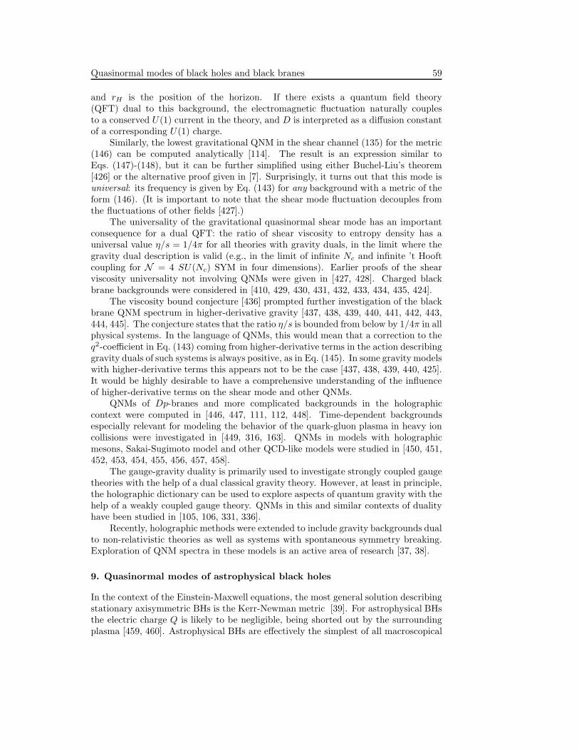
Quasinormal modes of black holes and black branes 59
and rH is the position of the horizon. If there exists a quantum field theory(QFT) dual to this background, the electromagnetic fluctuation naturally couplesto a conserved U(1) current in the theory, and D is interpreted as a diffusion constantof a corresponding U(1) charge.
Similarly, the lowest gravitational QNM in the shear channel (135) for the metric(146) can be computed analytically [114]. The result is an expression similar toEqs. (147)-(148), but it can be further simplified using either Buchel-Liu’s theorem[426] or the alternative proof given in [7]. Surprisingly, it turns out that this mode isuniversal: its frequency is given by Eq. (143) for any background with a metric of theform (146). (It is important to note that the shear mode fluctuation decouples fromthe fluctuations of other fields [427].)
The universality of the gravitational quasinormal shear mode has an importantconsequence for a dual QFT: the ratio of shear viscosity to entropy density has auniversal value η/s = 1/4π for all theories with gravity duals, in the limit where thegravity dual description is valid (e.g., in the limit of infinite Nc and infinite ’t Hooftcoupling for N = 4 SU(Nc) SYM in four dimensions). Earlier proofs of the shearviscosity universality not involving QNMs were given in [427, 428]. Charged blackbrane backgrounds were considered in [410, 429, 430, 431, 432, 433, 434, 435, 424].
The viscosity bound conjecture [436] prompted further investigation of the blackbrane QNM spectrum in higher-derivative gravity [437, 438, 439, 440, 441, 442, 443,444, 445]. The conjecture states that the ratio η/s is bounded from below by 1/4π in allphysical systems. In the language of QNMs, this would mean that a correction to theq2-coefficient in Eq. (143) coming from higher-derivative terms in the action describinggravity duals of such systems is always positive, as in Eq. (145). In some gravity modelswith higher-derivative terms this appears not to be the case [437, 438, 439, 440, 425].It would be highly desirable to have a comprehensive understanding of the influenceof higher-derivative terms on the shear mode and other QNMs.
QNMs of Dp-branes and more complicated backgrounds in the holographiccontext were computed in [446, 447, 111, 112, 448]. Time-dependent backgroundsespecially relevant for modeling the behavior of the quark-gluon plasma in heavy ioncollisions were investigated in [449, 316, 163]. QNMs in models with holographicmesons, Sakai-Sugimoto model and other QCD-like models were studied in [450, 451,452, 453, 454, 455, 456, 457, 458].
The gauge-gravity duality is primarily used to investigate strongly coupled gaugetheories with the help of a dual classical gravity theory. However, at least in principle,the holographic dictionary can be used to explore aspects of quantum gravity with thehelp of a weakly coupled gauge theory. QNMs in this and similar contexts of dualityhave been studied in [105, 106, 331, 336].
Recently, holographic methods were extended to include gravity backgrounds dualto non-relativistic theories as well as systems with spontaneous symmetry breaking.Exploration of QNM spectra in these models is an active area of research [37, 38].
9. Quasinormal modes of astrophysical black holes
In the context of the Einstein-Maxwell equations, the most general solution describingstationary axisymmetric BHs is the Kerr-Newman metric [39]. For astrophysical BHsthe electric charge Q is likely to be negligible, being shorted out by the surroundingplasma [459, 460]. Astrophysical BHs are effectively the simplest of all macroscopical
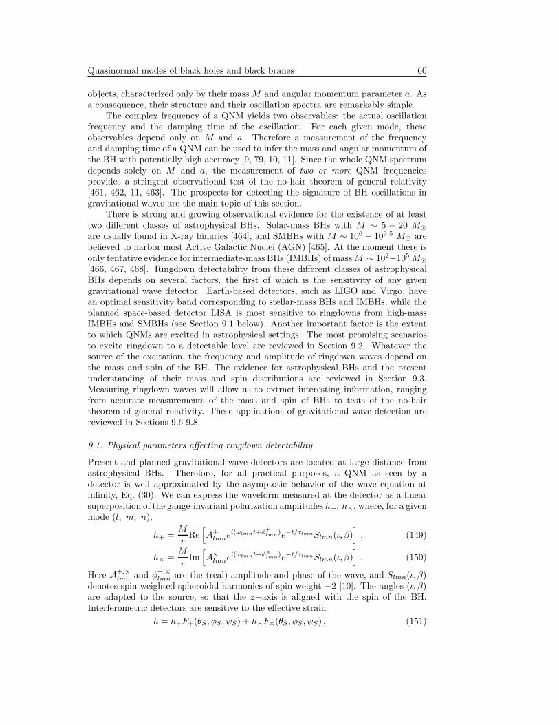
Quasinormal modes of black holes and black branes 60
objects, characterized only by their mass M and angular momentum parameter a. Asa consequence, their structure and their oscillation spectra are remarkably simple.
The complex frequency of a QNM yields two observables: the actual oscillationfrequency and the damping time of the oscillation. For each given mode, theseobservables depend only on M and a. Therefore a measurement of the frequencyand damping time of a QNM can be used to infer the mass and angular momentum ofthe BH with potentially high accuracy [9, 79, 10, 11]. Since the whole QNM spectrumdepends solely on M and a, the measurement of two or more QNM frequenciesprovides a stringent observational test of the no-hair theorem of general relativity[461, 462, 11, 463]. The prospects for detecting the signature of BH oscillations ingravitational waves are the main topic of this section.
There is strong and growing observational evidence for the existence of at leasttwo different classes of astrophysical BHs. Solar-mass BHs with M ∼ 5 − 20 M⊙
are usually found in X-ray binaries [464], and SMBHs with M ∼ 106 − 109.5 M⊙ arebelieved to harbor most Active Galactic Nuclei (AGN) [465]. At the moment there isonly tentative evidence for intermediate-mass BHs (IMBHs) of massM ∼ 102−105 M⊙
[466, 467, 468]. Ringdown detectability from these different classes of astrophysicalBHs depends on several factors, the first of which is the sensitivity of any givengravitational wave detector. Earth-based detectors, such as LIGO and Virgo, havean optimal sensitivity band corresponding to stellar-mass BHs and IMBHs, while theplanned space-based detector LISA is most sensitive to ringdowns from high-massIMBHs and SMBHs (see Section 9.1 below). Another important factor is the extentto which QNMs are excited in astrophysical settings. The most promising scenariosto excite ringdown to a detectable level are reviewed in Section 9.2. Whatever thesource of the excitation, the frequency and amplitude of ringdown waves depend onthe mass and spin of the BH. The evidence for astrophysical BHs and the presentunderstanding of their mass and spin distributions are reviewed in Section 9.3.Measuring ringdown waves will allow us to extract interesting information, rangingfrom accurate measurements of the mass and spin of BHs to tests of the no-hairtheorem of general relativity. These applications of gravitational wave detection arereviewed in Sections 9.6-9.8.
9.1. Physical parameters affecting ringdown detectability
Present and planned gravitational wave detectors are located at large distance fromastrophysical BHs. Therefore, for all practical purposes, a QNM as seen by adetector is well approximated by the asymptotic behavior of the wave equation atinfinity, Eq. (30). We can express the waveform measured at the detector as a linearsuperposition of the gauge-invariant polarization amplitudes h+, h×, where, for a givenmode (l, m, n),
h+ =M
rRe[
A+lmne
i(ωlmnt+φ+lmn
)e−t/τlmnSlmn(ι, β)]
, (149)
h× =M
rIm[
A×lmne
i(ωlmnt+φ×
lmn)e−t/τlmnSlmn(ι, β)
]
. (150)
Here A+,×lmn and φ+,×
lmn are the (real) amplitude and phase of the wave, and Slmn(ι, β)denotes spin-weighted spheroidal harmonics of spin-weight −2 [10]. The angles (ι, β)are adapted to the source, so that the z−axis is aligned with the spin of the BH.Interferometric detectors are sensitive to the effective strain
h = h+F+(θS , φS , ψS) + h×F×(θS , φS , ψS) , (151)

Quasinormal modes of black holes and black branes 61
where F+,× are pattern functions that depend on the orientation of the detector andthe direction of the source (specified by the polar angles θS , φS) and on a polarizationangle ψS [153, 469]. A crucial quantity for gravitational wave detection is the signal-to-noise ratio (SNR) ρ, defined as
ρ2 = 4
∫ ∞
0
h∗(f)h(f)
Sh(f)df , (152)
where h(f) is the Fourier transform of the waveform, and Sh(f) is the noise spectraldensity of the detector [79]. In discussing the SNR we will usually average oversource direction, detector and BH orientations, making use of the sky averages:〈F 2
+〉 = 〈F 2×〉 = 1/5, 〈F+F×〉 = 0, and 〈|Slmn|2〉 = 1/4π. An analysis taking into
account different sky locations and orientations of the source probably requires MonteCarlo methods. At the moment, such an analysis is still lacking.
Our chances of detecting and measuring ringdown waves are mainly determinedby the BH’s mass M , by the spin parameter a, and by the ringdown efficiency ǫrd.The latter quantity is defined as the fraction of the total mass-energy of the systemradiated in ringdown waves, and it is well approximated by [10, 89]
ǫrd ≈ QlmnMωlmn
32π
[
(
A+lmn
)2+(
A×lmn
)2]
. (153)
These three parameters (mass, spin and efficiency) affect the detectability andmeasurability of the signal in different ways.
The BH mass sets the frequency scale and damping time of the emitted radiation.For a Schwarzschild BH, the fundamental QNM with l = 2 (that dominates theradiation in most cases [89]) has frequency f and damping time τ given by
f = 1.207 · 10−2(106M⊙/M) Hz , (154)
τ = 55.37(M/106M⊙) s . (155)
Earth-based detectors are limited at low frequency by a seismic cutoff fs (aplausible estimate for second-generation detectors being fs ∼ 10 Hz for the EinsteinGravitational Wave Telescope, and fs ∼ 20 Hz for Advanced LIGO). Thereforethey can detect the fundamental l = m = 2 QNM as long as the BH massM . 1.2 × 10⁴(Hz/fs)M⊙ if the BH is non rotating, and M . 2.7 × 10⁴(Hz/fs)M⊙
if the BH is rotating near the Kerr limit (see Table I in Ref. [11]). LISA is limited athigh masses (low frequencies) by acceleration noise, and at low masses by the conditionthat the damping time τ should be longer than the light-travel time Tlight ≃ 16.7 scorresponding to the planned armlength (L ≃ 5 · 109 m). Thus LISA can detectringdown waves from BHs in the range 105M⊙ . M . 109M⊙ [10]. To summarize:Earth-based detectors are sensitive to the ringdown of stellar-mass BHs and ofrelatively low-mass IMBHs, and LISA can observe mergers of IMBHs and SMBHsthroughout the whole universe. There is a chance that the ongoing ringdown searchesin data from Earth-based gravitational wave detectors [12, 470, 471, 472, 473, 474, 13]may provide the first incontrovertible evidence of the existence of IMBHs.
As discussed in Section 5.3, the BH spin (for a given BH mass) determines allfrequencies of the Kerr QNM spectrum. For QNMs with m > 0 the quality factorincreases with spin (see Fig. 9). Since the detectability of a gravitational wave signal bymatched filtering scales with the square root of the number of cycles, highly spinningBHs could be the best candidates for detection [89]. However, exciting QNMs of fast-rotating BHs seems to be harder, as the excitation factors tends to zero as a/M → 1
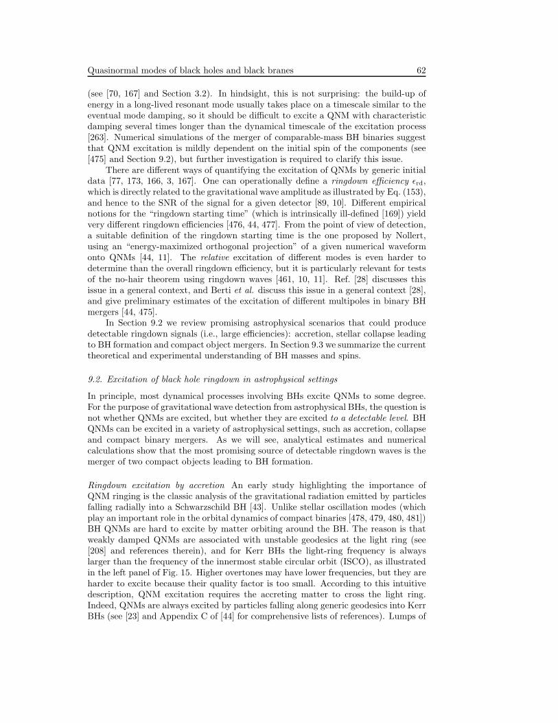
Quasinormal modes of black holes and black branes 62
(see [70, 167] and Section 3.2). In hindsight, this is not surprising: the build-up ofenergy in a long-lived resonant mode usually takes place on a timescale similar to theeventual mode damping, so it should be difficult to excite a QNM with characteristicdamping several times longer than the dynamical timescale of the excitation process[263]. Numerical simulations of the merger of comparable-mass BH binaries suggestthat QNM excitation is mildly dependent on the initial spin of the components (see[475] and Section 9.2), but further investigation is required to clarify this issue.
There are different ways of quantifying the excitation of QNMs by generic initialdata [77, 173, 166, 3, 167]. One can operationally define a ringdown efficiency ǫrd,which is directly related to the gravitational wave amplitude as illustrated by Eq. (153),and hence to the SNR of the signal for a given detector [89, 10]. Different empiricalnotions for the “ringdown starting time” (which is intrinsically ill-defined [169]) yieldvery different ringdown efficiencies [476, 44, 477]. From the point of view of detection,a suitable definition of the ringdown starting time is the one proposed by Nollert,using an “energy-maximized orthogonal projection” of a given numerical waveformonto QNMs [44, 11]. The relative excitation of different modes is even harder todetermine than the overall ringdown efficiency, but it is particularly relevant for testsof the no-hair theorem using ringdown waves [461, 10, 11]. Ref. [28] discusses thisissue in a general context, and Berti et al. discuss this issue in a general context [28],and give preliminary estimates of the excitation of different multipoles in binary BHmergers [44, 475].
In Section 9.2 we review promising astrophysical scenarios that could producedetectable ringdown signals (i.e., large efficiencies): accretion, stellar collapse leadingto BH formation and compact object mergers. In Section 9.3 we summarize the currenttheoretical and experimental understanding of BH masses and spins.
9.2. Excitation of black hole ringdown in astrophysical settings
In principle, most dynamical processes involving BHs excite QNMs to some degree.For the purpose of gravitational wave detection from astrophysical BHs, the question isnot whether QNMs are excited, but whether they are excited to a detectable level. BHQNMs can be excited in a variety of astrophysical settings, such as accretion, collapseand compact binary mergers. As we will see, analytical estimates and numericalcalculations show that the most promising source of detectable ringdown waves is themerger of two compact objects leading to BH formation.
Ringdown excitation by accretion An early study highlighting the importance ofQNM ringing is the classic analysis of the gravitational radiation emitted by particlesfalling radially into a Schwarzschild BH [43]. Unlike stellar oscillation modes (whichplay an important role in the orbital dynamics of compact binaries [478, 479, 480, 481])BH QNMs are hard to excite by matter orbiting around the BH. The reason is thatweakly damped QNMs are associated with unstable geodesics at the light ring (see[208] and references therein), and for Kerr BHs the light-ring frequency is alwayslarger than the frequency of the innermost stable circular orbit (ISCO), as illustratedin the left panel of Fig. 15. Higher overtones may have lower frequencies, but they areharder to excite because their quality factor is too small. According to this intuitivedescription, QNM excitation requires the accreting matter to cross the light ring.Indeed, QNMs are always excited by particles falling along generic geodesics into KerrBHs (see [23] and Appendix C of [44] for comprehensive lists of references). Lumps of
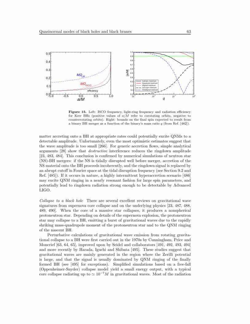
Quasinormal modes of black holes and black branes 63
-1.0 -0.5 0.0 0.5 1.0a/M
0.0
0.1
0.2
0.3
0.4
0.5
MΩISCO
efficiency
MΩLR
10-3
10-2
10-1
100
q0.0
0.1
0.2
0.3
0.4
0.5
0.6
0.7
0.8
0.9
1.0
|a/M
|
Isotropic maximumEquatorial maximumAligned maximumZero-spin minimumAntialigned minimum
Figure 15. Left: ISCO frequency, light-ring frequency and radiation efficiencyfor Kerr BHs (positive values of a/M refer to corotating orbits, negative tocounterrotating orbits). Right: bounds on the final spin expected to result froma binary BH merger as a function of the binary’s mass ratio q (from Ref. [482]).
matter accreting onto a BH at appropriate rates could potentially excite QNMs to adetectable amplitude. Unfortunately, even the most optimistic estimates suggest thatthe wave amplitude is too small [266]. For generic accretion flows, simple analyticalarguments [28] show that destructive interference reduces the ringdown amplitude[23, 483, 484]. This conclusion is confirmed by numerical simulations of neutron star(NS)-BH mergers: if the NS is tidally disrupted well before merger, accretion of theNS material onto the BH proceeds incoherently, and the ringdown signal is replaced byan abrupt cutoff in Fourier space at the tidal disruption frequency (see Section 9.2 andRef. [485]). If it occurs in nature, a highly intermittent hyperaccretion scenario [486]may excite QNM ringing in a nearly resonant fashion for large spin parameters, andpotentially lead to ringdown radiation strong enough to be detectable by AdvancedLIGO.
Collapse to a black hole There are several excellent reviews on gravitational wavesignatures from supernova core collapse and on the underlying physics [23, 487, 488,489, 490]. When the core of a massive star collapses, it produces a nonsphericalprotoneutron star. Depending on details of the supernova explosion, the protoneutronstar may collapse to a BH, emitting a burst of gravitational waves due to the rapidlyshriking mass-quadrupole moment of the protoneutron star and to the QNM ringingof the nascent BH.
Perturbative calculations of gravitational wave emission from rotating gravita-tional collapse to a BH were first carried out in the 1970s by Cunningham, Price andMoncrief [63, 64, 65], improved upon by Seidel and collaborators [491, 492, 493, 494]and more recently by Harada, Iguchi and Shibata [495]. These studies suggest thatgravitational waves are mainly generated in the region where the Zerilli potentialis large, and that the signal is usually dominated by QNM ringing of the finallyformed BH (see [495] for exceptions). Simplified simulations based on a free-fall(Oppenheimer-Snyder) collapse model yield a small energy output, with a typicalcore collapse radiating up to ≃ 10−7M in gravitational waves. Most of the radiation

Quasinormal modes of black holes and black branes 64
is quadrupolar (l = 2), radiation in l = 3 being typically two to three orders of mag-nitude smaller (see Fig. 9 in [63]). Recent perturbative studies suggest that magneticfields could increase the energy output by several orders of magnitude [496, 497].
The first numerical simulation of collapse in two dimensions was carried out byNakamura [498], but numerical problems prevented gravitational radiation extraction.For a long time the seminal 1985 work of Stark and Piran [71] has been the onlynonperturbative, axisymmetric calculation of gravitational wave emission from stellarcollapse. The waveform resembles that emitted by a point particle falling into aBH, but with a reduced amplitude. The total energy emitted increases with therotation rate, ranging from ∼ 10−8M for a/M = 0 to ∼ 7 × 10⁻⁴M as a/M → 1.Rotational effects halt the collapse for some critical value of (a/M)crit which is veryclose to unity, and depends on the artificial pressure reduction used to trigger thecollapse. Stark and Piran find that the energy emitted E/M ≃ 1.4 × 10⁻³(a/M)4
for 0 < a/M < (a/M)crit, and for larger spins it saturates to a maximum valueǫmax ∼ 10−4. Note however that the maximum energy radiated is very sensitiveto the amount of artificial pressure reduction used to trigger the collapse: the 99%pressure reduction used in the simulations of Stark and Piran essentially produced afree-fall collapse, presumably overestimating the radiation efficiency.
This calculation has recently been improved using a three-dimensional code[499, 500, 72, 501]. Ref. [500] choose as the initial configuration the most rapidlyrotating, dynamically unstable model described by a polytropic equation of state(EOS) with Γ = 2 and K = 100, having a dimensionless rotation rate ≃ 0.54,and trigger collapse by reducing the pressure by . 2%. The “+” polarization isessentially a superposition of modes with l = 2 and l = 4, and the “×” polarizationis a superposition of modes with l = 3 and l = 5. The energy lost to gravitationalwaves according to these simulations is at most ≃ 1.45 × 10⁻⁶(M/M⊙), two ordersof magnitude smaller than the estimate by Stark and Piran for the same value of theangular momentum, but larger than the energy losses found in recent calculations ofrotating stellar core collapse to protoneutron stars [502]. Ref. [501] confirms the basicscaling E/M ≈ (a/M)4 for a/M . 0.54 (the largest rotation rates yielding equilibriummodels in uniform rotation), but at variance with Stark and Piran’s simulations itfinds that the efficiency has a local maximum for large rotation rates. If the collapseis triggered only by pressure depletion, the overall efficiency for uniformly rotatingmodels is quite low (E/M ≈ 10−7 − 10−6), the mass quadrupole does not changevery rapidly, and higher multipoles are not significantly excited. However the totalenergy radiated can increase by up to two orders of magnitude if velocity perturbationsare present in the collapsing star. A rapidly rotating polytropic star at 10 kpc canproduce maximum characteristic amplitudes hc ≈ 5× 10⁻²²(M/M⊙) at characteristicfrequencies ranging between fc ≈ 500 Hz and fc ≈ 900 Hz, and could be detectablewith SNRs as large as about 30 by Earth-based interferometers.
In conclusion, the ringdown efficiency is very sensitive to poorly known details ofthe mechanism triggering the collapse. Simulations with more realistic microphysicsare required to study the complex signal preceding the ringdown phase, as well asdetails of QNM excitation by matter accreting onto the newly formed BH.
Mergers of compact objects leading to black hole formation Numerical relativitysimulations of compact binary mergers made enormous progress since 1999, whenthe two classic reviews on QNMs [4, 5] were written. This section is an attempt tosummarize aspects of this progress of interest for the detection of ringdown waves from

Quasinormal modes of black holes and black branes 65
astrophysical BHs.Since NSs cannot have masses larger than about 3M⊙, Eq. (84) implies that
NS-NS mergers are potentially relevant only for the detection of BH ringdowns byEarth-based interferometers, such as LIGO and Virgo. On the other hand, NS-BHand BH-BH mergers are plausible targets for ringdown detection by both Earth-basedand future space-based detectors, so we will discuss them in more detail.(1) NS-NS mergers - In 1999 Shibata and collaborators carried out the first successfulequal-mass NS-NS merger simulation for a polytropic index Γ = 2 [503, 93]. Thefirst reasonably accurate calculation of gravitational waveforms was possible a fewyears later, in 2002 [504]. Unequal-mass binaries with a Γ = 2 polytropic EOS werestudied in [505], where it was found that a BH forms when the total rest-mass of thesystem is larger than ∼ 1.7 times the maximum allowed rest-mass of spherical NSs,irrespective of mass ratio (which however affects significantly the waveforms and themass of the disk forming around the newly born BH). More realistic EOSs and largerparameter spaces were considered in Refs. [506, 507]. Ref. [507] uses stiff EOSs andmodels binary NSs of ADM mass M & 2.6M⊙. For all mass ratios 0.65 . q ≤ 1, aBH forms whenever the mass M > Mth. The threshold value Mth ≃ 1.3 − 1.35Mmax
(where Mmax is the maximum mass allowed by the given EOS for cold, spherical NSs)depends on the EOS. If M < Mth the merger results in a hypermassive NS of largeellipticity, emitting quasiperiodic gravitational waves at frequencies ∼ 3 − 4 kHz for. 100 ms. After this phase the NS may or may not collapse to a BH. For total binarymasses in the range M ≈ 2.7 − 2.9M⊙, the l = m = 2 ringdown frequency emittedin the collapse to a BH is ≈ 6.5 − 7 kHz, with amplitude ∼ 10−22 at a distance of50 Mpc. Therefore BH ringdown from NS-NS mergers is unlikely to be detected: theamplitude is too low and (most importantly) the frequency is too high for present andplanned Earth-based gravitational wave detectors. It is interesting to note that NS-NSmerger simulations typically lead to final BH spins a/M ≈ 0.8 [507, 508], not verydifferent from the value a/M ≃ 0.69 predicted by equal-mass BH merger simulations.Various groups have recently carried out NS-NS merger simulations with magneticfields, finding that aligned poloidal fields can delay the merger and strongly affect thegravitational wave signal [509, 510, 511].(2) NS-BH mergers - NS-BH binaries are potentially among the most interestingBH ringdown sources. From Eq. (154), the QNM frequency for non-spinning BHswith M & 10M⊙ is within the sensitivity window of LIGO and Virgo. Theory andobservations [512, 464, 513] suggest that binaries containing BHs with masses in thisrange should be common. Furthermore, high mass-ratio systems do not tidally stripthe NS, producing a merger with a clean ringdown signal. The simulations described inthe rest of this section suggest that NS-BH mergers are promising sources of ringdownwaves and (when the BH is spinning) excellent candidates as central engines forgamma-ray bursts (GRBs).
NS-BH merger simulations became possible once the moving puncture approach[15, 16] proved successful in evolving BH-BH binaries. Shibata and Uryu [514, 515] firstevolved two binaries consisting of (1) a non-rotating BH of mass ≈ 3.2M⊙ or ≈ 4M⊙,respectively, and (2) a NS of rest mass ≈ 1.4M⊙, modeled by a Γ-law EOS with Γ = 2.A larger set of simulations with non-spinning BHs of masses M ∼ 3.3 − 4.6M⊙ andNSs of massM ∼ 1.4M⊙ was performed in Ref. [516]. The NS is tidally disrupted, andthe system results in a BH with spin a/M ≈ 0.5 − 0.6. Non-spinning NS-BH mergerscan only produce massive tori and fuel short-hard GRBs if the NS has compactnessM/R . 0.145. Furthermore, when tidal disruption occurs the QNM amplitude quickly

Quasinormal modes of black holes and black branes 66
decreases, because the incoherent accretion of material is ineffective at resonantlyexciting the mode (see Fig. 6 of Ref. [516]).
The first code capable of handling NS-NS, NS-BH and BH-BH binary evolutionscomprising more than 4 orbits was recently described in Ref. [508]. Gravitationalwaveforms from NS-BH mergers were presented in Ref. [485] and classified into threeclasses as follows: 1) For small mass ratio q and small NS compactness (e.g., if q . 3for M/R = 0.145 and Γ = 2) tidal disruption occurs outside the ISCO, and thereis no QNM excitation; 2) For some systems, mass shedding occurs before the binaryreaches the ISCO. Most of the NS is swallowed by the BH before tidal disruption iscompleted and QNMs are excited, but only to a low amplitude; 3) If tidal effects donot play an important role the waveforms shows significant QNM excitation, as theyalways do for BH-BH mergers. The latter class of NS-BH mergers is clearly the mostpromising for BH ringdown detection. Whenever ringdown is not significantly excited,kicks are also suppressed: this confirms the crucial role played by the merger/ringdownphase in determining the magnitude of the kick resulting from compact binary mergers(see Section 9.8 below). The results of Ref. [485] are in good agreement with NS-BHcodes developed by other groups [517, 518, 519]. Ref. [517] deals with systems wherethe NS is irrotational, the BH is non-rotating and the mass ratio q = 1/3. Thesesimulations lead to the formation of BHs with a/M ≈ 0.5 − 0.8. Most of the NSmaterial is prompty accreted, and no more than 3% of the NS mass is ejected into agravitationally bound disk. This disk mass, while larger than the typical values foundin Ref. [485], is probably not enough to trigger short-hard GRBs.
Results from non-spinning NS-BH mergers show that the disk mass is typicallytoo low to fuel GRBs. For example, Fig. 7 of Ref. [485] shows that, if the BH isnon-spinning, the formation of a disk requires a “fat” NS with radius R & 14 km.The few simulations presently allowing for (aligned or anti-aligned) BH spins have adrastically different outcome, indicating that spin plays a crucial role in fueling GRBs[518]. In these simulations the number of orbits before merger increases as the spin isvaried between a/M = −0.5 (anti-aligned), 0.0 and 0.75 (for fixed mass ratio q ≃ 1/3).In the latter case the final BH spin is a/M ≃ 0.88, and the tidal disruption of theNS leads to the formation of a massive disk of about 0.2M⊙, potentially capableof driving GRBs. The production of GRBs by NS-BH mergers and the possibilityto detect the final spin orientation using observations of the merger/ringdown phaseare promising areas of research for multi-messenger astronomy using a network ofground-based detectors in conjunction with traditional electromagnetic observations(see e.g. [520, 521, 522, 523, 524]).(3) BH-BH mergers - After 40 years of developments in numerical relativity, recentbreakthroughs [14, 15, 16] finally allowed simulations of the merger and ringdownof BH binaries. Extensive collaborations to use numerical merger waveforms ingravitational wave searches have just started [525]. A discussion of the accuracyof numerical simulations and of their rapid progress in the last few years would takeus too far (see Refs. [14, 526] for reviews). From the point of view of this review,the main result of these merger simulations is that QNM ringing is observed in allbinary BH merger simulations. This is quite unlike NS-BH and NS-NS mergers, wheretidal effects can sometimes suppress ringdown excitation because of the incoherentaccretion of material onto the newly formed BH. Another important difference is thatthe gravitational waveform from a BH-BH merger depends on the total mass of thesystem via a trivial rescaling, so BH-BH systems are interesting for ringdown detectionby both Earth-based and space-based detectors.

Quasinormal modes of black holes and black branes 67
The mass-ratio dependence of the ringdown efficiency can be estimated by simplearguments [89, 44]. The quadrupole moment of a body of mass M with a ”bump” ofmass µ ≪ M is Q ∼ µM2. The oscillation frequency of the system f ∼ 1/M ; hence,
the radiated power dE/dt ∼(
d3Q/dt3)2 ∼ (f3Q)2 ∼ µ2/M2. For a binary with mass
ratio µ/M the inspiral lasts ∼ (M/µ) cycles times the orbital time scale T ∼ M ,so the total energy loss during the inspiral is Einsp ∼ (M/µ)(µ2/M2)M ∼ µ. Bycontrast, a typical ringdown waveform lasts only a few cycles, so the ringdown energyloss Eringdown ∼ M(µ2/M2) ∼ µ2/M (compare with the classic result for infallingparticles in Ref. [43]) and Eringdown/Einsp ∼ µ/M : ringdown is negligible with respectto inspiral for extreme-mass ratio binaries. If we naively extrapolate these estimatesto bodies of comparable masses (interpreting M as the total mass of the binary andµ → m1m2/M as the reduced mass) we find that Eringdown/M ∼ η2, where η ≡ µ/Mis the so-called symmetric mass ratio (η → 1/4 in the comparable-mass limit).
Physical arguments to estimate the prefactors suggest that the merger/ringdownwaveform should actually dominate over inspiral for binaries with mass ratio q & 1/10[89, 10], and numerical simulations of quasicircular inspirals of comparable-massmergers have borne out this expectation. For non-spinning binary BH mergers, thefraction of energy radiated (M −Mfin)/M (where M denotes the total mass of twoBHs in isolation and Mfin is the mass of the final BH), as well as the final spin a/M ,have been extensively studied [477, 44, 527, 528, 528]. Ref. [527] fits data from thesimulations by the Goddard group by a relation of the form
Mfin/M = 1 + (√
8/9 − 1)η − 0.498(±0.027)η2 , (156)
a/Mfin =√
12η − 2.900(±0.065)η2 . (157)
This result is consistent with the fitting formula given in [44] using a differentnormalization. Frequencies and damping times of different multipolar components canbe estimated using either a standard least-squares algorithm [477] or Prony methods,which are in many ways optimal to estimate the parameters of damped exponentialsin noise [529]. By monitoring the frequencies and damping times after merger we canmonitor inaccuracies in the higher multipolar components of numerical simulations,and possibly explore non-linear effects (see e.g. Section IV in Ref. [44]).
Quantifying the fraction of energy radiated in ringdown is inherently ambiguous.The reason for this difficulty can essentially be traced back to the non-completeness ofQNMs [169, 2, 3, 44]. An operational viewpoint to isolate the ringdown contribution isgiven by Nollert’s energy-maximized orthogonal projection (EMOP) criterion [169, 44].The idea is to determine the starting time of a ringdown waveform by assumingthat the frequency of the ringdown waveform is known, and performing matched-filtering (in white noise) of the numerical waveform, using a damped sinusoid as the“detection template”. Since ringdown is essentially monochromatic, this should givea reasonably good, frequency-independent and detector-independent estimate of thefraction of energy that we can expect to detect by a ringdown search. For more detailson ringdown search techniques, see Section 9.4 below.
An application of the EMOP criterion to numerical simulations shows thatringdown typically contributes ∼ 42% of the energy radiated by the last two cyclesof BH-BH mergers with mass ratio q ≥ 1/4 (see Tables VI and VII of Ref. [44]).By combining Prony methods for estimating frequencies and the EMOP approach toestimate the ringdown starting time, we find the following estimates for the energyemitted in ringdown as a result of the merger of non-spinning, quasi-circular BH
Quasinormal modes of black holes and black branes 68
binaries [44]
El=2ringdown
M≃ 0.271
q2
(1 + q)4,
El=3ringdown
M≃ 0.104
q2(q − 1)2
(1 + q)6. (158)
For non-spinning, equal-mass binaries, the merger/ringdown signal as thesystem’s orbital angular momentum is reduced (so a quasicircular merger slowly turnsinto an head-on collision) has been studied in Refs. [530, 531]. In the head-on limit onegets a radiated energy ∼ 0.1%M . In the intermediate regime, where two equal-massBHs merge along orbits with large residual eccentricity, the radiated energy decays(roughly) exponentially (see Table I and Fig. 7 in Ref. [530]) and the final BH spin hasa local maximum jfin ≃ 0.724±0.13 [530, 531]. For preliminary studies of the ringdownefficiency in the merger of quasicircular, spinning binaries, see Refs. [475, 532, 533].
Predictions of the spin of a BH resulting from a merger are very interesting fromthe point of view of ringdown detection. For example, if we measure the masses andspins during the inspiral we may be able to predict the final spin and reduce theerrors in parameter estimation [534, 535]. For a summary of semianalytic models andfitting formulas to predict the final spin from generic mergers, we refer the reader to[536, 537, 538, 539]. Some insight into the general outcome of a spinning merger canbe obtained by looking at the right panel of Fig. 15. For simplicity, consider threedifferent merger scenarios: i) in the isotropic scenario, both BH spins are distributedisotropically; ii) in the aligned spin scenario, the individual BH spins in the binaryare assumed to be aligned (for example, in “wet mergers” the alignment could becaused by torques from accreting gas, as suggested in [540]); iii) in the equatorialmerger scenario, the smaller BH is supposed to orbit in the equatorial plane of thelarger hole (e.g. because of Newtonian dynamical friction in a flattened system), butthe spin orientation of the smaller BH is distributed isotropically. The right panel ofFig. 15 shows the maximum and minimum spin resulting from a merger in these threescenarios. These curves are obtained by (1) fixing some value of the mass ratio q, (2)averaging over angles according to the three different assumptions listed above, and(3) maximizing or minimizing the final average spin resulting from a merger (where theaverage is computed using the fitting formulas of Ref. [537]) in the (|j1|, |j2|) plane,where |ji| is the spin magnitude of BH i = 1, 2. Not surprisingly, the minimumaverage final spin always corresponds to the case where both BHs are non-spinning(dashed black line). The maximum average spin in the three cases is shown by thecontinuous black (isotropic), red (equatorial) and blue (aligned) lines. The dashedblue line shows the (modulus of) the minimum spin that could be achieved if we allowfor antialignment of both spins with respect to the orbital angular momentum (a spinflip becomes possible when the mass ratio q ≈ 1/3). The most interesting predictionof this plot is the existence of a narrow funnel between the solid black and dashedblack lines: on average, isotropic major mergers (with q & 0.2 or so) always producea final spin which is very close to the spin resulting from equal-mass non-spinning BHbinaries, i.e. a/M ∼ 0.69. Furthermore, in all three scenarios the most likely spinresulting from “major” mergers with q & 0.1 is quite close to |jfin| ≃ 0.69.
A critical assessment of the available predictions on the final spin and on the finalkick is outside the scope of this review; the interested reader is referred to Ref. [541].
9.3. Astrophysical black holes: mass and spin estimates
From the discussion in the previous section it should be clear that ringdowndetectability depends crucially on the physical parameters of astrophysical BHs.

Quasinormal modes of black holes and black branes 69
What are the most promising scenarios leading to the formation of massive stellar-mass BHs that would predominantly be seen in merger/ringdown by Earth-basedinterferometers? What are the event rates for mergers to be observed by LISA? Giventhat ringdown detectability scales strongly with mass ratio, what is the most likelymass ratio for binaries whose merger is detectable by LIGO and LISA? What is themost likely spin magnitude of BHs in binaries, and what are the odds that we canunveil connections between merger/ringdown waveforms and the central engine ofGRBs? In this section we briefly survey theoretical expectations and state-of-the-art measurements of the mass and spin distribution of BHs. We summarize some ofthe most relevant information that astronomers have collected by working as busybees over the past thirty years, paying particular attention to the implications for thedetection of gravitational waves from the merger/ringdown of BH binaries.
Our focus here is on testing the BH nature of astrophysical objects bygravitational wave observations, but there are excellent reviews on measuring BHmasses, spins and (possibly) providing evidence of an event horizon by “traditional”electromagnetic astronomy. Narayan reviews the status of BH astrophysics, focusingon observational progress in measuring mass and spin and on (circumstantial)observational evidence for the defining property of a BH: the event horizon [8]. Psaltisdiscusses how electromagnetic observations of BHs and neutron stars can be used toprobe strong-field gravity; in the process he describes various ways of identifying BHsand measuring their properties, including continuum spectroscopy, line spectroscopy,and attempts at imaging the vicinity of BHs to constrain their angular size [32].
Stellar-mass black hole candidates The most accurate mass measurements for stellar-mass BH candidates are made via dynamical methods, that is, by looking at how theunseen BH affects the orbit of a companion star. Consider a test particle in circularorbit around the BH. If the orbit is wide enough for Newtonian physics to apply, thenthe mass M = ω2r3 = v2r = v3/ω, where r is the orbital separation, v is the orbitalvelocity and ω = 2π/T with T the orbital period (simple modifications can accountfor orbital eccentricity). By measuring any two of v, r and ω, we may estimate theBH mass M . In the case of BH X-ray binaries it is relatively easy to measure ω andthe maximum line-of-sight Doppler velocity Kc = v sin ι of the companion star. Fromthese quantities one can compute the “mass function”
f(M) ≡ Kc
ω=
M sin3 ι
(1 +Mc/M)2, (159)
where M,Mc are the masses of the BH candidate and of the companion, respectively.The inclination angle ι of the orbit can be estimated from the light curve of the binary,and sometimes it’s even possible to estimate Mc. By combining measurements of ωand Kc with estimates of ι and Mc, one can in principle determine the masses of bothbinary members. However, to identify BH candidates the essential point is to note thatthe mass function f(M), which depends only on ω and Kc, provides a strict lowerbound on M . Since NSs cannot be more massive than about 3M⊙ [542], all X-raybinaries for which f(M) & 3M⊙ should contain a BH. Remillard and McClintock[464] review the phenomenology of 20 X-ray binaries with dynamically confirmedBHs, presenting a census of BH candidates and a critique of different methods formeasuring spins. Their Table I provides a list of (lower bounds on) the mass of about20 BH candidates. The most massive stellar-mass BH candidate to date is IC 10X-1, with a minimum mass M = 23.1 ± 2.1M⊙ if the companion’s mass Mc = 17M⊙

Quasinormal modes of black holes and black branes 70
(M = 32.7 ± 2.6M⊙ if one trusts an estimate of Mc = 35M⊙ for the companion)[513]. This system is particularly interesting for gravitational wave detection, becauseit should become a close double BH binary with coalescence time of ∼ 2−3 Gyr [543].
The relative importance of ringdown with respect to inspiral waves decreasesfor extreme mass ratios. For the stellar-mass binaries of interest for Earth-basedinterferometers, population synthesis codes suggest that q should always be very closeto unity [512]. A rather speculative kind of source (in the absence of solid evidencefor IMBHs) consists of the intermediate mass ratio inspiral (IMRI) of a compactobject, such as a NS or BH, into an IMBH. The relatively low energy content inringdown waves is compensated, in this case, by the fact that the ringdown frequencyis close to the minimum of the Advanced LIGO noise power spectral density (seeAppendix B of Ref. [544]). Another promising ringdown source for advanced Earth-based interferometers (albeit with highly uncertain event rates) are IMBH-IMBHinspirals. These binaries, if they are numerous enough to be detectable, present aninteresting data analysis challenge: the initial inspiral phase could be detected byLISA, while the ringdown phase is in the optimal bandwidth for Advanced LIGO,that could therefore be used for “follow-up” ringdown searches [545].
Supermassive black hole candidates A good review of SMBH observations from ahistorical perspective can be found in Ref. [465]. The first quasar was identified in1963 [51], when the Kerr solution had just been discovered [50] and its astrophysicalrelevance was unclear. In the intervening years astronomers gathered strongobservational evidence for the presence of SMBHs in the bulges of nearly all local,massive galaxies [546, 547, 548]. Reliable mass estimates are available for many of thesesystems. The most precise measurement comes from observations of stellar propermotion at the center of our own galaxy, indicating the presence of a “dark object” ofmass M ≃ (4.1±0.6)×106M⊙ [549, 550] and size smaller than about one astronomicalunit [551]. A Schwarzschild BH of the given mass has radius R ≃ 0.081 astronomicalunits, compatible with the observations. Any distribution of individual objects withinsuch a small region (with the possible exceptions of dark matter particles or asteroids,which however should be kicked out by three-body interactions with stars) wouldbe gravitationally unstable [552, 553]. Theoretical alternatives to SMBHs (e.g., bosonstars and gravastars) have been proposed by various authors, but the formation processof these hypothetical objects is unclear, and many of these exotic alternatives can beshown to be unstable [554, 555]. Another accurate mass measurement comes fromthe motion of the gas disk at the centre of the nearby galaxy NGC 4258 [556], asmonitored by radio interferometry of the waves emitted from water molecules viamaser emission. The observations imply the presence of an object of mass 3.5×10⁷M⊙
within ∼ 4×10¹⁵ m. Other techniques include applications of the virial theorem to thevelocity dispersion of stars near the galactic center [546] and reverberation mapping toobtain more crude estimates for distant, variable AGNs [557]. The reader interestedin a SMBH mass census can consult Graham’s survey [558], listing 76 galaxies withdirect SMBH mass measurements and (when available) their host bulge’s centralvelocity dispersions. Graham also lists 8 stellar systems that could potentially hostintermediate-mass BHs. For our purposes, it suffices to note that SMBHs have massesin the range M ∼ 105 − 109M⊙, approximately proportional to the mass of the hostgalaxies, M ∼ 10−3 Mgalaxy [559]. There is an almost-linear relation between themass of a SMBH and the mass of the galactic bulge hosting it [546, 547, 548]. The BHmass is also tightly correlated with other properties of the galactic bulge, such as the

Quasinormal modes of black holes and black branes 71
central stellar velocity dispersion σ, the bulge light concentration and the near-infraredbulge luminosity [560, 561, 558]. These correlations clearly indicate that SMBHs arecausally linked to the surrounding galactic environment. The growth of galaxies andSMBHs must be intertwined, and observations of the merger and ringdown of SMBHswith LISA holds great promise to clarify their formation history.
Supermassive black hole binary candidates The SMBHs harboring nearby galacticcores are expected to grow via a combination of mergers and accretion, and hierarchicalmerger models of galaxy formation predict that binary SMBHs should be commonin the Universe [562, 563, 564]. The merger of SMBH binaries is one of the mostluminous gravitational wave events in the universe, and it is the strongest conceivableastrophysical source of ringdown waves. Observational evidence for close SMBHbinaries started emerging very recently, and it is one of the most exciting frontiersof relativistic astrophysics.
The formation of SMBHs during galaxy mergers is a challenging problem intheoretical astrophysics. The general scenario was outlined in a pioneering analysisby Begelman, Blandford and Rees [565] (see Ref. [562] for a more recent review). Theevolution of a SMBH binary can be roughly divided in three phases: i) as the galaxiesmerge, SMBHs sink to the center via dynamical friction; ii) the binary’s binding energyincreases because of gravitational slingshot interactions, i.e. the ejection of stars onorbits intersecting the binary (these stars’ angular momentum must be in a region ofphase space called the “loss cone”); iii) if the binary separation becomes small enough,gravitational radiation carries away the remaining angular momentum. Notice thatthe gravitational wave coalescence time is shorter for more eccentric binaries [566],so high-eccentricity binaries are slightly more likely to coalesce within a Hubble time(see e.g. [567]). The transition from phase ii) to phase iii) is a field of active research,that has been referred to as the “final parsec problem” [562]. Since the binary willquickly eject all stars through gravitational slingshot interaction, the problem is to findsome mechanism (such as gas accretion, star-star encounters and triaxial distortions ofgalactic nuclei) to refill the loss cone. It is generally believed, based on both theoreticaland observational arguments, that efficient coalescence should be the norm [567]. Themain point here is that only SMBH binaries with separations . 1 pc can merge withina Hubble time under the sole influence of gravitational radiation.
The mass ratio distribution is an important variable from the point of view ofringdown detection. The impact of different SMBH assembly models on the mass andmass ratio distribution of detectable binaries has been discussed by various authors.The general consensus is that mass ratios q . 1/10 (and down to q ≈ 10−3 − 10−4)should be common [568, 569, 570, 571, 572, 573]. This may not be true for mergersbetween BHs in separate dark matter halos, because the smaller halo could get tidallystripped and it would not be able to sink efficiently toward the center of the mainhalo [574]. In any case, SMBH mergers will be strong LISA ringdown sources even formodest mass ratios.
Possible observational smoking guns of SMBH binaries (such as X-shaped radiogalaxies, double-double radio galaxies, helical radio jet patterns, semi-periodic signalsin lightcurves, double-peaked emission-line profiles and galaxies which lack centralcusps) are reviewed by Komossa [575]. At the time of her review, the most spectacularexample of a SMBH binary was the ultraluminous infrared galaxy NGC 6240 [576],containing two active SMBHs separated by a relatively short projected distance∼ 1 kpc. Since then, more quasars have been identified as promising hosts of SMBH

Quasinormal modes of black holes and black branes 72
binaries+. Even more interestingly, in the last year three systems have been proposedto host binary SMBHs at separations smaller than one parsec [583, 584]. Theseobservations could be extremely important for our understanding of SMBH binarymergers and their rates [585]. Since they are still controversial and they would takeus too far from the main topic of this review, we briefly summarize them for theinterested reader in Appendix C.
Spins: theoretical expectations Estimating BH spins is an exciting observationalfrontier for the next decade of observational astronomy [586, 587, 588]. Presentspin estimates based on electromagnetic observations are all, to some extent, model-dependent. Few dependable and accurate measurements are available, and thereare different opinions on the expected spin magnitude of both stellar-mass BHs andSMBHs. The punchline of the theoretical work summarized in this section is as follows:1) stellar-mass BHs should typically retain their natal spin, and so they can be usedto infer information about the mechanism triggering the collapse; 2) SMBH spinsencode the history of the hole, and particularly the relative importance of mergersand accretion in the hierarchical formation process responsible for growing the holes.The rest of this section gives arguments in support of these conclusions.1) Stellar-mass black holes: Theoretical arguments suggest that stellar-mass BHs inbinaries retain the spin they had at birth: neither accretion nor angular momentumextraction are likely to change significantly their mass or spin. A BH must accrete anappreciable fraction of its original mass in order to significantly change its spin. ForBHs with low-mass companions, even the accretion of the entire companion star willonly change the spin by a small fraction; for BHs with high-mass companions, evenEddington-limited accretion will only grow the BH spin by a small amount before thehigh-mass companion explodes [589]. Therefore the spin of stellar-mass BHs shoulddepend mainly on their formation process.
Detailed studies of spin evolution in compact binaries have been carried out by theNorthwestern group, focusing mostly on NS-BH binary systems and using progressiveimprovements of the STARTRACK stellar evolution code (see [512] and referencestherein). The evolution prior to the supernova explosion involves mass-transfer phases,which are expected to align the spins of both the BH and the NS progenitor, buta significant natal kick of the NS at birth is required to form a coalescing NS-BHbinary [590]. In general, the plane of the post-supernova orbit is tilted with respect tothe pre-supernova plane, and hence tilted with respect to the BH spin axis by someangle ι, inducing precession of the binary’s orbital plane. Preliminary results suggestthat precession only marginally impacts the detection of gravitational waves from theinspiral waves, but it should be significant for parameter estimation [591, 512, 592].Belczynski et al. [512] consider both BH-BH and NS-BH binaries. For NS-BH binaries
+ A binary AGN with separation ∼ 4.6 kpc has been claimed in Arp 299 [577], and a system withprojected distance ∼ 10.5 kpc has been found in the galactic pair ESO 509-IG066 [578]. Evans etal. [579] reveal the AGN nature of the companion of the FRII radio source 3C 321. Bianchi etal. identify a binary AGN in Mrk 463 with projected separation ∼ 3.8 kpc [580]. Finally, usingmultifrequency observations with the Very Long Baseline Array (VLBA), Rodriguez et al. [581, 582]report the discovery of a SMBH binary in the radio galaxy 0402+379 with a total estimated mass of1.5×108M⊙ and a projected orbital separation of just 7.3 pc. This is the smallest orbital separation bymore than two orders of magnitude, but even for this relatively close binary the emitted gravitationalwaves have frequency ∼ 2 × 10⁻¹³ Hz, way too low to be observed by LISA, and a merger time∼ 1018 yr (much longer than the age of the Universe) if gravitational radiation is the only dissipativemechanism.

Quasinormal modes of black holes and black branes 73
they confirm the qualitative predictions of [589]: BHs cannot be significantly spun upby accretion in the common envelope phase. For example, only 20% of initially non-spinning BHs spin up to a/M > 0.1, and no BHs spin up to a/M & 0.5. The spin-upis even smaller for BH-BH binaries, with the highest attainable spins being very closeto the initial spins of the individual BHs (see Fig. 5 and Fig. 9 in [512]). Furthermore,the kick-induced tilt angle ι < 45 for ∼ 50% of NS-BH systems. The fraction ofevents that can potentially produce short-hard GRBs, and which therefore is relevantfor merger/ringdown searches in association with gamma-ray bursts, is significant (oforder ∼ 40%) only if the initial BH spin a/M & 0.6 [512].
These studies suggest that Advanced-LIGO measurements of BH spins in theinspiral of binaries containing stellar-mass BHs should be an excellent probe of thecollapse mechanism that produced the BH in the first place, because the BH essentiallyretains the spin it had at birth. Furthermore, in view of the NS-BH simulationsdiscussed in Section 9.2, NS-BH binaries where the BH is rapidly spinning are goodcandidates as central engines of GRBs, and the resulting gravitational wave signalmay have a significant ringdown component. This could potentially allow a ringdown-based measurement of the final BH spin magnitude and direction, with interestingimplications for coincident electromagnetic/gravitational observations of GRB events.2) Supermassive black holes: Since SMBHs are expected to grow by a combinationof mergers and accretion, their spin will depend on three main ingredients [593]: i)the spin of “seed” BHs at birth, that in some sense defines the initial conditions forthe problem; ii) the spin resulting from a binary BH merger; iii) the maximum spinattainable by accretion. We discuss these points, in turn, below.i) Natal spins - Little is known observationally about the formation of the first BHs inthe universe. A popular formation scenario involves the collapse of primordial, massive(M ∼ 30−300 M⊙), metal-free Population III stars at cosmological redshift z ∼ 20 toform primordial BHs with M ∼ 102 M⊙, clustering in the cores of massive dark-matterhalos [594], but details of the collapse are uncertain [595, 596]. Shibata and Shapirosimulated the collapse of uniformly rotating stars supported by radiation pressure andspinning at the mass-shedding limit, finding numerically [597] that the final BH spin(independently of the progenitor mass) is a/M ≈ 0.75, and supporting this resultby analytical arguments [598]. Alternative scenarios suggests that BH seeds wouldform at z>
∼12 from low-angular momentum material in protogalactic discs [599, 600];these seeds would have larger mass M ∼ 105 M⊙, but their angular momenta dependon the dynamics of the collapsing material. Whether this “initial value problem” isrelevant for the overall spin distribution of SMBHs is a matter of debate. Merger treesimulations where the accretion disk orientation is chosen randomly show that the spindistribution does indeed retain memory of the initial conditions [569, 482]. However,a recent model where the BH spin directions are “linked with the galaxies” suggeststhat the spin distribution could be largely independent of the initial conditions [601].ii) Spin from mergers - A pioneering attempt to study massive BH spin evolutionby repeated mergers, predating the 2005 numerical relativity breakthrough, is due toHughes and Blandford [602]. Extrapolating results from BH perturbation theory theyfound that “minor mergers” (q . 1/10) of a large BH with an isotropic distributionof small objects tend to spin down the hole. An implementation of the results shownin the right panel of Fig. 15 within merger tree scenarios confirms these results.Furthermore, it shows that SMBH spins cluster around a/M ∼ 0.7 if alignment andaccretion are inefficient, so that the BH spin growth is dominated by mergers [482].However, Volonteri et al. [569, 482] argued that on average accretion should dominate

Quasinormal modes of black holes and black branes 74
over mergers in determining the spin evolution in hierarchical SMBH formationscenarios.iii) Spin from accretion - The details of SMBH growth by accretion are veryuncertain. It is usually believed that prolonged accretion should lead to large spins[569]. However, King et al. [603, 604, 605, 606] suggested that gas accretion mayoccur through a series of chaotically oriented episodes, leading to moderate spinsa/M ∼ 0.1 − 0.3. Since numerical relativity suggests that comparable-mass mergersshould not be efficient at spinning up BHs, and such comparable-mass mergers areexpected to be common [540], a few measurements of spins a/M & 0.9 (such as thevalue of a/M = 0.989+0.009
−0.002 claimed by Brenneman and Reynolds [607] for the Seyfert1.2 galaxy MCG-06-30-15) would imply that chaotic accretion is not the norm.
Figure 16. Left panel: spin distributions for merging BHs. Red dashedhistograms show the spin distribution of inspiralling SMBHs in binaries, whileblack histograms show the spin distribution of SMBHs post-merger. Right panel:spin distribution of the whole MBH population in the mass range 105M⊙ ≤M ≤3 × 10⁷M⊙. For simplicity, we consider on ly the isotropic merger scenario. Leftto right in each panel, accretion is assumed to be inefficient, prolonged or chaotic,respectively (see Ref. [482] and the text for details).
Given the present uncertainty on the physical agents responsible for SMBHgrowth, it would be extremely valuable to find observational signatures ofdifferent formation scenarios. Figure 16 (adapted from Ref. [482]) shows thatelectromagnetic spin measurements and gravitational wave measurements from theinspiral and ringdown may provide an excellent way of discriminating between differentmechanisms of BH growth. The spins are assumed to be isotropically distributed(but efficient alignment, as suggested in Ref. [540], would only marginally alter thepicture: see Ref. [482]) and the seed BHs are assumed to be non-spinning. In the leftpanel, the red dashed histograms show theoretical estimates of the spin distributionthat could be measured by observing gravitational radiation from inspiralling SMBHbinaries; the black histograms show the distribution of SMBH spins post-merger, aswould be measured by observations of ringdown waves. Finally, the histograms inthe right panel show the distribution of spins of the whole BH population, that canbe probed by electromagnetic observations of the kind described in Appendix D. Ineach panel time runs upward (the histograms correspond to different redshift cuts, as

Quasinormal modes of black holes and black branes 75
indicated in the inset) and the three “columns”, from left to right, correspond to: (1)spin growth being determined only by mergers (inefficient accretion), (2) spin growthbeing driven by mergers and prolonged accretion [569], (3) spin growth being drivenby mergers and chaotic accretion [603, 604, 605]. The spin distributions are obviouslyvery different. According to the chaotic accretion scenario, ringdown measurementswould never observe BH spins larger than ∼ 0.7 or so, and most spins would be verylow. If prolonged accretion dominates, then most BHs should be rapidly spinning, andif accretion is inefficient the spin distribution should have an attractor around j ≈ 0.7.The spin distribution clearly encodes information on the SMBH merger history.
It is important to keep in mind that the expected spins of SMBHs may well dependstrongly on their masses. It has been suggested that SMBHs with M . 2 × 10⁶M⊙
may grow primarily by disruption of stars (see e.g. Fig. 9 of [608]), which wouldthen lead to low spins. These BHs would be in the optimal sensitivity window forLISA, but they are more difficult to observe electromagnetically. In contrast, theSoltan [609] argument that SMBHs grow mainly be accretion (see Appendix D) reallyapplies only to M & 107M⊙, because only a small fraction of SMBH mass is in BHswith M . 107M⊙ . As a result, higher-mass SMBHs could grow mainly by accretion,but lower-mass BHs would grow mainly by stellar disruption, mergers with stellar-mass compact objects and comparable-mass mergers. Therefore, the observation ofspin as a function of mass could be a powerful diagnostic of SMBH evolution.
Spins: observational estimates Spin estimates based on electromagnetic observationsmade enormous progress in the last three years. A summary of estimates availablein the literature is provided in Table 3. Notice that in some cases (most notablyfor 4U 1543-475 and GRO J1655-40) different methods yield sensibly different spinestimates (see e.g. [612]). The main methods used so far to estimate spins arecontinuum spectroscopy of accretion disks, spectroscopy of relativistically broadenedFe Kα fluorescence lines, and energetic arguments based on the radiative efficiencyof quasars. A discussion of these topics would take us too far, but it is essential toappreciate the statistical and systematic errors involved in the numbers listed in Table3. To improve readability, we review recent literature in this field in Appendix D.
A glance at the Table shows that the estimated spin magnitudes of stellar massBHs cover the whole range from zero to one. This seems to confirm the doctrine thatstellar-mass BHs in X-ray binaries essentially retain the spin they had at birth [589].The situation is even more unclear for SMBHs, where (as shown in the last two linesof Table 3) uncertainties in observational data on the mean efficiency of quasars leadto very different conclusions on the average values of SMBH spins. Gravitational wavedetection could be instrumental in resolving this controversy.
9.4. Detection range for Earth-based and space-based detectors
We usually say that a gravitational wave signal is detectable when the SNR, as definedin Eq. (152), is larger than some threshold, typically ρ > 10. Since the gravitationalwave amplitude decreases linearly with the (luminosity) distance DL from the source,the distance corresponding to ρ = 10 is sometimes called the detector range. In theleft panel of Fig. 17 we show LISA’s SNR for equal-mass inspirals (solid lines) andthe ensuing ringdown (dashed lines) as a function of the total mass of the systemM0, where the superscript “0” means that the mass is measured in the source frame(see Ref. [10] for details of the assumptions going into this calculation). Each line
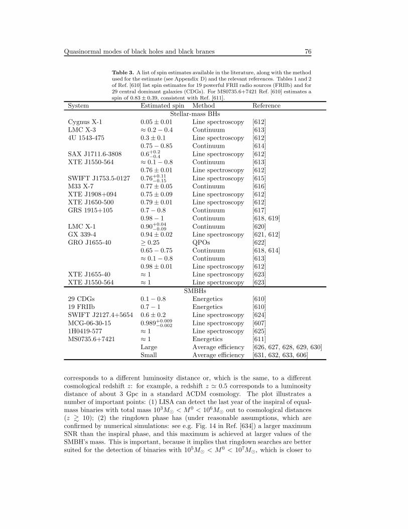
Quasinormal modes of black holes and black branes 76
Table 3. A list of spin estimates available in the literature, along with the methodused for the estimate (see Appendix D) and the relevant references. Tables 1 and 2of Ref. [610] list spin estimates for 19 powerful FRII radio sources (FRIIb) and for29 central dominant galaxies (CDGs). For MS0735.6+7421 Ref. [610] estimates aspin of 0.83 ± 0.39, consistent with Ref. [611].
System Estimated spin Method ReferenceStellar-mass BHs
Cygnus X-1 0.05 ± 0.01 Line spectroscopy [612]LMC X-3 ≈ 0.2 − 0.4 Continuum [613]4U 1543-475 0.3 ± 0.1 Line spectroscopy [612]
0.75 − 0.85 Continuum [614]SAX J1711.6-3808 0.6+0.2
−0.4 Line spectroscopy [612]XTE J1550-564 ≈ 0.1 − 0.8 Continuum [613]
0.76 ± 0.01 Line spectroscopy [612]SWIFT J1753.5-0127 0.76+0.11
−0.15 Line spectroscopy [615]M33 X-7 0.77 ± 0.05 Continuum [616]XTE J1908+094 0.75 ± 0.09 Line spectroscopy [612]XTE J1650-500 0.79 ± 0.01 Line spectroscopy [612]GRS 1915+105 0.7 − 0.8 Continuum [617]
0.98 − 1 Continuum [618, 619]LMC X-1 0.90+0.04
−0.09 Continuum [620]GX 339-4 0.94 ± 0.02 Line spectroscopy [621, 612]GRO J1655-40 ≥ 0.25 QPOs [622]
0.65 − 0.75 Continuum [618, 614]≈ 0.1 − 0.8 Continuum [613]0.98 ± 0.01 Line spectroscopy [612]
XTE J1655-40 ≈ 1 Line spectroscopy [623]XTE J1550-564 ≈ 1 Line spectroscopy [623]
SMBHs29 CDGs 0.1 − 0.8 Energetics [610]19 FRIIb 0.7 − 1 Energetics [610]SWIFT J2127.4+5654 0.6 ± 0.2 Line spectroscopy [624]MCG-06-30-15 0.989+0.009
−0.002 Line spectroscopy [607]1H0419-577 ≈ 1 Line spectroscopy [625]MS0735.6+7421 ≈ 1 Energetics [611]
Large Average efficiency [626, 627, 628, 629, 630]Small Average efficiency [631, 632, 633, 606]
corresponds to a different luminosity distance or, which is the same, to a differentcosmological redshift z: for example, a redshift z ≃ 0.5 corresponds to a luminositydistance of about 3 Gpc in a standard ΛCDM cosmology. The plot illustrates anumber of important points: (1) LISA can detect the last year of the inspiral of equal-mass binaries with total mass 103M⊙ < M0 < 106M⊙ out to cosmological distances(z & 10); (2) the ringdown phase has (under reasonable assumptions, which areconfirmed by numerical simulations: see e.g. Fig. 14 in Ref. [634]) a larger maximumSNR than the inspiral phase, and this maximum is achieved at larger values of theSMBH’s mass. This is important, because it implies that ringdown searches are bettersuited for the detection of binaries with 105M⊙ < M0 < 107M⊙, which is closer to

Quasinormal modes of black holes and black branes 77
103
104
105
106
107
M0
100
101
102
103
104
SNR
z=10
εrd=1%, j=0.8
z=0.54
102
103
M0
10-2
10-1
100
101
102
DL
(Gpc
)
LIGOAdvanced LIGOVirgoET
SNR=10j=0.6, εrd=3%
Figure 17. Left: typical SNR for equal-mass inspirals and ringdown signalsdetected by LISA, assuming a final spin j = 0.8 and a conservative ringdownefficiency ǫrd = 1% (from [10]). Top to bottom, the lines correspond to sourcesat redshift z = 0.54, 1, 2, 5, 10. Right: reach of Earth-based interferometers fora ringdown producing a BH with final spin j = 0.6 and ǫrd = 3%, as a functionof the mass of the final hole (from [11]).
the typical mass range estimated for SMBHs at galactic centres (see Section 9.3).In the right panel of Fig. 17 we show the ringdown detection range corresponding
to ρ = 10 for Earth-based detectors. The plot shows that Advanced LIGO and theEinstein Gravitational Wave Telescope (ET) have the potential to detect ringdownfrom IMBH-IMBH systems of mass up to ∼ 103M⊙ out to a luminosity distance ofa few Gpc [545]. In fact, third-generation Earth-based interferometers could probethe first generation of “light” seed BHs of M ∼ 102 − 103M⊙, providing informationcomplementary to LISA on the earliest BHs in the universe [635]. A more speculativesource is the intermediate-mass ratio inspiral (IMRI) of stellar-mass BHs into IMBHs.For these systems, ringdown would be suppressed relative to inspiral because of thesmall mass ratio. However, what is lost in terms of number of cycles is gained in termsof detector sensitivity: IMRI ringdowns would happen in the optimal frequency bandof second- and third-generation detectors, and therefore they could be detectable bya network of Advanced LIGOs [544].
9.5. Event rates
Gravitational wave interferometers (unlike traditional electromagnetic observatories)respond to the waves’ amplitude, not to their energy. Since the wave amplitude decayslinearly with distance, a modest increase of (say) a factor two in sensitivity means thatthe detectable volume increases by a factor eight. Given that merging compact binariesare the most promising ringdown source, the relevant question for ringdown detectionis then: how many merging compact binary events can we expect in a given volume?The issue of estimating event rates is one of the most pressing in gravitational wavedetection. The uncertainties involved are so large, and progress in the field is so rapid,that any estimates we quote are likely to become rapidly obsolete. For this reason wededicate little space to event rate estimates, providing a few references as a guide forthe interested reader.

Quasinormal modes of black holes and black branes 78
Stellar-mass and intermediate-mass black hole ringdowns In the simplest models,compact binary coalescence rates should be proportional to the stellar birth rate innearby spiral galaxies, which can be estimated from their blue luminosity. Thereforethe coalescence rates are usually given in units of Myr−1L−1
10 , where L10 is 1010 timesthe blue solar luminosity. To convert these numbers into detection rates, one musttake into account the fact that detection ranges for ringdowns are different from thosefor inspirals. If the distance to an event is above ∼ 50 Mpc the local over-densityof galaxies can be ignored, and the number of galaxies containing possible sourcesis N = [(4π)/3](D/Mpc)3(2.26)−30.0117 Milky-way equivalent galaxies, where 2.26is a correction factor to include averaging over all sky locations/orientations, and0.0117Mpc−3 is the density of Milky-Way equivalent galaxies. For shorter distancesone should use a sky catalog, such as Ref. [636].
For NS-NS binaries, early and conservative estimates were made by Phinney[637]. At present, the most reliable NS-NS merging rate estimates are obtainedby extrapolating from observed binary pulsars [638, 639]. Expected rates are ≈50Myr−1L−1
10 , but they could be an order of magnitude lower or larger. For NS-BHand BH-BH rates we have to rely mostly on population-synthesis models [640, 641].Plausible rate estimates are ≈ 2Myr−1L−1
10 for NS-BH binaries and ≈ 0.4Myr−1L−110
for BH-BH binaries, but they could be roughly two orders of magnitude larger or lower.These rates translate into tens to thousands of inspiral events per year in AdvancedLIGO. The typical end-product of these mergers are BHs of mass ∼ 10M⊙, and therange for Advanced LIGO detection of these BH ringdowns is more than an orderof magnitude less than the inspiral range, so ringdown rates should be ∼ 102 − 103
times smaller than inspiral rates. Rates for ringdowns involving IMBHs are even moreuncertain. In optimistic scenarios, Advanced LIGO could see ∼ 10 IMBH binarymergers per year [545] and perhaps ∼ 20 ringdowns from the merger of stellar-massBHs into IMBHs [544] (see also [642, 643]).
These predictions rapidly change as our understanding of the underlying physicsand compact binary observations improve. For example, Ref. [644] argues thatpotential BH-BH binary progenitors may undergo a common envelope phase whilethe donor is evolving through the Hertzsprung gap. This would probably lead to amerger, thus shutting off a channel for BH-BH production and sensibly reducing BH-BH merger rates. On the other hand, based on observations of a very massive BHbinary, Ref. [543] estimates an initial LIGO rate of order 0.5/yr for relatively massiveBH binaries (that therefore would be observed mostly in the merger/ringdown phase).
Particularly interesting for ringdown detection are compact binary mergers fromdense star clusters. Ref. [645] points out that a “high-mass” selection occurs because,in nuclear star clusters at the centers of low-mass galaxies, three-body interactionsusually “pair up” the two heaviest members of a triple system. This typically producesbinary mergers with M & 20M⊙, which means that Earth-based interferometers wouldusually observe the merger/ringdown phase. These findings are consistent with workby other authors [646, 647, 648].
Supermassive black hole ringdowns The LISA noise curve determines the optimalmass and redshift range where binary inspiral and ringdown events have large SNR,allowing a precise measurement of the source parameters. Reliable estimates of thenumber of events detectable during the mission’s lifetime, and of their mass spectrumas a function of redshift, will play a key role in the planning of LISA data analysis.For this reason, over the last few years the calculation of SMBH merger event rates

Quasinormal modes of black holes and black branes 79
and of their mass spectrum has become an active field of research.
Table 4. SMBH binary rates (events/year) predicted by different models(adapted and updated from Ref. [567]).
Reference Rate Redshift range
Haehnelt 2003 [649] 0.1-1 0 < z < 5 (gas collapse only)10-100 z > 5 (hierarchical buildup)
Enoki et al. 2004 [650] 1 z > 2Menou et al. 2001 [651] 10 z < 5Rhook and Wyithe 2005 [652, 653] 15 z ∼ 3 − 4Volonteri, Haardt and Madau [568, 570, 654] ∼ 30 z ∼ 4 − 16Begelman, Volonteri and Rees [600, 570, 654] ∼ 20 z ∼ 3 − 10Koushiappas and Zentner 2005 [571] & 103 mostly z ∼ 10, down to z ∼ 1Islam et al. 2003 [655] 104 − 105 z ∼ 4 − 6
A discussion of rate estimates is out of the scope of this review (see e.g. [567,654, 656]), but the large uncertainties in SMBH binary formation models and in thepredicted event rates are quite evident from Table 4. The numbers we list should beinterpreted with caution. Each prediction depends on a large number of poorly knownphysical processes, and the notion of “detectability” of a merger event is defined indifferent ways: some authors define detectability setting a threshold on the SNR,others set a threshold on the gravitational wave effective amplitude. Furthermore,different authors use different LISA noise curves. A tentative bottom line is that wecould face one of the following two scenarios. According to a class of models, we shouldobserve ≈ 10 events/year at redshifts (say) 2 <
∼ z <∼6. However, we cannot exclude the
possibility that hundreds or thousands of SMBH binaries will produce a large (andperhaps even stochastic) background in the LISA data. Clearly, the detection strategyto use strongly depends on which of the two scenarios actually occurs in nature.
Besides being able to observe SMBH mergers throughout the universe, LISAshould also be able to detect IMBH-IMBH binary mergers (that is, binaries containinga 10− 100 M⊙ BH orbiting a 100− 1000 M⊙ BH). Rates for IMBH binary detectionswere first estimated by Miller [657] and then revised by Will [658]. The revisedestimates are very pessimistic, predicting ∼ 10−6 events/year for typical values ofthe parameters. A more promising scenario involves an IMBH spiralling into a SMBH[659]. For these systems, Ref. [660] estimates a detection rate of a few events/year,suggesting that mergers of a 103 M⊙ IMBH into a 106 M⊙ SMBH could be observedout to z ∼ 20 with an SNR of 10 in a one-year integration. Ref. [661] predicts an evenmore optimistic rate of ∼ 102 events/year throughout the universe. These estimatesare very preliminary and even more uncertain than the corresponding estimates forSMBH binaries, but they should be taken into account in design choices concerning(for example) the optimal armlength of LISA.
9.6. Inferring black hole mass and spin from ringdown measurements
We have seen in Section 9.4 that the prospects for detection of ringdown radiationby LISA and advanced Earth-based detectors are quite encouraging. Interestingphysics can be extracted from the observation of BH ringdowns [10, 79, 461]. Since

Quasinormal modes of black holes and black branes 80
astrophysical BHs in general relativity are fully characterized by their mass andangular momentum, the detection of a single mode is in principle sufficient to estimatethe mass and spin parameter of the hole, by inverting the experimentally determinedωlmn(M,a/M), Qlmn(a/M). Indeed, one finds that accurate measurements of SMBHmass and angular momentum can be made.
0.0 0.2 0.4 0.6 0.8 1.0a/M
10-1
100
101
SN
R x
err
or
a/M
M
l=2, m=2
A
φ
104
105
106
107
108
M
10-6
10-5
10-4
10-3
10-2
10-1
100
erro
rs o
n j a
nd M
l=2, m=2
jM
Figure 18. Left: errors (multiplied by the signal-to-noise ratio ρ) inmeasurements of different parameters for the fundamental l = m = 2 mode asfunction of the rotation parameter a/M . Solid (black) lines give ρσa/M , dashed(red) lines ρσM/M , dot-dashed (green) lines ρσA/A, dot-dot-dashed (blue) linesρσφ, where σk denotes the estimated rms error for variable k, M denotes the massof the BH, and A and φ denote the amplitude and phase of the wave (adaptedfrom [10].) Right: actual errors in a LISA measurement for a source located adDL = 3 Gpc, with ringdown efficiency ǫrd = 3%.
For example, the left panel of Fig. 18 shows the estimated error (multiplied by theSNR ρ) in measuring the SMBH mass M , angular momentum parameter a/M , QNMamplitude A, and phase φ for circularly polarized radiation from the fundamentall = m = 2 bar mode (cf. Eq. (150) for definitions). If an energy ∼ 10−4M is radiatedinto the fundamental mode of a 106M⊙ SMBH with a/M = 0.8 at 3 Gpc (ρ ∼ 200), Mand a/M could be measured to 1%; if the energy deposition is only 10−6, they couldstill be measured to 10%. These numbers were computed for LISA in Ref. [10], butthey carry over to other detectors through a simple rescaling by ρ. Generalizing tomulti-mode detection (and specifically to the detection of two modes with a range ofrelative amplitudes) one finds similar results [10]. Gravitational wave detectors will beable to determine the mass and spin of BHs with excellent precision from observationsof the ringdown phase.
Event loss and bias in parameter estimation using single-mode templates Currentringdown searches are performed using matched filtering and single-mode templates,consisting of a single exponentially damped sinusoid. These are the simplest possibletemplates, and they are expected to capture the relevant physics of the problemwhen one ringdown mode dominates over the others. Unfortunately, this notion ofdominance must be precisely formulated. Consider for illustration the case of non-spinning binary BH mergers, and suppose for simplicity that there are only two modesin the signal, say l = m = 2 and l = m = 3. In particular, assume that the strain h

Quasinormal modes of black holes and black branes 81
as seen by a detector, Eq. (151), is of the form
h = A1e−π f1t/Q1 sin(2πf1 t−φ1)+A2e
−π f2t/Q2 sin(2πf2t−φ2) .(160)
Estimates of the multipolar energy distribution give a relative amplitude A2/A1 =h33/h22 ∼ 0.3−0.4(1−1/q), where q is the mass ratio and h22 (h33) are the amplitudesof the l = m = 2 (3) modes of the radiation, respectively [44]. For q > 3, which includesmost likely merger scenarios, we get h33/h22 ≥ 0.2 − 0.3. It is now natural to ask:given a relative amplitude of this order, how many events would we miss in a searchwith single-mode ringdown templates?
0.92
0.925
0.925
0.930.93
0.93
0.93
5
0.93
5
0.935
0.94
0.94
0.94
0.94
5
0.945
0.94
5
0.94
5
0.945
0.94
5
0.945
0.96
0.96 0.96
0.96
0.96
0.96
0.96
0.96
5
0.965
0.965
0.965
0.965
0.965
0.97
0.97
0.97
0.97
0.97
0.97
0.97
5
0.97
5
0.97
5
0.975
0.96
0.96
0.96
5
0.965
0.97
5
0.975
0.975
0.94
0.94
0.94
0.97
0.93
5
0.935
0.93
5
0.93
0.93
0.93
0.98
0.98
0.98
0.98
0.97
5
0.975
0.92
5
0.92
5
0.92
0.92
0.94
5
φ1
φ2
Fitting Factor, M0=200 M
sun, Advanced LIGO
−3 −2 −1 0 1 2 3
−3
−2
−1
0
1
2
3
0.925
0.93
0.935
0.94
0.945
0.95
0.955
0.96
0.965
0.97
0.975
1.75
1.75
2
22
2.25
2.25
2.25
2.25
2.25
2.5
2.5
2.5
2.5
2.5
2.25
2.25
2.25
2.25
2.75
2.75
2.75
2.75
2.75
2.5
2.5
2.5
2.53
3
3
3
3
2.75
2.75
2.75
2.75
3.25
3.25
3.25
3.25
3.25
33
3
3
3.5
3.5
3.5
3.5
3.5
3.25
3.25
3.25
3.25
3.5
3.5
3.5
3.75
3.75
3.75
3.75
3.75
3.75
3.75
3.75
2
2
2
2
4
4
44
4
4
4.25
4.25
4.25
4.25 1.75
1.75
4.5
4.5
4
φ1
φ2
Quality Factor, M0=200 M
sun, Advanced LIGO
−3 −2 −1 0 1 2 3
−3
−2
−1
0
1
2
3
2
2.5
3
3.5
4
Figure 19. Left: contour plots of the fitting factor as a function of the phaseangles of the signal. For this illustrative calculation we assume that the Kerrparameter of the final BH is j = 0.6, and that the relative amplitude of thesecond mode is A = 0.3. Right: quality factor estimated by a single-mode filter.The “true” frequencies and quality factors for a/M = 0.6 are MωR 1 = 0.4940,Q1 = 2.9490, MωR 2 = 0.7862, Q2 = 4.5507. See [11] for more details.
The answer is quantified in the left panel of Fig. 19, where we show Apostolatos’fitting factor (FF) [662, 663] resulting from searching a two-mode signal with single-mode templates from a 200M⊙, a/M = 0.6 BH, with relative amplitude A2/A1 = 0.3,in Advanced LIGO data. Contour plots of the FF are shown as a function of the(unknown) phases in Eq. (160). The FF is essentially the ratio ρ/ρmax, where ρ is theactual SNR achieved by matched filtering and ρmax is the maximum possible SNR,attained when the template and waveform coincide. FFs larger than 0.97, leading toa loss of less than about 10% in events, are typically considered acceptable. The FFachievable by a detection is usually assumed to correspond to the minimum of the FFin the space of the unknown parameters (φ1, φ2) (this is known as the “minimax”criterion). Therefore, according to this simplified calculation, single-mode templatesmay well lead to unacceptable SNR degradation in a search. The situation can beeven worse for larger masses and other detectors [11]; similar conclusions apply alsoto LISA, albeit in a completely different mass range.
Besides leading to a loss in the number of events, single-mode templates lead toa large bias in the estimation of the BH’s mass and spin. The estimated frequencyhas relatively small bias, and it always corresponds to the dominant (least-damped)mode in the pair. Results are more interesting for the estimated quality factor, shownin the right panel of Fig. 19 as a function of the phase angles. For our chosen value

Quasinormal modes of black holes and black branes 82
of the Kerr parameter the quality factor of the l = m = 2 and l = m = 3 modesare Q1 = 2.9490 and Q2 = 4.5507, respectively. Comparing with the left panel, wesee that relative minima in the FF (white “islands” in the left panel) occur, roughlyspeaking, when the quality factor “best fits” the subdominant, l = m = 3 mode. Thisis a rather remarkable result: the minimax filter “best fits” the subdominant modein the pair, leading to significant bias in the estimation of the quality factor (andhence of the spin). Unfortunately, maxima in the FF do not correspond to the filterbeing optimally adapted to the l = m = 2 mode. As the filter tries to maximize theSNR, the estimated value of the quality factor becomes significantly biased, and itdeviates quite sensibly from the value expected for the dominant (l = m = 2) mode.The bottom line is, again, that single-mode filters may be useful for detection, but amulti-mode post-processing will be necessary for accurate spin measurements.
There is, of course, a price to pay when using multi-mode templates. AboutN ∼ 6Qmax log fmax/fmin ∼ 500 single-mode templates are enough to cover theparameter space for Earth-based detector searches, if we assume an event loss ofno more than 10% (i.e., a minimal match larger than 0.97 [663]). For two-modetemplates, rough estimates suggest that this number may increase up to N ∼ b× 106,with b ∼ 1 a detector-dependent constant [11]. A more detailed data analysis study(e.g. using better template placing techniques, along the lines of [472, 473, 474, 13])will be needed to reduce computational requirements.
9.7. Tests of the no-hair theorem
The fact that all information is radiated away in the process leading to BH formation,so that astrophysical BHs in Einstein’s theory are characterized completely by theirmass and angular momentum, is known as the “no-hair theorem”. To test thistheorem, it is necessary (but not sufficient) to resolve two QNMs [10, 461]. Roughlyspeaking, one mode is used to measure M and a, and the other to test consistencywith the Kerr solution.
Can we tell if there really are two or more modes in the signal, and can weresolve their parameters? Physical intuition suggests that if the noise is large and theamplitude of the weaker signal is very low (or if the two signals have almost identicalfrequencies) the two modes could be difficult to resolve. A crude lower limit on theSNR required to resolve frequencies and damping times was presented in Refs. [10, 11].The analysis uses the statistical uncertainty in the determination of each frequencyand damping time, which a standard Fisher-matrix calculation estimates to be [10]
ρσf1 =π√2
f31
(
3 + 16Q41
)
A21Q
71
[ A21Q
31
f1 (1 + 4Q21)
+A2
2Q32
f2 (1 + 4Q22)
]
12
,(161)
ρστ1 =2
π
(
3 + 4Q21
)
A21f1Q1
[ A21Q
31
f1 (1 + 4Q21)
+A2
2Q32
f2 (1 + 4Q22)
]
12
. (162)
These errors refer to mode “1” in a pair; errors on f2 and τ2 are simply obtained byexchanging indices (1 ↔ 2) [10, 11]. The expressions above further assume white noisefor the detector, and that modes “1” and “2” correspond to different values of l or m.
A natural criterion (a la Rayleigh) to resolve frequencies and damping timesis that |f1 − f2| > max(σf1 , σf2 ), |τ1 − τ2| > max(στ1 , στ2). In interferometry thiswould mean that two objects are (barely) resolvable if the maximum of the diffractionpattern of object 1 is located at the minimum of the diffraction pattern of object 2.

Quasinormal modes of black holes and black branes 83
We can introduce two “critical” SNRs required to resolve frequencies and dampingtimes, ρf
crit = max(ρσf1 , ρσf2)/|f1 − f2| , ρτcrit = max(ρστ1 , ρστ2)/|τ1 − τ2|, and recast
our resolvability conditions as
ρ > ρcrit = min(ρfcrit, ρ
τcrit) , (163)
ρ > ρboth = max(ρfcrit, ρ
τcrit) . (164)
The first condition implies resolvability of either the frequency or the damping time,and the second implies resolvability of both.
Now let us consider how to resolve amplitudes, i.e. the minimum SNR needed todetermine whether two or more modes are present in a given ringdown signal. Supposeagain, for simplicity, that the true signal is a two-mode superposition. Then we expectthe weaker signal to be hard to resolve if its amplitude is low and/or if the detector’snoise is large. Appendix B of Ref. [11] quantifies this statement by deriving a criticalSNR for amplitude resolvability ρGLRT based on the generalized likelihood ratio test.The derivation of this critical SNR is based on the following simplifying assumptions:(i) using other criteria one has already decided for the presence of at least one dampedexponential in the signal, and (ii) the parameters of the ringdown signal (frequenciesand damping times), as well as the amplitude of the dominant mode, are known. Inpractice the latter assumption is not valid, so these estimates of the minimum SNRshould be considered optimistic. Fig. 20 compares the critical SNR ρGLRT (Eq. (B12)
1 1.5 2 2.5 3 3.5 4q
101
102
103
104
SN
Rcr
it
l’=m’=3l’=m’=4
ρcrit
ρboth
ρGLRT
Figure 20. Minimum SNR required to resolve two QNMs from a BH resultingfrom the inspiralling of a BH binary with mass ratio q. The dominant mode (mode“1”) is assumed to be the fundamental QNM with l = m = 2; mode “2” is eitherthe fundamental l = m = 3 QNM (solid lines) or the fundamental l = m = 4 QNM(dashed lines). The relative mode amplitude A(q) is estimated from numericalsimulations [44]. If ρ > ρGLRT we can tell the presence of a second mode in thewaveform, if ρ > ρcrit we can resolve either the frequency or the damping time,and if ρ > ρboth we can resolve both.
of Ref. [11]) and the two different criteria for frequency resolvability, Eqs. (163) and(164). The plot shows that ρcrit < ρGLRT < ρboth for all values of q. Therefore, given adetection, the most important criterion to determine whether we can carry out no-hairtests is the GLRT criterion. If ρ > ρGLRT we can decide for the presence of a second

Quasinormal modes of black holes and black branes 84
mode in the signal. Whenever the second mode is present, we also have ρ > ρcrit:that is, we can resolve at least the frequencies (if not also the damping times) of thetwo modes. A SNR ρ ∼ 30− 40 is typically enough to perform the GLRT test on thel = m = 3 mode, as long as q & 1.5. From Figs. 17-20 we conclude that not onlyLISA, but also advanced Earth-based detectors (Advanced LIGO and ET) have thepotential to identify Kerr BHs as the vacuum solutions of Einstein’s general relativity.
In conclusion, ringdown radiation can be used to distinguish BHs from exoticalternatives, such as boson stars [463] or gravastars [664]. Ringdown tests of the Kerrnature of astrophysical BHs are independent from (and complementary to) proposedtests using a multipolar mapping of the Kerr spacetime, as encoded in EMRI signalsaccording to “Ryan’s theorem” and its generalizations [665, 666, 667].
9.8. Matching inspiral and ringdown: problems and applications
Models of gravitational waveforms from inspiralling compact binaries usually rely onthe post-Newtonian approximation to general relativity [668]. Ideally, for matched-filtering detection we would like to have detection template banks with “complete”waveforms encompassing the inspiral, merger and ringdown. Phenomenologicaltemplate families based on physically motivated fits of numerical merger waveformsor on effective-one-body models are now available [669, 634, 670, 671]. However, itwould be desirable to have a full understanding of the merger process, connecting thepost-Newtonian approximation during the inspiral to a description of the ringdown asa superposition of QNMs.
QNM fits of numerical relativity waveforms are routinely used to check that thetotal angular momentum of the system is conserved during BH merger simulations.This is usually achieved by computing three independent quantities: the angularmomentum radiated at infinity, the angular momentum obtained from isolated horizoncalculations, and the angular momentum obtained by inverting the frequencies anddamping times resulting from a QNM fit of the ringdown of the final Kerr BH (seee.g. [477, 44, 672]). Buonanno, Cook and Pretorius noticed that, as more and moreovertones are included, a QNM expansion gets in better agreement with numericalwaveforms for equal-mass binaries [477].
So far, efforts to “stitch” the post-Newtonian approximation (or one of itseffective-one-body variants) to the ringdown have used rather crude models forringdown excitation. The original effective-one-body approach simply attached theplunge waveform to the fundamental l = m = 2 QNM of a Kerr BH [673]. Intheir study of recoils, Damour and Gopakumar attached the plunge waveform to thefundamental Schwarzschild QNMs with l = 2 and l = 3 [674]. A comprehensiveanalysis of Pretorius’ numerical waveforms for equal-mass BH binaries [477] clearlyillustrated the importance of higher-order overtones. Damour and Nagar obtained agood match to numerical relativity waveforms by requiring continuity of the plungewaveform with a (Schwarzschild) ringdown waveform including five overtones on a gridof points, or “comb” [176]. A “hybrid comb” procedure, imposing the continuity ofthe waveform and its derivatives, was later introduced in Ref. [174]. These stitchingmethods have great phenomenological interest, and they can do remarkably well atreproducing numerical waveforms. For example, the authors of Ref. [174] extend aneffective-one-body waveform through merger by stitching the inspiral waveform toQNMs, finding striking agreement (at the 0.1% level) between the numerical QNMfrequency and the perturbative prediction for the same frequency computed from the

Quasinormal modes of black holes and black branes 85
final mass and spin of the numerical simulation. A slightly different approach wasadopted in Ref. [670], where the frequency-domain waveform was truncated abruptlyat some cutoff frequency close to the QNM frequency. The truncated waveformsdisplay a Gibbs phenomenon in the time domain, and they are (surprisingly) quiteeffective at detecting the full signal. The reason is that a cutoff in the frequencydomain around the fundamental QNM frequency corresponds, in the time domain, toa damped sinusoid with frequency close to the cutoff frequency.
These phenomenological “stitching recipes” may well be enough for the purposeof gravitational wave detection, but it is desirable to have a complete understandingof QNM excitation in a compact object merger within perturbation theory, basedon the concept of excitation coefficients. Ref. [167] carried out a first step in thisdirection by computing the excitation factors for Kerr BHs (see Section 3.2), butmore work is required to compute the excitation coefficients for generic initial data,and to understand the validity of the linear approximation in a BH merger. Acorrect matching of effective-one-body waveforms with the ringdown signal may haveastrophysical implications because QNMs play an important role in the recoil ofmerging BH binaries, through a process sometimes called “ringdown braking” (see[675, 674, 676] and references therein). A complete analytical description of themerger of spinning, precessing binaries would also prove useful for statistical studiesof astrophysical relevance [677].
Even if phenomenological waveforms may be good enough at detectinggravitational wave signals, a complete description of the waveform (including bothinspiral and ringdown) has been shown to improve parameter estimation by effectivelydecorrelating the source parameters (see [534] for a study predating the numericalrelativity breakthrough, and [678, 679, 669, 634, 535] for recent efforts in thisdirection). Large-scale efforts (dubbed the NINJA and Samurai projects, respectively)are now attempting to use complete numerical waveforms in LIGO data analysis, andto cross-validate numerical waveforms produced by different codes [525, 680].
An important point to keep in mind is that inspiral and merger/ringdownreally probe different BH populations, so they provide complementary information.This should be quite clear by inspecting the red and black histograms in Fig. 16,which show that the spin distribution of SMBHs in binaries is usually different fromthe spin distribution of the remnant BHs formed as a result of the merger. Thiscomplementarity can be used for interesting physical applications. For example, if wecan determine accurately enough the masses and spins of BHs before and after mergerfor the same system, we could use this information to test Hawking’s area theorem inastrophysical settings [681].
10. Other recent developments
10.1. Black hole area quantization: in search of a log
One of the main driving forces behind the development of new tools to study QNMsis the possibility that classical BH oscillations could yield insights into their quantumbehavior. First suggested by York [68] and Hod [17], this idea was further exploredby Dreyer [97] in the context of Loop Quantum Gravity, and subsequently revisitedby many authors (see e.g. [682, 276, 683, 684, 685, 686, 687, 688, 689, 690, 691]).
The idea can be traced back to arguments by Bekenstein and collaborators[692, 693]. A semi-classical reasoning suggests that the BH area spectrum is quantized

Quasinormal modes of black holes and black branes 86
according to
AN = γ l2P , N = 1, 2, ... , (165)
where lP is the Planck length (but see [694] for criticism). Statistical physicsarguments impose a constraint on γ [693, 695]:
γ = 4 log k , (166)
where k is an integer, which in general is left undetermined (but see [696]).Inspired by Bekenstein’s ideas, Hod [17] proposed to determine k via a version ofBohr’s correspondence principle in which the highly-damped QNM frequencies playa fundamental role. At the time, the only available exploration of highly-dampedQNMs was the numerical study by Nollert [90], which indicated that gravitationalhighly-damped QNMs in the Schwarzschild geometry asymptote to
Mω = 0.0437123− i(2n+ 1)/8 . (167)
While looking for classical oscillation frequencies proportional to the logarithm of aninteger, Hod realized that 0.0437123 ∼ ln 3/(8π), and went on to suggest that theemission of a quantum with frequency ωR = ln 3/(8π) corresponds to the smallestenergy a BH can emit. The corresponding change in surface area would then be
∆A = 32πMdM = 32πM~ω = 4~ ln 3 . (168)
and by comparing with Eq. (165) we get k = 3, thus fixing the area spectrum to
An = 4l2P ln 3n ; n = 1, 2, ... (169)
A few years later Dreyer [97] used similar arguments to fix the Barbero-Immirziparameter of Loop Quantum Gravity. Shortly afterwards, Motl [91] and Motl andNeitzke [101] showed analytically that the highly damped QNM frequencies of aSchwarzschild BH are indeed given by Eq. (86), containing the desired logarithmof an integer.
Motl and Neitzke’s work lent some support to Hod’s ideas. It was followed by aflurry of activity to explore the highly-damped QNMs of several BH spacetimes, whoseoutcome has been described and summarized in previous sections. Unfortunatelythe conjectured relation between QNMs and area quantization stumbled before thecharged and rotating four-dimensional geometries, for which the highly-damped regimeis not as simple as suggested by Hod’s original argument (see Sections 5.3-5.2).Recently Maggiore [688] observed that Hod’s prescription was based on experiencewith “normal” quantum systems, for which the relevant frequency is ωR. For highly-damped systems, Maggiore noted that one should rather consider the imaginary partof the QNMs ωI , solving a number of puzzles and obtaining a different expressionfor the quantum of area. A similar prescription has been extended also to Kerr BHs[689, 690] and other geometries [691]. It is not clear whether Maggiore’s suggestioncan be extended consistently to all geometries. Whether a relation between QNMsand the quantum behavior of BHs exists or not, Hod’s suggestion was at the very leastan important thrust to complete our understanding of classical BH oscillation spectra.
10.2. Thermodynamics and phase transitions in black hole systems
In the last few years, remarkable relations between classical and thermodynamicalproperties of black objects have been uncovered. For instance, a correspondencebetween classical and thermodynamical instabilities of a large class of black branes

Quasinormal modes of black holes and black branes 87
conjectured by Gubser and Mitra [697, 698] was proved by Reall [699] (see [700] for areview). Manifestations of this duality are expected to appear in the QNM spectra.Indeed, some indications that phase transitions correspond to changes in the QNMspectrum were provided in specific cases by various authors [701, 702, 703, 704, 705,706]. However, at present there seems to be no obvious correspondence betweenthermodynamical phase transitions of the kind suggested by Davies [707, 708] andQNM spectra (see [709] and references therein).
Another connection between QNMs and BH thermodynamics may follow fromHod’s proposed “universal relaxation bound” [710, 711, 712]. Hod’s proposal assertsthat the relaxation time τ of any thermodynamic system is bounded by τ ≥ ~/(πT ),where T is the temperature of the system. For BHs this implies the existence of(at least one) QNM frequency with imaginary part ωI ≤ πT , where T is now theHawking temperature of the BH. The bound seems to be valid for various kinds ofBHs, and it may be saturated by extremal BHs. The significance of Hod’s bound isnot completely clear to us. The bound is trivially satisfied by any physical systemexhibiting hydrodynamic behavior, since such a system always possesses sufficientlylong-lived modes (and, correspondingly, QNMs with imaginary part sufficiently closeor even infinitely close to zero: these hydrodynamic frequencies are discussed in Section8.3). Finite-volume systems might be more interesting, but then the concept of the”relaxation time” used in the bound needs a proper definition. In any case, this is aninteresting idea which might require better understanding. The relation between Hod’sbound and the viscosity-entropy bound (see Section 8.4) was discussed in Ref. [713].
10.3. Non-linear quasinormal modes
QNMs are usually defined and studied by considering only first-order perturbations.Being an intrinsically non-linear theory, general relativity is expected to display non-linear effects, which might conceivably be captured by going to higher orders inperturbation theory. The second-order formalism laid down several years ago byvarious authors [85, 714, 715] has recently been used to compute corrections to theQNM frequencies, their detectability and their influence on the late-time behavior ofthe system [716, 717, 718]. The encouraging outcome of these studies is that non-linear effects may well be observable by future gravitational wave interferometers.Favata [719] explores the interesting possibility of detecting another important non-linear effect of general relativity (the so-called gravitational wave memory) throughgravitational wave observations of merging binaries.
Higher-order perturbations of BH spacetimes have been explored systematicallyby Brizuela et al. [720, 721], using the Gerlach-Sengupta formalism and the computeralgebra methods described in [722] (see also Kol [723]). A complete gauge-invariantformalism for second-order perturbations of Schwarzschild BHs was recently reported[724].
10.4. Quasinormal modes and analogue black holes
Strong-field effects of general relativity are very small in Earth-bound experiments.For this reason BH physics is most easily studied via observations of astrophysicalphenomena such as accretion, X-ray spectra, and hopefully gravitational waveemission. The possibility to devise gravitational experiments probing strong-fieldgeneral relativity in the lab, as appealing as it sounds, may seem out of reach. However,

Quasinormal modes of black holes and black branes 88
Unruh, Visser and others [725, 31] ingeniously showed that some defining propertiesof BHs can be reproduced and studied by “analogue BHs”. These systems display atleast a subset of the properties traditionally associated with BHs and event horizons.Unruh’s analogue BHs do not carry information about the dynamics of Einstein’sequations, but share many kinematical features with true general-relativistic BHs.
The basic idea behind these analogue BHs is quite simple. Let us focus on aparticular analogue BH, the acoustic or “dumb” hole [725, 726]. Consider a fluidmoving with a space-dependent velocity vi
0(xi), for example water flowing through a
variable-section tube. Suppose the fluid velocity increases downstream, and that thereis a point where the fluid velocity exceeds the local sound velocity c(xi) ≡
√
∂p/∂ρ,in a certain frame. At this point, in that frame, we get the equivalent of an apparenthorizon for sound waves. In fact, no (sonic) information generated downstream ofthis point can ever be communicated upstream (for the velocity of any perturbationis always directed downstream, by simple velocity addition). This is the acousticanalogue of a BH, sometimes referred to as a dumb hole. These are not true BHs,because the acoustic metric satisfies the equations of fluid dynamics and not Einstein’sequations. However, sound waves propagate according to the usual curved space Klein-Gordon equation with the effective metric [725, 726, 31],
guν ≡ 1
ρ0c
−1... −vj
0
. . . . . . . . . . . . . . . .
−vi0
... (c2δij − vi0v
j0)
. (170)
Analogue BHs should Hawking-radiate, though an experimental verification ofHawking radiation in the lab is not an easy feat [727, 31]. Furthermore, sound wavepropagation in these metrics should reproduce many features of wave propagationin curved spacetimes. Most importantly for this review, acoustic BHs have a (thistime literally!) “characteristic sound” [5] encoded in their QNM spectrum. QNMsof acoustic BHs, which may be important in experimental realizations of the idea,were computed in Refs. [728, 240, 729, 730] for a simple (2 + 1)−dimensional acoustic
hole, the “draining bathtub” [726], for which ~v0 = (−A~r + B~φ)/r. The modes of(3 + 1)-dimensional acoustic holes with a “sink” at the origin were computed inRefs. [728, 731, 732]. Scattering from these holes is discussed in Ref. [733].
The experimental confirmation of these predictions is an interesting topic forfuture research. In practice, one may need a device to accelerate the fluid up tosupersonic velocities, such as a Laval nozzle [734, 735] (see also Unruh’s discussion in[727]). Laval nozzles were first used in steam turbines, but they find applications inother contexts, including rocket engines and nozzles in supersonic wind tunnels. Theyconsist of a converging pipe where the fluid is accelerated, followed by a throat (thenarrowest part of the tube) where the flow undergoes a sonic transition, and finallya diverging pipe where the fluid continues to accelerate. QNMs of flows in de Lavalnozzles were discussed and computed in Refs. [736, 737].
Following on Unruh’s “dumb hole” proposal, many different kinds of analogueBHs have been devised, based on condensed matter physics, slow light etcetera. Werefer the reader to Refs. [727, 31] for thorough reviews on the subject. QNMs ofcondensed-matter analogue BHs were recently computed in Refs. [738, 739]. Finally,we should mention that accretion of material onto astrophysical BHs can give riseto supersonic walls, i.e., acoustic horizons outside the event horizon. This processis particularly interesting: astrophysical BHs may provide a nature-given setting for
Quasinormal modes of black holes and black branes 89
producing analogue BHs [740, 741].
11. Outlook
The investigations of the last decade show that quasinormal spectra encode a wealth ofinformation on the classical and quantum properties of BHs and black branes. Froma holographic, high-energy perspective, BH QNMs yield important information onthe quasiparticle spectra and transport coefficients of the dual theory, and have anintriguing hydrodynamic description. From an astrophysical viewpoint, gravitationalwave measurements of QNMs may allow us to accurately measure BH masses and spinswith unprecedented accuracy and to test the no-hair theorem of general relativity. Thesuggestion that BH oscillation frequencies may be related to their quantum propertiesis controversial, but at the very least it has stimulated tremendous technical progress inthe calculation of previously unexplored regimes of the QNM spectrum. In this reviewwe tried to summarize these recent developments. There is no doubt that furtherinteresting connections between QNM research, fundamental physics and astrophysicswill be unveiled in the future. In closing, we think it might be useful to list some ofthe outstanding, unresolved issues.General mathematical problems, asymptotic expansions and related issues – It wouldprobably be fair to say that the level of mathematical rigor in QNM studies deservesan improvement. Whether or not boundary value problems for dissipative systemscan be treated in the framework of a sufficiently general mathematical theory appearsto be an open question. Less ambitiously, a unified treatment of resonances (QNMsincluded) at the level of mathematical physics would be desirable. Reliable regular andasymptotic expansions based on systematic procedures rather than ad hoc recipes havenot yet been developed in many cases. Improving numerical algorithms, in particularfor QNMs with large imaginary parts, also remains an avenue of research.Black hole perturbation theory in asymptotically-flat spacetimes – Despite a fifty-yearlong history of investigation, BH perturbation theory in asymptotically flat spacetimeshas a number of unresolved issues. The problem of metric reconstruction from theTeukolsky formalism is still open. QNM excitation for generic perturbations of KerrBHs have not been fully explored yet. The eikonal limit of Kerr QNMs is stillpoorly understood, as is the relation of QNMs with generic (l,m) to unstable circulargeodesics in the Kerr metric. Finally, an outstanding problem concerns the decouplingof linear perturbations of the Kerr-Newman metric.Gauge-gravity duality – At the moment, computing QNMs in the context of the gauge-gravity duality is a thriving industry, naturally expanding to include models withhigher-derivative gravity, holographic models with spontaneous symmetry breaking,or backgrounds dual to non-relativistic theories. As discussed in Section 8, onedistinguishes hydrodynamic-type modes from the rest of the QNM spectrum. Ona technical level, these modes are characterized by small parameters and thus canoften be determined analytically. A full analysis of hydrodynamic QNMs for genericbackgrounds is currently lacking. In particular, it would be helpful to obtain anexpression for the parameters of the sound mode similar to Eq. (148) for the diffusionconstant. The spectra of fermionic fluctuations (e.g. of the Rarita-Schwinger field,see [417]) in black brane backgrounds have not yet been fully computed. It would bevery interesting to explore further the connection between holography and the blackhole membrane paradigm [117, 742, 114, 115].Gravitational wave astronomy – An important problem in gravitational wave physics

Quasinormal modes of black holes and black branes 90
concerns the matching of inspiral waveforms (as computed by post-Newtonian theory)to the ringdown phase. This is necessary to produce complete phenomenologicaltemplates to be used in gravitational wave detection. Most attempts at solvingthis problem have adopted a purely phenomenological approach, but a study of theexcitation coefficients induced by generic initial data (possibly considering non-linearcorrections) could provide a more consistent and systematic solution to the matchingproblem. A study of the QNM contribution to the Green function has recently beenshown to hold promise as a computational approach to solve the self-force problem[172], which is of fundamental importance to model extreme- and intermediate-massratio inspirals for LISA data analysis. Other open issues concern ringdown dataanalysis. Simple calculations show that single-mode templates only produce moderatelosses in SNR when detecting multi-mode signals. However, the loss in terms ofparameter estimation accuracy is much more significant. The problem of optimaltemplate placing for detection by multi-mode templates needs to be addressed. Thepotential of higher multipoles in estimating the source parameters without angle-averaging should also be explored: the different angular dependence of subdominantmultipoles may provide information on the spin direction of the final BH. If BH spinsare linked to jets, this information could be used for coincident searches of gamma-raybursts or other electromagnetic counterparts to compact binary mergers [522, 523].
In the last few years, unexpected connections between QNMs and seeminglyunrelated phenomena (such as analogue BHs or thermodynamical BH phasetransitions) have been uncovered or proposed. More intriguing connections will surelyemerge in the coming decades.
Acknowledgments
We thank Alessandra Buonanno, Manuela Campanelli, Marc Casals, Ruth Daly, SamDolan, Guido Festuccia, Martin Gaskell, Leonardo Gualtieri, Shahar Hod, RomanKonoplya, Cole Miller, Christian Ott, Luciano Rezzolla, Andrzej Rostworowski, AnaSousa, Uli Sperhake and Vilson Zanchin for very useful discussions and for sharingwith us some unpublished material. We also thank Ilya Mandel for clarificationson rate calculations; Luca Baiotti, Bruno Giacomazzo and Luciano Rezzolla forproviding numerical data from Ref. [46]; Marta Volonteri for preparing Figure 16;Lubos Motl and Andrew Neitzke for permission to reproduce Figure 4 from Ref. [101];Shijun Yoshida for providing numerical data from Ref. [234], and Alex Miranda fornumerous suggestions. V.C.’s work was partially funded by Fundacao para a Ciencia eTecnologia (FCT) - Portugal through projects PTDC/FIS/64175/2006, by a FulbrightScholarship, and by the National Science Foundation through LIGO Research Supportgrant NSF PHY-0757937.
Appendix A.
Isospectrality, algebraically special modes and naked singularities
A number of striking relations among gravitational perturbations of the Kerr geometrywere revealed by Chandrasekhar and colleagues [22, 141, 62, 142, 743]. Here we reviewthese relations specializing most of the discussion to the Schwarzschild geometry. Thereader is referred to the original works for more details and for extensions to the Kerrspacetime [22, 141, 62, 142].

Quasinormal modes of black holes and black branes 91
By direct substitution, it can be checked that the gravitational potentials V ±s=2
in Eqs. (14) and (15) can be rewritten in the form
V ±s=2 = W 2 ∓ dW
dr∗+ β , β = −λ
2(λ+ 1)2
9M2, (A.1)
where
W =3M
(
6Mr2 + 2λL2(2M − r))
λr2 (6M + 2λr)L2− λ(λ + 1)
3M− 3M
λL2. (A.2)
(these equations correct some typos in Ref. [130]). Eq. (A.1) emerged fromChandrasekhar’s investigations [62, 141, 142] of the nature of the gravitationalpotentials. Potentials of this form are called superpartner potentials [744], and theyimply the following relation between the corresponding wavefunctions Ψ− and Ψ+
[22, 130]:
Ψ± =1
β − ω2
(
∓W Ψ∓ +dΨ∓
dr∗
)
. (A.3)
Eq. (A.1) seems to be unique to four-dimensional spacetimes, and does not generalizeto higher dimensions [102, 103]. The potential for electromagnetic-type andgravitational-type perturbations of extremal RN BHs can also be expressed in theform (A.1) [259, 260]. This justifies the fact that electromagnetic perturbations withangular index l are isospectral to gravitational with index l−1, as discussed in Section5.2. The isospectrality is a manifestation of supersymmetry between electromagneticand gravitational perturbations for extremal charged BHs [259, 260, 261].Isospectrality and asymptotic flatness Suppose that ω is a QNM frequency for Ψ+, i.e.that Ψ+ → A+e−iωr∗ when r → r+ and Ψ+ → a+
outeiωr∗ when r → ∞. Here a+
out = 1for the Schwarzschild metric and, if we impose Dirichlet boundary conditions, a+
out = 0for the SAdS metric. Substituting into Eq. (A.3) we see that
Ψ− → A+
β − ω2(W (r+) − iω) e−iωr∗ , r → r+ , (A.4)
→ 1
β − ω2
(
−a+outW (∞)eiωr∗ +
dΨ−
dr∗
)
, r → ∞ . (A.5)
The key point is that dΨ−/dr∗ ∼ eiωr∗ at infinity for the Schwarzschild geometry.Therefore, if ω is a QNM frequency for Ψ+ it is also a QNM frequency for Ψ−,and the two types of gravitational perturbations are isospectral [62, 141]. In generaldΨ−/dr∗ 6= 0 for SAdS, so the isospectrality is broken. The above relations are validalso for dS backgrounds: since the outer boundary conditions are imposed at thecosmological horizon, it is easy to see that gravitational perturbations of both paritiesare again isospectral. A specialized analysis is needed at the points where β−ω2 = 0:this condition defines the so-called algebraically special modes, discussed below.Algebraically special modes A class of special modes can be found analytically usingEq. (A.1). In the Petrov classification, this condition corresponds to a change in thealgebraic character of the spacetime. For this reason, Chandrasekhar called thesemodes “algebraically special” (AS) [142, 22]. Defining ±W = d
dr∗logχ±, the wave
equation can be written as
1
Ψ±
d2Ψ±
dr2∗+(
ω2 − β)
=1
χ±
d2χ±
dr2∗, (A.6)

Quasinormal modes of black holes and black branes 92
where we have used the identity 1χ±
d2χ±
dr2∗
= W 2 ± dWdr∗
. AS modes have frequencies
ω = Ωl such that β − Ω2l = 0. In this case Eq. (A.6) can be easily integrated:
Ψ± = χ±
∫
dr∗/χ2± = χ±
(
C±1 + C±2
∫ r
0
dr∗/χ2±
)
, (A.7)
where χ± = exp[
±∫
Wdr∗]
. The special relation between the two gravitationalpotentials extends to the Kerr geometry, where AS modes correspond to a vanishingTeukolsky-Starobinsky constant [22]. The nature of the boundary conditions at theSchwarzschild AS frequency is extremely subtle, and has been studied in detail byMaassen van den Brink [745]. Let us introduce some terminology [745]:1) “standard” QNMs have outgoing-wave boundary conditions at both sides (that is,they are outgoing at infinity and “outgoing into the horizon”);2) total transmission modes from the left (TTML’s) are incoming from the left (theBH horizon) and outgoing to the right (spatial infinity);3) total transmission modes from the right (TTMR’s) are incoming from the right andoutgoing to the left.
The Regge–Wheeler equation and the Zerilli equation must be treated on differentfooting at the AS frequency, since the supersymmetry transformation leading to theproof of isospectrality is singular there. It turns out that the Regge-Wheeler equationhas no modes at all, while the Zerilli equation has both a QNM and a TTML at theAS frequency [745].
Numerical calculations of AS modes have yielded some puzzling results. Studyingthe Regge-Wheeler equation, Leaver [75] found a QNM very close (but not exactlyat) the AS frequencies of Eq. (83). Namely, he found QNMs at frequencies 2M Ω′
2 =0.000000−3.998000i and 2M Ω′
3 = −0.000259−20.015653i. Similarly, in the extremalRN case one finds a QNM frequency very close to, but not exactly equal to, theAS frequency [241]. Maassen van den Brink [745] speculated that the numericalcalculations may be inaccurate and that no conclusion can be drawn on the coincidenceof Ωl and Ω′
l, “if the latter does exist at all”.An independent calculation was carried out by Andersson [746], who found
that the Regge–Wheeler equation has pure imaginary TTMR’s very close to Ωl for2 ≤ l ≤ 6. He therefore suggested that the modes he found coincide with Ωl, whichwould then be a TTM. Maassen van den Brink [745] observed again that, if all figuresin the computed modes are significant, the coincidence of TTM’s and QNMs is notconfirmed by this calculation, since Ω′
l and Ωl are numerically (slightly) different.Onozawa [230] calculated the (TTM) AS mode for Kerr BHs, improving upon the
accuracy of the Kerr AS frequencies computed in Ref. [142]. He showed that the KerrQNM with overtone n = 9 tends to the AS frequency Ωl (as defined by the Teukolsky-Starobinsky identity) when a→ 0 and suggested that QNMs approaching Ωl from theleft and from the right may cancel at a = 0, leaving only a special (TTM) mode. Thesituation concerning Kerr QNMs branching from the AS Schwarzchild mode is still farfrom clear. Using slow-rotation expansions of the perturbation equations, Maassenvan den Brink [745] drew two basic conclusions on these modes. The first is that, fora > 0, the so–called Kerr special modes are all TTM’s (left or right, depending onthe sign of s). The TTMR’s should not survive as a → 0, since they do not exist inthe Schwarzschild limit. In particular, in this limit, the special Kerr mode becomes aTTML for s = −2; furthermore, the special mode and the TTMR cancel each otherfor s = 2. Studying the limit a → 0 in detail, Maassen van den Brink reached a

Quasinormal modes of black holes and black branes 93
second conclusion: the Schwarzschild special frequency Ωl should be a limit point fora multiplet of “standard” Kerr QNMs, which for small a are well approximated by
2Mω = −4i− 33078176
700009
ma
2M+
3492608
41177ia2
4M2+O(ma2)+O(a4)(A.8)
when l = 2, and by his Eq. (7.33) when l > 2. Numerical studies found QNMsclose to the AS frequency, but not in agreement with this analytical prediction[231]. It was suggested (note [46] in Ref. [745]) that QNMs corresponding to theAS frequency with m > 0 may have one of the following three behaviors in theSchwarzschild limit: they may merge with those having m < 0 at a frequency Ω′
l
such that |Ω′l| < |Ωl| (but |Ω′
l| > |Ωl| for l ≥ 4) and disappear, as suggested byOnozawa [230]; they may terminate at some (finite) small a; or, finally, they maydisappear towards ω = −i∞. Recently another alternative was suggested [747], thatin the Schwarzschild geometry a pair of “unconventional damped modes” should exist.For l = 2 these modes were identified by a fitting procedure to be located on theunphysical sheet lying behind the branch cut (hence the name “unconventional”) at2Mω± = ∓0.027+(0.0033−4)i. An approximate analytical calculation confirmed thepresence of these modes, yielding 2Mω+ ≃ −0.03248 + (0.003436− 4)i, in reasonableagreement with the above prediction. If the prediction is true, an additional QNMmultiplet should emerge near Ωl as a increases. This multiplet “may well be due toω± splitting (since spherical symmetry is broken) and moving through the negativeimaginary axis as a is tuned” [747]. The emergence of such multiplets was shown inRef. [231], but these do not seem to behave exactly as predicted [747].Instability of naked singularities AS modes play an important role in the stabilityanalysis of certain spacetimes containing naked singularities. An example of such aspacetime is the negative-mass Schwarzschild geometry, Eq. (3) with L → ∞ andM < 0. From the general solution (A.7) with C−2 = 0 it follows that
Ψ− = C−1χ− = C−1r (6M + (l − 1)(l + 2)r)−1e−
λ(λ+1)3M
r∗ , (A.9)
where r∗ = (r + 2M log[−2M + r]), is a regular Zerilli or scalar-type gravitationalmode in the entire spacetime with frequency ω = iλ(λ+ 1)/(3M). Since ωI > 0, thespacetime is unstable. This instability was first found numerically by Gleiser and Dotti[748] and recognized to be an “algebraically special instability” in Ref. [749]. In fact,the calculation above can be extended to (negative-mass) charged BHs in de Sitterspacetimes [749]. The AS mode is not unstable for negative-mass Kerr geometries, butnumerical results show that both negative-mass and overspinning “Kerr” geometriesare unstable [750, 751, 554, 555].

Quasinormal modes of black holes and black branes 94
Appendix B.
Highly damped modes of Kerr black holes
Here we reproduce the formulas from Kao and Tomino [222], that allow one to computeanalytically the highly damped modes of the Kerr spacetime, and which have been usedto compare against numerical results in Fig. 10. Define u1 = a(λ1/3 − λ−1/3)/2
√3,
v1 = a(λ1/3 + λ−1/3)/2 and λ = 3√
3M/a+√
1 + 27M2/a2. Define also
f0(r0) = ir0
√
3u21 + v2
1 + 2iu1v1E [Υ0] −i(r0 − u1)(9u
21 + v2
1)√
3u21 + v2
1 + 2iu1v1K [Υ0]
− i2r0(3u1 + iv1)(r0 − u1 + iv1)√
3u21 + v2
1 + 2iu1v1Π [Υ−1,Υ0]
− i(3u1 + iv1)(3u21 − v2
1 − 2r20)√
3u21 + v2
1 + 2iu1v1Π
[ −2iv13u1 − iv1
,Υ0
]
, (B.1)
with Υ−1 = −2iv1(r0+2u1)(r0−u1−iv1)(3u1−iv1) , Υ0 = 4iu1v1
3u21+v2
1+2iu1v1and
fm(r0) =2
r0√
3u21 + v2
1 − 2iu1v1×
F[
sin−1 Υ1,Υ2
]
−K [Υ2]
− 4u1
r0(r0 + 2u1)√
3u21 + v2
1 − 2iu1v1
×
Π[
Υ3, sin−1 Υ1,Υ2
]
− Π [Υ3,Υ2]
. (B.2)
Here Υ1 ≡√
3u21+v2
1−2iu1v1
3u21+v2
1+2iu1v1, Υ2 =
3u21+v2
1+2iu1v1
3u21+v2
1−2iu1v1and Υ3 = r0(3u1−iv1)
(r0+2u1)(u1−iv1) . The
functions E(m), E(ϕ,m),K(m), F (ϕ,m),Π(n,m) and Π(n, ϕ,m) are the ellipticalintegrals:
E(m) =
∫ π
2
0
√
1 −m sin2 θ dθ, E(ϕ,m) =
∫ ϕ
0
√
1 −m sin2 θ dθ,
K(m) =
∫ π
2
0
1√
1 −m sin2 θdθ, F (ϕ,m) =
∫ ϕ
0
1√
1 −m sin2 θdθ,
Π(n,m) =
∫ π
2
0
[1 − n sin2 θ]−1[1 −m sin2 θ]−1/2 dθ,
Π(n, ϕ,m) =
∫ ϕ
0
[1 − n sin2 θ]−1[1 −m sin2 θ]−1/2 dθ .
Because of the pole at r = r0 and branch cuts, there is an ambiguity in Eqs. (B.1)and (B.2). The correct analytic expression is
δ0 = −2i
[
f0(r+) − f0(r−)
r+ − r−+i4πMr+r+ − r−
Θ(3u1r+ − 3u21 − v2
1)
]
, (B.3)
where Θ(x) is the step function. The term with a step function is introduced to com-
pensate the discontinuity caused by the term Π[
−2iv1(r++2u1)(r+−u1−iv1)(3u1−iv1) ,
4iu1v1
3u21+v2
1+2iu1v1
]
.
Similarly,
δm = 4iMa [r+fm(r+, u1, v1) − r−fm(r−, u1, v1)] /(r+ − r−). (B.4)
Note that here there is no discontinuity and we do not need to introduce any termwith step function. The quantities , δωI , defined in Eqs. (99) and (101), are relatedto δ0, δm via = δm/δ0 , δωI = 2π/δ0.

Quasinormal modes of black holes and black branes 95
Appendix C.
Supermassive black hole binary candidates
At the moment of writing there are three plausible SMBH binary candidates at closeseparation. Due to the relevance of these observations for SMBH mergers and theirrates (see e.g. [585]), here we briefly summarize the observations and their currentinterpretations.SDSSJ092712.65+294344.0 – This quasar shows two sets of narrow emission lines,only one of which has associated broad lines, separated in velocity by 2650 km s−1,as well as additional emission and absorption lines at intermediate redshift. Komossaand collaborators [752] interpret the velocity separation between the two sets of linesas evidence for a recoiling BH with mass M ≈ 108.8M⊙. This large recoil speed canonly be achieved if the final BH formed from the merger of two large-spin BHs in theso-called “superkick” configuration [753, 754, 755]. The recoiling BH interpretationhas been criticized by various authors. Bogdanovic et al. [756] propose a model wherethe blueshifted narrow lines originate from an accretion stream within the inner rimof the circumbinary disk of a massive BH binary with mass ratio q ≈ 0.1 and massM2 ≈ 108M⊙ for the secondary. Dotti et al. [757] also propose a model with amassive BH binary embedded in a circumbinary disk, where the blueshifted linesoriginate from gas swirling around the secondary BH. The BH binary has mass ratioq ≈ 0.3, M1 ≈ 2 × 10⁹M⊙, a semi-major axis a ≈ 0.34 pc and an orbital periodP ≈ 370 yrs. More detailed observations seem to favor the idea that the systemrepresents the superposition of two AGN, rather than a recoiling SMBH [758]. Otherinterpretations suggest that the system is a more distant analog of NGC1275 [759], alarge and a small galaxy interacting near the center of a rich cluster [760].SDSSJ153636.22+044127.0 – This quasar shows two broad-line emission systems,separated in velocity by 3500 km/s, and unresolved absorption lines with intermediatevelocity. Boroson and Lauer [584] interpret this quasar as a binary system of twoSMBHs with masses M1 ≈ 108.9M⊙ and M2 ≈ 107.3M⊙ (hence q ≈ 40) separated by∼ 0.1 pc, with an orbital period of ∼ 100 yrs. Depending on unknown geometricalfactors of the orbit, this system could coalesce either in 3× 10¹¹ yrs or in 7× 10⁹ yrs.Several alternative interpretations of the observations have been proposed. Gaskell[761] points out that the blueshift/redshift of the broad emission lines in this systemcan be interpreted in terms of normal line emission from a disk in an AGN. Radioobservations by Wrobel and Laor [762] identify two faint, spatially distinct radiosources within the quasar’s optical localization region, and suggest that the systemcould consist of a quasar pair separated by ∼ 5 kpc. Chornock et al. [763, 764] find athird broad emission component in the system, note a lack in velocity shift between theblueshifted and redshifted components, and argue that the system may be an unusualmember of a class of AGNs known as “double-peaked emitters,” rather than a SMBHbinary or a quasar pair. Lauer and Boroson [765] remark that the lack of amplitudevariations is unusual for a double-peaked emitter, and that longer temporal baselinesare required to rule out the binary hypothesis.OJ287 – This BL Lac object shows quasi-periodical optical outbursts at 12-yearintervals, with two outburst peaks (separated by one to two years) per interval.Optical observations of this source date back to 1890. Valtonen and collaboratorsinterpret the two outbursts as happening when a smaller BH pierces the accretiondisk of the primary BH, producing two impact flashes per period (see [766] for

Quasinormal modes of black holes and black branes 96
details of the model). A model with non-spinning BHs of mass M1 = 1.8 × 10¹⁰M⊙,M2 = 1 × 10⁸M⊙, semi-major axis a ≃ 0.045 pc and eccentricity e ≃ 0.66 was ableto predict the date of the latest outburst. Remarkably, this model only reproducesthe observations if gravitational radiation reaction is included [583]. Indeed, ifthe interpretation is correct, the system would inspiral very quickly and merge in∼ 104 years. Alternative models attribute the observed behavior to (1) oscillations inthe accretion disk or jet of a single BH, or (2) variations of the accretion rate in a diskor a wobble of a jet in a binary BH (see [576, 583] for more details).
If the binary BH interpretation is correct, the orbital parameters of the twocandidate BH binaries from Refs. [583, 584] may not be too dissimilar: in gravitationalwave lingo, both systems would be IMRIs (intermediate mass ratio inspirals).
Appendix D.
Black hole spin estimates
Estimating BH masses is relatively easy because mass has a measurable effect even atlarge radii, where Newtonian gravity applies. Spin, on the contrary, is only measurableby looking at orbits close to the BH, where relativistic effects are important. Thereason is that the gravitational potential around a rotating object can be expanded as
Φ(r, θ) = −(M/r) − q(M/r)3P2(cos θ) + O(r−4) . (D.1)
The parameter q = Q/M3 is a measure of the mass quadrupole moment, and to lowestorder it scales quadratically with the spins [767, 768]; for BHs, Q = −Ma2. Since theleading-order spin contribution scales like (M/r)3, spin measurements must rely onobservations of test particles on orbits with very small radii.
Luckily, we do have a chance to observe such orbits by looking at accreting gasclose to the ISCO allowed by general relativity. All methods to measure spin usingelectromagnetic observations are based on variants of this idea, which is illustratedin the left panel of Fig. 15. There we show the variation of the ISCO frequencyMΩISCO and of the light-ring frequency MΩLR with the dimensionless spin parametera/M [160]. Positive values of a/M correspond to corotating orbits, and negativevalues correspond to counterrotating orbits. The orbital frequency at the ISCOhas a maximum when a/M = 1 (RISCO = M) and a minimum when a/M = −1(RISCO = 9M); for a Schwarzschild BH, RISCO = 6M and MΩISCO = 6−3/2. Thegas in an accretion disk spirals in through a sequence of quasi-circular orbits as itviscously loses angular momentum; when it reaches the ISCO, it accelerates radiallyand falls into the BH, so the ISCO can be thought of as the inner edge of the accretiondisk. The radiation efficiency η, also plotted in Fig. 15, yields the energy radiated bythe accretion disk per unit accreted mass. In principle η is determined by the bindingenergy of gas at the ISCO, which depends only on a/M .
Most spin estimates are based on the observation of electromagnetic emissionfrom accreting gas close to the ISCO. Unfortunately, all of these estimates are to somedegree model-dependent. Some corrections to the highly idealized scenario describedabove are discussed in a number of papers [618, 769, 770]. For example, Beckwith andHawley [770] claim that an accurate modeling of magnetic fields would significantlydisplace the “inner edge” of the accretion disk from the standard general relativisticISCO, and that this would lower the spin estimates inferred from Fe Kα observations.More in general, systematic errors originate from our limited understanding of i) the

Quasinormal modes of black holes and black branes 97
physical processes producing the X-ray spectra ∗ , and ii) accretion physics in strong-field gravity regions. Because of these uncertainties, different models are sometimescapable of fitting the observations while predicting different values of the spin (see e.g.Ref. [32] for examples). A discussion of accretion disk physics as applied to a studyof the strong-field gravity region around BHs is outside the scope of this paper, andwe refer the reader to the many excellent review articles on this topic ♯.
Schematically, we can classify the main techniques used so far to estimate BHspins as belonging to four groups [8, 464, 32]:(a) Continuum spectroscopy of accretion disks has been applied to various stellar-massBH candidates. This method was pioneered by Zhang et al. [618] to suggest thattwo galactic superluminal jet sources, GRO J1655-40 and GRS 1915+105, shouldharbor rapidly spinning BHs. Narayan, McClintock and collaborators have embarkedin a program to estimate spins for about a dozen BH candidates [614, 619, 778, 779,780, 616, 620] (but other groups are also very active [617, 781, 613, 782]). Theyalso proposed that accretion can be used to provide hints of the presence of an eventhorizon for galactic stellar-mass BH binaries [32, 8] (but see [783] for criticism).
The basic idea is that when BHs have a large mass accretion rate the accreting gastends to be optically thick, radiating approximately as a blackbody. In this spectralstate (known as the “high soft state”) the flux of radiation F (R) emitted by theaccretion disk can be computed [784] and used to obtain an effective temperature
profile T (r) = [F (R)/σ]1/4
, where σ is the Stefan-Boltzmann constant. By comparingthe blackbody radiation with the spectral flux received at Earth one can estimatethe quantity Rin cos ι/D, where Rin is the inner edge of the accretion disk, D is thedistance to the source and ι the inclination angle. Unfortunately the method relieson independent estimates of ι and D. Perhaps the major weakness of the methodconsists in the fact that, in practice, the observed spectrum deviates significantlyfrom a blackbody. These deviations are usually modeled by artificially increasing thetemperature of the emitted radiation by a poorly known “spectral hardening factor”,which is usually (and roughly) approximated by a constant fcol ≃ 1.7. Perhaps themost precise spin measurements to date using this technique regard the eclipsing X-ray binary M33 X-7, with a claimed value a/M = 0.77 ± 0.05 [616], and the firstextragalactic X-ray binary LMC X-1, for which a/M = 0.90+0.04
−0.09 [620].(b) Spectroscopy of relativistically broadened Fe Kα fluorescence lines has beenproposed as a promising alternative to continuum fitting. This method originatedfrom the discovery of a strong, broad spectral line in the X-ray spectrum of theSeyfert 1.2 galaxy MCG-6-30-15 [785]. Brenneman and Reynolds [607] applied themethod to XMM-Newton observations of this system, estimating the spin to be verynear the maximal limit: a/M = 0.989+0.009
−0.002. In this case, the largest source of errorcomes from the unknown dependence of the line emissivity on the disk radius R,which is usually modeled as a power law [8]. An analysis of systematic errors involvedin the Fe Kα measurements was carried out by Reynolds and Fabian [769]. Their
∗ The most pessimistic viewpoint on electromagnetic spin measurements is perhaps that of Millerand Turner: according to them, “with the uncertainty and debate on the physical processes thatdominate the X-ray spectrum in this energy range [...] it is not currently possible to constrain theBH spin in a model-independent way” [771] (see also [772]).♯ Liedahl and Torres [773] focus on the basic general relativistic equations, scattering processesand atomic transitions. Reynolds and Nowak [774] discuss theoretical problems in the modeling ofrelativistic disk lines. Fabian and Miniutti [775] and Miller [776] review relativistic X-ray emissionlines from the inner accretion disks around rotating BHs and observational prospects for constrainingthe spin history of SMBHs (see also [777] for a similar review focusing on stellar-mass BHs).

Quasinormal modes of black holes and black branes 98
main finding is that systematic errors can be significant for modest values of thespin, but they decrease for large spins, so large-spin measurements (such as the oneof Ref. [607]) should be more reliable. The method has been applied to other AGN[786, 787, 788, 789] and even to stellar mass BH candidates [777]. A very accuratemeasurement of a/M = 0.935 ± 0.01(statistical)±0.01(systematic) has recently beenclaimed by Miller et al. [621] and Reis et al. [790] for the stellar-mass BH GX 339-4in outburst. Ref. [612] discusses BH spin estimates for several different systems andtheir correlations with other physical properties of X-ray binaries.(c) Quasi-periodic oscillations (QPOs) are likely to offer the most reliable spinmeasurements for accreting systems that harbor stellar-mass BH candidates, once thecorrect model is known. Unfortunately, at present there are several competing modelsto explain QPOs (see [464, 32, 791] for a discussion and further references), and modelsbased on different physical assumptions typically yield very different spin estimates.For example, Figure 12 in Psaltis’s review [32] shows that the diskoseismology modelof Ref. [792] and the parametric resonance model of Ref. [793] give very different BHspin estimates in the case of GRO J1655-40. At the very least, an indication thatQPOs are related to dynamical frequencies near the ISCO comes from the fact thatthe QPO frequencies roughly scale with the inverse of the BH masses, as they shouldin general relativity. A relatively model-independent lower limit on the spin can thenbe obtained for GRO J1655-40: for this system one gets a lower limit of a/M ≥ 0.25by requiring only that the observed 450 Hz oscillation frequency must be limited bythe azimuthal frequency at the ISCO, a rather solid assumption [622].(d) Statistical methods based on the radiative efficiency of AGN. A rather generalargument constrains, in principle, the average properties of the spin distribution inAGN. The general idea is suggested by a glance at the efficiency η = Lacc/Mc2 (i.e.,the energy radiated Lacc per unit accreted mass) in the right panel of Figure 15. Fora non-rotating BH η = 1 − (8/9)1/2 ≃ 0.057, while for a maximally rotating Kerr BHη ≃ 0.42 is much larger. In a typical accretion system one can measure Lacc (providedthe distance is known), but not M , so there is no way of knowing η accurately enoughto estimate a/M . However, by observing high-redshift AGN one can estimate themean energy radiated by SMBHs per unit volume. By considering SMBHs in nearbygalaxies we can estimate the mean mass in SMBHs per unit volume of the currentuniverse. If we assume that SMBHs grow mostly by accretion, by dividing these twoquantities we can get the average radiative efficiency of AGN, hence their average spin(this is a variant of the famous “Soltan argument” [609]).
Elvis et al. [626] and Yu and Tremaine [627] use observational data to inferthat the mean efficiency η ∼ 0.10 − 0.15 on average, and η ∼ 0.2 (or larger) forthe most massive systems. This is possible only if SMBHs have significant rotation.Their arguments have been supported by several later studies, some of which claiman average efficiency η ∼ 0.3 − 0.35 for quasars at moderate redshift [628, 629, 630].However there is no general consensus on the interpretation of the data. Shankaret al. [631], Merloni and Heinz [632] and Daly [633] present arguments in favor oflow average radiative efficiencies, hence low spins. Wang et al. [606] argue that theradiative efficiency has a strong cosmological evolution, decreasing from η ≈ 0.3 atz ≈ 2 to η ≈ 0.03 at z ≈ 0. The uncertainties in disentangling radiative efficienciesfrom quasar lifetimes were pointed out in Ref. [794]. Daly [610] provides spin estimatesfor 19 powerful FRII radio sources and for 29 central dominant galaxies (CDGs). Forthe first class of sources the spins seem to decrease from near-extremal values at z = 2to ≈ 0.7 at z = 0, while for the (lower power) CDGs the estimated spins are in the

Quasinormal modes of black holes and black branes 99
range 0.1 − 0.8. In conclusion, the jury is still out on the mean radiative efficiency(and mean spin) of quasars. The outcome of this debate is fundamental to constrainSMBH evolution models [482, 601, 795].(e) Other methods. Besides the methods listed above, there are other avenues formeasuring BH spin that hold promise for the future. One of these is polarimetry.The idea is to exploit the fact that, in general relativity, the plane of polarizationof BH disk radiation changes with energy. This is a purely relativistic effect, absentin Newtonian gravity, and the magnitude of the change of the plane of polarizationcan give a direct measure of a/M [796, 464]. A second idea is based on Very LongBaseline Interferometry (VLBI) imaging of the silhouette of the SMBH in M87. Thissystem is at a distance of 16 Mpc, much farther away than the SMBH at the galacticcenter; however, because of its larger mass of ∼ 3.4 × 10⁹M⊙, the apparent diameterof M87’s horizon is 22µas, about half as large as Sgr A∗. Unlike Sgr A∗, M87 exhibitsa powerful radio jet, hence it holds promise for exploring the relation between the BHspin and the jet generation mechanism [797]. A third, indirect way to constrain BHspins is based on energetic considerations. The AGN outburst in the MS0735.6+7421cluster’s central galaxy implies that its putative SMBH grew by about 1/3 of itsmass in the past 100 Myr, accreting matter at ∼ 3 − 5M⊙/yr, inconsistent with theBondi mechanism. The energetics of the system could be explained instead by angularmomentum released from a rapidly spinning SMBH with M > 1010M⊙ [611].
[1] M. Kac, Am. Math. Mon. 73, 1 (1966).[2] E. S. C. Ching et al., Rev. Mod. Phys. 70, 1545 (1998).[3] H.-P. Nollert and R. H. Price, J. Math. Phys. 40, 980 (1999), [gr-qc/9810074].[4] K. D. Kokkotas and B. G. Schmidt, Living Rev. Rel. 2, 2 (1999), [gr-qc/9909058].[5] H.-P. Nollert, Class. Quant. Grav. 16, R159 (1999).[6] J. M. Maldacena, Adv. Theor. Math. Phys. 2, 231 (1998), [hep-th/9711200].[7] D. T. Son and A. O. Starinets, Ann. Rev. Nucl. Part. Sci. 57, 95 (2007), [0704.0240].[8] R. Narayan, New J. Phys. 7, 199 (2005), [gr-qc/0506078].[9] F. Echeverria, Phys. Rev. D40, 3194 (1989).
[10] E. Berti, V. Cardoso and C. M. Will, Phys. Rev. D73, 064030 (2006), [gr-qc/0512160].[11] E. Berti, J. Cardoso, V. Cardoso and M. Cavaglia, Phys. Rev. D76, 104044 (2007), [0707.1202].[12] J. D. E. Creighton, Phys. Rev. D60, 022001 (1999), [gr-qc/9901084].[13] TAMA, Y. Tsunesada, D. Tatsumi, N. Kanda and H. Nakano, Class. Quant. Grav. 22, S1129
(2005).[14] F. Pretorius, Phys. Rev. Lett. 95, 121101 (2005), [gr-qc/0507014].[15] M. Campanelli, C. O. Lousto, P. Marronetti and Y. Zlochower, Phys. Rev. Lett. 96, 111101
(2006), [gr-qc/0511048].[16] J. G. Baker, J. Centrella, D.-I. Choi, M. Koppitz and J. van Meter, Phys. Rev. Lett. 96,
111102 (2006), [gr-qc/0511103].[17] S. Hod, Phys. Rev. Lett. 81, 4293 (1998), [gr-qc/9812002].[18] V. Ferrari and L. Gualtieri, Gen. Rel. Grav. 40, 945 (2008), [0709.0657].[19] C. Cutler and K. S. Thorne, gr-qc/0204090.[20] B. S. Sathyaprakash and B. F. Schutz, Living Rev. Rel. 12, 2 (2009), [0903.0338].[21] K. S. Thorne, Rev. Mod. Phys. 52, 299 (1980).[22] S. Chandrasekhar, The Mathematical Theory of Black Holes (Oxford University Press, New
York, 1983).[23] T. Nakamura, K. Oohara and Y. Kojima, Prog. Theor. Phys. Suppl. 90, 1 (1987).[24] Y. Mino, M. Sasaki, M. Shibata, H. Tagoshi and T. Tanaka, Prog. Theor. Phys. Suppl. 128,
1 (1997), [gr-qc/9712057].[25] V. P. Frolov and I. D. Novikov, Black hole physics: Basic concepts and new developments ,
Dordrecht, Netherlands: Kluwer Academic (1998) 770 p.[26] M. Sasaki and H. Tagoshi, Living Rev. Rel. 6, 6 (2003), [gr-qc/0306120].[27] A. Nagar and L. Rezzolla, Class. Quant. Grav. 22, R167 (2005), [gr-qc/0502064].

Quasinormal modes of black holes and black branes 100
[28] E. Berti, V. Cardoso and C. M. Will, AIP Conf. Proc. 848, 687 (2006), [gr-qc/0601077].[29] E. Berti and M. Campanelli, Living Rev. Rel. (2009).[30] P. Amaro-Seoane et al., Class. Quant. Grav. 24, R113 (2007), [astro-ph/0703495].[31] C. Barcelo, S. Liberati and M. Visser, Living Rev. Rel. 8, 12 (2005), [gr-qc/0505065].[32] D. Psaltis, 0806.1531.[33] C. M. Will, Living Rev. Rel. 9, 3 (2005), [gr-qc/0510072].[34] R. Emparan and H. S. Reall, Living Rev. Rel. 11, 6 (2008), [0801.3471].[35] O. Aharony, S. S. Gubser, J. M. Maldacena, H. Ooguri and Y. Oz, Phys. Rept. 323, 183
(2000), [hep-th/9905111].[36] S. S. Gubser and A. Karch, 0901.0935.[37] S. A. Hartnoll, 0903.3246.[38] C. P. Herzog, 0904.1975.[39] M. Heusler, Living Rev. Rel. 1, 6 (1998).[40] S. W. Hawking and W. Israel, Cambridge, United Kingdom: Univ.Pr.(1979) 919p.[41] E. S. C. Ching, P. T. Leung, W. M. Suen and K. Young, Phys. Rev. D52, 2118 (1995),
[gr-qc/9507035].[42] C. V. Vishveshwara, Nature 227, 936 (1970).[43] M. Davis, R. Ruffini, W. H. Press and R. H. Price, Phys. Rev. Lett. 27, 1466 (1971).[44] E. Berti et al., Phys. Rev. D76, 064034 (2007), [gr-qc/0703053].[45] U. Sperhake, V. Cardoso, F. Pretorius, E. Berti and J. A. Gonzalez, Phys. Rev. Lett. 101,
161101 (2008), [0806.1738].[46] L. Baiotti, B. Giacomazzo and L. Rezzolla, Phys. Rev. D78, 084033 (2008), [0804.0594].[47] Webpage with Mathematica notebooks and numerical quasinormal mode Tables:
http://www.phy.olemiss.edu/∼berti/qnms.htmlhttp://gamow.ist.utl.pt/∼vitor/ringdown.html .
[48] T. Regge and J. A. Wheeler, Phys. Rev. 108, 1063 (1957).[49] E. Newman and R. Penrose, J. Math. Phys. 3, 566 (1962).[50] R. P. Kerr, Phys. Rev. Lett. 11, 237 (1963).[51] M. Schmidt, Nature 197, 1040 (1963).[52] C. T. Bolton, Nature 240, 124 (1972).[53] R. Ruffini and J. A. Wheeler, Physics Today 24, 30 (1971).[54] J. A. Wheeler, The Physics Teacher 7, 1 (1969).[55] J. A. Wheeler and K. Ford, New York, USA: Norton (1998) 380 p.[56] F. J. Zerilli, Phys. Rev. Lett. 24, 737 (1970).[57] F. J. Zerilli, Phys. Rev. D2, 2141 (1970).[58] W. H. Press, Astrophys. J. L170, 105 (1971).[59] C. J. Goebel, Astrophys. J. L172, 95 (1972).[60] S. A. Teukolsky, Phys. Rev. Lett. 29, 1114 (1972).[61] V. Moncrief, Ann. Phys. 88, 323 (1974).[62] S. Chandrasekhar and S. Detweiler, Royal Society of London Proceedings Series A 344, 441
(1975).[63] C. T. Cunningham, R. H. Price and V. Moncrief, Astrophys. J. 224, 643 (1978).[64] C. T. Cunningham, R. H. Price and V. Moncrief, Astrophys. J. 230, 870 (1979).[65] C. T. Cunningham, R. H. Price and V. Moncrief, Astrophys. J. 236, 674 (1980).[66] U. H. Gerlach and U. K. Sengupta, Phys. Rev. D19, 2268 (1979).[67] U. H. Gerlach and U. K. Sengupta, Phys. Rev. D22, 1300 (1980).[68] J. York, James W., Phys. Rev. D28, 2929 (1983).[69] B. Mashhoon, in Proceedings of the Third Marcel Grossmann Meeting on Recent Developments
of General Relativity, edited by H. Ning, p. 599, Amsterdam, 1983, North-Holland.[70] V. Ferrari and B. Mashhoon, Phys. Rev. D30, 295 (1984).[71] R. F. Stark and T. Piran, Phys. Rev. Lett. 55, 891 (1985).[72] L. Baiotti and L. Rezzolla, Phys. Rev. Lett. 97, 141101 (2006), [gr-qc/0608113].[73] B. Mashhoon, Phys. Rev. D31, 290 (1985).[74] B. F. Schutz and C. M. Will, Astrophys. J. L291, 33 (1985).[75] E. W. Leaver, Proc. Roy. Soc. Lond. A402, 285 (1985).[76] E. W. Leaver, J. Math. Phys. 27, 1238 (1986).[77] E. W. Leaver, Phys. Rev. D34, 384 (1986).[78] J. E. McClintock and R. A. Remillard, Astrophys. J. 308, 110 (1986).[79] L. S. Finn, Phys. Rev. D46, 5236 (1992), [gr-qc/9209010].[80] H.-P. Nollert and B. G. Schmidt, Phys. Rev. D45, 2617 (1992).[81] N. Froeman, P. O. Froeman, N. Andersson and A. Hoekback, Phys. Rev. D45, 2609 (1992).

Quasinormal modes of black holes and black branes 101
[82] P. Anninos, D. Hobill, E. Seidel, L. Smarr and W.-M. Suen, Phys. Rev. Lett. 71, 2851 (1993),[gr-qc/9309016].
[83] A. Bachelot and A. Motet-Bachelot, Annales Poincare Phys. Theor. 59, 3 (1993).[84] E. S. C. Ching, P. T. Leung, W. M. Suen and K. Young, Phys. Rev. Lett. 74, 2414 (1995),
[gr-qc/9410044].[85] R. J. Gleiser, C. O. Nicasio, R. H. Price and J. Pullin, Class. Quant. Grav. 13, L117 (1996),
[gr-qc/9510049].[86] R. J. Gleiser, C. O. Nicasio, R. H. Price and J. Pullin, Phys. Rev. Lett. 77, 4483 (1996),
[gr-qc/9609022].[87] S. S. Gubser, I. R. Klebanov and A. M. Polyakov, Phys. Lett. B428, 105 (1998), [hep-
th/9802109].[88] E. Witten, Adv. Theor. Math. Phys. 2, 253 (1998), [hep-th/9802150].[89] E. E. Flanagan and S. A. Hughes, Phys. Rev. D57, 4535 (1998), [gr-qc/9701039].[90] H.-P. Nollert, Phys. Rev. D 47, 5253 (1993).[91] L. Motl, Adv. Theor. Math. Phys. 6, 1135 (2003), [gr-qc/0212096].[92] G. T. Horowitz and V. E. Hubeny, Phys. Rev. D62, 024027 (2000), [hep-th/9909056].[93] M. Shibata and K. Uryu, Phys. Rev. D61, 064001 (2000), [gr-qc/9911058].[94] D. Birmingham, I. Sachs and S. N. Solodukhin, Phys. Rev. Lett. 88, 151301 (2002), [hep-
th/0112055].[95] V. Cardoso and J. P. S. Lemos, Phys. Rev. D63, 124015 (2001), [gr-qc/0101052].[96] J. G. Baker, M. Campanelli and C. O. Lousto, Phys. Rev. D65, 044001 (2002), [gr-qc/0104063].[97] O. Dreyer, Phys. Rev. Lett. 90, 081301 (2003), [gr-qc/0211076].[98] D. T. Son and A. O. Starinets, JHEP 09, 042 (2002), [hep-th/0205051].[99] A. O. Starinets, Phys. Rev. D66, 124013 (2002), [hep-th/0207133].
[100] A. Nunez and A. O. Starinets, Phys. Rev. D67, 124013 (2003), [hep-th/0302026].[101] L. Motl and A. Neitzke, Adv. Theor. Math. Phys. 7, 307 (2003), [hep-th/0301173].[102] H. Kodama and A. Ishibashi, Prog. Theor. Phys. 110, 701 (2003), [hep-th/0305147].[103] A. Ishibashi and H. Kodama, Prog. Theor. Phys. 110, 901 (2003), [hep-th/0305185].[104] H. Kodama and A. Ishibashi, Prog. Theor. Phys. 111, 29 (2004), [hep-th/0308128].[105] L. Fidkowski, V. Hubeny, M. Kleban and S. Shenker, JHEP 02, 014 (2004), [hep-th/0306170].[106] G. Festuccia and H. Liu, JHEP 04, 044 (2006), [hep-th/0506202].[107] J. Natario and R. Schiappa, Adv. Theor. Math. Phys. 8, 1001 (2004), [hep-th/0411267].[108] LIGO Scientific, 0711.3041.[109] P. K. Kovtun and A. O. Starinets, Phys. Rev. D72, 086009 (2005), [hep-th/0506184].[110] A. Parnachev and A. Starinets, JHEP 10, 027 (2005), [hep-th/0506144].[111] P. Benincasa, A. Buchel and A. O. Starinets, Nucl. Phys. B733, 160 (2006), [hep-th/0507026].[112] A. Buchel, Phys. Rev. D72, 106002 (2005), [hep-th/0509083].[113] P. Benincasa and A. Buchel, JHEP 01, 103 (2006), [hep-th/0510041].[114] A. O. Starinets, Phys. Lett. B670, 442 (2009), [0806.3797].[115] N. Iqbal and H. Liu, Phys. Rev. D79, 025023 (2009), [0809.3808].[116] S. Bhattacharyya, V. E. Hubeny, S. Minwalla and M. Rangamani, JHEP 02, 045 (2008),
[0712.2456].[117] T. Damour and M. Lilley, 0802.4169.[118] I. R. Klebanov, hep-th/0009139.[119] J. M. Maldacena, hep-th/0309246.[120] M. J. Duff, hep-th/9912164.[121] S. Cotsakis and G. W. Gibbons, Berlin, Germany: Springer (2000) 251 p.[122] J. P. S. Lemos, Class. Quant. Grav. 12, 1081 (1995), [gr-qc/9407024].[123] J. P. S. Lemos, Phys. Lett. B353, 46 (1995), [gr-qc/9404041].[124] J. P. S. Lemos and V. T. Zanchin, Phys. Rev. D54, 3840 (1996), [hep-th/9511188].[125] R. B. Mann, Class. Quant. Grav. 14, L109 (1997), [gr-qc/9607071].[126] L. Vanzo, Phys. Rev. D56, 6475 (1997), [gr-qc/9705004].[127] D. Birmingham, Class. Quant. Grav. 16, 1197 (1999), [hep-th/9808032].[128] B. Carter, Commun. Math. Phys. 10, 280 (1968).[129] F. Mellor and I. Moss, Phys. Rev. D41, 403 (1990).[130] V. Cardoso and J. P. S. Lemos, Phys. Rev. D64, 084017 (2001), [gr-qc/0105103].[131] V. Cardoso and J. P. S. Lemos, Class. Quant. Grav. 18, 5257 (2001), [gr-qc/0107098].[132] R. Ruffini, Black Holes: les Astres Occlus (Gordon and Breach Science Publishers, New York,
1973).[133] A. R. Edmonds, Angular momentum in quantum mechanics (Princeton University Press,
Princeton, 1996).
Quasinormal modes of black holes and black branes 102
[134] L. C. B. Crispino, A. Higuchi and G. E. A. Matsas, Phys. Rev. D63, 124008 (2001), [gr-qc/0011070].
[135] J. Mathews, J. Soc. Ind. Appl. Math. 10, 768 (1962).[136] C. V. Vishveshwara, Phys. Rev. D1, 2870 (1970).[137] L. A. Edelstein and C. V. Vishveshwara, Phys. Rev. D1, 3514 (1970).[138] N. Sago, H. Nakano and M. Sasaki, Phys. Rev. D67, 104017 (2003), [gr-qc/0208060].[139] O. Sarbach and M. Tiglio, Phys. Rev. D64, 084016 (2001), [gr-qc/0104061].[140] K. Martel and E. Poisson, Phys. Rev. D71, 104003 (2005), [gr-qc/0502028].[141] S. Chandrasekhar, Proc. R. Soc. Lond. A343, 289 (1975).[142] S. Chandrasekhar, Proc. R. Soc. Lond. A392, 1 (1984).[143] D. R. Brill and J. A. Wheeler, Rev. Mod. Phys. 29, 465 (1957).[144] D. N. Page, Phys. Rev. D13, 198 (1976).[145] W. G. Unruh, Phys. Rev. D14, 3251 (1976).[146] G. F. Torres del Castillo, J. Math. Phys. 30, 446 (1989).[147] H. T. Cho, Phys. Rev. D68, 024003 (2003), [gr-qc/0303078].[148] D. R. Brill, P. L. Chrzanowski, C. Martin Pereira, E. D. Fackerell and J. R. Ipser, Phys. Rev.
D5, 1913 (1972).[149] S. A. Teukolsky, Astrophys. J. 185, 635 (1973).[150] R. A. Breuer, editor, Gravitational perturbation theory and synchrotron radiation, Lecture
Notes in Physics, Berlin Springer Verlag Vol. 44 (, 1975).[151] R. M. Wald, General Relativity (University of Chicago Press, Chicago, 1984).[152] J. N. Goldberg, A. J. Macfarlane, E. T. Newman, F. Rohrlich and E. C. G. Sudarshan, J.
Math. Phys. 8, 2155 (1967).[153] E. Berti, V. Cardoso and M. Casals, Phys. Rev. D73, 024013 (2006), [gr-qc/0511111].[154] P. L. Chrzanowski, Phys. Rev. D11, 2042 (1975).[155] R. M. Wald, Phys. Rev. Lett. 41, 203 (1978).[156] L. S. Kegeles and J. M. Cohen, Phys. Rev. D19, 1641 (1979).[157] C. O. Lousto and B. F. Whiting, Phys. Rev. D66, 024026 (2002), [gr-qc/0203061].[158] B. F. Whiting and L. R. Price, Class. Quant. Grav. 22, S589 (2005).[159] N. Yunes and J. A. Gonzalez, Phys. Rev. D73, 024010 (2006), [gr-qc/0510076].[160] J. M. Bardeen, W. H. Press and S. A. Teukolsky, Astrophys. J. 178, 347 (1972).[161] N. Andersson, Phys. Rev. D55, 468 (1997), [gr-qc/9607064].[162] I. G. Moss and J. P. Norman, Class. Quant. Grav. 19, 2323 (2002), [gr-qc/0201016].[163] G. Michalogiorgakis and S. S. Pufu, JHEP 02, 023 (2007), [hep-th/0612065].[164] I. Bakas, JHEP 01, 003 (2009), [0809.4852].[165] I. Bakas, Class. Quant. Grav. 26, 065013 (2009), [0812.0152].[166] N. Andersson, Phys. Rev. D51, 353 (1995).[167] E. Berti and V. Cardoso, Phys. Rev. D74, 104020 (2006), [gr-qc/0605118].[168] P. M. Morse and H. Feshbach, Methods of Theoretical Physics (McGraw-Hill, New York, 1953).[169] H.-P. Nollert, Characteristic Oscillations of Black Holes and Neutron Stars: From
Mathematical Background to Astrophysical Applications (, 2000), Habilitationsschrift DerFakultat fur Physik der Eberhard-Karls-Universitat Tubingen.
[170] B. P. Jensen and P. Candelas, Phys. Rev. D33, 1590 (1986).[171] R. H. Price, Phys. Rev. D5, 2419 (1972).[172] M. Casals, S. R. Dolan, A. C. Ottewill and B. Wardell, 0903.0395.[173] Y. Sun and R. H. Price, Phys. Rev. D38, 1040 (1988).[174] A. Buonanno et al., 0902.0790.[175] T. Damour and A. Nagar, 0902.0136.[176] T. Damour and A. Nagar, Phys. Rev. D76, 064028 (2007), [0705.2519].[177] I. Amado, C. Hoyos-Badajoz, K. Landsteiner and S. Montero, JHEP , 133 (2008), [0805.2570].[178] I. Amado, C. Hoyos-Badajoz, K. Landsteiner and S. Montero, Phys. Rev. D77, 065004 (2008),
[0710.4458].[179] Poschl, G. and Teller, E., Z. Phys. 83, 143 (1933).[180] P. P. Fiziev, Class. Quant. Grav. 23, 2447 (2006), [gr-qc/0509123].[181] P. P. Fiziev, 0902.1277.[182] R. S. Borissov and P. P. Fiziev, 0903.3617.[183] P. P. Fiziev, 0906.5108.[184] M. Banados, C. Teitelboim and J. Zanelli, Phys. Rev. Lett. 69, 1849 (1992), [hep-th/9204099].[185] I. Sachs and S. N. Solodukhin, JHEP 08, 003 (2008), [0806.1788].[186] I. Sachs, JHEP 09, 073 (2008), [0807.1844].[187] M. Abramowitz and I. A. Stegun, Handbook of Mathematical Functions with Formulas,

Quasinormal modes of black holes and black branes 103
Graphs, and Mathematical Tables (Dover, New York, 1972).[188] S. Iyer and C. M. Will, Phys. Rev. D35, 3621 (1987).[189] S. Iyer, Phys. Rev. D35, 3632 (1987).[190] A. S. Barreto and M. Zworski, Math. Res. Lett. 4, 103 (1997).[191] V. Cardoso and J. P. S. Lemos, Phys. Rev. D67, 084020 (2003), [gr-qc/0301078].[192] A. Lopez-Ortega, Gen. Rel. Grav. 39, 1011 (2007), [0704.2468].[193] C. P. Burgess and C. A. Lutken, Phys. Lett. B153, 137 (1985).[194] V. Cardoso, R. Konoplya and J. P. S. Lemos, Phys. Rev. D68, 044024 (2003), [gr-qc/0305037].[195] A. Lopez-Ortega, Gen. Rel. Grav. 38, 1565 (2006), [gr-qc/0605027].[196] V. Cardoso, O. J. C. Dias and J. P. S. Lemos, Phys. Rev. D70, 024002 (2004), [hep-
th/0401192].[197] C. Molina, Phys. Rev. D68, 064007 (2003), [gr-qc/0304053].[198] L. Vanzo and S. Zerbini, Phys. Rev. D70, 044030 (2004), [hep-th/0402103].[199] H. Narai, Sci. Rep. Tohoku Univ. 34, 160 (1950).[200] H. Narai, Rep. Tohoku Univ. 35, 62 (1951).[201] M. Caldarelli, L. Vanzo and S. Zerbini, hep-th/0008136.[202] I. Ichinose and Y. Satoh, Nucl. Phys. B447, 340 (1995), [hep-th/9412144].[203] J. D. Brown, Singapore, Singapore: World Scientific (1988) 152p.[204] V. Cardoso, O. J. C. Dias and J. P. S. Lemos, Phys. Rev. D67, 064026 (2003), [hep-
th/0212168].[205] Y. Decanini and A. Folacci, Phys. Rev. D79, 044021 (2009), [0901.1642].[206] J. M. Stewart, Proc. R. Soc. London A424, 239 (1989).[207] Y. Decanini, A. Folacci and B. Jensen, Phys. Rev. D67, 124017 (2003), [gr-qc/0212093].[208] V. Cardoso, A. S. Miranda, E. Berti, H. Witek and V. T. Zanchin, Phys. Rev. D79, 064016
(2009), [0812.1806].[209] Y. Decanini and A. Folacci, 0906.2601.[210] S. Deser, R. Jackiw and S. Templeton, Ann. Phys. 140, 372 (1982).[211] S. Deser, R. Jackiw and S. Templeton, Phys. Rev. Lett. 48, 975 (1982).[212] R. Aros, C. Martinez, R. Troncoso and J. Zanelli, Phys. Rev. D67, 044014 (2003), [hep-
th/0211024].[213] D. Birmingham and S. Mokhtari, Phys. Rev. D74, 084026 (2006), [hep-th/0609028].[214] A. Ben-Menahem and S. J. Singh, Seismic waves anf sources (Dover, New York, 2000).[215] C. M. Bender and S. A. Orszag, Advanced Mathematical Methods for Scientists and Engineers
(McGraw-Hill, New York, 1978).[216] R. A. Konoplya, Phys. Rev. D68, 024018 (2003), [gr-qc/0303052].[217] S. R. Dolan and A. C. Ottewill, private communication.[218] N. Froeman and P. O. Froeman, JWKB Approximation: Contributions to the Theory
(Amsterdam, North-Holland Publishing Company, 1965).[219] N. Andersson and C. J. Howls, Class. Quant. Grav. 21, 1623 (2004), [gr-qc/0307020].[220] H.-P. Nollert, Phys. Rev. D47, 5253 (1993).[221] U. Keshet and A. Neitzke, Phys. Rev. D78, 044006 (2008), [0709.1532].[222] H.-c. Kao and D. Tomino, Phys. Rev. D77, 127503 (2008), [0801.4195].[223] V. Cardoso, J. Natario and R. Schiappa, J. Math. Phys. 45, 4698 (2004), [hep-th/0403132].[224] E. Berti and K. D. Kokkotas, Phys. Rev. D68, 044027 (2003), [hep-th/0303029].[225] E. Berti, V. Cardoso and S. Yoshida, Phys. Rev. D69, 124018 (2004), [gr-qc/0401052].[226] G. B. Arfken and H. J. Weber, Mathematical Methods for Physicists (Academic Press, New
York, 1995).[227] E. Berti, V. Cardoso and P. Pani, 0903.5311.[228] S. Chandrasekhar and V. Ferrari, Proc. Roy. Soc. Lond. A434, 449 (1991).[229] S. Chandrasekhar and V. Ferrari, Proc. Roy. Soc. Lond. A437, 133 (1992).[230] H. Onozawa, Phys. Rev. D55, 3593 (1997), [gr-qc/9610048].[231] E. Berti, V. Cardoso, K. D. Kokkotas and H. Onozawa, Phys. Rev. D68, 124018 (2003),
[hep-th/0307013].[232] E. W. Leaver, Phys. Rev. D41, 2986 (1990).[233] E. Berti and K. D. Kokkotas, Phys. Rev. D71, 124008 (2005), [gr-qc/0502065].[234] V. Cardoso, J. P. S. Lemos and S. Yoshida, Phys. Rev. D69, 044004 (2004), [gr-qc/0309112].[235] V. Cardoso, J. P. S. Lemos and S. Yoshida, JHEP 12, 041 (2003), [hep-th/0311260].[236] V. Cardoso, G. Siopsis and S. Yoshida, Phys. Rev. D71, 024019 (2005), [hep-th/0412138].[237] Y. Morisawa and D. Ida, Phys. Rev. D71, 044022 (2005), [gr-qc/0412070].[238] S. Yoshida and T. Futamase, Phys. Rev. D69, 064025 (2004), [gr-qc/0308077].[239] R. A. Konoplya and A. Zhidenko, JHEP 06, 037 (2004), [hep-th/0402080].

Quasinormal modes of black holes and black branes 104
[240] V. Cardoso, J. P. S. Lemos and S. Yoshida, Phys. Rev. D70, 124032 (2004), [gr-qc/0410107].[241] E. Berti, gr-qc/0411025.[242] H. T. Cho and Y. C. Lin, Class. Quant. Grav. 22, 775 (2005), [gr-qc/0411090].[243] A. Neitzke, hep-th/0304080.[244] A. Maassen van den Brink, J. Math. Phys. 45, 327 (2004), [gr-qc/0303095].[245] S. Musiri and G. Siopsis, Class. Quant. Grav. 20, L285 (2003), [hep-th/0308168].[246] S. Musiri and G. Siopsis, hep-th/0610170.[247] S. Musiri and G. Siopsis, Phys. Lett. B650, 279 (2007).[248] J.-l. Jing, Phys. Rev. D71, 124006 (2005), [gr-qc/0502023].[249] T. Padmanabhan, Class. Quant. Grav. 21, L1 (2004), [gr-qc/0310027].[250] H. Onozawa, T. Mishima, T. Okamura and H. Ishihara, Phys. Rev. D53, 7033 (1996), [gr-
qc/9603021].[251] D. L. Gunter, Phil. Trans. Roy. Soc. Lond. A296, 497 (1980).[252] K. D. Kokkotas and B. F. Schutz, Phys. Rev. D37, 3378 (1988).[253] N. Andersson, Royal Society of London Proceedings Series A 442, 427 (1993).[254] N. Andersson and H. Onozawa, Phys. Rev. D54, 7470 (1996), [gr-qc/9607054].[255] J. F. Chang and Y. G. Shen, Int. J. Theor. Phys. 46, 1570 (2007).[256] J.-l. Jing and Q.-y. Pan, Nucl. Phys. B728, 109 (2005), [gr-qc/0506098].[257] S. K. Chakrabarti, 0809.1004.[258] H. T. Cho, Phys. Rev. D73, 024019 (2006), [gr-qc/0512052].[259] H. Onozawa, T. Okamura, T. Mishima and H. Ishihara, Phys. Rev. D55, 4529 (1997), [gr-
qc/9606086].[260] T. Okamura, Phys. Rev. D56, 4927 (1997), [gr-qc/9703050].[261] R. Kallosh, J. Rahmfeld and W. K. Wong, Phys. Rev. D57, 1063 (1998), [hep-th/9706048].[262] S. Detweiler, Astrophys. J. 239, 292 (1980).[263] K. Glampedakis and N. Andersson, Phys. Rev. D64, 104021 (2001), [gr-qc/0103054].[264] V. Cardoso, Phys. Rev. D70, 127502 (2004), [gr-qc/0411048].[265] S. Hod, Phys. Rev. D78, 084035 (2008), [0811.3806].[266] C. L. Fryer, D. E. Holz and S. A. Hughes, Astrophys. J. 565, 430 (2002), [astro-ph/0106113].[267] S. Hod and U. Keshet, Class. Quant. Grav. 22, L71 (2005), [gr-qc/0505112].[268] U. Keshet and S. Hod, Phys. Rev. D76, 061501 (2007), [0705.1179].[269] D. N. Page, Phys. Rev. D14, 1509 (1976).[270] K. D. Kokkotas, Nuovo Cim. B108, 991 (1993).[271] R. A. Konoplya, Phys. Rev. D68, 124017 (2003), [hep-th/0309030].[272] E. Berti, M. Cavaglia and L. Gualtieri, Phys. Rev. D69, 124011 (2004), [hep-th/0309203].[273] A. Rostworowski, Acta Phys. Polon. B38, 81 (2007), [gr-qc/0606110].[274] R. A. Konoplya and A. Zhidenko, Nucl. Phys. B777, 182 (2007), [hep-th/0703231].[275] D. Birmingham, Phys. Lett. B569, 199 (2003), [hep-th/0306004].[276] G. Kunstatter, Phys. Rev. Lett. 90, 161301 (2003), [gr-qc/0212014].[277] A. J. M. Medved, D. Martin and M. Visser, Class. Quant. Grav. 21, 1393 (2004), [gr-
qc/0310009].[278] A. J. M. Medved, D. Martin and M. Visser, Class. Quant. Grav. 21, 2393 (2004), [gr-
qc/0310097].[279] S. Das and S. Shankaranarayanan, Class. Quant. Grav. 22, L7 (2005), [hep-th/0410209].[280] J. Kettner, G. Kunstatter and A. J. M. Medved, Class. Quant. Grav. 21, 5317 (2004), [gr-
qc/0408042].[281] R. G. Daghigh and G. Kunstatter, Class. Quant. Grav. 22, 4113 (2005), [gr-qc/0505044].[282] R. G. Daghigh, G. Kunstatter and J. Ziprick, Class. Quant. Grav. 24, 1981 (2007), [gr-
qc/0611139].[283] R. Gregory and R. Laflamme, Phys. Rev. Lett. 70, 2837 (1993), [hep-th/9301052].[284] R. Gregory and R. Laflamme, Nucl. Phys. B428, 399 (1994), [hep-th/9404071].[285] H. Kudoh, Phys. Rev. D73, 104034 (2006), [hep-th/0602001].[286] H. Ishihara et al., Phys. Rev. D77, 084019 (2008), [0802.0655].[287] P. Kanti, Int. J. Mod. Phys. A19, 4899 (2004), [hep-ph/0402168].[288] D. Ida, K.-y. Oda and S. C. Park, Phys. Rev. D67, 064025 (2003), [hep-th/0212108].[289] S. S. Seahra, C. Clarkson and R. Maartens, Phys. Rev. Lett. 94, 121302 (2005), [gr-
qc/0408032].[290] H. K. Kunduri, J. Lucietti and H. S. Reall, Phys. Rev. D74, 084021 (2006), [hep-th/0606076].[291] K. Murata and J. Soda, Class. Quant. Grav. 25, 035006 (2008), [0710.0221].[292] H. Kodama, R. A. Konoplya and A. Zhidenko, Phys. Rev. D79, 044003 (2009), [0812.0445].[293] H. Kodama, R. A. Konoplya and A. Zhidenko, 0904.2154.

Quasinormal modes of black holes and black branes 105
[294] S. W. Hawking and D. N. Page, Commun. Math. Phys. 87, 577 (1983).[295] E. Witten, Adv. Theor. Math. Phys. 2, 505 (1998), [hep-th/9803131].[296] A. Chamblin, R. Emparan, C. V. Johnson and R. C. Myers, Phys. Rev. D60, 064018 (1999),
[hep-th/9902170].[297] D. Yamada and L. G. Yaffe, JHEP 09, 027 (2006), [hep-th/0602074].[298] C. T. Asplund and D. Berenstein, Phys. Lett. B673, 264 (2009), [0809.0712].[299] R. M. Wald, J. Math. Phys. 21, 2802 (1980).[300] A. Ishibashi and R. M. Wald, Class. Quant. Grav. 20, 3815 (2003), [gr-qc/0305012].[301] A. Ishibashi and R. M. Wald, Class. Quant. Grav. 21, 2981 (2004), [hep-th/0402184].[302] C. P. Herzog and D. T. Son, JHEP 03, 046 (2003), [hep-th/0212072].[303] K. Skenderis and B. C. van Rees, Phys. Rev. Lett. 101, 081601 (2008), [0805.0150].[304] K. Skenderis and B. C. van Rees, 0812.2909.[305] J. S. F. Chan and R. B. Mann, Phys. Rev. D55, 7546 (1997), [gr-qc/9612026].[306] J. S. F. Chan and R. B. Mann, Phys. Rev. D59, 064025 (1999).[307] S. Kalyana Rama and B. Sathiapalan, Mod. Phys. Lett. A14, 2635 (1999), [hep-th/9905219].[308] U. H. Danielsson, E. Keski-Vakkuri and M. Kruczenski, Nucl. Phys. B563, 279 (1999), [hep-
th/9905227].[309] U. H. Danielsson, E. Keski-Vakkuri and M. Kruczenski, JHEP 02, 039 (2000), [hep-
th/9912209].[310] R. A. Konoplya, Phys. Rev. D66, 044009 (2002), [hep-th/0205142].[311] E. Berti and K. D. Kokkotas, Phys. Rev. D67, 064020 (2003), [gr-qc/0301052].[312] S. Musiri and G. Siopsis, Phys. Lett. B563, 102 (2003), [hep-th/0301081].[313] S. Musiri and G. Siopsis, Phys. Lett. B576, 309 (2003), [hep-th/0308196].[314] S. Musiri, S. Ness and G. Siopsis, Phys. Rev. D73, 064001 (2006), [hep-th/0511113].[315] A. S. Miranda and V. T. Zanchin, Phys. Rev. D73, 064034 (2006), [gr-qc/0510066].[316] J. J. Friess, S. S. Gubser, G. Michalogiorgakis and S. S. Pufu, JHEP 04, 080 (2007), [hep-
th/0611005].[317] T. R. Govindarajan and V. Suneeta, Class. Quant. Grav. 18, 265 (2001), [gr-qc/0007084].[318] J.-M. Zhu, B. Wang and E. Abdalla, Phys. Rev. D63, 124004 (2001), [hep-th/0101133].[319] V. Cardoso and J. P. S. Lemos, Phys. Rev. D66, 064006 (2002), [hep-th/0206084].[320] B. Wang, E. Abdalla and R. B. Mann, Phys. Rev. D65, 084006 (2002), [hep-th/0107243].[321] G. Siopsis, Phys. Lett. B590, 105 (2004), [hep-th/0402083].[322] G. Siopsis, Nucl. Phys. B715, 483 (2005), [hep-th/0407157].[323] A. Lopez-Ortega, Gen. Rel. Grav. 38, 1747 (2006), [gr-qc/0605034].[324] G. Siopsis, JHEP 05, 042 (2007), [hep-th/0702079].[325] M. Giammatteo and J.-l. Jing, Phys. Rev. D71, 024007 (2005), [gr-qc/0403030].[326] J.-l. Jing, gr-qc/0502010.[327] A. S. Miranda, J. Morgan and V. T. Zanchin, JHEP 11, 030 (2008), [0809.0297].[328] Y. S. Myung, Y.-W. Kim and Y.-J. Park, Eur. Phys. J. C58, 617 (2008), [0809.1933].[329] M. Natsuume and T. Okamura, Phys. Rev. D77, 066014 (2008), [0712.2916].[330] M. Natsuume and T. Okamura, Prog. Theor. Phys. 120, 1217 (2008), [0801.1797].[331] G. Festuccia and H. Liu, 0811.1033.[332] J. Grain and A. Barrau, Nucl. Phys. B742, 253 (2006), [hep-th/0603042].[333] V. Cardoso and O. J. C. Dias, Phys. Rev. D70, 084011 (2004), [hep-th/0405006].[334] V. Cardoso, O. J. C. Dias and S. Yoshida, Phys. Rev. D74, 044008 (2006), [hep-th/0607162].[335] R. G. Daghigh and M. D. Green, 0808.1596.[336] I. Amado and C. Hoyos-Badajoz, JHEP 09, 118 (2008), [0807.2337].[337] J. Morgan, V. Cardoso, A. S. Miranda, C. Molina and V. T. Zanchin, 0906.0064.[338] B. Wang, C.-Y. Lin and E. Abdalla, Phys. Lett. B481, 79 (2000), [hep-th/0003295].[339] B. Wang, C. Molina and E. Abdalla, Phys. Rev. D63, 084001 (2001), [hep-th/0005143].[340] R. A. Konoplya, Phys. Rev. D66, 084007 (2002), [gr-qc/0207028].[341] J.-l. Jing and Q.-y. Pan, Phys. Rev. D71, 124011 (2005), [gr-qc/0502011].[342] Y. Zhang and J.-L. Jing, Int. J. Mod. Phys. D15, 905 (2006).[343] R. A. Konoplya and A. Zhidenko, Phys. Rev. D78, 104017 (2008), [0809.2048].[344] B. Wang, C.-Y. Lin and C. Molina, Phys. Rev. D70, 064025 (2004), [hep-th/0407024].[345] C. M. Chambers and I. G. Moss, Class. Quant. Grav. 11, 1035 (1994), [gr-qc/9404015].[346] M. Giammatteo and I. G. Moss, Class. Quant. Grav. 22, 1803 (2005), [gr-qc/0502046].[347] V. Cardoso, O. J. C. Dias, J. P. S. Lemos and S. Yoshida, Phys. Rev. D70, 044039 (2004),
[hep-th/0404096].[348] H. Kodama, Prog. Theor. Phys. Suppl. 172, 11 (2008), [0711.4184].[349] A. N. Aliev and O. Delice, Phys. Rev. D79, 024013 (2009), [0808.0280].
Quasinormal modes of black holes and black branes 106
[350] K. Murata, 0812.0718.[351] W. H. Press and S. A. Teukolsky, Nature 238, 211 (1972).[352] P. R. Brady, C. M. Chambers, W. G. Laarakkers and E. Poisson, Phys. Rev. D60, 064003
(1999), [gr-qc/9902010].[353] E. Abdalla, C. Molina and A. Saa, gr-qc/0309078.[354] V. Suneeta, Phys. Rev. D68, 024020 (2003), [gr-qc/0303114].[355] J.-l. Jing, Phys. Rev. D69, 084009 (2004), [gr-qc/0312079].[356] J.-L. Jing and S.-B. Chen, Chin. Phys. 14, 683 (2005).[357] A. Zhidenko, Class. Quant. Grav. 21, 273 (2004), [gr-qc/0307012].[358] T. R. Choudhury and T. Padmanabhan, Phys. Rev. D69, 064033 (2004), [gr-qc/0311064].[359] R. A. Konoplya and A. Zhidenko, Phys. Rev. D76, 084018 (2007), [0707.1890].[360] F. Moura and R. Schiappa, Class. Quant. Grav. 24, 361 (2007), [hep-th/0605001].[361] J. T. Wheeler, Nucl. Phys. B268, 737 (1986).[362] J. T. Wheeler, Nucl. Phys. B273, 732 (1986).[363] D. G. Boulware and S. Deser, Phys. Rev. Lett. 55, 2656 (1985).[364] P. Kanti, N. E. Mavromatos, J. Rizos, K. Tamvakis and E. Winstanley, Phys. Rev. D54, 5049
(1996), [hep-th/9511071].[365] T. Torii, H. Yajima and K.-i. Maeda, Phys. Rev. D55, 739 (1997), [gr-qc/9606034].[366] S. O. Alexeev and M. V. Pomazanov, Phys. Rev. D55, 2110 (1997), [hep-th/9605106].[367] P. Pani and V. Cardoso, 0902.1569.[368] Z.-K. Guo, N. Ohta and T. Torii, Prog. Theor. Phys. 120, 581 (2008), [0806.2481].[369] Z.-K. Guo, N. Ohta and T. Torii, Prog. Theor. Phys. 121, 253 (2009), [0811.3068].[370] N. Ohta and T. Torii, 0902.4072.[371] G. Dotti and R. J. Gleiser, Class. Quant. Grav. 22, L1 (2005), [gr-qc/0409005].[372] G. Dotti and R. J. Gleiser, Phys. Rev. D72, 044018 (2005), [gr-qc/0503117].[373] R. J. Gleiser and G. Dotti, Phys. Rev. D72, 124002 (2005), [gr-qc/0510069].[374] T. Takahashi and J. Soda, 0902.2921.[375] P. Kanti, N. E. Mavromatos, J. Rizos, K. Tamvakis and E. Winstanley, Phys. Rev. D57, 6255
(1998), [hep-th/9703192].[376] B. R. Iyer, S. Iyer and C. V. Vishveshwara, Class. Quant. Grav. 6, 1627 (1989).[377] E. Abdalla, R. A. Konoplya and C. Molina, Phys. Rev. D72, 084006 (2005), [hep-th/0507100].[378] R. Konoplya, Phys. Rev. D71, 024038 (2005), [hep-th/0410057].[379] S. K. Chakrabarti, Gen. Rel. Grav. 39, 567 (2007), [hep-th/0603123].[380] R. A. Konoplya and A. Zhidenko, Phys. Rev. D77, 104004 (2008), [0802.0267].[381] N. Arkani-Hamed, S. Dimopoulos and G. R. Dvali, Phys. Lett. B429, 263 (1998), [hep-
ph/9803315].[382] I. Antoniadis, N. Arkani-Hamed, S. Dimopoulos and G. R. Dvali, Phys. Lett. B436, 257
(1998), [hep-ph/9804398].[383] G. R. Dvali, G. Gabadadze and M. Porrati, Phys. Lett. B485, 208 (2000), [hep-th/0005016].[384] L. Randall and R. Sundrum, Phys. Rev. Lett. 83, 4690 (1999), [hep-th/9906064].[385] L. Randall and R. Sundrum, Phys. Rev. Lett. 83, 3370 (1999), [hep-ph/9905221].[386] P. C. Argyres, S. Dimopoulos and J. March-Russell, Phys. Lett. B441, 96 (1998), [hep-
th/9808138].[387] A. Kaus and H. S. Reall, 0901.4236.[388] C. Clarkson and S. S. Seahra, Class. Quant. Grav. 22, 3653 (2005), [gr-qc/0505145].[389] P. Kanti and R. A. Konoplya, Phys. Rev. D73, 044002 (2006), [hep-th/0512257].[390] P. Kanti, R. A. Konoplya and A. Zhidenko, Phys. Rev. D74, 064008 (2006), [gr-qc/0607048].[391] U. A. al Binni and G. Siopsis, Phys. Rev. D76, 104031 (2007), [0708.3363].[392] S. Chen, B. Wang and R.-K. Su, Phys. Lett. B647, 282 (2007), [hep-th/0701209].[393] M. Nozawa and T. Kobayashi, Phys. Rev. D78, 064006 (2008), [0803.3317].[394] P. T. Leung, Y. T. Liu, W. M. Suen, C. Y. Tam and K. Young, Phys. Rev. Lett. 78, 2894
(1997), [gr-qc/9903031].[395] P. T. Leung, Y. T. Liu, W. M. Suen, C. Y. Tam and K. Young, Phys. Rev. D59, 044034
(1999), [gr-qc/9903032].[396] S. M. Carroll, Phys. Rev. Lett. 81, 3067 (1998), [astro-ph/9806099].[397] I. Zlatev, L.-M. Wang and P. J. Steinhardt, Phys. Rev. Lett. 82, 896 (1999), [astro-
ph/9807002].[398] R. R. Caldwell, Phys. Lett. B545, 23 (2002), [astro-ph/9908168].[399] B. McInnes, JHEP 08, 029 (2002), [hep-th/0112066].[400] S.-b. Chen and J.-l. Jing, Class. Quant. Grav. 22, 4651 (2005), [gr-qc/0511085].[401] Y. Zhang, Y. X. Gui and F. Li, Gen. Rel. Grav. 39, 1003 (2007), [gr-qc/0612010].
Quasinormal modes of black holes and black branes 107
[402] C. Ma, Y. Gui, W. Wang and F. Wang, Central Eur. J. Phys. 6, 194 (2008), [gr-qc/0611146].[403] Y. Zhang and Y. X. Gui, Class. Quant. Grav. 23, 6141 (2006), [gr-qc/0612009].[404] Y. Zhang, Y.-X. Gui and F. Yu, Chin. Phys. Lett. 26, 030401 (2009), [0710.5064].[405] N. Varghese and V. C. Kuriakose, 0802.1397.[406] S.-b. Chen and J.-l. Jing, JHEP 03, 081 (2009), [0812.2600].[407] J. Polchinski, Phys. Rev. Lett. 75, 4724 (1995), [hep-th/9510017].[408] G. ’t Hooft, gr-qc/9310026.[409] L. Susskind, J. Math. Phys. 36, 6377 (1995), [hep-th/9409089].[410] D. T. Son and A. O. Starinets, JHEP 03, 052 (2006), [hep-th/0601157].[411] D. Marolf, JHEP 05, 042 (2005), [hep-th/0412032].[412] D. Birmingham, Phys. Rev. D64, 064024 (2001), [hep-th/0101194].[413] G. Policastro, D. T. Son and A. O. Starinets, JHEP 12, 054 (2002), [hep-th/0210220].[414] I. Amado, M. Kaminski and K. Landsteiner, 0903.2209.[415] G. Policastro, D. T. Son and A. O. Starinets, JHEP 09, 043 (2002), [hep-th/0205052].[416] R. Baier, P. Romatschke, D. T. Son, A. O. Starinets and M. A. Stephanov, JHEP 04, 100
(2008), [0712.2451].[417] G. Policastro, JHEP 02, 034 (2009), [0812.0992].[418] S. A. Hartnoll and S. Prem Kumar, JHEP 12, 036 (2005), [hep-th/0508092].[419] A. Buchel, J. T. Liu and A. O. Starinets, Nucl. Phys. B707, 56 (2005), [hep-th/0406264].[420] A. Buchel, Nucl. Phys. B803, 166 (2008), [0805.2683].[421] R. C. Myers, M. F. Paulos and A. Sinha, Phys. Rev. D79, 041901 (2009), [0806.2156].[422] M. Haack and A. Yarom, Nucl. Phys. B813, 140 (2009), [0811.1794].[423] A. Ritz and J. Ward, 0811.4195.[424] R. C. Myers, M. F. Paulos and A. Sinha, 0903.2834.[425] S. Cremonini, K. Hanaki, J. T. Liu and P. Szepietowski, 0903.3244.[426] A. Buchel and J. T. Liu, Phys. Rev. Lett. 93, 090602 (2004), [hep-th/0311175].[427] P. Kovtun, D. T. Son and A. O. Starinets, Phys. Rev. Lett. 94, 111601 (2005), [hep-
th/0405231].[428] A. Buchel, Phys. Lett. B609, 392 (2005), [hep-th/0408095].[429] K. Maeda, M. Natsuume and T. Okamura, Phys. Rev. D73, 066013 (2006), [hep-th/0602010].[430] J. Mas, J. P. Shock and J. Tarrio, JHEP 01, 025 (2009), [0811.1750].[431] J. Mas, J. P. Shock and J. Tarrio, 0812.4432.[432] X.-H. Ge, Y. Matsuo, F.-W. Shu, S.-J. Sin and T. Tsukioka, Prog. Theor. Phys. 120, 833
(2008), [0806.4460].[433] J. Erdmenger, M. Haack, M. Kaminski and A. Yarom, JHEP 01, 055 (2009), [0809.2488].[434] S. Cremonini, K. Hanaki, J. T. Liu and P. Szepietowski, 0812.3572.[435] Y. Matsuo, S.-J. Sin, S. Takeuchi, T. Tsukioka and C.-M. Yoo, 0901.0610.[436] P. Kovtun, D. T. Son and A. O. Starinets, JHEP 10, 064 (2003), [hep-th/0309213].[437] M. Brigante, H. Liu, R. C. Myers, S. Shenker and S. Yaida, Phys. Rev. D77, 126006 (2008),
[0712.0805].[438] Y. Kats and P. Petrov, JHEP 01, 044 (2009), [0712.0743].[439] M. Brigante, H. Liu, R. C. Myers, S. Shenker and S. Yaida, Phys. Rev. Lett. 100, 191601
(2008), [0802.3318].[440] A. Buchel, R. C. Myers and A. Sinha, JHEP 03, 084 (2009), [0812.2521].[441] A. Buchel, R. C. Myers, M. F. Paulos and A. Sinha, Phys. Lett. B669, 364 (2008), [0808.1837].[442] R.-G. Cai, Z.-Y. Nie, N. Ohta and Y.-W. Sun, Phys. Rev. D79, 066004 (2009), [0901.1421].[443] N. Banerjee and S. Dutta, JHEP 03, 116 (2009), [0901.3848].[444] X.-H. Ge and S.-J. Sin, 0903.2527.[445] N. Banerjee and S. Dutta, 0903.3925.[446] J. Mas and J. Tarrio, JHEP 05, 036 (2007), [hep-th/0703093].[447] K. Maeda, M. Natsuume and T. Okamura, Phys. Rev. D72, 086012 (2005), [hep-th/0509079].[448] I. Kanitscheider and K. Skenderis, JHEP 04, 062 (2009), [0901.1487].[449] R. A. Janik and R. B. Peschanski, Phys. Rev. D74, 046007 (2006), [hep-th/0606149].[450] C. Hoyos-Badajoz, K. Landsteiner and S. Montero, JHEP 04, 031 (2007), [hep-th/0612169].[451] R. C. Myers, A. O. Starinets and R. M. Thomson, JHEP 11, 091 (2007), [0706.0162].[452] J. Erdmenger, M. Kaminski and F. Rust, Phys. Rev. D77, 046005 (2008), [0710.0334].[453] R. C. Myers and A. Sinha, JHEP 06, 052 (2008), [0804.2168].[454] N. Evans and E. Threlfall, Phys. Rev. D78, 105020 (2008), [0805.0956].[455] N. Evans and E. Threlfall, Phys. Rev. D77, 126008 (2008), [0802.0775].[456] A. Paredes, K. Peeters and M. Zamaklar, JHEP 05, 027 (2008), [0803.0759].[457] M. Ammon, J. Erdmenger, M. Kaminski and P. Kerner, 0903.1864.
Quasinormal modes of black holes and black branes 108
[458] C. V. Johnson and A. Kundu, 0904.4320.[459] G. W. Gibbons, Commun. Math. Phys. 44, 245 (1975).[460] R. D. Blandford and R. L. Znajek, Mon. Not. Roy. Astron. Soc. 179, 433 (1977).[461] O. Dreyer et al., Class. Quant. Grav. 21, 787 (2004), [gr-qc/0309007].[462] E. Berti, V. Cardoso and C. M. Will, AIP Conf. Proc. 873, 82 (2006).[463] E. Berti and V. Cardoso, Int. J. Mod. Phys. D15, 2209 (2006), [gr-qc/0605101].[464] R. A. Remillard and J. E. McClintock, Ann. Rev. Astron. Astrophys. 44, 49 (2006), [astro-
ph/0606352].[465] F. Melia, 0705.1537.[466] M. C. Miller and E. J. M. Colbert, Int. J. Mod. Phys. D13, 1 (2004), [astro-ph/0308402].[467] J. R. Hurley, Mon. Not. Roy. Astron. Soc. 379, 93 (2007), [0705.0748].[468] C. T. Berghea, K. A. Weaver, E. J. M. Colbert and T. P. Roberts, 0807.1547.[469] K. Thorne, 300 Years of Gravitation S.W. Hawking and W. Israel (Editors) (Cambridge
University Press, Cambridge, 1987).[470] LIGO Scientific, L. M. Goggin, Class. Quant. Grav. 23, S709 (2006).[471] The LIGO Scientific, . B. Abbott, 0905.1654.[472] H. Nakano, H. Takahashi, H. Tagoshi and M. Sasaki, Phys. Rev. D68, 102003 (2003), [gr-
qc/0306082].[473] H. Nakano, H. Takahashi, H. Tagoshi and M. Sasaki, Prog. Theor. Phys. 111, 781 (2004),
[gr-qc/0403069].[474] Y. Tsunesada et al., Phys. Rev. D71, 103005 (2005), [gr-qc/0410037].[475] E. Berti, V. Cardoso, J. A. Gonzalez, U. Sperhake and B. Bruegmann, Class. Quant. Grav.
25, 114035 (2008), [0711.1097].[476] E. N. Dorband, E. Berti, P. Diener, E. Schnetter and M. Tiglio, Phys. Rev. D74, 084028
(2006), [gr-qc/0608091].[477] A. Buonanno, G. B. Cook and F. Pretorius, Phys. Rev. D75, 124018 (2007), [gr-qc/0610122].[478] L. Bildsten and C. Cutler, Astrophys. J. 400, 175 (1992).[479] L. Gualtieri, E. Berti, J. A. Pons, G. Miniutti and V. Ferrari, Phys. Rev. D64, 104007 (2001),
[gr-qc/0107046].[480] J. A. Pons, E. Berti, L. Gualtieri, G. Miniutti and V. Ferrari, Phys. Rev. D65, 104021 (2002),
[gr-qc/0111104].[481] E. E. Flanagan and T. Hinderer, Phys. Rev. D77, 021502 (2008), [0709.1915].[482] E. Berti and M. Volonteri, Astrophys. J. 684, 822 (2008), [0802.0025].[483] C. O. Lousto and R. H. Price, Phys. Rev. D55, 2124 (1997), [gr-qc/9609012].[484] A. Nagar, O. Zanotti, J. A. Font and L. Rezzolla, Phys. Rev. D75, 044016 (2007), [gr-
qc/0610131].[485] M. Shibata, K. Kyutoku, T. Yamamoto and K. Taniguchi, Phys. Rev. D79, 044030 (2009),
[0902.0416].[486] R. A. Araya-Gochez, Mon. Not. Roy. Astron. Soc. 355, 336 (2003), [astro-ph/0311001].[487] C. L. Fryer and K. C. B. New, Living Reviews in Relativity 6 (2003).[488] K. Kotake, K. Sato and K. Takahashi, Rept. Prog. Phys. 69, 971 (2006), [astro-ph/0509456].[489] H.-T. Janka, K. Langanke, A. Marek, G. Martinez-Pinedo and B. Mueller, Phys. Rept. 442,
38 (2007), [astro-ph/0612072].[490] C. D. Ott, Class. Quant. Grav. 26, 063001 (2009), [0809.0695].[491] E. Seidel and T. Moore, Phys. Rev. D35, 2287 (1987).[492] E. Seidel, E. S. Myra and T. Moore, Phys. Rev. D38, 2349 (1988).[493] E. Seidel, Phys. Rev. D42, 1884 (1990).[494] E. Seidel, Phys. Rev. D44, 950 (1991).[495] T. Harada, H. Iguchi and M. Shibata, Phys. Rev. D68, 024002 (2003), [gr-qc/0305058].[496] H. Sotani, S. Yoshida and K. D. Kokkotas, Phys. Rev. D75, 084015 (2007), [gr-qc/0702091].[497] H. Sotani, 0904.1465.[498] T. Nakamura, Prog. Theor. Phys. 65, 1876 (1981).[499] L. Baiotti et al., Phys. Rev. D71, 024035 (2005), [gr-qc/0403029].[500] L. Baiotti, I. Hawke, L. Rezzolla and E. Schnetter, Phys. Rev. Lett. 94, 131101 (2005), [gr-
qc/0503016].[501] L. Baiotti, I. Hawke and L. Rezzolla, Class. Quant. Grav. 24, S187 (2007), [gr-qc/0701043].[502] E. Mueller, M. Rampp, R. Buras, H. T. Janka and D. H. Shoemaker, Astrophys. J. 603, 221
(2004), [astro-ph/0309833].[503] M. Shibata, Phys. Rev. D60, 104052 (1999), [gr-qc/9908027].[504] M. Shibata and K. Uryu, Prog. Theor. Phys. 107, 265 (2002), [gr-qc/0203037].[505] M. Shibata, K. Taniguchi and K. Uryu, Phys. Rev. D68, 084020 (2003), [gr-qc/0310030].

Quasinormal modes of black holes and black branes 109
[506] M. Shibata, K. Taniguchi and K. Uryu, Phys. Rev. D71, 084021 (2005), [gr-qc/0503119].[507] M. Shibata and K. Taniguchi, Phys. Rev. D73, 064027 (2006), [astro-ph/0603145].[508] T. Yamamoto, M. Shibata and K. Taniguchi, 0806.4007.[509] M. Anderson et al., Phys. Rev. Lett. 100, 191101 (2008), [0801.4387].[510] Y. T. Liu, S. L. Shapiro, Z. B. Etienne and K. Taniguchi, Phys. Rev. D78, 024012 (2008),
[0803.4193].[511] L. Baiotti, B. Giacomazzo and L. Rezzolla, 0901.4955.[512] K. Belczynski, R. E. Taam, E. Rantsiou and M. van der Sluys, astro-ph/0703131.[513] J. M. Silverman and A. V. Filippenko, 0802.2716.[514] M. Shibata and K. Uryu, Class. Quant. Grav. 24, S125 (2007), [astro-ph/0611522].[515] M. Shibata and K. Uryu, Phys. Rev. D74, 121503 (2006), [gr-qc/0612142].[516] M. Shibata and K. Taniguchi, Phys. Rev. D77, 084015 (2008), [0711.1410].[517] Z. B. Etienne et al., Phys. Rev. D77, 084002 (2008), [0712.2460].[518] Z. B. Etienne, Y. T. Liu, S. L. Shapiro and T. W. Baumgarte, 0812.2245.[519] M. D. Duez et al., Phys. Rev. D78, 104015 (2008), [0809.0002].[520] C. Cutler and E. E. Flanagan, Phys. Rev. D49, 2658 (1994), [gr-qc/9402014].[521] N. Seto, Phys. Rev. D75, 024016 (2007), [astro-ph/0512212].[522] J. Kanner et al., Class. Quant. Grav. 25, 184034 (2008), [0803.0312].[523] J. S. Bloom et al., 0902.1527.[524] S. Nissanke, S. A. Hughes, D. E. Holz, N. Dalal and J. L. Sievers, 0904.1017.[525] B. Aylott et al., 0901.4399.[526] M. Hannam, 0901.2931.[527] A. Buonanno et al., Phys. Rev. D76, 104049 (2007), [0706.3732].[528] J. G. Baker et al., Phys. Rev. D78, 044046 (2008), [0805.1428].[529] E. Berti, V. Cardoso, J. A. Gonzalez and U. Sperhake, Phys. Rev. D75, 124017 (2007),
[gr-qc/0701086].[530] U. Sperhake et al., Phys. Rev. D78, 064069 (2008), [0710.3823].[531] I. Hinder, B. Vaishnav, F. Herrmann, D. Shoemaker and P. Laguna, Phys. Rev. D77, 081502
(2008), [0710.5167].[532] B. Vaishnav, I. Hinder, F. Herrmann and D. Shoemaker, Phys. Rev. D76, 084020 (2007),
[0705.3829].[533] D. Shoemaker, B. Vaishnav, I. Hinder and F. Herrmann, Class. Quant. Grav. 25, 114047
(2008), [0802.4427].[534] M. Luna and A. M. Sintes, Class. Quant. Grav. 23, 3763 (2006), [gr-qc/0601072].[535] P. Ajith and S. Bose, 0901.4936.[536] A. Buonanno, L. E. Kidder and L. Lehner, Phys. Rev. D77, 026004 (2008), [0709.3839].[537] L. Rezzolla et al., Phys. Rev. D78, 044002 (2008), [0712.3541].[538] L. Rezzolla, Class. Quant. Grav. 26, 094023 (2009), [0812.2325].[539] E. Barausse and L. Rezzolla, 0904.2577.[540] T. Bogdanovic, C. S. Reynolds and M. C. Miller, astro-ph/0703054.[541] M. Kesden et al., in preparation.[542] J. Rhoades, Clifford E. and R. Ruffini, Phys. Rev. Lett. 32, 324 (1974).[543] T. Bulik, K. Belczynski and A. Prestwich, 0803.3516.[544] I. Mandel, D. A. Brown, J. R. Gair and M. C. Miller, Astrophys. J. 681, 1431 (2007),
[0705.0285].[545] J. M. Fregeau, S. L. Larson, M. C. Miller, R. W. O’Shaughnessy and F. A. Rasio, Astrophys.
J. 646, L135 (2006), [astro-ph/0605732].[546] J. Kormendy and D. Richstone, Ann. Rev. Astron. Astrophys. 33, 581 (1995).[547] E. Magorrian et al., Astron. J. 115, 2285 (1998).[548] R. J. McLure and J. S. Dunlop, Mon. Not. Roy. Astron. Soc. 331, 795 (2002).[549] R. Schodel et al., Nature 419, 694 (2002).[550] A. M. Ghez et al., 0808.2870.[551] Z.-Q. Shen, K. Y. Lo, M. C. Liang, P. T. P. Ho and J. H. Zhao, Nature 438, 62 (2005),
[astro-ph/0512515].[552] E. Maoz, Astrophys. J. 494, L181 (1998), [astro-ph/9710309].[553] M. Coleman Miller, Mon. Not. Roy. Astron. Soc. Lett. 367, L32 (2006), [astro-ph/0512194].[554] V. Cardoso, P. Pani, M. Cadoni and M. Cavaglia, Class. Quant. Grav. 25, 195010 (2008),
[0808.1615].[555] P. Pani, V. Cardoso, M. Cadoni and M. Cavaglia, 0901.0850.[556] J. R. Herrnstein et al., Nature 400, 539 (1999).[557] K. Gebhardt et al., Astrophys. J. 543, L5 (2000), [astro-ph/0007123].
Quasinormal modes of black holes and black branes 110
[558] A. W. Graham, 0807.2549.[559] D. Merritt and L. Ferrarese, Mon. Not. Roy. Astron. Soc. 320, L30 (2001), [astro-ph/0009076].[560] L. Ferrarese and D. Merritt, Astrophys. J. 539, L9 (2000), [astro-ph/0006053].[561] A. Marconi and L. K. Hunt, Astrophys. J. 589, L21 (2003), [astro-ph/0304274].[562] D. Merritt and M. Milosavljevic, Living Rev. Rel. 8, 8 (2005), [astro-ph/0410364].[563] P. F. Hopkins et al., Astrophys. J. Suppl. 163, 1 (2006), [astro-ph/0506398].[564] P. F. Hopkins et al., Astrophys. J. 630, 705 (2005), [astro-ph/0504190].[565] M. C. Begelman, R. D. Blandford and M. J. Rees, Nature 287, 307 (1980).[566] P. C. Peters and J. Mathews, Phys. Rev. 131, 435 (1963).[567] E. Berti, Class. Quant. Grav. 23, S785 (2006), [astro-ph/0602470].[568] M. Volonteri, F. Haardt and P. Madau, Astrophys. J. 582, 559 (2003), [astro-ph/0207276].[569] M. Volonteri, P. Madau, E. Quataert and M. J. Rees, Astrophys. J. 620, 69 (2005), [astro-
ph/0410342].[570] A. Sesana, M. Volonteri and F. Haardt, Mon. Not. Roy. Astron. Soc. 377, 1711 (2007), [astro-
ph/0701556].[571] S. M. Koushiappas and A. R. Zentner, Astrophys. J. 639, 7 (2006), [astro-ph/0503511].[572] L. A. Gergely and B. Mikoczi, 0808.1704.[573] L. A. Gergely and P. L. Biermann, 0704.1968.[574] G. Taffoni, L. Mayer, M. Colpi and F. Governato, Mon. Not. Roy. Astron. Soc. 341, 434
(2003), [astro-ph/0301271].[575] S. Komossa, AIP Conf. Proc. 686, 161 (2003), [astro-ph/0306439].[576] S. Komossa et al., Astrophys. J. 582, L15 (2003), [astro-ph/0212099].[577] L. Ballo et al., Astrophys. J. 600, 634 (2004), [astro-ph/0306436].[578] M. Guainazzi, E. Piconcelli, E. Jimenez-Bailon and G. Matt, Astron. Astrophys. 429, L9
(2005), [astro-ph/0411435].[579] D. A. Evans et al., 0712.2669.[580] S. Bianchi, M. Chiaberge, E. Piconcelli, M. Guainazzi and G. Matt, 0802.0825.[581] C. Rodriguez et al., Astrophys. J. 646, 49 (2006), [astro-ph/0604042].[582] C. Rodriguez, G. B. Taylor, R. T. Zavala, Y. M. Pihlstrom and A. B. Peck, 0902.4444.[583] M. J. Valtonen et al., Nature 452, 851 (2008), [0809.1280].[584] T. A. Boroson and T. R. Lauer, 0901.3779.[585] M. Volonteri, J. M. Miller and M. Dotti, 0903.3947.[586] L. Brenneman et al., 0902.4691.[587] J. E. McClintock and R. A. Remillard, 0902.3488.[588] J. M. Miller et al., 0902.4677.[589] A. R. King and U. Kolb, Mon. Not. Roy. Astron. Soc. 305, 654 (1999), [astro-ph/9901296].[590] V. Kalogera, Astrophys. J. 541, 319 (2000), [astro-ph/9911417].[591] R. O’Shaughnessy, J. Kaplan, V. Kalogera and K. Belczynski, Astrophys. J. 632, 1035 (2005),
[astro-ph/0503219].[592] P. Grandclement, M. Ihm, V. Kalogera and K. Belczynski, Phys. Rev. D69, 102002 (2004),
[gr-qc/0312084].[593] C. F. Gammie, S. L. Shapiro and J. C. McKinney, Astrophys. J. 602, 312 (2004), [astro-
ph/0310886].[594] P. Madau and M. J. Rees, Astrophys. J. 551, L27 (2001), [astro-ph/0101223].[595] T. Ohkubo et al., Astrophys. J. 645, 1352 (2006), [astro-ph/0507593].[596] Y. Suwa, T. Takiwaki, K. Kotake and K. Sato, Publ. Astron. Soc. Jap. 59, 771 (2007),
[0704.1945].[597] M. Shibata and S. L. Shapiro, Astrophys. J. 572, L39 (2002), [astro-ph/0205091].[598] S. L. Shapiro and M. Shibata, Astrophys. J. 577, 904 (2002), [astro-ph/0209251].[599] S. M. Koushiappas, J. S. Bullock and A. Dekel, Mon. Not. Roy. Astron. Soc. 354, 292 (2004),
[astro-ph/0311487].[600] M. C. Begelman, M. Volonteri and M. J. Rees, Mon. Not. Roy. Astron. Soc. 370, 289 (2006),
[astro-ph/0602363].[601] C. d. P. Lagos, N. D. Padilla and S. A. Cora, 0901.0547.[602] S. A. Hughes and R. D. Blandford, Astrophys. J. 585, L101 (2003), [astro-ph/0208484].[603] A. R. King, S. H. Lubow, G. I. Ogilvie and J. E. Pringle, Mon. Not. Roy. Astron. Soc. 363,
49 (2005), [astro-ph/0507098].[604] A. R. King and J. E. Pringle, Mon. Not. Roy. Astron. Soc. Lett. 373, L93 (2006), [astro-
ph/0609598].[605] A. R. King, J. E. Pringle and J. A. Hofmann, 0801.1564.[606] J. M. Wang et al., 0904.1896.

Quasinormal modes of black holes and black branes 111
[607] L. W. Brenneman and C. S. Reynolds, Astrophys. J. 652, 1028 (2006), [astro-ph/0608502].[608] J.-X. Wang and D. Merritt, Astrophys. J. 600, 149 (2004), [astro-ph/0305493].[609] A. Soltan, Mon. Not. Roy. Astron. Soc. 200, 114 (1982).[610] R. A. Daly, Astrophys. J. 696, L32 (2009), [0903.4861].[611] B. R. McNamara et al., 0811.3020.[612] J. M. Miller, C. S. Reynolds, A. C. Fabian, G. Miniutti and L. C. Gallo, 0902.2840.[613] S. W. Davis, C. Done and O. M. Blaes, Astrophys. J. 647, 525 (2006), [astro-ph/0602245].[614] R. Shafee et al., Astrophys. J. 636, L113 (2006), [astro-ph/0508302].[615] R. C. Reis, A. C. Fabian, R. R. Ross and J. M. Miller, 0902.1745.[616] J. Liu, J. McClintock, R. Narayan, S. Davis and J. Orosz, Astrophys. J. 679, L37 (2008),
[0803.1834].[617] M. Middleton, C. Done, M. Gierlinski and S. Davis, Mon. Not. Roy. Astron. Soc. 373, 1004
(2006), [astro-ph/0601540].[618] S. N. Zhang, W. Cui and W. Chen, Astrophys. J. 482, L155 (1997), [astro-ph/9704072].[619] J. E. McClintock et al., Astrophys. J. 652, 518 (2006), [astro-ph/0606076].[620] L. Gou et al., 0901.0920.[621] J. M. Miller et al., Astrophys. J. 679, L113 (2008), [0802.3882].[622] T. E. Strohmayer, Astrophys. J. 552, L49 (2001), [astro-ph/0104487].[623] J. M. Miller, A. C. Fabian, M. A. Nowak and W. H. G. Lewin, astro-ph/0402101.[624] G. Miniutti et al., 0905.2891.[625] A. C. Fabian, G. Miniutti, K. Iwasawa and R. R. Ross, Mon. Not. Roy. Astron. Soc. 361, 795
(2005), [astro-ph/0504472].[626] M. Elvis, G. Risaliti and G. Zamorani, Astrophys. J. 565, L75 (2002), [astro-ph/0112413].[627] Q.-j. Yu and S. Tremaine, Mon. Not. Roy. Astron. Soc. 335, 965 (2002), [astro-ph/0203082].[628] J.-M. Wang, Y.-M. Chen, L. C. Ho and R. J. McLure, Astrophys. J. 642, L111 (2006), [astro-
ph/0603813].[629] J.-M. Wang, Y.-R. Li, J.-C. Li and S. Zhang, 0802.4322.[630] X. Cao and F. Li, 0808.0759.[631] F. Shankar, D. H. Weinberg and J. Miralda-Escude, Astrophys. J. 690, 20 (2009), [0710.4488].[632] A. Merloni and S. Heinz, 0805.2499.[633] R. A. Daly, Astrophys. J. 691, L72 (2009), [0811.1897].[634] P. Ajith et al., Phys. Rev. D77, 104017 (2008), [0710.2335].[635] A. Sesana, J. Gair, I. Mandel and A. Vecchio, 0903.4177.[636] R. K. Kopparapu et al., Astrophys. J. 675, 1459 (2008), [0706.1283].[637] E. S. Phinney, Astrophys. J. 380, L17 (1991).[638] V. Kalogera et al., Astrophys. J. 601, L179 (2004), [astro-ph/0312101].[639] V. Kalogera et al., Astrophys. J. 614, L137 (2004).[640] R. O’Shaughnessy, C. Kim, T. Frakgos, V. Kalogera and K. Belczynski, Astrophys. J. 633,
1076 (2005), [astro-ph/0504479].[641] R. O’Shaughnessy, C. Kim, V. Kalogera and K. Belczynski, Astrophys. J. 672, 479 (2008),
[astro-ph/0610076].[642] D. A. Brown et al., Phys. Rev. Lett. 99, 201102 (2007), [gr-qc/0612060].[643] I. Mandel and J. R. Gair, 0811.0138.[644] K. Belczynski, V. Kalogera, F. A. Rasio, R. E. Taam and T. Bulik, Astrophys. J. 662, 504
(2007), [astro-ph/0612032].[645] M. C. Miller and V. M. Lauburg, Astrophys. J. 692, 917 (2009), [0804.2783].[646] R. M. O’Leary, F. A. Rasio, J. M. Fregeau, N. Ivanova and R. O’Shaughnessy, Astrophys. J.
637, 937 (2006), [astro-ph/0508224].[647] R. O’Leary, R. O’Shaughnessy and F. Rasio, Phys. Rev. D76, 061504 (2007), [astro-
ph/0701887].[648] R. M. O’Leary, B. Kocsis and A. Loeb, 0807.2638.[649] M. G. Haehnelt, Class. Quant. Grav. 20, S31 (2003).[650] M. Enoki, K. T. Inoue, M. Nagashima and N. Sugiyama, Astrophys. J. 615, 19 (2004), [astro-
ph/0404389].[651] K. Menou, Z. Haiman and V. K. Narayanan, Astrophys. J. 558, 535 (2001), [astro-ph/0101196].[652] K. J. Rhook and J. S. B. Wyithe, Mon. Not. Roy. Astron. Soc. 361, 1145 (2005), [astro-
ph/0503210].[653] J. S. B. Wyithe and A. Loeb, Astrophys. J. 590, 691 (2003), [astro-ph/0211556].[654] K. G. Arun et al., 0811.1011.[655] R. R. Islam, J. E. Taylor and J. Silk, Mon. Not. Roy. Astron. Soc. 354, 629 (2004), [astro-
ph/0309559].

Quasinormal modes of black holes and black branes 112
[656] T. Tanaka and Z. Haiman, Astrophys. J. 696, 1798 (2009), [0807.4702].[657] M. C. Miller, Astrophys. J. 581, 438 (2002), [astro-ph/0206404].[658] C. M. Will, Astrophys. J. 611, 1080 (2004), [astro-ph/0403644].[659] T. Matsubayashi, H. Shinkai and T. Ebisuzaki, Astrophys. J. 614, 864 (2004).[660] M. C. Miller, Astrophys. J. 618, 426 (2004), [astro-ph/0409331].[661] S. F. Portegies Zwart et al., astro-ph/0511397.[662] T. A. Apostolatos, Phys. Rev. D52, 605 (1995).[663] B. J. Owen, Phys. Rev. D53, 6749 (1996), [gr-qc/9511032].[664] C. B. M. H. Chirenti and L. Rezzolla, Class. Quant. Grav. 24, 4191 (2007), [0706.1513].[665] F. D. Ryan, Phys. Rev. D52, 5707 (1995).[666] F. D. Ryan, Phys. Rev. D56, 1845 (1997).[667] C. Li and G. Lovelace, Phys. Rev. D77, 064022 (2008), [gr-qc/0702146].[668] L. Blanchet, Living Rev. Rel. 5, 3 (2002), [gr-qc/0202016].[669] P. Ajith et al., Class. Quant. Grav. 24, S689 (2007), [0704.3764].[670] Y. Pan et al., Phys. Rev. D77, 024014 (2008), [0704.1964].[671] M. Boyle, D. A. Brown and L. Pekowsky, 0901.1628.[672] S. Dain, C. O. Lousto and Y. Zlochower, Phys. Rev. D78, 024039 (2008), [0803.0351].[673] A. Buonanno and T. Damour, Phys. Rev. D62, 064015 (2000), [gr-qc/0001013].[674] T. Damour and A. Gopakumar, Phys. Rev. D73, 124006 (2006), [gr-qc/0602117].[675] L. Blanchet, M. S. S. Qusailah and C. M. Will, Astrophys. J. 635, 508 (2005), [astro-
ph/0507692].[676] J. D. Schnittman et al., Phys. Rev. D77, 044031 (2008), [0707.0301].[677] J. D. Schnittman and A. Buonanno, Astrophys. J. 662, L63 (2007), [astro-ph/0702641].[678] S. Babak, M. Hannam, S. Husa and B. F. Schutz, 0806.1591.[679] J. I. Thorpe et al., 0811.0833.[680] M. Hannam et al., 0901.2437.[681] S. A. Hughes and K. Menou, Astrophys. J. 623, 689 (2005), [astro-ph/0410148].[682] A. Corichi, Phys. Rev. D67, 087502 (2003), [gr-qc/0212126].[683] J. Oppenheim, Phys. Rev. D69, 044012 (2004), [gr-qc/0307089].[684] Y. Ling and H.-b. Zhang, Phys. Rev. D68, 101501 (2003), [gr-qc/0309018].[685] M. R. Setare, Phys. Rev. D69, 044016 (2004), [hep-th/0312061].[686] C. Kiefer, Class. Quant. Grav. 21, L123 (2004), [gr-qc/0406097].[687] M. R. Setare and E. C. Vagenas, Mod. Phys. Lett. A20, 1923 (2005), [hep-th/0401187].[688] M. Maggiore, Phys. Rev. Lett. 100, 141301 (2008), [0711.3145].[689] E. C. Vagenas, JHEP 11, 073 (2008), [0804.3264].[690] A. J. M. Medved, Class. Quant. Grav. 25, 205014 (2008), [0804.4346].[691] S.-W. Wei, R. Li, Y.-X. Liu and J.-R. Ren, 0901.0587.[692] J. D. Bekenstein, Lett. Nuovo Cim. 11, 467 (1974).[693] J. D. Bekenstein and V. F. Mukhanov, Phys. Lett. B360, 7 (1995), [gr-qc/9505012].[694] I. B. Khriplovich, Sov. Phys. JETP, 99:460 (2004), [gr-qc/0404083].[695] J. D. Bekenstein, Phys. Rev. D7, 2333 (1973).[696] J. D. Bekenstein, gr-qc/9808028.[697] S. S. Gubser and I. Mitra, hep-th/0009126.[698] S. S. Gubser and I. Mitra, JHEP 08, 018 (2001), [hep-th/0011127].[699] H. S. Reall, Phys. Rev. D64, 044005 (2001), [hep-th/0104071].[700] T. Harmark, V. Niarchos and N. A. Obers, Class. Quant. Grav. 24, R1 (2007), [hep-
th/0701022].[701] G. Koutsoumbas, S. Musiri, E. Papantonopoulos and G. Siopsis, JHEP 10, 006 (2006), [hep-
th/0606096].[702] J. Shen, B. Wang, C.-Y. Lin, R.-G. Cai and R.-K. Su, JHEP 07, 037 (2007), [hep-th/0703102].[703] X.-P. Rao, B. Wang and G.-H. Yang, Phys. Lett. B649, 472 (2007), [0712.0645].[704] Y. S. Myung, Phys. Lett. B663, 111 (2008), [0801.2434].[705] G. Koutsoumbas, E. Papantonopoulos and G. Siopsis, JHEP 05, 107 (2008), [0801.4921].[706] G. Koutsoumbas, E. Papantonopoulos and G. Siopsis, Class. Quant. Grav. 26, 105004 (2009),
[0806.1452].[707] P. C. W. Davies, Proc. Roy. Soc. Lond. A353, 499 (1977).[708] P. C. W. Davies, Class. Quant. Grav. 6, 1909 (1989).[709] E. Berti and V. Cardoso, Phys. Rev. D77, 087501 (2008), [0802.1889].[710] S. Hod, Phys. Rev. D75, 064013 (2007), [gr-qc/0611004].[711] S. Hod, Class. Quant. Grav. 24, 4235 (2007), [0705.2306].[712] S. Hod, Phys. Lett. B666, 483 (2008), [0810.5419].

Quasinormal modes of black holes and black branes 113
[713] S. Hod, 0905.4113.[714] R. J. Gleiser, C. O. Nicasio, R. H. Price and J. Pullin, Phys. Rept. 325, 41 (2000), [gr-
qc/9807077].[715] A. Garat and R. H. Price, Phys. Rev. D61, 044006 (2000).[716] K. Ioka and H. Nakano, Phys. Rev. D76, 061503 (2007), [0704.3467].[717] H. Nakano and K. Ioka, Phys. Rev. D76, 084007 (2007), [0708.0450].[718] S. Okuzumi, K. Ioka and M. Sakagami, Phys. Rev. D77, 124018 (2008), [0803.0501].[719] M. Favata, 0812.0069.[720] D. Brizuela, J. M. Martin-Garcia and G. A. Mena Marugan, Phys. Rev. D74, 044039 (2006),
[gr-qc/0607025].[721] D. Brizuela, J. M. Martin-Garcia and G. A. M. Marugan, Phys. Rev. D76, 024004 (2007),
[gr-qc/0703069].[722] D. Brizuela, J. M. Martin-Garcia and G. A. M. Marugan, 0807.0824.[723] B. Kol, 0709.3254.[724] D. Brizuela, J. M. Martin-Garcia and M. Tiglio, 0903.1134.[725] W. G. Unruh, Phys. Rev. Lett. 46, 1351 (1981).[726] M. Visser, Class. Quant. Grav. 15, 1767 (1998), [gr-qc/9712010].[727] M. Novello, M. Visser and G. Volovik, Artificial Black Holes (World Scientific, 2002).[728] E. Berti, V. Cardoso and J. P. S. Lemos, Phys. Rev. D70, 124006 (2004), [gr-qc/0408099].[729] S. Lepe and J. Saavedra, Phys. Lett. B617, 174 (2005), [gr-qc/0410074].[730] S.-B. Chen and J.-L. Jing, Chin. Phys. Lett. 23, 21 (2006).[731] P. Xi and X.-Z. Li, Int. J. Mod. Phys. D16, 1211 (2007), [0709.3714].[732] J. Saavedra, Mod. Phys. Lett. A21, 1601 (2006), [gr-qc/0508040].[733] S. R. Dolan, E. S. Oliveira and L. C. B. Crispino, Phys. Rev. D79, 064014 (2009), [0904.0010].[734] V. Cardoso, physics/0503042.[735] M. Cadoni and P. Pani, Class. Quant. Grav. 23, 2427 (2006), [physics/0510164].[736] S. Okuzumi and M.-a. Sakagami, Phys. Rev. D76, 084027 (2007), [gr-qc/0703070].[737] E. Abdalla, R. A. Konoplya and A. Zhidenko, Class. Quant. Grav. 24, 5901 (2007), [0706.2489].[738] H. Nakano, Y. Kurita, K. Ogawa and C.-M. Yoo, Phys. Rev. D71, 084006 (2005), [gr-
qc/0411041].[739] C. Barcelo, A. Cano, L. J. Garay and G. Jannes, Phys. Rev. D75, 084024 (2007), [gr-
qc/0701173].[740] T. K. Das, N. Bilic and S. Dasgupta, JCAP 0706, 009 (2007), [astro-ph/0604477].[741] T. K. Das, 0704.3618.[742] M. Parikh and F. Wilczek, Phys. Rev. D58, 064011 (1998), [gr-qc/9712077].[743] R. M. Wald, Journal of Mathematics and Physics 14, 1453 (1973).[744] F. Cooper, A. Khare and U. Sukhatme, Phys. Rept. 251, 267 (1995), [hep-th/9405029].[745] A. Maassen van den Brink, Phys. Rev. D62, 064009 (2000), [gr-qc/0001032].[746] N. Andersson, Class. Quant. Grav. 11, L39 (1994).[747] P. T. Leung, A. Maassen van den Brink, K. W. Mak and K. Young, Class. Quant. Grav. 20,
L217 (2003), [gr-qc/0301018].[748] R. J. Gleiser and G. Dotti, Class. Quant. Grav. 23, 5063 (2006), [gr-qc/0604021].[749] V. Cardoso and M. Cavaglia, Phys. Rev. D74, 024027 (2006), [gr-qc/0604101].[750] G. Dotti, R. Gleiser and J. Pullin, Phys. Lett. B644, 289 (2007), [gr-qc/0607052].[751] G. Dotti, R. J. Gleiser, I. F. Ranea-Sandoval and H. Vucetich, Class. Quant. Grav. 25, 245012
(2008), [0805.4306].[752] S. Komossa, H. Zhou and H. Lu, Astrophys. J. 678, L81 (2008), [0804.4585].[753] J. A. Gonzalez, U. Sperhake, B. Bruegmann, M. Hannam and S. Husa, Phys. Rev. Lett. 98,
091101 (2007), [gr-qc/0610154].[754] M. Campanelli, C. O. Lousto, Y. Zlochower and D. Merritt, Astrophys. J. 659, L5 (2007),
[gr-qc/0701164].[755] M. Campanelli, C. O. Lousto, Y. Zlochower and D. Merritt, Phys. Rev. Lett. 98, 231102
(2007), [gr-qc/0702133].[756] T. Bogdanovic, M. Eracleous and S. Sigurdsson, 0809.3262.[757] M. Dotti et al., 0809.3446.[758] G. A. Shields, E. W. Bonning and S. Salviander, 0810.2563.[759] T. M. Heckman, J. H. Krolik, S. M. Moran, J. Schnittman and S. Gezari, Astrophys. J. 695,
363 (2009), [0810.1244].[760] C. J. Conselice, J. S. Gallagher and R. F. G. Wyse, Astron. J. 122, 2281 (2001), [astro-
ph/0108019].[761] C. M. Gaskell, 0903.4447.
Quasinormal modes of black holes and black branes 114
[762] J. M. Wrobel and A. Laor, Astrophys. J. 699, L22 (2009), [0905.3566].[763] R. R. Chornock et al., The Astronomer’s Telegram 1955, 1 (2009).[764] R. Chornock et al., 0906.0849.[765] T. R. Lauer and T. A. Boroson, 0906.0020.[766] M. J. Valtonen et al., Astrophys. J. 659, 1074 (2007).[767] W. G. Laarakkers and E. Poisson, gr-qc/9709033.[768] E. Berti and N. Stergioulas, Mon. Not. Roy. Astron. Soc. 350, 1416 (2004), [gr-qc/0310061].[769] C. S. Reynolds and A. C. Fabian, 0711.4158.[770] K. Beckwith, J. Hawley and J. Krolik, 0801.2974.[771] T. J. Turner and L. Miller, 0902.0651.[772] L. Miller, T. J. Turner and J. N. Reeves, 0803.2680.[773] D. A. Liedahl and D. F. Torres, Can. J. Phys. 83, 1149 (2005), [astro-ph/0510093].[774] C. S. Reynolds and M. A. Nowak, Phys. Rept. 377, 389 (2003), [astro-ph/0212065].[775] A. C. Fabian and G. Miniutti, astro-ph/0507409.[776] J. M. Miller, Ann. Rev. Astron. Astrophys. 45, 441 (2007), [0705.0540].[777] J. M. Miller, astro-ph/0609447.[778] R. Narayan, J. E. McClintock and R. Shafee, AIP Conf. Proc. 968, 265 (2008), [0710.4073].[779] R. Shafee, R. Narayan and J. E. McClintock, 0705.2244.[780] J. E. McClintock, R. Narayan and R. Shafee, 0707.4492.[781] S. W. Davis and I. Hubeny, Astrophys. J. Suppl. 164, 530 (2006), [astro-ph/0602499].[782] G. E. Brown, C.-H. Lee, E. Moreno-Mendez and F. M. Walter, astro-ph/0612461.[783] M. A. Abramowicz, W. Kluzniak and J.-P. Lasota, Astron. Astrophys. 396, L31 (2002), [astro-
ph/0207270].[784] D. N. Page and K. S. Thorne, Astrophys. J. 191, 499 (1974).[785] Y. Tanaka et al., Nature 375, 659 (1995).[786] K. Nandra, I. M. George, R. F. Mushotzky, T. J. Turner and T. Yaqoob, Astrophys. J. 477,
602 (1997), [astro-ph/9606169].[787] K. Nandra, P. M. O’Neill, I. M. George, J. N. Reeves and T. J. Turner, Astron. Nachr. 88,
789 (2006), [astro-ph/0610585].[788] K. Nandra, P. M. O’Neill, I. M. George and J. N. Reeves, 0708.1305.[789] J. N. Reeves et al., Astron. Nachr. 88, 789 (2006), [astro-ph/0610436].[790] R. C. Reis et al., Mon. Not. Roy. Astron. Soc. 387, 1489 (2008), [0804.0238].[791] L. Rezzolla, S. Yoshida, T. J. Maccarone and O. Zanotti, Mon. Not. Roy. Astron. Soc. 344,
L37 (2003), [astro-ph/0307487].[792] R. V. Wagoner, A. S. Silbergleit and M. Ortega-Rodriguez, Astrophys. J. 559, L25 (2001),
[astro-ph/0107168].[793] M. A. Abramowicz and W. Kluzniak, Astron. Astrophys. 374, L19 (2001), [astro-ph/0105077].[794] A. Rafiee and P. B. Hall, Astrophys. J. 691, 425 (2009), [0803.2335].[795] D. Sijacki, V. Springel and M. G. Haehnelt, 0905.1689.[796] P. A. Connors, R. F. Stark and T. Piran, Astrophys. J. 235, 224 (1980).[797] A. Broderick and A. Loeb, 0812.0366.