review on flow regime transitions

INTERNATIONAL JOURNAL OF CHEMICAL

REACTOR ENGINEERING

Volume5 2007 ReviewR1

A Review on Flow Regime Transition inBubble Columns

Ashfaq Shaikh∗ Muthanna H. Al-Dahhan†

∗Washington University, St. Louis, [email protected]†Washington University, [email protected]

ISSN 1542-6580Copyright c©2007 The Berkeley Electronic Press. All rights reserved.

A Review on Flow Regime Transition in BubbleColumns∗

Ashfaq Shaikh and Muthanna H. Al-Dahhan

Abstract

Due to varied flow behavior, the demarcation of hydrodynamic flow regimesis an important task in the design and scale-up of bubble column reactors. Thisarticle reviews most hydrodynamic studies performed for flow regime identifi-cation in bubble columns. It begins with a brief introduction to various flowregimes. The second section examines experimental methods for measurementof flow regime transition. A few experimental studies are presented in detail, fol-lowed by the effect of operating and design conditions on flow regime transition.A table summarizes the reported experimental studies, along with their operatingand design conditions and significant conclusions. The next section deals with thecurrent state of transition prediction, and includes purely empirical correlations,semi-empirical models, linear stability theory, and Computational Fluid Dynam-ics (CFD) based studies.

KEYWORDS: flow regime, bubble column, regime transition, gas holdup, hy-drodynamics

∗Global PET Intermediates Technology, Eastman Chemical Company, Kingsport, TN 37662.email:[email protected]

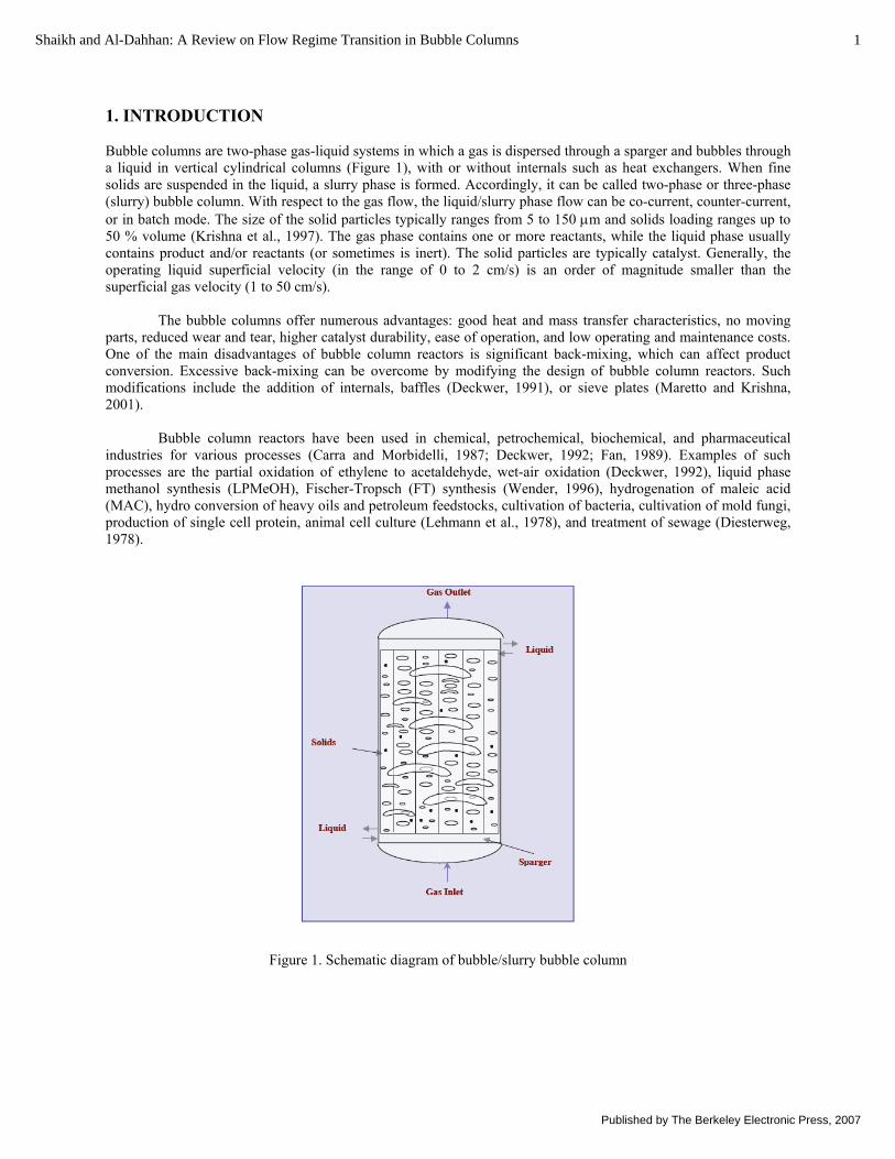
1. INTRODUCTION Bubble columns are two-phase gas-liquid systems in which a gas is dispersed through a sparger and bubbles through a liquid in vertical cylindrical columns (Figure 1), with or without internals such as heat exchangers. When fine solids are suspended in the liquid, a slurry phase is formed. Accordingly, it can be called two-phase or three-phase (slurry) bubble column. With respect to the gas flow, the liquid/slurry phase flow can be co-current, counter-current, or in batch mode. The size of the solid particles typically ranges from 5 to 150 μm and solids loading ranges up to 50 % volume (Krishna et al., 1997). The gas phase contains one or more reactants, while the liquid phase usually contains product and/or reactants (or sometimes is inert). The solid particles are typically catalyst. Generally, the operating liquid superficial velocity (in the range of 0 to 2 cm/s) is an order of magnitude smaller than the superficial gas velocity (1 to 50 cm/s).

The bubble columns offer numerous advantages: good heat and mass transfer characteristics, no moving parts, reduced wear and tear, higher catalyst durability, ease of operation, and low operating and maintenance costs. One of the main disadvantages of bubble column reactors is significant back-mixing, which can affect product conversion. Excessive back-mixing can be overcome by modifying the design of bubble column reactors. Such modifications include the addition of internals, baffles (Deckwer, 1991), or sieve plates (Maretto and Krishna, 2001).

Bubble column reactors have been used in chemical, petrochemical, biochemical, and pharmaceutical industries for various processes (Carra and Morbidelli, 1987; Deckwer, 1992; Fan, 1989). Examples of such processes are the partial oxidation of ethylene to acetaldehyde, wet-air oxidation (Deckwer, 1992), liquid phase methanol synthesis (LPMeOH), Fischer-Tropsch (FT) synthesis (Wender, 1996), hydrogenation of maleic acid (MAC), hydro conversion of heavy oils and petroleum feedstocks, cultivation of bacteria, cultivation of mold fungi, production of single cell protein, animal cell culture (Lehmann et al., 1978), and treatment of sewage (Diesterweg, 1978).

Figure 1. Schematic diagram of bubble/slurry bubble column

1Shaikh and Al-Dahhan: A Review on Flow Regime Transition in Bubble Columns

Published by The Berkeley Electronic Press, 2007

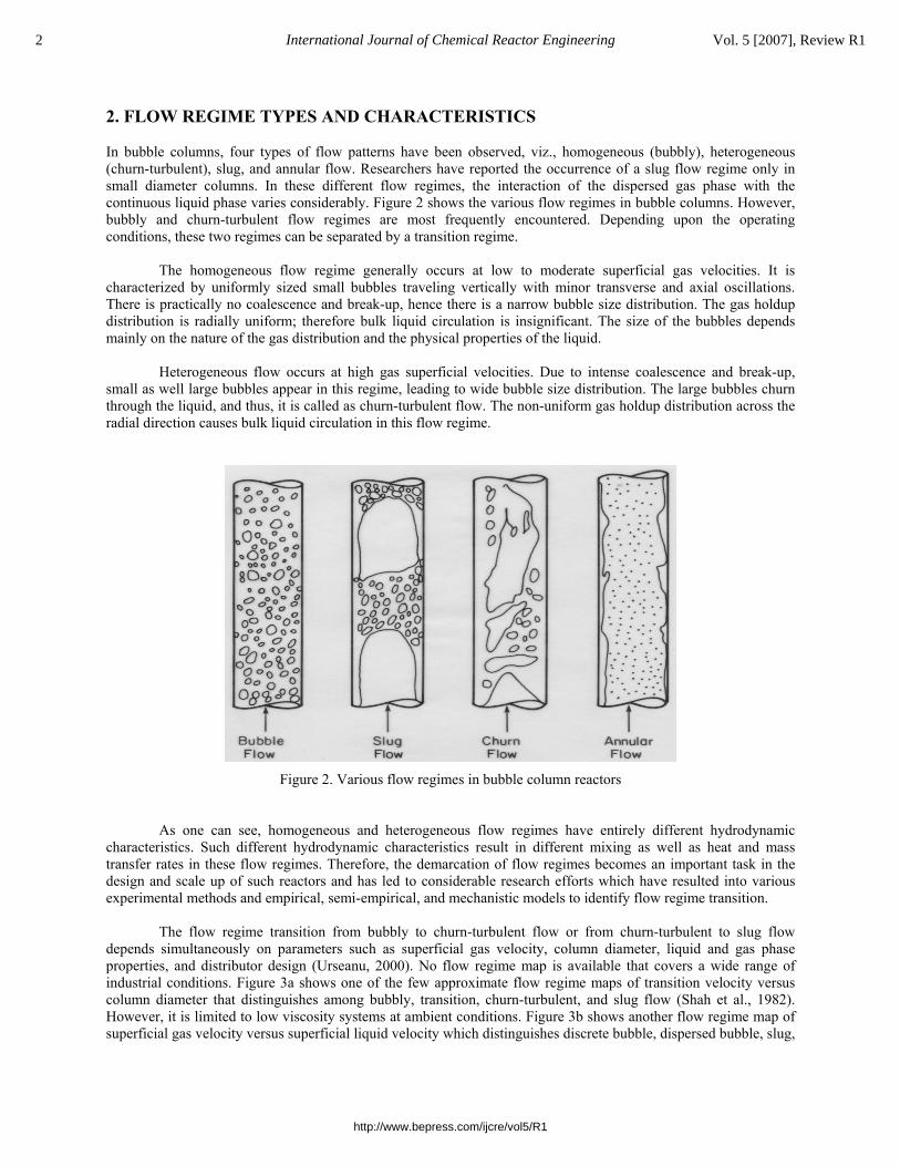
2. FLOW REGIME TYPES AND CHARACTERISTICS In bubble columns, four types of flow patterns have been observed, viz., homogeneous (bubbly), heterogeneous (churn-turbulent), slug, and annular flow. Researchers have reported the occurrence of a slug flow regime only in small diameter columns. In these different flow regimes, the interaction of the dispersed gas phase with the continuous liquid phase varies considerably. Figure 2 shows the various flow regimes in bubble columns. However, bubbly and churn-turbulent flow regimes are most frequently encountered. Depending upon the operating conditions, these two regimes can be separated by a transition regime.

The homogeneous flow regime generally occurs at low to moderate superficial gas velocities. It is characterized by uniformly sized small bubbles traveling vertically with minor transverse and axial oscillations. There is practically no coalescence and break-up, hence there is a narrow bubble size distribution. The gas holdup distribution is radially uniform; therefore bulk liquid circulation is insignificant. The size of the bubbles depends mainly on the nature of the gas distribution and the physical properties of the liquid.

Heterogeneous flow occurs at high gas superficial velocities. Due to intense coalescence and break-up,

small as well large bubbles appear in this regime, leading to wide bubble size distribution. The large bubbles churn through the liquid, and thus, it is called as churn-turbulent flow. The non-uniform gas holdup distribution across the radial direction causes bulk liquid circulation in this flow regime.

Figure 2. Various flow regimes in bubble column reactors

As one can see, homogeneous and heterogeneous flow regimes have entirely different hydrodynamic characteristics. Such different hydrodynamic characteristics result in different mixing as well as heat and mass transfer rates in these flow regimes. Therefore, the demarcation of flow regimes becomes an important task in the design and scale up of such reactors and has led to considerable research efforts which have resulted into various experimental methods and empirical, semi-empirical, and mechanistic models to identify flow regime transition.

The flow regime transition from bubbly to churn-turbulent flow or from churn-turbulent to slug flow depends simultaneously on parameters such as superficial gas velocity, column diameter, liquid and gas phase properties, and distributor design (Urseanu, 2000). No flow regime map is available that covers a wide range of industrial conditions. Figure 3a shows one of the few approximate flow regime maps of transition velocity versus column diameter that distinguishes among bubbly, transition, churn-turbulent, and slug flow (Shah et al., 1982). However, it is limited to low viscosity systems at ambient conditions. Figure 3b shows another flow regime map of superficial gas velocity versus superficial liquid velocity which distinguishes discrete bubble, dispersed bubble, slug,

2 International Journal of Chemical Reactor Engineering Vol. 5 [2007], Review R1

http://www.bepress.com/ijcre/vol5/R1

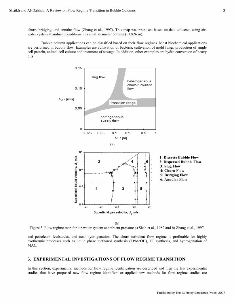
churn, bridging, and annular flow (Zhang et al., 1997). This map was proposed based on data collected using air-water system at ambient conditions in a small diameter column (0.0826 m).

Bubble column applications can be classified based on their flow regimes. Most biochemical applications

are performed in bubbly flow. Examples are cultivation of bacteria, cultivation of mold fungi, production of single cell protein, animal cell culture and treatment of sewage. In addition, other examples are hydro conversion of heavy oils

(a)

1: Discrete Bubble Flow 2: Dispersed Bubble Flow

3: Slug Flow 4: Churn Flow 5: Bridging Flow 6: Annular Flow

(b) Figure 3. Flow regime map for air-water system at ambient pressure a) Shah et al., 1982 and b) Zhang et al., 1997.

and petroleum feedstocks, and coal hydrogenation. The churn turbulent flow regime is preferable for highly exothermic processes such as liquid phase methanol synthesis (LPMeOH), FT synthesis, and hydrogenation of MAC. 3. EXPERIMENTAL INVESTIGATIONS OF FLOW REGIME TRANSITION In this section, experimental methods for flow regime identification are described and then the few experimental studies that have proposed new flow regime identifiers or applied new methods for flow regime studies are

1

2

3 5

4 6

10-3 10-2 10-1 100 10110-3

10-2

10-1

100

Superficial gas velocity, Ug, m/s

Supe

rfic

ial l

iqui

d ve

loci

ty, U

l,m

/s

1

2

3 5

4 6

10-3 10-2 10-1 100 10110-3

10-2

10-1

100

Superficial gas velocity, Ug, m/s

Supe

rfic

ial l

iqui

d ve

loci

ty, U

l,m

/s



discussed. Table 1 summarizes most of the studies’ operating and design conditions and includes significant remarks. Following that, experimental observations of the effect of various operating and design parameters are presented. 3.1 Methods for Flow Regime Identification The experimental methods used for regime transition identification can be broadly classified in the following groups:

• Visual observation • Evolution of global hydrodynamic parameter • Temporal signatures of quantity related to hydrodynamics • Advanced measurement techniques

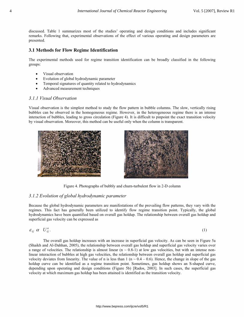
3.1.1 Visual Observation Visual observation is the simplest method to study the flow pattern in bubble columns. The slow, vertically rising bubbles can be observed in the homogeneous regime. However, in the heterogeneous regime there is an intense interaction of bubbles, leading to gross circulation (Figure 4). It is difficult to pinpoint the exact transition velocity by visual observation. Moreover, this method can be useful only when the column is transparent.

Figure 4. Photographs of bubbly and churn-turbulent flow in 2-D column

3.1.2 Evolution of global hydrodynamic parameter Because the global hydrodynamic parameters are manifestations of the prevailing flow patterns, they vary with the regimes. This fact has generally been utilized to identify flow regime transition point. Typically, the global hydrodynamics have been quantified based on overall gas holdup. The relationship between overall gas holdup and superficial gas velocity can be expressed as

Gε α nGU . (1)

The overall gas holdup increases with an increase in superficial gas velocity. As can be seen in Figure 5a

(Shaikh and Al-Dahhan, 2005), the relationship between overall gas holdup and superficial gas velocity varies over a range of velocities. The relationship is almost linear (n ~ 0.8-1) at low gas velocities, but with an intense non-linear interaction of bubbles at high gas velocities, the relationship between overall gas holdup and superficial gas velocity deviates from linearity. The value of n is less than 1 (n ~ 0.4 – 0.6). Hence, the change in slope of the gas holdup curve can be identified as a regime transition point. Sometimes, gas holdup shows an S-shaped curve, depending upon operating and design conditions (Figure 5b) [Rados, 2003]. In such cases, the superficial gas velocity at which maximum gas holdup has been attained is identified as the transition velocity.



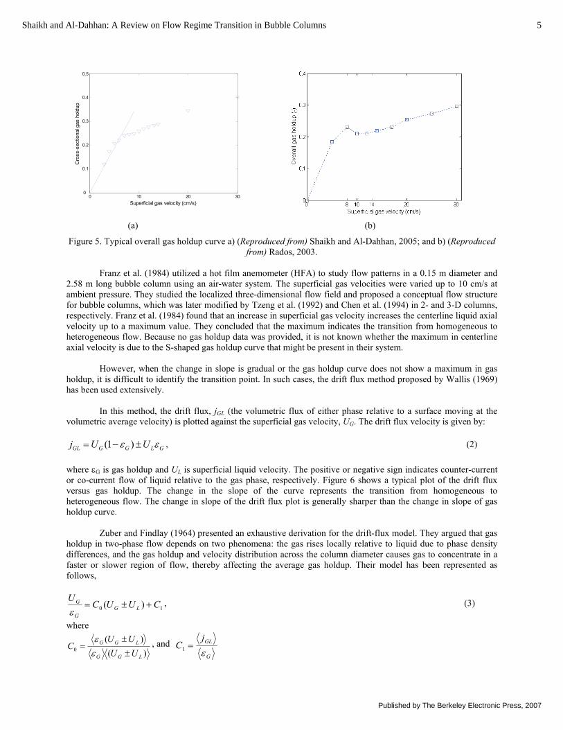
(a) (b)

Figure 5. Typical overall gas holdup curve a) (Reproduced from) Shaikh and Al-Dahhan, 2005; and b) (Reproduced from) Rados, 2003.

Franz et al. (1984) utilized a hot film anemometer (HFA) to study flow patterns in a 0.15 m diameter and

2.58 m long bubble column using an air-water system. The superficial gas velocities were varied up to 10 cm/s at ambient pressure. They studied the localized three-dimensional flow field and proposed a conceptual flow structure for bubble columns, which was later modified by Tzeng et al. (1992) and Chen et al. (1994) in 2- and 3-D columns, respectively. Franz et al. (1984) found that an increase in superficial gas velocity increases the centerline liquid axial velocity up to a maximum value. They concluded that the maximum indicates the transition from homogeneous to heterogeneous flow. Because no gas holdup data was provided, it is not known whether the maximum in centerline axial velocity is due to the S-shaped gas holdup curve that might be present in their system.

However, when the change in slope is gradual or the gas holdup curve does not show a maximum in gas holdup, it is difficult to identify the transition point. In such cases, the drift flux method proposed by Wallis (1969) has been used extensively.

In this method, the drift flux, jGL (the volumetric flux of either phase relative to a surface moving at the volumetric average velocity) is plotted against the superficial gas velocity, UG. The drift flux velocity is given by:

(1 )GL G G L Gj U Uε ε= − ± , (2) where εG is gas holdup and UL is superficial liquid velocity. The positive or negative sign indicates counter-current or co-current flow of liquid relative to the gas phase, respectively. Figure 6 shows a typical plot of the drift flux versus gas holdup. The change in the slope of the curve represents the transition from homogeneous to heterogeneous flow. The change in slope of the drift flux plot is generally sharper than the change in slope of gas holdup curve.

Zuber and Findlay (1964) presented an exhaustive derivation for the drift-flux model. They argued that gas holdup in two-phase flow depends on two phenomena: the gas rises locally relative to liquid due to phase density differences, and the gas holdup and velocity distribution across the column diameter causes gas to concentrate in a faster or slower region of flow, thereby affecting the average gas holdup. Their model has been represented as follows,

10 )( CUUCU

LGG

G +±=ε

, (3)

where

)()(

0LGG

LGG

UUUU

C±

±=

εε , and

G

GLjC

ε=1

0 10 20 300

0.1

0.2

0.3

0.4

0.5

Superficial gas velocity (cm/s)

Cro

ss-s

ectio

nal g

as h

oldu

p



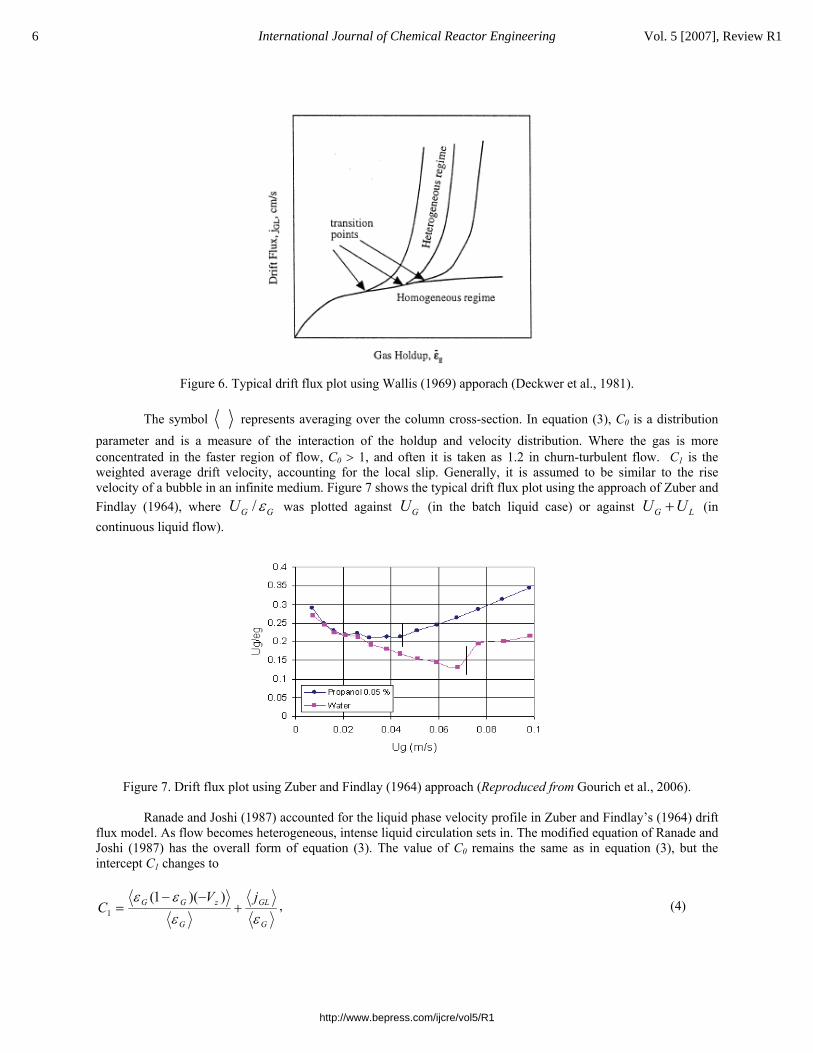
Figure 6. Typical drift flux plot using Wallis (1969) apporach (Deckwer et al., 1981).

The symbol represents averaging over the column cross-section. In equation (3), C0 is a distribution

parameter and is a measure of the interaction of the holdup and velocity distribution. Where the gas is more concentrated in the faster region of flow, C0 > 1, and often it is taken as 1.2 in churn-turbulent flow. C1 is the weighted average drift velocity, accounting for the local slip. Generally, it is assumed to be similar to the rise velocity of a bubble in an infinite medium. Figure 7 shows the typical drift flux plot using the approach of Zuber and Findlay (1964), where /G GU ε was plotted against GU (in the batch liquid case) or against G LU U+ (in continuous liquid flow).

Figure 7. Drift flux plot using Zuber and Findlay (1964) approach (Reproduced from Gourich et al., 2006).

Ranade and Joshi (1987) accounted for the liquid phase velocity profile in Zuber and Findlay’s (1964) drift

flux model. As flow becomes heterogeneous, intense liquid circulation sets in. The modified equation of Ranade and Joshi (1987) has the overall form of equation (3). The value of C0 remains the same as in equation (3), but the intercept C1 changes to

G

GL

G

zGG jVC

εεεε

+−−

=))(1(

1, (4)



where Vz is the local value of liquid velocity in the circulation flow pattern. The first term in the modified intercept C1 contributes to an increase in the rise velocity of bubbles due to liquid circulation. 3.1.3 Temporal signatures of quantity related to hydrodynamics The global parameters represent macroscopic phenomena that are result of prevailing microscopic phenomena. Several attempts have been made to capture the instantaneous flow behavior through an energetic parameter.

The following temporal signatures have been utilized for flow regime transition:

- Pressure fluctuations [Nishikawa, 1969; Matsui, 1984; Drahos et al., 1991; Letzel et al., 1997; Vial et al., 2001, Park and Kim, 2003]

- Local holdup fluctuations using resistive or optical probes [Bakshi et al., 1995; Briens et al., 1997] - Temperature fluctuations using a heat transfer probe [Thimmapuram et al., 1991] - Local bubble frequency measured using an optical transmittance probe [Kikuchi et al., 1997] - Conductivity probe [Zhang et al., 1997] - Sound fluctuations using an acoustic probe [Holler et al., 2003; Al-Masry, 2005; Al-Masry and Ali, 2007]

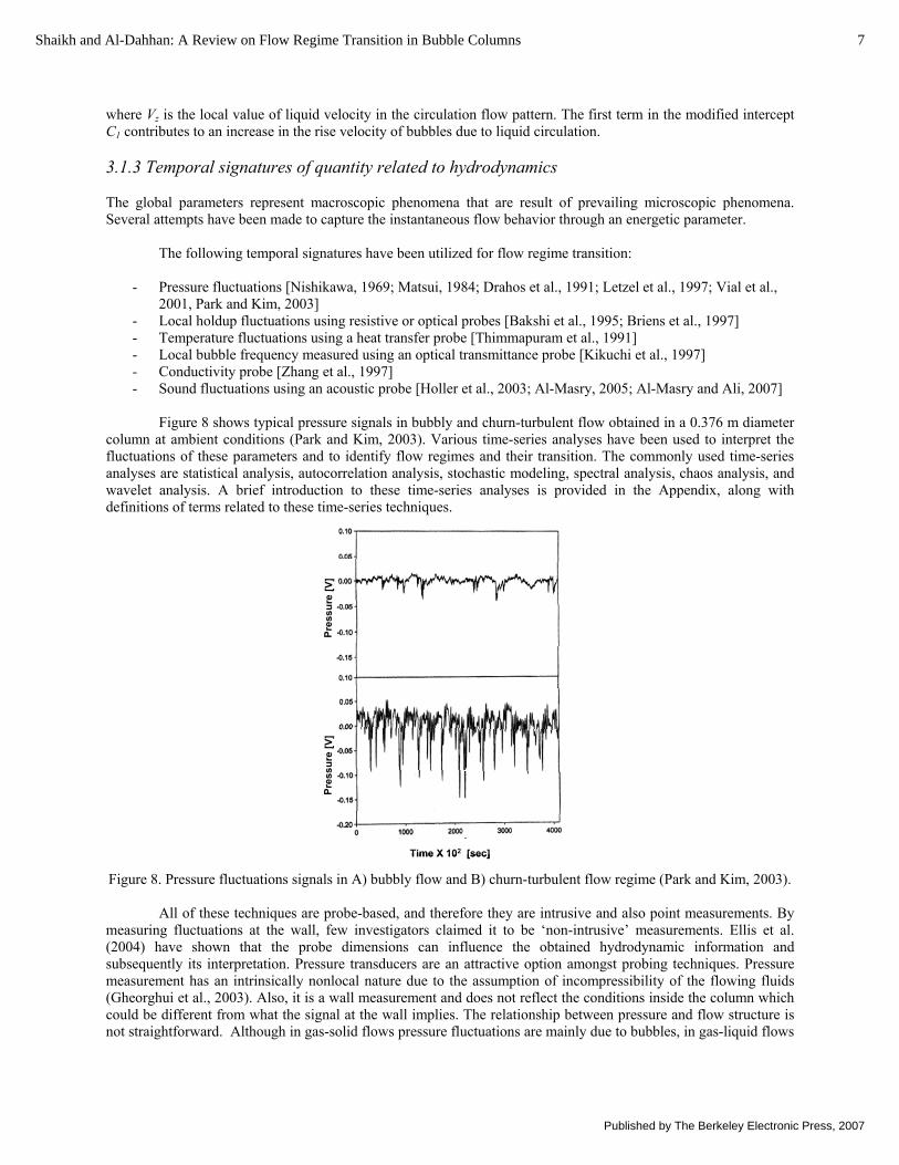
Figure 8 shows typical pressure signals in bubbly and churn-turbulent flow obtained in a 0.376 m diameter

column at ambient conditions (Park and Kim, 2003). Various time-series analyses have been used to interpret the fluctuations of these parameters and to identify flow regimes and their transition. The commonly used time-series analyses are statistical analysis, autocorrelation analysis, stochastic modeling, spectral analysis, chaos analysis, and wavelet analysis. A brief introduction to these time-series analyses is provided in the Appendix, along with definitions of terms related to these time-series techniques.

Figure 8. Pressure fluctuations signals in A) bubbly flow and B) churn-turbulent flow regime (Park and Kim, 2003).

All of these techniques are probe-based, and therefore they are intrusive and also point measurements. By measuring fluctuations at the wall, few investigators claimed it to be ‘non-intrusive’ measurements. Ellis et al. (2004) have shown that the probe dimensions can influence the obtained hydrodynamic information and subsequently its interpretation. Pressure transducers are an attractive option amongst probing techniques. Pressure measurement has an intrinsically nonlocal nature due to the assumption of incompressibility of the flowing fluids (Gheorghui et al., 2003). Also, it is a wall measurement and does not reflect the conditions inside the column which could be different from what the signal at the wall implies. The relationship between pressure and flow structure is not straightforward. Although in gas-solid flows pressure fluctuations are mainly due to bubbles, in gas-liquid flows

Time X 102 [sec]

Pres

sure

[V]

Pres

sure

[V]

Time X 102 [sec]

Pres

sure

[V]

Pres

sure

[V]



more complex phenomena exist as shown by Drahos et al. (1991) and Letzel et al. (1997). Hence, these fluctuations need careful analysis when applying novel time-series techniques to interpret the data. 3.1.4 Advanced measurement techniques With advances in measurement techniques, various imaging and velocimetric techniques have been used in flow regime transition studies.

- Particle Image Velocimetry (PIV) [Chen et al., 1994; Lin et al., 1996] - Electrical Capacitance Tomography (ECT) [Bennett et al., 1999] - Electrical Resistance Tomography (ERT) [Dong et al., 2001; Murugaian et al., 2005] - Laser Doppler Anemometry (LDA) [Olmos et al., 2003] - Computer Automated Radioactive Particle Tracking (CARPT) [Cassanello et al., 2001; Nedeltchev et al.,

2003] - γ-ray Computed Tomography (CT) [Shaikh and Al-Dahhan, 2005]

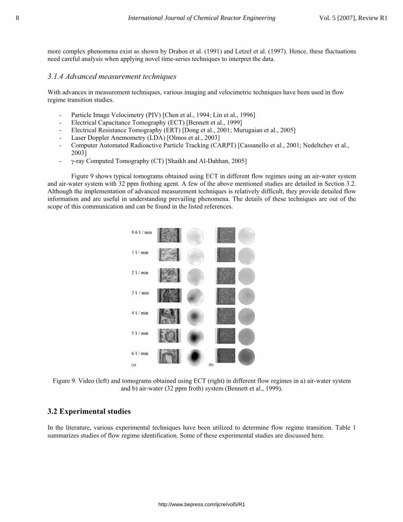
Figure 9 shows typical tomograms obtained using ECT in different flow regimes using an air-water system

and air-water system with 32 ppm frothing agent. A few of the above mentioned studies are detailed in Section 3.2. Although the implementation of advanced measurement techniques is relatively difficult, they provide detailed flow information and are useful in understanding prevailing phenomena. The details of these techniques are out of the scope of this communication and can be found in the listed references.

Figure 9. Video (left) and tomograms obtained using ECT (right) in different flow regimes in a) air-water system and b) air-water (32 ppm froth) system (Bennett et al., 1999).

3.2 Experimental studies In the literature, various experimental techniques have been utilized to determine flow regime transition. Table 1 summarizes studies of flow regime identification. Some of these experimental studies are discussed here.



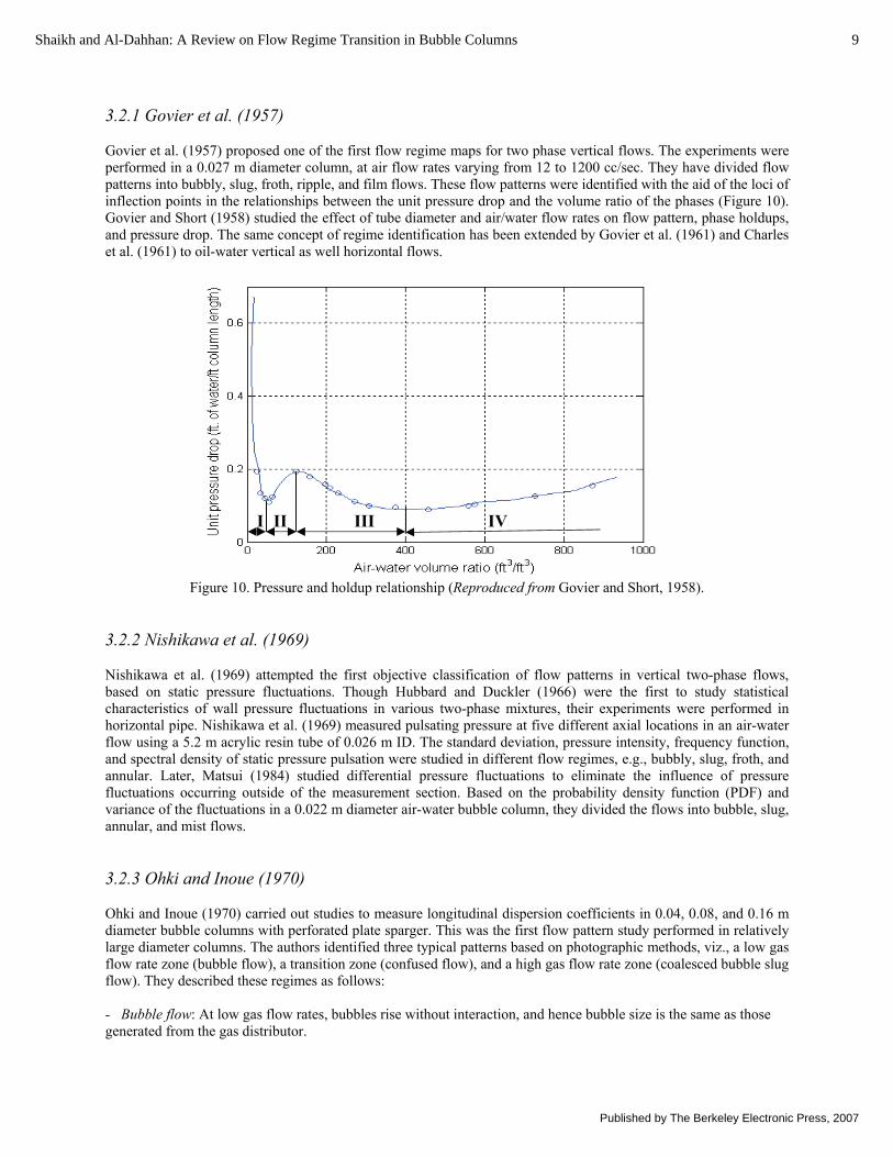
3.2.1 Govier et al. (1957) Govier et al. (1957) proposed one of the first flow regime maps for two phase vertical flows. The experiments were performed in a 0.027 m diameter column, at air flow rates varying from 12 to 1200 cc/sec. They have divided flow patterns into bubbly, slug, froth, ripple, and film flows. These flow patterns were identified with the aid of the loci of inflection points in the relationships between the unit pressure drop and the volume ratio of the phases (Figure 10). Govier and Short (1958) studied the effect of tube diameter and air/water flow rates on flow pattern, phase holdups, and pressure drop. The same concept of regime identification has been extended by Govier et al. (1961) and Charles et al. (1961) to oil-water vertical as well horizontal flows.

Figure 10. Pressure and holdup relationship (Reproduced from Govier and Short, 1958). 3.2.2 Nishikawa et al. (1969) Nishikawa et al. (1969) attempted the first objective classification of flow patterns in vertical two-phase flows, based on static pressure fluctuations. Though Hubbard and Duckler (1966) were the first to study statistical characteristics of wall pressure fluctuations in various two-phase mixtures, their experiments were performed in horizontal pipe. Nishikawa et al. (1969) measured pulsating pressure at five different axial locations in an air-water flow using a 5.2 m acrylic resin tube of 0.026 m ID. The standard deviation, pressure intensity, frequency function, and spectral density of static pressure pulsation were studied in different flow regimes, e.g., bubbly, slug, froth, and annular. Later, Matsui (1984) studied differential pressure fluctuations to eliminate the influence of pressure fluctuations occurring outside of the measurement section. Based on the probability density function (PDF) and variance of the fluctuations in a 0.022 m diameter air-water bubble column, they divided the flows into bubble, slug, annular, and mist flows. 3.2.3 Ohki and Inoue (1970) Ohki and Inoue (1970) carried out studies to measure longitudinal dispersion coefficients in 0.04, 0.08, and 0.16 m diameter bubble columns with perforated plate sparger. This was the first flow pattern study performed in relatively large diameter columns. The authors identified three typical patterns based on photographic methods, viz., a low gas flow rate zone (bubble flow), a transition zone (confused flow), and a high gas flow rate zone (coalesced bubble slug flow). They described these regimes as follows: - Bubble flow: At low gas flow rates, bubbles rise without interaction, and hence bubble size is the same as those generated from the gas distributor.

I II III IV



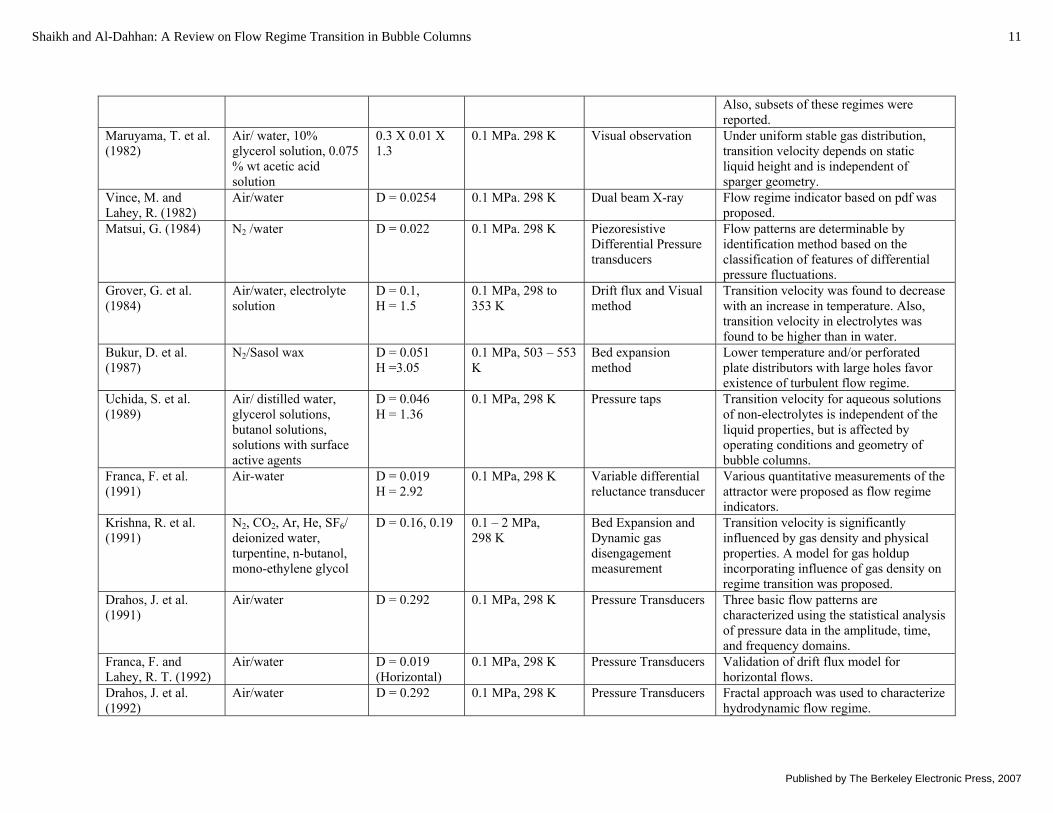
Table 1. Experimental studies performed for flow regime identification in bubble/slurry bubble columns For 3-D columns: D = diameter of column, m; H = length of column, m. For 2-D column: H = length, m; W = width, m; T = thickness, m.

Author System (Gas/Liquid)

Column Dimension (m)

Pressure/ Temperature

Measurement Technique

Methods and Findings

Govier et al. (1957) Air/water D = 0.0257 0.1 MPa, 298 K Pressure drop measurement

The flow patterns were identified with the aid of the loci of inflection points in the relationships between the unit pressure drop and the volume ratio of the phases.

Govier and Short (1958)

Air/water D = 0.016, 0.026, 0.0381, 0.0635

0.1 MPa, 298 K Pressure drop measurement

Effect of tube diameter on various flow parameters was studied.

Govier et al. (1961) Oil/water D = 0.0257 0.1 MPa, 298 K Pressure drop measurement

Flow patterns similar to those in gas-liquid mixture were observed. Superficial friction factor was correlated to superficial velocities.

Aoyama Y. et al. (1968)

Air/water, 61.5 % glycerin, 0.1 wt % Tween 20 water solution

D = 0.05, 0.1, 0.2

0.1 MPa, 298 K Longitudinal mass and thermal dispersion measurement

It was shown that the mechanism of thermal dispersion is governed by liquid mixing. The dispersion coefficient was related to three different flow regimes.

Nishikawa et al. (1969)

Air/water D = 0.026, H = 5.2

0.1 MPa, 298 K Static pressure fluctuations

The standard deviation, pressure intensity, frequency function, and spectral density of static pressure pulsation showed different behavior in different flow patterns, i.e. bubbly, slug, froth, and annular

Ohki and Inoue (1970)

Air/water D = 0.04, 0.08, 0.16

0.1 MPa, 298 K Photographic method and longitudinal dispersion coefficient measurement

Based on photographic method, three flow regimes were identified and described. Analytical models were developed to predict longitudinal dispersion coefficient for different flow regimes.

Yamashita and Inoue (1975)

Air/water D = 0.1 0.1 MPa, 298 K Gas holdup measurement

Regime based flow behavior was studied.

Jones, O. and Zuber, N. (1975)

Air/water 0.1 MPa. 298 K X-ray Three dominant patterns were identified, viz., bubbly, slug, and annular regime.



Also, subsets of these regimes were reported.

Maruyama, T. et al. (1982)

Air/ water, 10% glycerol solution, 0.075 % wt acetic acid solution

0.3 X 0.01 X 1.3

0.1 MPa. 298 K Visual observation Under uniform stable gas distribution, transition velocity depends on static liquid height and is independent of sparger geometry.

Vince, M. and Lahey, R. (1982)

Air/water D = 0.0254 0.1 MPa. 298 K Dual beam X-ray Flow regime indicator based on pdf was proposed.

Matsui, G. (1984) N2 /water D = 0.022 0.1 MPa. 298 K Piezoresistive Differential Pressure transducers

Flow patterns are determinable by identification method based on the classification of features of differential pressure fluctuations.

Grover, G. et al. (1984)

Air/water, electrolyte solution

D = 0.1, H = 1.5

0.1 MPa, 298 to 353 K

Drift flux and Visual method

Transition velocity was found to decrease with an increase in temperature. Also, transition velocity in electrolytes was found to be higher than in water.

Bukur, D. et al. (1987)

N2/Sasol wax D = 0.051 H =3.05

0.1 MPa, 503 – 553 K

Bed expansion method

Lower temperature and/or perforated plate distributors with large holes favor existence of turbulent flow regime.

Uchida, S. et al. (1989)

Air/ distilled water, glycerol solutions, butanol solutions, solutions with surface active agents

D = 0.046 H = 1.36

0.1 MPa, 298 K Pressure taps Transition velocity for aqueous solutions of non-electrolytes is independent of the liquid properties, but is affected by operating conditions and geometry of bubble columns.

Franca, F. et al. (1991)

Air-water D = 0.019 H = 2.92

0.1 MPa, 298 K Variable differential reluctance transducer

Various quantitative measurements of the attractor were proposed as flow regime indicators.

Krishna, R. et al. (1991)

N2, CO2, Ar, He, SF6/ deionized water, turpentine, n-butanol, mono-ethylene glycol

D = 0.16, 0.19 0.1 – 2 MPa, 298 K

Bed Expansion and Dynamic gas disengagement measurement

Transition velocity is significantly influenced by gas density and physical properties. A model for gas holdup incorporating influence of gas density on regime transition was proposed.

Drahos, J. et al. (1991)

Air/water D = 0.292

0.1 MPa, 298 K Pressure Transducers Three basic flow patterns are characterized using the statistical analysis of pressure data in the amplitude, time, and frequency domains.

Franca, F. and Lahey, R. T. (1992)

Air/water D = 0.019 (Horizontal)

0.1 MPa, 298 K Pressure Transducers Validation of drift flux model for horizontal flows.

Drahos, J. et al. (1992)

Air/water D = 0.292 0.1 MPa, 298 K Pressure Transducers Fractal approach was used to characterize hydrodynamic flow regime.



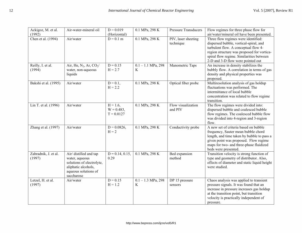
Ackigoz, M. et al. (1992)

Air-water-mineral oil D = 0.019 (Horizontal)

0.1 MPa, 298 K Pressure Transducers Flow regimes for three phase flow for air/water/mineral oil have been presented.

Chen et al. (1994) Air/water D = 0.1 m 0.1 MPa, 298 K PIV, laser sheeting technique

Three flow regimes were identified: dispersed bubble, vortical-spiral, and turbulent flow. A conceptual flow 4-region structure was proposed for vortica-spiral flow regime. Similarities between 2-D and 3-D flow were pointed out

Reilly, I. et al. (1994)

Air, He, N2, Ar, CO2/ water, non-aqueous liquids

D = 0.15 H = 2.7

0.1 – 1.1 MPa, 298 K

Manometric Taps An increase in density stabilizes the bubbly flow. A correlation in terms of gas density and physical properties was proposed.

Bakshi et al. (1995) Air/water D = 0.1, H = 2.2

0.1 MPa, 298 K Optical fiber probe Multiresolution analysis of gas holdup fluctuations was performed. The intermittance of local bubble concentration was related to flow regime transition.

Lin T. et al. (1996) Air/water H = 1.6, W = 0.483, T = 0.0127

0.1 MPa, 298 K Flow visualization and PIV

The flow regimes were divided into: dispersed bubble and coalesced bubble flow regimes. The coalesced bubble flow was divided into 4-region and 3-region flow.

Zhang et al. (1997) Air/water D = 0.0826, H = 2

0.1 MPa, 298 K Conductivity probe A new set of criteria based on bubble frequency, Sauter mean bubble chord length, and time taken by bubble to pass a given point was proposed. Flow regime maps for two- and three-phase fluidized beds were presented.

Zahradnik, J. et al. (1997)

Air/ distilled and tap water, aqueous solutions of electrolyte, aliphatic alcohols, aqueous solutions of saccharose

D = 0.14, 0.15, 0.29

0.1 MPa, 298 K Bed expansion method

Transition velocity is strong function of type and geometry of distributor. Also, effects of diameter and static liquid height were studied.

Letzel, H. et al. (1997)

Air/water D = 0.15 H = 1.2

0.1 – 1.3 MPa, 298 K

DP 15 pressure sensors

Chaos analysis was applied to transient pressure signals. It was found that an increase in pressure increases gas holdup at the transition point, but transition velocity is practically independent of pressure.



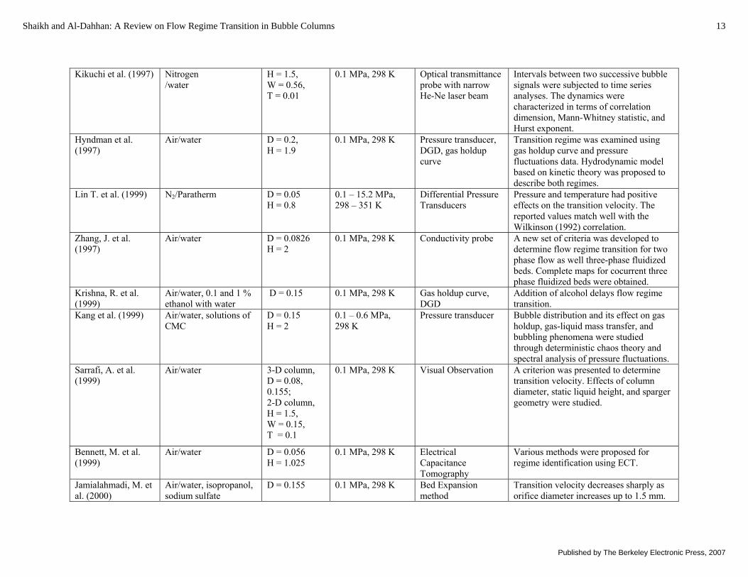
Kikuchi et al. (1997) Nitrogen /water

H = 1.5, W = 0.56, T = 0.01

0.1 MPa, 298 K Optical transmittance probe with narrow He-Ne laser beam

Intervals between two successive bubble signals were subjected to time series analyses. The dynamics were characterized in terms of correlation dimension, Mann-Whitney statistic, and Hurst exponent.

Hyndman et al. (1997)

Air/water D = 0.2, H = 1.9

0.1 MPa, 298 K Pressure transducer, DGD, gas holdup curve

Transition regime was examined using gas holdup curve and pressure fluctuations data. Hydrodynamic model based on kinetic theory was proposed to describe both regimes.

Lin T. et al. (1999) N2/Paratherm D = 0.05 H = 0.8

0.1 – 15.2 MPa, 298 – 351 K

Differential Pressure Transducers

Pressure and temperature had positive effects on the transition velocity. The reported values match well with the Wilkinson (1992) correlation.

Zhang, J. et al. (1997)

Air/water D = 0.0826 H = 2

0.1 MPa, 298 K Conductivity probe A new set of criteria was developed to determine flow regime transition for two phase flow as well three-phase fluidized beds. Complete maps for cocurrent three phase fluidized beds were obtained.

Krishna, R. et al. (1999)

Air/water, 0.1 and 1 % ethanol with water

D = 0.15 0.1 MPa, 298 K Gas holdup curve, DGD

Addition of alcohol delays flow regime transition.

Kang et al. (1999) Air/water, solutions of CMC

D = 0.15 H = 2

0.1 – 0.6 MPa, 298 K

Pressure transducer Bubble distribution and its effect on gas holdup, gas-liquid mass transfer, and bubbling phenomena were studied through deterministic chaos theory and spectral analysis of pressure fluctuations.

Sarrafi, A. et al. (1999)

Air/water 3-D column, D = 0.08, 0.155; 2-D column, H = 1.5, W = 0.15, T = 0.1

0.1 MPa, 298 K Visual Observation A criterion was presented to determine transition velocity. Effects of column diameter, static liquid height, and sparger geometry were studied.

Bennett, M. et al. (1999)

Air/water D = 0.056 H = 1.025

0.1 MPa, 298 K Electrical Capacitance Tomography

Various methods were proposed for regime identification using ECT.

Jamialahmadi, M. et al. (2000)

Air/water, isopropanol, sodium sulfate

D = 0.155 0.1 MPa, 298 K Bed Expansion method

Transition velocity decreases sharply as orifice diameter increases up to 1.5 mm.



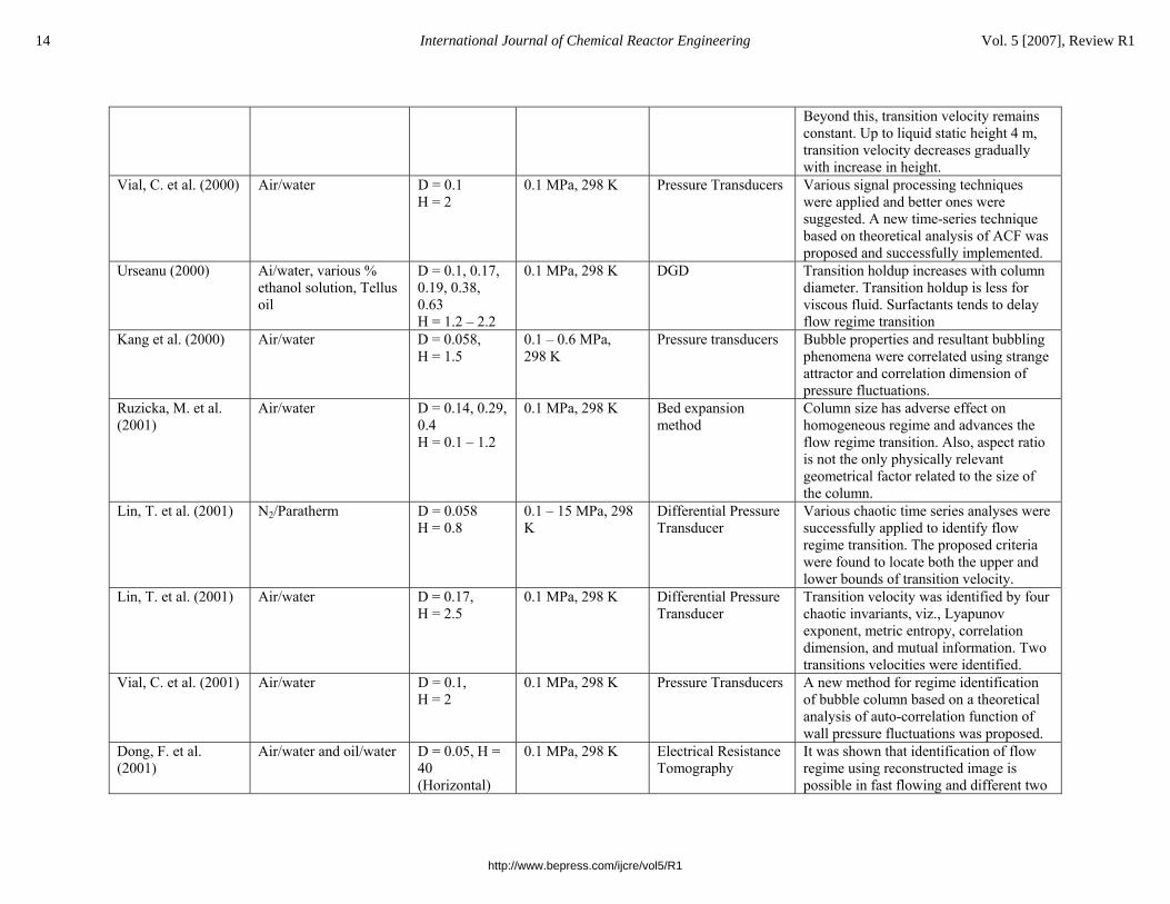
Beyond this, transition velocity remains constant. Up to liquid static height 4 m, transition velocity decreases gradually with increase in height.

Vial, C. et al. (2000) Air/water D = 0.1 H = 2

0.1 MPa, 298 K Pressure Transducers Various signal processing techniques were applied and better ones were suggested. A new time-series technique based on theoretical analysis of ACF was proposed and successfully implemented.

Urseanu (2000) Ai/water, various % ethanol solution, Tellus oil

D = 0.1, 0.17, 0.19, 0.38, 0.63 H = 1.2 – 2.2

0.1 MPa, 298 K DGD Transition holdup increases with column diameter. Transition holdup is less for viscous fluid. Surfactants tends to delay flow regime transition

Kang et al. (2000) Air/water D = 0.058, H = 1.5

0.1 – 0.6 MPa, 298 K

Pressure transducers Bubble properties and resultant bubbling phenomena were correlated using strange attractor and correlation dimension of pressure fluctuations.

Ruzicka, M. et al. (2001)

Air/water D = 0.14, 0.29, 0.4 H = 0.1 – 1.2

0.1 MPa, 298 K Bed expansion method

Column size has adverse effect on homogeneous regime and advances the flow regime transition. Also, aspect ratio is not the only physically relevant geometrical factor related to the size of the column.

Lin, T. et al. (2001) N2/Paratherm D = 0.058 H = 0.8

0.1 – 15 MPa, 298 K

Differential Pressure Transducer

Various chaotic time series analyses were successfully applied to identify flow regime transition. The proposed criteria were found to locate both the upper and lower bounds of transition velocity.

Lin, T. et al. (2001) Air/water D = 0.17, H = 2.5

0.1 MPa, 298 K Differential Pressure Transducer

Transition velocity was identified by four chaotic invariants, viz., Lyapunov exponent, metric entropy, correlation dimension, and mutual information. Two transitions velocities were identified.

Vial, C. et al. (2001) Air/water D = 0.1, H = 2

0.1 MPa, 298 K Pressure Transducers A new method for regime identification of bubble column based on a theoretical analysis of auto-correlation function of wall pressure fluctuations was proposed.

Dong, F. et al. (2001)

Air/water and oil/water D = 0.05, H = 40 (Horizontal)

0.1 MPa, 298 K Electrical Resistance Tomography

It was shown that identification of flow regime using reconstructed image is possible in fast flowing and different two



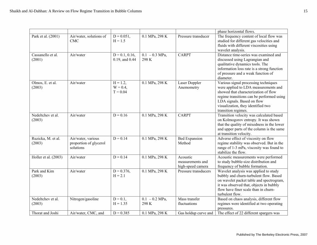
phase horizontal flows. Park et al. (2001) Air/water, solutions of

CMC D = 0.051, H = 1.5

0.1 MPa, 298 K Pressure transducer The frequency content of local flow was studied for different gas velocities and fluids with different viscosities using wavelet analysis.

Cassanello et al. (2001)

Air/water D = 0.1, 0.16, 0.19, and 0.44

0.1 – 0.3 MPa, 298 K

CARPT Distance time-series was examined and discussed using Lagrangian and qualitative dynamics tools. The information loss rate is a strong function of pressure and a weak function of diameter.

Olmos, E. et al. (2003)

Air/water H = 1.2, W = 0.4, T = 0.04

0.1 MPa, 298 K Laser Doppler Anemometry

Various signal processing techniques were applied to LDA measurements and showed that characterization of flow regime transitions can be performed using LDA signals. Based on flow visualization, they identified two transition regimes.

Nedeltchev et al. (2003)

Air/water D = 0.16 0.1 MPa, 298 K CARPT Transition velocity was calculated based on Kolmogorov entropy. It was shown that the quality of mixedness in the lower and upper parts of the column is the same at transition velocity.

Ruzicka, M. et al. (2003)

Air/water, various proportion of glycerol solutions

D = 0.14 0.1 MPa, 298 K Bed Expansion Method

Adverse effect of viscosity on flow regime stability was observed. But in the range of 1-3 mPa, viscosity was found to stabilize the flow.

Holler et al. (2003) Air/water D = 0.14 0.1 MPa, 298 K Acoustic measurements and high-speed camera

Acoustic measurements were performed to study bubble-size distribution and frequency of bubble formation.

Park and Kim (2003)

Air/water D = 0.376, H = 2.1

0.1 MPa, 298 K Pressure transducers Wavelet analysis was applied to study bubbly and churn-turbulent flow. Based on wavelet packet table and spectrogram, it was observed that, objects in bubbly flow have finer scale than in churn-turbulent flow.

Nedeltchev et al. (2003)

Nitrogen/gasoline D = 0.1, H = 1.35

0.1 – 0.2 MPa, 298 K

Mass transfer fluctuations

Based on chaos analysis, different flow regimes were identified at two operating pressures.

Thorat and Joshi Air/water, CMC, and D = 0.385 0.1 MPa, 298 K Gas holdup curve and The effect of 22 different spargers was



(2004) NaCl solutions drift flux plot studied. In addition, effect of nature of coalescence and aspect ratio were studied.

Mena et al. (2005) Air/water/calcium alginate beads

D = 0.14 0.1 MPa, 298 K Gas holdup curve Solids have a stabilizing effect at lower solids loading (up to 3 % vol.) and a destabilizing effect at higher solids loading (> 3 % vol).

Shaikh and Al-Dahhan (2005)

Air/Therminol LT D = 0.1615 0.1 – 1 MPa, 298 K

CT New flow regime identifier based on steepness of gas holdup radial profile was proposed and used to study the effect of pressure on flow regime transition.

Ruthiya et al. (2005) Air, Nitorgen/demineralized water

2-D column, H = 2, W = 0.3, T = 0.015 3-D column, D = 0.19, H = 4

0.1 MPa, 298 K Pressure transducer and high-speed video recordings

Proposed and demonstrated the use of coherent standard deviation and average cycle frequency as flow regime identifiers

Al-Masry et al. (2005)

Air/water D = 0.15, H = 0.66

0.1 MPa, 298 K Acoustic probe Acoustic measurements used to estimate bubble frequency, bubble size, and its distribution. The regime based study of these parameters was performed.

Wu et al. (2005) Air/water D = 0.15, H = 1.5

0.1 MPa, 298 K Pressure transducers CCF and Chaos analysis were applied to pressure fluctuation time-series. Transition velocities obtained using these analyses were close to that obtained by gas holdup curve. Recirculation velocity was calculated based on CCF analysis.

Vandu (2005) Air/Paraffin oil B/silica support

H = 0.95, W = 0.1, T = 0.02

0.1 MPa, 298 K Gas holdup measurement and high speed video camera

Effect of solids loading on transition was studied.



- Transition flow: At higher flow rates, bubbles do not rise vertically, and they begin to coalesce at a certain height. The starting level of coalescence moves downward with an increase in gas velocity. The fluid starts moving violently and many vortexes appear.

- Coalesced bubble-slug flow: At still higher flow rates, coalescence of bubbles occurs even at the bottom of the

column. Coalesced bubbles rise with much higher velocity than that of uncoalesced small bubbles.

Ohki and Inoue (1970) concluded that transition gas flow rates depend on column diameter and are generally higher for larger columns. Based on the observed flow patterns, they developed analytical models to predict the dispersion coefficient. For bubbly flow, they developed a model that combines the action of the velocity profile with bubble motion, based on Taylor’s theory. To describe the behavior of coalesced bubble slug flow, they developed an expansion model which assumes that a bubble bed consists of two parts. One is the liquid section occupied by liquid containing small dispersed bubbles, and the other is a gas section that consists of coalesced bubbles or slugs. 3.2.4 Jones and Zuber (1975) The first photon attenuation technique for flow regime identification in bubble column was developed by Jones and Zuber (1975). They studied air-water two phase flows in a rectangular column using a dual beam X-ray system. The flow patterns were divided on the basis of probability density function (PDF). Bubbly flow has been characterized by a single peak at low gas holdup, slug flow has a bimodal peak, and annular flow showed a single peak at higher gas holdup. Vince and Lahey (1982) employed a dual beam X-ray system in 0.0254 m vertical tube and analyzed their data in terms of four moments of PDF. They found that PDF variance discriminates among the bubbly, slug, and annular flow regimes for low pressure air-water flows. 3.2.5 Maruyama et al. (1981) Maruyama et al. (1981) studied flow transition in 2- and 3-dimensional bubble columns. The authors performed dynamic level change studies and observed the S-shaped gas holdup curve shown earlier. Using photographic studies (shutter speed 2 s), they attempted to explain the observed flow behavior. At maximum gas holdup, a symmetrical two-loop circulation upward in the middle and downward near the sidewalls appeared for the first time among the violent and frequent interactions of large bubble and asymmetrical circulation. The large eddies were found to be superimposed upon the liquid circulation. The transition velocity was determined from gas holdup curve, based on the superficial gas velocity at maximum gas holdup. The authors observed hysteresis of gas holdup behavior, which indicates that, once developed, flow with ordered liquid circulation is more stable than flow without it. They studied the effect of impurities on flow transition. They carried out experiments without using a water filter. The gas holdup values found for each case were different, but the maximum gas holdup was found to be at about the same superficial gas velocity. In addition, they performed gas holdup experiments using a 10 % glycerol solution and a 0.075 % acetic acid solution and found the same value of superficial gas velocity at maximum gas holdup, indicating that transition velocity is independent of gas holdup.

The authors studied gas holdup behavior under partial inlet gas distribution and also with insufficient pressure drop through the sparger which resulted in postponement of the transition due to lack of bubble interactions. A pressure drop sufficient to ensure constant flow irrespective of liquid motion was found to be 70 kPa, and this value was independent of bed height. 3.2.6 Tarmy et al. (1984) Tarmy et al. (1984) presented experimental results of hydrodynamic studies in various pilot reactors and cold flow units in a three-phase reactor for coal liquefaction. The cold flow units were 0.15 and 0.61 m in diameter and were operated at ambient temperature, and pressures up to 520 kPa, and superficial gas velocities up to 0.2 m/s. Pilot reactors of three different diameters (0.024, 0.066, and 0.61 m) were operated at actual operating conditions (T = 450 0 C, P = 17,000 kPa) with superficial gas velocities ranging up to 0.07 m/s. The three phases consist of gas (hydrogen and hydrocarbon vapors), liquid (hydrocarbons), and solids (unreacted coal and inert solids). The authors performed gas as well as liquid tracer tests to characterize mixing in terms of Peclet number and phase holdup



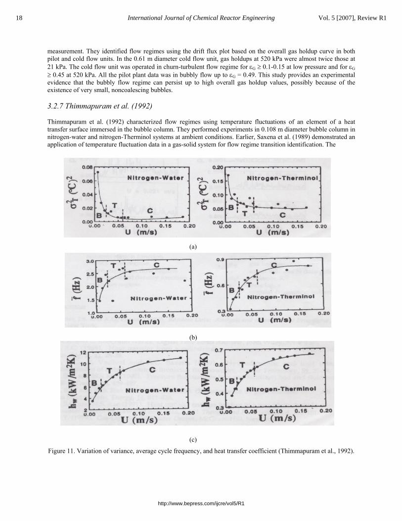
measurement. They identified flow regimes using the drift flux plot based on the overall gas holdup curve in both pilot and cold flow units. In the 0.61 m diameter cold flow unit, gas holdups at 520 kPa were almost twice those at 21 kPa. The cold flow unit was operated in churn-turbulent flow regime for εG ≥ 0.1-0.15 at low pressure and for εG ≥ 0.45 at 520 kPa. All the pilot plant data was in bubbly flow up to εG = 0.49. This study provides an experimental evidence that the bubbly flow regime can persist up to high overall gas holdup values, possibly because of the existence of very small, noncoalescing bubbles. 3.2.7 Thimmapuram et al. (1992) Thimmapuram et al. (1992) characterized flow regimes using temperature fluctuations of an element of a heat transfer surface immersed in the bubble column. They performed experiments in 0.108 m diameter bubble column in nitrogen-water and nitrogen-Therminol systems at ambient conditions. Earlier, Saxena et al. (1989) demonstrated an application of temperature fluctuation data in a gas-solid system for flow regime transition identification. The

(a)

(b)

(c)

Figure 11. Variation of variance, average cycle frequency, and heat transfer coefficient (Thimmapuram et al., 1992).



Instantaneous surface temperature time series exhibited a cyclic behavior. The amplitude of the surface temperature fluctuation and its frequency depend on the magnitude of the superficial gas velocity. Thimmapuram et al. (1992) determined the flow regime transition point using the drift flux method. They studied the rate of change of variance and found that these rates are distinctly different in different regimes (Figure 11a). There was a sudden drop in variance in bubbly flow, and the rate of change of variance became almost constant in churn-turbulent flow.

The authors performed spectral analysis and computed an average cycle frequency from the power spectral density function (PSDF). The bubbly flow regime was characterized by a rapid change of the average frequency, while the churn-turbulent flow regime had an almost constant average frequency (Figure 11b). In addition, they computed the wall heat transfer coefficient from the surface temperature fluctuation time-series and studied its variation in different flow regimes. They found that the heat transfer coefficient increases rapidly with superficial gas velocity in bubbly flow, while this variation is less rapid in the churn-turbulent flow regime (Figure 11c). This study proposed variance and average cycle frequency of surface temperature series as appropriate tools to identify flow regime transition. In addition, they demonstrated flow regime transition identification based on the heat transfer coefficient curve. 3.2.8 Drahos et al. (1991, 1992) Drahos et al. (1991) systematically studied the effect of various operating parameters on axial and radial profiles of basic statistical characteristics of pressure fluctuations. The experiments were performed in a 0.292 m diameter column with pressure transducers arranged at three axial locations. Three flow patterns were observed in their study: homogeneous, transition, and heterogeneous flow. To gain a better understanding of the space-time characteristics of the flow, the cross-correlations function (CCF) was evaluated from the two probes separated axially.

Figure 12 shows a typical CCF plot, which consists of two peaks.

a) At τ0 = 0, the peak is the result of a source of signal acting on both probes at the same time. Such an event might be the formation, coalescence, and passage of bubbles, liquid level fluctuations.

b) At τ1 < 0, the peak is the results of downward-oriented liquid flow close to the wall. The source of the signal is large-scale eddies superimposed upon liquid recirculation.

Figure 12. Typical CCF plot (Drahos et al., 1991).

Drahos et al. (1991) utilized time-delay τ1 to get rough information regarding the average velocity of the recirculating stream. They calculated the recirculation velocity using the known axial difference between two probes and time delay τ1. However, the flow structure does not necessarily travel in a straight line between the probes, which may result in underestimation of the time-delay obtained from CCF analysis. They compared the recirculation velocity evaluated based on CCF with that of the predictions of available correlations (Joshi and Sharma, 1979; Zehner et al., 1982). As shown in Figure 13, the recirculation velocities calculated from CCF reasonably matches with Zehner’s (1982) correlation. The approach proposed by Drahos et al. (1991) was later utilized by various authors to predict the velocity of flow structure in bubble column as well as other multiphase reactors.

-2 -1 0 1Time (sec)

-1

-2

-3

-4

-5

0

CC

F

-2 -1 0 1Time (sec)

-1

-2

-3

-4

-5

0

CC

F



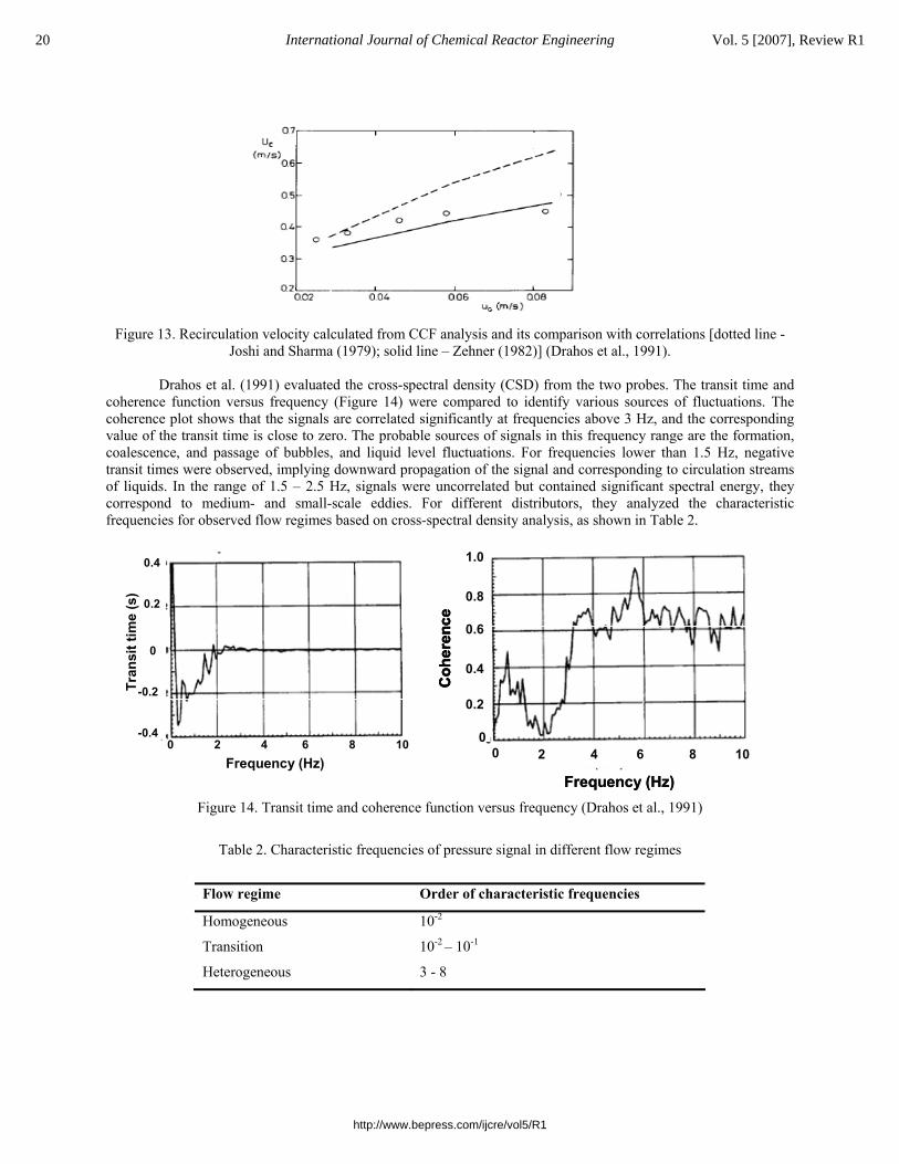
Figure 13. Recirculation velocity calculated from CCF analysis and its comparison with correlations [dotted line - Joshi and Sharma (1979); solid line – Zehner (1982)] (Drahos et al., 1991).

Drahos et al. (1991) evaluated the cross-spectral density (CSD) from the two probes. The transit time and

coherence function versus frequency (Figure 14) were compared to identify various sources of fluctuations. The coherence plot shows that the signals are correlated significantly at frequencies above 3 Hz, and the corresponding value of the transit time is close to zero. The probable sources of signals in this frequency range are the formation, coalescence, and passage of bubbles, and liquid level fluctuations. For frequencies lower than 1.5 Hz, negative transit times were observed, implying downward propagation of the signal and corresponding to circulation streams of liquids. In the range of 1.5 – 2.5 Hz, signals were uncorrelated but contained significant spectral energy, they correspond to medium- and small-scale eddies. For different distributors, they analyzed the characteristic frequencies for observed flow regimes based on cross-spectral density analysis, as shown in Table 2.

Figure 14. Transit time and coherence function versus frequency (Drahos et al., 1991)

Table 2. Characteristic frequencies of pressure signal in different flow regimes

Flow regime Order of characteristic frequencies

Homogeneous 10-2

Transition 10-2 – 10-1

Heterogeneous 3 - 8

0 2 4 6 8 10-0.4

-0.2

0.2

0.4

0

Frequency (Hz)

Tran

sit t

ime

(s)

0 2 4 6 8 10-0.4

-0.2

0.2

0.4

0

Frequency (Hz)

Tran

sit t

ime

(s)

Frequency (Hz)

0 2 4 6 8 100

0.2

0.4

0.6

0.8

1.0

Coh

eren

ce

Frequency (Hz)

0 2 4 6 8 100

0.2

0.4

0.6

0.8

1.0

Coh

eren

ce

0 2 4 6 8 100

0.2

0.4

0.6

0.8

1.0

Coh

eren

ce



Drahos et al. (1991) observed that flow regimes were better identified by the pressure probe positioned in the lower half of the bed. Also, they proposed a parametric approach to identify flow regimes in bubble columns.

van der Schaaf et al. (2002) and Chilekar et al. (2005a) separated the power in two signals into coherent output power spectral density (COP) and incoherent output power spectral density (IOP) to calculate large bubble diameter in gas-solid and gas-liquid systems, respectively. Ruthiya et al. (2005) utilized the standard deviation in COP and average cycle frequency to identify the flow regime transition point in bubble columns.

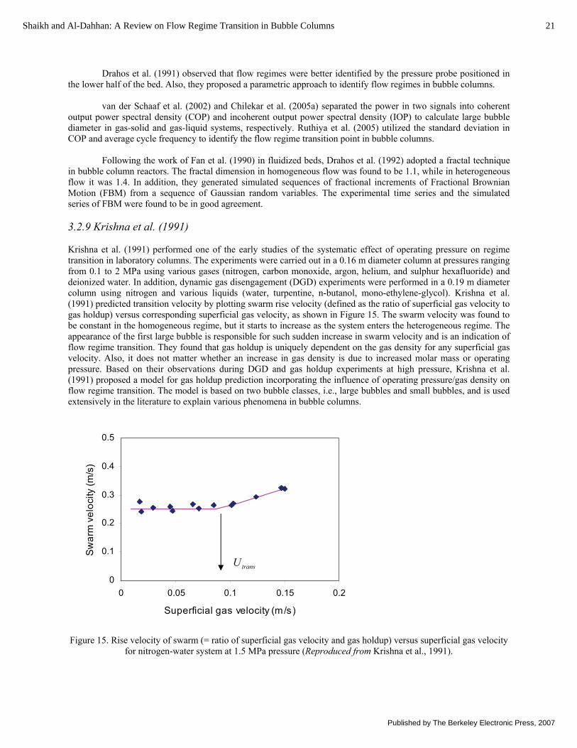
Following the work of Fan et al. (1990) in fluidized beds, Drahos et al. (1992) adopted a fractal technique in bubble column reactors. The fractal dimension in homogeneous flow was found to be 1.1, while in heterogeneous flow it was 1.4. In addition, they generated simulated sequences of fractional increments of Fractional Brownian Motion (FBM) from a sequence of Gaussian random variables. The experimental time series and the simulated series of FBM were found to be in good agreement. 3.2.9 Krishna et al. (1991) Krishna et al. (1991) performed one of the early studies of the systematic effect of operating pressure on regime transition in laboratory columns. The experiments were carried out in a 0.16 m diameter column at pressures ranging from 0.1 to 2 MPa using various gases (nitrogen, carbon monoxide, argon, helium, and sulphur hexafluoride) and deionized water. In addition, dynamic gas disengagement (DGD) experiments were performed in a 0.19 m diameter column using nitrogen and various liquids (water, turpentine, n-butanol, mono-ethylene-glycol). Krishna et al. (1991) predicted transition velocity by plotting swarm rise velocity (defined as the ratio of superficial gas velocity to gas holdup) versus corresponding superficial gas velocity, as shown in Figure 15. The swarm velocity was found to be constant in the homogeneous regime, but it starts to increase as the system enters the heterogeneous regime. The appearance of the first large bubble is responsible for such sudden increase in swarm velocity and is an indication of flow regime transition. They found that gas holdup is uniquely dependent on the gas density for any superficial gas velocity. Also, it does not matter whether an increase in gas density is due to increased molar mass or operating pressure. Based on their observations during DGD and gas holdup experiments at high pressure, Krishna et al. (1991) proposed a model for gas holdup prediction incorporating the influence of operating pressure/gas density on flow regime transition. The model is based on two bubble classes, i.e., large bubbles and small bubbles, and is used extensively in the literature to explain various phenomena in bubble columns.

Figure 15. Rise velocity of swarm (= ratio of superficial gas velocity and gas holdup) versus superficial gas velocity

for nitrogen-water system at 1.5 MPa pressure (Reproduced from Krishna et al., 1991).

0

0.1

0.2

0.3

0.4

0.5

0 0.05 0.1 0.15 0.2

Superficial gas velocity (m/s)

Swar

m v

eloc

ity (m

/s)

transU



Following the work of Krishna et al. (1991), the effect of pressure on regime transition was examined by various researchers (Wilkinson et al., 1992; Reilly et al., 1994; Letzel et al., 1997; Lin et al. 1999 etc.). The transition experiments performed by Lin et al. (1999) are some of the few to study the effect of temperature as well. One of the significant results amongst high pressure studies were presented by Letzel et al. (1997) described as follows. 3.2.10 Letzel et al. (1997) Letzel et al. (1997) calculated the transition from the homogeneous to the heterogeneous regime using the criteria proposed by Batchelor (1998) and Lammers and Bieshuvel (1996) based on linear stability theory. This analysis showed that the transition velocity is independent of operating pressure. This finding was inconsistent with the earlier reported findings. Letzel et al. (1997) then performed experiments to measure the pressure fluctuation time series as a function of superficial gas velocity and operating pressure (0.1 – 1.3 MPa) for an air-water system in a 0.15 m diameter column. The chaos analysis technique developed by van den Bleek and Schouten (1993) was applied to calculate the Kolmogorov entropy (KE) from the pressure fluctuation time series. Earlier, van den Bleek, Schouten, and coworkers applied chaos analysis of pressure fluctuations to study flow regime transition in gas-solid flows.

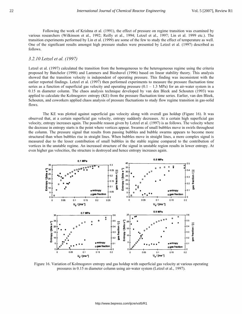
The KE was plotted against superficial gas velocity along with overall gas holdup (Figure 16). It was observed that, at a certain superficial gas velocity, entropy suddenly decreases. At a certain high superficial gas velocity, entropy increases again. The possible reason given by Letzel et al. (1997) is as follows. The velocity where the decrease in entropy starts is the point where vortices appear. Swarms of small bubbles move in swirls throughout the column. The pressure signal that results from passing bubbles and bubble swarms appears to become more structured than when bubbles rise in straight lines. When bubbles move in straight lines, a more complex signal is measured due to the lesser contribution of small bubbles in the stable regime compared to the contribution of vortices in the unstable regime. An increased structure of the signal in unstable region results in lower entropy. At even higher gas velocities, the structure is destroyed and hence entropy increases again.

Figure 16. Variation of Kolmogorov entropy and gas holdup with superficial gas velocity at various operating

pressures in 0.15 m diameter column using air-water system (Letzel et al., 1997).



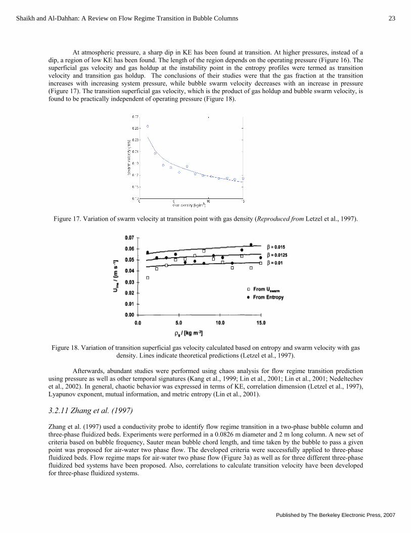
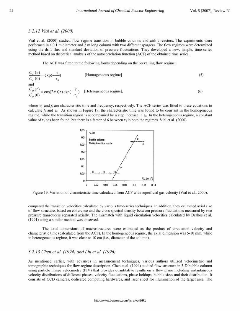
At atmospheric pressure, a sharp dip in KE has been found at transition. At higher pressures, instead of a dip, a region of low KE has been found. The length of the region depends on the operating pressure (Figure 16). The superficial gas velocity and gas holdup at the instability point in the entropy profiles were termed as transition velocity and transition gas holdup. The conclusions of their studies were that the gas fraction at the transition increases with increasing system pressure, while bubble swarm velocity decreases with an increase in pressure (Figure 17). The transition superficial gas velocity, which is the product of gas holdup and bubble swarm velocity, is found to be practically independent of operating pressure (Figure 18).

Figure 17. Variation of swarm velocity at transition point with gas density (Reproduced from Letzel et al., 1997).

Figure 18. Variation of transition superficial gas velocity calculated based on entropy and swarm velocity with gas

density. Lines indicate theoretical predictions (Letzel et al., 1997).

Afterwards, abundant studies were performed using chaos analysis for flow regime transition prediction using pressure as well as other temporal signatures (Kang et al., 1999; Lin et al., 2001; Lin et al., 2001; Nedeltechev et al., 2002). In general, chaotic behavior was expressed in terms of KE, correlation dimension (Letzel et al., 1997), Lyapunov exponent, mutual information, and metric entropy (Lin et al., 2001). 3.2.11 Zhang et al. (1997) Zhang et al. (1997) used a conductivity probe to identify flow regime transition in a two-phase bubble column and three-phase fluidized beds. Experiments were performed in a 0.0826 m diameter and 2 m long column. A new set of criteria based on bubble frequency, Sauter mean bubble chord length, and time taken by the bubble to pass a given point was proposed for air-water two phase flow. The developed criteria were successfully applied to three-phase fluidized beds. Flow regime maps for air-water two phase flow (Figure 3a) as well as for three different three-phase fluidized bed systems have been proposed. Also, correlations to calculate transition velocity have been developed for three-phase fluidized systems.



3.2.12 Vial et al. (2000) Vial et al. (2000) studied flow regime transition in bubble columns and airlift reactors. The experiments were performed in a 0.1 m diameter and 2 m long column with two different spargers. The flow regimes were determined using the drift flux and standard deviation of pressure fluctuations. They developed a new, simple, time-series method based on theoretical analysis of the autocorrelation function (ACF) of the obtained time series.

The ACF was fitted to the following forms depending on the prevailing flow regime:

0

( ) exp( )(0)

xx

xx

CC

τ ττ

= − [Homogeneous regime] (5)

and

00

( ) cos(2 )exp( )(0)

xx

xx

C fC

τ τπ ττ

= − [Heterogeneous regime], (6)

where τ0 and f0 are characteristic time and frequency, respectively. The ACF series was fitted to these equations to calculate f0 and τ0. As shown in Figure 19, the characteristic time was found to be constant in the homogeneous regime, while the transition region is accompanied by a step increase in τ0. In the heterogeneous regime, a constant value of τ0 has been found, but there is a factor of 6 between τ0 in both the regimes. Vial et al. (2000)

Figure 19. Variation of characteristic time calculated from ACF with superficial gas velocity (Vial et al., 2000).

compared the transition velocities calculated by various time-series techniques. In addition, they estimated axial size of flow structure, based on coherence and the cross-spectral density between pressure fluctuations measured by two pressure transducers separated axially. The mismatch with liquid circulation velocities calculated by Drahos et al. (1991) using a similar method was observed.

The axial dimensions of macrostructures were estimated as the product of circulation velocity and characteristic time (calculated from the ACF). In the homogeneous regime, the axial dimension was 5-10 mm, while in heterogeneous regime, it was close to 10 cm (i.e., diameter of the column). 3.2.13 Chen et al. (1994) and Lin et al. (1996) As mentioned earlier, with advances in measurement techniques, various authors utilized velocimetric and tomographic techniques for flow regime description. Chen et al. (1994) studied flow structure in 3-D bubble column using particle image velocimetry (PIV) that provides quantitative results on a flow plane including instantaneous velocity distributions of different phases, velocity fluctuations, phase holdups, bubble sizes and their distribution. It consists of CCD cameras, dedicated computing hardwares, and laser sheet for illumination of the target area. The



velocity vectors were derived from sub-sections of the target area of the particle-seeded (10-500 μm) flow by measuring the movement of particles between two light pulses. The image processing occurs in five steps: image acquisition, image enhancement, particle identification and calculation of centroids, discrimination of particle images between two phases, and matching of the particles in three consecutive video fields and calculation of the velocity.

Chen et al. (1994) observed three flow regimes, i.e., dispersed bubble flow, vertical-spiral flow, and turbulent flow (Figure 20). Compared to the general regime classifications, they divided churn-turbulent flow into two flow regimes – vortical spiral flow and turbulent flow, based on the inherently different flow mechanisms and flow structures observed in their study. In dispersed bubble flow, bubbles rise linearly and liquid falls downward between the bubble streams. In the vortical-spiral flow regime, clusters of bubbles form the central bubble stream, which moves in spiral manner with liquid moving in a vortical pattern as well as spiraling downwards in the region between the central bubble stream and the column wall. Chen et al. (1994) identified four flow regions in the vortical-spiral flow regime, viz., descending, vortical-spiral, fast bubble, and central plume regions (Figure 21). In turbulent flow, bubble coalescence becomes dominant and forms large bubbles. The authors related the transition of flow regimes and structure in the vortical-spiral flow regime to the Taylor instability for flow between two concentric rotating cylinders. They also pointed out similarities to 2-D flow structures studied by Tzeng et al. (1993) (Figure 22). The only difference between the two is the wavelike motion of the fast bubble flow region in the 2-D column, which becomes a spiral one in the 3-D bubble column.

Figure 20. Flow regimes in 3-D bubble column (Chen et al., 1994). .

Figure 21. 3-D flow structure in bubble columns proposed by Chen et al. (1994) in vorical-spiral flow regime.



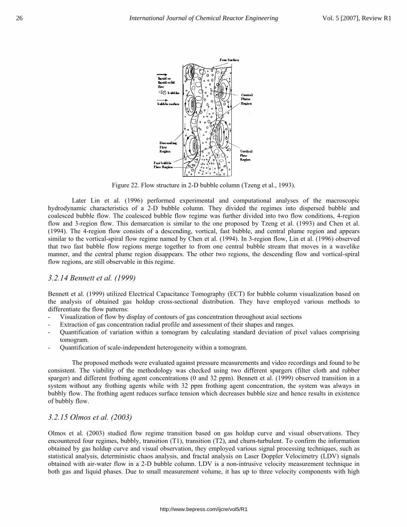
Figure 22. Flow structure in 2-D bubble column (Tzeng et al., 1993).

Later Lin et al. (1996) performed experimental and computational analyses of the macroscopic

hydrodynamic characteristics of a 2-D bubble column. They divided the regimes into dispersed bubble and coalesced bubble flow. The coalesced bubble flow regime was further divided into two flow conditions, 4-region flow and 3-region flow. This demarcation is similar to the one proposed by Tzeng et al. (1993) and Chen et al. (1994). The 4-region flow consists of a descending, vortical, fast bubble, and central plume region and appears similar to the vortical-spiral flow regime named by Chen et al. (1994). In 3-region flow, Lin et al. (1996) observed that two fast bubble flow regions merge together to from one central bubble stream that moves in a wavelike manner, and the central plume region disappears. The other two regions, the descending flow and vortical-spiral flow regions, are still observable in this regime. 3.2.14 Bennett et al. (1999) Bennett et al. (1999) utilized Electrical Capacitance Tomography (ECT) for bubble column visualization based on the analysis of obtained gas holdup cross-sectional distribution. They have employed various methods to differentiate the flow patterns: - Visualization of flow by display of contours of gas concentration throughout axial sections - Extraction of gas concentration radial profile and assessment of their shapes and ranges. - Quantification of variation within a tomogram by calculating standard deviation of pixel values comprising

tomogram. - Quantification of scale-independent heterogeneity within a tomogram.

The proposed methods were evaluated against pressure measurements and video recordings and found to be consistent. The viability of the methodology was checked using two different spargers (filter cloth and rubber sparger) and different frothing agent concentrations (0 and 32 ppm). Bennett et al. (1999) observed transition in a system without any frothing agents while with 32 ppm frothing agent concentration, the system was always in bubbly flow. The frothing agent reduces surface tension which decreases bubble size and hence results in existence of bubbly flow. 3.2.15 Olmos et al. (2003) Olmos et al. (2003) studied flow regime transition based on gas holdup curve and visual observations. They encountered four regimes, bubbly, transition (T1), transition (T2), and churn-turbulent. To confirm the information obtained by gas holdup curve and visual observation, they employed various signal processing techniques, such as statistical analysis, deterministic chaos analysis, and fractal analysis on Laser Doppler Velocimetry (LDV) signals obtained with air-water flow in a 2-D bubble column. LDV is a non-intrusive velocity measurement technique in both gas and liquid phases. Due to small measurement volume, it has up to three velocity components with high



accuracy and high spatial resolution. The basic components of an LDV include a continuous wave laser, a traversing system, transmitting and receiving optics, a signal conditioner, and a signal processor. Flow velocity information is obtained from light scattered by tiny “seeding” particles carried in the fluid. When a particle passes through the intersection volume formed by two coherent laser beams, the scattered light received by a detector has components from both beams. The components interfere on the surface of the detector. Due to changes in difference between the optical path lengths of the two components, this interference produces pulsating light intensity as the particle moves through the measurement volume.

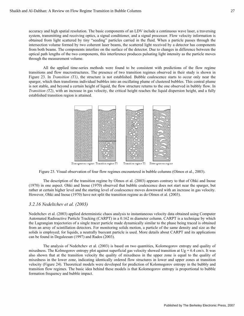
All the applied time-series methods were found to be consistent with predictions of the flow regime transitions and flow macrostructures. The presence of two transition regimes observed in their study is shown in Figure 23. In Transition (T1), the structure is not established. Bubble coalescence starts to occur only near the sparger, which then transforms individual bubbles into an oscillating plume of clustered bubbles. This central plume is not stable, and beyond a certain height of liquid, the flow structure returns to the one observed in bubbly flow. In Transition (T2), with an increase in gas velocity, the critical height reaches the liquid dispersion height, and a fully established transition region is attained.

Figure 23. Visual observation of four flow regimes encountered in bubble columns (Olmos et al., 2003).

The description of the transition regime by Olmos et al. (2003) appears contrary to that of Ohki and Inoue

(1970) in one aspect. Ohki and Inoue (1970) observed that bubble coalescence does not start near the sparger, but rather at certain higher level and the starting level of coalescence moves downward with an increase in gas velocity. However, Ohki and Inoue (1970) have not split the transition regime as do Olmos et al. (2003). 3.2.16 Nedeltchev et al. (2003) Nedeltchev et al. (2003) applied deterministic chaos analysis to instantaneous velocity data obtained using Computer Automated Radioactive Particle Tracking (CARPT) in a 0.162 m diameter column. CARPT is a technique by which the Lagrangian trajectories of a single tracer particle made dynamically similar to the phase being traced is obtained from an array of scintillation detectors. For monitoring solids motion, a particle of the same density and size as the solids is employed; for liquids, a neutrally buoyant particle is used. More details about CARPT and its applications can be found in Degaleesan (1997) and Rados (2003).

The analysis of Nedeltchev et al. (2003) is based on two quantities, Kolomogorov entropy and quality of mixedness. The Kolmogorov entropy plot against superficial gas velocity showed transition at Ug = 6.4 cm/s. It was also shown that at the transition velocity the quality of mixedness in the upper zone is equal to the quality of mixedness in the lower zone, indicating identically ordered flow structures in lower and upper zones at transition velocity (Figure 24). Theoretical models were developed for prediction of Kolomogorov entropy in the bubbly and transition flow regimes. The basic idea behind these models is that Kolomogorov entropy is proportional to bubble formation frequency and bubble impact.



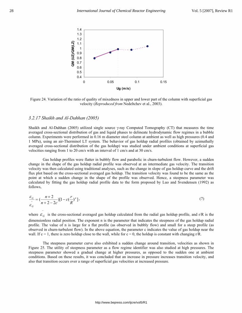
Figure 24. Variation of the ratio of quality of mixedness in upper and lower part of the column with superficial gas velocity (Reproduced from Nedeltchev et al., 2003).

3.2.17 Shaikh and Al-Dahhan (2005) Shaikh and Al-Dahhan (2005) utilized single source γ-ray Computed Tomography (CT) that measures the time averaged cross-sectional distribution of gas and liquid phases to delineate hydrodynamic flow regimes in a bubble column. Experiments were performed in 0.16 m diameter steel column at ambient as well as high pressures (0.4 and 1 MPa), using an air-Therminol LT system. The behavior of gas holdup radial profiles (obtained by azimuthally averaged cross-sectional distribution of the gas holdup) was studied under ambient conditions at superficial gas velocities ranging from 1 to 20 cm/s with an interval of 1 cm/s and at 30 cm/s.

Gas holdup profiles were flatter in bubbly flow and parabolic in churn-turbulent flow. However, a sudden change in the shape of the gas holdup radial profile was observed at an intermediate gas velocity. The transition velocity was then calculated using traditional analyses, such as the change in slope of gas holdup curve and the drift flux plot based on the cross-sectional averaged gas holdup. The transition velocity was found to be the same as the point at which a sudden change in the shape of the profile was observed. Hence, a steepness parameter was calculated by fitting the gas holdup radial profile data to the form proposed by Luo and Svendensen (1992) as follows,

])(1)[22

2( n

G

G

Rrc

cnn

−−++

=−

ε

ε , (7)

where −

Gε is the cross-sectional averaged gas holdup calculated from the radial gas holdup profile, and r/R is the dimensionless radial position. The exponent n is the parameter that indicates the steepness of the gas holdup radial profile. The value of n is large for a flat profile (as observed in bubbly flow) and small for a steep profile (as observed in churn-turbulent flow). In the above equation, the parameter c indicates the value of gas holdup near the wall. If c = 1, there is zero holdup close to the wall, while for c = 0, the holdup is constant with changing r/R.

The steepness parameter curve also exhibited a sudden change around transition, velocities as shown in Figure 25. The utility of steepness parameter as a flow regime identifier was also studied at high pressures. The steepness parameter showed a gradual change at higher pressures, as opposed to the sudden one at ambient conditions. Based on these results, it was concluded that an increase in pressure increases transition velocity, and also that transition occurs over a range of superficial gas velocities at increased pressure.

0.40.50.60.70.80.9

11.11.21.31.4

0 0.05 0.1 0.15

Ug (m/s)

QM

(UZ)

/QM

(LZ)



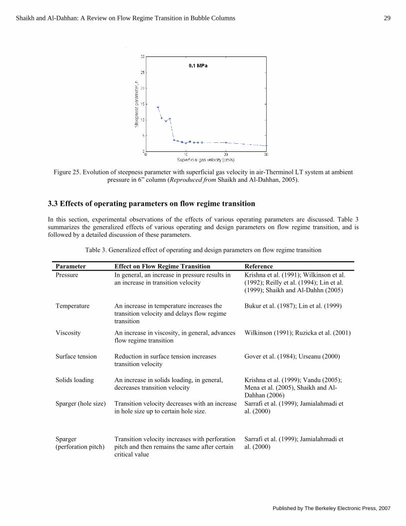
Figure 25. Evolution of steepness parameter with superficial gas velocity in air-Therminol LT system at ambient

pressure in 6” column (Reproduced from Shaikh and Al-Dahhan, 2005). 3.3 Effects of operating parameters on flow regime transition In this section, experimental observations of the effects of various operating parameters are discussed. Table 3 summarizes the generalized effects of various operating and design parameters on flow regime transition, and is followed by a detailed discussion of these parameters.

Table 3. Generalized effect of operating and design parameters on flow regime transition

Parameter Effect on Flow Regime Transition Reference Pressure In general, an increase in pressure results in

an increase in transition velocity Krishna et al. (1991); Wilkinson et al. (1992); Reilly et al. (1994); Lin et al. (1999); Shaikh and Al-Dahhn (2005)

Temperature An increase in temperature increases the transition velocity and delays flow regime transition

Bukur et al. (1987); Lin et al. (1999)

Viscosity An increase in viscosity, in general, advances flow regime transition

Wilkinson (1991); Ruzicka et al. (2001)

Surface tension Reduction in surface tension increases transition velocity

Gover et al. (1984); Urseanu (2000)

Solids loading An increase in solids loading, in general, decreases transition velocity

Krishna et al. (1999); Vandu (2005); Mena et al. (2005), Shaikh and Al-Dahhan (2006)

Sparger (hole size) Transition velocity decreases with an increase in hole size up to certain hole size.

Sarrafi et al. (1999); Jamialahmadi et al. (2000)

Sparger (perforation pitch)

Transition velocity increases with perforation pitch and then remains the same after certain critical value

Sarrafi et al. (1999); Jamialahmadi et al. (2000)



Liquid height An increase in liquid height reduces the transition velocity

Sarrafi et al. (1999); Ruzicka et al. (2001)

Column diameter Conflicting results. An increase in column diameter increases transition velocity (Group 1) while column diameter advances flow regime transition (Group 2)

Group 1: Ohki and Inoue (1970); Sarrafi et al. (1999); Jamialahmadi et al. (2000); Urseanu (2000) Group 2: Zahradnik et al. (1997); Ruzicka et al. (2001)

Aspect ratio Aspect ratio decreases the transition velocity. However, it alone is not sufficient to provide reliable information on flow regime stability

Ruzicka et al. (2001); Thorat and Joshi (2003)

3.3.1 Effect of operating pressure As most industrial operations are performed at high operating pressure, it is important to investigate its effect on flow regime transition. As mentioned previously, Krishna et al. (1991) performed one of the early studies in this direction. In general, most of the investigators have reported that an increase in pressure delays flow regime transition. An increase in pressure increases breakup rate, reduces coalescence rate, and delays the appearance of large bubble and thereby flow regime transition.

Except for studies by Letzel et al. (1997), most investigators have found a general trend of an increase in transition velocity with an increase in pressure (Wilkinson et al., 1991; Reilly et al., 1994; Lin et al., 1999; Lin et al., 2001, Shaikh and Al-Dahhan, 2005, Chilekar et al., 2005b) [Figure 26a]. Krishna et al. (1991) demonstrated the effect of pressure by varying gas density and observed a similar trend (Figure 26b).

(a) (b) Figure 26. Variation of transition velocity with a) operating pressure (Reproduced from Lin et al., 2001), and b) gas

density (Reproduced from Krishna et al., 1991).

It has been observed that at higher pressure transition occurs over a range of velocities (i.e., a transition region) and the length of this range (i.e., the size of the transition region) increases with an increase in pressure (Letzel



et al., 1997; Shaikh and Al-Dahhan, 2005). The presence of a transition zone at higher pressure has been linked to the appearance of ‘swirl’ and ‘large bubbles’ at different superficial gas velocities, whereas at atmospheric pressure these two phenomena coincide (van den Bleek et al., 2002). 3.3.2 Effect of temperature There are very few studies that have investigated the effect of temperature on flow regime transition (Grover et al., 1984; Bukur et al., 1987; Lin et al., 1999). It is generally recognized that an increase in temperature increases overall gas holdup due to the formation of small bubbles. The effect of temperature can be accounted for by the change in physical properties of fluid.

Lin et al. (1999) performed pressure drop fluctuation experiments in a 0.0508 m diameter column with a nitrogen-Paratherm system at various temperatures (298 – 350 K) and operating pressures (0.1 – 15 MPa). The transition velocities were determined based on the standard deviation of the pressure drop fluctuations and the drift flux plot.

They observed that, due to generation of small bubbles, flow regimes are sustained at higher velocities with an increase in temperature. An increase in pressure and temperature was found to have a favorable effect on flow regime stability and results in increasing transition velocity (Figure 27). Lin et al. (1999) also found that transition velocity does not vary as pressure exceeds a critical value, particularly at higher temperature. At 350 K, the critical value of pressure was 7 MPa.

Figure 27. Effect of temperature on transition velocity (Reproduced from Lin et al., 1999). 3.3.3 Effect of viscosity The liquid phase viscosity has been found to have a significant effect on the hydrodynamic characteristics of bubble columns. An increase in viscosity results in a stable bubble interface and thereby results in an increase in coalescence rate and decrease in breakup rate. This gives rise to an early appearance of large bubble and hence should advance the flow regime transition.

Ruzicka et al. (2001) systematically studied the effect of viscosity by using an air-aqueous solution of glycol in a 0.14 m diameter column at ambient conditions. They found that moderate viscosities (3-22 mPa-s) destabilize the homogeneous regime, thereby reducing transition velocity. Low viscosity (1-3 mPa-s) stabilizes the homogeneous regime, thereby increasing the transition velocity as viscosity increases in this narrow range. (Figure 28).

This result should be considered in terms of monocomponent and multicomponent liquids. For monocomponent liquids, Wilkinson et al. (1992) showed that gas holdup decreases with an increase in viscosity. By addition of glycerol or carboxymethyl cellulose (CMC), Eissa and Schugerl (1975) showed that gas holdup first increases (in the viscosity range up to 3 mPa-s) and then decreases with an increase in viscosity. The initial increase



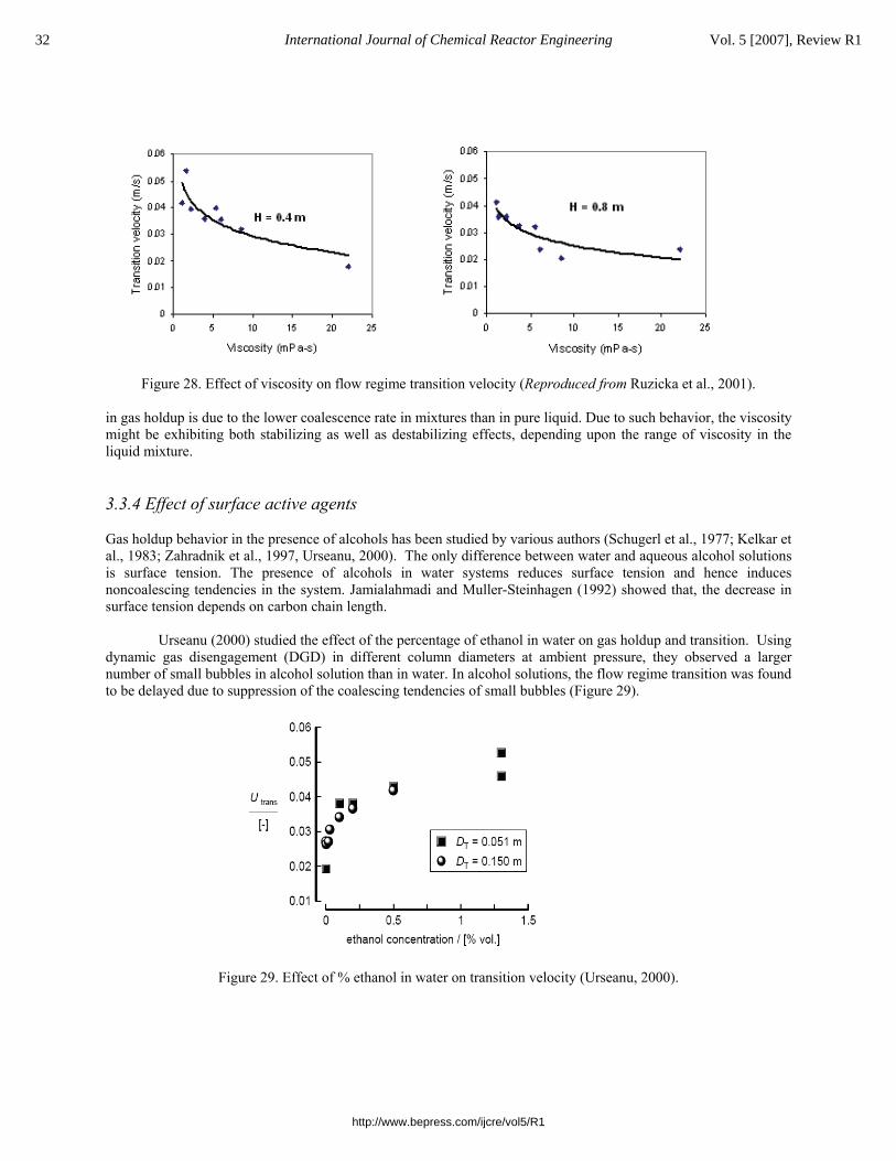
Figure 28. Effect of viscosity on flow regime transition velocity (Reproduced from Ruzicka et al., 2001). in gas holdup is due to the lower coalescence rate in mixtures than in pure liquid. Due to such behavior, the viscosity might be exhibiting both stabilizing as well as destabilizing effects, depending upon the range of viscosity in the liquid mixture. 3.3.4 Effect of surface active agents Gas holdup behavior in the presence of alcohols has been studied by various authors (Schugerl et al., 1977; Kelkar et al., 1983; Zahradnik et al., 1997, Urseanu, 2000). The only difference between water and aqueous alcohol solutions is surface tension. The presence of alcohols in water systems reduces surface tension and hence induces noncoalescing tendencies in the system. Jamialahmadi and Muller-Steinhagen (1992) showed that, the decrease in surface tension depends on carbon chain length.

Urseanu (2000) studied the effect of the percentage of ethanol in water on gas holdup and transition. Using dynamic gas disengagement (DGD) in different column diameters at ambient pressure, they observed a larger number of small bubbles in alcohol solution than in water. In alcohol solutions, the flow regime transition was found to be delayed due to suppression of the coalescing tendencies of small bubbles (Figure 29).

Figure 29. Effect of % ethanol in water on transition velocity (Urseanu, 2000).



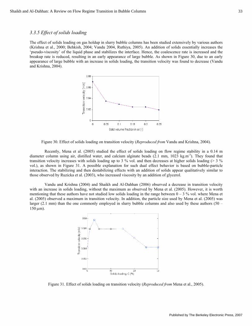
3.3.5 Effect of solids loading The effect of solids loading on gas holdup in slurry bubble columns has been studied extensively by various authors (Krishna et al., 2000; Behkish, 2004; Vandu 2004, Ruthiya, 2005). An addition of solids essentially increases the ‘pseudo-viscosity’ of the liquid phase and stabilizes the interface. Hence, the coalescence rate is increased and the breakup rate is reduced, resulting in an early appearance of large bubble. As shown in Figure 30, due to an early appearance of large bubble with an increase in solids loading, the transition velocity was found to decrease (Vandu and Krishna, 2004).

Figure 30. Effect of solids loading on transition velocity (Reproduced from Vandu and Krishna, 2004).

Recently, Mena et al. (2005) studied the effect of solids loading on flow regime stability in a 0.14 m diameter column using air, distilled water, and calcium alginate beads (2.1 mm, 1023 kg.m-3). They found that transition velocity increases with solids loading up to 3 % vol. and then decreases at higher solids loading (> 3 % vol.), as shown in Figure 31. A possible explanation for such dual effect behavior is based on bubble-particle interaction. The stabilizing and then destabilizing effects with an addition of solids appear qualitatively similar to those observed by Ruzicka et al. (2003), who increased viscosity by an addition of glycerol.

Vandu and Krishna (2004) and Shaikh and Al-Dahhan (2006) observed a decrease in transition velocity with an increase in solids loading, without the maximum as observed by Mena et al. (2005). However, it is worth mentioning that these authors have not studied low solids loading in the range between 0 – 3 % vol. where Mena et al. (2005) observed a maximum in transition velocity. In addition, the particle size used by Mena et al. (2005) was larger (2.1 mm) than the one commonly employed in slurry bubble columns and also used by these authors (50 – 150 μm).

Figure 31. Effect of solids loading on transition velocity (Reproduced from Mena et al., 2005).



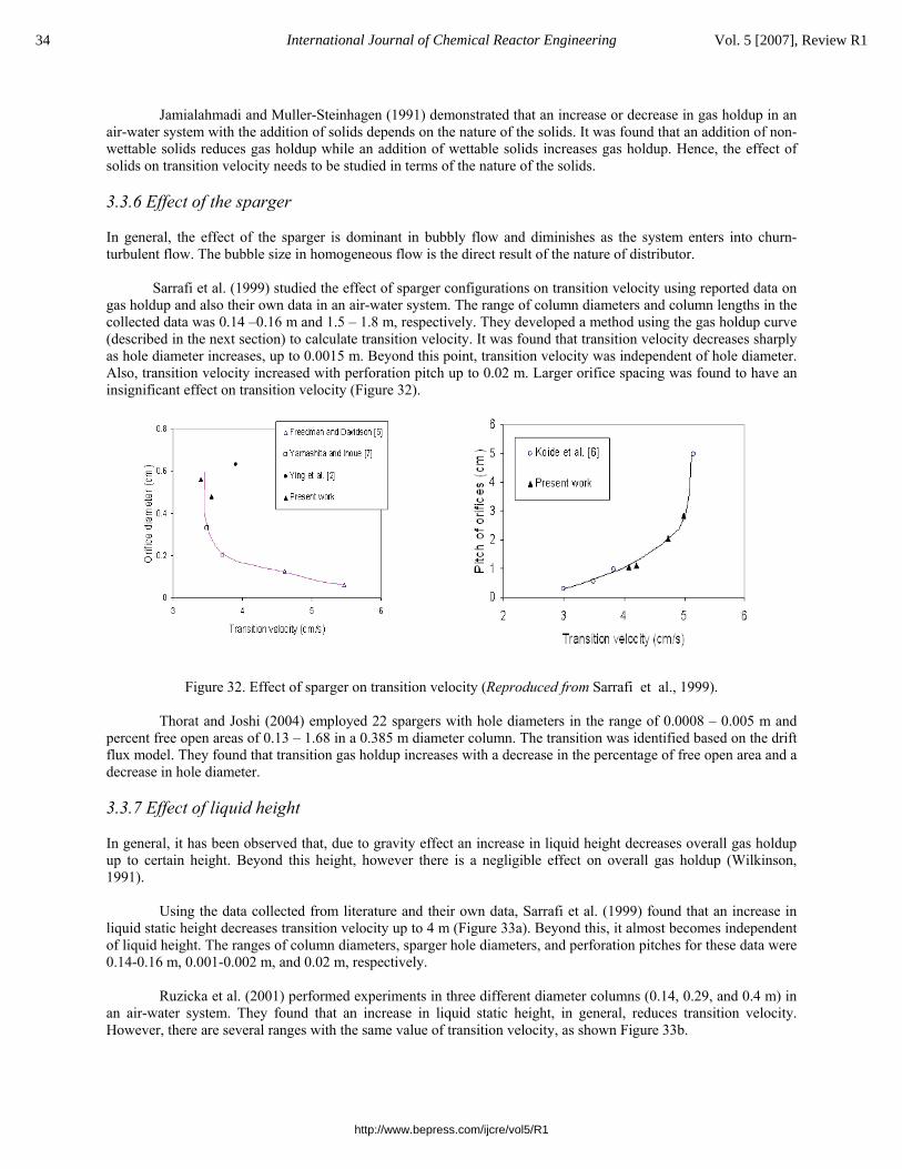
Jamialahmadi and Muller-Steinhagen (1991) demonstrated that an increase or decrease in gas holdup in an air-water system with the addition of solids depends on the nature of the solids. It was found that an addition of non-wettable solids reduces gas holdup while an addition of wettable solids increases gas holdup. Hence, the effect of solids on transition velocity needs to be studied in terms of the nature of the solids. 3.3.6 Effect of the sparger In general, the effect of the sparger is dominant in bubbly flow and diminishes as the system enters into churn-turbulent flow. The bubble size in homogeneous flow is the direct result of the nature of distributor.

Sarrafi et al. (1999) studied the effect of sparger configurations on transition velocity using reported data on gas holdup and also their own data in an air-water system. The range of column diameters and column lengths in the collected data was 0.14 –0.16 m and 1.5 – 1.8 m, respectively. They developed a method using the gas holdup curve (described in the next section) to calculate transition velocity. It was found that transition velocity decreases sharply as hole diameter increases, up to 0.0015 m. Beyond this point, transition velocity was independent of hole diameter. Also, transition velocity increased with perforation pitch up to 0.02 m. Larger orifice spacing was found to have an insignificant effect on transition velocity (Figure 32).

Figure 32. Effect of sparger on transition velocity (Reproduced from Sarrafi et al., 1999).

Thorat and Joshi (2004) employed 22 spargers with hole diameters in the range of 0.0008 – 0.005 m and percent free open areas of 0.13 – 1.68 in a 0.385 m diameter column. The transition was identified based on the drift flux model. They found that transition gas holdup increases with a decrease in the percentage of free open area and a decrease in hole diameter. 3.3.7 Effect of liquid height In general, it has been observed that, due to gravity effect an increase in liquid height decreases overall gas holdup up to certain height. Beyond this height, however there is a negligible effect on overall gas holdup (Wilkinson, 1991).

Using the data collected from literature and their own data, Sarrafi et al. (1999) found that an increase in liquid static height decreases transition velocity up to 4 m (Figure 33a). Beyond this, it almost becomes independent of liquid height. The ranges of column diameters, sparger hole diameters, and perforation pitches for these data were 0.14-0.16 m, 0.001-0.002 m, and 0.02 m, respectively.

Ruzicka et al. (2001) performed experiments in three different diameter columns (0.14, 0.29, and 0.4 m) in an air-water system. They found that an increase in liquid static height, in general, reduces transition velocity. However, there are several ranges with the same value of transition velocity, as shown Figure 33b.



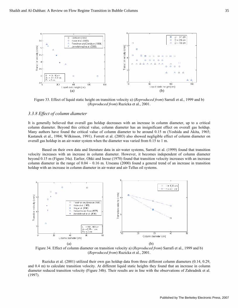
(a) (b)

Figure 33. Effect of liquid static height on transition velocity a) (Reproduced from) Sarrafi et al., 1999 and b) (Reproduced from) Ruzicka et al., 2001.

3.3.8 Effect of column diameter It is generally believed that overall gas holdup decreases with an increase in column diameter, up to a critical column diameter. Beyond this critical value, column diameter has an insignificant effect on overall gas holdup. Many authors have found the critical value of column diameter to be around 0.15 m (Yoshida and Akita, 1965; Kastanek et al., 1984; Wilkinson, 1991). Forrett et al. (2003) also showed negligible effect of column diameter on overall gas holdup in an air-water system when the diameter was varied from 0.15 to 1 m.

Based on their own data and literature data in air-water systems, Sarrafi et al. (1999) found that transition velocity increases with an increase in column diameter. However, it becomes independent of column diameter beyond 0.15 m (Figure 34a). Earlier, Ohki and Inoue (1970) found that transition velocity increases with an increase column diameter in the range of 0.04 – 0.16 m. Urseanu (2000) found a general trend of an increase in transition holdup with an increase in column diameter in air-water and air-Tellus oil systems.

(a) (b) Figure 34. Effect of column diameter on transition velocity a) (Reproduced from) Sarrafi et al., 1999 and b)

(Reproduced from) Ruzicka et al., 2001.

Ruzicka et al. (2001) utilized their own gas holdup data from three different column diameters (0.14, 0.29, and 0.4 m) to calculate transition velocity. At different liquid static heights they found that an increase in column diameter reduced transition velocity (Figure 34b). Their results are in line with the observations of Zahradnik et al. (1997).



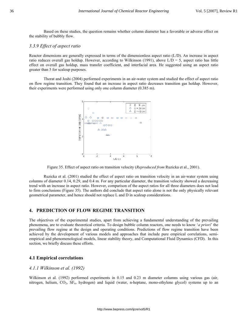
Based on these studies, the question remains whether column diameter has a favorable or adverse effect on the stability of bubbly flow. 3.3.9 Effect of aspect ratio Reactor dimensions are generally expressed in terms of the dimensionless aspect ratio (L/D). An increase in aspect ratio reduces overall gas holdup. However, according to Wilkinson (1991), above L/D = 5, aspect ratio has little effect on overall gas holdup, mass transfer coefficient, and interfacial area. He suggested using an aspect ratio greater than 5 for scaleup purposes.

Thorat and Joshi (2004) performed experiments in an air-water system and studied the effect of aspect ratio on flow regime transition. They found that an increase in aspect ratio decreases transition gas holdup. However, their experiments were performed using only one column diameter (0.385 m).

Figure 35. Effect of aspect ratio on transition velocity (Reproduced from Ruzicka et al., 2001).

Ruzicka et al. (2001) studied the effect of aspect ratio on transition velocity in an air-water system using columns of diameter 0.14, 0.29, and 0.4 m. For any particular diameter, the transition velocity showed a decreasing trend with an increase in aspect ratio. However, comparison of the aspect ratios for all three diameters does not lead to firm conclusions (Figure 35). The authors did conclude that aspect ratio alone is not the only physically relevant geometrical parameter, and hence should not replace L and D in scaleup considerations. 4. PREDICTION OF FLOW REGIME TRANSITION The objectives of the experimental studies, apart from achieving a fundamental understanding of the prevailing phenomena, are to evaluate theoretical criteria. To design bubble column reactors, one needs to know ‘a priori’ the prevailing flow regime at the design and operating conditions. Predictions of flow regime transition have been achieved by the development of various models and approaches that include pure empirical correlations, semi- empirical and phenomenological models, linear stability theory, and Computational Fluid Dynamics (CFD). In this section, we briefly discuss these efforts. 4.1 Empirical correlations 4.1.1 Wilkinson et al. (1992) Wilkinson et al. (1992) performed experiments in 0.15 and 0.23 m diameter columns using various gas (air, nitrogen, helium, CO2, SF6, hydrogen) and liquid (water, n-heptane, mono-ethylene glycol) systems up to an



operating pressure of 1.5 MPa. These gases with different densities were used to study the effect of gas density at ambient pressure.

They incorporated their experimental data with a gas holdup model they developed, similar to but slightly different from the one proposed by Krishna et al. (1991). For superficial gas velocities less than transition velocity, the gas holdup increased proportionally to the superficial gas velocity. Thus, the following equation was written for homogeneous flow for UG < Utrans :

GG AU=ε . (8) This can be then written in the following form:

bsGG UU ,/=ε , (9) where Us,b is the rise velocity of the bubbles.

On the basis of dimensional analysis, Wilkinson et al. (1992) proposed the following equation for bubble rise velocity:

3, 1 2

4[ ] [ ]s b L n nL L

L G

UC

gμ σ ρ ρ

σ μ ρ= . (10)

when UG > Utrans :

bl

transGbstransG U

UUUU

,,/

−+=ε . (11)

In equation (11), Ul,b is the rise velocity of large bubbles, which should be greater than Us,b. To maintain this condition, following dimensionless equation was chosen:

(12)

Considering the behavior of transition velocity with changes in liquid properties and gas density, an empirical equation for transition velocity was proposed:

( , , , )trans G L LU F σ ρ ρ μ= , (13) Based on their own experimental data as well as literature data, optimal values of parameters were calculated in equations (10), (12), and (13) with the aid of non-linear regression analysis. The regression analysis led the following equations to predict transition velocity and holdup:

3, 0.273 0.03

42.23[ ] [ ]s b L L L

L G

Ug

μ σ ρ ρσ μ ρ

−= , (14)

(15)

)193exp(5.0 11.05.061.0

,

σμρε LGtransbs

trans

UU −−== . (16)

3, , 3 4 5

4

( )[ ] [ ] [ ]L l b L s b n n nL G trans L L

L G

U U U UCg

μ μ μ σ ρ ρσ σ σ μ ρ

−= +

3, , 0.757 0.077 0.077

4

( )2.4[ ] [ ] [ ]L l b L s b L G trans L L

L G

U U U Ug

μ μ μ σ ρ ρσ σ σ μ ρ

−−= +



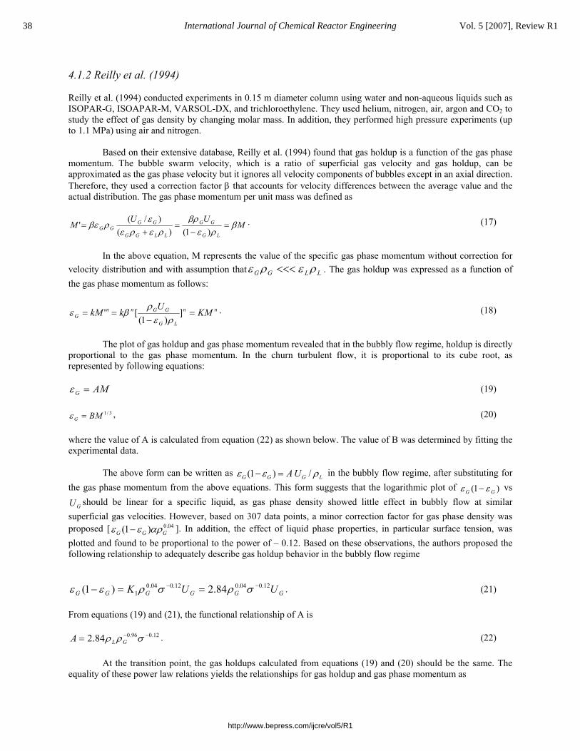
4.1.2 Reilly et al. (1994) Reilly et al. (1994) conducted experiments in 0.15 m diameter column using water and non-aqueous liquids such as ISOPAR-G, ISOAPAR-M, VARSOL-DX, and trichloroethylene. They used helium, nitrogen, air, argon and CO2 to study the effect of gas density by changing molar mass. In addition, they performed high pressure experiments (up to 1.1 MPa) using air and nitrogen.

Based on their extensive database, Reilly et al. (1994) found that gas holdup is a function of the gas phase momentum. The bubble swarm velocity, which is a ratio of superficial gas velocity and gas holdup, can be approximated as the gas phase velocity but it ignores all velocity components of bubbles except in an axial direction. Therefore, they used a correction factor β that accounts for velocity differences between the average value and the actual distribution. The gas phase momentum per unit mass was defined as

MUU

MLG

GG

LLGG

GGGG β

ρεβρ

ρερεε

ρβε =−

=+

=)1()(

)/(' . (17)

In the above equation, M represents the value of the specific gas phase momentum without correction for

velocity distribution and with assumption that LLGG ρερε <<< . The gas holdup was expressed as a function of the gas phase momentum as follows:

nn

LG

GGnnG KM

UkkM =

−== ]

)1(['

ρερ

βε . (18)

The plot of gas holdup and gas phase momentum revealed that in the bubbly flow regime, holdup is directly

proportional to the gas phase momentum. In the churn turbulent flow, it is proportional to its cube root, as represented by following equations:

AMG =ε (19)

3/1BMG =ε , (20) where the value of A is calculated from equation (22) as shown below. The value of B was determined by fitting the experimental data.

The above form can be written as (1 ) /G G G LA Uε ε ρ− = in the bubbly flow regime, after substituting for the gas phase momentum from the above equations. This form suggests that the logarithmic plot of )1( GG εε − vs

GU should be linear for a specific liquid, as gas phase density showed little effect in bubbly flow at similar superficial gas velocities. However, based on 307 data points, a minor correction factor for gas phase density was proposed [ 0.04(1 )G G Gε ε αρ− ]. In addition, the effect of liquid phase properties, in particular surface tension, was plotted and found to be proportional to the power of – 0.12. Based on these observations, the authors proposed the following relationship to adequately describe gas holdup behavior in the bubbly flow regime

GGGGGG UUK 12.004.012.004.01 84.2)1( −− ==− σρσρεε . (21)

From equations (19) and (21), the functional relationship of A is

12.096.084.2 −−= σρρ GLA . (22)

At the transition point, the gas holdups calculated from equations (19) and (20) should be the same. The equality of these power law relations yields the relationships for gas holdup and gas phase momentum as



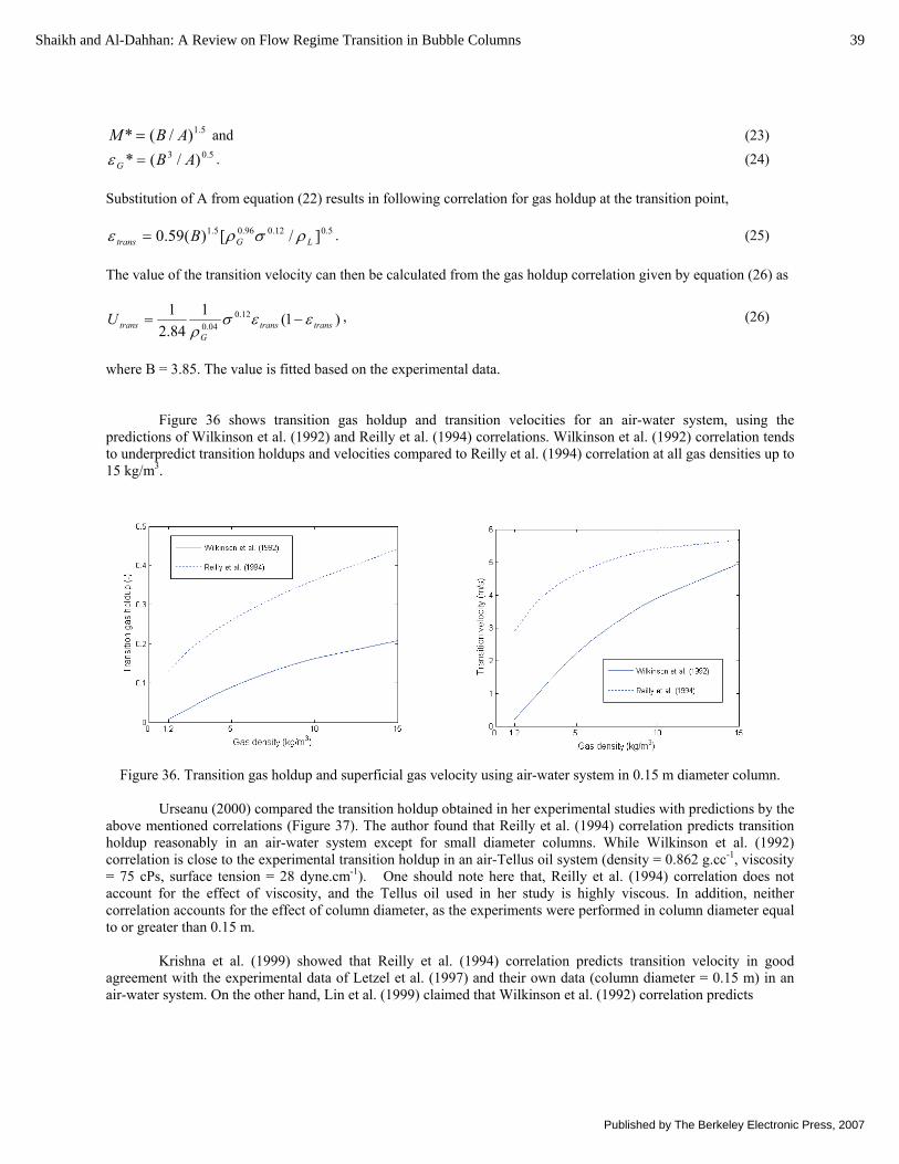
5.1)/(* ABM = and (23)

5.03 )/(* ABG =ε . (24) Substitution of A from equation (22) results in following correlation for gas holdup at the transition point,

5.012.096.05.1 ]/[)(59.0 LGtrans B ρσρε = . (25) The value of the transition velocity can then be calculated from the gas holdup correlation given by equation (26) as

)1(184.21 12.0

04.0 transtransG

transU εεσρ

−= , (26)

where B = 3.85. The value is fitted based on the experimental data.

Figure 36 shows transition gas holdup and transition velocities for an air-water system, using the predictions of Wilkinson et al. (1992) and Reilly et al. (1994) correlations. Wilkinson et al. (1992) correlation tends to underpredict transition holdups and velocities compared to Reilly et al. (1994) correlation at all gas densities up to 15 kg/m3.

Figure 36. Transition gas holdup and superficial gas velocity using air-water system in 0.15 m diameter column.

Urseanu (2000) compared the transition holdup obtained in her experimental studies with predictions by the

above mentioned correlations (Figure 37). The author found that Reilly et al. (1994) correlation predicts transition holdup reasonably in an air-water system except for small diameter columns. While Wilkinson et al. (1992) correlation is close to the experimental transition holdup in an air-Tellus oil system (density = 0.862 g.cc-1, viscosity = 75 cPs, surface tension = 28 dyne.cm-1). One should note here that, Reilly et al. (1994) correlation does not account for the effect of viscosity, and the Tellus oil used in her study is highly viscous. In addition, neither correlation accounts for the effect of column diameter, as the experiments were performed in column diameter equal to or greater than 0.15 m.

Krishna et al. (1999) showed that Reilly et al. (1994) correlation predicts transition velocity in good agreement with the experimental data of Letzel et al. (1997) and their own data (column diameter = 0.15 m) in an air-water system. On the other hand, Lin et al. (1999) claimed that Wilkinson et al. (1992) correlation predicts



(a) (b)

Figure 37. Comparison of experimental and correlation predicted transition holdup in a) air-water and b) air-Tellus oil system at ambient conditions (Urseanu, 2000).

results that are comparable to their experimental transition velocities at various temperatures and operating pressures (column diameter = 0.1 m) in an air-Paratherm NF system (density = 0.87 g.cc-1, viscosity = 31.7 cPs, surface tension = 29.5 dyne.cm-1). The viscosity of Paratherm NF is much higher than that of water.

Shaikh and Al-Dahhan (2005) compared the transition velocities obtained using CT in an air-Therminol LT system at ambient and high (0.4 and 1 MPa) pressures in a 0.1615 m diameter column with the prediction of these correlations. Quite surprisingly, both correlations showed maximum relative error at ambient pressure. Within the studied range of operating conditions, the average relative errors using the correlations of Wilkinson et al. (1992) and Reilly et al. (1994) are 70 and 49 %. Such discrepancies in transition velocities predicted by available correlations show that the state of prediction of transition based on the correlations is not yet reliable. 4.2 Semi-empirical models This section discusses approaches where physical mechanisms were combined with the experimental observations. 4.2.1 Small diameter bubble columns / vertical pipes 4.2.1.1 Taitel et al. (1980) Taitel et al. (1980) developed semi-empirical models to predict flow regime transition in vertical gas-liquid flows in small diameter columns. The approach to modeling flow regime transition in this work was similar in principle to that presented by Taitel and Dukler (1976) for horizontal flow systems. They presented criteria to discriminate bubbly, slug, churn, and annular flow patterns. Taitel et al. (1980) presented simple equations to obtain flow pattern transition boundaries for any column size and fluid properties.

The criterion for transition from bubbly to slug flow was defined by calculating the maximum allowable packing of bubbles. The bubble deformation and its random path were also taken into consideration. Based on this, the gas holdup at which bubbles can remain spherical and still be arranged in a cubic lattice was found to be 0.25.

The bubble rise velocity was related to superficial gas velocity by

G

Gb

Uu

ε= . (27)

Similarly, average liquid velocity was related to superficial liquid velocity by

G

LL

UV

ε−=

1. (28)



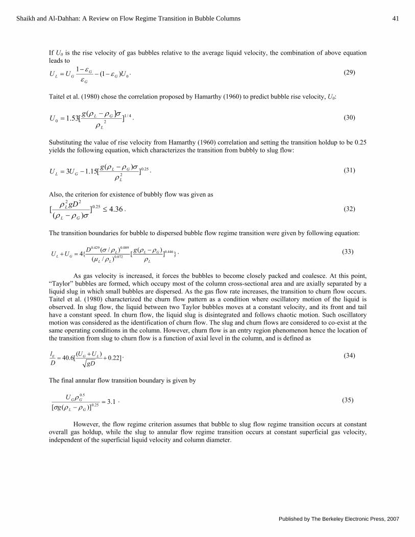
If U0 is the rise velocity of gas bubbles relative to the average liquid velocity, the combination of above equation leads to

0)1(1

UUU GG

GGL ε

εε

−−−

= . (29)

Taitel et al. (1980) chose the correlation proposed by Hamarthy (1960) to predict bubble rise velocity, U0:

4/120 ]

]([53.1

L

GLgU

ρσρρ −

= . (30)

Substituting the value of rise velocity from Hamarthy (1960) correlation and setting the transition holdup to be 0.25 yields the following equation, which characterizes the transition from bubbly to slug flow:

25.02 ]

)([15.13

L

GLGL

gUU

ρσρρ −

−= . (31)

Also, the criterion for existence of bubbly flow was given as

36.4])(

[ 25.022

≤− σρρ

ρ

GL

L gD. (32)

The transition boundaries for bubble to dispersed bubble flow regime transition were given by following equation:

0.429 0.0890.446

0.072

( )( / )4{ [ ] }( / )

L GLL G

L L L

gDU U ρ ρσ ρμ ρ ρ

−+ = . (33)

As gas velocity is increased, it forces the bubbles to become closely packed and coalesce. At this point,

“Taylor” bubbles are formed, which occupy most of the column cross-sectional area and are axially separated by a liquid slug in which small bubbles are dispersed. As the gas flow rate increases, the transition to churn flow occurs. Taitel et al. (1980) characterized the churn flow pattern as a condition where oscillatory motion of the liquid is observed. In slug flow, the liquid between two Taylor bubbles moves at a constant velocity, and its front and tail have a constant speed. In churn flow, the liquid slug is disintegrated and follows chaotic motion. Such oscillatory motion was considered as the identification of churn flow. The slug and churn flows are considered to co-exist at the same operating conditions in the column. However, churn flow is an entry region phenomenon hence the location of the transition from slug to churn flow is a function of axial level in the column, and is defined as

( )40.6[ 0.22]G LE U UlD gD

+= + . (34)

The final annular flow transition boundary is given by

1.3)]([ 25.0

5.0

=− GL

GG

gU

ρρσρ . (35)

However, the flow regime criterion assumes that bubble to slug flow regime transition occurs at constant

overall gas holdup, while the slug to annular flow regime transition occurs at constant superficial gas velocity, independent of the superficial liquid velocity and column diameter.



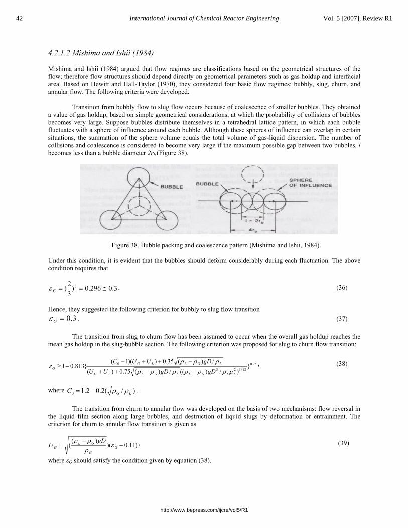
4.2.1.2 Mishima and Ishii (1984) Mishima and Ishii (1984) argued that flow regimes are classifications based on the geometrical structures of the flow; therefore flow structures should depend directly on geometrical parameters such as gas holdup and interfacial area. Based on Hewitt and Hall-Taylor (1970), they considered four basic flow regimes: bubbly, slug, churn, and annular flow. The following criteria were developed.

Transition from bubbly flow to slug flow occurs because of coalescence of smaller bubbles. They obtained a value of gas holdup, based on simple geometrical considerations, at which the probability of collisions of bubbles becomes very large. Suppose bubbles distribute themselves in a tetrahedral lattice pattern, in which each bubble fluctuates with a sphere of influence around each bubble. Although these spheres of influence can overlap in certain situations, the summation of the sphere volume equals the total volume of gas-liquid dispersion. The number of collisions and coalescence is considered to become very large if the maximum possible gap between two bubbles, l becomes less than a bubble diameter 2rb (Figure 38).

Figure 38. Bubble packing and coalescence pattern (Mishima and Ishii, 1984). Under this condition, it is evident that the bubbles should deform considerably during each fluctuation. The above condition requires that

3.0296.0)32( 3 ≅==Gε . (36)

Hence, they suggested the following criterion for bubbly to slug flow transition

3.0=Gε . (37)

The transition from slug to churn flow has been assumed to occur when the overall gas holdup reaches the mean gas holdup in the slug-bubble section. The following criterion was proposed for slug to churn flow transition:

75.018/123

0 })/)((/)(75.0)(

/)(35.0))(1({813.01

LLGLLGLLG

LGLLGG gDgDUU

gDUUCμρρρρρρ

ρρρε

−−++

−++−−≥ , (38)

where 0 1.2 0.2( / )G LC ρ ρ= − .

The transition from churn to annular flow was developed on the basis of two mechanisms: flow reversal in

the liquid film section along large bubbles, and destruction of liquid slugs by deformation or entrainment. The criterion for churn to annular flow transition is given as

)11.0)()(

( −−

= GG

GLG

gDU ε

ρρρ , (39)

where εG should satisfy the condition given by equation (38).



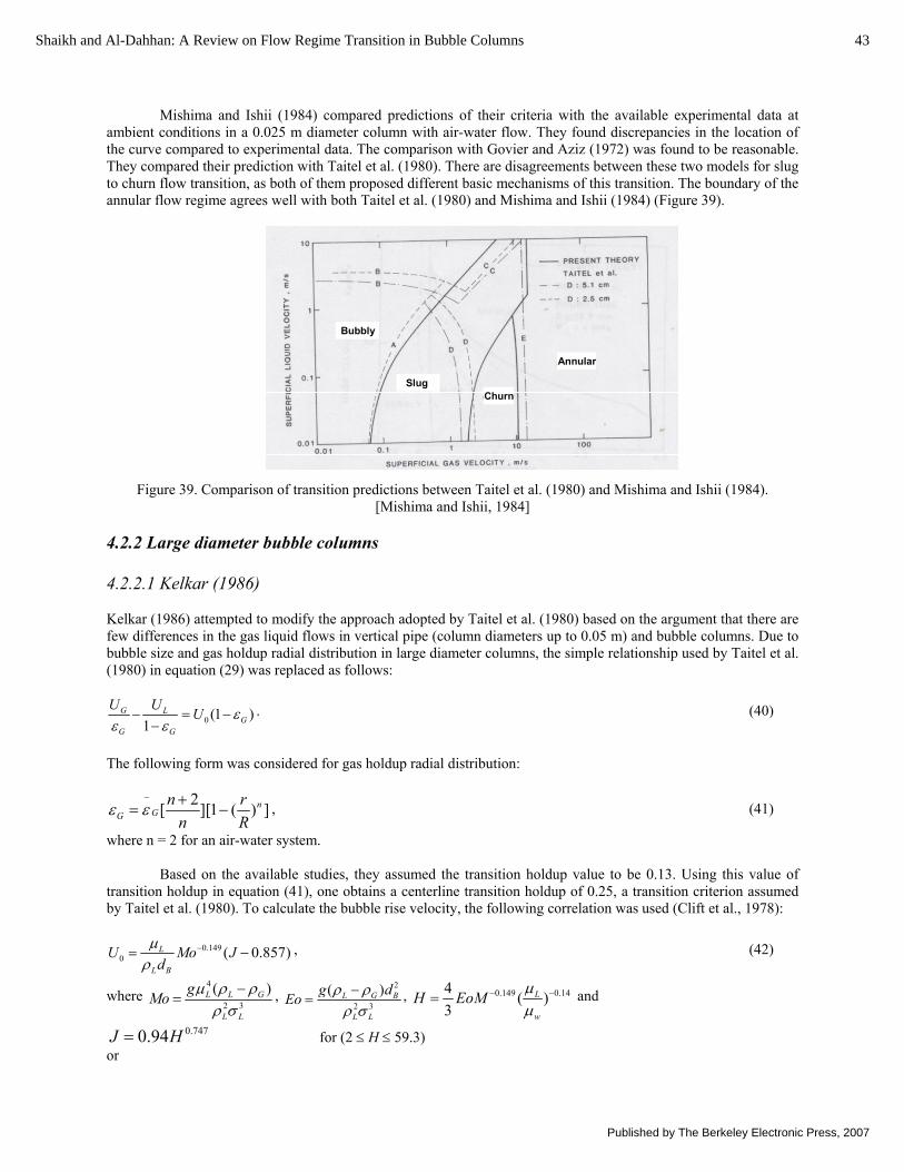
Mishima and Ishii (1984) compared predictions of their criteria with the available experimental data at ambient conditions in a 0.025 m diameter column with air-water flow. They found discrepancies in the location of the curve compared to experimental data. The comparison with Govier and Aziz (1972) was found to be reasonable. They compared their prediction with Taitel et al. (1980). There are disagreements between these two models for slug to churn flow transition, as both of them proposed different basic mechanisms of this transition. The boundary of the annular flow regime agrees well with both Taitel et al. (1980) and Mishima and Ishii (1984) (Figure 39).

Figure 39. Comparison of transition predictions between Taitel et al. (1980) and Mishima and Ishii (1984). [Mishima and Ishii, 1984]

4.2.2 Large diameter bubble columns 4.2.2.1 Kelkar (1986) Kelkar (1986) attempted to modify the approach adopted by Taitel et al. (1980) based on the argument that there are few differences in the gas liquid flows in vertical pipe (column diameters up to 0.05 m) and bubble columns. Due to bubble size and gas holdup radial distribution in large diameter columns, the simple relationship used by Taitel et al. (1980) in equation (29) was replaced as follows:

0 (1 )1

G LG

G G

U U U εε ε

− = −−

. (40)

The following form was considered for gas holdup radial distribution:

2[ ][1 ( ) ]nGG

n rn R

ε ε− +

= − , (41)

where n = 2 for an air-water system.

Based on the available studies, they assumed the transition holdup value to be 0.13. Using this value of transition holdup in equation (41), one obtains a centerline transition holdup of 0.25, a transition criterion assumed by Taitel et al. (1980). To calculate the bubble rise velocity, the following correlation was used (Clift et al., 1978):

0.1490 ( 0.857)L

L B

U Mo Jdμρ

−= − , (42)

where 4

2 3

( )L L G

L L

gMo μ ρ ρρ σ

−= ,

2

2 3

( )L G B

L L

g dEo ρ ρρ σ−

= , 0.149 0.144 ( )3

L

w

H EoM μμ

− −= and

0.7470.94J H= for (2 ≤ H ≤ 59.3) or

Bubbly

SlugChurn

Annular

Bubbly

SlugChurn

Annular



0.4413.42J H= for (H > 59.3). This relationship is valid between Mo ≤ 10-3, Eo < 40, and Re > 0.1.

Using equations (40), (41), and (42), Kelkar (1986) proposed the following correlation for transition velocity in coalescing liquids:

00.188 0.333trans LU U U= + . (43) Another correlation was recommended for prediction of Sauter mean bubble diameter (Calderbank, 1967):

0.60.5

0.4 0.24.15 9 4( / )

LB G

L

d eP V

σ ερ

= + − , (44)

where ( / ) L GP V gUρ= ,

0/G GU Uε = .

In the presence of surfactants, coalescence is inhibited, and therefore flow regime transition is delayed. Hence, the transition holdup assumed in this case (= 0.38) is higher than in the coalescing liquid medium. The following relation was proposed for the noncoalescing liquid medium:

00.228 0.538trans LU U U= + . (45) To calculate the Sauter mean bubble diameter, the following correlations were recommended for different spargers (Heijnen and van’t Riet, 1984):

1/301.7[ ]( )

LB

L G

ddg

σρ ρ

=−

for perforated plate, and (46)

0.1 0.08 0.380 0 06.1 3( ) ( )L

Bw

d e v d d σσ

= − for porous plate. (47)

Kelkar (1986) collected literature gas holdup data and calculated transition velocity by plotting logarithmic

graphs of gas holdup and superficial gas velocity. The predictions of the developed correlations were found to be close to the experimental ones. 4.2.2.2 Ranade and Joshi (1987) Ranade and Joshi (1987) assumed that transition would occur when the bubble rise velocity is equal to downward liquid velocity. Under this condition, the net bubble velocity with respect to the column wall is zero, and the gas phase accumulates in the column, leading to transition. The liquid phase balance was written as

(1 )G B G G DV Uζε ε ζε∞ = − − , (48)

where ζ = fractional wake volume, and DU = downward liquid velocity. At transition, the downward liquid velocity equals the bubble rise velocity:

(1 )G G Gζε ε ζε= − − , (49)

where 11/15ζ = [Kumar and Kuloor, 1972]. This yields a transition gas holdup value of 0.42.



4.2.2.3 Sarrafi et al. (1999) Sarrafi et al. (1999) and Jamialahmadi et al. (2000) developed a similar criterion to predict transition velocity based on the gas holdup curve. They accounted for the bubble interactions by using the Lapidus-Eglin (1957) relationship:

)(1 Gb

G

L

G

GS FU

UUU ε

εε=

−−= , (50)

where US and Ub denote slip velocity and the bubble terminal rise velocity. A characteristic velocity, UW , can be introduced from equation (50) as

GLGGGGGbW UUFUU εεεεε −−=−= )1()()1( . (51) F(εG) in the above equation shows the effect of the interaction of neighboring bubbles within the column. It is defined as

1)1()( −−= nGGF εε . (52)

The values of the constant n in equation (52) quoted by different investigators vary from –1 to 3. Sarrafi et al. (1999) preferred to use the value of n = 2.39 proposed by Richardson and Zaki (1954), for particle Reynolds number greater than 500. While this value was originally intended for solid-liquid fluidized bed systems, it has also been recommended for bubble flux in bubble columns (Deckwer, 1992). This value leads to

39.1)1( GGbW UU εε −= . (53) The characteristic velocity, UW, accounts for the bubble interaction and bubble coalescence within the column. To quantify the stability of the flow regime, the following dimensionless criteria was defined:

S

WSj U

UUU

−= (54)

The value of Uj, the scale of bubble aggregation, passes through a minimum as the gas velocity is increased through the range where the transition from homogeneous to heterogeneous regime occurs (Figure 40).

Based on the experimental data, Sarrafi et al. (1999) found that F(εG) can be well correlated by the equations

75.0)(7971.0)(b

GGG U

UF +−= εε (55)

and 5.0)(5.55.7045.0)(

b

GGG U

UF +−= εε (56)

for homogeneous and heterogeneous regimes, respectively. They proposed an iterative procedure to predict the transition velocity and gas holdup. Based on a comparison of their bubble size data with available correlations, Sarrafi et al. (1999) recommended using the correlation of Jamialahmadi et al. (1994) to predict bubble velocity and the theoretical model of Gaddis and Vogelpohl (1986) to predict bubble diameter. This model is expressed as



4/15/42

..3/40 ])

4135()81()

6[(

2

gV

gV

gd

dL

b ππν

ρσ

++= . (57)

Figure 40. Variation of gas holdup and scale of bubble aggregation with superficial gas velocity (Reproduced from Jamialahmadi et al., 2000).

4.2.2.4 Ruzicka et al. (2001) Ruzicka et al. (2001) developed a simple physical model for identifying flow regime transition in bubble columns. The model is based on hydrodynamic coupling between the gas and liquid phases. Based on the continuity equation, gas holdup was written as

/G G slipu uε = , (58)

where slipu = bubble rise velocity.

If the gas and liquid phases are uncoupled, bubble rise velocity equals the terminal velocity of an isolated bubble,

Oslip bu u= , (59)

where Obu = terminal velocity of an isolated bubble.

Gas holdup and superficial gas velocity have a linear relationship. Any deviation from linearity is a

measure of coupling between the phases. The model expresses this coupling in a simple manner:

Oslip bu u= ± correction. (60) Homogenous regime: The correction to equation (60) was given by liquid downflow. It was assumed that each rising bubble carries a certain amount of liquid, say portion ‘a’ of the total bubble volume. The bubbles generate the liquid upflow, aQ. Due to batch liquid operation, the liquid returns downward with velocity uL’. Based on this mechanism, the following equations were developed for transition velocity, transition gas holdup, and gas holdup in the homogenous regime. Here ‘, “, and ‘’’ refer to quantities in the homogeneous, heterogeneous, and transition regimes. The following equations were obtained for transition velocity,

* 'G bou Zu= , 21 2 2Z a a a= + − + , (61) and transition holdup,

0.86

0.88

0.9

0.92

0.94

0.96

0.98

0 2 4 6 8 10 12 14

Superficial gas velocity (cm/s)U

j (S

cale

of b

ubbl

e ag

greg

atio

n)

Distilled w ater (Expt)Distilled w ater (Pred)1 % Na2SO4 (Expt)1 % Na2SO4 (Pred)1 % w t isopropanol (Expt)1 % w t isopropanol (Pred)

0

0.1

0.2

0.3

0.4

0.5

0 2 4 6 8 10 12 14

Superficial gas velocity (cm/s)

Gas

hol

dup

Distilled water (Exp)

Distilled water (Pred)1% Na2SO4 (Exp)

1% Na2SO4 (Pred)1% wt isopropanol (Exp)

1% wt isopropanol (Pred)



1*2(1 )G

Za

ε +=

+. (62)

Additionally, the gas holdup in the homogeneous regime can be calculated as

2

(1 ' )1 1(1 ) ( )( )' ' '

G G

G bo G

UaU

εε ε

−= + + . (63)

The transition holdup depends on only one parameter ‘a’, while the gas holdup in the homogeneous regime is a function of '

Obu and ‘a’. Here 'Obu represents a velocity scale for the motion of the gas phase, while ‘a’ represents

the strength of coupling between the gas and liquid phases. Ruzicka et al. (2001) suggested using 'Obu , based on

measurements from video recordings or literature correlations. The value of ‘a’ needs to be found by trial and error to fit the experimental data. Heterogeneous regime: They assumed that the rise of the gas phase in the heterogeneous regime is enhanced by liquid upflow. The bubble transport by the down-flow has been neglected, and only the upward bubble advection has been considered. The following equation was derived for prediction of the gas holdup:

'' ( )''G

bo GG

U u c Uε

= + , (64)

It requires knowledge of two parameters, ''Obu and c, where ''

Obu is a velocity scale for gas phase motion and c is the strength of coupling between the phases. Transition regime: It was assumed that both homogeneous and heterogeneous regimes coexist in the column, and this was accounted by using an intermittency factor, p, that varies from 0 to 1. The following model was derived for the transition regime:

'''' (1 ) ' "

GG

bo L L

uu p u pu

ε =− − +

. (65)

In this equation, the unknown is the intermittency factor, which was then calculated as

( / "' ) ' '( )' ''

G G L boG

L L

u u up uu uε + −

=+

(66)

The models developed by Ruzicka et al. (2001) require knowing five parameters. All these parameters have

clear physical meanings and can be extracted from experimental data. The model was verified by experiments with four different air-water bubble columns and found to be in good agreement. The applicability of the model for different gas-liquid systems and design parameters has not been shown. The values of the model parameters may vary with system as well as design parameters. 4.3 Stability theory Following the pioneering work of Jackson (1963) in linear stability analysis of liquid-solid fluidized beds, attempts were made to extend these studies to gas-liquid bubble columns. Joshi et al. (2001) provided a detailed review of hydrodynamic stability studies in multiphase reactors. In this communication, we present a brief summary of studies that have performed linear stability analysis in bubble columns as follows.



4.3.1 Pauchon and Banerjee (1988) Pauchon and Banerjee (1988) used a two-fluid model to study the stability of bubbly flow. Spherical bubbles were assumed and axial stress was neglected in their analysis. The authors showed that the kinematic wave velocity based on a constant interfacial friction is weakly stable. It was assumed that turbulence provides the stabilizing mechanism through axial dispersion of the void fraction. Finally, the functional dependence of the interfacial friction factor on the void fraction was deduced. 4.3.2 Biesheuvel and Gorisson (1990) Biesheuvel and Gorisson (1990) used a one dimensional conservation equation to describe the propagation of gas holdup disturbances. Their method has similar features to the one developed by Batchelor (1988) for fluidized beds. The equation of motion for a ‘reference bubble’ was first derived and then integrated into bubbly dispersion flow. Spherical bubbles of equal size were considered for analysis. Ensemble averaging of equation of motion was performed. The basic equations of analysis are conservation for the mean number density and mean momentum of gas bubbles. The flow around the bubble was assumed to be laminar. The stability of uniform bubbly flow under planar disturbances was investigated. The transition to slug flow was studied and found to be influenced by non-uniformities over the cross-section of the tube, induced by the presence of the wall. The void fraction waves were found to be unstable for gas holdup above 0.35. 4.3.3 Shnip et al. (1992) Shnip et al. (1992) developed a criterion to predict flow regime transition in a two-dimensional bubble column, based on the theory of linear stability. The authors considered both semibatch as well continuous mode. For semibatch operation, the following stability criterion was proposed:

2

10 0 0

( )sinh( )

cosh( ) 1( 2 )(1 ) [1 ( 1) ]

B

mV G T s G G

gWV h

hK K V m

π ππ

ε ε ε

∞

−−

<−

+ − − +

(67)

For continuous operation, the proposed criterion is

2

0 0 0 0

( )coth( )

[ 2 ( )]( ' )

B

V G T s s G s

gWV

h

K K W V W V V

π π

ε ε

∞

− −

<

+ + + +

, (68)

where BV ∞ = terminal rise velocity, W = column width, R = % open area, 1.50.98 /V B LK R V ρ

∞= , 20.3 /T LK R ρ=

They compared their predictions with the experimental data of Chisti (1989), Maruyama et al. (1981), and

Yamashita and Inoue (1975) and found it to be in reasonable agreement. The maximum predicted value of the transition gas holdup was 0.42. The effects of the sparger, column height, column diameter, dispersion coefficient, and liquid phase properties on flow regime stability were studied using the proposed criteria. The authors found that coalescence in a system results into higher local holdup, generates local liquid recirculation, and results in higher bubble rise velocities; hence the value of the transition holdup reduces. The proposed transition criteria were found to be independent of liquid phase viscosity.

4.3.4 Lissester and Fowler (1992) Lissester and Fowler (1992) used a one-dimensional model of adiabatic bubbly flow in a vertical column. The equations were derived from full 3-D equations by performing instantaneous space-averaging. Various interfacial momentum terms were considered, and the relative size of these terms was determined based on the detailed scale analysis. A relationship was derived between the inlet gas holdup and the imposed pressure drop, and a simple expression for equilibrium gas holdup was also developed. Under steady flow conditions, the void fraction was



found to relax from its value at the inlet towards an asymptotic value within only a short distance from inlet. The critical void fraction was found to be 0.42. 4.3.5 Joshi et al. (2001) Joshi et al. (2001) provided a generalized stability criterion using a 1-D model for gas-liquid, gas-solid, solid-liquid, and gas-liquid-solid systems based on linear stability theory. The following unified stability criterion was proposed:

2

1 2

[ ( / ) / 2]1( ) ( / 4)A G F Bf

A Z C B−

= −− +

, (69)

where if f1 > 1, the system is stable; if f1 < 1, the system is unstable. The parameters in the above criterion were defined for a batch bubble column as follows:

1 1G V

L L

CA ρρ ε

+= + − , 2( )

(1 )G G

VL L

uB Cρρ ε

= +−

, 2( )( )(1 )

G GV

L L

uC Cρρ ε

= +−

, 0 ( )1

GL

L L L

DDZ βρ ε ε

= +−

, 0 1 1( )1L L L

F βρ ε ε

= +−

,

0 0' ( )(1 )

G G G Lz

L L L L

V VG gβ β ρ ρρ ε ρ ρ

−= + +

−,

0( )' G L

zs

gV

ρ ρβ −= , and

0( )G L G

zs

gV

ρ ρ εβ −= ,

where CV = virtual mass coefficient, DL = liquid dispersion coefficient, DG = gas dispersion coefficient, Vs = slip velocity, and β0 = drag interaction parameter.

Joshi et al. (2001) studied the effect on transition gas holdup of virtual mass coefficient, Richardson-Zaki index, and proportionality constant for dispersion. The predictions of the proposed criterion were compared with transition velocity data available in the literature for various liquids, at low and high operating pressures and column diameters up to 23 cm and found to be satisfactory. The accuracy of the virtual mass coefficient, Richardson-Zaki index, proportionally constant, and slip velocity appears to be critical in predicting transition gas holdup. 4.3.6 Leon-Becerril and Line (2001) Leon-Becerril and Line (2001) developed one-dimensional two-fluid model for bubbly flow. It was assumed that, instability occurs when the kinematic wave velocity is less than the slower dynamic wave velocity. The approaches of Pauchon and Banerjee (1988) and Bischeuvel and Gorrison (1990) were compared, and the differences between these models were pointed out. Additionally, the effect of non-sphericity was accounted for. They found that the transition gas holdup is larger for spherical bubbles due to pressure induced forces that stabilizes the flow. The transition holdups obtained by accounting bubble deformation were close to the experimental ones. However, the bubble diameter and also an eccentricity factor used to account for bubble deformation were assumed. Leon-Becerril et al. (2002) extended this work to a continuous bubble column. They also studied the transition from bubbly to slug flow in vertical pipes (column diameter = 5 cm) and in bubble columns (column diameter = 15 cm). The effect of sphericity in predicting transition velocity was emphasized. 4.3.7 Bhole and Joshi (2005) Bhole and Joshi (2005) developed a one-dimensional two-fluid model to study instability in uniform bubbly flow. Although the initial treatment is similar to Joshi et al (2001), the added mass force was modeled rigorously. Also, the drag force was formulated to take into account the dependence of drag coefficient on the slip velocity. Bubble deformation was also taken into consideration. The following equation was presented for prediction of transition gas holdup:

2 10

(1 ) 1[ ](1 2 ) (1 ) (1 )

trans

trans trans trans

GBm

G G GB

VCvgd

α εε ε ε

∞−

−=

+ + − −, (70)



where VB∞ = terminal bubble rise velocity, α = proportionality constant, and CVo = virtual mass coefficient of isolated bubble.

The predictions were compared with the reported experimental data of various authors for bubble columns and found to be in good agreement. The bubble rise velocity was found to be the most important parameter affecting the transition. An increase in bubble rise velocity reduces the gas holdup at which transition occurs. 4.4 Computational Fluid Dynamics (CFD) 4.4.1 Wang et al. (2005) Wang et al. (2005) utilized a population balance model (PBM) along with CFD simulations. They used two-fluid model with k-ε turbulence in Eulerian framework for theoretical prediction of flow regime transition. The basic goal was to calculate the variation of bubble size distribution with superficial gas velocity to provide information regarding flow regimes. For accurate prediction of gas holdup radial profile, lateral forces, including transverse lift force, wall lift force, and turbulent dispersion force, was considered in addition to drag force (Wang et al., 2006). Unlike earlier works, multiple mechanisms were considered to model coalescence and breakup. The bubble coalescence due to turbulent eddies, different rise velocities, wake entrainment, and breakup due to eddy collision and large bubble instability were considered. The model predictions were compared with the reported experimental data, and based on this evaluation, flow regime transition studies were performed.

The two-dimensional simulations over a range of superficial gas velocities could capture the variation of small bubble fraction properly, as shown in Figure 41. A sharp variation in the fraction of small bubbles was observed near the flow regime transition point. The predictions of PBM were found to be in agreement with the experimental data reported in the literature.

Figure 41. PBM Prediction of variation of small bubble fraction with superficial gas velocity (Reproduced from Wang et al., 2005).

5. REMARKS This overview shows that the methods to determine regime transition have progressed from visual observation, to the measurement of time-averaged global hydrodynamic parameters, to more quantitative analysis based on examination of temporal signatures related to hydrodynamics. Various linear and non-linear time-series techniques have been applied to the temporal signatures. The simpler techniques, such as statistical analysis, spectral analysis, do identify the flow regime transition point. Advanced non-linear techniques such as chaos analysis, stochastic modeling, and multiresolution analyses provide tools to extract additional features of the flow, apart from regime transition. However, these techniques can be computationally intensive. Hence, the choice of time-series techniques appears to be a compromise between what and how fast the information is needed. van der Schaaf et al. (2004) showed the linear relation between correlation entropy and average cycle frequency in gas-solid flows. An average



cycle frequency appears to be relatively simpler and faster. In this regard, the comments made by Drahos (2003) need consideration.

Most studies appear to focus on determining transition velocity by observing the evolution of secondary parameters over a range of superficial gas velocities. However, there is a need to develop techniques and corresponding flow regime identifiers that can provide information regarding prevailing flow regimes in an existing process without changing the operating conditions. Such an approach can be used for online flow regime monitoring and troubleshooting in industry. However, it demands the use of a time-series analysis that is simple, robust, fast, and easily used by non-experts working in the plant.

There are conflicting findings concerning the effect of few parameters on transition. A systematic experimental study needs to carry out to study the effect of column diameter, liquid phase viscosity, and the nature of different solids and loadings, particle size, and most importantly of sparger geometry.

We have shown that empirical correlations exhibit large discrepancies in their predictions at the same operating and design conditions. All of these studies calculated transition velocities from the gas holdup curve, however, the method of treatment to predict transition point from gas holdup curve differs in each case. The empirical correlations for transition prediction also need to account for the sparger geometry.

Most linear stability theory approaches were developed for an unbounded case modeled using a one-dimensional approach. Axial nonuniformities were considered as the cause of flow regime transition. It is known that uniform bubble size distribution changes to a wider one as transition occurs, resulting in a non-uniform gas holdup profile. In bubbly flow, the gas holdup profiles are flat changing to parabolic as the system enters into heterogeneous flow. The nonuniformities in radial gradients need to be considered in these cases by adopting 2/3-D models. Also, most of these approaches considered two-fluid models hence the problem of interfacial momentum closures remains. The real system does not have spherical bubbles, so the non-sphericity of the bubbles needs to be properly accounted for. CFD along with PBM provide an interesting tool for ‘a priori’ prediction of the transition point. However, the applicability of interfacial closures to different systems and conditions needs to be explored.

In short, it still remains a challenge to ‘a priori’ predict flow regime transition without resorting to extensive experimentation or a judicious estimate based on experience. 6. ACKNOLEDGEMENTS The authors are thankful to the High Pressure Slurry Bubble Column Reactor (HPSBCR) Consortium [ConocoPhillips (USA), EniTech (Italy), Sasol (South Africa), Statoil (Norway)] and UCR-DOE (DE-FG-26-99FT40594) grants that made this work possible. 7. NOTATION a drift velocity, m.s-1 A Fitting parameter (equation 37,40), dimensionless B Fitting parameter (equation 37,40), dimensionless c wall parameter (equation 22), dimensionless C0 Distribution parameter in drift flux model (equation 3,4), dimensionless C0 Orifice coefficient (equation 53), dimensionless C1 Weighted average drift velocity (equation 3,4), m.s-1

CV Virtual mass coefficient, dimensionless CV0 Virtual mass coefficient of an isolated bubble, dimensionless Cxx Autocorrelation function, dimensionless Cxy Correlation function, dimensionless D Column diameter, m d0 Hole diameter of distributor, cm



dB Bubble diameter, cm DG Gas dispersion coefficient, m2.s-1

DL Liquid dispersion coefficient, m2.s-1

Eo Etovos number, dimensionless f Frequency, Hz F(x) Fourier transform of x f1 stability criterion (equation 84), dimensionless fS Acquisition frequency, Hz

f−

Average cycle frequency, Hz g Gravity constant, m.s-2 H Information entropy, bits H Parameter defined in equation (59), dimensionless Hmax Minimum information entropy, bits Hmin Maximum information entropy, bits I information amount (equation 18), dimensionless j drift flux, m.s-1

J Parameter defined in equation (59), dimensionless KT Parameter in equation 82, 83 (= 20.3 / LR ρ )

KV Parameter in equation 82, 83 (= 1.50.98 / B LR V ρ∞

)

L Column length, m L Column length, m lE Entry length, m M Gas phase momentum per unit mass without correction (equation 32) M quality of mixedness, dimensionless M’ Gas phase momentum per unit mass with correction (equation 32) Mo Morton number, dimensionless N length of time series, dimensionless N Slope of gas holdup curve (equation 1), dimensionless p Intermittancy factor, dimensionless P Probability of hydrodynamic quantity, dimensionless Q Volumetric flow rate, m3.s-1

R % open area of distributor, dimensionless Richardson-Zaki index (equation 6), dimensionless Steepness parameter of gas holdup radial profile (equation 22), dimensionless

T length of time series, min U0 Bubble rise velocity (equations 44, 57, 59), m.s-1 ub Bubble rise velocity (equation 42), m.s-1

ub0 Terminal velocity of an isolated bubble, m.s-1 UG Superficial gas velocity, m.s-1 UGtrans Superficial gas velocity at flow regime transition, m.s-1 Uj Scale of bubble aggregation, m.s-1 UL Superficial liquid velocity, m.s-1 Ulb Large bubble rise velocity, m.s-1 Usb Small bubble rise velocity, m.s-1 UW Characteristic superficial velocity (equation 66), m.s-1 VB∞ Terminal bubble rise velocity, m.s-1 VL Axial liquid velocity, m.s-1 VS Slip velocity (equation 84), m.s-1 W Column width, m Z Parameter which is function of drift velocity (equation 76), dimensionless



Greek Letters

2xyγ Coherence function, dimensionless −

Gε Cross-sectionally averaged gas holdup, dimensionless

transGε Overall gas hold up at transition point, dimensionless

Gε Overall gas hold up, dimensionless ξ Fractional wake volume, dimensionless ν Kinematic viscosity, μ Mean of a time-series, dimension of time-series θ Phase angle of cross-spectral density function, rad α Proportionality factor, dimensionless σ Standard deviation of a time series, dimension of time-series τ0 Characteristic time-scale, sec β0 Drag interaction parameter (equation 84), dimensionless ρg Gas phase density, kg m-3 ρL Liquid phase density, kg m-3 σL Liquid surface tension, N m-1 μL Liquid viscosity, kg m-1 s-1

φxy Cross-spectral density function υxy Transit velocity, m.s-1 β Correction factor (equation 32), dimensionless τ Time lag, sec Abbrevations 2D Two-dimensional 3D Three-dimensional ACF Autocorrelation Function CARPT Computer Automated Radioactive Particle Tracking CCF Cross-correlation Function CFD Computational Fluid Dynamics CMC Carboxyl Methyl Cellulose COP Coherent Output Power Spectral Density CSD Cross-spectral Density Function CT Computed Tomography DGD Dynamic Gas Disengagement DWT Discrete Wavelet Transform ECT Electrical Capacitance Tomography ERT Electrical Resistance Tomography FBM Fractional Brownian Motion FT Fischer-Tropsch HFA Hot Film Anemometry ID Inner Diameter IOP Incoherent Output Power Spectral Density KE Kolmogorov Entropy LDA Laser Doppler Anemometry LPMeOH Liquid Phase Methanol Synthesis MAC Maleic Acid PBM Population Balance Model PDF Probability Density Function PIV Particle Image Velocimetry PSDF Power Spectral Density Function



8. REFERENCES Acikgoz, M.; Franca, F.; Lahey, R. T., Jr., (1992). An experimental study of three-phase flow regimes. International Journal of Multiphase Flow, 18(3), 327-336. Al-Masry, W. A.; Ali, E. M.; Aqeel, Y. M., (2005). Determination of bubble characteristics in bubble columns using statistical analysis of acoustic sound measurements. Chemical Engineering Research and Design, 83(A10), 1196-1207. Al-Masry, W. A. and Ali, E. M. (2007). Identification of hydrodynamic characteristics in bubble columns through analysis of acoustic sound measurements-Influence of the liquid phase properties. Chemical Engineering and Processing, 46 (2), 127-138. Bakshi, B. R.; Zhong, H.; Jiang, P.; Fan, L. S., (1995). Analysis of flow in gas-liquid bubble columns using multi-resolution methods. Chemical Engineering Research and Design, 73(A6), 608-14. Batchelor, G. K., (1988). A new theory of the instability of a uniform fluidized bed. Journal of Fluid Mechanics, 193, 75-110. Behkish, A., (2005). Hydrodynamics and mass transfer in slurry bubble column reactors. Ph.D. Thesis, University of Pittsburgh, USA. Bennett, M. A., West, R. M., Luke, S. P., Jia, X., Williams, R. A., (1999). Measurement and Analysis of Flows in Gas-Liquid Column Reactor, Chem. Eng. Sci., 54, 5003 – 5012. Bhole, Manish R.; Joshi, Jyeshtharaj B., (2005). Stability analysis of bubble columns: Predictions for regime transition. Chemical Engineering Science, 60(16), 4493-4507. Biesheuvel, A.; Gorissen, W. C. M., (1990). Void fraction disturbances in a uniform bubbly fluid. International Journal of Multiphase Flow, 16(2), 211-231. Briens, L. A., Briens, C. L., Margaritis, A., Hay J., (1997). Minimum liquid fluidization velocity in gas-liquid-solid fluidized bed of low-density particles, 52 (21-22), 4231-4238. Briens, L.A., and C.L. Briens, (2002). Cycle detection and characterization in chemical engineering, AIChE J., 48, 970–980. Brown, R. A. S.; Sullivan, G. A.; Govier, G. W., (1960). The upward vertical flow of air-water mixtures. III. Effect of gas-phase density on flow pattern, holdup, and pressure drop. Canadian Journal of Chemical Engineering, 38, 62-6. Bukur, Dragomir B.; Petrovic, Dragan; Daly, James G., (1987). Flow regime transitions in a bubble column with a paraffin wax as the liquid medium. Industrial & Engineering Chemistry Research, 26(6), 1087-92. Calderbank, Philip H., (1967). Gas absorption from bubbles. Chemical Engineer, 212. Carra, Sergio; Morbidelli, Massimo, (1987). Gas-liquid reactors. Chemical Industries (Dekker), 26(Chem. React. React. Eng.), 545-666. Cassanello, M., Larachi, F., Kemoun, A., Al-Dahhan, M. H., and Dudukovic, M. P., (2001). Inferring Liquid Chaotic Dynamics in Bubble Columns, Chem. Eng. Sci., 56, 6125-6134. Charles, M. E.; Govier, G. W., and Hodgson, G. W.; (1961). Horizontal pipeline flow of equal density oil-water mixture. Canadian Journal of Chemical Engineering, 27-36.



Chen, R. C.; Reese, J.; Fan, L.-S., (1994). Flow structure in a three-dimensional bubble column and three-phase fluidized bed. AIChE Journal, 40(7), 1093-1104. Chilekar, V. P.; Warnier, M. J. F.; van der Schaaf, J.; Kuster, B. F. M.; Schouten, J. C.; van Ommen, J. R., (2005a). Bubble size estimation in slurry bubble columns from pressure fluctuations. AIChE Journal, 51(7), 1924-1937. Chilekar, V. P.; van der Schaaf, J.; van Ommen, J. R.; Tinge, J. T.; Kuster, B. F. M.; Schouten, J. C., (2005). Effect of elevated pressures on hydrodynamics of slurry bubble columns. Presented at AIChE Annual Meeting, Cincinati, Ohio, Paper 413c. Chisti, Yusuf; Moo-Young, Murray, (1989). On the calculation of shear rate and apparent viscosity in airlift and bubble column bioreactors. Biotechnology and Bioengineering, 34(11), 1391-1392. Clark, N. N.; Van Egmond, J. W.; Nebiolo, E. P., (1990). The drift-flux model applied to bubble columns and low-velocity flows. International Journal of Multiphase Flow, 16(2), 261-279. Clift, R.; Grace, J. R.; Weber, M. E., (1978). Bubbles, Drops, and Particles. Academic, New York, N. Y. Deckwer, W., Bubble Column Reactors, John Wiley & Sons, 1991. Diesterwerg, G., Fuhr, H., and Reher, P., (1978), Die Bayer-Turmbiologie, Industrieabwasser, 7. Dong, Feng., Liu, Xiaoping., Deng, Xiang., Xu, Lijun., and Xu, Ling-au, (2001). Identification of Two-Phase Flow

Regime using Electrical Resistance Tomography, Proceedings of 2nd

World Congress on Industrial Process Tomography, Hannover, Germany. Drahos, J.; Zahradnik, J.; Puncochar, M.; Fialova, M.; Bradka, F., (1991). Effect of operating conditions on the characteristics of pressure fluctuations in a bubble column. Chemical Engineering and Processing, 29(2), 107-115. Drahos, J.; Bradka, F.; Puncochar, M., (1992). Fractal behavior of pressure fluctuations in a bubble column. Chemical Engineering Science, 47(15-16), 4069-4075. Drahos, Jiri., (2003). Quo vadis, the analysis of time series in reactor engineering? Chemical Engineering Research and Design, 81(A4), 411-412. E.E. Peters, (1994). Applying Chaos Analysis for Investment and Economics, Wiley, New York. Eissa, S. H., and Schugerl, K. (1975). Holdup and backmixing investigations in cocurrent and countercurrent bubble columns. Chemical Engineering Science, 30, 1251–1256. Ellis, N.; Bi, H. T.; Lim, C. J.; Grace, J. R., (2004). Influence of probe scale and analysis method on measured hydrodynamic properties of gas-fluidized beds. Chemical Engineering Science, 59(8-9), 1841-1851. Fan, L. T., Neogi, D., Yashima,M., and Nassar, R. (1990). Stochastic analysis of three phase fluidized bed: Fractal approach. AIChE J., 36:1529–1535. Fan, L.-S. (1989). Gas-Liquid-Solid Fluidization Engineering. Butterworth Series in Chemical Engineering, Boston, MA. Forret, A.; Schweitzer, J.-M.; Gauthier, T.; Krishna, R., Schweich, D., (2003). Influence of scale on the hydrodynamics of bubble column reactors: An experimental study in columns of 0.1, 0.4 and 1 m diameters. Chem. Eng. Sci. 58, 719. Franca, F.; Acikgoz, M.; Lahey, R. T., Jr.; Clausse, A. (1991). The use of fractal techniques for flow regime identification. International Journal of Multiphase Flow, 17(4), 545-552.



Franca, F.; Lahey, R. T., Jr., (1992). The use of drift-flux techniques for the analysis of horizontal two-phase flows. International Journal of Multiphase Flow, 18(6), 787-801. Franz, K., Borner, T., Kantoreck, H., and Buchcholz, R., (1984). Flow structure in bubble columns. Ger. Chem. Eng., 7, 365-374. Gaddis, E. S.; Vogelpohl, A., (1986). Bubble formation in quiescent liquids under constant flow conditions. Chemical Engineering Science, 41(1), 97-105. Gheorghiu, S.; Van Ommen, J. R.; Coppens, M.-O., (2003). Power-law distribution of pressure fluctuations in multiphase flow. Physical Review E: Statistical, Nonlinear, and Soft Matter Physics, 67(4-1), 041305/1-041305/7. Gourich, Bouchaib; Vial, Christophe; Essadki, Abdel Hafid; Allam, Fouad; Belhaj Soulami, Mohammed; Ziyad, Mahfud, (2006). Identification of flow regimes and transition points in a bubble column through analysis of differential pressure signal-Influence of the coalescence behavior of the liquid phase. Chemical Engineering and Processing, 45(3), 214-223. Govier, George Wheeler; Aziz, Khalid. The Flow of Complex Mixtures in Pipes. (1972), 792 pp. Govier, G. W.; Radford, B. A.; Dunn, J. S. C., (1957). The upward vertical flow of air-water mixtures. I. Effect of air and water rates on flow pattern, holdup, and pressure drop, Can. J. of Chem. Eng., 35, 58-70. Govier, G. W.; Short, W. Leigh, (1958). Upward vertical flow of air-water mixtures. II. Effect of tubing diameter on flow pattern, holdup, and pressure drop. Canadian Journal of Chemical Engineering, 36, 195-202. Govier, G. W.; Sullivan, G. A.; Wood, R. K., (1961). Upward vertical flow of oil-water mixtures. Canadian Journal of Chemical Engineering, 39, 67-75. Grassberger, P., Schreiber, Th. and Schraffrath, C. (1991) Nonlinear time sequence analysis, lnt. J. Bifurcation Chaos 1, 521-547. Grover, G. S.; Rode, C. V.; Chaudhari, R. V., (1986). Effect of temperature on flow regimes and gas hold-up in a bubble column. Canadian Journal of Chemical Engineering, 64(3), 501-504. Hurst, H.E., (1951). Methods of using long-term storage in reservoirs. Trans. Am. Soc. Civil Engrs., 116, 770–808. Harmathy, T. Z. (1960), “Velocity of large drops and bubbles in media of infinite or restricted extent”, AIChE J, 6: 281-288. Heijnen, J. J.; Van't Riet, K., (1984). Mass transfer, mixing and heat transfer phenomena in low viscosity bubble column reactors. Chemical Engineering Journal, 28(2), B21-B42. Hewitt GF, Hall Taylor NS, (1970). Annular Two Phase Flow, Pergamon Press. Holler, V.; Ruzicka, M.; Drahos, J.; Kiwi-Minsker, L.; Renken, A.(2003). Acoustic and visual study of bubble formation processes in bubble columns staged with fibrous catalytic layers. Catalysis Today, 79-80, 151-157. Hubbard, Martin G.; Dukler, Abraham E., (1966). Characterization of flow regimes for horizontal two-phase flow.-I. Statistical analysis of wall pressure fluctuations. Proceedings of the Heat Transfer and Fluid Mechanics Institute, 100-121. Hyndman, Caroline L.; Larachi, Faical; Guy, Christophe., (1996). Understanding gas-phase hydrodynamics in bubble columns: a convective model based on kinetic theory. Chemical Engineering Science, 52(1), 63-77. Jackson, R., (1963). The mechanics of fluidized beds I. The stability of the state of uniform fluidization. Trans. Inst. Chem. Engr., 41, 13-21.



Jamialahmadi, M.; Mueller-Steinhagen, H., (1991). Effect of solid particles on gas hold-up in bubble columns. Canadian Journal of Chemical Engineering, 69(1), 390-393. Jamialahmadi, M.; Mueller-Steinhagen, H., (1992). Effect of alcohol, organic acid and potassium chloride concentration on bubble size, bubble rise velocity and gas hold-up in bubble columns. Chemical Engineering Journal, 50(1), 47-56. Jamialahmadi, M.; Branch, C.; Mueller-Steinhagen, H., (1994). Terminal bubble rise velocity in liquids. Chemical Engineering Research and Design, 72(A1), 119-122. Jamialahmadi, M.; Muller-Steinhagen, H.; Sarrafi, A.; Smith, J. M., (2000). Studies of gas holdup in bubble column reactors. Chemical Engineering & Technology, 23(10), 919-921. Jones, O. C., and Zuber, N., (1975). The interrelation between void fraction fluctuations and flow patterns in two-phase flow. Int. J. Multiphase Flow, 2, 273-306. Joshi, J. B.; Deshpande, N. S.; Dinkar, M.; Phanikumar, D. V., (2001). Hydrodynamic stability of multiphase reactors. Advances in Chemical Engineering, 26, 1-130. Kang, Y.; Cho, Y. J.; Woo, K. J.; Kim, K. I.; Kim, S. D., (2000). Bubble properties and pressure fluctuations in pressurized bubble columns. Chemical Engineering Science, 55(2), 411-419. Kang, Y.; Cho, Y. J.; Woo, K. J.; Kim, S. D., (1999). Diagnosis of bubble distribution and mass transfer in pressurized bubble columns with viscous liquid medium. Chemical Engineering Science, 54(21), 4887-4893. Kastanek, F., Zahradnik, J., Kratochvil, J. and Cermak, J., (1984). Modeling of large-scale bubble column reactors for non-ideal gas-liquid systems, in Frontiers in Chemical Reaction Engineering. Ed. Doraiswamy, L. K., and Mashelkar, R. A., vol. 1, 330-344, Wiley Eastern Ltd., New Delhi. Kelkar, B. G., Godbole, S. P., Honath, M. F., Shah, Y. T., Carr, N. L. and Deckwer, W. D. (1983). Effect of addition of alcohols on gas holdup and backmixing in bubble columns. A.I.Ch.E. J., 29, 361-369. Kelkar, Balmohan G.,(1986). Flow regime characteristics in cocurrent bubble column reactors. Chemical Engineering Communications, 41(1-6), 237-251. Kikuchi, R.; Yano, T.; Tsutsumi, A.; Yoshida, K.; Punchochar, M.; Drahos, J., (1997). Diagnosis of chaotic dynamics of bubble motion in a bubble column. Chemical Engineering Science, 52(21/22), 3741-3745. Krishna, R.; Ellenberger, J.; Maretto, C.. (1999). Flow regime transition in bubble columns. International Communications in Heat and Mass Transfer, 26(4), 467-475. Krishna, R.; Wilkinson, P. M.; Van Dierendonck, L. L., (1991). A model for gas holdup in bubble columns incorporating the influence of gas density on flow regime transitions. Chemical Engineering Science, 46(10), 2491-2496. Lapidus, Leon; Elgin, J. C., (1957). Mechanics of vertical-moving fluidized systems. A.I.Ch.E. Journal, 3, 63-68. Lehman, J. and Hammer, J., (1978), Continuous fermentation in tower fermentor, I European congress on biotechnology, Interlaken, Part 1, 1. Leon-Becerril, E. and Line, A., (2001), Stability analysis of a bubble column, Chem.Eng. Sci., 56, 6135-6141. Leon-Becerril, Elizebeth; Cockx, Arnaud; Line, Alain., (2002). Effect of bubble deformation on stability and mixing in bubble columns. Chemical Engineering Science, 57(16), 3283-3297.



Letzel, H. M.; Schouten, J. C.; Krishna, R.; Van Den Bleek, C. M., (1997). Characterization of regimes and regime transitions in bubble columns by chaos analysis of pressure signals. Chemical Engineering Science, 52(24), 4447-4459. Lin, T.-J.; Juang, R.-C.; Chen, C.-C., (2001). Characterizations of flow regime transitions in a high-pressure bubble column by chaotic time series analysis of pressure fluctuation signals. Chemical Engineering Science, 56(21-22), 6241-6247. Lin, T.-J.; Juang, R.-C.; Chen, Y.-C.; Chen, C.-C., (2001). Predictions of flow transitions in a bubble column by chaotic time series analysis of pressure fluctuation signals. Chemical Engineering Science, 56(3), 1057-1065. Lin, T.-J.; Reese, J.; Hong, T.; Fan, L.-S., (1996). Quantitative analysis and computation of two-dimensional bubble columns. AIChE Journal, 42(2), 301-318. Lin, T.-J.; Tsuchiya, K.; Fan, Liang-Shih. (1999). On the measurements of regime transition in high-pressure bubble columns. Canadian Journal of Chemical Engineering, (1999), 77(2), 370-374. Liu, Ming-Yan; Hu, Zhong-Ding; Li, Jing-Hai., (2004). Multi-scale characteristics of chaos behavior in gas-liquid bubble columns. Chemical Engineering Communications, 191(8), 1003-1016. Luo, Hean; Svendsen, Hallvard F., (1991). Turbulent circulation in bubble columns from eddy viscosity distributions of single-phase pipe flow, Can. J. of Chem. Eng., (1991), 69(6), 1389 - 1394. Maretto, C.; Krishna, R., (2001). Design and optimisation of a multi-stage bubble column slurry reactor for Fischer-Tropsch synthesis. Catalysis Today, 66(2-4), 241-248. Maruyama, Toshiro; Yoshida, Satoshi; Mizushina, Tokuro., (1981). The flow transition in a bubble column. Journal of Chemical Engineering of Japan, 14(5), 352-7. Matsui, G., (1984). Identification of flow regimes in vertical gas-liquid two-phase flow using differential pressure fluctuations, Int. J. Multiphase Flow, 10 (6), 711 – 720. Mena, P. C.; Ruzicka, M. C.; Rocha, F. A.; Teixeira, J. A.; Drahos, J, (2005), Effect of solids on homogeneous-heterogeneous flow regime transition in bubble columns. Chemical Engineering Science, 60(22), 6013-6026. Mishima, Kaichiro; Ishii, Mamoru., (1984). Flow regime transition criteria for upward two-phase flow in vertical tubes. International Journal of Heat and Mass Transfer, 27(5), 723-37. Murugaian, V., Schaberg, H. I., and Wang, M., (2005). Effect of sparger geometry on the mechanism of flow pattern transition in a bubble column. Proceedings of 4th World Congress on Industrial Process Tomography, Aizu, Japan. Nedeltchev, Stoyan; Ookawara, Shinichi; Ogawa, Kohei., (1999). A fundamental approach to bubble column scale-up based on quality of mixedness. Journal of Chemical Engineering of Japan, 32(4), 431-439. Nedeltchev, Stoyan; Ookawara, Shinichi; Ogawa, Kohei., (2000). Time-dependent mixing behaviors in lower and upper zones of bubble column. Journal of Chemical Engineering of Japan, 33(5), 761-767. Nedeltchev, Stoyan, Kumar, Sailesh B., and Dudukovic, M. P., (2003). Flow Regime Identification in a Bubble Column based on both Kolmogorov Entropy and Quality of Mixedness Derived from CARPT Data, Can. J. Chem. Eng., 81, 367 – 374. Nishikawa, K.; Sekoguchi, K.; Fukano, T, (1969). On the pulsation phenomena in gas-liquid two-phase flow, Bulletin of JSME, 12(54), 1410-1416. Ogawa, Kohei; Ito, Shiro., (1975). Definition of quality of mixedness. Journal of Chemical Engineering of Japan, 8(2), 148-51.



Ohki, Yoshihiro; Inoue, Hakuai., (1970). Longitudinal mixing of the liquid phase in bubble columns. Chemical Engineering Science, 25(1), 1-16. Olmos, E.; Gentric, C.; Poncin, S.; Midoux, N., (2003). Description of flow regime transitions in bubble columns via laser Doppler anemometry signals processing. Chemical Engineering Science, 58(9), 1731-1742. Olmos, Eric; Gentric, Caroline; Midoux, Noel. (2003). Identification of flow regimes in a flat gas-liquid bubble column via wavelet transform. Canadian Journal of Chemical Engineering, 81(3-4), 382-388. Park, Soung Hee; Kang, Yong; Cho, Yong Jun; Fan, Liang Tseng; Kim, Sang Done., (2001). Characterization of pressure signals in a bubble column by wavelet transform. Journal of Chemical Engineering of Japan, 34(2), 158-165. Park, Soung Hee; Kang, Yong; Kim, Sang Done., (2001). Wavelet transform analysis of pressure fluctuation signals in a pressurized bubble column. Chemical Engineering Science, 56(21-22), 6259-6265. Park, Soung Hee; Kim, Sang Done., (2003). Characterization of pressure signals in a bubble column by wavelet packet transform. Korean Journal of Chemical Engineering, 20(1), 128-132. Pauchon, C.; Banerjee, S., (1988). Interphase momentum interaction effects in the averaged multifield model. Part II. Kinematic waves and interfacial drag in bubbly flows. International Journal of Multiphase Flow, 14(3), 253-264. Rados, N. (2003). Slurry bubble column hydrodynamics. D.Sc. Thesis, Washington University, St. Louis, MO. Ranade, V. V.; Gharat, S. D.; Joshi, J. B.. (1987). Pressure drop in multiphase reactors. Recent Trends Chem. React. Eng., [Proc. Int. Chem. React. Eng. Conf.], 2nd, 2, 164-80. Reilly, I. G.; Scott, D. S.; De Bruijn, T. J. W.; MacIntyre, D., (1994). The role of gas phase momentum in determining gas holdup and hydrodynamic flow regimes in bubble column operations. Canadian Journal of Chemical Engineering, 72(1), 3-12. Richardson, J. F.; Zaki, W. N., (1954). Sedimentation and fluidization-I. Transactions of the Institution of Chemical Engineers, 32, 35-53. Ruthiya, K., (2005). Mass transfer and hydrodynamics in catalytic slurry reactors. Ph.D. Thesis, Eindhoven University, the Netherlands. Ruthiya, Keshav C.; Chilekar, Vinit P.; Warnier, Maurice J. F.; van der Schaaf, John; Kuster, Ben F. M.; Schouten, Jaap C.; van Ommen, J. Ruud, (2005). Detecting regime transitions in slurry bubble columns using pressure time series. AIChE Journal, 51(7), 1951-1965. Ruzicka, M. C.; Drahos, J.; Fialova, M.; Thomas, N. H., (2001). Effect of bubble column dimensions on flow regime transition. Chemical Engineering Science, 56(21-22), 6117-6124. Ruzicka, M. C.; Drahos, J.; Mena, P. C.; Teixeira, J. A., (2003). Effect of viscosity on homogeneous-heterogeneous flow regime transition in bubble columns. Chemical Engineering Journal, 96(1-3), 15-22. Ruzicka, M. C.; Zahradnik, J.; Drahos, J.; Thomas, N. H., (2001). Homogeneous-heterogeneous regime transition in bubble columns. Chemical Engineering Science, 56(15), 4609-4626. Sarrafi, Amir; Jamialahmadi, Mohammad; Muller-Steinhagen, Hans; Smith, John M., (1999). Gas holdup in homogeneous and heterogeneous gas-liquid bubble column reactors. Canadian Journal of Chemical Engineering, 77(1), 11-21. Schügerl, K., Oels, U. and Lücke, J. (1977). Bubble columns bioreactors Adv. Biochem.Engng 7, 1-84.



Shah, Y. T.; Kelkar, B. G.; Godbole, S. P.; Deckwer, W. D. , (1982). Design parameters estimations for bubble column reactors. AIChE Journal, 28(3), 353-379. Shaikh, Ashfaq, and Al-Dahhan, Muthanna., (2005). Characterization of the hydrodynamic flow regime in bubble columns via computed tomography. Flow Measurement and Instrumentation, 16(2-3), 91-98. Shaikh, Ashfaq, and Al-Dahhan, Muthanna., (2006). Hydrodynamics of slurry bubble column reactors. CREL Internal Report Shnip, A. I.; Kolhatkar, R. V.; Swamy, D.; Joshi, J. B., (1992). Criteria for the transition from the homogeneous to the heterogeneous regime in two-dimensional bubble column reactors. International Journal of Multiphase Flow, 18(5), 705-26. Smith, Steven (1999). Digital signal processing. California Technical Publishing, San Diego, California. Taitel, Yemada; Dukler, A. E., (1976). A model for predicting flow regime transitions in horizontal and near horizontal gas-liquid flow. AIChE Journal, 22(1), 47-55. Taitel, Y.; Bornea, Dvora; Dukler, A. E., (1980). Modeling flow pattern transitions for steady upward gas-liquid flow in vertical tubes. AIChE Journal, 26(3), 345-54. Takens, F. (1981) Lecture notes in Mathematics, Vol. 898. Springer, New York, 366. Tarmy, B.; Chang, M.; Coulaloglou, C.; and Ponzi, P., (1984). Hydrodynamic characteristics of three phase reactors. The Chemical Engineer. 18. Thimmapuram, P. R., Rao, N. S., Saxena, S. C., (1992). Characterization of hydrodynamic regimes in a bubble column, Chem. Eng. Sci., 47 (13-14), 3335-3362. Thorat, B. N.; Joshi, J. B. (2004). Regime transition in bubble columns: experimental and predictions. Experimental Thermal and Fluid Science, 28(5), 423-430. Tzeng, J. W.; Chen, R. C.; Fan, L. S., (1993). Visualization of flow characteristics in a 2-D bubble column and three-phase fluidized bed. AIChE Journal, 39(5), 733-744. Uchida, S.; Tsuyutani, S.; Seno, T., (1989). Flow regimes and mass transfer in countercurrent bubble columns. Canadian Journal of Chemical Engineering, 67(5), 866-869. Urseanu, M., (2000). Scaling up bubble column reactors. Ph.D. Thesis, University of Amsterdam, Amsterdam, The Netherlands. van den Bleek, C. M., and Schouten, J. C. (1993). Deterministic chaos: A new tool in fluidised bed design and operation. Chemical Engineering Journal, 53, 75-87. van den Bleek, Cor M.; Coppens, Marc-Olivier; Schouten, Jaap C., (2002). Application of chaos analysis to multiphase reactors. Chem. Eng. Sci., 57(22-23), 4763-4778. van der Schaaf, J.; Schouten, J. C.; Johnsson, F.; van den Bleek, C. M., (2002). Non-intrusive determination of bubble and slug length scales in fluidized beds by decomposition of the power spectral density of pressure time series. International Journal of Multiphase Flow, 28(5), 865-880. van der Schaaf, J.; van Ommen, J. R.; Takens, F.; Schouten, J. C.; van den Bleek, C. M., (2004). Similarity between chaos analysis and frequency analysis of pressure fluctuations in fluidized beds. Chemical Engineering Science, 59(8-9), 1829-1840. Vandu, C. O.; Koop, K.; Krishna, R., (2004). Large bubble sizes and rise velocities in a bubble column slurry reactor. Chemical Engineering & Technology, 27(11), 1195-1199.



Vandu, C., (2005). Hydrodynamics and mass transfer in multiphase reactors. Ph.D. Thesis, University of Amsterdam, Amsterdam, The Netherlands. Vial, C.; Laine, R.; Poncin, S.; Midoux, N.; Wild, G., (2001). Influence of gas distribution and regime transitions on liquid velocity and turbulence in a 3-D bubble column. Chemical Engineering Science, 56(3), 1085-1093. Vial, C.; Poncin, S.; Wild, G.; Midoux, N., (2001). A simple method for regime identification and flow characterisation in bubble columns and airlift reactors. Chemical Engineering and Processing, 40(2), 135-151. Vince, M. A.; Lahey, R. T., Jr., (1982). On the development of an objective flow regime indicator. International Journal of Multiphase Flow, 8(2), 93-124. Wallis, G. B., (1969). One Dimensional Two Phase Flow, McGraw Hill, New York. Wang, Tiefeng; Wang, Jinfu; Jin, Yong., (2005). Theoretical prediction of flow regime transition in bubble columns by the population balance model. Chemical Engineering Science, 60(22), 6199-6209. Wang, Tiefeng; Wang, Jinfu; Jin, Yong., (2006). A CFD-PBM coupled model for gas-liquid flows. AIChE Journal, 52(1), 125-140. Wender, I., Reactions of Synthesis Gas, (1996) Fuel Processing Technology, 48, 189. Wilkinson, P.M., Physical Aspects and Scale-up of High Pressure Bubble Columns, Ph.D. Thesis, (1991), University of Groningen. Wilkinson, Peter M.; Spek, Arie P.; Van Dierendonck, Laurent L., (1992). Design parameters estimation for scale-up of high-pressure bubble columns. AIChE Journal, 38(4), 544-54. Wu, Jun Jian; Wang, Dong; Li, Li Hua; Zhou, Ji Ti., (2005). Characterization of flow regimes in bubble columns through CCF analysis of pressure fluctuations. Chemical Engineering & Technology, 28(10), 1109-1113. Yamashita, F. and Inoue, H. (1975). Gas holdup in bubble columns. J. Chem. Engng Japan 8, 334-336. Yoshida, F., and Akita, K., (1965). Performance of gas bubble columns: volumetric liquid-phase mass transfer coefficient and gas holdup. AIChE J., 11, 9-13. Zahradnik, J.; Fialova, M.; Ruzicka, M.; Drahos, J.; Kastanek, F.; Thomas, N. H., (1997). Duality of the gas-liquid flow regimes in bubble column reactors. Chemical Engineering Science, 52 (21/22), 3811-3826. Zhang, J.-P.; Grace, J. R.; Epstein, N.; Lim, K. S., (1997). Flow regime identification in gas-liquid flow and three-phase fluidized beds. Chemical Engineering Science, 52(21/22), 3979-3992. Zuber, N.; Findlay, J. A., (1965). Average volumetric concentration in two-phase flow systems. Journal of Heat Transfer, 87(4), 453-68.



APPENDIX: Time-Series Analysis Various time-series analyses have been adopted to delineate flow regime in bubble columns. They are based on the temporal signatures of parameters that are a function of the prevailing hydrodynamics. 1) Statistical Analysis:

Statistical analysis is an obvious method to study a time-series. The mean, μ, is given by

1

1 N

ii

xN

μ=

= ∑ .

The average deviation of a signal can be then written as:

Average deviation = 1

1 N

ii

xN

μ=

−∑ .

The average deviation provides a single number representing the typical distance that the samples are from

the mean (Smith, 1999). Although it is straightforward, the average deviation is not commonly used in statistical analysis. The important parameter is not the average deviation, but the power representing the deviation from the mean, called the standard deviation, σ or variance, σ2 and given as,

22

1

1 ( )( 1)

N

ii

xN

σ μ=

= −− ∑

Skewness, which is the third moment of the distribution, is a measure of symmetry expressed as

Skewness =

3

13

1( 1)

N

ii

x

N

μ

σ=

−

−

∑

The skewness of a normal distribution is zero, and any symmetric data should have skewness near zero.

Negative values indicate that data are skewed to left, i.e., the left tail is heavier than the right tail. Positive values indicate that data are skewed to right, i.e., the right tail is heavier than the left tail.

Kurtosis, a fourth moment of distribution, is an indication of whether data are peaked or flat relative to a normal distribution.

Kurtosis =

4

14

1( 1)

N

ii

x

N

μ

σ=

−

−

∑ .

The kurtosis of a normal distribution is 3, hence excess kurtosis is given by

Kurtosis =

4

14

1 3( 1)

N

ii

x

N

μ

σ=

−−

−

∑ .

Negative kurtosis indicates a flat distribution, while positive kurtosis indicates a peaked distribution.

2) Spectral Analysis: The goal of spectral analysis is to describe the distribution of the power contained in a signal over a frequency, based on a finite set of data. It converts information available in the time-domain into the frequency-domain.

Spectral analysis is performed using the Fourier transform, which is named after the French mathematician and physicist, Jean Baptiste Joseph Fourier. Fourier presented a paper in 1807 to the Institut de France on the use of



sinusoids to represent temperature distributions. The paper contained the (then) controversial claim that any continuous periodic signal could be represented as the sum of properly chosen sinusoidal waves. Among the reviewers were two of history's most famous mathematicians, Joseph Louis Lagrange and Pierre Simon de Laplace.

While Laplace and the other reviewers voted to publish the paper, Lagrange adamantly protested. For nearly years, Lagrange had insisted that such an approach could not be used to represent signals with corners, i.e., discontinuous slopes, such as in square waves. The Institut de France bowed to the prestige of Lagrange, and rejected Fourier's work. It was only after Lagrange died that the paper was finally published, some 15 years later (Smith, 1999). Ever since, it has been used abundantly to analyze the time-series in various fields. The Fourier transform of a time series x(t) can be given as

∫+∞

∞−

−= dttfjtxxF ).2exp()()( π .

The power spectral density function (PSDF) is the square of the magnitude of the continuous Fourier transform

1 ( ). *( )xxS

F x F xf

ϕ = .

The cross power spectral density (CPSD) function of two time series x(t) and y(t) which indicates coherence between the two time-series is given as

1 ( ). *( )xyS

F x F yf

ϕ = .

The coherence between the two time series at a certain frequency, f , is quantified using the coherence function:

)()()(*)(

)(2

ffff

fyyxx

xyxyxy φφ

φφγ = .

A coherence of unity indicates that two time series are fully correlated at that frequency, while a coherence of zero indicates that the time-series are uncorrelated at that frequency. The coherent output power spectral density (COP) and incoherent output power spectral density (IOP) can be written as

2( ) ( ) ( )x xy xxCOP f f fγ ϕ= ,

2( ) [1 ( )] ( )x xy xxIOP f f fγ ϕ= − . Using PSD information, one can compute the average frequency of the underlying process:

∫∫=

−

df

dfff

xx

xx

][

.][

φ

φ .

The transit time can be calculated as

( )2xy f

fθ

τπ

= ,

where θ is the phase angle of the PSDF.



3) Autocorrelation Analysis:

The cross correlation function (CCF) between two time-series x(t) and y(t) can be evaluated as 1( ) ( ) ( ).xyC x t y t dtT

τ τ+∞

−∞

= −∫ ,

where T is the total length of the time-series.

The autocorrelation function expresses the linear relationship between signal values at two different times and is mathematically written as

∫+∞

∞−

−= dttxtxT

Cxx ).()(1)( ττ .

))((])/(1[)(1

2 μμσ ∑−

=+ −−−=Δ

rN

triixx xxrNtrC

where τ is time lag, μ and σ are the first and second moments of the distribution.

The autocorrelation function is used to estimate how well the future values of a signal can be predicted from knowledge of the signal history. It provides information regarding the repetitiveness of a given signal. As long term processes do not appear in an autocorrelation curve, it is generally evaluated over a time lag of 0-2 sec without loss of any important information. 4) Hurst Analysis:

Hurst (1951) found significant long-term correlations among fluctuations in Nile River outflows and described these correlations in terms of power law. Later, Mandelbrot (1982) provided an axiomatic framework of Hurst’s work. The rescaled range (R/S) analysis gives the possibility of estimating the value of the Hurst exponent, H, for a given time-series. When H is equal to 0.5, the time-series corresponds to uncorrelated Gaussian white noise. When there is a positive correlation in time-series data, the values of H are between 0.5 and 1. For negatively correlated data or anti-persistency, H varies between zero and 0.5. The procedure of R/S analysis is as follows (Briens et al., 1997): i) Divide the time-series into N intervals of length τ (time lag), called sub periods ii) For each sub period, k, a) Calculate the average of a time-series

∫+−

=τ

τ

k

k

t

tk dttxx )(1

.

b) Calculate the standard deviation of a time-series

5.0}])([1{ dtxtxSk

k

t

tkk ∫

+ −

−=τ

τ.

c) Calculate the accumulated departure from the average

duxuxtXk

k

t

tkk ])([)( ∫

+ −

−=τ

.

d) Calculate the range Rk = max Xk (t) - min Xk (t). e) Calculate the rescaled range



k

kk S

RSR =)/( .

f) Compute the average of (R/S)k obtained for the N subperiods

∑=

=N

kkSR

NSR

1)/(1)/( τ

.

By repeating this procedure for different lags, one can obtain a series of values of R/S as a function of the lag. Hurst (1951) found that R/S is a random function of the scaling property as:

HSR ττ ~)/( where H is the Hurst exponent. It is clear from above equation that the slope of the log-log plot of R/S vs time lag (popularly known as a Pox diagram) will provide the value of the Hurst exponent. Feder (1988) related the Hurst exponent, H with fractal dimension as follows:

,2 HdF −= 10 << H . Two more parameters can be calculated using information collected during R/S analysis, i.e., V-statistics and P-statistics. Peters (1994) proposed V statistics to identify cyclic behavior in the stock markets:

ττ

τ)/( SR

V = .

P-statistics is more of a generalization of V-statistics, as follows:

a

SRP

ττ

τ)/(

= ,

where a varies between 0 and 1. P-statistics is equivalent to V-statistics when a is equal to 0.5. The break point in V- and/or P-statistics can be identified as the average cycle time. In some instances where V-statistics does not show a detectable break point, one needs to use P-statistics. Briens and Briens (2002) developed new methods to detect flow regimes in gas-solid systems, using the regularity of the cycle time, the cycle strength, and the regularity of the cycle amplitude. Regularity of cycle time The regularity of cycle time, RT, is defined as

TtVR T

TΔ

= ,

where Δt is the sampling interval, T is the average cycle time, and VT is a V-statistica that corresponds to T. The regularity of the time cycle can be obtained from P-statistics as

)1( aT

T TtPR −

Δ= ,

where PT is a P-statistics that corresponds to T.



Regularity of the cycle amplitude The procedure to calculate the regularity of the cycle amplitude is as follows (Briens and Briens, 2002):

a) Divide the time-series into N segments of length T, where T is the cycle time as determined with either V- or P-statistics.

b) Calculate the range of each segment by taking the difference between the maximum and minimum values. c) Repeat steps a) and b). The number of repeats is nr. d) Calculate the average, μ, and standard deviation, σ, of the (nr x Ns) range values. e) Calculate the regularity of the cycle amplitude,

μσ

−= 1AR .

Cycle Strength The cycle strength, A, can be calculated as follows;

a) Divide the time-series into N segments of length T, where T is the cycle time as determined with either V- or P-statistics.

b) For each segment, calculate the average, standard deviation, and the difference between the standard deviation and average, as.

c) Repeat steps a) and b). The number of repeats is nr. f) Calculate the average, A, of the (nr x Ns) range values of as. This average represents the cycle strength.

5) Chaos Analysis A chaotic system is a non-linear, deterministic system that exhibits a great sensitivity to small variations in initial conditions (van den Bleek and Schouten, 1993). It was observed that even if initial states are almost identical, different behavior could be observed for the same system due to exponential growth of initial differences with time. The rate at which this growth occurs is a characteristic of the system. The rate of loss of information in such cases is expressed in terms of Kolmogorov entropy (KE). When KE

a) = 0, the system is completely ordered, b) = ∞, the system is stochastic, and c) = +ve, the system is chaotic.

The details of calculation of various chaotic invariants can be found in Takens (1981), Grassberger et al.

(1991), and van den Bleek and Schouten (1993). 6) Quality of mixedness analysis

The concept of quality of mixedness is based on probability theory and was proposed by Ogawa and Ito (1975). Later, Nedeltchev et al., (1999, 2000) extended this approach to bubble columns. The column is divided into several regions, i. The probability of hydrodynamic quantities such as tracer concentration, bubble diameters, or particle occurrences in each region needs to be calculated. The information amount is a function of the probability of these quantities in each region:

( ) log( ( ))i iI t P t= − , where Pi is the probability of these quantities in each region and Ii is the information amount.

The information entropy is then calculated as:



1

1( ) ( )

N

ii

H t I t=

=∑ ,

where N1 is the number of regions in which the column is divided.

The total information entropy of N number of data points is defined as:

1( ) ( )

N

ii

H t H t=

=∑ .

The condition for the minimum value corresponds to no mixing in the bed, while the condition for the

maximum value corresponds to complete mixing in the bed, so that the hydrodynamic quantity is distributed uniformly everywhere. The quality of mixedness is then defined as:

min

max min

( )( ) H t HM tH H

−=

−.

7) Wavelet Analysis:

The conventional techniques such as Fourier analysis tend to lose the information on time in order to obtain the frequency features. Fourier basis function is localized only in the frequency but not in time as the estimation is performed throughout the time-series. To overcome this advantage, the sine or cosine function is replaced by wavelets.

The fundamental idea behind wavelets is to analyze according to scale. Wavelets are functions that satisfy certain mathematical requirements and are used in representing data or other functions. Wavelets are localized in time and are good building block functions for variety of signals with features that change over time and signals, which have jumps and other non-smooth features. Wavelet analysis decomposes a signal into multiresolution components. Temporal analysis is perfor med with a contracted, high-frequency version of ‘mother wavelet’ while frequency analysis is performed with a dilated, low frequency version of ‘mother wavelet’.

Due to its inherent time-level locality characteristics, the discrete wavelet transform (DWT) has received considerable attention in the area of digital signal processing. The term ‘wavelet’ refers to sets of function ψj,k (t) formed from a single function called ‘ mother wavelet’, ψ (t). The wavelet basis defined by

)2(2)( 2/, ktt jjkj −= ψψ

is an orthonormal basis for L2 (R). The mother wavelet, ψ (t) has a companion, the scaling function ϕ (t); they satisfy the following two scaling relations,

∑=

−=N

nn ntht

0

)2(2)( ϕϕ

∑−=

−=1

1)2(2)(

Nnn ntgt ϕψ

where, hn and gn are discrete low-pass and high-pass filter, and N is an odd integer.

According to theory of multiresolution analysis, DWT decomposes the signal x(n) into an ordered set of orthogonal approximation and detail functions i.e. Aj(n) and Dj(n), respectively as follows:

∑ −+ =m

jnmj mAhnA )()( 21 and



∑ −+ =m

jnmj nDgnD )()( 21.

The approximation functions are the high-level components of signal and detailed functions are low-level component of signal.

There are many type of wavelets, such as Harr, Daubechies, Maxican hat, and spline wavelet. Daubechies wavelet has been used frequently in multiphase flow analysis to decompose the given time-series. The wavelet multiresolution analysis consists of two steps,

- Wavelet coefficients of signal are computed based on the DWT, - Inverse wavelet transform to get original signal.

The original signal can be reconstructed as:

∑=

−

+=TJ

jjj nDnAnx

1)()()( ,

The decomposition error between original signal and reconstructed signal is defined as

∑−

−=TN

T

kxkxN

E1

)()(1 .



review on flow regime transitions

Documents

gas flow

flow behavior

gas phase

phase slurry bubble

liquidslurry phase flow

liquid phase

introduction bubble

flow regime identification